Contributions to High Range Resolution Radar Waveforms

HAL Id: tel-02945776https://tel.archives-ouvertes.fr/tel-02945776

Submitted on 22 Sep 2020

HAL is a multi-disciplinary open accessarchive for the deposit and dissemination of sci-entific research documents, whether they are pub-lished or not. The documents may come fromteaching and research institutions in France orabroad, or from public or private research centers.

L’archive ouverte pluridisciplinaire HAL, estdestinée au dépôt et à la diffusion de documentsscientifiques de niveau recherche, publiés ou non,émanant des établissements d’enseignement et derecherche français ou étrangers, des laboratoirespublics ou privés.

Contributions to High Range Resolution RadarWaveforms : Design of Complete Processing Chains of

Various Intra-Pulse Modulated Stepped-FrequencyWaveforms

Mahdi Saleh

To cite this version:Mahdi Saleh. Contributions to High Range Resolution Radar Waveforms : Design of Complete Pro-cessing Chains of Various Intra-Pulse Modulated Stepped-Frequency Waveforms. Automatic ControlEngineering. Université de Bordeaux, 2020. English. NNT : 2020BORD0024. tel-02945776

https://tel.archives-ouvertes.fr/tel-02945776

https://hal.archives-ouvertes.fr

THESE PRESENTEEPOUR OBTENIR LE GRADE DE

DOCTEUR DE L’UNIVERSITE DE BORDEAUX

.............

ECOLE DOCTORALE DES SCIENCES PHYSIQUES ET DE L’INGENIEURSpecialite : automatique, productique, signal et image, ingenierie cognitique

par Mahdi SALEH

Contributions to High Range Resolution Radar Waveforms:Design of Complete Processing Chains of

Various Intra-Pulse Modulated Stepped-Frequency Waveforms.........................

Sous la direction de Eric GRIVEL et de Samir OMAR

Membres du jury :

Mme Sylvie MARCOS Directeur de Recherche, CNRS PresidenteM. Dirk SLOCK Professeur, Eurecom RapporteurM. Jean-Philippe OVARLEZ Directeur de Recherche, ONERA RapporteurM. Eric GRIVEL Professor, Universite de Bordeaux Directeur de theseM. Samir OMAR Associate Professor, Lebanese univeristy Co-directeur de these

Preparee, dans un contexte de co-direction internationale, a l’Universite du Liban

et a l’Universite de Bordeaux, au laboratoire IMS, UMR CNRS 5218, 351 avenue de la

Liberation, 33405 Talence.

Soutenue le 27/02/2020

Acknowledgement

First, I would like to express my thanks to the jury members: Dirk SLOCK and Jean

Philippe OVARLEZ for their comments and suggestions when they reviewed the PhD

dissertation and Sylvie MARCOS for having accepted to be the President of the jury.

I express my sincere thanks to my supervisors Prof Eric GRIVEL and Dr Samir

Omar for their support, guidance, and advises during my PhD study.

I wish to extend my profound sense of gratitude to my parents for all the sacrifices

they made during my research and also providing me with moral support and encour-

agement whenever required. I would like to thank them for their love, caring, prayers.

Many thanks for the support of my brothers and my sister. Last but not the least, I

would like to thank my love Zeinab Hammoud for her caring, constant encouragement

and moral support along with patience and understanding.

3

Abstract

In various radar systems, a great deal of interest has been paid to selecting a wave-

form and designing a whole processing chain from the transmitter to the receiver to

obtain the high range resolution profile (HRRP). For the last decades, radar designers

have focused their attentions on different waveforms such as the pulse compression

waveforms and the stepped frequency (SF) waveform:

On the one hand, three different types of wide-band pulse compression waveforms have

been proposed: the linear frequency modulation (LFM) waveform, the phase coded

(PC) waveform, and the non-linear frequency modulation (NLFM) waveform. They are

very popular but the sampling frequency at the receiver is usually large. This hence re-

quires an expensive analog-to-digital convertor (ADC). In addition, the PC and NLFM

waveforms may be preferable in some high range resolution applications since they lead

to peak sidelobe ratio (PSLR) and integrated sidelobe ratio (ISLR) better than the ones

obtained with the LFM waveform.

On the other hand, when dealing with SF waveforms, a small sampling frequency can

be considered, making it possible to use a cheap ADC.

Pulse compression and SF waveforms can be combined to take advantage of both. Al-

though the standard combination of PC or NLFM with SF leads to the exploitation of

a cheap ADC, the performance of the PC waveform or NLFM waveform in terms of

PSLR and ISLR cannot be attained. As the PSLR and the ISLR have a great influence

on the probability of detection and probability of false alarm, our purpose in the PhD

dissertation is to present two new processing chains, from the transmitter to the receiver:

1. In the first approach, the spectrum of a wide-band pulse compression pulse is split

into a predetermined number of portions. Then, the time-domain transformed

versions of these various portions are transmitted. At the receiver, the received

echoes can be either processed with a modified FD algorithm or a novel time-

waveform reconstruction (TWR) algorithm. A comparative study is carried out

between the different processing chains, from the transmitter to the receiver, that

can be designed. Our simulations show that the performance in terms of PSLR

and ISLR obtained with the TWR algorithm is better than that of the modified FD

algorithm for a certain number of portions. This comes at the expense of an ad-

ditional computational cost. Moreover, whatever the pulse compression used, the

4

approach we present outperforms the standard SF waveforms in terms of PSLR

and ISLR.

2. In the second approach, we suggest approximating the wide-band NLFM by a

piecewise linear waveform and then using it in a SF framework. Thus, a variable

chirp rate SF-LFM waveform is proposed where SF is combined with a train of

LFM pulses having different chirp rates with different durations and bandwidths.

The parameters of the proposed waveform are derived from the wide-band NLFM

waveform. Then, their selection is done by considering a multi-objective opti-

mization issue taking into account the PSLR, the ISLR and the range resolution.

The latter is addressed by using a genetic algorithm. Depending on the weights

used in the multi-objective criterion and the number of LFM pulses that is con-

sidered, the performance of the resulting waveforms vary.

An appendix is finally provided in which additional works are presented dealing with

model comparison based on Jeffreys divergence.

Keywords: radar waveform, stepped frequency, HRRP, phase coded waveform, NLFM

waveform, waveform optimization.

5

RESUME

Dans divers systemes radar, un grand interet a ete porte a la selection d’une forme

d’onde et a la conception d’une chaıne de traitement complete, de l’emetteur au

recepteur, afin d’obtenir un profil distance haute resolution (HRRP, acronyme de High

Range Resolution Profile en anglais). Au cours des dernieres decennies, les concepteurs

d’algorithmes de traitement du signal radar ont concentre leur attention sur differentes

formes d’onde telles que les techniques de compression d’impulsion et les systemes a

bande synthetique (SF acronyme de stepped frequency, en anglais).

D’une part, trois types de formes d’onde de compression d’impulsions large bande ont

ete proposes dans la litterature : la forme d’onde modulee lineairement en frequence

(Linear Frequency Modulation), celle a codes de phase (Phase Coded) et la forme

d’onde modulee non lineairement en frequence (Non Linear Frequency Modulation).

Ces approches sont tres populaires, mais elles requierent une frequence

d’echantillonnage generalement elevee au niveau du recepteur, et par voie de

consequence un convertisseur analogique-numerique couteux. De plus, les formes

d’onde PC et NLFM peuvent etre preferables dans certaines applications a haute

resolution, car elles conduisent a de meilleures performances en termes de PSLR et

ISLR que celles obtenues avec la forme d’onde LFM.

D’autre part, lorsqu’il s’agit de schemas SF, une frequence d’echantillonnage moins

elevee peut etre envisagee, ce qui permet d’utiliser un convertisseur analogique numerique

(CAN) meilleur marche.

Ces deux approches peuvent etre combinees pour tirer avantage des deux familles. Bien

que la combinaison standard mene a l’exploitation d’un CAN bon marche, les perfor-

mances en termes de PSLR et ISLR ne sont pas necessairement adaptees. Comme le

PSLR et l’ISLR ont une grande influence sur la probabilite de detection et la probabilite

de fausse alarme, notre objectif est de trouver des solutions alternatives. Ainsi, notre

contribution dans ce memoire de these consiste a proposer deux nouvelles chaınes de

traitement, de l’emetteur au recepteur :

1. Dans la premiere approche, le spectre de la forme d’onde a large bande est

decompose en un nombre predetermine de portions. Puis, les versions tem-

porelles de ces dernieres sont successivement transmises. Le signal recu est alors

traite soit en utilisant un algorithme FD (pour frequency domain en anglais) mod-

6

ifie, soit un algorithme de reconstruction de forme d’onde realise directement

dans le domaine temporel (TWR pour time wave reconstruction). Dans cette

these, les formes d’ondes PC et NLFM ont ete selectionees. Une etude compar-

ative est alors menee entre les differentes chaınes de traitement, de l’emetteur

au recepteur, que l’on peut constituer. Nos simulations montrent que les perfor-

mances obtenues a partir de l’algorithme TWR sont le plus souvent meilleures

que celles de l’agorithme FD modifie. La contre-partie est une augmentation du

cout calculatoire. De plus, que ce soit avec une forme d’onde PC ou NLFM,

l’approche presentee fournit de meilleurs resultats en termes de PSLR et ISLR

que les formes d’onde SF classiques.

2. La seconde demarche proposee consiste a approximer une forme d’onde NLFM

a large bande par une forme d’onde LFM par morceaux, puis de la combiner

avec une approche de type SF. Cela donne lieu a une forme d’onde combinant SF

et un train d’impulsions LFM ayant differentes durees et largeurs de bande. La

selection des parametres de cette forme d’onde est faite en minimisant un critere

multi-objectif, tenant compte du PSLR, de l’ISLR et de la resolution distance.

Cette estimation est operee par algorithmes genetiques. Selon les poids utilises

dans le critere multi-objectif et le nombre d’impulsions LFM pris en compte, les

performances les formes d’onde resultantes varient.

Une annexe est en outre fournie qui presente des travaux complementaires sur la com-

paraison de modeles a partir de la divergence de Jeffreys.

Mots-cls: forme d’onde radar, systeme a bande synthetique, HRRP, forme d’onde PC,

forme d’onde NLFM, optimisation de formes d’onde.

7

TABLE OF CONTENTS

ACKNOWLEDGEMENT . . . . . . . . . . . . . . . . . . . . . . . . . . . . . 3

Abstract . . . . . . . . . . . . . . . . . . . . . . . . . . . . . . . . . . . . . . . 4

List of figures . . . . . . . . . . . . . . . . . . . . . . . . . . . . . . . . . . . . 14

List of tables . . . . . . . . . . . . . . . . . . . . . . . . . . . . . . . . . . . . 20

Abbreviations 22

Introduction . . . . . . . . . . . . . . . . . . . . . . . . . . . . . . . . . . . . 30

1 Radar waveforms and Signal Processing Overview 1

1.1 Introduction . . . . . . . . . . . . . . . . . . . . . . . . . . . . . . . . . 1

1.2 Radar concepts . . . . . . . . . . . . . . . . . . . . . . . . . . . . . . . 1

1.3 Generalities about the transmitted and received signals . . . . . . . . . . 2

1.4 Overview of threshold detection . . . . . . . . . . . . . . . . . . . . . . 6

1.4.1 Threshold detection concept . . . . . . . . . . . . . . . . . . . . 6

1.4.2 Probabilities of false alarm and detection . . . . . . . . . . . . . . 6

1.4.3 Optimum detector for nonfluctuating radar signals . . . . . . . . . 6

1.5 Radar ambiguity function . . . . . . . . . . . . . . . . . . . . . . . . . . 10

1.6 High range resolution radar waveforms . . . . . . . . . . . . . . . . . . . 10

1.6.1 Pulse compression waveforms . . . . . . . . . . . . . . . . . . . 11

1.6.1.1 Linear frequency modulation waveforms . . . . . . . . . 11

1.6.1.2 Phase coded (PC) waveforms . . . . . . . . . . . . . . . 14

1.6.1.2.1 Barker codes . . . . . . . . . . . . . . . . . 15

1.6.1.2.2 Polyphase Barker codes . . . . . . . . . . . 15

1.6.1.2.3 Polyphase P4 code . . . . . . . . . . . . . . 17

1.6.1.3 Non linear frequency modulation (NLFM) waveforms . 18

1.6.1.3.1 Tangent-based NLFM waveform . . . . . . 18

1.6.1.3.2 Piecewise (PW) NLFM waveform . . . . . . 19

8

1.6.1.4 Comments on the pulse compression waveforms . . . . 22

1.6.2 Stepped-frequency (SF) waveforms . . . . . . . . . . . . . . . . . 23

1.6.2.1 General modeling of SF waveforms . . . . . . . . . . . 23

1.6.2.2 SF-LFM waveform model . . . . . . . . . . . . . . . . 24

1.6.2.3 SFPC waveform model . . . . . . . . . . . . . . . . . . 25

1.6.2.4 SF-NLFM waveform . . . . . . . . . . . . . . . . . . . 26

1.6.2.5 Comments on SF waveforms . . . . . . . . . . . . . . . 26

1.6.2.6 Processing SF waveforms at the receiver . . . . . . . . . 26

1.6.2.6.1 Frequency domain (FD) algorithm . . . . . . 27

1.6.2.6.2 IFFT algorithm . . . . . . . . . . . . . . . . 31

1.6.2.6.3 Time domain (TD) algorithm . . . . . . . . 31

1.7 Performance measures . . . . . . . . . . . . . . . . . . . . . . . . . . . 32

1.8 Conclusions . . . . . . . . . . . . . . . . . . . . . . . . . . . . . . . . . 34

2 MODIFIED STEPPED-FREQUENCY WAVEFORMS 35

2.1 Introduction . . . . . . . . . . . . . . . . . . . . . . . . . . . . . . . . . 35

2.2 Our contribution: a processing chain of the modified SF radar waveform

combined with a pulse compression technique . . . . . . . . . . . . . . . 36

2.2.1 Generation of the modified SF waveform at the transmitter . . . . 36

2.2.2 Processing the modified SF waveform at the receiver . . . . . . . 39

2.2.2.1 Received signal model . . . . . . . . . . . . . . . . . . 39

2.2.2.2 Modified FD algorithm . . . . . . . . . . . . . . . . . . 40

2.2.2.3 Time waveform reconstruction (TWR) algorithm . . . . 42

2.2.3 Computational cost of the modified FD algorithm vs. that of the

TWR algorithm . . . . . . . . . . . . . . . . . . . . . . . . . . . 44

2.2.4 Removing the constraints of the modified SF waveform . . . . . . 45

2.2.5 Comments on the modified SF waveform . . . . . . . . . . . . . . 47

2.3 Results and discussions . . . . . . . . . . . . . . . . . . . . . . . . . . . 52

2.3.1 Simulation results when dealing with the modified SF-NLFM wave-

form . . . . . . . . . . . . . . . . . . . . . . . . . . . . . . . . . 52

2.3.1.1 About the relevance of the approximation done in (2.29)

in the TWR algorithm . . . . . . . . . . . . . . . . . . 52

9

2.3.1.2 About the reconstructed power spectrum of the modified

SF-NLFM waveform . . . . . . . . . . . . . . . . . . . 54

2.3.1.3 About the HRRP and the range resolution of the modi-

fied SF-NLFM waveform . . . . . . . . . . . . . . . . . 57

2.3.1.4 Performance of the modified SF-NLFM waveform . . . 58

2.3.2 Simulation results when dealing with the modified SFPC waveform 59

2.3.2.1 About the reconstructed power spectrum of the modified

SFPC waveform . . . . . . . . . . . . . . . . . . . . . 60

2.3.2.2 About the HRRP and the range resolution of the modi-

fied SFPC waveform . . . . . . . . . . . . . . . . . . . 61

2.3.2.3 Performance of the modified SFPC waveform: . . . . . 62

2.3.2.4 Modified SFPC waveform vs. PC waveform . . . . . . 64

2.3.2.5 Modified SFPC waveform vs. standard SFPC waveform 68

2.3.3 General comments on the results . . . . . . . . . . . . . . . . . . 74

2.3.4 Conclusions . . . . . . . . . . . . . . . . . . . . . . . . . . . . . 75

3 VARIABLE CHIRP RATE STEPPED-FREQUENCY LFM WAVE-

FORM 76

3.1 Introduction . . . . . . . . . . . . . . . . . . . . . . . . . . . . . . . . . 76

3.2 Our contribution: a processing chain of the variable chirp rate SF-LFM

waveform . . . . . . . . . . . . . . . . . . . . . . . . . . . . . . . . . . 76

3.2.1 Generalization of the SF-LFM waveform: the VCR SF-LFM wave-

form . . . . . . . . . . . . . . . . . . . . . . . . . . . . . . . . . 77

3.2.2 Generation of the VCR SF-LFM waveform at the transmitter . . . 78

3.2.3 Processing the VCR SF-LFM waveform at the receiver . . . . . . 81

3.3 Optimizing the parameters of the VCR SF-LFM waveform . . . . . . . . 89

3.3.1 Generalities about genetic algorithm . . . . . . . . . . . . . . . . 90

3.3.2 Selection of the VCR SF-LFM parameters using GA . . . . . . . 92

3.4 Results and discussions . . . . . . . . . . . . . . . . . . . . . . . . . . . 93

3.4.1 Simulation protocol . . . . . . . . . . . . . . . . . . . . . . . . . 93

3.4.2 Simulation results and comments, L = 1 . . . . . . . . . . . . . . 93

3.4.2.1 Waveform parameters based on a priori selection and

corresponding performance measures . . . . . . . . . . 93

10

3.4.2.2 Waveform parameters based on the multi-objective cri-

terion deduced by GA and corresponding performance

measures: predefined values of the weights . . . . . . . 95



measures: any set of weights . . . . . . . . . . . . . . . 96

3.4.3 Simulation results and comments, L = 2 . . . . . . . . . . . . . . 98



measures: predefined weights . . . . . . . . . . . . . . 98



measures: any set of weights . . . . . . . . . . . . . . . 99

3.4.4 Simulation results and comments, L = 10 . . . . . . . . . . . . . 101

3.4.5 General comments on the results . . . . . . . . . . . . . . . . . . 101

3.5 Conclusions . . . . . . . . . . . . . . . . . . . . . . . . . . . . . . . . . 102

4 Conclusions and perspectives 103

LIST OF PUBLICATIONS . . . . . . . . . . . . . . . . . . . . . . . . 116

Appendices

A JEFFREYS DIVERGENCE FOR PROCESS COMPARISON: Prop-

erties, asymptotic analysis, physical interpretation

and way to use it in practical cases 118

A.1 Introduction . . . . . . . . . . . . . . . . . . . . . . . . . . . . . . . . . 119

A.2 Definition of the Jeffreys divergence (JD) . . . . . . . . . . . . . . . . . 122

A.3 Presentation of the processes under study . . . . . . . . . . . . . . . . . . 123

A.3.1 About the sum of complex exponentials (SCE) disturbed by an

additive noise . . . . . . . . . . . . . . . . . . . . . . . . . . . . 123

A.3.1.1 Definition and spectral properties of the NSCE processes 123

A.3.1.2 Correlation properties of the NSCE processes . . . . . . 124

A.3.2 About ARMA processes . . . . . . . . . . . . . . . . . . . . . . 126

11

A.3.2.1 Definitions, poles and zeros and PSD expression of the

ARMA processes . . . . . . . . . . . . . . . . . . . . . 126

A.3.2.2 Correlation properties of the ARMA processes . . . . . 127

A.3.2.3 Minimum-phase filter and inverse filter associated to the

ARMA processes . . . . . . . . . . . . . . . . . . . . . 129

A.3.3 About ARFIMA(p, d, q) processes . . . . . . . . . . . . . . . . 131

A.3.3.1 Preamble . . . . . . . . . . . . . . . . . . . . . . . . . 131

A.3.3.2 Definitions and properties of fractionally integrated FI(d)

white noise . . . . . . . . . . . . . . . . . . . . . . . . 132

A.3.3.3 Definitions and properties of ARFIMA processes . . . . 134

A.3.4 Inverse filter associated to ARFIMA processes . . . . . . . . . . . 137

A.4 Jeffreys divergence between sums of complex exponentials disturbed by

additive noises . . . . . . . . . . . . . . . . . . . . . . . . . . . . . . . . 138

A.4.1 Expression of the trace Tr(Q−1NSCE,2,kQNSCE,1,k) . . . . . . . . . . 138

A.4.2 Analytic expression of the Jeffreys divergence . . . . . . . . . . . 141

A.4.3 Analysis of the increment of the Jeffreys divergence . . . . . . . . 142

A.4.4 Illustrations and comments . . . . . . . . . . . . . . . . . . . . . 142

A.4.4.1 Evolution of the JD between NSCE processes when k

increases . . . . . . . . . . . . . . . . . . . . . . . . . 142

A.4.4.2 Influence of the additive-noise variances . . . . . . . . . 144

A.4.4.3 Convergence speed towards the stationary regime . . . . 144

A.4.4.4 A more general case . . . . . . . . . . . . . . . . . . . 146

A.5 Jeffreys divergence between an autoregressive process and a sum of com-

plex exponential process . . . . . . . . . . . . . . . . . . . . . . . . . . 148

A.5.1 Expression of the trace Tr(Q−1NSCE,l,kQAR,l′,k) . . . . . . . . . . . 148

A.5.2 Expression of the trace Tr(Q−1AR,l′,kQNSCE,l,k) . . . . . . . . . . . 149

A.5.3 Analytic expression of the Jeffreys divergence . . . . . . . . . . . 150

A.5.4 Analysis of the increment of the JD . . . . . . . . . . . . . . . . . 151

A.5.5 Illustrations and comments . . . . . . . . . . . . . . . . . . . . . 153

A.5.5.1 Influence of the AR-parameter argument . . . . . . . . . 153

A.5.5.2 Influence of the AR-parameter modulus . . . . . . . . . 153

A.5.5.3 Influence of the additive-noise variance . . . . . . . . . 155

12

A.6 Interpreting the asymptotic increment of Jeffreys Divergence

between some random processes . . . . . . . . . . . . . . . . . . . . . . 155

A.6.1 Inverse-filtering interpretation . . . . . . . . . . . . . . . . . . . 155

A.6.2 Applications . . . . . . . . . . . . . . . . . . . . . . . . . . . . . 157

A.6.2.1 JD between two white noises . . . . . . . . . . . . . . . 157

A.6.2.2 JD between a 1st-order AR process and a white noise . . 158

A.6.2.3 JD between two 1st-order AR processes . . . . . . . . . 160

A.6.2.4 JD between two real 1st-order MA processes . . . . . . 161

A.6.2.5 JD between AR and MA processes . . . . . . . . . . . . 162

A.6.2.6 JD between qth-order MA processes . . . . . . . . . . . 163

A.7 JD between ARFIMA processes based on inverse filtering interpretation . 165

A.7.1 JD between two FI white noises . . . . . . . . . . . . . . . . . . 165

A.7.1.1 Theoretical analysis of the JD between FI white noises

based on inverse filtering interpretation . . . . . . . . . 165

A.7.1.2 Illustrations and comments . . . . . . . . . . . . . . . . 167

A.7.2 JD between two ARFIMA processes . . . . . . . . . . . . . . . . 174

A.7.2.1 Theoretical analysis of the JD betweenARFIMA(p, d, q)

processes based on inverse filtering interpretation . . . . 174

A.7.2.2 Illustrations and comments . . . . . . . . . . . . . . . . 175

A.7.3 JD between ARFIMA and ARMA processes . . . . . . . . . . . . 179

A.7.4 Some comments for the practitioner to apply this theory in practi-

cal cases . . . . . . . . . . . . . . . . . . . . . . . . . . . . . . . 181

A.8 Conclusions and perspectives . . . . . . . . . . . . . . . . . . . . . . . . 182

13

LIST OF FIGURES

1.1 Block diagram of a monostatic radar . . . . . . . . . . . . . . . . . . . 2

1.2 Radar transmission waveform . . . . . . . . . . . . . . . . . . . . . . . 3

1.3 Probability of detection vs. probability of false alarm, for different SNRs 9

1.4 Instantaneous frequency of the LFM waveform with Bp = 100 MHz

and Tp = 20 µs . . . . . . . . . . . . . . . . . . . . . . . . . . . . . . 12

1.5 Autocorrelation function of the Barker code of length 13 . . . . . . . . 15

1.6 Autocorrelation function of the polyphase Barker code of length 54 . . . 16

1.7 Power spectrum of the polyphase Barker code of length 54 where B =

54 MHz . . . . . . . . . . . . . . . . . . . . . . . . . . . . . . . . . . 16

1.8 Autocorrelation function of the polyphase Barker code of length 60 . . . 17

1.9 Power spectrum of the polyphase Barker code of length 60 where B =

60 MHz . . . . . . . . . . . . . . . . . . . . . . . . . . . . . . . . . . 17

1.10 Instantaneous frequency of the tangent-based NLFM waveform for dif-

ferent values of β with B = 100 MHz and Tp = 20 µs. . . . . . . . . . 19

1.11 Phase of the tangent-based NLFM waveform for different values of β . 19

1.12 Power spectrum of the tangent-based NLFM pulse, based on the DFT

with B = 200 MHz, when (a) β = 0.45 (b) β = 0.95 (c) β = 1.42. . . . 20

1.13 Instantaneous frequency of the PW NLFM waveform . . . . . . . . . . 20

1.14 Stepped-frequency linear frequency modulated waveform . . . . . . . . 25

1.15 Block diagram of the IFFT algorithm . . . . . . . . . . . . . . . . . . . 31

2.1 Block diagram of the whole processing chain of the modified SF wave-

form at both transmitter and receiver sides . . . . . . . . . . . . . . . . 37

2.2 Evolution of the difference of the computational costs D(N,Np) with

N and Np . . . . . . . . . . . . . . . . . . . . . . . . . . . . . . . . . 46

2.3 Real and imaginary parts of the modified SFPC pulses with B = 200

MHz, Tp = 1 µs, and Np = 4 . . . . . . . . . . . . . . . . . . . . . . . 49

14

2.4 Real and imaginary parts of the modified SF-NLFM pulses with B =

200 MHz, Tp = 1 µs, and Np = 4 . . . . . . . . . . . . . . . . . . . . 50

2.5 Normalized error vs. β when Np = 4 . . . . . . . . . . . . . . . . . . . 53

2.6 Normalized error vs. the mth pulse with β = 1.21, when (a) Np = 4 (b)

Np = 20 (c) Np = 50 . . . . . . . . . . . . . . . . . . . . . . . . . . . 53

2.7 Power spectrum of vNLFM(n) padded with N zeros when β = 1.21 . . 54

2.8 Reconstructed power spectrum of the modified SF-NLFM waveform

when β = 1.21 and Np = 4 using (a) the modified FD algorithm (b) the

TWR algorithm . . . . . . . . . . . . . . . . . . . . . . . . . . . . . . 55

2.9 Reconstructed power spectrum of the modified SF-NLFM waveform

when β = 1.21 and Np = 20 using (a) the modified FD algorithm (b)

the TWR algorithm . . . . . . . . . . . . . . . . . . . . . . . . . . . . 55

2.10 Spectral distance vs. β when the TWR algorithm is used for (a) Np = 4

(b) Np = 50. . . . . . . . . . . . . . . . . . . . . . . . . . . . . . . . . 56

2.11 Spectral distance vs. β when the modified FD algorithm is used for (a)

Np = 4 (b) Np = 50 . . . . . . . . . . . . . . . . . . . . . . . . . . . . 57

2.12 HRRP of the modified SF-NLFM waveform when Np = 4 using (a) the

TWR algorithm, (b) the modified FD algorithm . . . . . . . . . . . . . 57

2.13 HRRP of the modified SF-NLFM waveform when Np = 20 using (a)

the TWR algorithm, (b) the modified FD algorithm . . . . . . . . . . . 58

2.14 Mean value of the PSLR vs. SNR usingNp portions, when the modified

FD and the TWR algorithms are used. SF-NLFM case . . . . . . . . . . 59

2.15 Mean value of the ISLR vs. SNR using Np portions, when the modified

FD and the TWR algorithms are used. SF-NLFM case . . . . . . . . . . 59

2.16 Power spectrum of vPC(n) padded with N zeros when M = 100 . . . . 60

2.17 Reconstructed power spectrum of the modified SFPC waveform when

M = 100 andNp = 4 using (a) the modified FD algorithm (b) the TWR

algorithm . . . . . . . . . . . . . . . . . . . . . . . . . . . . . . . . . 61

2.18 Reconstructed power spectrum of the modified SFPC waveform when

M = 100 and Np = 20 using (a) the modified FD algorithm (b) the

TWR algorithm . . . . . . . . . . . . . . . . . . . . . . . . . . . . . . 61

15

2.19 HRRP of the modified SFPC waveform when Np = 4 using (a) the


2.20 HRRP of the modified SFPC waveform when Np = 20 using (a) the


2.21 Mean value of the PSLR vs. SNR using Np portions, when the FD and

the TWR algorithms are used. SFPC case . . . . . . . . . . . . . . . . 63

2.22 Mean value of the ISLR vs. SNR using Np portions, when the FD and

the TWR algorithms are used. SFPC case . . . . . . . . . . . . . . . . 63

2.23 Mean value of PSLR vs. SNR using Np portions of the polyphase P4

code (M = 100) . . . . . . . . . . . . . . . . . . . . . . . . . . . . . . 65

2.24 Mean value of ISLR vs. SNR, when using Np portions of the polyphase

P4 code (M = 100) . . . . . . . . . . . . . . . . . . . . . . . . . . . . 66

2.25 Mean value of the PSLR vs. SNR using Np portions of the polyphase

Barker code (M = 54) . . . . . . . . . . . . . . . . . . . . . . . . . . 66

2.26 Mean value of the PSLR vs. SNR using Np overlapping portions of the

polyphase P4 code (M = 100) . . . . . . . . . . . . . . . . . . . . . . 67

2.27 Mean value of the ISLR vs. SNR using Np overlapping portions of the

polyphase P4 code (M = 100) . . . . . . . . . . . . . . . . . . . . . . 67

2.28 HRRP of the SFPC waveform when using the FD algorithm. The phase

code used is the polyphase Barker code with M = 60 . . . . . . . . . . 70

2.29 Mean values of the PSLR and the ISLR vs. SNR for the SFPC, treated

with the FD algorithm, and for the modified SFPC waveforms using a

polyphase Barker code (M = 60) . . . . . . . . . . . . . . . . . . . . . 70

2.30 Mean values of the PSLR and the ISLR vs. SNR for the SFPC, treated

with IFFT, and for the modified SFPC, treated with the FD algorithm,

when using a polyphase P4 code (M = 100) . . . . . . . . . . . . . . . 72

3.1 Stepped-frequency linear frequency modulated waveform with variable

chirp rate . . . . . . . . . . . . . . . . . . . . . . . . . . . . . . . . . 77

3.2 Instantaneous frequency of (a) the tangent-based NLFM waveform with

β = 1.21 (b) the PW-NLFM waveform . . . . . . . . . . . . . . . . . . 79

16

3.3 Instantaneous frequency of (a) the train of baseband chirp pulses (b)

the transmitted variable chirp rate SF-LFM waveform with center fre-

quency fc . . . . . . . . . . . . . . . . . . . . . . . . . . . . . . . . . 80

3.4 Instantaneous frequency of (a) the train of received baseband chirp pulses

(b) the train of received chirp pulses shifted in frequency . . . . . . . . 83

3.5 Instantaneous frequency of the reconstructed PW-NLFM waveform . . . 83

3.6 Evolutionary process of GA . . . . . . . . . . . . . . . . . . . . . . . . 91

3.7 Instantaneous frequency of the tangent-based NLFM waveform and the

approximated PW-NLFM waveform when L = 1, λ1 = 0.4 and λ2 =

0.2. τ2 = 1.6099µs . . . . . . . . . . . . . . . . . . . . . . . . . . . . 96

3.8 HRRP of a stationary target located at R = 8000 when L = 1, λ1 = 0.4

and λ2 = 0.2. τ2 = 1.6099µs . . . . . . . . . . . . . . . . . . . . . . . 96

3.9 Value of the time instant versus λ1 and λ2 . . . . . . . . . . . . . . . . 97

3.10 Value of the PSLR versus λ1 and λ2 . . . . . . . . . . . . . . . . . . . 97

3.11 Value of the ISLR versus λ1 and λ2 . . . . . . . . . . . . . . . . . . . . 97

3.12 Value of the range resolution versus λ1 and λ2 . . . . . . . . . . . . . . 98


approximated PW-NLFM waveform when L = 2. . . . . . . . . . . . . 99

3.14 Value of the PSLR versus λ1 and λ2 when L = 2. . . . . . . . . . . . . 99

3.15 Value of the ISLR versus λ1 and λ2 when L = 2 . . . . . . . . . . . . . 100

3.16 Value of the range resolution versus λ1 and λ2 when L = 2 . . . . . . . 100

3.17 Value of the sampling frequency versus λ1 and λ2 when L = 2 . . . . . 100


approximated PW-NLFM waveform when L = 10, λ1 = 0.4 and λ2 =

0.2. . . . . . . . . . . . . . . . . . . . . . . . . . . . . . . . . . . . . . 101

A.1 JD(NSCE1,NSCE2)k defined in (A.5) for random vectors of dimension (a)

k = 5, (b) k = 15, (c) k = 50 . . . . . . . . . . . . . . . . . . . . . . . 143

A.2 Asymptotic JD increment and JD derivative between NSCE processes,

whose parameters are given in table A.1 . . . . . . . . . . . . . . . . . 144

A.3 Asymptotic increment vs increment with three simulations where σ22 is

modified . . . . . . . . . . . . . . . . . . . . . . . . . . . . . . . . . . 145

17

A.4 JD and its approximation with three simulations where θ2,1 becomes

closer and closer to θ1,1 = −π/5 . . . . . . . . . . . . . . . . . . . . . 145

A.5 Asymptotic increment vs increment with three simulations where θ2,1

becomes closer and closer to θ1,1 = −π/5 . . . . . . . . . . . . . . . . 146

A.6 JD and its approximation with three simulations where the processes

share 1, 2 and then 3 normalized angular frequencies . . . . . . . . . . 147

A.7 Asymptotic increment vs increment with three simulations where the

processes share 1, then 2 and then 3 normalized angular frequencies . . 147

A.8 Evolution of the asymptotic JD increment as a function of the argument

of a1,1 . . . . . . . . . . . . . . . . . . . . . . . . . . . . . . . . . . . 153

A.9 JD derivative vs number of variates, second simulation with six cases

where the modulus of a1 varies . . . . . . . . . . . . . . . . . . . . . . 154

A.10 Evolution of the asymptotic JD increment as a function of a1,1 where

the dotted points corresponds to the cases addressed in Fig. A.9. . . . . 154

A.11 Evolution of the asymptotic JD increment as a function of σ22 . . . . . . 155

A.12 JD between white noises vs relative difference between the white-noise

variances ∆σ2u . . . . . . . . . . . . . . . . . . . . . . . . . . . . . . . 158

A.13 Asymptotic JD increment between an AR process and a white noise as

a function of the AR parameter and the relative difference between the

noise-variances ∆σ2u . . . . . . . . . . . . . . . . . . . . . . . . . . . . 160

A.14 Frequency representation of the two 5th-order MA processes . . . . . . 164

A.15 JD derivative vs number of variates. The parameters of the two 5th-order

MA processes are given in table A.8 . . . . . . . . . . . . . . . . . . . 164

A.16 Evolutions of JDs and JD derivatives between two short-memory FI

white noises vs number of variates k . . . . . . . . . . . . . . . . . . . 168

A.17 Evolutions of JDs and JD derivatives between two long-memory FI

white noises vs number of variates k . . . . . . . . . . . . . . . . . . . 169

A.18 Evolutions of JDs and JD derivatives between long-memory FI and

short-memory FI white noises vs number of variates k . . . . . . . . . 170

A.19 Asymptotic increment of the JD between FI white noises as a function

of ∆d = d1 − d2 and ρ = σ12

σ22. . . . . . . . . . . . . . . . . . . . . . . 170

18

A.20 Evolutions of JD and JD derivatives between long-memory FI and

short-memory FI white noises vs number of variates k, |∆d| > 0.5 . . . 171

A.21 Steps to follow to compare two unit-power FI white noises . . . . . . . 172

A.22 Asymptotic JD increment as a function of d1 and d2 . . . . . . . . . . . 173

A.23 Evolutions of JDs and JD derivatives between two short-memoryARFIMA

processes vs number of variates k . . . . . . . . . . . . . . . . . . . . 177

A.24 Evolutions of JDs and JD derivatives between two long-memoryARFIMA

processes vs number of variates k . . . . . . . . . . . . . . . . . . . . 177

A.25 Evolutions of JDs and JD derivatives between long-memoryARFIMA

and short-memoryARFIMA processes vs number of variates k, |∆d| <12

. . . . . . . . . . . . . . . . . . . . . . . . . . . . . . . . . . . . . . 178

A.26 Evolutions of JD and JD derivatives between long-memory ARFIMA

and short-memory ARFIMA white noises vs number of variates k,

∆d > 12

. . . . . . . . . . . . . . . . . . . . . . . . . . . . . . . . . . 178

A.27 Evolutions of JDs and JD derivatives between short-memoryARFIMA

process and ARMA process vs number of variates k . . . . . . . . . . 180

A.28 Evolutions of JDs and JD derivatives between long-memoryARFIMA

process and ARMA process vs number of variates k . . . . . . . . . . 180

19

LIST OF TABLES

1.1 Polyphase Barker codes . . . . . . . . . . . . . . . . . . . . . . . . . . 16

1.2 Relation between the bandwidths of different waveforms . . . . . . . . 34

2.1 Computational costs of the modified FD algorithm and the TWR algo-

rithm. The symbol / is used when it is not applicable . . . . . . . . . . 45

2.2 Computational costs of the modifed SF and the standard SF waveforms

at the transmitter and receiver sides. The symbol / is used when it is

not applicable . . . . . . . . . . . . . . . . . . . . . . . . . . . . . . . 51

2.3 General parameters used in the simulation section . . . . . . . . . . . . 64

2.4 PSLR and ISLR of the modified SFPC waveform for overlapping vs.

corresponding non-overlapping cases, using the polyphase P4 code (M =

100) in a noiseless scenario . . . . . . . . . . . . . . . . . . . . . . . . 68

2.5 Parameters for contrasting the modified SFPC and SFPC waveforms

when using the FD algorithm. The polyphase Barker code (M = 60) is

used as an intra-pulse modulation . . . . . . . . . . . . . . . . . . . . . 71

2.6 Parameters for contrasting the modified SFPC and SFPC waveforms

when using the IFFT algorithm. The polyphase P4 code is used as an

intra-pulse modulation . . . . . . . . . . . . . . . . . . . . . . . . . . 72

2.7 Summary of the performance of various waveforms . . . . . . . . . . . 73

3.1 Reference measures taken into account for the optimization issue based

on GA. . . . . . . . . . . . . . . . . . . . . . . . . . . . . . . . . . . . 93

3.2 Performance measures of the approximated PW-NLFM using one time

instant based on a priori selection. . . . . . . . . . . . . . . . . . . . . 95

3.3 Performance measures and value of the time instant of the approximated

PW-NLFM when L = 1 and GA are used with λ1 = 0.4 and λ2 = 0.2. . 95

3.4 Performance measures and the values of the time instants of the approx-

imated PW-NLFM when L = 2. . . . . . . . . . . . . . . . . . . . . . 98

20

3.5 Performance measures and the values of the time instants of the approx-

imated PW-NLFM when L = 10. . . . . . . . . . . . . . . . . . . . . . 101

A.1 Parameters of the NSCE processes under study for the 1st simulation

protocol . . . . . . . . . . . . . . . . . . . . . . . . . . . . . . . . . . 142

A.2 Parameters of the NSCE processes under study for the 2nd simulation

protocol . . . . . . . . . . . . . . . . . . . . . . . . . . . . . . . . . . 144

A.3 Parameters of the NSCE processes under study for the 3rd simulation

protocol . . . . . . . . . . . . . . . . . . . . . . . . . . . . . . . . . . 145

A.4 Parameters of the NSCE processes under study for the 4th simulation

protocol . . . . . . . . . . . . . . . . . . . . . . . . . . . . . . . . . . 146

A.5 Parameters of the AR and NSCE processes under study . . . . . . . . . 153



A.8 Parameters of the MA processes under study . . . . . . . . . . . . . . . 164

A.9 Different cases under study . . . . . . . . . . . . . . . . . . . . . . . . 166

A.10 Parameters of the FI white noises under study . . . . . . . . . . . . . . 167

A.11 Different cases under study . . . . . . . . . . . . . . . . . . . . . . . . 174

A.12 Parameters of the ARFIMA processes under study . . . . . . . . . . . . 176

A.13 Parameters of the ARMA and ARFIMA processes under study . . . . . 179

21

Abbreviations

ADC analog-to-digital converter

AFA adaptive fractal analysis

AR autoregressive

ARFIMA autoregressive fractionally moving average

ARMA autoregressive moving average

AWGN additive white Gaussian noise

CPI coherent processing interval

DAC digital-to-analog converter

DFT discrete Fourier transform

DMA detrended moving average

DTFT discrete-time Fourier transform

ECG electrocardiograms

EEG electroencephalograms

FA fluctuation analysis

FD frequency domain

FIR finite-impulse response

HRRP high-resolution range profile

ID Itakura divergence

IDFT inverse discrete Fourier transform

22

IF intermediate frequency

IFFT inverse fast Fourier transform

IID independent and identically distributed

ISD Itakura-Saito divergence

ISLR integrated sidelobe ratio

JD Jeffreys Divergence

KL Kullback-Leibler divergence

KNN K-nearest neighbors

LFM linear frequency modulation

LNA low-noise amplifier

LPI low probability of intercept

LSD log-spectral distance

MA moving average

NLFM non-linear frequency modulation

NSCE noisy sum of complex exponentials

PC phase coded

PD probability of detection

PDFs probability density functions

PFA probability of false alarm

PSLR peak sidelobe ratio

RCS radar cross section

SF stepped-frequency

SIR signal-to-interference ratio

SNR signal-to-noise ratio

23

SSR state space representation

SVM support vector machine

TD time domain

TWR time waveform reconstruction

VCR variable chirp rate

w.s.s. wide sense stationary

24

Nomenclature

Chapter 1

∆f Frequency step size

η(t) Interference disturbing the signal at the receiver

γ Chirp rate

λ Wavelength

φ(t) Instantaneous phase

φi ith phase value of the phase code where i ∈ J0,M − 1K

σ Radar cross section

σ2n Additive-noise variance

A Amplitude of the tramsmitted signal

Ae Effective area of the antenna

B Bandwidth of the waveform in Hz

Bb Baseband bandwidth in Hz

Beff Effective bandwidth in Hz

Bp Passband bandwidth in Hz

f(t) Instantaneous frequency

f(m)c Carrier frequency of the m(th) pulse

fc Center carrier frequency of the waveform

G Antenna gain

H0 Hypothesis where the received signal contains only interference

H1 Hypothesis where the received signal contains the signal of interest and

interference

25

J0 Bessel function of the first kind

LR Likelihood ratio

M Refers to the length of the phase code

m Upperscript in bracket or index m referring to the mth pulse where

m ∈ J1, NpK

Np Number of pulses

p(x) Probability density function of x

PD Probability of detection

Pr Received power

Pt Transmitted power

PFA Probability of false alarm

Pr,min Minimum received power required to meet specified detection perfor-

mance

Prefl Reflected power

QM Marcum’s Q function

R Range of the target

Rmax Maximum detection range

Rres Range resolution

sref,m(t) mth reference pulse

srx,bb,m(t) mth baseband received pulse

srx,bb(t) Received signal

stx,m(t) mth transmitted pulse

T Detection threshold

Tc Duration of the subpulse

td Round trip travel time of a pulse

Tp Pulse width

Tr Pulse repetition interval

26

vbb,m(t) mth baseband pulse

c Speed of light equal to 3× 108 m/s

Q Power density at a distance R from the radiating antenna

Chapter 2

F(Rx)s Sampling frequency at the receiver

N Number of samples

pdownref,m(n) mth down-sampled discrete reference signal

Rv(n) Autocorrelation function of the sequence v(n)

T(Tx)s Sampling frequency at the transmitter

v•(t) Continuous-time baseband pulse where • stands for NLFM or PC

Chapter 3

δtm Duration used to time shift the mth pulse to its proper position

νm Instantaneous frequency at the mth time instant of the piece-wise func-

tion

τm mth time instant of the piece-wise function

x Vector storing the time instants

B(m) Passband bandwidth of the mth pulse in Hz

B(m)p,trn Bandwidth of the mth truncated pulse in Hz

F (x) Fitness function evaluated for the vector x

F(int)s Sampling frequency after interpolation

ftna(t) Instantaneous frequency of a specific tangent-based NLFM waveform

pM Probability of mutation

stshiftrx,bb,m(t) mth time-shifted pulse

sfshiftrx,bb,m(t) mth frequency-shifted received pulse

T(int)s Sampling time after interpolation

T(m)p,trn Duration of the mth truncated pulse

T(m)p Duration of the mth pulse

27

Tstart start time of the reconstructed waveform

um mth phase compensation term

Appendix

γl,m Variance of the magnitude of the mth complex exponential of the lth

NSCE process

µl,k Mean of the lth NSCE process, vector of length k

σ2l Variance of the white Gaussian noise added to the lth NSCE process

θl,m Normalized angular frequency of the mth complex exponential of the

lth NSCE process

ai,li=0,...,p AR parameters of the lth ARMA process

bi,li=0,...,p MA parameters of the lth ARMA process

pi,li=0,...,p Poles of the lth ARMA process

zi,li=0,...,q Zeros of the lth ARMA process

Am Magnitude of the mth complex exponential of the NSCE process

Hl(z) Transfer function of the lth random process

Ik Identity matrix of size k

JDk Jeffreys divergence between the joint distributions of two random vec-

tors of length k

k Number of samples of a random process

KLk Kullback-Leibler divergence between the joint distributions of two ran-

dom vectors of length k

l index l referring to the lth random process with l = 1, 2

Ml Number of complex exponentials

Pl Diagonal matrix of the lth random process

pl(x1:k) Joint distribution of k successive values of the lth random process

Ql,k k × k covariance matrix of the lth random process

rARMA,l,τ (z) Correlation function of the lth ARMA process where τ denotes the lag

28

un,l nth sample of the driving process of the lth ARMA process

xk Observation of the random process at time k

xk1:k2 Collection of samples of the process x from time k1 to k2

Tr Trace operator

29

INTRODUCTION

Radar has been widely used in various civil and military applications that include

police traffic radar, weather radar, earth resource monitoring, tracking of aircrafts and

many others. Although hardware and software limitations play a role in the design of

a radar system, the goal of each radar application has a great influence on the selection

of the radar waveform parameters by the designer. For the last decades, a great deal of

interest has been paid to obtaining a high range resolution in various radar applications,

from synthetic aperture radar (SAR) and ground penetrating radar (GPR) to radar target

recognition. The key way to obtain a high range resolution is to select a wide-band

waveform. For this purpose, two families can be considered.

On the one hand, waveforms with large instantaneous bandwidths can be used. The

most popular one is the pulse compression waveform. It consists of a train of mod-

ulated pulses transmitted on the same carrier frequency. These pulses are internally

modulated in phase or in frequency. In the literature, three different pulse compression

waveforms exist: the linear frequency modulation (LFM) waveform, the phase coded

(PC) waveform, and the non-linear frequency modulation (NLFM) waveform. The re-

ceived echoes of this family of waveforms are processed by using the matched filter

(MF) to produce the high range resolution profile (HRRP). The latter is representative

of the reflectivity of the target to an HRR radar waveform projected onto the radar line-

of-sight. Its mainlobe width and its sidelobe levels are characterized by the correlation

function of the waveform. When dealing with LFM waveforms, the sidelobe levels are

high. Hence, an amplitude windowing is generally combined with a MF in the fre-

quency domain to reduce them. This comes at the cost of a smaller signal-to-noise

ratio (SNR) at the output of the MF and an increase in the width of the mainlobe of the

HRRP, and consequently a degradation in the range resolution [95]. For some PC and

NLFM waveforms, there is no need to apply the amplitude windowing to the MF output

since the sidelobes of the HRRP are sufficiently low.

Based on Nyquist criterion, the high instantaneous bandwidth of this family of wave-

forms leads to a high sampling rate at the receiver, and hence, an expensive analog-to-

digital converter (ADC) is required.

On the other hand, a waveform that consists of a train of externally modulated pulses

can be considered. This waveform is known as the stepped-frequency (SF) waveform

30

[67] [116] [77]. In this case, a train of pulses that have a small instantaneous band-

width is transmitted on different equidistant carriers. This makes it possible to exploit

a cheaper ADC due to the small sampling rate. At the receiver, high range resolution

is obtained by synthesizing the wide bandwidth from the received echoes. The latter

can be processed with the MF to produce the HRRP. However, its computational cost is

high. In addition, grating lobes may appear in the HRRP [37]. One alternative can be

seen as a kind of stretch processing. It includes three different algorithms, namely the

IFFT, the time domain (TD), and the frequency domain (FD) algorithms [67]. The FD

and the IFFT algorithms have computational costs smaller than that of the MF-based

approach. However, they have some limitations. The IFFT algorithm produces ghost

targets in the HRRP of extended targets [67]. The TD algorithm [68] does not produce

ghost targets but suffers from the up-sampling requirement of the pulses. Finally, the

FD algorithm can cope with the drawbacks of the TD and the IFFT algorithms, but

a DFT must be computed on a relatively large number of samples. Nevertheless, the

recent advances in designing and fabricating powerful processors can facilitate its im-

plementation.

The pulse compression and SF waveforms can be combined to take advantage of the

features of both and produce a waveform for which the sampling rate and the number

of pulses within the coherent processing interval are reduced. The standard combination

consists in transmitting the train of pulses of a pulse compression waveform on different

equidistant carriers. In the literature, SF-LFM waveform has been well studied [123]

[120] [17] [66] [69] [70]. However, to the best of our knowledge, few papers deal with

SFPC and SF-NLFM waveforms [62] [37].

For the evaluation of radar waveforms, a detection test is usually designed and its per-

formance in terms of probability of false alarm (PFA) and probability of detection (PD)

must be evaluated [95]. Various authors have worked on waveform optimization based

on several criteria. The reader may refer to [99] [75] [97] for instance. In this thesis, we

focus our attention on three of the performance measures that have great influences on

the PD and the PFA. They characterize the HRRP and are known as the peak sidelobe-

ratio (PSLR), the integrated sidelobe ratio (ISLR), and the range resolution [32] [119].

In various high-resolution radar applications, PC waveform or NLFM waveforms can

be used to take advantage of their features in terms of PSLR and ISLR. Although the

31

standard combination of these waveforms with SF waveform reduces significantly the

sampling rate at the receiver, their features in terms of PSLR and ISLR cannot be at-

tained. This is due to the fact that the instantaneous frequency of the concatenated

pulses of the transmitted waveform does not correspond to a wide-band PC or NLFM

pulse.

In the light of the aforementioned problems, the work done in this thesis is decomposed

into two parts: The first one aims at overcoming the shortcoming when combining a SF

scheme with a PC waveform or NLFM waveform. The second part proposes another

approach to overcome the drawback of the standard combination of SF with an NFLM

waveform. To address these two issues, this thesis is organized as follows:

In chapter 1, we briefly recall the principles of radar operation, radar modeling at the

transmitter and receiver sides, and the principles of threshold detection. Then, high-

resolution radar waveforms including pulse compression waveforms and SF waveforms

are presented. The way to process them at the receiver is also recalled. Finally, perfor-

mance measures related to the range profile are defined.

In chapter 2, our first contribution is presented: it consists in designing a processing

chain from the transmitter to the receiver dealing with a SF scheme combined with one

of the pulse compression waveforms. More particularly, the spectrum of a wide-band

pulse compression pulse is split into a predetermined number of portions. Then, the

time-domain transformed versions of these various portions are transmitted. At the re-

ceiver, a modified FD algorithm and a time waveform reconstruction (TWR) algorithm

are proposed to process the received signals. After presenting this chain from a the-

oretical point of view, various simulation results are given. They make it possible to

compare the performance of the different processing chains that can be defined.

The third chapter deals with the design of a variable chirp rate SF-LFM waveform.

More particularly, we suggest approximating a wide-band NLFM by a piecewise linear

waveform and then using it in a SF framework. Thus, a variable chirp rate SF-LFM

waveform is proposed where SF is combined with a train of LFM pulses having differ-

ent chirp rates with different durations and bandwidths. In this PhD dissertation, the

parameters of the proposed waveform are derived from the wide-band tangent-based

NLFM waveform. Then, they are adjusted by means of a multi-objective optimization

issue. The multi-objective criterion is defined from the PSLR, the ISLR, and the range

32

resolution that could be obtained with respect to the ones that characterize the wide-

band NLFM waveform. It should be noted that the optimization issue is addressed by

using genetic algorithms.

This dissertation ends up by drawing some conclusions concerning the various ap-

proaches that have been tackled and highlighting some perspectives on how to develop

our work in the future.

It should be noted that the PhD dissertation also includes an appendix dealing with

Jeffreys divergence for model comparison. This additional work consists in analyzing

the Jeffreys divergence between different types of processes: sum of complex expo-

nentials disturbed by additive white noises, autoregressive moving average processes

(ARMA) and long-memory processes such as fractionally integrated (FI) white noises

and ARFIMA processes. Although this topic is not directly related to the core of the

PhD dissertation, it is representative of the work done before and at the beginning of

the PhD.

33

CHAPTER 1

Radar waveforms and Signal Processing Overview

1.1 Introduction

The word ”Radar” was originally an acronym that stood for radio detection and rang-

ing. This acronym summarizes two main tasks of a radar system: detecting a targetand determining its position. Nowadays, modern radar systems are not confined to thelatter task, but also deal with tracking, identifying and classifying targets. Thus, radarsystems are used in civilian and military applications that include police traffic radar,weather radar, air traffic control, collision avoidance, two- and three- dimensional map-ping, earth resources monitoring, missile guidance, tracking of aircrafts and ballisticmissiles and many others.In this chapter, the basics of a monostatic pulsed radar including operating principles,signal modeling, and threshold detection are briefly reviewed. Then, high range resolu-tion waveforms including pulse compression waveforms and stepped-frequency wave-forms are presented. Finally, as we will focus our attention on the range profile, threeperformance measures, namely the peak sidelobe ratio (PSLR), the integrated sideloberatio (ISLR), and the range resolution are defined.

1.2 Radar concepts

A radar system radiates electromagnetic waves in a region of interest. If there aresome objects, these waves are then reflected back toward the system. Finally, the back-scattered signals that are received by the radar antenna are processed.The monostatic radar system consists of different subsystems, as shown in Fig. 1.1.Thus, the transmitter is used to generate electrical radar signals. The antenna is theinterface between the radio waves propagating through the space and the transmit-ter/receiver (T/R). The T/R device plays the role of connecting the transmitter and thereceiver to the same antenna by providing isolation between them to protect the sensi-tive receiver components from the high-powered transmit signal.The electromagnetic waves reflected in the direction of the radar are picked up by theantenna and routed into the receiver in the form of an electrical signal. In the receiver,

1

Fig. 1.1 Block diagram of a monostatic radar

this signal usually passes through different stages [95]: first, it is amplified by using alow-noise amplifier (LNA). Then, it is converted to an intermediate frequency (IF) byusing a mixer and a local oscillator. Then, the IF signal is amplified by means of anIF amplifier. Afterward, the IF signal is down-converted to baseband using the detec-tor. Finally, the baseband signal is digitized using an analog-to-digital converter (ADC)where the output of the receiver is applied to the signal processor.The primary function of the signal processor is to detect the presence of a target in spiteof disturbances. The latter may include:

• The thermal noise, the electromagnetic waves reflected from the ocean or theground, known as clutter,

• An intentional jamming in the form of noise or false targets,

• The electromagnetic disturbance created by other human-made sources such astelevision broadcast station and communication systems.

1.3 Generalities about the transmitted and received signals

In general, a pulsed radar waveform is generated in two steps: first, a train of Np base-band rectangular pulses separated by a pulse repetition time Tr is produced. Then, thesepulses are modulated with the same sinusoidal carrier.Thus, by assuming that the duration of each pulse is denoted by Tp, the transmittedwaveform whose total bandwidth is equal to B can be described, for the mth pulse(m ∈ J1, NpK) and for the time instant satisfying (m− 1)Tr < t < (m− 1)Tr + Tp, asfollows:

stx(t) =

Np∑m=1

stx,m(t) =

Np∑m=1

vbb,m(t)exp(j2πfct) (1.1)

2

where stx,m(t) is the mth transmitted pulse, fc is the carrier frequency and vbb,m(t) isthe mth baseband pulse.When unmodulated pulses are considered, vbb,m(t) is shown in Fig.1.2 and defined by:

vbb,m(t) = Arect(t− (m− 1)Tr − Tp/2

Tp

)(1.2)

where A is the amplitude of each pulse and rect(t) stands for a rectangular pulse equalto 1 for−1

2≤ t ≤ 1

2and zero elsewhere. It should be noted that during the transmission

time, the pulsed radar system does not receive any echoes. The receiving time starts atthe end of each transmitted pulse. Thus, the minimum range through which the targetcan be detected by the radar is defined by:

Rmin =cTp2

(1.3)

The minimum range is an attractive feature for short-range radar applications such asautomotive radar and it should be as small as possible.

Fig. 1.2 Radar transmission waveform

Let us now briefly present what happens when the transmitted pulses hit an obstaclelocated at a distance R from the radiating antenna. Let us assume that the power at thetransmitter is Pt and the antenna is isotropic. The power density Q at a distance R fromthe radiating antenna is the transmitted power divided by the surface area of a sphere ofradius R:

Q =Pt

4πR2(1.4)

If a directional antenna is used instead of an isotropic one, the power density at thecenter of the antenna beam pattern is higher than the one obtained with an isotropic an-tenna, because the transmitted power is concentrated onto a smaller area on the surfaceof the sphere. In this case, the power density is given by:

Q =GPt4πR2

(1.5)

3

where G is the gain of the antenna.The transmitted signal that hits the target induces time-varying currents so that the targetbecomes a source of radio waves that propagate in various directions and more particu-larly in the direction of the radar. The power reflected back to the radar denoted Prefl isthe product of the Q and the radar cross section (RCS) of the target, denoted as σ. Thelatter is determined by many parameters such as the physical size, the shape, and thematerials of the target. Therefore, the reflected power can be expressed as follows:

Prefl = σQ =σGPt4πR2

(1.6)

Then, the power density at the radar receiving antenna Qr is given by:

Qr =Prefl4πR2

=σGPt

(4π)2R4(1.7)

The power received by the antenna with an effective area Ae is expressed as the productof the received power density and the effective area of the antenna:

Pr = QrAe =σGAePt(4π)2R4

(1.8)

The relation between the transmitted power and the received power in (1.8) is developedin the ideal case where no losses exist. However, in real cases, losses in the propagationpath and losses between transmitter/receiver and the antenna exist. If L represents thetotal system loss, (1.8) becomes:

Pr = QrAe =σGAePt(4π)2R4L

= K2Pt (1.9)

where K is the gain of the received signal.Given the above phenomenon and the time it takes for the signal to propagate a distanceR and return, the received signal is a delayed version of the transmitted signal usuallyaffected by a disturbance. As mentioned above, the latter usually includes the thermalnoise and might include clutter echoes, electromagnetic disturbance from other trans-mitting sources, and intentional jamming. Therefore, for a stationary point target1 atrange R, the received signal can be modeled as follows:

srx(t) =

Np∑m=1

srx,m(t) =

Np∑m=1

Kmstx,m(t− td) + η(t)

=

Np∑m=1

Kmvbb,m(t− td)exp(j2πfc(t− td)) + η(t) (1.10)

1Stationary target is a target whose relative velocity is equal to zero.

4

where srx,m(t) is the mth received pulse, and Km is the gain of the mth received pulse.In addition, if c = 3 × 108m/s is the speed of light, td = 2R

cis the time delay that

corresponds to the range of the target R. Since the target is stationary, td is the samefrom the 1st pulse to the N th

p pulse. Finally, η(t) represents the disturbance.Then, the received signal is down-converted to baseband by multiplying it by the refer-ence signal sref,m(t) = exp(−j2πfct). This process is called a demodulation process.After demodulation, the received baseband signal becomes:

srx,bb(t) = srx(t)sref,m(t) =

Np∑m=1

srx,m(t)sref,m(t) =

Np∑m=1

srx,bb,m(t)

=

Np∑m=1

Kmvbb,m(t− td)exp(− j2πfc

2R

c

)+ η(t)exp(−j2πfct) (1.11)

where srx,bb,m(t) denotes the mth received baseband pulse.The received baseband signal in (1.11) is then sampled at a frequency that respects theNyquist criterion, by using an ADC. If Bb is the baseband bandwidth and Bp = 2Bb isthe passband bandwidth, the sampling frequency at the receiver can be set at:

F (Rx)s = Bp = 2Bb (1.12)

Finally, the sampled data is processed.Remark: When a train of similar pulses are transmitted on the same carrier frequency,the bandwidth satisfies:

B = Bp (1.13)

In most radar systems, the traditional approach to process the sampled data at the re-ceiver consists in applying a matched filter (MF). The latter is a linear filter used tomaximize the instantaneous signal-to-noise ratio (SNR). Its impulse response is pro-portional to the time-reversed and complex conjugated copy of the transmitted signal.In the absence of Doppler effect, the shape of the MF output corresponds to a shiftedversion of the autocorrelation function of the transmitted signal. For more informationabout the derivation of the matched filter impulse response, the reader may refer to [95].At the MF output, a range profile is created. It is a representative of the reflectivity ofthe target to a radar waveform projected onto the radar line-of-sight. This 1-D signaturemakes it possible to estimate the target size and the positions of some scattering pointsof the target structure. The range profile of a single point scatterer is characterized bya mainlobe and sidelobes. The center of the mainlobe corresponds to the position ofthe point scatterer whereas the sidelobes are undesirable lobes that should be as low aspossible.Normally, in radar processing, a threshold detection test is applied to the output of the

5

MF to declare the presence or absence of targets. In the next section, an overview ofthreshold detection is presented.

1.4 Overview of threshold detection

1.4.1 Threshold detection concept

In radar systems, the detection is the decision whether a given signal return is the resultof an echo from a target or a disturbance. Detection is done automatically in the signalprocessor where a threshold level is set based on the voltage of the disturbance. Thevoltage of the returned signal is compared with the threshold. A target is declaredpresent if and only if the returned signal exceeds the threshold. In some cases when notarget is present, the return from the disturbance may exceed the threshold. This leads tothe creation of a false alarm. In practice, as the voltage of the disturbance varies, a fixedthreshold level cannot be considered. Therefore, the threshold should be set adaptivelyto obtain a constant false alarm rate [95].

1.4.2 Probabilities of false alarm and detection

In the presence of a target, the input signal at the receiver consists of a delayed versionof the transmitted signal combined with the disturbance. The latter can be modeled by arandomly varying voltage. Even if the delayed signal is modeled as a constant voltage,the output voltage of the receiver varies randomly due to the inherited thermal noise.Therefore, the process of detecting the presence of a target on the basis of the receivedsignal voltage is a statistical process. The resulting radar detection performance is usu-ally characterized by the probability that a target is detected, called the probability ofdetection (PD), and the probability that detection will be declared when no target ispresent, called the probability of false alarm (PFA). When the detection threshold de-creases, both the detection probability and the false alarm probability increase. In orderto enhance the PD while maintaining a constant PFA, the signal-to-interference ratio(SIR) must be increased. The latter is defined as the ratio between the power of thetransmitted signal and the power of the disturbance signal.Radar detection algorithms are usually designed according to the Neyman-Pearson cri-terion. This rule fixes the PFA that is allowed by the detection processor and thenmaximizes the PD, for a given SIR.

1.4.3 Optimum detector for nonfluctuating radar signals

Let us assume that sMF (t) denotes the output of the MF. When the latter is testedat a certain time tte, one of two hypothesis can be assumed: either the measurementsMF (tte) is the result of disturbance only and this hypothesis is denoted as H0 or

6

sMF (tte) is the result of the disturbance and echoes from targets. This hypothesis isdenoted as H1. Radar designers are interested in statistically describing the data undereach hypothesis to design good detection algorithms and analyze the radar performance.Hence, two probability density functions (PDFs) are required:

1. p(sMF (tte)|H1

)denotes the PDF of sMF (tte) under the hypothesisH1, i.e. when

a target is present,

2. p(sMF (tte)|H0

)denotes the PDF of sMF (tte) under the hypothesisH0, i.e. when

a target is not present.

Let us assume that the disturbance signal present at the receiver corresponds only to thethermal noise. The latter is independent and identically distributed (IID), zero-meanGaussian with variance σ2

n. Under H0, one has [52]:

p(sMF (tte)|H0

)=

1

πσ2n

exp(− |sMF (tte)|2

σ2n

)(1.14)

Under H1, and in the presence of a non-fluctuating target, let us assume that the mea-surement sMF (tte) is represented by a complex sample Cexp(jθ) added to the noisesample where C is a constant that represents the amplitude of the MF at tte. It dependson Km and the amplitude of η(t). The phase θ of the target echo can be modeled asa random variable distributed over (0,2π) and independent of C. Using the Bayesianapproach for random parameters, it can be shown that p

(sMF (tte)|H1

)is Rician dis-

tributed 2 [52]:

p(sMF (tte)|H1

)=

1

πσ2n

exp(− 1

σ2n

(|sMF (tte)|2 + C2))J0

(2C|sMF (tte)|σ2n

)(1.15)

where J0 is the Bessel function of the first kind of order zero defined by:

J0(x) =+∞∑i=0

(−1)ix2i

22i(i!)2, x > 0 (1.16)

2If x =√x21 + x22 with x1 ∼ N(µ1, σ

2) and x2 ∼ N(µ2, σ2), the rician PDF of x is:

p(x) =

xσ2 exp

(− 1

2σ2 (x2 + α2)

)J0

(αxσ2

)x > 0

0 x < 0

where α2 = µ21 + µ2

2 and J0(x) =∑+∞m=0

(−1)mx2m

22m(m!)2 with x > 0

7

Given (1.14) and (1.15), the logarithmic-likelihood ratio test can be written as:

ln(LR) = ln

(p(sMF (tte)|H1

)p(sMF (tte)|H0

)) = ln

(J0

(2C|sMF (tte)|σ2n

))− C2

σ2n

≷H1H0

lnT

(1.17)where T is the detection threshold.Rearranging the terms leads to:

ln

(J0

(2C|sMF (tte)|σ2n

))≷H1H0

C2

σ2n

+ lnT (1.18)

In (1.18), ln(J0

(2C|sMF (tte)|

σ2n

))is a monotonic increasing function. Thus, the same

detection results can be obtained by comparing its argument 2C|sMF (tte)|σ2n

with a modified

threshold Tm = σ2n

2CJ−10 (Te

C2

σ2n ). In this case, the detection test is:

|sMF (tte)| ≷H1H0

Tm (1.19)

Let z = |sMF (tte)|, then the detection test becomes z ≷H1H0

Tm. In this case, the dis-tribution of z under the two hypothesis is required. Under H0, z is Rayleigh distributed[52]:

pz(z|H0) =

2zσ2nexp(− z2

σ2n) z ≥ 0

0 z < 0

Therefore, the probability of false alarm is given by:

PFA =

∫ +∞

Tm

pz(z|H0)dz = exp(−T2m

σ2n

) (1.20)

The threshold Tm can be calculated by inverting (1.20) as follows:

Tm = σn√− ln(PFA) (1.21)

On the other hand, when H1 is considered, it can be shown that the PDF of z is givenby:

pz(z|H1) =

2zσ2nexp(− z2+C2

σ2n

)J0

(C2zσ2n

)z ≥ 0

0 z < 0(1.22)

8

Given (1.22), the probability of detection is hence:

PD =

∫ +∞

Tm

pz(z|H1)dz =

∫ +∞

Tm

2z

σ2n

exp(− z2 + C2

σ2n

)J0

(2C2z

σ2n

)dz (1.23)

At this stage, let us define the following variables a = 2C2

σ2n

and x = z√σ2n2

. The

integral in (1.23) becomes:

PD =

∫ +∞√2T2m

σ2n

xexp(− x2 + a2

2

)J0(ax)dx = QM

(√2AC2

σ2n

,

√2T 2

m

σ2n

)(1.24)

where QM is the Marcum’s function3 which can be evaluated iteratively since no closedform is known for it. Finally, using (1.21) and knowing that C2

σ2n

is the SNR, (1.24)reduces to:

PD = QM

(√2SNR,

√−2 ln(PFA)

)(1.26)

In Fig. 1.3, PD versus PFA for different values of the SNRs is illustrated. For a givenPFA, the PD increases as the SNR increases. Thus, in order to increase the PD, it isrequired to increase the SNR. Besides the SNR, the range resolution and the level of the

10−10

10−8

10−6

10−4

10−2

100

0

0.2

0.4

0.6

0.8

1

Probability of false alarm PFA

Pro

ba

bil

ity

of

de

tecti

on

PD

SNR= 6 dB

SNR= 9 dB

SNR= 3 dBSNR= 0 dB

Fig. 1.3 Probability of detection vs. probability of false alarm, for different SNRs

sidelobes should also be taken into account since they have a great influence on the PDand PFA. These metrics can be examined using the radar ambiguity function.

3The Marcum’s function is defined by:

QM (a, b) =

∫ +∞

b

xexp(− x2 + a2

2

)J0(ax)dx (1.25)

9

1.5 Radar ambiguity function

The radar ambiguity function is an analytical tool used by the designers to study dif-ferent radar waveforms. More particularly, it is used to analyze the response of thematched filter in the presence of moving targets. In addition, it is useful for examiningrange and Doppler resolutions, sidelobe behaviour, and range and Doppler ambiguitiesfor any radar waveform processed with a matched filter. The ambiguity function of aradar waveform is defined as [95]:

AF (τ, fd) =∣∣∣ ∫ +∞

−∞stx(t)stx(t− τ)exp(j2πfdt)dt

∣∣∣ (1.27)

where fd is the Doppler frequency that corresponds to the velocity of the target, and () isthe conjugate operator. For fd = 0, the ambiguity function returns the auto-correlationfunction of the waveform. It should be noted that the shape of the ideal4 range profile ofa stationary point scatterer can be deduced from the radar ambiguity function dependingon the range and the velocity of the target. As the radar waveform has an influence onthe ambiguity function, let us focus on high range resolution radar waveforms in thefollowing section.

1.6 High range resolution radar waveforms

Range resolution is a measure of the ability of a radar to discern between two closelyspaced objects along the line of sight of the radar [116]. As the range resolution isinversely proportional to the bandwidth of the transmitted waveform, the larger thebandwidth the higher the range resolution.High range resolution is required in various applications from ground penetrating radar(GPR), and synthetic aperture radar (SAR) to target recognition. The key way to attainhigh range resolution is to select a wide bandwidth waveform. In this case, a high-resolution range profile (HRRP) is obtained. For this purpose, two families can beconsidered:

1. On the one hand, a wide bandwidth waveform exploiting one of the pulse com-pression techniques can be considered. In this case, it possesses a high basebandbandwidth, and hence based on Nyquist criterion, a high sampling rate and con-sequently an expensive ADC are required. This type of waveforms is usuallyprocessed by using the MF.

2. On the other hand, a stepped-frequency (SF) waveform that exhibits small base-band bandwidth can be considered, and hence a simple ADC can be exploited [67]

4in the absence of noise.

10

[116] [77]. In addition, at the transmitter, the waveforms small baseband band-width lessens the dispersion effects in some systems (e.g., a wideband, phasedarray radar that does not employ time delay units) [77]. With SF waveforms, thewide bandwidth is synthesized at the receiver. This waveform can be processedby using various algorithms.

In the following subsection, let us recall the modeling and some properties of the pulsecompression waveforms.

1.6.1 Pulse compression waveforms

In various radar applications, it is desirable to have a high range resolution while main-taining adequate average transmitted power. The latter feature contributes well to gen-erating a low probability of intercept (LPI) radar waveform [85]. This can be achievedby using a technique known as pulse compression. In this technique, the pulses areinternally modulated in frequency or phase and this modulation is called the intra-pulsemodulation. In the literature, three main pulse compression waveforms exist, namely,the linear frequency modulation (LFM) waveform, the phase coded (PC) waveform,and the non-linear frequency modulation (NLFM) waveform. When dealing with astationary target, the MF output has the shape of the autocorrelation function of thepulse compression used. Let us introduce the three pulse compression waveforms inthe subsections to come.

1.6.1.1 Linear frequency modulation waveforms

A linear frequency modulation waveform consists of a sinusoid whose instantaneousfrequency changes linearly over time. It can be represented by (1.1) where the mth

baseband pulse is given by:

vbb,m(t) = Arect(t− (m− 1)Tr − Tp

2

Tp

)exp(jπγ(t− (m− 1)Tr −

Tp2)2)

(1.28)

where the chirp rate γ is given by:

γ =Bp

Tp=

(1.13)

B

Tp(1.29)

In addition, the instantaneous frequency of each pulse is equal to:

f(t) = γ(t− (m− 1)Tr −Tp2) (1.30)

The instantaneous frequency of an LFM pulse with Bp = 100 MHz and Tp = 20 µs ispresented in Fig. 1.4.

11

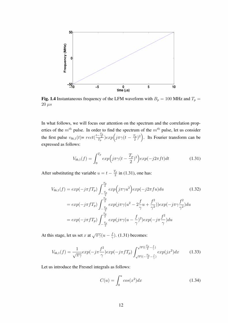
−10 −5 0 5 10−50

0

50

time (µs)

Fre

qu

en

cy

(M

Hz)

Fig. 1.4 Instantaneous frequency of the LFM waveform with Bp = 100 MHz and Tp =20 µs

In what follows, we will focus our attention on the spectrum and the correlation prop-erties of the mth pulse. In order to find the spectrum of the mth pulse, let us consider

the first pulse vbb,1(t)= rect(t−Tp

2

Tp)exp

(jπγ(t − Tp

2)2)

. Its Fourier transform can beexpressed as follows:

Vbb,1(f) =

∫ Tp

0

exp(jπγ(t− Tp

2)2)exp(−j2πft)dt (1.31)

After substituting the variable u = t− Tp2

in (1.31), one has:

Vbb,1(f) = exp(−jπfTp)∫ Tp

2

−Tp2

exp(jπγu2

)exp(−j2πfu)du (1.32)

= exp(−jπfTp)∫ Tp

2

−Tp2

exp(jπγ(u2 − 2f

γu+

f 2

γ2))exp(−jπγ f

2

γ2)du

= exp(−jπfTp)∫ Tp

2

−Tp2

exp(jπγ(u− f

γ)2)exp(−jπf

2

γ)du

At this stage, let us set x at√πγ(u− f

γ). (1.31) becomes:

Vbb,1(f) =1√πγexp(−jπf

2

γ)exp(−jπfTp)

∫ √πγ(Tp2− fγ)

√πγ(−Tp

2− fγ)

exp(jx2)dx (1.33)

Let us introduce the Fresnel integrals as follows:

C(u) =

∫ u

0

cos(x2)dx (1.34)

12

andS(u) =

∫ u

0

sin(x2)dx (1.35)

Consequently, one has:

∫ b

a

exp(jx2)dx =

∫ 0

a

exp(jx2)dx+

∫ b

0

exp(jx2)dx (1.36)

=t=−x

−∫ 0

−aexp(jt2)dt+

∫ b

0

exp(jx2)dx

=

∫ −a0

exp(jx2)dx+

∫ b

0

exp(jx2)dx

= C(−a) + jS(−a) + C(b) + jS(b)

Combining the above equations, (1.33) becomes:

Vbb,1(f) =1√πγexp(−jπf

2

γ)exp(−jπfTp)×

(C(√

πγ(Tp2

+f

γ))

(1.37)

+ jS(√

πγ(Tp2

+f

γ))+ C

(√πγ(

Tp2− f

γ))+ jS

(√πγ(

Tp2− f

γ)))

As vbb,m(t) is a shifted version of vbb,1(t), the Fourier transform of the mth pulse canexpressed in terms of Vbb,1(f). It is given for m ∈ J1, NpK by:

Vbb,m(f) = exp(− j2πf(m− 1)Tr

)Vbb,1(f) (1.38)

Therefore, the power spectrum of the mth pulse can be obtained by taking the square ofthe modulus of (1.38). Thus, the Np LFM pulses have the same power spectrum givenby:

V (f) =1

πγ

[(C(√

πγ(Tp2

+f

γ))+ C

(√πγ(

Tp2− f

γ)))2

(1.39)

+(S(√

πγ(Tp2

+f

γ))+ S

(√πγ(

Tp2− f

γ)))2]

Let us now express the autocorrelation function of vbb,1(t). It is defined by:

Rv(τ) =

∫ +∞

−∞vbb,1(t)vbb,1(t− τ)dt (1.40)

13

When −Tp ≤ τ ≤ 0, after some mathematical developments and simplifications, onehas:

Rv(τ) =

∫ τ+Tp

0

exp(−jπγτ 2)exp(j2πγτ(t− Tp/2)

)dt

= exp(−jπγτ 2)exp(−jπγτTp)∫ τ+Tp

0

exp(j2πγτt

)dt

= (Tp + τ)sinc(γτ(Tp + τ)

)(1.41)

where sinc(x) = sin(πx)/πx.When 0 ≤ τ ≤ Tp, similar analysis can be carried out where the integration limits arefrom τ to Tp. In this case, one has Rv(τ) = (Tp − τ)sinc

(γτ(Tp − τ)

). Therefore, the

expression of Rv(τ) for |τ | ≤ Tp is given by:

Rv(τ) = (Tp − |τ |)sinc(γ|τ |(Tp − |τ |)

)(1.42)

Given (1.42), one can deduce that the HRRP of a stationary target obtained with LFMwaveform has the shape of a sinc function multiplied by a triangular function. Thus, thesidelobes of the HRRP are relatively high. To reduce them, an amplitude windowing isgenerally applied in the frequency domain just before producing the HRRP. This comesat the cost of a smaller SNR at the output of the MF and an increase in the width of themainlobe of the HRRP [95].In the following subsection, phase coded waveforms are presented.

1.6.1.2 Phase coded (PC) waveforms

The phase coded (PC) waveform is represented by (1.1) where the mth baseband pulseis given by:

vbb,m(t) =M−1∑i=0

Arect(t− iTc −mTr − Tc/2

Tc

)exp(jφi) (1.43)

where M is the length of the phase code, Tc = TpM

is the duration of each subpulse,and φi (i ∈ J0,M − 1K) represents the phase sequence of the code. It should be notedthat φi intentionally varies from one subpulse to another in order to achieve the desiredmainlobe and sidelobe response for the autocorrelation function of the phase code. Inthe literature, phase codes are grouped into two categories:

• Bi-phase coded waveforms which exhibit two possible phase states: 0 and π [65][18] [24] [53].

• Polyphase coded waveforms which exhibit more than two phase states. This is

14

the case of the polyphase Barker codes [83] [31], Frank, P1, P2, P3, P4, [60] [61],and ZadoffChu codes [30].

In this thesis, the polyphase Barker and P4 codes are considered.

1.6.1.2.1 Barker codes These codes are widely used in radar applications. For anylength M , the autocorrelation function of the Barker code has equal sidelobes and awell-defined peak at its mainlobe. The peak sidelobe to mainlobe ratio is equal to 1

M.

Moreover, the maximum even length is equal to 4 and the maximum odd length is equalto 13 [23]. The autocorrelation function5 of the Barker code with M = 13 is presentedin Fig. 1.5.

−13 0 12

0

5

10

15

n

Valu

e

Fig. 1.5 Autocorrelation function of the Barker code of length 13

1.6.1.2.2 Polyphase Barker codes Due to the limitation in the length of Barkercodes, polyphase Barker codes were proposed to obtain peak sidelobe to mainlobe ratiosimilar to Barker codes with larger M . These codes can be derived by using varioussearch techniques [95]. Thus, the phases of the polyphase Barker codes are either un-restricted or restricted to a P th root of unity such that the allowable phase increment is∆φ = 2π

Pand P is an integer greater than 2. In [11], polyphase codes up to length 63

have been identified. Some of these codes used in this thesis are provided in Table. 1.1.In addition, their autocorrelation functions and power spectra are presented in Fig. 1.6,Fig. 1.7, Fig. 1.8, and Fig. 1.9.

5Here, the autocorrelation function of a sequence v(n) of length N is defined for n ∈ J1, 2N − 1K byRv(n) = X(n−N) where X(n) is defined by:

X(n) =

∑N−n−1i=0 v(i+ n)v(i) for n ≥ 0

X(−n) for n < 0(1.44)

15

Table 1.1 Polyphase Barker codes

Code length (M ) P φi, (i = 1, . . . ,M)54 200 0, 0, 23, 43, 16, 9, 40, 51, 20, 7, 67, 126, 178,

180, 71, 120, 144, 151, 61, 25, 45, 100, 86, 9,172, 161, 142, 22, 85, 8, 96, 128, 81, 1, 18,

137, 0, 95, 132, 59, 44, 155, 16, 129, 157, 98,47, 174, 73, 18, 145, 65, 170, 100

60 210 0, 0, 16, 208, 180, 153, 126, 161, 135, 78, 83,98, 143, 127, 162, 153, 183, 141, 72, 207, 149,

167, 15, 13, 146, 58, 23, 109, 169, 208, 75,143, 173, 199, 51, 50, 31, 142, 152, 84, 74, 6,147, 205, 151, 66, 51, 151, 27, 101, 170, 75,

172, 91, 20, 131, 1, 78, 166, 68

−54 0 530

10

20

30

40

50

60

n

Valu

e

Fig. 1.6 Autocorrelation function of the polyphase Barker code of length 54

−54 0 540

0.2

0.4

0.6

0.8

1

Frequency (MHz)

No

rmalized

mag

nit

ud

e

Spectrum

Fig. 1.7 Power spectrum of the polyphase Barker code of length 54 where B = 54MHz

16

−60 0 590

10

20

30

40

50

60

n

Valu

e

Fig. 1.8 Autocorrelation function of the polyphase Barker code of length 60

−60 0 600

0.2

0.4

0.6

0.8

1

Frequency (MHz)

No

rmalized

mag

nit

ud

e

Spectrum

Fig. 1.9 Power spectrum of the polyphase Barker code of length 60 where B = 60MHz

1.6.1.2.3 Polyphase P4 code The phase of the P4 code is conceptually derived bysampling the quadratic phase of an LFM waveform i.e. πB

Tpt2. Sampling the phase in

(1.28) at the chip interval τchip yields the phase sequence:

φi =πB

Tp(iτchip)

2 (1.45)

For a rectangular chip, the chip width is the reciprocal of the bandwidth, i.e. τchip = 1B

.After making the appropriate substitution and subtracting the result from πi, the phasesequence of P4 for i ∈ J0,M − 1K reduces to:

φi =πi2

M− πi (1.46)

In the next section, let us focus our attention on an alternative type of waveform whoseinstantaneous frequency varies over time in a non-linear way.

17

1.6.1.3 Non linear frequency modulation (NLFM) waveforms

There are some waveforms which are ”naturally” NLFM such as the Hybrid NLFM[122], tangent-based, and the sine-based waveforms [108] [19]. However, others can bedesigned to meet certain requirements. Thus, the principle of stationary phase can beused to synthesize an NLFM waveform that has a PSD similar to certain well-knownwindows such as the Taylor and Blackman-Harris windows [77] [98] [49]. Recently, in[100], a piecewise NLFM (PW-NLFM) waveform was proposed to enhance the imagingquality in SAR applications. In this thesis, the tangent-based NLFM and the PW-NLFMwaveforms are considered. Let us give some details about them in the paragraphs below.

1.6.1.3.1 Tangent-based NLFM waveform The tangent-based NLFM waveform isrepresented by (1.1) where:


Tp

)exp(jφ(t− (m− 1)Tr − Tp/2)

)(1.47)

where the phase φ(t) is given by:

φ(t) = −2π BpTp4βtanβ

ln

(cos(

2βt

Tp)

)=

(1.13)−2π BTp

4βtanβln

(cos(

2βt

Tp)

)(1.48)

It should be noted that:φ(t) = φ(−t) (1.49)

In (1.48), φ(t) is is related to the instantaneous frequency for −Tp2≤ t ≤ Tp

2as follows:

f(t) =1

2π

dφ(t)

dt= B

tan(2βt/Tp)

2tanβ= −f(−t) (1.50)

where β ∈ J0, π/2K is a parameter that can be adjusted by the practitioner.In Fig. 1.10 and 1.11, f(t) and φ(t) are respectively presented for different values ofβ. Note that the degree of non-linearity increases with β. Moreover, when β tendsto 0, this leads to the LFM case. As the instantaneous frequency varies with β, thepower spectrum also varies with β. In Fig. 1.12, the power spectrum is provided withB = 100 MHz for β = 0.01, β = 0.95 and β = 1.42. As the instantaneous frequencyvaries with β, the power spectrum also varies with β. When β tends to 0, the powerspectrum tends to be the one of an LFM waveform. The power is more or less ”uni-formly” distributed in the interval [−B/2, B/2]. When β increases and tends to π/2,Fig 1 provides the evolution of the instantaneous frequency of the waveform. One cannotice that exp(jφ(t)) can be approximated by exp(j2π × 0t) during a time intervalthat becomes larger and larger as β becomes larger and larger. Therefore, the powerspectrum of the tangent-based NLFM pulse is more and more spiky around zero as β

18

increases.

−0.5 0 0.5−100

−50

0

50

100

time (µs)

f(t)

(M

Hz)

β = 0.01

β = 0.45

β = 0.95

β = 1.21

β = 1.42

Fig. 1.10 Instantaneous frequency of the tangent-based NLFM waveform for differentvalues of β with B = 100 MHz and Tp = 20 µs.

−0.5 0 0.50

0.5

1

1.5

2

2.5

3

time (µs)

φ(t

)

β = 0.01

β = 0.45

β = 0.95

β = 1.21

β = 1.42

Fig. 1.11 Phase of the tangent-based NLFM waveform for different values of β

1.6.1.3.2 Piecewise (PW) NLFM waveform In the literature, various NLFM wave-forms have been studied [43] [13]. In this thesis, we focus on the one proposed in [100],the authors called PW-NLFM waveform. It consists of two symmetric sets, where eachone is composed of L + 1 concatenated LFM subpulses with different bandwidths anddurations. Its instantaneous frequency is shown in Fig. 1.13. In order to derive the ana-lytical expression of the PW-NLFM waveform, let us define the following parameters:

(τ1, ν1) = (0, 0)

(τL+2, νL+2) = (Tp2, B2)

γ(i) = νi+1−νiτi+1−τi with 1 ≤ i ≤ L+ 1.

(1.51)

Then, the instantaneous frequency of the PW-NLFM waveform, denoted as fPW (t), is

19

−100 −50 0 50 1000

0.2

0.4

0.6

0.8

1

Frequency (MHz)

Nor

mal

ized

mag

nitu

de

Power spectrum

(a)

−100 −50 0 50 1000

0.2

0.4

0.6

0.8

1

Frequency (MHz)

Nor

mal

ized

mag

nitu

de

Power spectrum

(b)

−100 −50 0 50 1000

0.2

0.4

0.6

0.8

1

Frequency (MHz)

Nor

mal

ized

mag

nitu

de

Power spectrum

(c)

Fig. 1.12 Power spectrum of the tangent-based NLFM pulse, based on the DFT withB = 200 MHz, when (a) β = 0.45 (b) β = 0.95 (c) β = 1.42.

time (µs)

Fre

qu

en

cy (

MH

z)

B/2

B

0T

p/2 T

p

ν2

ν3

ν4

ν5

τ2

τ3

τ4

τ5

Fig. 1.13 Instantaneous frequency of the PW NLFM waveform

given by:

fPW (t) = νi + γ(i)(t− τi)for τi ≤ t ≤ τi+1 with i = 1, ..., L+ 1

fPW (t) = B − fPW (Tp − t)= B − ν2L+3−i + γ(2L+3−i)(t− Tp + τ2L+3−i)

for τi ≤ t ≤ τi+1 with i = L+ 2, ..., 2L+ 2

(1.52)20

Remark: It should be noted the instantaneous frequency for i = L + 2, ..., 2L + 2 canbe written in different ways. In [100], the authors directly use:

fPW (t) = B − ν2L+4−i + γ(2L+3−i)(t− Tp + τ2L+4−i) (1.53)

The above expression is valid. This can be shown by subtracting (1.53) to (1.52) andthen by using definition of γ(i). However, in this thesis, (1.52) is used. Then, theinstantaneous phase φPW (t) can be derived by integrating (1.52) and multiplying by2π. This leads to:

φPW (t) = 2π(γ(i) t

2

2+ (νi − γ(i)τi)t+ li

)for τi ≤ t ≤ τi+1 and i = 1, ..., L+ 1

φPW (t) = 2π(γ(2L+3−i) t2

2+ (γ(2L+3−i)(τ2L+3−i − Tp) +B − ν2L+3−i)t+ li

)for τi ≤ t ≤ τi+1 and i = L+ 2, ..., 2L+ 2

(1.54)where l1,...,2L+2 are used to preserve the continuity between different stages of the phasefunction.Let us now express the set of phases lii=1,...,L+1. To this end, let us assume that l1 isset at 0. In this case, using the above expressions, the continuity of the phase at τ1 leadsto:

l2 = (γ(1) + γ(2))τ 222− ν2τ2

= γ(1)τ 222− ν2τ2 + γ(2)

τ 222

= −ν2τ22+ γ(2)

τ 222

(1.55)

More generally one has for i = 1, ..., L:

li+1 = li + (νi − νi+1)τi+1 + (γ(i) + γ(i+1))τ 2i+1

2− γ(i)τiτi+1 (1.56)

At this stage, as νi+1 − νi = γ(i)(τi+1 − τi), this leads to:

li+1 = li + (γ(i+1) − γ(i))τ 2i+1

2(1.57)

Then, it can be easily shown that:

lL+2 = lL+1 +Tp2(2νL+1 −B) + γ(L+1)(

Tp2(Tp − 2τL+1)) (1.58)

21

and for i = L+ 2, ..., 2L

li+1 = li + (ν2L+2−i − ν2L+3−i)τi+1 + γ(2L+3−i)(τ 2i+1

2+ (τ2L+3−i − Tp)τi+1) (1.59)

− γ(2L+2−i)(τ 2i+1

2+ (τ2L+2−i − Tp)τi+1)

By replacing τi+1 by (Tp − τ2L+3−i), the above expression can be rewritten as follows:

li+1 = li + (ν2L+2−i − ν2L+3−i)(Tp − τ2L+3−i) (1.60)

− (γ(2L+3−i) + γ(2L+2−i))(Tp − τ2L+3−i)

2

2

+ γ(2L+2−i)(Tp − τ2L+2−i)(Tp − τ2L+3−i)

In addition, by replacing ν2L+3−i − ν2L+2−i = γ(2L+2−i)(τ2L+3−i − τ2L+2−i), the aboveexpression becomes:

li+1 = li − (γ(2L+3−i) − γ(2L+2−i))(Tp − τ2L+3−i)

2

2(1.61)

As all the parameters of the instantaneous phase of the PW-NLFM waveform have beendefined, the expression of the transmitted waveform is represented by (1.1) where:


Tp/2

)exp(jφPW (t− (m− 1)Tr)

)(1.62)

Due to the expression (1.52) of the instantaneous phase, the spectrum of stx(t) is cen-tered at B

2.

The NLFM waveform employs frequency modulation to shape the spectrum and thusreduces the range sidelobes. These waveforms do not require an amplitude weightingto the MF output which is commonly used with an LFM waveform, and thereby avoidthe associated SNR loss.

1.6.1.4 Comments on the pulse compression waveforms

Even if the LFM remains the most popular waveform probably thanks to its simplicityto be generated and its Doppler tolerance, some phase codes exhibit a Doppler tolerancesimilar to that of an LFM [95]. In addition, the advent of high-speed and high dynamicrange digital-to-analog converter (DAC) and high-speed FPGA has facilitated the gen-erations of sophisticated NLFM waveforms [117]. Pulse compression waveforms canbe used in high range resolution radar application. However, they require a high sam-pling frequency and consequently an expensive ADC. To overcome the aferomentioneddrawback, SF waveforms were proposed. Let us present them in the following section.

22

1.6.2 Stepped-frequency (SF) waveforms

Stepped-frequency waveform is a waveform that transmits a train of narrow-band pulseswith equally-spaced carrier frequencies. At the receiver, a large bandwidth is synthe-sized by coherently combining the received echoes. This arrangement does not requirean expensive and complex ADC since the required sampling frequency at the receiverdepends on the baseband bandwidth rather than the total bandwidth covered by the re-ceived pulses.In the literature, SF waveforms have been well studied [67] [81] [45]. In addition, SFcan be combined at the transmitter with one of the pulse compression techniques. Thereader may refer to [37] [70] [120] [69] [62] [17] [66]. One main advantage of thisapproach is that it reduces the number of pulses within the coherent processing inter-val (CPI)6. For instance, in radar imaging, the size of the CPI is limited to avoid thedegradation caused by the motion through the resolution cells [4]. Moreover, with me-chanically scanning search radars, the number of transmitted pulses within the dwellbeam is constrained by the speed of rotation of the antenna. A great deal of interesthas been paid to SF-LFM [120] [17] [66] [69] [70]. On the contrary, few researchershave studied the stepped-frequency phase-coded (SFPC) waveform and the stepped fre-quency non-linear frequency modulation (SF-NLFM) waveform. In [62], the SFPCwaveform was used with the through-the-wall radar to enhance the anti-radio frequencydisturbance performance. In [37], the author illustrated the advantage of the SF-NLFMwaveform over the SF-LFM waveform in terms of reductions of the grating-lobe lev-els. In the next section, the general waveform modeling of a SF waveform is presented.Then, the modeling of the particular cases SF-LFM and SFPC are presented.

1.6.2.1 General modeling of SF waveforms

The SF radar transmits a burst ofNp > 1 pulses, whose carrier frequency monotonicallyincreases from pulse to pulse by a fixed frequency step size denoted as ∆f . For the mth

pulse (m ∈ J1, NpK), the transmitted SF waveform is described as follows:

stx(t) =

Np∑m=1

stx,m(t) =

Np∑m=1

vbb,m(t)exp(j2πf(m)c t) (1.63)

withf (m)c = fc +∆f (m) (1.64)

where∆f (m) =

(1−Np

2+m

)∆f (1.65)

6The time duration of theNp pulses processed coherently by using coherent integration or fast Fouriertransform processing is called the CPI.

23

In the above equations, f (m)c is the carrier frequency of the mth transmitted pulse, and

fc is the central carrier frequency of the complete train of pulses. In addition, usu-ally, ∆f ≤ Bp is chosen to avoid creating gaps in the transmitted waveform. When∆f = Bp, the total bandwidth covered by the waveform is B = NpBp. Finally in(1.63), vbb,m(t) corresponds to either modulated pulses or unmodulated pulses.In the sequel and for the sake of simplicity, the equations that are presented only dealwith the signal part. The disturbance is omitted. In addition, Km = 1 is consideredsince the Np pulses are assumed to be subjected to the same channel effect. Thus, the”ideal” received SF signal for a stationary point target at range R can be written asfollows:

srx(t) =

Np∑m=1

srx,m(t) =

Np∑m=1

vbb,m

(t− td

)exp(j2πf (m)

c (t− td))

(1.66)

The reference signal used for the demodulation process is defined by:

sref,m(t) = exp(− j2πf (m)

c t)

(1.67)

Therefore, the received baseband signal is given by:

srx,bb(t) =

Np∑m=1

srx,bb,m(t) =

Np∑m=1

vbb,m

(t− td

)exp(− j2πf (m)

c td

)(1.68)

1.6.2.2 SF-LFM waveform model

The SF-LFM waveform is derived from the combination of the SF waveform and theLFM waveform. In other words, the carrier frequency of each SF pulse is linearlymodulated. In this case, the resulting waveform is represented by (1.63) where vbb,m(t)is defined as in (1.28). Thus, the SF-LFM transmitted waveform whose instantaneousfrequency is presented in Fig. 1.14 can be expressed as:

stx(t) =

Np∑m=1

stx,m(t)

=

Np∑m=1

Arect(t− (m− 1)Tr − Tp/2

Tp

)exp(jπγ(t− (m− 1)Tr − Tp/2)2

)× exp

(j2πf (m)

c t)

(1.69)

24

Fig. 1.14 Stepped-frequency linear frequency modulated waveform

Given (1.68), the received baseband SF-LFM signal can be expressed as:

srx,bb(t) =

Np∑m=1

rect(t− (m− 1)Tr − Tp/2− td

Tp

)(1.70)

× exp(jπγ(t− (m− 1)Tr − Tp/2− td)2

)exp(− j2πf (m)

c td

)1.6.2.3 SFPC waveform model

The SFPC waveform is derived from the combination of the SF waveform and PC wave-form. In other words, the carrier frequency of each pulse in the PC waveform varies asin the case of the SF waveform. Therefore, the resulting waveform is represented by(1.63) where vbb,m(t) is defined as in (1.43). Thus, the SFPC waveform can be expressedas:

stx(t) =

Np∑m=1

stx,m(t)

=

Np∑m=1

M−1∑i=0

Arect(t− iTc − (m− 1)Tr − Tc/2

Tc

)exp(jφi)exp

(j2πf (m)

c t)

(1.71)

Given (1.68), the received SFPC baseband signal can be expressed as:

srx,bb(t) =

Np∑m=1

M−1∑i=0

rect(t− iTc − (m− 1)Tr − Tc/2− td

Tc

)× exp(jφi)exp

(− j2πf (m)

c td

)(1.72)

25

1.6.2.4 SF-NLFM waveform

The SF-NLFM waveform is derived from the combination of the SF waveform andthe NLFM waveform. Thus, the SF-NLFM waveform is represented by (1.63) wherevbb,m(t) is defined by:


Tp


)(1.73)

where φ(t) represents the instantaneous phase of the NLFM used. Thus, the SF-NLFMwaveform can be expressed as:

stx(t) =

Np∑m=1

stx,m(t)

=

Np∑m=1

Arect(t− (m− 1)Tr − Tp/2

Tp


)× exp

(j2πf (m)

c t)

(1.74)

Given (1.68), the received baseband SF-NLFM signal can be expressed as:

srx,bb(t) =

Np∑m=1

rect(t− (m− 1)Tr − Tp/2− td

Tp

)× exp

(jφ(t− (m− 1)Tr − Tp/2− td)

)exp(− j2πf (m)

c td

)(1.75)

1.6.2.5 Comments on SF waveforms

Since the instantaneous frequency of an LFM pulse is a linear function of time, theinstantaneous frequency of the concatenated pulses of the SF-LFM waveform corre-sponds to a wide-band LFM pulse. In this case, it is possible to synthesize a wide-bandLFM pulse at the receiver and thus the HRRP has the shape of the autocorrelation func-tion of a wide-band LFM pulse. However, with SFPC or SF-NLFM, the instantaneousfrequency of the concatenated pulses does not correspond to a wide-band PC or NLFMpulse.In order to process the SF received baseband signal, different algorithms can be used.Let us present them in the next section.

1.6.2.6 Processing SF waveforms at the receiver

The SF waveforms can be processed at the receiver by using the MF. However, it suffersfrom the upsampling process. In addition, grating lobes may appear in the HRRP [37].One alternative can be seen as a kind of stretch processing. It includes three different

26

algorithms:

• The frequency domain (FD) algorithm

• The inverse fast Fourier transform (IFFT) algorithm

• The time domain (TD) algorithm

The FD and the IFFT algorithms have computational costs smaller than that of the MF-based approach. However, they have some limitations. The IFFT algorithm producesghost targets in the HRRP of the extended targets due to the spill-over effect of en-ergy into consecutive coarse range bins [67]. As for the TD algorithm [68], it doesnot produce ghost targets but suffers from the up-sampling requirement of the narrow-bandwidth pulses prior to the frequency shift. Finally, the FD algorithm can cope withthe drawbacks of the TD and the IFFT algorithms, but a discrete Fourier transform(DFT) must be computed on a relatively large number of samples. Nevertheless, therecent advances in designing and fabricating powerful processors can facilitate its im-plementations.In order to process the received echoes of a SF waveform, the baseband signal srx,bb(t)is sampled at F (Rx)

s . The number of samples associated with each pulse is equal toN = bF (Rx)

s Tpc where b.c is the floor function. Then, the sampled data are processedwith one of the existing algorithms. Let us start with the FD algorithm.

1.6.2.6.1 Frequency domain (FD) algorithm It aims at reconstructing a large tar-get reflectivity spectrum by coherently combining the individual spectra of the receivedSF-LFM pulses in the frequency domain [118]. The resulting reconstructed spectrumis equivalent to the spectrum of a wide-band LFM pulse and thus the HRRP obtainedhas approximately the shape of a sinc function. In the following, the steps of the FDalgorithm, based on the SF-LFM waveform defined in (1.69), are presented:

1. Sample the received pulses in (1.70) atF

(Rx)s = 2Bb = B

Np. Thus, each received baseband pulse is defined for n ∈

J0, N − 1K by:

srx,bb,m(n) = exp(jπγ(nT (Rx)

s − Tp/2− td)2)exp(− j2πf (m)

c td

)(1.76)

where T (Rx)s = 1

F(Rx)s

is the sampling time at the receiver.

2. A DFT is computed on the received samples associated with each pulse in (1.76)padded with N − 1 zeros. Padding by zeros is necessary to make MF in thefrequency domain equivalent to a linear convolution in the time domain7, which

7Having two sequences of length L andN respectively, before applying MF in the frequency domain,each sequence should be padded by zeros so that its length is at least L+N − 1.

27

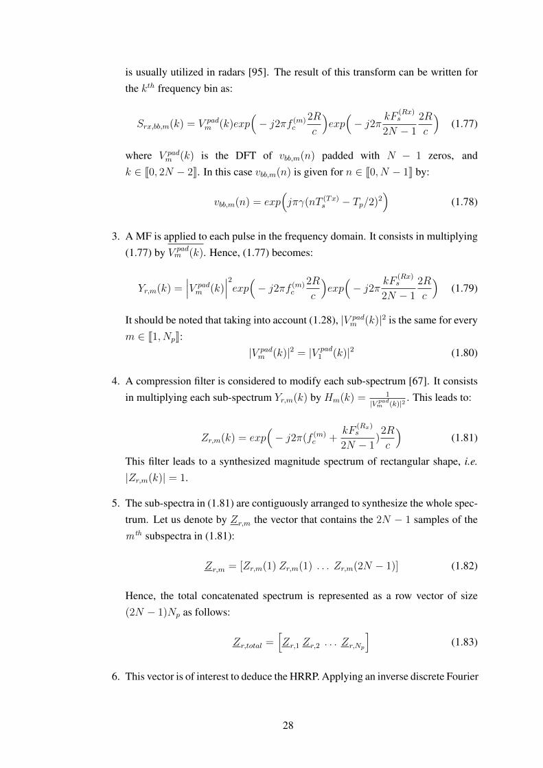
is usually utilized in radars [95]. The result of this transform can be written forthe kth frequency bin as:

Srx,bb,m(k) = V padm (k)exp

(− j2πf (m)

c

2R

c

)exp(− j2π kF

(Rx)s

2N − 1

2R

c

)(1.77)

where V padm (k) is the DFT of vbb,m(n) padded with N − 1 zeros, and

k ∈ J0, 2N − 2K. In this case vbb,m(n) is given for n ∈ J0, N − 1K by:

vbb,m(n) = exp(jπγ(nT (Tx)

s − Tp/2)2)

(1.78)

3. A MF is applied to each pulse in the frequency domain. It consists in multiplying(1.77) by V pad

m (k). Hence, (1.77) becomes:

Yr,m(k) =∣∣∣V padm (k)

∣∣∣2exp(− j2πf (m)c

2R

c

)exp(− j2π kF

(Rx)s

2N − 1

2R

c

)(1.79)

It should be noted that taking into account (1.28), |V padm (k)|2 is the same for every

m ∈ J1, NpK:|V padm (k)|2 = |V pad

1 (k)|2 (1.80)

4. A compression filter is considered to modify each sub-spectrum [67]. It consistsin multiplying each sub-spectrum Yr,m(k) by Hm(k) =

1

|V padm (k)|2. This leads to:

Zr,m(k) = exp(− j2π(f (m)

c +kF

(Rx)s

2N − 1)2R

c

)(1.81)

This filter leads to a synthesized magnitude spectrum of rectangular shape, i.e.

|Zr,m(k)| = 1.

5. The sub-spectra in (1.81) are contiguously arranged to synthesize the whole spec-trum. Let us denote by Zr,m the vector that contains the 2N − 1 samples of them th subspectra in (1.81):

Zr,m = [Zr,m(1) Zr,m(1) . . . Zr,m(2N − 1)] (1.82)

Hence, the total concatenated spectrum is represented as a row vector of size(2N − 1)Np as follows:

Zr,total =[Zr,1 Zr,2 . . . Zr,Np

](1.83)

6. This vector is of interest to deduce the HRRP. Applying an inverse discrete Fourier

28

transform (IDFT) to (1.83) yields:

zr(n) =1

(2N − 1)Np

×(2N−1)Np−1∑

l1=0

Zr,total(l1 + 1)exp( j2πl1n

(2N − 1)Np

)(1.84)

where Zr,total(l) is the lth element of Zr,total. Using (1.64), the above equationcan be expressed as follows:

zr(n) =exp(− j2π(fc +

(1−Np

2

)∆f)2Rc

)(2N − 1)Np

Np∑m=1

exp(− j2π(m− 1)(∆f

2R

c− n

Np))

(1.85)

×2N−2∑k=0

exp(− j 2πk

(2N − 1)

(2RF (Rx)s

c− n

Np

))Therefore, its modulus represents the HRRP and is equal to:

hFD(n) = |zr(n)| =1

(2N − 1)Np

|sin[Npπ(∆f

2Rc− n

Np)]|

|sin[π(∆f 2R

c− n

Np)]|

(1.86)

×|sin

[π(

2RF(Rx)s

c− n

Np

)]|

|sin[

π2N−1

(2RF

(Rx)s

c− n

Np

)]|

Providing that F (Rx)s = ∆f , (1.86) becomes:

hFD(n) =1

(2N − 1)Np

∣∣∣∣∣ sin(Npπ(F

(Rx)s

2Rc− n

Np))

sin(

π2N−1

(F

(Rx)s

2Rc− n

Np

))∣∣∣∣∣ (1.87)

where n ∈ J0, (2N − 1)Np − 1K and hFD(n) has its maximum equal to 1 when

n = 2RF(Rx)s Npc

= tdF(Rx)s Np. Moreover, if n was not reduced to the interval

J0, (2N − 1)Np − 1K, |zr(n)| would be (2N − 1)Np-periodic.

Remark about the compression filter: If the compression filterHm(k) = 1

|V padm (k)|2was not used, the IDFT of Zr,total would amount to com-

puting the IDFT of the product between the sequence defined from the Np setsexp

(− j2π(f

(m)c + kF

(Rx)s

2N−1 )2Rc

)k=0,...,2N−2 for m ∈ J1, NpK on one side and

the sequence defined by ∣∣∣V pad

1 (k)∣∣∣2k=0,...,2N−2 repeated Np times on the other.

This is equivalent to computing the circular convolution between the IDFTs. Thefirst one is given in (1.87) whereas the second can be given by:

29

1

(2N − 1)Np

×Np∑m=1

2N−2∑k=0

∣∣∣V padm (k)

∣∣∣2exp(j2π((m− 1)(2N − 1) + k)n

(2N − 1)Np

)(1.88)

Given (1.80), this can be rewritten as follows:

1

Np

Np∑m=1

exp(j2π(m− 1)n

Np

)× 1

(2N − 1)

2N−2∑k=0

∣∣∣V pad1 (k)

∣∣∣2exp( j2πkn

(2N − 1)Np

)(1.89)

In (1.89), 1Np

∑Npm=1 exp

(j2π(m−1)n

Np

)is equal to 0 except when n is a multiple of

Np. In addition, 1(2N−1)

∑2N−2k=0

∣∣∣V pad1 (k)

∣∣∣2exp( j2πkn(2N−1)Np ) is the autocorrelation

function of the LFM waveform interpolated at a rate of Np. Once this sequenceis multiplied by the other one which is either equal to 1 or 0, this leads to theautocorrelation function upsampled at a rate of Np. Therefore (1.89) correspondsto a sequence comprising the autocorrelation function of the waveform separatedby Np − 1 zeros.Given the above mathematical developments, if a compression filter was not used,the IDFT of Zr,total would be the circular convolution between the quantity givenin (1.87) and the autocorrelation function upsampled by a factor Np. Therefore,

the maximum of |zr(n)| remains reached for n = 2RF(Rx)s Npc

= tdF(Rx)s Np. As

the autocorrelation function of the LFM waveform is far from the Kronecker deltafunction, the HRRP obtained in (1.87) is modified. In [67], the authors did notprovide these mathematical details. They motivated the use of the compressionfilter by the fact that they noticed spectral ripples in the concatenated spectrum,leading to some artifacts in the HRRP in their simulations. Instead of using acompression filter, the authors in [77] suggest considering overlapped LFM spec-tra so that the reconstructed spectrum tends to be flat.Remark about a post weighting: Due to (1.87), amplitude weighting can beapplied to reduce the range sidelobes. It consists in multiplying (1.83) by anotherrow vector W of the same length containing the spectrum of a shaping window,for instance Hanning.

Gr,total = Zr,total . ∗W (1.90)

where .* stands for a multiplication of vectors element by element. An IDFT isfinally applied to the synthesized spectrum in (1.90) to create the HRRP.

30

Fig. 1.15 Block diagram of the IFFT algorithm

1.6.2.6.2 IFFT algorithm The IFFT method was described in detail by Wehner in[116]. It consists in taking the inverse FFT of the sampled SF data. Although the stepsdone in this algorithm are similar to those done for any traditional waveform that trans-mit pulses on the same carrier frequency to create a Doppler profile, the IFFT algorithmproduces a range profile and not a Doppler profile since the pulses are transmitted ondifferent carrier frequencies. In the following, the steps of the IFFT algorithm, basedon the SF waveform defined in (1.1), are recalled. In (1.1), vbb,m(t) corresponds toan unmodulated pulse as defined in (1.2). In this case, for n ∈ J0, N − 1K, one hasvbb,m(n) = 1. The steps of the IFFT algorithm presented in Fig. 1.15 can be summa-rized as follows [77]:

1. Sample the received pulses, whose expression is given in (1.68), at F (Rx)s =

2Bb = BNp

. Thus, each received baseband pulse is defined for n ∈ J0, N − 1Kby:

srx,bb,m(n) = vbb,m(nT(Rx)s − td)exp(−j2πf (m)

c td) (1.91)

2. A MF is applied to the samples given in (1.91). It consists in convolving srx,bb,m(n)with vbb,m(−n).

3. A sample is collected at each range gate and the process is repeated over the Np

pulses.

4. At each range gate, one range profile can be formed by applying an IDFT to thecollected samples. Finally, the obtained range profiles can be concatenated toproduce the HRRP.

1.6.2.6.3 Time domain (TD) algorithm The TD algorithm was proposed to processa SF-LFM waveform in the time domain [67]. It aims at reconstructing a wide-band

31

LFM waveform by combining the narrow-band LFM pulses in the time domain. Inthe following, the steps of the TD algorithm, based on the waveform defined in (1.69)where the frequency step size is assumed equal to the passband bandwidth of the pulse(i.e., ∆f = Bp), are presented:

1. For each received pulse, sample the baseband pulses in (1.70) by using the sam-pling frequency F (Rx)

s > 2Bb = ∆f = BNp

.

2. Interpolate the samples of each pulse so that the new sampling frequency be-comes:

F (int)s =

1

T(int)s

= B = NpF(Rx)s (1.92)

The interpolation operation can be done in the frequency domain by applying aDFT, zero-padding the result, and then applying an IDFT.

3. Frequency shift each pulse to its proper position. This is done by multiplyingeach pulse by the proper exponential factor exp(j2π∆f (m)nT

(int)s )

4. Add a phase correction term to each pulse to avoid any phase discontinuity in thereconstructed LFM waveform. It is done by multiplying the result of the m(th)

pulse in the previous step by exp(jπγT 2

p (m + 1−Np2

)2)

. This step may be donebefore the interpolation step, thus requiring fewer multiplications and leading toa faster implementation of the procedure.

5. Time shift the result obtained by δtm =(m+ 1−Np

2

)Tp.

6. Add the obtained pulses together.

7. Apply a MF in the frequency domain to the reconstructed waveform.

8. Produce the HRRP by applying an IDFT to the output of the MF.

1.7 Performance measures

In this section, the definitions of some performance measures that are used in the simu-lation parts are given. As mentioned in section 1.3, the range profile of a point scattereris characterized by one mainlobe and several sidelobes. The latter arise from the useof pulse compression techniques and are not desirable. Moreover, as indicated in sub-section 1.4.2, the enhancement of the PD while maintaining a constant PFA can beachieved by increasing the SIR. However, when multiple targets are present, besidesthe SIR, the range resolution and the level of the sidelobes should also be taken intoaccount since they have a great influence on the PD and PFA.As for the level of the sidelobes, they can be quantified using two ratios: the peak

32

sidelobe ratio (PSLR) and the integrated sidelobe ratio (ISLR) [32] [119]. The PSLRis defined as the ratio of the maximum peak magnitude of the sidelobes to the peakmagnitude of the mainlobe:

PSLR = 20log

[∣∣h(ns)∣∣∣∣h(np)∣∣]

(1.93)

where h represents the HRRP, and ns and np respectively denote the position of thehighest sidelobe and the peak value of the mainlobe in h(n). The peak magnitudeof the first sidelobe is not necessarily the maximum peak magnitude among the othersidelobes, although it could be the case in some situations. The better performance interms of PSLR mitigates the masking effect of nearby targets and increase the usefuldynamic range. The ISLR is defined as the ratio of the energy of the sidelobes to theenergy of the mainlobe:

ISLR = 10log

np−nz∑n=1

∣∣h(n)∣∣2 + np+N+L∑n=np+nz

∣∣h(n)∣∣2n=np+N∑n=np−nz

∣∣h(n)∣∣2 (1.94)

where nz denotes the position of the null of the mainlobe in h(n).The level of significance given for each performance measure, especially the PSLRand the ISLR, depends on the surrounding environment. Whenever the received signalis disturbed by a distributed clutter environment, the ISLR is of high importance andshould be maintained as low as possible to enable the detection of weak targets. How-ever, if the received signal is disturbed by a strong discrete clutter, the PSLR is morecritical to be kept low. Otherwise, sidelobes may be interpreted falsely as real targets[59].Finally, let us define the range resolution. In the literature, various criteria are used todefine the range resolution. Two of the more common criteria used to define it are [95]:

• The 3-dB width of the mainlobe which defines the range resolution as the separa-tion between the peak point and the point that corresponds to the half of the peakpower.

• The Rayleigh criterion which defines the range resolution as the separation be-tween the peak and the null. In this case, the range resolution can be commonlyexpressed as:

Rres =c

2Beff

(1.95)

where Beff is the effective bandwidth of the waveform. Table. 1.2 summarizesthe relationship between Bb, B and Beff for various waveforms.

33

Table 1.2 Relation between the bandwidths of different waveforms

Waveform Bb B BeffPC M/Tp 2M/Tp B/2

SF 1/Tp (Np−1)∆f+2Bb B/2

SFPC M/Tp (Np−1)∆f+2Bb B/2

1.8 Conclusions

In this chapter, generalities about radar have been presented. In addition, we havefocused our attention on high range resolution waveforms. After presenting the pulsecompression waveforms such as the LFM, the PC, and the NLFM waveforms, SF wave-forms have been introduced. The latter can be used to reduce the sampling frequency atthe receiver. Three types of algorithms, namely the IFFT algorithm, the TD algorithmand the FD algorithm, which aim at processing the SF waveforms at the receiver havebeen described. Finally, we have presented some performance measures that have agreat influence on the probability of detection and probability of false alarm.In chapter 2, a processing chain from the transmitter to the receiver is proposed to over-come the drawbacks of the standard combination of PC or NLFM with a SF waveform.

34

CHAPTER 2

MODIFIED STEPPED-FREQUENCY WAVEFORMS

2.1 Introduction

In chapter 1, we have mentioned that pulse compression waveforms can be used inhigh range resolution radar applications. For some of these applications, the PC andthe NLFM waveforms may be more attractive than the LFM waveform since they ex-hibit smaller PSLR and ISLR. As the sampling rate of such waveforms is high1, oneof the approaches that can be considered to reduce it is the standard combination ofthese waveforms with SF. However, when using this combination, the PSLR and theISLR of the pulse compression used cannot be attained. This is due to the fact that theinstantaneous frequency of the concatenated pulses of the resulting waveform does notcorrespond to a known wide-band PC or NLFM pulse. As a consequence, the obtainedHRRP does not have the shape of the autocorrelation function of a known wide-bandNLFM or PC pulse.In this chapter, in order to overcome the aforementioned drawback, i.e. in order toreduce the sampling rate while taking the advantage of the features of the pulse com-pression waveform used in terms of PSLR and ISLR, a new approach is suggested tocombine a SF scheme with pulse compression waveforms. More particularly, a gen-eral processing chain from the transmitter to the receiver is proposed. It consists insplitting the spectrum of a wide-band modulated pulse into a predetermined numberof portions. Then, the corresponding time-domain signals are successively transmitted.These signals constitute what we call a modified SF waveform in this dissertation. Atthe receiver, the HRRP can be reconstructed by processing the received echoes either inthe frequency domain or in the time domain. Accordingly, a modified version of the FDalgorithm and a novel time waveform reconstruction (TWR) algorithm are proposed toreconstruct the HRRP.This chapter is organized as follows: firstly, the processing chain from the transmitterto the receiver is presented. Then, the results of the simulations of the modified SFwaveforms in different scenarios are shown.

1In these days, an order of magnitude could be 100MHz.

35

2.2 Our contribution: a processing chain of the modified SF radar wave-form combined with a pulse compression technique

In this section, the processing chain from the transmitter to the receiver is presented.First, the steps that should be done at the transmitter to generate the modified SF wave-form are illustrated. Then, the different algorithms that can be considered to processthe received echoes at the receiver are presented. Afterwards, the computational costsof the modified FD algorithm and the TWR algorithm are compared. Suggestions toremove some constraints in the modified SF waveform are provided. In addition, somecomments on the proposed waveform are presented. Finally, a comparative study is car-ried out between the different variants that can be considered in the processing chain.In addition, the modified SF waveforms are compared with the standard SF waveformsin different scenarios.

2.2.1 Generation of the modified SF waveform at the transmitter

The whole processing chain of the modified SF waveform is presented in Fig. 2.1.

Let v•(t) be the continuous-time baseband pulse that exhibits a wide bandwidth, where• stands for NLFM or PC. It is defined for 0 ≤ t ≤ Tp by:

vPC(t) =∑M−1

i=0 Arect(t−iTc−Tc/2

Tc

)exp(jφi)

vNLFM(t) = Arect(t−Tp/2Tp

)exp(jφ(t− Tp/2)

) (2.1)

For the generation of the waveform, the discrete version of v•(t) is needed. By intro-ducing the sampling period T (Tx)

s at the transmitter which satisfies:

1

T(Tx)s

= F (Tx)s = B (2.2)

where F (Tx)s is the sampling frequency at the transmitter and B represents the band-

width of the pulse, (2.1) becomes for n ∈ J0, N − 1K with N = Tp

T(Tx)s

:

vPC(n) =∑M−1

i=0 Arect(nT

(Tx)s −iTc−Tc/2

Tc

)exp(jφi)

vNLFM(n) = Aexp(jφ(nT

(Tx)s − Tp/2)

) (2.3)

At this level, the following steps are carried out:

1. Apply a DFT to v•(n) to get V •(k), where k denotes the frequency bin.

2. Split V •(k) into Np non-overlapped equal portions. In the following, Np > 1

and N is necessarily an integer multiple of Np. This provides Np DFT denoted

36

Fig. 2.1 Block diagram of the whole processing chain of the modified SF waveform atboth transmitter and receiver sides

P •m(k), where m ∈ J1, NpK and k ∈ J0, N − 1K. Thus, one has:

P •m(k) =

V •(k) (m− 1) NNp ≤ k ≤mNNp− 1

0 elsewhere(2.4)

An interpretation of (2.4) could be the following: (2.4) could correspond to por-tions having equally-spaced carrier frequencies, similarly as in a SF waveformdefined in (1.63). Moreover, the frequency band occupied by P •m(k) is F

(Tx)s

Np.

3. Apply an IDFT to each separated portion P •m(k). This leads to Np sequences,p•1(n)n=0,...,N−1, . . . , p•Np(n)n=0,...,N−1. It should be noted that these Np se-quences and v•(n) satisfy:

v•(n) =

Np∑m=1

p•m(n) (2.5)

Let us now find an expression for p•m(n) in the discrete-time domain. For any

37

k ∈ J0, N − 1K, the sequences P •m(k)m=1,...Np can be expressed as:

P •m(k) = V •(k)Wm(k) m ∈ J1, NpK (2.6)

where the window Wm(k) is given by:

Wm(k) =

1 (m− 1) NNp≤ k ≤ m N

Np− 1

0 elsewhere(2.7)

Hence, the transmitted pulses can be expressed as the IDFT of V •(k)Wm(k):

p•m(n) = v•(n)~ wm(n) n ∈ J0, N − 1K (2.8)

where ~ denotes the circular convolution.Let us now recall the analytical expression of the sequences wm(n)m=1,...Np ,i.e. the inverse Fourier transform of Wm(k). For one thing, given (2.7), one candeduce that:

w1(n) =1

N

N−1∑k=0

W1(k)exp(j2πkn

N

)=

1

N

sin( πnNp

)

sin(πnN)exp(jπn

N −Np

NNp

)(2.9)

Moreover, as Wl(k) is a shifted version of W1(k), any sequence wm(n) can beexpressed in terms of w1(n). It is given for m ∈ J1, NpK by:

wm(n) = exp(j2πn(m− 1)

Np

)w1(n) (2.10)

Given (2.10), (2.8) becomes:

p•m(n) =1

Nv•(n)~

(sin( πnNp

)

sin(πnN)exp(jπn

N(2m− 1)−Np

NNp

))(2.11)

4. Scale the amplitudes of the Np sequences p•m(n)m=1,...,Np as follows:

p•s,m(n) =1

αmp•m(n) (2.12)

where αm =√

1N

∑N−1n=0 |p•m(n)|

2.The train of pulses p•s,m(n)m=1,...,Np represents the modified SF waveform. Thisstep is necessary to guarantee that the powers of the transmitted pulses are equal.In addition, they are equal to 1.

5. Convert the discrete sequences p•s,m(n)m=1,...,Np to the continuous-time domain

38

leading to the signals 1αmp•m(t)m=1,...,Np by using a DAC, as shown in Fig. 2.1.

6. Multiply the latter pulses by exp[j2πfct] to frequency translate each portion bythe central carrier frequency fc similar to that introduced in (1.64). The resultingsignal is hence given by:

stx,m(t) =1

αmp•m(t)exp

(j2πfct

)(2.13)

In some radar applications, it is of interest to design a processing chain that can preventthe opponent from getting information about the transmitted waveform. Indeed, a radarthat is settled on a platform does not necessarily generate different types of waveforms.Thus, identifying the radar waveforms makes it possible to get information about theplatform itself. In addition, if the opponent analyzer is able to infer the type of pulsecompression used, then some features of the radar itself, such as the range resolution,the PSLR, and the ISLR can be predicted. When the ”standard” radar waveforms areused, the time-domain pulses have the same shape, whereas this is not the case withour waveform, as shown in [101]. They hence could be seen as noisy signals. Inaddition, the signals in (2.13) are usually transmitted in an ordered way, from m = 1 tom = Np. Therefore, a degree of freedom can be added by transmitting the pulses in apseudo-random way that would be also known at the receiver part. Hence, by constantlyvarying the shuffling order of the transmitted portions from one scan to another, drawingsome conclusions about the capabilities of the radar becomes more challenging for theenemy. This feature is attractive for various applications.

2.2.2 Processing the modified SF waveform at the receiver

After expressing the baseband received signal of the modified SF waveform, we proposetwo ways to process it in order to deduce the HRRP. The first method is done in thefrequency domain whereas the second one operates in the time domain.

2.2.2.1 Received signal model

As mentioned in the first chapter, the received signal is a delayed version of the trans-mitted waveform disturbed by the white measurement noise and the clutter. For m ∈J1, NpK, it can be modeled by:

srx,m(t) = Kmstx,m(t− td) + η(t) (2.14)

In the following, the disturbances are not taken into account to focus the reader atten-tion on the signal part. Nevertheless, each step of the algorithm is also applied to the

39

disturbances. Thus, assuming that the environment does not vary much from one trans-mitted pulse to another, and that the target is stationary, the ”ideal” received signal form ∈ J1, NpK is given, using (2.13), by:

srx,m(t) =Km

αlp•m(t− td)exp

(j2πfc(t− td)

)(2.15)

Then, the received signal srx,m(t) is down-converted to the baseband by multiplying itwith exp

(− j2π(fc + (2m−1)B

2Np)t)

. The resulting baseband signal is given by:

sbb,m(t) =Km

αmp•m(t− td)exp

(− j2π((2m− 1)B

2Np

)t)exp(− j2πfctd

)(2.16)

In order to process the received waveform, sbb,m(t) is sampled at the sampling frequencyF

(Rx)s defined by:

F (Rx)s = 2Bb =

F(Tx)s

Np

=B

Np

(2.17)

For the sake of simplicity, let us assume that the delay td is strictly a multiple of thesampling period at the receiver T (Rx)

s . Hence, td is given by:

td =d

F(Rx)s

= dT (Rx)s (2.18)

Given (2.17) and (2.18), the mth baseband received discrete-time signal can be repre-sented for n ∈ J0, N

Np− 1K by:

sbb,m(n) =Km

αmp•m

((n− d)Np

)exp(− jπ(2m− 1)n

)exp(− j2πfcdT (Rx)

s

)(2.19)

To produce the HRRP, sbb,m(n) can be processed either in the frequency domain byusing the modified FD algorithm or in the time domain by using the TWR algorithm.Let us first give some details about the first approach.

2.2.2.2 Modified FD algorithm

In chapter 1, we have mentioned that the FD algorithm was proposed to process thereceived echoes of the SF-LFM waveform. In this algorithm, the compression filter isused to remove the spectral ripples in the concatenated spectrum and thus a magnitudespectrum of rectangular shape is obtained. However, with our proposed waveform, weaim at reconstructing the power spectrum of the pulse compression used. Therefore,the compression filter cannot be used. This leads to proposing a modified version of theFD algorithm to process the proposed waveform. It is presented in the remainder of this

40

section.In the modified FD algorithm, the MF is applied at the level of each pulse. For this pur-pose, Np reference pulses pref,m(n)m=1,...,Np have to be prepared. They respectivelycorrespond to the non-zero components of the spectraP •m(k)m=1,...,Np . Thus, for m ∈ J1, NpK, the reference signals are given by:

pref,m(n) = IDFT[P •m

(k − (2m− 1)B

2NpF(Tx)s

)]= p•m(n)exp

(− j2π (2m− 1)B

2Np

n

F(Tx)s

)=

(2.17)p•m(n)exp

(− jπ2m− 1

Np

n)

(2.20)

Then, the resulting sequence associated with each portion is down-sampled by a factorNp so that it is composed of N

Npsamples. For n ∈ J0, N

Np− 1K, it is given by:

pdownref,m(n) = pref,m(nNp) = p•m(nNp)exp(− jπ(2m− 1)n

)(2.21)

Finally, the output of the down-sampler is padded by NNp− 1 zeros to get the sequence

pdopadref,m(n). Then, a DFT is applied to the latter sequence to obtain P dopadref,m (k) , as shown

in Fig. 2.1. The various steps of the modified FD algorithm are illustrated in the follow-ing:

1. Apply an inverse scale to the result given in (2.19) by multiplying each receivedpulse by αm

Kmwhere Km can be estimated by comparing the powers of the trans-

mitted and received signals. Hence, for n ∈ J0, NNp− 1K, one has:

pdownref,m(n− d)exp(− j2πfcdT (Rx)

s

)exp(− jπ(2m− 1)d

)(2.22)

2. Pad each sequence obtained in (2.22) by NNp− 1 zeros. This yields a vector of

length Q = 2NNp− 1 on which a Q-size DFT is applied. The result is given for

k ∈ J0, 2NNp− 2K by:

P dopadref,m (k)exp

(− j2π k

Qd)exp(− j2πfcdT (Rx)

s

)exp(− jπ(2m− 1)d

)(2.23)

3. Apply an MF by multiplying each component of (2.23) by the complex conjugate

41

of P dopadref,m (k). The output is given by:

Zm(k) = |P dopadref,m (k)|2exp

(− j2π k

Qd)exp(− j2πfcdT (Rx)

s

)× exp

(− jπ(2m− 1)d

)(2.24)

The values in (2.24) are then stored in a vector of length Q = 2NNp− 1:

Zm = [Zm(0) Zm(1) . . . Zm(Q− 1)] (2.25)

4. Construct the whole spectrum by arranging the Np sub-spectra contiguously. Thetotal concatenated spectrum is represented by H•FD(k) of size NpQ = 2N − Np

as follows:H•FD(k) =

[Z1 Z2 . . . ZNp

](2.26)

Alternatively, this frequency shift can be achieved by multiplying the time do-main version of (2.24) with a linear phase ramp. However, using a cut and pastemethod in the frequency domain, as it is done here, results in a much more effi-cient algorithm [67].

5. To produce the HRRP, apply an IDFT to H•FD(k). This yields:

h•FD(n) =1

NpQ

Np∑m=1

Q−1∑k=0

H•FD((m− 1)Q+ k)exp(j2π((m− 1)Q+ k)n

NpQ

)(2.27)

A zero padding may be done in the frequency domain to force power of 2-sizeIFFT, or to interpolate further the HRRP to get a better view. It should be notedthat plotting the HRRP by directly using (2.27) constitutes a milestone to validatethe results of the simulation section.

As an alternative to the modified FD algorithm, we propose to directly process thereceived signal in the time domain. This leads to the time waveform reconstructionalgorithm presented in the next section.

2.2.2.3 Time waveform reconstruction (TWR) algorithm

The idea of the TWR algorithm stems from the fact that each received pulse correspondsto a base-band portion of the whole spectrum of v• in the time domain. When thesepulses are added together after being shifted to their proper position in the frequencydomain, the whole spectrum of v• can be retrieved.

42

The steps carried out in this algorithm are as follows:

1. Apply an inverse scale to the received baseband signal sbb,m(n) by multiplyingeach received pulse by αm

Km. Thus, for n ∈ J0, N

Np− 1K, one has:

sr,m(n) = p•m((n− d)Np)exp(− jπ(2m− 1)n


s

)(2.28)

2. Interpolate sr,m(n) so that the new sampling frequency becomesF

(int)s = NpF

(Rx)s = B. This can be done either in the time domain or in the

frequency domain2. Sampling at F (Rx)s and then interpolating the received signal

instead of directly sampling it at the sampling frequency B makes it possible touse a cheap ADC. Taken into account (13), the resulting signal denoted as sintr,m(n)can be approximated for n ∈ J0, N − 1K as follows:

sintr,m(n) ≈ p•m(n− d)exp(− jπ(2m− 1)

n

Np


s

)(2.29)

3. Frequency shift each pulse to its proper position. This is done by multiplyingeach pulse by the proper exponential factor as follows:

sint,fshiftr,m (n) = sintr,m(n)exp(jπ(2m− 1)

n

Np

)≈

(2.29)p•m(n− d)exp

(− j2πfcdT (Rx)

s

)(2.30)

4. Add theNp signals obtained in (2.30). The reconstructed waveform can be writtenas:

z(n) =

Np∑m=1

sint,fshiftr,m (n) ≈ exp(− j2πfcdT (Rx)

s

) Np∑m=1

p•m(n− d) (2.31)

Apply a MF to the reconstructed waveform. This can be done in two steps: applya DFT to z(n) after padding it with L zeros to get Zpad(k). Then, by definingV •pad(k) as the DFT of v•(n) padded with L zeros, multiply the result Zpad(k) byV •pad(k) which represents the complex conjugate of V •pad(k). It should be notedthat L should be at least equal to N − 1 to make the MF process in the frequency

2In the time domain, the signal is upsampled by a factor equal to Np and then is interpolated byusing a low-pass finite-impulse response (FIR) filter. Polyphase filters are often considered. As for thefrequency domain, the DFT of sr,m(n) is decomposed into two halves. Zeros are introduced in betweento obtain a sequence of length N . Then, the inverse DFT is computed [2]. In our case the latter methodis used.

43

domain equivalent to a linear convolution in the time domain which is usuallyutilized in radars [95]. For k ∈ J0, N + LK, one has:

H•TWR(k) ≈ Zpad(k)V •pad(k) (2.32)

≈ |V •pad(k)|2exp(−j2πfcdT (Rx)s )exp(−j 2πd

N + Lk)

= G|V •pad(k)|2

N + Lexp(−j 2πd

N + Lk)

where G = (N + L)exp(−j2πfcdT (Rx)s ).

Remark:It should be noted that

|H•TWR(k)| ≈ |G||V •pad(k)|2

N + L= (N + L)S•ref (k) (2.33)

where S•ref (k) =|V •pad(k)|

2

N+Lis the power spectrum of the time-domain waveform

that should be retrieved.

5. Apply an IDFT to H•TWR(k) in order to produce the HRRP. For this purpose, letus introduce the correlation function of the sequence v•(n):

Rv(n) = v•(n) ∗ v•(−n) (2.34)

where ∗ is the convolution. One has:

h•TWR(n) ≈ IDFT(H•TWR(k)

)(2.35)

= GRv(n)~ δ2N−1(n− d)

where δ2N−1(n − d) denotes the Kronecker symbol equal to 1 whenn = d+ r(2N − 1) where r ∈ Z. In the practical case, the modulus of h•TWR(n)

is considered. The HRRP corresponds to the modulus of the correlation functionof the waveform v•, the maximum of which is no longer at 0 but shifted at d. Itshould be noted that during this step, a standard IDFT is computed. However, azero padding could be done on H•TWR(k) for the two following reasons: forcinga power of 2-size IFFT or interpolating the HRRP.

2.2.3 Computational cost of the modified FD algorithm vs. that of the TWR algorithm

Table. 2.1 summarizes the computational cost of each step of each algorithm where theparameter L used during the MF step at the receiver is set at its minimum value, i.e.

N − 1. It also provides the total computational cost of each algorithm. They depend

44

on the number N of samples of the initial waveform v• and the number Np of spectrumportions or equivalently the number of pulses.

Table 2.1 Computational costs of the modified FD algorithm and the TWR algorithm.The symbol / is used when it is not applicable

Steps Modified FD algorithm TWR algorithm1 N N

2 (2N−Np)2Np

NpN2

3 2N −Np NpN4 / N(Np − 1)5 (2N −Np)2 2N(2N − 1)6 / (2N − 1)2

Total F (N,Np) = N2p +N(4N − 4Np − 1 + 4N

Np) T (N,Np) = 1 +N(NNp + 8N + 2Np − 6)

After computing the difference between the total computational cost of the TWR algo-rithm denoted as T (N,Np) and that of the modified FD algorithm denoted as F (N,Np),one has:

D(N,Np) = T (N,Np)− F (N,Np)

= 1 +NpN2 + 4N2 + 6NNp − 5N −N2

p −4N2

Np

(2.36)

The derivate of D(N,Np) with respect to N is equal to (2Np + 8 − 8Np

)N + 6Np − 5,which is always positive for any value of Np. Therefore, for a fixed value of the por-tions, D(N,Np) is necessarily an increasing function of N . In addition, the derivateof D(N,Np) with respect to Np is equal to N2 + 6N − 2Np + 4N

2

N2p

. It can be shown

that it is positive provided that Np <N2+6N

3. Therefore, in this interval and for a fixed

value of N , D(N,Np) is an increasing function of Np. The evolution of differenceD(N,Np) presented in Fig. 2.2. The computational cost required for the TWR algo-rithm becomes significantly larger than that of the modified FD algorithm only for largevalues ofN andNp. Although the TWR algorithm requires a computational cost higherthan the modified FD algorithm, the practitioner can use the TWR algorithm withoutpaying a high computational tax. This can be done by avoiding selecting the waveformparameters that simultaneously lead to large values of N and Np.

2.2.4 Removing the constraints of the modified SF waveform

Splitting the original spectrum into Np equal portions cannot be done when F (Tx)s /Np

is not an integer. When the modified FD algorithm is used at the receiver, there are twopossibilities:

1. Decomposing the spectrum into Np portions of unequal size: In this case,each portion has a different bandwidth. However, at the receiver, the pulses would

45

020

4060

80100

0

50

1000

5

10

15x 10

5

NNp

D(N

,Np)

Fig. 2.2 Evolution of the difference of the computational costs D(N,Np) with N andNp

have different bandwidths. The sampling frequency would be either confined tothe largest bandwidth of the portions or modified for each received echo.

2. Resorting to an overlapping methodology: The spectrum is still split into Np

equal portions, but the bandwidth of each portion is augmented and overlaps withits neighbor. The percentage of the overlap is the same between every two suc-cessive portions. By doing so, Np is maintained within the CPI whereas F (Rx)

s in-creases. The larger the overlapping, the higher the F (Rx)

s . Following this method-ology, as the second equality in (2.17) no longer holds, some simplifications donefor the equations at the receiver part are no longer valid. In this case, (2.22),(2.23), and (2.24) become respectively:

±pdownref,m(n− d)exp(− j2πfcdT (Rx)

s

)exp(− jπ (2m− 1)BdT

(Rx)s

Np

)(2.37)

±P dopadref,m (k)exp

(− j2π k

Qd)exp(−j2πfcdT (Rx)

s )exp(− jπ (2m− 1)BdT

(Rx)s

Np

)(2.38)

±|P dopadref,m (k)|2exp

(− j2π k

Qd)exp(−j2πfcdT (Rx)

s )

× exp(− jπ (2m− 1)BdT

(Rx)s

Np

)(2.39)

As a consequence, a trade-off has to be found in the selection of the methodology thatwould be followed for splitting the original spectrum. Selection relies on the specifiedapplication and the limitation one would have in terms of F (Rx)

s .

46

2.2.5 Comments on the modified SF waveform

• About the relation between Pdopadref ,l (k) and V(k)

In (2.24), Zm(k) is expressed in terms of P dopadref,l (k). However, it could be of

interest to express Zm(k) in terms of V •(k). This is useful for the simulationof the receiving steps. It also shows the influences of the downsampling andthe padding through the psinc function. For this purpose, let us find a relationbetween P dopad

ref,m (k) and V (k).By combining (2.2) and (2.20), Pref,m(k) can be written as follows:

Pref,m(k) = P •m

(k +

2m− 1

2

N

Np

)(2.40)

In order to find a relation between P dopadref,m (k) and P down

ref,m(k), let us recall thediscrete-time Fourier transform (DTFT) and the IDFT of pdownref,m(n):

P downref,m(θ) =

NNp−1∑

n=0

pdownref,m(n)exp(−jnθ) (2.41)

and

pdownref,m(n) =1

N/Np

NNp−1∑

k1=0

P downref,m(k1)exp

(j2πk1n

N/Np

)(2.42)

where θ the normalized angular frequency with respect to the sampling frequency.By substituting (2.42) in (2.41), the latter becomes:

P downref,m(θ) =

N/Np−1∑n=0

1

N/Np

N/Np−1∑k1=0

P downref,m(k1)exp

(j2πk1n

N/Np

).exp(−jnθ)

=

N/Np−1∑k1=0

P downref,m(k1).

1

N/Np

N/Np−1∑n=0

exp(j(

2πk1N/Np

− θ)n)

=

N/Np−1∑k=0

P downref,m(k1).exp

(− j(θ

2− πk1N/Np

)(N/Np − 1))

(2.43)

psincN/Np(θ −2πk1N/Np

)

where

psinc NNp(θ) =

Np

N

sin( NNpθ 12)

sin( θ2)

(2.44)

47

The latter is equal to 1 if θ = 0 and to 0 if θ is a multiple of 2πN/Np

. Otherwise,intermediate values are obtained. The DFT of the padded signal pdopadref,m(n) is givenby evaluating P down

ref,m(θ) at the normalized angular frequency θ = k 2π2N/Np−1 where

k ∈ J0, 2NNp− 2K. Hence, P dopad

ref,m (k) is given by:

P dopadref,m (k) =

NNp−1∑

k1=0

P downref,m(k1)exp

(− jπ( k

2N −Np

− k1N)(N −Np)

)×psinc N

Np

(2πNp

( k

2N −Np

− k1N

))(2.45)

The relation between the DTFT of the sequence pref,m(n) and that of its down-sampled version pdownref,m(n) is given by:

P downref,m(f) =

1

Np

Np−1∑l=0

Pref,m

(f − lF

(Tx)s

Np

)(2.46)

This amounts to reproducing Np times Pref (f), or equivalently a portion of theFourier transform V •(f), with a shift of frequency equal to kF

(Tx)s

Npwith

k = 1, ..., Np − 1. Since the latter is band-limited on a frequency band equalto F

(Tx)s

Np, the different terms of the sum in (2.46) do not overlap. Hence, by taking

advantage of the periodicity of the DTFT, (2.46) in the frequency band [0, F(Tx)s

Np]

reduces to:

P downref,m(f) =

1NpPref,m(f) if f ∈ [0, F

(Tx)s

2Np[

1NpPref,m(f + (Np − 1)F

(Tx)s

Np)

if f ∈ [F(Tx)s

2Np, F

(Tx)s

Np]

(2.47)

Given (2.47), a relation can be deduced between the DFT of pref,m(n)n=0,...,N−1

and that of pdownref,m(n)n=0,...,N/Np−1 computed at the sampling frequency F (Tx)s

and F(Tx)s

Nprespectively. This can be written for the kth frequency bin as follows:

P downref,m(k) =

1NpPref,m(k) if k ∈ J0, N

2Np− 1K

1NpPref,m(k + (Np − 1) N

Np)

if k ∈ J N2Np

, NNp− 1K

(2.48)

48

Combining (2.4), (2.48), (2.40) and (2.45) leads to:

P dopadref,m (k) =

1

Np

N2Np−1∑

k1=0

V •(k1 +

2m− 1

2

N

Np

)exp(− jπ( k

2N −Np

− k1N)(N −Np)

)

× psinc NNp

(2πNp

( k

2N −Np

− k1N

))+

1

Np

NNp−1∑

k1=N

2Np

V •(k1 +

2Np + 2m− 3

2

N

Np

)

× exp(− jπ( k

2N −Np

− k1N)(N −Np)

)psinc N

Np

(2πNp

( k

2N −Np

− k1N

))(2.49)

where k ∈ J0, 2NNp− 2K and k1 ∈ J0, N

Np− 1K.

Finally, to obtain |P dopadref,m (k)|2, one has to take the square modulus of (2.49).

• About the envelope of the modified SF waveformIn the traditional pulsed radar waveforms, the transmitted pulses have a constantenvelope even though they may have a phase or frequency modulation in the con-text of an intra-pulse modulation. However, in our modified SF waveform wherethe pulses are separated by a certain Tr, the resulting samples of each transmittedpulse have not only arbitrary phases but also arbitrary amplitudes, as shown inFig. 2.3 and Fig. 2.4. Having a non-constant envelope is a common feature ofsome proposed waveforms, e.g. the orthogonal frequency division multiplexing(OFDM), and the hybrid NLFM. [34] [33] [3].

0 0.5 1−0.8

−0.6

−0.4

−0.2

0

0.2

0.4

0.6

0.8

time (µs)

Ampl

itude

0 0.5 1−1.5

−1

−0.5

0

0.5

1

1.5

time (µs)

Ampl

itude

0 0.5 1−1.5

−1

−0.5

0

0.5

1

1.5

time (µs)

Ampl

itude

0 0.5 1−0.8

−0.6

−0.4

−0.2

0

0.2

0.4

0.6

0.8

time (µs)

Ampl

itude

Third pulse Fourth pulseSecond pulseFirst pulse

(a) Real part of the modified SFPC pulses

0 0.5 1−0.8

−0.6

−0.4

−0.2

0

0.2

0.4

0.6

0.8

time (µs)

Ampl

itude

0 0.5 1−1.5

−1

−0.5

0

0.5

1

1.5

time (µs)

Ampl

itude

0 0.5 1−1.5

−1

−0.5

0

0.5

1

1.5

time (µs)

Ampl

itude

0 0.5 1−0.8

−0.6

−0.4

−0.2

0

0.2

0.4

0.6

0.8

time (µs)

Ampl

itude

First pulse Third pulseSecond pulse Fourth pulse

(b) Imaginary part of the modified SFPC pulses

Fig. 2.3 Real and imaginary parts of the modified SFPC pulses with B = 200 MHz,Tp = 1 µs, and Np = 4

49

0 0.5 1−2

−1

0

1

2

time (µs)

Ampl

itude

0 0.5 1−4

−2

0

2

4

time (µs)

Ampl

itude

0 0.5 1−4

−2

0

2

4

time (µs)

Ampl

itude

0 0.5 1−2

−1

0

1

2

time (µs)

Ampl

itude

First pulse Second pulse Third pulse Fourth pulse

(a) Real part of the modified SF-NLFM pulses

0 0.5 1−2

−1

0

1

2

time (µs)

Ampl

itude

0 0.5 1−4

−2

0

2

4

time (µs)

Ampl

itude

0 0.5 1−4

−2

0

2

4

time (µs)

Ampl

itude

0 0.5 1−2

−1

0

1

2

time (µs)

Ampl

itude

First pulse Third pulse Fourth pulseSecond pulse

(b) Imaginary part of the modified SF-NLFM pulses

Fig. 2.4 Real and imaginary parts of the modified SF-NLFM pulses with B = 200MHz, Tp = 1 µs, and Np = 4

• About a trade-off between Rmin and Bp in the modified SFPC waveformRadar engineers are always interested in using the minimal possible pulse widthin short-range radar applications. In order to obtain high PSLRs with phase codedpulses, it is better to use polyphase codes of large length M . They lead to a trade-off between Rmin and Bp. On the one hand, exploiting these long codes witha fixed pulse width leads to a dramatic augmentation of Bp because the latter isproportional toM . On the other hand, if we augment the pulse width to grasp thislong code, Rmin increases according to (1.3). As a consequence, a trade-off hasalso to be found between the minimum range and the baseband bandwidth. Thisis the case of the SFPC waveform.With the modified SFPC waveform and thanks to the methodology followed atthe transmitting and receiving sides, the polyphase codes with large length M

can be exploited while each pulse of the modified SFPC waveform still has thesame width as the original pulse from which it is derived. Hence, for a certainvalue ofBp, the minimum range of the SFPC waveform is smaller than that of theSFPC waveform. It should be noted that this comment does not hold when themodified SF-NLFM waveform is considered. In this case, the minimum range ofthe SF-NLFM and the modified SF-NLFM is the same. This is due to the factthat Bp depends only on the sweep bandwidth rather than the pulse width.

• About the computational cost of modifed SF vs. standard SFFor a fair comparison, Np and Bp are set at the same values for both modifiedSFPC and SFPC. As a consequence, each pulse of the SFPC waveforms consists

50

of N samples whereas each pulse of the modified SFPC waveform consists of NNp

samples. Table. 2.2 summarizes the computational cost of each step for both the

Table 2.2 Computational costs of the modifed SF and the standard SF waveforms at thetransmitter and receiver sides. The symbol / is used when it is not applicable

Steps Transmitter ReceiverSFPC modified SFPC SFPC modified SFPC

1 / O(N2) O(Np.N2) O(N)

2 / / O(Np(2N − 1)) O((2N−Np)2

Np)

3 / O((N.Np)2) O(Np(2N − 1)) O(2N −Np)

4 / O(NNp) / /5 / / O(Np(2N − 1)) O((2N−Np)2)6 / / O(N2

p (2N −1)2) /

modified SFPC and the SFPC waveforms at the transmitter and receiver sides. Atthe receiver, the modified FD algorithm is considered for the former waveform.As for the latter waveform, the FD algorithm is considered.

On the one hand, at the transmitter side, generating the transmitted signal forthe SFPC waveform is straightforward and avoids all the procedures done forthe modified SFPC waveform. However, all the steps at the transmitter should beexecuted only once. When the waveform is generated for the first time, the result-ing samples are saved in the memory of the radar to be utilized later on for othertransmissions. As a consequence, the computational burden at the transmitter isalmost negligible compared with that of the receiver. Normally, radar engineersare interested in the latter rather than the former. This is due to the fact that allthe steps at the receiver should be repeated every time an echo arrives at its frontend.On the other hand, at the receiver side, given Table. 2.2, the addition of the com-putational power of the whole steps of each waveform reveals that the modifiedSFPC waveform requires less computational power than the SFPC waveform. Fi-nally, in our modified SFPC waveform, the generated pulses are multiplied bythe same carrier signal which eases the operation of the oscillator whereas in theSFPC waveform the frequency of the carrier signal varies in a fixed step frompulse to pulse.

• About the relation between Np and CPI It is important that all the Np pulsesthat carry the different portions of the split spectrum are transmitted within theCPI. This highly depends on the velocity of the target. If the target is fixed ormoving slowly, the number Np of split portions of the spectrum can be large, andconsequently, better performance is achieved. However, if the target is movingfast, then Np should be relatively small in order to guarantee that all the trans-mitted pulses lie within the CPI. Otherwise, the radar will not be able to receive

51

all the echoes within the CPI. One of the possible solutions for this issue is to re-sort to compressed sensing techniques that have been proposed to deal with suchscenarios where sparsity in the collected data exists [47] [46].

2.3 Results and discussions

In this section, the performance of the modified SF-NLFM waveform and the modi-fied SFPC waveforms is investigated. For this purpose, for each waveform, the recon-structed power spectrum and the performance in terms of the PSLR, ISLR, and Rres ofthe waveform processed by the TWR algorithm are compared with those of the wave-form processed by the modified FD algorithm. It should be noted that our approach iscompared with the standard SF waveform.

2.3.1 Simulation results when dealing with the modified SF-NLFM waveform

In this section, in order to validate the processing chain, three aspects are analyzed.Firstly, the approximation made in (2.29) with the TWR algorithm is studied in orderto check if it is relevant for any value of Np. Then, we focus our attention on the recon-structed power spectra obtained with the TWR and the modified FD algorithm. Theyare compared with the power spectrum SNLFMref (k) defined in (2.33) since the recon-struction step plays a key role to deduce the HRRP. Then, some examples of the HRRPof the modified SF-NLFM waveform processed by both the TWR and the modified FDalgorithms are provided. Finally, the performance of the modified SF-NLFM waveformin terms of PSLR and ISLR is analyzed.In the following, the modified SF-NLFM waveform is generated from a tangent-basedNLFM pulse. The general parameters used areB = 200 MHz, Tr = 40 µs, fc = 3 GHz,and Tp = 1 µs.

2.3.1.1 About the relevance of the approximation done in (2.29) in the TWR algorithm

In this section, we aim at investigating the relevance of the approximation done in(2.29) for different values of Np. For this purpose, denoting the right-hand side of(2.29) by sref,m(n), let us compute the normalized errorEl between sintr,m(n)n=0,...,N−1

and sref,m(n)n=0,...,N−1 for the different pulses, i.e. for the different values of m(1, ..., Np) equal to:

Em =||sintr,m − sref,m||2||sref,m||2

(2.50)

where ||.||2 denotes the Euclidean norm, and sintr,m and sref,m respectively denotes thevectors that store the set of samples of sintr,m(n) and sref,m(n) withn = 0, ..., N − 1.

52

We have launched simulations where β varies between 0 and π/2 with a step equalto 0.03. The results for Np = 4 are presented in Fig. 2.5 and show that the order ofmagnitude is the same for any value of β. Then, we have focused our attention onβ = 1.21.In Fig. 2.6, the normalized error is presented for Np = 4, 20, and 50 and for m =

1, ..., Np.For any value of Np, the normalized error is smaller than 10−13 and has the same orderof magnitude. Moreover, for each value of Np, the normalized errors among the Np

pulses slightly grow due to the accumulation of errors. Therefore, the approximationdone in (2.29) is relevant whatever Np.

01

23

0

0.5

1

1.50

2

4

6x 10

−14

lβ

Norm

alize

d er

ror

Fig. 2.5 Normalized error vs. β when Np = 4

0 1 2 30

1

2

3

4

5x 10

−14

l

Normalized

errorE

l

(a)

0 1 2 3 4 5 6 7 8 9 10 11 12 13 14 15 16 17 18 190

2

4

6

8x 10

−14

l

Normalized

errorE

l

(b)

0 10 20 30 40 500

0.2

0.4

0.6

0.8

1x 10

−13

l

Normalized

errorE

l

(c)

Fig. 2.6 Normalized error vs. the mth pulse with β = 1.21, when (a) Np = 4 (b)Np = 20 (c) Np = 50

53

2.3.1.2 About the reconstructed power spectrum of the modified SF-NLFM waveform

In this section, the reconstructed power spectra using either the TWR or the modifiedFD are compared with the reference spectrum SNLFMref (k).

Based on (2.33), the first one is defined by |HNLFMTWR (k)|L+N

for the kth frequency bin whereas

the second is equal to |HNLFMFD (k)|

(N/Np+Q)due to (2.26).

We choose L = N andQ = NNp

so that the number of bins of the different power spectraare the same and correspond to the same frequencies.Let us first have a look at the power spectra obtained by using both algorithms andcompare them with the reference power spectrum SNLFMref (k) when β = 1.21 and for

different values of Np. SNLFMref (k) is presented in Fig. 2.7 whereas |HNLFMTWR (k)|

2Nand

|HNLFMFD (k)|(2N/Np)

are respectively presented for Np = 4 and 20 in Fig. 2.8 and 2.9.

−100 −50 0 50 1000

0.5

1

1.5

Frequency (MHz)

Mag

nit

ud

e

Power spectrum

Fig. 2.7 Power spectrum of vNLFM(n) padded with N zeros when β = 1.21

On the one hand, one can notice that when the modified FD algorithm is used andwhen Np increases, the power spectrum differs more and more from SNLFMref (k). Thequality of reconstruction is no longer good when Np= 20. On the other hand, the powerspectra reconstructed with the TWR algorithm are almost the same and very close toSNLFMref (k).Let us now analyze the influence of β on the reconstructed power spectrum by using anobjective criterion. Toward this purpose, for β ∈ J0, 1.5K which varies with a step sizeequal to 0.03, the spectral distances3 betweenSNLFMref (k)k=0,...2N−1 and the reconstructed power spectra

|HNLFMTWR (k)|

2Nk=0,...,2N−1 and |H

NLFMFD (k)|(2N/Np)

k=0,...,2N−1 are computed.Different values of Np have been analyzed. In Fig. 2.10 and 2.11, the spectral distanceswith the modified FD algorithm and the TWR algorithm are respectively provided for

3If X and Y are two vectors that respectively store the power spectra X(k) and Y (k) computed atthe kth frequency bin with k = 0, ..., 2N − 1, the spectral distance between X and Y of length 2N isdefined as follows:

Sd =1

2N||X − Y ||22

54

−100 −50 0 50 1000

0.5

1

1.5

2

Frequency (MHz)

Mag

nit

ud

e

Power spectrum

(a)

−100 −50 0 50 1000

0.2

0.4

0.6

0.8

1

1.2

1.4

Frequency (MHz)

Mag

nitu

de

Power spectrum

(b)

Fig. 2.8 Reconstructed power spectrum of the modified SF-NLFM waveform whenβ = 1.21 and Np = 4 using (a) the modified FD algorithm (b) the TWR algorithm

−100 −80 −60 −40 −20 0 20 40 60 80 1000

0.2

0.4

0.6

0.8

1

Frequency (MHz)

No

rmal

ized

mag

nit

ud

e

Power spectrum

(a)

−100 −80 −60 −40 −20 0 20 40 60 80 1000

0.2

0.4

0.6

0.8

1

Power spectrum

No

rmal

ized

mag

nit

ud

e

Frequency (MHz)

(b)

Fig. 2.9 Reconstructed power spectrum of the modified SF-NLFM waveform whenβ = 1.21 and Np = 20 using (a) the modified FD algorithm (b) the TWR algorithm

Np = 4 and Np = 50.Different comments can be made:

• For each value of Np analyzed, the spectral distances have the same type of be-

55

haviour.

• Whatever Np and the method considered, the order of magnitude of the spectraldistance is the same when β is approximately in the interval [0, 1]. This phe-nomenon can be explained by the fact that when β is in this interval, the instan-taneous frequency is close to be a linear function of time and the power spectrumdoes not vary much as shown in Fig. 1.10.

• When the degree of non-linearity increases, the spectral distance increases.

• Finally, we can clearly observe that whatever the value of β and the number Np,the spectral distance that is computed when the TWR algorithm is used is muchsmaller than that when the modified FD algorithm is considered.

0 0.5 1 1.51.5

2

2.5

3

3.5

4

4.5x 10

−26Spectral distance when TWR algorithm is used with N

p=4

S d

β

(a)

0 0.5 1 1.50

0.5

1

1.5

2x 10

−25Spectral distance when TWR algorithm is used with N

p=50

S d

β

(b)

Fig. 2.10 Spectral distance vs. β when the TWR algorithm is used for (a) Np = 4 (b)Np = 50.

56

0 0.5 1 1.50

0.01

0.02

0.03

0.04

Spectral distance when FD algorithm is used with Np=4

Sd

β

(a)

0 0.5 1 1.50.04

0.06

0.08

0.1

0.12

0.14

Spectral distance when FD algorithm is used with Np=50

Sd

β

(b)

Fig. 2.11 Spectral distance vs. β when the modified FD algorithm is used for (a)Np = 4(b) Np = 50

2.3.1.3 About the HRRP and the range resolution of the modified SF-NLFM wave-form

In Fig. 2.12 and 2.13, the HRRPs of a stationary point target located at rangeR = 240 m are presented. They correspond to the modified SF-NLFM waveformwith β = 1.21 combined respectively with the TWR and the modified FD algorithmsin a noiseless environment when Np = 4 and Np = 20. The simulations done usingMATLAB confirm the theoretical analysis given in the above section. Moreover, therange resolution Rres obtained by using both algorithms is equal to 2.6 m which is thesame as that of a tangent-based NLFM waveform processed by using the MF.

100 150 200 250 300 350

100

Range (m)

Norm

alize

d lo

garit

hmic

am

plitu

de

Rres

= 2.6 m

X= 242.6X=240

X= 237.4

(a)

100 150 200 250 300 35010

−5

100

Range (m)Norm

alize

d lo

garit

hmic

am

plitu

de

X= 237.4

X=240

X= 242.6

Rres

= 2.6 m

(b)

Fig. 2.12 HRRP of the modified SF-NLFM waveform when Np = 4 using (a) the TWRalgorithm, (b) the modified FD algorithm

57

100 150 200 250 300 35010

−5

100

Range (m)

Norm

alize

d lo

garit

hmic

am

plitu

de

X=240

X= 242.6

Rres

= 2.6 m

X= 237.4

(a)

100 150 200 250 300 35010

−5

100

Range (m)

Norm

alize

d lo

garit

hmic

am

plitu

de

X=240X= 242.6

Rres

= 2.6 m

X= 237.4

(b)

Fig. 2.13 HRRP of the modified SF-NLFM waveform when Np = 20 using (a) theTWR algorithm, (b) the modified FD algorithm

2.3.1.4 Performance of the modified SF-NLFM waveform

Let us now compare the performance in terms of PSLR and ISLR of the modified SF-NLFM waveform combined with the modified FD algorithm and the TWR algorithm.The simulation protocol is the following: At the receiver, an additive white Gaussiannoise (AWGN) is considered, leading to a specific SNR. At each SNR, 7000 indepen-dent realizations of the AWGN are generated. The SNR varies from -5 dB to 30 dBwith a step equal to 1dB and it is defined at the very front end of the receiver, justbefore processing the received echoes, as:

SNR = 10 log 10(Pmσ2n

)(2.51)

where Pm = 1 denotes the power of themth pulse of the modified SF-NLFM waveformdefined in (2.12).In Fig. 2.14 and Fig. 2.15, the evolutions of the PSLR and the ISLR versus the SNR arepresented. It reveals that when the TWR algorithm is used, the PSLR converges to thesame value at high SNR, for instance at SNR= 30 dB for all Np. For large values of Np

(i.e. Np = 20 andNp = 50), the TWR approach outperforms the modified FD algorithmwhatever the SNR. For small values of Np (i.e. Np = 4 and Np = 10), the advantageof the TWR algorithm is obvious at low and moderate SNR, whereas it lags behind themodified FD algorithm by a couple of dBs at high SNR. In the same context, the ISLRobtained by using the TWR algorithm is smaller than that obtained with the modifiedFD algorithm whatever Np. For instance, at SNR=30 dB, The TWR outperforms themodified FD by around 10 dB for Np = 50 and Np = 20. The better results obtained

58

using the TWR algorithm compared to the modified FD algorithm comes at the cost ofan additional computational cost. It should be noted that Np = 50 is used to reflect thebehavior of our algorithm in a scenario where the proposed waveform can be used inradars designed to detect slowly-moving targets that have small RCS.

Fig. 2.14 Mean value of the PSLR vs. SNR using Np portions, when the modified FDand the TWR algorithms are used. SF-NLFM case

Fig. 2.15 Mean value of the ISLR vs. SNR using Np portions, when the modified FDand the TWR algorithms are used. SF-NLFM case

2.3.2 Simulation results when dealing with the modified SFPC waveform

In this section, the reconstructed power spectra obtained with the TWR and the modifiedFD algorithms are compared with the power spectrum SPCref (k). Then, some examplesof the modified SFPC waveform processed by both algorithms are provided. Moreover,the performance of the modified SFPC waveform in terms of PSLR , ISLR, and Rres isanalyzed. Afterwards, the performance of the modified SFPC is compared with that ofthe PC waveform. Then, its performance is compared with that of the standard SFPCwaveform.In the following, the modified SFPC waveform is generated from a polyphase P4 pulsewith Tp = 1 µs and M = 100. In addition, Tr = 40 µs and fc = 3 GHz.

59

2.3.2.1 About the reconstructed power spectrum of the modified SFPC waveform

In this section, the reconstructed power spectra of the modified SFPC obtained using theTWR defined by |HPC

TWR(k)|L+N

and the modified FD algorithms defined by|HPCFD(k)|

(N/Np+Q)for Np = 4 and 20 are respectively presented in Fig. 2.17 and Fig. 2.18. They

are compared with the reference power spectrum SPCref (k) presentedin Fig. 2.16 using the spectral distance. Similarly, as done in section 2.3.1.2, L andQ are respectively equal to N and N/Np. For any value of Np, the spectral distanceshave the same order of magnitude 10−29 when the TWR algorithm is used. When themodified FD algorithm is used, the spectral distances are much higher than that ob-tained with the TWR algorithm. They also have the same order of magnitude for anyNp. Thus, when Np = 4, Sd = 0.0264 and when Np = 20, Sd = 0.0875. This reflectsthe fact that the quality of reconstruction of the power spectrum is no longer good whenNp is large.

−100 −50 0 50 1000

0.5

1

1.5

Frequency (MHz)

Mag

nitu

de

Power spectrum

Fig. 2.16 Power spectrum of vPC(n) padded with N zeros when M = 100

60

−100 −50 0 50 1000

0.5

1

1.5

2

2.5

Frequency (MHz)

Magn

itude

Power spectrum

(a)

−200 −150 −100 −50 0 50 100 150 2000

0.2

0.4

0.6

0.8

1

1.2

1.4

Frequency (MHz)

Magn

itude

Power spectrum

(b)

Fig. 2.17 Reconstructed power spectrum of the modified SFPC waveform when M =100 and Np = 4 using (a) the modified FD algorithm (b) the TWR algorithm

−100 −80 −60 −40 −20 0 20 40 60 80 1000

0.2

0.4

0.6

0.8

1

Frequency (MHz)

Norm

alize

d m

agni

tude

Power spectrum

(a)

−100 −80 −60 −40 −20 0 20 40 60 80 1000

0.2

0.4

0.6

0.8

1

Frequency (MHz)

Norm

alize

d m

agni

tude

Power spectrum

(b)

Fig. 2.18 Reconstructed power spectrum of the modified SFPC waveform when M =100 and Np = 20 using (a) the modified FD algorithm (b) the TWR algorithm

2.3.2.2 About the HRRP and the range resolution of the modified SFPC waveform

In Fig. 2.19 and 2.20, the HRRPs of a stationary target located at range R = 240 mare presented. They respectively correspond to the modified SFPC waveform combinedwith the TWR and the modified FD algorithm in a noiseless environment. ForNp = 20,the range resolution is equal to 1.5 m when both algorithms are used, and is the sameas that of a polyphase P4 waveform processed by using the MF. For Np = 4, Rres isequal to 1.7 m using the modified FD algorithm which is slightly larger than Rres = 1.5m that obtained using the TWR algorithm.

61

100 150 200 250 300 350

10−6

10−4

10−2

100

Range (m)

Norm

alize

d lo

garit

hmic

am

plitu

de

X= 238.5X=240

X= 241.5

Rres

= 1.5 m

(a)

100 150 200 250 300 35010

−5

100

Range (m)

Norm

alize

d lo

garit

hmic

am

plitu

de

Rres

= 1.7 mX=240

X= 238.3 X= 241.7

(b)

Fig. 2.19 HRRP of the modified SFPC waveform when Np = 4 using (a) the TWRalgorithm, (b) the modified FD algorithm

100 150 200 250 300 350

10−6

10−4

10−2

100

Range (m)

Norm

alize

d lo

garit

hmic

am

plitu

de

X= 238.5X=240

X= 241.5

Rres

= 1.5 m

(a)

100 150 200 250 300 350

10−6

10−4

10−2

100

Range (m)

Norm

alize

d lo

garit

hmic

am

plitu

de

X=240R

res = 1.5 m

X= 238.5 X= 241.5

(b)

Fig. 2.20 HRRP of the modified SFPC waveform when Np = 20 using (a) the TWRalgorithm, (b) the modified FD algorithm

2.3.2.3 Performance of the modified SFPC waveform:

In this section, let us compare the performance of the modified SFPC waveform ob-tained with the modified FD algorithm with that obtained by using the TWR algorithm.The SNR is defined as in (2.51) where Pm now denotes the power of the mth pulse ofthe modified SFPC waveform.In Fig. 2.21 and Fig. 2.22, the evolutions of the PSLR and the ISLR verus SNR arepresented respectively. Similarly, as it is the case with the modified SF-NLFM wave-form, the PSLR obtained with the TWR algorithm is the same at SNR=30 dB for allNp. As the SNR decreases, the PSLR increases. The larger the number of portions, the

62

smaller the PSLR. The same comments can be drawn for the ISLR. When the modi-fied FD algorithm is used, the PSLR and the ISLR depends on Np over the whole SNRrange. Contrasting the results of the two algorithms reveals that the PSLR when usingthe TWR algorithm is smaller than that obtained with the modified FD algorithm forNp 6= 4. The interpretation of the distinguished result for Np = 4 is provided in [101]partially due to the fact that the cyclic-autocorrelation of the P4 code has zero sidelobes.This feature has been exploited recently to separate overlapping echoes in weather radar[84]. On the other hand, the ISLR obtained with the TWR algorithm is smaller than thatobtained when using the modified FD for all Np. Again, this difference is around 10 dBat SNR=30 dB for Np = 20 and Np = 50.To summarize the simulation, when the TWR approach is used, the PSLR and ISLRobtained for both waveforms are better than those obtained by using the modified FDalgorithm for certain number of portions. This comes at the expense of additional com-putational cost. In addition, the quality of reconstruction is no longer good for largevalues of Np. As a consequence, a trade-off exists between the selection of the algo-rithm, the number of portions and the computational cost.

−5 0 5 10 15 20 25 30−30

−25

−20

−15

−10

−5

SNR (dB)

PS

LR

(d

B)

FD; Np = 50 FD; N

p = 20 FD; N

p = 10 FD; N

p = 4 TWR; N

p = 50 TWR; N

p = 20 TWR; N

p = 10 TWR; N

p = 4

Fig. 2.21 Mean value of the PSLR vs. SNR using Np portions, when the FD and theTWR algorithms are used. SFPC case

Fig. 2.22 Mean value of the ISLR vs. SNR using Np portions, when the FD and theTWR algorithms are used. SFPC case

63

2.3.2.4 Modified SFPC waveform vs. PC waveform

Our purpose is to study the performance of the modified SFPC waveform with station-ary targets. An AWGN is considered at the receiver, leading to a specific SNR. Someof the common parameters used in the whole subsection are given in Table A.2, whilethe others are introduced gradually. In all the simulations, two cases (non-overlap andoverlap) are addressed. At the receiver, the PC waveform is processed by MF since it

Table 2.3 General parameters used in the simulation section

Parameter ValuePulse repetition frequency (PRF ) 250 Hz

Carrier frequency (fc) 3 GHzPulse width (Tp) 1 µs

consists of a single carrier whereas the steps given in section 2.2.2.2 are done for themodified SFPC waveform. Therefore, as F (Rx)

s is proportional to the bandwidth of thereceived signal, the sampling frequency at the receiver for the modified SFPC wave-form is Np times smaller than that of the PC. Even if this comparison could be unfairdue to this difference, we propose to analyze how much the PSLR and the ISLR vary.In the first illustration, the spectrum is split into non-overlapping portions, whereas inthe second one, it is split into overlapping portions.Simulation protocol: The SNR varies from -5 dB to 30 dB with a step equal to 1 dB.For each SNR, 7000 independent realizations of the noise are generated. The SNRis defined as the ratio between the power of the PC pulse, denoted as PPC, and thevariance of the noise, σ2

n.

SNR = 10log10(PPC

σ2n

) (2.52)

For the non-overlapping case and for a fair comparison, the sum of the powers of theNp

pulses of the modified SFPC waveform is equal to PPC . Hence, even when Np changes,the sum of the power of all pulses is kept fixed. As for the phase codes used in thisillustration, both P4 code with length M = 100 (B = 200 MHz) and polyphase Barkercode with length M = 54 (B = 108 MHz) are considered. It should be noted that inthis simulation, large values of Np are used to reflect the behavior of our algorithm in ascenario where the proposed waveform can be used in radars designed to detect targetsthat have small RCS. In addition, the larger Np is, the larger the time it will take toproduce the HRRP is.For the overlapping case, the percentage of the overlap is set at 50%. In this case, thetotal number of samples of the modified SFPC waveform is larger than that of the PCpulse by a factor of 1.5. Thus, for a fair comparison between both waveforms, the sumof the energy of Np pulses of the modified SFPC waveform is equal to the energy of the

64

PC pulse. Furthermore, only the P4 code with length M = 100 (B = 200 MHz) andTp = 1 µs are considered for all the simulations in this illustration. Hence, both Rmin

and Rres are fixed.Modified SFPC waveform with non-overlapping portions vs. PC waveform

Let us now study the evolutions of the PSLR and the ISLR with respect to the SNR. Ac-cording to Fig. 2.23, the mean value of the PSLR for both waveforms gets worse as theSNR decreases. At very low SNR, the mean of the PSLR of the modified SFPC wave-form is 1.5 dB worse than that of the PC forNp 6= 2. However, at high SNR the mean ofthe PSLR of the modified SFPC waveform is highly dependent on Np. This differenceappears since an MF is applied separately to each received pulse. Furthermore, the abil-ity of the modified SFPC waveform withNp = 4 to outperform the PC waveform comesat the expense of an increase of the range resolution, as shown in Fig. 2.19b. The goodperformance is mainly due to the interaction between two phenomena: First, the MF isapplied to each pulse separately instead of jointly applying it to all the received echoes.Second, the cyclic-autocorrelation of the P4 code has zero sidelobes. The last featurehas been exploited recently to separate overlapping echoes in weather radar [84]. InFig. 2.25, the evolution of the PSLR of the modified SFPC waveform using polyphaseBarker code is presented. The latter code does not exhibit the zero-sidelobes feature. Itreveals that the modified SFPC waveform is no longer capable of outperforming the PCwaveform. This result confirms our aforementioned interpretation.In the same context, Fig. 2.24 provides the mean value of the ISLR at different SNRfor both waveforms using a P4 code. At very low SNR, the value of the ISLR of themodified SFPC waveform is 2 dB worse than that of the PC waveform for Np 6= 2.However, at high SNR, this amount varies with Np.

−5 0 5 10 15 20 25 30−30

−25

−20

−15

−10

−5

SNR (dB)

PS

LR

(d

B)

Np = 50

Np = 40

Np = 20

Np = 10

Np = 5

Np = 4

Np = 2

SCPC

SCPC noise−free

Fig. 2.23 Mean value of PSLR vs. SNR using Np portions of the polyphase P4 code(M = 100)

65

−5 0 5 10 15 20 25 30−15

−10

−5

0

5

10

SNR (dB)

ISL

R (

dB

)

Np = 50

Np = 40

Np = 20

Np = 10

Np = 5

Np = 4

Np = 2

SCPC

SCPC noise−free

Fig. 2.24 Mean value of ISLR vs. SNR, when using Np portions of the polyphase P4code (M = 100)

−5 0 5 10 15 20 25 30−35

−30

−25

−20

−15

−10

−5

0

SNR (dB)

PS

LR

(d

B)

Np=36 N

p=18 N

p=9 N

p=6 N

p=3 N

p=2 SCPC SCPC noise−free

Fig. 2.25 Mean value of the PSLR vs. SNR using Np portions of the polyphase Barkercode (M = 54)

Modified SFPC waveform with overlapping portions vs. PC waveformLet us now investigate the performance of our modified SFPC waveform when an over-lap between different portions exists. For this purpose, a set of Monte-Carlo simulationsis carried out in which a P4 code is used as an intra-pulse modulation. In Fig. 2.26 andFig. 2.27, the mean values of the PSLR and the ISLR of the modified SFPC waveformare respectively presented as functions of the SNR. The PSLR ranges between -29 dBfor Np = 39 and -21 dB for Np = 99. Using the overlapping between the transmittedportions offers the possibility to enhance the performance compared to the non overlap-ping scenario. For instance, at SNR = 30 dB, when Np = 50 for the non-overlappingscenario and Np = 49 for the overlapping one, the gain in terms of PSLR is around6.8 dB. Although the number of transmitted pulses is almost the same in both scenar-ios, Bb for each transmitted portion in the non-overlapping scenario is equal to 4 MHz,whereas it is set at 8 MHz in the overlapping one. Therefore, this improvement comesat the expense of increasing the sampling frequency at the receiver. Moreover, as withnon-overlapping portions, the PSLR of the modified SFPC waveform is larger than thatof the PC waveform due to the same reasons. It is obvious that at low SNR, both thePSLR and ISLR of the modified SFPC waveform for the different number of portions

66

Np converge to the same value.In order to shed light more on the powerfulness of the overlapping scenario in attain-ing PSLR and ISLR values better than those obtained with the non-overlapping one,we present a summary of different simulations we have conducted in Table. 2.4. Inevery row of this table, the value of Np for the overlapping and the corresponding non-overlapping cases are carefully chosen. For Np = 9 in the overlapping case whichrequires F (Rx)

s = 40 MHz, we choose two corresponding values of Np for the non-overlapping case: Np = 5 which is almost twice smaller but used with the same sam-pling frequency at the receiver and Np = 10 which requires almost the same numberof portions but used with the sampling frequency which is twice smaller. Similar com-ments can be drawn for the other three cases presented in the table. Given the resultspresented in table 2.4, the overlapping scenario outperforms the non-overlapping one,in terms of PSLR and ISLR. The tax to be paid is either a higher F (Rx)

s or a larger Np.

−5 0 5 10 15 20 25 30−30

−25

−20

−15

−10

−5

SNR (dB)

PS

LR

(d

B)

Np=99 N

p=49 N

p=39 N

p=19 N


Fig. 2.26 Mean value of the PSLR vs. SNR using Np overlapping portions of thepolyphase P4 code (M = 100)

−5 0 5 10 15 20 25 30−15

−10

−5

0

5

10

SNR (dB)

ISL

R (

dB

)

Np=99 N

p=49 N

p=39 N

p=19 N


Fig. 2.27 Mean value of the ISLR vs. SNR using Np overlapping portions of thepolyphase P4 code (M = 100)

67

Table 2.4 PSLR and ISLR of the modified SFPC waveform for overlapping vs. corre-sponding non-overlapping cases, using the polyphase P4 code (M = 100) in a noiselessscenario

Np F(Rx)s (MHz) PSLR (dB) ISLR (dB) 50% Overlap

5910

404020

-26.46-27.04-24.15

-12.1-15.5-12.8

NoYesNo

101920

202010

-24.15-27.52-23.7

-12.8-15.76-7.9

NoYesNo

203940

10105

-23.7-29.63-22.62

-7.9-13.54-8.65

NoYesNo

5099100

442

-20.5-20.96

-12

-7.8-11.86-5.94

NoYesNo

2.3.2.5 Modified SFPC waveform vs. standard SFPC waveform

In this section, the performance of the modified SFPC waveform is compared withthat of the SFPC waveform. Both the IFFT and the modified FD algorithms are used,because the first one is usually considered whereas the second has not yet been appliedin the literature with the SFPC waveform.Simulation protocol: The SNR in both illustrations is defined by:

SNR = 10log10(PSFPCm

σ2n

) = 10log10(Pmσ2n

) (2.53)

where PSFPCm and Pm respectively denote the power of the mth pulse of SFPC andmodified SFPC waveforms. For a fair comparison in both illustrations, the followingequality holds true:

Np∑m=1

PSFPCm =

Np∑m=1

Pm ∀ Np (2.54)

Furthermore, the power of each transmitted pulse in both waveforms is kept fixed evenwhen Np changes.Concerning the parameters and the phase codes used, there are some variations depend-ing on the algorithm used at the receiver:

(a) The case of the FD algorithm: a Polyphase Barker code with length M = 60

is used instead of the P4 code as an intra-pulse modulation. The reason for thisselection is due to the fact that in the FD algorithm, the output of the MF ismultiplied by the inverse of the power spectrum (See section 1.6.2.6.1, step 3).

68

This arrangement cannot work properly with polyphase codes, such as P4, be-cause they exhibit small values in their power spectra, as illustrated previously inFig. 2.3.1.2. The polyphase Barker code is one of the codes that does not exhibitsmall values in its power spectrum. The parameters of each waveform are givenin Table. 2.5. For a fair comparison, Bp for both waveforms should be the same.Moreover, this table shows that Beff is also the same. This has been achieved bymaking 50% overlapping between the spectra of the different pulses of the SFPCwaveform at the transmitter. At the receiver, the spectrum of each received echoof the SFPC waveform is multiplied by a rectangular window of width B/(2Np).Hence, at the receiver, only half of the transmitted spectrum of each received echoof the SFPC waveform is exploited. This methodology is used for two reasons:To guarantee a fair comparison between both waveforms by maintaining the sameBeff , and to reduce the ISLR of the SFPC waveform as much as possible.

(b) The case of the IFFT algorithm: The parameters used in this simulation are givenin Table. 2.6. Again, the parameters are selected so that Bp is the same for bothwaveforms. Moreover, the polyphase P4 code with length M = 100 is used.

Modified SFPC vs. SFPC using FD algorithmFirst, in Fig. 2.28, the HRRP of the SFPC waveform in the absence of noise whenNp = 10 is presented. Then, in Fig. 2.29a, the PSLR versus SNR for both waveformsare depicted for different numbers of transmitted pulses. The PSLR of the SFPC wave-form cannot exceed -13.5 dB, in the best case with the absence of noise. This is becauseits spectrum is transformed into a rectangular form, after applying the compression fil-ter. Therefore, its PSLR is significantly worse than that of the modified SFPC at thewhole SNR range, no matter what Np is. In Fig. 2.29b the ISLR of both waveformsis shown. It is obvious that the modified SFPC substantially outperforms the SFPC atlow to moderate SNR, whereas the performance is equivalent at high SNR and largeNp. Furthermore, Table. 2.5 reveals that the pulse width in modified SFPC does notvary with Np. It exhibits a smaller minimum range compared with the SFPC. This isbecause the pulse width of the latter waveform grows with Np. The minimum rangemust be as small as possible for radars that search for targets at a close range. It turnsout that the exploitation of the FD algorithm with the SFPC is not favorable due to thenon-rectangular shape of any phase coded pulse. As a consequence, the modified SFPCwaveform is considered as an alternative to the SFPC waveform when the FD algorithmis used.

69

1520 1530 1540 1550 1560 1570 158010

−20

10−15

10−10

10−5

100

HRRP

Range (m)

Am

pli

tud

e

X=152.5

X=1550Y=1

X=1547.5

Y=0.2172

Rres

= 2.5 m

PSLR= −13.26 dB

Fig. 2.28 HRRP of the SFPC waveform when using the FD algorithm. The phase codeused is the polyphase Barker code with M = 60

−5 0 5 10 15 20 25 30−24

−22

−20

−18

−16

−14

−12

SNR (dB)

PS

LR

(d

B)

SFPC Np=30 SFPC N

p=20 SFPC N

p=10 M.SFPC N

p=30 M.SFPC N

p=20 M.SFPC N

p=10

SFPC

M.SFPC

(a) Mean value of the PSLR when the SFPC is processed with the FD algorithm

−5 0 5 10 15 20 25 30−10

−5

0

5

10

SNR (dB)

ISL

R (

dB

)

SFPC Np=30

SFPC Np=20

SFPC Np=10

M.SFPC Np=30

M.SFPC Np=20

M.SFPC Np=10

M.SFPC

(b) Mean value of the ISLR when the SFPC is processed with the FD algorithm

Fig. 2.29 Mean values of the PSLR and the ISLR vs. SNR for the SFPC, treated withthe FD algorithm, and for the modified SFPC waveforms using a polyphase Barker code(M = 60)

70

Table 2.5 Parameters for contrasting the modified SFPC and SFPC waveforms whenusing the FD algorithm. The polyphase Barker code (M = 60) is used as an intra-pulsemodulation

Parameter Modified SFPC SFPC∀ Np Np = 10 Np = 20 Np = 30

Tp (µs) 1 10 20 30Bb (MHz) B

2Np6 3 2

F(Rx)s (MHz) B

Np12 6 4

∆f (MHz) BNp

6 3 2

B (MHz) 120 120 120 120Beff (MHz) 60 60 60 60Rres (m) 2.5 2.5 2.5 2.5Rmin (m) 150 1500 3000 4500

Modified SFPC vs. SFPC using IFFT algorithmIn Fig. 2.30a and Fig. 2.30b, the evolutions of the mean value of the PSLR and ISLRof both waveforms for various Np are presented respectively. Fig. 2.30a shows clearlythe enhancement of the PSLR of the modified SFPC waveform compared to that of theSFPC waveform. As for the ISLR, the results are highly dependent on Np. Hence,the modified SFPC waveform outperforms the SFPC for certain values of Np, and theconverse occurs for other values. Looking at both waveforms from another viewpoint,the range resolution for the SFPC waveform is twice better than that of the modifiedSFPC. However, the minimum range of the modified SFPC waveform is kept constantfor any value of Np whereas that of the SFPC waveform varies with the selected Np.The larger Np is, the longer Rmin is. See Table. 2.6.

71

−5 0 5 10 15 20 25 30−26

−24

−22

−20

−18

−16

−14

−12

SNR (dB)

PS

LR

(d

B)

SFPC Np=40 SFPC N

p=20 SFPC N

p=10 M.SFPC N

p=40 M.SFPC N

p=20 M.SFPC N

p=10

SFPC

M.SFPC

(a) Mean value of the PSLR when the SFPC is processed with the IFFT algorithm

−5 0 5 10 15 20 25 30−15

−10

−5

0

SNR (dB)

ISL

R (

dB

)

SFPC Np=40

SFPC Np=20

SFPC Np=10

M.SFPC Np=40

M.SFPC Np=20

M.SFPC Np=10

(b) Mean value of the ISLR when the SFPC is processed with the IFFT algorithm

Fig. 2.30 Mean values of the PSLR and the ISLR vs. SNR for the SFPC, treatedwith IFFT, and for the modified SFPC, treated with the FD algorithm, when using apolyphase P4 code (M = 100)

Table 2.6 Parameters for contrasting the modified SFPC and SFPC waveforms whenusing the IFFT algorithm. The polyphase P4 code is used as an intra-pulse modulation

Parameter Modified SFPC SFPC∀ Np Np = 10 Np = 20 Np = 40

Tp (µs) 1 10 20 40Bb (MHz) B

2Np10 5 2.5

F(Rx)s (MHz) B

Np20 10 5

∆f (MHz) BNp

20 10 5

B (MHz) 200 200 200 200Beff (MHz) 100 200 200 200Rres (m) 1.5 0.75 0.75 0.75Rmin (m) 150 1500 3000 6000

Summary about modified SFPC vs. both PC and SFPC The various waveformsthat have been examined in this section are listed in Table. 2.7. The values of the PSLRand the ISLR are measured for a P4 code in a noiseless environment. This table illus-trates how the modified SFPC waveform processed with the FD algorithm outperforms

72

both the PC and the SFPC waveforms. From one side, both the PC and the modifiedSFPC waveforms exhibit same range resolution and minimum range. Nevertheless,F

(Rx)s is much smaller in the modified SFPC waveform, which is a great advantage.

Furthermore, the latter approximately achieves the same PSLR, and even better thanthat of the PC waveform in some situations depending on Np. From the other side,the comparison between the modified SFPC and the SFPC waveforms processed withthe FD algorithm, reveals that both waveforms attain the same range resolution and re-quire the same sampling frequency at the receiver for the same number of transmittedpulses. However, the former leads to better PSLR and ISLR. Moreover, Rmin is muchshorter. If the SFPC is processed with the IFFT algorithm instead, Rres is enhanced bya factor of two, and also the ISLR becomes much better. Nonetheless, compared withthe M.SFPC waveform, it still achieves higher PSLR and Rmin. In the same context,one may wonder why we do not exploit the amplitude windowing with the SFPC as analternative approach to the modified SFPC, knowing that both are processed with theFD algorithm. It is true that amplitude windowing reduces the range sidelobes of theHRRP. However, this reduction comes at an increase in the range resolution. To copewith this shortcoming, the modified SFPC waveform is designed to permit reconstruc-tion of a spectrum at the receiver that is close as much as possible to that of the phasecode initially used at the transmitter. In this case, there is no need to apply windowingto the reconstructed spectrum.

Table 2.7 Summary of the performance of various waveforms

Waveform PC SFPC SFPC Modified SFPCAlgorithm MF FD IFFT FD

F(Rx)s (MHz) B B/Np B/Np B/Np

Rres c/B c/B c/2B c/BNo. of pulses 1 Np Np Np

Rmin cTp/2 cTpNp/2 cTpNp/2 cTp/2PSLR(dB) −26.32 −13.2 −12 [−21;−29.3]ISLR(dB) −13.88 −6.67 −10.4 [−7.8;−13.7]

Artifacts No No Yes No

73

2.3.3 General comments on the results

In this section, we aim at giving some comments on the processing algorithm and thenumber of pulses that could be selected by the practitioner. According to the obtainedresults, three conclusions can be drawn:

1. For a fixed number of pulses, the PSLR and the ISLR depends on the processingalgorithm used at the receiver. Moreover, the computational cost of the TWRalgorithm becomes significantly larger than that of the modified FD algorithm fora large number of pulses.

2. For any processing method, the larger the number of pulses, the smaller the sam-pling frequency required at the receiver.

3. With the TWR algorithm, the larger the number of pulses, the smaller the ISLRand the PSLR, and the larger the computational cost.

4. With the FD algorithm, the quality of reconstruction of the power spectrum is nolonger good when Np is large.

The processing algorithm and the number of pulses that could be selected by the prac-titioner highly depend on the application of the radar. On the one hand, in scenarioswhere the speed of the target is fast, the dwell time4 is small and only a small numberof pulses can be used and thus the selection of the method depends on the requiredperformance measures. On the other hand, in scenarios where the speed of the target issmall, a larger number of pulses can be used. In this case, the selection of the methoddepends on the required performance measures and the computational cost. Therefore,a trade-off exists between the number of pulses, the processing algorithm, the samplingfrequency, and the performance measures.

4It is the time that an antenna beam spends on a target. It can correspond to the duration of one CPIor more CPIs

74

2.3.4 Conclusions

In this chapter, we have presented the processing chain of the modified SF waveform.Different variants can be considered in this chain.On the one hand, at the transmitter, the PC or the NLFM waveform can be used to gen-erate the proposed waveform. On the other hand, at the receiver, the modified FD andthe TWR algorithms can be used to reconstruct the HRRP.The conclusions that can be drawn from the comparative studies that have been pre-sented in this chapter are the following:

1. The proposed processing chain can be used with any type of PC and NLFM wave-forms.

2. The proposed scheme offers a degree of flexibility for the practitioner to adaptthe waveform to different scenarios. This can be done by varying the number ofportions. The larger the number of portions, the better the performance, but thelonger the time required for transmitting the pulses.

3. The performance of the proposed waveform processed by using the TWR in termsof PSLR and ISLR is better than that obtained with the modified FD algorithmfor a certain number of portions. This comes at the expense of an additionalcomputational cost.

4. The performance of the proposed waveform in terms of PSLR and ISLR is betterthan that of the traditional SF waveforms processed by either the IFFT, the FD, orthe MF. With the modified SFPC waveform, the minimum range is smaller thanthat of the traditional SFPC waveform.

5. There is considerable room to enhance the performance of the modified FD al-gorithm when it is applied to the modified SFPC waveform by exploiting theoverlapping methodology. This enhancement comes at the expense of a highercomputational cost.

6. The transmission of the pulses of the modified SF in a pseudo-random way pre-vent the opponent signal analyzer from reconstructing the transmitted waveformcorrectly.

7. In this chapter, we focus our attention on cases where there is no Doppler effect.This serves as a first step in the whole analysis that we aim at conducting.

75

CHAPTER 3

VARIABLE CHIRP RATE STEPPED-FREQUENCY LFMWAVEFORM

3.1 Introduction

In this chapter, a second processing chain is proposed to overcome the drawback of thestandard combination of SF with NLFM. More particularly, we suggest approximatingthe NLFM by a piecewise linear waveform and then using it in a SF framework. Thus, avariable chirp rate SF-LFM waveform is proposed where SF is combined with a train ofLFM pulses having different chirp rates, durations, and bandwidths. In this chapter, thelatter parameters are derived from a tangent-based NLFM waveform. At the receiver, ageneralized version of the TD algorithm is proposed to process the received echoes inorder to deduce the HRRP. As our purpose is to obtain an HRRP whose properties suchas the peak sidelobe ratio, the integrated sidelobe ratio and the range resolution are ofthe same magnitude orders as those obtained using a tangent-based NLFM waveform,an optimization issue is addressed by using a genetic algorithm to deduce the parame-ters of the proposed waveform.This chapter is organized as follows: firstly, the processing chain of the proposed wave-form is presented. This includes what is done at the transmitter and at the receiver.Secondly, the optimization issue is addressed. Finally, simulations and results are pro-vided.

3.2 Our contribution: a processing chain of the variable chirp rate SF-LFM waveform

In this section, we present two of our contributions: firstly, the proposed waveform ispresented. It is a generalization of the standard SF-LFM waveform whose chirp ratevaries from pulse to pulse. The latter is called variable chirp rate (VCR) SF-LFM,whose parameters correspond to a set of pulse bandwidths and of pulse durations. Weshow how to derive them from an NLFM waveform. In this chapter and without lossof generality, we suggest considering the tangent-based NLFM waveform presentedin chapter 1 (see section 1.6.1.3.1). Secondly, the whole processing chain from the

76

transmitter to the receiver is detailed. More particularly, we present how the parametersof the waveform are exploited to construct a train of baseband pulses at the transmitterand how the received signals are processed to produce the HRRP.

3.2.1 Generalization of the SF-LFM waveform: the VCR SF-LFM waveform

The proposed waveform is a generalized form of the SF-LFM waveform defined in(1.69) where the pulse duration and the bandwidth changes from one pulse to an-other, and hence the chirp rate varies from one pulse to another. Its notation becomesγ(m) =

B(m)p

T(m)p

where B(m)p and T (m)

p respectively denote the bandwidth and the duration

of the mth pulse, with∑Np

m=1B(m)p = B. In addition, the carrier frequency still follows

(1.64) but ∆f (m) now satisfies: ∆f (1) = −B2+

B(1)p

2

∆f (m) = −B2+∑m−1

l=1 B(l)p +

B(m)p

2for m = 2, . . . , Np

(3.1)

The resulting waveform will be called ”variable chirp-rate SF-LFM waveform” de-fined by the set of the pulse bandwidths B(m)

p m=1,...,Np and of the pulse durationsT (m)

p m=1,...,Np .

Fig. 3.1 Stepped-frequency linear frequency modulated waveform with variable chirprate

In the next section, let us see how to generate it from an NLFM waveform.

77

3.2.2 Generation of the VCR SF-LFM waveform at the transmitter

Let us first present some details of the different steps done at the transmitter.

1. From the tangent-based NLFM waveform to its linear piece-wise approxi-mation, called PW-NLFM: Let us consider a tangent-based NLFM waveformwhose instantaneous frequency satisfies:

ftan(t) = f(t− Tp/2)) +B/2 (3.2)

where f(t) is defined in (1.50). This instantaneous frequency is illustrated inFig. 3.2a.Remark: while f satisfies f(t) + f(−t) = 0 since its an odd function, ftan hasthe following property:

ftan(t)−B/2 = f(t− Tp/2) =fodd−f(−t+ Tp/2) (3.3)

=(3.2)−(ftan(−t+ Tp)−B/2)

Consequently, one has:

ftan(t) + ftan(Tp − t) = B (3.4)

This relation will be useful in the following to express the instantaneous fre-quency of this PW waveform.In order to derive the parameters of our waveform, we first suggest approximat-ing ftan(t) by a linear piece-wise function. We could select the time instantsbetween 0 and Tp, but as the tangent-based NLFM waveform is odd with respectto Tp/2, we suggest selecting the time instants between 0 and Tp/2. Then, thetime instants between Tp/2 and Tp as well as the frequencies can be deduced sothat the anti-symmetry is maintained. Thus, at different time instants denoted as0 ≤ τm ≤ Tp/2m=1,...,L+2, the instantaneous frequency takes the values 0 ≤νm ≤ B/2m=1,...,L+2 and coincides with ftan(t) as follows:

(τ1, ν1) = (0, 0)

(τL+2, νL+2) = (Tp/2, B/2)

νm = ftan(τm) = f(τm − Tp/2) +B/2

for m = 1, ..., L+ 2

(3.5)

For Tp/2 ≤ t ≤ Tp, the time instants and the corresponding frequencies can bededuced by taking into account the symmetry of the instantaneous frequency of

78

the tangent-based NLFM waveform. Thus, one has:(τ2L+3, ν2L+3) = (Tp, B)

τm = Tp − τ2L+3−m for m = L+ 3, ..., 2L+ 3

νm = ftan(τm) = B − ν2L+3−m

(3.6)

Therefore, given (3.6), the number of couples of parameters required to define aPW-NLFM waveform can be reduced to L+2, namely (τm, νm)m=1,...,L+2. It isworthy to note that only L couples are free to be selected by the practitioner since(τ1, ν1) and (τL+2, νL+2) are fixed as shown in (3.5). Using (3.5) and (3.6), thetangent-based NLFM waveform can be approximated by a PW-NLFM waveformas illustrated in Fig. 3.2.b.

time (µs)

Fre

qu

en

cy (

MH

z)

0

B

Tp

(a)

time (µs)

Fre

qu

en

cy (

MH

z)

B/2

B

0

ν1

ν2

ν3

Tp/2 T

pτ1

τ2

τ3

(b)

Fig. 3.2 Instantaneous frequency of (a) the tangent-based NLFM waveform with β =1.21 (b) the PW-NLFM waveform

2. From the PW-NLFM to the expression of the transmitted waveform: To getthe expression of the proposed waveform, the parameters in (3.5) and (3.6) areused to define a train of Np baseband LFM pulses with different chirp rates anddurations. As illustrated in Fig. 3.2b, the two pieces around Tp/2 have the same

79

duration and bandwidth. Two possibilities can hence be considered to definethe pulses of the proposed waveform from the SC-PW-NLFM waveform: Onthe hand, the two pieces around Tp/2 can be used to generate two pulses of theproposed waveform. In this case, Np = 2L+ 2.On the other hand, the two pieces are combined to represent a single pulse witha duration and a bandwidth equal to twice that of one piece. In this case, Np =

2L+ 1.In the following, we will focus our attention on an approximation where the firstpossibility is considered. There is no particular piece in this case and there are thesame number of pieces characterizing the intervals [0, Tp/2] and [Tp/2, Tp]. Thisis also in accordance with the definition of a train of piecewise linear functiongiven in [100]. Thus, the Np LFM baseband pulses shown in Fig. 3.3a can bemodeled for m = 1, ..., 2L+ 2 as:

sbb,m(t) =rect[ 1

τm+1 − τm(t− (m− 1)Tr −

τm+1 − τm2

)]

(3.7)

× exp(jπγ(m)(t− (m− 1)Tr −

τm+1 − τm2

)2)

where the term − τm+1−τm2

is required in the rect function to focus on the interval[(m−1)Tr, (m−1)Tr+ τm+1− τm]. It is also required in the exponential to havea spectrum centered around zero.

Fig. 3.3 Instantaneous frequency of (a) the train of baseband chirp pulses (b) the trans-mitted variable chirp rate SF-LFM waveform with center frequency fc

In addition, according to (3.6), the duration of the mth and the (2L + 3 − m)th

80

pulses is the same for m = 1, ..., L+ 1:T

(m)p = τm+1 − τm for m = 1, ..., L+ 1

T(m)p = T

(2L−m+3)p for m = L+ 2, ..., 2L+ 2

(3.8)

the bandwidth B(m)p of the mth pulse is defined as follows:B

(m)p = νm+1 − νm for m = 1, ..., L+ 1

B(m)p = B(2L−m+3) for m = L+ 2, ..., 2L+ 2

(3.9)

and the chirp rate of the mth pulse is given by:γ(m) =

B(m)p

τm+1−τm for m = 1, ..., L+ 1

γ(m) = γ(2L−m+3) for m = L+ 2, ..., 2L+ 2(3.10)

Afterwards, the whole train is frequency translated to the carrier frequency fc asshown in Fig. 3.3b. This is done by multiplying sbb,m(t) with the proper expo-nential term. For the mth pulse (m ∈ J1, 2L + 2K), the proposed transmittedwaveform can be expressed as follows:

stx,m(t) = sbb,m(t)exp(j2πf(m)c t) (3.11)

where f (m)c is defined in (1.64).

By combining (3.7), (3.8) and (3.11), the transmitted waveform can be expressedin a detailed manner as follows:

stx,m(t) = rect[ 1

T(m)p

(t− (m− 1)Tr −T

(m)p

2)]

(3.12)

exp(j2π(γ(m)

2(t− (m− 1)Tr −

T(m)p

2)2 + (fc +∆f (m))t

))In the next section, let us analyze how the receiver part is organized.

3.2.3 Processing the VCR SF-LFM waveform at the receiver

In order to process the back-scattered received echoes in the time domain, there existsa well-defined algorithm in the literature called the TD algorithm. However, the latterdeals with a train of pulses having a constant chirp rate, with constant pulse-width andbandwidth, which is not the case in this chapter. Thus, We suggest generalizing the

81

existing TD algorithm to fit with the variable chirp rate scenario. It aims at reconstruct-ing a wide-band NLFM waveform by coherently combining an ensemble of variablenarrow-bandwidth chirp waveforms in the time domain. The resulting time-frequencyrelationship of the reconstructed waveform is equivalent to a baseband version of thewide-band PW-NLFM waveform similar to the one shown in Fig. 3.2, but centered atzero Hz.At the receiver, the signal can be formulated as follows:

srx,m(t) = αmstx,m(t− td) + n(t) (3.13)

where αm and n(t) respectively denote the mth channel attenuation coefficient associ-ated with the mth pulse, and the additive measurement white Gaussian noise. In thesequel, αm = 1 is considered because the burst that consists of 2L + 2 pulses is as-sumed to be transmitted during the CPI, hence it is subject to the same channel effect.Furthermore, in order to ease the grasp of the steps of our algorithm, we will focus onthe signal part only. This amounts to addressing the ideal case.Subsequently, the ”ideal” received mth pulse is down converted to baseband as shownin Fig. 3.4a. This is done by multiplying the received mth pulse with the appropriatesinusoidal signal as follows:

srx,bb,m(t) =(3.13)

stx,m(t− td)exp(−j2πf (m)c t)

=(3.11)

sbb,m(t− td)exp(−j2πf (m)c td) (3.14)

This amounts to saying that:

srx,bb,m(t) = rect[ 1

T(m)p

(t− (m− 1)Tr −T

(m)p

2− td)

](3.15)

× exp(j2π(γ(m)

2(t− (m− 1)Tr −

T(m)p

2− td)2 − f (m)

c td)))

Then, we suggest frequency shifting each pulse to its proper position as shown inFig. 3.4b. This is done by multiplying each pulse by the proper exponential factoras follows:

sfshiftrx,bb,m(t) = srx,bb,m(t)exp(j2π∆f (m)t

)(3.16)

82

Fig. 3.4 Instantaneous frequency of (a) the train of received baseband chirp pulses (b)the train of received chirp pulses shifted in frequency

Fig. 3.5 Instantaneous frequency of the reconstructed PW-NLFM waveform

Using (3.15) and (3.16), one has:

sfshiftrx,bb,m(t) = rect[ 1

T(m)p

(t− (m− 1)Tr −T

(m)p

2− td)

](3.17)

× exp(j2π(γ(m)

2(t− (m− 1)Tr −

T(m)p

2− td)2

+∆f (m)(t− (m− 1)Tr −T

(m)p

2− td)

))× exp(−j2πfctd)exp

(j2π∆f (m)((m− 1)Tr +

T(m)p

2))

By introducing φshiftrx,bb,m(t) = 2π(γ(m)

2t2+∆f (m)t

), the above signal can be rewritten as

83

follows:

sfshiftrx,bb,m(t) = rect[ 1

T(m)p

(t− (m− 1)Tr −T

(m)p

2− td)

](3.18)

× exp(jφfshiftrx,bb,m(t− (m− 1)Tr −

T(m)p

2− td)

)× exp(−j2πfctd)exp

(j2π∆f (m)((m− 1)Tr +

T(m)p

2))

Given the set of received pulses that have been frequency-shifted, the purpose is nowto reconstruct the whole waveform. The reconstructed waveform can start at a timeTstart. Moreover, the time shifts cannot depend on td for two reasons: td is unknownand the delay lines that will be used to time shift the signals are pre-defined and cannotbe adjusted to td. Thus, we could consider that the reconstruction of the waveform startsTw seconds after receiving the last pulse. This means that:

Tstart = (2L+ 1)Tr + Tp − τ2L+2 + td + Tw (3.19)

In this case, as the first pulse has to start at time Tstart, it has to be time-shifted by:

δt1 = Tstart − td (3.20)

=(3.19)

(2L+ 1)Tr + Tp − τ2L+2 + Tw

The second pulse has to start at time Tstart+ τ1. Therefore, it has to be time-shifted by:

δt2 = Tstart + τ2 − (Tr + td) (3.21)

=(3.19)

2LTr + Tp + τ2 − τ2L+2 + Tw

More generally, the mth pulse has to start at time τm and hence must be time-shifted by:

δtm = Tstart + τm − ((m− 1)Tr + td) (3.22)

=(3.19)

(2L+ 3−m)Tr + Tp + τm − τ2L+2 + Tw

Given (3.22), the time shifted pulses can be written as:

stshiftrx,bb,m(t) = rect[ 1

T(m)p

(t− (m− 1)Tr − δtm −T

(m)p

2− td)

](3.23)

× exp(jφfshiftrx,bb,m(t− (m− 1)Tr − δtm −

T(m)p

2− td)

)× exp(−j2πfctd)exp

(j2π∆f (m)((m− 1)Tr +

T(m)p

2))

84

or, equivalently:

stshiftrx,bb,m(t) = rect[ 1

T(m)p

(t− (Tstart + τm +

T(m)p

2))]

(3.24)

× exp(jφfshiftrx,bb,m(t− (Tstart + τm +

T(m)p

2)))

× exp(−j2πfctd)exp(j2π∆f (m)((m− 1)Tr +

T(m)p

2))

In order to reconstruct the PW-NLFM waveform, a continuity in the phases of the pulsesshould be guaranteed before adding them. For this purpose, one just has to expressstshiftrx,bb,m(Tstart + τm+1) and stshiftrx,bb,m+1(Tstart + τm+1). At these time instants, the rectfunction is always equal to 1. Moreover, exp(−j2πfctd) does not play a role for thecontinuity as it appears for each time interval. Therefore, the continuity must be guar-anteed between:

exp(jφfshiftrx,bb,m(Tstart + τm+1 − (Tstart + τm +

T(m)p

2)))

(3.25)

× exp(j2π∆f (m)((m− 1)Tr +

T(m)p

2))

and

exp(jφfshiftrx,bb,m+1(Tstart + τm+1 − (Tstart + τm+1 +

T(m+1)p

2)))

(3.26)

× exp(j2π∆f (m+1)(mTr +

T(m+1)p

2))

Let us express the phases of both terms:

φfshiftrx,bb,m(T

(m)p

2)

+ 2π∆f (m)((m− 1)Tr +T

(m)p

2) = 2π

[γ(m)

2(T

(m)p

2)2 +∆f (m)((m− 1)Tr + T (m)

p )]

(3.27)

and

φfshiftrx,bb,m+1(−T

(m+1)p

2) + 2π∆f (m+1)(mTr +

T(m+1)p

2) (3.28)

= 2π[γ(m+1)

2(T

(m+1)p

2)2 +mTr∆f

(m+1)]

85

Let us start first the first case, i.e. m = 1, this leads to:

φfshiftrx,bb,1(T

(1)p

2) + 2π∆f (1)T

(1)p

2= 2π

(γ(1)2

(T

(2)p

2)2 +∆f (1)T (1)

p

)(3.29)

φfshiftrx,bb,2(−T

(2)p

2) + 2π∆f (2)(Tr +

T(2)p

2) = 2π

(γ(2)(

T(2)p

2)2 +∆f (2)Tr

)(3.30)

Let us introduce a phase compensation u2 so that:

φfshiftrx,bb,1(T

(1)p

2) + 2π∆f (1)T

(1)p

2= φfshiftrx,bb,2(−

T(2)p

2) + 2π∆f (2)(Tr +

T(2)p

2) + 2πu2

(3.31)

This means that stshiftrx,bb,2(t) is multiplied by exp(j2πu2). By combining the three equa-tions written above, one can deduce u2.

u2 = −γ(2)

2(T

(2)p

2)2 −∆f (2)Tr +

γ(1)

2(T

(1)p

2)2 +∆f (1)T (1)

p (3.32)

More generally, one has:u1 = 0

um = um−1 − γ(m)

2(T

(m)p

2)2 − (m− 1)∆f (m)Tr

+γ(m−1)

2(T

(m−1)p

2)2 +∆f (m−1)((m− 2)Tr + T

(m−1)p

)for 2 ≤ m ≤ 2L+ 2

(3.33)

At this stage, the reconstructed waveform should be processed by a MF in order toproduce the HRRP.So far, the signal processing steps have been illustrated in the continuous-time domain.In the sequel, the way to process the signal in the discrete-time domain is presented.Instead of directly sampling the received signal at a sampling frequency equal to B, wepropose to operate in two steps: sampling at a lower rate and then interpolating. Theadvantage of the proposed processing chain over the one used for the SC-PW-NLFMwaveform is to avoid a high sampling frequency thanks to the SF methodology used.More particularly, the following steps are carried out:

1. For each received pulse, sample the baseband signals in (3.14) by using the sam-pling frequency that satisfies:

F (Rx)s =

1

T(Rx)s

=B

η(3.34)

86

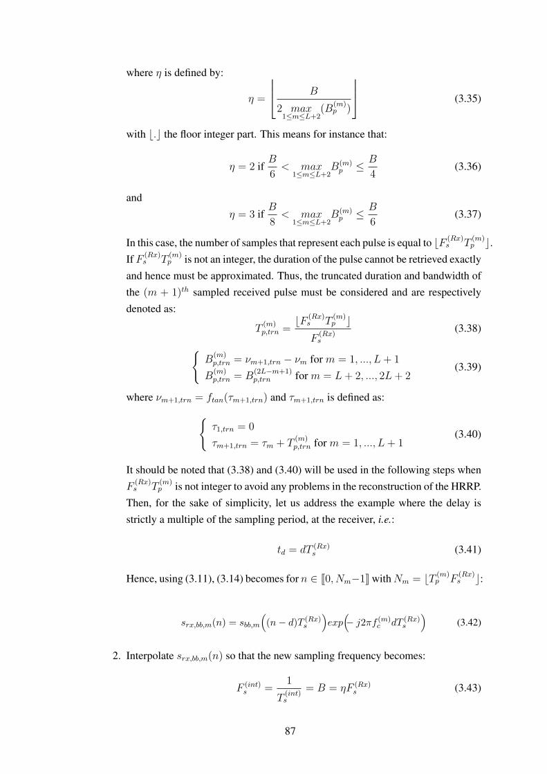
where η is defined by:

η =

B

2 max1≤m≤L+2

(B(m)p )

(3.35)

with b.c the floor integer part. This means for instance that:

η = 2 ifB

6< max

1≤m≤L+2B(m)p ≤ B

4(3.36)

andη = 3 if

B

8< max

1≤m≤L+2B(m)p ≤ B

6(3.37)

In this case, the number of samples that represent each pulse is equal to bF (Rx)s T

(m)p c.

If F (Rx)s T

(m)p is not an integer, the duration of the pulse cannot be retrieved exactly

and hence must be approximated. Thus, the truncated duration and bandwidth ofthe (m + 1)th sampled received pulse must be considered and are respectivelydenoted as:

T(m)p,trn =

bF (Rx)s T

(m)p c

F(Rx)s

(3.38)B

(m)p,trn = νm+1,trn − νm for m = 1, ..., L+ 1

B(m)p,trn = B

(2L−m+1)p,trn for m = L+ 2, ..., 2L+ 2

(3.39)

where νm+1,trn = ftan(τm+1,trn) and τm+1,trn is defined as:τ1,trn = 0

τm+1,trn = τm + T(m)p,trn for m = 1, ..., L+ 1

(3.40)

It should be noted that (3.38) and (3.40) will be used in the following steps whenF

(Rx)s T

(m)p is not integer to avoid any problems in the reconstruction of the HRRP.

Then, for the sake of simplicity, let us address the example where the delay isstrictly a multiple of the sampling period, at the receiver, i.e.:

td = dT (Rx)s (3.41)

Hence, using (3.11), (3.14) becomes for n ∈ J0, Nm−1K withNm = bT (m)p F

(Rx)s c:

srx,bb,m(n) = sbb,m

((n− d)T (Rx)

s

)exp(− j2πf (m)

c dT (Rx)s

)(3.42)

2. Interpolate srx,bb,m(n) so that the new sampling frequency becomes:

F (int)s =

1

T(int)s

= B = ηF (Rx)s (3.43)

87

This can be done either in the time domain or in the frequency domain1. Theresulting signals is denoted sintrx,bb,m(n) for n ∈ J0, ηNm − 1K. Sampling at F (Rx)

s

and then interpolating the received signal instead of directly sampling it at thesampling frequency B makes it possible to use a cheap ADC.Remark: For a proper interpolation of srx,bb,n(n), Nm should be greater than 2.Thus, the minimum duration between any two consecutive time instants shouldbe greater than a threshold ε. For any m ∈ J1, L+ 1K, this leads to:

T(m)p,trn ≥ T (m)

p ≥ ε =2

F(Rx)s

(3.44)

3. Frequency shift each pulse to its proper position so that it occupies a frequencyband shifted by−B/2 Hz compared with its corresponding one in the PW-NLFMwaveform shown in Fig. 3.2. This is done by multiplying each pulse by the properexponential factor as follows:

sint,fshiftrx,bb,m (n) = sintrx,bb,m(n)exp(j2π∆f (m)nT ints

)(3.45)

where ∆f (m) is defined in (3.1). When F (Rx)s T

(m)p is not integer, ∆f (m) satisfies:

∆f (1) = −B2 +

B(1)p,trn

2

∆f (m) = −B2 +

∑m−1l=1 B

(l)p,trn +

B(m)p,trn

2

for m = 2, . . . , Np

(3.46)

4. Time shift the result obtained for each pulse in (3.45) by δtm defined in (3.22).When F (Rx)

s T(m)p is not integer, δtm now satisfies:

δtm = (2L+ 3−m)Tr + Tp + τm,trn − τ2L+2 + Tw (3.47)

5. Add a phase correction term to each pulse to avoid any phase discontinuity inthe reconstructed PW-NLFM waveform. It is done by multiplying (3.45) with anappropriate exponential term, as follows:

sint,fshift,pcrx,bb,,m (n) = sint,fshiftrx,bb,m (n)exp(j2πum) (3.48)

1In the time domain, the signal is upsampled by a factor equal to η and then interpolated by using alow-pass finite-impulse response (FIR) filter. Polyphase filters are often considered. As for the frequencydomain, the discrete Fourier transform (DFT) of srx,bb,m is decomposed into two parts. Zeros are thenintroduced in between to obtain a sequence of length ητm. Then the real part of the inverse DFT iscomputed.[2]

88

where um is defined in (3.33). When F (Rx)s T

(m)p is not integer, um satisfies:

u1 = 0

um = um−1 − γ(m)

2

(T(m−1)p,trn − T

(m)p

2

)2 − (m− 1)∆f (m)Tr

+γ(m−1)

2

(T (m−1)p

2

)2+∆f (m−1)

((m− 2)Tr + T

(m−1)p,trn

)for 2 ≤ m ≤ 2L+ 2

(3.49)

6. Add the obtained pulses together. Therefore, the reconstructed waveform denotedas sPW−NLFMrx (nT

(int)s − dT

(int)s ), is a delayed discrete baseband version of a

PW-NLFM waveform whose instantaneous frequency is similar to the one givenin Fig. 3.2 but its spectral components are centred around the zero-componentinstead of B/2.

7. Apply a MF in the frequency domain to the reconstructed waveform. It consists inapplying an DFT to sPW−NLFMrx (nT

(int)s −dT (int)

s ) after padding it with ηNm− 1

zeros.Then, multiply the result by SPW−NLFMtx,bb (k) , where

(.)

denotes the conjugate,SPW−NLFMtx,bb (k) is the DFT of sPW−NLFMtx,bb,pad (n). The sequence sPW−NLFMtx,bb,pad (n)is apadded version of sPW−NLFMtx,bb (n)with ηNm − 1 zeros. Thus, the obtained resultcan be written for k ∈ J0, 2ηNm − 2K as:

Z(k) = |SPW−NLFMtx,bb (k)|2exp(− j2π k

2ηNm − 1

2R

c

)(3.50)

8. Produce the HRRP by applying an IDFT to (3.50).

In this section, the processing chain from the transmitter to the receiver has been pre-sented. Nevertheless, the performance are not optimized in terms of PSLR, ISLR, andrange resolution. The latter are mainly related to the selection of the parameters of thewaveform, namely the time instants τmm=2,...,L+1. In the following, we present a wayto choose them by using a genetic algorithm.

3.3 Optimizing the parameters of the VCR SF-LFM waveform

The performance in terms of PSLR, ISLR, and range resolution of the proposed wave-form depend on the set of parameters (τm, νm)m=2,...,L+1. Our purpose is to selectthe parameters that lead to performance the closest to that of the tangent-based NLFMwaveform. As the set of frequencies νmm=2,...,L+2 can be deduced from the set oftime instants τmm=2,...,L+2 by using (3.5), only τmm=2,...,L+1 have to be optimized.For this purpose a multi-objective optimization problem can be considered. It can takeinto account the performance of the processing chain in terms of PSLR, ISLR, and

89

range resolution. This can be done by minimizing a single fitness function that con-sists of a weighted sum of the normalized errors on the PSLR, the ISLR, and the rangeresolution. It is defined as follows:

F (x) = (1− λ1 − λ2)∣∣∣PSLR(x)− PSLRref

PSLRref

∣∣∣ (3.51)

+ λ1

∣∣∣ISLR(x)− ISLRref

ISLRref

∣∣∣+ λ2

∣∣∣Rres(x)−Rres,ref

Rres,ref

∣∣∣where 0 ≤ λ1 ≤ 1 and 0 ≤ λ2 ≤ 1 − λ1 are the weights. x denotes the vector storingthe time instants τmm=2,...,L+1. PSLR(x), ISLR(x), and Rres(x) are respectivelythe PSLR, the ISLR, and the range resolution obtained when using the waveform pa-rameters x. In addition, PSLRref , ISLRref , and Rres,ref are respectively the ISLR,the PSLR, and the range resolution of the tangent-based NLFM waveform.Various optimization algorithms have been proposed to solve optimization problemswhen locating the global optimum is a difficult task. A grid search approach can beused to explore the solution space in order to find the best candidate. Nevertheless, thecomputational cost is high. To alleviate this problem, alternative solutions exist suchas evolutionary algorithms (EAs). The principle is still the same: given a random pop-ulation of candidates selected in the space of solution, new populations are created inorder to explore the space of solutions and evolve towards the candidate that minimizesa beforehand defined fitness function. Several families of approaches have been pro-posed in the literature and used in a wide range of applications: simulated annealing,antcolony algorithms, particle swarm optimization, differential evolution (DE) and ge-netic algorithm (GA) [79] [110]. In this chapter, we focus our attention on this lastalgorithm.

3.3.1 Generalities about genetic algorithm

GA is a stochastic global search-based optimization technique based on the principleof genetics and natural selection [39]. It has been extensively used as search and op-timization tool in many fields and problem domains including sciences, manufacturingand engineering [103] [1].In Fig. 3.6, the different steps of the GA are presented in a flowchart. GA is an iterativeprocess. It starts with an initial population consisting of a certain number of candidates.The relevance of each candidate is evaluated according to a beforehand defined fitnessfunction. Then, new solutions are generated using selection, crossover, and mutationoperators.

1. Selection operator: a selection criterion is applied to select a certain number ofcandidates, each correspond to a vector of parameters, from the population ac-cording to their fitness values. Thus, candidates with the best fitness values have

90

more chance to be selected for crossover and mutation.

2. Crossover operator: it consists in generating new candidates from two selectedcandidates called parents. In the literature, different types of crossover exist suchas single-point, double-point, multi-point, matrix, uniform, etc [107]. In thischapter, we focus on the single-point crossover. It consists in randomly choosinga locus and exchanging the parameters between the parents to create two candi-dates.

3. Mutation operator: the mutation operator is applied individually to each candi-date. It alters each parameter randomly with a probability pM . In this chapter, weuse a specific mutation.

After mutation, a new population that consists of the best candidates is thus created.This process is iterated until convergence.

Fig. 3.6 Evolutionary process of GA

91

3.3.2 Selection of the VCR SF-LFM parameters using GA

In this section, we focus our attention on the way the steps of the GA are implementedwith the proposed waveform when taking into account the fact that there is a constrainton the minimum duration between any two consecutive time instants. See (3.44) insection 3.2.3. In this case, we operate as follows:

• Generation of the initial population: As τ1 = 0 and τL+2 = Tp/2, the initialpopulation is generated so that for m ∈ J1, LK, the time instants satisfy:

τm + ε < τm+1 < Tp/2− (L−m)ε

where ε was introduced in (3.44).As a consequence, the initial population corresponds to a set of Qp vectors of sizeL.

• Selection: It consists in randomly selecting two vectors, namelyCfi = [τ f2 , τ

f3 , ..., τ

fk−1, τ

fk , ..., τ

fL+1] andCm

i = [τm2 , τm3 , ..., τ

mk−1, τ

mk , ..., τ

mL+1] from

the population at the ith generation.

• Crossover: After using the single-point crossover, the resulting candidates, calledchildren, are:

C1 = [τ f2 , τf3 , ..., τ

fk−1, τ

mk , ..., τ

mL+1]

C2 = [τm2 , τm3 , ..., τ

mk−1, τ

fk , ..., τ

fL+1]

The time instants of one of the obtained candidates necessarily respect the con-straint. Thus, if τmk − τ fk−1 > ε, C1 is chosen. Otherwise, C2 is kept. Beforebelonging to the population of candidate vectors at the (i + 1)th iteration, a mu-tation will be done on the choosen child vector.Remark: When L is equal to 1, the above crossover cannot be applied. Therefore,we suggest using a linear crossover. In this case, the child is defined as follows:

C1 =1

2Cfi +

1

2Cmi (3.52)

• Mutation: Let us assume that C1 was chosen by the crossover operator. We sug-gest mutating each element, or equivalently each time instant, of C1 separately ina way that guarantees that the resulting candidate respect the constraint (3.44). Itis done as follows:The mutations on the time instants are done in a successive manner. Let us startwith the first time instant C1(1). A random number r uniformly distributed be-tween 0 and 1 is drawn. If r is smaller than the probability of mutation pM , the

92

mutation leads to the time instant equal to C1(1) + x1, where x1 is a randomnumber that belongs to the interval ]−C1(1)+ ε, C1(2)−C1(1)− ε[. Thus, aftermutating the first time instant, C1 becomes [τ f2 + x1, τ

f2 , ..., τ

fk−1, τ

mk , ..., τ

mL+1].

More generally, for m ∈ J1, LK, the mutation leads to the mth time instant equalto C1(m) + xm where xm ∈]C1(m− 1)− C1(m) + ε, C1(m+ 1)− C1(m)− ε[with C1(0) = 0. If r > pM , the value of the time instant is not changed.

The selection, crossover, and mutation are repeated until L new candidates are created.Then, the best L candidates among the new candidates and those of the ith populationare selected to create the population at the (i+ 1)th generation.

3.4 Results and discussions

In this section, the results obtained using GA are presented. This section is organizedas follows: firstly, the simulation protocol is given. Then, three illustrations are con-sidered. The first one deal with L = 1, the second with L = 2, and the last one withL = 10.

3.4.1 Simulation protocol

In the simulations, we focus on the tangent-based NLFM that has the following param-eters: Tp = 20 µs, β = 1.22 and B = 100 MHz. In addition, the reference measuresthat are considered in the optimization issue are given in Table 3.1. Concerning GA,the size of the population Qp is equal to 200 for L = 1, 2 and 1000 for L = 10. Theprobability of mutation pM is set at 0.1 and ε = 0.12 µs.

Table 3.1 Reference measures taken into account for the optimization issue based onGA.

PSLR (dB) ISLR (dB) Rres (m)-31.2 -25 1.37

3.4.2 Simulation results and comments, L = 1

3.4.2.1 Waveform parameters based on a priori selection and corresponding perfor-mance measures

Without taking into account optimization criteria based on the properties of the HRRP,various a priori approximations of the non-linear function describing the time evolutionof the instantaneous frequency could be considered.Among them, the first method would amount to searching for the time instant τ1 that

93

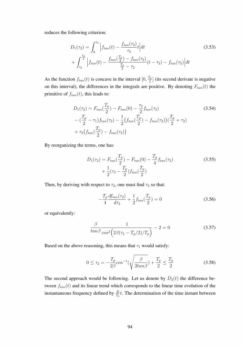
reduces the following criterion:

D1(τ2) =

∫ τ2

0

∣∣∣ftan(t)− ftan(τ2)

τ2t∣∣∣dt (3.53)

+

∫ Tp2

τ2

∣∣∣ftan(t)− ftan(Tp2)− ftan(τ2)

Tp2− τ2

(t− τ2)− ftan(τ2)∣∣∣dt

As the function ftan(t) is concave in the interval [0, Tp2] (its second derivate is negative

on this interval), the differences in the integrals are positive. By denoting Ftan(t) theprimitive of ftan(t), this leads to:

D1(τ2) = Ftan(Tp2)− Ftan(0)−

τ22ftan(τ2) (3.54)

− (Tp2− τ1)ftan(τ2)−

1

2

(ftan(

Tp2)− ftan(τ2)

)(Tp2

+ τ2)

+ τ2(ftan(

Tp2)− ftan(τ2)

)By reorganizing the terms, one has:

D1(τ2) = Ftan(Tp2)− Ftan(0)−

Tp4ftan(τ2) (3.55)

+1

2(τ2 −

Tp2)ftan(

Tp2)

Then, by deriving with respect to τ2, one must find τ2 so that:

−Tp4

dftan(τ2)

dτ2+

1

2ftan(

Tp2) = 0 (3.56)

or equivalently:

β

tanβ

1

cos2(2β(τ2 − Tp/2)/Tp

) − 2 = 0 (3.57)

Based on the above reasoning, this means that τ1 would satisfy:

0 ≤ τ2 = −Tp2βcos−1(

√β

2tanβ) +

Tp2≤ Tp

2(3.58)

The second approach would be following. Let us denote by D2(t) the difference be-tween ftan(t) and its linear trend which corresponds to the linear time evolution of theinstantaneous frequency defined by B

Tpt. The determination of the time instant between

94

0 and Tp2

would amount to find when the derivative of D2(t) is equal to 0, i.e.:

d

dtD2(t) =

B

Tp(β

tanβ

1

cos2(2β(t− Tp/2)/Tp

) − 1) (3.59)

0ne can deduce that D2(t) has its maxima at:

0 ≤ τ2 = −Tp2βcos−1(

√β

tanβ) +

Tp2≤ Tp

2(3.60)

The performance measures obtained with both methods are provided in Table. 3.2. Inaddition, the sampling frequency at the receiver in both cases is equal to 100 MHz.

Table 3.2 Performance measures of the approximated PW-NLFM using one time instantbased on a priori selection.

Method Time instants (µs) PSLR(dB)

ISLR(dB)

Rres(m)

1st meth. basedon (3.58)

τ2=3.1186 -16.3432 -11.8106 1.2377

2nd meth. basedon (3.60)

τ2=1.1612 -16.6322 -12.8179 1.1360

3.4.2.2 Waveform parameters based on the multi-objective criterion deduced by GAand corresponding performance measures: predefined values of the weights

Let us first address the case when the weights are selected as follows: λ1 = 0.4 andλ2 = 0.2. This means that we consider that the PSLR and ISLR has the same level ofimportance and greater than that of Rres.The time instants as well as the PSLR, the ISLR, and the range resolution that havebeen obtained using GA are given in Table.3.3. In addition, the sampling frequencyat the receiver is equal to 100 MHz. Moreover, the time evolution of instantaneousfrequency of the tangent-based waveform as well as the piecewise-linear approximationoptimized by taking into account the criterion (3.51) are provided in Fig.3.7. Finally, thecorresponding HRRP of a stationary target located at R = 8000 m is given in Fig.3.8.

Table 3.3 Performance measures and value of the time instant of the approximatedPW-NLFM when L = 1 and GA are used with λ1 = 0.4 and λ2 = 0.2.

Time instants (µs) PSLR (dB) ISLR (dB) Rres (m)τ2=1.6099 -20.4486 -13.2833 1.1892

95

0 1.6045 5 10 15 18.3955 200

20

50

80

100

time (µs)

Fre

qu

en

cy (

MH

z)

Tangent−based NLFM

Approximated PW−NLFM

Fig. 3.7 Instantaneous frequency of the tangent-based NLFM waveform and the ap-proximated PW-NLFM waveform when L = 1, λ1 = 0.4 and λ2 = 0.2. τ2 = 1.6099µs

7700 7800 7900 8000 8100 8200 8300

10−4

10−2

100

Range (m)

No

rmalized

Lo

gari

thm

ic a

mp

litu

de

Fig. 3.8 HRRP of a stationary target located at R = 8000 when L = 1, λ1 = 0.4 andλ2 = 0.2. τ2 = 1.6099µs

Let us compare the performance measures presented in Table. 3.3 with those given inTable. 3.2. We can notice that the PSLR, the ISLR, and the range resolution are muchsmaller when considering the optimization issue.

3.4.2.3 Waveform parameters based on the multi-objective criterion deduced by GAand corresponding performance measures: any set of weights

Let us now address the case when the weights vary. Thus, λ1 varies between 0.1 and 1,and λ2 varies between 0 and 1− λ1, both with a step equal to 0.1. In Fig. 3.9- 3.12, thetime instant, the PSLR, the ISLR, and the range resolution are respectively presented asfunctions of λ1 and λ2.

96

0.1 0.20.4

0.60.8 0.9 1

0

0.5

1

2

2.5

3

λ1

λ2

τ2

Fig. 3.9 Value of the time instant versus λ1 and λ2

0.1 0.20.4

0.60.8

1

0

0.5

1

−20

−18

−16

λ1

λ2

PS

LR

(d

B)

Fig. 3.10 Value of the PSLR versus λ1 and λ2

0.1 0.20.4

0.60.8 0.9 1

0

0.5

1

−13.2

−13

−12.8

−12.6

λ1

λ2

ISL

R (

dB

)

Fig. 3.11 Value of the ISLR versus λ1 and λ2

Let us look at λ1 = 0.1. In this case, based on (3.51), the performance in terms ofISLR does not necessarily play a key role in the criterion. For values of λ2 smaller than0.4, the time instant τ2 does not change. In addition, the range resolution is the sameand smaller than Rres,ref . When λ2 increases, the time instant and the range resolutionincrease. The latter becomes closer and closer to Rres,ref .Given Fig. 3.10, we can observe that for small values of λ1 and λ2, the PSLR is theclosest one to PSLRref . Indeed, in these cases, the criterion F (x) is mainly defined

97

0.10.4

0.60.8 0.9 1

0

0.5

1

1.2

1.25

1.3

λ1

λ2

Rre

s

Fig. 3.12 Value of the range resolution versus λ1 and λ2

by the normalized difference on the PSLR. When the sum of λ1 and λ2 becomes closerto 1, F (x) is mainly defined by the normalized differences on the ISLR and the rangeresolution and one can notice that the PSLR increases. For instance, for λ1 = 0.1. andλ2 < 0.6, the PSLR remains unchanged. When λ1 increases, the PSLR increases. Theperformance measures presented in Fig. 3.9-3.12 make it possible to define the Paretofront for the multi-objective optimization issue. Moreover, based on the time instantspresented in Fig.3.9, the sampling frequency at the receiver is equal to 100 MHz for anyset of weights.When comparing the values of the PSLR, the ISLR and the range resolution we obtainwith the performance measures of reference, it is true that there is a loss. The latter isprobably due to the strong approximation that is made when only one time instant isused. Thus, increasing L should reduce it. For this reason, in the next section, L = 2 isconsidered.


The same methodology as above is considered.

3.4.3.1 Waveform parameters based on the multi-objective criterion deduced by GAand corresponding performance measures: predefined weights

The weights are still selected as follows: λ1 = 0.4 and λ2 = 0.2. The results arepresented in Table. 3.4 and Fig.3.13.

Table 3.4 Performance measures and the values of the time instants of the approximatedPW-NLFM when L = 2.

Time instants (µs) PSLR (dB) ISLR (dB) Rres (m)τ2=2.2970; τ3=5.0211 -24.7427 -16.0011 1.3107

98

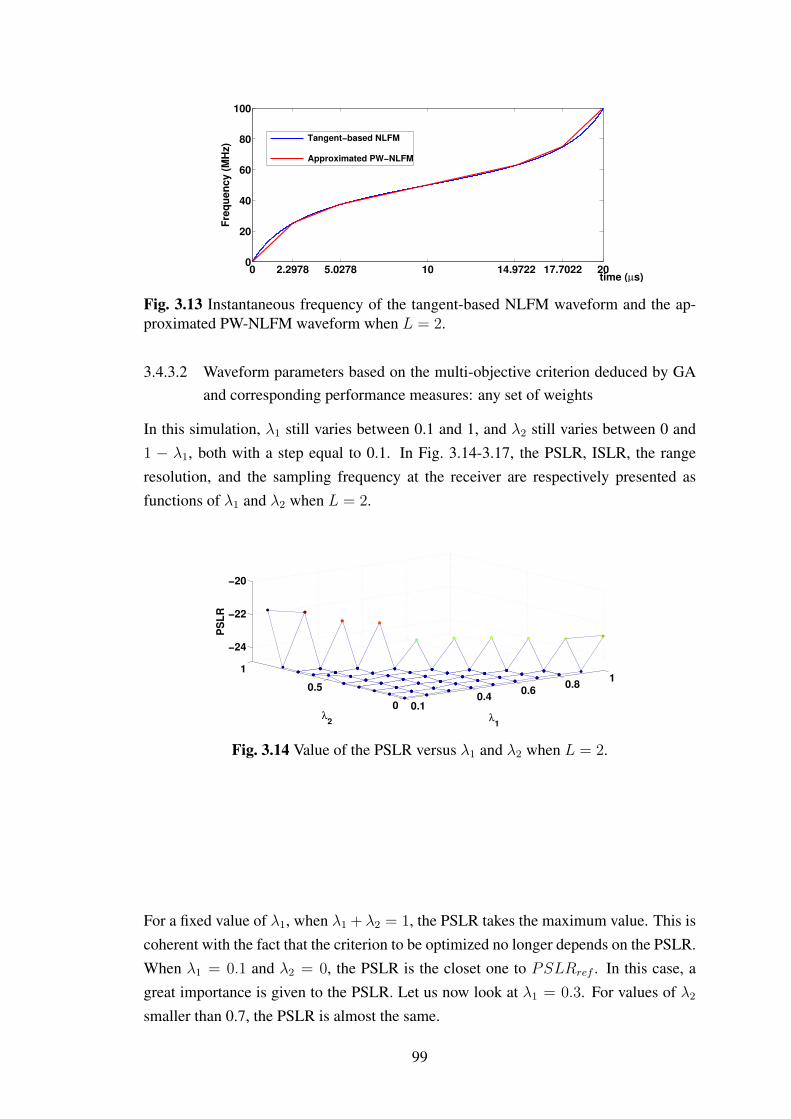
0 2.2978 5.0278 10 14.9722 17.7022 200

20

40

60

80

100

time (µs)

Fre

qu

en

cy (

MH

z)

Tangent−based NLFM


Fig. 3.13 Instantaneous frequency of the tangent-based NLFM waveform and the ap-proximated PW-NLFM waveform when L = 2.

3.4.3.2 Waveform parameters based on the multi-objective criterion deduced by GAand corresponding performance measures: any set of weights

In this simulation, λ1 still varies between 0.1 and 1, and λ2 still varies between 0 and1 − λ1, both with a step equal to 0.1. In Fig. 3.14-3.17, the PSLR, ISLR, the rangeresolution, and the sampling frequency at the receiver are respectively presented asfunctions of λ1 and λ2 when L = 2.

0.10.4

0.60.8

1

0

0.5

1

−24

−22

−20

λ1

λ2

PS

LR

Fig. 3.14 Value of the PSLR versus λ1 and λ2 when L = 2.

For a fixed value of λ1, when λ1 + λ2 = 1, the PSLR takes the maximum value. This iscoherent with the fact that the criterion to be optimized no longer depends on the PSLR.When λ1 = 0.1 and λ2 = 0, the PSLR is the closet one to PSLRref . In this case, agreat importance is given to the PSLR. Let us now look at λ1 = 0.3. For values of λ2smaller than 0.7, the PSLR is almost the same.

99

0.20.4

0.60.8

1

00.2

0.40.6

0.81

−16

−15.8

−15.6

λ1λ

2

ISL

R

Fig. 3.15 Value of the ISLR versus λ1 and λ2 when L = 2

0.10.4

0.60.8

1

0

0.5

1

1.35

1.4

1.45

1.5

λ1

λ2

Rre

s

Fig. 3.16 Value of the range resolution versus λ1 and λ2 when L = 2

0.20.4

0.60.8

1

0

0.5

15

10x 10

7

λ1

λ2

Sam

plin

g f

req

uen

cy

Fig. 3.17 Value of the sampling frequency versus λ1 and λ2 when L = 2

Given Fig. 3.15, the ISLR takes the maximum value when λ1 = 0.1 and λ2 = 0.9 andthe minimum value when λ1 = 1 and λ2 = 0.According to Fig. 3.17, the sampling frequency at the receiver depends on λ1 and λ2. Ittakes two distinct values: 50 MHz and 100 MHz.As a conclusion, when L increases to 2, the performance measures become more closerto the reference ones. Moreover, the sampling frequency at the receiver could be re-duced.We may a priori imagine that increasing the number of instants more and more shouldlead to better performance measures and a smaller sampling frequency at the receiver.

100

For this reason, in the following section, we suggest optimizing the waveform parame-ters when L = 10.


In this section, the waveform parameters when L = 10 are optimized by using GA forλ1 = 0.4 and λ1 = 0.2. In this case, Qp is equal to 1000. The results are presented inTable. 3.5 and Fig. 3.18. Based on the time instants provided in Table. 3.5, the samplingfrequency that should be used is equal to 33.3333 MHz.Given Table. 3.5, we can observe that the normalized differences on the PSLR and therange resolution are approximately equal to zero. As for the normalized difference onthe ISLR, it is equal to 0.1171.

Table 3.5 Performance measures and the values of the time instants of the approximatedPW-NLFM when L = 10.

Time instants (µs) PSLR(dB) ISLR(dB) Rres(m)τ1=0.7658;τ2=2.2058τ3=3.2628;τ4 = 4.2901τ5 = 5.4037;τ6 = 6.2491τ7 = 7.2719;τ8 = 8.7119τ9 = 9.3766;τ10 = 9.5402

-31.2 -22.0713 1.3816

0 10 200

20

40

60

80

100

time (µs)

Fre

qu

en

cy (

MH

z) Tangent−based NLFM


Fig. 3.18 Instantaneous frequency of the tangent-based NLFM waveform and the ap-proximated PW-NLFM waveform when L = 10, λ1 = 0.4 and λ2 = 0.2.

3.4.5 General comments on the results

In this section, we aim at giving some comments on the number of time instants, i.e.,the number of pulses within the CPI, that could be selected by the practitioner.According to the obtained results, two conclusions can be drawn:

101

• For a fixed number of time instants, the sampling frequency, the time instants,and the performance measures vary with the weights used in the multi-objectivecriterion

• Increasing the number of time instants leads to performances closer to the refer-ence ones and reduces the sampling frequency at the receiver.

In practice, the CPI is limited by several factors. They depend on the application of theradar. For instance, in radar target classification, the CPI is limited by the speed of thetarget. In scenarios where the speed of target is fast, the dwell time2 is small and thusonly a small number of time instants can be used. On the contrary, in scenarios wherethe speed of target is small or moderate, a larger number of time instants can be used.Therefore, a trade-off exists between the number of time instants on the one hand, andthe performance measures and the sampling frequency on the other hand.

3.5 Conclusions

In this chapter, a processing chain, from the transmitter to the receiver, of the VCRSF-LFM waveform is proposed. It is based on a piecewise linear approximation ofthe NLFM waveform and a generalized version of the TD algorithm. Our goal is toproduce an HRRP whose features are as close as possible as the ones of the HRRP of awideband NLFM waveform. To this end, the parameters defining the piecewise linearapproximation of the NLFM waveform are selected by considering a multi-objectiveoptimization problem taking into account the performance of the waveform in terms ofPSLR, ISLR and range resolution. More particularly, the criterion to be minimized isa linear combination of three normalized differences. For a given set of weights, theset of parameters is obtained by using a genetic algorithm. Although a tangent-basedNLFM is used, the proposed methodology can be applied to any NLFM waveform. Thesimulation results reveal that the performance of the resulting waveforms varies withthe weights used in the multi-objective criterion and the number of LFM pulses that isconsidered.

2It is the time that an antenna beam spends on a target. It can correspond to the duration of one CPIor more CPIs.

102

CHAPTER 4

Conclusions and perspectives

In this thesis, our purpose was to design different processing chains dedicated to highrange resolution radar waveforms:

1. A processing chain from the transmitter to the receiver has been proposed toovercome the drawbacks of the standard combination of SF waveform with ei-ther a PC or an NLFM waveform. It consists in splitting the spectrum of a PCor NLFM pulse into a predetermined number of portions, then transmitting thecorresponding time-domain signals. At the receiver, the modified FD and theTWR algorithms are proposed to process the received echoes. In this processingchain, we have also added one degree of freedom related to the pseudo-randomtransmission way to prevent the opponent signal analyzer from reconstructing thetransmitted waveform correctly.A comparative study was done between the different variants that can be con-sidered. For the proposed SFPC and SF-NLFM waveforms, the TWR algorithmoutperforms the modified FD algorithm in some cases using a certain number ofportions. This comes at the expense of an additional computational cost. In addi-tion, the quality of reconstruction of the power spectrum is no longer good whenNp is large. Moreover, a comparative study has been done between the proposedand the traditional SFPC and SF-NLFM waveforms. On the one hand, we haveshown that the performance of the proposed SFPC in terms of PSLR and ISLRobtained with either the modified FD or the TWR algorithm is better than thatobtained with the traditional SFPC waveform. The latter is processed by the stateof the art algorithms namely, IFFT and FD algorithms.On the other hand, we noticed that the proposed SF-NLFM waveform avoidsproducing grating lobes that usually appears when the traditional SF-NLFM isprocessed with the MF. As a consequence, they have the potential to detect smalltargets in the presence of large targets. This has been illustrated by conductingsome simulations using scenarios representative of real cases. This distinguish-able feature is attractive from a practical point of view.

103

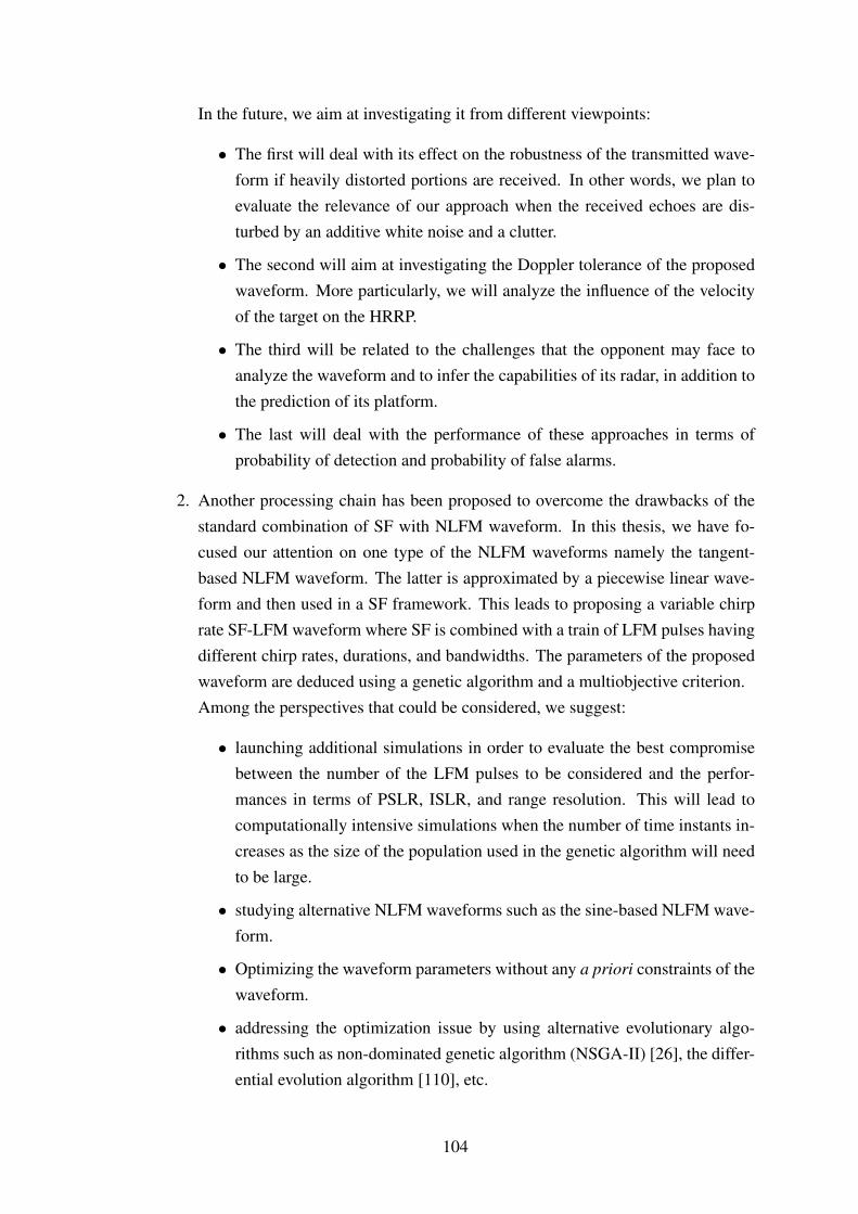
In the future, we aim at investigating it from different viewpoints:

• The first will deal with its effect on the robustness of the transmitted wave-form if heavily distorted portions are received. In other words, we plan toevaluate the relevance of our approach when the received echoes are dis-turbed by an additive white noise and a clutter.

• The second will aim at investigating the Doppler tolerance of the proposedwaveform. More particularly, we will analyze the influence of the velocityof the target on the HRRP.

• The third will be related to the challenges that the opponent may face toanalyze the waveform and to infer the capabilities of its radar, in addition tothe prediction of its platform.

• The last will deal with the performance of these approaches in terms ofprobability of detection and probability of false alarms.

2. Another processing chain has been proposed to overcome the drawbacks of thestandard combination of SF with NLFM waveform. In this thesis, we have fo-cused our attention on one type of the NLFM waveforms namely the tangent-based NLFM waveform. The latter is approximated by a piecewise linear wave-form and then used in a SF framework. This leads to proposing a variable chirprate SF-LFM waveform where SF is combined with a train of LFM pulses havingdifferent chirp rates, durations, and bandwidths. The parameters of the proposedwaveform are deduced using a genetic algorithm and a multiobjective criterion.Among the perspectives that could be considered, we suggest:

• launching additional simulations in order to evaluate the best compromisebetween the number of the LFM pulses to be considered and the perfor-mances in terms of PSLR, ISLR, and range resolution. This will lead tocomputationally intensive simulations when the number of time instants in-creases as the size of the population used in the genetic algorithm will needto be large.

• studying alternative NLFM waveforms such as the sine-based NLFM wave-form.

• Optimizing the waveform parameters without any a priori constraints of thewaveform.

• addressing the optimization issue by using alternative evolutionary algo-rithms such as non-dominated genetic algorithm (NSGA-II) [26], the differ-ential evolution algorithm [110], etc.

104

REFERENCES

[1] Y. Li Y. Chin A. Saldivar, C. Goh and H. Yu. Identifying smart design attributesfor industry 4.0 customization using a clustering genetic algorithm. 22nd Inter-

national Conference on Automation and Computing (ICAC), Octobe 2016.

[2] W. E. Alexandar and C. M.Williams. Digital Signal Processing: Principles, Al-

gorithms and System Design. John Wiley and Sons, Inc., Hoboken, New Jersey,NC,USA, 2016.

[3] S. Alphonse and G. A. Williamson. Novel radar signal models using nonlinearfrequency modulation. Proceedings of the 22nd European Signal Processing

Conference (EUSIPCO), pages 1024–1028, September 2014.

[4] D. A. Ausherman, J. L. Walker A. Kozma, H. M. Jones, and E. C. Poggio. De-velopments in radar imaging. IEEE Transactions on Aerospace and Electronic

Systems, 20 (4):363–400, July 1984.

[5] Y. Bar-Shalom, X. R. Li, and T. Kirubarajan. Estimation With Applications To

Tracking and Navigation. Wiley, Hoboken, NJ, USA, 2001.

[6] M. Basseville. Distance measures for signal processing and pattern recognition.Signal Processing, 18 (4):349–369, 1988.

[7] M. Basseville. Divergence measures for statistical data processing. an annotatedbibliography. Signal Processing, 93 (4):621–633, 2013.

[8] A. Bhattacharyya. On a measure of divergence between two statistical popula-tions defined by their probability distributions. Bulletin of the Calcutta Mathe-

matical Society, 35:99–109, 1943.

[9] W. Bobillet, R. Diversi, E. Grivel, R. Guidorzi, M. Najim, and U. Soverini.Speech enhancement combining optimal smoothing and errors-in-variables iden-tification of noisy AR processes. IEEE Transactions on Signal Processing,55:5564–5578, December 2007.

[10] L. Bombrun, N-E. Lasmar, Y. Berthoumieu, and G. Verdoolaege. Multivariatetexture retrieval using the SIRV representation and the geodesic distance. IEEE

ICASSP, pages 865–868, 2011.

105

[11] P. Borwein and R. Ferguson. Polyphase sequences with low autocorrelation.IEEE Transactions on Information Theory, 51 (4):15641567, April 2005.

[12] G. Box and G. Jenkins. Time Series Analysis, Forecasting, and Control. HoldenDay, San Francisco, 2008.

[13] K. C. Teh C. Gao and A. Liu. Piecewise nonlinear frequency modulation wave-form for mimo radar. IEEE Journal of Selected Topics in Signal Processing, 11(2):379 – 390, Octobor 2016.

[14] B. Cernuschi-Frias. A derivation of the gohberg-semencul relation [signal anal-ysis]. IEEE Transactions on Signal Processing, 39 (1):190–192, 1991.

[15] H. Chernoff. Measure of asymptotic efficiency for tests of a hypothesis based onthe sum of observations. Annals of Mathematical Statistics, 23:493–507, 1952.

[16] Y-W. Cheung. Long memory in foreign-exchange rates. Journal of Business and

Economic Statistic, 11:93–101, 1993.

[17] M. Y. Chua, V. C. Koo, H. S. Lim, and J . T. S Somantyo. Phase coded steppedfrequency linear frequency modulated waveform synthesis technique for low al-titude ultra wideband synthetic aperture radar. IEEE Access, 5:11391–11403,2017.

[18] M. N. Cohen, M. R. Fox, and J. M. Baden. Minimum peak sidelobe pulse com-pression codes. Proceedings of IEEE International Radar Conference, pages633–638, 1990.

[19] T. Collins. Active sonar pulse designs. PhD, University of Birmingham, 1996.

[20] P. Colwell. Blaschke products: bounded analytical functions. University ofMichigan Press, 1985.

[21] J.E. Contreras-Reyes. Analyzing fish condition factor index through skew-gaussian information theory quantifiers. Fluctuation and Noise Letters, 15 (2):1–16, 2016.

[22] J.E. Contreras-Reyes and R.B.Arellano-Valle. Kullbackleibler divergence mea-sure for multivariate skew-normal distributions. Entropy, 14 (9):1606–1626,2012.

[23] C. E. Cook and M. Bernfeld. Radar Signals, An Introduction to Theory and

Application. Artech House, 1993.

106

[24] G. E. Coxson and J. Russo. Efficient exhaustive search for optimal-peak-sidelobebinary codes. IEEE Transactions on Aerospace and Electronic Systems, 41:302–308, 2005.

[25] H. E. Daniels. The approximated distribution of serial correlation coefficients.Biometrika, 43:169–185, June 1956.

[26] K. Deb, A. Pratap, S. Agarwal, and T. Meyarivan. A fast and elitist multiobjectivegenetic algorithm: Nsga-ii. IEEE Transactions on Evolutionary computation, 6(2):182–197, 2002.

[27] R. Diversi, R. Guidorzi, and U. Soverini. Identification of autoregressive modelsin the presence of additive noise. Int. J. Adapt. Control Signal Process, 22:465–481, 2008.

[28] T. Van Erven and P. Harremos. Renyi divergence and Kullback-Leibler diver-gence. IEEE Transactions on Information Theory, 60 (7):3797–3820, 2014.

[29] H. Golub F. Van Loan. Matrix Computations. The Johns Hopkins UniversityPress, 1996.

[30] R. L. Frank and S. A. Zadoff. Phase shift pulse codes with good periodic cor-relation properties. IEEE Transactions on Aerospace and Electronic Systems, 8(6):381–382, 1962.

[31] M. Friese. Polyphase Barker sequences up to length 36. IEEE Transactions on

Information Theory, 42 (4):1248 – 1250, July 1996.

[32] G. Galati and G. Pavan. Waveforms design for modern and mimo radar. IEEE

EUROCON, pages 508–513, 2013.

[33] G. Galati, G. Pavan, and F. DePalo. Chirp signals and noisy waveforms for solid-state surveillance radars. MDPI Aerospace, 4 (2):., March 2017.

[34] Z. Ge, P. Huang, and W. Lu. Matched NLFM pulse compression method withultra-low sidelobes. In Proceedings of the 5th European Radar Conference, page92 95, October 2008.

[35] T. T. Georgiou and A. Lindquist. A convex optimization approach to arma mod-eling. IEEE Transactions on Automatic Control, 53 (5):1108–1119, 2008.

[36] J. Geweke and S. Porter-Hudak. The estimation and application of long-memorytime series models. Journal Of time series analysis, 4:221–238, 1983.

107

[37] I. Gladkova and D. Chebanov. Grating lobes suppression in stepped-frequencypulse train. IEEE Transactions on Aerospace and Electronic Systems, 44:1265 –1275, September 2008.

[38] A. R. Gladston, P. Vijayalakshmi, and N. Thangavelu. Improving speech intel-ligibility in Cochlear implants using Vocoder-centric acoustic models. Recent

Trends in Information Technology, pages 66–71, 2012.

[39] D. E. Goldberg. Genetic Algorithms in Search, Optimization and Machine Learn-

ing. Addison-Wesley Longman, Boston, MA, USA, 1989.

[40] I. S. Gradshteyn and I. M. Ryzhik. Table of Integrals, Series, and Products.Academic Press, 1943.

[41] C. W. J. Granger and R. Joyeux. An introduction to long-memory time seriesmodels and fractional differencing. Journal Of time series analysis, 1 (1):15–29,1980.

[42] R-M. Gray. Toeplitz and circulant matrices: a review. Foundations and trends in

communications and information theory, 2 (3):155–239, 2006.

[43] H. D. Griffiths and L. Vinagre. Design of low-sidelobe pulse compression wave-forms. Electronic letters, 30 (12):1004–1005, June 1994.

[44] E. Grivel and L. Legrand. Process comparison combining signal power ratio andJeffrey’s divergence between unit-power signals. GSI, Lecture Notes in Com-

puter Science series, 10589:532–540, 2017.

[45] W. D. Jiang H. Y. Chen, Y. X. liu and G. R. Guo. A new approach for synthesiz-ing the range profile of moving targets via stepped-frequency waveforms. IEEE

Geoscience and Remote Sensing Letters, 3 (3):406–409, July 2006.

[46] X. He, N. Tong, and X. Hu. Dynamic ISAR imaging of maneuvering targetsbased on sparse matrix recovery. Elsevier Signal Processing, 134:123 – 129,April 2017.

[47] X. He, N. Tong, and X. Hu. High-resolution imaging and 3-D reconstruc-tion of precession targets by exploiting sparse apertures. IEEE Transactions on

Aerospace and Electronic Systems, 53 (3):1212 – 1220, April 2017.

[48] E. Hellinger. Neue begrndung der theorie quadratischer formen von un-endlichvielen vernderlichen (in german). Journal fur die reine und angewandte

Mathematik, 136:210–271, 1909.

108

[49] F. Enache I-C . Vizitiu and F. Popescu. Sidelobe reduction in pulse-compressionradar using the stationary phase technique: An extended comparative study. 2014

International Conference on Optimization of Electrical and Electronic Equip-

ment (OPTIM), 2014.

[50] A. Inoue. Asymptic behaviour for partial autocorrelation functions of fractionnalarima processes. The Annals of Applied Probability, 12:1471–1491, April 2002.

[51] H. Jeffreys. Theory of probability. Oxford university press, United States, 1961.

[52] S. M. Kay. Fundamentals of Statistical Signal Processing, Vol. II: Detection

Theory. Prentice Hall, 1998.

[53] A. M. Kerdock, R. Mayer, and D. Bass. Longest binary pulse compression codeswith given peak sidelobe levels. Proceedings of the IEEE, 74 (2):366–368, 1986.

[54] P. S. Kozoszka and M. S. Taqqu. Fractional ARIMA for stable innovations.Stochastic processes and their applications, 60:19–47, 1995.

[55] S. Kullback and R. A. Leibler. On Information and Sufficiency. The Annals of

Mathematical Statistics, 22 (1):79–86, 1951.

[56] A. Laforgia and P. Natalini. On the asymptotic expansion of a ratio of gammafunctions. Journal of Mathematical Analysis and Applications, 389 (2):833–837,2012.

[57] L. Legrand and E. Grivel. Jeffrey’s divergence between moving-average andautoregressive models. IEEE ICASSP, 2017.

[58] L. Legrand and E. Grivel. Jeffrey’s divergence between moving-average modelsthat are real or complex, noise-free or disturbed by additive white noises. Elsevier

Signal Processing, 131:350–363, 2017.

[59] G. Lellouch, A. K. Michra, and M. Inggs. Design of OFDM radar pulses us-ing genetic algorithm based techniques. IEEE Transactions on Aerospace and

Electronic Systems, 52 (4):1953–1966, September 2016.

[60] B. L. Lewis and F. F. Kretschmer. A new class of polyphase pulse compressioncodes and techniques. IEEE Transactions on Aerospace and Electronic Systems,17 (3):364–372, 1981.

[61] B. L. Lewis and F. F. Kretschmer. Linear frequency modulation derivedpolyphase pulse compression codes. IEEE Transactions on Aerospace and Elec-

tronic Systems, 18 (5):637–641, 1982.

109

[62] T. Li, H. Yang, , and Z. Zhou. RFI suppression based on phase-coded stepped-frequency waveform in through-wall radars. IEEE Transactions on Geoscience

and Remote Sensing, 53:1583–1591, March 2015.

[63] X. R. Li and V. P. Jilkov. Survey of maneuvering target tracking. part v: Mul-tiple model methods. IEEE Transactions on Aerospace and Electronic Systems,41:1255–1321, 2005.

[64] F. Liese and I. Vajdal. On divergences and informations in statistics and infor-mation theory. IEEE Transactions on Information Theory, 52 (10):4394–4412,2006.

[65] J. Lindner. Binary sequences up to length 40 with best possible autocorrelationfunction. Electronic Letters, 11 (21):507, December 1975.

[66] R. Liu and Y. Wang. Imaging approach for airborne stepped-frequency syntheticaperture radar in the squinted mode. Journal of applied remote sensing, 11 (1):1–15, 2017.

[67] R. T. Lord. Aspects of stepped-frequency processing for low-frequency SAR sys-

tems. PhD thesis, University of Cape Town, Department of Electrical Engineer-ing, 2000.

[68] R. T. Lord and M. R. Inggs. High resolution SAR processing using steppedfrequencies. IEEE, Geoscience and Remote Sensing, IGARSS, pages 490–492,1997.

[69] X. luo, Y. Deng, R. Wang, and W. Guo. Imaging for MIMO sliding spotlightSAR using stepped frequency chirps. EUSAR, 10th European Conference on

Synthetic Aperture Radar, pages 221–224, 2014.

[70] Y. Luo, Q. Zhang, C. W. Qiu, X. J. Liang, and K. M. Li. Micro-Doppler effectanalysis and feature extraction in ISAR imaging with stepped-frequency chirpsignals. IEEE Transactions on Geoscience and Remote Sensing, 48 (4):2087–2098, April 2010.

[71] C. Magnant, A. Giremus, and E. Grivel. Jeffreys divergence between state mod-els: Application to target tracking using multiple models. EUSIPCO, pages 1–5,2013.

[72] C. Magnant, A. Giremus, and E. Grivel. On computing Jeffrey’s divergencebetween time-varying autoregressive models. IEEE Signal Processing Letters,22 (7):915–919, 2014.

110

[73] C. Magnant, E. Grivel, A. Giremus, B. Joseph, and L. Ratton. Jeffrey’s diver-gence for state-space model comparison. Signal Processing, 114:61–74, Septem-ber 2015.

[74] C. Magnant, E. Grivel, A. Giremus, L. Ratton, and B. Joseph. Classifying autore-gressive models using dissimilarity measures: A comparative study. EUSIPCO,pages 998–1002, 2015.

[75] A. De Maio, S. De Nicola, Y. Huang, L. Zhi-Quan, and S. Zhang. Designof phase codes for radar performance optimization with a similarity constraint.IEEE Transactions on Signal Processing, 57 (2):610–621, 2009.

[76] E. Mazor, A. Averbuch, Y. Bar-Shalom, and J. Dayan. Interacting multiple modelmethods in target tracking: A survey. IEEE Transactions on Aerospace and

Electronic Systems, 34:103–123, 1998.

[77] W. L. Melvin and J. A. Scheer. Principles of modern radar, Vol. II: Advanced

techniques. SciTech Publishing, 2013.

[78] R. Murthy, I. Pavlidis, and P. Tsiamyrtzis. Touchless monitoring of breathingfunction. IEEE EMBS, pages 1196–1199, 2004.

[79] R. Mallipeddi N. H. Awad, M. Z. Ali and P. N. Suganthan. An improved differ-ential evolution algorithm using efficient adapted surrogate model for numericaloptimization. Elsevier, Information sciences, pages 326–347, 2018.

[80] M. Najim. Modeling, estimation and optimal filtering in signal processing. Wi-ley, 2010.

[81] W. Nel, J. Tait, R. T. Lord, and A. Wilkinson. The use of frequency domainstepped frequency technique to obtain high range resolution on the CSIR X-BandSAR system. IEEE AFRICON, 2002.

[82] S. Noschese, L. Pasquini, and L. Reichel. Tridiagonal Toeplitz matrices: prop-erties and novel applications. Numerical Linear Algebra with Applications, 20(2):302–326, March 2013.

[83] C. J. Nunn and G. E. Coxson. Polyphase pulse compression codes with optimalpeak and integrated sidelobes. IEEE Transactions on Aerospace and Electronic

Systems, 45 (2):775 – 781, July 2009.

[84] S.-M. Omar, F. Kassem, R. Mitri, M. Saleh, and H. Hijazi. A novel barker codealgorithm for resolving range ambiguity in high PRF radars. Proceedings of the

12th European Radar Conference (EuRAD), pages 81–84, 2015.

111

[85] P. E. Pace. Detecting and Classifying Low Probability of Intercept Radar. Pren-tice Hall, Artech House, 2003.

[86] W. Palma. Long-Memory Time Series, Theory and Methods. Wiley series inprobability and statistics, 2007.

[87] K. Pearson. On the criterion that a given system of deviations from the proba-ble in the case of a correlated system of variables is such that it can reasonablybe supposed to have arisen from random sampling. Philosophical Magazine, 5(50):157–175, 1900.

[88] C. K. Peng, S. V. Buldyrev, S. Havlin, M. Simons, H.E. Stanley, and A.L.Goldberger. Mosaic organization of DNA nucleotides. Physical Review E, 49,(2):1685–1689, 1994.

[89] A.I. D. Polyanin and A. V. Manzhiron. Handbook of Mathematics for Engineers

and Scientists. Chapman and Hall CRC, 2007.

[90] A. A. Pranata, G. W. Adhane, and D. S. Kim. Detrended fluctuation analysis onECG device for home environment. 14th IEEE Annual Consumer Communica-

tions and Networking Conference (CCNC), pages 4233–4236, 2017.

[91] C. Rao. Information and the accuracy attainable in the estimation of statistical

parameters, volume 37, pages 81–89. Bull. Calcutta Math. Soc., 1945.

[92] C. E. Rasmussen and C. K. I. Williams. Gaussian processes for machine learn-

ing. MIT Press, 2006.

[93] A. G. Ravelo-Garcia, U. Casanova-Blancas, S. Martin-Gonzalez, E. Hernandez-Perez, I. Guerra-Moreno, P. Quintana-Morales, N. Wessel, and J. L. Navarro-Mesa. An approach to the enhancement of sleep apnea detection by means ofdetrended fluctuation analysis of RR intervals. Computing in Cardiology, pages905–908, 2014.

[94] A. Renyi. On measures of entropy and information. Fourth Berkeley Symposium

on Mathematical Statistics and Probability, Bulletin of the Calcutta Mathemati-

cal Society, 1:547–561, 1961.

[95] M. A. Richards, J. A. Scheer, and W. A. Holm. Principles of modern radar, Vol.

I: Advanced techniques. SciTech Publishing, 2010.

[96] M. A. Riley, S. Bonnette, N. Kuznetsov, S. Wallot, and J. Gao. A tutorial intro-duction to adaptive fractal analysis. Frontiers in Physiology, 3 (371), 2012.

112

[97] T. Rouffet, E. Grivel, P. Vallet, C. Enderli, and S. Kemkemian. Combining twophase codes to extend the radar unambiguous range and get a trade-off in termsof performance for any clutter. ICASSP, pages 1822–1826, 2015.

[98] Y. Jiang S. Boukeffa and T. Jiang. Sidelobe reduction with nonlinear frequencymodulated waveforms. 2011 IEEE 7th International Colloquium on Signal Pro-

cessing and its Applications, 2011.

[99] A. De Maio S. Zhang S. De Nicola, Y. Huang and A. Farina. Code optimiza-tion with similarity and accuracy constraints. in Proceedings of the IEEE Radar

Conference, pages 1–6, 2008.

[100] J. Saeedi and K. Faez. Synthetic aperture radar imaging using nonlinear fre-quency modulation signal. IEEE Transactions on Aerospace and Electronic Sys-

tems, 52 (1):99–110, February 2016.

[101] M. Saleh, S.-M.Omar, E. Grivel, and O. Bazzi. A modified stepped frequencyphase coding radar waveform designed for the frequency domain algorithm. Dig-

ital Signal Processing, (88):101–115, May 2019.

[102] S. Sanyal, A. Banerjee, R. Pratihar, A. Kumar Maity, S. Dey, V. Agrawal, R. Sen-gupta, and D. Ghosh. Detrended fluctuation and power spectral analysis of alphaand delta EEG brain rhythms to study music elicited emotion. International

Conference on Signal Processing, Computing and Control (2015 ISPCC), pages206–210, 2015.

[103] C. S.Chin and W. P. Lin. Robust genetic algorithm and fuzzy inference mecha-nism embedded in a sliding-mode controller for an uncertain underwater robot.IEEE/ASME Transactions on Mechatronics, 23 (2):655 – 666, February 2018.

[104] A. Schutz, L.Bombrun, Y. Berthoumieu, and M. Najim. Centroid-based textureclassification using the generalized gamma distribution. EUSIPCO, pages 1–5,2013.

[105] C. E. Shannon. A mathematical theory of communication. Bell system technical

journal, 27, 1948.

[106] Y-H. Shao, G-F. Gu, Z-Q. Jiang, W-X. Zhou, and D. Sornette. Comparing theperformance of FA, DFA and DMA using different synthetic long-range corre-lated time series. Scientific reports, 2 (835):1–5, 2012.

[107] S. N. Sivanandam and S. N. Deepa. Introduction to genetic algorithms. Springer,2008.

113

[108] M. Skolnik. Radar handbook. McGraw-Hill Book Co., United states, 2008.

[109] M. Sowell. Maximum likelihood estimation of stationary univariate fractionallyintegrated time series models. Journal of Econometrics, 53:165–188, 1992.

[110] R. Storn and K. Price. Differential evolution - a simple and efficient adaptivescheme for global optimization over continuous spaces. Journal of Global Opti-

mization, pages 341–359, January 1997.

[111] R. J. Stroeker. Approximations of the eigenvalues of the covariance matrix ofa first-order autoregressive process. Journal of Econometrics, pages 269–279,1983.

[112] R. Sun. Fractional order signal processing: techniques and applications. Thesis

of Master of science in electrical Engineering, Utah state University, 2007.

[113] B. C. Sutradhar and P. Kumar. The inversion of correlation matrix for MA(1)process. Applied Mathematics Letters, 16 (3):317–321, April 2003.

[114] M. Taqqu and V. Teverovsky. On estimating the intensity of long range depen-dence in finite and infinite variance time series. A practical guide to heavy tails:

statistical techniques and applications, pages 177–217, 1996.

[115] C.W. Therrien. Discrete random signals and statistical signal processing. Pren-tice Hall, 1992.

[116] D. R. Wehner. High resolution radar. Artech House, London, UK, 1995.

[117] G. Weinberg. Topics in Radar Signal Processing. IntechOpen, 2018.

[118] A. J. Wilkinson, R. T. Lord, and M. R. Inggs. Stepped-frequency processing byreconstruction of target reflectivity spectrum. Proceedings of the South African

Symposium on Communications and Signal Processing, pages 101–104, Septem-ber 1998.

[119] X. Xu and R. M. Narayanan. Range sidelobe suppression technique for coherentultra wide-band random noise radar imaging. IEEE Transactions on Antennas

and Propagation, 49 (12):1836–1842, 2002.

[120] H. Yuan, S. Wen, and Z. Cheng. Study on I SAR imaging of stepped-frequencychirp signal. Proceedings of the 26th Conference of Spacecraft TTandC Technol-

ogy, 187:197–210, 2012.

[121] W.-C. Yueh. Explicit inverses of several tridiagonal matrices. Applied Mathe-

matics E-Notes, pages 74–83, 2006.

114

[122] P. Huang Z. Ge and W. Lu. Matched NLFM pulse compression method withultra-low sidelobes. In Proceedings of the 5th European Radar Conference,pages 92–95, October 2008.

[123] W. Zhai and Y. Zhang. Application of super-SVA to stepped-chirp radar imag-ing with frequency band gaps between subchirps. Progress in electromagnetics

research B, 30:71–82, 2011.

115

LIST OF PUBLICATIONS

1. E. Grivel, M. Saleh and S. -M. Omar, Jeffreys Divergence between Complex-

Valued Sinusoidal Processes, EUSIPCO 2017.

2. E. Grivel, M. Saleh and S. -M. Omar, Comparing a Complex-Valued Sinusoidal

Process with Autoregressive Process Using Jeffreys Divergence, EUSIPCO 2017.

3. E. Grivel, M. Saleh and S. -M. Omar, Interpreting the asymptotic increment of

Jeffreys Divergence between some random processes, Elsevier Digital Signal Pro-

cessing, (75):120–133, 2017.

4. M. Saleh, E. Grivel and S. -M. Omar, Jeffrey’s Divergence Between Fractionally

Integrated White Noises, Statistical Signal Processing (SSP) 2018.

5. M. Saleh, E. Grivel and S. -M. Omar, Jeffrey’s divergence Between ARFIMA

processes, Elsevier Digital Signal Processing, (82):175–186, 2018.

6. M. Saleh, S. -M. Omar, E. Grivel, and O. Bazzi, A modified stepped frequency

phase coding radar waveform designed for the frequency domain algorithm, El-

sevier Digital Signal Processing, (88):101-115, May 2019.

7. M. Saleh, S. -M. Omar, and E. Grivel, and P. legrand, A variable chirp rate stepped

frequency linear frequency modulation waveform designed for the approximation

of wideband non-Linear radar Waveforms, to be submitted to Elsevier Digital

Signal Processing.

We also plan to submit a paper entitled ”Diversifying the processing chain of the

modified stepped frequency radar waveform combined with pulse compression tech-

niques” to 2020 IEEE radar conference. This paper deals with the TWR algorithm

presented in chapter 2.

116

Appendices

117

Appendix A

JEFFREYS DIVERGENCE FOR PROCESS COMPARISON:Properties, asymptotic analysis, physical interpretation

and way to use it in practical cases

At the very beginning of the collaboration between the University of Bordeaux and theUniversity of Lebanon, presentations of the research activities were organized. The se-lection and comparison of models, as well as the design of parametric signal processingapproaches based on an a priori model drew the attention of both research teams. In ad-dition, applications in mobile communication systems or radar processing were amongsome common applications of interest. Therefore, different works shared by both teamsstarted to be addressed. Among them, properly reconstructing the high-resolution rangeprofile of stepped frequency waveform in the presence of missed data, optimizing theselection of the waveform, modeling the clutter and comparing different types of clutterby comparing their statistics.As for the last issue, the idea was to use divergences. Divergences had been alreadyexploited by the French team to compare motion models and select two or three motionmodels in order to design target tracking based on multiple model approaches [73]. TheFrench team also focused its attention on the asymptotic behavior of the divergences.In information theory, this corresponds to analyze what is called the divergence rate[64]. Various works were conducted on the analysis of Jeffreys divergence between1st-order moving average (MA) processes and 1st-order autoregressive (AR) processes[57]. Although these results were of interest, they were dedicated to very specific sig-nals. Therefore, we decided to address more general cases, i.e. sum of complex expo-nentials disturbed by an additive white noise, autoregressive moving average (ARMA)processes and finally long-memory processes like autoregressive fractionally movingaverage (ARFIMA) processes. These different studies were conducted at the very be-ginning of the PhD. All these studies were finally useful since it enables us to provide aphysical interpretation of the JD.The purpose of this appendix is to present the complementary results that were obtainedduring this PhD.

118

A.1 Introduction

In the field of signal and image processing or even in the field of control, models orprocesses are often compared. This is, for instance, the case when dealing with identifi-cation issues where the estimated model parameters are compared with the true ones inorder to analyze the estimation accuracy [27] [9]. Model comparison also occurs whendesigning a Bayesian estimation approach based on Kalman filtering, H∞ filtering orparticle filtering [80]. In this case, a priori modeling the system under study is neces-sary and leads to the state space representation (SSR) of the system. However, severalproblems may arise.On the one hand, the performance of the estimation algorithm depends on how goodthe SSR fits the system. As it is not necessarily easy to set it properly, estimationapproaches combining different models, or equivalently different SSRs, can be consid-ered. This leads to multiple-model approaches such as the interactive multiple models[76] [63]. In this case, selecting dissimilar models is suggested by Bar-Shalom in [5].Therefore, a way to a priori compare models has to be designed.On the other hand, the practitioners may prefer to use models whose parameter es-timation may be ”easier” and which lead to SSRs that can be written in a ”simple”way. For instance, when dealing with short-memory processes, they can propose touse an autoregressive (AR) model, a moving average (MA) model or more generallyan ARMA model. Therefore, comparing ARMA models can be useful. When dealingwith long-memory processes1, autoregressive fractionally integrated with moving aver-age (ARFIMA) models can be compared. Process comparison can also be of interest,especially in the field of image processing when textures are compared [10]. In biomed-ical applications or flood forecast, change detection can be useful. In this latter case,the problem is to detect whether the statistical properties of a process change over time.In the above situations, one can see that statistical properties have to be analyzed.To address this issue, one could consider the spectral distance measures which includethe log-spectral distance (LSD), the Itakura-Saito divergence (ISD), the Itakura diver-gence (ID), the model distance measure proposed by Itakura and their symmetric ver-sions as well as parametric spectral distances such as the cepstral distance [6]. In [74], acomparative study was recently done between them. The l-norm (with l = 1, 2,∞) be-tween the true model parameter vector and the estimated one could be also used, as wellas the COSH distance which is the symmetric version of the Itakura-Saito divergence.[38].As an alternative, general distance measures [6] can be considered. After the pioneeringworks of Pearson [87] in 1900, Hellinger [48] in 1909, Bhattacharyya in 1943 [8] and

1A long-memory process in the covariance sense is characterized by a a normalized covariance func-tion which decays slowly so that the sum of these terms goes to infinity.

119

Shannon [105] in 1948 where the measure of entropy and the mutual information wereintroduced, several researchers focused their attentions on quantifying how close twodistributions are from one another: Kullback-Leibler divergence (KL) divergence [55],also known as the relative entropy, generalized the notion of mutual information. In1952, Chernoff [15] introduced another measure of divergence called Chernoff distanceof order λ. In 1961, Renyi [94] suggested an extension of the entropy of order α fordiscrete probabilities. Then, the Renyi divergence of order α, also called α-divergencewas introduced. In the 60ies, another degree of generalization was proposed through theso-called f -divergences where the probability density function (pdf) ratio is weightedby a function f . They are also known as Csiszar f -divergences, Csiszar-Morimoto di-vergences or Ali-Silvey distances. Depending on the choice of the function f , one canretrieve specific cases. Finally, f -dissimilarities have been introduced when more thantwo pdfs are considered. The reader may refer to [7] [28] for more details and for in-formation about recent works.

Among the above measures, the KL divergence remains one of the most popular. Sev-eral authors analyzed it in various fields of applications, for classification, identificationor change detection [10], [78], [74], [35] and [104]. Meanwhile, the estimations ofthe KL between two pdfs that are not necessarily Gaussian, by using sets of data, werestudied in [21] [22].When dealing with Gaussian processes, the expression of the KL depends on the loga-rithm of the ratio between the covariance matrix determinants. Secondly, the KL diver-gence is not a distance: it is not symmetric and does not satisfy the triangular inequality.For the above reasons, a great deal of interest has been paid to the symmetric KL di-vergence, known as Jeffreys Divergence (JD) [51]. When dealing with the JD, thesymmetry conditions are satisfied. As the logarithms compensate each other, they nolonger appear in the expression of the JD for the Gaussian case. Given all these consid-erations, we focus our attention on the JD in the following.When dealing with k-dimensional Gaussian random vectors of size k, the JD amountsto computing the sum of two traces of matrices, that can be expressed as the k × k

covariance matrix of the first process pre-multiplied by the inverse of the covariancematrix of the second process. When k increases, the resulting computational cost ofthe JD increases because the standard computational burden of a generic k × k matrixinversion is usually O(k3) [29]. To address this problem with processes that are er-godic wide sense stationary (w.s.s.) AR and/or MA, eigenvalue decomposition couldbe considered. Analytical expressions of the eigenvalues and the eigenvectors exist for1st-order MA processes [82]. Concerning 1st-order AR processes, estimates of eigen-values have been proposed for a large correlation matrix [111]. However, to the best ofour knowledge, these estimates do not exist for higher-order AR processes. For this rea-

120

son, for a pth-order AR process, a LDL factorization could be rather used and requiresthe parameters of the AR process where the order varies between 1 and p. Its computa-tional cost is of O(2k

3

3) [29]. Alternative approaches have been proposed. Thus, taking

advantage of the Markovian properties of the AR process, the JD between the pdfs ofthe k successive samples of two pth-order time-varying AR (TVAR) processes or ARprocesses can be recursively computed [72]. In this case, the expression of the JD fork−dimensional vectors only depends on matrices of size p, which significantly reducesthe computational cost. Then, this method has been used to classify more than two ARprocesses in different subsets [71]. The analytical expression of the JD between ergodicw.s.s. 1st-order MA processes, that can be real or complex, noise-free or disturbed byadditive white Gaussian noises, has also been studied in [58]. For this purpose, the au-thors use the analytical expression of each element of the tridiagonal-correlation-matrixinverse [121]. Unlike pth-order AR processes, no recursive expression of the JD can beobtained for 1st-order MA processes. Finally, comparing ergodic w.s.s. 1st-order ARand ergodic w.s.s. 1st-order MA processes by using the JD has been proposed in [57].It is based on the expression of the inverses of the AR correlation matrices [14].

Concerning the above cases, we can summarize the results obtained as follows:

1. Links with Rao distance [91] have been proposed when it was possible. It wasconfirmed that the square of the Rao distance was approximately twice the valueof the JD, except when a 1st-order MA process is considered whose zero is closeto the unit-circle in the z-plane.

2. The JD tends to have a stationary regime. The difference between two JDs com-puted for k and (k − 1)-dimensional random vectors tends to a constant when kincreases. When comparing two 1st-order MA processes, there is one exceptionif one of the MA processes has its zero on the unit-circle in the z-plane, differentfrom the zero of the second MA process. This difference is called asymptotic JDincrement when k becomes high. In previous papers [72] [58] [57], analyticalexpressions of the asymptotic JD increment are provided for AR and/or 1st-orderMA processes. They depend on the parameters of the processes.

3. The asymptotic JD increment can be used to compare the random processes in-stead of the JD between k successive samples of the processes.

4. As the asymptotic JD increment does not depend on k, the selection of the numberof variates k is no longer a problem for the practitioner.

In this appendix, we present complementary results. Thus, the JD betweeen two noisysum of complex exponentials (NSCE) is studied. More particularly, the influence of the

121

process parameters on the JD is analyzed. Then, a NSCE process is compared with anAR process. Moreover, an interpretation of the asymptotic JD increment for ergodicw.s.s. ARMA processes is proposed. Finally, the asymptotic JD increment betweenARFIMA processes based on the proposed interpretation is analyzed.In the following, the upperscripts T , ∗ and H denote the transpose, the conjugate andthe hermitian. xk1:k2 = (xk1 , ..., xk2) is the collection of samples from time k1 to k2.

A.2 Definition of the Jeffreys divergence (JD)

The Kullback-Leibler (KL) divergence between the joint distributions of k successivevalues of two random processes, denoted as p1(x1:k) and p2(x1:k), can be evaluated tostudy the dissimilarities between the processes [55].

KL(1,2)k =

∫x1:k

p1(x1:k)ln

(p1(x1:k)

p2(x1:k)

)dx1:k (A.1)

When the processes are both Gaussian and real with means µ1,k and µ2,k and covariancematricesQ1,k andQ2,k, it can be easily shown, by substituting p1(x1:k) and p2(x1:k) withthe expressions of real Gaussian multivariate distributions, that the KL satisfies2 [92]:

KL(1,2)k =

1

2

[Tr(Q2,k

−1Q1,k)− k − lndetQ1,k

detQ2,k

(A.2)

+ (µ2,k − µ1,k)TQ−12,k(µ2,k − µ1,k)

].

where Tr denotes the trace of a matrix and det is the determinant of a matrix.When dealing with zero-mean processes, (A.2) reduces to:

KL(1,2)k =

1

2

[Tr(Q−12,kQ1,k)− k − ln

detQ1,k

detQ2,k

]. (A.3)

However, the KL is not symmetric. To address this issue, different approaches canbe considered. The first one would consist in selecting the minimum value betweenKL

(1,2)k and KL(2,1)

k . The second one, which corresponds to the Jeffreys divergence,consists in taking the mean of KL(1,2)

k and KL(2,1)k . In some papers, the definition is

slightly different and corresponds to the sum of KL(1,2)k and KL(2,1)

k . In the following,for the sake of simplicity, the symmetric version of the KL is defined as :

JD(1,2)k = KL

(1,2)k +KL

(2,1)k (A.4)

2In the complex case, T is replaced by H and 12 disappears in (A.2). In the following, ∝ is used

instead of =.

122

Using (A.3) and (A.4) leads to the following expression of the JD between zero-meanGaussian processes:

JD(1,2)k = −k + 1

2

[Tr(Q−12,kQ1,k) + Tr(Q−11,kQ2,k)

]. (A.5)

(A.5) no longer involves a logarithm but depends on the k × k covariance matrices ofthe processes. Depending on the applications, the signals we can compare can have adiscrete or a continuous spectrum. They can be short or long-memory processes. Forthis reason, the next section deals with the properties of NSCE processes as well asARMA and ARFIMA processes. More particularly, some properties on the covariancematrices are presented as they will be useful for the computation of the JD and itsanalysis.

A.3 Presentation of the processes under study

This section is organized as follows. The NSCE processes are first presented. Then,the properties of the ARMA processes are detailed. Finally, we focus our attention onARFIMA processes.As our purpose is to compare two zero-mean processes by means of the JD, a subscript

l is introduced in the notations to refer the lth process under study, with l = 1, 2.

A.3.1 About the sum of complex exponentials (SCE) disturbed by an additive noise

A.3.1.1 Definition and spectral properties of the NSCE processes

The sum of complex exponentials (SCE) disturbed by an additive noise is widely usedin high-resolution spectrum analysis such as Pisarenko’s method or its generalizationcalled MUSIC. In this case, the nth sample of lth process is defined as follows:

xn,l =

Ml∑m=1

Am exp(jθl,mn) + ηn,l (A.6)

whereMl is the number of complex exponentials and θl,mm=1,...,Mlare the normalized

angular frequencies. For each process, these latter are in the interval [−π, π[ and areassumed to be different from each other. However, both processes can have commonnormalized angular frequencies. The magnitudes Amm=0,...Ml

are Gaussian, zero-mean with variances γl,mm=1,...,Ml

. Finally ηn,l is the nth sample of a zero-meanGaussian white noise with variance σ2

l , uncorrelated with the exponential magnitudes.This process is characterized by a power spectrum which has a discrete part due to thecomplex exponential functions and a continuous part equal to σ2

l due to the additivewhite noise.

123

A.3.1.2 Correlation properties of the NSCE processes

When storing k successive samples of a NSCE process in a vector, the correspondingcovariance matrix can be expressed as follows, with l = 1, 2:

QNSCE,l,k = Sl,kPlSHl,k + σ2

l Ik. (A.7)

where Ik is the identity matrix of size k, Pl is a diagonal matrix of size Ml ×Ml whosemain diagonal is defined as:

Pl =

γl,1 0 . . . 0

0 γl,2 . . . 0...

... . . . ...0 0 . . . γl,Ml

(A.8)

In addition, Sl,k is a matrix of size k ×Ml defined as follows:

Sl,k =[S1l,k . . . SMl

l,k

](A.9)

=

1 . . . 1

ejθl,1 . . . ejθl,Ml...

...ej(k−1)θl,1 . . . ej(k−1)θl,Ml

At this stage, let us recall the following properties that the vectors Sml,km=1,...Ml

satisfy.For any m = 1, ...Ml and n = 1, ...Ml with n 6= m, one has:

1k

(Sml,k)H

Sml,k = 11k

(Sml,k)H

Snl,k = 1k

∑k−1t=0 e

j(θl,m−θl,n)t

=sin(

k(θl,m−θl,n)

2)

ksin((θl,m−θl,n)

2)ej

((k−1)(θl,m−θl,n)

2

) (A.10)

As limk→+∞

| sin(k(θl,m−θl,n)

2

ksin((θl,m−θl,n)

2

)| = 0 for any set of normalized angular frequencies satisfying

θl,n 6= θl,m in the interval [−π, π[, (A.10) becomes:1k

(Sml,k)H

Sml,k = 1

limk→+∞

1k

(Sml,k)H

Snl,k = 0(A.11)

124

The same properties hold when we are dealing with one normalized angular fre-quency of the first process and another one with the second. The convergence speed totend to this limit when k increases depends on the difference between the normalizedangular frequencies. The smaller the difference, the slower the convergence. Given(A.7) and using the matrix inversion lemma 3, one has for l = 1, 2:

Q−1NSCE,l,k =1

σ2l

(Ik − Sl,k

(σ2l Pl−1 + SHl,kSl,k

)−1SHl,k

)(A.12)

In (A.12), let us now apply again the inversion matrix lemma on the matrix(SHl,kSl,k + σ2

l P−1l

)−1. This leads to:

(SHl,kSl,k + σ2l P−1l )−1 =

(SHl,kSl,k)−1 − (SHl,kSl,k)

−1(σ−2l Pl + (SHl,kSl,k)−1)−1(SHl,kSl,k)

−1

(A.13)

Given (A.13), the matrix(Sl,k

(σ2l P−1l + SHl,kSl,k

)−1SHl,k

)appearing in (A.12) can be

rewritten as the sum of two matrices, namely Vk and Uk:

Tk = Vk + Uk (A.14)

with:

Vk = Sl,k

(SHl,kSl,k

)−1SHl,k

Uk = −Sl,k(SHl,kSl,k)−1(σ−2l Pl + (SHl,kSl,k)−1)−1(SHl,kSl,k)

−1SHl,k(A.15)

When k increases, due to (A.10), (A.15) becomes: limk→+∞

Vk = 1kSl,kS

Hl,k

limk→+∞

Uk = −σ2

k2Sl,kP

−1l SHl,k

(A.16)

Therefore, given (A.16), the limit of Q−1NSCE,l,k when k increases and tends to infinity isgiven by:

limk→+∞

Q−1NSCE,l,k =1

σ2l

(Ik −1

kSl,kS

Hl,k +

σ2l

k2Sl,kP

−1l SHl,k) (A.17)

This result will be useful when the behavior of the JD will be studied. In the nextsubsection, let us give some information about ARMA processes.

3Given the matrices A, U , C and V where A and C are assumed to be invertible, one has:(A+ UCV )

−1= A−1 −A−1U

(C−1 + V A−1U

)−1V A−1.

125

A.3.2 About ARMA processes

A.3.2.1 Definitions, poles and zeros and PSD expression of the ARMA processes

Let us consider the lth w.s.s. ARMA(p,q) process [12]. Its nth sample, denoted as xn,l,is defined as follows:

xn,l = −p∑i=1

ai,lxn−i,l +

q∑j=0

bj,lun−j,l (A.18)

where un,l is the nth sample of the driving process, assumed to be white, Gaussian,zero-mean with variance σ2

u,l. In the remainder of this appendix, as ARMA and NSCEprocesses can be compared, the driving process is assumed to be uncorrelated with theadditive noises of the NSCE processes.By introducing a0,l = 1, ai,li=0,...,p are the AR parameters of the lth ARMA process.If b0,l = 1, bj,lj=0,...,q denote the MA parameters.Given (A.18), the ARMA processes can be seen as the outputs of filters whose inputsare zero-mean white sequences with unit-variance and whose transfer functions Hl(z)

are defined by their poles pi,li=1,...,p and their zeros zi,li=1,...,q:

Hl(z) = σu,l

∏qi=1 (1− zi,lz−1)∏pi=1 (1− pi,lz−1)

(A.19)

When ai,li=1,...,p = 0, the ARMA process which reduces to a MA process is alsocalled an all-zero process. Similarly, if bj,lj=1,...,q = 0, the process, which is only AR,is also called an all-pole process. They belong to the class of sourcefilter models.The PSDs, evaluated at the normalized angular frequency θ, are denoted as SARMA,l(θ)

and satisfy:

SARMA,l(θ) = σ2u,l

|q∑

k=0

bk,le−jkθ|2

|p∑

k=0

ak,le−jkθ|2= σ2

u,l

∏pi=1 |(1− zi,lz−1)|2z=exp(jθ)∏pi=1 |(1− pi,lz−1)|2z=exp(jθ)

(A.20)

Therefore, when the AR poles are close to the unit circle in the z-plane, the PSD exhibitsresonances which are located at the normalized angular frequencies around the polearguments whereas zeros located on the unit-circle in the z-plane lead to a PSD whichis null at the normalized angular frequencies corresponding to arguments of the zeros.

126

A.3.2.2 Correlation properties of the ARMA processes

Let us now focus our attention on the mean and the autocorrelation function of theARMA processes. As the driving process is zero-mean, the mean of the ARMA pro-cess is null. Therefore, the autocorrelation function (resp. matrix) and the covariancefunction (resp. matrix) are equal. As the ARMA parameters and the variance of thedriving process do not vary over time, the ARMA process is w.s.s. and can be charac-terized by the autocorrelation function rARMA,l,τ , where τ is the lag.When p = 0, i.e. when the ARMA process reduces to a qth-order MA process, thenumber of non-zero autocorrelation-function coefficients is finite: to the maximum,2q+1 coefficients are non zero. For instance, for a real 1st-order MA process with MAparameter b1,l and driving process variance σ2

u,l, one has:rMA,l,0 = (1 + (b1,l)

2)σ2u,l

rMA,l,|1| = b1,lσ2u,l

rMA,l,|τ | = 0 otherwise

(A.21)

More generally, for any real qth-order MA process, one has: rMA,l,|τ | =q∑

j=|τ |bj,lbj−|τ |,lσ

2u,l for 0 ≤ |τ | ≤ q

rMA,l,|τ | = 0 otherwise(A.22)

Therefore, for any order q,∑rMA,l,τ is absolutely summable.

Concerning a 1st-order AR process with AR parameter a1,l and driving-process varianceσ2u,l, the autocorrelation function satisfies:

rAR,l,τ =(−a1,l)|τ |

1− a21,lσ2u,l (A.23)

By using D’alembert criterion for series convergence [89], one can easily show that∑rAR,l,τ is absolutely summable.

For a pth-order AR process, the autocorrelation function satisfies the following pth-orderdifference equation for τ 6= 0:

rAR,l,τ = −p∑i=1

ai,lrAR,l,τ−i (A.24)

Given (A.24), it can be shown that rAR,l,τ can be expressed as a linear combinationof the poles pτi,li=1,...,p. Therefore, one can deduce that the autocorrelation functionexponentially decays as the lag τ increases. This property also holds for ARMA(p,q)processes, with p 6= 0. Therefore,

∑rAR,l,τ and

∑rARMA,l,τ are absolutely summable.

127

These processes are therefore known to be short-memory processes.The Toeplitz covariance matrices of the vector storing k consecutive samples xn:n+k−1are denoted as QARMA,l,k for l = 1, 2. They are defined by the covariance-functioncoefficients rARMA,l,τ with τ = 1− k, ..., k− 1. More particularly, the k elements of itsmain diagonal correspond to the autocorrelation function of the ARMA process for a lagequal to 0, i.e. rARMA,l,0. The τ th subdiagonal is defined by the autocorrelation functionwith lag τ , i.e. rARMA,l,τ . According to [42], when the normalized covariance matricesbelong to the Wiener class Toeplitz matrices, or equivalently have their elements whichare absolutely summable, i.e.

∑τ

∣∣∣ rARMA,l,τ

rARMA,l,0

∣∣∣ is finite, the covariance matrices are non-singular even if the PSDs of the processes are equal to zero at some frequencies. Theyare hence invertible. Nevertheless, it should be noted that when studying an infinite-size Toeplitz covariance matrix, the covariance matrix is no longer invertible when thecorresponding transfer function of the ARMA process has unit roots.Let us now give some additional information about the covariance matrix QAR,l,k of anAR process. There are various ways to compute the inverse of the covariance matrixof the AR process. An eigenvalue decomposition could be considered but there is noexplicit form for the eigenvalues of an AR covariance matrix. It is true that there aresome approaches that provide approximations of the eigenvalues when the size of theAR covariance matrix is large and when the order of the AR process is equal to 1 [111].As an alternative, an analytical expression based on the AR parameters exists [14]:

Q−1AR,l,k =1

σ2u,l

(FFH −GGH) (A.25)

with:

F = Ik +

p∑i=1

ai,lJki and G =

p∑i=1

ai,lJkk−i (A.26)

where Jk is the ”shift” matrix which has ones on the first sub-diagonal and zeros else-where.The LDL factorization of QAR,l,k can be also used. It involves the product between alower unit triangular matrix L and a diagonal matrixD defined from the AR parametersand the variance of the driving process of AR processes whose order varies from 0 tok−1. They are respectively denoted as aνi,li=0,...,ν and σ2

u,l,νi=0,...,ν with ν the order.In the latter case, the inverse of QAR,l,k can be deduced and is given by:

Q−1AR,l,k =(LH)−1

D−1L−1 (A.27)

whereD−1 = diag(

1

σ2u,l,k−1

. . .1

σ2u,l,0

) (A.28)

128

where diag(x) is the diagonal matrix whose main diagonal is defined by x.Finally, one has:

(LH)−1

=

1 0 . . . . . . 0

ak−11,l 1 0 . . . 0

ak−12,l ak−21,l 1...

... . . . . . . 0

ak−1k−1,l ak−2k−2,l . . . . . . 1

(A.29)

However, as the AR process is assumed to be a strict pth-order AR process, the matricesD−1 and

(LH)−1 become:

D−1 = diag(1

σ2u,l,p

. . .1

σ2u,l,p︸︷︷︸

k−p

1

σ2u,l,p−1

. . .1

σ2u,l,0

) (A.30)

and

(LH)−1

=

1 0 . . . . . . . . . . . . . . . 0

ap1,l 1 0 . . . . . . . . . . . . 0

ap2,l ap1,l 1 0...

...... . . . . . . . . . 0

app,l app−1,l. . . 1

. . . ...

0 app,l ap−11,l

. . . . . . ...0 0 . . . app,l ap−1p,l . . . a11,l 1

(A.31)

A.3.2.3 Minimum-phase filter and inverse filter associated to the ARMA processes

In this appendix, our purpose is to compare processes by using their pdfs. However, 2q

ARMA processes of order (p, q) have the same pdf. Indeed, the transfer function is al-ways defined by the same denominator, because the poles have to be inside the unit discin the z-plane in order to guarantee the asymptotic stability. As for the numerators of thetransfer functions, 2q numerators can be defined depending on whether the zeros or theirinverses are chosen. Once the numerator and the denominator are defined, the varianceof the driving process can be deduced. Therefore, comparing two ARMA processes byusing their pdfs amounts to comparing the ARMA processes whose transfer functionshave their zeros inside the unit-disc in the z-plane, i.e. whose transfer functions areminimum phase. As we will see in the rest of the analysis, this equivalency will havethe advantage of using stable inverse filters associated to the ARMA processes. Let usdefine this last notion in the rest of this subsection.The inverse filters are defined by the transfer functions H−1l (z). Thus, when dealing

129

with a real 1st-order MA process defined by the MA parameter b1,1, the inverse filter isstable if |b1,1| < 1:

H−11 (z) =1

σu,1(1 + b1,1z−1)if |b1,1| < 1 (A.32)

If |b1,1| > 1, the following relationship must be taken into account:

b1,1

(1 +

1

b1,1z−1)

=b1,1 + z−1

1 + b1,1z−1(1 + b1,1z

−1) (A.33)

where b1,1+z−1

1+b1,1z−1 can related to the Blaschke product4 [20], corresponding to the transferfunction of an all-pass filter. The inverse filter of the ”minimum-phase” MA process isdefined in this case by:

H−11 (z) =1

σu,1b1,1(1 +1b1,1z−1)

if |b1,1| > 1 (A.34)

It should be noted that when |b1,1| = 1, the zero of the MA process, equal to −b1,1,has also its modulus equal to 1. Therefore, the inverse filter is unstable. This meansthat the filter output is not bounded, except when the filter input is an ARMA processhaving a zero equal to−b1,1. Indeed, the simplest illustration is when the filter input is a1st-order MA process with MA parameter b1,1 = b1,2 and driving-process variance equalto σ2

u,2. The equivalent transfer function of the whole processing chain of a zero-meanunit-variance white noise is given by:

σu,2H2(z)H−11 (z) =

σu,2σu,1

(A.35)

The influence of the inverse-filter pole is compensated by the MA-process zero. Theoutput of the inverse filter H−11 (z) is hence a white noise with variance

σ2u,2

σ2u,1

.After discussing the stability of the inverse filter associated to the MA process, theinverse filter associated to the AR process is necessarily stable since it corresponds to afinite-impulse response (FIR) filter.More generally, when dealing with a minimum-phase ARMA(p,q) process, the inverse-filter transfer function is defined as follows: its zeros correspond to the poles of theARMA transfer function. Concerning its poles, they follow the same rules as the onespresented for MA processes. This means that unit-zeros can lead to unstable inversefiltering.

4A Blaschke product is defined as: B(a, z) = |a|a

a−z1−a∗z = 1

|a|1−az−1

1− 1a∗ z−1 , where a∗ denotes the conju-

gate of a. By taking a = a∗ = − 1b1,1

, one retrieves the expression b1,1+z−1

1+b1,1z−1 .

130

A.3.3 About ARFIMA(p, d, q) processes

A.3.3.1 Preamble

In time series analysis, an autoregressive integrated moving average processARIMA(p, d, q), where d is an integer, is a generalization of the ARMA process. Inthis case, the ARIMA process has d poles with modulus equal to 1. AnARIMA(0, 0, 0)

process is a white noise whereas an ARIMA(0, 1, 0) process is a random walk. In ad-dition, an ARIMA(0, 1, 1) process is an exponential smoothing process [12]. Theyare all non-stationary. The class of ARFIMA(p, d, q) processes is then a new level ofgeneralization, which allows the degree of differencing d to take any real value.Before presenting the properties of ARFIMA processes, let us introduce some mathe-matical definitions that will be useful in the following.

1. The gamma function, denoted as Γ (.), is defined by:

Γ (x) =

∫ +∞0

tx−1e−t dt for x > 0

x−1Γ (x+ 1) for x < 0

+∞ x = 0

(A.36)

When x is an integer larger or equal to 1, Γ (x) = (x− 1)!.

2. The Γ function satisfies Euler’s reflection formula, which is given by:

Γ (x)Γ (1− x) = π

sin(xπ)(A.37)

3. The binomial expansion, that will be used in the following, can be expressed asfollows:

(1− z−1)g =+∞∑i=0

(−1)iΓ (g + 1)

Γ (g − i+ 1)Γ (i+ 1)z−i =

(A.37)

+∞∑i=0

Γ (i− g)Γ (−g)Γ (i+ 1)

z−i

(A.38)

In the above equation, according to [56], for large value of i, one has:

Γ (i− g)Γ (−g)Γ (i+ 1)

≈ i−g−1

Γ (−g)(A.39)

At this stage, using the standard binomial expansion (A.38) of (1 − z−1)g forg = −d where d is an integer value, let us study the properties of a process xn

131

defined as follows:

xn = un ++∞∑i=1

id−1

Γ (d)un−i (A.40)

where un is a zero-mean white noise.

It should be noted that the variance of xn is proportional to 1 ++∞∑i=1

i2(d−1). This

infinite sum converges if 2(d− 1) < −1 or equivalently if d < 12.

In the next subsection, let us present a specific case of ARFIMA processes, namely thefractionnally integrated white noise before addressing the general case.

A.3.3.2 Definitions and properties of fractionally integrated FI(d) white noise

The nth sample of the lth fractionally integrated white noise, denoted as xn,l, can bedefined by looking at the relationship betweenXl(z) the z-transform of the FI(d) whitenoise and Ul(z) the z-transform of the driving process un:

Xl(z)(1− z−1)d = Ul(z) (A.41)

This amounts to saying that the process whose z-transform isXl(z)(1−z−1)d is a whitenoise. Using (A.41) and the link between the z-transform and the Fourier transform, thePSD of the lth FI white noise, denoted as SFI,l(θ), can be expressed as follows :

SFI,l(θ) = 2σ2u,l|sin(

θ

2)|−2d (A.42)

Therefore, the PSD tends to infinity when θ tends to 0 if d > 0 whereas it tends to 0

when θ tends to 0 if d < 0. It also means that the process has an infinite power when|d| > 1

2.

At this stage, using the inverse Fourier transform of (A.42) and taking advantage ofthe results of some integrals5 recalled by Gradshteyn and Ryzhik in [40], it can beshown that the autocorrelation function of the lth FI(d) white noise satisfies when−1

2< d < 1

2:

rFI,l,τ =(−1)τΓ (1− 2d)

Γ (τ + 1− d)Γ (1− τ − d)σ2u,l =

(A.37)

Γ (τ + d)Γ (1− 2d)

Γ (τ + 1− d)Γ (1− d)Γ (d)σ2u,l

(A.43)

Given (A.43), the ratio between two consecutive values of the autocorrelation functionis equal to:

rFI,l,τ+1

rFI,l,τ=

τ + d

τ + 1− d(A.44)

5∫ π0sinν−1(x)cos(ax)dx =

πcos( aπ2 )

2ν−1νB( ν+a+12 , ν−a+1

2 ), withRe(ν) > 0 andB(x, y) is the Beta function

which satisfies B(x, y) = Γ (x)Γ (y)Γ (x+y) .

132

The above relation will be useful in the simulation part to reduce the computational costand to avoid numerical issues.Taking into account the results introduced at the end of section A.3.3, it should be notedthat xn,l is mean square summable and stationary when d < 1

2. Using (A.37) and the

standard binomial expansion (A.38) of (1 − z−1)g with g = −d, xn,l can be expressedas an infinite-order finite-power causal MA process, whose ith MA parameter is definedby:

bi,l =Γ (i+ d)

Γ (i+ 1)Γ (d)(A.45)

Using D’Alembert criterion to analyze the convergence of∑i

|bi,l|, |bi+1,l||bi,l|

= i+di+1

< 1 as

long as d < 1. The corresponding infinite impulse response (IIR) filter whose transferfunction is HFI,l(z) =

∑i

bi,lz−i is hence stable in the bounded-input bounded-output

sense. Moreover, thanks to (A.43) and (A.45), it can be shown that the process poweris equal to:

Px,l =(A.45)

σ2u,l

+∞∑i=0

b2i,l = σ2u,l

+∞∑i=0

Γ 2(i+ d)

Γ 2(i+ 1)Γ 2(d)(A.46)

= rFI,l,0 = =(A.43)

Γ (1− 2d)

Γ 2(1− d)σ2u,l

When d > −12, xn,l is invertible and can be expressed as an infinite-order causal AR

process, the ith AR parameter of which is defined by:

ai,l =Γ (i− d)

Γ (i+ 1)Γ (−d)(A.47)

If −12< d < 0, xn,l is a short-memory process.

If 0 < d < 12,∑ rFI,l,τ

rFI,0,τis not absolutely summable. In this case, xn,l is a long-

memory process. Taking into account (A.44), the normalized autocorrelation function,i.e. rFI,l,τ

rFI,l,0, is proportional to Γ (1−d)

Γ (d)τ 2d−1 when τ becomes high. It decays at an hyper-

bolic rate.Let us now look at the properties of the Toeplitz correlation matrix, denoted as QFI,l,k.The determinant |QFI,k

rFI,l,0| of the Toeplitz normalized correlation matrix can be expressed

in terms of the partial correlation coefficients6 [25] as follows:

∣∣∣QFI,l,k

rFI,l,0

∣∣∣ = k−1∏τ=1

(1− ρ2τ,l)k−τ (A.48)

where the partial correlation coefficients are here equal to ρτ,l = dτ−d according to [86].

6It should be noted that the squares of the the partial correlation coefficients correspond to the squaresof the reflection coefficients.

133

Therefore, |ρτ,l| are necessarily strictly smaller than 1 and the finite-size correlationmatrix QFI,l,k is invertible.

A.3.3.3 Definitions and properties of ARFIMA processes

As done for the FI(d) processes, let us define the nth sample of an ARFIMA processfrom its z-transform as follows:

Xl(z)(1− z−1)d =∏q

i=1 (1− zi,lz−1)∏pi=1 (1− pi,lz−1)

Ul(z) (A.49)

where pi,li=1,...,p are the poles and zi,li=1,...,q are the non-unit zeros. In addition, dis chosen to describe the high-lag correlation structure, whereas the ARMA parametersdescribe the low-lag correlation structure of the time series.The corresponding transfer function between the ARFIMA process xn,l and the drivingprocess un,l is hence defined as follows:

HARFIMA,l(z) =

∏qi=1 (1− zi,lz−1)∏pi=1 (1− pi,lz−1)

(1− z−1)−d (A.50)

Under the assumption that the poles and the zeros are different and that all poles lieinside the unit circle in the z-plane, theARFIMA(p, d, q) time series defined in (A.49)can be expressed in a unique causal infinite-order MA form [54]:

xn,l =+∞∑i=0

ci,lun−i,l (A.51)

where the z-transform of ci,li=0,...,+∞, i.e.+∞∑i=0

ci,lz−i is equal to HARFIMA(z). It was

shown in [54] that the IIR filter coefficients ci,l are asymptotically proportional to id−1.Hence, the corresponding IIR filter is BIBO stable.

1. When d > 12, the process is non-stationary and it possesses infinite variance.

2. When 0 < d < 12, the process exhibits long memory or persistence, whereas it

has intermediate memory, also called anti-persistence when −12< d < 0.

134

The PSD, SARFIMA,l(θ), can be expressed as follows :

SARFIMA,l(θ) = 2σ2u,l

|∏q

i=1 (1− zi,le−jθ)|2

|∏p

i=1 (1− pi,le−jθ)|2|sin(θ

2)|−2d (A.52)

= 2σ2u,l

|q∑i=0

bi,le−jiθ|2

|p∑i=0

ai,le−jiθ|2|sin(θ

2)|−2d

Concerning the autocorrelation function, when 0 < d < 12, rARFIMA,l,τ is proportional

to τ 2d−1 when τ tends to infinity. It hyperbolically decays to 0 and can be expressed asfollows [86]:

rARFIMA,l,τ = σ2u,l

q∑i=−q

p∑j=1

φ(i)εjC(d, p+ i− τ, pj,l) (A.53)

where:

φ(i) =

min(q,q+i)∑m=max(0,i)

bm,lbm−i,l (A.54)

Given (A.54), φ(i) corresponds to the values of the autocorrelation function of the MApart defined from the zeros of the ARFIMA(p, d, q) process. Moreover, one has:

εj = [pj,l

p∏i=1

(1− pi,lpj,l)∏l 6=j

(pj,l − pm,l)]−1 (A.55)

andC(d, τ, pj,l) =

rFI,l,τσ2u,l

[p2pj,lβ(τ, pj,l) + β(−τ, pj,l)− 1] (A.56)

with β(τ, pj,l) = F (d+τ, 1, 1−d+τ, pj,l) and F the Gaussian hypergeometric function7.A recursive relation for the latter function exists [109] and is given by:

F (d+ τ, 1, 1− d+ τ, pj,l) =τ − d

pj,l(d+ τ − 1)

[F (d+ τ − 1, 1, τ − d, pj,l)− 1

](A.57)

7F (a, b, c, z) =+∞∑n=0

(a)n(b)n(c)n

zn

n! where (a)n is the Pochhammer symbol that satisfies: (a)n = 1 if

n = 0 and (a)n = a(a+ 1)...(a+ n− 1) = Γ (a+n)Γ (a) if n > 0.

135

Thus, given (A.56) and (A.57), it can be shown that:

C(d, p+ i− (τ + 1), pj,l) = pj,lC(d, p+ i− τ, pj l)

+rFI,l,p+i−τ

σ2u,l

[ (−d+ p+ i− τ)(d+ p+ i− τ − 1)

(p2pj,l − 1)+ (A.58)

(1− p2j,l)pj,l

(F (d− p− i+ τ, 1, 1− d− p− i+ τ, pj,l)− 1

)]Note that this relation will be useful in the simulation part to reduce the computationalcost and to avoid numerical issues.

Let us now study whether the correlation matrix QARFIMA,l,k is singular or not, forany finite size k. As recalled in (A.48), the correlation matrix is invertible if the moduliof the partial correlation coefficients are not equal to 1. However, there is no analyt-ical expression of these coefficients for ARFIMA processes. Therefore, let us look atthe reflection coefficients of the ARFIMA process, since they correspond up to a mul-tiplicative value equal to −1 to the partial correlation coefficients when the process isw.s.s.. They can be obtained with the Durbin-Levinson algorithm when the zeros areinside the unit circle in the z-plane [80]. Using a reductio ad absurdum, let us showthat the correlation coefficient for an order ν is not equal to 1. Thus, if the modulusof the reflection coefficient was equal to 1, the variance of the driving process of thecorresponding νth-order AR process defined by the AR parameters aνi,li=0,...,ν wouldbe equal to 0, meaning that for any lag τ (even τ = 0):

rARFIMA,l,τ = −ν∑i=1

aνi,lrARFIMA,l,τ−i (A.59)

The correlation matrix of size ν × ν would be rank deficient. The spectrum of theprocess under study would be defined by less than ν frequencies, which is not coherentwith the continuous feature of (A.52). When ν becomes very large and tends to infinity,we could wonder whether this justification could be still considered. In this case, thepartial correlation coefficients of a w.s.s. ARFIMA process with 0 < d < 1

2satisfies:

|ρν,l| ∼ dν

when ν tends to infinity [50]. Therefore, the finite-size correlation matrixQARFIMA,,l,k is still invertible when 0 < d < 1

2.

To end up this section, it should be noted there are various approaches for the estima-tions of the ARFIMA parameters based on the maximum likelihood criterion. Amongthem, d can be estimated from different variants of the log periodogram regression es-timator. The reader can refer to [36] and [16] for other existing estimation methods.

136

A.3.4 Inverse filter associated to ARFIMA processes

Given section A.3.3.3, the lth ARFIMA process can be seen as a BIBO-stable IIR fil-tering of a white noise, whose transfer function Hl(z) is given in (A.50) and can bere-expressed as follows:

HARFIMA,l(z) = (1− z−1)−dl∏ql

i=1Hi,l(z)∏pli=1 (1− pi,lz−1)

(A.60)

with Hi,l(z) = (1− zi,lz−1).Let us now define the corresponding ”stable” inverse filtering. It satisfies:

H−1ARFIMA,l(z) = (1− z−1)dlpl∏i=1

(1− pi,lz−1)ql∏i=1

H−1i,l (z) (A.61)

Depending on the position of the zero zi,l, the definition ofH−1i,l (z) differs to get a stablefilter:

1. If the zero zi,l is inside the unit-circle in the z-plane, H−1i,l (z) is defined by:

H−1i,l (z) =1

1− zi,lz−1(A.62)

2. When |zi,l| > 1 and as done for ARMA processes, the following relationshipmust be taken into account:

−zi,l(1− 1

zi,lz−1)=−zi,l + z−1

1− zi,lz−1(1− zi,lz−1

)(A.63)

where −zi,l+z−1

1−zi,lz−1 is a Blaschke product [20] that corresponds to the transfer func-tion of an all-pass filter. In this case, H−1i,l (z) is defined by:

H−1i,l (z) =1

−zi,l(1− 1

zi,lz−1) (A.64)

Whatever the positions of the zeros, the resulting inverse-filtering transfer functionH−1l (z) corresponds to an IIR filter that is stable in the BIBO sense provided thatdll=1,2 ∈ (−1

2, 12).

Given the statistical properties of the different processes we presented in this section,let us now compare them by using the JD. In the next section, we focus our attention onthe JD between sums of complex exponentials disturbed by additive noise. Our purposeis to analyze how the JD evolves when the number of variates k increases.

137

A.4 Jeffreys divergence between sums of complex exponentials disturbedby additive noises

In this section, using the definitions (A.7), and (A.12), as well as the properties of theJD and of the processes under study, we propose to study how Tr(Q−1NSCE,2,kQNSCE,1,k)

evolves when k increases.

A.4.1 Expression of the trace Tr(Q−1NSCE,2,kQNSCE,1,k)

Given (A.7) and (A.12), after some mathematical developments, the traceTr(Q−1NSCE,2,kQNSCE,1,k) can be written as follows:

Tr(Q−1NSCE,2,kQNSCE,1,k) = A(2,1) +B(2,1) + C(2,1) +D(2,1) (A.65)

As mentioned in the above equation, the trace corresponds to the sum of four termsdenoted as A(2,1), B(2,1), C(2,1) and D(2,1). The order of the upperscripts in these no-tations corresponds to the order of the matrices in the trace to be computed. Let usstart expressing the first one. Since Tr(FG) = Tr(GF ) where F and G are non squarematrices but FG and GF are square matrices, one has:

A(2,1) =1

σ22

Tr(S1,kP1S

H1,k

)=

1

σ22

Tr(SH1,kS1,kP1

)(A.66)

=k

σ22

Tr(P1) =(A.8)

k

σ22

M1∑m=1

γ1,m

Then, one has:

B(2,1) =1

σ22

Tr(σ21Ik)=σ21

σ22

k (A.67)

andC(2,1) = −σ

21

σ22

Tr(SH2,kS2,k

(SH2,kS2,k + σ2

2P2−1)−1) (A.68)

In (A.68), let us focus our attention on the matrix(SH2,kS2,k + σ2

2P−12

)−1. By applyingthe inversion matrix lemma, one has:

(SH2,kS2,k + σ22P−12 )−1 = (SH2,kS2,k)

−1 (A.69)

− (SH2,kS2,k)−1(σ−22 P2 + (SH2,kS2,k)

−1)−1(SH2,kS2,k)−1

Using (A.68) and (A.69) leads to:

C(2,1) = −σ21

σ22

Tr(IM2) +σ21

σ22

Tr((σ−22 P2 + (SH2,kS2,k)−1)−1(SH2,kS2,k)

−1) (A.70)

When k increases, due to the asymptotic properties (A.11) of ”orthogonality”, the sec-

138

ond term of C(2,1) in (A.70) tends to zero. Therefore, C(2,1) tends to the followingexpression:

limk→+∞

C(2,1) = −σ21

σ22

Tr (IM2) = −σ21

σ22

M2 (A.71)

Depending on the normalized angular frequencies of the second process, the conver-gence speed is more or less fast when k increases. The closer the normalized angularfrequencies are, the slower the convergence speed is.Finally, let us study the fourth term. It is defined as follows:

D(2,1) = − 1

σ22

Tr(SH1,kS2,k

(σ22P2

−1 + SH2,kS2,k

)−1SH2,kS1,kP1

)(A.72)

In the above equation (A.72), let us denote:

T1/2,k = S2,k

(σ22P2

−1 + SH2,kS2,k

)−1SH2,kS1,k (A.73)

As we already did for C(2,1), (A.73) can be rewritten by using (A.69) as follows:

T1/2,k = S2,k(SH2,kS2,k)

−1SH2,kS1,k (A.74)

− S2,k(SH2,kS2,k)

−1(σ−22 P2 + (SH2,kS2,k)−1)−1(SH2,kS2,k)

−1SH2,kS1,k

= S1/2,k + U1/2,k

where:S1/2,k = S2,k

(SH2,kS2,k

)−1SH2,kS1,k

U1/2,k = −S2,k(SH2,kS2,k)

−1(σ−22 P2 + (SH2,kS2,k)−1)−1(SH2,kS2,k)

−1SH2,kS1,k

(A.75)When substituting the expression (A.74) of T1/2,k into (A.72), D(2,1) can be expressedas the sum of two traces. In the following, we propose to evaluate both:

1. The first one is induced by S1/2,k: The matrix S1/2,k stores the orthogonalprojections of the columns of S1,k onto the space spanned by the columns ofS2,k. Given the ”asymptotic”’ properties (A.11) of orthogonality when k becomeslarge, the orthogonal projection of the mth column Sm1,k of S1,k onto S2,k is a nullcolumn vector except when the two processes have common normalized angularfrequencies. Indeed, if there exists n ∈ [[1,M2]] such as θ1,m = θ2,n, this leads to:

limk→+∞

S2,k

(SH2,kS2,k

)−1SH2,kS

m1,k = Sm1,k (A.76)

Therefore, limk→+∞

S1/2,k can be approximated by:

S1/2 = limk→+∞

S1/2,k ≈[S11,kδ

11,2 . . . SM1

1,k δM11,2

](A.77)

139

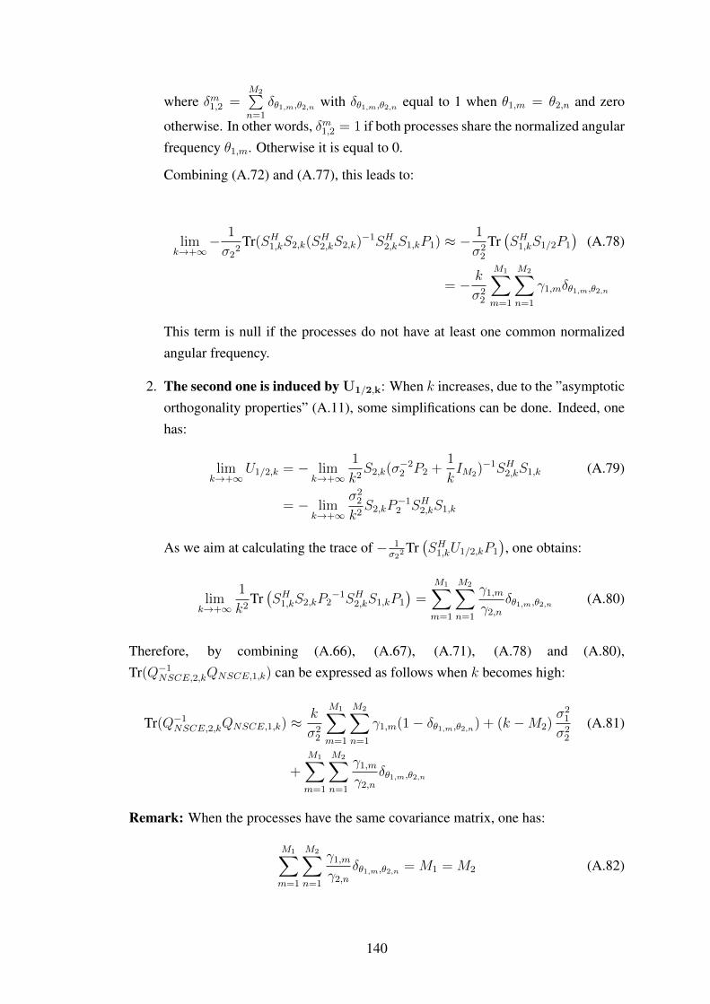
where δm1,2 =M2∑n=1

δθ1,m,θ2,n with δθ1,m,θ2,n equal to 1 when θ1,m = θ2,n and zero

otherwise. In other words, δm1,2 = 1 if both processes share the normalized angularfrequency θ1,m. Otherwise it is equal to 0.

Combining (A.72) and (A.77), this leads to:

limk→+∞

− 1

σ22Tr(SH1,kS2,k(S

H2,kS2,k)

−1SH2,kS1,kP1) ≈ −1

σ22

Tr(SH1,kS1/2P1

)(A.78)

= − k

σ22

M1∑m=1

M2∑n=1

γ1,mδθ1,m,θ2,n

This term is null if the processes do not have at least one common normalizedangular frequency.

2. The second one is induced by U1/2,k: When k increases, due to the ”asymptoticorthogonality properties” (A.11), some simplifications can be done. Indeed, onehas:

limk→+∞

U1/2,k = − limk→+∞

1

k2S2,k(σ

−22 P2 +

1

kIM2)

−1SH2,kS1,k (A.79)

= − limk→+∞

σ22

k2S2,kP

−12 SH2,kS1,k

As we aim at calculating the trace of − 1σ22

Tr(SH1,kU1/2,kP1

), one obtains:

limk→+∞

1

k2Tr(SH1,kS2,kP2

−1SH2,kS1,kP1

)=

M1∑m=1

M2∑n=1

γ1,mγ2,n

δθ1,m,θ2,n (A.80)

Therefore, by combining (A.66), (A.67), (A.71), (A.78) and (A.80),Tr(Q−1NSCE,2,kQNSCE,1,k) can be expressed as follows when k becomes high:

Tr(Q−1NSCE,2,kQNSCE,1,k) ≈k

σ22

M1∑m=1

M2∑n=1

γ1,m(1− δθ1,m,θ2,n) + (k −M2)σ21

σ22

(A.81)

+

M1∑m=1

M2∑n=1

γ1,mγ2,n

δθ1,m,θ2,n

Remark: When the processes have the same covariance matrix, one has:

M1∑m=1

M2∑n=1

γ1,mγ2,n

δθ1,m,θ2,n =M1 =M2 (A.82)

140

andM1∑m=1

M2∑n=1

γ1,m(1− δθ1,m,θ2,n) = 0 (A.83)

In this case, (A.81) becomes:

Tr(Q−1NSCE,2,kQNSCE,1,k) = (k −M2)σ21

σ22

+M1 = k = Tr(Ik) (A.84)

Given the above analysis, it is now possible to analyze how the JD between two NSCEprocesses evolves when k increases and tends to infinity. This is the goal of the nextsubsection.

A.4.2 Analytic expression of the Jeffreys divergence

As the expression of Tr(Q−1NSCE,1,kQNSCE,2,k) when k becomes high is similarly de-fined when the indices 1 and 2 are switched. Given (A.5) and (A.81), the JD can beapproximated when k becomes large as follows:

JDk(NSCE1,NSCE2) ∝ −k + 1

2[(k −M2)

σ21

σ22

+ (k −M1)σ22

σ21

(A.85)

+ k

M1∑m=1

M2∑n=1

(γ1,mσ22

+γ2,nσ21

)(1− δθ1,m,θ2,n)

+

M1∑m=1

M2∑n=1

(γ1,mγ2,n

+γ2,nγ1,m

)δθ1,m,θ2,n ]

The JD depends on the parameters of the processes, namely the normalized angularfrequencies of each process, the variances of the magnitudes of each component as wellas the variances of the additive noises. The first term of the expression includes theJD between two zero-mean white noises with variances σ2

1 and σ22 . Indeed, when there

is no complex exponentials in both processes, the processes under study correspond towhite noises and (A.85) reduces to:

JD(WN1,WN2)k = −k + k

2

(σ21

σ22

+σ22

σ21

)(A.86)

Note that the two other terms in (A.85) make it possible to point out the differencesbetween the sets of complex exponentials.In the following section, let us analyze how the JD evolves when k is incremented.

141

A.4.3 Analysis of the increment of the Jeffreys divergence

Given the expression (A.85) of the JD we obtained, let us now deduce the asymptoticincrement, i.e. the increment of the JD when k becomes large8:

∆JD(NSCE1,NSCE2) = limk→+∞

JDk(NSCE1,NSCE2) − JD(NSCE1,NSCE2)

k−1 (A.87)

Therefore, one can easily deduce that:

∆JD(NSCE1,NSCE2) = −1 + 1

2

[σ21

σ22

+σ22

σ21

+

M1∑m=1

M2∑n=1

(γ1,mσ22

+γ2,nσ21

)(1− δθ1,m,θ2,n)

](A.88)

The ratio of the additive-white-noise variances has an influence on the slope of theJD. In addition, when there are common normalized angular frequencies between twoprocesses, ∆JD is smaller.After this theoretical analysis, let us give some examples based on synthetic data andlet us comment the results we obtain.

A.4.4 Illustrations and comments

A.4.4.1 Evolution of the JD between NSCE processes when k increases

Let us present how the JD evolves when comparing two NSCE processes. Their param-eters are given in Table A.1.

Table A.1 Parameters of the NSCE processes under study for the 1st simulation protocol

1st-process NSCE parameters 2nd-process NSCE parametersM1 = 1 M2 = 1

θ1,1 varies in the interval [−π, π)with a step equal to 0.02

θ2,1 varies in the interval [−π, π)with a step equal to 0.02

γ1,1 = 100 γ2,1 = 40σ21 = 1 σ2

2 = 1

When looking at the JD between NSCE processes based on k = 5 in Fig. A.1a, itcan be difficult to give an interpretation of the values the JD obtains. This is also thesame problem when considering k = 15, as depicted in Fig. A.1b. However, whendealing with k = 50, Fig. A.1c shows that the JD tends to attain the same value whenthe set of normalized angular frequencies are different. When they are equal, the JD is

8In the equation below, the notation we use is limk→+∞

. This means that we always consider correlation

matrices of finite size k, where k becomes larger and larger.

142

equal to 0. For this purpose, instead of looking only at the JD, we propose to study theasymptotic JD increment.

(a)

(b)

(c)

Fig. A.1 JD(NSCE1,NSCE2)k defined in (A.5) for random vectors of dimension (a) k = 5,

(b) k = 15, (c) k = 50

In the following, let us show how the JD increment evolves when k increases for aspecific case, and let us analyze the influence of each parameter. We propose to startthe analysis by the additive-noise variances.

143

0 100 200 300 400 5000

20

40

60

80

100

120

Number of variates

JD

de

riva

tive

JD Derivative

Asymptotic JD increment

1st case

2nd case

3rd case

Fig. A.2 Asymptotic JD increment and JD derivative between NSCE processes, whoseparameters are given in table A.1

A.4.4.2 Influence of the additive-noise variances

The parameters of the NSCE processes are given in Table A.2.

Table A.2 Parameters of the NSCE processes under study for the 2nd simulation proto-col

1st-process NSCE parameters 2nd-process NSCE parametersM1 = 1 M2 = 1

θ1,1 = −π/5 θ2,1 = −2π/5γ1,1 = 100 γ2,1 = 40

1 value for σ21: 3 cases for σ2

2:σ21 = 1 1) σ2

2 = 0.52) σ2

2 = 13) σ2

2 = 2

As illustrated by Fig. A.3, the asymptotic increment is modified according to (A.88). Italways depends on σ12

σ22+ σ22

σ12and may depend on the set of ratios γ1,m

σ22

+ γ2,nσ21 with

m = 1, ...,M1 and n = 1, ...,M2 if the NSCE share the same normalized angularfrequencies.

A.4.4.3 Convergence speed towards the stationary regime

The parameters of the NSCE processes are given in Table (A.3).Given Fig. A.4, one can notice that the JD computed from (A.5) and (A.7) tends to bethe same for the three simulations when k increases. The main differences are locatedwhen k is small. For this reason, we suggest computing the derivatives of these JD.They are given in Fig. A.5 where they are compared with the asymptotic incrementgiven in (A.88).

144

0 50 100 150 200 250 3000

20

40

60

80

100

120

140

160

180

200

Number of variates

JD

derivative

JD derivatives vs. number of variates k

Second simulation

Third simulation

First simulation: JD derivative and asymptotic increment

Fig. A.3 Asymptotic increment vs increment with three simulations where σ22 is mod-

ified

Table A.3 Parameters of the NSCE processes under study for the 3rd simulation proto-col

1st-process NSCE parameters 2nd-process NSCE parametersM1 = 1 M2 = 1σ21 = 1 σ2

2 = 0.1γ1,1 = 100 γ2,1 = 40

1 value for θ1,1: 3 cases for θ2,1:θ1,1 = −π/5 1) θ2,1 = −2π/5

2) θ2,1 = −1.5π/53) θ2,1 = −1.1π/5

0 50 100 150 200 2500

2

4

6

8

10

12x 10

4

Number of variates

JD

Evolution of the JD vs. number of variates k

First simulation

Second simulation

Third simulation

Fig. A.4 JD and its approximation with three simulations where θ2,1 becomes closerand closer to θ1,1 = −π/5

145

0 50 100 150 200 250 3000

200

400

600

800

1000

Number of variates

JD

de

riva

tive


First case

Asymtotic JD increment

Second case

Third case

Fig. A.5 Asymptotic increment vs increment with three simulations where θ2,1 be-comes closer and closer to θ1,1 = −π/5

As presented in (A.88) in the theoretical analysis in section A.4.3, we can see thatthe asymptotic increment is here the same for all the simulations. The only differ-ence stands in the convergence speed towards the stationary regime. Indeed, givenFig. A.5, the convergence of the JD derivative towards the asymptotic increment isfaster when the difference between the normalized angular frequencies is large. Thefluctuations of the derivatives around the asymptotic increment are mainly due to theproducts such as SH1,kS2,k and SH2,kS1,k that must be computed. They correspond to val-

ues of sin(k(θl,m−θl,n)

2)

sin((θl,m−θl,n)

2

whose square is periodic with respect to k with period equal to2π

|θ1,n−θ2,m| .

A.4.4.4 A more general case

The parameters of the NSCE processes are given in Table A.4.

Table A.4 Parameters of the NSCE processes under study for the 4th simulation proto-col

1st-process NSCE parameters 2nd-process NSCE parametersM1 = 3 M2 = 3σ21 = 1 σ2

2 = 0.1γ1,1 = 100,γ1,2 = 50,γ1,3 = 75 γ2,1 = 40,γ2,2 = 60,γ2,3 = 80

Fixed values forθ1,1, θ1,2, θ1,3, θ2,1 and θ2,3:

3 cases for θ2,2:

θ1,1 = π/10, θ1,2 = π/4, 1) θ2,2 = π/2θ1,3 = 4π/5, θ2,1 = −π/10, 2) θ2,1 = π/4

and θ2,3 = 4π/5 3) θ2,1 = 4π/5

146

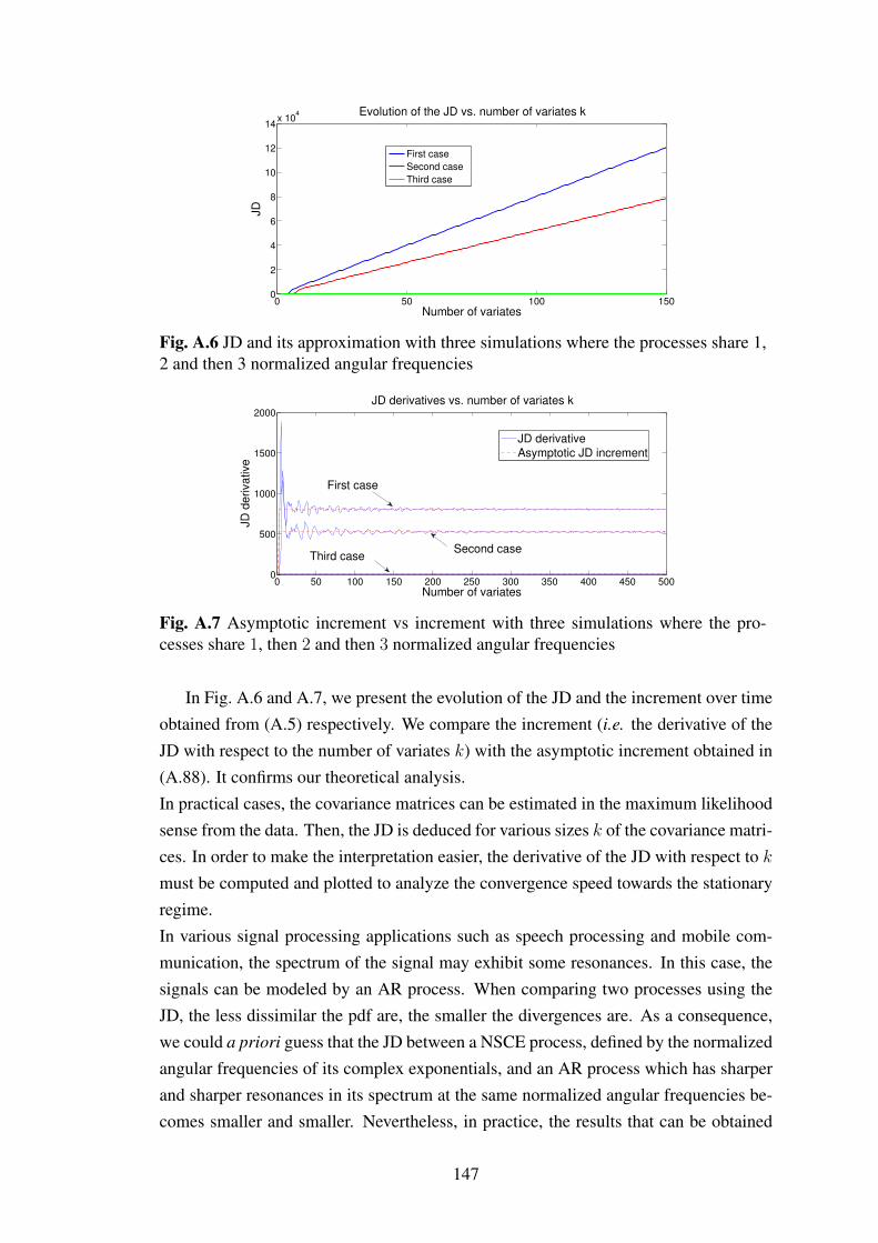
0 50 100 1500

2

4

6

8

10

12

14x 10

4

Number of variates

JD

Evolution of the JD vs. number of variates k

First case

Second case

Third case

Fig. A.6 JD and its approximation with three simulations where the processes share 1,2 and then 3 normalized angular frequencies

0 50 100 150 200 250 300 350 400 450 5000

500

1000

1500

2000

Number of variates

JD

de

riva

tive


JD derivative


First case

Third caseSecond case

Fig. A.7 Asymptotic increment vs increment with three simulations where the pro-cesses share 1, then 2 and then 3 normalized angular frequencies

In Fig. A.6 and A.7, we present the evolution of the JD and the increment over timeobtained from (A.5) respectively. We compare the increment (i.e. the derivative of theJD with respect to the number of variates k) with the asymptotic increment obtained in(A.88). It confirms our theoretical analysis.In practical cases, the covariance matrices can be estimated in the maximum likelihoodsense from the data. Then, the JD is deduced for various sizes k of the covariance matri-ces. In order to make the interpretation easier, the derivative of the JD with respect to kmust be computed and plotted to analyze the convergence speed towards the stationaryregime.In various signal processing applications such as speech processing and mobile com-munication, the spectrum of the signal may exhibit some resonances. In this case, thesignals can be modeled by an AR process. When comparing two processes using theJD, the less dissimilar the pdf are, the smaller the divergences are. As a consequence,we could a priori guess that the JD between a NSCE process, defined by the normalizedangular frequencies of its complex exponentials, and an AR process which has sharperand sharper resonances in its spectrum at the same normalized angular frequencies be-comes smaller and smaller. Nevertheless, in practice, the results that can be obtained

147

do not necessarily confirm this statement. For this purpose, we propose to analyze theJD between an AR process and a NSCE process in the next section.

A.5 Jeffreys divergence between an autoregressive process and a sum ofcomplex exponential process

In this section, using the definitions and properties of the JD and the processes un-der study, we first propose to express Tr(Q−1NSCE,l,kQAR,l′,k) and Tr(Q−1AR,l′,kQNSCE,l,k),with l and l′ defining the labels of the processes to be compared. We will see if one candeduce an analytic expression of these traces when the number of variates k increasesand tends to infinity. As done in the previous section, this step will be useful to deducethe asymptotic properties of the JD between an AR process and a NSCE process.

A.5.1 Expression of the trace Tr(Q−1NSCE,l,kQAR,l′,k)

Given (A.7) and (A.17), after developing, one can show that Tr(Q−1NSCE,l,kQAR,l′,k) canbe expressed as the sum of three terms denoted as Ω, Ψ and Υ :

Ω =1

σ2l

Tr (QAR,l′,k) =k

σ2l

rAR,l′,0 (A.89)

Ψ = − 1

kσ2l

Tr(Sl,kSHl,kQAR,l′,k) = −1

kσ2l

Tr(SHl,kQAR,l′,kSl,k) (A.90)

andΥ =

1

k2Tr(Sl,kP−1l SHl,kQAR,l′,k) =

1

k2Tr(P−1l SHl,kQAR,l′,kSl,k) (A.91)

In (A.90) and (A.91), SHl,kQAR,l′,kSl,k has to be computed. Given the definition of thematrix Sl,k in (A.9), let us study what the value of Sml,k

HQAR,l′,kSmk is when m =

1, ...,M :

Sml,kHQAR,l′,kS

mk (A.92)

=

[k−1∑τ=0

rAR,l′,τe−jτθl,m . . .

0∑τ=1−k

rAR,l′,τe−j(τ+k−1)θl,m

] [1 . . . ej(k−1)θl,m

]TBy rearranging the terms, (A.92) can be rewritten as follows:

Sml,kHQAR,l′,kS

ml,k =

k−1∑i=0

i∑τ=−i

rAR,l′,τe−jτθl,m (A.93)

Then, let us introduce a truncated correlogram CAR,l′,i based on a window of size 2i+1

148

and computed for the normalized angular frequency θl,m:

CAR,l′,i(θm) =i∑

τ=−i

rAR,l′,τe−jτθl,m (A.94)

By combining (A.90) with (A.93) and (A.94) on the one hand and (A.91) with (A.93)and (A.94) on the other hand, one has:

Ψ = − 1kσl2

M∑m=1

k−1∑i=0

CAR,l′,i(θl,m)

Υ = 1k2

M∑m=1

1γl,m

k−1∑i=0

CAR,l′,i(θl,m)

(A.95)

Given (A.89) and (A.95), Tr(Q−1NSCE,l,kQAR,l′,k) can be expressed as follows when kbecomes high:

Tr(Q−1NSCE,l,kQAR,l′,k) ≈k

σl2rAR,l′,0 +

M∑m=1

1

k(

1

kγl,m− 1

σl2)k−1∑i=0

CAR,l′,i(θl,m) (A.96)

A.5.2 Expression of the trace Tr(Q−1AR,l′,kQNSCE,l,k)

Given (A.7) and (A.27), Tr(Q−1AR,l′,kQNSCE,l,k) can be expressed as the sum of twotraces, denoted as ∆ and Θ:

∆ = Tr(σl2(LH)−1

D−1L−1) = σl2Tr(L−1

(LH)−1

D−1) (A.97)

where the inverses of L and D have been defined in (A.31) and (A.30).Using (A.31), this leads to:

∆ = (k − p) σ2l

σ2u,l′,p

p∑i=0

|api,l′ |2 +

p−1∑j=0

σ2l

σ2u,l′,j

j∑i=0

|aji,l′|2 (A.98)

= (k − p) σ2l

σ2u,l′,p

‖al′p‖2 +p−1∑j=0

σ2l

σ2u,l′,j

‖al′j‖2

with ‖al′j‖2 the 2-norm of the jth-order AR-parameter vector.Remark: When considering a 1st-order AR process, given (A.27), Q−1AR,l′,k has thefollowing simple expression:

Q−1AR,l′,k =1

σ2u,l′,1

(a1,l′Jk + a1,l′∗JTk + (1 + |a1,l′ |2)Ik − |a1,l′ |2(ek,1eTk,1 + ek,ke

Tk,k).

(A.99)

149

where ek,l denotes the column vector of size k with zeros except at the lth row wherethe element is equal to 1.Therefore, Tr(σ2

lQ−1AR,l′,k) =

σ2l

σ2u,1

(k + (k− 2)|a1,l′|2). This is also confirmed by (A.98).

Then, let us give some details about the second trace. Taking into account the expres-sion of the PSD of the AR process for any order i = 0, ..., p evaluated at normalizedangular frequencies θl,m with m = 1, ...,M , one has:

Θ = Tr(SHl,k(LH)−1D−1L−1Sl,kPl) =

M∑m=1

γl,m(k − p

SAR,l′,p(θl,m)+

p−1∑i=0

1

SAR,l′,i(θl,m))

(A.100)

It should be noted that in the above equation (A.100), we can organize the terms asfollows:

Θ =M∑m=1

γl,m

(k − p− 1

SAR,l′,p(θl,m)+

1

Scapon(θl,m)

)(A.101)

Indeed, the pseudo-spectrum Scapon that can be deduced using Capon’s method [115]can be expressed by:

Scapon(θl,m) =

[p∑i=0

1

SAR,l′,i(θl,m)

]−1(A.102)

=1

[1 . . . e−jpθl,m ]Q−1AR,l′,p+1 [1 . . . e−jpθl,m ]

H

Given the above analysis, let us deduce an expression of the JD when k increases in thenext subsection. This step will be useful to deduce the asymptotic increment of the JD.

A.5.3 Analytic expression of the Jeffreys divergence

Combining (A.96), (A.98) and (A.100), the JD can be approximated when k becomeslarge as follows:

JD(AR,NSCE)k ≈ −k + 1

2

(k

σ2l

rAR,l′,0 +M∑m=1

k−1∑i=0

1

k

( 1

kγl,m− 1

σl2

)CAR,l′,i(θl,m)

(A.103)

+((k − p) σ2

l

σ2u,l′,p

‖al′p‖2 +p−1∑j=0

σ2

σ2u,l′,j

‖al′j‖2)

+M∑m=1

γl,m

( k − pSAR,l′,p(θl,m)

+

p−1∑i=0

1

SAR,l′,i(θl,m)

))

150

A.5.4 Analysis of the increment of the JD

Given (A.86), let us now deduce the asymptotic increment, i.e. the increment of the JDwhen k becomes large:

∆JD(AR,NSCE) = limk→+∞

(JDk − JDk−1) (A.104)

For large values of k, one has:

∆JD(AR,NSCE) ≈ −1 + 1

2

rARl′,0σl2︸︷︷︸1stterm

+σ2l

σ2u,l′,p

‖al′p‖2︸︷︷︸2ndterm

+M∑m=1

γl,mSAR,l′,p(θl,m)︸︷︷︸3rdterm

(A.105)

151

According to (A.105), we can notice that the asymptotic JD increment depends onthree main terms:

1. rAR,l′,0σl2

is the power of the AR process filtered by an all-pass filter whose transferfunction is 1

σl,

2. σl2

σ2u,l′,p‖al′p‖2 is the power of the additive white noise with variance σ2

l that hasbeen filtered by the finite-impulse response (FIR) ”AR inverse filter” whose trans-fer function is Ap(z)

σu,l′,p,

3. the third term depends on the sum of the ratios between the NSCE process powerand the AR-process PSD at the normalized angular frequencies θl,mm=1,...,M .Nevertheless, by using (A.20), each term γl,m

SAR,l′,p(θl,m)can be also seen as the

power of the complex exponential at θl,m which has been filtered by the AR in-verse filter. Therefore, this third term corresponds to the power of the determin-istic part of the NSCE process filtered by the AR inverse filter.

The above results lead to some comments:

1. when M = p = 0, (A.105) reduces to:

∆JD(AR,NSCE) ≈ −1 + 1

2(σ2u,l′,1

σl2+

σl2

σ2u,l′,1

) (A.106)

It corresponds to the JD increment between white noises with variance σ2u,l′,1

and σl2.

2. The smaller the three terms in (A.105) are, the smaller the asymptotic JD in-crement is. However, they do not necessarily have the same behavior with re-spect to the process parameters. Thus, if p = M and if the arguments of theAR poles correspond to the normalized angular frequencies θl,mm=1,...,M , reso-nances may appear in the transfer function Hl′(z). The closer to the unit circle inthe z-plane the poles pi,l′i=1,...,p are, the sharper the resonances of Hl′(z) are.In this case, the 1st and the 2nd terms in (A.105) can grow9. Meanwhile, the 3rd

term in (A.105) tend to be smaller and smaller.

In the next section, we suggest illustrating the way the JD evolves when comparing twoprocesses. We propose to look at the influence of the process parameters on the JD.This will help us define some clues to give an interpretation of the JD.

9Indeed, one has: rAR,l′,0 ∝∫SAR,l′,p(θ) dθ

152

A.5.5 Illustrations and comments

In this section, for the sake of simplicity, we suggest comparing a 1st-order AR processwith a NSCE process. The influences of the different parameters can be also illustrated.Note that rAR,1,0 =

σ2u,1,1

1−|a1,1|2 .

A.5.5.1 Influence of the AR-parameter argument

The parameters of the processes under study are given in Table A.5.

Table A.5 Parameters of the AR and NSCE processes under study

NSCE process parameters AR process parametersM2 = 1 |a1,1| = 0.95σ22 = 1 σu,1,1 = 1

γ2,1 = 10 argument of a1,1 variesθ2,1 = π/2 in the interval ]− π, 0[

Based on Fig. A.8, which shows the asymptotic JD increment as a function of the ar-gument of a1,1, the asymptotic JD increment reaches its minimum when the argumentof a1,1 is equal to −π/2. In this case, the resonance in the AR process power spectrumappears at the same angular frequency as the one of the NSCE process.

−3 −2.5 −2 −1.5 −1 −0.5 0

6

8

10

12

14

argument of a1

1

asym

pto

tic J

D incre

ment

Evolution of asymptotic JD increment vs argument of a1

1

JD increment reaches its minimum

when argument of a1

1 is equal to −pi/2

Fig. A.8 Evolution of the asymptotic JD increment as a function of the argument of a1,1

A.5.5.2 Influence of the AR-parameter modulus

The parameters of the processes under study are given in Table A.6.

153


NSCE process parameters AR process parametersM2 = 1 a1,1 varies in ]− 1, 0[σ22 = 1 with step equal to 0.05

γ2,1 = 10 σu,1,1 = 1θ2,1 = 0

In Fig. A.9, the derivative of the JD obtained from the expressions of QAR,1,k andQNSCE,2,k tends to the asymptotic increment whatever the case under study. Tworegimes appear: a transient one and then a stationary-like one. This confirms our theo-retical study. Fig. A.10 shows the asymptotic increment as a function of a1,1 where the 6cases addressed above are pointed out. The asymptotic increment reaches its minimumwhen the modulus of a1,1 is not necessarily close to the unit-circle but around 0.7. Itillustrates our comments of section A.5.4.

0 50 100 150 200 250 3000

1

2

3

4

5

6

Number of variates

JD

derivative

JD derivatives vs number of variates k

JD derivative

Asymptotic increment

transient regime stationary−like regime

The modulus of a1

1 decreases

Fig. A.9 JD derivative vs number of variates, second simulation with six cases wherethe modulus of a1 varies

−1 −0.9 −0.8 −0.7 −0.6 −0.5 −0.4 −0.3 −0.2 −0.1 00

5

10

15

20

25

30

a1

1

Evolution of asymptotic JD increment vs a1

1

asym

pto

tic J

D incre

ment

Fig. A.10 Evolution of the asymptotic JD increment as a function of a1,1 where thedotted points corresponds to the cases addressed in Fig. A.9.

154

A.5.5.3 Influence of the additive-noise variance

The parameters of the processes under study are given in A.7


NSCE process parameters AR process parametersM2 = 1 a1,1 = −0.95θ2,1 = π/2 σu,1,1 = 1γ2,1 = 10

σ22 varies between 0.5 and 10

According to Fig. A.11, (A.105) tends to infinity if σ22 tends to zero. This illustrates

the main difference between the spectrum properties of both processes: one tends to bediscrete whereas the other is continuous.

0 1 2 3 4 5 6 7 8 9 103

4

5

6

7

8

9

10

ratio of power between the two processes

Evolution of asymptotic JD increment vs additive noise variance

asym

pto

tic J

D incre

ment

Fig. A.11 Evolution of the asymptotic JD increment as a function of σ22

In the next section, let us give a physical interpretation of the asymptotic JD incrementfor ergodic w.s.s. ARMA processes.

A.6 Interpreting the asymptotic increment of Jeffreys Divergencebetween some random processes

A.6.1 Inverse-filtering interpretation

In this section, we suggest giving an interpretation of the asymptotic JD increment inorder to better understand the influence of each process parameter on the JD and togeneralize the results obtained to ARMA(p,q) processes. For this reason, our purpose isto provide a new way to derive the asymptotic JD increment between zero-mean w.s.s.ARMA processes.Let us rewrite the definition of the asymptotic JD increment as follows:

∆JD(ARMA1,ARMA2) = −1+ 1

2

[∆T (ARMA2,ARMA1) +∆T ((ARMA1,ARMA2)

](A.107)

155

where the asymptotic increments of the traces ∆T (ARMAl,ARMAl′ ) satisfy with (l, l′)

equal to (1, 2) or (2, 1) :

∆T (ARMAl,ARMAl′ ) (A.108)

= limk→+∞

[Tr(Q−1ARMA,l,kQARMA,l′,k)− Tr(Q−1ARMA,l,k−1QARMA,l′,k−1)

]In the above equation, the covariance matrices are of finite sizes k and k − 1. Then, westudy how the increment of the matrix traces evolves when k increases. If infinite-sizecorrelation matrices are considered, the expressions of the KL (A.2) and of the JD (A.5)no longer hold when the corresponding transfer functions of the ARMA processes haveunit roots since the covariance matrices are no longer invertible. As we will see later,it is not a hazard if these cases lead to specific behaviors of the JD increment in ouranalysis.To evaluate∆T (ARMAl,ARMAl′ ), we propose a particular way for interpreting the asymp-totic JD increment. This basically avoids long mathematical developments.The covariance matrix QARMA,l,k can be decomposed by means of an eigenvalue de-composition:

QARMA,l,k = ElDlEHl (A.109)

where El denotes the unitary matrix storing the eigenvectors of QARMA,l,k and Dl is thediagonal matrix storing the non-null real positive eigenvalues.Then, one has:

Tr(Q−1ARMA,l,kQARMA,l′,k) = Tr(D−1/2l EHl QARMA,l′,kElD

−1/2l ) (A.110)

Our interpretation is the following: Let Xl,k be the zero-mean random vector storingk consecutive samples of the lth zero-mean process ARMA process associated withcovariance matrix QARMA,l,k = E

[Xl,kX

Hl,k

].

Pre-multiplying Xl,k by D−1/2l PHl amounts to whitening the process Xl,k and making

its power equal to unity. When k tends to infinity, it amounts to filtering all the samplesstored in Xl,k by an inverse filter whose transfer function is H−1l (z).Similarly, pre-multiplying Xl′,k by D

−1/2l PH

l is equivalent, when k tends to infinity,to filter the data stored in the vector Xl′,k by the inverse filter whose transfer functionis equal to H−1l (z). As a consequence, the asymptotic increment ∆T (ARMAl,ARMAl′ )

corresponds to the power of process whose samples are stored in Xl′,k and then filteredby H−1l (z).

156

Based on the inverse filtering interpretation, the asymptotic JD increment amountsto computing the power P (ARMAl,ARMAl′ ) of the lth random process filtered by the in-verse filter corresponding to the l′th process, with (l, l′) = (1, 2) or (2, 1):

∆JD(ARMA1,ARMA2) = limk→+∞

∆JD(ARMA1,ARMA2)k

= −1 + 1

2(P (ARMA1,ARMA2) + P (ARMA2,ARMA1)) (A.111)

A.6.2 Applications

In this section, we recall the results obtained in previous works [72], [58] and [57] andpropose to retrieve the expressions of the asymptotic JD increments by using the inversefiltering interpretation in the following cases:

1. the JD between two white noises,

2. the JD between a 1st-order AR process and a white noise,

3. the JD between two real 1st-order MA processes

4. the JD between 1st-order AR and MA processes.

Then, three new cases that were not addressed before can be now presented thanks tothe results of section A.6.1:

1. the JD between qth-order MA processes,

2. the JD between NSCE processes,

3. the JD between an NSCE process and a pth-order AR process.

In these latter cases, we propose to illustrate the influences of the parameters of theprocesses on the asymptotic JD increment and consequently on the JD.

A.6.2.1 JD between two white noises

Even if this is a trivial case, by starting from the definition (A.5), our proposed interpre-tation in section A.6.1 makes it possible to deduce the asymptotic increment of the JDbetween zero-mean Gaussian white noises (WN) with variances σ2

u,1 and σ2u,2. It can be

viewed as a toy example:

∆JD(WN1,WN2) = −1 + 1

2

(∆T (WN2,WN1) +∆T (WN1,WN2)

)(A.112)

− 1 +1

2

(σ2u,1

σ2u,2

+σ2u,2

σ2u,1

)

157

Indeed, the term ∆T (WN2,WN1) =σ2u,1

σ2u,2

can be explained as follows: the first white noisewith variance σ2

u,1 is filtered by an all-pass filter with a transfer function equal to 1σu,2

.

The power of the filter output is hence equal toσ2u,1

σ2u,2

. The term ∆T (WN1,WN2) =σ2u,2

σ2u,1

canbe explained similarly.By introducing

Ru =σ2u,2

σ2u,1

(A.113)

the above equation (A.112) becomes:

∆JD(WN1,WN2) = −1 + 1

2

(1

Ru

+Ru

)(A.114)

It should be noted that (A.114) can be rewritten by expressing σ2u,2 as σ2

u,1 + δσ2u and

by introducing the relative difference between the noise-variances ∆σ2u = δσ2

u

σ2u,1

. In thiscase, one has:

Ru = 1 +∆σ2u (A.115)

and∆JD(WN1,WN2) = −1 + 1

2

(1

1 +∆σ2u

+ 1 +∆σ2u

)(A.116)

0 2 4 6 8 10 12 14 16 18 200

5

10

15

20

25

30

35

40

45

50

relative difference between the noise variances

asym

pto

tic J

D incre

ment

Minimum value equal to 0

Fig. A.12 JD between white noises vs relative difference between the white-noise vari-ances ∆σ2

u

According to Fig. A.12 and (A.116), one can see that the asymptotic JD increment onlydepends on the relative difference between the white-noise variances.

A.6.2.2 JD between a 1st-order AR process and a white noise

By taking advantage of the inverse of the correlation matrix of a 1st-order AR process[14], the asymptotic JD increment can be expressed as follows:

158

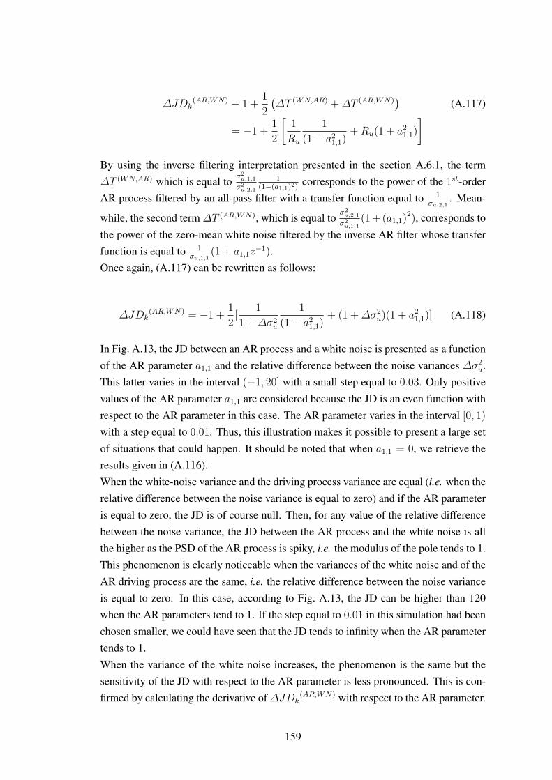
∆JDk(AR,WN) − 1 +

1

2

(∆T (WN,AR) +∆T (AR,WN)

)(A.117)

= −1 + 1

2

[1

Ru

1

(1− a21,1)+Ru(1 + a21,1)

]By using the inverse filtering interpretation presented in the section A.6.1, the term∆T (WN,AR) which is equal to

σ2u,1,1

σ2u,2,1

1(1−(a1,1)2) corresponds to the power of the 1st-order

AR process filtered by an all-pass filter with a transfer function equal to 1σu,2,1

. Mean-

while, the second term ∆T (AR,WN), which is equal toσ2u,2,1

σ2u,1,1

(1+ (a1,1)2), corresponds to

the power of the zero-mean white noise filtered by the inverse AR filter whose transferfunction is equal to 1

σu,1,1(1 + a1,1z

−1).Once again, (A.117) can be rewritten as follows:

∆JDk(AR,WN) = −1 + 1

2[

1

1 +∆σ2u

1

(1− a21,1)+ (1 +∆σ2

u)(1 + a21,1)] (A.118)

In Fig. A.13, the JD between an AR process and a white noise is presented as a functionof the AR parameter a1,1 and the relative difference between the noise variances ∆σ2

u.This latter varies in the interval (−1, 20] with a small step equal to 0.03. Only positivevalues of the AR parameter a1,1 are considered because the JD is an even function withrespect to the AR parameter in this case. The AR parameter varies in the interval [0, 1)with a step equal to 0.01. Thus, this illustration makes it possible to present a large setof situations that could happen. It should be noted that when a1,1 = 0, we retrieve theresults given in (A.116).When the white-noise variance and the driving process variance are equal (i.e. when therelative difference between the noise variance is equal to zero) and if the AR parameteris equal to zero, the JD is of course null. Then, for any value of the relative differencebetween the noise variance, the JD between the AR process and the white noise is allthe higher as the PSD of the AR process is spiky, i.e. the modulus of the pole tends to 1.This phenomenon is clearly noticeable when the variances of the white noise and of theAR driving process are the same, i.e. the relative difference between the noise varianceis equal to zero. In this case, according to Fig. A.13, the JD can be higher than 120when the AR parameters tend to 1. If the step equal to 0.01 in this simulation had beenchosen smaller, we could have seen that the JD tends to infinity when the AR parametertends to 1.When the variance of the white noise increases, the phenomenon is the same but thesensitivity of the JD with respect to the AR parameter is less pronounced. This is con-firmed by calculating the derivative of∆JDk

(AR,WN) with respect to the AR parameter.

159

One can also calculate the derivative of ∆JDk(AR,WN) with respect to the relative dif-

ference between the noise variances∆σ2u. In this case, one can notice that the minimum

value of the asymptotic JD increment is obtained when ∆σ2u =

√1

1−(a1,1)4− 1. In this

case, it is equal to√

1−(a1,1)4

1−(a1,1)2− 1.

05

1015

20

00.2

0.40.6

0.810

20

40

60

80

100

120

relative difference between the noise variances

asymptotic JD increment

AR parameter

Fig. A.13 Asymptotic JD increment between an AR process and a white noise as afunction of the AR parameter and the relative difference between the noise-variances∆σ2

u

A.6.2.3 JD between two 1st-order AR processes

In [72], a recursive way was suggested to deduce the JD between two 1st-order ARprocesses:

∆JD(AR1,AR2) = A+B (A.119)

with A = −1 + 1

2(Ru +

1Ru

)

B = (a1,2−a1,1)22

[1

1−(a1,1)21Ru

+ 11−(a1,2)2Ru

] (A.120)

However, by reorganizing the terms in the above equation, one has:

∆JD(AR1,AR2) (A.121)

= −1 + 1

2(Ru

1− 2a1,1a11,2 + a21,1

1− a21,2+

1

Ru

1− 2a1,1a1,2 + a21,21− a21,1

)

= −1 + 1

2(∆T (AR1,AR2) +∆T (AR2,AR1)) (A.122)

160

Following our interpretation, we could have obtained the same results by avoiding sev-eral mathematical developments presented in [72]. Indeed, the term∆T (AR1,AR2) whichis equal to Ru

1−2a1,1a11,2+a21,11−a21,2

corresponds to the power of the 2nd AR process filtered bythe inverse filter that corresponds to the 1st AR process. This amounts to computing theautocorrelation function of this filtered AR (fAR) process, for the lag equal to 0, de-noted as rfAR,2,0. This latter can be deduced from the definition of the autocorrelationfunction and the set of equations that define the second AR process and the filteringstep. More particularly, one has:

rfAR,2,0 =1 + a21,1σ2u,1,1

rAR,2,0 +a1,1σ2u,1,1

rAR,2,1 +a1,1σ2u,1,1

rAR,2,−1 (A.123)

By replacing in (A.123), rAR,2,τ with τ = −1, 0, 1 by their expressions recalled in(A.23), we retrieve Ru

1−2a1,1a1,2+a21,11−a21,2

.

Concerning the term ∆T (AR2,AR1) which is equal to 1Ru

1−2a1,1a1,2+a21,21−a21,1

, it is equal to thepower of the 1st AR process filtered by the inverse filter that corresponds to the 2nd ARprocess. The reasoning is similar. Since illustrations of the JD between AR processeshave already been proposed, interested readers can refer to [72] for further details.

A.6.2.4 JD between two real 1st-order MA processes

In [58], by deducing the expression of the inverse of the correlation matrix of the real1st-order MA process 10, it was shown after long mathematical developments that theasymptotic JD increment was constant when |b1,l| 6= 1. It was equal to:

∆JD(MA1,MA2)k = −1 + 1

2

(rMA,1,1

rMA,2,1

+rMA,2,1

rMA,1,1

)(A.124)

+1

2[(rMA,1,0

rMA,2,0

− rMA,1,1

rMA,2,1

)1 + b21,2|1− b21,2|

+ (rMA,2,0

rMA,1,0

− rMA,2,1

rMA,1,1

)1 + b21,1|1− b21,1|

].

= −1 + 1

2

(∆T (MA2,MA1) +∆T (MA1,MA2)

)However if |b1,l| = 1, the increment was not finite, except when the MA processes sharethe same zeros.We are now able to explain the reason why this phenomenon appears. By developingand reorganizing the terms, we can show that the term ∆T (MA2,MA1) which is equal torMA,1,1

rMA,2,1+ (

rMA,1,0

rMA,2,0− rMA,1,1

rMA,2,1)1+b21,2|1−b21,2|

can be re-expressed as follows:σ2u,1,1

σ2u,2,1

1+(b1,1)2−2b1,1b1,21−(b1,2)2 if |b1,2| < 1

σ2u,1,1

σ2u,2,1

(1+(b1,1)2−2b1,1b1,2

)

(b1,2)2−1 if |b1,2| > 1

(A.125)

10See [113] for more details.

161

If |b1,2| < 1, it corresponds to the power of the 1st-order MA process filtered by theinverse filter associated to the second 1st-order MA process. In this case, the transferfunction is defined by H−12 (z) = 1

σu,2,1(1+b1,2z−1). Then, one just has to compute the

autocorrelation function of the filtered process for the lag equal to 0. This leads to:

rfMA,1,0 = b21,2rfMA,1,0 +1

σ2u,2,1

rMA,1,0 −b1,2σ2u,2,1

(rMA,1,1 + rMA,1,−1)

=1

σ2u,2,1(1− b21,2)

(rMA,1,0 − 2b1,2rMA,1,|1|) (A.126)

By replacing in (A.126) rMA,1,τ with τ = 0, |1| by their expressions recalled in (A.21),we retrieve 1

Ru

1+(b1,1)2−2b1,1b1,21−(b1,2)2 . Similar reasoning can be done for |b1,2| > 1. When

the zero associated to the 1st-order MA process is on the unit circle in the z-plane, theinverse filter has its pole on the unit circle also. Therefore, the output of the inverse filtertends to infinity, except when the MA processes share the same zeros. This explains theatypical results identified for |b(l)1 | = 1.The same reasoning is applied for ∆T (MA1,MA2).

A.6.2.5 JD between AR and MA processes

In [57], the JD between a 1st-order MA process and a 1st-order AR process with thevariances of driving processes equal to σ2

u,1,1 and σ2u,2,1 was analyzed. The increment

satisfied:∆JDk

(AR,MA) = −1 + 1

2

[∆T

(MA,AR)k +∆T

(AR,MA)k

](A.127)

In (A.127), it can be shown that for k > 2:

∆T(AR,MA)k =

σ2u,2,1

σ2u,1,1

[2a1,1b1,2 + (1 + a21,1)(1 + b21,2)

](A.128)

whereas one has:∆T (MA,AR) = lim

k→+∞∆T

(MA,AR)k (A.129)

=

σ2u,1,1

σ2u,2,1(1−a21,1)

[1

(1−b21,2)+ 2 a1,1b1,2

(1−a1,1b1,2)(1−b21,2)

]if |b1,2| < 1

σ2u,1,1

σ2u,2,1(1−a21,1)

[1

(b21,2−1)+ 2 a1,1/b1,2

(1−a1,1/b1,2)(1−b21,2)

]if |b1,2| > 1

(A.130)

162

When |b1,2| = 1, one has:

∆T(MA,AR)k =

σ2u,1,1

σ2u,2,1(1− a21,1)

[2k + 3

6+

2(a1,1b1,2)k

k + 1(A.131)

+1

3

k∑j=1

(a1,1b1,2)j(k + 1− j)(k + 2− j)(2k + 3 + j)

(k + 1)(k + 2)

]

Note that in (A.128),∆T (AR,MA)k corresponds to the autocorrelation function of the MA

process filtered by the inverse AR filter, for a lag equal to 0. In this case, the transferfunction is defined by (1+a1,1z−1)

σu,1,1. Then, one just has to compute the autocorrelation

function of the filtered process for the lag equal to 0. This leads to:

rfMA,1,0 =1

σ2u,1,1

((1 + (a1,1)2)rMA,1,0 + a1,1(rMA,1,1 + rMA,1,−1) (A.132)

By replacing in (A.132), rMA,1,τ with τ = 0, |1| by their expressions recalled in (A.21)in the subsection A.3.2, we retrieve

σ2u,2,1

σ2u,1,1

[2a1,1b1,2 + (1 + (a1,1)2)(1 + (b1,2)

2)].

Similarly in (A.129), limk→+∞∆T(MA,AR)k corresponds to the autocorrelation function

of the AR process filtered by the inverse MA filter, for a lag equal to 0. Like the previouscase, the proof consists in computing the autocorrelation function of the filtered processfor the lag equal to 0.Once again, our interpretation makes it possible to explain the different behaviors ofthe JD regarding the value of the MA parameter. Finally, the asymptotic JD incrementclearly points out the fact that the 1st-order MA process which has a zero with a unitmodulus or equivalently whose PSD is null at a specific frequency and a 1st-order ARprocess whose PSD can exhibit a resonance are totally dissimilar with respect to the JDincrement.

A.6.2.6 JD between qth-order MA processes

Let us now analyze the asymptotic increment of the JD between two qth-order MAprocesses. It is not necessarily possible to generalize to qth-order MA processes theapproach we followed for 1st-order MA process in [58]. This would require the expres-sions of the inverses of matrices with 2q + 1 main and sub-diagonals. It is exactly thesame problem for ARMA processes. For all these processes, obtaining an analyticalexpression of the JD, its increment, and its asymptotic increment when it is finite is notstraightforward. Thanks to the interpretation we propose, it is now easier to deduce theasymptotic JD increment. For this purpose we propose to analyze the two followingcases:

163

Firstly, q = 5. The zeros of the MA processes are set at values recalled in Table A.8.

Table A.8 Parameters of the MA processes under study

1st-process MA parameters 2nd-process MA parametersz1,1 = 0.8ej

π3 z1,2 = 0.8ej

π5

z2,1 = 0.8e−jπ3 z2,2 = 0.8e−j

π5

z3,1 = 0.9ejπ4 z3,2 = 0.9ej

3π4

z4,1 = 0.9e−jπ4 z4,2 = 0.9e−j

3π4

z5,1 = 0.7 z5,2 = −0.7σ2u,1,1 = 1 σ2

u,2,1 = 2

The PSDs of both processes are given in Fig. A.14 below.

−3 −2 −1 0 1 2 30

50

100

150

200

PS

D, firs

t M

A p

rocess

Normalized angular frequency

−3 −2 −1 0 1 2 30

5

10

15

Normalized angular frequencyPS

D, second M

A p

rocess

Fig. A.14 Frequency representation of the two 5th-order MA processes

In this example, as the zeros are preliminarily defined, the MA parameters can be easilydeduced, the autocorrelation function of both MA processes can be obtained by using(A.22) and the Toeplitz covariance matrices can also be built. As a consequence, we cancompute the theoretical JD derivative for different values of k, as well as the asymptoticJD increment. They are given in Fig. A.15.

20 40 60 80 100 120 140 160 180 2000

20

40

60

80

100

120

140

160

JD

Derivative

Number of variates

JD Derivative


Fig. A.15 JD derivative vs number of variates. The parameters of the two 5th-orderMA processes are given in table A.8

164

Using the interpretation we have presented, it is now easy to deduce the asymptoticJD increment. We have generated a set of data (10000 samples) for both MA processes.Then each set of data is filtered by the inverse filter associated with the other processusing the true parameters defined at the beginning of this section. The powers of thefilter outputs are computed and the asymptotic JD increment is deduced. Finally, theaverage value of the asymptotic JD increment is computed over 200 realizations. It iscompared with the theoretical one obtained in Fig. A.15. The percentage of the normal-ized error11 E is 0.25%.Secondly, to address more general cases, Monte Carlo simulations were carried out.1000 situations were simulated where the zeros and the variance of the driving processof each real 5th-order MA process were uniformly randomly drawn. Note that the zeroswere necessarily complex conjugates or real. At the end of the simulations, the normal-ized error is averaged over the whole cases. The percentage of the average normalizederror obtained is 2.45%. It confirms the interpretation we have proposed.All this work can be easily generalized to any AR/MA or ARMA process of any order.

ARMA processes are short-memory processes. However, in some applications, long-memory processes such as ARFIMA processes are considered. In the following, the JDbetween ARFIMA processes is analyzed.

A.7 JD between ARFIMA processes based on inverse filtering interpre-tation

A.7.1 JD between two FI white noises

A.7.1.1 Theoretical analysis of the JD between FI white noises based on inverse fil-tering interpretation

Let us compare two FI white noises, defined by their differencing ordersdll=1,2 ∈ (−1

2, 12) and their driving process variances σ2

u,ll=1,2.As seen in section A.3.3.1, the lth FI white noise can be seen as a BIBO-stable IIRfiltering of a white noise, with l = 1, 2. The corresponding inverse filters are defined bythe following transfer functions:

H−1FI,l(z) =1

σu,l(1− z−1)dl =

(2)

+∞∑i=0

hi,l,invz−l (A.133)

11E = 100∣∣∣ ∆JD−∆JD∆JD

∣∣∣ where ∆JD represents the asymptotic JD increment that is computed byusing the interpretation while ∆JD represents the theoretical asymptotic JD increment.

165

Using the binomial expansion (A.38), the transfer function characterizes an IIR filterwhose impulse response is hi,l,inv. Given the D’Alembert criterion, one has:

|hi+1,l,inv||hi,l,inv|

=i− dll + 1

< 1 (A.134)

This means that the ith inverse filter is also BIBO stable.Let the first process be filtered by the inverse filter of the second, which is defined by1

σu,2(1−z−1)d2 . This amounts to filtering a white noise with a variance

σ2u,1

σ2u,2

by the trans-fer function (1 − z−1)d2−d1 . Depending on the values of d1 and d2, different situationsoccur. See table A.9.

Table A.9 Different cases under study

d1 ∈ (−0.5, 0) d1 ∈ (0, 0.5)

d2 ∈ (−0.5, 0)As |d1 − d2| < 0.5, the

filter output is a FIwhite noise

|d1− d2| can be smalleror larger than 0.5

d2 ∈ (0, 0.5)|d1− d2| can be smaller

or larger than 0.5

As |d1 − d2| < 0.5, thefilter output is a FI

white noise

Given the analysis of the JD we presented in previous papers for ARMA processes,the difference between two consecutive JDs should converge to a constant called theasymptotic JD increment. Based on table I, let us draw three comments :

1. If (d1, d2) ∈ (−0.5, 0), the processes to be compared are short memory. The out-puts of the inverse filters are stationary FI white noises: the one with differencingorder equal to −|d1 − d2| is a short-memory process, whereas the other with dif-ferencing order equal to |d1 − d2| is a long-memory process. Given (A.43), thepowers of the inverse-filter outputs for (l, l′) = (1, 2) or (l, l′) = (2, 1) are givenby:

P (l,l′) =Γ (1− 2(dl − dl′))Γ 2(1− (dl − dl′))

σ2u,l

σ2u,l′

(A.135)

2. When (d1, d2) ∈ (0, 0.5), the processes to be compared are long memory. Theinverse-filter outputs are stationary FI white noises and the same conclusions asin the previous case can be drawn.

3. When d1 and d2 have opposite signs, |d1 − d2| can be smaller or larger than 12. If

the difference is smaller than 12, the same comments as in the two previous cases

can be drawn. If it is larger, one of the filter outputs should correspond to a FI

166

white noise with an differencing order larger than 12. It is a non-stationary process

with an infinite variance [41].

In what follows, we propose to give some illustrations on the JD between FI whitenoises, by looking at the evolution of the JD with respect to the number of variatesk. Then, we analyze the influences of the process parameters on the asymptotic JDincrement ∆JD(FI1,F I2). We also check if the above theoretical analysis matches thesimulation results.

A.7.1.2 Illustrations and comments

JD between two FI white noise processesLet us study the evolutions of the JD and the JD increment with respect to the variatenumber, through four different situations depicted in Table A.10.

Table A.10 Parameters of the FI white noises under study

1st-processparameters

2nd-processparameters

Figures

Two short-memory FIprocesses

σ2u,1 = 15

d1 = −0.4

σ2u,2 = 5

d2 = −0.1,−0.2,−0.3

Fig. A.16a andFig. A.16b

Two long-memory FIprocesses

σ2u,1 = 10d1 = 0.4

σ2u,2 = 5

d2 = 0.2,0.25, 0.3


Long-memory andshort-memory FIprocesses, with|∆d| < 1

2

σ2u,1 = 5d1 = 0.1

σ2u,2 = 15

d2 = −0.16,−0.12,−0.08


Long-memory andshort-memory FIprocesses, with

∆d > 12

σ2u,1 = 5d1 = 0.4

σ2u,2 = 15

d2 = −0.4Fig. A.20a and

Fig. A.20b

In Fig. A.16a, Fig. A.17a and Fig. A.18a, the JDs tend to have constant slopes. InFig. A.16b, Fig. A.17b and Fig. A.18b, the JD derivative (or increment) converges tothe asymptotic JD increment ∆JD(FI1,F I2) obtained with (A.111) and (A.135).This illustrates the interpretation based on inverse filtering with stationary FI whitenoises. Based on the various simulations we conducted, the same types of results areobtained.

By combining (A.111) and (A.135), it can be shown that ∆JD(FI1,F I2) is a function oftwo variables ∆d = d1 − d2 and ρ =

σ2u,1

σ2u,2

. Let us now study their influences on theasymptotic JD increment.

167

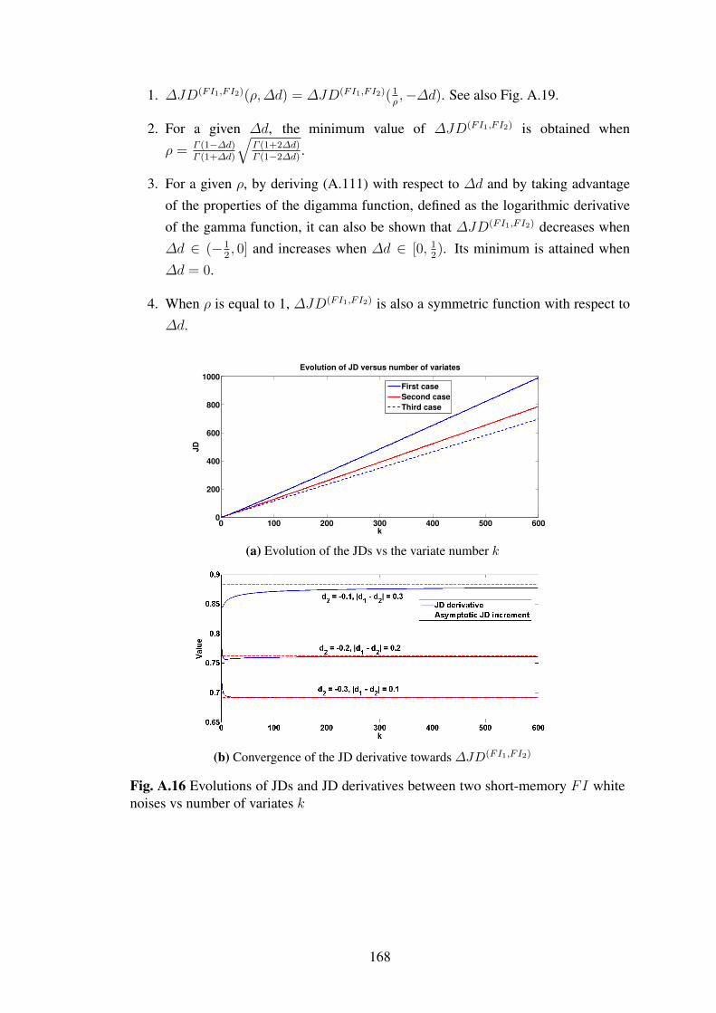
1. ∆JD(FI1,F I2)(ρ,∆d) = ∆JD(FI1,F I2)(1ρ,−∆d). See also Fig. A.19.

2. For a given ∆d, the minimum value of ∆JD(FI1,F I2) is obtained whenρ = Γ (1−∆d)

Γ (1+∆d)

√Γ (1+2∆d)Γ (1−2∆d) .

3. For a given ρ, by deriving (A.111) with respect to ∆d and by taking advantageof the properties of the digamma function, defined as the logarithmic derivativeof the gamma function, it can also be shown that ∆JD(FI1,F I2) decreases when∆d ∈ (−1

2, 0] and increases when ∆d ∈ [0, 1

2). Its minimum is attained when

∆d = 0.

4. When ρ is equal to 1, ∆JD(FI1,F I2) is also a symmetric function with respect to∆d.

0 100 200 300 400 500 6000

200

400

600

800

1000

k

JD

Evolution of JD versus number of variates

First case

Second case

Third case

(a) Evolution of the JDs vs the variate number k

(b) Convergence of the JD derivative towards ∆JD(FI1,F I2)

Fig. A.16 Evolutions of JDs and JD derivatives between two short-memory FI whitenoises vs number of variates k

168

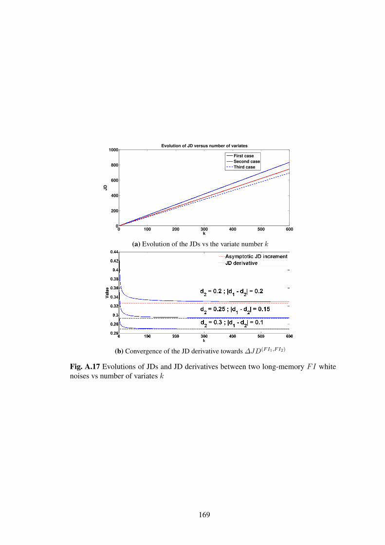
t

0 100 200 300 400 500 6000

200

400

600

800

1000

k

JD

Evolution of JD versus number of variates

First case

Second case

Third case



Fig. A.17 Evolutions of JDs and JD derivatives between two long-memory FI whitenoises vs number of variates k

169



Fig. A.18 Evolutions of JDs and JD derivatives between long-memory FI and short-memory FI white noises vs number of variates k

Fig. A.19 Asymptotic increment of the JD between FI white noises as a function of∆d = d1 − d2 and ρ = σ12

σ22

170

To end up this part, let us illustrate the comparison between two stationary ergodicFI white noise p rocesses when ∆d > 1

2. In this case, the asymptotic JD increment

should go to infinity since the power of a FI(∆d) process is infinite when ∆d > 12. In

Fig. A.20a and Fig. A.20b, we present the JD with respect to the number of the variatesk and the JD derivative respectively. This latter goes to infinity when k increases. Thisillustrates the inverse filtering interpretation we gave for the various cases.

(a) Evolution of the JD vs the variate number k

(b) Evolution of the JD derivative vs the variate number k

Fig. A.20 Evolutions of JD and JD derivatives between long-memory FI and short-memory FI white noises vs number of variates k, |∆d| > 0.5

In the following, let us analyze the JD between two unit-power FI prcesses.

JD between unit-power FI white noisesAs suggested in [44], we now propose to compare two unit-power FI white noises, de-noted as yn,l with l = (1, 2), in order to study the influences of d1 and d2 on the valueof the asymptotic JD increment ∆JD(FI1,F I2). As seen in Fig. A.21a which depicts thenormalization to be done, both unit-power FI white noises yn,ll=1,2 no longer dependon σ2

u,ll=1,2. Then, following the processing presented in Fig. A.21b, the power Pm,nof the inverse-filter output t(m,n)k , defined in Fig. A.21, satisfies:

171

P (FIl,F Il′ ) =Γ 2(1− dl)Γ (1− 2dl′)

Γ 2(1− dl)Γ (1− 2dl′).Γ (1− 2(dl − dl′))Γ 2(1− (dl − dl′))

(A.136)

Given (A.111) and (A.136), the asymptotic JD increment ∆JD(FI1,F I2) between twounit-power FI white noises is a function of d1 and d2 only. In addition, one has:

∆JD(FI1,F I2)(d1, d2) = ∆JD(FI1,F I2)(d2, d1) (A.137)

∆JD(FI1,F I2)(−d1,−d2) 6= ∆JD(FI1,F I2)(d1, d2) (A.138)

When d1 and d2 both tend to 0, 0.5 or −0.5, P (FI1,F I2) and P (FI2,F I1) tend to 1 ac-cording to (A.136). Therefore, ∆JD(FI1,F I2) tends to 0. When d1 is positive (resp.negative) and tends to 0, P (FI1,F I2) goes to infinity if d2 tends to 0.5 (resp. −0.5) sincelimx→0+

Γ (x) = +∞. Therefore, ∆JD(FI1,F I2) goes to infinity. For the other cases,

∆JD(FI1,F I2) takes strictly positive values. See Fig. A.22c. The influences of d1 and d2on the asymptotic JD increment are presented in Fig. A.22a (resp. Fig. A.22b) whichpoints out these properties.

(a) Power normalization of the lth FI white noise, l = 1, 2

(b) Inverse filtering to deduce the JD asymptotic increment

Fig. A.21 Steps to follow to compare two unit-power FI white noises

172

t

(a) ∆JD(FI1,F I2) when (d1, d2) ∈ (0, 0.5)× (0, 0.5)

(b) ∆JD(FI1,F I2) when (d1, d2) ∈ (−0.5, 0)× (−0.5, 0)

(c) Zoom on ∆JD(FI1,F I2) when (d1, d2) ∈ (0, 0.3)× (0, 0.3)

Fig. A.22 Asymptotic JD increment as a function of d1 and d2

173

A.7.2 JD between two ARFIMA processes

A.7.2.1 Theoretical analysis of the JD between ARFIMA(p, d, q) processes basedon inverse filtering interpretation

As it was done with FI white noises in the previous section, let us now investigate thevalidation of the inverse-filtering interpretation. For this purpose, let us consider twoARFIMA processes defined by their orders (pl, dl, ql)l=1,2 with dll=1,2 ∈ (−1

2, 12),

their driving-process variances σ2u,ll=1,2, their poles pj,lj=1,...,pl , and their zeros

zj,lj=1,...,ql with l = 1, 2.Filtering the first ARFIMA process by the inverse filter of the second amounts to filter-ing a white noise with a variance

σ2u,1

σ2u,2

by the following transfer function:

Hequ(z) = (1− z−1)d2−d1× (A.139)∏q1l=1 (1− zl,1z−1)∏p1l=1 (1− pl,1z−1)

p2∏l=1

(1− pl,2z−1)q2∏l=1

H−1l,2 (z)

where H−1l,2 (z)l=1,...,q2 are defined by following the rules we presented in (A.62)-(A.64) applied to the zeros of the second process.Depending on the values of d1 and d2, different situations occur and are summarized intable A.11.

Table A.11 Different cases under study

d1 ∈ (−0.5, 0) d1 ∈ (0, 0.5)

d2 ∈ (−0.5, 0)As |d1 − d2| < 0.5, the

filter output is aARFIMA process

|d1− d2| can be smalleror larger than 0.5

d2 ∈ (0, 0.5)|d1− d2| can be smaller

or larger than 0.5

As |d1 − d2| < 0.5, thefilter output is a

ARFIMA process

1. Let us look at the outputs of the two inverse filters when (d1, d2) ∈ (−0.5, 0)when the input are the ARFIMA processes to be compared. They are alsoARFIMA processes: one is an ARFIMA(p1 + q2, d1 − d2, q1 + p2), whereasthe other is ARFIMA(p2 + q1, d2− d1, q2 + p1). In addition, they are stationarysince |d1 − d2| < 0.5. More particularly, the one with a differencing order equalto−|d1−d2| is a short-memory process whereas the other with a differencing or-der equal to |d1 − d2| is a long-memory process. In this case, given (A.139),the inverse-filter output power P (ARFIMA1,ARFIMA2), with (l, l′) = (1, 2) or(l, l′) = (2, 1), can be seen as the power of anARFIMA(pl+ql′ , dl−dl′ , ql+pl′)process where the variance of the driving process is

σ2u,l

σ2u,l′

.

174

It is given by:

P (ARFIMAl,ARFIMAl′ ) =σ2u,l

σ2u,l′× (A.140)

ql+pl′∑i=−(ql+pl′ )

pl+ql′∑s=1

φl,l′(i)εl,l

′

s C(dl − dl′ , pl + ql′ + i, ps)

where pss=1,...pl+ql′are the poles of the ARFIMA(pl + ql′ , dl − dl′ , ql + pl′)

process, φm,n(i) corresponds to the value of the autocorrelation function for lag lof the MA part defined from the zeros of the ARFIMA(pl+ ql′ , dl−dl′ , ql+ pl′)process, and εl,l′s s=1,...pl+ql′

is similarly defined as in (A.55) but adjusted to thepoles pss=1,...pl+ql′

. Then the asymptotic JD increment can be deduced by using(A.111).

2. When (d1, d2) ∈ (0, 0.5), the processes to be compared are long-memoryARFIMA processes. The inverse-filter outputs are stationary ARFIMA processesand the same conclusions as in the previous case can be drawn.

3. When d1 and d2 have opposite signs, |d1 − d2| can be smaller or larger than 12. If

the difference is smaller than 12, the same comments as in the two previous cases

can be drawn. If it is larger than 12, one of the filter outputs should correspond

to an ARFIMA process with an differencing order larger than 12. It is a non-

stationary process with an infinite variance.

A.7.2.2 Illustrations and comments

Let us now study the evolutions of the JD and the JD increment with respect to thevariate number between two real ARFIMA(1, dl, 1) processes. For this purpose, threetypes of simulations were done.

1. In the first one, two short-memory ARFIMA(1, dl, 1) processes are compared.

2. In the second one, the case of two long-memory ARFIMA(1, dl, 1) processes isaddressed.

3. As for the last illustration, we compare a short-memory ARFIMA(1, d1, 1) witha long-memory ARFIMA(1, d2, 1) process.

Let us study the influence of the type of the ARFIMA(1, dl, 1) processes on the con-vergence of the JD derivative towards the asymptotic JD increment. The parameters ofthe processes in the three cases are given in Table. A.12. In each illustration, d2 takesthree values.

175

t

Table A.12 Parameters of the ARFIMA processes under study

1st-processparameters

2nd-processparameters

Figures

Two short-memoryARFIMA processes

σ2u,1 = 15

z1,1 = −0.6p1,1 = 0.2d1 = −0.3

σ2u,2 = 5

z1,2 = 0.4p1,2 = −0.7d2 = −0.1,−0.15,−0.2


Two long-memoryARFIMA processes

σ2u,1 = 10z1,1 = 0.5p1,1 = 0.3d1 = 0.4

σ2u,2 = 20z1,2 = 0.2p1,2 = 0.6

d2 = 0.1, 0.2, 0.3


Long-memory andshort-memory

ARFIMA processes,|∆d| < 1

2

σ2u,1 = 10z1,1 = 0.4p1,1 = 0.7d1 = 0.1

σ2u,2 = 25z1,2 = 0.6p1,2 = 0.2d2 = −0.15,−0.1,−0.05


Long-memory andshort-memory

ARFIMA processes,∆d > 1

2

σ2u,1 = 5

z1,1 = 0.4p1,1 = 0.7d1 = 0.0.45

σ2u,2 = 15z1,2 = 0.6p1,2 = 0.2d2 = −0.4,−0.1,−0.05


In Fig. A.23a, Fig. A.24a and Fig. A.25a, the different JDs tend to have constant slopes.In Fig. A.23b, Fig. A.24b, and Fig. A.25b, the JD derivative converges to the asymptoticJD increment ∆JD(ARFIMA1,ARFIMA2) obtained with (A.111) and (A.140).To end up this part, we will compare two stationary ergodic ARFIMA processes when∆d > 1

2as we did for the FI white noise processes. In Fig. A.26a and Fig. A.26b, the

JD derivative goes to infinity when k increases. This again validates the inverse filteringinterpretation.

176


(b) Convergence of the JD derivative towards ∆JD(ARFIMA1,ARFIMA2)

Fig. A.23 Evolutions of JDs and JD derivatives between two short-memoryARFIMAprocesses vs number of variates k



Fig. A.24 Evolutions of JDs and JD derivatives between two long-memory ARFIMAprocesses vs number of variates k

177



Fig. A.25 Evolutions of JDs and JD derivatives between long-memory ARFIMA andshort-memory ARFIMA processes vs number of variates k, |∆d| < 1

2

(a) Evolution of the JD vs the variate number k

(b) Evolution of the JD vs the variate number k

Fig. A.26 Evolutions of JD and JD derivatives between long-memory ARFIMA andshort-memory ARFIMA white noises vs number of variates k, ∆d > 1

2

178

A.7.3 JD between ARFIMA and ARMA processes

In this last section, we propose to study the evolution of the JD and the JD incrementversus the number of variates between a real ARFIMA(1, dl, 1) process and a realARMA(1, 1) process. For this purpose, two types of simulations were done. In the firstone, a real ARMA(1, 1) process is compared with a short-memoryARFIMA(1, dl, 1)

process. As for the second one, a realARMA process is compared with a long-memoryARFIMA(1, dl, 1) process. The parameters of processes under study are given inTable. A.13.

Table A.13 Parameters of the ARMA and ARFIMA processes under study

ARMA-processparameters

ARFIMA-process

parametersFigures

Short-memoryARFIMA and

ARMA process

σ2u,1 = 10z1,1 = 0.4p1,1 = 0.55

σ2u,2 = 25z1,2 = 0.6p1,2 = 0.2d2 = −0.2,−0.15,−0.1


Long-memoryARFIMA and

ARMA process

σ2u,1 = 15z1,1 = 0.4p1,1 = −0.3

σ2u,2 = 6

z1,2 = 0.7p1,2 = 0.35d2 = 0.25,0.2, 0.15


In Fig. A.27a and Fig. A.28a, the different JDs tend to have constant slopes.In Fig. A.27b and Fig. A.28b, the JD derivative converges to the asymptotic JD incre-ment ∆JD(ARFIMA,ARMA) obtained with (A.111) and (A.140).Finally, if our purpose was that we compare an ARMA(1, 1) process with anARFIMA(1, d1, 1) process when they share the poles and zeros. In this case, derivingthe asymptotic JD increment in (A.111) amounts to computing the power of a FI(d1)process. The influences of d1 and

σ2u,1

σ2u,2

on the asymptotic JD increment are similar tothat obtained in Fig. A.19. The only difference is that ∆d is replaced by -d1.

179


(b) Convergence of the JD derivative towards ∆JD(ARFIMA,ARMA)

Fig. A.27 Evolutions of JDs and JD derivatives between short-memory ARFIMAprocess and ARMA process vs number of variates k


(b) Convergence of the JD derivative towards ∆JD(ARFIMA,ARMA)

Fig. A.28 Evolutions of JDs and JD derivatives between long-memory ARFIMAprocess and ARMA process vs number of variates k

180

A.7.4 Some comments for the practitioner to apply this theory in practical cases

Interested users would like to make use of this theory in practical cases. In this subsec-tion, we propose some clues. In the field of change detection, to compare two segments,assumed to be of size N , by using the type of analysis we presented above, the covari-ance matrices for both segments have first to be estimated for two consecutive sizesk − 1 and k by using a robust estimator. The JD are then computed for both sizes andtheir difference is computed. Once smoothed over time, the difference between both JDmakes it possible to have an idea of the statistical change in the signal under study.Remark 1: the selection of the size k corresponds to a compromise. On the one hand,k must be sufficiently large so that the difference between the estimated JD can be con-sidered as an approximation of the asymptotic JD increment. On the other hand, it mustbe much smaller than the number of samples N since the estimates of the covariancematrices must be as accurate as possible.Remark 2: the estimations of the differencing orders dll=1,2 can also be of interestand can be useful to help the practitioner to give an interpretation of the results. Theyare related to the Hurst exponents, denoted as Hll=1,2 = dll=1,2 +

12. Different

families of methods have been proposed in the literature to estimate them:

1. The time-domain estimators gather the so-called rescaled range analysis, the ag-gregated variance method, the absolute-value method and the variance of residu-als method [114].

2. The frequency-domain estimators consist in analyzing the power spectral densityof the time series [112]. This is for instance the case of the local Whittle method,the periodogram method and the wavelet-based method.

3. The detrended fluctuations analysis (DFA) [88] and some variants such as theadaptive fractal analysis (AFA) [96], the detrended moving average (DMA)method either centered or backward, the fluctuation analysis (FA) [106] havealso shown good performance, especially to estimate the Hurst exponent of apure mono-fractal time series. It has been used in various applications to analyzeelectroencephalograms (EEG) [102] and electrocardiograms (ECG) [90] [93].

In other applications where the purpose is classification, the difference between theestimated differencing orders and the difference between two consecutive JDs that havebeen estimated as mentioned above can be considered as features for the classification.K-nearest neighbors (KNN) or support vector machine support vector machine (SVM)can then be used.

181

A.8 Conclusions and perspectives

The following conclusions and perspectives can be drawn:

1. We compared noisy sums of complex exponentials (NSCE) by means of theJD. The difference between two consecutive JD was analyzed. In this case, theasymptotic JD increment and the convergence speed towards the asymptotic JDincrement must be taken into account by the practitioner to draw conclusionsabout the similarity between the processes under study. Besides, we could a

priori guess that the JD between an NSCE process, defined by the normalizedangular frequencies of its complex exponentials, and an AR process which hassharper and sharper resonances in its spectrum at the same normalized angularfrequencies becomes smaller and smaller. Nevertheless, in practice, the resultsthat can be obtained do not necessarily confirm this statement as the JD also takesinto account the powers of the processes to be compared.

2. Without developing tedious calculations, our interpretation of the asymptotic JDincrement based on inverse filtering makes it possible to explain the atypical casesthat were identified in previous works and for which the asymptotic JD incrementwas not finite. The results we present in this appendix allow us to generalize ouranalysis to the JD between AR processes, ARMA, MA, etc. Now, we are ableto prove that all ARMA processes of any order and whose PSD is null for oneor more frequencies can give rise to non-finite asymptotic JD increments. More-over, there are now several ways to compute the JD: considering the definition ortaking advantage of the interpretation we propose in this paper, i.e. using inversefiltering.

3. We studied the JD between ergodic w.s.s. ARFIMA processes. We have shownthat the derivative of JD with respect to the number of variates k tends to a con-stant when the difference between the differencing order is absolutely smallerthan 0.5. Moreover, we have analyzed the influence of the process parameters onthe value of the asymptotic JD increment. Finally, it was shown that the interpre-tation of the asymptotic JD increment based on inverse filtering is also valid forthese processes.

4. It could be of interest to use this type of approach in various applications, frombiomedical applications to radar applications when analyzing the statistical prop-erties of the clutter. In the latter case, it could be of interest to see whether it ishomogeneous or not. This can be done by looking at secondary data. This typeof analysis could be a preamble to estimate the correlation matrix of the clutterthat would be used for space-time adaptive processing (STAP).

182

Contributions to High Range Resolution Radar Waveforms

Documents

Transcript of Contributions to High Range Resolution Radar Waveforms