For Peer ReviewMeasuring AEM waveforms with a ground loop

Journal: Geophysics

Manuscript ID: GEO-2007-0286.R1

Manuscript Type: Technical Paper

Date Submitted by the Author:

21-Feb-2008

Complete List of Authors: Davis, Aaron; RMIT University, Applied Physics Macnae, James; RMIT University, Department of Applied Sciences

Keywords: airborne survey, deconvolution, electromagnetics, modeling

Area of Expertise: Electrical and Electromagnetic Methods

GEOPHYSICS

For Peer Review

Measuring AEM waveforms with a ground loop

Aaron Davis1 and James Macnae1

1RMIT University

Applied Physics

GPO Box 2476V

Melbourne, Victoria

Australia 3001

(February 21, 2008)

Running head: AEM waveforms with a ground loop

ABSTRACT

Measurement of a transmitter current waveform provides critical data not otherwise avail-

able for some AEM systems; yet which is needed for quantitative modelling of AEM data.

We thus derive a method of measuring an airborne transmitter waveform by means of

monitoring the current induced in a closed, multi-turn, insulated ground loop of known

inductance L and resistance R. The transmitter waveforms of several different time-domain

systems are deconvolved from the measured ground loop response when excited by the pri-

mary electromagnetic field of the airborne electromagnetic (AEM) system itself. In general,

our measurements agree well with contractor-described transmitter current waveforms; al-

though crucial differences exist between our deconvolved waveforms and those described in

the literature. Using the pulse-per-second feature of a GPS antenna the induced ground

loop can monitor the frequency drift of a frequency-domain system. The ground loop be-

haves like a lossy electric field antenna when the resistance closing the ground loop is made

1

Page 1 of 48 GEOPHYSICS

123456789101112131415161718192021222324252627282930313233343536373839404142434445464748495051525354555657585960

For Peer Review

too large. This leads to negatives in the response of coincident-loop systems without the

need for induced polarisation effects. We observed exponentially decaying, oscillating cur-

rent responses in high-resistance ground loops. We modelled the observed current with an

LRC circuit whose resistance and capacitance represent generalised effective antenna and

free-space values. Our model predicts responses that closely match the damped oscillations

seen in the airborne response during flyover. There is a limitation to the method: it does

not work well on conductive ground.

2

Page 2 of 48GEOPHYSICS

123456789101112131415161718192021222324252627282930313233343536373839404142434445464748495051525354555657585960

For Peer Review

INTRODUCTION

Time-domain AEM systems are used for a broad range of applications including mineral

exploration, shallow water bathymetry, sea-ice thickness estimation and land management.

Unfortunately, precise timing and waveform details are not easily gained from published

descriptions of AEM systems; and operators change system waveforms and timing to suit

particular applications. Additionally, some concentric loop time-domain systems cannot use

their sensitive receivers during the transmitter on-time since the electronic amplifier gain

is extremum for optimum off-time measurement. Interpretations valid for shallow depths

in most environments rely on early-time data, which requires accurate receiver timing and

a precise knowledge of the transmitter waveform. Later in this paper we will show a 40 µs

timing difference. As an example, there are many methods for modelling and inversion of

AEM data, of which EMFlow (Macnae, 2004) is one established conductivity-depth imaging

(CDI) method. The CDI sections are derived by stitching together successive 1D models

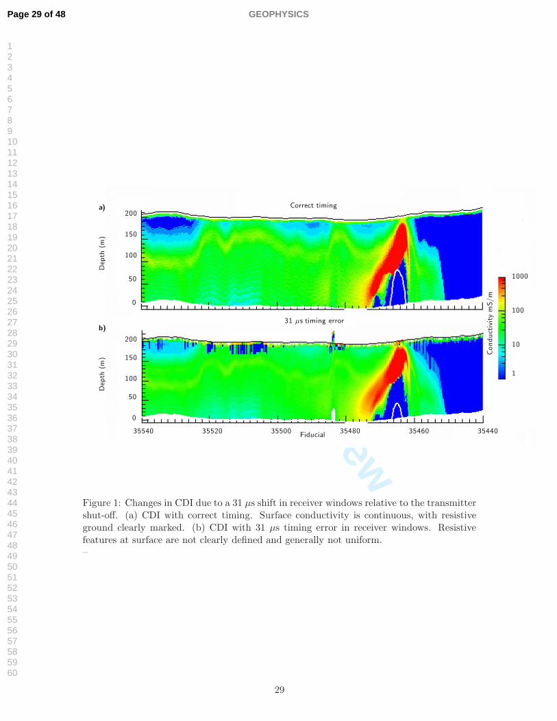
predicted from the data. Figure 1 shows the result of CDI processing of one survey line of

AEM data over the Walford Creek deposit, Queensland, using (a) the correct waveform and

windows and (b) the correct waveforms with a 31 µs timing shift of the sampling windows

relative to the transmitter shut-off. It is clear is that the CDI derived using incorrect

timing has poorer imaging of resistive near-surface features (blue tints), and is generally

less uniform. The CDI image of the dipping good conductor (red) is less affected by timing

errors since the response of this body extends to several milliseconds, and thus the relative

timing error is less important that the quickly decaying responses of near-surface features.

However, the benefits of establishing correct waveform timing are very clear. In order

to improve the quantitative interpretation of AEM data, we have designed a method of

indirectly measuring the transmitter waveform of any time-domain AEM system.

3

Page 3 of 48 GEOPHYSICS

123456789101112131415161718192021222324252627282930313233343536373839404142434445464748495051525354555657585960

For Peer Review

Different transmitter waveforms create different effects on the AEM response (Liu, 1998);

yet there is no independent method available to a client to determine the waveform of an

AEM transmitter as claimed by a contractor. As part of their routine base level adjustment,

many systems are flown at high altitude to obtain the receiver response to the transmitter

waveform in the absence of conductors; and while this yields some information, it does not

always provide the continuous waveform shape that is required for some software programs.

We propose the use of a closed multi-turn loop of known resistance R and self-inductance

L that is insulated from the ground beneath it. Flying an AEM system over the loop

generates an eddy current in it that can be measured and used for a system calibration

(Davis, 2007). The current induced in the ground loop is a convolution of the time derivative

of the transmitter current waveform with the natural response of the wire loop itself. By

measuring this induced current, it is possible to extract the transmitter current waveform

itself, thereby determining the transfer function of the transmitter-ground loop system. We

have applied this method to a variety of time-domain AEM systems and have compiled

several examples of transmitter current waveforms. We also identify some interesting

features in the ground loop current envelope that, we believe, have not been seen before.

METHOD

Ground loop response

A time-domain AEM system operates by energising the earth with a time-varying electro-

magnetic field which is created by a transmitter current that is pulsed or stepped repeatedly.

When flown in proximity to a ground loop of known resistance R and self-inductance L,

the field generated by the AEM transmitter (primary field) generates an emf EL(t) in the

4

Page 4 of 48GEOPHYSICS

123456789101112131415161718192021222324252627282930313233343536373839404142434445464748495051525354555657585960

For Peer Review

ground loop which depends on the transmitter current IT (t) and the mutual inductance

MTL coupling the transmitter to the ground loop:

EL(t) = −MTLd

dtIT (t). (1)

The emf induces a current IL(t) to flow around the ground loop. The induced current, de-

scribed by a first-order differential equation relating the transmitter current to the electrical

properties of the loop itself, may be written as

(

d

dt+

R

L

)

IL(t) =−MTL

LI ′T (t), (2)

where I ′T (t) is the time derivative of the transmitter current. We solve the differential

ground loop current equation 2 by viewing it as an input/output system and using the

Laplace transform L which uses Laplace variable s in the expression

L[

f(t)]

=

∫

∞

0

e−stf(t) dt, (3)

where f(t) is a piecewise continuous and differentiable function of time and e−st is the kernel

of the transformation. The transformation from the complex frequency-domain back to the

time-domain is straightforward:

L−[

L[

f(t)]]

= f(t), (4)

where L− is the inverse Laplace operator.

We assume that the transmitter current waveform satisfies the conditions of the Laplace

5

Page 5 of 48 GEOPHYSICS

123456789101112131415161718192021222324252627282930313233343536373839404142434445464748495051525354555657585960

For Peer Review

transform, i.e., that the time derivative of the transmitter current I ′T (t) exists everywhere

in positive time except at a few places where it is permitted to be discontinuous. We further

make the simplification that the transmitter current can be expressed as IT (t) = IT iT (t),

where IT is the peak transmitter current and iT (t) is a waveform that begins at t = 0 and

−1 ≤ iT (t) ≤ 1. Thus, the ground loop current is expressed by

IL(t) = −MTLIT

LL−

[

s

s + R/LL

[

i′T (t)]

]

. (5)

Equation 5 shows that the current induced in the ground loop due to a transmitter current

waveform of any shape is given by the convolution of the transmitter waveform with the

natural response of the wire loop itself. The magnitude of the ground loop current is

determined by the mutual inductance between the transmitter and ground loop, which is

itself a function of position. Clearly, maximum current generated in the ground loop would

occur if the transmitter were coincident with the loop itself. If the transmitter waveform in

the expression above is a simple step on at time t = 0, then we immediately see that the

ground loop current becomes

IL(t) = −MTLIT

Le−tR/L; (6)

the current experiences a discontinuous jump at t = 0 to the peak value of −MTLIT /L

and then decays with characteristic time τ = L/R. Dropping the amplitude term from the

right-hand side, we see that the natural response of the ground loop to a transmitter step

is simply

RL(t) = e−t/τ , (7)

6

Page 6 of 48GEOPHYSICS

123456789101112131415161718192021222324252627282930313233343536373839404142434445464748495051525354555657585960

For Peer Review

an exponential decay.

In our experiments, we closed the ground loop with a known resistor and measured the

potential drop across the resistor with an Edirol UA-5 analog-to-digital (A/D) converter.

This device sampled two channels at 96 kHz at 24 bit precision with a 20–20 000 Hz band

limiting filter. Assuming that we can express the voltage measured with the Edirol UA-5

data acquisition device (DAQ) as the actual loop emf convolved with the response function

of the DAQ itself, we write

VDAQ(t) = L−[

RDAQ(s)L[

IL(t)]]

, (8)

where VDAQ(t) is the measured voltage, RDAQ(s) is the response function of the DAQ and

IL(t) is the ground loop current, equation 5.

Deconvolution of the measured signal

The measured DAQ voltage expressed in equation 8 above is represented as a continuous

function of time. In reality, the signal is recorded at finite time intervals; we change the

notation above to reflect this. In place of the time variable t, we use the variable n to denote

a discrete sample in a time-series. Using ∗ to represent the convolution of two time-series,

the voltage measured by the DAQ vDAQ(n) becomes

vDAQ(n) = rDAQ(n) ∗ rL(n) ∗ i′T (n), (9)

where rDAQ(n), i′T (n) and rL(n) are respectively the time-series equivalents of the DAQ

response function, the time derivative of the transmitter current waveform and the natural

7

Page 7 of 48 GEOPHYSICS

123456789101112131415161718192021222324252627282930313233343536373839404142434445464748495051525354555657585960

For Peer Review

response of the ground loop, equation 7.

We extract iT (n) from the relation above by exploiting two properties of the discrete

Fourier transform: convolution in time-domain is equivalent to multiplication in frequency-

domain and integration of a time-series is easily accomplished by dividing each term of the

equivalent Fourier series by iωn, where ωn is the frequency of the nth term. Using the

notation F and F− to represent the forward and inverse discrete Fourier transforms, the

transmitter waveform is written as

iT (n) = F−

[

F[

vDAQ(n)]

F[

rDAQ(n)]

F[

rL(n)]

iωn+ ci

]

, (10)

where ci is a constant of integration which we can set to 0.

EXAMPLE: VTEM

Our first example we present is from a VTEM (Witherly et al., 2004) helicopter electro-

magnetic (HEM) system conducted outside Sudbury, Ontario, Canada in October, 2005.

The ground beneath the loop was composed of electrically resistive cover of less than 0.1 S

conductance over an even more resistive basement (< 1 mS/m). The VTEM system was

flown over the loop two times. On the first flyover, we closed the loop with a 1 Ω resistor,

across which the Edirol UA-5 was attached. The measured resistance of the ground loop for

the first flyover was 15.97 Ω; and the self-inductance was calculated the be 23.6 mH. The

characteristic decay constant for the ground loop during the first flyover was τ = 1.48 ms.

For the second flyover, the resistor used to close the ground loop was changed to 1 000 Ω,

thereby lowering the time constant of the loop to 1.48 µs. The flight lines and the corners

of the ground loop are shown in Figure 2.

8

Page 8 of 48GEOPHYSICS

123456789101112131415161718192021222324252627282930313233343536373839404142434445464748495051525354555657585960

For Peer Review

Figure 3 shows the envelope of the current induced in the ground loop during the line 1

VTEM flyover. The envelope starts and ends with small shoulders, crossing to a main lobe

in the centre where the mutual inductance coupling the transmitter to the loop is greatest.

The clear current nulls at 3 s and 12 s seconds indicate that the ground beneath the loop

is very resistive: the secondary fields generated in the earth produced negligible currents in

the ground loop during flyover (Davis and Macnae, submitted to Geophysics).

In order to complete the deconvolution of the VTEM waveform, we took several complete

ground current waveforms stacked together to increase the signal to (random) noise ratio.

Our stacking process was as follows: we calculated N the number of DAQ samples per

transmitter waveform by counting the number of samples over 100 repetitions of the recorded

ground-signal. We spline interpolated the ground signal by a factor of 10 and rounded the

number N×10 to the nearest integer as our stacking rate. For the 30 Hz VTEM transmitter

signal, we found N = 3198.6, which is very close to the 3 200 samples expected with the

Edirol DAQ (sampling rate 96 000 Hz, with a transmitter period of 30 Hz). We assert

this interpolation does not add any spurious high-frequency components to the signal since

AEM shut-offs are nominally 40 µs–1 ms in duration which, at the lower limit, is of the

order of the Edirol UA-5 bandwidth. For the VTEM current envelope shown in Figure 3, we

selected the signal where the transmitter was over the middle of the ground loop, thereby

producing maximum current. We selected a total of 118 repetitions for the fold, from 6 s to

10 s as marked by vertical lines in Figure 3. A symmetric portion of the signal was chosen

to minimise the standard error of the stacked waveform. Each waveform in the stack was

scaled to the mean in a least squares sense and the mean variance of at each point from

the fold was calculated. The result was a series of mean variances equal in length to the

mean waveform. We define our standard error of the stack by calculating the square root

9

Page 9 of 48 GEOPHYSICS

123456789101112131415161718192021222324252627282930313233343536373839404142434445464748495051525354555657585960

For Peer Review

of the median variance divided by the length of the stacked waveform time-series. For this

experiment, the standard error of the stacking process was less than 60 ppm.

To obtain the transmitter current waveform, equation 10, we applied the discrete Fourier

transform to: rDAQ(n) the response function of the DAQ, the time-series shown in Figure 4

(vDAQ(n)), and to the natural response of the ground loop (rL(n)). The deconvolved VTEM

waveform is shown with dots in Figure 5. On the second flyover, the resistor closing the

ground loop was changed to 1 000 Ω; thereby decreasing the time constant of the loop

significantly. The corresponding waveform deconvolved from the ground loop current is

shown in thick grey in Figure 5. The agreement of the 1 Ω and 1 000 Ω deconvolved

waveforms is better than 20 ppm. Figure 5 also shows a the VTEM current waveform

produced from streamed data acquired by the receiver in a high altitude test flight flown

concurrently with this experiment. By stacking the streamed VTEM receiver data in the

manner described earlier, we found that the median standard error from the entire fold

was better than 20 ppm. Our 1 Ω waveform agreed with the streamed waveform to about

13 ppm, which is similar in magnitude to the noise level of the VTEM system. Of course,

streamed data from the receiver during the transmitter on-time can be synchronised with the

waveform, and amplitudes do not change as much, which is an advantage over our method.

We recognize that contractors flying VTEM surveys now supply a measured waveform to

the client; however, not all contractors do this. We expect based on this direct comparison

that our other experiments had similar accuracy over resistive terrain.

10

Page 10 of 48GEOPHYSICS

123456789101112131415161718192021222324252627282930313233343536373839404142434445464748495051525354555657585960

For Peer Review

EXAMPLES OF AEM WAVEFORMS

We present the results of our experiments for several different AEM systems flown at dif-

ferent times over the past 4 years.

HOISTEM

The HoistEM (Boyd, 2004) helicopter electromagnetic (HEM) system experiment was con-

ducted in 2003. In this year, the HoistEM receiver could not be run during the transmitter

on-time so the published waveform was regarded as nominal. Problems have been encoun-

tered by the authors and others (e.g., Vrbancich and Fullagar (2007); John Paine, personal

communication, 2007) in quantitatively fitting HoistEM data to EM models, particularly at

early delay times. We used a 3-turn 100×100 m ground loop of self-inductance L = 7.91 mH

and resistance R = 25.7 Ω (τ = 0.29 ms) placed on a resistive ridge (0.1 S of cover over a

resistive basement of < 1 mS/m) near Paraburdoo, Western Australia. The ground loop

was closed with a 1 Ω resistor, across which the Edirol UA-5 was attached. The HoistEM

system was flown over the ground loop 3 times, two of which are described in this paper.

Figure 6 shows the envelope of the current induced in the ground loop during the flyover of

line 1. The clear current nulls at 3.3 s and 8.6 s are again indicative of extremely resistive

ground. As described earlier, we interpolated and stacked the ground signal from 5 s to 7 s:

the deconvolved waveform is shown in Figure 7.

As described by Boyd (2004), the transmitter on-times are approximately 5 ms, with a

11

Page 11 of 48 GEOPHYSICS

123456789101112131415161718192021222324252627282930313233343536373839404142434445464748495051525354555657585960

For Peer Review

repeat rate of 25 Hz. However, when we compare the deconvolved signal to the nominal

waveform description, differences become apparent. Since the transmitter waveform was

not directly measured, Vrbancich and Fullagar (2007) used the contractor-specified current

pulse of an exponential current rise (time constant 500 µs), followed by 4 ms of constant

current, then a linear shut-off of 40 µs, starting at 5 ms. Figure 8 shows our deconvolved

waveform superimposed on their nominal waveform. Panel (a) shows that the nominal

waveform rises to full current more quickly than the deconvolved waveform and that there

is a difference in the shut-off. The second panel shows this difference in much more detail.

Figure 8b shows the nominal waveform beginning its turn-off at 5 ms and ending 40 µs later.

Our analysis reveals that the HoistEM waveform begins turn-off at 4.96 ms and is almost

completely off by 5 ms, making the total waveform 40 µs shorter than claimed. Forward

models show that this creates an average 12% difference in predicted signal strength when

flying over our ground loop of τ = 0.29 ms.

TEMPEST

The fixed-wing towed-bird TEMPEST system (Fugro Airborne Surveys) has a nominally

square-wave waveform operating with a 50% duty cycle at 25 Hz. In this experiment,

conducted near Mandurah, Western Australia in 2003, the TEMPEST system was flown

over a 100×100 m ground loop, closed with a 1 Ω resistor and placed on fairly uniform terrain

of 10 S conductance in the top 100 m. The deconvolved transmitter current waveform,

shown in Figure 9, clearly shows that the actual TEMPEST waveform indeed approximates

a square-wave oscillating at 25 Hz, with a 50% duty cycle. Data are delivered to the client

as a 100% duty cycle square wave response after deconvolution processing.

12

Page 12 of 48GEOPHYSICS

123456789101112131415161718192021222324252627282930313233343536373839404142434445464748495051525354555657585960

For Peer Review

GEOTEM

Three months before the TEMPEST tests, a GEOTEM (also Fugro Airborne Surveys)

system was flown over a ground loop in the same area, closed with a 1 Ω resistor. The

measured induced current envelope is interesting because, as specified by the contractor,

the transmitter cycle was interrupted every second for 20 ms in order to measure magnetic

field. The measured ground loop signal, in arbitrary units, is shown in Figure 10. A complete

waveform of the interpolated and stacked ground-loop signal, with the DAQ and ground

loop responses deconvolved from it is shown in Figure 11a. The deconvolved and integrated

transmitter current waveform is shown in Figure 11b. As expected, the transmitter current

waveform consists of half sine waves of 5 ms in duration, repeating at a frequency of 25 Hz.

Since the 130 m distant GEOTEM receiver is capable of measuring during the on-time,

this waveform was also obtained from high altitude airborne observations. Panels (a) and

(b) of Figure 11 also show the high altitude responses, displaying good agreement between

airborne and ground measurements with a difference of about 300 ppm. The differences in

the turn-on and shut-off can be attributed to the conductive ground interacting with the

ground loop.

SkyTEM

The final example is from the helicopter-borne SkyTEM system (Halkjær et al., 2006).

SkyTEM was flown over conductive ground (8 S of cover over a 1 200 mS/m basement)

outside Berri, South Australia: we initially closed the ground loop with a 1 Ω resistor (line 1)

and subsequently with a 1 000 Ω resistor (line 2). For the first line flown, the decay constant

was 0.86 ms, while for the second, the decay constant was < 1 µs. SkyTEM is unique in

13

Page 13 of 48 GEOPHYSICS

123456789101112131415161718192021222324252627282930313233343536373839404142434445464748495051525354555657585960

For Peer Review

that it is capable of alternately transmitting a waveform at both high and low moments.

The current induced in the ground loop during the first flyover is shown in Figure 12. We

have marked sections on the envelope that are due to high and low moment transmitter

currents. The lack of current nulls on either edge of the envelope indicates that the ground

was not resistive. We attempted to use the ground loop current to predict the SkyTEM

waveform for both moments, but found that the conductive ground interfered with the

deconvolution by adding a response due to the interaction between the ground loop and the

earth. Our attempted transmitter waveform deconvolutions are shown in Figure 13. Panel

(a) shows our deconvolution attempts for the high moment transmitter waveform, using

both the 1 and 1 000 Ω resistor. Panel (b) shows the deconvolution for the low moment

transmitter waveform using the same resistors. This figure shows that increasing the loop

resistance decreases the time constant: for example, the 1 000 Ω deconvolved transmitter

waveform in panel (b) shows a much faster transmitter turn-off than the 1 Ω waveform.

This is because the extra signal in the ground loop due to the conductive earth decayed

much more quickly in the high resistance loop; hence it is more believable. However, due

to the high conductivity of the earth beneath the loop, we are sceptical that our 1 000 Ω

dewconvolved waveforms are as accurate as the VTEM examples.

ANTENNA EFFECTS IN THE WIRE LOOP

In Figure 13, we showed that changing the resistance of the ground loop affects the current

induced in it. However, we have also noticed that if the resistance of the ground loop is

increased by a large amount, the current in the loop changes and the loop itself begins

to act like a lossy electrical field antenna. In addition to the exponential decay observed

before, we also detect oscillations in the ground loop current that can be detected at the

14

Page 14 of 48GEOPHYSICS

123456789101112131415161718192021222324252627282930313233343536373839404142434445464748495051525354555657585960

For Peer Review

platform receiver; causing negative responses in the recorded signal. In this section, we

present conclusive evidence that coincident-loop negative responses can be detected at the

receiver without the presence of polarisable conductors (Jansen and Witherly, 2004).

During the HoistEM experiments, we significantly increased the value of the resistor

closing the ground loop. On the third flyover of the HoistEM experiments, we removed the

1 Ω resistor and connected the leads of our DAQ directly to the loop itself. This increased

the total resistance of the ground loop from 25.7 Ω to ∼12 000 Ω. We measured the current

induced in the loop during the HoistEM flyover; shown in Figure 14. As before, the envelope

consists of two small shoulders containing a large central lobe (10–15 s); however, the central

portion appears reduced or cut off at about 0.4 mA, most likely due to clipping of the signal

or slew rate issues in the DAQ. Looking to the side lobes, where the signal is not cut off,

the current only peaks at 0.25 mA: a factor of 100 less than the maximum side lobe current

in Figure 3. We interpolated and stacked the ground loop current over a set of complete

waveforms in order to reduce random noise in our signal. In this particular case, we stacked

the signal from 10 s to 15 s (marked by vertical lines in Figure 14). When we examined

the stacked ground loop current, we found that not only did the ground signal decay quickly

(as expected), but it also displayed ringing. Figure 15a shows one half-cycle of the induced

ground loop current obtained from stacking, while panel (b) displays the transmitter turn-

off at 5 ms at an enlarged scale. Evidently, the current induced in the high resistance

ground loop during the HoistEM transmitter shut-off oscillates and its envelope also decays

exponentially. We modelled the damped oscillation with the functional form of

F (t) = e−t

τ sin(ωt + φf ), (11)

15

Page 15 of 48 GEOPHYSICS

123456789101112131415161718192021222324252627282930313233343536373839404142434445464748495051525354555657585960

For Peer Review

where τ is a time constant, ω is an angular frequency and φf is a phase shift. We achieved

excellent agreement with our measured current with parameters τ = 58.5 µs, and ω =

116 516 rad/s. The exponential decay curves are marked in figure 15b with dashed lines,

while the fitted curve is shown with open circles connected with a dot-dashed line. The fit

breaks down at times less than 5.05 ms.

An LRC circuit

The modelling curve equation 11 represents an exponentially decaying curve of character-

istic time τ and oscillation frequency ω. When analysed with reference to a series circuit

containing an inductor L, a resistor R and a capacitor C, equation 11 is a solution to the

homogeneous differential equation that describes the current flowing in the series circuit in

response to a voltage change:

0 = Ld2

dt2i(t) + R

d

dti(t) +

1

Ci(t). (12)

This relation is well known: it shows that the characteristic decay τ and the angular fre-

quency ω can be expressed in terms of L,R and C in the following way:

τ =2L

R, and ω =

√

1

LC−

1

τ2. (13)

We assume that the self-inductance of the ground loop does not change during our

modelling, since the mutual inductance of the parallel wires and turns of the loop will not

change for the comparatively low frequency oscillation of only 116 516 rad/s (∼18 500 Hz),as

changes in mutual inductance due to skin depth effects do not become meaningful until much

16

Page 16 of 48GEOPHYSICS

123456789101112131415161718192021222324252627282930313233343536373839404142434445464748495051525354555657585960

For Peer Review

higher frequencies are reached (e.g., Jackson, 1999). Instead, we assume that the wires in

the loop are acting like transmission lines and possess distributed resistance, inductance,

capacitance and shunt resistance. The distributed parameters can be replaced by lumped

values in an LRC circuit with no loss of generality. Following this assumption, we calculated

an effective resistance of R = 271 Ω and a capacitance of C = 9.11 nF. These numbers are

generalised effective values representing the interaction of the wire loop with free space,

itself and, possibly, the ground beneath. The capacitance is reasonably a combination of

the distributed self-capacitance of the wire loop and a coupling between the loop and the

ground (Massarani and Kazimierczuk, 1997). The resistance must represent the effective

resistance of the loop as an electric field antenna that accounts for displacement currents

that exist in the transmission circuit. It is interesting to note that the effective resistance is

of the same order of magnitude as the impedance of free space: 377 Ω (e.g., Smith, 1993).

Current oscillations in an open circuit composed of parallel wires have also been dis-

cussed by Mutoh et al. (1997). They analysed the current patterns generated in parallel

lengths of housing wire after the sudden disconnection of a DC current. The application

sought there was to use housing wire as the transmission cable for Internet broadband (See

et al., 2005). We will not investigate the antenna effect of a high resistance ground loop;

but rather numerically model the observable phenomena associated with it. Evidently, very

little induced ground loop current went through the 12 000 Ω resistor closing it during the

flyover; yet the measured response in the first delay channel of the HoistEM receiver was

greater for this line than for the closed loop case, even though the towed bird was about

9 m higher in altitude for this open loop trial.

Figure 16 shows the HoistEM receiver response for the first 10 channels during the

line 3 flyover. The airborne response reflects the oscillating decay seen in the ground loop

17

Page 17 of 48 GEOPHYSICS

123456789101112131415161718192021222324252627282930313233343536373839404142434445464748495051525354555657585960

For Peer Review

current. Since the airborne response is related to the time derivative of the ground loop

current, we modelled the spatial average of the HoistEM response (from 130 m to 207 m,

marked with vertical lines in Figure 16) with the numerical time derivative of the stacked

ground loop half waveform in Figure 15. We averaged the ground loop signal using the

HoistEM windows reported in Davis (2007) and scaled the resulting points to the measured

airborne response using the following relation:

A =

10∑

i=2

FiRi

10∑

i=2

F 2

i

, (14)

where Fi is the numerical windowed average of the derivative of the ground loop signal for

each delay channel, Ri is the airborne response and i goes from 2 to 10. The amplitude A

was then applied to all channels. The numerical derivative of the ground current multiplied

by A is plotted in Figure 17. We also plot the averaged airborne receiver response for the

first 10 channels as well as the windowed averages calculated numerically from the ground

data. Channel 1 does not match the prediction; this may be due to the clipping and slew rate

problems mentioned earlier. The agreement between the measurements and the predictions

for channels 2–10 is excellent (about 1%), indicating that the HoistEM receiver detected

and resolved the oscillating current in the ground loop with the 12 000 Ω termination.

VTEM: Botswana

The antenna effect was also seen for lines flown with a VTEM system flown over an open

circuit ground loop flown in Botswana in 2004. In this case, the current completing the

ground loop circuit must have been due to displacement currents, as the loop ends were

separated by over a metre and were insulated from the ground. The airborne VTEM

18

Page 18 of 48GEOPHYSICS

123456789101112131415161718192021222324252627282930313233343536373839404142434445464748495051525354555657585960

For Peer Review

response, shown in Figure 18, displays a clear oscillation in the first 4 channels. In order to

fit an antenna effect to the data, we stripped the background responses from each channel

and spatially averaged the decays over the segment of line from 140 m to 180 m on the figure.

We minimised the error between the airborne response and a windowed, exponentially

decaying oscillation using parameters τ, ω and φf in the decay equation 11. We found

excellent agreement with τ = 172 µs, and ω = 78191 rad/s. Using the definitions for

τ and ω in equation 13 and the estimated self-inductance of L = 13.4 mH for the wire

loop, we found the generalised resistance R = 161 Ω and capacitance C = 11.7 nF. The

spatially averaged airborne responses for channels 1–10, the fitted windowed averages and

the predicted decay curve are shown in Figure 19; the agreement between the windowed

averages and the airborne data is excellent. Evidently, the LRC-type response of the

loop correctly models the observed response, showing that the ground loop acts as a lossy

electric field antenna even when the loop is left open circuit. Clearly, the parameters for

this experiment were different from the HoistEM example because the LRC circuit was

different inboth cases.

A FREQUENCY-DOMAIN EXAMPLE

As a final example of using a ground loop to gain information about the AEM transmit-

ter, we present the results from a ground loop trial conducted with the helicopter-borne

frequency-domain RESOLVE system of Fugro Airborne Surveys. The test, flown in July

2005, was conducted with a 100×100 m ground loop lain out over conductive ground (similar

to the SkyTEM example)in a survey block near Renmark, South Australia. It was unique

because the second channel of the DAQ was connected to the NMEA and pulse-per-second

feature of a GPS unit, which provided exact timing of the DAQ. The RESOLVE system,

19

Page 19 of 48 GEOPHYSICS

123456789101112131415161718192021222324252627282930313233343536373839404142434445464748495051525354555657585960

For Peer Review

which consists of 5 coplanar transmitter-receiver pairs and 1 coaxial pair, was flown over

the ground loop on 2 consecutive days. For each day, we analysed the frequency composi-

tion of the measured induced ground loop current for the 5 lowest frequencies. The highest

frequency, nominally 133 000 Hz, could not be resolved by our DAQ due to the sampling

rate of 96 000 Hz. The nominal, reported, and measured values for the 5 lowest frequencies

are displayed in Table 1. Very little variation is seen; although the difference between re-

ported and measured values for the nominal 8 200 Hz frequency is about 5 times as great

as any other. However, changes on this order represent at most a few ppm in the measured

response over a layered earth.

CONCLUSION

We have shown that the current induced in a closed, multi-turn ground loop is composed

of the characteristic ground loop response convolved with the time derivative of the trans-

mitter current waveform. In this paper, we derived the deconvolution process to obtain the

transmitter waveform by application of the Fourier transform.

In the HoistEM example, the deconvolved waveform resembles the one reported by Boyd

(2004) and Vrbancich and Fullagar (2007) with the exception of a slower current ramp and a

turn-off beginning at 4.96 ms instead of 5 ms. We then compiled several example waveforms

from time-domain AEM systems, specifically VTEM; SkyTEM; TEMPEST and GEOTEM.

The VTEM waveform is undoubtedly the most curious of them all, showing an interesting

sawtooth pattern, dissimilar to earlier generation as reported by Witherly et al. (2004). It

is important to note that the waveforms recovered are particular to each system at a certain

epoch; waveforms can be changed to match applications and through development.

20

Page 20 of 48GEOPHYSICS

123456789101112131415161718192021222324252627282930313233343536373839404142434445464748495051525354555657585960

For Peer Review

For the VTEM and SkyTEM examples, we showed how increasing the ground loop

resistance reduces the time constant of the loop. In our experience, faster decay times are

more accurate to deconvolve, since we are mainly interested in the speed of the transmitter

shut-off. For the VTEM test, changing the loop resistance changed the resulting predicted

waveform very little: this is because the highly resistive ground beneath the loop contributed

very little to the ground loop induced current (Davis and Macnae, submitted to Geophysics).

The SkyTEM test, on the other hand, showed how conductive ground can lead to problems;

with the high and low resistance deconvolved waveforms looking quite different from one

another. We recommend laying the loop out on resistive ground; and using at least two

overflights with a different resistor each time. Additionally, the ground loop method can be

used to exactly determine the frequency components of a frequency-domain AEM system.

The resistor closing the ground loop needs to be kept large enough to ensure a fast

decay, yet small enough to avoid unwanted complications. Once the resistor closing the

ground loop exceeds a certain limit, capacitive coupling and displacement currents become

dominant considerations. The ground loop then acts acts like an antenna, and the in-

duced current oscillates in addition to decaying. When the closing resistance was increased

to ∼12 000 Ω in the HoistEM tests, the oscillating ground loop current recorded by the

DAQ showed an oscillating envelope decay with a time constant of 58.5 µs and a period

of oscillation of 53.9 µs. This is consistent with an effective resistance R = 271 Ω and an

effective capacitance C = 9.11 nF, acting in series with an inductor L = 7.91 mH. Using

the HoistEM receiver time windows, the numerical average of the time derivative of the

ground loop current closely matched the measured response in most of the early-time chan-

nels. The HoistEM result was corroborated by the ringing seen in the response during the

VTEM Botswana example when the ground loop was left open circuit. These results are

21

Page 21 of 48 GEOPHYSICS

123456789101112131415161718192021222324252627282930313233343536373839404142434445464748495051525354555657585960

For Peer Review

be of interest to the geophysical community because they show that a coincident-loop neg-

ative response can be obtained without the presence of polarisable conductors (Jansen and

Witherly, 2004); and, we believe these responses could be obtained over cultural artifacts

such as wire fences.

The transmitter waveforms of Airborne EM systems may evolve and change according

to the application of the instrument, the needs of the client and research and development

advances. The VTEM waveform, for example, has gone through at least one metamorphosis

from a trapezoidal wave with sharp turn-on and turn-off to the saw-toothed square-wave as

detected in this paper. Unless monitored or reported by the contractor, it may be difficult for

a client to know the exact shape of the transmitter waveform if any quantitative modelling

is to be done with the recorded data. We therefore recommend that, if a ground loop

calibration is undertaken, the current induced in the ground loop should be monitored.

The measured current provides an excellent method to directly recover the waveform of the

AEM transmitter. For time-domain AEM systems like HoistEM, which in 2003 could not

record during the transmitter on-time, this is particularly important.

ACKNOWLEDGEMENTS

The authors would like to thank the sponsors of AMIRA project P407B: AngloGold Ashanti;

CRC LEME; CVRD; DSTO; Geoscience Australia; Noranda Inc/Falconbridge; Rio Tinto

Exploration; Xstrata Copper and Xstrata Nickel. We also acknowledge support from ARC

Linkage LP 0348409; and Andrew Boyd, Don Hunter, Nick Ebner and Tim Munday for field

work and data collection. Aaron Davis thanks the ASEG, the SEG and the GW Hohmann

Trust for scholarship support. We would also like to the thank the anonymous referees for

their valuable input.

22

Page 22 of 48GEOPHYSICS

123456789101112131415161718192021222324252627282930313233343536373839404142434445464748495051525354555657585960

For Peer Review

REFERENCES

Boyd, G. W., 2004, HoistEM—a new airborne electromagnetic system: Presented at the

PACRIM Proceedings.

Davis, A. C., 2007, Quantitative characterisation of airborne electromagnetic systems: PhD.

Thesis, RMIT University.

Halkjær, M., K. Sørensen, N. B. Christensen, and A. Esben, 2006, SkyTEM—status and

development: Preview, 123, 29–31.

Jackson, J. D., 1999, Classical Electrodynamics: John Wiley & Sons, Inc., 3 edition.

Jansen, J. and K. Witherly, 2004, The Tli Kwi Cho kimberlite complex, Northwest Terri-

tories, Canada: A geophysical case study: SEG Technical Program Expanded Abstracts,

1147–1150.

Liu, G., 1998, Effect of transmitter current waveform on airborne TEM response: Explo-

ration Geophysics, 29, 35–41.

Macnae, J. C., 2004, Improving the accuracy of shallow depth determinations in AEM

sounding: Exploration Geophysics, 35, 203–207.

Massarani, A. and M. K. Kazimierczuk, 1997, Self-capacitance of inductors: IEEE Trans-

actions on Power Electronics, 12, 671–676.

Mutoh, A., S. Nitta, M. Wakai, and T. Inomata, 1997, Estimation of frequency-impedance

characteristics of parallel wire: Presented at the IEEE 1997 International Symposium on

Electromagnetic Compatibility.

See, K. Y., P. L. So, A. Kamarul, and E. Gunawan, 2005, Radio-frequency common mode

noise propagation model for power-line cable: IEEE Transactions on Power Delivery, 20,

2443–2449.

Smith, G. S., 1993, Loop Antennas, in Johnson, R. C., ed., Antenna Engineering Handbook,

23

Page 23 of 48 GEOPHYSICS

123456789101112131415161718192021222324252627282930313233343536373839404142434445464748495051525354555657585960

For Peer Review

McGraw-Hill Inc.

Vrbancich, J. and P. K. Fullagar, 2007, Improved seawater depth determination using cor-

rected helicopter time domain electromagnetic data: Geophysical Prospecting, 55, 407–

420.

Witherly, K., D. Irvine, and E. Morrison, 2004, The Geotech VTEM time domain helicopter

EM system: 74th Annual International Meeting, SEG, Expanded Abstracts, 1217–1220.

24

Page 24 of 48GEOPHYSICS

123456789101112131415161718192021222324252627282930313233343536373839404142434445464748495051525354555657585960

For Peer Review

LIST OF TABLES

1 Nominal, reported and measured frequencies of the RESOLVE system during a

2-day test flown near Renmark, South Australia.

25

Page 25 of 48 GEOPHYSICS

123456789101112131415161718192021222324252627282930313233343536373839404142434445464748495051525354555657585960

For Peer Review

LIST OF FIGURES

1 Changes in CDI due to a 31 µs shift in receiver windows relative to the transmitter

shut-off. (a) CDI with correct timing. Surface conductivity is continuous, with resistive

ground clearly marked. (b) CDI with 31 µs timing error in receiver windows. Resistive

features at surface are not clearly defined and generally not uniform.

2 VTEM flight lines 1 (dots) and line 3 (circles) shown in the area around the ground

loop laid out over resistive terrain outside Sudbury, Ontario. Lines are flown from north to

south.

3 Envelope of current induced in the ground loop during VTEM line 1 flyover. Cur-

rent nulls at 3 s and 12 s indicate resistive ground beneath the loop. The 25 Hz repetition

rate is too fast to be seen at this horizontal time scale.

4 One complete cycle of the ground loop current constructed from interpolating and

stacking the signal in Figure 3 from 6 s to 10 s (note the expanded time scale compared to

Figure 3).

5 Deconvolved VTEM transmitter current waveform recovered from low (1 Ω) resis-

tance loop (dots), high resistance (1 000 Ω) loop (thick grey) and streamed VTEM data

(thin back line). All waveforms agree within 20 ppm.

6 Envelope of current induced in the ground loop during HoistEM line 1 flyover.

Current nulls at 3.3 s and 8.6 s indicate resistive ground beneath the loop.

7 HoistEM transmitter waveform deconvolved from the ground loop signal.

8 (a) Positive half-cycle of the deconvolved (black) and nominal (Vrbancich and Ful-

lagar, 2007) (thick grey) HoistEM waveform. (b) The turn-off, shown on an expanded time

scale.

9 Deconvolved TEMPEST transmitter current waveform.

26

Page 26 of 48GEOPHYSICS

123456789101112131415161718192021222324252627282930313233343536373839404142434445464748495051525354555657585960

For Peer Review

10 Current induced in the ground loop during a GEOTEM flyover in Western Aus-

tralia, 2003. ‘Dead’ times, where the GEOTEM transmitter was shut off for magnetometer

readings, are marked with arrows.

11 Complete cycle of the stacked and interpolated ground loop signal with the DAQ

response and the ground loop response deconvolved from it (a) before and (b) after integra-

tion. Corresponding responses obtained from high altitude GEOTEM measurements are

also displayed (thick dashed).

12 Current induced in the ground loop during a SkyTEM flyover near Berri, South

Australia in November, 2006. Asymmetry in the current envelope is caused by a non-zero

transmitter pitch during flyover.

13 Deconvolved SkyTEM transmitter current waveforms for (a) high moment and (b)

low moment transmitter waveforms. Note the change of time scales between the two panels.

14 Current induced in the ground loop during the HoistEM flyover, line 3.

15 (a) Stacked half-cycle of the ground loop current, HoistEM line 3. (b) Zoom on the

shut-off showing a characteristic decaying ringing in the observed ground loop current (solid

line). Exponential decay curves of τ = 53.9 µs are marked with thin dashed lines, while

a fitted damped oscillation is marked with open circles connected with a thin dot-dashed

line.

16 Channels 1–10 of the HoistEM response during the line 3 flyover. Channel 1 goes

off-scale in this figure in order to show the oscillations from channels 2–10.

17 Predicted HoistEM responses for channels 1–10 based on the numerical time deriva-

tive of the measured ground current (solid) averaged over the HoistEM window widths

marked at the bottom of the figure. Crosses mark the spatially averaged airborne receiver

response, while open circles are the predicted responses.

27

Page 27 of 48 GEOPHYSICS

123456789101112131415161718192021222324252627282930313233343536373839404142434445464748495051525354555657585960

For Peer Review

18 Channels 1–5 of the VTEM response over an open circuit loop.

19 Stripped and averaged VTEM response (crosses). Fitted response with τ = 0.172 ms,

and ω = 78191 rad/s (open circles). Solid line shows the airborne response curve that pro-

duces the windowed average. VTEM Sampling windows are marked on the bottom of the

figure.

28

Page 28 of 48GEOPHYSICS

123456789101112131415161718192021222324252627282930313233343536373839404142434445464748495051525354555657585960

For Peer Review

Conduct

ivity

mS/m

Dep

th(m

)D

epth

(m)

1

a)

b)

0

50

100

150

200

0

50

100

150

200

35540 35520 35500 35480 35460 35440Fiducial

1

10

100

1000

31 µs timing error

Correct timing

Figure 1: Changes in CDI due to a 31 µs shift in receiver windows relative to the transmittershut-off. (a) CDI with correct timing. Surface conductivity is continuous, with resistiveground clearly marked. (b) CDI with 31 µs timing error in receiver windows. Resistivefeatures at surface are not clearly defined and generally not uniform.–

29

Page 29 of 48 GEOPHYSICS

123456789101112131415161718192021222324252627282930313233343536373839404142434445464748495051525354555657585960

For Peer Review

300 350 400 450350

400

450

500

550

Easting (m)

Nort

hin

g(m

)

Flight lines for VTEM test: Sudbury, Ontario

line 1 ↓

line 2 ↓

Figure 2: VTEM flight lines 1 (dots) and line 3 (circles) shown in the area around theground loop laid out over resistive terrain outside Sudbury, Ontario. Lines are flown fromnorth to south.–

30

Page 30 of 48GEOPHYSICS

123456789101112131415161718192021222324252627282930313233343536373839404142434445464748495051525354555657585960

For Peer Review

0 2 4 6 8 10 12 14 16

−400

−200

0

200

400

Time (s)

Curr

ent

(mA)

Current induced in ground loop: VTEM

N S

Figure 3: Envelope of current induced in the ground loop during VTEM line 1 flyover.Current nulls at 3 s and 12 s indicate resistive ground beneath the loop. The 25 Hzrepetition rate is too fast to be seen at this horizontal time scale.–

31

Page 31 of 48 GEOPHYSICS

123456789101112131415161718192021222324252627282930313233343536373839404142434445464748495051525354555657585960

For Peer Review

0 5 10 15 20 25 30 35−400

−200

0

200

400

Time (ms)

Curr

ent

(mA)

Convolved current waveform: VTEM line 1

Tx on-time Tx off-time

Figure 4: One complete cycle of the ground loop current constructed from interpolatingand stacking the signal in Figure 3 from 6 s to 10 s (note the expanded time scale comparedto Figure 3).–

32

Page 32 of 48GEOPHYSICS

123456789101112131415161718192021222324252627282930313233343536373839404142434445464748495051525354555657585960

For Peer Review

0 5 10 15

−1

−0.5

0

0.5

1

Time (ms)

Tx

curr

ent

wav

eform

Deconvolved transmitter current waveforms: VTEM

1 Ω

1 000 Ω

streamed

Figure 5: Deconvolved VTEM transmitter current waveform recovered from low (1 Ω)resistance loop (dots), high resistance (1 000 Ω) loop (thick grey) and streamed VTEMdata (thin back line). All waveforms agree within 20 ppm.–

33

Page 33 of 48 GEOPHYSICS

123456789101112131415161718192021222324252627282930313233343536373839404142434445464748495051525354555657585960

For Peer Review

0 2 4 6 8 10−400

−300

−200

−100

0

100

200

300

400

Time (s)

Curr

ent

(mA)

Current induced in ground loop: HoistEM, line 1

N S

Figure 6: Envelope of current induced in the ground loop during HoistEM line 1 flyover.Current nulls at 3.3 s and 8.6 s indicate resistive ground beneath the loop.–

34

Page 34 of 48GEOPHYSICS

123456789101112131415161718192021222324252627282930313233343536373839404142434445464748495051525354555657585960

For Peer Review

0 10 20 30 40

−1

−0.5

0

0.5

1

Time (ms)

Tx

Curr

ent

Wav

eform

Deconvolved HoistEM transmitter waveform, line 1

Tx on-time Tx off-time

Figure 7: HoistEM transmitter waveform deconvolved from the ground loop signal. –

35

Page 35 of 48 GEOPHYSICS

123456789101112131415161718192021222324252627282930313233343536373839404142434445464748495051525354555657585960

For Peer Review

0 1 2 3 4 5

0

0.2

0.4

0.6

0.8

1

Tx

Curr

ent

Wav

eform

a)

Comparison of HoistEM waveforms

deconvolved

nominal

4.9 4.95 5 5.05 5.1

0

0.2

0.4

0.6

0.8

1

Time (ms)

Tx

Curr

ent

Wav

eform

b)

Figure 8: (a) Positive half-cycle of the deconvolved (black) and nominal (Vrbancich andFullagar, 2007) (thick grey) HoistEM waveform. (b) The turn-off, shown on an expandedtime scale.–

36

Page 36 of 48GEOPHYSICS

123456789101112131415161718192021222324252627282930313233343536373839404142434445464748495051525354555657585960

For Peer Review

0 10 20 30 40

−1

−0.5

0

0.5

1

Time (ms)

Tx

Curr

ent

Wav

eform

Deconvolved TEMPEST transmitter waveform

Figure 9: Deconvolved TEMPEST transmitter current waveform. –

37

Page 37 of 48 GEOPHYSICS

123456789101112131415161718192021222324252627282930313233343536373839404142434445464748495051525354555657585960

For Peer Review

0 1 2 3 4 5

−1

−0.5

0

0.5

1

Time (s)

Mea

sure

dcu

rren

t(a

rb.

units)

Current induced in ground loop: GEOTEM

magnetometer readings

Figure 10: Current induced in the ground loop during a GEOTEM flyover in Western Aus-tralia, 2003. ‘Dead’ times, where the GEOTEM transmitter was shut off for magnetometerreadings, are marked with arrows.–

38

Page 38 of 48GEOPHYSICS

123456789101112131415161718192021222324252627282930313233343536373839404142434445464748495051525354555657585960

For Peer Review

0 10 20 30 40

−1

−0.5

0

0.5

1

Gro

und

loop

curr

ent

(arb

.units)

Deconvolved GEOTEM transmitter waveform

a)

0 10 20 30 40

−1

−0.5

0

0.5

1

Time (ms)

Tx

Curr

ent

Wav

eform

b)

ground loop

airborne

Figure 11: Complete cycle of the stacked and interpolated ground loop signal with theDAQ response and the ground loop response deconvolved from it (a) before and (b) afterintegration. Corresponding responses obtained from high altitude GEOTEM measurementsare also displayed (thick dashed).–

39

Page 39 of 48 GEOPHYSICS

123456789101112131415161718192021222324252627282930313233343536373839404142434445464748495051525354555657585960

For Peer Review

0 2 4 6 8 10

−200

−100

0

100

200

Time (s)

Curr

ent

(mA)

Current induced in ground loop: SkyTEM

high moment

low moment

Figure 12: Current induced in the ground loop during a SkyTEM flyover near Berri, SouthAustralia in November, 2006. Asymmetry in the current envelope is caused by a non-zerotransmitter pitch during flyover.–

40

Page 40 of 48GEOPHYSICS

123456789101112131415161718192021222324252627282930313233343536373839404142434445464748495051525354555657585960

For Peer Review

0 10 20 30 40

−1

−0.5

0

0.5

1Tra

nsm

itte

rcu

rren

tw

avef

orm

Time (ms)

Deconvolved SkyTEM transmitter waveforms

a)

High Moment

0 1 2 3 4

−1

−0.5

0

0.5

1

Time (ms)

Tra

nsm

itte

rcu

rren

tw

avef

orm

b)

Low Moment

1 Ω

1 000 Ω

Figure 13: Deconvolved SkyTEM transmitter current waveforms for (a) high moment and(b) low moment transmitter waveforms. Note the change of time scales between the twopanels.–

41

Page 41 of 48 GEOPHYSICS

123456789101112131415161718192021222324252627282930313233343536373839404142434445464748495051525354555657585960

For Peer Review

0 5 10 15 20 25−0.5

−0.25

0

0.25

0.5

Time (s)

Curr

ent

(mA)

Current induced in ground loop: HoistEM, line 3

N S

Figure 14: Current induced in the ground loop during the HoistEM flyover, line 3. –

42

Page 42 of 48GEOPHYSICS

123456789101112131415161718192021222324252627282930313233343536373839404142434445464748495051525354555657585960

For Peer Review

0 5 10 15 20−0.5

−0.25

0

0.25

0.5

Time (ms)

Curr

ent

(mA)

Half-cycle of current induced in ground loopHoistEM, line 3

4.95 5 5.05 5.1 5.15 5.2 5.25 5.3 5.35−0.5

−0.25

0

0.25

0.5

Time (ms)

Curr

ent

(mA)

exponential decayτd = 58.5 µs

period of oscillation = 53.9 µsω = 116 516 rad/s

signalclipping

b)

a)

Figure 15: (a) Stacked half-cycle of the ground loop current, HoistEM line 3. (b) Zoom onthe shut-off showing a characteristic decaying ringing in the observed ground loop current(solid line). Exponential decay curves of τ = 53.9 µs are marked with thin dashed lines,while a fitted damped oscillation is marked with open circles connected with a thin dot-dashed line.–

43

Page 43 of 48 GEOPHYSICS

123456789101112131415161718192021222324252627282930313233343536373839404142434445464748495051525354555657585960

For Peer Review

0 50 100 150 200 250 300−25

−20

−15

−10

−5

0

5

10

15

20

25

1

2

3

4

5

6

7

8

9 10

Distance (m)

Res

ponse

(mV)

Airborne response: HoistEM, line 3

N S

Figure 16: Channels 1–10 of the HoistEM response during the line 3 flyover. Channel 1goes off-scale in this figure in order to show the oscillations from channels 2–10.–

44

Page 44 of 48GEOPHYSICS

123456789101112131415161718192021222324252627282930313233343536373839404142434445464748495051525354555657585960

For Peer Review

4.95 5 5.05 5.1 5.15 5.2 5.25 5.3 5.35−100

−50

0

50

100

150

200

Time (ms)

Res

ponse

(mV)

Predicted airborne response: HoistEM, line 3

1

3 57 9

predicted airborne responsemeasured responsepredicted averages

Figure 17: Predicted HoistEM responses for channels 1–10 based on the numerical timederivative of the measured ground current (solid) averaged over the HoistEM window widthsmarked at the bottom of the figure. Crosses mark the spatially averaged airborne receiverresponse, while open circles are the predicted responses.–

45

Page 45 of 48 GEOPHYSICS

123456789101112131415161718192021222324252627282930313233343536373839404142434445464748495051525354555657585960

For Peer Review

0 50 100 150 200 250 300−0.15

−0.1

−0.05

0

0.05

0.1

0.15

0.2

0.25

Distance (m)

Res

ponse

(mV)

Airborne response: VTEM

1

2

3

4

5

E W

Figure 18: Channels 1–5 of the VTEM response over an open circuit loop. –

46

Page 46 of 48GEOPHYSICS

123456789101112131415161718192021222324252627282930313233343536373839404142434445464748495051525354555657585960

For Peer Review

9.1 9.2 9.3 9.4 9.5−0.3

−0.2

−0.1

0

0.1

0.2

0.3

Time (ms)

Res

ponse

(mV)

Predicted airborne response: VTEM, Botswana

1

3

5 7 9

measured airborne responsepredicted responsepredicted curve

Figure 19: Stripped and averaged VTEM response (crosses). Fitted response with τ =0.172 ms, and ω = 78191 rad/s (open circles). Solid line shows the airborne response curvethat produces the windowed average. VTEM Sampling windows are marked on the bottomof the figure.–

47

Page 47 of 48 GEOPHYSICS

123456789101112131415161718192021222324252627282930313233343536373839404142434445464748495051525354555657585960

For Peer Review

Frequency (Hz)

Geometry Nominal Reported Day 1 (∆%) Day 2 (∆%)

Coplanar

400 390 390.7 (+0.18%) 390.9 (+0.23%)1 800 1 798 1 799.0 (+0.06%) 1 800.2 (+0.12%)8 200 8 177 8 130.8 (−0.56%) 8 136.6 (−0.49%)

40 000 39 470 39 512 (+0.11%) 39 527 (+0.14%)

Coaxial 3 300 3 242 3 243.1 (+0.03%) 3 244.5 (+0.08%)

Table 1: Nominal, reported and measured frequencies of the RESOLVE system during a2-day test flown near Renmark, South Australia.

48

Page 48 of 48GEOPHYSICS

123456789101112131415161718192021222324252627282930313233343536373839404142434445464748495051525354555657585960