Investigation and Classification of Field Leakage Current Waveforms

Dionisios Pylarinos High Voltage Lab, Department of Electrical and Computer Engineering,

University of Patras, 26504, Rio, Patras, Greece

Konstantinos Theofilatos Pattern Recognition Lab, Department of Computer Engineering and Informatics,

University of Patras, 26504, Greece

Kiriakos Siderakis

Electrical Engineering Dept., School of Applied Technology,

Technological Educational Institute of Crete, P.O.Box 1939, GR. 71004, Iraklion, Greece

Emmanuel Thalassinakis Public Power Corporation (P.P.C.),

Terma Kastorias Str, Katsambas, 71307, Iraklion, Greece

Isidoros Vitellas Public Power Corporation (P.P.C.),

27 Patision Str, Athens, 10432, Greece

Antonio T. Alexandridis Department of Electrical and Computer Engineering,

University Of Patras, 26504, Rio, Patras, Greece

and Eleftheria Pyrgioti Department of Electrical and Computer Engineering,

University Of Patras, 26504, Rio, Patras, Greece

ABSTRACT

Leakage current (LC) monitoring is a widely employed tool for the investigation of

surface electrical activity and the performance of high voltage insulators. Surface

activity is correlated to the shape of LC waveforms. Although field monitoring is

necessary in order to acquire an exact view of activity and insulators’ performance,

field waveforms are not often recorded due to the required long term monitoring and

the accumulation of data. Instead, extracted values, such as the peak value, charge and

number of pulses exceeding predefined thresholds, are recorded, with actual waveforms

either being recorded occasionally or not at all. However, a fully representative

extracted value is yet to be determined. In this paper, 1540 field waveforms are

investigated to acquire a detailed image of the waveforms’ shape in the field. Simple

classification rules are employed to distinguish between basic groups. Discharge

waveforms are further classified based on the duration of discharges. Twenty different

features, from time and frequency domain, two feature extraction algorithms (student

t-test and mRMR) and three classification algorithms (knn, 4aïve Bayes, Support

Vector Machines) are employed for the classification. Results described in this paper

can be used to maximize the efficiency of field LC monitoring.

Index Terms - Leakage current, insulators, insulator contamination, feature

extraction, feature selection, pattern classification.

Manuscript received on 17 March 2012, in final form 1 August 2012.

1 INTRODUCTION

LEAKAGE Current (LC) monitoring is a widely applied

technique for monitoring the electrical phenomena

experienced on outdoor insulators and evaluate insulators’

performance. On ceramic insulators activity mainly consists of

dry band arcs that, under favorable conditions, may lead to

flashover [1-3]. In case of non ceramic insulators, hydrophobic

surface retains water in the form of droplets, but

hydrophobicity loss periods are also experienced and therefore

activity may consist of corona discharges as well as dry band

arcs [4-5].

LC monitoring has been applied on various specimens,

under a large variety of conditions [6]. The basics stages of

activity have been correlated with certain waveform shapes. At

the very first stage of activity, insulator acts as a capacitor and

LC is sinusoid and capacitive [7-9]. As surface becomes

conductive, a sinusoid resistive current is recorded, and as

activity advances the waveform gets distorted [7, 9-12].

Advance from sinusoids to distorted sinusoids may be rapid

and pure sinusoids may even not be recorded at all [13-14].

Distortion at this stage has been correlated to surface condition

and the chemical content of the pollution layer [7, 15-19]. At

the next stage, pulses are recorded on the waveform’s crest

[11-12, 20]. Smaller pulses have been correlated with point

and filamentary discharges. As stronger discharges appear,

pulses become larger and more frequent [9-13, 20-21]. It

should be noted that isolated large pulses have also been

recorded in some cases [10, 13, 22]. At the next stage,

consequent large pulses are recorded, giving the waveform a

symmetrical shape, [10-13]. This is considered to be the final

stage prior to flashover.

It should be noted that, although surface activity is linked to

the shape of LC waveforms, continuous waveform recording

and investigation has been applied only in the laboratory,

whereas in the field, waveforms are recorded intermittently or

not at all [6], due to the long term monitoring required and the

size of acquired data. Several techniques have been applied on

LC waveforms in order to extract representative information

[6]. In the case of field monitoring, the most commonly

extracted values are the peak value, the charge and the number

of pulses exceeding pre-defined thresholds, whereas the

harmonic content is an added commonly investigated value in

the case of laboratory measurements [6]. However, a fully

representative value of the LC waveform’s shape is yet to be

determined. Classification and pattern recognition techniques

have been also applied in order to cope with the problem, but

only in case of laboratory measurements [6] or small sets of

field measurements [23]. The complexity of field waveforms

[24, 25] however, hints that further investigation is required in

order to adequately address the issue.

In this paper, a number of 1540 activity portraying field LC

waveforms are investigated to provide a detailed image of the

waveforms’ shapes, to show the limitations of conventional

techniques, such as peak value monitoring, and propose and

evaluate different techniques and criteria that can be employed

to classify field waveforms based on their shape. Simple

classification criteria are employed, using wavelet analysis, to

distinguish between basic types. Further investigation and

classification is performed on waveforms portraying

discharges. Twenty different features, ten from time domain

and ten from frequency domain are used. Two feature selection

algorithms (student t-test and Minimum Redudancy–Maximum

Relevance – or mRMR) and three classification algorithms (k-

nearest neighbors, Naïve Bayes, Support Vector Machines) are

employed. This paper complements previous work [23-29],

providing a detailed image of field LC waveforms and

proposing techniques capable to maximize the efficiency of the

LC monitoring technique.

2 EXPERIMENTAL SET UP

The LC waveforms investigated in this paper have been

recorded during a period exceeding six years, in two 150 kV

Substations of the Transmission System of Crete, in Greece.

The 150 kV Transmission network of Crete is exposed to

intense marine pollution and the Greek Public Power

Corporation (P.P.C. S.A.) has issued a large research project

in collaboration with the University of Patras and the

Technological Educational Institute of Crete, to monitor the

behavior of insulators. Details about the sites, the monitoring

system and the research project can be found in [23-29].

Waveforms investigated in this paper have been recorded on

eighteen 150 kV post insulators (porcelain, RTV SIR coated

and composite). The monitoring system employed

incorporated the time-window technique to record waveforms

[26-27]. Using this technique, a waveform of 480 ms around

the largest peak value in each time window (e.g. a day) is

recorded. The sampling rate is 2 kHz (960 data points per

waveform). The techniques described in [26-28] have been

applied in a group of more than 80,000 waveforms in order to

remove waveforms portraying field noise, resulting to the 1540

waveforms which are investigated in this paper.

3 INVESTIGATION AND

CLASSIFICATION

A schematic representation of the basic waveform shapes

towards flashover is shown in Figure 1, with field waveforms

selected and placed considering the waveform shapes and

correlated stages of activity described in the literature [7, 9-14,

20-22]. The three discrete steps of Figure 1 correspond to the

three basic stages of activity. The fact that field activity is not

straight forward is shown with the use of two arrays showing at

opposite directions. The dotted line at the lower right side

indicates that within the investigated set of measurements a

flashover has not been aloud, as the monitored insulators are

live parts of the transmission system. Typical noise [26-28] is

included with a typical noise waveform placed at the upper left

side. It should be noted that since waveforms have been

intermittently recorded on various insulators, Figure 1 is only

hypothetical aiming to show that the basic waveform shapes

reported in the literature in case of laboratory measurements,

are also recorded in the field and also to depict a coherent

hypothetical image of field LC waveforms’ shape towards

flashover based on relative literature regarding laboratory

measurements.

Figure 1. A hypothetical schematic representation of field waveforms as activity advances towards flashover.

However, the investigation of field waveforms revealed

certain characteristics which call for further investigation,

documented below.

3.1 SPIKES

The term “spikes” is used in this paper to describe single

measurement points recorded far from the rest of the waveform

and discriminate them from “pulses” which are consisted of

more than one points. The presence of isolated spikes or

Single Point Noise has been previously reported and

investigated [26-28]. The Maximum and Minimum Point

Smoothing technique [26-28] has been applied to the

waveforms considered in this paper and isolated spikes have

been removed. However, as shown in Figure 2, several

waveforms have been recorded portraying a significant number

of spikes. Further, the recorded spikes show a variety of

amplitudes and they do not always follow the current’s trend.

It should be noted that in some cases spikes are localized in

time, meaning that they appear only for a small number of

periods as shown in Figure 2. It should also be noted that such

spikes are also recorded at the transition from typical noise to

sinusoids and vice versa, as shown in Figure 3. Spikes do not

portray significant amplitude in the investigated set (always

portraying a peak value under 50 mA). It is not clear whether

these spikes illustrate electrical activity or noise. However,

their presence can lead to misleading results, e.g. if the peak

value is considered, and therefore such waveforms should be

identified. To classify these waveforms the SR ratio introduced

in [27] can be employed. The SR ratio is given by:

1 1

max max( )R

i

D DS

D D= =

where Di denotes the i-th value of the STD_MRA VECTOR

and Dmax the maximum value. The construction of the

STD_MRA VECTOR requires the decomposition of the

waveform using wavelet analysis and the calculation of the

standard deviation of the details in each level, as described in

[27]. The frequency bands for the different decomposition

levels are shown in Table 1 [23].

Table 1. Frequency bands for different MRA levels.

Decomposition

Level

Approximation Details

1 0-500 (Hz) 500-1000 (Hz)

2 0-250 (Hz) 250-500 (Hz)

3 0-125 (Hz) 125-250 (Hz)

4 0-62.5 (Hz) 62.5-125 (Hz)

5 0-31.25 (Hz) 31.25-62.5 (Hz)

6 0-15.625 (Hz) 15.625-31.25 (Hz)

Figure 2. Field waveforms portraying spikes superimposed on sinusoid

waveforms

Figure 3. Spikes recorded at the transition from sinusoids to typical noise and

vice versa.

The value of SR can be used as a measure of the impact of

spikes on the LC waveform. Waveforms similar to those

depicted in Figures 2 and 3, having spikes as a dominant part,

have an SR value that equals to 1 and using this criterion a total

of 220 waveforms is identified in the current set. As the SR

value decreases, spikes become less dominant. This means that

the SR ratio can be used to avoid misleading results due to the

presence of spikes, (e.g. in the case of peak value monitoring),

and also as a criterion for identifying waveforms having a

specific impact of superimposed spikes as shown in Figure 4.

The 20 waveforms in the investigated set having the highest SR

values, under 100%, are shown in Figure 5. However, as

shown in Figure 5, as lower SR limits are set some activity

portraying waveforms may exceed the limit due to the

presence of spikes. It should be noted however that in any

case, waveforms with SR lower than 50% are clear of spikes

and that only 69 out of the 1540 waveforms have an SR value

between 100% and 50%.

Figure 4. SR ratio value Vs. the number of waveforms

3.2 SINUSOIDS

Sinusoids and distorted sinusoids usually recorded in the

laboratory portray low peak values [7, 9-14]. However, in the

considered set sinusoids of various peak values are included,

with the largest recorded sinusoid having a peak value of

almost 50 mA, as shown in Figure 6. Classifying sinusoids is a

rather simple task since the presence of discharges has been

well correlated with the odd harmonic content and especially

the ratio of third to first harmonic [7, 10, 12-13, 30-33].

Therefore, the ratio D3/D5 of the STD_MRA VECTOR [23,

27], the frequency bands of which contains the third and first

harmonic is used in this paper to identify sinusoid waveforms,

with the value of 12% successfully identifying 367 sinusoid

waveforms in the considered set. The peak value distribution

of the 367 sinusoid waveforms is shown in Table II, showing

that sinusoid waveforms may provide misleading results if the

peak value and/or the charge is considered.

Table 2. Sinusoids.

Peak value range (mA) Number of waveforms

2.5-5 200

5-10 111

10-15 33

15-20 9

20-25 8

25-30 5

30-45 0

45-50 1

Figure 5. The 20 waveforms having the largest SR value under 100%.

Figure 6. Sinusoids of various peak values recorded in the field.

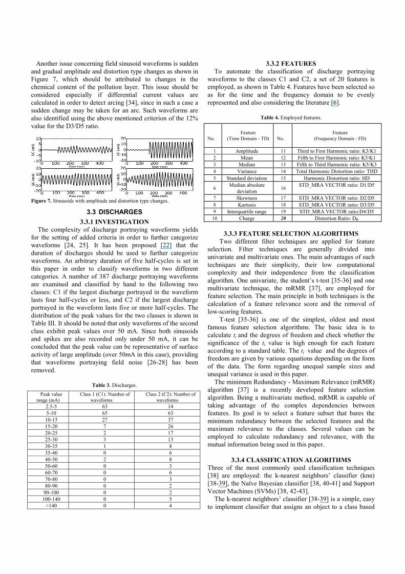
Another issue concerning field sinusoid waveforms is sudden

and gradual amplitude and distortion type changes as shown in

Figure 7, which should be attributed to changes in the

chemical content of the pollution layer. This issue should be

considered especially if differential current values are

calculated in order to detect arcing [34], since in such a case a

sudden change may be taken for an arc. Such waveforms are

also identified using the above mentioned criterion of the 12%

value for the D3/D5 ratio.

Figure 7. Sinusoids with amplitude and distortion type changes.

3.3 DISCHARGES

3.3.1 I4VESTIGATIO4

The complexity of discharge portraying waveforms yields

for the setting of added criteria in order to further categorize

waveforms [24, 25]. It has been proposed [22] that the

duration of discharges should be used to further categorize

waveforms. An arbitrary duration of five half-cycles is set in

this paper in order to classify waveforms in two different

categories. A number of 387 discharge portraying waveforms

are examined and classified by hand to the following two

classes: C1 if the largest discharge portrayed in the waveform

lasts four half-cycles or less, and C2 if the largest discharge

portrayed in the waveform lasts five or more half-cycles. The

distribution of the peak values for the two classes is shown in

Table III. It should be noted that only waveforms of the second

class exhibit peak values over 50 mA. Since both sinusoids

and spikes are also recorded only under 50 mA, it can be

concluded that the peak value can be representative of surface

activity of large amplitude (over 50mA in this case), providing

that waveforms portraying field noise [26-28] has been

removed.

Table 3. Discharges.

Peak value

range (mA)

Class 1 (C1): Number of

waveforms

Class 2 (C2): Number of

waveforms

2.5-5 63 14

5-10 65 63

10-15 27 37

15-20 7 26

20-25 2 17

25-30 3 13

30-35 1 8

35-40 0 6

40-50 2 8

50-60 0 3

60-70 0 6

70-80 0 3

80-90 0 2

90-100 0 2

100-140 0 5

>140 0 4

3.3.2 FEATURES

To automate the classification of discharge portraying

waveforms to the classes C1 and C2, a set of 20 features is

employed, as shown in Table 4. Features have been selected so

as for the time and the frequency domain to be evenly

represented and also considering the literature [6].

Table 4. Employed features.

No.

Feature

(Time Domain - TD)

No.

Feature

(Frequency Domain - FD)

1 Amplitude 11 Third to First Harmonic ratio: K3/K1

2 Mean 12 Fifth to First Harmonic ratio: K5/K1

3 Median 13 Fifth to Third Harmonic ratio: K5/K3

4 Variance 14 Total Harmonic Distortion ratio: THD

5 Standard deviation 15 Harmonic Distortion ratio: HD

6 Median absolute

deviation 16

STD_MRA VECTOR ratio: D1/D5

7 Skewness 17 STD_MRA VECTOR ratio: D2/D5

8 Kurtosis 18 STD_MRA VECTOR ratio: D3/D5

9 Interquartile range 19 STD_MRA VECTOR ratio:D4/D5

10 Charge 20 Distortion Ratio: DR

3.3.3 FEATURE SELECTIO4 ALGORITHMS

Two different filter techniques are applied for feature

selection. Filter techniques are generally divided into

univariate and multivariate ones. The main advantages of such

techniques are their simplicity, their low computational

complexity and their independence from the classification

algorithm. One univariate, the student’s t-test [35-36] and one

multivariate technique, the mRMR [37], are employed for

feature selection. The main principle in both techniques is the

calculation of a feature relevance score and the removal of

low-scoring features.

T-test [35-36] is one of the simplest, oldest and most

famous feature selection algorithms. The basic idea is to

calculate ti and the degrees of freedom and check whether the

significance of the ti value is high enough for each feature

according to a standard table. The ti value and the degrees of

freedom are given by various equations depending on the form

of the data. The form regarding unequal sample sizes and

unequal variance is used in this paper.

The minimum Redundancy - Maximum Relevance (mRMR)

algorithm [37] is a recently developed feature selection

algorithm. Being a multivariate method, mRMR is capable of

taking advantage of the complex dependencies between

features. Its goal is to select a feature subset that bares the

minimum redundancy between the selected features and the

maximum relevance to the classes. Several values can be

employed to calculate redundancy and relevance, with the

mutual information being used in this paper.

3.3.4 CLASSIFICATIO4 ALGORITHMS

Three of the most commonly used classification techniques

[38] are employed: the k-nearest neighbors’ classifier (knn)

[38-39], the Naïve Bayesian classifier [38, 40-41] and Support

Vector Machines (SVMs) [38, 42-43].

The k-nearest neighbors’ classifier [38-39] is a simple, easy

to implement classifier that assigns an object to a class based

on the classes of its k nearest neighbors. Several distances can

be used to find the nearest neighbors, with the Euclidian

distance being used in this paper.

The Naïve Bayes classifier [38, 40-41] is a well known

simple probabilistic classifier based on Bayes theory. It is one

of the oldest classification algorithms and despite its

simplicity, it is known to be rather effective. The algorithm

assumes that features are independent and its efficiency is

largely dependent on feature selection and also on the data

used for training.

Support Vector Machines (SVMs) [38, 42-43] are

considered as one of the most accurate machine learning

classifiers. The SVM algorithm is a supervised learning

method that addresses the problem of linear and non linear

classification by finding the maximum margin hyperplane that

best separates the classes. Non-linear SVMs map the training

samples from the input space into a higher-dimensional feature

space with the use of some mapping function, also known as

kernel function. Several kernel functions can be used and the

Radial Base Function has been employed in this paper. The

mapping procedure resembles the hidden neuron layer of

neural networks. However, SVMs do not suffer from local

minima or overfitting, as neural networks do, they have the

advantage of automatically selecting their model size and

provide superior generalization ability by maximizing the

margin of separation.

3.3.5 RESULTS

Twenty runs were conducted for each feature set and

classification algorithm. In case of knn, in each run, 40% of

the data was used as the training set, 10% as the evaluation set

(testing different values for k, from 3 to 15) and 50% as the

test set. In case of the Naïve Bayes classifier, in each run, 50%

of the data were used as the training set and 50% as the test

set. In case of SVMs, in each run, 40% of the data was used as

the training set, 10% as the evaluation set (selecting optimal

values for c and gamma parameters using grid search) and

50% as the test set. The mean identification success rate

(percentage) for the 20 runs is calculated and overall results

are shown in Table 5.

Table 5. Results for different feature sets and classification algorithms.

Features

TD

{1-10}

FD

{11-20}

All

{1-20}

t-test

{1, 3-11,

13-17, 19-

20}

mRMR

{3, 5, 7, 8, 11,

13, 15, 16, 18,

19}

knn 82.13% 86.77% 85.22% 83.85% 85.74%

Naïve Bayes 69.41% 77.66% 73.02% 73.88% 86.43%

SVMs 82.48% 88.49% 87.80% 87.80% 90.21%

Several results portrayed in Table 5 should be noted. At first

it is shown that frequency domain features give better results

for all three classification algorithms compared to the time

domain features or the time domain features along with the

frequency domain features. This fact, on the one hand shows

that adding more features does not necessarily mean higher

identification rate and on the other hand shows the higher

correlation between the frequency domain and the waveform

shape.

Regarding feature selection, it is shown that the student t-

test is ineffective since it removes only 3 features. It should

also be noted that the t-test features gives worst results

compared to the frequency domain set and better results

compared to the time domain set in all cases. The mRMR

algorithm removes 10 features and keeps 4 features from the

time domain and 6 features from the frequency domain. It

should be noted that, regarding time domain features, the

algorithm removes, among others, the commonly used values

of amplitude and charge and keeps only the median, the

standard deviation, skewness and kurtosis. Regarding

frequency domain features, the algorithm keeps the third to

first harmonic ratio, the fifth to third harmonic ratio and the

Harmonic Distortion but not the fifth to first harmonic ratio

and the Total Harmonic Distortion ratio. The algorithm also

keeps all ratios of the STD_MRA VECTOR values except for

D2/D5.

Regarding the classification, the superiority of SVMs is

documented in every case. The significance of feature

selection for the Naïve Bayes classifier is underlined. It is

shown that the mRMR feature set produces the best results for

all three algorithms with the only exception of the knn

algorithm that shows slightly better results for the frequency

domain set. It is noteworthy that knn and SVMs have similar

results in case of the time domain features (difference of

0.35%) and that overall best results are recorded in case of the

SVMs using the mRMR feature set. These results underline

two discrete approaches related to complexity and calculation

cost: the first approach is a simple identification using only

time domain values and the knn algorithm (success percentage

over 82%) and the second is a more complicated approach

employing SVMs and time and frequency domain features

selected using mRMR (success percentage over 90%).

4 CONCLUSION

It is widely accepted that field measurements are required in

order to acquire an exact image of surface activity and

insulators’ performance. However, field LC waveforms have

not been thoroughly investigated and researchers commonly

record and monitor extracted values such as the peak value and

the charge from the LC waveform. These values, however, are

not always representative of the waveforms’ shape and can be

misleading. In this paper, a large number of field LC

waveforms are investigated and classification techniques are

employed in order to investigate the issue and offer tools to

maximize the efficiency of field LC monitoring. Wavelet

analysis and the STD_MRA technique is employed to perform

basic identification. Further, three classification algorithms

(knn, Naïve Bayes, SVMs) and two feature selection

algorithms are employed in order to automate the classification

of discharge portraying waveforms. 20 different features are

employed, 10 from the time domain and 10 from the frequency

domain. A total of 5 feature sets are employed in combination

with the classification algorithms.

The main conclusions are as follows.

1) Field LC waveforms confirm the basic shapes reported in

the literature referring to laboratory measurements.

However, some peculiarities regarding field LC

waveforms are recorded, such as the occurrence of

spikes, sinusoids of exceptionally large amplitude and

sinusoids portraying gradual and sudden amplitude and

distortion type changes. Such waveforms show that

classification between basic waveform types is required

in order to avoid misleading results.

2) Wavelet STD_MRA analysis can be used to identify

basic waveform types. The SR ratio previously employed

for investigating waveforms of low amplitude, can also be

employed to identify waveforms portraying spikes.

Another ratio of the values from the STD_MRA

VECTOR (D3/D5 in this paper) can be used to identify

sinusoid waveforms. Waveforms portraying discharges

can be indirectly identified using the above ratios.

3) Discharge portraying waveforms are further categorized

in two classes in relation to the duration of portrayed

discharges. It is shown that waveforms of both classes

may exhibit small and medium peak values (up to 50mA),

but only waveforms of the second class (discharges with

duration over 5 half-cycles) exhibit significantly large

peak values (over 50mA)

4) The previous conclusion combined with the peak values

distribution for spikes and sinusoids yield the result that

the LC peak value can be a trustworthy indication of

activity and waveform type only in case of significant

activity that corresponds to significant peak value levels

(in this case, over 50mA).

5) Features from the frequency domain provide better results

compared to features from the time domain and also to a

set containing both. This shows the correlation of the

waveforms’ shape with the frequency content and hints

that using more features may lead to worst results.

6) Feature selection algorithms can be used to enhance the

classification performance and reduce the number of

features used.

7) Results show the superior performance of SVMs and of

the feature set provided by the mRMR algorithm.

8) If one is to consider the calculation complexity, results

underline two different approaches: the first being to

employ the time domain features and the knn algorithm

(success percentage over 82%) and the second one being

to employ SVMs and features from both time and

frequency domain, selected using the mRMR algorithm

(success percentage over 90%)

The work described in this paper complements previous

work coping with field related noise and the data accumulation

problem, providing a full image of field LC waveforms and

identification approaches that may be used to significantly

enhance the effectiveness of field LC monitoring.

REFERENCES

[1] CIGRE WG 33-04, “The measurement of site pollution severity and its

application to insulator dimensioning for A.C. systems”, Eletra, No. 64, pp.

101-115, 1979.

[2] CIGRE WG 33-04, TF 01, Polluted insulators: a review of current

knowledge, Cigre Publications, 1998.

[3] IEC/TS 60815, Selection and dimensioning of high-voltage insulators

intended for use in polluted conditions, IEC, 2008.

[4] S. Gubanski, “Ageing of composite insulators”, in Ageing of Composites,

Woodhead Publishing in Materials, United Kingdom, 2008.

[5] CIGRE WG B2.03, “Guide for the establishment of naturally polluted

insulator testing stations”, Cigre Publications, 2007.

[6] D. Pylarinos, K. Siderakis and E. Pyrgioti “Measuring and analyzing

leakage current for outdoor insulators and specimens”, Rev. Advanced

Materials Sci., Vol. 29, No. 1, pp. 31-53, 2011.

[7] M. A. R. M. Fernando and S. M. Gubanski, “Leakage current patterns on

contaminated polymeric surfaces”, IEEE Trans. Dielectr. Electr. Insul., Vol.

6, No. 5, pp. 688–694, 1999.

[8] I. J. S. Lopes, S. H. Jayaram and E. A. Cherney, “A Method For Detecting

The Transition from Corona from Water Droplets to Dry-Band Arcing on

Silicone Rubber Insulators”, IEEE Trans. Dielectr. Electr. Insul., Vol. 9, No.

6, pp. 964–971, 2002.

[9] I. A. Metwally, A. Al-Maqrashi, S. Al-Sumry and S. Al-Harthy,

“Performance Improvement of 33kV line-post insulators in harsh

environment”, Electr. Power Syst. Res., Vol. 76, No. 9-10, pp. 778-785,

2006.

[10] A. H. El-Hag, S. H. Jayaram and E. A. Cherney, “Fundamental and low

frequency harmonic components of leakage current as a diagnostic tool to

study aging of RTV and HTV silicone rubber in salt-fog”, IEEE Trans.

Dielectr. Electr. Insul., Vol. 10, No. 1, pp. 128–136, 2003.

[11] J. Li, W. Sima, C. Sun and S. A. Sebo, “Use of Leakage Current of

Insulators to Determine the Stage Characteristics of the Flashover Process and

contamination Level Predicition”, IEEE Trans. Dielectr. Electr. Insul., Vol.

17, No. 1, pp. 128–136, 2010.

[12] T. Suda, “Frequency characteristics of leakage current waveforms of an

artificially polluted suspension insulator”, IEEE Trans. Dielectr. Electr. Insul.,

Vol. 8, No. 4, pp. 705–709, 2001.

[13] Τ. Suda, “Frequency Characteristics of Leakage Current Waveforms of a

String of Suspension Insulators”, IEEE Trans. Power Deliv., Vol. 20, No. 1,

pp. 481–487, 2005.

[14] S. Chandrasekar, C. Kalaivanan, A. Cavallini and G. C. Montanari,

“Investigations on Leakage Current and Phase Angle Characteristics of

Porcelain and Polymeric Insulator under Contaminated Conditions”, IEEE

Trans. Dielectr. Electr. Insul., Vol. 16, No. 2, pp. 574-583, 2009.

[15] H. H. Kordkheili, H. Abravesh, N. Tabasi, M. Dakhem and M. M.

Abravesh, “Determining the Probability of Flashover Occurrence in

Composite Insulators by Using Leakage Current Harmonic Components”,

IEEE Trans. Dielectr. Electr. Insul., Vol. 17, No. 2, pp. 502-512, 2010.

[16] Waluyo, P. M. Pakpahan, Suwarno and M. A. Djauhari, “Study on

Leakage Current Waveforms of Porcelain insulator due to various Artificial

Pollutants”, World Academy of Sci., Eng. Techn., Vol. 32, pp. 293–298,

2007.

[17] I. Garniwa, B. Sudiarto and R. S. Ansorulah, “Effect of pollutant type

and concentration on harmonic characteristic of leakage current on resin

epoxy insulator”, 2nd Indonesia Japan Joint Scientific Sympos., pp. 1-6,

2006.

[18] F. Aulia, F. David, E. P. Waldy and H. Hazmi, “The leakage current

analysis of 20 kV porcelain insulator contaminated by salt moisture and

cement dust in Padang area”, IEEE 8th Int’l. Conf. Properties and

Applications of Dielectr. Materials, Bali, Indonesia, pp. 384-387, 2006

[19] N.A.B.T. Mahyudin, Study on Leakage Current of Insulators due to

Environmental Pollutans”, Bachelor Thesis, Faculty of Electrical

Engineering, Universiti Teknologi Malaysia, 2011.

[20] C. S. Richards, C. L. Benner, K. L. Butler-Purry and B. D. Russell,

“Electrical Behavior of Contaminated Distribution Insulators Exposed to

Natural Wetting”, IEEE Trans. Power Deliv., Vol. 18, No. 2, pp. 551-558,

2003.

[21] K. Siderakis, D. Agoris and S. Gubanski, “Influence of heat conductivity

on the performance of RTV SIR coatings with different fillers”, J. Phys. D:

Appl. Phys., Vol. 38, No. 19, pp. 3682-3689, 2005.

[22] M. Sato, A. Nakajima, T. Komukai and T. Oyamada, “Spectral Analysis

of Leakage Current on Contaminated Insulators by Auto Regressive Method”,

IEEE Conf. Electr. Insul. Dielectr. Phenomena (CEIDP), pp. 64–66, 1998.

[23] D. Pylarinos, K. Siderakis, E. Pyrgioti, E. Thalassinakis and I. Vitellas,

“Automating the classification of field leakage current waveforms”, Eng.

Technol. Appl. Sci. Res., Vol. 1, No. 1, pp. 8-12, 2011.

[24] D. Pylarinos, K. Siderakis, E. Pyrgioti, I. Vitellas and E. Thalassinakis,

“Monitoring leakage current waveforms in the field”, DEMSEE 5th Int’l.

Conf. Technical Exhibit on Deregulated Electricity Market issues in South-

Eastern Europe, Sitia, Greece, 2010.

[25] D. Pylarinos, K. Siderakis, E. Thalassinakis, E. Pyrgioti and I. Vitellas,

“Investigation of leakage current waveforms recorded in a coastal high

voltage substation”, Eng. Technol. Appl. Sci. Res., Vol. 1, No. 3, pp. 63-69,

2011.

[26] D. Pylarinos, K. Siderakis, E. Thalassinakis, E. Pyrgioti, I. Vitellas and

S. L. David, “Online applicable techniques to evaluate field leakage current

waveforms”, Electr. Power Syst. Res., Vol. 84, No. 1, pp. 65-71, 2012.

[27] D. Pylarinos, K. Siderakis, E. Pyrgioti, E. Thalassinakis and I. Vitellas,

“Impact of noise related waveforms on long term field leakage current

measurements”, IEEE Trans. Dielectr. Electr. Insul., Vol. 18, No. 1, pp. 122-

129, 2011.

[28] D. Pylarinos, K. Siderakis, E. Pyrgioti , E. Thalassinakis and I. Vitellas,

“Investigating and overcoming the noise and data size problems in long term

field leakage current monitoring”, 17th Int’l. Sympos. High Voltage Eng.

(ISH), Hannover, Germany, paper no. F032, 2011.

[29] D. Pylarinos, K. Siderakis, E. Thalassinakis, I. Vitellas and E. Pyrgioti,

“Recording and managing field leakage current waveforms in Crete.

Installation, measurement, software development and signal processing”,

ISAP 16th Int’l. Conf. Intelligent System Applications to Power Systems,

Hersonissos, Crete, Greece, pp. 1-6, 2011.

[30] J.H. Kim, W.C. Song, J. H. Lee, Y.K. Park, H.G. Cho, Y.S. Yoo and

K.J. Yang, “Leakage Current Monitoring and Outdoor Degradation of

Silicone Rubber”, IEEE Trans. Dielectr. Electr. Insul., Vol. 8, No. 6,

pp. 1108-1115, 2001.

[31] Y. Zhu, S. Yamashita, N. Anami and M. Otsubo, “Leakage Current

Analysis and Electric Field Calculation in Salt Fog Ageing Test on Polymer

Insulation Material”, IEEE Conf. Electr. Insul. Dielectr. Phenomena (CEIDP),

pp. 92-95, 2003.

[32] A. H. El-Hag, A. N. Jahromi and M. Sanaye-Pasand, “Prediction of

Leakage Current of Non-ceramic Insulators in Early Aging Period”, Electr.

Power Syst. Res., Vol. 78, No. 10, pp. 1686-1692, 2008.

[33] K. Siderakis and D. Agoris, “Performance RTV Silicone Rubber

Coatings Installed in Coastal Systems”, Electr. Power Syst. Res., Vol. 78, No.

2, pp. 248-254, 2008.

[34] M. Otsubo, T. Hashiguchi, C. Honda, O. Takenouchi, T. Sakoda and Y.

Hashimoto, “Evaluation of insulation performance of polymeric surface using

a novel separation technique of leakage current”, IEEE Trans. Dielectr.

Electrical Insulat, Vol. 10, No. 6, pp. 1053-1060, 2003.

[35] R.A. Johnson and G.K. Bhattacharyya, Statistics: Principles and

Methods, John Wiley & Sons Inc, 6th Edition, 2010.

[36] S. Welleck, Testing Statistical Hypothesis of Equivalence, Chapman and

Hall, CRC, Boca Raton, Florida, USA, 2003.

[37] H. Peng, F. Long and C. Ding, “Feature selection based on mutual

information: criteria of max-dependency, max-relevance, and min-

redundancy”, IEEE Trans. Pattern Anal. Mach. Intell., Vol. 27, No. 8, pp.

1226-1238, 2005.

[38] X. Wu, V. Kumar, J. R. Quinlan, J. Ghosh, Q. Yang, H. Motoda, G. J.

McLachlan, Angus Ng, B. Liu, P. S. Yu, Z. H. Zhou, M. Steinbach, D. J.

Hand and D. Steinberg, “Top 10 algorithms in data mining”, Knowledge and

Information Systems, Vol. 14, No. 1, pp. 1–37, 2008.

[39] T. M. Cover and P. E. Hart, “Nearest neighbor pattern classification”,

IEEE Trans. Inf. Theory, Vol. 13, No. 1, pp. 21–27, 1967.

[40] C. M. Bishop, Pattern Recognition and Machine Learning, Springer,

2006.

[41] V. N. Vapnik, The +ature of Statistical Learning Theory, Springer,

USA, 2000.

[42] C. J. C. Burges, “A Tutorial on Support Vector Machines for Pattern

Recognition”, Data Min. Knowl. Disc., Vol. 2, No. 2, pp. 121–167, 1998

[43] J. A. K. Suykens, “Support vector machines: A nonlinear modelling and

control perspective”, Eur. J. Control, special issue on fundamental issues in

control, Vol. 7, pp. 311-327, 2001

Dionisios Pylarinos was born in Athens, Greece in 1981. He received a

Diploma degree in Electrical and Computer Engineering in 2007 and the

Ph.D. degree in the same field in 2012 from the University of Patras, Greece.

He is presently a scientific consultant for the Public Power Corporation

(PPC), Greece. He is a member of the Technical Chamber of Greece. His

research interests include outdoor insulation, electrical discharges, leakage

current, signal processing and pattern recognition.

Konstantinos Theofilatos was born in Patras in 1983. He graduated in 2006

from the Department of Computer Engineering and Informatics of the

University of Patras, Greece. In 2009, he received a Master’s degree from the

same department. Since 2009, he has been a Ph.D. degree candidate in the

same department. He is a member of the Pattern Recognition Laboratory

(prlab.ceid.upatras.gr) since 2006. His research interests include

computational intelligence, machine learning, data mining, bioinformatics,

web technologies and time series forecasting and signal processing.

Kiriakos Siderakis was born in Iraklion in 1976. He received a Diploma

degree in Electrical and Computer Engineering in 2000 and the Ph.D. degree

in 2006 from the University of Patras. Presently, he is a Lecturer at the

Department of Electrical Engineering, at the Technological Educational

Institute of Crete. His research interests include outdoor insulation, electrical

discharges, high voltage measurements and high voltage equipment

diagnostics and reliability. He is a member of the Greek CIGRE and of the

Technical Chamber of Greece.

Emmanuel Thalassinakis received the Diploma in Electrical and Mechanical

Engineering and also the Ph.D. degree from the National Technical University

of Athens. After working for the Ministry of the Environment, in 1991 he

joined the Public Power Corporation (PPC) where he is now Assistant

Director of the Islands Network Operations Department.

Isidoros Vitellas was born in 1954 in Greece. He has a Diploma in Electrical

Engineering and the Ph.D. degree in the same field. He is currently Director

of the Islands Network Operations Department in PPC (Public Power

Corporation) Athens, Greece.

Antonio T. Alexandridis (M’88) received a Diploma in electrical

engineering from the Department of Electrical Engineering of the University

of Patras, Greece, in 1981. In 1987, he received the Ph.D. degree from the

Electrical and Computer Engineering Department of the W. Virginia

University, USA. He is a Professor and Head of the Power Systems Division

the Department of Electrical and Computer Engineering of the University of

Patras. His research interests include control theory, nonlinear dynamics,

optimal control, eigenstructure assignment, passivity and advanced control

applications on power systems and drive systems. His current interests are

focused on Renewable Power Generation Control and Stability (wind

generators, PV systems etc.). He is a member of the Technical Chamber of

Greece.

Eleftheria Pyrgioti was born in 1958 in Greece. She received the Diploma

degree in electrical engineering from Patras University in 1981 and the Ph.D.

degree from the same University in 1991. She is an assistant professor at the

department of Electrical and Computer Engineering at the University of

Patras. Her research activity is directed to the high voltage, lightning

protection, insulation coordination, distributed generation. She participates in

the permanent committee TE 63 of ELOT (Hellenic Organization for

Standardization) since 1989 and is a member of the Greek CIGRE and the

Technical Chamber of Greece.