Contribution to the modelling of the viscoelastic behavior of ...
167
HAL Id: tel-03229198 https://hal.archives-ouvertes.fr/tel-03229198v2 Submitted on 14 Feb 2022 HAL is a multi-disciplinary open access archive for the deposit and dissemination of sci- entific research documents, whether they are pub- lished or not. The documents may come from teaching and research institutions in France or abroad, or from public or private research centers. L’archive ouverte pluridisciplinaire HAL, est destinée au dépôt et à la diffusion de documents scientifiques de niveau recherche, publiés ou non, émanant des établissements d’enseignement et de recherche français ou étrangers, des laboratoires publics ou privés. Contribution to the modelling of the viscoelastic behavior of elastomers with Payne effect Adel Tayeb To cite this version: Adel Tayeb. Contribution to the modelling of the viscoelastic behavior of elastomers with Payne effect. Other. Université de Lyon, 2017. English. NNT: 2017LYSEC062. tel-03229198v2
-
Upload
khangminh22 -
Category
Documents
-
view
3 -
download
0
Transcript of Contribution to the modelling of the viscoelastic behavior of ...

HAL Id: tel-03229198https://hal.archives-ouvertes.fr/tel-03229198v2
Submitted on 14 Feb 2022
HAL is a multi-disciplinary open accessarchive for the deposit and dissemination of sci-entific research documents, whether they are pub-lished or not. The documents may come fromteaching and research institutions in France orabroad, or from public or private research centers.
L’archive ouverte pluridisciplinaire HAL, estdestinée au dépôt et à la diffusion de documentsscientifiques de niveau recherche, publiés ou non,émanant des établissements d’enseignement et derecherche français ou étrangers, des laboratoirespublics ou privés.
Contribution to the modelling of the viscoelasticbehavior of elastomers with Payne effect
Adel Tayeb
To cite this version:Adel Tayeb. Contribution to the modelling of the viscoelastic behavior of elastomers with Payne effect.Other. Université de Lyon, 2017. English. NNT : 2017LYSEC062. tel-03229198v2

Number order : 2017LYSEC62 Year : 2017
PhD ThesisSubmitted in partial fulfillment of the
requirements for the degree of
Doctor of Philosophyof École Centrale de Lyon - France
& National Engineering school of Tunis - Tunisia
École doctorale MEGA (Mechanics, Energy, Civil Engineering, Acoustics)École doctorale : Sciences et Techniques de l’ingénieur
F K;9NAB8CAM:<J F
Contribution to the modelling of the viscoelasticbehavior of elastomers with Payne effect
F K;9NAB8CAM:<J F
Specialty : Mechanics
Presented and defended on December 9, 2017 at ENIT de Tunis
by
Adel TAYEB
The dissertation committee consists of :
President : Hatem ZENZRI - Professor, ENIT - TunisiaReviewers : Noureddine BOUHADDI - Professor, FEMTO-ST - France
: Adnane BOUKAMEL - Professor, RAILENIUM - FranceAdvisors : Mohamed ICHCHOU - Professor, ECL - France
: Jalel BENABDALLAH - Professor, ENIT - TunisiaCo-advisors : Makrem ARFAOUI - Associate professor, ENIT - Tunisia
: Abdelmalek ZINE - Associate professor, ECL - France: Adel HAMDI - Associate professor, ENIT - Tunisia
Examiners : Maher MOAKHER - Professor, LAMSIN - ENIT - Tunisia: Olivier BAREILLE - Associate professor, ECL - France

Acknowledgment
i


Dedication
iii


ABSTRACT
It is well known that rubber-like materials exhibit nonlinear viscoelastic behavior over awide range of strain and strain rates confronted in several engineering applications suchas civil engineering, automotive and aerospace industries. This is due to their capacity toundergo high strain and strain rates without exceeding the elastic range of behavior. Fur-ther, the time dependent properties of these materials, such as shear relaxation modulusand creep compliance, are, in general, functions of the history of the strain or the stress.Therefore, in a wide range of strain, a linear viscoelasticity theory is no longer applicablefor such material and new models are required to fully depict the behavior of rubber-likematerials for quasi-static and dynamic configurations of huge interest in engineeringapplications. Despite the multitude of nonlinear viscoelastic models developed over theyears, there is a lack of models capable of depicting the nonlinear behavior of rubber-likematerials with ease of identification and implementation into commercial software.In this work, a nonlinear viscoelastic model at finite strain is developed to describenonfactorizable behavior of isotropic incompressible rubber-like materials. The model isdeveloped within the framework of rational thermodynamics and internal state variableapproach such that the second law of thermodynamics in the form of Clausius-Duheminequality is satisfied. From experimental results on Bromobutyl (BIIR) a dependenceof the shear relaxation modulus upon strain has been observed and introduced in themodel via a strain dependent relaxation times which led to a reduced time similar tothe thermorheologically simple material’s formulation. Then, a systematic identificationprocedure have been developed to identify the model’s parameters. A separation of theinstantaneous elastic and viscoelastic contributions to the stress was employed which ledto a separate identification of the characteristic functions of the model. This procedurewas applied to experimental data and generated data from the Pipkin-Rogers model anda good capacity of the model to predict both static and dynamic behaviors of the materialwas observed.Thereafter, the nonlinear viscoelastic model was implemented into Abaqus software usinga Umat subroutine. To this end, the discrete form of the model was written and the tan-gent stiffness was calculated (required for the Umat) using the objective rate derivativesof Jaumann. The implementation was validated using homogeneous transformationsof simple shear and simple extension for monotonic, sinusoidal and relaxation strainhistories. The non vanishing components of the Cauchy stress tensor were calculated forthe strain history considered and compared to the numerical results of the model. Fi-nally, a non homogeneous transformation was considered. Namely, the problem of simple
v

torsion of a hollow viscoelastic cylinder for several strain histories. From the equilibriumequations, the indeterminate pressure arising from the incompressibility was computedand then the components of the Cauchy stress were calculated along the radius of thecylinder. The analytic results showed a total agreement with the simulations performedwith the implemented model.
vi

RÉSUMÉ
vii

TABLE OF CONTENTS
Page
Acknowledgment i
Dedication iii
Abstract vi
Résumé viii
List of Figures xii
List of Tables xv
List of Abbreviations 1
Introduction 1
1 Physical aspects and hyperelastic behavior of rubber-like materials 51.1 Phenomenology of rubber . . . . . . . . . . . . . . . . . . . . . . . . . . . . . 6
1.1.1 Generalities and micro-structure . . . . . . . . . . . . . . . . . . . . 6
1.1.2 Quasi static response of rubber like materials . . . . . . . . . . . . . 8
1.1.3 Dissipative phenomena of rubber like materials . . . . . . . . . . . 9
1.1.4 Dynamic response of rubber like materials . . . . . . . . . . . . . . . 11
1.1.5 Thermal response of rubber like materials . . . . . . . . . . . . . . . 12
1.1.6 Other nonlinear phenomena . . . . . . . . . . . . . . . . . . . . . . . 13
1.1.6.1 Mullins effect . . . . . . . . . . . . . . . . . . . . . . . . . . 13
1.1.6.2 Payne effect . . . . . . . . . . . . . . . . . . . . . . . . . . . 14
1.2 Mechanical formulation in the high deformation . . . . . . . . . . . . . . . . 16
1.2.1 The deformation gradient . . . . . . . . . . . . . . . . . . . . . . . . . 16
1.2.2 Polar decomposition of the deformation gradient . . . . . . . . . . . 17
viii

TABLE OF CONTENTS
1.2.3 Volume changes and isochoric/volumetric split . . . . . . . . . . . . 18
1.2.4 Strain . . . . . . . . . . . . . . . . . . . . . . . . . . . . . . . . . . . . . 18
1.2.5 Stress . . . . . . . . . . . . . . . . . . . . . . . . . . . . . . . . . . . . . 19
1.2.5.1 The First Piola-Kirchhoff Stress . . . . . . . . . . . . . . . 20
1.2.5.2 The Second Piola-Kirchhoff Stress . . . . . . . . . . . . . . 20
1.2.5.3 The Kirchhoff Stress . . . . . . . . . . . . . . . . . . . . . . 20
1.3 Hyperelasticity . . . . . . . . . . . . . . . . . . . . . . . . . . . . . . . . . . . . 21
1.3.1 Deformation energy . . . . . . . . . . . . . . . . . . . . . . . . . . . . 21
1.3.2 The incompressibility condition . . . . . . . . . . . . . . . . . . . . . 22
1.3.3 Examples of strain energy densities . . . . . . . . . . . . . . . . . . . 23
1.3.3.1 Developement in function of the invariants . . . . . . . . . 24
1.3.3.2 Development in function of the principal streches . . . . . 25
1.4 Literature survey for nonlinear viscoelastic models . . . . . . . . . . . . . . 26
1.4.1 Internal variables formulation . . . . . . . . . . . . . . . . . . . . . . 26
1.4.2 Additive decomposition of the free energy density . . . . . . . . . . 27
1.4.3 Integral based formulation . . . . . . . . . . . . . . . . . . . . . . . . 30
1.4.4 Differential viscoelasticity . . . . . . . . . . . . . . . . . . . . . . . . . 31
1.5 Conclusion . . . . . . . . . . . . . . . . . . . . . . . . . . . . . . . . . . . . . . 33
2 Proposed nonlinear viscoelastic model 352.1 Experimental and rheological motivations . . . . . . . . . . . . . . . . . . . 36
2.1.1 Experimental motivation . . . . . . . . . . . . . . . . . . . . . . . . . 36
2.1.2 Rheological motivation . . . . . . . . . . . . . . . . . . . . . . . . . . . 37
2.1.3 Thermodynamic considerations . . . . . . . . . . . . . . . . . . . . . 39
2.2 Formulation restricted to linear kinematics . . . . . . . . . . . . . . . . . . . 40
2.2.1 Formulation of the model . . . . . . . . . . . . . . . . . . . . . . . . . 41
2.2.2 Thermodynamic considerations . . . . . . . . . . . . . . . . . . . . . 42
2.3 Fully nonlinear viscoelastic model . . . . . . . . . . . . . . . . . . . . . . . . 43
2.3.1 Mechanical framework and form of the Helmholtz free energy density 44
2.3.2 Rate and constitutive equations . . . . . . . . . . . . . . . . . . . . . 45
2.3.3 Functional formulation and thermodynamic considerations . . . . 47
2.4 Conclusion . . . . . . . . . . . . . . . . . . . . . . . . . . . . . . . . . . . . . . 48
3 Identification of the nonlinear viscoelastic model 493.1 Model identification . . . . . . . . . . . . . . . . . . . . . . . . . . . . . . . . . 50
3.1.1 Identification of the hyperelastic potential . . . . . . . . . . . . . . . 51
ix

TABLE OF CONTENTS
3.1.2 Identification of the viscoelastic kernel . . . . . . . . . . . . . . . . . 53
3.1.2.1 Identification from relaxation test . . . . . . . . . . . . . . 53
3.1.2.2 Identification from dynamic tests . . . . . . . . . . . . . . 54
3.1.3 Identification of the reduced time function . . . . . . . . . . . . . . . 55
3.2 Identification of the model using data from the Pipkin isotropic model . . 56
3.2.1 Pipkin isotropic model . . . . . . . . . . . . . . . . . . . . . . . . . . . 56
3.2.2 Identification results . . . . . . . . . . . . . . . . . . . . . . . . . . . . 57
3.2.2.1 Hyperelastic potential . . . . . . . . . . . . . . . . . . . . . 57
3.2.2.2 Viscoelastic kernel . . . . . . . . . . . . . . . . . . . . . . . 59
3.2.2.3 Reduced time function . . . . . . . . . . . . . . . . . . . . . 60
3.3 Application of the identification procedure to experimental data . . . . . . 63
3.3.1 Hyperelastic potential . . . . . . . . . . . . . . . . . . . . . . . . . . . 64
3.3.2 Viscoelastic kernel . . . . . . . . . . . . . . . . . . . . . . . . . . . . . 65
3.3.2.1 From shear relaxation experiment . . . . . . . . . . . . . . 65
3.3.2.2 From dynamic experiments . . . . . . . . . . . . . . . . . . 66
3.3.3 Reduced time function . . . . . . . . . . . . . . . . . . . . . . . . . . . 71
3.4 Conclusion . . . . . . . . . . . . . . . . . . . . . . . . . . . . . . . . . . . . . . 73
4 Numerical implementation and integration scheme 754.1 Integration scheme for one dimensional viscoelastic model . . . . . . . . . 76
4.1.1 Integration scheme . . . . . . . . . . . . . . . . . . . . . . . . . . . . . 77
4.1.2 Validation of the integration scheme . . . . . . . . . . . . . . . . . . 78
4.2 Implementation of the nonlinear viscoelastic model . . . . . . . . . . . . . . 78
4.2.1 Finite element method for nonlinear viscoelastic solids . . . . . . . 79
4.2.2 Discrete representation of the constitutive equations . . . . . . . . 83
4.2.2.1 Discrete stress-strain relationship . . . . . . . . . . . . . . 83
4.2.2.2 Tangent stiffness . . . . . . . . . . . . . . . . . . . . . . . . 86
4.2.2.3 Flowchart of the Umat subroutine . . . . . . . . . . . . . . 87
4.3 Conclusions . . . . . . . . . . . . . . . . . . . . . . . . . . . . . . . . . . . . . . 88
5 Validation of the implementation procedure with homogeneous andnon homogeneous transformations 915.1 Specification of the parameters of the model . . . . . . . . . . . . . . . . . . 92
5.2 Homogeneous transformations . . . . . . . . . . . . . . . . . . . . . . . . . . 94
5.2.1 Simple extension . . . . . . . . . . . . . . . . . . . . . . . . . . . . . . 94
5.2.2 Simple shear . . . . . . . . . . . . . . . . . . . . . . . . . . . . . . . . . 101
x

TABLE OF CONTENTS
5.3 Nonhomogeneous transformation: Simple torsion of hollow cylinder . . . . 108
5.4 Conclusions . . . . . . . . . . . . . . . . . . . . . . . . . . . . . . . . . . . . . . 114
Conclusions & Outlooks 117
A Appendix A 119
Bibliography 135
xi

LIST OF FIGURES
FIGURE Page
1.1 Molecular network of elastomers [78] . . . . . . . . . . . . . . . . . . . . . . . . 7
1.2 Stress strain curves for quasi-static loading [35] . . . . . . . . . . . . . . . . . . 8
1.3 Volume dilatation for a rubber specimen undergoing a uniaxial tensile experiment[121] 8
1.4 Nominal stress versus time for a relaxation experiment [79] . . . . . . . . . . 10
1.5 Nominal strain versus time for a creep experiment [138] . . . . . . . . . . . . . 10
1.6 Storage modulus versus frequency [83] . . . . . . . . . . . . . . . . . . . . . . . 11
1.7 Loss modulus versus frequency [83] . . . . . . . . . . . . . . . . . . . . . . . . . 12
1.8 Evolution of dynamic moduli with temperature [135] . . . . . . . . . . . . . . . 12
1.9 Mullins effect [93] . . . . . . . . . . . . . . . . . . . . . . . . . . . . . . . . . . . . 13
1.10 Payne effects on dynamic moduli [124] . . . . . . . . . . . . . . . . . . . . . . . . 15
1.11 Transformation from undeformed to deformed configuration . . . . . . . . . . 16
1.12 Two versions of the standard viscoelastic solid . . . . . . . . . . . . . . . . . . . 33
2.1 Dependence of the shear relaxation modulus upon strain for BIIR rubber . . 37
2.2 Generalized Maxwell model . . . . . . . . . . . . . . . . . . . . . . . . . . . . . . 38
3.1 Equilibrium stresses versus principle stretch for the Pipkin model (diamond)
and the Mooney-Rivlin model (solid curve) . . . . . . . . . . . . . . . . . . . . . 58
3.2 Normalized shear relaxation modulus of Pipkin model versus time for four
different strain levels. . . . . . . . . . . . . . . . . . . . . . . . . . . . . . . . . . . 60
3.3 Simple extension Cauchy stress versus principle stretch for two different
strain rates α1 = 1.19 10−2s−1 and α2 = 6 10−3s−1 . . . . . . . . . . . . . . . . . 60
3.4 Reduced time function and reduced time ratio versus principle stretch for two
strain rates α1 = 1.19 10−2s−1 and α2 = 6 10−3s−1 . . . . . . . . . . . . . . . . . 61
3.5 Relative error of the predicted Cauchy stress of the Pipkin model for pure
shear experiment . . . . . . . . . . . . . . . . . . . . . . . . . . . . . . . . . . . . 62
xii

LIST OF FIGURES
3.6 Pure shear Cauchy stress for the model (solid curve) and the Pipkin model
(diamond and square) . . . . . . . . . . . . . . . . . . . . . . . . . . . . . . . . . . 63
3.7 Equilibrium stresses versus principle stretch: Experimental (diamond) and
the identified Mooney-Rivlin model (solid curve) . . . . . . . . . . . . . . . . . . 64
3.8 Normalized shear relaxation modulus of BIIR rubber versus time. . . . . . . . 66
3.9 Storage and loss moduli versus frequency for simulated and perturbed data . 68
3.10 Storage and loss moduli versus frequency for dynamic experimental data for
different values of the regularization parameter µ . . . . . . . . . . . . . . . . . 70
3.11 Cauchy stress versus principle stretch for simple extension experiment . . . . 71
3.12 Reduced time coefficient for two strain rates 100% s−1 and 200% s−1 . . . . . 72
3.13 Cauchy stress versus principle stretch for pure shear experiment: experimen-
tal (diamond) model (solid curve) . . . . . . . . . . . . . . . . . . . . . . . . . . . 72
4.1 Stress versus time for a monotonic strain history . . . . . . . . . . . . . . . . . 79
4.2 Stress versus time for relaxation strain history . . . . . . . . . . . . . . . . . . 80
4.3 Stress versus time for a sinusoidal strain history . . . . . . . . . . . . . . . . . 81
4.4 Initial boundary value problem considered . . . . . . . . . . . . . . . . . . . . . 81
4.5 Flowchart for the interaction of Abaqus and Umat . . . . . . . . . . . . . . . . 88
5.1 Boundary conditions and deformed form of the cube undergoing simple exten-
sion deformation . . . . . . . . . . . . . . . . . . . . . . . . . . . . . . . . . . . . . 94
5.2 Comparison of analytic results with the implemented model in simple exten-
sion for a ramp stretch history . . . . . . . . . . . . . . . . . . . . . . . . . . . . . 98
5.3 Comparison of analytic results with the implemented model in simple exten-
sion for a relaxation (Heaviside) stretch history . . . . . . . . . . . . . . . . . . 99
5.4 Comparison of analytic results with the implemented model in simple exten-
sion for a sinusoidal stretch history . . . . . . . . . . . . . . . . . . . . . . . . . . 100
5.5 Boundary conditions and deformed form of the cube undergoing simple shear
deformation . . . . . . . . . . . . . . . . . . . . . . . . . . . . . . . . . . . . . . . . 101
5.6 Comparison of analytic results with the implemented model in simple shear
for a ramp strain history . . . . . . . . . . . . . . . . . . . . . . . . . . . . . . . . 105
5.7 Comparison of analytic results with the implemented model in simple shear
for a relaxation (Heaviside) shearing strain history . . . . . . . . . . . . . . . . 106
5.8 Comparison of analytic results with the implemented model in simple shear
for a sinusoidal shearing strain history . . . . . . . . . . . . . . . . . . . . . . . 107
xiii

LIST OF FIGURES
5.9 Boundary conditions and deformed form of the cylinder undergoing simple
torsion deformation . . . . . . . . . . . . . . . . . . . . . . . . . . . . . . . . . . . 108
5.10 Comparison of analytic results with the implemented model in simple torsion
of hollow cylinder for a ramp angle of twist . . . . . . . . . . . . . . . . . . . . . 112
5.11 Comparison of analytic results with the implemented model in simple torsion
of hollow cylinder for a relaxed angle of twist . . . . . . . . . . . . . . . . . . . . 113
xiv

LIST OF TABLES
TABLE Page
3.1 Prony series parameters . . . . . . . . . . . . . . . . . . . . . . . . . . . . . . . . 59
3.2 Prony series parameters for BIIR rubber . . . . . . . . . . . . . . . . . . . . . . 65
3.3 Prony series parameters from [110] . . . . . . . . . . . . . . . . . . . . . . . . . 69
3.4 Prony series parameters from experimental dynamic data . . . . . . . . . . . . 69
5.1 Model’s parameters . . . . . . . . . . . . . . . . . . . . . . . . . . . . . . . . . . . 93
5.2 Prony series parameters . . . . . . . . . . . . . . . . . . . . . . . . . . . . . . . . 93
xv


NOTATIONS
Symbol DesignationC0 Reference configurationCt Current configurationΩ0 Continuum body in the reference configurationΩt Continuum body in the current configurationX Point’s coordinates in the reference configurationx Point’s coordinates in the current configurationφ(X , t) Mapping function between C0 and CtF Deformation gradient tensorJ = det[F ] Jacobian of the deformationF Isochoric part of the deformation gradient tensorFτ Deformation gradient tensor with respect to time τx point’s coordinates in the current configurationC Right Cauchy-Green strain tensorC Isochoric right Cauchy-Green strain tensorB Left Cauchy-Green strain tensorB Isochoric left Cauchy-Green strain tensorΨ Free energy density functionΨ0 Instantaneous elastic free energy density functionσ Cauchy stress tensorτ Kirchhoff stress tensorπ First Piola-Kirchhoff stress tensorS Second Piola-Kirchhoff stress tensorC Fourth order tensor of tangent stiffnessCJ Fourth order tensor of tangent stiffness of JaumannCAbaqus Abaqus fourth order tensor of tangent stiffnessG(t) Shear relaxation modulusG′ Storage modulusG′′ Loss modulusg(t) Normalized shear relaxation modulus
xvii

INTRODUCTION
= T Industrial and scientific contextThis thesis is a part of an international partnership between the laboratory of Applied
Mechanics and Engineering of École Nationale d’Ingénieurs de Tunis and the labora-
tory of Tribology and Dynamics of Systems of École Centrale de Lyon as academics and
ArianeGroup as an industrial counterpart. The aim of the thesis is the development
of a nonlinear viscoelastic model able to describe the nonlinear viscoelastic behavior
of rubber-like materials at finite strain and its implementation into finite elements
software. The original industrial need is the design of the elastomeric device to be used in
the inter-stage of the launcher which the role is to ensure the static and dynamic filtering
and attenuate the vibrations caused by the boosters and transmitted to the stages of the
launcher. However, thanks to the general framework in which the model was developed,
it will fit this feature as well as other features needed in several engineering applications.
Nowadays, elastomers are frequently used in industrial applications, in particular in
automotive, aeronautics, civil engineering applications and aerospace. The mechanical
properties of these materials make them a class a part of materials. Their properties are
used for several applications such as sealing, damping and isolation etc. In particular,
they have high ability of deformability up to some hundred % associated with a quasi-
reversible hyperelastic behavior. In addition, they have a dissipative properties shown
when subjected to dynamic loading along with several softening phenomena. In general,
these materials are subjected to severe mechanical and thermal loading in real world
application.
In industry, the design of complex geometrical structures made of materials exhibiting
nonlinear constitutive behavior, such as rubber-like materials, rely on the use of finite
elements method. The performance of such tool is directly affected by the capacity of the
model to depict the behavior of the used material. The possibility of accurately simulat-
ing the behavior of the material in the industrial application circumstances avoids the
need of experimentation and therefore reducing the cost of the design process of such
1
8 Introduction
structures.
Rubber-like materials have a very special behavior which could be described by the
combination of elastic solid behavior and viscous fluid behavior. In addition, due to
their peculiar micro-structure, theses materials are characterized by several nonlin-
ear phenomena involving their response to static and dynamic loading. Therefore, the
development of nonlinear viscoelastic models is crucial.
= T Research problematic and ObjectivesThe theory of viscoelasticity is crucial in describing materials, such as filled rubber,
which exhibit time dependent stress-strain behavior. Over the years, several models
have been developed to study the viscoelastic behavior of rubber-like materials from
purely mathematical developments to applied studies where ease of application is for
huge interest. In fact, the combination of the ease of identification of the model’s para-
meters as well as the possibility to implement it in finite elements software plays a
key role in the development of constitutive equations for these materials. Furthermore,
several experimental investigation corroborated that the time-dependent properties of
these materials such as relaxations function and creep compliance are in general strain
dependent functions. The separability assumption used in linear viscoelasticity theory,
which states that the effect of time and strain are separable and hence the time-dependentproperties are function of time only, does not hold.
A review of the literature revealed significantly more well-established studies dealing
with hyperelastic constitutive models, than those dealing with finite viscoelasticity. Fur-
thermore, the task of identification of the material’s parameters is well-studied and
integrated in finite elements software such as Abaqus for the static (hyperelastic) case
providing all the experimental techniques to identify the material constitutive parame-
ters. However, for nonlinear viscoelastic materials such feature is lacking especially when
dealing with nonlinear phenomena such as the dependence of the relaxation modulus
upon strain.
On the other hand, in order to investigate the response of the material with the non-
linearities described above subjected to real industrial loading, the model describing
this behavior should be implemented into finite elements software. Hence, all quantities
involved in the model have to be defined carefully and therefore the simplicity of the
model plays a key role in fulfilling this task.
Therefore, the objectives of this work are, on one hand: the development of a nonlinear vis-
coelastic model at finite strain taking into account the dependence of the time-dependent
properties upon strain corroborated by experimental results done within this project on
K K;9NAB8
Page 2 ; Ph.D thesis at ECL/LTDS U
8
a Bromobutyl rubber-like material, on the other hand, the development of a systematic
identification procedure to identify all the model’s parameters using experimental data
and the implementation of the proposed model into one of the finite elements commercial
software.
= T MethodologyIn order to fulfill the objectives of this thesis the following methodology has been followed:
The three dimensional viscoelastic model at finite strain to describe nonseparable
behavior of rubber-like materials is developed within the framework of rational
thermodynamics and internal state variable approach such that the second law of
thermodynamics in the form of Clausius–Duhem inequality is satisfied. The model
represents a generalization of the Simo model implemented in Abaqus software.
Motivated by experimental results, the evolution law of the internal variables
is set to be nonlinear. This non linearity was introduced via a strain dependent
relaxation times which led to the use of the notion of reduced time via strain shift
function similar to the thermorheologically simple material’s behavior.
The material’s parameters are identified separately. In fact, the hyperelastic con-
tribution to the total stress is identified from equilibrium data on simple extension
and pure shear. The relaxation function was postulated by a Prony series and
identified using relaxation experimental data in the linear range of the behavior
with a strain relaxation level below 10%. The reduced time function is identified
thanks to a minimization procedure over the error between the discrete stress of
the model and the experimental stress.
The implementation of the model was performed with Abaqus software via a
subroutine Umat. To do so, first, the integration algorithm corresponding to the
discrete of the model was implemented using Matlab software and validated with
comparison with Abaqus software for one dimensional experiments of simple
extension and pure shear for several strain histories. Then, the subroutine Umat
was written: this requires the update formula for the stress using the objective
rate equation of Jaumann required in Abaqus software and the update formula
of the fourth order tangent stiffness tensor. The implementation of the model was
then validated by the solution of initial boundary value problems for homogeneous
transformations of simple shear and simple extension and non homogeneous one of
simple torsion of a hollow cylinder.
8CAM:<J J
T Tayeb Adel ; Page 3
8 Introduction
= T Thesis outlineThis thesis is decomposed in five chapters organized as follows:
The first chapter summarizes the most important physical phenomena related
to rubber-like materials and exposes the most known approaches and models
to deal with these phenomena in the development of hyperelastic potentials for
these materials. The last part of this chapter presents a literature survey for the
approach followed in the development of nonlinear viscoelastic models at finite
strain
The second chapter presents the nonlinear viscoelastic model proposed within
this work. First, a modification to the rheological model of Maxwell is carried out
using experimental arguments. Then, an extension to the fully three dimensional
domain is performed such that the second law of thermodynamics in terms of the
Clausius-Duhem inequality is valid. For each case, constitutive equations of the
stress, free energy density and intrinsic dissipation are obtained.
The third chapter presents the systematic identification procedure of the model’s
parameters to experimental data. This identification procedure was applied to data
generated from the Pipkin multi-integral model then applied to experimental data
for Bromobutyl (BIIR)
The fourth chapter deals with the numerical implementation of the nonlinear
viscoelastic model developed in the previous chapters. First, the integration scheme
of the one dimensional model is recalled. Then, the implementation of the three
dimensional viscoelastic model into Abaqus software is performed using an implicit
integration scheme in a Umat subroutine.
The last chapter presents the validation of the implementation of the nonlinear vis-
coelastic model presented in the previous chapter via the solution of homogeneous
and nonhomogeneous initial boundary problems numerically and analytically.
K K;9NAB8
Page 4 ; Ph.D thesis at ECL/LTDS U

CH
AP
TE
R
1PHYSICAL ASPECTS AND HYPERELASTIC BEHAVIOR OF
RUBBER-LIKE MATERIALS
Contents1.1 Phenomenology of rubber . . . . . . . . . . . . . . . . . . . . . . . . . . . . 6
1.1.1 Generalities and micro-structure . . . . . . . . . . . . . . . . . . . 6
1.1.2 Quasi static response of rubber like materials . . . . . . . . . . . 8
1.1.3 Dissipative phenomena of rubber like materials . . . . . . . . . 9
1.1.4 Dynamic response of rubber like materials . . . . . . . . . . . . . 11
1.1.5 Thermal response of rubber like materials . . . . . . . . . . . . . 12
1.1.6 Other nonlinear phenomena . . . . . . . . . . . . . . . . . . . . . 13
1.2 Mechanical formulation in the high deformation . . . . . . . . . . . . . . 16
1.2.1 The deformation gradient . . . . . . . . . . . . . . . . . . . . . . . 16
1.2.2 Polar decomposition of the deformation gradient . . . . . . . . . 17
1.2.3 Volume changes and isochoric/volumetric split . . . . . . . . . . 18
1.2.4 Strain . . . . . . . . . . . . . . . . . . . . . . . . . . . . . . . . . . . 18
1.2.5 Stress . . . . . . . . . . . . . . . . . . . . . . . . . . . . . . . . . . . 19
1.3 Hyperelasticity . . . . . . . . . . . . . . . . . . . . . . . . . . . . . . . . . . 21
1.3.1 Deformation energy . . . . . . . . . . . . . . . . . . . . . . . . . . 21
1.3.2 The incompressibility condition . . . . . . . . . . . . . . . . . . . 22
5

8 Chapter 1. Physical aspects and hyperelastic behavior of rubber-like materials
1.3.3 Examples of strain energy densities . . . . . . . . . . . . . . . . . 23
1.4 Literature survey for nonlinear viscoelastic models . . . . . . . . . . . . 26
1.4.1 Internal variables formulation . . . . . . . . . . . . . . . . . . . . 26
1.4.2 Additive decomposition of the free energy density . . . . . . . . 27
1.4.3 Integral based formulation . . . . . . . . . . . . . . . . . . . . . . 30
1.4.4 Differential viscoelasticity . . . . . . . . . . . . . . . . . . . . . . . 31
1.5 Conclusion . . . . . . . . . . . . . . . . . . . . . . . . . . . . . . . . . . . . . 33
THe first chapter aims to analyse the behavior of rubber-like materials from a
phenomenological stand point. These materials are used in several engineer-
ing applications such as automotive, civil engineering and aerospace. These
materials are capable of undergoing large deformation and recover to their original state.
Due to their peculiar micro-structure composed by long chain molecules with presence of
carbon black, their behavior is strongly nonlinear. This chapter is subdivided in three
parts : the first part summarizes the most important physical phenomena related to
rubber-like materials, the second one presents the mechanical framework of nonlinear
elasticity and highlights the most known approaches and models to describe the hy-
perelastic behavior for these materials and the third part presents the framework of
nonlinear viscoelasticity leading to the most known approaches and modeling procedures
followed in the development of nonlinear viscoelastic models at finite strain and discusses
the assumptions and limitations of each approach.
1.1 Phenomenology of rubber
1.1.1 Generalities and micro-structure
The term rubber is actually misleading: it is used both to indicate the material, techni-
cally referred to as natural rubber, and the broad class of synthetic elastomers which
share with natural rubber some fundamental chemical properties. Indeed, the majority
of rubber used for industrial applications are synthetically produced and derived from
petroleum. These materials are characterized by their high deformability and dissipative
properties which makes them widely used in several damping applications in many fields
[29],[111],[97],[87]...
K K;9NAB8
Page 6 ; Ph.D thesis at ECL/LTDS U

1.1. Phenomenology of rubber 8
Rubber, or elastomer, has an internal structure which consists of flexible, long chain
molecules that intertwine with each other and continually change contour due to thermal
agitation. Elastomers are polymers with long chains [43]. The morphology of an elas-
tomer can be described in terms of convolution, curls and kinks. Convolutions represent
the long-range contour of an entire molecular chain, which forms entanglements (knots).
Curls are shorter range molecular contours that develop between entanglements and
crosslinks, and kinks are molecular bonds within a curl. Each molecular bond has rota-
tional freedom that allows the direction of the chain molecule to change at every bond.
Thus the entire molecular chain can twist, spiral and tangle with itself or with adjacent
chains. This basic morphology is shared among all the fifty thousand compounds used in
the market today and generically referred to by the term rubber. Despite this intricate
internal structure, the random orientation of the molecular chains results in a material
which is externally isotropic and homogeneous. Figure 1.1 illustrates the form of the
molecular network of an elastomer
Before using, the elastomer is subjected to physical and chemical treatments to
ameliorate its mechanical properties. One of these treatment is the vulcanization which
consists of the addition of sulfur-based curatives which create crosslinks among the
macromolecules chains through heating see [17].
Figure 1.1: Molecular network of elastomers [78]
8CAM:<J J
T Tayeb Adel ; Page 7

8 Chapter 1. Physical aspects and hyperelastic behavior of rubber-like materials
1.1.2 Quasi static response of rubber like materials
Figure 1.2: Stress strain curves for quasi-static loading [35]
Figure 1.3: Volume dilatation for a rubber specimen undergoing a uniaxial tensileexperiment[121]
K K;9NAB8
Page 8 ; Ph.D thesis at ECL/LTDS U

1.1. Phenomenology of rubber 8
The behavior of rubber-like materials can be described primarily as hyperelastic un-
der static loading where time-dependent effects are negligible [123]. The response of
rubber-like materials to quasi-static loading conditions of shear, compression/tension
and equibiaxial tension have been widely studied in the literature [33],[82],[118] and
[138] among others. It has been shown for all these experimental conditions that the
stress-strain curves are strongly nonlinear.
The stress-strain curve response of a carbon black filled elastomer are shown in figure
1.2 [35]. The material is subjected to uniaxial tension/compression, and pure shear condi-
tions. The constitutive nonlinearity of the material are evident, in fact as the breaking
point approaches, the stiffness of the material increases significantly and as a result
the slope of the stress strain curve rise. It is also noticed that the material have a non
symmetric behavior between tensile and compression loads.
From figure 1.2 one could extract the value of the shear modulus G and the Young
modulus E in the undeformed configuration. The ratio E/
G is about 3 which means that
the Poisson’s ratio ν= 0.5. Therefore, the material is incompressible in the underformed
configuration.
Moreover, the incompressibility of rubber like materials have been studied in many
works [8], [91], [106], [114], [121]. The experiments by [121] reported in figure 1.3
show a limited volume change ∆V/
V0∼== 0.01 for a large stretch (λ = 4) confirms the
incompressibility constraint used in several constitutive equations.
1.1.3 Dissipative phenomena of rubber like materials
In addition to phenomena described in the previous section, elastomers have a fluid-like
or viscoelastic behavior when subjected to dynamic loading [44]. Two typical experiments
that prove the viscoelastic behavior of rubber like materials are : the relaxation exper-
iment for which a step-wise strain is applied to the specimen the stress response fall
from the peak value when the strain was applied to an asymptotic value as it is shown
in figure 4 from the experiment by [79] and the creep experiment when a sudden step
force is applied to the specimen the strain increases slowly from the instantaneous value
as shown in figure 1.5.
8CAM:<J J
T Tayeb Adel ; Page 9

8 Chapter 1. Physical aspects and hyperelastic behavior of rubber-like materials
Figure 1.4: Nominal stress versus time for a relaxation experiment [79]
Figure 1.5: Nominal strain versus time for a creep experiment [138]
These two phenomena are caused by the complex geometrical entanglements between
chains, which produce a local enhancement of the residual (Van der Walls) force. Under
prolonged loading, such “entanglement-cohesion” will slowly breakdown, giving rise to
the phenomena of stress-relaxation and creep presented above [138]. In the case of speed
loading these phenomena are limited and the response of the material is elastic. These
two phenomena emphasis the time dependent behavior of rubber like materials which
K K;9NAB8
Page 10 ; Ph.D thesis at ECL/LTDS U

1.1. Phenomenology of rubber 8
is still an active subject for research. Hence, the entire history of the strain must be
incorporated in the constitutive equations for these materials.
1.1.4 Dynamic response of rubber like materials
Figure 1.6: Storage modulus versus frequency [83]
From dissipative phenomena occurring for rubber like materials described in 1.1.3, it
is needful to investigate the dynamic response of these materials. This is achieved by
subjecting the material to a sinusoidal strain history of frequency ω of the form :
ε(t)= εa sin(wt), (1.1)
where εa is the dynamic amplitude. Under the dynamic loading the strain occur in the
material with a certain delay due to the viscous frictions inside the material, this delay
is observed for a harmonic deformation of equation (1.1) by a phase shift between the
displacement and the loading [9]. The harmonic deformation of equation (1.1) lead to
time-dependent stress of the form
σ=G∗εa, (1.2)
where G∗ is the complex modulus, its real part is denoted by G′ and referred to as the
storage modulus and its imaginary part is denoted by G′′ and referred to as the lossmodulus. These two moduli are dependent upon the dynamic amplitude especially for
8CAM:<J J
T Tayeb Adel ; Page 11

8 Chapter 1. Physical aspects and hyperelastic behavior of rubber-like materials
large value of εa. In figures 1.6 and 1.7 is reported the dependence of the storage and
loss moduli upon the frequency respectively using data from [83]. The storage modulus
has a nonzero value as w → 0 which corresponds to the equilibrium shear modulus since
t →∞ as w → 0.
Figure 1.7: Loss modulus versus frequency [83]
1.1.5 Thermal response of rubber like materials
Figure 1.8: Evolution of dynamic moduli with temperature [135]
For both quasi-static and dynamic loading, the behavior of rubber like materials is
strongly affected by temperature. The dynamic properties of the material exhibit big
K K;9NAB8
Page 12 ; Ph.D thesis at ECL/LTDS U

1.1. Phenomenology of rubber 8
changes with the temperature. In fact, at low temperatures the storage modulus is at its
maximum whereas the loss modulus is at its minimum. This range of temperature is
known as the glassy region. Increasing temperature from this region causes a brutal de-
crease of the storage modulus and an increase of the loss modulus in which it reaches its
maximum. This range of temperature is called the transition region. A further increase
in temperature, the material reach its rubbery plateau in which both dynamic moduli
are stable. This range is the perfect range for applications using rubber like materials.
This dependence of the dynamic moduli upon temperature is shown in figure 1.8.
On the other the hand the determination of the dynamic properties for wide range of
frequency is not possible experimentally. Therefore, an assumption has been made in
the modeling of rubber like materials which is the thermorehologically simple behavior.
Within this context, the time-dependent properties of the material such as relaxation
function, creep function and dynamic moduli when plotted versus the logarithm of time
or frequency at several temperatures can be superimposed to form a single curve [116]
and [146].
1.1.6 Other nonlinear phenomena
1.1.6.1 Mullins effect
Figure 1.9: Mullins effect [93]
8CAM:<J J
T Tayeb Adel ; Page 13
8 Chapter 1. Physical aspects and hyperelastic behavior of rubber-like materials
The Mullins effect is a strain induced softening phenomena. In fact the stress response
of the material to a cyclic loading decreases significantly at a given level of strain
during the unloading path compared to the stress reached in the loading path. This
phenomena is observed in the first five or six loading-unloading paths. It was firstly
discovered by [12] and then thoroughly studied by Mullins [100] and [101]. He suggested
some physical interpretations explaining this phenomena. The Mullins effect is more
pronounced for filled rubber than unfilled rubber.[15] and [16] explained this phenomena
by a damage mechanism in the polymeric chains of the material. [55], [50], [96], [108]
and [77] proposed several models to describe the Mullins effect. Figure 1.9 illustrates
the Mullins effect for a three cyclic loading-unloading paths.
1.1.6.2 Payne effect
Another softening phenomena which manifests the dependence of the stress upon the
entire history of deformation is the so-called Payne effect. Like the Mullins effect, this is a
softening phenomena but it concerns the behavior of carbon black-filled rubber subjected
to oscillatory displacement. Indeed, the dynamic part of the stress response presents a
rather strong nonlinear amplitude dependence, which is actually the Payne effect [20],
[73] and [112]. For a dynamic strain history, the storage and loss moduli are strongly
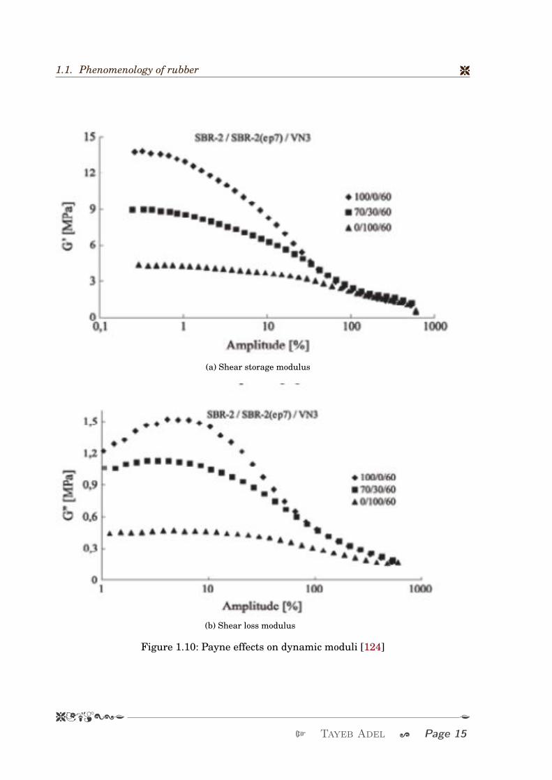
nonlinear of the dynamic amplitude εa as shown in figure 1.10. Several models have
been developed to explain the Payne effect. [20] made a classification to the Payne effect
models: (i) filler-structure models, (ii) matrix filler bonding and debonding models and
(iii) phenomenological or nonlinear network models. [112] suggested qualitatively that
the amplitude dependence of the storage and loss moduli were due to a filler network
in which the filler contacts depended on the strain amplitude. At lower amplitudes, he
argued that the filler contacts are largely intact and contribute to the high value of the
modulus. Conversely, at higher amplitudes the filler structure has broken down and does
not have time to reform. In another work [81] suggested an empirical model based on the
agglomeration/deagglomeration kinetics of filler aggregates, assuming a Van der Waals
type interaction between the particles. [89] proposed a phenomenological model within
the framework of continuum mechanics and nonlinear viscoelasticity. Experiments shown
in figure 1.10 [124] were performed using the Bromobutyl rubber BIIR.
K K;9NAB8
Page 14 ; Ph.D thesis at ECL/LTDS U
1.1. Phenomenology of rubber 8
(a) Shear storage modulus
(b) Shear loss modulus
Figure 1.10: Payne effects on dynamic moduli [124]
8CAM:<J J
T Tayeb Adel ; Page 15

8 Chapter 1. Physical aspects and hyperelastic behavior of rubber-like materials
1.2 Mechanical formulation in the high deformation
Consider an isotropic homogeneous elastic material which occupies the domain Ω0 in the
reference configuration or the unstressed one. Every material particle can be described
by the cartesin coordinates (X1, X2, X3) in the initial or the undeformed configuration
and (x1, x2, x3) in the current or deformed configuration which is illustrated in figure
1.11. The change of the mechanical state of the material particle moved from the initially
position X to the actual position x can be described mathematically using a mapping
function φ relating the reference and the current configuration as:
x =φ(X , t)= X +u(X , t). (1.3)
In the formulation of the continuum mechanics, it exists essentially two types of material
description: Lagrangian and Eulerian descriptions. The first description uses the initial
state of the material like a reference configuration and thus we can follow the material
particle in its trajectory. Although, the Eulerian description considers the trajectory of
the material particles passed by a chosen geometrical point in the space.
Figure 1.11: Transformation from undeformed to deformed configuration
1.2.1 The deformation gradient
In the continuum mechanics the deformation gradient plays an important role because
it is involved in the different mechanical quantities. The deformation gradient relates
K K;9NAB8
Page 16 ; Ph.D thesis at ECL/LTDS U

1.2. Mechanical formulation in the high deformation 8
the infinitesimal vector dx in the current configuration to the infinitesimal vector dX in
the undeformed configuration as the following:
dx = F dX . (1.4)
In that sense, F is also a two-point tensor, i.e. it relates quantities in two different
configurations. Now, tensor F can be defined as:
F = ∂x∂X
, (1.5)
where ∂ denoted the gradient operator with respect to the initial coordinates.
1.2.2 Polar decomposition of the deformation gradient
An advantageous use of the deformation gradient is its polar decomposition, that is de-
composing the total deformation F into a tensor describing the rotation and another one
describing the stretch. The polar decomposition is discovered by Cauchy using geometri-
cal arguments. Mathematically, the polar decomposition, in the material configuration,
is expressed as:
F = R U , (1.6)
where R is the rotation tensor which is an orthogonal tensor, i.e. RRT = I. While U is
the material stretch tensor which is a symmetric tensor, i.e.
UT =U .
Equivalently, in the spatial configuration, the polar decomposition is expressed as:
F =V R, (1.7)
where V is the spatial stretch tensor that is also symmetric. It can be shown that both
tensors U and V share the same principal values. As both tensors are symmetric, the
spectral theorem can be applied. Thus, tensors V and U can be conveniently expressed
as:
U =3∑
α=1λαNα⊗Nα
V =3∑
α=1λαnα⊗nα,
(1.8)
where λα are the principal stretches, Nα are the material principal directions of U, nαare the spatial principal directions of V , and n is the number of dimensions involved.
8CAM:<J J
T Tayeb Adel ; Page 17
8 Chapter 1. Physical aspects and hyperelastic behavior of rubber-like materials
1.2.3 Volume changes and isochoric/volumetric split
The deformation gradient is also used to obtain information about volume changes in
the body studied. It can be shown that the determinant of F gives the ratio between
differential volumes in the reference (dV ) and current configurations (dv). This can be
written as:
J = detF = dvdV
, (1.9)
where J is the jacobian of the deformation gradient tensor. If J = 1, then no volumetric
deformations are involved. It is crucial, when dealing with incompressible or nearly
incompressible materials, to split the deformation into volumetric components and
isochoric or distortional components. The aim of this split is to ensure that the isochoric
component of the deformation, denoted by F, does not contribute to any volume changes,
that is:
detF = 1. (1.10)
Such a condition is satisfied for the following form F wich is defined as:
F = J− 13 F, (1.11)
while the volumetric component Fv can be expressed as:
Fv = J13 I. (1.12)
1.2.4 Strain
Several strain tensors are constructed from the deformation gradient tensor. Strain ten-
sors are further categorized as material or spatial strain tensors based on the description
they refer to. Some of the strain tensors in each category will be described in the following.
The right Cauchy-Green tensor is a material strain tensor that is expressed in terms of
the deformation gradient tensor. It is defined as:
C = F t F =U2, (1.13)
where the polar decomposition (1.6) is used. In view of the equation (1.8), this can be
equivalently expressed as:
C =3∑
α=1λ2αNα⊗Nα. (1.14)
K K;9NAB8
Page 18 ; Ph.D thesis at ECL/LTDS U

1.2. Mechanical formulation in the high deformation 8
The strain tensor C is then used to define another material strain tensor, namely, the
Green-Lagrange strain tensor defined as:
E = 12
(C− I). (1.15)
Similarly, spatial strain tensors can be constructed. The left Cauchy-Green strain tensor
is given by:
B = F F t =V 2, (1.16)
where equation (1.7) is used to obtain the last equality. Using equation (1.9), B can hence
be expressed as:
B =3∑
α=1λ2αnα⊗nα. (1.17)
Another measure of spatial strain tensors is the Almansi tensor, defined based on the
left Cauchy-Green tensor as:
A = 12
(I −B−1). (1.18)
1.2.5 Stress
Consider an infinitesimal area ∆a in the vicinity of a particle position x belonging to a
deformable body in its current configuration Ωt. If the resultant force acting on this area
is denoted by ∆ f , the corresponding traction force is:
t(n)= lim∆a→0
∆ f∆a
, (1.19)
where n is the outward normal to ∆a at point x. The traction force satisfies Newton’s
third law, that is:
t(−n)=−t(n) (1.20)
This traction force is then related to the normal vector via the Cauchy stress tensor σ as:
t =σ.n, (1.21)
where
σ=3∑
i, j=1σi j e i ⊗ e j, (1.22)
in cartesian coordinates with basis unit vectors e in the current configuration. The
Cauchy stress is a spatial tensor as it relates the current force vector to the deformed
area. Other stress tensors can be constructed from the previously described measure of
stress. Some of these stress tensors are provided in the following.
8CAM:<J J
T Tayeb Adel ; Page 19
8 Chapter 1. Physical aspects and hyperelastic behavior of rubber-like materials
1.2.5.1 The First Piola-Kirchhoff Stress
The first Piola-Kirchhoff stress tensor, similar to F, is a two-point tensor that can be
related to the Cauchy stress via the following relation:
π= Jσ F−t, (1.23)
with
π=3∑
i, j=1πi j e i ⊗E j, (1.24)
where (E i)i=1,2,3 are the basis unit vectors in the reference configuration in cartesian
coordinates. The first Piola-Kirchhoff stress, in that sense, relates the traction force in the
current configuration to the corresponding differential area in the reference configuration.
This implies that the traction force vector t in the deformed configuration can be mapped
back to into the traction force T in the reference configuration. That is:
T =π N, (1.25)
where N is unit outward normal vector to the particle point X (the initial position of x).
Remark: Traction force vector T defined in Equation 2.22 does not represent an ac-
tual traction force applied on point X , but it represents a co-linear vector to t in the
reference configuration.
1.2.5.2 The Second Piola-Kirchhoff Stress
The second Piola-Kirchhoff stress tensor is completely defined in terms of quantities in
the initial configuration. This tensor is expressed in terms of the Cauchy stress and the
first Piola-Kirchhoff stress as:
S = JF−1 σ F−t = F−1 π. (1.26)
1.2.5.3 The Kirchhoff Stress
Another stress tensor that may be important for some constitutive laws is the Kirchhoff
stress tensor that is expressed, in terms of the previously described stress tensors, as:
τ= Jσ=π F t = F S F t. (1.27)
K K;9NAB8
Page 20 ; Ph.D thesis at ECL/LTDS U

1.3. Hyperelasticity 8
1.3 Hyperelasticity
1.3.1 Deformation energy
In the general theory of the elasticity, a material can be elastic with one condition, if
the Cauchy stress tensor depends only on the state of the deformation which is char-
acterized by any mesure of the strain. Thus, any measure of the stress is independent
of the deformation path. The word of "hyperelasticty" can be divided essentially into
two word "Hyper" and "Elasticity". In this scope, the first word denotes the range of
large deformations and the second one is equivalent to the previous definition of the
elasticity behaviour. To describe the non-linearity of the hyperelastic behavior, we need
to postulate a form of energy potential, and by derivation of this potential the stress
tensor can be obtained. This energy is also called deformation energy density or strain
energy density and is often denoted as W or Ψ in the literature.
Now, consider A as a measure of the deformation state. The objectivity is one of the
most important conditions to be verified by the energy potential which can be expressed
mathematically as:
Ψ(QAQ t)=Ψ(A). (1.28)
where Q is an orthogonal tensor, i.e. Q Q t = I. I is the second-order-unit tensor.
In other words, the objectivity of the deformation energy is nothing but its independence
of any material reference. It’s mentioned in [124], that to respect the objectivity principle,
the strain energy density can be chosen as:
Ψ=Ψ(C). (1.29)
In the case of an isotropic material, Ψ can be expressed in function of the invariants of Cand B. But using that, Both of C and B have the same eigenvalues. So in consequence
they have the same invariants.
I1(C)= I1(B)
I2(C)= I2(B)
I3(C)= I3(B)
. (1.30)
8CAM:<J J
T Tayeb Adel ; Page 21

8 Chapter 1. Physical aspects and hyperelastic behavior of rubber-like materials
These invariants can be expressed in this way:
I1 = trace(C)=λ21 +λ2
2 +λ23
I2 = 12
(I21 − trace(C2))=λ2
1λ22 +λ2
1λ23 +λ2
2λ23
I3 = det(C)= J2 =λ21λ
22λ
23
, (1.31)
where λ1, λ2, λ3 are the stretches in the principal direction of the two tensors C and B.
Now to find the expressions of the different stress tensors we have to remind the couples
of every strain measure and its ad-joint stress variable. We can present these couples in
this way:
-(σ, B)
-(τ, F)
-(S, E)
By the definition of the couple of the ad-joint variables we deduce:
σ= 1J
B∂Ψ
∂Bτ= ∂Ψ
∂FS = ∂Ψ
∂E. (1.32)
The derivative of the different invariants compared to the tensor C may be expressed as:
∂I1
∂C= I
∂I2
∂C= I1I −C
∂I3
∂C= I3C−1. (1.33)
From equations (1.32) and (1.33), it is deduced that:
S = 2∂Ψ
∂C= 2
∑i
∂Ψ
∂I i
∂I i
∂C, S = 2[(
∂Ψ
∂I1+ I1
∂Ψ
∂I2)I − ∂Ψ
∂I2C+ I3
∂Ψ
∂I3C−1]. (1.34)
Having the equation (1.26) we can derive:
σ= 2J
[(∂Ψ
∂I1+ I1
∂Ψ
∂I2)B− ∂Ψ
∂I2B2 + I3
∂Ψ
∂I3I]
τ= 2[(∂Ψ
∂I1+ I1
∂Ψ
∂I2)F − ∂Ψ
∂I2B F + I3
∂Ψ
∂I3F−t].
(1.35)
1.3.2 The incompressibility condition
Almost of the rubber-like materials are characterized by an incompressible behavior. In
fact, for this category of materials the compressibility module varies between 1000 and
2000MPa, while the magnitude of the shear modulus is about 1MPa. This difference
signifies that the rubber hardly changes in volume, even under high stress. Its behavior
is almost as incompressible. For most applications, modeling supposes a complete incom-
pressiblity. So the incompressibility assumption is a good approximation for the modeling
K K;9NAB8
Page 22 ; Ph.D thesis at ECL/LTDS U

1.3. Hyperelasticity 8
of rubbery materials. The incompressibility condition can be shown mathematically
through:
J = det(F)= 1. (1.36)
Returning to the definition of the parameter J we can deduce that in an incompress-
ible material, the volume is preserved and thus the transformation is isochoric. The
incompressibility condition in the strain-stress relation can be introduced directly by the
change of the formulation of the deformation energy which becomes:
Ψ=Ψ(I1, I2, I3 = 1)− p(J−1), (1.37)
where p denotes the Lagrange multiplier associated to the incompressibility condition.
So the stress-strain relation in the Lagrangian configuration can be expressed in this
way:
S = 2[(∂Ψ
∂I1+ I1
∂Ψ
∂I2)I − ∂Ψ
∂I2C]− pC−1. (1.38)
And in the eulerian configuration, it becomes:
σ= 2J
[(∂Ψ
∂I1+ I1
∂Ψ
∂I2)B− ∂Ψ
∂I2B2]− pI. (1.39)
Using the relation (1.26) one can also deduce for the Kirchhoff stress:
τ= 2[(∂Ψ
∂I1+ I1
∂Ψ
∂I2)F − ∂Ψ
∂I2B F]− pF−T . (1.40)
Identifying the multiplier of Lagrange in the spheric part of the Cauchy stress tensor, pcan be analyzed like a measure of the unknown hydrostatic pressure.
1.3.3 Examples of strain energy densities
Many forms of deformation energy densities have been proposed in the literature. Some
are based on a statistical theory, others are purely phenomenological. in this part we
will focus only on the deformation energy densities compatible with an incompressible
material. There are several ways to classify the different energies of deformation. One
way for example, it is to separate those expressed in terms of invariants, and those
that are expressed in terms of the principal streches. In the first case the deformation
energy depends linearly on the parameters of the constitutive law, and it is expressed in
terms of the invariants I1 and I2. The coefficients of this type of laws behavior can be
easily identified. They generally allow a good smoothing of the experimental results to
a moderate level of deformation. For higher strain rate, will often increase the order of
8CAM:<J J
T Tayeb Adel ; Page 23

8 Chapter 1. Physical aspects and hyperelastic behavior of rubber-like materials
the polynomial form. However, the fact of working with a large number of coefficients
leads to numerical instabilities in the limits of the investigative deformation field range.
For the models that are expressed as a power law as the model of Ogden, coefficients
involved in non-linear form (exponent). These models usually have a good smoothing
with few parameters for higher levels of deformation. However their identification is
more difficult. We can find a more complete review of different energies deformation in
this PHD thesis [124].
1.3.3.1 Developement in function of the invariants
The generalized model of Rivlin [123] implemented in most of finite element codes, is
given by the following series expansion:
Ψ=N∑
i+ j=1ci j(I1 −3)i(I2 −3) j. (1.41)
This type of behavior law is generally the most used. The strain energy is developed in
order proportional to the desired deformation range (for N = 3, we have generally a good
correlation with experimental measurements). In practice, most of the polynomial used
laws correspond to a particular case of Rivlin development. For example, keeping only
the first term of the expansion, we get the Neo-Hookean law:
Ψ= c10(I1 −3), (1.42)
which was first developed from statistical theory considering that the rubber vulcanized is
a three-dimensional network of long molecular chains connected in some points. The Neo-
Hookean model provides a good correlation to the degree of deformation moderate (up to
50 % [124]), but is not suitable for the incorporation of large deformations. The second
special case of development corresponds to the phenomenological model of Mooney-Rivlin,
widely used in the rubber industry. We then take the first 2 terms of Rivlin development,
which allows writing:
Ψ= c10(I1 −3)+C01(I2 −3). (1.43)
This time, a good correlation is obtained with the experimental results to levels deforma-
tion of the order of 150% [124].
K K;9NAB8
Page 24 ; Ph.D thesis at ECL/LTDS U

1.3. Hyperelasticity 8
1.3.3.2 Development in function of the principal streches
Ogden in [107] has proposed a strain energy in function of the principal stretches, which
describes the change of these fields during the deformation.
Ψ=Ψ(λ1,λ2,λ3)=N∑
k=1
µk
αk(λαk
1 +λαk2 +λαk
3 −3), (1.44)
where N is the chosen number of the terms in the series of the strain energy, while
µk denotes the shearing coefficients and αk are adimensional coefficients. Consider µ
the slope in the origin of the stress-strain graph during a shearing test. Then with
linearization we can obtain a relation between the Ogden shearing coefficient and µ:
µ=N∑
k=1αkµk, (1.45)
under the following condition:
αkµk > 0 ∀k ∈ 1, ..., N. (1.46)
Using the Ogden model, it is possible to have good correlation with the experimental
results. One of the advantages of this model, that we can fit well the experimental
data even for a high level of deformation, giving the ability of having a more stable
identification than the models expressed in function of the invariants. In the case of
an incompressible transformation λ1λ2λ3 = 1. So Using the previous incompressibility
condition, and having N = 2, α1 = 1 and α2 = −2 we can identify the Mooney Rivlin
model where c10 = µ
2 and c01 =−µ
2 . With the same way, we can obtain the Neo-Hookean
model with c10 = µ
2 when N = 1 and α1 = 2. Another form of the strain energy density,
also depending on the principal stretches, was proposed by Valanis and Landel [144].
The function of the strain energy density can be expressed as the sum of 3 separable
functions, every one depending on only one principal stretch variable which is equivalent
to:
Ψ(λ1,λ2,λ3)=ψ1(λ1)+ψ2(λ2)+ψ3(λ3). (1.47)
This form of the strain energy implies the absence of the interaction between the principal
stretches variables. Using the strain energy density, we can express the stress tensors in
the principal directions in the different configurations:
σα =λα ∂Ψ∂λα
Pα = ∂Ψ
∂λαSα = 1
λα
∂Ψ
∂λα(1.48)
8CAM:<J J
T Tayeb Adel ; Page 25

8 Chapter 1. Physical aspects and hyperelastic behavior of rubber-like materials
1.4 Literature survey for nonlinear viscoelasticmodels
It is well known that rubber-like materials exhibit nonlinear viscoelastic behavior over a
wide range of strain and strain rates confronted in several engineering applications such
as civil engineering, automotive and aerospace industries. This is due to their capacity
to undergo high strain and strain rates without exceeding the elastic range of behavior.
Further, the time dependent properties of these materials, such as shear relaxation
modulus and creep compliance, are, in general, functions of the history of the strain or
the stress [45].
The study of viscoelastic behavior of solid materials has a long history and several models
have been developed from purely mathematical approaches to applied studies where ease
of application is for huge interest. The first, ever, models dedicated to the modeling of
viscoelastic behavior have been established by Maxwell, Kelvin and Voigt who studied the
one dimensional responses of these materials which led to the establishing of rheological
models bearing their names which are still used to this day [92] (i.e. the Maxwell, Kelvin
and Voigt rheological models). These rheoligical models were used by [10] to formulate
the first three dimensional viscoelastic model for isotropic materials. This model is
restricted to the linear viscoelasticity. However, due to the constitutive nonlinearities
and the fact that these materials are able to undergo geometrical nonlinearities, in
a wide range of strain, a linear viscoelasticity theory is no longer applicable for such
material and new constitutive equations are required to fully depict the behavior of
rubber-like materials for quasi-static and dynamic configurations of huge interest in
engineering applications. In what follows, we present some of the most used modeling
strategies in the literature.
1.4.1 Internal variables formulation
This approach was firstly introduced by [27] which consists on the formulation of the
constitutive equation in terms of thermodynamic state variables : the internal energy is
expressed as a function of the strain (or stress) and a set of internal state variables [24],
[25], and [28]. These internal variables are related to their conjugate thermodynamic
forces, which are the derivative of the internal energy with respect to the internal
variables, via the evolution equations which could be linear or nonlinear.
One of the most known model following the internal state variable approach is the one
K K;9NAB8
Page 26 ; Ph.D thesis at ECL/LTDS U

1.4. Literature survey for nonlinear viscoelastic models 8
proposed by [131] which was the starting point for many contributions such as [51], [68],
[66], [148] and our model proposed in [136] and presented in chapter 2 among others.
The Simo’s approach was based on the split of the internal energy density following
a multiplicative decomposition of the deformation gradient tensor F into dilatational
and volume preserving parts. Despite that this model may lead to non-physical results
at finite strain [36], this model depict very well the behavior of rubber like materials
for several applications and different load configurations. For this model, the internal
energy is the sum of three different terms: a volumetric part depending on the jacobian
of the deformation gradient tensor J = det(F ), an isochoric part depending upon the
isochoric part of the deformation gradient tensor F = J−1F and a part depending upon
the internal variable noted q in the original paper which represents the non-equilibrium
part of the stress. The evolution law of the internal variable q is postulated such that
the generalized force is proportional to the derivative of the internal energy with respect
to the isochoric strain. This assumption means that the behavior of the material is
considered purely elastic for bulk, but it is viscoelastic for the shear. This formulation led
to a single convolution integral representation of the constitutive equation of the stress.
Similar formulations to the one used by [131] is due to the contribution by [51] where the
internal variables were represented by a set of stress-like variables and the work by [68]
where the internal variables were represented by a strain-like variables. The advantage
of such formulation is the possibility to be used for modeling anisotropic behavior such
as the work [66] in which the internal variables where dependent upon fiber orientation.
The Simo’s model is implemented in most of finite elements commercial software.
1.4.2 Additive decomposition of the free energy density
This approach relies on the decomposition of the deformation gradient tensor F as the
sum of elastic deformation gradient tensor and an inelastic deformation gradient tensor.
This decomposition was first proposed by [128] and followed by [90], [56], [41], [74] and
[88] among many others.
Within this framework the deformation gradient tensor F is decomposed as follows:
F =FeFi. (1.49)
The inelastic part Fi characterizes an intermediate configuration between the reference
and the actual configurations. This inelastic part of the deformation gradient tensor could
be decomposed into several intermediate configurations. From (1.49) the free energy
8CAM:<J J
T Tayeb Adel ; Page 27

8 Chapter 1. Physical aspects and hyperelastic behavior of rubber-like materials
density is also split as follows
Ψ=Ψe(C)+Ψo(Ce), (1.50)
where C is the right Cauchy-Green strain tensor and Ce = FetFe is the elastic right
Cauchy-Green strain tensor in the intermediate configuration. The free energy density
of (1.50) have been used in several works such as [56], [41] and [88] among many others.
[11] has proposed the following form for the free energy density
Ψ=Ψe(C)+Ψo(C,Ci), (1.51)
in which Ci =FitFi is the inelastic left Cauchy-Green strain tensor, the viscous compo-
nent of the free energy density Ψo(C,Ci) is assumed to be proportional to the elastic
component Ψe(C). The stress response in terms of the second Piola-Kirchhoff stress
tensor S are obtained after applying the Coleman and Noll procedure [27] by verifying
the Clausius-Duhem inequality for all admissible processes and is decomposed as
S =Se +Si, (1.52)
where Se is the equilibrium stress whereas Si is the over stress. Using an internal
energy of the form of equation (1.50) these stresses are given by
Se = ∂Ψe
∂C, Si = ∂Ψi
∂Ci(1.53)
In order to reach the expression of the stress, in addition to equation (1.53) one need
to define the evolution law of the internal variable Fi or Fe. A common choice for the
flow rule is to apply a generalization of the one-dimensional linear Maxwell-model to
the three-dimensional and nonlinear domain. In this case the evolution equations are
assumed to be linear, and the overstress term arising from them is the generalization
of the extra-stress arising in Maxwell element [66] and [73].Within this context and
the framework of irreversible thermodynamics, [13] proposed a double decomposition of
the deformation gradient tensor F . First, the deformation gradient tensor is split into
volumetric and isochoric parts, then the latter is split into elastic and inelastic parts :
F = (J13I)F = (J
13I)FeFi, (1.54)
where F is the incompressible deformation gradient tensor, Fe is the elastic incompress-
ible deformation gradient tensor and Fi is the inelastic deformation gradient tensor. This
K K;9NAB8
Page 28 ; Ph.D thesis at ECL/LTDS U

1.4. Literature survey for nonlinear viscoelastic models 8
decomposition implies that the inelastic processes are isochoric. The free energy density,
following (1.54), is decomposed as well into:
Ψ=Ψeq +Ψneq +Ψvol , (1.55)
where the subscript eq, neq and vol stand for the equilibrium, non-equilibrium and
volumetric parts of the free energy density respectively. The stress tensor is obtained
after satisfying the second law of thermodynamics in terms of the Clausius-Duhem
inequality and it is decomposed accordingly as
σ =σeq +σneq +σvol . (1.56)
For the evolution law of the internal variables, three different rheoligical models were
used [86]. The first model is the Zener model for which the evolution law takes the
followingg form:
˙Be =L ·Be +Be ·Lt − 23
(I :L)Be − 2ησneq ·Be, (1.57)
where Be = Fe · F te is the incompressible left Cauchy-Green strain tensor and it is
considered the internal variable, L is the velocity gradient tensor and η is the viscosity
coefficient. The second model is the Poynting–Thomson model for which the evolution
law reads˙Be =L ·Be +Be ·Lt − 2
3(I :L)Be − 2
ησneq ·Be
+ 4JηΨneq,1
(B− 1
3(B : B−1)Be
)+ 4
JηΨneq,2
(Be ·B−1 ·Be − 1
3(B−1 : Be
)Be
) (1.58)
where Ψneq,1 and Ψneq,2 are the derivative of the non equilibrium parts of the free
energy density of equation (1.55) with respect to the first and second invariants of the
inelastic left Cauchy-Green strain tensor Bi. The third model is the generalized Bingham
viscoplastic model.
[88] proposed nonlinear evolution equations based on strain, time and temperature. [11]
also used nonlinear evolution equations of rate type for the internal variables. These
are based on a particular linear relaxation form of the Maxwell model which leads to a
viscoelastic formulation that can be seen as a particular case of a large strain viscoplastic
model. A variational formulation of Bonet’s model has been developed in [40].
8CAM:<J J
T Tayeb Adel ; Page 29

8 Chapter 1. Physical aspects and hyperelastic behavior of rubber-like materials
1.4.3 Integral based formulation
The integral-based formulation is an extension to the finite strain domain of the simple
formulation of Boltzmann. Within this approach, the stress is decomposed into an
instantaneous elastic response typically modeled by an hyperelastic response for rubber-
like materials and an over-stress quantity which is expressed by a hereditary integral
containing all the history of the strain up to the actual time t. The first contribution to
this approach was the work by Green and Rivlin [52]. Inthis context, the internal energy
Ψ was developed accordingly in agreement with the fading memory property i.e., strains
which occurred in the distant past have less influence on the present value of Ψ than
those which occurred in the more recent past. This work have been followed by several
works who dealt with the definition of the internal energy accounting for deformation
histories [31], [39] and [49]. One of the most known models to this approach is the multi-
integral model proposed by Pipkin and Rogers [117] for which under incompressibility
assumption the second Piola-Kirchhoff stress reads
§ (t)=− pC−1 +∫ t
0r1
(t− t′
)E
(t′)
dt′+∫ t
0
∫ t
0r2(t− t′, t− t′′)E
(t′)E
(t′′
)dt′ dt′′+∫ t
0
∫ t
0
∫ t
0r3
(t− t′, t− t′′, t− t′′′
)tr
[E
(t′)E
(t′′
)]E
(t′′′
)dt′dt′′dt′′′+∫ t
0
∫ t
0
∫ t
0r4
(t− t′, t− t′′, t− t′′′
)E
(t′)E
(t′′
)E
(t′′′
)dt′dt′′dt′′′,
(1.59)
rk (k = 1..4) are the relaxation kernels expressed by a decaying exponential functions
and E (t) is the time derivative of the Green-Lagrange deformation tensor. Equation
(1.59)will be used later in chapter 3 to generate data which will be used in the identi-
fication procedure presented therein. This work was followed by several contributions
such as the pseudo-linear model proposed by [57] in which a the stress is expressed as
Boltzmann integral over the history of a nonlinear measure of strain.
Thanks to their simplicity for engineering applications, several models using this ap-
proach have been thoroughly investigated [4], [58] and [23] among others. In the latter,
a comparative study have been made to investigate seven single-integral viscoelastic
models response using data in compression for a filled rubber for relaxation and load-
ing/unloading/creep cycles at different strain rates, namely the models due to [47], [48],
[54], [147], [63], [89] and [127]. These models could be written in the same form in terms
K K;9NAB8
Page 30 ; Ph.D thesis at ECL/LTDS U
1.4. Literature survey for nonlinear viscoelastic models 8
of the first Piola-Kirchhoff stress as
π (t)=π(e) +F (t)Λ (t)∫ t
0
∂k (t− s)∂ (t− s)
Ψ (t− s)ds
π(e) =φ1 (t)F (t)+φ2 (t)F (t)C (t) ,(1.60)
where πe is the hyperelastic contribution to the stress and the functions φ1 and φ2
are functions of the first two invariants of the left Cauchy-Green strain tensor C. A
suitable choice for Λ, Ψ as well as the viscoelastic kernel k allows all the models under
consideration to be encompassed.
Another contributions in this context are the quasi-linear viscoelastic models which was
first proposed by [48] to describe the behavior of biological tissues. This model, which is
a special case of a more general Pipkin–Rogers constitutive model [117], predicts that at
any time a stress that is equal to the instantaneous elastic stress response decreased
by an amount depending on the past history, assuming that a Boltzmann superposition
principle holds. This work was followed by [99] and [98] where the linearized strain is
expressed in terms of a nonlinear measure of the stress.
1.4.4 Differential viscoelasticity
Finally, another approach to describe viscoelastic behavior of rubber-like materials is the
differential nonlinear viscoelasticity [7], [126] and [143]. Within this context, the stress
and strain tensors are related through differential equations. It is the generalization
to the three-dimensional nonlinear case of the linear rheological elementary models,
namely the Hook spring for which the stress is expressed by the following
σ=Gε, (1.61)
for the linear case and
σ=φe(ε), (1.62)
for the nonlinear case and the viscous dashpot for which the stress is expressed as
σ= ηε, (1.63)
for the linear case and
σ=φv(ε), (1.64)
for the nonlinear case. In general, the stress-strain differential relation arising from any
combination of these elementary models readsM∑
m=0am
∂mσ
∂tm =N∑
n=0bn∂nε
∂tn , (1.65)
8CAM:<J J
T Tayeb Adel ; Page 31

8 Chapter 1. Physical aspects and hyperelastic behavior of rubber-like materials
where am and bm are functions of the rheological characteristics of the elementary
models associated. In the case when m = n, the stress-strain relation arising from (1.65)
is equivalent to the one obtained from the generalized Maxwell model. The generalization
of these rheological models to the three-dimensional domain is done by replacing the
one dimensional stress σ and strain ε by their three-dimensional counterparts σ and ε
respectively. The Rivlin-Ericksen model is a simplified form of relation (1.65) which does
not include time derivative of the stress
σ=N∑
n=1bn∂nε
∂tn . (1.66)
In relation (1.66) σ is replaced by the Cauchy stress tensor σ and the derivative ∂nε∂tn by
the nth Rivlin-Ericksen tensor An [34].Therefore the Cauchy stress tensor is given by
σ =N∑
n=1bnAn. (1.67)
In particular, the second order model obeys the equation
σ = ηA1 +b12A21 +b21A2, (1.68)
where η, b12 and b21 are adjustable parameters. The model of equation (1.68) was
employed by [2], [3], [26] and [122] to study laminar flow of viscoelastic fluids.
Another model arising from (1.66) is the White-Metzner model for which ∂nε∂tn is replaced
by the nth White-Metzner tensor Bn. The model reads
σ =N∑
n=1bnBn, (1.69)
which was used by [2], [76] and [145].
Other contributions to this approach is the extension to finite strain domain of the
so-called Maxwell rheological model composed by a spring in series with a dashpot,
the Kelvin-Voigt model composed by a spring parallel to a dashpot or the standard
viscoelastic solid model composed by two springs and a dashpot with two configuration
as it is shown in figure 1.12. Version A was extended to large deformation by [59] in
which the linear dashpot was replaced by a nonlinear one and linear spring with Young’s
modulus E2 was replaced by an hyperelastic spring where the strain energy density was
taken in the Langevin form. This model was used to describe the effect of strain rate of
the yield stress in cellulose derivatives and poly(vinyl chloride). Version B was extended
to finite strains by [14]. In that model, the linear spring with Youn’s modulus E1 was
K K;9NAB8
Page 32 ; Ph.D thesis at ECL/LTDS U

1.5. Conclusion 8
replaced by a hyperelastic spring and the Maxwell element in parallel was replaced
by a nonlinear Maxwell element of Leonov’s type. Numerical simulation demonstrates
that this model provides qualitative agreement with experimental data for polymeric
materials [34].
Figure 1.12: Two versions of the standard viscoelastic solid
Thus in the simplest case, the stress depends upon the current values of strain and
strain rate only. In this sense, it can account for the nonlinear short-term response
and the creep behavior, but it fails to reproduce the long-term material response (e.g.,
relaxation tests)
1.5 Conclusion
Within this chapter, we tried to present a review of the behavior of rubber-like materials
from a phenomenological point of view. In the first part, we recalled the most known
physical aspect related to these materials evolving high deformability and damping
properties corroborated with several experiments found in literature. In the second part,
we recalled the basis mechanics for the nonlinear elasticity framework needed in the
development of nonlinear viscoelasticity models. In the third part, we tried to classify the
different approaches and modeling procedures followed in the development of nonlinear
viscoelatic models for rubber-like. The common thing about all these approaches is
8CAM:<J J
T Tayeb Adel ; Page 33
8 Chapter 1. Physical aspects and hyperelastic behavior of rubber-like materials
that the constitutive equation of the stress is represented by a hereditary integral over
the history of the strain or equivalent quantities. In the next chapter, we present the
nonlinear viscoelastic model proposed within this work.
K K;9NAB8
Page 34 ; Ph.D thesis at ECL/LTDS U
CH
AP
TE
R
2PROPOSED NONLINEAR VISCOELASTIC MODEL
Contents2.1 Experimental and rheological motivations . . . . . . . . . . . . . . . . . . 36
2.1.1 Experimental motivation . . . . . . . . . . . . . . . . . . . . . . . 36
2.1.2 Rheological motivation . . . . . . . . . . . . . . . . . . . . . . . . . 37
2.1.3 Thermodynamic considerations . . . . . . . . . . . . . . . . . . . 39
2.2 Formulation restricted to linear kinematics . . . . . . . . . . . . . . . . . 40
2.2.1 Formulation of the model . . . . . . . . . . . . . . . . . . . . . . . 41
2.2.2 Thermodynamic considerations . . . . . . . . . . . . . . . . . . . 42
2.3 Fully nonlinear viscoelastic model . . . . . . . . . . . . . . . . . . . . . . . 43
2.3.1 Mechanical framework and form of the Helmholtz free energy
density . . . . . . . . . . . . . . . . . . . . . . . . . . . . . . . . . . 44
2.3.2 Rate and constitutive equations . . . . . . . . . . . . . . . . . . . 45
2.3.3 Functional formulation and thermodynamic considerations . . 47
2.4 Conclusion . . . . . . . . . . . . . . . . . . . . . . . . . . . . . . . . . . . . . 48
IN this chapter we shall develop a nonlinear viscoelastic model at finite strain
within the framework of rational thermodynamics and the approach of inter-
nal state variables, the model is derived through a modification to approaches
35

8 Chapter 2. Proposed nonlinear viscoelastic model
in [131], [65] and [120] taking into account the dependence of the time dependent func-
tions upon the state of the strain.
In section 2.1, a one dimensional nonlinear viscoelastic model is developed using a
modified Maxwell rheological model. Section 2.2 is devoted to the extension of the model
to the three-dimensional domain under the assumption of linear kinematics. In section
2.3, this model is extended to the fully nonlinear formulation using a nonlinear set of
evolution equation of the internal state variables within the rational thermodynamic
framework. The shear relaxation modulus is set to be a function upon the invariants
of the right Cauchy-Green strain tensor via a strain shift function analogous to the
temperature shift function for the thermorheologically simple materials, this choice is
motivated experimentally following the experimental characterization of BIIR from [103].
The constitutive equation for the stress is then obtained by resolving the set of nonlinear
evolution equations.
2.1 Experimental and rheological motivations
In this section, we develop the rheological and experimental arguments leading to
the proposed finite strain viscoelastic model. To motivate the three dimensional model
developed below, we first highlight some experimental results leading to this model and
then we consider a suitable modification to the generalized Maxwell rheological model to
build the one dimensional nonlinear viscoelastic model.
2.1.1 Experimental motivation
A significant class of rubbers shows nonfactorizable behavior at low and average range
of strain. This phenomenon consists on the dependence of the shear relaxation modulus
upon strain level. Several works were dedicated to deal with this class of behavior
especially the series of papers by [134] and [104]. In a recent work [103], an experimental
characterization was carried out with three rubber-like materials: the natural rubber
(NR), the Bromobutyl (BIIR)and a mixture of these materials (NR-BIIR). Samples of
the three materials were subjected to monotonic experiments of simple extension and
pure shear with a relaxation of 10 minutes every 50% of strain in order to depict
the equilibrium behavior of the materials. Moreover, a dynamic characterization was
carried out in simple shear for a wide window of frequency at several temperatures and
predeformations in order to construct the master curve of the material. This material
K K;9NAB8
Page 36 ; Ph.D thesis at ECL/LTDS U

2.1. Experimental and rheological motivations 8
showed a dependence of the shear relaxation modulus upon strain. In figure 2.1 it is
plotted the logarithm of the shear relaxation modulus G(t) versus the logarithm of time
for two different level of strain 10% and 50% for BIIR material. The shear relaxation
modulus shows a dependence upon the strain level which leads according to [141] to a
shift in the time with a strain dependent function since the shear relaxation modulus at
any level could be obtained through a combination of a vertical and horizontal translation
from the reference curve at a strain level of 10%. Therefore, a one dimensional viscoelastic
model, taking in consideration these results, is developed in the next section through a
generalization of the Maxwell rheological model.
Log(t) 1 2 3 4 5 6 7 8 9 10
Log
(G)
12.2
12.3
12.4
12.5
12.6
12.7
12.8
12.9
Modulus for ǫ=10%Modulus for ǫ=50%
Figure 2.1: Dependence of the shear relaxation modulus upon strain for BIIR rubber
2.1.2 Rheological motivation
Before we develop the three-dimensional viscoelastic model, we shall investigate the
following formulation for a standard linear solid. In this model, which is a modification
to the rheological Maxwell model reported in figure 2.2, σ denotes the total stress, ε
denotes the total strain, G i and τi are the parameters of the Maxwell model. Unlike the
rheological model used in [129], the relaxation times τi are, due to the experimental result
outlined above, functions of the total strain ε . Furthermore, let αi be the deformation of
8CAM:<J J
T Tayeb Adel ; Page 37

8 Chapter 2. Proposed nonlinear viscoelastic model
the dashpot of each Maxwell branch and Q i =G iαi an internal variable stress measure
characterizing the model. The internal deformation variables variables αi, according to
the rheological model of figure 2.2, are governed by the following evolution equations.
Figure 2.2: Generalized Maxwell model
αi + 1τi (ε)
αi = 1τi (ε)
ε, αi| t=0 = 0. (2.1)
Which can be written in terms of the stress internal variables Q i as follow:
Q i + 1τi (ε)
Q i = 1τi (ε)
G iε, Q i| t=0 = 0. (2.2)
The total stress σ derive directly from the rheological model as the difference between
the elastic instantaneous stress and the non-equilibrium stresses Q i.
σ=Goε−∑
iQ i, (2.3)
where Go = G∞+∑i
G i is the instantaneous shear modulus. The time parameters of
the Maxwell model are set to be a strain dependent function; this idea follows from
K K;9NAB8
Page 38 ; Ph.D thesis at ECL/LTDS U

2.1. Experimental and rheological motivations 8
the description of thermorheologically simple materials’ behavior see [141] and [140],
for which all parameters are temperature dependent via a single variable function
called ‘temperature shift-function’. [95, 125] and [104] among others generalized this
notion to describe thermorheologically complex materials’ behavior where the shift
function depend upon temperature and stress or strain. Other contributions modeled
this phenomena by a strain-rate dependent relaxation times , see [21] and references
therein. In our work, since the study was carried out using relaxation data, the time
parameters take the following form.
τi (ε)= a (ε)τi, (2.4)
a(ε) is a positive strain function, following the dissipation inequality, called strain shift
function. Therefore, the law of evolution of the equation (2.1) became a linear differential
equation over the reduced time ξ
dαi
dξ+ 1τiαi = 1
τiε with ξ (t)=
∫ t
0
dt′
a (ε), (2.5)
where ξ(t) is an increasing function of time. Considering the form of the time parameters
of equation (2.4), the integration of the differential equations in (2.5) lead to the following
expression of αi:
αi (t)= 1τi
∫ t
0exp
[−(ξ−ξ′)/τi
]ε(t′)dξ′, (2.6)
which can be integrated by parts to lead to
αi (t)= ε (t)−∫ t
0exp
[−(ξ−ξ′)/τi
]ε(t′)dξ′. (2.7)
Substituting of α by its expression into (2.3) with Q i =G iαi yield the expression of the
total stress σ as a Boltzmann convolution integral of the strain as follow :
σ (t)=∫ ξ
0G
(ξ−ξ′) ε(
t′)dξ′, (2.8)
where G(t) is the shear relaxation modulus expressed by a Prony series as follows:
G (t)=G∞+∑i
G i exp(− tτi
)=Go −
∑i
G i
(1−exp
(− tτi
)). (2.9)
2.1.3 Thermodynamic considerations
Another way to motivate the evolution equations (2.1), is to consider the thermodynamic
arguments following from the modified Maxwell rheological model. Considering the set
8CAM:<J J
T Tayeb Adel ; Page 39

8 Chapter 2. Proposed nonlinear viscoelastic model
of variables governing the model, namely the total strain ε and the set of internal strains
αi, the total free energy density reads:
ψ (ε,α)= 12
G∞ε2 +∑i
12
(ε−αi)2, (2.10)
where α is the vector of strain internal variables αi. The forces in the dashpots of the
Maxwell model are given by
σvi =G i (ε−αi)= ηiαi, (2.11)
where ηi = τiG i are the viscosity coefficients characterizing the dashpots in the Maxwell
model which are functions of the total deformation ε following from the dependence of
the relaxation times τi upon ε due to equation (2.4). Equation (2.11) implies the evolution
law of equation (2.1) and thus the dissipation function D[ε,α,α] is given by
D[ε,α,α]=∑iσv
i αi =∑
iηi(αi)2 ≥ 0. (2.12)
These thermodynamic quantities could be be expressed as a convolution integrals in
terms of the history of the deformation ε by substituting the internal variables αi by
their expressions in equations (2.10) and (2.12) to lead to the following
D[ε,α,.α]=− 1
a (ε)12
∫ ξ
0
∫ ξ
0
∂G(2ξ−ξ′−ξ′′)∂ξ
∂ε
∂t′∂ε
∂t′′dξ′dξ′′, (2.13)
for the dissipation function, and
ψ= 12
∫ ξ
0
∫ ξ
0G
(2ξ+ξ′+ξ′′) ε(
t′)ε(t′′
)dξ′dξ′′, (2.14)
for the free energy density. Note that the positivity of the deformation shift function a(ε)
is a sufficient condition to the positivity of the dissipation function D[ε,α,α] in equation
(2.13).
2.2 Formulation restricted to linear kinematics
In this section, we extend the simple nonlinear models discussed in the preceding section
to three-dimensional physically nonlinear elasticity. This extension is patterned after
the model presented in section 2.1. First, we discuss the formulation of the general
three–dimensional constitutive model within the linear kinematics framework (i.e. small
strain domain). Next, we examine the thermodynamic aspects within the framework of
irreversible thermodynamics with internal state variables.
K K;9NAB8
Page 40 ; Ph.D thesis at ECL/LTDS U

2.2. Formulation restricted to linear kinematics 8
2.2.1 Formulation of the model
Viscoelastic constitutive equations arise when modeling the behavior of rubber-like
materials. The bulk response of these materials is elastic and much stiffer than the
deviatoric response. Further, for most engineering applications using these materials the
assumption of incompressibility holds with high degree of approximation. Considering
these assumptions, we introduce an additive split of the strain tensor into volumetric
and deviatoric parts as
ε= e+ 13ΘI , (2.15)
where e is the deviatoric strain given by
e= ε− 13
tr[ε]I , (2.16)
and Θ is the deviatoric strain defined by
Θ= tr[ε]. (2.17)
Following the additive split of the strain of equation (2.15) the initial stored elastic
energy density is split as well
Ψ0(ε)= Ψ0(e)+U0(Θ). (2.18)
Both Ψ0(e) and U0(Θ) are positive functions of their arguments. The initial elastic stress
is given by
σo = ∂Ψ0(ε)∂ε
, (2.19)
which can be expressed using equations (2.16) and (2.17) and the chain rule as follows:
σo =dev[∂Ψ0(e)∂e
]+U0′(Θ)I . (2.20)
Now, in accordance with the one dimensional model of 2.1 the total stress is given by
σ(t)=σo −∑iQi (t), (2.21)
where Qi, i = 1..N is a set of over-stress internal variables with the evolution law,
motivated by the one dimensional model of 2.1, defined by
Qi + 1τi (ε)
Qi = γi
τi (ε)dev
[∂Ψ0 (e)∂e
]. (2.22)
8CAM:<J J
T Tayeb Adel ; Page 41

8 Chapter 2. Proposed nonlinear viscoelastic model
Note that the set of relaxation times τi are dependent of the total strain ε as it was
postulated for the one dimensional model in equation (2.4)
τi (ε)= a (ε)τi, (2.23)
where a (ε) is the strain shift function. The solution of the set of linear differential
equations of (2.22) yields the convolution representation of the internal variables
Q(t)= γi
τi
∫ ξ
0exp
[−(t− t′
)/τi
]dev
[∂Ψ0 (e)∂e
]dt′. (2.24)
In equation (2.24), ξ is the reduced time. Substituting of (2.24) into (2.21), integration by
parts and use of the fact that the internal variables vanish for t < 0 gives the constitutive
equation of the stress tensor as the convolution integral
σ (t)=∫ ξ
0g
(ξ−ξ′) d
dt′
(dev
[∂Ψ0 (
e(t′))
∂e
])dt′+U0′ (Θ)I , (2.25)
where g(t) is the normalized relaxation function, in this case it is expressed by the
following
g(t)= γ∞+∑iγi exp
[−t/τi
]. (2.26)
Note that in equation (2.25) U0′ (Θ)I→−pI for incompressible materials, where p is
the hydraustatic pressure [30]. This completes the development of the three-dimensional
viscoelastic model in small strain domain.
2.2.2 Thermodynamic considerations
Once again motivated by the rheological arguments of the previous section, now we
proceed to investigate the thermodynamic foundation of this model within the framework
of irreversible thermodynamic and the internal state variables. It should be noted,
however, that this development is carried out under isothermal conditions. Therefore,
attention is restricted to purely mechanical theory. Our starting point is the form of the
free energy function which is postulated by the following:
Ψ(Qi,ε)=Ψ0(ε)−∑iQi ·e+Ξ
(∑iQi
). (2.27)
Note that the function Ξ is a positive function of the set of internal variablesQi and may
be expressed by a Taylor series especially in the case of small strains. The second law
K K;9NAB8
Page 42 ; Ph.D thesis at ECL/LTDS U

2.3. Fully nonlinear viscoelastic model 8
of thermodynamics in terms of the Clausius-Duhem inequality for a purely mechanical
theory leads to the inequality
−Ψ(Qi,ε)+σ : ε≥ 0. (2.28)
This inequality is regarded as a constitutive restriction to be satisfied by all admissible
states defined ε,Qi and for all strain rates ε for all admissible processes. From (2.28)
and using the chain rule it follows
Ψ=(∂Ψ0
∂ε−∑
idev [Qi]
): ε−D [
ε,Qi,Qi], (2.29)
where
D[ε,Qi,Qi
]=∑i
[e− ∂Ξ
∂Qi
]:Qi (2.30)
is the dissipation function. Substitution of equations (2.29)and (2.30) in (2.28) yields the
following inequality (σ− ∂Ψ0
∂ε+∑
idev [Qi]
): ε+D [
ε,Qi,Qi]≥ 0. (2.31)
Inequality (2.31) must hold for all rates ε,Qi, then standard arguments leads to
σ = ∂Ψ0
∂ε−∑
idev [Qi]
D[ε,Qi,Qi
]=∑i
[e− ∂Ξ
∂Qi
]:Qi.
(2.32)
The first relation of equation (2.32) is the generalization to the three-dimensional domain
of the stress expression for the rheological model of section 2.1 and the second one is the
three-dimensional counterpart of the dissipation of (2.12).
2.3 Fully nonlinear viscoelastic model
In this section, we extend the formulation outlined above to the fully nonlinear range.
Hence, the mechanical framework and the thermodynamic assumptions leading to the
model are outlined. It should be noted, however, that this model is derived through an
isothermal conditions.
8CAM:<J J
T Tayeb Adel ; Page 43

8 Chapter 2. Proposed nonlinear viscoelastic model
2.3.1 Mechanical framework and form of the Helmholtz freeenergy density
Consider a viscoelastic material with reference placement Ω0 in the reference configu-
ration C0. It occupies at the time t the placement Ω in the deformed configuration Ct.
Let ϕ denote a macroscopic motion between the two configurations, which maps any
point X in the reference configuration C0 to the point x in the deformed configuration.
Let F (X , t) = ∂x/∂X be the deformation gradient tensor. Likewise, let J = det(F ) be
the jacobian of the deformation gradient tensor. From the deformation gradient F (X , t)the deformation tensor of Green Lagrange E = 1
/2(C−I), the right and left Cauchy-
Green strain tensors C =F tF and B =FF t are obtained, together with their principal
invariants.
I1 = trC, I2 = 12
[(trC)2 − trC2] and I3 = det(C)= J2, (2.33)
which, otherwise, can be expressed in terms of principal stretches by
I1 =λ21 +λ2
2 +λ23, I2 =λ2
1λ22 +λ2
2λ23 +λ2
1λ23 and I3 =λ2
1λ22λ
23. (2.34)
The formulation in the nonlinear range is based on the decomposition of the gradient
F (X , t) into a volume-preserving and pure dilatational part as it is originally proposed
by [46] and used in several works such as [131] and [67] among others as follow:
F = F det(F )1/3I where det(F
)= 1, (2.35)
F is the volume-preserving gradient tensor. The Cauchy-Green strain tensor associated
and the Lagrangian strain tensor associated with the volume-preserving gradient are
expressed as
C = F tF = J−2/3C, E = 12
(C−I)
, (2.36)
I is the metric tensor in the reference configuration. Furthermore, several applications
of the chain rule lead to the following
∂E
∂E= ∂C
∂C= J−2/3
[I − 1
3C⊗C−1
], (2.37)
I is the fourth order unit tensor and the sign ⊗ designates the tensorial product. Hence,
we postulated an uncoupled free energy density as it is expressed in [131] by a Taylor
series in which terms higher than the second order are omitted. Moreover the behavior
in bulk is considered purely elastic.
Ψ (C,Q)=U0 (J)+Ψ0 (C
)− 12Q : C+ΨI (Q) , (2.38)
K K;9NAB8
Page 44 ; Ph.D thesis at ECL/LTDS U

2.3. Fully nonlinear viscoelastic model 8
Q is a second order overstress tensor internal variable akin to the second Piola-Kirchhoff
stress tensor S. The first two terms of the free energy density of equation (2.10) are
the dilatational and volume-preserving parts of the instantaneous elastic stored energy
density. The third and fourth terms are responsible for the time-dependent behavior
of the material. Note that ΨI (Q) is a convex function of the internal variable Q. This
decomposition of the free energy density leads to a decomposition in the stress into a
deviatoric (shear) and hydrostatic (bulk) parts.
2.3.2 Rate and constitutive equations
The rate equation of the internal variable Q is motivated by the rate equation (2.4) of
the rheological model in which the elastic stress is replaced by the deviatoric part of the
hyperelastic Second Piola-Kirchhoff stress tensor as it’s expressed in [131].
∂Q
∂ξ+ 1τQ = γ
τDEV
[2∂Ψ0 (
C)
∂C
]with ξ (t)=
∫ t
0
dt′
a(C
) , (2.39)
in which DEV (•) = (•)− 13 [C : (•)]C−1 denotes the deviator operator in the reference
configuration and γ ≤ 1 is the stiffness ratio. As in the previous section, a(C
)is a
function of the invariants of the volume-preserving right Cauchy-Green strain tensor
C and ξ is referred to as the reduced time and it is an increasing function of time. The
second law of thermodynamic is expressed in terms of the Clausius-Duhem inequality in
the reference configuration C0.
−Ψ+ 12S : C ≥ 0. (2.40)
Standard arguments [25] and [139] using inequality (2.12) lead to the expression of
intrinsic dissipation and the second Piola-Kirchhoff stress tensor.
− ∂Ψ (C,Q)∂Q
: Q≥ 0 and S = 12∂Ψ (C,Q)
∂C. (2.41)
Let Π= JσF −t =FS be the first Piola-Kirchhoff stress tensor which is the quotient of
the actual force by the indeformed area, where σ is the Cauchy stress tensor and S is
the second Piola-Kirchhoff stress tensor. Considering relations (2.9), (2.11) and (2.13)
one could simply lead to the convolution representation of the second Piola-Kirchhoff
stress tensor.
S = J−2/3∫ ξ
0g
(ξ−ξ′) ∂
∂ξ′DEV
(2∂Ψ0 (
C)
∂C
)dξ′+ J pC−1, (2.42)
8CAM:<J J
T Tayeb Adel ; Page 45

8 Chapter 2. Proposed nonlinear viscoelastic model
p = ∂U0 (J)/∂J is the hydrostatic part of the stress, for an incompressible material,
p is an undetermined pressure to be obtained by the boundary conditions. g is the
normalized shear relaxation modulus and it is a decaying function of time [22], it is often
expressed by a power law function or a decaying exponential function. For computational
reasons it is more efficient to consider the Cauchy stress tensor rather than the second
Piola-Kirchhoff stress tensor. Application of an integration by parts to the expression of
the second piola-Kirchhoff stress tensor of relation (2.14) and considering the relative
distortional deformation gradient tensor
Ft(t′)= J−1/3∂ϕ
(X , t′
)/∂ϕ (X , t) the Cauchy stress tensor reads
σ =σdo +dev
∫ ξ
0
∂g(ξ′
)∂ξ′
(F −1ξ
(ξ−ξ′)σd
o(ξ−ξ′) F −t
ξ
(ξ−ξ′))dξ′+ pI , (2.43)
in which dev (•) = (•)− 13 [I : (•)]I denotes the deviator operator in the current configu-
ration. σdo = dev (σo) is the deviatoric part of the instantaneous elastic Cauchy stress
tensor σo which may be written [139]
σo =β0I +β1B+β−1B−1, (2.44)
where β j =β j (I1, I2, I3) are the elastic response functions. In terms of the instantaneous
elastic stored energy density they are given by
β0 (I1, I2, I3)= 2J
[I2Ψ
01 + I3Ψ
03
]β1 (I1, I2, I3)= 2
JΨ01
β−1 (I1, I2, I3)=−2JΨ02,
(2.45)
where
Ψ0 =U0(J)+Ψ0(C) and Ψ0k =
∂Ψ0
∂Ik, k = 1,2,3. (2.46)
The instantaneous stored elastic energy density has an alternative form in terms of the
principle stretches given by
Ψo (λ1,λ2,λ3)=Ψo (I1, I2, I3) . (2.47)
From (2.35) and (2.36) the deviatoric part of the instantaneous elastic Cauchy stress is
expressed by
σd = 2J
[13
(I2Ψ
02 − I1Ψ
01)I +Ψ0
1B− I3Ψ02B
−1]
, (2.48)
or using Ψoi and the principle stretches by
σdoi =λiΨ
oi −
13
3∑j=1
λ jΨoj , (2.49)
K K;9NAB8
Page 46 ; Ph.D thesis at ECL/LTDS U

2.3. Fully nonlinear viscoelastic model 8
where Ψoi refers to the derivative Ψo with respect to λi. The first term of the right
hand side of (2.33) designates the instantaneous elastic response of the material, the
second one denotes the time dependent part of the material whereas the third one is the
hydrostatic pressure. For an incompressible material relation (2.33) holds with J = 1 and
Ft(t′)=Ft
(t′)= ∂ϕ
(X , t′
)/∂ϕ (X , t). Henceforth, the material is considered incompress-
ible.
2.3.3 Functional formulation and thermodynamicconsiderations
The formulation described in the previous sections can be obtained in a similar way
as in 2.1 for the three dimensional behaviour. Our starting point is the form of the
instantaneous stored elastic energy density of equation (2.38) and the evolution law of
the internal variable of equation (2.39). The resolution of the differential equation in
(2.39) lead to the following convolution representation of the internal variable Q
Q(t)= γ
τ
∫ ξ
0exp
[−(ξ−ξ′)/τ]DEV
2∂Ψ0
(C
)∂C
dξ′, (2.50)
From this expression of the internal variable one could lead to the functional formulation
of the model by substituting equation (2.50) in the expression of the instantaneous stored
elastic energy density of equation (2.38). Hence, (2.38) is expressed as
Ψ (C,Q)=U0 (J)+Ψ0(C
)− γ
2τ
∫ ξ
0exp
[−(ξ−ξ′)/τ]DEV
(2∂Ψ0 (
C)
∂C
)dξ′ :C
+ 14µoτ
∫ ξ
0
∫ ξ
0exp
[−(2ξ−ξ′−ξ′′)/τ]DEV
(2∂Ψ0 (
C)
∂C
)DEV
(2∂Ψ0 (
C)
∂C
)dξ′dξ′′
(2.51)
these convolution representations of the instantaneous stored elastic energy density Ψ
and the internal variableQ are obtained using a Taylor expansion of the energy function
ΨI (Q) as follow
ΨI (Q)= 14µoγ
Q :Q, (2.52)
8CAM:<J J
T Tayeb Adel ; Page 47

8 Chapter 2. Proposed nonlinear viscoelastic model
where µo is the initial shear modulus. The Clausius-Duhem inequality of equation (2.40)
is rewritten in terms of the functional representation by the following:(S−2
∂Ψ0
∂C+Q
): C−
γ
2τ2a(C
) (C :
∫ ξ
0exp
[−(ξ−ξ′)/τ]DEV
(2∂Ψ0 (
C)
∂C
)dξ′
)−
γ
2µo(τ2a
(C
))2
∫ ξ
0
∫ ξ
0exp
[−(2ξ−ξ′−ξ′′)/τ]DEV
(2∂Ψ0 (
C)
∂C
)DEV
(2∂Ψ0 (
C)
∂C
)dξ′dξ′′ ≥ 0.
(2.53)
The first terms of the equation (2.53) lead to the expression of the second Piola-Kirchhoff
stress tensor S of equation (2.42). The second and third terms of the inequality represent
the functional form of the dissipation function D for which a sufficient condition to ensure
the admissibility of any process is to consider a positive deformation shift function a(C
).
2.4 Conclusion
In this chapter, we presented the nonlinear viscoelastic model at finite strain proposed
by [136] that incorporates a strain dependent relaxation times to describe nonsepara-
ble behavior of rubber-like materials. Before presenting the model, an experimental
and rheological arguments leading to the model were recalled and a one-dimensional
nonlinear viscoelastic model was developed. Then, this model was extended to the
three-dimensional domain under the assumption of small strain. Finally, the fully non-
linear viscoelastic model was presented. The model is based upon the internal state
variables approach and the framework of rational thermodynamics and experimental
arguments. The free energy density is decomposed into a volumetric and deviatoric parts.
Furthermore, thermodynamic restrictions are fulfilled via a sufficient condition on the
model’s parameters resulting from the application of the Clausius-Duhem inequality for
an arbitrary process. For each model presented here (the one-dimensional model, the
three-dimensional model under small strain assumption and the fully three-dimensional
nonlinear viscoelastic model) the constitutive equations for the stress and the dissipation
were exposed. In the next chapter we present a systematic identification procedure of
the proposed model to experimental data.
K K;9NAB8
Page 48 ; Ph.D thesis at ECL/LTDS U

CH
AP
TE
R
3IDENTIFICATION OF THE NONLINEAR VISCOELASTIC
MODEL
Contents3.1 Model identification . . . . . . . . . . . . . . . . . . . . . . . . . . . . . . . 50
3.1.1 Identification of the hyperelastic potential . . . . . . . . . . . . . 51
3.1.2 Identification of the viscoelastic kernel . . . . . . . . . . . . . . . 53
3.1.3 Identification of the reduced time function . . . . . . . . . . . . . 55
3.2 Identification of the model using data from the Pipkin isotropic model . 56
3.2.1 Pipkin isotropic model . . . . . . . . . . . . . . . . . . . . . . . . . 56
3.2.2 Identification results . . . . . . . . . . . . . . . . . . . . . . . . . . 57
3.3 Application of the identification procedure to experimental data . . . . . 63
3.3.1 Hyperelastic potential . . . . . . . . . . . . . . . . . . . . . . . . . 64
3.3.2 Viscoelastic kernel . . . . . . . . . . . . . . . . . . . . . . . . . . . 65
3.3.3 Reduced time function . . . . . . . . . . . . . . . . . . . . . . . . . 71
3.4 Conclusion . . . . . . . . . . . . . . . . . . . . . . . . . . . . . . . . . . . . . 73
THis chapter presents the systematic identification procedure of the model’s
parameters to experimental data. The material’s parameters are identified
49

8 Chapter 3. Identification of the nonlinear viscoelastic model
separately. In fact, the hyperelastic contribution to the total stress is iden-
tified equilibrium data on simple extension and pure shear. The relaxation function
was postulated by a Prony series and identified using relaxation experimental data in
the linear range of the behavior with a strain relaxation level below 10%. The reduced
time function is identified thanks to a minimization procedure over the error between
the discrete stress of the model and the experimental stress. This identification proce-
dure was applied to data generated from the Pipkin multi-integral model [115] then
applied to experimental data for Bromobutyl (BIIR) from [103]. The capacity of the
model to reproduce the behavior of the material is then highlighted with comparison to
experiments.
3.1 Model identification
In this section, a systematic identification of the material parameters for an incom-
pressible nonfactorizable viscoelastic constitutive equation at finite strain is highlighted.
This procedure relies on the separate identification of hyperelastic potential, viscoelastic
kernel and the reduced time function. Considering the form of the constitutive equation
(2.43), each characteristic function identification reduces to the solution of a nonlinear op-
timization problem. The identification procedure is carried out considering homogenous
(in space) uniaxial transformations of simple extension and pure shear. For such trans-
formation, assuming incompressibility, in the material basis the deformation gradient
tensor may be specified as
F (t)= diag (λ1 (t) ,λ2 (t) ,λ3 (t)) . (3.1)
The condition of incompressibility J = 1 leads to the following expression of the deforma-
tion gradient tensor
F (t)= diag(λ (t) ,λ−1/2 (t) ,λ−1/2 (t)
), (3.2)
for simple extension and
F (t)= diag(λ (t) ,λ−1 (t) ,1
), (3.3)
for pure shear. In both cases only one component of the stress remains and the indeter-
minate hydrostatic pressure is eliminated
σ2 =σ3 = 0 and σ1 =σ1 −σ2. (3.4)
From (2.43) and (3.4) the expression of the stress in theses cases is given by
σ=σd01 −σd
02 +∫ ξ
0
∂g(ξ′
)∂ξ′
(λ2 (ξ)
λ2 (ξ−ξ′)σd01 −
λ(ξ−ξ′)λ (ξ)
σd02
)dξ′, (3.5)
K K;9NAB8
Page 50 ; Ph.D thesis at ECL/LTDS U

3.1. Model identification 8
for the simple extension and
σ=σd01 −σd
02 +∫ ξ
0
∂g(ξ′
)∂ξ′
(λ2 (ξ)
λ2 (ξ−ξ′)σd01 −
λ2 (ξ−ξ′)
λ2 (ξ)σd
02
)dξ′, (3.6)
for pure shear. The first two terms of relations (3.5) and (3.6) refer to the principle
components of the deviatoric instantaneous elastic part of the stress which can be
obtained from the equilibrium deviatoric elastic stress via:
σd0i =
G0
G∞σd∞i, (3.7)
in which G0 and G∞ refer to the instantaneous and equilibrium shear relaxation modulus,
whereas the integral term depicts the dissipative or the time dependent part of the stress.
A general identification procedure could be applied separately to each component of the
stress. Hence, let
Λ= (Λ1,Λ2, ...,Λm)t be the vector of experimental input data and
Θ = (Θ1,Θ2, ...Θm,)t be the vector of corresponding experimental response. For each
component of the stress the response function is written F (Λ, p) : R×Rn → R in which
p = (p1, p2, ..., pn)t is a vector of material parameters. The objective function is defined
through the Least square norm as follow
SF (p) : ‖F (Λ, p)−Θ‖22 =
m∑i=1
(F (Λi, p)−Θi)2. (3.8)
The identification procedure turns out into a minimization problem which reads as follow
minp
SF (p) . (3.9)
3.1.1 Identification of the hyperelastic potential
The instantaneous elastic stored energy density Ψo is a function of, either, the invariants
of the right Cauchy-Green strain tensor or the principles stretches. The condition of
incompressibility reads
λ1λ2λ3 = 1 or I3 = J2 = 1 (3.10)
The general form of Mooney-Rivlin [123] instantaneous elastic stored energy density is
considered which reads for an incompressible hyperelastic material as follow
Ψo (I1, I2)=∑i, j
ci j(I1 −3)i(I2 −3) j (3.11)
8CAM:<J J
T Tayeb Adel ; Page 51

8 Chapter 3. Identification of the nonlinear viscoelastic model
ci j are the material parameters of the instantaneous stored elastic energy density which
usually should satisfy the stability conditions to ensure an admissible response of the
model for any process see [119]. Note that the instantaneous stored elastic energy density
Ψo vanishes in the reference configuration so that c00 = 0. The conditions of stability are
expressed as follow:∂Ψo
∂I1> 0 and
∂Ψo
∂I2≥ 0. (3.12)
In the case of uniaxial experiment, the nominal stress which is the measured quantity,
actual force over reference area, and the principle stretch are related through the
instantaneous elastic stored energy density Ψo by the relation
Πo = ∂Ψo
∂λ=∑
i, jci jφ (i, j,λ), (3.13)
where φ(i, j,λ) is a nonlinear function of i, j and λ, given by
φ (i, j,λ)= 2i(λ− 1
λ2
)(λ2 + 2
λ−3
)i−1 (2λ+ 1
λ2 −3) j+
2 j(1− 1
λ3
)(λ2 + 2
λ−3
)i (2λ+ 1
λ2 −3) j−1
,(3.14)
for the simple extension and
φ (i, j,λ)= 2(i+ j)(λ− 1
λ3
)(λ2 + 1
λ2 −2)i+ j−1
, (3.15)
for pure shear. An alternative useful representation of equation (3.13) with respect to
the identification procedure is used.
Let ct = (c01, ..., c0 j, c10, ..., c1 j, ..., ci0, ..., ci j
)be the vector of material parameters, Φ be a
matrix representation of the function φ (i, j,λ) and Πo the discrete vector of nominal
stress. Equation (3.13) became
Πo =Φ c, (3.16)
The identification of the material parameters ci j is performed using data for simple
extension and pure shear simultaneously. Therefore, a modification of the objective
function (3.8) is adopted see [109]. The new objective function reads as follow
minc∈Ri× j
(∥∥Φse c− Πse∥∥22 +
∥∥Φps c− Πps∥∥22
). (3.17)
The superscript se and ps refers to the simple extension and pure shear respectively. Π
denotes the recorded experimental nominal stress vector. A least square minimization
procedure is then employed under conditions (3.12) using Matlab software to reach the
numerical values of ci j. The results of this identification and its efficiency are discussed
in sections 3.2 and 3.3 of this work.
K K;9NAB8
Page 52 ; Ph.D thesis at ECL/LTDS U

3.1. Model identification 8
3.1.2 Identification of the viscoelastic kernel
The time dependent part of the stress is characterized by the shear relaxation function
G(ξ) which is a decaying positive function of the reduced time ξ . It is often expressed
by, either, a sum of decaying exponential functions called Prony series function or a
power law functions. This identification is performed using experimental results from
relaxation tests and dynamic tests in the linear range of behavior so that the reduced
time is equal to the real time ξ= t and the behavior of the material is described by the
single Boltzmann convolution integral:
σ (t)=∫ t
0G
(t− t′
)ε
(t′)
dt′, (3.18)
ε is the linearized strain tensor.
3.1.2.1 Identification from relaxation test
The relaxation test is performed in shear deformation. The strain is suddenly increased
to a value εo and kept constant
ε (t)= H (t)εo with H (t)=
0, t < 0
1, t > 0. (3.19)
From equations (3.18) and (3.19) the shear relaxation modulus follows
G (t)= σ (t)εo
. (3.20)
In this work we adopted the Prony series form of the shear relaxation modulus
G (t)=G∞+N∑
i=1G i exp
(− tτi
), (3.21)
G∞ denotes the long term shear relaxation modulus, G i (i = 1, .., N) are the coefficients
of the Prony series and τi (i = 1, .., N) are the relaxation time constants. Furthermore, in
order to avoid the ill-conditioning of the optimization problem the set of the relaxation
times τi are a-priori fixed as one time constant per decade in the logarithmic time scale
for the experimental time window see [142] and [80]. The optimization problem arising
from the identification of the N-terms Prony coefficients is
minG∈RN
∥∥Γ G− G∥∥2
2 , (3.22)
8CAM:<J J
T Tayeb Adel ; Page 53
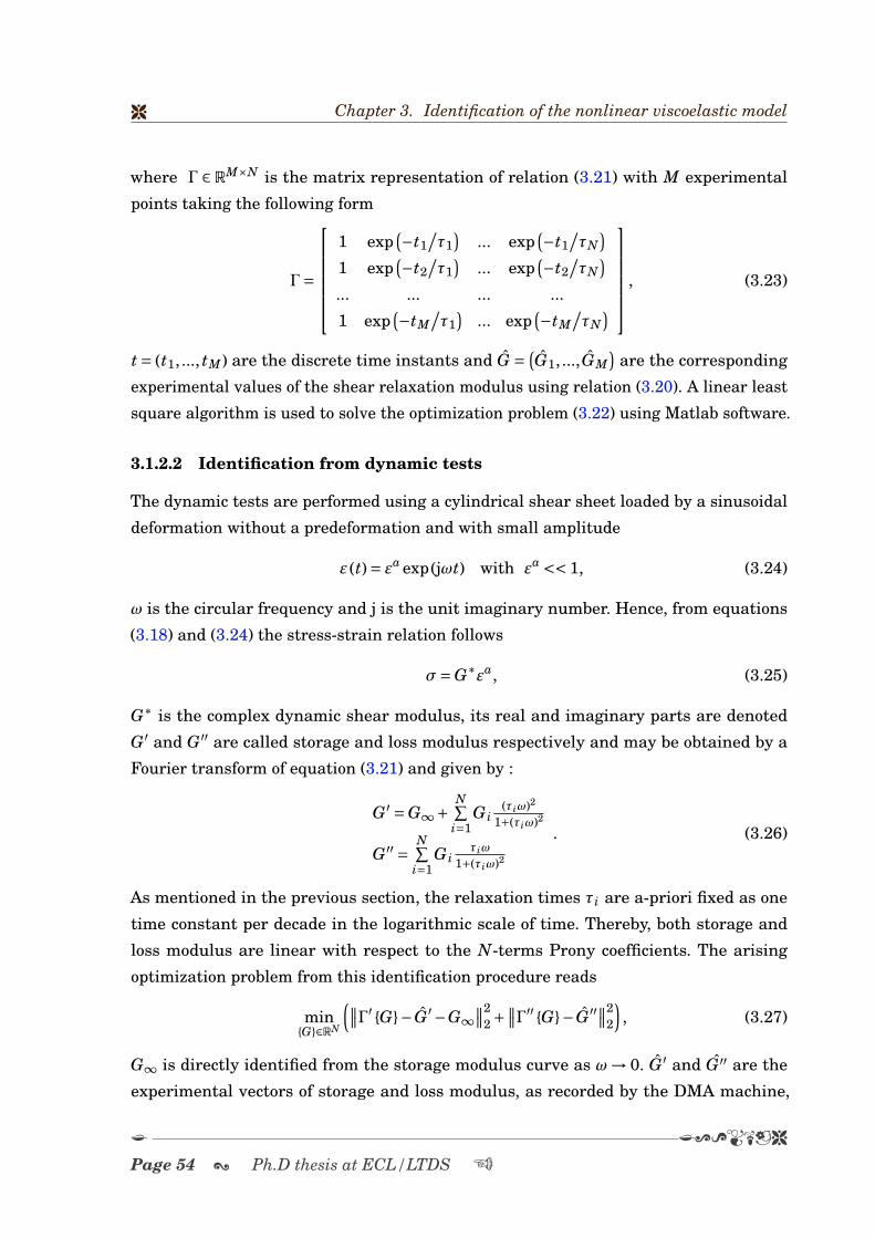
8 Chapter 3. Identification of the nonlinear viscoelastic model
where Γ ∈ RM×N is the matrix representation of relation (3.21) with M experimental
points taking the following form
Γ=
1 exp
(−t1/τ1
)... exp
(−t1/τN
)1 exp
(−t2/τ1
)... exp
(−t2/τN
)... ... ... ...
1 exp(−tM
/τ1
)... exp
(−tM/τN
)
, (3.23)
t = (t1, ..., tM) are the discrete time instants and G = (G1, ...,GM
)are the corresponding
experimental values of the shear relaxation modulus using relation (3.20). A linear least
square algorithm is used to solve the optimization problem (3.22) using Matlab software.
3.1.2.2 Identification from dynamic tests
The dynamic tests are performed using a cylindrical shear sheet loaded by a sinusoidal
deformation without a predeformation and with small amplitude
ε (t)= εa exp(jωt) with εa << 1, (3.24)
ω is the circular frequency and j is the unit imaginary number. Hence, from equations
(3.18) and (3.24) the stress-strain relation follows
σ=G∗εa, (3.25)
G∗ is the complex dynamic shear modulus, its real and imaginary parts are denoted
G′ and G′′ are called storage and loss modulus respectively and may be obtained by a
Fourier transform of equation (3.21) and given by :
G′ =G∞+N∑
i=1G i
(τiω)2
1+(τiω)2
G′′ =N∑
i=1G i
τiω
1+(τiω)2
. (3.26)
As mentioned in the previous section, the relaxation times τi are a-priori fixed as one
time constant per decade in the logarithmic scale of time. Thereby, both storage and
loss modulus are linear with respect to the N-terms Prony coefficients. The arising
optimization problem from this identification procedure reads
minG∈RN
(∥∥Γ′ G− G′−G∞∥∥2
2 +∥∥Γ′′ G− G′′∥∥2
2
), (3.27)
G∞ is directly identified from the storage modulus curve as ω→ 0. G′ and G′′ are the
experimental vectors of storage and loss modulus, as recorded by the DMA machine,
K K;9NAB8
Page 54 ; Ph.D thesis at ECL/LTDS U

3.1. Model identification 8
respectively. Γ′ and Γ′′ are two M by N matrices representing equation (3.26) and can be
expressed through the relaxation time constants and the discrete frequency vector by
Γ′ =
(τ1ω1)2
1+(τ1ω1)2... (τNω1)2
1+(τNω1)2
... ... ...(τ1ωM )2
1+(τ1ωM )2... (τNωM )2
1+(τNωM )2
,Γ′′ =
τ1ω1
1+(τ1ω1)2... τNω1
1+(τNω1)2
... ... ...τ1ωM
1+(τ1ωM )2... τNωM
1+(τNωM )2
. (3.28)
The optimization problem (3.27) is an ill-posed problem [37]. Therefore, a Tikhonov
[102] regularization method was employed to solve this system. The results of this
identification using randomly perturbed simulated and real experimental data are
shown in sections 3.2 and 3.3 of this chapter.
3.1.3 Identification of the reduced time function
Once the hyperelastic potential and the viscoelastic kernel are identified, the problem of
determining the reduced time function can be addressed. This identification relies on the
discretization of the stress-strain relation (2.43) with respect to the time. let t = (t1, ..., tM)be the discrete experimental time vector and ξ= (ξ1, ...,ξM) be the corresponding reduced
time vector, ∆t is the experimental time increment and ∆ξ is the reduced time increment.
The general form of this discretization formula for a nonlinear viscoelastic behavior
as it is described in [63] and [129] is reported in equation (3.29). The identification
of the reduced time vector ξ is performed thanks to a recursive dichotomy algorithm
applied to the error between the discretized stress (3.29) and the experimental stress
σ= (σ1, ..., σM).
σ (tn+1)=σdo (tn+1) −
N∑i=1σd
i (tn+1)+ pI
σdi (tn)= g i
τi
∫ ξ
0F −1ξ
(ξ−ξ′) σd
o(ξ−ξ′) F −t
ξ
(ξ−ξ′)exp
(− ξ
′
τi
)dξ′
σdi (tn+1)=αi g iσ
do (tn+1) +βi g iσ
do (tn) +γiσ
di (tn)
with
γi = exp(−∆ξτi
); αi = 1− τi
∆ξ
(1−γi
); βi = τi
∆ξ
(1−γi
)− γi
σdj (t)= Ft (t+∆t)σd
j (t)F t (t+∆t) ; j = 0,1, ...N.
(3.29)
Once the reduced time vector ξ is obtained the identification of the reduced time function
a(C) can be addressed since it is the inverse of the derivative of the reduced time with
respect to real time:1a= dξ
dt. (3.30)
8CAM:<J J
T Tayeb Adel ; Page 55

8 Chapter 3. Identification of the nonlinear viscoelastic model
The derivative in equation (3.30) is obtained numerically since the reduced time and the
real time are two discrete vectors. Hence, one leads to the numerical vector of function
a(C) : a = (a1, ...,aM). Furthermore, a sufficient condition on this function with respect
to the second principle of thermodynamics in terms of Clausius-Duhem inequality is to
adopt a positive function of the invariants of the right Cauchy-Green strain tensor.
a(C)= f (I1, I2)> 0. (3.31)
3.2 Identification of the model using data from thePipkin isotropic model
In this section, the capacity of the proposed model to depict the response of other
complicated viscoelastic models is presented. The main concern is to reformulate a
complicated model namely the isotropic viscoelastic model by Pipkin [115] in the form
of our simple model presented herein. To this end the identification procedure outlined
above is applied using data generated from the isotropic viscoelastic model proposed
by Pipkin [115] see equations (3.32) and (3.33). Data were generated from the stress-
strain relation in the case of simple extension and pure shear experiments. Several
strain histories were considered to provide a complete description of the behavior. The
hyperelastic potential was identified using data of simple extension and pure shear at
equilibrium, the relaxation function was obtained using a relaxation test performed in
simple extension and the reduced time was calculated using monotonic test in simple
extension for different strain rates. The identification procedure is validated by predicting
the behavior in pure shear monotonic tests for different strain rates.
3.2.1 Pipkin isotropic model
Pipkin [115] proposed a third order development of the tensorial response function Y for
an isotropic incompressible material. The principle of material indifference requires that
the Cauchy stress tensor takes the following form:
σ =RY Rt + pI , (3.32)
R is the rotation tensor obtained from the polar decomposition of the transformation
gradient tensor F and p is the indeterminate parameter due to incompressibility. The
K K;9NAB8
Page 56 ; Ph.D thesis at ECL/LTDS U

3.2. Identification of the model using data from the Pipkin isotropic model 8
third functional development of Y reads
Y (t)=∫ t
0r1
(t− t′
)E
(t′)
dt′+∫ t
0
∫ t
0r2(t− t′, t− t′′)E
(t′)E
(t′′
)dt′ dt′′+∫ t
0
∫ t
0
∫ t
0r3
(t− t′, t− t′′, t− t′′′
)tr
[E
(t′)E
(t′′
)]E
(t′′′
)dt′dt′′dt′′′+∫ t
0
∫ t
0
∫ t
0r4
(t− t′, t− t′′, t− t′′′
)E
(t′)E
(t′′
)E
(t′′′
)dt′dt′′dt′′′,
(3.33)
rk (k = 1..4) are the relaxation kernels expressed by a decaying exponential functions
and E (t) is the time derivative of the Green-Lagrange deformation tensor. Expression of
r i according to [57] is reported in equation (3.34), the choice of r2 (t1, t2)= 0 is motivated
by thermodynamic arguments to ensure the positivity of the free energy density. Further
arguments could be found in [57] and references therein.r1 (t)= a1 +b1 exp(c1 t)r2 (t1, t2)= 0
r3 (t1, t2, t3)= a3 +b3 exp(c3 (t1 + t2 + t3))r4 (t1, t2, t3)= b4 exp(c4 (t1 + t2 + t3)) .
(3.34)
A crucial choice of the parameters ak, bk and ck enables us to describe the behavior of
the material for any given strain history.
3.2.2 Identification results
3.2.2.1 Hyperelastic potential
The identification of the instantaneous elastic stored energy density requires data at
equilibrium in the case of simple extension and pure shear experiments. Hence, data
were generated by omitting the time-dependent part of the stress. Considering the
incompressibility of the behavior of equations (3.2) and (3.3) it is straightforward to
obtain from (3.33) the relations for the equilibrium stress
σ=(λ2 − 1
λ
)[a1
2+ a3
8
(λ4 −2λ2 − 4
λ+ 2λ2 +3
)], (3.35)
in the case of simple extension and
σ=(λ2 − 1
λ2
)[a1
2+ a3
8
(λ4 −2λ2 − 2
λ2 + 1λ4 +2
)], (3.36)
8CAM:<J J
T Tayeb Adel ; Page 57

8 Chapter 3. Identification of the nonlinear viscoelastic model
for the simple shear. Results of the identification using the generalized Mooney-
Rivlin model in terms of the first Piola-Kirchhoff stress are reported in figure 3.1 for
simple extension and pure shear experiments. A second order generalized Mooney-Rivlin
potential, in relation (3.11), was satisfactory to describe the hyperelastic part of the
Pipkin model.
1 1.5 2 2.5 3 3.5 4Principle stretch
0
2
4
6
8
10
12
14
PK1(
MPa
)
Pipkin ModelMooney-Rivlin Model
(a) Equilibrium stress for simple extension
1 1.5 2 2.5 3 3.5 4Principle stretch
0
2
4
6
8
10
12
14
PK1(
MPa
)
Pipkin modelMooney-Rivlin Model
(b) Equilibrium stress for pure shear
Figure 3.1: Equilibrium stresses versus principle stretch for the Pipkin model (diamond)and the Mooney-Rivlin model (solid curve)
K K;9NAB8
Page 58 ; Ph.D thesis at ECL/LTDS U

3.2. Identification of the model using data from the Pipkin isotropic model 8
g i τi(s)6.25 10−2 2.0032.84 10−5 14.061.12 10−4 82.76
Table 3.1: Prony series parameters
3.2.2.2 Viscoelastic kernel
The identification of the Prony series requires shear relaxation data at low level of strain.
To this end, a Heaviside strain history of relation (3.19) is considered. Introduction of
this strain history into (3.32) and (3.33) yields the relaxation stress-strain relationship.
σ (t)= r1 (t)2
(λ2 − 1
λ2
)+
r3 (3t)8
(λ2 − 1
λ2
)(λ4 −2λ2 − 2
λ2 + 1λ4 +2
)+
r4 (3t)8
(λ2 − 1
λ2
)(λ4 −3λ2 − 3
λ2 + 1λ4 +4
).
(3.37)
In figure 3.2 are reported curves of the normalized shear relaxation modulus versus time
for four different levels of strain. It is well shown that the hypothesis of separability
doesn’t hold for the Pipkin model since the normalized shear relaxation modulus depends
upon strain level. But for small value of the strain the normalized shear relaxation mod-
ulus is independent of the strain level. Hence, the identification procedure is performed
using results of the 5% level of strain. Prony series parameters are reported in Table 3.1.
8CAM:<J J
T Tayeb Adel ; Page 59

8 Chapter 3. Identification of the nonlinear viscoelastic model
Time (s)100 101 102
Nor
mal
ized
she
ar m
odul
e
0.4
0.6
0.8
1
1.2 Strain level :5%Strain level: 100%Strain level: 200%Strain level: 300%
Figure 3.2: Normalized shear relaxation modulus of Pipkin model versus time for fourdifferent strain levels.
3.2.2.3 Reduced time function
Principle Stretch1 1.5 2 2.5 3 3.5 4
Cau
chy
Stre
ss(M
Pa)
0
10
20
30
40
50
60Pipkin Model α1Pipkin Model α2
Figure 3.3: Simple extension Cauchy stress versus principle stretch for two differentstrain rates α1 = 1.19 10−2s−1 and α2 = 6 10−3s−1
In this part, monotonic tests of simple extension and pure shear were generated from
the Pipkin model. Simple extension test was used in the identification of the reduced
time function whereas pure shear test was used in the validation of the results. For
computational convenience with respect to the multi-integral form involved in (3.33),
K K;9NAB8
Page 60 ; Ph.D thesis at ECL/LTDS U

3.2. Identification of the model using data from the Pipkin isotropic model 8
the principle stretch corresponding to a monotonic test was set to be an increasing
exponential function of time of the form:
λ (t)= exp(α t) , (3.38)
1 1.5 2 2.5 3 3.5 4
Principal stretch
0.965
0.97
0.975
0.98
0.985
0.99
0.995
1
1.005
Red
uced
tim
e co
effi
ecie
nt
strain rate 1strain rate 2
(a) Reduced time ratio versus principle stretch
1 1.5 2 2.5 3 3.5 4
Principal stretch
0.995
1
1.005
1.01
1.015
1.02
1.025
1.03
1.035
Red
uced
tim
e fu
nctio
n
Strain rate 1Strain rate 2
(b) Reduced time function versus principle stretch
Figure 3.4: Reduced time function and reduced time ratio versus principle stretch fortwo strain rates α1 = 1.19 10−2s−1 and α2 = 6 10−3s−1
8CAM:<J J
T Tayeb Adel ; Page 61

8 Chapter 3. Identification of the nonlinear viscoelastic model
where α is a positive constant that could be interpreted as a strain rate. Replacing the
principle stretch in (3.33) by its expression yields the expression of the Cauchy stress. For
each test, two different strain rates were considered α1 = 1.19 10−2s−1 and α2 = 6 10−3s−1.
Data for simple extension Cauchy stress versus principle stretch are plotted in figure 3.3.
Hence, the identification procedure highlighted above was applied to identify the reduced
time function. Results are reported in figure 3.4 by means of the reduced time ratio ξ (t)/
tand the reduced time function a(C) for the two considered strain rates. The reduced time
function is obtained numerically via a numerical derivation of the reduced time with
respect to time. It shows a significant dependence upon strain level which is consistent
with the results shown in Figure 3.2. Furthermore, this function is independent of the
strain rate which motivate the choice of the form of the reduced time function of equation
(3.31). The capacity of the nonlinear viscoelastic model developed herein is evaluated
by predicting the behavior of the Pipkin model using the parameters identified in this
section. In order to avoid a division by small value of the force when the principle stretch
is near to one, a modified relative error formula was used as proposed in [105]
err i =∣∣σi −σi
P ∣∣max
0.5,σiP
, (3.39)
1 1.5 2 2.5 3 3.5 4
Principal stretch
0
0.005
0.01
0.015
0.02
0.025
Cau
chy
stre
ss r
elat
ive
erro
r
strain rate 1strain rate 2
Figure 3.5: Relative error of the predicted Cauchy stress of the Pipkin model for pureshear experiment
K K;9NAB8
Page 62 ; Ph.D thesis at ECL/LTDS U

3.3. Application of the identification procedure to experimental data 8
1 1.5 2 2.5 3 3.5 4Principle Stretch
0
10
20
30
40
50
60
Cau
chy
Stre
ss(M
Pa)
Pipkin Model 1Identified 1Pipkin Model 2Identified 2
Figure 3.6: Pure shear Cauchy stress for the model (solid curve) and the Pipkin model(diamond and square)
in which σi is the Cauchy stress computed using (2.43) and σiP is the Pipkin Cauchy
stress computed using (3.32) and (3.33). This function is plotted versus the principle
stretch in figure 3.5 in the case of pure shear experiment. For the two strain rates
considered, the relative error remains under 2.5%. In figure 3.6 is plotted the Cauchy
stress versus principle stretch for the Pipkin model and the proposed model.
3.3 Application of the identification procedure toexperimental data
In this section, the identification procedure outlined in section 3.1 is used to identify
the parameters of the proposed model using experimental data for a bromobutyl (BIIR)
rubber material. Experimental data used here are those from [103], in which a complete
experimental characterization was performed to obtain the response of the material for
several strain history configuration and several temperatures. In what follows, results of
the identification of the model’s parameters are highlighted and discussed.
8CAM:<J J
T Tayeb Adel ; Page 63

8 Chapter 3. Identification of the nonlinear viscoelastic model
3.3.1 Hyperelastic potential
Principle stretch1 2 3 4 5 6
PK1(
MPa
)
0
0.2
0.4
0.6
0.8
1
1.2
1.4Experiment BIIRSecond Order Mooney-Rivlin
(a) Equilibrium stress for simple extension
Principle stretch1 1.5 2 2.5 3 3.5 4 4.5 5
PK1(
MPa
)
0.1
0.2
0.3
0.4
0.5
0.6
0.7
0.8
0.9Experiment BIIRSecond Order Mooney-Rivlin
(b) Equilibrium stress for pure shear
Figure 3.7: Equilibrium stresses versus principle stretch: Experimental (diamond) andthe identified Mooney-Rivlin model (solid curve)
K K;9NAB8
Page 64 ; Ph.D thesis at ECL/LTDS U

3.3. Application of the identification procedure to experimental data 8
g i τi(s)4.46 10−3 14.793.77 10−2 125.715.69 10−2 460.75.84 10−2 1761.68.76 10−2 9598.5
Table 3.2: Prony series parameters for BIIR rubber
The identification of the instantaneous elastic stored energy density coefficients of
relation (3.17) is performed under stability conditions of the relation (3.12) using Matlab
software. A second order Mooney-Rivlin potential was able to describe the hyperelastic
behavior of the material for simple extension and pure shear experiments. In figure 3.7
are plotted experimental and identified Piola-Kirchhoff stresses versus principle stretch
at equilibrium for simple extension and pure shear. The relative error of the relation
(3.39) was calculated for both experiments, its average value is 0,5 % for simple extension
and 2,3 % for pure shear which are very satisfactory considering the non-linearity of the
material.
3.3.2 Viscoelastic kernel
The identification of the viscoelastic kernel, as it is described in section 3.1, is performed
using two different experimental data: shear relaxation experiment in the linear range of
the behavior and dynamic tests for low level of dynamic amplitude and without pre-strain.
In what follows, results of this identification procedure are discussed.
3.3.2.1 From shear relaxation experiment
The shear relaxation experiment is performed in simple shear deformation at a strain
level of 10 %. it is considered, however, in the linear range of the behavior since the
material is highly deformable. From figure 2.1 data for shear relaxation experiment
at 10 % are extracted and used in the identification of the Prony series parameters.
These parameters are reported in table 3.2. The average relative error between the
experimental and the identified viscoelastic kernel is in the order of 0.1 %. The identified
and the experimental normalized shear relaxation modulus are plotted versus time in
figure 3.8.
8CAM:<J J
T Tayeb Adel ; Page 65

8 Chapter 3. Identification of the nonlinear viscoelastic model
Time (s)0 2000 4000 6000 8000 10000 12000 14000
Nor
mili
zed
shea
r m
odul
e
0.8
0.85
0.9
0.95ExperimentalIdentified
Figure 3.8: Normalized shear relaxation modulus of BIIR rubber versus time.
3.3.2.2 From dynamic experiments
The dynamic experiments are performed in simple shear deformation with a small
dynamic amplitude and without a pre-strain of the form of equation (3.24). It is recalled
that the problem of the identification of the viscoelastic parameters from dynamic data
(3.27) is an ill-posed problem. Hence, a regularization procedure of Tikhonov is used.
In what follows, this method is recalled and applied to theoretical dynamic data using
parameters from [110] and then applied to dynamic data for BIIR material from [103].
Tikhonov regularization method:
The linear system arising from the identification of the Prony series parameters
from dynamic data is an ill-posed problem [37]. From the original system of equa-
tion (3.27) the following system arise:
Ax = b, (3.40)
in which A is the global matrix of the system to be calculated from (3.28), b is the
vector of experimental storage modulus and loss modulus vectors G′ and G′′ and xis the vector of the Prony series parameters G i, (i = 1..N). Tikhonov regularization
K K;9NAB8
Page 66 ; Ph.D thesis at ECL/LTDS U

3.3. Application of the identification procedure to experimental data 8
method replaces system (3.40) by:
(At A+µI
)x = Atb, (3.41)
in which µ> 0 is the regularization parameter and I is the identity matrix. The
regularization parameter is determined via an L-curve technique using Matlab
software. It is well established that the solution of system (3.41) noted xµ gives the
minimum residual for the minimization problem arising from system (3.40) which
means:
∀x ∈ RN∥∥A xµ−b∥∥2 É ‖A x−b‖2, such that ‖x‖2 É ∥∥xµ
∥∥2.(3.42)
The proof of (3.42) and further development of the convergence of the regularized
Tikhonov problem are well studied in [18].
Application of the Tikhonov method to simulated dynamic data:
The Tikhonov regularization procedure described above was applied to a simulated
dynamic data generated using Prony series parameters from [110] and relations
in (3.26). Moreover, in order to test the ability of the method to deal with noisy
experimental data, the second member of system (3.41) was perturbed randomly
as follow:
b = (1±ε)b, (3.43)
in which ε takes three different values: 10%, 15% and 20%. The Prony series
parameters from [110] are reported in table 3.3 with an equilibrium modulus
G∞ = 2.24 106 Pa. The results of this identification are reported in figure 3.9
in terms of the dynamic moduli versus frequency for the perturbed and original
simulated data. The mean relative error for the three perturbed data remains
under 10% and hence this procedure shows a huge capacity to predict the dynamic
response functions despite the perturbation of the second member of the system
(3.42).
8CAM:<J J
T Tayeb Adel ; Page 67
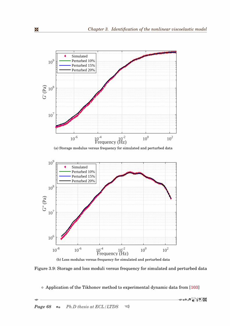
8 Chapter 3. Identification of the nonlinear viscoelastic model
Frequency (Hz)10-6 10-4 10-2 100 102
G' (
Pa)
107
108
109Simulated Perturbed 10%Perturbed 15%Perturbed 20%
(a) Storage modulus versus frequency for simulated and perturbed data
Frequency (Hz)10-8 10-6 10-4 10-2 100 102
G"
(Pa)
106
107
108
109
Simulated Perturbed 10%Perturbed 15%Perturbed 20%
(b) Loss modulus versus frequency for simulated and perturbed data
Figure 3.9: Storage and loss moduli versus frequency for simulated and perturbed data
Application of the Tikhonov method to experimental dynamic data from [103]
K K;9NAB8
Page 68 ; Ph.D thesis at ECL/LTDS U

3.3. Application of the identification procedure to experimental data 8
G i(Pa) τi(s)1.94 108 2 10−2
2.83 108 2 10−1
5.54 108 2 100
6.02 108 2 101
3.88 108 2 102
1.56 108 2 103
4.1 107 2 104
1.38 107 2 105
3.68 106 2 106
7.9 105 2 107
9.6 105 2 108
Table 3.3: Prony series parameters from [110]
G i(Pa) τi(s)3.13 108 7.1 10−8
2.61 107 1 10−6
9.86 106 1.4 10−5
1.94 106 1.98 10−4
9.42 105 2.8 10−3
3.03 105 3.92 10−2
1.4 105 5.52 10−1
8.53 104 7.77 100
8.45 104 1.09 102
7.72 104 1.53 103
7.71 104 2.16 104
2.06 104 3.05 105
Table 3.4: Prony series parameters from experimental dynamic data
The dynamic experiment are represented by the storage and loss moduli G′
and G′′ as functions of the frequency for the experimental frequency window
of [10−5, 107 Hz]. The tikhonov regularization is applied and a regularization
parameter µ is obtained for a 12 parameters Prony series reported in table 3.4. The
mean relative error is about 20%.
8CAM:<J J
T Tayeb Adel ; Page 69

8 Chapter 3. Identification of the nonlinear viscoelastic model
Frequency (Hz)100 105
G' (
Pa)
105
106
107
108
109
Experimentalmu = 2.229mu = 4.458mu = 6.687
(a) Storage modulus versus frequency for dynamic experimental data
Frequency (Hz)100 105
G"
(Pa)
104
105
106
107
108
109
Experimentalmu = 2.229mu = 4.458mu = 6.687
(b) Loss modulus versus frequency for dynamic experimental data
Figure 3.10: Storage and loss moduli versus frequency for dynamic experimental datafor different values of the regularization parameter µ
K K;9NAB8
Page 70 ; Ph.D thesis at ECL/LTDS U

3.3. Application of the identification procedure to experimental data 8
3.3.3 Reduced time function
The reduced time is identified using the discretization formula (3.29) and monotonic
experiments of simple extension for two strain rates: 100% s−1 and 200% s−1. Cauchy
stress versus principle stretch are plotted in figure 3.11. Results of the identification
are reported in figure 3.12 in terms of the reduced time coefficient which is a nonlinear
function of time for the strain rates considered. The pure shear experiment was predicted
using the reduced time, the predicted and experimental data for this experiment are
plotted in figure 3.13 against the principle stretch. From this result the relative error
of the Cauchy stress is calculated using relation (3.39), its mean value remains under
2.5%. Hence, the proposed model is suitable to describe the material’s behavior at low
and moderate strains.
1 2 3 4 5 6Principle stretch
0
2
4
6
8
10
12
Cau
chy
Stre
ss (
MPa
)
Experiment 200% s-1
Experiment 100% s-1
Figure 3.11: Cauchy stress versus principle stretch for simple extension experiment
8CAM:<J J
T Tayeb Adel ; Page 71

8 Chapter 3. Identification of the nonlinear viscoelastic model
1 2 3 4 5 6
Principal stretch
0.85
0.9
0.95
1
1.05
1.1
1.15
1.2
1.25R
educ
ed ti
me
coef
fiec
ient
strain rate=100% s-1
strain rate=200% s-1
Figure 3.12: Reduced time coefficient for two strain rates 100% s−1 and 200% s−1
1 1.1 1.2 1.3 1.4 1.5
Principle stretch
0
0.05
0.1
0.15
0.2
0.25
0.3
0.35
0.4
Cau
chy
Stre
ss (
MPa
)
Experiment 5% s-1
Model
Figure 3.13: Cauchy stress versus principle stretch for pure shear experiment: experi-mental (diamond) model (solid curve)
K K;9NAB8
Page 72 ; Ph.D thesis at ECL/LTDS U

3.4. Conclusion 8
3.4 Conclusion
Within this chapter, the identification of several functions involved in the model pre-
sented in the second chapter of this Thesis was addressed. Each function’s identification
procedure turns out to the resolution of a linear or nonlinear system. Moreover, a regu-
larization procedure of Tikhonov was applied in the resolution of the ill-posed problem
arising from the identification of the viscoelastic kernel from dynamic data.
This identification procedure was applied to a generated data from a multi-integral
viscoelastic model and a static and dynamic experimental characterization of a BIIR
rubber. The results of the identification has shown a huge capacity of the model to
describe the multi-integral viscoelastic model in the time domain of the behavior within
and outside the range of strain rates considered in deriving the model. The results from
the experimental characterization has shown a huge capacity to depict the behavior of
the material in the time domain for the equilibrium and instantaneous responses.
Our main object was to develop a constitutive equation compatible with the second law
of thermodynamics and suitable with the Finite-elements theory. The implementation of
the model within Abaqus software is the goal of the next chapter.
8CAM:<J J
T Tayeb Adel ; Page 73


CH
AP
TE
R
4NUMERICAL IMPLEMENTATION AND INTEGRATION
SCHEME
Contents4.1 Integration scheme for one dimensional viscoelastic model . . . . . . . . 76
4.1.1 Integration scheme . . . . . . . . . . . . . . . . . . . . . . . . . . . 77
4.1.2 Validation of the integration scheme . . . . . . . . . . . . . . . . 78
4.2 Implementation of the nonlinear viscoelastic model . . . . . . . . . . . . 78
4.2.1 Finite element method for nonlinear viscoelastic solids . . . . . 79
4.2.2 Discrete representation of the constitutive equations . . . . . . 83
4.3 Conclusions . . . . . . . . . . . . . . . . . . . . . . . . . . . . . . . . . . . . 88
IN general, the response of a viscoelastic material depends on the excitation
history. For an integral based formulation viscoelasticity, the entire excita-
tion history must be stored in order to evaluate the response numerically.
Therefore, the memory storage increases in time. The storage problem can be avoided
by representing the kernel function as a Prony series. Thanks to the semigroup prop-
erty of the exponential function, the use of Prony series in the kernel function leads
to an efficient recursive relation [129]. The incremental representation of the kernel
function is combined with an incremental form of the excitation history which describes
75

8 Chapter 4. Numerical implementation and integration scheme
the evolution of the excitation history inside the time increment. Several form have
been proposed in the literature, which goes from constant proposed by [150], piecewise
constant proposed by [61], linear suggested by [137] to exponential form proposed by [1].
These forms have been successfully used in the implementation of the Schapery model by
[6], [60] and [53] among others, for the Duvaut-Lions viscoplasticity model in [130] and
in finite strain viscoelasticity by [68]. For further details about the integration schemes
in viscoelasticity, the reader is directed to the work of [132] and [42].
On the other hand, in addition to the integration scheme of the kernel function, one needs
to derive the discrete form of the constitutive equation based on the decomposition of the
deformation gradient tensor into volumetric and isochoric parts. To this end, following
the formulation of the model, the Cauchy stress tensor is decomposed into an instanta-
neous hyperelastic and viscoelastic over-stress parts. The discrete representation of each
part of the stress tensor is calculated separately.
The aim of this chapter is to presents the numerical implementation of the nonlinear
viscoelastic model developed in the previous chapters. First, the integration scheme of
the one dimensional viscoelastic model is recalled. In fact, the integration scheme for
the one dimensional viscoelastic model was implemented using Matlab software and
validated through the comparison with numerical simulations performed with Abaqus
software for simple extension with several strain histories. Then, the implementation
of the three dimensional viscoelastic model into Abaqus software is performed using
an implicit integration scheme in a Umat subroutine. To this end, the discrete form of
the nonlinear viscoelatic model was performed following [63] using the objective rate
derivative of Jaumann. Finally the fourth order tangent stiffness needed in the coding of
the subroutine Umat is calculated accordingly.
4.1 Integration scheme for one dimensionalviscoelastic model
In this section, we present the integration scheme of the Simo [131] model implemented
in Abaqus software. The constitutive equation for a one dimensional experiment will be
implemented in a Matlab code then compared to the numerical simulation performed
with Abaqus software. Our starting point is the one dimensional model presented in 2.2
by the constitutive equation of the stress which reads in the absence of the reduced time
K K;9NAB8
Page 76 ; Ph.D thesis at ECL/LTDS U

4.1. Integration scheme for one dimensional viscoelastic model 8
ξ i.e. ξ(t)= t as follow
σ (t)=∫ t
0G
(t− t′
)ε(t′)dt′. (4.1)
4.1.1 Integration scheme
The integration scheme of the constitutive equation of the stress is performed in a discrete
manner. Hence, let [0, t], t > 0 be the time interval of interest. It will be decomposed into
sub-intervals as follows:
[0, t]=⋃n
[tn, tn+1], tn+1 = tn +∆tn. (4.2)
Without loss of generality, the time intervals ∆tn are assumed to be equals. Since the
model considered is a deformation driven model, the total deformation ε applied in the
time interval [0, t] is also subdivided into equal deformation increments ∆ε following
(4.2). Hence, the convolution integral in (2.8) does not need to be totally evaluated and it
is split into an integral over [0, tn] and an integral over the last time increment [tn, tn+1]
through the following recursive update formula
σ (tn+1)=G∞ε (tn+1)+∑
i
[G i exp
(−∆tτi
)∫ tn
0exp
(− tn − t′
τi
)ε(t′)dt′+G iτi
(1−exp
(−∆tτi
))∆ε
∆t
]=G∞ε (tn+1)+
∑i
[hi (tn+1)+G i pi∆ε],
with pi = τi
∆t
(1−exp
(−∆tτi
)),
(4.3)
where hi are the algorithmic stresses expressed by :
hi (t)=G i
∫ t
0exp
(− t− t′
τi
)ε(t′)dt′. (4.4)
The whole procedure is summarized in the following algorithm: Note that the update
Algorithm 1 Recursive update procedure1: Database σ(tn),hi(tn), i = 1..N at time tn2: Give the strain increment ∆ε3: Calculate the elastic stress σe(tn+1)=G∞ε(tn+1)4: Update the algorithmic stresses hi(tn+1)= exp
(−∆tτi
)hi (tn)+G i exp
(− ∆t
2τi
)∆ε
5: Compute the total stress using (4.3)
formula of the algorithmic stresses hi expressed in the previous algorithm is not unique
and alternative formulas could be found in [129]. With equations (4.3) and (4.4) and the
update procedure described above, we have all the quantities needed for the implemen-
tation of the one dimensional viscoelastic model which will be performed with Matlab
software.
8CAM:<J J
T Tayeb Adel ; Page 77

8 Chapter 4. Numerical implementation and integration scheme
4.1.2 Validation of the integration scheme
The validation of the integration scheme described in the previous section is performed
using three strain histories, for each case the total stress σ obtained from the discrete
scheme of equation (4.3) is compared to the stress obtained from the Abaqus simulation.
The Abaqus model consists of a single brick element undergoing simple extension strain.
The three strain histories considered here are defined by the following
ε (t)= εot, (4.5)
for monotonic strain history, where εo is a positive constant denoting the strain rate and
ε (t)=
0 for t < 0
εo for t ≥ 0, (4.6)
for the relaxation strain history, where εo is the relaxation level and
ε (t)= εA sin(wt) , (4.7)
for a sinusoidal strain history in which εA is the amplitude of the strain and w is its
frequency. Note that the form of the strain history of equation (4.6) can not be applied
neither experimentally nor numerically, hence a very fast ramp is applied to shift the
strain from 0 to εo. The results of the comparison between the discrete stress of equation
(4.3) and the one obtained from the Abaqus simulation are reported in figures 4.1, 4.2
and 4.3 in terms of the total stress versus time for monotonic, relaxation and sinusoidal
strain histories respectively. The material parameters used in this calculus are those
from [110]. From these results, it is concluded that the recurrence update formula of (4.3)
gives the same result as the viscoelastic model implemented in Abaqus software. This
result establish a big step to the implementation of the three dimensional viscoelastic
model since it has the same integration scheme as the Simo’s model [131] implemented
in Abaqus software. The implementation of the nonlinear viscoelastic model presented
in 2 will be presented in the next section of this chapter.
4.2 Implementation of the nonlinear viscoelasticmodel
In this section we address the implementation of the nonlinear viscoelastic model pre-
sented in chapter 2. To this end, we start by recalling the formulation of initial boundary
K K;9NAB8
Page 78 ; Ph.D thesis at ECL/LTDS U

4.2. Implementation of the nonlinear viscoelastic model 8
0 5 10 15 20
Temps (s)
0
1
2
3
4
5
6Discretized stressAbaqus stress
Figure 4.1: Stress versus time for a monotonic strain history
problems for a nonlinear viscoelastic solid. Then, we present the discrete form of the
constitutive equations of the model as well as the approximation of the tangent modulus
needed in the Umat subroutine.
4.2.1 Finite element method for nonlinear viscoelastic solids
Consider a continuum viscoelastic body occupying the reference placement Ω0 in the
reference configuration C0. It occupies at the time t the placement Ω in the deformed
configuration Ct. Let ϕ(X , t) denote a macroscopic motion between the two configurations,
which maps any point X in the reference configuration C0 to the point x in the deformed
configuration characterized by its displacement vector field noted u pointing from the
reference configuration to the current configuration. The typical use of the finite element
method is to resolve initial boundary value problem. In the absence of body forces, the
momentum equation is expressed, in the current configuration, as :
div (σ)= ρu, (4.8)
where ρ is density and div is the divergence operator with respect to the current
configuration. In the following we consider boundary and initial conditions for the motion
8CAM:<J J
T Tayeb Adel ; Page 79

8 Chapter 4. Numerical implementation and integration scheme
0 20 40 60 80 100
Temps (s)
20
40
60
80
100
120
Discretized stressAbaqus stress
Figure 4.2: Stress versus time for relaxation strain history
x =ϕ(X , t) required to satisfy the momentum equation (4.8). we assume afterwards that
the boundary surface ∂Ω of the continuum occupying Ω is decomposed into disjoint parts
so that
∂Ω= ∂uΩ∪∂FΩ with ∂uΩ∪∂FΩ =;. (4.9)
Figure 4.4 illustrates the decomposition of the boundary surface ∂Ω at the time t. There
are two classes of boundary conditions, namely the Dirichlet boundary conditions,which corresponds to the definition of a displacement field u= u(x, t) in the displacement
boundary surface ∂uΩ, and the Nuemann boundary conditions, which are identified
with σ.n = F (x, t) in the force boundary surface ∂FΩ. The second order differential
equations of (4.9) require additional data to be resolved in the form of initial conditions.
The displacement field u and the velocity field u at the initial time t = 0 are specified as
u (x, t)=u0 (X ) |t=0 , u (x, t)= u0 (X ) |t=0 (4.10)
In order to achieve the compatibility of the boundary conditions, the initial conditions of
equation (4.10) are also applied to the prescribed displacement field in the displacement
boundary surface ∂Ω. Hence, the problem now is to find a motion that satisfies equation
(4.8) with the prescribed initial and boundary conditions of equations (4.9) and (4.10).
K K;9NAB8
Page 80 ; Ph.D thesis at ECL/LTDS U

4.2. Implementation of the nonlinear viscoelastic model 8
0 1 2 3 4 5
Time (s)
-6
-4
-2
0
2
4
6 Discretized stressAbaqus stress
Figure 4.3: Stress versus time for a sinusoidal strain history
Figure 4.4: Initial boundary value problem considered
8CAM:<J J
T Tayeb Adel ; Page 81

8 Chapter 4. Numerical implementation and integration scheme
This leads to the formulation in the strong form of the initial boundary value problem:
find a displacement field u such that
div (σ)= ρu,
u= u on ∂uΩ,
σ.n=F on ∂FΩ,
u (x, t)=u0 (X ) |t=0 ,
u (x, t)= u0 (X ) |t=0,
(4.11)
where n is the unit exterior normal vector to the force boundary surface ∂FΩ. The
analytic solution of the nonlinear system of the initial boundary value problem of
equation (4.11) is only possible for some special cases. Therefore, solutions are often
obtained using the finite element method which is based on the variational formulation
of (4.11). The variational formulation of the initial boundary value problem reads∫Ω
div (σ)δudΩ−∫Ωρu.δudΩ= 0, (4.12)
where δu is a virtual displacement field which has to verify the initial and boundary
conditions. In practice, this virtual displacement field is set to be the displacement field u
since verifies all the required conditions for the virtual displacement field δu. Application
of the Divergence formula to the first integral in (4.12) yields the following form of the
variational formulation of the initial boundary value problem,∫Ωσ : grad (δu)dΩ−
∫Ωρu.δudΩ−
∫∂FΩ
F .δud∂FΩ= 0. (4.13)
The variational formulation of equation (4.13) is also known as the weak formulation of
the initial boundary value problem (4.11). The domain Ω will be subdivided into several
elements Ωe, the displacement field for any point M of the element Ωe is denoted by ue
and given by
ue(M)=NUe, (4.14)
in which N are the shape function of the element Ωe and Ue is its nodal displacement
vector. The internal force vector associated with the element Ωe, f inte according to [129]
is given by
f inte (t)=
∫Ωe
B teσ (t)dV
=∫2
[B t
eσ (t)]φe j (ξ)dξ
∼=nGauss∑
l=1B t
e (xl)σl (t)Wl jl ,
(4.15)
K K;9NAB8
Page 82 ; Ph.D thesis at ECL/LTDS U

4.2. Implementation of the nonlinear viscoelastic model 8
where φe : 2 → Ωe is the standard isoprametric map with Jacobian determinant
j = det[Dφe], Be is the discrete strain-displacement operator and Wl are the quadrature
weights corresponding to the quadrature point xl . In (4.15) the subscript l denotes
evaluation at the quadrature point xl ∈ Ωe with l = 1,2, · · · ,nGauss. This notation is
standard; see [75] and [149] for further development. From (4.15) it is concluded that the
evaluation of the internal force vector f inte (t) requires knowledge of the stress history
at the quadrature point σl(t) for the time interval considered assuming knowledge
of the strain at any given time in the time interval considered. Therefore, a discrete
representation of the convolution representation of the stress of equation (2.43) is
required to complete the resolution of the initial boundary value problem of equation
(4.11). Since our model is not existing in any finite element software, it should be
implemented into a finite element software (e.g. Abaqus) via a user defined subroutine.
The implementation procedure of the model will be presented in the remaining of this
chapter.
4.2.2 Discrete representation of the constitutive equations
In this section, the implementation of the nonlinear viscoelastic model at finite strain
into Abaqus software is presented via a user defined Umat subroutine. First, the discrete
representation of the model is presented in terms of the expression of the update formula
of the Cauchy stress (4.11). Then, the fourth order tangent stiffness tensor needed in the
writing of the Umat is calculated using the Jaumann objective derivative. Finally, the
use of the user defined Umat subroutine is explained.
4.2.2.1 Discrete stress-strain relationship
To investigate the performance of the proposed model in [136] and presented in chapter
2 of this thesis for boundary value problems, it is needful to implement the constitutive
equations into a finite element software e.g. Abaqus through a user-defined umat sub-
routine, which requires an update formulas for the Cauchy stress σ and the tangent
modulus C. Before we start with the formulation of the discrete form of the constitutive
equation of the model, it is necessary to point out that this implementation procedure
is done with a compressible viscoelastic model even thought the model proposed in this
thesis is an incompressible viscoelastic model. In fact, Abaqus software gives the possi-
bility to do so in the writing of the user defined Umat subroutine. According to [62], to
avoid the penalty formulation due to the incompressibility [64], it is sufficient to consider
8CAM:<J J
T Tayeb Adel ; Page 83

8 Chapter 4. Numerical implementation and integration scheme
a bulk modulus about 104 −106 times the shear modulus and use hybrid elements in
the mesh module of Abaqus see [63] for further details. First, for numerical reasons
[129] with respect to the implementation procedure, it is more convenient to consider
the constitutive equation of the stress of equation (2.43) in terms of the Kirchhoff stress
tensor τ = Jσ namely
τ = τ do +dev
∫ ξ
0
∂g(ξ′
)∂ξ′
(F −1
t(t− t′
)τ d
o(t− t′
)F −t
t(t− t′
))dξ′+ J pI . (4.16)
To present the discrete representation of the constitutive model of equations (2.43),
different functions of the model need to be defined. We start with the definition of the
reduced time function a(C). Motivated by the form proposed in [113] to describe the
behavior of ligaments, a more general form for the reduced time function is postulated
as follows:
a (C)= exp(c1 (I1 −3)+ c2 (I2 −3)) , (4.17)
where c1 and c2 are material parameters. Also, as it is explained in the formulation of the
model, the instantaneous stored elastic energy density Ψ is decomposed into volumetric
and isochoric parts
Ψ=Ψiso (B
)+Ψvol (J) , (4.18)
The superscript •iso and •vol denote the isochoric and volumetric parts of the instanta-
neous stored elastic energy density respectively. Ft(t′)= J−1/3∂ϕ
(X , t′
)/∂ϕ (X , t) is the
relative distortional deformation gradient tensor for the mapping function ϕ (X , t), gis the normalized shear relaxation modulus and it is expressed by a sum of decaying
exponential functions of time as
g (t)= g∞+∑r
gr exp(− tτr
), (4.19)
gr and τr are the coefficients of the Prony series and relaxation times respectively, g∞ is
the equilibrium normalized shear modulus. p = ∂Ψiso (J)/∂J is the hydrostatic part of
the stress which could be determined in the case of incompressibile behavior through
boundary conditions. In equation (4.16), τ do is the deviatoric part of the instantaneous
elastic Kirchhoff tensor which is expressed from the instantaneous stored elastic energy
density Ψ by
τo = 2B∂Ψ (B)∂B
. (4.20)
K K;9NAB8
Page 84 ; Ph.D thesis at ECL/LTDS U

4.2. Implementation of the nonlinear viscoelastic model 8
Using equation (4.20), the instantaneous elastic Kirchhoff stress τo is decomposed as
well into isochoric and volumetric parts
τo = τ ho (J)+τ d
o(B
), (4.21a)
τ ho (J)= 2JB
∂Ψvol (J)∂B
, (4.21b)
τ do
(B
)= 2B∂Ψiso (
B)
∂B. (4.21c)
From equation (4.21b) with ∂J/∂B = 0.5JB−1 it follows
τ ho (J)= J
∂Ψiso (J)∂J
I , (4.22)
and from equation (4.21c) and
∂B
∂B= J−2/3
(I− 1
3B⊗B−1
), (4.23)
in which I denotes the fourth order identity tensor defined by
Ii jkl =12
(δikδ jl +δilδ jk), (4.24)
and ⊗ designates the tensorial product operator, it follows
τ do
(B
)=P : τ . (4.25)
P is the fourth order projection tensor and τ is an algorithmic Kirchhoff stress tensor
derived from Ψiso(B) with respect to B. With all needed quantities been defined, we
shall now address the discretization of the constitutive equation of the Kirchhoff stress
tensor of equation (4.16) and the reduced time of equation (4.17). Let [0, t] be the time
interval of interest, this interval is subdivided into n increments as follows
[0, t]=⋃n
[tn, tn+1], tn+1 = tn +∆tn. (4.26)
The reduced time increment ∆ξn is related to the real time increment ∆tn defined in
equation (4.26) and may be expressed as follows
∆ξn = ∆tn
a(C). (4.27)
Since the implementation is performed in Abaqus software, the discrete form of equation
(4.16) is obtained in the same way as in [63] taking into account that all quantities are
8CAM:<J J
T Tayeb Adel ; Page 85

8 Chapter 4. Numerical implementation and integration scheme
known at tn and all strain quantities are known at tn+1. This discrete form reads
τ (tn+1)= τ do (tn+1) −
r∑i=1τ d
i (tn+1)+τ ho (tn+1)
τ di (tn)= g i
τi
∫ ξ
0F −1
t(t− t′
)τ d
o(t− t′
)F −t
t(t− t′
)exp
(− ξ
′
τi
)dξ′
τ di (tn+1)=αi g iτ
do (tn+1) +βi g iτ
do (tn) +γiτ
di (tn)
with
γi = exp(−∆ξn
τi
); αi = 1− τi
∆ξn
(1−γi
); βi = τi
∆ξn
(1−γi
)− γi
τ dj (t)= Ft (t+∆tn)τ d
j (t)Ftt (t+∆tn) ; j = 0,1, ...r.
(4.28)
In equation (4.28) r is the number of Prony series coefficients.
4.2.2.2 Tangent stiffness
In this section we specify the formula for the tangent modulus C required in the imple-
mentation of the model. To this end, it is essential to derive the stress rate quantities
that are objective. First, we start with the so-called Oldroyd stress rate (see [94]) of the
elastic part of the model and get,
Lvτo = τo −Lτo −τoLt = 4B
∂2Ψ (B)∂B2 B :D :=Ce :D, (4.29)
in which L is the velocity gradient tensor, D = 0.5(L+Lt) is the rate of deformation
tensor and Ce is the elastic tangent modulus. This tangent modulus is decomposed into
isochoric and volumetric parts as well
Ce =Cevol(J)+Ce
iso(B). (4.30)
Using equations (4.21b) and (4.21c) the isochoric and volumetric parts of the elastic
tangent modulus follow
Cevol(J)= 4B
∂2Ψvol (J)∂B2 B = (
∂2Ψvol (J)∂J2 + J
∂Ψvol (J)∂J
)I ⊗I −2J∂Ψvol (J)
∂JI, (4.31)
for the volumetric part and
Ceiso(B)= 4B
∂2Ψiso (B
)∂B2 B = 2
3tr (τ )P− 2
3
(τ d
o ⊗I +I ⊗τ do
)+P : C :P, (4.32)
for the isochoric part. In equation (4.32), tr(•) denotes the trace operator and C is an
algorithmic tangent modulus following from τ and has the following expression:
C= 4B∂2Ψiso (
B)
∂B2B. (4.33)
K K;9NAB8
Page 86 ; Ph.D thesis at ECL/LTDS U

4.2. Implementation of the nonlinear viscoelastic model 8
The viscoelastic isochoric and volumetric moduli, according to [63], could be easily
obtained from the elastic moduli through the following relations :
Cv =Cvvol(J)+Cv
iso(B), (4.34a)
Cvvol(J)=Ce
vol(J), (4.34b)
Cviso(B)=
(1−
r∑i=1
αi g i
)Ce
iso(B), (4.34c)
equation (4.34b) follows from the fact that the behavior is considered purely elastic in
bulk. αi are the functions deriving from the discrete form of the stress of equation (4.28)
and g i are the coefficients of the Prony series. Note that the viscoelastic tangent modulus
Cv was derived using Oldroyd objective derivative of equation (4.29) . Hence, to obtain
the Jaumann derivative used in Abaqus software we used the following transformation
(see [133])
CJabcd =Cv
abcd +12
(δacτbd +τacδbd +δadτbc +τadδbc) , (4.35)
the superscript •J refers to Jaumann and δ denotes the Kronecker symbol referring to
the second order identity tensor I. Finally, the tangent modulus to be implemented in
the umat subroutine reads
CAbaqus = 1JCJ . (4.36)
Equations (4.28) and (4.36) with σ = 1Jτ describe the implementation of the nonlinear
viscoelastic model for a compressible material. In order to investigate incompressible
material’s behavior using this model, it is sufficient to consider a bulk modulus about
104to 106 times the shear modulus with hybrid element, see [62] for details. In this case,
p in equations (4.16) became an indeterminate pressure to be obtained from boundary
conditions. Henceforth, the behavior is considered incompressible.
4.2.2.3 Flowchart of the Umat subroutine
In figure 4.5, the interaction of the subroutine UMAT with the Abaqus package is
illustrated for the Newton-Raphson iterative procedure during a single time increment
[62]. The subroutine Umat calculates the components of Cauchy stress and material
Jacobian for each Gauss integration point. These quantities are subsequently used by
Abaqus to form up the element stiffness matrix. Finally, the global stiffness matrix is
assembled by Abaqus using the element stiffness matrices. The user subroutines used
in other FE packages to define custom constitutive equations are integrated with the
remainder of the program in a similar way and play the same role. These two quantities
8CAM:<J J
T Tayeb Adel ; Page 87

8 Chapter 4. Numerical implementation and integration scheme
Figure 4.5: Flowchart for the interaction of Abaqus and Umat
are defined in the subroutine Umat by STRESS which is a 6×1 vector for the Cauchy
stress σ and DDSDDE which is a 6×6 matrix for the tangent stiffness modulus C.
The algorithm of the subroutine Umat is presented by the following algorithm. The
subroutine Umat is coded in Fortran 90 and reported in Appendix A
4.3 Conclusions
In this chapter, we presented the implementation of a nonlinear viscoelastic model at
finite strain previously proposed in [136] into Abaqus software via a user-defined umat
subroutine. The model incorporates a strain dependent relaxation times and based upon
the internal state variables approach and the framework of rational thermodynamics
and experimental arguments. The decomposition of the deformation gradient tensor into
volume-preserving and volumetric parts led to a decomposition in the stress response.
The implementation of the model was carried out in two steps. First, the discrete form of
the instantaneous stress was calculated from the instantaneous stored elastic energy
density. Then, the viscoelastic stress was computed from the instantaneous response
following the discretization scheme of Abaqus software. The tangent stiffness necessary
for the implementation was computed accordingly using the objective rate derivative of
Jaumann.
In the next chapter we present the validation of the implementation procedure outlined
in this chapter through the solution of boundary value problems for homogeneous and
non homogeneous transformations.
K K;9NAB8
Page 88 ; Ph.D thesis at ECL/LTDS U

Algorithm 2 Algorithm of the subroutine Umat1: Calculate Finger tensorBB =FF t
2: Calculate the JacobianJ = det[B]0.5 = det[F ]
3: Calculate the deviatoric part ofBB = J
−23 B
4: Calculate tr[B]5: Calculate ττ = 2B ∂Ψ
(B
)∂B
6: Establish unit tensor δi j and fourth order projection tensorPi jkl = 1
2(δikδ jl +δilδ jk
)− 13δi jδkl
7: Compute tr[τ ]8: Calculate isochric contribution τ d
oτ d
o i j = τi j − 13 τkkδi j
9: Calculate volumetric contribution τ ho
τ ho (J)= 2JB ∂Ψvol (J)
∂B10: Calculate C
C= 4B ∂2Ψiso(B
)∂B2 B
11: Calculate isochoric contribution Ceiso
Ceiso(B)= 4B ∂2Ψiso(
B)
∂B2 B = 23 tr (τ )P− 2
3
(τ d
o ⊗I +I ⊗τ do
)+P : C :P
12: Calculate volumetric contribution Cevol
Cevol (J)= 4B ∂2Ψvol (J)
∂B2 B = ( ∂2Ψvol (J)∂J2 + J ∂Ψvol (J)
∂J )I ⊗I −2J ∂Ψvol (J)∂J I
13: Compose elastic tangent stiffness modulus Ce
Ce =Cevol (J)+Ce
iso(B)14: Calculate Cv
iso
Cviso(B)=
(1−
r∑i=1
αi g i
)Ce
iso(B)
15: Compose the viscoelastic tangent stiffness modulus Cv
Cv =Cvvol (J)+Cv
iso(B)16: Calculate the Jaumann stiffness modulus CJ and the total stiffness modulus CAbaqus
CJabcd =Cv
abcd + 12
(δacτbd +τacδbd +δadτbc +τadδbc
)and CAbaqus = 1
JCJ
17: Calculate the total Kirchhoff stress τ from (4.28)18: Calculate the Cauchy stress from the Kirchhoff stress σ = 1
J τ


CH
AP
TE
R
5VALIDATION OF THE IMPLEMENTATION PROCEDURE
WITH HOMOGENEOUS AND NON HOMOGENEOUS
TRANSFORMATIONS
Contents5.1 Specification of the parameters of the model . . . . . . . . . . . . . . . . . 92
5.2 Homogeneous transformations . . . . . . . . . . . . . . . . . . . . . . . . . 94
5.2.1 Simple extension . . . . . . . . . . . . . . . . . . . . . . . . . . . . 94
5.2.2 Simple shear . . . . . . . . . . . . . . . . . . . . . . . . . . . . . . . 101
5.3 Nonhomogeneous transformation: Simple torsion of hollow cylinder . . 108
5.4 Conclusions . . . . . . . . . . . . . . . . . . . . . . . . . . . . . . . . . . . . 114
THis chapter presents the validation of the implementation of the nonlinear
viscoelastic model presented in the previous chapter via the solution of
homogeneous and nonhomogeneous initial boundary problems numerically
and analytically.
In the literature, several works have been dedicated to the resolution of boundary value
problems for nonlinear elastic solids such as the series of papers by Horgan and Sac-
comandi for simple torsion in [70], pure axial shear in [69], pure azimuthal shear in
[71] and helical shear in [72]. For nonlinear viscoelastic materials this subject has been
91

8Chapter 5. Validation of the implementation procedure with homogeneous and non
homogeneous transformations
addressed in many works as well, namely the work of Lee and Wineman for the response
of elastomeric bushings in [85] and [84] and the response of viscoelastic cylinder to
simple torsion due to [5] and [22].
On the other hand, from a numerical stand point, the definition of the boundary con-
ditions leading to the studied transformation presents a real challenge [32] because
an equivalence between the boundary conditions prescribed and the resulting transfor-
mation should be ensured. In fact, for a displacement driven study, such as the work
presented in this chapter and having the purpose of comparison between analytic and
numerical solutions, one needs to carefully define the boundary conditions prescribed in
order to obtain the desired transformation.
This chapter is subdivided to three parts. First, the parameters of the instantaneous
stored elastic energy density, the relaxation function and the reduced time function
involved in the model are specified. Then the validation of the implemented model is
addressed via the solution of two boundary value problems for homogeneous transforma-
tions which are the simple extension and the simple shear. The equilibrium equations
arising from these two transformations allows us to eliminate the indeterminate hy-
draustatic pressure p accounting for incompressibility. Finally, the problem of simple
torsion of hollow cylinder was addressed. Thanks to the axisymmetry of the problem, all
the stress components were functions of the radius r only.
5.1 Specification of the parameters of the model
The validation of the implementation procedure presented in the previous chapter is
presented in this chapter via the comparison between analytic results and numerical
results using the implemented model. To this end, we specify every characteristic function
and parameter used in the model. We start by the instantaneous stored elastic energy
density which is expressed following the decomposition of the deformation gradient tensor
into isochoric and deviatoric parts of equation (2.35) by a Mooney-Rivlin development
[123] asΨ (B)=c10
(I1 −3
)+ c20(I1 −3
)2 + c11(I1 −3
)(I2 −3
)+ c01
(I2 −3
)+ c02(I2 −3
)2 + 1D1
(J−1)2 .(5.1)
In which I1 and I2 are the first two invariants of the deviatoric Finger tensor B and
ci j, i, j = 0..2 and D1 are material parameters of the Mooney-Rivlin instantaneous elastic
stored energy density. Numerical value of these parameters of equation as well as those
K K;9NAB8
Page 92 ; Ph.D thesis at ECL/LTDS U

5.1. Specification of the parameters of the model 8
of the reduced time function of equation (4.17) are reported in table 5.1. The viscoelastic
parameters of the Prony series expansion of equation (4.19) are reported in table 5.2.
The initial bulk modulus is given by
k0 = 2D1
= 2.105 MPa, (5.2)
and the initial shear modulus is given by
µ0 = 2(c10 + c01)= 0,656 M pa. (5.3)
From equations (5.2) and (5.3), it is clear that the initial bulk modulus is large enough
according to [62] (about 104 to 106 times the initial shear modulus) to consider the
behavior incompressible and hence the ¯(•) notation for strain tensors and their invariants
will be omitted in the reminder of this chapter. Therefore, the Kirchhoff and Cauchy
stress tensors are equal.
Parameters Value (M pa)c10 3.15 10−1
c20 1.3 10−2
c11 2.11 10−2
c01 3.01 10−2
c02 −1.81 10−2
c1 1.62 10−1
c2 5.9 10−3
1D1
1 105
Table 5.1: Model’s parameters
g i τi(s)0.09 10.08 100.07 100
Table 5.2: Prony series parameters
As a result of the incompressibility of the material considered, the numerical simu-
lations for the boundary value problems will use hybrid type of element. The material
parameters defined in this section will be used in the reminder of this chapter for the
solution of homogeneous and non homogeneous boundary value problems.
8CAM:<J J
T Tayeb Adel ; Page 93

8Chapter 5. Validation of the implementation procedure with homogeneous and non
homogeneous transformations
5.2 Homogeneous transformations
In this section, we validate the implementation of the model using parameters of section
5.1 by solving boundary value problems of simple extension and simple shear.
5.2.1 Simple extension
Z
Y
X
RP−1X
Y
Z
(a) Boundary conditions applied to the cube
Step: Step−1Increment 1000: Step Time = 1000.
Deformed Var: U Deformation Scale Factor: +1.000e+00
ODB: monotone0_002.odb Abaqus/Standard 6.14−1 Tue Jul 11 16:35:57 GMT+02:00 2017
X
Y
Z
(b) Cube undergoing simple extension deformation
Figure 5.1: Boundary conditions and deformed form of the cube undergoing simpleextension deformation
K K;9NAB8
Page 94 ; Ph.D thesis at ECL/LTDS U

5.2. Homogeneous transformations 8
Consider a viscoelastic body undergoing simple extension deformation for which each
material point M is referred by its positions X and x(t) in the reference and deformed
configurations respectively. Since the transformation is homogeneous, it is sufficient
to consider a one cubic element in the simulation with Abaqus software instead of the
whole simple extension sample. The boundary conditions applied to the cube guarantees
that the transformation is homogeneous and that the Poisson’s effect is accepted. The
boundary conditions and the deformed form of the cube are reported in figure 5.1. This
transformation is defined by
x1 (t)=λ1 (t) X1, x2 (t)=λ2 (t) X2 and x3 (t)=λ2 (t) X3, (5.4)
where λ1 and λ2 are the principle stretches. From the constraint of incompressibility
J = 1, it follows that λ2 = λ1−1/2. Setting λ1 = λ, the expression of the deformation
gradient tensor F and the left Cauchy-Green strain tensor B using equation (5.4) read
F (t)=diag(λ (t) ,λ−1/2 (t) ,λ−1/2 (t)
)and
B(t)= diag(λ2 (t) ,λ−1 (t) ,λ−1 (t)
),
(5.5)
their invariants are
I1 =λ2 + 2λ
, I2 = 2λ+ 1λ2 and I3 = 1. (5.6)
Note that the only nonzero stress component, assuming free stress lateral surfaces, is
σ11(t)=σ(t) and σi j = 0 (i 6= 0 and j 6= 0). (5.7)
From equations (4.25), (5.1), (5.6) and (5.7) the nonzero components of the deviatoric
part of the instantaneous elastic Cauchy stress tensor are obtained
σd11 = 2
[13
((2λ+ 1
λ2
)Ψ2 −
(λ2 + 2
λ
)Ψ1
)+Ψ1λ
2 −Ψ2
λ2
]and
σd22 =σd
33 = 2[
13
((2λ+ 1
λ2
)Ψ2 −
(λ2 + 2
λ
)Ψ1
)+Ψ1
λ−Ψ2λ
],
(5.8)
where Ψ1 and Ψ2 denote the derivative of the instantaneous stored elastic energy
density Ψ with respect to I1 and I2 respectively. Using equation (5.6) these derivative
are expressed by
Ψ1 = c10 +2c20
(λ2 + 2
λ−3
)+ c11
(2λ+ 1
λ2 −3)
and
Ψ2 = c01 +2c02
(2λ+ 1
λ2 −3)+ c11
(λ2 + 2
λ−3
).
(5.9)
8CAM:<J J
T Tayeb Adel ; Page 95

8Chapter 5. Validation of the implementation procedure with homogeneous and non
homogeneous transformations
Hence, the nonzero Cauchy stress of equation (5.7), using equation (4.16) and (5.8) after
eliminating the undetermined pressure p using the second equality of equation (5.7),
reads
σ(t)=σd11(t)−σd
22(t)−3∑
i=1
g i
τi
∫ ξ
0
λ2 (t− t′
)λ2 (t)
σd11
(t− t′
)exp
(− ξ
′
τi
)dξ′
+3∑
i=1
g i
τi
∫ ξ
0
λ (t)λ (t− t′)
σd22
(t− t′
)exp
(− ξ
′
τi
)dξ′,
(5.10)
using equation (4.28) one leads to the discrete form of the Cauchy stress σ(t) in the
case of simple extension transformation. With the discrete form of the reduced time of
equation (4.27), the discrete form of (5.10) reads
σ(tn+1)=σd11(tn+1)−σd
22(tn+1)+3∑
i=1
(σi
22 (tn+1)−σi11 (tn+1)
),
σi22 (0)=σi
11 (0)= 0 ; i = 1..3,
σi11 (tn+1)= λ2 (tn+1)
λ2 (tn)
(βi g iσ
d11 (tn)+γiσ
i11 (tn)
)+αi g iσ
d11 (tn+1) ; i = 1..3,
σi22 (tn+1)= λ (tn)
λ (tn+1)
(βi g iσ
d22 (tn)+γiσ
i22 (tn)
)+αi g iσ
d22 (tn+1) ; i = 1..3,
(5.11)
where σi11 and σi
22 are the components of the viscoelastic contribution to the deviatoric
part of the Cauchy stress tensor representing the convolution integral in equation (4.16).
Equation (5.11) will be used in the comparison to the response of the implemented model
for different stretch histories λ(t). First, we consider a ramp stretch history defined by
λ(t)= 1+ λ t ; t ≥ 0, (5.12)
where λ is the stretch rate and it is a positive constant. Combining equation (5.11) with
the expression of λ in equation (5.12) one leads to the expression of the stress σ(t). In
figure 5.2 is reported the comparison between the implemented model and the analytic
results in terms of the Cauchy stress σ(t) and its relative error for the stretch rates of
0.2s−1, 0.02s−1 and 0.002s−1.
Then, a relaxation stretch history is considered for which the stretch is defined by a
Heaviside function as
λ(t)=
1 for t < 0
λo for t > 0, (5.13)
where λo is the stretch level of the relaxation process. It should be noted, however, that
the stretch history of equation (5.13) is impossible to define. Hence a very brief rise
K K;9NAB8
Page 96 ; Ph.D thesis at ECL/LTDS U
5.2. Homogeneous transformations 8
time (about 10−3s) to the relaxation level λo is employed. Substitution of λ of equation
(5.13) in the stress expression of equation (5.11) leads to σ(t) in the case of a relaxation
process. The analytic result of this stretch history is reported in 5.3 in comparison to
the implemented model via the Cauchy stress and its relative error for three values of
stretch levels λ= 3, λ= 2.5 and λ= 2.
Finally, a dynamic imposed stretch history is considered for which λ is defined by the
following expression
λ(t)= 1+ Ao sinωt ; t ≥ 0, (5.14)
where ω is the circular frequency and Ao is the dynamic amplitude of the stretch.
Substituting of λ(t) of equation (5.14) in equation (5.11) leads to the expression of the
stress σ(t) for a sinusoidal stretch history. Figure 5.4 shows the result of the comparison
between the implemented model and the analytic result in the case of a sinusoidal stretch
history for three different circular frequency ω= 6.28 Hz, ω= 3.14 Hz and ω= 0.628 Hz.
From figures 5.2, 5.3 and 5.4 it is concluded that the implementation of the viscoelastic
model into Abaqus software is validated since the relative error of the Cauchy stress for
the stretch histories considered remain less than 0.7%.
8CAM:<J J
T Tayeb Adel ; Page 97

8Chapter 5. Validation of the implementation procedure with homogeneous and non
homogeneous transformations
1 1.5 2 2.5 30
2
4
6
8
10
(t)
(MPa
)
(a) Cauchy stress versus stretch λ for several stretch rates: analytic results (symbol) implementedmodel (solid curve)
1 1.5 2 2.5 30
1
2
3
4
5
6
7
Rel
ativ
e er
ror
10-3
(b) Relative error of Cauchy stress versus stretch λ for several stretch rates
Figure 5.2: Comparison of analytic results with the implemented model in simple exten-sion for a ramp stretch history
K K;9NAB8
Page 98 ; Ph.D thesis at ECL/LTDS U

5.2. Homogeneous transformations 8
0 200 400 600 800 1000Time (s)
0
5
10
15
(t)
(MPa
)
(a) Cauchy stress time for several stretch levels: analytic results (symbol) implemented model(solid curve)
0 200 400 600 800 1000Time (s)
0
0.5
1
1.5
2
2.5
3
Rel
ativ
e er
ror
10-4
(b) Relative error of Cauchy stress versus time for several stretch levels
Figure 5.3: Comparison of analytic results with the implemented model in simple exten-sion for a relaxation (Heaviside) stretch history
8CAM:<J J
T Tayeb Adel ; Page 99

8Chapter 5. Validation of the implementation procedure with homogeneous and non
homogeneous transformations
0 1 2 3 4 5
Time (s)
-0.2
-0.1
0
0.1
0.2
0.3
0.4
(t)
(MPa
)
Analytic =0.628 HzUmat =0.628 HzAnalytic =3.14 HzUmat =3.14 HzAnalytic =6.28 HzUmat =6.28 Hz
(a) Cauchy stress versus time for several circular frequency ω: analytic results (symbol) imple-mented model (solid curve)
0 2 4 6 8 10Time (s)
0
0.5
1
1.5
(t)
(MPa
)
10-3
=0.628 Hz=3.14 Hz=6.28 Hz
(b) Relative error of Cauchy stress versus time for several circular frequency ω
Figure 5.4: Comparison of analytic results with the implemented model in simple exten-sion for a sinusoidal stretch history
K K;9NAB8
Page 100 ; Ph.D thesis at ECL/LTDS U

5.2. Homogeneous transformations 8
5.2.2 Simple shear
Z
Y
X
RP−1
X
Y
Z
(a) Boundary conditions applied to the cube
Step: Step−1Increment 1000: Step Time = 100.0
Deformed Var: U Deformation Scale Factor: +1.000e+00
ODB: shear0_7.odb Abaqus/Standard 6.14−1 Sun Jul 16 22:27:38 GMT+02:00 2017
X
Y
Z
(b) Cube undergoing simple shear deformation
Figure 5.5: Boundary conditions and deformed form of the cube undergoing simple sheardeformation
8CAM:<J J
T Tayeb Adel ; Page 101

8Chapter 5. Validation of the implementation procedure with homogeneous and non
homogeneous transformations
In this section, we investigate the response of the implemented model and analytic results
for the homogeneous transformation of simple shear. The model for this transformation
is also a single element cube fixed in the bottom face and undergoing a simple shear
motion in the top face as it is reported in figure. This transformation is defined by
x1 (t)= X1 +k (t) X2, x2 (t)= X2 and x3 (t)= X3, (5.15)
where k(t) is the shearing strain. From equation (5.15) the deformation gradient tensor
and the left Cauchy-Green strain tensor are obtained
F =
1 k (t) 0
0 1 0
0 0 1
, B =
k2 (t)+1 k (t) 0
k (t) 1 0
0 0 1
, (5.16)
their invariants are
I1 = I2 = k2(t)+3 and I3 = 1. (5.17)
From equations (4.16), (5.1), (5.16) and (5.17) the nonzero components of the deviatoric
part of the elastic instantaneous Cauchy stress tensor are obtained
σd11 = 2
[13
(k2 +3
)(Ψ2 −Ψ1)+Ψ1
(k2 +1
)−Ψ2]
σd22 = 2
[13
(k2 +3
)(Ψ2 −Ψ1)+Ψ1 −Ψ2
(k2 +1
)]σd
33 = 23
(k2 +2
)(Ψ2 −Ψ1)
σd12 =σd
21 = 2k (Ψ2 +Ψ1)where
Ψ1 = c10 + (2c20 + c11)k2
Ψ2 = c01 + (2c02 + c11)k2
. (5.18)
K K;9NAB8
Page 102 ; Ph.D thesis at ECL/LTDS U

5.2. Homogeneous transformations 8
Therefore, the nonzero components of the Cauchy stress are obtained from (4.16)
σ11(t)=σd11(t)+ p (t)−
3∑i=1
g i
τi
∫ ξ
0σd
11(t− t′
)exp
(− ξ
′
τi
)dξ′
−3∑
i=1
g i
τi
∫ ξ
02
(k (t)−k
(t− t′
))σd
12(t− t′
)exp
(− ξ
′
τi
)dξ′
−3∑
i=1
g i
τi
∫ ξ
0
(k (t)−k
(t− t′
))2σd
22(t− t′
)exp
(− ξ
′
τi
)dξ′
σ22(t)=σd22 (t)+ p (t)−
3∑i=1
g i
τi
∫ ξ
0σd
22(t− t′
)exp
(− ξ
′
τi
)dξ′
σ33(t)=σd33 (t)+ p (t)−
3∑i=1
g i
τi
∫ ξ
0σd
33(t− t′
)exp
(− ξ
′
τi
)dξ′
σ12(t)=σ21(t)=σd12 (t)−
3∑i=1
g i
τi
∫ ξ
0σd
12(t− t′
)exp
(− ξ
′
τi
)dξ′
−3∑
i=1
g i
τi
∫ ξ
0
(k (t)−k
(t− t′
))σd
22(t− t′
)exp
(− ξ
′
τi
)dξ′
. (5.19)
Our main interest in this work is the shearing stress σ12 which will be used in the
comparison to the implemented model. The discrete form of this stress reads
σ12(tn+1)=σd12 (tn+1)−
3∑i=1
(σi
12 (tn+1)−σi22 (tn+1)
)σi
12 (0)=σi22 (0)= 0
σi12 (tn+1)=
(βi g iσ
d12 (tn)+γiσ
i12 (tn)
)+αi g iσ
d12 (tn+1) ; i = 1..3
σi22 (tn+1)= (k (tn)−k (tn+1))
(βi g iσ
d22 (tn)+γiσ
i22 (tn)
)+
αi g iσd22 (tn+1) ; i = 1..3
, (5.20)
where σi12 and σi
22 are the components of the viscoelastic contribution to the deviatoric
part of the Cauchy stress tensor representing the convolution integral in equation
(4.16). As in the previous section, equation (5.20) will be used in the comparison to the
implemented model. Let us consider a monotonic shearing strain of the form
k(t)= kt (5.21)
where k is the rate of the shearing strain and it is a positive constant. In figure 5.6
is reported the comparison between the analytic response of equation (5.20) and the
implemented model in terms of the shearing Cauchy stress σ12(t) and its relative error
8CAM:<J J
T Tayeb Adel ; Page 103

8Chapter 5. Validation of the implementation procedure with homogeneous and non
homogeneous transformations
for the strain rates of 0.1s−1, 0.01s−1 and 0.001s−1.
The second shearing strain history considered here is the relaxation shearing strain
history for which the shearing strain takes the following form :
k(t)=
0 for t < 0
ko for t > 0, (5.22)
where ko is the level of the relaxation shearing strain. In figure 5.7 is reported the result
of the comparison between the analytic calculation from equations (5.20) and (5.22) and
the implemented model for a relaxation shearing strain of k = 1, k = 0.8 and k = 0.6. Note
that the difference observed in figure 5.7a is due to the difference in the rise time of
the shearing strain which is null for the analytic calculation and can not vanish for the
implemented model and is about 10−3s.
Now we consider a sinusoidal shearing strain history of the form
k(t)= kA sin(wt), (5.23)
where kA is the amplitude of the shearing strain and w is its circular frequency. The
results are reported in figure 5.8 in terms of the shearing Cauchy stress σ12(t) and its
relative error for three different circular frequencies of ω= 0.628 Hz, ω= 3.14 Hz and
ω= 6.28 Hz. The aim of this section was to further validate the implementation of the
model into Abaqus software with another homogeneous transformation of simple shear.
It is seen from the relative error of figures 5.6, 5.7 and 5.8 that the response of the
implemented model is identical to the analytic calculation since its value for the three
shearing strain histories considered remain under 1%.
The aim of this section was to validate the implementation of the nonlinear viscoelastic
model presented in chapter 2 for an incompressible isotropic material via homogeneous
transformations of simple extension and simple shear. The next section deals with
solution of a non homogeneous boundary value problem of simple torsion of a hollow
cylinder.
K K;9NAB8
Page 104 ; Ph.D thesis at ECL/LTDS U

5.2. Homogeneous transformations 8
0 0.2 0.4 0.6 0.8 10
0.1
0.2
0.3
0.4
0.5
0.6
0.7
(a) Shearing Cauchy stress versus shearing strain k for several stretch rates: analytic results(symbol) implemented model (solid curve)
0 0.2 0.4 0.6 0.8 10
0.002
0.004
0.006
0.008
0.01
0.012
Rel
ativ
e er
ror
(b) Relative error of Cauchy stress versus shearing strain k for several stretch rates
Figure 5.6: Comparison of analytic results with the implemented model in simple shearfor a ramp strain history
8CAM:<J J
T Tayeb Adel ; Page 105

8Chapter 5. Validation of the implementation procedure with homogeneous and non
homogeneous transformations
0 200 400 600 800 1000Time (s)
0.3
0.4
0.5
0.6
0.7
0.8
(a) Shearing Cauchy stress versus time for several shearing strain levels: analytic results(symbol) implemented model (solid curve)
0 200 400 600 800 1000Time (s)
0.008
0.01
0.012
0.014
0.016
0.018
Rel
ativ
e er
ror
(b) Relative error of shearing Cauchy stress versus time for several shearing strain levels
Figure 5.7: Comparison of analytic results with the implemented model in simple shearfor a relaxation (Heaviside) shearing strain history
K K;9NAB8
Page 106 ; Ph.D thesis at ECL/LTDS U

5.2. Homogeneous transformations 8
0 1 2 3 4 5
Time (s)
-0.04
-0.02
0
0.02
0.04
0.06Analytic =0.628 HzUmat =0.628 HzAnalytic =3.14HzUmat =3.14 HzAnalytic =6.28 HzUmat =6.28 Hz
(a) Shearing Cauchy stress versus time for several circular frequency ω: analytic results (symbol)implemented model (solid curve)
0 2 4 6 8 10Time (s)
-0.02
-0.015
-0.01
-0.005
0
0.005
0.01
0.015
Rel
ativ
e er
ror
=0.628 Hz=3.14 Hz=6.28 Hz
(b) Relative error of shearing Cauchy stress versus time for several circular frequency ω
Figure 5.8: Comparison of analytic results with the implemented model in simple shearfor a sinusoidal shearing strain history
8CAM:<J J
T Tayeb Adel ; Page 107

8Chapter 5. Validation of the implementation procedure with homogeneous and non
homogeneous transformations
5.3 Nonhomogeneous transformation: Simpletorsion of hollow cylinder
ZY
X
RP−1
X
YZ
(a) Boundary conditions applied to the cylinder
Step: Step−1Increment 1000: Step Time = 100.0
Deformed Var: U Deformation Scale Factor: +1.000e+00
ODB: monotone1.odb Abaqus/Standard 6.14−1 Tue Jul 18 18:31:59 GMT+02:00 2017
XY
Z
(b) Cylinder undergoing simple torsion
Figure 5.9: Boundary conditions and deformed form of the cylinder undergoing simpletorsion deformation
K K;9NAB8
Page 108 ; Ph.D thesis at ECL/LTDS U

5.3. Nonhomogeneous transformation: Simple torsion of hollow cylinder 8
In the previous subsections 5.2.1 and 5.2.2, it has been shown the validation of the
implemented model through homogeneous transformations of simple extension and
simple shear for several strain histories. In this section, we shall investigate a non-
homogeneous transformation of simple torsion of a hollow cylinder. Although, it has been
shown in [19] and [38] among others that this problem has a universal solution for elastic
and viscoelastic solids. The cylinder has an inner radius of Ri = 9.85 mm and an outer
radius of Ro = 18.2 mm and a length of L = 60 mm. In cylindrical coordinates, simple
torsion of a hollow cylinder is described by r = R, θ =Θ+ψZ and z = Z, where (r,θ, z)
are the cylindrical coordinates of a point in the deformed configuration, (R,Θ, Z) are the
cylindrical coordinates of a point in the reference configuration and ψ is the angle of
twist per unit length. The finite element model for the simulation of this transformation
is presented in figure 5.9 for the deformed and undeformed states. The bottom face of
the cylinder is fixed to the referential and an angle of twist is applied to the its top face.
The element type for the model is set to be an 8 node linear hybrid brick C3D8H. From
this transformation the deformation gradient tensor and the left Cauchy-Green strain
tensor read in the orthonormal cylindrical base
F =
1 0 0
0 1 ψr0 0 1
, B =
1 0 0
0 1+ (ψr
)2ψr
0 ψr 1
, (5.24)
their invariants are
I1 = I2 = (ψr)2 +3, I3 = 1. (5.25)
From equations (4.16), (5.1), (5.24) and (5.25) the nonzero components of the deviatoric
part of the instantaneous elastic Cauchy stress tensor are obtained
σdrr =
[(ψr)2+1
3 (Ψ2 −Ψ1)+Ψ1 −Ψ2
]σdθθ
=[
(ψr)2+13 (Ψ2 −Ψ1)+
((ψr
)2 +1)Ψ1 −Ψ2
]σd
zz =[
(ψr)2+13 (Ψ2 −Ψ1)+Ψ1 −
((ψr
)2 +1)Ψ2
]σdθz =σd
zθ = 2ψr (Ψ1 +Ψ2)where
Ψ1 = c10 + (2c20 + c11)(ψr
)2
Ψ2 = c01 + (2c02 + c11)(ψr
)2
. (5.26)
The nonzero Cauchy stress components following from the Constitutive equation (4.16)
8CAM:<J J
T Tayeb Adel ; Page 109

8Chapter 5. Validation of the implementation procedure with homogeneous and non
homogeneous transformations
in the case of simple torsion of a hollow cylinder are
σrr (t)=σdrr(t)+ p−
3∑i=1
g i
τi
∫ ξ
0σd
rr(t− t′
)exp
(− ξ
′
τi
)dξ′−
3∑i=1
g i
3τi
∫ ξ
0rσd
zz(t− t′
)(ψ (t)−ψ(
t− t′))2 exp
(− ξ
′
τi
)dξ′+
3∑i=1
2g i
3τi
∫ ξ
0rσd
zθ(t− t′
)(ψ (t)−ψ(
t− t′))
exp(− ξ
′
τi
)dξ′
σθθ (t)=σdθθ(t)+ p−
3∑i=1
g i
τi
∫ ξ
0σdθθ
(t− t′
)exp
(− ξ
′
τi
)dξ′+
3∑i=1
2g i
3τi
∫ ξ
0rσd
zz(t− t′
)(ψ (t)−ψ(
t− t′))2 exp
(− ξ
′
τi
)dξ′−
3∑i=1
4g i
3τi
∫ ξ
0rσd
zθ(t− t′
)(ψ (t)−ψ(
t− t′))
exp(− ξ
′
τi
)dξ′
σzz (t)=σdzz(t)+ p−
3∑i=1
g i
τi
∫ ξ
0σd
zz(t− t′
)exp
(− ξ
′
τi
)dξ′−
3∑i=1
g i
3τi
∫ ξ
0rσd
zz(t− t′
)(ψ (t)−ψ(
t− t′))2 exp
(− ξ
′
τi
)dξ′+
3∑i=1
2g i
3τi
∫ ξ
0rσd
zθ(t− t′
)(ψ (t)−ψ(
t− t′))
exp(− ξ
′
τi
)dξ′
σzθ (t)=σdzθ(t)−
3∑i=1
g i
τi
∫ ξ
0σd
zθ(t− t′
)exp
(− ξ
′
τi
)dξ′−
3∑i=1
2g i
3τi
∫ ξ
0rσd
zθ(t− t′
)(ψ (t)−ψ(
t− t′))
exp(− ξ
′
τi
)dξ′
. (5.27)
The hydrostatic pressure p in equation (5.27) is the most difficult variable to determine.
It is determined from the equilibrium equations
∂σrr
∂r+ σrr −σθθ
r= 0 (5.28a)
∂σzz
∂z= 0 (5.28b)
∂σzz
∂z= 0. (5.28c)
All stresses are function of r only, from equations (5.28b) and (5.28c) it follows that p is a
function of r only
p = p(r). (5.29)
K K;9NAB8
Page 110 ; Ph.D thesis at ECL/LTDS U

5.3. Nonhomogeneous transformation: Simple torsion of hollow cylinder 8
The hydraustatic pressure is then determined from the first equilibrium equation (5.28a)
through
σrr =∫ Ro
Ri
σθθ−σrr
rdr. (5.30)
Replacing σrr and σθθ by their expressions from (5.27) in equation (5.30) yield the
expression of the hydraustatic pressure p. The integral in equation (5.30) is evaluated
numerically through a discretization over the radius r using the discrete form of σrr
and σθθ following from equation (4.28). In what follows, a comparison between the
numerical simulation of the simple torsion and the analytic results of equation (5.27)
will be performed using different histories of the angle of twist ψ. In Abaqus, the cylinder
will be built-in from the bottom base and the angle of twist will be applied to the top
base of the cylinder. First, we consider a monotonic angle of twist of the form
ψ(t)= ψt (5.31)
where ψ is the rate of the angle of twist. The result of the comparison between the
response of the implemented model and equation (5.27) are reported in figure 5.10 in
terms of the Von Mises stress for several value of the radius r for a value of the rate of
the angle of twist of 1.5 10−2 rad s−1.
For a relaxation process the angle of twist reads
ψ (t)=
0 for t < 0
ψo for t > 0, (5.32)
where ψo = 1.5 rad is the level of the relaxation angle of twist. The components of the
Cauchy stress tensor are calculated using equations (5.27) and (5.32). The results are
reported in figure 5.11 in terms of the relaxed Von Mises stress for different radii and its
distribution along the cylinder.
8CAM:<J J
T Tayeb Adel ; Page 111

8Chapter 5. Validation of the implementation procedure with homogeneous and non
homogeneous transformations
0 20 40 60 80 100Time (s)
0
0.1
0.2
0.3
0.4
0.5
Von
Mis
es s
tres
s (M
Pa)
(a) Von Mises stress versus time for several radii: analytic results (symbol) implemented model(solid curve)
(b) Von Mises stress distribution in the cylinder
Figure 5.10: Comparison of analytic results with the implemented model in simpletorsion of hollow cylinder for a ramp angle of twistK K;9NAB8
Page 112 ; Ph.D thesis at ECL/LTDS U

5.3. Nonhomogeneous transformation: Simple torsion of hollow cylinder 8
0 50 100 150 200 250 300Time (s)
0.2
0.3
0.4
0.5
0.6
0.7
0.8
Von
Mis
es s
tres
s (M
Pa)
(a) Von Mises stress versus time for several radii: analytic results (symbol) implemented model(solid curve)
(b) Von Mises stress distribution in the cylinder
Figure 5.11: Comparison of analytic results with the implemented model in simpletorsion of hollow cylinder for a relaxed angle of twist
8CAM:<J J
T Tayeb Adel ; Page 113

8Chapter 5. Validation of the implementation procedure with homogeneous and non
homogeneous transformations
5.4 Conclusions
In this chapter, the implementation procedure explained in chapter 4 was validated
through the resolution of several boundary value problems analytically. First, we consid-
ered two homogeneous transformations of simple extension and simple shear which led
to a total validation of the implemented model. Then, a non-homogeneous transformation
was investigated, namely the torsion of a hollow cylinder. The resolution of the equilib-
rium equations led to the computation of the nonzero stresses for this transformation. A
good agreement between the response of the implemented model and analytic results was
found for the different strain and strain rates configurations considered. The simulation
of real component with complex industrial application such as elastomeric bushings and
tires compound is the goal of future work.
K K;9NAB8
Page 114 ; Ph.D thesis at ECL/LTDS U

CONCLUSION & OUTLOOKS
This thesis addresses three types of difficulty encountered when dealing with nonlinear
materials models
On the one hand, a behavioral difficulty concerning the choice of the modeling
approach to follow in order to build the model capable of predicting experimental
results
On the other hand, a numerical difficulty with respect to the identification of the
model’s parameters from experimental data arising essentially from the nonlin-
earity of the model and consequently the minimization problems and from the
exactitude of experiments.
Finally, another numerical difficulty with respect to the implementation of the
model into finite element software which needs a special expertise in this area.
In that sense, A three-dimensional viscoelastic model at finite strain that incorporate a
strain dependent relaxation times has been proposed to describe nonfactorizable behavior
of rubber-like materials. The model is based upon the internal state variables approach
and the framework of rational thermodynamics and experimental arguments. Following
the decomposition of the deformation gradient tensor, the free energy density was decom-
posed into a volumetric and deviatoric parts. Motivating by experimental results which
show that the relaxation function for the studied material is a function of the strain
level, a nonlinear evolution equation for the internal variables,originally postulated from
the generalized Maxwell rheological model, was postulated which incorporates a strain
dependent relaxation times. This formulation led to the use of the strain dependent
reduced time which is analogous to the so-called thermorheoligically simple behavior.
Therefore, the resulting model is a generalization of the nonlinear viscoelastic model
of Simo implemented in Abaqus software. Furthermore, thermodynamic restrictions
are fulfilled via a sufficient condition on the model’s parameters resulting from the
application of the Clausius-Duhem inequality for an arbitrary process. In fact we found
115

8 Conclusion & Outlooks
out that the positivity of the reduced time shift function ensures the positivity of the
intrinsic dissipation, thereby, the satisfaction of the second law of thermodynamics.
In second place, we made interest to the identification of different parameters involved
in the model to experimental data. In fact, a systematic identification of the material
parameters for an incompressible nonseparable viscoelastic behavior at finite strain was
developed. This procedure relies on the separate identification of hyperelastic potential,
viscoelastic kernel and the reduced time function. Considering the form of the consti-
tutive equation of the stress, each characteristic function identification reduces to the
solution of a nonlinear optimization problem. The identification of the hyperelastic free
energy density was performed using equilibrium experimental data of simple extension
and pure shear such that the constraint of stability of the behavior is guaranteed. This
constraint is imposed in order to avoid material’s parameters leading to non physical
responses. Depending on the linearity or nonlinearity of the free energy density with
respect to its arguments, the arising minimization problem is linear or nonlinear con-
strained system respectively. The relaxation function was expressed in terms of a Prony
series, its identification is assured using relaxation experiments at low levels of strain
typically below 10%. Another way to identify this function is by using dynamic data.
From the expression of the dynamic moduli, the Prony series coefficient were identified
thanks to a Tikhonov regularization procedure. Finally, the reduced time function was
identified numerically thanks to a minimization procedure over the error of the discrete
and experimental stresses. At every experimental time the corresponding reduced time
is obtained from the minimization of this error and the strain shift function was then
obtained numerically. The results of this identification were shown in the third chapter
of this thesis and good capacity of the model to depict the behavior of the material was
concluded. This identification was also applied to generated data from the multi-integral
model of Pipkin and similar results were found.
The second numerical difficulty addressed in this thesis was the implementation of
the proposed model into Abaqus software via a user-defined Umat subroutine. To this
end, the discrete form of the constitutive equations is computed using the discretization
formula used in Abaqus software. First, the instantaneous contribution to the stress
is computed by the derivation of the instantaneous stored elastic energy density with
respect to the invariants of the Cauchy-Green strain tensors. Then, the total Cauchy
stress tensor was computed by introducing the viscoelastic properties following the
discretization scheme. Accordingly, the tangent stiffness was calculated from the instan-
taneous and viscoelastic responses using the objective rate derivative of Jaumann. The
K K;9NAB8
Page 116 ; Ph.D thesis at ECL/LTDS U

8
validation of the implemented model was performed through the comparison between
analytic solutions of homogeneous boundary value problems of simple extension and sim-
ple shear and non-homogeneous one of simple torsion of a hollow cylinder to simulations
using the implemented model. Following the formulation of the model, the resolution of
the boundary value problems was done with the instantaneous elastic stress, then the
total viscoelastic stress is computed according to the constitutive equations. The results
reported in the last chapter of this thesis show a total agreement between the analytic
and numerical results.
Since the experimental results have shown the relaxation dependency to the level of
deformation, it is of huge interest to characterize this link by analytical form which allow
a better understanding of such behavior nonlinearity. Furthermore, since the model
developed in this work used traditional measure of strain, it is very important to consider
logarithmic measure of strain and develop the constitutive equations in this framework
and perform the identification of the model’s parameters. Also, a very interesting work is
to perform the identification of the model’s parameters via a minimization procedure over
the error between theoretical and experimental energy function like it was performed in
[57], which enables us to compare the results obtained from the two identification proce-
dures. Finally, with respect to the implementation of the model one can add the discrete
form of the energy function and the dissipation potential in the Umat subroutine since
these two quantities are very important especially for viscoelastic materials. Moreover,
thanks to the implementation of the model into Abaqus software, one can investigate the
response of real elastomeric compounds subjected to real world loading such as bushings,
tires and suspension compounds.
8CAM:<J J
T Tayeb Adel ; Page 117


AP
PE
ND
IX
AAPPENDIX A
In this appendix we present the code of the Umat subroutine for the nonlinear viscoelastic
model proposed within this work.subroutine umat( stress , statev , ddsdde , sse , spd , scd ,
1 rpl , ddsddt , drplde , drpldt ,2 stran , dstran , time , dtime , temp , dtemp , predef , dpred ,cmname,3 ndi , nshr , ntens , nstatv , props , nprops , coords , drot , pnewdt ,4 celent , dfgrd0 , dfgrd1 , noel , npt , layer , kspt , kstep , kinc )
cinclude ’ aba_param . inc ’
ccharacter *80 cmnamedimension stress ( ntens ) , statev ( nstatv ) ,
1 ddsdde ( ntens , ntens ) , ddsddt ( ntens ) , drplde ( ntens ) ,2 stran ( ntens ) , dstran ( ntens ) , time ( 2 ) , predef ( 1 ) , dpred ( 1 ) ,3 props ( nprops ) , coords ( 3 ) , drot (3 ,3 ) , dfgrd0 (3 ,3 ) , dfgrd1 (3 ,3 )
double prec is ion : : ib0 (3 ,3 ) , ib1 (3 ,3 ) , bbar0 (3 ,3 ) , bbar1 (3 ,3 )double prec is ion : : btau0 (3 ,3 ) , bbarcarre0 (3 ,3 ) , fbar0 (3 ,3 ) , fbar1 (3 ,3 ) , tauiso0 (3 ,3 )double prec is ion : : tauisovis2 (3 ,3 ,3 ) , tauiso1 (3 ,3 ) , tauvol0 (3 ,3 ) , tauvol1 (3 ,3 )double prec is ion : : tauisovis1 (3 ,3 ,3 ) , delta (3 ,3 ) , tau (3 ,3 ) , cb (3 ,3 ,3 ,3 ) , A_t (3 ,3 ,3 )double prec is ion : : i i p (3 ,3 ,3 ,3 ) , cbar1 (3 ,3 ,3 ,3 ) , c isoh (3 ,3 ,3 ,3 ) , cvolh (3 ,3 ,3 ,3 )double prec is ion : : i c (3 ,3 ,3 ,3 ) , btau1 (3 ,3 ) ,gama( 3 ) , a l fa ( 3 ) , beta ( 3 ) , term ( 3 )double prec is ion : : invfbar (3 ,3 ) , deltafbar (3 ,3 ) , tau i so t i ld0 (3 ,3 ) ! , a (3 ,3 ,3 )double prec is ion : : b (3 ,3 ,3 ) , bb (3 ,3 ,3 ) , tauvisd (3 ,3 ,3 ) , traced ( 3 ) , tauiso (3 ,3 )double prec is ion : : tauvol (3 ,3 ) , cbar (3 ,3 ,3 ,3 ) , cisovh (3 ,3 ,3 ,3 ) ! , tauvolvis2 (3 ,3 ,3 )double prec is ion : : cvolvh (3 ,3 ,3 ,3 ) , bbarcarre1 (3 ,3 ) , cbar11 (3 ,3 ,3 ,3 ) , cbar22 (3 ,3 ,3 ,3 )
double prec is ion : : invfb1 (3 ,3 ) , tau i so t i ld1 (3 ,3 ) , fb1 (3 ,3 ) , tau1 (3 ,3 ) , fb0 (3 ,3 )double precis ion , save : : a (3 ,3 ,3 ) , tauvolvis2 (3 ,3 ,3 ) , tauvolvis1 (3 ,3 ,3 )
integer : : i , j , k , l , s , t , u , v , i iparameter ( zero =0.0d0 , one=1.0d0 , two=2.0d0 , three =3.0d0 )parameter ( four =4.0d0 , nine =9.0d0 , mone=−1.0d0 , eight =8.0d0 ,
119

8 Appendix A. Appendix A
1 newton=10 , t o l e r =1.d−8)!−−−−−−−−−−−−−−−−−−−−−−−−−−−−−−−−−−−−−−−−−−−−−−−−−−−−−−−−−−−−−−−−! props of the model!−−−−−−−−−−−−−−−−−−−−−−−−−−−−−−−−−−−−−−−−−−−−−−−−−−−−−−−−−−−−−−−−
c10=props ( 1 )c01=props ( 2 )c02=props ( 3 )c20=props ( 4 )c11=props ( 5 )g1=props ( 6 )g2=props ( 7 )g3=props ( 8 )t1=props ( 9 )t2=props (10)t3=props (11)d1=props (12)
c1=props (13)c2=props (14)
!−−−−−−−−−−−−−−−−−−−−−−−−−−−−−−−−−−−−−−−−−−−−−−−−−−−−−−−−−−−−−−−−−−−−−−−! rotate deformation gradient tensor!−−−−−−−−−−−−−−−−−−−−−−−−−−−−−−−−−−−−−−−−−−−−−−−−−−−−−−−−−−−−−−−−−−−−−−−
do i =1 ,3fb0 ( i , i )=dexp ( stran ( i )+dstran ( i ) )enddofb0 (1 ,2 )=stran ( 4 ) +dstran ( 4 )fb0 (1 ,3 )=stran ( 5 ) +dstran ( 5 )fb0 (2 ,3 )=stran ( 6 ) +dstran ( 6 )do i =1 ,3do j =1 ,3fb0 ( j , i )=fb0 ( i , j )enddoenddofb1=matmul ( drot , fb0 )
!−−−−−−−−−−−−−−−−−−−−−−−−−−−−−−−−−−−−−−−−−−−−−−−−−−−−−−−−−−−−−−−−−−−−−−−−! f inger tensor at the begining of the step! f i l l ib0 ( i , j )!−−−−−−−−−−−−−−−−−−−−−−−−−−−−−−−−−−−−−−−−−−−−−−−−−−−−−−−−−−−−−−−−−−−−−−−
do i =1 ,3do j =1 ,3ib0 ( i , j )=zerodo k=1 ,3
! i f ( ( dfgrd0 ( i , k ) . gt . 1 .d−8) . and . ( ( dfgrd0 ( j , k ) . gt . 1 .d−8) ) ) thenib0 ( i , j )=ib0 ( i , j )+dfgrd0 ( i , k ) *dfgrd0 ( j , k )
! endifenddoenddo
enddo!−−−−−−−−−−−−−−−−−−−−−−−−−−−−−−−−−−−−−−−−−−−−−−−−−−−−−−−−−−−−−−−−−−−−−−−−! jacobian aj0=dte [ b0]^−.5!−−−−−−−−−−−−−−−−−−−−−−−−−−−−−−−−−−−−−−−−−−−−−−−−−−−−−−−−−−−−−−−−−−−−−−−−
aj0=dfgrd0 (1 , 1) *dfgrd0 (2 , 2) *dfgrd0 (3 , 3)+
K K;9NAB8
Page 120 ; Ph.D thesis at ECL/LTDS U

8
1 dfgrd0 (2 , 1) *dfgrd0 (3 , 2) *dfgrd0 (1 , 3)+2 dfgrd0 (3 , 1) *dfgrd0 (1 , 2) *dfgrd0 (2 , 3)−3 dfgrd0 (3 , 1) *dfgrd0 (2 , 2) *dfgrd0 (1 , 3)−4 dfgrd0 (1 , 1) *dfgrd0 (3 ,2 ) *dfgrd0 (2 , 3)−5 dfgrd0 (2 , 1) *dfgrd0 (1 , 2) *dfgrd0 (3 , 3)
!−−−−−−−−−−−−−−−−−−−−−−−−−−−−−−−−−−−−−−−−−−−−−−−−−−−−−−−−−−−−−−−−−−−−−−−! bbar0!−−−−−−−−−−−−−−−−−−−−−−−−−−−−−−−−−−−−−−−−−−−−−−−−−−−−−−−−−−−−−−−−−−−−−−−
do i =1 ,3do j =1 ,3bbar0 ( i , j )=zerobbar0 ( i , j )=ib0 ( i , j ) / ( aj0 **( two / three ) )enddo
enddo!−−−−−−−−−−−−−−−−−−−−−−−−−−−−−−−−−−−−−−−−−−−−−−−−−−−−−−−−−−−−−−−−−−−−−−−−! fbar0!−−−−−−−−−−−−−−−−−−−−−−−−−−−−−−−−−−−−−−−−−−−−−−−−−−−−−−−−−−−−−−−−−−−−−−−
do i =1 ,3do j =1 ,3fbar0 ( i , j )=zero
! i f ( dfgrd0 ( i , j ) . gt . 1 .d−8) thenfbar0 ( i , j )=dfgrd0 ( i , j ) / ( aj0 **( one / three ) )
! endifenddo
enddo!−−−−−−−−−−−−−−−−−−−−−−−−−−−−−−−−−−−−−−−−−−−−−−−−−−−−−−−−−−−−−−−−−−−−−−−! ca l cu l o f the inverse of fbar0 : invfbar!−−−−−−−−−−−−−−−−−−−−−−−−−−−−−−−−−−−−−−−−−−−−−−−−−−−−−−−−−−−−−−−−−−−−−−−
! ca l cu late the inverse of the matrixinvfbar (1 ,1 ) =( fbar0 (2 ,2 ) * fbar0 (3 ,3 )−
1 fbar0 (2 ,3 ) * fbar0 (3 ,2 ) )invfbar (2 ,1 ) = mone*( fbar0 (2 ,1 ) * fbar0 (3 ,3 )−
1 fbar0 (2 ,3 ) * fbar0 (3 ,1 ) )invfbar (3 ,1 ) = ( fbar0 (2 ,1 ) * fbar0 (3 ,2 )−
1 fbar0 (2 ,2 ) * fbar0 (3 ,1 ) )invfbar (1 ,2 ) = mone*( fbar0 (1 ,2 ) * fbar0 (3 ,3 )−
1 fbar0 (1 ,3 ) * fbar0 (3 ,2 ) )invfbar (2 ,2 ) =( fbar0 (1 ,1 ) * fbar0 (3 ,3 )−
1 fbar0 (1 ,3 ) * fbar0 (3 ,1 ) )invfbar (3 ,2 ) = mone*( fbar0 (1 ,1 ) * fbar0 (3 ,2 )−
1 fbar0 (1 ,2 ) * fbar0 (3 ,1 ) )invfbar (1 ,3 ) =( fbar0 (1 ,2 ) * fbar0 (2 ,3 )−
1 fbar0 (1 ,3 ) * fbar0 (2 ,2 ) )invfbar (2 ,3 ) = mone*( fbar0 (1 ,1 ) * fbar0 (2 ,3 )−
1 fbar0 (1 ,3 ) * fbar0 (2 ,1 ) )invfbar (3 ,3 ) =( fbar0 (1 ,1 ) * fbar0 (2 ,2 )−
1 fbar0 (1 ,2 ) * fbar0 (2 ,1 ) )!−−−−−−−−−−−−−−−−−−−−−−−−−−−−−−−−−−−−−−−−−−−−−−−−−−−−−−−−−−−−−−−−−−−−−−−! bbarcarre0!−−−−−−−−−−−−−−−−−−−−−−−−−−−−−−−−−−−−−−−−−−−−−−−−−−−−−−−−−−−−−−−−−−−−−−−
8CAM:<J J
T Tayeb Adel ; Page 121

8 Appendix A. Appendix A
do i =1 ,3do j =1 ,3bbarcarre0 ( i , j )=zerodo k=1 ,3bbarcarre0 ( i , j )=bbarcarre0 ( i , j )+bbar0 ( i , k ) *bbar0 (k , j )enddoenddo
enddotrb0=bbarcarre0 (1 ,1 )+bbarcarre0 (2 ,2 )+bbarcarre0 (3 ,3 )
!−−−−−−−−−−−−−−−−−−−−−−−−−−−−−−−−−−−−−−−−−−−−−−−−−−−−−−−−−−−−−−−−−−−−−! invariants bi10 and bi20 at the begining of the step!−−−−−−−−−−−−−−−−−−−−−−−−−−−−−−−−−−−−−−−−−−−−−−−−−−−−−−−−−−−−−−−−−−−−−
bi10=zerodo i =1 ,3bi10=bi10+bbar0 ( i , i )enddobi20=zerobi20 =(one / two ) * ( bi10*bi10−trb0 )
!−−−−−−−−−−−−−−−−−−−−−−−−−−−−−−−−−−−−−−−−−−−−−−−−−−−−−−−−−−−−−−−−! second order ident i ty tensor!−−−−−−−−−−−−−−−−−−−−−−−−−−−−−−−−−−−−−−−−−−−−−−−−−−−−−−−−−−−−−−−−
do i =1 ,3do j =1 ,3
delta ( i , j )=zeroenddo
enddodo i =1 ,3delta ( i , i )=oneenddo
!−−−−−−−−−−−−−−−−−−−−−−−−−−−−−−−−−−−−−−−−−−−−−−−−−−−−−−−−−−−−−−−−! tensor btau0!−−−−−−−−−−−−−−−−−−−−−−−−−−−−−−−−−−−−−−−−−−−−−−−−−−−−−−−−−−−−−−−−
do i =1 ,3do j =1 ,3btau0 ( i , j )=zerobtau0 ( i , j )=two*c10*bbar0 ( i , j )+
1 two*c01 *( bi10*bbar0 ( i , j )−bbarcarre0 ( i , j ) )+2 four *c20 *( bi10−three ) *bbar0 ( i , j )+3 four *c02 *( bi20−three ) * ( bi10*bbar0 ( i , j )−bbarcarre0 ( i , j ) )+4 two*c11 *( bi20−three ) *bbar0 ( i , j )+5 two*c11 *( bi10−three ) * ( bi10*bbar0 ( i , j )−bbarcarre0 ( i , j ) )
enddoenddo
!−−−−−−−−−−−−−−−−−−−−−−−−−−−−−−−−−−−−−−−−−−−−−−−−−−−−−−−−−−−−−−−−−−−−−−−! tauiso0 : hyperelast ic deviator o f k i r r c c ho f f s tress the! begining of the step!−−−−−−−−−−−−−−−−−−−−−−−−−−−−−−−−−−−−−−−−−−−−−−−−−−−−−−−−−−−−−−−−−−−−−−−
tracebtau0=btau0 (1 ,1 ) + btau0 (2 ,2 ) + btau0 (3 ,3 )tauiso0 (1 ,1 )=btau0 (1 ,1 ) − ( one / three ) * tracebtau0tauiso0 (2 ,2 )=btau0 (2 ,2 ) − ( one / three ) * tracebtau0tauiso0 (3 ,3 )=btau0 (3 ,3 ) − ( one / three ) * tracebtau0
K K;9NAB8
Page 122 ; Ph.D thesis at ECL/LTDS U

8
tauiso0 (1 ,2 )=btau0 (1 ,2 )tauiso0 (1 ,3 )=btau0 (1 ,3 )tauiso0 (2 ,3 )=btau0 (2 ,3 )tauiso0 (2 ,1 )=btau0 (2 ,1 )tauiso0 (3 ,1 )=btau0 (3 ,1 )tauiso0 (3 ,2 )=btau0 (3 ,2 )
!−−−−−−−−−−−−−−−−−−−−−−−−−−−−−−−−−−−−−−−−−−−−−−−−−−−−−−−−−−−−−−−−−−−−−−−! tauvol0 : hyperelast ic volumetric kirchhof f s tress at the! begining of the step!−−−−−−−−−−−−−−−−−−−−−−−−−−−−−−−−−−−−−−−−−−−−−−−−−−−−−−−−−−−−−−−−−−−−−−−
p =( ( two* aj0 ) * ( aj0−one ) ) / d1do i =1 ,3
do j =1 ,3tauvol0 ( i , j )=zerotauvol0 ( i , j )=p* delta ( i , j )enddo
enddo
!−−−−−−−−−−−−−−−−−−−−−−−−−−−−−−−−−−−−−−−−−−−−−−−−−−−−−−−−−−−−−−−−−−−−−−−−! f inger tensor at the end of the step!−−−−−−−−−−−−−−−−−−−−−−−−−−−−−−−−−−−−−−−−−−−−−−−−−−−−−−−−−−−−−−−−−−−−−−−−! set ib1 ( i , j ) to zero!−−−−−−−−−−−−−−−−−−−−−−−−−−−−−−−−−−−−−−−−−−−−−−−−−−−−−−−−−−−−−−−−−−−−−−−−
do i =1 ,3do j =1 ,3ib1 ( i , j )=zeroenddo
enddo!−−−−−−−−−−−−−−−−−−−−−−−−−−−−−−−−−−−−−−−−−−−−−−−−−−−−−−−−−−−−−−−−−−−−−−−! f i l l ib1 ( i , j )!−−−−−−−−−−−−−−−−−−−−−−−−−−−−−−−−−−−−−−−−−−−−−−−−−−−−−−−−−−−−−−−−−−−−−−−
do i =1 ,3do j =1 ,3ib1 ( i , j )=zerodo k=1 ,3
! i f ( ( dfgrd1 ( i , k ) . gt . 1 .d−8) . and . ( ( dfgrd1 ( j , k ) . gt . 1 .d−8) ) ) thenib1 ( i , j )=ib1 ( i , j )+dfgrd1 ( i , k ) *dfgrd1 ( j , k )
! endifenddoenddo
enddo!−−−−−−−−−−−−−−−−−−−−−−−−−−−−−−−−−−−−−−−−−−−−−−−−−−−−−−−−−−−−−−−−−−−−−−−−! jacobian aj1=dte [ b1]^−.5 , at the end of the time increment!−−−−−−−−−−−−−−−−−−−−−−−−−−−−−−−−−−−−−−−−−−−−−−−−−−−−−−−−−−−−−−−−−−−−−−−−
aj1=dfgrd1 (1 , 1) *dfgrd1 (2 , 2) *dfgrd1 (3 , 3)+1 dfgrd1 (2 , 1) *dfgrd1 (3 , 2) *dfgrd1 (1 , 3)+2 dfgrd1 (3 , 1) *dfgrd1 (1 , 2) *dfgrd1 (2 , 3)−3 dfgrd1 (3 , 1) *dfgrd1 (2 , 2) *dfgrd1 (1 , 3)−4 dfgrd1 (1 , 1) *dfgrd1 (3 , 2) *dfgrd1 (2 , 3)−5 dfgrd1 (2 , 1) *dfgrd1 (1 , 2) *dfgrd1 (3 , 3)
aj11=fb1 (1 , 1) * fb1 (2 , 2) * fb1 (3 , 3)+
8CAM:<J J
T Tayeb Adel ; Page 123

8 Appendix A. Appendix A
1 fb1 (2 , 1) * fb1 (3 , 2) * fb1 (1 , 3)+2 fb1 (3 , 1) * fb1 (1 , 2) * fb1 (2 , 3)−3 fb1 (3 , 1) * fb1 (2 , 2) * fb1 (1 , 3)−4 fb1 (1 , 1) * fb1 (3 , 2) * fb1 (2 , 3)−5 fb1 (2 , 1) * fb1 (1 , 2) * fb1 (3 , 3)
!−−−−−−−−−−−−−−−−−−−−−−−−−−−−−−−−−−−−−−−−−−−−−−−−−−−−−−−−−−−−−−−−−−−−−−−! bbar1 : at the end of the increment!−−−−−−−−−−−−−−−−−−−−−−−−−−−−−−−−−−−−−−−−−−−−−−−−−−−−−−−−−−−−−−−−−−−−−−−
do i =1 ,3do j =1 ,3bbar1 ( i , j )=zerobbar1 ( i , j )=ib1 ( i , j ) / ( aj1 **( two / three ) )enddo
enddo!−−−−−−−−−−−−−−−−−−−−−−−−−−−−−−−−−−−−−−−−−−−−−−−−−−−−−−−−−−−−−−−−−−−−−−−−! fbar1 : at the end of the increment!−−−−−−−−−−−−−−−−−−−−−−−−−−−−−−−−−−−−−−−−−−−−−−−−−−−−−−−−−−−−−−−−−−−−−−−
do i =1 ,3do j =1 ,3fbar1 ( i , j )=zero
! i f ( dfgrd1 ( i , j ) . gt . 1 .d−8) thenfbar1 ( i , j )=dfgrd1 ( i , j ) / ( aj1 **( one / three ) )
! endifenddo
enddo!−−−−−−−−−−−−−−−−−−−−−−−−−−−−−−−−−−−−−−−−−−−−−−−−−−−−−−−−−−−−−−−−−−−−−−−! ca l cu l o f the inverse of fbar1 : invfb1!−−−−−−−−−−−−−−−−−−−−−−−−−−−−−−−−−−−−−−−−−−−−−−−−−−−−−−−−−−−−−−−−−−−−−−−
invfb1 (1 ,1 ) =( fbar1 (2 ,2 ) * fbar1 (3 ,3 )−1 fbar1 (2 ,3 ) * fbar1 (3 ,2 ) )
invfb1 (2 ,1 ) = mone*( fbar1 (2 ,1 ) * fbar1 (3 ,3 )−1 fbar1 (2 ,3 ) * fbar1 (3 ,1 ) )
invfb1 (3 ,1 ) = ( fbar1 (2 ,1 ) * fbar1 (3 ,2 )−1 fbar1 (2 ,2 ) * fbar1 (3 ,1 ) )
invfb1 (1 ,2 ) = mone*( fbar1 (1 ,2 ) * fbar1 (3 ,3 )−1 fbar1 (1 ,3 ) * fbar1 (3 ,2 ) )
invfb1 (2 ,2 ) =( fbar1 (1 ,1 ) * fbar1 (3 ,3 )−1 fbar1 (1 ,3 ) * fbar1 (3 ,1 ) )
invfb1 (3 ,2 ) = mone*( fbar1 (1 ,1 ) * fbar1 (3 ,2 )−1 fbar1 (1 ,2 ) * fbar1 (3 ,1 ) )
invfb1 (1 ,3 ) =( fbar1 (1 ,2 ) * fbar1 (2 ,3 )−1 fbar1 (1 ,3 ) * fbar1 (2 ,2 ) )
invfb1 (2 ,3 ) = mone*( fbar1 (1 ,1 ) * fbar1 (2 ,3 )−1 fbar1 (1 ,3 ) * fbar1 (2 ,1 ) )
invfb1 (3 ,3 ) =( fbar1 (1 ,1 ) * fbar1 (2 ,2 )−1 fbar1 (1 ,2 ) * fbar1 (2 ,1 ) )
!−−−−−−−−−−−−−−−−−−−−−−−−−−−−−−−−−−−−−−−−−−−−−−−−−−−−−−−−−−−−−−−−−−−−−−−! ca l cu l o f the tensor deltafbar=fbar1 * fbar0^−1!−−−−−−−−−−−−−−−−−−−−−−−−−−−−−−−−−−−−−−−−−−−−−−−−−−−−−−−−−−−−−−−−−−−−−−−
do i =1 ,3do j =1 ,3
K K;9NAB8
Page 124 ; Ph.D thesis at ECL/LTDS U

8
deltafbar ( i , j )=zerodo k=1 ,3deltafbar ( i , j )=deltafbar ( i , j )+fbar1 ( i , k ) * invfbar (k , j )enddo
enddoenddo
!−−−−−−−−−−−−−−−−−−−−−−−−−−−−−−−−−−−−−−−−−−−−−−−−−−−−−−−−−−−−−−−−−−−−−−−! bbarcarre1 : b^2 at the end of the increment!−−−−−−−−−−−−−−−−−−−−−−−−−−−−−−−−−−−−−−−−−−−−−−−−−−−−−−−−−−−−−−−−−−−−−−−
do i =1 ,3do j =1 ,3bbarcarre1 ( i , j )=zerodo k=1 ,3bbarcarre1 ( i , j )=bbarcarre1 ( i , j )+bbar1 ( i , k ) *bbar1 (k , j )enddoenddoenddotrb1=bbarcarre1 (1 ,1 )+bbarcarre1 (2 ,2 )+bbarcarre1 (3 ,3 )
!−−−−−−−−−−−−−−−−−−−−−−−−−−−−−−−−−−−−−−−−−−−−−−−−−−−−−−−−−−−−−−−−−−−−−! invariants bi11 and bi21 at the end of the increment!−−−−−−−−−−−−−−−−−−−−−−−−−−−−−−−−−−−−−−−−−−−−−−−−−−−−−−−−−−−−−−−−−−−−−
bi11=zerodo i =1 ,3bi11=bi11+bbar1 ( i , i )enddobi21=zerobi21 =(one / two ) * ( bi11*bi11−trb1 )
!−−−−−−−−−−−−−−−−−−−−−−−−−−−−−−−−−−−−−−−−−−−−−−−−−−−−−−−−−−−−−−−−! tensor btau1 at the end of the increment!−−−−−−−−−−−−−−−−−−−−−−−−−−−−−−−−−−−−−−−−−−−−−−−−−−−−−−−−−−−−−−−−
do i =1 ,3do j =1 ,3btau1 ( i , j )=zerobtau1 ( i , j )=two*c10*bbar1 ( i , j )+
1 two*c01 *( bi11*bbar1 ( i , j ) − bbarcarre1 ( i , j ) )+2 four *c20 *( bi11−three ) *bbar1 ( i , j )+3 four *c02 *( bi21−three ) * ( bi11*bbar1 ( i , j ) − bbarcarre1 ( i , j ) )+4 two*c11 *( bi21−three ) *bbar1 ( i , j )+5 two*c11 *( bi11−three ) * ( bi11*bbar1 ( i , j ) − bbarcarre1 ( i , j ) )
enddoenddo
!−−−−−−−−−−−−−−−−−−−−−−−−−−−−−−−−−−−−−−−−−−−−−−−−−−−−−−−−−−−−−−−−−−−−−−−! tauiso1 : dev iator i c hyperelast ic kirchhof f s tress at the! end of the increment!−−−−−−−−−−−−−−−−−−−−−−−−−−−−−−−−−−−−−−−−−−−−−−−−−−−−−−−−−−−−−−−−−−−−−−−
tracebtau1=btau1 (1 ,1 ) + btau1 (2 ,2 ) + btau1 (3 ,3 )tauiso1 (1 ,1 )=btau1 (1 ,1 ) − ( one / three ) * tracebtau1tauiso1 (2 ,2 )=btau1 (2 ,2 ) − ( one / three ) * tracebtau1tauiso1 (3 ,3 )=btau1 (3 ,3 ) − ( one / three ) * tracebtau1tauiso1 (1 ,2 )=btau1 (1 ,2 )
8CAM:<J J
T Tayeb Adel ; Page 125

8 Appendix A. Appendix A
tauiso1 (1 ,3 )=btau1 (1 ,3 )tauiso1 (2 ,3 )=btau1 (2 ,3 )tauiso1 (2 ,1 )=btau1 (2 ,1 )tauiso1 (3 ,1 )=btau1 (3 ,1 )tauiso1 (3 ,2 )=btau1 (3 ,2 )
!−−−−−−−−−−−−−−−−−−−−−−−−−−−−−−−−−−−−−−−−−−−−−−−−−−−−−−−−−−−−−−−−−−−−−−−! tauvol1 : volumetric hyperelast ic kirchhof f s tress at the! end of the encrement!−−−−−−−−−−−−−−−−−−−−−−−−−−−−−−−−−−−−−−−−−−−−−−−−−−−−−−−−−−−−−−−−−−−−−−−
p1 =( ( two* aj1 ) * ( aj1−one ) ) / d1do i =1 ,3
do j =1 ,3tauvol1 ( i , j )=zerotauvol1 ( i , j )=p1* delta ( i , j )enddo
enddoi f ( ( kinc . l e . 1 ) . and . ( kstep . eq . 1 ) ) then
!! th is i s the f i r s t increment , o f the f i r s t step .! Give i n i t i a l condit ions .!do i =1 ,3
A_t ( i , : , : ) = zeroenddo!
e lse!! th is i s not the f i r s t increment , read old values!do i =1 ,3
i i = ( i −1)*6A_t ( i , 1 , 1 ) = statev (1+ i i )A_t ( i , 2 , 2 ) = statev (2+ i i )A_t ( i , 3 , 3 ) = statev (3+ i i )A_t ( i , 2 , 3 ) = statev (4+ i i )A_t ( i , 3 , 2 ) = A_t ( i , 2 , 3 )A_t ( i , 1 , 3 ) = statev (5+ i i )A_t ( i , 3 , 1 ) = A_t ( i , 1 , 3 )A_t ( i , 1 , 2 ) = statev (6+ i i )A_t ( i , 2 , 1 ) = A_t ( i , 1 , 2 )
enddo!
endif! pnewdt=two / three ! dexp (mone*c01 *( bi11−three ) )!−−−−−−−−−−−−−−−−−−−−−−−−−−−−−−−−−−−−−−−−−−−−−−−−−−−−−−−−−−−−−−−−−−−−−−−! ca l cu l o f v i s c o e l a s t i c functions : alfa , beta and gama!−−−−−−−−−−−−−−−−−−−−−−−−−−−−−−−−−−−−−−−−−−−−−−−−−−−−−−−−−−−−−−−−−−−−−−−
dt1=dexp (mone*c1 *( bi11−three )−c2 *( bi21−three ) ) *dtimedo i =1 ,3gama( i )=dexp (mone*( dt1 / props (8+ i ) ) )enddo
K K;9NAB8
Page 126 ; Ph.D thesis at ECL/LTDS U

8
do i =1 ,3term ( i )=props (8+ i ) / dt1a l fa ( i )=one−term ( i )+term ( i ) *gama( i )enddodo i =1 ,3beta ( i )=term ( i )−term ( i ) *gama( i )−gama( i )enddo
!−−−−−−−−−−−−−−−−−−−−−−−−−−−−−−−−−−−−−−−−−−−−−−−−−−−−−−−−−−−−−−−−−−−−−−−! ca l cu l o f tau i so t i ld0=deltafbar * tauiso0 * deltafbar^t!−−−−−−−−−−−−−−−−−−−−−−−−−−−−−−−−−−−−−−−−−−−−−−−−−−−−−−−−−−−−−−−−−−−−−−−
do i =1 ,3do j =1 ,3tau i so t i ld0 ( i , j )=zeroenddo
enddo
tau iso t i ld0=matmul (matmul ( invfbar , tauiso0 ) , transpose ( invfbar ) )tau i so t i ld1=matmul (matmul ( invfb1 , tauiso1 ) , transpose ( invfb1 ) )
!−−−−−−−−−−−−−−−−−−−−−−−−−−−−−−−−−−−−−−−−−−−−−−−−−−−−−−−−−−−−−−−−−−−−−! ca l cu l o f v i s c o e l a s t i c s tresses tauisovis1 and tauvolvis1! a ( i , j , k ) , b ( i , j , k ) : variables de passage!−−−−−−−−−−−−−−−−−−−−−−−−−−−−−−−−−−−−−−−−−−−−−−−−−−−−−−−−−−−−−−−−−−−−−
do k=1 ,3tauisovis2 (k , : , : ) =( beta (k ) *props (k+5)* tau i so t i ld0 )+
1 ( a l fa (k ) *props (k+5)* tau i so t i ld1 )+gama(k ) *A_t (k , : , : )
enddodo i =1 ,3
i i = ( i −1)*6statev (1+ i i ) = tauisovis2 ( i , 1 , 1 )statev (2+ i i ) = tauisovis2 ( i , 2 , 2 )statev (3+ i i ) = tauisovis2 ( i , 3 , 3 )statev (4+ i i ) = tauisovis2 ( i , 2 , 3 )statev (5+ i i ) = tauisovis2 ( i , 1 , 3 )statev (6+ i i ) = tauisovis2 ( i , 1 , 2 )
enddodo k=1 ,3
tauisovis1 (k , : , : ) =matmul (matmul ( fbar1 , tauisovis2 (k , : , : ) ) , transpose ( fbar1 ) )enddo
do k=1 ,3do i =1 ,3do j =1 ,3tauvolvis1 (k , i , j )=zero
tauvolvis1 (k , i , j )=a l fa (k ) *props (k+5)* tauvol1 ( i , j )
b (k , i , j )=tauvolvis1 (k , i , j )enddo
8CAM:<J J
T Tayeb Adel ; Page 127

8 Appendix A. Appendix A
enddoenddo
!−−−−−−−−−−−−−−−−−−−−−−−−−−−−−−−−−−−−−−−−−−−−−−−−−−−−−−−−−−−−−−−−−−−−−−! ca l cu l o f the deviator o f tauisovis1 : tauvisd ,! traced=trace ( tauisovis1 )!−−−−−−−−−−−−−−−−−−−−−−−−−−−−−−−−−−−−−−−−−−−−−−−−−−−−−−−−−−−−−−−−−−−−−−
traced ( 1 ) =tauisovis1 (1 ,1 ,1 )+tauisovis1 (1 ,2 ,2 )+tauisovis1 (1 ,3 ,3 )tauvisd (1 ,1 ,1 )=tauisovis1 (1 ,1 ,1 ) − ( one / three ) * traced ( 1 )tauvisd (1 ,2 ,2 )=tauisovis1 (1 ,2 ,2 ) − ( one / three ) * traced ( 1 )tauvisd (1 ,3 ,3 )=tauisovis1 (1 ,3 ,3 ) − ( one / three ) * traced ( 1 )tauvisd (1 ,1 ,2 )=tauisovis1 (1 ,1 ,2 )tauvisd (1 ,1 ,3 )=tauisovis1 (1 ,1 ,3 )tauvisd (1 ,2 ,3 )=tauisovis1 (1 ,2 ,3 )tauvisd (1 ,2 ,1 )=tauisovis1 (1 ,2 ,1 )tauvisd (1 ,3 ,1 )=tauisovis1 (1 ,3 ,1 )tauvisd (1 ,3 ,2 )=tauisovis1 (1 ,3 ,2 )traced ( 2 ) =tauisovis1 (2 ,1 ,1 )+tauisovis1 (2 ,2 ,2 )+tauisovis1 (2 ,3 ,3 )tauvisd (2 ,1 ,1 )=tauisovis1 (2 ,1 ,1 ) − ( one / three ) * traced ( 2 )tauvisd (2 ,2 ,2 )=tauisovis1 (2 ,2 ,2 ) − ( one / three ) * traced ( 2 )tauvisd (2 ,3 ,3 )=tauisovis1 (2 ,3 ,3 ) − ( one / three ) * traced ( 2 )tauvisd (2 ,1 ,2 )=tauisovis1 (2 ,1 ,2 )tauvisd (2 ,1 ,3 )=tauisovis1 (2 ,1 ,3 )tauvisd (2 ,2 ,3 )=tauisovis1 (2 ,2 ,3 )tauvisd (2 ,2 ,1 )=tauisovis1 (2 ,2 ,1 )tauvisd (2 ,3 ,1 )=tauisovis1 (2 ,3 ,1 )tauvisd (2 ,3 ,2 )=tauisovis1 (2 ,3 ,2 )traced ( 3 ) =tauisovis1 (3 ,1 ,1 )+tauisovis1 (3 ,2 ,2 )+tauisovis1 (3 ,3 ,3 )tauvisd (3 ,1 ,1 )=tauisovis1 (3 ,1 ,1 ) − ( one / three ) * traced ( 3 )tauvisd (3 ,2 ,2 )=tauisovis1 (3 ,2 ,2 ) − ( one / three ) * traced ( 3 )tauvisd (3 ,3 ,3 )=tauisovis1 (3 ,3 ,3 ) − ( one / three ) * traced ( 3 )tauvisd (3 ,1 ,2 )=tauisovis1 (3 ,1 ,2 )tauvisd (3 ,1 ,3 )=tauisovis1 (3 ,1 ,3 )tauvisd (3 ,2 ,3 )=tauisovis1 (3 ,2 ,3 )tauvisd (3 ,2 ,1 )=tauisovis1 (3 ,2 ,1 )tauvisd (3 ,3 ,1 )=tauisovis1 (3 ,3 ,1 )tauvisd (3 ,3 ,2 )=tauisovis1 (3 ,3 ,2 )
!−−−−−−−−−−−−−−−−−−−−−−−−−−−−−−−−−−−−−−−−−−−−−−−−−−−−−−−−−−−−−−−−−−−−−−−−! ca l cu l o f the deviator o f the hyper−v i s c o e l a s t i c kirchhof f! s tress : tauiso ( i , j )!−−−−−−−−−−−−−−−−−−−−−−−−−−−−−−−−−−−−−−−−−−−−−−−−−−−−−−−−−−−−−−−−−−−−−−−−
do i =1 ,3do j =1 ,3tauiso ( i , j )=zero
tauiso ( i , j )=tauiso1 ( i , j )−tauvisd (1 , i , j )−tauvisd (2 , i , j )−1 tauvisd (3 , i , j )
enddoenddo
!−−−−−−−−−−−−−−−−−−−−−−−−−−−−−−−−−−−−−−−−−−−−−−−−−−−−−−−−−−−−−−−−−−−−−−−−! ca l cu l o f the volumetric part o f hyper−v i s c o e l a s t i c kirchhof f! s tress : tauvol ( i , j )
K K;9NAB8
Page 128 ; Ph.D thesis at ECL/LTDS U
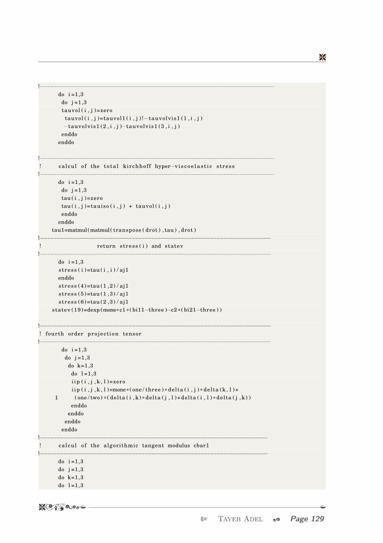
8
!−−−−−−−−−−−−−−−−−−−−−−−−−−−−−−−−−−−−−−−−−−−−−−−−−−−−−−−−−−−−−−−−−−−−−−−−do i =1 ,3
do j =1 ,3tauvol ( i , j )=zero
tauvol ( i , j )=tauvol1 ( i , j ) !− tauvolvis1 (1 , i , j )−tauvolvis1 (2 , i , j )−tauvolvis1 (3 , i , j )
enddoenddo
!−−−−−−−−−−−−−−−−−−−−−−−−−−−−−−−−−−−−−−−−−−−−−−−−−−−−−−−−−−−−−−−−−−−−−−−−! ca l cu l o f the t o t a l kirchhof f hyper−v i s c o e l a s t i c s tress!−−−−−−−−−−−−−−−−−−−−−−−−−−−−−−−−−−−−−−−−−−−−−−−−−−−−−−−−−−−−−−−−−−−−−−−−
do i =1 ,3do j =1 ,3tau ( i , j )=zerotau ( i , j )=tauiso ( i , j ) + tauvol ( i , j )enddo
enddotau1=matmul (matmul ( transpose ( drot ) , tau ) , drot )
!−−−−−−−−−−−−−−−−−−−−−−−−−−−−−−−−−−−−−−−−−−−−−−−−−−−−−−−−−−−−−−−−−−−−−−−! return stress ( i ) and statev!−−−−−−−−−−−−−−−−−−−−−−−−−−−−−−−−−−−−−−−−−−−−−−−−−−−−−−−−−−−−−−−−−−−−−−−
do i =1 ,3stress ( i )=tau ( i , i ) / aj1enddostress ( 4 ) =tau (1 ,2 ) / aj1stress ( 5 ) =tau (1 ,3 ) / aj1stress ( 6 ) =tau (2 ,3 ) / aj1
statev (19)=dexp (mone*c1 *( bi11−three )−c2 *( bi21−three ) )
!−−−−−−−−−−−−−−−−−−−−−−−−−−−−−−−−−−−−−−−−−−−−−−−−−−−−−−−−−−−−−−−−−−−−−−−! fourth order pro jec t i on tensor!−−−−−−−−−−−−−−−−−−−−−−−−−−−−−−−−−−−−−−−−−−−−−−−−−−−−−−−−−−−−−−−−−−−−−−−
do i =1 ,3do j =1 ,3
do k=1 ,3do l =1 ,3i i p ( i , j , k , l )=zeroi i p ( i , j , k , l )=mone*( one / three ) * delta ( i , j ) * delta (k , l )+
1 ( one / two ) * ( delta ( i , k ) * delta ( j , l )+delta ( i , l ) * delta ( j , k ) )enddo
enddoenddo
enddo!−−−−−−−−−−−−−−−−−−−−−−−−−−−−−−−−−−−−−−−−−−−−−−−−−−−−−−−−−−−−−−−−−−−−−−! ca l cu l o f the algorithmic tangent modulus cbar1!−−−−−−−−−−−−−−−−−−−−−−−−−−−−−−−−−−−−−−−−−−−−−−−−−−−−−−−−−−−−−−−−−−−−−−
do i =1 ,3do j =1 ,3do k=1 ,3do l =1 ,3
8CAM:<J J
T Tayeb Adel ; Page 129

8 Appendix A. Appendix A
cbar1 ( i , j , k , l )=zerodo s=1 ,3cbar1 ( i , j , k , l )=four *bbar1 ( i , j ) *bbar1 (k , l )−
1 two *( bbar1 ( i , k ) *bbar1 ( j , l )+bbar1 ( i , s ) *bbar1 ( s , l ) * delta ( j , k ) )enddoenddoenddoenddoenddo
!−−−−−−−−−−−−−−−−−−−−−−−−−−−−−−−−−−−−−−−−−−−−−−−−−−−−−−−−−−−−−−−−−−−−−−−−−−! ca l cu l o f the algorithmic tangent modulus cbar!−−−−−−−−−−−−−−−−−−−−−−−−−−−−−−−−−−−−−−−−−−−−−−−−−−−−−−−−−−−−−−−−−−−−−−−−−−
do i =1 ,3do j =1 ,3do k=1 ,3do l =1 ,3cbar11 ( i , j , k , l )=zerocbar22 ( i , j , k , l )=zerocbar11 ( i , j , k , l )=c01*cbar1 ( i , j , k , l )+
1 two*c02 *( bi21−three ) *cbar1 ( i , j , k , l )+2 c11 *( bi11−three ) *cbar1 ( i , j , k , l )+3 8.0d0*c20*bbar1 ( i , j ) *bbar1 (k , l )+4 8.0d0*c11*bi11*bbar1 ( i , j ) *bbar1 (k , l )
do s=1 ,3do t =1 ,3cbar22 ( i , j , k , l )=mone* four *c11*bbar1 ( i , s ) *bbar1 ( s , j ) *bbar1 (k , l )−
1 four *c11*bbar1 ( i , j ) *bbar1 (k , s ) *bbar1 ( s , l )+2 8.0d0*c02*bi11*bi11*bbar1 ( i , j ) *bbar1 (k , l )−3 8.0d0*c02*bi11*bbar1 ( i , j ) *bbar1 (k , s ) *bbar1 ( s , l )−4 8.0d0*c02*bi11*bbar1 ( i , s ) *bbar1 ( s , j ) *bbar1 (k , l )+5 8.0d0*c02*bbar1 ( i , s ) *bbar1 ( s , j ) *bbar1 (k , t ) *bbar1 ( t , l )
enddoenddoenddoenddoenddoenddodo i =1 ,3do j =1 ,3do k=1 ,3do l =1 ,3cbar ( i , j , k , l )=zerocbar ( i , j , k , l )=cbar11 ( i , j , k , l )+cbar22 ( i , j , k , l )enddoenddoenddoenddo
!−−−−−−−−−−−−−−−−−−−−−−−−−−−−−−−−−−−−−−−−−−−−−−−−−−−−−−−−−−−−−−−−−−−−−−−−−−! ca l cu l o f the dev iator i c hyperelast ic tangent modulus cisoh!−−−−−−−−−−−−−−−−−−−−−−−−−−−−−−−−−−−−−−−−−−−−−−−−−−−−−−−−−−−−−−−−−−−−−−−−−−
do i =1 ,3
K K;9NAB8
Page 130 ; Ph.D thesis at ECL/LTDS U

8
do j =1 ,3do k=1 ,3do l =1 ,3cisoh ( i , j , k , l )=zerodo s=1 ,3do t =1 ,3do u=1 ,3do v=1 ,3cisoh ( i , j , k , l ) =( two / three ) * tracebtau1 * i i p ( i , j , k , l )−
1 ( two / three ) * ( tauiso1 ( i , j ) * delta (k , l )+2 delta ( i , j ) * tauiso1 (k , l ) )+3 i i p ( i , j , s , t ) * cbar ( s , t , u , v ) * i i p (u , v , k , l )
enddoenddoenddoenddoenddoenddoenddoenddo
!−−−−−−−−−−−−−−−−−−−−−−−−−−−−−−−−−−−−−−−−−−−−−−−−−−−−−−−−−−−−−−−−−−−−−−−−−−−! ca l cu l o f the volumetric hyperelast ic tangent modulus cvolh!−−−−−−−−−−−−−−−−−−−−−−−−−−−−−−−−−−−−−−−−−−−−−−−−−−−−−−−−−−−−−−−−−−−−−−−−−−−
cs=two* aj1 * aj1 / d1do i =1 ,3
do j =1 ,3do k=1 ,3
do l =1 ,3cvolh ( i , j , k , l )=zerocvolh ( i , j , k , l ) =(p1+cs ) * delta ( i , j ) * delta (k , l )
1 −p1 *( delta ( i , k ) * delta ( j , l )+delta ( i , l ) * delta ( j , k ) )enddo
enddoenddo
enddo!−−−−−−−−−−−−−−−−−−−−−−−−−−−−−−−−−−−−−−−−−−−−−−−−−−−−−−−−−−−−−−−−−−−−−−−−−−−! ca l cu l o f the dev iator i c hyperv iscoe last i c tangent modulus cisovh!−−−−−−−−−−−−−−−−−−−−−−−−−−−−−−−−−−−−−−−−−−−−−−−−−−−−−−−−−−−−−−−−−−−−−−−−−−−
const1=zeroconst2=zero
const1=al fa ( 1 ) *g1+al fa ( 2 ) *g2+al fa ( 3 ) *g3const2=al fa ( 1 ) *g1+al fa ( 2 ) *g2+al fa ( 3 ) *g3
do i =1 ,3do j =1 ,3do k=1 ,3do l =1 ,3
cb ( i , j , k , l )=zerocb ( i , j , k , l )=delta ( i , k ) *tau ( j , l )+delta ( j , l ) *tau ( i , k )+delta ( i , l ) *tau ( j , k )+delta ( j , k ) *tau ( i , l )enddo
8CAM:<J J
T Tayeb Adel ; Page 131

8 Appendix A. Appendix A
enddoenddoenddo
do i =1 ,3do j =1 ,3do k=1 ,3do l =1 ,3cisovh ( i , j , k , l )=zerocisovh ( i , j , k , l ) =(one−const1 ) * cisoh ( i , j , k , l ) ! + ( one / ( aj1 *two ) ) *cb ( i , j , k , l )enddoenddoenddoenddo
!−−−−−−−−−−−−−−−−−−−−−−−−−−−−−−−−−−−−−−−−−−−−−−−−−−−−−−−−−−−−−−−−−−−−−−−−−−−! ca l cu l o f the volumetric hyperv iscoe last i c tangent modulus cvolvh!−−−−−−−−−−−−−−−−−−−−−−−−−−−−−−−−−−−−−−−−−−−−−−−−−−−−−−−−−−−−−−−−−−−−−−−−−−−
do i =1 ,3do j =1 ,3do k=1 ,3do l =1 ,3cvolvh ( i , j , k , l )=zerocvolvh ( i , j , k , l )=cvolh ( i , j , k , l )enddoenddoenddoenddo
!−−−−−−−−−−−−−−−−−−−−−−−−−−−−−−−−−−−−−−−−−−−−−−−−−−−−−−−−−−−−−−−−−−−−−−−−−−−! t o t a l tangent modulus i c!−−−−−−−−−−−−−−−−−−−−−−−−−−−−−−−−−−−−−−−−−−−−−−−−−−−−−−−−−−−−−−−−−−−−−−−−−−−
do i =1 ,3do j =1 ,3do k=1 ,3do l =1 ,3i c ( i , j , k , l )=zeroi c ( i , j , k , l )=cvolvh ( i , j , k , l ) / aj1+ cisovh ( i , j , k , l ) / aj1 +(one / ( aj1 *two ) ) *cb ( i , j , k , l )enddoenddoenddoenddo
!−−−−−−−−−−−−−−−−−−−−−−−−−−−−−−−−−−−−−−−−−−−−−−−−−−−−−−−−−−−−−−−−−−−−−−−−−−−−! return ddsdde ( i , j )= i c ( i , j , k , l )!−−−−−−−−−−−−−−−−−−−−−−−−−−−−−−−−−−−−−−−−−−−−−−−−−−−−−−−−−−−−−−−−−−−−−−−−−−−
do i =1 ,6do j =1 ,6ddsdde ( i , j )=zeroenddoenddoddsdde (1 ,1 )= i c (1 ,1 ,1 ,1 )ddsdde (1 ,2 )= i c (1 ,1 ,2 ,2 )ddsdde (1 ,3 )= i c (1 ,1 ,3 ,3 )
K K;9NAB8
Page 132 ; Ph.D thesis at ECL/LTDS U

8
ddsdde (1 ,4 )= i c (1 ,1 ,1 ,2 )ddsdde (1 ,5 )= i c (1 ,1 ,1 ,3 )ddsdde (1 ,6 )= i c (1 ,1 ,2 ,3 )ddsdde (2 ,2 )= i c (2 ,2 ,2 ,2 )ddsdde (2 ,3 )= i c (2 ,2 ,3 ,3 )ddsdde (2 ,4 )= i c (2 ,2 ,1 ,2 )ddsdde (2 ,5 )= i c (2 ,2 ,1 ,3 )ddsdde (2 ,6 )= i c (2 ,2 ,2 ,3 )ddsdde (3 ,3 )= i c (3 ,3 ,3 ,3 )ddsdde (3 ,4 )= i c (3 ,3 ,1 ,2 )ddsdde (3 ,5 )= i c (3 ,3 ,1 ,3 )ddsdde (3 ,6 )= i c (3 ,3 ,2 ,3 )ddsdde (4 ,4 )= i c (1 ,2 ,1 ,2 )ddsdde (4 ,5 )= i c (1 ,2 ,1 ,3 )ddsdde (4 ,6 )= i c (1 ,2 ,2 ,3 )ddsdde (5 ,5 )= i c (1 ,3 ,1 ,3 )ddsdde (5 ,6 )= i c (1 ,3 ,2 ,3 )ddsdde (6 ,6 )= i c (2 ,3 ,2 ,3 )do i =1 ,6do j =1 ,6ddsdde ( j , i )=ddsdde ( i , j )enddoenddo
print * , s tress ( 1 )returnend
8CAM:<J J
T Tayeb Adel ; Page 133

BIBLIOGRAPHY
[1] J. Argyris and I. S. Doltsinis. Constitutive modelling and computation of non-linear
viscoelastic solids. part i: Rheological models and numerical integration techniques.
Computer Methods in Applied Mechanics and Engineering, 88(2):135–163, 1991.
[2] G. Astarita and G. Marrucci. Principles of non-Newtonian fluid mechanics.
McGraw-Hill Companies, 1974.
[3] B.Y. Ballal and R.S. Rivlin. Flow of a viscoelastic fluid between eccentric cylinders.
Rheologica Acta, 18(3):311–322, 1979.
[4] R.C. Batra and J.H. Yu. Linear constitutive relations in isotropic finite viscoelas-
ticity. Journal of elasticity, 55(1):73–77, 1999.
[5] R.C. Batra and J.H. Yu. Torsion of a viscoelastic cylinder. journal of appliedmechanics-the american society of mechanical engineers, 67(2):424–426, 2000.
[6] J.G.J. Beijer and J.L. Spoormaker. Solution strategies for fem analysis with
nonlinear viscoelastic polymers. Computers & structures, 80(14):1213–1229, 2002.
[7] M. A. Biot. Theory of stress-strain relations in anisotropic viscoelasticity and
relaxation phenomena. Journal of Applied Physics, 25(11):1385–1391, 1954.
[8] J. E. Bischoff, E. M. Arruda, and K. Grosh. A new constitutive model for the com-
pressibility of elastomers at finite deformations. Rubber chemistry and technology,
74(4):541–559, 2001.
[9] A. V. Boiko, V. M. Kulik, B. M. Seoudi, H.H. Chun, and I. Lee. Measurement method
of complex viscoelastic material properties. International Journal of Solids andStructures, 47(3):374–382, 2010.
[10] L. Boltzmann. Zur theorie der elastischen nachwirkung. Annalen der Physik,
241(11):430–432, 1878.
135

8 Bibliography
[11] J. Bonet. Large strain viscoelastic constitutive models. International Journal ofSolids and Structures, 38(17):2953–2968, 2001.
[12] H. Bouasse and Z. Carrière. Sur les courbes de traction du caoutchouc vulcanisé.
In Annales de la Faculté des sciences de Toulouse: Mathématiques, volume 5,
pages 257–283. GAUTHIER-VILLARS, IMPRIMEUR-EDITEUR; ED. PRIVAT,
IMPRIMEUR-LIBRAIRE, 1903.
[13] A. Boukamel. Modélisation mécaniques et numériques des matériaux et structuresen élastomères. Habilitation à diriger des recherches, Université de la Méditerranée
- Aix-Marseille II, October 2006. URL: https://tel.archives-ouvertes.fr/
tel-00517997.
[14] C.P. Buckley and D.C. Jones. Glass-rubber constitutive model for amorphous
polymers near the glass transition. Polymer, 36(17):3301–3312, 1995.
[15] F. Bueche. Molecular basis for the mullins effect. Journal of Applied PolymerScience, 4(10):107–114, 1960.
[16] F. Bueche. Mullins effect and rubber–filler interaction. Journal of applied polymerScience, 5(15):271–281, 1961.
[17] W. D. Callister and D. G. Rethwisch. Materials science and engineering, volume 5.
John Wiley & Sons NY, 2011.
[18] D. Calvetti, S. Morigi, L. Reichel, and F. Sgallari. Tikhonov regularization and
the l-curve for large discrete ill-posed problems. Journal of Computational andApplied Mathematics, 123(1–2):423 – 446, 2000.
[19] M.M. Carroll. Controllable deformations of incompressible simple materials.
International Journal of Engineering Science, 5(6):515–525, 1967.
[20] L. Chazeau, J.D. Brown, L.C. Yanyo, and S.S. Sternstein. Modulus recovery kinetics
and other insights into the payne effect for filled elastomers. Polymer composites,
21(2):202–222, 2000.
[21] J. Chen, H. Hu, S. Li, and K. Zhang. Quantitative relation between the relaxation
time and the strain rate for polymeric solids under quasi-static conditions. Journalof Applied Polymer Science, 133(42), 2016.
[22] R. Christensen. Theory of viscoelasticity: an introduction. Elsevier, 2012.
K K;9NAB8
Page 136 ; Ph.D thesis at ECL/LTDS U

Bibliography 8
[23] J. Ciambella, A. Paolone, and S. Vidoli. A comparison of nonlinear integral-based
viscoelastic models through compression tests on filled rubber. Mechanics ofMaterials, 42(10):932–944, 2010.
[24] B. D. Coleman. Thermodynamics of materials with memory. Archive for RationalMechanics and Analysis, 17(1):1–46, 1964.
[25] B. D. Coleman and M. E. Gurtin. Thermodynamics with internal state variables.
The Journal of Chemical Physics, 47(2):597–613, 1967.
[26] B. D. Coleman, H. Markovitz, and W. Noll. Viscometric flows of non-Newtonianfluids: theory and experiment, volume 5. Springer Science & Business Media, 2012.
[27] B. D. Coleman and W. Noll. Foundations of linear viscoelasticity. Reviews ofModern Physics, 33(2):239, 1961.
[28] B. D. Coleman and W. Noll. The thermodynamics of elastic materials with heat
conduction and viscosity. Archive for Rational Mechanics and Analysis, 13(1):167–
178, 1963.
[29] V. A. Coveney. Elastomers and Components: Service Life Prediction-Progress andChallenges. Woodhead Publishing, 2006.
[30] R. De Pascalis, I. D. Abrahams, and W. J. Parnell. On nonlinear viscoelastic
deformations: a reappraisal of fung’s quasi-linear viscoelastic model. In Proc. R.Soc. A, volume 470, page 20140058. The Royal Society, 2014.
[31] G. Del Piero and L. Deseri. On the concepts of state and free energy in linear
viscoelasticity. Archive for Rational Mechanics and Analysis, 138(1):1–35, 1997.
[32] Michel Destrade, Jerry G Murphy, and Giuseppe Saccomandi. Simple shear is not
so simple. International Journal of Non-Linear Mechanics, 47(2):210–214, 2012.
[33] A. D. Drozdov and A. Dorfmann. Finite viscoelasticity of filled rubber: experiments
and numerical simulation. Archive of Applied Mechanics, 72(9):651–672, 2003.
[34] A.D. Drozdov. Viscoelastic structures: mechanics of growth and aging. Academic
Press, 1998.
[35] A.D. Drozdov. Constitutive equations in finite elasticity of rubbers. InternationalJournal of Solids and Structures, 44(1):272–297, 2007.
8CAM:<J J
T Tayeb Adel ; Page 137

8 Bibliography
[36] W. Ehlers and G. Eipper. The simple tension problem at large volumetric strains
computed from finite hyperelastic material laws. Acta Mechanica, 130(1):17–27,
1998.
[37] C. Elster, J. Honerkamp, and J. Weese. Using regularization methods for the de-
termination of relaxation and retardation spectra of polymeric liquids. Rheologicaacta, 31(2):161–174, 1992.
[38] J.L. Ericksen. Deformations possible in every compressible, isotropic, perfectly
elastic material. Studies in Applied Mathematics, 34(1-4):126–128, 1955.
[39] M. Fabrizio and A. Morro. Mathematical problems in linear viscoelasticity. SIAM,
1992.
[40] E.A. Fancello, J.P. Ponthot, and L. Stainier. A variational framework for nonlinear
viscoelastic models in finite deformation regime. Journal of Computational andApplied Mathematics, 215(2):400–408, 2008.
[41] M.S.H. Fatt and A.A. Al-Quraishi. High strain rate constitutive modeling for
natural rubber. In CONSTITUTIVE MODELS FOR RUBBER-PROCEEDINGS-,volume 5, page 53. Balkema, 2008.
[42] W. W. Feng. A recurrence formula for viscoelastic constitutive equations. Interna-tional journal of non-linear mechanics, 27(4):675–678, 1992.
[43] J. D. Ferry. Viscoelastic properties of polymers. John Wiley & Sons, 1980.
[44] W. N. Findley and F.A. Davis. Creep and relaxation of nonlinear viscoelasticmaterials. Courier Corporation, 2013.
[45] W.N. Findley and F.A. Davis. Creep and relaxation of nonlinear viscoelastic materi-als. Courier Corporation, 2013.
[46] P. J. Flory. Thermodynamic relations for high elastic materials. Transactions ofthe Faraday Society, 57:829–838, 1961.
[47] R. L. Fosdick and J.H. Yu. Thermodynamics, stability and non-linear oscillations of
viscoelastic solids—i. differential type solids of second grade. International journalof non-linear mechanics, 31(4):495–516, 1996.
K K;9NAB8
Page 138 ; Ph.D thesis at ECL/LTDS U

Bibliography 8
[48] Y.C. B. Fung. Stress-strain-history relations of soft tissues in simple elongation.
Biomechanics its foundations and objectives, pages 181–208, 1972.
[49] J. Golden. A proposal concerning the physical rate of dissipation in materials with
memory. Quarterly of applied mathematics, 63(1):117–155, 2005.
[50] S. Govindjee and J. Simo. A micro-mechanically based continuum damage model for
carbon black-filled rubbers incorporating mullins’ effect. Journal of the Mechanicsand Physics of Solids, 39(1):87–112, 1991.
[51] S. Govindjee and J.C. Simo. Mullins’ effect and the strain amplitude dependence
of the storage modulus. International journal of solids and structures, 29(14-
15):1737–1751, 1992.
[52] A. E. Green and R. S. Rivlin. The mechanics of non-linear materials with memory.
Archive for Rational Mechanics and Analysis, 1(1):1–21, 1957.
[53] R.M. Haj-Ali and A.H. Muliana. Numerical finite element formulation of the
schapery non-linear viscoelastic material model. International Journal for Numer-ical Methods in Engineering, 59(1):25–45, 2004.
[54] J. O. Hallquist et al. Ls-dyna theory manual. Livermore software technologycorporation, 3:25–31, 2006.
[55] J.A.C. Harwood, L. Mullins, and A.R. Payne. Stress softening in rubbers: a review.
Journal of the IRI, 1:17–27, 1967.
[56] K. Hasanpour, S. Ziaei-Rad, and M. Mahzoon. A large deformation framework
for compressible viscoelastic materials: Constitutive equations and finite element
implementation. International Journal of Plasticity, 25(6):1154–1176, 2009.
[57] S. Hassani, A. A. Soulimani, and A. Ehrlacher. A nonlinear viscoelastic model: the
pseudo-linear model. European Journal of Mechanics-A/Solids, 17(4):567–598,
1998.
[58] P. Haupt and A. Lion. On finite linear viscoelasticity of incompressible isotropic
materials. Acta Mechanica, 159(1):87–124, 2002.
[59] R.N. Haward and G. Thackray. The use of a mathematical model to describe
isothermal stress-strain curves in glassy thermoplastics. In Proceedings of the
8CAM:<J J
T Tayeb Adel ; Page 139

8 Bibliography
Royal Society of London A: Mathematical, Physical and Engineering Sciences,
volume 302, pages 453–472. The Royal Society, 1968.
[60] M. Henriksen. Nonlinear viscoelastic stress analysis—a finite element approach.
Computers & structures, 18(1):133–139, 1984.
[61] L.R. Herrmann and F.E. Peterson. A numerical procedure for viscoelastic stress
analysis. In Seventh meeting of ICRPG mechanical behavior working group,Orlando, FL, CPIA Publication, number 177, pages 60–69, 1968.
[62] D. Hibbit, B. Karlsson, and P. Sorensen. Abaqus User Subroutine Reference Manual,volume 6. Rhode Island, 2007.
[63] D. Hibbit, B. Karlsson, and P. Sorensen. Abaqus/theory manual. Rhode Island,
6(7), 2007.
[64] A. G. Holzapfel. Nonlinear solid mechanics ii. 2000.
[65] G. Holzapfel and R. A. Simo. A new viscoelastic constitutive model for continuous
media at finite thermomechanical changes. International Journal of Solids andStructures, 33:3019–3034, 1996.
[66] G. A. Holzapfel and T. C. Gasser. A viscoelastic model for fiber-reinforced compos-
ites at finite strains: Continuum basis, computational aspects and applications.
Computer methods in applied mechanics and engineering, 190(34):4379–4403,
2001.
[67] G. A. Holzapfel and J. C. Simo. A new viscoelastic constitutive model for continuous
media at finite thermomechanical changes. International Journal of Solids andStructures, 33(20):3019–3034, 1996.
[68] G.A. Holzapfel. On large strain viscoelasticity: continuum formulation and finite el-
ement applications to elastomeric structures. International Journal for NumericalMethods in Engineering, 39(22):3903–3926, 1996.
[69] C.O. Horgan and G. Saccomandi. Pure axial shear of isotropic, incompressible
nonlinearly elastic materials with limiting chain extensibility. Journal of elasticity,
57(3):307–319, 1999.
K K;9NAB8
Page 140 ; Ph.D thesis at ECL/LTDS U

Bibliography 8
[70] C.O. Horgan and G. Saccomandi. Simple torsion of isotropic, hyperelastic, in-
compressible materials with limiting chain extensibility. Journal of elasticity,
56(2):159–170, 1999.
[71] C.O. Horgan and G. Saccomandi. Pure azimuthal shear of isotropic, incompressible
hyperelastic materials with limiting chain extensibility. International journal ofnon-linear mechanics, 36(3):465–475, 2001.
[72] C.O. Horgan and G. Saccomandi. Helical shear for hardening generalized neo-
hookean elastic materials. Mathematics and Mechanics of Solids, 8(5):539–559,
2003.
[73] G. Huber, T. A. Vilgis, and G. Heinrich. Universal properties in the dynamical
deformation of filled rubbers. Journal of Physics: Condensed Matter, 8(29):L409,
1996.
[74] N. Huber and C. Tsakmakis. Finite deformation viscoelasticity laws. Mechanics ofmaterials, 32(1):1–18, 2000.
[75] T.J.R. Hughes. The finite element method: linear static and dynamic finite elementanalysis. Courier Corporation, 2012.
[76] R.R. Huilgol. Viscoelastic fluid theories based on the left cauchy-green tensor
history. Rheologica Acta, 18(4):451–455, 1979.
[77] M.A. Johnson and M.F. Beatty. The mullins effect in uniaxial extension and its
influence on the transverse vibration of a rubber string. Continuum Mechanicsand Thermodynamics, 5(2):83–115, 1993.
[78] H. Khajehsaeid, J. Arghavani, R. Naghdabadi, and S. Sohrabpour. A visco-
hyperelastic constitutive model for rubber-like materials: A rate-dependent re-
laxation time scheme. International Journal of Engineering Science, 79:44–58,
2014.
[79] A. S. Khan, O. Lopez-Pamies, and R. Kazmi. Thermo-mechanical large deformation
response and constitutive modeling of viscoelastic polymers over a wide range of
strain rates and temperatures. International Journal of Plasticity, 22(4):581–601,
2006.
[80] W. G. Knauss and J. Zhao. Improved relaxation time coverage in ramp-strain
histories. Mechanics of Time-Dependent Materials, 11(3-4):199–216, 2007.
8CAM:<J J
T Tayeb Adel ; Page 141

8 Bibliography
[81] G. Kraus. Mechanical losses in carbon-black-filled rubbers. In Journal of AppliedPolymer Science: Applied Polymer Symposium, volume 39, pages 75–92, 1984.
[82] F. Laraba-Abbes, P. Ienny, and R. Piques. A new ‘tailor-made’methodology for
the mechanical behaviour analysis of rubber-like materials: Ii. application to the
hyperelastic behaviour characterization of a carbon-black filled natural rubber
vulcanizate. Polymer, 44(3):821–840, 2003.
[83] J.H. Lee and K.J. Kim. Characterization of complex modulus of viscoelastic
materials subject to static compression. Mechanics of Time-Dependent Materials,
5(3):255–271, 2001.
[84] S.B. Lee and A. Wineman. A model for nonlinear viscoelastic torsional response of
an elastomeric bushing. Acta mechanica, 135(3-4):199–218, 1999.
[85] S.B. Lee and A. Wineman. A model for non-linear viscoelastic coupled mode
response of an elastomeric bushing. International journal of non-linear mechanics,
35(2):177–199, 2000.
[86] S. Lejeunes, A. Boukamel, and S. Méo. Finite element implementation of nearly-
incompressible rheological models based on multiplicative decompositions. Com-puters & structures, 89(3):411–421, 2011.
[87] C. Lewitzke and P. Lee. Application of elastomeric components for noise and
vibration isolation in the automotive industry. Technical report, SAE Technical
Paper, 2001.
[88] A. Lion. A physically based method to represent the thermo-mechanical behaviour
of elastomers. Acta Mechanica, 123(1):1–25, 1997.
[89] A. Lion and C. Kardelky. The payne effect in finite viscoelasticity: constitutive
modelling based on fractional derivatives and intrinsic time scales. InternationalJournal of Plasticity, 20(7):1313–1345, 2004.
[90] J. Lubliner. A model of rubber viscoelasticity. Mechanics Research Communications,
12(2):93–99, 1985.
[91] W. J. MacKnight. Volume changes accompanying the extension of rubber-like
materials. Journal of Applied Physics, 37(12):4587–4587, 1966.
[92] A. I. Malkin. Rheology fundamentals. ChemTec Publishing, 1994.
K K;9NAB8
Page 142 ; Ph.D thesis at ECL/LTDS U

Bibliography 8
[93] G. Marckmann. Contribution à l’étude des élastomères et des membranes soufflées.
PhD thesis, Ecole Centrale de Nantes (ECN)(ECN)(ECN)(ECN); Université de
Nantes, 2004.
[94] J. E. Marsden and T. J.R. Hughes. Mathematical foundations of elasticity. Courier
Corporation, 1994.
[95] S. Matsuoka, C. J. Aloisio, and H. E. Bair. Interpretation of shift of relaxation
time with deformation in glassy polymers in terms of excess enthalpy. Journal ofApplied Physics, 44(10):4265–4268, 1973.
[96] C. Miehe. Discontinuous and continuous damage evolution in ogden-type large-
strain elastic materials. European journal of mechanics. A. Solids, 14(5):697–720,
1995.
[97] K. N. Morman Jr and T. Y. Pan. Application of finite-element analysis in the
design of automotive elastomeric components. Rubber chemistry and technology,
61(3):503–533, 1988.
[98] A. Muliana, K.R. Rajagopal, and D. Tscharnuter. A nonlinear integral model for
describing responses of viscoelastic solids. International Journal of Solids andStructures, 58:146–156, 2015.
[99] A. Muliana, K.R. Rajagopal, and A.S. Wineman. A new class of quasi-linear models
for describing the nonlinear viscoelastic response of materials. Acta Mechanica,
224(9):2169–2183, 2013.
[100] L. Mullins. Effect of stretching on the properties of rubber. Rubber Chemistry andTechnology, 21(2):281–300, 1948.
[101] L. Mullins. Softening of rubber by deformation. Rubber chemistry and technology,
42(1):339–362, 1969.
[102] M.Z. Nashed. The theory of tikhonov regularization for fredholm equations of the
first kind (cw groetsch). SIAM Review, 28(1):116–118, 1986.
[103] J. Nidhal, S. Michelle, H. Adel, B. Olivier, A. Makrem, I. Mohamed, and B. Jalel.
Predeformation and frequency-dependence : Experiment and fe analysis. Proceed-ing of international conference on dynamics of composite structure, pages 105–112,
2015.
8CAM:<J J
T Tayeb Adel ; Page 143

8 Bibliography
[104] P.A. Oconnell and G.B. McKenna. Large deformation response of polycarbon-
ate: Time-temperature, time-aging time, and time-strain superposition. PolymerEngineering and Science, 37(9):1485–1495, 1997.
[105] R. W. Ogden, G. Saccomandi, and I. Sgura. Fitting hyperelastic models to experi-
mental data. Computational Mechanics, 34(10):484–502, August 2004.
[106] R.W. Ogden. Volume changes associated with the deformation of rubber-like solids.
Journal of the Mechanics and Physics of Solids, 24(6):323–338, 1976.
[107] R.W. Ogden. Nearly isochoric elastic deformations: application to rubberlike solids.
Journal of the Mechanics and Physics of Solids, 26(1):37–57, 1978.
[108] R.W. Ogden and D.G. Roxburgh. A pseudo–elastic model for the mullins effect
in filled rubber. In Proceedings of the Royal Society of London A: Mathematical,Physical and Engineering Sciences, volume 455, pages 2861–2877. The Royal
Society, 1999.
[109] R.W. Ogden, G. Saccomandi, and I. Sgura. Fitting hyperelastic models to experi-
mental data. Computational Mechanics, 34(6):484–502, 2004.
[110] S. W. Park and R. A. Schapery. Methods of interconversion between linear vis-
coelastic material functions. part i—a numerical method based on prony series.
International Journal of Solids and Structures, 36(11):1653–1675, 1999.
[111] C. Patrick and E. Isabelle. Physique des polymères tome i structure, fabrication,
emploi. Hermann Editeurs des Sciences et des Arts: Paris, page 42, 2005.
[112] A. R. Payne. The dynamic properties of carbon black loaded natural rubber
vulcanizates. part ii. Journal of Applied Polymer Science, 6(21):368–372, 1962.
[113] E. Peña, J. A. Peña, and M. Doblaré. On modelling nonlinear viscoelastic effects in
ligaments. Journal of Biomechanics, 41:2659–2666, 2008.
[114] R. W. Penn. Volume changes accompanying the extension of rubber. Transactionsof the Society of Rheology, 14(4):509–517, 1970.
[115] A. C. Pipkin. Small finite deformations of viscoelastic solids. Reviews of ModernPhysics, 36(4):1034–1041, 1964.
K K;9NAB8
Page 144 ; Ph.D thesis at ECL/LTDS U

Bibliography 8
[116] A. C. Pipkin. Lectures on viscoelasticity theory, volume 7. Springer Science &
Business Media, 2012.
[117] A.C. Pipkin and T.G. Rogers. A non-linear integral representation for viscoelastic
behaviour. Journal of the Mechanics and Physics of Solids, 16(1):59–72, 1968.
[118] P.A. Przybylo and E.M. Arruda. Experimental investigations and numerical
modeling of incompressible elastomers during non-homogeneous deformations.
Rubber Chemistry and Technology, 71(4):730–749, 1998.
[119] E. Pucci and G. Saccomandi. A note on the gent model for rubber-like materials.
Rubber chemistry and technology, 75(5):839–852, 2002.
[120] S. Reese and S. Govindjee. A theory of viscoelasticity and numerical applications.
International Journal of Solids and Structures, 35:3455–3482, 1998.
[121] W.F. Reichert, M.K. Hopfenmüller, and D. Göritz. Volume change and gas transport
at uniaxial deformation of filled natural rubber. Journal of materials science,
22(10):3470–3476, 1987.
[122] R. S. Rivlin and J. L. Ericksen. Stress-deformation relations for isotropic materials.
Journal of Rational Mechanics and Analysis, 4:323–425, 1955.
[123] R.S. Rivlin. Large elastic deformations of isotropic materials. iv. further develop-
ments of the general theory. Philosophical Transactions of the Royal Society ofLondon A: Mathematical, Physical and Engineering Sciences, 241(835):379–397,
1948.
[124] P. Saad. Modélisation et identification du comportement non linéaire des cales encaoutchouc. PhD thesis, École Centrale de Lyon, 2003.
[125] R. A. Schapery. On the characterization of nonlinear viscoelastic materials. Poly-mer Engineering & Science, 9(4):295–310, 1969.
[126] R. A. Schapery. Nonlinear viscoelastic and viscoplastic constitutive equations
based on thermodynamics. Mechanics of Time-Dependent Materials, 1(2):209–240,
1997.
[127] V.P.W. Shim, L.M. Yang, C.T. Lim, and P.H. Law. A visco-hyperelastic constitutive
model to characterize both tensile and compressive behavior of rubber. Journal ofApplied Polymer Science, 92(1):523–531, 2004.
8CAM:<J J
T Tayeb Adel ; Page 145

8 Bibliography
[128] F. Sidoroff. Nonlinear viscoelastic model with intermediate configuration. JOUR-NAL DE MECANIQUE, 13(4):679–713, 1974.
[129] J. C. Simo and T. J. R. Hughes. Computational inelasticity, volume 7. Springer
Science & Business Media, 2006.
[130] J.C. Simo, J.G. Kennedy, and S. Govindjee. Non-smooth multisurface plasticity
and viscoplasticity. loading/unloading conditions and numerical algorithms. In-ternational Journal for Numerical Methods in Engineering, 26(10):2161–2185,
1988.
[131] R. A. Simo. On a fully three-dimensional finite-strain viscoelastic damage model:
Formulation and computational aspects. Computer Methods in Applied Mechanicsand Engineering, 60:153–173, 1987.
[132] J. Sorvari and J. Hämäläinen. Time integration in linear viscoelasticity—a com-
parative study. Mechanics of Time-Dependent Materials, 14(3):307–328, 2010.
[133] E. Stein and G. Sagar. Convergence behavior of 3d finite elements for neo-hookean
material. Engineering Computations, 25(3):220–232, 2008.
[134] J.L. Sullivan. A nonlinear viscoelastic model for representing nonfactorizable
time-dependent behavior in cured rubber. Journal of Rheology (1978-present),31(3):271–295, 1987.
[135] TA. Instruments Training Courses. Woodlands, 2010.
[136] A. Tayeb, M. Arfaoui, A.M. Zine, A. Hamdi, J. Benabdallah, and M. Ichchou. On the
nonlinear viscoelastic behavior of rubber-like materials: Constitutive description
and identification. International journal of mechanical sciences, 130:437 – 447,
2017.
[137] R. L. Taylor, K. S. Pister, and G. L. Goudreau. Thermomechanical analysis of
viscoelastic solids. International Journal for Numerical Methods in Engineering,
2(1):45–59, 1970.
[138] L. R. G. Treloar. The physics of rubber elasticity. Oxford University Press, USA,
1975.
[139] C. Truesdell and W. Noll. The non-linear field theories of mechanics, volume 3.
Springer, 2004.
K K;9NAB8
Page 146 ; Ph.D thesis at ECL/LTDS U

Bibliography 8
[140] N. W. Tschoegl. Time dependence in material properties: An overview. Mechanicsof Time-Dependent Materials, 1(1):3–31, 1997.
[141] N. W. Tschoegl, W. G. Knauss, and I. Emri. The effect of temperature and pressure
on the mechanical properties of thermo-and/or piezorheologically simple polymeric
materials in thermodynamic equilibrium–a critical review. Mechanics of Time-Dependent Materials, 6(1):53–99, 2002.
[142] N.W. Tschoegl and I. Emri. Generating line spectra from experimental responses.
part ii: Storage and loss functions. Rheologica Acta, 32(3):322–327, 1993.
[143] B. Tvedt. Quasilinear equations for viscoelasticity of strain-rate type. Archive forRational Mechanics and Analysis, 189(2):237–281, 2008.
[144] K.C. Valanis and R. F. Landel. The strain-energy function of a hyperelastic material
in terms of the extension ratios. Journal of Applied Physics, 38(7):2997–3002,
1967.
[145] J.L. White and A.B. Metzner. Development of constitutive equations for polymeric
melts and solutions. Journal of Applied Polymer Science, 7(5):1867–1889, 1963.
[146] M. L. Williams, R. F. Landel, and J. D. Ferry. The temperature dependence of
relaxation mechanisms in amorphous polymers and other glass-forming liquids.
Journal of the American Chemical society, 77(14):3701–3707, 1955.
[147] L.M. Yang, V.P.W. Shim, and C.T. Lim. A visco-hyperelastic approach to modelling
the constitutive behaviour of rubber. International Journal of Impact Engineering,
24(6):545–560, 2000.
[148] J. Yoshida, M. Abe, and Y. Fujino. Constitutive model of high-damping rubber
materials. Journal of Engineering Mechanics, 130(2):129–141, 2004.
[149] O. C. Zienkiewicz and R. L. Taylor. The finite element method, volume 3. McGraw-
hill London, 1977.
[150] O.C. Zienkiewicz, M. Watson, and I.P. King. A numerical method of visco-elastic
stress analysis. International Journal of Mechanical Sciences, 10(10):807–827,
1968.
8CAM:<J J
T Tayeb Adel ; Page 147