Ecological Models

MODELING THE CONTRIBUTION OF TOXICOKINETIC AND TOXICODYNAMIC PROCESSESTOTHERECOVERYOFGAMMARUS PULEX POPULATIONSAFTEREXPOSURETO PESTICIDES

NIKA GALIC,*yz ROMAN ASHAUER,xk HANS BAVECO,# ANNA-MAIJA NYMAN,x ALPAR BARSI,yy PERNILLE THORBEK,zzERIC BRUNS,§§ and PAUL J. VAN DEN BRINKy#

yDepartment of Aquatic Ecology and Water Quality Management, Wageningen University and Research Centre, Wageningen, The NetherlandszSchool of Biological Sciences, University of Nebraska-Lincoln, Lincoln, Nebraska, USA

xEawag, Swiss Federal Institute of Aquatic Science and Technology, Dübendorf, SwitzerlandkEnvironment Department, University of York, Heslington, York, United Kingdom

#Alterra, Wageningen University and Research Centre, Wageningen, The NetherlandsyyEcologie et Sant�e des Ecosystèmes, Equipe Ecotoxicologie et Qualit�e des Milieux Aquatiques, French National Institute for Agricultural Research,

Rennes, FrancezzSyngenta, Bracknell, United Kingdom

xxBayer CropScience, Monnheim, Germany

(Submitted 28 May 2013; Returned for Revision 22 July 2013; Accepted 20 October 2013)

Abstract: Because aquatic macroinvertebrates may be exposed regularly to pesticides in edge-of-the-field water bodies, an accurateassessment of potential adverse effects and subsequent population recovery is essential. Standard effect risk assessment tools are not ableto fully address the complexities arising from multiple exposure patterns, nor can they properly address the population recovery process.In the present study, we developed an individual-based model of the freshwater amphipodGammarus pulex to evaluate the consequencesof exposure to 4 compounds with different modes of action on individual survival and population recovery. Effects on survivalwere calculated using concentration–effect relationships and the threshold damage model (TDM), which accounts for detailedprocesses of toxicokinetics and toxicodynamics. Delayed effects as calculated by the TDM had a significant impact on individualsurvival and population recovery. We also evaluated the standard assessment of effects after short-term exposures using the 96-hconcentration–effect model and the TDM, which was conservative for very short-term exposure. An integration of a TKTD submodelwith a population model can be used to explore the ecological relevance of ecotoxicity endpoints in different exposure environments.Environ Toxicol Chem 2014;9999:1–13. # 2014 SETAC

Keywords: Pesticide risk assessment Toxicokinetics Toxicodynamics Recovery Individual-based model

INTRODUCTION

Freshwater nontarget biota may be exposed to pesticides inedge-of-the-field waterbodies in agroecosystems, which maylead to adverse effects on their survival. The magnitude of sucheffects depends on the intrinsic sensitivity of exposed organismsand pesticide load and fate in aquatic environments. Pesticidesenter the water bodies via multiple pathways, such as throughdrift, leaching, or drainage, making not only the exposurerisk assessment but also the risk assessment of biotic effectsincreasingly complex [1,2]. Where the exposure risk assessmenthas developed sophisticated tools to account for all thiscomplexity [3], the effect risk assessment still relies heavilyon relatively simplistic testing methods.

Current pesticide risk assessment practices in the EuropeanUnion include standard toxicity tests that provide informationabout the magnitude of lethal or sublethal effects across differentexposure concentrations [1]. The results of these tests areanalyzed using concentration–effect models to obtain concen-tration–effect relationships that describe the occurrence of acertain effect, such as mortality or immobility, over a range ofexposure concentrations. From these concentration–effectrelationships, statistics such as median effective concentration

and median lethal concentration (LC50)—that is, the concen-trations that affect or kill 50% of tested organisms—are used infirst tiers of prospective risk assessment for deriving conserva-tive safe concentrations and in the retrospective risk assessmentto assess the toxicity of existing concentrations [4,5]. Such testsare performed at constant concentrations maintained for fixedperiods of time and are regulated within legal documents [6].The risk characterization is carried out by comparing effectiveconcentration or lethal concentration values with predictedenvironmental concentration of the pesticide, typically ex-pressed in a toxicity-exposure ratio or risk quotient. Althoughconcentration–effect relationships are widely used for riskassessment and comparison of potential effects across differentexposure regimens and different pesticides, they are based oneffects visible only within defined durations of standard toxicitystudies.

Standard testing methods focus on estimating the magnitudeof adverse effects to individual organisms, whereas the currentlegislation regulating the placement of pesticides on themarket [6] aims at protecting populations of species, such asnontarget invertebrates in the freshwater compartment [7].Higher tiers of the risk assessment process do take into accountcommunities of species in different compartments by conductingmesocosm studies [1,8]. However, mesocosm studies come withlimitations of temporal and spatial realism. Furthermore, thelegislation explicitly allows for small adverse effects if therecovery of exposed populations can be accomplished withina given period. Recovery of populations from exposure to

All Supplemental Data may be found in the online version of this article.* Address correspondence to ngalic2@unl.edu.Published online 4 December 2013 in Wiley Online Library

(wileyonlinelibrary.com).DOI: 10.1002/etc.2481

Environmental Toxicology and Chemistry, Vol. 9999, No. 9999, pp. 1–13, 2014# 2014 SETAC

Printed in the USA

1

pesticides is considered to mitigate the short-term negativeeffects of exposure [4] and is an important endpoint in pesticiderisk assessment [7]. Various factors may have an important rolein the recovery process after stress [9,10]. These comprise thespecies life history, including voltinism and fecundity [11], itsdispersal abilities in relation to landscape features [12,13], andthe dynamics and fate of the stressor [14]. The combination ofthe relevant factors will then determine how fast a specifiedendpoint, such as population abundance or population sizestructure of the control population, can be attained andpopulation deemed as recovered.

As recommended tools [1], ecological models are able tointegrate different factors relevant for the recovery process andbring added value to ecological risk assessment [15–17]. Thisintegration is crucial if we want to correctly translate responsesof organisms to complex exposure patterns to population-levelrelevant endpoints [1,18]. Furthermore, a modeling approach forlinking exposure to lethal effects that takes into account detailedprocesses of toxicokinetics and toxicodynamics has also beenproposed for more frequent use in pesticide risk assessment [1].Toxicokinetic-toxicodynamic (TKTD) models are dynamicmodels for toxic processes and simulate endpoints such assurvival at the level of individual organisms or their averages in auniform population (see Ashauer and Escher [19] for anintroduction).We use a TKTDmodel that simulates a populationin which all organisms are equally sensitive to toxic exposure(assumption of stochastic death). Toxicokinetic-toxicodynamicmodels in which individuals vary in their sensitivity (assumptionof individual tolerance distribution) are also available [20–22]but are parameterized for a limited number of compounds andwere therefore not used in the present study. Toxicokineticprocesses consider uptake of the pesticide from the environmentinto the exposed organism and elimination back to theenvironment, whereas toxicodynamics account for the internalprocesses of damage and organism recovery. More refinedtoxicokinetic models also may include the process of biotrans-formation or internal distribution of the compound. Thethreshold damage model (TDM) [23] considers both toxicoki-netic and toxicodynamic processes, which are mostly internalprocesses in organisms, in simulating survival of aquaticinvertebrates during and after exposure to pesticides. Becausethese processes are largely separated from the exposure itself, theTDM is therefore able to calculate pesticide toxicity that goesbeyond the exposure period. The impact on survival is calculatedvia the hazard rate that grows above zero if the threshold fordamage is exceeded (see the Methods section).

In the present study, we compared a survival model thatincludes temporal aspects of toxicity, such as delayed and carry-over effects (TDM) with one that does not (concentration–effectmodel). We integrated the chosen survival models with apopulation model that includes the main life-history character-istics of our model species, allowing us to assess the long-termeffects of exposure to chemicals at the level of populations. Wechose to model the life-history of the freshwater amphipod,Gammarus pulex, an important contributor to organic materialdecomposition in freshwater ecosystems [24,25]. Because of itsrelatively low resistance to hypoxia [26], it is extensively used asan indicator species for ecosystem health and in biomonitoringstudies [25,27]. Because it is relatively sensitive to variousinsecticides [28], it also represents a good model organism forecotoxicological research [29].

The main objective of the present study was to evaluate thecontribution of a modeling approach to the risk assessment of 4compounds on the long-term population effects of our model

organism. We compared the adverse effects of exposure todifferent pesticides on individual survival, calculated by thestandardly used concentration–effect model and the TDM,and the consequences of decreased survival on populationabundance and recovery.

We carried out simulations in different, very simple exposurescenarios to evaluate the consequences of delayed toxicity (i.e.,effects occurring after the exposure has ended in standard tests)on individual survival, and to assess the consequences of theseeffects for population recovery. The exposure scenariosresemble those standardly performed in current pesticide riskassessment schemes, including both short and long exposure. Allthe TDM parameters are species and compound specific, and themodel is currently parameterized for simulating effects onsurvival of G. pulex after exposure to 4 active ingredients ofpesticides with different modes of action, namely diazinon,chlorpyrifos, carbaryl, and pentachlorophenol (Table 1) [30–32]. Diazinon, chlorpyrifos, and carbaryl are acetylcholinester-ase (AChE) inhibitors. Diazinon and chlorpyrifos are organo-phosphorus compounds whose oxon analogs bind irreversibly toAChE, so that recovery of AChE is only possible via de novosynthesis of AChE. Carbaryl binds reversibly to AChE and thusallows faster recovery of AChE levels. Pentachlorophenol is anuncoupler of oxidative phosphorylation, an action that is quicklystopped as soon as the compound is removed from the target site.The compound is a common ingredient of pesticides that areused for wood preservation.

Finally, we compared the effects of chosen pesticides onsurvival of G. pulex calculated by the TDM and a standardlyused 96-h concentration–effect relationship in different short-term exposure scenarios. Because modern pesticides typicallyhave relatively short half-lives [33], the exposure duration isoften in the range of hours (e.g., in case of some pyreth-roids [34]), especially in flowing water bodies such as streams.Standard risk assessment applies a 96-h concentration–effectrelationship to evaluate effects of such short-term exposure onaquatic invertebrates.

MATERIALS AND METHODS

We developed an individual-based model of G. pulex, afreshwater amphipod commonly found in Eurasian freshwaterecosystems [35]. The model is described following theoverview, design concepts, details (ODD) protocol [36]. Inthe present study, we provide just a brief overview of thepopulation model; the full description of the model assumptions,and structure can be found in Supplemental Data, Section S1.The sensitivity analysis of the model and the comparison ofmodel output and field data is described in Supplemental Data,Section S2.

Purpose

The purpose of the individual-based model was to quantifythe adverse effects on survival after exposure to differentpesticides and the consequences of decline in survival forpopulation recovery of G. pulex. Furthermore, we investigatedthe importance of accounting for detailed toxicokinetic andtoxicodynamic processes by implementing the TDM [23].

Entities, variables, and scales

Entities in the model were individual females and square cellsrepresenting the landscape. We distinguished between a juvenileand an adult stage. Individual state variables were age (days),size (length in mm), and location (continuous x and y

2 Environ Toxicol Chem 9999, 2014 N. Galic et al.

coordinates) in the ditch. The TDM state variables of individualsincluded internal concentration (nmol/g), amount of damage(�), and, only in the case of diazinon, internal concentrationof diazoxon (nmol/g). In addition, adult females, individualsbigger than 6.5mm, had a counter that counted the number ofrealized broods. By excluding any processes that might warrantmodeling males in the population, such as territorial behavior ordifferential sensitivity to pesticides, and because of the females’dominant role in population growth, we modeled only femaleindividuals in the population.

We simulated one longitudinal landscape, a ditch, consistingof a string of 200 cells of aquatic habitat, with periodic boundaryconditions for individual movement. The state variables of cellswere the exposure concentrations in different scenarios and themortality probability induced by the density of individuals in thecell. Each cell represented 1 m2.

The basic time step in the model was 1 d, whereas the within-individual TDM dynamics were modeled in 5-min time steps.Simulations started on day 1 (1 January) and continued for 8 yror until no surviving individuals were left; each year had 365 d.Populations were exposed to pesticides in the first year of thesimulation.

All pesticide- and species-relevant parameters are listed inTable 1 and Table 2, respectively. This model was implementedin the NetLogo platform version 5.0.3 [37], and the code will beshared on request. The implementation of the TDM in NetLogowas verified by comparing simulations in NetLogo with a TDMimplemented in ModelMaker (v4.0, Cherwell Scientific Ltd,Oxford, UK), a software platform designed for numericalsimulations of dynamic systems.

Process overview and scheduling

Processes in the population model included mortality,movement, reproduction, and individual growth and werescheduled in a set sequence, whereas the order at which modelentities executed the processes was randomized in each timestep. In every time step, each individual had a constantbackground mortality probability but also a probability of dyingas a result of a total number of conspecifics in a local cell.Surviving individuals moved and changed positions in thesimulated ditch, followed by reproduction (i.e. release ofoffspring from gravid females). The females were assumed tobe reproducing during the whole year; however, most of thepopulation growth took place betweenMarch and October in the

Table 1. Pesticide parameters, both for the TDM and for the concentration–effect model used to evaluate the different exposure profilesa

Parameter Diazinon Chlorpyrifos Carbaryl Pentachlorophenol Unit

Uptake rate, kin 118.9 747 23.4 89 L/kg/dElimination rate, kout 8.464 0.45 0.27 1.76 /dDiazoxon activation rateb 0.896 — — — /dDiazoxon elimination rateb 3.278 — — — /dKilling rate, kk 0.000897 0.000047 0.000085 0.0000162 g/pmol/dRecovery rate, kr 0.11 0.169 0.97 66 /dThreshold 0.197 0.022 0.067 0.037 —

Proportionality constant, u 1 1 1 1 /d24h LC50 1237 130.7 2882 105989 nmol/L24h slope �1.852 �1.509 �1.635 �1.568 L/nmol96h LC50 75.13 3.449 120.1 19306 nmol/L96h slope �2.784 �1.67 �2.027 �1.895 L/nmol16d LC50 14.25 0.2558 19.65 6880 nmol/L16d slope �5.674 �2.235 �3.535 �3 L/nmol

aAll TDMparameters are obtained fromAshauer et al. [32,41]. The concentration-effect model parameters were calculated using the TDM for respective pesticides(see text for more detail).bParameters specific only for the biotransformation of diazinon.

Table 2. Species-specific life-history parameters used in the individual-based model

Parameter Value Unit Interpretation Reference

m0 0.01 /d Background mortality probability [34]m1 0.0003 m2/ind/d Density-dependent mortality scaling factor [66]Broods 5 or 6 broods Number of broods per female [20,46]Mature size threshold 6.5 mm Individual size at maturation [46,47]a 445.86 d Temperature-dependent brood development factor [67]b 0.8747 — Temperature-dependent brood development factor [67]c 0.0389 — Temperature-dependent brood development factor [67]s1 11.37 — Temperature-dependent brood survival factor [68]s2 �0.43 /8C2 Temperature-dependent brood survival factor [68]s3 75.99 — Temperature-dependent brood survival factor [68]l0 1.3–2 mm Uniformly distributed individual length at hatching [20,46,69]r 0.0061 /d Individual growth rate [70]lmax 13� 0.1 mm Normally distributed maximum length [20,46,47]Topt 12.2 8C Optimum temperature for individual growth [70]Tmax 40 8C Maximum temperature for individual growth [70]Q10 1.85 /8C Temperature-dependent growth coefficient [70]meanDistanceDistr, SDDistanceDistr 0� 6 m Normally distributed moving daily distances [38,44]

ind¼ individual.

Modeling TKTD and amphipod population recovery Environ Toxicol Chem 9999, 2014 3

simulated year (see Supplemental Data, Sections S1 and S2 fordetails about temperature-dependent individual growth andbrood development and survival). Those females that releasedtheir young were assumed to be immediately fertilized again. Allindividuals grew until they attained their maximum assignedsize. Finally, individuals in treated populations had a certainprobability of dying based on exposure to 4 differentcompounds; this was modeled in separate simulations. Thisprobability was calculated using a concentration–effect sub-model or a TDM submodel. All life-history parameters wereconstant throughout the year.

In the present study, we describe only the mortality submodelin detail. A detailed description of all other processes can befound in Supplemental Data, Section S1.Mortality consisted of aconstant background, density-dependent, and toxicant-inducedmortality. We implemented a constant background mortalityprobability of 0.01 for all individuals, which translated into 1%of the initial population of 1000 organisms surviving up to 510 d(simulated), which was within the lifespan range observed bySutcliffe et al. [38]. Density-dependent mortality assumed anegative effect on individual survival through realized densitiesin the local cell. Background and density-dependent mortalityprobability were added, and their sum determined the probabilityof an individual surviving in each time step.

Pesticide mortality

Modeled individuals were exposed to LC50 concentrationsof 4 active ingredients of pesticides in 2 different setsof scenarios (see Simulated exposure scenarios section). Effectson survival were calculated separately via a log-logisticconcentration-effect model and the TDM.

Threshold damage model. The TDM accounts for theprocesses of toxicokinetics and toxicodynamics. The TDMassumes stochastic death, similar to the stochastic death variantof the recently established General Unified Threshold model ofSurvival [22]. Toxicokinetics is described as one-compartment,first-order kinetics and simulates the dynamics of internalconcentration in relation to environmental concentrations,

dCintðtÞdt

¼ kin � CðtÞ � kout � CintðtÞ ð1Þ

where Cint is the internal concentration (amount�mass�1), Cis the environmental concentration (amount� volume�1), kin isthe uptake constant (volume�mass�1� time�1), and kout is theelimination rate constant (time�1).

Toxicodynamics consists of damage accrual and organismrecovery or repair of damage

dDðtÞdt

¼ kk � Cint � kr � DðtÞ ð2Þ

where D is damage (�), kk is the killing rate constant(mass� amount�1� time�1), and kr is the recovery or damagerepair rate constant [time–1].

The amount of damage will determine the hazard rate, whichis the probability of the organisms dying at a given time

dHðtÞdt

¼ u �max DðtÞ � threshold; 0½ � ð3Þ

where threshold is a threshold parameter (�) and u is aproportionality constant (time�1) set to 1, because it cannot beestimated independently of kk. If the level of damage exceeds the

threshold, the hazard rate increases and impacts the survivalprobability, S(t), which is the probability of a randomly selectedindividual to survive until time t.

SðtÞ ¼ e�HðtÞ ð4Þ

Concentration–effect model. We used a sigmoidal, log-logistic concentration–effect model to calculate individualmortality probability based on the exposure dose (i.e.,concentration)

Mortality ðconcentrationÞ ¼ 11þ eb�ðlnðconcentrationÞ�lnðLC50ÞÞ

ð5Þ

where b is the slope of the sigmoidal function (volume/amount).Based on the concentration–effect model, effects on survival

probability were calculated for each day of exposure. Becausethe TDM accounts for processes of uptake, elimination, damage,and recovery of individual organisms, the effects on survivalprobability were calculated as long as there was internal damage.Consequently, toxicant-induced mortality was considered evenafter the exposure period. We evaluated only adverse effects onsurvival and did not include or simulate any effects of toxicantson sublethal endpoints such as growth or reproduction.

To ensure that only the effect of the delayed toxicity, aspredicted by the TDM, was evaluated, the LC50s for thedifferent exposure durations data were generated using theTDM. If experimental LC50s data were used, additional sourcesof variation would have been added to the model comparison,and the effect of the delayed toxicity could not have beenisolated from, for example, interexperimental variation (seeSupplemental Data, Section SI, for a comparison of simulatedand experimentally derived values for chlorpyrifos and diazi-non). Furthermore, generating LC50s for any desired testduration is straightforward using the TDM, which was calibratedin previous studies for the 4 pesticides investigated in the presentstudy [31,32]. The simulated survival data was then used to fit aconventional, sigmoidal (log-logistic) concentration–effectmodelfor exposure durations of 24 h, 96 h, and 16 d (Equation 5). Fromthese concentration–effect models we derived LC50 values andslope parameters. Deriving LC50 concentrations with the TDMwas carried out in ModelMaker (Ver 4.0; Cherwell Scientific),and concentration–effect models were fit using GraphPad Prism(Ver 4.03; GraphPad Software).

We thus generated LC50 concentrations for diazinon,chlorpyrifos, carbaryl, and pentachlorophenol for G. pulexthat were based on the same experiments as used to parameterizethe TDM. Note that only the TDM-derived LC50 concentrationswere used in all of our comparisons and throughout the presentstudy and will be, from here on, termed predicted LC50concentrations.

Simulated exposure scenarios

To address the proposed aims, we conducted simulationswith the population model in 2 scenarios (Figure 1). In scenario1, for each exposure scenario (24-h, 96-h, and 16-d exposure to24-h LC50, 96-h LC50, and 16-d LC50, respectively), the TDMand the corresponding concentration–effect relationships wereimplemented separately to estimate the difference in survivor-ship (i.e., the concentration–effect model, but not the TDM,would in each case predict a 50% decrease) and theconsequences for time to population recovery (Figure 1A, 1B,

4 Environ Toxicol Chem 9999, 2014 N. Galic et al.

and 1C). In the second scenario, survivorship after exposure of6 h, 12 h, 24 h, and 48 h to the predicted 96-h LC50 was assessedseparately by the 96-h concentration–effect model and the TDM(Figure 1D, 1E, 1F, and 1G). Calculations were performed for all4 compounds; exposure started on day 150, representing June 1,and the full length of the modeled ditch was exposed.

For practicality, populations in which exposure and effectswere linked via a concentration–effect model and TDM weretermed CE and TDM populations, respectively.

Analysis of population recovery times

The model outputs of daily population abundances fromtreated populations were compared with those from controlpopulations. For the analysis of recovery times after each of thesimulated exposures, we used 20 replicate simulations of each ofthe treatments and controls. Daily abundances of 20 treatedpopulations were compared with 20 replicates of controlpopulations, yielding 400 recovery times. Recovery timeswere measured from the first day after exposure. A treatedpopulation was considered to be potentially recovered once itsabundance reached or was higher than 95% of abundance of thecontrol population. If this condition wasmet for 5 dwithin a 10-dperiod, we deemed the population recovered. The day ofrecovery was then noted to be in the middle of this 10-dperiod [39]. Consequently, even when population recovery wasimmediate—that is, there was no impact on the population— ouranalysis would yield 5 d to recovery. All recovery timedistributions are presented in boxplots, with depicted medianvalues.

It is important to emphasize that we distinguish betweenpopulation recovery and organism recovery. Organism recoveryis used within the TDM and is a result of the toxicokinetic andtoxicodynamic processes at the organism level. Populationrecovery comprises many other processes, including organism

recovery, species life-history, and dispersal abilities within setlandscapes [10,40].

RESULTS

Control population simulations

Modeled populations of G. pulex exhibited distinct popula-tion growth starting in mid-March (Figure 2), coinciding withthe increase of water temperature. Populations were dominatedby juveniles and had an average of 25% of adults throughout theyear. Lowwinter temperatures yielded slow brood development,and there was very little population growth in colder months ofthe year. The overwintering females gave the population theinitial boost in abundances in the spring months. As the newjuveniles were maturing and the overwintering, larger, adultsdying, the average reproductive output was smaller and caused adecrease in the population size after July. By mid-October,current year adult females had grown in length and startedproducing larger broods; this is clearly visible in the plateau of anotherwise decreasing population (Figure 2). Most of theoverwintering individuals attained large sizes and released theirlarge broods in the beginning of March, giving rise to the springgeneration of the new season.

The total modeled population fluctuated between approxi-mately 3700 individuals and 13 100 individuals (Figure 2). Suchhigh numbers of simulated individuals reduced the influence ofstochasticity implemented in the model, such as initial andmaximum individual size and mortality events. The coefficientof variation of our simulated populations was on average 1.8%.

We analyzed the sensitivity of the model to smallperturbations in the parameter set and found that the modelwas quite stable overall (Supplemental Data, Section S2).When 11 of the baseline parameters—including backgroundmortality, individual growth rate, and temperature-dependent

96-h LC50 96-h LC50 96-h LC50 96-h LC50

24-h LC50

96-h LC50

16-d LC50 C

Time Time Time

C C

A

C

Time Time Time Time

C C C

B C

D E F G

Figure 1. Simulated exposure scenarios: (A) 24-h exposure to predicted 24-h median lethal concentration (LC50); (B) 96-h exposure to predicted 96-h LC50; (C)16-d exposure to predicted 16-d LC50; (D) 6-h exposure to predicted 96-h LC50; (E) 12-h exposure to predicted 96-h LC50; (F) 24-h exposure to predicted 96-hLC50; and (G) 48-h exposure to predicted 96-h LC50. c¼ concentration.

Modeling TKTD and amphipod population recovery Environ Toxicol Chem 9999, 2014 5

parameters—were changed by 10%, the resulting change in thepopulation size never exceeded the coefficient of variation inthe baseline model. The perturbations in the other 2 baselineparameters, the number of broods per female and the watertemperature profile, yielded change in the population size thatexceeded the coefficient of variation of the baseline model.Because of the nature of these 2 parameters, the testedperturbations exceeded the 10% perturbations as in otherparameters; that is, the brood size was changed by 2 broods/yr(see Supplemental Data, Section S2 for more detail).

Delayed effects on individual survival and consequences forpopulation recovery

Calculations of survivorship, defined as the probability of arandomly selected individual to survive until time t, from thedifferent exposure scenarios yielded different outcomes for theTDM and the concentration–effect model (Figure 3). Bydefinition, the concentration–effect model yielded a 50%decrease in survival in all exposure scenarios. The concentra-tion–effect model was implemented in such a way that 50% ofthe population would die over a given exposure period, and thismortality was equally spread over the entire period (Figure 3).

In contrast, the TDM calculated effects on survival by takinginto account detailed toxicity processes that did not end with theexposure period; that is, a decrease in survival was calculatedeven after 24 h, 96 h, and 16 d. The amount of decrease insurvival after the exposure period was similar between the 3AChE-inhibiting insecticides, whereas for pentachlorophenol,only limited additional adverse effects on survival wereobserved beyond the exposure period (Figure 3). The 96-hexposure to the predicted 96-h LC50 concentrations of diazinonand chlorpyrifos resulted in barely any predicted survival within20 d, whereas 96-h exposure to the predicted 96-h LC50 ofcarbaryl and pentachlorophenol resulted in survivorship ofapproximately 0.08 and 0.45, respectively. A long exposure (16d) to the relatively low concentrations of the predicted 16-dLC50 resulted in long-term survivorship of approximately 0.3for diazinon and chlorpyrifos, 0.42 for carbaryl, and 0.48 forpentachlorophenol.

When exposure to the 96-h and the 16-d LC50 was evaluatedby the TDM, it took several days before the first adverse effects

on survival emerged (Figure 3). The lag in the decline of survivalwas especially visible in the case of 16-d exposure to diazinon,where it took 9 d after the first day of exposure for the survival tostart decreasing in TDM populations. This was followed by asteep decrease in the survival probability curve; and by day 21,5 d after the exposure has ended, the survivorship was at itsminimum, coming close to the survivorship calculated forchlorpyrifos using the same exposure regimen (Figure 3).

Differences in individual survivorship, as calculated by the 2survival models, had a substantial impact on the dynamicsof treated populations and time they required for recovery(Figure 4). The TDM populations always showed slowerrecovery than CE populations, with the exception of pentachlo-rophenol exposure (Figures 5 and 6). We show the results ofthe 96-h exposure to the predicted 96-h LC50 (Figure 5) and the16-d exposure to the predicted 16-d LC50 for all chemicals(Figure 6) because the TDM calculated almost no individualsurvival for the 24-h exposure to the predicted 24-h LC50(Figure 3), resulting in the extinction of the modeled populationafter exposure to all pesticides, with the exception ofpentachlorophenol. Exposure to the predicted 96-h LC50 todiazinon and chlorpyrifos resulted in the TDM predicting verylow individual survival (Figure 3) and, consequently, very longrecovery times for the population (Figure 5). The medianrecovery times were 833 d for diazinon and 1154 d forchlorpyrifos, indicating that it took up to more than 3 yr forpopulations to recover. Exposure to the predicted 96-h LC50 ofcarbaryl resulted, according to the TDM, in less than 10%population survival and also in a relatively long populationrecovery period, with the median time to recovery of more than700 d, indicating that it took the population almost 2 yr torecover (Figure 5). Recovery times of TDM populations afterexposure to pentachlorophenol were comparable to those of CEpopulations (Figure 5), resulting in median values of 401 d and380 d, respectively, indicating that half of all recoveries wereaccomplished by August of the following year. Recovery timesof CE populations did not differ based on the type of compoundapplied, because the concentration–effect model always calcu-lated 50% decrease in survival within the exposure period.Therefore, for comparison, we plotted only 1 distribution ofrecovery times for CE populations (Figure 5).

Figure 2. Yearly dynamics of a simulated control Gammarus pulex population, including juveniles, adults, and the total population. The year starts on 1 Januaryand lasts 365 d.

6 Environ Toxicol Chem 9999, 2014 N. Galic et al.

Evaluation of the 16-d exposure to the predicted 16-d LC50yielded recovery times that were similar between the compoundsand between the survival models. The median time to recoveryof TDM populations was 452 d for chlorpyrifos, 443 d fordiazinon, 425 d for carbaryl, and 397 d for pentachlorophenol,

whereas the median time to recovery for the CE populations was380 d, indicating that 50% of treated populations recovered bythe end of August of the following year. The ranges of recoverydistributions differed, however, indicating that after exposureto chlorpyrifos, some TDM populations took up to 800 d to

00.10.20.30.40.50.60.70.80.91

1 6 11 16 21 26 31 36 41

Chlorpyrifos

24-h TDM

24-h CE

96-h TDM

96-h CE

16-d TDM

16-d CE

00.10.20.30.40.50.60.70.80.91

1 6 11 16 21 26 31

Cum

ulat

ive

surv

ival

Diazinon

00.10.20.30.40.50.60.70.80.91

1 6 11 16 21 26

Cum

ulat

ive

surv

ival

Carbaryl

00.10.20.30.40.50.60.70.80.91

1 6 11 16 21

Pentachlorophenol

24-h TDM

24-h CE

96-h TDM

96-h CE

16-d TDM

16-d CE

A B

C D

Time – Exposure and post-exposure (d)

Figure 3. Survival probability curves calculated with the threshold damage model (TDM) and the concentration–effect model (CE) for different exposurescenarios to diazinon (A), chlorpyrifos (B), carbaryl (C), and pentachlorophenol (D). Calculations do not include population dynamics of Gammarus pulex.

0

0.2

0.4

0.6

0.8

1

1.2

1.4

0 200 400 600 800 1000 1200

Rel

ativ

e ab

unda

nce

Time (d)

Control

Treated 24-h CE

Treated 24-h TDM

Treated 96-h CE

Treated 96-h TDM

Treated 16-d CE

Treated 16-d TDM

Figure 4. Comparison of the control and treatment population dynamics (y-axis, relative abundance) in a set of exposure scenarios where the median lethalconcentration (LC50) corresponds to exposure duration. Treatment populations are plotted as a deviation from control (treatment/control). The dashed regionindicates an example recovery period for illustration (16-d LC50, TDM), starting with the first day of exposure until the population abundance reaches the recoverycriterion. For example, the arrow depicts the recovery time of TDM populations exposed to 16-d LC50 for 16 d. CE¼ concentration–effect model;TDM¼ threshold damage model.

Modeling TKTD and amphipod population recovery Environ Toxicol Chem 9999, 2014 7

recover, whereas the maximum recovery time predicted usingthe concentration–effect model was 463 d. The lower ranges ofrecovery time distributions after exposure to carbaryl andpentachlorophenol indicated that some of the treated populationsrecovered within the same year.

Short-term exposure and population recovery

We then evaluated decrease in survival probability afterexposure for 6 h, 12 h, 24 h, and 48 h to the predicted 96-h LC50concentration of the 4 compounds (Figure 7). Exposure of only6 h resulted in decreased survival probability only forchlorpyrifos (higher than 0.9, Figure 7A), whereas doublingthe period of exposure to 12 h yielded survival probabilitieslower than 1 for all compounds except diazinon. Survivalprobability remained above 0.9 for carbaryl and pentachloro-phenol, but decreased to less than 0.7 in the case of chlorpyrifos

(Figure 7B). Further extension of the exposure period resulted inlower survival probabilities (Figure 7C and 7D). However, in thecase of diazinon, only exposure of 48 h yielded a significantdecrease in survival probability, where it decreased from 0.99(24-h exposure) to 0.45.

Increasing exposure duration to chlorpyrifos consistentlydecreased the survivorship, whereas exposure to diazinonshowed first adverse effects on survival probability only afterexposure of 24 h, with a very steep decrease when exposure wasextended to 48 h (Figure 7).

Recovery of TDM populations after short-term exposure(Figure 8) followed the trends in calculated survival curves asshown in Figure 7, with chlorpyrifos consistently showing thehighest impact on survival and, consequently, the longestpopulation recovery. Because the survival probability afterexposure to chlorpyrifos remained above 0.9 (Figure 7A),

Figure 5. Population recovery times (y-axis) after 96-h exposure to the predicted 96-h median lethal concentrations of diazinon, chlorpyrifos, carbaryl, andpentachlorophenol. Survival probabilities were calculated with the threshold damage model (TDM) or a concentration–effect model for 4 pesticides (in gray). Alldistributions of recovery times are in boxplots, with denoted median values; boxplot whiskers extend to the full range of values. The concentration–effect modelsresulted in the same recovery distributions for all 4 pesticides; therefore, only 1 is plotted.

Figure 6. Population recovery times (y-axis) after 16-d exposure to the predicted 16-d median lethal concentration of diazinon, chlorpyrifos, carbaryl, andpentachlorophenol. Survival probabilities were calculated with the threshold damage model (TDM) or a concentration–effect model (in gray) for the 4 pesticides.All distributions of recovery times are in boxplots, with denoted median values; boxplot whiskers extend to the full range of values. The concentration–effectmodels resulted in the same recovery distributions for all 4 pesticides; therefore, only 1 is plotted.

8 Environ Toxicol Chem 9999, 2014 N. Galic et al.

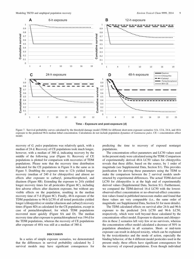
recovery of G. pulex populations was relatively quick, with amedian of 24 d. Recovery of CE populations took much longer,however, with a median of 380 d, indicating recovery by themiddle of the following year (Figure 8). Recovery of CEpopulations is plotted for comparison with recoveries of TDMpopulations. Please note that the recovery time distributionindicated for the CE populations in Figure 8 is the same as inFigure 5. Doubling the exposure time to 12 h yielded longerrecovery (median of 240 d for chlorpyrifos) and almost noeffects after exposure to carbaryl, pentachlorophenol, anddiazinon (Figure 8B). Extending the exposure to 24 h yieldedlonger recovery times for all pesticides (Figure 8C), includingfirst adverse effects after diazinon exposure, but without anyvisible effects on the population, resulting in the medianrecovery time of 5 d (Figure 8C). Finally, 48-h exposure of theTDM populations to 96-h LC50 of all tested pesticides yieldedlonger (chlorpyrifos) or similar (diazinon and carbaryl) recoverytimes (Figure 8D) as calculated for the CE population, except incase of pentachlorophenol, for which TDM populationsrecovered more quickly (Figure 8A and D). The medianrecovery time after exposure to pentachlorophenol was 194 d forthe TDM populations, whereas the recovery of CE populationsafter exposure of 48 h was still at a median of 380 d.

DISCUSSION

In a series of simple exposure scenarios, we demonstratedthat the differences in survival probability calculated by 2survival models may have significant consequences for

predicting the time to recovery of exposed nontargetpopulations.

The concentration–effect parameters and LC50 values usedin the present study were calculated using the TDM. Comparisonof experimentally derived 48-h LC50 values for chlorpyrifosreveals that these differ, based on the source, by 1 order ofmagnitude (see Supplemental Data, Section S1). This providesjustification for deriving these parameters using the TDM tomake the comparison between the 2 survival models unob-structed by experimental differences. The actual TDM-derivedLC50 for chlorpyrifos is at the high end of experimentallyderived values (Supplemental Data, Section S1). Furthermore,we compared the TDM-derived 16-d LC50 with the lowest-observed-effect concentration or no-observed-effect concentra-tion values found in published mesocosm studies and found thatthese values are very comparable (i.e., the same order ofmagnitude; see Supplemental Data, Section S1 for more details).

The TDM calculated effects on survival after 24-h and 96-hexposure to the predicted 24-h LC50 and 96-h LC50,respectively, which were well beyond those calculated by theconcentration–effect model. Exposure to diazinon and chlorpyr-ifos in these 2 scenarios left very few or no survivors, whereasthe concentration–effect model calculated a decrease of 50% inpopulation abundance in all scenarios. Short- or mid-termexposure can result in delayed toxicity, which can be explainedby the toxicokinetics and the mode of action, especially thebinding behavior, of the 4 different model pesticides used in thepresent study; these effects have significant consequences forthe recovery of exposed populations. Even though individual

0

0.1

0.2

0.3

0.4

0.5

0.6

0.7

0.8

0.9

1

1 4 7 10 13 16 19

Cum

ulat

ive

surv

ival

6-h exposure

0

0.1

0.2

0.3

0.4

0.5

0.6

0.7

0.8

0.9

1

1 4 7 10 13 16 19

Cum

ulat

ive

surv

ival

12-h exposure

00.10.20.30.40.50.60.70.80.91

1 4 7 10 13 16 19 22

Cum

ulat

ive

surv

ival

24-h exposure

00.10.20.30.40.50.60.70.80.91

1 4 7 10 13 16 19 22 25

Cum

ulat

ive

surv

ival

48-h exposure DiazinonChlorpyrifosCarbarylPentachlorophenol96-h CE

A B

C D

Time – Exposure and post-exposure (d)

Figure 7. Survival probability curves calculated by the threshold damage model (TDM) for different short-term exposure scenarios: 6-h, 12-h, 24-h, and 48-hexposure to the predicted 96-h median lethal concentration. Calculations do not include population dynamics of Gammarus pulex. CE¼ concentration–effectmodel.

Modeling TKTD and amphipod population recovery Environ Toxicol Chem 9999, 2014 9

survival was extremely low after exposure to diazinon andchlorpyrifos (on average below 100 individuals), we assumed nosublethal effects on reproduction or any transfer of accumulatedpesticides to the offspring. Exposed adults, therefore, producedunexposed offspring ultimately responsible for the persistence ofmodeled populations. The difference in individual survival afterlonger-term exposure to relatively low concentrations of the4 compounds, as calculated by the TDM and concentration–effect model, was much smaller than in previous scenarios,indicating that using the concentration–effect model for mortalityin long-term exposure might be protective for exposed biota.

Because current risk assessment of short-term exposureapplies the 96-h concentration–effect model, we conducted a setof very short exposure duration simulations to compare thepredictions by the 2 survival models to shed light on theprotectiveness of standard practice. We demonstrated that whenexposure duration is relatively short (e.g., shorter than 50% ofthe time span used to derive the concentration–effect relation-ship; see Figures 7 and 8), the concentration–effect modelpredicts lower survival probability (i.e., more mortality) than theTDM as well as longer population recovery times. This indicatesthat the current risk assessment practice of using a 4-d LC50 or2-d LC50 value applied to peaks of very short duration (2 d or 1 dor less) might be protective for biota when mortality is theendpoint of concern.

The differences in toxicity among the 4 tested compoundscannot be assigned to a single TDM parameter, with theexception of pentachlorophenol. This compound has a highrecovery rate (kr), in combination with fast elimination, whichdirectly translates into quick organism recovery, which in turnleads to relatively high survival after the exposure and thereforefaster population recovery. Organism recovery times are aproduct of both toxicokinetic and toxicodynamic processes.

They differ from population recovery times because these arecalculated using the TDM related to 1 endpoint, in our casesurvival, whereas population recovery times combine differentlife-history traits or endpoints of the species. Organism recoverytimes for the TDM are defined as the interval when the internaldamage level falls below 5% of its maximum level after a 24-hpulse that kills 50% of the population after infinite time [41]. TheTDM predicts 28-d organism recovery for diazinon [32], and 25,15, and 3 for chlorpyrifos, carbaryl, and pentachlorophenol,respectively [31]. The TDM for diazinon explicitly simulates thetoxicokinetic process of activation of diazinon to diazoxon,whereas the corresponding process is not simulated forchlorpyrifos, carbaryl, and pentachlorophenol, because infor-mation on biotransformation kinetics became available onlyrecently [42] and has not been integrated into TKTDmodels yet.For diazinon, however, we know that the slow organismrecovery is likely caused by toxicodynamics because thetoxicokinetics, including biotransformation, are fast; that is,diazinon and diazooxon are quickly eliminated from thebody [32]. The mechanistic explanation of the different valuesfor organism recovery for the different pesticides is, thus,uncertain. The overall speed of organism recovery, however, ismore certain, because the toxicodynamic parameters, whichwere fitted to survival time series, compensate for errors in thetoxicokinetic parameters [43].

In theory, the TKTD model parameters can be applied to anyexposure scenario, including very complex scenarios. However,the limits of applicability for TKTD model parameters arecurrently unknown. We assumed in the present study that theTDM parameters are sufficiently robust because the exposurescenarios and concentrations used for model parameterizationare sufficiently similar to the exposure scenarios simulated in thepresent study.

Figure 8. Population recovery times (y-axis) after short-term (6-h, 12-h, 24-h, and 48-h) exposure to the predicted 96-h median lethal concentrations of diazinon,chlorpyrifos, carbaryl, and pentachlorophenol. Recoveries of concentration–effect (CE) populations are equal for all exposure scenarios and are plotted (in gray),for comparison, with recoveries of threshold damage model (TDM) populations. All distributions of recovery times are in boxplots, with denoted median values;boxplot whiskers extend to the full range of values.

10 Environ Toxicol Chem 9999, 2014 N. Galic et al.

Trends in population recovery times closely followed thoseof organism recovery times, where exposure to diazinon andchlorpyrifos yielded severe effects on individual survivalprobability and subsequent long population recovery times,relative to the other 2 tested pesticides. Furthermore, the effectsof delayed toxicity were only calculated by the TDM with clearsuppression of population abundance, resulting in longerrecovery times in short- and mid-term exposure durations.When populations were exposed to the 16-d LC50 for 16 d,however, the differences in recovery times between CE andTDM populations were not as striking. Exposure to relativelylow pesticide concentrations yielded higher individual survivalthan in shorter exposure duration scenarios. The TDM calculatedadverse effects for almost 3 wk after the first day of exposure, inwhich time individual organisms continued reproducing, as wedid not account for any sublethal effects of the pesticides, such aseffects on reproduction, which are included in regulatory chronictests [6]. A combination of higher individual survival andconstant compensation throughout the period of exposure to lowpesticide concentrations yielded similar recovery times of TDMand CE populations.

Populations of G. pulex are considered to have high recoverypotential because of the quick colonization process governed bydrifting individuals [44,45] in natural systems. Liess andSchulz [46], for instance, report a 6-mo recovery time afterthe population, exposed to multiple run-off events, experienceda 50% decrease in abundances. Besides the reproductivepotential by the survivors of the stress, such swift recovery,however, requires proximity of untreated parts of the landscapethat serve as sources of individuals that enhance the populationrecovery process [10,12,14,47]. In the present study, we used theworst-case scenario of a closed or isolated population that wasfully exposed in each scenario. This allowed us to focusexclusively on the comparison of predictions of adverse effectsby the 2 survival models and the consequences for populationrecovery. Our recovery analysis, therefore, predicted relativelylong recovery periods, because in such isolated systems,population recovery is based solely on surviving individualsand their reproductive output [39,48,49]. Finally, the timing ofexposure has direct consequences on recovery of populations inseasonal environments [10], because population growth, andthus recovery potential, is higher in warmer months of the year.In our study, we have therefore chosen a single date (day 150) toallow for a fair comparison of all simulated exposure scenarios.

Modeled control populations of the freshwater amphipodshowed a distinct onset of population growth, or reproductiveactivity, in March and April. Given that the environmentaltemperature acts as a forcing factor for the dynamics of naturalpopulations of most aquatic invertebrates [50,51], the increaseand decline in abundance of the modeled populations arecomparable to those in natural populations (see SupplementalData, Section S2 for comparison of model output with fielddata). Different sizes and shapes of population peaks occurbecause of a change in the age structure of the population, inwhich older, overwintering females produce larger broods andare substituted with younger and smaller females that carrysmaller broods, observed also in natural populations [50,52].Gammarid populations are dependent on leaf litter input andfood limited in late summer in many streams [53], showing aprominent peak in population size in early summer and then asteady decline until autumn. However, the gammarid group hasbeen shown to be much more plastic in their feeding preferencesthan previously thought, including predation and grazing onalgae, in addition to shredding conditioned leaves [54]. Our

model does not currently include population dependency on leaflitter. As straightforward as a comparison of timing of activitywithin 1 yr may be, correctly capturing the microdistribution andspecific densities is much more complicated. Factors such asdiurnal migrations [55], the size of substrate particles [56], andthe presence of refugia [57] have all been shown to play animportant role in population growth and distribution withinhabitats. Even though such detail was beyond the currentmodeling study, our model may be modified when necessary. Agreat strength of individual-based models is their flexibility forincluding additional data when such data exist. Consequently,this inevitably results in models that are highly species- andsystem-specific. The specificity, complexity, and data require-ments are also the main limitations of such a modelingapproach [17].

Possible use of ecological models within the ecological riskassessment of pesticides

The ecosystem services framework is being increasinglydiscussed as a promising way for translating general protectiongoals into manageable and quantifiable objectives [58]. In thisframework, by protecting populations or communities, we maybe protecting the life-sustaining services in the agroecosystem.To this end, more information than just organism survival afterexposure is required. Ecological models are currently the onlytools able to integrate different factors relevant for assessingrisks to populations, communities, and services [15,16,59] andare gaining momentum in the field [60–62].

With the implementation of a TKTD model, we directly linkexposure concentrations and effects on individual survival, withthe advantage that such models can address the consequences oftime-variable exposure for nontarget macroinvertebrate pop-ulations. The parameterization of TKTD models is species andcompound specific; that is, each new chemical must be tested ona new species in a set of experiments. This challenges a broaderuse of these models for the purposes of pesticide risk assessment.Currently, methods are being developed that may facilitate theextrapolation of TKTD parameters between chemicals andspecies [63–65]. Moreover, with some adaptations to currentstudy designs, standard ecotoxicological studies could be mademore useful for the parameterization of TKTD models, forexample, by adding a recovery period after the end of exposureand using a combination of constant and pulsed exposure [66].This would allow the use of TKTD models for an evaluation ofchronic or delayed effects by including nonlethal endpoints [67],which is currently assessed experimentally by the use of long-term or higher-tier studies [2].

Finally, the integration of a TKTD model with an individual-based model allows for assessing lethal effects of time-variableexposure on populations in different climatic regions. Forinstance, the results of different scenarios developed by theForum for Co-Ordination of Pesticide Fate Models and TheirUse (FOCUS) [3], together with the complementing temperatureprofiles, can be straightforwardly integrated for a more realisticrisk assessment of short- and long-term effects on this nontargetmacroinvertebrate. Furthermore, such an assessment mayinclude the contribution of refugia or nonexposed parts of thehabitat [47] for the dynamics of the population in the wholelandscape. Existing data on gammarid movement [44,68] and itscolonization potential [69] enable a spatially explicit assessmentof risk.

The changes in the exposure assessment in the last decaderesulted in very complex and variable exposure profiles. This hasbeen intensively discussed, and the possible role of ecological

Modeling TKTD and amphipod population recovery Environ Toxicol Chem 9999, 2014 11

models to address these time-variable exposure regimens hasbeen identified [1]. The results presented in the present studydemonstrate that the combination of a TKTD model and apopulation model for G. pulex is able to fill the role of anadditional tool for a more realistic and ecologically relevantrisk assessment of pesticides to this nontarget aquaticmacroinvertebrate.

Acknowledgements—We are grateful to the participants of the SETACEurope Technical Workshop MODELINK for fruitful discussions that werereflected in the model development in this manuscript. NG acknowledgesfinancial support from Syngenta and Bayer CropScience for a part of thisstudy, and current support from the Program of Excellence in PopulationBiology, University of Nebraska-Lincoln. RA, AMN and AB werefinancially supported by the European Union under the 7th FrameworkProgramme project Mechanistic Effect Models for Ecological RiskAssessment of Chemicals (CREAM), contract number PITN-GA-2009-238148. We would like to thank three anonymous reviewers who providedhelpful and constructive comments on an earlier version of the manuscript.

SUPPLEMENTAL DATA

Sections S1 and S2. (1.2 MB PDF).

REFERENCES

1. Brock T, Hommen U, Ashauer R, Van den Brink PJ, Caquet T, DucrotV, Lagadic L, Ratte T. 2010. Linking Aquatic Exposure and Effects in theRegistration Procedure of Plant Protection Products. Society ofEnvironmental Toxicology and Chemistry, Boca Raton, FL, USA.

2. Reinert KH, Giddings JM, Judd L. 2002. Effects analysis of time-varying or repeated exposures in aquatic ecological risk assessment ofagrochemicals. Environ Toxicol Chem 21:1977–1992.

3. Forum for Co-Ordination of Pesticide Fate Models and Their Use. 2001.FOCUS surface water scenarios in the EU evaluation process under 91/414/EEC. Brussels, Belgium.

4. European Commission Health & Consumer Protection Directorate-General. 2002. Guidance document on aquatic toxicology in the contextof the Directive 91/414/EEC. Working Document. Sanco/3268/2001.Brussels, Belgium.

5. Schäfer RB, Gerner N, Kefford BJ, Rasmussen JJ, Beketov MA, deZwart D, Liess M, von der Ohe PC. 2013. How to characterize chemicalexposure to predict ecologic effects on aquatic communities? EnvironSci Technol 47:7996–8004.

6. European Commission. 2009. Regulation (EC) No 1107/2009 of theEuropean Parliament and of the Council of 21 October 2009 concerningthe placing of plant protection products on the market and repealingCouncil Directives 79/117/EEC and 91/414/EEC. Official J Eur UnionL309:1–50.

7. Hommen U, Baveco JM, Galic N, Van den Brink PJ. 2010. Potentialapplication of ecological models in the European environmental riskassessment of chemicals I: Review of protection goals in EU directivesand regulations. Integr Environ Assess Manag 6:325–337.

8. Brock TCM, Arts GHP, Maltby L, Van den Brink PJ. 2006. Aquaticrisks of pesticides, ecological protection goals, and common aims inEuropean Union legislation. Integr Environ Assess Manag 2:20–46.

9. Gore J, Kelly J, Yount J. 1990. Application of ecological theory todetermining recovery potential of disturbed lotic ecosystems: Researchneeds and priorities. Environ Manage 14:755–762.

10. Galic N, Baveco H, Hengeveld GM, Thorbek P, Bruns E, Van den BrinkPJ. 2012. Simulating population recovery of an aquatic isopod: Effectsof timing of stress and landscape structure. Environ Pollut 163:91–99.

11. Stark JD, Banks JE, Vargas R. 2004. How risky is risk assessment: Therole that life history strategies play in susceptibility of species to stress.Proc Natl Acad Sci U S A 101:732–736.

12. Lake PS, Bond N, Reich P. 2007. Linking ecological theory with streamrestoration. Freshw Biol 52:597–615.

13. Galic N, Hengeveld GM, Van den Brink PJ, Schmolke A, Thorbek P,Bruns E, Baveco HM. 2013. Persistence of aquatic insects acrossmanaged landscapes: Effects of landscape permeability on re-coloniza-tion and population recovery. PLOS ONE 8:e54584.

14. Devine G, Furlong M. 2007. Insecticide use: Contexts and ecologicalconsequences. Agriculture and Human Values 24:281–306.

15. Forbes VE, Calow P, Sibly RM. 2008. The extrapolation problemand how population modeling can help. Environ Toxicol Chem 27:1987–1994.

16. Forbes VE, Hommen U, Thorbek P, Heimbach F, Van den Brink PJ,Wogram Jr, Thulke H-H, GrimmV. 2009. Ecological models in supportof regulatory risk assessments of pesticides: Developing a strategy forthe future. Integr Environ Assess Manag 5:167–172.

17. Galic N, Hommen U, Baveco JM, Van den Brink PJ. 2010. Potentialapplication of population models in the European ecological riskassessment of chemicals II: Review of models and their potential toaddress environmental protection aims. Integr Environ Assess Manag6:338–360.

18. Maltby L. 1999. Studying stress: The importance of organims-levelresponses. Ecol Appl 9:431–440.

19. Ashauer R, Escher BI. 2010. Advantages of toxicokinetic andtoxicodynamic modelling in aquatic ecotoxicology and risk assessment.J Environ Monit 12:2056–2061.

20. Nyman A-M, Schirmer K, Ashauer R. 2012. Toxicokinetic-toxicody-namic modelling of survival of Gammarus pulex in multiple pulseexposures to propiconazole: Model assumptions, calibration datarequirements and predictive power. Ecotoxicology 21:1828–1840.

21. Ashauer R. 2010. Toxicokinetic–toxicodynamic modelling in anindividual based context: Consequences of parameter variability. EcolModel 221:1325–1328.

22. Jager T, Albert C, Preuss TG, Ashauer R. 2011. General unifiedthreshold model of survival: A toxicokinetic-toxicodynamic frameworkfor ecotoxicology. Environ Sci Technol 45:2529–2540.

23. Ashauer R, Boxall ABA, BrownCD. 2007. New ecotoxicological modelto simulate survival of aquatic invertebrates after exposure to fluctuatingand sequential pulses of pesticides. Environ Sci Technol 41:1480–1486.

24. Welton JS, Clarke RT. 1980. Laboratory studies on the reproduction andgrowth of the amphipod,Gammarus pulex (L). J Anim Ecol 49:581–592.

25. Maltby L, Clayton SA, Wood RM, McLoughlin N. 2002. Evaluation ofthe Gammarus pulex in situ feeding assay as a biomonitor of waterquality: Robustness, responsiveness, and relevance. Environ ToxicolChem 21:361–368.

26. Maltby L. 1995. Sensitivity of the crustaceansGammarus-pulex (L) andAsellus-aquaticus (L) to short-term exposure to hypoxia and unionizedammonia: Observations and possible mechanisms. Water Res 29:781–787.

27. Gerhardt A, Svensson E, ClostermannM, Fridlund B. 1994. Monitoringof behavioral-patterns of aquatic organisms with an impedanceconversion technique. Environ Int 20:209–219.

28. Rubach MN, Baird DJ, Van den Brink PJ. 2010. A new method forranking mode-specific sensitivity of freshwater arthropods to insecti-cides and its relationship to biological traits. Environ Toxicol Chem29:476–487.

29. Kunz PY, Kienle C, Gerhardt A. 2010. Gammarus spp. in aquaticecotoxicology and water quality assessment: Toward integratedmultilevel tests. In Whitacre DM, ed. Reviews of EnvironmentalContamination and Toxicology, Vol 205. Springer, New York, NY,USA, pp 1–76.

30. Ashauer R, Boxall A, Brown C. 2006. Uptake and elimination ofchlorpyrifos and pentachlorophenol into the freshwater amphipodGammarus pulex. Arch Environ Contam Toxicol 51:542–548.

31. Ashauer R, Boxall ABA, Brown CD. 2007. Simulating toxicity ofcarbaryl to Gammarus pulex after sequential pulsed exposure. EnvironSci Technol 41:5528–5534.

32. Ashauer R, Hintermeister A, Caravatti I, Kretschmann A, Escher BI.2010. Toxicokinetic and toxicodynamic modeling explains carry-overtoxicity from exposure to diazinon by slow organism recovery. EnvironSci Technol 44:3963–3971.

33. vanWijngaarden RPA, Brock TCM,Van den Brink PJ. 2005. Thresholdlevels for effects of insecticides in freshwater ecosystems: A review.Ecotoxicology 14:355–380.

34. Laskowski DA. 2002. Physical and chemical properties of pyrethroids.Rev Environ Contam Toxicol 174:49–170.

35. Meijering MPD. 1971. Die Gammarus-Fauna der SchlitzerländerFließgewässer. Archiv für Hydrobiologie 68.

36. Grimm V, Berger U, Bastiansen F, Eliassen S, Ginot V, Giske J, Goss-Custard J, Grand T, Heinz SK, Huse G, Huth A, Jepsen JU, Jørgensen C,Mooij WM, Mâller B, Pe’er G, Piou V, Railsback SF, Robbins AM,RobbinsMM, Rossmanith E, Râger N, Strand E, Souissi S, Stillman RA,Vabø R, Visser U, DeAngelis DL. 2006. A standard protocol fordescribing individual-based and agent-based models. Ecol Model198:115–126.

12 Environ Toxicol Chem 9999, 2014 N. Galic et al.

37. Wilensky U. 1999. NetLogo. Centre for Connected Learning andComputer-Based Modelling, Northwestern University, Evanston, IL,USA.

38. Sutcliffe DW, Carrick TR, Willoughby LG. 1981. Effects of diet, bodysize, age and temperature on growth rates in the amphipod Gammaruspulex. Freshw Biol 11:183–214.

39. Galic N, Baveco JM, Hengeveld GM, Thorbek P, Bruns E, Van denBrink PJ. 2012. Simulating population recovery of an aquatic isopod:Effects of timing of stress and landscape structure. Environ Pollut163:91–99.

40. Niemi G, DeVore P, Detenbeck N, Taylor D, Lima A, Pastor J, Yount J,Naiman R. 1990. Overview of case studies on recovery of aquaticsystems from disturbance. Environ Manage 14:571–587.

41. Ashauer R, Boxall ABA, Brown CD. 2007. Modeling combined effectsof pulsed exposure to carbaryl and chlorpyrifos on Gammarus pulex.Environ Sci Technol 41:5535–5541.

42. Ashauer R, Hintermeister A, O’Connor I, Elumelu M, Hollender J,Escher BI. 2012. Significance of xenobiotic metabolism for bioaccu-mulation kinetics of organic chemicals inGammarus pulex. Environ SciTechnol 46:3498–3508.

43. Hack EC. 2006. Bayesian analysis of physiologically based toxicoki-netic and toxicodynamic models. Toxicology 221:241–248.

44. Elliott JM. 2002. The drift distances and time spent in the drift byfreshwater shrimps, Gammarus pulex, in a small stony stream, and theirimplications for the interpretation of downstream dispersal. Freshw Biol47:1403–1417.

45. Maltby L, Hills L. 2008. Spray drift of pesticides and streammacroinvertebrates: Experimental evidence of impacts and effectivenessof mitigation measures. Environ Pollut 156:1112–1120.

46. Liess M, Schulz R. 1999. Linking insecticide contamination andpopulation response in an agricultural stream. Environ Toxicol Chem18:1948–1955.

47. Brock TCM, Belgers JDM, Roessink I, Cuppen JGM, Maund SJ. 2010.Macroinvertebrate responses to insecticide application between sprayedand adjacent nonsprayed ditch sections of different sizes. EnvironToxicol Chem 29:1994–2008.

48. Trekels H, Van deMeutter F, Stoks R. 2011. Habitat isolation shapes therecovery of aquatic insect communities from a pesticide pulse. J ApplEcol 48:1480–1489.

49. Van den Brink PJ, van Donk E, Gylstra R, Crum SJH, Brock TCM.1995. Effects of chronic low concentrations of the pesticideschlorpyrifos and atrazine in indoor freshwater microcosms. Chemo-sphere 31:3181–3200.

50. Hynes HBN. 1955. The reproductive cycle of some british freshwaterGammaridae. J Anim Ecol 24:352–387.

51. Welton JS. 1979. Life-history and production of the amphipodGammarus pulex in a Dorset chalk stream. Freshw Biol 9:263–275.

52. Franken RJM, Gardeniers JJP, Peeters ETHM. 2007. Secondaryproduction of Gammarus pulex Linnaeus in small temperate streamsthat differ in riparian canopy cover. Fundamental and AppliedLimnology 168:211–219.

53. Gee JHR. 1988. Population dynamics and morphometrics ofGammaruspulexL.: Evidence of seasonal food limitation in a freshwater detritivore.Freshw Biol 19:333–343.

54. Macneil C, Dick JTA, Elwood RW. 1997. The trophic ecology offreshwater Gammarus spp. (Crustacea, Amphipoda): Problems andperspectives concerning the functional feeding group concept. Biol Rev72:349–364.

55. Elliott JM. 2005. Day–night changes in the spatial distribution andhabitat preferences of freshwater shrimps, Gammarus pulex, in a stonystream. Freshw Biol 50:552–566.

56. Adams J, Gee J, Greenwood P, McKelvey S, Perry R. 1987. Factorsaffecting the microdistribution of Gammarus pulex (Amphipoda): Anexperimental study. Freshw Biol 17:307–316.

57. Franken RJM, Batten S, Beijer JAJ, Gardeniers JJP, Scheffer M, PeetersETHM. 2006. Effects of interstitial refugia and current velocity ongrowth of the amphipodGammarus pulexLinnaeus. J N AmBenthol Soc25:656–663.

58. Nienstedt KM, Brock TCM, van Wensem J, Montforts M, Hart A,Aagaard A, Alix A, Boesten J, Bopp SK, Brown C, Capri E, Forbes V,Kopp H, Liess M, Luttik R, Maltby L, Sousa JP, Streissl F, Hardy AR.2012. Development of a framework based on an ecosystem servicesapproach for deriving specific protection goals for environmental riskassessment of pesticides. Sci Total Environ 415:31–38.

59. Galic N, Schmolke A, ForbesV, BavecoH, Van denBrink PJ. 2012. Therole of ecological models in linking ecological risk assessment toecosystem services in agroecosystems. Sci Total Environ 415:93–100.

60. Forbes VE, Calow P. 2012. Promises and problems for the newparadigm for risk assessment and an alternative approach involvingpredictive systems models. Environ Toxicol Chem 31:2663–2671.

61. Forbes VE, Calow P, Grimm V, Hayashi TI, Jager T, Katholm A,Palmqvist A, Pastorok R, Salvito D, Sibly R, Spromberg J, Stark J,Stillman RA. 2011. Adding value to ecological risk assessment withpopulation modeling. Hum Ecol Risk Assess 17:287–299.

62. Thorbek P, Forbes V, Heimbach F, Hommen U, Thulke HH, Van denBrink P, Wogram J, Grimm V, eds. 2009. Ecological Models forRegulatory Risk Assessments of Pesticides: Developing a Strategy forthe Future. Society of Environmental Toxicology and Chemistry andCRC Press, Pensacola, FL, USA.

63. Rubach M, Baird D, Boerwinkel M-C, Maund S, Roessink I, Van denBrink P. 2012. Species traits as predictors for intrinsic sensitivity ofaquatic invertebrates to the insecticide chlorpyrifos. Ecotoxicology21:2088–2101.

64. Rubach M, Crum S, Van den Brink P. 2011. Variability in the dynamicsof mortality and immobility responses of freshwater arthropods exposedto chlorpyrifos. Arch Environ Contam Toxicol 60:708–721.

65. Rubach MN, Ashauer R, Maund SJ, Baird DJ, Van den Brink PJ. 2010.Toxicokinetic variation in 15 freshwater arthropod species exposed tothe insecticide chlorpyrifos. Environ Toxicol Chem 29:2225–2234.

66. Albert C, Ashauer R, Künsch HR, Reichert P. 2012. Bayesianexperimental design for a toxicokinetic–toxicodynamic model. Journalof Statistical Planning and Inference 142:263–275.

67. Ashauer R, Agatz A, Albert C, Ducrot V, Galic N, Hendriks J, Jager T,Kretschmann A, O’Connor I, Rubach MN, Nyman AM, Schmitt W,Stadnicka J, Van den Brink PJ, Preuss TG. 2011. Toxicokinetic-toxicodynamic modeling of quantal and graded sublethal endpoints: Abrief discussion of concepts. Environ Toxicol Chem 30:2519–2524.

68. Elliott JM. 2002. A continuous study of the total drift of freshwatershrimps, Gammarus pulex, in a small stony stream in the English LakeDistrict. Freshw Biol 47:75–86.

69. Elliott JM. 1971. Upstreammovements of benthic invertebrates in a lakedistrict stream. J Anim Ecol 40:235–252.

70. Moenickes S, Schneider AK, Muhle L, Rohe L, Richter O, Suhling F.2011. From population-level effects to individual response: modellingtemperature dependence in Gammarus pulex. J Exp Biol 214:3678–3687.

Modeling TKTD and amphipod population recovery Environ Toxicol Chem 9999, 2014 13