Molecules 2014, 19, 7388-7414; doi:10.3390/molecules19067388

molecules ISSN 1420-3049

www.mdpi.com/journal/molecules

Article

Molecular Classification of Pesticides Including Persistent Organic Pollutants, Phenylurea and Sulphonylurea Herbicides

Francisco Torrens 1,* and Gloria Castellano 2

1 Institut Universitari de Ciència Molecular, Universitat de València, Edifici d’Instituts de Paterna,

P.O. Box 22085, E-46071 València, Spain 2 Facultad de Veterinaria y Ciencias Experimentales, Universidad Católica de Valencia San Vicente

Mártir, Guillem de Castro-94, E-46001 València, Spain; E-Mail: gloria.castellano@ucv.es

* Author to whom correspondence should be addressed; E-Mail: torrens@uv.es;

Tel.: +34-963-544-431; Fax: +34-963-543-274.

Received: 8 April 2014; in revised form: 29 May 2014 / Accepted: 30 May 2014 /

Published: 5 June 2014

Abstract: Pesticide residues in wine were analyzed by liquid chromatography–tandem

mass spectrometry. Retentions are modelled by structure–property relationships. Bioplastic

evolution is an evolutionary perspective conjugating effect of acquired characters and

evolutionary indeterminacy–morphological determination–natural selection principles; its

application to design co-ordination index barely improves correlations. Fractal dimensions

and partition coefficient differentiate pesticides. Classification algorithms are based on

information entropy and its production. Pesticides allow a structural classification by

nonplanarity, and number of O, S, N and Cl atoms and cycles; different behaviours

depend on number of cycles. The novelty of the approach is that the structural parameters

are related to retentions. Classification algorithms are based on information entropy.

When applying procedures to moderate-sized sets, excessive results appear compatible

with data suffering a combinatorial explosion. However, equipartition conjecture selects

criterion resulting from classification between hierarchical trees. Information entropy

permits classifying compounds agreeing with principal component analyses. Periodic

classification shows that pesticides in the same group present similar properties; those

also in equal period, maximum resemblance. The advantage of the classification is to

predict the retentions for molecules not included in the categorization. Classification

extends to phenyl/sulphonylureas and the application will be to predict their retentions.

OPEN ACCESS

Molecules 2014, 19 7389

Keywords: periodic law; periodic property; periodic table; molecular classification

1. Introduction

Twenty-six billion litres of wine were produced worldwide and 24 billion litres, consumed in 2010

according to the International Organization of Vine and Wine. Wine, especially red wine, is rich in

polyphenols (e.g., resveratrol, catechin, epicatechin), which are antioxidants that protect cells from

oxidative damage caused by free radicals. Red-wine antioxidants inhibit cancer development, e.g., that

of prostate cancer. Red-wine consumption presents heart-health benefits. Application of pesticides

(e.g., fungicides, insecticides) to improve grape yields is common. However, pesticides permeate via

the plant tissues and remain in harvested grapes/processed products (e.g., grape juice, wine). Because

pesticides are a source of toxicants that are harmful to human beings it is important to test for their

levels in grapes, juice and wine. Although EU has set maximum residue levels (MRLs) for pesticides

in wine grapes of 0.01–10 mg·kg−1 it has not done so for wine. An EU-wine study revealed that 34 out

of 40 bottles contained at least one pesticide. Average number was >4 pesticides per bottle while the

highest number was 10. Pesticide analysis in red wine is challenging because of the complexity of the

matrix that contains alcohol, organic acids, sugars, phenols and pigments, e.g., anthocyanins.

Traditional red-wine sample preparation methods include liquid–liquid extraction (LLE) with organic

solvents [1,2] and solid-phase extraction (SPE) with reversed-phase C18/polymeric sorbents [3–5].

However, LLE is labour-intensive, consumes large amounts of organic solvents and forms emulsions

making difficult to separate organic/aqueous phases. In contrast, SPE demands more development.

Solid-phase microextraction (SPME) [6,7], hollow-fibre liquid-phase microextraction [8] and stir-bar

sorptive extraction (SBSE) [9] are lesser reproducible. Typical detections incorporate gas

chromatography (GC), GC coupled to mass spectrometry (MS) (GC–MS) and liquid chromatography

coupled to tandem MS (LC–MS–MS).

Quick, easy, cheap, effective, rugged and safe (QuEChERS) is a sample preparation method that

was reported for pesticide-residue determination in vegetables/fruits [10]; it was used for

pesticide/compound analysis in various food, oil and beverage matrices [11–13]; QuEChERS involves

pesticide extraction from a sample with high water content into acetonitrile, with addition of salts to

separate phases and partition the pesticides into the organic layer, which is followed by dispersive SPE

(dSPE) to clean up various matrix co-extractives and achieve mixing of an aliquot of sample extract

with sorbents prepacked in a centrifuge tube. Pesticide determination in red wine was reported [14].

Eight pesticides belonging to the insecticide (methamidophos, diazinone, pyrazophos, chlorpyrifos),

fungicide (carbendazim, thiabendazole, pyrimethanil, cyprodinil, pyrazophos) and parasiticide

(thiabendazole) classes were selected. Their polarities are different. Some are planar (carbendazim,

thiabendazole, pyrimethanil, cyprodinil). Cyprodinil was most usually detected on grapes

with chlorpyrifos, diazinone and methamidophos, frequent. Carbendazim was detected in three out

of six red-wine samples. Occurrence and removal efficiency of pesticides in sewage treatment plants

from Spanish, Mediterranean, Brazilian and other rivers were reviewed [15,16] and reported [17,18].

Transport of organic persistent microcontaminants associated with suspended particulate material in

Molecules 2014, 19 7390

the Ebro River Basin was described [19,20]. Several researchers have reported the quantitative

structure–activity/property relationships (QSAR/QSPR) of pesticides. The Benfenati group modelled

the QSPR of the octanol/water partition coefficient of organometallic substances by optimal SMILES-

based descriptors [21], QSAR of the toxicity of organic substances to Daphnia magna via freeware

CORAL [22], and optimal descriptor as a translator of eclectic data into endpoint prediction and

mutagenicity of fullerene as a mathematical function of conditions [23]. The Roy group modelled

predictive chemometrics and three-dimensional toxicophore mapping of diverse organic chemicals

causing bioluminescent repression of the bacterium genus Pseudomonas [24] and QSAR for toxicity of

ionic liquids to D. magna analyzing aromaticity vs. lipophilicity [25].

The chromatographic retention time was correlated to the stationary and mobile phases of the

system. In earlier publications the free energy of solvation and partition coefficients in methanol–water

binary mixtures were analized [26]. Stationary phase was modelled in size-exclusion chromatography

with binary eluents as a strategy in size-exclusion chromatography [27]. Stationary–mobile phase

distribution coefficient for polystyrene standards was represented [28]. A new chemical index inspired

by plastic evolution was presented [29] and applied to valence-isoelectronic series of aromatics [30].

QSPR of retention times of phenylureas [31,32] and pesticides [33] was described by plastic evolution.

A simple computerized algorithm was proposed to be useful for establishing relationships between

chemical structures and biosignificance [34,35]. Starting point is to use information entropy for pattern

recognition. Entropy is formulated on basis of similarity matrix between two biochemical species. As

entropy is weakly discriminating for classification, the more powerful concepts of entropy production

and equipartition conjecture were introduced [36]. The aim of the present report is to find properties

that distinguish pesticide structures according to retention times. The study applies a chemical index to

pesticides. The goal is index usefulness validation via the capability to distinguish between pesticides,

and interest as a predictive index for retention as compared with fractal dimensions and partition

coefficients. Section 2 illustrates and discusses the results. Section 3 presents the computational

method, including classification algorithm, information entropy, equipartition conjecture of entropy

production and learning procedure. Finally, the last section summarizes our conclusions.

2. Results and Discussion

For pesticides, LC–MS–MS retention times Rt were taken from Wang and Telepchak.

Methamidophos was taken as the reference Rt (Rt°) because of its least Rt (cf. Table 1). Internal

standard (IS) triphenyl phosphate (TPP) was included in the classification. The (Rt–Rt°)/Rt° ratios were

calculated. Molecular fractal dimensions were computed with our program TOPO [37].

Variations of (Rt − Rt°)/Rt° vs. 1-octanol–water partition coefficient and fractal dimension averaged

for nonburied atoms minus molecular fractal dimension D’–D show fit. The regression turns out to be:

Rt − Rto( ) Rt

o = −0.188 + 0.367 log P + 19.6 D′ − D( ) , n = 9, r = 0.973, s = 0.337, F = 53.3

MAPE = 8.77% AEV = 0.0533(1)

where mean absolute percentage error (MAPE) is 8.77% and approximation error variance (AEV),

0.0533. If IS TPP is excluded the results are improved:

Molecules 2014, 19 7391

Rt − Rto( ) Rt

o = −0.229 + 0.420 log P + 19.1 D′ − D( ) , n = 8 r = 0.982 s = 0.295

F = 67.5 , MAPE = 7.17% AEV = 0.0357 (2)

and AEV decays by 33%. When D’ is included in the fit the correlation is bettered:

Rt − Rto( ) Rt

o = −11.6 + 0.272log P + 9.44D′ , n = 8 r = 0.987 s = 0.253 F = 93.2

MAPE = 5.81% AEV = 0.0261 (3)

and AEV drops by 51%. The best quadratic model vs. D’ improves the fit:

Rt − Rto( ) Rt

o = −112 + 151D′ − 49.3D′ 2 , n = 9 r = 0.988 s = 0.224 F = 125.2

MAPE = 5.39% AEV = 0.0234 (4)

and AEV decreases by 56%. If IS TPP is excluded the results are bettered:

Rt − Rto( ) Rt

o = −107 + 144 D′ − 46.7D′ 2 , n = 8 r = 0.989 s = 0.228 F = 114.4

MAPE = 5.84% AEV = 0.0214(5)

and AEV decays by 60%. Model (3) is linear and expected to perform better than Equations (4) and (5)

for extrapolation. However, the latter are nonlinear and could function better than Equation (3) for

intrapolation. Additional fitting parameters were tested: absolute/differential formation enthalpies,

molecular dipole moment, organic solvent/water partition coefficients, free energies of solvation and

water → organic solvent transfer, molecular volume, surface area, globularity, rugosity, hydrophobic,

hydrophilic and total solvent accessible surfaces, and numbers of P and total atoms. However, the

results do not improve Equations (3)–(5).

Table 1. Vector property (cyc123, O0345, NP, S=, N13, Cl3), retention, logP, pKa and

dimensions for pesticides.

Compound Rt

(min) Rt − Rt° (min)

(Rt − Rt°)/Rt° logP pKa D D’

1. Methamidophos C2H8NO2PS <001010> 2.78 0.00 0.00000 −0.779 −0.58 1.235 1.2662. Carbendazim C9H9N3O2 <100010> 6.48 3.70 1.33094 1.52 5.66 1.284 1.3323. Thiabendazole C10H7N3S <110010> 6.91 4.13 1.48561 2.47 3.40 1.288 1.3314. Pyrimethanil C12H13N3 <110010> 10.43 7.65 2.75180 2.558 4.41 1.314 1.4075. Cyprodinil C14H15N3 <110010> 11.44 8.66 3.11511 3.012 4.22 1.344 1.4706. TPP (IS) C18H15O4P <111000> 11.78 9.00 3.23741 4.63 −5 1.394 1.5047. Diazinone C12H21N2O3PS <111100> 11.92 9.14 3.28777 3.766 1.21 1.398 1.5098. Pyrazophos C14H20N3O5PS <111110> 12.24 9.46 3.40288 2.810 −1.37 1.403 1.5059. Chlorpyrifos C9H11NO3PSCl3 <111111> 13.42 10.64 3.82734 5.004 −5.28 1.394 1.494

Pearson correlation coefficient matrix R was calculated between pairs of vector properties <i1, i2, i3,

i4, i5, i6> for nine pesticides. Intercorrelations are illustrated in the partial correlation diagram, which

contains high (r ≥ 0.75), medium (0.50 ≤ r < 0.75), low (0.25 ≤ r < 0.50) and zero (r < 0.25) partial

autocorrelations. Pairs of molecules with higher partial correlations show similar vector property.

However, results should be taken with care, because Entry 9 with constant vector <111111> shows

null standard deviation, causing greatest partial correlations r = 1 with any compound, which is an

artefact. With the equipartition conjecture the upper triangle of R resulted:

Molecules 2014, 19 7392

R =

0.984 0.359 0.109 0.109 0.109 0.203 0.141 0.172 0.156

0.984 0.734 0.734 0.734 0.578 0.516 0.547 0.531

0.984 0.984 0.984 0.828 0.766 0.797 0.781

0.984 0.984 0.828 0.766 0.797 0.781

0.984 0.828 0.766 0.797 0.781

0.984 0.922 0.891 0.875

0.984 0.953 0.938

0.984 0.969

0.984

Some correlations are high, e.g., R3,4 = R3,5 = R4,5 = 0.984. They are illustrated in the partial

correlation diagram, which contains 21 high (cf. Figure 1, red lines), seven medium (orange), one low

(yellow) and seven zero (black) partial correlations. Two out of eight high partial correlations of Entry 9

are corrected: its correlation with Entry 2 is medium and its correlation with Entry 1 is zero partial

correlation. For instance, pesticide 2 (carbendazim) shows medium partial correlations with molecules

3–9 (0.50 ≤ r < 0.75, orange) and low partial correlation with compound 1 (0.25 ≤ r < 0.50, yellow).

The grouping rule in the case with equal weights ak = 0.5 for b1 = 0.93 allows the classes:

C − b1 = (1)(2)(3,4,5)(6)(7,8,9)

Five clusters are obtained with the associated entropy h – R – b1 = 10.70 matching to

<i1,i2,i3,i4,i5,i6> and C − b1 [38–40]; the binary taxonomy (Table 1) separates the classes 1, 2, 3, 4 and

5 with 1, 1, 3, 1 and 3 pesticides, respectively [41]. The planar molecules 3–5 with low retention are

grouped into the same class; nonplanar thiophosphates 7–9 with the greatest retention are aggregated

into the same cluster. Substances belonging to the same grouping appear highly correlated in the

partial correlation diagram (Figure 1). However, C – b1 results should be taken with care because

classes (1), (2) and (6) with only one substance could be outliers. At level b2 with 0.74 ≤ b2 ≤ 0.76, the

set of groupings turns out to be:

C − b2 = (1)(2)(3,4,5,6,7,8,9)

Three clusters result and entropy decays to h – R – b2 = 3.71 going with <i1,i2,i3,i4,i5,i6> and C − b2

dividing classes: 1–3 with 1, 1 and 7 pesticides. Again, nonplanar thiophosphates 7–9 with the greatest

retention are aggregated into the same class. Compounds in the same cluster appear highly correlated

in partial correlation diagram (Figure 1). Notwithstanding, C – b2 results should be taken with caution

because groupings (1) and (2) with a unique compound could be outliers. Table 2 shows comparative

analysis of the set containing 1–9 classes in agreement with partial correlation diagram (Figure 1).

From the previous partial correlation diagram (Figure 1) and set of nine classifications (Table 2), we

suggest splitting the data into three groupings:

(1,2)(3,4,5)(6,7,8,9)

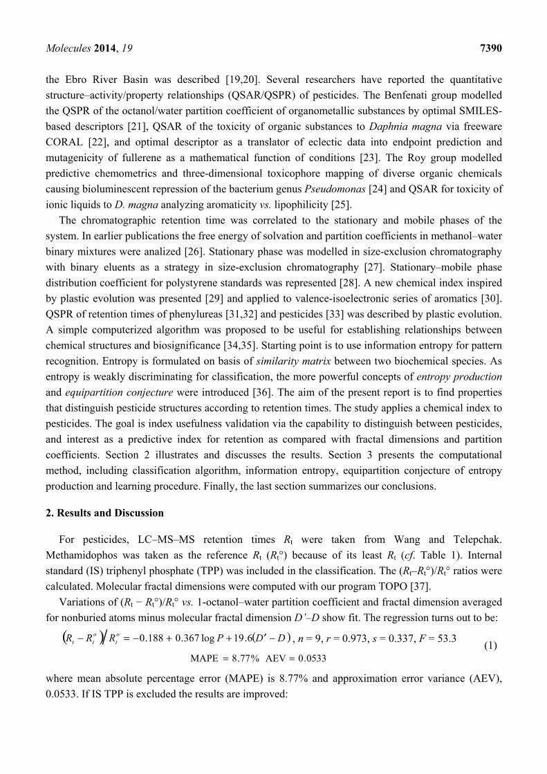
The pesticides dendrogram (cf. Figure 2) shows different behaviour depending on the number of

cyles. One more time, the planar molecules 3–5 with low retention are grouped into the same class and

nonplanar thiophosphates 6–9 with the greatest retention are aggregated into the same cluster.

Molecules 2014, 19 7393

Figure 1. Partial correlation diagram: High (red), medium (orange) and low (yellow)

correlations of pesticides.

Table 2. Classification level, number of classes and entropy for vector property of pesticides.

Classification Level b Number of Classes Entropy h

1.00 9 32.49 0.98 7 20.01 0.96 6 15.13 0.93 5 10.70 0.87 4 6.77 0.76 3 3.71 0.51 2 1.47 0.10 1 0.08

Molecules 2014, 19 7394

Figure 2. Dendrogram of pesticides according, top → bottom, to: (1,2)(3,4,5)(6,7,8,9).

The illustration of the classification above in a radial tree (cf. Figure 3) shows the different

behaviour of the pesticides depending on the number of cyles. The same classes above are recognized,

in qualitative agreement with partial correlation diagram and dendrogram (Figures 1 and 2). One more

time, planar molecules 3–5 with low retention are grouped into the same class, and nonplanar

thiophosphates 6–9 with the greatest retention are aggregated into identical cluster.

Methamidophos

Carbendazim

Thiabendazole

Pyrimethanil

Cyprodinil

TPP

Diazinone

Pyazophos

Chlorpyrifos

Molecules 2014, 19 7395

Figure 3. Radial tree of pesticides according, from top to bottom, to: (1,2)(3,4,5)(6,7,8,9).

Program SplitsTree allows examining cluster analysis (CA) data [42]. Based on split decomposition

it takes as input a distance matrix and produces as output a graph, which represents relations between

taxa. For ideal data the graph is a tree whereas less ideal data will give rise to a tree-like net, which is

interpreted as possible evidence for conflicting data. As split decomposition does not attempt to force

Molecules 2014, 19 7396

data on to a tree it can provide a good indication of how tree-like are given data. In the splits graph for

nine pesticides (cf. Figure 4), points 4 and 5 are superimposed on 3, and 9 on 8. It reveals conflicting

relationship between class 1, and groupings 2 and 3 because of interdependences. It indicates spurious

relation resulting from base-composition effects. It shows different pesticides behaviour depending on

number of cycles in agreement with partial correlation diagram, binary and radial trees (Figures 1–3).

Figure 4. Splits graph of pesticides according, top → bottom, to: (1,2)(3,4,5)(6,7,8,9).

In QSPR, the data file contains less than 100 objects and thousands of X-variables. So many

X-variables exist that no one can discover by inspection patterns, trends, clusters, etc. in objects.

Principal components analysis (PCA) is a technique useful to summarize all information contained in

X-matrix and put it understandable [43–48]. The PCA works decomposing X-matrix as the product of

two smaller matrices P and T. Loading matrix (P) with information about the variables contains few

vectors, the principal components (PCs), which are obtained as linear combinations of the original

X-variables. In the score matrix (T) with information about objects, every object is described in terms

of the projections on to PCs instead of the original variables: X = TP’ + E, where ’ denotes the

transpose matrix. The information not contained in the matrices remains as unexplained X-variance in

the residual matrix (E). Every PCi is a new co-ordinate expressed as linear combination of old features

xj: PCi = ∑jbijxj. The new co-ordinates PCi are named scores/factors while the coefficients bij are called

loadings. The scores are ordered according to their information content with regard to the total

variance among all objects. Score–score plots show positions of compounds in the new co-ordinate

system while loading–loading plots indicate the locations of the features that represent the compounds

Pesticide.nex

Fit=104.5 ntax=9

2

7

1

3,4,5

6

9

8

0.1

Molecules 2014, 19 7397

in the new co-ordinates. The PCs present two interesting properties. (1) They are extracted in decaying

order of importance. First PC F1 always contains more information than the second F2 does, F2 more

than the third F3, etc. (2) Every PC is orthogonal to one another. There is no correlation between the

information contained in different PCs. A PCA was performed for the vector properties. The

importance of PCA factors F1–F6 for {i1,i2,i3,i4,i5,i6} is collected in Table 3. The use of the first factor

F1 explains 39% of variance (61% error), combined application of two factors F1/2 accounts for 66% of

variance (34% error), utilization of factors F1–3 justifies 87% of variance (13% error), etc.

Table 3. Importance of the principal component analysis factors for vector property

of pesticides.

Factor Eigenvalue Percentage of Variance Cumulative Percentage of Variance

F1 2.33109829 38.85 38.85 F2 1.62998318 27.17 66.02 F3 1.25482746 20.91 86.93 F4 0.38517751 6.42 93.35 F5 0.33518718 5.59 98.94 F6 0.06372637 1.06 100.00

The PCA factor loadings are shown in Table 4.

Table 4. Principal component analysis loadings for the vector property of pesticides.

Property PCA Factor Loadings a

F1 F2 F3 F4 F1 F6

i1 0.30822766 0.64474701 0.02673332 −0.04594797 0.50138891 −0.48485077 i2 0.44804795 0.45046774 −0.05731613 0.08927231 −0.76002034 0.08629170 i3 0.40956062 −0.56947041 −0.18574529 0.04102918 −0.15327503 −0.66954134 i4 0.55772042 −0.17916516 0.17892539 0.59525799 0.32511366 0.40595876 i5 −0.31588577 0.04253838 0.72852310 0.44514023 −0.20425092 −0.35748077 i6 0.35450381 −0.15222972 0.63145758 −0.66011661 0.00822715 0.12881324

a Loadings greater than 0.7 are boldfaced.

The PCA F1–F3 profile for the vector property is listed in Table 5. For F1, variable i4 shows the

greatest weight in the profile; however, F1 cannot be reduced to two variables {i2,i4} without 49%

error. For F2, variable i1 presents the greatest weight; notwithstanding, F2 cannot be reduced to

two variables {i1,i3} without 26% error. For F3, variable i5 displays the greatest weight; nevertheless,

F3 cannot be reduced to two variables {i5,i6} without 7% error. For F4, variable i6 exhibits the greatest

weight; however, F4 cannot be reduced to two variables {i4,i6} without 21% error. For F5, variable i2

reveals the greatest weight; notwithstanding, F5 cannot be reduced to two variables {i1,i2} without 17%

error. For F6, variable i3 bares the greatest weight; nevertheless, F6 cannot be reduced to two variables

{i1,i3} without 32% error. Factors F1–6 can be considered as the linear combinations of {i2,i4}, {i1,i3},

{i5,i6}, {i4,i6}, {i1,i2} and {i1,i3} with 49%, 26%, 7%, 21%, 17% and 32% errors.

Molecules 2014, 19 7398

Table 5. Profile of the principal component analysis factors for the vector property

of pesticides.

Percentage of i1 a % of i2 % of i3 % of i4 % of i5 % of i6

F1 9.50 20.07 16.77 31.11 9.98 12.57 F2 41.57 20.29 32.43 3.21 0.18 2.32 F3 0.07 0.33 3.45 3.20 53.07 39.87 F4 0.21 0.80 0.17 35.43 19.81 43.58 F5 25.14 57.76 2.35 10.57 4.17 0.01 F6 23.51 0.74 44.83 16.48 12.78 1.66

a Percentages greater than 50% are boldfaced.

In PCA F2–F1 scores plot (cf. Figure 5), points 4 and 5 appear superimposed on 3. It shows different

behaviour depending on number of cyles. It distinguishes three clusters: class 1 (two molecules,

F1 < F2, left), grouping 2 (three compounds, F1 << F2, top) and cluster 3 (four units, F1 >> F2, right).

Figure 5. F2 versus F1 scores plot of the principal component analysis for the pesticides.

From PCA factor loadings of pesticides, F2–F1 loadings plot (cf. Figure 6) depicts the six

properties. In addition as a complement to the scores plot (Figure 5) for the loadings (Figure 6), it is

confirmed that pesticide 2 located on the left side presents a contribution of cyc123 situated near the

same side of Figure 5. Class 2 on the top shows more pronounced contribution of O0345 placed in the

same position (Figure 6). Two classes of properties are clearly distinguished in the loadings plot: class

1 {cyc123,O0345,N13} (F1 < F2, top) and grouping 2 {NP,S=,Cl3} (F1 >> F2, bottom).

-2

-1

0

1

F2

-1 0 1

F1

Class 3

Class 2

Class 1

1

2

3,4,5

6

7

8

9

Molecules 2014, 19 7399

Figure 6. F2 versus F1 loadings plot of the principal component analysis for the pesticides.

Instead of nine pesticides in the ℜ6 space of six vector properties, consider six properties in the ℜ9

space of nine molecules. The upper triangle of matrix R between pairs of properties resulted in:

R =

0.998 0.748 0.029 0.514 0.475 0.502

0.998 0.279 0.764 0.225 0.752

0.998 0.482 0.506 0.471

0.998 0.021 0.986

0.998 0.025

0.998

Correlations are high, e.g., R4,6 = 0.986. Properties dendrogram (cf. Figure 7) separates cyc123 and

O0345 from N13 (class 1), and Cl3 from NP/S= (cluster 2) in agreement with PCA loadings plot (Figure 6).

The radial tree for the vector properties (cf. Figure 8) separates the same two classes as PCA

loadings plot and dendrogram (Figures 6 and 7). Splits graph for properties (cf. Figure 9) reveals

conflicting relation between classes because of interdependences. It is in agreement with PCA loadings

plot and binary/radial trees (Figures 6–8).

A PCA was performed for the vector properties. Factor F1 explains 50% of variance (50% error),

factors F1/2 account for 69% of variance (31% error), factors F1–3 rationalize 82% of variance (18%

error), etc. In PCA F2–F1 scores plot, the same two groupings of properties are distinguished: class 1

{cyc123,O0345,N13} (F1 >> F2, cf. Figure 10, right) and grouping 2 {NP,S=,Cl3} (F1 << F2, left) in

qualitative agreement with PCA loadings plot, binary/radial trees and splits graph (Figures 6–9).

-0.5

0

0.5

F2

-0.2 0 0.2 0.4 0.6

F1

Class 2

Class 1

N13

cycle123

O0345

Cl3

S=

nonplanarity

Molecules 2014, 19 7400

Figure 7. Dendrogram for the vector properties corresponding to the pesticides.

Figure 8. Radial tree for the vector properties corresponding to the pesticides.

Molecules 2014, 19 7401

Figure 9. Splits graph for the vector properties corresponding to the pesticides.

Figure 10. PCA F2 vs. F1 scores plot for the vector properties corresponding to pesticides.

The recommended format of the pesticides periodic table (PT, cf. Table 6) shows that they are

classified first by i1, i2, i3, i4, i5 and, finally, by i6. Vertical groups are defined by <i1,i2,i3,i4,i5> and

horizontal periods, by <i6>. Periods of eight units are assumed; e.g., group g00101 stands for

<i1,i2,i3,i4,i5> = <00101>: <001010> (cyc0,O2,NP,S=0,N1,Cl0), etc. Pesticides in the same column

appear close in partial correlation diagram, binary/radial trees, splits graph and PCA scores (Figures 1–5).

Pesticide2.nex

Fit=83.9 ntax=6

O0345

N13S_double_bond

Cl3

nonplanarity

cycle1230.1

-1

0

1

F2

-1 -0.5 0 0.5

F1

Class 2

Class 1

cycle123

O0345

N13

Cl3

S=

nonplanarity

Molecules 2014, 19 7402

Phenylurea herbicides were determined in tap water/soft drink samples by HPLC–UV [49]. Table 6

includes five phenylureas: metazachlor is similar to carbendazim. Can et al. determined

sulphonyl/phenylurea herbicides toxicities [50]. Table 6 includes 27 sulphonyl/phenylurea herbicides:

(1) phenylureas are similar to metoxuron, monuron, diuron and linuron; (2) sulphonylureas

flazasulphuron, triasulphuron, azimsulphuron and chlorsulphuron go with TPP. High-resolution and

ultratrace analyses of pesticides were reported via silica (SiO2) monoliths [51]. Table 6 takes in six

new pesticides: (1) metamitron and phenylurea isoproturon match metoxuron; (2) metolachlor goes

with carbendazim; (3) carbofuran agrees with thiabendazole. Qualitative LC–MS analysis of pesticides

was informed via monolithic SiO2 capillaries [52]. Table 6 contains two novel pesticides: phenylurea

pencycuron tallies metamitron. Analytical standards were provided for persistent organic pollutants

(POPs) [53]. Table 6 embraces five POPs: lindane and pentachlorobenzene equal carbetamide

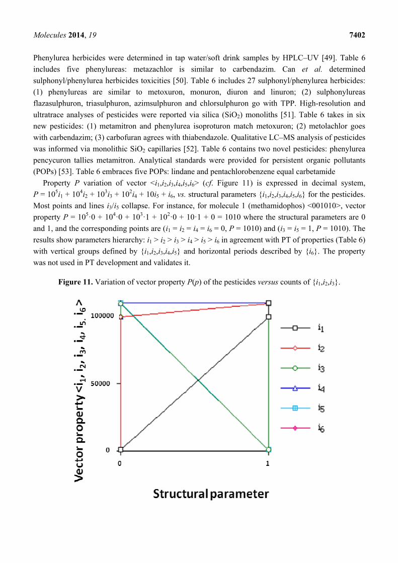
Property P variation of vector <i1,i2,i3,i4,i5,i6> (cf. Figure 11) is expressed in decimal system,

P = 105i1 + 104i2 + 103i3 + 102i4 + 10i5 + i6, vs. structural parameters {i1,i2,i3,i4,i5,i6} for the pesticides.

Most points and lines i3/i5 collapse. For instance, for molecule 1 (methamidophos) <001010>, vector

property P = 105·0 + 104·0 + 103·1 + 102·0 + 10·1 + 0 = 1010 where the structural parameters are 0

and 1, and the corresponding points are (i1 = i2 = i4 = i6 = 0, P = 1010) and (i3 = i5 = 1, P = 1010). The

results show parameters hierarchy: i1 > i2 > i3 > i4 > i5 > i6 in agreement with PT of properties (Table 6)

with vertical groups defined by {i1,i2,i3,i4,i5} and horizontal periods described by {i6}. The property

was not used in PT development and validates it.

Figure 11. Variation of vector property P(p) of the pesticides versus counts of {i1,i2,i3}.

Molecules 2014, 19 7403

Table 6. Table of periodic properties for pesticides, persistent organic pollutants, phenylureas and sulphonylureas.

P. g00100 g00101 g01100 g10000 g10001 g10100 g11000 g11001 g11100 g11110 g11111

p0 Chlordecone ** Methamidophos PFOS **

Metamitron *

BDE-99 **

Metoxuron

Monuron

Diuron

Linuron

Buturon

Chlorotoluron

Daimuron

Fenuron

Methyldimuron

Fluometuron

Siduron

Neburon

Isoproturon

Pencycuron

Carbendazim

Metolachlor *

Metazachlor

AMS

BSM

CME

CNS

EMS

MSM

NCS

OXS

PSE

TFS

TBM

TFO

3FS

RMS

IDS

Carbetamide *

Prometryne *

Lindane **

PCB **

Thiabendazole

Pyrimethanil

Cyprodinil

Carbofuran *

TPP

Flazasulphuron

Triasulphuron

Azimsulphuron

Chlorsulphuron

Diazinone Pyrazophos

p1 Chlorfenvinphos ** Chlorpyrifos

PFOS: perfluoroctane sulphonate. BDE-99: 2,2',4,4',5-pentabromodiphenylether. AMS: amidosulphuron. BSM: bensulphuron-methyl. CME: Chlorimuron-ethyl. CNS: Cinosulphuron. EMS:

ethametsulphuron-methyl. MSM: metsulphuron-methyl. NCS: nicosulphuron. OXS: oxasulphuron. PSE: pyrazosulphuron-ethyl. TFS: Thifensulphuron-methyl. TBM: Tribenuron-methyl.

TFO: Trifloxysulphuron-Na. 3FS: triflusulphuron-methyl. RMS: rimsulphuron. IDS: iodosulphuron. PCB: pentachlorobenzene. Regular typeface: pesticides (this work). Regular typeface *:

pesticides taken from Ref. [51]. Regular typeface **: persistent organic pollutants. Italics: phenylureas. Bold: sulphonylureas.

Molecules 2014, 19 7404

Property P change of vector <i1,i2,i3,i4,i5,i6> in base 10 (cf. Figure 12) is represented vs. number of

group in PT, for pesticides (Table 1 subset of Table 6). It reveals minima corresponding to compounds

with <i1,i2,i3,i4,i5> ca. <00101> (group g00101) and maxima with <i1,i2,i3,i4,i5> ca. <11111> (group

g11111). For group 6, period 2 is superimposed on 1. For instance, for group g001010 and period p0,

molecule 1 (methamidophos) <001010> lies in the first group in the subset with P = 1010 and the point

is (group = 1, P = 1010). Periods p0 and p1 represent rows 1 and 2, respectively, in Table 6. Function

P(i1,i2,i3,i4,i5,i6) denotes two periodic waves clearly limited by two maxima, which suggest a periodic

behaviour that recalls form of a trigonometric function. For <i1,i2,i3,i4,i5,i6>, a maximum is shown.

Distance in <i1,i2,i3,i4,i5,i6> units between each pair of consecutive maxima is six, which coincides with

pesticide sets in successive periods. The maxima occupy analogous positions and are in phase. The

representative points in phase should correspond to elements in the same group in PT. For both

maxima, <i1,i2,i3,i4,i5,i6> some coherence exists between two representations; however, the consistency

is not general. Waves comparison shows two differences: period 1 is somewhat step-like and period 2

is incomplete. The most characteristic points are maxima, which lie about group g11111. The values of

<i1,i2,i3,i4,i5,i6> are repeated as the periodic law (PL) states.

Figure 12. Variation of the vector property P(p) of the pesticides versus group number.

An empirical function P(p) reproduces the different <i1,i2,i3,i4,i5,i6> values. The minimum of P(p)

has meaning only if it is compared with former P(p – 1) and later P(p + 1) points needing to fulfill:

Pmin p( )< P p − 1( )

Pmin p( )< P p + 1( ) (6)

The order relations (6) should repeat at determined intervals equal to period size and are equivalent to: ( ) ( ) 01min <−− pPpP

P p + 1( )− Pmin p( ) > 0 (7)

Molecules 2014, 19 7405

As relations (7) are valid only for minima, more general ones are desired for all values of p.

Differences D(p) = P(p + 1) − P(p) are calculated assigning every value to pesticide p:

D p( )= P p + 1( )− P p( ) (8)

Instead of D(p), R(p) = P(p + 1)/P(p) is taken, assigning them to pesticide p. If PL were general,

elements in the same group in analogous positions in different periodic waves would satisfy:

either D p( )> 0 or D p( )< 0 (9)

and either R p( )> 1 or R p( )< 1 (10)

However, the results show that this is not the case so that PL is not general, existing some

anomalies; e.g., D(p) variation vs. group number (cf. Figure 13) presents lack of coherence between

<i1,i2,i3,i4,i5,i6> Cartesian and PT representations. For instance, for group g001010 and period p0,

pesticide 1 (methamidophos) <001010> (group = 1, P = 1010) presents, in the next PT position,

molecule 2 (carbendazim) <100010> (g100010, group = 2, P = 100010), D = 100010 − 1010 = 99000

and the point is (group = 1, D = 99000). If consistency were rigorous, all points in each period would

have the same sign. In general, a trend exists in points to give D(p) > 0, especially for lower groups.

Figure 13. Variation of property D(p) = P(p + 1) − P(p) versus group. P: vector property.

The change of R(p) vs. group number (cf. Figure 14) confirms the lack of constancy between

Cartesian and PT charts. For instance, for group g001010 and period p0, pesticide 1 (methamidophos)

<001010> (group = 1, P = 1010) shows, in the next PT cell, molecule 2 (carbendazim) <100010>

(g100010, group = 2, P = 100010), R = 100010/1010 = 99.0198 and the point is (group = 1,

R = 99.0198). If the steadiness were exact, all points in each period would show R(p) either lesser or

greater than one. A trend exists to give R(p) > 1, especially for the lower groups.

Molecules 2014, 19 7406

Figure 14. Variation of property R(p) = P(p + 1)/P(p) vs. group number. P: vector property.

3. Experimental

The key problem in classification studies is to define similarity indices when several criteria of

comparison are involved. The first step in quantifying similarity concept for pesticides is to list the

most important chemical characteristics of molecules. The vector of properties i = <i1,i2,…ik,…>

should be associated with every pesticide i, whose components correspond to different molecular

features in a hierarchical order according to their expected importance in retention. If characteristic

m-th is chromatographically more significant for retention than k-th then m < k. Components ik are

either “1” or “0”, according to whether a similar characteristic of rank k is either present or absent in

pesticide i compared to a reference. Analysis includes six structural and constitutional characteristics:

presence of cycle (cyc123), occurrence of either none or 3–5 O atoms (O0345), nonplanarity (NP),

double-bonded S atom (S=), incidence of either one or three N atoms (N13) and existence of three Cl

atoms (Cl3, cf. Figure 15). It is assumed that the chemical characteristics can be ranked according to

their contribution to retention in the following order of decaying importance: cyc123 > O0345 > NP > S=

> N13 > Cl3. Index i1 = 1 denotes cyc123 (i1 = 0 for cyc0), i2 = 1 means O0345 (i2 = 0 for O2), i3 = 1

signifies NP, i4 = 1 indicates S=, i5 = 1 stands for N13 (i5 = 0 for N0 or N2) and i6 = 1 represents

Cl3 (i6 = 0 for Cl0). In chlorpyrifos number of cycles is one, O is three, it is NP and S=, number of N is

one and number of Cl atoms is three; obviously its associated vector is <111111>. In this study

chlorpyrifos was selected as reference because of its greatest retention. Table 1 contains vectors

associated with nine pesticides. Vector <001010> is associated with methamidophos since it shows

cyc0, O2, NP, not S=, N1 and Cl0.

Molecules 2014, 19 7407

Let us denote by rij (0 ≤ rij ≤ 1) similarity index of two pesticides associated with vectors i and j ,

respectively. Similitude relation is characterized by similarity matrix R = [rij]. Similarity index

between two pesticides i = <i1,i2,…ik…> and j = <j1,j2,…jk…> is defined as:

rij = tk ak( )k

k (k = 1,2,…) (11)

where 0 ≤ ak ≤ 1 and tk = 1 if ik = jk but tk = 0 if ik ≠ jk. Definition assigns a weight (ak)k to any property

involved in description of molecule i or j.

Figure 15. Pesticides: (a) methamidophos, (b) carbendazim, (c) thiabendazole,

(d) pyrimethanil, (e) cyprodinil, (f) diazinone, (g) pyrazophos and (h) chlorpyrifos.

3.1. Classification Algorithm

Grouping algorithm uses the stabilized similarity matrix by applying max–min composition rule o:

R oS( )ij = max k mink rik ,skj( )[ ] (12)

P

O

NH2

OS

CH3H3C

N

HN

NH

OCH3

O

N

HN

N

S

N

N

NH

N

NHNH3C

N N

OP

O

O

S

N

N

H3C

O

O

H2C

H3CN

O

P

O

OS CH2

CH3

H2C

CH3

N

Cl

Cl

Cl

OP

SO

O

a

b

c d

e

f

g

h

Molecules 2014, 19 7408

where R = [rij] and S = [sij] are matrices of equal type and (RoS)ij is the (i,j)-th element of matrix

RoS [54–57]. When applying composition rule max–min iteratively so that R(n + 1) = R(n) o R, an

integer n exists such that: R(n) = R(n + 1) = … Matrix R(n) is called stabilized similarity matrix. Its

importance lies in fact that in classification it generates partition into disjoint classes. Stabilized matrix

is designated by R(n) = [rij(n)]. Grouping rule follows: i and j are assigned to the same class if rij(n) ≥ b.

Class of i noted i is set of species j that satisfies rule: rij(n) ≥ b. Matrix of classes is:

R n( ) =

r i j [ ]= max s,t rst( ) (s ∈

i , t ∈

j ) (13)

where s stands for any index of species belonging to class i (similarly for t and

j ). Rule (13) means

finding largest similarity index between species of two different classes.

3.2. Information Entropy

In information theory, information entropy h measures the surprise that source emitting sequences,

e.g., cannon-shots, can give [58,59]. Consider use of qualitative spot test to determine the presence of

Fe in a water sample. Without any history of testing the analyst must begin by assuming that the two

outcomes 0/1 (Fe absent/present) are equiprobable with probabilities 1/2. When up to two metals may

be present in sample, e.g., Fe or Ni, four possible outcomes exist, ranging from neither (0,0) to both

present (1,1) with equal probabilities 1/4. Which of four possibilities turns up can be determined via

two tests each having two observable states. Similarly with three elements eight possibilities exist each

with probability of 1/8 = 1/23; three tests are needed. Pattern relates uncertainty and information

needed to resolve it. Number of possibilities is expressed to power of 2. Power to which 2 must be

raised to give number of possibilities N is defined as logarithm to base 2 of that number.

Information/uncertainty can be defined in terms of logarithm to base 2 of number of possible analytical

outcomes: I = H = log2 N = log2 1/p = –log2 p, where I is information contained in answer given that N

possibilities existed, H, initial uncertainty resulting from need to consider N possibilities and p,

probability of each outcome if all N possibilities are equally likely to occur. The expression is

generalized to a situation in which the probability of every outcome is unequal. If one knows from past

experience that some elements are more likely to be present than others, the equation is adjusted so that

logarithms of individual probabilities suitable weighted are summed: H = – Σ pi log2 pi, where Σ pi = 1.

Consider original example except that now past experience showed that 90% of samples contained no

Fe. Degree of uncertainty is calculated using: H = –(0.9 log2 0.9 + 0.1 log2 0.1) = 0.469 bits. For a

single event occurring with probability p degree of surprise is proportional to −ln p. Generalizing result

to random variable X (which can take N possible values x1, …, xN with probabilities p1, …, pN) average

surprise received on learning X value is: – Σ pi ln pi. Information entropy associated with similarity

matrix R is:

h R( ) = − rij ln riji , j − 1 − rij( )ln 1− rij( )

i, j (14)

Denote by Cb set of classes and by R b similarity matrix at grouping level b. Information entropy

satisfies following properties. (1) h(R) = 0 if either rij = 0 or rij = 1; (2) h(R) is maximum if rij = 0.5,

Molecules 2014, 19 7409

i.e., when imprecision is maximum; (3) ( ) ( )RR hh b ≤ for any b, i.e., classification leads to entropy

loss; (4) hR b1( )≤ h

R b2

( ) if b1 < b2, i.e., entropy is monotone function of grouping level b.

3.3. Equipartition Conjecture of Entropy Production

In classification algorithm every hierarchical tree corresponds to entropy dependence on grouping

level and diagram h − b is obtained. Tondeur and Kvaalen equipartition conjecture of entropy

production is proposed as selection criterion among hierarchical trees. According to conjecture for

given charge, dendrogram (binary tree) with best configuration is that in which entropy production is

most uniformly distributed. One proceeds by analogy using information instead of thermodynamic

one. Equipartition implies linear dependence so that equipartition line results:

heqp = hmax b (15)

Since classification is discrete, way of expressing equipartition would be regular staircase function.

Best variant is chosen to be that minimizing sum of squares of deviations:

SS = h − heqp( )2

bi

(16)

3.4. Learning Procedure

Learning procedures were implemented similar to those encountered in stochastic methods [60].

Consider a given partition into classes as good from practical observations, which corresponds to

reference similarity matrix S = [sij] obtained for equal weights a1 = a2 = … = a and for an arbitrary

number of fictious properties. Next consider the same set of species as in the good classification and

actual properties. Degree of similarity rij is computed with Equation (11) giving matrix R. Number of

properties for R and S differs. Learning procedure consists in finding classification results for R as

close as possible to good classification. First weight a1 is taken constant and only following weights a2,

a3,… are subjected to random variations. New similarity matrix is obtained using Equation (11) and

new weights. Distance between partitions into classes characterized by R and S is:

D = − 1 − rij( )ln1 − rij

1− sijij − rij ln

rij

sijij ∀0 ≤ rij , sij ≤ 1( )

(17)

Definition was suggested by that introduced in information theory to measure distance between two

probability distributions [61]. In the present case it is distance between matrices R and S. Since for

every matrix a corresponding classification exists two classifications will be compared by distance,

which is nonnegative quantity that approaches zero as resemblance between R and S increases. The

algorithm result is a set of weights allowing classification. The procedure was applied to the synthesis

of complex dendrograms using information entropy [62–65]. Our program MolClas is simple, reliable,

efficient and fast procedure for molecular classification, based on equipartition conjecture of entropy

production according to Equations (11)–(17); it reads number of properties and molecular properties; it

allows optimization of coefficients; it optionally reads starting coefficients and number of iteration

cycles. Correlation matrix can be either calculated by program or read from input file. The MolClas

calculates property similarity matrix in symmetric storage mode; it applies graphical correlation model

Molecules 2014, 19 7410

for partial correlation diagram; it computes classifications, calculates distances between clusters,

computes groupings similarity matrices, works out classifications information entropy, optimizes

coefficients, performs single/complete-linkage hierarchical cluster analyses and plots cluster diagrams;

it was written not only to analyze the equipartition conjecture of entropy production but also to explore

the world of molecular classification.

4. Conclusions

From the present results and discussion the following conclusions can be drawn:

(1) The objective was to develop a structure–property relation for qualitative and quantitative

prediction of chromatographic retention times of pesticides. Results of the present work

contribute to relation prediction of pesticide residues, in food and environmental samples.

Code TOPO allows fractal dimensions, and SCAP, solvation free energies and partition

coefficient, which show that for a given atom energies and partitions are sensitive to the

presence in the molecule of other atoms and functional groups. Fractal dimensions,

partition coefficient, etc. differentiated pesticides. Parameters needed for co-ordination

index are molar formation enthalpy, molecular weight and surface area. The morphological

and co-ordination indices barely improved equations. Correlation between molecular area

and weight points not only to a homogeneous molecular structure of pesticides,

but also to the ability to predict and tailor their properties; the latter is nontrivial in

environmental toxicology.

(2) Several criteria selected to reduce the analysis to a manageable quantity of pesticides,

referred to structural and constituent characteristics related to nonplanarity, and the number

of rings, and O, double-bonded S, N and Cl atoms. Classification was in agreement with

the principal component analyses. Program MolClas is a simple, reliable, efficient and fast

procedure for molecular classification based on equipartition conjecture of entropy

production. It was written to analyze equipartition conjecture of entropy production and

explore molecular-classification world.

(3) Periodic law does not satisfy physics-law status: (a) pesticides retentions are not repeated;

perhaps chemical character; (b) order relations are repeated with exceptions. Analysis

forces statement: Relations that any compound p has with its neighbour, p + 1, are

approximately repeated for each period. Periodicity is not general; however, if substance

natural order is accepted law must be phenomenological. Retention is not used in periodic-

table generation and serves to validate it. The analysis of other properties would give an

insight into the possible generality of the periodic table. The periodic classification was

extended to phenylureas and sulphonylureas.

Acknowledgments

This work was funded by the own resources of our universities.

Molecules 2014, 19 7411

Author Contributions

Both authors designed and performed research, and analyzed the data; FT wrote the report. Both

authors read and approved the final manuscript.

Conflicts of Interest

The authors declare no conflict of interest.

References

1. De Melo Abreu, S.; Caboni, P.; Cabras, P.; Garau, V.L.; Alves, A. Validation and global

uncertainty of a liquid chromatographic with diode array detection method for the screening of

azoxystrobin, kresoxim-methyl, trifloxystrobin, famoxadone, pyraclostrobin and fenamidone in

grapes and wine. Anal. Chim. Acta 2006, 291, 573–574.

2. Oliva, J.; Navarro, S.; Barba, A.; Navarro, G. Determination of chlorpyrifos, penconazole,

fenarimol, vinclozolin and metalaxyl in grapes, must and wine by on-line microextraction and gas

chromatography. J. Chromatogr. A 1999, 833, 43–51.

3. Jiménez, J.J.; Bernal, J.L.; del Nozal, M.J.; Toribio, L.; Arias, E. Analysis of pesticide residues

in wine by solid-phase extraction and gas chromatography with electron capture and

nitrogen–phosphorus detection. J. Chromatogr. A 2001, 919, 147–156.

4. Wang, J.F.; Luan, L.; Wang, Z.Q.; Jiang, S.R.; Pan, C.P. Determination of 19 multi-residue

pesticides in grape wine by gas chromatography-mass spectrometry with micro liquid-liquid

extraction and solid phase extraction. Chin. J. Anal. Chem. 2007, 35, 1430–1434.

5. Economou, A.; Botitsi, H.; Antoniou, S.; Tsipi, D. Determination of multi-class pesticides

in wines by solid-phase extraction and liquid chromatography-tandem mass spectrometry.

J. Chromatogr. A 2009, 1216, 5856–5867.

6. Hu, Y.; Liu, W.M.; Zhou, Y.M.; Guan, Y.F. Determination of organophosphorous pesticide

residues in red wine by solid phase microextraction-gas chromatography. Chin. J. Chromatogr.

2006, 24, 290–293.

7. Wu, J.; Tragas, C.; Lord, H.; Pawliszyn, J. Analysis of polar pesticides in water and wine samples

by automated in-tube solid-phase microextraction coupled with high-performance liquid

chromatography–mass spectrometry. J. Chromatogr. A 2002, 976, 357–367.

8. Bolaños, P.P.; Romero-González, R.; Frenich, A.G.; Vidal, J.L.M. Application of hollow fibre

liquid phase microextraction for the multiresidue determination of pesticides in alcoholic

beverages by ultra-high pressure liquid chromatography coupled to tandem mass spectrometry.

J. Chromatogr. A 2008, 1208, 16–24.

9. Vinas, P.; Aguinaga, N.; Campillo, N.; Hernández-Córdoba, M. Comparison of stir bar sorptive

extraction and membrane-assisted solvent extraction for the ultra-performance liquid chromatographic

determination of oxazole fungicide residues in wines and juices. J. Chromatogr. A 2008, 1194,

178–183.

Molecules 2014, 19 7412

10. Anastassiades, M.; Lehotay, S.J.; Stajnbaher, D.; Schenck, F.J. Fast and easy multiresidue method

employing acetonitrile extraction/partitioning and “dispersive solid-phase extraction” for the

determination of pesticide residues in produce. J. AOAC Int. 2003, 86, 412–431.

11. Lehotay, S.J. Mass Spectrometry in Food Safety; Zweigenbaum, J., Ed.; Methods in Molecular

Biology No. 747; Humana: Totowa, NJ, USA, 2011; pp. 65–91.

12. Cunha, S.C.; Lehotay, S.J.; Mastovska, K.; Fernandes, J.O.; Beatriz, M.; Oliveira, P.P. Evaluation

of the QuEChERS sample preparation approach for the analysis of pesticide residues in olives.

J. Sep. Sci. 2007, 30, 620–632.

13. Whelan, M.; Kinsella, B.; Furey, A.; Moloney, M.; Cantwell, H.; Lehotay, S.J.; Danaher, M.

Determination of anthelmintic drug residues in milk using ultra high performance liquid

chromatography–tandem mass spectrometry with rapid polarity switching. J. Chromatogr. A

2010, 1217, 4612–4622.

14. Wang, X.; Telepchak, M.J. Determination of pesticides in red wine by QuEChERS extraction,

rapid mini-cartridge cleanup and LC–MS–MS detection. LC·GC Eur. 2013, 26, 66–76.

15. Blasco, C.; Picó, Y. Prospects for combining chemical and biological methods for integrated

environmental assessment. Trends Anal. Chem. 2009, 28, 745–757.

16. Guia de Potabilidade para Substàncias Químicas; de Umbuzeiro, A.G., Ed.; Limiar: São Paulo,

Brazil, 2012. Available online: http://www.abes-sp.org.br/arquivos/ctsp/guia_potabilidade.pdf

(accessed on 5 June 2014).

17. Moganti, S.; Richardson, B.J.; McClellan, K.; Martin, M.; Lam, P.K.S.; Zheng, G.J. Use of the

clam Asaphis deflorata as a potential indicator of organochlorine bioaccumulation in Hong Kong

coastal sediments. Mar. Pollut. Bull. 2008, 57, 672–680.

18. Barco-Bonilla, N.; Romero-González, R.; Plaza-Bolaños, P.; Garrido Frenich, A.; Martínez Vidal, J.L.

Analysis and study of the distribution of polar and non–polar pesticides in wastewater effluents

from modern and conventional treatments. J. Chromatogr. A 2010, 1217, 7817–7825.

19. Navarro, A.; Tauler, R.; Lacorte, S.; Barceló, D. Chemometrical investigation of the presence and

distribution of organochlorine and polyaromatic compounds in sediments of the Ebro River Basin.

Anal. Bioanal. Chem. 2006, 385, 1020–1030.

20. Navarro-Ortega, A.; Tauler, R.; Lacorte, S.; Barceló, D. Occurrence and transport of PAHs,

pesticides and alkylphenols in sediment samples along the Ebro River Basin. J. Hydrol. 2010,

383, 5–17.

21. Toropov, A.A.; Toropova, A.P.; Benfenati, E. QSPR modelling of the octanol/water partition

coefficient of organometallic substances by optimal SMILES-based descriptors. Cent. Eur. J.

Chem. 2009, 7, 846–856.

22. Toropova, A.P.; Toropov, A.A.; Benfenati, E.; Gini, G. QSAR models for toxicity of organic

substances to Daphnia magna built up by using the CORAL freeware. Chem. Biol. Drug Des.

2011, 79, 332–338.

23. Toropov, A.A.; Toropova, A.P. Optimal descriptor as a translator of eclectic data into endpoint

prediction: Mutagenicity of fullerene as a mathematical function of conditions. Chemosphere

2014, 104, 262–264.

Molecules 2014, 19 7413

24. Kar, S.; Roy, K. Predictive chemometric modeling and three-dimensional toxicophore mapping of

diverse organic chemicals causing bioluminescent repression of the bacterium genus Pseudomonas.

Ind. Eng. Chem. Res. 2013, 52, 17648–17657.

25. Roy, K.; Das, R.N.; Popelier, P.L.A. Quantitative structure–activity relationship for toxicity of

ionic liquids to Daphnia magna: Aromaticity vs. lipophilicity. Chemosphere 2014, 112, 120–127.

26. Torrens, F. Free energy of solvation and partition coefficients in methanol–water binary mixtures.

Chromatographia 2001, 53, S199–S203.

27. Soria, V.; Campos, A.; Figueruelo, J.E.; Gómez, C.; Porcar, I.; García, R. Modelling of stationary

phase in size-exclusion chromatography with binary eluents. In Strategies in Size Exclusion

Chromatography; Potschka, M., Dubin, P.L., Eds.; ACS Symposium Series. No. 635; American

Chemical Society: Washington, DC, USA, 1996; Chapter 7, pp. 103–126.

28. Torrens, F.; Soria, V. Stationary-mobile phase distribution coefficient for polystyrene standards.

Sep. Sci. Technol. 2002, 37, 1653–1665.

29. Torrens, F. A new chemical index inspired by biological plastic evolution. Indian J. Chem. Sect. A

2003, 42, 1258–1263.

30. Torrens, F. A chemical index inspired by biological plastic evolution: Valence-isoelectronic series

of aromatics. J. Chem. Inf. Comput. Sci. 2004, 44, 575–581.

31. Torrens, F.; Castellano, G. QSPR prediction of retention times of phenylurea herbicides by

biological plastic evolution. Curr. Drug Saf. 2012, 7, 262–268.

32. Torrens, F.; Castellano, G. Molecular categorization of phenylurea and sulphonylurea herbicides,

pesticides and persistent organic pollutants. In QSAR in Drug and Environmental Research;

Roy, K., Ed.; IGI Global: Hershey, PA, USA, 2015; in press.

33. Torrens, F.; Castellano, G. QSPR prediction of chromatographic retention times of pesticides:

Partition and fractal indices. J. Environ. Sci. Health Part B 2014, 49, 400–407.

34. Varmuza, K. Pattern Recognition in Chemistry; Springer: New York, NY, USA, 1980.

35. Benzecri, J.P. L’Analyse des Données; Dunod: Paris, France, 1984; Volume 1.

36. Tondeur, D.; Kvaalen, E. Equipartition of entropy production. An optimality criterion for transfer

and separation processes. Ind. Eng. Chem. Fundam. 1987, 26, 50–56.

37. Torrens, F. Characterizing cavity-like spaces in active-site models of zeolites. Comput. Mater. Sci.

2003, 27, 96–101.

38. IMSL. Integrated Mathematical Statistical Library (IMSL); IMSL: Houston, TX, USA, 1989.

39. Tryon, R.C. A multivariate analysis of the risk of coronary heart disease in Framingham.

J. Chronic Dis. 1939, 20, 511–524.

40. Jarvis, R.A.; Patrick, E.A. Clustering using a similarity measure based on shared nearest neighbors.

IEEE Trans. Comput. 1973, C22, 1025–1034.

41. Page, R.D.M. Program TreeView; Universiy of Glasgow: Glasgow, UK, 2000.

42. Huson, D.H. SplitsTree: Analizing and visualizing evolutionary data. Bioinformatics 1998, 14,

68–73.

43. Hotelling, H. Analysis of a complex of statistical variables into principal components.

J. Educ. Psychol. 1933, 24, 417–441.

44. Kramer, R. Chemometric Techniques for Quantitative Analysis; Marcel Dekker: New York, NY,

USA, 1998.

Molecules 2014, 19 7414

45. Patra, S.K.; Mandal, A.K.; Pal, M.K. State of aggregation of bilirubin in aqueous solution:

Principal component analysis approach. J. Photochem. Photobiol. A 1999, 122, 23–31.

46. Jolliffe, I.T. Principal Component Analysis; Springer: Berlin, Germany, 2002.

47. Xu, J.; Hagler, A. Chemoinformatics and drug discovery. Molecules 2002, 7, 566–600.

48. Shaw, P.J.A. Multivariate Statistics for the Environmental Sciences; Hodder-Arnold: New York,

NY, USA, 2003.

49. Kaur, M.; Malik, A.K.; Singh, B. Determination of phenylurea herbicides in tap water and soft

drink samples by HPLC–UV and solid-phase extraction. LC·GC Eur. 2012, 25, 120–129.

50. Can, A.; Yildiz, I.; Guvendik, G. The determination of toxicities of sulphonylurea and phenylurea

herbicides with quantitative structure–toxicity relationship (QSTR) studies. Environ. Toxicol.

Pharmacol. 2013, 35, 369–379.

51. Cabrera, K.; Altmaier, S. High-resolution and ultra trace analysis of pesticides using silica

monoliths. Int. Labmate 2013, 38, 4–5.

52. Forster, S.; Altmaier, S. Qualitative LC–MS analysis of pesticides using monolithic silica

capillaries and potential for assay of pesticides in kidney. LC·GC Eur. 2013, 26, 488–496.

53. Nold, M. Analytical standards for persistent organic pollutants. Analytix 2009, 2009, 11–12.

54. Kaufmann, A. Introduction à la Théorie des Sous-ensembles Flous; Masson: Paris, France, 1975;

Volume 3.

55. Cox, E. The Fuzzy Systems Handbook; Academic: New York, NY, USA, 1994.

56. Kundu, S. The min–max composition rule and its superiority over the usual max–min composition

rule. Fuzzy Sets Sys. 1998, 93, 319–329.

57. Lambert-Torres, G.; Pereira Pinto, J.O.; Borges da Silva, L.E. Minmax techniques. In Wiley

Encyclopedia of Electrical and Electronics Engineering; Wiley: New York, NY, USA, 1999.

58. Shannon, C.E. A mathematical theory of communication: Part I, discrete noiseless systems.

Bell Syst. Tech. J. 1948, 27, 379–423.

59. Shannon, C.E. A mathematical theory of communication: Part II, the discrete channel with noise.

Bell Syst. Tech. J. 1948, 27, 623–656.

60. White, H. Neural network learning and statistics. AI Expert 1989, 4, 48–52.

61. Kullback, S. Information Theory and Statistics; Wiley: New York, NY, USA, 1959.

62. Iordache, O.; Corriou, J.P.; Garrido-Sánchez, L.; Fonteix, C.; Tondeur, D. Neural network frames.

application to biochemical kinetic diagnosis. Comput. Chem. Eng. 1993, 17, 1101–1113.

63. Iordache, O. Modeling Multi-Level Systems; Springer: Berlin, Germany, 2011.

64. Iordache, O. Self-Evolvable Systems: Machine Learning in Social Media; Springer: Berlin,

Germany, 2012.

65. Iordache, O. Polytope Projects; CRC: Boca Raton, FL, USA, 2014.

Sample Availability: Not available.

© 2014 by the authors; licensee MDPI, Basel, Switzerland. This article is an open access article

distributed under the terms and conditions of the Creative Commons Attribution license

(http://creativecommons.org/licenses/by/3.0/).