RICE CRC

FINAL RESEARCH REPORT

P1301FR06-05

ISBN 1 876903 36 8

Title of Project : The persistence of pesticides in floodwaters and how this is influenced by water management and layout.

Project Reference number : 1301

Research Organisation Name : CSIRO Land and Water

Principal Investigator Details :

Name : Wendy C. Quayle

Address : PMB 3 Griffith NSW 2680

Telephone contact : 02-6960 1500

This report was partly prepared by Ms Danielle Oliver, CSIRO Land and Water while Wendy Quayle was on leave.

Copyright and Disclaimer © 2005 CSIRO To the extent permitted by law, all rights are reserved and no part of this publication covered by copyright may be reproduced or copied in any form or by any means except with the written permission of CSIRO Land and Water. Important Disclaimer: CSIRO advises that the information contained in this publication comprises general statements based on scientific research. The reader is advised and needs to be aware that such information may be incomplete or unable to be used in any specific situation. No reliance or actions must therefore be made on that information without seeking prior expert professional, scientific and technical advice. To the extent permitted by law, CSIRO (including its employees and consultants) excludes all liability to any person for any consequences, including but not limited to all losses, damages, costs, expenses and any other compensation, arising directly or indirectly from using this publication (in part or in whole) and any information or material contained in it.

CORE Metadata, citation and similar papers at core.ac.uk

Provided by Sydney eScholarship

TABLE OF CONTENTS SUMMARY ........................................................................................................................................................... 1

1. BACKGROUND TO THE PROJECT....................................................................................................... 3 1.1. PESTICIDE MONITORING............................................................................................................................... 4 1.2. MAINTENANCE OF DRAINAGE WATER QUALITY THROUGH FARMING PRACTISES .......................................... 5

2. OBJECTIVES .............................................................................................................................................. 7

3. INTRODUCTORY TECHNICAL INFORMATION CONCERNING THE PROBLEM OR RESEARCH NEED...................................................................................................................................... 7

3.1. THE RICE GROWING ENVIRONMENT.............................................................................................................. 7 3.2. WATER MANAGEMENT................................................................................................................................. 9

3.2.1. Breaching of rice field levee banks ..................................................................................................... 9

3.3. PESTICIDE PHYSICO-CHEMICAL CHARACTERISTICS .................................................................................... 11 3.3.1. Pesticide adjuvants............................................................................................................................ 16 3.3.2. Pesticide degradation products.......................................................................................................... 17

3.4. ACCUMULATION OF SALT IN RICE FIELDS................................................................................................... 18

3.4.1. Effects of salinity on rice............................................................................................................... 18 4. METHODOLOGY..................................................................................................................................... 20

4.1. YEAR 1 – 2000............................................................................................................................................ 20 4.1.1. Description of the field site and sampling ......................................................................................... 20 4.1.2. Laboratory preparation – water........................................................................................................ 21 4.1.3. Water analysis - pesticides ................................................................................................................ 22 4.1.4. Water analysis – electrical conductivity, pH, chloride, total suspended solids and total dissolved solids ............................................................................................................................................................ 23

4.2. YEAR 2 – 2001............................................................................................................................................ 23

4.2.1. Description of field site and sampling............................................................................................... 23 4.2.2. Laboratory preparation – water........................................................................................................ 24 4.2.3. Water analysis - pesticides ................................................................................................................ 24

4.3. YEAR 3 - 2002 ............................................................................................................................................ 25

4.3.1. Description of the field site and sampling ......................................................................................... 25 4.3.2. Laboratory preparation - water ........................................................................................................ 27 4.3.3. Pesticide analysis – water ................................................................................................................. 27 4.3.4. Laboratory preparation – soil ........................................................................................................... 27 4.3.5. Pesticide analysis – soil .................................................................................................................... 27

4.4. YEAR 4 – 2003............................................................................................................................................ 27

4.4.1. Description of the field site and sampling ......................................................................................... 27 4.4.2. Laboratory preparation - water ........................................................................................................ 28 4.4.3. Pesticide analysis – water ................................................................................................................. 28 4.4.4. Laboratory preparation - soils ........................................................................................................ 28 4.4.5. Pesticide analysis – soil .................................................................................................................... 28

4.5. STATISTICAL ANALYSES............................................................................................................................. 28

5. RESULTS AND DISCUSSION................................................................................................................. 29 5.1. PESTICIDE DATA- 2000 .............................................................................................................................. 29 5.2. CHLORIDE, EC, PH, TOTAL DISSOLVED SOLIDS, TOTAL SUSPENDED SOLIDS............................................... 31 5.3. PESTICIDE DATA - 2001.............................................................................................................................. 35 5.4. WATER CHEMISTRY - 2001 ........................................................................................................................ 35 5.5. SALT ACCUMULATION IN RICE BAYS – 2001............................................................................................... 36 5.6. PESTICIDE CONCENTRATION IN SOILS - 2002.............................................................................................. 37 5.7. PESTICIDES CONCENTRATIONS IN WATER – 2002........................................................................................ 40 5.8. ELECTRICAL CONDUCTIVITY AND WATER DEPTH – 2002............................................................................ 42

5.9. PESTICIDES IN SOILS 2003.......................................................................................................................... 43 5.10. MODELLING THE FATE OF MOLINATE IN RICE PADDIES IN SOUTH-EASTERN AUSTRALIA. ........................ 44 5.11. DEVELOPMENT OF A RISK ASSESSMENT MODEL FOR RICE ........................................................................ 45

5.11.1. Application methods for pesticides.................................................................................................. 45 5.11.2. Physico-chemical environmental conditions ................................................................................... 45 5.11.3. Escape pathways from rice fields to non-target areas .................................................................... 46

5.12. INFLUENCE OF RICE PESTICIDES ON THE SURVIVAL AND FECUNDITY OF THE WATER-FLEA, CERIODAPHNIA DUBIA ................................................................................................................................................................ 46

6. IMPLICATIONS AND RECOMMENDATIONS................................................................................... 46 6.1. PESTICIDE MANAGEMENT .......................................................................................................................... 46

7. RECOMMENDATIONS ON THE ACTIVITIES OR OTHER STEPS THAT MAY BE TAKEN TO FURTHER DEVELOP, DISSEMINATE, OR TO COMMERCIALLY EXPLOIT THE RESULTS OF THE PROJECT. .................................................................................................................................. 48

8. ACKNOWLEDGEMENTS....................................................................................................................... 48

9. REFERENCES........................................................................................................................................... 48

APPENDIX 1: DETERMINATION OF DETECTION LIMIT .................................................................... 52

APPENDIX 2: RECOVERY OF PESTICIDES USING SPE-HPLC WITH 1 ML ACETONITRILE ELUENT. .................................................................................................................................................... 53

APPENDIX 3: RECOVERY OF PESTICIDES USING LIQUID-LIQUID EXTRACTION (LLE) FOLLOWED BY HPLC-DAD.................................................................................................................. 54

APPENDIX 4: RELATIONSHIPS BETWEEN PESTICIDE CONCENTRATION AND SELECTED WATER CHEMISTRY PARAMETERS, 2000 ...................................................................................... 55

APPENDIX 5: 1991 SURVEY OF MOLINATE CONCENTRATION IN RICE BAYS ON 2 FARMS (BOWMER, 1998) ...................................................................................................................................... 58

APPENDIX 6: WATER CHEMISTRY DATA FROM SUPPLY WATER, 2001 ....................................... 59

APPENDIX 7: WATER CHEMISTRY IN THREE BAYS MONITORED OVER THE RICE GROWING PERIOD, 2001 ............................................................................................................................................ 60

APPENDIX 8: METEOROLOGICAL DATA 2001....................................................................................... 61

APPENDIX 9: 2002 WATER CHEMISTRY IN BAYS ................................................................................. 63

APPENDIX 10: 2003 WATER CHEMISTRY IN BAYS ............................................................................... 64

APPENDIX 11: NOTIFICATION LEVELS FOR CHEMICALS TO BE MONITORED IN RICE DRAINAGE WATER IN MURRUMBIDGEE IRRIGATION AREA (NSW ENVIRONMENT PROTECTION AUTHORITY) ................................................................................................................ 66

APPENDIX 12: INFLUENCE OF RICE PESTICIDES ON THE SURVIVAL AND FECUNDITY OF THE WATER-FLEA, CERIODAPHNIA DUBIA ................................................................................... 67

-1-

SUMMARY

The detection of pesticides in drainage water from rice in the MIA that frequently exceeded NSW Environmental Protection Agency guidelines for the protection of aquatic ecosystems led to rice growers with-holding water for up to 28 days. This project investigated the effects of different irrigation management systems on the dissipation of these chemicals after they are sprayed onto the free water of rice fields and accumulation of salt when water containing pesticides was retained on farm. A model was evaluated for its ability to simulate the fate of the pesticide molinate and hence predict the load in rice floodwaters prior to drainage. The aim of the project was to provide improved methods to minimize off-farm pesticide contamination.

Dissipation of molinate and thiobencarb was determined in a 27 ha commercial rice field using a ‘static’ bankless channel irrigation system. The half-life was found to be 2.7 days for molinate (@2 L/ha), and 3.6 days for thiobencarb, (@3.75 L/ha). The time required for the highest average concentration to dissipate to EPA Notification Levels of 3.4 µg/L for molinate and 2.8 µg/L for thiobencarb would be 24.4 days and 21.5 days, respectively.

Subsequently, the dissipation of molinate, thiobencarb, clomazone and chlorpyrifos was determined in a small plot trial consisting of 12 individual plots. The half-life for molinate was 4.7 days @2L/ha and 4.2-5.6 days @3.75 L/ha. The half-life for thiobencarb ranged between 3.4 - 4.1 days when applied at 3.75 L/ha. The half-life of clomazone applied at 0.5L/ha was 2.9-7.2 days. The half-life for chlorpyrifos applied at 0.1L/ha was 5.4 days. The persistence for molinate ranged from 33.6 to 42 days; for thiobencarb ranged from 22.2 to 29.6 days and for chlorpyrifos ranged from 48.6 to 59.4 days to reach EPA notification levels. Although there are no set EPA Notification Levels for clomazone, it would take 14 days for values to dissipate to 3µg/L. These data would suggest that the current withholding period of 28 days is adequate for complete dissipation of thiobencarb and clomazone but in some situations is inadequate for dissipation of molinate and chlorpyrifos.

The effect of sampling position within bays and proximity of bays to water inflow points on pesticide concentration was studied in a commercial rice field with a bankless channel and zig-zag water flow pattern. Sampling position within a bay had a significant (P<0.05) effect on the concentration of the insecticide chlorpyrifos and the herbicide molinate but only in the bay which was closest to the water inflow point, not in other bays. The concentration of both molinate and chlorpyrifos increased significantly (P<0.05) in a direction distal from the bankless channel. There was no significant effect on the proximity of levees to sampling position. Concentrations of molinate and chlorpyrifos were significantly lower (P<0.05) in the top bay compared with two other bays located down the fall of the field, further away from the supply of water. The herbicide benzofenap was not affected by the sampling position within any of the bays, but the concentrations in the bay nearest the supply were all significantly (P<0.05) lower than in other two bays. The highest Cl, EC, TDS and TSS measurements and lowest pH were found in bays furthest from the water inflow.

Salinity in floodwaters was monitored to determine typical values and the behaviour of salt in rice field floodwaters in relation to with-holding periods and pesticide persistence. Water salinity was found to be higher in the bottom bays than in the top bays. EC values, rose to 0.8 dS/m in bottom bays compared with <0.1-0.2 dS/m in bays nearest the water supply point. The water salinity increased as distance from supply increased, with the highest values recorded at dead ends.

-2-

The rice pesticide model RICEWQ model was evaluated for its applicability in simulating pesticide in run off in south eastern Australia. The model was successfully calibrated against the field data on molinate concentrations and water depths. It was found that the calibrated model was able to simulate the field data in a bay nearest the supply adequately. However, it was not capable of modelling rice fields with multiple bays. Ecotoxicity studies using Ceriodaphnia dubia showed that using a combination of the newer chemicals, clomazone, benzofenap and fipronil is likely to have lower impact on aquatic invertebrates than combinations of molinate and chlorpyrifos. Thiobencarb and chlorpyrifos apparently exert the most persistent toxicity to this class of organism.

Recommended Management Guidelines

• An optimal field layout consists of a double inlet, staggered stop over ~60 acres for minimisation of accumulated pockets of pesticides and salts in dead ends and bottom bays. The number of bays within a field should be minimised or multiple supply inlets should be used to prevent increases of salinity beyond threshold limits. A layout, which allows the application of fresh water to each individual bay, is considered advisable where it is feasible. Since pesticides and salt tend to accumulate in the bottom bay furthest from the supply it would be prudent to design the field such that there is linked drainage from all bays to allow for any drainage from less contaminated bays nearer the supply to dilute more highly contaminated bottom bays.

• Maximum concentrations of pesticides occur in water immediately after spraying. Where possible growers should attempt to maximise water depth at these times in order to keep concentrations of pesticide to a minimum.

• Currently spraying of pesticide onto bare ground is not a practise that is carried out in rice

growing areas of Australia. Only the insecticide fipronil comes into direct contact with soil rather than water due to its use as a seed dressing. However, our modelling studies have indicated (Christen et al., 2005) that pesticide sprayed onto bare ground and then ponding the field results in lower concentrations of pesticide in water.

• Chemical combinations that are known be the most environmentally benign should be

used as much as possible. For example combinations of fipronil, clomazone and benzofenap should be used in preference to chlorpyrifos, molinate and thiobencarb.

• Growers should carefully assess the real need for repeat applications of the insecticide

chlorpyrifos for the control of bloodworm in order to minimise the use of this toxic agrochemical. A farmer education program of bloodworm assessment 14-21 days after sowing may be considered useful through experts and agronomists in NSW DPI.

• A small release of water from bottom bays may be necessary to provide bottom bay

refreshment to ensure water column oxygenation and minimise salt build up. Growers are encouraged to continually measure EC and dissolved oxygen concentrations in bottom bays to determine whether such a release is necessary. Small hand held EC and dissolved oxygen meters are available through commercial outlets for approximately $100. In such situations where small releases do occur the water must be retained on-farm until the withholding period has been met.

-3-

1. BACKGROUND TO THE PROJECT. Up to about 150,000 ha (depending on water availability) of rice are planted in irrigated areas of New South Wales annually, producing in excess of 1 million tones of rice. This provides A$500 million (US$~300 million) in annual revenue mainly through exports (Anonymous, 2001; Thompson, 2002; Ricegrowers’ Association of Australia, Inc., 2003). Most Australian rice is produced in the Murrumbidgee Irrigation Area (MIA), the Coleambally Irrigation Area (CIA) and the Murray Valley Irrigation Area (MV) (Figure 1). Figure 1: Rice growing districts of New South Wales (Kealy Hedditch and Clampett,

2000)

Limited water resources and high demand for water from a wide variety of stakeholders nationally has resulted in the rice industry being heavily scrutinised for the impact it has on drainage water quality and implications for downstream users and the environment. During the early 1990's pesticides detected in drainage from rice and other crops in the Murray Region and the MIA frequently exceeded water quality guidelines for the protection of aquatic ecosystems (Slessar, 1991, Bowmer et al., 1994, Korth, 1995, Korth et al., 1995). At this time, community awareness was increasing about how off target contamination of waterways by pesticides may be damaging to aquatic ecosystems and new legislation in NSW was being set and implemented by the NSW Environmental Protection Agency through water licensing. Irrigators themselves were concerned about how water quality (pesticides, nutrients and salt) may impact the sustainability of the water resource. The chemicals exceeding the guidelines in these early studies included thiobencarb, molinate and chlorpyrifos. Nearly half the detections of molinate were above the environmental guideline of 2.5 µg /L (Bowmer et al., 1994). These factors drove the development of i) comprehensive pesticide monitoring program in the irrigation areas ii) improved rice growing practises that worked towards minimising off-target pesticide contamination.

-4-

1.1. Pesticide monitoring The program in the MIA evolved through consultation between CSIRO Land and Water, Murrumbidgee Irrigation Ltd, the NSW EPA NSW Department of Primary industries (DPI) , DIPNR (formally DLWC) and agricultural commodity groups. It formally began in 1997. The program involves manual water sampling carried out at a number of strategic points representing different drainage catchment areas within the irrigation area. (Figure 2). Figure 2: Murrumbidgee Irrigation Area supply and drainage water channel network

and monitoring sites (from Murrumbidgee Irrigation, 2001).

The usual procedure followed by irrigation companies is to follow up incidences of pesticide detection at strategic points by further sampling upstream to eventually identify the source of contamination from a particular property. Other factors considered when developing the pesticide program included use patterns and chemical residue characteristics, environmental risk, likelihood of detection based on monitoring results from other irrigation areas, analysis cost and method (Parker, 1995). Monthly samples are screened for the recognition of

Main supply canal

Drain

Natural water courses

Water monitoring points

-5-

approximately 20 pesticides which includes those used on broadacre crops other than rice within rice based farming systems as well as chemicals used on horticultural crops. Sampling is increased to a weekly frequency during the peak time of rice pesticide application (12 weeks from the beginning of October). Weekly samples are analysed for molinate which, owing to its relatively extensive usage in the area and high environmental mobility, is used as a sensitive surrogate for the possible presence of other rice pesticides (Murrumbidgee Irrigation Annual Environmental Report, 2004). Similar programs are in place in the other rice growing areas of NSW (Coleambally Irrigation Environmental Report, 2004; Murray Irrigation Annual Environment Report 2004). The results of these programs assist in identifying solutions for continuing to reduce the number of incidences above EPA notification or action levels (Appendix 11). Occasional groundwater sampling and pesticide testing of ground waters is undertaken by irrigation companies but groundwater contamination from rice pesticides has not been found to be a problem. Groundwater studies undertaken in the Murray Valley found no detections of rice pesticides (Watkins et al., 1998, Watkins and Bauld, 1999). This is likely due to the land suitability regulations imposed on rice farmers i.e. rice can only be grown on soils that have > 2-3 m of continuous medium or heavy clays (Beecher et al., 2000) with soil infiltration rates occurring at between 1-2mm/day. 1.2. Maintenance of drainage water quality through farming practises Under ideal agronomic and climatic conditions there should be little drainage from rice paddocks as the water application rate should match water usage. However, there is often excessive drainage water produced during crop establishment and prior to harvesting (Harrison, 1994) and usually there is insufficient on-farm storage for run off which occurs during severe storms that occur during the growing season (Bowmer et al., 1994). The possible impact of drainage leaving the MIA is minimized through regional re-use and storage. However, drainage water from the MIA and other irrigation areas may still reach large rivers (Lachlan River and Murrumbidgee River), particularly during high wind and rainfall (Korth et al., 1995).

By 1997 rice growers in the MIA and MV were with-holding water for 28 days after chemical application to allow time for pesticide residue dissipation prior to discharge. In the CIA a period of 21 days was adopted. Other measures that are recommended through Ricecheck (NSW DPI guide to objective crop management that includes improved environmental sustainability), the Rice Growers Association (Ricegrowers’ Association of Australia, Inc., 2003) and irrigation companies (Parker, 1995) include the following: • Aim for a consolidated bank height from the bay surface of 40 cm with higher banks

(up to 60 cm) on bottom bays • A toe furrow to toe furrow width of 4-5 m • New banks should have at least 3 months consolidation (6 months on cracking clay

soils). • On-farm drainage recycling systems • Rice crops should be planted a minimum of 150m from any water course • Efficient irrigation application by strict daily water control to keep rice bays at

appropriate levels. • Strict adherence to chemical registration label recommendations particularly

application rates, withholding periods and irrigation immediately after application. • Minimise chemical application as much as possible and use the most environmentally

benign chemicals where practical.

-6-

• Never fill spray tanks near or from channels and never discharge anything into the drain.

• Dispose of chemical containers and obsolete chemicals through ‘drumMuster’ (www.drummuster.com.au) or by triple rinsing, recycling, crushing and burying.

This project was developed following a water quality workshop that was held at CSIRO Land and Water Griffith (14 June, 2000) aimed at identifying further water quality research needs. The workshop was attended by representatives for irrigators and environmental custodians (BRS, MDBC, DIPNR, Inland Rivers Network). Attendees rated the importance of the identified research needs.

Table 1: Identified research needs at water quality workshop, Griffith, 14 June, 2000

Rating Research Needs

0 Potential for using rice fields late season for cleansing waters

Management

1 Impact of chemicals on food quality Impact

2 Alternative management to limit impact of contaminants

Management

3 Rice varieties- frost tolerant, short season, salinity tolerance at establishment, alternative water management including weed control strategies

Management

3 Better understanding of metabolites and their impacts

Impact

4 Understanding the implications of changing surface and ground water quality

Monitoring

4 Rainfall impacts on water quality @ monitoring points

Monitoring

4 Effects of cocktails vs. single entities Impact

4 Interaction between salinity and fate of pesticides

6 Field test kits for other pesticides besides Molinate – eg thiobencarb

Monitoring

8 Role and design and management of wetlands in mitigating contamination

Management

9 Development of tools/models (at a range of levels – valley, district, farm) to evaluate the impact of policy

Management

-7-

10 Salinity and chemical tolerances- invertebrates, vegetation (terrestrial, aquatic)

Impact

11 Strategic monitoring plans Monitoring

11 Methods – rapid – what, how and when (entities, indicators)

Monitoring

14 Amelioration of contaminated waters Managing

15 Science to underpin strategic targeted approach to monitoring

Monitoring

16 Biological significance of contaminant levels Impact The workshop identified the research needs fell into environmental impact, monitoring and management. It was considered that significant improvements had been made in controlling pesticide contamination off-farm over the previous decade. However, there was still a need for farmers and the industry to have access to management tools that would ensure improved chemical management and hence industry sustainability. This project was designed to address alternative management to limit impact of contaminants, rated second most important out of 16 identified research needs. The project is concerned with improving the understanding of the fate of a range of older and more recent chemicals used in Australian rice cropping. These were studied in rice fields with different layouts and water management and in small trial plots. The overall aim was to improve the guidelines for farmers on when it is safe to drain, and to provide management options that may lead to more rapid removal of pesticides from floodwaters. 2. OBJECTIVES

• To determine the persistence of a range of old and new chemicals in floodwaters on rice

fields. • To determine the effect of water management and layout in rice cropping on the

concentration of soluble pesticides and salts in floodwaters. • To develop a model to simulate and hence predict the load of pesticides in irrigation

waters prior to drainage in rice growing regions of southern NSW. 3. INTRODUCTORY TECHNICAL INFORMATION CONCERNING

THE PROBLEM OR RESEARCH NEED. 3.1. The rice growing environment The Australian rice industry is considered to be one of the lowest users of agrochemicals of all rice producers in the world, attributed to the crop being grown in rotation with field crops which usually include legumes and pasture. This type of growing system minimises the build up of pests and disease (Ricegrowers’ Association of Australia, Inc., 2003). Despite these practices, pesticide use remains significant (Simpson and Haydn, 1998).

-8-

Pesticides used in rice in the MIA are summarised in Table 2 and further details of their use can be found in NSW DPI and RIRDC, 2003 Ricecheck recommendations RICE NOTES. The newly sown crop is usually treated with chlorpyrifos or the seed is treated with fipronil, (insecticide for bloodworm (Chironomid midge larvae) control) and the herbicide molinate. Thiobencarb, benzofenap, and clomazone are other herbicides which are commonly used in prescribed combinations at different rice growth stages to provide multiple modes of action for the suppression of barnyard grass (Echinocloa sp.), Silvertop (Leptochloa fusca), and aquatic weeds including Alisma (Alisma lanceolatum) Arrowhead (Saggitaria montevidensis) and Starfruit (Damasonium minus) Dirty Dora (Cyperus difformis). (NSW DPI Ricecheck recommendations, 2003 Kealey and Clampett, 2000). A comprehensive review of the use of pesticides in all agricultural industries in the irrigation areas of south-western NSW was originally carried out by Bowmer et al, (1988). This report included details of the irrigation systems in the different areas and districts, crops grown, water supply, pesticide use, fate, monitoring and sampling and a review of pesticide concentration data in supply, field and drainage water samples. Some of these agricultural chemicals can be harmful to aquatic organisms and contamination of drainage channels and creeks with pesticides used in rice production remains a concern in south eastern Australia. Regulatory agencies favour zero discharge of drainage water from rice. Providing water is held long enough, pesticide dissipation is considered to occur through biological and chemical degradation such that levels are reached that meet irrigation water quality guidelines (Crosby and Mabury, 1992 , ANZECC, 2000). However, such practices tend to lead to water salinity levels increasing which in some cases can lead to yield decline (Collings, 2002, Scardacci et al., 2002). Further water quality decline with respect to use on other crops maybe experienced should rice floodwater be recycled for subsequent irrigation on farm. Rice pesticides such as molinate, thiobencarb and chlorpyrifos under rice field conditions have been previously extensively studied primarily to understand dissipation mechanisms such as biodegradation, photolysis, hydrolysis and oxidation (Crosby and Mabury, 1992; Sonderquist et al., 1977; Ross and Sava, 1986). However, there have been relatively few studies on the effects of different irrigation management systems and application rate on the dissipation of these chemicals (Deuel et al., 1978). This is of particular interest to the rice industry because growers need to be provided with information on best management practices in order to minimize environmental impacts. The persistence of chemicals is of concern to both the land user and the irrigation companies controlling the quality of the surface water drainage from rice fields. The requirement to hold treated waters on-farm for a set minimum time after the addition of pesticides can restrict their management options in achieving good crop establishment. The requirement to withhold water is one reason why some rice growers circulate the water on-farm which effectively acts as a buffer system that prevents off-farm contamination as well as for the significant advantages in water savings. Of particular concern is the herbicide molinate that has been known to occur in over 25% of water samples taken annually (Coleambally Irrigation Environmental Report, 2002). This pesticide has been the focus of researchers and environmental protection authorities due to continuing frequent detection off farm despite improved application methods and water management guidelines.

-9-

3.2. Water management Irrigation water is applied in several ways depending on channel infrastructure and field layout on individual farms (Figure 3). Historically rice was grown in bays which followed the contours of the landscape and although some remain, since the 1980's most rice growing land in NSW has been laser levelled for substantial improvements in crop management and water use efficiency. Newer systems use bankless channels since it allows a higher degree of control on the movement of water on and off the land. Water can be applied and taken off the paddock extremely quickly within these landformed systems. Any deliberate releases of water that may be necessary to optimise growing conditions or control pests, slime or salinity build up should be recycled on farm or retained on farm. For a full consideration of water balance of rice the reader is referred to Humphreys (1999) but usually the following ball park figures are used (Beecher et al., 2000): Target Rice Water Use (ML/ha) = ETrice – Rainfall + 4 (ML/ha) ETrice: 8-12 ML/ha (average) Rainfall: 1.3-1.5 ML/ha Infiltration 1-2 ML/ha Groundwater Recharge: < 2 ML/ha Surface drainage : 0.5-1.0 ML/ha ETrice (evapotranspiration from rice is taken as equal to ETref ETref is the reference crop evapotranspiration calculated from meteorological data using a locally calibrated form of the Penman equation. Net evaporative loss from a rice field can vary from season to season. Target rice water use is calculated each year for 151 days of ponding from1 October to 28 February and is automatically adjusted to take into account seasonal variation, duration of ponding and actual data range. 3.2.1. Breaching of rice field levee banks Levee banks, constructed with a consolidated height of 40 cm, toe furrow to toe furrow of 4-5 m and have been formed for at least 3 months generally provide containment of ponded water in rice fields that may be loaded with pesticides. Usually these banks prevent significant contamination of water courses if regularly checked and well maintained. The processes that may lead to significant off-farm pesticide pollution events from rice fields include the following:

• Holes in levee banks that occur due to activity by animals such as crayfish or rodents • Overspills due to high rainfall events • Levee bank failure due to wet and windy conditions. Usually these weather conditions

are associated with thunderstorms occurring between October – November coinciding with the period when floodwater pesticide concentrations are at their highest, approximately a month after sowing. Large volumes of water can be lost by a levee bank in an upper bay in a field being breached which then washes out levee banks in lower bays i.e. if an upper bank fails there is a tendency for the entire volume of field water to be lost during intense rainfall.

• Seepage through unconsolidated banks. This is a minor loss, probably accounting for <1% of applied water but may occur early in the growing season when new banks are not properly consolidated and pesticide concentrations are at their highest.

• Deliberate release to control slime, aquatic worms, leaf miner, muddy water or bottom bay refreshment for reductions of salt accumulation.

-10-

Figure 3: Four irrigation layouts used for rice growing in Australia (Beecher, Beale

and Clampett, 2000; Scardaci et al., 2002) ,,,,,,,,,,

Supply

Drainage

Basic/Conventional Irrigation System

Supply

Drainage

Full Contour Irrigation System

Drainage

KEY

Drainage

Bankless Channel Irrigation System

Static Irrigation System

Direction of slope (applies to all diagrams)

Supply Supply or Drainage

Drainage Stop or Inlet

Supply Supply

-11-

Table 2: Summary of pesticides used in rice in South-western NSW, Australia

# Values obtained from Simpson and Haydn (1998) * Assuming a water depth of 10 cm

3.3. Pesticide physico-chemical characteristics The risk of rice pesticides entering waterways and impacting on ecology is determined by application factors, field characteristics, chemical properties and toxicity. Tables 2, 3, 4 and 5 are intended to provide a summary of technical information that addresses these issues.

#Agricultural Chemical Use

in MIA

Active Chemical Ingredient

Solution Concentration

(g/L)

Application Rate

(L/ha)

Total Applied (g/ha)

*Applied Concentration

(µg/L) ORDRAM®

82,000 kg/year Molinate 960 2.0 1920 1920

SATURN® 20,000 kg/year Thiobencarb 800 3.75 3000 3000

MCPA 6, 375 kg/year MCPA 250 2.8 700 700

LORSBAN® 7,500 kg/year Chlorpyrifos 500 0.1 50 50

TAIPAN ® 3, 470 kg/year Benzofenap 300 2 600 600

LONDAX® 910 kg/year

Bensulfuron methyl 600 0.07 42 42

MAGISTER® 172 kg/year Clomazone 480 0.5 240 240

COSMOS® 80 kg/year Fipronil 500 0.025 12.5 12.5

ROUNDUP® Glyphosate 450 1 450 Sod seeding GRAMOXONE

® 250 Paraquat 250 1.5 375 375

SPRAY-SEED®250

Paraquat + diquat 135 + 115 2 270 +230 270+230

RONACIL®PPROPANIL

Propanil 360 10 -16.5 3600-

5940 3600 - 5940

STOMP 330E® Pendimethalin 330 3 990 990

BANVEL 200®

KAMBA 200 Dicamba 200 1.4 280 280

COPTROL® CUPRICIDE®

Copper chelates 107 5 137 137

MALDISON FYFANON® Maldison 500 0.6 300 300

HYMAL® Maldison 1150 0.26 299 299 DIPTEREX® Trichlorfon 500 0.8 400 400 DIAZINON Diazinon 800 0.15 120 120

-12-

Table 3: Pesticide Characteristics and Major Dissipation Pathways CHEMICAL Half Life in

water (Days) Half Life in Soil (Days)

Sorption to soil Koc (ml/g)

pH stability

Solubility (mg/L)

Volatility Vapour

pressure (mm Hg)

Photolysis Rate (Days)

Biodegradation Rate

Toxicity (LC50 96 hr

Rainbow trout mg/L)

Hydrolysis Half Life (Days)

Likelihood of Leaching

Likelihood of surface run-off

43 (intermittent

irrigation) 2.253 (continuous flow irrigation)

8-25 (aerobic)2

5-217

Slow

1.64,45, 1.7-56

<58

Weak Stable3 High High Rapid 2,3, Medium3 15601

40-1602 (anaerobic) 186-1991,3,7 9701 (5.6x 10-3)7

Molinate

132

high high

Slow

5-78, 6-910 217 Medium Stable2 Medium Low Rapid11

6 hours Medium3 1601 Thiobencarb

1601 (anaerobic)

9007, 5301, 13803 302 (2.2 x 10-5)7

0.792

Medium-high high

90-276 aerobic13

60 aerobic13 38 paddy

sediment13

Weak-medium High Low

28-8412 150-5622 11002 (1.4 x 10-4)7

30-1352

Clomazone 513

5-11714

Stable2,13

Medium >3013

More rapid under

anaerobic than aerobic

conditions13

192 Medium - not

beyond top 10cm

high

MCPA sodium salt

Very

stable2

MCPA 250 7 3-58 147 Weak >3.2 Non-volatile7

1103 200,0007

Rapid 25.42 Rapid2 2322 low high

5 1-38 4-62 Weak Stable

>5.22,7 Medium-

High Low

3702 120@ (2.1 x 10-14)7 ? Rapid2

pH72

Bensulfuron methyl

>1502 low

Strong2 Stable Low Low Benzofenap ? 382

(Unknown) <pH92 0.132 9.75 X10-8 ? ? >10 (48 hr)2 Low Low

-13-

Very strong High

Glyphosate

12-70 up to 912

<14 aerobic2

14-22 anaerobic2

3-1742

35-63 477

10-7015 24,0007 Stable2

11,6002 Non-volatile2

Medium <282 (water) Slow soil2

Medium-15 Rapid 860002 ? Low

Low (adsorbed to particulates)

CHEMICAL Half Life in water (Days)

Half Life in Soil (Days)

Sorption to soil Koc (ml/g)

pH stability

Solubility (mg/L)

Volatility Vapour

pressure (mm Hg)

Photolysis Rate (Days)

Biodegradation Rate

Toxicity (LC50 96 hr

Rainbow trout mg/L)

Hydrolysis Half Life (Days)

Likelihood of Leaching

Likelihood of surface run-off

40 (anaerobic)1 Strong Low Low Medium

Pendimethalin 1320 (aerobic)1

50007

Stable2

0.32 (3 x 10-5)7 (<21)15

Slow unless under

anaerobic conditions15

1402 28 Low High

Weak Medium-high Propanil 21,15 17-21

1497

Stable2

1302

Low2 Rapid2 1172 Low - due to

rapid degradation

Low - due to rapid

degradation

Strong Unstable7

>pH52

Low Low

60707 1.42 (1.7 x 10-5)7 Chlorpyrifos 0.2-0.3316

0.5-416

0.617

0.83-9.616

307

10-1202 7-152

21-2815 Slow16 32

Variable according to pH17 0.01 (pH 12.9)-141.6 (pH 6.11)

Low Low

123 anaerobic 19 427-12482

Stable at pH5 an

pH7 Low Low

High in aqueous

solution(0.3)19

630-693 aerobic19

Variable

depending on soil type18

Strong pH9 (28days)18 1.92 (2.8 x 10-9)7 Low on bare

soil -3419

72718 3% loss after

12 days18

Fipronil

0.4-5.4 14.519 116

(anaerobic)18

Slow18 2482 Low Low

Copper Sulphate

Rapidly sediments out

due to complexation

Accumulates in soils

bound to organic

matter and mineral surfaces

Strong Stable 230.5 (25C) Non-volatile Adsorption

inhibits bioavailability

Very toxic to fish Low Low

-14-

> 10002,15 Very strong2

1000,00015 High

Non-volatile Slow2

Rapid in soils when

unadsorbed < 7 days2

Very persistent in soils and on particulates

but generally inactivated.

Inactivated by soil

adsorption.

>100,000 – cation

exchange 6200002 (<7.5 x10-8)7 1402 Negligible after

adsorption2,15 Does not

leach

Paraquat

<1 – sediments out with

particles)2 13-16115

Cation exchange

Stable2

320002

High

CHEMICAL Half Life in water (Days)

Half Life in Soil (Days)

Sorption to soil Koc (ml/g)

pH stability

Solubility (mg/L)

Volatility Vapour

pressure (mm Hg)

Photolysis Rate (Days)

Biodegradation Rate

Toxicity (LC50 96 hr

Rainbow trout mg/L)

Hydrolysis Half Life (Days)

Likelihood of Leaching

Likelihood of surface run-off

< 2 days2,15 >10002,15 Very strong2,15 Rapid when

unadsorbed

Peristent in soils and on particulates

but generally inactivated by

cation exchange

(sediments out with particles) Inactivated >1000000 High Non-volatile7

74 days in simulated sunlight2

< 7days2

Diquat dibromide

Cation exchange

7180007 <10-5 Negligible after adsorption

210002

Does not leach

High

<142 Non-volatile in soil

881 (anaerobic) 1.3 x10-5 7 1-28 days15 Dicamba < 7days1

22 Stable2 High 610002

medium

1350002 301 High Low

1 16 hrs in river water 6@pH71

2 aerobic1

6 weeks in distilled water Breaks down to malaoxon

May be important at pH< 7 where hydrolysis is

slow1

107@pH51

30 anaerobic1 0.49@pH91

Maldison 111

291-18001

Relatively stable in neutral aqueous media2

1452 8x10-6

0.12

Low High

-15-

pH4 510 days2

pH7 46 hrs2 Trichlorfon < 2 hours in

pond water pH 8.515

101

Aerobic 3-2715

1015 > pH62 unstable 1200002 3.75 x 10-6 2 Slow 0.7 2

pH9 <30 mins2

High High

1Pesticide Action Network Database, 2003 2Tomlin, 2000 3Crosby and Mabury, 1992 4Sonderquist et al., 1977 5Tanji et al., 1974 6 Deuel et al., 1978 7Wauchope et al., 1992 8Mabury et al., 1996 9 Hornsby (1992) 10 Ross and Sava, 1986 11 Crosby, 1983 12 Zanella et al., 2000 13California Department of Pesticide Regulation, Clomazone Public Report 14Cummings et al., 2002 15Ecotoxnet http://extoxnet.orst.edu 16 Knuth and Heinis (1992) 17 Racke, 1997 18 Tingle et al., 2003 19 Connelly, 2001

-16-

Table 4: Ingredients of chemicals used in rice crops in South Eastern Australia Inert

Ingredients'' is a term defined by the U.S. Environmental Protection Agency under the Federal Insecticide, Fungicide, and Rodenticide Act (40 CFR 158.153). It refers to any substance, other than an active ingredient, which is intentionally added to a pesticide product. Some inert ingredients may be hazardous chemicals, as defined by the Federal OSHA Hazard Communication Standard (29 CFR 1910.1200). 3.3.1. Pesticide adjuvants In addition to the active ingredient, pesticide formulations contain surfactants, emulsifiers and carriers which may also be toxic. As with the active ingredient, the exposure risk to adjuvants is highest to the chemical user when handling the concentrate. Adjuvants should be taken into consideration by users when considering environmental impacts. The adjuvants of commonly used chemicals used in rice cropping in South Eastern Australia are shown in Table 4. Many contain petroleum distillates or organic solvents which can be flammable, corrosive and irritating. Data on ecotoxicity of these compounds in the formulations used in agrochemicals is either non-existent or extremely limited.

Chemical (a.i and trade name (italics)

Additive Concentration (g/L)

Molinate Ordram Kaolin Clay Kerosene

10-100

10-100 Thiobencarb Saturn Aromatic

Hydrocarbon solvent Emulsifiers

180

120

Clomazone Magister Hydrocarbon liquid 450

MCPA sodium salt MCPA 250

Water and inert ingredients 750

Bensulfuron methyl Londax

Inert ingredients 400

Benzofenap Taipan 8 adjuvants more toxic than active ingredient

700

Glyphosate Roundup Amine salt of alkyl ethoxyphosphatePolyethoxylated tallowamines Sorbic acid Isopropylamine

800 - 900

Pendimethalin Stomp Solvesso 150 solvent Inert

568 100

Chlorpyrifos Lorsban Hydrocarbon liquid 495

-17-

3.3.2. Pesticide degradation products Chemicals break down in the environment or through metabolism to products which may present greater health and environmental risk than the parent compound through increased persistence, enhanced bioaccumulation and greater or different toxicity. An assumption of many compilations of pesticide properties is that the active ingredients can be used to predict their behaviour in the environment. Hydrolysis, photolysis and microbial and chemical processes may quickly convert a pesticide to another less active or more active chemical species. Thus, the chemistry of the active ingredient may be a poor indicator of the behaviour of an important degradation product - a “significant residue”. (Wauchope et al., 1992). An example is MCPA. The parent acid itself has a solubility in water of 273 mg/L @25ºC. However, as the salt, the form in which it is synthesised for chemical formulation, has a solubility as high as 200,000 mg/L.

Table 5: Rice chemical breakdown products Chemical Breakdown products Significant environmental risk

from degradation products Molinate Molinate sulfoxide

4-ketomolinate Reproductive risks

Thiobencarb 4-chlorobenzylmercaptan p-chlorbenzyl alcohol p-chlorobenzoic acid hydroxylated thiobencarb thiobencarb S-oxide deschlorothiobencarb

Benzofenap No data Clomazone N-[(2’-

chlorphenyl)methyl]-3-hydroxy-2,2-dimethylpropanamide (Froelich et al., 1984)

Bensulfuron methyl

Hydrolysis of sulfonylurea Breakdown of ortho-carbomethoxy group

MCPA sodium salt

Hydrolysis of ether linkage Oxidation of methyl group Displacement of chlorine

Propanil 3,4 dichloroaniline quinone amide dechlorinated products tetrachloroazobenzene tetrachloro-azooxybenzene

Binds to soil. May have increased persistence in soils. Mutagenic but not identified in rice fields

Chlorpyrifos Tri-chloro-2-pyridinol Ambrust, K (2001) Desethylchlorpyrifos

Less toxic than parent but more mobile

Fipronil Desulfinyl Sulfide

Yes. Increased persistence, greater toxicity

-18-

3.4. Accumulation of salt in rice fields Saline irrigation water and/or saline soil can lead to the development of areas of highly saline water where there is little or no flow. Figure 4 shows the theoretical distribution of these higher salt levels for different irrigation systems. According to the diagram, static systems (a) develop the largest saline areas as they have more dead ends or areas of stagnant water, while the basic system (b) has slightly less high salinity areas. This diagram demonstrates the benefit of the staggered stop configuration (c). It promotes flow throughout the paddock, with the only stagnant area occurring in the bottom bay. This method means that only a small area in the bottom bay will by affected by salinity and experience a lower yield (Beecher, Beale and Clampett, 2000).

Figure 4: Theoretical distribution of saline water in different irrigation systems (Beecher et al., 2000).

Scardaci et al. (2002) found that there were significant differences between the irrigation water EC of the top and bottom basins, especially during water holding periods. The EC values of the top basins were similar to those for the supply water, with EC values then increasing with distance from the inlet. The amount of increase depends on the quality of the supply water. EC values were lower in bottom bays when the supply water EC was also lower. This was reflected in the yield. When the supply water had a high EC lower yields occurred in bottom bays. However, when the supply water was of a higher quality there was little difference between the top and bottom bay yields. Schroo (1983) found that, depending on the irrigation system and circulation within the field, areas with a salinity of 3 to 15 times the supply water could be found, particularly in dead ends. A higher supply water salinity caused higher dead end salinities and therefore had more affect on rice growth. Management options suggested included a more direct supply of water to each bay, or maintaining a consistent flow from top to bottom bays. These can be achieved in the full contour irrigation system (Figure 25), and by using a staggered stop configuration respectively. Schroo (1983) also suggested maintaining a small drainage flow throughout the season. Although drainage off-farm is strictly not permitted due to water holding periods, farmers may drain some water for bottom bay refreshment and recycling or retaining the released water on-farm. 3.4.1. Effects of salinity on rice The possible effects of a high soil and/or field water salinity on rice include: - poor stand establishment, - lower plant and tiller density, - reduced straw and grain yield,

-19-

- less panicles, tillers and spikelets per plant, - decreased plant size, individual grain size and root mass, - floret sterility, and - delayed heading. (Beecher, Beale and Clampett, 2000; Grattan et al., 2002). Guidelines for crop salt tolerance were first developed by Mass and Hoffman (1977). The EC of saturation extracts, ECe, from the active root zone was used as it accounts for the range of field-moistures for soils of different textures. They determined rice yield is affected above 3.0 dS/m, with a yield decline of 12% for each unit increase in ECe above 3.0 dS/m. They also note that rice is less tolerant during the emergence and early seedling stage. Mass and Hoffman (1977) suggest that rice is a moderately sensitive crop and that the ECe should not exceed 4 to 5 dS/m. This guideline has been accepted as the international standard and appears in most current literature and grower manuals (Grattan et al., 2002). A soil salinity criteria table (Table 6) has been developed based on the work of Mass and Hoffman (1977). This table enables the EC1:5 readings, based on clay content to be used. In Mass and Hoffman (1977) rice is considered to be a moderately sensitive crop, however the terminology has been modified in the table and rice falls into the moderately tolerant crop category. The soil classification criteria for rice land states that medium (40 to 60 % clay) to heavy clays (60 to 80 % clay) are suitable for rice growing in the Murrumbidgee Valley (Beecher, Beale and Clampett). Therefore, according to the table, EC1:5 values from 0.24 to 0.7 dS/m can produce a 10% yield reduction in rice crops in the Murrumbidgee Valley (The Department of Natural Resources Queensland, 1997).

Table 6: Soil salinity criteria for EC1:5 for four fanges of soil clay content (The Department of Natural Resources Queensland, 1997)

Rice is generally reasonably tolerant of salinity. However, at the early seedling stage and the reproductive development stage (between panicle initiation and flowering) it becomes very sensitive. Medium and short grain rice varieties are more tolerant of salinity than long grain varieties (Beecher et al., 2000). It is considered that rice growth is limited when the soil EC exceeds 3 dS/m, when the water EC exceeds 2 dS/m and when the water EC exceeds 1 dS/m during the sensitive stages of growth mentioned above.

-20-

4. METHODOLOGY 4.1. Year 1 – 2000 4.1.1. Description of the field site and sampling Prior to commencement of a full-scale study it was necessary to determine the significance of sampling locations in rice bays with respect to the dissipation of pesticides in irrigation waters in a rice paddock. The results of this preliminary work were used to identify the variability of the concentration of pesticides and salts across a number of bays in a rice paddock and indicate how chemical conditions of the water (suspended solids, pH) and water flow within a small area in a bay (such as levee proximity, bay corners) affect these levels. Figure 5. Intensive water sampling was carried out on a farmer’s field to determine the

significance of sampling locations in rice bays with respect to water flow and levee position.

Pesticides were applied directly into water from a motorbike on the October 10, 2000 (Table 7) and grab samples were collected on the October 11, 2000 on a rice farm at Willbriggie near Griffith. The sampling points are shown in Figure 5.

Table 7: Details of pesticide application – 2000

Pesticide Applied Solution (g/L) Rate (L/Ha) Molinate (Ordram) 960 2

Benzofenap (Taipan) 300 2 Chlorpyrifos (Lorsban) 500 0.15

Thin wooden stakes were located at the edges of the field and water samples were taken by visual alignment with the stakes and through measurement by a number of strides. Two water samples of 500 ml were collected at each site in detergent and acid washed amber bottles. A third water sample was collected in a clean 120 ml HDPE bottle. All samples were transported back to the laboratory on ice in an esky.

-21-

4.1.2. Laboratory preparation – water The rice field floodwater environment is complex because it can provide a range of redox conditions throughout the water column, surface micro-layers (Gever et al., 1996), suspended particulate matter and saturated soil conditions. Methods for the collection and analysis of rice pesticides in waters and soils from flooded rice fields have been well documented n Australia and overseas (Ross and Sava, 1986; Deuel et al., 1978; Crepeau et al., 1994; Korth and Forster, 1998). Many studies have used liquid-liquid extraction as the preferred method for the extraction of pesticides from field floodwater samples. Using a polar solvent such as dichloromethane, this method efficiently extracts pesticides with a wide range of chemical properties and concentrations from solution and sorbed to any suspended particulate phase that may be present. The downside of such a method is that it is time consuming and uses large volumes of organic solvents which require subsequent disposal. Although a variety of modern methods for sampling and analysis of pesticides from aquatic environments have been developed and evaluated solid phase extraction (SPE) remains one of the most common extraction and concentration methods currently being used. However, difficulties may arise using SPE in the extraction of rice field floodwaters due to blocking of cartridges by suspended material or precipitated metal species (Doran et al., 2005). This is particularly the case when large volumes of sample need to be loaded to attain quantitation limits that meet the levels required by regulatory agencies (Appendix 11). In this study two 400-500 ml water samples were stored at -20ºC after collection since immediate analysis for pesticides was not possible. In 2001, these samples were analysed 9 months later after being thawed at 4ºC. Water samples (approximately 400 ml) were filtered through dichloromethane rinsed 0.45 µM glass fibre filters. Extraction of filtered samples was carried out by SPE using 3ml IST ENV+ cartridges with 200 mg of DVB sorbent set in an IST vacuum SPE manifold. This allowed 10 samples to be extracted simultaneously. Some samples were noted to contain particulate matter which in some cases caused blockage of the SPE columns. Generally however, in samples which had been thawed in a cold room at 4° C, particulate material had sedimented out and only the upper clear water was removed for loading onto the SPE columns. Where SPE column blockage did occur, the volume of sample loaded onto the columns was noted and was factored into concentration calculations when subsequently quantified by HPLC-DAD analysis. The cartridges were conditioned with three cartridge volumes of acetonitrile followed by three cartridge volumes of Milli-Q water. The sample was applied and the columns dried under a gentle stream of N2. Elution was carried out passively using 1 ml of acetonitrile followed by 1 ml DCM. The eluent was dried gently under N2 and resuspended in 1.0 ml acetonitrile. Recoveries of pesticides using this elution procedure are given in Table 5.

Table 8: % Recoveries of pesticides eluted from SPE using 1 ml acetonitrile + 1 ml DCM, taken to dryness and then resuspended in 1 ml acetonitrile.

% RECOVERY

Sample Molinate Thiobencarb Chlorpyrifos Clomazone BenzofenapMilli-Q water + Spike (n = 5)

70 (±2) 86 ±3 83±5 86±1 66.5±15

Floodwater 1 + Spike (n= 5)

39 (±2) 80 ±1 80 ±4 85 ±2 57 ± 4

Floodwater 1 contained 8 mg/L suspended solids An experiment was conducted to test the effectiveness of using 1mL acetonitrile as the eluent rather than 1 ml of acetonitrile followed by 1 ml dichloromethane (DCM). This change in

-22-

protocol was assessed in order to avoid taking the eluent to dryness, which was considered may be causing some of the losses in pesticides ranging from 20% for thiobencarb and chlorpyrifos to 61% for molinate (Table 6). Other losses may come from sorption to glassware or the plastic tubing and surfaces of the SPE extraction manifold or to reduced metal species that precipitate out and are not loaded onto the columns. From this experiment it was determined that 1 ml acetonitrile provided poor recoveries (Appendix 2). The final extraction step that was employed involved elution with 3 ml acetonitrile followed by gentle blow down to ~0.5 ml followed by resuspension in 1 ml of acetonitrile. 4.1.3. Water analysis - pesticides An Agilent 1100 high performance liquid chromatograph with diode array detection (HPLC-DAD ), a quaternary pump, and an autosampler with electric sample valve was used to simultaneously analyse molinate, MCPA, bensufuron methyl, thiobencarb, benzofenap clomazone and chlorpyrifos. The system was fitted with a Agilent Zorbax SB C18 column (4.6 x 250mm x 5µM), Sample volume was 20µl. Detector wavelengths monitored were 220 nM for molinate, clomazone, thiobencarb, benzofenap, bensufluron methyl and 230nM for MCPA and chlorpyrifos. Mobile phase conditions and retention times are shown in Table 9 and Table 10.

Table 9: Mobile phase conditions for analysis of molinate, thiobencarb, clomazone, bensulfuron methyl, MCPA, benzofenap and chlorpyrifos by HPLC.

Eluent A = 100%acetonitrile; Eluent B = 20mM KH2PO4 Eluent C = water

Time (minutes) %A %B %C 0 50 50 5 50 50 6 40 60 20 90 10

Table 10: Retention times of pesticides using HPLC-ECD Analyte Retention Time (minutes)

MCPA 3.47 Bensulfuron methyl 6.8 Clomazone 8.5 Molinate 10.7 Thiobencarb 14.68 Benzofenap 15.69 Chlorpyrifos 18.87 Details of the determination of quantitation and detection limits are given in Appendix 1. Quantitation limits (on column) were > 0.1 ppm for molinate, clomazone, thiobencarb and benzofenap and > 0.4 ppm for chlorpyrifos. MCPA and bensulfuron methyl were included in method development but were subsequently not analysed due to both chemicals never having been identified in the MIA drainage water monitoring programs carried out by Murrumbidgee Irrigation Ltd (MIL environmental reports, 1996-2003 and Bowmer et al, 1988). The risk of bensulfuron methyl breaching guideline levels would seem almost negligible under typical rice growing practises since the usual applied concentration is 42 µg/L (assuming 10 cm of water at an application of 2L/Ha), while the NSW EPA environmental guideline level is 100 µg/L. To minimise column degradation which can occur when using buffered mobile phases the mobile phase conditions were subsequently made

-23-

isocratic consisting of 80% acetonitrile: 20% water. All other HPLC operating conditions remained the same as noted above. Retention times were: clomazone 4.5 mins, molinate 6.3 mins, thiobencarb 9.3 mins, benzofenap 10.3 mins and chlorpyrifos 16.2 mins. It should be noted that benzofenap is difficult to analyse in waters due to its highly immiscible formulation which causes it to produce a dense precipitate when it is added in low concentrations to water resulting in an uneven dispersion (Wilson et al., 2000). Further method development is recommended for this particular chemical and the results gained can only be considered preliminary. 4.1.4. Water analysis – electrical conductivity, pH, chloride, total suspended solids and total

dissolved solids Upon arrival at the laboratory pH and EC was measured on unfiltered samples immediately using calibrated bench top sensors. Chloride was analysed using standard and Perstorp autoanlayser methods (APHA, 1992). Total suspended solids (TSS) and total dissolved solids (TDS) were measured using standard methods (APHA, 1992). 4.2. Year 2 – 2001 4.2.1. Description of field site and sampling At the field site used in the 2000 field season the application of pesticide to the bays was by motorbike, which we concluded may be biasing results due to uneven application between rice bays. Therefore, in the second field season of the study we sought a farmer who practiced aerial pesticide application. A rice field that was identified as a suitable field site at Farm 490, Murrami had a bankless channel design (Plate 1, Figure 6). In this particular bankless channel system the water control structures were located at one end of the bays adjacent to the bankless channel. The seed was aerially sown on October 15, 2001. Molinate (2.0 L/ha, a.i. 960 g/L) and chlorpyrifos (0.1L/ha, a.i. 500g/L) were applied on October 17, 2001. Water was held for 4 days dropping from 11cm to 9.4 cm over the period with no inflow or outflow of water. After the holding period, water was topped up and maintained at 8-16 cm water depth for 10 days with intermittent inflow and outflow from the bottom bay to allow for ‘freshening’ of this bay which tended to accumulate salt. Two weeks later (November 1, 2001) chlorpyrifos (0.1 L/ha; 500g/L) and thiobencarb (3.75 L/ha, a.i. 800 g/L) were applied. The field was locked up again for 12 days. From November 1 to December 11, 2001 water flowed on the field to maintain a depth of approximately 10-12 cm in response to evapotranspiration. Plate 1: Rice field at Murrami, NSW, 2001

-24-

Water samples were collected in 1 L amber bottles, which were rigorously cleaned in detergent, 10%, HCl and methanol (Korth and Foster, 1998). At collection, the bottle was first rinsed with approximately 100 ml of sample three times and these rinses discarded prior to the sample being collected. The bottle was filled with sample to minimise headspace and the opening covered with aluminium foil and sealed with a screw on lid. Samples were stored on-ice in an esky for transport to the laboratory. Water depth was measured manually using rulers mounted on pegs at three positions in each bay. Water temperature and EC were measured using a Horiba DC10 water sensor during each sampling event. 4.2.2. Laboratory preparation – water Upon arrival at the laboratory, the samples were either frozen or buffered to pH 6.9 and stored at ~ 4ºC to minimise pesticide degradation. Samples were buffered by the addition of 10 ml of phosphate buffer to 1 L of sample. Once buffered samples were stored at 4ºC. The samples were prepared using SPE. 4.2.3. Water analysis - pesticides Water samples were analysed by HPL C-DAD using an isocratic solvent systems as described for samples collected in 2000.

Figure 6. Schematic of rice field layout at Murrami, NSW used for studies in 2001

BAY 3

BAY 2

BAY 1

X X X

X X X

X X X

X

Supply Water Flow

X Sampling point

Drainage Water

Levee Bank

Access road

Water control structure

-25-

4.3. Year 3 - 2002 4.3.1. Description of the field site and sampling In the third year of fieldwork (2002), we aimed to make measurements of water volumes applied to rice as well as field pesticide concentrations. A replicated small plot trial was set up at Willow Park, Warrawidgee, a farm approximately 40 km from Griffith. A single row of 12 plots ( 5m x 10 m) with earthen banks, separated by a furrow (approx 3 m wide and 1 m deep) were used in the trial (Plate 2 ).

Plate 2: Rice experimental plot near Griffith, NSW, 2002

Each plot was supplied independently with water from a supply channel running parallel to the plots. Water volume into three of the plots was obtained by measuring flow depth using circular flumes enabling water application rates to be calculated (Hager, 1988; Samani, 1991). Water depth in the flumes (to allow calculation of flow rates), pH, EC and temperature, were logged continuously at half hourly intervals by a Campbell 21X datalogger.

Plate 3: Rice experimental plot showing walkways and circular flumes

-26-

Water depth was also measured manually (mean of two measurements/ plot). Metal walkways (approximately 2m long) were installed at both ends of each plot that allowed for soil and water sampling to be undertaken with minimal disturbance to the water column or sediment (Plate 3 ). All treatments were replicated four times in a randomized block design (Figure 7). Details of the two pesticide treatments that were applied are given in Table 11. Control plots received no chemicals. The two pesticide treatments were applied by pouring a 5L solution from a carboy while walking through a bay in a single sweep.

Table 11: Details of chemicals and application rates used in 2002

Treatment 2002

Application Date

Pesticides Application Rate (L/Ha)

TREATMENT 1 (T1)

17th October 30th October

Chlorpyrifos Molinate Thiobencarb Chlorpyrifos

0.1 2.00 3.75 0.1

TREATMENT 2 (T2)

17th October 30th October

Molinate Benzofenap Clomazone Chlorpyrifos Chlorpyrifos

3.75 2.00 0.50 0.1 0.1

A single composite water sample was collected by combining two water samples taken approximately 1.5- 2 m from either end of the plots. Samples were taken immediately after application and then at the following time intervals: 1, 2, 3, 4, 5, 8, 11, 19, 20, 21, 22, 23, 24, 27, 32, 41, 46, 48 days. Water samples were returned to the laboratory on ice and buffered as described above according to Korth and Foster (1998).

Figure 7: Schematic diagram of the field design for the 2002 and 2003 experiments. Control treatments (C), T1 (treatment 1) and T2 (treatment 2).

Arrows indicate direction of water flow.

Treatment C T1 T2 T2 C T1 T1 C T2 T1 T2 C

SUPPLY CHANNEL

-27-

Two soil samples (one from each end of the bay) were collected by inserting a 10cm tube into the soil. Soil samples were collected at the following time intervals: 4, 8, 11, 13, 18, 23, 27, 32, 34, 39, 41, 46, and 48 days after application. The samples were deep frozen at ~ -20ºC immediately after collection. 4.3.2. Laboratory preparation - water The sample was split into 2 x 400 ml aliquots. One aliquot was applied to IST ENV+; 3ml; 200 mg SPE cartridges, eluted with 3 ml acetonitrile to extract molinate, clomazone and thiobencarb. Recoveries for chlorpyrifos and benzofenap were considered unsatisfactory using this method and the second 400 ml aliquot was extracted into dichloromethane to obtain these pesticides, blown down to dryness under a gentle stream of nitrogen and redissolved in one millilitre acetonitrile. 4.3.3. Pesticide analysis – water Following extraction the pesticides were analysed using HPLC-DAD as described previously (page 22). 4.3.4. Laboratory preparation – soil Soils were taken from the freezer at ~-20°C and allowed to thaw at 4˚C overnight. Excess surface water was removed. An upper 2 cm slice of soil core was taken and homogenised using a teaspoon. An aliquot (approximately 5 g) of wet soil was taken for soil water determination. A second aliquot of approximately 25 g soil was placed in a 50 ml centrifuge tube and 25 mL of 90% acetonitrile was added. The tube was shaken in an end-over-end shaker for 4 hours followed by centrifugation at 3000 rpm for 35 minutes. The extract (1- 2 ml) was filtered through 0.45 µM Teflon coated syringe filters into a labelled vial. 4.3.5. Pesticide analysis – soil Following extraction the pesticides were analysed using HPLC-DAD as described previously. 4.4. Year 4 – 2003 4.4.1. Description of the field site and sampling

The field site used was the same as that in 2002 (page 26). Details of the chemicals and application rates for the two treatments are shown in Table 12.

Table 12: Details of chemicals and application rates used in 2003 Treatment Application Date Pesticides Application Rate (L/Ha)

TREATMENT 1 (T1) 20th October

3rd November

Chlorpyrifos Molinate

Thiobencarb Chlorpyrifos

0.15 3.75

3.75 0.15

TREATMENT 2 (T2) 20th October

Benzofenap Clomazone

Fipronil

2 0.5

0.025

-28-

A composite water sample, made up of 2 sub-samples collected approximately 1.5 m from either end of each bay, was sampled the day before application of pesticides and then at the following time intervals after application: 1, 3, 5, 7, 10, 14, 17 and 32 days. A total of 2 soil samples were collected from each plot, one approximately 1.5 m from each end of a plot. The soils were collected on the following days: 13/10/03, 22/10/03, 30/10/03, 6/11/03, 14/11/03, 6/12/03. The soils were collected by pushing plastic tubing (5 cm diameter x 10 cm length) into the soil with the aim of collecting the sediment water interface and an intact soil core. The bottom was immediately capped. The tubes were stood upright and transported on ice to the laboratory within 2 hours of collection. At the laboratory they were frozen at -20°C until extraction was possible, approximately 4-6 months later. 4.4.2. Laboratory preparation - water Water samples were buffered and stored at 4°C prior to analysis. Water samples were extracted using liquid-liquid extraction with dichloromethane according to the method of Korth and Foster (1998). 4.4.3. Pesticide analysis – water

Water pesticide extracts in dichloromethane were analysed using a Hewlett Packard 5890 Series II gas chromatograph coupled to a Hewlett Packard 5972 mass spectrometer as the detector (GC-MS). The analytical column was a HP-5 MS (30m x 0.25mm; film thickness 0.25 µM). Operating conditions for the GC were selective ion monitoring mode, 2 µl injection (splitter off 1 minute); injector temperature 200°C; column temperature, 50ºC (isocratic 1 minute) ramped at 20C/minute to 160C (isocratic 1 minute); ramped at 4C/min to 190C (isocratic 4 minutes) and ramped at 7ºC/minute to a final temperature of 250°C (isocratic 2 minutes); interface temperature was set at 290°C The helium flow rate was 0.5 ml/minute Data was processed using HPchem software. The retention times (minutes) were: 10.67, 13.37, 16.00, 19.91, 21.31, 21.98, 24.42 and 34.56 for molinate, chlorotetradecane (internal standard), clomazone, fenchlorphos (surrogate standard), thiobencarb, chlorpyrifos, fipronil and benzofenap respectively. Compounds were identified by their mass spectra (Table X). Quantification is based on the ratio of the fenchlorphos surrogate standard to the pesticide of interest determined for the sample and the ratio of surrogate to the same pesticide determined for the matrix standards. The chlortetradecane internal standard added to the extract just prior to analysis monitors fenchlorphos recovery. The ratio of chlortetradecane to fenchlorphos did not differ by more than 20% for standards or samples (Korth and Foster, 1998). 4.4.4. Laboratory preparation - soils The same method was used as described for the samples collected in 2002. 4.4.5. Pesticide analysis – soil Following extraction the pesticides were analysed using HPLC-DAD as described previously. 4.5. Statistical analyses Data were analysed by Analysis of Variance (ANOVA). When the pesticide concentration was below the detection limit the value used for ANOVA was half the detection limit. Relationships between pesticide concentration and water chemistry were determined using regression analysis.

-29-

All statistical analyses were determined using the commercially available software Genstat. Half-lives were determined from regression analyses of log mean pesticide concentration against days since application. The half-life and upper and lower 95% confidence intervals were determined from log (2)/slope of the regression. 5. RESULTS AND DISCUSSION 5.1. Pesticide data- 2000 In order to adequately describe the fate of chemicals in rice floodwaters and to devise an appropriate water sampling strategy for flooded rice bays it was necessary to determine that the water compartment was well mixed. A detailed investigation of pesticide partitioning into different compartments of the water column such as the surface microlayer (Gever et al., 1996, Southwood et al., 1999) was considered beyond the scope of this project. However, a preliminary study was carried out to ascertain how pesticide concentrations varied within bays and between bays. The study indicated that the concentration of chlorpyrifos and molinate increased within the bay nearest the supply water inlet as distance from the water supply point increased. However, within bays which were further away from the water supply point, there were no statistical differences in concentration with sampling position (Figures 8 and 9). By contrast within the first bay, the concentrations for benzofenap were all significantly (P<0.05) lower than in the second and third bays (Figure 10) although the sampling position within the bay nearest the supply had no significant effect on the concentration of this pesticide. These results were not conclusive but suggest that there will be greater variability within the bay closest to the location of water input even after field ‘lock up’. In the case of molinate and chlorpyrifos the homogeneity of water concentrations observed throughout locked up bays may be partly due to mixing by wind and wave action and enhanced by the dispersive properties of kerosene or a hydrocarbon mixture which is an adjuvant for these chemicals (Table 4). Hydrocarbon mixtures are miscible with molinate and chlorpyrifos but immiscible with water. These properties cause the chemical to be dispersed, very rapidly and evenly from the point where it was applied across the water surface throughout a bay area. We did not sample the very corners of bays where there is a tendency for organic debris to accumulate and water to remain static. These characteristics may be hypothesised to concentrate some pesticides through adsorption onto the detritus leading to elevated concentrations in these areas. We consider these effects are probably negligible for the following reasons; firstly, at the start of the growing season when the water has recently been applied to the field just after chemical application, there is little accumulation of debris which may facilitate a preferential accumulation of pesticides. Secondly, when debris has had time to accumulate and pesticide levels are high (after the second application) the areas of static water and of debris accumulation are a very small proportion of the total field; in the order of a few square meters in total.

-30-

Figure 8: Mean molinate concentration in different positions in the 3 bays sampled (n=5).

Different letters denote means are statistically different at 5% level.

Mean molinate

0

500

1000

1500

2000

2500

3000

3500

top middle bottom

position in bay

conc

entra

tion

g/L

Bay 1Bay 2Bay 3

a

b

c

c c c cc c

Figure 9: Mean chlorpyrifos concentration in different positions in the 3 bays sampled

(n=5). Different letters denote means are statistically different at 5% level.

Mean Chlorpyrifos

0

5

10

15

20

25

top middle bottom

position in bay

conc

entra

tion

g/L

Bay 1Bay 2Bay 3

a b

cc c c c c c

-31-

Figure 10: Mean benzofenap concentration in different positions in the 3 bays sampled

(n=5). Different letters denote means are statistically different at 5% level.

Mean Benzofenap

0

5

10

15

20

25

30

top middle bottom

position in bay

conc

entra

tion

g/L

Bay 1Bay 2Bay 3

a

a a

b

c c c cc

5.2. Chloride, EC, pH, total dissolved solids, total suspended solids Chemical parameters of the rice floodwaters were measured to characterise the field site water as some properties can exert an influence on the fate of pesticides (Liu et al., 2001). When environmental models are used to predict the fate of pesticides pH, EC, and dissolved solids can be important factors for influencing outcomes. For example hydrolysis is the dominant process for the degradation of chlorpyrifos in water and half life can range from 53 days at pH 5.9, 141.6 days at pH 6.11 and 10 days at pH 9.77 (Macaladay and Wolfe, 1983). Generally, chloride, EC, pH, TSS and TDS did not vary significantly with sampling location within each of the bays. However, Cl, EC, TDS and TSS all increased significantly (P<0.05) in the bays as distance from the location of water input increased (Figures 11, 12, 14 and 15). These data suggest a correlation between the parameters and the distance that water travels through the bays. Alternatively, the elevations in these different parameters, which are all conservative, are caused by evaporative concentration. In this particular irrigation set up the water in the third bay was filled for longer than bays closer to the supply and thus may have been subject to some evaporative concentration. By contrast, the opposite was found for pH, which decreased in the bays moving away from the location of the water input (Figure 13). A decrease in pH in Bays 2 and 3 suggests reduced photosynthetic activity in bays more distant from the water supply. A possible explanation is that the supply water was being sourced from a channel or dam where conditions for algal growth (and hence higher photosynthetic activity) were more favourable than in the rice field. Mean water quality data for the field floodwater are shown in Table 13.

-32-

Figure 11: Mean chloride concentration in bays 1 and 2 in water collected from top, middle and bottom of each bay. Different letters denote means are statistically different at 5% level.

Mean chloride

0.005.00

10.0015.0020.0025.0030.0035.0040.0045.00

top middle bottom

position

Cl m

g/L Bay 1

Bay 2a a a

b bc

Figure 12: Mean EC in water collected from top, middle and bottom of each bay. Different letters denote means are statistically different at 5% level.

mean EC

0.000.050.100.150.200.250.300.350.40

top middle bottom

position

EC d

S/m Bay 1

Bay 2Bay 3

a a ab b b

c c c

-33-

Figure 13: Mean pH in water from bays 1, 2 and 3 in water collected from top, middle and

bottom of each bay. Different letters denote means are statistically different at 5% level.

Mean pH

0.00

2.00

4.00

6.00

8.00

10.00

top middle bottom

position

pH

Bay 1Bay 2Bay 3

a bc deef f f

Figure 14: Mean total dissolved sediment (TDS) in water from bays 1, 2 and 3 in water collected from top, middle and bottom of each bay. Different letters denote means are statistically different at 5% level.

mean TDS

0.00

50.00

100.00

150.00

200.00

250.00

300.00

top middle bottom

position

TDS

mg/

L Bay 1Bay 2Bay 3

ab

bc

cc,dd

fe

-34-

Figure 15: Mean total suspended sediment (TSS) in water from bays 1, 2 and 3 in water collected from top, middle and bottom of each bay. Different letters denote means are statistically different at 5% level.

Mean TSS mg/L

0.00

20.00

40.00

60.00

80.00

100.00

120.00

140.00

top middle bottom

position

TSS

mg/

L Bay 1Bay 2Bay 3

aa

a

aa

b

c c

d

Table 13. Water quality characteristics of field water 2000

Parameter Units Mean Minimum Maximum n Conductivity dS/m 0.29 0.22 0.34 50

pH 7.49 6.32 8.09 50 Total

dissolved solids

Mg/L 55.3 32.76 128.74 41

Total suspended

solids

Mg/L 163.7 95.5 243.8 41

Chloride Mg/L 3.26 22 53 34 TOC Mg/L 15.9 10 24 7 DOC Mg/L 13.8 5.7 19 7

-35-

5.3. Pesticide data - 2001 Concentrations of molinate and thiobencarb in the rice field water in days after application are presented in Figure 16 and Figure 17 respectively. The half-life in water was found to be 2.74 days for molinate and 3.58 days for thiobencarb when commercial product was applied at rates of 2.0L/ha and 3.75L/ha respectively. The current NSW EPA Notification Levels for molinate and thiobencarb, respectively, are 3.4 and 2.8 µg/L (New South Wales Environment Protection Authority, 2003). Consequently, the time required for the pesticides to dissipate to the NSW EPA Notification Level would be 24.7 days for molinate and 21.5 days for thiobencarb. From this data the current withholding period of 28 days for these chemicals does not appear overly stringent. The highest mean concentration in this study was 1043 µg/L for molinate and 105 µg/L for thiobencarb. This is lower than the predicted maximum concentrations (1613µg /L and 1886 µg /L) when the mean depths of water are used at the time of chemical application (Table 14). The reason for the discrepancy could be due to a number of reasons; significant instantaneous application losses which may be attributed to drift and volatilisation. Rapid dissipation from the water column within one day of application. Underestimation of field water volume. Losses of chemical during storage through settling of insoluble Fe (III) oxyhydroxides (Doran et al., 2005). 5.4. Water chemistry - 2001 The EC, suspended solids and pH in the supply water generally did not change dramatically during the irrigation period (Appendix 6). The TSS (mg/L) however, did decrease significantly after the commencement of the experiment. The average temperature during this irrigation period ranged from 10-25 oC (Appendix 8). Figure 16: Mean molinate concentration (µg/L) + standard deviation (sd) in water over

time in three different bays in the rice field. Half-life is 2.74 days with the upper and lower 95% confidence intervals being 3.12 and 2.44 days, respectively.

Mean Molinate Concentration

y = 1503.5e-0.25x

R2 = 0.97

0

200

400

600

800

1000

1200

1400

1600

0 5 10 15 20 25 30

days since spraying

conc

entr

aion

ug/

L

-36-

Figure 17: Mean thiobencarb concentration (µg/L) + standard deviation (sd) in water over time in three different bays in the rice field. Half-life is 3.58 days.

Mean Thiobencarb Concentration

y = 143.73e-0.19x

R2 = 0.95

0

20

40

60

80

100

120

140

0 5 10 15 20 25 30Days after spraying

conc

entr

atio

n ug

/L

Table 14: Mean water depths in top bay (nearest water supply), 2001

Date Mean water depth (cm)

Standard error (cm)

18/10/2001 11.9 0.25 20/10/2001 11.1 1.00 22/10/2001 8.5 0.79 24/10/2001 14.7 0.25 28/10/2001 Na 31/10/2001 Na 2/11/2001 15.9 0.27

5/11/2001 Na 7/11/2001 13.7 0.25

14/11/2001 10.7 1.45 19/11/2001 10.5 1.06 23/11/2001 9.5 0.50

5.5. Salt accumulation in rice bays – 2001 Salinity distribution within the field bays tended to increase consistently towards the bottom of all the bays by 2-5 mg l-1 chloride in the irrigated field layout. Chloride concentrations maximised at 38 mg l-1, 40 days after sowing in the bay furthest from supply and increased as water depth decreased (Figure 18, Appendix 7). However, field water salinity did not apparently behave conservatively since chloride concentrations were restored to supply water concentrations with a relatively small increase in field water depth.

-37-

Figure 18. Chloride concentrations in rice field water at the top middle and bottom bays of

a commercial rice field.

0

5

10

15

20

25

30

35

40

45

-10 0 10 20 30 40 50 60 70

Number of days after sowing

Chl

orid

e (m

g l-1

)

BOTTOM BAYMIDDLE BAYTOP BAYWater Depth Bottom Bay

5.6. Pesticide concentration in soils - 2002 Molinate arising from Ordram applied at 2L/ha to the water maximised in the soil at concentrations of 1192µg/kg 8 days after spraying and declined to 263 µg/kg after 48 days when monitoring ended (Figure 19). Soil half-life was determined to be 27.2 days with the upper and lower 95% confidence intervals being 67.9 and 17.0 days, respectively. When molinate was applied at 3.75L/ha to the flooded plots, soil concentrations ranged between 457 – 2174 µg/kg. Half-life was determined to be 20.5 days with the upper and lower 95% confidence intervals being 27.8 and 16.2 days respectively (Figure 20). The difference in half life may be caused by differences in water depth or water temperature but we were unable to conclude the significance of these parameters on the variation in half life from the data collected here. The mean half lives for molinate in soil determined in this study are lower than the range of 40-160 days for anaerobic soil half lives quoted in previous literature (Table 3, PAN database, 2005). However, the literature refers to data that were obtained from laboratory experiments rather than field studies. Soil oxygen concentrations were not monitored in this study but anaerobic conditions are assumed to develop rapidly within a small depth interval in the soil due to it being overlain by ponded water. The high solubility of molinate and the dispersive, flocculant nature of the soil at the soil/ water interface may result in some degree of continual re-equilibration of the chemical between soil and water column. These factors may be causing the half life of molinate to be increased relative to chemical in surface water due to some inhibition of microbial degradation but shorter than in completely anoxic soil conditions.

-38-

Figure 19: Mean molinate concentration + standard deviation (sd) in soil over time in four different bays in the rice field when ORDRAM™ applied at 2.0L/ha.

Mean molinate + std dev Trt 1 2002

y = 0.35x2 - 32.29x + 1053R2 = 0.61

0.00

400.00

800.00

1200.00

1600.00

11-Oct 21-Oct 31-Oct 10-Nov 20-Nov 30-Nov 10-Dec

date

conc

entr

atio

n ug

/kg

Figure 20: Mean molinate concentration + standard deviation (sd) in soil over time in four different bays in the rice field when Ordram™ applied at 3.75L/ha

2002 Treat 2 Soil Molinate

y = 0.64x2 - 48420x + 9E+08R2 = 0.90

0.00

500.00

1000.00

1500.00

2000.00

2500.00

3000.00

11/10/02 21/10/02 31/10/02 10/11/02 20/11/02 30/11/02 10/12/02

date

conc

entr

atio

n ug

/kg

Concentrations of thiobencarb in the soil arising from Saturn being applied at 3.75L/ha ranged between 1756 – 2655 µg/kg. Over the 48 day monitoring period there was apparently little degradation of thiobencarb resulting in a half life not being able to be determined. In other rice growing environments thiobencarb has been found to be degraded slowly under flooded anaerobic soil conditions (Nakamura et al., 1977). Ishikawa et al. (1980) reported a half life of 100 days and hypothesised that degradation is influenced by the oxidation-reduction state of the soil (Crosby and Mabury, 1992).

-39-

Figure 21: Mean thiobencarb concentration + standard deviation (sd) in soil over time in

four different bays in the rice field when Saturn™ applied at 3.75L/ha

2002 Mean Soil Thiobencarb Trt 1

1000.00

1500.00

2000.00

2500.00

3000.00

3500.00

4000.00

4500.00

4-Nov 9-Nov 14-Nov 19-Nov 24-Nov 29-Nov 4-Dec 9-Dec

Date

conc

entr

atio

n ug

/kg

The half life for clomazone in soil was determined to be 14.6 days with the upper and lower 95% confidence intervals being 18.4 and 12.1 days, respectively (Figure 22). In previous reports the soil half life varies from 7-117 days depending on soil type and environmental conditions (Cumming et al., 2002). However, half lives for clomazone in soils under ponded water conditions have not previously been determined. There are no regulatory guidelines set for clomazone in water in the irrigation company licenses. The time required for clomazone to dissipate to a nominal level of 3 µg/L was calculated as 14 days. Figure 22: Mean clomazone concentration + standard deviation (sd) in sediment over time

in four different bays in the rice field when Magister ™ applied at 0.5L/ha

2002 Clomazone in SoilApplied Oct 17 to Treatment 2 only

y = 0.20x2 - 15088x + 3E+08R2 = 0.94

0

100

200

300

400

500

600

700

800

11/10/02 21/10/02 31/10/02 10/11/02 20/11/02 30/11/02 10/12/02

Date

Con

cent

ratio

n g/

kg

Applied Oct 30 to Treatment 1 only

-40-

5.7. Pesticides concentrations in water – 2002 Concentrations of molinate applied as Ordram @ 2L/ha dissipated from a maximum of 471to < 2 µg/L over the 60 days of monitoring (Figure 23). The half life was 4.7 days with the upper and lower 95% confidence intervals being 5.8 and 3.9 days, respectively. When an application rate of 3.75 L/ha was used the half-life was 5.6 days with the upper and lower 95% confidence intervals being 8.2 and 4.3 days, respectively. Details of the time required for molinate to dissipate to regulatory guideline levels are summarized in Table 16. Figure 23: Mean molinate concentration in water over time in four different bays in the

rice field.

Mean + s.d. molinate concentration 2002

0.00

200.00

400.00

600.00

800.00

1000.00

1200.00

11-Oct 21-Oct 31-Oct 10-Nov 20-Nov 30-Nov 10-Dec 20-Dec

Date

conc

entr

atio

n ug

/L ControlTreatment 1Treatment 2

Mean clomazone concentrations in field water dissipated from 202µg/L to < 1µg/L over the 60 days of monitoring when 0.5L/ha of Magister™ was applied. The half-life was 7.2 days with the upper and lower 95% confidence intervals being 9.7 and 5.8 days, respectively (Figure 24). Figure 24: Mean clomazone concentration in water over time in four different bays in the

rice field.

Mean + clomazone concentration 2002

0.00

50.00

100.00

150.00

200.00

250.00

11-Oct 21-Oct 31-Oct 10-Nov 20-Nov 30-Nov 10-Dec 20-Dec

Date

conc

entr

atio

n ug

/L

ControlTreatment 1Treatment 2

Clomazone applied only to Treatment 2

-41-

Mean thiobencarb concentrations in water ranged from 148µg/L to < 1 µg/L over 46 days of monitoring. The half-life was 3.4 days with the upper and lower 95% confidence intervals being 4.1 and 2.9 days, respectively (Figure 25). Details of the time required for thiobencarb to dissipate to regulatory guideline levels are summarized in Table 16. The concentration of thiobencarb in the water soon after application was somewhat similar to that which was found in the commercial rice field in 2001 accounting for only approximately 5% of the pesticide applied assuming 10 cm water. Concentrations in the soil accounted for 0.02 of the pesticide applied using a mass balance normalized to area using a soil depth of 2cm and a soil density of 1.3kg/m3. Evidently there are large quantities of pesticide that are unaccounted for. A proportion may be volatilized but this is unlikely to account for the entire ‘missing’ amounts in our mass balance. Some maybe accounted for by deeper water values than the assumed 10 cm. However, even if water volumes were doubled (predicted pesticide concentrations halved) this would still leave large quantities of ‘missing’ pesticide. Figure 25: Mean thiobencarb concentration in water over time in four different bays in the

rice field.

Mean + s.d. thiobencarb concentration 2002

0.00

50.00

100.00

150.00

200.00

250.00

11-Oct 21-Oct 31-Oct 10-Nov 20-Nov 30-Nov 10-Dec 20-Dec

Date

conc

entr

atio

n ug

/L

ControlTreatment 1Treatment 2

Thiobencarb applied T1 only

Benzofenap is difficult to analyse in waters due to its highly immiscible formulation which causes it to produce a dense precipitate when it is added in low concentrations to water resulting in an uneven dispersion (Wilson et al., 2000) Figure 26: Mean benzofenap concentration in water over time in four different bays in the

rice field.

Mean + s.d. benzofenap concentration 2002

0.00

1.00

2.00

3.00

4.00

5.00

6.00

7.00

8.00

9.00

11-Oct 21-Oct 31-Oct 10-Nov 20-Nov 30-Nov 10-Dec 20-Dec

Date

conc

entr

atio

n ug

/L

ControlTreatment 1Treatment 2

Benzofenap applied T2

l

-42-

Half life for benzofenap was determined to be 11.7 days with the upper and lower 95% confidence intervals being 31.7 and 7.2 days, respectively (Figure 26). There is little information on the fate and behaviour of benzofenap in the environment and it is considered here that further method development on the extraction and analysis is necessary to obtain reliable data for benzofenap. There are no guideline levels for this chemical in irrigation license conditions. However, due to its formulation, it precipitates very quickly and so would seem to pose a low risk to off-farm ecosystems through surface run-off when applied at the recommended registration label rates (Wilson et al., 2000).

Figure 27: Mean chlorpyrifos concentration in water over time in four different bays in the

rice field.

Mean chlorpyrifos concentration 2002

0.002.004.006.008.00

10.0012.0014.0016.00

11-Oct 21-Oct 31-Oct 10-Nov 20-Nov 30-Nov 10-Dec 20-Dec

Date

conc

entr

atio

n ug

/L ControlTreatment 1Treatment 2

Maximum chlorpryifos concentrations of 14µg/L were recorded in the experimental plot waters dissipating to <0.05 ug/L after 5 days (Figure 27). There was high variability in the data across the 4 replicates which made the statistical determination of half life impossible. The NSW EPA guideline levels for chlorpyrifos are set at 0.01 µg/L which poses difficulties for analysts when detection levels tend to only be attainable at a minimum of 0.03 µg/L with current methodologies. 5.8. Electrical conductivity and water depth – 2002 Electrical conductivity, water temperature and water depth were automatically logged in the plots in 2002. In the trial plots conductivity levels steadily increased to a maximum value of 0.6 dS m-1, 31 days after the enclosures had been filled when water depths were reduced to 40% of initial filling depths (Figure 28). Electrical conductivity levels were restored back to approximately the same values during each irrigation event irrespective of the volume of irrigation water applied. In enclosures where water levels dropped significantly, only a relatively small volume of irrigation water was required to bring the conductivity values back to supply water levels (Figure 28).

Second application of chlorpyrifos

First application of chlorpyrifos

-43-

Figure 28: Electrical conductivity and water volume from irrigation events measured by automated logging in trial enclosures.

5.9. Pesticides in soils 2003 The trial plot was repeated in 2003 as detailed in Section 4. The half-lives determined for sediments and waters are summarised across all years in Tables 14 and 15, respectively. The persistence, or time taken for the maximum average concentration measured each year to reach the NSW EPA Notification Levels, was calculated for molinate, thiobencarb and chlorpyrifos. This was done using the average half-life determined across all years (Table 16).

Table 14: Summary of half-lives (days) calculated for the different compounds in water.

Water 2001 2002 2003 Mean1

Molinate 2.7 (3.1, 2.4) Trt 1: 4.7 (5.8, 3.9) Trt 2: 5.6 (8.2, 4.3)

Trt 1: 4.2 (5.3, 3.5)

4.2

Thiobencarb 3.6 (5.0, 2.8) 3.4 (4.1, 2.9) 4.1 (7.0, 2.9) 3.7 Clomazone 7.2 (9.7, 5.8) 2.9 (3.9, 2.3) 5.1 Benzofenap 11.7 Chlorpyrifos Trt 1: 5.4 (12.2, 3.5) 5.4 The upper and lower 95% confidence intervals are given in parentheses. 1Mean was determined from the average half-life calculated for each year.

0

1000

2000

3000

4000

5000

6000

7000

8000

09/10/2002 19/10/2002 29/10/2002 08/11/2002 18/11/2002 28/11/2002

Date

Wat

er v

olum

e (l)

-0.1

0

0.1

0.2

0.3

0.4

0.5

0.6

0.7

EC

(dS

m-1

)

IrrigationwatervolumeEC (dS/m)

-44-

Table 15: Summary of half-lives (days) calculated for the different compounds in sediments.

Sediment 2002 2003 Molinate Trt 1: 27.2 (67.9,17.0)

Trt 2: 20.5 (27.8,16.2) Trt 1: 22.2 (29.3,17.8)

Clomazone 14.6 (18.4,12.1) The upper and lower 95% confidence intervals are given in parentheses.

Table 16: Calculation of persistence in water (days to reach notification level1) There are no notification levels for benzofenap or clomazone so these

chemicals have not been included.

Molinate Thiobencarb Chlorpyrifos Notification

Level1 (µg/L) 3.4 2.8 0.01

Mean Half-life2 (days)

4.2 3.7 5.4

2001 Max. Ci (µg/L) 1043 105 -

Persistence3

(days) 37.8 22.2 -

2002 Max. Ci (µg/L) T1:471

T2:1010 148 T1: 5

T2: 14 Persistence3

(days) 33.6 37.8

22.2 48.6 59.4

2003 Max. Ci (µg/L) T1: 2864 411 15

Persistence3

(days) 42 29.6 59.4

1Further details of the Notification Levels are given in Appendix 11. 2Mean was determined from the half-lives calculated for each year (Table 14). 3Days for maximum concentration to reach environmental notification level for freshwater aquatic ecosystems determined using the average half-life. The half-life determined in 2001 for molinate in the commercial rice field with a flow through water system was lower than that determined in 2002 and 2003 in the small-scale enclosures. Using the average half-life (calculated from half-lives for all years) the current withholding period appears adequate for dissipation of thiobencarb but too short to allow dissipation of molinate or chlorpyrifos to reach the NSW EPA Notification Levels (Table 16). 5.10. Modelling the fate of molinate in rice paddies in South-Eastern Australia. See technical report.

-45-

5.11. Development of a risk assessment model for rice A risk assessment package specific to the Australian rice industry is currently being developed based on the more generic pesticide impact ranking index (PIRI) . PIRI has been compared with results of pesticide monitoring in the MIA and the Ord Irrigation Area and found to be correct in more than 80% of cases. PIRI has been used successfully for a wide range of crops. The package considers four pathways - • Aerial drift; • Surface run off; • Pesticide carried with preferential flow; and • Leaching to the groundwater. Currently in the development phase, the following factors are being considered for integration and calibration for a PIRI specific to rice. The basic difference between rice and most other crops is that there is typically 100 – 150 mm of ponded water covering the soil in the field. This water causes a range of effects as listed below. 5.11.1. Application methods for pesticides The pesticides are applied in a several ways as described below. • Direct application of the pesticide (typically an insecticide) to the seed - e.g. fipronil. • Herbigation™. In this practice pesticide is trickled into the supply water as it enters the field. • Soluble Chemical Water Injection in Rice Technique (SCWIIRT). In this practice herbicide

is sprayed out from a vehicle on to the surface of the water. From there it forms a monolayer and disperses uniformly across the ponded water surface.

• The formulations contain emulsifiers (typically short-chained hydrocarbon) so the

formulation disperses quickly when it is applied, i.e. it can be dropped at one point and it immediately spreads out across the whole area of water.

• Aerial spraying. Spray is applied from a plane or helicopter. A boom is used whereby

chemical is applied as a solid stream rather than a spray to minimise drift. Weather conditions, proximity to sensitive crops and waterways and operator timetables can put limitations on the practicality of this technique although it is used by 70-80% of Australian rice growers.

5.11.2. Physico-chemical environmental conditions • Pesticides are subject to aerobic conditions in the water phase and anaerobic conditions in

the soil due to permanent flooded water. • pH of water varies diurnally from between 6.3 – >9.0 • Water temperatures range between 10°-30°C

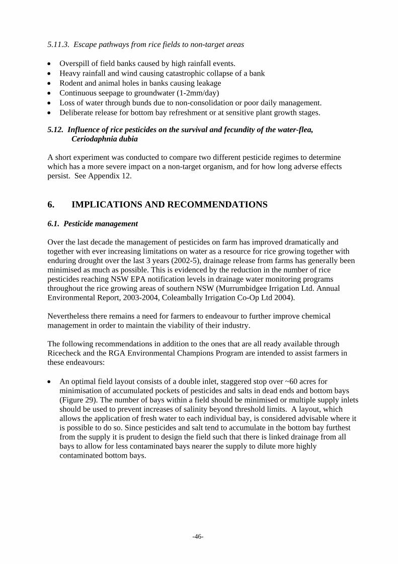
-46-

5.11.3. Escape pathways from rice fields to non-target areas

• Overspill of field banks caused by high rainfall events. • Heavy rainfall and wind causing catastrophic collapse of a bank • Rodent and animal holes in banks causing leakage • Continuous seepage to groundwater (1-2mm/day) • Loss of water through bunds due to non-consolidation or poor daily management. • Deliberate release for bottom bay refreshment or at sensitive plant growth stages. 5.12. Influence of rice pesticides on the survival and fecundity of the water-flea,

Ceriodaphnia dubia A short experiment was conducted to compare two different pesticide regimes to determine which has a more severe impact on a non-target organism, and for how long adverse effects persist. See Appendix 12. 6. IMPLICATIONS AND RECOMMENDATIONS 6.1. Pesticide management Over the last decade the management of pesticides on farm has improved dramatically and together with ever increasing limitations on water as a resource for rice growing together with enduring drought over the last 3 years (2002-5), drainage release from farms has generally been minimised as much as possible. This is evidenced by the reduction in the number of rice pesticides reaching NSW EPA notification levels in drainage water monitoring programs throughout the rice growing areas of southern NSW (Murrumbidgee Irrigation Ltd. Annual Environmental Report, 2003-2004, Coleambally Irrigation Co-Op Ltd 2004). Nevertheless there remains a need for farmers to endeavour to further improve chemical management in order to maintain the viability of their industry. The following recommendations in addition to the ones that are all ready available through Ricecheck and the RGA Environmental Champions Program are intended to assist farmers in these endeavours: • An optimal field layout consists of a double inlet, staggered stop over ~60 acres for

minimisation of accumulated pockets of pesticides and salts in dead ends and bottom bays (Figure 29). The number of bays within a field should be minimised or multiple supply inlets should be used to prevent increases of salinity beyond threshold limits. A layout, which allows the application of fresh water to each individual bay, is considered advisable where it is possible to do so. Since pesticides and salt tend to accumulate in the bottom bay furthest from the supply it is prudent to design the field such that there is linked drainage from all bays to allow for less contaminated bays nearer the supply to dilute more highly contaminated bottom bays.

-47-

Figure 29: Optimal field layout for rice to minimise accumulation of salts and pockets of pesticides in dead end areas and bottom bays.

• Maximum concentrations of pesticides occur in water immediately after spraying. Where

possible growers should attempt to maximise water depth at these times in order to keep concentrations of pesticide to a minimum.

• Currently spraying of pesticide onto bare ground is not a practise that is carried out in rice

growing areas of Australia. Only the insecticide fipronil comes into direct contact with soil rather than water due to its use as a seed dressing. However, our modelling studies have indicated (Christen et al., 2005) that pesticide sprayed onto bare ground and then ponding the field results in lower concentrations of pesticide in water. Further field study is necessary to corroborate these findings.

• Chemical combinations that are known be the most environmentally benign should be used

as much as possible. For example combinations of fipronil, clomazone and benzofenap should be used in preference to chlorpyrifos, molinate and thiobencarb.

• Growers should carefully assess the real need for repeat applications of the insecticide

chlorpyrifos for the control of bloodworm in order to minimise the use of this toxic agrochemical. A farmer education program of bloodworm assessment 14-21 days after sowing may be considered useful through experts and agronomists in NSW DPI.

• A small release of water from bottom bays may be necessary to provide bottom bay refreshment to ensure water column oxygenation and minimise salt build up. Growers are encouraged to continually measure EC and dissolved oxygen concentrations in bottom bays to determine whether such a release is necessary. Small hand held EC and dissolved oxygen meters are available through commercial outlets for approximately $1000. In such situations where small releases do occur the water must be retained on-farm.

-48-

7. RECOMMENDATIONS ON THE ACTIVITIES OR OTHER STEPS THAT MAY BE TAKEN TO FURTHER DEVELOP, DISSEMINATE, OR TO COMMERCIALLY EXPLOIT THE RESULTS OF THE PROJECT.

Some of the findings within this report are currently being incorporated into manuscripts for peer reviewed journal publication journal publication. The risk assessment model PIRI is being calibrated for some of the conditions specific to rice and will be demonstrated to farmers through the Ricegrowers’ Association of Australia “Environmental Champions Program” in July, 2005. Some of the recommendations from this report are being considered for introduction into Ricecheck through evaluation by NSW DPI agronomists and the participating farmers in the Champions Program. 8. ACKNOWLEDGEMENTS The financial support of the Rice CRC is gratefully acknowledged. Mr G. Andreazza, Mr R.Williams and Mr G. Barden are thanked for generously allowing their farms to be used for the 2000, 2001, 2002 and 2003 field data collection. 9. REFERENCES APHA, 1992. APHA 1995. Standard methods for the examination of water and wastewater. Australian and New Zealand Guidelines for Fresh and Marine Water Quality (2000). Chapter 3~Aquatic Ecosystems. Ambrust, K.L. (2001). Chlorothalonil and chlorpyrifos degradation products in golf course leachate. Pest Manag. Sci. 57: 797-802. Beecher, G., Beale, P & Clampett, W. 2000, ‘Land for Growing Rice’ in Production of Quality Rice in South Eastern Australia, eds. L. M. Keally & W. S. Clampett, Rural Industries Research & Development Corporation, ACT, Australia, Chapter 4. Bowmer, K, Korth, W, Thomas, M and McCorkelle, G (1994). River pollution with agricultural chemicals in: 'The Murrumbidgee, past and present' - proceedings of a forum at Griffith, April 1992, J. Roberts and R. Oliver (Eds.) , Division of Water Resources. 7-19. Christen, E.W., Quayle, W.C. Chung, S-O and Park, K.J. Modelling the fate of Molinate in rice paddies of south eastern Australia using RICEWQ. CSIRO Technical Report. Coleambally irrigation Co-Operative Ltd. Annual Environmental Report (2004). http://env.colyirr.com.au/aer2004/ California Department of Pesticide Regulation, Clomazone Public Report 200301. Collings, A (2002). Floodwater salinity in rice bays. Farmers Newsletter 160: 36-37. Crosby, D.G. (1983). The fate of herbicides in Californian Rice Culture. IUPAC Pesticide Chemistry; Human Welfare and the Environment J. Miayamoto et al., (Eds.) 339-346.

-49-

Crosby, D.G. and Mabury, S. (1992). Management of pesticide residues in ricefield tailwater. A report to the Soil Conservation Service of the US Department of Agriculture. Cumming, J.P., Doyle, R. B and Brown, P.H. (2002). Clomazone dissipation in four Tasmanian topsoils. Weed Science, 50,: 405-409. Deuel, L.E, Turner, F.T., Brown K.W. and Price, J.D> (1978). Persistence and factors affecting the dissipation of Molinate under flooded rice culture. J. Environ. Qual. 7:3, 373-377. Doran, G., Helliwell, S and Eberbach, P. (2005). J. AOAC International, 88, 3. Ecotoxnet http://extoxnet.orst.edu Gever, J.R., Mabury, S.A. and Crosby, D.G. (1996). Rice field surface microlayers: collection, composition and pesticide enrichment. Env. Toxicol. and Chem. 15:10, 1676-1682 Grattan, S. R., Zeng, L., Shannon, M. C. & Roberts, S. R. 2002, ‘Rice is more sensitive to salinity than previously thought’, California Agriculture, 56:6, 189-195 Hager, W. (1988) Mobile flume for circular channel, Journal of Irrigation and Drainage Engineering, 114: 3, August, ASCE Harrison, J. (12994). Review of nutrients in irrigation drainage in the Murray-Darling Basin. CSIRO Division of Water Resources. Seeking Solutions Water Resources Series No. 11. CSIRO. Hornsby (1992). Site-Specific Pesticide Recommendations: The Final Step in Environmental Impact prevention. Weed Technology, 6: 736-742. Humphreys, L. (1999). Rice water Use Efficiency Workshop. 12th March, 1999. CSIRO Land and Water. CRC Sustainable Rice Production Workshop Report. Ishikawa, K. Nakamura, Y and Kuwatsuka, S. (1976). Degradation of benthiocarb herbicide in soil. J. Pest. Sci. 1:49-57. Kealey, LM and Clampett, WS (2000). Production of quality rice in South Eastern Australia. Weed Management. Chapter 9. Rural Industries Research and Development Corporation, ACT, Australia. Knuth, M. L. and Heinis, L.J. (1992). Dissipation and persistence of chlorpyrifos within littoral enclosures. J. Agric Food Chem., 40, 1257-1263. Korth, W. (1995). Can pesticides used in agriculture get into drainage water? Farmers Newsletter 145:33-36. Korth, W, Thomas, M, McCorkelle, G and Forster, S. (1995). Pesticide and toxicity testing of MIA drainage water. CSIRO Division of Water Resources, Griffith, NSW, Consultancy Report 95/25. Korth W. and S. Foster (1998). A method for the collection, preservation and analysis of agricultural chemicals (pesticides) used in the Murrumbidgee Irrigation Area. CSIRO Land and Water, Griffith. Technical Report 11/98. Liu, B., Connell, L.L. and Torrents, A. (2001). Hydrolysis of chlorpyrifos in natural waters of the Chesapeake Bay. Chemosphere 44: 1315-1323. Mabury SA, Cox JS, Crosby DG. (1996). Environmental fate of rice pesticides in California. Rev Environ Contam Toxicol. 147:71-117. Macalady, D.L. and Wolfe, N.L. (1985). Effects New perspectives on the hydrolytic degradation of the organophorothionate insecticide chlorpyrifos . J. Agric. Food Chem. 31: 1139-1147.

-50-

Mass, E. V. & Hoffman, G. J. (1977). ‘Crop Salt Tolerance-Current Assessment’, Journal of the Irrigation and Drainage Division, vol. 103: 115-134. Murrumbidgee Irrigation Ltd. Environmental Performance Summary. 2003-2004. http://www.mirrigation.com.au/ Nakamura, Y. Ishikawa, K. and Kuwatsuka, S. (1977). Degradation of benthiocarb in soils as affected by soil conditions. J. Pesticide Sci, 2: 7-16. New South Wales Environment Protection Authority (2003) Murrumbidgee Irrigation Ltd Environment Protection License . License no. 4561. http://www.epa.nsw.gov.au/prpoeo/licences.htm Pesticide Action Network North America, 2003. Website URL http://www.pesticideinfo.org/ Ricecheck Recommendations. Best Management Practises for Ricegrowing. New South Wales Agriculture and the RIRDC Research and Development Committee 2003. Parker, L. (1995). Farm chemical use strategy for MIA landholders. Farmers Newsletter. 146,10-11. Racke, K.D. (1993). Environmental fate of chlorpyrifos. Rev. Env. Contam. Toxicol 131: 1-150. Richards, L. A. (ed.). 1954, Diagnosis and Improvement of Saline and Alkali Soils, U.S. Government Printing Office, Washington D.C., USA. Rice Growers’ Association of Australia Inc., 2003. (http://www.rga.org.au/) Samani, Z., Jorat, S., & Yousaf, M (1991) Hydraulic characteristics of circular flume, Journal of Irrigation and Drainage Engineering, 117: 4, July/August, ASCE. Scardaci, S. C., Shannon, M. C., Grattan, M. C., Eke, A. U., Roberts, S. R., Goldman-Smith, S. & Hill, J. E. 2002, ‘Water management practices can affect salinity in rice fields’, California Agriculture, 56: 6, 184-188. Ross, L.J. and Sava, R.J. (1986). Fate of thiobencarb and molinate in rice fields. J. Environ. Qual. 15, 3, pp 220-225. Schroo, H. 1983, Salinity Increase in Water Ponded for Rice Cultivation (unpublished). Simpson, B.W. and Haydn, G.F. (1998). Pesticide usage study in the Murrumbidgee Irrigation Area of New South Wales. Queensland Department of Natural Resources, March, 1999. Technical Report. Slessar, P (1991). Berriquin Irrigation District Nutrient Monitoring Program – Review of data Nov. 1990 to July 1991. Resource Assessment and Water Supply Group, Water Resources Murray Region, NSW Department of Water Resources, Deniliquin, NSW Southwood, J.M., Muir, D.C.G. and Mackay, D. (1999). Modelling agrochemical dissipation in surface microlayers following aerial deposition. Chemosphere 38:1, 121-141. Sonderquist, C.J., Brown, J.B. and Crosby, D. G. ., 1977. Dissipation of molinate in a rice field. J. Agric. Food. Chem. 25, 940-945 Tanji, K.K., Biggar, J.W., Mehran M., Cheung, M.W. and Henderson, D.W. (1974). Herbicide persistence and movement studies with molinate in rice irrigation management. Calif. Agric. May, 10-12. Tingle, C.C.D., Rother, J.A. Dewhurst, C. A. Lauer, S. and King, W. J. (2003). Fipronil: Environmental fate, ecotoxicology and human health concerns. Rev. Env. Contam. Toxicol. 176, 10-19. Tomlin, C.D.S. (2000). The Pesticide Manual (2000) Twelfth Edition. CDS Tomlin (Ed). The British Crop Protection Council.

-51-

Watkins, K. L. Kulatunga, N. and Bauld, J. (1998) Groundwater Quality of the Murray-Riverina Catchment, NSW:Wakool-Cadell and Denimein-Berriquin Regions. Australian Groundwater Quality Assessment Project Report No. 5. Australian Geological Survey Organisation. Department of Industry, Science and Resources. Canberra, 1998. Watkins, K. L. and Bauld, J. (1999). A Groundwater Quality Assessment of Shallow Aquifers in the Murray Region, NSW. Australian Groundwater Quality Assessment Project Report No. 6. Australian Geological Survey Organisation. Department of Industry, Science and Resources. Canberra, 1999. Wauchope, R. D., Buttler, T. M., Hornsby A. G., Augustijn-Beckers, P. W. M. and Burt, J. P. SCS/ARS/CES Pesticide properties database for environmental decision making. Rev. Environ. Contam. Toxicol. 123:1-157, 1992.4-21. Wilson, A.L., Stevens, M.M. and Watts, R.J. (2000). Acute and chronic toxicity of the herbicide benzofenap (Taipan 300) to Chironomus tepperi iSkuse (Dipters: Chironomidae) and Isidorella newcombi (Adams and Angas) (Gastropoda: Planorbidae). Arch. Environ. Contam. Toxicol. 38: 176-181. Zanella, R., Primel, E.G. Gonçalves, F.F. and Martins, A.F. (2000). Development and validation of a high-performance liquid chromatograic method for the determination of clomazone residues in surface water. J. Chromatography A, 994, 257-262, 19 Connelly, 2001.

-52-

APPENDIX 1: Determination of detection limit Composite standards were run by direct injection onto the HPLC to determine a detection limit for each compound. Our results indicated that the method was most robust for levels > 0.1 ppm for molinate, clomazone, thiobencarb and benzofenap and > 0.4 ppm for chlorpyrifos (Table 1.1). Table 1.1 - Concentrations and % recovery for clomazone, molinate, thiobencarb, benzofenap and chlorpyrifos.

Sample ID Clomazone (ppm)

Molinate (ppm)

Thiobencarb (ppm)

Benzofenap (ppm)

Chlorpyrifos (ppm)

STD G Expected 0.136 0.224 0.177 0.159 0.211 Measured (1) 0.135 0.22 0.117 0.19 Not detected% 99 98 66 119

Measured (2) 0.164 0.1079 0.177 not detected Not detected

% 121 48 100 Measured (3) 0.148 0.239 0.137 0.181 Not detected% 109 107 77 114 Measured (4) 0.1513 0.243 0.0928 0.1854 Not detected% 111 108 52 117 STD F Expected 0.263 0.462 0.378 0.336 0.408 Measured (1) 0.2598 0.452 0.373 0.327 0.406 % 94 99 103 101 94 Measured (2) 0.264 0.464 0.375 0.336 0.412 % 96 102 104 104 96 Measured (3) 0.263 0.462 0.378 0.336 0.408 % 95 101 105 104 95 STD E Expected 1.025 1.99 1.577 1.413 1.875 Measured (1) 1.14 1.92 1.58 1.42 1.87 % 111 96 100 100 100 Measured (2) 1.159 1.944 1.599 1.437 1.89 % 113 98 101 102 101 Measured (3) 1.16 1.94 1.62 1.44 1.9 % 113 97 103 102 101 Measured (4) 1.176 1.9798 1.651 1.463 1.955 % 115 99 105 104 104

-53-

APPENDIX 2: Recovery of pesticides using SPE-HPLC with 1 ml acetonitrile eluent. Dichloromethane (DCM) is incompatible with the HPLC elution gradient (acetonitrile:water). Consequently the eluent was blown down with N2 to dryness and resuspended in acetonitrile. Taking the eluent to dryness lead to some losses. It was of interest to determine the effectiveness of using acetonitrile only as an SPE eluent which could then be injected directly without the need for further preparation steps. The same procedure as in “Experiment 1’ was carried out with the exception of the elution solvent for which 1 ml acetonitrile was used.

Recovery (%) of standards using 1mL acetonitrile eluent.

Sample Volume Extracted (ml)

Mol Thiob Chlorp Clom Benzof.

Blank Floodwater

500 0 0 0 0 0

Blank Floodwater

500 0 0 0 0 0

Milli-Q + Spike

500 22 10 26 52 5

Milli-Q + Spike

500 39 23 26 68 23

Floodwater 1 + Spike

500 40 23 23 70 17

Floodwater 2 + Spike

500 21 6 21 52 26

-54-

APPENDIX 3: Recovery of pesticides using liquid-liquid extraction (LLE) followed by HPLC-DAD. Pesticide Clomazone Molinate Thiobencarb Benzofenap ChlorpyrifosExpected (ppm) 18.136 29.957 23.736 21.2688 28.217 Mean Recovery (n=6 ) 55 26 19 8 58 Standard deviation 6 1.7 1.7 1 0.4 Expected (ppm) 5.684 9.388 7.439 6.665 8.843 Mean Recovery (n=6 ) 51 22 15 5 55 Standard deviation 13 2 0.7 0.4 1.8

-55-

APPENDIX 4: Relationships between pesticide concentration and selected water chemistry parameters, 2000

Molinate

Molinate vs pH

0

1000

2000

3000

6.00 6.50 7.00 7.50 8.00 8.50

pH

mol

inat

e co

nc u

g/L

Molinate vs EC

0

1000

2000

3000

0.20 0.25 0.30 0.35

EC dS/m

con

c ug

/L

Molinate vs TSS

0

1000

2000

3000

0.2 20.2 40.2 60.2 80.2 100.2 120.2 140.2

TSS mg/L

con

c ug

/L

Molinate vs TDS

0

1000

2000

3000

50 100 150 200 250 300

TDS mg/L

con

c ug

/L

-56-

Benzofenap

Benzofenap vs pH

0

10

20

30

6.00 6.50 7.00 7.50 8.00 8.50

pH

con

c ug

/L

Benzofenap vs EC y = -3354x2 + 2064.5x - 296.4

R2 = 0.75

0

10

20

30

0.20 0.25 0.30 0.35

EC dS/m

con

c ug

/L

Benzofenap vs TSS

0

10

20

30

0.2 20.2 40.2 60.2 80.2 100.2 120.2 140.2

TSS mg/L

con

c ug

/L

Benzofenap vs TDSy = 0.17x - 13.33R2 = 0.45

0

10

20

30

50 100 150 200 250 300

TDS mg/L

con

c ug

/L

-57-

Chlorpyrifos

Chlorpyrifos vs pH

05

10152025

6.00 6.50 7.00 7.50 8.00 8.50

pH

con

c ug

/L

Chlorpyrifos vs EC

05

10152025

0.20 0.25 0.30 0.35

EC dS/m

con

c ug

/L

Chlorpyrifos vs TSS

05

10152025

20 40 60 80 100 120 140

TSSmg/L

con

c ug

/L

Chlorpyrifos vs TDS

0

10

20

30

70 120 170 220 270

TDSmg/L

con

c ug

/L

-58-

APPENDIX 5: 1991 Survey of molinate concentration in rice bays on 2 farms (Bowmer, 1998)

Farm A 1991 Molinate concentration

0500

1000150020002500300035004000

18/10

/1991

20/10

/1991

22/10

/1991

24/10

/1991

26/10

/1991

28/10

/1991

30/10

/1991

1/11/1

991

3/11/1

991

5/11/1

991

date

conc

entr

atio

n ug

/L

Near supplyNear Drain

Half-life of molinate (with upper and lower 95% confidence intervals) determined for water collected on Farm A near the drain was 3.9 days (5.4, 3.1).

Farm B 1991 Molinate concentration

0100200300400500600700800900

15/10

/1991

17/10

/1991

19/10

/1991

21/10

/1991

23/10

/1991

25/10

/1991

27/10

/1991

29/10

/1991

31/10

/1991

2/11/1

991

4/11/1

991

6/11/1

991

8/11/1

991

date

conc

entr

atio

n ug

/L Near supplyNear Drain

2nd application

Half-life of molinate (with upper and lower 95% confidence intervals) determined for the first application (Farm B) was 3.6 days (4.5, 3.0) and for the second application (Farm B) was 2.9 days (7.3, 1.8).

-59-

APPENDIX 6: Water chemistry data from supply water, 2001

2001 supply water

0.0000.0200.0400.0600.0800.1000.1200.140

1-Oct 6-Oct 11-Oct 16-Oct 21-Oct 26-Oct 31-Oct 5-Nov

date

Suspended solids g/L

EC

2001 Supply water

7.27.47.67.8

88.28.4

1-Oct 6-Oct 11-Oct 16-Oct 21-Oct 26-Oct 31-Oct 5-Nov

date

pH

2001 mean TSS

0

0.005

0.01

0.015

0.02

0.025

0.03

0.035

16-Oct 21-Oct 26-Oct 31-Oct 5-Nov 10-Nov 15-Nov 20-Nov 25-Nov 30-Novdate

g/L

-60-

APPENDIX 7: Water chemistry in three bays monitored over the rice growing period, 2001

Chloride

01020304050

6-Oct 16-Oct 26-Oct 5-Nov 15-Nov 25-Nov 5-Dec 15-Dec 25-Dec

date

mg/

L

Bay nearest supply (3)

Middle bay (2)

Bay nearest drain (1)

pH

7.27.47.67.8

88.28.4

6-Oct 16-Oct 26-Oct 5-Nov 15-Nov 25-Nov 5-Dec 15-Dec 25-Dec

date

pH

Bay nearest supply (3)

Middle bay (2)

Bay nearest drain (1)

EC

0

0.2

0.4

0.6

0.8

6-Oct 16-Oct 26-Oct 5-Nov 15-Nov 25-Nov 5-Dec 15-Dec 25-Dec

date

EC d

S/m

Bay nearest supply (3)

Middle bay (2)

Bay nearest drain (1)

Dissolved Oxygen

02468

1012

6-Oct 16-Oct 26-Oct 5-Nov 15-Nov 25-Nov 5-Dec 15-Dec 25-Dec

date

DO

mg/

L

Bay nearest supply (3)

Middle bay (2)

Bay nearest drain (1)

-61-

APPENDIX 8: Meteorological data 2001 Mean Temperature 2001

0.05.0

10.015.020.025.030.0

6-Oct 16-Oct 26-Oct 5-Nov 15-Nov 25-Nov 5-Dec 15-Dec 25-Decdate

tem

pera

ture

Mean Relative Humidity 2001

0

10

20

30

40

50

60

70

80

90

6-Oct 16-Oct 26-Oct 5-Nov 15-Nov 25-Nov 5-Dec 15-Dec 25-Dec

date

Rh

%

Radiation 2001

0.0

5.0

10.0

15.0

20.0

25.0

30.0

35.0

40.0

6-Oct 16-Oct 26-Oct 5-Nov 15-Nov 25-Nov 5-Dec 15-Dec 25-Decdate

radi

atio

n M

J/sq

m

-62-

Rain 2001

0.02.04.06.08.0

10.012.014.016.018.020.0

6-Oct 16-Oct 26-Oct 5-Nov 15-Nov 25-Nov 5-Dec 15-Dec 25-Decdate

rain

mm

Wind 2001

050

100150200250300350400450500

6-Oct 16-Oct 26-Oct 5-Nov 15-Nov 25-Nov 5-Dec 15-Dec 25-Decdate

win

d km

/day

-63-

APPENDIX 9: 2002 water chemistry in bays 2002 Mean pH

7.00

7.50

8.00

8.50

9.00

9.50

10.00

11-Oct 21-Oct 31-Oct 10-Nov 20-Nov 30-Nov 10-Dec 20-Dec

Date

pH

ControlTreatment 1Treatment 2

Mean EC 2002

0.000.100.200.300.400.500.600.700.80

21-Oct 31-Oct 10-Nov 20-Nov 30-Nov 10-Dec 20-DecDate

EC

ControlTreatment 1Treatment 2

2002 Suspended Solids

0.00

40.00

80.00

120.00

160.00

11-Oct 21-Oct 31-Oct 10-Nov 20-Nov 30-Nov 10-Dec

Date

Susp

ende

d So

lids

ControlTreatment 1Treatment 2

-64-

APPENDIX 10: 2003 water chemistry in bays

2003 Water pH

7.007.508.008.509.009.50

10.0010.5011.00

6-Oct 16-Oct 26-Oct 5-Nov 15-Nov 25-Nov

Date

pHControlT1T2

2003 Water EC

0.00

0.10

0.20

0.30

0.40

0.50

6-Oct 16-Oct 26-Oct 5-Nov 15-Nov 25-Nov

Date

EC (d

S/m

)

ControlT1T2

2003 Water Turbidity

0.00

50.00

100.00

150.00

200.00

250.00

300.00

11-Oct 16-Oct 21-Oct 26-Oct 31-Oct 5-Nov 10-Nov 15-Nov 20-Nov

Date

Turb

idity

ControlT1T2

-65-

2003 Water Dissolved Oxygen

0.00

5.00

10.00

15.00

20.00

11-Oct 16-Oct 21-Oct 26-Oct 31-Oct 5-Nov 10-Nov 15-Nov 20-Nov

Date

Dis

solv

ed O

xyge

nControlT1T2

2003 Water Temperature

141618202224262830

11-Oct 16-Oct 21-Oct 26-Oct 31-Oct 5-Nov 10-Nov 15-Nov 20-Nov

Date

Tem

pera

ture

C

ControlT1T2

-66-

APPENDIX 11: Notification levels for chemicals to be monitored in rice drainage water in Murrumbidgee Irrigation Area (NSW Environment Protection Authority) Chemical Notification Level (µg/L) Action Level (µg/L) Atrazine 13 45 Chlorpyrifos 0.01 0.11 Diazinon 0.01 0.2 Diuron 0.2 1 Endosulfan 0.03 0.2 Malathion 0.05 0.2 Metolachlor 0.02 0.1 Molinate 3.4 14 Simazine 3.2 11 Thiobencarb 2.8 4.6 Trifluralin 2.6 4.4 2,4-D 6 30 Notification Level This is equivalent to the 95% “trigger value” Table 3.4.1, Australian and New Zealand Guidelines for Fresh and Marine Water Quality (Chapter 3~Aquatic Ecosystems) (2000). This is defined as the concentration at which 95% of all species will be protected with 50% confidence.

Action Level This is equivalent to the 90% “trigger value” Table 3.4.1, Australian and New Zealand Guidelines for Fresh and Marine Water Quality (Chapter 3~Aquatic Ecosystems) (2000). This is defined as the concentration at which 90% of all species will be protected with 50% confidence.

-67-

APPENDIX 12: Influence of rice pesticides on the survival and fecundity of the water-flea, Ceriodaphnia dubia Objective To compare two different pesticide regimes to determine which has a more severe impact on a non-target organism, and for how long adverse effects persist. Methods - field Six small rice bays were constructed, each about 80 sq. metres in size. Two were randomly designated as Treatment 1, two as Treatment 2, and the remaining bays were set aside as untreated controls. Bays were all flooded on 12 October 2003. No treatments were applied until one week after flooding, allowing a pre-treatment test to be conducted. The following chemical regimes were then applied: 7 days: Treatment 1: Lorsban 150mL/ha; Ordram 3.75 L/ha Treatment 2: Taipan 2 L/ha; Magister 0.5L/ha, Fipronil 12.5 gai/ha 21 days: Treatment 1: no further chemicals Treatment 2: Lorsban 150mL/ha; Saturn 3.75 L/ha Methods – laboratory Water samples were taken daily from all 6 fields. Each toxicity test lasted for 7 days. Aliquots of field collected water were placed in 5 separate cups for each bay (i.e. 30 cups total). Into each cup was placed one mature female water flea. Young produced over the following 24 hours were counted and removed, then the female was transferred to a new cup containing water collected on that day (ie. a static renewal bioassay). After 7 days the adult survival was recorded and the number of offspring totalled for each of the 30 individuals. This was repeated 7 times, each with new females, once pre-treatment and 6 times post treatment (see graph and data). Within the data set some points are missing due to accidents or accidental use of males. The average of the 2 block averages and the SEs of these 2 values were taken and graphed. After chemical application 1, treatment 1 killed all water fleas outright for the next 2 weeks. Consequently no data is available. Fecundity then improved progressively. Treatment 2 suppressed fecundity in the first week. However, it recovered to near control levels by the following week. The second application of chemicals in treatment 2 produced lethal effects for the duration of the tests. Data Pre-pesticide application 13/10/03 - 20/10/03 Total number of young produced by each individual over 7 day period

Block Treatment 1 Treatment 2 control Bays 1 19 19 30 1 18 33 34 1 27 25 34 1 35 17 19 1

-68-

Mean 24.75 23.5 29.25 2 49 45 2 2 39 29 39 2 29 34 36 2 22 13 24

Mean 34.75 25.33333333 36 average of bays 29.75 24.41666667 32.625 SE of bays 5 0.916666667 3.375 Survival of females @ day 7 8/8 7/7 8/8 20/10/03 Pesticides applied T1 150 mL/Ha Lorsban, 3.75 L/Ha Ordram T2 2 L/Ha Taipan, 0.5 L/Ha Magister, 12.5 gai/ha fipronil Test duration 20/10/03 - 27/10/03 Total number of young produced by each individual over 7 day period

Block Treatment 1 Treatment 2 control Bays 1 Dead day 1 7 1 Dead day 1 7 17 1 Dead day 1 6 1 Dead day 1 6 15 1 Dead day 1 8 13

Mean 6.75 13 2 Dead day 1 12 42 2 Dead day 1 0 31 2 Dead day 1 9 55 2 Dead day 1 6 29 2 Dead day 1 5 43

Mean 6.4 40 average of bays 6.575 26.5 SE of bays 0.175 13.5 Survival of females @ day 7 0/10 9/9 9/10 No further pesticide application Test duration 27/10/03 - 3/11/03 Total number of young produced by each individual over 7 day period

Block Treatment 1 Treatment 2 control Bays 1 Dead day 1 19 20 1 Dead day 1 24 40 1 Dead day 1 23 33 1 Dead day 1 26 31 1 Dead day 1 18 30

Mean 22 30.8 2 Dead day 1 24 29 2 Dead day 1 40 49 2 Dead day 1 24 20 2 Dead day 1 37 43 2 Dead day 1 23 28

Mean 29.6 33.8 average of bays 25.8 32.3 SE of bays 3.8 1.5 Survival of females @ day 7 0/10 10/10 10/10

-69-

11/04/2003 2nd pesticide application T1 - no additional pesticides applied T2 - 3.75L/Ha Saturn, 0.15 L /Ha Lorsban Test duration 10/11/03 - 17/11/03 Total number of young produced by each individual over 7 day period

Block Treatment 1 Treatment 2 control Bays 1 20 Dead day 1 29 1 2 Dead day 1 37 1 37 Dead day 1 39 1 11 Dead day 1 52 1 7 Dead day 1 29

Mean 15.4 37.2 2 39 Dead day 1 48 2 39 Dead day 1 48 2 27 Dead day 1 41 2 32 Dead day 1 33 2 46 Dead day 1 55

Mean 36.6 45 average of bays 26 41.1 SE of bays 10.6 3.9 Survival of females @ day 7 10/10 0/10 10/10 Test duration 18/11/03 - 25/11/03 Total number of young produced by each individual over 7 day period

Block Treatment 1 Treatment 2 control Bays 1 29 Dead day 1 28 1 27 Dead day 1 12 1 25 Dead day 1 18 1 10 Dead day 1 26 1 25 Dead day 1 31

Mean 23.2 23 2 22 Dead day 1 32 2 20 Dead day 1 33 2 43 Dead day 1 38 2 Dead day 1 18 2 34 Dead day 1 29.75 30.25

average of bays 26.475 26.625 SE of bays 3.275 3.625 Survival of females @ day 7 9/10 0/10 9/9

-70-

Test duration 24/11/03 - 1/12/03 Total number of young produced by each individual over 7 day period

Block Treatment 1 Treatment 2 control Bays 1 13 Dead day 1 17 1 31 Dead day 1 38 1 Dead day 1 35 1 18 Dead day 1 34 1 7 Dead day 1

Mean 17.25 31 2 48 Dead day 1 36 2 47 Dead day 1 42 2 12 Dead day 1 41 2 51 Dead day 1 37 2 43 Dead day 1 32

Mean 40.2 37.6 average of bays 28.725 34.3 SE of bays 11.475 3.3 Survival of females @ day 7 9/10 0/10 9/9 Test duration 2/12/03 - 10/12/03 Total number of young produced by each individual over 7 day period

Block Treatment 1 Treatment 2 control Bays 1 31 Dead day 1 0 1 24 Dead day 1 35 1 31 Dead day 1 27 1 28 Dead day 1 33 1 28 Dead day 1 27 28.4 24.4

2 44 Dead day 1 28 2 36 Dead day 1 26 2 46 Dead day 1 47 2 47 Dead day 1 44 2 39 Dead day 1 21

Mean 42.4 33.2 average of bays 35.4 28.8 SE of bays 7 4.4 Survival of females @ day 7 10/10 0/10 10/10