arX

iv:a

stro

-ph/

0511

140v

2 2

0 M

ar 2

006

Accepted by ApJ

Constraints on the Physics of Type Ia Supernovae from the X-Ray Spectrum of

the Tycho Supernova Remnant

Carles Badenes1, Kazimierz J. Borkowski2, John P. Hughes1, Una Hwang3 and Eduardo Bravo4

ABSTRACT

In this paper we use high quality X-ray observations from XMM-Newton and Chan-

dra to gain new insights into the explosion that originated Tycho’s supernova 433 years

ago. We perform a detailed comparison between the ejecta emission from the spatially

integrated X-ray spectrum of the supernova remnant and current models for Type Ia

supernova explosions. We use a grid of synthetic X-ray spectra based on hydrodynamic

models of the evolution of the supernova remnant and nonequilibrium ionization calcu-

lations for the state of the shocked plasma. We find that the fundamental properties of

the X-ray emission in Tycho are well reproduced by a one-dimensional delayed detona-

tion model with a kinetic energy of ∼ 1.2 · 1051 erg. All the other paradigms for Type

Ia explosions that we have tested fail to provide a good approximation to the observed

ejecta emission, including one-dimensional deflagrations, pulsating delayed detonations

and sub-Chandrasekhar explosions, as well as deflagration models calculated in three

dimensions. Our results require that the supernova ejecta retain some degree of chem-

ical stratification, with Fe-peak elements interior to intermediate mass elements. This

strongly suggests that a supersonic burning front (i.e., a detonation) must be involved

at some stage in the physics of Type Ia supernova explosions.

Subject headings: hydrodynamics — ISM:individual(SN1572) — nuclear reactions, nu-

cleosynthesis, abundances, — supernova remnants — supernovae:general — X-rays:ISM

1Department of Physics and Astronomy, Rutgers University, 136 Frelinghuysen Rd., Piscataway NJ 08854-8019;

badenes@physics.rutgers.edu; jph@physics.rutgers.edu

2Department of Physics, North Carolina State University, Box 8202, Raleigh NC 27965-8202;

kborkow@unity.ncsu.edu

3NASA Goddard Space Flight Center, Code 622, Greenbelt MD 20771; and Department of Physics and Astronomy,

The Johns Hopkins University, 3400 Charles St, Baltimore MD 21218; hwang@orfeo.gsfc.nasa.gov

4Departament de Fisica i Enginyeria Nuclear, Universitat Politecnica de Catalunya, Diagonal 647, Barcelona 08028,

Spain; and Institut d’Estudis Espacials de Catalunya, Campus UAB, Facultat de Ciencies. Torre C5. Bellaterra,

Barcelona 08193, Spain; eduardo.bravo@upc.es

– 2 –

1. INTRODUCTION

The stella nova of 1572 is the only historical supernova (SN) that can be classified with

some degree of confidence as Type Ia based on its observed light curve and color evolution (Ruiz-

Lapuente 2004). Our knowledge of the universe has improved greatly since this momentous event

was recorded by Tycho Brahe and other astronomers in the sixteenth century, but now, as then,

there are many unanswered questions regarding the nature of supernovae. Type Ia SNe play a key

role as cosmological probes (Riess et al. 1998; Perlmutter et al. 1999), and they constitute the most

direct evidence for the accelerating universe (Leibundgut 2001), but despite the continuing efforts

of theorists during the last decades, our understanding of these objects is far from being complete.

There is a general agreement that Type Ia SNe are the result of the thermonuclear explosion of a

C+O white dwarf (WD) that is destabilized by accretion from a companion star in a close binary

system. This so-called ‘single degenerate’ scenario has been recently substantiated by the discovery

of a G-type star near the center of the Tycho supernova remnant (SNR) that appears to be the

surviving companion to the WD that exploded as a SN in 1572 (Ruiz-Lapuente et al. 2004), and by

the presence of a weak Hα signature in the late time spectrum of the unusual Type Ia SN 2002ic

(Hamuy et al. 2003). However, the fundamental details of the explosion itself are still obscure, and

a number of contending models or paradigms are currently being considered.

Most of these paradigms assume that the WD becomes unstable and then explodes when its

mass approaches the Chandrasekhar limit (1.4M⊙). In this case, the properties of the explosion are

determined mainly by the propagation mode of the burning front through the star, which can be

supersonic (detonations), subsonic (deflagrations), or a combination of both (delayed detonations,

pulsating delayed detonations). In the prompt detonation models, the burning front propagates

supersonically through the star, incinerating almost its entire mass to Fe-peak nuclei. In pure

deflagration models, the burning front propagates subsonically and the star has the time to expand

ahead of the flame. When the expansion velocity of the unburnt material becomes comparable to

that of the burning front, the flame quenches, leaving a mixture of unburnt fuel (C and O) and ashes

(Fe-peak nuclei) in the ejecta, usually with trace amounts of intermediate mass elements (IMEs:

Si, S, Ar, Ca, etc.). In one-dimensional deflagration models, the ejecta are layered, with the ashes

interior to the fuel, but three-dimensional calculations have shown that the turbulent properties of

the burning front lead to an efficient mixture of fuel and ashes through the ejecta. In the delayed

detonation models, the burning front begins as a deflagration and then it is artificially forced to

make the transition to a detonation, usually when a prescribed transition density ρtr is reached.

In this kind of explosions, most of the WD is burnt and very little C and O is left behind, but the

expansion of the star during the initial deflagration allows for the detonation to burn a sizable mass

of ejecta at intermediate densities, leading to a significant production of IMEs. Pulsating delayed

detonations are a variation of this scenario, where the flame quenches after a brief deflagration

phase and the WD re-collapses, triggering a detonation in the process. The ejecta are stratified

in all the flavors of delayed detonations simulated in one dimension, with Fe-peak nuclei interior

to IMEs, and some unburnt C and O in the outermost layers. Whether this is also the case for

– 3 –

three-dimensional delayed detonations is still under debate. Given the appropriate circumstances,

it is also possible for the WD to explode with a sub-Chandrasekhar mass, leading to an entirely

different class of models whose initial conditions are not so well determined. Sub-Chandrasekhar

explosions usually involve the ignition under degenerate conditions of a layer of accreted He on

top of the C+O WD, which sends a strong pressure wave towards the center of the star that

eventually triggers a detonation. The structure of the ejecta is complex, with unburnt C and O and

IMEs sandwiched between two regions rich in Fe-peak nuclei. For more details on these explosion

paradigms and a complete set of references, see the reviews by Hillebrandt & Niemeyer (2000)

(mostly one-dimensional models), Bravo et al. (2005) (three-dimensional deflagrations), and the

recent works by Garcia-Senz & Bravo (2003) and Gamezo et al. (2005) (three-dimensional delayed

detonations).

There have been numerous attempts to constrain these theoretical models, mostly through the

optical/IR spectra (e.g., Hoflich & Khokhlov 1996; Fisher et al. 1997; Hoflich et al. 1998; Wheeler

et al. 1998; Branch et al. 2005; Kozma et al. 2005) and light curves (e.g., Hoflich et al. 1998;

Stritzinger et al. 2005) of Type Ia SNe, and also through the few available gamma-ray observations

(Milne et al. 2004, and references therein). Although some preference has been shown for delayed

detonation models in these studies, it cannot be said that a general consensus has been reached

in this matter, and the physical mechanism responsible for Type Ia SN explosions still remains

an open issue. In the present paper, we address the problem of constraining the physics of Type

Ia SN explosions from a different perspective. Instead of focusing on the emission from the SNe

themselves, we take advantage of the excellent quality of the existing X-ray observations of SNRs

provided by XMM-Newton and Chandra to probe the physical mechanism responsible for the

explosions. The necessary theoretical groundwork was laid down in Badenes et al. (2003) and

Badenes et al. (2005a) (henceforth, Paper I and Paper II), where we showed that the structure

of the SN ejecta has a profound impact on the thermal X-ray emission from Type Ia SNRs. As

a consequence, the X-ray spectra have the potential to pose strong constraints on the kind of

explosion that originated the SNR. Here we apply the models developed in Papers I and II to the

X-ray spectrum of the Tycho SNR. We begin by summarizing the observations of this object in § 2.

Based on the observational properties of Tycho, we outline our strategy for comparing our models

to the observations in § 3. In § 4, we extract spatially integrated spectra from large regions of

an XMM-Newton observation of Tycho and derive the fundamental properties of the line emission

from the shocked SN ejecta. We compare our models with these observations in two stages: first

we select the most promising models based on the properties of their line emission in § 5 and then

we compare the best candidates to the spatially integrated spectrum in § 6. In § 7 we consider

the spatial distribution of the line emission from a Chandra ACIS-I observation, and examine the

implications for our models. Finally, we discuss the performance of the models from a global point

of view in § 8, and we summarize our conclusions in § 9.

– 4 –

2. OBSERVATIONS

2.1. The supernova of 1572

As early as 1945, Baade used the observations made and compiled by Tycho Brahe to derive

a light curve that enabled him to identify the stella nova of 1572 as a Type I supernova (Baade

1945). Since then, the classification of the supernova as determined from its light curve has been

controversial, and some authors have claimed that SN 1572 was a subluminous event (see van den

Bergh 1993; Schaefer 1996, and references therein). Ruiz-Lapuente (2004) performed a detailed

reanalysis of the sixteenth century records and evaluated the uncertainties in the data in order to

describe the light curve in the terms used nowadays to characterize Type Ia SNe. According to

Ruiz-Lapuente, SN 1572 was a normal Type Ia SN within the uncertainties associated with the

data (which are large), with a peak visual magnitude of MV = −19.24 − 5log(D/3.0kpc) ± 0.42

mag, and a stretch factor 1 s ∽ 0.9. The author found an extinction of AV = 1.86 ± 0.12 mag

and an average reddening of E(B − V ) = 0.6 ± 0.04 in that direction of the sky, which combined

with the value of MV yield an estimate of 2.8 ± 0.4 kpc for the distance to the SN, assuming

H0 = 65km · s−1 · Mpc−1.

2.2. The Tycho SNR: Radio and optical observations

In the radio continuum observations at 1375 MHz (λ = 21 cm), the Tycho SNR appears as a

clearly defined shell with an approximate angular diameter of 8’. The shell is nearly spherical from

the northwest to the southeast, with an irregular outbreak accompanied by a slight brightening

to the north, northeast and east. Reynoso et al. (1997), used VLA observations to estimate the

expansion parameter of the forward shock, ηfwd (defined as η = dlog(rfwd)/dlog(t)), along the rim

of the SNR shell. They found an average of ηfwd = 0.47±0.03, with distinctly lower values towards

the north and east. It was found later that the lower value of ηfwd in the northeast is due to an

interaction with a dense cloud of neutral hydrogen (Reynoso et al. 1999; Lee et al. 2004). There

is a puzzling, and still unsolved, disagreement between these radio measurements and the value of

ηfwd = 0.71 ± 0.06 inferred from X-ray observations by Hughes (2000). The expansion parameters

of several interior features, measured using the same techniques, are consistent in radio (η ≃ 0.44,

Reynoso et al. 1997) and X-rays (η ≃ 0.45, Hughes 2000).

At optical wavelengths, only a few faint filaments of Balmer line emission from H are visible

at the outer rim of the SNR. No evidence for any optical emission other than the Balmer H lines

was found in the interior of the SNR (Kirshner & Chevalier 1978; Smith et al. 1991; Ghavamian

1The stretch factor s is a parameterization of the light curve width/shape relationship, defined as the linear

broadening or narrowing of the rest-frame time scale of an average template light curve that is required to match

the observed light curve. Values of s close to 1 denote ‘normal’ Type Ia SNe. See Perlmutter et al. (1997) for more

details.

– 5 –

et al. 2000). In particular, optical emission from radiatively cooled ejecta has not been detected. In

Ghavamian et al. (2001), the spectrum of the brightest knot in the eastern rim (knot g from Kamper

& van den Bergh 1978) was examined in detail, yielding a velocity between 1940 and 2300 km · s−1

for the forward shock. This bright knot, however, is situated in the eastern rim, where the SNR

is interacting with denser material, and its properties might not be representative of the overall

dynamics of the blast wave.

As is often the case with Galactic SNRs, the distance to Tycho is very uncertain. Different

techniques yield different and even contradictory results ranging anywhere between 1.5 and 4.5 kpc,

with most estimates converging around 2.5 kpc (see Schaefer 1996, for a review). Among these, we

believe that the most reliable results are obtained through the combination of velocity estimates

from knots in the Balmer-dominated forward shock with optical proper motions measured over

long temporal baselines. We will adopt the range of 1.5-3.1 kpc obtained by Smith et al. (1991)

with this method as a conservative estimate for the distance, and we note that the value of 2.8 kpc

found by Ruiz-Lapuente (2004) for SN 1572 falls within this range.

2.3. The Tycho SNR: X-ray observations

The most fundamental properties of the X-ray emission from the Tycho SNR have been known

since the time of the ASCA satellite (Hwang & Gotthelf 1997; Hwang et al. 1998), but the quality

of the available data has increased dramatically thanks to XMM-Newton (Decourchelle et al. 2001)

and Chandra (Hwang et al. 2002; Warren et al. 2005). Morphologically, the X-ray emission from

the Tycho SNR has a shell-like structure with a thin rim of high energy continuum emission. This

rim is coincident in position, but not in brightness, with the outer edge of the radio emission, and

traces the position of the forward shock. The regions interior to this rim show very strong emission

lines of Si, S, Ca, Ar and Fe, which are thought to arise from the shocked supernova ejecta.

Several significant results about the dynamics and X-ray emission of the Tycho SNR were

presented in Warren et al. (2005), where a principal component analysis technique was applied to a

∼ 150 ks Chandra ACIS-I observation. Warren et al. determined the positions of the forward shock

(FS), reverse shock (RS) and contact discontinuity (CD) between ejecta and AM, and derived ratios

for their average radii of 1:0.93:0.71 (FS:CD:RS). Because the CD is so close to the FS, these ratios

are incompatible with one-dimensional adiabatic hydrodynamics with γ = 5/3 for the shocked AM.

Three explanations for the presence of ejecta close to the FS can be found in the literature: the

presence of clumps with a high density contrast in the ejecta (Wang & Chevalier 2001), the effect

of cosmic ray (CR) acceleration at the FS (Decourchelle et al. 2000; Blondin & Ellison 2001), and

the interaction of Rayleigh-Taylor fingers with circumstellar cloudlets (Jun et al. 1996). The last

mechanism is unlikely to be relevant in the case of the Tycho SNR, because there is no known process

that would produce an almost isotropic distribution of cloudlets in the circumstellar environment

of a Type Ia SN progenitor (see Figure 4 in Warren et al. 2005, for the azimuthal distribution of

FS and CD radii). According to Warren et al., the absence of prominent variations in the spectral

– 6 –

properties of the ejecta along the CD seems to favor CR acceleration over ejecta clumping as the

dominating mechanism.

Warren et al. also found that the properties of the X-ray emission from the shocked AM are

compatible with a CR-dominated blast wave. On one hand, the emitting region behind the FS

is much thinner than would be predicted by the thermal emission behind an adiabatic shock (see

also Ballet 2005). On the other hand, the featureless spectra extracted from the shocked ambient

medium (AM) were well fitted by a power law with an index of ∼ 2.7. This value is consistent

with the index of 2.72 found in the high energy Ginga observations by Fink et al. (1994). Fits

with thermal models at kT ≃ 2 keV are also possible, but they require extremely low values for the

ionization timescale (a few times 108 cm−3 · s, Hwang et al. 2002), which are incompatible with the

basic properties of the Tycho SNR (see the discussion in § 7.4.1 of Warren et al. 2005)

The emission from the shocked ejecta, as seen in the spectral bands corresponding to the most

prominent emission lines from heavy elements, has a shell-like morphology, with the Fe Kα line

image appearing more diffuse and peaking at a smaller radius than the others (Hwang & Gotthelf

1997; Decourchelle et al. 2001). The Fe Kα emission is not only spatially distinct from the other lines

(including the Fe L complex); it also has different spectral properties, with a higher temperature

and a lower ionization timescale (Hwang et al. 1998). The apparent symmetry of the X-ray line

emission and the absence of significant Doppler shifts suggests an overall spherical geometry, but

local inhomogeneities in the line emission are manifest, particularly in the form of bright clumps

in the southeast (see Vancura et al. 1995; Decourchelle et al. 2001).

3. GOALS AND STRATEGY

The goal of this paper is to model the thermal X-ray emission from the shocked ejecta in the

Tycho SNR using the grid of synthetic spectra presented in Papers I and II. Our objective is to use

these synthetic spectra to constrain the physics of the Type Ia SN explosion that gave birth to the

remnant in 1572. We shall make no attempt to model the featureless emission from the shocked

AM. Instead, we adopt the view expressed in Warren et al. (2005) that this emission is predom-

inantly nonthermal, and that the dynamics of the FS are strongly modified by CR acceleration.

Although the one-dimensional hydrodynamic calculations with γ = 5/3 that underlie our synthetic

spectra cannot reproduce the properties of the shocked AM or the dynamics of the FS under these

conditions, this is not a serious drawback. Several fundamental quantities like the temperature of

the shocked AM or the expansion parameter of the FS are not known with a significant degree

of accuracy (see the discussions in § 2.2 and § 2.3). Rather than use these poorly determined

quantities to constrain the hydrodynamic models underlying our synthetic spectra, we attempt to

reproduce the observed X-ray emission first and then verify that the SNR dynamics is compatible

with the known properties of the AM and FS.

Regardless of the conditions at the FS, we believe that our hydrodynamic models with γ = 5/3

– 7 –

are a good approximation for the dynamics of the shocked ejecta. Diffusive shock acceleration is

mediated by strong magnetic fields, and leads to high compression ratios and low temperatures

in the shocked plasma (see Ellison et al. 2004; Ellison et al. 2005). From an observational point

of view, both the position of the RS measured by Warren et al. (2005), deep into the ejecta and

away from the CD, and the strong Fe Kα emission that originates from the hot plasma just behind

the RS are strong arguments against efficient CR acceleration at the RS. From a theoretical point

of view, it is hard to see how the necessary magnetic fields could have survived for hundreds of

years inside the freely expanding SN ejecta, even making the most optimistic assumptions about

the initial magnetic field strength in the progenitor systems of Type Ia SNe.

As we discussed in Paper II (§ A.2), a detailed comparison between our synthetic spectra and

observations is not straightforward. On one hand, the uncertainties in the atomic data and other

factors do not make the model spectra amenable to the usual χ2 fitting techniques, and on the

other hand, the parameter space is very large even for one-dimensional calculations. In the present

work, we solve these problems by taking advantage of the characteristics of the X-ray emission from

the Tycho SNR to devise an efficient comparison strategy. First, we extract spatially integrated

spectra from large regions in the SNR, and determine the fundamental properties of the high-

energy (> 1.5 keV) line emission (§ 4). As we have seen in § 2.3, this line emission comes entirely

from the shocked ejecta, so we use the observed line flux ratios and line centroids to reduce the

dimensionality of the problem. We require that our synthetic X-ray spectra reproduce as many of

these flux ratios and centroids as possible, and in the process we identify the most successful Type

Ia SN explosion models and the most promising regions of the associated parameter space (§ 5).

Finally, we compare the best models to the entire spatially integrated spectrum, applying several

consistency checks to the requirements of each model, such as interstellar absorption, AM flux, and

derived distance estimates (§ 6).

4. SPATIALLY INTEGRATED X-RAY SPECTRUM AND LINE EMISSION

Among the publicly available X-ray observations of the Tycho SNR, the best spatially inte-

grated spectra are provided by the EPIC MOS cameras on board XMM-Newton. The observation

analyzed in Decourchelle et al. (2001) has a total exposure time of about 12 ks for each of the

EPIC MOS CCDs, providing spectra of good quality for this bright object 2. Since our models are

one-dimensional, we focus on the western sector of Tycho, avoiding the prominent inhomogeneities

in the ejecta emission found in the southeast and the interaction with a denser AM towards the

northeast (see discussion in § 2.2 and § 2.3). In the west, the ejecta emission is homogeneous, and

the FS has a smooth, almost circular shape. Using the standard XMM-Newton science analysis

system, we have selected two spectral extraction regions in the EPIC MOS1 image (see Fig. 1).

2The data are available from the XMM-Newton science archive (XSA):

http://xmm.vilspa.esa.es/external/xmm data acc/xsa/.

– 8 –

Region A covers the entire western sector between two major outbreaks in the FS in the north and

south; it corresponds loosely to region V in Reynoso et al. (1997), with a range in position angle

of 200 ≤ θ ≤ 345 degrees (counterclockwise from the north). Region B is a subset of region A,

covering the range 200 ≤ θ ≤ 300, and has been selected to exclude an area in the northwest that

shows an increased flux in the Fe and Si emission (see Figs. 2 and 3 in Decourchelle et al. 2001).

The spectra extracted from regions A and B are shown in Figure 2.

Many of the lines and line complexes in the spectra of Figure 2 are blended due to the limited

spectral resolution of CCD cameras in the X-ray band. In order to characterize the properties of

the line emission in regions A and B, we have fitted the extracted spectra between 1.65 and 9.0

keV with a model adapted from Hwang & Gotthelf (1997), consisting of fourteen Gaussian lines

plus two components for the continuum (a thermal bremsstrahlung and a power law), attenuated

by the interstellar absorption. For the neutral hydrogen column density, we have adopted a value

of NH = 0.6 ·1022 cm−2, which is compatible with the 0.55−0.59 ·1022 cm−2 range found by Hwang

et al. (1998) from fits to the integrated ASCA spectrum. It is also close to the values determined

by fitting the Chandra spectra in several locations along the western rim with nonthermal models:

0.58−0.69 ·1022 cm−2 (Warren et al. 2005); 0.71−0.79 ·1022 cm−2 (Hwang et al. 2002). Conversion

of the value of AV obtained by Ruiz-Lapuente (2004) to NH with the AV –NH relation of Predehl

& Schmitt (1995) yields a lower column density of 0.34 ·1022 cm−2, but the uncertainties associated

with this estimate are large. We stress that the interstellar absorption in the X-ray band is hard

to constrain in objects with complex spectra such as SNRs, and variation of NH across the surface

of an object as extended as Tycho cannot be discarded (see § 5.2 for a discussion). For the power

law index, we have adopted the value of 2.72 found by Fink et al. (1994) and confirmed by Warren

et al. (2005).

The fits to regions A and B are shown in Figure 3. The statistics for the fit to region A are

χ2 = 462.04 with χ2/DOF = 1.52, and for region B χ2 = 373.75 with χ2/DOF = 1.38. The

fitted temperatures for the thermal bremsstrahlung component are 0.48 and 0.40 keV, respectively.

We note that these values are rather different from those obtained by Hwang & Gotthelf (1997)

assuming a purely thermal continuum (these authors used a main component at 0.99 keV, with

another at 10.0 keV to reproduce the high energy continuum). The fourteen lines included in the

model, along with the fitted centroids and fluxes, are given in Table 1, where the common notation

of α, β, and γ has been used to label the lines corresponding to transitions from quantum levels

2, 3, and 4 to level 1. The quality of the data set did not allow the centroids of the weakest lines

to be fitted independently, so these parameters were fixed. The Heγ/Heβ line flux ratios of Si, S

and Ar, and the Si Lyβ/Si Lyα ratio, were also fixed in the fits to the values listed in Table 1,

which correspond to the values at T = 107 K 3. This allows for an adequate (if simple) treatment

of these blended lines, and is justified because the flux ratios vary by only 10%-20% over a decade

3Some of these flux ratios have been updated with respect to the values listed in Hwang & Gotthelf (1997) using

the atomic data from the ATOMDB compilation available at http://cxc.harvard.edu/atomdb/.

– 9 –

in temperature (for details, see Hwang & Gotthelf 1997). The most important line flux ratios are

listed in Table 2. For these flux ratios, we have used the S Heα blend as a reference instead of Si

Heα in order to make their values less dependent on NH .

An inspection of Tables 1 and 2 reveals that the properties of the line emission in the western

half of Tycho are remarkably uniform. Indeed, the only noticeable differences between the two

extraction regions are in the centroids of the Ar Heα, Ca Heα and Fe Kα blends, which are a few

eV lower in region B (the deviation is below 0.5% in all cases, and within the 90% confidence ranges

for Ca Heα and Fe Kα). This suggests a lower ionization state for these elements in region B, but

the origin of this lower ionization and its relationship to the brightening in the ejecta emission

in the northern part of region A is unclear. In the absence of a plausible physical interpretation

for these effects, we use region B as representative of the shocked ejecta emission in the reminder

of the paper, but we stress that the differences between regions A and B are very small. Our

XMM-Newton results for the western half of Tycho are very similar to those obtained by Hwang

& Gotthelf (1997) for the ASCA observation of the entire SNR. Although the measurements were

made in different regions of the SNR, assuming different values for NH , with different models for

the continuum, and with different instruments, the error bars overlap in almost all the line flux

ratios and centroids, and the deviations are never larger than a few percent. The only case where

this is not true is the centroid of the Ca Heα blend (3.879 and 3.867 keV in regions A and B vs.

3.818 keV in Hwang & Gotthelf 1997). The neighboring Ar Heβ line is stronger in our fits, shifting

the Ca Heα centroid towards higher energies that are closer to the expected value of 3.88 keV.

5. MODELING THE LINE EMISSION

5.1. Synthetic spectra

The method to generate the synthetic X-ray spectra that we use to model the line emission

from the Tycho SNR is described in Papers I and II. For each Type Ia SN explosion model, we

simulate the interaction of the ejecta with a uniform AM using a one-dimensional hydrodynamic

code. We assume that the plasma is a nonrelativistic monoatomic ideal gas with γ = 5/3. Then

we calculate the nonequilibrium ionization (NEI) and associated processes for each fluid element in

the shocked ejecta, taking as inputs the temporal evolution of density and specific internal energy

from the hydrodynamic simulation and the chemical composition from the SN explosion model.

To perform these calculations, we use a method adapted from Hamilton & Sarazin (1984), which

takes into account important details that are relevant to the specific case of a plasma dominated

by heavy elements. In particular, the influence of the large number of electrons ejected during the

ongoing ionization on variables like the plasma temperature (noted by Brinkmann et al. 1989) is

dealt with in a self-consistent way. Once the electron temperatures and ionization states in all the

shocked ejecta are calculated in this way, a spatially integrated X-ray spectrum is produced using

an appropriate spectral code.

– 10 –

This simulation scheme does not take into account radiative or ionization losses or thermal

conduction in the shocked plasma. Hamilton & Sarazin (1984) showed that ionization and radiative

losses are of the same order in a plasma dominated by heavy elements. In order to assess the

importance of these processes, we applied the post-facto estimation of radiative losses described

in section 3.5 of Paper I and section A.3 of Paper II to all the models presented here. We found

that radiative losses are unimportant for an object of the age of the Tycho SNR, with only a

few inconsequential exceptions that we will specify in § 5.3. This is in agreement with both the

conspicuous absence of optically emitting ejecta (see § 2.2) and the results of simulations that do

include radiative and ionization losses, like Sorokina et al. (2004). These authors also showed that

efficient thermal conduction destroys any temperature gradients on timescales that are shorter than

the age of the Tycho SNR. Thus, the presence of efficient thermal conduction is incompatible with

the spatial morphology of the Fe Kα and Fe L emission in the Tycho SNR (see § 2.3), which implies

that a temperature gradient must exist in the shocked ejecta.

The synthetic spectra for the shocked SN ejecta are characterized by four parameters only:

the Type Ia SN explosion model used, the age of the SNR t, the density of the AM ρAM , and the

ratio between the specific internal energies of the electrons and ions at the reverse shock, β = εe/εi,

which represents the efficiency of collisionless electron heating. The dependence of the ejecta X-ray

emission on each of these parameters is discussed in Papers I and II.

The 32 Type Ia SN explosion models presented in Papers I and II include examples of all the

paradigms described in § 1. Among these, we have selected a more convenient subgrid of 12 models:

three delayed detonations (DDTa, DDTc, and DDTe), three pulsating delayed detonations (PDDa,

PDDc, and PDDe), three deflagrations (DEFa, DEFc, and DEFf), one prompt detonation (DET),

one sub-Chandrasekhar explosion (SCH), and one deflagration calculated in three dimensions with

a smooth particle hydrodynamics code (B30U from Garcıa-Senz & Bravo 2005). In order to bench-

mark the results obtained using this subgrid of models, we have chosen to add three well-known

Type Ia SN explosion models calculated by other groups: model W7 (Nomoto et al. 1984), a ‘fast

deflagration’ that has become a widespread standard for comparison with observations of Type Ia

SNe, model 5p0z22.25 (Hoflich et al. 2002), a delayed detonation calculated with a resolution 4

times greater than the DDT models of our grid, and model b30 3d 768 (Travaglio et al. 2004), a

deflagration calculated in three dimensions with an Eulerian code and a high spatial resolution.

Of the three remaining parameters in the synthetic spectra, the age t is known to be 433 years

for the Tycho SNR (428 years at the time of the XMM-Newton observation). Thus, only ρAM and

β can be varied for each of our Type Ia SN explosion models. We have sampled this parameter

space with five points in ρAM ( 2 · 10−25 , 5 · 10−25, 10−24, 2 · 10−24, and 5 · 10−24 g · cm−3 ) and

three points in β (βmin4, 0.01, and 0.1), setting t to 430 yr in all the models. These ranges are

selected to encompass the likely values of β (see discussion in § 2.2 of Paper II) and ρAM in the

4Defined as βmin = Zsme/mi, with Zs the mean preshock ionization state, me the electron mass and mi the

average ion mass, see § 2.2 in paper II.

– 11 –

Tycho SNR. For each Type Ia SN explosion model, 15 synthetic SNR spectra have been generated,

for a total of 225 synthetic spectra.

5.2. Comparing the models to the observed line emission

We have selected thirteen observable parameters as diagnostic quantities for the comparison

between our models and the observations: the eight line flux ratios listed in Table 3 (He(β+γ)/Heα

and Lyα/Heα ratios for Si and S, and the ratios of the Heα blends of Si, Ar, and Ca, and the Kα

blend of Fe, relative to S Heα), plus the centroids of the Si Heα, S Heα, Ar Heα, Ca Heα, and Fe Kα

blends. In the synthetic spectra, the properties of the line emission are sensitive to variations in β,

ρAM , and the Type Ia SN explosion model. The model with 14 Gaussian lines used in § 4 to derive

the observed values for the thirteen diagnostic quantities cannot be applied to these synthetic

spectra, because some of its underlying assumptions (like the fixed value for the Heγ/Heβ flux

ratios) might break down in extreme cases. However, the calculation of line fluxes and centroids in

the synthetic spectra is straightforward if it is performed before convolution with an instrumental

response. In this format, the lines that contribute to a given blend can be singled out in most cases

without the risk of contamination from neighboring lines, and the continuum can be subtracted

easily. The selection energy windows for each of the lines in the unconvolved model spectra are

listed in Table 3.

We have verified that these two methods used to determine line fluxes and ratios in the observed

spectra and in the synthetic spectra give consistent results. To do so, we have generated fake

data from one particular model with line emission similar to that of the Tycho SNR (from those

selected in § 5.3), and we have fitted the fake data with the 14 Gaussian line model. Since our

synthetic spectra only include thermal emission, we substituted the power law continuum by thermal

bremsstrahlung in the fit. The line centroids derived from the Gaussian fit were indistinguishable

from those obtained directly from the unconvolved synthetic spectrum, except for Ar Heα, where

a ∼ 0.4% deviation was observed. The deviation in the line fluxes never exceeded 7%, except again

in the case of Ar Heα, where it was 11%.

Before we proceed with the comparison between models and observations, it is important to

review all the possible sources of uncertainty in the line fluxes and centroids, both for the observed

spectrum and for the synthetic spectra:

Instrumental Limitations Several issues related to instrument calibration and data processing

can limit the accuracy of the energies and fluxes obtained from X-ray spectra, but these limits are

often hard to estimate. For the instruments on board XMM-Newton, Cassam-Chenai et al. (2004)

list the deviations found in the centroids of strong lines in a single observation of the Kepler SNR.

The maximum deviations between the values measured by the different EPIC cameras (MOS1,

MOS2, and PN) were of 13.5 eV (0.7%) for Si Heα, 16.1 eV (0.7%) for S Heα and 28.1 eV (0.4%)

– 12 –

for Fe Kα (see Table 2 in Cassam-Chenai et al. 2004). Cassam-Chenai et al. also give a value of

∼ 10% for the flux loss in single events, which should be comparable to the value in the Tycho SNR.

We use these deviations as estimates of the instrumental accuracy for the XMM-Newton spectra.

Interstellar Absorption The unabsorbed line fluxes determined from the observed spectra de-

pend on the adopted value of the interstellar absorption. Varying NH between 0.4 and 0.8·1022 cm−2

leads to ∼ 10% deviations in the Si Heα flux with respect to the value obtained with our fiducial

hydrogen column density of 0.6 · 1022 cm−2. For the S Heα blend, the deviations are ∼ 5%, and

they become smaller for lines above 3 keV. The Si Heα/S Heα flux ratio, however, is never affected

by more than ∼ 5%, because the flux variations are always correlated.

Line Extraction and Overlap Due to the complexity of the line emission in the thermal spectra

of SNRs, it can be difficult to isolate the contribution of a single line. In the observed spectrum,

the Ar Heα and Ca Heα blends are most affected by this due to the presence of neighboring weak

lines (e.g., S Heγ and Ar Heγ) that cannot be measured directly5. In the synthetic spectra, this

problem can be minimized by using the extraction windows listed in Table 3. The only conflict

that cannot be resolved in this way is in the Ca Heα blend, which completely overlaps with Ar

Heγ. In any case, this should not have a major impact on the derived Ca Heα fluxes and centroids

for the synthetic spectra, because the flux in the Ar Heγ line only amounts to a few percent of the

total flux in the Ca Heα energy window (see Table 1).

Atomic Data In Papers I and II, we used the Hamilton & Sarazin (HS) code to calculate synthetic

spectra (for a description of the original code and the most important updates, see Hamilton et al.

1983; Borkowski et al. 2001). This code is implemented in XSPEC, and several simple NEI spectral

models in this software package make use of its atomic data by default (this is known as version

1.1 of the NEI atomic data, or NEI v1.1 for short). However, the HS code is not adequate to

model the high quality XMM-Newton spectrum of Tycho, and we used the atomic data from

version 2.0 of the NEI models in XSPEC instead. These atomic data are from the ATOMDB data

base available at http://cxc.harvard.edu/atomdb/ (for a description, see Smith et al. 2001). We

augmented this atomic data base by adding inner-shell processes, which are missing in NEI v2.0,

but are important for transient plasmas. We used the most recent published atomic calculations

for inner-shell processes, such as the K-shell electron impact excitation rates or the radiative and

Auger rates for K-vacancy states for Fe+16 to Fe+22 from Bautista et al. (2004) and Palmeri et al.

(2003). Because the relevant ionization and excitation cross sections for many ions of interest are

not available, extrapolation along electronic isosequences was often necessary. The quality of inner-

shell atomic data varies greatly among ions, resulting in potentially large errors that are hard to

5This might be the origin of the small discrepancies in the centroid and flux of Ar Heα mentioned above between

the Gaussian line fit to the fake data and the windowing of the unconvolved synthetic spectrum.

– 13 –

estimate at this time. There are also other problems with the atomic data from ATOMDB in NEI

v2.0. This data base was originally designed for plasmas in collisional ionization equilibrium, and

sometimes line emissivities are not reliable under extreme NEI conditions. For example, we find

significant differences in the L-shell emission from Fe between NEI v1.1 and v2.0 under conditions

relevant for the shocked ejecta in the Tycho SNR, although both codes are based on the atomic

calculations of Liedahl et al. (1995) and should produce similar results. This is of no consequence

for the high energy line emission discussed here, but it will become important when the entire

spectrum is considered in § 6. In the particular case of Fe L, we use the atomic data from NEI

v1.1.

Doppler Effect The Doppler effect has not been taken into account in the generation of the

synthetic spectra. Significant Doppler shifts affecting the entire SNR are not expected from the

low bulk velocities (> −7 · 106 cm · s−1) in the receding environment of Tycho determined by Lee

et al. (2004). Regarding shifts associated with the dynamics of the SNR, they should be minimal

in our spatially integrated spectra, which cover very large regions of the SNR. It is possible that

some of the lines in the XMM-Newton spectrum are Doppler broadened to some extent (see § 8.3),

but this kind of effect is very hard to study in CCD data. We shall not pursue this line of research

in the present work.

From the preceding discussions, it is clear that a perfect agreement between models and ob-

servations is not to be expected. In general, we have found that the statistical and instrumental

uncertainties that affect the observational data are rather small (a few times 10% in the fluxes and

below 1% in the energies), but the systematic uncertainties that affect the models can be much

larger, and in many cases they are impossible to quantify. In this context, the tolerance ranges on

the observed diagnostic quantities should be at once generous enough to provide some flexibility

in the comparisons and restrictive enough to discriminate the most successful models. For the

line flux ratios, we have settled on a factor two range above and below the observed value. An

exception was made for the Si Lyα/Si Heα and S Lyα/S Heα ratios, where only upper limits can

be confidently derived from the observations. For the line centroids, we imposed a tolerance range

of 2% around the observed value. In the case of Fe Kα, which is an isolated line with well known

atomic data and has the centroid at the highest energy, we imposed a more stringent requirement

of 1% around the observed value. These tolerance ranges are rather crude, but they are sufficent

for our present goal of distinguishing between different explosion models.

5.3. Results for the line emission

It is not necessary to present here a complete comparison between the values of the diagnostic

line flux ratios and centroids in the 225 synthetic ejecta spectra and the observed values. Instead, we

concentrate on six Type Ia SN explosion models (DDTc, PDDa, DEFc, W7, SCH, and b30 3d 768)

that are representative of all the pertinent features, and we display their behavior across the ρAM ,

– 14 –

β parameter space in Figures 4, 5, and 6. In these plots, it is easy to identify which models are able

to reproduce most of the diagnostic quantities within the specified tolerance ranges (areas shaded

in gray) for a given combination of ρAM and β. We have repeated this process with each of the 15

Type Ia SN explosion models listed in § 5.1, identifying the best values of ρAM and β and noting

how many of the diagnostic quantities are reproduced - the results are given in Tables 4 and 5.

Before discussing each class of models in detail, we make a few general comments about the

results seen in Figures 4, 5, and 6. First, the choice of values for ρAM and β seems adequate

in that reasonable results are obtained in the middle range, if at all, while the extrema can be

discarded in most cases. Variations in ρAM affect the line emission of all elements in most models,

while variations in β affect primarily the Fe Kα emission (see discussion in § 2.4 of Paper II). As

ρAM increases, so does the emission measure averaged ionization timescale 〈net〉 in the plasma.

This moves most line centroids towards higher energies, and increases line fluxes. In particular,

the Lyα/Heα ratios of Si and S pose very important constraints on the maximum allowed ρAM .

Further constraints come from the Ca Heα centroid, which is displaced towards lower energies at

low ρAM in most models, and from the Fe Kα centroid, which is displaced towards Fe Heα (∼ 6.7

keV) at high ρAM in most models. An increase of β leads to higher electron temperatures towards

the reverse shock (see § 2.2 and § 2.4 in Paper II). This enhances the emissivity of the Fe Kα

line, but also inhibits collisional ionization, displacing the Fe Kα centroid towards lower energies.

Within these general trends, the detailed behavior of each class of models has its own peculiarities:

Delayed detonations (DDT) This is by far the most successful class of models. In the case

of model DDTc (see Fig. 4), 12 of the 13 diagnostic quantities are reproduced for ρAM = 2.0 ·

10−24 g · cm−3 and β between 0.01 and 0.1. The only discrepant quantity is the centroid of the Ca

Heα blend, whose energy is slightly underpredicted. The other DDT models from the grid, DDTa

and DDTe, have a very similar behavior, as shown in Tables 4 and 5. The off-grid delayed detonation

5p0z22.25 is also very successful, but it requires a higher AM density of 5.0 · 10−24 g · cm−3.

Pulsating delayed detonations (PDD) This class of models is also relatively successful, spe-

cially models PDDa (see Figure 4) and PDDc, which manage to reproduce 12 and 11 of the 13

diagnostic quantities, respectively. As was discussed in § 4.2 of Paper I, PDD models have chemi-

cal composition profiles that are very similar to DDT models, but their density profiles are much

steeper. This leads to higher values of 〈net〉 in the shocked plasma so that the Lyα/Heα ratios of

Si and S become incompatible with the observations for ρAM above 2.0 · 10−25 g · cm−3. The high

ionization timescales in the ejecta also affect the Fe Kα centroid, which moves rapidly to higher

energies as Fe Heα lines become more prominent. We note that PDD models provide a better

approximation to the Ca Heα centroid than DDT models.

One-dimensional deflagrations (DEF) The one-dimensional deflagrations from our model

grid have several serious shortcomings. As can be seen in Figure 5 for model DEFc, many important

– 15 –

lines only appear at the highest values of ρAM , and even then the properties of the Si and S line

emission are hard to reconcile with those of other elements. Models DEFa and DEFf behave

similarly to model DEFc, and none of them can reproduce more than 9 of the 13 diagnostic

quantities at once, even under the most favorable conditions. Models DEFc and DEFf at ρAM =

5.0 · 10−24 g · cm−3 have the peculiarity of being the only models where radiative losses are of some

importance at the age of Tycho. In these two models, approximately 0.05 M⊙ of C and O in the

outermost ejecta might undergo runaway cooling. This is only a minor effect, and will not modify

our conclusions, because the line emission from the other elements is not affected.

One-dimensional ‘fast’ deflagrations (W7) It is interesting to analyze the performance of

this model, because it has been used in attempts to reproduce the X-ray emission from the Tycho

SNR by several authors (Hamilton et al. 1986; Itoh et al. 1988; Brinkmann et al. 1989; Sorokina

et al. 2004). All these previous works used NEI calculations coupled to hydrodynamic models with

varying degrees of sophistication, and all of them came to the same conclusion: the W7 model does

not have enough Fe in the outer layers of ejecta to reproduce the Fe Kα flux in the Tycho SNR.

Our simulations without collisionless electron heating (β = βmin) are in agreement with this, as

shown by the absence of diamonds in the corresponding panels of Fig. 5. Nevertheless, we note

that partial collisionless heating of electrons at the reverse shock (β = 0.1) can explain the Fe Kα/S

Heα flux ratio for a wide range of ρAM values (see the squares in the same panels of Fig. 5). In

any case, model W7 can only reproduce 9 of the 13 diagnostic quantities, and must be discarded.

Sub-Chandrasekhar explosions (SCH) Sub-Chandrasekhar explosions lead to a complex

structure in the ejecta, with an outer region dominated by Fe-peak nuclei bound between two

strong density peaks (see § 2 in Paper I). This results in high values of 〈net〉, which in turn restrict

the range of ρAM that can reproduce both the Fe Kα centroid and the Lyα/Heα ratio of Si and S

(see Fig. 6). At these low ambient medium densities, the emission measure of Ar and Ca in the

shocked ejecta is not high enough to account for the observed line emission.

Prompt detonations (DET) These models are known to be unrealistic for Type Ia SNe, be-

cause the ejecta are essentially pure Fe with only trace amounts of intermediate mass elements.

Not surprisingly, they fail to reproduce the line emission from all the elements in the SNR spectrum

except Fe. We do not show plots comparing model and observations in this case.

Three-dimensional deflagrations (B30U, b30 3d 768) These models represent the most

sophisticated self-consistent calculations of Type Ia SN explosions that have been performed to

date. Model b30 3d 768 (see Figure 6) is more successful in reproducing the line emission from

Tycho than model B30U due to its higher Ar and Ca content. Yet, its predictions are clearly in

conflict with the observations, mainly due to the presence of large amounts of Fe in the outer ejecta,

where the plasma is hotter and more highly ionized. Under these conditions, the centroid of the Fe

– 16 –

Kα blend and the Fe Kα/S Heα ratio do not match the observations, even for the lowest values of

ρAM . In Paper II, we suggested that the high degree of mixing in the ejecta that is characteristic

of all three-dimensional deflagrations is in conflict with the X-ray observations of several Type Ia

SNRs, which seem to indicate that Fe and Si are emitting under different physical conditions. This

conclusion is confirmed by the more detailed work presented here.

6. MODELING THE SPATIALLY INTEGRATED SPECTRUM

6.1. Comparing the models to the observed spectrum

After identifying the most promising explosion models as decribed in § 5, the next step is to

compare them to the spatially integrated spectrum. In order to perform these comparisons, we

assume that all the emission from the shocked AM is nonthermal, and describe it with a power

law continuum of index 2.72 (see discussion in § 2.3). This assumption is based on the results of

Warren et al. (2005), who used the morphology of the rim emission to constrain the contribution to

the X-ray flux from a thermal shocked AM component, and found an upper limit of 9% in a subset

of our region B (226 ≤ θ ≤ 271). We note that this limit might be somewhat higher in other parts

of region B where the rim is thicker, but in any case the temperature of the thermal component

would have to be well below the 2 keV determined by Hwang et al. (1998), because the high energy

(E>1.5 keV) continuum is known to be dominated by nonthermal emission. Since the exact value

of the hydrogen column density is unknown, the properties of this low temperature AM component

would be very difficult to determine from the integrated spectrum. For simplicity, we assume that

its contribution is negligible.

As we mentioned in § 3, direct comparison between our models and the observed spectrum is

not straightforward. Given the limitations of the models and the substantial uncertainties in the

atomic data included in the spectral codes, it is unrealistic to expect a ‘valid fit’ from the statistical

point of view (i.e., with a reduced χ2 below the required limit). Under these circumstances, it

is not appropriate to rely solely on the value of χ2 as a measure of the best ‘fit’, and we use

additional criteria to decide which models are most satisfactory. In our case, there are only three

parameters that can be adjusted for each ejecta model: the normalization of the ejecta and AM

components (normej, normAM) and the value of the hydrogen column density NH . We will adjust

these parameters in two steps. In a first step, the normalization of the two components will be

determined by minimizing the χ2 statistic in the spectrum between 1.6 and 9.0 keV, with the

hydrogen column density set to our fiducial value of NH = 0.6 · 1022 cm−2. By doing this, we

guarantee that the high energy spectrum will be approximated to the best ability of the ejecta

model. In a second step, the normalization parameters will be frozen and the interstellar absorption

will be adjusted, again by minimizing the χ2 statistic, but this time using the spectrum between

0.8 keV (the location of the brightest line in the Fe L complex) and 10 keV. The goal of this second

adjustment is to determine whether the ejecta model is capable of reproducing the Fe L/Fe Kα

– 17 –

ratio for any given value of NH . No adjustment whatsoever will be performed on the spectrum

below 0.8 keV in order to prevent ejecta models with excess emission in this region from forcing

high values of NH that might disrupt the Fe L/Fe Kα ratio.

In addition to the quality of the spectral ‘approximation’ (as opposed to fit) provided by each

ejecta model, we employ other consistency checks to evaluate its performance. First, NH should

not depart significantly from the values discussed in § 4. Any model requiring NH to be much

higher than 0.8 or much lower than 0.4 · 1022 cm−2 is probably overpredicting or underpredicting

the amount of Fe L emission. Second, the normalization distance Dnorm inferred from the value

of normej should be within the 1.5-3.1 kpc range mentioned in § 2.2. The value of Dnorm can be

determined using the equation

Dnorm =10kpc

√

ξ · normej

(1)

where 10 kpc is the fiducial distance to the source used in the calculation of the ejecta models and

ξ is a correction factor that accounts for the incomplete spatial coverage of region B (which only

contains photons from ∼ 30% of the SNR surface, or 1/ξ of the total flux). A more accurate value of

ξ can be found by comparing the fitted line fluxes for the brightest lines in region B listed in Table

1 to the fluxes for the entire SNR determined by Hwang & Gotthelf (1997). For the four brightest

line blends, this flux ratio is equal to 2.91 (Si Heα), 2.77 (Si Heβ), 2.87 (S Heβ), and 2.82 (Ar Heα);

we adopt a value of 2.8 for ξ as the best approximation to the mean. Third, the value of normAM

should make the power law the main contributor to the continuum at high energies, in agreement

with the results of Warren et al. (2005). Quantitatively, normAM corresponds to the the normalized

flux at 1 keV from the AM in region B, expressed in units of phot · cm−2 · s−1 · keV−1. This number

can be converted to a flux from the shocked AM in the entire remnant using the correction factor ξ,

so that FAM = ξ ·normAM should be within the 7.4−8.9 phot · cm−2 · s−1 · keV−1 range determined

by Fink et al. (1994). Finally, an independent constraint on the distance is provided by matching

the angular sizes of the fluid discontinuities (RS, CD and FS) determined by Warren et al. (2005).

Since the dynamics of the FS are strongly modified by CR acceleration and the surface of the CD

is corrugated due to dynamic instabilities, the only straightforward match that we can perform to

our one-dimensional models with γ = 5/3 is the angular radius of the RS. We denote by DRS the

distance required by each model to reproduce the 183” RS radius found by Warren et al. (2005).

6.2. Results for the spatially integrated spectra

In Figure 7, we compare the spatially integrated spectrum from region B with eight ejecta

models selected from our grid. Four of these models have proven the most successful in reproducing

the diagnostic quantities for the line emission (see § 5.3): DDTa (ρAM = 2·10−24 g · cm−3, β = 0.01),

DDTc (ρAM = 2 · 10−24 g · cm−3, β = 0.03), 5p0z22.25 (ρAM = 5 · 10−24 g · cm−3, β = 0.05), and

PDDa (ρAM = 2 · 10−25 g · cm−3, β = 0.005). Models DDTc, 5p0z22.25, and PDDa require values

of β that are off the nodes of the original (ρAM , β) grid (see Tables 4 and 5). We have selected

– 18 –

the values that provide the best possible approximation to the Fe Kα emission (i.e., match the

observed Fe Kα/S Heα ratio and Fe Kα centroid). Four other ejecta models are also included

in Figure 7, mainly for illustrative purposes. Model DDTe (ρAM = 2 · 10−24 g · cm−3, β = 0.1)

completes the sequence of DDT models, and models W7 (ρAM = 5 · 10−25 g · cm−3, β = 0.1),

SCH (ρAM = 5 · 10−25 g · cm−3, β = 0.01), and b30 3d 768 (ρAM = 2 · 10−25 g · cm−3, β = 0.01)

are provided to assess the viability of one-dimensional deflagrations, sub-Chandrasekhar explosions

and three-dimensional deflagrations.

The adjusted values for NH , normAM , and normej are listed in Table 6, along with FAM and

the distance estimates Dnorm and DRS . These two distance estimates are mutually inconsistent

in all the models presented here. In general, models with higher ρAM have higher fluxes in the

shocked ejecta and lower radii of the RS, which result in higher values of Dnorm and lower values

of DRS , and vice versa (the extreme examples are models 5p0z22.25 and PDDa). We will discuss

the inconsistency in the distance estimates in § 8.1.

Delayed detonations (DDTa, DDTc, DDTe, 5p0z22.25) Delayed detonation models are

clearly superior to the other classes of Type Ia SN explosions. The low energy X-ray emission

poses strong constraints on the main parameter in one-dimensional DDT models, the deflagration-

to-detonation transition density ρtr. Model DDTa (ρAM = 2 · 10−24 g · cm−3, β = 0.01), which has

the highest ρtr and therefore synthesizes more Fe and less intermediate mass elements than the

other models, overpredicts the flux in the Fe L complex, requiring a hydrogen column density of

0.94 · 1022 cm−2 to compensate this. The shocked Fe is also overionized, as indicated by the excess

flux coming from the L-shell lines of Fe+20 and other ions of higher charge around 1.1 keV. Model

DDTe (ρAM = 2 · 10−24 g · cm−3, β = 0.1), on the other hand, is probably underpredicting the Fe

L flux judging from the low NH that it requires, 0.36 · 1022 cm−2. Although the shape of the Fe L

complex is approximately correct in this case, the model clearly overpredicts the O Lyα flux at 0.65

keV, indicating that there is too much O in the outer layers of the ejecta, and that ρtr is probably

too low. The best results are obtained for the intermediate model DDTc (ρAM = 2 ·10−24 g · cm−3,

β = 0.03), which can reproduce with reasonable accuracy both the shape of the Fe L complex and

the flux of the O Lyα line for NH = 0.55 · 1022 cm−2. The only features that this model does not

approximate well are the Mg Heα flux at 1.35 keV and an Fe L-shell line at 0.7 keV. A relationship

between ρtr and the properties of the synthetic spectra was already hinted at by Tables 4 and 5,

because DDT and PDD models with lower ρtr required lower values of β (see Badenes et al. 2005b,

for a more general discussion of this topic). The ‘off-grid’ model 5p0z22.25 (ρAM = 5·10−24 g · cm−3,

β = 0.05) is better than DDTa or DDTe, but inferior to DDTc. It requires a hydrogen column

density of 0.57 ·1022 cm−2, and provides a good approximation to the spatially integrated spectrum,

fitting the Mg Heα line better than DDTc, but it fails to reproduce the O Lyα flux. We note that

in all the DDT models presented here, the high energy continuum is dominated by the nonthermal

AM component, with values of FAM between 8.3 and 7.9 ·10−2 phot · cm−2 · s−1 · keV−1, within the

range determined by Fink et al. (1994). The distance DRS , obtained by matching the location of

– 19 –

the RS is within the 1.5-3.1 kpc range in all cases, but the normalization distance Dnorm is always

too large.

Pulsating delayed detonations (PDDa) The pulsating delayed detonation model PDDa

(ρAM = 2 · 10−25 g · cm−3, β = 0.005) provides a good approximation to the spectrum at high

energies, but fails at low energies. Although the model requires a reasonable hydrogen column

density of 0.76 · 1022 cm−2, the prominent Fe+16 line at ∼ 0.8 keV does not appear in the syn-

thetic spectrum, and neither does the O Lyα line. The value of FAM for this model, 7.9 ·

10−2 phot · cm−2 · s−1 · keV−1, is similar to those required by the DDT models, and also within

the expected range. The low value of ρAM , however, implies a low emitted flux in the shocked

ejecta and a large RS radius, which result in an unrealistically low Dnorm (0.72 kpc) and a high

DRS (4.38 kpc).

One-dimensional deflagrations (W7) In addition to the obvious shortcomings at high ener-

gies, the W7 (ρAM = 5 · 10−25 g · cm−3, β = 0.1) model is extremely poor at low energies. This is

mainly due to the high mass of Mg in the ejecta of W7 (8.5 · 10−3 M⊙, compared to < 10−3 M⊙

in other models). In this case, it is the high flux in the Mg Heα complex, and not an excess of

Fe L emission, that results in the high value of NH . The thermal continuum from the W7 model

is higher than in the DDT and PDD models because of the high amount of unburned C and O in

the outer layers of ejecta, which leads to a value of FAM below the expected range. The distance

Dnorm is within the expectations, but DRS is too high.

Sub-Chandrasekhar Explosions (SCH) The SCH (ρAM = 5 ·10−25 g · cm−3, β = 0.01) model

is clearly unable to reproduce the observed Fe L/Fe Kα flux ratio. The Fe Kα flux can be increased

by increasing β, but this moves the centroid of this line blend to too high energies (see Fig. 6).

We have verified that an increase in β cannot solve problems with Fe L emission either: the flux

is too high (as indicated by the required NH of 1.03 · 1022 cm−2) and the overall shape does not

correspond with the observed spectrum. The AM flux is 7.3 · 10−2 phot · cm−2 · s−1 · keV−1, which

is just outside the tolerance range derived by Fink et al. (1994). As in the case of model W7, Dnorm

is within the estimated distance range, but DRS is too high.

Three-dimensional deflagrations (b30 3d 768) A comparison with the spatially integrated

spectrum reveals the shortcomings of three dimensional deflagrations even more clearly than the

diagnostic quantities for the line emission. In the case of model b30 3d 768 (ρAM = 2·10−25 g · cm−3,

β = 0.01), the discrepancy between the predicted Fe L/Fe Kα flux ratio and the observed spectrum

is dramatic, with the model requiring a hydrogen column density of 2.33 · 1022 cm−2. In fact, it

can be said that the spectral adjustment is poor everywhere, and it is clear from Figure 6 that no

combination of ρAM and β is going to improve it. The high level of thermal continuum in the ejecta

model, which comes mostly from the large amounts of unburned C and O in the outer ejecta layers,

– 20 –

forces a very low value of FAM (1.0 · 10−2 phot · cm−2 · s−1 · keV−1) that is impossible to reconcile

with the Ginga observations. As in most models that require a low value of ρAM , Dnorm is too low

and DRS is too high.

To conclude this section, we mention an unrelated, but interesting fact about the high energy

continuum that we have noticed during our attempts to approximate the integrated spectrum of

the Tycho SNR. Hwang et al. (2002) and Warren et al. (2005) found that the featureless rim emis-

sion extracted from Chandra observations could be fitted equally well by thermal and nonthermal

models. In our integrated XMM-Newton spectra, however, we have found that thermal models for

the continuum always underpredict the flux above 8 keV (e.g., see Figure 2 in Bravo et al. 2005).

This is revealed by the higher effective area of XMM at high energies, and it constitutes yet another

argument in favor of the predominantly nonthermal origin for the shocked AM emission advocated

in Warren et al. (2005).

7. SPATIAL MORPHOLOGY OF THE LINE EMISSION

Although the focus of this paper is on the spatially integrated X-ray emission from the Tycho

SNR, the spatial distribution of this X-ray emission also contains interesting information that can

shed light on the properties of the SN ejecta and the SNR shocks. In Paper II, for instance,

we proposed that partial collisionless heating at the reverse shock could explain why the Fe Kα

emission peaks interior to Fe L and Si Heα in both Tycho (Hwang & Gotthelf 1997) and Kepler

(Cassam-Chenai et al. 2004). We note that partial collisionless electron heating has been required

by all the models that have shown some level of success in reproducing the spatially integrated

spectrum of the Tycho SNR in the previous sections. We want to conclude our study by doing a

preliminary comparison between our models and the spatial distribution of the line emission in the

Tycho SNR.

We have chosen two models for this comparison: DDTc (ρAM = 2 · 10−24 g · cm−3, β = 0.03)

and b30 3d 768 (ρAM = 2 ·10−25 g · cm−3, β = 0.01). Both models have a similar amount of partial

collisionless electron heating at the RS, but their ejecta structures are very different (layered vs.

well-mixed), and the order of magnitude difference in ρAM places them at very different evolutionary

stages. At the age of Tycho, the RS has heated ∼ 1.0M⊙ of ejecta in model DDTc, but only

∼ 0.5M⊙ in model b30 3d 768. However, physical conditions in the shocked ejecta are qualitatively

similar (see Figs. 8 and 9): ρ and net increase monotonically from RS to CD, but Te has local

maxima at the CD (due to collisional heating in the plasma over time) and close to the RS (due to

collisionless heating at the RS).

Taking advantage of the superior spatial resolution of Chandra, we have produced radial profiles

for the emission in three spectral bands, using data from the ACIS-I CCD detectors: 0.8-0.95 keV

(Fe L), 1.63-2.26 keV (Si K, including Si Heα, Si Heβ, and Si Lyα), and 6.10-6.80 keV (Fe Kα).

The data are from the ∼ 150 ks observation described in Warren et al. (2005), and were extracted

– 21 –

from the same region B whose spatially integrated spectrum we have used throughout the present

work. For the Fe Kα profile, the underlying continuum was subtracted as in Warren et al. (2005).

In Figure 10, we plot the three line emission profiles alongside the predictions from the two models.

The model profiles have been scaled so the position of the RS coincides with the 183” radius found

by Warren et al. (2005) (first vertical dotted line in Fig. 10), which is equivalent to placing each

model at the distance DRS listed in Table 6. The model profiles have also been normalized to the

peak value in the data for each energy band. From the spectra presented in Fig. 7, it is clear that

model DDTc produces the correct spatially integrated flux in each of the three spectral bands (for

NH = 0.55 · 1022 cm−2), but model b30 3d 768 does not.

Our one-dimensional models look very different from the data, in part because they do not

extend to the observed radius of the CD, with the radius of the outermost ejecta falling ∼ 10%

short for model DDTc and ∼ 20% short for model b30 3d 768. There are several processes that

we have not included in our simulations and could increase the radial extent of the ejecta, but the

morphology of the CD and its power spectrum seem to indicate that Rayleigh-Taylor instabilities

(RTI) are the dominant mechanism in the Tycho SNR (see § 4, § 7.3 and Fig. 6 in Warren et al.

2005). Wang & Chevalier (2001) explored the development of RTI in the context of an exponential

density profile (which is considered the best generic approximation to Type Ia SN ejecta, see

Dwarkadas & Chevalier 1998) interacting with a uniform AM, and found an increase of ∼ 10% in

the radius of the outermost ejecta at the age of the Tycho SNR (see their Figure 4). This would be

sufficient for model DDTc, but not for model b30 3d 768. Despite the obvious limitations of our

one-dimensional models, we note that model DDTc gives roughly the right morphology: the Fe Kα

profile peaks interior to the other two, the maxima of the Fe L and Si K profiles are at the right

locations, and the Si K-shell emission extends a little bit beyond the Fe L-shell emission. This is

the result of the combination of the layered structure of the ejecta with the distribution of physical

conditions in the shocked plasma represented in Fig 8. The peaks in the Fe L and Si K emission

coincide with the most dense layers with high Fe and Si abundances. The Fe Kα emission, on the

other hand, has a strong temperature dependence, and is greatly enhanced in the hot region close

to the RS produced by the collisionless electron heating at the shock front. For model b30 3d 768,

on the other hand, all the predicted profiles have the same morphology. In this case, the peak of

the Fe Kα emission coincides with the other two because the outermost ejecta layers are rich in Fe.

A higher amount of collisionless electron heating will enhance the Fe Kα emission close to the RS,

but this would not be beneficial for the spatially integrated spectrum of this model (see Fig. 6).

8. DISCUSSION

In the present work we have compared the X-ray emission from the shocked ejecta in the Tycho

SNR to the predictions from our models based on one-dimensional hydrodynamic simulations and

NEI calculations. We have focused on the spatially integrated X-ray spectrum, but we have also

taken into consideration the spatial morphology of the line emission and the dynamics of the

– 22 –

underlying hydrodynamic calculations. We have shown that our best models achieve a remarkable

level of success in explaining the global properties of the ejecta emission. The only inconsistency

that we have found in our comparisons is the conflict between the distance estimates Dnorm and

DRS . In this section, we will discuss this conflict and the impact that it has on our results, and

we will summarize the case for a delayed detonation as the physical mechanism responsible for SN

1572.

8.1. The distance estimates: Dnorm vs. DRS

The distance estimates Dnorm and DRS never agree with each other in the models listed in

Table 6 or, for that matter, in any of the models that we have tested. In the most successful class

of models (the delayed detonations), DRS is always within the expected 1.5-3.1 kpc range, while

Dnorm is systematically larger, with values ranging between 3.58 and 6.95 kpc. Some insight into

the origin of this discrepancy can be gained by inspecting the radial line brightness profiles given in

Figure 10. The volume of X-ray emitting ejecta can be estimated from the measured locations of the

RS and CD given by Warren et al. (2005) (vertical dotted lines in Fig. 10). This volume is always

considerably larger than the volume occupied by the ejecta in our one-dimensional models, assuming

the RS radius in the models matches that of Tycho. As we have discussed in the previous section,

this is probably due to the effect of Rayleigh-Taylor instabilities at the CD. Whatever the cause,

spreading a fixed mass of shocked ejecta over a larger volume will decrease the average density,

reducing the intrinsic emissivity of the model and lowering the inferred normalization distance

Dnorm. The value of DRS , being determined by the hydrodynamic evolution, should remain nearly

the same (see § 3.1 in Wang & Chevalier 2001).

The specific details of how the development of RTI will affect the emitted flux, the properties of

the spatially integrated spectrum and the spatial morphology of the line emission are complex, and a

detailed study of these issues is outside the scope of this paper. However, we want to point out here

that the differences in the spatially integrated synthetic spectrum between a one-dimensional model

and a multi-dimensional model including RTI might be relatively small. The spatially integrated

emission is determined by the spectrum emitted by each individual fluid element in the SN ejecta,

which only depends on its composition, its preshock density (or equivalently, the time at which it is

overrun by the RS) and its postshock evolution. The dynamics of the RS do not change significantly

in multi-D simulations including RTI (see Chevalier et al. 1992; Wang & Chevalier 2001), so the

density at which a fluid element with a given composition is shocked will not be altered. After

the passage of the RS, the development of RT fingers will enhance the adiabatic expansion of the

fluid element, reducing the density in the postshock evolution. The extent of this reduction can be

estimated by looking at Figure 4 in Wang & Chevalier (2001): at the age of the Tycho SNR, the

angle-averaged density profile affected by RTI only shows a factor 2 decrease with respect to the

highest density ejecta in a one-dimensional simulation (which is just behind the CD). In this region,

the high density RT fingers penetrate into the low density shocked AM, with the latter component

– 23 –

filling most of the volume (see Figure 2 in Wang & Chevalier 2001), so the actual drop in density

of the shocked ejecta should be less than a factor 2. We know that the emissivity and emission

measure of an X-ray plasma scale with the square of the density, while the collisional processes in

the plasma (ionization, electron heating) only have a linear density dependence (see Eqns. 1, 2,

and 6 in paper I). Therefore, it does not seem unreasonable to think that the flux emitted by the

shocked ejecta may drop by ∼ 50% (driving Dnorm in the DDT models into the expected range),

without major changes being introduced to the value of net and Te inside each fluid element and

hence to the properties of the spatially integrated spectrum. In this context, the differences in the

synthetic spectra from one Type Ia SN explosion model to another should be conserved to a large

extent. However, we insist that detailed multi-dimensional simulations are required to investigate

these issues. We plan to perform such simulations in a forthcoming paper.

We conclude that the discrepancy between Dnorm and DRS that we have encountered might be

an intrinsic feature of one-dimensional calculations. From what we know about the structure and

growth of RT fingers at the CD, their effect on the properties of the synthetic spectra in terms of

ionization timescales and electron temperatures might be limited. From a practical point of view,

the presence of RTI at the CD might modify the optimum value of ρAM for a given Type Ia SN

explosion model, but it is very unlikely that it will make viable the synthetic spectrum of a model

that did not prove valid in a one-dimensional calculation.

8.2. A delayed detonation as the origin of SN 1572

The main result of our work is that one-dimensional delayed detonation models are successful

in reproducing the fundamental properties of the X-ray emission from the shocked ejecta in the

Tycho SNR. None of the other explosion paradigms that we have tested (prompt detonations,

sub-Chandrasekhar explosions, pulsating delayed detonations, one-dimensional deflagrations and

three-dimensional deflagrations) shows a comparable level of success, and most of them fail even

simple comparisons to the observations. The delayed detonation models reproduce 12 out of the

13 diagnostic quantities for the line emission (see Figs. 4, 5, and 6; and Tables 4 and 5), and they

provide good approximations to the spatially integrated XMM-Newton spectrum at high energies

(see fig.7). All the delayed detonation models that we have tested require similar values of ρAM

(2 · 10−24 g · cm−3 for our grid DDT models, 5 · 10−24 g · cm−3 for the ‘off-grid’ model 5p0z22.25)

and β (between 0.01 and 0.1). These values lead to estimates for the distance DRS , the nonthermal

flux from the shocked AM FAM , and (in the case of model DDTc) the hydrogen column density

NH , which are fully consistent with the available observational constraints. We emphasize that,

by taking these estimates into account, we are evaluating our models from a global point of view,

not based on the properties of their synthetic spectra alone. We have also shown that the spatial

morphology of the line emission predicted by delayed detonation models with partial collisionless

electron heating is roughly consistent with the Chandra observations of the Tycho SNR, at least

within the limitations of one-dimensional models. The inconsistency between the distance estimates

– 24 –

from matching the RS radius (DRS) and from the normalization of the spectrum (Dnorm) that we

found in all the models could also be related to the limitations of our one-dimensional hydrodynamic

calculations. A detailed study of the effect of the Rayleigh-Taylor instability on the X-ray emission

from the shocked ejecta would be necessary to gain further insight on the spatial morphology of

the line emission and the values of Dnorm.

We believe that the unavoidable limitations of one-dimensional simulations do not compromise

our results concerning delayed detonation models (see discussion in 8.1). This is specially true

because we have found no alternative paradigm with an acceptable level of success whose predictions

could be reconciled with the observations by invoking the limited modifications that we expect

from multi-dimensional effects like RTI. We note that our conclusions do not agree with those of

Sorokina et al. (2004), who show a preference for three-dimensional deflagrations for the Tycho

SNR. However, these authors only consider two deflagration models (W7 and a model similar to

b30 3d 768), and their results are based on a very simple qualitative comparison between models

and observations. To evaluate the merits of our slightly different approaches on an equal footing,

synthetic spectra from delayed detonation models should be produced using the methods of Sorokina

et al., and they should be compared to the observations in a rigorous, quantitative way.

8.3. The case for model DDTc (ρAM = 2 · 10−24 g · cm−3, β = 0.03)

Among the delayed detonation models that we have tested, model DDTc (ρAM = 2·10−24 g · cm−3,

β = 0.03) gives by far the best approximation to the spatially integrated X-ray spectrum. The

performance of this model is surprisingly good: despite the limitations of our one-dimensional cal-

culations and the large uncertainties in the atomic data used to generate the synthetic spectra, the

model can reproduce the fluxes and centroids of almost all the lines from O, Si, S, Ar, Ca and Fe

in the shocked ejecta between 0.6 and 7.0 keV (see Fig. 7). Our preference for this model is based

on the constraints posed by the spectrum at low energies (below 1 keV) on the main parameter

involved in delayed detonation explosions, the transition density from deflagration to detonation

ρtr. Model DDTc matches both the Fe L/Fe Kα flux ratio and the O Lyα emission for a reasonable

value of NH (0.55 · 1022 cm−2), unlike models with higher or lower ρtr such as DDTa or DDTe. The

second most successful delayed detonation model, 5p0z22.25, although calculated using a different

SN explosion code, is very similar to DDTc. Both models have similar values of ρtr (2.2·107 g · cm−3

for DDTc and 2.5 · 107 g · cm−3 for 5p0z22.25), similar kinetic energies (1.16 and 1.20 · 1051 erg),

and they synthesize similar amounts of most elements (Fe: 0.80 and 0.74 M⊙, Si: 0.17 and 0.22

M⊙, S: 0.13 and 0.12 M⊙).

The fact that the model agrees so well with the observed spectrum implies that the bulk

properties of the synthetic spectrum (i.e., emission measures and emission measure averaged tem-

peratures and ionization timescales) are roughly correct for the most prominent elements, and can

be considered representative of the state of the shocked ejecta in the Tycho SNR. The spectral

adjustment provided by the model, however, is not perfect. As we discussed in § 5.2, the centroid

– 25 –

of the Ca Heα blend is underpredicted by the model. A close examination of the residuals in Fig.

7 reveals that the centroids of the Si Heα, S Heα, Ar Heα and Fe Kα blends in the synthetic spec-

trum are also offset towards lower energies with respect to the data. The shape of these residuals

is suggestive of a gain shift, but we have verified that this is not the case - the shift is indeed real,

and indicates that the plasma in the model is slightly underionized. Increasing the value of ρAM

gradually between 2.0 and 5.0 · 10−24 g · cm−3 might solve this issue, but given the limitations of

one-dimensional models discussed in § 8.1, we do not believe that such refinements are justified.

The mean velocity of the shocked ejecta in this model is ∼ 2 · 108 cm · s−1. For a radius

of ∼ 7 · 1018 cm (see Fig. 8), this gives an expansion of ∼ 0.09% yr−1. This is in very good

agreement with the expansion parameters of the interior features of the SNR measured in radio

(η ≃ 0.44, Reynoso et al. 1999) and X-rays (η ≃ 0.45, Hughes 2000), which translate into a

percentual expansion of of ∼ 0.11% yr−1. We note that, when the peaks of the Si Heα blend are

aligned, the width of the blend seems larger in the data than in the synthetic spectrum, suggesting a

Doppler broadening of the line emission in the shocked ejecta. This would certainly have interesting

implications for the dynamics of the Tycho SNR, but a quantitative analysis of this effect would be

challenging given the spectral resolution of the CCD cameras onboard Chandra and XMM-Newton.

We conclude our comments with a reference to the historical observations of SN 1572. The

light curve calculated for model DDTc yields a bolometric magnitude at light curve maximum

Mmax of -19.51 mag (see Table 3 in Paper II), which is at the upper limit of the MV = −19.24 −

5log(D/3.0kpc) ± 0.42 range derived by Ruiz-Lapuente (2004) taking the value of 2.8 kpc for D

proposed by this author, but 0.17 mag too bright at DRS = 2.59 kpc. Given the fact that the

estimates of Ruiz-Lapuente are based on naked eye observations, and the large range of peak

bolometric magnitudes in our Type Ia SN model grid (more than 2 mag, see Table 1 in Paper I),

this can be considered a good agreement. An explosion that synthesizes ∼ 0, 8M⊙ of 56Ni (like

model DDTc) is consistent with the hypothesis that SN 1572 was a ‘normal’ Type Ia SN, and not

a subluminous event.

9. CONCLUSIONS

In the present work, we have compared synthetic X-ray spectra for the ejecta emission in Type

Ia SNRs with the X-ray observations of the Tycho SNR, with the goal of constraining the explosion

mechanism that gave birth to the supernova of 1572. In our comparisons, we have found a very

strong bias towards delayed detonation models, to the point that no other Type Ia SN explosion

paradigm has even come close to reproducing the fundamental properties of the X-ray emission

from the ejecta in the Tycho SNR. This result has a high significance, and we believe that it is not

affected by the limitations of our one-dimensional models.

Among the delayed detonation models that we have tested, we obtained the best results for

model DDTc, expanding into a uniform AM of ρAM = 2 ·10−24 g · cm−3, and with a modest amount

– 26 –

of collisionless heating at the RS (β = 0.03). At the age of the Tycho SNR, the synthetic spectrum

calculated for this model can account for almost all the fundamental properties of the ejecta emission

in the XMM-Newton observation, including the line emission from O, Si, S, Ar, Ca, and Fe between

0.6 and 7.0 keV. In agreement with the results of Warren et al. (2005), the spectrum only requires

a nonthermal contribution from the AM, with a flux of 8.1 · 10−2 phot · cm−2 · s−1 · keV−1, which is

within the range determined by Fink et al. (1994), and a hydrogen column density of 0.55·1022 cm−2,

which is also compatible with previous observations (e.g. Hwang et al. 1998). By matching the

radius of the RS in the model to the 183” radius found by Warren et al. (2005), we obtain a

distance estimate of 2.59 kpc, within the range determined by Smith et al. (1991). The distance

estimated from the normalization of the emitted spectrum is not consistent with this, but the origin

of this discrepancy is probably in the inherent limitations of the one-dimensional hydrodynamic

calculations that underlie our synthetic spectra. The spatial morphology of the line emission

is qualitatively consistent with the Chandra observations of the Tycho SNR, although multi-D

simulations are required for a quantitative comparison with observations. We conclude that model

DDTc represents the closest approximation to the structure of the ejecta in the Tycho SNR that

we can find within our grid of synthetic spectra. The deflagration-to-detonation transition density

of this model is ρtr = 2.2 · 107 g · cm−3, its kinetic energy is Ek = 1.16 · 1051 erg, and it synthesizes

0.12M⊙ of C and O, 0.17M⊙ of Si, 0.13M⊙ of S, 0.033M⊙ of Ar, 0.038M⊙ of Ca, and 0.80M⊙

of Fe. We note that a future analysis based on more sophisticated (e.g., multi-D) SNR models

and/or a different grid of Type Ia explosion models might lead to a revision of the specific values

for the kinetic energy and nucleosynthetic yields that we cite here, but we do not anticipate major

changes.

Our results have interesting implications for the analysis of X-ray observations of Type Ia

SNRs. Our models allow to consider the emission from all the elements in the ejecta at once,

and they are characterized by very few parameters with a clear physical meaning: the age of

the SNR t, the AM density ρAM , the efficiency of collisionless electron heating at the RS β, and

the explosion mechanism. These models constitute a promising way to approach the analysis of

the ejecta emission, foregoing many of the ambiguities inherent to more conventional techniques

based on spectral fitting (for a discussion, see Rakowski et al., ApJ, submitted). Futhermore, by

interpreting the X-ray spectrum of the SNR in terms of realistic supernova explosion models, it is

possible to distinguish between remnants originated by core collapse or thermonuclear supernovae

with a higher level of confidence. In future papers, we plan to apply our grid of synthetic spectra

to the other prototype Galactic Type Ia SNR, SN 1006, and to improve our models by including

multi-dimensional effects like Rayleigh-Taylor instabilities.

The implications for the study of SN explosions are also interesting. The X-ray observations

of SNRs open a new window onto the structure of the SN ejecta, totally independent of the optical,

ultraviolet and infrared light curves and spectra of SNe. The two approaches are complementary,

because they involve completely different challenges and constraints: modeling the radiative transfer

in the expanding ejecta in the case of the spectral evolution of Type Ia SNe (see Branch et al. 2005,

– 27 –

and references therein) vs. modeling the dynamics of the shocked plasma in Type Ia SNRs. One

advantage of SNRs is that the emitting plasma is optically thin, and all the elements can be seen

in the X-rays at the same time. This makes the success of delayed detonation models for the Tycho

SNR all the more significant, and the agreement with previous studies of Type Ia SNe, which also

showed a preference for delayed detonations (e.g. Hoflich & Khokhlov 1996), more compelling. It is

worth noting that we have only examined the properties of the ejecta emission from the Tycho SNR

on the western side of the remnant, where they are reasonably homogeneous. Significant spatial

inhomogeneities exist in the eastern side (Vancura et al. 1995), which could provide important clues

about asymmetries in Type Ia SN explosions.

We conclude with a reminder that, despite their apparent success, delayed detonations are

just a phenomenological model for Type Ia SNe. Since this explosion paradigm was first proposed

by Khokhlov (1991) 6, all attempts to provide a physically consistent mechanism that can explain

the transition from deflagration to detonation have failed. Some simulations have explored delayed

detonation explosions in three dimensions (Gamezo et al. 2005), but without providing any further

insight into the physical mechanism that governs the transition. Yet, our results provide unambigu-

ous evidence that the ejecta of the Type Ia SN that originated the Tycho SNR are stratified, which

implies that a detonation was involved at some stage in the physics of the explosion. Very recently,

two new explosion mechanisms for Type Ia SNe have been proposed that lead to detonations in a

self-consistent way: gravitationally confined detonations (Plewa et al. 2004) and pulsating reverse

detonations (Bravo & Garcia-Senz, ApJ, submitted). Both these paradigms result in a stratified

structure for the SN ejecta, which is qualitatively compatible with our results, but a quantitative

comparison is required to evaluate their merits in the context of the X-ray emission from Type Ia

SNRs. There is clearly much work left to be done before the physics of Type Ia SN explosions can

be completely understood, and we expect the X-ray observations of young, ejecta-dominated Type

Ia SNRs to make a significant contribution to this crucial issue.

This work is dedicated to the memory of Vicente Badenes, the grandfather of Carles, who

passed away on March 9, 2005.

We are grateful to Ken’ichi Nomoto, Peter Hoflich, Claudia Travaglio and Wolfgang Hille-

brandt for providing their Type Ia explosion models W7, 5p0z22.25 and b30 3d 768, and to Manuel

Bautista for providing corrected tables for Fe Kα inner-shell electron collisional excitation cross sec-

tions. We wish to thank Martin Laming and Cara Rakowski for many stimulating discussions on

the SN-SNR connection, and Craig Gordon, Bryan Irby, and the rest of the XSPEC helpdesk for

assistance with running local models in XSPEC 12. Part of this work was conducted during a stay

of C.B. at NASA-GSFC in the summer of 2003, funded by the Generalitat de Catalunya. C.B.

would also like to acknowledge support from Generalitat de Catalunya (grant 2000FI 00376) and

6A pulsating regime of detonation was proposed in 1974 by Ivanova et al., but see the discussion in p. 230 of

Khokhlov et al. (1993)

– 28 –

IEEC in Barcelona, and from grant GO3-4066X from SAO at Rutgers. K.J.B. is supported by

NASA through grant NAG 5-7153. E.B. has received support from the DURSI of the Generalitat

de Catalunya and the Spanish DGICYT grants AYA2002-0494-C03 and AYA2004-06290-C02-02.

REFERENCES

Baade, W. 1945, ApJ, 102, 309

Badenes, C., Borkowski, K., & Bravo, E. 2005a, ApJ, 624, 198 [Paper II]

Badenes, C., Bravo, E., & Borkowski, K. 2005b, Adv. Space Res., 35, 987

Badenes, C., Bravo, E., Borkowski, K., & Dominguez, I. 2003, ApJ, 593, 358 [Paper I]

Ballet, J. 2005, Adv. Space Res., 35, 765

Bautista, M. A., Mendoza, C., Kallman, T. R., & Palmeri, P. 2004, A&A, 418, 1171

Blondin, J. & Ellison, D. 2001, ApJ, 560, 244

Borkowski, K., Lyerly, W., & Reynolds, S. 2001, ApJ, 548, 820

Branch, D., Baron, E., Hall, N., Melakayil, M., & Parrent, J. 2005, PASP, 117, 545

Bravo, E., Badenes, C., & Garcia-Senz, D. 2005, in Interacting Binaries: Accretion, Evolution and

Outcomes, ed. L. Antonelli, L. Burderi, F. D’Antona, T. DiSalvo, G. Israel, L. Piersanti,

O. Straniero, & A. Tornambe (AIP Conference Series), in press, [astro-ph/0412155]

Brinkmann, W., Fink, H., Smith, A., & Haberl, F. 1989, A&A, 221, 385

Cassam-Chenai, G., Decourchelle, A., Ballet, J., Hwang, U., Hughes, J., & Petre, R. 2004, A&A,

414, 545

Chevalier, R., Blondin, J., & Emmering, R. 1992, ApJ, 392, 118

Decourchelle, A., Ellison, D., & Ballet, J. 2000, ApJ, 543, L57

Decourchelle, A., Sauvageot, J., Audard, M., Aschenbach, B., Sembay, S., Rothenflug, B., Ballet,

J., Stadlbauer, T., & West, R. 2001, A&A, 365, L218

Dwarkadas, V. & Chevalier, R. 1998, ApJ, 497, 807

Ellison, D., Decourchelle, A., & Ballet, J. 2004, A&A, 413, 189

Ellison, D. C., Decourchelle, A., & Ballet, J. 2005, A&A, 429, 569

Fink, H. H., Asaoka, I., Brinkmann, W., Kawai, N., & Koyama, K. 1994, A&A, 283, 635

– 29 –

Fisher, A., Branch, D., Nugent, P., & Baron, E. 1997, ApJ, 481, 89

Gamezo, V., Khokhlov, A., & Oran, E. 2005, ApJ, 623, 337

Garcia-Senz, D. & Bravo, E. 2003, in From Twilight to Highlight: The Physics of Supernovae, ed.

W. Hillebrabdt & B. Leibundgut (Springer), 158, [astro-ph/0211242]

Garcıa-Senz, D. & Bravo, E. 2005, A&A, 430, 585

Ghavamian, P., Raymond, J., Hartigan, P., & Blair, W. 2000, ApJ, 535, 266

Ghavamian, P., Raymond, J., Smith, R., & Hartigan, P. 2001, ApJ, 547, 995

Hamilton, A., Sarazin, C., & Chevalier, R. 1983, ApJS, 51, 115

Hamilton, A. & Sarazin, C. 1984, ApJ, 287, 282

Hamilton, A., Sarazin, C., & Szymkowiak, A. 1986, ApJ, 300, 713

Hamuy, M., Phillips, M., Suntzeff, N., Maza, J., Gonzalez, L., Roth, M., Krisciunas, K., Morrell,

N., Green, E., Persson, S., & McCarthy, P. 2003, Nature, 424, 651

Hillebrandt, W. & Niemeyer, J. 2000, ARA&A, 38, 191

Hoflich, P., Gerardy, C., Fesen, R., & Sakai, S. 2002, ApJ, 568, 791

Hoflich, P. & Khokhlov, A. 1996, ApJ, 457, 500

Hoflich, P., Wheeler, J., & Thielemann, F. 1998, ApJ, 495, 617

Hughes, J. 2000, ApJ, 545, L53

Hwang, U., Decourchelle, A., Holt, S., & Petre, R. 2002, ApJ, 581, 1101

Hwang, U. & Gotthelf, E. 1997, ApJ, 475, 665

Hwang, U., Hughes, J., & Petre, R. 1998, ApJ, 497, 833

Itoh, H., Masai, K., & Nomoto, K. 1988, ApJ, 334, 279

Ivanova, L., Imshennik, V., & Chechetkin, V. 1974, Ap&SS, 31, 497

Jun, B.-I., Jones, T. W., & Norman, M. L. 1996, ApJ, 468, L59+

Kamper, K. W. & van den Bergh, S. 1978, ApJ, 224, 851

Khokhlov, A. M. 1991, A&A, 245, 114

Khokhlov, A., Muller, E., & Hoflich, P. 1993, A&A, 270, 223

– 30 –

Kirshner, R. & Chevalier, R. 1978, A&A, 67, 267

Kozma, C., Fransson, C., Hillebrandt, W., Travaglio, C., Sollerman, J., Reinecke, M., Ropke, F. K.,

& Spyromilio, J. 2005, A&A, 437, 983

Lee, J., Koo, B., & Tatematsu, K. 2004, ApJ, 605, L113

Leibundgut, B. 2001, ARA&A, 39, 67

Liedahl, D., Osterheld, A., & Goldstein, W. 1995, ApJ, 438, L115

Milne, P. A., Hungerford, A. L., Fryer, C. L., Evans, T. M., Urbatsch, T. J., Boggs, S. E., Isern, J.,

Bravo, E., Hirschmann, A., Kumagai, S., Pinto, P. A., & The, L.-S. 2004, ApJ, 613, 1101

Nomoto, K., Thielemann, F.-K., & Yokoi, K. 1984, ApJ, 286, 644

Palmeri, P., Mendoza, C., Kallman, T. R., & Bautista, M. A. 2003, A&A, 403, 1175

Perlmutter, S., et al. 1999, ApJ, 517, 565

Perlmutter, S., et al. 1997, ApJ, 483, 565

Plewa, T., Calder, A. C., & Lamb, D. Q. 2004, ApJ, 612, L37

Predehl, P. & Schmitt, J. H. M. M. 1995, A&A, 293, 889

Reynoso, E., Moffett, D., Goss, W., Dubner, G., Dickel, J., Reynolds, S., & Giacani, E. 1997, ApJ,

491, 816

Reynoso, E. M., Velazquez, P. F., Dubner, G. M., & Goss, W. M. 1999, AJ, 117, 1827

Riess, A., et al. 1998, AJ, 116, 1009

Ruiz-Lapuente, P. 2004, ApJ, 612, 357

Ruiz-Lapuente, P., Comeron, F., Mendez, J., Canal, R., Smartt, S., Filippenko, A., Kurucz, R.,

Chornock, R., Foley, R., Stanishev, V., & Ibata, R. 2004, Nature, 431, 1069

Schaefer, B. 1996, ApJ, 459, 438

Smith, R., Kirshner, R., Blair, W., & Winkler, P. 1991, ApJ, 375, 652

Smith, R. K., Brickhouse, N. S., Liedahl, D. A., & Raymond, J. C. 2001, ApJ, 556, L91

Sorokina, E. I., Blinnikov, S. I., Kosenko, D. I., & Lundqvist, P. 2004, Astronomy Letters, 30, 737

Stritzinger, M., Leibundgut, B., Walch, S., & Contardo, G. 2005, ArXiv Astrophysics e-prints

Travaglio, C., Hillebrandt, W., Reinecke, M., & Thielemann, F.-K. 2004, A&A, 425, 1029

– 31 –

van den Bergh, S. 1993, ApJ, 413, 67

Vancura, O., Gorenstein, P., & Hughes, J. 1995, ApJ, 441, 680

Wang, C.-Y. & Chevalier, R. 2001, ApJ, 549, 1119

Warren, J., Hughes, J., Badenes, C., Ghavamian, P., McKee, C., Moffett, D., Plucinsky, P.,

Rakowski, C., Reynoso, E., & Slane, P. 2005, ApJ, 634, 376

Wheeler, J., Hoflich, P., Harkness, R., & Spyromilio, J. 1998, ApJ, 496, 908

This preprint was prepared with the AAS LATEX macros v5.2.

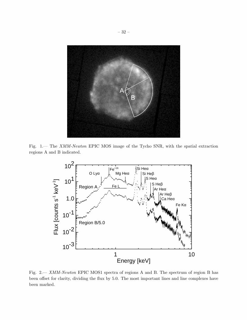
– 32 –

BA

Fig. 1.— The XMM-Newton EPIC MOS image of the Tycho SNR, with the spatial extraction

regions A and B indicated.

1 10Energy [keV]

10-3

10-2

10-1

1.0

101

102

Flu

x [c

ount

s s-1

keV

-1]

Region A

Region B/5.0

O LyαFe+16

Mg Heα

Fe L

Si HeαSi Heβ

S HeαS HeβAr Heα

Ar HeβCa Heα

Fe Kα

Fig. 2.— XMM-Newton EPIC MOS1 spectra of regions A and B. The spectrum of region B has

been offset for clarity, dividing the flux by 5.0. The most important lines and line complexes have

been marked.

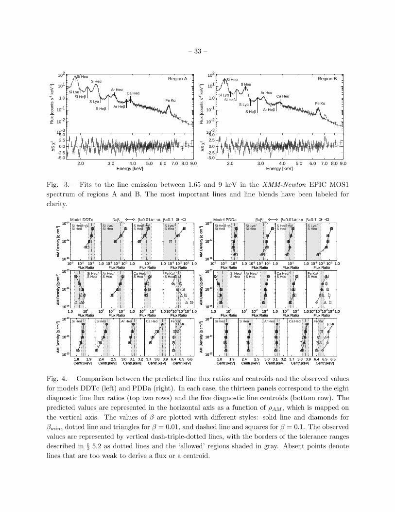
– 33 –

10-3

10-2

10-1

1.0

101

102

Flu

x [c

ount

s s-1

keV

-1]

Region ASi Heα

Si LyαSi Heβ

S Heα

S Lyα

S Heβ

Ar Heα

Ar Heβ

Ca Heα

Fe Kα

2.0 3.0 4.0 5.0 6.0 7.0 8.0 9.0Energy [keV]

-5.0-2.5

0.0

2.55.0

∆S χ

2

10-3

10-2

10-1

1.0

101

102

Flu

x [c

ount

s s-1

keV

-1]

Region BSi Heα

Si LyαSi Heβ

S Heα

S Lyα

S Heβ

Ar Heα

Ar Heβ

Ca Heα

Fe Kα

2.0 3.0 4.0 5.0 6.0 7.0 8.0 9.0Energy [keV]

-5.0-2.5

0.0

2.55.0

∆S χ

2

Fig. 3.— Fits to the line emission between 1.65 and 9 keV in the XMM-Newton EPIC MOS1

spectrum of regions A and B. The most important lines and line blends have been labeled for

clarity.

10-3 10-2 10-1 1.0Flux Ratio

10-25

10-24

10-23

AM

Den

sity

[g c

m-3]

10-3 10-2 10-1 1.0Flux Ratio

10-25

10-24

10-23

AM

Den

sity

[g c

m-3] Si He(β+γ)/

Si Heα

10-3 10-2 10-1 1.0Flux Ratio

10-3 10-2 10-1 1.0Flux Ratio

Si Lyα/Si Heα

10-1 1.0Flux Ratio

10-1 1.0Flux Ratio

S He(β+γ)/S Heα

10-3 10-2 10-1 1.0Flux Ratio

10-3 10-2 10-1 1.0Flux Ratio

S Lyα/S Heα

1.0 101 102

Flux Ratio

10-25

10-24

10-23

AM

Den

sity

[g c

m-3]

1.0 101 102

Flux Ratio

10-25

10-24

10-23

AM

Den

sity

[g c

m-3] Si Heα/

S Heα

10-2 10-1 1.0Flux Ratio

10-2 10-1 1.0Flux Ratio

Ar Heα/S Heα

10-2 10-1 1.0Flux Ratio

10-2 10-1 1.0Flux Ratio

Ca Heα/S Heα

10-410-310-210-1 1.0Flux Ratio

10-410-310-210-1 1.0Flux Ratio

Fe Kα/S Heα

1.8 1.9Centr.[keV]

10-25

10-24

10-23

AM

Den

sity

[g c

m-3]

1.8 1.9Centr.[keV]

10-25

10-24

10-23

AM

Den

sity

[g c

m-3] Si Heα

2.4 2.5Centr.[keV]

2.4 2.5Centr.[keV]

S Heα

3.0 3.1 3.2Centr.[keV]

3.0 3.1 3.2Centr.[keV]

Ar Heα

3.7 3.8 3.9Centr.[keV]

3.7 3.8 3.9Centr.[keV]

Ca Heα

6.4 6.5 6.6Centr.[keV]

6.4 6.5 6.6Centr.[keV]

Fe Kα

β=βmin

β=0.01 β=0.1Model DDTc

10-3 10-2 10-1 1.0Flux Ratio

10-25

10-24

10-23

AM

Den

sity

[g c

m-3]

10-3 10-2 10-1 1.0Flux Ratio

10-25

10-24

10-23

AM

Den

sity

[g c

m-3] Si He(β+γ)/

Si Heα

10-3 10-2 10-1 1.0Flux Ratio

10-3 10-2 10-1 1.0Flux Ratio

Si Lyα/Si Heα

10-1 1.0Flux Ratio

10-1 1.0Flux Ratio

S He(β+γ)/S Heα

10-3 10-2 10-1 1.0Flux Ratio

10-3 10-2 10-1 1.0Flux Ratio

S Lyα/S Heα

1.0 101 102

Flux Ratio

10-25

10-24

10-23

AM

Den

sity

[g c

m-3]

1.0 101 102

Flux Ratio

10-25

10-24

10-23

AM

Den

sity

[g c

m-3] Si Heα/

S Heα

10-2 10-1 1.0Flux Ratio

10-2 10-1 1.0Flux Ratio

Ar Heα/S Heα

10-2 10-1 1.0Flux Ratio

10-2 10-1 1.0Flux Ratio

Ca Heα/S Heα

10-410-310-210-1 1.0Flux Ratio

10-410-310-210-1 1.0Flux Ratio

Fe Kα/S Heα

1.8 1.9Centr.[keV]

10-25

10-24

10-23

AM

Den

sity

[g c

m-3]

1.8 1.9Centr.[keV]

10-25

10-24

10-23

AM

Den

sity

[g c

m-3] Si Heα

2.4 2.5Centr.[keV]

2.4 2.5Centr.[keV]

S Heα

3.0 3.1 3.2Centr.[keV]

3.0 3.1 3.2Centr.[keV]

Ar Heα

3.7 3.8 3.9Centr.[keV]

3.7 3.8 3.9Centr.[keV]

Ca Heα

6.4 6.5 6.6Centr.[keV]

6.4 6.5 6.6Centr.[keV]

Fe Kα

β=βmin

β=0.01 β=0.1Model PDDa

Fig. 4.— Comparison between the predicted line flux ratios and centroids and the observed values

for models DDTc (left) and PDDa (right). In each case, the thirteen panels correspond to the eight

diagnostic line flux ratios (top two rows) and the five diagnostic line centroids (bottom row). The

predicted values are represented in the horizontal axis as a function of ρAM , which is mapped on

the vertical axis. The values of β are plotted with different styles: solid line and diamonds for

βmin, dotted line and triangles for β = 0.01, and dashed line and squares for β = 0.1. The observed

values are represented by vertical dash-triple-dotted lines, with the borders of the tolerance ranges

described in § 5.2 as dotted lines and the ‘allowed’ regions shaded in gray. Absent points denote

lines that are too weak to derive a flux or a centroid.

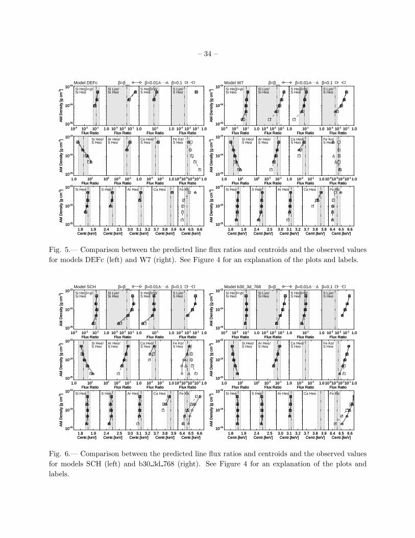
– 34 –

10-3 10-2 10-1 1.0Flux Ratio

10-25

10-24

10-23

AM

Den

sity

[g c

m-3]

10-3 10-2 10-1 1.0Flux Ratio

10-25

10-24

10-23

AM

Den

sity

[g c

m-3] Si He(β+γ)/

Si Heα

10-3 10-2 10-1 1.0Flux Ratio

10-3 10-2 10-1 1.0Flux Ratio

Si Lyα/Si Heα

10-1 1.0Flux Ratio

10-1 1.0Flux Ratio

S He(β+γ)/S Heα

10-3 10-2 10-1 1.0Flux Ratio

10-3 10-2 10-1 1.0Flux Ratio

S Lyα/S Heα

1.0 101 102

Flux Ratio

10-25

10-24

10-23

AM

Den

sity

[g c

m-3]

1.0 101 102

Flux Ratio

10-25

10-24

10-23

AM

Den

sity

[g c

m-3] Si Heα/

S Heα

10-2 10-1 1.0Flux Ratio

10-2 10-1 1.0Flux Ratio

Ar Heα/S Heα

10-2 10-1 1.0Flux Ratio

10-2 10-1 1.0Flux Ratio

Ca Heα/S Heα

10-410-310-210-1 1.0Flux Ratio

10-410-310-210-1 1.0Flux Ratio

Fe Kα/S Heα

1.8 1.9Centr.[keV]

10-25

10-24

10-23

AM

Den

sity

[g c

m-3]

1.8 1.9Centr.[keV]

10-25

10-24

10-23

AM

Den

sity

[g c

m-3] Si Heα

2.4 2.5Centr.[keV]

2.4 2.5Centr.[keV]

S Heα

3.0 3.1 3.2Centr.[keV]

3.0 3.1 3.2Centr.[keV]

Ar Heα

3.7 3.8 3.9Centr.[keV]

3.7 3.8 3.9Centr.[keV]

Ca Heα

6.4 6.5 6.6Centr.[keV]

6.4 6.5 6.6Centr.[keV]

Fe Kα

β=βmin

β=0.01 β=0.1Model DEFc

10-3 10-2 10-1 1.0Flux Ratio

10-25

10-24

10-23

AM

Den

sity

[g c

m-3]

10-3 10-2 10-1 1.0Flux Ratio

10-25

10-24

10-23

AM

Den

sity

[g c

m-3] Si He(β+γ)/

Si Heα

10-3 10-2 10-1 1.0Flux Ratio

10-3 10-2 10-1 1.0Flux Ratio

Si Lyα/Si Heα

10-1 1.0Flux Ratio

10-1 1.0Flux Ratio

S He(β+γ)/S Heα

10-3 10-2 10-1 1.0Flux Ratio

10-3 10-2 10-1 1.0Flux Ratio

S Lyα/S Heα

1.0 101 102

Flux Ratio

10-25

10-24

10-23

AM

Den

sity

[g c

m-3]

1.0 101 102

Flux Ratio

10-25

10-24

10-23

AM

Den

sity

[g c

m-3] Si Heα/

S Heα

10-2 10-1 1.0Flux Ratio

10-2 10-1 1.0Flux Ratio

Ar Heα/S Heα

10-2 10-1 1.0Flux Ratio

10-2 10-1 1.0Flux Ratio

Ca Heα/S Heα

10-410-310-210-1 1.0Flux Ratio

10-410-310-210-1 1.0Flux Ratio

Fe Kα/S Heα

1.8 1.9Centr.[keV]

10-25

10-24

10-23

AM

Den

sity

[g c

m-3]

1.8 1.9Centr.[keV]

10-25

10-24

10-23

AM

Den

sity

[g c

m-3] Si Heα

2.4 2.5Centr.[keV]

2.4 2.5Centr.[keV]

S Heα

3.0 3.1 3.2Centr.[keV]

3.0 3.1 3.2Centr.[keV]

Ar Heα

3.7 3.8 3.9Centr.[keV]

3.7 3.8 3.9Centr.[keV]

Ca Heα

6.4 6.5 6.6Centr.[keV]

6.4 6.5 6.6Centr.[keV]

Fe Kα

β=βmin

β=0.01 β=0.1Model W7

Fig. 5.— Comparison between the predicted line flux ratios and centroids and the observed values

for models DEFc (left) and W7 (right). See Figure 4 for an explanation of the plots and labels.

10-3 10-2 10-1 1.0Flux Ratio

10-25

10-24

10-23

AM

Den

sity

[g c

m-3]

10-3 10-2 10-1 1.0Flux Ratio

10-25

10-24

10-23

AM

Den

sity

[g c

m-3] Si He(β+γ)/

Si Heα

10-3 10-2 10-1 1.0Flux Ratio

10-3 10-2 10-1 1.0Flux Ratio

Si Lyα/Si Heα

10-1 1.0Flux Ratio

10-1 1.0Flux Ratio

S He(β+γ)/S Heα

10-3 10-2 10-1 1.0Flux Ratio

10-3 10-2 10-1 1.0Flux Ratio

S Lyα/S Heα

1.0 101 102

Flux Ratio

10-25

10-24

10-23

AM

Den

sity

[g c

m-3]

1.0 101 102

Flux Ratio

10-25

10-24

10-23

AM

Den

sity

[g c

m-3] Si Heα/

S Heα

10-2 10-1 1.0Flux Ratio

10-2 10-1 1.0Flux Ratio

Ar Heα/S Heα

10-2 10-1 1.0Flux Ratio

10-2 10-1 1.0Flux Ratio

Ca Heα/S Heα

10-410-310-210-1 1.0Flux Ratio

10-410-310-210-1 1.0Flux Ratio

Fe Kα/S Heα

1.8 1.9Centr.[keV]

10-25

10-24

10-23

AM

Den

sity

[g c

m-3]

1.8 1.9Centr.[keV]

10-25

10-24

10-23

AM

Den

sity

[g c

m-3] Si Heα

2.4 2.5Centr.[keV]

2.4 2.5Centr.[keV]

S Heα

3.0 3.1 3.2Centr.[keV]

3.0 3.1 3.2Centr.[keV]

Ar Heα

3.7 3.8 3.9Centr.[keV]

3.7 3.8 3.9Centr.[keV]

Ca Heα

6.4 6.5 6.6Centr.[keV]

6.4 6.5 6.6Centr.[keV]

Fe Kα

β=βmin

β=0.01 β=0.1Model SCH

10-3 10-2 10-1 1.0Flux Ratio

10-25

10-24

10-23

AM

Den

sity

[g c

m-3]

10-3 10-2 10-1 1.0Flux Ratio

10-25

10-24

10-23

AM

Den

sity

[g c

m-3] Si He(β+γ)/

Si Heα

10-3 10-2 10-1 1.0Flux Ratio

10-3 10-2 10-1 1.0Flux Ratio

Si Lyα/Si Heα

10-1 1.0Flux Ratio

10-1 1.0Flux Ratio

S He(β+γ)/S Heα

10-3 10-2 10-1 1.0Flux Ratio

10-3 10-2 10-1 1.0Flux Ratio

S Lyα/S Heα

1.0 101 102

Flux Ratio

10-25

10-24

10-23

AM

Den

sity

[g c

m-3]

1.0 101 102

Flux Ratio

10-25

10-24

10-23

AM

Den

sity

[g c

m-3] Si Heα/

S Heα

10-2 10-1 1.0Flux Ratio

10-2 10-1 1.0Flux Ratio

Ar Heα/S Heα

10-2 10-1 1.0Flux Ratio

10-2 10-1 1.0Flux Ratio

Ca Heα/S Heα

10-410-310-210-1 1.0Flux Ratio

10-410-310-210-1 1.0Flux Ratio

Fe Kα/S Heα

1.8 1.9Centr.[keV]

10-25

10-24

10-23

AM

Den

sity

[g c

m-3]

1.8 1.9Centr.[keV]

10-25

10-24

10-23

AM

Den

sity

[g c

m-3] Si Heα

2.4 2.5Centr.[keV]

2.4 2.5Centr.[keV]

S Heα

3.0 3.1 3.2Centr.[keV]

3.0 3.1 3.2Centr.[keV]

Ar Heα

3.7 3.8 3.9Centr.[keV]

3.7 3.8 3.9Centr.[keV]

Ca Heα

6.4 6.5 6.6Centr.[keV]

6.4 6.5 6.6Centr.[keV]

Fe Kα

β=βmin

β=0.01 β=0.1Model b30_3d_768

Fig. 6.— Comparison between the predicted line flux ratios and centroids and the observed values

for models SCH (left) and b30 3d 768 (right). See Figure 4 for an explanation of the plots and

labels.

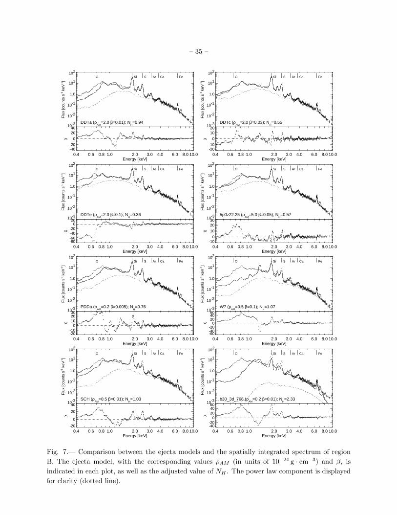
– 35 –

1 1010-3

10-2

10-1

1.0

101

102

Flu

x [c

ount

s s-1

keV

-1]

O Si S Ar Ca Fe

DDTa (ρAM

=2.0 β=0.01); NH=0.94

0.4 0.6 0.8 1.0 2.0 3.0 4.0 6.0 8.0 10.0Energy [keV]

-40-20

0

2040

χ

1 1010-3

10-2

10-1

1.0

101

102

Flu

x [c

ount

s s-1

keV

-1]

O Si S Ar Ca Fe

DDTc (ρAM

=2.0 β=0.03); NH=0.55

0.4 0.6 0.8 1.0 2.0 3.0 4.0 6.0 8.0 10.0Energy [keV]

-20-10

0

1020

χ

1 1010-3

10-2

10-1

1.0

101

102

Flu

x [c

ount

s s-1

keV

-1]

O Si S Ar Ca Fe

DDTe (ρAM

=2.0 β=0.1); NH=0.36

0.4 0.6 0.8 1.0 2.0 3.0 4.0 6.0 8.0 10.0Energy [keV]

-80-60-40-20

020

χ

1 1010-3

10-2

10-1

1.0

101

102

Flu

x [c

ount

s s-1

keV

-1]

O Si S Ar Ca Fe

5p0z22.25 (ρAM

=5.0 β=0.05); NH=0.57

0.4 0.6 0.8 1.0 2.0 3.0 4.0 6.0 8.0 10.0Energy [keV]

-100

10

2030

χ

1 1010-3

10-2

10-1

1.0

101

102

Flu

x [c

ount

s s-1

keV

-1]

O Si S Ar Ca Fe

PDDa (ρAM

=0.2 β=0.005); NH=0.76

0.4 0.6 0.8 1.0 2.0 3.0 4.0 6.0 8.0 10.0Energy [keV]

-20-10

0102030

χ

1 1010-3

10-2

10-1

1.0

101

102

Flu

x [c

ount

s s-1

keV

-1]

O Si S Ar Ca Fe

W7 (ρAM

=0.5 β=0.1); NH=1.07

0.4 0.6 0.8 1.0 2.0 3.0 4.0 6.0 8.0 10.0Energy [keV]

-60-40-20

0204060

χ

1 1010-3

10-2

10-1

1.0

101

102

Flu

x [c

ount

s s-1

keV

-1]

O Si S Ar Ca Fe

SCH (ρAM

=0.5 β=0.01); NH=1.03

0.4 0.6 0.8 1.0 2.0 3.0 4.0 6.0 8.0 10.0Energy [keV]

-20

0

20

40

χ

1 1010-3

10-2

10-1

1.0

101

102

Flu

x [c

ount

s s-1

keV

-1]

O Si S Ar Ca Fe

b30_3d_768 (ρAM

=0.2 β=0.01); NH=2.33

0.4 0.6 0.8 1.0 2.0 3.0 4.0 6.0 8.0 10.0Energy [keV]

-40-20

0204060

χ

Fig. 7.— Comparison between the ejecta models and the spatially integrated spectrum of region

B. The ejecta model, with the corresponding values ρAM (in units of 10−24 g · cm−3) and β, is

indicated in each plot, as well as the adjusted value of NH . The power law component is displayed

for clarity (dotted line).

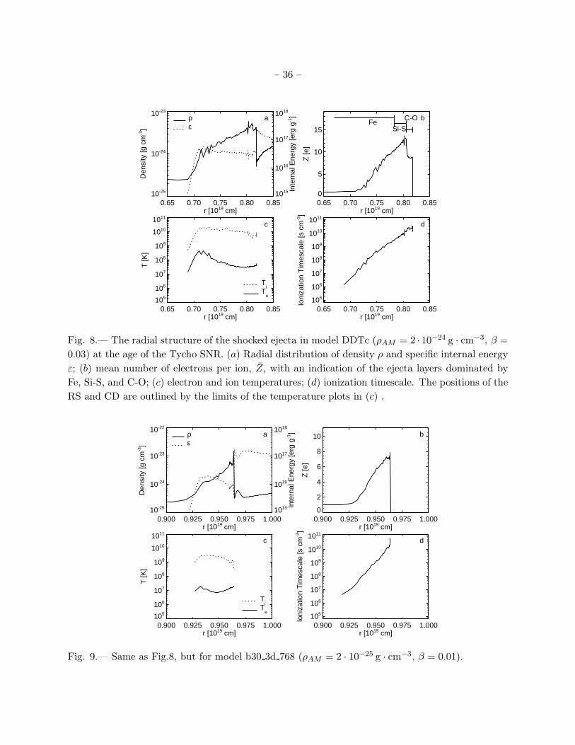
– 36 –

0.65 0.70 0.75 0.80 0.85r [1019 cm]

10-25

10-24

10-23

Den

sity

[g c

m-3]

1015

1016

1017

1018

Inte

rnal

Ene

rgy

[erg

g-1]ρ

εa

0.65 0.70 0.75 0.80 0.85r [1019 cm]

0

5

10

15

Z [e

]

FeSi-S

C-O b

0.65 0.70 0.75 0.80 0.85r [1019 cm]

105

106

107

108

109

1010

1011

T [K

]

Te

Ti

c

0.65 0.70 0.75 0.80 0.85r [1019 cm]

105

106

107

108

109

1010

1011

Ioni

zatio

n T

imes

cale

[s c

m-3]

d

Fig. 8.— The radial structure of the shocked ejecta in model DDTc (ρAM = 2 · 10−24 g · cm−3, β =

0.03) at the age of the Tycho SNR. (a) Radial distribution of density ρ and specific internal energy

ε; (b) mean number of electrons per ion, Z, with an indication of the ejecta layers dominated by

Fe, Si-S, and C-O; (c) electron and ion temperatures; (d) ionization timescale. The positions of the

RS and CD are outlined by the limits of the temperature plots in (c) .

0.900 0.925 0.950 0.975 1.000r [1019 cm]

10-25

10-24

10-23

10-22

Den

sity

[g c

m-3]

1015

1016

1017

1018

Inte

rnal

Ene

rgy

[erg

g-1]ρ

εa

0.900 0.925 0.950 0.975 1.000r [1019 cm]

0

2

4

6

8

10

Z [e

]

b

0.900 0.925 0.950 0.975 1.000r [1019 cm]

105

106

107

108

109

1010

1011

T [K

]

Te

Ti

c

0.900 0.925 0.950 0.975 1.000r [1019 cm]

105

106

107

108

109

1010

1011

Ioni

zatio

n T

imes

cale

[s c

m-3]

d

Fig. 9.— Same as Fig.8, but for model b30 3d 768 (ρAM = 2 · 10−25 g · cm−3, β = 0.01).

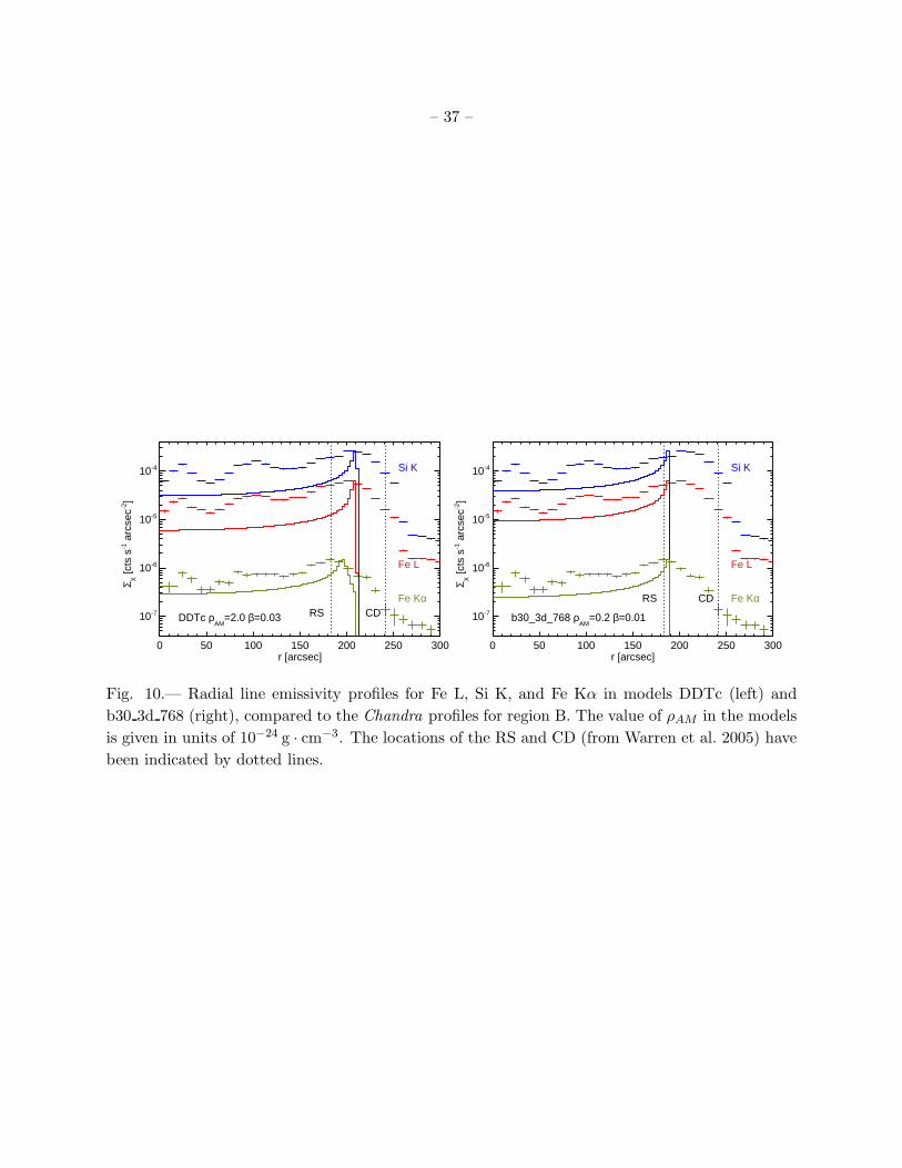
– 37 –

0 50 100 150 200 250 300r [arcsec]

10-7

10-6

10-5

10-4

Σ X [c

ts s

-1 a

rcse

c-2]

RS CD

Si K

Fe L

Fe Kα

DDTc ρAM

=2.0 β=0.03

0 50 100 150 200 250 300r [arcsec]

10-7

10-6

10-5

10-4Σ X

[cts

s-1 a

rcse

c-2]

RS CD

Si K

Fe L

Fe Kα

b30_3d_768 ρAM

=0.2 β=0.01

Fig. 10.— Radial line emissivity profiles for Fe L, Si K, and Fe Kα in models DDTc (left) and

b30 3d 768 (right), compared to the Chandra profiles for region B. The value of ρAM in the models

is given in units of 10−24 g · cm−3. The locations of the RS and CD (from Warren et al. 2005) have

been indicated by dotted lines.

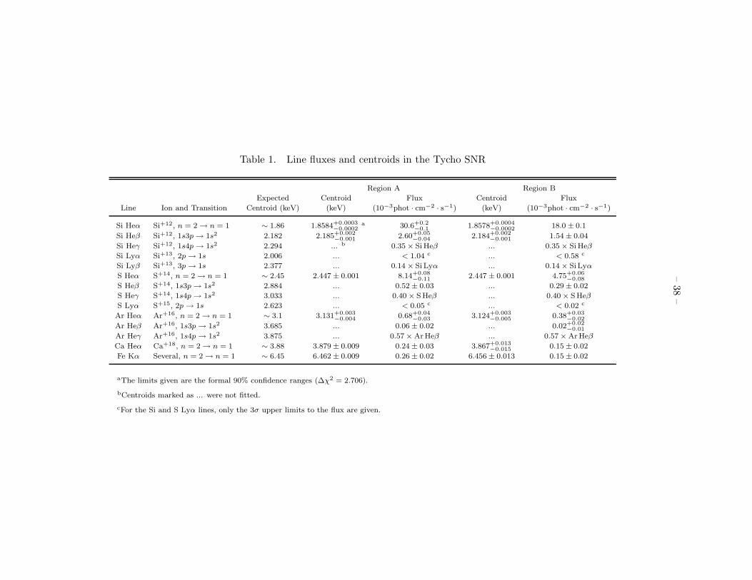
–38

–

Table 1. Line fluxes and centroids in the Tycho SNR

Region A Region B

Expected Centroid Flux Centroid Flux

Line Ion and Transition Centroid (keV) (keV) (10−3phot · cm−2 · s−1) (keV) (10−3phot · cm−2 · s−1)

Si Heα Si+12, n = 2 → n = 1 ∼ 1.86 1.8584+0.0003−0.0002

a 30.6+0.2−0.1 1.8578+0.0004

−0.0002 18.0 ± 0.1

Si Heβ Si+12, 1s3p → 1s2 2.182 2.185+0.002−0.001 2.60+0.05

−0.04 2.184+0.002−0.001 1.54 ± 0.04

Si Heγ Si+12, 1s4p → 1s2 2.294 ... b 0.35 × Si Heβ ... 0.35 × Si Heβ

Si Lyα Si+13, 2p → 1s 2.006 ... < 1.04 c ... < 0.58 c

Si Lyβ Si+13, 3p → 1s 2.377 ... 0.14 × Si Lyα ... 0.14 × Si Lyα

S Heα S+14, n = 2 → n = 1 ∼ 2.45 2.447 ± 0.001 8.14+0.08−0.11 2.447 ± 0.001 4.75+0.06

−0.08

S Heβ S+14, 1s3p → 1s2 2.884 ... 0.52 ± 0.03 ... 0.29 ± 0.02

S Heγ S+14, 1s4p → 1s2 3.033 ... 0.40 × S Heβ ... 0.40 × S Heβ

S Lyα S+15, 2p → 1s 2.623 ... < 0.05 c ... < 0.02 c

Ar Heα Ar+16, n = 2 → n = 1 ∼ 3.1 3.131+0.003−0.004 0.68+0.04

−0.03 3.124+0.003−0.005 0.38+0.03

−0.02

Ar Heβ Ar+16, 1s3p → 1s2 3.685 ... 0.06 ± 0.02 ... 0.02+0.02−0.01

Ar Heγ Ar+16, 1s4p → 1s2 3.875 ... 0.57 × ArHeβ ... 0.57 × ArHeβ

Ca Heα Ca+18, n = 2 → n = 1 ∼ 3.88 3.879 ± 0.009 0.24 ± 0.03 3.867+0.013−0.015 0.15 ± 0.02

Fe Kα Several, n = 2 → n = 1 ∼ 6.45 6.462 ± 0.009 0.26 ± 0.02 6.456 ± 0.013 0.15 ± 0.02

aThe limits given are the formal 90% confidence ranges (∆χ2 = 2.706).

bCentroids marked as ... were not fitted.

cFor the Si and S Lyα lines, only the 3σ upper limits to the flux are given.

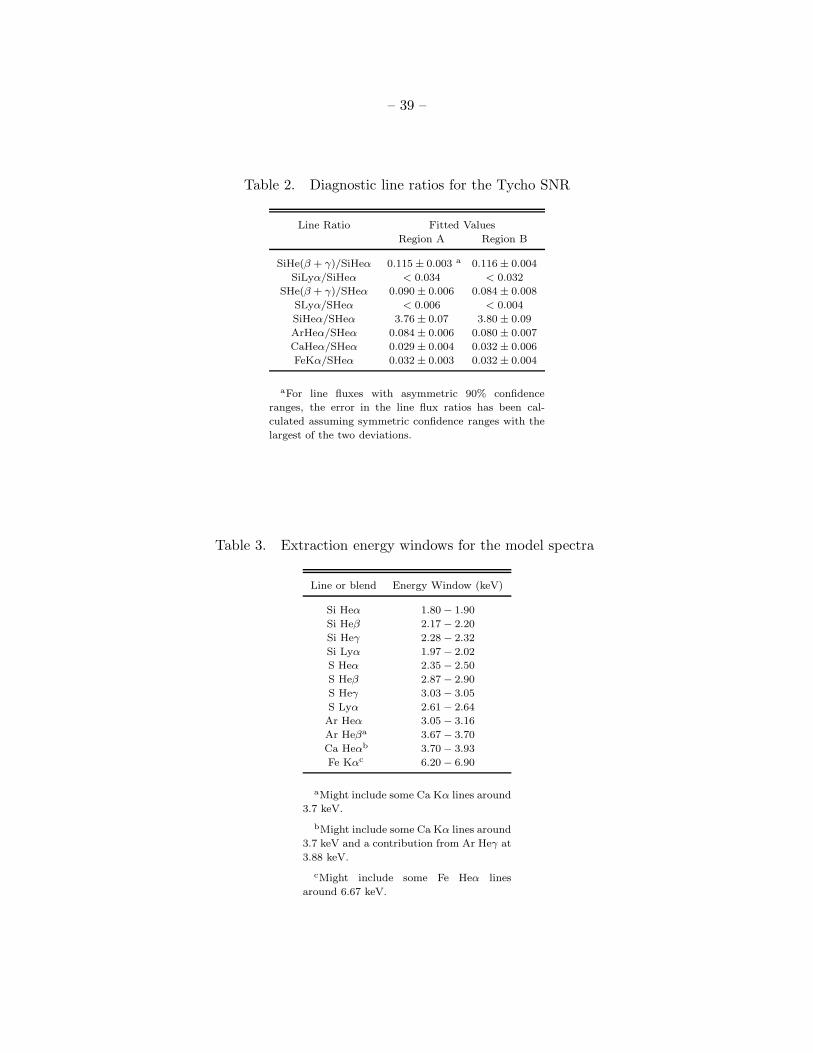
– 39 –

Table 2. Diagnostic line ratios for the Tycho SNR

Line Ratio Fitted Values

Region A Region B

SiHe(β + γ)/SiHeα 0.115 ± 0.003 a 0.116 ± 0.004

SiLyα/SiHeα < 0.034 < 0.032

SHe(β + γ)/SHeα 0.090 ± 0.006 0.084 ± 0.008

SLyα/SHeα < 0.006 < 0.004

SiHeα/SHeα 3.76 ± 0.07 3.80 ± 0.09

ArHeα/SHeα 0.084 ± 0.006 0.080 ± 0.007

CaHeα/SHeα 0.029 ± 0.004 0.032 ± 0.006

FeKα/SHeα 0.032 ± 0.003 0.032 ± 0.004

aFor line fluxes with asymmetric 90% confidence

ranges, the error in the line flux ratios has been cal-

culated assuming symmetric confidence ranges with the

largest of the two deviations.

Table 3. Extraction energy windows for the model spectra

Line or blend Energy Window (keV)

Si Heα 1.80 − 1.90

Si Heβ 2.17 − 2.20

Si Heγ 2.28 − 2.32

Si Lyα 1.97 − 2.02

S Heα 2.35 − 2.50

S Heβ 2.87 − 2.90

S Heγ 3.03 − 3.05

S Lyα 2.61 − 2.64

Ar Heα 3.05 − 3.16

Ar Heβa 3.67 − 3.70

Ca Heαb 3.70 − 3.93

Fe Kαc 6.20 − 6.90

aMight include some Ca Kα lines around

3.7 keV.

bMight include some Ca Kα lines around

3.7 keV and a contribution from Ar Heγ at

3.88 keV.

cMight include some Fe Heα lines

around 6.67 keV.

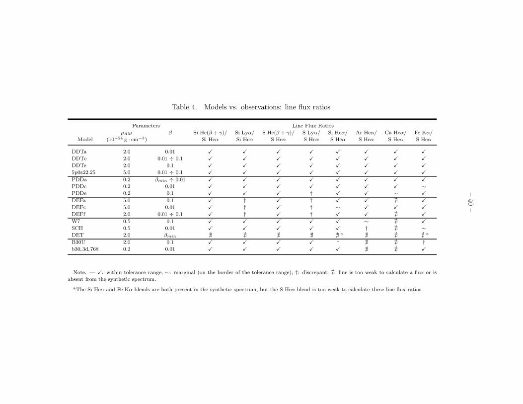
–40

–

Table 4. Models vs. observations: line flux ratios

Parameters Line Flux Ratios

ρAM β Si He(β + γ)/ Si Lyα/ S He(β + γ)/ S Lyα/ Si Heα/ Ar Heα/ Ca Heα/ Fe Kα/

Model (10−24 g · cm−3) Si Heα Si Heα S Heα S Heα S Heα S Heα S Heα S Heα

DDTa 2.0 0.01 X X X X X X X X

DDTc 2.0 0.01 ÷ 0.1 X X X X X X X X

DDTe 2.0 0.1 X X X X X X X X

5p0z22.25 5.0 0.01 ÷ 0.1 X X X X X X X X

PDDa 0.2 βmin ÷ 0.01 X X X X X X X X

PDDc 0.2 0.01 X X X X X X X ∼

PDDe 0.2 0.1 X X X † X X ∼ X

DEFa 5.0 0.1 X † X † X X ∄ X

DEFc 5.0 0.01 X † X † ∼ X X X

DEFf 2.0 0.01 ÷ 0.1 X † X † X X ∄ X

W7 0.5 0.1 X X X X X ∼ ∄ X

SCH 0.5 0.01 X X X X X † ∄ ∼

DET 2.0 βmin ∄ ∄ ∄ ∄ ∄ a ∄ ∄ ∄ a

B30U 2.0 0.1 X X X X † ∄ ∄ †

b30 3d 768 0.2 0.01 X X X X X ∄ ∄ X

Note. — X: within tolerance range; ∼: marginal (on the border of the tolerance range); †: discrepant; ∄: line is too weak to calculate a flux or is

absent from the synthetic spectrum.

aThe Si Heα and Fe Kα blends are both present in the synthetic spectrum, but the S Heα blend is too weak to calculate these line flux ratios.

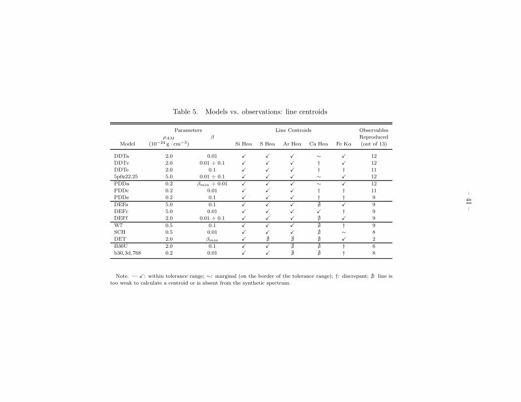
–41

–

Table 5. Models vs. observations: line centroids

Parameters Line Centroids Observables

ρAM β Reproduced

Model (10−24 g · cm−3) Si Heα S Heα Ar Heα Ca Heα Fe Kα (out of 13)

DDTa 2.0 0.01 X X X ∼ X 12

DDTc 2.0 0.01 ÷ 0.1 X X X † X 12

DDTe 2.0 0.1 X X X † † 11

5p0z22.25 5.0 0.01 ÷ 0.1 X X X ∼ X 12

PDDa 0.2 βmin ÷ 0.01 X X X ∼ X 12

PDDc 0.2 0.01 X X X † † 11

PDDe 0.2 0.1 X X X † † 9

DEFa 5.0 0.1 X X X ∄ X 9

DEFc 5.0 0.01 X X X X † 9

DEFf 2.0 0.01 ÷ 0.1 X X X ∄ X 9

W7 0.5 0.1 X X X ∄ † 9

SCH 0.5 0.01 X X X ∄ ∼ 8

DET 2.0 βmin X ∄ ∄ ∄ X 2

B30U 2.0 0.1 X X ∄ ∄ † 6

b30 3d 768 0.2 0.01 X X ∄ ∄ † 8

Note. — X: within tolerance range; ∼: marginal (on the border of the tolerance range); †: discrepant; ∄: line is

too weak to calculate a centroid or is absent from the synthetic spectrum.

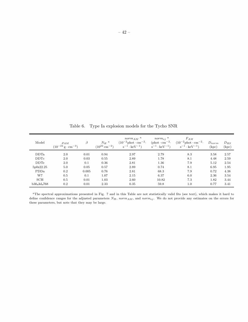
– 42 –

Table 6. Type Ia explosion models for the Tycho SNR

normAMa normej

a FAM

Model ρAM β NHa (10−2phot · cm−2· (phot · cm−2· (10−2phot · cm−2· Dnorm DRS

(10−24 g · cm−3) (1022 cm−2) s−1 · keV−1) s−1 · keV−1) s−1 · keV−1) (kpc) (kpc)

DDTa 2.0 0.01 0.94 2.97 2.79 8.3 3.58 2.57

DDTc 2.0 0.03 0.55 2.89 1.78 8.1 4.48 2.59

DDTe 2.0 0.1 0.36 2.81 1.36 7.9 5.12 2.54

5p0z22.25 5.0 0.05 0.57 2.89 0.74 8.1 6.95 1.95

PDDa 0.2 0.005 0.76 2.81 68.3 7.9 0.72 4.38

W7 0.5 0.1 1.07 2.15 6.37 6.0 2.36 3.54

SCH 0.5 0.01 1.03 2.60 10.82 7.3 1.82 3.44

b30 3d 768 0.2 0.01 2.33 0.35 59.8 1.0 0.77 3.41

aThe spectral approximations presented in Fig. 7 and in this Table are not statistically valid fits (see text), which makes it hard to

define confidence ranges for the adjusted parameters NH , normAM , and normej . We do not provide any estimates on the errors for

these parameters, but note that they may be large.