
The Hipparcos and Tycho Catalogues - cosmos.esa.int
418
The Hipparcos and Tycho Catalogues
-
Upload
khangminh22 -
Category
Documents
-
view
4 -
download
0
Transcript of The Hipparcos and Tycho Catalogues - cosmos.esa.int

The Hipparcos and Tycho Catalogues


SP–1200June 1997
The Hipparcos and Tycho Catalogues
Astrometric and Photometric Star Catalogues
derived from the
ESA Hipparcos Space Astrometry Mission
A Collaboration Between
the European Space Agency
and
the FAST, NDAC, TDAC and INCA Consortia
and the Hipparcos Industrial Consortium led by
Matra Marconi Space
and
Alenia Spazio
European Space AgencyAgence spatiale europeenne
Cover illustration: an impression of selected stars in their true positions around the Sun, as determined by
Hipparcos, and viewed from a distant vantage point. Inset: sky map of the number of observations made by
Hipparcos, in ecliptic coordinates.
Published by: ESA Publications Division, c/o ESTEC, Noordwijk, The Netherlands
Scientific Coordination: M.A.C. Perryman, ESA Space Science Department
and the Hipparcos Science Team
Composition: Volume 1: M.A.C. Perryman
Volume 2: K.S. O’Flaherty
Volume 3: F. van Leeuwen, L. Lindegren & F. Mignard
Volume 4: U. Bastian & E. Høg
Volumes 5–11: Hans Schrijver
Volume 12: Michel Grenon
Volume 13: Michel Grenon (charts) & Hans Schrijver (tables)
Volumes 14–16: Roger W. Sinnott
Volume 17: Hans Schrijver & W. O’Mullane
Typeset using TEX (by D.E. Knuth) and dvips (by T. Rokicki)
in Monotype Plantin (Adobe) and Frutiger (URW)
Film Production: Volumes 1–4: ESA Publications Division, ESTEC, Noordwijk, The Netherlands
Volumes 5–13: Imprimerie Louis-Jean, Gap, France
Volumes 14–16: Sky Publishing Corporation, Cambridge, Massachusetts, USA
ASCII CD-ROMs: Swets & Zeitlinger B.V., Lisse, The Netherlands
Publications Management: B. Battrick & H. Wapstra
Cover Design: C. Haakman
1997 European Space Agency
ISSN 0379–6566
ISBN 92–9092–399-7 (Volumes 1–17)
Price: 650 Dfl ($400) (17 volumes)
165 Dfl ($100) (Volumes 1 & 17 only)
Volume 2
The Hipparcos Satellite Operations
Compiled by:
M.A.C. Perryman & K.S. O’Flaherty (ESA–ESTEC)
D. Heger (ESA–ESOC) & A.J.C. McDonald (ESOC/Logica UK Ltd)
with the support of
The Hipparcos Science Team,
M. Bouffard (Matra Marconi Space),
and
B. Strim (Alenia Spazio)


Launch of the Hipparcos Satellite by Ariane 4 Flight V33, 8 August 1989 (Photo: CSG Kourou)


ix
Volume 2: The Hipparcos Satellite Operations
Contents
Foreword . . . . . . . . . . . . . . . . . . . . . . . . . . . . . . . xiiiPrologue . . . . . . . . . . . . . . . . . . . . . . . . . . . . . . . . 1
Section A: Background
1. Overview of the Hipparcos Satellite . . . . . . . . . . . . . . . . . . 111.1. Operating Principle . . . . . . . . . . . . . . . . . . . . . . . 111.2. Constraints and Properties of the Nominal Orbit . . . . . . . . . . 171.3. Satellite Environmental Conditions . . . . . . . . . . . . . . . . 181.4. Attitude Control Concept . . . . . . . . . . . . . . . . . . . . 211.5. Data Handling and Processing . . . . . . . . . . . . . . . . . . 221.6. Operational Concept . . . . . . . . . . . . . . . . . . . . . . 241.7. Satellite Mechanical and Electrical Design . . . . . . . . . . . . . 251.8. Ground Segment Overview . . . . . . . . . . . . . . . . . . . 29
2. The Payload: Overview and Optical Elements . . . . . . . . . . . . . 332.1. Introduction . . . . . . . . . . . . . . . . . . . . . . . . . . 332.2. Payload Configuration and Layout . . . . . . . . . . . . . . . . 352.3. Payload Hardware . . . . . . . . . . . . . . . . . . . . . . . 412.4. Telescope Mirrors . . . . . . . . . . . . . . . . . . . . . . . 432.5. Modulating Grid and Baffle Unit . . . . . . . . . . . . . . . . . 472.6. Relay Lens Systems . . . . . . . . . . . . . . . . . . . . . . . 56
3. The Payload: Detectors, Electronics, and Structure . . . . . . . . . . . 653.1. Detectors . . . . . . . . . . . . . . . . . . . . . . . . . . . 653.2. Payload Electronics and Mechanisms . . . . . . . . . . . . . . . 713.3. Baffles . . . . . . . . . . . . . . . . . . . . . . . . . . . . 753.4. Payload Structure . . . . . . . . . . . . . . . . . . . . . . . 79
Section B: Launch and Early Orbit Phases
4. Launch and Revised Mission Definition . . . . . . . . . . . . . . . . 854.1. Introduction . . . . . . . . . . . . . . . . . . . . . . . . . . 854.2. Operations Until Revised Mission Implementation . . . . . . . . . 864.3. Apogee Boost Motor Failure Investigations . . . . . . . . . . . . 874.4. Revised Mission Definition . . . . . . . . . . . . . . . . . . . 884.5. Ground Station Utilisation . . . . . . . . . . . . . . . . . . . 914.6. Mission Planning . . . . . . . . . . . . . . . . . . . . . . . . 944.7. Orbit Manoeuvres and Commissioning Activities . . . . . . . . . . 97

x
5.InitialPayloadCalibration ......................1035.1.CalibrationPlan ........................1035.2.DetectorNoise.........................1045.3.StarMapperSingle-SlitResponse ................1065.4.InitialImageDissectorTubePiloting ...............1075.5.TransverseandLongitudinalOffsets ...............1115.6.Focusing ...........................1125.7.InstantaneousFieldofViewProfile ................1135.8.Chromaticity .........................1145.9. Straylight . . . . . . . . . . . . . . . . . . . . . . . . . . . 115
6. The Operational Orbit . . . . . . . . . . . . . . . . . . . . . . . . 1176.1. Orbital Elements . . . . . . . . . . . . . . . . . . . . . . . . 1176.2. Radiation Environment . . . . . . . . . . . . . . . . . . . . . 1196.3. Eclipses . . . . . . . . . . . . . . . . . . . . . . . . . . . . 1196.4. Occultations . . . . . . . . . . . . . . . . . . . . . . . . . . 1216.5. Ground Station Coverage . . . . . . . . . . . . . . . . . . . . 1216.6. Perturbing Torques . . . . . . . . . . . . . . . . . . . . . . . 1226.7. Loss of Real-Time Attitude Determination . . . . . . . . . . . . 1226.8. Micrometeoroids . . . . . . . . . . . . . . . . . . . . . . . . 123
7. Radiation Background and Related Effects . . . . . . . . . . . . . . . 1277.1. Introduction . . . . . . . . . . . . . . . . . . . . . . . . . . 1277.2. The Radiation Environment in Space . . . . . . . . . . . . . . . 1287.3. Modelling the Radiation Dose Absorbed by the Satellite . . . . . . . 1327.4. Effects of the Radiation Background on the Mission . . . . . . . . . 135
Section C: Interfaces with the Scientific Consortia
8. The Observation Programme and Interface with the INCA Consortium . . 1438.1. Scanning Law . . . . . . . . . . . . . . . . . . . . . . . . . 1438.2. Star Observations . . . . . . . . . . . . . . . . . . . . . . . 1508.3. Input Catalogue Consortium Interfaces with ESOC . . . . . . . . . 1568.4. Programme Star File Generation . . . . . . . . . . . . . . . . . 1608.5. Modulation Strategy . . . . . . . . . . . . . . . . . . . . . . 163
9. Interfaces with the Data Reduction Consortia . . . . . . . . . . . . . . 1679.1. Introduction . . . . . . . . . . . . . . . . . . . . . . . . . . 1679.2. Data Distribution from ESOC to the Consortia . . . . . . . . . . 1699.3. Data from FAST to ESOC in Support of Satellite Operations . . . . 1759.4. Data from NDAC to ESOC in Support of Satellite Operations . . . . 176

xi
Section D: Payload and Spacecraft Performances
10. Routine Calibration and Payload Evolution . . . . . . . . . . . . . . . 17910.1. Routine Monitoring Activities at ESOC . . . . . . . . . . . . . 17910.2. Payload Calibration . . . . . . . . . . . . . . . . . . . . . . 18210.3. Focus Evolution . . . . . . . . . . . . . . . . . . . . . . . 18510.4. Photometric Evolution . . . . . . . . . . . . . . . . . . . . . 19310.5. Payload Modelling . . . . . . . . . . . . . . . . . . . . . . 19310.6. Star Mapper Sensitivity during Suspended Operations . . . . . . . 207
11. Solar Array Performance . . . . . . . . . . . . . . . . . . . . . . . 20911.1. Introduction . . . . . . . . . . . . . . . . . . . . . . . . . 20911.2. Power Subsystem Degradation . . . . . . . . . . . . . . . . . 21111.3. Solar Array Degradation . . . . . . . . . . . . . . . . . . . . 21411.4. Eclipse-Induced Attitude Jitter . . . . . . . . . . . . . . . . . 224
12. Thermal Control . . . . . . . . . . . . . . . . . . . . . . . . . . 22712.1. Introduction . . . . . . . . . . . . . . . . . . . . . . . . . 22712.2. Heater Design . . . . . . . . . . . . . . . . . . . . . . . . 22912.3. Payload Thermal Control History . . . . . . . . . . . . . . . . 22912.4. Thermal Anomalies and the Basic Angle . . . . . . . . . . . . . 232
Section E: Real-Time Attitude Control and Determination
13. Attitude and Orbit Control System and Performances . . . . . . . . . . 23713.1. Functions of the Attitude and Orbit Control System . . . . . . . . 23713.2. Equipment Description . . . . . . . . . . . . . . . . . . . . 23813.3. Reaction Control Assembly . . . . . . . . . . . . . . . . . . . 24113.4. Inertial Reference Unit . . . . . . . . . . . . . . . . . . . . . 24413.5. Gyro Performances . . . . . . . . . . . . . . . . . . . . . . 24513.6. Gyro Related Ground Investigations . . . . . . . . . . . . . . . 24913.7. Gas Consumption . . . . . . . . . . . . . . . . . . . . . . . 25213.8. Normal Mode Controller . . . . . . . . . . . . . . . . . . . . 25213.9. Thruster Monitoring and Normal Mode Software Patch . . . . . . 25513.10. Disturbance Torques . . . . . . . . . . . . . . . . . . . . . 25613.11. Real-Time Attitude Determination . . . . . . . . . . . . . . . 256
14. Real-Time Attitude Determination with Three Gyros . . . . . . . . . . 25714.1. Introduction and Overall Concept . . . . . . . . . . . . . . . . 25714.2. On-Board Real-Time Attitude Determination using Three Gyros . . 26014.3. On-Ground Real-Time Attitude Determination . . . . . . . . . . 26514.4. Real-Time Attitude Determination Performance . . . . . . . . . . 281

xii
15. Real-Time Attitude Determination with Two Gyros . . . . . . . . . . . 28715.1. Two-Gyro Operations Development History . . . . . . . . . . . 28715.2. Operational Requirements . . . . . . . . . . . . . . . . . . . 28915.3. On-Board Software . . . . . . . . . . . . . . . . . . . . . . 29115.4. On-Ground Software . . . . . . . . . . . . . . . . . . . . . 29415.5. Operational Experience . . . . . . . . . . . . . . . . . . . . 300
16. Real-Time Attitude Determination with Zero Gyros . . . . . . . . . . . 30516.1. Activities during Suspended Operations . . . . . . . . . . . . . 30516.2. On-Board Software . . . . . . . . . . . . . . . . . . . . . . 30716.3. On-Ground Software . . . . . . . . . . . . . . . . . . . . . 31116.4. Operational Experience . . . . . . . . . . . . . . . . . . . . 315
Section F: End of Mission
17. End of Mission Activities and Conclusions . . . . . . . . . . . . . . . 31717.1. End-of-Life History . . . . . . . . . . . . . . . . . . . . . . 31717.2. End-of-Life Tests . . . . . . . . . . . . . . . . . . . . . . . 31817.3. Satellite Reliability Assessment . . . . . . . . . . . . . . . . . 32217.4. Data Archiving Policy . . . . . . . . . . . . . . . . . . . . . 32217.5. Miscellaneous Considerations . . . . . . . . . . . . . . . . . . 32217.6. Overall Success of the Hipparcos Mission . . . . . . . . . . . . . 329
Appendices
Appendix A. The ESA-ESOC Operations Team . . . . . . . . . . . . . . 331
Appendix B. Satellite Anomalies . . . . . . . . . . . . . . . . . . . . . 337
Appendix C. References . . . . . . . . . . . . . . . . . . . . . . . . . 349
Appendix D. Bibliography . . . . . . . . . . . . . . . . . . . . . . . . 351
Appendix E. The Hipparcos Mission Costs . . . . . . . . . . . . . . . . 379
Appendix F. The Hipparcos Satellite During Development . . . . . . . . . . 383
Index . . . . . . . . . . . . . . . . . . . . . . . . . . . . . . . . . 397
xiii
Foreword
The Hipparcos astrometry mission was accepted within the European Space Agency’sscientific programme in 1980. The Hipparcos satellite was designed and constructedunder ESA responsibility by a European industrial consortium led by Matra MarconiSpace (France) and Alenia Spazio (Italy), and launched by Ariane 4 flight V33 on8 August 1989. High-quality scientific data were acquired between November 1989and March 1993, and communications with the satellite were terminated on 15 August1993. The Hipparcos and Tycho Catalogues, representing the most accurate and com-prehensive astrometric and photometric star catalogues compiled to date, were finalisedwithin three years of the end of the satellite operations—almost exactly correspondingto the schedule anticipated by the scientific consortia before the satellite launch. All ofthe scientific goals motivating the mission’s adoption in 1980 were surpassed.
An enormous effort—scientific, technical, and managerial—was devoted to the satellitedesign, construction, testing and calibration, in a commitment extending over approxi-mately eight years; in parallel, teams of European scientists worked closely with ESA toprepare a complex chain of computer programs ready to process nearly 1000 Gbits ofsatellite data in what amounted to the largest single data analysis problem ever under-taken in astronomy.
Ultimate success was not easily won. After a nominal launch, the failure of the apogeeboost motor left the satellite in an unplanned, highly eccentric geostationary transferorbit. A mission which was designed to have a single ground station, operated ina geostationary orbit for 24 hours a day, turned out instead to consist of a satellite incontact with the ground station for less than 10 hours a day, repeatedly crossing the harshradiation environment of the van Allen belts. Further ground stations were brought intothe telecommunications network. ESOC, in collaboration with Matra Marconi Space,developed new operational procedures to accommodate the new orbit, the revised data tobe sent to the scientific data reduction groups, and contingency procedures to maintainthe flow of scientific data. The payload and spacecraft subsystems all worked within theirdesign specifications, the satellite was eventually operated for more than the 2.5 yearsnominal mission duration, and scientific data of extremely high quality were acquired.
This volume is intended as a detailed description of the manner in which the scientificdata were collected. In addition, it provides a summary of the satellite and payloadperformances, and a record of the technological investigations and resulting knowledgederived from the operation of the Hipparcos satellite. It includes details of the majorspacecraft and payload subsystems, the radiation environment, understanding of thepayload evolution, perturbing torques acting on the satellite, and details of the de-velopment of two- and zero-gyro operational procedures implemented as gyro failuresthreatened to terminate operations prematurely.
The material in this volume has been based on the pre-launch technical description,published in 1989 as ESA SP-1111 Volume I, combined with the ESOC OperationsReport produced by the Operations Team at the end of the mission. Significant parts ofthe report are taken from the Matra Marconi Space ‘In-Orbit Performance VerificationReport’ prepared under ESA contract. Other material was taken from technical notescompiled throughout the satellite operations phase.

xiv
Significant additional material was included as follows:
• material in Chapter 5 is based on Davies, P.E. & McDonald, A.J.C., 1991 Resultsof the Hipparcos In-Orbit Payload Calibration, Journal of the British InterplanetarySociety, Vol. 44, 37;
• material in Chapter 7 is based on Crabb, R.L., 1994 Solar cell radiation damage, Ra-diat. Phys. Chem. 43, 93–103; Nieminen, P.J., 1995 Standard radiation environmentmonitor detector design and simulations, ESTEC Working Paper 1829; Section 7.4 isfrom Daly, E.J. et al., 1994 Radiation-belt and transient solar-magnetospheric effects onHipparcos radiation background, IEEE Trans. Nucl. Sci. NS-41, 6, 2376;
• parts of Chapter 10 are from Lindegren, L. et al., 1992 Geometrical stability andevolution of the Hipparcos telescope, Astronomy & Astrophysics, 258, 35, and updatedby L. Lindegren and F. van Leeuwen;
• material in Chapter 11 was taken from Crabb, R.L. & Robben, A.P., 1993 In-flight Hipparcos solar array performance degradation after three and a half years, Proc.European Space Power Conference, Graz, Austria, ESTEC/XPG-WPP-054;
• parts of Chapter 14 were taken from Batten, A.J. & McDonald, A.J.C., 1989,Hipparcos precise attitude determination: methods and results, Int. Symp. Space Dy-namics, Toulouse, France;
• material in Chapter 15 is based on Auburn, J.H.C., Batten, A.J. & McDonald,A.J.C., 1991 Hipparcos attitude determination with two gyros and a star mapper, Proc.3rd International Symp. Spacecraft Flight Dynamics, Darmstadt, Germany, ESASP-326, 213.
The composition of the ESA-ESOC Launch and Operations Teams are given in Ap-pendix A to this volume. The key personnel involved from Matra Marconi Space (thesatellite Prime Contractor) and Alenia Spazio (responsible for the spacecraft and for thesatellite integration), along with the industrial sub-contractors, are given in Volume 1.Detailed acknowledgments are also included in Volume 1.
The Bibliography covers all aspects of the Hipparcos mission published up until 1996,including scientific papers referring to the construction of the Hipparcos Input Cata-logue and to the data analysis tasks, and published progress reports, in both refereedjournals, conference proceedings, and the popular press.
We take this opportunity to attribute the overall success of ESA’s Hipparcos spaceastrometry mission to the scientific and political groups who encouraged and supportedthe possibilities of space astrometry from the project’s origins in 1967 through to theESA advisory structure which ultimately ensured its completion; to the ESA ProjectTeam which supervised all technical aspects; to European industry under the leadershipof Matra Marconi Space and Alenia Spazio which turned concept into reality; to theESOC Operations Team for meeting a seemingly impossible challenge of maintainingsatellite operations for more than three years; and to the Hipparcos scientific teams fortheir relentless pursuit of milliarcsec astrometry.
M.A.C. Perryman, Hipparcos Project ScientistD. Heger, Hipparcos Spacecraft Operations Manager

PROLOGUE
This chapter provides a general background to the Hipparcos mission lead-ing up to launch. It summarises the requirements for improved astrometricmeasurements (positions, parallaxes and proper motions) of the stars, a shorthistory of the development of astrometric measurements, and a summary ofthe development of the Hipparcos project itself.
Introduction and Historical Background
Introduction
The achievable accuracy of stellar positions measured from the ground is limited bynumerous observational difficulties, important among them being the effects of aninhomogeneous and fluctuating atmosphere, instrumental flexure, and the inabilityto observe all parts of the celestial sphere simultaneously or even sequentially fromany single observing location. There are, nevertheless, important astronomical andastrophysical reasons why more precise positional measurements have been urgentlyneeded.
The observational situation promised to make a rapid and dramatic change when,at the request of the scientific community, and following an internal feasibility studysupported by its member state scientists, the European Space Agency (ESA) undertookthe Hipparcos space mission. This mission was dedicated to the precise positionalmeasurement of some 120 000 stars. Launched by Ariane 4 on 8 August 1989, the finaloutcome of the mission is two major catalogues—the Hipparcos and Tycho Catalogues—of star positions, parallaxes, and proper motions, along with photometric and other dataon the stars observed.
Historical Context
Confirmation of the Earth’s spherical form, assumed by the Pythagorian School asearly as the sixth century B.C., first emerged with the evidence provided by Aristotlein De Caelo (around 340 B.C.) and the first scientific measurements of the Earth’ssize by Eratosthenes in about 240 B.C. And while the principle of the measurement of
2 Prologue
the Earth–Moon distance had already been described by Aristarchus of Samos around250 B.C., it was about 120 B.C. when Hipparchus first calculated the distance of theMoon from the Earth, by measuring the Moon’s parallax. A comparison of Hipparchus’star catalogue of 1080 stars with the work of his predecessors led to the discovery of theprecession of the equinoxes and the eccentricity of the Sun’s path. All this was achievedby measurements with the naked eye, the resolution power of which is limited to a fewminutes of arc. These early observations were rarely accurate to better than about 30minutes of arc, due to the primitive instruments used.
Little advance was made in astrometry, as in other branches of science, during the mil-lenium of the ‘Middle Ages’, in which western civilisation remained with the conceptof a universe with the Earth at its centre. However, the awakening of man’s scientificcuriosity at the time of the Reformation led to revised interest in astrometry. Copernicuspropounded the heliocentric concept, and Tycho Brahe, using his brass azimuth quad-rant and many other new instruments, carried out a long series of observations duringthe second half of the sixteenth century. These observations were to provide the basisfor Kepler’s Laws of planetary motion.
Although observations were still being made with the naked eye, this was soon to change.By 1609 Galileo, using information obtained from Holland (where the instrumentwas invented and first built in 1604), was making use of the optical telescope, andthis landmark was to be of particular significance for astrometry. The angular errorin astrometric measurements fell to about 15 seconds of arc by 1700, and to about8 seconds of arc by 1725. This made it possible to detect stellar aberration (smallpositional displacements due to the vectorial composition of the velocity of light tothe Earth’s orbital velocity) and nutation (an 18.6 year wobble in the Earth’s spin axisproduced by the gravitational influence of the Sun and Moon).
Remeasurement of the rate of precession was made by Edmund Halley, who comparedcontemporary observations with those that Hipparchus and others had made. Whilemost of the stars displayed a general drift amounting to a precession of about 50 secondsof arc per year, Halley announced in 1718 that three stars, Aldebaran, Sirius andArcturus, were displaced from their expected positions by large fractions of a degree.Halley deduced that each star had its own ‘proper motion’.
Eventual improvements in observational precision during the 18th century (see Fig-ure 1), revealed the motions of many more stars, and in 1783 William Herschel foundthat he could partly explain these motions by assuming that the Sun itself was moving.This suggested that some stars might be relatively close to the Sun, and so astronomersintensified their efforts to detect ‘trigonometric parallax’, the apparent oscillation in astar’s position arising from the Earth’s annual motion around the Sun.
Friedrich Bessel was the first to publish a parallax value, in 1838, following his studies ofthe motion of 61 Cygni. Bessel’s careful analysis of the measurement errors and his useof both coordinates on the sky gave credibility to his results, after many previous claimsfrom astronomers to have measured a stellar parallax. Thomas Henderson is creditedwith the first measurement of stellar parallax, that of the bright star Alpha Centauri,from observations made at the Cape of Good Hope, in 1832–33, although he did notanalyse the measurements for some years; the two components of this star, togetherwith a faint companion called Proxima Centauri, form the nearest known group of starsto the Sun, at a distance of a little more than 4 light years. Wilhelm Struve measuredthe parallax of Vega in 1837–38.

Prologue 3
Jenkins - 6000
PPM - 400 000
USNO - 100
Bessel - 1 star
Hipparchus - 1000 stars
150 BC
GAIA
TYCHO
HIPPARCOS
and parallaxes
Argelander - 26000
1000
Tycho Brahe - 1000
best star positions
50 million
120 000
1 million
Flamsteed - 4000
The Landgrave of Hessen - 1000
arcsec
100
10
1
0.01
0.001
0.1
0.000,1
0.000,01
FK5 - 1500
1600 1800 2000
Errors of
year
100
10
1
0.01
0.001
0.1
0.000,1
0.000,01
1600 1800 2000
Figure 1. Improvement in the angular precision of astrometric measurements as a function of time. All points refer to
ground-based observations or catalogues, with the exception of the Hipparcos and Tycho Catalogues derived from the
Hipparcos mission, and the proposed GAIA space astrometry mission (courtesy E. Høg).
Observations improved substantially with the invention of photography, which gaveastrometry yet another tool it could use. In 1887 a world-wide cooperative programmewas started to make a full photographic survey of the sky. Eighteen countries wereinvolved in this project, called the ‘Carte du Ciel’. All observatories involved used thesame design of astrograph, plates, and observing protocols. In the mean, a precision ofaround 1 arcsec was obtained by this programme for 13 million stars.
Determinations of photographic trigonometric parallaxes have been made at more thana dozen observatories since the early part of this century. The technique is to measurethe shift of the selected star relative to a few stars surrounding it on some 20 or moreplates taken over a number of years. Several thousand trigonometric parallaxes havenow been measured from the ground; however, only a few hundred are considered tobe known with an accuracy of better than about 20 per cent, while the systematic effectsremain both conspicuous but uncertain.
Effort over the past one hundred years or so has resulted in observational uncertainties inastrometric measurements being reduced by an order of magnitude due to instrumentalrefinements. However, further rapid progress on the ground was considered unlikely,since the most significant uncertainties remaining are caused by the Earth’s atmosphere.Averaging out the dominant effects of atmospheric turbulence proved to be relativelyefficient, yet the comparisons between results from different observatories still showedsystematic differences due to slowly varying refraction effects. The study of these effectshas as yet eluded their precise description; in consequence they cannot therefore bereduced with confidence.
4 Prologue
10
12
16
23
7.5
9
HIPPARCOS
TYCHO
GROUND-BASEDFUNDAMENTALCATALOGUES
MERIDIANREFERENCE STAR
CATALOGUES
PHOTOGRAPHICREFERENCE STAR
CATALOGUES
ASTROGRAPHIC REFRACTORS
AUTOMATIC
LONG FOCUS/SCHMIDT
TELESCOPES
LARGETELESCOPES
HUBBLE SPACETELESCOPE
PRE-HIPPARCOS HIPPARCOS AND TYCHOCATALOGUES
m V
-2
-2
-2
-2(~25 stars deg )
(3 stars deg )(~1 star deg )
(~10 stars deg )
-2(<0.1 star deg )
MERIDIAN CIRCLES
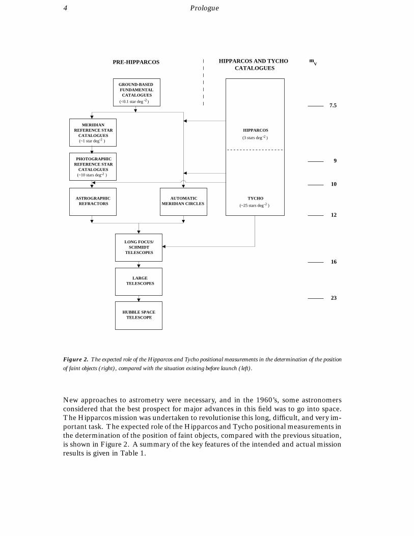
Figure 2. The expected role of the Hipparcos and Tycho positional measurements in the determination of the position
of faint objects (right), compared with the situation existing before launch (left).
New approaches to astrometry were necessary, and in the 1960’s, some astronomersconsidered that the best prospect for major advances in this field was to go into space.The Hipparcos mission was undertaken to revolutionise this long, difficult, and very im-portant task. The expected role of the Hipparcos and Tycho positional measurements inthe determination of the position of faint objects, compared with the previous situation,is shown in Figure 2. A summary of the key features of the intended and actual missionresults is given in Table 1.
Prologue 5
Evolution of the Hipparcos Project
Developments before Acceptance by ESA
A preliminary proposal for a space astrometry mission was submitted by P. Lacroute tothe Centre National de la Recherche Scientifique (CNRS) in France in March 1966.The proposal was made to build up a reference system using about 700 stars brighterthan 7 mag, with relative positions known to better than about 0.01 arcsec. Already,in his first proposal, two key features of Hipparcos were used: a beam combiner (morecomplex than that eventually adopted, with three surfaces resulting in a symmetricimage), and the observation of the light modulated by scanning slits.
In August 1967, a new version of the project was presented in Prague at the meetingof the International Astronomical Union (IAU). A revision of this proposal was thenpresented to the Centre National d’Etudes Spatiales (CNES) in France, in November1967. Not only was this version technically more elaborate than before, but also, andperhaps more importantly, the scientific significance of the prospective results was betteremphasised. Amongst the ideas that were submitted to CNES in order to demonstratethe feasibility of the project, was the idea—quickly rejected—that it could be flownon a balloon. Some funds were subsequently made available by CNES for opticalcalculations, and for the trial manufacture of a ‘beam-combining mirror’ in 1969. Itproved to be impossible, however, to construct such a mirror that would be able to resistthe vibrations encountered during launch.
In August 1970, a paper was presented at the IAU meeting in Brighton on the subjectof astrometric measurements from space. There were no major changes to the technicalproposal, and it served to draw the attention of the astronomical community to thepossibility of measuring absolute trigonometric parallaxes to better than 0.005 arcsec.In 1970, CNES stopped their studies of the project, not only because of technicaldifficulties which, at that time, seemed to be beyond the state of the art in spacetechnology, but also as a result of the political decision taken to stop the French nationalspace programme, and to use the funds to support European cooperation within theEuropean Space Research Organisation (ESRO).
New ideas were introduced at the Astrometry Symposium in Perth in 1973. A descrip-tion of the mission was made at a meeting of the ESRO Astronomy Working Groupin Frascati in 1973 by J. Kovalevsky. The Working Group selected thirteen projectsthat merited further consideration. In November 1973, a report was submitted to theEuropean Space Research Organisation pointing out—in addition to a design based onthat of the earlier satellite TD1—the technical potential of a similar system that couldbe flown on Spacelab. Such a system could use more powerful optics and could reachfainter stars, but would not have yielded as many measurements as a scanning satellite.By that time, the prohibitive cost of the eight shuttle launches required for an astrometricSpacelab mission was not fully recognised.
This report was followed by a symposium on ‘Space Astrometry’ organised by ESRO,soon to become the European Space Agency, in October 1974 in Frascati. This sympo-sium was organised in order to assess the support of these ideas amongst astronomers,and many astronomers interested in the possibilities of space astrometry attended thismeeting.

6 Prologue
Table 1. Summary of the results from the Hipparcos mission intended before launch, and the actual results
contained in the Hipparcos and Tycho Catalogues.
Intended Actual
Hipparcos Catalogue:
Number of stars 100 000 (in 1980) 118 218
Limiting magnitude V = 12.4 mag V = 12.4 mag
Completeness 7.3–9.0 mag 7.3–9.0 mag
Positional accuracy (B = 9 mag) 0.002 arcsec ~ 0.001 arcsec
Parallax accuracy (B = 9 mag) 0.002 arcsec ~ 0.001 arcsec
Annual proper motion accuracy (B = 9 mag) 0.002 arcsec ~ 0.001 arcsec
Systematic errors <0.001 arcsec ~ 0.0001 arcsec
Tycho Catalogue:
Number of stars > 400 000 (in 1982) 1 058 332
Limiting magnitude B = 10 − 11 mag B ~ 12.2 mag
Positional accuracy (B = 10 mag) 0.03 arcsec ~ 0.01 arcsec
Photometric precision (B = 10 mag) 0.05 mag ~ 0.02 mag
Observations per star ~ 100 130
Depending on galactic latitude and spectral type
A mission definition study was subsequently carried out, by a group of European as-tronomers with the support of ESA personnel. This study was able to define a missionwith more emphasis on the astrophysical aspects of an astrometry satellite, because newtechnical ideas made it possible to observe a larger number of stars, and also faint ones,with a higher precision than previously, and even with a smaller telescope aperture.The following technical innovations were introduced in December 1975 by E. Høgof Copenhagen University Observatory, and were incorporated in the final Hipparcossatellite.
A grid with only one slit direction was introduced for scanning the stars in only onecoordinate, namely along the great circle connecting the two fields of view. The relativeadvantages of chevron and parallel slits had been the subject of lengthy discussions, withthe simpler one-dimensional modulating grid having been adopted following simulationswhich showed that, even with one-dimensional measurements, good rigidity of thesphere solution would result. The one-dimensional scanning utilises the fact that thetwo-beam telescope is primarily a one-dimensional device. An image dissector tube wasproposed instead of the previous photomultipliers, allowing the selection of target stars,and consequently longer and cleaner integration per passage, providing an improvementin overall efficiency of about 100 times with respect to the use of photomultipliers alone.This also allowed for a pre-selection of programme stars, corresponding to the adopted‘input catalogue’ concept. The passive attitude stabilisation of the TD1 satellite wasreplaced by an active attitude control, which in turn opened the way for a ‘revolvingscanning’ attitude motion, giving a more efficient coverage of the sky. The preferredmission was a dedicated astrometric satellite with a measurement lifetime of three years,during which the positions, parallaxes, and annual proper motions of about 100 000selected stars would be obtained to some ±0.002 arcsec accuracy.
The study results were presented at an international Colloquium on Space Astrometryheld at Copenhagen University in June 1976. Shortly afterwards, ESA approved afeasibility study of the project.
Prologue 7
The problem of deriving the astrometric data from one-dimensional measurementsof the sky by a scanning satellite was studied at Copenhagen, where L. Lindegrenwas introduced to the problem in September 1976. He subsequently presented themathematical formulation of the three-step method, and estimates of the precision andcorrelation coefficients of the five astrometric parameters. The three-step method waslater developed by both data reduction consortia. Their implementations are basedon contributions by the geodetic institutes in Copenhagen and Delft starting in 1977,thus exploiting their expertise in solving large systems of similar geodetic networks withleast-squares methods.
When the Phase A study started in 1977, ESA had just decided that the Ariane launchershould be used for future missions. This opened the way for a heavier payload and a geo-stationary orbit. The new possibility was adopted by the science team, and the previousconcept of a near-Earth spacecraft in polar sun-synchronous orbit was abandoned.
The proposed active attitude control was based on the use of reaction wheels in thespacecraft, although the small disturbances (or ‘attitude jitter’) from the mechanicalbearings might have jeopardised the astrometric mission, aimed at angular measure-ments in the range of 2 milliarcsec. In fact, the studies were never able to supply reliableestimates of the attitude jitter before attitude control by cold-gas jets was introducedby the satellite prime contractor in 1982. This control provides the same very smoothattitude motion between each jet firing as the passive stabilisation would have given.The smooth motion can be used to improve the precision for bright stars by ‘dynamicalsmoothing’, an idea advocated by P. Lacroute since the TD1-concept was proposed.
The dialogue with the international scientific community was continued at special meet-ings: at the General Assemblies of the International Astronomical Union in Grenoble in1976 and in Montreal in 1979, and at the Colloquium on ‘European Satellite Astrom-etry’ in Padua in 1978. Coordination with ground-based astrophysical observations ofthe stars to be selected for Hipparcos was emphasised at these meetings, and so wasthe coordination with the planned space astrometry from the Hubble Space Telescope.Technical studies by ESA and outside contractors were continued, and members of theESA science team investigated the data reduction aspects.
From June 1978 until February 1980, a large promotional campaign was conductedthroughout Europe in favour of Hipparcos. An early and informal call for stars to beincluded in the observing programme, in an attempt to judge the scientific interest inthe project, was released independently by E. Høg and C. Turon—they were able tocollect about 170 research proposals submitted by 125 astronomers from 12 countries.P.L. Bernacca generated interest in 24 scientific institutes, from 8 countries, for hard-ware and software aspects of the mission, and demonstrated the potential availability ofabout 330 man years of effort necessary for the preparation of the data analysis facilities,one of the critical requirements for mission approval. As a result, the project obtainedincreasing attention from the national delegates in the ESA Science Programme Com-mittee, which approved the project in March 1980.
Many of the astronomers and other scientists involved in the early assessment studieshave continued their involvement with the mission, both through the ESA advisoryteams, and through the setting up, in 1982, of the consortia who took responsibilityfor the scientific aspects of this project. The detailed design study was completed inDecember 1983, and the hardware development phase began early in 1984.
8 Prologue
Technical and Scientific Involvement in Hipparcos after 1980
With the inclusion of the Hipparcos project within its mandatory science programmein 1980, the European Space Agency assumed overall responsibility for the satellitedesign and hardware manufacture, including the payload. This was contracted out toa European industrial consortium, with Matra Espace (France, now Matra MarconiSpace) as industrial prime contractor, and with Aeritalia (Italy, now Alenia Spazio)responsible for procurement of the spacecraft, as well as for the integration and testingof the complete satellite.
Industrial responsibility at system level covered management, engineering and assembly,as well as integration and testing of the complete satellite. This responsibility was sharedby eleven European firms, with some thirty five sub-contracted European firms, and atotal of about 1800 individuals, participating at all levels (see Volume 1).
Working closely with the European Space Agency since the project’s approval in 1980,European scientific teams undertook the scientific tasks necessary for the successfulcompletion of the project as a whole. This included the Hipparcos Science Team, setup to advise the Agency on the detailed scientific considerations related to the payloaddesign and development, and operational and calibration aspects, both on ground inadvance of the satellite launch, and subsequently in orbit. While the scientific advisoryrole has been essential for the successful design of the mission concept, and is one sharedby all ESA scientific missions, the scientific participation in the Hipparcos project hasbeen especially fundamental.
One aspect of this scientific involvement was the preparation of the Hipparcos Input Cat-alogue by a consortium of institutes known as the Input Catalogue Consortium (INCA).This consortium was selected by ESA on the basis of responses to an Announcement ofOpportunity issued in 1981. The consortium was subsequently entrusted with the taskof defining the unique list of stars that were to be observed by the satellite, on the basisof scientific merit and satellite operational requirements.
An Invitation for Proposals was issued by ESA in 1982 to the worldwide (and notonly European) scientific community. This resulted in more than 200 observationproposals being submitted, together comprising more then 600 000 objects. Adviceon the scientific aspects of the selection of stars from the proposals was given by theScientific Proposals Selection Committee and the Hipparcos Science Team.
The complete reduction of data from the satellite, from some 1012 bits of photon countsand ancillary data, to a catalogue of astrometric parameters and magnitudes for the120 000 programme stars, was independently undertaken by two scientific consortia,NDAC (the Northern Data Analysis Consortium) and FAST (the Fundamental Astron-omy by Space Techniques) Consortium. Both consortia were also selected on the basisof responses to a parallel Announcement of Opportunity issued by ESA in 1981. Theselection of two parallel data reduction teams was motivated by the size and complexityof the reductions. The two independent approaches also facilitated the overall validationof the final results. The end product was a single, agreed-upon catalogue.
A later enhancement to the project, which emerged during the detailed design study, wasthe addition of the two-colour star mapper channels that led to the Tycho experiment,proposed by E. Høg in March 1981, and the subsequent formation of the Tycho DataAnalysis Consortium (TDAC) in 1982. The Tycho Consortium was set up to analyse

Prologue 9
the data from the star mapper data stream, eventually resulting in the Tycho Catalogueof more than a million stars.
The close collaboration between the Agency and the scientific teams led to a satellitedesign which fully reflected the scientific requirements. The activities of all of theparticipating scientific institutes were funded by national agencies, universities, andprivate foundations. Altogether, some 200 scientists were involved in the work of thefour scientific consortia. These activities, and the organisation of the scientific consortia,are described in detail in Volumes 3 and 4.

10

1. OVERVIEW OF THE HIPPARCOS SATELLITE
This chapter describes the operating principle of the Hipparcos satellite, withreference to the measurement principle, the constraints and properties of thenominal satellite orbit, and the satellite environmental conditions. An overviewof the main satellite subsystems: attitude control, data handling and on-boardprocessing, the mechanical and electrical design, and the overall operationalconcept—is given, along with a description of the ground segment. The sci-entific and operational concepts introduced in this chapter are described ingreater detail in subsequent chapters.
1.1. Operating Principle
The primary goal of the Hipparcos mission was the measurement of the positions, propermotions, and trigonometric parallaxes of about 120 000 stars. To achieve this, a specialoptical telescope was designed to function on a spacecraft placed in geostationary orbit,above the Earth’s atmosphere. The telescope had two fields of view, each of size 0.9 ×0.9, and separated by about 58. The satellite was designed to spin slowly, completinga full revolution about its spin axis in just over two hours. At the same time, it could becontrolled so that there was a slow change in the direction of the axis of rotation. In thisway, the telescope could scan the complete celestial sphere.
Measurements of the angles between pairs of stars, inferred from the relative phasesof the modulated signals created by the main grid, were built up over the three-yearlifetime of the satellite in orbit. From many such measurements, made at many differentorientations, and at many different epochs, a whole-sky astrometric catalogue (theHipparcos Catalogue) was built up, containing the positions, parallaxes, and propermotions of all of the stars on the pre-defined observing list. This list, which containedabout 120 000 stars, constituted the so-called ‘Hipparcos Input Catalogue’. The TychoCatalogue was constructed from the data sent to the ground from the satellite’s starmapper.
The measurement principle of Hipparcos is illustrated in Figure 1.1. The payload wascentred around an all-reflective Schmidt telescope with an entrance pupil of 290 mm anda focal length of 1400 mm, the light from two sections or ‘fields’ of the sky was conveyedthrough two baffles, set at a fixed angle of close to 58. A ‘beam combiner’ allowed the

12 Overview of the Hipparcos Satellite
Figure 1.1. The measurement principle of the Hipparcos satellite. The two fields of view scanned the sky continuously,
and relative positions of the stars along the scanning direction were determined from the modulated signals resulting
from the satellite motion. Although the nominal geostationary orbit was not achieved, the same scanning motion was
implemented in the actual (transfer) orbit.
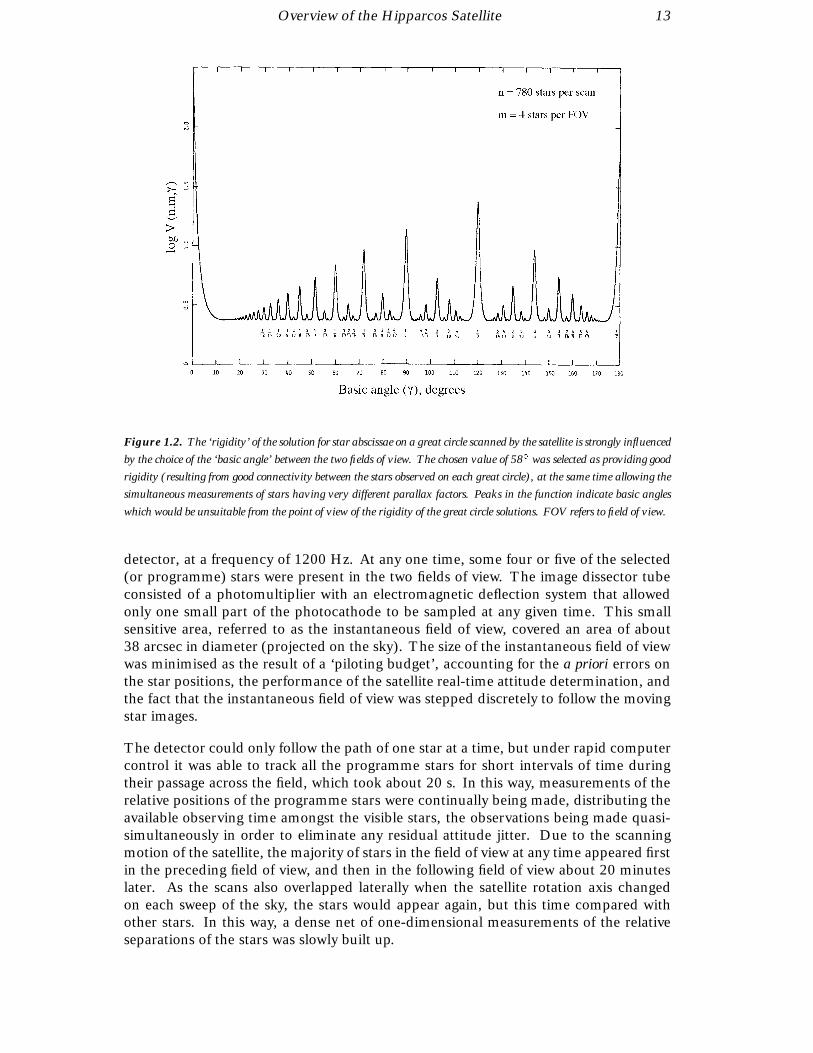
two fields to be projected onto the same focal surface by means of the spherical primarymirror. It was then possible to determine the true angle between two stars, one in eachfield of view, by using the known or ‘basic angle’ of 58 between the two fields of view,plus the apparent separation measured on the focal surface of the telescope. This choicefor the basic angle was influenced by the goal of connecting stars with very differentparallax factors by measurements within the combined field of view. The precise valuechosen was selected by considering the ‘rigidity’ of the resulting measurements madeover a great circle scanned by the satellite, as illustrated in Figure 1.2.
As the satellite slowly rotated at its nominal scanning velocity of approximately 1 rev-olution every 2 hours 8 minutes, the images of the stars in the fields of view movedacross the focal plane grids. These signals were sampled by detectors behind thesegrids. Two different types of detector were used in the Hipparcos payload—an imagedissector tube for the main grid and photomultiplier tubes for the star mapper grids. Toprotect the detectors from excessive illumination due to occultations by the Earth andMoon, shutters were built into the payload so that the detector photocathodes could beshielded from the bright occulting source.
The surface on which the two fields of view were focused contained 2688 parallelslits in an area of about 2.5 × 2.5 cm2, covering about 0.9 × 0.9 on the sky (seeFigure 2.10). As the telescope slowly scanned the sky, the star light was modulatedby the slit system, and the modulated light was sampled by an image dissector tube
Overview of the Hipparcos Satellite 13
Figure 1.2. The ‘rigidity’ of the solution for star abscissae on a great circle scanned by the satellite is strongly influenced
by the choice of the ‘basic angle’ between the two fields of view. The chosen value of 58 was selected as providing good
rigidity (resulting from good connectivity between the stars observed on each great circle), at the same time allowing the
simultaneous measurements of stars having very different parallax factors. Peaks in the function indicate basic angles
which would be unsuitable from the point of view of the rigidity of the great circle solutions. FOV refers to field of view.
detector, at a frequency of 1200 Hz. At any one time, some four or five of the selected(or programme) stars were present in the two fields of view. The image dissector tubeconsisted of a photomultiplier with an electromagnetic deflection system that allowedonly one small part of the photocathode to be sampled at any given time. This smallsensitive area, referred to as the instantaneous field of view, covered an area of about38 arcsec in diameter (projected on the sky). The size of the instantaneous field of viewwas minimised as the result of a ‘piloting budget’, accounting for the a priori errors onthe star positions, the performance of the satellite real-time attitude determination, andthe fact that the instantaneous field of view was stepped discretely to follow the movingstar images.
The detector could only follow the path of one star at a time, but under rapid computercontrol it was able to track all the programme stars for short intervals of time duringtheir passage across the field, which took about 20 s. In this way, measurements of therelative positions of the programme stars were continually being made, distributing theavailable observing time amongst the visible stars, the observations being made quasi-simultaneously in order to eliminate any residual attitude jitter. Due to the scanningmotion of the satellite, the majority of stars in the field of view at any time appeared firstin the preceding field of view, and then in the following field of view about 20 minuteslater. As the scans also overlapped laterally when the satellite rotation axis changedon each sweep of the sky, the stars would appear again, but this time compared withother stars. In this way, a dense net of one-dimensional measurements of the relativeseparations of the stars was slowly built up.
14 Overview of the Hipparcos Satellite
The satellite spin axis was kept at a constant inclination of approximately 43 to thedirection of the Sun, and revolved around the Sun once in approximately eight weeks,resulting in a continuous and systematic scanning of the celestial sphere. Throughoutthe scanning motion the satellite therefore remained in a constant thermal environment,modulated only by the satellite rotation. Any region of the sky was scanned many timesduring the mission by great circles which intersected at well-inclined angles as a result ofthe choice of the 43 sun aspect angle. A typical star was observed some 80 times in eachfield of view throughout the lifetime of the satellite. The number of possible connectionsbetween the observed stars was considerably enhanced due to the almost simultaneousobservation of stars separated by the large basic angle. The individual measurementswere combined to form the final Hipparcos Catalogue, including the displacements dueto parallax and proper motion, using techniques similar to those used in triangulationin surveying the Earth’s surface.
The real-time attitude determination on board, required for autonomous piloting of thedetector’s instantaneous field of view, was achieved by the on-board computer usingthe spacecraft rotation rates, as measured by three independent gyros, the biases inthose gyros (the gyro drifts), knowledge of times and durations of thruster firings, andcritically, the measurements of transit times of stars crossing the star mapper grid. Bycomparing the measured crossing times of designated stars with those expected fromthe theoretical motion of the spacecraft, it was possible for the on-board computer,using a Kalman filter, to estimate the amount that the spacecraft had deviated from thepredefined attitude.
The image dissector tube signal, as modulated by the main grid, was assumed to be ofthe form (see Figure 1.3):
I (t) = IBG + I0[1 + M1 cos(2πωt + θ1) + M2 cos(4πωt + θ2)] [1.1]
where:
I (t) is the instantaneous count rate at time t
IBG is an additional signal due to background noise and detector dark current
I0 is the mean count rate for the observed star (dependent on magnitude and colour)
M1 is the first modulation coefficient for the observed star
M2 is the second modulation coefficient for the observed star
t is the time relative to a reference observation (mid-frame) time (s)
ω is the grid frequency of the image dissector tube signal in Hz, i.e. ω = v /s wherev is the angular scanning velocity of the satellite (arcsec s−1), and s is the grid slitspacing (arcsec)
θ1 is the phase of the first harmonic of the signal at t = 0
θ2 is the phase of the second harmonic of the signal at t = 0
In addition to the main instrument (there was a second image dissector tube detectorprovided for redundancy), the payload included two star mappers, the second also beingprovided for redundancy purposes—the non-operational detectors were usually switchedoff when not in use. The function of the star mapper was to provide data allowing real-time satellite attitude determination, a task performed on-board the satellite, as well asthe a posteriori reconstruction of the attitude, a task carried out on the ground. Thecontinuous flow of star mapper data was also used to create the Tycho Catalogue,

Overview of the Hipparcos Satellite 15
comprising astrometric and two-colour photometric measurements of all stars, down toabout 10–11 mag.
The star mapper consisted of a star mapper grid, located at opposite sides of the pri-mary modulating grid (see Figure 2.10), and two photomultipliers measuring the lighttransmitted by the whole star mapper grid in two different spectral bands, roughly cor-responding to the Johnson B (blue) and V (visual) bands. The spectral separation wasperformed by means of a dichroic beam splitter, which directed that part of the signalwith λ < 465 nm toward the ‘blue’ photomultiplier (referred to as the BT channel)and that part of the signal with λ > 475 nm toward the ‘visible’ photomultiplier (the VT
channel)—the subscripts ‘T’ referring to Tycho, and drawing attention to the distinctionbetween the Tycho and Johnson photometric systems.
Each star mapper consisted of two sets of four slits, each set at different inclinations withrespect to the scanning direction, so that the satellite attitude could be derived from thephotomultiplier signals as the star images moved across the grid. Both channels weresampled at 600 Hz by the on-board data handling subsystem. In total, the imagedissector tube and star mapper data comprised 83 per cent of the telemetry stream.
The photomultiplier tube signal for each of the star mapper channels was assumed tobe of the form (see Figure 1.4):
I (t) = I BG + I 0
NX
k=1
S(vt − pk) [1.2]
where:
I (t) is the instantaneous count rate at time t
I BG is an additional signal due to background noise and detector dark current
I 0 is the peak count rate at the centre of a slit
N is the number of slits in a slit system (N = 4)
S(x) is the single-slit response function, i.e. the normalised signal transmission factoras a function of distance from the source to the centre of the slit, in arcsec
v is the angular scanning velocity of the satellite (arcsec s−1)
t is the time relative to the central observation time (s)
pk is the position of the k-th slit in the slit system (arcsec)
The payload is described in detail in Chapters 2 and 3. The nominal scanning lawand the star observing strategy are described in Chapter 8. The processing of the maingrid and star mapper data, leading to the construction of the Hipparcos and TychoCatalogues, are described in detail in Volumes 3 and 4 respectively.
The spacecraft provided the structure platform for mounting the payload main assemblyvia an interface structure, the external baffles to protect the detectors from stray lightfrom the Sun and the Earth, and the appropriate mounting surfaces for all spacecrafthardware including the apogee boost motor, solar arrays and antennae. In addition,the spacecraft supported a shade structure surrounding the payload which ensuredmaximum thermal decoupling from the external environment.

16 Overview of the Hipparcos Satellite
Figure 1.3. Image dissector tube signal. The information transmitted to the ground from the main detector consisted
of the photon counts per 1200 Hz sample. The main peaks correspond to the first signal harmonic, and the (marginally
visible) intermediate peaks correspond to the second harmonic. The brightness of the star at the time of the measurement
is given by the amplitude of the signal, while the phase of the modulated signal with respect to some reference phase
provides the relative position of the star image, along the scanning direction, modulo one grid step. The data corresponds
to observations of 1/15 s for HIP 114347, Hp = 5.3 mag, in April 1991.
Figure 1.4. Photomultiplier tube signal (blue channel) for the transit of one star over a single slit system. The
information transmitted to the ground from the star mapper detector consisted of the photon counts per 600 Hz sample
measured simultaneously in the BT and VT channels. The four peaks corresponding to the four aperiodically spaced
star mapper slits, yield the star intensity and position after appropriate filtering. The observation is for HIP 35946,
BT = 6.62 mag, transits for the vertical slits and the following field of view.
Overview of the Hipparcos Satellite 17
1.2. Constraints and Properties of the Nominal Orbit
Due to the measurement principle of Hipparcos, which needed as input a continuouslyupdated ‘programme star file’ of star positions predicted to cross the instrument’s fieldof view as a function of time, the satellite required permanent attendance by the groundsegment in order to pursue the nominal mission. This requirement would have been bestfulfilled by a geostationary orbit (equatorial plane, 36 000 km height, 24-hour period),which would have kept the satellite in a fixed position with respect to a single groundstation. From this orbit, as opposed to low-Earth orbits, the Earth obscures only a smallportion of the celestial sphere being scanned. The station 12W was originally chosenfrom the geostationary orbit segments available in order to optimise the accuracy of theorbit determination from the single ground station. In practice, the target geostationaryorbit was not achieved, and the mission was conducted with the satellite in a highlyelliptic geostationary transfer orbit, as described more fully in subsequent chapters.
Eclipse Operations
For a period of 45 days around the two equinoxes, the orientation of the nominalHipparcos (geostationary) orbit relative to the ecliptic was such that the Earth wouldhave passed between the Sun and the satellite every 24 hours. Such eclipses wouldhave lasted up to 72 minutes, during which time there would be no energy input to thesolar arrays and the power subsystem would have to rely on its batteries. At the sametime, the heat input would fall, changing the thermal balance of the satellite. Whilethe satellite had been designed for these eclipse conditions, extreme eclipse durationswere considerably longer for the actual geostationary transfer orbit, placing complexconstraints on the power subsystem at these times.
Occultation of the Fields of View
The satellite scanned the sky with its spin axis pointed in a direction that moved onlyslowly, with an orbital period in its actual geostationary transfer orbit of 10.66 hours.This meant that the scanning great circle intercepted the Earth’s disc about four timesper day, with all or part of each field of view being exposed to this bright source inone or more consecutive scans. Since the Earth is very bright from such an orbit,shutters in front of the detectors were closed some time before the actual disc of theEarth entered the field of view, and they remained closed until after it had passed.The actual duration of the interruption was determined by the straylight protectioncharacteristics of the payload baffles, and ranged from a few minutes to more than onehour. Similar interruptions were caused by occultation due to the Moon although,subtending a smaller angle and being less bright, the corresponding interruptions wereshorter.
The impacts of such interruptions in data collection were threefold: (i) the ‘dead time’had to be accounted for in estimating the mission duration needed for the requirednumber of scientific measurements; (ii) the rigidity of solution of the great-circle equa-tions would be degraded if measurements could not be linked between the two fieldsof view and between consecutive revolutions; and (iii) while the star mapper was not
18 Overview of the Hipparcos Satellite
operating the satellite attitude would drift with only gyroscope measurements, leadingto degradation in pointing accuracy and even additional operations needed to return tothe nominal scanning law after the interruption.
Simulations showed that the dead time for the nominal geostationary orbit, due tooccultations, would be about 5 per cent, which was within the budget foreseen duringmission definition, and that mission accuracy requirements could be achieved with up to40 per cent of great circles interrupted, which exceeded the predicted percentage for thenominal geostationary orbit with a clear margin. The real-time attitude determinationperformance was also demonstrated in simulations, showing that conditions leading tothe need for a full reinitialisation of the pointing would occur only once or twice inthe entire mission. In practice, as a consequence of the revised orbit, dead time wassignificantly larger, and pointing reinitialisation was frequently required.
1.3. Satellite Environmental Conditions
The following environment conditions expected for the nominal geostationary orbitwere taken into account in the overall satellite design.
Mechanical Environment
The dominant mechanical environment driving the satellite design was that encoun-tered during the launch phase, which exposed the satellite to static and quasi-staticaccelerations, random vibration, and acoustic sound pressure.
Thermal Environment
There were two cases of thermal environment driving the design: (a) the transfer andnear synchronous orbit, when the satellite was spinning, the solar arrays were stowed, theinternal power consumption was low, and the sun aspect angle with respect to the spinaxis was between 90 and 115 (the upper limit of the sun aspect angle determined by thelaunch window); and (b) the geosynchronous orbit, when the satellite would be three-axes controlled, the solar arrays would be deployed, the internal power consumptionwould be high, and the sun aspect angle would be 43.
The sun aspect angle was given by the nominal scanning law, but could go to 0 (‘sun-pointing’) for emergency sun acquisition and for initialisation. The thermal design hadto cope with both somewhat contradictory cases by appropriate multi-layer insulation,radiators, and electrical heaters. The compliance of the satellite with the thermalenvironment, in addition to comprehensive mathematical modelling and analyses, wasverified by thermal-balance and the thermal-vacuum tests before launch.
Electromagnetic Environment
The electromagnetic environment was generated externally by the launch vehicle andthe passenger satellite in the dual launch, and internally by the satellite electrical equip-ment. A margin between electromagnetic emission and electromagnetic susceptibility

Overview of the Hipparcos Satellite 19
was ensured by introducing a strict grounding and isolation scheme, careful shieldingof units and harness, and interface circuits with common mode rejection capability.
Radiation Environment
Semiconductor lifetime: Semiconductors degrade when exposed to ionising radia-tion. The degradation of high-reliability component parameters as a function of ra-diation dose is well known, and this degradation had to be taken into account as alife-limiting factor. For each electronic unit, a radiation analysis was performed, con-sisting of computing the dose a component would be subjected to, taking into accountthe radiation shielding of the surrounding material of the unit and the satellite. Then,either the circuit design was able to accommodate the degraded parameters at the pro-jected end of life, or additional local shielding had to be applied.
Single event upset: The ‘single event upset’ effect is the result of a high-densityionisation due to heavy and high-energy particles. It can cause such a high local chargedeposition in a semiconductor that the logical state of a flop-flip or a memory cell ischanged. Although this is generally a recoverable error, and no permanent damageresults, it can upset the on-board computer systems. The satellite system was designedin such a way that no computer function was crucial for the satellite safety. However, afrequent computer upset would interrupt and degrade the mission.
The following measures were taken to protect the satellite against single event upsets:(a) the control law electronics used a processor of low radiation susceptibility, whilethe control law electronics memory employed an ‘error detection and correction logic’which corrected any single bit error; and (b) the on-board computer used a radiation-hardened processor. The on-board computer memory was continuously checked forparity errors, which then had to be corrected from ground.
Electrostatic discharge: Electrostatic discharges have troubled many geostationarysatellites. In a plasma environment, the satellite surfaces are charged up to differentpotentials, depending on the material properties and sun illumination. The potentialdifferences can reach a few thousand volts, sufficient to cause sudden electrostaticdischarges which interfere with the satellite electrical system. Hipparcos was designedto avoid differential charge-up, and also to provide protection against discharge effectsshould they occur.
To avoid differential charge-up, all surfaces exposed to space were required to be elec-trically conductive. This requirement had a significant impact on the thermal controldesign, as it ruled out the most conventional thermal control materials. The sur-face materials selected for the satellite were conductive black paint, aluminium andindium-tin-oxide coated optical surface reflectors. The only compromise, made forcost reasons, was the non-conductive glass cover of the solar cells. To verify that nodifferential charge-up could occur, mathematical models to analyse the phenomenon ofelectrostatic discharge were performed. The properties of the satellite surface materials,which were a sensitive input to the analyses, were measured in a special test programmeperformed within the development programme.
To protect against discharge effects, the whole spacecraft was shielded. This was doneimplicitly in the lower part of the spacecraft by aluminium panels forming a metallic boxto house the spacecraft equipment. The upper part was mainly framework, supporting

20 Overview of the Hipparcos Satellite
the multi-layer insulation to protect the payload. A 0.1 mm thick aluminium foilsurrounding the framework formed the electrostatic discharge shield.
Electrostatic discharge protection was also the driver for the electrical grounding andisolation concept. The concept chosen was a distributed single-point grounding scheme.Each box had its own secondary power supply, isolated from the main bus and groundedto the box structure, thus providing the box signal ground. Signal lines between boxeshad common-mode rejection capability—signal receivers were either differential ampli-fiers, opto-couplers, or floating relay coils. For digital links, standardised transmittersand receivers were developed for use by all electrical subsystems, referred to as the‘standard balanced digital link’.
Darkening of optical elements: Prolonged exposure to ionising radiation can alterthe transmission characteristics of optical materials. The extent of transmission lossis wavelength-dependent, being more significant for shorter wavelengths. During itsoperation, the satellite would be continuously exposed to trapped electrons and protonsin the Earth’s outer radiation belts. Although the protons would not normally be suffi-ciently energetic to penetrate the outer wall of the satellite, any so-called ‘anomalouslylarge solar events’ could generate increased levels of high-energy protons.
In order to minimise the effects of this radiation, the transmitting optical elements weremade of glass types that showed maximum resistance to irradiation darkening, subjectto their general properties (spectral transmission and refractive index) being compatiblewith the requirements of the mission. At the same time, the relay optics and detectorwindows were shielded by layers of aluminium, and additional material was added tothe structural elements to provide shielding in directions where this was not alreadyprovided by existing hardware.
In assessing the predicted end-of-mission performance in advance of launch, the ex-pected degradation of optical transmission was calculated on the basis of the best-available knowledge of the radiation environment in geostationary orbit, and accountingfor two anomalously large solar flares. This was considered to be consistent with previ-ous experience at the phase of the solar cycle (around maximum) at which the Hipparcosmeasurements would take place.
The Cerenkov effect: A charged particle passing through a transparent dielectricmedium with a velocity greater than the velocity of light in the medium, emits visibleelectromagnetic (Cerenkov) radiation. The Earth’s outer radiation belts, through whichthe (nominal and actual) orbit of Hipparcos passed, contained electrons sufficientlyenergetic to generate light by this effect in the dioptric elements of the payload optics.
Depending on the direction of motion of the individual electron and the distance ofeach optical element from the detector, the part of the emitted light that falls withinthe spectral measurement range may make a significant contribution to the backgroundcount rate, against which the stellar signals had to be detected and measured. However,the pulse width of the Cerenkov light flash being much smaller (~ 0.1 ns) than thetime resolution of the photomultiplier (~ 40 ns), one or more photons generated byeach incident high-energy electron would produce just one pulse recognised above thediscriminator threshold as a background count.
The measures implemented to counteract this effect included the provision of additionalmaterial to shield sensitive elements in directions where such shielding was not provided

Overview of the Hipparcos Satellite 21
by the satellite hardware itself, and the masking of unused areas of transmitting optics.The radiation shielding requirements were estimated by Monte-Carlo studies.
It was verified that the predicted residual count rate would not induce an unacceptabledegradation of mission performance. The effect was particularly important for thestar mapper, because of its large field of view, where it was expected to contribute themajor part of the background count rate. For the main mission, the use of a restrictedinstantaneous field of view was expected to reduce drastically the proportion of theemitted light to which the detector was sensitive.
1.4. Attitude Control Concept
The attitude and orbit control subsystem provided the control, stabilisation and mea-surement about the three satellite axes during all phases of the mission, and performedall orbit manoeuvres. Orbit reconstitution data with an accuracy of about 1.5 km in theinstantaneous satellite position and 0.2 m s−1 in the instantaneous velocity vector wereperformed at ESOC. The attitude determination used rate-integrating gyroscopes, thedrifts of which were calibrated in real-time using star mapper data from star crossingsoccurring every 20 s on average, although later in the mission, as a result of progressivegyro failures, the gyro input had to be replaced by star mapper data and a disturbance-torque model. Cold nitrogen thrusters (with a nominal thrust of 0.02 N) were used forthe attitude control.
An extremely smooth satellite motion was required because of the measurement princi-ple. The sequential detection of the grid-modulated light from each star made the phaseextraction sensitive to any jitter during this sequence. Furthermore, the interlacing ofbright and well-measured stars along a great circle depended on the smoothness andpredictability of the motion. This interlacing significantly improved the astrometric ac-curacy. Therefore, the trade-off and selection of the attitude control concept was one ofthe key decisions influencing the feasibility and performance of the Hipparcos mission.The decision was complicated by the difficulty of acquiring experimental data on mi-crovibration in a 1g environment, and by doubts about the applicability of conventionalfinite-element models to this problem. The attitude control candidates considered dur-ing the early phases of the satellite design were reaction wheels, magnetic actuators andsmall thrusters:
(i) reaction wheels, the classical means of providing a continuous attitude control, werediscarded, because of the resulting high level of attitude jitter caused by bearing noise.This problem could not be solved by considering the use of mini reaction wheels, orreaction wheels with magnetic bearings, or special suspension mounts for the wheels;
(ii) magnetic torquers, i.e. magnetic coils generating a torque within the Earth’s magneticfield, were discarded, because there are uncontrollable areas depending on the anglebetween the coil and the Earth’s magnetic field, which would still require additionalreaction wheels. The control is complex, and depends on the attitude to the Earth’smagnetic field, which would vary throughout the mission as a consequence of theadopted scanning law. Also, the Earth’s magnetic field itself can vary significantlyduring magnetic storms. Furthermore, the magnetic actuators could interfere with theimage dissector tube detector, which was inherently magnetically sensitive;
22 Overview of the Hipparcos Satellite
(iii) small thrusters, when actuated, cause an attitude discontinuity and excite an attitudejitter. This was shown to be acceptable if the actuations were not too frequent, suffi-ciently weak and with higher frequencies suppressed, and if the jitter could be dampedout to acceptable levels in a time period small compared with the time for which a starwould be observed.
The last of these attitude-control concepts was chosen, with specially designed 0.02 N‘cold gas’ thrusters. The satellite was designed to operate in free drift in a ±10 arcminband around the orientation given by the nominal scanning law. If any axis exceededthis band, the thrusters would be fired. If, at the same time, the other axes exceeded anarrower inner band, their thrusters would also be fired in a synchronised manner. Thissynchronised firing scheme, plus an optimisation of impulse bit and disturbance torqueprediction, led to a predicted average time between thruster firings of 400 s, with thefirings causing a disturbance for less than 2 s.
Other sources of jitter that had been carefully assessed before launch, in addition to thatdue to gas jet actuations, were gyro mechanical noise, apogee boost motor residuals,payload shutter mechanism actuations, and the impact effects of micrometeorites. Inaddition, the frequencies to which the measurement principle and the star observingstrategy were especially sensitive were avoided by suitable control of the satellite naturalfrequencies.
1.5. Data Handling and Processing
The system design for the on-board data handling and data processing was determinedby the following requirements:
(a) the continuous uplink of a priori star position and magnitude information from theHipparcos Input Catalogue in the form of the programme star file, for a look-aheadtime of several minutes;
(b) the real-time computation of the star observing strategy and the image dissector tubepiloting from the programme star file and the actual satellite attitude;
(c) the real-time attitude determination from gyro and star mapper data with a highdegree of accuracy (1 arcsec) as an input to the star observing strategy and imagedissector tube piloting;
(d) the time tagging of the measurements with a stability of 5 µs over 5 minutes, corre-sponding to a satellite spin phase of about 1 milliarcsec (5 minutes roughly correspondedto the time between bright, well-measured stars to be linked on a great circle).
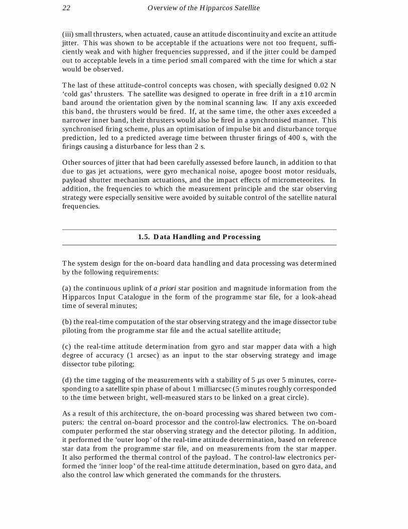
As a result of this architecture, the on-board processing was shared between two com-puters: the central on-board processor and the control-law electronics. The on-boardcomputer performed the star observing strategy and the detector piloting. In addition,it performed the ‘outer loop’ of the real-time attitude determination, based on referencestar data from the programme star file, and on measurements from the star mapper.It also performed the thermal control of the payload. The control-law electronics per-formed the ‘inner loop’ of the real-time attitude determination, based on gyro data, andalso the control law which generated the commands for the thrusters.
Overview of the Hipparcos Satellite 23
PAYLOAD
TELEMETRY
DATATION
ATTITUDE CONTROL SYSTEM
GAS JETS GYROS
TELECOMMAND
IMAGE DISSECTOR
OBSERVATION REPORTATTITUDE + GYROS
TYCHO DATA
IDT DATA
COIL CURRENTS
10 Hz
ON-BOARD COMPUTER
ATTITUDECONTROL LAW
REAL TIME ATTITUDE (1 Hz)DETERMINATION
STAR MAPPERPROCESSING
STAROBSERVATION
STRATEGY
PROGRAMMESTAR FILE (1 Hz)MANAGEMENT
STAR MAPPERDATA
TELEMETRY FORMAT GENERATOR(EVERY 10.67 s)
LOADING OFPROGRAMME
STAR FILE
STAR MAPPER
150 Hz
1200 Hz
600 Hz
Figure 1.5. A block diagram of the main measurement and operational functions on board the satellite. To the top
left, the uplinked programme star file was used by the on-board computer to determine the details of the star observing
strategy over the coming minutes. Information on the satellite attitude was provided by a combination of gyro and star
mapper data (bottom left), which was also used to determine the gas jet actuations necessary to maintain the satellite in
its pre-defined scanning law. Attitude information and information from the programme star file was used to point the
instantaneous field of view of the image dissector tube, and to acquire relevant extracts of the star mapper data stream
(top right). All relevant data were interleaved and sent to ground in real time (bottom right).
The whole on-board system was synchronised by broadcast pulses. The piloting, theimage dissector tube sampling, and the format generation was synchronised in 150 Hzcycles. Thus, the time tagging of the payload data was given implictly by the locationwithin the telemetry format. The less time-critical on-board computer and control-lawelectronics data were interleaved into fixed telemetry format slots as packet telemetry.The on-board computer and control-law electronics computations were synchronisedby the telemetry format pulse.
The overall concept of the acquisition of scientific data by the satellite is depicted inFigure 1.5. The programme star file was loaded from ground. It contained informationon the programme stars to be observed by the image dissector tube, and reference starsused to perform the attitude determination on-board. The programme star file wasmanaged by the central on-board software.
The central on-board software retrieved information about the reference stars fromthe programme star file and, by means of attitude information from the attitude andorbit control system, computed the expected transit time of the reference stars passingover the star mapper slits. In a time window around the expected transit time, starmapper samples were acquired and filtered to determine the actual transit time of thereference star. The difference between expected and measured transits was then usedas an error signal for the attitude determination, which was continuously performed forthe three axes by means of gyro measurements. The real-time attitude determination

24 Overview of the Hipparcos Satellite
outputs were used for attitude control within a band of ±10 arcmin around the nominalscanning law, and for computing the positions of programme stars in the field of viewfor proper piloting of the image dissector tube.
The central on-board software retrieved information about the programme stars thatwere to appear in the field of view for the next observation frame of T4 = 2.133 . . . sand computed the star observing strategy, i.e. the pattern of interleaved subsequent starobservations, according to star criteria contained in the programme star file. Thesecriteria were priority, target observation time, and minimum observation time (seeChapter 8 for further details of the observation programme and the star observingstrategy).
By means of the real-time attitude determination, the expected star position in the fieldof view needed to pilot the image dissector tube was computed as a function of time.With this information, the star observation pattern was converted into a series of coilcurrent pairs, which commanded the instantaneous field of view of the image dissectortube to the star images to be observed. The resulting image dissector tube counts persampling period were inserted into the satellite telemetry as a continuous data stream.The corresponding observation frame characteristics were inserted into the telemetryby the central on-board software as data packets.
In addition to providing the on-board attitude reference, the star mapper performedastrometric and photometric measurements as part of the Tycho experiment. The lightpassing through the star mapper grid was measured with two photomultiplier tubesin two different colours, the BT and VT channels. The photomultiplier counts persampling period, after data compression, were also inserted into the satellite telemetryas a continuous data stream.
1.6. Operational Concept
The complexity of on-board processing, and the intensive ground segment involvement,required that the system design was based on a clear operational concept.
Hipparcos was designed as a geostationary satellite with permanent single station groundcontact, run to the maximum extent from the ground. On-board processing was in-tended only if ground processing was prohibitive due to excessive uplink rates (e.g. theimplementation of the star observing strategy), or was not feasible due to the telemetryor telecommand turnaround time (e.g. attitude determination and control, image dis-sector tube piloting). On-board scientific data reduction was not accepted, in order toavoid systematic errors imposed by the associated modelling. The ground segment wasdesigned to monitor satellite health and to initiate corrective actions in case of failure.Only if a failure required a fast reaction to avoid permanent damage to the satellite wasan automatic back-up mode provided.
Normal operation was to be performed by means of on-board computers and software.Re-configuration and configuration status monitoring would be performed on a higher,independent level. Automatic back-up modes would override normal operation andconfiguration. Direct ground commands would override any automatic back-up mode.

Overview of the Hipparcos Satellite 25
During transfer and drift orbit, the satellite would be spinning, and its survival woulddepend on the proper function of the active nutation damping. A malfunction resultingin excessive nutation would be detected on-board by an accelerometer. It would triggeran automatic switch-over to a completely redundant control and actuation system.
In the intended geostationary phase, when the solar arrays were deployed and thesatellite was three-axis controlled, the satellite would be sensitive to attitude errors. Atexcessively large solar aspect angles, partial shadowing could damage the solar cells anddirect sunlight could blind the payload. In sunlight, an attitude error would be detectedby a special attitude anomaly detector. An automatic sun acquisition would be triggeredby independent back-up hardware. In eclipse, an attitude error would be detected bymonitoring the thruster actuations. An anomaly would trigger an automatic spin-upto increase the gyroscopic stiffness. This would keep the satellite in a safe attitudesufficiently long for the ground segment to detect the failure and initiate recovery actions.
Permanent electrical power supply would be essential for the survival of the satellite.Anomalies would be detected through main-bus undervoltage and battery-cell under-voltage, and these would trigger an automatic shedding of non-essential loads.
1.7. Satellite Mechanical and Electrical Design
The satellite consisted of two major hardware elements, namely the spacecraft and thepayload. These two hardware elements, together with the on-board software madeup the satellite system. As the satellite exploded view shows (Figure 1.6), there wasa spacecraft module providing: structural support for its subsystems and for the pay-load via the interface structure; electrical power supply by solar arrays and batteries;telecommunication and data handling; and the attitude and orbit control required toplace the satellite on station and then execute the scanning law. Another spacecraftelement was the apogee boost motor, which was designed to inject the satellite fromtransfer-orbit apogee into near-synchronous orbit. Finally, there was the shade structureneeded to provide a stable thermal environment for the payload. The Hipparcos launchand on-station configurations are shown in Figure 1.7.
The electrical subsystems are listed in Table 1.1. The primary power supply was aregulated 50 V DC power bus. At subsystem level (data handling, attitude and orbitcontrol, and payload), there were DC/AC inverters supplying the units with squarewave 50 V AC power. The communication between subsystems was through the ESA-standard on-board data handling bus.
The electrical power subsystem supplied the primary electrical power, generated by thesolar generator, to the payload and the spacecraft subsystems. Power distribution wasthrough a 50 V DC mains regulated bus and AC secondary power buses. Two recharge-able nickel-cadmium batteries, each with the capacity of 10 Ah, provided continuouspower supply during launch and eclipse periods.
The solar generator provided electrical power by use of solar cells arranged on threeidentical solar panels. The subsystem generated electrical power in transfer orbit whenthe solar arrays were folded against the satellite body, as well as in operational orbitwhen the panels were deployed. When deployed, the three panels together provided
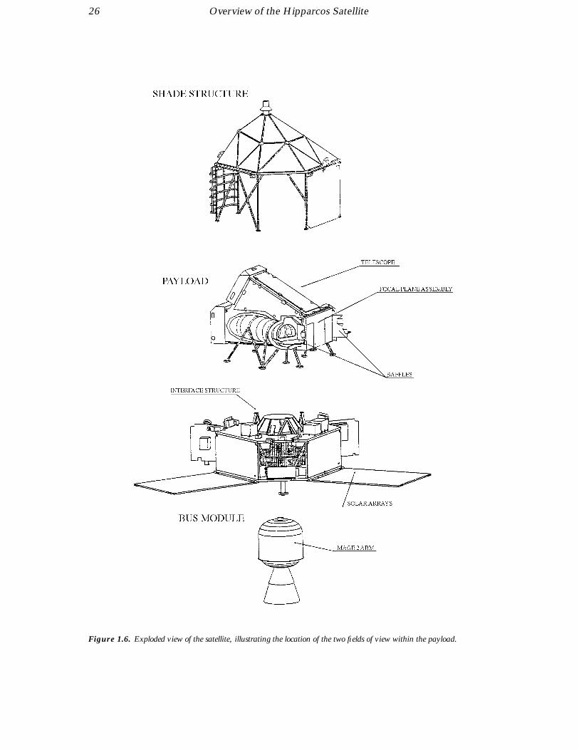
26 Overview of the Hipparcos Satellite
Figure 1.6. Exploded view of the satellite, illustrating the location of the two fields of view within the payload.

Overview of the Hipparcos Satellite 27
Figure 1.7. (a) Satellite launch configuration with the solar arrays stowed, and (b) on-station configuration with
the solar arrays deployed (and with the shade structure removed for illustration purposes).
some 350 W of power to the on-board systems. The adopted scanning law meant thatthe solar panels were at a constant inclination to the Sun throughout routine operations.
Some of the main characteristics of the satellite and its operational environment arelisted in Table 1.2. The mass budget for the satellite at launch, rounded to the nearestkilogram, is given in Table 1.3. The power budget is given in Table 1.4 for the pre-operational phase (i.e. in transfer and near synchronous orbit, when the satellite wasspinning, the solar arrays were stowed and the payload and on-board computer wereoff), and for the operational phase (i.e. when the satellite was spinning, the solar arrayswere deployed and at a sun aspect angle of 43).

28 Overview of the Hipparcos Satellite
Table 1.1. Electrical subsystems and acronyms.
Subsystem Description Acronym
Telecommunication subsystem TCMS
Data handling subsystem DHSS
Solar generation subsystem SGSS
Electrical power subsystem EPSS
Spacecraft thermal control subsystem STCS
Attitude and orbit control subsystem AOCS
Reaction control assembly RCA
Detection subsystem DTSS
Payload service electronics units SEU
Table 1.2. Main satellite characteristics.
Launch mass 1140 kg
Power requirements 295 W (nominal)
Uplink data rate 2 kbits s−1
Downlink data rate 24 kbits s−1
Satellite orbit Geostationary transfer (Geostationary planned)
Inclination to sun 43
Spin rate 11.25 rev per day (168.75 arcsec s−1)
Table 1.3. Satellite mass budget.
Element Mass (kg)
Spacecraft 400
Payload 210
Apogee boost motor propellant 463
Hydrazine (expelled after station acquisition) 32
Cold gas (nitrogen) 10
Balancing mass 25
Total launch mass 1140
Table 1.4. Satellite power budget for the pre-operational and operational periods.
System Pre-operational Operational
Period (W) Period (W)
Electrical power subsystem 22 22
Telecommunication subsystem 31 31
Data handling subsystem 21 45
Attitude and orbit control subsystem 31 80
Spacecraft thermal control 10 3
Payload thermal control – 64
Payload – 25
Total 115 270
Solar generation power 155 368

Overview of the Hipparcos Satellite 29
1.8. Ground Segment Overview
Ground segment activities were controlled throughout the mission from the EuropeanSpace Operations Centre (ESOC) whose role throughout the mission was to ensure thatthe maximum science data was collected with the best quality possible. This impliedthat not only the safety of the satellite was ensured, but also its efficiency was kept ashigh as possible at all times. This was achieved by setting up a mission control teamseveral years before launch to prepare it and to operate the mission after launch. To dothis, the team organised a ground segment which comprised all the facilities needed tocontrol the satellite and collect the science data.
The operations team throughout the routine phase comprised some twenty persons.While the functions of the control team were numerous, they could be separated intothe following three major areas:
(a) the first group, the spacecraft control team, dealt with the monitoring and controlof the satellite, the creation of the mission plan, the command generation, the manage-ment of spacecraft parameters and commands (ground-resident satellite data base), thespacecraft performance evaluation, and the on-board software updates;
(b) the second group, the flight dynamics team, dealt mainly with the real-time attitudemonitoring and correction of the spacecraft, the programme star file generation, missionplan preparation, the payload performance monitoring, the payload calibrations, andthe Hipparcos Input Catalogue maintenance;
(c) the third group, the software support team, was responsible for maintaining thesoftware which processed telemetry and telecommanding in real-time. In additionthey performed the data archiving and produced the final tapes which were sent to theHipparcos data reduction consortia for subsequent processing.
In addition to the above, ESOC infrastructure support guaranteed appropriate hardwareavailability, the scheduling of ground station coverage, the link configurations to thevarious ground stations and computers, satellite ranging support, orbit determinationand other facilities common to all ESOC controlled satellites.
The Hipparcos ground segment was originally intended to comprise only a single groundstation at Odenwald, combined with the operations control centre at ESOC. Withthe non-nominal 10.66-hour orbit, a single ground station would have provided onlylimited operational coverage, insufficient to allow the development of an interconnectedobservational network critical to the data reduction concept. Within a few monthsof launch, additional ground stations were brought into the network, so that the finaloperational network ultimately comprised three major elements: ground stations locatedin Odenwald (Germany), Perth (Australia), Kourou (French Guyana) and Goldstone(USA); the operations control centre at the European Space Operations Centre inDarmstadt, Germany; and a communications system interconnecting these sites.
During the mission, the spacecraft was controlled from the following control roomsbased at ESOC: (i) the operations control centre had the overall responsibility for allsatellite and mission control activities; (ii) the main control room was only used during

30 Overview of the Hipparcos Satellite
critical mission control phases or emergency operations; (iii) all routine operations werecontrolled from the Hipparcos dedicated control room. This room was equipped withthree workstations connected to the Hipparcos dedicated computer system; (iv) the flightdynamics room was used during critical mission phases and important manoeuvres, withthe routine flight dynamics attitude and payload functions transferred to the Hipparcosdedicated control room to ease the operational interface between the control teams; and(v) the ground control room established the connections between the relevant groundstations and the operations control centre as well as the data line connections betweenthe computer systems.
The main control room was used during the launch and early orbit phase of the mis-sion. All operations were performed using the allocated general-purpose interactiveworkstations which interfaced with the data processing facilities and data files of theHipparcos dedicated control system computer. Ranging operations were initiated fromthe multi-satellite support system. Each workstation was equipped with three displaysfor alphanumeric and graphical presentation of telemetry data in real-time or retrievalmode. Hardcopy devices allowed instant record of the displays. The operations controlcenter had a number of intercom voice loops which allowed two-way voice communi-cations between all teams in the operations control center, the ground stations and thelaunch range.
During the routine phase of the mission, the dedicated control room was used for allmonitoring and control functions. The room was equipped with three workstations andhad in addition terminals connected to the off-line computer. Hardcopy devices wereattached to each workstation. Voice loop and telephone communications facilities wereprovided. During critical or contingency phases additional workstations were connectedon-line in the main control room.
The flight dynamics control room was equipped with terminals to both the on-lineand the off-line Hipparcos computers as well as to the multi-satellite support systemcomputers for use in the launch and early operations phase. Hardcopy facilities wereavailable for printing information from the computer displays. Voice contact betweenthe main control room and/or dedicated control room was possible by means of theintercom facility.
The Hipparcos operational software consisted of two separated systems: (i) the on-linesoftware, providing support to all activities related to the near real-time satellite controloperations, and (ii) the off-line software, providing support to all non real-time activities.
The on-line software was resident on a VAX 785 machine, with a VAX 785 as back-up(one of the VAX 785 computers was replaced by a more powerful VAX 8650 machinein January 1990). In addition, a VAX 4090 workstation was installed in early 1993to deal with the large increase in software demands precipitated by the satellite’s gyrofailures. The off-line software (referred to as the multiple virtual system, or MVS) wasrun on a Comparex 8/96 mainframe computer, the two computers being interconnectedby a high-speed data link. This allowed the use of both machines during some on-lineactivities, such as the programme star file production, and payload calibration andmonitoring. Additional off-line processing was supplied on an IBM-PC PS/2 for use inperforming real-time attitude determination.
The on-line software supported the following tasks: the telemetry processing chain,the telecommanding chain, real-time operator interface, maintenance of operationaldata bases, telemetry filing and archiving, report generation, and ranging support. In

Overview of the Hipparcos Satellite 31
addition it also supported on-board computer and control law electronics monitoringand updating real-time attitude monitoring, ground real-time attitude determination,payload performance monitoring, real-time payload calibration, and link control andmonitoring.
In addition to the Hipparcos specific software, a number of general software facilitieswere implemented on the on-line software system. This general software was calledthe spacecraft control and operating system, or SCOS, and provided standard telemetryprocessing, workstation displays, reading telemetry data from history files, and data baseediting facilities.
The off-line software system concentrated on the following tasks: off-line telecommandpreparation, on-board software maintenance, spacecraft performance evaluation system,mission planning support, programme star file support, Hipparcos Input Cataloguemaintenance, payload calibrations and monitoring, calibration support and analysis,data reduction consortia tape production, and star pattern matching.
In addition, orbit determination was performed on the multi-satellite support system.

32
2. THE PAYLOAD:OVERVIEW AND OPTICAL ELEMENTS
This chapter gives an overview of the Hipparcos payload with particular refer-ence to the optical elements. Images of stars from the two fields of view werebrought together by the ‘beam-combining mirror’, the spherical mirror, andthe flat folding mirror, to a focal surface where the modulating grid was located.Manufactured on the same substrate, the ‘main grid’ consisted of 2688 parallelslits, with a projected spacing of 1.208 arcsec and covering a field of 0.9×0.9,and the ‘star mapper grids’ each consisting of two sets of four slits (vertical andchevron). Modulated signals from the main grid represented the basic primarymission data, while the modulated signals from the star mapper grid yieldedinformation on the three-axis attitude of the satellite. Light coming throughthe main grid was transferred to the image dissector tube detector by the maindetector relay lens assembly, and light modulated by the star mapper grid was‘picked off’ by a 45 prism and transferred to the photomultiplier (star map-per) detectors by the star mapper relay lens assembly. A ‘chromaticity filter’could be inserted into the parallel beam to provide in-orbit measurements ofthe telescope’s chromatic aberration.
2.1. Introduction
The Hipparcos payload was built around an all-reflective Schmidt telescope, working inthe visible part of the electromagnetic spectrum. It had an entrance pupil of 290 mmdiameter and a focal length of 1400 mm. A modulating grid was located at the telescope’sfocal surface, consisting of 2688 parallel slits with a period of 1.208 arcsec, and coveringa square field of about 0.9 × 0.9.
The modulating grid was re-imaged onto the photocathode of an image dissector tubeby means of a set of folding mirrors and relay lenses, constituting the image dissectortube relay optics. Two image dissector tube detectors and two sets of relay optics wereused in cold redundancy (i.e. the redundant detector was switched off when not in use),the selection being performed by means of a switching mirror.
The instantaneous field of view of each image dissector tube was nominally circular,with a diameter of about 38 arcsec. It could be directed to any point of the 0.9 × 0.9field by varying the currents applied to the deflection coils.
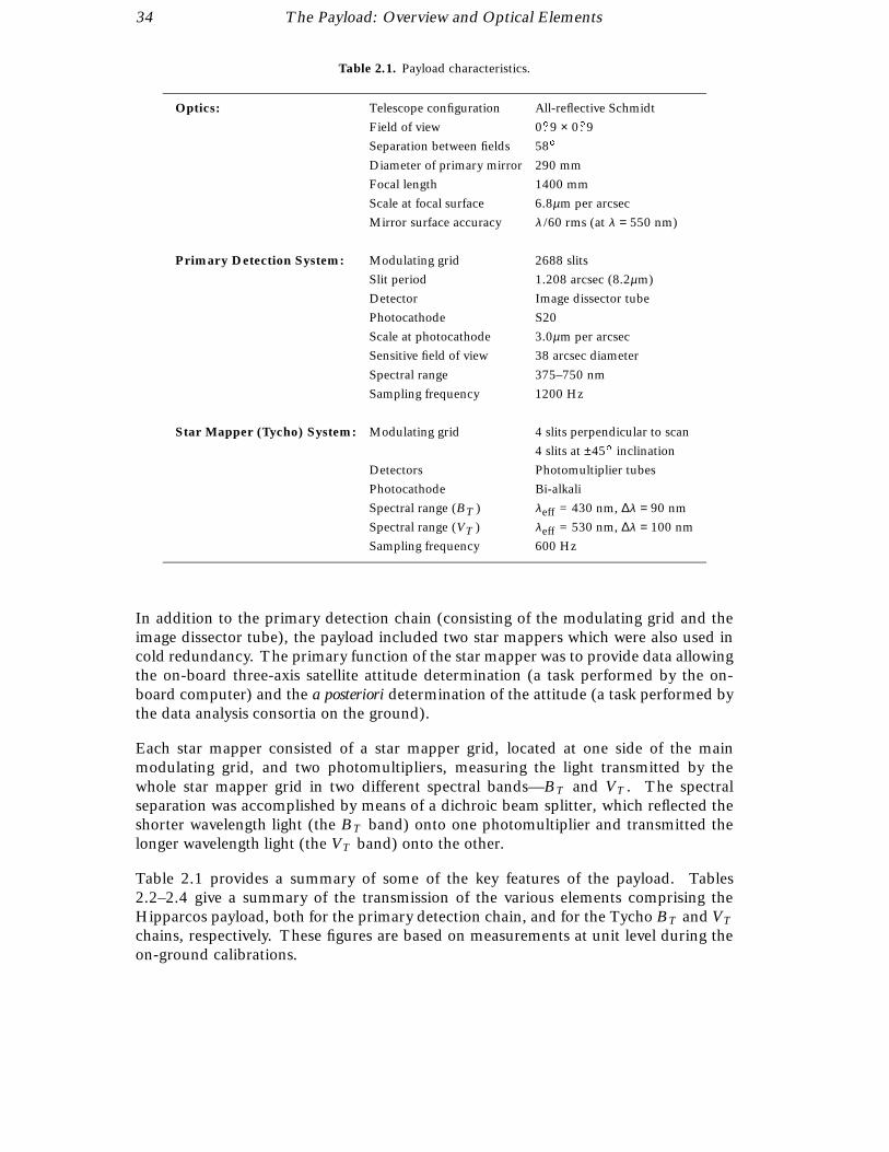
34 The Payload: Overview and Optical Elements
Table 2.1. Payload characteristics.
Optics: Telescope configuration All-reflective Schmidt
Field of view 0.9 × 0.9
Separation between fields 58
Diameter of primary mirror 290 mm
Focal length 1400 mm
Scale at focal surface 6.8µm per arcsec
Mirror surface accuracy λ /60 rms (at λ = 550 nm)
Primary Detection System: Modulating grid 2688 slits
Slit period 1.208 arcsec (8.2µm)
Detector Image dissector tube
Photocathode S20
Scale at photocathode 3.0µm per arcsec
Sensitive field of view 38 arcsec diameter
Spectral range 375–750 nm
Sampling frequency 1200 Hz
Star Mapper (Tycho) System: Modulating grid 4 slits perpendicular to scan
4 slits at ±45 inclination
Detectors Photomultiplier tubes
Photocathode Bi-alkali
Spectral range (BT ) λeff = 430 nm, ∆λ = 90 nm
Spectral range (VT ) λeff = 530 nm, ∆λ = 100 nm
Sampling frequency 600 Hz
In addition to the primary detection chain (consisting of the modulating grid and theimage dissector tube), the payload included two star mappers which were also used incold redundancy. The primary function of the star mapper was to provide data allowingthe on-board three-axis satellite attitude determination (a task performed by the on-board computer) and the a posteriori determination of the attitude (a task performed bythe data analysis consortia on the ground).
Each star mapper consisted of a star mapper grid, located at one side of the mainmodulating grid, and two photomultipliers, measuring the light transmitted by thewhole star mapper grid in two different spectral bands—BT and VT . The spectralseparation was accomplished by means of a dichroic beam splitter, which reflected theshorter wavelength light (the BT band) onto one photomultiplier and transmitted thelonger wavelength light (the VT band) onto the other.
Table 2.1 provides a summary of some of the key features of the payload. Tables2.2–2.4 give a summary of the transmission of the various elements comprising theHipparcos payload, both for the primary detection chain, and for the Tycho BT and VT
chains, respectively. These figures are based on measurements at unit level during theon-ground calibrations.

The Payload: Overview and Optical Elements 35
Table 2.2. Spectral transmittance/quantum efficiency (QE) of the main detection chain, taking into account
all payload elements (predicted performance at the start of the mission based on ground calibrations).
λ Beam Mirrors Grid Relay Detector Total
(nm) Combiner Substrate Optics QE
350 0.86 0.74 0.73 0.16 0.02 0.002
375 0.85 0.72 0.82 0.56 0.03 0.009
400 0.95 0.90 0.91 0.79 0.04 0.027
425 0.96 0.92 0.92 0.81 0.06 0.042
450 0.97 0.94 0.93 0.83 0.08 0.058
475 0.97 0.94 0.94 0.85 0.08 0.060
500 0.97 0.94 0.94 0.88 0.07 0.055
525 0.97 0.94 0.94 0.90 0.06 0.050
550 0.97 0.94 0.94 0.91 0.05 0.044
575 0.97 0.94 0.94 0.92 0.05 0.038
600 0.97 0.95 0.94 0.91 0.04 0.033
625 0.97 0.95 0.94 0.90 0.04 0.027
650 0.97 0.95 0.94 0.84 0.03 0.022
675 0.97 0.95 0.93 0.78 0.03 0.018
700 0.97 0.95 0.93 0.72 0.02 0.014
725 0.97 0.95 0.93 0.65 0.02 0.010
750 0.97 0.95 0.92 0.58 0.01 0.008
775 0.97 0.95 0.91 0.52 0.01 0.005
800 0.97 0.95 0.90 0.45 0.01 0.004
825 0.97 0.95 0.90 0.40 0.01 0.002
In determining the average count rate from a star, the total efficiency given is further affected by the opaque
parts of the modulating grid. This factor is nominally given by the ratio of the slit width to the grid period,
or 3.13/8.20 ' 0.38 (Table 2.5), but in reality it is further reduced by diffraction. The absolute detection
efficiency, of about 10−2, takes this into account.
2.2. Payload Configuration and Layout
The overall payload configuration is shown in Figure 2.1. The payload functionaldiagram is shown in Figure 2.2 and the payload electrical block diagram in Figure 2.3.The payload consisted of four main assemblies (see Figure 2.4):
(a) the two baffle assemblies: two external baffles protected the telescope assembly fromstray light. They were mounted separately on the spacecraft upper platform, with nomechanical link with the other assemblies of the payload, except for the overlappingmulti-layer insulation;
(b) the telescope assembly: this included all elements between the two optical entranceapertures and the grid unit: the three telescope mirrors and all associated structuralelements necessary to maintain them at their nominal positions. All hardware associatedwith the thermal control (the multi-layer insulation, heaters, and thermistors) rested onseparate structural elements. The telescope assembly also ensured the mechanical andthermal conductive interfaces with the spacecraft. An isostatic mounting of the payloadonto the spacecraft employed three titanium bipods;
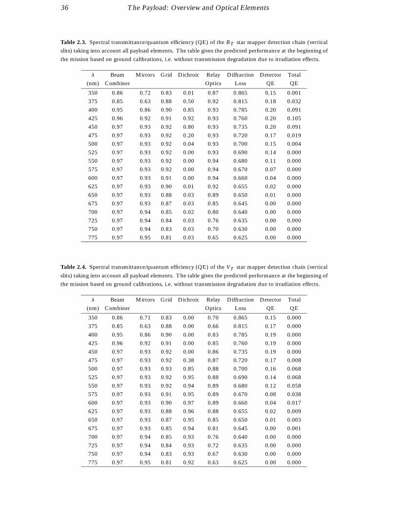
36 The Payload: Overview and Optical Elements
Table 2.3. Spectral transmittance/quantum efficiency (QE) of the BT star mapper detection chain (vertical
slits) taking into account all payload elements. The table gives the predicted performance at the beginning of
the mission based on ground calibrations, i.e. without transmission degradation due to irradiation effects.
λ Beam Mirrors Grid Dichroic Relay Diffraction Detector Total
(nm) Combiner Optics Loss QE QE
350 0.86 0.72 0.83 0.01 0.87 0.865 0.15 0.001
375 0.85 0.63 0.88 0.50 0.92 0.815 0.18 0.032
400 0.95 0.86 0.90 0.85 0.93 0.785 0.20 0.091
425 0.96 0.92 0.91 0.92 0.93 0.760 0.20 0.105
450 0.97 0.93 0.92 0.80 0.93 0.735 0.20 0.091
475 0.97 0.93 0.92 0.20 0.93 0.720 0.17 0.019
500 0.97 0.93 0.92 0.04 0.93 0.700 0.15 0.004
525 0.97 0.93 0.92 0.00 0.93 0.690 0.14 0.000
550 0.97 0.93 0.92 0.00 0.94 0.680 0.11 0.000
575 0.97 0.93 0.92 0.00 0.94 0.670 0.07 0.000
600 0.97 0.93 0.91 0.00 0.94 0.660 0.04 0.000
625 0.97 0.93 0.90 0.01 0.92 0.655 0.02 0.000
650 0.97 0.93 0.88 0.03 0.89 0.650 0.01 0.000
675 0.97 0.93 0.87 0.03 0.85 0.645 0.00 0.000
700 0.97 0.94 0.85 0.02 0.80 0.640 0.00 0.000
725 0.97 0.94 0.84 0.03 0.76 0.635 0.00 0.000
750 0.97 0.94 0.83 0.03 0.70 0.630 0.00 0.000
775 0.97 0.95 0.81 0.03 0.65 0.625 0.00 0.000
Table 2.4. Spectral transmittance/quantum efficiency (QE) of the VT star mapper detection chain (vertical
slits) taking into account all payload elements. The table gives the predicted performance at the beginning of
the mission based on ground calibrations, i.e. without transmission degradation due to irradiation effects.
λ Beam Mirrors Grid Dichroic Relay Diffraction Detector Total
(nm) Combiner Optics Loss QE QE
350 0.86 0.71 0.83 0.00 0.70 0.865 0.15 0.000
375 0.85 0.63 0.88 0.00 0.66 0.815 0.17 0.000
400 0.95 0.86 0.90 0.00 0.83 0.785 0.19 0.000
425 0.96 0.92 0.91 0.00 0.85 0.760 0.19 0.000
450 0.97 0.93 0.92 0.00 0.86 0.735 0.19 0.000
475 0.97 0.93 0.92 0.38 0.87 0.720 0.17 0.008
500 0.97 0.93 0.93 0.85 0.88 0.700 0.16 0.068
525 0.97 0.93 0.92 0.95 0.88 0.690 0.14 0.068
550 0.97 0.93 0.92 0.94 0.89 0.680 0.12 0.058
575 0.97 0.93 0.91 0.95 0.89 0.670 0.08 0.038
600 0.97 0.93 0.90 0.97 0.89 0.660 0.04 0.017
625 0.97 0.93 0.88 0.96 0.88 0.655 0.02 0.009
650 0.97 0.93 0.87 0.95 0.85 0.650 0.01 0.003
675 0.97 0.93 0.85 0.94 0.81 0.645 0.00 0.001
700 0.97 0.94 0.85 0.93 0.76 0.640 0.00 0.000
725 0.97 0.94 0.84 0.93 0.72 0.635 0.00 0.000
750 0.97 0.94 0.83 0.93 0.67 0.630 0.00 0.000
775 0.97 0.95 0.81 0.92 0.63 0.625 0.00 0.000

The Payload: Overview and Optical Elements 37
Colour figure to be inserted here
Figure 2.1. Overview of the payload. Light entered from the two baffles (shown red and blue) and fell onto the
beam-combining mirror, where it was brought to a common focus where the modulating grids were located (top). In
the bottom figure, the path of the light reaching the (main) image dissector tube detector is shown as a red-dashed line,
while the light reaching the star mapper detector is shown in blue. A dichroic filter split the latter into the BT and VTchannels, which were detected separately.

38 The Payload: Overview and Optical Elements
PRECEDINGFIELD OF VIEW
FOLLOWINGFIELD OF VIEWBAFFLE BAFFLE
BEAM COMBINER
FOLDING MIRROR
SPHERICAL MIRROR
MAIN GRID
DEVIATOR
STAR MAPPERGRID 2
DEVIATOR
FOCUSMECHANISM
FIELD LENS
STARMAPPERGRID 1
FOLDING MIRROR
SWITCHINGMIRROR
INTERNAL STARPATTERN
MECHANISM
SHUTTER MECHANISM MECHANISM SHUTTER SHUTTER MECHANISM MECHANISM SHUTTER
GRID REFERENCE
MARKS
DICHROICFILTER
NARROWBAND
FILTER
MECHANISMNARROWBAND
FILTER
MECHANISMDICHROICSPLITTER
RELAYOPTICS
RELAYOPTICS
RELAYOPTICS
RELAYOPTICS
PMTB 1
PMTV 1
IDT 1
IDTELECTRONICS
IDTELECTRONICS
PMTELECTRONICS
PMTELECTRONICS
PMTELECTRONICS
PMTELECTRONICS
RELAYOPTICS
RELAYOPTICS
PMTB 2
PMTV 2
IDT 2
REMOTETERMINAL
UNIT
THERMALCONTROL
ELECTRONICS
MECHANISMDRIVE
ELECTRONICS
INVERTER
ON-BOARDDATA
HANDLINGBUS
DATA HANDLINGAC FROM
SUBSYSTEM
TELESCOPE
OPTICAL PATH
ELECTRICAL LINE
GRID ASSEMBLY
DETECTION SUBSYSTEM
MECHANISMS
DC BUS
ACSPACECRAFT
HEATERSTHERMISTORS
Figure 2.2. Payload functional diagram, illustrating the path of the light through the payload, along with the
corresponding shutters, mechanisms, and detectors associated with the (main) image dissector tube detectors (IDT)
and the star mapper photomultiplier tubes (PMT). Redundant systems (indicated 1/2) were provided in all paths,
eliminating single-point failures in the payload.
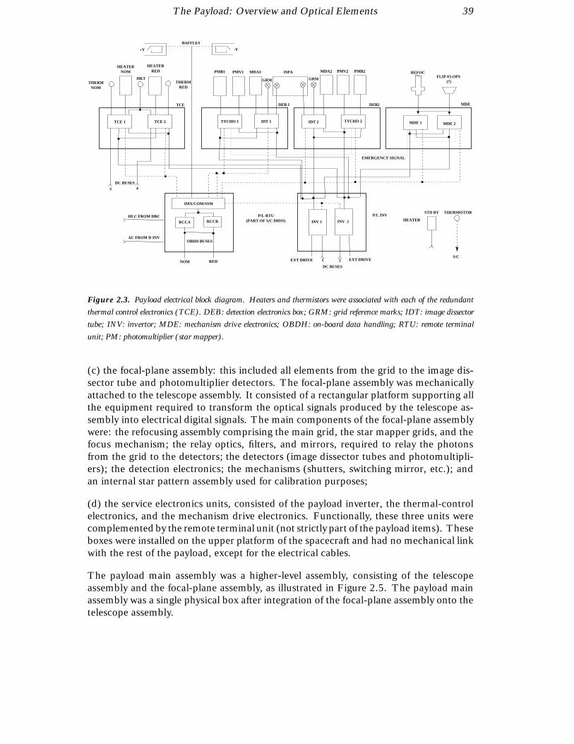
The Payload: Overview and Optical Elements 39
TCE 2TCE 1
HEATERNOM
HEATERRED
THERMRED
THERMNOM
TYCHO 1 IDT 1 TYCHO 2IDT 2 MDE 2
FLIP-FLOPS(7)
MDE 1
RCCA RCCB
IMX/COM/SSM
STD BY THERMISTORP/L RTU
(PART OF S/C DHSS)
TCE
PMV1PMB1 MDA1
DEB 1
GRM GRM
PMB2PMV2MDA2
DEB2
REFOC
MDE
BAFFLES
+Y -Y
OBDH BUSES
HLC FROM DBC
AC FROM D INV
3
DC BUSES4
HEATERINV 1 INV 2
P/L INV
S/CNOM RED EXT DRIVEEXT DRIVE
DC BUSES
21
EMERGENCY SIGNAL
HKT
ISPA
Figure 2.3. Payload electrical block diagram. Heaters and thermistors were associated with each of the redundant
thermal control electronics (TCE). DEB: detection electronics box; GRM: grid reference marks; IDT: image dissector
tube; INV: invertor; MDE: mechanism drive electronics; OBDH: on-board data handling; RTU: remote terminal
unit; PM: photomultiplier (star mapper).
(c) the focal-plane assembly: this included all elements from the grid to the image dis-sector tube and photomultiplier detectors. The focal-plane assembly was mechanicallyattached to the telescope assembly. It consisted of a rectangular platform supporting allthe equipment required to transform the optical signals produced by the telescope as-sembly into electrical digital signals. The main components of the focal-plane assemblywere: the refocusing assembly comprising the main grid, the star mapper grids, and thefocus mechanism; the relay optics, filters, and mirrors, required to relay the photonsfrom the grid to the detectors; the detectors (image dissector tubes and photomultipli-ers); the detection electronics; the mechanisms (shutters, switching mirror, etc.); andan internal star pattern assembly used for calibration purposes;
(d) the service electronics units, consisted of the payload inverter, the thermal-controlelectronics, and the mechanism drive electronics. Functionally, these three units werecomplemented by the remote terminal unit (not strictly part of the payload items). Theseboxes were installed on the upper platform of the spacecraft and had no mechanical linkwith the rest of the payload, except for the electrical cables.
The payload main assembly was a higher-level assembly, consisting of the telescopeassembly and the focal-plane assembly, as illustrated in Figure 2.5. The payload mainassembly was a single physical box after integration of the focal-plane assembly onto thetelescope assembly.

40 The Payload: Overview and Optical Elements
TELESCOPEASSEMBLY
FOCALPLANE
ASSEMBLY
SERVICEELECTRONICSAND PAYLOAD
REMOTETERMINAL UNITBAFFLE
ASSEMBLY 2
BAFFLEASSEMBLY 1
HARNESS
PAYLOAD MAIN ASSEMBLY
Figure 2.4. Breakdown of the payload hardware at assembly level.
(BFSS)
BAFFLESSUBSYSTEMS
FRONTCOVERS
EXTERNALTUBES
TRUSSSTRUCTURES
DETECTIONSUBSYSTEM
(DTSS)
IDTDETECTORS X 2
SDA
DEB(X2)
GRID
ISPA
OPTICALUNITS(OPU)
BEAMCOMBINER
MIRROR
TELESCOPEOPTICS
OPTICAL RELAYSMRL + SRL
FILTERSAND
DICHROICS
HARNESSSUBSYSTEM
(PHSS)
TELESCOPEHARNESS
FPAHARNESS
INTERCONNECTINGHARNESS
SERVICEELECTRONICS
(SEU)
MECHANISMSDRIVE
ELECTRONIC(MDE)
THERMALCONTROL
ELECTRONIC(TCE)
INVERTER(INV)
RTU
MECHANISMUNITS(PMU)
IDT SHUTTERS
PMTSHUTTERS
SWITCHINGMECHANISM
SWM
CHROMATISMMECHANISM
CRM
REFOCUSINGMECHANISM
MLI
HEATERS
THERMISTORS
PAYLOAD THERMALCONTROL
SUBSYSTEM (PTCS)
PAYLOADSTRUCTURESUBSYSTEM
(PSTS)
FPAPLATFORM
SECONDARYSTRUCTURES
TELESCOPESTRUCTURE
MIRRORMOUNTS
PAYLOAD
Figure 2.5. Breakdown of the payload hardware at subsystem level (DEB: detection electronics box; FPA: focal plane
assembly; IDT: image dissector tube; ISPA: internal star pattern assembly; MLI: multi-layer insulation; MRL: main
relay lens; PMT: photomultiplier tube; RTU: remote terminal unit; SRL: star mapper relay lens).

The Payload: Overview and Optical Elements 41
2.3. Payload Hardware
The payload system was divided into eight subsystems (see Figure 2.5). This sectionprovides a brief description of these subsystems, outlining major design features andassociated technology.
The payload structure: The payload structure was centred around a box built fromfive carbon-fibre reinforced plastic (type GY 70), single-skin panels, which providedall necessary interfaces to connect the three mirror mounts, the focal-plane assemblyplatform, and the various secondary structures. The carbon-fibre reinforced plasticelements gave the payload structure a low thermal susceptibility.
The focal-plane platform was a rigid, carbon-fibre reinforced plastic sandwich platemade of two face sheets of carbon-fibre reinforced plastic bonded on an aluminiumhoneycomb and equipped with specific inserts used to connect the different focal-planeassembly units—the optical relays, detectors, mechanisms, and electronic boxes. Thisplatform was hard-mounted onto the telescope.
Each of the three telescope mirrors was supported by a mount consisting of a carbon-fibre reinforced plastic frame barrel rigidly connected to the main structure at threepoints. Three identical flexural-blade systems made of invar and titanium connectedthe mirror to its barrel.
In addition to the main structure, the secondary structures included the internal baffles,necessary for the protection against straylight, and the heater-mat carriers and covers,which were required to ensure light-tightness of the enclosure and to provide mechan-ical support to the thermal hardware multi-layer insulation, heater, thermistors andassociated harnesses.
The optical units: The telescope optics consisted of the (flat) folding mirror, thespherical mirror, and the beam-combiner mirror, all made of zerodur and light-weightedby about 40 per cent. The optical surface quality of the folding and spherical mirrorswas better than λ /60 rms at a reference wavelength of λ = 550 nm, and the overalloptical quality of the telescope was λ /20 rms.
The grid assembly was based on a main substrate made of silica. The main grid and thetwo star mapper patterns were etched into the chromium layer on its front convex faceusing an electron-beam pattern generating technique. The rear side of the substrateconstituted the field lens associated with the relay optics. A set of deviators folded thestar mapper beam in the direction of the star mapper relay optics. These elements weremounted on an invar barrel, extended by the focal-plane baffle which protected theelements from stray light.
Relay optics imaged the main grid onto one of the image dissector tube photocathodes.One or other of the two optical chains was selected by means of a Suprasil switch-ing prism, fixed onto a bi-stable positions mechanism, which allowed the beam to beswitched between the nominal and redundant channels. Relay optics also conveyedthe light from each of the two star mapper grids onto their respective blue/visual pho-tomultipliers. Each of these star mapper relay optics was equipped with a dichroic

42 The Payload: Overview and Optical Elements
beam splitter, which provided the colour separation of the beam for the purposes of theTycho experiment. The selection of the preceding or following star mapper was madeelectronically.
Also included in the optical units were the internal star pattern assembly which, inconjunction with the switching prism mechanism, gave the possibility of an in-orbitgeometric calibration of the deflection coil currents of the main detectors, and theswitchable chromaticity filters (one per image dissector tube relay optics), which gavethe possibility of an in-orbit measurement of the system chromaticity.
The mechanism units: The re-focusing mechanism held the grid package and anassociated folding mirror, which folded the resulting optical beam. This mechanismallowed movement of the grid position with respect to the telescope focal surface. Thebest focus position, maximising the signal modulation of the two fields of view, wasdetermined in orbit.
The switching mirror mechanism provided the mechanical support to the switchingprism, which permitted the selection of either one of the two main detectors.
There were two chromaticity mechanisms, one per image dissector tube channel, eachof them being equipped with a chromaticity filter and a broad-band filter of identicaloptical path length. Switching from the broad-band filter to the chromaticity filterallowed the in-orbit calibration of the instrumental chromaticity.
There were four shutter mechanisms, preventing the detectors from damage induced bylight overload as the fields of view scanned the Earth or the Moon.
The detection subsystem: The detection subsystem included the two primary detec-tors, each of them consisting of an image dissector tube, equipped with its high-voltagepower supply and its pre-amplifier combined in a single package, and four photomul-tipliers, each of them integrated with its own high-voltage power supply and its ownpre-amplifier. There were two detection electronic boxes, each of them dedicated tothe operation of one main detector assembly and two star mapper detector assemblies(nominal or redundant chains).
The thermal control subsystem: The thermal control subsystem included the multi-layer insulation blankets, the heater mats, and the thermistors. All components wereinstalled on the secondary structure. The control law for the heaters was implementedin the satellite on-board computer. Control of heaters and thermistors was performedby the thermal control electronics, part of the service electronics. Twenty-one ther-mal zones were used to achieve payload thermal control, fifteen being devoted to thetelescope enclosure and six to the focal-plane assembly.
The service electronic units: The service electronic units consisted of three boxeslocated on the upper platform of the spacecraft: (i) the inverter unit, which was usedto convert the main DC bus regulated voltage into an AC voltage distributed to thepayload electronic boxes (mechanism drive electronics, thermal control electronics, anddetection electronic boxes); (ii) the thermal-control electronics, which controlled andmonitored the temperature of the payload, using a control law which was implementedin the spacecraft on-board computer; and (iii) the mechanism drive electronics, whichcontrolled and monitored the positions of the payload mechanisms.

The Payload: Overview and Optical Elements 43
Figure 2.6. Configuration of the Schmidt telescope. Light entered from the two baffle directions, and was brought
together at the beam combiner, which was figured as a Schmidt corrector. The combined light was reflected from the
folding and spherical primary mirrors onto the focal surface where the modulating grids were located.
These three electronic boxes interfaced with the payload remote terminal unit, whichwas responsible for transfer of data commands and clocks from the spacecraft data-handling system to the electronic units of the payload, as well as the transfer of scientific,engineering and housekeeping data from the payload to the spacecraft data-handlingsystem.
The baffle subsystem: The baffle subsystem consisted of two external baffles, whichprotected the payload from straylight originating from the Sun, the Earth, or the Moon.They were made of carbon-fibre reinforced plastic and were connected directly ontothe spacecraft upper shelf. Each of these baffles was equipped with entrance covers,closed during ground handling and launch. They were opened in orbit by activation ofassociated pyrotechnic devices.
2.4. Telescope Mirrors
The telescope was based on the all-reflecting Schmidt concept, and consisted of threemirrors: a beam combiner, a primary spherical mirror, and a (flat) folding mirror (Fig-ure 2.6). The folding mirror folded the optical beam to provide a more compact overallconfiguration. The beam combining mirror also performed the (off-axis) correction ofspherical aberration.
A reflective coating was used for all three mirrors. It was chosen for its very highefficiency (in particular in the blue part of the spectrum), together with the fact thatit had already been space qualified. It consisted of a layer of Ag, protected by a ThF4
coating, on a layer of chromium to enhance its adherence. The metallic layer of thiscoating was grounded by bonding a grounding strap to an area, outside the useful coated

44 The Payload: Overview and Optical Elements
Figure 2.7. Spectral reflectivity of the mirror coating as a function of wavelength.
area, which was kept free of the dielectric protective layer. The performances of thiscoating, in terms of reflective efficiency is given in Figure 2.7. The mirror efficienciesare summarised in Tables 2.2–2.4 as part of the overall payload efficiencies.
The Beam Combiner
The beam combiner had three main functions: to combine the two fields of view;to define the entrance pupil; and to perform the correction of the aberrations of thespherical mirror.
The beam combiner mirror was made from a ‘light-weighted’ polished zerodur blank,325.6 mm in diameter and 100 mm thick, cut into two halves and reassembled with awedge angle of 29. The optical surfaces of the half-mirrors were figured asphericallyand the reflective coating defined the pupil area. The beam combiner assembly alsoincluded three fixation pads made of invar and bonded to the lateral side of the mirror.These pads interfaced with the beam combiner’s isostatic mounts.
A beam combiner ‘decentre sensor’, consisting of a light source and a quadrant sensor,was bonded onto the two halves of the mirror and was used to align the spherical mirror’scentre of curvature with the aspherical profile centre. The sensor was also used to verifyalignment stability during on-ground operations.
The aspherical figuring of the beam combiner was of the Schmidt-Kerber type (see,for example, Buacher 1967). In this design, optical aberrations are minimised bycorrections of the optical path at the level of the entrance pupil. The profile (Figure 2.8)was defined by its deviation with respect to the ideal flat surface:
X = αρ4 +β2
ρ2 [2.1]
where α is the aspherisation parameter (α = −5.16726 × 10⁻¹² mm−3), β is the vertexcurvature (β = 3.47724 × 10⁻⁷ mm−1), and ρ is the radial coordinate in mm.
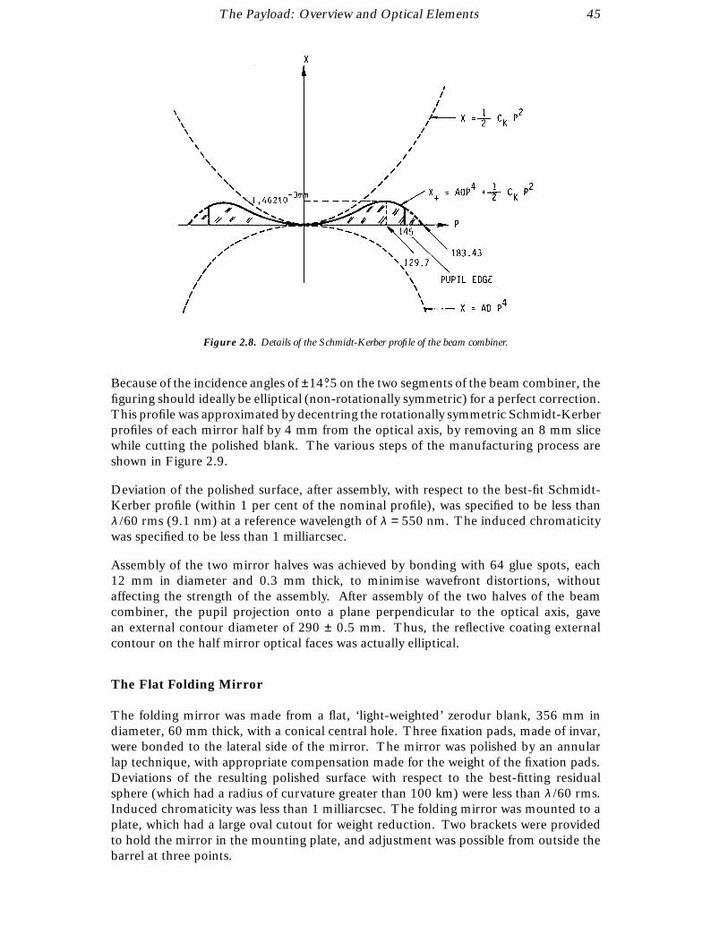
The Payload: Overview and Optical Elements 45
Figure 2.8. Details of the Schmidt-Kerber profile of the beam combiner.
Because of the incidence angles of ±14.5 on the two segments of the beam combiner, thefiguring should ideally be elliptical (non-rotationally symmetric) for a perfect correction.This profile was approximated by decentring the rotationally symmetric Schmidt-Kerberprofiles of each mirror half by 4 mm from the optical axis, by removing an 8 mm slicewhile cutting the polished blank. The various steps of the manufacturing process areshown in Figure 2.9.
Deviation of the polished surface, after assembly, with respect to the best-fit Schmidt-Kerber profile (within 1 per cent of the nominal profile), was specified to be less thanλ /60 rms (9.1 nm) at a reference wavelength of λ = 550 nm. The induced chromaticitywas specified to be less than 1 milliarcsec.
Assembly of the two mirror halves was achieved by bonding with 64 glue spots, each12 mm in diameter and 0.3 mm thick, to minimise wavefront distortions, withoutaffecting the strength of the assembly. After assembly of the two halves of the beamcombiner, the pupil projection onto a plane perpendicular to the optical axis, gavean external contour diameter of 290 ± 0.5 mm. Thus, the reflective coating externalcontour on the half mirror optical faces was actually elliptical.
The Flat Folding Mirror
The folding mirror was made from a flat, ‘light-weighted’ zerodur blank, 356 mm indiameter, 60 mm thick, with a conical central hole. Three fixation pads, made of invar,were bonded to the lateral side of the mirror. The mirror was polished by an annularlap technique, with appropriate compensation made for the weight of the fixation pads.Deviations of the resulting polished surface with respect to the best-fitting residualsphere (which had a radius of curvature greater than 100 km) were less than λ /60 rms.Induced chromaticity was less than 1 milliarcsec. The folding mirror was mounted to aplate, which had a large oval cutout for weight reduction. Two brackets were providedto hold the mirror in the mounting plate, and adjustment was possible from outside thebarrel at three points.

46 The Payload: Overview and Optical Elements
Figure 2.9. Steps in the manufacture of the beam combiner. All three steps provided a considerable technical challenge
in order to retain the overall high quality of the optical wavefront.
The Spherical Mirror
The spherical mirror was made from a ‘light-weighted’ zerodur blank, 393 mm indiameter, 66 mm thick, with a small central hole (for alignment purposes). The opticalsurface was of concave spherical shape. Three fixation pads, made of invar, were bondedto the lateral side of the mirror. A lens, called the beam converger, was bonded to thecentral part of the rear side of the mirror, and this allowed for stability testing of thetelescope, between the spherical mirror and the grid assembly.
The mirror was polished by conventional techniques, with appropriate compensationmade for the weight of the fixation pads. Deviations of the resulting polished surfacewith respect to the best-fitting sphere (with radius of curvature 2800 ± 3 mm) were lessthan λ /60 rms. Induced chromaticity was less than 1 milliarcsec.
Beam Combiner and Mirrors Fixation Pads
The invar fixation pads of the mirrors and of the beam combiner were designed tominimise the wavefront distortion induced during the integration of the mirrors in theirbarrels with the isostatic mounts. They were bonded to the sides of the mirror witha glue film (type EC 2216) 0.3 mm thick. This resulted in a lack of symmetry in the(three-point) mounting of the two halves of the beam combiner.
The fixation pads were 50 × 70 mm2 in size, with a thickness of 14.2 mm. They weretightened to isostatic mounts by twelve M4 studs, and positive locking was achieved bymeans of two expandable pins per pad. To avoid induced wavefront distortions, the
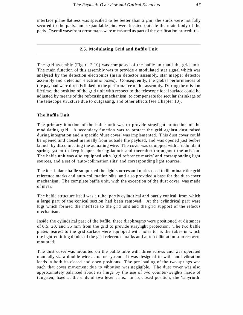
The Payload: Overview and Optical Elements 47
interface plane flatness was specified to be better than 2 µm, the studs were not fullysecured to the pads, and expandable pins were located outside the main body of thepads. Overall wavefront error maps were measured as part of the verification procedures.
2.5. Modulating Grid and Baffle Unit
The grid assembly (Figure 2.10) was composed of the baffle unit and the grid unit.The main function of this assembly was to provide a modulated star signal which wasanalysed by the detection electronics (main detector assembly, star mapper detectorassembly and detection electronic boxes). Consequently, the global performances ofthe payload were directly linked to the performance of this assembly. During the missionlifetime, the position of the grid unit with respect to the telescope focal surface could beadjusted by means of the refocusing mechanism, to compensate for secular shrinkage ofthe telescope structure due to outgassing, and other effects (see Chapter 10).
The Baffle Unit
The primary function of the baffle unit was to provide straylight protection of themodulating grid. A secondary function was to protect the grid against dust raisedduring integration and a specific ‘dust cover’ was implemented. This dust cover couldbe opened and closed manually from outside the payload, and was opened just beforelaunch by disconnecting the actuating wire. The cover was equipped with a redundantspring system to keep it open during launch and thereafter throughout the mission.The baffle unit was also equipped with ‘grid reference marks’ and corresponding lightsources, and a set of ‘auto-collimation slits’ and corresponding light sources.
The focal-plane baffle supported the light sources and optics used to illuminate the gridreference marks and auto-collimation slits, and also provided a base for the dust-covermechanism. The complete baffle unit, with the exception of the dust cover, was madeof invar.
The baffle structure itself was a tube, partly cylindrical and partly conical, from whicha large part of the conical section had been removed. At the cylindrical part werelugs which formed the interface to the grid unit and the grid support of the refocusmechanism.
Inside the cylindrical part of the baffle, three diaphragms were positioned at distancesof 6.5, 20, and 35 mm from the grid to provide straylight protection. The two baffleplates nearest to the grid surface were equipped with holes to fix the tubes in whichthe light-emitting diodes of the grid reference marks and auto-collimation sources weremounted.
The dust cover was mounted on the baffle tube with three screws and was operatedmanually via a double wire actuator system. It was designed to withstand vibrationloads in both its closed and open positions. The pre-loading of the two springs wassuch that cover movement due to vibration was negligible. The dust cover was alsoapproximately balanced about its hinge by the use of two counter-weights made oftungsten, fixed at the ends of two lever arms. In its closed position, the ‘labyrinth’
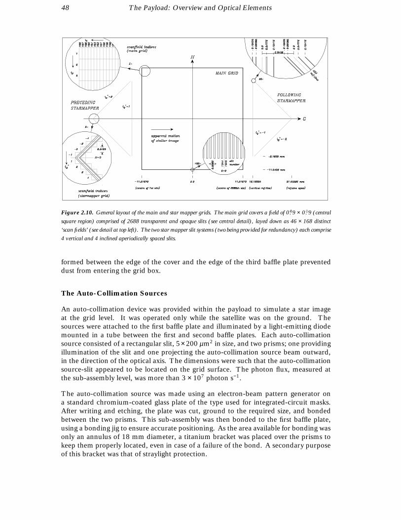
48 The Payload: Overview and Optical Elements
Figure 2.10. General layout of the main and star mapper grids. The main grid covers a field of 0.9 × 0.9 (central
square region) comprised of 2688 transparent and opaque slits (see central detail), layed down as 46 × 168 distinct
‘scan fields’ (see detail at top left). The two star mapper slit systems (two being provided for redundancy) each comprise
4 vertical and 4 inclined aperiodically spaced slits.
formed between the edge of the cover and the edge of the third baffle plate preventeddust from entering the grid box.
The Auto-Collimation Sources
An auto-collimation device was provided within the payload to simulate a star imageat the grid level. It was operated only while the satellite was on the ground. Thesources were attached to the first baffle plate and illuminated by a light-emitting diodemounted in a tube between the first and second baffle plates. Each auto-collimationsource consisted of a rectangular slit, 5× 200 µm2 in size, and two prisms; one providingillumination of the slit and one projecting the auto-collimation source beam outward,in the direction of the optical axis. The dimensions were such that the auto-collimationsource-slit appeared to be located on the grid surface. The photon flux, measured atthe sub-assembly level, was more than 3 × 10⁷ photon s−1.
The auto-collimation source was made using an electron-beam pattern generator ona standard chromium-coated glass plate of the type used for integrated-circuit masks.After writing and etching, the plate was cut, ground to the required size, and bondedbetween the two prisms. This sub-assembly was then bonded to the first baffle plate,using a bonding jig to ensure accurate positioning. As the area available for bonding wasonly an annulus of 18 mm diameter, a titanium bracket was placed over the prisms tokeep them properly located, even in case of a failure of the bond. A secondary purposeof this bracket was that of straylight protection.
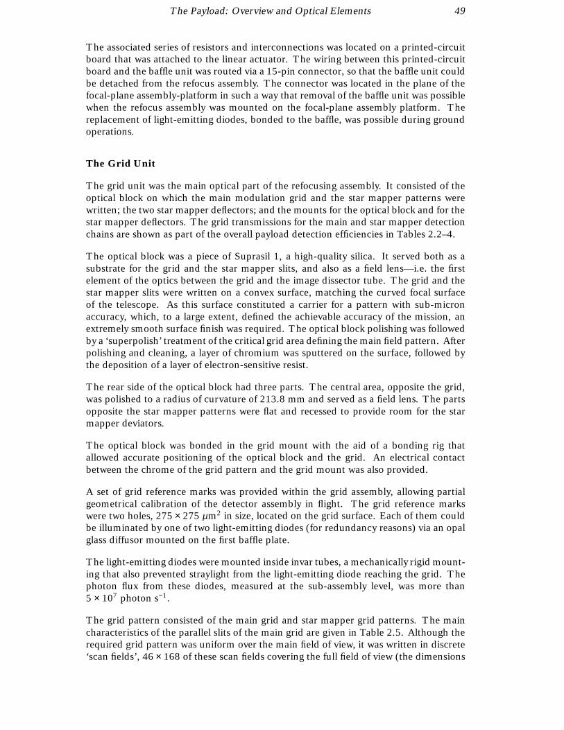
The Payload: Overview and Optical Elements 49
The associated series of resistors and interconnections was located on a printed-circuitboard that was attached to the linear actuator. The wiring between this printed-circuitboard and the baffle unit was routed via a 15-pin connector, so that the baffle unit couldbe detached from the refocus assembly. The connector was located in the plane of thefocal-plane assembly-platform in such a way that removal of the baffle unit was possiblewhen the refocus assembly was mounted on the focal-plane assembly platform. Thereplacement of light-emitting diodes, bonded to the baffle, was possible during groundoperations.
The Grid Unit
The grid unit was the main optical part of the refocusing assembly. It consisted of theoptical block on which the main modulation grid and the star mapper patterns werewritten; the two star mapper deflectors; and the mounts for the optical block and for thestar mapper deflectors. The grid transmissions for the main and star mapper detectionchains are shown as part of the overall payload detection efficiencies in Tables 2.2–4.
The optical block was a piece of Suprasil 1, a high-quality silica. It served both as asubstrate for the grid and the star mapper slits, and also as a field lens—i.e. the firstelement of the optics between the grid and the image dissector tube. The grid and thestar mapper slits were written on a convex surface, matching the curved focal surfaceof the telescope. As this surface constituted a carrier for a pattern with sub-micronaccuracy, which, to a large extent, defined the achievable accuracy of the mission, anextremely smooth surface finish was required. The optical block polishing was followedby a ‘superpolish’ treatment of the critical grid area defining the main field pattern. Afterpolishing and cleaning, a layer of chromium was sputtered on the surface, followed bythe deposition of a layer of electron-sensitive resist.
The rear side of the optical block had three parts. The central area, opposite the grid,was polished to a radius of curvature of 213.8 mm and served as a field lens. The partsopposite the star mapper patterns were flat and recessed to provide room for the starmapper deviators.
The optical block was bonded in the grid mount with the aid of a bonding rig thatallowed accurate positioning of the optical block and the grid. An electrical contactbetween the chrome of the grid pattern and the grid mount was also provided.
A set of grid reference marks was provided within the grid assembly, allowing partialgeometrical calibration of the detector assembly in flight. The grid reference markswere two holes, 275 × 275 µm2 in size, located on the grid surface. Each of them couldbe illuminated by one of two light-emitting diodes (for redundancy reasons) via an opalglass diffusor mounted on the first baffle plate.
The light-emitting diodes were mounted inside invar tubes, a mechanically rigid mount-ing that also prevented straylight from the light-emitting diode reaching the grid. Thephoton flux from these diodes, measured at the sub-assembly level, was more than5 × 107 photon s−1.
The grid pattern consisted of the main grid and star mapper grid patterns. The maincharacteristics of the parallel slits of the main grid are given in Table 2.5. Although therequired grid pattern was uniform over the main field of view, it was written in discrete‘scan fields’, 46 × 168 of these scan fields covering the full field of view (the dimensions

50 The Payload: Overview and Optical Elements
Table 2.5. Summary of the calibration results of the main grid.
Item Performance
Slit geometry:
average grid period 8.20 ± 0.001 µm
average slit width 3.13 ± 0.03 µm
slit width standard deviation < 0.033 µm (rms)
total number of slits 2688
number of scan fields 46 × 168
scan field dimensions 131.2 × 480 µm2
Medium-scale grid irregularities:
Mpq −0.038 < Mpq < 0.053 µm
gradient (scan field to scan field) 0.009 µm (rms)
Small-scale grid irregularities:
individual slit (random) 0.015 µm (rms)
regular ‘saw tooth step’ 0.000 µm (mean value)
irregular ‘saw tooth step’ 0.016 µm (rms)
correlated scan field orientation 0.009 µm (rms)
uncorrelated scan field orientation −0.009 µm (mean value)
Grid reference marks:
shape square
edge dimension 22.04–22.08 mm
centering accuracy ±0.001 mm
orientation ±0.25 arcmin
Table 2.6. Summary of the principal specifications for the star mapper grid.
Item Specification
Medium-scale grid irregularities:
vertical < 0.5 µm (max)
inclined < 0.5 µm (max)
transverse gradient (vertical) < 0.077 µm (rms)
transverse gradient (inclined) < 0.077 µm (rms)
Small-scale grid irregularities:
vertical < 0.05 µm (rms)
inclined < 0.05 µm (rms)
magnification factor < 0.15 (max)
scan field orientation (vertical) < 0.034 µm
scan field orientation (inclined) < 0.034 µm
slit width value 6.20 µm
slit width variation < 0.35 µm (max)
Grid calibration:
vertical < 0.055 µm (rms)
inclined < 0.077 µm (rms)
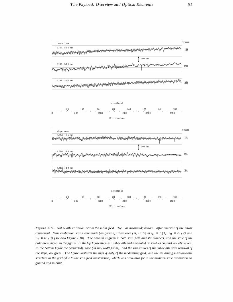
The Payload: Overview and Optical Elements 51
Figure 2.11. Slit width variation across the main field. Top: as measured; bottom: after removal of the linear
component. Nine calibration scans were made (on ground), three each (A, B, C) at iH = 1 (1), iH = 23 (2) and
iH = 46 (3) (see also Figure 2.10). The abscissa is given in both scan field and slit numbers, and the scale of the
ordinate is shown in the figures. In the top figure the mean slit-width and associated rms values (in nm) are also given.
In the bottom figure the (corrected) slope (in nm(width)/mm), and the rms values of the slit-width after removal of
the slope, are given. The figure illustrates the high quality of the modulating grid, and the remaining medium-scale
structure in the grid (due to the scan field construction) which was accounted for in the medium-scale calibration on
ground and in orbit.

52 The Payload: Overview and Optical Elements
Figure 2.12. The medium-scale irregularity of the main grid, in the scan direction. The geometry of the grid
corresponds to the configuration shown in Figure 2.10. The scale in the upper figure is such that one scan-field ‘unit’
corresponds to 40 nm. The lower figure shows the mean value in the scan direction (solid line), and the standard
deviation (dotted line).
of each scan field were 131.2 × 480 µm2, with the longer dimension in the direction ofthe slits, i.e. normal to the scan direction). Two star mapper patterns lay on either sideof the main grid—their principal characteristics are summarised in Figure 2.10.
Considerable attention was given to the manufacture and calibration of the grids, giventhat the final mission accuracies of around 1 milliarcsec corresponded to approximately0.007 µm at the focal plane. Deviations of the main grid from a perfectly regular onewere classified into large, medium, and small-scale grid irregularities. The large-scalegrid irregularities were defined as deviations that could be expressed as a second-orderpolynomial fitted to the distortion map—these could be calibrated by the data reductionconsortia during the ‘great-circle’ step of the data reductions. The medium-scale gridirregularities were defined as a matrix of Mpq elements, where each element representedthe average distortion of the scan field (p, q) after removal of the large-scale component.The range of Mpq, and its field-to-field gradient, are tabulated in Table 2.5.
Small-scale grid irregularities were defined as the residual distortion, after the removal ofthe large- and medium-scale components. Their characterisation would have requireda very large ground calibration effort, followed by the correction of the satellite data ata very high spatial resolution. The grid manufacture concentrated on producing a gridin which the small-scale irregularities could be neglected, a fact eventually confirmedin orbit. In the manufacturing and calibration process, the small-scale irregularitieswere split into various components (see Table 2.5). The ‘individual slit’ contribution
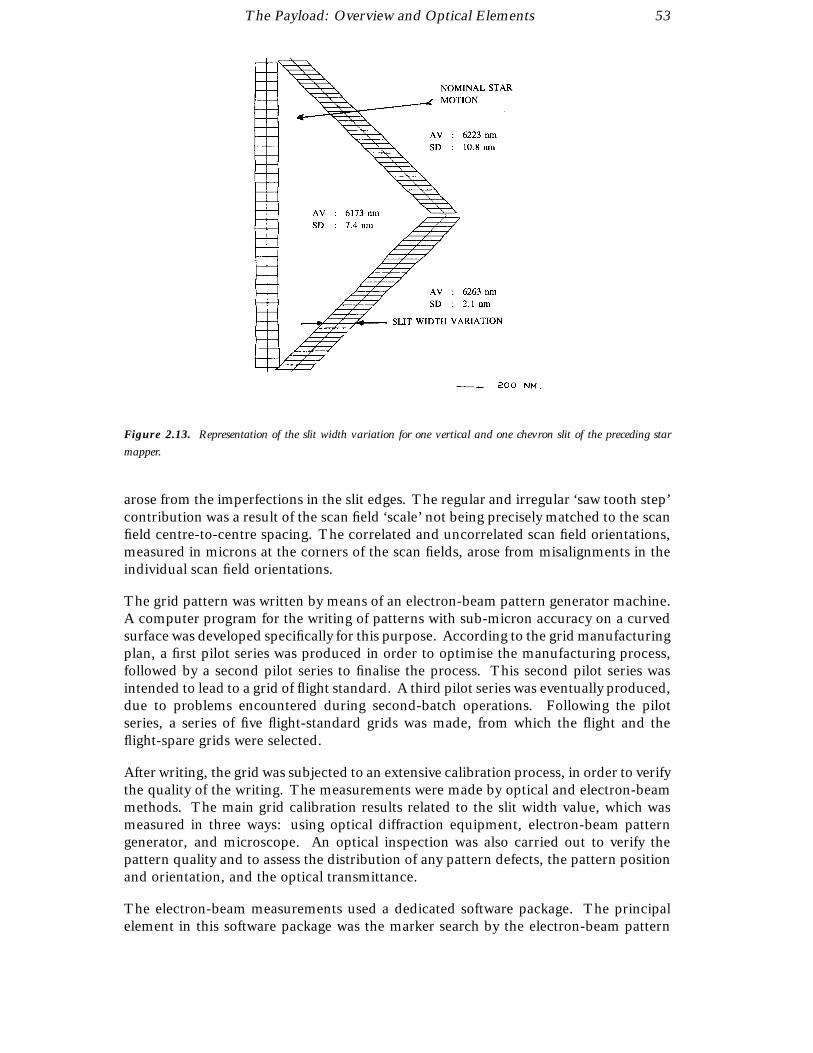
The Payload: Overview and Optical Elements 53
Figure 2.13. Representation of the slit width variation for one vertical and one chevron slit of the preceding star
mapper.
arose from the imperfections in the slit edges. The regular and irregular ‘saw tooth step’contribution was a result of the scan field ‘scale’ not being precisely matched to the scanfield centre-to-centre spacing. The correlated and uncorrelated scan field orientations,measured in microns at the corners of the scan fields, arose from misalignments in theindividual scan field orientations.
The grid pattern was written by means of an electron-beam pattern generator machine.A computer program for the writing of patterns with sub-micron accuracy on a curvedsurface was developed specifically for this purpose. According to the grid manufacturingplan, a first pilot series was produced in order to optimise the manufacturing process,followed by a second pilot series to finalise the process. This second pilot series wasintended to lead to a grid of flight standard. A third pilot series was eventually produced,due to problems encountered during second-batch operations. Following the pilotseries, a series of five flight-standard grids was made, from which the flight and theflight-spare grids were selected.
After writing, the grid was subjected to an extensive calibration process, in order to verifythe quality of the writing. The measurements were made by optical and electron-beammethods. The main grid calibration results related to the slit width value, which wasmeasured in three ways: using optical diffraction equipment, electron-beam patterngenerator, and microscope. An optical inspection was also carried out to verify thepattern quality and to assess the distribution of any pattern defects, the pattern positionand orientation, and the optical transmittance.
The electron-beam measurements used a dedicated software package. The principalelement in this software package was the marker search by the electron-beam pattern

54 The Payload: Overview and Optical Elements
Figure 2.14. Optical micrographs of part of the main modulating grid (top figure) and the star mapper grid (lower
figure). The grids represented one of the main technical challenges of the Hipparcos payload, and were of an extremely
high quality.
generator. Another important element was the ‘almost undeflected electron-beam op-eration’, in order to minimise the contribution of main beam deflection errors. As aconsequence, an xy table movement was required for each slit or marker measurement.The location of the position-calibration markers was obtained with an accuracy of 10 nmrms from its four marker edge positions. Each edge position was the average of 20 mea-surements on a centred 10 µm part of the marker edge. The marker search algorithmwas based on a signal bandwidth reduction and a binary search scheme.
The slit position was obtained with an accuracy of 10 nm rms by the same marker searchalgorithm applied to both slit edges. The parameters were adapted to fit the nominal
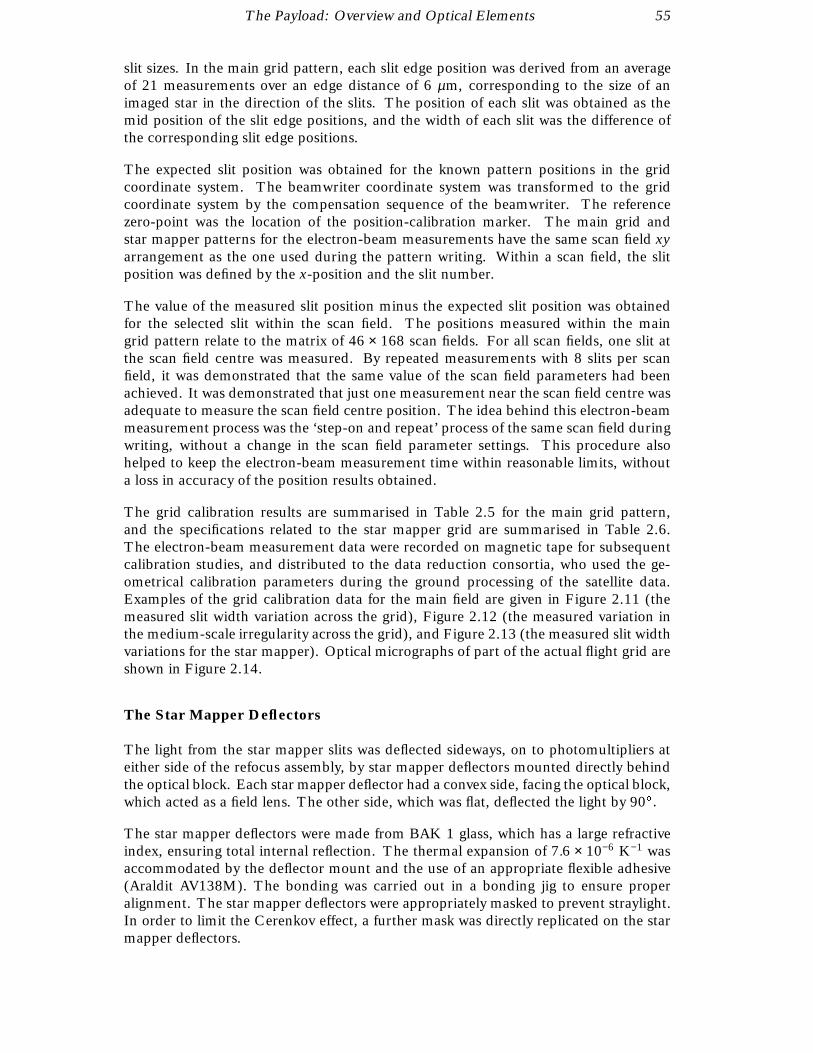
The Payload: Overview and Optical Elements 55
slit sizes. In the main grid pattern, each slit edge position was derived from an averageof 21 measurements over an edge distance of 6 µm, corresponding to the size of animaged star in the direction of the slits. The position of each slit was obtained as themid position of the slit edge positions, and the width of each slit was the difference ofthe corresponding slit edge positions.
The expected slit position was obtained for the known pattern positions in the gridcoordinate system. The beamwriter coordinate system was transformed to the gridcoordinate system by the compensation sequence of the beamwriter. The referencezero-point was the location of the position-calibration marker. The main grid andstar mapper patterns for the electron-beam measurements have the same scan field xyarrangement as the one used during the pattern writing. Within a scan field, the slitposition was defined by the x-position and the slit number.
The value of the measured slit position minus the expected slit position was obtainedfor the selected slit within the scan field. The positions measured within the maingrid pattern relate to the matrix of 46 × 168 scan fields. For all scan fields, one slit atthe scan field centre was measured. By repeated measurements with 8 slits per scanfield, it was demonstrated that the same value of the scan field parameters had beenachieved. It was demonstrated that just one measurement near the scan field centre wasadequate to measure the scan field centre position. The idea behind this electron-beammeasurement process was the ‘step-on and repeat’ process of the same scan field duringwriting, without a change in the scan field parameter settings. This procedure alsohelped to keep the electron-beam measurement time within reasonable limits, withouta loss in accuracy of the position results obtained.
The grid calibration results are summarised in Table 2.5 for the main grid pattern,and the specifications related to the star mapper grid are summarised in Table 2.6.The electron-beam measurement data were recorded on magnetic tape for subsequentcalibration studies, and distributed to the data reduction consortia, who used the ge-ometrical calibration parameters during the ground processing of the satellite data.Examples of the grid calibration data for the main field are given in Figure 2.11 (themeasured slit width variation across the grid), Figure 2.12 (the measured variation inthe medium-scale irregularity across the grid), and Figure 2.13 (the measured slit widthvariations for the star mapper). Optical micrographs of part of the actual flight grid areshown in Figure 2.14.
The Star Mapper Deflectors
The light from the star mapper slits was deflected sideways, on to photomultipliers ateither side of the refocus assembly, by star mapper deflectors mounted directly behindthe optical block. Each star mapper deflector had a convex side, facing the optical block,which acted as a field lens. The other side, which was flat, deflected the light by 90.
The star mapper deflectors were made from BAK 1 glass, which has a large refractiveindex, ensuring total internal reflection. The thermal expansion of 7.6 × 10⁻⁶ K−1 wasaccommodated by the deflector mount and the use of an appropriate flexible adhesive(Araldit AV138M). The bonding was carried out in a bonding jig to ensure properalignment. The star mapper deflectors were appropriately masked to prevent straylight.In order to limit the Cerenkov effect, a further mask was directly replicated on the starmapper deflectors.
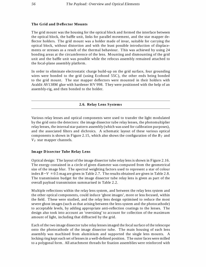
56 The Payload: Overview and Optical Elements
The Grid and Deflector Mounts
The grid mount was the housing for the optical block and formed the interface betweenthe optical block, the baffle unit, links for parallel movement, and the star mapper de-flector holders. The grid mount was a holder made of invar, suitable for carrying theoptical block, without distortion and with the least possible introduction of displace-ments or stresses as a result of the thermal behaviour. This was achieved by using 24bonding areas at the circumference of the lens. Mounting and dismounting of the gridunit and the baffle unit was possible while the refocus assembly remained attached tothe focal-plane assembly platform.
In order to eliminate electrostatic charge build-up on the grid surface, four groundingwires were bonded to the grid (using Ecobond 55C), the other ends being bondedto the grid mount. The star mapper deflectors were mounted in their holders withAraldit AV138M glue with hardener HV 998. They were positioned with the help of anassembly-rig, and then bonded to the holder.
2.6. Relay Lens Systems
Various relay lenses and optical components were used to transfer the light modulatedby the grid onto the detectors: the image dissector tube relay lenses, the photomultiplierrelay lenses, the internal star pattern assembly (which was used for calibration purposes),and the associated filters and dichroics. A schematic layout of these various opticalcomponents is shown in Figure 2.15, which also shows the configuration of the BT andVT star mapper channels.
Image Dissector Tube Relay Lens
Optical design: The layout of the image dissector tube relay lens is shown in Figure 2.16.The energy contained in a circle of given diameter was computed from the geometricalsize of the image blur. The spectral weighting factors used to represent a star of colourindex B−V = 0.5 mag are given in Table 2.7. The results obtained are given in Table 2.8.The transmission budget for the image dissector tube relay lens is given as part of theoverall payload transmission summarised in Table 2.2.
Multiple reflections within the relay lens system, and between the relay lens system andthe other optical components, could induce ‘ghost images’, more or less focused, withinthe field. These were studied, and the relay lens design optimised to reduce the mostsevere ghost images (such as that arising between the lens system and the photocathode)to acceptable levels, by adding appropriate anti-reflection coatings to the lenses. Thedesign also took into account an ‘oversizing’ to account for collection of the maximumamount of light, including that diffracted by the grid.
Each of the two image dissector tube relay lenses imaged the focal surface of the telescopeonto the photocathode of the image dissector tube. The main housing of each lensassembly was machined from aluminium and supported the single lens mounts. Alocking ring kept each set of lenses in a well-defined position. The outer faces were milledto a polygonal form. All attachment threads for fixation assemblies were reinforced with
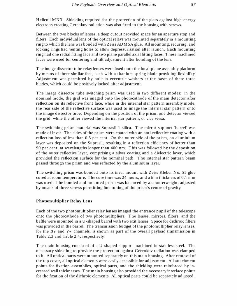
The Payload: Overview and Optical Elements 57
Helicoil MN3. Shielding required for the protection of the glass against high-energyelectrons creating Cerenkov radiation was also fixed to the housing with screws.
Between the two blocks of lenses, a deep cutout provided space for an aperture stop andfilters. Each individual lens of the optical relays was mounted separately in a mountingring to which the lens was bonded with Zeiss ADM5A glue. All mounting, securing, andlocking rings had venting holes to allow depressurisation after launch. Each mountingring had one radial fitting face and two plane parallel axial fitting faces. These machinedfaces were used for centering and tilt adjustment after bonding of the lens.
The image dissector tube relay lenses were fixed onto the focal-plane assembly platformby means of three similar feet, each with a titanium spring blade providing flexibility.Adjustment was permitted by built-in eccentric washers at the bases of these threeblades, which could be positively locked after adjustment.
The image dissector tube switching prism was used in two different modes: in thenominal mode, the grid was imaged onto the photocathode of the main detector afterreflection on its reflective front face, while in the internal star pattern assembly mode,the rear side of the reflective surface was used to image the internal star pattern ontothe image dissector tube. Depending on the position of the prism, one detector viewedthe grid, while the other viewed the internal star pattern, or vice versa.
The switching prism material was Suprasil 1 silica. The mirror support ‘barrel’ wasmade of invar. The sides of the prism were coated with an anti-reflective coating with areflection loss of less than 0.5 per cent. On the outer side of the prism, an aluminiumlayer was deposited on the Suprasil, resulting in a reflection efficiency of better than90 per cent, at wavelengths longer than 400 nm. This was followed by the depositionof the outer reflective layer, comprising a silver coating and a dielectric layer, whichprovided the reflection surface for the nominal path. The internal star pattern beampassed through the prism and was reflected by the aluminium layer.
The switching prism was bonded onto its invar mount with Zeiss Kleber No. 51 gluecured at room temperature. The cure time was 24 hours, and a film thickness of 0.1 mmwas used. The bonded and mounted prism was balanced by a counterweight, adjustedby means of three screws permitting fine tuning of the prism’s centre of gravity.
Photomultiplier Relay Lens
Each of the two photomultiplier relay lenses imaged the entrance pupil of the telescopeonto the photocathode of two photomultipliers. The lenses, mirrors, filters, and thebaffle were mounted in a U-shaped barrel with two exit lenses. Space for dichroic filterswas provided in the barrel. The transmission budget of the photomultiplier relay lenses,for the BT and VT channels, is shown as part of the overall payload transmission inTable 2.3 and Table 2.4, respectively.
The main housing consisted of a U-shaped support machined in stainless steel. Thenecessary shielding to provide the protection against Cerenkov radiation was clampedto it. All optical parts were mounted separately on this main housing. After removal ofthe top cover, all optical elements were easily accessible for adjustment. All attachmentpoints for fixation assemblies, optical parts, and the shielding were reinforced by in-creased wall thicknesses. The main housing also provided the necessary interface pointsfor the fixation of the dichroic elements. All optical parts could be separately adjusted.
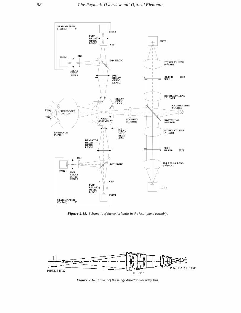
58 The Payload: Overview and Optical Elements
TELESCOPE OPTICS
2 PARTIDT RELAY LENS
nd
1 PARTIDT RELAY LENS
st
1 PARTIDT RELAY LENS
st
2 PARTIDT RELAY LENS
nd
SOURCE
IDT 2
STAR MAPPER(Tycho 2)
PMB2 BBF
PMV2
VBF
DICHROIC
RELAYOPTICLENS 3
PMTRELAYOPTICLENS 3
PMTRELAYOPTICLENS 2
F
FOV
FOV
P
F
ENTRANCEPUPIL
RELAYOPTICLENS 1
FOLDING MIRROR
IDTRELAYOPTICFIELDLENS
DEVIATORRELAYOPTICLENS 1
DICHROIC
BBF
PMB 1
VBF
PMV1
PMTRELAYOPTICLENS 3
PMTRELAYOPTICLENS 3
STAR MAPPER(Tycho 1) P
IDT 1
(CF)PUPIL FILTER
SWITCHINGMIRROR
(CF)FILTERPUPIL
CALIBRATION
ASSEMBLYGRID
Figure 2.15. Schematic of the optical units in the focal-plane assembly.
Figure 2.16. Layout of the image dissector tube relay lens.

The Payload: Overview and Optical Elements 59
The interface with the focal-plane assembly platform consisted of two spring blades forflexibility, and a third fixed point. Adjustment was achieved by eccentric washers at thebase of the blades and fixed point, which were positively locked.
One lens had its own adjustment capability (shift of 2 mm in the X and Z directionsand tilt of 5 about the X and Z axes). The bracket rested with its spherical face (thecentre of sphere was the centre of the lens) in a spherical cap. Tilting and fixation of thelens was effected with four screws on the rear face of the mount. Lateral and verticaladjustment was made relative to a frame fixed to the barrel. Adjustment was positivelyfixed with tuned plates.
Internal Star Pattern Assembly
An internal ‘fiducial’ star pattern assembly was incorporated into the payload to allow in-flight calibration of the transformation from grid coordinates to deflection coil currentsof the main detector assembly.
The internal star pattern was projected onto the photocathode of the main detectorassembly to be calibrated. This assembly then scanned the fiducial star pattern, whilethe output data and the corresponding deflection currents were transmitted to ground.From these data, the relation between the deflection currents and the optical coordi-nates, as defined by the internal star pattern assembly, was derived. What were reallyneeded however, were not the internal star pattern assembly coordinates, but the gridcoordinates. For that reason, the optical path between the star pattern in the internalstar pattern assembly and the main detector assembly was an exact duplicate of thatbetween the grid and main detector assembly.
The switching between calibration and observation of the grid was done by the sameswitching mirror that deflected the grid output to either of the two redundant maindetector assemblies. The thickness of the mirror was essentially zero, but the presenceof the glass prism, supporting the mirror surface in the optical path between internal starpattern assembly and main detector assembly, made it necessary to apply a correctionto the path length.
The internal star pattern assembly consisted of two major parts: a star source, containingthe star pattern, a light diffusor, and two sets of light-emitting diodes; and a frame,supporting the star source and two folding mirrors. This frame also carried the electricalconnectors. It had three adjustable feet, constituting the interface with the focal-planeassembly platform and providing an alignment facility.
During calibration, the star pattern was substituted for the main grid in such a waythat the optical path from the star pattern to the main detector assembly optics wasnominally equal to that from the grid. The only difference was that a correction wasapplied due to the fact that the glass prism, supporting the switching mirror, was in theinternal star pattern assembly optical path and not in the grid one. The very limitedspace available made it necessary to fold the optical path twice, a function performedby two flat mirrors in the internal star pattern assembly. Also, the substrate carrying thestar pattern had the same dimensions as that carrying the grid and was made from thesame material.
The star pattern consisted of 275 µm square holes on a regular square grid with a2.2727 mm pitch, resulting in a projected pattern of light spots with 1 mm pitch on
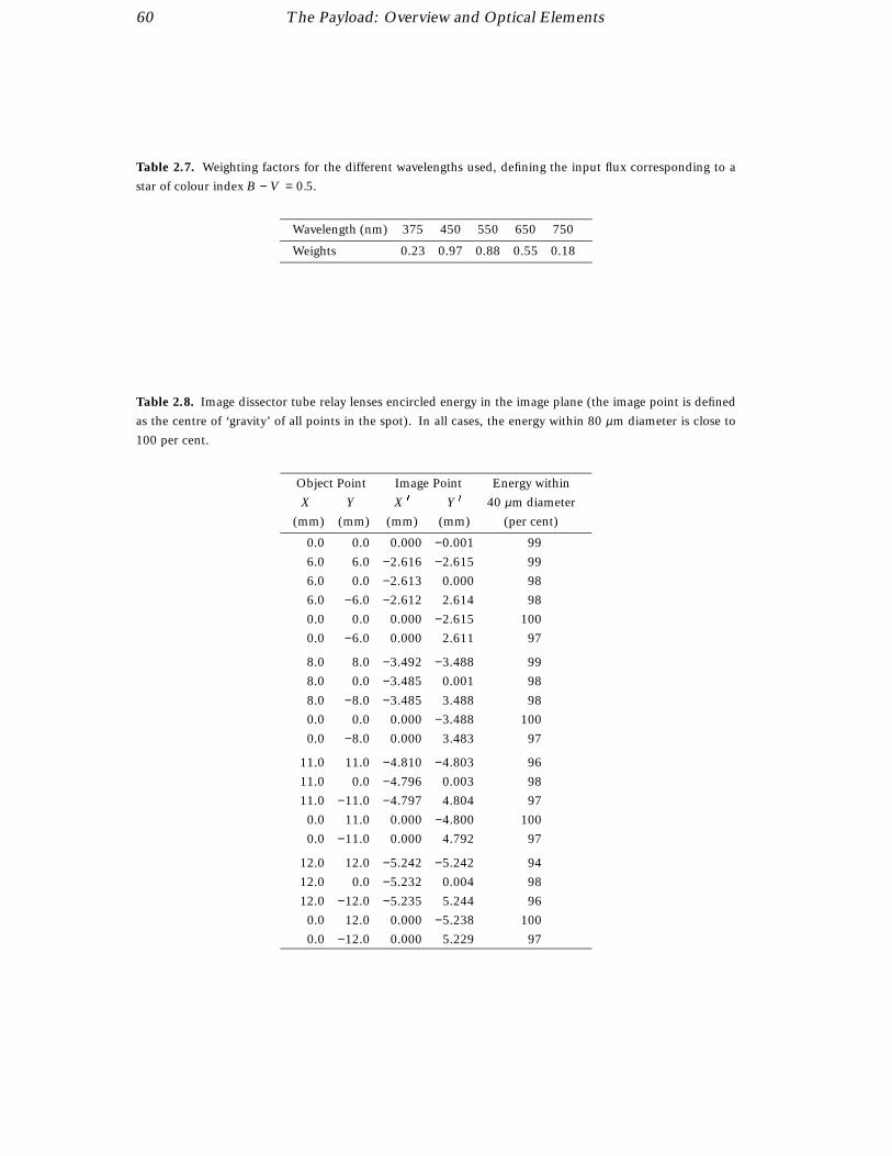
60 The Payload: Overview and Optical Elements
Table 2.7. Weighting factors for the different wavelengths used, defining the input flux corresponding to a
star of colour index B − V = 0.5.
Wavelength (nm) 375 450 550 650 750
Weights 0.23 0.97 0.88 0.55 0.18
Table 2.8. Image dissector tube relay lenses encircled energy in the image plane (the image point is defined
as the centre of ‘gravity’ of all points in the spot). In all cases, the energy within 80 µm diameter is close to
100 per cent.
Object Point Image Point Energy within
X Y X 0 Y 0 40 µm diameter
(mm) (mm) (mm) (mm) (per cent)
0.0 0.0 0.000 −0.001 99
6.0 6.0 −2.616 −2.615 99
6.0 0.0 −2.613 0.000 98
6.0 −6.0 −2.612 2.614 98
0.0 0.0 0.000 −2.615 100
0.0 −6.0 0.000 2.611 97
8.0 8.0 −3.492 −3.488 99
8.0 0.0 −3.485 0.001 98
8.0 −8.0 −3.485 3.488 98
0.0 0.0 0.000 −3.488 100
0.0 −8.0 0.000 3.483 97
11.0 11.0 −4.810 −4.803 96
11.0 0.0 −4.796 0.003 98
11.0 −11.0 −4.797 4.804 97
0.0 11.0 0.000 −4.800 100
0.0 −11.0 0.000 4.792 97
12.0 12.0 −5.242 −5.242 94
12.0 0.0 −5.232 0.004 98
12.0 −12.0 −5.235 5.244 96
0.0 12.0 0.000 −5.238 100
0.0 −12.0 0.000 5.229 97

The Payload: Overview and Optical Elements 61
the main detector assembly cathode. The pattern was defined by an electron beampattern generator and etched in a chronium layer, vacuum deposited onto a bi-convexlens made of Suprasil 1 (fused silica). The material and the dimensions of this lens werethe same as those of the grid substrate. The manufacturing of the star patterns wasdone in parallel with the manufacture of the main and star mapper grids.
The star pattern was mounted inside an invar tube and illuminated by four light-emittingdiodes via a diffusor consisting of two opal-glass plates. The set of four light-emittingdiodes was completely redundant, and the light-emitting diodes of one group wereconnected in such a way that, if one or more light-emitting diodes failed, the other oneswould continue to emit light.
The frame was built up from three separate parts: the lower, middle, and top frames.The lower frame, connected to the focal-plane assembly platform by three flexible andadjustable feet, supported the middle frame and the connector bracket. The lower fold-ing mirror was bonded to the bottom of the lower frame. The middle frame supportedthe star source and the top frame. The top frame was a bracket carrying the top foldingmirror.
The main body and the mounting feet of the internal star pattern assembly were madefrom titanium. This metal was selected since its thermal expansion coefficient wassufficiently low to meet the stability requirement, while entailing a smaller mass penaltythan that resulting from the use of invar. Pure titanium was used for the main bodyas this was more easily machinable. For the mounting feet, however, a titanium alloyTiAl6V4 was selected, as the greater strength allowed thinner blades, resulting in lowerstresses in the focal-plane assembly platform. BK7 glass was used for the mirrors, asthis had the same thermal expansion coefficient as titanium. The only part made outof invar was the star source housing, where a match with the much lower expansion ofsilica glass was required.
The optical block was made of Suprasil 1. It had a chromium layer coating with the starpattern at the front side of the optical block (R = 1400 mm), and an iraline coating atthe rear side. The reflective coating consisted of three layers: chromium for adhesion,aluminium for reflection, and silica for protection.
The installation specification required provisions for shifting the internal star patternassembly by 5 mm in three mutually perpendicular directions. Alignment devicesbetween the flexible feet and the lower frame were used. As clamping by friction onlywas judged to be insufficient, shims were used throughout, even though this complicatedthe alignment. A further alignment possibility was provided by the rotation of the starsource in the internal star pattern assembly frame. This was possible when the internalstar pattern assembly was mounted on the focal-plane assembly platform.
Filters and Dichroics
In the chain of the image dissector tube relay optics, there was a switchable filter set,consisting of a chromaticity filter and a wide-band filter. There was a dichroic filter inthe photomultiplier relay optics chain.
In order to calibrate the chromaticity of the payload in orbit (i.e. the geometrical shift inthe grid coordinate position of stars of different colours—expected to be of the order of
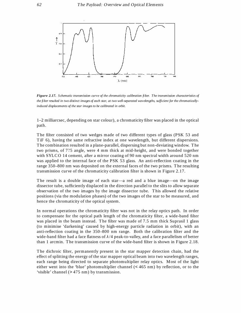
62 The Payload: Overview and Optical Elements
Figure 2.17. Schematic transmission curve of the chromaticity calibration filter. The transmission characteristics of
the filter resulted in two distinct images of each star, at two well-separated wavelengths, sufficient for the chromatically-
induced displacements of the star images to be calibrated in orbit.
1–2 milliarcsec, depending on star colour), a chromaticity filter was placed in the opticalpath.
The filter consisted of two wedges made of two different types of glass (PSK 53 andTiF 6), having the same refractive index at one wavelength, but different dispersions.The combination resulted in a plane-parallel, dispersing but non-deviating window. Thetwo prisms, of 7.5 angle, were 4 mm thick at mid-height, and were bonded togetherwith SYLCO 14 cement, after a mirror coating of 90 nm spectral width around 520 nmwas applied to the internal face of the PSK 53 glass. An anti-reflection coating in therange 350–800 nm was deposited on the external faces of the two prisms. The resultingtransmission curve of the chromaticity calibration filter is shown in Figure 2.17.
The result is a double image of each star—a red and a blue image—on the imagedissector tube, sufficiently displaced in the direction parallel to the slits to allow separateobservation of the two images by the image dissector tube. This allowed the relativepositions (via the modulation phases) of the two images of the star to be measured, andhence the chromaticity of the optical system.
In normal operations the chromaticity filter was not in the relay optics path. In orderto compensate for the optical path length of the chromaticity filter, a wide-band filterwas placed in the beam instead. The filter was made of 7.5 mm thick Suprasil 1 glass(to minimise ‘darkening’ caused by high-energy particle radiation in orbit), with ananti-reflection coating in the 350–800 nm range. Both the calibration filter and thewide-band filter had a face flatness of λ /4 peak-to-valley, and a face parallelism of betterthan 1 arcmin. The transmission curve of the wide-band filter is shown in Figure 2.18.
The dichroic filter, permanently present in the star mapper detection chain, had theeffect of splitting the energy of the star mapper optical beam into two wavelength ranges,each range being directed to separate photomultiplier relay optics. Most of the lighteither went into the ‘blue’ photomultiplier channel (< 465 nm) by reflection, or to the‘visible’ channel (> 475 nm) by transmission.

The Payload: Overview and Optical Elements 63
Figure 2.18. Schematic transmission curve of the wide-band filter.
Figure 2.19. Schematic transmission curves of the VT (a), and BT (b) star mapper channels.
64 The Payload: Overview and Optical Elements
The dichroic filter was a coating deposited on 4-mm thick GG 475 glass. It worked atan incidence angle of 25, where polarisation effects are limited. The 50 per cent pointof this coating was at 465 nm in reflection and at approximately 475 nm in transmission.The second face of the dichroic filter was anti-reflection coated in the range 500–800 nm.
To increase the wavelength separation between the two parts of the spectrum, a bluefilter was also included in the reflected path. This was a coating deposited on a 4-mmthick GG 375 Schott coloured glass window, giving zero transmission between 500–600nm. An anti-reflection coating was applied to the second face in the range 350–500 nm.The dichroic coating and low-pass coating of the dichroic filter and blue filter were madeof ZrO2 and SiO2, respectively, to get very hard layers, fully transparent as far as 300 nm.The flatness of the dichroic and blue filter face was λ /2 peak-to-valley. The resultingoverall spectral transmission curves for the two channels are shown in Figures 2.19(a)and (b), (see also Table 2.3 and Table 2.4, which give the overall payload transmission,including the contribution of the dichroic filter).

3. THE PAYLOAD:DETECTORS, ELECTRONICS, AND STRUCTURE
Two different types of detectors were used for Hipparcos—the image dissectortube detector which sampled the modulated images of the stars as they crossedthe main field of view, and the star mapper (photomultiplier) detectors, whichsampled the entire field of the star mapper. The resulting signals providedthe main sources of data analysed in the ground processing. There weretwo photomultiplier detectors for each star mapper channel, sampling thevisual and blue wavelength ranges respectively. Mechanisms were used withinthe payload to protect the detectors as the fields of view swept across theilluminated Earth or Moon, to switch between the prime and redundant imagedissector tube detectors (and introduce the corresponding internal star patternassembly, used for geometrical calibration, into the field of view), to introducethe chromaticity calibration filter into the image dissector tube relay lens, andto adjust the focus position of the modulating grid. Each of the telescope’sfields of view was protected by ‘external’ and ‘internal’ baffles, attenuatingstraylight from the Sun, Earth and Moon, and minimising the ‘dead time’due to Earth and Moon occultations. Extremely high thermal and temporalstability of the relative positions of the optical components was also required.
3.1. Detectors
The function of both the main detection chain and the star mapper detection chain wasthe detection of the images of stars, which were modulated by the grid and focused bythe relay optics, as described in Chapter 2. The photons detected were converted intoelectrical signals, and the processed signals were output according to a given protocolbetween the detection subsystem and the remote terminal unit.
The detection subsystem was located on the focal-plane assembly platform. It consistedof prime and redundant halves, each containing main and star mapper chains. As thepower and switching of each section was independent, cross-strapping was provided,allowing either or both detection chains to be in operation in both halves of the subsys-tem. The star mapper detection chain was also responsible for the acquisition of dataused for the Tycho experiment.
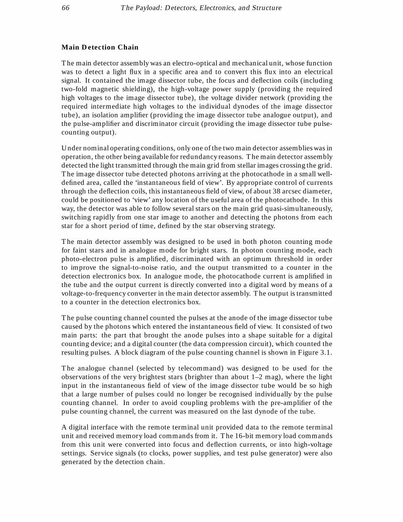
66 The Payload: Detectors, Electronics, and Structure
Main Detection Chain
The main detector assembly was an electro-optical and mechanical unit, whose functionwas to detect a light flux in a specific area and to convert this flux into an electricalsignal. It contained the image dissector tube, the focus and deflection coils (includingtwo-fold magnetic shielding), the high-voltage power supply (providing the requiredhigh voltages to the image dissector tube), the voltage divider network (providing therequired intermediate high voltages to the individual dynodes of the image dissectortube), an isolation amplifier (providing the image dissector tube analogue output), andthe pulse-amplifier and discriminator circuit (providing the image dissector tube pulse-counting output).
Under nominal operating conditions, only one of the two main detector assemblies was inoperation, the other being available for redundancy reasons. The main detector assemblydetected the light transmitted through the main grid from stellar images crossing the grid.The image dissector tube detected photons arriving at the photocathode in a small well-defined area, called the ‘instantaneous field of view’. By appropriate control of currentsthrough the deflection coils, this instantaneous field of view, of about 38 arcsec diameter,could be positioned to ‘view’ any location of the useful area of the photocathode. In thisway, the detector was able to follow several stars on the main grid quasi-simultaneously,switching rapidly from one star image to another and detecting the photons from eachstar for a short period of time, defined by the star observing strategy.
The main detector assembly was designed to be used in both photon counting modefor faint stars and in analogue mode for bright stars. In photon counting mode, eachphoto-electron pulse is amplified, discriminated with an optimum threshold in orderto improve the signal-to-noise ratio, and the output transmitted to a counter in thedetection electronics box. In analogue mode, the photocathode current is amplified inthe tube and the output current is directly converted into a digital word by means of avoltage-to-frequency converter in the main detector assembly. The output is transmittedto a counter in the detection electronics box.
The pulse counting channel counted the pulses at the anode of the image dissector tubecaused by the photons which entered the instantaneous field of view. It consisted of twomain parts: the part that brought the anode pulses into a shape suitable for a digitalcounting device; and a digital counter (the data compression circuit), which counted theresulting pulses. A block diagram of the pulse counting channel is shown in Figure 3.1.
The analogue channel (selected by telecommand) was designed to be used for theobservations of the very brightest stars (brighter than about 1–2 mag), where the lightinput in the instantaneous field of view of the image dissector tube would be so highthat a large number of pulses could no longer be recognised individually by the pulsecounting channel. In order to avoid coupling problems with the pre-amplifier of thepulse counting channel, the current was measured on the last dynode of the tube.
A digital interface with the remote terminal unit provided data to the remote terminalunit and received memory load commands from it. The 16-bit memory load commandsfrom this unit were converted into focus and deflection currents, or into high-voltagesettings. Service signals (to clocks, power supplies, and test pulse generator) were alsogenerated by the detection chain.

The Payload: Detectors, Electronics, and Structure 67
Figure 3.1. Detection subsystem block diagram. The figure shows the schematic arrangement of the image dissector
tube (IDT) and photomultiplier tube (PMT) detection chains, the latter used for the star mapper (Tycho) measurements.
Each star mapper detection chain included a BT and VT channel, and each of the primary and star mapper detection
chains was duplicated for redundancy reasons. (DE: detector electronics; HV: high voltage; ISPA: internal star pattern
assembly; GRM: grid reference mark; P/L: payload; MDE: mechanism drive electronics.)
The main detector assembly received its power from the detection electronics box andincluded its own high-voltage power supply, delivering the image section voltage, fixedat 400 V, and the multiplier section voltage, which could be adjusted by ±20 per centaround its nominal voltage of 1200 V by telecommand through the detection electronicsbox. The exact value of the high voltage was selected so as to have a nominal gain forthe multiplier of 5 × 10⁵.
For correct image dissector tube operation, the focus current had to be adjusted to obtaina good instantaneous field of view profile. The deflection currents of the image dissectortube were updated, during normal operations, at a frequency of 150 Hz (correspondingto ‘slots’ of the star observing strategy, as described in Chapter 8). These deflectioncurrents defined the exact positioning of the instantaneous field of view at any instant.
Image dissector tube: The image dissector tube is a photomultiplier tube with a simpleelectromagnetic deflection system to sample one small part of its photocathode at atime. It had no memory to store an image, and so a strict sampling protocol was notrequired. The principle of operation is illustrated in Figure 3.2.
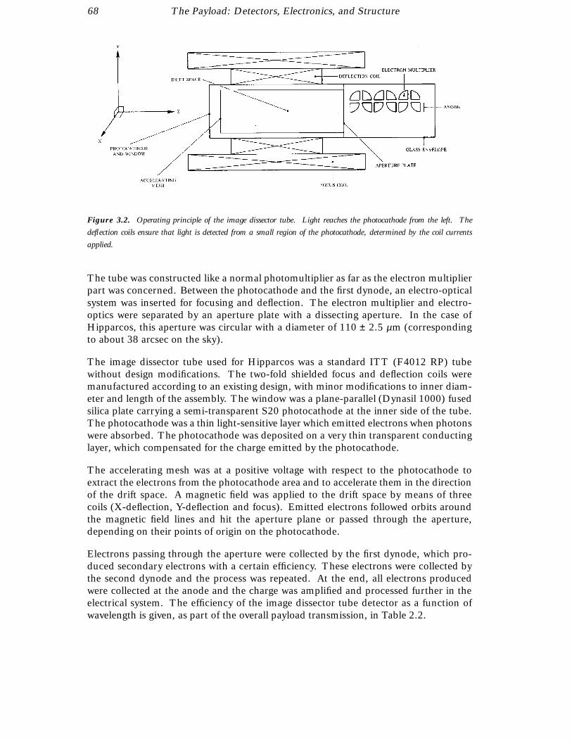
68 The Payload: Detectors, Electronics, and Structure
Figure 3.2. Operating principle of the image dissector tube. Light reaches the photocathode from the left. The
deflection coils ensure that light is detected from a small region of the photocathode, determined by the coil currents
applied.
The tube was constructed like a normal photomultiplier as far as the electron multiplierpart was concerned. Between the photocathode and the first dynode, an electro-opticalsystem was inserted for focusing and deflection. The electron multiplier and electro-optics were separated by an aperture plate with a dissecting aperture. In the case ofHipparcos, this aperture was circular with a diameter of 110 ± 2.5 µm (correspondingto about 38 arcsec on the sky).
The image dissector tube used for Hipparcos was a standard ITT (F4012 RP) tubewithout design modifications. The two-fold shielded focus and deflection coils weremanufactured according to an existing design, with minor modifications to inner diam-eter and length of the assembly. The window was a plane-parallel (Dynasil 1000) fusedsilica plate carrying a semi-transparent S20 photocathode at the inner side of the tube.The photocathode was a thin light-sensitive layer which emitted electrons when photonswere absorbed. The photocathode was deposited on a very thin transparent conductinglayer, which compensated for the charge emitted by the photocathode.
The accelerating mesh was at a positive voltage with respect to the photocathode toextract the electrons from the photocathode area and to accelerate them in the directionof the drift space. A magnetic field was applied to the drift space by means of threecoils (X-deflection, Y-deflection and focus). Emitted electrons followed orbits aroundthe magnetic field lines and hit the aperture plane or passed through the aperture,depending on their points of origin on the photocathode.
Electrons passing through the aperture were collected by the first dynode, which pro-duced secondary electrons with a certain efficiency. These electrons were collected bythe second dynode and the process was repeated. At the end, all electrons producedwere collected at the anode and the charge was amplified and processed further in theelectrical system. The efficiency of the image dissector tube detector as a function ofwavelength is given, as part of the overall payload transmission, in Table 2.2.

The Payload: Detectors, Electronics, and Structure 69
Star Mapper Detection Chain
The star mapper detector assembly was an electro-optical and mechanical unit, whosefunction was to detect a light flux and to convert this flux into an electrical signal. Fourphotomultipliers constituted the whole detection subsystem. In nominal operatingconditions, two of the four star mapper detector assemblies were functioning, while theother two were available for redundancy reasons. In operation, the star mapper detectorassemblies detected the light of stars that passed across the payload’s star mapper grids.In each combination, the two photomultipliers were dedicated to a specific bandpass,with a wavelength centred at about 430 nm for the BT photomultiplier chain, and atabout 530 nm for the VT photomultiplier chain.
Each star mapper detector assembly contained: a photomultiplier tube with shieldsagainst radiation and magnetic fields; high-voltage supply circuits (providing the re-quired high voltage to the photomultiplier); a voltage divider chain (providing the re-quired intermediate high voltages to the individual dynodes of the photomultiplier); apulse-amplifier and discriminator circuit, for electrical processing of the electrical pulsesproduced in the photomultiplier, as a result of detection of photons at the photomulti-plier photocathode; an anode-current monitor circuit, enabling the detection subsystemto generate an emergency command in case of over-exposure of the photomultiplier;and a light-emitting diode, providing optical test input to the photomultiplier.
Each detector assembly also had a mechanical structure, mechanical interfaces betweenthe star mapper detector assembly and the focal-plane assembly, and electrical interfaces.The detection chain also generated service signals (to clocks, power supplies, and testpulse generator).
Photomultiplier tube: The photomultiplier tube used for Hipparcos was a special versionof the Thorn-EMI 9924 B tube. The anode was modified as a result of extensivevibration tests performed by the manufacturer. The window was made as thin aspossible, to reduce Cerenkov radiation caused by absorbed high-energy electrons. Toincrease the sensitivity, the window surface was vapour-blasted.
The photomultiplier had a 30 mm outer tube dimension, with a 23 mm effective cath-ode diameter. The photocathode had a bi-alkali spectral sensitivity. Photo-electrons,produced in the photocathode by incident photons, were amplified by means of 11 suc-cessive box-and-grid dynodes creating, on the photomultiplier anode, a charge pulse of5 − 10 × 106 electrons per detected photon. The efficiency of the photomultiplier tubedetectors as a function of wavelength is given, as part of the overall payload transmission,in Tables 2.3 and 2.4 for the BT and VT channels, respectively.
Detection Electronics Box and Signal Coding
The detection electronics box was an electronic unit whose main functions were: tointerface with the remote terminal unit, inverter, and mechanism drive electronics;to interface with the main detector assembly and star mapper detector assemblies; togenerate power supplies from the AC power; and to generate digital data from the starmapper detector assemblies and main detector assembly output.

70 The Payload: Detectors, Electronics, and Structure
Since the detection electronics box was the only interface for telemetry and telecom-mand, it received on/off commands for proper configuration of the detection subsystem,one 16-bit memory load command for the main detection chain (used for high-voltagesetting, focus current, deflection current, and test generation operation), and one mem-ory load command for the star mapper detection chain and test generation operation(this command was used for high-voltage setting of the BT and VT photomultipliers).
The detection electronics box was the interface for the transmission of scientific data.For each primary detection chain, sampled at 1200 Hz, the scientific data consisted ofone serial digital 8-bit channel corresponding to the compressed data word in pulse-counting mode, and to the analogue-to-digital converter word in analogue mode (thepulse-counting or analogue-to-digital word was sent to the ground according to thestatus of an appropriate bit in the programme star file uplinked to the satellite).
For each star mapper detection chain, the scientific data, sampled at 600 Hz, consistedof one serial digital 16-bit word resulting from the concatenation of the two compressed8-bit data words coming from the two star mapper detector chains—the most significantbits containing the VT data, and the least significant bits containing the BT data.
In photon counting mode, the 8-bit scientific data (for both the primary detection chainand the star mapper detection chain) represented the number of counts correspondingto the sampling period (1200 Hz for the primary detection chain, and 600 Hz for the starmapper chain), applying a ‘semi-logarithmic’ data compression. The maximum countrate that could be coded in pulse counting mode using this compression law was 8159counts per sample, corresponding to a maximum flux for the image dissector tube dataof 9 790 800 counts per second, and 4 895 400 counts per second for the star mapperdata.
In this compression, the 8-bit word was the concatenation of a 5-bit mantissa, M , anda 3-bit exponent, E . The determination of E and M for counts, N , in the range0 ≤ N ≤ 8159 proceeded as follows: first the exponent E was determined such that2E ≤ 1 + N /32 < 2E+1, then M was taken to be the integer part of (N + 32)/2E − 32.Note that counts up to N = 31 were coded without loss of information (E = 0, M = N );this condition applied to all stars fainter than B = 7 − 8 mag.
Assuming image dissector tube count rates of between 2000–4000 counts per secondfor a star of B = 9 mag, depending on star colour, this implied that the analoguemode would be required for the observations of stars brighter than B = 1 − 2 mag.Similar considerations for the star mapper implied that the photon-counting channelwould saturate for stars brighter than about B = 2 − 3 mag. In the case of the starmapper channel, no analogue mode was available, and stars brighter than the saturationthreshold were not expected to yield valid data; this was not considered to be a limitationin the design, since the function of the star mapper was primarily one of real-time attitudedetermination, and the threshold limit for the use of stars as attitude ‘reference’ in thereal-time attitude determination algorithm on-board was fainter than this saturationlimit, actually about B = 4 − 5 mag, due to the range over which the reference starmagnitude could be coded on board.
In practice, the analogue mode for the image dissector tube was not used, the photoncounting mode being satisfactory even for the very brightest stars, while the star mapperobservations were similarly only marginally affected for the brightest stars.

The Payload: Detectors, Electronics, and Structure 71
3.2. Payload Electronics and Mechanisms
The Payload Service Electronics
Mechanism drive electronics: The mechanism drive electronics unit supplied the motorsfor the mechanisms within the payload with suitable pulses. The programming wastransferred via memory load telecommands from the payload remote terminal unit.The mechanism drive electronics unit also provided conditioned status informationabout the mechanisms to the remote terminal unit. Three different interface types wereforeseen to drive the stepper motors, electromagnets, and torque motors.
The mechanism drive electronics unit contained two completely stand-by redundantmechanism control electronics, inclusive of AC/DC converters. Each one was able todrive and monitor all mechanisms. Mechanisms were driven by power pulses deliveredby one of the two mechanism drive electronics sections. Both redundant chains werecontrolled and monitored by the payload remote terminal unit.
Thermal control electronics: The thermal control electronics provided the transforma-tion of resistance values from housekeeping and temperature control thermistors intoanalogue voltages, the acquisition and processing of six memory load commands (con-taining control information for the heater DC-voltage levels and allocation of individualDC-voltage levels from the primary DC bus to payload heaters), and the generation ofsecondary DC-power for internal supply of the thermal control electronics powered bycold-redundant AC-buses.
The thermal control electronics included two redundant sections, with the exception ofthe housekeeping thermistor-conditioning circuits. These circuits were supplied withsecondary power from both sets of thermal control electronics, which were dedicatedto the 24 thermally controlled areas, nominal and redundant heaters, and thermistors.Both chains were controlled by the payload remote terminal unit.
Mechanisms
The following mechanisms were contained within the payload:
(1) the refocusing mechanism, which interfaced with the grid package and associatedmirror necessary to fold the main beam. This mechanism allowed the focusing ofthe grid position with respect to telescope focal surface;
(2) the switching mirror mechanism, which provided the mechanical support to theswitching prism. It allowed the optical beam to be switched to one of the tworedundant main detectors;
(3) the two chromaticity mechanisms, one per image dissector tube channel; each wasequipped with a chromaticity filter and a wide-band filter. Switching from thewide-band filter, which was used in normal operation, to the chromaticity filterallowed in-orbit calibration of the payload chromaticity;
(4) the four shutter mechanisms, which protected the detectors from light overloaddamage.

72 The Payload: Detectors, Electronics, and Structure
Refocusing mechanism: The main function of this mechanism was to allow the grid unitto be refocused during the mission to compensate for factors having long-term effectson the focus position, in particular moisture release and optical surface deformationas a result of radiation damage. The mechanism was split into four separate parts(Figure 3.3): the linear actuator, the linkage, the parallel movement element, and themechanism frame.
The linear actuator comprised a stepper motor, a two-stage gear box, and some monitor-ing devices. The motor was activated via the mechanism drive electronics and drove therefocusing mechanism spindle. This spindle movement was transformed into a parallelmotion of the grid, via the linkage, and the grid unit was moved along the optical beamaxis direction. One cycle activation corresponded to four elementary motor steps, andinduced a spindle displacement of 46 µm, which resulted in a grid movement of 1.2 µm.The total grid movement amplitude was ±1.2 mm with respect to the mid-position.
The position of the spindle of the linear actuator was monitored by a linear poten-tiometer (a device capable of converting the movement along a straight line into aresistance change proportional to the displacement). The resistance range was about1330 − 3670 Ω. The linear potentiometer did not give a very accurate indication of therefocusing mechanism’s position (the accuracy was about 50 µm), and was used onlyas a real-time check that the refocusing mechanism was working nominally. A specialcoupling was used which freed at a force higher than about 20 N if the potentiometerjammed.
Each end of the linear actuator spindle stroke was monitored by two reed-switches, onebeing for redundancy reasons. The linkage was used to convert the displacement of thelinear actuator into a reduced displacement of the grid barrel. The linkage was builtfrom three spring blades. The two main blades were bolted to the mechanism frameand to the grid barrel, respectively, with zero-tolerance fixtures to ensure a high stability.The blades were fixed to each other at their other ends in a connecting block. Fromthis block, a thinner spring blade went to the linear actuator. Parasitic rotation of thelinkage-blades was prevented by two bearing wheels guiding the spindle of the actuator.
This linkage, made of titanium alloy, led to a reduction in the displacement, whichvaried from 1 : 4.08 to 1 : 4.76 in extreme positions. All connections between theparts of the linkage were made by electron beam welding performed in high vacuum.The parallel movement was required to shift the grid along its stroke without parasiticmovements. To that extent, the guidance of the grid barrel was designed with circularsprings to ensure low parasitic rotations around the optical beam axis. The parallelmovement element was divided into the grid support unit and the folding mirror. Thegrid support unit consisted of the mounting for the grid mount and the barrel, whichconnected the membrane supports and the folding mirror system. Openings for theoptical beams toward the main detector assembly and star mapper detector assemblywere made in this barrel.
The attachment for the grid mount was on one side of a circular invar tube with tworigid lugs to connect to one of the springs, and four smaller lugs to fix the grid mountand the baffle unit. All fixtures were with zero tolerance. In this way, a stable basewas created which allowed mounting and dismounting of the grid assembly with agood reproducibility. On the other side of the tube, four rigid lugs were available forconnecting both the half membranes. There were also provisions for mounting thefolding mirror and connection to the linkage.
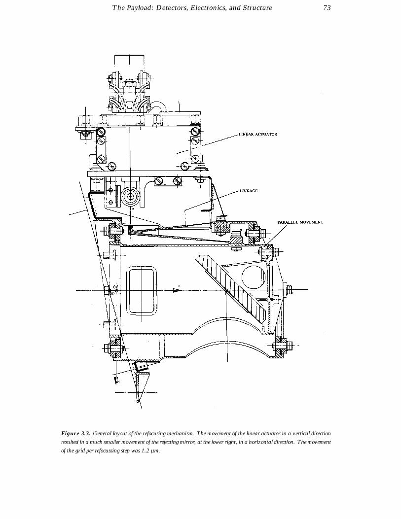
The Payload: Detectors, Electronics, and Structure 73
Figure 3.3. General layout of the refocusing mechanism. The movement of the linear actuator in a vertical direction
resulted in a much smaller movement of the refecting mirror, at the lower right, in a horizontal direction. The movement
of the grid per refocussing step was 1.2 µm.
74 The Payload: Detectors, Electronics, and Structure
The folding mirror was located at the back side of the grid barrel tube. This mirror,having an angle of 45 to the optical beam, deflected the main light beam towards theswitching mirror and the main detector assembly packages. It was made of zerodur andwas bonded in its mount, which was machined with sufficiently tight tolerances for thereto be no need for adjustment. This mounting could be easily removed and re-installedwith sufficient reproducibility, as a result of the zero-tolerance fixings.
The mechanism frame was the main structure to which the different assemblies werefixed: the parallel movement element with grid unit and baffle unit; the linear actuator;and the linkage. This frame was mounted onto the focal-plane assembly platform, usinga device capable of adjusting the complete mechanism in three degrees of freedom toavoid the effects of shift and rotation during launch.
Flip-flop mechanisms: The basic function of each mechanism was to provide a two-position capability for the optical elements (filters and mirror) and the shutters. Theprincipal differences between the types of mechanism were the rotation angle of theelements (45 for shutters and filters, and 90 for the switching mirror), the mass inertiaand geometry of the different elements, and the accuracy and stability requirementsfor the different elements. The following operational modes were provided for eachmechanism:
(i) normal mode, from rest to working position: on telecommand, the torque motordrove the element into its working position while torquing the spiral torsion spring.When the motor was switched off, the position was maintained by the attractive forcebetween a permanent magnet fixed on the housing bracket and a soft iron core fixed toa paddle;
(ii) normal mode, from working to rest position: on telecommand, the torque motordrove the element back to its rest position. When the motor was switched off, the restposition was maintained by the rest torque of the spiral torsion spring;
(iii) back-up: the fail-safe device that provided partial drive redundancy consisted of theabove-mentioned spiral torsion spring and an electromagnet mounted on the housingbracket. If a failure occurred in the nominal driving branch when the mechanism wasin working position, the electromagnet could be activated. It produced a repulsiveforce, which compensated for the attractive force between the permanent magnet andassociated soft iron core, and the spiral torsion spring drove the optical element back toits rest position.
The design was based on identical mechanisms for the main detector assembly and starmapper detector assembly shutters, and for the main detector assembly chromaticityfilter. As far as the switching mirror was concerned, the design was adapted to morestringent accuracy and stability requirements.
Each mechanism consisted of a bearing box with an electrical torque motor as primemover and a rotating shaft which carried the optical element. The mechanism housingwas made of aluminium. The two mechanical end stops were located at the front of themechanism in order to minimise the offset and the corresponding relative distortionsbetween the moving element and its mechanical end stops.
The two end positions were maintained without power on the motor by means of the resttorque of the torsion spring in one position, and, in the other position, by the attractiveforce between a soft iron core fixed on the flip-flop disc and a permanent magnet fixed on

The Payload: Detectors, Electronics, and Structure 75
the mechanism bracket. The two ends of travel were monitored by means of reed end-switches mounted on the housing. The permanent magnet needed for activation of thereed switches was mounted on the flip-flop disc. A damping system was implementedon the flip-flop disc to reduce the rebounds generated in the mechanical end stops.
The mechanism bracket was made of invar to minimise the thermal load interactionbetween the mechanism and the focal-plane assembly. The aluminium housing wasmounted on the bracket by means of three fixing points. A rigid fixing point was locatedat the front of the mechanism, and two flexible fixing points were located at the rear ofthe mechanism. The purpose of the two flexible fixings was to reduce the internal loadsgenerated at this interface by the different expansions of the housing and the bracketunder the given thermal environment.
Adjustment capabilities in the x, y, and z directions were achieved by means of shims.For x-direction adjustment, the shim was located between the flip-flop disc and theoptical hardware; for the y-direction, on the fixing points between housing and fix-ing bracket; and for the z-direction, at the interface between the mechanism and thefocal-plane assembly. The positioning accuracy caused by the x, y, and z adjustmentoperations was given by the shim manufacturing tolerances. Taking into account thesetolerances the positioning accuracies of the flip-flop mechanisms were found to be withinthe specified initial positioning accuracy range. The interface to the electrical harnesswas provided by means of a 15-pin connector fixed to the housing.
3.3. Baffles
The ‘External’ Baffles
Each of the two baffles was divided into three major constituents: the support structure,the baffle tube, and the front aperture assembly.
The support structure was formed by six struts, four attachments to the spacecraft upperplatform, and one adjustment device on each strut. It supported the other componentsand provided for ground alignment of the baffle optical axis. The struts, shown inFigure 3.4, were carbon-fibre reinforced plastic tubes of diameters 30 and 40 mm, witha wall thickness of 1.2 mm. They had titanium fittings at each end. The attachmentswere aluminium milled parts, screwed to the spacecraft upper platform attachmentpoints. On them were fixed the lower adjustment devices. The lower adjustment devicewas formed by half spheres, spherical washers, and nuts. When the nuts were loose, anychange in length induced by turning the nut moved the baffle as a rigid body, withoutintroducing any load because of the isostatic function of a six-bar system. When all nutswere tightened, the struts were fixed in length and angular position.
The main optical requirement for the baffle tube was that all light from outside a givenEarth angle envelope had to be intercepted by a set of fins. In addition, it supported thefront aperture assembly. It was formed by nine segments—two of them were structuralwith 2 mm wall thickness, while the others were mainly optical with 0.52 mm wallthickness.
For stability reasons, there was no mechanical contact between the baffles and the pay-load structure. A ‘labyrinth’ system was provided by means of a carbon-fibre reinforced

76 The Payload: Detectors, Electronics, and Structure
Figure 3.4. The baffle assemblies. Light entered from the right of the figure. Internal ‘labyrinths’ suppressed
the scattered light. The baffle assemblies were supported by struts to the spacecraft platform (below), mechanically
decoupling them from the payload.
plastic ring bonded on the baffle tube and the associated carbon-fibre reinforced plasticring bonded on the payload structure. Four external brackets with aluminium rein-forcements were bonded to the tube, onto which the upper adjustment devices werefixed.
In the front plate assembly, the front plate aperture defined the design beam envelopeand the Earth angle envelope. The fixed screen and the cover in open configurationprevented any direct sunlight from reaching the front plate aperture. Moreover, themulti-layer insulation frame provided a flat mounting area for the shade structure ther-mal insulation. This assembly was formed by the front-plate fixed screen, the cover,hinges, the closing latch, the labyrinth, and the multi-layer insulation frame.
The front-plate fixed screen was a carbon-fibre reinforced plastic sandwich, fixed to thetube, on which the front plate aperture was machined. The hinges and the correspondinglabyrinth and closing latch were fixed on the front plate. The cover was a carbon-fibrereinforced plastic sandwich panel connected to the front plate through the hinges andthe closing latch in closed configuration. The other part of the labyrinth was fixed to it.There were two hinges in each baffle, so the system was redundant in driving torque,locking and monitoring.
During ground operations, and also throughout launch and the early operations, thebaffles were closed by the covers, in order to protect the optics against contamination.When closed, the covers ensured the required telescope venting during launch andduring transport by aircraft, through the labyrinth and venting holes. The covers weredeployed in orbit by means of a pyrotechnic device. When opened, the cover preventedsunlight entrance into the baffle.

The Payload: Detectors, Electronics, and Structure 77
The ‘Internal’ Baffles
A set of internal baffles was connected to the main structure. Their prime functionwas to ensure separation of the half-pupil beams and of telescope inner enclosures, andconsequently help to meet the light-tightness and straylight requirements. These bafflescomprised:
(1) the straylight pupil baffle, consisting of carbon-fibre reinforced plastic plates (thick-ness 0.7 mm) assembled by means of bonded carbon-fibre reinforced plastic cornerprofiles. This baffle was located approximately half way between the beam combinerand the folding mirror, and was connected to the +Z panel of the main structure and tothe enclosure separator baffle by means of anchor floating nuts and screws;
(2) the enclosure separator baffle, consisting of a carbon-fibre reinforced plastic plate(thickness 0.7 mm) and parallel carbon-fibre reinforced plastic stiffeners (thickness1.44 mm) bonded and riveted. This baffle was connected to the stiffener of the lateralpanels by means of the two hard points and ten flexible blocks, cutting the enclosureinto two parts: the beam combiner mirror plus folding mirror part, and the sphericalmirror plus folding mirror part;
(3) the beam separator baffles, consisting of carbon-fibre reinforced plastic plate (thick-ness 0.7 mm) with a beam-shaped hole. These baffles were located around the twobeam entrance apertures and were connected to lateral panels of the main structure bymeans of screws and floating anchor nuts;
(4) the pupil baffle, consisting of a box made from aluminium (type AG5) sheets of0.3 mm thickness and black painted. Surrounding the beam combiner, it was connectedto the barrel by means of blades;
(5) the grid baffle, attached to the grid assembly and described in Chapter 2;
(6) Cerenkov shielding: the external sides of the focal-plane assembly cover wereequipped with shielding to protect the optics against Cerenkov radiation. The shielding,with a total weight of 2 kg, was made of aluminium sheets bonded on the external skinof the focal-plane assembly cover.
Straylight Performances
The main function of the baffles was to attenuate parasitic light coming from the Sun,the Earth and the Moon which would otherwise fall on the detectors. Straylight origi-nating from the Sun was specified to be less than the average sky background (using abackground figure of B = 22.5 mag arcsec−2 and a colour index of B − V = 0.7 mag), andstraylight coming from the Earth or the Moon was specified to be less than ten timesthe background (defined to be the ‘interruption limit’), when these bodies lay outside arectangle of ±24 (in the scan direction) by ±13.5 (in the transverse direction), centredon the optical axis.
The straylight performances of the payload, which also depended on mirror scattering,were measured before launch in a dedicated test using a light source representing the

78 The Payload: Detectors, Electronics, and Structure
Figure 3.5. Straylight test configuration. The rotating system moved the light source to different angles with respect
to the viewing direction, leading to the production of the straylight attenuation curves shown in Figure 3.6. The light
trap was directly in front of the entrance aperture, preventing other light from entering the payload.
Moon directed onto the baffle aperture. The simulator was rotated around the baffleentrance along each of eight directions with respect to the scan axis, to provide rep-resentative positions of the illuminating source (see Figure 3.5). Measurements werecorrected to account for the scattering of incident light due to the presence of air, andstraylight performances for the Earth were computed from the measurements. Attenu-ation of the sun straylight was evaluated by simulating worst cases of sun aspect angleusing the same simulator.
Measurements of the detected straylight intensity at a given position in the field of view,and of the incident light intensity on the baffle aperture, provided the data with whichto determine the ‘attenuation’ in that direction, defined as the ratio of the equivalentstraylight on the baffle aperture to the incident irradiance in the same direction (atten-uations are therefore expressed in sr−1). Figure 3.6 shows an example of an attenuationcurve applicable to the case of the full Earth moving in the scan direction and crossing
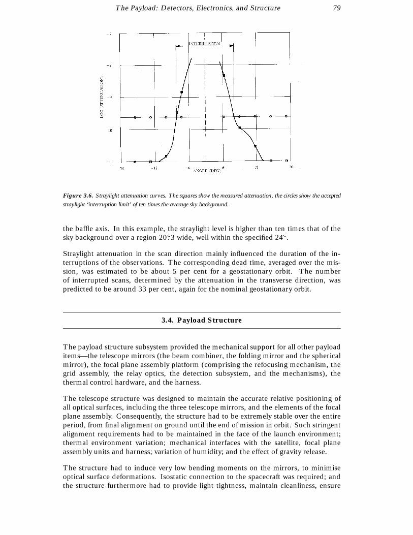
The Payload: Detectors, Electronics, and Structure 79
Figure 3.6. Straylight attenuation curves. The squares show the measured attenuation, the circles show the accepted
straylight ‘interruption limit’ of ten times the average sky background.
the baffle axis. In this example, the straylight level is higher than ten times that of thesky background over a region 20.3 wide, well within the specified 24.
Straylight attenuation in the scan direction mainly influenced the duration of the in-terruptions of the observations. The corresponding dead time, averaged over the mis-sion, was estimated to be about 5 per cent for a geostationary orbit. The numberof interrupted scans, determined by the attenuation in the transverse direction, waspredicted to be around 33 per cent, again for the nominal geostationary orbit.
3.4. Payload Structure
The payload structure subsystem provided the mechanical support for all other payloaditems—the telescope mirrors (the beam combiner, the folding mirror and the sphericalmirror), the focal plane assembly platform (comprising the refocusing mechanism, thegrid assembly, the relay optics, the detection subsystem, and the mechanisms), thethermal control hardware, and the harness.
The telescope structure was designed to maintain the accurate relative positioning ofall optical surfaces, including the three telescope mirrors, and the elements of the focalplane assembly. Consequently, the structure had to be extremely stable over the entireperiod, from final alignment on ground until the end of mission in orbit. Such stringentalignment requirements had to be maintained in the face of the launch environment;thermal environment variation; mechanical interfaces with the satellite, focal planeassembly units and harness; variation of humidity; and the effect of gravity release.
The structure had to induce very low bending moments on the mirrors, to minimiseoptical surface deformations. Isostatic connection to the spacecraft was required; andthe structure furthermore had to provide light tightness, maintain cleanliness, ensure
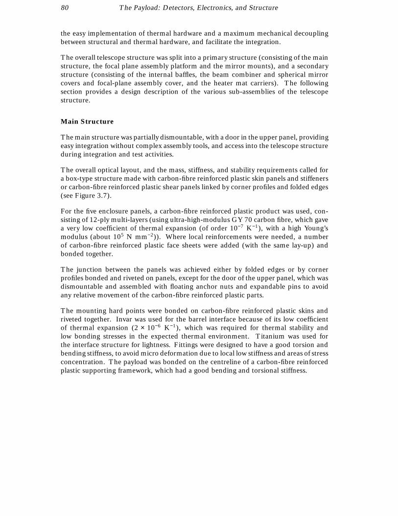
80 The Payload: Detectors, Electronics, and Structure
the easy implementation of thermal hardware and a maximum mechanical decouplingbetween structural and thermal hardware, and facilitate the integration.
The overall telescope structure was split into a primary structure (consisting of the mainstructure, the focal plane assembly platform and the mirror mounts), and a secondarystructure (consisting of the internal baffles, the beam combiner and spherical mirrorcovers and focal-plane assembly cover, and the heater mat carriers). The followingsection provides a design description of the various sub-assemblies of the telescopestructure.
Main Structure
The main structure was partially dismountable, with a door in the upper panel, providingeasy integration without complex assembly tools, and access into the telescope structureduring integration and test activities.
The overall optical layout, and the mass, stiffness, and stability requirements called fora box-type structure made with carbon-fibre reinforced plastic skin panels and stiffenersor carbon-fibre reinforced plastic shear panels linked by corner profiles and folded edges(see Figure 3.7).
For the five enclosure panels, a carbon-fibre reinforced plastic product was used, con-sisting of 12-ply multi-layers (using ultra-high-modulus GY 70 carbon fibre, which gavea very low coefficient of thermal expansion (of order 10−7 K−1), with a high Young’smodulus (about 105 N mm−2)). Where local reinforcements were needed, a numberof carbon-fibre reinforced plastic face sheets were added (with the same lay-up) andbonded together.
The junction between the panels was achieved either by folded edges or by cornerprofiles bonded and riveted on panels, except for the door of the upper panel, which wasdismountable and assembled with floating anchor nuts and expandable pins to avoidany relative movement of the carbon-fibre reinforced plastic parts.
The mounting hard points were bonded on carbon-fibre reinforced plastic skins andriveted together. Invar was used for the barrel interface because of its low coefficientof thermal expansion (2 × 10⁻⁶ K−1), which was required for thermal stability andlow bonding stresses in the expected thermal environment. Titanium was used forthe interface structure for lightness. Fittings were designed to have a good torsion andbending stiffness, to avoid micro deformation due to local low stiffness and areas of stressconcentration. The payload was bonded on the centreline of a carbon-fibre reinforcedplastic supporting framework, which had a good bending and torsional stiffness.

The Payload: Detectors, Electronics, and Structure 81
Figure 3.7. The main structure. The structure was based around carbon-fibre reinforced panels, which were bolted
together, with additional stiffeners in the areas of the aperture openings.
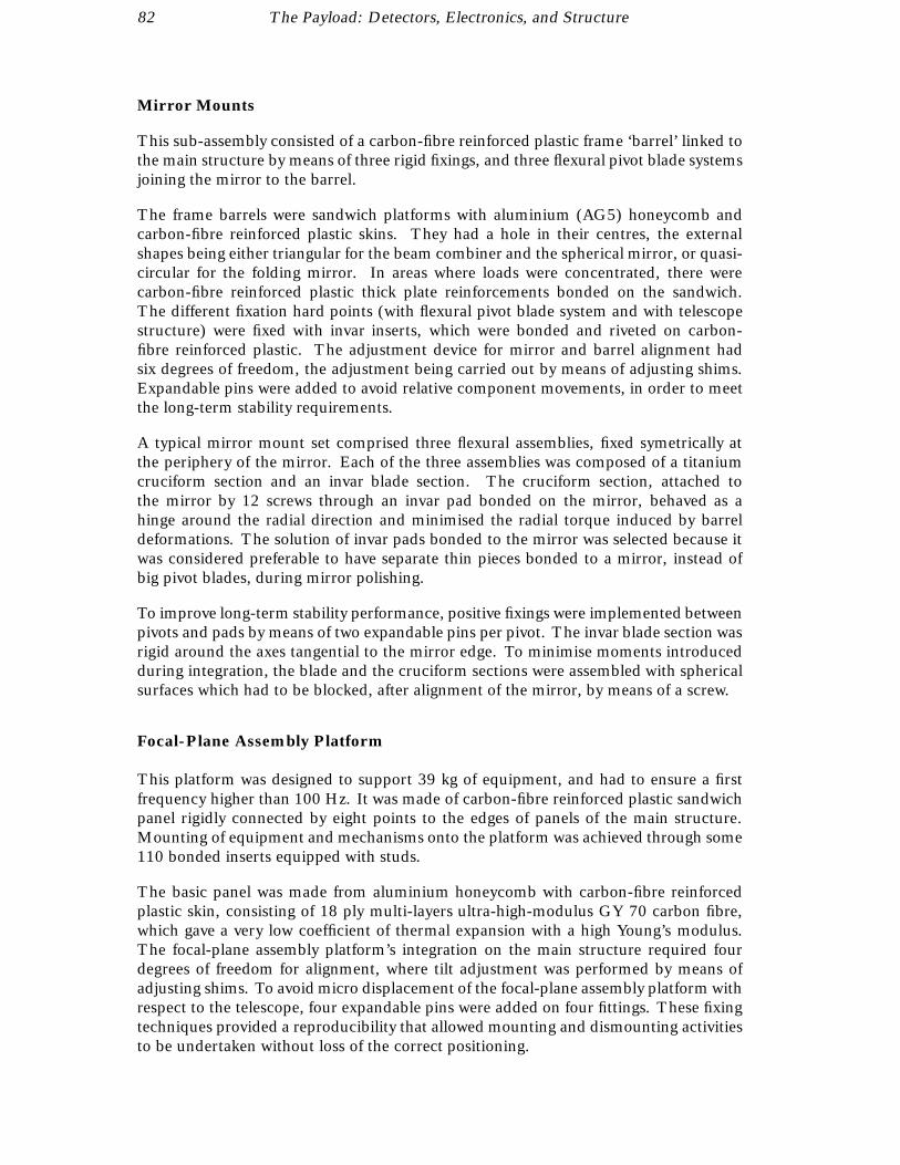
82 The Payload: Detectors, Electronics, and Structure
Mirror Mounts
This sub-assembly consisted of a carbon-fibre reinforced plastic frame ‘barrel’ linked tothe main structure by means of three rigid fixings, and three flexural pivot blade systemsjoining the mirror to the barrel.
The frame barrels were sandwich platforms with aluminium (AG5) honeycomb andcarbon-fibre reinforced plastic skins. They had a hole in their centres, the externalshapes being either triangular for the beam combiner and the spherical mirror, or quasi-circular for the folding mirror. In areas where loads were concentrated, there werecarbon-fibre reinforced plastic thick plate reinforcements bonded on the sandwich.The different fixation hard points (with flexural pivot blade system and with telescopestructure) were fixed with invar inserts, which were bonded and riveted on carbon-fibre reinforced plastic. The adjustment device for mirror and barrel alignment hadsix degrees of freedom, the adjustment being carried out by means of adjusting shims.Expandable pins were added to avoid relative component movements, in order to meetthe long-term stability requirements.
A typical mirror mount set comprised three flexural assemblies, fixed symetrically atthe periphery of the mirror. Each of the three assemblies was composed of a titaniumcruciform section and an invar blade section. The cruciform section, attached tothe mirror by 12 screws through an invar pad bonded on the mirror, behaved as ahinge around the radial direction and minimised the radial torque induced by barreldeformations. The solution of invar pads bonded to the mirror was selected because itwas considered preferable to have separate thin pieces bonded to a mirror, instead ofbig pivot blades, during mirror polishing.
To improve long-term stability performance, positive fixings were implemented betweenpivots and pads by means of two expandable pins per pivot. The invar blade section wasrigid around the axes tangential to the mirror edge. To minimise moments introducedduring integration, the blade and the cruciform sections were assembled with sphericalsurfaces which had to be blocked, after alignment of the mirror, by means of a screw.
Focal-Plane Assembly Platform
This platform was designed to support 39 kg of equipment, and had to ensure a firstfrequency higher than 100 Hz. It was made of carbon-fibre reinforced plastic sandwichpanel rigidly connected by eight points to the edges of panels of the main structure.Mounting of equipment and mechanisms onto the platform was achieved through some110 bonded inserts equipped with studs.
The basic panel was made from aluminium honeycomb with carbon-fibre reinforcedplastic skin, consisting of 18 ply multi-layers ultra-high-modulus GY 70 carbon fibre,which gave a very low coefficient of thermal expansion with a high Young’s modulus.The focal-plane assembly platform’s integration on the main structure required fourdegrees of freedom for alignment, where tilt adjustment was performed by means ofadjusting shims. To avoid micro displacement of the focal-plane assembly platform withrespect to the telescope, four expandable pins were added on four fittings. These fixingtechniques provided a reproducibility that allowed mounting and dismounting activitiesto be undertaken without loss of the correct positioning.

The Payload: Detectors, Electronics, and Structure 83
Cerenkov Shielding
Some of the optical elements, such as the grid and the relay optics, generated photons(Cerenkov effect) and were expected to degrade in transmission (‘darkening’) as a resultof irradiation by high-energy electrons in geostationary orbit. Such optical elements wereprotected by the so-called ‘Cerenkov shielding’. A total of about 12 kg of protectivematerial was placed around the relay optics and on the shade structure, complementinginherent shielding provided by the structure and the equipment surrounding the sensitiveoptical elements.

84

4. LAUNCH AND REVISEDMISSION DEFINITION
Following a perfectly nominal launch of the Hipparcos satellite, by Ariane 4flight V33, from Kourou on 8 August 1989, the satellite did not reach itsintended geostationary orbit due to the failure of the apogee boost motor. Thescientific mission was destined to be conducted from the highly elliptical non-nominal geostationary transfer orbit, with only small orbital changes possible(making use of the remaining hydrazine fuel intended for station keeping).The activities necessary to recover an operational mission, and to carry outthe first phases of the planned mission operations—sun acquisition, real-timeattitude determination, scanning law acquisition, and the start of the payloadcalibrations—are described. At this stage of the mission, the expected lifetimewas highly uncertain, in particular due to the difficulty of predicting the long-term solar array performances in view of the hostile radiation environment inthe geostationary transfer orbit.
4.1. Introduction
Hipparcos was launched as the lower passenger by Ariane 4 flight V33 at 23:25:53 UTCon 8 August 1989 from the launch site at Kourou, French Guyana. Hipparcos and thesecond passenger satellite (TV-SAT2) were injected by the Ariane launch vehicle withoutproblems. The transfer orbit into which the satellite was launched had a period of about10 hours reaching an apogee of 36 000 km (120 km lower than nominal) and a perigeeof 200 km. The nominal injection attitude after launch was α = 200.816, δ = −8.882.
At first acquisition of signal at the Malindi ground station a spin rate of 6.92 rpm wascalculated. The solar aspect angle was 70.5, approximately 5 lower than expected. Theestimated nutation at injection was about 1.0, a value which reduced to 0.5 throughthe first spin-up of the satellite.
On 10 August 1989 at 12:14:00 UTC, the telecommands to initiate the firing of theapogee boost motor were executed from the operations control centre at ESOC. How-ever, no subsequent change in Doppler rate was observed at the supporting groundstations, and it was evident that the apogee boost motor firing had not taken place.The uplinked commands were immediately verified and confirmed to be correct, so the

86 Launch and Revised Mission Definition
failure was almost certainly on-board the satellite. Further unsuccessful firing attemptswere conducted in subsequent orbits.
During the following weeks detailed investigations were performed in order to under-stand what had happened on-board. A reformatting of the telemetry allowed the sam-pling of the currents in the pyrotechnic relay unit at intervals of 5 ms. From the datadownlinked during subsequent apogee boost motor firing attempts, it was possible toreconstruct the behaviour of the firing relays, and the fault was located to be somewherein the pyrotechnics chain. A total of five firing attempts (each consisting of multiplefirings) were made until 25 August 1989 without any success.
The most optimistic outlook for the mission at the time was that, if a ‘hibernation mode’for the first long eclipse season could be devised (involving a reduction in spacecraftheating and deactivation of the payload to save power), there could be a chance ofsatellite survival until the next eclipses starting in mid-1990. By that time, it wasexpected that the on-board power generation would be so degraded that meaningfulscience data could no longer be collected.
Under the latter scenario, the outcome of the mission would have been reduced tosomething between 5 per cent and 10 per cent of the original mission objectives, butthis would have still represented an achievement which would be hard to accomplishwith ground-based astronomical observations. As a minimum, it was hoped that thesemeasurements would still be useful in order to validate the Hipparcos mission concept.In reality, the mission lasted much longer.
4.2. Operations Until Revised Mission Implementation
This section summarises the main events which happened, day by day, through theattempts to fire the apogee boost motor, leading up to the decision to terminate furtherfiring attempts, and concentrate on the implementation of a ‘revised’, or ‘recovery’,mission.
89-08-08: Launch of Ariane flight V33 at 23:25:53 UTC.
89-08-08: At 23:49:36 UTC, the spacecraft was successfully ejected from the launcher.
89-08-09: The first sun sensor data (at 00:21:00 UTC) registered a spin rate of 6.92 rpmand a solar aspect angle of 70.5 (compared with the expected value of 75.15). A seriesof spin-up manoeuvres were carried out to increase the spacecraft spin rate in a numberof steps: firstly to 18.57 rpm, then to 62.33 rpm, followed by a correction manoeuvre toachieve the target spin rate of 60 rpm. At 02:52:00 UTC, the ground system derived anattitude (in right ascension and declination) of α = 204.9, δ = −10.1. The spacecraftwas commanded to slew (in two stages) to the required attitude for the apogee boostmotor firing attempt at apogee number 4 namely α = 213.91, δ = −8.87. Betweenthe two slews, a spin trim manoeuvre to 60.13 rpm was performed. These manoeuvreswere completed by 01:50:00 UTC on 89-08-10.
89-08-10: The first apogee boost motor firing attempt was performed at 12:14:00UTC without success. At 21:45:00 UTC, the spacecraft was slewed to the requiredattitude for a second apogee boost motor firing attempt at apogee number 6, namelyα = 212.29, δ = −8.36.

Launch and Revised Mission Definition 87
89-08-11: Three further apogee boost motor firing attempts were performed between09:10:00 and 09:25:00 UTC, without success. At 10:15:00 UTC, the spacecraft wasslewed to the required attitude for a further apogee boost motor firing attempt at apogeenumber 8, namely α = 211.49, δ = −8.32. In the event, the decision was later takennot to make a further attempt at apogee 8.
89-08-13: A further apogee boost motor firing attempt was performed at apogee num-ber 11 (13:51:00 UTC), without success. During this attempt, a newly designed high-rate telemetry format (Format 4) was selected to allow oversampling of the apogee boostmotor firing ignition current in order to investigate the failure. After the failed attempt,a slew manoeuvre to an ‘average’ attitude of α = 214.40, δ = −9.60 was deemed to besufficient for subsequent firing attempts.
89-08-14: To reduce the strain on various components caused by the prolonged expo-sure to high spin rates, a spin-down of the spacecraft from 60 to 30 rpm was performedin two steps. The final attitude was α = 213.63, δ = −9.50.
89-08-17: Further apogee boost motor firing attempts were performed at apogee num-ber 20 (between 11:55:00 and 12:05:00 UTC), without success. The Format 4 teleme-try was used during the attempts to gather extra information.
89-08-18: It was decided that the next firing attempt should be made after heating theapogee boost motor. This was achieved by slewing the spacecraft such that the motorwas oriented more toward the Sun (the solar aspect angle was reduced from 115 to95). This attitude (α = 277.8, δ = −13.7) was maintained for 6 days prior to the nextapogee boost motor firing attempt.
89-08-19: The fill-in antenna was tested at 11:46 UTC.
89-08-24: The spacecraft was slewed to the apogee boost motor firing attitude (α =217.69, δ = −8.11) changing the solar aspect angle from 103 to 113.
89-08-25: The spin rate of the spacecraft was increased once more from 29.9 to 37.0 rpmat 08:20:00 UTC, prior to the fifth apogee boost motor firing attempt at apogee num-ber 38 at 08:35:00 UTC. The Format 4 telemetry was used during this final attemptin order to gather extra information. One hour after apogee 38, a slew manoeuvre wasperformed to an attitude of α = 235.88, δ = −14.73. The attitude achieved meant thatthe daily drift of the solar aspect angle could be left uncompensated for several daysthereafter.
89-08-26: The decision was taken to abandon any hope of successful boost motor firing,and all effort was dedicated to designing and optimising a ‘recovery’ or ‘revised’ missionoperations scenario.
4.3. Apogee Boost Motor Failure Investigations
An enquiry board was set up in September 1989 to examine all aspects of the apogeeboost motor anomaly, establish the most probable cause or causes, and to make appro-priate recommendations to prevent re-occurrences.
The enquiry board identified and studied the most likely causes of the failure in theapogee boost motor pyrotechnic subsystem, which were: (a) mechanical failure of the

88 Launch and Revised Mission Definition
flexible explosive transfer assembly under vibration load; and (b) failure of the ‘through-bulkhead initiators’ (the pyrotechnic initiators). A characterisation programme to deter-mine the detonator electrical resistance after firing was performed to establish whetherthe failure was of electrical or pyrotechnical nature. The characterisation programmeconsisted of manufacturing, testing and firing 40 detonators. Flexible explosive transferassemblies were vibrated up to the qualification level of 20g at resonance, X-rayed andinspected. They did not show any deterioration. Then they were successfully fired.Study of the electrical resistance after the firing was in accordance with the telemetryvalues proving that the detonators had indeed been fired.
Through-bulkhead initiator tests were thorough and very complex. Drop tests wereperformed which proved that the through-bulkhead initiators were not damaged bysuch shocks. After the two through-bulkhead initiator firings performed in 1989, threemore from the Hipparcos lot were fired and one of them failed. In total six through-bulkhead initiators from the Hipparcos lot were fired and two failed. However due tothe limited number available it was not possible to conclude the direct cause of thesefailures.
The enquiry board, recognising that both redundant through-bulkhead initiators musthave failed, concluded that the boost motor failure was related to the non-functioningof the through-bulkhead initiators.
4.4. Revised Mission Definition
Immediately following the first firing attempts, investigations were initiated to check thepossibility of fulfilling at least part of the mission objectives within the given constraints.The prospects were not very promising, since the available hydrazine fuel (intended forstation acquisition) would allow the orbit to be raised by not more than a few hundredkilometres: therefore, the satellite would be exposed to the effects of the van Allenradiation belts during each orbit. It was expected that the radiation would degrade thesolar arrays to such an extent that the on-board power would not be sufficient for thesatellite to survive the long eclipses (of over 100 minutes duration) starting in March1990 (Figure 4.1).
A concentrated effort of ESOC, ESTEC, and industry experts was devoted to all relevantsystem, spacecraft, payload and associated operational aspects of a revised mission. Atthe same time, the Hipparcos Science Team performed investigations into the scienceimplications of the revised mission. Their simulations indicated clearly that the groundstation coverage should be increased to the maximum extent: only with close to full timestation coverage, would it be possible to establish a full sky network of star measurementswithin a limited mission lifetime using the nominal attitude scanning law and starobservation strategy which were implemented in the on-board software.
The objective of the mission redesign efforts was to recover as much as possible ofthe original Hipparcos mission objectives. The operational problems to be addressedwere essentially those of a new mission with a few significant differences: (i) therewas little flexibility left on the satellite system design: only limited on-board softwaremodifications were possible within the practical constraints available; (ii) only narrowmargins were available on the orbit selection because of fuel constraints; and finally, (iii)any day spent on the definition of the mission represented a full day of lost mission time.
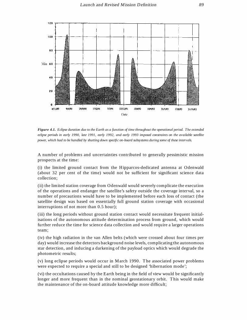
Launch and Revised Mission Definition 89
Figure 4.1. Eclipse duration due to the Earth as a function of time throughout the operational period. The extended
eclipse periods in early 1990, late 1991, early 1992, and early 1993 imposed constraints on the available satellite
power, which had to be handled by shutting down specific on-board subsystems during some of these intervals.
A number of problems and uncertainties contributed to generally pessimistic missionprospects at the time:
(i) the limited ground contact from the Hipparcos-dedicated antenna at Odenwald(about 32 per cent of the time) would not be sufficient for significant science datacollection;
(ii) the limited station coverage from Odenwald would severely complicate the executionof the operations and endanger the satellite’s safety outside the coverage interval, so anumber of precautions would have to be implemented before each loss of contact (thesatellite design was based on essentially full ground station coverage with occasionalinterruptions of not more than 0.5 hour);
(iii) the long periods without ground station contact would necessitate frequent initial-isations of the autonomous attitude determination process from ground, which wouldfurther reduce the time for science data collection and would require a larger operationsteam;
(iv) the high radiation in the van Allen belts (which were crossed about four times perday) would increase the detectors background noise levels, complicating the autonomousstar detection, and inducing a darkening of the payload optics which would degrade thephotometric results;
(v) long eclipse periods would occur in March 1990. The associated power problemswere expected to require a special and still to be designed ‘hibernation mode’;
(vi) the occultations caused by the Earth being in the field of view would be significantlylonger and more frequent than in the nominal geostationary orbit. This would makethe maintenance of the on-board attitude knowledge more difficult;
90 Launch and Revised Mission Definition
(vii) the Earth albedo effect would provide a thermal input to the payload in the perigeeregion. This could lead, for example, to significant distortions in the fine modulatinggrid of the payload;
(viii) the high perturbing torques in the perigee region would introduce difficulties forthe attitude control. In any case, it would require the inhibition of the satellite emergencymode triggering on the basis of too high thruster actuation demands.
The following list summarises a few of the most significant mission design aspectsstudied at ESOC during the first few weeks after the failure:
(a) evolution of the geostationary transfer orbit and the satellite attitude orientation forsubsequent apogee boost motor firing attempts and solar aspect angle violations;
(b) redesign of the attitude acquisition sequence (directly from the attitude required forapogee boost motor firing to the sun-pointing attitude);
(c) station coverage predictions of the transfer orbit and potential recovery orbits;
(d) eclipse and occultation predictions of the potential recovery orbits;
(e) potential implications of modifying the nominal scanning law and the star observationstrategy;
(f) fuel budget requirements and predictions under the revised orbit and attitude acqui-sition strategies;
(g) strategies for covering the long periods without ground contact, and the implemen-tation of a sparse programme star file as a means of survival of the on-board attitudeknowledge;
(h) new attitude control parameters designed to cope with the high disturbance torquesin the perigee region.
At the same time, ESTEC and contractor experts were evaluating the radiation effects ofthe van Allen belts on solar array and payload degradation. Thermal and power aspectsof the new attitude acquisition strategy, and associated risks, were also being assessedand evaluated.
Immediately following the first apogee boost motor firing failure on 10 August 1989, ateam of mission analysis and flight dynamics experts started investigations concerningpotential recovery orbits. After it was found that 12-hour or 8-hour orbital periods werenot practically feasible, the orbit selection concentrated on achieving a perigee altitudeabove 400 km taking account of fuel constraints and to reduce the influences of air dragand atomic oxygen with, at the same time, a synchronisation between the scanning lawperiod (2 hrs 8 mins) and the orbital period: this was considered to be beneficial as itwould limit the effects of albedo heating on the payload and minimise the duration ofpayload occultations in the perigee region by a proper tuning of the initial scan angle.
Fortunately, a 10 hour 39 min orbital period fulfilled both criteria, and was within reachof the available fuel resources. The necessary orbit adjustments were performed afterimplementation, validation and simulation of the required new software and controlprocedures, in a series of five manoeuvres during the period 7–18 September 1989 (seeFigure 4.2).

Launch and Revised Mission Definition 91
Occultations, with
coverageproviding 80-90%
Extended3 ground stations
frequent attitude adjustmentsat perigee
detector background and damaged
optical throughput
eclipses
solar arrays and
Radiation belts enhanced
Perigee distance 500 km
10.8 hr orbit
Apogee distance 36000 km
Attitude degradation aftersignal re-aquisition and
perigee transit
Figure 4.2. The ‘revised’ or ‘recovery’ orbit from which the Hipparcos observations were conducted. The features
of the orbit which provided considerable operational complications are indicated. The satellite could be observed for
about 80–90 per cent of the time with three ground stations, compared with 100 per cent of the time in the intended
geostationary orbit.
4.5. Ground Station Utilisation
During the launch and early orbit phase, the ESTRACK launch and early orbit phaseS-band network was used for telemetry acquisition, telecommanding and tone-ranging.The launch and early orbit phase ground stations were operated under control fromthe operations control centre. The launch and early orbit phase network consisted ofthe following ground stations: Kourou-100 (French Guyana), Malindi (Kenya), andPerth (Australia). Back-up support was given by the Odenwald ground station and theVillafranca transportable station when the satellite was visible.
For routine operations, the Hipparcos ground station network eventually consisted offive S-band stations: three stations belonging to the ESA ground station network (ES-TRACK) and located in Germany (Odenwald), Australia (Perth) and French Guyana(Kourou). A fourth ground station, located in the U.S.A. (Goldstone) and belongingto the NASA deep space network, was added in the first half of 1990. The Kouroustation, whose coverage was largely superseded by the Goldstone station, was subse-quently taken out of the network in mid-July 1990. However, during the last months ofthe satellite’s lifetime, Kourou was re-activated. All ground stations provided full track-ing measurement, satellite data (telemetry) acquisition operations, and commanding for
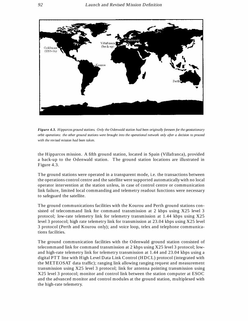
92 Launch and Revised Mission Definition
Figure 4.3. Hipparcos ground stations. Only the Odenwald station had been originally foreseen for the geostationary
orbit operations: the other ground stations were brought into the operational network only after a decision to proceed
with the revised mission had been taken.
the Hipparcos mission. A fifth ground station, located in Spain (Villafranca), provideda back-up to the Odenwald station. The ground station locations are illustrated inFigure 4.3.
The ground stations were operated in a transparent mode, i.e. the transactions betweenthe operations control centre and the satellite were supported automatically with no localoperator intervention at the station unless, in case of control centre or communicationlink failure, limited local commanding and telemetry readout functions were necessaryto safeguard the satellite.
The ground communications facilities with the Kourou and Perth ground stations con-sisted of telecommand link for command transmission at 2 kbps using X25 level 3protocol; low-rate telemetry link for telemetry transmission at 1.44 kbps using X25level 3 protocol; high rate telemetry link for transmission at 23.04 kbps using X25 level3 protocol (Perth and Kourou only); and voice loop, telex and telephone communica-tions facilities.
The ground communication facilities with the Odenwald ground station consisted oftelecommand link for command transmission at 2 kbps using X25 level 3 protocol; low-and high-rate telemetry link for telemetry transmission at 1.44 and 23.04 kbps using adigital PTT line with High Level Data Link Control (HDCL) protocol (integrated withthe METEOSAT data traffic); ranging link allowing ranging request and measurementtransmission using X25 level 3 protocol; link for antenna pointing transmission usingX25 level 3 protocol; monitor and control link between the station computer at ESOCand the advanced monitor and control modules at the ground station, multiplexed withthe high-rate telemetry.
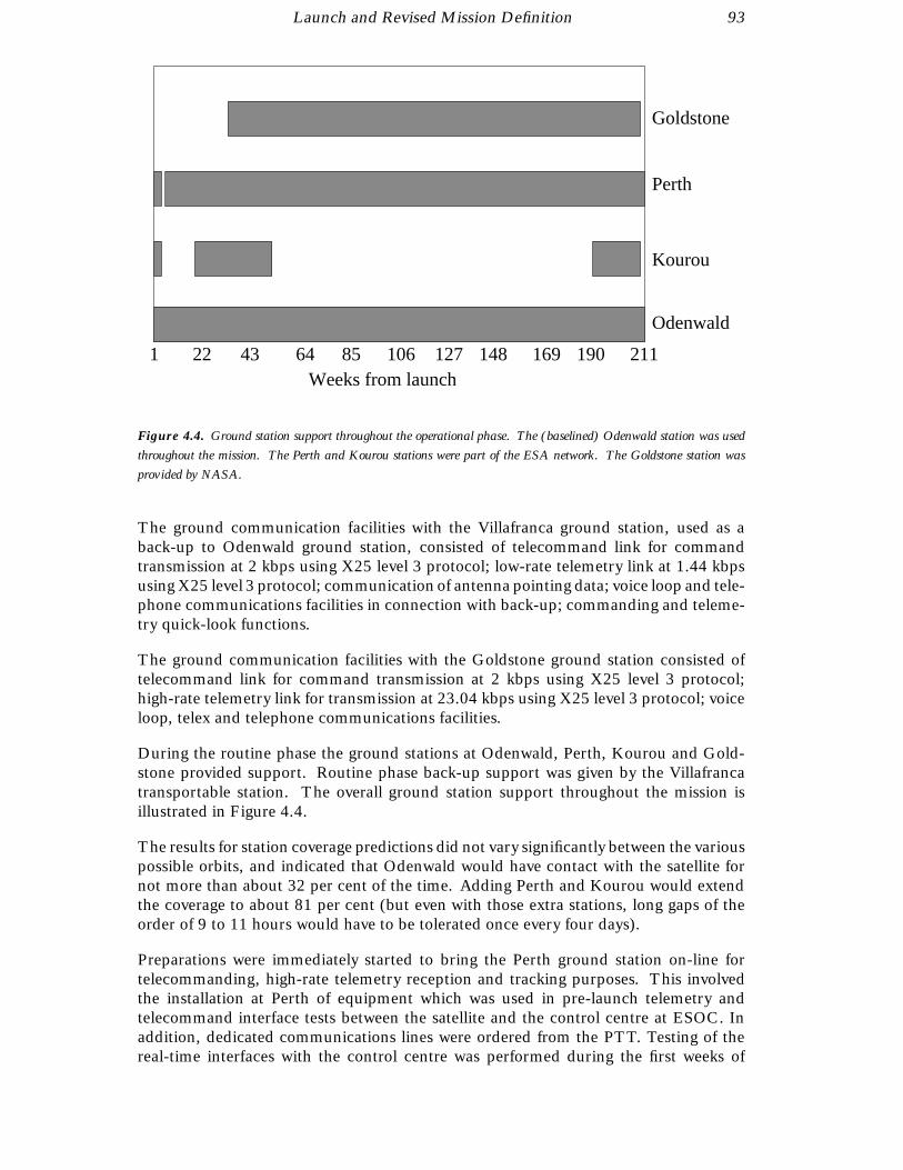
Launch and Revised Mission Definition 93
Perth
Odenwald
Kourou
Goldstone
Weeks from launch22 43 64 85 106 127 148 169 1901 211
Figure 4.4. Ground station support throughout the operational phase. The (baselined) Odenwald station was used
throughout the mission. The Perth and Kourou stations were part of the ESA network. The Goldstone station was
provided by NASA.
The ground communication facilities with the Villafranca ground station, used as aback-up to Odenwald ground station, consisted of telecommand link for commandtransmission at 2 kbps using X25 level 3 protocol; low-rate telemetry link at 1.44 kbpsusing X25 level 3 protocol; communication of antenna pointing data; voice loop and tele-phone communications facilities in connection with back-up; commanding and teleme-try quick-look functions.
The ground communication facilities with the Goldstone ground station consisted oftelecommand link for command transmission at 2 kbps using X25 level 3 protocol;high-rate telemetry link for transmission at 23.04 kbps using X25 level 3 protocol; voiceloop, telex and telephone communications facilities.
During the routine phase the ground stations at Odenwald, Perth, Kourou and Gold-stone provided support. Routine phase back-up support was given by the Villafrancatransportable station. The overall ground station support throughout the mission isillustrated in Figure 4.4.
The results for station coverage predictions did not vary significantly between the variouspossible orbits, and indicated that Odenwald would have contact with the satellite fornot more than about 32 per cent of the time. Adding Perth and Kourou would extendthe coverage to about 81 per cent (but even with those extra stations, long gaps of theorder of 9 to 11 hours would have to be tolerated once every four days).
Preparations were immediately started to bring the Perth ground station on-line fortelecommanding, high-rate telemetry reception and tracking purposes. This involvedthe installation at Perth of equipment which was used in pre-launch telemetry andtelecommand interface tests between the satellite and the control centre at ESOC. Inaddition, dedicated communications lines were ordered from the PTT. Testing of thereal-time interfaces with the control centre was performed during the first weeks of
94 Launch and Revised Mission Definition
September 1989. By mid-September, Perth was declared to be fully operational, andcontact with the satellite was then available for about 62 per cent of the time.
Subsequently, similar activities were initiated to bring the Kourou Galliot station on-linefor high-rate telemetry and telecommanding functions, the necessary equipment beingprocured or retrieved from other stations. By early November 1989, this station was alsoable to support all required real-time interactions between the satellite and ESOC. Thesupport from Kourou was essential for obtaining a better understanding of the attitudecontrol performance in the perigee region, as it was the only feasible station to provideoccasional coverage in this region, being located near the equator.
Coverage was subsequently further improved by the assistance of NASA, through theiroffer of the Goldstone Deep Space Station (DSS-16) station in the Californian Mojavedesert for the Hipparcos revised mission. In order to ensure that the data interfaceswith ESOC were the same as for the other stations used in the Hipparcos revised mis-sion, it was necessary to install ESA telemetry, telecommand, and data communicationsequipment on-site at Goldstone. The equipment was procured and integrated at ESOCbefore it was transported to Goldstone at the beginning of 1990. The real-time com-munications interface with ESOC was quite complex, and it took considerable effort onboth ESA and NASA sides to get this station in a satisfactory operational condition (inthe period from mid-March to the beginning of May 1990).
Since the Kourou station coverage intervals were almost completely contained withinthose of Goldstone, the Kourou support was not considered to be cost-effective withinthe existing network of stations. Kourou support to the Hipparcos revised mission wastherefore terminated by mid-1990. During the last few months of the satellite’s lifetime,the station was re-implemented into the ground stations network because of reducedGoldstone support due to competing demands.
Contact with the satellite became possible for about 90 per cent of the time and theduration of loss-of-contact periods was limited to not more than 1.5 hours: this easedthe operations somewhat since the on-board attitude knowledge was less likely to belost during the non-coverage periods. However, the complexity of the revised missionoperations remained significantly above what would have been considered acceptableduring the design phase. The coverage percentages are shown in Figure 4.5.
4.6. Mission Planning
The Hipparcos Mission Plan was regularly generated for a seven-day period startingalways five days in advance, using a specifically designed software tool on the off-linecomputer system at ESOC. It included all orbit and attitude related events as well asground-triggered ones (e.g. ground station non-availability).
The generation of a mission plan was based on both manual inputs e.g. payload cali-brations, ground station availability times, and automatically computed events. Valid-ity checks were performed according to pre-defined rules and any inconsistency wasbrought to the attention of the operator who could then modify the inputs. The outputof the mission plan tool was a time-ordered sequence of events (ground station visibil-ity, payload calibrations, antenna switching, occultations, eclipses and apogee/perigeecontrol parameters changing) which could trigger possible satellite or ground segment
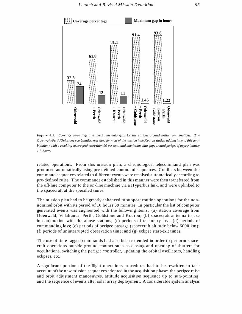
Launch and Revised Mission Definition 95
Odenw
ald+ P
erth
Odenw
ald+ P
erth+K
ourou+G
oldstone
61.8
12
24
11
1.45 1.22
32.3
81.1
91.4 93.8
Odenw
ald
Odenw
ald
+ Kourou
+ Goldstone
+ Perth
Odenw
ald+ P
erth
Maximum gap in hours
Coverage percentage
Figure 4.5. Coverage percentage and maximum data gaps for the various ground station combinations. The
Odenwald/Perth/Goldstone combination was used for most of the mission (the Kourou station adding little to this com-
bination) with a resulting coverage of more than 90 per cent, and maximum data gaps around perigee of approximately
1.5 hours.
related operations. From this mission plan, a chronological telecommand plan wasproduced automatically using pre-defined command sequences. Conflicts between thecommand sequences related to different events were resolved automatically according topre-defined rules. The commands established in this manner were then transferred fromthe off-line computer to the on-line machine via a Hyperbus link, and were uplinked tothe spacecraft at the specified times.
The mission plan had to be greatly enhanced to support routine operations for the non-nominal orbit with its period of 10 hours 39 minutes. In particular the list of computergenerated events was augmented with the following items: (a) station coverage fromOdenwald, Villafranca, Perth, Goldstone and Kourou; (b) spacecraft antenna to usein conjunction with the above stations; (c) periods of telemetry loss; (d) periods ofcommanding loss; (e) periods of perigee passage (spacecraft altitude below 6000 km);(f) periods of uninterrupted observation time; and (g) eclipse start/exit times.
The use of time-tagged commands had also been extended in order to perform space-craft operations outside ground contact such as closing and opening of shutters foroccultations, switching the perigee controller, updating the orbital oscillators, handlingeclipses, etc.
A significant portion of the flight operations procedures had to be rewritten to takeaccount of the new mission sequences adopted in the acquisition phase: the perigee raiseand orbit adjustment manoeuvres, attitude acquisition sequence up to sun-pointing,and the sequence of events after solar array deployment. A considerable system analysis
96 Launch and Revised Mission Definition
effort involving individuals from ESOC, ESTEC and external experts was needed toensure that the operations were compatible with the satellite design characteristics. Alloperations had to be arranged into sequences which would fit within the interval ofground station coverage (about 8 − 10 hours for Odenwald). Furthermore, it wasessential that, before contact was lost, the satellite was brought into a safe configurationwhich would allow it to survive the long periods without ground contact.
The operations were by necessity extremely risky since the time pressure did not allowfull assessment of all possible eventualities, nor to prepare for potential contingencies.Validation (as far as feasible) of the new procedures was carried out using the ESOCsoftware simulator, often not more than one day prior to their execution in actualoperations.
The failure or back-up modes for the real-time attitude control had to be revised asthe nominal criterion (using the interval between thruster pulses) was no longer validbecause of the high torques in the perigee region. The redesign of the operations forthe revised mission had to take account of the following new constraints: (i) stationcontact was frequently interrupted: this resulted in the need for procedures to ensurethe spacecraft and payload safety during periods without ground contact; (ii) eclipseperiods were of a much longer duration (maximum of 104 minutes) and the morefrequent occurrence demanded a careful monitoring of the on-board power generationand associated battery management functions; (iii) payload occultation periods occurredwith higher frequency (up to 28 per day) and longer duration: this led to a higher riskin losing the on-board attitude knowledge and required more frequent support fromground. Also, more telecommand uplinks had to be prepared (to open and close thepayload shutters); and (iv) crossing of the van Allen radiation belts often led to difficultiesin attitude knowledge (re)-acquisitions and the data collected over these periods werenot of the required quality to be forwarded to the scientific data analysis teams.
The operational support of the on-board attitude determination process was one of themost demanding tasks. Because of the long ground station loss-of-contact periods anddue to the noise in the star mapper signals induced by the radiation belts, frequentloss of attitude knowledge had to be anticipated: in that case, ground control hadto re-establish the on-board attitude knowledge using downlinked star mapper signalsand a star pattern recognition technique. A new team for supporting these unforeseenactivities around the clock was recruited and trained within a very short time. In theearly days of the revised mission, this specific support was required after almost everyperigee passage. New on-ground support software was implemented to prepare themanoeuvres required for achieving the recovery orbit, i.e. the perigee raise and theperiod adjustment manoeuvres, and the new attitude acquisition sequence.
The mission planning software had to be redesigned and extended to include many moreunforeseen events related to the specific orbit characteristics and van Allen belts passage.These included (a) ground station coverage start and end times, (b) switching of theon-board torque model in the perigee region, (c) implementation of a special attitudecontrol strategy in perigee region, (d) switching of shutters and antennae outside groundstation contact periods, (e) calculation of revised eclipse durations, and (f) predictionof payload occultation intervals.
Updates to the on-board software were necessary in order to extend both the time-taggedtelecommand and the programme star file buffers (see Section 8.4), which had to besized to accommodate the many commands needed during the long periods without

Launch and Revised Mission Definition 97
ground contact. More sophisticated ground software was installed to allow real-timemonitoring of the on-board attitude convergence using payload measurements.
The data interface definition between ESOC and the scientific data reduction consortiawas also significantly affected by the revised mission: the necessary modifications to theinterface were implemented and validated (using actual telemetry tapes) in the courseof 1990.
4.7. Orbit Manoeuvres and Commissioning Activities
The initial payload switch-on and initialisation of the payload operations were conductedin the last week of September and the beginning of October 1989. The initialisationwas severely hampered by extremely high solar activity with an exceptional solar flareoccurring just at the time when the first star mapper samples were received: it wasenough to ensure that no star transits could be observed.
After scanning law acquisition and successful calibration of the payload star mapper andmain (image dissector tube) detectors, the actual scientific data collection started on 26November 1989. The initial data recovery rate was about 50 per cent: this meant that‘good’ data which could be used for the scientific data reduction were collected overabout 48 hours during every four-day period, after which the ground station coveragepattern was repeated.
The computer system installed for the ground segment support was severely overloadedbecause of the many additional software tasks required, and the machine was replacedby a more powerful VAX computer in the beginning of 1990. This exchange resulted inextremely stable computer support conditions thereafter.
By summer 1990, the science data recovery rate had increased to about 65 per centwith the addition of the Goldstone station and because of further improvements andtuning of the operations support, mainly in the area of initialisation of on-board attitudedetermination and payload control.
Perigee Raising Manoeuvres
This section summarises the main events which happened, day by day, during therecovery mission implementation.
89-09-06: At 12:00:00 UTC, the spacecraft was de-spun from 37.03 to 30.05 rpm(12:00:00 UTC). The solar aspect angle at that time was 72.46, with nutation less than0.05.
89-09-07: The decision having been taken to use almost all of the remaining hydrazinefuel to raise the perigee height, the first manoeuvre took place at 10:30:00 UTC andraised the perigee by 98 km.
89-09-08: A second perigee raising manoeuvre at 07:25:00 UTC raised the perigee by102 km.

98 Launch and Revised Mission Definition
89-09-11: A third perigee raising manoeuvre at 09:14:00 UTC raised the perigee to thefinal target of 532 km.
Hydrazine Sun Acquisition
89-09-11: On the same day as the final perigee raising manoeuvre, the spacecraft wasde-spun in two further manoeuvres. The first spin-down manoeuvre at 10:45:00 UTCreduced the spin rate from 29.49 to 19.90 rpm. The second spin-down manoeuvre at11:45:00 UTC reduced the spin rate from 19.90 to 10 rpm.
89-09-12: Between 04:30:00 and 04:50:00 UTC, the two-stage slew to reorient thespin-axis to point at the Sun was performed. The first stage ‘spin axis orientation’was performed using the on-board Earth/Sun sensor. The second stage ‘hydrazine sunacquisition’ used the sun acquisition sensor output. The solar panels were deployed at05:02:00 UTC resulting in a decrease in the spin rate from 10.0 to 8.9 rpm. The fill-inantenna was then deployed.
89-09-13: The Perth ground station became operational for high-rate data telemetry.
Orbit Period Adjustment
89-09-14: The orbit was adjusted using the remaining hydrazine fuel to give a periodwhich was commensurate with station coverage. In order to keep the spin rate withinoperational limits during the orbit period adjustment manoeuvres, the spacecraft wasspun-up to 11.6 rpm. The first orbit adjustment manoeuvre started at 14:22:30.
89-09-15: The Perth ground station became operational for commanding.
89-09-16: The central on-board software was loaded and activated.
89-09-18: The central on-board software and payload were activated. The second orbitadjustment manoeuvre started at 13:52:00.
Hydrazine Fuel Dump
To prevent fuel sloshing during payload operations, the remaining hydrazine fuel sup-ply was emptied out of the tanks while the spacecraft retained some degree of spinstabilisation. Following this, the helium pressurant was also drained.
89-09-19: Between 04:50:00 and 10:20:00 UTC, the first part of the remaining hy-drazine was drained through cycles of firings of the hot gas thrusters. Nutation dampingwas performed using the cold gas thrusters.
89-09-20: Between 03:50:00 and 07:05:00 UTC, the second part of the remaininghydrazine was drained. Between 07:10:00 and 08:10:00 UTC, the helium was dumped.During the course of the fuel dumping exercise, the spin rate increased from 11.0 to12.0 rpm.
Launch and Revised Mission Definition 99
Cold Gas Despin and Sun Acquisition
89-09-21: Between 09:30:00 and 14:14:00 UTC, the spacecraft was de-spun from 11.9to 5.6 rpm using the cold gas thrusters.
89-09-22: Between 06:02:00 and 12:55:00 UTC, the spacecraft was de-spun in fivemanoeuvres from 5.6 to 0.2 rpm. After the third manouevre at 0.73 rpm, nutationdamping was performed. At 13:03:00 UTC, the on-board sun acquisition software wastriggered causing a final de-spin to the nominal spin rate of 168 arcsec s−1. At 13:25:00UTC, the on-board sun acquisition software was triggered orienting the spin axis of thespacecraft towards the direction of the Sun.
Real-Time Attitude Determination Initialisation
Real-time attitude determination activities proceeded as follows:
89-09-23: By collecting data at the nominal spin rate and at zero spin rate, a calibrationof the biases of the sun acquisition sensor, and of the drifts on gyros 1 and 2, wasperformed. The sun acquisition sensor biases were uplinked to the spacecraft to optimisethe sun-pointing accuracy, and the gyro drift estimates were used as first estimates forthe ground real-time attitude determination software. Payload baffles were ejected on26 September 1989, and star mapper transits were immediately detected.
89-09-27: The first attempt was made to run the ground real-time attitude determina-tion software. Star pattern matching was achieved after tuning of the ground software.The basic angle separating the two fields of view was also calibrated.
89-09-30: The second attempt to run ground real-time attitude determination wasaborted due to a solar flare giving extremely high background counts in the star mapperdetectors. This phenomenon lasted several days.
89-10-04: The third attempt to run ground real-time attitude determination resultedin convergence of the ground software and an accurate attitude determination. Severalattempts were made to command real-time attitude determination initialisation on-board. Convergence of on-board real-time attitude determination was not howeverassured, lasting for less than a minute after each attempt. The problem was subsequentlytraced to a problem in the ground software which was using the incorrect coordinatesystem for the on-board gyro drift representation.
89-10-08: The fourth attempt to run ground real-time attitude determination resultedin convergence of the ground software leading to the first successful initialisation ofon-board real-time attitude determination at 10:30 UTC.
Between 9 and 31 October 1989, further successful attempts at real-time attitude deter-mination initialisations were achieved, allowing payload calibration activities to proceed.In particular, a newly calibrated star mapper single-slit response was used to improvethe performance of both real-time attitude determination and ground real-time attitudedetermination software.
During the same period, experiments were performed by varying the density of theprogramme star file. Real-time attitude determination performance was found to be

100 Launch and Revised Mission Definition
satisfactory even for losses of signal lasting longer than one complete orbit. Real-timeattitude determination performance was shown to deteriorate through the van Allenbelts. The need for real-time attitude determination initialisation activities after everyperigee passage was demonstrated.
Scanning Law Acquisition
To bring the spacecraft from sun-pointing mode to the nominal scanning law in which thesolar aspect angle was maintained close to 43, it was necessary to perform a ‘scanninglaw acquisition manoeuvre’. This manoeuvre was first performed on 1 November 1989,as part of the planned commissioning activities and subsequently repeated at varioustimes in the mission when spacecraft contingencies required a return to sun-pointingmode.
The main sequence of events for the first scanning law acquisition manoeuvre were asfollows:
08:15:00 The spacecraft was de-spun from 168.75 to 0.0 arcsec s−1. This lasted twominutes, but there then followed a wait period of 25 minutes to account for damping ofany overshoot and to prepare the next set of commands.
08:42:00 The spacecraft slewed about the −Y axis from a solar aspect angle of 0 oneof 43. A further wait period lasting 24 minutes was required to damp any overshoot.
09:22:00 The spacecraft was spun-up from 0.0 to 168.75 arcsec s−1.
09:23:00 The spacecraft normal mode controller was selected to prevent any drift awayfrom the nominal scanning law (see Chapter 8).
Before the manoeuvre start, preparation of nominal scanning law-based mission plan-ning and programme star file was performed.
Real-Time Attitude Determination Initialisation at 43 Degrees
On 1 November 1989, having completed the scanning law acquisition manoeuvre,operations were immediately started to initialise real-time attitude determination at asolar aspect angle of 43 (i.e. according to the nominal scanning law).
Between 1 and 26 November 1989, further real-time attitude determination initialisationwere achieved, allowing payload calibration activities to proceed. The commissioningphase was formally terminated on 26 November 1989, and routine operations startedfrom that time.

Launch and Revised Mission Definition 101
Payload Calibration
The initial payload calibration activities were carried out between 4–26 November 1989,as described in detail in Chapter 5. Following this phase, routine science data collectionwas performed.
The following additional events took place in this period:
89-11-14: The parameters affecting the performance of the thrusters within the normalmode control software were altered for perigee passage. The transition between normaland perigee controllers was set at 18 000 km altitude.
89-11-15: Gyro 3 was activated for the first time, without problem.
89-11-20: The real-time attitude determination and central on-board software process-ing was enabled during the entire orbit for the first time.
89-11-23: A revised input star catalogue for the recovery mission was received.
89-11-24: The innovation thresholds within which the real-time attitude determinationsoftware would accept star mapper transit information were increased for both narrowand extended window modes.
89-11-25: Gyro 5 was activated for the first time, without problem.

102

5. INITIAL PAYLOAD CALIBRATION
This chapter summarises the initial activities performed at ESOC to calibrateand monitor the health of the payload prior to the start of routine operations.These calibration activities corresponded to mission critical performance as-pects related to the detectors (noise, detector ‘piloting’, and single-slit re-sponses of the star mapper), and to the optical distortion, focusing, chromatic-ity, and straylight.
5.1. Calibration Plan
Before the start of routine operations, a series of geometric and photometric calibrationswere undertaken in orbit, in order to verify the payload performances in mission criticalareas, and to determine the system response and geometrical transformation param-eters necessary for the conduct of the mission itself. For the geostationary mission,about 20 days would have sufficed to calibrate both nominal and redundant detectionchains. The revised orbit (with a period of 10.66 hours) caused this time to increasesignificantly due to the greatly reduced observation time, the satellite only being ableto collect calibration data when: (a) there was ground station coverage, (b) there wereno occultations by Earth or Moon, (c) on-board real-time attitude determination wasconverged, and (d) the satellite was outside regions of high background noise (the vanAllen radiation belts).
The following geometric calibrations were performed by ESOC, according to thechronological order shown in Figure 5.1: (a) transformation of a star’s grid coordi-nates into image dissector tube piloting currents (including non-linearity of the imagedissector tube, rigid body displacement of the image dissector tube with respect tothe grid, transverse offset of the transformation, and longitudinal offset of the trans-formation); and (b) chromaticity of the main field of view. In addition, the followingphotometric calibrations were performed: (c) detector noise, (d) modulation factors forthe image dissector tube signal, (e) detector background and straylight counting rates,(f) sensitivity of the instantaneous field of view of the image dissector tube, and (g)single-slit response of the star mapper grids.
Many results from the calibration activities had a direct feedback into satellite operations.For example, the calibration of the star mapper single slit response was used to optimise

104 Initial Payload Calibration
Refocussing
Focussedsingle slitresponse
Transverseoffset
Longitudinaloffset
Instantaneousfield of view
profile
Normalmode data
Detector noise
Defocussed single slit response
Image dissector tube piloting
Transverse offset
Chromaticity
To data reductionconsortia
Figure 5.1. Calibration operational plan.
the on-board real-time attitude determination by improving the filter used to processstar transits on-board. The results of the calibration of the grid to image dissector tubecurrent transformation were regularly uplinked to the satellite to ensure optimum imagedissector tube piloting.
5.2. Detector Noise
There were three detectors operating at any given time: the main grid image dissectortube, the star mapper BT photomultiplier tube and the star mapper VT photomultipliertube. Each detector had a backup in case of failure making a total of six detectorson-board the satellite.
The purpose of the detector noise calibration was to measure the dark count rate of thethree detectors as a function of several key parameters such as altitude, and to monitorthe daily variation in the count rates. For the nominal mission this would have beenrather straightforward. In the revised mission, the orbit with perigee height of about500 km took the satellite through the Earth radiation (van Allen) belts. In addition, thecalibration was performed at a solar maximum and several solar flares were observede.g. 30 September and 20 October 1989.
Finally, various spacecraft configurations were used, in particular employing detectionchains 1 and 2, shutters open and closed, and telescope baffle covers in place andreleased. Table 5.1 shows the results of several days processing for high altitudes (above35 000 km). The effect of opening the shutters on 22 September was very small and
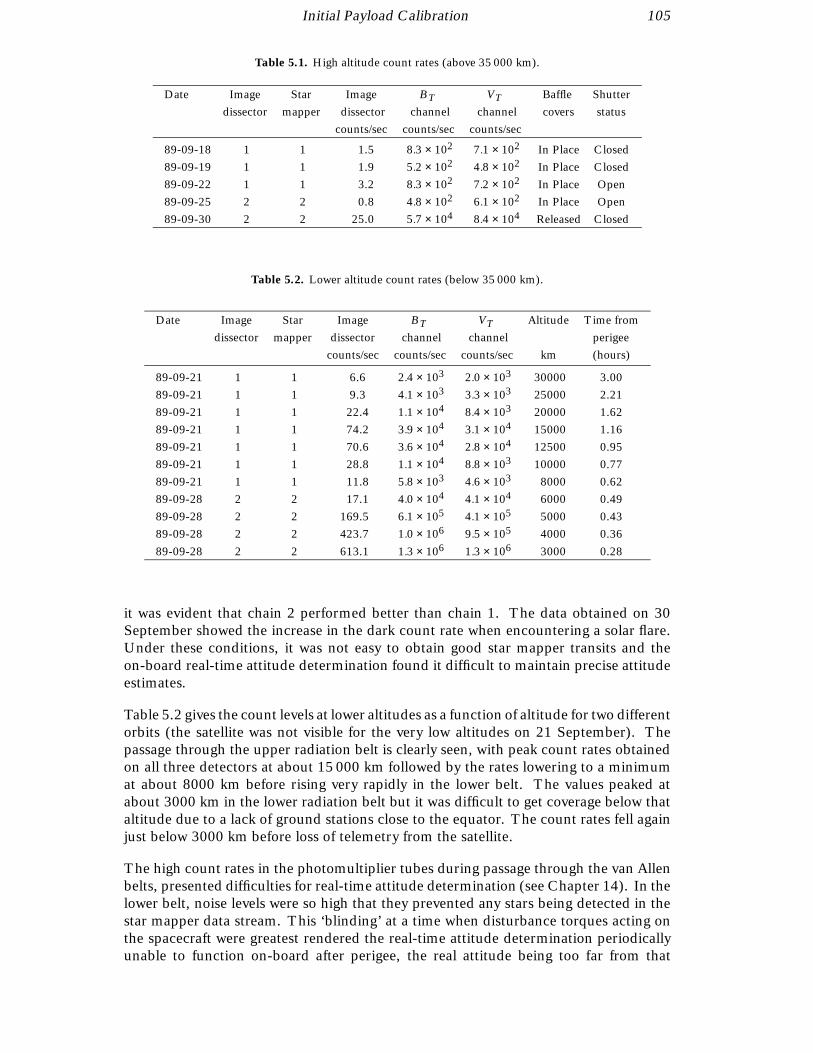
Initial Payload Calibration 105
Table 5.1. High altitude count rates (above 35 000 km).
Date Image Star Image BT VT Baffle Shutter
dissector mapper dissector channel channel covers status
counts/sec counts/sec counts/sec
89-09-18 1 1 1.5 8.3 × 10² 7.1 × 10² In Place Closed
89-09-19 1 1 1.9 5.2 × 10² 4.8 × 10² In Place Closed
89-09-22 1 1 3.2 8.3 × 10² 7.2 × 10² In Place Open
89-09-25 2 2 0.8 4.8 × 10² 6.1 × 10² In Place Open
89-09-30 2 2 25.0 5.7 × 10⁴ 8.4 × 10⁴ Released Closed
Table 5.2. Lower altitude count rates (below 35 000 km).
Date Image Star Image BT VT Altitude Time from
dissector mapper dissector channel channel perigee
counts/sec counts/sec counts/sec km (hours)
89-09-21 1 1 6.6 2.4 × 10³ 2.0 × 10³ 30000 3.00
89-09-21 1 1 9.3 4.1 × 10³ 3.3 × 10³ 25000 2.21
89-09-21 1 1 22.4 1.1 × 10⁴ 8.4 × 10³ 20000 1.62
89-09-21 1 1 74.2 3.9 × 10⁴ 3.1 × 10⁴ 15000 1.16
89-09-21 1 1 70.6 3.6 × 10⁴ 2.8 × 10⁴ 12500 0.95
89-09-21 1 1 28.8 1.1 × 10⁴ 8.8 × 10³ 10000 0.77
89-09-21 1 1 11.8 5.8 × 10³ 4.6 × 10³ 8000 0.62
89-09-28 2 2 17.1 4.0 × 10⁴ 4.1 × 10⁴ 6000 0.49
89-09-28 2 2 169.5 6.1 × 10⁵ 4.1 × 10⁵ 5000 0.43
89-09-28 2 2 423.7 1.0 × 10⁶ 9.5 × 10⁵ 4000 0.36
89-09-28 2 2 613.1 1.3 × 10⁶ 1.3 × 10⁶ 3000 0.28
it was evident that chain 2 performed better than chain 1. The data obtained on 30September showed the increase in the dark count rate when encountering a solar flare.Under these conditions, it was not easy to obtain good star mapper transits and theon-board real-time attitude determination found it difficult to maintain precise attitudeestimates.
Table 5.2 gives the count levels at lower altitudes as a function of altitude for two differentorbits (the satellite was not visible for the very low altitudes on 21 September). Thepassage through the upper radiation belt is clearly seen, with peak count rates obtainedon all three detectors at about 15 000 km followed by the rates lowering to a minimumat about 8000 km before rising very rapidly in the lower belt. The values peaked atabout 3000 km in the lower radiation belt but it was difficult to get coverage below thataltitude due to a lack of ground stations close to the equator. The count rates fell againjust below 3000 km before loss of telemetry from the satellite.
The high count rates in the photomultiplier tubes during passage through the van Allenbelts, presented difficulties for real-time attitude determination (see Chapter 14). In thelower belt, noise levels were so high that they prevented any stars being detected in thestar mapper data stream. This ‘blinding’ at a time when disturbance torques acting onthe spacecraft were greatest rendered the real-time attitude determination periodicallyunable to function on-board after perigee, the real attitude being too far from that
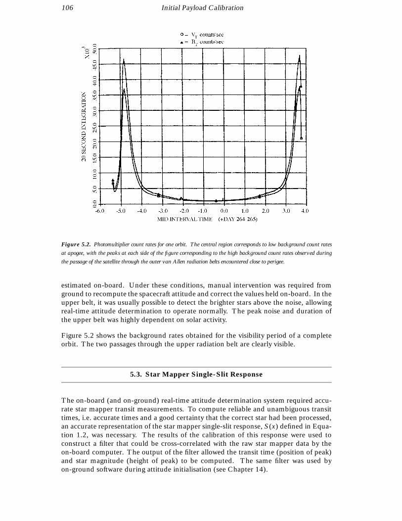
106 Initial Payload Calibration
Figure 5.2. Photomultiplier count rates for one orbit. The central region corresponds to low background count rates
at apogee, with the peaks at each side of the figure corresponding to the high background count rates observed during
the passage of the satellite through the outer van Allen radiation belts encountered close to perigee.
estimated on-board. Under these conditions, manual intervention was required fromground to recompute the spacecraft attitude and correct the values held on-board. In theupper belt, it was usually possible to detect the brighter stars above the noise, allowingreal-time attitude determination to operate normally. The peak noise and duration ofthe upper belt was highly dependent on solar activity.
Figure 5.2 shows the background rates obtained for the visibility period of a completeorbit. The two passages through the upper radiation belt are clearly visible.
5.3. Star Mapper Single-Slit Response
The on-board (and on-ground) real-time attitude determination system required accu-rate star mapper transit measurements. To compute reliable and unambiguous transittimes, i.e. accurate times and a good certainty that the correct star had been processed,an accurate representation of the star mapper single-slit response, S(x) defined in Equa-tion 1.2, was necessary. The results of the calibration of this response were used toconstruct a filter that could be cross-correlated with the raw star mapper data by theon-board computer. The output of the filter allowed the transit time (position of peak)and star magnitude (height of peak) to be computed. The same filter was used byon-ground software during attitude initialisation (see Chapter 14).

Initial Payload Calibration 107
The response itself was calibrated by analysing the transits of bright stars, B < 6 mag,across the star mapper slits. It was simple, using a filter based on a priori knowledgeof the slit response and optimised for the actual scanning velocity of the satellite, tocompute very accurate transit times for these stars. These transit times, together withpre-launch knowledge of the slit geometry, allowed the relative position of each samplewith respect to the slit centres to be determined. All collected data were normalisedand a least-squares estimator was used to fit a 12th order polynomial to the collecteddata subdivided according to BT or VT channel, and vertical or inclined slit system.Figure 5.3 shows four typical calibrated responses.
5.4. Initial Image Dissector Tube Piloting
The piloting of the instantaneous field of view of the image dissector tube to a star’simage was performed by the on-board computer every 1
150 s. To do this accurately, thefollowing information was needed by the on-board computer: (i) a priori estimate ofthe star’s position, (ii) knowledge of the satellite pointing direction, (iii) knowledge ofgeometric distortions in the optical system, and (iv) knowledge of the transformationbetween grid position and image dissector tube piloting currents.
Star Positions
The star positions were uplinked to the on-board computer in the form of a programmestar file based on the pre-defined Hipparcos Input Catalogue of stars to be observed.This catalogue contained positional information for about 120 000 pre-selected starsdown to a limiting magnitude of B = 13 mag. The programme star file produced fromthe Hipparcos Input Catalogue was defined relative to a nominal scanning law, i.e. thepointing directions of the two fields of view were pre-defined and uniquely identified thestars’ expected transit times at the centre of the field of view together with the ordinateand drift angle at the time of transit. All this information was uplinked to the satellitefor all stars to be observed. From this information, the stars’ positions on the grid asa function of time from the expected transit time could be computed by the on-boardcomputer:
ηN = ωN (t − ts) [5.1]
ζN = ζs + µsωN (t − ts)
where:
(ηN , ζN ) is the nominal position of the star on the grid (radians)
ωN is the nominal scanning velocity (radians s−1)
t is time (s)
ts is the expected transit time (s)
ζs is the expected ordinate at transit (radians)
µs is the drift angle of the star (radians)

108 Initial Payload Calibration
Figure 5.3. Star mapper single-slit response for the BT channel (upper pair), the VT channel (lower pair), and for
the vertical (left pair) and inclined (right pair) slits.
Initial Payload Calibration 109
Attitude De-Pointing and Optical Distortion
Equation 5.1 defines the position of the star on the grid assuming a perfect opticalsystem, and assuming that the satellite did not deviate from the nominal scanninglaw. However, the satellite did not follow this law perfectly but was allowed to driftby up to 10 arcmin along any axis from the nominal. Also, during the initial payloadcalibration phase, there were the major effects of basic angle error and grid rotation tobe compensated for. A final correction was made for the transverse offset of the imagedissector tube.
The deviation from the nominal scanning law was computed on-board by the real-timeattitude determination software as a set of three Tait-Bryan error angles (φ, θ, ψ ) andtheir rates of change with time (φ, θ , ψ ). This is discussed in more detail in Chapter 14.
Applying all these effects together, the equations for the star’s grid position (ηC ,ζC)could be expressed as:
ηC = ηN + (ψi + fδγ2
) + (µi + µGi )ζN − µGi νi [5.2]
ζC = ζN − νi − (µi + µGi )ηN − µGi (ψi + fδγ2
) + δζi
where:
δγ is the correction for the basic angle error (radians)
µGi is the grid rotation for field of view i (radians)
i is the field of view selector (1=preceding, 2=following)
f is +1 when i = 1, and −1 when i = 2
δζi is the transverse offset for field of view i (radians)
and:
µi = cos(γN
2)φ + f sin(
γN
2)θ
νi = cos(γN
2)θ − f sin(
γN
2)φ [5.3]
ψi = ψ +12
(φθ − µi νi )
with γN the satellite’s nominal basic angle (radians).
Grid Coordinates to Image Dissector Tube Piloting Currents
The electrical piloting of the instantaneous field of view to the computed positionof the star’s image was performed by the on-board computer using a ‘coil currentcalibration matrix’ of 11 × 11 points defining a regularly spaced mesh on the grid. Foreach point in the mesh, the electrical currents to pilot to that position were known.Thus, for any given position on the grid, the on-board computer performed a two-dimensional linear interpolation using the four surrounding points of the calibrationmatrix mesh to compute the best currents for the given position. The computation ofthe calibration matrix itself was performed by on-ground software in three steps: (i)

110 Initial Payload Calibration
using an internal star pattern assembly; (ii) using grid reference marks close to the maingrid; (iii) computing the coil current calibration matrix.
Internal Star Pattern Assembly
The calibration of the non-linearity of the image dissector tube piloting was performedusing an internal star pattern assembly. This consisted of a pattern of 196 dummy lightsources illuminated by two light-emitting diodes (see Section 2.6). These were imageddirectly onto the photocathode of the image dissector tube by a switching mirror in theoptical path. The on-board computer performed a special cross scan around each ofthese dummy light sources and on-ground software then analysed the raw telemetrygenerated and worked out the optimum currents that piloted the sensitive area of theimage dissector tube to each of these dummy stars. The result of this calibration wasa non-linearity matrix for the image dissector tube but still without any well-definedreference on the grid. This was provided by the next step.
Grid Reference Marks
The rigid body displacement of the image dissector tube with respect to the grid wascomputed using two fixed grid reference marks. These marks were built into the gridat known positions and illuminated by light-emitting diodes. In a similar way to theinternal star pattern assembly calibration, the on-board computer scanned cross patternsaround each of the reference marks and on-ground software then computed the bestcurrents to pilot the sensitive area of the image dissector tube to each mark.
Coil Current Calibration Matrix Computation
The best currents computed in the grid reference mark calibration were used to define atransformation matrix that converted between the photocathode and the grid referenceframes, i.e. the rotation and translation of the image dissector tube with respect to thegrid were then known. The final step in the coil current calibration matrix computationwas to use the non-linearity data obtained from the internal star pattern assemblycalibration to compute the currents needed to scan to the fixed positions in the coilcurrent calibration matrix mesh. This was achieved by performing a least-squares fit forthe best currents using the four closest positions in the non-linearity matrix. If the resultswere in fairly good agreement with the previous coil current calibration matrix, then thenew one was automatically uplinked from the on-ground software to the satellite withoutmanual intervention. The complete cycle of telecommanding, ground processing anduplink of results could be performed automatically, driven by the mission planningsoftware.
Initial Payload Calibration 111
5.5. Transverse and Longitudinal Offsets
The first in-orbit calibration of the image dissector tube piloting was performed on 5October 1989 and it was repeated on 19 October. As well as calibrating the non-linearityof the image dissector tube, through use of the coil current calibration matrix, it was alsonecessary to assess the constant offset in the transformation of a star’s grid coordinatesinto image dissector tube piloting currents. Two offsets were assessed: in the transverseand longitudinal directions.
Transverse Offset
One effect, compensated for in Equation 5.2, was the addition of the transverse offset,δζi for field of view i. This was caused by the photocentre of the star’s image beingoffset from the telescope’s chief ray due to the semi-circular geometry of the field ofview entrance pupil. It was calibrated, in-orbit, by dedicated observations made witha modified programme star file. Instead of piloting the image dissector tube to thecomputed position of the star, the on-board computer piloted the image dissector tubeto positions offset from the actual star image. This was achieved by the insertion of‘dummy’ stars into the programme star file, with the same transit times as the actual starbut with different ordinate values, ζs. A pattern of 10 of these ‘dummy’ stars was placedaround each of the actual stars scheduled for observation (generally these were brightstars). By analysing the count rates at each of the 10 positions, the on-ground softwarecould compute the offset from the actual star to the position that gave the highest countrate. By averaging many such observations, the mean offset for each field of view couldbe computed. The resulting offsets were then uplinked to the satellite.
Longitudinal Offset
The longitudinal offset of the image dissector tube piloting is not directly compensatedfor in Equation 5.2 as it was expected to be very small. This was verified, in-orbit,by dedicated observations with another modified programme star file. The specialprogramme star file contained ‘dummy’ stars positioned close to an actual star withthe same ordinate, ζs, but with modified transit times. Ground software, based on thetransverse offset program, was used to compute the mean offset for each field of view.If the absolute value of the result had been the same for each field of view but withopposite sign, it would probably have been due to an error in the basic angle and couldhave been compensated for by modifying the value of δγ used in Equation 5.2.
Image Dissector Tube Piloting Offset Results
The offset calibrations were performed four times during the calibration phase. Thefirst calibration was carried out on 13 October 1989 before the telescope refocusingoperations had been performed. Only the transverse offsets for each field of view werecalibrated. The results obtained were −4.029 and −4.126 arcsec for the preceding andfollowing fields of view respectively.
112 Initial Payload Calibration
The transverse offsets were recalibrated on 1 November after refocusing, giving −3.766and −4.251 arcsec for the preceding and following fields of view respectively. The lon-gitudinal offsets were calibrated for the first time on 3 November after refocusing giving−1.004 and −0.380 arcsec for the preceding and following fields of view respectively.
An analysis was subsequently performed to investigate residual piloting offsets after theprevious calibration. As a result, an empirical correction was introduced into the coilcurrent calibration matrix computation. To verify this correction, both longitudinal andtransverse offsets were recalibrated on 24 and 25 November 1989. The results for thetransverse offsets were in good agreement with those previously obtained. Moreover therevised values for the longitudinal offsets showed a reduced spread of values about themean, indicating that the empirical correction had been successful.
The grid rotation angle and basic angle (separating the two fields of view) were subse-quently calibrated to high accuracy by the data reduction consortia. Corrected valueswere first used on-board on 23 January 1990, without empirical correction. The trans-verse offsets were recalibrated, giving −3.797 and −4.219 arcsec for the preceding andfollowing fields of view respectively. These were the values used on-board throughoutthe rest of the mission. The longitudinal offsets were recalibrated giving −0.306 and−0.300 arcsec for the preceding and following fields of view respectively. The spreadin the values obtained for the longitudinal offset showed a further reduction indicat-ing a further improvement. It was not deemed necessary to re-compute any empiricalcorrections.
5.6. Focusing
The telescope could be refocused using a mechanism that allowed the grid assembly tomove with respect to the telescope focal surface (see Section 3.2). This was necessaryfor two main reasons: (a) to enable the position of best focus to be determined at thestart of the mission; and (b) to compensate for effects such as moisture release whichaltered the focus throughout the mission.
The quality of the focus for any given position of the grid assembly was assessed byground processing of image dissector tube data collected for bright stars (B < 9 mag) inthe central portion of a 3 × 3 subdivision of the main grid. As the focus was improved,the value of the first modulation coefficient, M1 in Equation 1.1, increased. This valuewas determined by the ground processing software from 45 minutes of observations foreach focus setting, as a function of star colour and field of view. Operationally, data wascollected for ten different focus settings close to the predicted beginning-of-life positionbetween 12 and 28 October 1989. The results are presented graphically in Figure 5.4as a function of three colour groups.
The standard deviations of the residuals from a least-squares parabolic fit varied between0.9 per cent and 1.9 per cent for the six cases considered.
There was evidence from this for a differential defocus, i.e. the position of best focuswas not the same for each field of view. The position of best focus for the preceding fieldof view after launch was −44 µm and that for the following field of view was −26 µm.The actual position chosen as best overall focus immediately after launch, −35 µm,gave a differential defocus of ±9 µm. In December 1989, a revised grid scale factor was
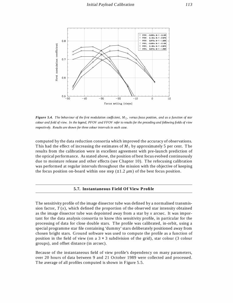
Initial Payload Calibration 113
Figure 5.4. The behaviour of the first modulation coefficient, M1, versus focus position, and as a function of star
colour and field of view. In the legend, PFOV and FFOV refer to results for the preceding and following fields of view
respectively. Results are shown for three colour intervals in each case.
computed by the data reduction consortia which improved the accuracy of observations.This had the effect of increasing the estimates of M1 by approximately 5 per cent. Theresults from the calibration were in excellent agreement with pre-launch prediction ofthe optical performance. As stated above, the position of best focus evolved continuouslydue to moisture release and other effects (see Chapter 10). The refocusing calibrationwas performed at regular intervals throughout the mission with the objective of keepingthe focus position on-board within one step (±1.2 µm) of the best focus position.
5.7. Instantaneous Field Of View Profile
The sensitivity profile of the image dissector tube was defined by a normalised transmis-sion factor, T (x), which defined the proportion of the observed star intensity obtainedas the image dissector tube was depointed away from a star by x arcsec. It was impor-tant for the data analysis consortia to know this sensitivity profile, in particular for theprocessing of data for close double stars. The profile was calibrated, in-orbit, using aspecial programme star file containing ‘dummy’ stars deliberately positioned away fromchosen bright stars. Ground software was used to compute the profile as a function ofposition in the field of view (on a 3 × 3 subdivision of the grid), star colour (3 colourgroups), and offset distance (in arcsec).
Because of the instantaneous field of view profile’s dependency on many parameters,over 20 hours of data between 9 and 21 October 1989 were collected and processed.The average of all profiles computed is shown in Figure 5.5.
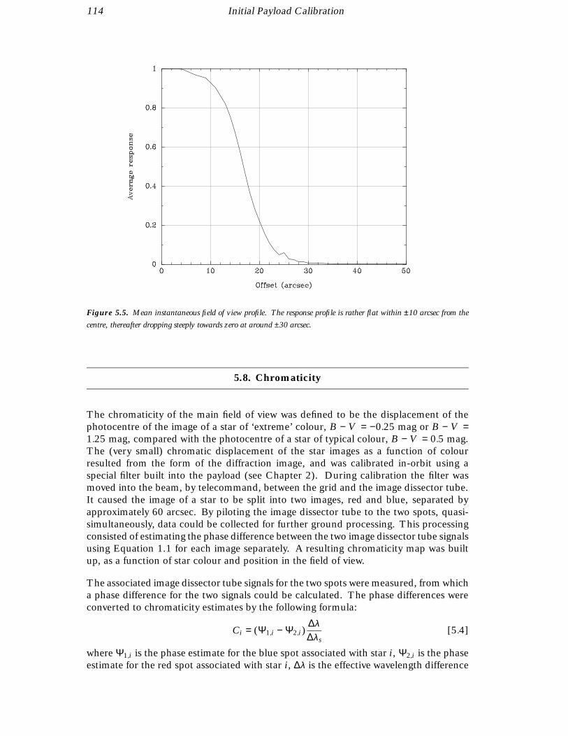
114 Initial Payload Calibration
Figure 5.5. Mean instantaneous field of view profile. The response profile is rather flat within ±10 arcsec from the
centre, thereafter dropping steeply towards zero at around ±30 arcsec.
5.8. Chromaticity
The chromaticity of the main field of view was defined to be the displacement of thephotocentre of the image of a star of ‘extreme’ colour, B − V = −0.25 mag or B − V =1.25 mag, compared with the photocentre of a star of typical colour, B − V = 0.5 mag.The (very small) chromatic displacement of the star images as a function of colourresulted from the form of the diffraction image, and was calibrated in-orbit using aspecial filter built into the payload (see Chapter 2). During calibration the filter wasmoved into the beam, by telecommand, between the grid and the image dissector tube.It caused the image of a star to be split into two images, red and blue, separated byapproximately 60 arcsec. By piloting the image dissector tube to the two spots, quasi-simultaneously, data could be collected for further ground processing. This processingconsisted of estimating the phase difference between the two image dissector tube signalsusing Equation 1.1 for each image separately. A resulting chromaticity map was builtup, as a function of star colour and position in the field of view.
The associated image dissector tube signals for the two spots were measured, from whicha phase difference for the two signals could be calculated. The phase differences wereconverted to chromaticity estimates by the following formula:
Ci = (Ψ1,i − Ψ2,i )∆λ∆λs
[5.4]
where Ψ1,i is the phase estimate for the blue spot associated with star i, Ψ2,i is the phaseestimate for the red spot associated with star i, ∆λ is the effective wavelength difference
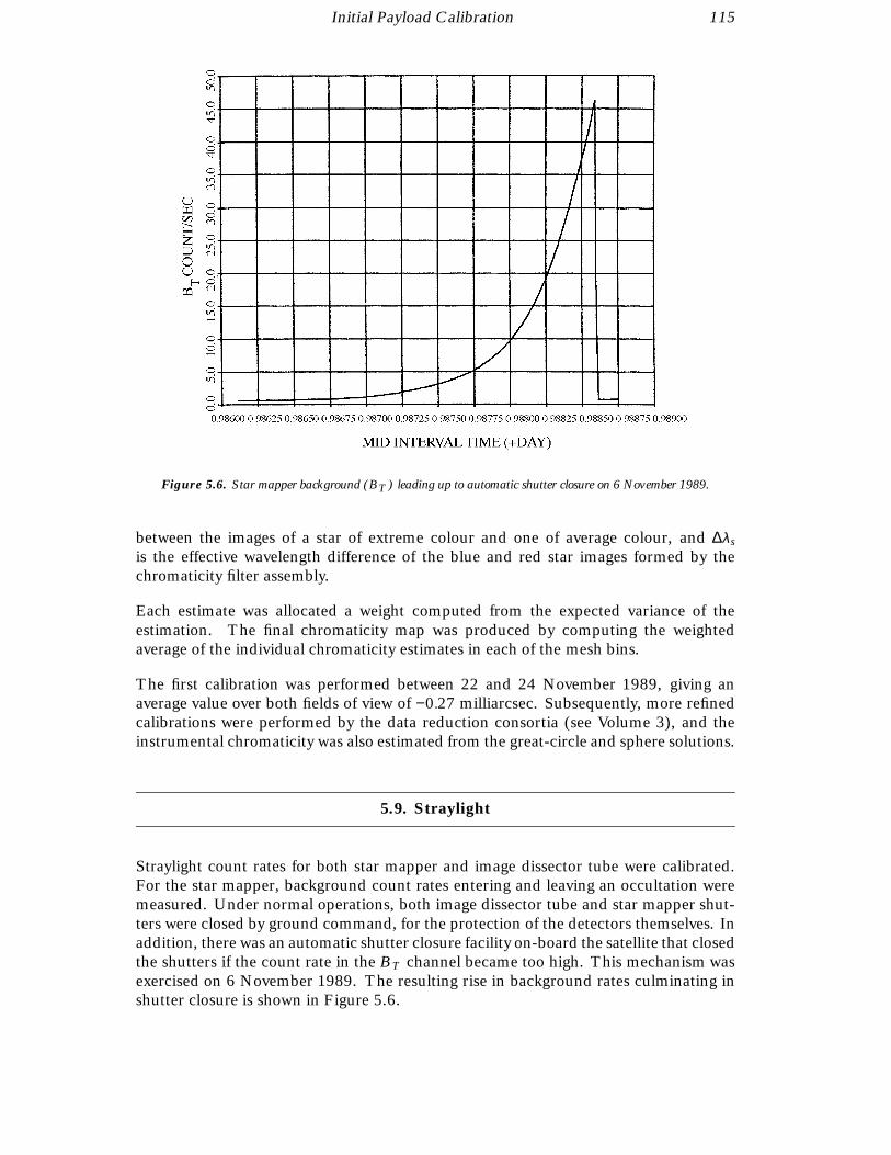
Initial Payload Calibration 115
Figure 5.6. Star mapper background (BT ) leading up to automatic shutter closure on 6 November 1989.
between the images of a star of extreme colour and one of average colour, and ∆λs
is the effective wavelength difference of the blue and red star images formed by thechromaticity filter assembly.
Each estimate was allocated a weight computed from the expected variance of theestimation. The final chromaticity map was produced by computing the weightedaverage of the individual chromaticity estimates in each of the mesh bins.
The first calibration was performed between 22 and 24 November 1989, giving anaverage value over both fields of view of −0.27 milliarcsec. Subsequently, more refinedcalibrations were performed by the data reduction consortia (see Volume 3), and theinstrumental chromaticity was also estimated from the great-circle and sphere solutions.
5.9. Straylight
Straylight count rates for both star mapper and image dissector tube were calibrated.For the star mapper, background count rates entering and leaving an occultation weremeasured. Under normal operations, both image dissector tube and star mapper shut-ters were closed by ground command, for the protection of the detectors themselves. Inaddition, there was an automatic shutter closure facility on-board the satellite that closedthe shutters if the count rate in the BT channel became too high. This mechanism wasexercised on 6 November 1989. The resulting rise in background rates culminating inshutter closure is shown in Figure 5.6.

116 Initial Payload Calibration
The telemetry collected during the instantaneous field of view profile calibration alsocontained many observations away from programme stars permitting measurement ofthe sky background count rate on the image dissector tube. The algorithm used wasto position a dummy star in the programme star file away from the programme stars.Analysis of the image dissector tube data was then performed and the modulation coeffi-cients were computed. Any observation with M1 < 0.325 was rejected and observationsclose together in time were averaged. In total, there were 3043 observations duringthis phase of the initial payload calibration, with a mean of 36 counts/sec and standarddeviation of 16 counts/sec.
6. THE OPERATIONAL ORBIT
Planned to be operated in geostationary orbit by means of a single groundstation, the satellite was actually operated from a highly elliptical (geostation-ary transfer) orbit. The parameters of the actual orbit are given, along with asummary of the features of the elliptical orbit which complicated the satelliteoperations and performances: the resulting radiation environment (consideredin more detail in Chapter 7), eclipses (affecting the power budget), Earth andMoon occultations (affecting the observation programme), and the complexground-station requirements—a single ground station would have resulted ina maximum of 30 per cent of useful data collection, and additional groundstations had to be rapidly brought into the telecommunication network. Theproblems affecting the satellite attitude control—perturbing torques especiallythose around perigee, and the consequences on the real-time attitude determi-nation, and the (general) problem of micrometeoroid impacts—are discussed.
6.1. Orbital Elements
The orbital characteristics for the epoch 18 September 1989, when the revised missionmanoeuvres had been completed, were as follows:
– perigee height: 526 km
– apogee height: 35 900 km
– orbital period: 640 min
– eccentricity: 0.72
– inclination: 6.8
– ascending node: 105
– argument of perigee: 214
The observed evolution of some of these parameters during the mission is shown inFigure 6.1 and Figure 6.2. Additional information on the orbit evolution can be foundin Volume 3, Chapter 8.

118 The Operational Orbit
Figure 6.1. Evolution of perigee height during the mission.
For Hipparcos, a critical assessment of the accuracy and precision of the orbit data wasessential. Preliminary analysis of the orbit determination accuracy assumed a perigeealtitude of 600 km and three ranging stations. The covariance analysis showed that thesemi-major axis could be determined to better than 10 m and the inclination to about0.001. The positional and velocity accuracy would vary along the orbit, as shown inTable 6.1. These data compared well with the orbit determination accuracy at that time:
– perigee/apogee altitude: ±150 m
– semi-major axis: ±50 m
– inclination: ±0.2
– apogee position: ±1.5 km
– apogee velocity: ±0.08 m s−1
Specifications for the revised orbit included an instantaneous knowledge of the positionto 1.5 km (in order to be able to account for positional observations of solar system ob-jects), and the velocity to 0.2 m s−1 (in order to be able to correct for aberration). Thesecriteria were achieved by the adopted ranging and orbital reconstruction procedures.
The orbit data, which included the time interval, the state vector components at agiven reference time in the mean equinox of date frame, auxiliary Keplerian motionparameters, and Chebychev expansion of each of the six state components, was sent tothe data reduction teams with the telemetry data.

The Operational Orbit 119
Table 6.1. Variation in the position and velocity accuracy along the orbit.
Time since perigee Position accuracy Velocity accuracy
(hours) (km) (m/s)
0.0 0.87 0.78
0.5 0.70 0.32
1.0 0.79 0.18
2.0 1.03 0.11
3.0 1.20 0.07
4.0 1.28 0.06
5.0 1.30 0.06
6.2. Radiation Environment
The revised orbit meant that the satellite was subject to a much higher particle radiationexposure than anticipated prior to launch. Consequently, radiation damage to thesolar arrays and other payload and spacecraft equipment was higher than had beenanticipated. In particular, the increased radiation led to the progressive degradation ofthe solar arrays, difficulties in maintaining the on-board attitude control and the failureof the satellite gyros. Details of the associated problems are presented in more detail inChapters 7, 11, and 15.
6.3. Eclipses
In geostationary transfer orbit between zero and six eclipses due to the Moon occurredannually, with an average of three. The duration of these eclipses ranged from a fewminutes to over four hours. Long eclipses occurred at the Sun-Moon-apogee-Earthconjunction. Eclipses by the Earth occurred about four times per day, with a durationrange of a few minutes to more than one hour. Long eclipses occurred at a Sun-Earth-apogee conjunction. The duration of the eclipses are illustrated in Figure 4.1.
The distribution of eclipse durations are tabulated in Table 6.2. During its lifetime thecritical eclipses for Hipparcos were March 1989 (eclipse duration 104 min), April 1993(63 min) and August 1993 (82 min).
Coupled with the solar panel degradation problem was the fact that, in the ellipticalorbit, the eclipses of the Sun by the Earth were much longer (up to 100 min) and muchmore frequent than in the geostationary case. During eclipses, the spacecraft couldonly function by extracting power from its batteries. Thus the power deficit problemwas enhanced during the period of the longest eclipses and had to be solved with moredrastic measures. Detailed power budgets and the relevant operational procedures wereprepared to ‘hibernate’ the spacecraft in such cases when the batteries could not supplyenough energy to maintain a fully nominal mission throughout the eclipse.

120 The Operational Orbit
Figure 6.2. Evolution of inclination, eccentricity, and angle during the mission.

The Operational Orbit 121
Table 6.2. Distribution of eclipse durations for a three-year mission in geostationary transfer orbit (approxi-
mately 2500 orbits).
Eclipse duration %
0 to 20 min 18
20 to 30 min 44
30 to 60 min 26
over 60 min 12
In order to survive the long eclipse period (up to 104 min), a power saving strategy wasdeveloped, which guaranteed a positive power budget by decreasing or switching offloads. As a reference criterion the remaining time between end of charge of the batteriesand the start of the next eclipse was taken. This time was calculated and extrapolated inreal-time to ensure immediate implementation of the relevant power saving procedures.However, no such drastic measures were actually needed up to 30 March 1993, sinceeven at the longest eclipse times the batteries were always fully charged before the nexteclipse entry.
6.4. Occultations
Occultations occurred when one of the two fields of view crossed the Earth or theMoon. The payload detectors would have been damaged by these events, if they hadnot been shielded by shutters which closed at these times. The Earth occultations,like the eclipses, occurred more frequently and lasted longer in the elliptical than inthe geostationary orbit, again reducing the amount and uniform time coverage of goodscience data. Also, when they occurred near perigee, they increased the risk of loss ofattitude control by blinding the star mapper.
6.5. Ground Station Coverage
One of the most serious operational consequences of being in a geostationary transfertype orbit is that one ground station is not sufficient to track the satellite at all times.At the beginning of the mission, complete operational support was only available forabout one third of the time, posing major problems on how to manage the missionoutside visibility periods. The major problems to be solved were how to keep real-timeattitude determination convergence until the next visibility period and how to protectthe spacecraft, with appropriate reconfigurations of the subsystems, against such eventsas eclipses, occultations, perigee passages and possible on-board failures.
As described in Chapter 4 the number of ground stations was quickly increased to three.However, the lowest part of the orbit was only rarely trackable, and in any case onlyfrom Kourou (near the equator).
122 The Operational Orbit
6.6. Perturbing Torques
In geostationary orbit, the only significant external disturbance torques acting on thespacecraft were expected to be due to the solar radiation pressure and the constantlyspinning gyros. However, away from apogee of the revised orbit, other effects becamesignificant, e.g. atmospheric, magnetic dipole and gravity gradient torques all playeda role depending on the altitude and attitude of the satellite. Their combined effectdegraded the on-board attitude control to the extent that ground support was oftenrequired. In addition, greatly increased cold gas consumption was necessary to controlthe attitude through these variable conditions, implying a shorter lifetime, based only onconsumables. The higher torques also degraded the on-ground attitude determination.
6.7. Loss of Real-Time Attitude Determination
The difficulties involved in controlling the spacecraft attitude in the revised mission,arose from the critical link between the stellar measurements, the attitude measurementsmade on-board, and the attitude control. The approximate positions of all stars to beobserved by the main detector were uplinked to the satellite in the form of expectedtimes at which the stars were predicted to cross the star mapper slit measurement system,based on the nominal attitude of the satellite. The actual star transits across the starmapper slit system were detected and converted into actual crossing times. These timesallowed the on-board computer to calculate the difference between the nominal andactual satellite attitude for a subset of the brighter programme stars.
Radiation from the van Allen belts blinded the photomultiplier which sampled the starmapper data: the on-board processor was then not able to filter out a star transit fromthe noise. At such times, the spacecraft was without external references and had to relyon the gyros alone for real-time attitude determination, except for increasingly refinedmodelling carried out towards the end of the mission allowing attitude control in theabsence of one or more gyros (see Chapters 14–16). Close to perigee, the externaldisturbance torques were greatest, causing long thruster firings approximately once perminute. Studies later in the mission suggested that the gyro drifts also evolved morequickly around perigee. Both phenomena combined to cause a drift of the spacecraftwithout correction from the star mapper.
When the real-time attitude determination estimate differed by more than 10 arcsec fromthe actual spacecraft attitude, ground intervention was required to increase tolerancesto the maximum value of 30 arcsec. If the real-time attitude determination estimatediffered by more than 30 arcsec, further intervention was required using ground softwareto re-initialise real-time attitude determination. The resulting effects are described inmore detail in Chapters 13 and 14.
The Operational Orbit 123
6.8. Micrometeoroids
A potential hazard faced by satellite experiments is the impact of micrometeoroids.Although no specific events were ever attributed to micrometeoroid impacts on theHipparcos satellite, a careful evaluation was made of the expected effects in advance oflaunch, both in order to assess possible attitude perturbations caused by impacts withthe more common, lighter particles, and the risk of catastrophic damage by the rarerbut more massive particles. In view of its applicability to other missions, a summary ofthe predicted effects are therefore given hereafter.
A dust experiment on HEOS-2 provided much data on the micrometeoroid environmentin near-Earth orbit. The data could be categorised into three groups according to theobserved rate. Event rates of 1 or more events per 15 min were classified as swarms,between 1 event per 15 min and 2 events per day was considered a group, and fewer than2 events per day was attributed to random particles. Analysis of the event rates indicatedthat the apex particles (where the apex is the direction of the Earth’s velocity around theSun) were most frequent. Their average impact velocity was around 10 km s−1 resultingin a flux of φapex = 4 × 10⁻⁴ m−2 s−1 (2π sr)−1 for masses ≥ 10−12 g. The ‘ecliptic-southparticles’, although almost as frequent as the apex particles, were much smaller andfaster giving a correspondingly lower flux. These latter particles are believed to befragmentation products from larger micrometeoroids.
An important result from the HEOS-2 experiment was that more than 80 per cent ofall the detected particles arrived in swarms or groups. The groups showed a correlationwith the Moon position suggesting a lunar origin—these particles may be ejected fromthe Moon’s surface by impacting meteorites in the kg range. The swarms were foundmainly in the near-Earth part of the orbit, and showed no lunar correlation promptingsuggestions that they may be produced by meteors impinging on the Earth’s atmosphere.
Simulations of the Effect of Micrometeoroids on Hipparcos
Simulations based on published data (Naumann, 1966) were undertaken before launchto assess the effect of micrometeoroid impacts on Hipparcos in orbit. The simulationswere constructed as follows: (i) the satellite was hit by a random sized meteoroid at timeswhich were uniformly distributed within the interval 0 to 10 000 s; (ii) the meteoroidvelocity (v) was uniformly distributed in the range ± 47 km s−1; (iii) each impact reacheda target point on one of the solar panels at r = 1.8 m from the centre of the satelliteand hits on the satellite body were neglected; (iv) the number of hits was calculatedfrom the flux data as twice the product of the cumulative flux (for particles heavier than1 × 10−15 kg), the total area of the solar panels (6.8 m2) and the integration time. Thefactor of two arose from allowing both forward and backward hits; (v) the cumulativeflux (given in impacts per m2) of Landolt-Bornstein (1981) was used:
φ = 5 × 10⁻⁵
m
10−15
−0.4
for m < 1.4 × 10⁻¹⁰ kg [6.1]
φ = 2 × 10⁻¹
m
10−15
−1.1
for m > 1.4 × 10⁻¹⁰ kg
124 The Operational Orbit
This gave a change in angular momentum per hit of δL = mvr, and a change in angularvelocity of δω = δL / I , where a mean value (I = 400 kg m2) of the satellite’s moment ofinertia was used.
In this way successive impacts gave positive or negative increments of the angular velocity.In each time interval between hits, the velocity increment was integrated up to a changein angle. The nominal rotation of the satellite and the smooth perturbations due to solarradiation pressure were not included, so that the results only represent the additionaleffects caused by micrometeoroids.
The cumulative flux was also used to predict the masses of the impacting meteoroids.The data can be represented by the relation:
mm0
a
=φφ0
= R [6.2]
where m0 is the smallest mass considered, φ0 is the flux of particles with m > m0 and a isa negative constant. Two different values of a were used: a = −0.4 for m < 1.4× 10⁻¹⁰ kgand a = −1.1 for higher masses (see Equation 6.1). Masses consistent with the flux datacould be generated according to the formula:
m = m0Ra−1
[6.3]
when R is uniformly distributed between 0 and 1. To increase the number of datapoints, angle values were linearly interpolated between impact times such that one datapoint was obtained for every 10 s of the 10 000 s interval. A cubic spline was then fitwith a knot every 100 s and the difference between the data and the spline function wasthen calculated. The residuals of this fit were taken as a measure of the micrometeoroideffect. A total of 1000 simulations of 10 000 s were made.
The results showed that the most frequent residual lay around 1 × 10⁻⁵ arcsec whichwas a factor of 10−3 smaller than the expected accuracy of the individual measurementsmade by the Hipparcos instruments. Only a few of the 1000 simulations had rmsresiduals in the vicinity of 10−2 and the median rms effect was 2.6 × 10⁻⁶ arcsec. In 2.5years the simulations predicted about 500 impacts resulting in residuals > 10−2 arcsec.The single largest impact during that period was predicted to produce residuals of theorder of 10 arcsec.
The following analysis of the micrometeoroid problem also yielded similar results. Tak-ing particles with mass m = 10−12 g as representative, a satellite moment of inertia,I = 350 kg m2, v = 30 km s−1 and an impact distance of d = 1 m from the center of massyielded: δω = mvd / I = 10−8 arcsec s−1, with an average occurrence of about 1 event per100 s. At the extreme end of the mass range (see Figure 6.3) particles of mass 10−3 gwould give an increment to the spin velocity of approximately 10 arcsec s−1 about onceper year.
The conclusion of these studies was that it was unlikely that most micrometeoroidimpacts would have any major effects on the accuracy of the Hipparcos observations,but that larger, more infrequent events could significantly perturb the satellite attitude.In reality, it was difficult to ascribe any evolution of the satellite attitude unambiguouslyto the effects of micrometeoroids, and they certainly resulted in no evident threat ordegradation of the mission performances.
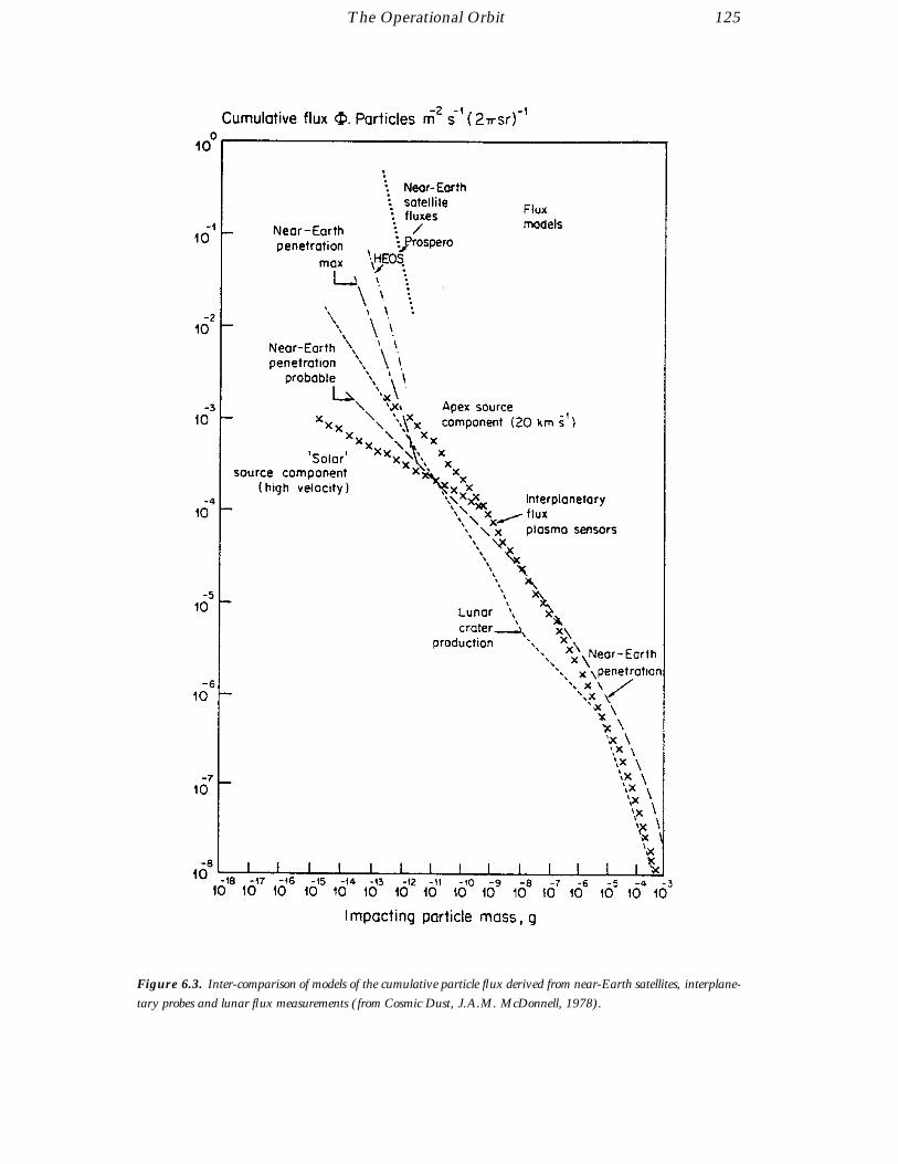
The Operational Orbit 125
Figure 6.3. Inter-comparison of models of the cumulative particle flux derived from near-Earth satellites, interplane-
tary probes and lunar flux measurements (from Cosmic Dust, J.A.M. McDonnell, 1978).

126 The Operational Orbit
The 1993 Perseid Meteoroid Shower
Although the Hipparcos mission was terminated before the 1993 Perseid shower, acareful evaluation of its potential effect was made, since periodic, seasonally correlatedenhancements of meteoroid flux towards the Earth are quite normal, and are associatedwith trails of dust material along cometary orbits which the Earth crosses at fixed timesof the year. The given maxima are very stable in terms of epoch, but they may increaseconsiderably if the Earth crosses the path of the comet shortly after the comet itself.
As simulations had shown, the impact of meteoroid showers on the Hipparcos satelliteduring its mission were in general expected to be almost negligible. An exception tothis might have been the 12 August 1993 Perseid shower, which was predicted to beunusually strong as a result of the perihelion passage of the Perseid’s source comet,Swift-Tuttle, the previous year (31 December 1992). This expectation was based onanalogy with the largest known meteor storm prior to this, the 17 November 1966Leonid storm. Both the Leonids and the Perseids are of cometary origin, the formerbeing associated with comet Temple-Tuttle with a period of 33.25 years, the latter withcomet Swift-Tuttle with period 130 years. Prior to the storm of November 1966 therewas a steady increase in Leonid meteoroid activity, a pattern also seen in the tenfoldincrease in Perseid activity in the previous two years. Less than one year prior to theLeonid storm the source comet passed its perihelion. The Perseid’s source comet,Swift-Tuttle, passed its perihelion less than one year prior to expected storm activity.
At the time of the 1966 Leonid storm the Earth was within 450 000 km of the comet’sorbital plane. During the Perseid storm the Earth would be within 140 000 km of thecomet’s orbital plane. The increase in meteoroid flux, above the mean background, forthe Leonid 1966 storm was more than a factor of 1000. The increased Perseid activitywas expected to be even greater than this. In particular the flux enhancement withrespect to the average meteoroid background flux was expected to be of the order of1000 or more (it has been shown that during periods of meteor storm activity, the impactprobability increases by more than 104 over the sporadic background of meteoroids; seeBeech, Brown & Jones, 1995). This would imply approximately 0.5 hits m−2 hr−1 bymeteoroids of diameter larger than 0.1 mm on an exposed satellite surface. The impactvelocity was expected to be of the order of 60 km s−1, giving an equivalent penetrationdepth in Al of 5 to 10 times the diameter of the projectile. A 1 mm projectile couldcause substantial damage, and even smaller particles of 0.1 mm diameter could disablesensitive spacecraft components such as the solar arrays.
Given the potential risk to the spacecraft and its components from the 1993 Perseidshower, ESOC carried out an assessment of the flux geometry for the predicted time ofthe Perseid storm relative to the spacecraft. The spin-axis of Hipparcos pointed towardsthe Sun and thus only the smaller side of the satellite (3.5 m2) could be targeted by themeteoroids. The configuration between the meteoroids stream and the Sun indicatedthat the Perseid storm would not be dangerous to Hipparcos. Since the solar arrayswere oriented towards the Sun, the solar arrays and the meteoroid stream were almostin the same plane (i.e. the Sun direction was α = 142, δ = 15, and the Perseid streamwas α = 46, δ = 58). The angle between the two directions was about 80.5 andthus the angle of impact would be about 9.5 from the rear of the solar arrays, giving areduction in the projected surface area of a factor of 6. On this basis it was consideredthat the overall risk to the spacecraft from this exceptional Perseid storm was not undulyalarming.

7. RADIATION BACKGROUNDAND RELATED EFFECTS
The most critical problem faced by the satellite, and consequently also im-pacting on its operations, was the radiation environment in the geostationarytransfer orbit. The regular crossings of the van Allen radiation belts meantthat the satellite was repeatedly exposed to very high proton and electron radi-ation levels, much higher than those for which the satellite and payload weredesigned. The radiation damage resulted in the progressive degradation of thesolar array performance (described in Chapter 11), heater anomalies (Chap-ter 12), the failure of the gyroscopes (Chapters 13–16), and eventually theloss of the mission through failure of the telecommunication subsystem. Inaddition, the radiation environment was responsible for an increased star map-per signal background which complicated and degraded the real-time attitudedetermination, as well as the Tycho data analysis.
7.1. Introduction
The Hipparcos payload was known and predicted to be sensitive to background signalsinduced by energetic electrons and protons. Radiation effects were an important con-sideration even in the planned geostationary orbit, and careful analysis of the focal planeshielding was made before launch.
After the failure of the apogee boost motor to raise the satellite into its planned orbit,there was concern that the considerably harsher radiation environment of geostationarytransfer orbit would severely limit the mission lifetime due to solar cell degradation orcomponent failure. It is likely that the eventual failure of four out of five gyroscopes wasdue to radiation damage to control electronics. There was an additional initial concernthat the background signal induced in the telescope systems by energetic particle hits onthe optics or the photomultiplier detectors would strongly limit the possible observationtime during the orbit.
This chapter provides a summary of the radiation environment in near-Earth orbit, anddetails the effects of the radiation background on the satellite. From the perspective ofunderstanding the radiation environment in geostationary transfer orbit, the Hipparcosobservations over the mission lifetime yielded a long-term data set which strongly reflectsthe structure of the radiation belts, their dynamics and the effects of solar particle events.

128 Radiation Background and Related Effects
7.2. The Radiation Environment in Space
The space radiation environment presents a hazard to most satellite missions, irrespec-tive of the orbit. There are many high-energy particle populations in the different regionsof space which can cause damage to spacecraft and instrument components. In additionthey can give rise to detector interference, single-event upset and electrostatic charging.
Some regions, however, pose more of a threat to satellite experiments than others.For example, the trapping of charged particles, in particular electrons and protons, bythe Earth’s magnetic field, creates the toroidal radiation belts known as the van Allenbelts. As a consequence of being in geostationary transfer orbit Hipparcos crossedthe van Allen belts slightly more than four times per day. The inner belt, between1000 and 4000 km from the Earth’s surface, contains mainly high-energy protons,while the outer belt between 8000 and 12 000 km, contains high-energy electrons.The degradation of directly exposed subsystems, e.g. solar generators and electronicequipment, are important because of repeated exposure to radiation. Out of the vanAllen belts, radiation rates are caused by particle events and galactic cosmic rays, andthese can induce single event upsets.
During the early part of the mission, the effects of the radiation background on thesolar array performance was considered to be a crucial factor in the overall satellitelifetime, and a particular effort was therefore devoted to understanding and predictingthe solar array in-orbit power loss due to radiation damage. In practice, this was basedon a correlation of laboratory solar-cell radiation damage data with an estimate of theradiation dose for the anticipated spacecraft trajectory. This estimate, therefore, alsorequired an accurate knowledge of the spacecraft flight path exposure to the Earth’scharged-particle trapping domains.
Steady improvements and refinements to our knowledge of the magnetosphere have beenmade since the discovery of the van Allen radiation belts in 1959. Static trapped-particle-environment models have evolved to the point where spatial and temporal variationsmay be allowed for. The radial electron and proton flux profiles depicted in Figure 7.1demonstrate the complexity of the task and why different types of orbits will be damagingor benign. The prediction of solar particle event proton fluxes is more difficult, andpresent models are based on a probabilistic analysis involving mission duration andevent confidence levels (Feynman et al., 1992; Tranquille & Daly 1992). The high solarparticle event doses in the lower energy range can be particularly damaging for spacecraftin eccentric or geostationary orbits (36 000 km) whereas spacecraft in low-inclination,near-Earth orbits (600 km) are protected from solar particle events by geomagneticshielding effects.
The radiation belt models used in the analysis of the Hipparcos data are AE8 and AP8.AE8 (Vette 1991) is a model for the electron environment for energies of 40 keV to7 MeV and altitudes of 1.2 to 11 Earth radii. Since solar activity can have a pronouncedeffect on the radiation environment experienced in an orbit the model comes in twoforms. AE8MAX is appropriate for solar maximum conditions, while AE8MIN is forsolar minimum. Similarly AP8 (Sawyer & Vette 1976) is a model of the trapped proton

Radiation Background and Related Effects 129
Figure 7.1. The Earth’s trapped electron and proton radial average flux profiles as a function of altitude (the
Hipparcos satellite operated between 400 − 36 000 km). The different curves refer to different proton and electron
energies (Ep and E respectively). For electrons, the solid and dotted lines indicate the dependence at solar minimum
and solar maximum respectively.
environment for energies 100 keV to 400 MeV and altitudes of 1.15 to 6.6 Earth radii.This also has appropriate versions for solar maximum and solar minimum conditions.
An associated phenomenon—geomagnetic sub-storms—can lead to spacecraft anoma-lies and secondary solar-array damage. In this case occasional injections of hot plasmafrom the geomagnetic tail cause charging of surfaces to large negative potentials withrespect to the surrounding plasma or different dielectric materials. Surfaces not neu-tralised by solar UV-induced photo-electron emission can develop large differentialpotentials leading to arc discharges. Electromagnetic interference from discharges is thecause of many anomalies on spacecraft and arcing can also damage exposed areas suchas solar arrays. Special design features have to be incorporated to obviate this type ofsecondary damage and the associated electromagnetic interference.

130 Radiation Background and Related Effects
Also troublesome are the solar eruptions producing energetic electrons, protons, α parti-cles and nuclei such as C, N and O, although the most damaging components for space-craft are typically protons. Galactic cosmic rays consist of approximately 90 per centprotons, 8 per cent α particles and 2 per cent nuclei of heavier elements. The energiesare in the GeV range, but the fluxes are extremely low, around 2.5 particles cm−2 s−1.However they are particularly penetrating and generate free charge in microelectronics,giving rise to single event upsets.
Protons
The energetic proton populations in space can be divided into three categories: (i)geomagnetically trapped radiation-belt protons with energies up to 300 − 400 MeV,which are primarily relevant for low-Earth and highly elliptic orbit missions; (ii) solarprotons, notably those generated during a solar particle event. These may have energiesfrom 10’s to 100’s of MeV, and occur sporadically. During a solar particle event, theirfluxes can be extremely high. They tend to be deflected by the Earth’s magnetic field(geomagnetic shielding) and thus pose a smaller threat to missions in low-Earth orbit.For missions with orbits outside the immediate vicinity of the geomagnetic shielding theireffects can be crucial; (iii) protons originating from outside the solar system. These canbe either galactic or extragalactic in origin. The galactic magnetic field can accelerateand contain protons with energies up to about 1019 eV, above which the particles arethought to originate outside the Galaxy. Such particles are extremely rare, such thatthey do not pose significant problems for satellites.
The daily positional proton flux encountered by Hipparcos is illustrated in Figure 7.2.
Electrons
In the vicinity of the Earth the largest contributor to the electron environment is thetrapped radiation belt electrons, located in two zones: one at an altitude of L = 1.6Earth radii, coincident with the proton belt, and an ‘outer zone’ at L = 4.5 Earth radii,where L is the geomagnetic dipolar field line equatorial radius. The largest electronfluxes are observed in the outer belt. Since the energy spectrum of trapped electronsdrops exponentially, fluxes above 7 MeV are normally negligible. The dimensions ofthe two-component electron belt are much larger than those of the proton belt. Thehighest electron fluxes above the energy cutoff provided by typical spacecraft shieldingare at least one order of magnitude higher than the respective maximum proton fluxes.
An important feature of the electron environment is its extremely dynamic nature.During disturbances, electron enhancements of several orders of magnitude can occur,and energies of tens of MeV have been observed. Current empirical models of theelectron belts, however, consider the environment as static.
A population of high-energy electrons is also created during a solar flare. Due tothe smaller magnetic rigidity of electrons, most of these remain trapped in the stronglocal solar magnetic fields—those that do obtain relativistic velocity and manage toescape lose much of their energy by emitting synchrotron radiation as they traverse theinterplanetary magnetic fields. In the Earth’s vicinity therefore the contribution to thehigh-energy radiation environment by solar flare originated electrons is very small. Thesame reasoning applies also to electrons arriving from outside the solar system.

Radiation Background and Related Effects 131
Figure 7.2. The daily positional proton flux (in protons cm−2 s−1) encountered by Hipparcos as it penetrated the
van Allen belts four times per day in its elliptical orbit. The shaded regions correspond to the flux of > 10 MeV protons,
and the open regions below the curves to > 3 MeV protons. Perigee passages correspond to the intervals close to 0 hrs
and 10.7 hrs in the figure.
Cosmic Ions
Cosmic ions also contribute to the charged particle environment in space, of which themost important are hydrogen and helium. The heavier nuclei are also of interest dueto their high ionisation loss-rate in materials. There is also a small trapped heavy ionpopulation in the radiation belts: the trapped anomalous cosmic rays. These particlesin general tend to have low energies and consequently small ranges in matter comparedto the equivalent shielding provided by most spacecraft, and are therefore of less interestfrom the radiation protection and monitoring point of view. However ions from outsidethe solar system, galactic cosmic rays, and accompanying solar particle events, are highlypenetrating and deposit enough energy in sensitive nodes of microelectronic componentsto cause single event upsets or background.

132 Radiation Background and Related Effects
Figure 7.3. Evolution of solar activity throughout the relevant solar cycle. The points give the monthly value of the
sunspot number, the curve giving the smoothed values. The Hipparcos mission operated around the period of solar
maximum.
Solar Activity
Figure 7.3 shows the solar activity for the years preceding and during the Hipparcos mis-sion. The solar maximum occurred during July 1989. After that the activity decreased.These determinations were made by the National Oceanic and Atmospheric Adminis-tration Center in Boulder, Colorado, U.S.A. In practice, Hipparcos was subject to threeperiods of intensive solar activity between the start of the mission and mid-1992—at theend of 1989, in the middle of 1990, and in the middle of 1991. Two exceptional solarproton events occurred in October 1989 and March 1991. The daily proton fluence isillustrated in Figure 7.4.
7.3. Modelling the Radiation Dose Absorbed by the Satellite
Following the implementation of the revised mission plan, studies were undertaken in anattempt to predict the future solar array performance as affected by the actual radiationbackground (see Chapter 11), and also the effects on the other spacecraft and payloadelectronics. This was carried out by comparing the effects of being in geostationarytransfer orbit rather than its intended geostationary orbit using a simple scaling of theoverall radiation dose levels. These studies resulted in a wide margin of uncertainty,but suggested that the electronic parts could withstand 32 months in the more severeenvironment.
Dose depth curves (Figure 7.5) were combined with a sector analysis to fit reality asclose as possible. Sector analysis using a solid sphere dose depth curve corresponds to

Radiation Background and Related Effects 133
Figure 7.4. Daily proton fluence during the mission, as indicated by solar activity reports communicated by the
Observatoire de Paris-Meudon.
an upper bound of total dose received, while sector analysis using a shell sphere dosedepth curve corresponds to a lower bound but is closer to reality.
A margin of a factor of two had been applied when predicting the dose that a componentcould theoretically be exposed to, compared with its tested radiation hardness, meaningthat the Hipparcos electronic parts were able to absorb at least twice the limiting dosespecified for geostationary operation. Results are given in Figure 7.6, calculated for a32 month mission according to the following two ratios:
solid sphere dose2 × specified geostationary dose
andshell sphere dose
2 × specified geostationary dose
The figure demonstrates that a significant divergence appears between the two extremeassumptions, depending on the equivalent aluminium thickness.
Another relevant aspect when interpreting various experimental data is the test condi-tions of components, particularly the dose rate used during irradiation tests. The doserates in orbit are much lower than the testing dose rates, and experience in radiationtesting shows that the behaviour of components under high dose rate conditions is worsethan when using low dose rate exposures, except for a very few particular cases. Thisconsideration gave an additional margin, difficult to assess quantitatively, which mightalso be expected to vary from one component to another.
For the studies of the radiation effects on the silicon solar-cell arrays, described indetail in Chapter 11, it was found to be desirable and possible to convert predictedintegral proton and electron spectra outputs into a monoenergetic 1 MeV equivalentelectron flux which, when time integrated, yields a 1 MeV equivalent electron dose flux(1 MeV electrons cm−2). These flux values are readily and inexpensively simulated byvan de Graaf accelerators, thereby enabling a solar cell’s degradation characteristics tobe assessed in the laboratory. The ‘equivalence’ concept holds good for penetratingradiation for which proton and electron irradiation produce the same qualitative solar-cell device degradation. The conversion of proton fluxes to equivalent 1 MeV electron

134 Radiation Background and Related Effects
Figure 7.5. Dose depth curves comparison for the actual Hipparcos orbit. Triangles and squares correspond to the
dose curves for a solid sphere and a shell sphere respectively, the diamonds to two infinite slabs for comparison (see text
for details).
Figure 7.6. Predicted dose ratio for a solid sphere (triangles) and a shell sphere (squares) with respect to twice the
geostationary specified dose.
fluxes is made by means of experimentally determined electron/proton damage ratiocurves such as those depicted in Figure 7.7, from which it may be seen that 3000 1 MeVelectrons are required to produce the same degradation as one 10 MeV proton in a 10 Ωcm n-p silicon solar cell. These proton-damage ratios are not universal constants, buthave to be determined for each new type of silicon solar cell.

Radiation Background and Related Effects 135
Figure 7.7. Curves used to determine 1 MeV equivalent electron fluences as a function of proton energy. Different
curves correspond to the effects of irradiation on the front and back sides of the panels (i.e. as a result of the shielding
thickness). The curves permit the evaluation of the effects of orbital proton fluences in terms of equivalent 1 MeV
electrons, and the subsequent testing of these cells using monoenergetic irradiation on ground. The ‘silicon’ curves
correspond to the Hipparcos solar array, as used in the calculations described in the text. The GaAs/Ge relationships
are shown for comparison.
7.4. Effects of the Radiation Background on the Mission
Based on studies carried out before launch, the minimum shielding required to protectthe sensitive spacecraft and payload components from radiation damage in the plannedgeostationary orbit was established to be equivalent to 8 mm aluminium. Particlespenetrating normally (and therefore normal to the optical axis) retain most residualenergy and are more numerous. This shielding corresponded to protons of about40 MeV and electrons of roughly 3.5 MeV. However, electrons undergo considerableangular multiple scattering, and it is not possible to assign a unique penetration cut-offenergy to them. Protons on the other hand travel in approximately straight lines. Nearthe end of their ranges they have a high linear energy transfer and a large contributionto the background signal is expected from fluorescence induced by protons within afew MeV of the penetration threshold.
Photomultipliers convert photon hits on a photocathode into an electrical signal viaan amplified photo-electron cascade. Therefore radiation background signals can arisefrom: (a) secondary emission from photomultiplier window, cathodes or dynodes (in-ternal electron-multiplying electrodes) induced by charged particle hits; (b) Cerenkovradiation in the spectral region of interest produced by charged particles passing throughoptical components (including the photomultiplier window); (c) fluorescence (scintil-lation) produced by charged particles in optical components; and (d) bremsstrahlungwhich can produce Cerenkov and fluorescence emissions via the generation of Compton-scatter electrons.
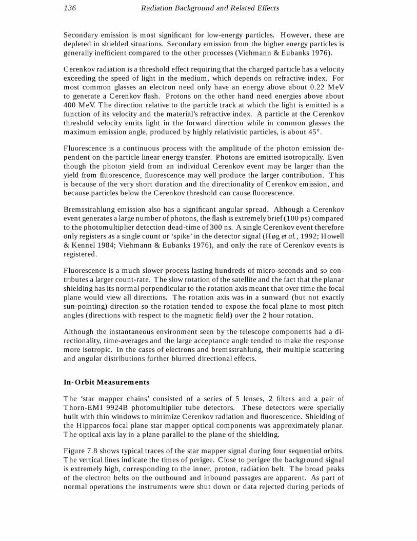
136 Radiation Background and Related Effects
Secondary emission is most significant for low-energy particles. However, these aredepleted in shielded situations. Secondary emission from the higher energy particles isgenerally inefficient compared to the other processes (Viehmann & Eubanks 1976).
Cerenkov radiation is a threshold effect requiring that the charged particle has a velocityexceeding the speed of light in the medium, which depends on refractive index. Formost common glasses an electron need only have an energy above about 0.22 MeVto generate a Cerenkov flash. Protons on the other hand need energies above about400 MeV. The direction relative to the particle track at which the light is emitted is afunction of its velocity and the material’s refractive index. A particle at the Cerenkovthreshold velocity emits light in the forward direction while in common glasses themaximum emission angle, produced by highly relativistic particles, is about 45.
Fluorescence is a continuous process with the amplitude of the photon emission de-pendent on the particle linear energy transfer. Photons are emitted isotropically. Eventhough the photon yield from an individual Cerenkov event may be larger than theyield from fluorescence, fluorescence may well produce the larger contribution. Thisis because of the very short duration and the directionality of Cerenkov emission, andbecause particles below the Cerenkov threshold can cause fluorescence.
Bremsstrahlung emission also has a significant angular spread. Although a Cerenkovevent generates a large number of photons, the flash is extremely brief (100 ps) comparedto the photomultiplier detection dead-time of 300 ns. A single Cerenkov event thereforeonly registers as a single count or ‘spike’ in the detector signal (Høg et al., 1992; Howell& Kennel 1984; Viehmann & Eubanks 1976), and only the rate of Cerenkov events isregistered.
Fluorescence is a much slower process lasting hundreds of micro-seconds and so con-tributes a larger count-rate. The slow rotation of the satellite and the fact that the planarshielding has its normal perpendicular to the rotation axis meant that over time the focalplane would view all directions. The rotation axis was in a sunward (but not exactlysun-pointing) direction so the rotation tended to expose the focal plane to most pitchangles (directions with respect to the magnetic field) over the 2 hour rotation.
Although the instantaneous environment seen by the telescope components had a di-rectionality, time-averages and the large acceptance angle tended to make the responsemore isotropic. In the cases of electrons and bremsstrahlung, their multiple scatteringand angular distributions further blurred directional effects.
In-Orbit Measurements
The ‘star mapper chains’ consisted of a series of 5 lenses, 2 filters and a pair ofThorn-EMI 9924B photomultiplier tube detectors. These detectors were speciallybuilt with thin windows to minimize Cerenkov radiation and fluorescence. Shielding ofthe Hipparcos focal plane star mapper optical components was approximately planar.The optical axis lay in a plane parallel to the plane of the shielding.
Figure 7.8 shows typical traces of the star mapper signal during four sequential orbits.The vertical lines indicate the times of perigee. Close to perigee the background signalis extremely high, corresponding to the inner, proton, radiation belt. The broad peaksof the electron belts on the outbound and inbound passages are apparent. As part ofnormal operations the instruments were shut down or data rejected during periods of
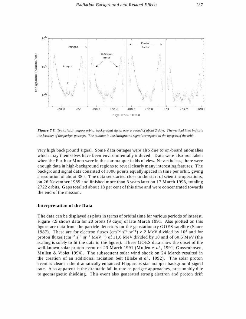
Radiation Background and Related Effects 137
Figure 7.8. Typical star mapper orbital background signal over a period of about 2 days. The vertical lines indicate
the location of the perigee passages. The minima in the background signal correspond to the apogees of the orbit.
very high background signal. Some data outages were also due to on-board anomalieswhich may themselves have been environmentally induced. Data were also not takenwhen the Earth or Moon were in the star mapper fields of view. Nevertheless, there wereenough data in high-background regions to reveal clearly many interesting features. Thebackground signal data consisted of 1000 points equally spaced in time per orbit, givinga resolution of about 38 s. The data set started close to the start of scientific operations,on 26 November 1989 and finished more than 3 years later on 17 March 1993, totaling2722 orbits. Gaps totalled about 18 per cent of this time and were concentrated towardsthe end of the mission.
Interpretation of the Data
The data can be displayed as plots in terms of orbital time for various periods of interest.Figure 7.9 shows data for 20 orbits (9 days) of late March 1991. Also plotted on thisfigure are data from the particle detectors on the geostationary GOES satellite (Sauer1987). These are for electron fluxes (cm−2 s−1 sr−1) > 2 MeV divided by 103 and forproton fluxes (cm−2 s−1 sr−1 MeV−1) of 11.6 MeV divided by 10 and of 60.5 MeV (thescaling is solely to fit the data in the figure). These GOES data show the onset of thewell-known solar proton event on 23 March 1991 (Mullen et al., 1991; Gussenhoven,Mullen & Violet 1994). The subsequent solar wind shock on 24 March resulted inthe creation of an additional radiation belt (Blake et al., 1992). The solar protonevent is clear in the dramatically enhanced Hipparcos star mapper background signalrate. Also apparent is the dramatic fall in rate as perigee approaches, presumably dueto geomagnetic shielding. This event also generated strong electron and proton drift
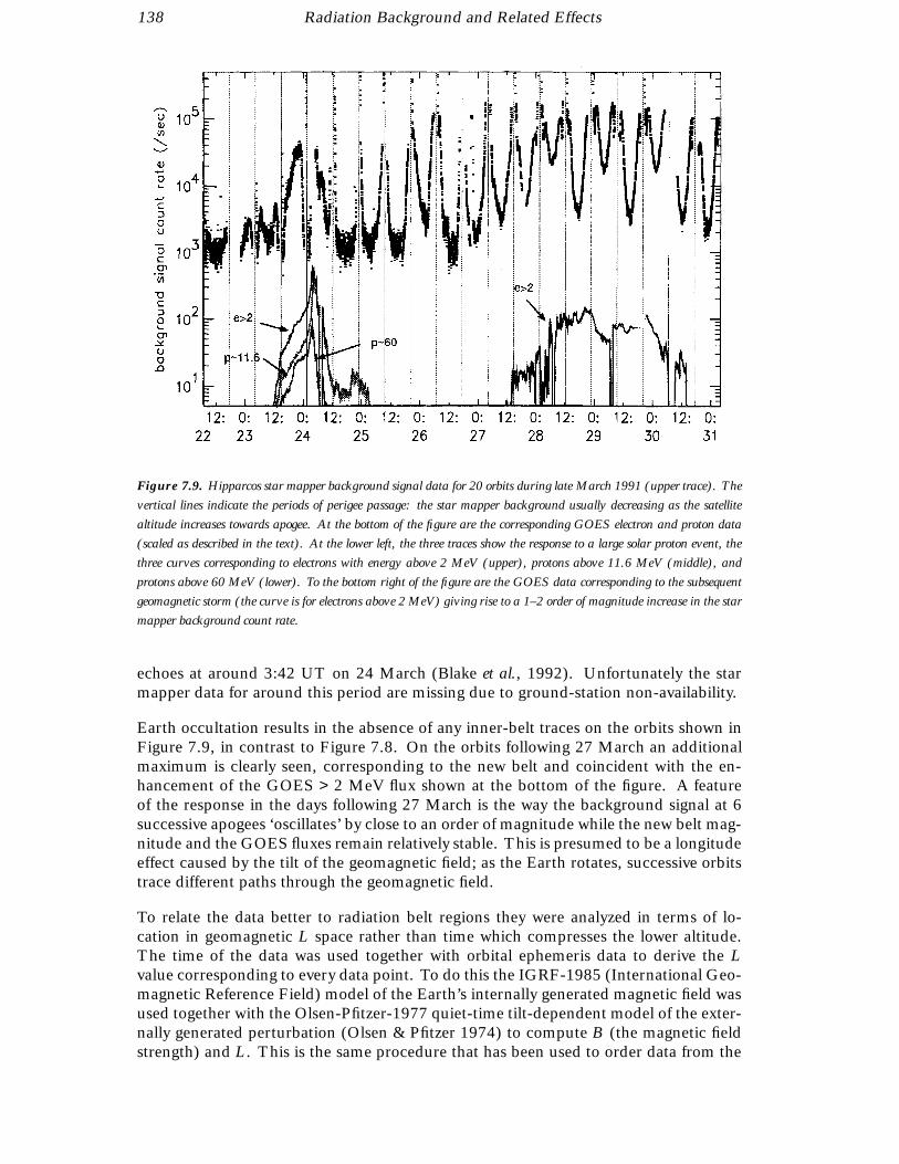
138 Radiation Background and Related Effects
Figure 7.9. Hipparcos star mapper background signal data for 20 orbits during late March 1991 (upper trace). The
vertical lines indicate the periods of perigee passage: the star mapper background usually decreasing as the satellite
altitude increases towards apogee. At the bottom of the figure are the corresponding GOES electron and proton data
(scaled as described in the text). At the lower left, the three traces show the response to a large solar proton event, the
three curves corresponding to electrons with energy above 2 MeV (upper), protons above 11.6 MeV (middle), and
protons above 60 MeV (lower). To the bottom right of the figure are the GOES data corresponding to the subsequent
geomagnetic storm (the curve is for electrons above 2 MeV) giving rise to a 1–2 order of magnitude increase in the star
mapper background count rate.
echoes at around 3:42 UT on 24 March (Blake et al., 1992). Unfortunately the starmapper data for around this period are missing due to ground-station non-availability.
Earth occultation results in the absence of any inner-belt traces on the orbits shown inFigure 7.9, in contrast to Figure 7.8. On the orbits following 27 March an additionalmaximum is clearly seen, corresponding to the new belt and coincident with the en-hancement of the GOES > 2 MeV flux shown at the bottom of the figure. A featureof the response in the days following 27 March is the way the background signal at 6successive apogees ‘oscillates’ by close to an order of magnitude while the new belt mag-nitude and the GOES fluxes remain relatively stable. This is presumed to be a longitudeeffect caused by the tilt of the geomagnetic field; as the Earth rotates, successive orbitstrace different paths through the geomagnetic field.
To relate the data better to radiation belt regions they were analyzed in terms of lo-cation in geomagnetic L space rather than time which compresses the lower altitude.The time of the data was used together with orbital ephemeris data to derive the Lvalue corresponding to every data point. To do this the IGRF-1985 (International Geo-magnetic Reference Field) model of the Earth’s internally generated magnetic field wasused together with the Olsen-Pfitzer-1977 quiet-time tilt-dependent model of the exter-nally generated perturbation (Olsen & Pfitzer 1974) to compute B (the magnetic fieldstrength) and L. This is the same procedure that has been used to order data from the

Radiation Background and Related Effects 139
Combined Release and Radiation Effects Satellite (CRRES, Gussenhoven et al., 1992;Brautigam, Gussenhoven & Mullen 1992). Since the orbit is of low inclination, L aloneshould produce reasonably good ordering of the data. However, as mentioned above,the tilt of the geomagnetic field and the 7 inclination combine with the Earth’s rotationto produce a shift between orbits in L space. In other words subsequent apogees willnot lie on the same L value. Around apogee, different orbital traces which were wellordered (overlapping) in orbital time were sometimes less well ordered when traced inL, indicating that the model fields were inadequate at high altitudes. At low altitudes,organising the data according to L was very effective at revealing the belt structures, evenwith patchy data. L distributions of the data for each orbit were derived by averaging thedata in bins of 0.05 Earth radius in L. The complete mission background signal dataand their temporal and L distribution are summarized in Figure 7.10. In this figure, aswith other authors’ method of plotting CRRES data summaries (Gussenhoven, Mullen& Violet 1994; Brautigam, Gussenhoven & Mullen 1992), the counts are displayed as acolour-scale with the vertical axis corresponding to the radial L variation (the bottom ofthe figure, L = 1, can be thought of as approximately the Earth’s surface) and the hori-zontal axis corresponding to time, covering more than 3 years of data. To condense theplot and in order to remove residual longitude effects, the single-orbit L-distributionswere averaged in 9-orbit segments, corresponding to the repeat period of 4 days. Justover 300 data segments are displayed horizontally, and there are 115 L bins within eachsegment.
The figure clearly illustrates the quiet period from September 1990 until the March 1991event, the subsequent generation of the new radiation belt around L = 2, and the largeevent of July 1991 which was reported to remove some of the new belt (Gussenhoven,Mullen & Violet 1994).
This behaviour was also registered in the Hipparcos solar array degradation, whichdegraded at an unusually slow rate just before the March event and at a fast rateafterwards (Crabb & Robben 1993, see also Chapter 11). The Hipparcos data withits longer time-coverage also captured the events of April 1990, November 1991 and,largest of all, May 1992. The April 1990 event is seen to add slightly to the edge ofthe inner belt for a period of about a month. The November 1991 event produced adistinct narrowing of the second belt. The large May 1992 event, however, producedlittle lasting effect on the inner belt or the second belt which had all but decayed awayby then.
Comparison with CRRES dosimeter data supports the view that both electrons andprotons produced the background signal: the signal was strong in the inner belt belowL = 1.5; it was temporarily very strong in the second inner (L ' 2) belt followingthe March 1991 event but subsequently decayed; and it responded readily to electronevents seen by other spacecraft. In the CRRES data there is less obvious decay of theHiLET second belt (in the region 2 < L < 2.5) than the LoLET second belt whilethe Hipparcos second belt decays noticeably. This would imply that protons are lessimportant. However, the inner belt shows up stronger in the Hipparcos data than inthe LoLET data. From this it appears that in this region Cerenkov radiation fromvery energetic protons is becoming an important component, while at higher altitudes,electrons and bremsstrahlung are the main contributors.
Because inner zone protons capable of generating Cerenkov radiation are of very highenergy, the shielding around the telescope was largely ineffective. These protons there-fore could access the telescope from a much greater range of directions. Using the

140 Radiation Background and Related Effects
Colour figure to be inserted here
Figure 7.10. The L-distribution of the Hipparcos background signal over most of the mission showing several solar
proton events, and the creation and decay of the second inner belt around L = 2 around March 1991. The data are a
4-day (9-orbit) average, binned in 0.05 RE in ordinate. The red regions for L > 3 (corresponding to the outer electron
belt) arise from injection events.
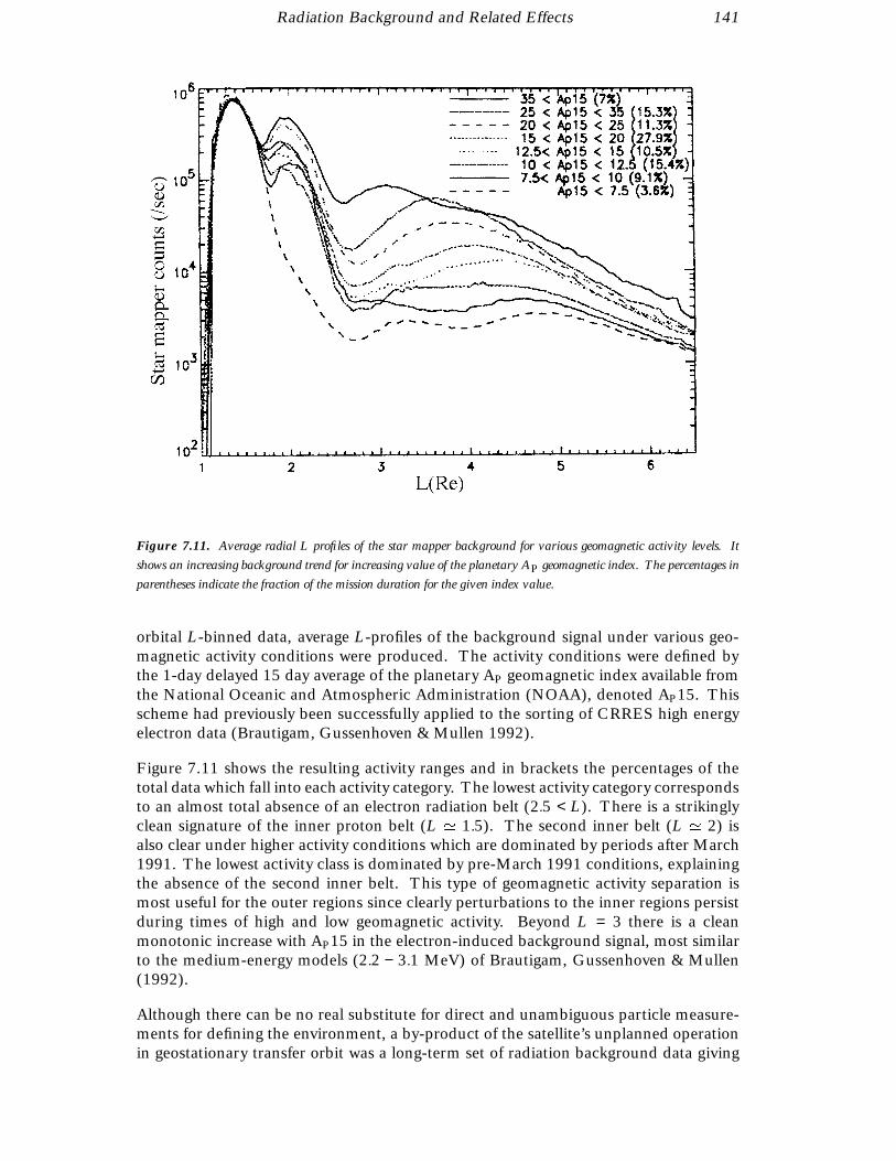
Radiation Background and Related Effects 141
Figure 7.11. Average radial L profiles of the star mapper background for various geomagnetic activity levels. It
shows an increasing background trend for increasing value of the planetary AP geomagnetic index. The percentages in
parentheses indicate the fraction of the mission duration for the given index value.
orbital L-binned data, average L-profiles of the background signal under various geo-magnetic activity conditions were produced. The activity conditions were defined bythe 1-day delayed 15 day average of the planetary AP geomagnetic index available fromthe National Oceanic and Atmospheric Administration (NOAA), denoted AP15. Thisscheme had previously been successfully applied to the sorting of CRRES high energyelectron data (Brautigam, Gussenhoven & Mullen 1992).
Figure 7.11 shows the resulting activity ranges and in brackets the percentages of thetotal data which fall into each activity category. The lowest activity category correspondsto an almost total absence of an electron radiation belt (2.5 < L). There is a strikinglyclean signature of the inner proton belt (L ' 1.5). The second inner belt (L ' 2) isalso clear under higher activity conditions which are dominated by periods after March1991. The lowest activity class is dominated by pre-March 1991 conditions, explainingthe absence of the second inner belt. This type of geomagnetic activity separation ismost useful for the outer regions since clearly perturbations to the inner regions persistduring times of high and low geomagnetic activity. Beyond L = 3 there is a cleanmonotonic increase with AP15 in the electron-induced background signal, most similarto the medium-energy models (2.2 − 3.1 MeV) of Brautigam, Gussenhoven & Mullen(1992).
Although there can be no real substitute for direct and unambiguous particle measure-ments for defining the environment, a by-product of the satellite’s unplanned operationin geostationary transfer orbit was a long-term set of radiation background data giving
142 Radiation Background and Related Effects
information on the radiation environment in important orbital regimes. These dataare interesting in a number of respects. Comparison with data from an overlappingtime period from CRRES facilitates the deduction of the cause of many elements ofthe background signal’s spatial and temporal dependence. As with previous CRRESresults, the data illustrate the highly dynamic nature of the electron component of theradiation environment. They show how the geostationary transfer orbit environment,thoroughly monitored for 14.5 months by CRRES, behaved in the 6 months before and12 months after CRRES. In particular the long-term decay of the second inner (L ' 2)belt following the March 1991 event is seen, the very large event of May 1992 producednegligible effect on the belt structure and the November 1991 event produced a distinctloss from the second belt. Qualitatively, Hipparcos data and CRRES data are consistentduring the overlapping period, especially the LoLET dosimeter in the outer zone andthe secondary inner belt.
Comparison with GOES data following the March 1991 event reveals some interestingfeatures at high altitudes in the background signal data related to geomagnetic fieldeffects. In the inner parts of the orbit there was interesting evidence of geomagneticshielding of solar proton events. While it is not possible to identify a unique particlespecies or detection mechanism, it is reasonable to conclude that the signal is fromCerenkov radiation and fluorescence caused by electrons, protons and bremsstrahlung.
In conclusion, although the geostationary transfer orbit environment can be a severeone, it has its quiet moments. It was never seriously contemplated to perform space-based astronomy from geostationary transfer orbit but these data and the eventualsuccess of the Hipparcos mission show that it is feasible under certain circumstances.The possibility of operating in orbits which are normally considered too hazardous forspacecraft has obvious cost benefits, provided the protection aspects can be managed.These data are highly relevant for ESA’s future space-based astronomy missions whichwill take place in highly-eccentric Earth orbits. They should yield important statistics forobservation planning. They should also provide an interesting additional geostationarytransfer orbit data set to add to those from CRRES. Finally they demonstrate thesuitability of geostationary transfer orbit for radiation-belt and solar-terrestrial studies.

8. THE OBSERVATION PROGRAMMEAND INTERFACE WITH THE
INPUT CATALOGUE CONSORTIUM
This chapter describes the manner in which the satellite scanned the sky (theecliptic-based scanning law). This scanning law ensured even coverage of thesky during the mission lifetime. The observation programme was nominallyfixed before satellite launch, and the entire satellite operations and scientificobservations were conducted on the basis of the pre-defined Hipparcos InputCatalogue. Nevertheless, considerable ‘tuning’ of the observing programmewent on throughout the mission, especially during the early months of themission. Very few objects had significantly erroneous positions or magni-tudes, which were duly corrected as they became evident. Several updatesof the global positions were made on the basis of the early data reductions,in order to improve the real-time attitude determination performances, andresulting photometric measurements. The parameters of the global observingprogramme were also adjusted throughout the mission taking into account thepast and future (expected) observation times allocated to each object. Theway in which the star observations were carried out—by interlacing observa-tions of all stars simultaneously present in the combined field of view of thetelescope—is described. Predicted appearances of the individual stars werecomputed on ground, on the basis of the Hipparcos Input Catalogue, andtarget observation times were pre-computed, based on the star’s magnitudeand priority and, ultimately, on the previous observing history of the star.
8.1. Scanning Law
Scanning Law Definition
Each object in the Hipparcos Input Catalogue was scheduled to be observed manytimes with different scanning orientations (typically some 100 times, although thisvaried considerably according principally to the object’s ecliptic latitude) to increasethe accuracy and precision of the parameters which would constitute the end results ofthe mission. This was achieved by constraining the attitude of the spacecraft to follow acomplex ‘revolving scanning’ motion, called the nominal scanning law, which ensuredreasonably even coverage of the sky over the lifetime of the mission whilst adhering

144 The Observation Programme and Interface with INCA
Figure 8.1. Definition of the telescope reference frame (X, Y, Z). The spin axis of the satellite, Z, precessed around
the sun line at a constant inclination angle of ξ = 43, with the satellite rotating around this axis at a rate of R = 11.25
revolutions per day. E signifies the ecliptic plane, and λs the ecliptic latitude of the Sun. The precession angle, ν, and
the heliotropic angle, Ω, define the elements of the scanning law through Equation 8.8. PFOV and FFOV refer to the
preceding and following fields of view; G is the scanning great circle, and γ is the ‘basic angle’ between the two viewing
directions.
to thermal and other constraints. Three-axis control of the spacecraft was performedby regular firings of cold-gas thrusters (approximately every 10 min). In this way, thespacecraft rotated at 168.75 per hour about its principal rotation axis, which itself wasconstrained to precess at roughly 6.3 per day about a 43 half-cone centred on the Sundirection. It should be noted that the principles of the nominal scanning law, and ofthe programme star file and the star observing strategy, were not affected by the revisedorbit.
The satellite attitude motion was most easily described in terms of the movement of thetelescope with respect to the ecliptic reference system. The telescope reference frame(Figure 8.1) is the rectangular right-handed frame (OXYZ), where the origin, O, is theintersection of the two lines of sight, OP and OF, of the telescope; the plane (X,Y) iscoincident with the plane (P,F); and the X-axis is the bisector of the basic angle POF.The satellite scanning motion was then defined as follows: the Z-axis of the telescopereference frame rotated at a constant angle ξ = 43 around the Sun direction, followingthe Sun in its apparent motion along the ecliptic and performing K = 6.4 revolutionsper year. At the same time, the satellite rotated around the Z-axis in the (X,Y)-planeperforming R = 11.25 revolutions per day. The motions of the axes OP and OF ofthe preceding and following fields of view, which scanned the celestial sphere, resulteddirectly from this scanning motion.

The Observation Programme and Interface with INCA 145
Quantitative Description of the Scanning Law
In precise terms, the nominal sun line is defined by the following orientation:
s(d) = l cos λs + j sin λs [8.1]
l j k being the ecliptic coordinate triad for the mean ecliptic and equinox of J2000.0,and:
λs = L + 2e sin g +54
e2 sin 2g [8.2]
L = −1.386 91 + 0.017 202 124 0d [8.3]
g = −0.041 14 + 0.017 201 969 6d [8.4]
e = +0.016 714 [8.5]
where d is the time in mean solar days from the reference epoch adopted for the nominalscanning law, defined as 1988 January 1, 12h00m00s UTC (in practice, d was definedin terms of the satellite on-board clock).
The composition of the precession of the spin axis Z and the rotation of the Earth (andsatellite) around the Sun resulted in a motion of the Z-axis on the celestial sphere, witha speed designated VZ. The orientation of the telescope reference frame with respect tothe heliotropic reference frame was described by the attitude angles ν, ξ , Ω. The speedVZ was kept approximately constant by modulating the precession angle ν:
ν = ν + a1 cos(ν) + a2 sin(2ν) + a3 cos(3ν) + a4 sin(4ν) [8.6]
where ν = ν0 + 6.4λs, and the coefficients ai are the following:
a1 = −0.163 784 59
a2 = −0.013 077 77
a3 = +0.001 232 43 [8.7]
a4 = +0.000 123 41
The instantaneous spin rate, ωZ, was kept approximately constant by modulating theheliotropic attitude angle, Ω, as follows:
Ω(d) = Ω0 + 2πR(d − d0) − ν cos ξ + (b1ν + b2 cos ν + b3 sin(2ν))sin ξK
[8.8]
where:
b1 = +0.082 152 69
b2 = +0.990 061 17 [8.9]
b3 = +0.040 452 13
The parameters used in the nominal scanning law were the spin rate, R = 11.25 revolu-tions per day (168.75 arcsec s−1), the revolving scanning angle, ξ = 43± 0.5, and theaverage precession rate, K = 6.400 ± 0.002 revolutions per year. The principle of the

146 The Observation Programme and Interface with INCA
Figure 8.2. The scanning motion of the Hipparcos satellite on the celestial sphere, shown in ecliptic coordinates.
The top figure shows the path of the spin axis between 22 May 1990 and 23 September 1991. The scan direction is
indicated by the arrows. The bottom figure shows one reference great circle for each orbit (5 revolutions of the satellite)
for the period between 22 May 1990 and 14 July 1990. The actual scanning was 5 times denser.
scanning measurements is illustrated in Figure 1.1, and the resulting scanning of thecelestial sphere is shown in Figure 8.2.
The above description defines the ‘nominal scanning law’, i.e. the nominal paths of thefields of view on the sky throughout the mission. Deviations of up to ± 10 arcmin aboutthe three satellite axes were tolerated in practice, attitude motion within these limitsbeing controlled autonomously on-board by means of the attitude and orbit controlsystem.
The Observation Programme and Interface with INCA 147
Optional Variations in the Definition
The choice of nominal scanning law parameters had been carefully analysed in the yearspreceding launch to ensure maximum homogeneity of coverage over the entire sky aswell as accuracy of the final catalogue. The results of these studies optimised for thelaunch data of 8 August 1989, gave values of ξ = 43 and ν0 = 40. The value of Ω0 wasless critical and could be defined by ESOC in orbit. The concept employed by ESOCduring the commissioning phase after launch was to use the prescribed values of ξ andν0 to position the rotation axis of the spacecraft at the correct part of the 43 cone. Atthat time, using star pattern recognition techniques with the ground real-time attitudedetermination system, the phase of the fields of view as the spacecraft rotated could becalibrated and hence Ω0 could be derived.
Although ESOC were in principle able to change the nominal scanning law through theground software, mission constraints were prescribed which prevented any change toeither ξ or ν0. In addition Ω0 should only be changed if necessary. Therefore in general,ESOC maintained a constant nominal scanning law throughout the routine (three-gyro)phase of the mission. The only times when it was deemed necessary to change Ω0 duringthis period were during a small number of contingencies where the spacecraft assumeda non-nominal spin rate for a significant period of time. In order to re-acquire attitudecontrol, ESOC had the choice of options, either to perform a large firing of the cold gasthrusters to slew the spacecraft around its principal rotation axis thereby re-acquiringthe previous nominal scanning law attitude, or to calibrate the value of Ω0 for the currentphase and calculate a new mission plan and programme star file. In all cases where thedrift around the rotation axis was more than one or two degrees, the second option wasfaster to implement, safer and less expensive in fuel.
During the two-gyro operations towards the end of the mission, significant drifts aroundthe rotation axis occurred during every perigee, making re-calibration of Ω0 necessaryevery orbit. A full discussion is given in Chapter 15. Moreover, the drifting phase anglealso affected the accuracy of the on-board model for the precession around the 43
cone. The result was that the rotation axis itself was prone to drift. ESOC was thenfaced with a similar but more difficult decision concerning the method of re-acquiringattitude control under these conditions. The options in this case were to perform alarge firing of the cold gas thrusters to slew the spin axis back to that position definedby ν0 = 40 or to calibrate the value of ν0 for the current attitude and calculate a newmission plan and programme star file.
The second option was selected for the same reasons as for Ω0 although it was realisedthat there may be a penalty to pay in terms of homogeneity of coverage. To monitor anypossible biasing, the tables of nominal scanning law parameters used during the missionwere monitored by the NDAC Consortium.
During the final brief period of attempted zero-gyro operations, efforts were madeto initialise the real-time attitude determination in quasi sun-pointing mode wherethe solar aspect angle was close to but not exactly zero (see Chapter 16 for a morecomplete discussion). These attempts were largely unsuccessful, and further attemptswere restricted to using a scanning law with ξ = 0.
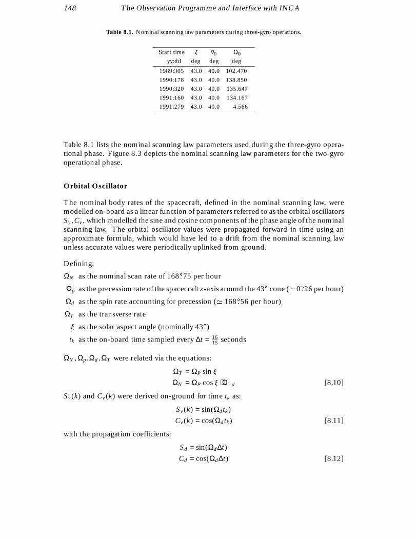
148 The Observation Programme and Interface with INCA
Table 8.1. Nominal scanning law parameters during three-gyro operations.
Start time ξ ν0 Ω0
yy:dd deg deg deg
1989:305 43.0 40.0 102.470
1990:178 43.0 40.0 138.850
1990:320 43.0 40.0 135.647
1991:160 43.0 40.0 134.167
1991:279 43.0 40.0 4.566
Table 8.1 lists the nominal scanning law parameters used during the three-gyro opera-tional phase. Figure 8.3 depicts the nominal scanning law parameters for the two-gyrooperational phase.
Orbital Oscillator
The nominal body rates of the spacecraft, defined in the nominal scanning law, weremodelled on-board as a linear function of parameters referred to as the orbital oscillatorsSv , Cv, which modelled the sine and cosine components of the phase angle of the nominalscanning law. The orbital oscillator values were propagated forward in time using anapproximate formula, which would have led to a drift from the nominal scanning lawunless accurate values were periodically uplinked from ground.
Defining:
ΩN as the nominal scan rate of 168.75 per hour
Ωp as the precession rate of the spacecraft z-axis around the 43 cone (' 0.26 per hour)
Ωd as the spin rate accounting for precession (' 168.56 per hour)
ΩT as the transverse rate
ξ as the solar aspect angle (nominally 43)
tk as the on-board time sampled every ∆t = 1615 seconds
ΩN , Ωp, Ωd , ΩT were related via the equations:
ΩT = ΩP sin ξ
ΩN = ΩP cos ξ + Ωd [8.10]
Sv(k) and Cv(k) were derived on-ground for time tk as:
Sv(k) = sin(Ωd tk)
Cv(k) = cos(Ωd tk) [8.11]
with the propagation coefficients:
Sd = sin(Ωd ∆t)
Cd = cos(Ωd ∆t) [8.12]
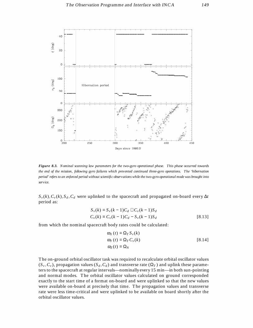
The Observation Programme and Interface with INCA 149
Figure 8.3. Nominal scanning law parameters for the two-gyro operational phase. This phase occurred towards
the end of the mission, following gyro failures which prevented continued three-gyro operations. The ‘hibernation
period’ refers to an enforced period without scientific observations while the two-gyro operational mode was brought into
service.
Sv(k), Cv(k), Sd , Cd were uplinked to the spacecraft and propagated on-board every ∆tperiod as:
Sv(k) = Sv(k − 1)Cd + Cv(k − 1)Sd
Cv(k) = Cv(k − 1)Cd − Sv(k − 1)Sd [8.13]
from which the nominal spacecraft body rates could be calculated:
ωX (t) = ΩT Sv(k)
ωY (t) = ΩT Cv(k) [8.14]
ωZ (t) = ΩN
The on-ground orbital oscillator task was required to recalculate orbital oscillator values(Sv , Cv), propagation values (Sd , Cd ) and transverse rate (ΩT ) and uplink these parame-ters to the spacecraft at regular intervals—nominally every 15 min—in both sun-pointingand normal modes. The orbital oscillator values calculated on ground correspondedexactly to the start time of a format on-board and were uplinked so that the new valueswere available on-board at precisely that time. The propagation values and transverserate were less time-critical and were uplinked to be available on board shortly after theorbital oscillator values.
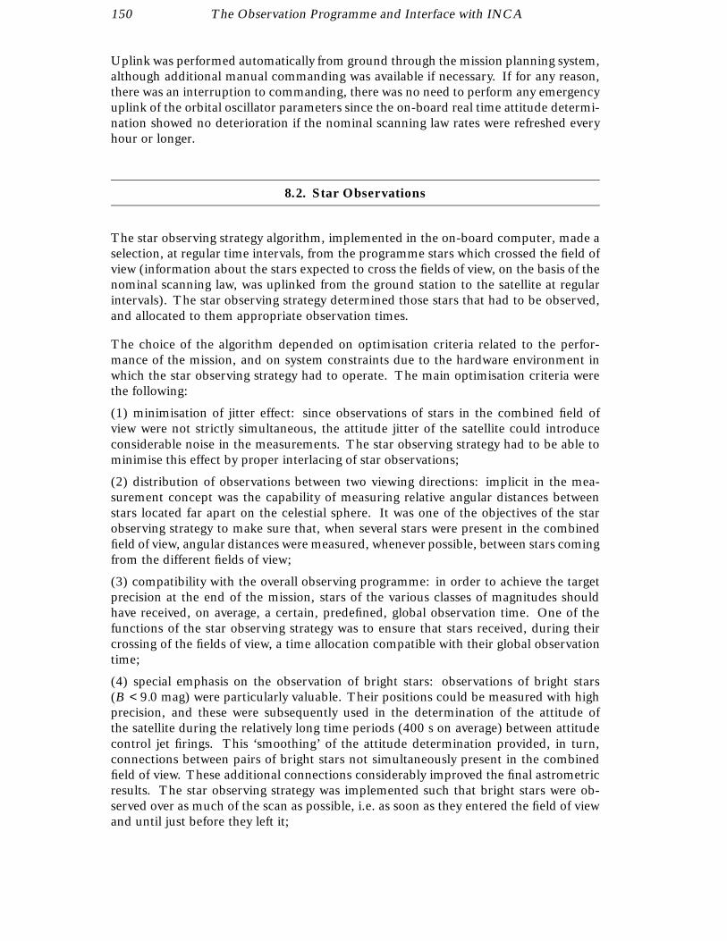
150 The Observation Programme and Interface with INCA
Uplink was performed automatically from ground through the mission planning system,although additional manual commanding was available if necessary. If for any reason,there was an interruption to commanding, there was no need to perform any emergencyuplink of the orbital oscillator parameters since the on-board real time attitude determi-nation showed no deterioration if the nominal scanning law rates were refreshed everyhour or longer.
8.2. Star Observations
The star observing strategy algorithm, implemented in the on-board computer, made aselection, at regular time intervals, from the programme stars which crossed the field ofview (information about the stars expected to cross the fields of view, on the basis of thenominal scanning law, was uplinked from the ground station to the satellite at regularintervals). The star observing strategy determined those stars that had to be observed,and allocated to them appropriate observation times.
The choice of the algorithm depended on optimisation criteria related to the perfor-mance of the mission, and on system constraints due to the hardware environment inwhich the star observing strategy had to operate. The main optimisation criteria werethe following:
(1) minimisation of jitter effect: since observations of stars in the combined field ofview were not strictly simultaneous, the attitude jitter of the satellite could introduceconsiderable noise in the measurements. The star observing strategy had to be able tominimise this effect by proper interlacing of star observations;
(2) distribution of observations between two viewing directions: implicit in the mea-surement concept was the capability of measuring relative angular distances betweenstars located far apart on the celestial sphere. It was one of the objectives of the starobserving strategy to make sure that, when several stars were present in the combinedfield of view, angular distances were measured, whenever possible, between stars comingfrom the different fields of view;
(3) compatibility with the overall observing programme: in order to achieve the targetprecision at the end of the mission, stars of the various classes of magnitudes shouldhave received, on average, a certain, predefined, global observation time. One of thefunctions of the star observing strategy was to ensure that stars received, during theircrossing of the fields of view, a time allocation compatible with their global observationtime;
(4) special emphasis on the observation of bright stars: observations of bright stars(B < 9.0 mag) were particularly valuable. Their positions could be measured with highprecision, and these were subsequently used in the determination of the attitude ofthe satellite during the relatively long time periods (400 s on average) between attitudecontrol jet firings. This ‘smoothing’ of the attitude determination provided, in turn,connections between pairs of bright stars not simultaneously present in the combinedfield of view. These additional connections considerably improved the final astrometricresults. The star observing strategy was implemented such that bright stars were ob-served over as much of the scan as possible, i.e. as soon as they entered the field of viewand until just before they left it;

The Observation Programme and Interface with INCA 151
(5) minimisation of errors due to grid imperfections: imperfections in the manufactureof the grid could induce errors in the phase measurements of a star. These errors wereconsiderably reduced by a proper choice of the observation scheme.
The main system constraints related to the hardware environment in which the starobserving strategy had to operate were the memory and time limitations of the on-boardcomputer; the synchronisation with the telemetry format, the attitude and orbit controlsystem, and the cold gas thruster firing; and constraints due to the downlink telemetryresources.
The Star Observing Strategy
The star observing strategy algorithm was built around a rigid time hierarchy and itsoperation was driven by three star-dependent parameters uplinked from ground. Thetime hierarchy was based on the following definitions:
(1) the sampling period, T1 = 11200 s, was the sampling time during which photoelectron
counts were accumulated by the image dissector tube;
(2) the instantaneous field of view repositioning period, T2 = 8T1 = 1150 s, was the
shortest time interval (or ‘slot’) during which the instantaneous field of view remainedpointed on a given star. Each star was always observed for an integer number of slots,and the instantaneous field of view remained pointed at the same location on the gridthroughout a slot. If a star was observed for more than one slot, the position of theinstantaneous field of view was updated for the next slot;
(3) the interlacing period, T3 = 20T2 = 215 s, was the period of time during which a
group of up to 10 stars were observed;
(4) the observation frame period, T4 = 16T3 = 2.133 . . . s, was the period of time duringwhich essentially the same group of stars were observed in the same order and with agiven observation time allocation (exceptions are discussed below);
(5) the transit time, T5 = 9T4 = 19.2 s, was roughly the time interval taken for any givenstar to cross one of the fields of view of the telescope.
Star-Dependent Parameters
The star-dependent parameters uplinked from ground, and on which the star observingalgorithm operated, were:
(1) the selection index: the parameter used to calculate the priority with which a pro-gramme star must be observed with respect to the other programme stars simultaneouslypresent in the field of view;
(2) the minimum observation time: the minimum number of slots of T2 which, at framelevel, had to be allocated to a star in order to achieve a sufficient precision in phaseextraction (this was a function of the magnitude of the star);
(3) the target observation time: the observation time which, at frame level, had tobe allocated to a given star in order to achieve, at the end of the mission, the globalobservation time associated with that star (this was also a function of the magnitude ofthe star).

152 The Observation Programme and Interface with INCA
The values of the star-dependent parameters could vary during the mission, to take intoaccount the past and projected observational history of the star, but they were fixedduring each crossing of the field of view by the star. The values of the minimum andtarget observation times for a star of given magnitude were determined on the basis ofsimulations carried out by the INCA Consortium and the data reduction consortia, andwere uplinked during the mission from ESOC to the satellite, where the star observingstrategy was implemented.
Other parameters included in the star observing strategy algorithm were: the pre-dicted time of entrance of the star in the field of view; its magnitude; a flag indicatingwhether the star was observed in the preceding or following viewing direction; and a flagindicating whether the star should have been observed by the star mapper for attitude-measurement purposes (a subset of some 40 000 programme stars, in particular brightstars with good a priori positional accuracies, fell into this category).
During the operations, ESOC processed the data derived from the Hipparcos InputCatalogue and the observational history of the programme stars to produce a so-called‘programme star file’, which contained the information to be uplinked to the satellite.The programme star file contained star identifications, magnitudes, field of view enteringtimes, viewing direction flags (the transverse coordinate needed for detector pilotingand real-time attitude estimation), and the current values of the three star-dependentparameters discussed above. A scheme for the data processing involved in the generationof the programme star file is shown in Figure 8.4.
Fully and Partially Observable Stars
When a frame of T4 = 2.133 . . . s was considered, stars that remained in the combinedfield of view during the entire frame were called fully observable stars; those that re-mained in the combined field of view only for a part of the frame, but not less than threeinterlacing periods (3T3), were called partially observable stars—these could be starsthat either left or entered the combined field of view during the frame period.
One way to visualise the flow of programme stars in and out of the combined field ofview is by means of a time diagram, such as that shown in Figure 8.5. A star Si enteredthe field of view at time ti
0 and left it at time ti0 + T5. The ‘transit line’:
fi(t) =t − ti
0
T5[8.15]
represents the fraction of transit time spent by the star in the field of view:
0 ≤ fi(t) ≤ 1 [8.16]
The stars that were present in the field of view at a given time t0 could easily be identifiedby drawing the line t = t0: they are those whose transit lines are intercepted by t = t0.
By marking on the t-axis the time intervals corresponding to subsequent frames ofT4 = 2.133 . . . s, one can also identify the stars present in a given frame. For example,in frame number 10 of Figure 8.5, there are three stars present in the combined fieldof view, of which two are fully observable stars and one is a partially observable star,leaving the field of view before the end of the frame period.
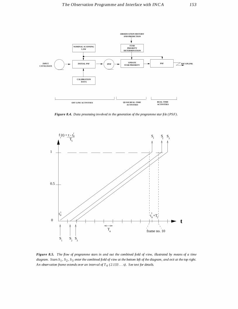
The Observation Programme and Interface with INCA 153
INPUTCATALOGUE
NOMINAL SCANNINGLAW
INITIAL PSF
CALIBRATIONDATA
STARPRIORITY
DETERMINATION
UPDATESTAR PRIORITY
QUASI REAL-TIMEACTIVITIES
REAL-TIMEACTIVITIES
OBSERVATION HISTORYAND PREDICTION
IPSF PSF
OFF-LINE ACTIVITIES
PSF UPLINK
Figure 8.4. Data processing involved in the generation of the programme star file (PSF).
S S S31 2
t
0.5
0
1
frame no. 10T4
S3i
t +T1
0 5
i0
T5
0
S1
S2
t 1
f (t) = t - t
Figure 8.5. The flow of programme stars in and out the combined field of view, illustrated by means of a time
diagram. Stars S1, S2, S3 enter the combined field of view at the bottom left of the diagram, and exit at the top right.
An observation frame extends over an interval of T4 (2.133 . . . s). See text for details.
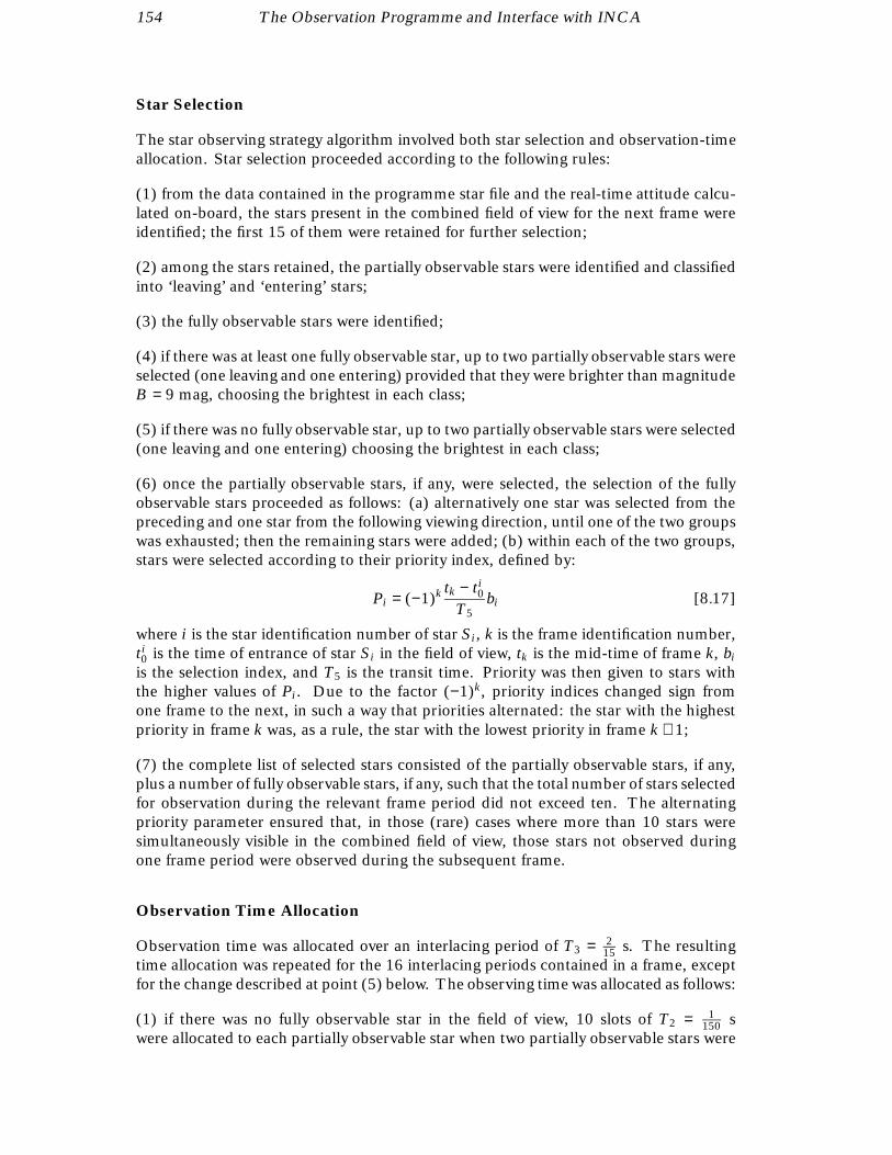
154 The Observation Programme and Interface with INCA
Star Selection
The star observing strategy algorithm involved both star selection and observation-timeallocation. Star selection proceeded according to the following rules:
(1) from the data contained in the programme star file and the real-time attitude calcu-lated on-board, the stars present in the combined field of view for the next frame wereidentified; the first 15 of them were retained for further selection;
(2) among the stars retained, the partially observable stars were identified and classifiedinto ‘leaving’ and ‘entering’ stars;
(3) the fully observable stars were identified;
(4) if there was at least one fully observable star, up to two partially observable stars wereselected (one leaving and one entering) provided that they were brighter than magnitudeB = 9 mag, choosing the brightest in each class;
(5) if there was no fully observable star, up to two partially observable stars were selected(one leaving and one entering) choosing the brightest in each class;
(6) once the partially observable stars, if any, were selected, the selection of the fullyobservable stars proceeded as follows: (a) alternatively one star was selected from thepreceding and one star from the following viewing direction, until one of the two groupswas exhausted; then the remaining stars were added; (b) within each of the two groups,stars were selected according to their priority index, defined by:
Pi = (−1)k tk − ti0
T5bi [8.17]
where i is the star identification number of star Si , k is the frame identification number,ti0 is the time of entrance of star Si in the field of view, tk is the mid-time of frame k, bi
is the selection index, and T5 is the transit time. Priority was then given to stars withthe higher values of Pi . Due to the factor (−1)k, priority indices changed sign fromone frame to the next, in such a way that priorities alternated: the star with the highestpriority in frame k was, as a rule, the star with the lowest priority in frame k + 1;
(7) the complete list of selected stars consisted of the partially observable stars, if any,plus a number of fully observable stars, if any, such that the total number of stars selectedfor observation during the relevant frame period did not exceed ten. The alternatingpriority parameter ensured that, in those (rare) cases where more than 10 stars weresimultaneously visible in the combined field of view, those stars not observed duringone frame period were observed during the subsequent frame.
Observation Time Allocation
Observation time was allocated over an interlacing period of T3 = 215 s. The resulting
time allocation was repeated for the 16 interlacing periods contained in a frame, exceptfor the change described at point (5) below. The observing time was allocated as follows:
(1) if there was no fully observable star in the field of view, 10 slots of T2 = 1150 s
were allocated to each partially observable star when two partially observable stars were

The Observation Programme and Interface with INCA 155
selected, or all 20 slots of T2 to the one partially observable star, if only one partiallyobservable star was selected;
(2) if there was at least one fully observable star in the field of view, two slots wereallocated to each partially observable star selected. Once the observation time allocationto partially observable stars was completed, the remaining slots available were allocatedto the selected fully observable stars as follows:
(3) each fully observable star was allocated, in sequence, its minimum observation time,until either the list of stars was exhausted or the number of slots available (20) in theinterlacing period was exceeded. In the latter case, the remaining fully observable starswere dropped from the observation list and no longer considered. In the absence of anypartially observable stars, at least two fully observable stars, if present, would alwaysbe observed, by allocating, if necessary, an observation time shorter than the minimumobservation time (for the faintest stars the nominal minimum observation time waslarger than 10 slots);
(4) the remaining slots, if any, were allocated one by one to the fully observable starsactually observed, on the basis of their so-called ‘performance index’ zi , defined as:
zi =ni
ti[8.18]
where ni is the actual number of slots which had already been allocated to the star inthe interlacing period, and ti is the target time. The first available slot was allocated tothe star with the lowest performance index, and so on;
(5) if a partially observable star was actually observed, the 2 slots which were free whenthe star was not present in the field were allocated to the fully observable star with thelowest performance index—referred to below as its ‘associated’ fully observable star.
Execution of the Observing Sequence
The observation sequence was then executed in the following order:
(1) in each interlacing period fully observable stars were observed in order of entry;
(2) all slots devoted to the same star were contiguous;
(3) during the interlacing periods in which partially observable stars were present, theobservation slots of each partially observable star were contiguous with the ones of itsassociated fully observable star;
(4) the entering partially observable star was observed after its associated fully observablestar;
(5) the leaving partially observable star was observed before its associated fully observ-able star;
(6) if there was no fully observable star, the leaving partially observable star was observedbefore the entering partially observable star.
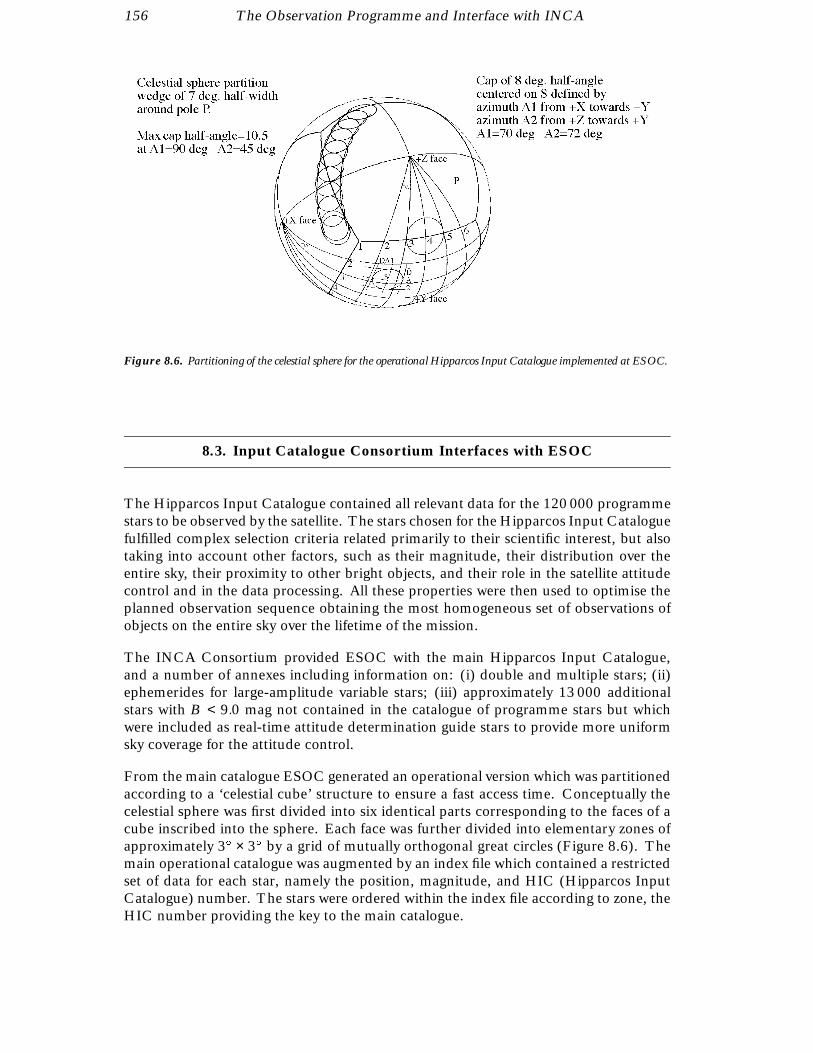
156 The Observation Programme and Interface with INCA
Figure 8.6. Partitioning of the celestial sphere for the operational Hipparcos Input Catalogue implemented at ESOC.
8.3. Input Catalogue Consortium Interfaces with ESOC
The Hipparcos Input Catalogue contained all relevant data for the 120 000 programmestars to be observed by the satellite. The stars chosen for the Hipparcos Input Cataloguefulfilled complex selection criteria related primarily to their scientific interest, but alsotaking into account other factors, such as their magnitude, their distribution over theentire sky, their proximity to other bright objects, and their role in the satellite attitudecontrol and in the data processing. All these properties were then used to optimise theplanned observation sequence obtaining the most homogeneous set of observations ofobjects on the entire sky over the lifetime of the mission.
The INCA Consortium provided ESOC with the main Hipparcos Input Catalogue,and a number of annexes including information on: (i) double and multiple stars; (ii)ephemerides for large-amplitude variable stars; (iii) approximately 13 000 additionalstars with B < 9.0 mag not contained in the catalogue of programme stars but whichwere included as real-time attitude determination guide stars to provide more uniformsky coverage for the attitude control.
From the main catalogue ESOC generated an operational version which was partitionedaccording to a ‘celestial cube’ structure to ensure a fast access time. Conceptually thecelestial sphere was first divided into six identical parts corresponding to the faces of acube inscribed into the sphere. Each face was further divided into elementary zones ofapproximately 3 × 3 by a grid of mutually orthogonal great circles (Figure 8.6). Themain operational catalogue was augmented by an index file which contained a restrictedset of data for each star, namely the position, magnitude, and HIC (Hipparcos InputCatalogue) number. The stars were ordered within the index file according to zone, theHIC number providing the key to the main catalogue.

The Observation Programme and Interface with INCA 157
In deriving the operational input catalogue various other parameters were computed,including, (a) variability flags, (b) target observation times, (c) lower and upper min-imum observation times, (d) accuracy test vectors and (e) initial covariance matricesfor the modulation strategy. The target observing time, t, represented the mean time astar should be observed when crossing one of the fields of view. It was derived from theoverall target time T (for the entire mission) and the average number N (β) of crossingsthroughout the mission, where β was the ecliptic latitude of the star, and was given by:
t = T /N (β) [8.19]
where T (in seconds) was a function of the Hipparcos magnitude (Hp):
T = −750 + 560Hp − 89.5Hp2 + 4.88Hp3 (Hp > 5.0)
T = 420 (Hp ≤ 5.0) [8.20]
N (β) was derived by interpolation from Table 8.2.
Hipparcos Input Catalogue Updating
As the data reduction consortia processed the science data, more accurate positionswere determined for the catalogue stars. These results were made available to ESOC foruse in the programme star file, thereby improving the overall accuracy, not only of theinstantaneous field of view positioning, but also of the real-time attitude determinationperformance, which in turn led to further improvements in overall mission accuracies.In addition, a small number of star positions and magnitudes had to be corrected at thestart of the mission. Table 8.3 provides a summary of the principal catalogue updatescarried out at ESOC during the mission.
Variable Star Ephemerides
Large-amplitude variable stars required special consideration since, to optimise observ-ing time, it was important to be able to predict their apparent magnitudes. This wasdone by using specific variable star ephemerides, provided by the INCA Consortium.Once a variable star had been observed by the satellite, the data was processed at ESOCand the results were communicated back to the INCA Consortium, once per month,to further refine the ephemerides. Periodically, a new version of these ephemerides wassent to ESOC for use in generating the programme star file (see Table 8.3).
ESOC processed the observations of variable stars in two stages: (i) payload monitoring,performed in near real-time, and (ii) payload reporting, running off-line. The payloadmonitoring software is described in detail in Chapter 10. Every 60 s, the programselected one star observed in the preceding 30 s. The selection criteria were heavilyweighted in favour of the large-amplitude variable stars, so that if one was present in theinterval it was invariably selected for processing.
The second payload reporting program ran daily on the off-line main-frame computerat ESOC processing the previous 24 hours of payload monitoring results, and compil-ing statistics on various aspects of the general results. In addition, a longer run wasperformed every week specifically to obtain the large-amplitude variable star results.

158 The Observation Programme and Interface with INCA
Table 8.2. Mean scanning frequency as a function of ecliptic latitude.
jβj 0 10 20 30 40 47 55 65 75 85 90
N (β) 120 124 134 148 190 280 200 164 150 146 146
Piloting and Magnitude Monitoring
The main reason for running payload reporting every 24 hours was to obtain informationconcerning the intervals when image dissector tube piloting was ‘good’ in some sense.The intervals of ‘good’, ‘bad’ and ‘unknown’ image dissector tube piloting were used bythe FAST and NDAC Consortia who only processed data when piloting was ‘good’. Ahistory of the piloting throughout the mission was held on a sequential file on the IBMmain-frame. The information was also used by the observation modulation strategysoftware which updated observation priorities in the newly generated programme starfile given the previous history of observations.
‘Good’ piloting was defined to be when the last three payload monitoring reports fromboth fields of view, showed agreement between predicted and measured Hp magnitudesto within 1.5 mag. ‘Bad’ piloting was defined to be when three consecutive payloadmonitoring reports from one field of view disagreed by more than 1.5 mag in theirpredicted and measured Hp magnitudes. ‘Unknown’ piloting was defined when therewere no payload monitoring reports for over 45 min (usually during loss of signal aroundperigee). Piloting status flags in the telemetry data stream switched when any of theseconditions were satisfied.
This piloting information was incorporated into the variable star reports which weregenerated in the weekly runs of payload reporting. The main processing steps withinthe payload reporting task which were relevant for variable star processing and imagedissector tube piloting determination were:
(1) each payload monitoring record in the prescribed interval was extracted from thehistory file (normally extending some 20 days in the past);
(2) the predicted Hp magnitude was extracted from the input catalogue for the non-variable stars. For the variable stars the predicted Hp magnitude was calculated bylinear interpolation from the ephemerides (data points separated by 10 days);
(3) the image dissector tube piloting at the time of observation was extracted from thepiloting file if the data was available from previous results from payload reporting;
(4) the measured Hp magnitude was calculated (as described below). A record waswritten to the variable star report file containing the following information:
– time of on-board observation;– Hipparcos Input Catalogue (HIC) identifier of monitored star;– blue magnitude of star;– colour of star;– sample count, i.e. observation time in units of 1/1200 s;– quality of preceding observation (see Chapter 10);– quality of image dissector tube piloting;
The Observation Programme and Interface with INCA 159
– field of view indicator (1 for preceding, 2 for following);– observed intensity, I0 in counts per s;– measured modulation coefficient M1;– measured modulation coefficient M2;– predicted Hp magnitude;– measured Hp magnitude;– the difference between the predicted and measured Hp magnitudes.
The measured Hp magnitude as calculated above was dependent on (i) the measuredcount rate I0; (ii) the field of view, = +1 (preceding field of view), = −1 (followingfield of view); (iii) the coordinates of the star on the main grid (G, H), and (iv) thecolour index of star, c = B − V − 0.5.
A calibration of the transformation between measured count rates and Hp magnitudewas conducted routinely by the FAST Consortium’s ‘first-look’ facility at Utrecht. Thecalibration was performed using a least-squares fit, for photometric standard stars only,to the 17 unknown coefficients ri in the following equations:
R = r0 + r1 + r2I0 + r3I 20 + r4G + r5H + r6G2 + r7GH + r8H2 + r9G3 [8.21]
+ r10G2H + r11GH2 + r12H3 + r13c + r14c2 + r15cG + r16cH
and:IC = IR R 100.4(9−Hp) [8.22]
where IC is the corrected value of I0 for a star of Hipparcos magnitude Hp and IR isa reference intensity for a star of magnitude Hp = 9 mag. (IR = 1760 for the imagedissector tube used throughout the mission). With IR known and R calculated, theHipparcos magnitude was given by:
Hp = 9 − 2.5 log10(I0 /(IRR)) [8.23]
Minor and Major Planet Ephemerides
In addition to the stars defined in the Hipparcos Input Catalogue, several solar systemobjects were contained within the original observing programme: 48 minor planets;the Jovian moon, Europa; and the Saturnian moon, Titan. In order to schedule theseobjects within the programme star file, accurate ephemerides for the major and minorplanets were provided by the Bureau des Longitudes. These ephemerides were updatedon a regular basis. In addition, a further Saturnian moon, Iapetus, was added to theobserving programme part way through the mission. It had been expected that theMoon’s brightness and separation from Saturn would make it a difficult candidate forobservation. Nevertheless, the payload proved to be sufficiently sensitive to be able tomake a series of good observations.
One other object which was added after the mission was started was the quasar 3C 273.This object, always considered to be at the very limit of the satellite’s observationalcapabilities, was added in view of its possible role in defining an inertial reference system.As expected, however, the observations of this object provided very little additionalweight in this respect.

160 The Observation Programme and Interface with INCA
Table 8.3. History of principal catalogue updates at ESOC.
Date Description
01/12/89 Hipparcos Input Catalogue Version 6
20/12/89 Variable Star Ephemerides
23/03/90 Variable Star Ephemerides
21/06/90 Minor Planet Ephemerides
04/07/90 Hipparcos Input Catalogue Version 7
04/07/90 Variable Star Ephemerides
27/10/90 Variable Star Ephemerides
22/01/91 Variable Star Ephemerides
21/02/91 Hipparcos Input Catalogue Version 8
21/04/91 Hipparcos Input Catalogue Version 9
03/07/91 Minor Planet Ephemerides
03/07/91 Variable Star Ephemerides
06/08/91 Major Planet Ephemerides
06/08/91 Minor Planet Ephemerides
22/11/91 Europe, Titan, Iapetus Ephemerides
19/03/92 Variable Star Ephemerides
01/12/92 Hipparcos Input Catalogue Version 10
30/11/92 Minor Planet Ephemerides
16/12/92 Europe, Titan, Iapetus Ephemerides
History of Hipparcos Input Catalogue Updates during Operations
Table 8.3 lists the main updates which were made to the various catalogues andephemerides throughout the mission. Versions 1 to 5 of the Hipparcos Input Cata-logue were implemented at ESOC before launch. Smaller incremental changes wereoccasionally made at other times.
8.4. Programme Star File Generation
Basic Methodology
To hold the complete Hipparcos Input Catalogue (with details of the 120 000 starsand other objects to be observed) on-board and implement the observation strategy de-scribed in the previous section would have imposed too much of a computational burdenon the on-board computer. The solution was to hold only the relevant star observationparameters for the next 20–30 minutes, and to refresh it by regular commands fromground. This buffer was called the ‘programme star file’.
The programme star file contained star identifications, magnitudes, field of view entrytimes, field of view identifications and the observation strategy parameters discussedin the previous section. The observation duration was calculated taking into accountthe brightness of the star (the fainter the star the longer the observation), its scientific

The Observation Programme and Interface with INCA 161
priority, the number of other programme stars within the field of view competing for theavailable observing time, and the number of times the star had already been observedduring the mission. Because there were long periods without ground station support,some stars were under-observed over a particular time interval. Consequently, therelative importance of observing these stars later was increased. In this way, all the starsin the catalogue were observed sufficiently to provide reasonably uniform accuracies inposition, parallax and proper motion, by the end of the mission.
The off-line IBM mainframe at ESOC prepared an on-ground ‘extended programmestar file’, from where it was transferred to the Hipparcos dedicated control system on thereal-time VAX. The extended programme star file contained not only data required bythe on-board programme star file, but also additional data required for the on-groundpayload monitoring software.
During the routine operational phase, the extended programme star file was generatedon a daily basis, then transferred and uplinked regularly. In the two- and zero-gyrooperational phases, where the nominal scanning law parameters were varying afterevery perigee, the extended programme star file could only be generated once the newnominal scanning law parameters had been determined. A history of the latest two weeksof data was maintained to allow post processing for payload calibration activities andmaintenance of the modulation strategy. The creation of the daily extended programmestar file is summarised as follows:
(1) a coarse selection was made of objects which would cross the field of view inthe given period. The basic principle was to calculate the nominal scanning lawattitude at very close intervals of time and for each field of view extract from the starcatalogue the stars which were in the vicinity of the pointing directions. For eachcandidate star, an accurate transit time and ordinate was computed. If the ordinatewas within the allowed range a star transit record was generated. This selectionprocedure was made efficiently through the use of the partitioned operational inputcatalogue (see Section 8.3);
(2) as soon as a star had been selected in the coarse selection phase, its accurate transittime was computed, taking account of: (a) proper motion in ecliptic longitudeand latitude, (b) parallaxes for nearby stars, and (c) stellar aberration due to thecombined motions of the spacecraft around the Earth and the Earth around theSun;
(3) observation parameters were computed for each object to be observed on the maingrid. These observation parameters were the minimum observation time expressedin a number of slots per interlacing period and the target observation time expressedin a number of slots per frame (2.133 . . . s). These two parameters were used bythe on-board star observation strategy to share the observation time between theprogramme stars present in the combined field of view (see previous section). Forprogramme stars, these parameters were derived from the initial values modulatedby the current observation history, characterised by the covariance matrix B (de-scribed in Section 8.5). For variable stars and solar system objects the observationparameters were only a function of the current magnitude and the ecliptic latitude.
In addition to nominal programme star files, ESOC were responsible for generatingthe special programme star files to support the initial calibration activities (Chapter 5).These programme star files were classified into two categories: those derived from thenominal scanning law, but with special requirements on the stars to be observed (e.g.
162 The Observation Programme and Interface with INCA
star magnitude, star density) and those derived from a non-nominal scanning law (e.g.the non-nominal sun-pointing operations with solar aspect angle ξ = 0).
Mission planning products acted as input for the extended programme star file gener-ation since the mission plan (generated on a weekly basis) provided the times of anyspecial calibration, Earth and Moon occultations when one or both fields of view wereobscured, and ground station outage when a sparse programme star file was required(see below). A fuller description of the mission planning system is given in Section 4.6.
Real-Time Attitude Determination Guide Stars
Approximately 60 per cent of all programme stars were selected as guide stars for theon-board attitude control. The conditions for selection were that (a) the star had avariability range less than 0.02 mag; (b) its BT magnitude was in the range 5.0–9.5 mag;and (c) its position accuracy was better than 0.8 arcsec. A component of a double ormultiple star system could be selected if certain additional conditions were satisfied:(a) the distance to other components was larger than 23 arcsec; or (b) the differencein magnitude was larger than 1.5 for separations between 0.8 and 23 arcsec; or (c)for a separation not exceeding 0.8 arcsec, the root-mean-square of the separation andposition accuracy did not exceed 0.8 arcsec.
Sparse Programme Star File
Significant modifications to the programme star file generation software were necessaryfor the revised mission. With the revised elliptical orbit, non-coverage periods lastingseveral hours were occurring routinely. Particularly, during the first months of the re-vised mission, before two further ground stations were made available on a regular basis,complete orbits were without coverage at times. Given that there was only sufficientmemory for a nominal programme star file to last for about 20–30 min, real-time attitudedetermination would have diverged within a few minutes of the end of the programmestar file. For an extended loss of coverage lasting 10 hours, the attitude of the spacecraftcould have deviated from the nominal scanning law sufficiently to cause the on-boardemergency sun acquisition mode to trigger.
This prompted the development of the so called ‘sparse programme star file’ for non-coverage periods to ensure permanent convergence of real-time attitude determination.This sparse programme star file consisted of only the brightest reference stars, spanningthe non-visibility periods of up to 12 hours, thus providing continuous information forthe attitude control system between two successive stations’ support.
Alternating Strategy
On 20 September 1991, the programme star file generation software was revised toinclude an alternating selection strategy for stars in the open cluster NGC 2516, wherefour stars in a small region of the sky were added to the programme to serve as calibrationobjects for the Fine Guidance Sensors on-board the Hubble Space Telescope.
Straightforward inclusion of these stars was not possible, as they exceeded the pro-gramme star file requirements for adequate observation time for each object. Thesolution was to allow approximately half the objects to be observed during one rotation
The Observation Programme and Interface with INCA 163
period of the spacecraft, then to allow those which were not observed in the previousperiod to be observed in the following. Subsequent scans across this area of the skyresulted in alternating selections of stars within the programme star file.
8.5. Modulation Strategy
Target observing times defined in Section 8.2 had been defined initially in order toachieve, as far as possible, uniform accuracy of the final Hipparcos astrometric dataover the whole celestial sphere assuming nominal scanning. At the start of the mission,in order to fix those target times, it was necessary to compute, for each programmestar, the 5 × 5 target covariance matrix, B, of the five astrometric unknowns (the eclipticlongitude and latitude, the ecliptic components of proper motion, and the parallax)based on the nominal scanning law. The memory of those target covariances was keptthroughout the mission, while actual covariances were obtained via the routine updatingprocess defined below. This process was equivalent to substituting each day in matrix Bthe actual observing times compared with the target ones. Comparing actual to targetvariances indicated whether stars were running under- or over-observed with respectto plans. Star-dependent parameters were then modified in the programme star filein order to give highest priority to the most important observations occurring over thecoming hours.
The computation of the initial matrix B was performed at ESOC after receiving the maincatalogue from the INCA Consortium. The most computationally efficient method todo this was to compute the matrix for each star in sequence, calculating all expectedtransit times over the predicted mission duration. The following steps were performedfor each programme star:
(1) the information matrix A(5,5) was initialised to zero;
(2) on the assumption that the parameters defining the nominal scanning law werefixed throughout the mission, the precession rates and rotation rates were used toextrapolate from the last observation to the next observation time. The use of thetransit time was limited to the derivation of the inclination angle, i, which wasdefined to be the angle between the scan direction and the local ecliptic meridian atthe time of observation. It followed that the level of accuracy was not as stringentas in the case of programme star file generation. In particular the effects of propermotion, parallax and aberration were neglected. It was however necessary to checkwhether the star crossed one or both fields of view setting ni to 1 or 2 accordingly;
(3) for each transit, the five observation coefficients a(1) . . . a(5) were computed asfollows. Defining:
(λ, β) as the star ecliptic longitude and latitude
λs as the sun ecliptic longitude
(X0, Y0, Z0) as the orientation of the scan axis
Ti is the computed transit time (years)
T0 is the expected mission mid-point time (years)
µs is the drift angle of the star (radians)
164 The Observation Programme and Interface with INCA
Then:
cos i = X0 sin λ − Y0 cos λ
sin i = ±p
1 − cos2 i [8.24]
where sin i takes the sign of Z0. Finally:
a(1) = sin i
a(2) = cos i
a(3) = (Ti − T0) sin i [8.25]
a(4) = (Ti − T0) cos i
a(5) = sin(λs − λ) sin i − cos(λs − λ) cos i cos β
(4) the information matrix was then updated using the number of observations ni inthe current revolution period, and the target observing time t:
A( j, k) = A( j, k) + a( j)a(k)ni t [8.26]
(5) the symmetric matrix A was inverted to derive the covariance matrix B.
Routine Updating
Since the target observing time was derived from the covariance matrix of observationsas available for each star in the main catalogue, the main catalogue at ESOC had to beupdated on a daily basis taking account of the telemetered image dissector tube obser-vation reports since the previous processing run. The processing of the image dissectortube observations was scheduled automatically on the off-line mainframe computer atESOC. Again, this procedure only applied to the non-variable programme stars; solarsystem objects were not considered. The sequence of events was as follows:
– the image dissector tube reports were retrieved from the archive files on the front-end dedicated computer system and transferred to the off-line machine;
– the programme star file star identifiers (running from 0 to 255) were correlatedwith the HIC identifier in the extended programme star file, using the expectedand observed transit times;
– the reports were archived and sorted according to HIC number;– the total accumulated observation time was computed for every star each time it
crossed one of the fields of view;– the covariance matrices in the input catalogue records were updated according to
the total observation times;– a record was maintained of the last image dissector tube report to be successfully
processed to allow the next processing run to continue from the correct time.
In order to update a covariance matrix, the HIC number in the (ground-based) extendedprogramme star file record was used to extract the corresponding input catalogue record.The new covariance matrix was then computed using the old covariance matrix, the totalobservation time in this processing interval as well as certain additional data containedin the extended programme star file record.
Defining:tobs as the total accumulated observation time for the star in question as it transited
a field of view
The Observation Programme and Interface with INCA 165
t as the target observing time per field of view transit (defined in the previoussection)
~a as the five observation coefficients, a(1) . . . a(5)B as the covariance matrix
Then B was updated using the following equations:
s = sign(t − t)
~o =pjt − tj~a
~u = B~oT [8.27]
c = −s~o~u + 1
B = B +sc~u.~uT
Consequences for the Revised Mission
On 9 May 1990, the revised observation modulation strategy taking account of therevised mission profile, was implemented within the flight dynamics system at ESOC.Significant revision to the strategy was necessary in order to account for long periodiclosses of signal and loss of real-time attitude determination convergence around perigeewhen computing the initial covariance matrices, as follows:
(1) re-computation of the initial covariance matrix. The observation time which wouldbe lost for each star due to perigee passage, ground station outages, occultations by theMoon and the Earth, and consequent loss of good measurements could not be predictedaccurately over the projected 2.5 years of the revised mission. A coarse estimate wasmade of the loss, estimated to be between 20 and 30 per cent, depending on the eclipticlatitude of the star. For each star of the programme the overall target time T (seeSection 8.3) was modified accordingly and the initial covariance matrix recomputed asa function of all nominal transits over the mission duration;
(2) recording of good observation periods. In the initial implementation of the modu-lation strategy it was assumed that all measurements would be of good quality. Accessto the telemetry was required only to find how much time was effectively devoted to theobservation of a star for a particular transit. In the actual mission the real-time attitudedetermination on-board diverged frequently mainly during perigee passage. This ledto bad piloting of the image dissector tube and hence useless star measurements. Thedetailed time allocation recorded in the telemetry star observation reports was then of novalue. Fortunately times of good observation periods could be provided by an alreadyexisting payload reporting program, running off-line on a daily basis (see Chapter 10).The modulation strategy package was modified to interface with this program, thushaving access to the periods of ‘good’, ‘bad’ and ‘unknown’ piloting quality.
Results
Current values of the observation parameters were regularly communicated to the INCAConsortium for cross-checking that the modulation strategy was producing optimisedobserving times. Performance assessments made in May 1991 and March 1992 showedthat the revised modulation strategy worked according to expectations. A detailed reportof the May 1991 assessment study was given in Creze & Chareton (1991). In particular

166 The Observation Programme and Interface with INCA
some stars which had been drastically under-observed in the early part of the missionslowly recovered the accuracy expected later in the mission as a result. The modulationstrategy was eventualy switched off towards the end of 1992 when it became clear thatno reliable long-term prediction of the nominal scanning law could be given in view ofthe gyro failures and consequent attitude control problems.
9. INTERFACES WITH THE DATAREDUCTION CONSORTIA
This chapter describes the key areas in the Hipparcos operations which re-quired an exchange of information between the control team at ESOC andthe various groups of scientists responsible for the data processing. Particularattention is paid to the nominal scientific data distribution to the Data Reduc-tion Consortia. In addition to providing the input and final catalogues, theData Reduction Consortia were able to supply refined payload calibration andother information which proved crucial for both the safety of the spacecraftand the quality of the final results.
9.1. Introduction
The satellite operating principle and the interfaces with the scientific data reductionconsortia is illustrated in Figure 9.1. The satellite was fully controlled by ESOC, atDarmstadt (Germany). Using remote ground stations, all the necessary telecommand-ing was performed and all the telemetered data was received from the spacecraft atESOC. The data was divided into several categories such as attitude control, spacecrafthousekeeping, and science data. By monitoring this data (in real-time and off-line), itwas possible, through ESOC’s Hipparcos dedicated computer system, to control andoperate the spacecraft in an optimum way. Of primary importance were spacecraftsafety, on-board and on-ground systems maintenance, and effective science data return.
The Hipparcos Input Catalogue, as defined by the INCA Consortium, was used byESOC for routine operations involving the generation of the programme star file, de-scribed in Chapter 8. Appropriate subsets of this file were uplinked to the satellite, alongwith the other telecommands necessary to maintain satellite operations. Typically, a 30-minute buffer of observations was maintained on-board, with observations being madecontinuously. After the on-board compression of the image dissector and star mapperdata, the formatted scientific data was telemetered to ground. The telemetry alloweddiagnosis of the performance of both spacecraft and payload, providing feed-back fortelecommanding and future programme star file generation.
ESOC was also responsible for archiving all spacecraft data and for pre-processing anddistributing the data to the data analysis consortia. Preliminary results from the datareduction consortia processing were then used to refine on-board parameters and theon-ground control. In particular, early observational results were sent to the Input

168 Interfaces with the Data Reduction Consortia
ProgrammeStar File
Control
SpacecraftData
Science Data
SpaceSegment
Archived Data
DataReductionConsortia
Telemetry
ESOC
INCA
InputCatalogue
Telecommand
Figure 9.1. Ground segment operating principle and data distribution. The Hipparcos Input Catalogue, constructed
by the Input Catalogue Consortium (INCA), was the basis for the scientific observations and for the satellite attitude
control. Data from the Input Catalogue were extracted in the form of the Programme Star File, uplinked regularly
to the satellite. Scientific data from the satellite were formatted and archived at ESOC, and despatched to the data
reduction consortia. Improved star positions were introduced into the operational scheme as the mission progressed.
Catalogue Consortium for incorporation into an updated input catalogue for use in theprogramme star file, thereby improving the reliability of future observations through im-proved on-board attitude determination using the updated positions, improved detectorpointing, and optimised assignment of observation times through the incorporation ofimproved magnitudes for large-amplitude variable stars.
A full description of the operational interfaces between ESOC and the Input CatalogueConsortium is given in Chapter 8. This chapter describes the interfaces between ESOCand the other Hipparcos scientific consortia, i.e. the FAST and NDAC Consortia, jointly(and in parallel) responsible for the analysis of the main mission data leading to theconstruction of the Hipparcos Catalogue, and the TDAC Consortium, responsible forthe analysis of the star mapper data leading to the construction of the Tycho Catalogue.
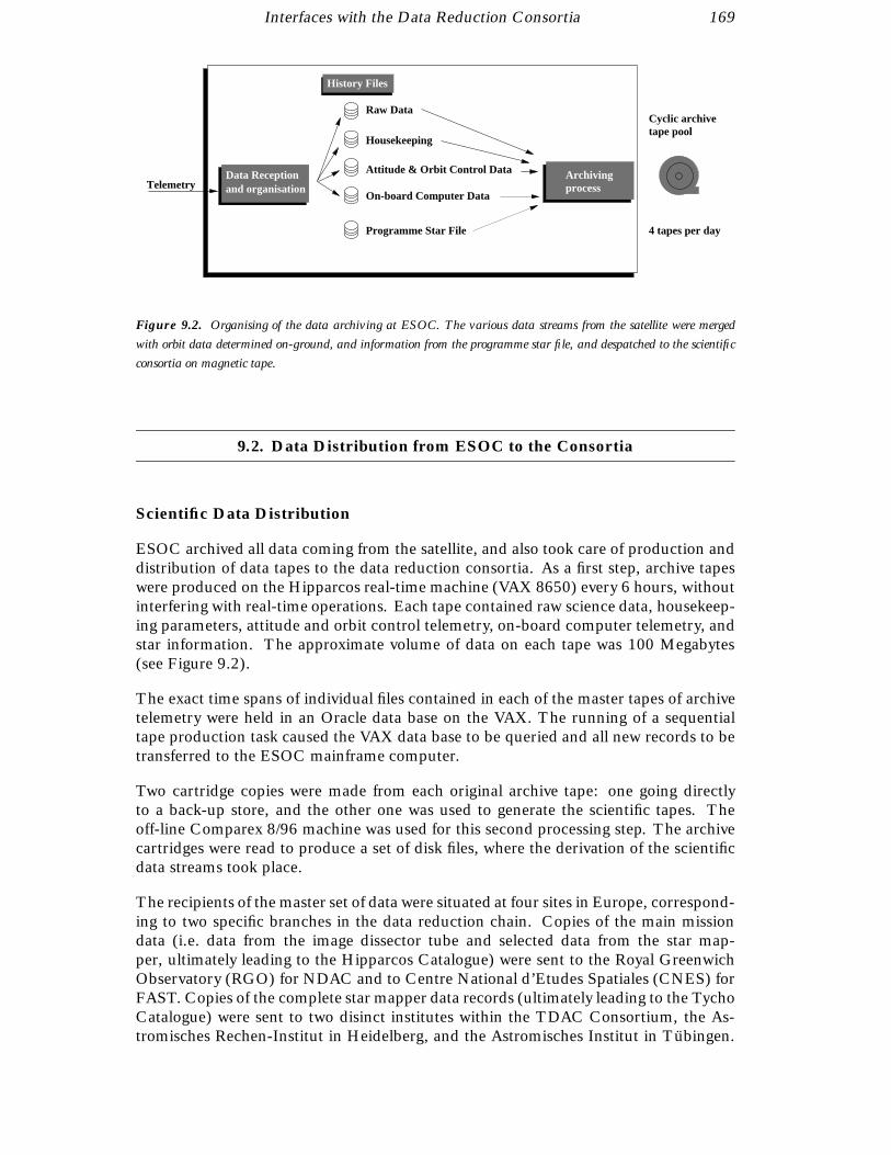
Interfaces with the Data Reduction Consortia 169
Archiving processand organisation
Data Reception
4 tapes per day
Raw Data
Housekeeping
On-board Computer Data
tape poolCyclic archive
TelemetryAttitude & Orbit Control Data
Programme Star File
History Files
Figure 9.2. Organising of the data archiving at ESOC. The various data streams from the satellite were merged
with orbit data determined on-ground, and information from the programme star file, and despatched to the scientific
consortia on magnetic tape.
9.2. Data Distribution from ESOC to the Consortia
Scientific Data Distribution
ESOC archived all data coming from the satellite, and also took care of production anddistribution of data tapes to the data reduction consortia. As a first step, archive tapeswere produced on the Hipparcos real-time machine (VAX 8650) every 6 hours, withoutinterfering with real-time operations. Each tape contained raw science data, housekeep-ing parameters, attitude and orbit control telemetry, on-board computer telemetry, andstar information. The approximate volume of data on each tape was 100 Megabytes(see Figure 9.2).
The exact time spans of individual files contained in each of the master tapes of archivetelemetry were held in an Oracle data base on the VAX. The running of a sequentialtape production task caused the VAX data base to be queried and all new records to betransferred to the ESOC mainframe computer.
Two cartridge copies were made from each original archive tape: one going directlyto a back-up store, and the other one was used to generate the scientific tapes. Theoff-line Comparex 8/96 machine was used for this second processing step. The archivecartridges were read to produce a set of disk files, where the derivation of the scientificdata streams took place.
The recipients of the master set of data were situated at four sites in Europe, correspond-ing to two specific branches in the data reduction chain. Copies of the main missiondata (i.e. data from the image dissector tube and selected data from the star map-per, ultimately leading to the Hipparcos Catalogue) were sent to the Royal GreenwichObservatory (RGO) for NDAC and to Centre National d’Etudes Spatiales (CNES) forFAST. Copies of the complete star mapper data records (ultimately leading to the TychoCatalogue) were sent to two disinct institutes within the TDAC Consortium, the As-tromisches Rechen-Institut in Heidelberg, and the Astromisches Institut in Tubingen.

170 Interfaces with the Data Reduction Consortia
From these four starting points the data were further distributed to groups contributingto the overall reduction and processing chain within the NDAC, FAST, and TDACConsortia (see Volumes 3 and 4 for further details). In addition, subsets of the datawere sent to the FAST Consortium’s ‘first-look’ facility at SRON, Utrecht, for rapidbut in-depth appraisal of the scientific data quality (see Section 9.3).
The Hipparcos tape production system for the data reduction consortia ran on themainframe computer at ESOC. It consisted of six main components as follows:
(1) Tape Read: this read data from cartridges of archived telemetry into disk-based files.The files were organised as keyed sequential circular, and provided the input for thestream derivation task described below;
(2) Interactive Task: this provided a menu-driven interface allowing the user to configurethe system for a single processing run and then to initiate processing by starting the MainControl Task or the Copy/Print Task. The different run types, ‘First-Look’, ‘Sequential’and ‘Ad Hoc’ were all controlled at this level;
(3) Main Control: this acted as a scheduler for the following tasks. The status of theindividual tasks was monitored by main control which could then spawn successive‘Read’, ‘Stream Derivation’ and ‘Write’ operations depending on the return codes fromthe previous task;
(4) Tape Write: this wrote the reformatted telemetry onto magnetic tapes. The datawas written when the system had sufficient data in its disk files to fill an output tape.The last tape written ended on the last full catalogue period present in the processeddata. For sequential processing, two master tapes were produced, for the FAST andTDAC (Tubingen) groups;
(5) Copy/Print: this produced copies of the data reduction consortia tapes for the othergroups (NDAC and TDAC Heidelberg) and printed tape labels and dispatch forms;
(6) Stream Derivation: this reformatted the telemetry in the format defined by theHipparcos ‘Data Delivery Interface Document’, while performing quality checks andfiltering the data. The main part of the processing was carried out in this task. Syn-chronisation of the various data streams to ensure that all streams covered exactly thesame time intervals and removal of any spurious data was carried out here. Once thedata had been checked for bad quality and valid satellite configuration, the remainingspan was then divided into catalogue periods.
Final tapes for distribution to the scientific teams were created in an agreed interfaceformat, specified completely by the Data Delivery Interface Document, which hadbeen defined through dialogue and exchange of simulated data between ESOC and theConsortia well in advance of launch. The final tape contruction also added eclipse, orbit,payload monitoring and coil current calibration matrix files to the scientific streams. Thescientific tapes were then distributed to the scientific consortia. Figure 9.3 shows thevarious steps in this tape production system.
ESOC also responded to specific requests from the consortia during the mission, toprovide data tapes covering different time spans, used to evaluate anomalous trends inthe behaviour of the payload or to validate specific aspects of the consortia software.
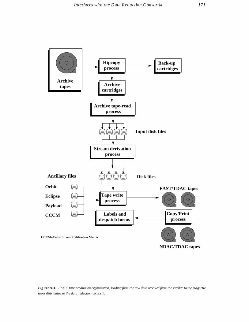
Interfaces with the Data Reduction Consortia 171
Archivetapes
Hipcopyprocess
Back-upcartridges
Archivecartridges
Archive tape-readprocess
Stream derivationprocess
Tape writeprocess
Copy/Printprocess
Labels anddespatch forms
Disk files
FAST/TDAC tapes
NDAC/TDAC tapes
Ancillary files
CCCM
Payload
Eclipse
Orbit
CCCM=Coils Current Calibration Matrix
Input disk files
Figure 9.3. ESOC tape production organisation, leading from the raw data received from the satellite to the magnetic
tapes distributed to the data reduction consortia.
172 Interfaces with the Data Reduction Consortia
The tape production system was designed with the nominal mission and nominal satelliteconfiguration in mind. Certain changes were introduced as a result of the non-nominalorbit. The failure of on-board components also meant that certain parameters could nolonger be reliably extracted from the telemetry. A method of inputting these ‘adjustableparameters’ was developed and extended throughout the mission as each new anomalyoccurred. For example, gyro configurations, star mapper and image dissector tubeselections plus additional nominal scanning law parameters were all entered. Checks onthe satellite configuration were carried out by the stream derivation task. The changing,‘cross-strapping’, patching and re-routing of the on-board systems demanded constantupdates to the model against which the configuration was checked.
Once per week, several off-line tasks were performed to analyze all reports from thepayload monitoring software in that period. One product from the analysis was a list ofintervals in which the image dissector tube quality flag consistently showed that goodscientific data was being collected. A file containing all such intervals over the entiremission was input to the tape production software. The consortia only processed datawhich was flagged as ‘good’ in this way.
The original raw telemetry was sorted and merged as follows: (i) decommutation into‘floating streams’ corresponding to image dissector tube, star mapper data, housekeep-ing, attitude and orbital control system, and on-board computer data; (ii) associationof telemetry reports from on-board computer streams with their corresponding datasamples; (iii) extraction of star mapper data from the full star mapper data stream fortransits of a magnitude-limited selection of programme stars; (iv) addition of orbit dataand eclipse data; (v) addition of other ancillary data (payload monitoring results, coilcurrents calibration matrix data); and (vi) derivation of a data catalogue which describedthe payload and on-board computer status and identified periods of unchanging status.The files were transferred from ESOC to the consortia on magnetic tape.
The magnetic tapes were recorded at 6250 bytes per inch with a 7-bit ASCII characterset. The maximum allowed blocksize in any file was fixed at 28 800 bytes and themaximum number of logical records were packed into each block. Each tape wasself-contained and self-describing, with no multi-volume data sets.
There were two independent sources of timing information given on the tapes: thespacecraft (on-board) time and the ground station time. The ground station times hada resolution of 0.1 µs, but an absolute error of ±1.0 µs which included a quantisationerror of ±0.2 µs associated with the clock. All telemetry frame times were retained andstored in compressed form with the attitude and orbit control system data stream. Foreach record of every stream only the initial ground station time and mean frame durationwere stored in the telemetry header. The initial ground station time was not correctedfor spacecraft-to-ground station propagation delay, nor for the internal ground stationdelay (these corrections were subsequently made by the data reduction consortia). Theon-board time was stored in some records either as a 24-bit format counter or a 32-biton-board time counter.
The structure of each tape was determined well in advance of satellite launch, followingan extended period of dialogue between ESOC and the data reduction consortia, alsoinvolving the provision and analysis of simulated data, and leading to a complete speci-fication of the tape structure and contents in the form of the Hipparcos ‘Data DeliveryInterface Document’.

Interfaces with the Data Reduction Consortia 173
At the start of every tape was a ‘volume header’ which gave a unique identifier to thistape, followed by a ‘tape header’ file which identified the tape as a Hipparcos tape,recorded the date of production and described the structure and contents of the rest ofthe tape. Every tape then consisted of a series of files, each preceded by a header whosepurpose was to identify the consortia for whom the tape was made and to describe thetype of file. The end of each file was marked with an end-of-file record which wouldlist the number of blocks in the preceding file. All subsequent files fitted into thisstructure in a systematic way, no matter which combination of data streams was writtento a particular tape. The tape contents generally consisted of the data catalogue, andscience and ancillary files. The latter consisted of the image dissector tube file, starmapper file, raw housekeeping (including derived parameters), Tycho data file, attitudeand orbit control system data, orbit data, eclipse data, coil currents calibration matrixand payload monitoring results.
Data catalogue file: The data catalogue file was a catalogue of payload status changesderived from the application of an algorithm to the housekeeping data stream. The aimof the data catalogue was to provide a log where the sequence of payload operations wasavailable in a convenient form, and to aid direct access to parts of the data from a tapeafter it was transferred to disk. A catalogued period was defined as a period containingan integral number of consecutive telemetry formats during which no significant statuschange occurred. For each such period one record was added to the catalogue.
Telemetry header: All files which were pointed to by the data catalogue had recordswith a common header containing timing, datation and quality information. All timinginformation in the header referred to the start of a record. If part of the informationfor a particular record was missing from the telemetry stream, the timing would still bedefined as if the record had been of perfect quality.
Image dissector tube file: Each image dissector tube record was formed by mergingan image dissector tube observation report, its associated photon counts and relevantinformation from the Hipparcos Input Catalogue (in particular the details of the starobservation strategy, described in Chapter 8, could be derived from this file). The filealso included data received during calibrations of the grid reference marks and internalstar pattern assembly (see Chapter 2), in which case the appropriate calibration reportswere used. A flag in the image dissector tube header indicated which of the possiblealternatives (i.e. normal image dissector tube, or calibration report) was contained in aparticular file. Observation reports were merged into the image dissector tube reportswithout modification.
Counts were integrated over 1/1200 s and were compressed on board in one of twoways, depending on how the star was observed. In the analogue mode (for stars ofmagnitude brighter than 1.5) counts were 8-bit integers, with nominal quanta of 250counts per sample period for image dissector tube number 1 and 220 counts per samplefor image dissector tube number 2. For stars with magnitude fainter than 1.5, thephoton counting mode was used in which counts were expressed as a 3-bit exponent(E ) and a 5-bit mantissa (M). For N counts (0 < N < 8159), with JI = 32(2I − 1)(0 < I < 7), if JI ≤ N < JI+1 then E = I and M = (N − JI) /2I. Any fractional partof M was truncated. To reconstitute the image dissector tube signal the algorithm wasapplied in reverse, with appropriate allowance for the effects of truncation and a non-linearity correction factor. This encoding method was also used for data samples in gridreference marks and internal star pattern assembly observation frames. In practice theanalogue mode was never used (see Section 3.1).

174 Interfaces with the Data Reduction Consortia
Star mapper file: The star mapper file contained selected parts of the Tycho stream cov-ering the calculated crossing times of selected programme stars merged with associatedinformation from the programme star file. Crossing times were calculated for only oneof the star mappers, whichever one was operational. For each transit 200 star mappersample pairs (comprising BT and VT samples) were needed. To simplify the subsequentuse of these records they were aligned on telemetry frame boundaries and contained10 consecutive (i.e. separated by 0.04166 . . . s) frames centered around the calculatedtransit (Tcalc). Star mapper records were stored in chronological order, and stars withB > 10.25 mag were disregarded. The transit in a given star mapper record occured atsample number [(Tcalc − Tstart) × 0.25] + 1.625 within the record, thus the 200 samplesof B or V could be extracted from the 250 samples in each record. The constant 1.625was the delay between the accumulation of a sample and its appearance in the telemetry.The star mapper samples were encoded with the same semi-log compression law as forthe image dissector tube photon-counting mode. There was no corresponding analoguemode for bright stars in the case of the star mapper data.
Tycho file: Each data record contained data extracted from one high-rate telemetryformat, namely: (a) standard telemetry header and (b) the Tycho data stream of inter-leaved BT and VT star mapper counts, encoded with the same semi-log formula usedfor the image dissector tube data.
Raw housekeeping and derived parameters: This file contained housekeeping dataextracted from the raw frame of the high telemetry format, and included additionalinformation appended by ESOC to each record. There was a one-to-one correspon-dence between raw housekeeping records and the original raw formats. The contentsof any bad or missing formats were set to zero. The additional information consisted ofthe temperature and powers associated with the 24 payload thermal control cells. Thehousekeeping data also included the complete spacecraft and payload memory-load-command readouts, along with other parameters which were duplicated in the datacatalogue records.
Attitude and orbit control system file: The attitude and orbit control system parametersin each telemetry frame were extracted and stored, without modification, as a separatestream with one record per original format. The telemetered parameters were arrangedinto two groups: (i) those data expected to be of primary interest to the data reductionconsortia, and (ii) housekeeping and status data which was not of primary relevance tothe data reduction but may be necessary or helpful for scientific checks which were notforeseen at the time. Parameters associated with missing or bad frames were includedand processed, but were tagged with an appropriate quality flag. These attitude and orbitcontrol system files also contained the full datation of all incoming telemetry frames,although this was only expected to be used in the event that the on-board oscillator wasunstable. Records were only created when the normal attitude and orbit control systemformat was being telemetered.
Orbit data: Orbit data were organised into a cumulative file covering the satellite lifetime.There was no relation or precise synchronisation between orbit records and telemetryrecords, thus the orbit data were not pointed to by the data catalogue, instead a descrip-tion of the whole orbit file was contained in the first record. The time interval covered bya record was normally about 7–8 hours around apogee, and 0.5–1 hour around perigee.

Interfaces with the Data Reduction Consortia 175
Eclipse data: The eclipse file was another ancillary file pointed to by the tape header fileand not by the data catalogue. It contained details of all eclipses that occurred duringthe mission.
Coil currents calibration matrix data: Real-time calibration generated one such recordeach time an internal star pattern or grid reference marks sequence resulted in an updateof this calibration matrix.
Payload monitoring results: Payload monitoring generated long-term image dissectortube and star mapper reports, approximately one record per week.
First-Look Monitoring
Every week a special ‘First Look’ tape was sent from ESOC to SRON, Utrecht, amember of the FAST Consortium, for preliminary analysis of the science data. Unlikethe main data processing which might only be processed weeks or months after theobservations were made, the ‘First-Look’ task processed the data within a few daysof delivery to assess the scientific data quality. Through rapid calibration of certainparameters associated with the instrument (e.g. basic angle, grid rotation, and single-slit response) ESOC were informed promptly if unexpected trends or disturbances wereobservable. ESOC were then able to examine the operations logs around the time of anevent to see if there was a correlation with spacecraft activities at that time, and to takeappropriate action if necessary. In addition, the ‘First Look’ facility provided payloadcalibration data to FAST, NDAC and ESOC.
Focus Evolution and Photometry Results
Results from the weekly payload monitoring analysis included an averaging of the in-tensities and grid modulation coefficients contained in the image dissector tube and starmapper reports. This gave an evaluation of the photometric degradation of the pay-load due to, for example, radiation darkening of the optics, or temperature instabilities.The best focus position evolved continuously throughout the mission, primarily due tomoisture release. The refocusing calibration was performed every week throughout themission (or more regularly in the case of anomalies) to monitor the best focus positionand when necessary to change the actual focus position on-board. Details of the focusevolution and photometric degradation were communicated to Matra Marconi Spacefor further evaluation. A discussion of both phenomena is presented in Chapter 10.
9.3. Data from FAST to ESOC in Support of Satellite Operations
First-Look Monitoring Feedback
This interface (described above) proved to be very successful in identifying any trends inbasic angle evolution and other payload phenomena. Already during the routine phase,as on-board heaters started to fail, Utrecht were able to provide important informationwhen it was necessary for ESOC to perform special thermal control operations (seeChapter 12). Given that thermal instabilities could cause payload deformation, it wascritical for ESOC to know within days rather than weeks if operations were degrading
176 Interfaces with the Data Reduction Consortia
the scientific data. This would allow corrective actions to be attempted. Additionalimportant assistance was given in analysing the star mapper data during the two-gyrooperational phase, as attempts were made to revive the spacecraft after hibernation (seeChapter 15).
Basic Angle and Grid Rotation
During the commissioning phase, it was necessary for ESOC to perform an initial coarsecalibration of the basic angle (the angle between two fields of view) and grid rotation(the misalignment of the image dissector tube and star mapper grids with respect to thescanning plane), to refine the operations of the ground real-time attitude determinationsoftware. Thereafter, Utrecht were able to process the scientific data to yield moreaccurate values, which were fed back into the ground real-time attitude determinationinput data, giving rise to improved convergence of the attitude determination software.In addition, on 23 January 1990, the first calibrated grid rotation was used on-boardresulting in a significant improvement in on-board real-time attitude determinationperformance. The real-time attitude determination ‘innovations’, which give a measureof the attitude corrections necessary between star mapper transits, were reduced fromabout ±5 arcsec to about ±2 arcsec. Subsequent monitoring of the basic angle by theconsortia is described in Section 10.2.
9.4. Data from NDAC to ESOC in Support of Satellite Operations
Gyro Misalignment
The on-board real-time attitude determination system relied on integrated gyro outputsfor determining the attitude between star mapper transits. The conversion of the satellitebody rates around the operational gyro input axes was performed on-board and on-ground using a suitable projection matrix, and assuming the pre-launch calibration ofthe alignments. The NDAC Consortium, unlike the FAST Consortium, used the gyrooutput for the scientific data reduction. A by-product of the initial NDAC processing,conducted at the Royal Greenwich Observatory (RGO), was a calibration of the gyromisalignments with respect to the nominal positions. On 4 July 1991, the RGO was ableto supply a newly calibrated projection matrix for uplink to the spacecraft. Subsequently,as the gyro configuration changed, due to gyro failures, particularly at the start of two-gyro operations, further projection matrices were supplied by the RGO for operationaluse.
External Disturbance Torque and Thruster Calibration
A further product of the NDAC processing, performed by the RGO, was a detailed studyof the external disturbance torques acting on the spacecraft as well as the evolution ofthe thruster performance with time (see Volume 3, Chapter 8 for further details). Thethruster performance results were used by ESOC to perform tuning of the thrusteron-time coefficients as part of the on-board attitude control. One significant resultwas to show a difference in performance between the plus and minus thruster aroundeach axis. This however could not be compensated for in the original real-time attitude
Interfaces with the Data Reduction Consortia 177
determination design since separate on-time coefficients were only available for eachthruster axis and assumed identical performance for both thrusters around that axis.
This was valuable information in defining the real-time attitude determination algorithmfor zero-gyro operations (see Chapter 16). The revised real-time attitude determinationrelied on an on-board disturbance torque model, which had to be updated on a regularbasis from ground predictions. In addition, independent on-time thruster coefficientswere applied for each thruster. The RGO participated with ESA and Matra MarconiSpace in defining the new algorithm, using the experience already gained in determiningthe variability of the various torques around the orbit.
Although the disturbance torques around each of the spacecraft axes were broadlyrepeatable, with combined periods equal to the spacecraft rotation and orbital periods,the effect of the Earth’s magnetic field, and a number of small partially-explained torques(such as gravity gradient and magnetic torques), could change fairly rapidly. For zero-gyro operations, this required a fast response time to re-calibrate and uplink the revisedtorques. To this end, the RGO supplied their on-ground attitude reconstitution softwareto ESOC for use in operations, to perform disturbance torque and thruster calibrationsduring every perigee passage for the next orbital period.
Preliminary Catalogue Results
NDAC were able to feed back their preliminary star positions and brightnesses to ESOC,via the INCA Consortium, to be used for the on-board programme star file. This wasdone in two stages as more results became available.
In February 1991, Input Catalogue Version 8 was received and implemented at ESOC,containing approximately half the programme stars updated from Hipparcos data. ByNovember 1992, Input Catalogue Version 10 was received, with nearly all of the inputcatalogue stars now containing early Hipparcos results. The improvements in accuracyof the positions were, by that time (as expected), largely masked by the intrinsic perfor-mance accuracy of the real-time attitude determination. This and the greater reliabilityin the magnitude estimates allowed ESOC to tune the selection criteria for real-timeattitude determination guide stars and to tune the on-board star mapper processingparameters to optimise the correct identification of guide stars in the star mapper datastream and virtually eliminate any possibility of mis-identifying stars, which could leadto an unexpectedly large innovation error in the on-board control.
All of the above support from the FAST and NDAC Consortia, when combined withadditional work performed by ESOC and Matra Marconi Space, contributed stronglyto the overall improvement in real-time attitude determination performance which wasachieved by 1992, before significant problems with noisy gyros were experienced (seeChapters 14–15). By that time, real-time attitude determination innovations were con-sistently around ±1 arcsec, compared to the start of the mission figure of ±5 arcsec.Moreover the regularity with which real-time attitude determination was staying con-verged after perigee was also increased.

178
10. ROUTINE CALIBRATIONAND PAYLOAD EVOLUTION
Continuous monitoring of the geometric and photometric performances of thepayload was necessary throughout the mission. This was conducted partly atESOC (in particular for the photometric aspects), and partly by the FASTConsortium as part of their ‘first-look analysis’ (in particular for the geometricaspects). The focus monitoring resulted in semi-regular focus adjustmentsto take account of progressive evolution of the payload structure, the resultsof which are described in detail, and which led to a comprehensive model ofmoisture release and optical degradation accounting for the observed focusevolution with time. The radiation darkening of the optics, especially of thestar mapper relay optics, led to an evolution of the photometric performances,which had to be accounted for in the observation time allocation, as well asduring the rigorous photometric calibration as part of the data reductions.
10.1. Routine Monitoring Activities at ESOC
Payload Monitoring
A subset of the software developed for calibration purposes was adapted and built intoa separate payload monitoring program for use in near real-time. The selected starswere processed to estimate their intensities and modulation coefficients. The estimatedvalues were compared with the expected values based on the photometric parametersdefining the star (brightness and colour) and based on the calibrated response of thetelescope and detectors. Reports were generated for each processed observation.
The software for this task ran on the Hipparcos dedicated computer system continuouslythroughout the mission. It performed many tasks associated with verifying the correctperformance of the on-board science data collection and processing. Every 60 s, theprogram selected one star observed in the preceding 30 s. The selection criteria werebased on the following: (i) stars present for less than a complete observation frameof 2.133 . . . s were not used; (ii) multiple stars and minor planets were not used; (iii)large-amplitude variable stars were preferentially selected (in order to maintain up-to-date ephemerides for them); (iv) photometric secondary standard and constant starswere preferred over non-photometric stars; (v) brighter stars were preferred over faint

180 Routine Calibration and Payload Evolution
stars; (vi) if the previous star to be processed was observed in the following field of view,preference for the next observation was given to stars observed in the preceding field ofview, and vice versa.
This last constraint was important for quick and reliable verification of the attitudecontrol system (see below). One star was selected, out of those possible, in a pseudo-random manner where the probability of selection was weighted according to the abovecriteria. The largest weighting was given to large-amplitude variable stars, so they werealmost always processed, if observed.
Regardless of star type, analysis proceeded as follows. The raw image dissector tubesamples were extracted from the scientific telemetry, and the rotational (body) rates ofthe spacecraft were extracted from the attitude control system telemetry. The raw imagedissector tube samples were then decompressed and corrected for detector saturationeffects according to pre-defined decompression tables. The resulting data resulted in amodulated signal I (t) of the form given in Equation 1.1. The five unknown parametersI0, M1, M2, θ1, θ2 were estimated from a Fourier analysis of the signal. Except for thestars flagged a priori as variable, a check of the measurement quality was made. Thiswas done by comparing the values of I0 and M1 against their expected values.
I0 quality 0, 1, 2, 3 meant that the ratio of measured to expected I0 corresponded to amagnitude difference of less than 1, 2, 3, or 4 respectively for B < 10 mag; or less than2, 3, 4, or 4 respectively for B > 10 mag. M1 quality 0, 1, 2 meant that the ratio ofmeasured to expected M1 lay in the range 0.8–1.2, 0.6–1.4, or 0.4–1.6 respectively forB < 10 mag; or in the range 0.6–1.4, 0.4–1.6, or 0.2–1.8 respectively for B > 10 mag;The I0 and M1 quality flags were summed to give the overall quality flag (setting anupper limit of 3), and the results were monitored in real-time by the spacecraft analystsbut were also filed for later retrieval.
The quality flag information was used to determine if the on-board real-time attitudedetermination system was controlling the attitude adequately. If the attitude began todrift, this would affect the ability of the on-board software to pilot the image dissectortube to the correct portion of the grid. Consequently, the measurements taken underconditions of poor real-time attitude usually resulted in quality 3 star measurements inone or both fields of view. Only if results from both fields of view showed consistentlyquality 0 measurements was real-time attitude determination considered to be operatingsuccessfully.
A further off-line task analysed the payload monitoring results on a weekly basis com-piling a list throughout the mission of intervals of ‘good’, ‘bad’ or ‘unknown’ piloting.This was supplied to the data reduction consortia to assist in the routine data reductionactivities. Only intervals of ‘good’ data would be processed. When starting to processan interval of data, the algorithm assumed a status of ‘unknown’ until the first payloadmonitoring report. Piloting status would only change to ‘good’ if three consecutiveobservations in both fields of view were assigned as quality 0 measurements. Pilotingstatus would only change to ‘bad’ once three consecutive observations in one or otherfield of view were assigned with non-zero quality flags. This proved to be an effective setof criteria for defining when real-time attitude determination was converged and usefulscientific data was being obtained.

Routine Calibration and Payload Evolution 181
Focus Monitoring
The monitoring of the focus evolution and offset from current to best focus was done bymeans of the M1 values computed by processing a four-hour batch of image dissectortube telemetry, in a similar manner to that described in Section 5.6. Since the positionof best focus was evolving continuously the refocusing calibration was performed everyweek throughout the mission (or more regularly in the case of anomalies). The bestfocus position could be calibrated by computing the average grid modulation coefficientsM1 over a four hour period of data. These M1 averages were then converted into a focusoffset and hence, via the history of grid movements, into an absolute focus positionusing the calibrated curves shown in Figure 5.4.
The motor which changed the focus position, did so in steps of 1.38 µm, and theintention was to keep the focus position on-board within ±1 step of the best focusposition. In December 1989, the results from the ground software appeared to implythat the best focus position was changing at an increasing rate, in contradiction withpre-launch predictions. It was subsequently found that the change of focus was notactually taking place, but rather that the stepping motor was incapable of moving byonly one step at a time. This was later confirmed by the manufacturer. Subsequently,only focus moves of two or more steps were commanded without further problems ordegradation of the science data.
Background Noise Monitoring
The star mapper proved to be very sensitive to the radiation environment in the vanAllen belts and during periods of high solar activity. The result was blinding close toperigee. Moreover the radiation environment could change rapidly, as a result of solarflares. This had a direct impact on the altitude at which re-initialisation of the on-boardreal-time attitude determination could be attempted following perigee passage, sinceground-based star pattern recognition required frequent star transits to be identified inthe star mapper data stream.
As a result, the overall star mapper signal in both channels was constantly monitoredwith a report produced every minute giving an integrated average to the ESOC flightcontrol team. Only once noise levels were at an acceptable level, were ground real-timeattitude determination initialisation procedures performed (see Chapter 14).
Spacecraft Performance Evaluation System
For Hipparcos, ESOC used a software system called the ‘spacecraft performance eval-uation system’ for close to real-time anomaly analysis as well as long-term historyperformance evaluation studies. This service software, running alongside the space-craft control and operating system (at the time the ESA standard for spacecraft controland operations), regularly transferred housekeeping telemetry, event data and gener-ated telecommand history, from the on-line mission dedicated computers to the off-line spacecraft performance evaluation machine, via a high speed HYPERBUS inter-computer link.
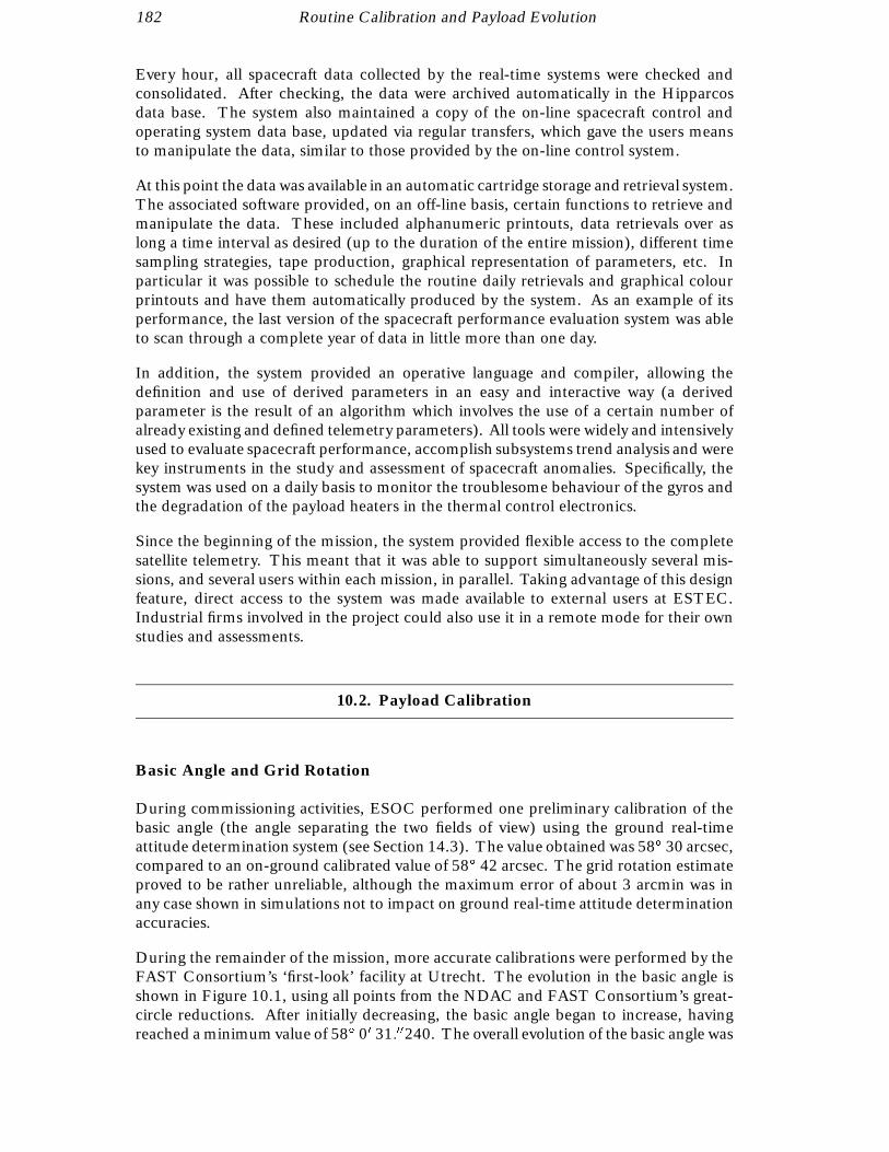
182 Routine Calibration and Payload Evolution
Every hour, all spacecraft data collected by the real-time systems were checked andconsolidated. After checking, the data were archived automatically in the Hipparcosdata base. The system also maintained a copy of the on-line spacecraft control andoperating system data base, updated via regular transfers, which gave the users meansto manipulate the data, similar to those provided by the on-line control system.
At this point the data was available in an automatic cartridge storage and retrieval system.The associated software provided, on an off-line basis, certain functions to retrieve andmanipulate the data. These included alphanumeric printouts, data retrievals over aslong a time interval as desired (up to the duration of the entire mission), different timesampling strategies, tape production, graphical representation of parameters, etc. Inparticular it was possible to schedule the routine daily retrievals and graphical colourprintouts and have them automatically produced by the system. As an example of itsperformance, the last version of the spacecraft performance evaluation system was ableto scan through a complete year of data in little more than one day.
In addition, the system provided an operative language and compiler, allowing thedefinition and use of derived parameters in an easy and interactive way (a derivedparameter is the result of an algorithm which involves the use of a certain number ofalready existing and defined telemetry parameters). All tools were widely and intensivelyused to evaluate spacecraft performance, accomplish subsystems trend analysis and werekey instruments in the study and assessment of spacecraft anomalies. Specifically, thesystem was used on a daily basis to monitor the troublesome behaviour of the gyros andthe degradation of the payload heaters in the thermal control electronics.
Since the beginning of the mission, the system provided flexible access to the completesatellite telemetry. This meant that it was able to support simultaneously several mis-sions, and several users within each mission, in parallel. Taking advantage of this designfeature, direct access to the system was made available to external users at ESTEC.Industrial firms involved in the project could also use it in a remote mode for their ownstudies and assessments.
10.2. Payload Calibration
Basic Angle and Grid Rotation
During commissioning activities, ESOC performed one preliminary calibration of thebasic angle (the angle separating the two fields of view) using the ground real-timeattitude determination system (see Section 14.3). The value obtained was 58 30 arcsec,compared to an on-ground calibrated value of 58 42 arcsec. The grid rotation estimateproved to be rather unreliable, although the maximum error of about 3 arcmin was inany case shown in simulations not to impact on ground real-time attitude determinationaccuracies.
During the remainder of the mission, more accurate calibrations were performed by theFAST Consortium’s ‘first-look’ facility at Utrecht. The evolution in the basic angle isshown in Figure 10.1, using all points from the NDAC and FAST Consortium’s great-circle reductions. After initially decreasing, the basic angle began to increase, havingreached a minimum value of 58 00 31.00240. The overall evolution of the basic angle was

Routine Calibration and Payload Evolution 183
Figure 10.1. Basic angle evolution as a function of time, determined from the preliminary great-circle reductions
(see also Figures 10.12(a) and (b)). The smooth evolution with time results from contributions such as outgassing
of the structure, radiation effects on the optics, and other ageing processes. Outlier points typically arise from thermal
variations in the payload, described in further detail in Section 12.4. The overall evolution of the basic angle was well
within specification, and well within the changes that could be modelled in the instrumental calibration on ground.
well within the design specification, which called for a variation of below 1 milliarcsecwithin any 12-hour interval.
Instantaneous Field Of View Pointing
A description of the internal star pattern assembly and grid reference marks calibrations,relevant for the instantaneous field of view pointing calibration, was given in Section 5.4.The internal star pattern assembly calibration was repeated every two weeks throughoutthe mission. The grid reference marks calibration and coil currents calibration matrixuplink were performed daily. Typically, the standard deviation of the variation of thepiloting currents was measured as 0.9 arcsec per day, i.e. the stability of both the imagedissector tube pointing non-linearity, and the rigid body displacement, was very good.
Optics Darkening
Once per week, several off-line tasks were performed to analyse all data acquired bythe payload monitoring software during that period. The products from the analysisincluded an averaging of the intensities and grid modulation coefficients contained inthe image dissector tube and star mapper reports. This gave an overall evaluation ofthe photometric degradation of the payload due to, for example, glass darkening or
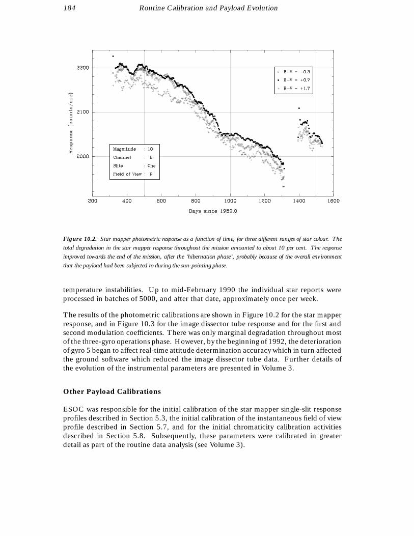
184 Routine Calibration and Payload Evolution
Figure 10.2. Star mapper photometric response as a function of time, for three different ranges of star colour. The
total degradation in the star mapper response throughout the mission amounted to about 10 per cent. The response
improved towards the end of the mission, after the ‘hibernation phase’, probably because of the overall environment
that the payload had been subjected to during the sun-pointing phase.
temperature instabilities. Up to mid-February 1990 the individual star reports wereprocessed in batches of 5000, and after that date, approximately once per week.
The results of the photometric calibrations are shown in Figure 10.2 for the star mapperresponse, and in Figure 10.3 for the image dissector tube response and for the first andsecond modulation coefficients. There was only marginal degradation throughout mostof the three-gyro operations phase. However, by the beginning of 1992, the deteriorationof gyro 5 began to affect real-time attitude determination accuracy which in turn affectedthe ground software which reduced the image dissector tube data. Further details ofthe evolution of the instrumental parameters are presented in Volume 3.
Other Payload Calibrations
ESOC was responsible for the initial calibration of the star mapper single-slit responseprofiles described in Section 5.3, the initial calibration of the instantaneous field of viewprofile described in Section 5.7, and for the initial chromaticity calibration activitiesdescribed in Section 5.8. Subsequently, these parameters were calibrated in greaterdetail as part of the routine data analysis (see Volume 3).
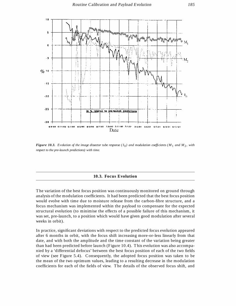
Routine Calibration and Payload Evolution 185
Figure 10.3. Evolution of the image dissector tube response (I0) and modulation coefficients (M1 and M2, with
respect to the pre-launch predictions) with time.
10.3. Focus Evolution
The variation of the best focus position was continuously monitored on ground throughanalysis of the modulation coefficients. It had been predicted that the best focus positionwould evolve with time due to moisture release from the carbon-fibre structure, and afocus mechanism was implemented within the payload to compensate for the expectedstructural evolution (to minimise the effects of a possible failure of this mechanism, itwas set, pre-launch, to a position which would have given good modulation after severalweeks in orbit).
In practice, significant deviations with respect to the predicted focus evolution appearedafter 6 months in orbit, with the focus shift increasing more-or-less linearly from thatdate, and with both the amplitude and the time constant of the variation being greaterthan had been predicted before launch (Figure 10.4). This evolution was also accompa-nied by a ‘differential defocus’ between the best focus position of each of the two fieldsof view (see Figure 5.4). Consequently, the adopted focus position was taken to bethe mean of the two optimum values, leading to a resulting decrease in the modulationcoefficients for each of the fields of view. The details of the observed focus shift, and
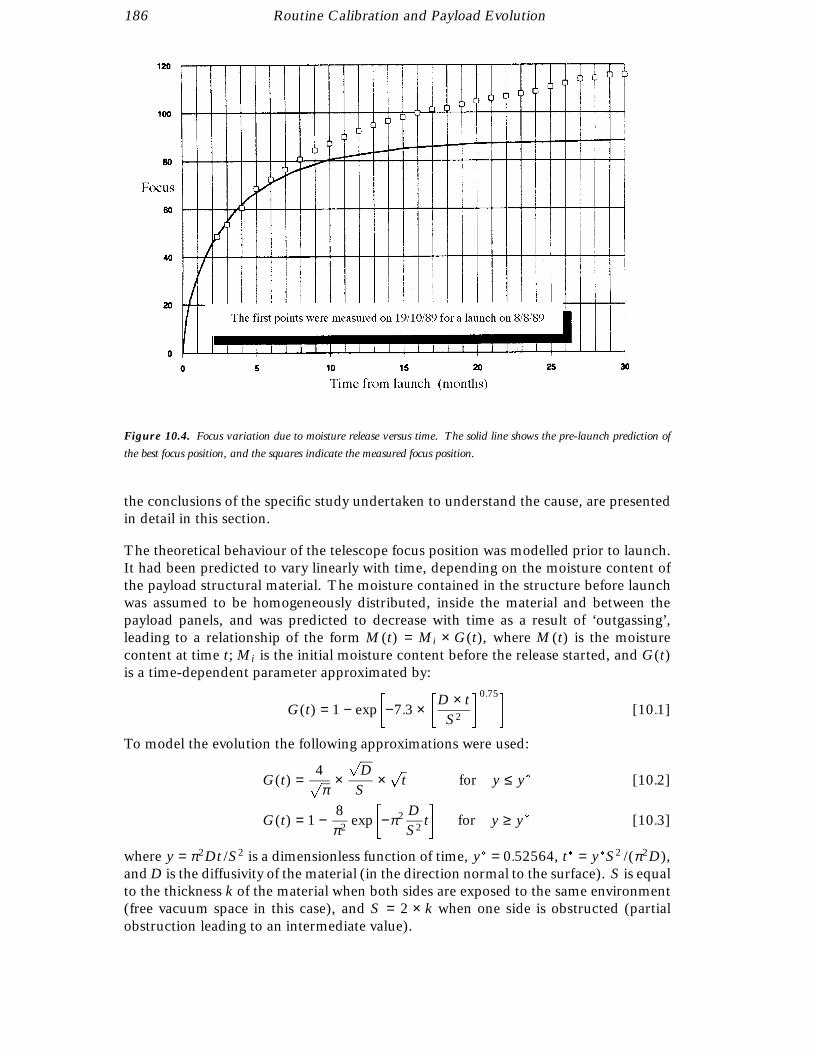
186 Routine Calibration and Payload Evolution
Figure 10.4. Focus variation due to moisture release versus time. The solid line shows the pre-launch prediction of
the best focus position, and the squares indicate the measured focus position.
the conclusions of the specific study undertaken to understand the cause, are presentedin detail in this section.
The theoretical behaviour of the telescope focus position was modelled prior to launch.It had been predicted to vary linearly with time, depending on the moisture content ofthe payload structural material. The moisture contained in the structure before launchwas assumed to be homogeneously distributed, inside the material and between thepayload panels, and was predicted to decrease with time as a result of ‘outgassing’,leading to a relationship of the form M(t) = Mi × G(t), where M(t) is the moisturecontent at time t; Mi is the initial moisture content before the release started, and G(t)is a time-dependent parameter approximated by:
G(t) = 1 − exp
−7.3 ×
D × tS2
0.75[10.1]
To model the evolution the following approximations were used:
G(t) =4pπ
×p
DS
×p
t for y ≤ y [10.2]
G(t) = 1 −8
π2exp
−π2 DS2
t
for y ≥ y [10.3]
where y = π2Dt /S2 is a dimensionless function of time, y = 0.52564, t = yS2 /(π2D),and D is the diffusivity of the material (in the direction normal to the surface). S is equalto the thickness k of the material when both sides are exposed to the same environment(free vacuum space in this case), and S = 2 × k when one side is obstructed (partialobstruction leading to an intermediate value).

Routine Calibration and Payload Evolution 187
Figure 10.5. Measured focus position and best fitting curve assuming pure moisture release according to Equation 10.6.
This simple model fit to three free parameters did not provide a convincing physical explanation of the observed focus
change.
The diffusivity of the material depends on the temperature according to:
D = D0 expC
T − T0
T × T0
[10.4]
with C = 6000 K. A typical figure for carbon-fibre reinforced plastic is D0 = 3.8 ×10⁻⁸ mm2 s−1 at T0 = 300 K. From the linear variation of the focus position with themoisture content, the actual focus position can be written:
F (t) = Fi + fm × G(t) [10.5]
where Fi is the initial focus position, and fm is the amplitude of the variation of the focusposition from the initial (moist environment) position to the final (completely dry) posi-tion, which is proportional to the final moisture content Mi . A best fit of the measureddata with Equation 10.5 using for G(t) the approximation given by Equation 10.1 yields:
F (t) = 30.3 + 104.2 (1 − exp(−0.134 × t0.75)) [10.6]
where F (t) is measured in microns and t in months. The plot of Equation 10.6 with themeasured data indicates an apparently good fit for t > 6 months (Figure 10.5). Howeverwith three free parameters (Fi , fm, and the exponent), a good fit is not necessarilyconsistent with the known physical properties of the system.
At the constant temperature of the telescope panels, 19 C, the diffusivity is given byD = 2.2×10⁻⁸ mm2 s−1 (from Equation 10.4), with the best fit provided by Equation 10.6yielding a substrate thickness S = 3.42 mm. Being roughly twice the average panelthickness (1.7 mm), this result suggested that moisture release was taking place through

188 Routine Calibration and Payload Evolution
one side only, as if the secondary structure on the other side of the telescope panels(accommodating the heater mat carriers) was creating a hermetical sealing on the outersides.
The most significant change of focus position occurred within about 6–8 months afterlaunch (see Figures 10.4 and 10.5). For this interval, the approximation given byEquation 10.2 for the case y ≤ y is applicable, since t ≤ t = 324 days on the basis ofthe above values of D and S. This indeed results in a rather reasonable fit, i.e. a lineardependence of the focus position with the square root of time:
F (t) = 5.7 + 27.7 ×p
t [10.7]
as depicted in Figure 10.6(a). Equation 10.7 relates the amplitude of the variation offocus fm to the thickness S as:
fm ×4pπ
×p
DS
= 27.7 [10.8]
Using the value of S deduced above, i.e. S = 3.42 mm, leads to fm = 175 µm, inconsistentwith the value of fm given by Equation 10.8, fm = 104 µm. On the other hand, withS = 1.7 mm (corresponding to moisture release through both sides) fm = 87 µm, veryclose to the pre-launch prediction of 89 µm. Figure 10.6(b) indicates that the focusevolution is well approximated by Equation 10.3 as:
F (t) = 5 + 90 ×
1 −8
π2
exp(−0.195 × t) [10.9]
yielding approximately the same value for t = 0 (Fi = 5 µm) as Equation 10.7, and alsoroughly the same amplitude of focus variation ( fm = 90 µm). This tended to confirm thevalidity of the initial moisture release prediction, and suggested that conclusions drawndirectly from the overall best fit to the measured data may be misleading.
The pre-launch prediction of the focus variation due to moisture release was basedon the dry-out of several carbon-fibre reinforced plastic samples after thermal vacuumtesting (weighed before and after the dryout sequence), and a test campaign includingspace conditioning at 50 C over 5 days before the thermal vacuum test itself. A totalfocus variation of 38 µm was measured during the test. Samples of the carbon-fibrereinforced plastic were placed within the payload and weighed before and after thetest. The prediction of the total focus variation of the telescope was obtained fromfm × (MB /MD) where MB is the mass loss (before the thermal vacuum tests) of thecarbon-fibre reinforced plastic samples after dry-out, and MD is the mass loss of thesamples during the thermal vacuum tests. This assumed that the amount of moisturerelease of the telescope structure during the thermal vacuum tests was equal to that ofthe samples. The time constant followed from an assessment of the diffusivity itselfobtained from the measured focus variation over the space conditioning (33 µm during5 days at 50 C) and an assumed temperature of 20 C during the orbital life. Theresulting prediction was:
F (t) = 89 × (1 − exp(−0.427 × t0.75)) [10.10]
with t in months. Closer analysis of the space conditioning sequence revealed an intervalwhere the temperature was stable, and where a ‘pure’ moisture release effect presumablytook place. Before and after this stable interval, thermoplastic effects due to the largetemperature variations were superimposed on the moisture release effect. During this
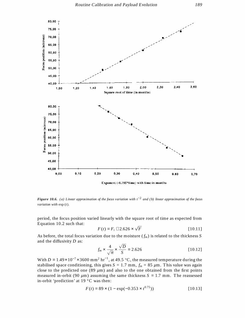
Routine Calibration and Payload Evolution 189
Figure 10.6. (a) Linear approximation of the focus variation with t−2 and (b) linear approximation of the focus
variation with exp (t).
period, the focus position varied linearly with the square root of time as expected fromEquation 10.2 such that:
F (t) = Fi + 2.626 ×p
F [10.11]
As before, the total focus variation due to the moisture ( fm) is related to the thickness Sand the diffusivity D as:
fm ×4pπ
×p
DS
= 2.626 [10.12]
With D = 1.49×10−7 ×3600 mm2 hr−1, at 49.5 C, the measured temperature during thestabilised space conditioning, this gives S = 1.7 mm, fm = 85 µm. This value was againclose to the predicted one (89 µm) and also to the one obtained from the first pointsmeasured in-orbit (90 µm) assuming the same thickness S = 1.7 mm. The reassessedin-orbit ‘prediction’ at 19 C was then:
F (t) = 89 × (1 − exp(−0.353 × t0.75)) [10.13]

190 Routine Calibration and Payload Evolution
Figure 10.7. Initial and reassessed moisture release predictions.
very close to the initial prediction given by Equation 10.10 with, however, a slightlyhigher time constant (Figure 10.7).
Before turning to the origin of the discrepancy in the measured versus predicted focusevolution in-orbit, further evidence that the payload evolution had not been fully un-derstood was given by the change in the modulation factors M1, M2 at the commonbest focus. The common best focus was adopted to be the mean of the best focusof the preceding and following fields of view. While the common best focus positionhad been evolving roughly according to the pre-launch predictions, the individual focuspositions of the two fields of view were diverging, leading to a ‘differential defocus’,and a significant (and unexpected) degradation of the modulation coefficients with time(see Figure 10.3), albeit at a rate (−2.5 per cent per year for M1) not large enough toseverely impact the scientific data. The evolution of the differential defocus is shown inFigure 10.8.
Meanwhile the intrinsic optical quality of the telescope remained essentially unchangedsince the beginning of the mission, as indicated by the stability of the modulation factorsM1, M2 at the individual best focus for each field of view.
The differential defocus continuously increased with time, apparently linearly up toabout 20 months after launch at a rate of ' 0.66 µm per month, thereafter remainingalmost stable. This suggested a phenomenon other than moisture release was occurring,inducing deformations of the mirror surfaces, and resulting in changes of curvatureswhich were somewhat different for the two fields of view.
The identification of the increasing differential defocus with time suggested an averagelinearly varying defocus additional to the moisture release. The measured focus positionswere found to be well represented by (Figure 10.9):
F (t) = 89 × (1 − exp(−0.353 × t0.75)) + 0.82 × t [10.14]
The additional linear variation amounted to 0.82 µm per month, corresponding to anincrease of the telescope focal length. Two possibilities were considered: (a) stressrelease within the telescope mirrors, and (b) irradiation effects on the telescope mirrors.
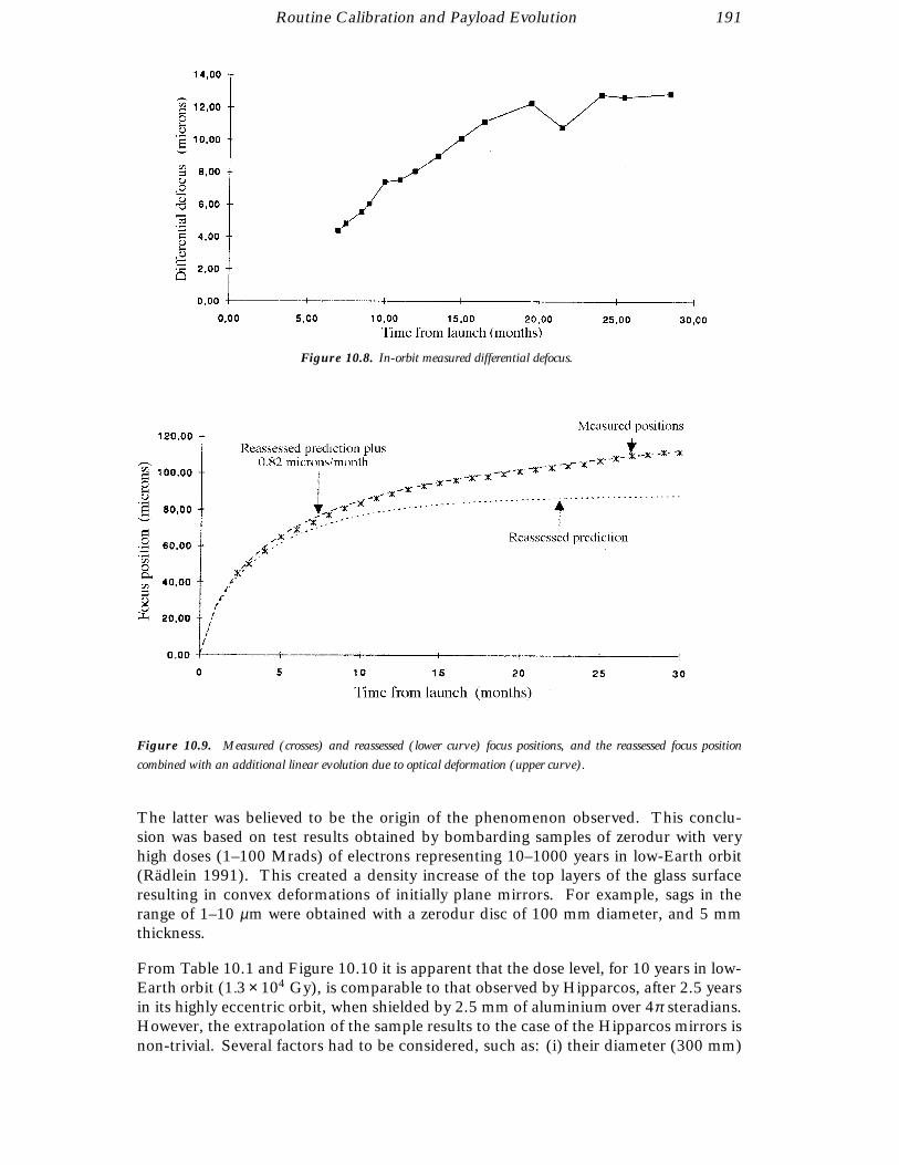
Routine Calibration and Payload Evolution 191
Figure 10.8. In-orbit measured differential defocus.
Figure 10.9. Measured (crosses) and reassessed (lower curve) focus positions, and the reassessed focus position
combined with an additional linear evolution due to optical deformation (upper curve).
The latter was believed to be the origin of the phenomenon observed. This conclu-sion was based on test results obtained by bombarding samples of zerodur with veryhigh doses (1–100 Mrads) of electrons representing 10–1000 years in low-Earth orbit(Radlein 1991). This created a density increase of the top layers of the glass surfaceresulting in convex deformations of initially plane mirrors. For example, sags in therange of 1–10 µm were obtained with a zerodur disc of 100 mm diameter, and 5 mmthickness.
From Table 10.1 and Figure 10.10 it is apparent that the dose level, for 10 years in low-Earth orbit (1.3 × 10⁴ Gy), is comparable to that observed by Hipparcos, after 2.5 yearsin its highly eccentric orbit, when shielded by 2.5 mm of aluminium over 4π steradians.However, the extrapolation of the sample results to the case of the Hipparcos mirrors isnon-trivial. Several factors had to be considered, such as: (i) their diameter (300 mm)
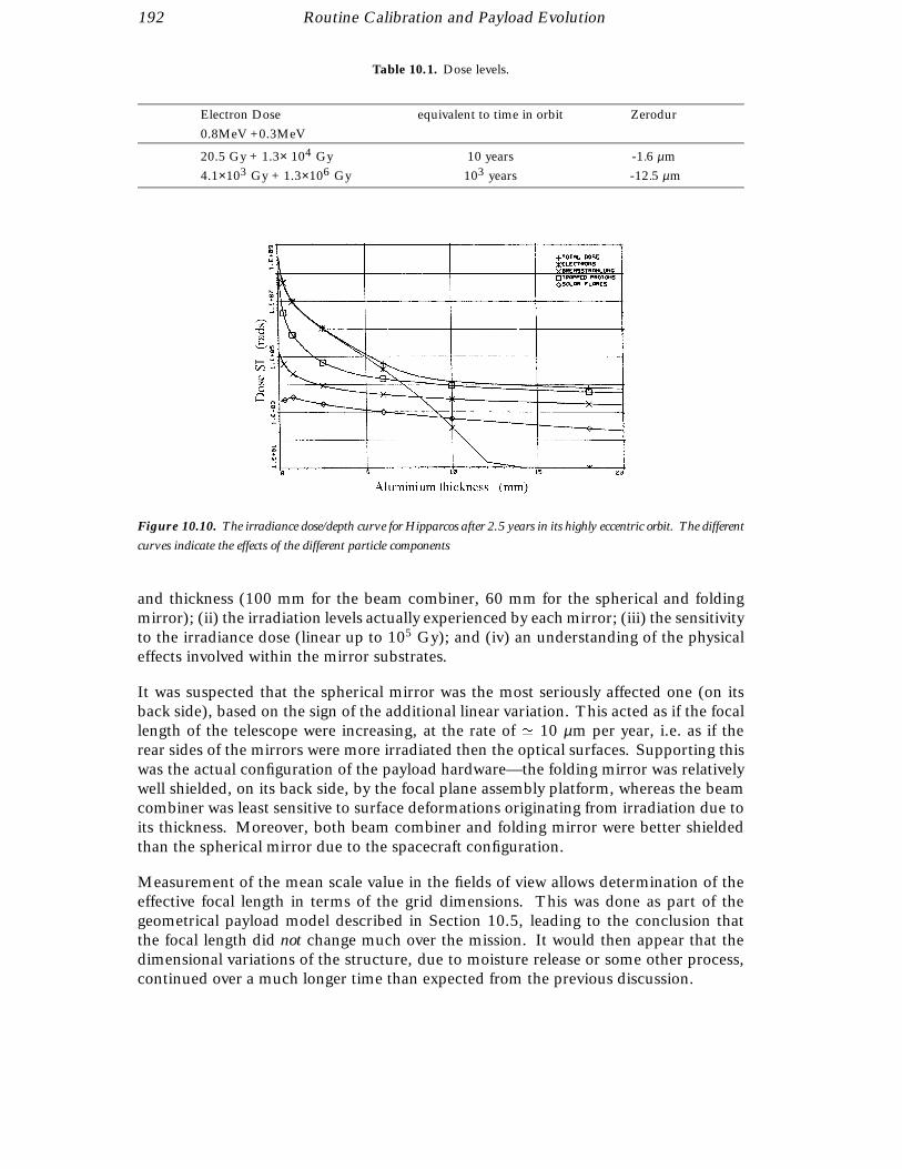
192 Routine Calibration and Payload Evolution
Table 10.1. Dose levels.
Electron Dose equivalent to time in orbit Zerodur
0.8MeV +0.3MeV
20.5 Gy + 1.3× 10⁴ Gy 10 years -1.6 µm
4.1×10³ Gy + 1.3×10⁶ Gy 103 years -12.5 µm
Figure 10.10. The irradiance dose/depth curve for Hipparcos after 2.5 years in its highly eccentric orbit. The different
curves indicate the effects of the different particle components
and thickness (100 mm for the beam combiner, 60 mm for the spherical and foldingmirror); (ii) the irradiation levels actually experienced by each mirror; (iii) the sensitivityto the irradiance dose (linear up to 105 Gy); and (iv) an understanding of the physicaleffects involved within the mirror substrates.
It was suspected that the spherical mirror was the most seriously affected one (on itsback side), based on the sign of the additional linear variation. This acted as if the focallength of the telescope were increasing, at the rate of ' 10 µm per year, i.e. as if therear sides of the mirrors were more irradiated then the optical surfaces. Supporting thiswas the actual configuration of the payload hardware—the folding mirror was relativelywell shielded, on its back side, by the focal plane assembly platform, whereas the beamcombiner was least sensitive to surface deformations originating from irradiation due toits thickness. Moreover, both beam combiner and folding mirror were better shieldedthan the spherical mirror due to the spacecraft configuration.
Measurement of the mean scale value in the fields of view allows determination of theeffective focal length in terms of the grid dimensions. This was done as part of thegeometrical payload model described in Section 10.5, leading to the conclusion thatthe focal length did not change much over the mission. It would then appear that thedimensional variations of the structure, due to moisture release or some other process,continued over a much longer time than expected from the previous discussion.
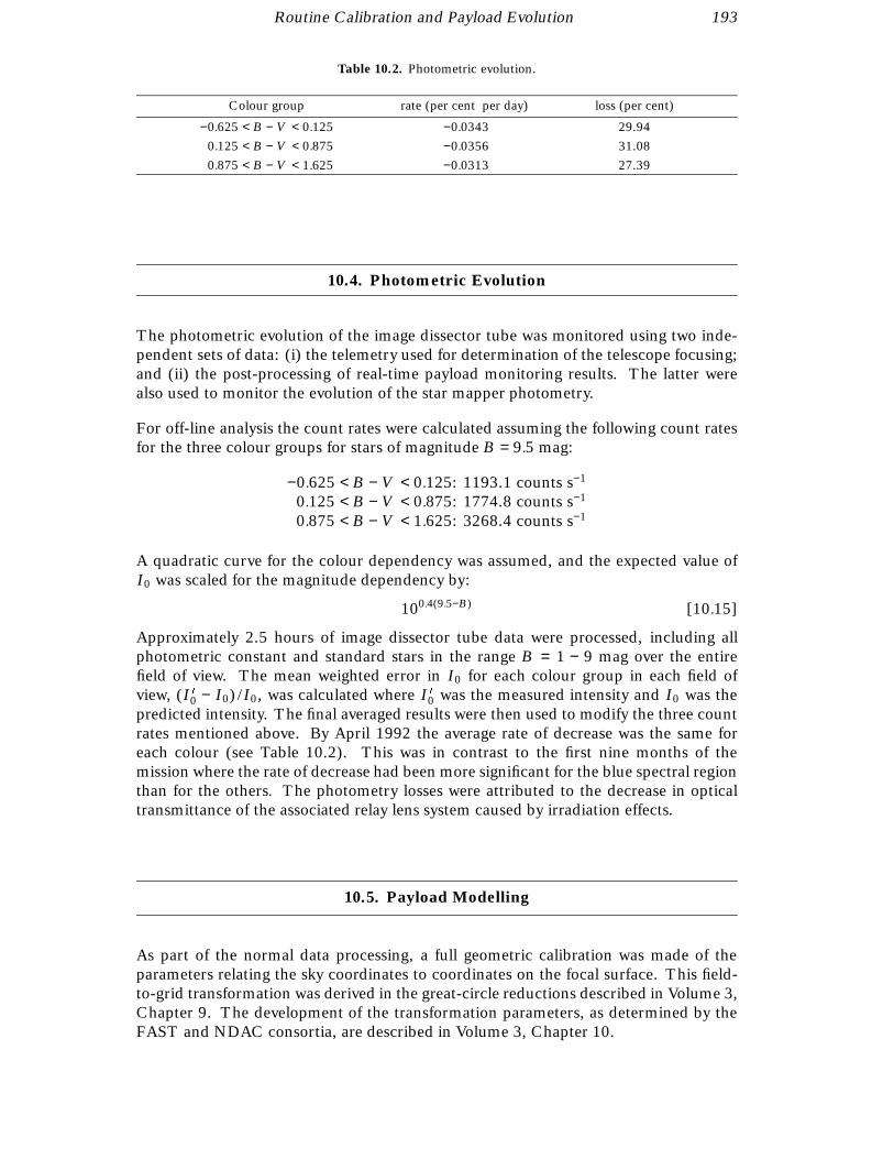
Routine Calibration and Payload Evolution 193
Table 10.2. Photometric evolution.
Colour group rate (per cent per day) loss (per cent)
−0.625 < B − V < 0.125 −0.0343 29.94
0.125 < B − V < 0.875 −0.0356 31.08
0.875 < B − V < 1.625 −0.0313 27.39
10.4. Photometric Evolution
The photometric evolution of the image dissector tube was monitored using two inde-pendent sets of data: (i) the telemetry used for determination of the telescope focusing;and (ii) the post-processing of real-time payload monitoring results. The latter werealso used to monitor the evolution of the star mapper photometry.
For off-line analysis the count rates were calculated assuming the following count ratesfor the three colour groups for stars of magnitude B = 9.5 mag:
−0.625 < B − V < 0.125: 1193.1 counts s−1
0.125 < B − V < 0.875: 1774.8 counts s−1
0.875 < B − V < 1.625: 3268.4 counts s−1
A quadratic curve for the colour dependency was assumed, and the expected value ofI0 was scaled for the magnitude dependency by:
100.4(9.5−B) [10.15]
Approximately 2.5 hours of image dissector tube data were processed, including allphotometric constant and standard stars in the range B = 1 − 9 mag over the entirefield of view. The mean weighted error in I0 for each colour group in each field ofview, (I 0
0 − I0) / I0, was calculated where I 0
0 was the measured intensity and I0 was thepredicted intensity. The final averaged results were then used to modify the three countrates mentioned above. By April 1992 the average rate of decrease was the same foreach colour (see Table 10.2). This was in contrast to the first nine months of themission where the rate of decrease had been more significant for the blue spectral regionthan for the others. The photometry losses were attributed to the decrease in opticaltransmittance of the associated relay lens system caused by irradiation effects.
10.5. Payload Modelling
As part of the normal data processing, a full geometric calibration was made of theparameters relating the sky coordinates to coordinates on the focal surface. This field-to-grid transformation was derived in the great-circle reductions described in Volume 3,Chapter 9. The development of the transformation parameters, as determined by theFAST and NDAC consortia, are described in Volume 3, Chapter 10.
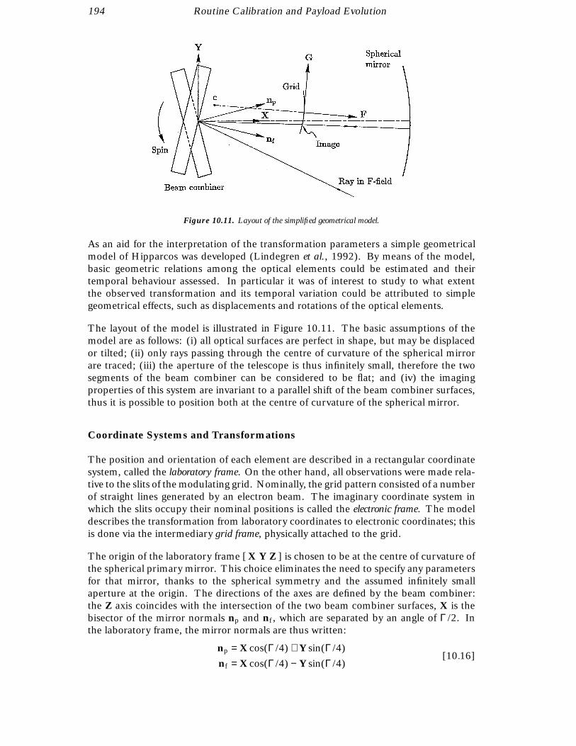
194 Routine Calibration and Payload Evolution
Figure 10.11. Layout of the simplified geometrical model.
As an aid for the interpretation of the transformation parameters a simple geometricalmodel of Hipparcos was developed (Lindegren et al., 1992). By means of the model,basic geometric relations among the optical elements could be estimated and theirtemporal behaviour assessed. In particular it was of interest to study to what extentthe observed transformation and its temporal variation could be attributed to simplegeometrical effects, such as displacements and rotations of the optical elements.
The layout of the model is illustrated in Figure 10.11. The basic assumptions of themodel are as follows: (i) all optical surfaces are perfect in shape, but may be displacedor tilted; (ii) only rays passing through the centre of curvature of the spherical mirrorare traced; (iii) the aperture of the telescope is thus infinitely small, therefore the twosegments of the beam combiner can be considered to be flat; and (iv) the imagingproperties of this system are invariant to a parallel shift of the beam combiner surfaces,thus it is possible to position both at the centre of curvature of the spherical mirror.
Coordinate Systems and Transformations
The position and orientation of each element are described in a rectangular coordinatesystem, called the laboratory frame. On the other hand, all observations were made rela-tive to the slits of the modulating grid. Nominally, the grid pattern consisted of a numberof straight lines generated by an electron beam. The imaginary coordinate system inwhich the slits occupy their nominal positions is called the electronic frame. The modeldescribes the transformation from laboratory coordinates to electronic coordinates; thisis done via the intermediary grid frame, physically attached to the grid.
The origin of the laboratory frame [ X Y Z ] is chosen to be at the centre of curvature ofthe spherical primary mirror. This choice eliminates the need to specify any parametersfor that mirror, thanks to the spherical symmetry and the assumed infinitely smallaperture at the origin. The directions of the axes are defined by the beam combiner:the Z axis coincides with the intersection of the two beam combiner surfaces, X is thebisector of the mirror normals np and nf , which are separated by an angle of Γ /2. Inthe laboratory frame, the mirror normals are thus written:
np = X cos(Γ /4) + Y sin(Γ /4)
nf = X cos(Γ /4) − Y sin(Γ /4)[10.16]

Routine Calibration and Payload Evolution 195
The grid frame [ F G H ] is physically attached to the grid, with origin at the nominalcentre of the grid and the (G, H) coordinates measured in the plane tangent to thegrid at the origin, with the slits of the main grid parallel to the H axis. F is measuredpositively on the convex side of the grid. The radius of curvature, R, which shouldstrictly be a model parameter, is consider a fixed parameter, since a very large change inR would be required to observe a measurable distortion. F can be related to (G, H) by:
F =−(G2 + H2)
R +p
R2 − (G2 + H2)≡ F (G, H) [10.17]
The relation between the grid frame and the laboratory frame is given by six parame-ters specifying the displacement and rotation bringing a coordinate triad aligned with[ X Y Z ] into coincidence with [ F G H ]. To effect this realignment the following stepsare applied: (1) displace the origin to (X0, Y0, Z0); (2) rotate an angle ψ about the thirdaxis; (3) rotate an angle θ about the second axis; (4) rotate an angle φ about the firstaxis. The resulting transformation is: X
YZ
!=
X0
Y0
Z0
!+ A
FGH
![10.18a]
where:
A =
cos θ cos ψ sin φ sin θ cos ψ − cos φ sin ψ cos φ sin θ cos ψ + sin φ sin ψcos θ sin ψ sin φ sin θ sin ψ + cos φ cos ψ cos φ sin θ sin ψ − sin φ cos ψ
− sin θ sin φ cos θ cos φ cos θ
!
[10.18b]
Ideally, the slit centres should be straight and equidistant lines in the (G, H) plane.However, due to imperfections in the electron beam pattern generator used to producethe grid, they are not. It is therefore necessary to convert from electronic coordinates(g, h) (in which the slits occupy their nominal positions) to the geometrical coordinates(G, H). The transformation from (g, h) to (G, H) includes, in the real instrument,at least the small and medium-scale irregularities of the grid pattern. However, inthe present idealised model, only the large-scale distortion caused by a tilting of theelectronic frame [ f g h ] with respect to the grid frame is considered. This may bedescribed by two successive rotations: (1) by the angle α about the third axis, and (2) bythe angle β about the second axis, which brings [ F G H ] into coincidence with [ f g h ].This gives the transformation: F
GH
!=
cos β cos α − sin α sin β cos αcos β sin α cos α sin β sin α
− sin β 0 cos β
! fgh
![10.19]
Calculating (G, H) from (g, h) may be achieved by iterating the equations:
G = g sec α + F tan α
H = h sec β − F sec α tan β − g tan α tan β
F = F (G, H)
[10.20]
starting from F = 0. The inverse conversion is obtained from Equation 10.17 and theinverse of Equation 10.19.
196 Routine Calibration and Payload Evolution
Model Parameters
The instrument model, in this simple approximation, can be parameterised by Γ, R,X0, Y0, Z0, φ, θ, ψ , α, and β. This can be further simplified, since some of theseparameters are redundant. The radius of curvature of the grid, R, is fixed. Y0 and ψare coupled since displacing the grid along the Y axis is equivalent to a simultaneousrotation of the grid and beam combiner about their respective Z axes, plus some secondorder adjustment of the distance between the two elements. Since a rotation of thebeam combiner about Z does not change the field-to-grid transformation, Y0 and ψ arein effect indistinguishable, and thus ψ = 0 is chosen. β does not enter the expressionfor g as a function of (F, G, H) and therefore cannot be determined from the observeddistortion of the main field, thus β = 0 must be assumed. The remaining parameters(Γ, X0, Y0, Z0, φ, θ, α) can be freely adjusted to represent the observed field-to-gridtransformation as closely as possible.
Relation to the Instrument Frame
The laboratory frame is not directly accessible to observation. Rather, the great-circlereductions establish the relation between the (observable) electronic coordinates and anideal system of angular coordinates in the two fields of view, the so-called instrumentframe. In order to interpret the field-to-grid transformation in terms of the modelparameters, it is therefore necessary to derive also the relation between the laboratoryand the instrument frames.
Given the model, specified by the parameters listed above, the field-to-grid transforma-tion is obtained by tracing a number of rays from different directions in either field ofview through the origin X = Y = Z = 0 and up to its intersection with the grid surface.If u is the unit vector towards a star, the direction of the ray after reflection in the beamcombiner is given by:
v = 2nn0u − u [10.21]
where n is the mirror normal from Equation 10.16. After reflection in the sphericalmirror, the ray returns to the origin in direction −v. The ray’s interception with the gridis computed from the parametric equation jvt − cj = R. c, the position of the centre ofcurvature of the grid, is obtained by setting F = −R and G = H = 0 in Equation 10.18.Solving for t gives:
t = v0c +p
R2 + (v0c)2 − c0c [10.22]
The point of interception is vt in the laboratory system, which can be transformed to thegrid frame and then to the electronic frame, via Equation 10.18 and Equation 10.19,yielding the (g, h) coordinates of the ray. To trace a ray in the opposite direction, startingin the laboratory frame, involves the application of Equations 10.20, 10.18 and 10.21.
The instrument frame [ x y z ] with associated field coordinates (w, z) are defined by theoptics together with a reference value γ0 of the basic angle and two features of the grid:(1) the chevron apex of the active star mapper, which defines the origin of the transversefield coordinate z; (2) the centre line of the main field, halfway between the 1344th and1345th slits, which defines the origin of the longitudinal coordinate w.

Routine Calibration and Payload Evolution 197
The star mapper apex, in electronic coordinates, is (gA, 0) with gA = −21.63385 mm;the centre line of the main grid is defined by g = 0. In the instrument system the twodirections in space corresponding to the field point (w, z) are:
u = [ x y z ]
+−w sin(γ0 /2) +p
1 − w2 − z2 cos(γ0 /2)+w cos(γ0 /2) ±
p1 − w2 − z2 sin(γ0 /2)z
![10.23]
where the upper/lower sign refers to the preceding/following field.
To calculate [ x y z ] in the laboratory system, the following procedure is adopted. Aray from (gA, 0) is traced through the preceding field. Let ap be the resulting unit vectortowards the point on the sky that is imaged on the star mapper apex. Similarly thecorresponding direction af through the following field is traced. Then:
z = haf × ap i [10.24]
with hi denoting vector normalisation. Next we must find the two viewing directions 0p
and 0f , perpendicular to z, which are imaged onto the main field centre line, g = 0. Thismay be done by writing 0p = hap + z × aps i where s is a scalar to be found by solvingthe equation g(0p) = 0. The following viewing direction is similarly found by solving sin 0f = haf + z × af s i. The remaining instrument axes are then obtained as:
x = h 0p + 0f iy = z × x
[10.25]
The basic angle is γ = arccos(00
p0f ).
Model Fitting
Stellar observations on the main grid provide a determination of the longitudinal elec-tronic coordinate g as a function of time. The basic assumption is that g increments byexactly 8.2 µm for each light modulation period. The observations are combined in thegreat-circle reductions to establish an empirical relation between g and (w, z) which maybe expressed in terms of polynomial coefficients gi j , hi j in the simplified field-to-gridtransformation formula:
g = −F0w +Xi , j
(gi j ± hi j ) wiz j [10.26]
where F0 is the reference value for the equivalent focal length. Terms up to 4th order(i + j < 4) were included. The lowest-order terms have a simple physical interpretation:by convention g00 = 0, which defines the origin of the w coordinate; g10 represents acorrection to the scale value corresponding to F0, while g01 represents a rotation aboutthe optical axis of the (w, z) frame with respect to the grid. Among the differential terms,h00 represents half the correction to the reference basic angle γ0, h10 represents half thedifference in scale between the preceding and following fields, and h01 represents halfthe differential rotation of the (w, z) frame.
Given the coefficients gi j , hi j in Equation 10.26 and the corresponding reference valuesγ0, F0, the observed electronic coordinate gO is obtained for an arbitrary position (w, z)in either field of view. From the geometrical model the ‘calculated’ coordinate gC isobtained from Equation 10.23 and a tracing from u to the electronic frame. gC depends

198 Routine Calibration and Payload Evolution
on the model parameters which are now adjusted to minimise the mean square deviationin both fields of view:
RMS2 =1
2n2
XFOVs
nXk=1
nXl=1
[gO(wk, zl ) − gC(wk, zl )]2 [10.27]
Analysis of the coefficients was done with 98 rays (n = 7) with a digitisation step of0.0022 in w and z.
The model was applied separately to the field-to-grid transformation data obtained bythe NDAC and FAST consortia in their final iterations of the great-circle reductions.Since the consortia used slightly different representations of this transformation theNDAC version, defined by Equation 10.26, was chosen as a common convention forthe purpose of this analysis. Converting the FAST results to the NDAC conventionsinvolved a reversal of the axis directions, change of units, and the addition of thenominal transformation. In general a separate great-circle reduction was made foreach ‘orbit’ of science data, i.e. for the (usually) several hours of data collected aroundeach apogee passage in the ' 10.7 hour period orbit. Consequently one independentdetermination of the model parameters Γ, X0, Y0, Z0, φ, θ, and α could usually bemade for each orbit during the periods when ‘good’ data were acquired. The results areplotted in Figures 10.12 and 10.13, with NDAC and FAST results on opposite pages.Tables 10.3–6 give examples of the pattern of residuals for the NDAC data at selectedpoints of the mission.
Results
Comparison of the NDAC and FAST results in Figures 10.12–13 shows a remarkablygood agreement in some of the parameters (Γ, X0, Z0), while systematic shifts are seenin other parameters; in all cases the evolution of the parameters is very similar in thetwo reductions. There is a striking difference in the amount of scatter, with the FASTresults appearing to be significantly more precise. To some extent this reflects a truedifference in precision: the FAST great-circle reductions are generally more precisethan the NDAC ones, mainly due to the use of both signal harmonics in the FASTanalysis (see below). However, the main difference in scatter seen in the diagrams isprobably caused by the cubic terms of the field-to-grid transformation, which in NDACwere estimated independently for each great-circle reduction, while in FAST they werekept at constant values for certain time intervals (see Volume 3, Chapter 10).
The systematic shifts of some model parameters between NDAC and FAST may becaused by differences in the reduction procedures that are known to influence thedetermination of the field-to-grid transformations, such as:
• the FAST reductions used a weighted mean for the first and second harmonics ofthe main detector signal, whereas only the phase of the fundamental harmonic wasused in NDAC data. The phase difference between the two harmonics is of theorder of 10 − 20 milliarcsec and variable across both fields of view and with time;
• the observed phases were corrected for medium-scale irregularities of the grid,before they were used to determine the field-to-grid transformation parameters.The medium-scale irregularities were determined from the residuals of the provi-sional great-circle reductions, and may contain distortion components which arenot orthogonal to the present model parameters;
Routine Calibration and Payload Evolution 199
• the determination of some parameters is sensitive to the adopted origin of the fieldcoordinates (w, z), which depends on the assumed geometry of the star mappergrid and on details of the attitude determination, all of which differed somewhatbetween FAST and NDAC.
While the actual values of the model parameters must consequently be interpretedwith some caution, their general evolution in time most likely represents a real physicaldevelopment of the instrument.
Discussion
The evolution of all model parameters except X0 are generally rather smooth up today ' 1270. However, there are a few significant jumps especially in Γ and Z0, e.g.around day 450, 780, 820 and 1000. Some of them can be related to incidents inthe thermal control system of the satellite. The evolution of X0 is characterised bythe sudden changes effected by refocusing operations, usually by +2 steps or 2.76 µm.Since X0 is actually the optical distance between the grid and the curvature centre of thespherical mirror, it is concluded that the mechanical structure connecting the sphericalmirror and the flat folding mirror was steadily shrinking; this is compensated by theperiodic refocusing moving the grid away from the flat mirror. The rate of shrinkingwas ' 1.3 × 10⁻⁷ day−1 at the beginning of the mission and ' 1.6 × 10⁻⁸ day−1 two yearslater.
At the times of optimum focus, which presumably occurred half-way between successiverefocusing events, the parameter X0 equals the effective focal length of the telescope (themeasuring-rod being the mean grid step of 8.2 µm). This quantity shows relatively smallchanges up to day ' 1200, the total amplitude being less than 5 µm for most of themission. This contradicts the tentative conclusion in Section 10.3 that there may be asecular drift of the focal length, by ' 10 µm/yr, caused by irradiation of the sphericalmirror.
The parameter α is constant to within the measurement errors which is to be expectedif this particular distortion pattern was generated during the manufacturing of the grid.The offset in mean value between FAST and NDAC appears to be related to the adoptedorigin of the z coordinate.
The long-term drifts in X0, Y0 and Z0 are all of the order of 0.1 µm day−1. Also themean drift in θ, when converted to a linear rate at a distance of 50–100 mm (the sizeof the grid assembly) is of similar size, while it is 30 times less in φ. The typical driftin Γ corresponds to only 10−5 µm day−1 at the edges of the beam combiner. Withthe exception of Γ the general tendency is for the drift rates to decrease with time, upto the anomalous behaviour from day 1270. From X0, φ and θ a time constant ofapproximately one year can be inferred. This is roughly consistent with the assumptionthat the main changes in the supporting structure are caused by moisture release, asdiscussed in Section 10.3.
Of considerable interest is to see which terms in the field-to-grid transformation maybe ‘explained’ in terms of the present model, i.e. as arising from simple translations androtations of the optical elements. A closer examination of the residuals shows that theonly terms that attain significant values in the model are: h00 (related to the basic angle),g10 (scale value), g01 (grid rotation about the optical axis), h01 (grid displacement alongthe Z axis), and the terms g20, g11, g02, which may account for a tilting of the grid.

200 Routine Calibration and Payload Evolution
Figure 10.12(a). Temporal evolution of the model parameters Γ, X0, Y0 and Z0, using data from NDAC.
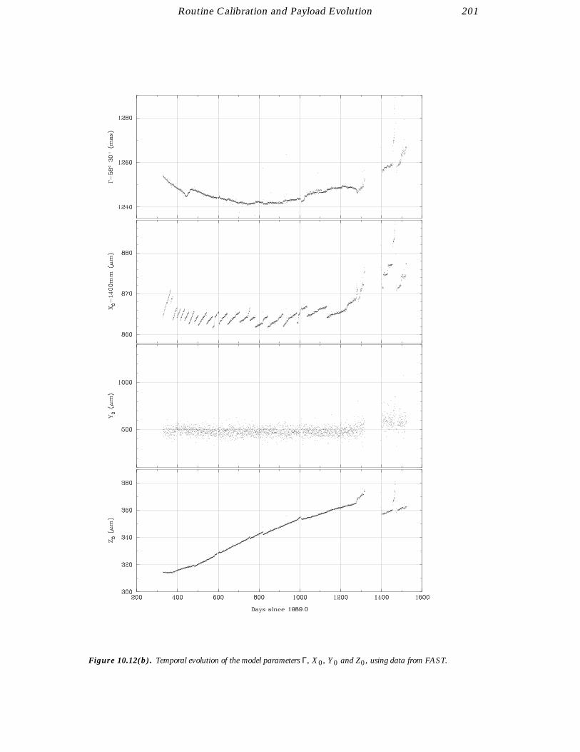
Routine Calibration and Payload Evolution 201
Figure 10.12(b). Temporal evolution of the model parameters Γ, X0, Y0 and Z0, using data from FAST.

202 Routine Calibration and Payload Evolution
Figure 10.13(a). Temporal evolution of the model parameters φ, θ and α, and of the rms residual of the model fits,
using data from NDAC.
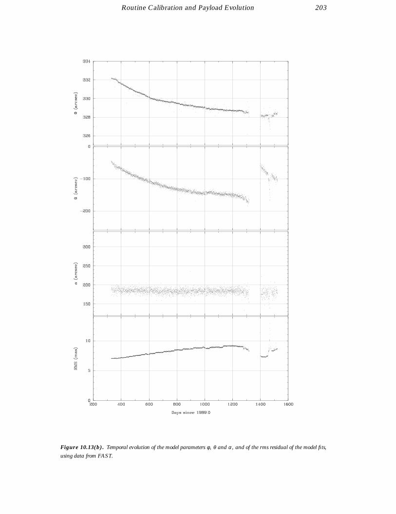
Routine Calibration and Payload Evolution 203
Figure 10.13(b). Temporal evolution of the model parameters φ, θ and α, and of the rms residual of the model fits,
using data from FAST.

204 Routine Calibration and Payload Evolution
Table 10.3. Residuals gO − gC (in milliarcsec) versus position in field (w, z) (in milli-rad) from the model fit
to the NDAC transformation data for day 309 (5 November 1989, orbit 1).
z nw –6.6 –4.4 –2.2 0.0 2.2 4.4 6.6
Following field of view:
–6.6 –3.53 –1.47 –0.68 –0.39 0.19 1.84 5.33
–4.4 –1.73 –0.61 –0.69 –1.20 –1.36 –0.37 2.54
–2.2 –0.16 0.26 –0.45 –1.51 –2.15 –1.57 0.99
0.0 1.02 1.00 –0.08 –1.45 –2.32 –1.91 0.57
2.2 1.67 1.46 0.25 –1.17 –2.03 –1.53 1.11
4.4 1.66 1.50 0.41 –0.81 –1.40 –0.57 2.47
6,6 0.83 0.97 0.26 –0.52 –0.60 0.83 4.52
Preceding field of view:
–6.6 –2.90 0.30 1.71 1.73 0.73 –0.92 –2.83
–4.4 –0.56 1.87 2.70 2.30 1.05 –0.67 –2.47
–2.2 0.46 2.32 2.74 2.12 0.82 –0.78 –2.29
0.0 0.43 1.90 2.12 1.45 0.29 –1.00 –2.03
2.2 –0.40 0.88 1.07 0.56 –0.28 –1.07 –1.42
4.4 –1.76 –0.49 –0.13 –0.30 –0.62 –0.72 –0.21
6.6 –3.39 –1.94 –1.22 –0.86 –0.48 0.30 1.86
Table 10.4. Residuals gO − gC (in milliarcsec) versus position in field (w, z) (in milli-rad) from the model fit
to the NDAC transformation data for day 1196 (10 April 1992, orbit 2000).
z nw –6.6 –4.4 –2.2 0.0 2.2 4.4 6.6
Following field of view:
–6.6 –17.77 –10.58 –4.88 –0.07 4.45 9.28 15.00
–4.4 –14.17 –8.41 –4.00 –0.36 3.10 7.00 11.91
–2.2 –11.50 –6.75 –3.23 –0.35 2.47 5.84 10.36
0.0 –9.94 –5.78 –2.74 –0.22 2.38 5.64 10.16
2.2 –9.66 –5.69 –2.71 –0.13 2.64 6.20 11.15
4.4 –10.85 –6.65 –3.33 –0.28 3.08 7.35 13.13
6.6 –13.68 –8.85 –4.77 –0.85 3.51 8.91 15.93
Preceding field of view:
–6.6 5.11 6.61 5.14 1.72 –2.63 –6.88 –10.02
–4.4 10.45 10.00 6.84 1.99 –3.54 –8.71 –12.51
–2.2 13.20 11.37 7.08 1.36 –4.78 –10.32 –14.23
0.0 13.81 11.15 6.30 0.26 –5.94 –11.28 –14.74
2.2 12.71 9.78 4.91 –0.88 –6.58 –11.16 –13.61
4.4 10.31 7.68 3.36 –1.63 –6.26 –9.53 –10.41
6.6 7.05 5.28 2.07 –1.56 –4.58 –5.97 –4.72
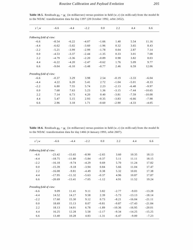
Routine Calibration and Payload Evolution 205
Table 10.5. Residuals gO − gC (in milliarcsec) versus position in field (w, z) (in milli-rad) from the model fit
to the NDAC transformation data for day 1397 (28 October 1992, orbit 2452).
z nw –6.6 –4.4 –2.2 0.0 2.2 4.4 6.6
Following field of view:
–6.6 –8.54 –6.22 –4.07 –1.66 1.40 5.54 11.16
–4.4 –6.62 –5.02 –3.60 –1.96 0.32 3.65 8.43
–2.2 –5.21 –3.99 –2.99 –1.78 0.04 2.87 7.14
0.0 –4.53 –3.37 –2.44 –1.35 0.33 3.01 7.08
2.2 –4.79 –3.36 –2.20 –0.89 0.98 3.82 8.03
4.4 –6.22 –4.20 –2.47 –0.62 1.76 5.09 9.77
6.6 –9.04 –6.10 –3.48 –0.77 2.46 6.59 12.06
Preceding field of view:
–6.6 –0.37 3.29 3.98 2.54 –0.19 –3.33 –6.04
–4.4 4.22 6.20 5.41 2.72 –1.04 –5.01 –8.33
–2.2 6.80 7.55 5.74 2.23 –2.13 –6.48 –9.97
0.0 7.68 7.63 5.23 1.36 –3.15 –7.44 –10.65
2.2 7.14 6.73 4.20 0.40 –3.81 –7.59 –10.08
4.4 5.47 5.15 2.93 –0.35 –3.83 –6.66 –7.98
6.6 2.96 3.18 1.71 –0.60 –2.90 –4.33 –4.05
Table 10.6. Residuals gO − gC (in milliarcsec) versus position in field (w, z) (in milli-rad) from the model fit
to the NDAC transformation data for day 1466 (4 January 1993, orbit 2607).
z nw –6.6 –4.4 –2.2 0.0 2.2 4.4 6.6
Following field of view:
–6.6 –23.42 –15.65 –8.90 –2.65 3.60 10.35 18.13
–4.4 –18.75 –11.80 –5.84 –0.37 5.11 11.11 18.15
–2.2 –16.18 –9.74 –4.29 0.69 5.70 11.24 17.82
0.0 –15.39 –9.18 –3.94 0.84 5.66 11.04 17.47
2.2 –16.08 –9.81 –4.49 0.38 5.32 10.81 17.38
4.4 –17.95 –11.32 –5.63 –0.37 4.96 10.87 17.87
6.6 –20.69 –13.41 –7.05 –1.12 4.91 11.52 19.24
Preceding field of view:
–6.6 9.09 11.41 9.11 3.82 –2.77 –9.03 –13.28
–4.4 14.52 14.17 9.58 2.39 –5.73 –13.13 –18.14
–2.2 17.60 15.30 9.12 0.73 –8.21 –16.04 –21.11
0.0 18.69 15.13 8.07 –0.81 –9.87 –17.43 –21.84
2.2 18.13 14.01 6.78 –1.89 –10.36 –16.95 –20.01
4.4 16.25 12.28 5.58 –2.17 –9.34 –14.25 –15.25
6.6 13.40 10.28 4.83 –1.31 –6.47 –9.00 –7.23

206 Routine Calibration and Payload Evolution
The model cannot reproduce the remaining terms, in particular h10 (scale differencebetween the fields of view) and the cubic terms (i + j = 3).
The steadily growing rms residual seen in the bottom panels of Figure 10.12(b) andFigure 10.13(b) is mainly due to the increasing difference in scale between the precedingand following field of view, and to a smaller extent to the cubic coefficients g30, g21
and g12. The cubic terms are much more prominent in the FAST residuals than inNDAC, and have a rather significant magnitude already at the beginning of the mission,which explains the higher level of rms residuals in Figure 10.13(b) compared withFigure 10.13(a). In fact, the evolution of the rms residual in Figure 10.13(a) almostexactly mirrors the evolution of the differential scale h10 (see Volume 3, Chapter 10),suggesting that this is the main reason for the model mismatch. This is confirmed by adirect inspection of the residuals in Tables 10.3–6.
In contrast to the drifts discussed previously, the evolution of the differential scale andcubic terms, reflected in the increasing rms residuals, can only be understood in termsof deformations of one or several of the mirror surfaces. The scale difference betweenthe preceding and following field of view must be caused by a difference in (mean)curvature between the two halves of one or more of the mirrors (beam combiner, flatfolding mirror, or spherical primary mirror).
The differential scale (and consequently the rms residual) was significantly reduced fromday 1397, immediately after the period of suspended operations (day 1315 to 1396),until day ' 1450. This interval of reduced differential scale (1992.82 to 1992.97)coincides with the period of low (' −10 C) payload temperature shown in Figure 12.4.The sharp increase in differential scale thereafter coincides with the operation in sun-pointing mode (day 1453 to 1466), after which the parameters assumed more normalvalues. This suggests a thermal mechanism for the development of the differential scale,rather than radiation exposure, at least for the changes on a short time scale. Tables 10.3to 10.6 show the residuals of the NDAC data at some key dates of this evolution:
Table 10.3: day 309 (beginning of mission);
Table 10.4: day 1196 (after gradual build-up of differential scale);
Table 10.5: day 1397 (immediately after suspension period, low payload tempera-ture);
Table 10.6: day 1466 (end of sun-pointing period).
The residuals of the FAST data are not shown. They are similar to the NDAC residualsexcept that a strong cubic distortion is superposed, partly obscuring the evolution of thedifferential scale.
To produce a cubic distortion seems to require a 4th-order deformation of a mirrorwhich is not in the plane of the entrance pupil, i.e. of the folding or spherical mirror.The required deformation is of the order of 50 nm peak value. The correspondingrms wavefront error would be of the order of λ /30, hardly enough to decrease the lightmodulation by a significant amount.
Routine Calibration and Payload Evolution 207
10.6. Star Mapper Sensitivity during Suspended Operations
During the first period of suspended operations (see Chapters 15–16) the payload wasswitched off to save power. When starting the two-gyro real-time attitude determinationthe star mapper process did not function until a minimum payload mean temperaturewas reached (approximately 5C).
On 2 October 1992, the spacecraft was spun down from 0.45 rpm to the nominal spinrate, using modified on-board control software which used only the transverse gyros.Nutation damping was performed. No real-time attitude determination initialisationwas possible due to the high background noise in the star mapper signal which was not,however, correlated with the actual solar activity.
A re-commissioning of the payload proceeded over the next three weeks to re-calibratethe single-slit response, basic angle, grid rotation, internal star pattern assembly, gridreference marks, transverse offset and focus position. No significant geometric defor-mations were detected, although the profile of the single-slit response was significantlybroadened, accounting for the difficulties in successfully processing the star mapperdata on-board and on-ground. At first, it was thought that the best focus position couldbe at fault and subsequently the focus position was moved ±80 steps from the previousbest focus position. No improvement was seen however.
During the period of suspended operations, the payload had been cooled to −40 Cto reduce the load on the surviving payload heaters. There was no technical reason tobelieve that the cold payload temperature should affect the star mapper signal in this way.Nevertheless, the decision was taken to re-heat the payload on 25 October 1992. Withina few hours, the star mapper response had improved sufficiently to allow ground real-time attitude determination to initialise the on-board real-time attitude determination.The reason for the sensitivity to temperature of the star mapper detectors was never fullyunderstood. While at low temperatures, the calibrations of the image dissector tube didnot suggest any such problems.
After the period of suspended operations, the star mapper response improved signifi-cantly (see Figure 10.2), and other instrumental parameters also changed significantly(see Volume 3) for reasons presumably related to the thermal environment experiencedduring suspended operations, but which were not fully understood.

208

11. SOLAR ARRAY PERFORMANCE
The solar arrays provided power for the satellite and payload in all but theeclipse conditions (when the batteries were used). Degradation of the solararrays occurred much more rapidly than had been predicted for the nominalgeostationary orbit. During the early months of the mission, the available solararray power was expected to lead to a constraint on the overall mission dura-tion. Modelling of the radiation damage, and predicting power margins andoperational contingency procedures during extended eclipses, was therefore animportant part of the operational procedure. This led to improved modellingof the degradation mechanisms, and good prediction of the available powerduring the later part of the mission.
11.1. Introduction
The power system comprised a solar array, associated sequential switching shunt regula-tor and battery discharge regulators which regulated the main bus potential to 50±1 V inboth sunlight and eclipse periods. Recharge of the power system batteries was achievedby allocating specific solar array cell strings or sections to this particular function.
The solar array consisted of three lightweight panels 120 apart. The panels were verysimilar to those used on most of the ESA communication spacecraft such as ECS andMARECS. These panels embodied six electrical sections of 142 series connected cellsby 7 parallel cells for powering the main bus. A separate battery charge array wascomposed of six independent cell strings of 126 series connected cells which could beused for either sequential or parallel recharge of the two 28 cell 10 Ah nickel cadmiumbatteries of the system.
The solar cells were arranged to form main and charge sections. The solar array wasbased on proven solar generator design concepts, but with some important improve-ments, including the use of materials such as aluminium honeycomb, together withcarbon-fibre reinforced plastic. This gave a lightweight, but highly-loadable structure.Some redesign on the hinge configuration was performed to minimise shock loads cre-ated during the latch up of a deploying panel at high satellite spin rates. Each panelwas equipped with two hold-down units and one pyro-actuated cable cutter as a releaseunit.

210 Solar Array Performance
For the electrical layout, the goal was to design a highly failure-resistant cell design.The solar generator design involved single stringing in all main sections, with individualblocking diodes to limit the effect of power loss in case of a short circuit, as well asan extra thick kapton insulation layer to give a high degree of protection against shortcircuits. Protection against adverse effects of shadowing of the inner parts of the solararray wings due to attitude control subsystem failure was achieved by incorporatingshunt diodes for cell protection.
The protection against electrostatic discharge, which had caused many problems in thepast, was designed with great care. To prevent charging of non-conductive structuralparts of the front side of the panel, all areas not covered with solar cells were protectedwith an aluminised kapton foil, which was grounded to the structure of the solar array.The complete rear side, as well as the so-called ‘edge members’, were painted withconductive black paint. All panel wiring was carefully routed through the edge membersand on the panel’s rear side, wherever possible.
Mechanical Properties
Each of the three solar arrays was based on a lightweight structure built of aluminiumhoneycomb and carbon-fibre reinforced plastic: with kapton foil to electrically insulatethe cell area from the array structure; special hinges to decrease latch-up shock loadsduring deployment at high spin rates (up to 10 rpm); and two hold-down points, withpyrotechnic cable cutter release mechanisms. Each of the arrays was 1690 mm long,1190 mm wide, and 23 mm high. All three panels together weighed about 31 kg.
Electrical Properties
Each of the three solar arrays had two main sections, made up of seven strings with 142serial connected cells (each string was equipped with a blocking and shunt diode), andtwo charge sections, each with 126 serial connected cells and shunt diodes to protectagainst shadowing effects. The cells were back-surface-reflecting high-efficiency unitswith a thickness of 180 µm. Electrostatic discharge protection was provided by meansof grounded aluminised kapton on the panel’s front side and conductive black painton the rear and on edge members. An integrated thermocouple provided subsystemtemperature data during the mission, and array deployment and successful latch-up wasmonitored by separate switches for each panel.
One of the consequences of the satellite being in a geostationary transfer orbit was thatthe efficiency of its solar panels was degraded by the repeated radiation exposure at amuch higher rate than if the satellite had been in geostationary orbit. The consequenceof this process led to a potentially shorter lifetime for the mission.
To estimate the lifetime of the satellite, periodic measurements were obtained from theopen circuit voltage of the charge array strings. The first results from these calculationsresulted in a very pessimistic forecast for the mission. The degradation was consideredto be very high and a potential lifetime of only about 6 months was predicted. However,after first collection of real spacecraft data the degradation proved to be far less than theoriginally predicted values.
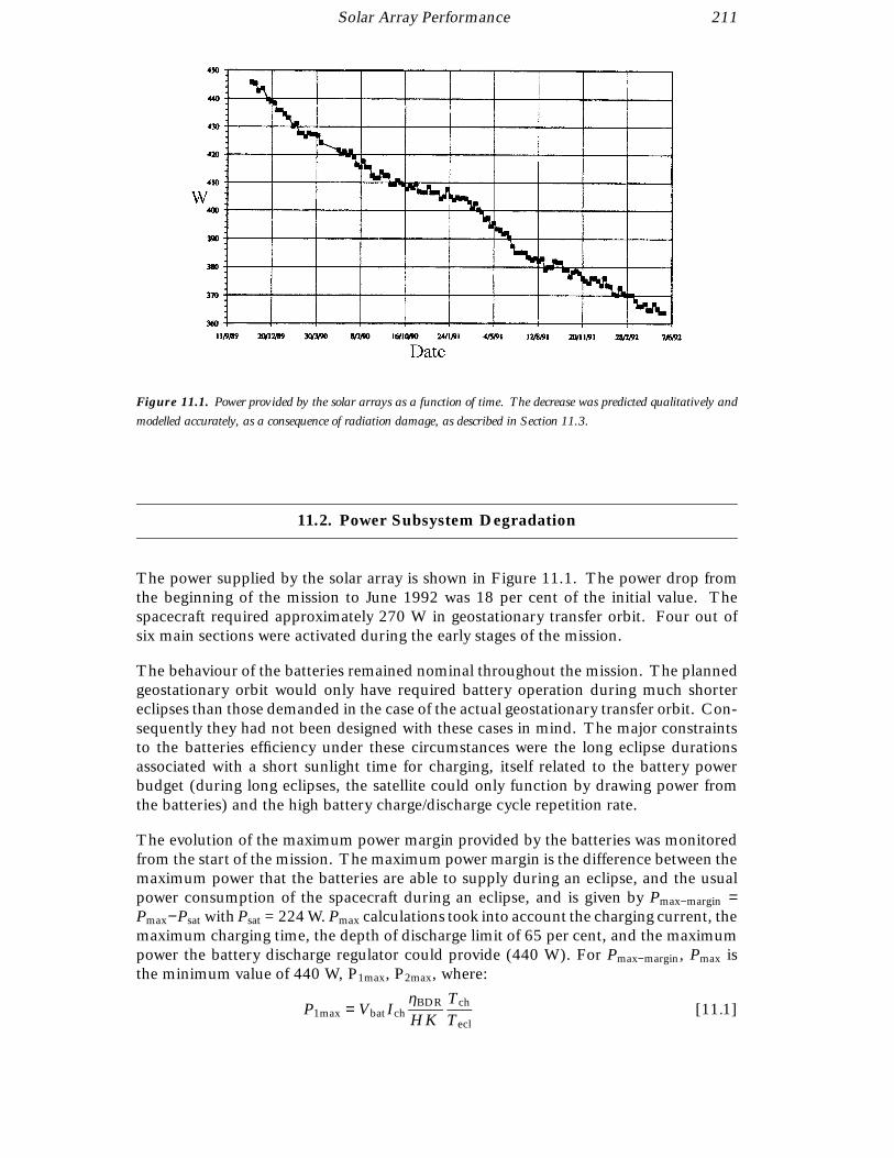
Solar Array Performance 211
Figure 11.1. Power provided by the solar arrays as a function of time. The decrease was predicted qualitatively and
modelled accurately, as a consequence of radiation damage, as described in Section 11.3.
11.2. Power Subsystem Degradation
The power supplied by the solar array is shown in Figure 11.1. The power drop fromthe beginning of the mission to June 1992 was 18 per cent of the initial value. Thespacecraft required approximately 270 W in geostationary transfer orbit. Four out ofsix main sections were activated during the early stages of the mission.
The behaviour of the batteries remained nominal throughout the mission. The plannedgeostationary orbit would only have required battery operation during much shortereclipses than those demanded in the case of the actual geostationary transfer orbit. Con-sequently they had not been designed with these cases in mind. The major constraintsto the batteries efficiency under these circumstances were the long eclipse durationsassociated with a short sunlight time for charging, itself related to the battery powerbudget (during long eclipses, the satellite could only function by drawing power fromthe batteries) and the high battery charge/discharge cycle repetition rate.
The evolution of the maximum power margin provided by the batteries was monitoredfrom the start of the mission. The maximum power margin is the difference between themaximum power that the batteries are able to supply during an eclipse, and the usualpower consumption of the spacecraft during an eclipse, and is given by Pmax−margin =Pmax−Psat with Psat = 224 W. Pmax calculations took into account the charging current, themaximum charging time, the depth of discharge limit of 65 per cent, and the maximumpower the battery discharge regulator could provide (440 W). For Pmax−margin, Pmax isthe minimum value of 440 W, P1max, P2max, where:
P1max = Vbat IchηBDR
HKTch
Tecl[11.1]
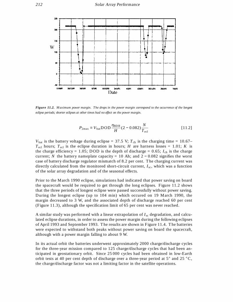
212 Solar Array Performance
Figure 11.2. Maximum power margin. The drops in the power margin correspond to the occurrence of the longest
eclipse periods; shorter eclipses at other times had no effect on the power margin.
P2max = VbatDODηBDR
H(2 − 0.082)
NTecl
[11.2]
Vbat is the battery voltage during eclipse = 37.5 V; Tch is the charging time = 10.67–Tecl hours; Tecl is the eclipse duration in hours; H are harness losses = 1.01; K isthe charge efficiency = 1.05; DOD is the depth of discharge = 0.65; Ich is the chargecurrent; N the battery nameplate capacity = 10 Ah; and 2 − 0.082 signifies the worstcase of battery discharge regulator mismatch of 8.2 per cent. The charging current wasdirectly calculated from the monitored short-circuit current, Isc, which was a functionof the solar array degradation and of the seasonal effects.
Prior to the March 1990 eclipse, simulations had indicated that power saving on boardthe spacecraft would be required to get through the long eclipses. Figure 11.2 showsthat the three periods of longest eclipse were passed successfully without power saving.During the longest eclipse (up to 104 min) which occured on 19 March 1990, themargin decreased to 3 W, and the associated depth of discharge reached 60 per cent(Figure 11.3), although the specification limit of 65 per cent was never reached.
A similar study was performed with a linear extrapolation of Isc degradation, and calcu-lated eclipse durations, in order to assess the power margin during the following eclipsesof April 1993 and September 1993. The results are shown in Figure 11.4. The batterieswere expected to withstand both peaks without power saving on board the spacecraft,although with a power margin falling to about 9 W.
In its actual orbit the batteries underwent approximately 2000 charge/discharge cyclesfor the three-year mission compared to 125 charge/discharge cycles that had been an-ticipated in geostationary orbit. Since 25 000 cycles had been obtained in low-Earthorbit tests at 40 per cent depth of discharge over a three-year period at 5 and 25 C,the charge/discharge factor was not a limiting factor in the satellite operations.
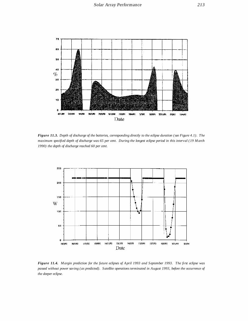
Solar Array Performance 213
Figure 11.3. Depth of discharge of the batteries, corresponding directly to the eclipse duration (see Figure 4.1). The
maximum specified depth of discharge was 65 per cent. During the longest eclipse period in this interval (19 March
1990) the depth of discharge reached 60 per cent.
Figure 11.4. Margin prediction for the future eclipses of April 1993 and September 1993. The first eclipse was
passed without power saving (as predicted). Satellite operations terminated in August 1993, before the occurrence of
the deeper eclipse.
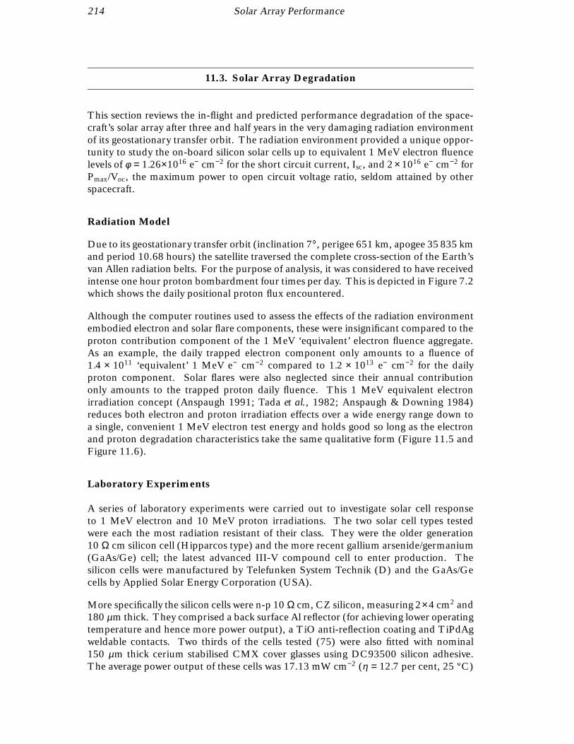
214 Solar Array Performance
11.3. Solar Array Degradation
This section reviews the in-flight and predicted performance degradation of the space-craft’s solar array after three and half years in the very damaging radiation environmentof its geostationary transfer orbit. The radiation environment provided a unique oppor-tunity to study the on-board silicon solar cells up to equivalent 1 MeV electron fluencelevels of φ = 1.26×10¹⁶ e− cm−2 for the short circuit current, Isc, and 2× 10¹⁶ e− cm−2 forPmax/Voc, the maximum power to open circuit voltage ratio, seldom attained by otherspacecraft.
Radiation Model
Due to its geostationary transfer orbit (inclination 7, perigee 651 km, apogee 35 835 kmand period 10.68 hours) the satellite traversed the complete cross-section of the Earth’svan Allen radiation belts. For the purpose of analysis, it was considered to have receivedintense one hour proton bombardment four times per day. This is depicted in Figure 7.2which shows the daily positional proton flux encountered.
Although the computer routines used to assess the effects of the radiation environmentembodied electron and solar flare components, these were insignificant compared to theproton contribution component of the 1 MeV ‘equivalent’ electron fluence aggregate.As an example, the daily trapped electron component only amounts to a fluence of1.4 × 1011 ‘equivalent’ 1 MeV e− cm−2 compared to 1.2 × 10¹³ e− cm−2 for the dailyproton component. Solar flares were also neglected since their annual contributiononly amounts to the trapped proton daily fluence. This 1 MeV equivalent electronirradiation concept (Anspaugh 1991; Tada et al., 1982; Anspaugh & Downing 1984)reduces both electron and proton irradiation effects over a wide energy range down toa single, convenient 1 MeV electron test energy and holds good so long as the electronand proton degradation characteristics take the same qualitative form (Figure 11.5 andFigure 11.6).
Laboratory Experiments
A series of laboratory experiments were carried out to investigate solar cell responseto 1 MeV electron and 10 MeV proton irradiations. The two solar cell types testedwere each the most radiation resistant of their class. They were the older generation10 Ω cm silicon cell (Hipparcos type) and the more recent gallium arsenide/germanium(GaAs/Ge) cell; the latest advanced III-V compound cell to enter production. Thesilicon cells were manufactured by Telefunken System Technik (D) and the GaAs/Gecells by Applied Solar Energy Corporation (USA).
More specifically the silicon cells were n-p 10 Ω cm, CZ silicon, measuring 2×4 cm2 and180 µm thick. They comprised a back surface Al reflector (for achieving lower operatingtemperature and hence more power output), a TiO anti-reflection coating and TiPdAgweldable contacts. Two thirds of the cells tested (75) were also fitted with nominal150 µm thick cerium stabilised CMX cover glasses using DC93500 silicon adhesive.The average power output of these cells was 17.13 mW cm−2 (η = 12.7 per cent, 25 C)
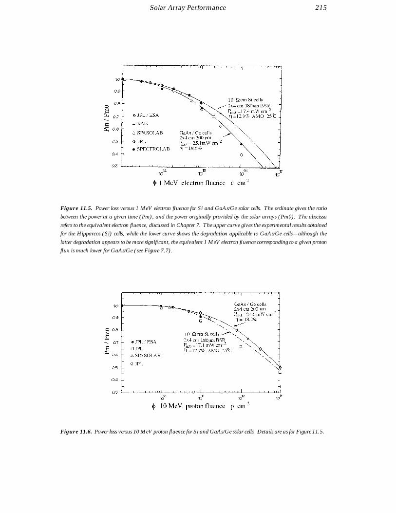
Solar Array Performance 215
Figure 11.5. Power loss versus 1 MeV electron fluence for Si and GaAs/Ge solar cells. The ordinate gives the ratio
between the power at a given time (Pm), and the power originally provided by the solar arrays (Pm0). The abscissa
refers to the equivalent electron fluence, discussed in Chapter 7. The upper curve gives the experimental results obtained
for the Hipparcos (Si) cells, while the lower curve shows the degradation applicable to GaAs/Ge cells—although the
latter degradation appears to be more significant, the equivalent 1 MeV electron fluence corresponding to a given proton
flux is much lower for GaAs/Ge (see Figure 7.7).
Figure 11.6. Power loss versus 10 MeV proton fluence for Si and GaAs/Ge solar cells. Details are as for Figure 11.5.

216 Solar Array Performance
i.e. 170 W m−2. The average uncovered cell weight was 439 mg yielding a power-to-weight ratio of 38.7 W kg−1 for the basic cell.
Six separate CMX cerium stabilised cover glasses were also supplied by Pilkington SpaceTechnology (UK) for testing to facilitate differentiation of radiation-induced opticaldarkening from basic cell degradation.
The GaAs/Ge cells tested (60) were p-n, metal organic chemical vapour depositioncells (Cheng et al., 1991) measuring 2 × 4 cm2 and 200 µm thick. The GaAs toGe interface was inactive. Half of the cells were covered with 50 µm thick ceriumstabilised CMX cover glasses. The average power output of the cells was 24.60 mW cm−2
(η = 18.3 per cent, 25 C) i.e. 246 W m−2. The average uncovered cell weight was886.9 mg yielding a power-to-weight ratio of 27.7 W kg−1 for the basic cell.
Solar Cell Performance Measurements
Solar cell I–V performance measurements were made using reliable pulsed or continuousxenon solar simulators as a light source. A primary standard cell of similar spectralresponse to that of the test cells was used to set the simulator intensity. The solar cellsI–V characteristics were measured with a conventional four-probe measurement systemand a power supply for a load. The solar cell temperature was controlled to 25 ± 0.2 Cduring I–V measurements.
1 MeV Electron and 10 MeV Proton Irradiations
The 1 MeV electron irradiations of the covered silicon solar cells were performed usingthe JPL (USA) Dynamitron accelerator (Anspaugh 1991). The electron beam wasspread into a wide uniform beam using an aluminium foil 127 µm thick. Beam intensityis highest at the beam centre and falls off to 91 per cent of the centre value at the edges.The cells were mounted on a copper cell-mounting plate using vacuum grease for goodthermal contact. The cell-mounting plate was then bolted onto a fixed target planein the irradiation chamber. This target plane was temperature controlled to hold thesolar cell temperature at 28 C during the electron irradiations and a Faraday cup wasmounted in the centre of this plane for flux and fluence dosimetry. Cumulative fluenceexposures were 1 × 10¹³, 2 × 10¹³, 5 × 10¹³, 1 × 10¹³, 2 × 10¹³, 5 × 10¹³ and 1 × 10¹⁵
e− cm−2. All irradiations were carried out in vacuum at a pressure below 5 × 10⁻⁵ torr.
RAE (UK) subsequently repeated these tests on the uncovered Hipparcos Si cells usinga water-cooled vacuum cell holder at their BICC van de Graaff accelerator in London.The 1 MeV electron fluence was extended to 3 × 10¹⁵ e− cm−2.
Spasolab irradiated their assignment of GaAs/Ge solar cells up to a 1 MeV electronfluence of 2 × 10¹⁵ e− cm−2 using the University of Delft (NL) van de Graaff acceler-ator. This facility was also used to irradiate the covered silicon cells together with theindividual CMX cover glasses up to very high fluences (3 × 10¹⁶ e− cm−2) to evaluatethe radiation ‘hardness’ of the glasses and their adhesive (DC93500). This particularexperiment was repeated, with the inclusion of directly glassed (electrostatically bondedwith no adhesive) control cells, on account of the physical effects observed.
The 10 MeV proton irradiations were performed using Tandem van de Graaff accel-erators (Anspaugh 1991; Anspaugh & Downing 1984). Beam energy was controlled

Solar Array Performance 217
by 90 magnetic analysis and the accelerator energy was stabilised by a slit-feedbacksystem to control the van de Graaff terminal voltage. All irradiations and dosimetrywere performed in vacuum (less than 5 × 10⁻⁶ torr). The small focused proton beamproduced by the accelerator was spread into a wide area uniform beam by means ofscattering foils. The target plane was approximately 3 m from the scattering foils. Thefoils were chosen so that the beam intensity at the edge of a 10 cm diameter circle in thetarget plane varied no more than 7 per cent from the beam intensity at the centre.
The solar cell target plane was rotated at a rotation rate dΘ/dt proportional to 1/sin Θ,thereby providing a good simulation of the omni-directional space radiation environmentby rotation about only one axis. Fluence levels up to 1 × 10¹¹ protons cm−2 werestudied by JPL for the covered Si Hipparcos cells. Spasolab irradiated their GaAs/Gecell assignment up to a 10 MeV fluence of 1.59 × 10¹² protons cm−2 using the CEAaccelerator near Paris.
The I–V characteristics of the irradiated cells were measured following ‘cool-down’ andperformance stabilisation by photon irradiation (i.e. under simulated illumination at25 C for 48 hours).
In-Orbit Hipparcos Solar Cell Data
The most fundamental indication of the radiation influence was initially obtained fromtelemetry data of the open circuit voltage (Voc, Figure 11.7) of the charge array strings.A further indication of the radiation environment effect was also regularly obtained fromtelemetry data of the short circuit current (Isc, Figure 11.8) of one of the main solararray sections, this section being permanently dumped at launch as a result of loweron-board power consumptions than originally anticipated for the mission.
The Isc and Voc data were transmitted from ESOC on a regular basis after normalisationof the data to a solar aspect angle of 0, air-mass-zero illumination and a cell temperatureof 25 C. The data was also correlated with solar intensity to account for the cyclicvariation of the Earth-Sun distance. After February 1990, only solar arrays 1 and 2were taken into account, since solar array 3 had suffered a thermistance failure. Thenominal Hipparcos operating mode was with a solar aspect angle of 43 and a celltemperature of 33. This was backed up by a ‘safe mode’ configuration with a solaraspect angle of 0 and a cell temperature of 55 C. The flight data is probably accurateto ±2 per cent.
The final Isc values result from the satellite sun-pointing mode during the final fifteendays. The operational voltage limit was taken to be 53 V which corresponded to anominal voltage of 51 V, together with the voltage drop, the blocking diode and thecharged quad. The average degradation was about 3 V per year, and extrapolation ofthe curve shown in Figure 11.8 indicated a lifetime up to the middle of 1994. However,since there was a direct correlation between the degradation of the solar generator andthe solar particle flux (particularly the proton flux), the lifetime could be reduced in theevent of stronger than predicted solar activity.

218 Solar Array Performance
Figure 11.7. Hipparcos in-flight solar array open circuit voltage (Voc) degradation, normalised to 25 C, 0 sun
aspect angle (SAA), and air-mass-zero illumination (AMO). The dashed line indicates the degradation predicted
early in the revised mission (in December 1989). The data points (open circles) correspond to the measured data. The
shaded region corresponds to the final predicted performance described in the text, the uncertainty region corresponding
to the tolerance on the cover glass thickness (nominally 6 mil; or 0.006 inches). The observed degradation corresponded
fairly well with the final assessment of the cell performance.
Figure 11.8. Hipparcos in-flight solar array short circuit current (Isc) degradation. Details are as for Figure 11.7.
The observed degradation (solid circles) was less severe than the original (December 1989) prediction. The lower
shaded region corresponds to the final model for the actual (6 mil thick) cover glass used for the Hipparcos solar arrays.
The upper shaded region indicates the improvement in performance expected had 12 mil thick cover glass (used for
GEOS) been used.
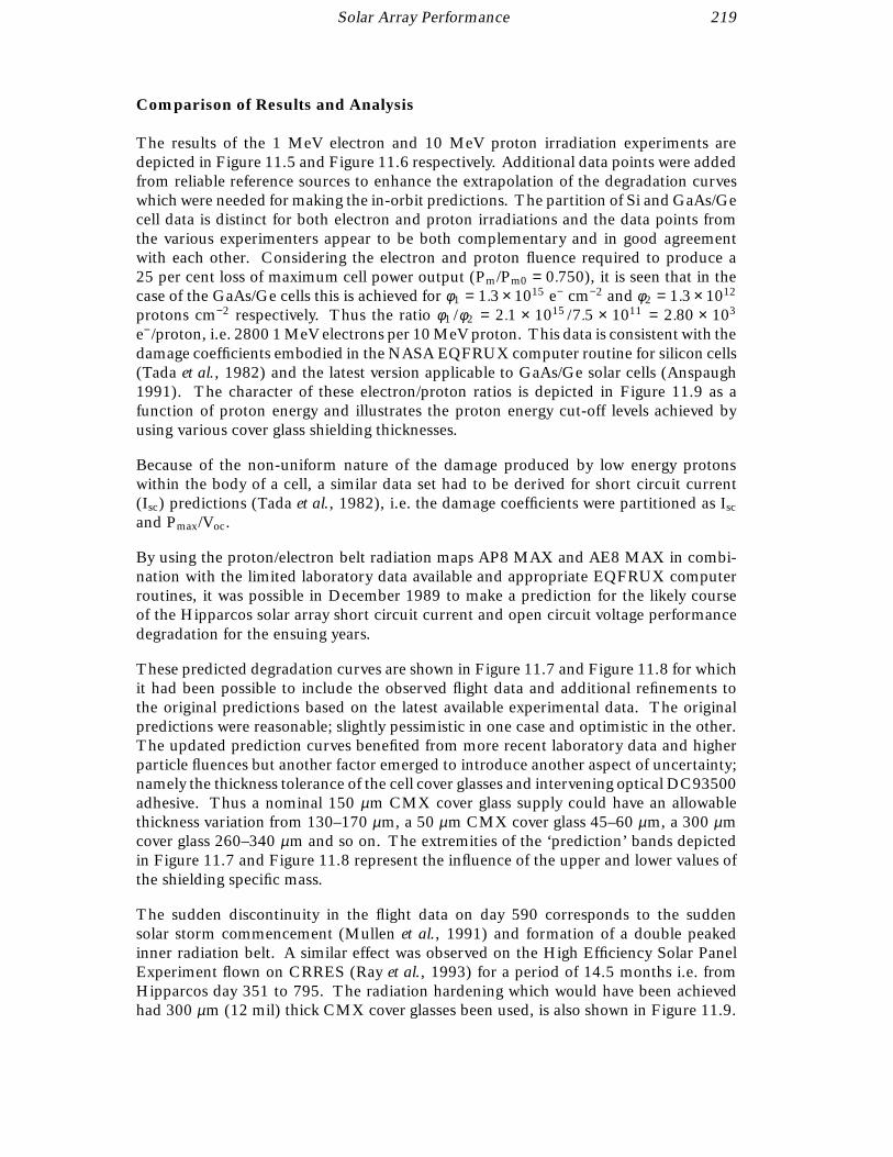
Solar Array Performance 219
Comparison of Results and Analysis
The results of the 1 MeV electron and 10 MeV proton irradiation experiments aredepicted in Figure 11.5 and Figure 11.6 respectively. Additional data points were addedfrom reliable reference sources to enhance the extrapolation of the degradation curveswhich were needed for making the in-orbit predictions. The partition of Si and GaAs/Gecell data is distinct for both electron and proton irradiations and the data points fromthe various experimenters appear to be both complementary and in good agreementwith each other. Considering the electron and proton fluence required to produce a25 per cent loss of maximum cell power output (Pm/Pm0 = 0.750), it is seen that in thecase of the GaAs/Ge cells this is achieved for φ1 = 1.3 × 10¹⁵ e− cm−2 and φ2 = 1.3 × 10¹²
protons cm−2 respectively. Thus the ratio φ1 /φ2 = 2.1 × 10¹⁵ /7.5 × 1011 = 2.80 × 10³
e− /proton, i.e. 2800 1 MeV electrons per 10 MeV proton. This data is consistent with thedamage coefficients embodied in the NASA EQFRUX computer routine for silicon cells(Tada et al., 1982) and the latest version applicable to GaAs/Ge solar cells (Anspaugh1991). The character of these electron/proton ratios is depicted in Figure 11.9 as afunction of proton energy and illustrates the proton energy cut-off levels achieved byusing various cover glass shielding thicknesses.
Because of the non-uniform nature of the damage produced by low energy protonswithin the body of a cell, a similar data set had to be derived for short circuit current(Isc) predictions (Tada et al., 1982), i.e. the damage coefficients were partitioned as Isc
and Pmax/Voc.
By using the proton/electron belt radiation maps AP8 MAX and AE8 MAX in combi-nation with the limited laboratory data available and appropriate EQFRUX computerroutines, it was possible in December 1989 to make a prediction for the likely courseof the Hipparcos solar array short circuit current and open circuit voltage performancedegradation for the ensuing years.
These predicted degradation curves are shown in Figure 11.7 and Figure 11.8 for whichit had been possible to include the observed flight data and additional refinements tothe original predictions based on the latest available experimental data. The originalpredictions were reasonable; slightly pessimistic in one case and optimistic in the other.The updated prediction curves benefited from more recent laboratory data and higherparticle fluences but another factor emerged to introduce another aspect of uncertainty;namely the thickness tolerance of the cell cover glasses and intervening optical DC93500adhesive. Thus a nominal 150 µm CMX cover glass supply could have an allowablethickness variation from 130–170 µm, a 50 µm CMX cover glass 45–60 µm, a 300 µmcover glass 260–340 µm and so on. The extremities of the ‘prediction’ bands depictedin Figure 11.7 and Figure 11.8 represent the influence of the upper and lower values ofthe shielding specific mass.
The sudden discontinuity in the flight data on day 590 corresponds to the suddensolar storm commencement (Mullen et al., 1991) and formation of a double peakedinner radiation belt. A similar effect was observed on the High Efficiency Solar PanelExperiment flown on CRRES (Ray et al., 1993) for a period of 14.5 months i.e. fromHipparcos day 351 to 795. The radiation hardening which would have been achievedhad 300 µm (12 mil) thick CMX cover glasses been used, is also shown in Figure 11.9.

220 Solar Array Performance
Figure 11.9. The dependence of the number of equivalent 1 MeV electrons per proton as a function of proton energy,
for various cover glass (shielding) thicknesses, and for Si and for GaAs solar cells. The figure illustrates the proton
energy cut-off levels achieved by using various cover glass thicknesses. The Hipparcos cells corresponded to the 6 mil
(0.006 inch ~ 150 µm) cover glasses on Si.
Since the Hipparcos solar cell’s operating point was now beyond the knee of its I–Vcurve it was possible to reconstitute its I–V characteristic by monitoring the batteryrecharge current in this region. This is shown in Figure 11.10 along with estimates ofthe associated 1 MeV equivalent electron fluences for Isc and Pmax/Voc degradation.
As a consequence of the advanced stage of performance deterioration an interestingphenomenon was observed. The solar array delivered less power when pointed normalto the Sun (a safe mode in the event of gyro problems) than when in its normal operatingmode (solar aspect angle = 43). This arose because pointing at the Sun causes thecell’s temperature to rise from 33 to 55 C thereby lowering Voc still further.
Concerning the durability of the cell’s optical components at high fluence 1 MeV electronirradiation (Delft University), at φ = 3 × 10¹⁶ e− cm−2, it was observed that several coverglasses had started to delaminate. This is shown in Figure 11.11. Subsequent micro-scopic examination and dissection revealed that advanced polymerisation and hardeningof the DC93500 silicone adhesive had taken place and was followed by delaminationat the cover glass/adhesive interface. The influence on the electrical performance ofthe cell was negligible (1 per cent). A repeat experiment was conducted with directly‘glassed’ cells (i.e. electrostatically bonded with no adhesive) included as a control.These cells showed no such deterioration but several of the conventionally covered cellsagain displayed cover glass delamination. The six individual CMX cover glasses werealso subjected to this high fluence level but exhibited no measurable deterioration oftheir transmission characteristics (Figure 11.12.)

Solar Array Performance 221
Figure 11.10. Hipparcos solar cell I–V characteristics; at launch and after 1280 days in geostationary transfer orbit.
Voc and Isc were measured for the array, and the figure indicates the estimated corresponding performance of the cell.
The values of Pm indicate the maximum power points at the beginning-of-life (BOL) and end-of-life (EOL).
Figure 11.11. Cover glass adhesive degradation. The vertical white lines are contacts on the solar cell (the separation
between two such contacts is approximately 1 mm). The ‘crazed’ areas indicate delamination in the cover glass adhesive
at very high radiation levels, typical of the end-of-life of the Hipparcos mission.
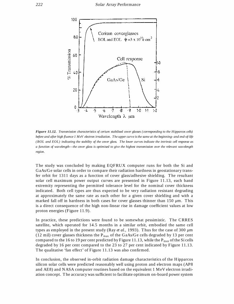
222 Solar Array Performance
Figure 11.12. Transmission characteristics of cerium stabilised cover glasses (corresponding to the Hipparcos cells)
before and after high fluence 1 MeV electron irradiation. The upper curve is the same at the beginning- and end-of-life
(BOL and EOL) indicating the stability of the cover glass. The lower curves indicate the intrinsic cell response as
a function of wavelength—the cover glass is optimised to give the highest transmission over the relevant wavelength
region.
The study was concluded by making EQFRUX computer runs for both the Si andGaAs/Ge solar cells in order to compare their radiation hardness in geostationary trans-fer orbit for 1311 days as a function of cover glass/adhesive shielding. The resultantsolar cell maximum power output curves are presented in Figure 11.13, each bandextremity representing the permitted tolerance level for the nominal cover thicknessindicated. Both cell types are thus expected to be very radiation resistant degradingat approximately the same rate as each other for a given cover shielding and with amarked fall off in hardness in both cases for cover glasses thinner than 150 µm. Thisis a direct consequence of the high non-linear rise in damage coefficient values at lowproton energies (Figure 11.9).
In practice, these predictions were found to be somewhat pessimistic. The CRRESsatellite, which operated for 14.5 months in a similar orbit, embodied the same celltypes as employed in the present study (Ray et al., 1993). Thus for the case of 300 µm(12 mil) cover glasses thickness the Pmax of the GaAs/Ge cells degraded by 13 per centcompared to the 16 to 19 per cent predicted by Figure 11.13, while the Pmax of the Si cellsdegraded by 16 per cent compared to the 23 to 27 per cent indicated by Figure 11.13.The qualitative ‘fan effect’ of Figure 11.13 was also confirmed.
In conclusion, the observed in-orbit radiation damage characteristics of the Hipparcossilicon solar cells were predicted reasonably well using proton and electron maps (AP8and AE8) and NASA computer routines based on the equivalent 1 MeV electron irradi-ation concept. The accuracy was sufficient to facilitate optimum on-board power system
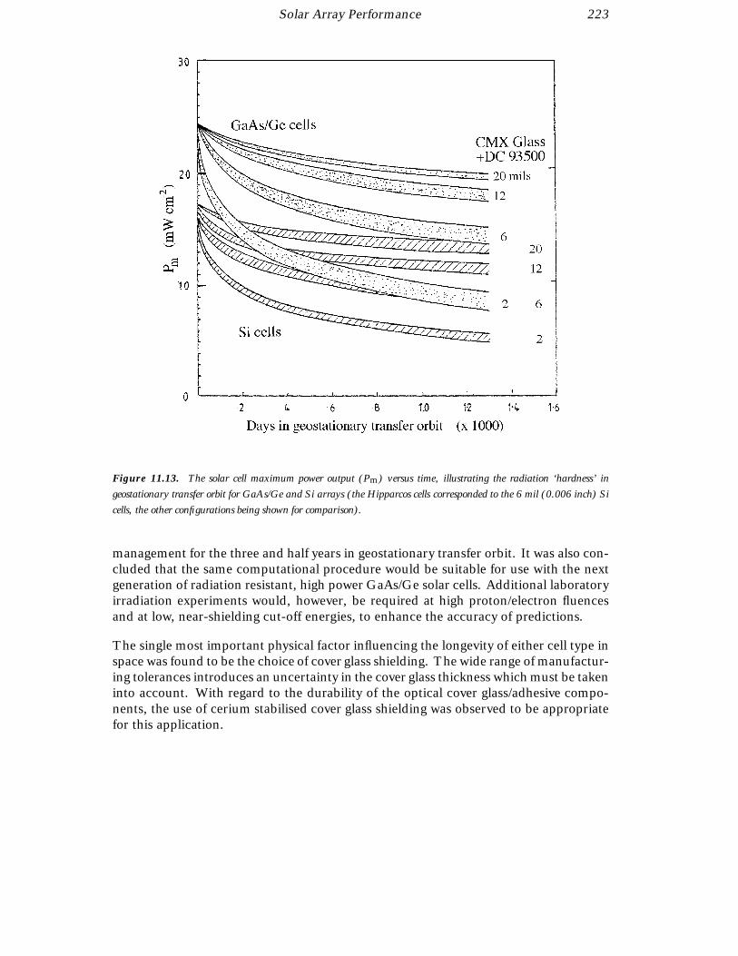
Solar Array Performance 223
Figure 11.13. The solar cell maximum power output (Pm) versus time, illustrating the radiation ‘hardness’ in
geostationary transfer orbit for GaAs/Ge and Si arrays (the Hipparcos cells corresponded to the 6 mil (0.006 inch) Si
cells, the other configurations being shown for comparison).
management for the three and half years in geostationary transfer orbit. It was also con-cluded that the same computational procedure would be suitable for use with the nextgeneration of radiation resistant, high power GaAs/Ge solar cells. Additional laboratoryirradiation experiments would, however, be required at high proton/electron fluencesand at low, near-shielding cut-off energies, to enhance the accuracy of predictions.
The single most important physical factor influencing the longevity of either cell type inspace was found to be the choice of cover glass shielding. The wide range of manufactur-ing tolerances introduces an uncertainty in the cover glass thickness which must be takeninto account. With regard to the durability of the optical cover glass/adhesive compo-nents, the use of cerium stabilised cover glass shielding was observed to be appropriatefor this application.
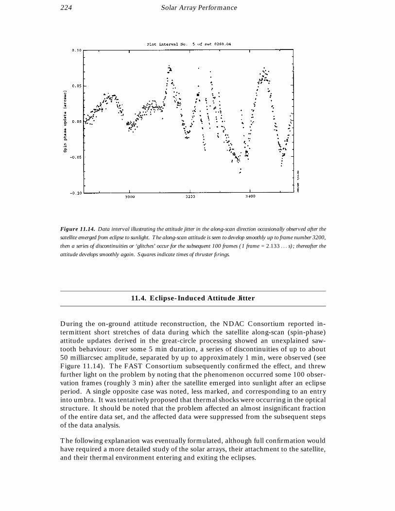
224 Solar Array Performance
Figure 11.14. Data interval illustrating the attitude jitter in the along-scan direction occasionally observed after the
satellite emerged from eclipse to sunlight. The along-scan attitude is seen to develop smoothly up to frame number 3200,
then a series of discontinuities or ‘glitches’ occur for the subsequent 100 frames (1 frame = 2.133 . . . s); thereafter the
attitude develops smoothly again. Squares indicate times of thruster firings.
11.4. Eclipse-Induced Attitude Jitter
During the on-ground attitude reconstruction, the NDAC Consortium reported in-termittent short stretches of data during which the satellite along-scan (spin-phase)attitude updates derived in the great-circle processing showed an unexplained saw-tooth behaviour: over some 5 min duration, a series of discontinuities of up to about50 milliarcsec amplitude, separated by up to approximately 1 min, were observed (seeFigure 11.14). The FAST Consortium subsequently confirmed the effect, and threwfurther light on the problem by noting that the phenomenon occurred some 100 obser-vation frames (roughly 3 min) after the satellite emerged into sunlight after an eclipseperiod. A single opposite case was noted, less marked, and corresponding to an entryinto umbra. It was tentatively proposed that thermal shocks were occurring in the opticalstructure. It should be noted that the problem affected an almost insignificant fractionof the entire data set, and the affected data were suppressed from the subsequent stepsof the data analysis.
The following explanation was eventually formulated, although full confirmation wouldhave required a more detailed study of the solar arrays, their attachment to the satellite,and their thermal environment entering and exiting the eclipses.

Solar Array Performance 225
Fixed hinge
Floating hinge
Solar panel
Satellite Body
Rotation
Figure 11.15. The configuration of one of the solar arrays and its attachment to the body of the satellite. Thermal
shocks after eclipses were considered responsible for small discontinuities in the along-scan attitude.
For each of the three deployable solar panels, one of the hinges was rigidly fixed to thesatellite body, while the other allowed some movement along the line of the attachmentof the array to the satellite body, this construction allowing for differential expansionbetween the satellite body and the panels themselves (see Figure 11.15). The solar arraysare held by a carbon-fibre reinforced plastic structure having a very low coefficient ofthermal expansion of about 1.5 × 10⁻⁶ K−1. For a panel dimension of about 1 m, anda change in solar array temperature of about 100–150 K (the ambient temperaturesbeing about 300 K in sunlit phase, and 170 K in eclipse) a change in dimension of some0.2 mm (total) would result from passage from umbra to sunlight, and vice versa (thethermal variation of the satellite body was very much smaller because of its larger thermalcapacity). It is considered likely that the resulting differential expansion occurred with a‘slip-stick’ or ‘stiction’ behaviour, with the timescales involved (i.e. with the start of thephenomenon occurring 2–4 min after the thermal discontinuity, with an overall durationof a few minutes) well matched to the thermal time constant of the solar arrays providedin the manufacturer’s reports.
The sharpness of the transition from umbra to sunlight depended on the satellite positionalong the orbit, and it was inferred that the effect would be more dramatic for shorterpenumbra durations, or less dramatic for shorter total eclipse durations (where the max-imum temperature excursion would not be reached). These features were qualitativelyconfirmed by the data analysis groups.
The transition from shade to sunlight had a more dramatic effect on the satellite motionthan that from sunlight to shade. In the former case, with the arrays initially colder, thecoefficient of friction between the affected surfaces would be larger than in the latter,and the stiction effect correspondingly larger. At the same time, the lower temperaturewould result in higher stresses in the hinges or joints (due to thermal contraction) andwould thus also increase the friction between the moving surfaces. In summary, itwas also considered likely that the effects on entering/exiting eclipse would indeed be‘asymmetrical’.
The magnitude of the phenomenon (50 milliarcsec discontinuities) was consistent withthe slip-stick effect of the 10 kg solar array mass located 1 m from the satellite centre

226 Solar Array Performance
of mass. The following analysis provided an order-of-magnitude estimate of the effect.The impulse of the moving element was estimated from:
i = m∆v [11.3]
where m is the solar panel mass. Assuming that the impulse duration corresponds tothe fundamental frequency of the solar panel in the relevant plane:
∆v = 2πn∆u [11.4]
and assuming n = 100 Hz, ∆u = 0.2 mm, m = 10 kg, gives ∆v = 0.1 m/s and i = 1.2 kgm/s. The assumed n was taken as a realistic upper limit for the solar panels, but itcould be as low as 10 Hz.
For a satellite moment of inertia of 1000 kg m2 about the z-axis, the effect on the satellitemovement is:
a i = I ∆Ω [11.5]
where a is the distance between the mass and the centre of gyration, and:
∆θ = ∆Ω /(2πn) [11.6]
Assuming n = 100 Hz for the satellite (this could perhaps be in the range 30 − 200 Hz),and a = 1 m gives ∆θ = 1.8 × 10⁻⁶ rad = 0.4 arcsec.
There are certain complications in applying this simple model: (i) n and (especially) n
are unknown; (ii) a i is an upper limit due to the fact that plane of the panels are offsetfrom the satellite centre of mass (a similar but smaller effect would therefore also bepredicted about the other two axes); (iii) the combined effects of the three panels makesthe results more complex; (iv) the above calculations led to an oscillatory motion of thegiven amplitude at the fundamental frequency, not a uni-directional displacement. But,in summary, it did not seem surprising that the effect was observable.
The solar array explanation seems most plausible, given the mass of the panels, ratherthan any effect of, say, the aluminium fill-in antenna albeit with its larger coefficient ofthermal expansion. Effects on the payload itself were also considered to be unrealisticgiven the known thermal environment.

12. THERMAL CONTROL
To ensure the relative stability of the optical components within the Hipparcospayload, active and passive thermal control resulted in a temperature stabilityof better than 0.05 C over short periods, and ±2 C over the entire missionduration. Temperature measurements were collected at various points in thepayload throughout the spacecraft’s lifetime, and relayed both to the on-boardcomputer (which monitors and regulates the thermal control) and the ground.Despite some loss of heater supply later in the mission, attributable to theexcessive radiation damage experienced by the thermal control electronics,the payload thermal control proved to be extremely robust, permitting properpayload operation until the end of the mission.
12.1. Introduction
The thermal control of the Hipparcos payload was driven by very stringent require-ments on the temperature stability of the payload structure, the optical elements andthe detectors. Typical long-term temperature requirements were 20 ± 2 C over thetotal mission duration when the payload was operational. Short-term temperature re-quirements on the mirrors were ±0.05 C. These requirements could only be achievedby proper thermal design of enclosures, where the boundaries were used to balanceinternal and external thermal disturbances.
The payload structure was manufactured from carbon-fibre reinforced plastic with avery low coefficient of thermal expansion, using a box-type arrangement (see Fig-ure 12.1). The optical elements and the detection systems were arranged inside thestructure. In order to get isothermal boundaries, thin foil heater mats were placed onhoneycomb panels (heater mat carriers), which were loosely connected mechanically tothe carbon-fibre reinforced plastic structure. This design concept was chosen to min-imise mechanical disturbance of the carbon-fibre structure due to thermal expansion ofthe honeycomb, and to keep the coefficient of thermal expansion constant by avoidingattaching a different material to the carbon-fibre structure. The entire payload was cov-ered with multilayer insulation, except for two radiators, which were needed to dumpthe internally dissipated power of the detectors.
Depending upon the payload assembly, thermal control was achieved by either passive oractive means, as shown in Table 12.1. The active thermal control relied on 21 ‘thermally
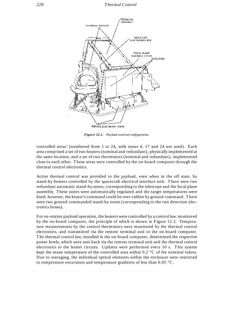
228 Thermal Control
Figure 12.1. Payload external configuration.
controlled areas’ (numbered from 1 to 24, with zones 4, 17 and 24 not used). Eacharea comprised a set of two heaters (nominal and redundant), physically implemented atthe same location, and a set of two thermistors (nominal and redundant), implementedclose to each other. These areas were controlled by the on-board computer through thethermal control electronics.
Active thermal control was provided to the payload, even when in the off state, bystand-by heaters controlled by the spacecraft electrical interface unit. There were tworedundant automatic stand-by zones, corresponding to the telescope and the focal planeassembly. These zones were automatically regulated and the target temperatures werefixed; however, the heater’s command could be over-ridden by ground command. Therewere two ground commanded stand-by zones (corresponding to the two detection elec-tronics boxes).
For on-station payload operation, the heaters were controlled by a control law, monitoredby the on-board computer, the principle of which is shown in Figure 12.2. Tempera-ture measurements by the control thermistors were monitored by the thermal controlelectronics, and transmitted via the remote terminal unit to the on-board computer.The thermal control law, installed in the on-board computer, determined the respectivepower levels, which were sent back via the remote terminal unit and the thermal controlelectronics to the heater circuits. Updates were performed every 10 s. This systemkept the mean temperature of the controlled area within 0.2 C of the nominal values.Due to averaging, the individual optical elements within the enclosure were restrictedto temperature excursions and temperature gradients of less than 0.05 C.
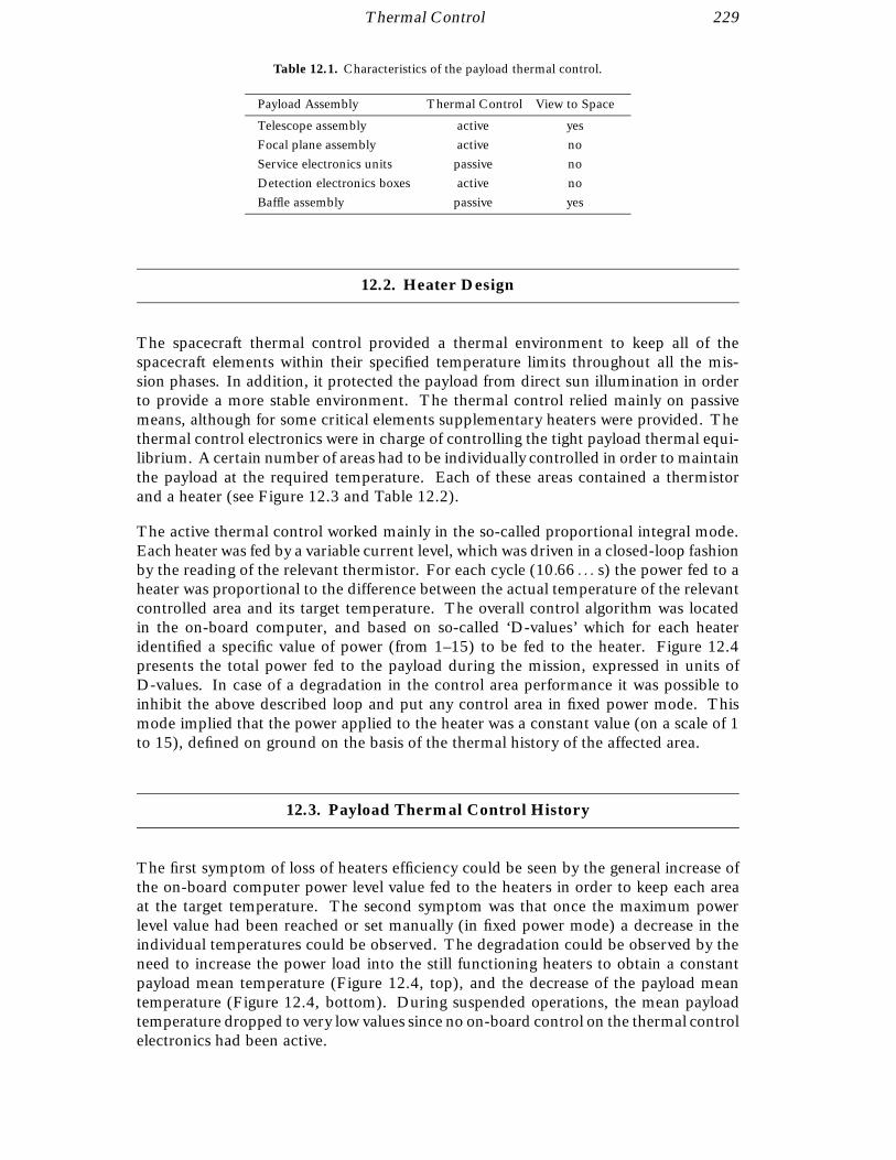
Thermal Control 229
Table 12.1. Characteristics of the payload thermal control.
Payload Assembly Thermal Control View to Space
Telescope assembly active yes
Focal plane assembly active no
Service electronics units passive no
Detection electronics boxes active no
Baffle assembly passive yes
12.2. Heater Design
The spacecraft thermal control provided a thermal environment to keep all of thespacecraft elements within their specified temperature limits throughout all the mis-sion phases. In addition, it protected the payload from direct sun illumination in orderto provide a more stable environment. The thermal control relied mainly on passivemeans, although for some critical elements supplementary heaters were provided. Thethermal control electronics were in charge of controlling the tight payload thermal equi-librium. A certain number of areas had to be individually controlled in order to maintainthe payload at the required temperature. Each of these areas contained a thermistorand a heater (see Figure 12.3 and Table 12.2).
The active thermal control worked mainly in the so-called proportional integral mode.Each heater was fed by a variable current level, which was driven in a closed-loop fashionby the reading of the relevant thermistor. For each cycle (10.66 . . . s) the power fed to aheater was proportional to the difference between the actual temperature of the relevantcontrolled area and its target temperature. The overall control algorithm was locatedin the on-board computer, and based on so-called ‘D-values’ which for each heateridentified a specific value of power (from 1–15) to be fed to the heater. Figure 12.4presents the total power fed to the payload during the mission, expressed in units ofD-values. In case of a degradation in the control area performance it was possible toinhibit the above described loop and put any control area in fixed power mode. Thismode implied that the power applied to the heater was a constant value (on a scale of 1to 15), defined on ground on the basis of the thermal history of the affected area.
12.3. Payload Thermal Control History
The first symptom of loss of heaters efficiency could be seen by the general increase ofthe on-board computer power level value fed to the heaters in order to keep each areaat the target temperature. The second symptom was that once the maximum powerlevel value had been reached or set manually (in fixed power mode) a decrease in theindividual temperatures could be observed. The degradation could be observed by theneed to increase the power load into the still functioning heaters to obtain a constantpayload mean temperature (Figure 12.4, top), and the decrease of the payload meantemperature (Figure 12.4, bottom). During suspended operations, the mean payloadtemperature dropped to very low values since no on-board control on the thermal controlelectronics had been active.

230 Thermal Control
HEATER THERMISTOR
POWER
DIGITISATION
TEMPERATURE
DETERMINATION
TEMPERATURE
CORRECTION
POWER LEVEL
DETERMINATION
ELECTRONICS)
(ON-BOARDCOMPUTER)
(PAYLOAD
TO GROUND
TO GROUND
THERMAL CONTROL
ELECTRONICSHOUSEKEEPING
THERMISTOR
PAYLOAD REMOTE
TERMINAL UNIT
Figure 12.2. Principles of the active thermal control.
Figure 12.3. Location of payload heaters.

Thermal Control 231
Table 12.2. Payload heater locations.
Payload Section Heaters
Beam Combiner Mirror cover heaters 1, 2, 3 and 5
Spherical Mirror cover heater 7
Telescope Structure +Y heaters 8 and 11
Baffle Assembly +Y heater 15
Telescope Structure -Y heaters 9 and 12
Baffle Assembly -Y heater 16
Telescope Structure +Z heaters 13 and 14
Telescope Structure -Z heaters 6 and 10
Focal Plane Assembly heaters 18, 21, 22 and 23
Focal Plane Assembly cover heaters 19 and 20
Spares heaters 4, 17 and 24
The following provides a summary of the changes occurring within the payload ther-mal control system during the mission (AR refer to formal ‘Anomaly Reports’, listedsequentially in Appendix B, and TCE refers to the Thermal Control Electronics):
90-07-19: AR number 37: loss of heater power supply on TCE 1 (area 17).
91-01-21: AR number 44: loss of heater power supply on TCE 1 (area 20).
91-01-25: Switch from TCE 1 to TCE 2.
91-09-18: TCE 2 area 20 set to fixed power mode value 11.
92-04-21: TCE 2 area 5 set to fixed power mode value 13.
92-07-06: AR number 61: TCE 2 loss of heater power supply (three heaters had nowfailed, three others were underperforming).
92-07-08: AR number 63: TCE 1 test (complete loss of the unit).
92-07-20: TCE 2 test (five heaters had now failed, two others were underperforming).
92-07-28: Payload TCE 1 and 2 tests (seven heaters had now failed).
92-09-02: Complete payload TCE 2 to fixed power mode.
93-02-10: TCE 1 and 2 test.
93-03-23: Payload off. TCE 2 left on.
93-03-24: TCE 2 configured to wide range to allow greater temperature variations.
93-03-30: All TCE 2 heaters to fixed power with value zero.
93-04-27: TCE 1 and 2 test. As further heaters had failed, all TCE 2 heaters were setto fixed power value 15.
93-06-07: TCE 2 test; out of 21 heaters only four were still functioning.
93-07-29: TCE 2 test.
During the mission lifetime a gradual degradation of the thermal control electronics2 performance was noted since switch-on (on 25 January 1991), with occasional butsignificant peaks in the degradation rate (see Figure 12.4).
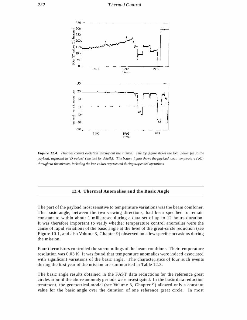
232 Thermal Control
Figure 12.4. Thermal control evolution throughout the mission. The top figure shows the total power fed to the
payload, expressed in ‘D values’ (see text for details). The bottom figure shows the payload mean temperature (C)
throughout the mission, including the low values experienced during suspended operations.
12.4. Thermal Anomalies and the Basic Angle
The part of the payload most sensitive to temperature variations was the beam combiner.The basic angle, between the two viewing directions, had been specified to remainconstant to within about 1 milliarcsec during a data set of up to 12 hours duration.It was therefore important to verify whether temperature control anomalies were thecause of rapid variations of the basic angle at the level of the great-circle reduction (seeFigure 10.1, and also Volume 3, Chapter 9) observed on a few specific occasions duringthe mission.
Four thermistors controlled the surroundings of the beam combiner. Their temperatureresolution was 0.03 K. It was found that temperature anomalies were indeed associatedwith significant variations of the basic angle. The characteristics of four such eventsduring the first year of the mission are summarised in Table 12.3.
The basic angle results obtained in the FAST data reductions for the reference greatcircles around the above anomaly periods were investigated. In the basic data reductiontreatment, the geometrical model (see Volume 3, Chapter 9) allowed only a constantvalue for the basic angle over the duration of one reference great circle. In most
Thermal Control 233
Table 12.3. Payload temperature anomalies found during the interval studied.
year:day:hour Temp. (K) Anomaly Report (Appendix B)
1990:089:16 16.3 Payload remote terminal unit telemetry (AR26)
1990:118:11 20.5 On-board computer halted (AR29)
1990:243:14 17.9 Anomalous behaviour of on-board computer (AR38)
1990:322:04 19.0
Table 12.4. Results for the reference great circle reductions solving for a variable basic angle. The model
for the basic angle is γ0 + γ1(t − t0) + γ2(t − t0)2 where the times are expressed in days of 1990 (day 1.0
corresponding to 1 January 1990 0h UT). The angles are expressed in mas, mas/day and mas/day2 (standard
errors in parentheses).
t0 γ0 − 58 γ1 γ2
(days) (mas) (mas/day) (mas/day2)
89.715 31245.5 (0.3) −3.8 (3.1) 18 (69)
90.121 31246.6 (0.3) 70.4 (1.7) −452 (27)
90.560 31246.5 (0.4) −7.0 (3.1) 60 (61)
118.575 31255.5 (0.3) 88.4 (4.1) −1204 (132)
118.962 31248.3 (0.2) −9.6 (1.4) 44 (18)
243.743 31249.0 (0.3) 86.8 (2.6) −616 (40)
244.145 31243.9 (0.3) −8.2 (1.8) 36 (21)
322.314 31244.7 (0.3) 80.6 (3.0) −510 (54)
322.696 31242.4 (0.3) −7.4 (1.3) 4 (15)
cases, during and after the anomaly, deviant values were found. Consequently, thegreat-circle reduction was repeated for all reference great circles associated with thetemperature anomalies, and those immediately after. In these specific reductions, aquadratic variation with time was assumed for the basic angle. Although there was noreason to assume that such a model is particularly well suited to describe the basic anglevariations, it had the advantage of being readily available in the software. A cubic modelwas not attempted because many of the data sets, in particular those during the mostsignificant changes, were shorter than the minimum length required to apply such amodel meaningfully. Table 12.4 gives the results obtained.
The basic angle indeed appeared to be responding to the temperature changes followinga more-or-less fixed pattern: starting at a value of about 15 mas lower than the currentlynormal value, it increased quickly to a value above this normal value, and then returnedto it much more slowly, on a time scale of about half a day. The rise sometimes seenat the end of the decreasing phase was never really significant, and was presumably anartefact of the quadratic model used to describe an exponential decrease.
In order to verify whether the low values at the start were real, or also due to thequadratic description, two of the reference great circles were reprocessed using only thefirst 4200 frames (i.e. one rotation plus one basic angle) allowing a constant basic angleand a linear variation with time. The results for these models were compared with thoseobtained previously, and confirmed the credibility of the initial low values of the basicangle.
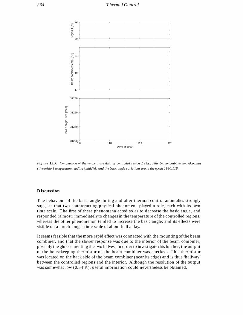
234 Thermal Control
20
22
Reg
ion
1 [°
C]
17
19
21
Bea
m c
ombi
ner
tem
p. [°
C]
117 118 119 120Days of 1990
31230
31240
31250
31260
Bas
ic a
ngle
- 5
8° [m
as]
Figure 12.5. Comparison of the temperature data of controlled region 1 (top), the beam-combiner housekeeping
(thermistor) temperature reading (middle), and the basic angle variations arond the epoch 1990:118.
Discussion
The behaviour of the basic angle during and after thermal control anomalies stronglysuggests that two counteracting physical phenomena played a role, each with its owntime scale. The first of these phenomena acted so as to decrease the basic angle, andresponded (almost) immediately to changes in the temperature of the controlled regions,whereas the other phenomenon tended to increase the basic angle, and its effects werevisible on a much longer time scale of about half a day.
It seems feasible that the more rapid effect was connected with the mounting of the beamcombiner, and that the slower response was due to the interior of the beam combiner,possibly the glue cementing the two halves. In order to investigate this further, the outputof the housekeeping thermistor on the beam combiner was checked. This thermistorwas located on the back side of the beam combiner (near its edge) and is thus ‘halfway’between the controlled regions and the interior. Although the resolution of the outputwas somewhat low (0.54 K), useful information could nevertheless be obtained.
Thermal Control 235
Temperatures were derived from the telemetry values using the ESOC calibration curves.The temperatures from the thermistors were significantly lower than those of the con-trolled regions, which could be explained by the fact that the beam combiner radiatedto the heat sinks presented by the baffles and open space.
In order to permit a better comparison, the controlled region temperatures, housekeep-ing thermistor temperature, and basic angle evolution for the two more obvious caseswere combined. From this, it was clearly evident that the beam combiner tempera-ture reacted much more slowly after a temperature anomaly (on a timescale of order10 hours) than the controlled region temperature (on a timescale of 2–3 hours). Thisseemed to confirm the above hypothesis of a fast and a slower effect combined (seeFigure 12.5).
An extra tilt of the beam combiner could explain the decrease in basic angle, but it wouldalso have caused a very significant increase in differential field rotation. No evidence forthis was found in the geometrical calibration, so that this explanation does not appearto be valid.

236
13. ATTITUDE AND ORBIT CONTROL SYSTEMAND PERFORMANCES
The attitude and orbit control system performed two major tasks. Duringthe spin-stabilised phase, it provided a reference for the control of most ofthe flight-related functions, such as pointing antennas or solar panels, or ori-enting the apogee boost motor for orbit manoeuvres. During the three-axisstabilised phase, it coped with the most severe attitude requirements imposedby the payload, the attitude constraints being one of the limiting factors forthe experimental accuracy demanded. In the framework of these overall tasks,the attitude and orbit control system carried out a variety of specific functionsclosely linked to the various operational aspects of the mission.
13.1. Functions of the Attitude and Orbit Control System
Spin-Stabilised Phase
During the spin-stabilised phase at the start of the mission, the attitude and orbit controlsystem was involved in the separation of the satellite from the launch vehicle, the apogeeboost motor ignition attempts, the perigee raising manoeuvres and sun acquisition. Itwas designed to provide:
(i) attitude control by maintaining the nutation angle within acceptable limits for allhydrazine propellant fill ratios and an inertia ratio below 1;
(ii) facilities to control the spin rate, employing 5 N hydrazine thrusters;
(iii) attitude information based on data from an Earth/Sun sensor, to allow the satelliteattitude to be determined by the ground;
(iv) facilities to control the satellite spin axis by means of the 5 N thrusters;
(v) means to acquire and maintain the satellite east–west geostationary orbital positionby means of 5 N hydrazine thrusters (not used in the revised mission);
(vi) means for a complete evacuation of all residual hydrazine propellant at the end ofthe spin phase;
(vii) back-up facilities to overcome failures, not handled by the ground station, whichwould lead to loss of the mission.
238 Attitude and Orbit Control System and Performances
Three-Axis Stabilised Phase
During the three-axis stabilised phase, the attitude and orbit control system was involvedin sun pointing, sensor calibration, scanning law initialisation, and normal operation. Itwas designed to:
(i) provide a stable sun pointing, by means of sun acquisition sensor data and 20 mNcold-gas thrusters, to enable gyro calibration and star pattern recognition;
(ii) slew the spacecraft rotation axis from the sun-pointing attitude to its position on thenominal scanning law;
(iii) control the satellite attitude, in order to follow the pre-determined scanning lawwith a maximum error cone semi-angle of 10 arcmin on the spin axis orientation, and amaximum error angle of 10 arcmin around the spin axis;
(iv) estimate the satellite attitude in real time with an accuracy such that the position ofthe telescope optical axes could be derived with an accuracy of better than 1 arcsec rms(cone semi-angle).
13.2. Equipment Description
The attitude and orbit control subsystem (Figure 13.1) comprised the control law elec-tronics, the control and actuation electronics, the accelerometer package, the Earth/Sunsensor, the sun acquisition sensor, the attitude anomaly detector, the reaction controlassembly and the inertial reference unit (the gyro measurement electronics and the gyropackage).
Control Law Electronics
The control law electronics was the core of the subsystem. A microprocessor ranthe attitude control software and interfaced with the rest of the spacecraft via the on-board data handling bus. Within the attitude and orbit control system, it interfacedwith the control and actuation electronics and the gyro measurement electronics. Itsmain functions were subsystem telecommand and telemetry management, closed-loopattitude control, open-loop attitude manoeuvres, real-time attitude determination andsubsystem configuration, and equipment monitoring.
The control law electronics was based on a TI SBP 9989 I2L 16-bit microprocessorand a memory bank of 16 k PROM and 4 k RAM, with error detection and correctioncapability (16 bits of data and 6 bits for Hamming code implementation). The unitwas internally fully redundant, and main and redundant functions were properly cross-strapped. The main functional blocks were as follows:
(1) telemetry and telecommand electronics: this module performed the on-board datahandling bus interface, the acquisition of analogue data, relay status, and telemetrysignals from the attitude and orbit control system, timing extraction from on-boarddata handling bus and distribution to the subsystem, and telecommand handling anddistribution to the attitude and orbit control system users;

Attitude and Orbit Control System and Performances 239
Figure 13.1. Attitude and orbit control subsystem block diagram, showing the inter-relationship between the various
on-board subsystems involved: AAD: attitude anomaly detector; ACP: accelerometer package; CAE: control and
actuation electronics; CLE: control law electronics; DHSS: data handling subsytem; ESS: Earth/Sun sensor; GME:
gyro mechanism electronics; GYP: gyro package; OBC: on-board computer; SAS: sun acquisition sensor; TM:
telemetry; TC: telecommand.
(2) central processing electronics: the central processing electronics board containedthe microprocessor and power supply, the RAM array with error-detection circuitry,the interrupt controller, the memory page decoder, the up clock and general timingfunctions, the memory-mapped I/O interface, and the central processing electronicsextension. The main functions of the central processing electronics extension wereto interface with the attitude control system bus, the Earth/Sun sensor, telemetry andtelecommand, failure detection, timing and switching, and PROM supply;
(3) the PROM board: the configuration of the board was based on 8 k × 8 PROM chipsproviding a 16 k × 16 array for the central processing electronics. They were suppliedthrough a switching system providing power only to the addressed chips;
(4) the sensor acquisition electronics: this module performed the analogue-to-digitalconversion of the various analogue signals of the subsystem, by means of a front-endoperational amplifier array, an analogue multiplexer and a 12-bit analogue-to-digitalconverter. The result of the conversion could be sent on the modular attitude controlsystem bus, via a dedicated telecom controller and bus driver/receiver. Timing andswitching functions, along with interface to internal buses, were also implemented;
(5) switching electronics: this board was the power interface to the relay coils. It wasdriven by the central processing electronics extension that sent the proper line andcolumn addresses in compliance with the matrix organisation of this board. The relaystatus acquisition electronics was also implemented;
240 Attitude and Orbit Control System and Performances
(6) DC/DC converter: the converter module provided the supply voltages required bythe various control law electronics circuits, together with the relevant current limitationmonitoring and power management capabilities. The circuit also supplied the Earth/Sunsensor. The electrical power was provided by the 50 V DC main and redundant buses,and primary and secondary power lines were isolated.
Control Actuation Electronics
The control and actuation electronics interfaced with the control law electronics, viathe internal bus. Its functions were to condition the outputs of the sun acquisitionsensors, the attitude anomaly detector, and the accelerometer package, to drive thereaction control subsystem latch valves, flow control valves, and catalyst bed heatersin response to commands from the control law electronics, to provide sensor powerswitching, to provide hardwired emergency attitude control modes during on-stationoperation, overriding the control law electronics, and to provide automatic fault detec-tion and recovery during the spin-stabilised phase, initiating automatic reconfigurationof the control law electronics and reaction control assembly. Furthermore, it performedsubsystem initialisation at separation.
The AC/DC converter module provided the proper power supply lines to the box, andit was connected to the data handling subsystem inverter as power source. The galvanicisolation requirement was met by means of shielded transformers connected to the twoAC lines. The cross-strapping function was implemented at a secondary level, after thecurrent limitation functions. A dedicated converter section, with serial regulators, wasimplemented to provide power to the accelerometer package.
The reaction control assembly was supplied directly from the 50 V DC lines through thehigh-power and pulse-capability current limit circuits, able to deliver to the valve coilsthe proper current pulse. The ‘failure detection electronics’ was the module in charge offailure detection and hardwired back-up mode management. Due to the failure recoveryphilosophy adopted, this module was not redundant. It implemented five failure criteria:active nutation damping failure detection, thruster impulse monitoring, and pressureanomaly detection in the spin-stabilised phase, and thruster impulse monitoring andattitude anomaly detection in the three-axis stabilised phase.
Any criterion, if verified, generated a reconfiguration signal that could be overridden byon-ground commands. Each failure detection electronics block was fully independentand was driven by proper enable/disable telecommands, in such a way that at any missionphase a dedicated failure detection strategy could be selected.
Accelerometer Package
The accelerometer package was used as nutation sensor during the spinning phase.It comprised three Sunstrand QA 2000-type accelerometers (A, B, and M) and therelevant conditioning circuitry. The A and B output signals were sent to the control lawelectronics through sensor acquisition electronics, in order to drive the software-basedactive nutation damping function. The M output signal was routed to the control andactuation electronics, to be used in the hardware-based active nutation damping failuredetection.

Attitude and Orbit Control System and Performances 241
Earth/Sun Sensor
The Earth/Sun sensor provided the attitude and spin-rate measurement during the firstpart of the mission, when the satellite was spin stabilised. It employed the Galileosensor flown on many telecommunications satellites. The attitude determination wasperformed by correlating the cross times of the Sun into the two sun slits and measuringthe length of the Earth chord, by means of the two infrared telescopes and a timingcircuitry in the control law electronics.
Sun Acquisition Sensor
The sun acquisition sensors gave the attitude and orbit control system a rough estimation(1.6 accuracy) of the sun aspect angle along two axes for sun acquisition purposes, bothin the nominal case or for emergency sun reacquisition. Each sensor was made up of 8photovoltaic cells (4 main, 4 redundant) delivering a current proportional to the cosineof the angle between the sun line and the normal to the cell surface. The actual sensorconfiguration gave a field of view of more than 2 steradians and the full set of three unitsgave a spherical coverage around the satellite. The load resistor and the conditioningelectronics were in the control and actuation electronics.
Attitude Anomaly Detector
The attitude anomaly detector monitored the satellite attitude in order to avoid thepossibility of the sun damaging the solar generator or the payload. The device wasbased on a solar cell inside a baffling system. In normal conditions (normal mode), theSun should have stayed at about 43 sun aspect angle. If the sun aspect angle driftedfrom this value by more than 3, the sensor would issue a current pulse that wouldtrigger the attitude anomaly detector criterion in the control and actuation electronicsfailure detection circuitry, commanding a reconfiguration strategy.
13.3. Reaction Control Assembly
The reaction control assembly provided impulses for velocity corrections, for satellitepositioning, spin-up and spin-down, and for attitude control. The assembly consistedof two separate, functionally independent sub-assemblies which were used sequentially:a hot-gas reaction control assembly, which used hydrazine (N2H4) propellant, and acold-gas reaction control assembly, which used nitrogen propellant. Each sub-assemblyincorporated two redundant and independent functional branches.
Hot-Gas Reaction Control Assembly
The hot-gas reaction control assembly was a conventional monopropellant hydrazinesystem. The propellant was stored in two identical tanks, which operated in a blow-down pressure mode over a range from 22 to 5.5 bar. The tanks did not contain anypositive expulsion devices. The hydrazine was pressurised by gaseous helium. The pro-pellant/pressurant interface required for positive propellant expulsion was maintained

242 Attitude and Orbit Control System and Performances
by the centrifugal acceleration produced by the satellite spin. The tank shape was cono-spherical to maximise expulsion efficiency. Both tanks were fed and pressurised by asingle fill and drain valve and a common feed line. The fill and drain valve incorporateda 25 µm filter. Another line linked the pressurant ports.
Four thrusters were required to meet the subsystem attitude control and velocity require-ments. Hydrazine was fed through a flow control valve and was chemically decomposedthrough a catalyst-induced combustion process inside the thrust chamber. The hot gasesexpanded through a nozzle and produced thrust. Thrust chamber assemblies incorpo-rated electrical heaters, which raised the catalyst temperature to approximately 190 C,prior to hydrazine injection into the combustion chamber. The thruster branches couldbe isolated from either tank by latching-type isolation valves.
The thruster assemblies were protected from particulate contamination by one 10 µmfilter, located between tanks and isolation valves. In addition, one 10 µm filter wasinstalled in the inlet of each thruster propellant valve, in order to provide increasedcomponent protection. A pressure transducer was located immediately downstreamof the propellant tanks. Its reading, combined with that of tank temperature sensors,provided information to establish the propellant mass inside the tanks, throughout thehot-gas reaction control assembly life. The propellant feed-lines consist of 6.4 mm outerdiameter titanium tubing. Hydrazine tubing, tanks, latching, and flow control valveswere insulated and thermally controlled in order to prevent the hydrazine temperaturedropping below its freezing point, at approximately 2 C.
Mechanical connections between feed-lines and thruster valves, latching valves, andpressure transducer, consisted of standard flare-type fittings; all other joints were TiGwelded. Every item of equipment had been qualified for previous space programmes.
Cold-Gas Reaction Control Assembly
The cold-gas reaction control assembly was a pressure-regulated system, using gaseousnitrogen propellant. The nitrogen was stored at a maximum pressure of 285 bar in twoequally sized tanks. The tanks were not interconnected, and separate fill and vent valveswere used in order to pressurise the tanks. These valves incorporated a 5 µm filter. Eachtank fed one pressure regulator, which reduced the gas pressure from tank level to anaverage of 1.5 bar.
Impulse for all manoeuvres was provided by one of two redundant branches of sixthrusters each. Gas was fed from the pressure regulators to the two thruster branchesthrough a system of four isolation valves. These latching type valves permitted theisolation of either thruster branch and its feeding by either regulator. During normaloperation, only one regulator would be used to provide regulated pressure. A highpressure, 10 µm filter was installed upstream of each pressure regulator. In addition,integral filters were installed in the inlets of the regulators and the propellant valves toprovide additional protection. The pressure regulator incorporated a relief valve whichprevented over-pressurisation of the low pressure line. Over-pressurisation could occurin two instances: in the case of pressure regulator leakage and/or temperature effectsduring which the thrusters were not operated, or in the case of pressure regulator failure.In the worst case, the low pressure line could experience pressures similar to those inthe high pressure lines.

Attitude and Orbit Control System and Performances 243
To vent the resulting mass flow, a so-called ‘zero thrust device’ (a calibrated T-fitting)was installed near the pressure regulators, so as to minimise the impingement of gason spacecraft units. In the case of pressure regulator failure, the gas that exited thespacecraft through its vents may have caused disturbance torques in the order of 10−3
to 10−4 Nm. The high-pressure transducers located in each branch of the sub-assemblyand the tank temperature monitors provided the information needed to establish thepropellant mass inside the tanks throughout mission life. Low-pressure transducerswere included in each half of the sub-assembly, to measure the regulated pressure andmonitor regulator operations.
The feed lines consisted of 6.4 mm outer diameter titanium tubing. Mechanical connec-tions were made by TiG welding with the exception of the thruster assemblies, pressureregulators, pressure transducers, and latching valves, which were installed using stan-dard flare-type fittings. Except for the 20 mN thruster, all equipment had been qualifiedfor previous programmes. An extensive qualification programme was performed for thecold-gas thruster.
Operating Modes
The hot-gas reaction control assembly was to have been used at the start of the missionduring the transfer orbit, near synchronous orbit, and the initial geostationary orbitoperations. In practice the sequence of operations for the revised mission were quitedifferent (see Chapter 4).
The hydrazine thrusters were used to spin up the satellite after separation from thelaunch vehicle from 7 rpm to 60 rpm in a series of manoeuvres. After this the satellitespin axis was oriented for the apogee boost motor firing. In the course of variousattempts to ignite the apogee boost motor, the spacecraft was de-spun from 60 rpm to30 rpm. During the de-spin manoeuvres, the hydrazine thruster also provided activenutation damping. After all further attempts to ignite the apogee boost motor hadceased, virtually all of the remaining hydrazine was used to increase the perigee heightof the transfer orbit in a series of three manoeuvres. The spacecraft was then de-spunto 10 rpm and oriented with its spin-axis pointing at the Sun. A final orbit manoeuvrewas performed to synchronise the orbital period with the satellite’s rotation period. Theresidual liquid hydrazine was then expelled from the sub-assembly, in order to avoidmass shifts caused by hydrazine sloshing during nominal operating modes and, thus, toavoid unwanted attitude jitter.
The subsequent control forces were provided by the cold-gas reaction control assembly.The satellite was further despun, reoriented, and stabilised. Emergency manoeuvresduring routine operations were also served by the cold-gas reaction control assembly.
A summary of the mission phases, the thrusters used, and the thruster operating modesis presented in Table 13.1.
Assembly Performance
The hot-gas reaction control assembly thrusters provided a nominal thrust of between2–6 N, depending on the supply pressure. Nominal specific impulse during steady-stateoperations ranged between 215–225 s. During pulsed mode operation, the specific
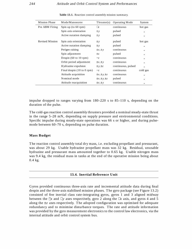
244 Attitude and Orbit Control System and Performances
Table 13.1. Reaction control assembly mission summary.
Mission Phase Mode/Manoeuvre Thruster(s) Operating Mode System
Pre ABM Firing Spin up (to 60 rpm) +z continuous hot gas
Spin axis orientation ± y pulsed „
Active nutation damping ± y pulsed „
Revised Mission Spin axis orientation ± y pulsed hot gas
Active nutation damping ± y pulsed „
Perigee raising ±x, ± y continuous „
Spin adjustment ±z pulsed „
Despin (60 to 10 rpm) −z continuous „
Orbit period adjustment ±x, ± y continuous „
Hydrazine expulsion ± y, ±z continuous, pulsed „
Final despin (10 to 0 rpm) −z continuous cold gas
Attitude acquisition ±x, ± y, ±z continuous „
Nominal mode ±x, ± y, ±z pulsed „
Attitude reacquisition ±x, ± y continuous „
impulse dropped to ranges varying from 180–220 s to 85–110 s, depending on theduration of the pulse.
The cold-gas reaction control assembly thrusters provided a nominal steady-state thrustin the range 5–28 mN, depending on supply pressure and environmental conditions.Specific impulse during steady-state operations was 66 s or higher, and during pulse-mode between 60–70 s, depending on pulse duration.
Mass Budget
The reaction control assembly total dry mass, i.e. excluding propellant and pressurant,was about 29 kg. Usable hydrazine propellant mass was 32 kg. Residual, unusablehydrazine and pressurant mass amounted together to 0.65 kg. Usable nitrogen masswas 9.4 kg, the residual mass in tanks at the end of the operative mission being about0.4 kg.
13.4. Inertial Reference Unit
Gyros provided continuous three-axis rate and incremental attitude data during finaldespin and the three-axis stabilised mission phases. The gyro package (see Figure 13.2)consisted of five inertial class rate-integrating gyros, gyros 1 and 3 aligned midwaybetween the +−x and + y axes respectively, gyro 2 along the +x axis, and gyros 4 and 5along the ±z axes respectively. The adopted configuration was optimised for adequateredundancy and to minimise disturbance torques. The rate and attitude informationwas provided by the gyro measurement electronics to the control law electronics, via theinternal attitude and orbit control system bus.

Attitude and Orbit Control System and Performances 245
The inertial reference unit was the satellite measurement device for attitude and angularrates during commissioning and normal mode phases. The output of this unit, togetherwith star mapper data, were processed by the control law electronics software. Innominal operating mode the results influenced the output of the scientific mission;therefore, the inertial reference unit performances were of extreme importance for thesatellite. The inertial reference unit of Hipparcos was a direct derivation from the oneflying on the French Earth observation satellite SPOT. With the progressive failure of thegyroscopes, these functions were ultimately fully transferred to the spacecraft/payload,where the star mapper readings provided very high accuracy attitude sensing, albeit at alow frequency.
Based on a SAGEM GYPSE gyrometer, the inertial reference unit was split physicallyinto two boxes, gyro package and gyro measurement electronics, and functionally intofive measurement chains organised into three independent channels. The gyro packagecontained the gyrometers with their mechanical support, thermal insulation, and thethermal control electronics; the gyro measurement electronics contained the inertialreference unit power supply DC/DC converter (from 50V DC bus), the switchingelectronics, the telemetry and telecommand, and the modular attitude control systembus interface, the spin motor power supply, the pick-off supply, the rebalance loop,the clock and general timing function, and the so-called angular rate digital integratorthat senses the current flowing in the rebalance loop and converts it into a pulse trainat a frequency proportional to the angular rate seen on the input axis of the relevantgyrometer; with a proper accumulator register read at a fixed time, it was possible toobtain the required information on attitude and angular rate.
The main measurement characteristics of the inertial reference unit were: angularresolution 0.032 arcsec in fine mode, and 0.26 arcsec in coarse mode; a full scale of0.125 s−1 in fine mode and 0.83 s−1 in coarse mode, and a constant drift of less than2 per hour.
As a consequence of the revised mission orbit, the performance of the gyros in the highradiation environment to which the satellite was exposed started to degrade shortly afterthe launch.
13.5. Gyro Performances
The first gyro problems were traced back to November 1989 when increasing noise ongyro 4 (z axis) was observed. By mid 1990, the gyro deteriorated to the point whereit had to be taken out of the control loop and replaced by the redundant one (gyro 5).Gyro 5 soon developed the same problems as gyro 4. In July 1992, it deteriorated tothe point of affecting the spacecraft attitude and had to be taken out of the control loop.The new two-gyro software was then implemented (see Chapter 15). In September1992 both gyro 2 and 5 showed anomalous behaviour. At the end of the month gyro1 had several spin-downs and broke completely two weeks later, and was replaced bygyro 3. In December 1992 gyro 2 showed large spikes, breaking down in March 1993.An overview of the gyro performance during the mission is shown in Figure 13.3. Asummary of the behaviour of the various gyros is given hereafter.

246 Attitude and Orbit Control System and Performances
Gyro input axis
Satellite axis
1
3α
α
4
5
2
-Y Y
-Z
Z
X
-X
Figure 13.2. The configuration of the five on-board gyros, illustrating the relationship between the gyro input axes
and the satellite axes.
1989 1991 199319921990
*1,2,4 2,3
RU
NN
ING
HO
UR
S (X
100
0)
30
20
15
10
5
0
25
1,2,5
Gyro 1,2
Gyro 3
Gyro 5
Gyro 1Gyro 2
Gyro 4
Gyro 1,2,4Launch
*=1,2 Gyros in the Control Loop
GYRO CONFIGURATION AND USAGE
Figure 13.3. The combination of gyros used at different stages of the mission. The bottom panel summarises which
gyroscopes were operational during the mission. The upper panel indicates the cumulative running hours for each of
the gyros. The two-gyro operations started towards the end of 1992.

Attitude and Orbit Control System and Performances 247
Gyro 1
July 92: Gyro 1 drift began to change erratically affecting real-time attitude determina-tion performance.
92-09-25: The output of the gyro changed rapidly several times.
92-09-27: The output of the gyro again changed rapidly several times.
92-10-11: The gyro output went suddenly to zero. Several attempts were made to getthe gyro working again, but with no success; finally the gyro was switched off. Fromthat time, the gyro was used only for increasing the gyro measurement electronics boxtemperature as no real output could be obtained.
Gyro 2
92-08-11: The gyro was switched off by an automatic re-configuration order caused byan emergency sun reacquisition. The gyro was switched back on, but it developed thefirst spikes in the output and had to be switched off.
92-10-03: The gyro was switched off by an automatic re-configuration order caused byan emergency sun reacquisition. On the same day the gyro was switched on again, butthere were several commanding problems due to the low gyro mechanical electronicsbox temperature; soon after the spikes in the output reappeared.
92-10-15: The gyro was switched off by an automatic re-configuration order caused byan emergency sun reacquisition. On the same day the gyro was switched on again, butsoon after the spikes in the output reappeared. The same had to be repeated again laterthe same day due to a second emergency sun reacquisition.
92-10-27: The gyro output was tested via the gyro 2/5 de-multiplexing patch; thismodification allowed the suppression of the output of gyro 2, gyro 5 or both.
92-10-13: The gyro output developed several spikes, but it recovered after the switch-offof gyro 5.
92-12-22: The spikes on the output of the gyro became severe enough to cause a lossof real-time attitude determination convergence outside perigee.
Gyro 3
91-07-28: During a regular gyro destorage, the gyro heater did not operate. The heaterdid not operate throughout the rest of the mission.
91-09-27: A test was conducted on the gyro to see if it would operate correctly at alower temperature.
92-08-13: The gyro was switched on to replace gyro 2.
92-10-27: The gyro was switched off to allow the testing of gyros 2 and 5; it was turnedback on at the end of the test.
Gyro 4
November 89: First noise on the gyro was observed.
90-06-26: The gyro output presented large variations for the first time.

248 Attitude and Orbit Control System and Performances
90-06-29: The gyro was switched off and replaced by gyro 5.
90-10-18: A week long gyro destorage was started, where the gyro was left runningoutside the control loop.
90-11-15: During a normal gyro destorage, the output variations re-appeared severaltimes.
90-12-20: During a normal destorage, the output did not change from zero and it tookthree attempts to finally get a correct spin rate. The gyro was then left on, but not inthe control loop.
From 91-01-12 to 91-02-26: Occasional changes in the gyro spin rate caused the real-time attitude determination loop to diverge although it was not in the control loop.
91-03-01: The gyro was finally switched off.
92-10-04: Due to the problem with gyros 2 and 5, the gyro was switched on to get acorrect spin-rate estimate. Then the gyro was switched off.
92-10-11: The gyro was again switched on.
92-10-27: The gyro was switched off.
92-11-13: The gyro was switched on to replace gyro 5 after an emergency sun reacqui-sition.
From 92-11-26 to 92-11-29: Gyro output variations were observed.
92-12-22: The gyro was finally switched off. On the same day, an emergency sunreacquisition occurred; the gyro was again switched on to increase the gyro mechanicalelectronics box temperature, but the output stayed at zero. After the temperature hadstabilised, the gyro was switched off. From this day on, the gyro was used only forincreasing the gyro mechanical electronics box temperature as no real output could beobtained.
Gyro 5
90-06-29: The gyro was switched on to replace gyro 4.
92-03: Deterioration on gyro 5 started to have a noticeable impact on overall real-timeattitude determination performance.
92-07-03: The first large spikes occurred, causing the divergence of the on-board real-time attitude determination loop.
92-07-10: The gyro was taken out of the control loop but left on and was replaced bythe two-gyro real-time attitude determination patch.
92-08-04: The gyro was switched off by an automatic reconfiguration order caused byan emergency sun reacquisition. The gyro was switched back on and large spikes wereobserved on its output.
92-08-08: Gyro 5 recovered sufficiently to return to three-gyro operations.
92-08-11: Scanning law acquisition manoeuvre return to 43 nominal scanning law.Glitches on gyro 5 output caused an emergency sun reacquisition. The spacecraft wasthen spun up and the gyro left off. From this day on, the gyro was not used again forthe actual control of the satellite.
92-08-14: The gyro was switched on for a test and was then switched off again.
92-10-02: The gyro was switched on after an emergency sun reacquisition.
Attitude and Orbit Control System and Performances 249
92-10-03: The gyro was switched off by an automatic reconfiguration order caused byan emergency sun reacquisition. On the same day, the gyro was switched on again butthere were several commanding problems due to the low gyro mechanical electronicsbox temperature.
92-10-15: The gyro was switched off by an automatic reconfiguration order caused byan emergency sun reacquisition. On the same day, the gyro was switched on again withthe same commanding problem experienced a few days earlier. It happened again laterthe same day due to a second emergency sun reacquisition.
92-10-27: The gyro output was tested via the gyro 2/5 de-multiplexing patch.
92-11-13: The gyro noise increased and the output indicated a spin-down to a levelequal to 60 per cent of the nominal rate. After a check carried out with the star mapperoutput, the gyro was switched off.
92-12-22: After emergency sun reacquisition occurred the gyro was switched on toincrease the gyro mechanical electronics box temperature, but the output stayed atzero. The gyro was left on, although the output had been disabled via the gyro 2/5 de-multiplexing patch and it was only being used to increase the gyro mechanical electronicsbox temperature.
Gyro Drift
Studies showed that on short timescales, gyro drifts were sensitive to long eclipses whichgave rise to thermoelastic effects. During eclipses, the variation in drift for a thirtyminute eclipse was approximately 10−7 arcsec s−1. The estimated gyro drift over longertimescales (from the beginning of the mission) is illustrated in Figure 13.4. The largerdiscontinuities coincide with on-board gyro reconfigurations, since different operationalgyros gave rise to different biases. The cause of the smaller variations was investigated.Thermal effects were believed to be the cause of this behaviour.
13.6. Gyro Related Ground Investigations
Ultimately the successive failures of the gyros was to lead to the complete redefinition ofthe on-board and on-ground real-time attitude determination systems using firstly twoand then no gyros in the control loop (see Chapters 15 and 16 respectively). Before or inparallel with this development, a series of less drastic measures were taken to minimisethe risk to the spacecraft of maintaining three-gyro operations.
Ground Procedures and Software Changes
In February 1991, while both gyro 4 and gyro 5 were switched on (with gyro 5 in thecontrol loop), the specialised real-time attitude monitor software at ESOC was enhancedto perform limit checking on both gyros and to raise an alarm should the operational onego out of limits. The spacecraft controller would then have been able to swap the failinggyro out of the control loop before significant deviations from the nominal scanning lawcould accumulate, possibly leading to an autonomous triggering of the emergency sunreacquisition manoeuvre. This software was made largely redundant after gyro 4 was
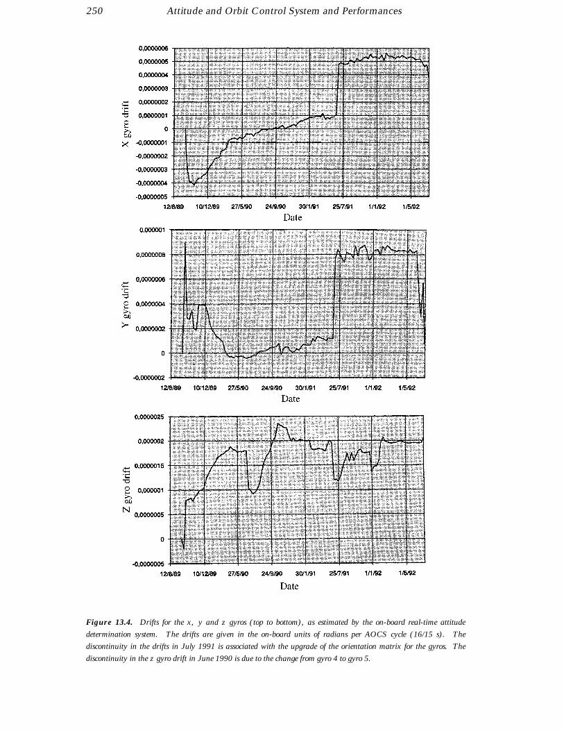
250 Attitude and Orbit Control System and Performances
Figure 13.4. Drifts for the x, y and z gyros (top to bottom), as estimated by the on-board real-time attitude
determination system. The drifts are given in the on-board units of radians per AOCS cycle (16/15 s). The
discontinuity in the drifts in July 1991 is associated with the upgrade of the orientation matrix for the gyros. The
discontinuity in the z gyro drift in June 1990 is due to the change from gyro 4 to gyro 5.
Attitude and Orbit Control System and Performances 251
switched off and the monitoring of the gyro 5 output was achieved via the gyro 5 filteron-board software patch, described below.
In March 1992, in response to increased noise on gyro 5 having a detrimental effecton the real-time attitude determination performance, it was believed that any changesto the gyro drifts around perigee was most likely due to biased corrections by the real-time attitude determination (see Chapter 14). Therefore the ground procedures werechanged to allow the resetting of the on-board drift estimates as soon as possible afterperigee to the last values observed before perigee. Subsequent careful monitoring fordrift evolution was then performed throughout the orbit to ensure that the best driftestimates were maintained.
Gyro 5 Filter On-Board Patch
Matra Marconi Space, as spacecraft prime contractor, were responsible for the devel-opment of a series of on-board software patches.
This patch was designed to reject all gyro 5 pre-processed outputs that were outsidea given window (for example 168.75 hr−1 ± 10). In case a bad value was detected(outside the ground defined window) it was then replaced by the previous value. Thispatch became practically obsolete when the frequency of occurrence of bad valuesincreased.
Gyro 2/5 De-Multiplexing On-Board Patch
Gyro 2 and 5 were part of the same inertial reference unit channel. It appeared that theiroutput were at times swapped causing erroneous performance by the real-time attitudedetermination. A modification was then designed so that the software gave the optionto read only one gyro output. This software became obsolete when the gyro electronicproblem worsened and mechanical problems appeared.
Other Satellite Missions
In the case of Hipparcos the failures of the gyroscopes were characterised by high outputnoise, high amplitude output spikes, repeated spin-rate anomalies, followed (except forone out of five gyroscope systems) by a final spin-down. The thermal control of theremaining gyroscope system failed and its output was severely degraded.
Hipparcos was not the only mission to be affected in an adverse manner by failure of thegyroscope systems. Three of the four gyroscope systems on board the German satelliteROSAT showed output transients whose polarity was correlated with the immediatelypreceding angular manoeuvre. Two gyroscope systems exhibited apparent spin-rateanomalies, leading to final spin-down for one of them. However, similar gyroscopesystems flying on other European satellites showed very few in-orbit anomalies.
An inter-agency ‘gyroscope systems working group’, maintained by ESA, CNES (F),DARA (D), and DRA (UK) from 1992 until mid-1993, conducted systematic investiga-tions of Hipparcos and ROSAT flight data through contracts placed with gyroscope man-ufacturers. These investigations were later supported by the Laboratoire de RecherchesBalistiques et Aerodynamiques (F). A general conclusion reached by all parties to the

252 Attitude and Orbit Control System and Performances
investigation was that the primary source of all the failures lay in the electronics of thegyroscope system and not in its electro-mechanical gyroscope unit.
The in-orbit failures of the Hipparcos satellite were investigated by Matra MarconiSpace, who integrated the inertial reference unit and supplied most of the gyroscopeelectronics, and SAGEM (F), the gyroscope manufacturer. All anomalous behaviourand failures of the gyroscope systems could be explained in terms of radiation-induceddegradation of electronic components. This was deduced from the abnormal orbit flownand the time which elapsed before the most serious failures were observed, about threeyears after launch, after the nominal lifetime had expired.
Causes of failure were traced to the spin motor supply circuitry, while other failures werethought to have most probably originated in sensitive electronic interfaces. Anomaliesoccurring in the ROSAT satellite were investigated by GEC-Ferrari (UK). These con-cluded that the most probable cause of failure was the electronic circuitry supplyingthe spin motor, although other electronic failures were also noted. The recommenda-tions for improving gyroscope systems, resulting from this inquiry, were passed to ESAprojects and industry.
13.7. Gas Consumption
The cold-gas mass (Mcg) in the tanks was calculated as follows:
Mcg =PVzrT
[13.1]
where P is the tank pressure (Pa), V is the tank volume (m3), z is the compressibilityfactor for nitrogen, T the temperature (K) and r a constant. The evolution of the coldgas, since October 1989, is shown in Figure 13.5. By May 1992 tank 1 was almostempty, with only 0.6 kg remaining. Tank 2 still had 4 kg out of the original 5.07 kg.
The average consumption was 0.15 kg per month. The consumption followed a linearlaw. Extrapolating that law predicted an attitude and control ability until after 1994,well beyond the final termination of satellite operations in August 1993.
13.8. Normal Mode Controller
The primary output from the on-board real-time attitude determination system (seeChapter 14) were the estimated angular deviations from the nominal scanning law (errorangles) and their rates of change (error rates). These error angles and error rates werecombined within the ‘normal mode’ control software to produce error signals. Whenan error signal exceeded the preset threshold level, thruster firings were commanded onall three axes. The lengths of the pulses were determined as a function of the angles,rates and a preset estimate of the disturbance torque.

Attitude and Orbit Control System and Performances 253
Figure 13.5. Hipparcos cold gas consumption: (a) tank 1 and (b) tank 2.
On-board Disturbance Torque Modelling
The disturbance torque estimates were based on the assumption that the satellite wouldoperate from a geostationary orbit. Therefore the on-board disturbance torque modelwas designed to give a first-order estimate only, based on the expected predominanttorques, i.e. a constant torque arising from the moments of the spinning gyros, anda periodic torque arising from radiation pressure. In practice, other torques such asgravity gradient, magnetic torques, and atmospheric drag (near to perigee) played avery significant role at lower altitudes resulting in modifications to the normal modecontrol around perigee.
The radiation pressure torque varied according to the geometric surfaces of the space-craft which were exposed to sun-light. Consequently, the torques around the spacecraftx and y axes had a periodicity equal to that of the spacecraft rotation rate (2 hours8 min). Due to the approximate 120 rotational symmetry of the spacecraft about thez axis, the radiation pressure torque around the z axis had a periodicity of 1/3 of thespacecraft rotation period. It was sufficient for the normal mode control to assume asinusoidal model for the radiation pressure torque.

254 Attitude and Orbit Control System and Performances
The orbital oscillator parameters, Sv(k), Cv(k), described in Chapter 8, were used tomodel the phase angle of the periodic torques around the x and y axes. For the z axis,a further two phase angle parameters were required. Recalling that Sv(k) and Cv(k)are the sine and cosine of phase angle Ωd tk respectively, it was possible to model thedisturbance torques around the z axis using a phase angle of 3Ωd tk. Therefore theon-board computer was capable of evaluating:
Sv3(k) = sin(3Ωd tk) [13.2]
Cv3(k) = cos(3Ωd tk)
by addition and multiplication only, using the standard trigonometrical expansions ofsin(3θ) = sin((θ + θ) + θ) (similarly for cosine).
On-board Algorithm
The following variables (updated every 1615 s) were input from other areas of the control
software:
φ(k), θ(k), ψ (k): x, y and z error angles from real-time attitude determination (seeChapter 14).
φ(k), θ(k), ψ (k): x, y and z error rates from real-time attitude determination.
Sv(k), Cv(k), Sv3(k), Cv3(k): Orbital oscillator outputs (see Chapter 8 and above).
The following on-board constants were used:
Kx, K y, Kz: X, Y and Z rate gains
µx, µ y, µz: X, Y and Z thresholds
Ax, Ay, Az: coefficients of φk, θk, ψk
Bx, B y, Bz: coefficients of Tx, Ty, Tz
Cx, Cy , Cz: coefficients of φk, θk, ψk
Txc, Tyc, Tzc: constant disturbance torque estimates
Txss, Tyss, Tzss: disturbance torque sine coefficients
Txsc, Tysc, Tzsc: disturbance torque cosine coefficients
Defining additionally:
x, y, z: error signals
Tx, Ty, Tz: external disturbance torque estimates
ton,x, ton,y, ton,z: calculated on-times
the error signals were given by:
x = φk + Kx φk
y = θk + K y θk [13.3]
z = ψk + Kzψk
The thruster on-time calculation was only performed if an error exceeded in magnitudeits corresponding threshold µ.
Attitude and Orbit Control System and Performances 255
(i) Disturbance torque estimates:
Tx = 2 Txc + Txss Sv(k) Txsc Cv(k)
Ty = 2 Tyc + Tyss Sv(k) Tysc Cv(k) [13.4]
Tz = 2 Tzc + Tzss Sv3(k) Tzsc Cv3(k)
(ii) On-time calculation:
ton,x = Ax φk + Bx Tx + Cx φk
ton,y = Ay θk + B y Ty + Cy θk [13.5]
ton,z = Az ψk + Bz Tz + Cz ψk
At the start of the mission, an upper limit of 500 ms and a lower limit of 50 ms wasimposed on any calculated on-time.
Ground Disturbance Torque Calibration
The disturbance torque coefficients Txc, Tyc, Tzc, Txss, Tyss, Tzss, Txsc, Tysc and Tzsc wereregularly calibrated on ground and uplinked at the same time as the orbital oscillatorcoefficients. The torque estimation was performed by fitting sine curves to the measuredangular accelerations derived from gyro data. In the course of the mission, this groundbased calibration was enhanced to include gravity gradient torques, thereby allowingaccurate calibrations to be performed over more of the orbit. Ultimately, this distur-bance torque estimation procedure underwent significant modification for the two-gyrooperations (Chapter 15).
Perigee Control
As mentioned above, the disturbance torques around perigee were arising from othereffects such as gravity gradient and atmospheric drag. Consequently, the disturbancetorque model was redundant in this region and the on-times had to be much greaterto combat the torques encountered. A different set of on-time coefficients were seton-board before each perigee passage. In particular, the coefficients Bx, B y, Bz wereset to zero and the values of Cx, Cy, Cz were increased.
13.9. Thruster Monitoring and Normal Mode Software Patch
At the start of the mission, particular attention was paid to fuel consumption aroundperigee, since the mission lifetime could have been decided on cold-gas consumption.Early in 1990, the on-ground real-time attitude monitoring software was modified togive extra thruster performance monitoring. As a result of this and other studies, thealtitude at which the switch from normal mode to perigee mode control occurred wasoptimised to minimise ‘double-sided’ firings. Such double-sided firing occurred whenthe perigee control software commanded too large an actuation causing a rapid changein error signal from one error threshold to the other. This was indicative of inefficientcontrol. However, the perigee control parameters could not readily be made weakersince they would have to command long enough actuations to avoid continuous and
256 Attitude and Orbit Control System and Performances
inaccurate control at closest perigee approach. Another aspect of both the normal andperigee control software was the coupling of actuations around all three axes. Althoughless efficient in fuel consumption, this coupling was effected to allow longer periods ofscience observations without the jitter caused by an actuation.
However, as the data reduction consortia began to process the science data it was noticedwithin their own on-ground attitude reconstitution, that the small actuations around thez axis which were being commanded because the x and y error signals were hitting thethreshold were very often entirely superfluous, wasting fuel and hindering the derivationof accurate scan-rate measurements.
Subsequently, Matra Marconi Space were commissioned to produce an on-board at-titude and control software patch called the ‘z thrusters de-coupling and accumulatorpatch’, consisting of two different modifications to the normal mode controller. Thefirst change compared the computed z thruster on-times with a given threshold, andif this was not exceeded, no firing was actually performed. The second modificationaccumulated all z thruster on-times and compared them with another threshold; whenthe given value was exceeded, the software inhibited the z normal mode control (nofurther firings allowed). This was to avoid excessive z-thrust (spin-up/spin-down of thespacecraft) in case of a z-gyro failure. As this could possibly have occurred outsideground station contact, it avoided the possibility of a significant loss of propellant asa result of a single failure. Both thresholds could be modified and reset via groundcommands. The hardwired on-board safety protection had been disabled because ofthe nature of the orbit.
13.10. Disturbance Torques
The third attitude and control software modification developed by Matra MarconiSpace, the ‘spy’ patch, allowed the storage of N words (16 bits) each cycle of theattitude and control software memory. These data were stored in a random accessmemory (RAM) area specified by a low and a high limit. This could be dumpedusing the normal attitude and control software dump routine. The patch had beenprimarily developed to gather data around the non-visibility periods (perigee) in orderto obtain more information about the torques acting on the spacecraft causing attitudedivergences almost every perigee. The nature of the disturbance torques is discussedfully in Volume 3, Chapter 8.
13.11. Real-Time Attitude Determination
The definition of the revised mission and the subsequent performance of the attitudeand orbit control system hardware had a profound effect on the performance of the on-board real-time attitude determination system as well as the ground real-time attitudedetermination system used for initialisation of the on-board system. In particular,the failures of the gyros led to major re-design work being required on both systems.The three gyro systems, upgrades and re-design for two- and zero-gyro operations aredescribed fully in Chapter 14 (three gyros), Chapter 15 (two gyros) and Chapter 16 (nogyros).
14. REAL-TIME ATTITUDE DETERMINATIONWITH THREE GYROS
This chapter describes the details of the attitude determination and controlusing the nominal three-gyro configuration. In acquiring the scanning law—aprocedure which would have been required just once in the nominal geo-stationary scenario, but which had to be repeated many hundreds of timesthroughout the revised mission (attitude knowledge was lost during perigeepassages and during periods of high star mapper background levels)—a seriesof procedures had to be followed: initial star transit recognition, star patternmatching, and precise attitude determination. Since the procedures had to beused repeatedly, considerable effort went into their optimisation.
14.1. Introduction and Overall Concept
The spacecraft was constrained to rotate once every 2 hours 8 min about its principalspin axis, and this spin axis precessed about a 43 half-cone centred on the Sun. Thismotion was called the nominal scanning law, and was defined in a heliotropic referenceframe (see Chapter 8 for details). The heliotropic attitude angle Ω was defined withrespect to an initial heliotropic angle Ω0, which was not known before the initial starpattern recognition. The actual orientation of the satellite (x, y, z frame) with respect tothe predefined nominal scanning law (X, Y, Z frame) was described using the Tait-Bryanerror angles φ, θ, ψ shown in Figure 14.1.
In practice, the spacecraft was allowed to deviate from the nominal scanning law by upto 500 arcsec, before being corrected by the cold-gas thrusters (approximately every10 min). This ‘normal mode’ control is described in more detail in Chapter 13.
Since the image dissector tube could only sample one star at a time, the instantaneousfield of view was controlled by the on-board computer to track the programme starsfor short intervals, switching rapidly from one to the other. The computer had to beable to calculate the expected position of a star on the grid at any given time. Excessivememory would have been required to hold the entire catalogue on-board permanentlyand to calculate the expected times. Instead a memory buffer of transit times (theprogramme star file, described in detail in Chapter 8) for the next 30 min of observationswas maintained and regularly refreshed by ground command. The transit times were
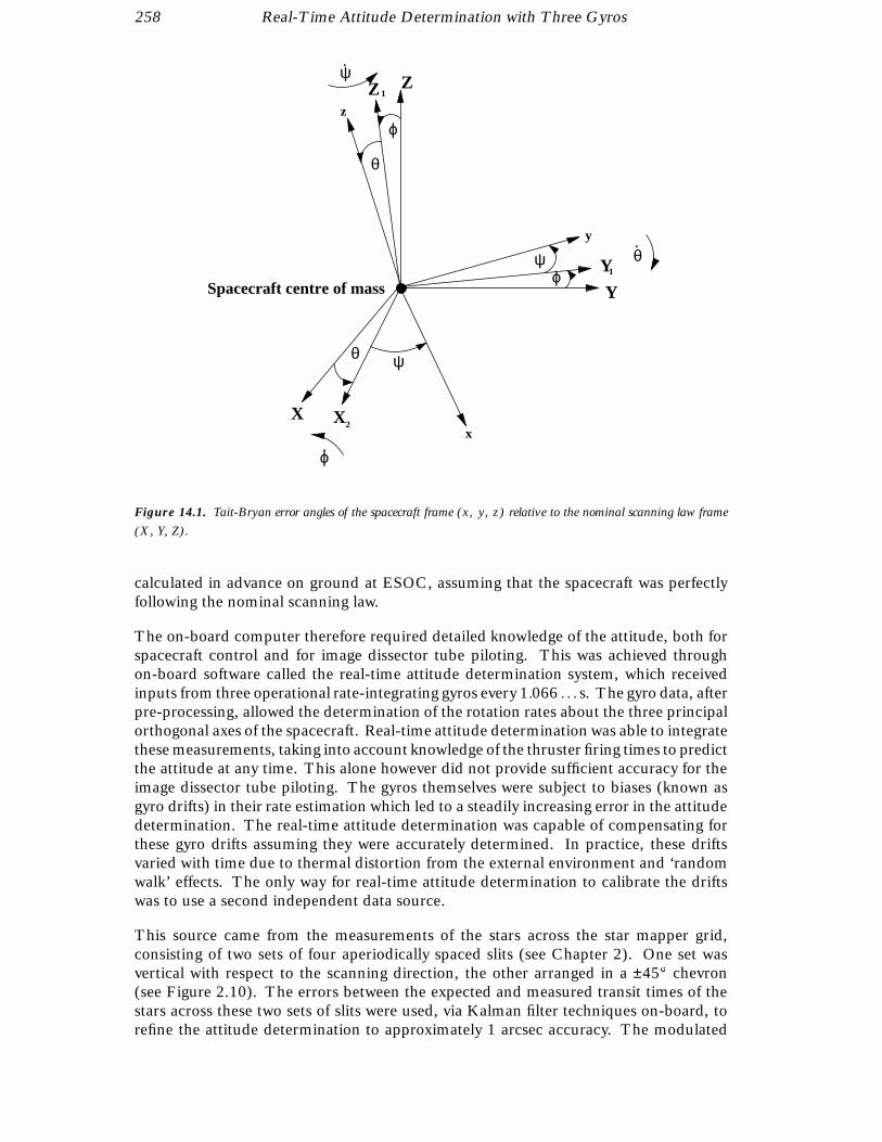
258 Real-Time Attitude Determination with Three Gyros
Z
y
Z
Y1
1
Y
z
ϕψ
ϕ
ψ
θ
θ
Spacecraft centre of mass
X X2x
θ
ψ
ϕ
Figure 14.1. Tait-Bryan error angles of the spacecraft frame (x, y, z) relative to the nominal scanning law frame
(X, Y, Z).
calculated in advance on ground at ESOC, assuming that the spacecraft was perfectlyfollowing the nominal scanning law.
The on-board computer therefore required detailed knowledge of the attitude, both forspacecraft control and for image dissector tube piloting. This was achieved throughon-board software called the real-time attitude determination system, which receivedinputs from three operational rate-integrating gyros every 1.066 . . . s. The gyro data, afterpre-processing, allowed the determination of the rotation rates about the three principalorthogonal axes of the spacecraft. Real-time attitude determination was able to integratethese measurements, taking into account knowledge of the thruster firing times to predictthe attitude at any time. This alone however did not provide sufficient accuracy for theimage dissector tube piloting. The gyros themselves were subject to biases (known asgyro drifts) in their rate estimation which led to a steadily increasing error in the attitudedetermination. The real-time attitude determination was capable of compensating forthese gyro drifts assuming they were accurately determined. In practice, these driftsvaried with time due to thermal distortion from the external environment and ‘randomwalk’ effects. The only way for real-time attitude determination to calibrate the driftswas to use a second independent data source.
This source came from the measurements of the stars across the star mapper grid,consisting of two sets of four aperiodically spaced slits (see Chapter 2). One set wasvertical with respect to the scanning direction, the other arranged in a ±45 chevron(see Figure 2.10). The errors between the expected and measured transit times of thestars across these two sets of slits were used, via Kalman filter techniques on-board, torefine the attitude determination to approximately 1 arcsec accuracy. The modulated
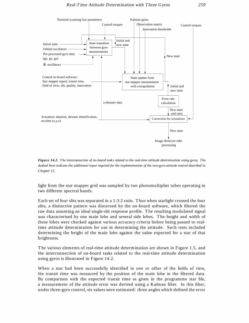
Real-Time Attitude Determination with Three Gyros 259
State transitionbetween gyromeasurements
new stateInitial and
Pre-processed gyro data
Orbital oscillators
Initial state
(gx, gy, gz)
Star mapper report: transit time,field of view, slit, quality, innovation
Central on-board software: State update fromstar mapper measurement
with extrapolation
oscillatorsψ
Error ratecalculation
new stateInitial and
Correction for actuations
New state and rates
Image dissector tubeprocessing
Actuation: datation, thruster identification, on-time (x,y,z)
Kalman gains
Observation matrix
Innovation thresholds
New state
Control torques
Nominal scanning law parameters
Control torques
New state
z-thruster data
Figure 14.2. The interconnection of on-board tasks related to the real-time attitude determination using gyros. The
dashed lines indicate the additional input required for the implementation of the two-gyro attitude control described in
Chapter 15.
light from the star mapper grid was sampled by two photomultiplier tubes operating intwo different spectral bands.
Each set of four slits was separated in a 1:3:2 ratio. Thus when starlight crossed the fourslits, a distinctive pattern was discerned by the on-board software, which filtered theraw data assuming an ideal single-slit response profile. The resulting modulated signalwas characterised by one main lobe and several side lobes. The height and width ofthese lobes were checked against various accuracy criteria before being passed to real-time attitude determination for use in determining the attitude. Such tests includeddetermining the height of the main lobe against the value expected for a star of thatbrightness.
The various elements of real-time attitude determination are shown in Figure 1.5, andthe interconnection of on-board tasks related to the real-time attitude determinationusing gyros is illustrated in Figure 14.2.
When a star had been successfully identified in one or other of the fields of view,the transit time was measured by the position of the main lobe in the filtered data.By comparison with the expected transit time as given in the programme star file,a measurement of the attitude error was derived using a Kalman filter. In this filter,under three-gyro control, six values were estimated: three angles which defined the error
260 Real-Time Attitude Determination with Three Gyros
between the current spacecraft attitude and the nominal scanning law (the Tait-Bryanerror angles), and three gyro drifts converted into rates along the principal spacecraftaxes.
As a result of tuning since the start of the mission involving ESOC, Matra Marconi Spaceand the scientific consortia, the real-time attitude determination system was capable ofworking to an accuracy of 1 to 2 arcsec in attitude determination if stars were beingsuccessfully identified in the star mapper processing. However, if errors had built upto over 10 arcsec, star measurements could no longer be used by real-time attitudedetermination, which diverged from the real attitude. This happened after 50 per centof all perigee passes, where higher disturbance torques and noise in the star mappersignal (caused by van Allen belt radiation) made divergence more likely.
As a protection against falsely identified stars, the attitude determination on boardnormally rejected any star transit times which showed that the spacecraft attitude relativeto the nominal scanning law had drifted by more than 10 arcsec since the last startransit was processed by real-time attitude determination. During normal operationsthis was not expected to happen, because the gyro drifts were accurate to less than5 milliarcsec s−1 and real-time attitude determination received star transit data every10 s on average.
Should anomolous conditions cause such an error to build up, it was possible to increasethis 10 arcsec limit (‘narrow window’) to 30 arcsec (‘extended window’) to allow real-time attitude determination to use these larger transit time errors to update its attitudeknowledge. If the errors were greater than 30 arcsec, then intervention was requiredfrom ground, because the on-board software was no longer capable of processing thecorrect buffer of raw star mapper data for stars to be detected. A suite of programs calledthe ground real-time attitude determination system was developed and used at ESOCfor this purpose. This software was designed to process on-ground all star mapper dataand estimate the attitude independently of any real-time attitude determination results.
14.2. On-board Real-Time Attitude Determination using Three Gyros
On-board real-time attitude determination involved estimating in real-time a state vectorconsisting of:
φ: Tait-Bryan error angle around the spacecraft x-axis;
θ: Tait-Bryan error angle around the spacecraft y-axis;
ψ : Tait-Bryan error angle around the spacecraft z-axis;
dx: gyro drift around the spacecraft x-axis;
dy: gyro drift around the spacecraft y-axis;
dz: gyro drift around the spacecraft z-axis.
Data from three gyros gave angular velocities (spacecraft body rates) about all three axes.This allowed a complete prediction of the attitude from one processing cycle (16/15 s)to another, assuming the previous attitude estimate was correct. Small corrections tothese predictions were made by comparing expected and measured star mapper crossingtimes.

Real-Time Attitude Determination with Three Gyros 261
Real-Time Attitude Determination Definitions
The following variables were input to the real-time attitude determination algorithm:
Gx(k + 1), Gy(k + 1), Gz(k + 1): angular measurements currently available from the gyrodata cyclic acquisition software.
td : star detection time derived from the on-board star mapper processing.
R: star angular measurement derived from the on-board star mapper processing.
(, f ): star mapper slit identifier of the detected star:– = 0: vertical slit– = −1: inclined slit, upper half of field of view– = +1: inclined slit, lower half of field of view– f = +1: preceding field of view– f = −1: following field of view
IQ: star quality:– IQ = 1 for a quality 1 star (more accurate on-ground position, typically better than
0.4 arcsec)– IQ = 2 for a quality 2 star (less accurate on-ground position, typically in the range
0.4–0.8 arcsec)
T: time of real-time attitude determination estimate (multiple of the real-time attitudedetermination cycle time ti ).
Sv(k), Cv(k): sine and cosine values produced by the orbital oscillator, but correspond-ing to the previous time interval (see Chapter 8).
ton,x, ton,y, ton,z: the X, Y, and Z cold-gas thruster on-times provided by the nominalmode control algorithm (see Chapter 13).
ΩT : transverse rate defined by Equation 8.10.
ΩN : estimate of the absolute Z-axis nominal scanning law spin rate provided by theon-board computer.
The following on-board constants were used:
ti : the cycle time (16/15 s) between inputs from the inertial reference unit.
KG1 (6,6): the 6 × 6 matrix of fixed gains associated with quality 1 stars.
KG2 (6,6): the 6 × 6 matrix of fixed gains associated with quality 2 stars.
One column of KG1 or KG2 was used in a star mapper update of the real-time attitudedetermination filter estimate. The column used was determined by the slit identifier asfollows:
– column 1: (, f ) = (0, 1)– column 2: (, f ) = (−1, 1)– column 3: (, f ) = (1, 1)

262 Real-Time Attitude Determination with Three Gyros
– column 4: (, f ) = (0, −1)– column 5: (, f ) = (−1, −1)– column 6: (, f ) = (1, −1)
The rows corresponded to the six components of the filter state vector:
V =
0BBBBB@
φ(k + 1)θ(k + 1)ψ (k + 1)dx(k + 1)dy(k + 1)dz(k + 1)
1CCCCCA
[14.1]
where dx(k + 1), dy(k + 1), dz(k + 1) were the current estimates of the gyro drifts.
H (6,6): star mapper observation matrix. The row used in a star mapper update wasdetermined by the slit identifier (exactly as for the column of KG1). The columnscorresponded to the six components of the filter state.
Tax, Tay, Taz: control torques applied about the spacecraft x, y and z axes.
Ixx, I yy , Izz: principal moments of inertia about the x, y and z axes.
µ: innovation threshold for narrow and extended windows.
Defining additionally:
ωX (k), ωY (k), ωZ (k): angular rates with respect to inertial space expressed in scanninglaw X, Y and Z axes and relating to the previous time interval.
dx(k + 1), dy(k + 1), dz(k + 1): current estimates of drift rates about the spacecraft x, y,and z axes.
RI : the innovation to be used in the filter star update, i.e. the difference between theextrapolated star mapper measurement and the linear approximation of the star mappermeasurement using the present real-time attitude determination attitude estimates.
The following outputs were obtained:
φ(k + 1), θ(k + 1), ψ (k + 1): current estimates of attitude error angles.
φ(k + 1), θ(k + 1), ψ (k + 1): current estimates of attitude error rates.
φm(k + 1), θm(k + 1), ψm(k + 1): modified (predicted) estimates of attitude error anglesaround actuation.
φm(k + 1), θm(k + 1), ψm(k + 1): modified (predicted) estimates of attitude error ratesaround actuation.
Three-Gyro Real-Time Attitude Determination Algorithm
At each sampling interval the real-time attitude determination produced estimates of theTait-Bryan angles and their derivatives from the output of the gyro data cyclic acquisitionsoftware (see Figure 14.2).
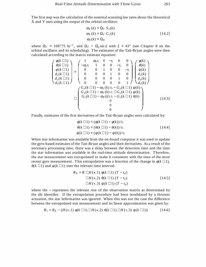
Real-Time Attitude Determination with Three Gyros 263
The first step was the calculation of the nominal scanning law rates about the theoreticalX and Y axes using the output of the orbital oscillator:
ωX (k) = ΩT Sv(k)
ωY (k) = ΩT Cv(k)
ωZ (k) = ΩN
[14.2]
where ΩT = 168.75 hr−1, and ΩT = Ωp sin ξ with ξ = 43 (see Chapter 8 on theorbital oscillator and its scheduling). The estimates of the Tait-Bryan angles were thencalculated according to the matrix estimate equation:
0BBBBB@
φ(k + 1)θ(k + 1)ψ (k + 1)dx(k + 1)dy(k + 1)dz(k + 1)
1CCCCCA
=
0BBBBB@
1 ωzti 0 −ti 0 0−ωzti 1 0 0 −ti 0
0 0 1 0 0 −ti
0 0 0 1 0 00 0 0 0 1 00 0 0 0 0 1
1CCCCCA
0BBBBB@
φ(k)θ(k)ψ (k)dx(k)dy(k)dz(k)
1CCCCCA
+
0BBBBB@
Gx(k + 1) − ωX (k) ti − Gy(k + 1) ψ (k)Gy(k + 1) − ωY (k) ti + Gx(k + 1) ψ (k)Gz(k + 1) − ωZ (k) ti − Gx(k + 1) θ(k)
000
1CCCCCA
[14.3]
Finally, estimates of the first derivatives of the Tait-Bryan angles were calculated by:
φ(k + 1) = (φ(k + 1) − φ(k)) /ti
θ(k + 1) = (θ(k + 1) − θ(k)) /ti
ψ (k + 1) = (ψ (k + 1) − ψ (k)) /ti
[14.4]
When star information was available from the on-board computer it was used to updatethe gyro-based estimates of the Tait-Bryan angles and their derivatives. As a result of thenecessary processing time, there was a delay between the detection time and the timethe star information was available in the real-time attitude determination. Therefore,the star measurement was extrapolated to make it consistent with the time of the mostrecent gyro measurement. This extrapolation was a function of the change in φ(k + 1),θ(k + 1) and ψ (k + 1) over the relevant time interval:
RE = R + H(, 1) φ(k + 1) (T − td )
+ H(, 2) θ(k + 1) (T − td ) [14.5]
+ H(, 3) ψ (k + 1) (T − td )
where the represents the relevant row of the observation matrix as determined bythe slit identifier. If the extrapolation procedure had been invalidated by a thrusteractuation, the star information was ignored. When this was not the case the differencebetween the extrapolated star measurement and its linear approximation was given by:
RI = RE − (H(, 1) φ(k + 1) + H(, 2) θ(k + 1) + H(, 3) ψ (k + 1)) [14.6]

264 Real-Time Attitude Determination with Three Gyros
If this innovation was less than the innovation threshold µ, the Tait-Bryan angles togetherwith the estimates of the gyro drift were updated according to the filtering equation:
φ(k + 1) = φ(k + 1) + KG1(1, ) RI
θ(k + 1) = θ(k + 1) + KG1(2, ) RI
ψ (k + 1) = ψ (k + 1) + KG1(3, ) RI
dx(k + 1) = dx(k + 1) + KG1(4, ) RI
dy(k + 1) = dy(k + 1) + KG1(5, ) RI
dz(k + 1) = dz(k + 1) + KG1(6, ) RI
[14.7]
If the innovation was greater than the innovation threshold the star information wasignored. In Equation 14.7 the update is associated with a quality 1 star. For a quality 2star KG1 was replaced by KG2 in the above equations.
Additional Attitude Prediction in the Case of Actuation
The output of the real-time attitude determination was used in the attitude and orbitcontrol system control loop and in the pointing of the image dissector tube beam. Asthe normal pointing of the image dissector tube beam used information two time cyclesout of date, an additional attitude prediction was necessary around a thruster actuationto prevent the situation where the image dissector tube beam was pointed withoutaccounting for the thruster firing.
The real-time attitude determination outputs corresponding to the observation frame(k + 1) preceding the actuation, and to the observation frame (k + 2) including theactuation were extrapolated from the nominal real-time attitude determination estimatesaccording to equations of the form:
φm(k + 2) = φm(k + 1) = f (φ(k + 1), ton,x , Tax, Ixx)
θm(k + 2) = θm(k + 1) = f (θ(k + 1), ton,y , Tay , I yy) [14.8]
ψm(k + 2) = ψm(k + 1) = f (ψ (k + 1), ton,z , Taz, Izz)
and:
φm(k + 2) = φm(k + 1) = g(φ(k + 1), φ(k + 1), φm(k + 1), ton,x , ti , Tax , Ixx)
θm(k + 2) = θm(k + 1) = g(θ(k + 1), θ(k + 1), θm(k + 1), ton,y , ti , Tay , I yy)
ψm(k + 2) = ψm(k + 1) = g(ψ (k + 1), ψ (k + 1), ψm(k + 1), ton,z , ti , Taz, Izz)
[14.9]
Modified Attitude Prediction
If during a given cycle k, the scanning law control determined that an actuation wasnecessary this actuation was synchronised with the observation frame cycle (k + 1).The real-time attitude determination outputs corresponding to cycle k preceding theactuation and to cycle (k + 1) including the actuation were extrapolated from real-timeattitude determination estimates and from applied thruster on-times. The real-timeattitude determination outputs corresponding to cycle (k + 2) following the actuationwere then nominal again.
Real-Time Attitude Determination with Three Gyros 265
For cycle k, preceding the actuation, real-time attitude determination outputs weregiven by:
φm(k) = φ(k) + Taxton,x
θm(k) = θ(k) + Tayton,y
ψm(k) = ψ (k) + Tazton,z
φm(k) = φ(k) − 12Taxt2
on,x − Taxton,xti [14.10]
θm(k) = θ(k) − 12Tayt2
on,y − Tayton,yti
ψm(k) = ψ (k) − 12Tazt2
on,z − Tazton,zti
For cycle (k + 1), including the actuation, real-time attitude determination outputs weregiven by:
φm(k + 1) = φ(k + 1) + Taxton,x
θm(k + 1) = θ(k + 1) + Tayton,y
ψm(k + 1) = ψ(k + 1) + Tazton,z
φm(k + 1) = φ(k + 1) − 12Taxt2
on,x [14.11]
θm(k + 1) = θ(k + 1) − 12Tayt2
on,y
ψm(k + 1) = ψ (k + 1) − 12Tazt2
on,z
The modified estimates were computed only for on-board computer acquisition pur-poses. They were never used in the nominal attitude prediction.
14.3. On-Ground Real-Time Attitude Determination
The initial on-ground attitude initialisation could be split into two distinct phases:
Initial Star Pattern Recognition: This phase generated off-line pairings between ob-served star transits and star identifications from a catalogue, identifying both the slitsystem crossed and the field of view of observation. This allowed the initial attitude ofthe scanning law to be determined, and provided initialisation for the next phase of theattitude determination.
The on-ground initial star pattern recognition was divided into five stages, each of whichpassed its output data as input to the next stage. These stages were:
(a) telemetry pre-processing and star mapper filtering;(b) slit distinction and gyro correction;(c) field of view separation;(d) star pattern matching against a star catalogue;(e) initialisation of the nominal scanning law.
All of the above steps were necessary if Ω0 was unknown (as it was at the start of themission). Generally however, under three-gyro control, attitude drifts after perigeewere less than 100 arcsec. Therefore in general, ESOC maintained a constant value ofΩ0 throughout the routine (three-gyro) phase of the mission. The only times when itwas deemed necessary to change Ω0 during this period were during a small number ofcontingencies where the spacecraft assumed a non-nominal spin rate for a significantperiod of time. In order to re-acquire attitude control, ESOC had the choice of options,either to perform a large firing of the cold gas thrusters to slew the spacecraft around its

266 Real-Time Attitude Determination with Three Gyros
principal rotation axis thereby re-acquiring the previous nominal scanning law attitude,or to calibrate the value of Ω0 for the current phase and calculate a new programmestar file. In all cases where the drift around the rotation axis was more than one or twodegrees, the second option was faster to implement, safer and less expensive in fuel.This implied that in those cases where Ω0 was known, only the first two stages up to ‘slitdistinction and gyro correction’ needed to be taken before moving on to precise attitudedetermination.
Precise Attitude Determination: This activity paired, in close to real-time, observedstar transits and star identifications from the operational catalogue, identifying the slitsystem crossed, whether the upper or lower half of the chevron slit system was crossed,and the field of view of observation. This information was used to generate a preciseattitude in near real-time and to estimate the gyro drifts. Linear extrapolation was usedto predict the spacecraft attitude at a precise time (approximately 25 s in the future)and the attitude along with the gyro drifts were uplinked to the spacecraft to be receivedon-board at precisely the time at which the attitude was valid. This uplink allowedinitialisation of the on-board real-time attitude determination.
The precise attitude determination was divided into four distinct stages, each of whichpassed its output data as input to the next stage. These stages were:
(a) star pattern monitoring;(b) fine attitude estimation;(c) basic angle calibration;(d) initialisation of the on-board real-time attitude determination.
The basic angle calibration was a subsidiary task, only used at the start of the missionand thereafter infrequently. The other stages were all critical to real-time attitudedetermination initialisation.
Telemetry Pre-processing and Star Mapper Filtering
This stage of the initial star pattern recognition involved the collection of both starmapper and attitude and orbit control system telemetry data, together with processingof the star mapper data. This was a time-critical task which ran throughout the attitudedetermination. The raw data from the satellite telemetry were received as telemetry‘bundles’. Each bundle contained 0.666 . . . s of raw telemetry data equivalent to 16telemetry formats (1 format = 41.666 . . . ms). Data from the on-board attitude andorbit control system required by tasks in the attitude initialisation chain were extractedand made available to all tasks.
The star mapper samples for both the BT and the VT channels were also extractedand placed in a circular buffer. Every raw star mapper sample in the VT channel wastested against a threshold (usually corresponding to VT = 9 mag). This threshold wasadaptive to reflect changes in the background noise level, for example as experiencedas the spacecraft passed through the van Allan radiation belts. A sample exceeding thisthreshold could be from a peak from a star crossing one of the slits (vertical or inclined).Therefore a window of data around this sample was correlated with a four-peakedmatching filter function which corresponded approximately to the expected signal froma bright star. The uneven spacing of each slit system (and also of the matching filterfunction) gave one correlation peak with distinct determinable side lobe peaks for a validstar transit.

Real-Time Attitude Determination with Three Gyros 267
A transit was identified if a correlation peak was found with the same time datation inboth the BT and the VT channels. The height and location of the peaks allowed a transittime and approximate BT and VT magnitudes to be determined, which were passed tothe next task in the initialisation chain. It was of course possible to have peaks frommore than one transit after correlation. In this case each transit was identified by thealgorithm except where there was interference between main peaks and side lobes ofother peaks.
Figure 14.3 shows the star mapper data for the VT channel contained in a 0.666 . . . sbundle of raw telemetry data. The crossing by a bright star of one of the slit systems isclearly seen and would have been detected by the correlation process. Figure 14.4 alsoshows the star mapper data for the VT channel contained in a 0.666 . . . s bundle of rawtelemetry data. The solitary large spike would have exceeded the raw threshold thustriggering the star mapper filtering. However in this case no peaks would have beendetected after correlation. Figure 14.5 shows similar data for the BT channel in whichmultiple transits can be seen.
Slit Distinction and Gyro Correction
The transit data from the filtering process described above did not contain entirelyaccurate information, since the correlation function was not optimal for a given transitcrossing for the following reasons: (i) the exact focus of the telescopes was not knownat the start of the mission; (ii) the filter was matched to the nominal rotation rate ofthe satellite, so that deviations from the nominal rate would smear the response; (iii)the star mapper photometric performance and slit characteristics were different for thevertical slits and the inclined slits. There was no a priori information about the slitsystem crossed and hence a correlation function had to be used for an ‘average’ slitperformance.
The first two error sources led to a magnitude bias while the third led to a bias betweenthe magnitude calculated by a star transit of the vertical slit system and the magnitudecalculated by a transit of the same star through the inclined slit system. Successivetransits of the same star image across the vertical and inclined slit systems were separatedby between 0.3 and 7.2 s (see Figure 2.10). A star crossing the centre of the star mapperslit system would transit the second slit systems 7.2 s after it transited the first whereasthis time separation was 0.3 s for one crossing at the extremes of the star mapper. Theslit distinction algorithm attempted to ‘pair’ transits separated by no more than 7.2 s bycomparison of their magnitudes. Two transits occurring within 7.2 s of each other werepaired if their BT and VT magnitudes and colour (BT − VT ) were equal within certaintolerances; these tolerances being set to take account of the errors referred to above.Each member of the pair was then tested separately to ensure that it could not form partof any other pair. Any pairs containing a transit that could belong to more than one pairwere discarded and their data were not used by following tasks.
This process led to approximately 40 per cent of transits being discarded. Real-timeslit distinction was not possible: on receipt of data from a bright star transit crossingthe first slit system at most 7.2 s delay could occur before data were received from thesecond slit crossing. Besides, following ‘pairing’ of two transits a further delay of 7.2 safter reception of the second transit of the pair was needed to ensure that the pairingwas unique. Once a successful pairing had been found a revised magnitude estimatecould be formed by taking the arithmetic mean of the two magnitudes of the two transits
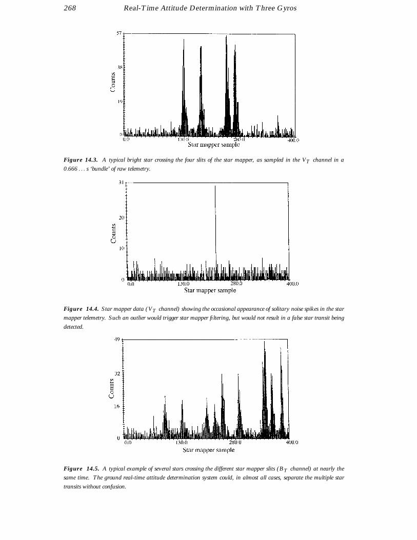
268 Real-Time Attitude Determination with Three Gyros
Figure 14.3. A typical bright star crossing the four slits of the star mapper, as sampled in the VT channel in a
0.666 . . . s ‘bundle’ of raw telemetry.
Figure 14.4. Star mapper data (VT channel) showing the occasional appearance of solitary noise spikes in the star
mapper telemetry. Such an outlier would trigger star mapper filtering, but would not result in a false star transit being
detected.
Figure 14.5. A typical example of several stars crossing the different star mapper slits (BT channel) at nearly the
same time. The ground real-time attitude determination system could, in almost all cases, separate the multiple star
transits without confusion.
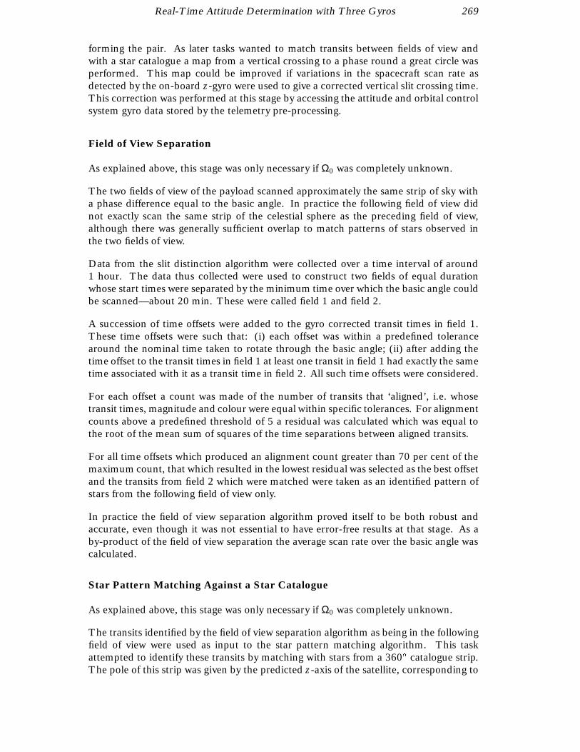
Real-Time Attitude Determination with Three Gyros 269
forming the pair. As later tasks wanted to match transits between fields of view andwith a star catalogue a map from a vertical crossing to a phase round a great circle wasperformed. This map could be improved if variations in the spacecraft scan rate asdetected by the on-board z-gyro were used to give a corrected vertical slit crossing time.This correction was performed at this stage by accessing the attitude and orbital controlsystem gyro data stored by the telemetry pre-processing.
Field of View Separation
As explained above, this stage was only necessary if Ω0 was completely unknown.
The two fields of view of the payload scanned approximately the same strip of sky witha phase difference equal to the basic angle. In practice the following field of view didnot exactly scan the same strip of the celestial sphere as the preceding field of view,although there was generally sufficient overlap to match patterns of stars observed inthe two fields of view.
Data from the slit distinction algorithm were collected over a time interval of around1 hour. The data thus collected were used to construct two fields of equal durationwhose start times were separated by the minimum time over which the basic angle couldbe scanned—about 20 min. These were called field 1 and field 2.
A succession of time offsets were added to the gyro corrected transit times in field 1.These time offsets were such that: (i) each offset was within a predefined tolerancearound the nominal time taken to rotate through the basic angle; (ii) after adding thetime offset to the transit times in field 1 at least one transit in field 1 had exactly the sametime associated with it as a transit time in field 2. All such time offsets were considered.
For each offset a count was made of the number of transits that ‘aligned’, i.e. whosetransit times, magnitude and colour were equal within specific tolerances. For alignmentcounts above a predefined threshold of 5 a residual was calculated which was equal tothe root of the mean sum of squares of the time separations between aligned transits.
For all time offsets which produced an alignment count greater than 70 per cent of themaximum count, that which resulted in the lowest residual was selected as the best offsetand the transits from field 2 which were matched were taken as an identified pattern ofstars from the following field of view only.
In practice the field of view separation algorithm proved itself to be both robust andaccurate, even though it was not essential to have error-free results at that stage. As aby-product of the field of view separation the average scan rate over the basic angle wascalculated.
Star Pattern Matching Against a Star Catalogue
As explained above, this stage was only necessary if Ω0 was completely unknown.
The transits identified by the field of view separation algorithm as being in the followingfield of view were used as input to the star pattern matching algorithm. This taskattempted to identify these transits by matching with stars from a 360 catalogue strip.The pole of this strip was given by the predicted z-axis of the satellite, corresponding to
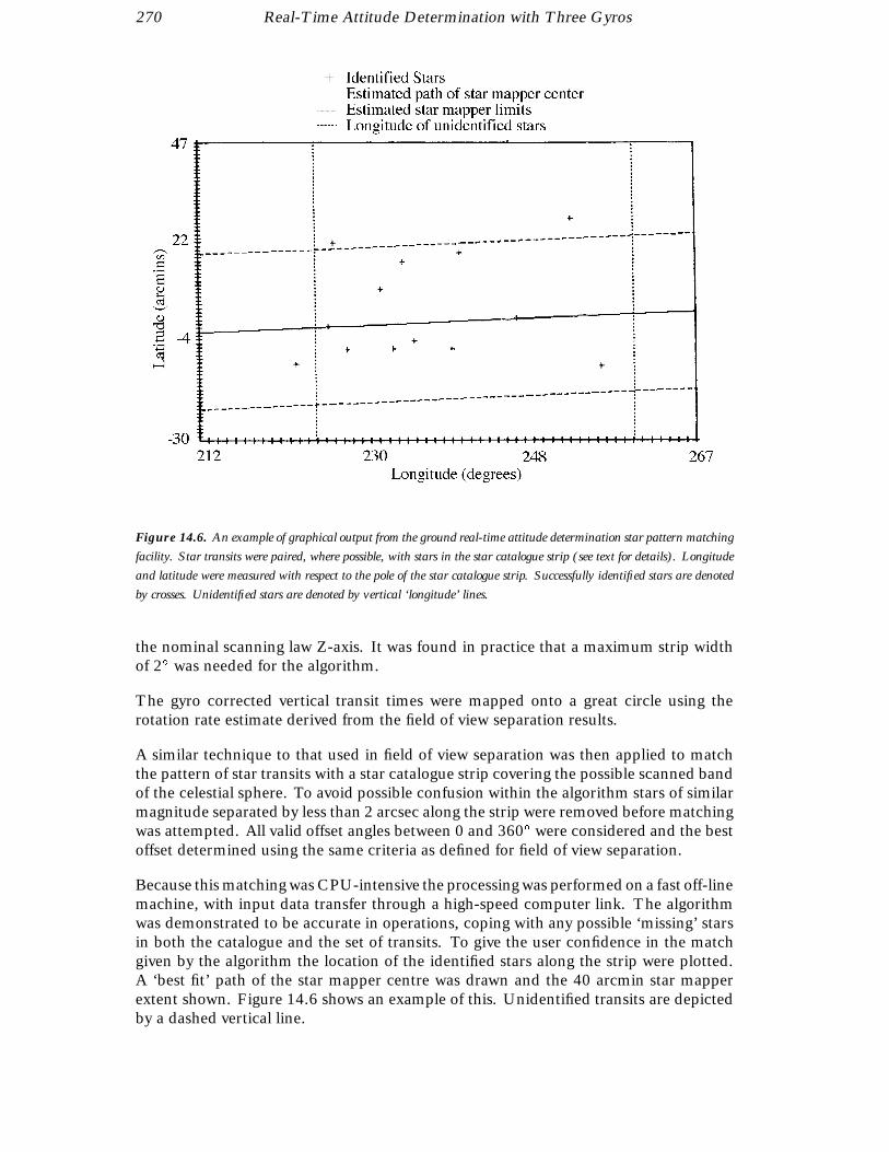
270 Real-Time Attitude Determination with Three Gyros
Figure 14.6. An example of graphical output from the ground real-time attitude determination star pattern matching
facility. Star transits were paired, where possible, with stars in the star catalogue strip (see text for details). Longitude
and latitude were measured with respect to the pole of the star catalogue strip. Successfully identified stars are denoted
by crosses. Unidentified stars are denoted by vertical ‘longitude’ lines.
the nominal scanning law Z-axis. It was found in practice that a maximum strip widthof 2 was needed for the algorithm.
The gyro corrected vertical transit times were mapped onto a great circle using therotation rate estimate derived from the field of view separation results.
A similar technique to that used in field of view separation was then applied to matchthe pattern of star transits with a star catalogue strip covering the possible scanned bandof the celestial sphere. To avoid possible confusion within the algorithm stars of similarmagnitude separated by less than 2 arcsec along the strip were removed before matchingwas attempted. All valid offset angles between 0 and 360 were considered and the bestoffset determined using the same criteria as defined for field of view separation.
Because this matching was CPU-intensive the processing was performed on a fast off-linemachine, with input data transfer through a high-speed computer link. The algorithmwas demonstrated to be accurate in operations, coping with any possible ‘missing’ starsin both the catalogue and the set of transits. To give the user confidence in the matchgiven by the algorithm the location of the identified stars along the strip were plotted.A ‘best fit’ path of the star mapper centre was drawn and the 40 arcmin star mapperextent shown. Figure 14.6 shows an example of this. Unidentified transits are depictedby a dashed vertical line.
Real-Time Attitude Determination with Three Gyros 271
Initialisation of the Scanning Law
Again, as explained above, this stage was only necessary if Ω0 was completely unknown.
The value of the Ω0 of the nominal scanning law was not known before initial starpattern recognition. However if Ωt is the heliotropic angle derived from the nominalscanning law for the attitude initialisation zero time assuming Ω0 = 0, Ωm is the offsetcalculated from the following field of view to the star catalogue strip, Ωs is the offsetof the centre of the star mapper vertical slit system from the spacecraft x-axis, then theinitial heliotropic angle is given as: Ω0 = Ωm − Ωt + Ωs and thus from this point on thescanning law could be determined.
Star Pattern Monitoring
Whereas the initial star pattern recognition identified detected transits retrospectively,the aim of star pattern monitoring was to identify transits as close to real time as possible.It did this by maintaining a sliding window of six matched vertical transits in each fieldof view. New transit pairs which had been identified by the slit distinction algorithm innear real-time were received. The vertical transit time was mapped to an angle roundthe great circle and added to the existing pattern in both fields of view. A pattern matchwas attempted on each field of view using a similar—though not identical—algorithm tothat used to calculate Ωm, based on a small range of offsets centred around the previousoffset for each field of view.
If the transit was identified in one and only one of the fields of view it was accepted.The window for that field of view was updated by releasing the ‘oldest’ star and addingthe new identification. The transit pair data and star identification were passed to thefine attitude estimation task.
Once an accurate value for Ω0 was known (either from previous spacecraft operationsor as a direct result of the full initial star pattern recognition just described) the two fieldof view windows required by star pattern monitoring were easily initialised. The offsetcalculated in star pattern matching was used to calculate offsets to the catalogue strip foreach field of view. The set of following field of view transits from field 2 of the separationalgorithm (see field of view separation above) was used to initialise the following fieldof view, and the remaining transits in field 2 were assumed to be rich in precedingfield of view transits and these were used to initialise the preceding field of view. Ifthe on-board real-time attitude determination needed to be subsequently re-initialised,providing the nominal scanning had been maintained, the star pattern monitoring couldbe re-initialised using the nominal scanning law to determine the offsets to the cataloguestrip for each field of view.
Up to 20 transit pairs identified by slit distinction were used as trial patterns for bothfields of view and pattern matching was attempted. If a pattern was identified uniquelyin both fields of view then the star pattern matching task was initialised and could beginnear real-time identifications. Otherwise further transit pairs were collected from slitdistinction and further pattern matches attempted. Figure 14.7 shows the results frominitialising one of these windows in this manner. Here a succession of closely spacedoffsets, each giving an alignment count of 11 transits, can be seen. The residual isplotted on top of this and the local minimum, corresponding to the best pattern match,

272 Real-Time Attitude Determination with Three Gyros
Figure 14.7. An example of graphical output from the ground real-time attitude determination star pattern monitoring
facility, during the initialisation phase. The angular offset from the strip origin which gives the best pattern match is
that showing the maximum alignment count and lowest residual (see text for details).
is located toward the centre of this offset grouping. (This is also the behaviour observedfor field of view separation and star pattern matching.)
The star pattern monitoring task ran throughout the remainder of the operations. Agraphics display was used to illustrate the real-time identifications. An example is shownin Figure 14.8. The display is split up into 5 sections: the top panel displays the incomingtransits as a function of time. Each incoming star transit is represented by a separatepoint. The symbol used for the star shows whether the transit has been identified and ifso in which field of view. The two central graphs display the identifications in each fieldof view. The left hand graph displays the following field of view and the right hand graphthe preceding field of view. Each identified transit is plotted in star catalogue coordinatesin the appropriate field of view. The path of each field of view across the catalogue stripcan therefore be seen—this was useful for determining the best half-width to use for thestrip. The lower two graphs show the residuals for the two fields of view as functions oftime. The residuals will be small—any increase in the residuals shows a deterioration inthe quality of the pattern match possibly because of star misidentification.
Fine Attitude Estimation
The requirement for the fine attitude estimation algorithm was to estimate in near realtime the spacecraft attitude, body rates and gyro drift rates. At this stage, the attitudewas determined by defining three Tait-Bryan attitude angles (φ, θ, ψ ) in an inertialreference frame.
(φ, θ) defined the scan plane orientation and ψ defined the rotational phase of thespacecraft. Hence (φ, θ) oscillated about zero, while ψ changed secularly at the same
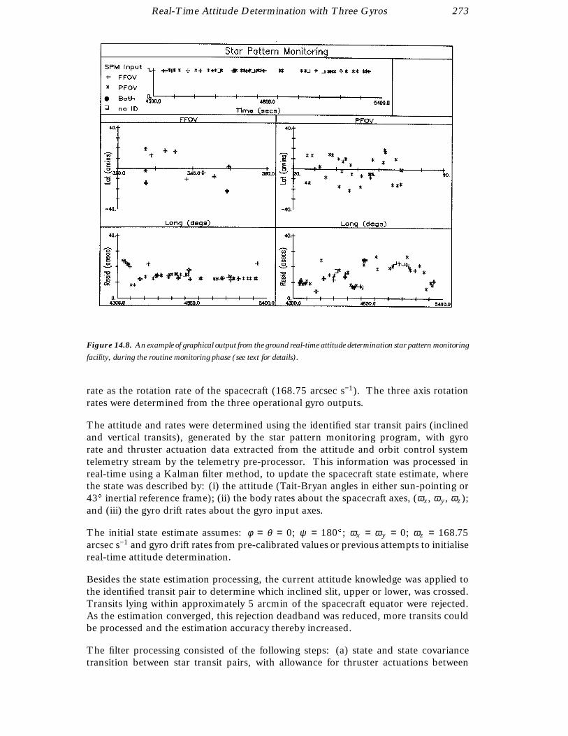
Real-Time Attitude Determination with Three Gyros 273
Figure 14.8. An example of graphical output from the ground real-time attitude determination star pattern monitoring
facility, during the routine monitoring phase (see text for details).
rate as the rotation rate of the spacecraft (168.75 arcsec s−1). The three axis rotationrates were determined from the three operational gyro outputs.
The attitude and rates were determined using the identified star transit pairs (inclinedand vertical transits), generated by the star pattern monitoring program, with gyrorate and thruster actuation data extracted from the attitude and orbit control systemtelemetry stream by the telemetry pre-processor. This information was processed inreal-time using a Kalman filter method, to update the spacecraft state estimate, wherethe state was described by: (i) the attitude (Tait-Bryan angles in either sun-pointing or43 inertial reference frame); (ii) the body rates about the spacecraft axes, (ωx, ω y, ωz);and (iii) the gyro drift rates about the gyro input axes.
The initial state estimate assumes: φ = θ = 0; ψ = 180; ωx = ω y = 0; ωz = 168.75arcsec s−1 and gyro drift rates from pre-calibrated values or previous attempts to initialisereal-time attitude determination.
Besides the state estimation processing, the current attitude knowledge was applied tothe identified transit pair to determine which inclined slit, upper or lower, was crossed.Transits lying within approximately 5 arcmin of the spacecraft equator were rejected.As the estimation converged, this rejection deadband was reduced, more transits couldbe processed and the estimation accuracy thereby increased.
The filter processing consisted of the following steps: (a) state and state covariancetransition between star transit pairs, with allowance for thruster actuations between

274 Real-Time Attitude Determination with Three Gyros
transit pairs; (b) pre-processing of star transit pair data and gyro rates to generate ameasurement for input to the Kalman filter; and (c) state vector and covariance matrixupdate resulting from a new measurement.
State and State Covariance: The state vector and state covariance transition betweenstar mapper measurements was performed as a series of transitions over intervals withoutactuations, with covariance updates at actuations. Between measurements a discretisedlinear state model was used, which could be derived from kinematic and dynamical(Euler equations) relationships for the attitude and the body rates respectively. Thedrift rates were modelled as a random walk with the drift noise incorporated into themodel’s system noise. Gyro reaction torques and solar radiation pressure torques weretaken account of in the forcing function which was used to perform the transition ofthe state vector. Other disturbance torques (e.g. gravity gradient and magnetic) weremodelled as torque noise within the overall system noise.
The performance of the Kalman filter could be tuned by varying the power spectraldensities in the system noise matrix. There were six power spectral densities which couldbe independently tuned: three for the torque drifts and three for the gyro drifts. Thepower spectral densities used affected the performance of the filter; if they were too largethe filter tended to track the raw measurements (including noise), if they were too smallthe filter response would be slow and the estimates would lag behind the optimal values.The effects of actuations were allowed for by updating the state covariance at the timeof the actuation. Specifically, the rate covariance on the axis about which an actuationtorque acts was relaxed—the covariance was reset to a comparatively large preset value.The state and the remaining state covariance components were not updated.
Measurement pre-processing: This covered the calculation of a measurement, measure-ment observation matrix and measurement covariances given a star transit pair and/orthe attitude and orbit control system gyro output history. The different measurementtypes generated were:
(i) transverse measurement (ζm), giving the longitude of the star measured from thespacecraft equator, which was a function of:
– inclined/vertical star transit times;– estimated attitude (φ, θ, ψ ) in the catalogue strip reference frame at the vertical
slit transit time;– estimated body rates at the vertical slit transit time;– star latitude and longitude in the catalogue strip reference frame;– inclined/vertical slit mounting angles in the spacecraft reference frame.
(ii) phase measurement giving the phase of the spacecraft x-axis measured from thecatalogue strip reference x-z plane about the scan axis direction. Whereas star transitpairs for both preceding fields of view and following fields of view were processedto give transverse measurements, only transits of one field of view were processed togive phase measurements. This measurement incorporated the scan phase and scan rateknowledge. By considering only one field of view, possible bias effects due to uncertaintyin the basic angle separating the two fields of view were removed from the scan phaseand scan-rate estimates. After initial calibration of the basic angle at the start of themission (see next section), this bias was removed and it was safe to use measurementsfrom both fields of view for updating the state vector;
(iii) gyro rates for the two equatorial and the z-axis gyro at a given time.
Real-Time Attitude Determination with Three Gyros 275
The measurements were treated as scalars rather than as a 5-dimensional measurementvector.
State Vector and Covariance Matrix Update: The updating of the state and state covari-ance from the measurement, measurement covariances and observation matrices wasperformed using the standard Kalman Filter algorithms. The state vector was updatedusing the differences (innovations) between the observed measurements and those pre-dicted from the previous estimate of the state. The star pattern monitoring may havesent a small number of misidentified stars which led to unexpectedly large differencesin the measurements. If these differences had been used the convergence of the filterwould have been badly disrupted. To avoid this, a measurement innovation thresholdcould be set for each of the three types of measurement. These thresholds could bealtered during the operation of fine attitude determination to protect the accuracy ofthe estimates. Using the conventional Kalman Filter equations, it was found that thegyro drift estimates were particularly sensitive to high innovations. Reasonably accurateinitial estimates were obtained for these drifts and a way needed to be found to protectthose values from excessive alteration at the start of fine attitude estimation when theinitial attitude and rates were not so well known. The solution was to modify the mea-surement innovations going into the drifts estimates by factors which could be tunedduring operation of fine attitude estimation. Initially these values were set low to fix thedrifts at a constant value until such times as the Tait-Bryan angles and body rates havebegun to converge. They could then be increased, once the innovation thresholds werelow enough to protect against star misidentifications, so that more accurate final valuesfor the drifts could be obtained.
Convergence of fine attitude estimation was usually achieved within 20 min, but timesvaried considerably depending on the frequency of star transits. Convergence wasimproved by having a mixture of transits in both fields of view. Examples of the Tait-Bryan angles, body rates, gyro drifts rates and innovation levels are given in Figure 14.9to Figure 14.12 for a typical real-time attitude determination initialisation attempt at43 from sun-pointing.
Basic Angle Calibration
As described in the previous section, a difference between the actual and the measuredbasic angle (nominally 58) led to a bias in the predicted attitude (particularly the Tait-Bryan angle ψ ). The solution was to collect transits once fine attitude estimation wasconverged and process them using a least-squares method to derive a better estimateof the basic angle, which could then be used to further improve the convergence offine attitude estimation. The process consisted of three activities: collecting star transitand attitude information from fine attitude estimation; pre-processing the fine attitudeestimation results to obtain a ‘batch’ of measurements; and estimation of the basicangle and grid rotation parameters by the application of a batch weighted least-squaresmethod.
Once fine attitude estimation was approximately converged, it was possible to collecttransit information including: transit time; field of view (following or preceding); cat-alogue position of observed star; current orientation of the scan plane as estimated byfine attitude estimation; and current rotation rate about the spacecraft z-axis.
These data were collected over 40–60 min by which time approximately 100 measure-ments should have been collected. During this period only phase measurements from

276 Real-Time Attitude Determination with Three Gyros
Figure 14.9. On-ground estimates of the φ (A) and θ (B) Tait-Bryan attitude angles from the ground real-time
attitude determination fine attitude estimation facility. The discontinuities result from thruster actuations.
Figure 14.10. On-ground estimate of body rate about the spacecraft y-axis from the ground real-time attitude
determination fine attitude estimation facility.

Real-Time Attitude Determination with Three Gyros 277
Figure 14.11. On-ground estimates of the drift rates of gyro 1 (A), 2 (B) and 4 (C), from the ground real-time
attitude determination fine attitude estimation facility.
Figure 14.12. On-ground transverse measurement innovation used in the Kalman filter within the ground real-time
attitude determination fine attitude estimation facility. Convergence of the algorithm to a stable attitude estimate is
seen as the size of the innovations reduces towards zero.
278 Real-Time Attitude Determination with Three Gyros
one field of view could be used to update the state vector. This eliminated possiblebiases in the state vector estimates.
At the end of this collection period, the raw measurement data were pre-processed.Near-simultaneous (within a specified time tolerance) transits of the vertical star map-per slits of the two fields of view (preceding and following) were required. For eachpreceding/following pair selected, the expected star separation was calculated from theknown star catalogue positions. The transverse coordinates of each star at the corre-sponding vertical slit transit time were calculated using the attitude estimated by thefine attitude estimation program and the catalogues star positions. The mean scan rateover the interval spanned by the results stored on disk was computed by integrating theinstantaneous z-axis body rate results—as calculated by fine attitude estimation—withtime and dividing by the interval duration. These measurements were then combinedin a least-squares formulation which provided estimates of the rotation angle of the grid(nominally zero) and the basic angle.
The basic angle was calibrated at the start of the mission while the spacecraft was sun-pointing. The value obtained was 58 30 arcsec, compared to an on-ground calibratedvalue of 58 42 arcsec. The grid rotation estimate proved to be unreliable. The maxi-mum error of 3 arcmin was in any case shown in simulations not to impede convergenceof fine attitude estimation. Convergence of fine attitude estimation during operationsassumed that the value was zero and no problems had been met. The new value forthe basic angle was thereafter used by fine attitude estimation. Subsequent attempts tore-initialise real-time attitude determination were performed using phase measurementsfrom both fields of view without impeding convergence. Within a few weeks of the startof the mission, the data reduction consortia had derived a more accurate value for thebasic angle, which was used by the ground real-time attitude determination system.
Initialisation of the On-Board Real-Time Attitude Determination
The final stage of the on-ground attitude initialisation was to provide for the spacecraftan instantaneous attitude estimate in terms of the Tait-Bryan error angles plus the threegyro drifts projected onto the spacecraft axes.
The spacecraft attitude estimated on-ground at any given time would have been derivedfrom data collected on-board the spacecraft at some earlier time. Although this timedelay could be calculated by using the computer clock and the correlation between thespacecraft clock and UTC, further time delays would occur in uplinking the attitude tothe spacecraft. The following solution was adopted.
A future time, t1 was selected according to the following criteria: t1 was at least 20 sin the future; it corresponded exactly to an on-board telemetry format start time (1telemetry format = 10.666 . . . s); and the total delay from the time, t0, of on-boardacquisition of the data used for the attitude estimate to the time t1 was calculated. Theattitude estimate and the estimated body rates calculated by the fine attitude estimationtask and valid for time t0 were used to linearly extrapolate through the time interval (t1
- t0) to give an attitude estimate valid for time t1. The attitude estimate for time t1 wasconverted to the ecliptic reference frame and compared with the nominal scanning lawattitude for time t1 to derive the Tait-Bryan error angles φ, θ, ψ . These Tait-Bryan errorangles together with the gyro drift estimates calculated by fine attitude estimation wereuplinked to the spacecraft.
Real-Time Attitude Determination with Three Gyros 279
The uplink command was time-tagged to expire 5 s before the time t1, but was formatsynchronised so that the command was only executed at the start of a format. Thisensured that the uplinked attitude estimate was accepted on-board at precisely the timeat which the estimate was valid.
Note that the above method did not remain valid if there was an actuation of the on-boardthrusters during the interval t1 − t0, as this would invalidate the extrapolation. Thrusteractuations were monitored on-ground and the uplink was only performed during aperiod when no actuations were expected. The Tait-Bryan error estimate had to bewithin 28 arcsec of the true attitude for the on-board real-time attitude determinationto converge following the uplink. To meet this requirement it was essential to keepthe time interval t1 − t0 as small as possible. This illustrates the time-criticality of theon-ground processing from the telemetry pre-processing and star mapper filtering taskthrough to the final attitude estimation. The value of t1 − t0 was monitored duringoperations and the uplink was only permitted when this value was less than 60 s. Underconditions of normal computer load this criterion was easily met. Figure 14.13 andFigure 14.14 show the effect of the attitude initialisation uplink on the on-board real-time attitude determination.
Subsequent Ground Operations
Following the uplink the on-board real-time attitude determination took over controlof the spacecraft. During the period of attitude initialisation a programme star filewas prepared on ground containing expected star transit data and this was uplinked tothe spacecraft before the attitude initialisation. If the value of Ω0 was already known,the programme star file could already be generated in advance of the start of real-timeattitude determination initialisation procedures. In general, therefore, during the three-gyro operations, the programme star file was generated automatically every 24 hours onthe off-line mainframe computer, transferred to the real-time system and uplinked tothe spacecraft, regardless of the status of real-time attitude determination.
The on-board real-time attitude determination was enabled after the attitude initiali-sation, controlling the spacecraft using observations of reference stars across the starmapper and data from the attitude and orbit control system. The on-ground attitudeestimation process continued and the difference between on-ground and on-board es-timates of the Tait-Bryan error angles and gyro drifts were monitored along with theon-board innovations to allow the on-ground support team to assess the convergence ofthe on-board algorithms. When the initial Tait-Bryan uplink was large (of the order of0.5) then it was necessary to wait until the on-board controller had recovered the initialattitude error and then fine-tune by uplinking a further set of Tait-Bryan error anglesbefore switching control to the on-board algorithm.
Once real-time attitude determination had been seen to converge on-board, the imagedissector tube should be capable of tracking stars. The image dissector tube was theprimary detector for the scientific data, and its correct operation was an indication ofreal-time attitude determination convergence. Thus once the attitude and the gyrodrifts were known on-ground, the values could be uplinked to the spacecraft for use byreal-time attitude determination and normal operations could continue. In this way, theattitude was accurately known and the gyro drifts could be continually calibrated.

280 Real-Time Attitude Determination with Three Gyros
Figure 14.13. Tait-Bryan angle uplink. The figure shows three lines denoting the differences between the on-board
and on-ground estimates of the Tait-Bryan error angles φ, θ, ψ (lines A, B, C respectively). All three curves reduce
to zero at uplink (to the right of the diagram).
Figure 14.14. Gyro drift relative to the spacecraft axes, as used on-board, for the x, y and z drifts (labelled A, B, C
respectively). Values change after the uplink of new values from ground.

Real-Time Attitude Determination with Three Gyros 281
14.4. Real-Time Attitude Determination Performance
In addition to ground real-time attitude determination, software ran continuously tomonitor the attitude and the behaviour of the gyros and thrusters. Various alarms wereto be triggered, on-board and on-ground, when an attitude anomaly occurred, such asa failed gyro or jammed thruster. If the spacecraft was visible from one of the groundstations, procedures could be implemented to minimise attitude drift. On-board, therewere other safety measures, which could be triggered automatically or manually fromground, to protect the spacecraft should it start to drift for any reason. A sun sensor wasused to protect the spacecraft from drifting more than 3 off the nominal scanning lawwith the immediate danger of the sun shining directly into the telescope, damaging thegrid or detectors. If the spacecraft drifted past this threshold a so called emergency sunreacquisition order was triggered on board. The spacecraft then immediately slewedback to sun-pointing.
Data Recovery Percentages
The revised orbit induced real-time attitude determination divergence after approxi-mately half of all perigee passes. The requirement to re-initialise real-time attitudedetermination prompted the decision to introduce a shift team of flight dynamics spe-cialists to support spacecraft operations. Real-time attitude determination performancewas continually monitored using the image dissector tube observations as the defini-tive criterion for convergence, i.e. if stars were being consistently observed by the im-age dissector tube, then real-time attitude determination must be converged. Oncereal-time attitude determination diverged (most often seen immediately after perigee)re-initialisation would take place using the ground real-time attitude determination soft-ware.
The overall percentage of science data achieved over the mission is shown in Fig-ure 14.15. The figures are derived from ESOC’s ground-based payload monitoringsoftware (described in Chapter 10). ‘Good’ data refers to periods when stars wereconsistently observed by the image dissector tube during coverage periods. ‘Bad’ datarefers to periods when real-time attitude determination diverged (usually immediatelyafter perigee) during coverage periods. ‘No data’ refers to periods without groundstation or computer support. The hibernation periods refer to those times when thespacecraft was spun up between three- and two-gyro phases and between two- andzero-gyro phases.
Once all three ground stations were made available, ‘good’ data recovery was around71 per cent during the three-gyro operations (71 per cent of 24 hours per day). ‘Good’data was recovered 87 per cent of the coverage time.
The time to perform real-time attitude determination re-initialisation varied greatly.This was due to two primary factors: (a) star mapper noise in the van Allen belts and(b) occultations after acquisition of signal.
The star mapper was particularly sensitive to background radiation in the van Allenbelts. When highly active, after a solar flare, the star mapper could be blinded for
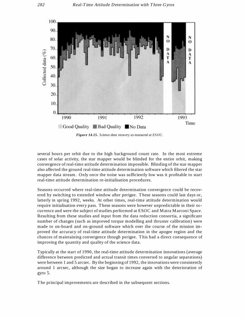
282 Real-Time Attitude Determination with Three Gyros
Figure 14.15. Science data recovery as measured at ESOC.
several hours per orbit due to the high background count rate. In the most extremecases of solar activity, the star mapper would be blinded for the entire orbit, makingconvergence of real-time attitude determination impossible. Blinding of the star mapperalso affected the ground real-time attitude determination software which filtered the starmapper data stream. Only once the noise was sufficiently low was it profitable to startreal-time attitude determination re-initialisation procedures.
Seasons occurred where real-time attitude determination convergence could be recov-ered by switching to extended window after perigee. These seasons could last days or,latterly in spring 1992, weeks. At other times, real-time attitude determination wouldrequire initialisation every pass. These seasons were however unpredictable in their oc-currence and were the subject of studies performed at ESOC and Matra Marconi Space.Resulting from these studies and input from the data reduction consortia, a significantnumber of changes (such as improved torque modelling and thruster calibration) weremade to on-board and on-ground software which over the course of the mission im-proved the accuracy of real-time attitude determination in the apogee region and thechances of maintaining convergence though perigee. This had a direct consequence ofimproving the quantity and quality of the science data.
Typically at the start of 1990, the real-time attitude determination innovations (averagedifference between predicted and actual transit times converted to angular separations)were between 1 and 5 arcsec. By the beginning of 1992, the innovations were consistentlyaround 1 arcsec, although the size began to increase again with the deterioration ofgyro 5.
The principal improvements are described in the subsequent sections.

Real-Time Attitude Determination with Three Gyros 283
Central On-Board Software Patch and Parameter Tuning
As described in Chapter 9, in January 1990, the first calibrated grid rotation from theFAST Consortium was used on-board resulting in a significant improvement in on-board real-time attitude determination performance. The resulting innovations, whichgive a measure of the attitude corrections necessary between star mapper transits, werereduced from an average distribution of around ±5 arcsec, to around ±2 arcsec.
In March 1990, a new version (4.02) of the central on-board software was uplinked tothe spacecraft. The new patch contained the following changes:
(a) extensions of the time-tagged buffer with an increase of allocated space from 640words to 1504 words;
(b) extension of the memory area for the star data blocks which was increased from1983 star data blocks (11898 words) to 2314 star data blocks (13884 words);
(c) improved star mapper filtering to eliminate false star mapper identifications inhigh noise.
The first change was necessary to perform efficient operations through long groundstation outage. The second change allowed a denser selection of real-time attitude de-termination reference stars through long ground station outage (the ‘sparse programmestar file’ described in Chapter 8). Clearly, the likelihood of maintaining real-time atti-tude determination convergence was proportional to the frequency of good star mappermeasurements.
The third change was necessary since it became clear that high star mapper noiseduring van Allen belt passage was occasionally causing the on-board software to make a‘false star’ detection. This erroneous measurement could be seen as real-time attitudedetermination as a larger than average innovation. Although the largest errors wouldbe trapped by setting an appropriate innovation rejection threshold on-board, moderatesized errors were still apparent leading to increased noise in the overall real-time attitudedetermination performance. After the on-board patch was included, a clear reductionin the largest innovations was seen. Moreover, it became possible to make better useof the ‘extended window’ innovation threshold of 30 arcsec during high noise to helpre-converge real-time attitude determination.
In May 1990, a swap from the BT to the VT channel for star mapper processing wasmade. This was due to the higher response in the VT channel giving a higher numberof successfully processed stars.
Over the following months, other tuning of on-board software parameters associatedwith star mapper rejection criteria was made. Statistics of reasons of star mapper mea-surement rejection were compiled over several weeks, correlating them to backgroundnoise and magnitudes of the reference stars. In this way, certain magnitude dependentparameters relating to expected height and width of the filtered signal were tuned. Theresult was a steady increase in the frequency of successful star mapper measurementsfor use by the real-time attitude determination system.
284 Real-Time Attitude Determination with Three Gyros
Reference Star Rejection Criteria
It was observed early on in the mission that the faintest real-time attitude determinationreference stars were invariably rejected in the star mapper processing (95 per cent).Therefore, in March 1990, the limiting magnitude of such reference stars (flagged inthe programme star file) was reduced from 10 to 9 mag. The result was a reduction inthe load on central on-board software processing, allowing more of the brighter stars tobe successfully processed.
Hipparcos Input Catalogue Updates
As described in Chapter 9, the NDAC Consortium was able to feed back their prelimi-nary star positions and magnitudes to ESOC, via the INCA Consortium, to be used forthe on-board programme star file.
In February 1991, Version 8 of the Hipparcos Input Catalogue was received and im-plemented at ESOC, containing approximately half the programme stars with positionsupdated from the preliminary data reductions. By November 1992, Version 10 wasreceived, with nearly all of the programme stars containing updated results. The im-provement in accuracy of the positions was, by that time, superior to the intrinsicperformance accuracy of the real-time attitude determination.
This and the greater reliability in the magnitude estimates allowed ESOC to tune theselection criteria for attitude guide stars and to tune the on-board star mapper processingparameters to optimise the correct identification of guide stars in the star mapper datastream and virtually eliminate any possibility of mis-identifying stars, which could leadto an unexpectedly large innovation error in the on-board control.
Occultations and Eclipses
An occultation occurred when the Earth or Moon crossed one of the fields of view ofthe telescope (the definition of the nominal scanning law prevented the Sun from everdoing so). Light from either body could have damaged the sensitive detectors, henceshutters were closed to protect them. Unfortunately that meant that no stars could beseen by either the image dissector tube or star mapper and real-time attitude knowledgecould deteriorate, resulting ultimately in divergence.
Occultations by the Earth or the Moon required that the star mapper shutters be closedfor up to 30 min at a time, near the perigee region. These would often hinder groundreal-time attitude determination re-initialisation procedures. At times, it would be nec-essary to restart the procedure, if the occultation interrupted the star pattern recognitionbefore convergence of the ground software could be achieved.
In 1991, the mission planning software at ESOC was modified to allow the shutters toremain open during occultations whenever a dark area of the Earth’s surface occultedone or both fields of view. Since there was no risk to the instruments from the darkside of the Earth, real-time attitude determination was more likely to be maintainedusing star measurements from the other field of view. This was particularly valuable at

Real-Time Attitude Determination with Three Gyros 285
lower altitudes, where the Earth’s disc was much larger and the occultation durationconsequently longer.
Gyro Projection Matrices
As described in Chapter 9, in July 1991, the NDAC Consortium was able to supply anewly calibrated gyro projection matrix for uplink to the spacecraft, to account for gyromisalignments with respect to the nominal positions.
Gyro Drift Monitoring and Correction
As described in Chapter 13, from March 1992 onwards, ground procedures werechanged to allow the resetting of the on-board drift estimates as soon as possible afterperigee to the last values observed before perigee. Subsequent careful monitoring fordrift evolution was then performed throughout the orbit to ensure that the best driftestimates were maintained.

286
15. REAL-TIME ATTITUDE DETERMINATIONWITH TWO GYROS
Radiation damage was considered to be responsible for the progressive failureof the gyroscopes. In the nominal mode of operation these gyros were essentialfor acquisition and maintenance of attitude knowledge and control. In princi-ple the satellite itself, with adequately known external and internally-actuatedtorques, allows the integration of its attitude evolution with less noise thanintegration of the gyro outputs. However, this would require both a very ac-curate starting point and very sophisticated modelling. The accuracy of sucha description of attitude evolution could only be maintained through the ob-servation of star transits across the star mapper grids. The time between theseevents must be sufficiently short for the integration to maintain the requiredaccuracy. In the originally intended geostationary orbit it seems likely thatthis notion would have provided the incentive to operate with the gyros turnedoff, thus suppressing jitter and parasitic torque. In the actual geostationarytransfer orbit the long interruptions of star transit observations coincided withthe least known, yet highest perturbing torques, which would inevitably causeloss of attitude to the point of requiring reinitialisation. Thus for a less thanthree-gyro mode of operation not only a model to replace the real-time on-board input of the absent gyro was needed, but also a much faster, and thusmore sophisticated attitude determination and initialisation on ground. Asredundancy in the gyroscopes disappeared, a substantial effort was put intodeveloping the procedures to work with only two gyroscopes, and eventuallywithout gyroscopes altogether. The two-gyro mode was fully implemented,and eventually used for the last months of scientific observations.
15.1. Two-Gyro Operations Development History
In June 1990, gyro 4, which monitored the scan rate about the principal spin axis,failed. It was replaced in the attitude control loop by the backup unit, gyro 5. Beforethe failure, gyro 4 had exhibited a large and fluctuating noise envelope (exceeding1 arcsec s−1 amplitude at times). Subsequent monitoring showed that gyro 5 exhibitedsimilar noise characteristics to those of the failed gyro.
Given the repeated apparent run-downs of gyro 4 and the anomalous noise propertiesof gyro 5, there was a high risk that both could fail irreparably. In order to continue

288 Real-Time Attitude Determination with Two Gyros
the mission without any z-gyro (the z referring to the z-axis in the spacecraft referencesystem used for real-time attitude determination, as described in Chapter 14), a seriesof studies were performed. They resulted in an attitude control software modification,called the ‘two-gyro patch’, and a number of ground software changes/updates whichallowed the continuation of the mission using only two gyros.
The revised on-board real-time attitude determination algorithm replaced the z-gyroinput by a simple sinusoidal model for the disturbance torque around the z-axis nearapogee, combined with a revised Kalman filter to estimate not only the z-axis Tait-Bryanerror angle (as for the three-gyro real-time attitude determination) but also the differencebetween the nominal and actual spin rate and the acceleration around the z-axis. Boththe Kalman filter state vector and the sinusoidal model had to be initialised from groundafter every perigee using the revised ground real-time attitude determination software.The on-board attitude control logic, indicating the changes necessary in going fromthree-gyro to two-gyro operations, are shown in Figure 14.2.
The patch was run successfully in parallel with the actual real-time attitude determina-tion in order to validate both the on-board and ground modifications. These changeswere extensively tested during the second half of 1991 and proven to function correctly.
On 10 July 1992, after continuous poor performance, gyro 5 was removed from thecontrol loop and the two-gyro real-time attitude determination system was used tocontrol the spacecraft for the first time. By 11 July 1992, after parameter tuning on-board and refinement of ground procedures, the first scientific data were obtained.The concept of two-gyro real-time attitude determination had been proven, and whenconverged, gave better performance than the three-gyro real-time attitude determinationwith the noisy gyro 5.
Although it had been proved that the ground software developed during 1991 and 1992was adequate for initialising real-time attitude determination, it was far from optimal.Moreover, although giving generally better performance in the apogee region, the two-gyro real-time attitude determination suffered two distinct disadvantages:
(a) divergence after occultations was frequent, leading to lost science data before theground real-time attitude determination software could re-initialise on-board real-timeattitude determination;
(b) there was little control of the spin rate through perigee, leading to a lengthy procedureof real-time attitude determination initialisation after every perigee. This procedure tookbetween 1.5 and 2 hours at that time, in comparison with 20–40 min with the three-gyro real-time attitude determination (with a high probability that real-time attitudedetermination would remain converged after perigee). Given that typically 9.5 hourswas covered by ground station per orbit, a loss of 1 to 2 hours science data per orbit wasconsiderable.
After an emergency sun reacquisition on 4 August 1992, in which the satellite spinaxis was autonomously slewed to the Sun direction, a recovery in the performance ofgyro 5 prompted a return to three-gyro real-time attitude determination operations on8 August 1992. However, on 11 August after a scanning law acquisition manoeuvre toreturn to the nominal scanning law, gyro 5 failed for the last time causing an emergencysun reacquisition and a spin-up to 0.45 rpm. The decision was taken to extend thespacecraft spin-up phase as much as possible, i.e. until the increasing solar aspect anglereached the limit of 43. There were two main reasons for doing so:

Real-Time Attitude Determination with Two Gyros 289
(a) the early operational experience with the two-gyro real-time attitude determinationbefore the emergency sun reacquisition occurred, proved to be valuable in highlightingvarious improvements which could be made to speed up real-time attitude determi-nation initialisation. While the spacecraft was spin-stabilised, it was safe enough toremove the flight dynamics team from operational shift work to daytime developmentof enhanced ground real-time attitude determination software, thereby increasing thespeed of production of the software by a factor of 3 to 4. As stated above, these changesincreased the speed and reliability of real-time attitude determination initialisation oncethe operations were resumed;
(b) it was hoped at that time that the mission lifetime would be dictated by the gasconsumables. Given that no gas was being used in the spin-up phase, by delayingspin-down, one was actually extending the lifetime of the mission with a subsequentimprovement in the final accuracies of the proper motions.
This approach was agreed between ESOC, ESTEC and the data reduction consortia.The spacecraft remained spun up until 1 October 1992, when the increasing sun aspectangle necessitated an additional manoeuvre to sun-pointing mode. By this time, mostof the planned software changes had been completed. Full operations resumed with thenew system, collecting science data for approximately four more months.
15.2. Operational Requirements
In running with two-gyro control, several new operational procedures had to be per-formed:
(a) the higher disturbance torques close to perigee caused a net angular accelerationaround the rotation axis. These acceleration terms were difficult to model and predictas there was no ground station coverage possible at so low a height (500 − 600 km).Nominally, the scan rate was constrained by the on-board attitude control software tobe within approximately 2 per cent of the nominal rate of 168.75 arcsec s−1. Withoutthe z-axis gyro input, much larger excursions were expected. As far as possible, theseexcursions had to be minimised through perigee;
(b) on receiving signal from the spacecraft after perigee it was necessary to measure thescan rate on-ground and correct it, if necessary, by direct thruster command;
(c) the spacecraft lost real-time attitude determination control through perigee. There-fore it was necessary to estimate on-ground the attitude, body rates, (particularly aroundthe z-axis) and correct the on-board values in real-time. It was also necessary to be ableto reset the drift values on the remaining gyros;
(d) most importantly, after re-initialisation, the revised real-time attitude determinationsoftware on-board had to be capable of remaining converged on the correct attitudeestimate to allow scientific data to be collected, accurate attitude information beingnecessary for the image dissector tubes to pilot successfully.

290 Real-Time Attitude Determination with Two Gyros
On-Board Memory Constraints
Memory space on-board was limited. Some of the spare memory already providedadditional gyro/thruster monitoring during loss of signal, preventing an irretrievablespin-up of the spacecraft should the second spin-rate gyro fail. A highly sophisticatedmodel would not fit the available space that was left. The model that was adopted isdescribed in detail in the next section.
The revised on-board software was devised to fit into the available spare memory andcould be run in parallel with the nominal three-gyro system. This allowed, during thefirst half of 1992, the new software to be tested on-board in a monitoring mode, i.e.the attitude was estimated without using the (still) operational spin-axis gyro. Howeverthis information was merely dumped in the telemetry and was not used to control thespacecraft. Rather the nominal on-board system continued to control the satellite untilthe time that the z-axis gyro failed.
Ground System Requirements
In addition to the dramatic changes required to the on-board real-time attitude deter-mination, the ground system also required significant modification.
Raw star mapper data were only processed by the telemetry pre-processing and star map-per filtering task in the ground real-time attitude determination chain (see Chapter 14).Therefore it had to perform the scan-rate estimation if no z-gyro was operational. Thisled to the following constraints on the scan-rate estimation algorithm:
(a) the algorithm performance had to comply with the real-time constraints of theground attitude determination within the resource limitations imposed by the availablehardware and other essential control tasks running in parallel;
(b) implementation of the scan-rate estimation algorithm had to involve minimumchanges to the existing telemetry pre-processing and star mapper filtering software.Algorithms and techniques employed in the nominal algorithm had to be retained wher-ever possible and interfaces to the original software kept simple. This reduced problemsof integrating and testing new software and minimised development time. This wasimportant at the start of the development since the lifetime of the remaining z-gyro wasunknown;
(c) the scan-rate estimation algorithm could not rely on a priori knowledge of either theexpected transit time or detailed characteristics of the slit system being crossed, sincethis information was only derivable from subsequent tasks in the ground system;
(d) the interfaces to other tasks in the ground attitude system had to be unalteredwherever possible to minimise software changes.
The operational constraints imposed on the on-ground real-time attitude determinationgave it distinctive problems in star recognition which were quite different from eitherthe on-board real-time attitude determination system or the post-processing work per-formed by the scientific data reduction consortia. For example, on-board real-timeattitude determination could not successfully recognise stars in the star mapper dataunless it could calculate the spacecraft attitude accurately. Ground real-time attitude

Real-Time Attitude Determination with Two Gyros 291
determination had to identify stars, with little or no a priori information concerningthe spacecraft rotational phase around the spin axis. Besides, ground real-time attitudedetermination had also to be able to operate under these new conditions with verymuch larger deviations in the spin rate. Ground real-time attitude determination hadalso to straddle the twin hurdles of providing sufficiently robust and accurate attitudedetermination, when the finite resources of the on-board system were unable to cope,and performing it in near real-time. This latter constraint was not imposed on thedata reduction consortia who were able to re-constitute the attitude off-line to muchhigher accuracy, given the good a priori attitude information of the on-board system,that enabled the image dissector tube piloting for the acquisition of good scientific data.
15.3. On-Board Software
On-Board Real-Time Attitude Determination using Two Gyros
As discussed above, given that on-board memory was limited, changes to the real-timeattitude determination algorithm were limited in scope. A full description of the designconcepts of real-time attitude determination was given in Chapter 14. This sectionconcentrates on the differences between the three- and two-gyro systems.
In the nominal on-board system, the state vector in the Kalman filter consisted ofthe three Tait-Bryan error angles and three gyro drifts. All six were defined withrespect to a co-rotating cartesian coordinate system. The integrated gyro outputs wereused to estimate the attitude evolution and the star mapper transit times were used asmeasurements to update the state vector.
Without a z-gyro, it was necessary to include the angular rate around the z-axis withinthe state vector and to allow that to be updated by the star mapper measurements.Studies by Matra Marconi Space showed that it was feasible to replace the z-gyro rateinputs by a dynamic model predicting ψ , the Tait-Bryan error angle around the z-axis.The vector would be increased to dimension 8 to include separately first and second-order terms in ψ and the z-gyro drift would be replaced by dψ /dt and d2ψ /dt2.
Consequently the revised state vector was:– φ: Tait-Bryan error angle around the spacecraft x-axis;– θ: Tait-Bryan error angle around the spacecraft y-axis;– ψ1: Tait-Bryan error angle around the spacecraft z-axis (first-order term);– ψ2: Tait-Bryan error angle around the spacecraft z-axis (second-order term);– dx: gyro drift around the spacecraft x-axis;– dy: gyro drift around the spacecraft y-axis;– dz: scan rate drift from nominal (168.75 arcsec s−1);– γz: rate of scan rate drift.
Above 20 000 km where the radiation pressure was the dominant disturbance torque, theacceleration around the z-axis could be successfully modelled by a harmonic of threetimes the nominal scan-rate. Such a model already existed on-board in the ‘normalmode’ control software for use in optimising thruster on-times (see Chapter 13), butup to now had not been used for attitude determination. The time dependency of themodel was provided by the variables (Sv3(k), Cv3(k)), which were already derived for
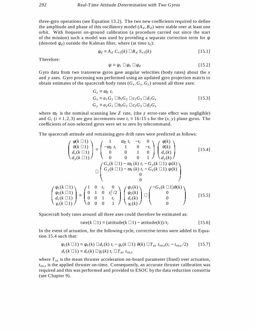
292 Real-Time Attitude Determination with Two Gyros
three-gyro operations (see Equation 13.2). The two new coefficients required to definethe amplitude and phase of this oscillatory model (Ad , Bd ) were stable over at least oneorbit. With frequent on-ground calibration (a procedure carried out since the startof the mission) such a model was used by providing a separate correction term for ψ(denoted ψd) outside the Kalman filter, where (at time tk):
ψd = Ad Cv3(k) + Bd Sv3(k) [15.1]
Therefore:ψ = ψ1 + ψ2 + ψd [15.2]
Gyro data from two transverse gyros gave angular velocities (body rates) about the xand y axes. Gyro processing was performed using an updated gyro projection matrix toobtain estimates of the spacecraft body rates (Gx , Gy , Gz) around all three axes:
Gz = ωZ ti
Gx = a1G1 + b1G2 + c1G3 + d1Gz [15.3]
Gy = a2G1 + b2G2 + c2G3 + d2Gz
where ωZ is the nominal scanning law Z rate, (the z error-rate effect was negligible)and Gi (i = 1, 2, 3) are gyro increments over ti = 16/15 s for the (x, y) plane gyros. Thecoefficients of non-selected gyros were set to zero by telecommand.
The spacecraft attitude and remaining gyro drift rates were predicted as follows:0B@
φ(k + 1)θ(k + 1)dx(k + 1)dy(k + 1)
1CA =
0B@
1 ωZ ti −ti 0−ωZ ti 1 0 −ti
0 0 1 00 0 0 1
1CA
0B@
φ(k)θ(k)dx(k)dy(k)
1CA [15.4]
+
0B@
Gx(k + 1) − ωX (k) ti − Gy(k + 1) ψ (k)Gy(k + 1) − ωY (k) ti − Gx(k + 1) ψ (k)
00
1CA
0B@
ψ1(k + 1)ψ2(k + 1)dz(k + 1)γz(k + 1)
1CA =
0B@
1 0 ti 00 1 0 t2
i /20 0 1 ti
0 0 0 1
1CA
0B@
ψ1(k)ψ2(k)dz(k)γz(k)
1CA +
0B@
−Gx(k + 1)θ(k)000
1CA [15.5]
Spacecraft body rates around all three axes could therefore be estimated as:
rate(k + 1) = (attitude(k + 1) − attitude(k)) /ti [15.6]
In the event of actuation, for the following cycle, corrective terms were added to Equa-tion 15.4 such that:
ψ1(k + 1) = ψ1(k) + dz(k) ti − gx(k + 1) θ(k) + Taz ton,z(ti − ton,z /2) [15.7]
dz(k + 1) = dz(k) + γz(k) ti + Taz ton,z
where Taz is the mean thruster acceleration on-board parameter (fixed) over actuation,ton,z is the applied thruster on-time. Consequently, an accurate thruster calibration wasrequired and this was performed and provided to ESOC by the data reduction consortia(see Chapter 9).

Real-Time Attitude Determination with Two Gyros 293
Figure 15.1. z-thruster on-time differences (expressed in rtc units of 1/75 s) as accumulated around perigee and
apogee for 240 orbits. See text for details.
Measurement extrapolation and innovation (RI ) computation were performed in a sim-ilar manner to that used for three-gyro real-time attitude determination except that newfixed gain sets KGnew were used. Attitude updates were consequently computed as:
X +new = Xnew + RI KGnew(slit, quality) [15.8]
where:
Xnew = (φ, θ, ψ , dx , dy , xz , γz)
ψ +1 = ψ + − ψd [15.9]
ψ +2 = 0
Modification of the attitude for on-board computer extrapolation on cycles aroundactuation was performed as for three-gyro real-time attitude determination.
Perigee Scan-Rate Control
Through perigee passage, the complex disturbance torques around the z-axis were notmodelled on-board to sufficient accuracy for attitude determination. In addition the ac-celerations could not be determined in the Kalman filter from star transit measurementsbecause the star mapper electronics were blinded by noise from the van Allen belts.
It was soon realised that a further z-gyro failure could result in an irretrievable spin-upof the spacecraft. A software patch was implemented which allowed the accumulationof the +z and −z thruster on-times. Should either exceed a certain threshold which wasreset every orbit, further firings of the z-thruster would be inhibited. This facility hadthe additional benefit of giving, on readout, information about the torques around thez-axis. The difference between the +z and −z total on-time allowed the determinationof the total spin-up/down of the spacecraft if actuations about the z-axis were inhibited.Figure 15.1 shows a graph of on-time differences around perigee and apogee over 240orbits (approximately 107 days). Thruster units (rtc) are in 1/75 s, which equated toa change in angular velocity of approximately 0.12 arcsec s−1 rtc−1. Apogee differencesalways remained small. However perigee differences could be as great as 800 rtc units(100 arcsec s−1 change from the nominal rate of 168.75 arcsec s−1).

294 Real-Time Attitude Determination with Two Gyros
No direct information was available about the likely phase angle drift around perigee,but drifts of several degrees were expected. To get more information on this aspect andprovide a better overall understanding of the torques in this region, a further on-boardsoftware patch was later implemented, which allowed the storage and later dumping oftelemetry parameters during loss of coverage. This ‘spy patch’ allowed ground to replayselected gyro and thruster information around the perigee region, giving more insightand more accurate predictions of scan-rate and scan angle deviations.
15.4. On-Ground Software
Scan-Rate Estimation and Correction
Ground real-time attitude determination, required a more sophisticated approach thanthat employed on-board, where the star mapper would not only measure the virtualtransit time of a star as it crossed one of the sets of four slits, but would measurethe spread in the four peak data stream to obtain the spin rate directly. This involveddetermining the best correlated signal as a function of the position and spread of the four-peak signal. Support was also required from ground in re-calibration and maintenanceof the on-board harmonic model.
After the perigee passage the spacecraft would have an unknown scan rate about thez-axis. Once the ground station had acquired a signal from the spacecraft and thebackground noise had decreased to an acceptable level, the scan rate could be estimated.This was a time-critical task which directly affected the quantity of scientific data whichcould be collected in each orbit. It was an additional task to the standard operations andthus had to be performed as quickly as possible, but without sacrificing the accuracy ofthe achieved scan-rate after firing the thrusters.
The basis of the method was to estimate as accurately as possible the time taken tocross between the first and fourth slits. Since the distance between these slits had beenaccurately calibrated in orbit, this transit time allowed the scan rate to be calculated.
The approach in the nominal three-gyro system was carried out in the telemetry pro-cessing and filtering task (see Chapter 14) as follows:
(1) star mapper data for both the BT and the VT channels (sampled at 600 Hz) wereextracted from the telemetry frames and placed in a circular buffer;
(2) each data sample from the VT channel was tested against a threshold (nominallycorresponding to VT = 9 mag). This threshold was adaptive to reflect changes in thebackground noise level;
(3) a window (nominally 500 data samples) was created for further processing;
(4) the VT channel data (which had a better signal-to-noise ratio than the BT channel)was correlated with a four-peaked matching filter function corresponding to an averagesingle-slit response based on the nominal vertical and chevron slit responses (see Fig-ure 5.3). For the star mapper the slit separation in data samples was 20, 60, 40. For
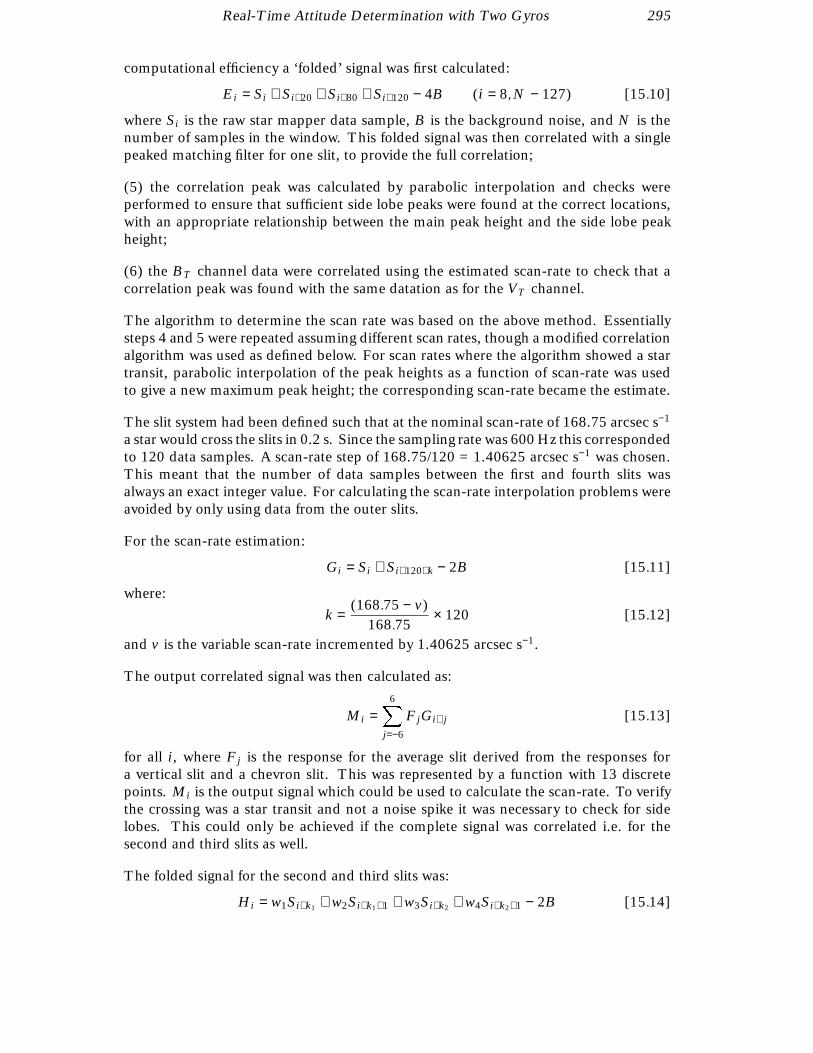
Real-Time Attitude Determination with Two Gyros 295
computational efficiency a ‘folded’ signal was first calculated:
Ei = Si + Si+20 + Si+80 + Si+120 − 4B (i = 8, N − 127) [15.10]
where Si is the raw star mapper data sample, B is the background noise, and N is thenumber of samples in the window. This folded signal was then correlated with a singlepeaked matching filter for one slit, to provide the full correlation;
(5) the correlation peak was calculated by parabolic interpolation and checks wereperformed to ensure that sufficient side lobe peaks were found at the correct locations,with an appropriate relationship between the main peak height and the side lobe peakheight;
(6) the BT channel data were correlated using the estimated scan-rate to check that acorrelation peak was found with the same datation as for the VT channel.
The algorithm to determine the scan rate was based on the above method. Essentiallysteps 4 and 5 were repeated assuming different scan rates, though a modified correlationalgorithm was used as defined below. For scan rates where the algorithm showed a startransit, parabolic interpolation of the peak heights as a function of scan-rate was usedto give a new maximum peak height; the corresponding scan-rate became the estimate.
The slit system had been defined such that at the nominal scan-rate of 168.75 arcsec s−1
a star would cross the slits in 0.2 s. Since the sampling rate was 600 Hz this correspondedto 120 data samples. A scan-rate step of 168.75/120 = 1.40625 arcsec s−1 was chosen.This meant that the number of data samples between the first and fourth slits wasalways an exact integer value. For calculating the scan-rate interpolation problems wereavoided by only using data from the outer slits.
For the scan-rate estimation:
Gi = Si + Si+120+k − 2B [15.11]
where:
k =(168.75 − v)
168.75× 120 [15.12]
and v is the variable scan-rate incremented by 1.40625 arcsec s−1.
The output correlated signal was then calculated as:
Mi =6X
j=−6
FjGi+ j [15.13]
for all i, where Fj is the response for the average slit derived from the responses fora vertical slit and a chevron slit. This was represented by a function with 13 discretepoints. Mi is the output signal which could be used to calculate the scan-rate. To verifythe crossing was a star transit and not a noise spike it was necessary to check for sidelobes. This could only be achieved if the complete signal was correlated i.e. for thesecond and third slits as well.
The folded signal for the second and third slits was:
Hi = w1Si+k1 + w2Si+k1+1 + w3Si+k2 + w4Si+k2+1 − 2B [15.14]

296 Real-Time Attitude Determination with Two Gyros
where wi are the weighting factors dependent on the scan rate being processed, calculatedusing linear interpolation. k1 and k2 are also scan-rate dependent centred around 20and 80 respectively. Then:
Ni =6X
j=−6
FjHi+ j [15.15]
and the sum Oi = Mi + Ni was checked for the requisite number of side lobes. Theheights of the side lobes were checked as before. The positions of the side lobes, whichare a function of velocity, were also checked.
The estimated scan-rate was updated if there was only one good transit in the datawindow. This avoided incorrect estimates due to transit coupling or interference betweenmain peaks and side lobes of the other peaks.
As presented above, the scan-rate should have been controllable within ±30 arcsec s−1
of the nominal 168.75 arcsec s−1. 51 trial scan-rates were processed by the algorithm.The accuracy of the scan-rate estimation required at this stage was of the order of0.5 arcsec s−1. This allowed the nominal scan-rate to be achieved with sufficient accu-racy.
Once a consistent estimate of the scan-rate had been achieved, the number of scan-ratesprocessed was reduced to 11. This gave a band of approximately 7 arcsec s−1 around thelatest estimate. This very significantly reduced the processing time required. More sidelobes were checked for than in the nominal telemetry pre-processing and star mapperfiltering to eliminate spurious harmonics.
Once 5–10 min of closely correlated scan-rate estimates had been achieved, the thrusteron time required to correct the scan-rate would be calculated. Before the scan-ratecorrection was sent, the number of scan rates processed would be increased to cover thenominal scan-rate case. The software would then automatically track the thruster firingand calculate new scan-rates for each transit received. Once the scan-rate had settleddown the number of scan-rates could be reduced back to 11.
When a scan-rate close to the nominal value had been reached the software had to cal-culate an accurate estimate of the full spacecraft attitude. The telemetry pre-processingand star mapper filtering task had now to calculate precisely the same information as forthe nominal mission. Thus for each transit an accurate estimate of the star transit timeover the virtual slit centre and the BT and VT magnitudes were required. Since tasksfurther down the chain process the z-gyroscope data this was now replaced by the scanrate estimate.
The BT and VT magnitudes were calculated using only data from the outer slits, and soavoided inaccuracies due to data interpolation.
Tests were performed at non-nominal scan-rates using the attitude and payload simulatorin ESOC, which was adapted for the purpose. Various scan-rates were used. Themaximum deviations from the nominal rate used were 30 arcsec s−1, corresponding tothe expected maximum error in correcting the scan-rate after perigee. Some results aresummarised in Table 15.1.
Scan-rates are measured in arcsec s−1. Over runs of typically an hour or more, startransits of varying brightness taken from the Hipparcos Input Catalogue, were simulatedat these different scan-rates. For each star, a rate estimate was produced. Their mean

Real-Time Attitude Determination with Two Gyros 297
Table 15.1. Results from on-ground simulations (see text).
Simulated Mean Error Standard Deviation
200.0 -0.14 0.30
168.75 -0.09 0.14
138.75 -0.13 0.27
and standard deviation were computed. As expected, the error in determining thecorrect scan rate grew as the scan rate moved further away from the nominal. However,the accuracy was still good enough even at highly irregular scan-rates to allow for therate to be corrected by direct thruster commanding.
For the later stages, with near-nominal scan-rates the on-ground Kalman filter wascapable of smoothing out irregularities in the rate estimates.
Ground Real-Time Attitude Determination
The remaining tasks in the ground real-time attitude determination chain (describedmore fully in Chapter 14) are now summarised. One new task was developed to supportthe ground real-time attitude determination: ‘star pattern offset matching’ which isdescribed below.
Slit distinction and gyro correction: The slit distinction algorithm remained unalteredfrom the nominal case. The gyro correction algorithm ‘corrected’ the transit times ofvertical slit crossings to remove the effects of spin-rate variation i.e. it produced a set ofpseudo vertical transit times as if the spacecraft had been spinning at a constant rate.Although the algorithm for gyro-correction remained unaltered for the non z-gyro casethe (less accurate) scan-rate estimations were used rather than the measured gyro rates;this had implications for the next task in the chain.
Star pattern monitoring: Star pattern monitoring used star pattern recognition to iden-tify each transit pair and determine the field of view of observation. The algorithmmapped the transit times to angles around a great circle. This mapping was less pre-cise when no gyro data was available for the transit time correction. Consequentlylarger tolerances were needed in the pattern recognition, which raised the probabilityof confusion or misidentification. An enhanced algorithm was implemented to improvethe performance of this task, both in the initialisation phase and during the normalreal-time execution. In addition, the user interface was re-worked to provide greaterflexibility in obtaining the initial star through parameter options and through improvedalphanumeric and graphical displays.
Fine attitude estimation: In the nominal ground real-time attitude determination, anine element state vector defining Tait-Bryan attitude error angles, body rates and gyrodrifts was used in a Kalman filter, receiving measurements from star mapper transittimes and the gyros rates at those transit times. Changes were necessary for the newversion to allow the star mapper scan-rate estimates to replace those from the z-gyro.Obviously, the estimation of the z-gyro drift was suppressed and the gyro misalignmentprojection matrix adjusted accordingly. The user interface was altered to allow thespacecraft operator to monitor closely the estimated scan-rate. In tests it was foundthat a misidentification could have serious impacts for the scan-rate estimate and henceafter parameter tuning, a much smoother scan-rate estimate was obtained, obviously at

298 Real-Time Attitude Determination with Two Gyros
the cost of sensitivity. Another significant enhancement was the inclusion of actuationon-times to improve ground body rate estimates.
Real-time attitude initialisation: This task provided an instantaneous estimate of theon-board real-time attitude determination state-vector which was valid at precisely thetime that the data were accepted on-board.
The real time attitude initialisation software was updated to calculate the values for thenew state vector implemented in the on-board real-time attitude determination for thenon z-gyro case.
For state vector initialisation:
(i) φn, θn and ψn the angular errors, were derived as the difference between theattitude as calculated by fine attitude estimation and the expected attitude fromthe nominal scanning law;
(ii) transverse gyro rates and drifts were calculated by fine attitude estimation;
(iii) ψd was derived as follows:
ψd = Ad cos 3Ωd t + Bd sin 3Ωd t [15.16]
where Ωd = 168.56 arcsec s−1 (the scan-rate including precession, Ad and Bd
were calculated by orbital oscillator routines (see below);
(iv) ψ2 was set to zero;
(v) then ψ1 = ψn − ψd ;
(vi) ψ was provided by fine attitude estimation (from the scan-rate estimate calculatedby telemetry pre-processing and star mapper filtering);
(vii) ψ2 was set to zero;
(viii) ψ was set to zero.
On-Board Torque Model Support
The ground software for computing orbital oscillator parameters refreshed the on-boardreal-time attitude determination orbital oscillator model, (cos Ωd t, sin Ωd t) at 15 minintervals (see Chapter 8). For the new on-board real-time attitude determination thedeterministic ψ model coefficients, Ad , Bd had also to be maintained. But:
ψd =Tz
Izzsin(3Ωd t + γz0) [15.17]
where Tz is the torque around the z-axis, Izz is the z inertia, and γz0 the phase of thetorque model about z. By double differentiation of the equation for ψd , expressions forAd and Bd were derived. Tz and γz0 were in any case calculated by the ground software.
Real-Time Attitude Determination with Two Gyros 299
Star Pattern Offset Matching
This program provided a more efficient way of determining the initial heliotropic angleΩ0 to within 0.1 accuracy. During three-gyro operations, this task was performed intwo steps (Chapter 14): field of view separation, and star pattern matching. These twotasks were performed off-line once sufficient star transits had been identified as a resultof star mapper filtering and slit distinction. Typically around 20 identified stars wererequired before a reliable star pattern match could be performed. The process involvedconsiderable manual intervention and a stable scan rate (taking approximately 30 min).Fortunately, during three-gyro operations, Ω0 remained constant except during rarecontingencies. Subsequently, this task was rarely required.
It was clear that, for two-gyro operations, changes of several degrees in Ω0 could beexpected after every perigee. It therefore became productive to look for ways to improvethe speed and reliability of this part of the ground procedure. This was achieved bytaking a more statistical approach to the determination of Ω0. The ground systemassumed knowledge of the spacecraft z-axis orientation (even if Ω0 was unknown).Consequently, matching of star mapper transits could be limited to a strip on the skyrather than the complete celestial sphere. The ‘star pattern offset matching’ algorithmwould make no a priori assumptions concerning the field of view in which a particularstar transit was seen; rather the algorithm would identify all stars around the sky-stripwith similar magnitude (in both BT and VT ) and calculate, for each candidate star,and for both fields of view, the value of Ω0 which would allow the specified star to beobserved in the specified field of view at the measured transit time.
In this way, all the measured star transits gave rise to several candidate values for Ω0.However when these were binned into small intervals (typically 1) and displayed as ahistogram, a clear peak around the true value was invariably apparent (unless the scanrate was not well controlled to the nominal value at the time).
The real-time ‘star pattern monitoring’ task was adapted to allow the input value of Ω0 tobe changed on-line. Consequently, the operator at the start of initialisation procedurescould attempt to establish a match with ‘star pattern monitoring’ based on the value ofΩ0 in the previous orbit. Simultaneously the same star data were being used off-line tobuild up a histogram of potential Ω0 values. Typically a trend was visible with as fewas 10 transits. Assuming the operator was unsuccessful in obtaining a good match fromthe previous value of Ω0, a new value could be used in real-time as soon as it becameapparent.
Additional Changes
Additional ground software changes to support the two-gyro real-time attitude determi-nation operations were:
(i) modifications to nominal scanning law routines to allow slow precession from sun-pointing to 43 maintaining real-time attitude determination convergence in the eventthat no other way could be found to recover from an emergency sun pointing manoeuvretaking place. This modification was never used operationally;
300 Real-Time Attitude Determination with Two Gyros
(ii) an additional command was developed to reset the deterministic z-axis error angleon-board. This allowed the inhibition of the z-axis precession around the 43 cone foruse during long losses of signal. This operation is described more fully below;
(iii) gyro configuration checking was suppressed in other gyro monitoring software;
(iv) programme star file observation covariance matrices used for the modulation strat-egy (see Chapter 8) were re-calculated for the extended mission;
(v) given that several attitude and orbit control system software patches were nowactive, a new facility was developed for the ground system to perform the selection andautomatic uplink of the software patches to the spacecraft. This was first used for thetwo-gyro patch and the decoupling of the z-thrusters.
15.5. Operational Experience
Parallel Tests During Three-Gyro Operations
The on-board software was designed to run in parallel with the nominal real-time at-titude determination software. It was implemented and had been initialised on severaloccasions, for performance testing, using the new ground real-time attitude determi-nation system. Figure 15.2 shows a graph of the nominal and new ψ Tait-Bryan errorangles over 40 min on 26 September 1991.
The nominal real-time attitude determination was converged throughout this period (asin all tests performed with the spacecraft). However, at the start of this graph, the newreal-time attitude determination was diverged. After 13 min, ground real-time attitudedetermination software had calculated and reset the new state vector to the correct value.For the remainder of this period, the two methods kept good agreement, even acrosstwo z-thruster firings (shown by the discontinuous changes in gradient).
It was also interesting to compare the performance of the individual components makingup the new ψ estimate over the same period. Figure 15.3 shows the values of ψ1 andψd . ψd is the sinusoidal curve. The effectiveness of the ψd model in describing thedisturbance torques in the apogee region was seen by the fact that the ψ1 term wasnearly linear between thruster firings. ψ2 remained much smaller throughout. In tests,the new real-time attitude determination was found to remain converged throughout theapogee region (i.e. for several hours). Like the nominal real-time attitude determination,it was however incapable of surviving the perigee region, below 6000 km, where thedisturbance torques were greatest.
It was necessary to close the shutters on the payload detectors, whenever the Earth orMoon crossed one of the fields of view. During these occultations, real-time attitudedetermination ran on gyro and thruster data alone. With three operational gyros, thispresented no problems. However, without a z-gyro, z-thruster on-times affected therate estimates after a firing. Figure 15.4 shows one such firing taking place during anoccultation with a subsequent divergence of the new real-time attitude determinationfrom the nominal.
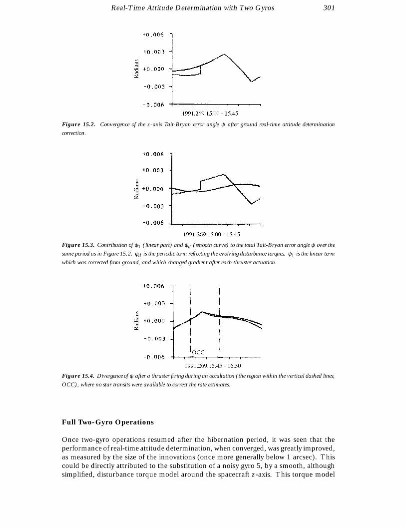
Real-Time Attitude Determination with Two Gyros 301
Figure 15.2. Convergence of the z-axis Tait-Bryan error angle ψ after ground real-time attitude determination
correction.
Figure 15.3. Contribution of ψ1 (linear part) and ψd (smooth curve) to the total Tait-Bryan error angle ψ over the
same period as in Figure 15.2. ψd is the periodic term reflecting the evolving disturbance torques. ψ1 is the linear term
which was corrected from ground, and which changed gradient after each thruster actuation.
Figure 15.4. Divergence of ψ after a thruster firing during an occultation (the region within the vertical dashed lines,
OCC), where no star transits were available to correct the rate estimates.
Full Two-Gyro Operations
Once two-gyro operations resumed after the hibernation period, it was seen that theperformance of real-time attitude determination, when converged, was greatly improved,as measured by the size of the innovations (once more generally below 1 arcsec). Thiscould be directly attributed to the substitution of a noisy gyro 5, by a smooth, althoughsimplified, disturbance torque model around the spacecraft z-axis. This torque model

302 Real-Time Attitude Determination with Two Gyros
was designed specifically to model the radiation pressure torque at apogee. As a result,real-time attitude determination performance would deteriorate as the altitude of thespacecraft dropped near perigee due to the increase in size in un-modelled torquesand high star mapper background noise. During perigee, there was no possibility thatreal-time attitude determination would remain converged due to a total absence ofinformation about orientation around the z-axis: no gyro, a blind star mapper andan uncalibrated disturbance torque model. It was expected that the spacecraft wouldspin-down or spin-up through perigee by as much as 30 arcsec s−1 every orbit.
Hibernation studies had suggested that it might be possible to partially predict in anempirical manner the likely amount of spin-up/down. In practice, this proved to beineffective. Initially, much higher changes in spin rate were seen (50 − 60 arcsec s−1).This was traced in part to futile attempts by the on-board normal mode control soft-ware to take erroneous real-time attitude determination output and fire the z-thrusters,sometimes exacerbating the change in spin rate. A procedure was put in place, involvingresetting various real-time attitude determination variables on-board which completelydisabled the z-thruster around perigee. This decreased the size of the spin-rate changes,as well as saving gas. However, predictions still proved unreliable and manual com-pensation through perigee for possible spin rate changes was abandoned. Correction ofthe spin rate was earlier made easy by the use of gyro 4. Although too unreliable foruse with real-time attitude determination, the deteriorated gyro output could be usedwhen telemetry was re-acquired after perigee, while the star mapper was still blindedand unusable by the ground software.
On 22 December 1992, gyro 4 failed completely, thereby making it necessary to runground real-time attitude determination to obtain spin-rate estimates based on the fourpeak separation of a star mapper transit. Although the on-ground star mapper filterwas capable of determining the scan rate over a wide range of potential values, it wasinefficient in the high noise regions of van Allen belts. Moreover, occasional deviationsfrom the nominal scan rate of up to 50 arcsec s−1 were still apparent making an initialestimate very difficult. Extra facilities were quickly added to allow a graphical display ofparticularly bright star mapper transits. This allowed a crude visual estimate of the scanrate to be obtained, even in high noise, so that scan rate corrections could be achievedas quickly as possible after perigee.
At the start of two-gyro operations, some difficulty was found in initialising the on-board real-time attitude determination system from ground. The errors in the on-ground attitude determination, particularly in the rate estimation around the z-axis,were higher than for three-gyro operations. Given that the delay of between 30 and60 s from the time of last good star observation to the execution time of the on-boardinitialisation command, errors were building in the on-ground extrapolation of the on-board state vector. The result was that the attitude was sufficiently accurate to be withinthe 30 arcsec innovation threshold on-board, but produced a large initial innovationbefore bringing the on-board estimate within the narrow threshold range of 10 arcsec.This innovation was also used, to update the transverse gyro drifts (see Equation 15.8)when in fact the drifts were reasonably stable over the short period of the initialisation.The now erroneous drift values subsequently led to erratic convergence of the on-board system or even divergence again. Work continued to improve the accuracy ofthe ground software. However an additional measure was taken by devising a secondset of fixed gains for use on-board. This set was used during initialisation proceduresand contained much smaller gains for updating the gyro drifts. The first gain setsproduced for the two-gyro operations had assumed gyro drift gains 100 times higher

Real-Time Attitude Determination with Two Gyros 303
than those used during three-gyro operations. Values closer to the previous sets usedin three-gyro operations were re-adopted for the new ‘extended window’ set. Thesesafeguarded the gyro drifts during initial convergence. Once convergence was achievedand the innovation threshold was set to narrow range, a more sensitive set of gains wasimplemented on-board to produce smoother performance of the attitude determinationduring science data collection.
Further tuning of the gains was carried out as the performance of the remaining gyrosworsened to lessen the effects of erratic drifts diverging the on-board system. In additioncalibration studies by ESOC and the Royal Greenwich Observatory (RGO) resulted inmore accurate z-thruster performance figures being used on-board.
After 1 November 1992, it was necessary to make occasional changes to the initialprecession angle defining the z-axis position on the 43 cone around the sun vector.This was to safeguard the spacecraft through long losses of signal (more than 5 hoursaround perigee). During a long loss of signal, the nominal scanning law precessionrate was set to zero. Without this, a spin-up/down of the spacecraft through perigeecould have resulted in a large change to the initial heliotropic angle, which defined theorientation of the spacecraft x and y axes. In the worst case, the initial heliotropic anglecould have changed by up to 90. In this case the last orbital oscillator command sentbefore loss of signal would have driven the z-axis perpendicular to the nominal scanninglaw. Left without correction over a typical lost pass, (12 hour loss of signal), the z-axiscould drift in solar aspect angle by more than 3 and would consequently have comedangerously close to triggering an emergency sun reacquisition order.
Figure 14.15, showing the overall science data return, clearly indicates that significantlyless data were collected per orbit. Overall ‘good’ data were returned 37 per cent ofthe total time, or 51 per cent of the covered time. There were three main reasons forthis: (1) the real-time attitude determination initialisation procedure was required everyorbit; (2) despite the improvement made during the hibernation period, the initialisationprocedure was still lengthier than during three-gyro operations; (3) real-time attitudedetermination divergence after occultations was rather frequent (over 50 per cent of thetime), usually occurring over the longer ones where a thruster firing took place in themiddle.
Occultations occurred in seasons: sometimes only at perigee, thereby securing unin-terrupted coverage for most of the orbit; sometimes occurring in pairs every revolutionof the spacecraft, making data return exceptionally poor. Analysis was performed bythe NDAC Consortium and ESOC into the possibility of slewing the spacecraft aroundthe 43 nominal scanning law cone to avoid occultations, but it was concluded that thiswould be detrimental to the overall observation programme.
Software changes were made to improve the performance of the ground real-time at-titude determination software immediately after occultations in an effort to reduce thetime to re-initialise real-time attitude determination. Steps were also taken to under-stand the disturbance torques and thruster performance better in the hope of improvingthe probability of real-time attitude determination survival through occultations. Suchimprovements were still on-going when further gyro failures necessitated the use of thezero-gyro real-time attitude determination system.

304

16. REAL-TIME ATTITUDE DETERMINATIONWITH ZERO GYROS
In response to the continuing deterioration of all gyros, the zero-gyro oper-ations and software were developed, in principle allowing the real-time atti-tude control to function with perturbing torque models in place of the gyrodata. Catastrophic failure of the telecommunications subsystem terminatedthe mission before this mode was used. The procedures used to handle thesecontingencies are nevertheless described.
16.1. Activities during Suspended Operations
On 18 March 1993, the total failure of gyro 2 prompted an emergency sun reacqui-sition and a spin-up to 0.25 rpm of the spacecraft. This state was maintained until11 June 1993, when attempts began to operate under the zero-gyro real-time attitudedetermination control. There were two principal reasons for the delay:
(1) the software for on-board and on-ground real-time attitude determination withoutgyros was still under development. However, operations resumed when sufficient (if notoptimised) ground software was in place for support;
(2) there were concerns that solar panel degradation was too great to allow the spacecraftto be fully operated during the long eclipse season (ending on 21 May 1993). In practice,the degradation was less than that predicted.
The return to full operations was further hampered on 5 and 6 May 1993 by thediscovery that both star mappers were partially damaged (no output on the BT channelof star mapper 1 and the VT channel of star mapper 2). The only operational solutionwas to use two different telemetry formats. The first (prepared on-ground and loadedon-board) combined both star mapper outputs but at the cost of the image dissector tubedata. This format was required for use in the ground real-time attitude determinationsystem to perform initial star pattern recognition. The second (available on-board) wascombining star mapper 2 and image dissector tube 2 data for use once real-time attitudedetermination convergence was achieved and good science had to be collected. Becausethe ground software had to work with both formats, a further re-design was necessary.

306 Real-Time Attitude Determination with Zero Gyros
Event History during Suspended Operations
The progressive failures occurring during the last months of attempted operations wereattributed to radiation damage of the associated electronics. A summary of the problemsencountered during the period in which zero-gyro operations were attempted is givenhereafter, with further details of the various anomalies given in Appendix B.
93-03-18: Gyro 2 failure (Anomaly 77): the on-board system automatically triggeredan emergency sun reacquisition.
93-03-19: The spacecraft was spun-up to 0.25 rpm and the gyros switched off to savepower. Nutation damping was then performed.
93-03-23: The decision was taken to suspend spacecraft operations. The payload wasswitched off, with the thermal control electronics branch 2 left on.
93-03-24: Thermal control electronics 2 was configured to wide range.
93-03-28: The nominal antenna switching command failed (Anomaly 78).
93-03-30: All thermal control electronics 2 heaters were set to fixed power with valuezero, i.e. switched off, due to power constraints.
93-04-01: Both antenna switching commands failed.
93-04-05: Commands 62 and 65 were used to switch antennas.
93-04-23: Due to the orbital rotation of the Earth around the Sun, the solar aspect angleof the spin axis had been steadily increasing at approximately 1/day. Power efficiencyof the solar panels was highest near the nominal 43 solar aspect angle. This promptedthe design and implementation of a series of manoeuvres to reduce the solar aspectangle, which was already larger than 43, without de-spinning the satellite. This wasperformed by direct thruster commanding, using the sun acquisition sensor as guidance.Nutation damping was also performed at this time.
93-04-27: The increased efficiency of the panels at 43 combined with the decreasingeclipse durations, allowed the payload thermal control electronics 1 and 2 to be switchedon and tested. Consequently, the thermal control electronics 2 heaters were set to fixedpower value 15.
93-05-04: The payload was switched on. A preliminary check showed that the imagedissector tubes were undamaged by the suspended operations.
93-05-05: Star mapper 2 VT channel had ceased to function (Anomaly 79).
93-05-06: Star mapper 1 BT channel had ceased to function (Anomaly 79).
93-05-10: Further manoeuvres were performed to reduced the solar aspect angle andperform nutation damping.
93-05-11: The control law electronics branch A failed (Anomaly 80). The switch to theredundant branch B was made.
93-05-12: A new telemetry was introduced (format 4) combining the star mapper 1 andstar mapper 2 telemetry.

Real-Time Attitude Determination with Zero Gyros 307
93-05-13: Further manoeuvres were performed to reduced the solar aspect angle andperform nutation damping.
93-05-14: The battery discharge regulator 1 module 2 overvoltage status changed.
93-05-17: Further manoeuvres were performed to reduced the solar aspect angle andperform nutation damping.
93-05-24: The eclipse season ended. Gyros 1 and 4 were switched on to increase thegyro electronics box temperature. No usable output was obtained.
93-05-25: Further manoeuvres were performed to reduced the solar aspect angle andperform nutation damping. Gyros 2 and 5 were switched on to increase the gyroelectronics box temperature. No usable output was obtained.
93-05-26: Gyro 3 was switched on but within a few hours was showing very high noise(Anomaly 81). The gyro was declared unusable and switched off.
93-05-27: The zero-gyro real-time attitude determination software patch was loadedon-board.
93-06-02: Further manoeuvres were performed to reduced the solar aspect angle andperform nutation damping. The new sun acquisition manoeuvre 4 software patch wasloaded on-board.
93-06-04: Further tests were performed with gyros 1, 3 and 5.
93-06-05: The inertial reference unit was completely switch-off.
93-06-06: The attitude control software crashed when the new sun acquisition ma-noeuvre 4 software was enabled. The problem was traced to an invalid checksum andcorrected.
93-06-09: Further manoeuvres were performed to reduced the solar aspect angle andperform nutation damping.
93-06-11: Prior to the resumption of scientific operations, the spacecraft was de-spunfrom 0.25 rpm to 0.15 rpm.
93-06-12: The spacecraft was further de-spun to 0.05 rpm, and an emergency sunreacquisition was commanded from ground to bring the spacecraft to the safe sun-pointing mode. Operations with the zero-gyro real-time attitude determination systembegan.
16.2. On-Board Software
Zero-gyro Real-Time Attitude Determination
A full description of the design concepts of real-time attitude determination was givenin Chapter 14. Although the basic concepts of filtering were the same in three-, two-and zero-gyro systems (see Figure 14.2), the zero-gyro real-time attitude determinationsystem constituted a complete re-design of the on-board real-time attitude determina-tion.

308 Real-Time Attitude Determination with Zero Gyros
The body rates derived from gyro measurements were replaced on all three axes byangular accelerations which were integrated using discretised perturbation equations on-board. The result of these calculations was an on-board attitude state vector containingTait-Bryan attitude error angles and body rate estimates which were corrected usingKalman filter techniques by the star mapper measurements. Further parameters wereintroduced to account for thruster misalignments and differences in performance.
As with the two-gyro system, the design had to take into account the limited memoryspace for the on-board software.
A critical new component of the system was an on-board acceleration model for allthree spacecraft axes. Although the two-gyro system could work with a sinusoidal on-board disturbance torque model (see Chapter 15), the disturbance torques around thex and y axes were far from sinusoidal. The most accurate solution possible was tocompute the predicted angular accelerations arising from external disturbance torquesby using empirical tables of points spanning on average two hours and refreshed byground command (two hours was the maximum allowable given the memory spaceand the resolution of points required). Each table was capable of being refreshedin two halves thereby avoiding discontinuities when the tables were reset. The on-board angular acceleration tables were computed on-ground from predicted disturbancetorques, calibrated from the most recent history of the attitude.
The following revised state vector had to be initialised using the modified ground real-time attitude determination system:
– φ: Tait-Bryan error angle around the spacecraft x-axis
– θ: Tait-Bryan error angle around the spacecraft y-axis
– ψ : Tait-Bryan error angle around the spacecraft z-axis
– φ: error rate around the spacecraft x-axis
– θ: error rate around the spacecraft y-axis
– ψ : error rate around the spacecraft z-axis
– γx: angular acceleration around the spacecraft x-axis
– γ y: angular acceleration around the spacecraft y-axis
– γz: angular acceleration around the spacecraft z-axis
Each component of the state vector v was broken down into a predicted (determinis-tic) component vd taking the spacecraft dynamics into account, and the other was acorrective term v1 taking into account uncertainties in the modelling:
(a) nominal scanning law rates ωX , ωY , ωZ were computed as for the three-gyro real-time attitude determination (see Equation 8.14);
(b) the deterministic components of the angular accelerations (γd ,x, γd ,y, γd ,z) werederived from the on-board acceleration tables, via quadratic interpolation based onthe neighbouring points at the time of computation;
(c) the other deterministic components of the state vector, namely the Tait-Bryan errorangles (φd , θd , ψd ) and error rates (φd , θd , ψd ) were propagated forward from timetk to time tk+1. Defining the time step ti = 16/15 s, then the propagation equationswere:

Real-Time Attitude Determination with Zero Gyros 309
0BBBBB@
φd (k + 1)
θd (k + 1)
ψd (k + 1)
φd (k + 1)
θd (k + 1)
ψd (k + 1)
1CCCCCA
=
0BBBBB@
1 ωZ ti 0 ti (1 + Γ1)ωZ t2i /2 0
−ωZ ti 1 0 −(1 + Γ1)ωZ t2i /2 ti 0
0 0 1 0 0 ti0 0 0 1 Γ1 ωZ ti 0
0 0 0 Γ2 ωZ ti 1 0
0 0 0 0 0 1
1CCCCCA
0BBBBB@
φd (k)
θd (k)
ψd (k)
φd (k)
θd (k)
ψd (k)
1CCCCCA
+
0BBBBB@
γd ,x t2i /2 − ωX tiγd ,y t2i /2 − ωY ti
γd ,z t2i /2
γd ,x tiγd ,y tiγd ,z ti
1CCCCCA
[16.1]
(d) the correction components of the state vector, namely the Tait-Bryan error angles(φ1, θ1, ψ1), error rates (φ1, θ1, ψ1) and angular accelerations γ1,x, γ1,y, γ1,z werepropagated forward in a similar manner to above:
0BBBBBBBBBBB@
φ1(k + 1)
θ1(k + 1)
ψ1(k + 1)
φ1(k + 1)
θ1(k + 1)
ψ1(k + 1)
γ1,x(k + 1)
γ1,y(k + 1)
γ1,z(k + 1)
1CCCCCCCCCCCA
= [16.2]
0BBBBBBBBBBB@
1 ωZ ti 0 ti (1 + Γ1)ωZ t2i /2 0 t2i /2 0 0
−ωZ ti 1 0 −(1 + Γ1)ωZ t2i /2 ti 0 0 t2i /2 0
0 0 1 0 0 ti 0 0 t2i /2
0 0 0 1 Γ1 ωZ ti 0 ti Γ1ωZ t2i /2 0
0 0 0 −Γ2 ωZ ti 1 0 −Γ2 ωZ ti ti 0
0 0 0 0 0 1 0 0 ti0 0 0 0 0 0 1 0 0
0 0 0 0 0 0 0 1 0
0 0 0 0 0 0 0 0 1
1CCCCCCCCCCCA
0BBBBBBBBBBB@
φ1(k)
θ1(k)
ψ1(k)
φ1(k)
θ1(k)
ψ1(k)
γ1,x(k)
γ1,y(k)
γ1,z(k)
1CCCCCCCCCCCA
where:
Γ1 =I yy − Izz
Ixx
Γ2 =Ixx − Izz
I yy[16.3]
are ratios involving the principal spacecraft moments of inertia (Ixx, I yy, Izz);
(e) corrections for actuations are performed on the vector (φd , θd , ψd , φd , θd , ψd ) using:
φ0
d = φd + λx(Taxδtx + Tax ton,x)(1 − 12 (ton,x + δtx))
+ λxz(Tazδtz + Taz ton,z)(1 − 12 (ton,z + δtz))
θ0
d = θd + λ y(Tayδt y + Tay ton,y)(1 − 12 (ton,y + δt y))
+ λ yz(Tazδtz + Taz ton,z)(1 − 12 (ton,z + δtz ))

310 Real-Time Attitude Determination with Zero Gyros
ψ 0
d = ψd + λz(Tazδtz + Taz ton,z)(1 − 12 (ton,z + δtz)) [16.4]
φ0
d = φd + λx(Taxδtx + Tax ton,x) + λxz(Tazδtz + Taz ton,z)
θ0
d = θd + λ y(Tayδt y + Tay ton,y) + λ yz(Tazδtz + Taz ton,z)
ψ 0
d = ψd + λz(Tazδtz + Taz ton,z)
where:
– Tax, Tay, Taz are the calibrated accelerations of the +x, + y, and +z thrustersrespectively;
– λx, λ y, λz are set to 1 if the actuation is on a positive thruster. If the actuationoccurs on the negative thruster, λ = Ta(−) /Ta(+) (the ratio of the negativethruster to the positive thruster);
– λxy, λ yz are corrective coupling terms;
– δtx, δt y , δtz are thruster time offsets which are independent of the length of anyactuation;
– ton,x, ton,y, ton,z are the computed thruster on-times;
(f) the new updated Tait-Bryan error angles and error rates combined the deterministicand corrective terms:
φ(k + 1) = φd (k + 1) + φ1(k + 1)
θ(k + 1) = θd (k + 1) + θ1(k + 1)
ψ (k + 1) = ψd (k + 1) + ψ1(k + 1)
φ(k + 1) =(φ(k + 1) − φ(k))
ti[16.5]
θ(k + 1) =(θ(k + 1) − θ(k))
ti
ψ (k + 1) =(ψ (k + 1) − ψ (k))
ti
(g) the measurement extrapolation and innovation computation were similar to thefilter used for three-gyro real-time attitude determination. However the state vector(φ, θ, ψ , φ, θ, ψ , γ1,x, γ1,y, γ1,z) was now updated using a (9 × 6) array of fixed gains(9 elements to the state vector and 6 different star mapper slits). As before, separategain sets were included for Quality 1 and Quality 2 stars;
(h) after update, the corrective terms had to be recalculated before the next cycle:
φ1 = φ − φd
θ1 = θ − θd [16.6]
ψ1 = ψ − ψd

Real-Time Attitude Determination with Zero Gyros 311
Sun Acquisition Sensor Controller
There was a need to maintain the spacecraft stability and achieve a certain operationalsafety with a zero-gyro system. The questions how to manoeuvre the spacecraft andhow to maintain the attitude of the spacecraft at any solar aspect angle still needed ananswer. Looking for alternative ways of operations, the spacecraft equipment used onlyfor launch and early orbit phase was examined and the sensing and measuring devicesstill operational in the spacecraft were scrutinised. Finally, using existing features, a wayto maintain and correct the measured angles with respect to the Sun was achieved usingthe sun acquisition sensor aligned with the z-axis. The resulting modification was calledthe sun acquisition sensor controller (modified sun acquisition manoeuvre 4).
The sun acquisition sensor was capable of sensing the direction of the Sun along twoperpendicular axes, provided that the solar aspect angle, (the angle between the Sunand the spacecraft z-axis) never exceeded approximately 70. Each of the two aspectangles output from the sun acquisition sensor formed a sine wave whose frequency andamplitude were a function of the spacecraft spin rate and of the solar aspect angle.The faster the spacecraft was spinning, the higher the frequency of the sine waves; thefurther the Sun was from the spacecraft z-axis, the bigger the amplitude. If the spacecraftcould have two reference sine waves representing together the nominal spin-rate and thenominal spacecraft angle with respect to the Sun, those references could be comparedwith the actual waves seen by the solar aspect angle. Then, if deviations induced byexternal factors could be corrected, the sun acquisition sensor and spin rate would bemaintained under control.
The new sine models were propagated using the same orbital oscillator coefficients thatcontrolled the precession of the z-axis around the 43 cone centred on the Sun. Also,the attitude and orbit control system supported an operational mode used for early orbitsun acquisition able to correct deviations in x and y axes by firing the relevant thrusters,with the property that it was triggered by error signals coming from the solar aspectangle. When combining both of the above, an alternative way to control the spacecraftattitude could be derived.
16.3. On-Ground Software
Ground Real-Time Attitude Determination
The major changes in the ground real-time attitude determination chain (describedmore fully in Chapter 14 and Chapter 15) are now summarised. One new task wasdeveloped to support the ground real-time attitude determination: ‘full sky matching’which is described below.
In order to perform initial star pattern recognition, it was necessary to have informationfrom both BT and VT channels to provide not only brightness but colour information.Without both, the range of candidate stars for each match would have been too large toachieve a successful match sufficiently quickly. Once a match was achieved however andthe on-board real-time attitude determination was successfully initialised, the knowledgeof which stars should be observable in the immediate future meant that the ground
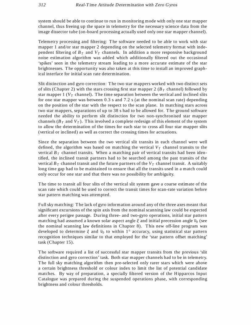
312 Real-Time Attitude Determination with Zero Gyros
system should be able to continue to run in monitoring mode with only one star mapperchannel, thus freeing up the space in telemetry for the necessary science data from theimage dissector tube (on-board processing actually used only one star mapper channel).
Telemetry processing and filtering: The software needed to be able to work with starmapper 1 and/or star mapper 2 depending on the selected telemetry format with inde-pendent filtering of BT and VT channels. In addition a more responsive backgroundnoise estimation algorithm was added which additionally filtered out the occasional‘spikes’ seen in the telemetry stream leading to a more accurate estimate of the starbrightnesses. The opportunity was also taken at this time to install an improved graph-ical interface for initial scan rate determination.
Slit distinction and gyro correction: The two star mappers worked with two distinct setsof slits (Chapter 2) with the stars crossing first star mapper 2 (BT channel) followed bystar mapper 1 (VT channel). The time separation between the vertical and inclined slitsfor one star mapper was between 0.3 s and 7.2 s (at the nominal scan rate) dependingon the position of the star with the respect to the scan plane. In matching stars acrosstwo star mappers, separations of up to 38 s had to be allowed for. The ground softwareneeded the ability to perform slit distinction for two non-synchronised star mapperchannels (BT and VT ). This involved a complete redesign of this element of the systemto allow the determination of the times for each star to cross all four star mapper slits(vertical or inclined) as well as correct the crossing times for actuations.
Since the separation between the two vertical slit transits in each channel were welldefined, the algorithm was based on matching the vertical VT channel transits to thevertical BT channel transits. When a matching pair of vertical transits had been iden-tified, the inclined transit partners had to be searched among the past transits of thevertical BT channel transit and the future partners of the VT channel transit. A suitablylong time gap had to be maintained to ensure that all the transits used in a match couldonly occur for one star and that there was no possibility for ambiguity.
The time to transit all four slits of the vertical slit system gave a coarse estimate of thescan rate which could be used to correct the transit times for scan-rate variation beforestar pattern matching was attempted.
Full sky matching: The lack of gyro information around any of the three axes meant thatsignificant excursions of the spin axis from the nominal scanning law could be expectedafter every perigee passage. During three- and two-gyro operations, initial star patternmatching had assumed a known solar aspect angle ξ and initial precession angle ν0 (seethe nominal scanning law definitions in Chapter 8). This new off-line program wasdeveloped to determine ξ and ν0 to within 1 accuracy, using statistical star patternrecognition techniques similar to that employed for the ‘star pattern offset matching’task (Chapter 15).
The software required a list of successful star mapper transits from the previous ‘slitdistinction and gyro correction’ task. Both star mapper channels had to be in telemetry.The full sky matching algorithm then pre-selected only rarer stars which were abovea certain brightness threshold or colour index to limit the list of potential candidatematches. By way of preparation, a specially filtered version of the Hipparcos InputCatalogue was prepared during the suspended operations phase, with correspondingbrightness and colour thresholds.

Real-Time Attitude Determination with Zero Gyros 313
The algorithm proceeded to match the reduced list of star transits against the filteredinput catalogue to produce, for each transit, a list of potential matching stars. Individualcandidates for different transits were then considered in a pairwise manner. If thecombination of transit times and angular separation were such that the star could havebeen observed at those times in one or other of the two fields of view, the cross productof the two star vectors (giving the spin axis orientation) was calculated and stored. Onceall possible combinations had been considered, the resulting cross product vectors werebinned in small areas (typically 2 × 2) of the celestial sphere and displayed graphicallyas a colour coded density map. A clear peak around the true spin axis orientation wasinvariably apparent.
The algorithm used for the two-gyro operations to determine the initial heliotropic angleΩ0 was incorporated into the new software. Once ξ and ν0 had been identified in thisway, the same transits could be used to determine Ω0. With this knowledge of the ‘bestfit’ nominal scanning law parameters to the current attitude, the real-time star patternmonitoring was able to be initialised.
Typically a good match was obtained with 10 to 15 rare transits, which took between 3and 5 minutes to collect, assuming that the spacecraft z-axis did not drift by more than3 in that period.
Star pattern monitoring: The original algorithm for star pattern matching was capableof working with one star mapper channel information or two by suitable changing ofon-line parameters. It was however fully expected that the number of ambiguities inmatching would rise when only one star mapper channel was available.
Fine attitude estimation: The on-ground Kalman filter was adapted to replace the gyroinformation by the same theoretical disturbance torque model as was used on-board.Additional thruster misalignments and calibration results were modelled in the attitudeand body rate prediction. It was possible to obtain a coarse estimate of the spacecraftbody rates by calculating the time for a star to transit all four slits of the vertical andinclined slit systems of one of the star mappers. The time to cross the vertical slits gavethe scan rate around the z-axis. The angular speed across the inclined slits, less the scanrate, gave a body rate about an axis perpendicular to the plane containing the z-axisand the star mapper field of view direction. These two measurements were input to theKalman filter.
Real-time initialisation: The final task was required to reset the new format on-boardstate vector. Previous versions of the task had performed automatic uplink of the statevector command as soon as a star transit had provided a recent update to the on-groundattitude estimate. This was to prevent accumulation of error due to extrapolation. Amanual override was now added to allow the operator to manually command within afew seconds of receiving an on-ground update, after verifying its accuracy. The taskwas also capable of finding the best fitting nominal scanning law parameters before theprogramme star file was generated. This would minimise attitude corrections with asubsequent saving in fuel and time.
On-Ground Attitude Reconstitution
A very significant step was the inclusion of the NDAC Consortium’s on-ground attitudereconstitution software at ESOC for use in calibrating external disturbance torques andthruster performance. The experience of the Royal Greenwich Observatory (RGO) in

314 Real-Time Attitude Determination with Zero Gyros
calibrating the external torques and thruster throughout the mission provided consid-erable insight into the problems confronting the development of the zero-gyro systems.Studies with Matra showed that it was likely that the disturbance torques would re-quire calibration every orbit to provide accurate enough information for the on-boardacceleration tables.
The RGO collaborated closely with ESOC to establish a way of installing an adaptedversion of their system within the ground control system using an additional high perfor-mance work-station. They also provided test data for both the on-board and on-groundsystems, through the system.
Discrete Disturbance Torque Model
In addition to the off-line on-ground attitude reconstitution software described above, anew program was developed to uplink the commands necessary to refresh the on-boardacceleration tables at regular intervals, using input from on-ground attitude reconsti-tution results. This software had to note when one of the two tables had expired anduplink the next set of data while the other table was active. These tables were obviouslydependent on the nominal scanning law and could only be uplinked once the first coarseattitude estimates had been achieved on-ground.
Modified Sun Acquisition Sensor Support
The two new sine wave models for the sun acquisition sensor controller required to becalculated and refreshed once the current nominal scanning law parameters had beendefined. These coefficients were calculated off-line and uplinked by manual command.
Additional changes
The nominal focus monitoring task had used gyro derived rate information. Thisinformation was replaced by the telemetered real-time attitude determination errorrates.
The real-time telemetry and telecommanding chain underwent numerous changes forzero-gyro operations, including:
– additional routing of telemetry to the new workstation required for the ground real-time attitude determination and on-ground attitude reconstitution software andreceipt of commands;
– development of a telemetry template and format to allow the recovery of both starmapper streams;
– development of a filing system for the new workstation, keeping a local copy of allrequired telemetry. Details of on-board time and frame number were also stored;
– conversion of the data reduction consortia tape production software to produce diskformat output for transfer to the workstation. The data fed the on-ground attitudereconstitution software. This data reduction consortia tape software incorporatedflags for the solar aspect angle and the telemetry mode;
– modification of the uplink system to decompose all commands before transmission.

Real-Time Attitude Determination with Zero Gyros 315
16.4. Operational Experience
The spacecraft remained spinning at 0.25 rpm until 11 June 1993 when the on-groundsoftware was completed. An initial de-spin to 0.15 rpm was then performed with nu-tation damping. The next day the spacecraft was de-spun to 0.05 rpm and emergencysun reacquisition was triggered to bring the spacecraft to sun-pointing mode. Earlierfears that the power margin at sun-pointing would be so low that a quick manoeuvreto the nominal 43 solar aspect angle would be required, were unfounded. It wastherefore agreed to remain sun-pointing and to attempt to converge real-time attitudedetermination. The ground real-time attitude determination software worked as ex-pected and was able to perform star mapper filtering with the two semi-functioning starmappers. The attitude was subsequently determined and initialisation of real-time atti-tude determination on-board attempted. It was then found that the on-board softwarewas incapable of responding accurately to the frequent thruster firings caused by theinitialisation command, resulting in an unpredictable divergence after each command.
Within a few hours the ground software was modified to limit changes in the uplinkedon-board state vector in such a way as to reduce thruster on-times at the normal modeboundary. In the following days further modifications were made to the on-board andground real-time attitude determination software.
On-board real-time attitude determination: Convergence of real-time attitude deter-mination under simulations showed sensitivity to star mapper transit frequency. Someattempts were made to incorporate Tycho catalogue stars into the program star file atsparse areas. This was not tested with the spacecraft however. Having verified theperformance of the ground real-time attitude determination software in determiningbody rates, some changes to the on-board Kalman gain set were made to increase thesensitivity to innovations of the transverse body rates on-board. This helped by allowingthe real-time attitude determination to stay converged after initialisation from ground,making it possible to collect real-time attitude determination converged data every passfor further analysis. From this it was possible to correlate later divergences with firings,leading to the conclusion that a new thruster calibration was required. Insufficient datafor use with calibration software on-ground, was obtained before the end of the mission.
Ground real-time attitude determination: After real-time attitude determination opera-tions resumed, some significant changes were made when it was found that a less strictapproach to using three out of four sets of slit crossings still maintained star patternmonitoring and allowed more measurements for on-ground attitude convergence. Afurther modification was made which limited the commanded change to the on-boardstate vector to lie just outside the normal mode control bounds. In this way, convergenceof the on-board body rate estimates could be maintained. An additional command wasadded to allow only the on-board body rates to be initialised, while maintaining the oldattitude.
Short periods of converged real-time attitude determination were achieved, rangingfrom 15 minutes to 1 hour, over the next days in sun-pointing mode. The frequencywith which these periods of convergence could be achieved was steadily increasing, withthe further tuning and familiarisation with the new operations mode.
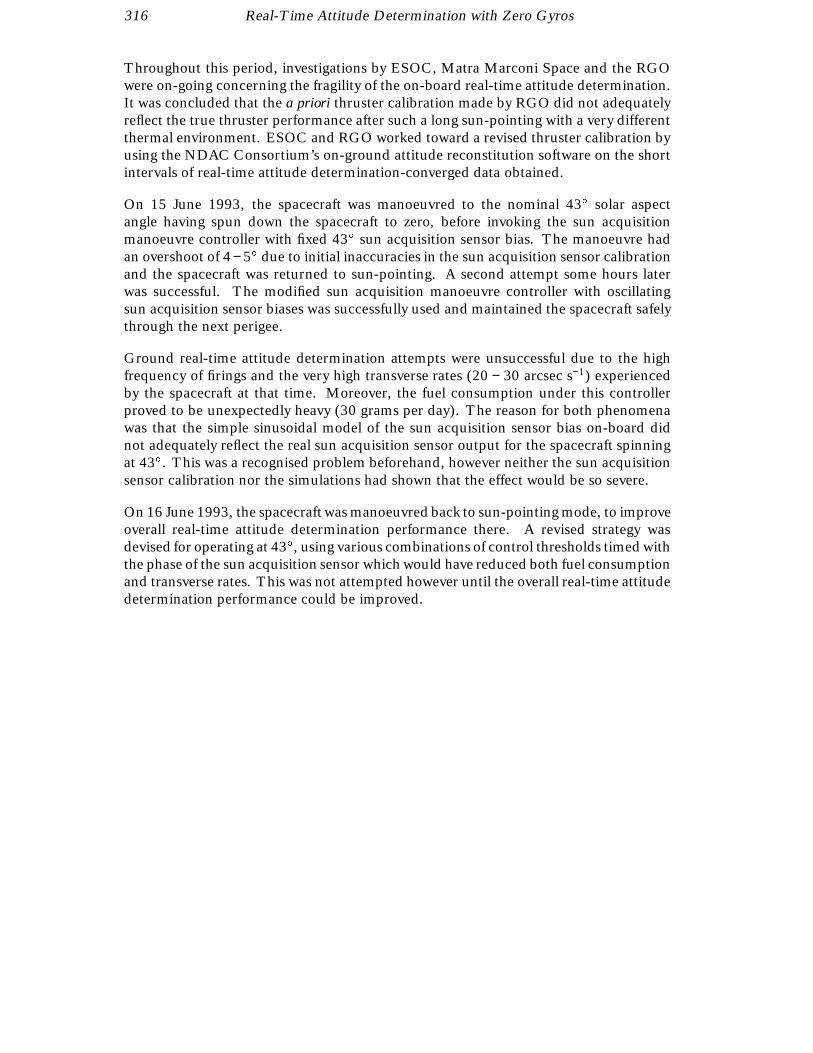
316 Real-Time Attitude Determination with Zero Gyros
Throughout this period, investigations by ESOC, Matra Marconi Space and the RGOwere on-going concerning the fragility of the on-board real-time attitude determination.It was concluded that the a priori thruster calibration made by RGO did not adequatelyreflect the true thruster performance after such a long sun-pointing with a very differentthermal environment. ESOC and RGO worked toward a revised thruster calibration byusing the NDAC Consortium’s on-ground attitude reconstitution software on the shortintervals of real-time attitude determination-converged data obtained.
On 15 June 1993, the spacecraft was manoeuvred to the nominal 43 solar aspectangle having spun down the spacecraft to zero, before invoking the sun acquisitionmanoeuvre controller with fixed 43 sun acquisition sensor bias. The manoeuvre hadan overshoot of 4− 5 due to initial inaccuracies in the sun acquisition sensor calibrationand the spacecraft was returned to sun-pointing. A second attempt some hours laterwas successful. The modified sun acquisition manoeuvre controller with oscillatingsun acquisition sensor biases was successfully used and maintained the spacecraft safelythrough the next perigee.
Ground real-time attitude determination attempts were unsuccessful due to the highfrequency of firings and the very high transverse rates (20 − 30 arcsec s−1) experiencedby the spacecraft at that time. Moreover, the fuel consumption under this controllerproved to be unexpectedly heavy (30 grams per day). The reason for both phenomenawas that the simple sinusoidal model of the sun acquisition sensor bias on-board didnot adequately reflect the real sun acquisition sensor output for the spacecraft spinningat 43. This was a recognised problem beforehand, however neither the sun acquisitionsensor calibration nor the simulations had shown that the effect would be so severe.
On 16 June 1993, the spacecraft was manoeuvred back to sun-pointing mode, to improveoverall real-time attitude determination performance there. A revised strategy wasdevised for operating at 43, using various combinations of control thresholds timed withthe phase of the sun acquisition sensor which would have reduced both fuel consumptionand transverse rates. This was not attempted however until the overall real-time attitudedetermination performance could be improved.
17. END OF MISSION ACTIVITIESAND CONCLUSIONS
Satellite operations were continued under increasingly difficult technical cir-cumstances, in the face of solar array and power degradation, gyroscope andthermal control failures, all attributable to the harsh radiation environment inwhich the Hipparcos satellite was destined to carry out its measurements. Nev-ertheless, operations were maintained for a total duration of four years, longerthan the nominal 2.5-year operational period intended before launch, andlong enough for all of the scientific mission goals to be significantly surpassed.Operations were terminated on 15 August 1993, after repeated attempts tocommunicate with the satellite on-board computer were finally abandoned.The end of the satellite operations was accompanied by a series of diagnostictests undertaken to establish the final performances of several of the spacecraftand payload subsystems. An assessment of the overall satellite reliability, thedata archiving policy, and some considerations of the mission in retrospect arepresented.
17.1. End-of-Life History
On 24 June 1993, the central on-board software halted. Subsequent attempts to reloadprime and redundant computers failed. Without the central on-board software, noscientific data could be obtained. Investigations indicated that the fault lay with a failedopto-coupler in the on-board computer. These components are radiation sensitive andmay have been the cause of the earlier demise of on-board computer 2. It was decidedto cool the spacecraft to improve the performance of the opto-couplers.
On 8 July 1993, on-board computer 1 accepted a run command and restarted. Overthe next few days, the entire central on-board software was reloaded, although the com-mand failure rate remained high. Once the central on-board software was reloadedand started, investigation began into reducing the high command rejection rate. Theproblem was traced to the checksum packet at the end of each command being cor-rupted. It was then possible to load some parameters by slightly modifying the values,thereby changing the checksum. The payload was re-heated to allow ground real-timeattitude determination to be performed and to attempt real-time attitude determinationinitialisation. This was partially successful with real-time attitude determination re-maining converged for one hour in one period. However, commanding was still failing

318 End of Mission Activities and Conclusions
frequently, making initialisation and maintenance of real-time attitude determinationconvergence impossible for most of the time.
It was realised that a central on-board software patch would be required to providerobust enough commanding for a reasonable science return. Before this possibilityhad been properly assessed, however, a further deterioration in the on-board computerbecame apparent, when the last checksum packets were rejected without exception,making any further commanding of that type impossible. A swap of central data unitswas performed, without improvement. This required that on-board computer 1 wouldhave to be restarted. This was not possible.
No solution was found to work around the failure of the two on-board computers,and the decision was taken by the ESA Project Manager and the ESOC SpacecraftOperations Manager to terminate operations. Before shut down, certain end-of-life testswere carried out, and subsequently the spacecraft was spun up to 10 rpm—there beinginsufficient fuel to de-orbit the satellite or to change the perigee height significantly. Atmission termination all end-of-life tests had been completed and the payload was turnedoff. The attitude and control system remained on, and the power and data handlingsub-systems were nominal. No fuel remained in one tank, while the other had 20 bars(0.75 kg of cold gas) remaining.
Operations of the Hipparcos satellite ceased on 15 August 1993 at 16:00 UTC, whenthe transmitter was switched off for the last time.
17.2. End-of-Life Tests
In the last two weeks of operations, the satellite was subject to a series of engineeringtests. These tests were used to assess the conditions of the various subsystems after thefour year period in the revised transfer orbit with its regular passages through the vanAllen belts. The tests involved many on-board re-configurations in order to verify unitswhich had never been used before, or units that had already failed in the past and hadbeen substituted by the back-up ones. All test were carried out via mode 3 memoryload commands since packet commands were not usable due to the on-board computerfailure.
The following sections describe the tests that were carried out, ordered by subsystem.Unless specifically noted otherwise, the tests carried out were terminated after the statednumber of cycles (rather than failing at that point).
Payload
Image Dissector Tube 1: the status of image dissector tube 1 was last verified on29 July 1993 using the internal star pattern assembly. Image dissector tube 1 was stillworking, but both the electronics and the high voltage power supply voltage readoutswere not correct, probably due to a faulty input multiplexer on the payload remoteterminal unit.
Image Dissector Tube 1 Chromaticity Filter: the image dissector tube 1 chromaticityfilter underwent a destructive test starting on 12 August 1993. It was commanded to thecalibration position and then to the wide band again (using a purpose built command

End of Mission Activities and Conclusions 319
sequence) for 288 cycles without any problem. The sequence contained the memoryload, reset, and execute commands spaced to allow the verification of each, and theverification of the filter position via the telemetry.
Image Dissector Tube 1 Shutter: the image dissector tube 1 shutter underwent a de-structive test starting on 10 August 1993. It was commanded open and then closedagain (using a purpose built command sequence) for 244 cycles without any problem.The sequence contained the memory load, the reset, and the execute commands spacedto allow the verification of each, and the verification of the status of the shutter via thetelemetry.
Image Dissector Tube 2 Shutter: the image dissector tube 2 shutter underwent a de-structive test starting on 4 August 1993. The shutter was commanded open and thenclosed again (using a purpose-built command sequence) for 60 cycles before the teleme-try readout stopped updating. Then, the internal star pattern assembly light sourceswere turned on to verify the position of the shutter. The sequence contained the mem-ory load, the reset, and the execute commands spaced to allow the verification of each,and the verification of the status of the shutter via the telemetry.
Internal Star Pattern Assembly: the internal star pattern assembly lights underwent adestructive test starting on 13 August 1993. The switching mirror was moved towardimage dissector tube 1 thus allowing image dissector tube 2 to detect the light; then theinternal star pattern assembly lights were switched on and off again (using a purposebuilt command sequence) for 720 cycles without any problem. The commands wereverified via the light’s associated telemetry parameter and via the image dissector tuberaw output.
Electro-Magnetic Torquer: the status of the mechanism drive electronics 2 electro-magnetic torquer was last verified on 13 August 1993. The test showed that, apartfrom the star mapper 2 shutter which went to an intermediate position, none of themechanisms actually worked.
Mechanism Drive Electronics: the status of the mechanism drive electronics 1 and 2were last verified on 13 August 1993. The test confirmed that the units were still inworking condition, although the secondary voltage of mechanism drive electronics 1had dropped to 1.44 V instead of the 1.88 V registered at the time of its first anomaly.
Refocusing Mechanism: the functioning of the refocusing mechanism was last testedon 11 August 1993. The results of this test confirmed the correct functioning of therefocusing mechanism, but they showed a discrepancy in the maximum and minimumlimits reachable by the grid as the calibration curve indicated a minimum of 20 per centand a maximum of 80 per cent of the allowed range which were not achieved.
Thermal Control Electronics: the status of the thermal control electronics 1 was lastverified on 6 August 1993. The results of this test were in line with the previous testsconducted on thermal control electronics 1, and they confirmed that the unit was notworking. The status of the thermal control electronics 2 was last verified on 29 July 1993for each of the 21 actively controlled areas. Of the 24 controlled areas (21 with connectedheaters and 3 spare with no heaters) only 4 still functioned.
Star Mapper 2 Shutter: the star mapper 2 shutter underwent a destructive test startingon 14 August 1993. The shutter was commanded open and then closed again (using apurpose built command sequence) for 160 cycles without any problem. The sequence

320 End of Mission Activities and Conclusions
contained the memory load, the reset, and the execute commands spaced to allow theverification of each, and the verification of the status of the shutter via the telemetry.
Radio Frequency
Transmitter 2: the status of transmitter 2 was last verified on 14 August 1993. Theresults of this test indicated that transmitter 2 was working without any problem, butit also showed a lower on-board automatic gain control reading for receiver 2. Thissituation did not appear to hinder the commanding function of the satellite, and it hadalready been observed in the past during ground station checks.
Solar Arrays
Solar Panel Degradation Test: the degradation level of the solar arrays was last verifiedon 10 August 1993 using the open circuit test. The results of this test indicated thatthere was no major change in the performance of the solar arrays since the previous testshad been conducted.
Solar Panel Shadowing Test: the solar panel shadowing test was carried out on 12 Au-gust 1993, using the modified sun acquisition manoeuvre phase 4 controller. Usingthe modified sun acquisition manoeuvre phase 4 control loop, the spacecraft was firstmoved to 55 where its status was checked out; using the same method, the satellite wasthen moved to 65 where the charge current started to drop, but no discharge was ob-served. The satellite was finally moved to about 75 where the charge current droppedcompletely, and the batteries started to discharge. Once the desired solar aspect anglehad been reached, the attitude control software was configured to standby mode 2, andthe spacecraft was spun up to about 500 arcsec s−1. Shortly afterwards, sun acquisitionsensor 3 entered its shadow area, and the spacecraft started to drift while it was trying tore-acquire the Sun; from the output of both sun acquisition sensor 1 and sun acquisitionsensor 2 it was seen that the satellite completed a revolution around the x axis. As soonas sun acquisition sensor 3 re-acquired the Sun, an emergency sun reacquisition wasinitiated from ground, and the satellite was brought back to the Sun. At the end of thetest, no noticeable difference was seen in the behaviour of the solar arrays.
Attitude and Orbit Control System
Accelerometer Package and Earth/Sun Sensor: the Earth/Sun sensor 2 and the ac-celerometer package B, were last tested during the spin-up manoeuvre carried outbetween 13 and 14 August 1993. The results of this test showed that the units werestill working, although it was not possible to fully test the Earth/Sun sensor due to thesatellite’s sun-pointing position and spin rate.
Control Processing Electronic Cross Strap Configuration: the two control law electron-ics systems were last tested in a cross-strapped configuration on 12 August 1993. Theresults of this test verified the feasibility of this unorthodox configuration.
Gyro Oversampling: the gyros outputs were last tested, using the 10 Hz oversamplingsystem (format 3), on 4 and 5 August 1993; the data samples related to the testswere forwarded to ESTEC, Matra Marconi Space and the ‘Laboratoire de RecherchesBalistiques et Aerodynamiques’ for further analysis.

End of Mission Activities and Conclusions 321
Gyro Heaters: the status of the gyro heaters was verified in two parts on 27 July and5 August 1993, due to the gyro mechanism electronics temperature problem. Theresults of this test confirmed the correct functioning of the heaters of gyros 1, 2, 4 and 5and the failure in the heater of gyro 3.
Latching Valve: the status of the latching valve A1 was last verified on 29 July. Theresults of this test confirmed the correct functioning of the latching valve.
Spin-up Manoeuvre: the spacecraft was spun-up to its final rotation speed of 10 rpmin several steps starting on 13 August 1993, via direct thruster firing commands. As afirst step, the satellite was moved 8 away from the sun-pointing position using the sunacquisition manoeuvre phase 4 controller and direct thruster firing commands on the−x axis. Once the rates had abated to an acceptable level, the first +z direct thrusterfiring command was sent bringing the spin rate to 0.25 rpm; this first manoeuvre alsointroduced a nutation of about 9 half-cone which had to be reduced before progressingany further.
After the nutation had been successfully reduced to less than 1 half-cone, a secondstep was started bringing the spin rate to 1 rpm. A third step brought the satellite to3.02 rpm, and was immediately followed by another step which should have broughtthe satellite to a spin rate of about 5 rpm. During this period, in order to preparefor a different test, a series of attitude and orbit control system re-configurations werecarried out; unfortunately, one of them caused the manoeuvre to abort prematurely (theattitude and orbit control system telemetry format was changed from high rate to lowrate). Once the re-configuration was completed the spin-up was resumed with a fifthstep which brought the rotation rate from 3.75 to 5.1 rpm.
Two more steps were carried out, bringing the spin rate to 9.07 rpm. On 14 August,a spin-down was performed to introduce nutation around the z-axis in order to verifythe accelerometer package; during this manoeuvre, tank B was emptied, and had to beswapped for tank A. The de-spin was manually stopped at about 8.52 rpm as there waslittle or no effect on the nutation amplitude. The last step of the spin-up manoeuvre,was then carried out bringing the spin rate to its final value of 10.04 rpm and leavingabout 21 bars in tank A.
Data Handling Subsystem
Central Decoding Unit: the status of central decoding unit 2 was last verified on23 and 24 July 1993. The result of the test indicated that there was a problem withthe commanding chain of central decoding unit 2 (mode 3 commands), thus making itcompletely unusable.
Memory Bank Module: the status of memory bank module 3 was last verified on23 and 24 July 1993. The results of these tests indicated that memory bank module 3was working correctly.
Spacecraft Remote Terminal Unit 2: the status of spacecraft remote terminal unit 2 waslast verified on 14 August 1993. The results of this test indicated that spacecraft remoteterminal unit 2 worked without any problem.

322 End of Mission Activities and Conclusions
17.3. Satellite Reliability Assessment
A summary study of the reliability of the Hipparcos satellite during its three years ofoperation in geostationary transfer orbit compared to the expected reliability after threeyears in the nominal geostationary orbit was undertaken by Matra Marconi Space. Thefollowing hypotheses were assumed for the study: (a) the computed anomalies referredto satellite anomalies only, with ground-segment anomalies not taken into account, and(b) the satellite was considered to be one instrument, rather than an association ofdifferent subsystems each with their own reliability.
Figure 17.1 represents the evolution of the reliability of the satellite versus time ingeostationary orbit (nominal mission), and the geostationary transfer orbit (revisedmission). Figure 17.2 represents the evolution of the failure rate versus time in geo-stationary transfer orbit (revised mission). It is apparent that the reliability decreasedquickly and remained very low after three years in geostationary transfer orbit (between0 and 0.2) compared to the expected reliability (around 0.6) for the nominal mission ingeostationary orbit. The failure rate continuously increased.
17.4. Data Archiving Policy
In accordance with the general data archiving policy at ESOC, the raw satellite data willbe archived for a period of 10 years. It is, however, considered most unlikely that accessto the raw satellite data at ESOC would again be needed. The data processing tasksundertaken by the data reduction teams were so lengthy, and so complex, that a repeatof the Hipparcos data analysis starting from the raw data will almost certainly neverbe embarked upon. Intermediate data archives generated by the data reduction teamswould be the natural starting point for further analysis, should this ever be consideredappropriate.
17.5. Miscellaneous Considerations
Design and Development of the Satellite
Concerning the relationship between the instrument design, manufacture and operationon the one hand, and the data analysis effort on the other, several features of theHipparcos mission implementation contributed to the mission’s success:
(i) acceptance of the mission within the ESA scientific programme was only undertakenafter a very thorough scientific and technical evaluation of the end-to-end system (up tothe final product) had been made;
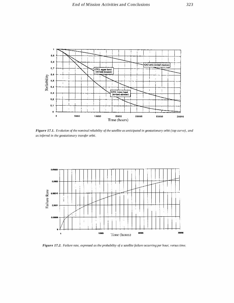
End of Mission Activities and Conclusions 323
Figure 17.1. Evolution of the nominal reliability of the satellite as anticipated in geostationary orbit (top curve), and
as inferred in the geostationary transfer orbit.
Figure 17.2. Failure rate, expressed as the probability of a satellite failure occurring per hour, versus time.
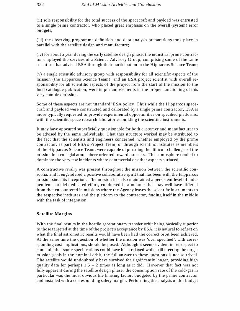
324 End of Mission Activities and Conclusions
(ii) sole responsibility for the total success of the spacecraft and payload was entrustedto a single prime contractor, who placed great emphasis on the overall (system) errorbudgets;
(iii) the observing programme definition and data analysis preparations took place inparallel with the satellite design and manufacture;
(iv) for about a year during the early satellite design phase, the industrial prime contrac-tor employed the services of a Science Advisory Group, comprising some of the samescientists that advised ESA through their participation in the Hipparcos Science Team;
(v) a single scientific advisory group with responsibility for all scientific aspects of themission (the Hipparcos Science Team), and an ESA project scientist with overall re-sponsibility for all scientific aspects of the project from the start of the mission to thefinal catalogue publication, were important elements in the proper functioning of thisvery complex mission.
Some of these aspects are not ‘standard’ ESA policy. Thus while the Hipparcos space-craft and payload were constructed and calibrated by a single prime contractor, ESA ismore typically requested to provide experimental opportunities on specified platforms,with the scientific space research laboratories building the scientific instruments.
It may have appeared superficially questionable for both customer and manufacturer tobe advised by the same individuals. That this structure worked may be attributed tothe fact that the scientists and engineers concerned, whether employed by the primecontractor, as part of ESA’s Project Team, or through scientific institutes as membersof the Hipparcos Science Team, were capable of pursuing the difficult challenges of themission in a collegial atmosphere oriented towards success. This atmosphere tended todominate the very few incidents where commercial or other aspects surfaced.
A constructive rivalry was present throughout the mission between the scientific con-sortia, and it engendered a positive collaborative spirit that has been with the Hipparcosmission since its inception. The mission has also maintained a persistent level of inde-pendent parallel dedicated effort, conducted in a manner that may well have differedfrom that encountered in missions where the Agency leaves the scientific instruments tothe respective institutes and the platform to the contractor, finding itself in the middlewith the task of integration.
Satellite Margins
With the final results in the hostile geostationary transfer orbit being basically superiorto those targeted at the time of the project’s acceptance by ESA, it is natural to reflect onwhat the final astrometric results would have been had the correct orbit been achieved.At the same time the question of whether the mission was ‘over specified’, with corre-sponding cost implications, should be posed. Although it seems evident in retrospect toconclude that some specifications could have been relaxed while still meeting the targetmission goals in the nominal orbit, the full answer to these questions is not so trivial.The satellite would undoubtedly have survived for significantly longer, providing highquality data for perhaps 1.5 – 2 times as long as it did. However that fact was notfully apparent during the satellite design phase: the consumption rate of the cold-gas inparticular was the most obvious life limiting factor, budgeted by the prime contractorand installed with a corresponding safety margin. Performing the analysis of this budget

End of Mission Activities and Conclusions 325
to the level required to make a significantly more precise cold-gas budget would verysoon surpass in cost the savings that might be made on cold-gas mass. In particular,improvements beyond the already very sophisticated attitude control strategy were notforeseen, and would have required an in-depth study of ideas like gyroless operations,before creative hopes could have been turned into reality.
There was actually one significant concern that was eliminated by the failure of theapogee motor: the contribution to the pre-launch error budget arising from a potentiallysignificant jitter source through the interior ‘bouncing’ of the remaining propellantflakes after burnout. Design efforts had been aimed at making the power spectrumof the jitter as weak as possible at the higher frequencies, and the apogee boost motorresiduals were the most significant remaining jitter concern. For the same reason thehot-gas (hydrazine) system for orbit manoeuvres was replaced by the cold gas for theoperational phase of the mission. The cold-gas thrusters were specifically designed forthe low thrusts required, again basically to minimise their impulsive character. Evennow it is not clear how much the apogee motor residuals would have affected themeasurements. Undoubtedly, the absence of the boost motor mass, and the presenceof the residuals, would also have affected the cold-gas consumption. The benefits of asmooth attitude motion, free from such residuals, had been anticipated, but these couldnever be guaranteed.
In most other respects any ‘over specification’ can only be identified in retrospect. Thephoton noise budget, for example, took into account the radiation darkening of theoptical elements, allowing for a certain number of solar events during the period of solarmaximum which could never be properly predicted before launch. Indeed, for mostidentified error sources, a small margin was normally demanded, and the cumulativeeffects proved significant, outweighing the negative effects of a reduction of observingtime due to the lack of full orbital coverage.
The mission operational life had been specified as 2.5 years, and the survival for almost4 years in this harsh environment is certainly more than might have been hoped. Yeta specification of mission survivability for at least 3 years is not the same as specifyingits demise after 3.1 years, as evident from experience with other missions such as IUE.It was also clear from the beginning that a longer mission duration would lead toimprovements in the proper motions according to time to the power of 1.5, rather thanwith time to the power of 0.5 as for the parallaxes and positions. These facts may wellhave provided at least the scientific advisors with an incentive to optimise the marginsaffecting the mission duration, but only to convincing levels for the prime contractorand the ESA Project Team.
The fact that the mission, even in its adverse orbit, fully surpassed its original goals isbasically due to its impressive survival of the harsh conditions, with an unprecedentedcreativity of the operations team in overcoming increasingly failing hardware. Thus inthe end the mission provided as much data as foreseen, but stretched over a somewhatlonger time.
Orbit and Perturbing Torques
The successful operation of the Hipparcos satellite in its geostationary transfer orbitprovided an unprecedented experiment providing insight into operational possibilitiesfor scientific missions in this harsh environment. It gave information about the radiationconditions at solar maximum in considerable detail, and also gave details of the decay

326 End of Mission Activities and Conclusions
of semiconductor-based systems with inadequate shielding. The radiation-induceddeterioration of the optics, including induced stresses deforming the highly accuratemirrors, was modelled in detail.
The carefully designed thermal control subsystem performed well within the revised mis-sion, avoiding significant deterioration of the science data. Also the detailed descriptionof the disturbing torques, such as due to the magnetic field and gravity gradient torques,will facilitate the future design of attitude control systems for very demanding missionsin such orbits. In order to avoid the atmospheric drag, which is very difficult to model,the minimum perigee height should be around 550 km.
Many other aspects of the satellite functioned flawlessly, including the image dissectortube and photomultiplier (star mapper) detectors, and their associated electronics.
The mass implications for going to geostationary orbit instead of operating in the transferorbit are very significant, amounting to almost 50 per cent. It may be that the dedicateddesign of a mission and its associated hardware might be optimised for such an orbit,with resulting benefits even when taking into consideration the significant additionaloperational constraints. Mission planning with more forward uplink, supporting signifi-cant periods of loss of direct satellite contact, could minimise operational implications ina manner which was impossible for Hipparcos. Improved uplink and downlink storagecapabilities on board, and increased uplink and downlink budgets during periods ofvisibility, may evolve in the future to make that less of a drawback.
A future astrometric mission aiming at improved accuracies of tens of microarcsec willface as large an advance in terms of precision as has been achieved with Hipparcos.It is not at all evident that such goals could be achieved with ‘only’ a Hipparcos-typeunderstanding of the hardware and mission analysis. The demands of such a missionwould evidently not tolerate a geostationary transfer orbit operation, and a geostationaryor L2 orbit would be vastly preferable, given the environmental stability. A solid boostmotor would not be employed, although this choice for Hipparcos was determined byits record for dependability as well as cost. In retrospect it might well have been abetter choice to have included a larger supply of hydrazine; even the rather low thrustof the hydrazine thrusters was good enough for the perigee raise manoeuvre in only afew orbits. The high thrust of the original solid fuel boost motor also resulted in certaindesign constraints: acceleration forces of more than 6g, and the potential jitter source ofthe motor residuals referred to above. A lower thrust propellant would demand a longerperiod required to reach the final orbit, but already with the solar generators deployed.
Another issue that will merit a more detailed analysis for a future high-accuracy astro-metric mission is operation with the gyroscopes turned off. A rotating spacecraft which‘observes’ its own attitude with high accuracy is potentially a better gyro than almost any‘regular’ high accuracy gyroscopes system. The performance would mainly depend onthe maximum unmodelled angular accelerations, i.e. on external disturbing torques andmoments of inertia. These contributions can be kept small enough when the satelliteis kept well away from the Earth surface, but become too complicated to handle in ageostationary transfer orbit.
While clearly required during the early orbit and station acquisition phases, gyroscopespresent two drawbacks thereafter: residual torques (depending on the configuration ofthe active gyros), consuming cold gas or other attitude actuations, and moving parts,at undesirable angular frequencies which may generate jitter in the measurements. For

End of Mission Activities and Conclusions 327
a future mission targeting two orders of magnitude higher precision such concerns willneed to be carefully addressed.
Understanding the Hipparcos Payload
A driving concern during the design and construction of the satellite and payload wasalways that of some unforeseen and ‘indescribable’ effect appearing in the satellite or inits data stream. In engineering terms, the mission’s success centred around the conceptof a measurement apparatus, mechanically defining a measurement reference (albeitwith an optical readout, to about 1 nm in a device of 1.5 metre in size). This concernresulted in the satellite and payload specifications being formulated in very fine detail(reflected in the ‘Invitation to Tender’ prepared by ESA for industry in 1981). Whileall significant effects were indeed duly accounted for, at least three smaller unforeseeneffects became apparent in the data. Although these were so well ‘documented’ in themeasurements themselves, and facilities existed in either the on-board or on-grounddata analysis, or on-board hardware, to correct for them, their unforeseen appearanceshould be noted:
(i) differential grid rotation: this had not been anticipated, although the software forboth data reduction consortia were very easily able to accommodate the unforeseeneffect of different rotation angles of the main grid about the optical axis for the twodifferent fields of view;
(ii) (differential) flexure of mirrors due to radiation exposure. The effect is described inChapter 10. In addition to a common linear component, an additional differential effectwas caused by non-uniform shielding of the back of the folding flat mirror, and causedboth a differential evolution of the focus for the two fields and an evolving discrepantphase difference between the first and the second harmonic of the modulation. Suchan effect qualified as one of the effects for which it was mandatory to downlink the rawphoton counts, rather than just compressed modulation parameters;
(iii) along-scan attitude jitter due to mechanical relaxation in the solar arrays due tothermal effects after emergence from eclipses (see Chapter 11). In practice, this affectedan almost insignificant fraction of the overall data set, which was easily recognised ascorrupted, and duly discarded.
With the emphasis of the satellite design being focussed on the accurate control ofrandom and systematic errors, it is noted that two other means of suppressing potentialsystematic errors were discussed in advance of launch, but never implemented:
(i) the sense of the satellite rotation was not strictly part of the instrumental design, andthus reversing the spin could have helped determine and suppress errors affected by thespin sense, or by the sequence of observations resulting from a particular spin sense.This was considered (but never placed as a requirement) during the mission design andplanning, but was abandoned around 1986 for reasons of induced additional complexityin the on-board and on-ground software. In practice, no effect that could only be tracedby spin reversal had been identified, and even in retrospect, no parameter affecting thefinal results has been identified that could have been (better) determined by means ofspin reversal;
(ii) another feature that might have been exploited more rigorously was the independentuse of the first and the second harmonics of the modulation by the main grid at the
328 End of Mission Activities and Conclusions
level of the great circle-reductions and the sphere solution. These measurements al-most correspond to independent instruments, the discussion of which might well havecontributed to the detailed understanding of the payload. That little, if any, astrometricweight was lost using the adopted data reduction procedures is, however, evident.
On-Ground Versus In-Orbit Calibration
A sizeable ground-based calibration programme was carried out for Hipparcos, in com-mon with all space programmes, and these revealed certain payload problems, mostnotably a problem of vignetting in one of the fields of view due to misalignment. Ther-mal cycling was also demonstrated to leave hysteresis in the glue originally selected forthe mounting pads, a problem avoided by an alternative choice of glue, and resulting inthe spare flat folding mirror becoming the flight model. Although effective in putting awell adjusted and properly verified payload together, the on-ground calibration there-after strictly provided only starting values for the parameters to be evaluated in flight.Without exception the in-orbit calibration proved more extensive than what had beenachieved on ground: in particular improved photometric and spectral responses werederived in orbit. These in-orbit improvements were not surprising, and even modifica-tions to certain of the calibration parameters had been foreseen—thus it was consideredunlikely that the payload would retain its calibrated parameters through the heavy loadphase of launch and early orbit manoeuvre, and moisture outgassing was expected tolead to an evolution of the best focus position after launch.
The only on-ground calibration that was not fully re-performed in flight, although itwas subject to considerable verification using the in-flight data, was the medium-scalegrid calibration. The verifications carried out confirmed the details of the on-groundcalibration, and proved the grid to be of very high quality. Any remaining grid-inducederrors were not capable of even marginally acting as an additional ‘noise source’ in thedata.
On-Board Data Compression
At the time of the mission design the downlink budget, amongst other things, was drivenby a requirement to avoid significant data processing on board: this was considered tobe too high a risk for such an advance in measurement precision in an area that hadbeen hampered historically by significant systematic errors. Any data reduction onboard (beyond the actual coding of the photon counts as used for Hipparcos) wouldimplicitly have imposed some model into the data. ‘Undoing’ such a model on-groundwould have been impossible, and this risk far outweighed other considerations such asthe consequent demands on the downlink budget, both in terms of photon counts (thedominant contribution to the telemetry), as well as in many instrumental parameters,such as the on-board thermistors.
Subsequent experience of the Hipparcos data analysis has confirmed that the end resultof the complex data reductions has indeed led to an understanding and modelling ofthe missions measurements, the payload mechanics, the optics, and the detection sys-tems, and that these may be considered to have been essentially ‘perfectly’ understood,resulting in photon noise largely dominating the final error source. That experiencewas guided throughout the scientific data reductions by the detailed comparisons be-tween the two reduction consortia. It seems evident that any errors that would haveremained in any (encoded) data analysis algorithms would have seriously weakened this

End of Mission Activities and Conclusions 329
conclusion. While the data could have been downlinked after compression of the pho-ton counts according to Equation 1.1, such a conclusion might not have been reachedwithout the ‘luxury’ of the raw data, and indeed without the two reduction consortiawith basically independent approaches to the data analysis.
17.6. Overall Success of the Hipparcos Mission
Targeted for an operational lifetime of two and a half years, more than three years ofhigh-quality star measurements were eventually accumulated. The Hipparcos missionfinally superseded all of its original scientific goals, resulting in milliarcsec astrometricmeasurements of positions, distances and space motions for more than 100 000 stars,and an additional catalogue of high-precision astrometric and photometric data for morethan one million stars.

330

APPENDIX A
THE ESA-ESOC OPERATIONS TEAM
The following is a list of people in the Hipparcos launch team and recovery mission teamat ESOC. Many other permanent and contract staff were also involved in such areas asground station manning, general technical and administrative support. Their contri-bution is also recognised and appreciated. The launch team is listed by technical areaincluding company affiliation where appropriate. When no such company informationappears, it should be inferred that the person in question was permanently employed byESA.
Launch Team
Flight Control
D. Wilkins Flight Operations Director
W. Wimmer Deputy Flight Operations Director
M. Barrett Ground Operations Manager
J. Dohm Ground Operations Manager
E. Garcia Ground Operations Manager
D. Heger Spacecraft Operations Manager
H. Nye Spacecraft Operations Manager
M. McCaig Vega Spacecraft Operations Engineer
J. Nolan Vega Spacecraft Operations Engineer
C. Sollazzo Spacecraft Operations Engineer
R. Leroux Thomson Spacecraft Analyst
P. Vogt Elekluft Spacecraft Analyst
E. Schambion Thomson Spacecraft Controller
R. Southworth Thomson Spacecraft Controller
J. Kouwenberg Mission Planning
R. Maertens Mission Planning
J. Murray Thomson OCC Support
A. Vega-Izquierdo OCC Support

332 Appendix A: The ESA-ESOC Operations Team
Mission Analysis
J. van der Ha Ground Segment Manager
H. Klinkrad Mission Analysis
G. Janin Mission Analysis
Flight Dynamics
R. Muench Flight Dynamics Coordinator
L. Fraiture Flight Dynamics Coordinator
M. Soop Flight Dynamics Coordinator
A. Schutz Flight Dynamics Coordinator
L. Agrotis Logica Orbit Determination
J. Dow Orbit Determination
O. Mikkelsen CRI Orbit Determination
S. Pallaschke Orbit Determination
W. Peterhaensel mbp Orbit Determination
M. Schaefer Orbit Determination
H. Deasy Captec Attitude Determination
R. Ellis Science Systems Attitude Determination
G. Gienger Attitude Determination
J. Palmer Logica Attitude Determination
M. Walker Science Systems Attitude Determination
N. Wiengarn Attitude Determination
A. Batten Science Systems Attitude Support
J. MacLaren Logica Attitude Support
A. McDonald Logica Attitude Support
F. Tesseyre Attitude Support
J. Allan Logica Payload Support
P. Davies Logica Payload Support
F. Hechler Manoeuvre Optimisation
T. Morley Manoeuvre Optimisation
R. Mugellesi Manoeuvre Optimisation
J. Bishop Science Systems Manoeuvre Support
P. Mahr Manoeuvre Support
H. Stace Logica Manoeuvre Support
P. de Broeck† Quality Assurance
P. Kristiansen CRI Quality Assurance
W. Meyer mbp Quality Assurance
H. Mueller mbp Quality Assurance
H. Ruegheimer mbp Quality Assurance
S. Baltzer Task and Data Handling
P. Gladney CRI Task and Data Handling
T. McFarlane Science Systems Task and Data Handling

Appendix A: The ESA-ESOC Operations Team 333
Software Support
N. Head HDCS Software Coordinator
R. Blake Logica HDCS Software Support
G. Di Girolamo HDCS Software Support
J. Harborne Logica HDCS Software Support
M. Keenan Logica HDCS Software Support
K. Keyte Logica HDCS Software Support
C. Spanholtz Logica HDCS Software Support
A. Wollenberg Logica HDCS Software Support
P. Maigne MSSS/SCOS Software Coordinator
M. Ahier Logica MSSS/SCOS Software Support
J. Bowers Logica MSSS/SCOS Software Support
B. Mullet MSSS/SCOS Software Support
F. Prati CAP-SESA MSSS/SCOS Software Support
H. Thielmann CAP-SESA MSSS/SCOS Software Support
M. Vanhamme CAP-SESA MSSS/SCOS Software Support
T. Velin CAP-SESA MSSS/SCOS Software Support
Computer Support
H. Loetterle Computer Coordination
P. Neumeister Computer Coordination
K. Stehling Computer Coordination
R. Gale Serco Computer Operations
N. Godfrey Serco Computer Operations
C. Clark Science Systems DMSS Computer Software Support
J. Franks DMSS Computer Software Support
P. Hughes Science Systems DMSS Computer Software Support
T. Norris Science Systems DMSS Computer Software Support
I. Diddams Science Systems MSSS Computer Software Support
J. Everitt Science Systems MSSS Computer Software Support
B. Komasa MSSS Computer Software Support
S. Lane Shade MSSS Computer Software Support
A. Habermann Serco OPSLAN Support
S. Jespersen CRI OPSLAN Support
H. Hammann Off-line Mainframe Support
F. Kelly Cara Off-line Mainframe Support
T. Kennedy Cara Off-line Mainframe Support
S. Llorente Off-line Mainframe Support
Engineering Support
T. Beck Engineering Support
W. Wittwer Engineering Support

334 Appendix A: The ESA-ESOC Operations Team
Network Support
A. Martin-Crespo Malindi Ground Station
J. Comas-Bullo Malindi Ground Station
G. Wittig Odenwald Ground Station
N. Bobrinsky Kourou Ground Station
P. Fauquet Kourou Ground Station
A. Nicot OCC
H. Dorner Elekluft OCC Maintenance
H. Groll Elekluft OCC Maintenance
D. Rossin Elekluft OCC Maintenance
J. Schloesser Elekluft OCC Maintenance
T. Spoerer Elekluft OCC Maintenance
D. Weinitschke Elekluft OCC Maintenance
P. Jensen Simulations Support
S. Rodgold Simulations Support
G. Schreiber Elekluft Simulations Support
M. Sheldon Serco Simulations Support
J. Fay DPSS Support
J. Huber Elekluft DPSS Support
A. Kabir CAP-SESA DPSS Support
GTS Support
G. Schellenberg GTS Coordinator
W. Waechter GTS Support

Appendix A: The ESA-ESOC Operations Team 335
Revised Mission Operations Team
Dietmar Heger 1989–93 MOD Spacecraft Operations Manager
Howard Nye 1989–90 MOD Spacecraft Operations Manager
Jozef van der Ha 1989–93 MOD Ground Segment Manager
Hans-Heinrich Klinkrad 1989 MOD Mission Analysis
Oscar Ojanguren 1989–93 MOD Spacecraft Operations Engineer
Claudio Sollazzo 1989–93 MOD Spacecraft Operations Engineer
Mike McCaig Vega 1989–90 MOD Spacecraft Operations Engineer
John Nolan Vega 1989–90 MOD Spacecraft Operations Engineer
Joerg Fischer mbp 1990–93 OAD Flight Dynamics Engineer
„ Vega 1993 MOD Spacecraft Operations Engineer
Rene Leroux Thomson 1989–90 MOD Spacecraft Analyst
Peter Vogt Elekluft 1989–90 MOD Spacecraft Analyst
Richard Southworth Thomson 1989–90 MOD Spacecraft Controller
„ „ 1990–91 MOD Spacecraft Analyst
Mario Monaldi Vitrociset 1989–90 MOD Spacecraft Controller
„ „ 1990–93 MOD Spacecraft Analyst
Eric Schambion Thomson 1989–91 MOD Spacecraft Controller
„ „ 1991–93 MOD Spacecraft Analyst
John Barry Thomson 1989–93 MOD Spacecraft Controller
Rudi Ciarletta Vitrociset 1989–93 MOD Spacecraft Controller
Alan Flowers Thomson 1989–92 MOD Spacecraft Controller
Trevor Thomson Serco 1990–93 MOD Spacecraft Controller
Aldo Ingegnieri Vitrociset 1990–91 MOD Spacecraft Controller
Mike Seidel Elekluft 1991–93 MOD Spacecraft Controller
Lance Hayward Serco 1991–93 MOD Spacecraft Controller
Frank Lautenschlaeger Thomson 1992–93 MOD Spacecraft Controller
Andrew Andris Elekluft 1993 MOD Spacecraft Controller
Steve Grant Serco 1993 MOD Spacecraft Controller
Alain Schutz 1989–93 OAD Flight Dynamics Coordinator
Paul de Broeck† 1989–92 OAD Flight Dynamics Quality Assurance
C. van der Beken 1989 OAD Flight Dynamics Engineer
Alastair McDonald Logica 1989–93 OAD Flight Dynamics Engineer
Alan Batten Science Systems 1989–93 OAD Flight Dynamics Engineer
Poul Kristiansen CRI 1989–93 OAD Flight Dynamics Quality Assurance
John Auburn Science Systems 1989–91 OAD Flight Dynamics Engineer
Philip Davies Logica 1989–90 OAD Flight Dynamics Engineer
John Allan Logica 1989 OAD Flight Dynamics Engineer
„ „ 1990–93 DPD Software Support
Jimmy MacLaren Logica 1989 OAD Flight Dynamics Engineer
Kevin Galloway Science Systems 1989–91 OAD Flight Dynamics Engineer
Beatrice Mueller mbp 1989–90 OAD Flight Dynamics Engineer
Lisa Retbøll Logica 1989–90 OAD Flight Dynamics Engineer
Steen Retbøll CRI 1990–93 OAD Flight Dynamics Engineer
Mark Thomas Science Systems 1990–92 OAD Flight Dynamics Engineer
Dom Lindars Logica 1990 OAD Flight Dynamics Engineer
Paul Shah Logica 1990–91 OAD Flight Dynamics Engineer

336 Appendix A: The ESA-ESOC Operations Team
Nick White Logica 1990–92 OAD Flight Dynamics Engineer
„ „ 1992–93 DPD Software Support
Vippin Gupta Science Systems 1991–93 OAD Flight Dynamics Engineer
Juan Morras GMV 1991–93 OAD Flight Dynamics Engineer
Karen Rollin Logica 1991–93 OAD Flight Dynamics Engineer
Mike Walker Science Systems 1992–93 OAD Flight Dynamics Engineer
Carsten Petersen CRI 1992–93 OAD Flight Dynamics Engineer
Pedro Schoch GMV 1992–93 OAD Flight Dynamics Engineer
Francisco Martinez GMV 1993 OAD Flight Dynamics Engineer
Rainer Kresken mbp 1993 OAD Flight Dynamics Engineer
Johann Schoenmaekers 1993 OAD Flight Dynamics Quality Assurance
Nigel Head 1989–91 DPD Software Support Coordinator
Angela Wollenberg 1991–93 DPD Software Support Coordinator
Jon Harborne Logica 1989–90 DPD Software Support
Charles Spanholtz Logica 1989–90 DPD Software Support
Rick Blake Logica 1989–92 DPD Software Support
Mike Keenan Logica 1989–90 DPD Software Support
Honour Luckins Logica 1990–91 DPD Software Support
Mark Hampson Logica 1990–91 DPD Software Support
Matthew Couch Logica 1991–92 DPD Software Support
Stuart McMillan Logica 1992–93 DPD Software Support
John Calladine Logica 1992–93 DPD Software Support
Acronyms:
DMSS Distributed Mission Support System
DPD Data Processing Division
DPSS Data Packet Switching System
GTS General Technical Services
HDCS Hipparcos Dedicated Control System
MOD Mission Operations Department
MSSS Multi-Satellite Support System
OAD Orbit and Attitude Division
OCC Operations Control Centre
OPSLAN Operational Local Area Network
SCOS Spacecraft Control and Operations System
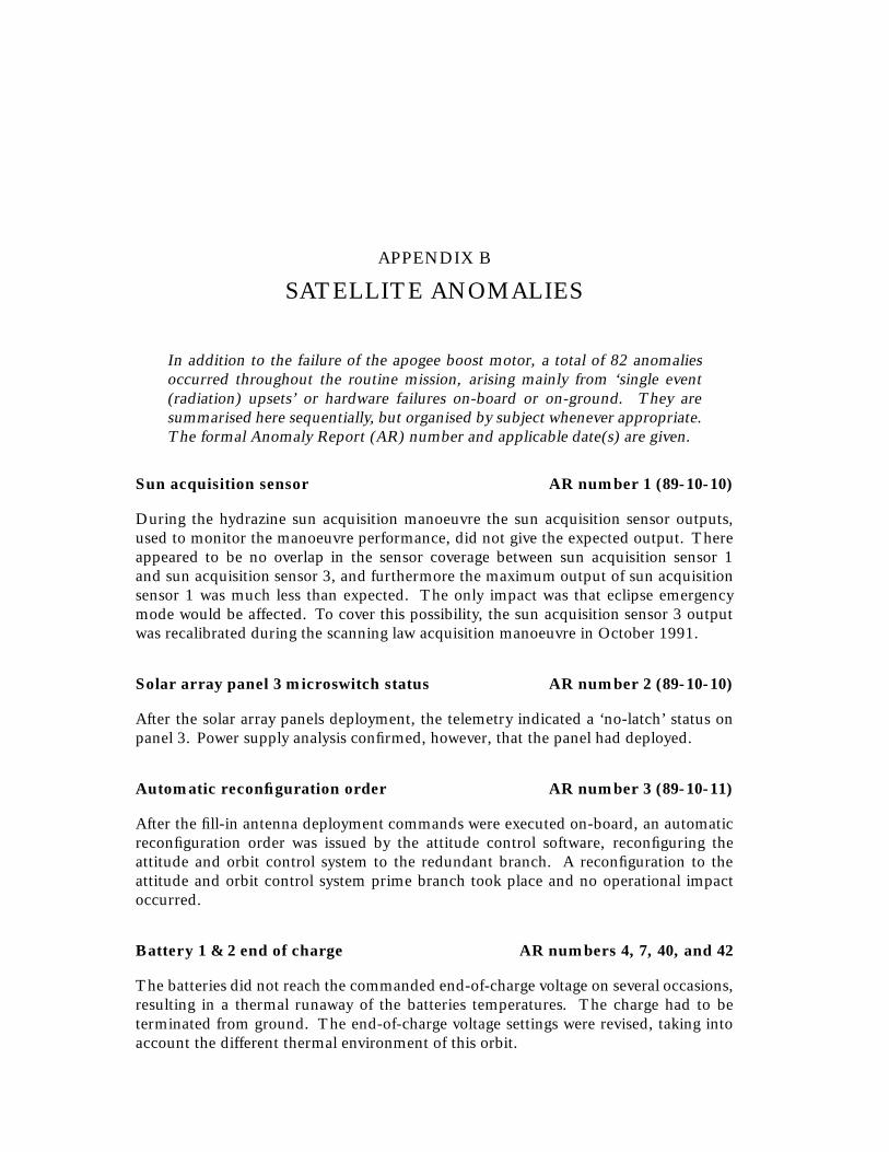
APPENDIX B
SATELLITE ANOMALIES
In addition to the failure of the apogee boost motor, a total of 82 anomaliesoccurred throughout the routine mission, arising mainly from ‘single event(radiation) upsets’ or hardware failures on-board or on-ground. They aresummarised here sequentially, but organised by subject whenever appropriate.The formal Anomaly Report (AR) number and applicable date(s) are given.
Sun acquisition sensor AR number 1 (89-10-10)
During the hydrazine sun acquisition manoeuvre the sun acquisition sensor outputs,used to monitor the manoeuvre performance, did not give the expected output. Thereappeared to be no overlap in the sensor coverage between sun acquisition sensor 1and sun acquisition sensor 3, and furthermore the maximum output of sun acquisitionsensor 1 was much less than expected. The only impact was that eclipse emergencymode would be affected. To cover this possibility, the sun acquisition sensor 3 outputwas recalibrated during the scanning law acquisition manoeuvre in October 1991.
Solar array panel 3 microswitch status AR number 2 (89-10-10)
After the solar array panels deployment, the telemetry indicated a ‘no-latch’ status onpanel 3. Power supply analysis confirmed, however, that the panel had deployed.
Automatic reconfiguration order AR number 3 (89-10-11)
After the fill-in antenna deployment commands were executed on-board, an automaticreconfiguration order was issued by the attitude control software, reconfiguring theattitude and orbit control system to the redundant branch. A reconfiguration to theattitude and orbit control system prime branch took place and no operational impactoccurred.
Battery 1 & 2 end of charge AR numbers 4, 7, 40, and 42
The batteries did not reach the commanded end-of-charge voltage on several occasions,resulting in a thermal runaway of the batteries temperatures. The charge had to beterminated from ground. The end-of-charge voltage settings were revised, taking intoaccount the different thermal environment of this orbit.

338 Appendix B: Satellite Anomalies
Bad telemetry with ranging transponder on AR number 5 (89-10-11)
The telemetry quality changed from ‘good’ to ‘bad’ with every telecommand transactionwhen the ranging transponder was on and high data rate selected. This anomaly wasalready detected during ground test, but not reflected in relevant documentation. Theoperational procedures were updated such that ranging and commanding were exclusive.
Tank temperature AR number 6 (89-10-11)
Two temperature parameters of the hot gas tanks showed inconsistent values. A ther-mistor failure of one temperature reading seemed to have been the cause. The fault hadno impact on the mission.
Emergency sun reacquisition order AR number 8 (89-10-11)
After acquisition of signal, following a perigee and eclipse pass, an emergency sunreacquisition order was triggered and a reconfiguration to the B branch was initiated.From an investigation of the telecommand history file, the workstation event log, andthe Hipparcos dedicated control system message file, it was possible to confirm that theemergency sun reacquisition order disable command sent was rejected by the satellitedue to sequence counter error.
Real-time attitude initialisation AR numbers 9, 10 and 11 (89-10-12)
Several attempts to achieve real-time attitude convergence during sun-pointing opera-tions failed due to early loss of signal or too high background noise on the star mapper.
Image dissector tube piloting AR number 12 (89-10-19)
Using the computed coil currents calibration matrix from the latest grid reference marksand internal star pattern assembly results, the image dissector tube data generated fromthe on-board processing of real stars indicated that the instantaneous field of view wasnot correctly piloted over the image dissector tube. Based on Matra inputs, the coilcurrents calibration matrix calculations were revised curing this anomaly.
Excessive star mapper noise AR number 13 (89-11-09)
The problem of no real-time attitude determination due to excessive star mapper noise,arising from solar flares and excitation of van Allen belts, occurred repeatedly in thenon-nominal orbit, and led to loss of observing time throughout the mission.
Single event upsets AR numbers 14–15, 18, 20–21, 28–29, 34, 38, 45–49
The anomalies related to the single event upsets were of a recurring nature and wererecovered by, for example, reloading the on-board computer, the programme star file,or by resetting the logic of the unit affected. Two anomalies were detected duringsubsequent reloading of the on-board computer and were of non-reoccurring nature(AR number 21 and AR number 46).

Appendix B: Satellite Anomalies 339
Star mapper shutter closure AR number 16 (89-11-09)
On 6 November 1989, the mechanism drive electronics 1 over-exposure flag triggered,indicating that the star mapper shutter had not closed before the occurrence of anoccultation. Subsequent analysis showed that the shutter did not close at the expectedtime since the time-tagged command had an incorrect time entered for execution by themission plan.
Multiplexer failure AR number 17 (89-12-04)
Multiplexer channel 8 of input multiplexer 2 failed. All subsequent telemetry acquiredthrough this channel was therefore false.
Focus activation AR number 19 (90-01-04)
The focus monitoring performed during periods with a step-by-step activation of therefocusing mechanism indicated that the on-board focusing operation was not workingproperly. Investigation confirmed that the origin of the anomaly was in the refocusingmechanism itself. The design of this mechanism was such that a motor rotation of 60
corresponded to a grid movement of a refocusing step (1.4 µm) and a rotation of 13.5
at the level of the wheel acting as magnetic brake. During ground testing the refocusingmechanism had been activated in a step by step manner. No malfunction was detected,except that the magnetic brake was found to be too small. The permanent magnets hadbeen replaced by stronger magnets. After this change, the refocussing mechanism wasnot re-tested in a step by step manner, but only by several steps and no malfunction wasdetected. Due to the stronger magnets, the step by step mode did not function and hadto be replaced by at least a two step operation. To allow a better fit between the actualdefocus curve and the model (straight line), the last 30 days of observations (instead of50 days) were used to compute the next grid displacement.
Image dissector tube analogue mode AR number 22 (90-01-31)
The bright star Alpha Centauri was scheduled to be observed in the analogue mode, butthe analogue mode triggered too early, thus corrupting the observation of the precedingstar (a faint one) which was supposed to be observed in the photon-counting mode.Thereafter, all stars were observed in photon-counting mode.
Central on-board software error AR number 23 (90-02-14)
This anomaly was detected whilst preparing special procedures for the ‘long’ eclipseseason. A cross-correlation was made between the power the central on-board softwarecommanded to the thermal control electronics and the actual thermal control electronicsinput current. From the averaging of the thermal control electronics input current overtime it was determined that the thermal control electronics consumed about 47 W. Thecentral on-board software however indicated consistently, via the thermal report packet,that it was sending approximately 60 W. The calibration curve to determine the centralon-board software telemetered power used a least significant bit of 0.004 W. A newcalibration curve was calculated and implemented with a least significant bit of 0.003 Wwhich corrected the anomaly.

340 Appendix B: Satellite Anomalies
Emergency sun reacquisition order AR number 24 (90-02-14)
On the morning of 12 February 1990 the automatic commanding task failed to send thecommands to disable/enable the emergency sun reacquisition order for the upcomingeclipse. Following an investigation it was discovered that no eclipse commands had beenscheduled by the mission planning task for all eclipses after midnight on 11 February1990. The source of the problem was identified as a typing error in the sequence activityfile used by the mission planning task to attach command sequences to activities suchas occultation, eclipses and calibrations. Prior to the generation of the mission plan, on9 February 1990, for the coming week, the sequence activity file was modified to supportGoldstone. The fields for occultation, eclipses and calibrations were not modified andhence not checked following the generation of the new mission plan. On generation ofthe mission plan the software failed to find a match for the eclipse activity sequence andhence failed to generated the appropriate commands.
Unexpected closing of shutters AR number 25 (90-03-07)
At 05:28 UTC of 12 February 1991 the image dissector tube 2 shutter closed followedwithin 10 s by the closing of the star mapper 2 shutter. After investigation of thetelemetry, mission plan, command history and time-tag display, it was concluded that:(a) the shutter closure was not triggered by the bright object detector; (b) the missionplan did not identify any commands to be uplinked at this time; (c) the commandhistory did not show any command being uplinked at this time (manually) or as a time-tagged command to be executed at this time; (d) the time-tag displayed confirmed (c)above. The two commands to close the shutters were sent about 6.5 days earlier justas a change of ground stations from Odenwald to Kourou took place. UnfortunatelyKourou had portable simulator system data on-line at the time the two commandswere uplinked automatically. Therefore, the on-board time from which the Hipparcosdedicated control system calculated the execution time of the time-tagged commandswas based on the format counter from the portable simulator system data instead of thesatellite data.
Payload remote terminal unit AR number 26 (90-04-02)
In the prime payload remote terminal unit, which provided the data interface betweenthe payload and the satellite central processor, the remote control core failed causingthe loss of all payload housekeeping telemetry. A reconfiguration to the back-up unithad to be implemented.
Solar array 3 temperature AR number 32 (90-05-15)
The average temperature readings over one spacecraft revolution (128 mins) from thethree solar arrays should have been within one least significant bit (4) of the calibrationcurve. Moreover, the measured minimum and maximum temperatures for each solararray should have been identical for this time period. However, after 6 February 1990,the average temperature of solar array 3 started to differ from the temperatures of array 1and 2. By 14 February 1993 the difference was almost 4.6 in the average temperature.The temperature difference was caused by power not being dumped on this panel. Thusthe temperature was lower than on the other panels.

Appendix B: Satellite Anomalies 341
Star mapper rejection of very bright stars AR number 33 (90-05-28)
This anomaly refers to the rejection of very bright stars on the basis of ‘main lobetruncation at the border’. The observed anomaly was a direct effect of the central on-board software patch which was implemented to correct for false stars detection duringhigh background noise periods. The objective of this patch was the deletion of all startransits which were characterized by only one valid maximum after correlation. All thestar transits which were rejected for the above mentioned reason were assigned an errorcode which, for simplicity reasons, was the same as the one allocated for the ‘main lobetruncation error’. The majority of these rejections were due to the star side lobes beingbelow the minimum allowed threshold. However, this problem applied only to a limitednumber of bright stars. This anomaly had no impact on the mission.
Gyros 3 and 4 AR numbers 35 (90-07-03) and 52 (91-08-06)
The satellite was equipped with five rate-integrating gyros. Two of these measuredrates around the spin axis (gyros 4 and 5), one being for back-up. The other threegyros were in the plane perpendicular to the spin axis (gyros 1 to 3), one being theback-up for the other two. Gyro 3, which acts as a back-up to gyro 1 or 2, suffereda failure in its electronics such that the operating temperature of 70 C could notbe reached, and this implied that no gyro back-up in the plane perpendicular to thespin axis existed any more. Gyro 4 (along the spin axis) showed erratic behaviouron several occasions which caused irregular attitude control firings leading to loss ofreal-time attitude convergence. Reconfiguration to gyro 5, the back-up spin-axis gyro,was performed in order to continue the nominal mission. This of course impliedthat no back-up existed any more for this axis. With the possibility of a further gyrofailure, investigations and modifications were carried out to operate the spacecraft withonly two gyros. Software modifications to the on-board control logic and the groundsupporting software modules were developed to cope with a possible gyro 5 failure.Further modifications were developed should gyro 1 or 2 fail.
Loss of spacecraft attitude AR number 36 (90-08-22)
After the perigee pass in the evening of 16 August 1990 and the subsequent crossing ofthe inner and outer van Allen belt, the spacecraft had diverged from its optimal pointing,necessitating an uplink of the Tait-Bryan error angles. The error angles were uplinkedat 23:15 UTC causing several attitude and orbit control system parameters to raise outof limit alarms because of large thruster firings around all three axes. Moreover, noconvergence of real-time attitude had been achieved. During the subsequent validationof the ground data used to uplink the error angles, the limited history file did not containthe magnitude of the uplinked angles, but it was believed that the magnitude had beenapproximately 0.9.
Payload thermal control AR numbers 37 (90-09-04) and 44 (91-01-28)
Several heater and/or thermistor failures occurred in the payload active thermal control.As a consequence, a reconfiguration to the back-up thermal control electronics had tobe performed. On the second unit, some thermistors also failed. These were excludedfrom the control loop by setting the relevant heaters to a fixed power level.

342 Appendix B: Satellite Anomalies
Radio frequency 1 AR number 39 (90-09-04)
The on-board automatic control gain of receiver 1 and 2 showed high variations when-ever telecommands were being uplinked. The variations were in the order of −21 dbm.The analysis of this anomaly concluded that the automatic control gain bandwidth wastoo wide and out of specification. However, no evidence of a generic problem with thetelemetry, tracking and command transponder design and corresponding specificationswas found, as the automatic control gain malfunction and corresponding discrepancieswere not critical with respect to the overall uplink function.
Payload mechanism drive electronics 1 AR number 41 (90-09-26)
On 24 September 1990 at 17:26 UTC, mechanic drive electronics 1 secondary voltage(parameter J001) dropped from 2.44 V to 1.88 V, falling below the nominal operatingrange (‘out of limits’ status). A short test showed that both shutters (image dissectortube and star mapper) were still able to work (opening and closing properly) underthis anomalous voltage. However, the decision was taken to switch to redundant unitmechanic drive electronics 2 and the spacecraft was subsequently reconfigured at 19:23UTC. On 14 March 1991 tests were performed and proved that mechanic drive elec-tronics 1 was in fact functioning thus implying a fault in the multiplexer of the payloadremote terminal unit.
Loss of attitude AR number 50 (91-06-17)
Ultimately triggered by high solar activity, severe problems were experienced with real-time attitude determination from 5 − 11 June 1991. On 6 June at 18:16 UTC thespacecraft attitude was lost after a series of large innovations caused real-time attitudedetermination to diverge.
Erroneous orbital oscillator command AR number 53 (91-10-08)
On 29 September 1991 at 17:01 UTC an orbital oscillator command was executedon-board with a value for the z component of the torque six orders of magnitude largerthan the nominal calculated value, (this command was ground-calculated and uplinkedevery 15 mins for time-tagged execution on board) triggering a z thruster firing requestof 213.33 s.). The spacecraft started to move away from its nominal spin-rate of−168.75 arcsec s−1 through zero and to the other direction. Corrective action was takento bring the spacecraft back to safe sun-pointing configuration.
Suspect pre-processed gyro readings AR number 54 (91-10-15)
During the recovery from the ‘erroneous orbital oscillator anomaly’, the pre-processedon-board estimates of the body rates were shown to be inconsistent with the actualgyro outputs. In particular, the x and y body rates were about eight times largerthan expected. The attitude control software was in standby mode 2 at the time.Confirmation was needed that the software mode standby mode 2 assumed the gyros tobe in coarse range.

Appendix B: Satellite Anomalies 343
Gyro heating AR number 55 (91-10-15)
On 30 September 1991 at 02:10 UTC gyros 1, 2 and 5 were switched on as part of therecovery following the anomaly AR number 53. The temperature behaviour of all gyroswas not as expected, since normally a continuous and smooth increase of temperatureup to 70 C was observed followed by a steady state lasting approximately 10–15 min.The anomaly had no impact on the mission.
Status reading of switching mirror AR number 56 (91-10-15)
On 30 September 1991 at 07:14 UTC when the payload was switched on followingthe recovery from the ‘erroneous orbital oscillator command’ (see AR number 53), thetelemetry readings of the switching mirror both indicated a ‘CLOSED’ status, whichdid not reflect a valid position. However, from science data analysis it could be verifiedthat the switching mirror was pointing towards detector 2 as it was commanded beforepayload switch-off. The anomaly had no impact on the mission.
Image dissector tube 1 voltages AR number 57 (91-10-15)
On 10 October 1991 at 11:42 UTC a procedure to switch image dissector tube 1 on andto perform a calibration was implemented to verify correct functioning of the detectorchain before the switching mirror was moved. After switching the image dissector tube 1electronics on, the secondary supply voltages telemetered in parameters G007 (imagedissector tube 1 +15/ − 12 V) and G008 (image dissector tube 1 +6/ − 5.2/ + 30 V)indicated a low out of limit. The procedure was terminated and image dissector tube 1was switched off again. The anomaly had no impact on the mission since only imagedissector tube 2 was normally used for the operations. A telemetry problem (faultypayload remote terminal unit multiplexer) was suspected and confirmed on 29 July1993 implying that image dissector tube 1 could have been used operationally.
Battery charge during perigee AR number 58 (92-01-13)
Since the end of the eclipse season, 21 October 1991, it was noted that both batterieswere commanded to ‘charge’ by the on-board logic. This change of status was onlyhappening during perigee (non-visibility periods) and was observed at almost everypass. Because no eclipses occurred during that time, the only change of spacecraftstatus was caused by occultations where the payload shutters were closed and openedvia time-tagged commands. This abnormal behaviour was explained by orbit geometry.The spacecraft was crossing the Earth albedo and during these periods, the alreadydegraded solar panels generated less power. Thus, high power demanding commandswere enough to trigger the battery logic. The anomaly had no impact on the mission.
Gyro 1 real-time attitude drift AR number 59 (92-06-11)
At acquisition of signal from the Goldstone ground station at 23:23 UTC on 9 June1992, following 6 hours of non-coverage, the gyro 1 drift had changed from its previousrecorded value of 0.16 to 0.12 arcsec s−1 and was further decreasing. Correction to the‘old’ drift value was uplinked at 23:25 UTC. However, the drift rate started to decreaseagain, until real-time attitude diverged (at about 01:00 UTC on the next day) and thedrift started to increase. The anomaly had no impact on the mission.

344 Appendix B: Satellite Anomalies
Telemetry after radio frequency switching AR number 60 (92-06-23)
On 6 June 1992 at 18:04:50 UTC, the command to change transponder 1 to the fill-inantenna and transponder 2 to the cardioid antenna was executed from the on-boardtime-tag buffer previously loaded by the uplinked mission plan (one command for thetwo functions). The subsequent telemetry readout showed that transponder 1 wasconnected to the fill-in antenna. However, the telemetry readout for transponder 2 didnot indicate the expected change to the cardioid antenna, but remained on the fill-inantenna. Since the on-board automatic control gain had changed as expected after theantenna switch command was executed it was concluded that the radio frequency switchhad functioned as expected, the anomaly seemed to be a ‘false’ telemetry readout.
Thermal control electronics AR number 61 (92-07-07)
Temperatures of the telescope focal plane and the beam combiner decreased below spec-ified minimum even after the maximum power to some of the control area heaters wereapplied. No action could be taken besides a close monitoring of the relevant thermalareas since thermal control electronics 2 was replacing thermal control electronics 1after the failure of the heaters used for the same areas.
Gyro 5 AR number 62 (92-07-07)
From 3 July 1992, occurrences of ‘false’ gyro readouts were experienced. These readoutsresulted in spurious z-thruster firings and in most cases caused real-time attitude todiverge. The attitude had to be subsequently corrected by ground intervention.
Gyro 5 and two gyro implementation AR number 63 (92-07-10)
On 10 July 1992 after acquisition of signal by Goldstone at 00:30 UTC ‘glitches’ inthe raw output of gyro 5 occurred for approximately one hour during the outer vanAllen belt crossing. The same was experienced during the following Odenwald pass. Inboth cases the z thruster firings were inhibited by the action of the on-board z thrusteraccumulator patch which stopped the firings when the accumulated thruster on-timereached the limit (60 s). However, because the normal mode z error angle was outsidelimits, and could not be corrected by the disabled z thruster, continuous demands tofire the z thruster were present, which resulted also in x and y thruster firings. Thethruster firings were short but continuous until the ‘glitches’ disappeared, then the on-board software patch was reset from ground thus re-enabling the z thruster firings. At16:01 UTC gyro 5 was taken out of the control loop and its function replaced by thetwo-gyro patch. Real-time attitude convergence was maintained confirming that thenew on-board software was working correctly.
Attitude and orbit control system AR number 66 (92-08-05)
On 4 August 1992, just before loss of signal at the Odenwald ground station at 13:21UTC, attitude and orbit control system telemetry packets were not present in thedownlink. Furthermore, an attitude control software error was observed as well asseveral central on-board software errors. Special support was immediately requestedfrom the Perth station, and the data received between 13:59 UTC and 14:16 UTC(loss of signal at Perth) confirmed that no communication was available between the
Appendix B: Satellite Anomalies 345
central on-board software and the attitude control software. At about 14:06 UTC,power was generated by the solar arrays and the batteries were discharging. This wasa clear indication of a serious attitude anomaly. Goldstone was requested to provideemergency support some four hours ahead of schedule starting at 14:48 UTC. Thisallowed an immediate reconfiguration of the attitude and orbit control system to theredundant branch to be carried out, and by 17:17 UTC good attitude and orbit controlsystem telemetry was again received. It was then confirmed from sun sensor and gyrodata, that the spacecraft was badly nutating (half-cone of about 19). At 17:57 UTC aground commanded emergency sun reacquisition brought the spacecraft to a safe sun-pointing mode. Thereafter the spacecraft was configured for sun-pointing operation.The spacecraft was moved back to the nominal scanning law at 43 and convergencewas achieved on 11 August 1992. Another emergency sun reacquisition was causedby the failure of gyro 5 a few hours later. After a 3-month hibernation period routineoperations at 43 were resumed on 29 October 1992.
Gyro 5 and gyro 2 failure AR number 67 (92-08-12)
At 10:45 UTC on 11 August 1992, gyro 5 failed (output data corruption), inducing hightorques around all three axes. At this time, the two gyro real-time attitude convergencehad not been achieved. Immediate ground interventions failed to reduce the rapidlyincreasing body rates. The on-board anomaly detector triggered the emergency sunreacquisition and the spacecraft returned to a safe sun-pointing mode. In order tosafeguard the attitude at sun-pointing for the upcoming perigee passage including aneclipse, the spacecraft was spun up to about 0.4 rpm which would guarantee stabledynamic behaviour. However, during the spin-up nutation had arisen and could notbe damped before the loss of signal. Goldstone was requested to provide emergencysupport some three hours ahead of schedule starting at 17:04 UTC. At acquisitionof signal another anomaly, this time on gyro 2, was detected. The gyro 2 output wascorrupted in an identical manner to gyro 5. The additional failure of gyro 2 complicatedthe nutation control from ground, which was finally achieved around 18:00 UTC.
On-board computer 1 AR number 68 (92-09-07)
On 5 September 1992 at acquisition of signal by Perth (02:24 UTC) a continuousstream of memory error alarms was received. The error was identified as related to theprogramme star file buffer area, which was not being used in the present mode. Anattempt to reset the on-board computer was unsuccessful; a reset of the programme starfile buffer did not clear the problem. In addition on-board computer 1 could not becommanded to monitoring mode. A central on-board software reload was commanded,but the watchdog 1 could not be enabled. Power was removed and enabled into on-board computer 1 to reset the watchdog 1 signal. After a period of loss of signal (05:45to 06:50 UTC), several attempts were made to bring on-board computer 1 to a properinitial state (therefore disabling the watchdog) by removing/restoring power to on-boardcomputer 1, but all subsequent attempts to reconfigure the watchdog failed. Commandswere verified through the demodulator and frame synchronizer channels, other possiblesources of error were checked (receiver, decoder chain, etc.) and discarded. At thispoint a reconfiguration to the redundant unit (on-board computer 2) was carried out.A reload of the central on-board software software was performed without problems.Watchdog 2 was enabled successfully on the first attempt. Reconfiguration was finishedat 09:08 UTC.

346 Appendix B: Satellite Anomalies
On-board computer 2 AR number 69 (92-09-22)
On 16 September 1992, a test was performed on on-board computer 2 in order to checkall of its functions, whilst the watchdog was disabled. All functioned nominally and itwas therefore concluded that on-board computer 1 was usable having the watchdogdisabled. To finally validate the proper function of on-board computer 1, a switch-overwas attempted. However, the command necessary to reset on-board computer 2 didnot work. On-board computer 2 remained then the operational unit.
Gyro 1 spin-down AR number 70 (92-09-28)
Since 25 September 1992 three spin-downs of gyro 1 had taken place. The first occur-rence lasted about 3 mins with a maximum variation of 36 arcsec s−1. This was followed15 mins later by a second spin-down of a smaller magnitude. The third occurrence wasnoticed two days later.
Gyro 1 breakdown AR number 71 (92-10-14)
On 10 October 1992 at 23:26 UTC gyro 1 stopped functioning completely. The gyrostopped spinning, and could not be started again. All attempts, including change ofattitude and orbit control system from branch A to branch B and switching off/on thepower supply channel, failed. Gyro 4, fed by the same channel, was switched on andspun up nominally. This excluded a failure of the power supply.
Emergency sun reacquisition order AR number 72 (92-10-14)
On 14 October 1992, an emergency sun reacquisition order was triggered at eclipse exitwhich reconfigured the spacecraft to the attitude and orbit control system branch B.Emergency sun reacquisition order had to be disabled by time-tagged command foreach eclipse period while sun-pointing because at this attitude the on-board attitudeanomaly detector sensor was illuminated by the Sun and triggered. The required uplinktimes had been miscalculated, thus emergency sun reacquisition order was not disabledduring the eclipse period and consequently triggered.
Emergency sun reacquisition order AR number 73 (92-11-13)
On 10 November 1992, emergency sun reacquisition order triggered at 15:33 UTC asa consequence of a command resetting the z gyro drift rates to zero. The spacecraft re-turned to sun-pointing mode and reconfiguration from attitude and orbit control systembranch A to branch B was immediately performed. Real-time attitude determinationat sun-pointing was initialised at 20:31 UTC. At 20:48 UTC the manoeuvre to returnthe spacecraft to the nominal scanning law (43 solar aspect angle) was started andsuccessfully terminated at 21:36 UTC. Real-time attitude determination was initialisedat 22:06 UTC and science data collection re-commenced.
Appendix B: Satellite Anomalies 347
Gyro 5 AR number 74 (92-11-13)
The noise of gyro 5 raw output increased suddenly on 18 November 1992 at about03:45 UTC and remained high until loss of signal (06:02 UTC). At acquisition ofsignal (06:51 UTC), the gyro output noise characteristic had not changed, but alsohigh spin variations between 100 and 200 arcsec s−1 were observed. Furthermore, gyro2 (sharing the same power supply as gyro 5) had similar spin variations. Gyro 4 wasswitched on, confirming a constant spacecraft spin rate. Gyro 5 was switched off at10:31 UTC and gyro 2 output immediately recovered.
Gyro 2 spikes AR number 75 (92-12-28)
At acquisition of signal (17:44 UTC) on 22 December 1992, gyro 2 raw output datashowed an increasing noise envelope. At around 18:40 UTC, spikes on the gyro datasimilar to the previously observed spikes on gyro 5 triggered the emergency sun reac-quisition order which returned the satellite to sun-pointing mode. The satellite wasreconfigured and gyros 2 and 3 switched on. The noise (spikes) on gyro 2 was stillpresent, but disappeared after the temperature of the gyro electronics had passed 22 C.
On-board computer 2 AR number 76 (93-02-18)
On 16 February 1993 at 08:17 UTC a few packet commands were rejected on-boarddue to checksum error. The number of rejections varied depending upon the commanduplink rate, but with increasing tendency. The anomaly was present with all four groundstations. No evidence of a ground problem was detected. On 17 February 1993 startingat 13:15 UTC, a reload of on-board computer 2 was attempted but failed because someof the load commands were rejected on-board. The ground system was again thoroughlychecked, including a further attempt to reload on-board computer 2 with the back-upsystem resulting again in on-board command rejections. A reconfiguration from on-board computer 2 to on-board computer 1 was done followed by a successful reload ofon-board computer 1. Science collection re-commenced at 18:15 UTC.
Gyro 2 failure AR number 77 (93-03-18)
On 18 March 1993 at 20:26 UTC gyro 2 failed causing an emergency sun reacquisition.Prior to this, increased noise had been observed on the raw gyro output data. Attemptsto restart gyro 2 (and any of the previously failed gyros) were unsuccessful. Only gyro3 started. The satellite was spun up to 0.25 rpm followed by nutation damping.
Antenna switch command failure AR number 78 (93-03-30)
On 28 March 1993 the command to connect transponder 1 to the fill-in antenna andtransponder 2 to the cardioid antenna failed execution. The command was sent as atime-tagged command from the on-board computer. The command was transmittedfrom ground for immediate execution, but failed again. The back-up command wasthen used and correct antenna switching was achieved. From then on, only the back-upcommand was used to switch antennae. A possible explanation could be a fault in therelevant on/off module. An on/off module was a module of the payload remote terminalunit responsible for the distribution of the commands (de-multiplexer).

348 Appendix B: Satellite Anomalies
Star mapper 1 and 2 partial failures AR number 79 (93-05-25)
On 5 May 1993 star mapper 2 was switched on and it was found that the VT channelwas no longer working. The following day star mapper 1 was tested and it was foundthat on this unit the BT channel did not work. Ground real-time attitude determinationrequired both channels to identify star magnitude and colour to perform correct starpattern matching. The ground software was then modified to operate with both starmapper streams available in telemetry (BT channel of star mapper 1 and VT channel ofstar mapper 2).
Suspect control law electronics AR number 80 (93-05-27)
The processor of the control law electronics of the attitude and orbit control systembranch A stopped twice during the week 28 June to 4 July 1993. Once without any errormessages and once with the error indicating a ‘CPU overload’. The attitude and orbitcontrol system was configured into a cross-strapped mode using the branch B controllaw electronics and the branch A control actuation electronics, which retained all safetyaspects in case of attitude anomaly detection.
Gyro 3 noise AR number 81 (93-05-31)
On 26 May 1993 gyro 3 was switched on at 07:02 UTC and showed nominal behaviour.During the early morning hours of 27 May increasing noise (spikes) appeared, reachingpeak values of more than 50 arcsec s−1. The gyro was switched off at 08:12 UTC.
On-board software 1 and 2 failure AR number 82 (93-06-28)
On 24 June 1993 at 14:41 UTC central on-board software 1 halted with an errormessage indicating an ‘illegal instruction’ in memory. Prior to this, three error messageswere received indicating checksum errors at the same location. Several further attemptsto start either central on-board software 1 or central on-board software 2 during thefollowing days were unsuccessful.
APPENDIX C
REFERENCES
Anspaugh, B.E., 1991. Proton and electron damage coefficients for GaAs/Ge solar cells,Proceedings IEEE, PVSC, Las Vegas.
Anspaugh, B.E., Downing, R.G., 1984. Radiation effects in Silicon and Gallium Arsenidesolar cells using isotropic and normally incident radiation, JPL Publication 84-61.
Auburn, J.H.C., Batten, A.J., McDonald, A.J.C., 1991. Hipparcos attitude determina-tion with two gyros and a star mapper, Proc. 3rd International Symp. Spacecraft FlightDynamics, Darmstadt, Germany, ESA SP-326, 213.
Batten, A.J., McDonald, A.J.C., 1989. Hipparcos precise attitude determination: methodsand results, Int. Symp. Space Dynamics, Toulouse, France.
Beech, M., Brown, P., Jones, J., 1995. The potential danger to space platforms from meteorstorm activity, Quarterly Journal of the Royal Astronomical Society, 36, 127.
Bernard, J., Reulet, R., Crabb, R.L., 1984. Proc. 4th European Symp. PhotovoltaicGenerators in Space, ESA SP-210, 407.
Blake, J.B., Gussenhoven, M.S., Mullen, E.G., Fillius, R.W., 1992. Identification of anunexpected space radiation hazard, IEEE Trans. Nucl. Sci. NS-39, 6, 1761.
Brautigam, D.H., Gussenhoven, M. S., Mullen E.G., 1992. Quasi-static model of outerzone electrons, IEEE Trans. Nucl. Sci. NS-39, 6, 1797.
Buacher, J., 1967. Les combinaisons optiques: practique des calculs, Editions de la Revued’Optique Theorique et Instrumentale.
Cheng, C. et al., 1991. Improved MOCVD technology in high-throughput high-efficiencyGaAs/Ge solar cell manufacture, Proceedings IEEE, PVSC, Las Vegas.
Crabb, R.L., 1994. Solar cell radiation damage, Radiat. Phys. Chem. 43, 93-103.
Crabb, R.L., Robben, A.P., 1993. In-flight Hipparcos solar array performance degradationafter three and a half years in GTO, Proc. European Space Power Conference, Graz,ESTEC/XPG-WPP-054.
Creze, M., Chareton, M., 1991. Accuracy uniformity of Hipparcos parallaxes and propermotions: strategy and current status, Highlights of Astronomy, Vol 9, Bergeron J. (ed).
Daly, E.J., et al., 1994. Radiation-belt and transient solar-magnetospheric effects on Hipparcosradiation background, IEEE Trans. Nucl. Sci. NS-41, 6, 2376.
Davies, P.E., McDonald, A.J.C., 1991. Results of the Hipparcos In-Orbit Payload Calibra-tion, Journal of the British Interplanetary Society, 44, 37.
Feynman, J., Armstrong, T.P., Dao-Gibner, L., Silverman, S., 1992. New interplanetaryproton and fluence model, J. Spacecraft, 27, 403.

350 Appendix C: References
Gussenhoven, M.S., Mullen, E.G., Sperry, M., Kerns, K.J., Blake, J.B., 1992. Theeffect of the March 1991 storm on accumulated dose from selected satellite orbits: CRRES dosemodels, IEEE Trans. Nucl. Sci. NS-39, 6, 1765.
Gussenhoven, M.S., Mullen, E.G., Violet, M.D., 1994. Solar particle events as seen onCRRES, Adv. Space Res., 14, (10)619.
Howell, L.W., Kennel, H.F., 1984. A stochastic model for photon noise induced by chargedparticles in multiplier phototubes of the Space Telescope Fine Guidance Sensors, NASA TP-2337.
Høg, E. et al., 1992. Tycho data analysis: overview of adopted reduction software and firstresults, Astron. Astrophys., 258, 177.
Lindegren, L. et al., 1992. Geometrical stability and evolution of the Hipparcos telescope,Astron. Astrophys., 258, 35.
McDonnell, J.A.M., 1978. Cosmic Dust, John Wiley & Sons.
Mullen, E.G., Gussenhoven, M.S., Ray, K., Violet, M., 1991. A double-peaked innerradiation belt: Cause and Effect as Seen on CRRES, IEEE Trans. Nucl. Sci. NS-38, 6,1713.
Naumann, R.J., 1966. The near-Earth meteoroid environment, NASA TN D-3717.
Nieminen, P.J., 1995. Standard radiation environment monitor detector design and simula-tions, ESTEC Working Paper 1829.
Olsen, W.P., Pfitzer, K.A., 1974. A quantitative model of the magnetospheric magnetic field,J. Geophys. Res., 79, 3739.
Radlein, E., 1991. Simulation der Wechselwirkung von Weltraumstrahlung mit Glas undGlaskeramik, Dissertation zur Erlangung des Grades eines Doktor (publication in En-glish issued from the Conference of Physics of Non-Crystalline Solids, 4–9 August 1991,Cambridge.
Ray, K.P., Mullen, E.G., Trumble, T.M., 1993. Results from the high-efficiency solar panelexperiment flown on CRRES, (Phillips Laboratory USAF), IEEE Trans. Nucl. Science,40, 6, 1505.
Sauer, H.H., 1987. A personal computer-based GOES data archive, NOAA TechnicalMemorandum ERL-SEL-74.
Sawyer, D.M., Vette, J.I., 1976. AP-8 trapped proton environment for solar maximum andsolar minimum, NSSDC 76-06.
Soo, D., Schuyer, M., 1994. Preparing for the Future, ESA Publication, Vol. 4, No. 2.
Tada, J., et al., 1982. In Solar Cell Radiation Handbook, 3rd Edition, NASA JPL Publi-cation 82-69 and Addendum 1 JPL Publication 82-69.
Tranquille, C., Daly, E.J., 1992. An evaluation of solar proton event models for ESAmissions, ESTEC Working Paper 1647.
Vette, J.I., 1989. Trapped radiation models: development of improved models of the Earth’sradiation environment, Technical Note 1, Chapter 4.
Vette, J.I., 1991. The AE8 trapped electron model environment, NSSDC Report 91-24,NASA/GSFC.
Viehmann, W., Eubanks, A.G., 1976. Noise limitations in multiplier phototubes in theradiation environment of space, NASA TN-8147.

APPENDIX D
BIBLIOGRAPHY
This bibliography applies to both the technical (this Volume) and scientific (Volumes3–4) aspects of the Hipparcos mission, and includes refereed papers, conference pro-ceedings, and articles of a more popular nature, published up until the end of 1996.
Amoretti, M., Badiali, M., Cardini, D., Emanuele A., 1985. The signal of the Hipparcos nominal system. Proc.
Marseille Coll. ‘Processing of Scientific Data from Hipparcos’, Second FAST Thinkshop, 21–25 January
1985, Kovalevsky, J. (ed.), 49.
Arenou, F., 1993. Contribution a la validation statistique des donnees d’Hipparcos: Catalogue d’Entree et donnees
preliminaires. These de doctorat, Observatoire de Paris.
Arenou, F., Grenon, M., Gomez, A., 1992. A tridimensional model of the galactic interstellar extinction. A&A, 258,
104.
Arenou, F., Lindegren, L., Frœschle, F., Gomez, A.E., Turon, C., Perryman, M.A.C., Wielen, R., 1995. Zero-point
and external errors of Hipparcos parallaxes. A&A, 304, 52.
Arenou, F., Morin, D., 1988. The INCA data base for the Hipparcos mission. Astronomy from large databases:
scientific objectives and methodological approaches, Garching, Murtagh, F., Heck, A. (eds), 269.
Argue, A.N., 1985. Report by INCA subgroup 2130 (link to extragalactic reference objects). Proc. Aussois Coll.
‘Scientific Aspects of the Input Catalogue Preparation’, 3–7 June 1985, Turon, C., Perryman, M.A.C. (orgs),
ESA SP-234, 237.
Argue, A.N., 1986. Hipparcos: link with the extragalactic reference frame. IAU Highlights of Astronomy Vol. 7,
Swings, J.P. (ed.), 719.
Argue, A.N., 1986. The reconciliation of optical and radio positions. IAU Symp. 109, ‘Astrometric Techniques’,
Gainsville, 9–12 January 1984, Eichhorn, H.K., Leacock, R.J. (eds), 757.
Argue, A.N., 1988. Report to subgroup 2130 (link to extragalactic objects). Proc. Sitges Coll. ‘Scientific Aspects of
the Input Catalogue Preparation’, 25–29 January 1988, Torra, J., Turon, C. (eds.), 439.
Argue, A.N., 1990. A strategy for linking Hipparcos to an extragalactic reference frame. IAU Proc. ‘Inertial coordinate
system on the sky’, Lieske, J.H., Abalakin, V.K. (eds.), 323.
Argue, A.N., 1991. Hipparcos: its link to an extragalactic reference frame. Proc. IAU Coll. 127 ‘Reference systems’,
Hughes, J.A., Smith, C.A., Kaplan, G.H. (eds), US Naval Observatory Publ., 63.
Argue, A.N., Baxter, R.D., Morgan, B.L., Vine, H., 1982. The selection of stars for linking the Hipparcos frame to
extragalactic radio sources by Space Telescope (progress report). Proc. Strasbourg Coll. ‘Scientific Aspects of the
Hipparcos Space Astrometry Mission’, 22–23 February 1982, Perryman, M.A.C., Guyenne, T.D. (eds), ESA
SP-177, 53.
Argue, A.N., White, G.M., 1992. Link to an inertial system. Highlights of Astronomy, 9, 429.

352 Appendix D: Bibliography
Argue, A.N. et al., 1984. A catalogue of selected compact radio sources for the construction of an extragalactic radio/optical
reference frame. A&A, 130, 191.
Arlot, J.E., Bec-Borsenberger, A., Dourneau, G., 1991. Observations of the planetary satellites Europa and Titan by
Hipparcos. Proc. IAU Coll. 127, ‘Reference systems’, Hughes, J.A., Smith, C.A., Kaplan, G.H. (eds), US
Naval Observatory Publ., 202.
Baarda, W., 1968. A testing procedure for the use in geodetic networks. Neth. Geodetic Commission, Publ. on Geodesy.
Vol. 2, 5.
Baarda, W., 1973. S-transformation and criterion matrices. Neth. Geodetic Commission, Publ. on Geodesy. Vol. 5,
1.
Bacchus, P., 1974. Space astrometry project: optical concept. Proc. Frascati Symp. ‘Space Astrometry’, 22–23
October 1974, Nguyen, T.D., Battrick, B.T. (eds), ESA SP-108, 31.
Bacchus, P., 1974. Space astrometry project: reduction by multilateration. Proc. Frascati Symp. ‘Space Astrometry’,
22–23 October 1974, Nguyen, T.D., Battrick, B.T. (eds), ESA SP-108, 37.
Bacchus, P., 1982. Caracteristiques des etoiles doubles observables par Hipparcos. Proc. Strasbourg Coll. ‘Scientific
Aspects of the Hipparcos Space Astrometry Mission’, 22–23 February 1982, Perryman, M.A.C., Guyenne,
T.D. (eds), ESA SP-177, 153.
Bacchus, P., Lacroute, P., 1974. Prospects of space astrometry. in New Problems in Astrometry, Gliese, W., Murray,
C.A., Tucker, R.H. (eds), 277.
Badiali, M., Amoretti, M., Cardini, D., Emanuele, A., 1986. Tests on the Hipparcos real system. Proc. Bari Coll.
‘Processing of Scientific Data from Hipparcos’, Third FAST Thinkshop, 3–6 November 1986, Bernacca,
P.L., Kovalevsky, J. (eds), 305.
Badiali, M., Cardini, D., Emanuele, A., Prezioso, G., Pannunzio, R., 1991. Expected performances of Hipparcos
satellite in detecting double star systems. Advances in Space Research, 11-2, 71.
Baglin, A., 1988. Hipparcos mission and fundamental physics. Proc. Sitges Coll. ‘Scientific Aspects of the Input
Catalogue Preparation’, 25–29 January 1988, Torra, J., Turon, C. (eds.), 103.
Barbieri, C., Bernacca, P.L. (eds.), 1979. Proc. Padova Coll. on European Satellite Astrometry. University of
Padua.
Barbieri, C., Nota, A., 1983. The sky background from a space station. Proc. Asiago Coll. ‘Processing of Scientific
Data from Hipparcos’, The FAST Thinkshop, 24–27 May 1983, Bernacca, P.L. (ed.), 135.
Barthes, D., Davies, P., Menessier, M.O., 1991. Luminosity of large amplitude variable stars: comparison between
ground-based predictions and observations by the Hipparcos satellite. Advances in Space Research, 11-2, 67.
Bassgen, G., Wicenec, A., Andreasen, G.K., Høg, E., Wagner, K., Wesselius, P., 1992. Tycho transit detection. A&A,
258, 186.
Bastian, U., 1985. Treatment of the Hipparcos grid step ambiguity problem. Proc. Marseille Coll. ‘Processing of
Scientific Data from Hipparcos’, Second FAST Thinkshop, 21–25 January 1985, Kovalevsky, J. (ed.), 295.
Bastian, U., 1986. Hipparcos, der 100000-Sterne-Satellit. Sterne und Weltraum 25, 524.
Bastian, U., 1994. Hipparcos, ein Astrometrie-Satellit der ESA. Astronomie und Raumfahrt, 33, 4.
Bastian, U., 1994. Hipparcos-Mission abgeschlossen. Sterne und Weltraum 33, 12.
Bastian, U., Born, E., Agerer, F., Dahm, M., Großmann, V., Makarov, V., 1996. Confirmation of the classification of
a new Tycho variable: HD 32456 is a 3.3-day Cepheid. Inf. Bull. Variable Stars, No. 4306.
Bastian, U., Lederle, T., 1985. The ARI catalogue of astrometric data for the Hipparcos Input Catalogue. Proc. Aussois
Coll. ‘Scientific Aspects of the Input Catalogue Preparation’, 3–7 June 1985, Turon, C., Perryman, M.A.C.
(orgs), ESA SP-234, 185.
Bec-Borsenberger, A., 1985. Petites planetes du programme Hipparcos. Proc. Aussois Coll. ‘Scientific Aspects of the
Input Catalogue Preparation’, 3–7 June 1985, Turon, C., Perryman, M.A.C. (orgs), ESA SP-234, 175.
Bec-Borsenberger, A., 1988. Petites planetes et satellites a observer par Hipparcos. Proc. Sitges Coll. ‘Scientific
Aspects of the Input Catalogue Preparation’, 25–29 January 1988, Torra, J., Turon, C. (eds.), 303.
Bec-Borsenberger, A., 1992. Solar system objects observed by Hipparcos. A&A, 258, 94.

Appendix D: Bibliography 353
Bec-Borsenberger, A., Bange, J-F., Bougeard, M-L., 1995. Hipparcos minor planets: first step towards the link between
the Hipparcos and the dynamical reference frames. A&A, 304, 176.
Beeckmans, F., 1980. The astrometry satellite Hipparcos. ESA Journal, 4, 15.
Belforte, P., 1986. Report on the attitude reconstitution task. Proc. Bari Coll. ‘Processing of Scientific Data from
Hipparcos’, Third FAST Thinkshop, 3–6 November 1986, Bernacca, P.L., Kovalevsky, J. (eds), 41.
Belforte, P., Canuto, E., Carlucci, D., Fassino, B., 1983. The jitter error in grid coordinate estimation. Proc. Asiago
Coll. ‘Processing of Scientific Data from Hipparcos’, The FAST Thinkshop, 24–27 May 1983, Bernacca,
P.L. (ed.), 197.
Belforte, P., Canuto, E., Donati, F., Villa A., 1983. An approach to on-ground attitude reconstitution: preliminary
results. Proc. Asiago Coll. ‘Processing of Scientific Data from Hipparcos’, The FAST Thinkshop, 24–27 May
1983, Bernacca, P.L. (ed.), 163.
Belforte, P., van der Marel, H., Canuto, E., 1986. On two different ways of modelling the Hipparcos attitude. Proc.
Bari Coll. ‘Processing of Scientific Data from Hipparcos’, Third FAST Thinkshop, 3–6 November 1986,
Bernacca, P.L., Kovalevsky, J. (eds), 81.
Bernacca, P.L. (ed.), 1983. Processing of the scientific data for the ESA astrometry satellite Hipparcos. Proc. Asiago
Coll. ‘Processing of Scientific Data from Hipparcos’, The FAST Thinkshop, 24–27 May 1983, Bernacca,
P.L. (ed.).
Bernacca, P.L., 1985. Progetto Hipparcos. Letture, Giornale di Astronomia, 375.
Bernacca, P.L., 1985. Project Hipparcos. Astrophys. Space Sci., 110, 21.
Bernacca, P.L., Kovalevsky, J. (eds), 1986. Processing of scientific data for the ESA astrometry satellite Hipparcos. Proc.
Bari Coll. ‘Processing of Scientific Data from Hipparcos’, Third FAST Thinkshop, 3–6 November 1986.
Bernstein, H.H., 1985. Numerical results on astrometric parameters and accuracy assessment. Proc. Marseille Coll.
‘Processing of Scientific Data from Hipparcos’, Second FAST Thinkshop, 21–25 January 1985, Kovalevsky,
J. (ed.), 291.
Bernstein, H.H., Hering, R., Walter, H.G., 1988. Astrometric parameters of visual double stars derived from simulated
Hipparcos measurements. Astrophys. Space Sci., 142, 161.
Bertani, D., Cetica, M., Iorio-Fili, D., 1985. Optical model for the Hipparcos telescope in its real configuration. Proc.
Marseille Coll. ‘Processing of Scientific Data from Hipparcos’, Second FAST Thinkshop, 21–25 January
1985, Kovalevsky, J. (ed.), 43.
Bertani, D., Cetica, M., Iorio-Fili, D., 1986. Field to grid transformation for the real Hipparcos system. Proc. Bari Coll.
‘Processing of Scientific Data from Hipparcos’, Third FAST Thinkshop, 3–6 November 1986, Bernacca, P.L.,
Kovalevsky, J. (eds), 315.
Bertani, D., Cetica, M., Iorio-Fili, D., Borriello, L., 1986. The Hipparcos telescope relay response in real configuration.
Proc. Bari Coll. ‘Processing of Scientific Data from Hipparcos’, Third FAST Thinkshop, 3–6 November
1986, Bernacca, P.L., Kovalevsky, J. (eds), 297.
Bertotti, B., Farinella, P., Milani, A., Nobili, A.M., Sacerdote, F., 1984. Linking reference systems from space. A&A,
133, 231.
Betti, B., Migliaccio, F., Sanso, F., 1986. A rigorous approach to attitude and sphere reconstitution in the Hipparcos
project. Proc. Bari Coll. ‘Processing of Scientific Data from Hipparcos’, Third FAST Thinkshop, 3–6
November 1986, Bernacca, P.L., Kovalevsky, J. (eds), 391.
Betti, B., Mussio, L., Sanso, F., 1983. A new proposal of sphere reconstitution in the Hipparcos project. Proc. Asiago
Coll. ‘Processing of Scientific Data from Hipparcos’, The FAST Thinkshop, 24–27 May 1983, Bernacca,
P.L. (ed.), 281.
Betti, B., Mussio, L., Sanso, F., 1985. Experiments with the arcwise sphere reconstitution. Proc. Marseille Coll.
‘Processing of Scientific Data from Hipparcos’, Second FAST Thinkshop, 21–25 January 1985, Kovalevsky,
J. (ed.), 263.
Betti, B., Sanso, F., 1983. A detailed analysis of rank deficiency in the Hipparcos project. Proc. Asiago Coll. ‘Processing
of Scientific Data from Hipparcos’, The FAST Thinkshop, 24–27 May 1983, Bernacca, P.L. (ed.), 317.

354 Appendix D: Bibliography
Betti, B., Sanso, F., 1985. A continuous model for the arcwise sphere reconstitution. Proc. Marseille Coll. ‘Processing
of Scientific Data from Hipparcos’, Second FAST Thinkshop, 21–25 January 1985, Kovalevsky, J. (ed.), 255.
Betti, B., Sanso, F., 1986. A possible use of the results of Hipparcos project in satellite-to-satellite tracking. Manuscripta
Geodaetica, 11, 188.
Betti, B., Sanso, F., 1986. The continuous analogue of the sphere reconstruction in Hipparcos project. Manuscripta
Geodaetica, 11, 133.
Blaauw, A., 1982. Trigonometric parallaxes: the stellar content of the volume of space covered by Hipparcos and some of
its astrophysical implications. Proc. Strasbourg Coll. ‘Scientific Aspects of the Hipparcos Space Astrometry
Mission’, 22–23 February 1982, Perryman, M.A.C., Guyenne, T.D. (eds), ESA SP-177, 97.
Bois, E., 1987. First order theory of satellite attitude motion, application to Hipparcos. Celestial Mechanics, 39, 309.
Bois, E., 1987. Theorie analytique de la rotation d’un satellite artificiel: application a Hipparcos. These de Doctorat
nouveau regime, Observatoire de Paris.
Bonnefoy, R.B., Fade, G., Gricourt, C., 1985. The scientific payload of the Hipparcos astrometry satellite. Proc. 36th
Congress International Aeronautical Federation, Pergammon.
Borriello, L., 1986. Imaging approach to multiple star recognition. Proc. Bari Coll. ‘Processing of Scientific Data
from Hipparcos’, Third FAST Thinkshop, 3–6 November 1986, Bernacca, P.L., Kovalevsky, J. (eds), 189.
Borriello, L., 1987. Hipparcos: the imaging approach to multiple star recognition. Fourth Int. Conf. on Image Analysis
and Processing, Cefalu.
Borriello, L., 1987. Hipparcos: the imaging approach to multiple star recognition: the algorithm and the results. IAU
Coll. 97, Bruxelles.
Borriello, L., d’Alessandro, F., Murgolo, F.P., Prezioso, G., 1985. Hipparcos: the reduction chain of observations
and double star recognition using an image processing approach. Second Int. Workshop on Data Analysis in
Astronomy, Vulcano.
Bouffard, M., 1985. Hipparcos: the first satellite devoted to global astrometry. 19th European Space Symp., NASA
GSFC Publication.
Bouffard, M., Zeis, E., 1983. The Hipparcos Satellite. Proc. Asiago Coll. ‘Processing of Scientific Data from
Hipparcos’, The FAST Thinkshop, 24–27 May 1983, Bernacca, P.L. (ed.), 31.
Brosche, P., Geffert, M., 1988. A small extragalactic link for Hipparcos. Proc. Sitges Coll. ‘Scientific Aspects of the
Input Catalogue Preparation’, 25–29 January 1988, Torra, J., Turon, C. (eds.), 475.
Brosche, P., Sinachopoulos, D., 1988. The optical fraction of a Hipparcos sample of wide binaries. Astrophys. Space
Sci., 142, 255.
Bucciarelli, B., Lattanzi, M.G., Migliaccio, F., Sanso, F., Sarasso, M., 1991. A comparison between two strategies of
data reduction of the Hipparcos mission. Advances in Space Research, 11-2, 79.
Bucciarelli, B., Lattanzi, M.G., Tommasini, T., 1986. Sphere reconstitution: parallel methods and numerical experiments.
Proc. Bari Coll. ‘Processing of Scientific Data from Hipparcos’, Third FAST Thinkshop, 3–6 November
1986, Bernacca, P.L., Kovalevsky, J. (eds), 97.
Burnage, R., Fehrenbach, Ch., Duflot, M., 1988. Vitesses radiales pour Hipparcos. Proc. Sitges Coll. ‘Scientific
Aspects of the Input Catalogue Preparation’, 25–29 January 1988, Torra, J., Turon, C. (eds.), 427.
Calaf, J., 1988. Orbital elements and ephemerides of the minor planets included in the Hipparcos mission. Proc. Sitges
Coll. ‘Scientific Aspects of the Input Catalogue Preparation’, 25–29 January 1988, Torra, J., Turon, C. (eds.),
321.
Canuto, E., DeLuca, A., Fassino, B., 1983. The photon noise error in grid coordinate estimation. Proc. Asiago Coll.
‘Processing of Scientific Data from Hipparcos’, The FAST Thinkshop, 24–27 May 1983, Bernacca, P.L.
(ed.), 187.
Canuto, E., Donati, F., 1986. On-ground attitude reconstitution of the Hipparcos satellite. Proc. Second Int. Symp. on
Spaceflight Dynamics, Darmstadt, 379.
Canuto, E., Donati, F., 1991. The On-Ground Attitude Reconstitution of the Hipparcos Satellite. Proc. Third Int.
Symp. on Spacecraft Flight Dynamics, ESA SP-326, 97.
Appendix D: Bibliography 355
Canuto, E., Donati, F., 1992. The on-ground attitude reconstitution of the Hipparcos satellite. International Journal of
Modelling and Simulation, 12, 125.
Canuto, E., Fassino, B., 1986. IDT data processing in the presence of veiling glare. Proc. Bari Coll. ‘Processing of
Scientific Data from Hipparcos’, Third FAST Thinkshop, 3–6 November 1986, Bernacca, P.L., Kovalevsky,
J. (eds), 207.
Canuto, E., Fassino, B., Villa, A., 1983. The star mapper data processing. Proc. Asiago Coll. ‘Processing of Scientific
Data from Hipparcos’, The FAST Thinkshop, 24–27 May 1983, Bernacca, P.L. (ed.), 155.
Caprioli, G., 1983. Precise apparent places of stars by vector transformation. Proc. Asiago Coll. ‘Processing of
Scientific Data from Hipparcos’, The FAST Thinkshop, 24–27 May 1983, Bernacca, P.L. (ed.), 255.
Carlucci, D., Donati, F., 1981. Attitude estimation for a spinning satellite from gyroscope and star mapper data. Proc.
IFAC 8th World Congress, Tokyo, XVI, 64.
Carlucci, D., Donati, F., 1981. Data processing for high accurcay star mapper. Proc. IFAC 8th World Congress,
Tokyo, XVI, 70.
Carlucci, D., Donati, F., Fassino, B., 1984. The Hipparcos astrometry satellite: closed-loop digital attitude control using
gas jets. Proc. IFAC 9th World Congress, Budapest, III, 12.
Catullo, V., 1985. Apparent places of stars as seen by the Hipparcos satellite. Proc. Marseille Coll. ‘Processing of
Scientific Data from Hipparcos’, Second FAST Thinkshop, 21–25 January 1985, Kovalevsky, J. (ed.), 329.
Cayrel de Strobel, G., 1982. Hipparcos could make the distance of the Hyades into a conventional constant. Proc.
Strasbourg Coll. ‘Scientific Aspects of the Hipparcos Space Astrometry Mission’, 22–23 February 1982,
Perryman, M.A.C., Guyenne, T.D. (eds), ESA SP-177, 173.
Clausen, K., Perryman, M.A.C., 1989. The Hipparcos mission. IAF Proceedings. Vol. 22, Acta Astronautica, 229.
Cordoni, J.P., Mennessier, M.O., 1986. Les catalogues d’etoiles variables et le satellite astrometrique Hipparcos. Bull.
Inf. CDS, 30, 55.
Creze, M., 1985. Optimising the Hipparcos Input Catalogue through simulations. Proc. Aussois Coll. ‘Scientific
Aspects of the Input Catalogue Preparation’, 3–7 June 1985, Turon, C., Perryman, M.A.C. (orgs), ESA
SP-234, 79.
Creze, M., 1988. Algorithm for PSF generation. Proc. Sitges Coll. ‘Scientific Aspects of the Input Catalogue
Preparation’, 25–29 January 1988, Torra, J., Turon, C. (eds.), 135.
Creze, M., 1992. Hipparcos et la dynamique galactique. ‘Hipparcos, une nouvelle donne pour l’astronomie’, Benest,
D., Frœschle, C. (eds.), Editions Societe Francaise des Specialistes d’Astronomie, 499.
Creze, M., Chareton, M., 1988. Basic ideas of simulations and observability of INCA stars. Proc. Sitges Coll.
‘Scientific Aspects of the Input Catalogue Preparation’, 25–29 January 1988, Torra, J., Turon, C. (eds.), 49.
Creze, M., Chareton, M., 1992. Accuracy and uniformity of Hipparcos parallaxes and proper motions: Strategy and
current status. Highlights of Astronomy, 9, 393.
Creze, M., Chareton, M., Oblak, E., 1985. Optimising the observing strategy through simulations. Proc. Aussois Coll.
‘Scientific Aspects of the Input Catalogue Preparation’, 3–7 June 1985, Turon, C., Perryman, M.A.C. (orgs),
ESA SP-234, 97.
Crifo, F., 1988. Completeness of the Survey. Proc. Sitges Coll. ‘Scientific Aspects of the Input Catalogue
Preparation’, 25–29 January 1988, Torra, J., Turon, C. (eds.), 79.
Crifo, F., Grenon, M., Jahreiß, H., McLean, B., 1991. Search of the latest non-astrometric Hipparcos stars in the HST
Guide Star Catalog. Advances in Space Research, 11-2, 137.
Crifo, F., Gomez, A., Arenou, F., Morin, D., Schrijver, H., 1992. Reliability of the Hipparcos Input Catalogue tested
by the ‘First Look’. A&A, 258, 116.
Crifo, F., Gomez, A., Morin, D., Turon, C., 1985. The Hipparcos Input Catalogue: an example of intensive use of the
SIMBAD data base. Mem. Soc. Astr. It., 56, 377.
Crifo, F., Turon, C., Grenon, M., 1985. Definition of the survey. Proc. Aussois Coll. ‘Scientific Aspects of the
Input Catalogue Preparation’, 3–7 June 1985, Turon, C., Perryman, M.A.C. (orgs), ESA SP-234, 67.
Cruise, A.M., 1982. Hipparcos: space-age astrometry. Nature, 298, 324.

356 Appendix D: Bibliography
Daalen, D.T. van, 1983. General considerations on reduction on circles. Proc. Asiago Coll. ‘Processing of Scientific
Data from Hipparcos’, The FAST Thinkshop, 24–27 May 1983, Bernacca, P.L. (ed.), 235.
Daalen, D.T. van, 1985. The current state of the reduction on circles. Proc. Marseille Coll. ‘Processing of Scientific
Data from Hipparcos’, Second FAST Thinkshop, 21–25 January 1985, Kovalevsky, J. (ed.), 193.
Daalen, D.T. van, 1986. The astrometry satellite Hipparcos: its possible contribution to geodesy: the geodesists contribution
to Hipparcos. Proc. First Marussi-Hotine Symp., Sanso, F. (ed.), Rome, 259.
Daalen, D.T. van, Bucciarelli, B., Lattanzi, M.G., 1986. Rank deficiency during the sphere reconstitution. Proc.
Bari Coll. ‘Processing of Scientific Data from Hipparcos’, Third FAST Thinkshop, 3–6 November 1986,
Bernacca, P.L., Kovalevsky, J. (eds), 369.
Daalen, D.T. van, van der Marel, H., 1986. Geodetic, geometric and computational aspects of Hipparcos. Manuscripta
Geodaetica, 11, 146.
Davies, P.E., Burrows, C.J., 1988. The Hipparcos main mission accuracy simulation. Journal of the British Interplan-
etary Society, 41, 435.
Davies, P.E., van der Ha, J.C., 1986. Real-time payload monitoring of the Hipparcos satellite. Proc. Bari Coll.
‘Processing of Scientific Data from Hipparcos’, Third FAST Thinkshop, 3–6 November 1986, Bernacca,
P.L., Kovalevsky, J. (eds), 325.
Delaney, W., 1985. Double star analysis strategy. Proc. Marseille Coll. ‘Processing of Scientific Data from
Hipparcos’, Second FAST Thinkshop, 21–25 January 1985, Kovalevsky, J. (ed.), 153.
Didelon, P., Egret, D., 1987. Cross-matching SIMBAD and the Guide Star Catalogue for the Tycho Input Catalogue:
first tests. Bull. Inf. CDS, 32, 27.
Dommanget, J., 1982. The interest of double star observations by Hipparcos. Proc. Strasbourg Coll. ‘Scientific
Aspects of the Hipparcos Space Astrometry Mission’, 22–23 February 1982, Perryman, M.A.C., Guyenne,
T.D. (eds), ESA SP-177, 161.
Dommanget, J., 1985. Concerns, realisations and prospects of the double star sub-group of the Hipparcos INCA Consortium.
Proc. Aussois Coll. ‘Scientific Aspects of the Input Catalogue Preparation’, 3–7 June 1985, Turon, C.,
Perryman, M.A.C. (orgs), ESA SP-234, 153.
Dommanget, J., 1985. Hipparcos astrometric binaries. Astrophys. Space Sci., 110, 47.
Dommanget, J., 1985. Observabilite par Hipparcos des etoiles doubles spectroscopiques. Proc. Aussois Coll. ‘Scientific
Aspects of the Input Catalogue Preparation’, 3–7 June 1985, Turon, C., Perryman, M.A.C. (orgs), ESA
SP-234, 165.
Dommanget, J., 1985. The sub-group double stars of the Hipparcos INCA consortium. Proc. Aussois Coll. ‘Scientific
Aspects of the Input Catalogue Preparation’, 3–7 June 1985, Turon, C., Perryman, M.A.C. (orgs), ESA
SP-234, 153.
Dommanget, J., 1988. Concerns, realisations and prospects of the sub-group double stars of the Hipparcos INCA consortium
II. Proc. Sitges Coll. ‘Scientific Aspects of the Input Catalogue Preparation’, 25–29 January 1988, Torra, J.,
Turon, C. (eds.), 191.
Dommanget, J., 1988. Known and unknown double and multiple stars in the Hipparcos mission. Proc. Sitges Coll.
‘Scientific Aspects of the Input Catalogue Preparation’, 25–29 January 1988, Torra, J., Turon, C. (eds.), 221.
Dommanget, J., 1988. The contribution of the Hipparcos mission and of the CCDM Catalogue to the study of wide systems.
Astrophys. Space Sci., 142, 23.
Dommanget, J., 1989. Hipparcos: demi-echec ou demi-succes? Ciel et Terre, 105, 111.
Dommanget, J., 1989. The CCDM astrometric catalogue for double and multiple stars. Contributions of the Van Vleck
Observatory, 8, 77. (Star catalogues: A Centennial Tribute to A.N. Visstosky).
Dommanget, J., 1990. Hipparcos ou la perseverance maitrisant l’infortune... Ciel et Terre, 106, 69.
Dommanget, J., 1992. L’astronomie des etoiles doubles visuelles. Comptes Rendus de la Seizieme Ecole de Printemps
de Goutelas: Hipparcos, une nouvelle donne pour l’Astronomie, 243 & Comm. de l’Obs. R. de Belg., Serie B,
No. 162.

Appendix D: Bibliography 357
Dommanget, J., 1995. Is this orbit really necessary? (III). On the use of Hipparcos double star measurements for orbit
computation. A&A, 301, 919.
Dommanget, J., Lampens, P., 1992. L’apport scientifique de la mission Hipparcos dans le domaine des etoiles doubles
visuelles. ‘Hipparcos, une nouvelle donne pour l’astronomie’, Benest, D., Frœschle, C. (eds.), Editions Societe
Francaise des Specialistes d’Astronomie, 287.
Dommanget, J., Lampens, P., 1993. How double star astronomy may develop after Hipparcos. Astrophys. Space
Science, 200, 221, & Comm. de l’Obs. R. de Belg., Serie B, No. 161.
Dommanget, J., Nys, O., 1993. Etoiles doubles nouvelles decouvertes au cours de la preparation du catalogue d’entree
Hipparcos. Bull. Inf. CDS, 43, 27.
Dommanget, J., Nys, O., 1994. Catalogue des composantes d’etoiles doubles et multiples (CCDM) - premiere edition.
Comm. de l’Obs. R. de Belg., Serie A, No. 115, 1. (Deposited at the CDS, Strasbourg, under the reference:
I-211).
Dommanget, J., Nys, O., 1994. Erreurs relevees dans le Catalogue Index. Bull. Inf. CDS, 45, 7.
Dommanget, J., Nys, O., 1995. Catalogue d’entree Hipparcos: Corrections et donnees complementaires. Bull. Inf. CDS,
46, 13.
Dommanget, J., Nys, O., 1995. Catalogue of the components of double and multiple stars (CCDM), First Edition. Bull.
Inf. CDS, 46, 3.
Dommanget, J., Nys, O., 1996. Catalogue d’Entree Hipparcos: corrections et donnees complementaires (II). Bull. Inf.
CDS, 48, 19.
Donati, F., 1986. Some considerations about the Hipparcos reference system. Proc. Bari Coll. ‘Processing of Scientific
Data from Hipparcos’, Third FAST Thinkshop, 3–6 November 1986, Bernacca, P.L., Kovalevsky, J. (eds),
377.
Donati, F., Belforte, P., Canuto, E., Carlucci, D., Villa, A., 1984. High accuracy on-ground attitude reconstitution for
the ESA Hipparcos astrometry mission. Proc. IFAC 9th World Congress, Budapest, III, 18.
Donati, F., Canuto, E., 1985. Report on the task attitude reconstitution. Proc. Marseille Coll. ‘Processing of Scientific
Data from Hipparcos’, Second FAST Thinkshop, 21–25 January 1985, Kovalevsky, J. (ed.), 111.
Donati, F., Canuto, E., 1985. Report on the task raw data treatment. Proc. Marseille Coll. ‘Processing of Scientific
Data from Hipparcos’, Second FAST Thinkshop, 21–25 January 1985, Kovalevsky, J. (ed.), 117.
Donati, F., Canuto, E., Belforte, P., 1985. Modelling the Hipparcos attitude motion in solar eclipse conditions. Proc.
Marseille Coll. ‘Processing of Scientific Data from Hipparcos’, Second FAST Thinkshop, 21–25 January
1985, Kovalevsky, J. (ed.), 113.
Donati, F., Canuto, E., Carlucci, D., Villa, A., 1983. The CSS approach to attitude reconstitution and raw data
treatment. Proc. Asiago Coll. ‘Processing of Scientific Data from Hipparcos’, The FAST Thinkshop, 24–27
May 1983, Bernacca, P.L. (ed.), 147.
Donati, F., Canuto, E., Falin, J.L., Frœschle, M. Kovalevsky, J., 1992. On-ground attitude determination in the
Hipparcos mission. Highlights of Astronomy, 9, 405.
Donati, F., Canuto, E., Fassino, B., 1985. First improvement of the accuracy of the Input Catalogue star coordinates
by star mapper data reduction. Proc. Marseille Coll. ‘Processing of Scientific Data from Hipparcos’, Second
FAST Thinkshop, 21–25 January 1985, Kovalevsky, J. (ed.), 115.
Donati, F., Canuto, E., Fassino, B., Belforte, P., 1986. High accuracy on-ground attitude reconstitution for the ESA
astrometry Hipparcos mission. Manuscripta Geodaetica, 11, 115.
Donati, F., Frœschle, M., Falin, J.L., Canuto, E., Kovalevsky, J., 1992. Attitude determination in the Hipparcos revised
mission. A&A, 258, 41.
Donati, F., Sechi, G., 1992. Method of comparison between determinations of the Hipparcos attitude. A&A, 258, 46.
Eeg, J., 1986. On the adjustment of observations in the presence of blunders. Geodaetisk Institut, Technical Report 1,
Copenhagen, Denmark.

358 Appendix D: Bibliography
Egret, D., 1985. Les donnees existantes pour les etoiles candidates au catalogue d’entree. Proc. Aussois Coll. ‘Scientific
Aspects of the Input Catalogue Preparation’, 3–7 June 1985, Turon, C., Perryman, M.A.C. (orgs), ESA
SP-234, 105.
Egret, D., 1985. The Tycho Input Catalogue and the Guide Star Catalogue of the Space Telescope. Proc. Aussois Coll.
‘Scientific Aspects of the Input Catalogue Preparation’, 3–7 June 1985, Turon, C., Perryman, M.A.C. (orgs),
ESA SP-234, 231.
Egret, D., 1988. The INCA catalogues: complementary data and output format. Proc. Sitges Coll. ‘Scientific Aspects
of the Input Catalogue Preparation’, 25–29 January 1988, Torra, J., Turon, C. (eds.), 405.
Egret, D., 1992. Le programme Tycho. ‘Hipparcos, une nouvelle donne pour l’astronomie’, Benest, D., Frœschle,
C. (eds.), Editions Societe Francaise des Specialistes d’Astronomie, 119.
Egret, D., Didelon, P., McLean, B., 1988. Tycho Input Catalogue: cross-matching the GSC with the SIMBAD database.
Proc. Sitges Coll. ‘Scientific Aspects of the Input Catalogue Preparation’, 25–29 January 1988, Torra, J.,
Turon, C. (eds.), 419.
Egret, D., Didelon, P., McLean, B.J., Russell, J.L., Turon, C., 1992. The Tycho Input Catalogue. Cross-matching the
Guide Star Catalog with the Hipparcos INCA Data Base. A&A, 258, 217.
Egret, D., Gomez, A., 1985. Astrophysical aspects of the contents of the Input Catalogue. Proc. Aussois Coll. ‘Scientific
Aspects of the Input Catalogue Preparation’, 3–7 June 1985, Turon, C., Perryman, M.A.C. (orgs), ESA
SP-234, 87.
Egret, D., Halbwachs, J.L., Bassgen, G., Bastian, U., Didelon, P., Høg, E., McLean, B., Schwekendiek, P., Turon,
C., Wagner, K., Wicenec, A., 1992. The Tycho Input Catalogue compared with the first results of Tycho star
recognition. ESO Conference and Workshop Proceedings No. 43, ‘Astronomy from Large Databases II’, 259.
Egret, D., Høg, E., 1988. The Tycho survey of stars brighter than eleventh. IAU Proc. ‘Mapping the sky’, Debarbat,
S., Eddy, J.A., Eichhorn, H.K., Upgren, A.R. (eds.), 265.
Estalella, R., Paredes, J.M., Rius, A., 1983. Flux density monitoring of radio stars observable by Hipparcos at S-band
and X-band. A&A, 124, 309.
Estalella, R., Paredes, J.M., Rius, A., 1985. Radio observations of Hipparcos stars. Proc. Aussois Coll. ‘Scientific
Aspects of the Input Catalogue Preparation’, 3–7 June 1985, Turon, C., Perryman, M.A.C. (orgs), ESA
SP-234, 255.
Evans, D.W., van Leeuwen, F., Penston, M.J., Ramamani, N., Høg, E., 1992. Hipparcos photometry: NDAC
reductions. A&A, 258, 149.
Falin, J.L., 1992. La mission Hipparcos. ‘Hipparcos, une nouvelle donne pour l’astronomie’, Benest, D., Frœschle,
C. (eds.), Editions Societe Francaise des Specialistes d’Astronomie, 11.
Falin, J.L., Kovalevsky, J., 1985. Etat d’avancement de la chaine de traitement des donnees du consortium FAST. Proc.
Aussois Coll. ‘Scientific Aspects of the Input Catalogue Preparation’, 3–7 June 1985, Turon, C., Perryman,
M.A.C. (orgs), ESA SP-234, 37.
Fassino, B., 1986. Report on the grid coordinate task. Proc. Bari Coll. ‘Processing of Scientific Data from Hipparcos’,
Third FAST Thinkshop, 3–6 November 1986, Bernacca, P.L., Kovalevsky, J. (eds), 51.
Feaugas, J.-C., 1985. Hipparcos: simulation des observations sur une longue periode. Proc. Aussois Coll. ‘Scientific
Aspects of the Input Catalogue Preparation’, 3–7 June 1985, Turon, C., Perryman, M.A.C. (orgs), ESA
SP-234, 91.
Fehrenbach, C., Burnage, R., Duflot, M., 1985. Vitesses radiales pour Hipparcos avec les prismes objectifs. Proc.
Aussois Coll. ‘Scientific Aspects of the Input Catalogue Preparation’, 3–7 June 1985, Turon, C., Perryman,
M.A.C. (orgs), ESA SP-234, 213.
Fehrenbach, C., Duflot, M., 1982. Proposition de mesure de vitesses radiales stellaires pour le programme Hipparcos.
Proc. Strasbourg Coll. ‘Scientific Aspects of the Hipparcos Space Astrometry Mission’, 22–23 February
1982, Perryman, M.A.C., Guyenne, T.D. (eds), ESA SP-177, 221.
Feissel, M., Gomez, A., 1978. The contribution of Hipparcos to the study of open clusters. IAU Coll. 48, ‘Modern
Astrometry’, Vienna, 12–14 September 1978, Prochazka, F.V., Tucker, R.H. (eds.), 591.

Appendix D: Bibliography 359
Fitzgibbon, J., 1988. The Hipparcos dedicated control system. Journal of the British Interplanetary Society, 41, 469.
Fontijn, L.A., van Agthoven, H.J., van der Kraan, M.R., 1986. E-beam calibration of the Hipparcos grid pattern.
Proc. SPIE Symp., Santa Clara, 632.
Fricke, W., 1985. Fundamental catalogues: past, present and future. Cel. Mech., 36, 207.
Frœschle, M., 1988. Bilan des interruptions d’observation du satellite Hipparcos. Proc. Sitges Coll. ‘Scientific Aspects
of the Input Catalogue Preparation’, 25–29 January 1988, Torra, J., Turon, C. (eds.), 159.
Frœschle, M., 1992. Le systeme de reference Hipparcos. ‘Hipparcos, une nouvelle donne pour l’astronomie’, Benest,
D., Frœschle, C. (eds.), Editions Societe Francaise des Specialistes d’Astronomie, 197.
Frœschle, M., Canuto, E., Donati, F., Falin, J.L., Mignard, M., 1991. Amelioration des positions des etoiles Hipparcos
par l’utilisation des observations star-mapper. Advances in Space Research, 11-2, 59.
Frœschle, M., Dupic, J., Falin, J.L., Mignard, F., 1986. Simulation des donnees de telemetrie ESOC. Proc. Bari Coll.
‘Processing of Scientific Data from Hipparcos’, Third FAST Thinkshop, 3–6 November 1986, Bernacca,
P.L., Kovalevsky, J. (eds), 129.
Frœschle, M., Falin, J.L, Mignard, F., 1986. Simulation des donnees pour les taches etoiles doubles et magnitudes. Proc.
Bari Coll. ‘Processing of Scientific Data from Hipparcos’, Third FAST Thinkshop, 3–6 November 1986,
Bernacca, P.L., Kovalevsky, J. (eds), 145.
Frœschle, M., Kovalevsky, J., 1982. The connection of a catalogue of stars with an extragalactic reference frame. A&A,
116, 89.
Frœschle, M., Kovalevsky, J., Mignard, F., 1983. Effects of various types of noise on phase determination. Proc. FAST
Thinkshop, Asiago. University of Padua, Bernacca, P.L. (ed.), 209.
Frœschle, M., Kovalevsky, J., Mignard, F., 1985. Les corrections de l’effet de voile (veiling glare) dans les observations
Hipparcos. Proc. Aussois Coll. ‘Scientific Aspects of the Input Catalogue Preparation’, 3–7 June 1985, Turon,
C., Perryman, M.A.C. (orgs), ESA SP-234, 133.
Frœschle, M., Mignard, F., 1981. Numerical simulation of the signal and data processing of the Hipparcos satellite. Appl.
Opt., 20, 3251.
Gall, J.Y. le, 1983. L’image de diffraction polychromatique de la mission d’astrometrie spatiale Hipparcos. These,
Universite de Paris-sud.
Gall, J.Y. le, 1985. Hipparcos payload modelling. Proc. Marseille Coll. ‘Processing of Scientific Data from
Hipparcos’, Second FAST Thinkshop, 21–25 January 1985, Kovalevsky, J. (ed.), 29.
Gall, J.Y. le, Saisse, M., Tayeb, C., Frœschle, M., Mignard, F., 1983. A photon journey through Hipparcos: from
the payload to the signal. Proc. Asiago Coll. ‘Processing of Scientific Data from Hipparcos’, The FAST
Thinkshop, 24–27 May 1983, Bernacca, P.L. (ed.), 51.
Galligani, I., Betti, B., Bernacca, P.L., 1986. The sphere reconstitution problem in the Hipparcos project. Manuscripta
Geodaetica, 11, 124.
Gazengel, F., Spagna, A., Pannunzio, R., Morbidelli, R., Sarasso, M., 1995. The Hipparcos multiple stars: reduction
methods and preliminary results. A&A, 304, 105.
Gerbaldi, M. et al., 1985. Astrophysical parameters for Ap and Am stars with Hipparcos. Proc. Strasbourg Coll.
‘Scientific Aspects of the Hipparcos Space Astrometry Mission’, 22–23 February 1982, Perryman, M.A.C.,
Guyenne, T.D. (eds), ESA SP-177, 111.
Gomez, A.E., 1988. Fulfilment of astrophysical programmes. Proc. Sitges Coll. ‘Scientific Aspects of the Input
Catalogue Preparation’, 25–29 January 1988, Torra, J., Turon, C. (eds.), 63.
Gomez, A.E., 1988. The INCA data base: source of the Input Catalogue. Proc. Sitges Coll. ‘Scientific Aspects of the
Input Catalogue Preparation’, 25–29 January 1988, Torra, J., Turon, C. (eds.), 33.
Gomez, A.E., Crifo, F., 1985. Present status of the Input Catalogue. Proc. Aussois Coll. ‘Scientific Aspects of the
Input Catalogue Preparation’, 3–7 June 1985, Turon, C., Perryman, M.A.C. (orgs), ESA SP-234, 57.
Gomez, A.E., Crifo, F., 1988. Hipparcos: an example of astrophysical uses of astrometric data. IAU Symp. 133,
‘Mapping the Sky’, Paris, 1–5 June 1987, Debarbat, S., Eddy, J.A., Eichhorn, H.K., Upgren, A.R. (eds)

360 Appendix D: Bibliography
Gomez, A.E., Luri, X., 1992. Hipparcos et la determination de la magnitude absolue. ‘Hipparcos, une nouvelle donne
pour l’astronomie’, Benest, D., Frœschle, C. (eds.), Editions Societe Francaise des Specialistes d’Astronomie,
367.
Gomez, A.E., Torra, J., 1987. Hipparcos: the Input Catalogue. Rev. Mexicana Astron. Astrof., 14, 441.
Gomez, A.E., Turon, C., 1995. The Luminosity determination, based on observations made with the ESA Hipparcos
satellite. Highlights of Astronomy, Vol. 10, 399.
Granes, P., Mignard, F., 1983. The Hipparcos photometric system. Proc. Asiago Coll. ‘Processing of Scientific Data
from Hipparcos’, The FAST Thinkshop, 24–27 May 1983, Bernacca, P.L. (ed.), 99.
Grenier, S., 1988. Radial velocities obtained at the Haute-Provence Observatory from the Marly Slit spectrograph for B0
to F5 stars. Proc. Sitges Coll. ‘Scientific Aspects of the Input Catalogue Preparation’, 25–29 January 1988,
Torra, J., Turon, C. (eds.), 433.
Grenon, M., 1985. New ground-based photometric observations. Proc. Aussois Coll. ‘Scientific Aspects of the Input
Catalogue Preparation’, 3–7 June 1985, Turon, C., Perryman, M.A.C. (orgs), ESA SP-234, 117.
Grenon, M., 1985. Standard stars for the on-orbit photometric payload calibration. Proc. Aussois Coll. ‘Scientific
Aspects of the Input Catalogue Preparation’, 3–7 June 1985, Turon, C., Perryman, M.A.C. (orgs), ESA
SP-234, 113.
Grenon, M., 1986. Hipparcos: preparation of the mission: earth-based photometry. IAU Highlights of Astronomy
Vol. 7, Swings, J.P. (ed.), 691.
Grenon, M., 1988. The Hipparcos and Tycho photometric systems. Proc. Sitges Coll. ‘Scientific Aspects of the Input
Catalogue Preparation’, 25–29 January 1988, Torra, J., Turon, C. (eds.), 21.
Grenon, M., 1988. The new ground-based photometric measurements. Proc. Sitges Coll. ‘Scientific Aspects of the
Input Catalogue Preparation’, 25–29 January 1988, Torra, J., Turon, C. (eds.), 343.
Grenon, M., Mattei, J., Mennessier, M.O., 1992. The Input Catalogue tested by the first Hipparcos observations -
Photometry and variable stars. Highlights of Astronomy, 9, 388.
Grenon, M., Mermilliod, M., Mermilliod, J.C., 1992. The Hipparcos Input Catalogue. III. Photometry. A&A, 258,
88.
Grewing, M., Høg, E., 1986. Hipparcos/Tycho: photometry and astrometry for more than 500 000 stars. IAU Highlights
of Astronomy Vol. 7, Swings, J.P. (ed.), 707.
Großmann, V., 1993. Tycho photometry: calibration and first results. IAU Coll. 136, ‘Stellar photometry — current
techniques and future developments’, Butler, C.J., Elliott, I. (eds.), Cambridge University Press, 346.
Großmann, V., Bassgen, G., Evans, D.W., Grenon, M., Grewing, M., Halbwachs, J.L., Høg, E., Mauder, H.,
Snijders, M.A.J., Wagner, K., Wicenec, A., 1995. Results on Tycho photometry. A&A, 304, 110.
Groten, E., 1982. Geodetic applications of Hipparcos results. Proc. Strasbourg Coll. ‘Scientific Aspects of the
Hipparcos Space Astrometry Mission’, 22–23 February 1982, Perryman, M.A.C., Guyenne, T.D. (eds), ESA
SP-177, 71.
Guibert, J., Egret, D., 1982. Interstellar reddening and distribution of B stars in the solar neighbourhood: impact of
the Hipparcos/Tycho Mission. Proc. Strasbourg Coll. ‘Scientific Aspects of the Hipparcos Space Astrometry
Mission’, 22–23 February 1982, Perryman, M.A.C., Guyenne, T.D. (eds), ESA SP-177, 195.
Guyenne, T.D., Battrick, B. (eds.), 1975. Proc. Frascati Symp. ‘Space Astrometry’, 22–23 October 1974.
Ha, J.C. van der, 1987. Initial attitude determination for the Hipparcos satellite. Acta Astronautica, 15, 421.
Ha, J.C. van der, 1987. The ground segment’s vital role in the Hipparcos scientific mission. ESA Bulletin, 51, 27.
Ha, J.C. van der, 1988. Implementation and validation of Hipparcos payload support. Proc. Sitges Coll. ‘Scientific
Aspects of the Input Catalogue Preparation’, 25–29 January 1988, Torra, J., Turon, C. (eds.), 121.
Ha, J.C. van der, Caldwell, S.P., 1986. Hipparcos precise attitude determination: a balance between on-board and
on-ground capabilities. Proc. Sec. Int. Symp. on Spacecraft Flight Dynamics, Darmstadt, ESA SP–255, 385.
Halbwachs, J.L., 1988. Tycho et les binaires a eclipses. CR de la Xe journee de Strasbourg, 21 avril 1988, ‘Detection
et classification des etoiles variables’, 53.
Halbwachs, J.L., 1988. Tycho et les etoiles doubles. l’Astronomie, decembre 1988, 503.

Appendix D: Bibliography 361
Halbwachs, J.L., 1992. First double star observations in the Tycho project of the Hipparcos satellite. IAU Coll. 135,
‘Complementary approaches to double and multiple star research’, ASP Conference Series, Vol. 32, 429.
Halbwachs, J.L., 1992. Tycho, millionnaire en etoiles. l’Astronomie, octobre 1992, 11.
Halbwachs, J.L., 1992. Le traitement des donnees Tycho. Hipparcos, une nouvelle donne pour l’astronomie’, Benest,
D., Frœschle, C. (eds.), Editions Societe Francaise des Specialistes d’Astronomie, 137.
Halbwachs, J.L., 1993. La mission Tycho. J. des Astr. Francais, 45, 26.
Halbwachs, J.L., Bassgen, G., Bastian, U., Egret, D., Høg, E., van Leeuwen, F., Petersen, C., Schwekendiek, P.,
Wicenec, A., 1994. A preliminary list of stars from Tycho observations. A&A, 281, L25.
Halbwachs, J.L., Egret, D., 1995. Tycho: etat actuel et perspectives. Atelier du GDR 051, ‘De l’utilisation des donnees
Hipparcos’, Frœschle, M., Mignard, F. (eds.), 75.
Halbwachs, J.L., Høg, E., Bastian, U., Hansen, P.C., Schwekendiek, P., 1992. Tycho star recognition. A&A, 258,
193.
Halbwachs, J.L., Høg, E., Makarov, V.V., Wagner, K., Wicenec, A., 1996. The treatment of double stars in the Hipparcos
Tycho programme. Workshop ‘Visual double stars: foundation, dynamics and evolutionary tracks’, Santiago de
Compostela, Spain, 1996, Astrophysics and Space Space Science Library Series, Kluwer Academic Publishers
Hassan, H., Perryman, M.A.C., Clausen, K., van der Ha, J., Heger, D., 1990. Hipparcos - on the road to recovery.
ESA Bulletin 64, 59.
Hemenway, P.D., 1985. Using space telescope to tie the Hipparcos and extragalactic reference frames together. Proc.
Aussois Coll. ‘Scientific Aspects of the Input Catalogue Preparation’, 3–7 June 1985, Turon, C., Perryman,
M.A.C. (orgs), ESA SP-234, 261.
Hemenway, P.D., 1986. The use of Space Telescope to tie the Hipparcos reference frame to an extragalactic reference frame.
In Eichhorn, H.K., Leacock, R.J. (eds), Astrometric Techniques, 613.
Hemenway, P.D., Benedict, G.F., Jefferys, W.H., Shelus, P.J., Duncombe, R.L., 1988. The extragalactic link.
Operational preparations for the Hubble Space Telescope observations. Proc. Sitges Coll. ‘Scientific Aspects of the
Input Catalogue Preparation’, 25–29 January 1988, Torra, J., Turon, C. (eds.), 461.
Hemenway, P.D. Jefferys, W.H., Shelus, P.J., Duncombe, R.L., 1982. Fiducial reference for the Hipparcos reference
system. Proc. Strasbourg Coll. ‘Scientific Aspects of the Hipparcos Space Astrometry Mission’, 22–23
February 1982, Perryman, M.A.C., Guyenne, T.D. (eds), ESA SP-177, 61.
Henseberge, H., Jongenelen, A., Le Poole, R.S., 1988. Wide binaries in a Hipparcos sample centred around b = 0 , l =300. Astrophys. Space Sci., 142, 259.
Hering, R., Roser, S., 1983. On the spatial, brightness and colour distribution of IRS stars. Proc. Asiago Coll.
‘Processing of Scientific Data from Hipparcos’, The FAST Thinkshop, 24–27 May 1983, Bernacca, P.L.
(ed.), 131.
Hering, R., Walter, H.G., 1986. The current state of astrometric parameter determination. Proc. Bari Coll. ‘Processing
of Scientific Data from Hipparcos’, Third FAST Thinkshop, 3–6 November 1986, Bernacca, P.L., Kovalevsky,
J. (eds), 121.
Hestroffer, D., Morando, B., Mignard, F., Bec-Borsenberger, A., 1995. Astrometry of minor planets with Hipparcos.
A&A, 304, 168.
Heuvel, F.A. van den, 1986. Astrometric Satellite Hipparcos: grid-step inconsistency correction during reduction on circles.
Thesis, Delft University of Technology.
Heuvel, F.A. van den, van Daalen, D.T., 1985. Grid-step inconsistency correction during reduction on circles. Proc.
Marseille Coll. ‘Processing of Scientific Data from Hipparcos’, Second FAST Thinkshop, 21–25 January
1985, Kovalevsky, J. (ed.), 221.
Høg, E., 1978. The ESA astrometry satellite. IAU Coll. 48, ‘Modern Astrometry’, Vienna, 12–14 September 1978,
Prochazka, F.V., Tucker, R.H. (eds.), 557.
Høg, E., 1979. A new start for astrometry. Proc. Padova Coll. on European Satellite Astrometry, Barbieri, C.,
Bernacca, P.L. (eds.), 7.
Høg, E., 1980. Space astrometry as NASA and ESA projects. Mitteil. der Astron. Ges., 48, 127.

362 Appendix D: Bibliography
Høg, E., 1980. The European astrometry satellite Hipparcos. Highlights of Astronomy, 5, 783.
Høg, E., 1985. Exchange of information between FAST and NDAC. Proc. Marseille Coll. ‘Processing of Scientific
Data from Hipparcos’, Second FAST Thinkshop, 21–25 January 1985, Kovalevsky, J. (ed.), 365.
Høg, E., 1985. Meridian Observation of the faint stars proposed for Hipparcos. Proc. Aussois Coll. ‘Scientific Aspects
of the Input Catalogue Preparation’, 3–7 June 1985, Turon, C., Perryman, M.A.C. (orgs), ESA SP-234, 201.
Høg, E., 1985. Overview of the Tycho data analysis. Proc. Aussois Coll. ‘Scientific Aspects of the Input Catalogue
Preparation’, 3–7 June 1985, Turon, C., Perryman, M.A.C. (orgs), ESA SP-234, 225.
Høg, E., 1985. Tycho astrometry and photometry. IAU Symp. 109, ‘Astrometric Techniques’, Gainsville, 9–12
January 1984, Eichhorn, H.K., Leacock, R.J. (eds).
Høg, E., 1986. Tycho astrometry and photometry. In Astrometric Techniques, Eichhorn, H.K., Leacock, R.J. (eds),
625.
Høg, E., 1990. The Tycho project on-board the Hipparcos satellite. IAU Proc. ‘Inertial coordinate system on the sky’,
Lieske, J.H., Abalakin, V.K. (eds.), 307.
Høg, E., 1994. Astrometri fra rummet: nu og i fremtiden. KVANT, Fysisk Tidsskrift, 25.
Høg, E., 1995. Tycho astrometry from 30 months of the mission. IAU Symposium No. 166, The Hague, August 1994,
‘Astronomical and Astrophysical Objectives of Sub-milliarcsecond Optical Astrometry’, Høg, E., Seidelmann,
P.K. (eds.) 61.
Høg, E., 1995. Mælkevejens historie: Astrometri med Hipparcos-Tycho-Roemer-Gaia. ESA Følgeforskning 1994,
Forskningsministeriet, Internationalt forskningskontor 1995, XI–XIV.
Høg, E., 1995. Tycho properties from 30 months of satellite mission. IAU Proc. ‘Astronomical and Astrophysical
objectives of sub-milliarcsecond optical astrometry’, Høg, E., Seidelmann, P.K. (eds.), 61.
Høg, E. 1995. A new era of global astrometry and photometry from space and from ground. Proc. ‘G. Colombo’
Memorial Conference, Padova, 1994, ‘Ideas for Space Research after the year 2000’, University of Padova,
Angrilli, F., Bernacca, P.L., Bianchini, G. (eds.), 247.
Høg, E., Bassgen, G., Bastian, U., Egret, D., Halbwachs, J.L., 1988. An early Tycho astrometric catalogue. Proc.
Sitges Coll. ‘Scientific Aspects of the Input Catalogue Preparation’, 25–29 January 1988, Torra, J., Turon,
C. (eds.), 423.
Høg, E., Bassgen, G., Bastian, U., Egret, D., Halbwachs, J.L., 1991. An early Tycho astrometric catalogue. IAU Coll.
100, ‘Fundamentals of Astrometry’, Astrophys. Space Sci., 177, 109.
Høg, E., Bastian, U., Egret, D., Grewing, M., Halbwachs, J.L., Wicenec, A., Bassgen, G., Bernacca, P.L., Donati,
F., Kovalevsky, J., van Leeuwen, F., Lindegren, L., Pedersen, H., Perryman, M.A.C., Petersen, C., Scales,
D., Snijders, M.A.J., Wesselius, P.R., 1992. Tycho data analysis. Overview of the adopted reduction software and
first results. A&A, 258, 177.
Høg, E., Bastian, U., Halbwachs, J.L., van Leeuwen, F., Lindegren, L., Makarov, V.V., Pedersen, H., Petersen,
C.S., Schwekendiek, P., Wagner, K., Wicenec, A., 1995. Tycho astrometry from half of the mission. A&A, 304,
150.
Høg, E., Bastian, U., Hansen, P.C., van Leeuwen, F., Lindegren, L., Pedersen, H., Saust, A.B., Schwekendiek, P.,
Wagner, K., 1992. Tycho astrometry calibration. A&A, 258, 201.
Høg, E., Fogh Olsen, H.J., 1977. Future astrometry from space and from ground. Highlights of Astronomy, 4, Part I.
Høg, E., Jaschek, C., Lindegren, L., 1982. Tycho: a planned astrometric and photometric survey from space. Proc.
Strasbourg Coll. ‘Scientific Aspects of the Hipparcos Space Astrometry Mission’, 22–23 February 1982,
Perryman, M.A.C., Guyenne, T.D. (eds), ESA SP-177, 21.
Høg, E., Lindegren, L., 1985. Precision and method for Hipparcos photometry. Proc. Marseille Coll. ‘Processing of
Scientific Data from Hipparcos’, Second FAST Thinkshop, 21–25 January 1985, Kovalevsky, J. (ed.), 133.
Høg, E., Makarov, V.V., Pedersen, H., 1994. Tycho astrometry of one million stars. Galactic and Solar System Optical
Astrometry, Morrison, L.V., Gilmore, G. (eds.), Cambridge University Press, 71.
Høg, E., Wicenec, A., 1991. Tycho assessment. Advances in Space Research, 11-2, 35.

Appendix D: Bibliography 363
Høyer, P., Poder, K., Lindegren, L., Høg, E., 1981. Derivation of positions and parallaxes from simulated observations
with a scanning astrometry satellite. A&A, 101, 228.
Huc, C., 1985. The general structure of the data reduction and its consequences on the exploitation phase. Proc.
Marseille Coll. ‘Processing of Scientific Data from Hipparcos’, Second FAST Thinkshop, 21–25 January
1985, Kovalevsky, J. (ed.), 387.
Huc, C., Villenave, M., Pieplu, J.L., Guerry, A., 1991. Hipparcos project main reduction operations within the FAST
consortium. Advances in Space Research, 11-2, 45.
Husson, J.C., 1974. Faisabilite d’un satellite astrometrique: resultat d’une etude CNES. Proc. Frascati Symp. ‘Space
Astrometry’, 22–23 October 1974, Nguyen, T.D., Battrick, B.T. (eds), ESA SP-108, 43.
Jahreiß, H., 1985. Astrometric data for nearby stars. Proc. Aussois Coll. ‘Scientific Aspects of the Input Catalogue
Preparation’, 3–7 June 1985, Turon, C., Perryman, M.A.C. (orgs), ESA SP-234, 189.
Jahreiß, H., 1988. The compilation of astrometric data for the Hipparcos input catalogue. Proc. Sitges Coll. ‘Scientific
Aspects of the Input Catalogue Preparation’, 25–29 January 1988, Torra, J., Turon, C. (eds.), 289.
Jahreiß, H., Requieme, Y., Argue, A.N., Dommanget, J., Rousseau, M., Lederle, T., Le Poole, R.S., Mazurier,
J.M., Morrison, L.V., Nys, O., Penston, M.J., Perie, J.P., Prevot, L., Tucholke, H.J., de Vegt, C., 1992. The
Hipparcos Input Catalogue. II. Astrometric data. A&A, 258, 82.
Jahreiß, H., Requieme, Y., Crifo, F., Schwan, H., Roser, S., Bastian, U., Frœschle, M., Lindegren, L., 1995.
Comparison of ground-based proper motions from meridian observations and Astrographic Catalogue plates with
Hipparcos proper motions. A&A, 304, 127.
Jaschek, C., 1982. Photometric aspects of Tycho. Proc. Strasbourg Coll. ‘Scientific Aspects of the Hipparcos Space
Astrometry Mission’, 22–23 February 1982, Perryman, M.A.C., Guyenne, T.D. (eds), ESA SP-177, 133.
Jaschek, C., 1985. The CDS and Hipparcos: afterthoughts. Proc. Aussois Coll. ‘Scientific Aspects of the Input
Catalogue Preparation’, 3–7 June 1985, Turon, C., Perryman, M.A.C. (orgs), ESA SP-234, 47.
Jaschek, C., 1988. Some reflections on calibration and stellar kinematics. Proc. Sitges Coll. ‘Scientific Aspects of the
Input Catalogue Preparation’, 25–29 January 1988, Torra, J., Turon, C. (eds.), 97.
Johnston, K.J., Florkowski, D., Vegt de, C., 1988. Precise VLA astrometry of Hipparcos radio link stars. Proc. Sitges
Coll. ‘Scientific Aspects of the Input Catalogue Preparation’, 25–29 January 1988, Torra, J., Turon, C. (eds.),
447.
Jonge, P.J. de, 1987. On the ordering of unknowns during the Hipparcos reduction on circles. Thesis, Delft University of
Technology.
Kok, J.J., 1985. Some notes on numerical methods and techniques for the least squares adjustments. Surveying Science in
Finland, 2, 1.
Kovalevsky, J., 1974. Contributions possibles de l’astrometrie spatiale a la definition d’un systeme de reference absolu. Proc.
Frascati Symp. ‘Space Astrometry’, 22–23 October 1974, Nguyen, T.D., Battrick, B.T. (eds), ESA SP-108,
67.
Kovalevsky, J., 1979. The expected accuracy of the astrometric satellite and its consequences for possible programmes. Bull.
Inf. CDS, 16, 24.
Kovalevsky, J., 1980. Global astrometry by space techniques. Celestial Mechanics, 22, 153.
Kovalevsky, J., 1984. Prospects for space stellar astrometry. Space Science Reviews, 39, 1.
Kovalevsky, J., 1985. Systemes de reference terrestres et celestes. Bulletin Astronomique, Observatoire Royal de
Belgique, Vol. X, 2, 87.
Kovalevsky, J. (ed.), 1985. Proc. Marseille Coll. ‘Processing of Scientific Data from Hipparcos’, Second FAST
Thinkshop, 21–25 January 1985.
Kovalevsky, J., 1986. Astronomical support to double and multiple star reduction. Proc. Bari Coll. ‘Processing of
Scientific Data from Hipparcos’, Third FAST Thinkshop, 3–6 November 1986, Bernacca, P.L., Kovalevsky,
J. (eds), 235.
Kovalevsky, J., 1986. Hipparcos and celestial reference frames. IAU Highlights of Astronomy Vol. 7, Swings, J.P. (ed.),
85.

364 Appendix D: Bibliography
Kovalevsky, J., 1986. The Hipparcos satellite and the organisation of the project. In Astrometric Techniques, Eichhorn,
H.K., Leacock, R.J. (eds), 581.
Kovalevsky, J., 1986. The Hipparcos satellite and the organisation of the project. IAU Symp. 109, ‘Astrometric
Techniques’, Gainsville, 9–12 January 1984, Eichhorn, H.K., Leacock, R.J. (eds), 581.
Kovalevsky, J., 1986. The project Hipparcos. Manuscripta Geodaetica, 11, 89.
Kovalevsky, J., 1988. Double and multiple star reduction procedures in FAST. Proc. Sitges Coll. ‘Scientific Aspects of
the Input Catalogue Preparation’, 25–29 January 1988, Torra, J., Turon, C. (eds.), 245.
Kovalevsky, J., 1990. Astrometry from earth and space. Sky and Telescope, May 1990, 493.
Kovalevsky, J., 1992. Bilan d’Hipparcos. Journal des Astronomes Francais, 43, 17.
Kovalevsky, J., 1992. Hipparcos: Astrometry enters space age. Science International, Sept.-Dec., 39.
Kovalevsky, J., 1993. The Hipparcos mission. Memorie Soc. Astron. Ital., 64, 23.
Kovalevsky, J., 1993. The mission Hipparcos. ‘Galactic High Energy, High Accuracy timing and Positional Astron-
omy’, van Paradijs, J., Maitzen, H.M. (eds.), Springer Verlag, 255.
Kovalevsky, J., 1995. The Hipparcos extragalactic link. IAU Proc. ‘Astronomical and Astrophysical objectives of
sub-milliarcsecond optical astrometry’, Høg, E., Seidelmann, P.K. (eds.), 127.
Kovalevsky, J., 1996. Bilan d’Hipparcos. ‘Interferometrie visible et IR dans l’espace’, Vakili, F., Loiseau, S. (eds.),
Observatoire de Paris, 21.
Kovalevsky, J., Bois, E., 1986. Attitude determination of the Hipparcos satellite. Space Dynamics and Celestial
Mechanics, Bhatnagan, K.B. (ed.), 345.
Kovalevsky, J., Dumoulin, M.T., 1983. Observing and dwell time strategies. Proc. Asiago Coll. ‘Processing of
Scientific Data from Hipparcos’, The FAST Thinkshop, 24–27 May 1983, Bernacca, P.L. (ed.), 271.
Kovalevsky, J., Falin, J.L., 1985. Reception and preparation task. Proc. Marseille Coll. ‘Processing of Scientific Data
from Hipparcos’, Second FAST Thinkshop, 21–25 January 1985, Kovalevsky, J. (ed.), 309.
Kovalevsky, J., Falin, J.L., Frœschle, M., Mignard, F., 1985. The nominal scanning law and the interruptions by the
moon. Proc. Marseille Coll. ‘Processing of Scientific Data from Hipparcos’, Second FAST Thinkshop, 21–25
January 1985, Kovalevsky, J. (ed.), 59.
Kovalevsky, J., Falin, J.L., Pieplu, J.L., Bernacca, P.L., Donati, F., Frœschle, M., Galligani, I., Mignard, F.,
Morando, B., Perryman, M.A.C., Schrijver, H., van Daalen, D.T., van der Marel, H., Villenave, M., Walter,
H.G., Badiali, M., Borriello, L., Brouw, W.N., Canuto, E., Guerry, A., Hering, R., Huc, C., Iorio-Fili, D.,
Lacroute, P., Lattanzi, M.G., Le Poole, R.S., Murgolo, F.P., Preston, R.A., Roser, S., Sanso, F., Wielen, R.,
Belforte, P., Bernstein, H.H., Bucciarelli, B., Cardini, D., Emanuele, A., Fassino, B., Lenhart, H., Lestrade,
J.F., Prezioso, G., Tommasini Montanari, T., 1992. The FAST Hipparcos Data Reduction Consortium: overview
of the reduction software. A&A, 258, 7.
Kovalevsky, J., Frœschle, M., 1993, Hipparcos, three years after launch. IAU Proc. ‘Developments in Astronomy and
their impact on Astrophysics and Geodynamics’, Mueller, I.I., Kolaczek, B. (eds.), 1.
Kovalevsky, J., Frœschle, M., Falin, J.L., Mignard, F., 1985. Weighting of phases and grid coordinates. Proc.
Marseille Coll. ‘Processing of Scientific Data from Hipparcos’, Second FAST Thinkshop, 21–25 January
1985, Kovalevsky, J. (ed.), 119.
Kovalevsky, J., Frœschle, M., Mignard, F., Falin, J.L., Donati, F., Hering, H., Schrijver, H., van der Marel, H.,
Walter, H.G., 1994. Premiers resultats de la reduction de 30 mois de donnees du satellite Hipparcos. Comptes
rendus de l’Academie des Sciences, Paris, 318, serie II, 1203.
Kovalevsky, J., Lindegren, L., Frœschle, M., van Leeuwen, F., Perryman, M.A.C., Falin, J.L., Mignard, F., Penston,
M.J., Petersen, C.S., Bernacca, P.L., Bucciarelli, B., Donati, F., Hering, R., Høg, E., Lattanzi, M.G., van der
Marel, H., Schrijver, H., Walter, H.G., 1995. Construction of the intermediate Hipparcos astrometric catalogue.
A&A, 304, 34.
Kovalevsky, J., Lindegren, L., Perryman, M.A.C., Hemenway, P.D., Johnston, K.J., Kislyuk, V.S., Lestrade, J.-F.,
Morrison, L.V., Platais, I., Roser, S., Schilbach, E., Tucholke, H.-J., de Vegt, C., Vondrak, J., Arias, F.,
Gontier, A.M., Arenou, F., Brosche, P., Florkowski, D.R., Garrington, S.T., Hirte, S., Kozhurina-Platais,

Appendix D: Bibliography 365
V., Preston, R.A., Ron, C., Rybka, S.P., Zacharias, N., 1996. The Hipparcos Catalogue as a realisation of the
extragalactic reference system. A&A.
Kovalevsky, J., Mignard, F., Frœschle, M., 1986. Space Astrometry prospects and limitations. IAU Proc. ‘Relativity
in Celestial Mechanics and Astrometry’, Kovalevsky, J., Brumberg, V.A. (eds), 369.
Kovalevsky, J., Pacault, R., 1981. Hipparcos: le satellite astrometrique de l’Agence Spatiale Europeenne. L’Aeronautique
et l’Astronautique, 89, 22.
Kovalevsky, J., Petersen, C., van der Marel, H., Donati, F., 1992. Performances of the Hipparcos data reduction on the
great circle. Highlights of Astronomy, 9, 409.
Kovalevsky, J., Schrijver, H., 1986. Objectives and principles of the FAST calibration task. Proc. Bari Coll. ‘Processing
of Scientific Data from Hipparcos’, Third FAST Thinkshop, 3–6 November 1986, Bernacca, P.L., Kovalevsky,
J. (eds), 359.
Lacroute, P., 1974. Space astrometry projects. Proc. Frascati Symp. ‘Space Astrometry’, 22–23 October 1974,
Nguyen, T.D., Battrick, B.T. (eds), ESA SP-108, 5.
Lacroute, P., 1976. Perspectives spatiales pour l’astrometrie. l’Astronomie, 90, 223.
Lacroute, P., 1982. Histoire du projet d’astrometrie spatiale: evolutions et perspectives. Proc. Strasbourg Coll. ‘Scientific
Aspects of the Hipparcos Space Astrometry Mission’, 22–23 February 1982, Perryman, M.A.C., Guyenne,
T.D. (eds), ESA SP-177, 3.
Lacroute, P., 1983. Le lissage d’attitude dans le projet Hipparcos. Proc. Asiago Coll. ‘Processing of Scientific Data
from Hipparcos’, The FAST Thinkshop, 24–27 May 1983, Bernacca, P.L. (ed.), 141.
Leeuwen, F. van, Evans, D.W., Lindegren, L., Penston, M.J., Ramamani, N., 1992. Early improvements to the
Hipparcos Input Catalogue through the accumulation of data from the satellite (including the NDAC attitude recon-
struction description). A&A, 258, 119.
Leeuwen, F. van, Penston, M.J., Perryman, M.A.C., Evans, D.W., Ramamani, N., 1992. Modelling the torques
affecting the Hipparcos satellite. A&A, 258, 53.
Leeuwen, F. van, Snijders, M.A.J. (eds.), 1986. Hipparcos Data Simulations. In RGO Workshop Proceedings, 22–23
September.
Lestrade, J.F., Jones, D.L., Preston, R.A., Phillips, R.B., Titus, M.A., Kovalevsky, J., Lindegren, L., Hering,
R., Frœschle, M., Falin, J.L., Mignard, F., Jacobs, C.S., Sovers, O.J., Eubanks, M., Gabuzda, D., 1995.
Preliminary link of the Hipparcos and VLBI reference frames. A&A, 304, 182.
Lestrade, J.F., Phillips, R.B., Preston, R.A., Gabuzda, D.C., 1992. High-precision VLBI astrometry of the radio-
emitting star σ CrB – a step in linking the Hipparcos and extragalactic reference frames. A&A, 258, 112.
Lestrade, J.F., Preston, R.A., Gabudza, D.C., Phillips, R.B., 1991. VLBI astrometry and the Hipparcos link to
extragalactic reference frame. Advances in Space Research, 11-2, 129.
Lestrade, J.F., Preston, R.A., Mutel, R.L., Niell, A.E., Phillips, R.B., 1985. Linking the Hipparcos catalogue to
the VLBI inertial reference system, high angular resolution structures and VLBI positions of 10 radio stars. Proc.
Marseille Coll. ‘Processing of Scientific Data from Hipparcos’, Second FAST Thinkshop, 21–25 January
1985, Kovalevsky, J. (ed.), 87.
Lestrade, J.F., Preston, R.A., Niell, A.E., 1986. Astrometric precision in very long baseline interferometry observations
of radio stars. Proc. Bari Coll. ‘Processing of Scientific Data from Hipparcos’, Third FAST Thinkshop, 3–6
November 1986, Bernacca, P.L., Kovalevsky, J. (eds), 383.
Lestrade, J.F., Preston, R.A., Niell, A.E., Mutel, R.L., Phillips, R.B., 1986. VLBI observations of radio stars and
the link between the Hipparcos and extragalactic reference frames. IAU Symp. 109, ‘Astrometric Techniques’,
Gainsville, 9–12 January 1984, Eichhorn, H.K., Leacock, R.J. (eds), 779.
Lestrade, J.F., Preston, R.A., Requieme, Y., Rapaport, M., Mutel, R.L., 1985. Milli-arcsecond structures, VLBI
and optical positions of 8 Hipparcos radio stars. Proc. Aussois Coll. ‘Scientific Aspects of the Input Catalogue
Preparation’, 3–7 June 1985, Turon, C., Perryman, M.A.C. (orgs), ESA SP-234, 251.

366 Appendix D: Bibliography
Lestrade, J.F., White, G.L., Jauncey, D.L., Preston, R.A., 1988. VLBI astrometry in the southern hemisphere sky for
the link of the Hipparcos and extragalactic frames. Proc. Sitges Coll. ‘Scientific Aspects of the Input Catalogue
Preparation’, 25–29 January 1988, Torra, J., Turon, C. (eds.), 481.
Lindegren, L., 1985. Data reduction for Hipparcos. IAU Symp. 109, ‘Astrometric Techniques’, Gainsville, 9–12
January 1984, Eichhorn, H.K., Leacock, R.J. (eds).
Lindegren, L., 1985. Hipparcos data reductions: principles and limitations. Proc. Aussois Coll. ‘Scientific Aspects of
the Input Catalogue Preparation’, 3–7 June 1985, Turon, C., Perryman, M.A.C. (orgs), ESA SP-234, 31.
Lindegren, L., 1986. Hipparcos data reductions. In Astrometric Techniques, Eichhorn, H.K., Leacock, R.J. (eds),
593.
Lindegren, L., 1986. Hipparcos observations of minor planets and natural satellites. Proc. Bari Coll. ‘Processing of
Scientific Data from Hipparcos’, Third FAST Thinkshop, 3–6 November 1986, Bernacca, P.L., Kovalevsky,
J. (eds), 285.
Lindegren, L., 1986. Treatment of double stars in the overall NDAC data processing. Proc. Bari Coll. ‘Processing of
Scientific Data from Hipparcos’, Third FAST Thinkshop, 3–6 November 1986, Bernacca, P.L., Kovalevsky,
J. (eds), 169.
Lindegren, L., 1988. A correlation study of simulated Hipparcos astrometry. Proc. Sitges Coll. ‘Scientific Aspects of
the Input Catalogue Preparation’, 25–29 January 1988, Torra, J., Turon, C. (eds.), 179.
Lindegren, L., 1991. Hipparcos data reduction overview. Advances in Space Research 11, (2)25,
Lindegren, L., 1992. Status and early results of the Hipparcos astrometry project. Proc. Conf. ‘Space Sciences with
particular emphasis on High-Energy Astrophysics’, Munich, 30 March–4 April 1992, ESA ISY-3, 3.
Lindegren, L., 1995. Properties of the Hipparcos Catalogue: what confidence can we have in the final data? IAU Proc.
‘Astronomical and Astrophysical objectives of sub-milliarcsecond optical astrometry’, Høg, E., Seidelmann,
P.K. (eds.), 55.
Lindegren, L., 1995. Estimating the external accuracy of Hipparcos parallaxes by deconvolution. A&A, 304, 61.
Lindegren, L., Høg, E., van Leeuwen, F., Murray, C.A., Evans, D.W., Penston, M.J., Perryman, M.A.C., Petersen,
C., Ramamani, N., Snijders, M.A.J., Soderhjelm, S., Andreasen, G.K., Cruise, A.M., Elton, N., Lund, N.,
Poder, K., 1992. The NDAC Hipparcos data analysis consortium. Overview of the reduction methods. A&A, 258,
18.
Lindegren, L., Kovalevsky, J., 1986. Hipparcos: activities of the data reduction consortia. IAU Highlights of Astronomy
Vol. 7, Swings, J.P. (ed.), 699.
Lindegren, L., Kovalevsky, J., 1992. Accuracy predictions and final prospects for the Hipparcos mission. Highlights of
Astronomy, 9, 425.
Lindegren, L., Kovalevsky, J., 1995. Linking the Hipparcos Catalogue to the extragalactic reference system. A&A, 304,
189.
Lindegren, L., Kovalevsky, J., Høg, E., Turon, C., Perryman, M.A.C., 1994. Some insights into the Hipparcos results.
ESA Bulletin No. 77, 42.
Lindegren, L., Leeuwen, F. van, 1985. Attitude reconstitution by the Northern Data Analysis Consortium. Proc.
Marseille Coll. ‘Processing of Scientific Data from Hipparcos’, Second FAST Thinkshop, 21–25 January
1985, Kovalevsky, J. (ed.), 103.
Lindegren, L., Leeuwen, F. van, Petersen, C., Perryman, M.A.C., Soderhjelm, S., 1992. Positions and parallaxes
from the Hipparcos satellite. A first attempt at a global astrometric solution. A&A, 258, 134.
Lindegren, L., Petersen, C., 1985. Great circle reduction by the Northern Data Analysis Consortium. Proc. Mar-
seille Coll. ‘Processing of Scientific Data from Hipparcos’, Second FAST Thinkshop, 21–25 January 1985,
Kovalevsky, J. (ed.), 183.
Lindegren, L., Le Poole, R.S., Perryman, M.A.C., Petersen, C., 1992. Geometrical stability and evolution of the
Hipparcos telescope. A&A, 258, 35.

Appendix D: Bibliography 367
Lindegren, L., Roser, S., Schrijver, H., Lattanzi, M.G., van Leeuwen, F., Perryman, M.A.C., Bernacca, P.L.,
Falin, J.L., Frœschle, M., Kovalevsky, J., Lenhardt, H., Mignard, F., 1995. A comparison of ground-based
stellar positions and proper motions with provisional Hipparcos results. A&A, 304, 44.
Lindegren, L., Soderhjelm, S., 1985. Sphere reconstitution by the Northern Data Analysis Consortium. Proc. Mar-
seille Coll. ‘Processing of Scientific Data from Hipparcos’, Second FAST Thinkshop, 21–25 January 1985,
Kovalevsky, J. (ed.), 237.
Makarov, V.V., Bastian, U., Høg, E., Großmann, V., Wicenec, A., 1994. 35 new bright medium- and high-amplitude
variables discovered by the Tycho instrument of the Hipparcos satellite. Inf. Bull. Variable Stars, No. 4118, 1.
Makarov, V.V., Høg, E., 1995. Random errors of Tycho astrometry. IAU Symposium No. 166, ‘Astronomical
and Astrophysical Objectives of Sub-milliarcsecond Optical Astrometry’, Høg, E., Seidelmann, P.K. (eds.),
Kluwer Academic Publishers, Holland, 376.
Manuscripta Geodaetica, 1986. Special Issue on Hipparcos. Springer International, 11, No. 2.
Marel, H. van der, 1983. Numerical smoothing of attitude data. Proc. Asiago Coll. ‘Processing of Scientific Data
from Hipparcos’, The FAST Thinkshop, 24–27 May 1983, Bernacca, P.L. (ed.), 263.
Marel, H. van der, 1985. Large-scale calibration during reduction on circles. Proc. Marseille Coll. ‘Processing of
Scientific Data from Hipparcos’, Second FAST Thinkshop, 21–25 January 1985, Kovalevsky, J. (ed.), 209.
Marel, H. van der, 1985. Star abscissae improvement by smoothing of attitude data. Proc. Marseille Coll. ‘Processing
of Scientific Data from Hipparcos’, Second FAST Thinkshop, 21–25 January 1985, Kovalevsky, J. (ed.), 197.
Marel, H. van der, 1988. On the Great-Circle Reduction in the data analysis for the astrometry satellite Hipparcos. PhD
Thesis, Delft University of Technology. Neth. Geodetic Comm., Publ. on Geodesy, 8, No. 2.
Marel, H. van der, van Daalen, D.T., 1986. On the geodetic aspects of the astrometry satellite Hipparcos. Proc. CSTG
Symp., Toulouse.
Marel, H. van der, van Daalen, D.T., 1986. Recent results in reduction on circles. Proc. Bari Coll. ‘Processing of
Scientific Data from Hipparcos’, Third FAST Thinkshop, 3–6 November 1986, Bernacca, P.L., Kovalevsky,
J. (eds), 65.
Marel, H. van der, Petersen, C., 1992. Hipparcos great-circle reduction. Theory, results and intercomparisons. A&A,
258, 60.
Mattei, J.A., 1988. The AAVSO and its variable star data bank. Proc. Sitges Coll. ‘Scientific Aspects of the Input
Catalogue Preparation’, 25–29 January 1988, Torra, J., Turon, C. (eds.), 379.
Mauder, H., Høg, E., 1987. Expected number of new variable stars by Tycho photometry with Hipparcos. A&A, 185,
349.
Mayor, M., 1982. Radial velocity measurements complementary to Hipparcos. Proc. Strasbourg Coll. ‘Scientific
Aspects of the Hipparcos Space Astrometry Mission’, 22–23 February 1982, Perryman, M.A.C., Guyenne,
T.D. (eds), ESA SP-177, 217.
Mayor, M., 1985. Radial velocity measurements of late spectral-type stars. Proc. Aussois Coll. ‘Scientific Aspects of
the Input Catalogue Preparation’, 3–7 June 1985, Turon, C., Perryman, M.A.C. (orgs), ESA SP-234, 217.
Mennessier, M.O., 1985. Specific problems related to the variability. Proc. Aussois Coll. ‘Scientific Aspects of the
Input Catalogue Preparation’, 3–7 June 1985, Turon, C., Perryman, M.A.C. (orgs), ESA SP-234, 127.
Mennessier, M.O., 1988. How accurate will be the absolute magnitudes deduced from Hipparcos parallaxes?. Proc.
Sitges Coll. ‘Scientific Aspects of the Input Catalogue Preparation’, 25–29 January 1988, Torra, J., Turon,
C. (eds.), 113.
Mennessier, M.O., Baglin, A., 1988. The variable stars in the Hipparcos mission. Proc. Sitges Coll. ‘Scientific
Aspects of the Input Catalogue Preparation’, 25–29 January 1988, Torra, J., Turon, C. (eds.), 361.
Mennessier, M.O., Barthes, D., Boughaleb, H., Figueras, F., Mattei, J.A., 1992. Computation of ephemerides for
long-period variable stars for the Hipparcos mission. A&A, 258, 99.
Mennessier, M.O., Guibert, J., Nguyen Quang Rieu, 1982. Mira-type variable stars and the impact of the Hipparcos
mission. Proc. Strasbourg Coll. ‘Scientific Aspects of the Hipparcos Space Astrometry Mission’, 22–23
February 1982, Perryman, M.A.C., Guyenne, T.D. (eds), ESA SP-177, 137.

368 Appendix D: Bibliography
Mermilliod, J.C., 1985. Selection of stars in open clusters for the Hipparcos mission. Proc. Aussois Coll. ‘Scientific
Aspects of the Input Catalogue Preparation’, 3–7 June 1985, Turon, C., Perryman, M.A.C. (orgs), ESA
SP-234, 141.
Mermilliod, J.C., Mermilliod, M., 1985. Photometric data related to the formation of the Input Catalogue. Proc.
Aussois Coll. ‘Scientific Aspects of the Input Catalogue Preparation’, 3–7 June 1985, Turon, C., Perryman,
M.A.C. (orgs), ESA SP-234, 111.
Mermilliod, J.C., Turon, C., 1988. The choice of stars in galactic clusters for Hipparcos observation. Proc. Sitges Coll.
‘Scientific Aspects of the Input Catalogue Preparation’, 25–29 January 1988, Torra, J., Turon, C. (eds.), 91.
Mignard, F., 1988. FAST catalogues from IC1. Proc. Sitges Coll. ‘Scientific Aspects of the Input Catalogue
Preparation’, 25–29 January 1988, Torra, J., Turon, C. (eds.), 171.
Mignard, F., 1989. Ou sont les etoiles? La Recherche, 206, 34.
Mignard, F., 1990. Hipparcos and reference systems. IAU Proc. ‘Inertial coordinate system on the sky’, Lieske, J.H.,
Abalakin, V.K. (eds.), 311.
Mignard, F., 1992. La reduction des donnees Hipparcos. ‘Hipparcos, une nouvelle donne pour l’astronomie’, Benest,
D., Frœschle, C. (eds.), Editions Societe Francaise des Specialistes d’Astronomie, 37.
Mignard, M., 1995. Double star astrometry with the Hipparcos data. IAU Proc. ‘Astronomical and Astrophysical
objectives of sub-milliarcsecond optical astrometry’, Høg, E., Seidelmann, P.K. (eds.), 69.
Mignard, F., Falin, J.L., Frœschle, M., Granes, P., 1985. About the accuracy in magnitude determination. Proc.
Marseille Coll. ‘Processing of Scientific Data from Hipparcos’, Second FAST Thinkshop, 21–25 January
1985, Kovalevsky, J. (ed.), 143.
Mignard, F., Frœschle, M., Badiali, M., Cardini, D., Emanuele, A., Falin, J.L., Kovalevsky, J., 1992. Hipparcos
double star recognition and processing within the FAST consortium. A&A, 258, 165.
Mignard, F., Frœschle, M., Falin, J.L., 1986. Photometry with the IDT: I. single stars. Proc. Bari Coll. ‘Processing of
Scientific Data from Hipparcos’, Third FAST Thinkshop, 3–6 November 1986, Bernacca, P.L., Kovalevsky,
J. (eds), 247.
Mignard, F., Frœschle, M., Falin, J.L., 1986. Photometry with the IDT: II. double stars. Proc. Bari Coll. ‘Processing
of Scientific Data from Hipparcos’, Third FAST Thinkshop, 3–6 November 1986, Bernacca, P.L., Kovalevsky,
J. (eds), 263.
Mignard, M., Frœschle, M., Falin, J.L., 1992. Hipparcos main mission photometric processing. Highlights of Astron-
omy, 9, 418.
Mignard, F., Frœschle, M., Falin, J.L., 1992. Hipparcos photometry: FAST main mission reduction. A&A, 258, 142.
Mignard, M., Grenon, M., Falin, J.L., Frœschle, M., 1991. Hipparcos: First results of the photometric processing.
Advances in Space Research, 11-2, 63.
Mignard, F., Soderhjelm, S., Bernstein, H.H., Pannunzio, R., Kovalevsky, J., Frœschle, M., Falin, J.L., Lindegren,
L., Martin, C., Badiali, M., Cardini, D., Emanuele, A., Spagna, A., Bernacca, P.L., Borriello, L., Prezioso,
G., 1995. Astrometry of double stars with Hipparcos. A&A, 304, 94.
Moine, M. le, Ranzoli, P., Clausen, K., 1985. The Hipparcos mission: from system design to spacecraft hardware. Proc.
36th Congress International Astronautical Federation, Pergammon.
Monet, D.G., 1988. Recent advances in optical astrometry. Ann. Rev. Astron. Astrophys., 26, 413.
Morando, B., 1985. The modulation curve of a minor planet. Proc. Marseille Coll. ‘Processing of Scientific Data
from Hipparcos’, Second FAST Thinkshop, 21–25 January 1985, Kovalevsky, J. (ed.), 125.
Morando, B., 1986. A more elaborate model for the modulation curve of a minor planet. Proc. Bari Coll. ‘Processing of
Scientific Data from Hipparcos’, Third FAST Thinkshop, 3–6 November 1986, Bernacca, P.L., Kovalevsky,
J. (eds), 277.
Morando, B., Bec-Borsenberger, A., 1990. The reference frame determined from the observations of minor planets by
Hipparcos. IAU Proc. ‘Inertial coordinate system on the sky’, Lieske, J.H., Abalakin, V.K. (eds.), 329.
Morel, P., 1988. Improvement of the mass ratio determination in binaries from Hipparcos data. Proc. Sitges Coll.
‘Scientific Aspects of the Input Catalogue Preparation’, 25–29 January 1988, Torra, J., Turon, C. (eds.), 235.

Appendix D: Bibliography 369
Morin, D., Arenou, F., 1985. The INCA data base: sub-base from Simbad. Proc. Aussois Coll. ‘Scientific Aspects
of the Input Catalogue Preparation’, 3–7 June 1985, Turon, C., Perryman, M.A.C. (orgs), ESA SP-234, 63.
Morrison, L.V., Gibbs, P., 1985. Carlsberg automatic transit circle observations for INCA. Proc. Aussois Coll.
‘Scientific Aspects of the Input Catalogue Preparation’, 3–7 June 1985, Turon, C., Perryman, M.A.C. (orgs),
ESA SP-234, 197.
Muinos, J.L., Quijano, L., Morrison, L.V., Gibbs, P., Helmer, L., Fabricius, C., 1988. Carlsberg automatic meridian
circle observations for INCA II. Proc. Sitges Coll. ‘Scientific Aspects of the Input Catalogue Preparation’,
25–29 January 1988, Torra, J., Turon, C. (eds.), 273.
Murgolo, F.P., Schirone, M.G., 1986. Sphere reconstitution: numerical experiments and operative software implementa-
tion. Proc. Bari Coll. ‘Processing of Scientific Data from Hipparcos’, Third FAST Thinkshop, 3–6 November
1986, Bernacca, P.L., Kovalevsky, J. (eds), 111.
Murray, C.A., 1981. Relativistic astrometry. Mon. Not. R. Astr. Soc., 195, 639.
Murray, C.A., 1982. Catch a hundred thousand stars. New Scientist, 95 (1321), 31.
Murray, C.A., 1985. Trigonometric parallaxes from the ground and from Hipparcos. Proc. Strasbourg Coll. ‘Scientific
Aspects of the Hipparcos Space Astrometry Mission’, 22–23 February 1982, Perryman, M.A.C., Guyenne,
T.D. (eds), ESA SP-177, 115.
Murray, C.A., 1987. Optical astronomy in the UK. Quart. J. R. Astr. Soc., 28, 347.
Nicolet, B., Creze, M., 1985. Simulations: the role played by static pressures. Proc. Aussois Coll. ‘Scientific Aspects
of the Input Catalogue Preparation’, 3–7 June 1985, Turon, C., Perryman, M.A.C. (orgs), ESA SP-234, 75.
Nicolet, B., Creze, M., 1988. Static pressures: effects of some refinements on the selection. Proc. Sitges Coll. ‘Scientific
Aspects of the Input Catalogue Preparation’, 25–29 January 1988, Torra, J., Turon, C. (eds.), 55.
Nunez, J., Hernandez, M., Moreno, M., Codina, J.M., Torras, N., 1988. Complementary astrometric activities in
Barcelona. Proc. Sitges Coll. ‘Scientific Aspects of the Input Catalogue Preparation’, 25–29 January 1988,
Torra, J., Turon, C. (eds.), 335.
Nunez, J., Jordi, C., Calaf, J., Codina, J.M., 1985. Complementary astrometric observations of minor planets at
Barcelona. Proc. Aussois Coll. ‘Scientific Aspects of the Input Catalogue Preparation’, 3–7 June 1985,
Turon, C., Perryman, M.A.C. (orgs), ESA SP-234, 179.
Nys, O., 1985. New wide double stars in the Hipparcos input catalogue. Proc. Aussois Coll. ‘Scientific Aspects of the
Input Catalogue Preparation’, 3–7 June 1985, Turon, C., Perryman, M.A.C. (orgs), ESA SP-234, 161.
Oblak, E., Mermilliod, M., 1988. Photometrie des etoiles doubles du catalogue d’entree Hipparcos. Proc. Sitges Coll.
‘Scientific Aspects of the Input Catalogue Preparation’, 25–29 January 1988, Torra, J., Turon, C. (eds.), 207.
Pannunzio, R., 1991. The anomalous cases in the double star reductions of the Hipparcos missions. Advances in Space
Research, 11-2, 75.
Pannunzio, R., Scaltriti, F., 1983. Statistical model of double stars: approach to the Hipparcos mission. Proc. Asiago
Coll. ‘Processing of Scientific Data from Hipparcos’, The FAST Thinkshop, 24–27 May 1983, Bernacca,
P.L. (ed.), 119.
Pannunzio, R., Spagna, A., Lattanzi, M.G., Morbidelli, R., Sarasso, M., 1992. The treatment of Hipparcos observations
of some peculiar double stars: anomalous cases. A&A, 258, 173.
Paredes, J.M., Estalella, R., Rius, A., 1987. Flux density and polarisation observations of Hipparcos radio stars. A&A,
186, 177.
Paredes, J.M., Estalella, R., Rius, A., 1987. Recent radiometric observations of radio stars from the Hipparcos Input
Catalogue. Proc. 5th Working Meeting on European VLBI for Geodesy and Astrometry, Campbell, J., Schuh,
H. (eds), Bonn.
Paredes, J.M., Estalella, R., Rius, A., 1988. Monitoring of the radio emission of Hipparcos stars. Proc. Sitges Coll.
‘Scientific Aspects of the Input Catalogue Preparation’, 25–29 January 1988, Torra, J., Turon, C. (eds.), 453.
Peraldi, A., 1982. The Hipparcos Payload Optics. American Institute of Aeronautics, 82–1852.
Perrin, M.-N., 1982. Hipparcos and the determination of the helium content of some low-mass, non-evolved halo and
disk stars of the solar neighbourhood, inferred from the fine structure of the H-R diagram. Proc. Strasbourg Coll.

370 Appendix D: Bibliography
‘Scientific Aspects of the Hipparcos Space Astrometry Mission’, 22–23 February 1982, Perryman, M.A.C.,
Guyenne, T.D. (eds), ESA SP-177, 125.
Perryman, M.A.C., 1981. The Hipparcos space astrometry mission: a report on the project (I). Bull. Inf. CDS, 21, 40.
Perryman, M.A.C., 1982. The Hipparcos space astrometry mission: a report on the project (II). Bull. Inf. CDS, 22, 87.
Perryman, M.A.C., 1982. Scientific organisation of the Hipparcos project. Proc. Strasbourg Coll. ‘Scientific Aspects of
the Hipparcos Space Astrometry Mission’, 22–23 February 1982, Perryman, M.A.C., Guyenne, T.D. (eds),
ESA SP-177, 31.
Perryman, M.A.C., 1983. The Hipparcos space astrometry mission: a report on the project (III). Bull. Inf. CDS, 24,
57.
Perryman, M.A.C., 1983. The Hipparcos Mission: astrometry from space. Surveys of the Southern Galaxy. Burton,
W.B., Israel, F.P. (eds.), Reidel Pub. Co., 281.
Perryman, M.A.C., 1983. The Hipparcos space astrometry mission. COSPAR Symposium, Ottawa, Adv. Space
Research, 1983, Vol. 2, No. 4, 51.
Perryman, M.A.C., 1985. Ad Astra - Hipparcos: The European Space Agency’s Astrometry Mission. ESA BR-24.
Perryman, M.A.C., 1986. Hipparcos - the ESA space astrometry mission: overview and status. In IAU (1986)
Highlights of Astronomy, ed. J.P. Swings, 673.
Perryman, M.A.C., 1986. Measuring the stars. in Space Education (British Interplanetary Society Publication), 1,
No. 12, 557.
Perryman, M.A.C., 1986. The ESA Space Astrometry Mission: Overview and Status. IAU Highlights of Astronomy
Vol. 7, Swings, J.P. (ed.), 673.
Perryman, M.A.C., 1986. The Hipparcos space astrometry mission and its scientific goals. The Observatory, 106, 137.
Perryman, M.A.C., 1987. Hipparcos - high precision astrometric data from space. Proc. 10th IAU Regional Meeting,
Prague, Vol. 3, Sidlichovsky, M. (ed.), 11.
Perryman, M.A.C., 1989. Hipparcos: astrometry from space. Nature, 340, 111.
Perryman, M.A.C., 1990. In-orbit status of the Hipparcos astrometry mission. IAU Symposium 141: The Inertial
Reference Frame, Leningrad, 297.
Perryman, M.A.C., 1990. The Hipparcos mission - will it be a scientific success?. IAU Colloquium 123: Observatories
in Earth Orbit and Beyond, GSFC, 1990, Y. Kondo (ed.), 27.
Perryman, M.A.C., 1991. Hipparcos revised mission overview. Proceedings of XXVIII COSPAR (The Hague, 1990),
1991, Adv. Space Research Vol. 11, 15.
Perryman, M.A.C., 1992. The Hipparcos astrometry satellite: two years after launch. Highlights of Astronomy, 9, 383.
Perryman, M.A.C., 1994. Some insights into the Hipparcos results. ESA Bulletin 77, 42.
Perryman, M.A.C., 1994. Astrometric and astrophysical insight into the Hipparcos data quality. IAU General Assembly,
The Hague. In ‘Astronomical and Astrophysical Objectives of Sub-Milliarcsecond Optical Astrometry’, Høg,
E., Seidelmann, P.K. (eds), 83.
Perryman, M.A.C., 1995. Astrometric and astrophysical insights into the Hipparcos data quality. IAU Proc. ‘Astro-
nomical and Astrophysical objectives of sub-milliarcsecond optical astrometry’, Høg, E., Seidelmann, P.K.
(eds.), 83.
Perryman, M.A.C. and the Hipparcos Science Team, 1992. Early scientific results from Hipparcos and future expecta-
tions. ESA Bulletin 69, 51.
Perryman, M.A.C. and the Hipparcos Science Team, 1994. The contribution of Hipparcos to fundamental astronomy.
27th ESLAB Symp., Frontiers of Space and Ground-Based Astronomy, Wamsteker W. et al. (eds), Kluwer,
95.
Perryman, M.A.C., Hassan, H., 1989. Hipparcos. ESA Bulletin, 58, 77.
Perryman, M.A.C., Hassan, H. et al., 1989 The Hipparcos Mission, Pre-Launch Status, Volume I: The Hipparcos
Satellite. ESA SP-1111.
Perryman, M.A.C., Heger, D., 1993. Hipparcos - four years after launch. ESA Bulletin 75.

Appendix D: Bibliography 371
Perryman, M.A.C., Høg, E., Kovalevsky, J., Lindegren, L., Turon, C., Bernacca, P.L., Creze, M., Donati, F.,
Grenon, M., Grewing, M., van Leeuwen, F., van der Marel, H., Murray, C.A., Le Poole, R.S., Schrijver, H.,
1992. In-orbit performance of the Hipparcos astrometry satellite. A&A, 258, 1.
Perryman, M.A.C., Lindegren, L., Arenou, F., Bastian, U., Bernstein, H.H., Leeuwen van, F., Schrijver, H.,
Bernacca, P.L., Evans, D.W., Falin, J.L., Frœschle, M., Grenon, M., Hering, R., Høg, E., Kovalevsky, J.,
Mignard, F., Murray, C.A., Penston, M.J., Petersen, C.S., Le Poole, R.S., Soderhjelm, S., Turon, C., 1996.
Hipparcos distances and mass limits for the planetary system candidates: 47 UMa, 70 Vir, and 51 Peg. A&A, 310,
L21.
Perryman, M.A.C., Lindegren, L., Casertano, S.C., Lattanzi, M.G., 1996. Searches for planets beyond our Solar
System: how astrometry helps. ESA Bulletin, 87, 65.
Perryman, M.A.C., Lindegren, L., Kovalevsky, J., Turon, C., Høg, E., Grenon, M., Schrijver, H., Bernacca, P.L.,
Creze, M., Donati, F., Evans, D.W., Falin, J.L., Frœschle, M., Gomez, A., Grewing, M., van Leeuwen, F.,
van der Marel, H., Mignard, F., Murray, C.A., Penston, M.J., Petersen, C.S., Le Poole, R.S., Walter, H.,
1995. Parallaxes and the Hertzsprung-Russell diagram from the preliminary Hipparcos solution H30. A&A, 304,
69.
Perryman, M.A.C., Lindegren, L., Murray, C.A., Høg, E., Kovalevsky, J. et al., 1989 The Hipparcos Mission,
Pre-Launch Status, Volume III: The Data Reductions. ESA SP-1111.
Perryman, M.A.C., Schuyer, M., 1985. The present status of the Hipparcos project. Proc. Aussois Coll. ‘Scientific
Aspects of the Input Catalogue Preparation’, 3–7 June 1985, Turon, C., Perryman, M.A.C. (orgs), ESA
SP-234, 13.
Perryman, M.A.C., Turon, C., 1988. Publication of the INCA and Hipparcos data. Proc. Sitges Coll. ‘Scientific
Aspects of the Input Catalogue Preparation’, 25–29 January 1988, Torra, J., Turon, C. (eds.), 409.
Perryman, M.A.C., Turon, C. et al., 1989 The Hipparcos Mission, Pre-Launch Status, Volume II: The Input Catalogue.
ESA SP-1111.
Pieplu, J.L., 1983. Review of the data processing task. Proc. Asiago Coll. ‘Processing of Scientific Data from
Hipparcos’, The FAST Thinkshop, 24–27 May 1983, Bernacca, P.L. (ed.), 333.
Pieplu, J.L., 1985. Review of the data processing task. Proc. Marseille Coll. ‘Processing of Scientific Data from
Hipparcos’, Second FAST Thinkshop, 21–25 January 1985, Kovalevsky, J. (ed.), 379.
Pieplu, J.L., 1986. Hipparcos balaiera 120 000 etoiles. Journal de liaison du CNES, 44, 2.
Pieplu, J.L., 1986. Progress status of the data processing task. Proc. Bari Coll. ‘Processing of Scientific Data from
Hipparcos’, Third FAST Thinkshop, 3–6 November 1986, Bernacca, P.L., Kovalevsky, J. (eds), 135.
Pieplu, J.L., 1988. FAST main reduction system structure. Proc. Sitges Coll. ‘Scientific Aspects of the Input
Catalogue Preparation’, 25–29 January 1988, Torra, J., Turon, C. (eds.), 145.
Pinard, M., Stellmacher, I., van der Marel, H., Kovalevsky, J., Saint-Crit, L., 1983. Hipparcos attitude simulation.
Proc. Asiago Coll. ‘Processing of Scientific Data from Hipparcos’, The FAST Thinkshop, 24–27 May 1983,
Bernacca, P.L. (ed.), 91.
Platais, I., Girard, T.M., van Altena, W.F., Ma, W.Z., Lindegren, L., Crifo, F., Jahreiß, H., 1995. A study of
systematic positional errors in the SPM plates. A&A, 304, 141.
Poole le, R.S., Hensberge, H., Jongeneelen, A., 1988. Plate measurements at Leiden Observatory. Proc. Sitges Coll.
‘Scientific Aspects of the Input Catalogue Preparation’, 25–29 January 1988, Torra, J., Turon, C. (eds.), 279.
Preston, R.A., Lestrade, J.F., Mutel, R.L., 1983. Linking Hipparcos observations to an extragalactic VLBI frame by use
of optically bright radio stars. Proc. Asiago Coll. ‘Processing of Scientific Data from Hipparcos’, The FAST
Thinkshop, 24–27 May 1983, Bernacca, P.L. (ed.), 395.
Prevot, L., 1985. Stars in the direction of the Magellanic Clouds. Proc. Aussois Coll. ‘Scientific Aspects of the Input
Catalogue Preparation’, 3–7 June 1985, Turon, C., Perryman, M.A.C. (orgs), ESA SP-234, 137.
Prevot, L., 1988. Choice of stars in and around the Magellanic Clouds. Proc. Sitges Coll. ‘Scientific Aspects of the
Input Catalogue Preparation’, 25–29 January 1988, Torra, J., Turon, C. (eds.), 89.

372 Appendix D: Bibliography
Quijano, L., Muinos, J.L., Cano, F., 1988. Photographic observations of minor planets at San Fernando. Proc. Sitges
Coll. ‘Scientific Aspects of the Input Catalogue Preparation’, 25–29 January 1988, Torra, J., Turon, C. (eds.),
331.
Rapaport, M., Ducourant, C., 1988. The observations of the 62 minor planets of Hipparcos programme at Bordeaux
Observatory. Comparison with ephemerides. Proc. Sitges Coll. ‘Scientific Aspects of the Input Catalogue
Preparation’, 25–29 January 1988, Torra, J., Turon, C. (eds.), 333.
Ratier, G., 1985. Performances of Hipparcos optical telescope. Proc. Aussois Coll. ‘Scientific Aspects of the Input
Catalogue Preparation’, 3–7 June 1985, Turon, C., Perryman, M.A.C. (orgs), ESA SP-234, 23.
Ratier, G., Arnoux, J.J., Fruit, M., 1985. Some optical test methods used in performance evaluation of the Hipparcos
telescope. Proc. SPIE/ANRT Conf., Cannes.
Ratier, G., van Katwijk, K., Fade, G., Perryman, M.A.C., 1992. The Hipparcos payload’s in-orbit performance. ESA
Bulletin 69, 27.
Requieme, Y., 1986. Hipparcos: preparation of the mission: earth-based astrometry. IAU Highlights of Astronomy
Vol. 7, Swings, J.P. (ed.), 695.
Requieme, Y., 1988. Ground-based astrometry for Hipparcos: the end of the task? Proc. Sitges Coll. ‘Scientific Aspects
of the Input Catalogue Preparation’, 25–29 January 1988, Torra, J., Turon, C. (eds.), 267.
Requieme, Y., Morrison, L.V., Helmer, L., Fabricius, C., Lindegren, L., Frœschle, M., van Leeuwen, F., Mignard,
F., Perryman, M.A.C., Turon, C., 1995. Meridian circle reductions using preliminary Hipparcos positions. A&A,
304, 121.
Requieme, Y., Turon, C., 1991. The Hipparcos Input Catalogue: a progress report from an astrometric point of view.
Astrophys. Space Sci., 177, 115.
Reynolds, J.E., Jauncey, D.L., Staveley-Smith, L., Tzioumis, A.K., de Vegt, C., Zacharias, N., Perryman, M.A.C.,
van Leeuwen, F., King, E.A., McCulloch, P.M., Russell, J.L., Johnston, K.J., Hindsley, R., Malin, D.F.,
Argue, A.N., Manchester, R.N., Kesteven, M.J., White, G.L., Jones, P.A., 1995. Accurate registration of radio
and optical images of SN1987A. A&A, 304, 116.
Robichon, N., Turon, C., Makarov, V.V., Perryman, M.A.C., Høg, E., Frœschle, M., Evans, D.W., Guibert, J., Le
Poole, R.S., van Leeuwen, F., Bastian, U., Halbwachs, J.L., 1995. Schmidt plate astrometric reductions using
preliminary Hipparcos and Tycho data. A&A, 304, 132.
Roser, S., 1983. Link of the Hipparcos system with the FK5. Proc. Asiago Coll. ‘Processing of Scientific Data from
Hipparcos’, The FAST Thinkshop, 24–27 May 1983, Bernacca, P.L. (ed.), 391.
Roser, S., 1986. Connection between the Hipparcos catalogue and the FK5. In Astrometric Techniques, Eichhorn,
H.K., Leacock, R.J. (eds), 773.
Roser, S., Høg, E., 1993. Tycho Reference Catalogue: a catalogue of positions and proper motions of one million stars.
Workshop ‘Databases for galactic structure’, Davis Philip, A.G., Hauck, B., Upgren, A.R. (eds.), L. Davis
Press.
Roser, S., Walter, H.G., 1986. Astrometry satellite Hipparcos: star selection and data reduction. Bull. Inf. CDS, 20,
55.
Roulet, M.E., Oppliger, Y., Stauffer, L., Luginbuhl, H., Fontijn, L.A., van der Kraan, M.R., 1986. Diffraction grid
fabricated by advanced microelectronics techniques for Hipparcos. Proc. SPIE Symp., Santa Clara, 632.
Rousseau, J.M., Perie, J.P., Gachard, M.T., 1996. Hemisphere Sud, Catalogue de Bordeaux, Volumes 1-5. Observatoire
de Bordeaux.
Rousseau, J.M., Perie, J.P., Gachard, M.T., 1996. Stars of the southern hemisphere proposed for the Hipparcos mission.
A&A SS, 116, 301.
Russell, J.L., Egret, D., 1986. Hipparcos: the Tycho Input Catalogue. IAU Highlights of Astronomy Vol. 7, Swings,
J.P. (ed.), 713.
Scales, D.R., Snijders, M.A.J., Andreasen, G.K., Grenon, M., Grewing, M., Høg, E., van Leeuwen, F., Lindegren,
L., Mauder, H., 1992. Tycho photometry calibration and first results. A&A, 258, 211.

Appendix D: Bibliography 373
Schober, H.J., 1982. Search for binary asteroids with the ESA space astrometry satellite Hipparcos. Proc. Strasbourg
Coll. ‘Scientific Aspects of the Hipparcos Space Astrometry Mission’, 22–23 February 1982, Perryman,
M.A.C., Guyenne, T.D. (eds), ESA SP-177, 169.
Schrijver, J., 1983. Aspects of the FAST quick-look processing. Proc. Asiago Coll. ‘Processing of Scientific Data from
Hipparcos’, The FAST Thinkshop, 24–27 May 1983, Bernacca, P.L. (ed.), 339.
Schrijver, J., 1985. First look processing. Proc. Marseille Coll. ‘Processing of Scientific Data from Hipparcos’,
Second FAST Thinkshop, 21–25 January 1985, Kovalevsky, J. (ed.), 375.
Schrijver, J., 1986. Hipparcos: the instrument. Manuscripta Geodaetica, 11, 97.
Schrijver, J., 1986. The advancement of the first-look task. Proc. Bari Coll. ‘Processing of Scientific Data from
Hipparcos’, Third FAST Thinkshop, 3–6 November 1986, Bernacca, P.L., Kovalevsky, J. (eds), 345.
Schrijver, H., 1991. Hipparcos calibration. Advances in Space Research, 11-2, 51.
Schrijver, H., 1992. Calibration and characteristics of the Hipparcos payload. Highlights of Astronomy, 9, 401.
Schrijver, H., 1992. Comparison of Hipparcos results obtained on different dates on the same great circle. A&A, 258, 70.
Schrijver, H., van der Marel, H., 1992. Geometrical calibration and assessment of the stability of the Hipparcos payload.
A&A, 258, 31.
Schutz, B.F., 1982. Relativistic effects in Hipparcos data. Proc. Strasbourg Coll. ‘Scientific Aspects of the Hipparcos
Space Astrometry Mission’, 22–23 February 1982, Perryman, M.A.C., Guyenne, T.D. (eds), ESA SP-177,
181.
Schuyer, M., 1985. Hipparcos: a European astrometry satellite. Mission objectives, technical issues and approaches.
IAF-22-206.
Schuyer, M., 1985. The Hipparcos satellite mission: the objectives and their implementation. ESA Bulletin, 42, 22.
Schuyer, M., 1987. Hipparcos: a breakthrough in fundamental astronomy; an achievement in inertial guidance. Advances
in the Astronautical Sciences, 55.
Soderhjelm, S., 1985. Statistical models for Hipparcos binaries. Astrophys. Sp. Sci. 110, 77.
Soderhjelm, S., 1986. NDAC simulations of double and multiple stars: detectability and astrometric accuracy. Proc.
Bari Coll. ‘Processing of Scientific Data from Hipparcos’, Third FAST Thinkshop, 3–6 November 1986,
Bernacca, P.L., Kovalevsky, J. (eds), 155.
Soderhjelm, S., 1988. Double star processing by NDAC. Proc. Sitges Coll. ‘Scientific Aspects of the Input Catalogue
Preparation’, 25–29 January 1988, Torra, J., Turon, C. (eds.), 257.
Soderhjelm, S., 1991. Double star observations with Hipparcos. Proc. ‘Nordic-Baltic Astronomy Meeting’, 18–21
June 1990, Lagerkvist, C.-I., Kiselman, D., Lindgren, M. (eds), 329.
Soderhjelm, S., Evans, D.W., van Leeuwen, F., Lindegren, L., 1992. Detection and measurement of double stars with
the Hipparcos satellite: NDAC reductions. A&A, 258, 157.
Soderhjelm, S., Lindegren, L., 1982. Inertial frame determination using minor planets: a proposal for Hipparcos
observations. Proc. Strasbourg Coll. ‘Scientific Aspects of the Hipparcos Space Astrometry Mission’, 22–23
February 1982, Perryman, M.A.C., Guyenne, T.D. (eds), ESA SP-177, 191.
Soderhjelm, S., Lindegren, L., 1982. Inertial frame determination using minor planets: a simulation of Hipparcos
observations. A&A, 110, 156.
Soderhjelm, S., Lindegren, L., 1986. Accuracy estimates for the determination of the solar space-time metric by Hipparcos.
IAU Proc. ‘Relativity in Celestial Mechanics and Astrometry’, Kovalevsky, J., Brumberg, V.A. (eds), 393.
Soderhjelm, S., Lindegren, L., van Leeuwen, F., Evans, D.W., 1992. Detection and measurement of double stars with
Hipparcos: Provisional results from NDAC. Proc. IAU Coll. 135, Astronomical Society of the Pacific Conference
Series, Vol. 32, McAlister, H.A., Hartkopf, W.I. (eds), 412.
Strim, B., Cugno, W., 1986. Assembly, integration and testing of the Hipparcos satellite in Aeritalia. Proc. Bari Coll.
‘Processing of Scientific Data from Hipparcos’, Third FAST Thinkshop, 3–6 November 1986, Bernacca,
P.L., Kovalevsky, J. (eds), 7.
Strim, B., Cugno, W., Morsillo, G., 1987. The Hipparcos satellite: Aeritalia involvement and system test activities and
results. IAF-87-453.

374 Appendix D: Bibliography
Swings, J.-P. (ed.), 1986. The ESA Space Astrometry Mission Hipparcos. IAU Highlights of Astronomy Vol. 7.
Tammann, G., 1979. Implications of astrometric programmes for the extragalactic distance scale. Proc. Padova Coll. on
European Satellite Astrometry, Barbieri, C., Bernacca, P.L. (eds.), 271.
Teunissen, P.J.G., 1985. The geometry of geodetic inverse linear mapping and non-linear adjustment. Neth. Geodetic
Commission, Publ. on Geodesy. Vol. 8, 1.
Tommasini Montanari, T., Bucciarelli, B., Lattanzi, M.G., 1985. Continuous experiments on the great circle reduction.
Proc. Marseille Coll. ‘Processing of Scientific Data from Hipparcos’, Second FAST Thinkshop, 21–25
January 1985, Kovalevsky, J. (ed.), 229.
Tommasini Montanari, T., Bucciarelli, B., Tramontin, C., 1985. Two different methods for the solution of the large
least squares problem in the sphere reconstitution. Proc. Marseille Coll. ‘Processing of Scientific Data from
Hipparcos’, Second FAST Thinkshop, 21–25 January 1985, Kovalevsky, J. (ed.), 243.
Torra, J., Figueras, F., Jordi, C., Paredes, J.M., Rossello, G., 1988. A contribution to the photometric observations for
Hipparcos. Proc. Sitges Coll. ‘Scientific Aspects of the Input Catalogue Preparation’, 25–29 January 1988,
Torra, J., Turon, C. (eds.), 355.
Torra, J., Figueras, F., Paredes, J.M., Rossello, Sala, F., 1985. Complementary photometric observations for Hipparcos.
Proc. Aussois Coll. ‘Scientific Aspects of the Input Catalogue Preparation’, 3–7 June 1985, Turon, C.,
Perryman, M.A.C. (orgs), ESA SP-234, 219.
Tucholke, H.J., 1988. Astrometry of southern open cluster stars for the preparation of the Hipparcos Input Catalogue.
Proc. Sitges Coll. ‘Scientific Aspects of the Input Catalogue Preparation’, 25–29 January 1988, Torra, J.,
Turon, C. (eds.), 285.
Tuohey, W.G., Campbell, J.G., O’Mongain, E., Gardelle, J.P., Wills, R.D., 1987. In-Orbit scientific calibration of
Hipparcos. ESA Journal, 87/1, 1.
Turon, C., 1975. Some astrophysical consequences of an improvement in parallaxes. Proc. Frascati Symp. ‘Space
Astrometry’, 22–23 October 1974, Nguyen, T.D., Battrick, B.T. (eds), ESA SP-108, 115.
Turon, C., 1979. Some consequences of Space Astrometry on Galactic Astrophysics. European Satellite Astrometry,
Barbieri, C., Bernacca, P.L. (eds), 231.
Turon, C., 1980. Hipparcos, une nouvelle base pour l’astronomie. La Recherche, 11, No. 12, 709.
Turon, C., 1981. Hipparcos et les etoiles proches. Bull. Inf. CDS, 20, 49.
Turon, C., 1984. Compilation of the Hipparcos Input Catalogue: an extensive use of Schmidt Sky Surveys. IAU Coll. 78.
Turon, C., 1985. Progress report of the Input Catalogue preparation. Proc. Marseille Coll. ‘Processing of Scientific
Data from Hipparcos’, Second FAST Thinkshop, 21–25 January 1985, Kovalevsky, J. (ed.), 77.
Turon, C., 1986. A first possible Input Catalogue. Proc. Bari Coll. ‘Processing of Scientific Data from Hipparcos’,
Third FAST Thinkshop, 3–6 November 1986, Bernacca, P.L., Kovalevsky, J. (eds), 17.
Turon, C., 1988. A very special catalogue: the Hipparcos Input Catalogue. IAU Symp. 133, ‘Mapping the Sky’, Paris,
1–5 June 1987, Debarbat, S., Eddy, J.A., Eichhorn, H.K., Upgren, A.R. (eds)
Turon, C., 1988. Content and publication of INCA catalogues. Proc. Sitges Coll. ‘Scientific Aspects of the Input
Catalogue Preparation’, 25–29 January 1988, Torra, J., Turon, C. (eds.), 397.
Turon, C., 1988. Double star and veiling glare processing in INCA simulations. Proc. Sitges Coll. ‘Scientific Aspects
of the Input Catalogue Preparation’, 25–29 January 1988, Torra, J., Turon, C. (eds.), 215.
Turon, C., 1988. Fulfilment of astrometric proposals. INCA tuning. Proc. Sitges Coll. ‘Scientific Aspects of the Input
Catalogue Preparation’, 25–29 January 1988, Torra, J., Turon, C. (eds.), 71.
Turon, C., 1996. Hipparcos, a new start for many astronomical and astrophysical topics. Rev. Mod. Astron., 9, 69.
Turon, C., Arenou, F., Baylac, M.-O., Boumghar, D., Crifo, F., Gomez, A., Marouard, M., Mekkas, M., Morin,
D., Sellier, A., 1991. The Hipparcos INCA Database. Databases and On-line Data in Astronomy, Albrecht,
M.A., Egret, D. (eds), 67.
Turon, C., Arenou, F., Crifo, F., Gomez, A., Morin, D., 1992. The Hipparcos observing programme: performances of
the Input Catalogue. Highlights of Astronomy, Vol. 9, 388.

Appendix D: Bibliography 375
Turon, C., Arenou, F., Crifo, F., Gomez, A., Morin, D., Sellier, A., 1992. The Hipparcos Input Catalogue: contents
of the printed version. Highlights of Astronomy, Vol. 9, 397.
Turon, C., Arenou, F., Evans, D.W., van Leeuwen, F., 1992. Comparison of the first results from the Hipparcos star
mappers with the Hipparcos Input Catalogue. A&A, 258, 125.
Turon, C., Arenou, F., Frœschle, M., Van Leeuwen, F., Lindegren, L., Mignard, F., Morin, D., Perryman, M.A.C.,
1992. The performance of the Hipparcos Input Catalogue as compared with the first results of the Hipparcos mission.
Astronomy from Large Databases II, Heck, A., Murtagh, F. (eds), 135.
Turon, C., Crifo, F., 1986. Hipparcos: Activities of the Input Catalogue Consortium. IAU Highlights of Astronomy
Vol. 7, Swings, J.P. (ed.), 683.
Turon, C., Crifo, F., 1986. Le satellite Hipparcos: preparation du catalogue d’entree ou un dialogue nouveau entre
astrophysiciens et astrometristes. Journal des Astronomes Francais, 26, 4.
Turon, F., Crifo, F., Morin, D., 1994. Hipparcos and the red dwarf populations. Astrophys. Space Sci., 217, 77.
Turon, C., Gomez, A., Crifo, F., 1988. Scientific uses of the INCA data base. Astronomy from large databases:
scientific objectives and methodological approaches, Garching, Murtagh, F., Heck, A. (eds), 73.
Turon, C., Gomez, A., Crifo, F., Creze, M., Perryman, M.A.C., Morin, D., Arenou, F., Nicolet, B., Chareton, M.,
Egret, D., 1992. The Hipparcos Input Catalogue. I. Star selection. A&A, 258, 74.
Turon, C., Gomez, A., Morin, 1994. Scientific content of the Hipparcos Input Catalogue. IAU Symp. 166., Høg, E.,
Seidelmann P.K. (eds), 77.
Turon, C., van Leeuwen, F., 1995. Hipparcos data on pulsating stars. IAU Coll. 155, Astronomical Society of the
Pacific Conferences Series, Vol. 83, Stobie, R.S., Whitelock, P.A. (eds), 241.
Turon, C., Nicolet, B., Creze, M., 1985. Expected fulfilments of observation proposals versus ESA priority. Proc.
Aussois Coll. ‘Scientific Aspects of the Input Catalogue Preparation’, 3–7 June 1985, Turon, C., Perryman,
M.A.C. (orgs), ESA SP-234, 83.
Turon, C., Perryman, M.A.C. (eds.), 1985. Proc. Aussois Coll. ‘Scientific Aspects of the Input Catalogue
Preparation’, 3–7 June 1985, ESA SP-234.
Turon, C., Requieme, Y., 1986. Preparation of the Hipparcos Input Catalogue: preliminary astrometric observations.
IAU Symp. 109, ‘Astrometric Techniques’, Gainsville, 9–12 January 1984, Eichhorn, H.K., Leacock, R.J.
(eds), 605.
Turon, C., Requieme, Y., Grenon, M., Gomez, A., Morin, D., Crifo, F., Arenou, F., Frœschle, M., Mignard,
F., Perryman, M.A.C., Argue, A.N., Creze, M., Dommanget, J., Egret, D., Jahreiß, H., Mennessier, M.O.,
Pham, A., Evans, D.W., van Leeuwen, F., Lindegren, L., 1995. Properties of the Hipparcos Input Catalogue.
A&A, 304, 82.
Turon, C. et al., 1992. The Hipparcos Input Catalogue, Volumes 1–7. ESA SP-1136.
Turon, C. et al., 1992. The Hipparcos Input Catalogue. Tape version, Bull. Inf. CDS, 41, 9.
Turon, C. et al., 1993. Version 2 of The Hipparcos Input Catalogue. Tape version, Bull. Inf. CDS, 43, 5.
Turon, C. et al., 1994. The Hipparcos Input Catalogue and HICIS. CD-ROM Version.
Vaghi, S., 1985. The star observation strategy for Hipparcos. Data Analysis in Astronomy, (Di Gesu, V. et al., eds.),
Plenum Publishing Co.
Vaghi, S., 1988. Development, testing and on-ground calibration of the Hipparcos payload. Proc. Sitges Coll. ‘Scientific
Aspects of the Input Catalogue Preparation’, 25–29 January 1988, Torra, J., Turon, C. (eds.), 13.
Vargas, A., 1985. Present estimate of the computer workload. Proc. Marseille Coll. ‘Processing of Scientific Data from
Hipparcos’, Second FAST Thinkshop, 21–25 January 1985, Kovalevsky, J. (ed.), 397.
Vegt, C. de, 1982. On the importance of the Hipparcos stellar net for photographic catalogue work. Proc. Strasbourg Coll.
‘Scientific Aspects of the Hipparcos Space Astrometry Mission’, 22–23 February 1982, Perryman, M.A.C.,
Guyenne, T.D. (eds), ESA SP-177, 49.
Vegt, C. de, Johnston, K.J., Florkowski, D.R., 1985. Relating the Hipparcos reference frame to the radio reference frame.
Proc. Aussois Coll. ‘Scientific Aspects of the Input Catalogue Preparation’, 3–7 June 1985, Turon, C.,
Perryman, M.A.C. (orgs), ESA SP-234, 247.

376 Appendix D: Bibliography
Vegt, C. de, Johnston, K.J., Russell, J., Hughes, J.A., Jauncey, D., Nicholson, G., 1988. Towards the establishment
of a radio-optical reference frame. Proc. Sitges Coll. ‘Scientific Aspects of the Input Catalogue Preparation’,
25–29 January 1988, Torra, J., Turon, C. (eds.), 469.
Vegt, C. de, Zacharias, N., Johnson, K.J., 1991. Ground-based and radio astrometry of Hipparcos extragalactic link
objects. Advances in Space Research, 11-2, 133.
Vilain, D.P., Harris, R.S., 1984. Attitude Determination and Control of the Hipparcos Satellite. Annual Rocky Mountain
Guidance and Control Conference, American Astronautical Society.
Vilain, D.P., Pauvert, C.M., 1985. On-ground attitude reconstitution for the Hipparcos satellite. IFAC Automatic
Control in Space, 59.
Wagner, K., Halbwachs, J.L., 1996. Double-star detection in the Tycho photon counts. Workshop ‘Visual double
stars: foundation, dynamics and evolutionary tracks’, Santiago de Compostela, Spain, 1996, Astrophysics
and Space Space Science Library Series, Kluwer Academic Publishers
Walter, H.G., 1982. Radio stars as connecting link of the Hipparcos and VLBI reference frames. Proc. Strasbourg Coll.
‘Scientific Aspects of the Hipparcos Space Astrometry Mission’, 22–23 February 1982, Perryman, M.A.C.,
Guyenne, T.D. (eds), ESA SP-177, 65.
Walter, H.G., 1983. Astrometric parameters determination. Proc. Asiago Coll. ‘Processing of Scientific Data from
Hipparcos’, The FAST Thinkshop, 24–27 May 1983, Bernacca, P.L. (ed.), 325.
Walter, H.G., 1983. Recognition of grid step ambiguities. Proc. Asiago Coll. ‘Processing of Scientific Data from
Hipparcos’, The FAST Thinkshop, 24–27 May 1983, Bernacca, P.L. (ed.), 275.
Walter, H.G., 1985. Generation of geometric and apparent star positions. Proc. Marseille Coll. ‘Processing of Scientific
Data from Hipparcos’, Second FAST Thinkshop, 21–25 January 1985, Kovalevsky, J. (ed.), 323.
Walter, H.G., 1986. Astrometric treatment of double star abscissae. Proc. Bari Coll. ‘Processing of Scientific Data
from Hipparcos’, Third FAST Thinkshop, 3–6 November 1986, Bernacca, P.L., Kovalevsky, J. (eds), 223.
Walter, H.G., Frœschle, M., Falin, J.L., Hering, H., Kovalevsky, J., Lenhardt, H., 1993 Analysis of Hipparcos
measurements: positions, proper motions and parallaxes. IAU Proc. ‘Developments in Astronomy and their
impact on Astrophysics and Geodynamics’, Mueller, I.I., Kolaczek, B. (eds.), 11.
Walter, H.G., Hering, R., 1988. Revised positions and proper motions of radio stars. Proc. Sitges Coll. ‘Scientific
Aspects of the Input Catalogue Preparation’, 25–29 January 1988, Torra, J., Turon, C. (eds.), 487.
Walter, H.G., Hering, R., Bastian, U., Bernstein, H.H., 1985. Astrometric parameter determination, methods, algo-
rithms and program implementation. Proc. Marseille Coll. ‘Processing of Scientific Data from Hipparcos’,
Second FAST Thinkshop, 21–25 January 1985, Kovalevsky, J. (ed.), 281.
Walter, H.G., Mignard, F., Hering, R., Frœschle, M., Falin, J.L., 1986. Apparent and geometric star positions for the
Hipparcos mission. Manuscripta Geodaetica, 11, 103.
Walter, H.G., de Vegt, C., Kleine, T., 1985. A critical examination of radio star data. Proc. Aussois Coll. ‘Scientific
Aspects of the Input Catalogue Preparation’, 3–7 June 1985, Turon, C., Perryman, M.A.C. (orgs), ESA
SP-234, 241.
Westerhout, G., Hughes. J.A., 1982. US Naval Observatory parallaxes and the fundamental reference frame: their
interaction with Hipparcos. Proc. Strasbourg Coll. ‘Scientific Aspects of the Hipparcos Space Astrometry
Mission’, 22–23 February 1982, Perryman, M.A.C., Guyenne, T.D. (eds), ESA SP-177, 69.
White, G.L., Jauncey, D.L., Preston, R.A., 1985. A radio-optical frame tie programme in the southern hemisphere. Proc.
Aussois Coll. ‘Scientific Aspects of the Input Catalogue Preparation’, 3–7 June 1985, Turon, C., Perryman,
M.A.C. (orgs), ESA SP-234, 259.
Wicenec, A., 1991. Tycho/Hipparcos: A successful mission. First results and further improvements. Rev. Mod. Ast. 4,
188.
Wicenec, A., Bassgen, G., 1992. Tycho background determination and monitoring. A&A, 258, 206.
Wicenec, A.J., Bassgen, G., Großmann, V., Snijders, M.A.J., Wagner, K., Bastian, U., Schwekendiek, P., Egret,
D., Halbwachs, J.L., Høg, E., Makarov, V.V., 1993. Data analysis and expected results of the Tycho mission.

Appendix D: Bibliography 377
Astronomical Data Analysis Software and Systems III (ADASS), Crabtree D.R., Hanisch R.J., Barnes J.
(eds.), A.S.P. Conference Series, Vol. 61, 147.
Wicenec, A., van Leeuwen, F., 1995. The Tycho star mapper background analysis. A&A, 304, 160.
Wielen, R., 1982. Hipparcos proper motions. Proc. Strasbourg Coll. ‘Scientific Aspects of the Hipparcos Space
Astrometry Mission’, 22–23 February 1982, Perryman, M.A.C., Guyenne, T.D. (eds), ESA SP-177, 77.
Wielen, R., 1988. Precise proper motions and positions of stars from a combination of fundamental catalogues with the
Hipparcos Catalogue. IAU Symp. 133, ‘Mapping the Sky’, Paris, 1–5 June 1987, Debarbat, S., Eddy, J.A.,
Eichhorn, H.K., Upgren, A.R. (eds)
Wielen, R., Dettbarn, C., 1985. Hipparcos proper motions for open star clusters. Proc. Aussois Coll. ‘Scientific Aspects
of the Input Catalogue Preparation’, 3–7 June 1985, Turon, C., Perryman, M.A.C. (orgs), ESA SP-234, 145.
Wills, R.D., Tuohey, W.G., O’Mongain, E., Gardelle, J.P., 1986. In-Orbit calibration of the Hipparcos Payload. Proc.
Bari Coll. ‘Processing of Scientific Data from Hipparcos’, Third FAST Thinkshop, 3–6 November 1986,
Bernacca, P.L., Kovalevsky, J. (eds), 349.
Yoshizawa, M., Andreasen, G.K., Høg, E., 1985. Astrometric and photometric estimators for Tycho photon counts.
A&A, 147, 227.
Zeis, E., Camus, J.P., Wills, R.D., van Katwijk, K., 1985. The Hipparcos mission: overall approach for scientific
performance assessment. Proc. 36th Congress International Astronautical Federation, Pergammon.

378

APPENDIX E
THE HIPPARCOS MISSION COSTS
Project Costs
The following table summarises the costs of the Hipparcos mission to the EuropeanSpace Agency, since the time of the project’s acceptance within the Agency’s mandatoryscientific programme in 1980. These costs cover industrial development and man-agement, satellite manufacture and testing, manpower, ‘overhead charges’, computer,travel, test facilities (ESTEC and external), launch, satellite operations, and all post-operation costs.
Cost Cost Updated Cost Updated Cost
mixed 82 EC 90 EC 95 EC
(kAU) (MAU) (MAU) (MAU)
Item (1) (2) (3) (4)
A. Satellite development 225 221 177.6 259.6 337.0
B. ESA internal costs 49 506 39.0 57.0 74.1
C. Launch 41 391 32.6 47.7 62.0
D. Satellite operations 70 590 55.7 81.3 105.7
E. Science operations 817 0.6 0.9 1.2
Total 387 525 305.5 446.5 580.0
Economic Conditions
In the table, ‘cost’ refers to the ‘cost at completion’ in ESA terminology, with figurescalculated in ‘accounting units’ (or AU; in 1990 and 1995, 1 AU = 1 ECU) accordingto specific economic conditions (EC). The columns having the following meanings:(1) cost to completion in ‘mixed economic conditions’. Basically the cumulative costs
reflect the actual prices in the year for which the costs were incurred, up to 1995.These costs, therefore, ignore the effects of inflation. Since these costs were directlyaccountable, they are presented at the level of kAU.
(2) the formally backdated cost at ‘1982 economic conditions’, using a backdatingindex of 0.7882. Backdated costs must be taken as indicative, since the actual costswere not tracked on this basis (columns 2–4 are therefore presented only at the levelof MAU).

380 Appendix E: The Hipparcos Mission Costs
(3) the backdated cost at 1982 economic conditions (column 2) updated to 1990economic conditions, using the Wiesbaden indices for the total ESA scientific pro-gramme. These combine the weighted price variation and the weighted conversionrate variation of the AU, together resulting in an updating index of 1.4616. Costsin 1990 economic conditions can be transformed to national currencies using therelevant exchange rates (for example, average 1990 conversion rates were 6.926 FF,2.059 DM, 0.715 GBP, or 1.223 $ per AU).
(4) as column 3, but updated to 1995 economic conditions, resulting in an updatingindex of 1.8989. Costs in 1995 economic conditions can be transformed to nationalcurrencies using the relevant exchange rates (for example, average 1995 conversionrates were 6.545 FF, 1.865 DM, 0.835 GBP, or 1.331 $ per AU).
Columns (1–4) include the additional contributions to the operations costs incurred asa result of the non-nominal orbit. These costs, which were met from outside of thescientific programme (4700 kAU in 1990, 7227 kAU in 1991, and 6941 kAU in 1992)amounted to 18 868 kAU (mixed economic conditions) or 12 162 kAU (backdated to1982 economic conditions). Without these additional costs, the cost at completion in1982 economic conditions was 293 302 kAU, to be compared with a target envelopecost of 243 750 kAU at the time of the project’s acceptance, again in 1982 economicconditions, a cost over-run of 20 per cent over the 15 year project duration. Part ofthese cost over-runs were attributed to the launch delay of almost one year resultingfrom Ariane launch delays. A small part, approximately 2 MAU, was attributed to theinclusion of the Tycho experiment in 1981. The target envelope cost updated to 1990or 1995 economic conditions would be 356.3 MAU or 462.9 MAU respectively.
Breakdown of Project Costs
The figures in the table cover the following items:(A) Satellite development: these costs include the industrial costs during the project
definition phase (Phase B) (9%); and the industrial cost for the development ofthe satellite (including spacecraft, payload, and all sub-systems), i.e. Phase C/D,as well as the industrial support for launch preparations (91%). [Phase A studieswere funded outside the scientific programme.]
(B) ESA internal costs: these costs include the cost for ESA project management(67%), technical support within ESTEC (9%), and the utilisation of test facilities(24%). [These are further broken down as follows. The principal contributions tothe costs for ESA project management comprised the salary of permanent ESA staffassociated with the project (37%); missions (travel) of ESA staff during the projectlifetime (8%); and ESA internal overheads (50%). The remaining costs (5%) wereincurred for local and part-time staff, young graduates, packing and freight, publicrelations and international affairs, rental of internal ESTEC facilities, technicalconsumables and spare parts, ‘experts and consultants’ including the HipparcosScience Team, software development, costs of the ESA team at the launch range,and mission specific launch services. The costs for technical support coveredESTEC manpower (50%) and ESA internal overheads (50%). The cost for testfacilities comprises the cost for utilising ESTEC and coordinated test facilities(95%), and ESA internal overheads (5%).]
(C) Launch: this was the cost to ESA of the shared Ariane 4 launch of the Hipparcossatellite (dual launch with TV-SAT2).

Appendix E: The Hipparcos Mission Costs 381
(D) Satellite operations: this covered the total cost for the satellite operations, brokendown into the cost for development of the Mission Operations Centre at ESOC(15%), operational costs at ESOC (60%), and ESA internal overheads (25%). Thespacecraft operations costs covered permanent staff and contractual manpower atESOC, computers and associated equipment, and the operation of all four groundstations, including industrial manpower, dedicated equipment, data communica-tions, and tracking, telemetry and ranging. The cost figure includes the additionalcosts incurred by the non-nominal orbit (see above) which were funded by a Councilcontribution outside the ‘science level’ of the ESA scientific programme.
(E) Science operations: the total cost to ESA of the three-year post operational phase,including external contracts, and ‘experts and consultants’ including the HipparcosScience Team costs, covering the costs of coordinating and supervising the cataloguecompletion, publication, and archival on ASCII CD-ROM. The printed cataloguepublication costs do not appear under this heading, since they are intended to befully covered by catalogue sales.
These figures are finally supplemented by the cost of the ESA Project Scientist (one ESAstaff member for 16 years), and approximately one man-year of contractual supportrelated to the preparation of the final mission products financed from within the ESASpace Science Department.
Costs of the European Scientific Participation in the Mission
Detailed estimates of the additional costs of the mission incurred through the partic-ipation of the scientific consortia, as funded directly by participating nations, are lesseasy to quantify than the ESA project costs, due to the different accounting procedures,charging policies, and incompleteness of detailed records. The total involvement ofnearly 200 scientists within the four scientific consortia, would probably correspond tosome 60 man-years per year averaged over the 16 year lifetime of the project (INCA 25;NDAC 7; TDAC 8, FAST 20), supplemented by the appropriate computer, infras-tructure, and travel costs. An indicative cost of around 80 MAU (1990 economicconditions) would probably be a realistic estimate, but this figure must be viewed assomewhat dependent on the charges for overheads, computer resources, etc.

382

APPENDIX F
THE HIPPARCOS SATELLITEDURING DEVELOPMENT


Appendix F: The Hipparcos Satellite During Development 385
Figure F1. (top): the beam combiner at REOSC during verification. The clearly defined inner reflective part of
each mirror half was a flat surface for alignment purposes. The support structure minimised loads during on-ground
activities.
Figure F2. (bottom): preparation of the spherical mirror wavefront error test, Zeiss, Germany (1987).

386 Appendix F: The Hipparcos Satellite During Development
ESA 86.09.026-025
ESA 86.09.026-118
Figure F3. (top): integration of the spherical mirror into the flight model telescope structure, Matra, Toulouse (1987).
Figure F4. (bottom): alignment of the flight model telescope at Matra (1987); the baffle entrance aperture is visible at the front.

Appendix F: The Hipparcos Satellite During Development 387
Figure F5. The payload, in its ‘clean tent’, in preparation for thermal vacuum testing, Liege, October 1986 (courtesy D. Morin).

388 Appendix F: The Hipparcos Satellite During Development
ESA: picture report 88077.1
Figure F6. Integration of the satellite flight model. The payload is at the top, enclosed in its thermally protective
multi-layer insulation. The satellite subsystems are the black boxes lying between the two lower horizontal plates. The
apogee boost motor is at the bottom.

Appendix F: The Hipparcos Satellite During Development 389
Figure F7. The Hipparcos spacecraft qualification model in preparation for vibration tests at Intespace, Toulouse.

390 Appendix F: The Hipparcos Satellite During Development
Figure F8. The satellite flight model in ESTEC’s Large Solar Simulator undergoing thermal vacuum testing, at a
spin rate of 5 rpm.

Appendix F: The Hipparcos Satellite During Development 391
Figure F9. Testing of the Hipparcos satellite thermal model using the solar simulation facilities at IABG, Munchen (1987).

392 Appendix F: The Hipparcos Satellite During Development
ESA: 88.04.022.002
Figure F10. Satellite testing (including electrical checkout tests) at ESTEC (1988).

Appendix F: The Hipparcos Satellite During Development 393
ESA: picture report 88075.2
Figure F11. The Hipparcos satellite in the Large Solar Simulator, ESTEC, February 1988. In these tests of
the satellite’s thermal equilibrium under simulated solar illumination, the solar panels are in their stowed (launch)
configuration.

394 Appendix F: The Hipparcos Satellite During Development
ESA: picture report 88096.2
Figure F12. The Hipparcos satellite in the Large Solar Simulator, ESTEC, February 1988, with solar panels deployed.

Appendix F: The Hipparcos Satellite During Development 395
Figure F13. The Main Control Room at ESOC.

396 Appendix F: The Hipparcos Satellite During Development
Figure F14. The Hipparcos satellite before launch, at CSG, Kourou (Photo CSG Kourou).

INDEX
3C 273 159
Aberration, see orbit
Accelerometer package 240
Accuracy, actual 6
—, planned 6
Acoustic sound pressure 18
Alenia Spazio 8
Altitude, see orbit
Analogue mode, see detectors
Announcement of Opportunity for consortia 8
Anomalies, satellite 337-348
Antennae, switching 94
Apogee boost motor, effect of residuals 22
—, failure investigations 87-88
—, firing attempts 85-87
Apogee, see orbit
Archiving of satellite data, see data archiving
Ariane 4, see launch
Atmospheric drag, see torques
Attitude and orbit control system 174, 237-256, 320
—, block diagram 239
Attitude control, magnetic torquers 21
—, see also gyros
Attitude determination, angular resolution 245
—, anomaly detector 241
—, control concept 21
—, fine attitude estimation 272, 313
—, full sky matching 312
—, ground real-time 297
—, innovations 259, 283
—, Kalman filtering 258-259, 275
—, loss of real-time control 122
—, modified attitude prediction 264
—, on-ground 265, 313
—, orbital oscillator 148, 254, 263
—, partitioning of celestial sphere 156
—, precise 266
—, quality flag 174
—, real-time algorithm 262
—, real-time concept 14, 22, 256
—, real-time definitions 261
—, real-time initialisation 99, 313
—, real-time performance 281
—, slit distinction 265, 267, 312
—, thruster on-time calculation 255
—, thruster on-time coefficients 177
Attitude, jitter 150
—, smoothing 150
Auto-collimation sources 48
Background, high altitude count rates 105
—, low altitude count rates 105
—, monitoring 181
Baffles 35, 75
—, assemblies 76
—, external 75
—, internal 77
—, structure 47
—, subsystem 43
—, unit 47
Basic angle 12, 176, 182, 199, 232-235, 278
—, calibration 275
—, evolution 183
—, rigidity 13
—, variations 234
Batteries 25
—, depth of discharge 129, 213
Beam combiner mirror, see optics
Bibliography 351-377
Bremsstrahlung, see radiation
Bright stars 150, 268
BT, see Tycho BT
Calibration, 103-115, 179-207
—, cubic terms 206
—, geometric model 194
—, in-orbit 328

398 Index
—, longitudinal detector offset 111
—, main grid 50
—, payload 101, 103-116, 182
—, plan 103-104
—, routine 179-207
—, star mapper grid 108
—, temporal evolution 200-205
—, transverse detector offset 111
Carbon fibre structure 41, 80, 227
Central processing electronics 239
Cerenkov radiation 20, 55, 57, 135-136
—, shielding 77, 83
Chromaticity, see optics
Coil current calibration matrix 109-110, 175
Cold gas, see thrusters
Commissioning 97
Compression law, see detectors
Computer support 333
Control actuation electronics 22, 238-241
Coordinate systems 194
Cosmic ions, see radiation
Cosmic rays, see radiation
Costs, of European Scientific Participation 381
—, of mission to ESA 379
CRRES satellite 139, 142, 219
Darkening of optics, see radiation
Data analysis, first-look facility 159, 175-176, 182
—, three-step method 7
Data archiving 167, 169, 322
Data compression, on board 70, 328
Data Delivery Interface Document 170-173
Data distribution 168-169
Data gaps, maximum 95
Data handling subsystem 22, 321
Data pre-processing 167
Data rate, downlink 28
Data recovery rates 281-282
Data reduction, interfaces with ESOC 167-177
De-multiplexing on-board patch 251
Dead time 17
Detectors 33, 65-70
—, analogue mode 66, 70
—, background 103-104
—, compression law 70, 173-174
—, detection electronics 69
—, detection subsystem 42
—, detection subsystem block diagram 67
—, sampling frequency 34, 70
—, signal coding 69
Dichroic filter 57, 61-64
Disturbance torques, see torques
Double and multiple stars 156
Dust cover 47
Earth occultations, see occultations
Earth/Sun sensor 237, 241
Eclipses 119, 249, 284
—, duration 89, 119, 121, 175, 213
—, induced attitude jitter 224-226
—, operations during 17
—, periods 89
Electromagnetic environment 18
Electron environment, see radiation
Electron-beam pattern generator machine 53
Electrostatic charging 128
Electrostatic discharge 19
Emergency sun reacquisition 281
End of mission 317-322
—, history 317
—, satellite tests 318-321
ESOC 29-31, 103-116
—, interfaces with reduction consortia 167-177
—, interfaces with INCA Consortium 143-166
—, main control room 395
—, off-line software 30
—, on-line software 30
ESTRACK, see ground stations
Europa 159
Failure rate 323
FAST Consortium 8, 167-177
—, see also first-look facility
First-look facility, see data analysis
Flat folding mirror, see optics
Flight control 331
Flight dynamics 332
Flight dynamics team 29
Fluorescence, see radiation
Focal-plane assembly 39, 58, 82
Focus 190, 199
—, activation 112, 339
—, evolution 175, 185-192
—, mechanism 71-73, 319
—, monitoring 181
—, pre-launch prediction of variation 188
—, variation 186
Fuel consumption 252, 255
Fully observable stars, see observing programme
Gas consumption, see fuel consumption
Geostationary orbit 17
Geostationary transfer orbit 117
Global programme, see observing programme

Index 399
GOES satellite 137, 142
Goldstone, see ground stations
Gravity gradient torques, see torques
Grid, 47-56
—, calibration 50, 53
—, deflector mounts 56
—, imperfections 151
—, main 33, 47-49, 54
—, medium-scale irregularities 50, 52, 198
—, optical micrographs 54
—, reference marks 49-50, 110
—, rotation 176, 182, 199
—, scan fields 48, 52
—, slit geometry 50
—, slit period 34
—, slit width variation 51, 53
—, small-scale irregularities 50, 52
—, star mapper 48-49, 54
—, star mapper specifications 50
—, star mapper vertical slit 108
—, unit 49
Ground segment 29-31
—, operating principle 168
Ground stations 92
—, availability 94
—, coverage 89, 93-94, 121
—, coverage percentage 95
—, ESTRACK network 91
—, Goldstone 29, 91, 94
—, Kourou 29, 91-94
—, Malindi 91-94
—, Odenwald 29, 91-94
—, Perth 29, 91-94
—, time scale 172
—, utilisation 91-94
—, Villafranca 91-94
Gyro 1 247
Gyro 2 247
Gyro 3 247
Gyro 4 247
Gyro 5 248
Gyros 237-256
—, attitude control 21
—, combination of 246
—, configuration 246
—, correction 265, 267, 312
—, drifts 99, 240, 245, 249, 280, 285
—, glitches 248
—, ground investigations 249
—, heaters 321
—, input axes 246
—, mechanical noise 22
—, misalignment 176
—, on-board system 244-245
—, other satellite missions 251
—, oversampling 320
—, performances 245
—, projection matrices 285
—, ROSAT experience 251
—, running hours 246
—, spikes 251
—, spin-down 251
Heaters 71, 228-229
Helium 98, 241
HEOS-2 satellite 123
Hibernation, see suspended operations
Hipparcos Input Catalogue 107, 143, 160
—, updates 143, 157, 160, 284
Hipparcos Science Team 324
Historical background, see mission
Hot gas, see thrusters
Housekeeping data 174
Hydrazine 241
—, fuel dump 98
—, propellant mass 244
—, sun acquisition 98
—, thrusters 237
Iapetus 159
IDT, see image dissector tube
Image dissector tube 67, 318
—, analogue mode 339
—, file 173
—, photon counting mode 66, 70
—, piloting 107, 111, 158
—, piloting currents 109
—, piloting quality 165
—, piloting status 180
—, relay lens 56-58
—, response 185
—, shutter 319
—, signal 14-16
—, spectral transmission 35
INCA Consortium, see Input Catalogue Consortium
Inertial reference unit 244-245
Initial star pattern recognition 265
Input Catalogue Consortium 8, 143-166, 177
Instantaneous field of view 33, 66
—, pointing 183
—, profile 113
Internal star pattern assembly 59, 110, 319
Jitter, see attitude

400 Index
Johnson B, V 15
Jupiter, see Europa
Kourou, see ground stations
Large solar simulator 390, 393-394
Large-amplitude variable stars, ephemerides 156
Latching valve 321
Launch team 331
Launch vii, 85, 379, 396
Light overload 71
Light-emitting diodes 49
Lunar occultations, see occultations
Magnetic tape, production 171-172
Magnitude monitoring 158
Main control room, see ESOC
Main detection chain 66
Major planets, ephemerides 159
Mass, launch budget 28
Matra Marconi Space 8, 177, 251, 256, 291, 322
Measurement principle 12
Mechanical design 25-26
Mechanical environment 18
Mechanical properties 210
Mechanisms 42, 71
—, drive electronics 71, 319
—, flip-flop 74
—, shutter 42, 71, 104
—, shutter, automatic closure 115
—, switching mirror 42, 71
Memory, on-board 290
Micrometeoroids 22, 123
—, Perseids 126
—, simulations 123
Minor planets 159
Mirrors, see optics
Mission, overall concept 11-31
—, acceptance by ESA 5-7
—, analysis 332
—, evolution of the project 5-7
—, historical background 1-4
—, overall success 329
—, planning 94
Modulating grid, see grid
Modulation coefficients 103, 113, 181, 185, 190
—, degradation of 190
Moisture release 183-188
Moon occultations, see occultations
Moon, see occultations
Multiple star transits 268
NDAC Consortium 8, 167-177
Network support 334
NGC 2516 162
Nitrogen gas, see cold gas
Nitrogen thrusters, see thrusters
Nominal scanning law 145, 257, 281
—, initialisation 265, 271
—, parameters 148, 259
Non-visibility periods 162
Normal mode controller 252-255
Normal mode software patch 255-256
Nutation damping 98
Observation frame 24, 151
Observing programme 150-166
—, accuracy test vectors 157
—, alternating strategy 162
—, completeness 6
—, distribution of observations 150
—, ecliptic latitude 158
—, FGS support 162
—, flow of programme stars 153
—, fully observable stars 152, 155
—, global observation time 150
—, global observing programme 143, 151
—, initial covariance matrices 157
—, limiting magnitude 6, 107
—, minimum observation time 151
—, modulation strategy 163-166
—, number of stars 6
—, observational history 152
—, observing sequence 155
—, performance assessments 165
—, performance index 155
—, revised modulation strategy 165
—, sparse programme star file 162
—, time allocation 154-155
Occultations 12, 17, 89, 121, 162, 284, 303
—, interruption limit 77
—, moon 121
Odenwald, see ground stations
On-board algorithm 254
On-board clock 145
On-board computer 22, 317
On-board data compression 70, 328
On-board disturbance torque modelling 253
On-board patch 251
On-board software 291
On-board time 172
On-board torque model 298
On-ground attitude determination, see attitude
determination

Index 401
On-ground software 294, 311
Operational concept 24-25
Operational experience 315
Operational functions 23
Operational life 325
Operational phase 149
Operational principle 11, 68
Operational requirements 289
Operations Team (ESOC) 331-336
Operations Team, revised mission 335
Optics 33-64
Optics, beam combiner 11, 41, 44-46, 385
—, beam combiner aspherical figuring 44
—, beam combiner manufacture 46
—, chromaticity 45, 103, 114
—, chromaticity filter 42, 62, 71, 318
—, darkening 183
—, deformation 191, 206
—, differential defocus 185, 190
—, differential grid rotation 327
—, differential scale 206
—, diffraction 35
—, distortion 109
—, encircled energy 60
—, field of view separation 265, 269
—, field-to-grid transformation 198-199
—, filters 61-64
—, flat folding mirror 41, 45
—, focal length 34
—, mirror mounts 82
—, mirror surface accuracy 34
—, mirrors 43-47
—, overview 33-64
—, primary mirror diameter 34
—, reflective coating 43
—, relay 41
—, scale 34, 199
—, schematic 58
—, Schmidt configuration 11, 33, 43, 45
—, spectral range 34
—, spectral reflectivity 44
—, spherical mirror 41, 46, 386
—, surface quality 41
—, transmission curves 63
—, wavefront error test 385
—, weight reduction of mirrors 45
Opto-coupler 317
Orbit 91, 117-126
—, aberration effects 118
—, apogee 91, 117-118
—, argument of perigee 117
—, ascending node 117
—, data on 118, 174
—, eccentricity 117, 120
—, electron/proton environment, see radiation
—, inclination 117-118, 120
—, manoeuvres 97
—, orbital elements 117
—, perigee height 118
—, period 117
—, period adjustment 98
—, perturbing torques 325
—, ranging 118
—, reconstruction 118
—, see also occultations
—, semi-major axis 118
—, transfer 85
Outgassing, see moisture release
Over-observed stars, see star observing strategy
Partially observable stars, see star observing strategy
Payload 33-83
—, calibration, see calibration
—, diagram 38
—, electrical block diagram 39
—, electronics 71-75
—, geometrical evolution 179-207
—, hardware 40
—, heater locations 231
—, heaters 230
—, modelling 193-207, 327
—, monitoring 175, 179
—, overview 33-64
—, photographs 385-388
—, photometric evolution 179-207
—, structure 41, 79, 227
Perigee, altitude 91, 117-118
—, control of satellite during 255
—, passages 95, 121
—, raising manoeuvres 97
—, region 300
—, scan-rate control 293
—, see also orbit
Perseids, see micrometeoroids
Perth, see ground stations
Perturbing torques 122
Phase A study 7
Photometric evolution 193
Photomultiplier, count rates 106
—, relay lens 57
—, see also star mapper
—, tube 69
—, tube signal 16
Power, budget 28

402 Index
—, loss 215
—, primary supply 25
—, requirements 28
—, subsystem degradation 211
Primary detection system 34
Primary mirror, see optics
Programme star file 17, 22, 153, 160, 177
Proton environment, see radiation
Radiation effects, interpretation 137
Radiation pressure torque, see torques
Radiation, background 127-142
—, belt models 128
—, belts 91
—, bremsstrahlung 135-136
—, cosmic ions 131
—, cosmic rays 128, 130
—, daily proton fluence 133
—, damage 128
—, damage 211, 287
—, darkening of optics 20
—, dose absorbed by the satellite 132
—, dose depth curves 132
—, dose levels 192
—, dynamic nature of belts 130
—, effects on optics 183
—, effects on telescope mirrors 190
—, electron/proton flux profiles 129
—, electron environment 128, 130
—, environment 119, 128
—, equivalent electron fluences 135
—, fluorescence 135-136
—, geomagnetic index 141
—, geomagnetic shielding 130
—, geomagnetic sub-storms 129
—, injection events 140
—, irradiance dose/depth curve 192
—, irradiation effects 193
—, lower radiation belt 105
—, model 214
—, predicted dose 134
—, proton fluences 135
—, proton flux 131
—, proton irradiations 216
—, protons 130
—, secondary emission 135-136
—, sector analysis 132
—, semiconductor lifetime 19
—, shielding 136
—, single event upset 19, 128, 130, 338
—, upper radiation belt 105
—, van Allen belts 88-89, 105, 127-142
Radio frequency transmitter 320
Reaction control assembly 241-244
Reaction wheels 21
Real-time attitude determination, see attitude
determination
Reference frame, telescope 144
Reference stars, rejection criteria 284
References 349-350
Refocus, see focus
Relay optics, see optics
Reliability, of satellite 323
Revised mission, definition 88
RGO 176-177, 303, 313
Sampling period, see star observations
Satellite, design and development 322
—, development 379
—, electrical design 25-26
—, exploded view 26
—, launch configuration 27
—, margins 324
—, operations 379
—, photographs 383-396
—, position and velocity determination 21, 119
—, positional accuracy 118
—, reliability 322
—, testing 392
—, velocity accuracy 118
Saturn, see Iapetus, Titan
Scan fields, see grid
Scanning law 143-146
—, acquisition 100
—, average precession rate 145
—, description 145
—, deviations from nominal 146
—, heliotropic reference frame 145
—, mean scanning frequency 158
—, motion 14, 146
—, precession angle 145
—, revolving scanning angle 145
—, velocity 107
Schmidt telescope, see optics
Schmidt-Kerber profile, see optics
Science operations 379
Scientific involvement 8
SCOS 31
Semiconductor lifetime, see radiation
Sensitivity 103
Service electronics units 39, 42
Shade structure 25
Shutters, see mechanisms
Single event upset, see radiation
Index 403
Single-slit response, see star mapper
Small-scale grid irregularities, see grid
Software support 333
Software support team 29
Solar activity 132
Solar array 25, 209, 320
—, cell performance 209, 216
—, charge array 209
—, charge/discharge cycle 211-212
—, cover glass adhesive degradation 221
—, degradation 214-224
—, electrical properties 210
—, GaAs/Ge 223
—, I-V-characteristics 221
—, in-orbit data 217
—, laboratory experiments 214
—, maximum power margin 212
—, maximum power output 223
—, open circuit voltage 218
—, performance 209-226
—, shadowing test 320
—, short circuit current 218
—, Si arrays 223
—, transmission characteristics 222
Solar aspect angle 148
Solar cells, see solar array
Solar eruptions 130
Solar flare 130
Solar maximum 128
Solar panel, see solar array
Solar particle events 127-128
Solar proton event 137
Solar simulation 391
Solar system objects 159
—, see Europa, Iapetus, Titan
—, see minor planets
Spacecraft control team 29
Spacecraft performance evaluation system 181
Spectral range, see optics
Spherical mirror, see optics
Spin rate 28, 145
—, anomalies 251
—, nominal 99
Spin reversal 327
Spin-stabilised phase 237
Spin-up manoeuvre 321
SRON, Utrecht 175-176
Star mapper 14
—, Tycho system 34
—, grid, see grid
—, background 115
—, background signal 137-138
—, data 268
—, deflectors 55
—, detection chain 69
—, file 174
—, filtering 265-266
—, photometric response 184
—, see also photomultipler, Tycho
—, sensitivity 207
—, shutter 319
—, signal 15
—, single-slit response 103, 106, 108
—, slit calibration 108
—, spectral transmission 36
Star observing strategy 24, 150-166
—, expected transit time 107
—, frame period (T4) 151
—, interlacing period (T3) 151, 154
—, over-observed stars 163
—, partially observable stars 152, 155
—, priority index 154
—, repositioning period (T2) 151
—, sampling period (T1) 151
—, see also observing programme
—, selection index 151
—, slots 151
—, star-dependent parameters 151
—, target covariances 163
—, target observation time 151, 157
—, transit time (T5) 151
—, under-observed stars 163
Star pattern matching 99, 265, 269
Star pattern monitoring 271, 273
Star pattern offset matching 299
Star pattern recognition 147
Star positions 107
Star selection 154
Straylight 77, 103, 115
—, attenuation curves 79
—, test configuration 78
Structure, satellite 80-81
—, stress release 190
Sun acquisition 99
Sun acquisition sensor 241, 281, 311, 337
Suspended operations 207, 305-316
—, period 119, 149, 184
Switching mirror mechanism, see mechanism
Switching prism 57
Tait-Bryan angles 258-265, 272-280
TDAC Consortium 8, 167-177
Technical involvement 8
Telemetry and telecommand electronics 238
404 Index
Telescope assembly 35
Thermal anomalies 232-235
Thermal control 227-235
—, active 228, 230
—, anomalies 231
—, electronics 71, 228, 319
—, history 229
—, law 228
—, subsystem 42
Thermal environment 18
Thermal stability 227
Thermal vacuum tests 188
Thermistors 71, 228
Thermoelastic effects 249
Three-axis stabilised phase 238
Three-gyro configuration 257-285
Three-gyro operations 300
Thruster, calibration 176
—, cold gas 21-22, 144
—, cold gas mass 244
—, cold gas reaction control assembly 242
—, despin using 99
—, firing 264
—, hot gas reaction control assembly 241
—, monitoring 255-256
—, specific impulse 243
Timing, internal ground station delay 172
—, propagation delay 172
—, time tagging 22
Titan 159
Torques 176, 259
—, atmospheric drag 122, 253
—, calibration 255
—, disturbance 255-256
—, gravity gradient 122, 253
—, magnetic 122, 253
—, radiation pressure 253
Transfer orbit, see orbit
Transit time, see star observations
Transmission curves, see optics
Transmitter 320
Transverse offset 111
Two-gyro operations 147, 287-303
Tycho BT 36
Tycho Catalogue 14
Tycho data file 174
Tycho VT 36
Under-observed stars, see star observing strategy
Uplink data rate 28
Van Allen belts, see radiation
Variable stars, ephemerides 157
—, large-amplitude 157, 168
Vibration tests 389
Villafranca, see ground stations
VT, see Tycho VT
Wavefront error test, see optics
Zero-gyro configuration 147, 305-316