arX

iv:p

hysi

cs/0

6091

79v2

[ph

ysic

s.ge

o-ph

] 2

9 M

ay 2

007

Geophys. J. Int. (2000) 142, 000–000

Multifractal Omori Law for Earthquake Triggering:

New Tests on the California, Japan and Worldwide

Catalogs

G. Ouillon1 ⋆, E. Ribeiro2 † and D. Sornette3,4 ‡

1 Lithophyse, 1 rue de la croix, 06300 Nice, France,

2 Laboratoire de Physique de la Matiere Condensee, CNRS UMR 6622,

Universite de Nice-Sophia Antipolis, Parc Valrose, 06108 Nice, France,

3 D-MTEC, ETH Zurich, Kreuzplatz 5, CH-8032 Zurich, Switzerland,

4 Department of Earth and Space Sciences and Institute of Geophysics and Planetary Physics,

University of California, Los Angeles, California 90095-1567

SUMMARY

The Multifractal Stress-Activated (MSA) model is a statistical model of triggered

seismicity based on mechanical and thermodynamic principles. It predicts that,

above a triggering magnitude cut-off M0, the exponent p of the Omori law for

the seismic decay of aftershocks is a linear increasing function p(M) = aM + b of

the main shock magnitude M . We previously reported empirical support for this

prediction, using the Southern California SCEC catalog. Here, we confirm this law

using an updated, longer version of the same catalog, as well as new methods to

estimate p. One of this methods is the newly defined Scaling Function Analysis,

adapted from the wavelet transform. This method is able to measure a singularity

(p-value), erasing the possible regular part of a time series. The Scaling Function

Analysis also proves particularly efficient to reveal the coexistence of several types of

2 G.Ouillon, E. Ribeiro, D. Sornette

relaxation laws (typical Omori sequences and short-lived swarms sequences) which

can be mixed within the same catalog. The same methods are used on data from

the worlwide Harvard CMT and show results compatible with those of Southern

California. For the Japanese JMA catalog, we still observe a linear dependence of

p on M , yet with a smaller slope. The scaling function analysis shows however that

results for this catalog may be biased by numerous swarm sequences, despite our

efforts to remove them before the analysis.

Key words: Seismology, Aftershocks, Earthquakes, Seismicity, Fractals, Seismic-

events rate, Statistical Methods, Stress Distribution

1 INTRODUCTION

The popular concept of triggered seismicity reflects the growing consensus that earthquakes

interact through a variety of fields (elastic strain, ductile and plastic strains, fluid flow, dy-

namical shaking and so on). The concept of triggered seismicity was first introduced from

mechanical considerations, by looking at the correlations between the spatial stress change

induced by a given event (generally referred to as a main shock), and the spatial location

of the subsequent seismicity that appeared to be temporally correlated with the main event

(the so-called aftershocks) (King et al. 1994; Stein 2003). Complementarily, purely statistical

models have been introduced to take account of the fact that the main event is not the sole

event to trigger some others, but that aftershocks may also trigger their own aftershocks and

so on. Those models, of which the ETAS (Epidemic Type of Aftershock Sequences) model

(Kagan and Knopoff 1981; Ogata 1988) is a standard representative with good explanatory

power (Saichev and Sornette 2006), unfold the cascading structure of earthquake sequences.

This class of models show that real-looking seismic catalogs can be generated by using a par-

simonious set of parameters specifying the Gutenberg-Richter distribution of magnitudes, the

Omori-Utsu law for aftershocks and the productivity law of the average number of triggered

events as a function of the magnitude of the triggering earthquake.

Very few efforts have been devoted to bridge these two approaches, so that a statisti-

cal mechanics of seismicity based on physical principles could be built (see (Sornette 1991;

⋆e-mail : lithophyse@free.fr

†e-mail : shinigami@tele2.fr

‡e-mail : dsornette@ethz.ch

Multifractal Omori Law 3

Miltenberger et al. 1993; Sornette et al. 1994) early attempts). Dieterich (1994) has consid-

ered both the spatial complexity of stress increments due to a main event and one possible

physical mechanism that may be the cause of the time-delay in the aftershock triggering,

namely state-and-rate friction. Dieterich’s model predicts that aftershocks sequences decay

with time as t−p with p ≃ 1 independently of the main shock magnitude, a value which is

often observed but only for sequences with a sufficiently large number of aftershocks triggered

by large earthquakes, typically for main events of magnitude 6 or larger. Dieterich’s model

has in particular the drawback of neglecting the stress changes due to the triggered events

themselves and cannot be considered as a consistent theory of triggered seismicity.

Recently, two of us (Ouillon and Sornette 2005; Sornette and Ouillon 2005) have pro-

posed a simple physical model of self-consistent earthquake triggering, the Multifractal Stress-

Activated (MSA) model, which takes into account the whole deformation history due to seis-

micity. This model assumes that rupture at any scale is a thermally activated process in which

stress modifies the energy barriers. This formulation is compatible with all known models of

earthquake nucleation (see Ouillon and Sornette 2005 for a review), and in particular contains

the state-and-rate friction mechanism as a particular case. At any given place in the domain,

the seismicity rate λ is given by λ(t) = λ0 exp(σ(t)/σT ), where σ(t) is the local stress at time

t and σT = kT/V is an activation stress defined in terms of the activation volume V and an

effective temperature T (k is the Boltzmann constant). Among others, Ciliberto et al. (2001)

and Saichev and Sornette (2005) have shown that the presence of frozen heterogeneities, al-

ways present in rocks and in the crust, has the effect of renormalizing and amplifying the

temperature of the rupture activation processes through the cascade of micro-damage to the

macro-rupture, while conserving the same Arrhenius structure of the activation process. The

prefactor λ0 depends on the loading rate and the local strength. The domain is considered as

elasto-visco-plastic with a large Maxwell time τM . For t < τM , the model assumes that the

local stress relaxes according to h(t) = h0/(t + c)1+θ, where c is is a small regularizing time

scale. The local stress σ(t) depends on the loading rate at the boundaries of the domain and

on the stress fluctuations induced by all previous events that occurred within that domain.

At any place, any component s of the stress fluctuations due to previous events is considered

to follow a power-law distribution P (s)ds = C/(s2 + s20)

(1+µ)/2ds. For µ(1 + θ) ≃ 1, Ouil-

lon and Sornette (2005) found that (i) a magnitude M event will be followed by a sequence

of aftershocks which takes the form of an Omori-Utsu law with exponent p, (ii) this expo-

nent p depends linearly on the magnitude M of the main event and (iii) there exists a lower

magnitude cut-off M0 for main shocks below which they do not trigger (considering that trig-

4 G.Ouillon, E. Ribeiro, D. Sornette

gering implies a positive value of p). In contrast with the phenomenological statistical models

such as the ETAS model, the MSA model is based on firm mechanical and thermodynamical

principles.

Ouillon and Sornette (2005) have tested this prediction on the SCEC catalog over the

period from 1932 to 2003. Using a superposed epoch procedure to stack aftershocks series

triggered by events within a given magnitude range, they found that indeed the p-value in-

creases with the magnitude M of the main event according to p(M) = aM + b = a(M −M0),

where a = 0.10, b = 0.37,M0 = −3.7. Performing the same analysis on synthetic catalogs gen-

erated by the ETAS model for which p is by construction independent of M did not show an

increasing p(M), suggesting that the results obtained on the SCEC catalog reveal a genuine

multifractality which is not biased by the method of analysis.

Here, we reassess the parameters a and b for Southern California, using an updated and

more recent version of the catalog, and extend the analysis to other areas in the world (the

worlwide Harvard CMT catalog and the Japanese JMA catalog), to put to test again the

theory and to check whether the parameters a and b are universal or on the contrary vary

systematically from one catalog to the other, perhaps revealing meaningful physical differences

between the seismicity of different regions. The methodology we use to measure values of p

are different from the one in Ouillon and Sornette (2005), based on the construction of binned

approximations of stacked time series. Here, we introduce a new method specifically designed

to take account of the possible contamination of the singular signature of the Omori law by

a regular and non-stationnary background rate contribution that may originate from several

different origins described in section 2.3.

2 METHODOLOGY OF THE MULTIFRACTAL ANALYSIS

2.1 Step 1: selection of aftershocks

The method used here to construct stacked aftershocks time series is slightly different from the

one used in (Ouillon and Sornette 2005), especially concerning the way we take account of the

time dependence of the magnitude threshold Mc(t) of completeness of earthquake catalogs.

All earthquakes in the catalog are considered successively as potential main shocks. For

each event, we examine the seismicity following it over a period of T = 1 year and within

a distance R = 2L, where L is the rupture length of the main shock, which is determined

empirically from the magnitude using Wells and Coppersmith (1994)’s relationship. The same

relationship is used for all catalogs as no such relationship has been developed specifically for

Multifractal Omori Law 5

the Japanese JMA catalog. Concerning the Harvard CMT catalog, it can be expected that a

relationship relating magnitudes to rupture length would be a weighted mixture of different

relationships holding in different parts of the world, with variations resulting from local tec-

tonic properties. We will see below that our new method, the Scaling Function Analysis, is

actually devised to take account of the uncertainties resulting from the use of approximate

length-magnitude relationships. If the radius R is smaller than the spatial location accuracy

∆ (which is assumed here for simplicity in a first approach to be a constant for all events in

a given catalog), we set R = ∆. If an event has previously been tagged as an aftershock of a

larger event, then it is removed from the list of potential main shocks, as its own aftershocks

series could be contaminated by the influence of the previous, larger event. Even if an event

has been removed from the list of main shocks, we look for its potential aftershocks and tag

them as well if necessary (yet they are themselves excluded from the stacked time series).

Aftershock time series are then sorted according to the magnitude of the main event, and

stacked using a superposed epoch procedure within given main shock magnitude ranges. We

choose main shock magnitude intervals to vary by half-unit magnitude steps, such a magnitude

step being probably an upper-bound for the magnitude uncertainties.

This methodology to build aftershocks stacked series is straightforward when the magni-

tude threshold Mc(t) of completeness is constant with time, which is the case for the Harvard

catalog, for example. For the SCEC and JMA catalog, we take into account the variation of

Mc(t) as follows. Individual aftershock times series are considered in the stack only if the mag-

nitude of the main event, occurring at time t0, is larger than Mc(t0). If this main event obeys

that criterion, only its aftershocks above Mc(t0) are considered in the series. This methodology

allows us to use the maximum amount of data with sufficient accuracy to build a single set

of stacked time series of aftershock decay rates. Ouillon and Sornette (2005) used a slightly

different strategy accounting for the variation of Mc with time by dividing the SCEC catalog

into subcatalogs covering different time intervals over which the catalog was considered as

complete above a given constant magnitude threshold. This led Ouillon and Sornette (2005)

to analyze four such subcatalogs separately.

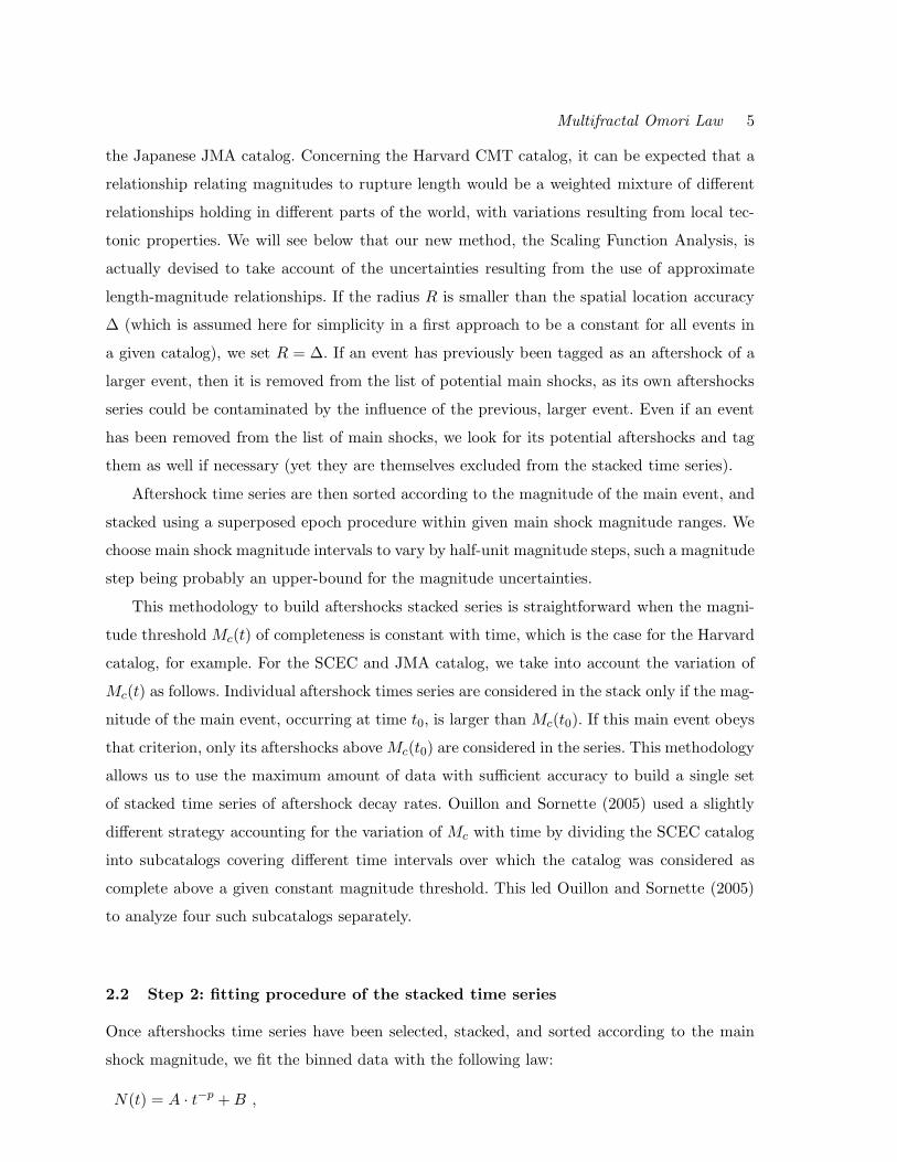
2.2 Step 2: fitting procedure of the stacked time series

Once aftershocks time series have been selected, stacked, and sorted according to the main

shock magnitude, we fit the binned data with the following law:

N(t) = A · t−p + B ,

6 G.Ouillon, E. Ribeiro, D. Sornette

which includes an Omori-like power-law term and a constant background rate B. Here, N(t)

is the rate of triggered seismicity at time t after a main shock that occured at t = 0. The

time axis is binned in intervals according to a geometrical series so that the width of the time

intervals grows exponentially with time. We then simply count the number of aftershocks

contained within each bin, then divide this number by the linear size of the interval to obtain

the rate N . The fitting parameters A,B, p are then obtained by a standard grid search.

As the linear density of bins decreases as the inverse of time, each bin receives a weight

proportional to time, balancing the weight of data points along the time axis. In our binning,

the linear size of two consecutive intervals increases by a factor r > 1. Since the choice of r is

arbitrary, it is important to check for the robustness of the results with respect to r. We thus

performed fits on time series binned with 20 different values of r, from r = 1.1 to r = 3 by

step of 0.1. We then checked whether the fitted parameters A, B and p were stable with r. We

observed that the inverted parameters do not depend much on r, so that we computed the

average values and standard deviations of all fitting parameters over the 20 r values. For some

rare cases, we obtained p-values departing clearly from the average (generally for the largest

or smallest values of r) - we thus excluded them to perform a new estimate of p. In order to

provide reliable fits, we excluded the early times of the stacked series, where aftershock catalogs

appear to be incomplete (Kagan 2004). Finally, a p-value (and its uncertainty) determined

within the main shock magnitude interval [M1;M2] was thus associated with the magnitude

M1+M2

2 . Our approach extends that of Ouillon and Sornette (2005) who performed fits on the

same kind of data using only a single value r = 1.2.

For each magnitude range, we thus have 20 different binned time series corresponding to

different values of r. For the sake of clarity, we only plot the binned aftershocks time series

whose p-value is the closest to the average p-value obtained over the 20 different values r for

that magnitude range. Its fit using Eq. 1 will be plotted as well.

2.3 Step 3: scaling function analysis

The method presented above to fit binned data uses a magnitude-dependent spatio-temporal

window within which aftershocks are selected. Consider a main event E1 whose linear rupture

size is L. The present methodology assumes that any event located within a distance 2L of

E1 and occurring no more than 1 year after it is one of its aftershocks. Conversely, any event

located at the same distance but which occurred after only just a little more than 1 year

after the main shock is not considered as its aftershock but as a potential main shock E2,

with its own aftershocks sequence which can be used for stacking. Actually, any size for the

Multifractal Omori Law 7

time window to select aftershocks is quite arbitrary and will not remove the possibility that

the aftershocks sequence of event E2 may still be contaminated by the sequence triggered by

event E1, especially if M(E1) > M(E2). Since the formula of Wells and Coppersmith [1994]

does not strictly apply to each event in a given catalog, one can imagine many other scenarios

of such a contamination that may also originate in the underestimation of L. A step towards

taking into account this problem is to rewrite expression (1) for the time evolution of the

sequence triggered by E2 as

N(t) = A · t−p + B(t) , (2)

where B(t) is a non-stationnary function that describes both the constant background seismic-

ity rate and the decay of the sequence(s) triggered by E1 (and possibly other events occuring

prior to E2). Here, t is the time elapsed since the event E2 occurred, as we want to characterize

the sequence which follows that event. As the event E1 occurred before the event E2, B(t)

is not singular at t = 0. It is thus a regular contribution to N(t), which we expect do decay

rather slowly, so that it can be approximated by a polynomial of low degree nB. We thus

rewrite Eq. 2 as

N(t) = A · t−p +nB∑

i=0

biti , (3)

where the sum on the right-hand side now stands for B(t). We have a priori no information

on the precise value of nB. For nB = 0, we recover the constant background term B of

expression (1). On the other hand, nB might be arbitrarily large in which case the coefficients

bi’s can be expected to decrease sufficiently fast with the order i to ensure convergence, so

that only the few first terms of the sum will contribute significantly to B(t). Their number

will depend on the fluctuations of the seismicity rate at times prior to the event E2. The effect

of this polynomial trend is to slow down the apparent time decay of the aftershocks sequence

triggered by event E2, hence possibly leading to the determination of a spurious small p-value.

This could be a candidate explanation for Ouillon and Sornette (2005)’s report of small values

of p’s for main events with small magnitudes. One could argue that their stacked aftershocks

time series might be contaminated by the occurrence of previous, much larger events (as well

as of previous, smaller but numerous events).

In order to address this question, that is, to take account of the possible time-dependence

of B, two strategies are possible:

(i) The 20 different binned time series can be fitted using Eq. (3) with the unknowns being

A, nB and the b′is,

8 G.Ouillon, E. Ribeiro, D. Sornette

(ii) One can use weights in the fitting procedure of the original data so that the polynomial

trend is removed. One is then left with a simple determination of A and p alone.

We have implemented the second strategy in the form of what we refer to as the “scaling

function analysis”. The Appendix describes in details this method that we have developed,

inspired by the pioneering work of Bacri et al. (1993), and presents several tests performed

on synthetic time series to illustrate its performance and the sensitivity of the results to the

parameters.

3 RESULTS

3.1 The Southern California catalog

3.1.1 Selection of the data

Ouillon and Sornette (2005) have analyzed the magnitude-dependence of the p-value for af-

tershocks sequences in Southern California. However, since we have here developed different

methods to build binned stacked series and to fit those series, it is instructive to reprocess the

Southern California data in order to 1) test the robustness of Ouillon and Sornette (2005)’s

previous results and 2) provide a benchmark against which to compare the results obtained

with the other catalogs (Japan and Harvard). This also provides a training ground for the

new scaling function analysis method.

The SCEC catalog we use is the same as in (Ouillon and Sornette 2005), except that it now

spans a larger time interval (1932 − 2006 inclusive). The magnitude completeness threshold

is taken with the same time dependence as in (Ouillon and Sornette 2005): M0 = 3.0 from

1932 to 1975, M0 = 2.5 from 1975 to 1992, M0 = 2.0 from 1992 to 1994, and M0 = 1.5 since

1994. We assume a value ∆ = 5 km for the spatial location accuracy (instead of 10 km in

Ouillon and Sornette (2005)). This parameterization allows us to decluster the whole catalog

and build a catalog of aftershocks, as previously explained.

3.1.2 An anomalous zone revealed by the Scaling Function Analysis

The obtained binned stacked series are very similar to those presented by Ouillon and Sornette

(2005). However, the scaling function analysis reveals deviations from a pure power-law scaling

of the aftershock sequences, which take different shapes for different magnitude ranges, as we

now describe.

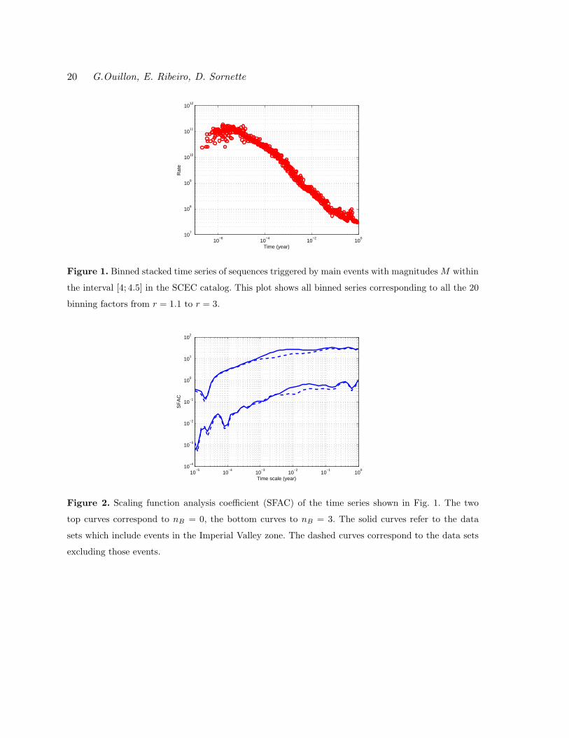
Let us first consider Fig. 1, which shows the binned stacked series obtained for main shock

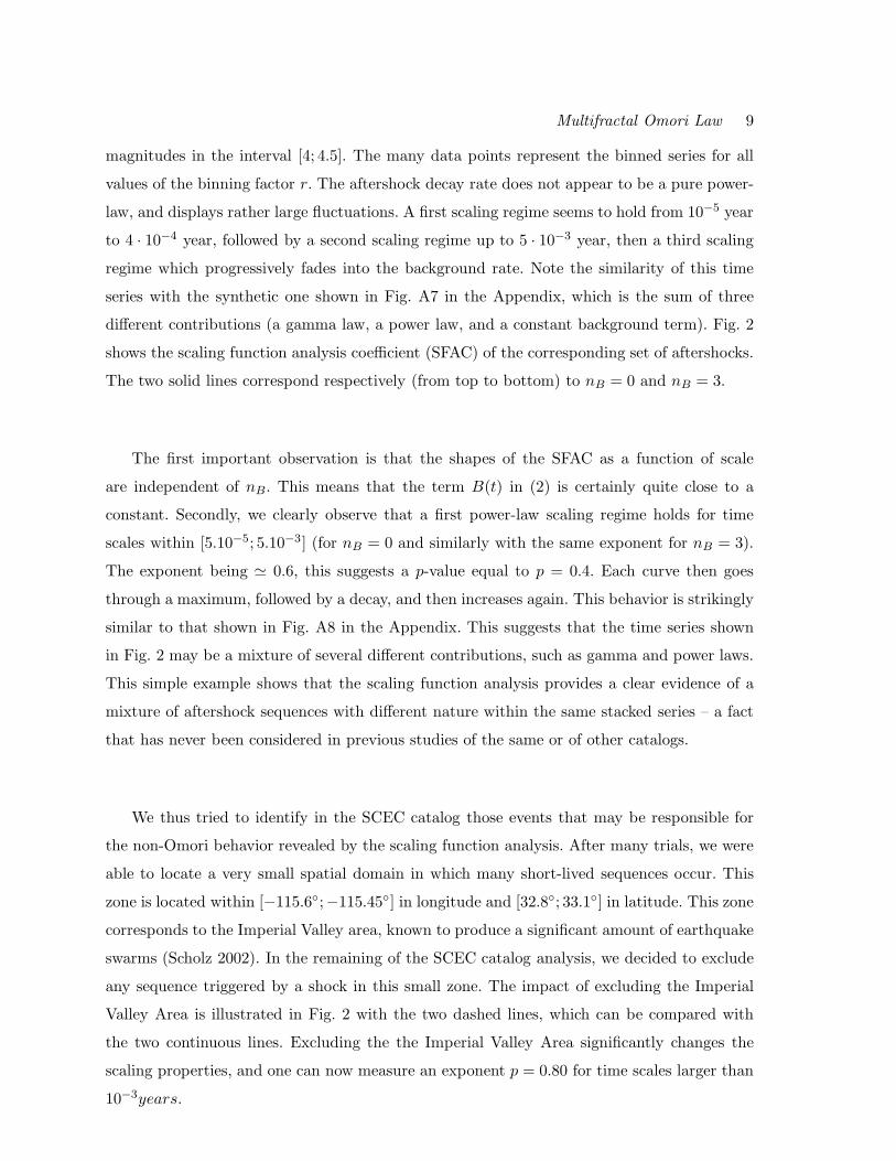
Multifractal Omori Law 9

magnitudes in the interval [4; 4.5]. The many data points represent the binned series for all

values of the binning factor r. The aftershock decay rate does not appear to be a pure power-

law, and displays rather large fluctuations. A first scaling regime seems to hold from 10−5 year

to 4 · 10−4 year, followed by a second scaling regime up to 5 · 10−3 year, then a third scaling

regime which progressively fades into the background rate. Note the similarity of this time

series with the synthetic one shown in Fig. A7 in the Appendix, which is the sum of three

different contributions (a gamma law, a power law, and a constant background term). Fig. 2

shows the scaling function analysis coefficient (SFAC) of the corresponding set of aftershocks.

The two solid lines correspond respectively (from top to bottom) to nB = 0 and nB = 3.

The first important observation is that the shapes of the SFAC as a function of scale

are independent of nB. This means that the term B(t) in (2) is certainly quite close to a

constant. Secondly, we clearly observe that a first power-law scaling regime holds for time

scales within [5.10−5; 5.10−3] (for nB = 0 and similarly with the same exponent for nB = 3).

The exponent being ≃ 0.6, this suggests a p-value equal to p = 0.4. Each curve then goes

through a maximum, followed by a decay, and then increases again. This behavior is strikingly

similar to that shown in Fig. A8 in the Appendix. This suggests that the time series shown

in Fig. 2 may be a mixture of several different contributions, such as gamma and power laws.

This simple example shows that the scaling function analysis provides a clear evidence of a

mixture of aftershock sequences with different nature within the same stacked series – a fact

that has never been considered in previous studies of the same or of other catalogs.

We thus tried to identify in the SCEC catalog those events that may be responsible for

the non-Omori behavior revealed by the scaling function analysis. After many trials, we were

able to locate a very small spatial domain in which many short-lived sequences occur. This

zone is located within [−115.6◦;−115.45◦] in longitude and [32.8◦; 33.1◦] in latitude. This zone

corresponds to the Imperial Valley area, known to produce a significant amount of earthquake

swarms (Scholz 2002). In the remaining of the SCEC catalog analysis, we decided to exclude

any sequence triggered by a shock in this small zone. The impact of excluding the Imperial

Valley Area is illustrated in Fig. 2 with the two dashed lines, which can be compared with

the two continuous lines. Excluding the the Imperial Valley Area significantly changes the

scaling properties, and one can now measure an exponent p = 0.80 for time scales larger than

10−3years.

10 G.Ouillon, E. Ribeiro, D. Sornette

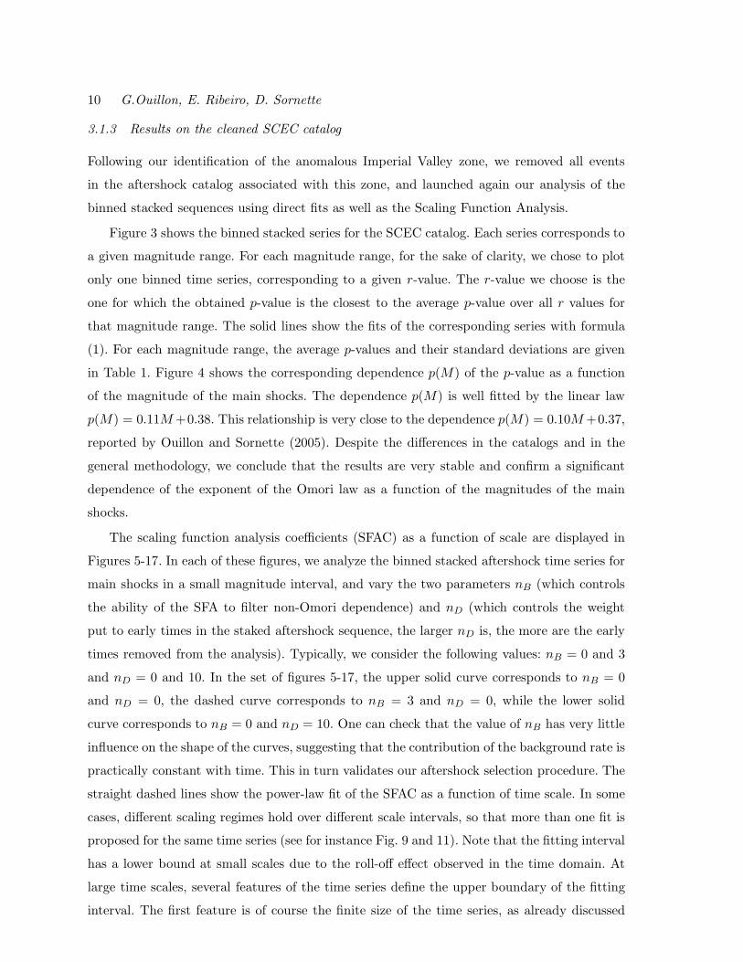
3.1.3 Results on the cleaned SCEC catalog

Following our identification of the anomalous Imperial Valley zone, we removed all events

in the aftershock catalog associated with this zone, and launched again our analysis of the

binned stacked sequences using direct fits as well as the Scaling Function Analysis.

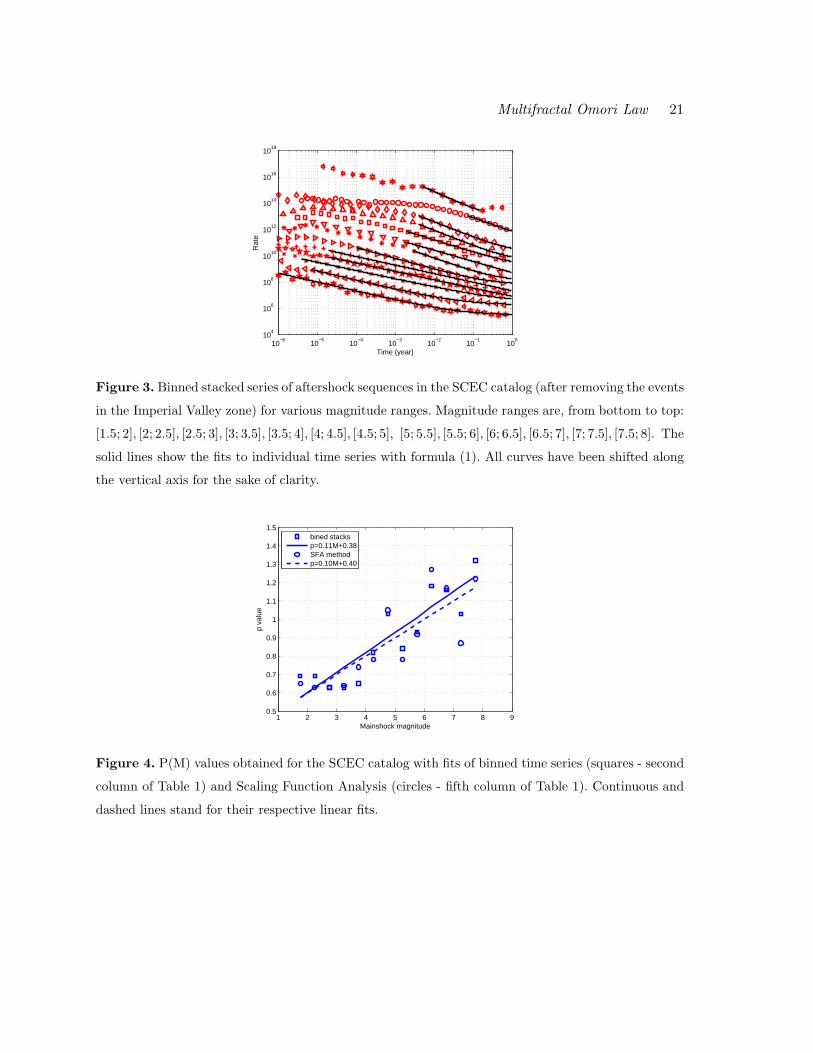
Figure 3 shows the binned stacked series for the SCEC catalog. Each series corresponds to

a given magnitude range. For each magnitude range, for the sake of clarity, we chose to plot

only one binned time series, corresponding to a given r-value. The r-value we choose is the

one for which the obtained p-value is the closest to the average p-value over all r values for

that magnitude range. The solid lines show the fits of the corresponding series with formula

(1). For each magnitude range, the average p-values and their standard deviations are given

in Table 1. Figure 4 shows the corresponding dependence p(M) of the p-value as a function

of the magnitude of the main shocks. The dependence p(M) is well fitted by the linear law

p(M) = 0.11M +0.38. This relationship is very close to the dependence p(M) = 0.10M +0.37,

reported by Ouillon and Sornette (2005). Despite the differences in the catalogs and in the

general methodology, we conclude that the results are very stable and confirm a significant

dependence of the exponent of the Omori law as a function of the magnitudes of the main

shocks.

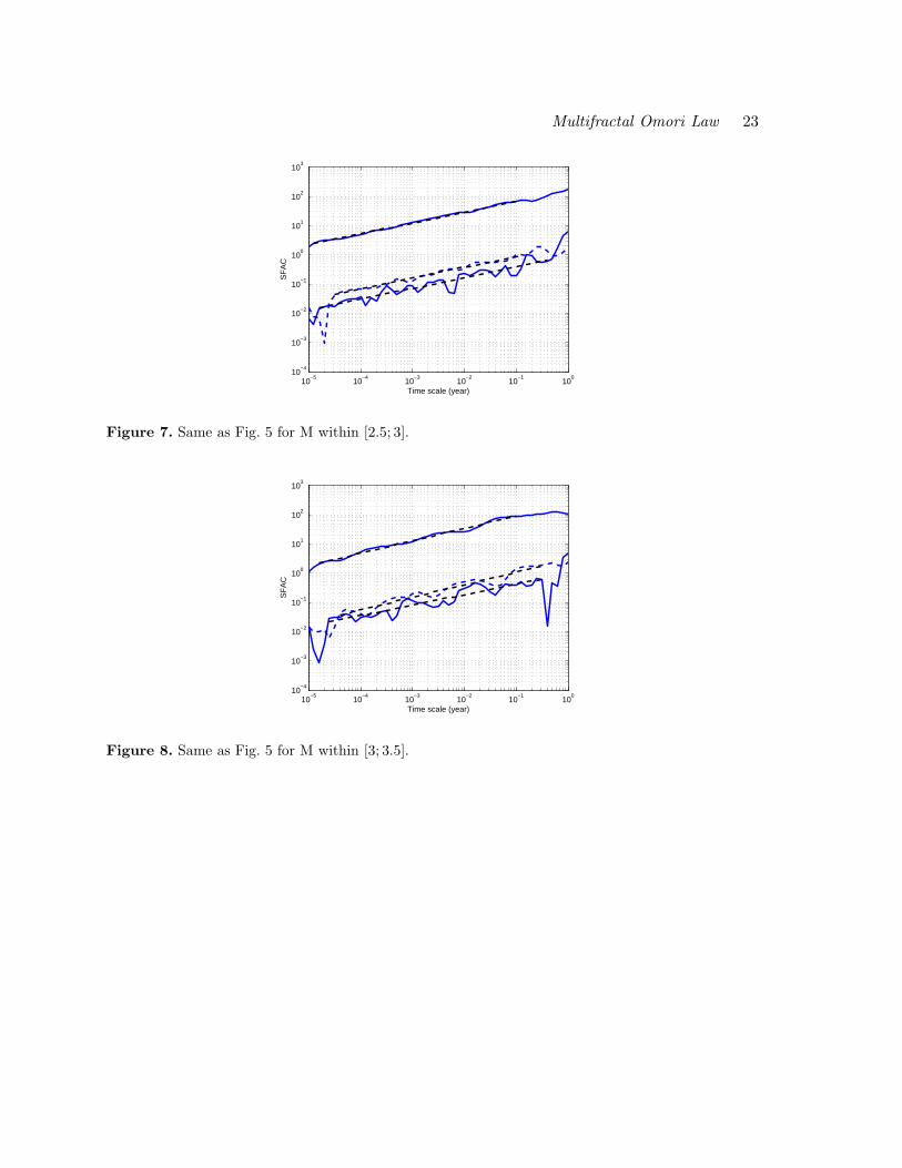
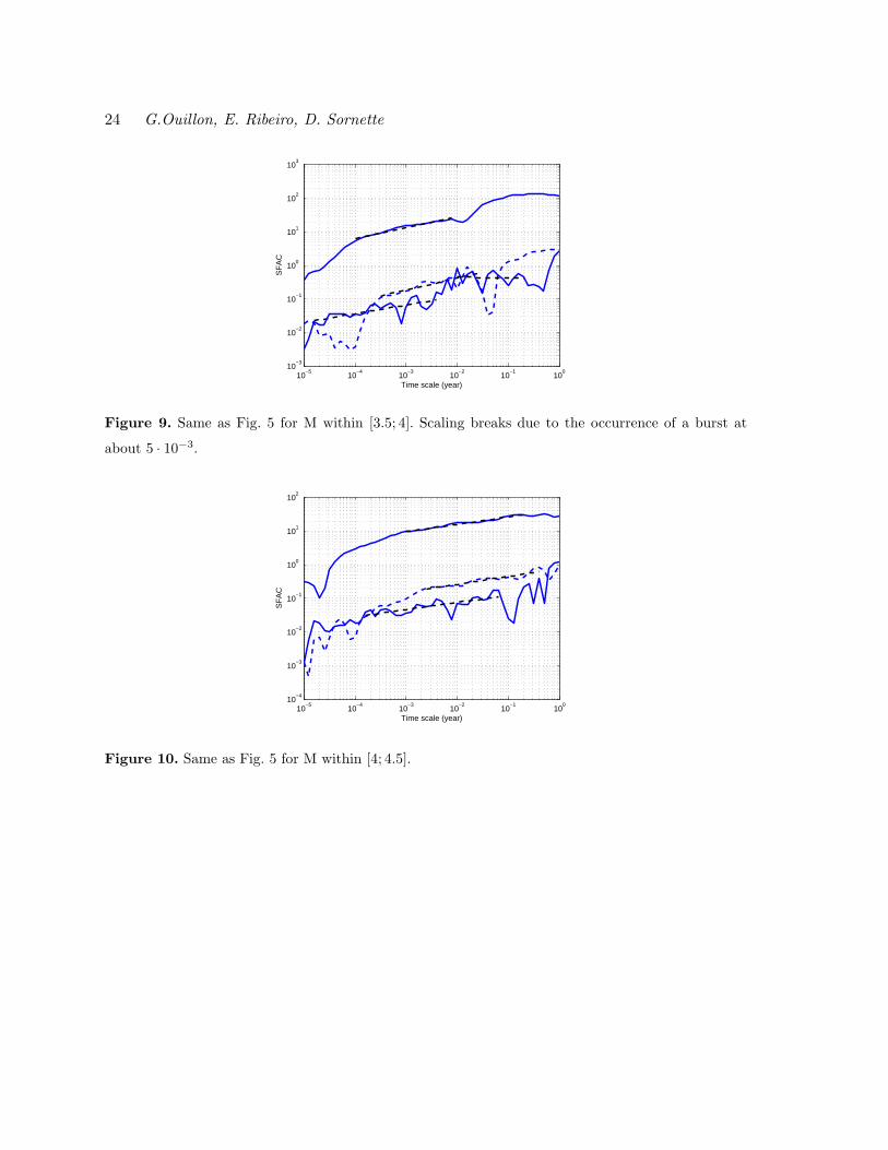
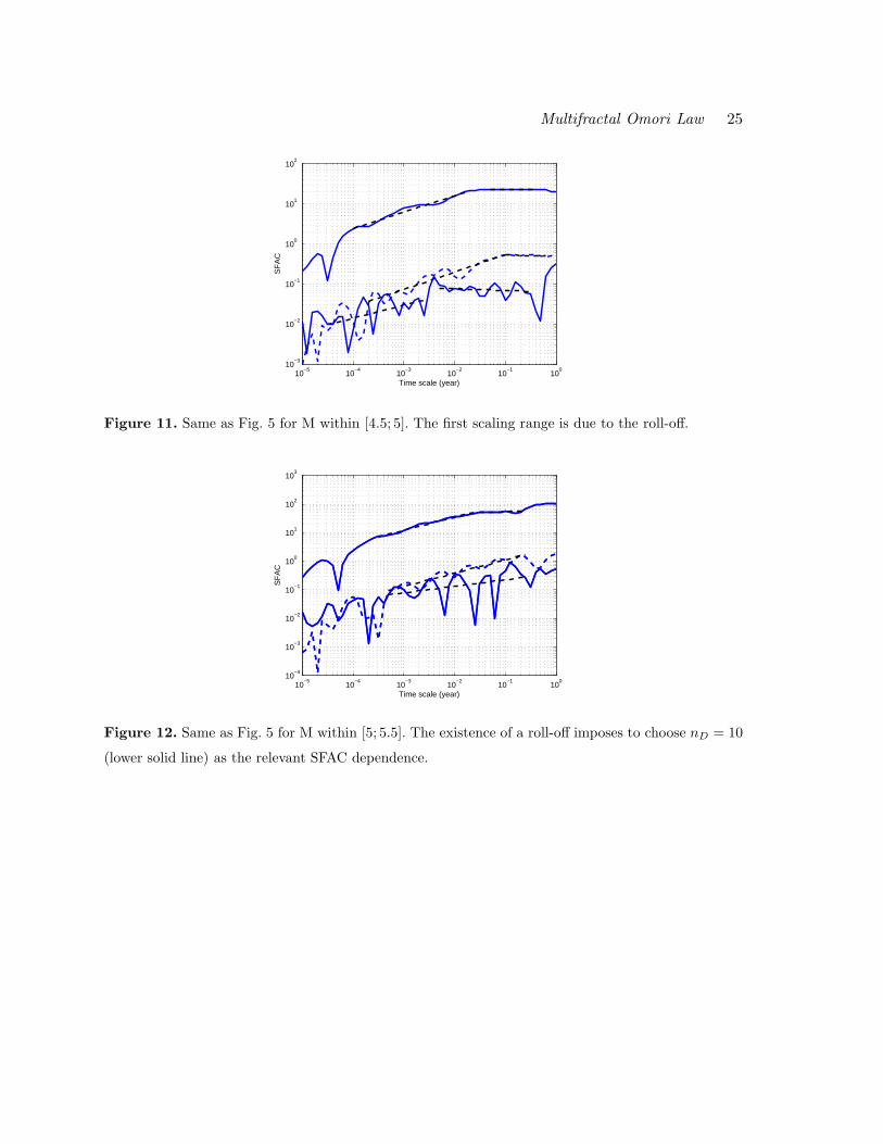
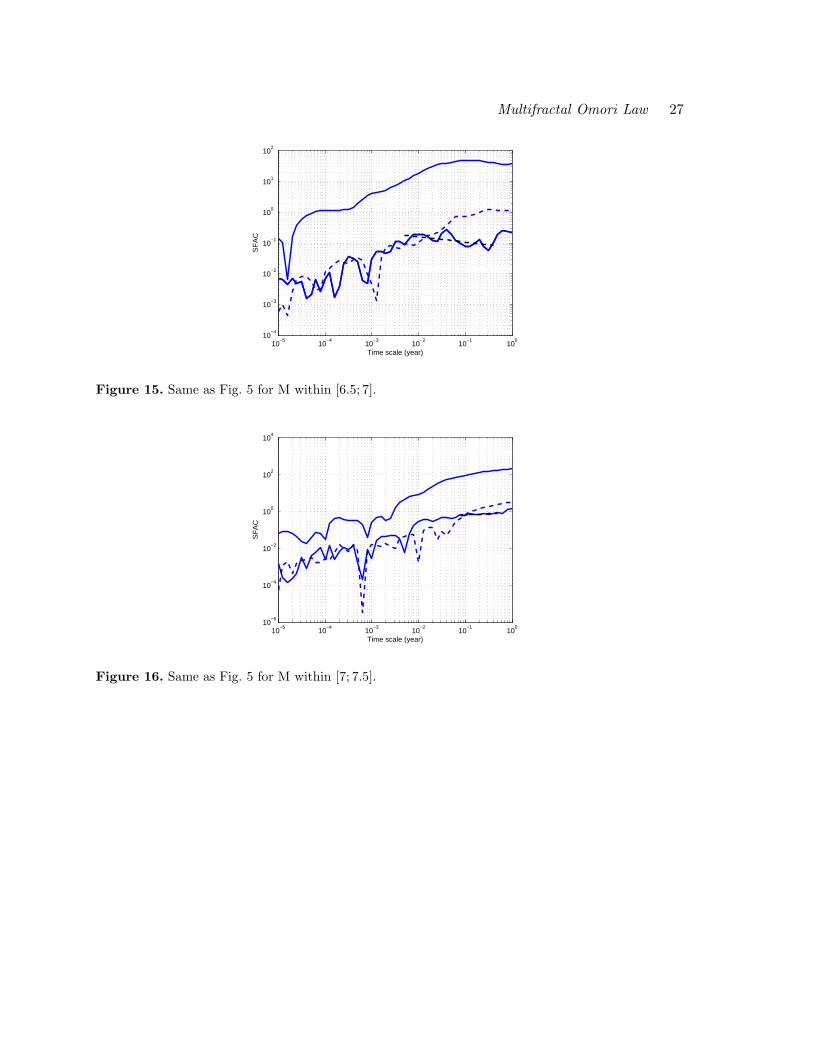
The scaling function analysis coefficients (SFAC) as a function of scale are displayed in

Figures 5-17. In each of these figures, we analyze the binned stacked aftershock time series for

main shocks in a small magnitude interval, and vary the two parameters nB (which controls

the ability of the SFA to filter non-Omori dependence) and nD (which controls the weight

put to early times in the staked aftershock sequence, the larger nD is, the more are the early

times removed from the analysis). Typically, we consider the following values: nB = 0 and 3

and nD = 0 and 10. In the set of figures 5-17, the upper solid curve corresponds to nB = 0

and nD = 0, the dashed curve corresponds to nB = 3 and nD = 0, while the lower solid

curve corresponds to nB = 0 and nD = 10. One can check that the value of nB has very little

influence on the shape of the curves, suggesting that the contribution of the background rate is

practically constant with time. This in turn validates our aftershock selection procedure. The

straight dashed lines show the power-law fit of the SFAC as a function of time scale. In some

cases, different scaling regimes hold over different scale intervals, so that more than one fit is

proposed for the same time series (see for instance Fig. 9 and 11). Note that the fitting interval

has a lower bound at small scales due to the roll-off effect observed in the time domain. At

large time scales, several features of the time series define the upper boundary of the fitting

interval. The first feature is of course the finite size of the time series, as already discussed

Multifractal Omori Law 11

above. The other property is related to the occurrence of secondary aftershock sequences, that

appear as localized bursts in the time series and distort it. For example, consider the time

series corresponding to the main shock magnitude range [1.5; 2] in Fig. 3, for which one can

observe the occurrence of a burst at a time of about 6 ·10−2year. This corresponds to a break

in the power law scaling of the SFAC at time scales of about 10−1 year. We thus only retained

the p-values measured using time scales before such bursts occur. As the magnitude of the

main shocks increases, the roll-off at small time scales extends to larger and larger time scales,

so that the measure of p proves impossible when nD = 0. This is the reason why we consider

the p-value measured with nD = 10 and nB = 0 as more reliable, especially for the large main

shock magnitudes. Table 1 summarizes all our results obtained for the p-value using the SFA

method. Notice that they agree very well with those obtained with the direct binning and

fitting approach. Figure 4 shows the p-values obtained with nD = 10 as a function of M . A

linear fit gives p(M) = 0.10M + 0.40, in excellent agreement with the results obtained using

the direct fit to the binned stacked series.

3.2 JMA catalog

The JMA catalog used here extends over a period from May 1923 to January 2001 inclusive.

We restricted our analysis to the zone (+130◦E to +145◦E in longitude and 30◦N to 45◦N

in latitude), so that its northern and eastern boundaries fit with those of the catalog, while

the southern and eastern boundaries fit with the geographic extension of the main japanese

islands. This choice selects the earthquakes with the best spatial location accuracy, close to

the inland stations of the seismic network. In our analysis, the main shocks are taken from

this zone and in the upper 70 km, while we take into account their aftershocks which occur

outside and at all depths.

Our detailed analysis of the aftershock time series at spatial scales down to 20 km reveals

a couple of zones where large as well as small main events are not followed by the standard

Omori power-law relaxation of seismicity. The results concerning these zones will be presented

elsewhere. Here, we simply removed the corresponding events from the analysis. The geograph-

ical boundaries of these two anomalous zones are [130.25◦E; 130.375◦E]× [32.625◦N; 32.75◦N]

for the first zone, and [138.75◦E; 139.5◦E] × [33◦N; 35◦N] for the second one (the so-called

Izu islands area). This last zone is well-known to be the locus of earthquakes swarms, which

may explain the observed anomalous aftershock relaxation. We have been conservative in the

definition of this zone along the latitude dimension so as to avoid possible contamination in

the data analysis which would undermine the needed precise quantification of the p-values.

12 G.Ouillon, E. Ribeiro, D. Sornette

The completeness of the JMA catalog is not constant in time, as the quality of the seismic

network increased more recently. We computed the distribution of event sizes year by year,

and used in a standard way (Kagan 2003) the range over which the Gutenberg-Richter law

is reasonably well-obeyed to infer the lower magnitude of completeness. For our analysis,

we smooth out the time dependence of the magnitude threshold Mc above which the JMA

catalog can be considered complete from roughly Mc(1923) = 6, to Mc(1930 − 1960) = 5,

Mc(1960− 1990) = 4.5 with a final progressive decrease to Mc = 2.5 for the most recent past.

This time-dependence of the threshold Mc(t) will be used for the selection of main shocks and

aftershocks. The assumed value of events location uncertainty ∆ has been set to 10 km.

3.2.1 Binned stacked times series

For the JMA catalog, 12 magnitude intervals were used from [2.5; 3] to [8; 8.5]). Figure 18 shows

the 12 individual stacked aftershocks time series and their fits (using a value for the binning

factor r determined as described above for the SCEC catalog). Figure 19 plots the exponent

p averaged over the 20 values of r as a function of the middle value of the corresponding

magnitude interval. These values are also given in Table 2. A linear fit gives p = 0.06M +0.58

(shown by the solid straight line in Fig.19). The p-value thus seems much less dependent on

the main shock magnitude M than for the SCEC catalog.

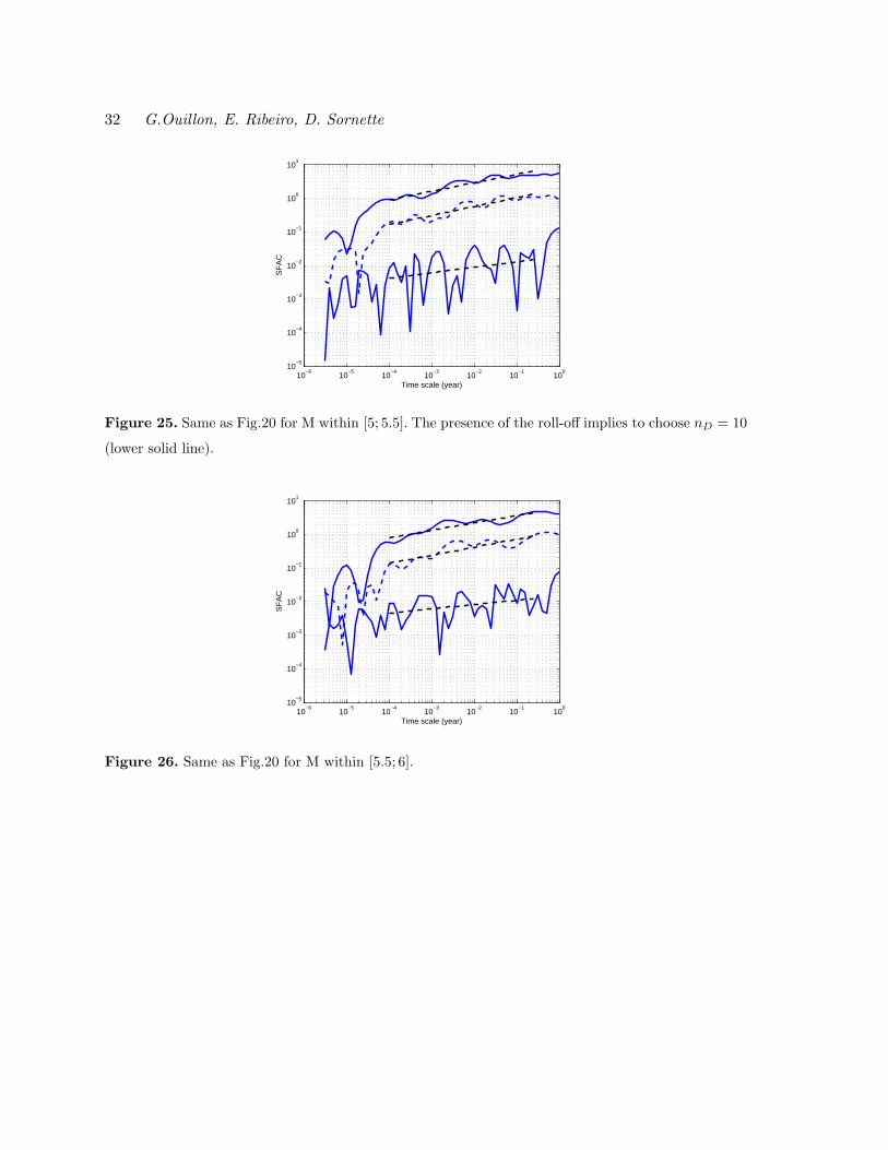
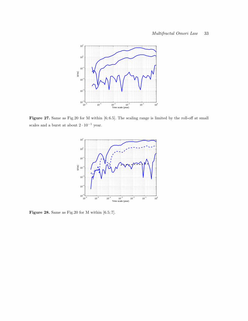
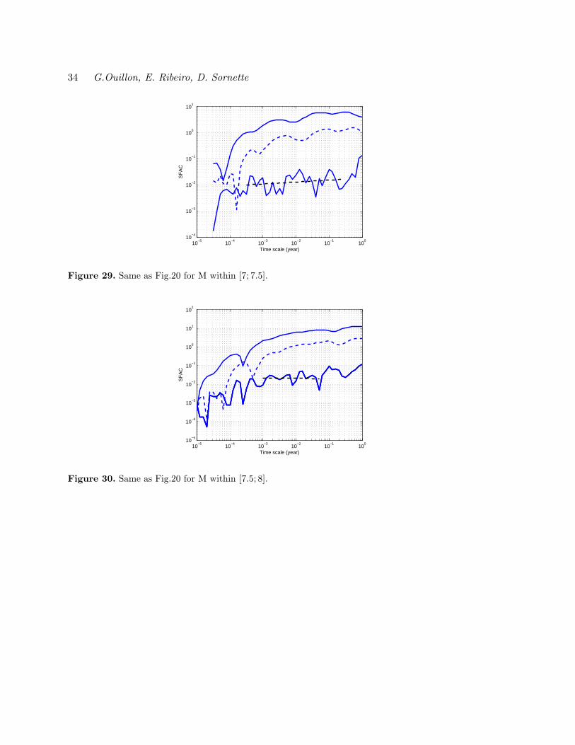
3.2.2 SFA method

We also applied the SFA method to the same dataset. We checked that the resulting curves

were not dependent on the value of nB, suggesting that the background term is constant. Fig.

20 to 31 show the SFAC as a function of scale for different values of (nB, nD): (0, 0) (upper

solid curve), (3, 0) (dashed curve), and (0, 10) (lower solid curve). One can observe that some

of them exhibit a more complex scaling behavior than found for the SCEC catalog. This may

reveal a complex mixture of sequences with different properties (see for example Fig.24 and

26 which exhibit two characteristic time scales of about 10−3 year and 10−1 year), despite

our efforts to exclude zones that have a large number of swarms. The characteristic scales

disappear with nD = 10, but this may just be due to the strongly oscillating character of the

filter and therefore of the SFAC which may mask its local maxima. Table 2 and Fig. 19 report

the corresponding measured exponents. There is a general agreement between the p-values

mesured using different sets of parameters or methods. Using the set of p-values corresponding

to nB = 0 and nD = 10, we obtain the following dependence of the p-value as a function of

the magnitude M of the main shocks: p = 0.07M + 0.50. Excluding the largest magnitude

Multifractal Omori Law 13

range leads to a weaker dependence: p = 0.05M +0.58. Note that the dispersion of data points

around the best fit line is much smaller for the p-values obtained by the SFA method. This

thus confirms the weaker dependence of p as a function of M for the JMA catalog. Our SFA

suggests that this weaker dependence may have to do with the presence of many swarms in

the Japanese catalogs. Our methodology has allowed us to diagnose the existence of mixtures

of aftershock relaxation regimes, probably swarms and standard Omori standard sequences.

3.3 The Harvard CMT catalog

The worldwide CMT Harvard catalog used here goes from January 1976 to August 2006

inclusive. This catalog is considered to be complete for events of magnitude 5.5 or larger. We

thus removed events below this threshold before searching for the aftershocks. Due to the

rather small number of events in this catalog, we did not impose any limit on the depth of

events. The assumed value of location uncertainties has been set to ∆ = 10 km. Note that

instead of using the hypocenter location as we did for the two other catalogs, we considered

the location of the centroid, which is certainly closer to the center of the aftershock zone.

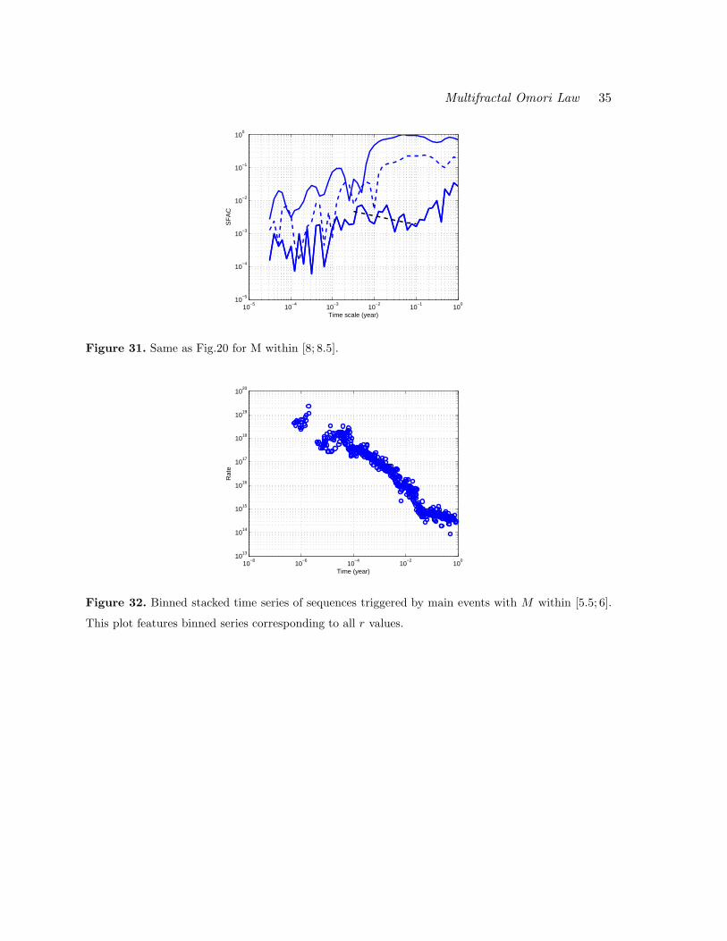
3.3.1 Binned stacks

For the Harvard catalog, seven magnitude intervals were used from [5.5; 6] to [9; 9.5] (the

[8.5; 9] interval being empty). The binned stacked times series for the [5.5; 6] magnitude range

is shown in Fig. 32, using all values of the binning factor r. The underlying decay law is

obviously not of Omori-type, which suggest that it is the result from the superposition of

different distributions. We attribute the different behavior of the ([5.5; 6]) magnitude range

to the fact that the corresponding times series contain many events occurring at mid-oceanic

ridges, where many swarms are known to occur. As very few events of magnitude > 6 occur

in this peculiar tectonic settings, swarms (from the mid-ocean ridges) do not contaminate

too much the time series associated with larger magnitude main shocks. We will see below

that the SFA confirms this intuition, and doesn’t provide any evidence of a power law scaling

for the ([5.5; 6]) magnitude range while the other magnitude ranges (except the largest) give

reliable estimates for the Omori exponent p.

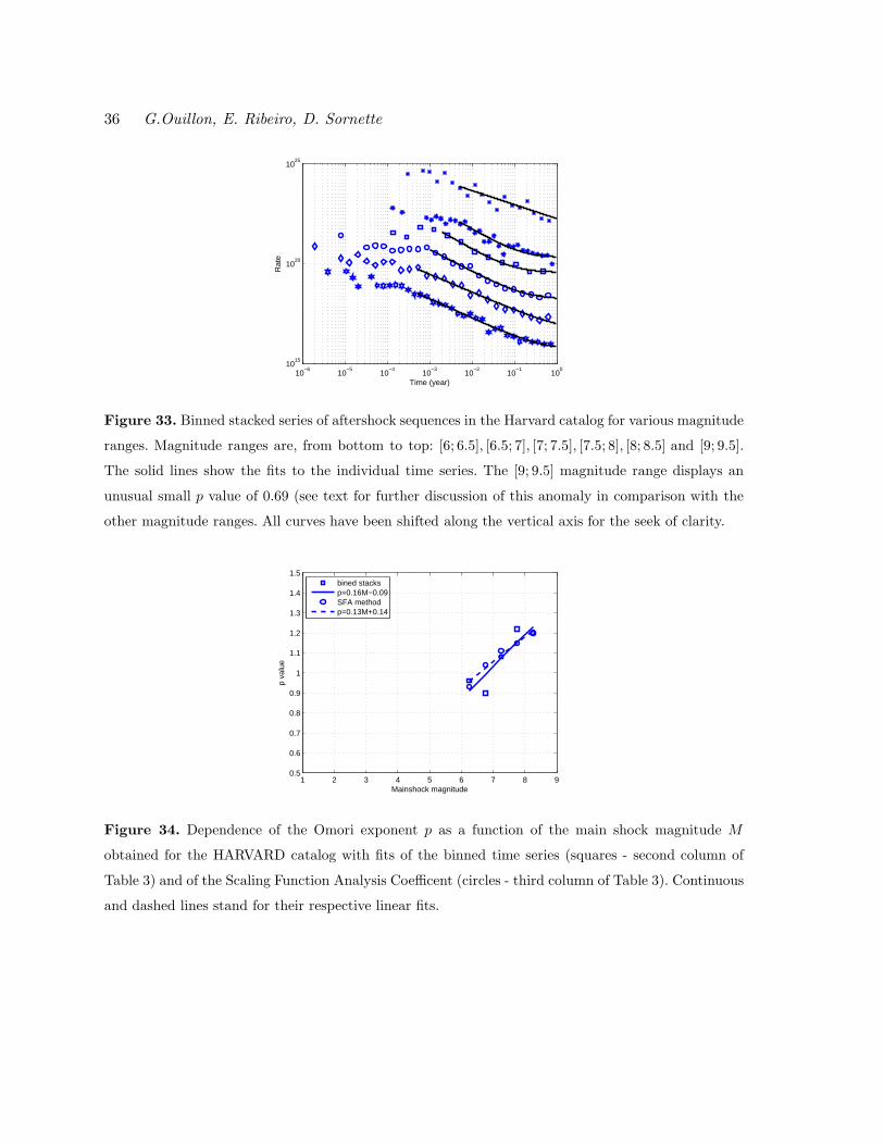
Figure 33 shows the six remaining stacked aftershocks time series and their fits (con-

structed as in Figs. 3 and 18). One can clearly observe Omori-like behaviors. The correspond-

ing p-values are reported in Table 3 and in Fig. 34 as a function of the main shock magnitudes

M . The linear fit of the dependence of p as a function of M gives p(M) = 0.16M − 0.09.

The magnitude dependence of M is thus much larger than found in Southern California but

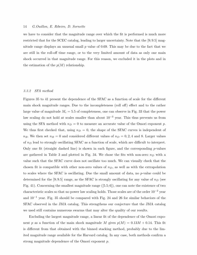
14 G.Ouillon, E. Ribeiro, D. Sornette

we have to consider that the magnitude range over which the fit is performed is much more

restricted that for the SCEC catalog, leading to larger uncertainty. Note that the [9; 9.5] mag-

nitude range displays an unusual small p value of 0.69. This may be due to the fact that we

are still in the roll-off time range, or to the very limited amount of data as only one main

shock occurred in that magnitude range. For this reason, we excluded it in the plots and in

the estimation of the p(M) relationship.

3.3.2 SFA method

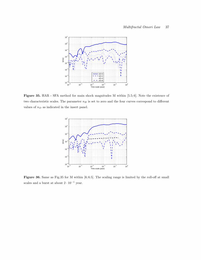
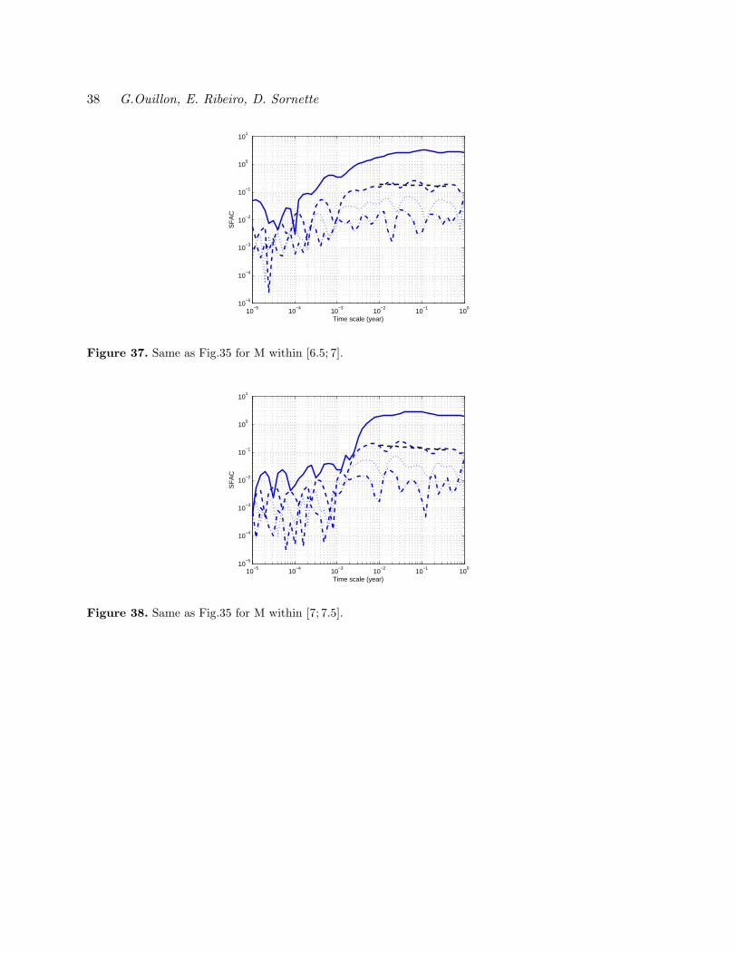
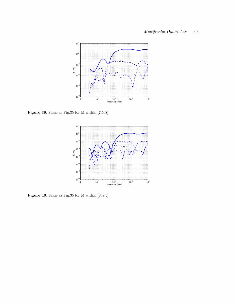
Figures 35 to 41 present the dependence of the SFAC as a function of scale for the different

main shock magnitude ranges. Due to the incompleteness (roll off) effect and to the rather

large value of magnitude Mc = 5.5 of completeness, one can observe in Fig. 33 that the power

law scaling do not hold at scales smaller than about 10−3 year. This thus prevents us from

using the SFA method with nD = 0 to measure an accurate value of the Omori exponent p.

We thus first checked that, using nD = 0, the shape of the SFAC curves is independent of

nB. We then set nB = 0 and considered different values of nD = 0, 2, 4 and 8. Larger values

of nD lead to strongly oscillating SFAC as a function of scale, which are difficult to interpret.

Only one fit (straight dashed line) is shown in each figure, and the corresponding p-values

are gathered in Table 3 and plotted in Fig. 34. We chose the fits with non-zero nD with a

value such that the SFAC curve does not oscillate too much. We can visually check that the

chosen fit is compatible with other non-zero values of nD, as well as with the extrapolation

to scales where the SFAC is oscillating. Due the small amount of data, no p-value could be

determined for the [9; 9.5] range, as the SFAC is strongly oscillating for any value of nD (see

Fig. 41). Concerning the smallest magnitude range ([5.5; 6]), one can note the existence of two

characteristic scales so that no power law scaling holds. Those scales are of the order 10−2 year

and 10−1 year. Fig. 35 should be compared with Fig. 24 and 26 for similar behaviors of the

SFAC observed in the JMA catalog. This strengthens our conjecture that the JMA catalog

we used still contains numerous swarms that may alter the quality of our results.

Excluding the largest magnitude range, a linear fit of the dependence of the Omori expo-

nent p as a function of the main shock magnitude M gives p(M) = 0.13M + 0.14. This fit

is different from that obtained with the binned stacking method, probably due to the lim-

ited magnitude range available for the Harvard catalog. In any case, both methods confirm a

strong magnitude dependence of the Omori exponent p.

Multifractal Omori Law 15

4 CONCLUSION

We have introduced two methods to analyze the time-relaxation of aftershock sequences. One

is based on standard binning methods, while the other one is based on the wavelet transform

adapted to the present problem, leading to the Scaling Function Analysis (SFA) method.

We analyzed three different catalogs using a very simple declustering technique based on the

definition of a magnitude-dependent space-time window for each event. The SFA method

showed that this declustering method was certainly sufficient as aftershock sequences of small

events are not contaminated by aftershock sequences triggered by previous larger events. Both

methods yield very similar results for each of the three catalogs, suggesting that our results

are reliable. The SFA method confirms the results of the binning method already presented

by Ouillon and Sornette (2005), showing that the p-value of the Omori law increases linearly

as a function of the magnitude of the main shock for the SCEC catalog. Those results are

also in good agreement with the p(M) dependence measured for the Harvard CMT catalog

(see Figs. 42 and 43 which present the results for both catalogs and methods). The magnitude

dependence of p is much less obvious for the Japanese JMA catalog, but the SFA method

clearly diagnosed that a rather significant number of swarm sequences are still mixed with

more standard Omori-like sequences, so that the obtained results should not be considered

as representative of the latter. Overall, the extensive analysis presented here strengthens

the validity of the major prediction of the MSA model, namely that the relaxation rate of

aftershock sequences is an Omori power law with an exponent p increasing significantly with

the main shock magnitude. To the best of our knowledge, the MSA model is the only one

which predict this remarkable multifractal property.

16 G.Ouillon, E. Ribeiro, D. Sornette

REFERENCES

Bacry, E., J. Muzy, and A. Arneodo, 1993. Singularity spectrum of fractal signals from wavelet analysis:

exact results, Journal of Statistical Physics, 70 (3/4), 635-674.

Ciliberto, S., A. Guarino, and R. Scorretti, 2001. The effect of disorder on the fracture nucleation

process, Physica D, 158, 83-104.

Dieterich, J., 1994. A constitutive law for rate of earthquake production and its application to earth-

quake clustering, J. Geophys. Res.,99(B2), 2601-2618.

Kagan, Y.Y., 2003. Accuracy of modern global earthquake catalogs, Phys. Earth & Plan. Int.,135

(2-3), 173-209.

Kagan, Y.Y., 2004. Short-term properties of earthquake catalogs and models of earthquake source,

Bull. Seism. Soc. Am.,94 (4), 1207-1228.

Kagan, Y.Y., and L. Knopoff, 1981. Stochastic synthesis of earthquake catalogs, J. Geophys. Res., 86,

2853-2862.

King, G.C.P., R.S. Stein, and J. Lin, 1994. Static stress changes and the triggering of earthquakes,

Bull. Seism. Soc. Am.,84 (3), 935-953.

Miltenberger, P., D. Sornette and C. Vanneste, 1993. Fault self-organization as optimal random paths

selected by critical spatio-temporal dynamics of earthquakes, Phys.Rev.Lett.,71, 3604-3607.

Ogata, Y., 1988. Statistical models for earthquake occurrence and residual analysis for point processes,

J. Am. stat. Assoc., 83, 9-27.

Ouillon, G. and D. Sornette, 2005. Magnitude-Dependent Omori Law: Theory and Empirical Study,

J. Geophys. Res.,110, B04306, doi:10.1029/2004JB003311.

Saichev, A. and D. Sornette, 2005. Andrade, Omori and Time-to-failure Laws from Thermal Noise in

Material Rupture, Phys. Rev. E,71, 016608.

Saichev, A. and D. Sornette, 2006. Power law distribution of seismic rates: theory and data, Eur. Phys.

J. B,49, 377-401.

Scholz, C., 2002. The Mechanics of Earthquakes and Faulting, 2nd Ed., Cambridge University Press,

Cambridge.

Sornette, D., 1991. Self-organized criticality in plate tectonics, in the proceedings of the NATO ASI

“Spontaneous formation of space-time structures and criticality,” Geilo, Norway 2-12 april 1991,

edited by T. Riste and D. Sherrington, Dordrecht, Boston, Kluwer Academic Press (1991), 349,

57-106.

Sornette, D., P. Miltenberger and C. Vanneste, 1994. Statistical physics of fault patterns self-organized

by repeated earthquakes, Pure and Applied Geophysics,142 (3/4), 491-527.

Sornette, D. and G. Ouillon, 2005. Multifractal Scaling of Thermally-Activated Rupture Processes,

Phys. Rev. Lett.,94, 038501.

Stein, R.S., Earthquake conversations, 2003. Scientific American, 288 (1), 72-79.

Wells, D.L., and K.J. Coppersmith, 1994. New empirical relationships among magnitude, rupture

Multifractal Omori Law 17

length, rupture width, rupture area, and surface displacement, Bull. Seism. Soc. Am.,84(4), 974-

1002.

18 G.Ouillon, E. Ribeiro, D. Sornette

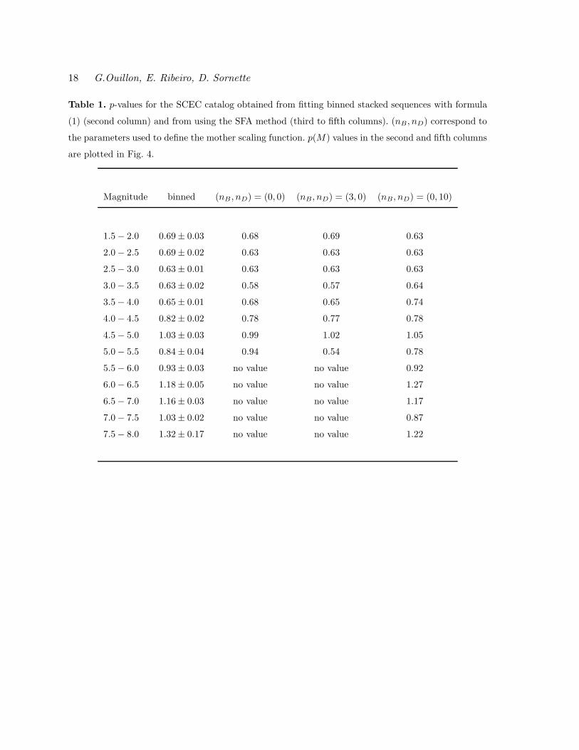
Table 1. p-values for the SCEC catalog obtained from fitting binned stacked sequences with formula

(1) (second column) and from using the SFA method (third to fifth columns). (nB, nD) correspond to

the parameters used to define the mother scaling function. p(M) values in the second and fifth columns

are plotted in Fig. 4.

Magnitude binned (nB , nD) = (0, 0) (nB, nD) = (3, 0) (nB, nD) = (0, 10)

1.5 − 2.0 0.69 ± 0.03 0.68 0.69 0.63

2.0 − 2.5 0.69 ± 0.02 0.63 0.63 0.63

2.5 − 3.0 0.63 ± 0.01 0.63 0.63 0.63

3.0 − 3.5 0.63 ± 0.02 0.58 0.57 0.64

3.5 − 4.0 0.65 ± 0.01 0.68 0.65 0.74

4.0 − 4.5 0.82 ± 0.02 0.78 0.77 0.78

4.5 − 5.0 1.03 ± 0.03 0.99 1.02 1.05

5.0 − 5.5 0.84 ± 0.04 0.94 0.54 0.78

5.5 − 6.0 0.93 ± 0.03 no value no value 0.92

6.0 − 6.5 1.18 ± 0.05 no value no value 1.27

6.5 − 7.0 1.16 ± 0.03 no value no value 1.17

7.0 − 7.5 1.03 ± 0.02 no value no value 0.87

7.5 − 8.0 1.32 ± 0.17 no value no value 1.22

Multifractal Omori Law 19

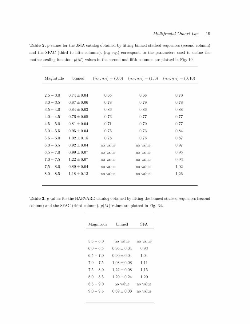
Table 2. p-values for the JMA catalog obtained by fitting binned stacked sequences (second column)

and the SFAC (third to fifth columns). (nB, nD) correspond to the parameters used to define the

mother scaling function. p(M) values in the second and fifth columns are plotted in Fig. 19.

Magnitude binned (nB , nD) = (0, 0) (nB, nD) = (1, 0) (nB, nD) = (0, 10)

2.5 − 3.0 0.74 ± 0.04 0.65 0.66 0.70

3.0 − 3.5 0.87 ± 0.06 0.78 0.79 0.78

3.5 − 4.0 0.84 ± 0.03 0.86 0.86 0.88

4.0 − 4.5 0.76 ± 0.05 0.76 0.77 0.77

4.5 − 5.0 0.81 ± 0.04 0.71 0.70 0.77

5.0 − 5.5 0.95 ± 0.04 0.75 0.73 0.84

5.5 − 6.0 1.02 ± 0.15 0.78 0.76 0.87

6.0 − 6.5 0.92 ± 0.04 no value no value 0.97

6.5 − 7.0 0.99 ± 0.07 no value no value 0.95

7.0 − 7.5 1.22 ± 0.07 no value no value 0.93

7.5 − 8.0 0.89 ± 0.04 no value no value 1.02

8.0 − 8.5 1.18 ± 0.13 no value no value 1.26

Table 3. p-values for the HARVARD catalog obtained by fitting the binned stacked sequences (second

column) and the SFAC (third column). p(M) values are plotted in Fig. 34.

Magnitude binned SFA

5.5 − 6.0 no value no value

6.0 − 6.5 0.96 ± 0.04 0.93

6.5 − 7.0 0.90 ± 0.04 1.04

7.0 − 7.5 1.08 ± 0.08 1.11

7.5 − 8.0 1.22 ± 0.08 1.15

8.0 − 8.5 1.20 ± 0.24 1.20

8.5 − 9.0 no value no value

9.0 − 9.5 0.69 ± 0.03 no value

20 G.Ouillon, E. Ribeiro, D. Sornette

10−6

10−4

10−2

100

107

108

109

1010

1011

1012

Time (year)

Rat

e

Figure 1. Binned stacked time series of sequences triggered by main events with magnitudes M within

the interval [4; 4.5] in the SCEC catalog. This plot shows all binned series corresponding to all the 20

binning factors from r = 1.1 to r = 3.

10−5

10−4

10−3

10−2

10−1

100

10−4

10−3

10−2

10−1

100

101

102

Time scale (year)

SF

AC

Figure 2. Scaling function analysis coefficient (SFAC) of the time series shown in Fig. 1. The two

top curves correspond to nB = 0, the bottom curves to nB = 3. The solid curves refer to the data

sets which include events in the Imperial Valley zone. The dashed curves correspond to the data sets

excluding those events.

Multifractal Omori Law 21

10−6

10−5

10−4

10−3

10−2

10−1

100

104

106

108

1010

1012

1014

1016

1018

Time (year)

Rat

e

Figure 3. Binned stacked series of aftershock sequences in the SCEC catalog (after removing the events

in the Imperial Valley zone) for various magnitude ranges. Magnitude ranges are, from bottom to top:

[1.5; 2], [2; 2.5], [2.5; 3], [3; 3.5], [3.5; 4], [4; 4.5], [4.5; 5], [5; 5.5], [5.5; 6], [6; 6.5], [6.5; 7], [7; 7.5], [7.5; 8]. The

solid lines show the fits to individual time series with formula (1). All curves have been shifted along

the vertical axis for the sake of clarity.

1 2 3 4 5 6 7 8 90.5

0.6

0.7

0.8

0.9

1

1.1

1.2

1.3

1.4

1.5

Mainshock magnitude

p va

lue

bined stacksp=0.11M+0.38SFA methodp=0.10M+0.40

Figure 4. P(M) values obtained for the SCEC catalog with fits of binned time series (squares - second

column of Table 1) and Scaling Function Analysis (circles - fifth column of Table 1). Continuous and

dashed lines stand for their respective linear fits.

22 G.Ouillon, E. Ribeiro, D. Sornette

10−5

10−4

10−3

10−2

10−1

100

10−4

10−3

10−2

10−1

100

101

102

Time scale (year)

SF

AC

Figure 5. SCEC - SFA method: main shock magnitudes M within [1.5; 2]. Scaling breaks down due to

the occurrence of a burst. The upper solid curve corresponds to nB = 0 and nD = 0, the dashed curve

corresponds to nB = 3 and nD = 0, while the lower solid curve corresponds to nB = 0 and nD = 10.

10−5

10−4

10−3

10−2

10−1

100

10−4

10−3

10−2

10−1

100

101

102

103

Time scale (year)

SF

AC

Figure 6. Same as Fig. 5 for M within [2; 2.5]. Scaling breaks due to the occurrence of a burst.

Multifractal Omori Law 23

10−5

10−4

10−3

10−2

10−1

100

10−4

10−3

10−2

10−1

100

101

102

103

Time scale (year)

SF

AC

Figure 7. Same as Fig. 5 for M within [2.5; 3].

10−5

10−4

10−3

10−2

10−1

100

10−4

10−3

10−2

10−1

100

101

102

103

Time scale (year)

SF

AC

Figure 8. Same as Fig. 5 for M within [3; 3.5].

24 G.Ouillon, E. Ribeiro, D. Sornette

10−5

10−4

10−3

10−2

10−1

100

10−3

10−2

10−1

100

101

102

103

Time scale (year)

SF

AC

Figure 9. Same as Fig. 5 for M within [3.5; 4]. Scaling breaks due to the occurrence of a burst at

about 5 · 10−3.

10−5

10−4

10−3

10−2

10−1

100

10−4

10−3

10−2

10−1

100

101

102

Time scale (year)

SF

AC

Figure 10. Same as Fig. 5 for M within [4; 4.5].

Multifractal Omori Law 25

10−5

10−4

10−3

10−2

10−1

100

10−3

10−2

10−1

100

101

102

Time scale (year)

SF

AC

Figure 11. Same as Fig. 5 for M within [4.5; 5]. The first scaling range is due to the roll-off.

10−5

10−4

10−3

10−2

10−1

100

10−4

10−3

10−2

10−1

100

101

102

103

Time scale (year)

SF

AC

Figure 12. Same as Fig. 5 for M within [5; 5.5]. The existence of a roll-off imposes to choose nD = 10

(lower solid line) as the relevant SFAC dependence.

26 G.Ouillon, E. Ribeiro, D. Sornette

10−5

10−4

10−3

10−2

10−1

100

10−4

10−3

10−2

10−1

100

101

102

Time scale (year)

SF

AC

Figure 13. Same as Fig. 5 for M within [5.5; 6].

10−5

10−4

10−3

10−2

10−1

100

10−5

10−4

10−3

10−2

10−1

100

101

102

Time scale (year)

SF

AC

Figure 14. Same as Fig. 5 for M within [6; 6.5]. The scaling range is limited by the roll-off at small

scales and by a burst at about 2 · 10−1year.

Multifractal Omori Law 27

10−5

10−4

10−3

10−2

10−1

100

10−4

10−3

10−2

10−1

100

101

102

Time scale (year)

SF

AC

Figure 15. Same as Fig. 5 for M within [6.5; 7].

10−5

10−4

10−3

10−2

10−1

100

10−6

10−4

10−2

100

102

104

Time scale (year)

SF

AC

Figure 16. Same as Fig. 5 for M within [7; 7.5].

28 G.Ouillon, E. Ribeiro, D. Sornette

10−5

10−4

10−3

10−2

10−1

100

10−8

10−6

10−4

10−2

100

102

Time scale (year)

SF

AC

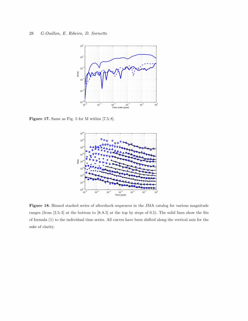
Figure 17. Same as Fig. 5 for M within [7.5; 8].

10−6

10−5

10−4

10−3

10−2

10−1

100

108

1010

1012

1014

1016

1018

1020

1022

1024

Time (year)

Rat

e

Figure 18. Binned stacked series of aftershock sequences in the JMA catalog for various magnitude

ranges (from [2.5; 3] at the bottom to [8; 8.5] at the top by steps of 0.5). The solid lines show the fits

of formula (1) to the individual time series. All curves have been shifted along the vertical axis for the

sake of clarity.

Multifractal Omori Law 29

1 2 3 4 5 6 7 8 90.5

0.6

0.7

0.8

0.9

1

1.1

1.2

1.3

1.4

1.5

Mainshock magnitude

p−va

lue

binned stacksp=0.06M+0.58SFA methodp=0.07M+0.50

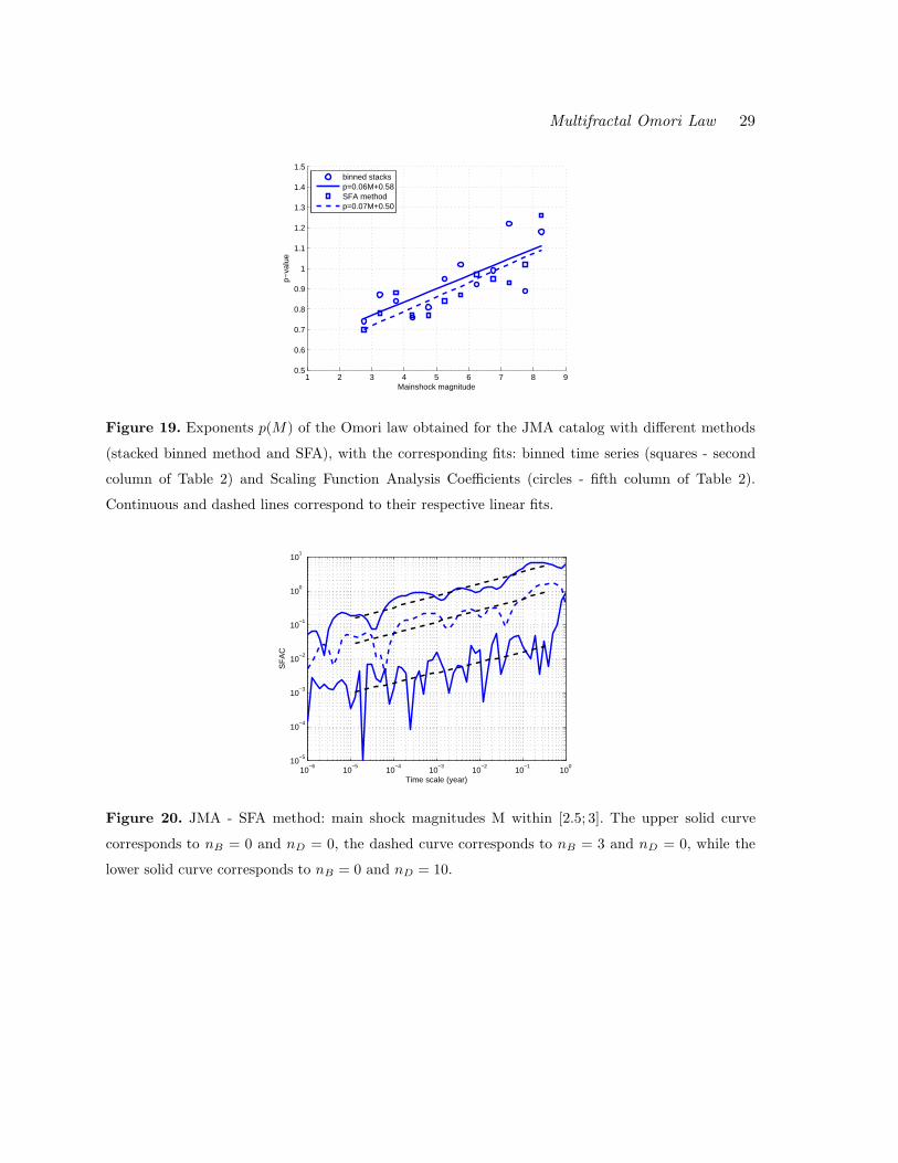
Figure 19. Exponents p(M) of the Omori law obtained for the JMA catalog with different methods

(stacked binned method and SFA), with the corresponding fits: binned time series (squares - second

column of Table 2) and Scaling Function Analysis Coefficients (circles - fifth column of Table 2).

Continuous and dashed lines correspond to their respective linear fits.

10−6

10−5

10−4

10−3

10−2

10−1

100

10−5

10−4

10−3

10−2

10−1

100

101

Time scale (year)

SF

AC

Figure 20. JMA - SFA method: main shock magnitudes M within [2.5; 3]. The upper solid curve

corresponds to nB = 0 and nD = 0, the dashed curve corresponds to nB = 3 and nD = 0, while the

lower solid curve corresponds to nB = 0 and nD = 10.

30 G.Ouillon, E. Ribeiro, D. Sornette

10−6

10−5

10−4

10−3

10−2

10−1

100

10−4

10−3

10−2

10−1

100

101

Time scale (year)

SF

AC

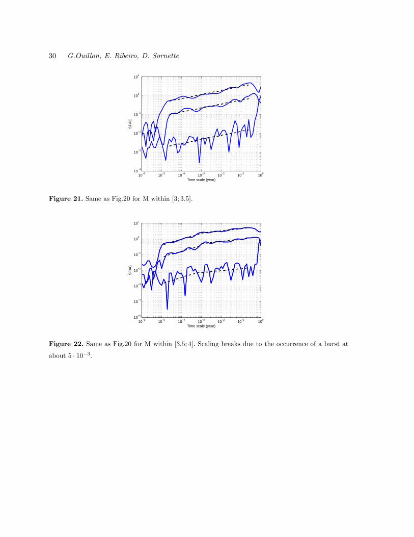
Figure 21. Same as Fig.20 for M within [3; 3.5].

10−6

10−5

10−4

10−3

10−2

10−1

100

10−5

10−4

10−3

10−2

10−1

100

101

Time scale (year)

SF

AC

Figure 22. Same as Fig.20 for M within [3.5; 4]. Scaling breaks due to the occurrence of a burst at

about 5 · 10−3.

Multifractal Omori Law 31

10−6

10−5

10−4

10−3

10−2

10−1

100

10−4

10−3

10−2

10−1

100

101

Time scale (year)

SF

AC

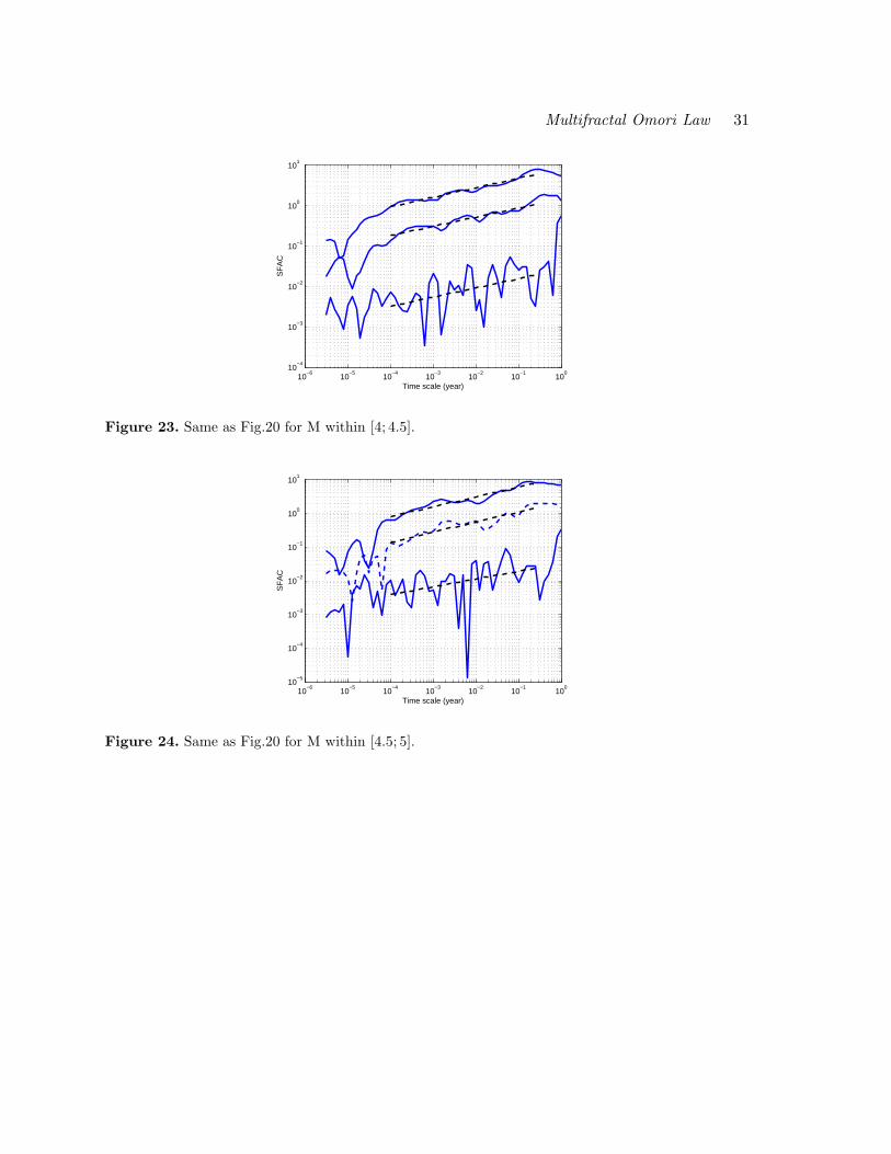
Figure 23. Same as Fig.20 for M within [4; 4.5].

10−6

10−5

10−4

10−3

10−2

10−1

100

10−5

10−4

10−3

10−2

10−1

100

101

Time scale (year)

SF

AC

Figure 24. Same as Fig.20 for M within [4.5; 5].

32 G.Ouillon, E. Ribeiro, D. Sornette

10−6

10−5

10−4

10−3

10−2

10−1

100

10−5

10−4

10−3

10−2

10−1

100

101

Time scale (year)

SF

AC

Figure 25. Same as Fig.20 for M within [5; 5.5]. The presence of the roll-off implies to choose nD = 10

(lower solid line).

10−6

10−5

10−4

10−3

10−2

10−1

100

10−5

10−4

10−3

10−2

10−1

100

101

Time scale (year)

SF

AC

Figure 26. Same as Fig.20 for M within [5.5; 6].

Multifractal Omori Law 33

10−5

10−4

10−3

10−2

10−1

100

10−4

10−3

10−2

10−1

100

101

Time scale (year)

SF

AC

Figure 27. Same as Fig.20 for M within [6; 6.5]. The scaling range is limited by the roll-off at small

scales and a burst at about 2 · 10−1 year.

10−6

10−5

10−4

10−3

10−2

10−1

100

10−5

10−4

10−3

10−2

10−1

100

101

Time scale (year)

SF

AC

Figure 28. Same as Fig.20 for M within [6.5; 7].

34 G.Ouillon, E. Ribeiro, D. Sornette

10−5

10−4

10−3

10−2

10−1

100

10−4

10−3

10−2

10−1

100

101

Time scale (year)

SF

AC

Figure 29. Same as Fig.20 for M within [7; 7.5].

10−5

10−4

10−3

10−2

10−1

100

10−5

10−4

10−3

10−2

10−1

100

101

102

Time scale (year)

SF

AC

Figure 30. Same as Fig.20 for M within [7.5; 8].

Multifractal Omori Law 35

10−5

10−4

10−3

10−2

10−1

100

10−5

10−4

10−3

10−2

10−1

100

Time scale (year)

SF

AC

Figure 31. Same as Fig.20 for M within [8; 8.5].

10−8

10−6

10−4

10−2

100

1013

1014

1015

1016

1017

1018

1019

1020

Time (year)

Rat

e

Figure 32. Binned stacked time series of sequences triggered by main events with M within [5.5; 6].

This plot features binned series corresponding to all r values.

36 G.Ouillon, E. Ribeiro, D. Sornette

10−6

10−5

10−4

10−3

10−2

10−1

100

1015

1020

1025

Time (year)

Rat

e

Figure 33. Binned stacked series of aftershock sequences in the Harvard catalog for various magnitude

ranges. Magnitude ranges are, from bottom to top: [6; 6.5], [6.5; 7], [7; 7.5], [7.5; 8], [8; 8.5] and [9; 9.5].

The solid lines show the fits to the individual time series. The [9; 9.5] magnitude range displays an

unusual small p value of 0.69 (see text for further discussion of this anomaly in comparison with the

other magnitude ranges. All curves have been shifted along the vertical axis for the seek of clarity.

1 2 3 4 5 6 7 8 90.5

0.6

0.7

0.8

0.9

1

1.1

1.2

1.3

1.4

1.5

Mainshock magnitude

p va

lue

bined stacksp=0.16M−0.09SFA methodp=0.13M+0.14

Figure 34. Dependence of the Omori exponent p as a function of the main shock magnitude M

obtained for the HARVARD catalog with fits of the binned time series (squares - second column of

Table 3) and of the Scaling Function Analysis Coefficent (circles - third column of Table 3). Continuous

and dashed lines stand for their respective linear fits.

Multifractal Omori Law 37

10−5

10−4

10−3

10−2

10−1

100

10−6

10−5

10−4

10−3

10−2

10−1

100

101

Time scale (year)

SF

AC

nD=0nD=2nD=4nD=8

Figure 35. HAR - SFA method for main shock magnitudes M within [5.5; 6]. Note the existence of

two characteristic scales. The parameter nB is set to zero and the four curves correspond to different

values of nD as indicated in the insert panel.

10−5

10−4

10−3

10−2

10−1

100

10−5

10−4

10−3

10−2

10−1

100

101

Time scale (year)

SF

AC

Figure 36. Same as Fig.35 for M within [6; 6.5]. The scaling range is limited by the roll-off at small

scales and a burst at about 2 · 10−1 year.

38 G.Ouillon, E. Ribeiro, D. Sornette

10−5

10−4

10−3

10−2

10−1

100

10−5

10−4

10−3

10−2

10−1

100

101

Time scale (year)

SF

AC

Figure 37. Same as Fig.35 for M within [6.5; 7].

10−5

10−4

10−3

10−2

10−1

100

10−5

10−4

10−3

10−2

10−1

100

101

Time scale (year)

SF

AC

Figure 38. Same as Fig.35 for M within [7; 7.5].

Multifractal Omori Law 39

10−4

10−3

10−2

10−1

100

10−4

10−3

10−2

10−1

100

101

Time scale (year)

SF

AC

Figure 39. Same as Fig.35 for M within [7.5; 8].

10−4

10−3

10−2

10−1

100

10−6

10−5

10−4

10−3

10−2

10−1

100

101

Time scale (year)

SF

AC

Figure 40. Same as Fig.35 for M within [8; 8.5].

40 G.Ouillon, E. Ribeiro, D. Sornette

10−4

10−3

10−2

10−1

100

10−4

10−3

10−2

10−1

100

101

Time scale (year)

SF

AC

nD=0nD=1nD=2

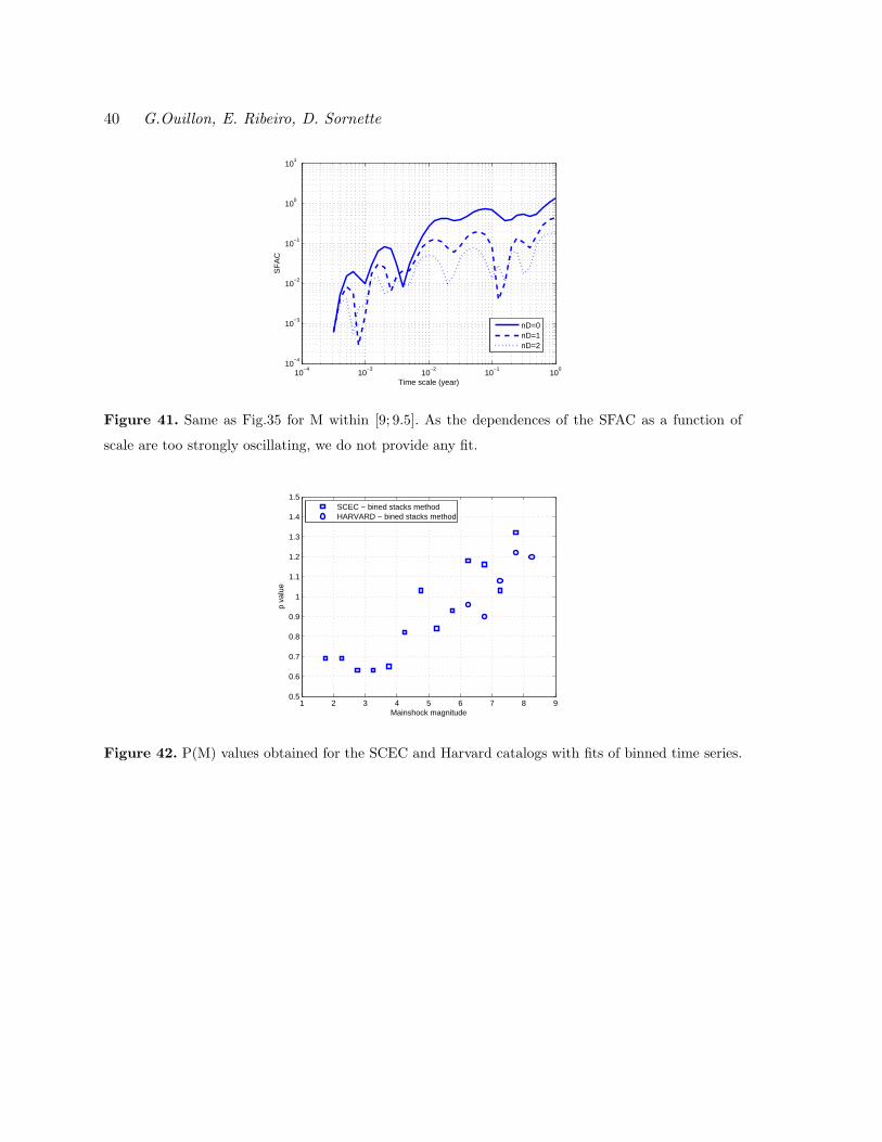
Figure 41. Same as Fig.35 for M within [9; 9.5]. As the dependences of the SFAC as a function of

scale are too strongly oscillating, we do not provide any fit.

1 2 3 4 5 6 7 8 90.5

0.6

0.7

0.8

0.9

1

1.1

1.2

1.3

1.4

1.5

Mainshock magnitude

p va

lue

SCEC − bined stacks methodHARVARD − bined stacks method

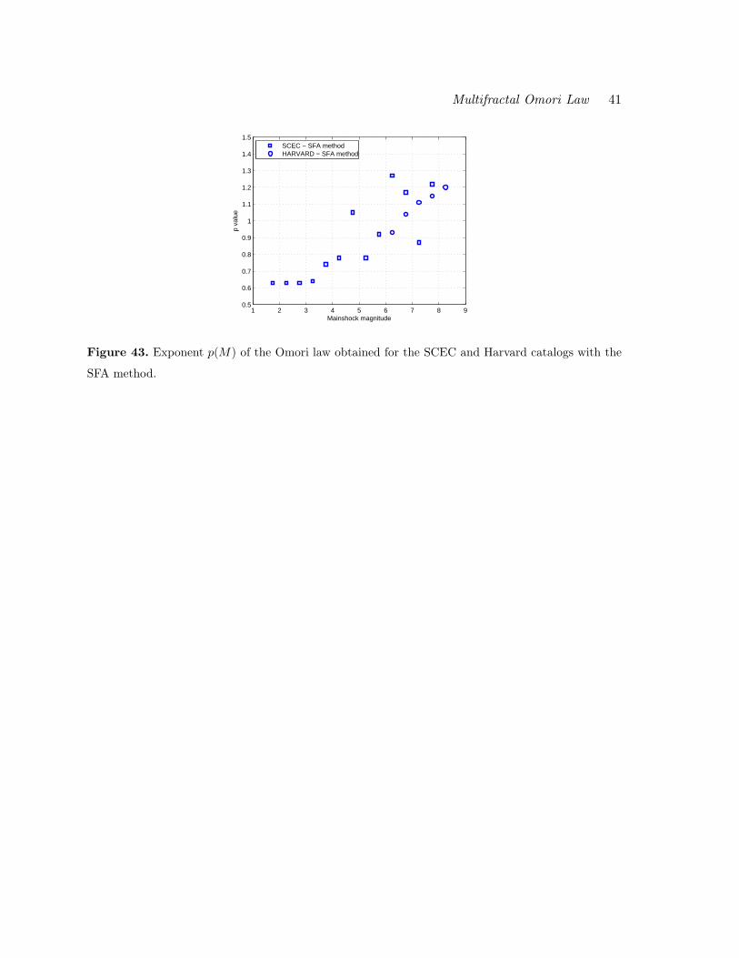
Figure 42. P(M) values obtained for the SCEC and Harvard catalogs with fits of binned time series.

Multifractal Omori Law 41

1 2 3 4 5 6 7 8 90.5

0.6

0.7

0.8

0.9

1

1.1

1.2

1.3

1.4

1.5

Mainshock magnitude

p va

lue

SCEC − SFA methodHARVARD − SFA method

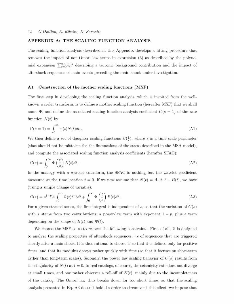
Figure 43. Exponent p(M) of the Omori law obtained for the SCEC and Harvard catalogs with the

SFA method.

42 G.Ouillon, E. Ribeiro, D. Sornette

APPENDIX A: THE SCALING FUNCTION ANALYSIS

The scaling function analysis described in this Appendix develops a fitting procedure that

removes the impact of non-Omori law terms in expression (3) as described by the polyno-

mial expansion∑nB

i=0 biti describing a tectonic background contribution and the impact of

aftershock sequences of main events preceding the main shock under investigation.

A1 Construction of the mother scaling functions (MSF)

The first step in developing the scaling function analysis, which is inspired from the well-

known wavelet transform, is to define a mother scaling function (hereafter MSF) that we shall

name Ψ, and define the associated scaling function analysis coefficient C(s = 1) of the rate

function N(t) by

C(s = 1) =

∫ ∞

0Ψ(t)N(t)dt . (A1)

We then define a set of daughter scaling functions Ψ( ts), where s is a time scale parameter

(that should not be mistaken for the fluctuations of the stress described in the MSA model),

and compute the associated scaling function analysis coefficients (herafter SFAC):

C(s) =

∫ ∞

0Ψ

(

t

s

)

N(t)dt . (A2)

In the analogy with a wavelet transform, the SFAC is nothing but the wavelet coefficient

measured at the time location t = 0. If we now assume that N(t) = A · t−p + B(t), we have

(using a simple change of variable):

C(s) = s1−pA

∫ ∞

0Ψ(t)t−pdt +

∫ ∞

0Ψ

(

t

s

)

B(t)dt . (A3)

For a given stacked series, the first integral is independent of s, so that the variation of C(s)

with s stems from two contributions: a power-law term with exponent 1 − p, plus a term

depending on the shape of B(t) and Ψ(t).

We choose the MSF so as to respect the following constraints. First of all, Ψ is designed

to analyze the scaling properties of aftershock sequences, i.e of sequences that are triggered

shortly after a main shock. It is thus rational to choose Ψ so that it is defined only for positive

times, and that its modulus decays rather quickly with time (so that it focuses on short-term

rather than long-term scales). Secondly, the power law scaling behavior of C(s) results from

the singularity of N(t) at t = 0. In real catalogs, of course, the seismicity rate does not diverge

at small times, and one rather observes a roll-off of N(t), mainly due to the incompleteness

of the catalog. The Omori law thus breaks down for too short times, so that the scaling

analysis presented in Eq. A3 doesn’t hold. In order to circumvent this effect, we impose that

Multifractal Omori Law 43

Ψ(t = 0) = 0, so that aftershocks occurring at short times will have a negligible weight in the

computation of C(s), preserving the announced scaling properties of the SFAC. Thirdly, in

order to measure p more easily, we impose that Ψ should filter out polynomials, so that the

second term in the right-hand side of Eq. A3 gives a vanishing contribution to C(s). These

three conditions are fulfilled with the following construction

Ψ(t) =nP∑

i=0

aiti exp

(

−at2)

, (A4)

where the coefficients a and ai, i = 0, ..., nP are determined as follows. For all integer values

j = 0, ..., nB , we impose that the function Ψ obeys the conditions∫ ∞

0tjΨ(t)dt = 0 , (A5)

If we find the corresponding coefficients ai’s, then our goal of removing the influence of the

non-stationary background and of previous main shocks will be fulfilled. Expression (A5) leads

tonP∑

i=0

Ii+jai = 0 , (A6)

where

Im =

∫ ∞

0tm exp

(

−at2)

dt =Γ[(m + 1)/2]

2a(m+1)/2. (A7)

As equation A6 must hold for all j values between 0 and nB , and as we also impose Ψ(0) = 0,

the set of conditions (A6) defines a linear system of nB + 2 equations which can be solved

to obtain the nP + 1 unknowns ai. In order to obtain a non-degenerate solution, we impose

nP = nB +2 and arbitrarily fix anP= ±1. The sign of anP

is chosen so that the most extreme

value of the MSF is positive. The MSF is then normalized so that its maximum value is 1. In

order to fully define the MSF, we still have to specify the two parameters a and nB . In the

remaining of this paper, we shall fix a = 5 yr−2 (which ensures a good temporal localization of

Ψ). As for the parameter nB , it requires a specific discussion for each of the studied catalogs.

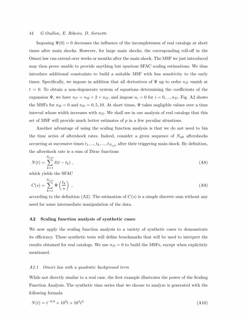
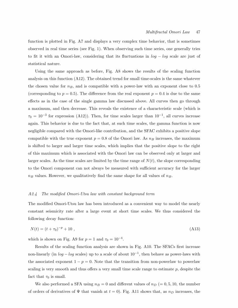
Figure A1 shows the shape of the function Ψ for

• nB = 0 (nP = 2) (which filters out only constant background terms B(t) = b0),

• nB = 1 (nP = 3) (which filters out linear trends like B(t) = b0 + b1t), and

• nB = 2 (nP = 4) (which filters out quadratic trends like B(t) = b0 + b1t + b2t2).

The higher the order of the polynomial that needs to be filtered out, the more oscillating is

the MSF. It is noteworthy that the shape of the MSF is independent of the precise shape of

the function B(t) (and of its coefficients bi). Only the degree nB of the polynomial is needed

to determine the corresponding MSF.

44 G.Ouillon, E. Ribeiro, D. Sornette

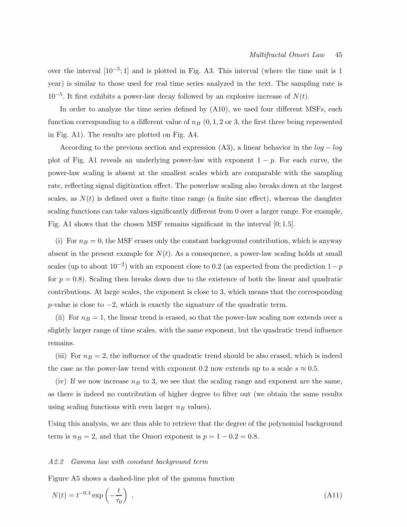
Imposing Ψ(0) = 0 decreases the influence of the incompleteness of real catalogs at short

times after main shocks. However, for large main shocks, the corresponding roll-off in the

Omori law can extend over weeks or months after the main shock. The MSF we just introduced

may then prove unable to provide anything but spurious SFAC scaling estimations. We thus

introduce additional constraints to build a suitable MSF with less sensitivity to the early

times. Specifically, we impose in addition that all derivatives of Ψ up to order nD vanish at

t = 0. To obtain a non-degenerate system of equations determining the coefficients of the

expansion Ψ, we have nP = nB + 2 + nD, and impose ai = 0 for i = 0, ..., nD . Fig. A2 shows

the MSFs for nB = 0 and nD = 0, 5, 10. At short times, Ψ takes negligible values over a time

interval whose width increases with nD. We shall see in our analysis of real catalogs that this

set of MSF will provide much better estimates of p in a few peculiar situations.

Another advantage of using the scaling function analysis is that we do not need to bin

the time series of aftershock rates. Indeed, consider a given sequence of Naft aftershocks

occurring at successive times t1, ..., tk , ..., tNaftafter their triggering main shock. By definition,

the aftershock rate is a sum of Dirac functions

N(t) =

Naft∑

k=1

δ(t − tk) , (A8)

which yields the SFAC

C(s) =

Naft∑

k=1

Ψ

(

tks

)

, (A9)

according to the definition (A2). The estimation of C(s) is a simple discrete sum without any

need for some intermediate manipulation of the data.

A2 Scaling function analysis of synthetic cases

We now apply the scaling function analysis to a variety of synthetic cases to demonstrate

its efficiency. These synthetic tests will define benchmarks that will be used to interpret the

results obtained for real catalogs. We use nD = 0 to build the MSFs, except when explicitely

mentioned.

A2.1 Omori law with a quadratic background term

While not directly similar to a real case, the first example illustrates the power of the Scaling

Function Analysis. The synthetic time series that we choose to analyze is generated with the

following formula

N(t) = t−0.8 + 103t + 104t2 (A10)

Multifractal Omori Law 45

over the interval [10−5; 1] and is plotted in Fig. A3. This interval (where the time unit is 1

year) is similar to those used for real time series analyzed in the text. The sampling rate is

10−5. It first exhibits a power-law decay followed by an explosive increase of N(t).

In order to analyze the time series defined by (A10), we used four different MSFs, each

function corresponding to a different value of nB (0, 1, 2 or 3, the first three being represented

in Fig. A1). The results are plotted on Fig. A4.

According to the previous section and expression (A3), a linear behavior in the log − log

plot of Fig. A1 reveals an underlying power-law with exponent 1 − p. For each curve, the

power-law scaling is absent at the smallest scales which are comparable with the sampling

rate, reflecting signal digitization effect. The powerlaw scaling also breaks down at the largest

scales, as N(t) is defined over a finite time range (a finite size effect), whereas the daughter

scaling functions can take values significantly different from 0 over a larger range. For example,

Fig. A1 shows that the chosen MSF remains significant in the interval [0; 1.5].

(i) For nB = 0, the MSF erases only the constant background contribution, which is anyway

absent in the present example for N(t). As a consequence, a power-law scaling holds at small

scales (up to about 10−2) with an exponent close to 0.2 (as expected from the prediction 1−p

for p = 0.8). Scaling then breaks down due to the existence of both the linear and quadratic

contributions. At large scales, the exponent is close to 3, which means that the corresponding

p-value is close to −2, which is exactly the signature of the quadratic term.

(ii) For nB = 1, the linear trend is erased, so that the power-law scaling now extends over a

slightly larger range of time scales, with the same exponent, but the quadratic trend influence

remains.

(iii) For nB = 2, the influence of the quadratic trend should be also erased, which is indeed

the case as the power-law trend with exponent 0.2 now extends up to a scale s ≈ 0.5.

(iv) If we now increase nB to 3, we see that the scaling range and exponent are the same,

as there is indeed no contribution of higher degree to filter out (we obtain the same results

using scaling functions with even larger nB values).

Using this analysis, we are thus able to retrieve that the degree of the polynomial background

term is nB = 2, and that the Omori exponent is p = 1 − 0.2 = 0.8.

A2.2 Gamma law with constant background term

Figure A5 shows a dashed-line plot of the gamma function

N(t) = t−0.4 exp

(

−t

τ0

)

, (A11)

46 G.Ouillon, E. Ribeiro, D. Sornette

It exhibits a power law behavior at small times, followed by an exponential roll-off at large

times. This law could describe the time decay of swarms in volcanic areas, for example, with τ0

being the characteristic duration of the swarm (here we took τ0 = 10−3). The continuous line

on the same figure shows the same function to which a constant background term B = 20 has

been added. Note that this new time series could very easily be mistaken for a pure Omori-law

with a constant background. We performed a scaling function analysis of this last time-series,

and Fig. A6 shows the obtained results using the same four scaling functions as above.

As the only polynomial trend in N(t) is a constant term, all curves exhibit the same scaling

behavior, which results from two complementary effects. The first effect is that the gamma

function can be described as an effective Omori-like power law with a tangent exponent p

that continuously increases with time. Since the effective exponent is smaller than 1 at small

times and larger than 1 at large times, the SFAC first increases and then decreases with time

scale. The second effect is of a different nature. Fig. A5 illustrates that the Gamma function

takes values significantly different from zero within a finite interval spanning roughly [0; 10−2].

As the time scale increases, the associated SFAC will thus increase as the daughter scaling

function progressively enters a kind of resonance with this finite-size feature. The maximum

resonance is obtained when the scale of the daughter scaling function is of the order of 10−2.

Further increasing the time scale, the resonance amplitude decreases, leading to a decreasing

SFAC. The interplay between those two effects leads to a reasonably well-defined maximum

of the dependence of the SFAC as a function of the scale s, providing a rough estimate of τ0.

The drawback is that the left side of the power-law scaling behavior in Fig. A6 is distorted

and doesn’t provide an accurate measure of p (in the present example, the measured p value

is 0.2, compared with the true value p = 0.4). Overall, we conclude that the scaling function

analysis clearly reveals the existence of a characteristic scale which precludes the existence

of a genuine Omori scaling over the whole range of time. In this sense, the scaling function

analysis provides a useful diagnostic.

A2.3 Mix of gamma law, Omori law and constant background term

The next synthetic example we wish to present is a sum of an Omori-like power law, a gamma-

law and a constant background term:

N(t) = 0.02 t−0.8 + t−0.4 exp

(

−t

τ0

)

+ 0.1 , (A12)

with τ0 = 10−3. This function can describe the mixture of pure Omori-like sequences with

swarm sequences in the presence of a constant background noise within the same data set. This

Multifractal Omori Law 47

function is plotted in Fig. A7 and displays a very complex time behavior, that is sometimes

observed in real time series (see Fig. 1). When observing such time series, one generally tries

to fit it with an Omori-law, considering that its fluctuations in log − log scale are just of

statistical nature.

Using the same approach as before, Fig. A8 shows the results of the scaling function

analysis on this function (A12). The obtained trend for small time-scales is the same whatever

the chosen value for nB, and is compatible with a power-law with an exponent close to 0.5

(corresponding to p = 0.5). The difference from the real exponent p = 0.4 is due to the same

effects as in the case of the single gamma law discussed above. All curves then go through

a maximum, and then decrease. This reveals the existence of a characteristic scale (which is

τ0 = 10−3 for expression (A12)). Then, for time scales larger than 10−1, all curves increase

again. This behavior is due to the fact that, at such time scales, the gamma function is now

negligible compared with the Omori-like contribution, and the SFAC exhibits a positive slope

compatible with the true exponent p = 0.8 of the Omori law. As nB increases, the maximum

is shifted to larger and larger time scales, which implies that the positive slope to the right

of this maximum which is associated with the Omori law can be observed only at larger and

larger scales. As the time scales are limited by the time range of N(t), the slope corresponding

to the Omori component can not always be measured with sufficient accuracy for the larger

nB values. However, we qualitatively find the same shape for all values of nB.

A2.4 The modified Omori-Utsu law with constant background term

The modified Omori-Utsu law has been introduced as a convenient way to model the nearly

constant seismicity rate after a large event at short time scales. We thus considered the

following decay function:

N(t) = (t + τ0)−p + 10 , (A13)

which is shown on Fig. A9 for p = 1 and τ0 = 10−4.

Results of the scaling function analysis are shown in Fig. A10. The SFACs first increase

non-linearly (in log − log scales) up to a scale of about 10−1, then behave as power-laws with

the associated exponent 1 − p = 0. Note that the transition from non-powerlaw to powerlaw

scaling is very smooth and thus offers a very small time scale range to estimate p, despite the

fact that τ0 is small.

We also performed a SFA using nB = 0 and different values of nD (= 0, 5, 10, the number

of orders of derivatives of Ψ that vanish at t = 0). Fig. A11 shows that, as nD increases, the

48 G.Ouillon, E. Ribeiro, D. Sornette

power law scaling now holds for time scales larger than 10−2, so that we can provide a more

reliable determination of p.

A2.5 Piecewise powerlaw scaling

The last synthetic example we consider is the case of a piecewise powerlaw scaling with

constant background,

N(t) = min

[

(

t

10−2

)−0.5

;

(

t

10−2

)−1]

+ 0.1 , (A14)

which is plotted in Fig. A12. This function has a characteristic time scale of 10−2.

The result of the scaling function analysis is plotted in Fig. A13. As the time scale in-

creases, two powerlaw scaling regimes are revealed, separated by a smooth step at a time scale

of about 2 · 10−2, not too far from the built-in characteristic time scale of the process defined

by expression (A14). The left part of the curves allows one to infer that the corresponding

p-value is close to 0.5. The second right scaling range is not long enough to determine the

scaling exponent with sufficient accuracy, but it gives however a rather good description of

the change of exponent with scale/time.

Now, setting nB = 0 and using non-zero values for nD, one can get a better picture of the

complex scaling of N(t). Fig. A14 shows that increasing nD sharpens the transition at time

scale ≃ 10−2, and that two different scaling ranges can clearly distinguished, over which the

corresponding two values of the exponent p can be determined with high accuracy.

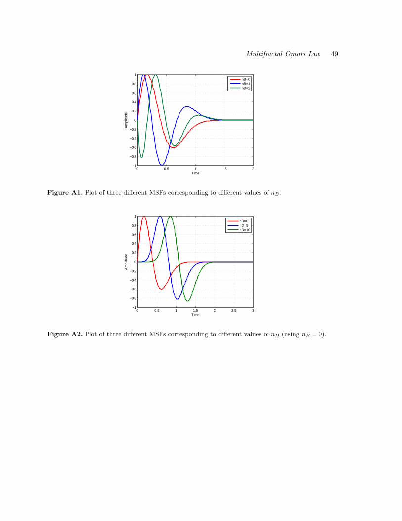
Multifractal Omori Law 49

0 0.5 1 1.5 2−1

−0.8

−0.6

−0.4

−0.2

0

0.2

0.4

0.6

0.8

1

Time

Am

plitu

de

nB=0nB=1nB=2

Figure A1. Plot of three different MSFs corresponding to different values of nB.

0 0.5 1 1.5 2 2.5 3−1

−0.8

−0.6

−0.4

−0.2

0

0.2

0.4

0.6

0.8

1

Time

Am

plitu

de

nD=0nD=5nD=10

Figure A2. Plot of three different MSFs corresponding to different values of nD (using nB = 0).

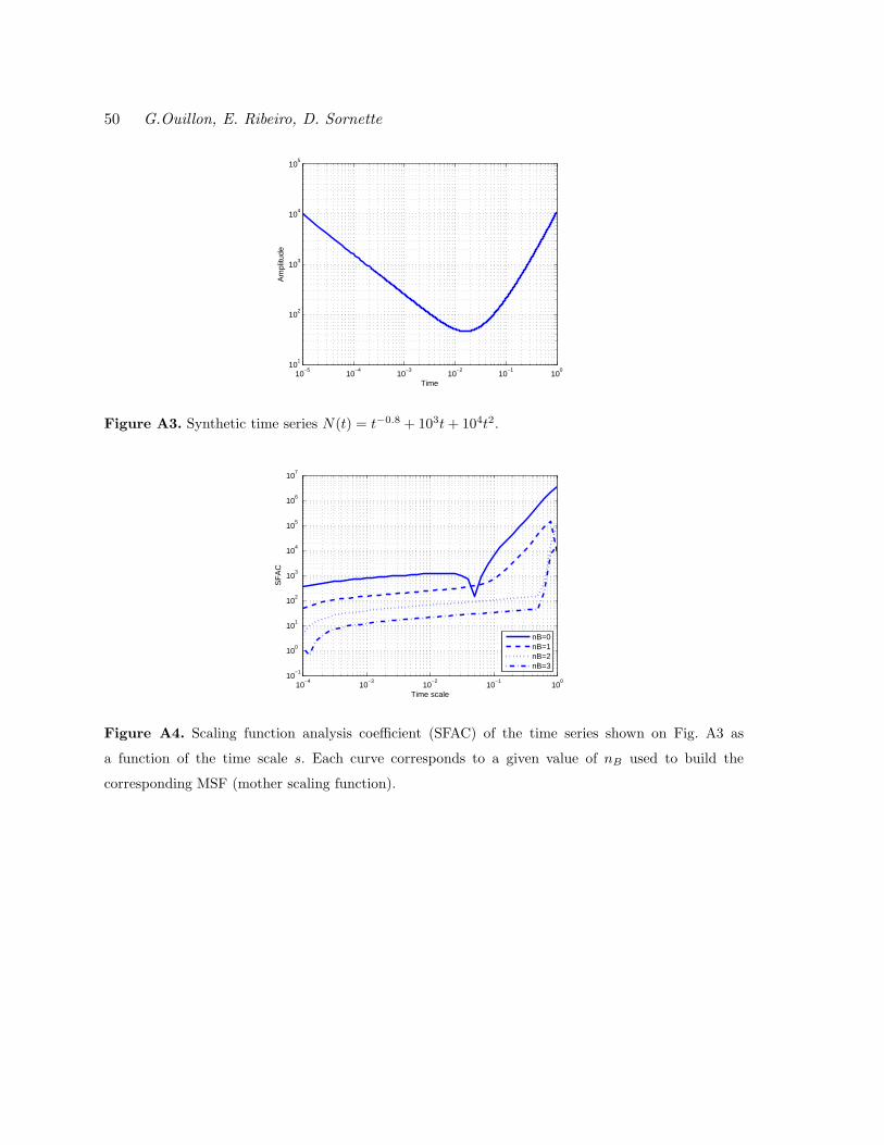
50 G.Ouillon, E. Ribeiro, D. Sornette

10−5

10−4

10−3

10−2

10−1

100

101

102

103

104

105

Time

Am

plitu

de

Figure A3. Synthetic time series N(t) = t−0.8 + 103t + 104t2.

10−4

10−3

10−2

10−1

100

10−1

100

101

102

103

104

105

106

107

Time scale

SF

AC

nB=0nB=1nB=2nB=3

Figure A4. Scaling function analysis coefficient (SFAC) of the time series shown on Fig. A3 as

a function of the time scale s. Each curve corresponds to a given value of nB used to build the

corresponding MSF (mother scaling function).

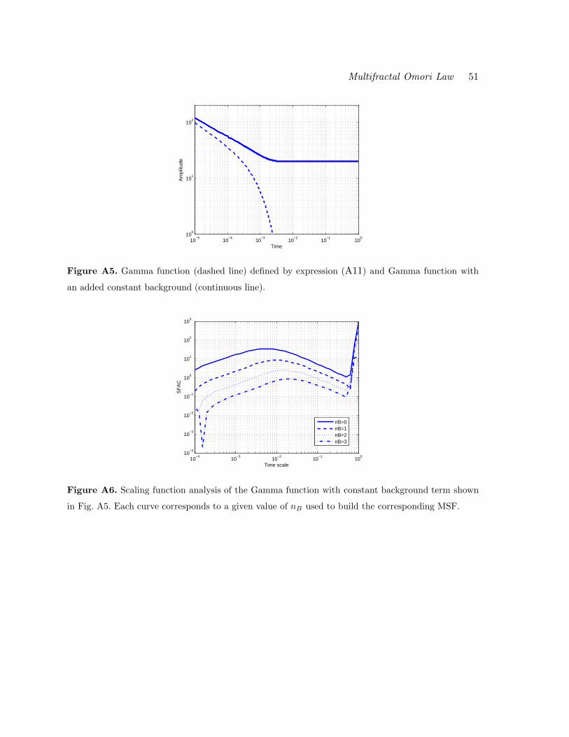
Multifractal Omori Law 51

10−5

10−4

10−3

10−2

10−1

100

100

101

102

Time

Am

plitu

de

Figure A5. Gamma function (dashed line) defined by expression (A11) and Gamma function with

an added constant background (continuous line).

10−4

10−3

10−2

10−1

100

10−4

10−3

10−2

10−1

100

101

102

103

Time scale

SF

AC

nB=0nB=1nB=2nB=3

Figure A6. Scaling function analysis of the Gamma function with constant background term shown

in Fig. A5. Each curve corresponds to a given value of nB used to build the corresponding MSF.

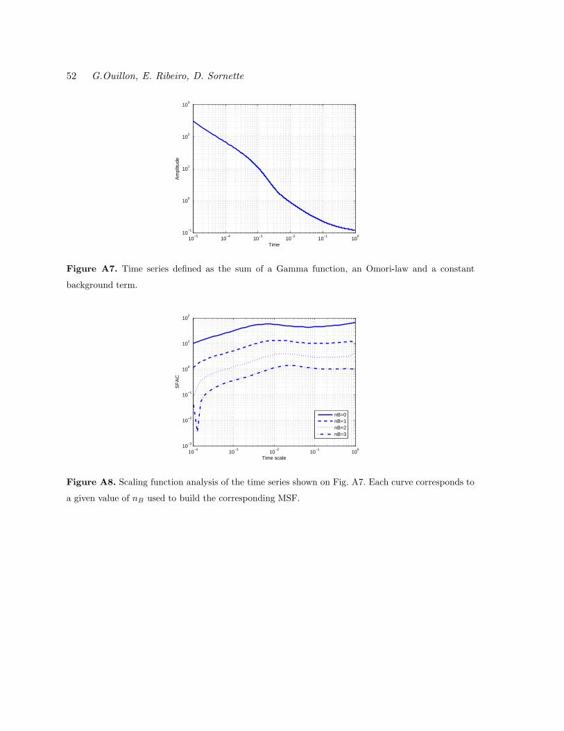
52 G.Ouillon, E. Ribeiro, D. Sornette

10−5

10−4

10−3

10−2

10−1

100

10−1

100

101

102

103

Time

Am

plitu

de

Figure A7. Time series defined as the sum of a Gamma function, an Omori-law and a constant

background term.

10−4

10−3

10−2

10−1

100

10−3

10−2

10−1

100

101

102

Time scale

SF

AC

nB=0nB=1nB=2nB=3

Figure A8. Scaling function analysis of the time series shown on Fig. A7. Each curve corresponds to

a given value of nB used to build the corresponding MSF.

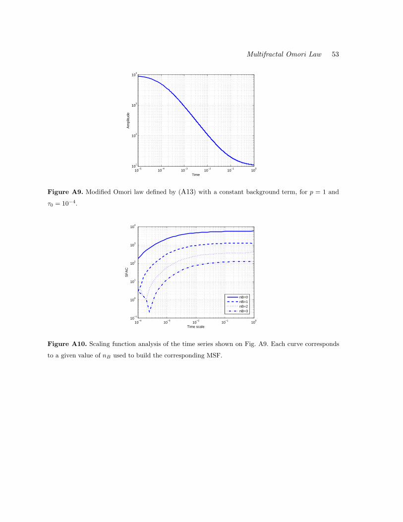
Multifractal Omori Law 53

10−5

10−4

10−3

10−2

10−1

100

101

102

103

104

Time

Am

plitu

de

Figure A9. Modified Omori law defined by (A13) with a constant background term, for p = 1 and

τ0 = 10−4.

10−4

10−3

10−2

10−1

100

10−1

100

101

102

103

104

Time scale

SF

AC

nB=0nB=1nB=2nB=3

Figure A10. Scaling function analysis of the time series shown on Fig. A9. Each curve corresponds

to a given value of nB used to build the corresponding MSF.

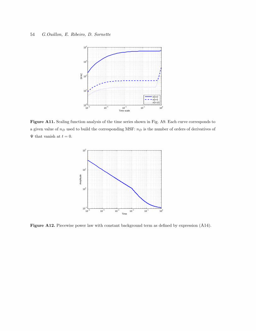
54 G.Ouillon, E. Ribeiro, D. Sornette

10−4

10−3

10−2

10−1

100

100

101

102

103

104

Time scale

SF

AC

nD=0nD=5nD=10

Figure A11. Scaling function analysis of the time series shown in Fig. A9. Each curve corresponds to

a given value of nD used to build the corresponding MSF: nD is the number of orders of derivatives of

Ψ that vanish at t = 0.

10−5

10−4

10−3

10−2

10−1

100

10−1

100

101

102

Time

Am

plitu

de

Figure A12. Piecewise power law with constant background term as defined by expression (A14).

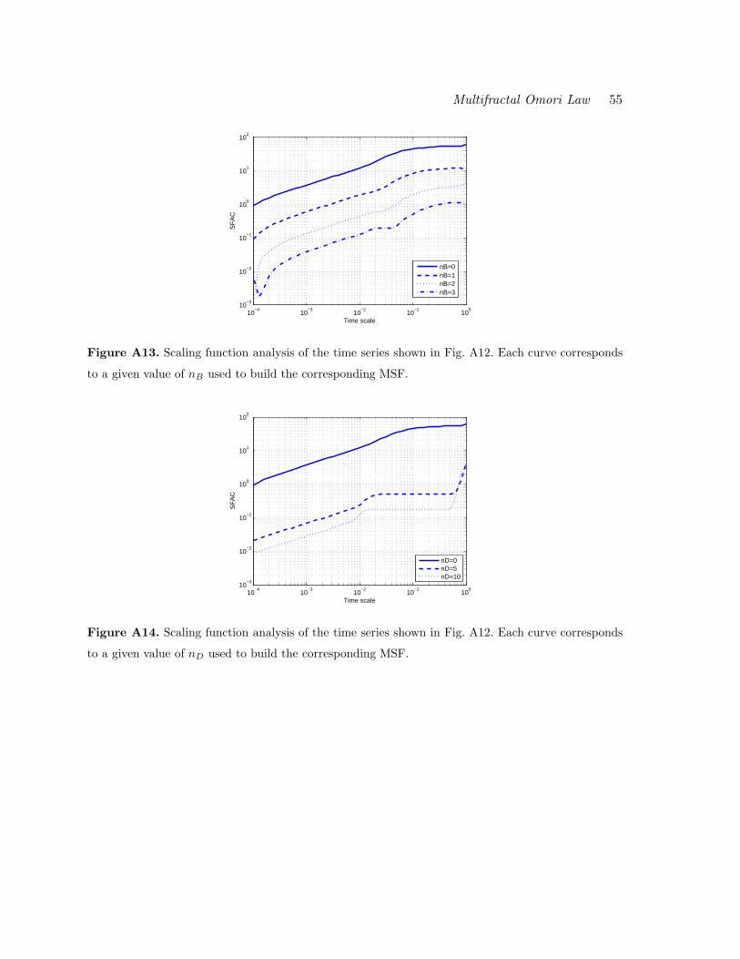
Multifractal Omori Law 55

10−4

10−3

10−2

10−1

100

10−3

10−2

10−1

100

101

102

Time scale

SF

AC

nB=0nB=1nB=2nB=3

Figure A13. Scaling function analysis of the time series shown in Fig. A12. Each curve corresponds

to a given value of nB used to build the corresponding MSF.

10−4

10−3

10−2

10−1

100

10−3

10−2

10−1

100

101

102

Time scale

SF

AC

nD=0nD=5nD=10

Figure A14. Scaling function analysis of the time series shown in Fig. A12. Each curve corresponds

to a given value of nD used to build the corresponding MSF.