Multifractal observations of eddies, oil spills and natural slicks in the ocean surface

$: Multifractal observations of eddies, oil spills and natural slicks in the ocean surface$
DOI 10.1393/ncc/i2009-10349-0

IL NUOVO CIMENTO Vol. 31 C, N. 5-6 Settembre-Dicembre 2008

Multifractal observations of eddies, oil spills and natural slicks inthe ocean surface

A. Platonov(1), A. Carrillo(1), A. Matulka(1), E. Sekula(1), J. Grau(1),J. M. Redondo(1)(∗) and A. M. Tarquis(2)(1) Departamento de Fisica Aplicada, Universitat Politecnica de Catalunya - B5 UPC

Campus Nord, Barcelona, 08034, Spain(2) Departamento de Matematica Aplicada a la Ingenierıa Agronomica

E.T.S. de Ingenieros Agronomos, U.P.M. Ciudad Universitaria s.n. - Madrid 28040, Spain

(ricevuto il 10 Novembre 2008; approvato il 30 Marzo 2009; pubblicato online il 25 Giugno 2009)

Summary. — Natural and man-made distributions of tensioactive substance con-centrations in the sea surface features exhibit self-similarity at all radar reflectivitylevels when illuminated by SAR. This allows the investigation of the traces producedby vortices and other features in the ocean surface. The man-made oil spills besidesoften presenting some linear axis of the pollutant concentration produced by movingships also show their artificial production in the sea surface by the reduced rangeof scales, which widens as time measured in terms of the local eddy diffusivity dis-torts the shape of the oil spills. Thanks to this, multifractal analysis of the differentbackscattered intensity levels in SAR imagery can be used to distinguish betweennatural and man-made sea surface features due to their distinct self-similar prop-erties. The differences are detected using the multifractal box-counting algorithmon different sets of SAR images giving also information on the age of the spills.Different multifractal algorithms are compared presenting the differences in scalingas a function of some physical generating process such as the locality or the spectralenergy cascade.

PACS 92.10.Sx – Coastal, estuarine, and near shore processes.PACS 93.85.Bc – Computational methods and data processing, data acquisitionand storage.

1. – Introduction

Most mixing processes in the ocean depend both on advection and diffusion charac-teristics with energetic inputs at many different scales, the topology of tracers in theocean surface probable depends on the local characteristics of the turbulent cascades.

(∗) E-mail: [email protected]

c© Societa Italiana di Fisica 861

862 A. PLATONOV, A. CARRILLO, A. MATULKA, ETC.

For example, in the detected vortices in the ocean, local shear will transform slicks inthe surface to align and follow the local flow so the resulting pattern is spiral as shownby Munk [1]. The mixing processes at large scale produce stirring, which maintains largegradients of the tracers. But in order to mix at molecular level in an irreversible fashion,the energy has to cascade to the smallest internal scales (Kolmogorov or Batchelor scales).

An important topological tool, fractal analysis was pioneered by Richardson andpopularized by Mandelbrot. The fractal dimension is a very useful indicator of thecomplex environmental flow dynamics [2,3], but it only reflects the self-similar geometry,not the dynamics of the flow. Because the oceans receive energy inputs at a wide rangeof scales, and the non-linear interactions that follow produce turbulent cascades of thetype described by Richardson and Kolmogorov [4-6] (3D) and Kraichnan [7] (2D). Thecharacteristics of these turbulent cascades, which may be assumed to conserve energy,energy dissipation, enstrophy, enstrophy dissipation or helicity, will affect the dispersionof the pollutants as well as the natural tracers in the ocean surface.

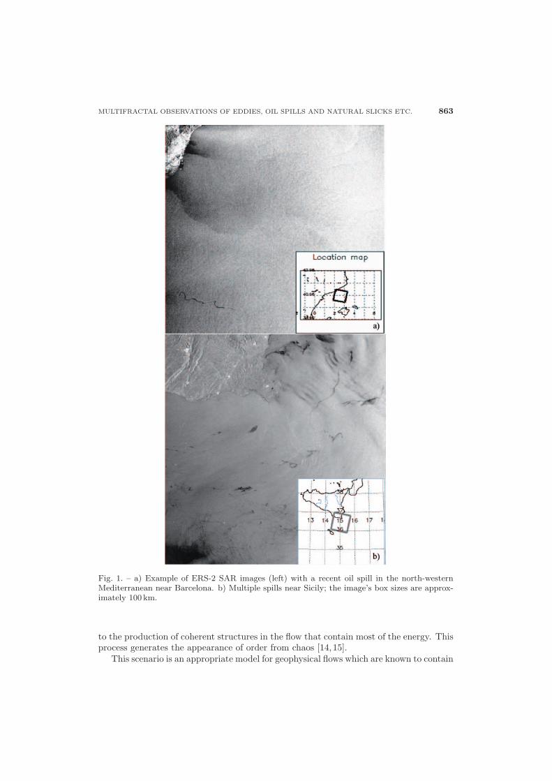
The ability of the SAR equipped satellites to monitor a large sea area and the factthat radar reflections are sensible to either surface tension-actives or pollutants thatchange the sea surface roughness make them an important tool in environmental re-search. Man-made oil/water wash spills dampen the small-scale surface waves, these inturn are responsible for the radar backscattering from the water surface, and are clearlyvisible as dark patches or lines in SAR images (fig. 1) that most times strike out fromthe rest of the image. Other types of oceanic and atmospheric phenomena also causespecific signatures due to changes in the surface capillary waves similar to those dueto oil slicks. These features are advected by the local currents so they are also ableto reveal the structure of the ocean surface [8-10]. It is important to point out thatthe detection ability of oceanic surface films by SAR sensors strongly depends on windspeed: at either very low wind speeds (below approximately 2 m/s) or very high windspeed (above approximately 10 m/s) oceanic surface films cannot, or may only barely,be identified [10-13]. On the other hand, the sunshine illumination conditions are not alimiting factor for the acquisition of SAR images as the cloud cover is transparent forSAR sensors. The nocturnal conditions are not limiting either because SAR is an activesensor that radiates its own energy.

These effects allow us to use remote sensing of the ocean surface even to monitorand police pollution from space. Here we will discuss several techniques that are ableto extract geometrical information from the ocean surface linked in several ways to thedynamics of a certain area. Multifractal analysis is useful on different accounts as aquantitative technique to distinguish the origin of several features.

Oceanic and atmospheric flows may be considered as turbulent motions under theconstraints of geometry, stratification and rotation. At large scales these flows tend tooccur mostly along isopycnal surfaces due to the combined effects of the very low aspectratio of the flows (the motion is confined to thin layers of fluid) and the existence of stabledensity stratification. The effect of the Earth’s rotation is to reduce the vertical shearin these almost planar flows. The combined effects of these constraints are to produceapproximately two-dimensional turbulent flows termed as geophysical turbulence.

2. – Geophysical turbulence

In a strictly two-dimensional flow with weak dissipation, energy input at a given scaleis transferred to larger scales, because these constraints stop vortex lines being stretchedor twisted. Physically this upscale energy transfer occurs by merging of vortices and leads

https://www.researchgate.net/publication/3821254_Marine_pollution_in_European_coastal_waters_monitored_by_the_ERS-2_SAR_a_comprehensive_statistical_analysis?el=1_x_8&enrichId=rgreq-7f0919a34f148b9f5fa8255dbafe5fe3-XXX&enrichSource=Y292ZXJQYWdlOzIzNjY1OTc5NjtBUzoyMDQ3ODI4NzE1NTIwMDBAMTQyNTgzNTQ0OTU3Nw==

MULTIFRACTAL OBSERVATIONS OF EDDIES, OIL SPILLS AND NATURAL SLICKS ETC. 863

Fig. 1. – a) Example of ERS-2 SAR images (left) with a recent oil spill in the north-westernMediterranean near Barcelona. b) Multiple spills near Sicily; the image’s box sizes are approx-imately 100 km.

to the production of coherent structures in the flow that contain most of the energy. Thisprocess generates the appearance of order from chaos [14,15].

This scenario is an appropriate model for geophysical flows which are known to contain


very energetic vortices mesoscale oceanic eddies and atmospheric highs and lows. Thisupscale transfer of energy is inhibited at the Rossby deformation radius:

LR =N

fh,

where h is the characteristic scale of the depth of the thermocline, N the Brunt-Vaisalafrequency and f the Coriolis parameter.

The energy limitation is caused by baroclinic instability at larger scales, which ac-counts for the dominant observed size of geophysical vortices detected in laboratoryexperiments on annulus flow, where the flow is driven in a rotating annulus by differ-ential heating of the lateral walls of the annulus, or by internal heating of the fluid. Ahorizontal temperature gradient is established which drives a zonal flow via the “thermalwind” balance. For certain values of the parameters this flow is unstable to baroclinicmodes that feed on the energy in the temperature or density fields.

Many features have been identified with structures and phenomena observed in sev-eral experiments, and understanding of atmospheric and ocean dynamics has been sig-nificantly advanced. The experiments have provided new insights about the dynamicsand have revealed a wide range of nonlinear behaviours.

Experiments performed by Linden et al. [15] showed the effect of mixing from the edgeon a rotating stratified system. When the instability is caused by differential heating orby buoyancy there seems to be a range of very different dynamic regimes. Work byCarrillo [16] has revealed the possible complex interactions between lateral (or coastal)stirring and the rotating-stratified flow dynamics.

The investigation of such strongly non-homogeneous flow, which leads to intermittenttwo-dimensional turbulence [17,18] is believed to be very important if correct parameter-izations of pollutant dispersion (such as Oil spills) in coastal areas are to be made. Theavailability of a large-scale flow allows both to measure Eulerian velocities with preci-sion as well as Lagrangian flows using particle tracking as well as local measurements ofdiffusivity by video recording the dispersion of neutral tracers. A possible oil spill predic-tion technique involves the releasing of hundreds of small and inexpensive tracer (GPS)Lagrangian buoys near an accident to aid the predictions of coastal currents [12,13].

Recent man-made oil spills in the sea surface are characterized by the low fractaldimension values (D < 1.2) over the region of low reflectivity in SAR images, on theother hand, natural oil slicks show a typical parabolic shape with a maximum of D < 1.5.Most of the SAR images analyzed were obtained during 1996-1998 (near 900 images ofEuropean coastal waters with 300 in the NW Mediterranean Sea area) but SAR andASAR images from ENVISAR have also been used. One of the problems in order toidentify oil spills is the possibility of confusion with natural tensioactive spills, whichmay be due to plankton, algae or even wind pattern reflections on the ocean surface,one of the possibilities is to use the scaling properties of the turbulence that advects anddiffuses the tracers [19,20].

3. – Multifractal objects and fractal dimensions

Fractals are geometric entities that present self-similarity and they are often the resultof iterative processes such as turbulence. The self-similarity implies that if we accomplishobservations from different scales the results are similar, although in natural systems it isenough to have only a certain statistical similarity. These entities have usually anisotropic


nature and then there may be different scaling laws for the different directions. Examplesof these are the surface topography and the clouds, where the vertical coordinate has asmaller magnitude than horizontal coordinates due to stratification. Fractal analysis isa very useful tool to characterize these objects in which an additional possibility is thecalculation of the corresponding fractal dimension along the different coordinates so itmay also reflect the anisotropic scaling [21,22].

3.1. Fractal scalar fields. – The theory applied here links fractal analysis to the turbu-lence self-similarity [22-24]. Turbulent diffusivities and Richardson’s law applied to theocean surface probed by the SAR images will be discussed. If we consider the varianceof a special signal, then

(1) V (λ) = V (0) − S2(λ)2

= 〈(ρ(x + λ)ρ(x))2〉.

The self-similar character of the signal, that for velocity differences, including inter-mittency, was popularized in [6, 21] through the use of structure functions may scalethrough the Hausdorff dimension H when the limit

(2) limλ→0

〈(ρ(x + λ) − ρ(x))〉λH

converges and then the dependence corresponds to a fractal set, either in space or in theform of a time series (when the coordinate is time and instead of a wave-number we havea period).

With the stated conditions, the variance of the signal under study will show a scaledependence such that V (λ) ≈ λ2H [22-25].

Using λ = 2π/k and the description of the spatial spectral density function, E(k), wehave

(3) E(λ) ≈ λβ

and relating the scalar equivalent to the turbulence energy spectrum as a Fourier trans-form of the correlation, also directly related to the second-order structure function as

(4) S2(x, λ) = 〈ρ2(x, λ)〉 = V − 12

⟨(ρ(x + λ) − ρ(x))2

⟩.

We may write in terms of the spatial equivalent to the turbulent energy density

(5) E(k)α λ

∫ λ

0

ρ2(x) eikx dx ≈ λV

so relating the Euclidean, fractal and Hausdorff dimensions, using (H = E − D) [2]

(6) E(k) ≈ λV ≈ λ2H+1 ≈ λ2E+1−2D.

Thus the relationship between the exponent of the spectral density function and themaximum fractal dimension may be written as

(7) β = 2E + 1 − 2D


and inversely

(8) D = E +1 − β

2.

These relationships may be used to relate the maximum fractal dimension of a spatialsignal to the spectral power slope (including intermittency) of the environment. If thesignal used is the SAR radar intensity D would reflect the ocean surface type of horizontalturbulent cascade assuming that the tensioactive tracers act in a passive way beingadvected by the velocity field.

3.2. Theory of multifractal measurements. – The measurement of multifractals ismainly the measurement of a statistic distribution which is why the results yield usefulinformation even if the underlying structure does not show a self-similar or self-affinebehavior as shown by Plotnick et al. [26].

For a monofractal object, as mentioned above, the number n of features of a certainsize δ varies as

(9) n(δ) ∝ δ−D0 ,

where the fractal dimension D0

(10) D0 = limδ→0

log n(δ)

log1δ

can be measured by counting the number n of boxes needed to cover the object underinvestigation for increasing box sizes δ and estimating the slope of a log-log plot.

There are several methods for implementing multifractal analysis; in this section themoment method [2, 3] is explained. This method uses mainly three functions: τ(q),called the mass exponent function, α, which is known as the coarse Holder exponent,and finally the function f(α), or multifractal spectrum. For a measure (or field) definedin a two-dimensional support of the L×L pixels image, μ (may be considered as the greytone from 0 to 255 in a normal 8 bit image), it could be spatially decomposed in termsof infinitely many intertwined sets of fractal dimensions. If that is the case, one fractaldimension cannot characterize all the complexity and several fractal dimensions will beestimated depending on the position. Applying box-counting “up-scaling” partitioningprocess we can get the partition function χ(q, δ) defined as [3]

(11) χ(q, δ) =n(δ)∑i=1

μqi (δ) =

n(δ)∑i=1

mqi ,

where m is the mass of the measure, q is the mass exponent, δ is the length size of thebox and n(δ) is the number of boxes in which mi > 0. Based on this, the mass exponentfunction (τ(q)) shows how the moments of the measure scale with the box size:

(12) 〈τ(q)〉 = limδ→0

log〈χ(q, δ)〉log(δ)

= limδ→0

log⟨∑n(δ)

i=1 mqi

⟩log(δ)

,


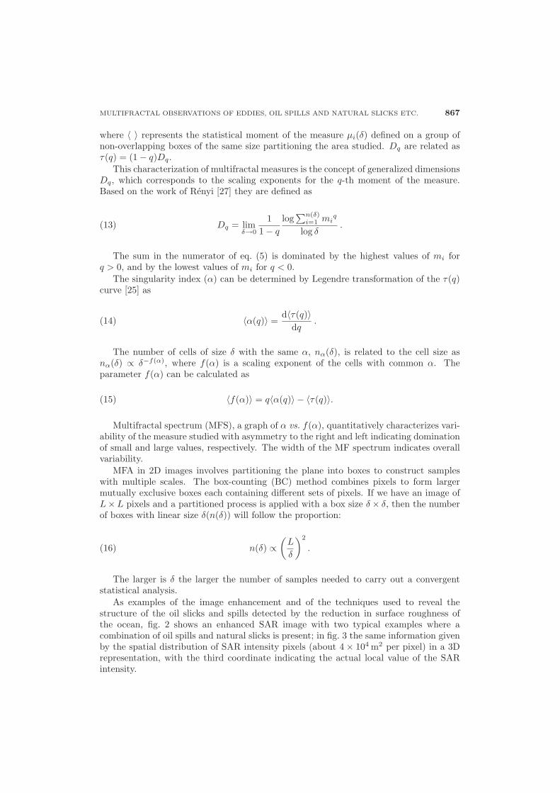
where 〈〉 represents the statistical moment of the measure μi(δ) defined on a group ofnon-overlapping boxes of the same size partitioning the area studied. Dq are related asτ(q) = (1 − q)Dq.

This characterization of multifractal measures is the concept of generalized dimensionsDq, which corresponds to the scaling exponents for the q-th moment of the measure.Based on the work of Renyi [27] they are defined as

(13) Dq = limδ→0

11 − q

log∑n(δ)

i=1 miq

log δ.

The sum in the numerator of eq. (5) is dominated by the highest values of mi forq > 0, and by the lowest values of mi for q < 0.

The singularity index (α) can be determined by Legendre transformation of the τ(q)curve [25] as

(14) 〈α(q)〉 =d〈τ(q)〉

dq.

The number of cells of size δ with the same α, nα(δ), is related to the cell size asnα(δ) ∝ δ−f(α), where f(α) is a scaling exponent of the cells with common α. Theparameter f(α) can be calculated as

(15) 〈f(α)〉 = q〈α(q)〉 − 〈τ(q)〉.

Multifractal spectrum (MFS), a graph of α vs. f(α), quantitatively characterizes vari-ability of the measure studied with asymmetry to the right and left indicating dominationof small and large values, respectively. The width of the MF spectrum indicates overallvariability.

MFA in 2D images involves partitioning the plane into boxes to construct sampleswith multiple scales. The box-counting (BC) method combines pixels to form largermutually exclusive boxes each containing different sets of pixels. If we have an image ofL×L pixels and a partitioned process is applied with a box size δ × δ, then the numberof boxes with linear size δ(n(δ)) will follow the proportion:

(16) n(δ) ∝(

L

δ

)2

.

The larger is δ the larger the number of samples needed to carry out a convergentstatistical analysis.

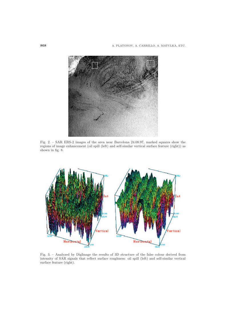
As examples of the image enhancement and of the techniques used to reveal thestructure of the oil slicks and spills detected by the reduction in surface roughness ofthe ocean, fig. 2 shows an enhanced SAR image with two typical examples where acombination of oil spills and natural slicks is present; in fig. 3 the same information givenby the spatial distribution of SAR intensity pixels (about 4 × 104 m2 per pixel) in a 3Drepresentation, with the third coordinate indicating the actual local value of the SARintensity.


Fig. 2. – SAR ERS-2 images of the area near Barcelona 24.08.97, marked squares show theregions of image enhancement (oil spill (left) and self-similar vertical surface feature (right)) asshown in fig. 8.

Fig. 3. – Analyzed by DigImage the results of 3D structure of the false colour derived fromintensity of SAR signals that reflect surface roughness: oil spill (left) and self-similar verticalsurface feature (right).


3.3. Multifractal measurements. – To calculate the fractal dimension, the box-countingmethod used produces a coverage of the object as discussed above. For the plane theseboxes will be squares and for an object in space they will be cubes. The distribution ofthe boxes is accomplished systematically, the intersection of these with the object carriesthe fact that we have N boxes with a non-void intersection, but as they are not exactlythe result of the better coverage possible, the concept of self-similarity may be appliedand thus the basic covering is accomplished repeating the process for many differentpossible diminishing observation scales.

When we work with real images they do not have generally some perfectly definedcontours, but we have some wide quite ranges of scalar intensity values to process. If wegroup the available data and describe them by a single large set and calculate the fractaldimension, we then lose the corresponding information due to the intensity variation.

It is also possible to accomplish a segmentation in many intervals that contains eachone a very well-defined intensity range. For each one of these ranges the usual fractaldimension calculation with the box-counting method will be applied and we will obtainthe corresponding fractal dimension for each intensity level. The result of the processwill be a set of dimension values, function of the intensity, and this measure will notneed to rely on the evaluation of a limit neither to the smallest nor to the largest scales.An advantage of this straightforward method is that the best fit to calculate D may beperformed choosing freely the scale, the scale interval and the number of pixel valuesthat will be used.

The fractal dimension D(ρ) is then a function of pixel intensity (we may relate μ toρ) and may be calculated using

(17) D(ρ) = − log N(ρ)log λ

,

where N(ρ) is the number of boxes of size λ needed to cover the SAR contour of inten-sity ρ.

The box-counting algorithm divides the embedding Euclidean plane in smaller andsmaller boxes (e.g., by dividing the initial length λ0 by n, which is the recurrence level ofthe iteration). For each box of size λ0/n it is then decided if the convoluted line, whichis analyzed, is intersecting that box. Finally, N versus λ0/n (i.e. the size of the box e)in a log-log plot is plotted, and the slope of that curve, within reasonable experimentallimits, gives the fractal dimension. This method of box-counting is used in ImaCalcsoftware [10] that we applied to detect the self-similar characteristics for different SARimage grey intensity levels ρ and to identify different sea surface dynamic processes. Eachof the intensity values may reflect different physical processes and lead to a different valueof its fractal dimension, this whole entity can be either fractal or non-fractal but exhibitsa range of values 0–2 for each intensity.

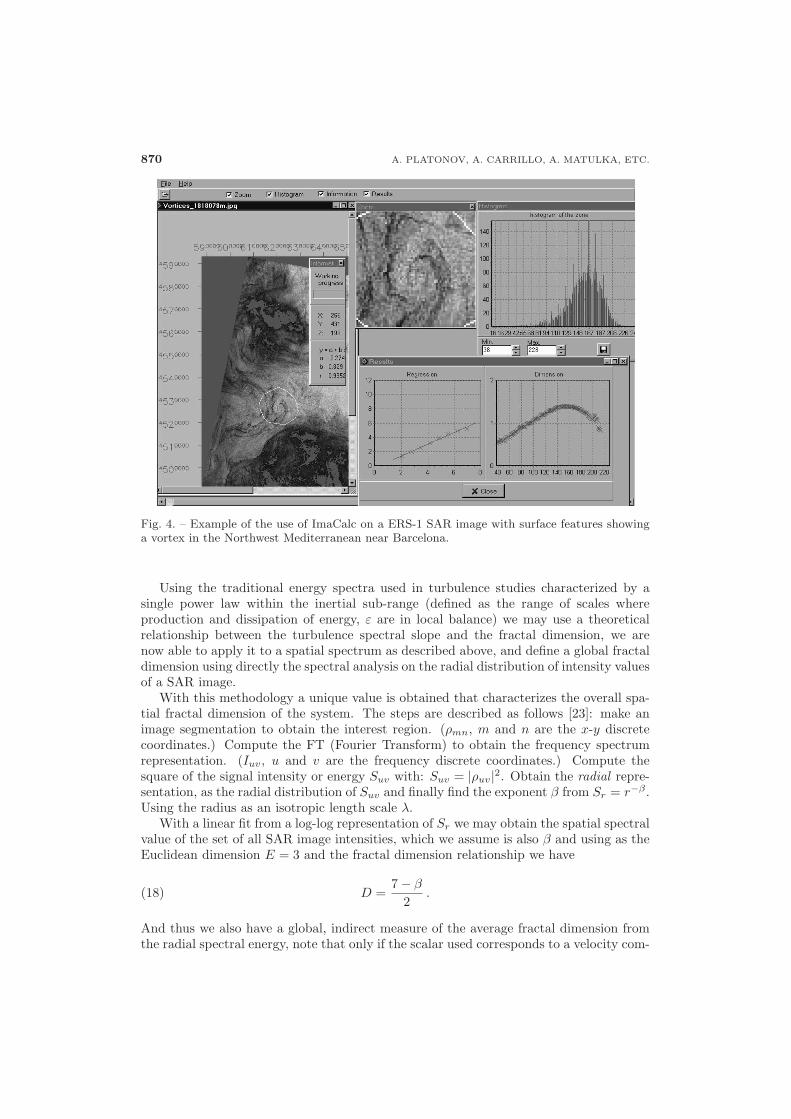
The program ImaCalc [10-13] performs interactively most of the multifractal box-counting methods as well as the spectral ones. Different regions may be equalized de-pending on their intensity histogram distribution. Figure 4 shows the dialog box withthe zoom, histogram and a fractal fit. With this application we can define the imageregion of interest, select an intensity range to analyze and execute the multifractal char-acterization process in a simple iterative way. On the right side of fig. 4, other smallerboxes show the observed dimension values as a grey-level function of the characterizedintervals, which may also be selected.


Fig. 4. – Example of the use of ImaCalc on a ERS-1 SAR image with surface features showinga vortex in the Northwest Mediterranean near Barcelona.

Using the traditional energy spectra used in turbulence studies characterized by asingle power law within the inertial sub-range (defined as the range of scales whereproduction and dissipation of energy, ε are in local balance) we may use a theoreticalrelationship between the turbulence spectral slope and the fractal dimension, we arenow able to apply it to a spatial spectrum as described above, and define a global fractaldimension using directly the spectral analysis on the radial distribution of intensity valuesof a SAR image.

With this methodology a unique value is obtained that characterizes the overall spa-tial fractal dimension of the system. The steps are described as follows [23]: make animage segmentation to obtain the interest region. (ρmn, m and n are the x-y discretecoordinates.) Compute the FT (Fourier Transform) to obtain the frequency spectrumrepresentation. (Iuv, u and v are the frequency discrete coordinates.) Compute thesquare of the signal intensity or energy Suv with: Suv = |ρuv|2. Obtain the radial repre-sentation, as the radial distribution of Suv and finally find the exponent β from Sr = r−β .Using the radius as an isotropic length scale λ.

With a linear fit from a log-log representation of Sr we may obtain the spatial spectralvalue of the set of all SAR image intensities, which we assume is also β and using as theEuclidean dimension E = 3 and the fractal dimension relationship we have

(18) D =7 − β

2.

And thus we also have a global, indirect measure of the average fractal dimension fromthe radial spectral energy, note that only if the scalar used corresponds to a velocity com-


ponent energy will have the correct physical dimension, otherwise the energy spectrumwill just indicate the square of the physical signal used.

4. – Results

The measurement of multifractals is mainly the measurement of a statistic distributionwhich is why the results yield useful information even if the underlying structure does notshow a self-similar or self-affine behaviour. For a monofractal object, the number N offeatures of a certain size e varies as can be measured by counting the number N of boxesneeded to cover the object under investigation for increasing box sizes e and estimatingthe slope of a log-log plot. For multifractal measurements, a probability distribution ismeasured. In practice, using the box-counting method, for every box i the probability of“containing the object”, or in this application, the values of a certain SAR reflectivity, isalso called the partition function, which may be obtained for different moments q whichcan vary from −8 to +8. Both methods described above may be used to extract usefulinformation about the age of the oil spills as well as about other mixing processes in theoceal surface.

Thus it is possible to define D as described above. The well-known [24-28] multifractalfunction f(a) may be seen as the fractal dimension of the set of intervals that correspondsto a singularity a, and a graph of a vs. f(a) is called the multifractal spectrum of themeasure. A measure is multifractal when its multifractal spectrum exists and has theshape of an inverted parabola. A generally equivalent way to describe a multifractalscaling is by considering the scaling laws of the moments of the measure.

In practice, the object density is taken to the respective power of q, summed forall i, and plotted versus the box size in a log-log coordinate system. From the slope,which is also called the mass exponent t, the generalized dimensions are estimated asD(q) = t(q)/(1 − q).

Images can be pre-processed using any image processor, e.g., to convert fromcolour/grey images to black-and-white using different types of algorithms, to invert back-ground and foreground, to extract boundaries. With SAR images from the ocean surfacewe cannot rely strictly on theoretical limit for the calculation of the fractal, non-fractalor multifractal behaviour, because they have a finite size, and we have assigned a fixedrange of values to the different SAR reflectivity intensity. The ranges of scale boundariesare defined by the image resolution, and we use numerical log/log fits (which tend tostraighten any curve) to obtain the Renyi dimensions.

Generalized dimensions D(q) can be obtained with the method of moments for anyimage and box size described.

In order to compare the two multifractal analysis procedures involving either a singlefractal measure for each of the intensity levels (or grouped in sets) with the momentcalculation for the generalized dimensions, we checked the numerical values at each al-gorithm step. Outside of this scale range, the theoretical values of D(q) (calculated asthe limit when r approaches zero) and the numerical values of D(q) (calculated from theregression fits) are still very close if we select the range of scale and a grid matching thetheoretical generation pattern. We applied this for a range of oil spill images.

The study of the structured distribution in the space such that at any resolution theset is the union of similar subsets to the whole will indicate the same fractal dimension forevery intensity value. But the scale factor at different parts of the set is not the same formost SAR images. If more than one dimension is needed, then the measure consideredis characterized by the union of fractal sets, each one with a different fractal dimension.


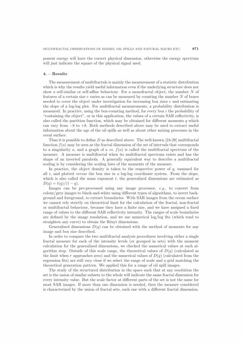
Fig. 5. – Range of functions χ(q, δ) for a recent oil spill (top) and for a weathered one (bottom).

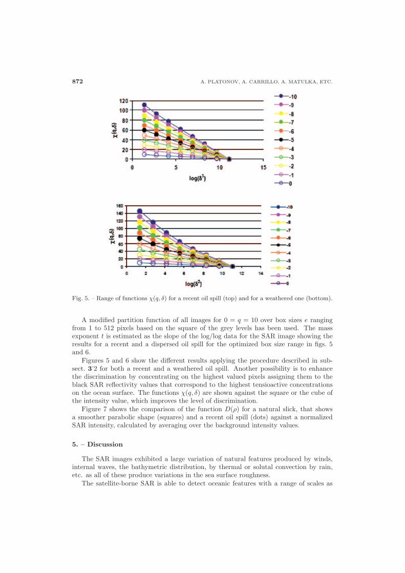
A modified partition function of all images for 0 = q = 10 over box sizes e rangingfrom 1 to 512 pixels based on the square of the grey levels has been used. The massexponent t is estimated as the slope of the log/log data for the SAR image showing theresults for a recent and a dispersed oil spill for the optimized box size range in figs. 5and 6.

Figures 5 and 6 show the different results applying the procedure described in sub-sect. 3.2 for both a recent and a weathered oil spill. Another possibility is to enhancethe discrimination by concentrating on the highest valued pixels assigning them to theblack SAR reflectivity values that correspond to the highest tensioactive concentrationson the ocean surface. The functions χ(q, δ) are shown against the square or the cube ofthe intensity value, which improves the level of discrimination.

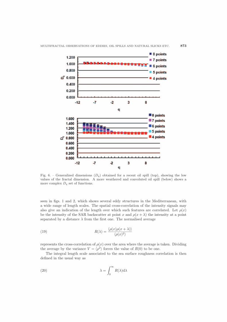
Figure 7 shows the comparison of the function D(ρ) for a natural slick, that showsa smoother parabolic shape (squares) and a recent oil spill (dots) against a normalizedSAR intensity, calculated by averaging over the background intensity values.

5. – Discussion

The SAR images exhibited a large variation of natural features produced by winds,internal waves, the bathymetric distribution, by thermal or solutal convection by rain,etc. as all of these produce variations in the sea surface roughness.

The satellite-borne SAR is able to detect oceanic features with a range of scales as


Fig. 6. – Generalized dimensions (Dq) obtained for a recent oil spill (top), showing the lowvalues of the fractal dimension. A more weathered and convoluted oil spill (below) shows amore complex Dq set of functions.

seen in figs. 1 and 2, which shows several eddy structures in the Mediterranean, witha wide range of length scales. The spatial cross-correlation of the intensity signals mayalso give an indication of the length over which such features are correlated. Let ρ(x)be the intensity of the SAR backscatter at point x and ρ(x + λ) the intensity at a pointseparated by a distance λ from the first one. The normalised average

(19) R(λ) =〈ρ(x)ρ(x + λ)〉

〈ρ(x)2〉

represents the cross-correlation of ρ(x) over the area where the average is taken. Dividingthe average by the variance V = 〈ρ2〉 forces the value of R(0) to be one.

The integral length scale associated to the sea surface roughness correlation is thendefined in the usual way as

(20) λ =∫ ∞

0

R(λ)dλ


0.4 0.8.2

1

1. 2

1. 4

1. 6

0

Frac

tal d

imen

sion

D (i

)

Normalized SAR intensity i/io1

Fig. 7. – Multifractal set of dimensions D(μ) obtained for a recent oil spill (dots), showingthe low values between 0.1 and 0.4 of the normalized SAR intensity. A natural spill is moreconvoluted (squares) and shows a more uniform parabolic type of D(μ) functions.

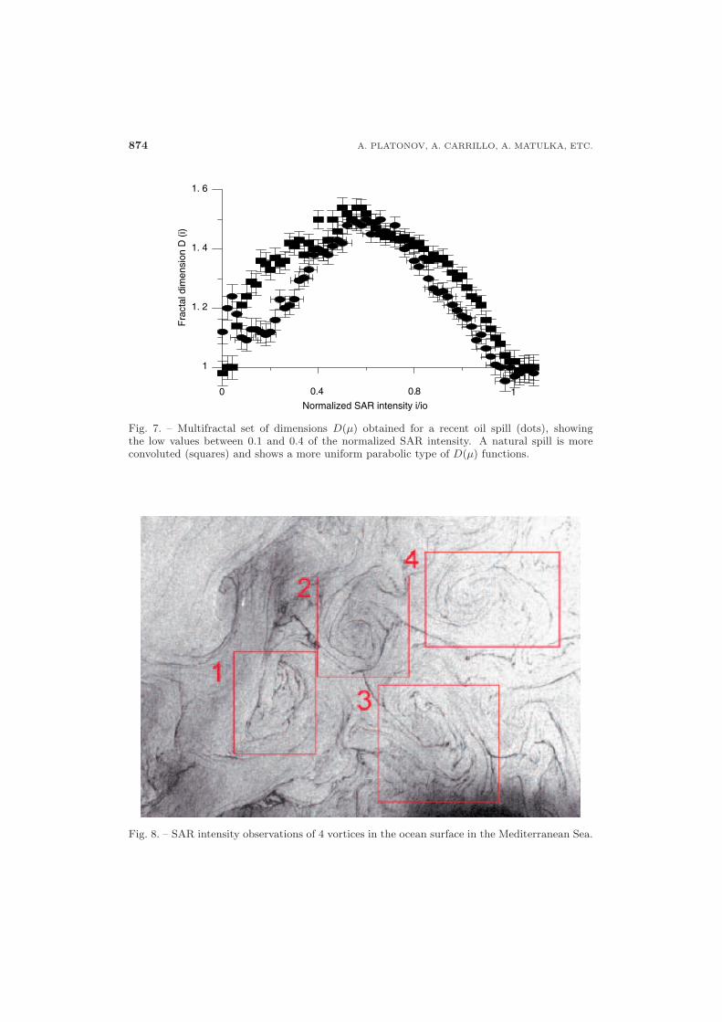
Fig. 8. – SAR intensity observations of 4 vortices in the ocean surface in the Mediterranean Sea.


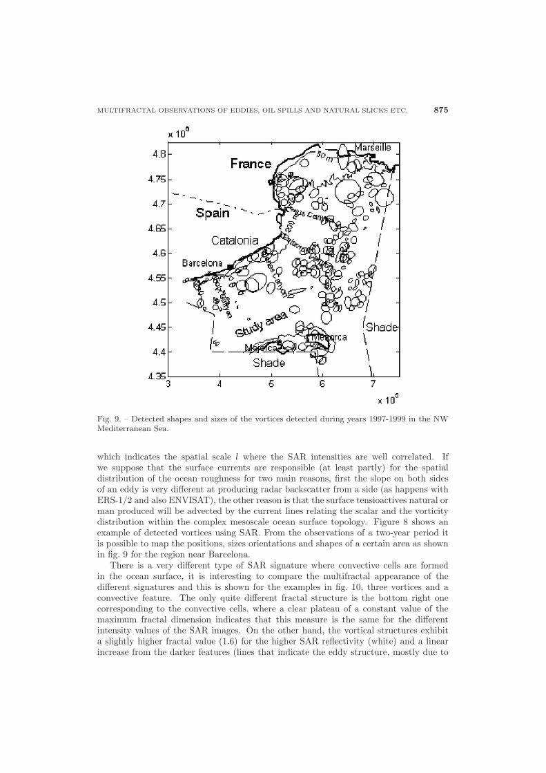
Fig. 9. – Detected shapes and sizes of the vortices detected during years 1997-1999 in the NWMediterranean Sea.

which indicates the spatial scale l where the SAR intensities are well correlated. Ifwe suppose that the surface currents are responsible (at least partly) for the spatialdistribution of the ocean roughness for two main reasons, first the slope on both sidesof an eddy is very different at producing radar backscatter from a side (as happens withERS-1/2 and also ENVISAT), the other reason is that the surface tensioactives natural orman produced will be advected by the current lines relating the scalar and the vorticitydistribution within the complex mesoscale ocean surface topology. Figure 8 shows anexample of detected vortices using SAR. From the observations of a two-year period itis possible to map the positions, sizes orientations and shapes of a certain area as shownin fig. 9 for the region near Barcelona.

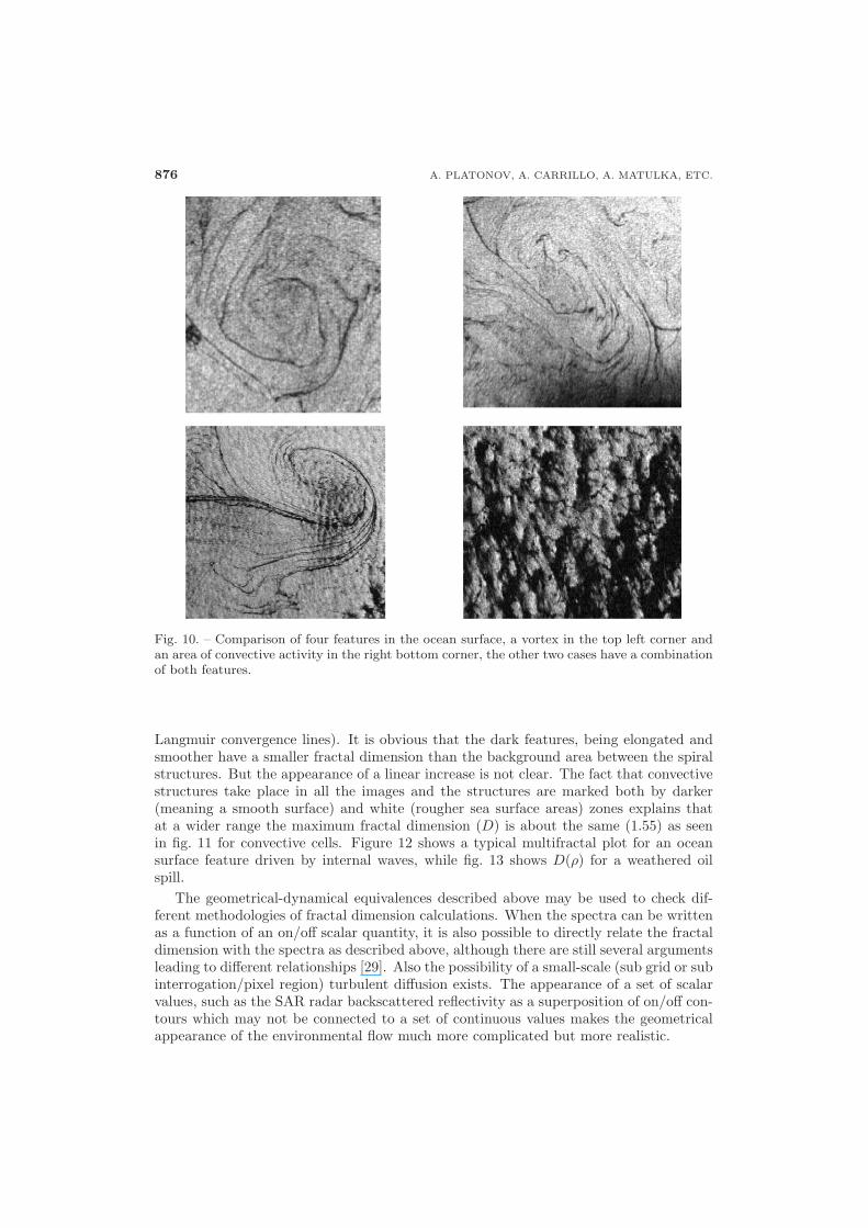
There is a very different type of SAR signature where convective cells are formedin the ocean surface, it is interesting to compare the multifractal appearance of thedifferent signatures and this is shown for the examples in fig. 10, three vortices and aconvective feature. The only quite different fractal structure is the bottom right onecorresponding to the convective cells, where a clear plateau of a constant value of themaximum fractal dimension indicates that this measure is the same for the differentintensity values of the SAR images. On the other hand, the vortical structures exhibita slightly higher fractal value (1.6) for the higher SAR reflectivity (white) and a linearincrease from the darker features (lines that indicate the eddy structure, mostly due to


Fig. 10. – Comparison of four features in the ocean surface, a vortex in the top left corner andan area of convective activity in the right bottom corner, the other two cases have a combinationof both features.

Langmuir convergence lines). It is obvious that the dark features, being elongated andsmoother have a smaller fractal dimension than the background area between the spiralstructures. But the appearance of a linear increase is not clear. The fact that convectivestructures take place in all the images and the structures are marked both by darker(meaning a smooth surface) and white (rougher sea surface areas) zones explains thatat a wider range the maximum fractal dimension (D) is about the same (1.55) as seenin fig. 11 for convective cells. Figure 12 shows a typical multifractal plot for an oceansurface feature driven by internal waves, while fig. 13 shows D(ρ) for a weathered oilspill.

The geometrical-dynamical equivalences described above may be used to check dif-ferent methodologies of fractal dimension calculations. When the spectra can be writtenas a function of an on/off scalar quantity, it is also possible to directly relate the fractaldimension with the spectra as described above, although there are still several argumentsleading to different relationships [29]. Also the possibility of a small-scale (sub grid or subinterrogation/pixel region) turbulent diffusion exists. The appearance of a set of scalarvalues, such as the SAR radar backscattered reflectivity as a superposition of on/off con-tours which may not be connected to a set of continuous values makes the geometricalappearance of the environmental flow much more complicated but more realistic.

https://www.researchgate.net/publication/236595400_Mixing_efficiency_of_different_kinds_of_turbulent_processes_and_instabilities?el=1_x_8&enrichId=rgreq-7f0919a34f148b9f5fa8255dbafe5fe3-XXX&enrichSource=Y292ZXJQYWdlOzIzNjY1OTc5NjtBUzoyMDQ3ODI4NzE1NTIwMDBAMTQyNTgzNTQ0OTU3Nw==


Fig. 11. – Comparison of the multifractal D(ρ) plots for the four features in the ocean surfaceshown in fig. 9 a vortex in the top left corner, with a parabolic shape, and an area of convectiveactivity in the right bottom corner, with a uniform value of D over a wide range of SAR intensityvalues, the other two cases have a combination of both features.

0 0.4 0.8 1.2 1.6

iN

1

2

0.9

0.8

0.7

0.6

0.5

0.4

0.3

0.2

D

2

Fig. 12. – Multifractal D(ρ) plot for a region of internal waves detected by SAR, with a parabolicshape, and a maximum value of D of 1.4.


0 0.4 0.8 1.2 1.6

iN

1

2

0.9

0.8

0.7

0.6

0.5

0.4

0.3

0.2

D2

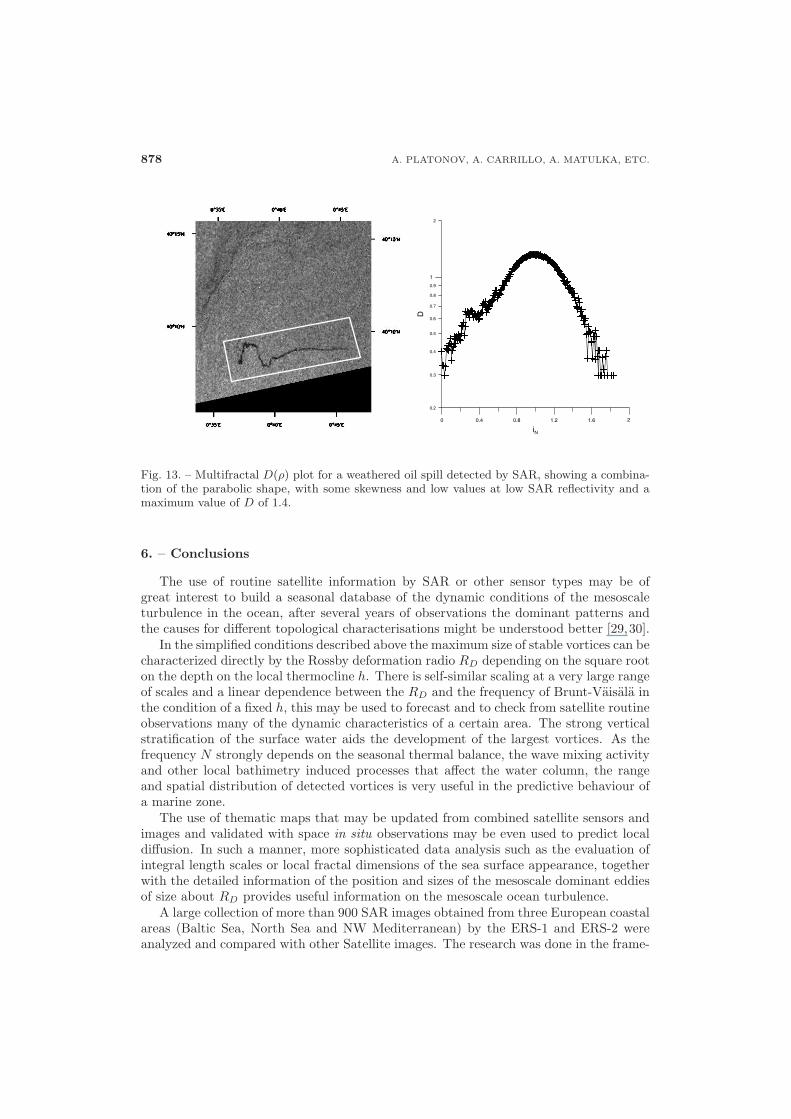
Fig. 13. – Multifractal D(ρ) plot for a weathered oil spill detected by SAR, showing a combina-tion of the parabolic shape, with some skewness and low values at low SAR reflectivity and amaximum value of D of 1.4.

6. – Conclusions

The use of routine satellite information by SAR or other sensor types may be ofgreat interest to build a seasonal database of the dynamic conditions of the mesoscaleturbulence in the ocean, after several years of observations the dominant patterns andthe causes for different topological characterisations might be understood better [29,30].

In the simplified conditions described above the maximum size of stable vortices can becharacterized directly by the Rossby deformation radio RD depending on the square rooton the depth on the local thermocline h. There is self-similar scaling at a very large rangeof scales and a linear dependence between the RD and the frequency of Brunt-Vaisala inthe condition of a fixed h, this may be used to forecast and to check from satellite routineobservations many of the dynamic characteristics of a certain area. The strong verticalstratification of the surface water aids the development of the largest vortices. As thefrequency N strongly depends on the seasonal thermal balance, the wave mixing activityand other local bathimetry induced processes that affect the water column, the rangeand spatial distribution of detected vortices is very useful in the predictive behaviour ofa marine zone.

The use of thematic maps that may be updated from combined satellite sensors andimages and validated with space in situ observations may be even used to predict localdiffusion. In such a manner, more sophisticated data analysis such as the evaluation ofintegral length scales or local fractal dimensions of the sea surface appearance, togetherwith the detailed information of the position and sizes of the mesoscale dominant eddiesof size about RD provides useful information on the mesoscale ocean turbulence.

A large collection of more than 900 SAR images obtained from three European coastalareas (Baltic Sea, North Sea and NW Mediterranean) by the ERS-1 and ERS-2 wereanalyzed and compared with other Satellite images. The research was done in the frame-



work of the CLEAN SEAS European Union project and more information is availableat [13-16].

The use of routine satellite information by SAR or other sensor types may be ofgreat interest to build a seasonal database of the dynamic conditions of the mesoscaleturbulence in the ocean, after several years of observations the dominant patterns and thecauses for different topological characterisations might be understood. It is important tocharacterize the types and structure of the main vortices detected as well as the spectralcascade processes that take place, these may be investigated by using fractal methods onimages of the area as well as with models of the turbulent cascade and field measurementsof diffusion [30-32].

The different multifractal formalisms can be used to discriminate between differentphysical processes that, despite being similar, have different transport mechanisms forthe different scales, or in time. From the comparison of the multifractal plots of the well-defined SAR detected vortices with those of convective cells, vortices show a maximumcomplexity for the low reflectivity values, while convection, probably because the basicinstability happens everywhere at the same time, exhibits almost the same fractal dimen-sion for a wide range of intermediate SAR reflectivity. The analysis of recent versus moreconvoluted oil spills is also interesting both in the formalisms presented in subsect. 3.2and 3.3. The recent oil spills pave a well-defined spatial and temporal origin, so as timedevelops (measured in terms of the turbulence of the area) the fractal measures tend tobe those of the turbulent environment, initially for low SAR reflectivity the generaliseddimensions are low but in time they increase to a limit of 1.5–1.6.

∗ ∗ ∗This work was supported by the Ministerio de Educacion y Ciencia of Spain and

the Universitat Politecnica de Catalunya (RYC-2003-005700, FTN-2001-2220, ESP2005-07551). Authors also acknowledge the CLEAN SEAS (ENV4-CT96-0334) EuropeanUnion Project and the ESA (AO-ID C1P.2240) for the SAR images provided.

REFERENCES

[1] Munk W., Sciencia Marina, 65 (2001) 193.[2] Turcotte D. L., Annu. Rev. Fluid Mech., 20 (1988) 5.[3] Feder J., Fractals in Physics (Cambridge University Press, Cambridge) 1988.[4] Richardson L. F., Proc. R. Soc. London, Ser A, 110 (1926) 709.[5] Kolmogorov A. N., C. R. Acad. Sci. USSR, 30 (1941) 301.[6] Kolmogorov A. N., J. Fluid Mech., 13 (1962) 82.[7] Kraichnan R., Phys. Fluids, 10 (1967) 1417.[8] Gade M. and Alper W., Sci. Total Environ., 237/238 (1999) 441.[9] Gade M. and Redondo J. M., Marine pollution in European coastal waters monitored

by the ERS-2 SAR: a comprehensive statistical analysis. IGARSS 99. Hamburg, Vol. III(1999), p. 1239.

[10] Grau J., Analysis of the Meteosat images sequences using the digital processing method.PhD Thesis UPC, Barcelona (2005).

[11] Platonov A. K., SAR satellite images applications to both sea contamination anddynamic studies in the NW Mediterranean, PhD Thesis, UPC Barcelona (2002), http://www.tdcat.cesca.es/TDCat-0905102-135541/.

[12] Redondo J. M. and Platonov A. K., Environ. Res. Lett., 4 (2009) 14008.[13] Redondo J. M. and Platonov A., Ing. Agua, 8 (2001) 15.[14] Zouari N. and Babiano A., Phys. D, 76 (1994) 318.





[15] Linden P. F., Boubnov B. M. and Dalziel S. B., J. Fluid Mech., 298 (1996) 81.[16] Carrillo A. A., Sanchez M. A., Platonov A. and Redondo J. M., Phys. Chem.

Earth B, 26 (2001) 305.[17] Chen X. and Allen S. E., J. Geophys. Res., 101 (1996) 18043.[18] Mahjoub O. B., Redondo J. M. and Babiano A., J. Flow Turbul. Combust., 59 (2000)

299.[19] Seuront L., Schmitt F., Lagadeuc Y., Schertzer D. and Lovejoy S., J. Plankton

Res., 21 (1999) 877.[20] Bezerra M. O., Diez M., Medeiros C., Rodriguez A., Bahia E., Sanchez-Arcilla

A. and Redondo J. M., J. Flow Turbul. Combust., 59 (1998) 191.[21] Mandelbrot B. B., Physica Scripta, 32 (1985) 257.[22] Redondo J. M. and Linden P. F., Geometrical Observations of Turbulent Interfaces:

The Mathematics of Deforming Surfaces (IMA, Clarendon Press, Oxford) 1996.[23] Vassilicos J. C. and Hunt J. C. R., Proc R. Soc. London, Ser A., 435 (1991) 505.[24] Dubucm B., Zucker S. W., Tricot C., Quiniou J. F. and Wehbi D., Phys. Rev. A,

425 (1989) 113’27.[25] Evertsz C. J. G. and Mandelbrot B. B., Multifractal measures, in Chaos and Fractals:

New Frontiers of Science, edited by Peitgen H., Jurgens H. and Saupe D. (Springer-Verlag, NY) 1992, pp. 921-953.

[26] Plotnick R. E., Gardner R. H., Hargrove W. W., Prestegaard K. andPerlmutter M., Phys. Rev. E, 53 (1996) 5461.

[27] Renyi A., Acta Math. Hung., VI (1955) 285.[28] Stanley H. and Meakin P., Nature, 335 (1988) 405.[29] Redondo J. M., Mixing efficiency of different kinds of turbulent processes and instabilities.

Applications to the environment, in Turbulent Mixing in Geophysical Flows, edited byLinden P. F. and Redondo J. M. (CIMNE, Barcelona) 2002, pp. 131-157.

[30] Berrizi F., Dalle Mese E. and Martorella M., Int. J. Remote Sens., 25 (2004) 1265.[31] Fung J. C. H., Hunt J. C. R., Malik N. A. and Perkins R. J., J. Fluid Mech., 236

(1992) 281.[32] Rodriguez A., Sanchez-Arcilla A., Redondo J. M., Bahia E. and Sierra J. P.,

Water Sci. Technol., 32 (1995) 169.




Multifractal observations of eddies, oil spills and natural slicks in the ocean surface

Documents

Transcript of Multifractal observations of eddies, oil spills and natural slicks in the ocean surface