Ecological Modelling, 47 (1989) 161-173 161 Elsevier Science Publishers B.V., Amsterdam - Printed in The Netherlands

F A S T G R A P H I C A L S I M U L A T I O N S O F S P I L L S A N D P L U M E S F O R A P P L I C A T I O N T O T H E G R E A T L A K E S

ISAAC WONG and D.A. SWAYNE

Department of Computing and Information Science, University of Guelph, Guelph, Ont. NIG 2W1 (Canada)

C.R. MURTHY and D.C.L. LAM

National Water Research Institute, 867 Lakeshore Road, Box 5050, Burlington, Ont. LTR 4,46 (Canada)

ABSTRACT

Wong, I., Swayne, D.A., Murthy, C.R. and Lam, D.C.L., 1989. Fast graphical simulations of spills and plumes for applications to the Great Lakes. Ecol. Modelling, 47: 161-173.

This paper deals with the development of coastal effluent models of two locations on Lake Ontario, Pickering and the Niagara River. The models employ microcomputers to simulate the entry into Lake Ontario of spills or effluent plumes at either site.

A spill or plume is observed as it interacts with shore currents. Observations have indicated that the coastal currents are highly correlated with the alongshore wind component. A simple linear impulse response function is applied which relates current to wind history. The current response is calibrated by observing the behaviour of drogues released in the river mouth for the Niagara River compared with wind measurement. Current measurements from fixed devices and daily wind observations have been used to derive the coefficients in the Picketing response function. Comparisons with drogue history for Niagara and water temperature distribution for Picketing have been used to assess the accuracy of the results, at least in a few interesting situations.

Software enabling the user to work from existing wind observations or to operate in predictive mode by entering hypothetical wind data has been developed, and a number of display options for the plume or patch are offered.

INTRODUCTION

The in ten t ion of this pape r is to descr ibe the imp lemen ta t i on of micro- c o m p u t e r compa t ib le spill models for a shore-based c o n t a m i n a t i o n source

on Lake Ontar io . Us ing only local wind history, a s imula t ion of the effects of wind in mod i fy ing under ly ing currents is carr ied out which has qual i ta-

0304-3800/89/$03.50 © 1989 Elsevier Science Publishers B.V.

1 6 2 1. W O N G ET AL.

tively correct behaviour, as measured against observations. The models illustrate the feasibility of designing simulations of complex physical systems to run on relatively inexpensive microcomputer equipment.

Two locations on Lake Ontario were chosen for the development of coastal effluent models, Picketing and the Niagara River. The models employ microcomputers to simulate the entry into Lake Ontario of spills or effluent plumes at either site. The original code was developed to model the transport of radionuclide contaminants in the wind-driven shore currents of the lake (Lam et al., 1986; Murthy et al., 1986b; Swayne et al., 1986). This work led to a successful model of radionuclide spills and heat discharges plumes from a nuclear power plant into Lake Ontario near Pickering.

The information relevant to the shore current simulation consists of depth contours adjacent to the shore, wind history at half-day intervals from the previous 30 days, and impulse response measurements recording the effect of wind history on the current at various depths. Values for the response coefficients have been measured by observation (Murthy et al., 1984, 1986a, b). For Picketing, a line of measuring devices was placed along a line roughly perpendicular to the shore. Impulse responses were then calculated for the positions of the devices. This information was then interpolated between depth contours and moved along the shoreline from the point of measurement. For the Niagara plume, the Picketing coefficients were mod- ified using data recorded from drogues released at the mouth of the river, with a simple transition function to blend the shore current results with the momentum imparted to the drogues by the river currents.

DESCRIPTION OF THE MODELS

Pickering model

The shore currents associated with the Picketing plume are mainly wind- driven. Following (Murthy, 1986), we reproduce the arguments from which part of our current predictions are computed. Assuming a uniform wind field, the current u(t) induced by wind stress "r at a point is given by:

- foUR (1) u(t)= f' s) ~'(s)ds=_ (s)~(t-s)ds

where R(t) is the impulse response at each point. In the presence of friction, the interval of integration is finite, and the integral may be satisfactorily approximated by a finite sum with time interval At over a number of intervals N such that N At = T. The average wind-stress-induced current u~ over the interval i At replaces the instantaneous u(t). The wind stress history "r in the integral (1) is approximated by an averaged value:

r,=r[(i + ½) At]

FAST GRAPHICAL SIMULATIONS OF SPILLS AND PLUMES FOR APPLICATION TO THE GREAT LAKES ] 63

The impulse response function R is replaced by:

R. = At R(n At) The approximation to the integral:

foTR(s) ¢( t - -s) ds

becomes: N

u i = ~ zi-nRn n = l

The unknown impulse response R , may be determined empirically from the calibration with observed data collected by current meters (as was the case with the previous work) or otherwise inferred from observations.

The shallow-water circulation is assumed to be confined to streamlines parallel to the depth contours. This simplifying assumption is known to be valid, in that about 97% of the flow energy is accounted for by tangential flow (Murthy et al., 1986b). The velocity at any point at or near the surface is calculated from the depth of water at that point.

To continue with the wind-driven current analysis, let (x, y) be the tangent and normal directions to the mean shoreline direction, and let:

U = {Uj, j = l . . . . . m}

represent the surface current computed from the wind-driven model, where j = 0 at the shore and each successive index value is the surface current at one kilometer intervals as defined from the data fitting. Suppose { Yj(x), Yj+l(X)} are the bounding depth-contour lines. For a given particle (poilu- tant), let (x~, y~) be the coordinate at time t~, and let (Au, Av) be the turbulent velocity components of the volume containing the particle. (The magnitude of these components determines the speed of fan-out of the particles in the simulation, and must be chosen to mimic the 97% contain- ment - or 3% dispersion - mentioned in the preceeding paragraph.) The coordinates of the particle at time t,+ 1 = ti + At are computed in a sequence of steps. First, Yj(x,), and Yj+l(xi) are determined from intersection with the depth contour information stored with the map. Next, we compute the fraction:

Y i - ~ ( x i ) r-~

Y j + I ( X i ) - Yj(x i )

representing the linearly interpolated spacing of y between the main depth contours. A proportional value u~ for current transport is computed from:

Uj + r(Uj+l - Uj) u , =

164 i. WONG ET AL.

Suitable random values for Au and Av (Lam et al., 1986) are added to the velocity components to generate new coordinates (xi+ 1, Yi+l):

xi+ 1 = x i+ (u i+ Au)A t

and

Yi+l = Y j ( x i + I ) + r[Yj+l(Xi+l)- Y j ( X i + l ) ] q- Av A t

We used ten contours (m = 10), approximately parallel to the coastline, each requiring a set of R/s . Wind episodes of less than half-day duration do not affect the result, and 30 half-day wind records produce an approxima- tion to the actual currents to within 75% of the variance (Murthy et al., 1986b). Thus, our program needs to store a vector of 300 (30 × 10) values R.,j to calculate interpolatory currents.

Niagara river model

The Niagara River model is an extension of the Picketing model. For the Niagara system, the response data had to be calculated from the behavior of drogues released into the fiver near the mouth. The model was complicated by the interaction between the river current and the shore current of the lake. The response coefficients of the north shore (The Pickering model) were applied to the Niagara system due to the unavailability of current data measurements near Niagara River. Outside the domain of influence of the river, the surface current behaviour was thought to be similar to that in the Pickering model. River outflow measurements and behaviour are measured in hourly time-units rather than half-daily as in the shore currents. There- fore, hourly simulations of fiver currents are superimposed on shore current simulations with half-day time-steps.

The outflow has been modelled by the continuous release of moving points ('pixels') representing hypothetical drogues into the region repre- senting the river, with the momentum-dominated initial flow gradually replaced by the influence of the shore current.

The validity of our approach is tested tentatively by comparison with the drogue data.

Modelling the effluent of Niagara River The effluent model is not derived strictly from physical principles, but is

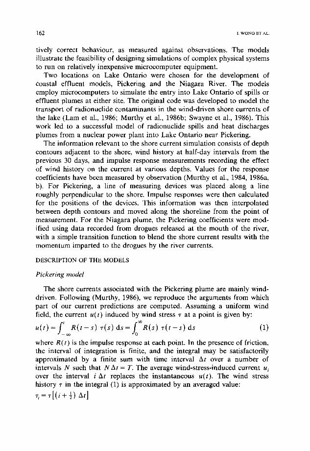
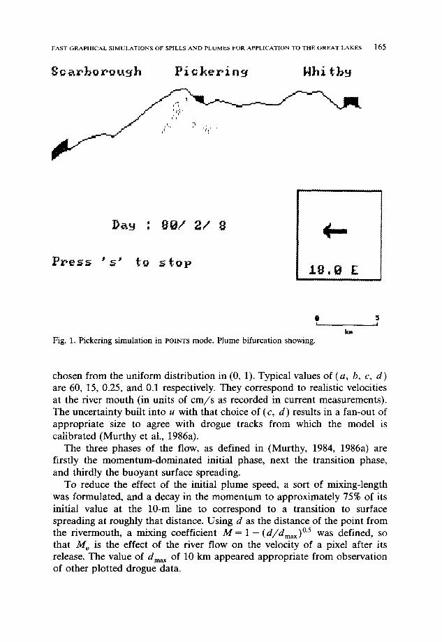
designed to deliver an approximately correct flow at the shelf-edge defined by the 10 m depth contour (Fig 1).

The initial velocity v = (u, v) is defined by the normal component v = a + bz, where z is chosen from the uniform (random) distribution in (0, 1). The tangential component u is defined by u = - (c + dz) v, where z is again

F A S T G R A P H I C A L S I M U L A T I O N S O F S P I L L S A N D P L U M E ~ F O R A P P L I C A T I O N T O T H E G R E A T L A K E S

S rbo ou h Pi keri Nhi tb l

,j;;. t ' l

i "1 ,

165

.i i i

I I

Fig. 1. Pickering simulation in POINTS mode. Plume bifurcation showing. km

chosen from the uniform distribution in (0, 1). Typical values of (a, b, c, d) are 60, 15, 0.25, and 0.1 respectively. They correspond to realistic velocities at the river mouth (in units of cm/s as recorded in current measurements). The uncertainty built into u with that choice of (c, d) results in a fan-out of appropriate size to agree with drogue tracks from which the model is calibrated (Murthy et al., 1986a).

The three phases of the flow, as defined in (Murthy, 1984, 1986a) are firstly the momentum-dominated initial phase, next the transition phase, and thirdly the buoyant surface spreading.

To reduce the effect of the initial plume speed, a sort of mixing-length was formulated, and a decay in the momentum to approximately 75% of its initial value at the 10-m line to correspond to a transition to surface spreading at roughly that distance. Using d as the distance of the point from the rivermouth, a mixing coefficient M = 1 - (d/dmax) °-5 was defined, so that M v is the effect of the river flow on the velocity of a pixel after its release. The value of dma x of 10 km appeared appropriate from observation of other plotted drogue data.

16 6

COMPUTER IMPLEMENTATIONS

1. W O N G E T AL.

Working versions of the simple plume models have been developed and calibrated (Swayne et al., 1986; Wong et al., 1987) with some of the results shown in Figs. 2-5. The source code was written in the programming language C, using the Multihalo graphics library package. The program and the related files are stored in one diskette and may be obtained from the authors upon request.

The response coefficients R, , j are static inputs to the program. Users may direct the wind inputs and contour lines from static files. Underlying offshore currents and parallel shore currents may be input. A description on how to use the pograms can be found in Appendix A and HELP.DOC in the diskette provided.

S o g r b o ~ o u ~ h Pi o k e r i ng blhi tb~j

Dg~ : 8 0 / 2 / 1 2 4,.,

X l . g E

I k m

Fig. 2. Picketing simulation in VECTOR mode.

FAST GRAPHICAL SIMULATIONS OF SPILLS AND PLUMES FOR APPLICATION TO THE G R E A T LAKES 1 6 7

S PboPou h Pi kerins Hhitbs

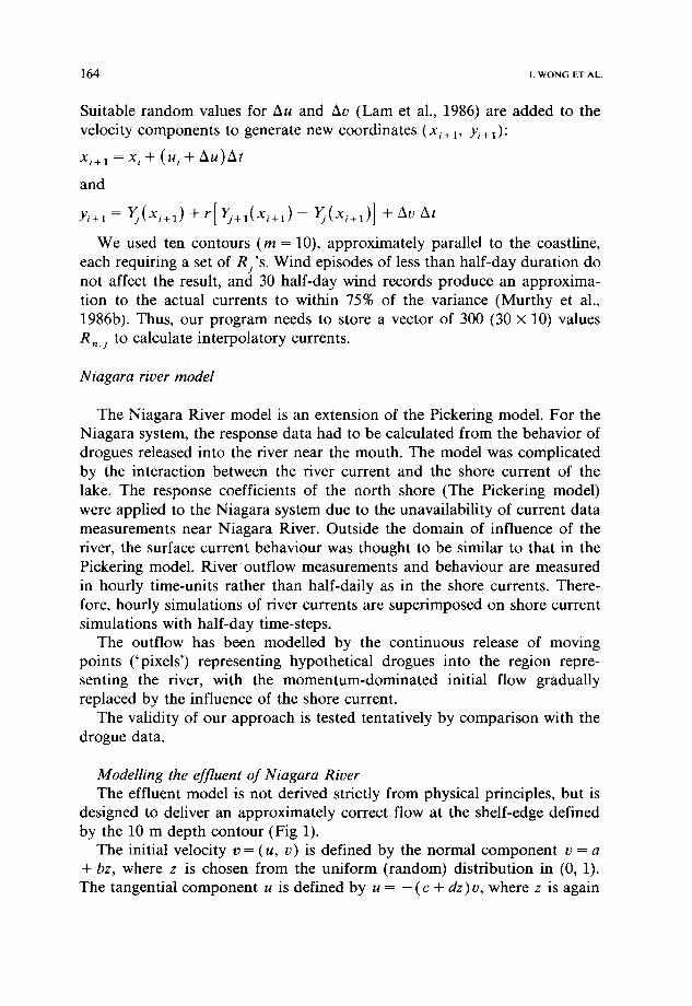
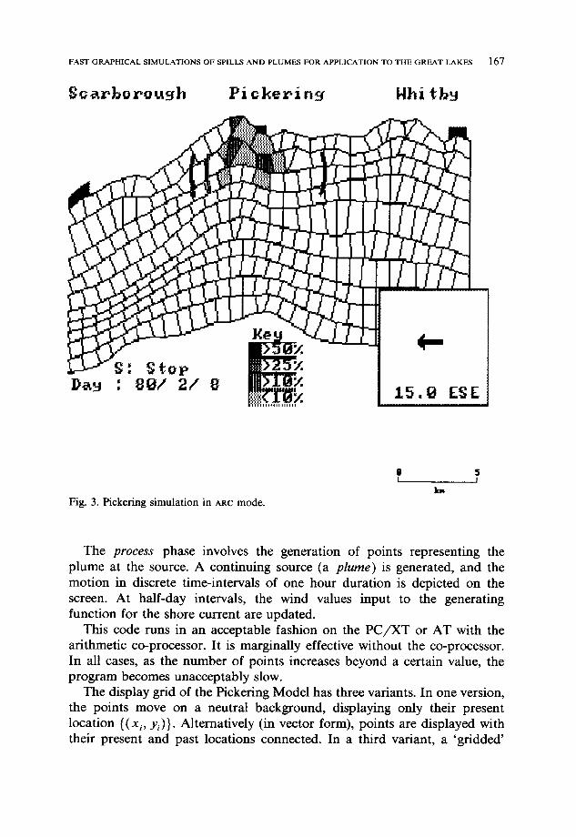
F i g . 3. P i c k e r i n g s i m u l a t i o n i n ARC m o d e .

0 I I

io4

The process phase involves the generation of points representing the plume at the source. A continuing source (a plume) is generated, and the motion in discrete time-intervals of one hour duration is depicted on the screen. At half-day intervals, the wind values input to the generating function for the shore current are updated.

This code runs in an acceptable fashion on the P C / X T or AT with the arithmetic co-processor. It is marginally effective without the co-processor. In all cases, as the number of points increases beyond a certain value, the program becomes unacceptably slow.

The display grid of the Pickering Model has three variants. In one version, the points move on a neutral background, displaying only their present location {(xi, yi)}. Alternatively (in vector form), points are displayed with their present and past locations connected. In a third variant, a 'gridded'

1 6 8 I. WONG ET A L

display is also provided, which describes the number of points in a control volume, color-coded to show the percentage in this volume of the total number of points yet released. As the points disperse, an arc is generated to represent the mean direction of the travel (a sort of 'front'). The display is intended to describe in rough terms the likelihood of pollutant being present in a given volume of water, and the current direction in which it is spreading.

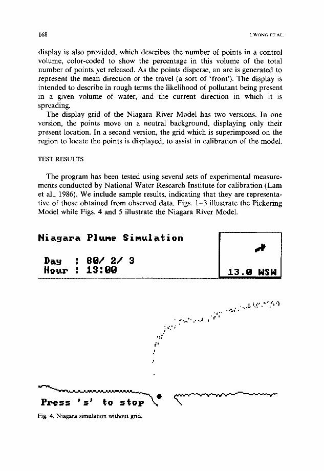
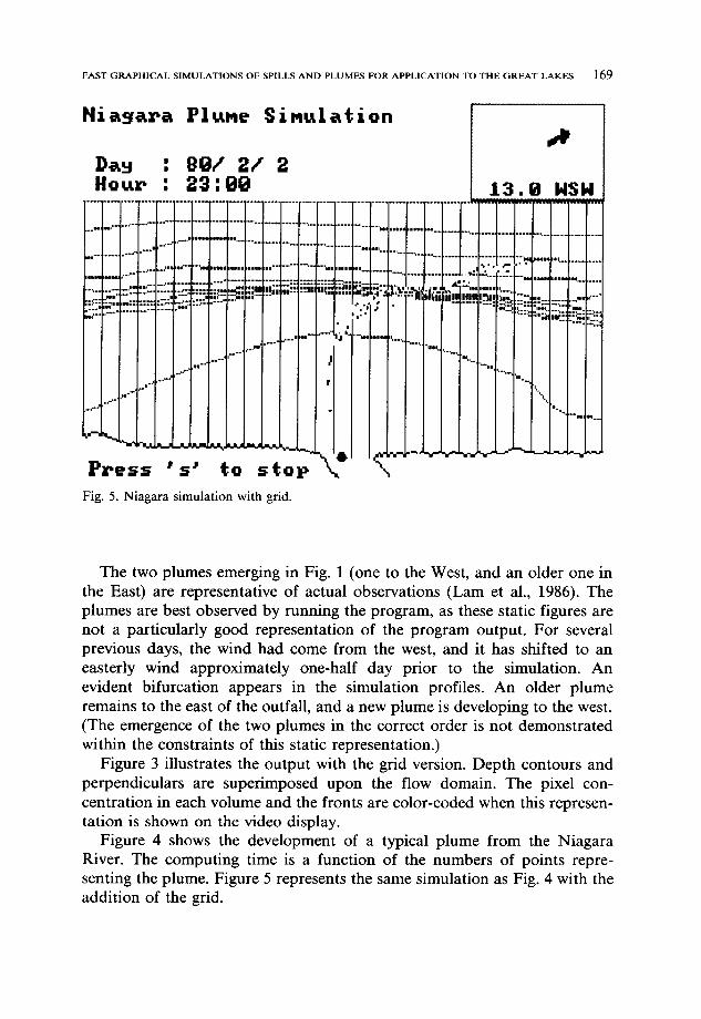
The display grid of the Niagara River Model has two versions. In one version, the points move on a neutral background, displaying only their present location. In a second version, the grid which is superimposed on the region to locate the points is displayed, to assist in calibration of the model.

TEST RESULTS

The program has been tested using several sets of experimental measure- ments conducted by National Water Research Institute for calibration (Lam et al., 1986). We include sample results, indicating that they are representa- tive of those obtained from observed data. Figs. 1-3 illustrate the Picketing Model while Figs. 4 and 5 illustrate the Niagara River Model.

Hi ~ g ~ r a Plume ~ i ~ u l ~ t i o n

] ) ~ : 8 0 / ' 2 / 3 H o u r : 1 3 : 0 0

,,ae

1 3 . B 1,4S1,,I

• ,~ o~.b I " . , o . J I

,::"

i'

,

" 1 " " • i . m

• • • Oo . # - - • , ~ , | °

Fig. 4. Niagara simulation without grid.

FAST GRAPHICAL SIMULATIONS OF SPILLS AND PLUMES FOR APPLICATION TO THE GREAT LAKES 169

Hietgar.a P l ~ e S i m u l a t i o n

HoCr p . . . . . . . . . . . . . . . . . . . . . . . . . . . . . . . . . . . . . . . . . . . . ~ . . . . . . .

i , " - nu t . , - . , ' . . , o ) u~u~

10mo~ . . . . . . . . . . . . . " "

. . . . . . . . . , . ,mn~ m ' * ' ° ' - - d n~

. . . . . ................ . . . . . . _ - ,.:,-..; .'.I

"~!i!ii ;;;"" ":: : : : : := ...... :.~w :: .....

: 8 0 / 2 / 2 : 33 :00

.............. L~iii

u l . . . . . . . . . . . . . .

n ~ l ImNM r o m a n OU, . . . .

OUn : , - , , , ~ ,,,,,!N m a " I ~ . . ~ m ,

, - - , . .

~ ! l l

lgNI j "

"" i •

,H"

• i •

, , n " 1 "

• m J m ~ | l l a m i a

P r e ~ s ' s ' to ~ t o p

,,,,iP

1 3 . 0 H S H . . . . . . . I . . , - * . , , . e . . . . . . . . . . . . . . . . . . . . . . . . . . . . . . . . . . . . . . . . . . . . . . . . . . . . . .

. . . . . . F " - ' + ...........................................................

° * " . . . . . . . . . . . . . U r n . n . n m n u . . . . .

~ ~':~r" ........... In ~ m ~ , , '.I.'Z . . . . . . . . ,,,,, ," .... , . , . , o . . . . , . . . . .

' - - : . , : . . ;~:':: ' ~ . . . . . . . . , , . .

am::: :";'-:;

bNDMI,

i- . . . .-f, , . . . . . HU n , .~ .w~

i. .

"1.

Nf~b

Fig . 5. N i a g a r a s i m u l a t i o n w i t h gr id .

The two plumes emerging in Fig. 1 (one to the West, and an older one in the East) are representative of actual observations (Lam et al., 1986). The plumes are best observed by running the program, as these static figures are not a particularly good representation of the program output. For several previous days, the wind had come from the west, and it has shifted to an easterly wind approximately one-half day prior to the simulation. An evident bifurcation appears in the simulation profiles. An older plume remains to the east of the outfall, and a new plume is developing to the west. (The emergence of the two plumes in the correct order is not demonstrated within the constraints of this static representation.)

Figure 3 illustrates the output with the grid version. Depth contours and perpendiculars are superimposed upon the flow domain. The pixel con- centration in each volume and the fronts are color-coded when this represen- tation is shown on the video display.

Figure 4 shows the development of a typical plume from the Niagara River. The computing time is a function of the numbers of points repre- senting the plume. Figure 5 represents the same simulation as Fig. 4 with the addition of the grid.

1 7 0 I. WONG ET AL.

APPLICABILITY AND LIMITATIONS

The applicability of both of these simulations rests on the implicit assumption that the underlying steady currents are simple to describe and that the complexity of the plume is due primarily to the effects of wind. A complicated and varying flow underlying the wind-driven currents would greatly undermine the utility of these simulations in a microcomputer environment, unless the steady flow patterns could be parametrized or at least the number of distinct patterns kept small. Then a knowledge base of sufficient simplicity might be queried for the most appropriate underlying flow. Like the wind history for the shore currents, observation of triggering mechanisms for the underlying pattern would be required.

Alternatively, a large-scale finite-difference or finite element simulation, updated by observation, could provide the underlying current information. The microcomputer simulation would then be superimposed on the resulting solution. Thus the gross flow could be computed with coarser resolution (and shorter computation times) and the numerical solution could be satis- factorily augmented by simulation such as presented here. Uncertainty in prediction and computation time can then be balanced in a visual represen- tation. Our simulation has been largely set in the graphics memory of the microcomputer. We have transformed the problem into screen coordinates and reduced the computation overhead by working in the graphics (' visual') display, to produce a realistic and qualitatively correct representation.

CONCLUSION

The application of this simple wind-driven model in a microcomputer program represents a fast, realistic simulation of the events following a spill or of an effluent plume. The low cost of microcomputer technology coupled with the speed of the computation and the ability of the model to correlate at least qualitatively with the observed phenomena present an interesting alternative to large-scale (and therefore costly) computer simulations of spills and plumes.

ACKNOWLEDGEMENT

This work was partially supported through Environment Canada Re- search Contracts. The dedication of the referees and the guest editor are gratefully acknowledged.

FAST GRAPHICAL SIMULATIONS OF SPILLS AND PLUMES FOR APPLICATION TO THE GREAT LAKES 171

APPENDIX

Program user guide

The followings should be ready when running the programs

POINTS, VECTOR and ARC.

I, Prepare your wind data (e.g. filel.pc) as shown below.

80 2 2 29 <---YEAR, MONTH, DAY, NO.OF DAY THAT MONTH

34. 250 34 250. 26. 250 26 250. 26. 250. <--

37. 250 37 250. 37. 250 37 250. 35. 250.

35. 250 26 250. 26. 250 26 250. 26. 250.

21. 250 21 250. 21. 250 21 250. 21. 250.

18. 250 18 250. 18. 250 ii 250. iI. 250.

15. 250 15 250. 15. 250 16 250. 16. 250. <--

15. <---NO. OF DAYS TO SIMULATE

13. 250. 13. 250. ii. 225. ii. 225. 10. 15. <--] NEXT 15

18. 90. 18. 90. 15. 90. 15. 75. 16. 90. [ DAYS WIND

II. 75. ii. 90. 18. 105. 15. 105. 19. 105. <--] ESTIMATION

II. Your directory should contain the following files:

-POINTS.EXE (the 'POINTS' version of the programs)

-VECTOR.EXE (the 'VECTOR' version of the programs)

-ARC.EXE (the 'ARC' version of r_he programs)

-FILE1 .PC (sample wind file)

-C3.PC (shore line file)

-HALOEPSN. PRN ~rinter device)

-HELP.BAT (starting help file)

III. Type J4~LP for help.

30 DAYS

WIND HISTORY

SPD (cm/s) ,

DIRECTION

(Degrees from

North)

IV. To run the 'POINTS' version of the programs, enter: NIAGARA

To run the 'VECTOR' version of the programs, enter: VECTOR

To run the 'ARC' version of the programs, enter: ARC

-WIND.PC (resp. coeff, file)

-G~ID.PC (grid file for 'ARC')

-HALOIBMG.DEV (graphic device)

-HELP.DAT help file)

1 7 2 i. WONG ET AL

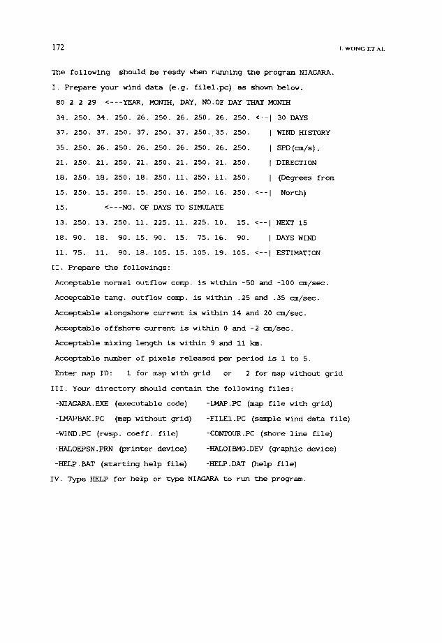
The following should be ready when running the program NIAGARA.

I. Prepare your wind data (e.g. filel.pc) as shown below.

80 2 2 29 <---YEAR, MONTH, DAY, NO.0F DAY THATMONTH

34. 250. 34. 250. 26. 250. 26. 250. 26. 250. <-- 30 DAYS

37 250. 37. 250. 37. 250. 37. 250. 35. 250. WIND HISTORY

35 250. 26. 250. 26. 250. 26. 250. 26. 250. SPD(cm/s),

21 250. 21. 250. 21. 250. 21. 250. 21. 250. DIRECTION

18 250. 18. 250. 18. 250. ii. 250. ii. 250. (Degrees from

15 250. 15. 250. 15. 250. 16. 250. 16. 250. <-- North)

15 <---NO. OF DAYS TO SIMULATE

13. 250. 13. 250. ii. 225. ii. 225. i0. 15. <-- NEXT 15

18. 90. 18. 90. 15. 90. 15. 75. 16. 90. DAYS WIND

ii. 75. ii. 90. 18. 105. 15. 105. 19. 105. <-- ESTIMATION

[I. Prepare the followings:

Acceptable normal outflow comp. is within -50 and -I00 cm/sec.

Acceptable tang. outflow comp. is within .25 and .35 cm/sec.

Acceptable alongshore current is within 14 and 20 cm/sec.

Acceptable offshore current is within 0 and -2 cm/sec.

Acceptable mixing length is within 9 and ii km.

Acceptable number of pixels released per period is 1 to 5.

Enter map ID: 1 for map with grid or 2 for map without grid

III. Your directory should contain the following files:

-NIAGARA.EXE (executable code)

-LMAPBAK.PC (map without grid)

-WIND.PC (resp. coeff, file)

-HALOEPSN.PRN ~rinter device)

-HELP.BAT (starting help file)

-LMAP.PC (map file with grid)

-FILEI.PC (sample wind data file)

-CONTOUR.PC (shore line file)

-HALOIBMG.DEV (graphic device)

-HELP.DAT ~elp file)

IV. Type HELP for help or type NIAGARA to run the program.

F A S T G R A P H I C A L S I M U L A T I O N S O F S P I L L S A N D P L U M E S F O R A P P L I C A T I O N T O T H E G R E A T L A K E S 173

REFERENCES

Lam, D.C.L., Swayne, D.A., Middleton, M. and Walma, M., 1986. A microcomputer-based model of radionuclide spills and discharge plumes. In: 1st Can. Congr. Computer Applications in Civil Engineering/Micro-Computers, Vol. 1, 21-22 May 1986, McMaster University, Hamilton, Ont., pp. 443-457.

Murthy, C.R., Lam, D.C.L., Simons, T.J., Jedrasik, J., Miners, K.C., Bull, J.A. and Schertzer, W.M., 1984. Dynamics of the Niagara river plume in Lake Ontario. NWRI Contrib. 84-7, 57 pp.

Murthy, C.R., Simons, T.J. and Lam, D.C.L., 1986a. Dynamic and transport modelling of the Niagara river plume in Lake Ontario. Rapp. P.-V. Rrun. Cons. Int. Explor. Mer, 186: 150-164.

Murthy, C.R., Simons, T.J. and Lain, D.C., 1986b. Simulation of pollutant transport in homogeneous coastal zones with application to Lake Ontario. J. Geophys. Res., 91 (C8): 9771-9779.

Swayne, D.A., Lam, D.C.L. and Middleton, M., 1986. A microcomputer-based model of radionuclide spills and discharge plumes for application to the Great Lakes. In: R. Crosbie and P. Luker (Editors), Proc. 1986 Summer Simulation Conf., 28-30 July 1986, Reno, NV. Society for Computer Simulation, San Diego, CA, pp. 435-437.

Wong, I.W., Swayne, D.A., Murthy, C.R. and Lam, D.C.L., 1987. A microcomputer simula- tion of the Niagara River outflow into Lake Ontario. In: M. Willumsen, R.D. Cruz, W.G. Vogt and M.H. Nickle (Editors), 18th Annu. Pittsburgh Conf. Modeling and Simulation. Modelling and Simulation, 18 (5). Instrument Society of America, Research Triangle Park, NC, pp. 1873-1877.