Journal of Membrane Science, 59 (1991) 81-99 Elsevier Science Publishers B.V.. Amsterdam

81

Concentration polarisation build-up in hollow fibers: a method of measurement and its modelling in ultrafiltration

Pierre Aimar*, John A. Howell School of Chemical Engineering, University of Bath, Claverton Down, Bath BA2 7AY (UK)

Michael J. Clifton and Victor Sanchez URA CNRS de Gtkie Chimique, Laboratoire de GEnie Chimique et Electrochimie, UniversitB P. Sabatier, 118 route de Narbonne, 31062 Toulouse Cedex (France)

(Received February 20,1989; accepted in revised form January 25,199l)

Abstract

A simple technique allows both polarisation and fouling to be studied independently at constant permeation flux during ultrafiltration of protein solutions with hollow fibers. The build-up of the concentration polarisation layer was recorded and measurements of the amount of proteins in- volved in the boundary layer were carried out before fouling had had time to alter polarisation. Using a film model with a linear or an exponential boundary layer concentration profile average values of the wall concentration and of the mass transfer coefficients are calculated, the latter being in good agreement with the predictions of the LQvdque formula. An integral model of the growth of the polarisation layer is compared to direct measurements in the boundary layer, with a generally good agreement being found. The advantage of the integral model is the detailed picture given of what is occuring along the membrane surface. The rate of material deposition on the membrane was also measured. The mechanism of fouling appears to be strongly dependent on the concentration polarisation.

Keywords: concentration polarization; fouling; ultrafiltration; proteins, ultrafiltration of; poly- sulfone membrane; hollow fiber membrane

Introduction

Considerable theoretical work has been dedicated to concentration polaris- ation (c.p. ) in ultrafiltration during the last two decades but few direct exper- imental measurements have been reported. This owes much to the experimen- tal difficulties. The low diffusivity of macromolecules (around 5~ lo-l1 m”/

*To whom correspondence should be directed; present address: URA CNRS de GEnie Chimique, Laboratoire de GEnie Chimique et Electrochimie, Universiti P. Sabatier, 118 route de Narbonne, 31062 Toulouse Cedex (France).

0376-7388/91/$03.50 0 1991- Elsevier Science Publishers B.V.

82

set) implies that the boundary layer thickness is generally far too small to be directly investigated by any physical method without considerable disturbance of the boundary layer itself. The only easily measured experimental quantities open to direct comparison with theory are the macroscopic consequences of c.p. such as the flux of solvent and the rejection of macromolecules.

(1) One must first choose a theoretical model to correlate the wall concen- tration with the permeation flux. There are at least three possibilities each postulating a different flux limiting mechanism: gel model [ 11, osmotic theory [ 21, pressure drop in the boundary layer [ 31.

(2) One must then account for the fouling of the membrane by the process fluids. This takes place at the same time as polarisation and has an additional effect.

Fouling and c.p. effects are distinguished by the state of the molecules in- volved (in solution for c.p., no longer in solution for fouling) and by the time scale (normally less than a minute for c.p., as long as the experiment for fouling).

A major problem found when modelling c.p. is the superposition of a slow fouling transient on the permeation flux which then alters the c.p. Studying c.p. on the basis of flux measurements requires that fouling mechanisms be perfectly known or controlled. Conversely the study of fouling would require an excellent model for c.p. Control of fouling by some authors has involved synthetic molecules, such as dextran or polyvinylpyrrolidone (PVP) (Clifton et al. [ 4]), which are non-fouling under appropriate conditions.

Other authors working on dead-end ultrafiltration have tried direct mea- surements in the boundary layer. Vilker et al. [5] observed the build-up of a polarisation layer in an unstirred cell, using a light scattering technique. Their conclusions support an osmotic model but are not directly applicable to cross flow filtration. Using holographic interferometry, Clifton [ 61 studied the dif- fusion of molecules from a polarisation layer after the driving force (pressure )

had been released. The conclusions are a little uncertain due to the small amount of matter involved in the polarisation mechanism. Ingham et al. [ 71 were the first to suggest that a spectrophotometer connected on-line in the retentate circuit could provide accurate measurements of the polarisation and adsorp- tion mechanisms, assuming that proteins missing from the bulk were merely involved in one of the surface mechanisms. A very similar set-up was revived by Turker and Hubble [8] whose system was designed to operate at constant permeation flux which provides a great advantage for modelling boundary layer phenomena or membrane reactors since the permeation flux appearing in mass balance equations is no longer a dependent variable but an experimentally controlled variable. These authors could achieve a quantitative study of pro- tein adsorption and of “flow induced fouling” at low Reynolds numbers. They introduced the concept of protein “associated” with the membrane, pointing out the problem of the description of the state of those molecules (gelled or solvated).

83

In the present work a similar set-up was adopted for an experimental study aimed at measuring the build-up of matter on a membrane surface during the very first moments after a pressure difference has been applied. Some inter- esting information was expected from the recording of the optical density changes in the retentate just after the permeate line was closed and the pres- sure released (i.e. when there was no longer any driving force maintaining the boundary layer). The kinetics of restoration of the retentate concentration were studied to allow various mechanisms to be distinguished.

The results are compared with the predictions of two models. One of them is the classical LQv6que formula for laminar mass transfer. The other one is based on an integral model previously developed by Clifton et al. [4] for the growth of the polarisation layer in ultrafiltration of synthetic molecules with hollow fibers.

Materials and methods

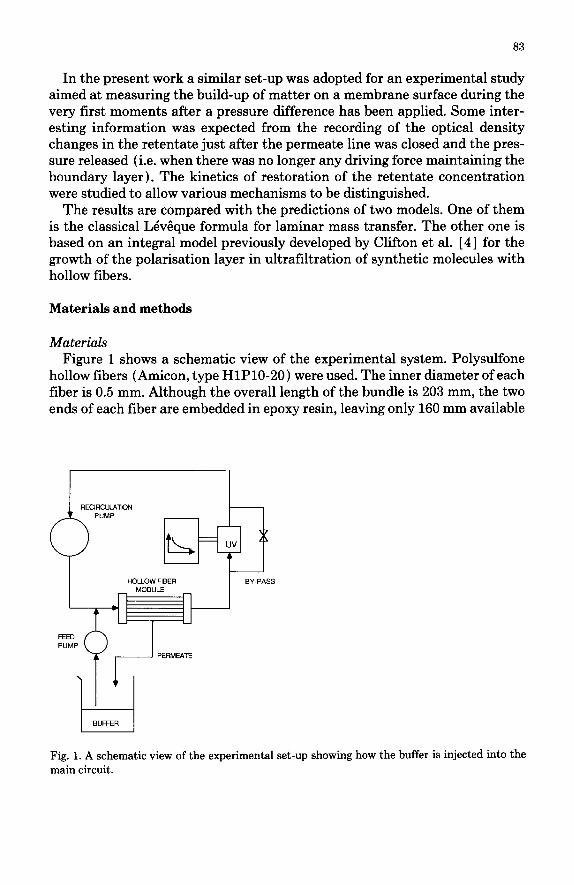
Materials Figure 1 shows a schematic view of the experimental system. Polysulfone

hollow fibers (Amicon, type HlPlO-20) were used. The inner diameter of each fiber is 0.5 mm. Although the overall length of the bundle is 203 mm, the two ends of each fiber are embedded in epoxy resin, leaving only 160 mm available

HOLLOW FIBER

Fig. 1. A schematic view of the experimental set-up showing how the buffer is injected into the main circuit.

84

for permeation. For every fiber, ink was injected at one end of each fiber with a syringe needle, and a blue spot was expected at the other end if the fiber was not blocked: it was the case for 225 out of 250 of the fibers. The actual mem- brane area was therefore 0,0565 m2. The nominal molecular weight cut-off is 10 kDa. After some use at very low Reynolds number, the membrane was heav- ily fouled. Its permeability just after cleaning was in the range 4.2~10-~- 5 x lop6 m/set kPa (25-30 l/hr/m’/bar) and was measured before each experiment.

Bovine serum albumin (Fraction V powder, 98-99%, Sigma cat. No A7906) was dissolved (1 g/l) in phosphate buffer (0.05 M, pH = 6.8). Although the permeate often had a non-negligible optical density at 278 mm, this was not due to albumin but to small species (4 kDa) also present in the retentate as proved by high pressure gel permeation chromatography analysis (TSK G3000 SWXL column, A=278 nm). The rejection coefficient (1 -C,/C,) was then better than 0.99. All the solutions were microfiltered prior to use (Whatman, cellulose nitrate, 0.2 pm).

The spectrophotometer was an LKB Uvicord II (A=278 nm, range 0.05). The nylon tubing connecting the flow cell to the main circuit induced the major pressure drop of the system. When the flow was changed a drift in the baseline was observed, making corrections necessary in some time-dependent optical density measurements. The albumin concentration vs. optical density calibra- tion curve was a straight line up to 1 g/l. The sensitivity (dOD/dC) decreases for higher concentrations and between 8 and 10 g/l, it is only one fifth of the sensitivity between 0 and 1 g/l. The photometer was calibrated before every experiment. The optical density (00) was continuously monitored with a chart recorder (sensitivity: 20 mV) .

Both pumps were Watson Marlow peristaltic pumps (501 U for cross flow, 101 U/R for the feed) fitted with 4 mm i.d. tubing. In order to reduce the circuit volume u (45~ 10e6 m”) no flow-meter was used on line but the cross flow pump was calibrated before the runs using a similar circuit including the pho- tometer. The ratio (membrane area/circuit volume) was 1256 m-l. The op- erating temperature was 21 ‘C.

Method The protein solution was circulated for over 30 min before every experiment

to allow the adsorption mechanisms to reach their equilibrium. The feed pump was then turned on, injecting pure buffer in the closed circuit at a constant flow rate. The same flow of permeate was then passing through the membrane since it was the only outlet from the main circuit. The optical density was continuously recorded. After five minutes the feed pump was turned off, the permeate line closed, and the optical density recorded for another five minutes.

85

A new feed pump setting was then chosen. After a series of experiments at a given cross flow, the membrane was cleaned using 0.2 M NaOH and a gentle back flush.

Any variation in optical density, dOD, can be simply converted into a con- centration variation by using the calibration constant t, and then into a mass of protein, o, involved in the polarisation layer per unit of membrane area, A:

CT= (AOD/E) (u/A) (1)

For a given polarisation, the lower the u/A, the higher the dOD. So u/A must be kept as low as possible so as to increase the sensitivity of the technique.

Theory

The main mechanism by which solute molecules are brought to the mem- brane surface is convection of solvent flowing up to and through the porous wall. The reasons why they are staying in the vicinity of the membrane are numerous. One is the low diffusion rate away from the membrane-fluid inter- face and this results in c.p.

Another effect is the chemical affinity of the solute for the membrane ma- terial which leads to the deposition of molecules inside or on the porous struc- ture and which is often called adsorption. A third one can be the affinity of solute molecules for each other at high concentration (c.p. ) or catalysed by the membrane material: this has been called gelation or polymerisation. A fourth effect can be a mechanical blockage of the molecules or particles inside the porous structure or in the surface roughness. All mechanisms except for c.p. are considered as being fouling mechanisms.

The description of the content of the polarization layer requires assumptions on the wall concentration and boundary layer thickness. Among the peculari- ties of mass transfer in ultrafiltration one finds convection through the wall, and dramatic variations in viscosity in the radial direction due to c.p., which both can affect the value of the mass transfer coefficient. These effects are normally not accounted for in standard models describing the variations of boundary layer thickness or of mass transfer coefficient as a function of the distance from the reactor inlet. We have therefore used two models to analyse the experimental data: (a) one with an imaginary boundary layer, constant in thickness all along the fiber. This one gives an averaged value for the mass transfer coefficient and for the wall concentration; (b) one with a developing boundary layer described by an integral model accounting for both convection through the wall and viscosity variations. This model simulates the variations in boundary layer thickness (hence in mass transfer coefficient) and in wall concentration along the fiber.

86

Constant boundary layer averaged along the fiber

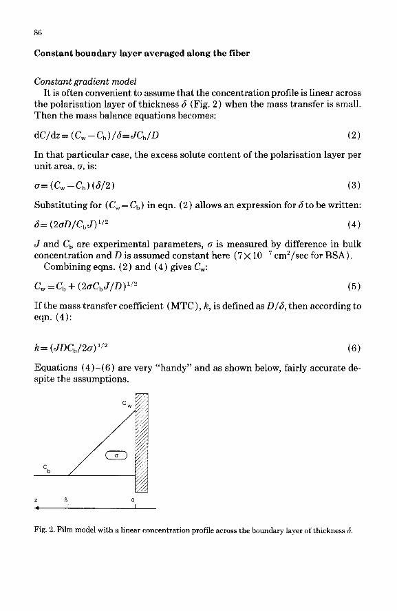
Constant gradient model It is often convenient to assume that the concentration profile is linear across

the polarisation layer of thickness 6 (Fig. 2) when the mass transfer is small. Then the mass balance equations becomes:

dC/dz= (C, -C,,)/6=JC,/D (2)

In that particular case, the excess solute content of the polarisation layer per unit area, 0, is:

fJ= (Gv-G) (d/2) (3)

Substituting for (C, - C,) in eqn. (2) allows an expression for 6 to be written:

6= (2oD/CsJ)l’2 (4)

J and C’s are experimental parameters, o is measured by difference in bulk concentration and D is assumed constant here (7 x 10W7 cm2/sec for BSA).

Combining eqns. (2) and (4) gives C,:

C,=C,,+ (2aC,J/D)1’2 (5)

If the mass transfer coefficient (MTC ) , k, is defined as D/6, then according to eqn. (4):

k= (JDC,,/~O)“~ (6)

Equations (4)-(6) are very “handy” and as shown below, fairly accurate de- spite the assumptions.

Fig. 2. Film model with a linear concentration profile across the boundary layer of thickness 6.

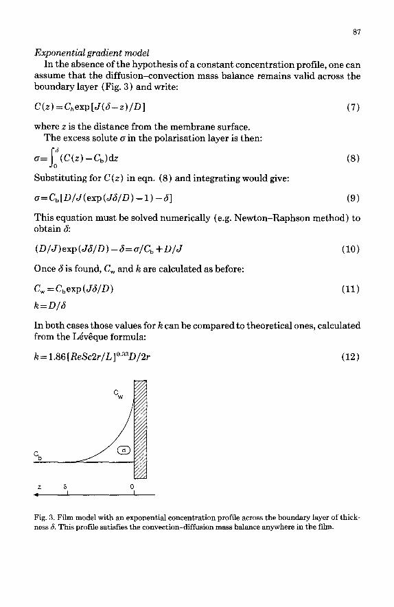
Exponential gradient model In the absence of the hypothesis of a constant concentration profile, one can

assume that the diffusion-convection mass balance remains valid across the boundary layer (Fig. 3 ) and write:

C(z) =C,exp[J(6-2)/D]

where z is the distance from the membrane surface.

(7)

The excess solute CJ in the polarisation layer is then:

o= i(C(z) -C,)dz s (8)

Substituting for C(z) in eqn. (8) and integrating would give:

o=C,[D/J(exp(J6/D) -1) -61 (9)

This equation must be solved numerically (e.g. Newton-Raphson method) to obtain 6:

(D/J)exp(Ja/D) -S=o/C, +D/J

Once 6 is found, C, and k are calculated as before:

C, = Cbexp (J&/D)

k=D/6

(IO)

(11)

In both cases those values for k can be compared to theoretical ones, calculated from the LQv@que formula:

k= 1.86 [ReSc2r/L]0.33D/2r (12)

Fig. 3. Film model with an exponential concentration profile across the boundary layer of thick- ness S. This profile satisfies the convection-diffusion mass balance anywhere in the film.

88

Developing boundary layer

The other model here has proved to be convenient with hollow fibers and synthetic macromolecules such as dextran or PVP [4]. The main features of this model are given hereafter, although a more detailed description can be found in the original paper [ 41. This model assumes that the cross flow de- creases along the fiber since a part of the solvent leaves the membrane through the wail:

dq/dx= - ‘2mJ (13)

where r is the fiber radius. The flow inside the fiber is assumed to be governed by a Hagen-Poiseuille equation, and so is the pressure drop along the fiber:

dp/dx= -8pq/d (14)

A concentration profile is assumed:

C=C, + (C, -C,)exp( -z/6) (15)

where 6 is defined as:

6=D(C, -C,)JC, (16)

An exponential relationship is then used to account for the variation of vis- cosity with concentration in the boundary layer:

p= kexp(KC) (17)

This approximate relationship allows the mass transfer equation:

.Z’{d/dZ[DZ(dC/dZ)])= UdC/d_r+ Vdc/dZ

to be solved analytically at any distance x from the fiber inlet, given:

s(6/Z)‘t1-exp(K(C,-CCb))l=KCb(qo-q)/q (18)

where 6, C, and q depend on x and Z is the distance from the fiber axis

Z=r-z (19)

The other requirement is that the flux satisfies an osmotic model:

J= (AP-417)/R (20)

R is the membrane resistance, the variations of which are assumed negligible if compared with the variation of the c.p. during the first minute of pressuri- zation, and:

AI7= 5 a$‘% (21) i=l

One must then find an appropriate value for J which would solve simultane-

89

ously eqns. (20) and (16) (in which 6 is given by eqn. 18)) and then use this value to solve simultaneously eqns. (13) and (14) (Runge-Kutta, order 4).

This procedure allows the flux, the wall concentration, the cross flow and the pressure to be calculated at any distance from the inlet of the fiber.

The excess solute content of the polarisation layer, 6, is then calculated as follows:

If the boundary layer thickness is small compared to the radius then:

In the present work, a value for K was computed from the viscosity data given by Kozinski and Lightfoot [ 91. The best value for Kin a solution with a protein content between 1 and 300 g/l was 7.06 x 10e3, with a regression coefficient of 0.96 and ,u._.= 10m3 Pa-sec. The values of the osmotic coefficients were deduced from the data published by Ma et al. [lo]: a1 =36.71; U2= 24.08X 1oe2; a3 = 48.16 x 10m5 for l7in Pa and C in g/l.

Results and discussion

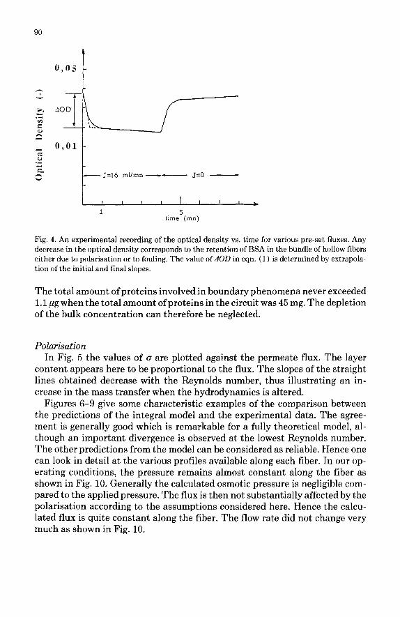
A typical experimental curve is shown in Fig. 4. Due to the kind of spectro- photometer used, a slight drift was observed during the experiments, modifying the absolute values of the apparent rate of deposition and rates of removal. The sharp decrease in the bulk optical density when the feed pump is switched on is totally and quickly reversible as shown by the shape of the curve after the feed pump has been turned off. This indicates a fast and reversible mechanism which is most probably the build-up of the concentration polarisation. It is achieved within 30 set in all of our experiments. This value confirms various theoretical calculations (Velicangil [ 111).

The optical density variation dOD necessary to calculate cr in eqn. (1) is experimentally determined as shown in Fig. 4. The slow decrease in OD sub- sequent to the polarisation is interpreted as an apparent rate of deposition, (r&bs, of matter on the surface of the membrane, and a corresponding rate of removal, ( r, ) obs, could be observed after the permeate line has been closed:

(rd)oss = (rd)true - (rr)true -drift

(rr)oss = (rr)true +drift

We shall then only consider the sum of rd and rr which is not affected by the “drift”, and which corresponds to the actual rate of deposition, r&

rd=(rdb.%+ br)obs

90

Y 0,Ol -

.: z C - J=16 mllmn -- ,J=o -

t I I I , I I I I *

1 5 time (mn)

Fig. 4. An experimental recording of the optical density vs. time for various pre-set fluxes. Any decrease in the optical density corresponds to the retention of BSA in the bundle of hollow fibers either due to polarisation or to fouling. The value of dOD in eqn. (1) is determined by extrapola- tion of the initial and final slopes.

The total amount of proteins involved in boundary phenomena never exceeded 1.1 ,ug when the total amount ofproteins in the circuit was 45 mg. The depletion of the bulk concentration can therefore be neglected.

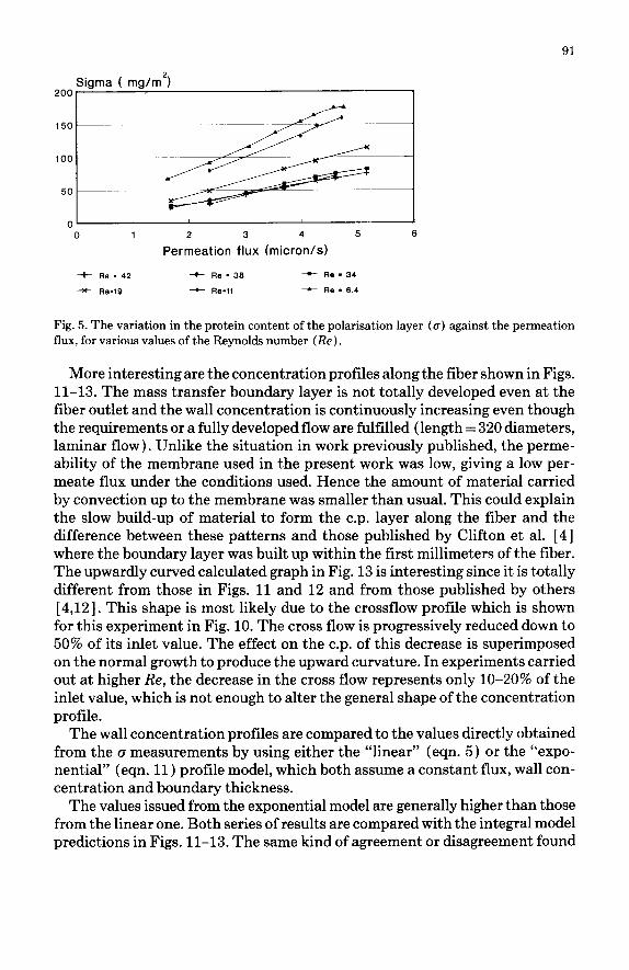
Polarisation In Fig. 5 the values of (T are plotted against the permeate flux. The layer

content appears here to be proportional to the flux. The slopes of the straight lines obtained decrease with the Reynolds number, thus illustrating an in- crease in the mass transfer when the hydrodynamics is altered.

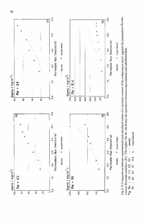
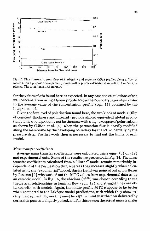
Figures 6-9 give some characteristic examples of the comparison between the predictions of the integral model and the experimental data. The agree- ment is generally good which is remarkable for a fully theoretical model, al- though an important divergence is observed at the lowest Reynolds number. The other predictions from the model can be considered as reliable. Hence one can look in detail at the various profiles available along each fiber. In our op- erating conditions, the pressure remains almost constant along the fiber as shown in Fig. 10. Generally the calculated osmotic pressure is negligible com- pared to the applied pressure. The flux is then not substantially affected by the polarisation according to the assumptions considered here. Hence the calcu- lated flux is quite constant along the fiber. The flow rate did not change very much as shown in Fig. 10.

91

Sigma ( mg/mY I 200

150

100

50

0’ J 0 1 2 3 4 5 6

Permeation flux (micron/s)

+ e-42 --c Rem 38 - R9.34

++ Fe.19 + h-11 - Re . 6.4

Fig. 5. The variation in the protein content of the polarisation layer (g) against the permeation flux, for various values of the Reynolds number (Re).

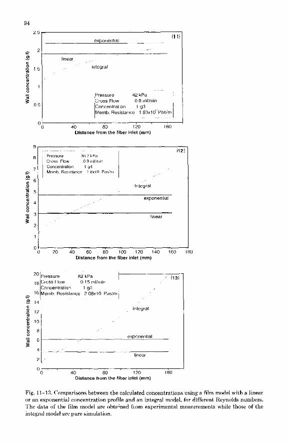
More interesting are the concentration profiles along the fiber shown in Figs. 11-13. The mass transfer boundary layer is not totally developed even at the fiber outlet and the wall concentration is continuously increasing even though the requirements or a fully developed flow are fulfilled (length = 320 diameters, laminar flow). Unlike the situation in work previously published, the perme- ability of the membrane used in the present work was low, giving a low per- meate flux under the conditions used. Hence the amount of material carried by convection up to the membrane was smaller than usual. This could explain the slow build-up of material to form the c.p. layer along the fiber and the difference between these patterns and those published by Clifton et al. [4] where the boundary layer was built up within the first millimeters of the fiber. The upwardly curved calculated graph in Fig. 13 is interesting since it is totally different from those in Figs. 11 and 12 and from those published by others [4,12]. This shape is most likely due to the crossflow profile which is shown for this experiment in Fig. 10. The cross flow is progressively reduced down to 50% of its inlet value. The effect on the c.p. of this decrease is superimposed on the normal growth to produce the upward curvature. In experiments carried out at higher Re, the decrease in the cross flow represents only lo-20% of the inlet value, which is not enough to alter the general shape of the concentration profile.

The wall concentration profiles are compared to the values directly obtained from the cr measurements by using either the “linear” (eqn. 5) or the “expo- nential” (eqn. 11) profile model, which both assume a constant flux, wall con- centration and boundary thickness.

The values issued from the exponential model are generally higher than those from the linear one. Both series of results are compared with the integral model predictions in Figs. 11-13. The same kind of agreement or disagreement found

sigm

a (

mg/

m’)

100

Re

q

42

(6

80

t

t

t

60

+

+

40

+

t

20

8C

6C

4c

2c C

0.0

1.0

2.0

3.0

4.0

5.0

6.0

(

Per

mea

tion

flux

(mic

ron/

s)

Mo

del

+

experiment

Mo

del

+

experiment

2oo

Sig

ma

( m

g/m

2 1

Re

n

19

Sl 1 1.0 ia

ma

( m

g/m

2,

Re

= 3

4 t

t

+

+

+

+ _.

(7

1.0

2.0

3.0

4.0

5.0

Per

mea

te

flux

(mic

ron/

s)

600

500

400

300

200

100 0 1

Re

q

6.4

+

+t

++

+

+

+

IS

0.0

1.0

2.0

3.0

4.0

5.0

6.0

0.0

1.0

2.0

3.0

4.0

5.0

Per

mea

te

flux

(mic

ron/

s)

Per

mea

te

flux

(mic

ron/

s)

Model

+

experiment

Model

+

experiment

Fig.

6-9

: C

ompa

riso

ns

betw

een

expe

rim

enta

l an

d ca

lcul

ated

va

lues

of

u (

prot

ein

cont

ent

of t

he

pola

risa

tion

laye

r)

agai

nst

the

perm

eatio

n fl

ux f

or

vari

ous

Rey

nold

s nu

mbe

rs

(Re)

. The

hi

gher

th

e R

e, t

he

bette

r th

e ag

reem

ent

betw

een

expe

rim

enta

l an

d ca

lcul

ated

da

ta.

Fig.

N

o.

: (6

) (7

) (8

) (9

) -

: m

odel

R

e :

42

34

19

6.4

+

: ex

peri

men

t

93

= 6 81.5 :

1 !! p 5 7

& 4 ~81 g 3 FIUX b

2 3 3 2 80.5

2 G 1

Cross flow at Re = 6.4 0

0 20 40 60 80 100 120 140 ,608’ f

Distance from the fiber inlet (mm)

Fig. 10. Flux (pm/see), cross flow (0.1 ml/min) and pressure (kPa) profiles along a fiber at Re = 6.4. For a purpose of comparison, the cross-flow profile calculated at Re = 34 (0.1 ml/min) is plotted. The total flux is 13.5 ml/min.

for the values of o is found here as expected. In any case the calculations of the wall concentration using a linear profile across the boundary layer seem closer to the average value of the concentration profile (eqn. 14) obtained by the integral model.

Given the low level of polarisation found here, the two kinds of models (film of constant thickness and integral) provide almost equivalent global predic- tions. This would probably not be the same with a higher degree of polarisation, as shown by Clifton et al. [ 41, when the permeation flux is heavily modified along the membrane by the developing boundary layer and incidentally by the pressure drop. Further work then is necessary to find out the limits of each model.

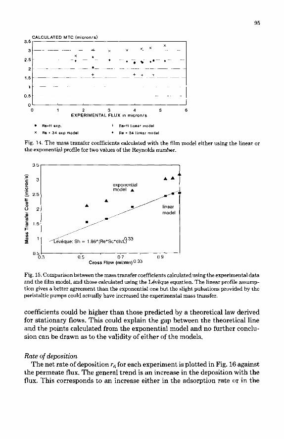
Mass transfer coefficients Average mass transfer coefficients were calculated using eqns. (6) or (12)

and experimental data. Some of the results are presented in Fig. 14. The mass transfer coefficients calculated from a “linear” model remain remarkably in- dependent of the permeation flux, whereas they increase slightly when calcu- lated using the “exponential” model. Such a trend was pointed out at low fluxes by Jonsson [ 21 who worked out the MTC values from experimental data using an osmotic model. In Fig. 15, the abscissa (q”.33) was chosen according to the theoretical relationships in laminar flow (eqn. 12) and straight lines are ob- tained with both models. Again, the linear profile MTC’s appear to be better when compared to the LQvGque model predictions, with which they show ex- cellent agreement. However it must be kept in mind that the flow delivered by peristaltic pumps is slightly pulsed, and for this reason the actual mass transfer

exponential (11)

linear

_-

15 _- integral

I Pressure 42 kPa I Cross Flow 0.8 mlimin ’ Concentratron 1 g/l Mernb. Resistance 1.93xld”Pasim

0 0 40 80 120

Distance from the fiber inlet (mm) 160

8

7

Pressure 35 7 kPa

Cross Flow 0.9 ml:min

Concentration 1 y/l Memb. Rwstance 1 8x10 Pas/m

(12)

6

Integral

exponential

,’ linear

1

0 0 20 40 60 80 100 120 140 160 1

Distance from the fiber inlet (mm)

2o Pressure 82 kPa 1~ Cross Flow 0.15 mlimin

(13)

Concentration 1 g/l 16 Mernb Resistance 2 08x10 Pas/m

14

121 integral

10

8

6

4

2 “

0 0

exponential

’ , linear

40 80 120 160 Distance from the fiber inlet (mm)

80

Fig. 11-13. Comparisons between the calculated concentrations using a film model with a linear or an exponential concentration profile and an integral model, for different Reynolds numbers. The data of the film model are obtr;ned from experimental measurements while those of the integral model are pure simulation.

95

1

0.5 t

“0 1 2 3 4 5 6 EXPERIMENTAL FLUX in micron/s

. Rs.11 exp. + Re=ll linear model

x lb - 34 OXP model * Ra - 34 linear model

Fig. 14. The mass transfer coefficients calculated with the film model either using the linear or the exponential profile for two values of the Reynolds number.

3.5 -

f g 3

; .- g 2.5

F

s 2

5 e m 1.5 c

:: i 1

exponential

model

0.5 1 0.3 0.5 0.7 0.9

Cross Flow (ml/mn) 0.33

Fig. 15. Comparison between the mass transfer coefficients calculated using the experimental data and the film model, and those calculated using the LBvSque equation. The linear profile assump- tion gives a better agreement than the exponential one but the slight pulsations provided by the peristaltic pumps could actually have increased the experimental mass transfer.

coefficients could be higher than those predicted by a theoretical law derived for stationary flows. This could explain the gap between the theoretical line and the points calculated from the exponential model and no further conclu- sion can be drawn as to the validity of either of the models.

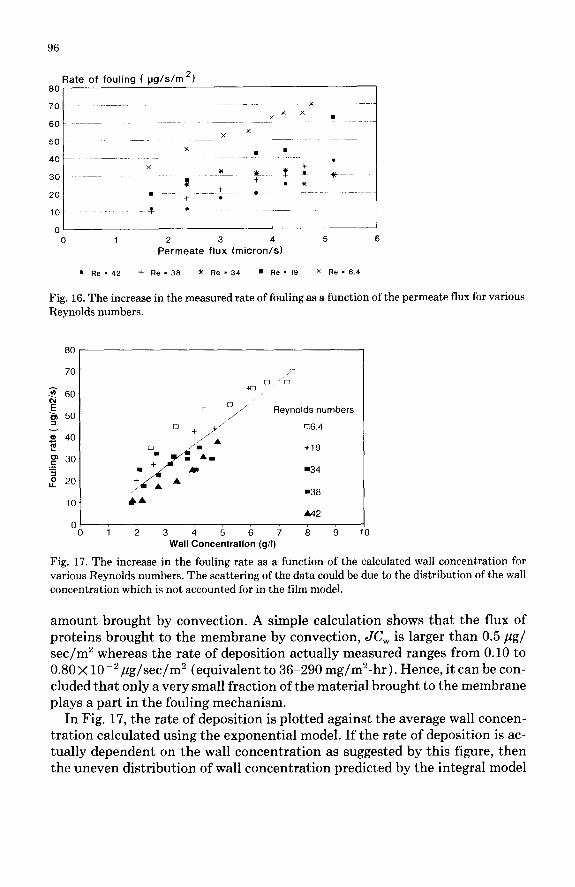
Rate of deposition The net rate of deposition rd for each experiment is plotted in Fig. 16 against

the permeate flux. The general trend is an increase in the deposition with the flux. This corresponds to an increase either in the adsorption rate or in the

96

Rate of fouling ( pg/s/m*) 801

2 3 4 Permeate flux (micron/s)

6

Fig. 16. The increase in the measured rate of fouling as a function of the permeate flux for various Reynolds numbers.

. +

Reynolds numbers

06 4

+19

-34

138 10 +A

A42 0

0 12 3 4 5 6 7 8 9 Wall Concentration (g/l)

0

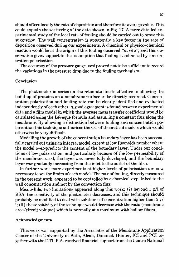
Fig. 17. The increase in the fouling rate as a function of the calculated wall concentration for various Reynolds numbers. The scattering of the data could be due to the distribution of the wall concentration which is not accounted for in the film model.

amount brought by convection. A simple calculation shows that the flux of proteins brought to the membrane by convection, JC, is larger than 0.5 ,ug/ sec/m2 whereas the rate of deposition actually measured ranges from 0.10 to 0.80 x 10e2 pg/sec/m2 (equivalent to 36-290 mg/m2-hr ). Hence, it can be con- cluded that only a very small fraction of the material brought to the membrane plays a part in the fouling mechanism.

In Fig. 17, the rate of deposition is plotted against the average wall concen- tration calculated using the exponential model. If the rate of deposition is ac- tually dependent on the wall concentration as suggested by this figure, then the uneven distribution of wall concentration predicted by the integral model

97

should affect locally the rate of deposition and therefore its average value. This could explain the scattering of the data shown in Fig. 17. A more detailed ex- perimental study of the local rate of fouling should be carried out to prove this suggestion. The wall concentration is apparently a key factor in the rate of deposition observed during our experiments. A chemical or physico-chemical reaction would be at the origin of this fouling observed “in situ”, and this ob- servation gives support to the assumption that fouling is enhanced by concen- tration polarisation.

The accuracy of the pressure gauge used proved not to be sufficient to record the variations in the pressure drop due to the fouling mechanism.

Conclusion

The photometer in series on the retentate line is effective in allowing the build-up of proteins on a membrane surface to be directly recorded. Concen- tration polarisation and fouling rate can be clearly identified and evaluated independently of each other. A good agreement is found between experimental data and a film model in which the average mass transfer coefficient would be calculated using the LevVgque formula and assuming a constant flux along the membrane. By allowing a distinction between fouling and concentration po- larisation this technique authorises the use of theoretical models which would otherwise be very difficult.

Modelling the growth of the concentration boundary layer has been success- fully carried out using an integral model, except at low Reynolds number where the model over-predicts the content of the boundary layer. Under our condi- tions of low polarisation, and particularly because of the low permeability of the membrane used, the layer was never fully developed, and the boundary layer was gradually increasing from the inlet to the outlet of the fiber.

In further work more experiments at higher levels of polarisation are now necessary to set the limits of each model. The rate of fouling, directly measured in the present work, appeared to be controlled by a chemical step linked to the wall concentration and not by the convection flux.

Meanwhile, two limitations appeared along this work; (i) beyond 1 g/l of BSA, the sensitivity of the photometer decreases, and this technique should probably be modified to deal with solutions of concentration higher than 5 g/ 1; (ii) the sensitivity of the technique would decrease with the ratio (membrane area/circuit volume) which is normally at a maximum with hollow fibers.

Acknowledgments

This work was supported by the Associates of the Membrane Application Center of the University of Bath, Alcan, Domnick Hunter, ICI and PC1 to- gether with the DTI. P.A. received financial support from the Centre National

98

de la Recherche Scientifique and the Royal Society as part of the European Science Exchange Programme.

List of symbols

A

Cf.3

c, cw D J K k L P

;e

k u V V

;

z

membrane area ( m2 ) bulk concentration (g/l) permeate concentration (g/l) wall concentration (g/l) diffusion coefficient (m”/sec) permeation flux ( m3/m2/sec ) or (micrometer/set ) coefficient in eqn. (17) (l/g) mass transfer coefficient (m”/m”/sec) or (micrometer/set) fiber length (m) or (mm) relative pressure inside the fiber (Pa) cross flow (ml/min) or ( cm3/sec) Reynolds number ( = 2pq/xrp) fiber radius (m) or (mm) Schmidt number ( = ,u/pD) axial velocity (m/set) radial velocity (m/set) volume of the circuit ( m3) axial coordinate in the fiber (m) distance from the fiber axis (m) radial coordinate in the fiber (m )

Greek symbols 6 thickness of the boundary layer (cm)

!z viscosity of the solution (Pa-set) osmotic pressure (Pa)

0 amount of proteins involved in the liquid concentration polarisation layer (mg/cm”) or @g/cm”)

Abbreviations b.1. boundary layer BSA bovine serum albumin c.p. concentration polarisation MTC mass transfer coefficient O.D. optical density

99

References

1

2

3

4

5

6

7

8

9

10

11

12

AS. Michaels, New separation technique for the CPI, Chem. Eng. Progr., 64( 12) (1968) 31- 44. G. Jonsson, Boundary layer phenomena during ultrafiltration of dextran and whey protein solutions, Desalination, 51 (1984) 61. J.G. Wijmans, S. Nakao, G.B. van den Berg, F.R. Troelstra and C.A. Smolders, Hydrody- namic resistance of concentration polarisation layers in ultrafiltration, J. Membrane Sci., 22 (1985) 117-35. M.J. Clifton, N. Abidine, P. Aptel and V. Sanchez, Growth of the polarisation layer in ultra- filtration with hollow fiber membranes, J. Membrane Sci., 21 (1984) 233-46. V.L. Vilker, C.K. Colton and K.A. Smith, Concentration polarisation in protein ultrafiltra- tion, part I and II, AIChE J., 27(4) (1981) 620-45. M.J. Clifton, Polarisation de concentration dans divers pro&de de separation a membranes, These No. 1036, Universitk P. Sabatier, Toulouse, (1982 ). KC. Ingham, T.F. Busby, Y. Sahlestrom and F. Castino, Separation of macromolecules by ultrafiltration, in: A.R. Cooper (Ed.), Ultrafiltration Membranes and Applications, Plenum Press, New York, NY, 1980, p. 141-58. M. Turker and J. Hubble, Membrane fouling in a constant flux ultrafiltration cell, J. Mem- brane Sci., 34 (1987) 267-81. A.A. Kozinski and E.N. Lightfoot, A general example of boundary layer filtration, AIChE J., 31(1972)1031-41. R.P. Ma, C.H. Gooding and W.K. Alexander, A dynamic model for low pressure hollow-fiber ultrafiltration, AIChE J., 31 (1985) 1728-32. 0. Velicangil, Self-cleaning membranes for ultrafiltration, PhD Thesis, University of Wales, 1979. R. Rautenbach and H. Holtz, Effect of concentration dependance of physical properties on ultrafiltration, Ger. Chem. Eng., 3 (1980) 180-5.