Computer Aided Dimensional Control in Building Construction
159
Computer Aided Dimensional Control in Building Construction PROEFSCHRIFT ter verkrijging van de graad van doctor aan de Technische Universiteit Eindhoven, op gezag van de Rector Magnificus, prof.dr. R.A. van Santen, voor een commissie aangewezen door het College voor Promoties in het openbaar te verdedigen op woensdag 6 maart 2002 om 16.00 uur door Rui Wu geboren te Shanxi, China
-
Upload
khangminh22 -
Category
Documents
-
view
1 -
download
0
Transcript of Computer Aided Dimensional Control in Building Construction

Computer Aided Dimensional Control in Building Construction
PROEFSCHRIFT
ter verkrijging van de graad van doctor aan de Technische Universiteit Eindhoven, op gezag van de
Rector Magnificus, prof.dr. R.A. van Santen, voor een commissie aangewezen door het College voor
Promoties in het openbaar te verdedigen op woensdag 6 maart 2002 om 16.00 uur
door
Rui Wu
geboren te Shanxi, China

Dit proefschrift is goedgekeurd door de promotoren:
prof.ir. G.J. Maas
en
prof.ir. F.P. Tolman
CIP-DATA KONINKLIJKE BIBLIOTHEEK, DEN HAAG
Wu, Rui
Computer aided dimensional control in building construction / by Rui Wu. –
Eindhoven: Technische Universiteit Eindhoven, Faculteit Bouwkunde,
Capaciteitsgroep Uitvoeringstechniek, 2002.
Proefschrift. - ISBN 90-6814-564-9
Cover design by Ton van Gennip, Tekenstudio Faculteit Bouwkunde
Printed by UniversiteitsDrukkerij

To the memory of my dear mother,
to my father
and Dianwen


i
Preface The Building-Construction industry is facing increased demands from society, i.e.
higher quality, shorter lead times, more customisation, more care for the
environment, better working conditions, less disturbance for the surrounding, and
more.
Improving the quality of the construction process is one of the responses to
society’s demands that the Building-Construction can make, which is worthwhile
looking into. Many problems relate to measurement and dimensional control
errors. Tolerances can’t be met; components do not fit; and cheaper work-methods
can’t be applied. All are waste and produce cost of failure, delay, and agony, often
even leading to legal hassling where nobody can win.
This thesis focuses on the improvement of dimensional control and possible ICT
usage to contribute to solving the problems.
The research has been carried out at Eindhoven University of Technology (TUE)
in the Netherlands where the Department of Construction Engineering and
Management (UT) is working on dimensional control for many years, providing
me with a large body of dimensional control knowledge that sips through in
almost every page and paragraph.
This research has been sponsored by TUE, TNO Bouw, and SBR (Stichting
BouwResearch). I am very grateful to these organizations. Also this research and
thesis cannot and should not be credited to me alone. I could not have achieved
without the help of others. First of all I would like to thank my supervisor Ger
Maas for his guidance and enthusiasm. It was a pity that halfway my study Ger
mostly left TUE to stay only for one day a week. I also want to thank Frits Tolman
from Delft University of Technology (TUD) who has supported the ICT-part of
my work. My thanks also go to Arjen Broens for his support on construction
surveying and help with arranging my case study on the construction site in
Apeldoorn. I also like to thank Peter van der Veer from TUD and Henk van

ii
Tongeren from University Twente, for reviewing the draft thesis and their
constructive comments. I also thank Peter van Hoof for his support in the first two
years. My thanks also go to colleagues and students of UT who helped me in one
way or another. I also like to thank my colleagues at TUD for their discussions
with me about product modelling and other ICT related topics. Also to be thanked
are my friends who created a social environment for my stay in the Netherlands. I
also thank my sisters for their constant and unconditional love. Last but not least,
my love and thanks go to Dianwen for his love, support and patience. Hopefully I
will soon cross the Atlantic Ocean, see him in good health and live happily ever
after.
Rui Wu
Eindhoven
November 2001

iii
Contents
Preface i
1 Introduction 1
1.1 Introduction to the Research ............................................................................ 1
1.2 Structure of the Thesis...................................................................................... 3
2 Dimensional Control in Building Construction 5
2.1 Introduction ...................................................................................................... 5
2.2 Building Design and Construction ................................................................... 6
2.3 Building Construction Processes...................................................................... 7
2.4 Designing the Plan of Dimensional Control .................................................. 20
2.5 The Research Problem.................................................................................... 24
3 Current Situation of Dimensional Control 27
3.1 Introduction .................................................................................................... 27
3.2 Investigation of Research Problem ................................................................ 28
3.3 Conclusions on Dimensional Control ............................................................ 38
4 State of Art of Information Technology Relevant for Dimensional Control
in the Building Industry 41
4.1 Introduction .................................................................................................... 41
4.2 Bridging Design and Dimensional Control.................................................... 42
4.3 Knowledge Technology ................................................................................. 52
4.4 Graphical User Interfaces............................................................................... 61
4.5 Implementing the DCS................................................................................... 62
4.6 Conclusions .................................................................................................... 66
5 Reformulation of the Research Questions 67
5.1 Introduction .................................................................................................... 67
5.2 Reformulation................................................................................................. 68

iv
6 Simulation of Dimensional Deviations 69
6.1 Recapitulating the Problem ............................................................................ 69
6.2 Prediction of Dimensional Quality................................................................. 70
6.3 Simulation of Deviations and Representation of Knowledge Rules.............. 72
6.4 The UML Model ............................................................................................ 88
6.5 Concluding Remarks ...................................................................................... 89
7 System Design and Implementation 91
7.1 Development of a Computer Aided System for Dimensional Control .......... 91
7.2 System Design and Implementation............................................................... 93
7.3 Concluding Remarks .................................................................................... 102
8 Case Study 103
8.1 Objective ...................................................................................................... 103
8.2 Case Description........................................................................................... 103
8.3 Comparison of the Model with Practice....................................................... 106
8.4 Practical Knowledge..................................................................................... 107
8.5 Test ............................................................................................................... 108
8.6 Measuring on the Construction Site ............................................................. 109
8.7 Analysing the Data ....................................................................................... 111
8.8 Conclusions .................................................................................................. 123
9 Conclusions and Recommendations 125
9.1 Recapitulating the Problem .......................................................................... 125
9.2 Conclusions .................................................................................................. 126
9.3 Recommendations ........................................................................................ 127
Appendix 129
Bibliography 133
Summary 139
Samenvatting 141
Curriculum Vitae 143

1
INTRODUCTION This chapter introduces the research problem, describes the initial research
objectives, scope and methodology, and gives an overview of the structure of the
thesis.
1.1 INTRODUCTION TO THE RESEARCH
Dimensional control in the building industry can be defined as the operational
techniques and activities that are necessary for the assurance of the defined
dimensional quality of a building (Hoof, 1986). The purpose of dimensional
control is to minimize the negative effects of deviations on: the functioning of the
building, and on cost and labour. To ensure adequate dimensional control, building
components and formworks must be set out and assembled in correct positions,
with an overall accuracy that meets the requirements.
The increased use of prefabricated components, the complexity of new building
shapes, and the speeding up of production in construction, demand an efficient and
precise dimensional control. Meanwhile Information and Communication
Technology (ICT) increasingly supports construction. Besides Computer Aided
1

2
Drawing and Design, Cost Estimation, Project Management, Planning and
Scheduling, advanced electronic instruments, such as Total Stations, are being
used to support setting out and positioning of building components on construction
sites.
In order to achieve precise and efficient dimensional control, a dimensional
control plan must be designed before the building is constructed. The plan
includes: (1) a tolerance plan, (2) an assembling plan, (3) a setting out plan and (4)
a dimension-monitoring plan.
Presently the contractor and engineers often make the dimension control plan
based on drawings and specifications delivered by the architect. The drawings are
often in CAD format, mostly AutoCAD drawings. The dimensional control plan
constitutes, to a great extent, information on points for different aspects of
dimensional control, which can then be transferred into a Total Station. Designing
such a plan is a complex issue requiring detailed information and a lot of
experience. Planners must interpret the CAD drawings, make an inventory of
points needed, select appropriate points for different purposes and often add them
to the drawings. Every project is different and not every planner is experienced,
consequently the quality of the plan varies from project to project, and also from
designer to designer.
Although, as described above, CAD systems and Total Stations have been used for
the purpose of dimensional control, the link between them is missing, which often
makes digital points information hard to find.
To improve the dimensional control of on-site construction projects, this research
(1) tries to capture the knowledge required to design an adequate dimensional
control plan and make that knowledge more generally available and (2) build a
digital connection between CAD systems and Total Stations. And the research is
focused on prefabricated concrete building structural elements.

3
The initial research questions are formulated as follows:
• Is it possible to develop an ‘intelligent’ instrument that supports the less
experienced planners to develop adequate dimensional control plans?
• How to facilitate the digital information flow between CAD systems and
Total Stations?
1.2 STRUCTURE OF THE THESIS
The structure of the thesis is described in the following paragraphs:
Chapter 2 gives a detailed description of the subject of dimensional control in
building construction with the focus on setting out and positioning prefabricated
structural elements. The setting out process and positioning process including the
use of Total Station and other often used equipment are described in detail; the
concept of main control points, references, setting out points, positioning points,
product measure, setting out measure and positioning measure is introduced; the
process of designing the plan of dimensional control is discussed and finally the
research problem is pointed out.
Chapter 3 analyses the current situation of dimensional control in building
construction with the focus on the Netherlands. It describes the Dutch standards
for measures and measuring in construction NEN series 14. It also depicts a
picture of the fragmentation of the building design and construction process. It
also investigates the dimensional control situation of prefabricated structural
elements on building sites by conducting surveys on 21 sites in the Netherlands.
Finally the conclusion on dimensional control is drawn.
Chapter 4 analyses the state-of-art of Information and Communication Technology
(ICT) relevant for dimensional control in building construction, including the
development of CAD systems, Product Data Technology, Knowledge Technology,
Virtual Reality, and programming languages and environments.

4
Chapter 5 reformulates the research questions based on the analyses of the
previous chapters.
Chapter 6 analyses the research problem, proposes a solution for simulating the
dimensional deviations including representation of engineering experience
knowledge, and presents the underlying information model defined in UML
(Unified Modelling Language).
Chapter 7 proposes a computer-aided system for dimensional control based on the
model presented in Chapter 6. It defines the system requirement, presents the
system’s functional design and gives some details on the prototype
implementation.
Chapter 8 evaluates the model and computer aided system by studying the results
of a case study performed in Apeldoorn, Netherlands.
Chapter 9 presents the conclusions of this whole Ph.D. study and recommends
some further work for the future.

5
DIMENSIONAL CONTROL IN BUILDING CONSTRUCTION
This chapter gives a detailed description of the subject of dimensional control in
Building Construction with the focus on setting out and positioning prefabricated
structural elements. Also the research problem is indicated.
2.1 INTRODUCTION
After briefly explaining of the role of dimensional control in building design and
construction, an introduction is given to the building construction process of direct
importance to ensure dimensional quality. The principle of the Total Station and
its latest development including communicating with a computer is explained; the
setting out process and positioning process including the use of Total Stations and
other often used equipment is described in detail; the concept of main control
points, references, setting out points, positioning points, product measure, setting
out measure and positioning measure is introduced. Then the process of designing
the plan of dimensional control is discussed and finally the research problem is
pointed out.
2

6
2.2 BUILDING DESIGN AND CONSTRUCTION
Dimensional control in the building industry can be defined as the operational
techniques and activities that are necessary for the assurance of the predefined
dimension quality of a building (Hoof, 1986). The purpose of dimensional control
is to minimize negative influence of too big deviations with respect to functioning
of the building, cost and labour circumstances. To achieve this purpose, three
groups of people participate in construction process and they must coordinate with
one another. They are designers of the building, designers of the construction plan
and constructor of the building. Figure 2.1 shows the role of dimensional control
in building design and construction. It also gives an overview of three groups of
participants, as mentioned above, and their work related to dimensional control.
As shown in Figure 2.1, with requirements reasonably defined, the architect begins
designing the building with the help of the structure engineer. They complete the
design in documented form - in a combination of the building drawings and
Designbuilding
Constructionon site
Design construction
plan
Dimensiontolerances
Idealdimensions
Predicted dimensiontolerances
- Tolerance plan- Assembling plan- Setting out plan- Monitoring plan
Work drawings &plans
Requirements
Practical dimensions
Material& equipment
ConstructorProduct designer(Architect, structureengineer)
Process designer(Contractor, engineer)
Figure 2.1 The role of dimensional control in building design and construction

7
written specifications. The drawings assure proper form and dimensions, and
specifications control the quality of the construction. With regard to dimensional
control, ideal dimensions of building components are given in the drawing, and
dimension tolerances are specified in the specifications.
Before the building is constructed, the contractor and engineers must deliver a
construction plan and work drawings. Generally, a construction plan consists of a
transport plan, a site plan, a dimensional control plan, a time and cost plan, a
logistics plan, and a safety and health plan. In a dimensional control plan, the
tolerance plan, assembling plan, setting out plan, and dimension monitoring plan
are indispensable. In work drawings, building details with their dimensions are
shown. After the dimensional control plan is worked out, the predicted dimension
quality is known and additional information is put in the work drawings.
Finally, constructors produce building components and even the whole building
with practical dimensions using material and equipment on site.
2.3 BUILDING CONSTRUCTION PROCESSES
This section gives a description of building construction processes, focusing on the
construction of building structures in non-traditional ways, either prefabricated
building components, or in-situ casting of concrete. As shown in Figure 2.2, four
kinds of construction processes can be distinguished, and they have relationship
with one another. These four are prefabricating, setting out, assembling and in-situ
casting. Although Figure 2.2 shows especially the processing of concrete as
building material, it also holds true for the construction made of other materials.
With respect to concrete precasting, a mould is manufactured in the factory, and
then concrete is poured in. After hardening, prefabricated products are transported
to and assembled on construction site. That is to say, the products can be brought
to a certain position, assembled with one another, and then fastened. In addition to
prefabricating, one can also construct a formwork by assembling its separate parts.
To ensure precise dimensional control, building components or formworks must
be set out in a correct position, and then must be assembled, with an overall

8
accuracy that meets the requirements set to them. The dimensional accuracy
should be checked during the construction process.
Setting out has close relation with land surveying. The field of land surveying,
which, put in its simplest form, is the science and art of measuring, recording and
drawing to scale, the size and shape of the natural and man-made features on the
surface of the earth (Irvine, 1995). The objective of land surveying is to produce a
scaled plan of an area. The process of setting out involves locating precisely the
position of a building using the information provided by the architect’s or
engineer’s drawing. The basic equipment used in traditional surveying and setting
out is: the tape for measuring lengths, the level for measuring height differences
Mould parts
Mould
Building components
Assembling
Precasting Land surveying
Setting outAssembling
Marks
Building material
Formwork parts
Formworks
Assembling
In-situ casting
Positioning marks
Construction time t
Construction time t+1
Figure 2.2 Construction processes of direct importance to ensure dimensional quality in concrete buildings construction

9
and the theodolite for measuring angles (Bell, 1993). With the rapid development
of electronic instruments, EDM (electromagnetic distance measurement) and Total
Stations have also been introduced into the field of land surveying and setting out
process. Total Stations are one of the most advanced electronic surveying
instruments.
In the following sections, the subject of Total Stations, setting out and assembling
has been given more detailed description, which includes the definitions, processes
and equipment used during the process.
2.3.1 Total Stations
Figure 2.3 A Total Station
A Total Station is the combination of a traditional theodolite (optical angle
measurement device) and a laser distance measurement sensor. It measures the

10
location of a reflecting prism and gives spherical coordinates. It can be best
described as very accurate, distance-measuring electronic theodolites capable of
diverse mapping and position-measuring tasks. Figure 2.3 shows a Total Station.
Total Stations combine a number of technologies. Concerning angle and distance
measuring, they have remarkable accuracy. As an extension of traditional transits
and theodolites, they have an ability to register very fine angular divisions; they
measure the distance to the target point with an infrared laser emitted by the EDM
(electronic distance measuring device) and reflected by a prism held vertically
above or below the actual point of interest. The actual accuracy is determined by
the wavelength of the light used.
Total Stations have one or two LCD (liquid crystal) displays, and some are
capable of simple graphical display. Apart from producing the same basic
spherical measures as optical survey instruments, Total Stations take additional
data and then calculate additional measures; most importantly, they most are
capable of simultaneous trigonometric conversion of spherical survey coordinates
into Cartesian orthogonal measures--usually east, north, and altitude. Beyond these
simple transformations, and most Total Stations carry a number of useful
programs in their memory. Another function is useful for setting out and
positioning building components. The coordinates of desired points can be input
manually or from data registers, and then the instrument will direct the user to the
points. The screen will indicate the horizontal and vertical alignments of the point
to be found, and then will report how far the prism target and must be displaced
out or in along the radial line of alignment. The diversity and capability of
available programs is increasing through new input and linkage devices that permit
the use of complex code. The standardization of PCMCIA-type cards and the
inclusion of such slots on the Total Stations now allow personal computer
programs to be easily transferred to the instrument.
To be effective, the data the Total Station gathers and transforms must be input
into a computer, and vice versa. These upload and download transfers can be done
directly or through an intermediary storage device. One can use a memory card or
fieldbook as an intermediary device, as shown in Figure 2.4.

11
Figure 2.4 Communication between a Total Station and a computer
With the development of Total Stations, in addition to ever-increasing accuracy,
there are some very useful features emerging. Most outstanding are the motorized
and automatic target recognition instruments starting to appear on the market.
Automatic target recognition helps in setting out and positioning building
components. Normally, two persons need to work together when using a Total
Station. One of the most time-consuming tasks is bringing the rod person into line
with the theodolite's orientation. The new feature makes one-person operation
possible, because the Total Station will track the reflector and its functions can be
radio-controlled by the person holding the reflector.

12
2.3.2 Setting out
Every building or engineering structure that is constructed must undergo a setting
out procedure to ensure that it is the correct size, in the correct plan position and at
the correct level. In general terms, setting out consists of transferring detail from a
drawing to a piece of ground. On the drawing details are given of nearby existing
buildings and features and the proposed work to be set out. It is possible to extract
from the existing detail lines of reference to which new work can be referred such
as building lines, base lines and grid lines.
Setting out on building sites is a combination of measuring and marking. The
marks, as the result of setting out, can be pencil lines, nails, scratches and so forth.
Setting out has two purposes. The first purpose is to define intended positions of
building(s) horizontally and vertically on the accessible building construction
terrain. That is to say, one needs to set out the building(s) and to establish a point
of known level on the site which can be used to determine floor and drain invert
levels. The second purpose is to define positions of individual building
components and temporary works such as formworks. Figure 2.5 shows that two
persons work together to set out by means of a Total Station, with one sighting and
the other marking on the floor.
Figure 2.5 Setting out by means of a Total Station
Setting out can be divided into horizontal setting out and vertical setting out. For
horizontal setting out, gridlines are often used. As shown in Figure 2.6, there are

13
three types of gridlines, namely, orthogonal, non-orthogonal gridlines and radial
gridlines. Setting out can be done by offset methods when using the former two
types of gridlines. Polar setting out should be used when working under radial
gridlines.
Orthogonal gridlines Non-orthogonal gridlines Radial gridlines
Figure 2.6 Three types of gridlines
Methods of ensuring vertical alignment includes (Bell, 1993):
-Spirit level. This is effective for plumbing columns and formwork up to a
height of one storey.
-Plumb bobs. These give a visual indication of the vertical when used in a
suitable situation. The best conditions are a wind-free environment with a
heavy bob immersed in a liquid to dampen the pendulum effects.
-Two theodolites. These are placed away from the building in positions where
they can check vertically in two directions at right angles to each other.
-One theodolite employing a diagonal eyepiece. The optical plummet is used
to set above a mark. The diagonal eyepiece makes it possible to view through
the telescope when the telescope tube points vertically upwards.
-Optical plumbing device (auto plumb). This is a tripod-mounted instrument
which produces a vertical sight upwards and one downwards, and
automatically levels itself when the instrument is approximately level.
-Laser light. Many laser instruments can be adjusted to project the red laser
light vertically up or down. In most conditions the practical range is limited to
around 60m.
-Plumbing devices.

14
Vertical alignment of a building means transferring points from lower levels to
upper levels of the building. Generally, in a building project, setting out is done
respectively for the foundation, the ground floor and the upper floors. As each
floor is added a new datum should be established directly above the datums on the
floors beneath. Measurements to column centres should be referred to the new
datum to ensure verticality as the building progresses. Generally speaking, to
ensure vertical alignment, people can use two theodolites or the auto plumb.
Figure 2.7 shows a method to ensure the vertical alignment of tall buildings.
One practical method to establish a good grid system for each floor level is to use
the auto plumb internally at three or preferably four points as shown in Figure 2.7.
This requires that holes be placed in each floor directly above the ground reference
marks. A transparent plastic sheet in a frame shown in Figure 2.7 is placed above
each hole in turn and intersecting lines of a chinagraph pencil mark on the plastic
can provide a target. When the target is accurately located the frame is partially
screwed down until a final check is made. Final adjustment, if necessary, is made
by a slight tap with a hammer and then the frame is screwed down. To check the
verticality of walls or columns the auto plumb may be set up externally at a
distance d from the edge and checked at each floor level using the external frame
shown in Figure 2.7.
Also, a vertical alignment system, MOUS-System is widely used in building
construction in the Netherlands. Figure 2.8 shows its principle of transferring
points from lower level to upper levels.

15
d
External auto plumb
Reference ground mark
Internalauto plumb
Holes covered withplastic sheet
Figure 2.7 Vertical alignment of tall buildings: a practical method

16
Setting out should be done with respect to a reference. The reference is the origin
from which measurement is made. References are of two forms, either marks or
points belonging to a neighbouring object. Therefore, in terms of the reference,
setting out can be divided into mark-based setting out and object-based setting out.
References can be in one, two or three directions. Therefore there exist 1D, 2D and
3D reference points, as shown in Figure 2.9. Reference points set out by the Total
Station are in the X and Y directions, thus they are 2D points. By means of the
Total Station, one can set out points that are more meaningful for positioning
objects.
Figure 2.8 Vertical alignment with the MOUS-System

17
References are composed of points; marks are points themselves. Therefore, in
essence, setting out is to define the positions of points. It must be known in
advance which points should be set out and the answer should be found in the
setting out plan.
2.3.3 Assembling
Assembling is a combination of positioning and fastening. The final position of
building components or formwork parts, which are termed as objects, can be
reached in several ways. When assembling an object, people don’t bring the whole
object to a certain position, but bring several important points of that object to the
position. Position is a relative concept. When assembling objects, people must
relate their points with certain positions termed as references. References muse be
set out in advance. Also, the reference must be compared with special points of the
component to be assembled. These special points are termed positioning points. A
positioning point can be defined as “ a point of an object that must be put in a
certain position with respect to a reference." The amount of positioning points
depends on, amongst others, the amount of freedom degree, with respect to the
position of an object, which can be distinguished in the space. For a bending-stiff
and torsion-stiff object, there are six freedom degrees, as shown in Figure 2.10.
Three freedom degrees have relationship with the movement or translation of a
point of the object in the space; the other three have relationship with the rotation
of the object in a three-dimensional coordinate system.
When assembling a completely stiff object, at least three points should be brought
into position. An example is shown in Figure 2.11. In this example, two points are
used for positioning in three and two directions respectively, and the third point
for positioning in only one direction. In practice, most objects are assembled by
1D 2D 3D
Figure 2.9 1D, 2D and 3D reference points

18
giving the correct position to their points only in one direction. Therefore, the
amount of positioning points reaches six. This amount can still be increased, if, for
example, the concerned object is not stiff enough. The exact amount of points
depends on the demanded dimension accuracy.
Figure 2.10 The position of an objectin the space: six degrees of freedom
Figure 2.11 Three points at least are usedwhen assembling an object, to get a correct position in three, two and onedirection, respectively
A positioning point must also be accessible in order to be related to a
corresponding reference. Take a prefabricated column as an example. Its four
corner points and four side middle points can be used as positioning points in
practice.
Two positioning ways can be distinguished, namely, free positioning and forced
positioning. Therefore, there exist free assembling and forced assembling, as
shown in Figure 2.12. Free positioning can be defined as the combination of
measuring and positioning an object; forced positioning can be defined as
positioning an object in a forced way, by means of, e.g., a template or a guiding
device. Figure 2.13 shows an example of free positioning and forced positioning
as well as the positioning points concerned. You can see that corner points will be
used for forced positioning, and middle points will be used for free positioning.

19
Figure 2.12 Free assembling and forced assembling
1 2
34
o
o
1 2
34
1 2
34
Figure 2.13 An example of free positioning and forced positioning
When positioning, the reference can be in several forms, as explained in the
following:
(a) one or more marks, for example, in the form of a pencil line. These marks are
formed by setting out. Positioning on the basis of marks is termed as mark-
dependent positioning.
(b) one or more object points that constitute a neighboured object in the form of
either realized building component or formwork.
(c) one or more object points that constitute the object to be assembled. This is a
form of object dependent positioning.
Measuring
Positioning
Fastening
Free assembling
Positioning
Fastening
Forced assembling

20
One can position partially an object, either free positioning or forced positioning,
in more advanced ways, when Total Stations with automatic target recognition
feature are available. For example, one can put reflectors on the top of a column,
and the Total Station can track it automatically. See Figure 2.14.
TotalStation
Figure 2.14 The advanced way of free positioning (column as an example)
After the component has been positioned correctly, it must be fastened to the
neighbouring components.
Again, positioning an object is indeed defining the positions of points. It must be
known in advance which points should be used for positioning. The answer should
be found in the assembling plan.
2.4 DESIGNING THE PLAN OF DIMENSIONAL CONTROL
The purpose of dimensional control is to meet the predefined dimensional quality.
The requirements that are put on the dimensional quality of a building can be
technical quality, esthetical quality and the combination of these two. Dimensional
control is concerned with the whole activities including predicting, realizing and

21
monitoring the dimensional quality. Figure 2.15 shows the scope of the
dimensional control.
The objective of making a dimensional control plan is to meet the prescribed
accuracy standards as accurately as necessary, and as inaccurately as possible, in
view of accuracy-cost relation, to minimize the cost and to be acceptable in labour
circumstance.
Figure 2.15 The scope of dimensional control
2.4.1 Predicting Dimensional Quality
In building construction, three types of measures can be distinguished, namely,
setting out measure, positioning measure and product measure. The setting out
measure can be defined as the distance between a mark and the reference point. It
is the result of setting out process. The positioning measure can be defined as the
distance between a positioning point and the reference point that is held against
when positioning an object. The product measure can be defined as the
Predicting
dimensional
quality
Tolerance plan
Setting out plan
Positioning plan
Realizing
dimensional
quality
Dimension
monitoring plan
Monitoring
dimensional
quality

22
characteristic measure of building products. It includes length, breadth, height and
so forth.
Dimensional deviations are the differences between actual values and ideal values.
Dimensional deviations cause consequences in a building’s functioning and cost.
Deviation limits reflect dimensional quality of a building. Therefore, it is very
important to predict dimension deviation limits when making a dimensional
control plan. Dimensional deviations originate from two reasons, namely people
handling and environment influence. The building construction process can be
considered as a stochastic process with respect to statistics. Within the whole
process, each separate production process will cause dimensional deviations.
These separate deviations will propagate and add up to one another. In this way,
deviation limits can be calculated.
2.4.2 Designing the Plan
The dimensional control plan is designed on the basis of building drawings and
specifications delivered by architects. Figure 2.16 shows the designing process.
First, a conceptual plan can be designed. The conceptual plan must fit within the
whole conceptual construction plan.
When making an assembling plan, one needs to plan how the building components
are positioned and fastened, and predict corresponding deviations. In other words,
the following questions should be answered:
(a) which points of an object are positioning points?
(b) which points are referred by positioning?
(c) which points can be used by free positioning, and which can be used by forced
positioning?
(d) which equipments are used, and what procedures are followed to measure, in
the case of free positioning?
(e) which ways of dimensional correction can be used to reduce dimension
deviations?
(f) in which ways and with which equipments can exact position be maintained
temporarily?

23
Assembling Plan
Setting out Plan
Monitoring Plan
Building Drawing &
Specifications
Deviation limits <= Tolerances ?
Yes
Figure 2.16 Designing a Dimensional Control Plan
Conceptually Planning
ConceptTolerance
Plan
Fit within Preliminary Construction Plan?
Concept
Assembling Plan
Setting out Plan
Monitoring Plan
Tolerance Plan
No
No
Final
Yes
When making a setting out plan, one needs to plan how a building is set out
horizontally and vertically, and predict corresponding dimension deviations. In
other words, one should decide that which points either of building components or
formworks need to be set out, in what ways, and by which equipments. He or she
also should calculate dimension deviations of these points.
When making a tolerance plan, one allocates the tolerance for product measure,
setting out measure and positioning measure.

24
After conceptually designing the assembling plan, the setting out plan and
tolerance plan, the predicted dimension deviation limits of must be in accordance
with the tolerances specified in conceptual tolerance plan. Then the final
assembling plan, setting out plan and tolerance plan can be worked out.
Dimension monitoring is another process in the dimensional control process. The
execution of monitoring measures can happen from various viewpoints, but the
ultimate purpose of it is to ensure or improve the dimensional quality. This can be
done internally by the contractors or externally by the inspector or independent
institute depending on the purpose of the dimension monitoring. To execute the
task of dimension monitoring, a plan of dimension monitoring should be designed.
This plan is closely related with the tolerance plan, setting out plan and positioning
plan.
When making a plan of dimension monitoring, one should decide that, which
points of an object can be chosen and monitored during the construction process,
and which points can be checked after the construction process, in order to achieve
prescribed accuracy. Upon other three plans, i.e. assembling, setting out and
tolerance plan, the final dimension monitoring plan can be worked out.
2.5 THE RESEARCH PROBLEM
The essence of designing a dimensional control plan is to make an assessment of
all the points needed and their related information, and decide which points should
be chosen, for different purposes, such as setting out, assembling building
components and temporary works like formworks, and monitoring the dimensional
accuracy. The points and related information can then be transferred into a Total
Station. Figure 2.17 shows an example of the setting out plan.
Designing the dimensional control plan is a complex task. The designers must
interpret the drawings, make an inventory of points needed, select appropriate
points for different purposes and often add them to the drawings. When designing
the plan, a lot of factors, such as prescribed accuracy and construction methods
etc., should be considered. The designing process is in fact a decision-making and
knowledge engineering process. Also, the plan varies from project to project, and

25
from designer to designer. Therefore, one of the objectives of our research is to
study all the factors involved and their influence on the decision-making. Such
kind of knowledge can be obtained by integrating theoretical principles and
experiences of experts. This research therefore tries to capture such knowledge
and make it available in a tool (Dimensional Control System, DCS) that supports
designers of dimensional control plans.

26
Figure 2.17 An example of the setting out plan

27
CURRENT SITUATION OF DIMENSIONAL CONTROL
This chapter starts with investigating the current situation of dimensional control
in building construction in the Netherlands by studying standards, analysing the
fragmentation in the process of building design and construction, and conducting
site surveying. It is concluded that there is a lack of explicitly structured
knowledge that can be used as a basis for designing the dimensional control plan.
3.1 INTRODUCTION
As stated before, this research tries to capture and apply some knowledge that is
needed for designing the dimensional control plan. This chapter is an effort
towards that goal. First, this chapter studies and describes the current Dutch
Standards for Measures and Measuring in Construction. It also depicts a picture of
the fragmentation of the building design and construction process. Then surveying
has been conducted on 21 building sites in the Netherlands, which includes
observations on construction sites and interviews with site personnel including
project managers, construction engineers and workers. Based on the surveying,
several forms of building process contracts, including traditional contract, building
team and design & construct, have been discussed, and current process of setting
3

28
out, positioning and fixing elements has been described. It is concluded that there
is a lack of explicitly structured knowledge for designing the dimensional control
plan that provides necessary information for the construction process.
3.2 INVESTIGATION OF RESEARCH PROBLEM
As steps towards capturing knowledge, this section studies the Dutch standards for
measures and measuring in construction (NEN series 14), and also describes
findings on the construction site.
3.2.1 Standards
In the NEN- series 14, the standards for measures and measuring in construction,
which are specified by the Dutch Normalization Institute (NNI), NEN 2881, 2886,
2887, 2888 and 2889 are related to the dimensional quality. As shown in Figure
3.1, NEN 2886 is about the maximal allowable dimensional deviations in the
(finished) buildings. It is therefore related to the end result. On the contrary, NEN
2887, 2888 and 2889 are related to the separate measures, respectively, setting out
measures, positioning measures and product measures (prefabricated concrete).
Figure 3.1 shows the relationship between partial results and end results.
Figure 3.1 Relationship between partial results and end results (Hoof, 1997)
Setting out
Positioning
Production
Setting out measures (NEN 2887)
Positioning measures (NEN 2888)
Product measures (NEN 2889)
Construction measures Clearance measures (NEN 2886)
Building

29
Figure 3.2 The relation between tolerances and maximal allowable deviations
In NEN 2886, the relationship among setting out measures, positioning measures
and product measures is also defined. As shown in Figure 3.2, the concept “place
tolerance” is defined as the tolerance related with the place of a point of the
building part. It is calculated according to the formula 3-1. According to this
method, the place tolerance of each point in the construction work can be
calculated. The place tolerance doesn’t have much use in the practice because the
desired place of a point is usually not pointed out in the building. What is more
used in the practice is the position of points in respect to each other. In formula 3-
2, the deviation of the position of two points in respect to each other is calculated.
2222suie TTTT ++= (3-1)
D=1/2√( Te12 + Te2
2 + 8l) (3-2)
You can see the deviation D depends on the place tolerances Te of point1 and
point2, and also the distance l between these two points.
In NEN 2881, terminologies and general rules related to dimensional tolerances
for the building industry are described. The tolerance is defined as the difference
between the upper limit (biggest allowable dimension) and the lower limit
Shape and measure of products
Setting out
Positioning
Production tolerance(Ti)
Setting out tolerance(Tu)
Positioning tolerance(Ts)
Place tolerance
(Te)
Clearance measure and
joints
Maximal allowable dimension deviation
Maximal allowable dimension deviation
Sort of tolerance

30
(smallest allowable dimension). The difference between the upper limit and the
ideal dimension is defined as the maximal allowable positive dimension deviation;
and the difference between the lower limit and the ideal dimension is defined as
the maximal allowable negative dimension deviation. The adding up of tolerances
is calculated by the formula 3-3:
Ttotal2=T1
2+T22+Ti
2 (3-3)
NEN 2887 defines the maximal allowable dimensional deviations for setting out
on the building sites. The maximal allowable dimensional deviation is equal to
half of the tolerance (D=T/2). The maximal allowable dimensional deviations for
the distance should not be greater than √(16+2l), where l is the distance between
the measuring points.
NEN 2888 defines the maximum permissible dimensional deviations for the
erection of load bearing structures of buildings. The standard makes distinction
between sheet form and rod form elements, and also between horizontal and
vertical orientation.
NEN 2889 defines the maximum permissible dimensional deviations for the
concrete components. See Table 3.1.
For more information on NEN standards, the reader can refer to the publication of
Netherlands Normalization Institute.
3.2.2 Building Process Contract Forms
Chapter 2 has shown generally the process of building design and construction. It
also should be noticed that there are different parties involved in this process,
namely architects, engineers, specialists, contractors and so on. These parties can
form different kinds of working contracts, such as traditional contract, building
team, and design & construct. Figure 3.3, 3.4 and 3.5 shows respectively the
traditional contract, building team, and design & construct. Table 3.2 compares
these three types of contract forms.

31
Table 3.1 Maximum allowable dimension deviations
NPS: non pre-stressed
PS: pre-stressed
TT: double T floor slabs
Dimension Form Accessories
perpendicularity
Product
length
mm
width
mm
thick-
ness
mm
height
mm
diagonal
mm
curv-
ature
mm/m
bend-
ing
mm/m
warp
top
edge
support
surface
one
mm
group
mm
columns - 7 7 11 - 1.4 - 5 10 6 11 5
beams:
<=10m
NPS;
<=10m
PS;
> 10 m
PS
11
17
21
-
-
-
7
7
8
11
11
11
-
-
-
1.4
2.0
2.0
1.4
2.8
2.0
8
10
14
10
14
16
6
6
8
11
14
14
5
5
5
truss
form
elements
11
7
7
11
-
1.4
2.0
10
10
6
11
5
floor
slabs:
NPS
PS
TT
28
28
21
12
12
7
12
12
7
-
-
7
28
28
21
2.0
1.0
2.0
1.6
2.0
2.8
8
8
10
20
20
20
-
-
6
50
50
28
-
-
5
walls 11 - 7 8 11 1.4 - 8 10 - 11 5
facades –
inner
walls
7
-
5
7
9
2.0
-
8
10
-
11
5
stairs 14 11 11 - - 2.0 - 8 10 - 11 5
balconies 7 7 5 - 9 1.4 2.0 8 10 - 11 5

32
ArchitectContractor
sub-contractorssuppliers
Traditional
Client
Responsible for Design Reponsible for Construction
Advisors:-construction-installation
-building physicsetc..
Figure 3.3 Traditional Contract
Client
Architect Specialist(s) Contractor
sub-contractorssuppliers
Building team
Figure 3.4 Building Team

33
Design & Construct
Partner
Architect Specialist(s) Contractor
sub-contractorssuppliers
Design & Construct
Client
Figure 3.5 Design & Construct
As seen from Figure 3.3, 3.4, 3.5 and Table 3.2, the traditional contract form
separates the design and construction, which causes separate responsibility,
increases construction risks and delivers bad quality. It also hinders the
cooperation between various parties and causes the discontinuity of ICT
infrastructure, which is a barrier to apply DCS. The contract form of Building
Team is an improvement, but the responsibility of design and construction, and the
liability are still separated. The form of Design & Construct is the best suitable one
because of its integration in all aspects.
Knowledge management is also an issue. Everybody involved in the building
design and construction process, especially the architect needs to go through a
learning cycle in regard to dimensional control, which will promote the
constructability of design. A long-term coalition will provide such a knowledge
learning and management environment.

34
Table 3.2 Comparison of three types of contract forms
Contract Forms
Characteristics Traditional Building Team Design &
Construct
Responsibility for
design & construction
separate separate combined
Possibility to reduce
construction risk
bad good very good
Possibility to reduce
performance risk
average good very good
Liability client for the total
project, architect &
advisors for
design/advice,
relation tuning
client for the final
responsibility,
contractor co-
responsible for
chosen solutions,
relation tuning
combined
partner
Quality bad good good
Integration of design
& construction
no yes yes
Complexity of
building project
average big big
3.2.3 Current Situation of Dimensional Control on Building Sites
To investigate the current situation of dimensional control, 21 building sites have
been visited in the Netherlands. Observations of the setting out and positioning of
prefabricated structural elements have been done. In the meantime, interviews
have been carried out with site personnel including project managers, construction
engineers and workers. Table 3.3 shows the site locations and the types of each
separate structural element. Table 3.4 shows the list of questions put forward to the
site personnel. During the observations and interviews, the building elements have
been studied in three directions, namely, height, depth and length direction. Figure
3.6 shows the whole process of bringing the prefabricated concrete elements to
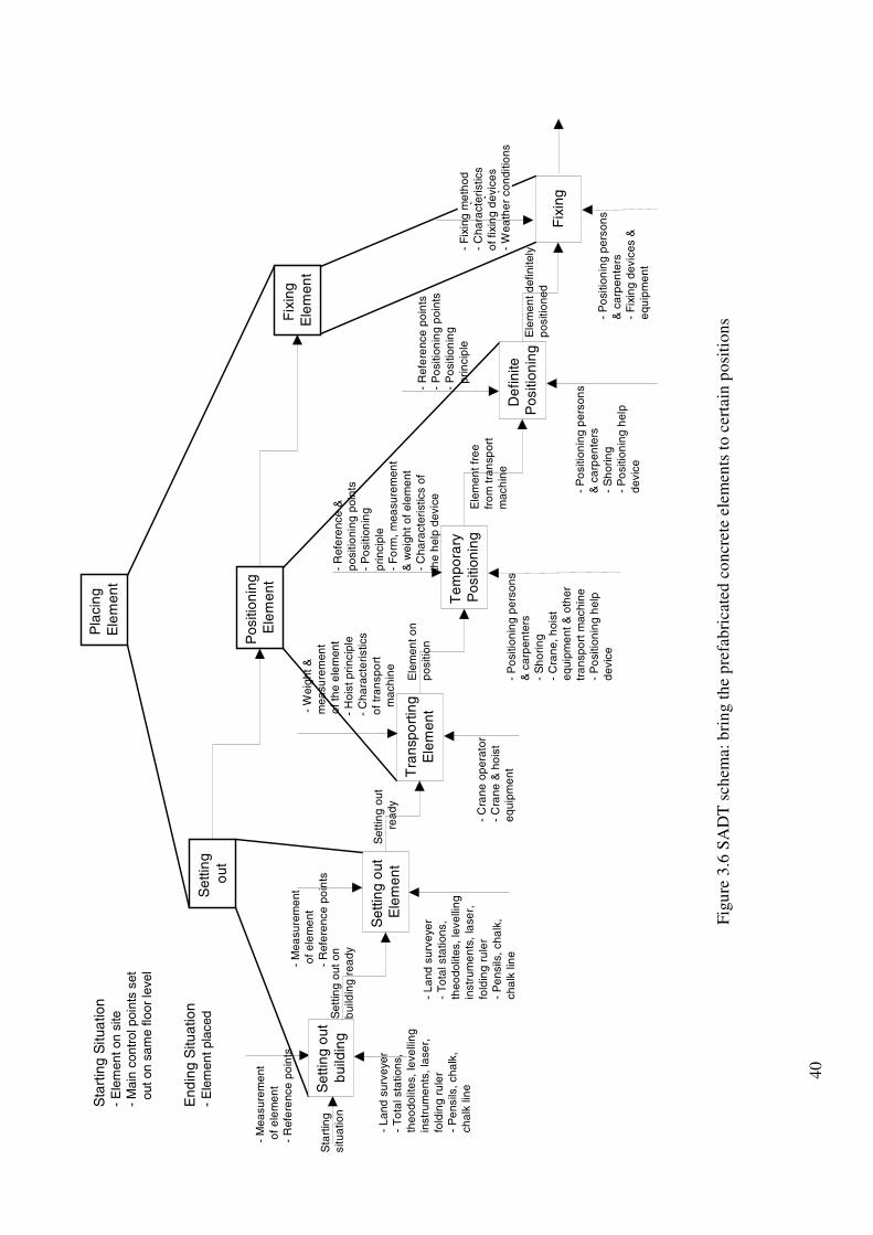
certain positions.

35
Table 3.3 Observation of different types of prefabricated structural elements on 21
building sites in the Netherlands
Code Location Wall Floor Beam Column Total
17 Voorburg Wilma 2 2 1 5
04 Maasland 1 1
11 Moerdijk Shell 1 1 2
08 Leiden 1 1
25 Utrecht 3 1 1 5
06 Helmond Adriaans 1 2 1 4
30 Voorburg BN 1 1
03 Den Bosch 1 1 1
02 Den Bosch 1 1
06 Helmond Adriaans 1 1
15 Zwolle 2 1 1 4
18 Venlo 1 1
13 Barneveld 1 1 2 4
19 Utrecht 1 1
14 Hengelo 1 1 1 3
05 Nijmegen 2 2
21 Heerlen 1 1
22 Maastricht 1 1
23 Helmond NBM 1 1 1 3
24 Naaldwijk 1 1
18 Venlo 1 1
Total 17 9 8 11 45
From the observations and interviews, some conclusions can be drawn on
dimensional control for the building and each separate element. Although Total
Stations are being widely used, traditional measuring instruments are still in use.
The positioning methods include free positioning and forced positioning, with the
latter as a majority. Whenever a building is higher than 30 meter, the main control
point for the horizontal setting out work always consists of a MOUS-point. Also,
the MOUS system is sometimes applied in lower buildings.

36
Table 3.4 List of questions put forward to site personnel
Question Answer Amount Percentage
Surface of the element
Supply in the element
Marks on the element
Poured in plate
What do the positioning
points consist of?
Cover for bolt
In the factory
On the building site
Where have the positioning
points been brought?
Not applicable
Marks
Template (positioned,
unchangeable)
Template (positioned,
changeable)
Neighbouring construction
Own surface
Template (not positioned,
unchangeable)
Pencil line
Chalk line
Nail
Wood/block
Bolt
Piece on the bolt
Piece on demu-anker
Neoprene block
Wood/block
What do the reference
points consist of?
Tile
Forced positioning What is the positioning
method? Free positioning
No correction Which correction methods
are used? Individual deviation

37
For the columns, when positioning in the height direction, all are forced
positioning; when positioning in the length and depth direction, most (80%) are
free positioning because marks are set out; when plumbing, all are free
positioning; the reference points for plumbing are the surface of the element with
levelling instrument.
For the walls, the positioning points consist of, in almost all cases and for all three
directions, the own surface of the element itself. The reference points exist in a
variety. For the height direction, high and low buildings have been distinguished.
For a high building (>30m), in which the accuracy plays an important role, there
exists always a help device, which has been positioned in height with the help of a
levelling instrument or laser. Whenever a building is not higher than 20 meter,
mostly the neighbouring construction work or a non-positioned help device (a
distance keeper) will be the reference. For the depth direction of the underside of
the element, mostly the beneath construction work will be the reference. For the
plumbing of the above side in the depth direction, apart from the parapet/breast
wall, the own surface of the element itself is always used as reference. The
reference points for the positioning in the length direction, consist of a marking or
the surface of the neighbouring construction work.
For the beams, it is not specially set out in the horizontal plain, but the elements
already positioned are used as the help device; for the height direction, sometimes
it is set out with the normal instruments such as levelling instrument and laser; on
the element itself nothing is set out. There is no distinction between temporary
positioning and definite positioning, and the beams are put on their place in one
go. There are minimal six points used for positioning. The positioning points
consist of the own surface of the element. Only in depth direction is positioning
measure correction used. It is a correction on the basis of individual deviation.
Whenever the correction is used, one or two extra positioning points are used.
For floor slabs, in 90% of the cases, there is nothing set out on the elements. There
is never positioning measure correction used. The required accuracy is low. In the
height direction, the reference points consist of the neighbouring construction
work, and the way is forced positioning; the floor slab is definitely positioned by

38
the gravity. In length direction, the floor is definitely positioned by friction. In the
depth direction, the floor slab is also definitely positioned by friction and
positioning points consist of the surface of the element.
In Figure 3.6, you can find the process of setting out, positioning and fixing
elements. The working equipments, information needed for each stage and
information flow between each stage are all depicted in this figure. In essence, the
basic information needed is the positioning ways, positioning points and
corresponding reference points which should be set out in advance. All these kinds
of information should be actually found in the dimensional control plan.
Therefore, it is very important to give the right information in the plan. To design
such a plan, the engineers must consider a lot of aspects. However, from the
interviews and observations, you can feel that most engineers design such plans
and choose positioning points and corresponding references just according to
experiences without explaining the reason. There is a lack of explicitly structured
knowledge.
3.3 CONCLUSIONS ON DIMENSIONAL CONTROL
In the beginning, one of the research objectives has been to investigate the body of
knowledge used by the engineers to design the dimensional control plan. After
observations on building sites and interviews with the engineers, contractors and
site personnel, it is concluded that there is little explicitly expressed knowledge
generally available. That is to say, there are no clear answers to the question of
which points to be used for the different aspects of dimensional control including
setting out, positioning and dimension monitoring and why. Also, in the NEN
standards, the answer cannot be found though it gives some insight to tolerances
and deviations.
The dimensional control problem is basically of a stochastic nature, because every
measure originating from construction process has a stochastic deviation and each
solution first has to find a way to handle this.

39
To summarize, the following conclusions on dimensional control can be drawn:
1) There is, as yet, very little dimensional control knowledge available that has
been formally expressed;
2) There is a lot of factual dimensional control knowledge that resides quite –
in the form of rules of thumb – in the heads of experienced planners;
3) There are so many forms of deviations and dimensional differences
following different construction methods for various types of projects, that
it is not reasonable to expect that the whole body of dimensional control
knowledge will ever be fully formalized at all;
4) Handling the stochastic deviations originating from construction processes
like prefabrication, setting out and positioning, is quite problematic for
humans but ideally suited for computers.
40
Figu
re 3
.6 S
AD
T s
chem
a: b
ring
the
pref
abri
cate
d co
ncre
te e
lem
ents
to c
erta
in p
ositi
ons
Ele
men
t def
inite
ly
pos
itio
ned
Ele
men
t fre
e fr
om
tra
nsp
ort
mac
hin
e
Ele
men
t on
posi
tion
- W
eigh
t &
m
easu
rem
ent
o
f th
e e
lem
ent
- H
oist
pri
ncip
le
- C
hara
cte
ristic
s of
tran
spor
t m
ach
ine
Sta
rtin
g si
tua
tion
Pla
cing
E
lem
ent
Set
ting
out
Pos
ition
ing
Ele
men
tF
ixin
g E
lem
ent
Set
ting
out
build
ing
Set
ting
out
Ele
men
tT
rans
port
ing
Ele
men
t
Tem
pora
ry
Pos
ition
ing
Def
inite
P
ositi
onin
g
Fix
ing
Sta
rtin
g S
ituat
ion
- E
lem
ent o
n si
te
- M
ain
cont
rol p
oint
s se
t o
ut o
n sa
me
floor
leve
l
End
ing
Situ
atio
n -
Ele
men
t pla
ced
- M
easu
rem
ent
o
f ele
men
t -
Ref
ere
nce
po
ints
- L
and
sur
veye
r -
To
tal s
tatio
ns,
th
eodo
lites
, lev
elli
ng
in
stru
me
nts,
lase
r,
fold
ing
rule
r
- P
ens
ils, c
halk
, ch
alk
lin
e
Set
ting
out
on
bui
ldin
g re
ady
- L
and
sur
veye
r -
To
tal s
tatio
ns,
th
eodo
lites
, lev
elli
ng
in
stru
me
nts,
lase
r,
fold
ing
rule
r
- P
ens
ils, c
halk
, ch
alk
lin
e
Set
ting
out
read
y
- M
easu
rem
ent
o
f ele
men
t -
Ref
ere
nce
po
ints
- C
rane
op
erat
or
- C
rane
& h
ois
t
equ
ipm
ent
- R
efe
renc
e &
p
ositi
oni
ng p
oin
ts
- P
osi
tion
ing
p
rinci
ple
- F
orm
, mea
sure
men
t &
wei
ght o
f el
eme
nt
- C
hara
cter
istic
s of
th
e h
elp
dev
ice
- P
osi
tion
ing
per
son
s &
car
pen
ters
-
Sh
orin
g -
Cra
ne, h
oist
e
quip
me
nt &
oth
er
tra
nspo
rt m
achi
ne
- P
osi
tion
ing
hel
p d
evic
e
- P
osi
tion
ing
per
son
s &
car
pen
ters
-
Sh
orin
g -
Po
sitio
nin
g h
elp
dev
ice
- R
efe
renc
e p
oin
ts
- P
osi
tion
ing
poi
nts
- P
osi
tion
ing
prin
cip
le-
Fix
ing
me
thod
-
Cha
ract
eris
tics
of f
ixin
g d
evic
es
- W
eath
er
con
ditio
ns
- P
osi
tion
ing
per
son
s &
car
pen
ters
-
Fix
ing
devi
ces
&
equ
ipm
ent

41
ANALYSIS OF THE STATE OF THE ART INFORMATION
TECHNOLOGY RELEVANT FOR DIMENSIONAL CONTROL IN
THE BUILDING INDUSTRY
Information and Communication Technology (ICT) has been playing an important
role in the building industry. This chapter gives a brief analysis of some leading
technologies that are relevant for dimensional control.
4.1 INTRODUCTION
Application of ICT in the building industry started somewhere in the 1960s with
do-it-yourself programming in BASIC. Simple algorithmic programming was
ideal for the early days when often differential equations had to be solved by hand.
Structural engineering was the subject most suited to the technology of that time.
In later years, when centralised computers gave way for PCs, a wide variety of
commercial applications came into being. Some of the underlying technologies
4

42
most relevant for dimensional control will be reviewed below. The main areas that
have to be looked into are:
• Logical connections of the floor plan design to the Dimensional Control
(DC) application that will be developed as part of this study;
• Physical connection, i.e. the standards used for electronic data exchange;
• Knowledge Technology;
• Graphical User Interfaces;
• Programming languages and environments.
The next sections discuss these topics in more detail.
4.2 BRIDGING DESIGN AND DIMENSIONAL CONTROL
There are several ways that designers and engineers can represent their designs.
These ways range from traditional paper-based approaches to product modelling.
Each approach has its consequences for this study. For each approach, the
available possibilities and exchange standards are also looked into.
4.2.1 Paper-based Approach
The obvious consequence of using traditional paper-based design-drawings is that
the Dimensional Control System (DCS) envisioned in this study cannot pick up
the required design data in electronic form. The user of the DCS has to input all
the data himself. This calls for a tool that resembles an existing building modeller.
Getting the required design data in house is no problem. Just rely on the postman
and take your time.
4.2.2 Computer Aided Drawing (CADr)
Computer Aided Drawing or Drafting (CADr) systems, starting from 2D
modelling techniques in the 1960s, are capable of representing objects
mathematically in the computer. A wire-frame model is the simplest and most
verbose type of 2D model. In the 1970's, the 3D wire-frame was subjected to 3D
translation and rotation, giving greater illusion of solidity, relieving users from the
burden of interpreting 2D drawings. Over the past years, the development of solid

43
modelling systems enabled a wide range of applications to be modelled in 3D,
including mass properties, volumes and moments of inertia.
CADr (Computer Aided Drawing or Drafting) systems have been widely used in
the building construction industry. CADr systems concentrate on the production of
traditional technical drawings. CADr drawings have advantages over traditional
physical drawings. Amongst others, CADr drawings can be reused to make design
and drafting efforts more efficient; CADr drawings can be easily changed to
accommodate design modifications and additions; CADr systems layer design
information for efficient editing, viewing and plotting; CADr systems plot
complex shapes and give accurate dimensions for construction layout (Mahoney,
1990).
CADr systems are able to create the geometrical representation of building
objects, and allow the addition of more semantic information as needed for input
into the data model. Therefore their inherent structure to classify data has to be
used in a standardized manner. Methods to structure CADr data are classified into
layers, macros and attached attributes. Layers are mainly used to control visibility.
In addition, they offer the possibility to group sets of data, such as all load-bearing
walls of ground floor. Many CADr systems still restrict the use of layers in such a
way that any entity is only allowed to be a member of one particular layer. Macros
can be used to label and control all geometric entities, which are representations of
one building element. Macros thus offer grouping mechanisms on the instance
level, which is necessary to keep unique identifiers for the bi-directional exchange
of meaningful descriptions of building elements. Attached attributes are mainly
used to store non-geometric information on entities or macros, such as the
material, the building code and optional explanations.
Shortcomings of current CADr
Until now, CADr systems are still used mainly as a drawing tool, though some
attempts have been made to extend their functionality with meaning and
intelligence. This is due to the inherent bottlenecks of CADr systems (Liebich,
1995). First, almost all conventional CADr systems rely on a pure geometric data
model consisting of lines and points. All non-geometric information about objects

44
has to be attached to these geometric entities. This restricts the ability to describe
semantically dependant relationships. In the real architectural and engineering
design process the representation of design objects is context dependant. Second,
the data exchange remains restricted since it is based on a fairly low semantic level
of document based exchange of information, the level of technical drawings, such
as geometric representation in DXF or IGES, rather than on a high semantic level
of a model based exchange. Third, although CADr systems offer a programming
interface, they require advanced programming skills, much effort, and time to
bring knowledge or additional information into systems. Even so, systems still
often have low performance. Thus CADr systems are not intelligent. CAD systems
have limited achievements due to the deficiencies of their underlying database.
CADr systems have drawbacks also in presentation techniques. The CADr
database is the prime source of design information. However, the majority of
current CADr packages provide users and developers alike with only one view, i.e.
the entity view, which represents the raw CADr data as an unordered set of
graphical primitives such as points, lines, and arcs. Software vendors' primary goal
is to optimise the performance of their CADr packages, as a drawing tool, through
the employed method of data storage. Meanwhile, a users' view of the drawing
model in building elements format, is not accounted for. This constitutes a major
obstacle for the acceptance of a free flow of information between CADr systems
and other applications packages used by professionals in industry. Furthermore,
geometry alone is limited in its usefulness for driving the some applications
packages where other non-geometrical information is required. New CADr
systems support both element representation and non-geometrical data. However,
these systems define elements by tagging the geometry with labels. As a result the
object integrity is not maintained. Clients' limited ability to visualize 2D design
solutions usually lead to misinterpretation of the design. This problem has been
partially overcome by animation techniques in which 3D images (frames) can be
rendered and generated to simulate 3D walkthroughs. The limitation imposed by
the predefined animated paths, the high cost of reproducing the animated images,
and the inability to interact with these images has not helped designers/clients to
fully solve this problem.

45
Data exchange standards
There are several standards available for the exchange of drawing files.
AutoCAD’s DXF and DWG are the two standards most often used. One problem
here is that both standards are vendor dependant (AutoDesk) and not completely
platform independent and error free. Several projects report problems with using
these standards in practice.
Other standards are developed by STEP (see below) and ISO. None of these
standards is used in the building industry.
Conclusions on CADr and DC
Though it is technically possible to import the DXF/DWG drawing files and
reconstruct the elements (columns, beams, walls) of the floor plan from the
available data, it is not possible to do that in general without an industry wide
layering and mark-up convention. If the designers are willing to adopt a layering
and mark-up convention for the purpose of dimensional control, it seems possible
to extract the DCS input automatically from the drawing files.
CADr is a typical example of the common innovation process. Just like the first
motorcar strongly resembled the horse wagon, CADr systems strongly resemble
the drawing board. Subsequent development cycles show and eliminate the
shortcomings inherited from the past, in this case the need to build a 3D model
from points and lines only.
4.2.3 3D Geometric Modelling
3D geometric modelling extends the notion of points and lines with faces, volumes
and primitives shapes. 3D geometric modelling does not play the same role in the
building industry as in other sectors of industry, like Mechanical and Automotive.
In those sectors Constructive Solid Geometry (CSG), Boundary representations
(B-rep) and surface modelling are often used. In our sector only one special type
of B-rep called Cellular model, or Relational Model plays (RM-rep) a role.

46
RM-modellers
The RM-rep was for instance used in the COMBINE-project (Augenbroe, 1993 &
1995). The essence of an RM-rep is (i) that it starts with Spaces that are enclosed
by Faces (or face sides) and (ii) that it includes relations like point-on-a-line,
point-on-a-face, face-on-a-face, etc. This makes the RM-rep particularly suited for
building design.
If the design of a floor plan has been described with an RM-modeller it is also
known which lines and faces represent which elements and consequently
extracting the input required by the DCS is not too big a problem. Unfortunately
standards for data exchange of RM-rep data do not exist, so a general connection
to different systems cannot be implemented.
4.2.4 Product Data Technology
Product Data Technology (PDT) has been introduced in the 1980s. Basically the
ideas follow the concept of feature modelling used by the designers of mechanical
parts in the automotive industry. A feature is a small area of a part with
‘engineering meaning’ (Shah). Examples are holes, pockets, ribs and such.
Essentially a feature does not require any further design; given its parameters,
everything is known, including the way to produce the feature. Mechanical
engineers design their parts by designing and dimensioning the required features.
PDT in the building industry also attempts to design a building by designing and
dimensioning semantic entities. However in our industry we want to design a
building by dimensioning and placing walls, floors, beams, columns etc. So the
features of the Mechanical engineers became the walls, floors, beams and columns
of the architects and structural engineers.
This section evaluates some of the Information Technologies that are important for
PDT.
Product Modelling
Product modelling aims at the production of a generic data description for a
particular product domain - a “universe of discourse”, for actors within that

47
domain - containing ‘complete’ and unambiguous information about a product
(building). Complete in the sense that all information required for a specific
application, if available, will be specified as an integral part of the product model
or can be derived from it (Gielingh, 1990). In the case of building design systems,
it aims at producing generic information models for various categories of buildings
(Ramscar, 1995). A data model provides the basic tools for describing the data
types, relationships and constraints of the information stored in a database,
expressed in documents or in speech. An analogy would be the basic grammar
utilized in natural language (Bjork, 1991). Thus, a building product data model
defines generic data types and relationships (“product grammar rules”)
encapsulating the kinds of objects that will be instantiated within the building
domain (Ramscar, 1995).
The product model comes into being to meet the trends towards integration. In the
late 80s a product model was defined in (Vajna, 1991) as a model, consisting of
geometrical model as well as some other models, for instance:
• Procedural models (consisting of instructions for building element
production);
• Topological models (consisting of relative position of the geometrical
elements);
• Method models;
• Technological methods (dimensional and location tolerance, tasks for
creating surrounding surface, information texts about production methods).
More general and abstract is the following definition (Junge, 1993): Product
modelling aims to describe unambiguously all the objects with their attributes and
relations, which range the solving task.
Construction is a process that involves diverse parties having different
professional skills and intersects. Drawings, standard methods of measurement,
building specifications and standard forms of contract are all paper-based models
that provide formalized methods of communication (Munns, 1995). Open
integration of computer applications in construction requires true product
descriptions rather than 3D models or 2D drawings (Bakkeren, 1997). That is

48
because only meaningful descriptions can contain all relevant product information
in a computer interpretable way; three dimensional models contain information on
a limited set of product aspects only, usually geometry; two dimensional drawings
contain even less product information interpretable by computer. The latter two
are meaningful to human beings only.
The future intelligent applications ‘know’ the information they process and can
therefore interpret this information, maintain its consistency and derive other
information from it without human intervention. Since these applications
understand product descriptions and posses encoded domain knowledge they can
even augment the creativity and knowledge. Integrating these intelligent
applications requires meaningful product descriptions. Computer integration based
on geometric models can never reach the level that is possible with meaningful
product descriptions.
Product data technology (PDT) is the technology directed at the definition, use and
management of meaningful product information in computer-integrated processes.
Product modelling is that part of PDT that focuses on defining meaningful product
descriptions in a computer interpretable way. The physical realization of a product
model is a shared database, an exchange file or any other way of computer
interpretable storage of information. A product model can first be defined in
generic level, and then be instantiated.
Open application integration requires that all applications can read and write
information in a standardized format and assign the same standardized meaning to
this information. The format used for exchange is usually referred to as the syntax.
The meaning of the information is usually referred to as the semantics. Syntax is
often associated with file exchange, but not limited. A data dictionary defines the
words that can be used to describe information on semantics. It is an equivalent to
the term “ontology” in the field of artificial intelligence. Olsen et al. (Olsen, 1995)
defines ontology as “a dictionary of classes, relations, functions and object
constants along with their definition in human readable text and machine
interpretable sentences”.

49
There are some general-purpose product modelling systems primarily for building
design. Examples are AutoCAD Architectural Desktop, Allplan, ArchiCad and
Speedikon. These systems often have an internal format for storing building
information and several modules that can use that format. Most of the systems still
use a 3D geometry model as the core of the building information. Other non-
geometric information is attached to this three-dimensional model and often stored
in a database that is separated from the geometry model.
Conclusions on PDT
PDT undoubtedly is a key technology for ICT in construction. The problem is the
implementation in our industry. PDT requires (1) standardisation of the formats,
(2) implementation by the vendors, (3) adoption by the industry and (4)
application in real life projects. This process takes a lot of time and effort. Other
industries with strong industrial market leaders, like aerospace and automotive
have made much more progress than the building industry.
STEP (STandard for the Exchange of Product model data)
STEP (STandard for the Exchange of Product model data) is an emerging
international standard (ISO 10303) for representing and exchanging product model
information. It includes an object-flavoured data specification language,
EXPRESS, to describe the representation of the data. The data model is
graphically represented by EXPRESS-G. STEP defines also implementation
methods, for instance, a physical transfer file, and offers different resources, e.g.,
geometric and topological representation.
The development of STEP started in 1984 as a worldwide collaboration. The goal
was to define a standard to cover all aspects of a product (i.e. geometry, topology,
tolerances, materials, etc.), during its lifetime. STEP is a collection of standards to
represent and exchange product information. The main parts of STEP are already
international standards, while many parts are still under development. The
development is performed under the control of the International Standards
organisation (ISO), Technical Committee 184 (TC184, Industrial Automation

50
Systems), Subcommittee 4 (SC4, Industrial Data and Global Manufacturing
Programming Languages).
The objective of STEP is to offer system-independent mechanism to describe the
product information in computer aided systems throughout its lifetime. It separates
the representation of product information from the implementation methods.
Implementation methods are used for data exchange. The representation offers a
definition of product information to many applications. STEP provides also a basis
for archiving product information and a methodology for the conformance testing
of implementations.
EXPRESS is a formal data specification language used to specify the
representation of product information. The use of a formal data specification
language facilitates development of implementation. It also enables consistency of
representation. STEP specifies the implementation methods used for data
exchange that support the representation of product information.
STEP does not only define the geometric shape of a product, but also includes
topology, features, tolerance specifications, material properties, etc. necessary to
completely define a product for the purposes of design, analysis, manufacture, test,
inspection and product support. The use of STEP is still very modest but it is
growing all the time. The majority of CAD system vendors have implemented or
are implementing STEP pre- and post-processors for their CAD systems. STEP is
an evolving standard that will cover the whole product life cycle in terms of data
sharing, storage and exchange. It is the most important and largest effort ever
established in engineering domain and will replace current CAD exchange
standards.
Conclusions on STEP
STEP is not yet important for the building industry, though several STEP parts
may well be used with advantage, notably the Express modelling language, the
resource schemas and in the future the STEP equivalent of the IAI/IFC (see next
section).

51
Industry Foundation Classes (IFC)
The International Alliance for Interoperability (IAI) is committed to creating a
standard to enable true interoperability among all of the players - and the software
they use - who are involved throughout the life cycle of a building.
As of this writing the IAI has over 300 member companies in seven international
chapters, and is growing daily. Its vision is to enable software interoperability in
the AEC/FM industry; its mission is to define, promote and publish a specification
for sharing data throughout the project life-cycle, globally, across disciplines and
across technical applications; it is a not-for-profit industry organization and its
membership is open to any company working in the AEC/FM industry.
The intention of the IAI is to define all of the objects that could occur in a building
(such as doors, windows, walls, and so on). Then, define a specification for how
each object will be represented electronically. These specifications are called
Industry Foundation Classes (IFC). Together they represent a data structure
supporting an electronic project model useful in sharing data across applications.
The IFC require that each object has known characteristics. It is more than a
simple collection of lines and geometric primitives. An object is stored and
manipulated in a manner consistent with the designer’s intent. IFC-based objects
allow all AEC/FM professionals to share an underlying building information
model, yet allows each profession to define its own view of each of the objects
contained in that model; the objects designed by an architect can later be used by
other professionals. This leads to improved efficiency in cost estimating, building
services design, construction, and facility management.
IFC enable interoperability among AEC/FM software applications. Information
modelling in IFC is based on EXPRESS-G. The classes can be used by software
developers who are familiar with object-orientated programming methods to create
applications that use universal AEC/FM objects based on the IFC specification.
An object created in one application can communicate with another IFC-compliant
application. This second application recognizes the object and is able to
understand these characteristics and add information to the object, because it also
uses the IFC specifications defined by the IAI. Applications that support IFC will

52
allow members of a building project team to share data (such as drawings, reports,
and specifications) in an electronic format. This will ensure that the data is
consistent and coordinated. Furthermore, this shared data can continue to evolve
after design, through construction, and occupation of the building. Information
generated by the project design team will be available in intelligent, electronic
format to the building construction team through their IFC compliant software and
to building facilities managers through their IFC compliant software.
Several product modellers such as Allplan and AutoCAD Architecture Desktop,
can already read and write IFC 1.5 shape representations. However, exchange of
product model data is cumbersome because the required attributes have to be
derived from the neutral geometrical model. In the Brite-Euram CONCUR-project
these ‘derived attributes’ will be standardised.
Conclusions on IFC
The Industry Foundation Classes are becoming the default standard for product
modelling in the building industry. Most vendors of Building Design Systems
support IFC. When the current shortcomings are eliminated in the future, IFC will
be of great benefit.
4.3 KNOWLEDGE TECHNOLOGY
This section looks into the applicability of Knowledge Technology for the
development of a Dimensional Control System.
Knowledge Technology (KT) is what in the old days was called Artificial
Intelligence (AI). Intelligent computer systems that use certain design principles
(like separating the knowledge part and applying a knowledge engine) are called
Knowledge Base Systems.
4.3.1 Background and Definition
A knowledge based system (KBS) is a software system capable of supporting the
explicit representation of knowledge in some specific competence domain and
exploiting it through appropriate reasoning mechanisms in order to provide high
level problem solving performance. Therefore, a KBS is a specific, dedicated,

53
computer based problem solver, able to face complex problems, which, if solved
by man, would require advanced reasoning capabilities, such as deduction,
abduction, hypothetical reasoning, model based reasoning, analogical reasoning,
learning, etc. (Guida and Tasso, 1994).
Knowledge in this context is a technical word. It covers for example the content of
building regulations, codes of practice, all kinds of algorithmic and procedural
knowledge (as implemented in analysis systems), as well as less well-defined
experience-based knowledge, or very precisely defined knowledge found in
predicative logic, or propositional logic.
For the purpose of this study the main focus is on the knowledge that plays a role
in DC.
4.3.2 Importance for the Building Industry
Construction and Dimensional Control is very much a business of experience,
expertise, and good judgment. Expert systems could capture and broadly
disseminate the knowledge of scientists and experienced consultants in this area.
The main reason for trying to apply KT and specifically, expert systems to
construction is to deal with the qualitative and judgment-based types of problems
that are prevalent in this industry. In the case of DC the main problems are (1)
place of control points, (2) place of Total Station, (3) handling of deviations.
Experience and knowledge of experts can be captured in computer programs so
that other construction engineers and managers can access it and apply it, perhaps
even after the experts who provided the knowledge are no longer available. Such
programs also provide a means to integrate and validate the knowledge and
experience of many experts and thus provide a means for accumulating and
improving a body of knowledge over time.
There are different types of knowledge, each requiring another representation.
Figure 4.1 shows a matrix that tries to classify the field according to two
parameters: “Data Intensive” and “Degree of Difficulty”. Data Intensive classifies
the representations according to the amount of data that can be processed, and
Degree of Difficulty classifies the representations according to the amount of

54
knowledge and the way the knowledge is known (well defined, weakly defined,
and undefined). The horizontal classification distinguishes between deductive
reasoning (where the relations between input and output are well known) and
inductive reasoning, where the relations between input and output are less well
known or even unknown.
-Modelling-Logic-Simulation
-Rule Based Systems
-Expert Systems
-Databases-Data Mining
-Planning-Fuzzy Systems
-Assembly-Configuration
-Statistics-Intelligent Design
-Neural Networks
-Genetic Algorithms
-Truth Maintenance
-Case Based Reasoning
-Constraint Satisfaction
Data Intensive
Degree of Complexity
Figure 4.1 Classification of knowledge representations. The vertical axis groups
the representations according to the amount of data that can be processed. The
horizontal axis groups the representations according to the amount and preciseness
of the knowledge that plays a role. The application of formal logic, for example, is
useful for problems with relative little data and a small amount of well-defined
knowledge.
For the “Data Intensive” categories such as Data Mining, there are typically many
dimensions (up to several hundreds) and many data points (many thousands or
even millions). Dimensional control is not a problem that requires the processing
of such a large amount of data, so its representation belongs to one of the three
groups at the bottom of the matrix.

55
Along the Complexity axis dimensional control is less easy to classify. It is partly
a problem with well-defined knowledge (if all the measurement points are well
defined and the measuring equipment is able to view each point). In that sense it
belongs to the left group where modelling and simulation seem representations of
interest. However dimensional control also involves elements of stochastic
uncertainty that places it in the middle group. And finally DC also involves
circumstances where people base their decisions solely on experience, without
being able to explain why they make these decisions. This might place the DC
problem partly in the right group. In the next sections these three groups will be
investigated somewhat deeper.
For the development of the DCS and the formalization of measurement control
experience, the most important knowledge technologies seem to be:
• Simulation
• Rule Based Systems
• Fuzzy Logic
• Inductive Knowledge (Neural Networks, Genetic Algorithms and Case
Based Reasoning)
Simulation
Determining the best position for the measurement control points and the place of
the Total Station is largely related to the prediction of dimensional deviation
limits. This can be done by simulation techniques. Numerical methods that involve
sampling from random numbers are called Monte-Carlo Methods. Monte-Carlo
simulation is often used in risk analysis and problems involving statistic or
stochastic variables. As dimensional control is a problem covered by stochastic
deviations with uncertainty, Monte-Carlo simulation seems an attractive
technology.
Rule Based Systems (RBS)
RBS are particularly suited to problems involving expert reasoning. RBS typically
store heuristic knowledge in a rule base. The facts are generally stored in the form
of “IF-THEN” rules. The RBS use the rules as they are needed to solve problems

56
when presented with data. As measurement control knowledge in most cases can
be expressed as rules of thumb RBS seem to be most applicable for DC.
Fuzzy Logic
Fuzzy Logic is interesting if linguistic ambiguity comes into play, like in the
following rules:
IF distance_measurement is LONG
THEN deviation_accuracy is LOW
To make use of these rules both parameters LONG and LOW must be formalized,
i.e. how small is small and how low is low? This type of problems can be tackled
with fuzzy sets (i.e. the sets LONG and NOT-LONG) and membership functions
that express the degree of membership of a variable of both sets.
Linguistic ambiguity always plays a role in the building industry, so probably also
in DC.
Inductive Knowledge (Neural Networks, Genetic Algorithms and Case Based
Reasoning)
Representations in this group aim to learn to predict improved solutions from
experience. Neural Networks mimic the working of the brain. In a Neural Network
system the relation between a small set of inputs and outputs is formed by a
network of nodes with weights that can either stimulate or suppress its
contribution to the solution.
Artificial neural networks can be most adequately characterised as “computational
models” with particular properties such as the ability to adapt or learn, to
generalise, or to cluster or organise data, and which operation is based on parallel
processing.
An artificial network consists of a pool of simple processing units that
communicate by sending signals to each other over a large number of weighted
connections.

57
A neural network has to be configured such that the application of a set of inputs
produces (either “direct” or via a relaxation process) the desired set of outputs.
Various methods to set the strengths of the connections exist. One way is to set the
weights explicitly, using a priori knowledge. Another way is to “train” the neural
network by feeding it teaching patterns and letting it change its weights according
to some learning rule. Genetic Algorithm can also be utilised to optimise a neural
network.
Neural networks are particularly effective for predicting events when the networks
have a large database of prior examples to draw on.
Genetic Algorithms (GA) mimics the evolution of species and the principle of
survival of the fittest. GA is one of the evolutionary algorithms (EA), which are
used to describe computer-based problem solving systems that use computational
models of evolutionary processes as key elements in their design and
implementation. EAs all share a common conceptual base of simulating the
evolution of individual structures via processes of selection, mutation, and
reproduction. The processes depend on the perceived performance of the
individual structures as defined by an environment.
More precisely, EAs maintain a population of structures, which evolve according
to rules of selection and other operators, which are referred to as “search
operators”, (or genetic operators), such as recombination and mutation. Each
individual in the population receives a measure of its fitness in the environment.
Reproduction focuses attention on high fitness individuals, thus exploiting the
available fitness information. Recombination and mutation perturb those
individuals, providing general heuristics for exploration. Although simplistic from
a biologist's viewpoint, these algorithms are sufficiently complex to provide robust
and powerful adaptive search mechanisms.
The Genetic Algorithm is a model of machine learning that derives its behaviour
from a metaphor of the processes of evolution in nature. This is done by the
creation within a machine of a population of individuals represented by
chromosomes, in essence a set of character strings that are analogous to the base-4

58
chromosomes that we see in our own DNA. The individuals in the population then
go through a process of evolution.
Genetic Algorithms are used for a number of different application areas. An
example of this would be multidimensional optimisation problems in which the
character string of the chromosome can be used to encode the values for the
different parameters being optimised.
Evolutionary Programming is a stochastic optimisation strategy similar to Genetic
Algorithms, but instead places emphasis on the behavioural linkage between
parents and their offspring, rather than seeking to emulate specific genetic
operators as observed in nature.
Like GAs, EP is a useful method of optimisation when other techniques such as
gradient descent or direct, analytical discovery are not possible. Combinatory and
real-valued function optimisation, in which the optimisation surface or fitness
landscape is “rugged”, possessing many locally optimal solutions, are well suited
for Evolutionary Programming.
Neural network systems can help in the following situations:
-where it is impossible to formulate an algorithmic solution.
-where it is possible to get lots of examples of the behaviour as required.
-where it is necessary to pick out the structure from existing data.
GA is applicable for optimisation problems and requires that you can immediately
qualify a solution, i.e. you should be able to say if a solution is better or worth than
an earlier solution.
For the problem of dimensional control, the stochastic dimensional deviation
variables are according to normal distribution. Each deviation variable is out of
N(0, σi) and in the range of (-Dmax, Dmax). The Dmax can be determined according
to standards and σi can be approximated from samples. The value of Dmax and σi
can be optimised in order to generate random numbers that simulate the stochastic
deviations as close as possible. And neural network can also be trained for this
goal, mapping inputs consisting of measured data or observations of the stochastic

59
dimensional deviations of various sorts to output consisting of Dmax and σi. The
appropriate network would be a combined one with data classification and
mapping. Therefore neural network and genetic algorithm would help to optimise
a random number generator in Monte-Carlo simulation.
To solve other problems where the relation between cause and effect is unknown
(can not be explained), for example, if a surveyor always knows the best place for
the Total Station, but is not able to explain why, you need a lot of examples to
train the neural network. Unfortunately, right now there are no such examples
available, therefore for this type of problem, it is only possible to apply NN in the
future.
GA might also be used in situations of error propagation in the problem of
dimensional control (DC). In DC, there are typical structural assembly situations.
You can choose components with known deviations and analyse the total
deviations. Then you can change components from the set of available
components and predict which components to use where. GA seems interesting as
an extension to analysing these situations.
In case-based reasoning (CBR) systems expertise is embodied in a library of past
cases, rather than being encoded in classical rules. Each case typically contains a
description of the problem, plus a solution and/or the outcome. The knowledge
and reasoning process used by an expert to solve the problem is not recorded, but
is implicit in the solution.
To solve a current problem: the problem is matched against the cases in the case
base, and similar cases are retrieved. The retrieved cases are used to suggest a
solution that is reused and tested for success. If necessary, the solution is then
revised. Finally the current problem and the final solution are retained as part of a
new case.
All case-based reasoning methods have in common the following process:
• retrieve the most similar case (or cases) comparing the case to the library of past cases;

60
• reuse the retrieved case to try to solve the current problem;
• revise and adapt the proposed solution if necessary;
• retain the final solution as part of a new case.
Case-based reasoning is often used where experts find it hard to articulate their
thought processes when solving problems. This is because knowledge acquisition
for a classical KBS would be extremely difficult in such domains, and is likely to
produce incomplete or inaccurate results. When using case-based reasoning, the
need for knowledge acquisition can be limited to establishing how to characterise
cases.
Case-based reasoning allows the case-base to be developed incrementally, while
maintenance of the case library is relatively easy and can be carried out by domain
experts.
To apply CBR into DC field requires, in the first place, a database filled with cases
(DC plans). There isn’t such a database yet; therefore, it is not yet feasible to apply
CBR.
In conclusion, Neural Networks, Genetic Algorithms and Case Based Reasoning
are able to capture experience where the relation between cause and effect is
unknown (can not be explained). Also Neural Networks can be used for data
classification and mapping inputs to outputs, and Genetic Algorithm can be used
for optimisation. Conceptually, it is possible to apply these technologies if there
exists a large set of data, examples, cases or a procedure that can quickly analyse
the results of the chosen solution. Currently, as these requirements are not yet
completely fulfilled, the application of inductive knowledge is not yet fully
feasible, though it may come into play in the future. To apply these technologies,
more research should be performed.
Conclusions on Knowledge Technology support for DC
For the development of the DCS, the Monte-Carlo simulation, the application of
Rule Based Systems and Fuzzy Logic seem to be most important. Other
technologies could be used to solve particular problems. For example, inductive

61
knowledge might become important in the future, and it might be possible to build
more autonomous measurement control systems. For now, however, it seems that
simulation, RBS and Fuzzy Logic are the most appropriate knowledge
technologies for DC.
4.4 GRAPHICAL USER INTERFACES
Building a DCS that suites the end-users needs, will need decisions about the
graphical user interface (GUI) that the user will have to work with. There are
several aspects that have to be looked into, among others, the graphics, including
Virtual Reality.
4.4.1 Virtual Reality (VR)
A Virtual Reality scene or ‘world’ is a simulation of a real or imaginary world,
which a user can interact with. A VR world of a project provides designers,
clients, suppliers, contractors, authorities and public with a common basis for
communication that is widely available over the Internet. Designers can add the
shapes of the design objects they create to the scene and make the information
related to the design objects generally available by a mouse click.
The most important Internet-based VR language available is VRML.
VRML
VRML is an acronym for Virtual Reality Modelling Language. VRML, by use, is
a 3D scene-description format that has plugs built in to provide networking and
multi-user accessibility. It's quite possible to create a VRML world just using a
text editor. However, to build more complex scenes, modelling software will be
required. There are different software packages that can create VRML worlds.
There are basically two types of VRML modellers: object builders and scene
assemblers. An object builder enables the user to create arbitrary shapes
interactively and then export the geometry in the VRML format. These packages
usually support other 3D file formats as well. A scene assembler allows the user to
assemble 3D objects into VRML scene, and include hyperlinks, inlines and Level-
of-Detail.

62
There are also a number of different tools available for converting models from
other commonly used 3D file formats (such as AutoDesk's DXF and 3Dstudio)
into VRML. Some tools are programs freely available via the Internet.
VRML allows developers to create "virtual worlds" of arbitrary visual and
geometric complexity, with the added feature of attaching WWW hyper-links to
any object. These worlds are downloaded over the Internet just like any other file,
and displayed in a VRML browser (such as WebSpace). VRML browsers are used
in concert with a normal Web browser (such as Netscape), which provides a
mechanism for viewing standard text and multimedia resources.
VR versus CAD
As mentioned before, CAD systems have drawbacks in presenting information. As
VRML is generally available for free and able to combine output of many different
modellers, the emerging VR technology complements the limitations of CAD.
Conclusions on Virtual Reality
The application of VR for Dimensional Control seems to be in the ‘world wide’
sharing and exchange of design information. As discussed above, the application
of CAD systems and PDT systems rely on a process of standardisation, vendor
implementation, company-adoption and project agreement, which is time
consuming and cumbersome.
VRML on the other hand is basically an Internet technology that is generally
available without special hardware requirements (though broadband Internet
helps). If in the future project partners decide to create and maintain a common
VR project scene, DC can also use the scene to extract the required information
about each floor plan and to communicate the resulting details about the DC plan.
4.5 IMPLEMENTING THE DCS
There are several ways the Dimensional Control System can be implemented. Two
broad divisions are obvious. First the systems can be implemented in Visual Basic
or Java. Second the system can be built on top of, or strongly related to AutoCAD.

63
4.5.1 Visual Basic (VB)
Visual Basic is a Microsoft (MS) product. VB has the advantage that it integrates
very well in the MS environment and with a large number of related systems and
tools.
Visual Basic is an object-based programming language and system builder. The
first step to creating an application with Visual Basic is to create the interface, the
visual part of the application with which the user will interact. Forms and controls
are the basic building blocks used to create the interface; they are the objects that a
programmer will work with to build his application.
The programming language, a modern version of Basic, is an up to date and
powerful language that is quite simple to understand and use.
Conclusions on VB
Microsoft VB is a widely available industry standard and, despite its simplicity, a
powerful programming environment that suites the needs of the building industry.
4.5.2 Visual Basic for Applications (VBA)
Visual Basic for Applications is both a subset and a superset of VB. The two have
lots in common but they differ in that VBA contains application-specific
properties, methods and events. Every VBA-enabled application has its own object
model. Typically, the programmer needs to add a reference to the application's
type library in his project. From that point, he uses the VBA commands as if they
were native to VB itself.
VBA is found as a component in AutoCAD and many Microsoft applications
including Access and Excel. This provides a mechanism to integrate different
applications.
Conclusions on VBA
Although VB is more powerful than VBA, VBA makes it possible to integrate
AutoCAD with Microsoft applications such as MS Access and MS Excel in the
DCS.

64
4.5.3 Java
Java is the preferred programming language of today. Using Java has some strong
advantages. It is vendor independent, platform independent, nicely object oriented
and well documented and available. Because of the very structured programming
language in combination with the readability of the code, Java becomes a powerful
tool for implementing complex and not so complex programs. Mastering Java
however is much more difficult than mastering VB.
Conclusions on Java
For developing the DCS, Java has no particular advantages over Visual Basic.
Java is much more difficult and largely inaccessible for casual programmers.
4.5.4 AutoCAD
AutoDesk’s AutoCAD is the leading computer-aided design and drafting (CAD)
program in the world. In the building industry, AutoCAD is the default industry
standard. Over the years, AutoCAD has kept pace with developments in the
computer industry.
Conclusions on AutoCAD
As AutoCAD is so important in the building industry it is the prime candidate for
implementing the DCS.
4.5.5 Architectural Desktop
AutoCAD’s latest product line is AutoCAD Architectural Desktop (ADT). ADT
is developed mainly for architecture and building design. It embraces the potential
of 3D model-based design and object-oriented software, without sacrificing any of
the CAD productivity gains. ADT introduces basic building model objects so that
all applications built for AutoCAD software or ObjectDBX™ can now share the
same definition of these objects.
In addition, as discussed before, AutoDesk is a founding member of the
International Alliance for Interoperability (IAI), an organization dedicated to
sharing building model data across the building life cycle and to creating the IFC

65
(Industry Foundation Class) specification for model data exchange between CAD
systems.
Conclusions on ADT
ADT seems quite capable and powerful for the job of implementing the DCS.
However it is also still too advanced. Though the number of designers working
with ADT is rapidly growing, its popularity is greatly overshadowed by
AutoCAD. Also ADT has strong competitors, like ArchiCad and Allplan. ADT is
not dominating the PDT-market and cannot be seen as a default industry standard.
AutoCAD VBA
AutoCAD VBA is a new development line of AutoCAD that uses the ActiveX
Automation Interface to integrate AutoCAD with VBA. AutoCAD VBA permits
the Visual Basic environment to run simultaneously with AutoCAD and provides
programmatic control of AutoCAD. There are three fundamental elements that
define ActiveX and VBA programming in AutoCAD. The first is AutoCAD itself,
which has a rich set of objects that encapsulates AutoCAD entities, data, and
commands. The second element is the AutoCAD ActiveX Automation interface,
which establishes messages (communication) with AutoCAD objects. The third
element is the VBA programming environment that has its own set of objects,
keywords, constants, and so forth, which provide program flow, control,
debugging, and execution.
Conclusions on AutoCAD VBA
The linking of AutoCAD, ActiveX Automation, and VBA provides an extremely
powerful interface. A VBA application for AutoCAD is much faster than a VB
application, because VBA application is in-process that means it works in the
same address as AutoCAD, and VB application should communicate with
AutoCAD by Inter Process Communication (IPC). The VBA API is integrated in
AutoCAD and no additional software is needed to develop such an application,
whereas Visual Basic is needed to develop a VB application. In addition, VBA is

66
also available in MS applications. Considering these facts, VBA is the primary
candidate of programming language for implementing the DCS.
4.6 CONCLUSIONS
The previous sections discussed the state of the art in ICT as seen relevant for the
development of a Dimensional Control System. The main conclusions are:
• AutoCAD and Visual Basic provide the development environment most
suitable for DC. Besides the fact that AutoCAD is market leader in design
software of the building industry, it also provides an entrance to the world
of Product Data Technology and related next generation tools. With the
integration of Visual Basic, a simple but powerful programming language
and application builder, it seems possible to build a DCS that can be
accessible for the future users to add their own experience to the system.
VBA is the programming environment most suited to the job, as it is able to
work with a domain specific object model. This object model can be
tailored to the needs of DC. Moreover with ADT also a product-modelling
interface (IFC) becomes available. Finally there are several ways to import
and export VR.
• Knowledge Technology, especially Rule Based Systems, provides
mechanisms suitable for DC to express engineering experience in the form
of rules of thumb. Simulation and modelling are suited for prediction and
calculation of error propagation of dimensional deviations. Fuzzy logic can
be used to add greater flexibility to the expressions if linguistic ambiguity
comes into play.

67
REFORMULATION OF THE RESEARCH QUESTIONS This chapter summarizes the analysis of previous chapters and reformulates the
research questions.
5.1 INTRODUCTION
In Chapter 1, it has been stated that, to improve the dimensional control of on-site
construction projects, while focusing on prefabricated concrete building structural
elements, this research (1) tries to capture the knowledge required to design an
adequate dimensional control plan and make that knowledge more generally
available and (2) build a digital connection between CAD systems and Total
Stations.
The initial research questions have been formulated as follows:
• Is it possible to develop an ‘intelligent’ instrument that supports the less
experienced planners to develop adequate dimensional control plans?
• How to facilitate the digital information flow between CAD systems and
Total Stations?
5

68
After literature review, observation on construction sites and interviewing experts,
it is concluded that there is very little explicitly structured and formalized
knowledge available to be put in a knowledge base as a general solution to
dimensional control problems. Dimensional uncertainty, dimensional deviation,
and the stacking up of deviations springing from several sources form the core of
the problem. On the other hand, it could still be possible to design a system
capable of capturing rules of thumb when they come along.
Another observation has been that the DCS envisioned could also support
experienced planners in complicated positioning situations. In fact the use of the
DCS in complicated positioning jobs seems to be more attractive than the
application of the DCS by inexperienced planners.
Finally the idea that it is mandatory to automatically input the design data into the
DCS has been dropped. The reasons are:
• The fact that the DCS will most probably be mainly used (at least for a
start) by experienced planners in complicated situations. In those cases
inputting the required data is only a very small part of the job.
• Automatic information flows from CAD to DCS can be easily
implemented using the IFC-format once it becomes the default industry
standard, provided of course that the DCS is based on PDT-principles.
5.2 REFORMULATION
Based on the evaluations given in section 5.1 above, in this section, the research
questions have been reformulated as follows:
• How to design and implement an ‘intelligent’ DCS that supports the
planners to develop adequate dimensional control plans, and supports the
site personnel to realize the requested dimensional quality?
• How to handle the dimensional deviations aspects of dimensional control
problem?
• How to express some knowledge rules for dimensional control problem in
addition to handling stochastic deviations?

69
SIMULATION OF DIMENSIONAL DEVIATIONS
This chapter presents a method and a model that can be used to simulate setting
out deviations, positioning deviations and product deviations, and the prediction
of the dimensional deviation limits that show the dimensional quality.
6.1 RECAPITULATING THE PROBLEM
In previous chapters, it is concluded that there is a lack of theory and knowledge
that can be used as a basis for designing the dimensional control plan that provides
necessary information for the construction process. This chapter starts to tackle the
problem by looking into the aspect of dimensional quality of a building and its
components. It presents a method to simulate setting out deviations, positioning
deviations and product deviations, and the prediction of the dimensional deviation
limits that show the dimensional quality. Also, some influencing factors for
dimensional control have been added to this method. Then, using PDT principles,
the Dimensional Control information model is defined using the Unified
Modelling Language (UML).
6

70
6.2 PREDICTION OF DIMENSIONAL QUALITY
The essence of designing a dimensional control plan is to find out which points
should be used as positioning points, which points should be set out in advance or
controlled afterwards, and why. These questions are in fact, to a great extent,
related to the aspect of dimensional quality. Therefore, one must be able to predict
the dimensional deviation limits that show the dimensional quality. Also there are
some other factors that influence the choice of choosing certain points, for
example, the location and positioning method of an object, and the visibility of the
positioning points. These factors will also be expressed in some knowledge rules.
In building construction, design or “ideal” dimensions and actual dimensions are
distinguished. The architects give the ideal dimensions of building components in
the drawing, and specify dimension tolerances in the specifications. The actual
dimensions occur after components are produced, or during or after the
construction of the building. The actual dimensions can never be the same as the
ideal dimensions. The differences between these two are termed dimensional
deviations. Deviation-limits reflect the dimensional quality of a building.
Also, in building construction, three types of measures are distinguished, i.e. the
setting out measure, the positioning measure and the product measure. The setting
out measure can be defined as the distance between a mark and the reference point
being used. It is the result of the setting out process. The positioning measure can
be defined as the distance between a positioning point and the reference point used
for positioning an object. The product measure can be defined as the characteristic
measure of building products. It includes length, width, height and so forth. See
Figure 6.1.
Dimensional deviations originate from people handling, instrument accuracy and
environment influences. For example, the measuring deviations come from
persons who do the measurement; the measuring instrument has a system
deviation coming from manufacturing; also the temperature changes can cause
deformation of building components. The building construction process can be
considered as a stochastic process with respect to statistics. Under certain
circumstances, the construction process can be considered as a normally

71
distributed process. That is to say, if the value and frequency of a certain
production process is put in a histogram, it is a normal distribution curve. Another
statistical principle is that when more (independent, normally distributed)
processes are put together, the combined process is also normally distributed.
Figure 6.1 Basic elements causing place deviation of a point
Therefore, predicting the deviation limit of each object requires considering the
deviation as a result of chain-processes. Especially, the processes of prefabricating
production, setting out and positioning should be taken into account. These three
processes cause (1) product deviation, (2) setting out deviation and (3) positioning
deviation. To calculate the final deviation they should be added together. The final
“place deviation” which can be defined as the deviation related to the place of a
point of the building part, is equal to the sum of these separate deviations.
Each object will be viewed as a collection of points. For the prediction of the
dimensional deviation limits of each point of an object two methods can be used.

72
The first method recognizes the stochastic characteristics of each individual
deviation; that is to say, each individual deviation is distributed according to a
normal distribution. Then the total deviation is calculated according to the
following formula: 2
LP∆ = 2RP∆ + 2P∆ + 2S∆ (6-1)
( LP∆ : Place deviation, RP∆ : Product deviation, P∆ : Positioning deviation, S∆ :
Setting out deviation).
Using this method, you need to know the value of each individual deviation in
order to get the total deviation.
The second method assumes that each individual deviation belongs to a certain
range that has a certain percentage of certainty. For example, the deviation can be
within the range of ,10mm± with the certainty of 98%. Each deviation is randomly
picked out of certain range and put together. If this is done a large number of times
(e.g. 1000 times), the distribution of the total deviation can be predicted. This
approach, following the Monte Carlo simulation technique, can be termed the
simulation method.
The predicted dimensional deviation limits should be within the specified
tolerances. Also, after predicting the dimensional quality, the predicted quality
should be achieved following some procedures. This can be done by means of,
among others, a combination of working methods that are statistically controlled
processes. Otherwise, the prediction of dimensional quality will not be true or
cannot be achieved. The working methods are related to setting out and
positioning processes, and must be specified in the setting out plan and positioning
plan.
6.3 SIMULATION OF DEVIATIONS AND REPRESENTATION OF
KNOWLEDGE RULES
Determining various sorts of dimension deviations separately and then putting
them together will make the simulation of concrete elements. Positioning

73
deviations, setting out deviations and product deviations are simulated respectively
in the following sections.
6.3.1 Simulating Setting Out Deviations and Positioning Deviations
To position an object, minimum 6 1D points are needed to overcome the
translation and rotation of the object. Using a set of points as positioning points
will have influence on all the other points regarding the final place deviation. The
simulation method is used to calculate the final place deviation. To find out the
influence, it is better to first study the final place deviation of the origin of the
object. Then the final place deviations of other points from the changed origin can
be calculated.
As shown in Figure 6.2, to define the origin of the object with deviation, link the
middle point of AD and BC; find the centre point of plane EFCH; then create the
plane MIJ and define the origin that is its centre point.
Figure 6.2 Defining the origin and positioning points of an object
TotalStation
AB
C
A: x, y, z direction;B: y, z direction;C: z direction;
A B
G
D
E F
C
H
O
IJ
M
N

74
The maximal allowable setting out deviation in x, y and z direction is respectively
Sxmax, Symax and Szmax (with 98% certainty). The computer will choose a value
randomly (with normal distribution) within these limits respectively for the setting
out deviation in x, y and z direction, that is to say Sx, Sy and Sz.
The position of the origin of the element in regard to the origin of the building can
be calculated by bringing the following steps: the translation of the origin of the
building to the reference point, the translation of the reference point to a
positioning point of the element, the translation of the positioning point of the
element to the origin and finally the rotation of the element around the x, y and z
axis.
The rotation of the x, y and z axis of the element in regard to the coordinate
system of the building can be calculated by the rotation caused by the dimensional
deviations in the positioning measures in regard to the coordinate system of the
building, plus the rotation caused by the deviations in the product measures in
regard to the coordinate system of element.
If an element in the building is positioned following the setting out points and
positioning points, two different coordinate systems are put together, which are the
coordinate system for the building and for the individual element. This requires a
transformation of the element coordinate system to the building coordinate system.
To determine the position of points of an element in the building coordinate
system, it is calculated as follows:
The translation of the origin of the building coordinate system and the origin of the
element coordinate system;
The translation of the origin of the element and the point itself;
The rotation in x, y and z direction of the element coordinate system.
This means that, to determine the rotation around z-axis, two x or y positioning
coordinates that lie in the same surface are needed. Accordingly, the similar goes
for the rotation around x or y axis. See Figure 6.3.

75
Choosing a set of positioning points has consequences on all the points. The final
place deviation of each point is seen as a result of the product deviations, the
setting out deviations and positioning deviations of the selected points. Each of
these three kinds of deviations will result in three translations and three rotations
of the object.
y1
rotation around y axisrotation around x axisrotation around z axis
y2
x2
�
x1
d1
tan � = d1 / d2
y1
y2
x2x1
d2 d2
�
z1
z2
y2y1
tan � = d1/d2
z1
z2
y2y1
�
x1
x2
z2z1
tan � = d1 /d2
x1
x2
z2z1
�
� �
d1 d1
d2 d2
d1
d1 d1
d2
d2
Figure 6.3 Rotation around each axis of the element
In Figure 6.4, a simulated situation of rotations in three directions has been drawn.
In this simulation, the object first has a rotation around Z axis, which results a new
X axis and Y axis; then the object has a rotation around the new X axis, which
results a new Z axis; finally the object rotates around the new Y axis. Following
these three steps, a point (X,Y,Z) will get a new position (X3,Y3, Z3). Figure 6.4
shows the projection of each rotation respectively seen from the third positive axis.
The matrix Rz, Rx and Ry respectively shows the rotation around Z, X and Y axis.
The final position (X3, Y3, Z3) of the point is calculated by formula (6-5).
Rz =
−
100
0cossin
0sincos
αααα
(6-2)

76
Rx =
− ββββ
cossin0
sincos0
001
(6-3)
Ry =
−
γγ
γγ
cos0sin
010
sin0cos
(6-4)
[ ] [ ] yxz RRRZYXZYX ××=333 (6-5)
�
x
y
�
x’
y’
y’
z�
�
z’
y”
�
z’
x’
�z”
x”
Figure 6.4 Simulated rotation of the object in three directions
6.3.2 Simulating Product Deviations
For the simulation of product deviations, floor slabs, beams, walls and columns are
all characterized by their rectangular form and consist of 6 surfaces, 3 symmetry
axes and further 8 conceptual corner points and 12 edges. It is termed
“conceptual” because in fact corner points and edges don’t exist. They are always
in more or less measure rounded off.

77
To orient, a coordinate system has been chosen in which the X, Y and Z direction
is in accordance with the width, the thickness and height direction of the element
respectively. The origin is the centre gravity point of the element.
Each surface is defined by 9 (grid)points. See Figure 6.5. In fact, the number of
points doesn’t matter. The principle keeps the same for either more or less points.
It matters however for the accuracy, that is to say, the more points, the more
accurate. The middle (grid)point is coincident with the cutting point of the surface
with an axis of the coordinate system. The other points are equally divided so that
the distance to the edge (r) of the element in each case is same. It will show that at
the end the dimension deviation of these points is perpendicular to the surface.
r
nominal length (l)
Figure 6.5 Defining a surface by 9 grid points
The element is now defined by 6*9 = 54 points. For the simulation, the element is
divided in 3 separate segments. Each segment consists of 2 either opposite or
parallel surfaces, combined with each other by one of the axes of the coordinate
system. For the clarity, a column is drawn as an example in Figure 6.6, but it can
also be a wall, beam or floor element.
Now consider randomly 2 parallel surfaces of the element, connected by one of the
axes of the coordinate system, the so-called connection axis. Assume that the
deviation in the direction of the connection axis of the 18 points on these 2 parallel
surfaces is zero and bring the various sorts of deviations in the direction of the
connection axis in calculation for these points.

78
Z-axis
X-axis
Y-axis
Z-axis
Y-axis
X-axis
Figure 6.6 Dividing an element into parallel surfaces
For a three dimensional object, one can distinguish the various sorts of deviations
also in three dimensions. The following deviations are valid for a segment of the
element:
1 Dimensional: The distance between the opposite surfaces, measured along the
connection axis, characterized the dimensions (length, width, height or thickness)
of the element. A deviation on this distance moves itself along the line of the
connection axis.
2 Dimensional: The direction of the surface in regard to the connection axis, is
determined by 2 randomly unparalleled lines, which lie in the surface. The cutting
point of the surface and the connection axis can be viewed as a spherical hinge
point around which the surface can rotate. A deviation on the direction of the
surface characterized the (un)perpendicularity of an individual surface in regard to
the connection axis and the (un)parallelness of the surfaces with respect to each
other.

79
3 Dimensional: The form of the individual surface. Due to the deviation in the
flatness of the surface, it is a 3 dimensional object. The surface is in fact not a
surface. The unflatness is caused by deviations that can be characterized as
curvature and warp.
The above-mentioned deviations are defined as the characteristics of the individual
element and will be simulated by determining them individually and then adding
them on top of one another. The segment that consists of the under surface, the Z
axis and the top surface is graphically illustrated as an example. The principles
that apply to this segment are also valid for the other two segments.
The distance between the opposite surfaces: 1D product deviation
By dimension of the element, it means actually the length, height, thickness or
width of the element. Here the dimension of the element is defined as the distance
perpendicular to and between 2 parallel surfaces at which the cutting points of
these 2 surfaces with the connection axis serving as measuring points. The
distance between the under surface and the top surface of the element is thus
defined by the length of the Z axis between the cutting points of the under surface
and above surface with this axis. The deviation on this distance is determined by a
random number, which is distributed according to normal distribution, and can be
considered as a constant deviation that is valid for both surfaces. For the nominal
distance (A), it is defined that the maximal allowable deviation amax mm (98%
certainty) may be carried. Whenever the computer randomly chooses a value (a)
within this limit, then the top surface and the under surface gets a deviation of 0.5a
respectively seen from the origin. The points in the surface all get therefore the
same positive or negative deviation of 0.5a in the direction of the connection axis.
See Figure 6.7.
The direction of the surface: 2D product deviation
It means by the direction of the surface in fact the direction of the surface in regard
to the connection axis. For the under surface and the top surface, the Z axis is the
connection axis. A deviation in the direction of the surface can be described by the
unperpendicularity of the individual surface and the (un)parallelness of both
surfaces in regard to the connection axis.

80
Figure 6.7 1D product deviation
If a plane independent from the opposite plane gets a deviation in connection with
the direction of the plane in regard to the connection axis, this is called the
unperpendicularity of the individual plane. The unperpendicularity can be defined
as a variable deviation of the individual plane. The plane can take each direction.
The unperpendicularity of the under plane and the top plane can be expressed in
the X direction and Y direction. The unperpendicularity of the individual plane is
defined by two random numbers that are distributed according to normal
distribution. The maximal allowable deviation for the unperpendicularity of the
under plane and top plane in the X and Y direction is defined respectively as hxmax
and hymax mm/m (98% certainty). Whenever the computer chooses randomly two
values (hx and hy) within these limits, the plane gets an unperpendicularity of these
two values. For two opposite planes, four independent numbers are chosen. The
points in a plane all get an unequal positive or negative deviation in the direction
of the connection axis as a result of the unperpendicularity of the involved plane.
Figure 6.8 shows how the various deviations in the Z direction for the points in the
under plane or top plane interrelates.

81
The (un)parallelness of two opposite planes is analog to the unperpendicularity of
two opposite planes. This is concerned with a deviation in the direction of both
planes in regard to the connection axis. The (un)parallelness can be considered as
a constant deviation of the opposite planes. The planes can take each direction.
The (un)parallelness of the under plane and top plane can be expressed in the X
and Y direction respectively. The (un)parallelness of these opposite planes is
defined by two random numbers that are distributed according to normal
distribution. The maximal allowable deviation for the (un)parallelness of the under
plane and top plane in the X and Y direction is defined respectively as exmax and
eymax mm/m (98% certainty). Whenever the computer chooses randomly two
values (ex and ey) within these limits, the plane gets a (un)parallelness of these two
values. For two opposite planes, two independent numbers are chosen that are
valid for both planes. The points in these planes all get an unequal positive or
negative deviation in the direction of the connection axis as a result of the
(un)parallelness of the involved planes.
Figure 6.8 2D product deviation: unperpendicularity and (un)parallelness

82
The form of the plane: 3D product deviation
The form of the individual plane depends on the deviations in the flatness of the
plane. It means by the unflatness of the plane in fact the measure in which the
points don’t lie mutually in a plane. The unflatness is independent on the
coordinate system. The surface is in fact not a surface, but a 3 dimensional object.
By randomly choosing 3 gridpoints on the surface that don’t lie on a line, one can
define a reference surface. The bigness of the spreading of the distance in the
direction of the connection axis of the other gridpoints to this reference surface is a
measure for the unflatness. The unflatness is caused by deviations that can be
distinguished as the curvature and warp of the plane.
The curvature of a line or a surface can be defined by its length and the radius of
the belonging circle or sphere. Regarding the curvature of a segment of the
element, three types have been considered, namely the common curvature of both
surfaces, the curvature of the individual surface and the curvature of a gridline of
the individual surface.
Figure 6.9 Common curvature

83
Figure 6.9 shows the common curvature of two opposite surfaces. It can be
considered as a constant deviation that is valid for both surfaces and is defined in
two directions. For the under surface and top surface, the curvature is expressed in
the X direction and Y direction respectively, and is defined by two random
numbers that are distributed according to normal distribution. For the curvature of
the under surface and top surface, the maximal allowable deviation in the X and Y
direction may have kz;x,max mm/m and kz;y,max mm/m (98% certainty) respectively.
Whenever the computer chooses randomly two values (kz;x and kz;y) within these
limits, then these surfaces get a curvature with a result of these two values. For
two opposite surfaces, two independent numbers are chosen that are valid for both
surfaces. All the gridpoints in the opposite surfaces, except the cutting point with
the connection axis, get therefore an unequal positive or negative deviation in the
direction of the connection axis as a result of the common curvature.
The curvature of the individual surface can be considered as a variable deviation
of both surfaces and is defined in two directions. For the under surface and top
surface, the curvature is expressed in the X direction and Y direction respectively.
The curvature of the individual surface is defined by two random numbers that are
distributed according to normal distribution. For the curvature of the top surface, it
is defined that the maximal allowable deviation in the X and Y direction may have
kz1;x,max mm/m and kz1;y,max mm/m (98% certainty) respectively. Whenever the
computer chooses randomly two values (kz1;x and kz1;y) within these limits, then
the top surface gets a curvature with a result of these two values. Similarly, for the
curvature of under surface, whenever the computer chooses randomly two values
(kz2;x and kz2;y) within the limits of kz2;x,max mm/m and kz2;y,max mm/m (98%
certainty) respectively, the under surface gets a curvature with a result of these two
values. For two opposite surfaces, four independent numbers are chosen that are
valid for the curvature of both surfaces. All the gridpoints in a surface, except the
cutting point with the connection axis, get therefore an unequal positive or
negative deviation in the direction of the connection axis as a result of the
curvature of the individual surface. See Figure 6.10.

84
Figure 6.10 Curvature of individual surface
The curvature of a gridline of the individual surface can be considered as a
variable deviation of all gridlines. Each surface has six gridlines and the curvature
of a few gridlines of the individual surface of a segment is defined in one
direction. This means that there is more curvature in one direction within an
individual surface. For the under surface or top surface, the curvature of a few
gridlines is expressed in either the X direction or the Y direction. The curvature of
a gridline in a surface is defined by a random number that is distributed according
to normal distribution. For the curvature of a gridline in the top surface or under
surface, it is defined that the maximal allowable deviation in the X and Y direction
may have kz;1;x,max mm/m and kz;1;y,max mm/m (98% certainty) respectively.
Whenever the computer chooses randomly a value (kz;1;x or kz;1;y) within these
limits, a few gridlines get a curvature from which the most outside gridpoints on
this line get a positive or negative deviation in the direction of the connection axis.
For two opposite surfaces, 12 (6 in each surface) independent numbers are chosen
that are valid for the curvature of the gridlines in both surfaces. All gridpoints in a
surface, except the cutting point with the connection axis, get therefore an unequal

85
positive or negative deviation in the direction of the connection axis as a result of
the curvature of the gridlines in the individual surface. See Figure 6.11.
Figure 6.11 Curvature of gridline
The warp of a surface can be defined by the measure in which 4 points don’t lie in
a plane. The plane is in more or less degrees tortured. Warp can be measured by an
imaginary plane drawn by three random corner points. The distance between the
fourth corner point and the corner point of the imaginary plane is a measure of the
warp. See Figure 6.12. By dividing the warp over 4 corner points, you will find no
warp within the original plane. This plane creates the starting point for the
simulation of the warp. For the warp of the plane of a segment, the common warp
of both planes and the individual warp are considered.

86
Figure 6.12 Defining warp
The common warp of two opposite planes can be considered as a constant
deviation that is valid for both planes, and is defined by a random number that is
distributed according to normal distribution. For the warp of the under plane and
above plane, it is defined that the maximal allowable deviation may carry sz,max
mm (98% certainty). Whenever the computer randomly chooses a value (sz) within
this area, these planes will get a warp that is distributed over 4 corner points. One
number is picked and valid for both two opposite planes. All gridpoints in the
opposite planes, except the cutting point with the connecting axis, get thus an
unequal positive or negative deviation in the direction of the connecting axis as a
result of the common warp. See Figure 6.13 (left part).
The warp of the individual plane can be considered as a variable deviation of both
planes and is defined by a random number that is distributed according to normal
distribution. For the warp of the above plane, it is defined that the maximal
allowable deviation may carry sz1,max mm (98% certainty). Whenever the computer
randomly chooses a value (sz1) within this limit, then the above plane will get a
warp that is distributed over 4 corner points. Similarly, for the warp of the under
plane, whenever the computer randomly chooses a value (sz2) within the maximal
allowable deviation sz2,max mm (98% certainty), the under plane will get a warp
that is distributed over 4 corner points. For two opposite planes, two independent

87
values are therefore picked that are valid for the warp of both planes. All
gridpoints in a plane, except the cutting point with the connecting axis, get thus an
unequal positive or negative deviation in the direction of the connecting axis as a
result of the warp of the individual plane. See Figure 6.13 (right part).
Figure 6.13 Common warp and individual warp
For the form of the surface, there are more characteristics such as straightness and
warp to be considered. Also there can be more directions for the curvature of the
surface. However, apparently the parameters given in the above have a satisfied
simulation of the practice.
The tolerance concerned with 1 grid point
In this simulation method, the coordinates of each grid point of each concrete
element in respect to the origin of the building are known. The place deviation of
each grid point should be compared with the place tolerance. The place tolerance
is the tolerance concerned with the place of a point of the building part in respect
to the desired place. It should be noted that in the practice, people do not check
whether the place tolerance is exceeded, because the desired place of a point in the
building is not often defined, and usually the maximum allowable dimensional
deviation between two physical points is used on building sites. In the simulation,
however, the place tolerance is used. The place tolerance is the area that
symmetrically lies in respect to the desired place of a point of the building part.

88
6.3.3 Expression of Knowledge Rules
Some influencing factors for dimensional control of building components are
discussed in this section. First, the positioning method of a component influences
the choice of positioning points. If a component is positioned using free method,
one needs to consider the location of the component. For example, if a column is
located on the edge or corner of a floor, its corner points can’t be used as
positioning points for the horizontal positioning. If a component is positioned
using forced method, then the location doesn’t matter. Also if the component is
positioned using direct positioning in 3D, then the visibility of its positioning
points seen from the Total Station should be taken account. These are some
example rules for dimensional control of building components and will also be
modelled in the UML information model.
6.4 THE UML MODEL
Figure 6.14 on page 90 shows the Dimensional Control information model in
UML. The Appendix at the end of the thesis gives a simplified description of the
UML syntax.
What the model says is that a Floorplan limits the scope of the Dimensional
Control view. Floorplan describes the relevant physical objects of a floor in a
World Coordinate System (WCS). A WCS is a Coordinate System defined by an
Origin and X, Y and Z-axis all defined as 3D vectors, where 3D vector is defined
by an X, Y and Z value.
Each Floorplan has one Main Control Point, which is a 3D-Point. Each 3D-Point
has X, Y, and Z-values and a Name or Number. A Floorplan consists of a set of
Typical Structural Assemblies.
A Typical Structural Assembly has a World Coordinate System of its own, and
consists of several Positioning Objects.

89
A Positioning Object (a physical object that has to be positioned) is either a
Structural Element (like a Beam, Wall, Column, Facade or Slab), or Formwork1.
Each Positioning Object refers to an Object Coordinate System (OCS) that can be
transformed to WCS, and has an Origin. A Rectangular Box with a Height, Width
and Length value represents a Positioning Object. A Positioning Object has an ID
and one or more Positioning Points that are again 3D Points. A Positioning Object
also has the attribute of Location that can be on the edge, corner or middle of a
floor. A Positioning Object has also Positioning Method that can be either Free or
Forced Positioning. A Positioning Object has also the operation of Translate,
Rotate and Set Positioning Method.
Positioning Points can be selected or not. Positioning Points also have the
operation of Set Visibility that sets the attribute of Visibility to True or False
according to angle, light or other factors. Positioning Points have Product
Tolerance, Setting out Tolerance and Positioning Tolerance. Positioning Points
refer to Reference Points, which are 3D-Points. Reference Points refer to Setting
out Points and Setting out Points refer to Main Control Point. Positioning Points
have Setting out Deviation, Positioning Deviation and Product Deviation. Product
Deviation can be 1D, 2D and 3D. 1D Deviation includes the deviation in Length,
Width and Height. 2D Deviation includes Unparallelness and Unperpendicularity.
3D Deviation includes the deviation of Curvature and Warp.
6.5 CONCLUDING REMARKS
The Dimensional Control information model structures the entities or objects
needed for both the simulation of dimensional deviation limits and expression of
engineering experience. Also example knowledge rules have been incorporated to
the objects. This model is open and more knowledge rules can be added when
available.
1 The subtypes of Positioning Object in the model are in fact only examples; other objects can be handled
just as well.

90
Str
uc
tura
lEle
me
nt
Be
am
Wa
llF
ac
ad
e
Co
lum
nS
lab
3D
ve
cto
r
X :
Do
ub
le
Y :
Do
ub
le
Z :
Do
ub
le
Fo
rmw
ork
3D
-Po
int
X :
Do
ub
le
Y :
Do
ub
le
Z :
Do
ub
le
No
: S
trin
g
Ma
inC
on
tro
lPo
int
Flo
orP
lan
11
11
co
ntr
ol
Re
cta
ng
ula
rBo
x
Le
ng
th :
Do
ub
le
Wid
th :
Dou
ble
He
igh
t :
Dou
ble
Ty
pic
alS
tru
ctu
ralA
ss
em
bly
Co
ord
ina
teS
ys
tem
Ori
gin
: 3
Dv
ecto
r
X-a
xis
: 3
Dv
ecto
r
Y-a
xis
: 3
Dv
ec
tor
Z-a
xis
: 3
Dv
ec
tor
WC
S
WC
S
Se
ttin
go
utP
oin
t
1..
*1
..*
refe
r_to
To
lera
nc
e
Po
siti
on
ing
Ob
jec
t
ID :
Str
ing
Ori
gin
: 3
Dv
ec
tor
Lo
ca
tio
n :
Str
ing
Po
sit
ion
ing
Me
tho
d :
Str
ing
Tra
ns
late
()
Ro
tate
()
Se
tPo
sit
ion
ing
Me
tho
d()
1
1
1
1b
ou
nd
ed
_b
ox
OC
S
Ref
ere
nce
Poi
nt1
..*
1..
*
refe
r_to
De
via
tio
n
Me
an
: D
ou
ble
Sta
nd
ard
De
v :
Do
ub
le
Po
siti
on
ing
Po
int
Se
lec
ted
: B
oo
lea
n
Vis
ibili
ty :
Bo
ole
an
Se
tVis
ibili
ty()
pro
du
ct
po
sit
ion
ing
se
ttin
go
ut
1..
*
1
1..
*
1p
os
itio
np
oin
t
1..
*
1..
*
1..
*
1..
*
refe
r_to
Se
ttin
g o
ut
Un
pa
ralle
l(2
DP
rod
)
Gri
dC
urv
atu
re(3
DP
rod
)
Un
pe
rpe
nd
icu
lar(
2D
Pro
d)
Com
Cu
rva
ture
(3D
Pro
d)
1D
Pro
d
Ind
ivC
urv
atu
re(3
DP
rod
)
Ind
ivW
arp
(3D
Pro
d)
Com
War
p(3
DP
rod
)
Pos
itio
nin
g
Fi
gure
6.1
4 D
imen
sion
al C
ontr
ol I
nfor
mat
ion
Mod
el in
UM
L

91
SYSTEM DESIGN AND IMPLEMENTATION
This chapter proposes a computer-aided system for dimensional control based on
the model presented in Chapter 6. It starts with defining the system requirements,
followed by the system functional design; then the system is implemented by
prototyping; finally some concluding remarks are given.
7.1 DEVELOPMENT OF A COMPUTER AIDED SYSTEM FOR
DIMENSIONAL CONTROL
In order to improve the dimensional quality of on-site construction projects, this
chapter proposes to develop a support tool that fits into the current trend of using
standardized electronic product models as the main carrier of construction
information. Figure 7.1 shows the proposed system and its overall environment.
Basically the idea of this support tool is that a project database holds a detailed
description of the facility under construction in a “neutral” (vendor independent)
product model format. A product model described in the neutral format describes a
facility (building, road, bridge) in the semantics of the construction industry.
Product models can be exchanged or accessed by computer networks.
7

92
Figure 7.1 Structural elements in the Real System are positioned using a Total
Station. The Total Station is fed with control data produced in the Information
System by the DC-Tool .
For the Building and Construction industry, currently the most promising product
model format candidate is the format developed by the International Alliance for
Interoperability (IAI) called the Industry Foundation Classes (IFC). (Refer to
Chapter 4 for more on IFC). This format is already available for several Design
systems, like Speedikon, Allplan and AutoCAD Architectural Desktop.
To improve the dimensional quality of a project by applying Product Data
Technology, the project database is filtered and converted by the Dimensional
Control tool (DC-Tool) to a local database that describes the facility as a
collection of physical objects (structural elements, equipment and temporary
structures) accompanied by coordinate systems and setting-out points. Next the
positioning points are defined on the physical objects, using reference points, and
the deviation and tolerance data is analyzed. The DC-Tool feeds the required
control data to the Total Station on the construction site.
DesignSystem
IFCProductModel
DCTool
ExternalDesigning Systemsproduce IFC Product ModelData
TotalStation
DC_ProductModel
AutoCad Architectural Desktop,Allplan,Speedikon,Etc.
DC_toolfeeds Total Stationwith Control Data
InformationSystem
RealSystem
Analysisvisibility linesand positionsTotal Station
Comparesactual andrequiredpositions
DC_toolextracts relevantobjects and addsPositioning andControl Data
Slab
Column row
Feeds backactual positions Visibility
line

93
7.2 SYSTEM DESIGN AND IMPLEMENTATION
7.2.1 System Requirements
The system should function as follows:
1. The user chooses a typical structural assembly and inputs parameters like the
length, width and height of each element representation. The system can also
read AutoCAD drawings if they are in IFC format, otherwise if in other format
like plain AutoCAD drawing, the system can only open them and then special
converter needs to convert point, line and arc into IFC format objects.
2. The system displays the chosen typical situation or extracts structural objects
from the drawing, generates a collection of points and asks the user to select
certain positioning points of an element.
3. The user clicks certain points and the system predicts the deviation limits by
putting together all kinds of product deviations, setting out deviation and
positioning deviation as well, and also gives the possibility distribution of
deviation limits.
4. The system advises the user on selecting positioning points according to the
prediction results and checking of some relevant knowledge rules regarding the
visibility of points, positioning methods and location of building components.
If the deviation limits are within the prescribed tolerances, these points are
recommended; otherwise, choose some other points. Sometimes, if the
prescribed tolerance is too small, the system might suggest enlarging it.
5. The system will add setting out points, reference points according to the
selected positioning points.
7.2.2 Implementation Environment and Approach
To design the application tool, first the software environment should be chosen.
As analyzed in Chapter 4, the system can be strongly related with AutoCAD
environment. With the development of CAD systems and product data technology,
AutoCAD Architectural Desktop introduces the IFC utility and has some
intelligent objects such as walls, columns and openings. It can thus read and write
IFC file partially. AutoCAD also introduces the concept of exposing AutoCAD
objects through an ActiveX interface and programming those objects using Visual

94
Basic for Applications programming environment. Therefore, AutoCAD
Architecture Desktop, Access and Excel have been chosen as the software
platform, and VBA as the programming language to implement the model.
AutoCAD objects and AutoCAD ADT (Architectural Desktop) objects have been
used to implement the graphical objects in the model, such as wall, window,
opening, and grid. 3dbox can also be used to represent other rectangular objects.
Additional non-graphical attributes can be stored in Access database. Attributes
can also be extracted to Excel and statistical analysis can be performed. All these
can be done by programming in VBA which is found as a component in AutoCAD
and many Microsoft Office applications including Access and Excel. Figure 7.2
shows the implementation environment and approach for the application tool.
Figure 7.2 Implementation environment and approach 7.2.3 Design and Implementation of a Prototype
Functional design of the system includes the design of Graphical User Interface
(GUI), the design of tables in the Access database, linking graphical objects with
the Access database, and data output to Excel for statistical analysis.
([FHO'DWD DQDO\VLV DQG GLDJUDP
6WDWLVWLFDO $QDO\VLV
%XLOGLQJ 0RGHO�$XWR&$' 2EMHFW�
�$XWR&$' $'7 2EMHFW�
([WHQGHG 'DWD
$FFHVV
$SSOLFDWLRQ 7RRO
,)& )LOH
�3DUWLDOO\� ,)& )LOH
9%$

95
For the design of graphical user interface (GUI), Forms of VBA and the following
controls have been used: Multipage control, Option button, Checkbox, Label,
Textbox, RichTextbox, Command button etc. The Multipage control has been
used for main functions of the application tool, such as Generate Structure, Input
Drawing, Link to Excel, View Deviation, etc. In each main function, other
controls, such as Option button, Checkbox, Label, Textbox, Command button,
have been exploited for sub-functions. Figure 7.3 shows the user interface of
function Generate Structure. Figure 7.4 and Figure 7.5 shows respectively the user
interface of function View Deviation and Output.
Figure 7.3 The User Interface: Generate Structure
In Figure 7.4, apart from other controls, Frame control has also been used to group
different kinds of deviations. In Figure 7.5, CommonDialogBox control has been
exploited for file operation, and RichTextBox for displaying the texts.

96
Figure 7.4 The User Interface: View Deviation
The graphical objects in AutoCAD drawings have been linked with the tables in
Access database by Data Access Objects (DAO) from VBA. Also, AutoCAD’s
database connectivity feature can be used for this purpose. Database links within
an AutoCAD drawing are simply pointers to a database table that references data
from one or more records in that table.
Random number generator (normal distribution)
Most programming languages incorporate routines for sampling a random number
between 0 and 1, which is also the case in VBA. An approximate sample from a
univariate standardized normal distribution can be obtained from the formula:
612
1
−= ∑=i
iRε (7-1)
where the Ri are independent random numbers between 0 and 1 (1 ≤ i ≤ 12) and ε
is the required sample from φ(0,1)1. This approximation can be used to generate
1 ϕ denotes the cumulative distribution function (CDF) of the standard normal variable.

97
variables of standard normal distribution with mean 0 and standard deviation 1,
and it is satisfactory for most purposes.
If a set of observations {x1, x2, …., xn} are obtained for a particular random
variable X, then the true mean µx can be approximated by the sample mean x and
true standard deviation σx can be approximated by the sample standard deviation
sx. Also probability paper can be used to obtain µx and σx.
∑=
=n
i
ixn
x1
1 (7-2)
11
2
)(−
=∑ −
=
ns
n
ii
x
xx (7-3)
To generate a normally distributed random variable X with mean µx and standard
deviation σx, the following formula is used:
X = µx + εσx (7-4)
In the implementation, the above-mentioned method has been used for generating
random numbers of deviations that are distributed according to the normal
distribution N(0, σx). The range of each deviation variable can be determined
according to standards (NEN series 14), and σx can be approximated from
samples.

98
Figure 7.5 The User Interface: Output
In the implementation, in addition to the forms, there are also some modules to
achieve certain functions such as Draw, Calculate etc., and they can also be called
by the program for the forms.
7.2.4 Running Prototype
When running the prototype, it can generate typical structural assembly or read an
IFC format drawing. Figure 7.6 shows a simplified floor plan in IFC format and it
has been used as an input for the prototype.

99
Figure 7.6 A simplified floor plan in IFC format
Figure 7.7 shows that the tool marks positioning points on an element when the
user selects the element. For each possible positioning point of an element, 100
random numbers of normal distribution have been generated. Figure 7.8 shows the
generated numbers in the Access database. Figure 7.9 gives the X, Y, Z
coordinates of the marked positioning points. Figure 7.10 and 7.11 depicts
resepectively the distribution of the predicted deviation limits of 2 positioning
points, which is approximately the normal distribution.

100
Figure 7.7 Marking positioning points on an element
Figure 7.8 Generated random numbers of normal distribution in Access database

101
Figure 7.9 The X, Y, Z coordinates of marked positioning points of an element
Figure 7.10 Distribution of predicted deviation limits of Positioning Point 1

102
Figure 7.11 Distribution of predicted deviation limits of Positioning Point 2
7.3 CONCLUDING REMARKS
This chapter has presented the idea of designing a computer aided dimensional
control system (DCS). The implementation of a prototype of the DCS provides a
digital way to bridge the floor plan design with dimensional control, predict
dimensional deviation limits and output the data needed for a Total Station.
The DCS has used AutoCAD 3D objects to model the building structural
elements. It can also read and use IFC based building models. However, in the
building industry, AutoCAD 2D drawings are still widely used. With the
development of IFC standards in the building industry, IFC based building
modelling systems will replace current 2D drawing systems, which makes the DC
system future proof.

103
CASE STUDY
This chapter describes a case study in which the model and prototype have been
applied into practice. The data has been collected on the construction site and
analysed in house. Then the conclusion has been made based on the data analysis.
8.1 OBJECTIVE
The purpose of doing this case study is to test the model and prototype, and show
the proof of concept. This can be done by using the prototype tool in practice to
position several building elements and comparing with the traditional way in the
aspect of position accuracy.
8.2 CASE DESCRIPTION
The office-building project “La Tour” concerns an office building with 21 floor
levels. Around this building a parking garage of 3 levels will be constructed. The
construction of this building will be going on as follows: foundation of
prefabricated piles, cellar, in-situ casting concrete core by way of climbing
formwork, prefabricated inner wall plates, floor slabs, and further façade elements
which will be prepared as much as possible on the construction site.
8

104
The project gets a local coordinate system in combination with the given
municipal points from Apeldoorn. It should be noted that the municipal points are
within R. D. system in Netherlands and have a scale factor, but the local
coordinate system for construction doesn’t have a scale factor.
The local coordinate system is fixed outside the building area. It is fixed outside
because the following reasons. First it reduces the risk of deformation of fixed
points because once the points are fixed outside, fewer happenings will occur
outside. Second it follows the rule of working from large to small area. Third there
is more space outside than inside the building area and it gives foremen more play
space.
When fixing the points (usually minimal 3) of local coordinate system, points
should be fixed randomly and X, Y, and Z coordinates of each point should be
measured using the municipal points as the base. This can be done by putting
reflecting stickers on the existing objects and nails on the road outside around the
building area.
From the outside points, then it is moving inside the building area until the
foundation is poured. Then the MOUS system phase has arrived. The MOUS
System consists of a set of specially designed materials, tools, instruments and
procedures that can be used to establish main control points in buildings. The
characteristics of the system is the way in which the main control points are
marked – a piece of metal fixed to the floor with a specific inner diameter.
Through openings in the construction, these pieces of pipe are aligned according
to a vertical reference line and then fixed firmly to a part of the structure. The
application of the system starts on the lowest concrete floor; main control points
are set out and marked in the traditional way with a pencil, or set to the position
with a Total Station. Over these pencil lines, a marker plate, a steel plate with a
piece of pipe on it, is centred. Then the marker plate is fixed to the floor with
mortar. Later on this MOUS point will be used as a reference for the local setting
out process and once the upper floors are ready, for transferring MOUS points to
these floors. The number of MOUS points on each floor depends on the number of

105
pours of floors and sequence of pouring. Usually minimal 2 points are needed for
each pouring of the floor.
Figure 8.1 is the floor plan of the third level, Figure 8.2 is the section view of the
building, and Figure 8.3 shows some pictures of the building project under
construction.
Figure 8.1 Floor plan of the third level
Figure 8.2 Section view of the building

106
Figure 8.3 Pictures of the building project
8.3 COMPARISON OF THE MODEL WITH PRACTICE
The UML model and prototype developed in previous chapters are project
independent and represents a more theoretical view of the dimensional control
knowledge. In the model, the way to direct set out points using Total Station from
a known point has been presented. Also, the building elements are viewed as
columns, beams, floor slabs, walls and facades, which are objects instead of plain
lines. In building construction practice, people use gridlines, offset method,
MOUS systems and help devices etc. for setting out and positioning. This has
been learned from interviewing the experts and visiting construction sites. Also, in
practice, people still use plain AutoCAD drawings that consist of points, lines and
arcs. This can be seen from the two figures above. This shows that people don’t
think object oriented nor 3D yet.
In fact, the advantage of a Total Station is direct setting out points using
coordinates or angle plus distance. This, in principle, improves accuracy because it
reduces some unnecessary intermediate steps. Also the use of 3D building objects
has more advantage than plain 2D drawings. This is because 3D objects are more

107
meaningful, easy to use and visualize. It should be noted that construction
surveying and dimensional control is more advanced than other fields in
construction. Construction surveying is already capable of working with 3D
objects and other fields in construction need to catch up in this aspect.
8.4 PRACTICAL KNOWLEDGE
This section discusses some practical knowledge.
Horizontally, starting from 2 municipal points, main control points are set out
outside the building area. These main control points can be used as a reference to
check whether the building itself has absolute movement. This is because the main
control points are fixed outside and are not moving along when the building
moves. Also from these main control points, the MOUS points can be set out on
the ground floor of the building. The number of MOUS points depends on the
number of pours of floor and sequence of pouring. Usually for every pour,
minimum two points are needed and an additional point is recommended for
check. The location of the MOUS points has relationship with the gridline, usually
a fixed offset of 0.5m or 1m.
The MOUS points can be used as the reference for later setting out of other
positioning marks or intermediate points. From MOUS points, surveyors can set
out directly the positioning marks for positioning objects using Total Stations.
Some intermediate points can also be set out, upon which other site personnel than
surveyors can work with and set out positioning marks using offset methods. The
first approach delivers higher accuracy in principle, but demands high quality of
people because only surveyors can do the work. The second alternative saves work
and time, because once the intermediate points are set out, the surveyor doesn’t
need to come back and set out again.
When people position building elements on construction sites, 75% use forced
positioning and 25% use free positioning. And this is based on the assumption that
the element itself is in theoretical dimensions. The method of forced positioning
delivers higher accuracy because once the help device is positioned, the
positioning crew can just put the building element against it. This way however
perhaps takes more time and it requires additional help devices. The alternative of

108
free positioning can’t assure the required accuracy because the positioning crew
can’t assure that the building element is positioned according to the marks set out
on the floor.
In building construction, only the surveyors know the absolute level of points and
people talk about the relative level of points for each floor. For the absolute level,
the absolute construction level is based on the absolute country level that is NAP.
Vertically, first, level 0 is defined and marked somewhere on the floor, usually a
good safe position, preferably a MOUS point or a bolt; Then 1m plus level is
created from the floor. Then the MOUS points can be transferred to upper floors
by putting measuring tape through the holes of MOUS points or using other
surveying equipment like a levelling instrument. Therefore for each floor, the
same process repeats itself, that is, first level 0, then 1m plus.
To conclude, you can get the x and y coordinates of points on the floor by
referring to the x and y coordinates of MOUS points, and z coordinate by referring
to the top of MOUS points or bolts.
8.5 TEST
For this particular project of La Tour, the prototype developed before has been
tested and improved. It functions as follows:
The GUI can read AutoCAD drawings of the floor plan and give advices on
setting out the core construction horizontally and vertically by asking the user
questions. The GUI first defines own coordinate system called RCS. This is
because each drawing can have its own coordinate system and everything should
be brought back to the same coordinate system. Then the GUI asks the user how
many pours of floor there are and the sequence of pouring, and then it gives the
number of MOUS points. The location of the MOUS point has relationship with
the gridline, usually a fixed offset. Knowing the locations of the points, the system
can add them into the floor plan. For vertical setting out, the MOUS points will be
transferred upwards. The GUI asks the user to check for obstacles in the space
with a range of 150mm. If obstacles are found, change the offset for everywhere
and keep a safe offset; and also be careful with the distortion of signal/light. In the
drawing of every floor, MOUS points have the same X, Y coordinate.

109
Steps:
1) Input drawing (third level floor plan, .dwg) completely or partially and then
create IFC format objects.
2) Define own coordinate system RCS by asking two points from the drawing and
then providing two new coordinates for them.
3) GUI asks questions:
Horizontal setting out Vertical setting out
Question Answer Question Answer
Pours of floor Number of MOUS
points
Obstacles in the
space
Change offset
distance (change it
for each floor)
Offset distance Position of MOUS
points
No obstacles in the
space
Transfer MOUS
points upwards
8.6 MEASURING ON THE CONSTRUCTION SITE
The following steps have been carried out on the construction site of La Tour in
Apeldoorn to measure and collect data.
1) Select two columns as study objects, one sloped and the other vertical. The
locations of the two columns have theoretical relationships with the
position of MOUS points (X, Y), and the line of 1m plus for the height (Z).
The Total Station must be set up in a location where the MOUS points, 1m
plus line and two columns can be easily seen. Figure 8.4 shows the
foundation plan including the sloped column numbered as 212 and the
vertical one 216. See Figure 8.5 for the location of the Total Station and the
vertical column on the site, and Figure 8.6 for the location of the sloped
column on the site.
2) Put the reflecting stickers on two columns. On the sloped column, choose
one side surface and find the practical centre line of it. The width of the
surface is 60cm as measured, therefore the centre line is 30cm from both
edges. Then find another two points each having a distance of 10cm from
the edge, that is to say, 10cm and 50cm. For the height, use the line of 1m
plus on the column as the basis. From this line, create the line of 3.5m and

110
6.0m respectively. Put the reflecting sticker respectively on these nine
points. The process of this step should repeat for the vertical column, but
only 6 points on one side surface of it are chosen, because of the non-
accessibility of the top 3 points. See Figure 8.5, 8.6 and 8.7.
3) Put the reflecting aiming device on the two MOUS points and the reflecting
sticker on the line of 1m plus. See Figure 8.8, 8.9 and 8.10.
4) Set up the tripod and the Total Station using Free Station method.
Comparing Free Station with Fixed Station, the former skips out centring
error and gives a better sight. The tripod legs must be firmly pressed into
the ground so that no movement can occur in the instrument as the surveyor
moves round or when traffic moves nearby, and the wing nuts clamping the
legs must be tight. The Total Station must be levelled according to the
following procedure. Rotate the inner axis so that the bubble tube is parallel
to two of the foot screws. Turning those foot screws, the bubble is brought
to the centre of its run. The foot screws are turned simultaneously with the
thumbs moving towards each other or away from each other. The left
thumb movement gives the direction of the consequent movement of the
bubble. Check the bubble by turning half round (180°) and the bubble
movement should be within half of the unit of the hairline. This step is an
internal check of the bubble to ensure it is all right. Rotate the inner axis so
that the bubble tube is at right angles to its former position, when it should
be parallel to a line joining the third foot screw to the mid-point of the line
joining the other two. Bring the bubble to the centre of its run using the
third screw only. A correctly adjusted instrument will now be levelled, and
as the horizontal circle rotates and takes the bubble tube round, then the
bubble should remain at the centre of its run everywhere. See Figure 8.5
and 8.11.
5) Choose “Free Station” in the software of the Total Station. The Total
Station asks for the first aiming position number; if the number is not
known in its memory, the point information including number, X, Y and Z
needs to be input by the surveyor; sight at the first position (MOUS point 1)
and record horizontal plus vertical angle and slope distance. This is the first
reading. Repeat the process for the second position (MOUS point 2) and

111
record the reading. Use the “Calculation” function of Total Station and
calculate the deviation between theoretical distance of two positions and
practical distance. It is acceptable when the deviation is below 2mm.
Otherwise, the surveyor should repeat the above process. After knowing the
system deviation is within 2mm, proceed and use the Total Station to
calculate the X, Y, and Z coordinates of its own position and the horizontal
origin. Sight the line of 1m plus and record the reading.
6) Sight the reflecting stickers on the sloped column and the vertical one, and
measuring the X, Y, Z coordinate of each point. When sighting the
reflecting sticker, usually aim at the middle. However, for the top 3 points
of the sloped column, aim at the top line of the sticker, because the top
position of the column is known.
8.7 ANALYZING THE DATA
The final position deviation of an object comes from the deviation of surveying
instrument, the deviation of setting out marks including main control points and
positioning marks for the object, positioning deviation, and the product deviation
of the object. In this case study, the surveying instrument is the Total Station that
has a deviation of 2mm in distance measurement and 0.0006g in angle
measurement; the main control points are two MOUS points having a deviation of
2mm position; the positioning deviation of objects includes 3 translation and 3
rotation in the 3D space; and the product deviation includes deviation in 1D, 2D
and 3D.
8.7.1 The Vertical Column
Figure 8.12 shows the vertical column with numbered points on one side surface.
Table 8.1 lists the data collected on the construction site as well as theoretical data
obtained from the drawing.

112
Figure 8.4 The two study columns in the foundation plan
Figure 8.5 Location of the Total Station and the vertical column on the site

113
Figure 8.6 The sloped column on the site
Figure 8.7 Zooming in of the 3 stickers (middle, left and right) on the sloped column
Figure 8.8 Putting the reflecting aiming device on one MOUS point on the site

114
Figure 8.9 Putting the reflecting aiming device on the other MOUS point on the site
Figure 8.10 Putting reflecting stickers on the level of 1m plus
Figure 8.11 Setting up the Tripod and Total Station using Free Station

115
Figure 8.12 The vertical column with numbered points on one side surface
Table 8.1 Data about points on the side surface of vertical column
Measured Data (m) Theoretical Data (m) Point
No. X Y Z X Y Z
2010 115.297 1000.991 1.003 115.300 1001.000 1.000
2011 115.495 1000.992 1.002 115.500 1001.000 1.000
2012 115.695 1000.995 1.002 115.700 1001.000 1.000
2013 115.296 1000.995 3.433 115.300 1001.000 Not Available
2014 115.496 1000.998 3.430 115.500 1001.000 Not Available
2015 115.696 1001.000 3.430 115.700 1001.000 Not Available
1) Check the rotation of points around Z-axis on the line of 1m plus and the line of
3.43m plus.
1.1) Check the Y coordinates of point 2010, 2011 and 2012, compare them with
the theoretical Y coordinates 1001.000.
1.2) Check the Y coordinates of point 2013, 2014 and 2015, compare them with
the theoretical Y coordinates 1001.000.
1.3) Draw Figure 8.13.

116
Figure 8.13 Rotation of points around Z-axis on the line of 1m plus and the line of
3.43m plus.
Figure 8.13 shows that the column not only rotates around Z-axis, but also has a
translation along Y direction. It also shows that the column has a rotation around
X-axis. At the level of 1m plus, the rotation around Z-axis is 4mm in 400mm,
which equals to 0.57°. Due to the 2mm deviation from Total Station, it can only be
said that the rotation is in the range of 2mm to 6mm, which means 0.29° to 0.86°.
Also at this level, it can be concluded that there is a 5mm translation along Y
direction. At the level of 3.43m plus, the rotation around Z-axis is 5mm in 400mm,
which equals to 0.72°. Considering the 2mm deviation from Total Station, it can
only be said that the rotation is in the range of 3mm to 7mm, which means 0.43° to
1.00°.
2) Check the translation in X direction.
2.1) Calculate the average of X coordinates of point 2010 and 2012, compare this
average value with the X coordinate of point 2011. This is an internal check of
object itself, which shows the product deviation in width (X direction, at the
height of 1m plus) of the column.

117
X2011Ave = (115.297+115.695)/2 =115.496
You can see from the table that the practical X coordinate of point 2011 is
115.495. Therefore it shows that the product deviation in width is 1mm.
Considering the fact that the distance measuring deviation of the Total Station is
2mm, the product deviation in width is within the specification of the factory.
Now define the average of X2011Ave and practical X2011 as X2011Abs and it is
115.4955.
2.2) Calculate the average of X coordinates of point 2013 and 2015, compare this
average value with the X coordinate of point 2014. This is an internal check of
object itself, which shows the product deviation in width (X direction, at the
height of 3.42m plus) of the column.
X2014Ave = (115.296+115.696)/2 =115.496
You can see from the table that the practical X coordinate of point 2014 is
115.496. Therefore it shows that the product deviation in width is 0mm.
Now define the average of X2014Ave and practical X2014 as X2014Abs and it is 115.496.
2.3) Compare X2011Abs with X2014Abs, you get the translation of 0.0005mm in X-axis,
which can be neglected.
3) Check the rotation around X-axis and Y-axis respectively.
3.1) Check the rotation around X-axis by comparing three pairs of Y coordinates:
Y2010, Y2013 derive the rotation in left (4mm)
Y2011, Y2014 derive the rotation in centre (6mm)
Y2012, Y2015 derive the rotation in right (5mm)
The average of above three values is 5mm, therefore the difference in left, centre
and right is respectively –1mm, 1mm, and 0mm. These values are all within the
specification of Total Station (2mm). And you get a rotation of 5mm in 2.430m
around X-axis, that is to say, the rotation angle is 0.1°. Considering the 2mm
deviation from Total Station, it can only be said that the rotation is in the range of
3mm to 7mm, which means 0.07° to 0.16°.
3.2) Check the rotation around Y-axis by comparing three pairs of X coordinates:
X2010, X2013 derive the rotation in left (-1mm)

118
X2011, X2014 derive the rotation in centre (-1mm)
X2012, X2015 derive the rotation in right (-1mm)
The average of above three values is –1mm, therefore the difference in left, centre
and right is all 0mm and it is within the specification of Total Station. There is no
rotation around Y-axis.
4) Check the translation in Z direction.
Considering the fact that:
(Z2010 + Z2011 + Z2012) / 3 =1.002m
the theoretical Z is 1.000m
you get a deviation of 2mm.
For the height of 3.43m:
(Z2013 + Z2014 + Z2015) / 3 =3.431m
But no theoretical reference is available, therefore no conclusion can be drawn.
To summarize above 4 steps, it can be concluded that the column rotates around
Z-axis and X-axis, translates in X, Y and Z direction. See the following for details.
Rotation around Z-axis:
at 1m plus level: in the range of 0.29° to 0.86°
at 3.43m plus level: in the range of 0.43° to 1.00°
Rotation around X-axis: in the range of 0.07° to 0.16°
Translation in X direction: 0.0005mm
Translation in Y direction: 5mm (at 1m plus level)
Translation in Z direction: 2mm (at 1m level)
8.7.2 The Sloped Column
Figure 8.14 shows the sloped column with numbered points on one side surface.
Table 8.2 lists the data collected on the construction site, the theoretical data
derived from the drawing, as well as the theoretical data obtained from calculation
(see calculation at 3.1 on page 120).

119
Figure 8.14 The sloped column with numbered points on one side surface
Table 8.2 Data about points on the side surface of sloped column
Measurement Data (m) Theoretical Data (m) Point No.
X Y Z X Y Z
2001 136.595 1004.697 1.004 136.600 1004.695 1.000
2002 136.595 1004.493 1.003 136.600 1004.494 1.000
2003 136.597 1004.294 1.004 136.600 1004.293 1.000
2004 136.598 1004.495 3.500 136.600 1004.495 Not Available
2005 136.599 1004.293 3.485 136.600 1004.295 Not Available
2006 136.598 1004.096 3.471 136.600 1004.095 Not Available
2007 136.596 1004.282 6.151 136.600 1004.282 Not Available
2008 136.598 1004.085 6.137 136.600 1004.082 Not Available
2009 136.596 1003.886 6.117 136.600 1003.883 Not Available
1) Check all X coordinates of the nine points and compare them with the
theoretical X coordinates and draw Figure 8.15.
Figure 8.15 shows that the column not only rotates around Z-axis, but also has a
translation along X direction. It also shows that the column has a rotation around
Y-axis. At the level of 1.004m plus, the rotation around Z-axis is 2mm in 402mm,

120
which equals to 0.3°. Due to the 2mm deviation from Total Station, it can only be
said that the rotation is in the range of 0mm to 4mm, which means 0° to 0.6°. Also
at this level, it can be concluded that there is a 3mm translation along X direction.
At the level of 3.485m plus, the rotation around Z-axis is 1mm in 402mm, which
equals to 0.1°. Considering the 2mm deviation from Total Station, you can say that
there is no rotation around Z-axis at this level. At the level of 6.137m plus, the
rotation around Z-axis is 2mm in 402mm, which equals to 0.3°. Also there is 2mm
translation in X direction. Considering the 2mm deviation from Total Station, you
can say that the rotation is in the range of 0 to 0.6°, and the translation in X
direction is between 0 to 4mm.
2) Check the translation in Z direction
Considering the fact that:
(Z2001 + Z2002 + Z2003) / 3 =1.004m
(Z2004 + Z2005 + Z2006) / 3 =3.485m
(Z2007 + Z2008 + Z2009) / 3 =6.135m
You get a deviation of 4mm at the level of 1m. Considering the specification of
Total Station, the translation is between 2mm and 6mm. For the level of 3.485m
and 6.137m, there are no theoretical data available, thus no conclusion can be
drawn for the translation at these two heights.
3) Check the Y coordinates of all three levels.
3.1) Calculation of the theoretical coordinates
The calculation is done according to the following formula:
Yside-final= Ybase−height*height_ratio −Ymeasurement_shift
Y2001 = 1004.900 – (1.004 + 0.300)* 273/3400 – 0.100 = 1004.695
Y2002 = (1004.900 + 1004.298)/2 – (1.003 + 0.300)* 273/3400 = 1004.494
Y2003 = 1004.298 – (1.004 + 0.300)* 273/3400 + 0.100 = 1004.293
Y2004 = 1004.900 – (3.5 + 0.300)* 273/3400 – 0.100 = 1004.495
Y2005 = (1004.900 + 1004.298)/2 – (3.485 + 0.300)* 273/3400 = 1004.295
Y2006 = 1004.298 – (3.471 + 0.300)* 273/3400 + 0.100 = 1004.095
Y2007 = 1004.900 – (6.151 + 0.300)* 273/3400 – 0.100 = 1004.282

121
Figure 8.15 Rotation around Z-axis
Y2008 = (1004.900 + 1004.298)/2 – (6.137 + 0.300)* 273/3400 = 1004.082
Y2009 = 1004.298 – (6.117 + 0.300)* 273/3400 + 0.100 = 1003.883
3.2) Calculate the average of Y coordinates of point 2001 and 2003, compare this
average value with the Y coordinate of point 2002. This is an internal check of
object itself, which shows the product deviation in width (Y direction, at the
height of 1.004m plus) of the column.
Y2002Ave = (1004.697+1004.294)/2 =1004.4955
You can see from the table that the practical Y coordinate of point 2011 is
1004.493. Therefore it shows that the product deviation in width is 2.5mm.
Considering the fact that the distance measuring deviation of the Total Station is
2mm, the product deviation in width is in the range of 0.5mm and 4.5mm.
Now define the average of Y2002Ave and practical Y2002 as Y2002Abs and it is
1004.4943.
3.3) Calculate the average of Y coordinates of point 2004 and 2006, compare this
average value with the Y coordinate of point 2005. This is an internal check of
object itself, which shows the product deviation in width (Y direction, at the
height of 3.485m plus) of the column.

122
Y2005Ave = (1004.495+1004.096)/2 =1004.2955
You can see from the table that the practical Y coordinate of point 2005 is
1004.293. Therefore it shows that the product deviation in width is 2.5mm.
Considering the fact that the distance measuring deviation of the Total Station is
2mm, the product deviation in width is in the range of 0.5mm and 4.5mm.
Now define the average of Y2005Ave and practical Y2005 as Y2005Abs and it is
1004.2943.
3.4) Calculate the average of Y coordinates of point 2007 and 2009, compare this
average value with the Y coordinate of point 2008. This is an internal check of
object itself, which shows the product deviation in width (Y direction, at the
height of 6.137m plus) of the column.
Y2008Ave = (1004.282+1003.886)/2 =1004.084
You can see from the table that the practical Y coordinate of point 2008 is
1004.085. Therefore it shows that the product deviation in width is 1mm.
Considering the fact that the distance measuring deviation of the Total Station is
2mm, the product deviation in width is within the specification of the factory.
Now define the average of Y2008Ave and practical Y2008 as Y2008Abs and it is
1004.0845.
The translation in Y is 2mm, and it also shows a rotation around X at 1mm in
2.57m that can be neglected.
4) Check the rotation around X-axis by comparing three sets of Y coordinates:
Y2001, Y2004, Y2007 derive the rotation in left (2mm)
Y2002, Y2005, Y2008 derive the rotation in centre (2mm) and
translation in Y (2mm)
Y2003, Y2006, Y2009 derive the rotation in right (2mm) and
translation in Y (1mm)
The rotation around X-axis is 2mm in 5.133m and the translation in Y is 2mm.
Considering the 2mm deviation from Total Station, it can only be said that the
rotation around X-axis is in the range of 0mm to 4mm, which means 0 to 0.04°.

123
5) Check the rotation around Y-axis by comparing three sets of X coordinates:
X2001, X2004, Y2007 derive the rotation in left (2mm) and translation
in X (3mm)
X2002, X2005, Y2008 derive the rotation in centre (3mm) and
translation in X (2mm)
X2003, X2006, Y2009 derive the rotation in right (1mm) and
translation in X (3mm)
The rotation around Y-axis is 2mm in 5.133m and the translation in X is 2.67mm.
Considering the 2mm deviation from Total Station, it can only be said that the
rotation around Y-axis is in the range of 0 to 4mm, which means 0 to 0.04°. And
the translation in X is in the range of 0.67mm to 4.67mm.
To summarize above steps, it can be concluded that the column rotates around Z-,
Y- and X-axis, translates in X, Y and Z direction. See the following for details.
Rotation around Z-axis:
at 1.004m plus level: in the range of 0° to 0.6°
at 3.485m plus level: no rotation
at 6.137m plus level: in the range of 0° to 0.6°
Rotation around X-axis: in the range of 0° to 0.04°
Rotation around Y-axis: in the range of 0° to 0.04°
Translation in X direction: in the range of 0.67mm to 4.67mm
Translation in Y direction: 2mm
Translation in Z direction: in the range of 2mm to 6mm (at 1m level)
8.8 CONCLUSIONS
The DCS has been applied in the case study by using AutoCAD drawing, Total
Station plus storing device and stickers, whereas the traditional technique is paper,
theodolite plus notes and measuring tape. Comparing the case method with the
traditional technique, you get a list of advantages and disadvantages as follows.
Advantages of the DCS method over traditional technique:
- Speed is higher because there is no intermediate points
- Accuracy is higher because there is no intermediate points

124
- Reliability is higher because it reduces the chances of human mistakes by
inputting data directly from computer to Total Station instead of paper
notes
- Low cost for the overall method
- It can work in 3D where traditional methods cannot
- It works very well with (pre)positioning of free form object in 3D
- Temperature independent
- It can reach NEN very easily
Disadvantages of the DCS method:
- Expensive as a start. Total Station costs NLG 18000
- People with higher quality of knowledge required
Weighing the advantages over disadvantages, the following conclusions on the
DCS method can be drawn:
- Higher accuracy
- Less time consuming (around 50%)
- Highly profitable
- Can be used on all construction works
Therefore the case study shows that the method presented in the model and
prototype of the DCS has big benefit for the construction companies if applied
appropriately.

125
CONCLUSIONS AND RECOMMENDATIONS This chapter summarizes the conclusions of the research and formulates some
recommendations for further study.
9.1 RECAPITULATING THE PROBLEM
The increased use of prefabricated components, the complexity of new building
shapes, and the speeding up of production in construction, demand an efficient and
precise dimensional control. Meanwhile Information and Communication
Technology (ICT) increasingly supports construction, among others, CAD systems
and Total Stations, are being used for the purpose of dimensional control.
In order to improve the dimensional control of on-site construction projects, this
research tries to capture the knowledge required to design an adequate
dimensional control plan and make that knowledge more generally available, and
build a connection between CAD systems and Total Stations by applying state-of-
art ICT, focusing on prefabricated concrete building structural elements.
9

126
9.2 CONCLUSIONS
This thesis presents a method for estimating dimensional deviations and an
information model that defines the various deviations and represents engineering
experience knowledge using UML. The model has been implemented in a
Dimensional Control System (DCS) and applied in the “La Tour” construction
project in Apeldoorn, the Netherlands.
The conclusions of this research have been summarized as follows:
1) The proposed simulation method and UML information model show a way
to handle the dimensional deviations and structure the dimensional control
knowledge in a computer interpretable manner.
2) The implementation of a prototype of the DCS provides a digital way to
bridge the floor plan design with dimensional control, predict dimensional
deviation limits and output the data needed for a Total Station.
3) The case study tests the UML model and prototype of the DCS. The results
prove that direct positioning of objects (by putting reflectors on the objects and
using a Total Station and by inputting coordinates extracted and calculated
from the AutoCAD drawings) provides higher speed, accuracy and reliability.
It also shows a way to (pre)position a free form object in 3D where traditional
methods cannot. This means that fulfilling the clients’ desire to increased
freedom in shapes can be supported by the DCS.
4) With the development of IFC standards in the building industry, IFC based
building modelling systems will replace current 2D drawing systems, which
makes the DC system future proof.
5) Applying the DCS in the building industry needs a consistent ICT
infrastructure in different phases of building design and construction. The
contract form of Design & Construct stands out as a good way of working to
facilitate the consistency and to provide a knowledge learning and
management environment. Also, there is a trend towards performance
contracts. Dimensional quality is a performance. Performance specifications
are only useful if it is possible to control the performance, which requires a

127
DCS that can predict and measure the dimensional quality. Therefore, in turn,
the DCS will contribute to the improvement of building process.
To conclude, from the scientific point of view, this research is a first step towards
providing dimensional quality in a construction process covered by stochastic
dimensional uncertainty, even for positioning of free form objects. The application
of the DCS will contribute to increased confidence in dimensional control and the
reduction of costs of failure, which potentially could support the increased use of
cheaper construction methods, and will also contribute to the improvement of
building design and construction process.
9.3 RECOMMENDATIONS
This research has produced results from an effort to develop an intelligent system
for designing dimensional control plans. These results have been shown in the
conclusion. Based on this research experience, some recommendations can also be
given as follows:
1) Increase the knowledge contents of the DCS and perform more research on
the application of Knowledge Technology (KT) in the field of dimensional
control
Using the DCS in practice might result in situations where the system fails and the
implementation of additional knowledge rules can be helpful. Therefore it is
recommended to elicit more knowledge from practice and add it to the DCS. Also
more research should be done on the application of KT in the field of dimensional
control, which includes Fuzzy logic and inductive knowledge such as Neural
Networks, Genetic Algorithm and Case Based reasoning.
2) Develop the DCS into a commercial product with added features
The DCS is not as user friendly as it could be in regard to presenting the
information. In presenting information, Virtual Reality (VR) is more attractive
than current 3D graphics. VR allows the user to see the virtual construction site
including the components at hand and their positioning points plus the Total
Station on the scene. This will present the user with better insight in the

128
positioning problems, which might be quite beneficial especially in complex
measurement situations. In further development, VR functionality should be
added.
To conclude, it is worthwhile to develop the current DCS into a commercial
product with added features.
3) Develop a national or international CAD layering convention extension for
dimensional control
As mentioned above, the DCS is not as user friendly as it could be, which is also
true in inputting or extracting the design data. The DCS has used AutoCAD 3D
objects to model the building structural elements. It can also read and use IFC
based building models. However, in the building industry, AutoCAD 2D drawings
are still widely used. This raises an issue to develop a national or international
CAD layering convention extension for dimensional control, because currently it
seems that each company has its own CAD layer naming conventions. If there is a
common layer naming convention extension that serves the purpose of
dimensional control (i.e. a convention that can be added to existing layering
conventions to produce the same input for the DCS), it is possible to write some
macros and directly pick up the input data for the DCS directly from a traditional
set of electronic AutoCAD drawings.
4) Create a long-term coalition among different parties in the building
industry
The trend toward performance process contracts demands better cooperation
among various parties in the building industry. The contract form of Design &
Construct proves as a good collaboration way. Currently the collaboration is
temporary because it is gone after the building project is finished. Therefore it is
recommended that various parties can form a long-term coalition.

129
Appendix
The Unified Modelling Language (UML) is a language for specifying, visualizing,
constructing, and documenting the artefacts of software systems, as well as for
business modelling and other non-software systems. In terms of the views of a
model, the UML defines the following graphical diagrams:
• use case diagram
• class diagram
• behaviour diagrams:
• statechart diagram
• activity diagram
• interaction diagrams:
• sequence diagram
• collaboration diagram
• implementation diagrams:
• component diagram
• deployment diagram
This part gives a simplified description of UML class diagram and its elements.
Class
Class1
Attribu te1Attribu te2
Opera tion1()Opera tion2()
Genera lization
N ew ClassDependancy or Ins tantiates
Class 2Un id irectiona l Association
Class4Class3
Aggregate
Asso ciat ion

130
In this diagram, the graphical representation of Class and some relationships
between classes are depicted.
Class
A class is a set of objects that share a common structure and common behaviour
(the same attributes, operations, relationships and semantics). A class is an
abstraction of real-world items. When these items exist in the real world, they are
instances of the class and are referred to as objects.
A class icon is drawn as a 3-part box, with the class name in the top part, a list of
attributes (with optional types and values) in the middle part, and a list of
operations (with optional argument lists and return types) in the bottom part.
The attribute and operation sections of the class box can be suppressed to reduce
detail in an overview. Suppressing a section makes no statement about the
absence of attributes or operations, but drawing an empty section explicitly states
that there are no elements in that part.
An object has state, behaviour, and identity. The structure and behaviour of similar
objects are defined in their common class. Each object in a diagram indicates some
instance of a class. An object that is not named is referred to as a class instance.
Relationships
You can draw the following relationships between classes:
Aggregate
Association
Generalize
In this appendix, the above-mentioned three kinds of relationships have been
explained. For more on UML, the reader can refer to other books listed in the
references.

131
Aggregation
Use the aggregate relationship to show a whole and part relationship between two
classes.
The class at the client end of the aggregate relationship is sometimes called the
aggregate class. An instance of the aggregate class is an aggregate object. The
class at the supplier end of the aggregate relationship is the part whose instances
are contained or owned by the aggregate object.
Use the aggregate relationship to show that the aggregate object is physically
constructed from other objects or that it logically contains another object. The
aggregate object has ownership of its parts.
By default, the aggregation tool on the toolbox is uni-directional and drawn on a
diagram with a single arrow on one end of the aggregation and a diamond on the
other end. A uni-directional aggregate only allows navigation to flow one way.
The end with the arrow indicates who or what is receiving the action.
In the above graphic, a uni-directional aggregation with graphical representation
of a diamond appears between class2 and class3. The diamond end designates the
client class.
Generalize
A generalize relationship between classes shows that the subclass shares the
structure or behaviour defined in one or more superclasses. Use a generalize
relationship to show an "is-a" relationship between classes.
A generalize relationship is a solid line with an arrowhead pointing to the
superclass.

132
Association
An association provides a pathway for communication. The communication can be
between use cases and actors, between two classes or between a class and an
interface. Associations are the most general of all relationships and
consequentially the most semantically weak. If two objects are usually considered
independently, the relationship is an association.
An association relationship is an orthogonal or straight solid line with an arrow at
one end. By default, the association tool on the toolbox is uni-directional and
drawn on a diagram with a single arrow at one end of the association. The end
with the arrow indicates who or what is receiving the communication.

133
Bibliography Alshawi, M. (1996), Virtual Reality: Future implications on construction. SPACE documentation. Salford University.
Ambrose, J. (1992), Building Construction and Design.
Ammeraal, L. (1998), Computer Graphics for Java Programmers. John Wiley &
Sons Ltd, England.
Anderson, James M. (1998), Surveying: theory and practice. Boston
WCB/McGraw-Hill.
Anderson R.G. et. (1992), Information and Knowledge-based Systems: an Introduction. Prentice Hall.
Aouad, G.F. (1994), Knowledge elicitation using protocol analysis in a workshop environment. Construction Management and Economics, 1994. Vol 12, pp 271-278.
Augenbroe, G.L.M. (1993), editor. COMBINE 1 Final report, CEC-Joule report,
Delft University of Technology, The Netherlands.
Augenbroe, G.L.M. (1995), editor. COMBINE 2 Final report, CEC-Joule report,
Delft University of Technology, The Netherlands.
AutoDesk 1999. AutoCAD 2000 User’s Guide, 00120-090000-5011, February 5,
1999.
Bakkeren, W. (1997), Computer-integrated Structural Engineering, Supporting the structural engineer’s participation in a computer-integrated construction process.
Ph.D. Dissertation. Delft University of Technology.
Ballast D. K. (1994), Handbook of construction tolerances, London, McGraw-Hill,
1994.
Bannister, A. (1998), Surveying. Harlow Longman.

134
Barry, B.A. (1988), Construction Measurements, 2nd Edition. John Wiley & Sons, Inc.
Bell, Frank (1993), Surveying and setting out procedures. Aldershot Avebury.
Berends, G. (1997), Een Keuzemodel voor Positionerings Markeringen bij Prefab Kolommen (in Dutch). Internal Report. Eindhoven University of Technology.
Bjork, B-C (1991), “Intelligent front-ends and product models”, AI in
Engineering, 6:1, pp. 46-56.
Boggs W. & M. Boggs (1999), Mastering UML with rational rose. Sybex Inc., Alameda, U.S.A.
Cornell G. (1997), Visual Basic 5 from the Ground up. McGraw-Hill Companies.
Diehl, S. (2001), Distributed Virtual Worlds: Foundations and Implementation Techniques using VRML, Java, and CORBA. Springer-verlag Berlin Heidelberg.
Ericsson, K.A. (editor, 1996), The Road to Excellence, The Acquisition of Expert performance in the Arts and Sciences, Sports, and Games. Lawrence Erlbaum Associates, Publishers. Mahwah, New Jersey.
Ericsson, K.A. and Simon, H.A. (1993), Protocol Analysis, Verbal Reports as Data. Revised Edition. The MIT Press.
Erve, van het H.J. (1999), Bouwprocesleer (in Dutch). Lecture notes. Eindhoven University of Technology. The Netherlands.
Gielingh, W.F. (1990), “Computer integrated construction: a major STEP forward”, Computer integrated construction 1(1), Wix Mclelland.
Goldberg, D.E. (1989), Genetic Algorithms in Search, Optimisation & Machine Learning. Addison-Wesley Publishing Company, Inc. U.S.A.
Gu, X.L. (1990), Surveying (in Chinese). Tongji University Publisher. China.
Guida, G. and Tasso, C. (1994), Design and Development of Knowledge-based Systems: from Life Cycle to Methodology. John Wiley & Sons Ltd.

135
He, K. et. (1986), Building Construction (in Chinese), 2nd Edition. China Construction Industry Publisher.
Hoof, van P. (1997). “Maatbeheersing in de bouw” (in Dutch). Cement 1997/1, pp.
15-19.
Hoof, van P. (1986), “Maatbeheersing in de bouw, een ontwikkeling van
uitzetmethoden” (in Dutch), Ph.D. Dissertation, Eindhoven University of
Technology, the Netherlands.
Hoof, van P. (1994), Maatbeheersingsplan. Uitvoeringstechniek 2 (in Dutch). Lecture notes. Eindhoven University of Technology.
Hoof, van P. (1994), Montageplan. Uitvoeringstechniek 2 (in Dutch). Lecture notes. Eindhoven University of Technology.
Hoof, van P. (1994), Uitzetten. Uitvoeringstechniek 1 (in Dutch). Lecture notes. Eindhoven University of Technology. Hoof, van P. (1995), Vertical Alignment System for Building. GIM: International Journal for Geomatics.
IAI: International Alliance for Interoperability, (1996), Industry Foundation
Classes (IFC) 1.0 Documentation.
Irvine, William (1995), Surveying for construction. London McGraw-Hill.
ISO: International Organization for Standardization, STandard for the Exchange of Product model data (STEP) Documentation.
Jagbeck A. (1998), IT support for construction planning – A system design based on integrated information, Ph.D thesis, Royal Institute of Technology, Construction management and economics, Stockholm.
Leeuwen, van J. (1999), Modelling architectural design information by features. Ph.D. thesis. Eindhoven University of Technology.

136
Liebich, T. (1995), Managing design data: Including CAD in integrated environments. Product and Process Modelling in the Building Industry. ECPPM ’94, pp 11-18.
Liu, Z.G. et. (1995), Surveying (in Chinese), 4th Edition. China Construction Industry Publisher.
Mahoney, J.J. (1990), Construction site applications of CAD. CIFE Technical Report. Stanford University.
Moffitt, Francis H. (1982), Surveying 7th edition. Harper & Row, Inc.
Nederlands Normalisatie-instituut (1991), Normen voor maten en meten in de bouw (Standards for measures and measuring in construction) NEN-bundel 14 (in Dutch), Delft.
Nederveen van S. (2000), Object Trees: Improving electronic communication between participants of different disciplines in large-scale construction projects. Ph.D. thesis, Delft University of Technology.
Nowak, A.S. and Collins K.R. (2000), Reliability of Structures. McGraw-Hill Companies, Inc. Singapore.
Nunnally, S.W. (1980), Construction Methods and Management. Prentice-Hall, Inc., Englewood Cliffs.
Papantonopoulos, S.N., Barlow, R.P.G. and Fisher G.N. (1995), Concurrent knowledge based engineering: Strategic issues in product modelling for the construction industry. Product and Process Modelling in the Building Industry. ECPPM ’94, pp 91-94.
Ramscar, M. (1995), “Static models and dynamic designs - An empirical impasse vs an inductive solution”, Proceedings ECPPM: European Conference on Product and Process Modelling in the Building Industry, Dresden, October 1994, Ed. R. J. Scherer, Rotterdam: Balkema, 1995, pp. 69-76.
Reins, J. (1999). Maatcontrole in de bouw: De ontwikkeling van een simulatiemodel voor het voorspellen van kritieke maten in betonnen draagconstructies (in Dutch). M.Sc thesis. Eindhoven University of Technology.

137
Rubinstein, R.Y. (1981). Simulation and the Monte Carlo Method. John Wiley & Sons, Inc. U.S.A.
Rick, J.W. (1997), Total stations in archaeology. Internet.
Roe, A. G. (1999), Using Visual Basic with AutoCAD. International Thomson Publishing. AutoDesk Press.
Schafer, W. (1993), Instruments for the management of Knowledge. Automation in Construction. Elsevier.
Scherer, R.J. (1994) editor. ECPPM ’94. Product and Process modelling in the building industry. Rotterdam: Balkema. Seeley, I.H. (1993), Building Technology. Fourth Edition. The Macmillan Press Ltd.
Sokkisha. Surveying Instruments. Information Brochure.
STandard for the Exchange of Product model data (STEP) Documentation.
Sutphin J. (1999), AutoCAD 2000 VBA Programmer’s reference. Wrox Press Ltd. Birmingham, U.S.A.
Tuthill, G.S. (1990), Knowledge Engineering, Concepts & Practices for Knowledge-based Systems. TAB BOOKS Inc.
Vastert, E. W. (1992), De visuele beleving van maatafwijkingen. Ph.D thesis (in Dutch), Eindhoven University of Technology.
Veelenturf, L.P.J. (1995), Analysis and Applications of Artificial Neural Networks. Prentice Hall International (UK) Ltd.
Walton D. (1995), Building Construction Principles and Practices. Macmillan Education Ltd, London and Basingstoke.
Winston P. H. (1992), Artificial Intelligence, 3rd ed., Addison-Wesley, Amsterdam.

138
Wu, R., van Hoof, P., Maas, G. and Tolman, F. (1997), “Towards a computer aided system for dimensional control on building sites”, Proceedings of the first international conference on Construction Industry Development: Building the Future Together, Singapore, 1997, pp. 272-279.
Wu, R., P. van Hoof, G. Maas & F. Tolman (1998), Product modelling for
dimensional control in the building industry. Proceedings of First International
Conference on New Information Technologies for Decision Making in Civil
Engineering: 389 – 400, Montreal, Canada, October 1998.
Wu, R., Berends, G., Hoof, van P., Maas, G. & Tolman, F. (1998), Supporting
Dimensional Control by Information Technology, Proceedings of the International
Computing Congress held in conjunction with 1998 ASCE Annual Convention &
Exhibition: Computing in Civil Engineering, Page 407 – 418, Boston, U.S.A.,
October 1998.
Wu, R., P. van Hoof, G. Maas & F. Tolman (2000). Product Modelling for
Dimensional Control in the Building Industry, Computer-Aided Civil and
Infrastructure Engineering 15 (2000) 330-341, Blackwell Publishers, U.S.A.,
2000.
Wu, R., Maas, G. & Tolman, F. (2000), Information Technology Support for
Dimensional Control in Building Construction, Proceedings of the Third European
Conference on Product and Process Modelling in the Building and Related
Industries: Product and Process Modelling in Building and Construction, Page 399
– 406, Lisbon, Portugal, September 2000.
Yin, R.K. (1994), Case Study Research, Design and Methods. 2nd edition. Sage Publications, Inc.

139
Summary
Dimensional control in the building industry can be defined as the operational
techniques and activities that are necessary, during the construction process of a
building, for the assurance of the defined dimension quality of a building (Hoof,
1986). Efficient and precise dimensional control of buildings under construction is
becoming ever more important because of changes in the construction industry.
More prefabricated components are used; more regulations appear; newly
designed buildings have more complex shapes, and building construction is
speeding up.
To ensure the predefined dimensional quality, a plan of dimensional control must
be designed, on the basis of building drawings and specifications delivered by
architects, before the building is constructed. The dimensional control plan must
provide site personnel with adequate information on, among others, setting out and
assembling building components, which can often be done by means of Total
Stations.
The essence of designing a dimensional control plan is to find out which points
should be used as positioning points, which points should be set out in advance or
controlled afterwards, and not to forget why.
In an effort to contribute to the improvement of the dimensional control of on-site
construction projects, this research tries to capture the knowledge required to
design an adequate dimensional control plan and make that knowledge more
generally available, and build a digital connection between CAD systems and
Total Stations, focusing on prefabricated concrete building structural elements.
The instrument developed in this research for capturing of essential dimensional
control information and knowledge makes use of Product Data Technology (PDT)
and Knowledge Technology (KT). The chosen solution supports the stochastic
analysis of optimal positioning points taking account of various sorts of deviations
and their mutual relationships.

140
The resulting information model has been written in a standardized information
modelling language called UML (Unified Modelling Language).
The model has been implemented in a Dimensional Control System (DCS) and
applied in the “La Tour” construction project in Apeldoorn, the Netherlands. The
DCS provides a digital way to bridge the floor plan design with dimensional
control, predict dimensional deviation limits and output the data needed for a Total
Station. The case study of “La Tour” tests the UML model and prototype of the
DCS.
The results prove that direct positioning of objects (by putting reflectors on the
objects and using a Total Station and by inputting coordinates extracted and
calculated from the AutoCAD drawings) provides higher speed, accuracy and
reliability. It also shows a way to (pre)position free form objects in 3D where
traditional methods cannot.
In conclusion:
(1) it seems to be justified to expect that the application of the DCS will
contribute to increased confidence in dimensional control and the reduction
of costs of failure, which potentially could support the increased use of
cheaper construction methods, and will also contribute to the improvement
of building design and construction process.
(2) the scientific contribution of this research is a first step towards providing
dimensional quality in a construction process covered by stochastic
dimensional uncertainty, even for positioning of free form objects.

141
Samenvatting
Maatbeheersing kan worden gedefinieerd als de operationele techniek en
activiteiten die tijdens het uitvoeringsproces van een bouwwerk nodig zijn voor
het verzekeren van de gewenste maatkwaliteit van het bouwwerk (Hoof, 1986).
Efficiente en juiste maatbeheersing van in uitvoering zijnde bouwwerken wordt,
door veranderingen in de Bouw, in toenemde mate van belang. Er worden jaarlijks
meer geprefabriceerde componenten gebruikt. Nieuwe gebouwen hebben
complexere vormen. Bouwtijden lopen terug. Regelgeving en –toetsing neemt toe.
Om vooraf bepaalde maatkwaliteiten te garanderen moeten er, op basis van de
door de architect aangeleverde ontwerptekeningen en bestek, maatbeheersings-
plannen worden ontworpen. Een maatbeheersingsplan moet de werkers op de
bouwplaats optimale informatie verschaffen met betrekking tot uitzetten en
assembleren van bouwelementen. Bij het uitzetten en assembleren van
bouwelementen wordt tegenwoordig vaak gebruik gemaakt van Total Stations.
De essentie van het ontwerpen van een maatbeheersingsplan is vast te stellen
welke meetpunten als positioneringspunten gebruikt moeten worden en welke
punten vooraf moeten worden uitgezet, of achteraf gecontroleerd, en (vooral ook)
waarom.
In een poging om bij te dragen aan de maatbeheersing van bouwprojecten probeert
dit onderzoek kennis die nodig is om een doelmatig maatbeheersingsplan te
ontwerpen breed toegankelijk te maken door deze vast te leggen in een instrument,
te weten een computergesteund maatbeheersingssysteem. Ook wordt het mogelijk
gemaakt electronisch gegevens uit te wisselen tussen CAD-systemen en Total
Stations. Bij de verdere uitwerking ligt de nadruk op het uitzetten en assembleren
van geprefabriceerde constructieve elementen.
Het in dit onderzoek ontwikkelde instrument maakt voor het vastleggen van de
benodigde maatvoeringsinformatie en -kennis gebruik van Product Data
Technologie (PDT) en Kennis Technologie (KT). De gekozen oplossing

142
ondersteunt de statistische berekening van de optimale positionereingspunten
rekening houdend met een groot aantal mogelijke maatafwijkingen en hun
onderlinge samenhang. Het resulterende informatiemodel is beschreven in de
gestandaardiseerde, object georienteerde modelleringstaal UML (Unified
Modelling Language). Het UML model is vervolgens geimplementeerd en getest
in het “La Tour” bouwproject in Apeldoorn. Uit veldtesten blijkt dat het
ontwikkelde instrument beter scoort dan de bestaande methoden met betrekking
tot snelheid, nauwkeurigheid en betrouwbaarheid, met name bij complexe
positioneringsproblemen. Tevens wordt aangetoond dat het instrument instaat is
om willekeurig gevormde objecten te positioneren, iets waar in de praktijk
behoefte aan bestaat (speciaal bij geprefabriceerde betonelementen) en dat niet
mogelijk is met de bestaande methoden.
Het realiseerde instrument biedt een digitale brug tussen vloerplanontwerp en
maatbeheersing, voorspelt maximale maatafwijkingen en levert direct bruikbare
invoer voor Total Stations.
De volgende conclusies lijken derhalve gerechtvaardigd:
(1) het ontwikkelde instrument zal bij kunnen dragen aan een toenemend
vertrouwen in de beheersbaarheid van maatvoering in de Bouw en daarmee
aan een afname van faalkosten, een toename van goedkopere bouw-
methoden en aan het verbeteren van het ontwerp- en uitvoeringsproces.
(2) de wetenschappelijke bijdrage van dit onderzoek is een eerste stap in het
bereiken van maatkwaliteit in bouwprocessen die worden beheerst door
stochastische maatonzekerheid, ook in geval van vrij gevormde objecten.

143
Curriculum Vitae
Rui Wu (1971, China), completed high school study in 1988 and was enrolled at
the Department of Electrical Engineering at Taiyuan University of Technology in
the same year. In 1992 she graduated from the university with the degree of
Bachelor of Engineering and with the award of Excellent Graduate. After working
for half a year, she attended Wuhan Technical University of Surveying &
Mapping for postgraduate study of Geographical Information System in 1993. Due
to her excellent study results, she was recommended to continue her postgraduate
study at International Institute for Aerospace Survey and Earth Sciences (ITC), the
Netherlands, in the fall of 1994. She graduated from ITC in June 1996 with the
degree of Master of Science and the award of distinction. She started her Ph.D
research at Eindhoven University of Technology in September 1996.


Stellingen Behorende bij het proefschrift “Computer Aided Dimensional Control in Building
Construction” door Rui Wu
1. As Monte-Carlo simulation is able to handle a large amount of stochastic
variables, it is suited for predicting the dimensional deviation limits in building
construction.
This thesis.
2. Direct positioning of objects using reflectors, Total Stations and the DCS
(Dimensional Control System), provides higher speed, accuracy and reliability.
This thesis.
3. With the development of IFC standards in the building industry, IFC based
building modelling systems will replace current 2D CAD drawing systems in the
future.
This thesis.
4. The next generation, XML-based Internet will finally allow the construction
industry to replace its paper based Information System (IS) by an electronic IS, as
it will be safe, secure, fast, inexpensive and generally available.
5. If the current trend towards “intelligent documents” progresses, in the future
traditional paper based construction documents will be replaced by intelligent
electronic construction documents. At that time an intelligent dimensional control
plan will know what it should achieve and be able to achieve it, i.e. dimensional
accuracy.
6. The crash of once high-flying dot.coms shows that Internet technology can be
best utilized for traditional industries, but not replace the latter as some had
expected.

7. Looking at what is happening in the world around us, it might not be a bad idea
to replace human intelligence by computer intelligence after all.
8. The people of a country and the government of a country are often considered
as the same concept though in fact they are different.
9. The world is still divided, and it is more difficult to overcome the cultural
barriers than to remove the country borders.
10. There will be no fish in extremely clean waters (Chinese saying).