Computational analysis of flowering in pea ( Pisum sativum )

Research

© The Authors (2009) New Phytologist (2009) 184: 153–167 153Journal compilation © New Phytologist (2009) www.newphytologist.org 153

Blackwell Publishing LtdOxford, UKNPHNew Phytologist0028-646X1469-8137© The Authors (2009). Journal compilation © New Phytologist (2009)295210.1111/j.1469-8137.2009.02952.xJune 200900153???167???Original ArticleXX XX

Computational analysis of flowering in pea (Pisum sativum)

Bénédicte Wenden1, Elizabeth A. Dun2,3, Jim Hanan2,4, Bruno Andrieu5, James L. Weller6, Christine A. Beveridge2,3 and Catherine Rameau1

1INRA, Institut JP Bourgin, UR 254 Station de Génétique et d’Amélioration des Plantes, 78026 Versailles, France; 2The University of Queensland, Australian

Research Council Centre of Excellence for Integrative Legume Research, St. Lucia, Qld 4072, Australia; 3The University of Queensland, School of Biological

Sciences, St. Lucia, Qld 4072, Australia; 4The University of Queensland, Centre for Biological Information Technology, St. Lucia, Qld 4072, Australia; 5INRA,

UMR 1091 Environnement et Grandes Cultures, 78850 Thiverval-Grignon, France; 6School of Plant Science, University of Tasmania, Hobart, Tas. 7001, Australia

Summary

• During plant development, the transition from a vegetative to reproductive stateis a critical event. For decades, pea (Pisum sativum) has been used as a model speciesto study this transition. These studies have led to a conceptual, qualitative modelfor the control of flower initiation, referred to as the ‘classical’ model. This modelinvolves many inputs, namely photoperiod, genetic states and two mobile signalswhich interact to determine the first node of flowering.• Here, we developed a computational model based on the hypotheses of theclassical model. Accordingly, we converted qualitative hypotheses into quantitativerules.• We found that new hypotheses, in addition to those already described for theclassical model, were required that explicitly described the signals. In particular,we hypothesized that the key flowering gene HR interacts with the photoperiodpathway to control flowering. The computational model was tested against a widerange of biological data, including pre-existing and new experimental resultspresented here, and was found to be accurate.• This computational model, together with ongoing experimental advances, willassist future modelling efforts to increase our understanding of flowering in pea.

Abbreviations: DNE, DIE NEUTRALIS; FD/FT, FLOWERING LOCUS D/T; FS, floweringsignal; GI, GIGAS; HR, HIGH RESPONSE TO PHOTOPERIOD; LF, LATE FLOWERING;NFI, node of flower initiation; PPD, PHOTOPERIOD; RE, relative error; SN, STERILENODES; TF, duration from sowing to first flower; TFL1, TERMINAL FLOWER1.

Author for correspondence:C. RameauTel: +33 130833289Email: [email protected]

Received: 3 March 2009Accepted: 7 May 2009

New Phytologist (2009) 184: 153–167 doi: 10.1111/j.1469-8137.2009.02952.x

Key words: flowering, long-distance signals, modelling, photoperiod, Pisum sativum.

Introduction

The decision of when to flower is of major importance toplant species, contributing to both reproductive fitness andyield. This decision is regulated by complex signalling networksthat integrate environmental and endogenous factors which,together, determine the time of flowering (Boss et al., 2004).Since the early 1950s, garden pea (Pisum sativum) has beenused as a model species to study the genetic control offlowering time. This is because of the availability of manyflowering mutants and the natural variation in flowering timebetween different wild-type pea cultivars (Murfet & Reid,

1993). This natural variation in flowering time has since beenattributed to naturally occurring allelic variation in genescontrolling the transition to flowering, for which mutants arealso available (King & Murfet, 1985; Taylor & Murfet, 1993,1996; Arumingtyas & Murfet, 1994; Beveridge & Murfet,1996).

Pea displays an indeterminate shoot growth habit and, onceflowering is initiated at a specific node, termed the first nodeof flower initiation (NFI), all subsequent later formed nodesare floral. When the plant undergoes the transition to flowering,flowers are initiated with the node in the apex. Consequently,the time of initiation of the first flowering node is considered

New Phytologist (2009) 184: 153–167 © The Authors (2009)www.newphytologist.org Journal compilation © New Phytologist (2009)

Research154

to be the time of floral induction. We define the floweringnode as the lowest node bearing a fully developed flower, andthe NFI as the lowest node bearing an initiated flower whichmay or may not develop fully (Truong & Duthion, 1993).In this work, we focused on the NFI.

Many studies have been conducted to identify potentialsignalling pathways controlling flowering time in pea, includ-ing the physiological characterization of flowering mutantsgrown in different environmental conditions (for example, long-day or short-day photoperiods) and grafting studies (reviewedin Weller et al., 1997). Environmental factors, includingvernalization and photoperiod, are important regulators offlowering time in pea (Reid et al., 1996; Weller et al., 1997),the latter being the most studied. For example, a wild-type peaplant (which is a long-day plant) flowers earlier when grownunder long-day conditions, and its flowering time is highlysensitive to changes in photoperiod.

Natural variation in the flowering time of different peacultivars, defined by the NFI on the main shoot of the plant,have been classified phenotypically (Murfet, 1977). This naturalvariation was found to be caused by variation in the mainflowering loci: SN (STERILE NODES), LF (LATE FLOWER-ING) and HR (HIGH RESPONSE TO PHOTOPERIOD)(Murfet, 1971b, 1973). Subdivision into classes of NFIhas been useful to elucidate the genetic basis of floweringdifferences. NFI is usually within the range of nodes 7–8 forthe very early initiating genotypes (Murfet, 1977), and nodes9–16 for the early initiating genotypes (Murfet, 1971a). Afterthe identification of loci controlling the response to photo-period, the day-neutral class was defined. Day-neutral plantsare very early flowering, but the NFI is not changed by thephotoperiod (for example, sn; King & Murfet, 1985). In thelate classes, the flowering time and NFI are delayed by short-dayphotoperiods with NFI usually in the range of nodes 14–40(Murfet, 1971a). Plants that flower late but are highly responsiveto photoperiod, whereby flowering is dramatically delayed inshort days, generally have an NFI in the range of nodes 20–60 (for example, Hr ; Murfet, 1973).

For several decades, a descriptive, qualitative model for theregulation of flowering in pea has been used to explain howenvironmental and genetic factors control the NFI (reviewedin Weller et al., 1997). This model, based on physiologicalexperiments conducted over the past 30 yr, is herein referredto as the ‘classical’ model. In this model, two graft-transmissiblesignals are synthesized in the leaves and move towards theapex to regulate the transition to flowering. These signalsare a flowering inhibitor produced by a system of three genes,SN (Barber & Paton, 1952; Murfet, 1971c; Murfet & Reid,1973), DNE (DIE NEUTRALIS) (King & Murfet, 1985)and PPD (PHOTOPERIOD) (Taylor & Murfet, 1996),and a flowering stimulus that is dependent on the geneGI (GIGAS) (Beveridge & Murfet, 1996) (Fig. 1a). Thetransition to flowering is triggered when the floweringsignal, which is defined by the ratio of the flowering stimulus

to the flowering inhibitor, exceeds a certain threshold (Murfet,1971a,c).

As mentioned above, HR and LF are also known to playimportant roles in the regulation of the transition to floweringin pea. The HR gene has little effect in long-day photoperiods,but dramatically delays flowering time, and hence increasesNFI, in short-day photoperiods (Murfet, 1973). LF is adominant gene involved in the determination of the lowestpossible NFI (Murfet, 1971a,c). Four main naturally occurringalleles of LF have been identified, lf-a, lf, Lf, Lf-d, each withincreasing dominance conferring increasing NFI and hencedelaying the time of flowering (Murfet, 1975, 1977). Theaction of LF is not graft transmissible, and it has been pro-posed that LF operates at the apex to determine the minimumlevel, or threshold, of the flowering signal required to induceflower initiation (Murfet, 1989).

Different approaches have been used to study the regulationof flowering time in pea. The duration from sowing to firstflower (TF) and the rate of progress from sowing to flowering(1/TF) have been found to show a linear relationship to themean temperature and photoperiod (Berry & Aitken, 1979;Alcalde et al., 1999a, 2000). These relationships were directlyrelated to the LF, SN and HR genotypes (Berry & Aitken,1979; Alcalde et al., 2000). By observing responses tophotoperiod and temperature, Alcalde et al. (1999b) couldpredict the SN, LF and HR genotypes for cultivars withunknown genotypes. However, these models do not describethe underlying genetic signalling network.

As proposed, the classical model for the regulation ofNFI in pea was successful in providing a scheme to interpretexperimental results. However, although the classical modeldescribes the trends of flowering behaviour based on genotypeand environmental conditions, it does not provide a precise,quantitative NFI.

Research in biological sciences is turning to mathematicaland computational approaches to help solve complex problems(for example, Bayliss, 1902; Mendoza & Alvarez-Buylla, 2000;Espinosa-Soto et al., 2004; Heisler & Jönsson, 2006; Kramer,2006), because it allows the rigorous testing of hypotheses.Some mechanistic models of plant development incorporategenetic regulatory networks, such as those controlling flowermorphogenesis and root hair development in Arabidopsis(Arabidopsis thaliana; Mendoza et al., 1999; Mendoza &Alvarez-Buylla, 2000; Espinosa-Soto et al., 2004; Chaos et al.,2006). There are also examples of qualitative genetic networksthat have been converted into quantitative predictive tools, suchas that of Welch et al. (2003), which predicts flowering timeunder the control of seven genes and temperature in Arabidopsis.

Our aim was to use a computational modelling approach totest whether the classical model for flowering regulation inpea, based on the wide set of genetic and phenotypic data,accurately accounts for all NFI data. This work shouldprovide a basis for further modelling analyses and should, inthe future, facilitate the integration of new molecular data (for

© The Authors (2009) New Phytologist (2009) 184: 153–167Journal compilation © New Phytologist (2009) www.newphytologist.org

Research 155

example, Foucher et al., 2003; Hecht et al., 2005, 2007). Inthe literature, NFI is usually reported, but the time of floralinitiation is not. Consequently, we designed our computationalmodel to predict the NFI rather than the time of floral initiation.In this work, prediction of the NFI is achieved by solvingequations that are based on hypotheses describing the inter-action of genotype and photoperiod in the regulation of NFIin pea. This allowed us to assess quantitatively whether oneset of hypotheses could explain all NFI experimental resultsfor different pea lines grown under different photoperiods.Although the NFI for many different genotypes grown underdifferent photoperiod conditions have been reported pre-viously, some genotype–environment interactions havenot been tested as yet, particularly for genotypes with thedominant allele Hr. Accordingly, to examine these genotype–

environment interactions, we conducted experiments todetermine the NFI for different genotypes grown in differentphotoperiods.

In this paper, the general principles and components of themathematical model are first described, leading to the initialexpression of the classical model for the regulation of NFI ina quantitative form. The hypotheses of the classical model arecomplemented by new hypotheses that were necessary tobuild the computational model. In particular, new hypotheseswere required to specify the effects of the interaction betweenthe HR genotype and photoperiod on NFI. The computationalmodel was refined, fitted and evaluated against a wide rangeof NFI data, including already published and new experimentalresults. Finally, perspectives for model application and theability to integrate new data are discussed.

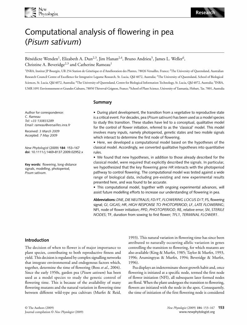
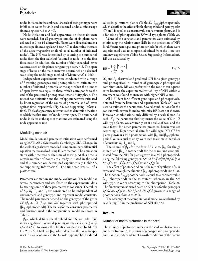
Fig. 1 Classical model for the regulation of flowering node in pea (Pisum sativum). (a) Schematic representation of the control of flowering in pea: a mobile flowering inhibitor (I) and mobile flowering stimulus (S) are integrated as a flowering signal (FS), which is equal to the ratio S/I. Flowering occurs when FS exceeds a certain threshold defined by the allele for LF. Signals are under genetic and photoperiod control (mobile signals are indicated with broken lines, and genes in italic). Arrowheads indicate promotion, and flat-ended lines represent repression. (b, c, d) Based on the classical model hypothesis, the computational model simulates the level of FS over time. Flowering is triggered when FS reaches the flowering threshold, which is defined by the LF allele (lf-a, lf, Lf, Lf-d; represented by horizontal lines). (c, d) Change in the level of FS as nodes are initiated at the apex in sn and gi mutants grown in a 24-h photoperiod (c) and in the wild-type (WT) grown under different photoperiods (d). WT has the genotype (SN GI hr). DNE, DIE NEUTRALIS; GI, GIGAS; HR, HIGH RESPONSE TO PHOTOPERIOD; LF, LATE FLOWERING; PPD, PHOTOPERIOD; SN, STERILE NODES.


Research156

Model description

General principles

The hypotheses on the regulation of NFI in pea, developed byMurfet and colleagues, described two signals and the genescontrolling the production of these signals (Murfet, 1989;Beveridge & Murfet, 1996; Weller et al., 1997). In this work,we propose what we believe to be the simplest way to modelthe classical hypotheses for the effect of genotype andphotoperiod on NFI in pea. The proposed equations quantifythe level of signals in different genotypes and photoperiods.Because the true nature of these signals have not yet beenelucidated, our modelling approach is not based on theirquantification or on the fine regulation of gene expressionand protein translation, such as that used in circadian clockmodelling (e.g., Locke et al., 2005). Rather, we have modelledthe hypothetical signal levels in the whole plant, based on thehypotheses. Although grafting studies have demonstrated thatthe signals are produced and perceived in different locations(leaves and apex, respectively), we assume here that signaltransport takes place at a rate sufficiently fast such that nosignificant delay occurs between production and perception.Accordingly, our modelling approach represents the plant as onefully integrated entity. The model can be used to determinethe NFI for different genotypes grown in photoperiodsranging from 8 to 24 h.

In pea, temperature affects flowering time via the rate ofleaf initiation and emergence, but does not affect the NFI(Truong & Duthion, 1993). As a consequence, in our model,time is expressed in plastochron units from the time of sowing.A plastochron is the physiological time interval separating theinitiation of two successive nodes. The number of nodesalready initiated in the embryo (within the seed) is describedas a model parameter.

The model simulates the concentration of the two mobilesignals controlling flowering in pea, the flowering inhibitor (I)and the flowering stimulus (S), over time. The two signalsinteract to regulate the level of a flowering signal (FS), whichincreases over time (Fig. 1b). A flowering threshold determinesthe minimum level of FS necessary to trigger flower initiation(Fig. 1b). The photoperiod and the genotypes of each of theflowering genes (SN, LF and HR) are defined by the user.Photoperiod affects signal levels (Fig. 1d) according to a functionthat is dependent on the genotype of the flowering genes(Fig. 1c). In many plant species, a juvenile photoperiod-insensitive phase has been identified (Collinson et al., 1992).That early flowering genotypes do not respond to changes inphotoperiod supports the hypothesis that a juvenile stageprobably exists in pea. Using grafting experiments, it has beenshown that the photoperiod is likely to be perceived by fullyexpanded leaves (Lang et al., 1977; Colasanti & Sundaresan,2000). Early versions of the model (data not shown) wereunable to predict the flowering behaviour of very early flower-

ing lines, such as lf-a plants, until this insensitivity period wasincorporated. As such, in the model, the pea plant is insensitiveto the photoperiod until the first leaf is open, which correspondsto node 3 (counting cotyledons as node 0 and scale leaves asnodes 1 and 2).

Hypotheses were formulated based on the literature andexperiments. They are reported in the results, listed in Table 1,and referred to as hypothesis ‘#’ throughout the text. Threesteps were then taken to create the computational model.Firstly, hypotheses were converted to equations, including oneordinary differential equation, describing the rates of changeof signal levels. Parameter values were then estimated usingoptimization methods. Finally, the sensitivity of the model tovariations in the constant and parameter values was determined.

Flowering stimulus

The ability of early day-neutral rootstocks to induce earlyflowering in late photoperiod-responsive scions providedevidence for a graft-transmissible floral stimulus in pea(Haupt, 1969; Murfet, 1971c). The gi mutant (Murfet, 1989)flowered later than the wild-type in all conditions tested, anddid not flower at all in some conditions (Beveridge & Murfet,1996). In reciprocal grafts between gi and the wild-type,flowering was promoted in gi shoots when a wild-type scionor rootstock was present (Beveridge & Murfet, 1996). Theseresults suggest that the gi mutation blocks the synthesis of aflowering stimulus. It is therefore hypothesized that theproduction of a mobile flowering stimulus is mediated byGI (Fig. 1a; Table 1; hypothesis 1). As gi plants do eventuallyflower in most conditions, the mutant allele might be leaky,producing some functional product (Beveridge & Murfet,1996) (Table 1; hypothesis 2).

In the computational model, the flowering stimulus (S) isconstant over time, and depends on the genotype at the GI locus:

S = KS × βGI Eqn 1; hypotheses 1, 2

(KS, quantity of stimulus S in GI plants; βGI, genotypeparameter, which is equal to unity in the GI wild-type with areduced value in gi mutant plants; see Table 2 for values ofparameters and constants; see Materials and Methods forparameter estimation).

Flowering inhibitor

Grafting experiments conducted with mutants have providedevidence that the SN, DNE and PPD genes might controlsteps in a biosynthetic pathway that leads to the productionof a flowering inhibitor (I) (Barber & Paton, 1952; Murfet,1971c; Murfet & Reid, 1973; King & Murfet, 1985; Taylor& Murfet, 1996) (Fig. 1; Table 1; hypothesis 3). For example,mutant sn rootstocks promote flowering in wild-type shoots,whereas wild-type rootstocks cause a small delay in flowering


Research 157

in sn scions compared with sn self-grafts. Grafting results fromplants of different ages grown in different photoperiods suggestthat the level of I decreases with age (Table 1; hypothesis4) and long-day photoperiods (Fig. 1; Table 1; hypothesis 5)(Murfet & Reid, 1973; Reid, 1979). Double-mutant analyseshave shown that the response to photoperiod in pea is

conferred by the joint presence of SN, DNE and PPD(Arumingtyas & Murfet, 1994) (Table 1; hypothesis 6).Mutation in any of the three genes produced a similar earlyflowering phenotype. Consequently, in this study, SN, DNEand PPD are considered together as a system that is writtenas ‘SN’.

Table 1 Hypotheses used to build the computational model based on the literature and new results

Hypothesis Source

Hypotheses based on previous studies1 GI constitutively promotes the production of a mobile floral stimulus Haupt (1969); Murfet (1971c);

Beveridge & Murfet (1996)2 The gi mutant is a leaky mutant, producing some functional product Beveridge & Murfet (1996)3 SN DNE PPD system controls the production of a mobile floral inhibitor;

the three-gene system is considered as one in the computational modelBarber & Paton (1952); Murfet (1971c); Murfet & Reid (1973); King & Murfet (1985); Taylor & Murfet (1996)

4 The inhibitor level decreases with age Murfet & Reid (1973); Reid (1979)5 The production of the inhibitor decreases with increasing day length (photoperiod) Murfet & Reid (1973); Reid (1979)6 SN, DNE and PPD genes are all required for the flowering response to the photoperiod Arumingtyas & Murfet (1994)7 HR acts by maintaining the inhibitor production over time Murfet (1973); Reid (1979)8 The flowering signal is the ratio of a flowering stimulus and a flowering inhibitor Murfet (1971a,c)9 Flower initiation occurs when the flowering signal (FS) reaches a flowering threshold Murfet (1971a,c)10 The flowering threshold is determined by the LF allele Murfet (1971a, 1989)11 The flowering threshold is constant over time Murfet (1989)

Hypotheses derived from this study12 The number of nodes already initiated in the seed is considered to be constant,

independent of genotype and photoperiod, and is equal to 6.4Table S2 (see Supporting Information)

13 The plant is day length insensitive until it has produced one true expanded leaf (node 3, counting the scales as nodes 1 and 2)

14 The number of nodes initiated at the apex when node 3 is fully open is considered to be constant and independent of genotype and photoperiod, and is equal to 9.9

Table S5 (see Supporting Information)

15 HR interacts with the photoperiod input on the inhibitor synthesis rate Fig. 2

Table 2 Values of constants and parameters used in the computational model

dt 0.1KS 2I0 3KR 0.05I∞ 0.2βGI

βLF

β(SN,HR)(photoperiod)

dt corresponds to the time step of the model; constants are KS, the quantity of stimulus S in GI wild-type (WT); I0 and I∞, the initial and steady-state levels of inhibitor I, respectively; and KR, the synthesis rate of inhibitor I set for WT at a 24-h photoperiod; βGI and βLF are genotype parameters for GI and LF genes, respectively; β(SN,HR)(photoperiod) is the photoperiod function which includes the genotype for SN and HR as parameters. GI, GIGAS; HR, HIGH RESPONSE TO PHOTOPERIOD; LF, LATE FLOWERING; SN, STERILE NODES.

10 43

in wild typein mutant

GIgi

-.

⎧⎨⎩

124 27 3

forfor

forfor

lf alf

LfLf d

-

-..

⎧

⎨⎪⎪

⎩⎪⎪

1 31 10

100 0469 0 046

.

( . .

in mutantif node

if nodephotoperiod

sn≤

>− + × )). .

in plantse in plantsphotoperiod

hrHr0 0222 0 1565×

⎧⎨⎩

⎧

⎨⎪⎪

⎩⎪⎪ ×


Research158

From grafting experiments, it was concluded that theHR gene prevented the decrease in I over time (Fig. 1, Table 1;hypothesis 7) (Murfet, 1973; Reid, 1979), hence delayingNFI in short-day photoperiods (Murfet, 1973).

According to hypothesis 4 (Table 1), the level of I decreaseswith time in a wild-type plant, from an initial level I0 to a steady-state level I∞, as a result of simultaneous processes of synthesisat a constant rate and degradation following first-order kinetics.This was modelled using an ordinary differential equation:

Eqn 2a; hypotheses 3, 4, 5

(r, rate of synthesis of I). According to hypotheses 3 and 5(Table 1), the degradation rate of I is implicitly incorporatedin the steady-state I∞, which corresponds to the ratio betweendegradation and synthesis. Accordingly, if I∞ is constant,variations in the synthesis rate r in the model result invariations in the implicit degradation rate. The synthesis rateof I depends on the SN genotype and varies with photoperiod:

r = KR × β(SN)(photoperiod) Eqn 3a; hypotheses 3, 5, 6

[KR, synthesis rate of I set for wild-type grown in a 24-hphotoperiod; β(SN)(photoperiod), photoperiod responsefunction (Table 1, hypothesis 5), which includes the genotypeof SN as a parameter (Table 1, hypothesis 6, see Materials andMethods for estimation of function)].

When r is constant, Eqn 2a has an analytical solution:

Eqn 2b

In addition to this analytical solution, Eqn 2a can be solvednumerically. Both solutions are equivalent in the cases analysedhere. However, to allow easy modification of the model infuture studies, including situations in which the photoperiod,and thus r, would change over time, Eqn 2a was solvednumerically in the simulations (see Modelling methods).

The HR gene has been suggested to affect the synthesis ofI and to be responsible for the high response to photoperiod.However, it is not known whether the effect on the synthesisof I is dependent on photoperiod or whether a simple changein the rate of synthesis of I may result in the high photoperiodresponse. These two alternative hypotheses are investigated inthis study.

Decision to flower

As suggested by Murfet (1971a,c), the flowering signal(FS) is defined as the ratio of the flowering stimulus S tothe flowering inhibitor I (Fig. 1; Table 1, hypothesis 8):

Eqn 4, hypothesis 8

Flowering is triggered when FS at the apex exceeds a certainthreshold (Table 1; hypothesis 9) (Murfet, 1971a,c). The LFallele is hypothesized to define this flowering threshold (Table 1,hypothesis 10) (Murfet, 1989). This threshold remainsconstant over time (Table 1, hypothesis 11) and is defined bythe model parameter βLF, which has a certain value for eachLF allele (Table 2). Thus, the transition to flowering occurswhen FS reaches the βLF threshold. When this occurs, thenext node to be initiated at the apex is floral, and therefore isthe model-predicted NFI.

Materials and Methods

A wide set of experimental data was necessary to allowparameter estimation for the model. Although numerous datacould be obtained from the literature for various genotypesand photoperiod conditions, previous work has not beencarried out with a wide range of genotypes under the samephotoperiods. In this work, in addition to a summary of theexperimental data from the literature, we propose a first realcomparison of the flowering behaviours for different genotypesgrown under three photoperiods. In order to complete thisphysiological study, we carried out an analysis on the numberof preformed nodes in the embryo for these same variousgenotypes. Combined, the data obtained from both the literatureand new experiments presented here, were used to make andtest the computational model.

Biological methods

Plant material Plant material consisted of three wild-typelines (Torsdag, Borek and WL1771) of pea (Pisum sativum L.)and flowering mutants for the genes LF, SN, DNE and HRobtained in these backgrounds. Mutants sn-4 (Hecht et al.,2007) and lf-a were obtained in a dwarf Torsdag backgroundNGB5839, a derivative of Torsdag carrying the le-3 mutation(Lester et al., 1999). Mutant lines WL1769 and WL1770were obtained by fast-neutron treatment of the WL1771line (Taylor & Murfet, 1993). The genotype of each line isincluded in Table S1 (see Supporting Information).

Growth conditions For all glasshouse experiments, plants weregrown in sand, under natural light extended to a photoperiodof 11, 16 and 20 h by sodium vapour lamps. Nutrientsolution was applied to the plants twice a week during theearly vegetative phase and then three times a week. The meanglasshouse temperatures were 18.2°C, 18.7°C and 21.7°C,respectively.

Plant measurement To test the effect of genotype and growthconditions of the parent on the number of preformed nodesin the seed, and to calculate the average number of nodesinitiated before sowing, seeds of several genotypes fromdifferent harvests were dissected. To count the number of

d

d

I

I

I

tr= −

⎛

⎝⎜⎜

⎞

⎠⎟⎟

∞1

I I I e II( ) ( )tr

t= − +∞

−

∞∞

0

FSS

I=


Research 159

nodes initiated in the embryo, 10 seeds of each genotype wereimbibed in water for 24 h and dissected under a microscope(increasing size × 8 to × 40).

Node initiation and leaf appearance on the main stemwere recorded. For all genotypes, samples of six plants werecollected at 7- to 14-d intervals. Plants were dissected under amicroscope (increasing size × 8 to × 40) to determine the stateof the apex (vegetative or floral, total number of initiatednodes). The NFI was determined by counting the number ofnodes from the first scale leaf (counted as node 1) to the firstfloral node. In addition, the number of fully expanded leaveswas measured on six plants per genotype every 4 d. The openstage of leaves on the main stem was determined on a decimalscale using the nodal stage method of Maurer et al. (1966).

Independent experiments were conducted with a rangeof flowering genotypes and photoperiods to estimate thenumber of initiated primordia at the apex when the numberof open leaves was equal to three, which corresponds to theend of the presumed photoperiod insensitivity phase. Therates of node initiation and the leaf appearance were estimatedby linear regression of the counts of primordia and of leavesagainst time, respectively (Fig. S1, see Supporting Informa-tion). The leaf appearance rate was used to determine the timeat which the first true leaf (node 3) was open. The number ofnodes initiated at the apex at that time was estimated using thenode appearance rate.

Modelling methods

Model simulation and parameter estimation were performedusing MATLAB 7 (Mathworks, Cambridge, UK). Changes inthe levels of signals were modelled using an ordinary differentialequation that was solved using Euler’s method. The simulationstarts with time zero as the time of sowing. At this time, acertain number of nodes are already initiated in the seedand this number was determined experimentally (Table S2,see Supporting Information). The time step was 0.1 of aplastochron.

Parameter estimation and model evaluation The model hasseveral parameters and was fitted to the experimental databy treating some of these parameters as constants. The valuesof KS, KR, I∞ and I0 are considered to be independent ofenvironment and genotype, and represent model constants.The model parameters depend on the genotype of the genesLF (βLF), GI (βGI) and SN together with photoperiod[β(SN)(photoperiod)]. The values for the constants, parametersand functions used in the computational model are shown inTable 2.

βLF, which defines the threshold for FS, can take fourincreasing discrete values depending on the LF alleles (lf-a, lf,Lf and Lf-d ), following the classification described by Murfet(1975, 1977) (Table 2). βGI, which describes the GI genotype,is set to a value of unity in the GI wild-type and has a reduced

value in gi mutant plants (Table 2). β(SN)(photoperiod),which describes the effect of both photoperiod and genotype forSN on I, is equal to a constant value in sn mutant plants, and isa function of photoperiod in SN wild-type plants (Table 2).

Values of the constants and parameters were estimated byminimizing the relative error (RE) in the prediction of NFIfor different genotypes and photoperiods for which there wereexperimental data to compare, obtained from the literatureand new experiments (Table S3, see Supporting Information).RE was calculated by:

Eqn 5

(Oi and Pi, observed and predicted NFI for a given genotypeand photoperiod; n, number of genotype × photoperiodcombinations). RE was preferred to the root-mean-squareerror because the experimental variability of NFI within atreatment was found to increase with higher NFI values.

All NFI data for different genotypes and photoperiods,obtained from the literature and experiments (Table S3), wereused to estimate the parameters. Several combinations for theconstant values were found to minimize RE (data not shown).However, combinations only differed by a scale factor. Assuch, KS, the parameter that represents the value of S in GIwild-type plants, was arbitrarily set at a value of two, and thescale factor for other parameters presented herein was setaccordingly. Experimental data for wild-type (SN GI hr)plants grown in a 24-h photoperiod, with βGI and β(SN)(photo-period) values equal to unity, were used to estimate the valuesof constants KR, I∞ and I0.

The values of βLF for the four LF alleles, βGI for the gimutant and β(sn)(photoperiod) for the sn mutant were esti-mated from the NFI for plants grown in a 24-h photoperiod,using the following genotypes: SN GI hr lf-a/lf /Lf /Lf-d, lf snhr, Lf sn hr, Lf dne hr, Lf ppd hr and Lf gi hr.

The effect of photoperiod on r, the rate of synthesis of I, isexpressed through the function β(SN)(photoperiod) (Eqn 3a).The function β(SN)(photoperiod) is equal to a constant valueβ(sn)(photoperiod) in the sn mutant, whereas, in the SNwild-type, it varies according to the photoperiod (Table 2).The function was estimated based on NFI data for the genotypesLf GI hr, Lf gi hr, Hr Lf and Hr Lf-d grown in a range ofphotoperiods, from 8 to 24 h.

The accuracy of the computational model was evaluated bycalculating RE in the prediction of NFI (Eqn 5).

Results

Number of nodes preformed in the seed

The number of preformed nodes in the seed was between sixand seven (mean 6.4) for a range of genotypes and photoperiods,and was thus independent of growth conditions of the parent

RE i i

i

=−

=∑1

1n

O P

Oi

n


Research160

plant (Table S2). The number of preformed nodes in the seedis considered to be a constant in the model, and is accordinglyset to 6.4. As a result, the first step of the model correspondsto a physiological age of 6.5 plastochrons (Table 1, hypothesis 12).

Pattern of NFI variations with photoperiod

Data from previous studies (Table S3) and our experiments(Table S4, see Supporting Information) show that earlyflowering lines (lf-a, lf and sn) flower at a very low node, anddo not respond to photoperiod. By contrast, late varieties (Lf,Lf-d, gi) show a response to photoperiod, flowering later whenthe day length is shorter. Late high-response flowering linesassociated with the Hr genotype respond dramatically tophotoperiod, flowering later than hr plants in all conditions,and particularly in short-day photoperiods. This high responseis inhibited by early alleles of LF (lf-a and l f ).

Photoperiod insensitivity phase

The earliest flowering genotypes show a low NFI independentof photoperiod. Despite being very low, this NFI is still higherthan the number of preformed nodes. This suggests that, likeother species (Collinson et al., 1992), pea plants experience ajuvenile phase in which they are insensitive to day length. Wehypothesized that this period extends until one true leaf (node3, counting the scale leaves as nodes 1 and 2) is fully expanded(Table 1; hypothesis 13). Estimations indicated that anaverage of 9.9 ± 0.2 nodes are initiated at the apex when thefirst true leaf opens (Table S5, see Supporting Information).Analysis of variance (ANOVA) indicated that photoperiodhad a significant effect on this value (at the 5% level), but withno obvious trend; insufficient data were available to design aregression for the effect. As a result, we used 9.9 as a constantin the model to describe the number of nodes initiated at theapex when the first true leaf opens. Accordingly, in the model,the plant is considered to be insensitive to photoperiod untilnode 10 is initiated (Table 1; hypothesis 14). This means that,in the computational model, the photoperiod affects the

synthesis of I only after node 10 is initiated. Consequently, abasal synthesis rate for I, equal to KR, is set between sowingand node 10, which corresponds to the native synthesis rate.As the photoperiod does not affect S, FS displays the sameevolution over time between nodes 6 and 10 for differentphotoperiods (Fig. 1d). For very early flowering genotypes(for example, lf-a), FS reaches the flowering threshold beforethe photoperiod affects FS and, consequently, NFI is constantwithin the range of photoperiods.

Modelling photoperiod and HR effect

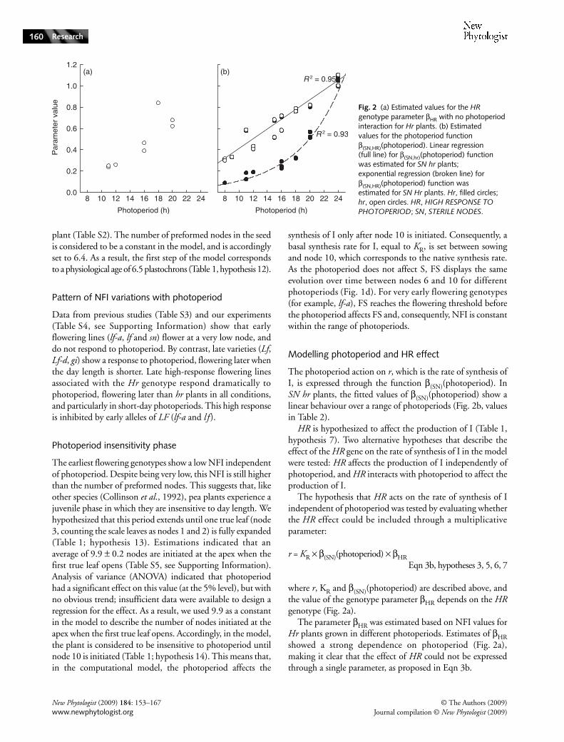
The photoperiod action on r, which is the rate of synthesis ofI, is expressed through the function β(SN)(photoperiod). InSN hr plants, the fitted values of β(SN)(photoperiod) show alinear behaviour over a range of photoperiods (Fig. 2b, valuesin Table 2).

HR is hypothesized to affect the production of I (Table 1,hypothesis 7). Two alternative hypotheses that describe theeffect of the HR gene on the rate of synthesis of I in the modelwere tested: HR affects the production of I independently ofphotoperiod, and HR interacts with photoperiod to affect theproduction of I.

The hypothesis that HR acts on the rate of synthesis of Iindependent of photoperiod was tested by evaluating whetherthe HR effect could be included through a multiplicativeparameter:

r = KR × β(SN)(photoperiod) × βHREqn 3b, hypotheses 3, 5, 6, 7

where r, KR and β(SN)(photoperiod) are described above, andthe value of the genotype parameter βHR depends on the HRgenotype (Fig. 2a).

The parameter βHR was estimated based on NFI values forHr plants grown in different photoperiods. Estimates of βHRshowed a strong dependence on photoperiod (Fig. 2a),making it clear that the effect of HR could not be expressedthrough a single parameter, as proposed in Eqn 3b.

Fig. 2 (a) Estimated values for the HR genotype parameter βHR with no photoperiod interaction for Hr plants. (b) Estimated values for the photoperiod function β(SN,HR)(photoperiod). Linear regression (full line) for β(SN,hr)(photoperiod) function was estimated for SN hr plants; exponential regression (broken line) for β(SN,HR)(photoperiod) function was estimated for SN Hr plants. Hr, filled circles; hr, open circles. HR, HIGH RESPONSE TO PHOTOPERIOD; SN, STERILE NODES.


Research 161

As a single parameter value could not present an accurateestimation of the HR effect (Fig. 2a), we considered the otherhypothesis that the photoperiod function should includeHR as a parameter. For hr plants, the photoperiod effect iscomputed through a linear photoperiod function β(SN)(photo-period) (Fig. 2b). The photoperiod function β(SN,HR)(photo-period) takes into account that the genotype for HR affectsthe photoperiod effect on the synthesis rate of I (Table 1,hypotheses 6 and 7) and, in particular, HR interacts with thephotoperiod input (Table 1, hypothesis 15):

r = KR × β(SN, HR)(photoperiod) × βHREqn 3c, hypotheses 3, 5, 6, 7, 15

[β(SN,HR)(photoperiod), photoperiod function which includesthe genotypes for SN and HR as parameters].

For short-day photoperiods, the value and rate of change ofβ(SN,Hr)(photoperiod) for Hr genotypes are lower than for hrgenotypes (Fig. 2b). However, for Hr genotypes under longerphotoperiods, β(SN,Hr)(photoperiod) increases sharply.

We described this behaviour by considering an exponentialform for β(SN,HR)(photoperiod) (Fig. 2b, values in Table 2).Other functions could have been used: for instance, the dataare also compatible with a bi-linear behaviour. However, usingsuch a function would require the fitting of three parameters.Our choice reflects the fact that the exponential functioncould fit the experimental data with only two parameters,which is justified given the limited amount of available data.Accordingly, the values of β(SN,HR)(photoperiod) that bestfitted the experimental NFI data increased exponentially withincreasing photoperiod (Fig. 2b, values in Table 2).

The model predictions capture the biological data

As shown in Figs 3 and 4, the model predictions accuratelycapture the biological data with an RE between the modeloutput and the experimental data of 9%. For hr plants, the REis only 8%. The model is less accurate for Hr predictions, as

Fig. 3 The node of flowering initiation (NFI) predicted by the computational model fits the experimental data for hr (circles) and Hr (squares) plants. The data here were used to estimate the parameter values. Symbols in parentheses were not used for the optimization of parameters. HR, HIGH RESPONSE TO PHOTOPERIOD.

Fig. 4 Experimental and predicted data from the computational model for the node of flowering initiation (NFI) for different genotypes in different photoperiods [expressed in daily hours (h) of light]. Symbols represent the experimental data used to set the parameters and the lines represent the model predictions. Symbols in parentheses were not used for the optimization of parameters. WT has the genotype (SN GI hr). GI, GIGAS; HR, HIGH RESPONSE TO PHOTOPERIOD; LF, LATE FLOWERING; SN, STERILE NODES; WT, wild-type.


Research162

the RE is 14%. Variations for experimental data for eachgenotype and photoperiod condition can be up to 18% (Lfplants under an 8-h photoperiod). Consequently, with an REof 9%, we consider the model predictions to be within anadequate range of error for the photoperiod conditionsstudied here.

Consistent with the experimental data for hr sn and Hrsn plants, predictions for sn mutants show no response to photo-period. In addition, NFI predictions for gi mutants display ahigh response to photoperiod in an Lf background (Fig. 4),which accurately reproduces the experimental results. Modelpredictions also show that early lines corresponding to earlyLF alleles (lf-a and lf ) on hr or Hr backgrounds do not respondto photoperiod, whereas late flowering genotypes (Lf, Lf-d)display a high response to photoperiod (Fig. 4). Theseflowering behaviours are observed in the experimental data.

Predictions for nonexisting allele combinations

No experimental results could be found in the literature forgenotypes sn Lf-d, sn gi double mutants, gi lf-a /lf /Lf-d and giHr. Model outputs predict that sn gi double mutants arerelatively late in comparison with sn GI, but do not respondto photoperiod (Fig. 4). In addition, for all LF alleles, sn Hr andsn hr plants are predicted to not respond to photoperiod. giplants are predicted to initiate flowering very late, particularlyin the Hr background where the photoperiod response isenhanced (Fig. 4).

Sensitivity of FS prediction to the synthesis and steady state of I

The change in I over time depends on the synthesis rate r andthe steady-state I∞. The range of flowering behaviours couldbe described by considering I∞ as a constant. The modelsensitivity to I∞ was tested by varying the I∞ value in wild-typeplants in 24-h photoperiod conditions. As shown in Fig. S2a(see Supporting Information), the value for the constant I∞,with the synthesis rate r kept constant, has a strong impacton FS. FS corresponds to the ratio of S to I (Eqn 4), andconsequently the steady-state FS∞ also depends on I∞:

Eqn 6

For low I∞ values (e.g. 0.05, Fig. S2a), the steady state FS∞ isstrongly increased. This results in a reduction in the timetaken to reach this steady state. As expected, the model is highlysensitive to variations in I∞, particularly for I∞ values that aremuch lower than the initial condition I0.

The constant KR corresponds to the basal synthesis rate ofI, r, set for the wild-type (SN, hr) in a 24-h photoperiod.When fitting the model to our experimental data, we foundthat r can vary with genotype and photoperiod, within the

range 0.004–0.065. Over the considered range and, in particu-lar, when KR is close to zero, the values of KR strongly impacton the rate at which FS reaches a steady-state value (FS∞;Fig. S2b). Flower initiation is triggered when FS reaches theflowering threshold determined by LF. As shown in Fig. S2b,interactions between the rate at which FS reaches FS∞ andthese thresholds are highly correlated with NFI. In particular,for low KR values (0.004–0.007, Fig. S2b), FS increases veryslowly and never reaches Lf or Lf-d thresholds, which resultsin a vegetative state at the end of the simulation (80 nodesinitiated at the apex, Fig. S2b).

To test how the model output would respond to differentr values, the number of steps needed for FS to reach 95% ofthe steady-state value was calculated for different values of r(Fig. S2c). Consistent with preliminary results (Fig. S2b), thedata indicate that FS predictions are highly sensitive to valuesof r below 0.1. These results are consistent with the differencesobserved between β(SN,HR)(photoperiod) for Hr and hrgenotypes. Values for β(SN,HR)(photoperiod) in Hr genotypesunder short-day photoperiods are very low and display a lowslope, which results in a very low value of r (equivalent to KRvalues of 0.004–0.013; Fig. S2b) and high values of NFI.

Sensitivity of NFI to βLF

The sensitivity of the model predictions for NFI to thethreshold parameter βLF was analysed for different genotypesand photoperiods (Fig. S2d). All response curves convergetowards the number of preformed nodes already initiated inthe seed when βLF is close to zero (Fig. S2d). This confirmsthat, when no threshold is present, flower initiation is triggeredas soon as the plant germinates.

As shown in Fig. S2d, gi plants are more sensitive tochanges in βLF than GI plants (Fig. S2d). The model is highlysensitive to βLF variation when βLF is close to FS∞ in value,suggesting a strong interaction. Consequently, the modelsensitivity to variations in βLF depends on S and I∞. Comparisonwith experimental data indicated that the model-predictedNFI for late flowering plants on a mutant gi background wasvery sensitive to βLF (Fig. S2d). By contrast, the model-predictedNFI for plants on a wild-type GI background was not sensitiveto variations in βLF (Fig. S2d). These results suggest that themodel is strongly sensitive to parameter variations for lateflowering phenotypes.

Discussion

Flowering has been extensively studied in pea through theidentification and physiological analysis of mutants andwild-type lines showing variation in flowering time. Thesestudies have led to the development of hypotheses about thegenetic and physiological regulation of flowering in pea. Theresulting flowering model, herein termed the ‘classical’ model,integrates the response to photoperiod and two mobile signals

FSS

I∞∞

=


Research 163

(a flowering stimulus and a flowering inhibitor), and athreshold that the flowering signal (FS), defined as the ratio ofa stimulus (S) to an inhibitor (I), must reach for flowering tooccur. To test whether the classical model for flowering inpea was accurate and able to account for the wide range ofexperimental data, in addition to the prediction of new data,we developed a computational model based on these hypothesesand tested it against data collected from the literature andfrom experimental results presented here. As it currently allowsthe prediction of NFI for various genotypes and photoperiods,in the future, the model could be integrated into agronomicmodels to improve their capacity to predict yields in responseto environmental conditions. In addition, improving thecurrent model with new molecular data could provide a usefultool to test new hypotheses on the underlying mechanismscontrolling flowering in pea. The molecular nature of thegenes described in the model are just starting to be discovered(e.g., Foucher et al., 2003; Hecht et al., 2007; Weller, 2007).Future gene discoveries will enable better comparisons withother model species, such as Arabidopsis, and will lead tonew experimental data and the development of newhypotheses to improve the model and our understanding offlowering control.

A simple formalism is sufficient to capture experimental data

The proposed model is based on our simplest expression ofthe classical hypothesis for flowering regulation in pea. Inparticular, the model includes a number of parameters andwas fitted to the range of experimental data. To do so, someparameters were set arbitrarily, whereas others were setaccordingly to fit the experimental data. This represented themost straightforward method of determining parameters.However, in the future, further experiments to provide moreNFI data could allow a more accurate fitting of parameters.Sensitivity analyses suggested that βLF, I∞ and KR had a strongimpact on the model predictions of NFI. For instance,although NFI predictions were shown to be robust within acertain range of βLF values, the model was highly sensitive tovariations when values for βLF were close to the steady statefor FS. Consequently, high variations observed for NFIpredictions in conditions in which the steady state for FS wasclose to βLF might result from the model construction ratherthan from the actual biological mechanism. This, in additionto testing the β(SN,HR)(photoperiod) functions, will requiremore biological data to improve the accuracy of parametervalues.

Although the computational model will need to be testedagainst new experimental data, the predictions of NFI ofexisting genotype and photoperiod data are very satisfactory.We showed that a simple linear function could accuratelypredict that late flowering lines (hr Lf-d and hr Lf gi geno-types) display an enhanced response to photoperiod. Model

predictions for sn, dne and ppd mutants are consistent withthe experimental results (Fig. 4), supporting the concept thatthe photoperiod and flowering inhibitor (I) pathway interact(Fig. 1a). Predictions for Hr genotypes accurately captureexperimental data (Fig. 4), suggesting that HR indeed hasa role in the photoperiod response. However, because thephotoperiod still affects the flowering node in hr mutants, inboth the model and experimentally, it could be hypothesizedthat HR somehow enhances the effect of photoperiod, but isnot necessary for a photoperiod response. New moleculardata, in particular molecular characterization of the pea genesinvolved, should help us to further develop an understandingof the photoperiod pathway and how HR acts on this pathwayand hence on flowering regulation.

Because the true nature of the signals involved in theregulation of flowering have not been identified, their quanti-fication and modes of action were hypothesized. In particular,we hypothesized that the level of I would change over time, assuggested by Murfet & Reid (1973). Changes were a result ofthe simulated level of I displaying a sigmoid evolution overtime, tending to a steady state I∞. In addition, the stimuluslevel was considered to be constant over time and to dependonly on the genotype for GI. Based on this construction, thelevel of FS changes over time towards a steady state, FS∞. Inthe case in which FS∞ is lower than the flowering threshold,the model predicts that certain genotypes should remainvegetative (for example, gi Lf-d; data not shown). This issupported by observations that some genotypes do not flowerin some conditions (Beveridge & Murfet, 1996).

Observations that early flowering genotypes do notrespond to photoperiod led to the hypothesis that these linestransition to flowering during a developmental stage at whichthe plant is not sensitive to photoperiod. In the computa-tional model, we chose to define the photoperiod-insensitivephase as the period before the first true leaf at node 3 is open.However, estimations of the number of initiated primordiaat the apex at this time point show that the number of nodesinitiated at the apex, before the first leaf is open, displays astatistically significant response to photoperiod, but with noobvious trend. These results indicate that the photoperiodinsensitivity phase might be shorter than expected in someconditions. Experiments in which plants are transferred fromlong-day to short-day photoperiods, and further studies onphytochrome light receptors, will be necessary to determinethe duration of this photoperiod-insensitive phase.

Because most of the existing experimental data werereported as NFI (for example, Murfet, 1971c, 1973; Alcaldeet al., 2000), the computational model used 0.1 plastochronas the unit of time (where a plastochron is the time taken toinitiate a new node). This is based on the assumption that thelevel of the signals could be expressed as a function of thenumber of nodes. The number of nodes is a function ofthermal time rather than the calendar age of the plant (Collins& Wilson, 1974). Using the nodes as a time interval assumes


Research164

that temperature similarly influences the synthesis rate of Iand the rate of node initiation. However, the hypothesis thatNFI is independent of temperature arose from observationsperformed under field conditions (Truong & Duthion, 1993);this should be further evaluated by experiments in controlledconditions with a wide range of temperature × photoperiodcombinations. In particular, if the temperature is shown todifferentially affect the rate of node initiation and the synthesisrate of I, the model could be enhanced by incorporatingtemperature into the ordinary differential equation for I,together with an equation describing the temperature influenceon the node initiation rate.

The computational model predicts NFI for nonexisting allele combinations

In addition to accurately predicting NFI for known genotypes,we used the computational model to predict NFI for allelecombinations that have not been tested previously. For example,sn mutations combined with late alleles, including Lf-dand Hr, should not respond to photoperiod, but shouldexhibit a later flowering phenotype compared with single snmutants (Fig. 4). As SN is hypothesized to be necessary forphotoperiod response, inhibition of photoperiod response insn double mutants is expected. In a wild-type SN background,early LF genotypes (lf-a, l f ) do not respond to photoperiod,whereas late genotypes are characterized by a high photoperiodresponse (Fig. 4). Accordingly, experimental results for snmutants indicate that the absence of photoperiod responsecould be linked exclusively to their early phenotype, instead ofan effective inhibition of photoperiod response. Consequently,further experimental results for sn mutants associated withlate alleles will be necessary to test whether the modelpredictions capture the role for the SN gene product. Inaddition, future studies to ascertain NFI for these and othernonexisting allele combinations will allow the testing ofwhether the model predictions are consistent with experimentaldata.

Applications of the current model

For agronomic purposes, the manipulation of the floweringtime is essential to develop improved pea cultivars. Witha better understanding and prediction of flowering time, new‘virtual’ pea genotypes could be constructed and their floweringphenotypes predicted under different environmental conditions(Lejeune-Hénaut et al., 1999, 2008). The development ofwinter pea cultivars is necessary to improve pea crop pro-ductivity (Lejeune-Hénaut et al., 2008). For winter pea crops,the manipulation of flowering regulatory genes appears to bea promising way to control key developmental stages, such asthe dates of floral initiation and flowering. An ideal winter peashould initiate its flower primordia sufficiently late to avoidwinter frosts, but flower sufficiently early to escape drought

and heat stresses in late spring. The current strategy is tocombine the dominant HR allele, which confers highresponse to short-day photoperiods, with an appropriate alleleof LF. A good combination of alleles should allow an idealflowering time in the ideal winter pea candidates.

The computational model presented here allowed theprediction of NFI for different allele combinations for HRand LF, which are essential components of the winter peabreeding strategy. By combining our computational modelwith the calculation of leaf initiation and appearance inthermal time, such as that introduced by Truong & Duthion(1993), the prediction of NFI could be integrated into a cropmodel to quantitatively predict the time of flower initiation.This could be performed for virtual candidate genotypes undera range of different climates, allowing breeders to choose idealallele combinations that give their desired flowering time andenvironmental responses.

However, for agronomic purposes, it is essential to alsoconsider flower development from initiation to opening,as fully developed flowers are key factors for yield. Therefore,it will be necessary to study, and later include in the compu-tational model, floral abortion and the time that flowerstake to develop. This will allow the accurate prediction of theflowering node and time under different photoperiod condi-tions. Currently, the computational model can be simulatedfor constant photoperiods; new biological and modellingexperiments are needed to test whether the model allows theaccurate prediction of the flowering node under changingphotoperiods, similar to field conditions. It may be necessaryto alter the model to integrate the response to natural changesin photoperiod.

Perspectives for improving the flowering model

New hypotheses, derived from emerging molecular data, shouldallow more accurate modelling of flowering regulation in pea.This will allow us to explicitly describe underlying mechanismsand to integrate molecular, genetic and physiological data.Molecular analyses of flowering in pea have been, and willcontinue to be, accelerated by the extensive work in Arabidopsis,together with the development of sequence databases for modellegumes and the well-documented synteny between pea andMedicago (Zhu et al., 2005; Aubert et al., 2006).

Currently, the best option to improve our understanding offlowering control in pea is to compare new results in pea withwhat is well known in other model species. Mechanisms thatcontrol the timing of flower initiation have been extensivelystudied in Arabidopsis. The isolation of new photoperiodresponse mutants and Arabidopsis photoperiod pathway genehomologues in pea suggests that the regulation of flowering inpea is very similar to that in Arabidopsis (Hecht et al., 2005, 2007).Notably, the LF locus, which was the first of the classicalpea flowering loci to be identified at the molecular level,was shown to be homologous to the Arabidopsis flowering


Research 165

inhibitor gene TERMINAL FLOWER1 (TFL1) (Foucheret al., 2003). In the classical model for flowering control in pea,the flowering threshold is determined by the different allelesof LF. Recent discoveries in Arabidopsis suggest a molecularmechanism for this threshold. TFL1 is a repressor of floweringand is homologous to FLOWERING LOCUS T (FT), a keytarget and integrator of several flowering pathways, includingphotoperiod, vernalization and gibberellins. FT and TFL1proteins are similar in structure, except in a few regions (Hanzawaet al., 2005). FT and TFL1 do not interact with each other, butdo interact antagonistically with the protein FLOWERINGLOCUS D (FD) (Abe et al., 2005; Wigge et al., 2005; Ahn et al.,2006). When interacting with TFL1, FD inhibits flowering,whereas its interaction with FT activates flowering (Wiggeet al., 2005). Antagonism between FT and TFL1 implies that,the higher the level of TFL1 at the apex, the higher the levelof FT that is needed to overcome the TFL1/FD inhibition totrigger flowering initiation. Accordingly, the level of TFL1 atthe apex represents a flowering threshold for the floweringsignal (Ahn et al., 2006). This model for interaction of FDwith FT and TFL1 led to the hypothesis that the abundanceof TFL1 can be seen as a threshold for flowering initiation. Asimilar mechanism may explain the role of LF in determininga threshold level for flowering in pea. Further investigationwill allow for a more accurate modelling of this LF effect.

The pea GI gene was found to colocalize in the region ofan FT cluster. This supports the hypothesized role of GI as aflowering promoter (Hecht et al., 2005). Molecular charac-terization of GI will allow the quantification of its productduring development, and testing of the model hypothesis thatthe level of the flowering stimulus is constant over time in pea.

The photoperiod response in pea involves rhythmicregulation by the circadian clock via mechanisms similarto those in rice and Arabidopsis (Hecht et al., 2007; Kobayashi& Weigel, 2007; Tamaki et al., 2007; Weller, 2007). This was

not included in our computational model because the moleculardata in pea are currently not sufficient to develop such acomputational model. Future studies should incorporate suchmechanisms when sufficient data are available.

Future computational models of the regulation of floweringin pea might consider whether the circadian clock affectsthe flowering signal as it affects FT in Arabidopsis. In sucha model, the production of the flowering signal would bereduced in unfavourable day length conditions by a mech-anism controlled by the circadian clock (Fig. 5). These newhypotheses will require new equations to describe the regulationof the flowering signal by photoperiod. This should be inte-grated into the model in the future when sufficient moleculardata are available to build such a model. In such a model, theflowering signal would accumulate over time, independent ofthe node appearance rate. When it reached a flowering thresholddetermined by the LF allele, equivalent to the classical modelthreshold, flower initiation would be triggered. Furthermolecular experiments will be necessary to identify and quantifythe flowering signal, together with its regulation by the circadianclock. The ongoing identification of pea circadian clock genes(Hecht et al., 2007) and their expression levels under differentphotoperiod conditions should lead to a better understandingof the control of photoperiod response by the circadian clock.

In this study, the ‘classical’ hypothesis was incorporatedinto a quantitative model that improved our ability to accuratelytest hypotheses against observations. We found that ourhypotheses could accurately explain NFI data for manydifferent genotypes grown in different photoperiods. As afirst modelling attempt, this work has opened up a numberof avenues for modelling genetic control of developmentalprocesses in pea.

Acknowledgements

This work was supported by INRA (B.W.). The authors thankJean-Paul Pillot for technical assistance and the two anony-mous reviewers for helpful comments.

References

Abe M, Kobayashi Y, Yamamoto S, Daimon Y, Yamaguchi A, Ikeda Y, Ichinoki H, Notaguchi M, Goto K, Araki T. 2005. FD, a bZIP proteinmediating signals from the floral pathway integrator FT at the shoot apex. Science 309: 1052–1056.

Ahn JH, Miller D, Winter VJ, Banfield MJ, Lee JH, Yoo SY, Henz SR, Brady RL, Weigel D. 2006. A divergent external loop confers antagonistic activity on floral regulators FT and TFL1. The EMBO Journal 25: 605–614.

Alcalde J, Wheeler T, Summerfield R. 1999a. Flowering genes and the photothermal flowering responses of pea (Pisum sativum): a re-analysis. Australian Journal of Plant Physiology 26: 379–386.

Alcalde J, Wheeler T, Summerfield R, Norero A. 1999b. Quantitative effects of the genes LF, SN, E, and HR on time to flowering in pea (Pisum sativum L.). Journal of Experimental Botany 50: 1691–1700.

Fig. 5 New conceptual model for the regulation of flowering in pea (Pisum sativum). The synthesis of a putative mobile flowering signal (FS) is under genetic and photoperiodic control via the circadian clock. Flowering is triggered when FS exceeds a certain threshold defined by the different alleles of LF. Mobile signals are shown as broken lines, and genes are given in italic. Arrowheads indicate a promotion, and flat-ended lines represent repression. DNE, DIE NEUTRALIS; GI, GIGAS; HR, HIGH RESPONSE TO PHOTOPERIOD; LF, LATE FLOWERING; PPD, PHOTOPERIOD; SN, STERILE NODES.


Research166

Alcalde JA, Wheeler TR, Summerfield RJ. 2000. Genetic characterization of flowering of diverse cultivars of pea. Agronomy Journal 92: 772–779.

Arumingtyas EL, Murfet I. 1994. Flowering in Pisum: a further gene controlling response to photoperiod. Journal of Heredity 85: 12–17.

Aubert G, Morin J, Jacquin F, Loridon K, Quillet MC, Petit A, Rameau C, Lejeune-Henaut I, Huguet T, Burstin J. 2006. Functional mapping in pea, as an aid to the candidate gene selection and for investigating synteny with the model legume Medicago truncatula. Theoretical and Applied Genetics 112: 1024–1041.

Barber HN, Paton DM. 1952. A gene controlled flowering inhibitor in Pisum. Nature 169: 592.

Bayliss WM. 1902. On the local reactions of the arterial wall to changes in internal pressure. Journal of Physiology 28: 220–231.

Berry GJ, Aitken Y. 1979. Effect of photoperiod and temperature on flowering in pea (Pisum sativum L.). Australian Journal of Plant Physiology 6: 573–587.

Beveridge CA, Murfet IC. 1996. The gigas mutant in pea is deficient in the floral stimulus. Physiologia Plantarum 96: 637–645.

Boss PK, Bastow RM, Mylne JS, Dean C. 2004. Multiple pathways in the decision to flower: enabling, promoting, and resetting. Plant Cell 16: S18–S31.

Chaos Á, Aldana M, Espinosa-Soto C, de León BGP, Alvarez-Buylla ER. 2006. From genes to flower patterns and evolution: dynamic models of gene regulatory networks. Journal of Plant Growth Regulation 25: 278–289.

Colasanti J, Sundaresan V. 2000. ‘Florigen’ enters the molecular age: long-distance signals that cause plants to flower. Trends in Biochemical Sciences 25: 236–240.

Collins WJ, Wilson JH. 1974. Node of flowering as an index of plant development. Annals of Botany 38: 175–180.

Collinson ST, Ellis RH, Summerfield S, Roberts EH. 1992. Durations of the photoperiod-sensitive and photoperiod-insensitive phases of development to flowering in four cultivars of rice (Oryza sativa L.). Annals of Botany 70: 339–346.

Espinosa-Soto C, Padilla-Longoria P, Alvarez-Buylla ER. 2004. A gene regulatory network model for cell-fate determination during Arabidopsis thaliana flower development that is robust and recovers experimental gene expression profiles. Plant Cell 16: 2923–2939.

Foucher F, Morin J, Courtiade J, Cadioux S, Ellis N, Banfield MJ, Rameau C. 2003. DETERMINATE and LATE FLOWERING are two TERMINAL FLOWER1/CENTRORADIALIS homologs that control two distinct phases of flowering initiation and development in pea. Plant Cell 15: 2742–2754.

Hanzawa Y, Money T, Bradley D. 2005. A single amino acid converts a repressor to an activator of flowering. Proceedings of the National Academy of Sciences, USA 102: 7748–7753.

Haupt W. 1969. Pisum sativum L. In: Evans LT, ed. The induction of flowering. Melbourne, Australia: Macmillan, 393–408.

Hecht V, Foucher F, Ferrandiz C, Macknight R, Navarro C, Morin J, Vardy ME, Ellis N, Beltran JP, Rameau C et al. 2005. Conservation of Arabidopsis flowering genes in model legumes. Plant Physiology 137: 1420–1434.

Hecht V, Knowles CL, Vander Schoor JK, Liew LC, Jones SE, Lambert MJ, Weller JL. 2007. Pea LATE BLOOMER1 is a GIGANTEA ortholog with roles in photoperiodic flowering, deetiolation, and transcriptional regulation of circadian clock gene homologs. Plant Physiology 144: 648–661.

Heisler MG, Jönsson H. 2006. Modeling auxin transport and plant development. Journal of Plant Growth Regulation 25: 302–312.

King WM, Murfet IC. 1985. Flowering in Pisum: a sixth locus, dne. Annals of Botany 56: 835–846.

Kobayashi Y, Weigel D. 2007. Move on up, it’s time for change – mobile signals controlling photoperiod-dependent flowering. Genes and Development 21: 2371–2384.

Kramer EM. 2006. Wood grain pattern formation: a brief overview. Journal of Plant Growth Regulation 25: 290–301.

Lang A, Chailakhyan MK, Frolova IA. 1977. Promotion and inhibition of flower formation in a dayneutral plant in grafts with a short-day plant and a long-day plant. Proceedings of the National Academy of Sciences, USA 74: 2412–2416.

Lejeune-Hénaut I, Bourion V, Etévé G, Cunot E, Delhaye K, Demyter C. 1999. Floral initiation in field-grown forage peas is delayed to a greater extent by short photoperiods, than in other types of European varieties. Euphytica 109: 201–211.

Lejeune-Hénaut I, Hanocq E, Bethencourt L, Fontaine V, Delbreil B, Morin J, Petit A, Devaux R, Boilleau M, Stempniak JJ et al. 2008. The flowering locus HR colocalizes with a major QTL affecting winter frost tolerance in Pisum sativum L. Theoretical and Applied Genetics 116: 1105–1116.

Lester DR, Mackenzie-Hose AK, Davies PJ, Ross JJ, Reid JB. 1999. The influence of the null le-2 mutation on gibberellin levels in developing pea seeds. Plant Growth Regulation 27: 83–89.

Locke JC, Millar AJ, Turner MS. 2005. Modelling genetic networks with noisy and varied experimental data: the circadian clock in Arabidopsis thaliana. Journal of Theoretical Biology 234: 383–393.

Maurer AR, Jaffray DE, Fletcher HF. 1966. Responses of peas to environment III. Assessment of the morphological development of peas. Canadian Journal of Plant Science 46: 285–290.

Mendoza L, Alvarez-Buylla ER. 2000. Genetic regulation of root hair development in Arabidopsis thaliana: A network model. Journal of Theoretical Biology 204: 311–326.

Mendoza L, Thieffry D, Alvarez-Buylla ER. 1999. Genetic control of flower morphogenesis in Arabidopsis thaliana: a logical analysis. Bioinformatics 15: 593–606.

Murfet IC. 1971a. Flowering in Pisum. A three-gene system. Heredity 27: 93–110.

Murfet IC. 1971b. Flowering in Pisum. Three distinct phenotypic classes determined by the interaction of a dominant early and a dominant late gene. Heredity 26: 243–257.

Murfet IC. 1971c. Flowering in Pisum: Reciprocal grafts between known genotypes. Australian Journal of Biological Sciences 24: 1089–1101.

Murfet IC. 1973. Flowering in Pisum. HR, a gene for high response to photoperiod. Heredity 31: 157–164.

Murfet I. 1975. Flowering in Pisum: multiple alleles at the LF locus. Heredity 35: 85–98.

Murfet IC. 1977. The physiological genetics of flowering. In: Sutcliffe JF, Pate JS, eds. The physiology of the garden pea. Academic Press, London, UK, pp. 385–430.

Murfet IC. 1989. Flowering genes in Pisum. In: Lord EM, Bernier G, eds. Plant Reproduction: From Floral Induction to Pollination. American Society of Plant Physiologists, Rockville, MD, USA, pp. 10–18.

Murfet IC, Reid JB. 1973. Flowering in Pisum: evidence that gene SN controls a graft-transmissible inhibitor. Australian Journal of Biological Sciences 26: 675–677.

Murfet I, Reid JB. 1993. Developmental mutants. In: Casey R, Davies DR, eds. Peas: genetics, molecular biology and biotechnology. Wallingford, UK: CAB International.

Reid JB. 1979. Flowering in Pisum: the effect of age on the gene SN and the site of action of gene HR. Annals of Botany 44: 163–173.

Reid JB, Murfet IC, Singer SR, Weller JL, Taylor SA. 1996. Physiological-genetics of flowering in Pisum. Seminars in Cell and Developmental Biology 7: 455–463.

Tamaki S, Matsuo S, Wong HL, Yokoi S, Shimamoto K. 2007. Hd3a protein is a mobile flowering signal in rice. Science 316: 1033–1036.

Taylor S, Murfet I. 1993. Flowering in pea: a mutation from Lfd to lfa and a summary of induced LF mutations. Pisum Genetics 25: 60–63.

Taylor SA, Murfet I. 1996. Flowering in Pisum: identification of a new ppd allele and its physiological action as revealed by grafting. Physiologia Plantarum 97: 719–723.


Research 167

Truong HH, Duthion C. 1993. Time of flowering of pea (Pisum sativum L.) as a function of leaf appearance rate and node of first flower. Annals of Botany (Lond) 72: 133–142.

Welch SM, Roe JL, Dong Z. 2003. A genetic neural network model of flowering time control in Arabidopsis thaliana. Agronomy Journal 95: 71–81.

Weller JL. 2007. Update on the genetics of flowering. Pisum Genetics 39: 1–8.

Weller JL, Reid JB, Taylor SA, Murfet IC. 1997. The genetic control of flowering in pea. Trends in Plant Science 2: 412–418.

Wigge PA, Kim MC, Jaeger KE, Busch W, Schmid M, Lohmann JU, Weigel D. 2005 Integration of spatial and temporal information during floral induction in Arabidopsis. Science 309: 1056–1059.

Zhu H, Choi HK, Cook DR, Shoemaker RC. 2005. Bridging model and crop legumes through comparative genomics. Plant Physiology 137: 1189–1196.

Supporting Information

Additional Supporting Information may be found in theonline version of this article:

Fig. S1 Number of nodes initiated at the apex and open leaveson the main stem vs thermal time, expressed in cumulativedegree-days, from sowing for NGB5839 plants grown ina glasshouse under an 11-h photoperiod.

Fig. S2 Sensitivity of the flowering signal (FS) and node offlower initiation (NFI) predictions to parameter variation.

Table S1 Genotype of each line used in the experiments inthis study

Table S2 Number of preformed nodes observed in seeds fordifferent genotypes and harvests

Table S3 Node of flowering initiation (NFI) for differentgenotypes obtained from previous studies

Table S4 Node of flowering initiation (NFI) for each gen-otype grown in 11, 16 and 20-h photoperiods in a glasshouse

Table S5 Estimation of the number of nodes initiated at theapex when the first true leaf (node 3) is open

Please note: Wiley-Blackwell are not responsible for thecontent or functionality of any supporting materials suppliedby the authors. Any queries (other than missing material)should be directed to the corresponding author for thearticle.

About New Phytologist

• New Phytologist is owned by a non-profit-making charitable trust dedicated to the promotion of plant science, facilitating projectsfrom symposia to open access for our Tansley reviews. Complete information is available at www.newphytologist.org.

• Regular papers, Letters, Research reviews, Rapid reports and both Modelling/Theory and Methods papers are encouraged.We are committed to rapid processing, from online submission through to publication ‘as-ready’ via Early View – our averagesubmission to decision time is just 29 days. Online-only colour is free, and essential print colour costs will be met if necessary.We also provide 25 offprints as well as a PDF for each article.

• For online summaries and ToC alerts, go to the website and click on ‘Journal online’. You can take out a personal subscription tothe journal for a fraction of the institutional price. Rates start at £139 in Europe/$259 in the USA & Canada for the online edition(click on ‘Subscribe’ at the website).

• If you have any questions, do get in touch with Central Office ([email protected]; tel +44 1524 594691) or, for a localcontact in North America, the US Office ([email protected]; tel +1 865 576 5261).

Computational analysis of flowering in pea ( Pisum sativum )

Documents

Transcript of Computational analysis of flowering in pea ( Pisum sativum )