Comparison of the morphogenesis of three genotypes of pea (Pisum sativum) grown in pure stands and...

Research Article

Comparison of the morphogenesis of three genotypesof pea (Pisum sativum) grown in pure stands andwheat-based intercropsRomain Barillot1,2, Didier Combes3, Sylvain Pineau1, Pierre Huynh1 and Abraham J. Escobar-Gutierrez3*1 LUNAM Universite, Groupe Ecole Superieure d’Agriculture, UPSP Legumineuses, Ecophysiologie Vegetale, Agroecologie,55 rue Rabelais, BP 30748, F-49007 Angers Cedex 01, France2 Present address: INRA, Centre de Versailles-Grignon, U.M.R. INRA/AgroParisTech Environnement et Grandes Cultures,78850 Thiverval-Grignon, France3 INRA, UR4 P3F, Equipe Ecophysiologie des plantes fourrageres, Le Chene – RD 150, BP 6, F-86600 Lusignan, France

Received: 11 September 2013; Accepted: 7 February 2014; Published: 18 February 2014

Citation: Barillot R, Combes D, Pineau S, Huynh P, Escobar-Gutierrez AJ. 2014. Comparison of the morphogenesis of three genotypesof pea (Pisum sativum) grown in pure stands and wheat-based intercrops. AoB PLANTS 6: plu006; doi:10.1093/aobpla/plu006

Abstract. Cereal–legume intercrops represent a promising way of combining high productivity and agriculture sus-tainability. The benefits of cereal–legume mixtures are highly affected by species morphology and functioning, whichdetermine the balance between competition and complementarity for resource acquisition. Studying species morpho-genesis, which controls plant architecture, is therefore of major interest. The morphogenesis of cultivated species hasbeen mainly described in mono-specific growing conditions, although morphogenetic plasticity can occur in multi-specific stands. The aim of the present study was therefore to characterize the variability of the morphogenesis ofpea plants grown either in pure stands or mixed with wheat. This was achieved through a field experiment that in-cluded three pea cultivars with contrasting earliness (hr and HR type) and branching patterns. Results show thatmost of the assessed parameters of pea morphogenesis (phenology, branching, final number of vegetative organsand their kinetics of appearance) were mainly dependent on the considered genotype, which highlights the import-ance of the choice of cultivars in intercropping systems. There was however a low variability of pea morphogenesisbetween sole and mixed stands except for plant height and branching of the long-cycle cultivar. The information pro-vided in the present study at stand and plant scale can be used to build up structural–functional models. These modelscan contribute to improving the understanding of the functioning of cereal–legume intercrops and also to the defin-ition of plant ideotypes adapted to the growth in intercrops.

Keywords: Morphogenesis; Pisum sativum; plant architecture; plasticity; Triticum aestivum; wheat–pea intercropping.

IntroductionIn order to ensure agriculture sustainability, efforts havebeen made by researchers and farmers to reduce the useof fertilizers and pesticides. This challenges the mainten-ance of efficient and profitable agrosystems being able toface demographic growth. Because of their ability to fix

atmospheric N2, legume species can improve the sustain-ability of cropping systems by helping to decrease the useof nitrogen fertilizers and favouring the diversification ofcrop rotations (Crews and Peoples 2004; Duc et al. 2010).Also, seeds or forages of legumes are among the richestsources of proteins in crops, with a high nutritional value

* Corresponding author’s e-mail address: [email protected]

Published by Oxford University Press on behalf of the Annals of Botany Company.This is an Open Access article distributed under the terms of the Creative Commons Attribution License (http://creativecommons.org/licenses/by/3.0/), which permits unrestricted reuse, distribution, and reproduction in any medium, provided the original work is properly cited.

AoB PLANTS www.aobplants.oxfordjournals.org & The Authors 2014 1

at INR

A A

vignon on October 8, 2014

http://aobpla.oxfordjournals.org/D

ownloaded from

http://aobpla.oxfordjournals.org/

for animals (Duc et al. 2010). However, the potential prod-uctivity of legumes has not been reached, mainly becauseof a strong sensitivity of these species to lodging and foliardiseases (Ney and Carrouee 2005). This is in particular thecase for pea (Pisum sativum), which is the main source ofvegetable proteins in Europe. In this context, the increas-ing interest in growing cereal– legume intercrops (IC),such as wheat–pea mixtures, represents an alternativefor reintroducing legume species in cropping systems. Sev-eral studies reported that these mixtures can provide highand stable yields compared with pure mono-specificstands (Ofori and Stern 1987; Jensen 1996; Corre-Hellouet al. 2006; Hauggaard-Nielsen et al. 2008). Such advan-tages result from a balance between complementary(e.g. separate root and canopy areas) and competitionprocesses for light, water and nitrogen that occur betweenintercropped species. These complex interactions dependon the pedo-climatic conditions, agricultural practices andalso on the morphology and functioning of the compo-nent species (Corre-Hellou et al. 2006; Launay et al.2009; Louarn et al. 2010; Naudin et al. 2010; Barillot 2012).

The latter point is mainly related to the choice of culti-vars, which therefore appears as a determinant factor of(i) the proportion of each component species at harvestand (ii) mixture productivity. Cultivars are usually discrimi-nated according to their earliness, sensitivity to diseases orpotential yield. However, in the particular case of multi-specific stands, the above-ground architecture of a culti-var, given by its geometry, optical properties and topologyof the phytoelements (Godin 2000), should also be takeninto account. Indeed, plant architecture defines the plantinterface with biotic (e.g. with Mycosphaerella pinodes;Beasse et al. 2000; Le May et al. 2009) and abiotic factors(e.g. light; Ross 1981). In the case of multi-specific stands,the complementarity between the architecture of themixed species represents a crucial issue as it will deter-mine their respective ability to compete for light that inturn drives the production and allocation of biomass(Varlet-Grancher et al. 1993; Sinoquet and Caldwell 1995).

For pea, several genes involved in the development ofthe above-ground architecture have been identified (fora review see Huyghe 1998). For instance, numerous ramo-sus mutants were described because of their alteredbranching behaviour (Arumingtyas et al. 1992). Plantheight can also be altered through mutations made ongenes involved in internode growth (Kusnadi et al.1992). Genetic control of the compound leaf shape ofpea has also been assessed and appears to be relatedto the UNIFOLIATA gene (Gourlay et al. 2000). Precocityof pea cultivars has been shown to be regulated bygenes (Hr and Lf) that control the sensitivity to photo-period for floral initiation and flowering (Murfet 1973,1975). These studies have promoted the breeding of

several pea cultivars with contrasting architectures thattherefore constitute as much as potential combinationsfor wheat–pea IC. Characterizing the morphogenesis (se-quence of developmental and growth processes leadingto plant architecture) of these various pea genotypes istherefore of major interest for improving the manage-ment of intercropped stands. Several descriptors canbe used to characterize pea architecture, the most com-monly used being those related to the leaf area and itsspatial distribution as this strongly determines a plant’sability to compete for light interception. On a finerscale, both the amount and distribution of foliar areaare related to the number and geometry of stems andleaves produced during the initiation of each phytomerby the apex. A phytomer is defined as a basic unit re-peated along the stem and including an internode, anode, a leaf and one or several axillary buds (Gray 1849;White 1979). The sharing of resources within multi-specific stands also depends on the respective heightreached by the component species (Sinoquet and Cald-well 1995; Schwinning and Weiner 1998; Louarn et al.2010; Barillot et al. 2011, 2012). Although the architec-tural parameters involved in the leaf area and height ofplants are key factors of the mixture development, theyhave been mainly described in mono-specific growingconditions (for a review see Munier-Jolain et al. 2005a).However, the morphogenesis of plants can be highly plas-tic when facing environmental variations; hence thequestion arises as to whether morphogenetic variationscan occur between mono- and multi-specific stands.

The aim of the present study was therefore to charac-terize the variability of pea morphogenesis grown eitherin pure stands or mixed with wheat. In order to have alarge range of plant architectures and morphogenetic re-sponses, a field experiment was performed using threepea cultivars with contrasting growth habits. The growthand phenology of the pea cultivars were measured regu-larly during their growing cycle. This study provides infor-mation at both stand and plant scale in order to identifyplant traits of interest that can contribute to the concep-tion of plant ideotypes.

Methods

Plant material and growing conditions

A field experiment was carried out in 2010–11 at Brain-sur-l’Authion, western France (47826′N, 00826′W) in aclay soil (51 % clay, 26 % silt and 23 % sand). Daily meanair temperature, precipitation and photosyntheticallyactive radiation (PAR) were recorded by a standard auto-matic agro-meteorological station located close to the field.

Winter wheat (Triticum aestivum) cv. Cezanne andthree cultivars of winter field pea (Pisum sativum), cv.

2 AoB PLANTS www.aobplants.oxfordjournals.org & The Authors 2014

Barillot et al. — Morphogenesis of pea cultivars in sole crops and intercropped with wheat

at INR

A A



ownloaded from


Lucy (hr type), AOPH10 (hr type) and 886/01 (HR type),were sown on 28 November 2010 in sole crops (SC) andIC. Unlike hr types, flowering of the HR cultivar is sensi-tive to photoperiod. The sowing density of SC was250 plants m22 for wheat. Optimal densities of pea culti-vars were chosen with respect to their ability for lateraldevelopment and the underlying risk of lodging. Solecrops composed of pea cultivars Lucy and AOPH10 weresown at 80 plants m22 whereas cultivar 886/01 wassown at 40 plants m22. Intercrops followed a substitutivedesign where the two species were mixed within the row.Wheat and pea crops in IC were sown at half their re-spective density in pure stands. From seedbed prepar-ation to harvest, local agronomic recommendationswere followed and pest and weed were chemically con-trolled. Stands of sole wheat were fertilized with 14 gN m22 whereas pea SC and wheat–pea IC were not sup-plied with external nitrogen.

Statistical analyses described below were thus per-formed considering two factors: (i) pea genotype withthree levels (Lucy, AOPH10 and 886/01) and (ii) croppingsystem with two levels (SC and IC). A sole crop of wheatwas added to those six treatments but was not consid-ered for statistical analyses. These seven treatments(3 SC of pea, 3 IC and 1 SC of wheat) were arranged in ex-perimental units of 1.2 × 10 m2 within a randomizedcomplete block design with three replicates.

Plant sampling and measurement of peamorphogenesis

On the one hand, integrated parameters defined at can-opy scale (biomass, height, yield) were measured in eachplot. Samplings were carried out on 0.75 m2 in the centreof each experimental unit. The above-ground biomassand the maximal height of each SC (wheat and pea)and IC plot were measured during the growing cycle at645, 1525 growing degree days (GDD) from emergence(base temperature 0 8C) and, lastly, at crop maturity(Table 1). The land equivalent ratio (LER) for grain yieldsof wheat–pea IC was also estimated according to De

Wit and Van den Bergh (1965). Land equivalent ratio isthe sum of partial LER values for wheat (LERwheat) andpea (LERPea):

LERwheat =YICw

YSCw, LERpea =

YICp

YSCp, LER = LERwheat +LERpea

where YICw and YSCw are yields of wheat and pea in IC, re-spectively, and YSCw and YSCp are yields of wheat and peain SC, respectively. Land equivalent ratio values above 1indicate a benefit of intercropping over sole cropping.

On the other hand, specific measurements on pea cul-tivars were made at plant scale. The morphogenesis offive pea plants per plot was characterized for each vege-tative axis, i.e. main stems and lateral branches. Only onebranch at each nodal position of the main stem was fol-lowed up. Branches were denoted according to theirtopological position, i.e. main stems were denoted asAxis-0, then branches that emerged from node n of themain stem were referenced as Axis-n. For each axisgroup, the kinetics of phytomer appearance (unfoldingleaf visible to the naked eye) were measured and fittedwith Schnute’s non-linear model (Schnute 1981) usingthe least-squares method. The model is written as

y = yBmax

1 − e−A(t)

1 − e−A(tmax)

[ ]1/B

+ 1i

where y is the number of visible phytomers; estimatedparameters are A and B which implicitly define theshape of the curve; tmax is the last value of the time (t) do-main for which the model is fitted, corresponding to theend of the vegetative development of the stem; param-eter ymax is the value of Y at tmax and 1 is the residual.Parameters were optimized using the Levenberg–Marquardt iterative method (Marquardt 1963) with auto-matic computation of the analytical partial derivatives.The fitting procedure was performed for each axis groupof each plant. The first derivatives of Schnute’s adjust-ments were also used in order to estimate the rates ofphytomer production of the pea cultivars.

Statistical analyses

Exploratory data analysis, analysis of variance and non-linear regression techniques were performed with Rsoftware (R Development Core Team 2012). Analyses ofvariance (ANOVAs) were performed following a two-factor linear model such that

yijk = m+ Bi + Gj + Ck + (G × C) jk + 1ijk

where Y is any dependent variable, m the mean value of Y,Bi the effect of block i, Gj the effect of genotype j, Ck the

. . . . . . . . . . . . . . . . . . . . . . . . . . . . . . . . . . . . . . . . . . . . . . . . . . . . . . . . . . . . . . . . . . . . . . . . . . . . . . . . . .

Table 1. Harvest time, expressed in growing degree day (DD) fromemergence (base, 0 8C), of pea and wheat grown in SC and in IC.

Species Genotype Harvest time

in SC (DD)

Harvest time

in IC (DD)

Pea Lucy 1900 2275

Pea AOPH10 1985 2275

Pea 886/01 2130 2275

Wheat Cezanne 2275 2275



at INR

A A



ownloaded from


effect of cropping system k (either SC or IC) and 1 the ran-dom error of measurement ijk.

Normal distributions of the residuals of ANOVAs as wellas those of Schnute’s adjustments were tested using theShapiro–Wilk test. Homoscedasticity was checked by ran-dom distribution of the residuals. Tukey’s HSD tests wereused for mean separation when three or more meanswere compared.

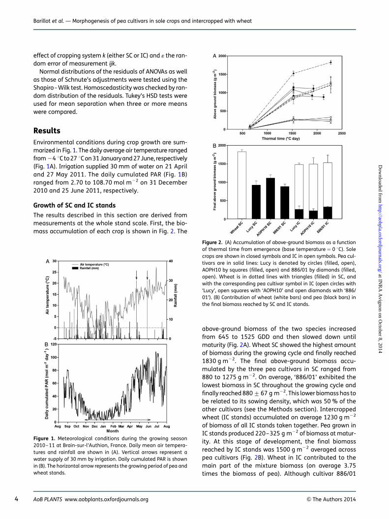
ResultsEnvironmental conditions during crop growth are sum-marized in Fig. 1. The daily average air temperature rangedfrom 24 8Cto27 8Con 31 Januaryand 27 June, respectively(Fig. 1A). Irrigation supplied 30 mm of water on 21 Apriland 27 May 2011. The daily cumulated PAR (Fig. 1B)ranged from 2.70 to 108.70 mol m22 on 31 December2010 and 25 June 2011, respectively.

Growth of SC and IC stands

The results described in this section are derived frommeasurements at the whole stand scale. First, the bio-mass accumulation of each crop is shown in Fig. 2. The

above-ground biomass of the two species increasedfrom 645 to 1525 GDD and then slowed down untilmaturity (Fig. 2A). Wheat SC showed the highest amountof biomass during the growing cycle and finally reached1830 g m22. The final above-ground biomass accu-mulated by the three pea cultivars in SC ranged from880 to 1275 g m22. On average, ‘886/01’ exhibited thelowest biomass in SC throughout the growing cycle andfinally reached 880+67 g m22. This lower biomass has tobe related to its sowing density, which was 50 % of theother cultivars (see the Methods section). Intercroppedwheat (IC stands) accumulated on average 1230 g m22

of biomass of all IC stands taken together. Pea grown inIC stands produced 220–325 g m22 of biomass at matur-ity. At this stage of development, the final biomassreached by IC stands was 1500 g m22 averaged acrosspea cultivars (Fig. 2B). Wheat in IC contributed to themain part of the mixture biomass (on average 3.75times the biomass of pea). Although cultivar 886/01

Figure 1. Meteorological conditions during the growing season2010–11 at Brain-sur-l’Authion, France. Daily mean air tempera-tures and rainfall are shown in (A). Vertical arrows represent awater supply of 30 mm by irrigation. Daily cumulated PAR is shownin (B). The horizontal arrow represents the growing period of pea andwheat stands.

Figure 2. (A) Accumulation of above-ground biomass as a functionof thermal time from emergence (base temperature ¼ 0 8C). Solecrops are shown in closed symbols and IC in open symbols. Pea cul-tivars are in solid lines: Lucy is denoted by circles (filled, open),AOPH10 by squares (filled, open) and 886/01 by diamonds (filled,open). Wheat is in dotted lines with triangles (filled) in SC, andwith the corresponding pea cultivar symbol in IC (open circles with‘Lucy’, open squares with ‘AOPH10’ and open diamonds with ‘886/01’). (B) Contribution of wheat (white bars) and pea (black bars) inthe final biomass reached by SC and IC stands.



at INR

A A



ownloaded from


exhibited the lowest biomass in SC stands, this cultivarproduced more biomass when intercropped with wheatcompared with ‘Lucy’ and ‘AOPH10’, despite being sownat half density.

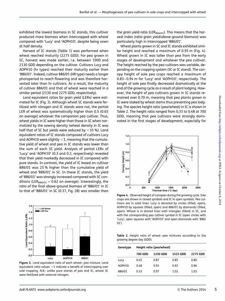
Harvest of IC stands (Table 1) was performed whenwheat reached maturity (2275 GDD). For pea grown inSC, harvest was made earlier, i.e. between 1900 and2130 GDD depending on the cultivar. Cultivars Lucy andAOPH10 (hr types) reached their maturity earlier than‘886/01’. Indeed, cultivar 886/01 (HR type) needs a longerphotoperiod to reach flowering and was therefore har-vested later than hr cultivars. As a result, the maturityof cultivar 886/01 and that of wheat were reached in asimilar period (2130 and 2275 GDD, respectively).

Land equivalent ratios for grain yield (LERs) were esti-mated for IC (Fig. 3). Although wheat SC stands were fer-tilized with nitrogen and IC stands were not, the partialLER of wheat was systematically higher than 0.5 (0.65on average) whatever the companion pea cultivar. Thus,wheat yields in IC were higher than those in SC when nor-malized by the sowing density (wheat density in IC washalf that of SC but yields were reduced by ,35 %). Landequivalent ratios of IC stands composed of cultivars Lucyand AOPH10 were slightly ,1, meaning that the cumula-tive yield of wheat and pea in IC stands was lower thanthe sum of each SC yield. Analysis of partial LERs of‘Lucy’ and ‘AOPH10’ (0.3 and 0.2, respectively) revealedthat their yield markedly decreased in IC compared withpure stands. In contrast, the yield of IC based on cultivar886/01 was 25 % higher than the cumulative yield ofwheat and ‘886/01’ in SC. In these IC stands, the yieldof ‘886/01’ was strongly increased compared with SC con-ditions (LER886/01 ¼ 0.62 on average). Interestingly, theratio of the final above-ground biomass of ‘886/01’ in ICto that of ‘886/01’ in SC (0.37, Fig. 2B) was smaller than

the grain yield ratio (LER866/01). This means that the har-vest index (ratio grain yield/above-ground biomass) wasparticularly high in intercropped ‘886/01’.

Wheat plants grown in SC and IC stands exhibited simi-lar height and reached a maximum of 0.95 m (Fig. 4).Wheat grown in IC was taller than pea from the earlystages of development and whatever the pea cultivar.The height reached by the pea cultivars was variable, de-pending on the cropping system (SC or IC stand). The can-opy height of sole pea crops reached a maximum of0.83–0.94 m for ‘Lucy’ and ‘AOPH10’, respectively. Theheight of sole pea finally decreased dramatically at theend of the growing cycle as a result of plant lodging. How-ever, the height of pea cultivars grown in IC stands re-mained over 0.70 m, meaning that pea plants grown inIC were staked by wheat stems thus preventing pea lodg-ing. The species height ratio (pea/wheat) in IC is shown inTable 2. The height ratio ranged from 0.33 to 0.48 at 700GDD, meaning that pea cultivars were strongly domi-nated in the first stages of development, especially for

Figure 3. Land equivalent ratio of each wheat–pea mixture. Landequivalent ratio values .1 indicate a benefit of intercropping oversole cropping. N.B.: unlike pure stands of pea and IC, wheat SCwere fertilized with external nitrogen.

Figure 4. Observed height of canopies during the growing cycle. Solecrops are shown in closed symbols and IC in open symbols. Pea cul-tivars are in solid lines: Lucy is denoted by circles (filled, open),AOPH10 by squares (filled, open) and 886/01 by diamonds (filled,open). Wheat is in dotted lines with triangles (filled) in SC, andwith the corresponding pea cultivar symbol in IC (open circles with‘Lucy’, open squares with ‘AOPH10’ and open diamonds with ‘886/01’).

. . . . . . . . . . . . . . . . . . . . . . . . . . . . . . . . . . . . . . . . . . . . . . . . . . . . . . . . . . . . . . . .

. . . . . . . . . . . . . . . . . . . . . . . . . . . . . . . . . . . . . . . . . . . . . . . . . . . . . . . . . . . . . . . . . . . . . . . . . . . . . . . . . .

Table 2. Height ratio of wheat–pea mixtures according to thegrowing degree day (GDD).

Genotype Height ratio (pea/wheat)

700 GDD 1330 GDD 1525 GDD 2275 GDD

Lucy 0.45 0.87 0.85 0.80

AOPH10 0.48 0.93 0.93 0.96

886/01 0.33 0.97 1.02 1.03



at INR

A A



ownloaded from


‘886/01’. From 1330 GDD on, the Lucy and AOPH10 culti-vars were slightly shorter than wheat, whereas ‘886/01’reached the height of wheat.

Morphogenesis of pea cultivars

In a second step, measurements were made at plantscale in order to compare the morphogenesis of pea cul-tivars grown in pure stands with those intercropped withwheat.

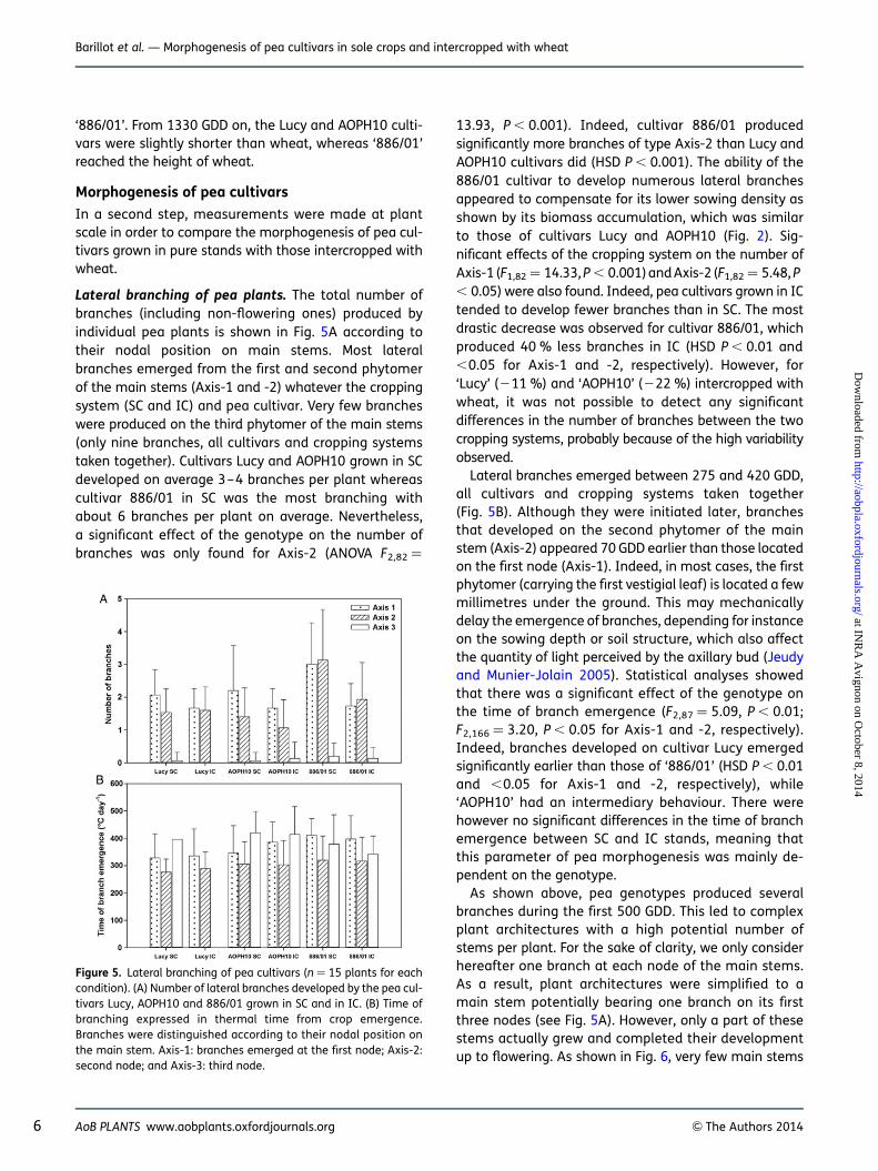
Lateral branching of pea plants. The total number ofbranches (including non-flowering ones) produced byindividual pea plants is shown in Fig. 5A according totheir nodal position on main stems. Most lateralbranches emerged from the first and second phytomerof the main stems (Axis-1 and -2) whatever the croppingsystem (SC and IC) and pea cultivar. Very few brancheswere produced on the third phytomer of the main stems(only nine branches, all cultivars and cropping systemstaken together). Cultivars Lucy and AOPH10 grown in SCdeveloped on average 3–4 branches per plant whereascultivar 886/01 in SC was the most branching withabout 6 branches per plant on average. Nevertheless,a significant effect of the genotype on the number ofbranches was only found for Axis-2 (ANOVA F2,82 ¼

13.93, P , 0.001). Indeed, cultivar 886/01 producedsignificantly more branches of type Axis-2 than Lucy andAOPH10 cultivars did (HSD P , 0.001). The ability of the886/01 cultivar to develop numerous lateral branchesappeared to compensate for its lower sowing density asshown by its biomass accumulation, which was similarto those of cultivars Lucy and AOPH10 (Fig. 2). Sig-nificant effects of the cropping system on the number ofAxis-1 (F1,82 ¼ 14.33, P , 0.001) and Axis-2 (F1,82 ¼ 5.48, P, 0.05) were also found. Indeed, pea cultivars grown in ICtended to develop fewer branches than in SC. The mostdrastic decrease was observed for cultivar 886/01, whichproduced 40 % less branches in IC (HSD P , 0.01 and,0.05 for Axis-1 and -2, respectively). However, for‘Lucy’ (211 %) and ‘AOPH10’ (222 %) intercropped withwheat, it was not possible to detect any significantdifferences in the number of branches between the twocropping systems, probably because of the high variabilityobserved.

Lateral branches emerged between 275 and 420 GDD,all cultivars and cropping systems taken together(Fig. 5B). Although they were initiated later, branchesthat developed on the second phytomer of the mainstem (Axis-2) appeared 70 GDD earlier than those locatedon the first node (Axis-1). Indeed, in most cases, the firstphytomer (carrying the first vestigial leaf) is located a fewmillimetres under the ground. This may mechanicallydelay the emergence of branches, depending for instanceon the sowing depth or soil structure, which also affectthe quantity of light perceived by the axillary bud (Jeudyand Munier-Jolain 2005). Statistical analyses showedthat there was a significant effect of the genotype onthe time of branch emergence (F2,87 ¼ 5.09, P , 0.01;F2,166 ¼ 3.20, P , 0.05 for Axis-1 and -2, respectively).Indeed, branches developed on cultivar Lucy emergedsignificantly earlier than those of ‘886/01’ (HSD P , 0.01and ,0.05 for Axis-1 and -2, respectively), while‘AOPH10’ had an intermediary behaviour. There werehowever no significant differences in the time of branchemergence between SC and IC stands, meaning thatthis parameter of pea morphogenesis was mainly de-pendent on the genotype.

As shown above, pea genotypes produced severalbranches during the first 500 GDD. This led to complexplant architectures with a high potential number ofstems per plant. For the sake of clarity, we only considerhereafter one branch at each node of the main stems.As a result, plant architectures were simplified to amain stem potentially bearing one branch on its firstthree nodes (see Fig. 5A). However, only a part of thesestems actually grew and completed their developmentup to flowering. As shown in Fig. 6, very few main stems

Figure 5. Lateral branching of pea cultivars (n ¼ 15 plants for eachcondition). (A) Number of lateral branches developed by the pea cul-tivars Lucy, AOPH10 and 886/01 grown in SC and in IC. (B) Time ofbranching expressed in thermal time from crop emergence.Branches were distinguished according to their nodal position onthe main stem. Axis-1: branches emerged at the first node; Axis-2:second node; and Axis-3: third node.



at INR

A A



ownloaded from


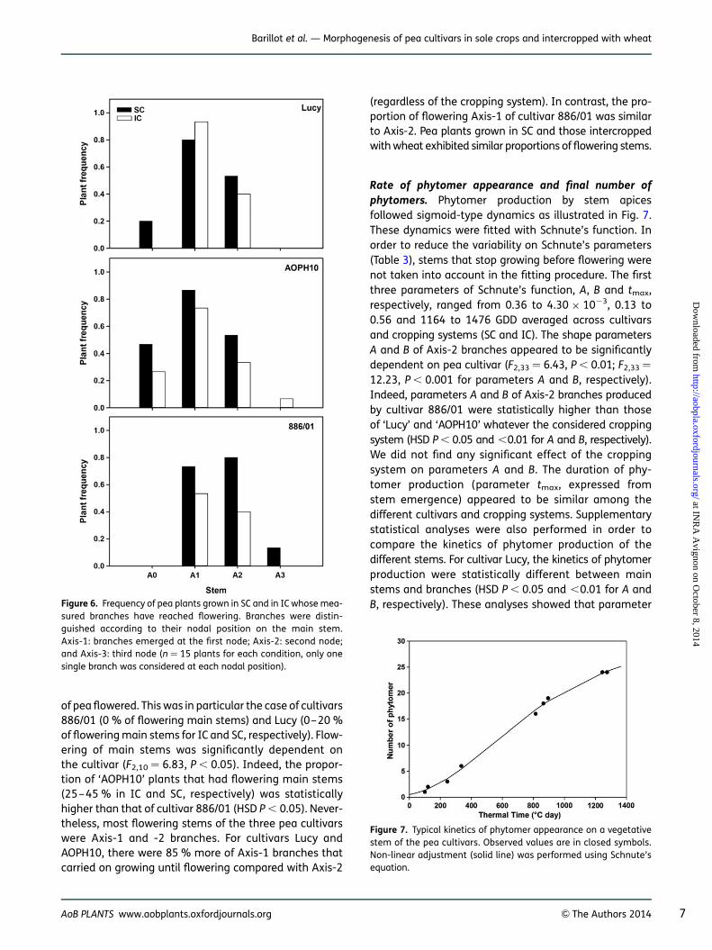
of pea flowered. This was in particular the case of cultivars886/01 (0 % of flowering main stems) and Lucy (0–20 %of flowering main stems for IC and SC, respectively). Flow-ering of main stems was significantly dependent onthe cultivar (F2,10 ¼ 6.83, P , 0.05). Indeed, the propor-tion of ‘AOPH10’ plants that had flowering main stems(25–45 % in IC and SC, respectively) was statisticallyhigher than that of cultivar 886/01 (HSD P , 0.05). Never-theless, most flowering stems of the three pea cultivarswere Axis-1 and -2 branches. For cultivars Lucy andAOPH10, there were 85 % more of Axis-1 branches thatcarried on growing until flowering compared with Axis-2

(regardless of the cropping system). In contrast, the pro-portion of flowering Axis-1 of cultivar 886/01 was similarto Axis-2. Pea plants grown in SC and those intercroppedwith wheat exhibited similar proportions of flowering stems.

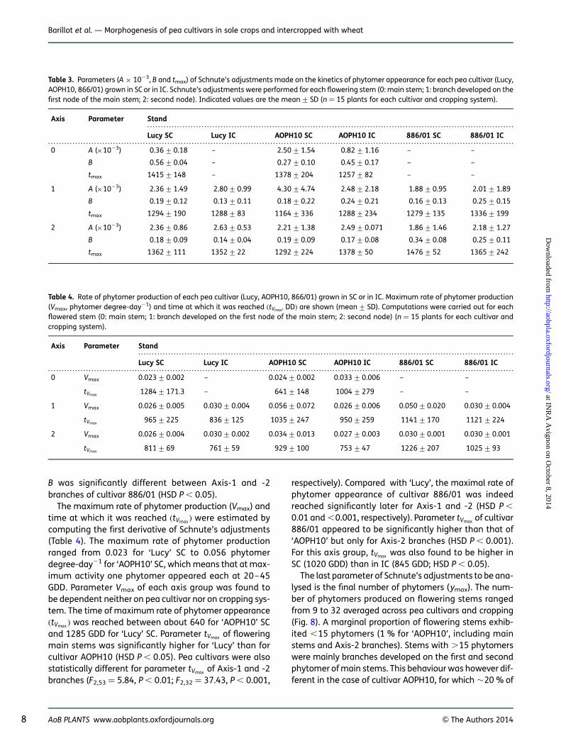
Rate of phytomer appearance and final number ofphytomers. Phytomer production by stem apicesfollowed sigmoid-type dynamics as illustrated in Fig. 7.These dynamics were fitted with Schnute’s function. Inorder to reduce the variability on Schnute’s parameters(Table 3), stems that stop growing before flowering werenot taken into account in the fitting procedure. The firstthree parameters of Schnute’s function, A, B and tmax,respectively, ranged from 0.36 to 4.30 × 1023, 0.13 to0.56 and 1164 to 1476 GDD averaged across cultivarsand cropping systems (SC and IC). The shape parametersA and B of Axis-2 branches appeared to be significantlydependent on pea cultivar (F2,33 ¼ 6.43, P , 0.01; F2,33 ¼

12.23, P , 0.001 for parameters A and B, respectively).Indeed, parameters A and B of Axis-2 branches producedby cultivar 886/01 were statistically higher than thoseof ‘Lucy’ and ‘AOPH10’ whatever the considered croppingsystem (HSD P , 0.05 and ,0.01 for A and B, respectively).We did not find any significant effect of the croppingsystem on parameters A and B. The duration of phy-tomer production (parameter tmax, expressed fromstem emergence) appeared to be similar among thedifferent cultivars and cropping systems. Supplementarystatistical analyses were also performed in order tocompare the kinetics of phytomer production of thedifferent stems. For cultivar Lucy, the kinetics of phytomerproduction were statistically different between mainstems and branches (HSD P , 0.05 and ,0.01 for A andB, respectively). These analyses showed that parameterFigure 6. Frequency of pea plants grown in SC and in IC whose mea-

sured branches have reached flowering. Branches were distin-guished according to their nodal position on the main stem.Axis-1: branches emerged at the first node; Axis-2: second node;and Axis-3: third node (n ¼ 15 plants for each condition, only onesingle branch was considered at each nodal position).

Figure 7. Typical kinetics of phytomer appearance on a vegetativestem of the pea cultivars. Observed values are in closed symbols.Non-linear adjustment (solid line) was performed using Schnute’sequation.



at INR

A A



ownloaded from


B was significantly different between Axis-1 and -2branches of cultivar 886/01 (HSD P , 0.05).

The maximum rate of phytomer production (Vmax) andtime at which it was reached (tVmax ) were estimated bycomputing the first derivative of Schnute’s adjustments(Table 4). The maximum rate of phytomer productionranged from 0.023 for ‘Lucy’ SC to 0.056 phytomerdegree-day21 for ‘AOPH10’ SC, which means that at max-imum activity one phytomer appeared each at 20–45GDD. Parameter Vmax of each axis group was found tobe dependent neither on pea cultivar nor on cropping sys-tem. The time of maximum rate of phytomer appearance(tVmax ) was reached between about 640 for ‘AOPH10’ SCand 1285 GDD for ‘Lucy’ SC. Parameter tVmax of floweringmain stems was significantly higher for ‘Lucy’ than forcultivar AOPH10 (HSD P , 0.05). Pea cultivars were alsostatistically different for parameter tVmax of Axis-1 and -2branches (F2,53 ¼ 5.84, P , 0.01; F2,32 ¼ 37.43, P , 0.001,

respectively). Compared with ‘Lucy’, the maximal rate ofphytomer appearance of cultivar 886/01 was indeedreached significantly later for Axis-1 and -2 (HSD P ,

0.01 and ,0.001, respectively). Parameter tVmax of cultivar886/01 appeared to be significantly higher than that of‘AOPH10’ but only for Axis-2 branches (HSD P , 0.001).For this axis group, tVmax was also found to be higher inSC (1020 GDD) than in IC (845 GDD; HSD P , 0.05).

The last parameter of Schnute’s adjustments to be ana-lysed is the final number of phytomers (ymax). The num-ber of phytomers produced on flowering stems rangedfrom 9 to 32 averaged across pea cultivars and cropping(Fig. 8). A marginal proportion of flowering stems exhib-ited ,15 phytomers (1 % for ‘AOPH10’, including mainstems and Axis-2 branches). Stems with .15 phytomerswere mainly branches developed on the first and secondphytomer of main stems. This behaviour was however dif-ferent in the case of cultivar AOPH10, for which �20 % of

. . . . . . . . . . . . . . . . . . . . . . . . . . . . . . . . . . . . . . . . . . . . . . . . . . . . . . . . . . . . . . . . . . . . . . . . . . . . . . . . . . . . . . . . . . . . . . . . . . . . . . . . . . . . . . . . . . . . . . . . . . . . . . . . . . . . . . .

. . . . . . . . . . . . . . . . . . . . . . . . . . . . . . . . . . . . . . . . . . . . . . . . . . . . . . . . . . . . . . . . . . . . . . . . . . . . . . . . . . . . . . . . . . . . . . . . . . . . . . . . . . . . . . . . . . . . . . . . . . . . . . . . . . . . . . . . . . . . . . . . . . . . . . . . . . . . . . . . . . . . . . . . . . . .

Table 3. Parameters (A × 1023, B and tmax) of Schnute’s adjustments made on the kinetics of phytomer appearance for each pea cultivar (Lucy,AOPH10, 866/01) grown in SC or in IC. Schnute’s adjustments were performed for each flowering stem (0: main stem; 1: branch developed on thefirst node of the main stem; 2: second node). Indicated values are the mean+SD (n ¼ 15 plants for each cultivar and cropping system).

Axis Parameter Stand

Lucy SC Lucy IC AOPH10 SC AOPH10 IC 886/01 SC 886/01 IC

0 A (×1023) 0.36+0.18 – 2.50+1.54 0.82+1.16 – –

B 0.56+0.04 – 0.27+0.10 0.45+0.17 – –

tmax 1415+148 – 1378+204 1257+82 – –

1 A (×1023) 2.36+1.49 2.80+0.99 4.30+4.74 2.48+2.18 1.88+0.95 2.01+1.89

B 0.19+0.12 0.13+0.11 0.18+0.22 0.24+0.21 0.16+0.13 0.25+0.15

tmax 1294+190 1288+83 1164+336 1288+234 1279+135 1336+199

2 A (×1023) 2.36+0.86 2.63+0.53 2.21+1.38 2.49+0.071 1.86+1.46 2.18+1.27

B 0.18+0.09 0.14+0.04 0.19+0.09 0.17+0.08 0.34+0.08 0.25+0.11

tmax 1362+111 1352+22 1292+224 1378+50 1476+52 1365+242

. . . . . . . . . . . . . . . . . . . . . . . . . . . . . . . . . . . . . . . . . . . . . . . . . . . . . . . . . . . . . . . . . . . . . . . . . . . . . . . . . . . . . . . . . . . . . . . . . . . . . . . . . . . . . . . . . . . . . . . . . . . . . . . . . . . . . . . . . .

. . . . . . . . . . . . . . . . . . . . . . . . . . . . . . . . . . . . . . . . . . . . . . . . . . . . . . . . . . . . . . . . . . . . . . . . . . . . . . . . . . . . . . . . . . . . . . . . . . . . . . . . . . . . . . . . . . . . . . . . . . . . . . . . . . . . . . . . . . . . . . . . . . . . . . . . . . . . . . . . . . . . . . . . . . . .

Table 4. Rate of phytomer production of each pea cultivar (Lucy, AOPH10, 866/01) grown in SC or in IC. Maximum rate of phytomer production(Vmax, phytomer degree-day21) and time at which it was reached (tVmax,DD) are shown (mean+ SD). Computations were carried out for eachflowered stem (0: main stem; 1: branch developed on the first node of the main stem; 2: second node) (n ¼ 15 plants for each cultivar andcropping system).

Axis Parameter Stand

Lucy SC Lucy IC AOPH10 SC AOPH10 IC 886/01 SC 886/01 IC

0 Vmax 0.023+0.002 – 0.024+0.002 0.033+0.006 – –

tVmax 1284+171.3 – 641+148 1004+279 – –

1 Vmax 0.026+0.005 0.030+0.004 0.056+0.072 0.026+0.006 0.050+0.020 0.030+0.004

tVmax 965+225 836+125 1035+247 950+259 1141+170 1121+224

2 Vmax 0.026+0.004 0.030+0.002 0.034+0.013 0.027+0.003 0.030+0.001 0.030+0.001

tVmax 811+69 761+59 929+100 753+47 1226+207 1025+93



at INR

A A



ownloaded from


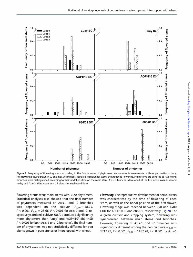
flowering stems were main stems with .20 phytomers.Statistical analyses also showed that the final numberof phytomers measured on Axis-1 and -2 brancheswas dependent on the cultivar (F2,60 ¼ 58.24,P , 0.001; F2,37 ¼ 25.66, P , 0.001 for Axis-1 and -2, re-spectively). Indeed, cultivar 886/01 produced significantlymore phytomers than ‘Lucy’ and ‘AOPH10’ did (HSDP , 0.001 for both Axis-1 and -2 branches). The final num-ber of phytomers was not statistically different for peaplants grown in pure stands or intercropped with wheat.

Flowering. The reproductive development of pea cultivarswas characterized by the time of flowering of eachstem, as well as the nodal position of the first flower.Flowering stage was reached between 950 and 1400GDD for AOPH10 IC and 886/01, respectively (Fig. 9). Fora given cultivar and cropping system, flowering wassynchronized between main stems and branches.However, flowering of Axis-1 and -2 branches wassignificantly different among the pea cultivars (F2,61 ¼

1717.29, P , 0.001; F2,37 ¼ 1452.78, P , 0.001 for Axis-1

Figure 8. Frequency of flowering stems according to the final number of phytomers. Measurements were made on three pea cultivars: Lucy,AOPH10 and 886/01 grown in SC and in IC with wheat. Results are shown for stems that reached flowering. Main stems are denoted as Axis-0 andbranches were distinguished according to their nodal position on the main stem. Axis-1: branches developed at the first node; Axis-2: secondnode; and Axis-3: third node (n ¼ 15 plants for each condition).



at INR

A A



ownloaded from


and -2, respectively). Indeed, the flowering stage ofcultivar 886/01 was reached significantly later (1400GDD) than for ‘Lucy’ and ‘AOPH10’ (HSD P , 0.001 forboth cultivars). The first flowering phytomer (Fig. 10)was located between the ninth and the 28th phytomeraveraged across pea cultivars and cropping systems.First flowers of cultivar 886/01 (Axis-1 and -2 branches)were observed at higher phytomer positions (24thphytomer on average) than those measured for ‘Lucy’and ‘AOPH10’ (HSD P , 0.001 for both axis group andcultivars). As observed for the time of flowering, thenodal position of the first flower was similar betweenpea plants grown in pure stands and those mixed withwheat whatever the cultivars.

DiscussionThe aim of the present study was to address the questionof the morphological responses of pea to the competitionwhen intercropped with wheat. To this end, a field experi-ment was conducted on three pea cultivars that werecharacterized at both stand and plant scale whengrown in pure stands and mixed with wheat.

Although the present study was conducted throughout1 year only, our results on crop biomass, species heightand maturity were consistent with previous studies per-formed on different cultivars grown under contrastingpedo-climatic conditions (e.g. Corre-Hellou et al. 2009;Naudin et al. 2010). The results presented in this study

can therefore be assumed to be representative ofthe conditions commonly encountered in wheat–peamixtures. These results were obtained from unfertilizedmixtures as usually performed in cereal– legume inter-cropping systems. Furthermore, some authors (Jensen1996; Corre-Hellou et al. 2006) found that the contribu-tion of the component species to the biomass of the mix-ture was dependent on the available nitrogen, anincrease of which enhances the growth of the cereal spe-cies. The level and timing of nitrogen fertilization (Naudin2009; Naudin et al. 2010) therefore constitute a key factorenabling one to manage the hierarchy between themixed species. The present study also shows that thethree pea cultivars exhibited a similar level of biomass,especially when grown in mixtures. This suggests thatdespite the genotypic differences and contrasting initialsowing densities, the three pea cultivars had a similaroverall development even when they were in competitionwith wheat. However, this does not necessarily mean thatthe morphological processes of the pea cultivars hadsimilar responses to the competition with wheat, buttheir integration at the stand scale leads to an equivalentgrowth in biomass.

Our results also show that pea was strongly affected bylodging when grown in SC. Corre-Hellou et al. (2011) re-ported that the high sensitivity of pea to lodging causedsignificant yield losses as well as an enhanced growth ofweeds. Pea lodging was however strongly decreased inmixed stands, pea branches being stacked by wheat.

Figure 9. Time of flowering of pea cultivars Lucy, AOPH10 and 886/01 grown in SC or in IC. Main stems are denoted as Axis-0 and branches weredistinguished according to their nodal position on the main stem. Axis-1: branches developed at the first node; Axis-2: second node; and Axis-3:third node (n ¼ 15 plants for each condition).



at INR

A A



ownloaded from


Intercropping cereals and legumes is therefore a promis-ing way of both reintroducing legume species withinagrosystems and solving the problems encountered inpure stands of legumes. Moreover, the height reachedby each species in the canopy is an important feature ofthe stand which determines, but also emerges from, thecompetition processes occurring between plants. Compo-nent species height ratio has been widely shown to affectlight sharing in a mixture (Sinoquet and Caldwell 1995;Louarn et al. 2010; Barillot et al. 2011, 2012) and is there-fore a strong component of the inter-specific competitionoccurring within the mixture. The results described in the

present study illustrate that the species height ratio is notconstant throughout the growing cycle; pea cultivarswere much shorter than wheat until 700 GDD and thenreached a similar height. Differences among pea cultivarswere also observed but were not constant over time.Although ‘886/01’ was the shorter one in the early stagesof development, this cultivar finally reached the sameheight as that of wheat afterwards. Therefore, it seemsthat the competition which occurs among the inter-cropped species cannot be assessed by punctual mea-surements of the species height ratio (in particularduring the early stages of development). This is

Figure 10. Plant frequency according to the first flowering phytomer of stems. Results are shown for the pea cultivars Lucy, AOPH10 and 886/01grown in SC or in IC (n ¼ 15 plants for each condition). Main stems are denoted as Axis-0 and branches were distinguished according to theirnodal position on the main stem. Axis-1: branches developed at the first node; Axis-2: second node; and Axis-3: third node.



at INR

A A



ownloaded from


consistent with the findings reported in a previous study(Barillot et al. 2012) where a virtual plant approach wasused to demonstrate that the ability of plants to interceptlight was mainly determined by the architectural para-meters involved in (i) the LAI (number of branches andphytomers, leaf area) during the early stages and (ii)plant height (internode length, number of phytomers)once canopy closure was established.

The time lag between the physiological maturity ofwheat and pea is a well-known issue of these mixtures.The choice of harvest timing is indeed complicated bythe fact that pea generally reaches its maturity earlierthan wheat. Nevertheless, physiological maturity of peavaries among the cultivars according to their earliness,which is assumed to be mainly driven by the sensitivityof flowering to the photoperiod that involves the Hrgene (Murfet 1973). The maturity of the HR cultivar(886/01) was therefore almost synchronized with that ofwheat, whereas the hr cultivars had to be harvested earl-ier. Gaps of maturity, as encountered with hr cultivars,represent a strong practical constraint at harvest (Louarnet al. 2010); HR pea cultivars therefore appeared to bewell suited to intercropping with wheat.

In order to deepen the analysis of the variability ofpea morphogenesis in response to intercropping, a com-parison was performed at plant scale with particular at-tention to pea branching, flowering, final number ofphytomers and their kinetics of appearance. Branchinghas been shown to be dependent on several factorssuch as genotype, hormonal balance, environmental fac-tors, e.g. low temperatures (Jeudy and Munier-Jolain2005), and also plant density (Spies et al. 2010). In thepresent study, contrasting abilities for branching were in-deed found between the genotypes [Lucy–AOPH10] and886/01. Cultivar 886/01 was the most branching cultivar,which balanced its lower sowing density (50 % less than‘Lucy’ and ‘AOPH10’). Moreover, the number of branchestended to decrease in IC compared with pure stands, inparticular for cultivar 886/01. Some authors like Casalet al. (1986), Ballare and Casal (2000) or Evers et al.(2011) showed that branching of several species is af-fected by the quantity (PAR) and quality (red/far-redratio) of light perceived by the axillary buds. In the presentstudy, we can therefore hypothesize that quantity of lightand/or its quality were quite similar between the respect-ive pure stands and IC of cultivars Lucy and AOPH10. Thiswould mean that the replacement of a ‘Lucy’ or an‘AOPH10’ plant by a wheat one leads to similar variationsof light microclimate. This could be the result of small dif-ferences in the architectural patterns of the two speciesin terms of leaf area, height, geometry and/or opticalproperties. As cultivar 886/01 has a late development(HR type), we can also hypothesize that when

branching started, wheat plants were more developedthan neighbour ‘886/01’ pea plants would have been ina pure stand. This could cause variations of the microcli-mate perceived by axillary buds, leading to an inhibitionof branching.

The kinetics of phytomer appearance were assessed formain stems and a randomly selected branch at eachnode by using non-linear fittings. Our analysis showedthat there were few statistical differences betweenthe parameters belonging to the different genotypesand cropping systems. It was only found that (i) Axis-2branches of cultivar 886/01 had kinetics different fromthose of ‘Lucy’ and ‘AOPH10’ and (ii) the maximum rateof phytomer appearance of ‘886/01’ was reached latercompared with the other cultivars. These results meanthat the kinetics of phytomer production of differentstems can be analysed/modelled by using similarSchnute’s functions, at least for Lucy and AOPH10 culti-vars whether they were grown in sole stands or mixedwith wheat. Turc and Lecoeur (1997) also reported similarrates of leaf primordium initiation and emergence forcontrasting plant growth rates, cultivars and sowingdensities in spring pea. One drawback of using Schnute’sfunction lies in the fact that some of the parameters, es-pecially A and B, cannot be directly related to a biologicalmeaning. It would be tempting to use linear regressionsbecause of the reduced number of parameters and easyinterpretation. However, phytomer production is not in-trinsically constant and is actually characterized by amaximum rate (which can be estimated by the derivativeof Schnute’s functions) and a time at which developmentstops. These aspects cannot be handled by linear models.Supplementary statistical analyses (data not shown)showed that the residual sum of squares was significantlyhigher for linear regressions than that obtained withSchnute’s function (HSD P , 0.001). These tests also indi-cated that the residuals of most linear regressions werenot normally distributed and have means differing fromzero. Nevertheless, the estimated parameters derivedfrom Schnute’s adjustments were highly variable. Thisvariability is related to pea branching which is rather com-plex, particularly in the case of winter-sown cultivars.Winter conditions often cause frost damage, which in-duces the cessation of the development of the mainstems and the initiation of numerous branches at differ-ent times (Fig. 5A and B). The result is a high variability inthe characteristics of branches.

In the present study, a significant difference was ob-served among the pea genotypes for the final numberof phytomers reached on stems. Indeed, ‘886/01’ (HRtype) was found to produce more phytomers than theother cultivars. Similar results were also reported forthis particular cultivar but grown in controlled conditions



at INR

A A



ownloaded from


and individual pots (Barillot et al. 2012). In contrast, thenumber of initiated phytomers was similar whether peaplants were grown in pure stands or mixed with wheat,whatever the genotype. Moreover, our results show thatthe canopy of the three pea cultivars was mainly com-posed of branches as main stems had stopped growingwith few phytomers. As reported by Jeudy and Munier-Jolain (2005), the development of branches is increasedin winter pea cultivars because of the frost damage ex-perienced on the apex of the main stem. Such conditionswere encountered during the first months of the growingcycle (December–February; Fig. 1) which corresponds tothe emergence of the lateral branches (Fig. 5B).

Flowering is a crucial stage of the growing cycle thathas been widely studied and used in order to model peagrowth. Truong and Duthion (1993) showed that the timeof flowering is a function of leaf appearance rate and pos-ition of the node bearing the first flower. The reproductivedevelopment of pea cultivars was therefore characterizedby two main indicators: the nodal position of the firstflower and its emergence time. As also reported by Jeuf-froy and Sebillotte (1997), we found similar time of flow-ering between main stems and basal branches (althoughthese were produced later) for all cultivars and croppingsystems. Furthermore, the position of the first floweringnode was similar among the genotypes and cropping sys-tems. Some authors also showed that for a given geno-type, the position of the first flowering node wasconstant over various conditions (Roche et al. 1998;Munier-Jolain et al. 2005b).

Finally these results highlight that in the present ex-periment, the morphogenesis of pea was mainly deter-mined by the genotype and was only little affected bythe competition with wheat. This suggests that the archi-tectures of pea and wheat may be quite similar, so thatthe environmental conditions perceived by plants in thecanopy (phylloclimate; Chelle 2005) were not strongly dif-ferent between sole pea crops and wheat–pea mixtures.Functional–structural models (Vos et al. 2010; DeJonget al. 2011) are able to take into account the explicit archi-tecture of plants and its interactions with physiologicalprocesses and environmental conditions. Such modelstherefore constitute suitable tools for assessing these hy-potheses and can in particular be used to characterize themicroclimate perceived by plants located in mono- andmulti-specific stands.

ConclusionTo our knowledge, the present study is the first to comparethe morphogenesis of pea grown in sole stands with thatof pea grown intercropped with wheat. On the one hand,the present results show that most of the assessed

parameters of pea morphogenesis (phenology, branching,final number of phytomers and their kinetics of appear-ance) were mainly dependent on the considered genotype.This emphasizes the importance of the selection of culti-vars, in particular for intercropping systems, as this will de-termine the level of competition and complementaritybetween the component species. On the other hand,there was a low variability of pea morphogenesis betweensole and mixed stands except for plant height and branch-ing of the late cultivar 886/01. Complementary studies onwheat–pea mixtures under contrasting levels of nitrogenfertilization are now needed to provide information onhow nitrogen would affect plant morphogenesis and inter-specific competition. The information provided in the pre-sent study can be used for modelling pea morphogenesisin pure and mixed stands and therefore contributes to abetter understanding of the functioning of cereal–legumeIC. This kind of approach is also well suited for the identi-fication of plant traits to be integrated in the definition ofplant ideotypes.

Sources of FundingThis research was supported by ‘La Region Pays de laLoire’, France through a Ph.D. fellowship to R.B. The re-search of D.C. and A.E.-G. was partially funded by‘La Region Poitou-Charentes’, France.

Contributions by the AuthorsAll authors have contributed substantially to this manu-script. R.B. completed the writing and was involved in eachstep of the experimentation and analysis. D.C. and A.E.G.were actively involved in the conception and design of theexperiment as well as in the analyses and writing of themanuscript. S.P. was involved in the conception of the ex-periment and also performed the measurements. P.H. wasinvolved in database programming and data analysis.

Conflicts of Interest StatementNone declared.

AcknowledgementsWe gratefully acknowledge the technical staff of LEVA(Legumineuses, Ecophysiologie Vegetale, Agroecologie)as well as the experimental station of Brain sur l’Authion(FNAMS, Federation Nationale des Agriculteurs Multiplica-teurs de Semences). We also thank Dr Guenaelle Corre-Hellou (LEVA, Groupe ESA) for valuable discussions. Wealso thank reviewers for particularly helpful commentson this article.



at INR

A A



ownloaded from


Literature Cited

Arumingtyas EL, Floyd RS, Gregory MJ, Murfet IC. 1992. Branching inPisum: inheritance and allelism tests with 17 ramosus mutants.Pisum Genetics 24:17–31.

Ballare CL, Casal JJ. 2000. Light signals perceived by crop and weedplants. Field Crops Research 67:149–160.

Barillot R. 2012. Modelisation du partage de la lumiere dans l’associationde cultures ble—pois (Triticum aestivum L.–Pisum sativum L.)—Uneapproche de type plante virtuelle. PhD Thesis, Groupe Ecole Super-ieure d’Agriculture, UPSP Legumineuses, Ecophysiologie Vegetale,Agroecologie, Angers, France.

Barillot R, Louarn G, Escobar-Gutierrez AJ, Huynh P, Combes D. 2011.How good is the turbid medium-based approach for accountingfor light partitioning in contrasted grass–legume intercroppingsystems? Annals of Botany 108:1013–1024.

Barillot R, Combes D, Chevalier V, Fournier C, Escobar-Gutierrez AJ.2012. How does pea architecture influence light sharing in virtualwheat–pea mixtures? A simulation study based on pea geno-types with contrasting architectures. AoB PLANTS 2012:pls038;doi:10.1093/aobpla/pls038.

Beasse C, Ney B, Tivoli B. 2000. A simple model of pea (Pisum sativum)growth affected by Mycosphaerella pinodes. Plant Pathology 49:187–200.

Casal JJ, Sanchez RA, Deregibus VA. 1986. The effect of plant densityon tillering: the involvement of R/FR ratio and the proportion ofradiation intercepted per plant. Environmental and ExperimentalBotany 26:365–371.

Chelle M. 2005. Phylloclimate or the climate perceived by individualplant organs: what is it? How to model it? What for? New Phytol-ogist 166:781–790.

Corre-Hellou G, Fustec J, Crozat Y. 2006. Interspecific competition forsoil N and its interaction with N2 fixation, leaf expansion and cropgrowth in pea–barley intercrops. Plant and Soil 282:195–208.

Corre-Hellou G, Faure M, Launay M, Brisson N, Crozat Y. 2009. Adap-tation of the STICS intercrop model to simulate crop growth andN accumulation in pea–barley intercrops. Field Crops Research113:72–81.

Corre-Hellou G, Dibet A, Hauggaard-Nielsen H, Crozat Y, Gooding M,Ambus P, Dahlmann C, von Fragstein P, Pristeri A, Monti M,Jensen ES. 2011. The competitive ability of pea–barley intercropsagainst weeds and the interactions with crop productivity andsoil N availability. Field Crops Research 122:264–272.

Crews TE, Peoples MB. 2004. Legume versus fertilizer sources of nitro-gen: ecological tradeoffs and human needs. Agriculture, Ecosys-tems & Environment 102:279–297.

DeJong TM, Da Silva D, Vos J, Escobar-Gutierrez AJ. 2011. Using func-tional–structural plant models to study, understand and inte-grate plant development and ecophysiology. Annals of Botany108:987–989.

De Wit CT, Van den Bergh JP. 1965. Competition between herbageplants. Journal of Agricultural Science 13:212–221.

Duc G, Mignolet C, Carrouee B, Huyghe C. 2010. Importance econo-mique passee et presente des legumineuses: Role historiquedans les assolements et les facteurs d’evolution. InnovationsAgronomiques 11:1–24.

Evers JB, van der Krol AR, Vos J, Struik PC. 2011. Understanding shootbranching by modelling form and function. Trends in PlantScience 16:464–467.

Godin C. 2000. Representing and encoding plant architecture: a re-view. Annals of Forest Science 57:413–438.

Gourlay CW, Hofer JMI, Ellis THN. 2000. Pea compound leaf architec-ture is regulated by interactions among the genes UNIFOLIATA,COCHLEATA, AFILA, and TENDRIL-LESS. The Plant Cell Online 12:1279–1294.

Gray A. 1849. On the composition of the plant by phytons, and someapplications of phyllotaxis. Proceedings of the American Associ-ation for the Advancement of Science 438–444.

Hauggaard-Nielsen H, Jørnsgaard B, Kinane J, Jensen ES. 2008. Grainlegume–cereal intercropping: the practical application of diver-sity, competition and facilitation in arable and organic croppingsystems. Renewable Agriculture and Food Systems 23:3–12.

Huyghe C. 1998. Genetics and genetic modifications of plant archi-tecture in grain legumes: a review. Agronomie 18:383–411.

Jensen ES. 1996. Grain yield, symbiotic N2 fixation and interspecificcompetition for inorganic N in pea–barley intercrops. Plant andSoil 182:25–38.

Jeudy C, Munier-Jolain N. 2005. Developpement des ramifications.In: Munier-Jolain N, Biarnes V, Chaillet I, Lecoeur J,Jeuffroy M-H, eds. Agrophysiologie du pois proteagineux. Paris:Inra-Quae, 51–58.

Jeuffroy MH, Sebillotte M. 1997. The end of flowering in pea: influ-ence of plant nitrogen nutrition. European Journal of Agronomy6:15–24.

Kusnadi J, Gregory M, Murfet IC, Ross JJ, Bourne F. 1992. Internodelength in Pisum: phenotypic characterisation and genetic identityof the short internode mutant Wt11242. Pisum Genetics 24:64–74.

Launay M, Brisson N, Satger S, Hauggaard-Nielsen H, Corre-Hellou G,Kasynova E, Ruske R, Jensen ES, Gooding MJ. 2009. Exploringoptions for managing strategies for pea–barley intercroppingusing a modeling approach. European Journal of Agronomy 31:85–98.

Le May C, Ney B, Lemarchand E, Schoeny A, Tivoli B. 2009. Effect ofpea plant architecture on spatiotemporal epidemic developmentof ascochyta blight (Mycosphaerella pinodes) in the field. PlantPathology 58:332–343.

Louarn G, Corre-Hellou G, Fustec J, Lo-Pelzer E, Julier B, Litrico I,Hinsinger P, Lecomte C. 2010. Determinants ecologiques etphysiologiques de la productivite et de la stabilite des associa-tions graminees-legumineuses. Innovations Agronomiques 11:79–99.

Marquardt DW. 1963. An algorithm for least-squares estimation ofnonlinear parameters. Journal of the Society for Industrial andApplied Mathematics 11:431–441.

Munier-Jolain N, Biarnes V, Chaillet I, Lecoeur J, Jeuffroy M-H,Carrouee B, Crozat Y, Guilioni L, Lejeune I, Tivoli B. 2005a. Agro-physiologie du pois proteagineux, Paris: INRA-Quae.

Munier-Jolain N, Turc O, Ney B. 2005b. Developpement reproducteur.In: Munier-Jolain N, Biarnes V, Chaillet I, Lecoeur J, Jeuffroy M-H,eds. Agrophysiologie du pois proteagineux. Paris: Inra-Quae,45–50.

Murfet IC. 1973. Flowering in Pisum. Hr, a gene for high response tophotoperiod. Heredity 31:157–164.

Murfet IC. 1975. Flowering in Pisum: multiple alleles at the lf locus.Heredity 35:85–98.

Naudin C. 2009. Nutrition azotee des associations Pois-Ble d’hiver(Pisum sativum L.–Triticum aestivum L.): Analyse, modelisation



at INR

A A



ownloaded from


et propositions de strategies de gestion. PhD Thesis, Groupe EcoleSuperieure d’Agriculture, UPSP Legumineuses, EcophysiologieVegetale, Agroecologie, Angers, France.

Naudin C, Corre-Hellou G, Pineau S, Crozat Y, Jeuffroy M-H. 2010. Theeffect of various dynamics of N availability on winter pea–wheatintercrops: crop growth, N partitioning and symbiotic N2 fixation.Field Crops Research 119:2–11.

Ney B, Carrouee B. 2005. Preface. In: Munier-Jolain N, Biarnes V,Chaillet I, Lecoeur J, Jeuffroy M-H, eds. Agrophysiologie du poisproteagineux. Paris: Inra-Quae.

Ofori F, Stern WR. 1987. Cereal– legume intercropping systems.Advances in Agronomy 41:41–90.

R Development Core Team. 2012. R: a language and environment forstatistical computing. Vienna, Austria: R Foundation for StatisticalComputing.

Roche R, Jeuffroy M-H, Ney B. 1998. A model to simulate the finalnumber of reproductive nodes in pea (Pisum sativum L.). Annalsof Botany 81:545–555.

Ross J. 1981. Role of phytometric investigations in the studies ofplant stand architecture and radiation regime. In: Ross J, ed.The radiation regime and architecture of plant stands. TheHague, The Netherlands: Junk, W, 9–11.

Schnute J. 1981. A versatile growth model with statistically stableparameters. Canadian Journal of Fisheries and Aquatic Sciences38:1128–1140.

Schwinning S, Weiner J. 1998. Mechanisms determining the degreeof size asymmetry in competition among plants. Oecologia 113:447–455.

Sinoquet H, Caldwell MM. 1995. Estimation of light capture and par-titioning in intercropping systems. In: Sinoquet H, Cruz P, eds.Ecophysiology of tropical intercropping. Paris: INRA Editions,79–97.

Spies JM, Warkentin T, Shirtliffe S. 2010. Basal branching in field peacultivars and yield–density relationships. Canadian Journal ofPlant Science 90:679–690.

Truong HH, Duthion C. 1993. Time of Flowering of Pea (Pisum sativumL.) as a function of leaf appearance rate and node of first flower.Annals of Botany 72:133–142.

Turc O, Lecoeur J. 1997. Leaf primordium initiation and expandedleaf production are co-ordinated through similar response toair temperature in pea (Pisum sativum L.). Annals of Botany 80:265–273.

Varlet-Grancher C, Bonhomme R, Sinoquet H. 1993. Crop structureand light microclimate. Paris: INRA Editions.

Vos J, Evers JB, Buck-Sorlin GH, Andrieu B, Chelle M, de Visser PHB.2010. Functional–structural plant modelling: a new versatiletool in crop science. Journal of Experimental Botany 61:2101 – 2115.

White J. 1979. The plant as a metapopulation. Annual Review ofEcology and Systematics 10:109–145.



at INR

A A



ownloaded from


Comparison of the morphogenesis of three genotypes of pea (Pisum sativum) grown in pure stands and...

Documents

Transcript of Comparison of the morphogenesis of three genotypes of pea (Pisum sativum) grown in pure stands and...