1

Complex band structure and plasmon lattice Green’s function of a periodic metal-nanoparticle chain

Kin Hung Fung, Ross Chin Hang Tang, and C. T. Chan

Department of Physics, The Hong Kong University of Science and Technology,

Hong Kong, China

When the surface plasmon resonance in a metal-nanoparticle chain is excited at one point,

the response signal will generally decay down the chain due to absorption and radiation

losses. The decay length is a key parameter in such plasmonic systems. By studying the

plasmon lattice Green’s function, we found that the decay length is generally governed by

two exponential decay constants with phase factors corresponding to guided Bloch modes

and one power-law decay with a phase factor corresponding to that of free space photons.

The results show a high level of similarity between the absorptive and radiative decay

channels. By analyzing the poles (and the corresponding residues) of the Green’s

function in a transformed complex reciprocal space, the dominant decay channel of the

real-space Green’s function is understood.

PACS number(s): 78.67.Bf, 73.22.Lp, 73.20.Mf, 78.70.-g

I. INTRODUCTION

Band theoretic techniques are widely applied in describing the eigenmodes of periodic

systems. With the help of the Bloch’s theorem,1 a band structure for propagating modes

in a lossless periodic system is usually displayed as a plot of the eigenmode as a function

2

of real frequency (ω ) versus real Bloch wave vector (k ) in the reduced-zone scheme.2

Such a “real-k ” band-structure description has been generalized for including evanescent

waves within bandgap by allowing the Bloch wave vectors to be complex quantities.3 4

This generalized “complex- k ” description is sometimes called the complex-band-

structure description.

There are several advantages of considering the complex band structure. For example, the

magnitude of the imaginary part of the k -vector gives the strength and the physical

nature of the bandgaps. In addition, it can describe the decaying waves in lossy systems.

It is generally believed that a non-zero imaginary part of k implies an exponential decay

(or growth) of the wave with a decay constant given by 1/ Im( )k= . Although the actual

decay profile may depend on the incident field of a particular problem, such kind of

exponential decay characteristics are indeed embedded in the Green’s function.5 6 For

example, the frequency-domain Green’s function for a homogeneous one-dimensional

(1D) wave equation takes the form,5 Re( )| | Im( )| |( , ) ~ i k x k xG x e eω − , where ω is the excitation

frequency, k is the corresponding complex wave number, and x is the spatial coordinate.

Since the Green’s function contains all the essential information on wave propagation, we

can have a useful interpretation of the complex wave properties by studying the decay

profile of the Green’s function and its relation to the complex band structure.

Although there were some studies in the literature that is concerned with the Green’s

function for inhomogeneous lossy media, only a few of them focus on surface plasmons,7

8 which have been shown to exhibit many interesting properties in recent years.9 In

3

plasmonic systems, which are intrinsically lossy due to absorption and radiation, the

primary concern is the decay length of the plasmonic modes that can be excited in a

certain point. In this paper, we study the Green’s function for the plasmonic waves that

propagate along a linear array of metal nanoparticles (MNPs).10 11 12 13 14 15 We will first

discuss the numerical results on the complex band structure (Sec. II) and the lattice

Green’s function (Sec. III) for such MNP array. Then, we will propose an ansatz which

gives a closed-form expression for the lattice Green’s function and we will show that the

ansatz is indeed the correct solution by considering a generating function for the lattice

Green’s function (Sec. IV).

II. COMPLEX BAND STRUCTURE

We consider a linear array of identical MNPs (with lattice constant a and particle radius

0r ). For 03a r≥ and frequencies close to the Fröhlich frequency,16 the electromagnetic

modes of the MNPs can be accurately described by the coupled-dipole equations,17

⎥⎦

⎤⎢⎣

⎡ −+= ∑≠

nmn

nmextmm pRRWEp )(α , (1)

where mp is the electric dipole moment of the m th particle, α is the single-particle

dynamic polarizability, and extmE is the external electric field acting on the m th particle.

The dynamic propagator, )(rW , for a dipole in a homogeneous host medium can be

written as17 )(ruvW ]/)()([ 23 rrrrkBrkAk vuhuvhh += δ , where hh ck /ω= , hc is the speed of

light in the host medium, )(xA ( ) ixexixx 321 −−− −+= , )(xB ( ) ixexixx 321 33 −−− +−−= , and

4

3 ,2 ,1 , =vu are component indices in Cartesian coordinates. Equation (1) can be written

as

extmu

vnnvmunv EpM =∑

,, (2)

where mup and extmuE are the u th components of the mp and ext

mE , respectively. For a linear

array of MNPs, Eq. (2) can be further split into decoupled equations in the form,

extmn nmn EpM =∑ , for either the transverse modes (with mp perpendicular to the chain

axis) or longitudinal modes ( mp parallel to the chain axis). Since the transverse modes

have richer properties in its band structure (such as negative slope13 and strong coupling

to free photon7), we will focus on the transverse mode.

The band structure can be calculated by setting 0=extmE and finding pairs of ω and k so

that Eq. (2) has non-trivial Bloch solutions of the form ikmam e0pp = . More explicitly, we

have to find the solutions of the equation,14

0),()(/3 =− ka ωκωα , (3)

where ),( kωκ 32122 Σ−Σ+Σ= aikak hh for the transverse mode, nΣ )( )( akki

nheLi −=

)( )( akkin

heLi ++ , and )(xLin is the polylogarithm function of order n . For lossless systems,

ω and k are real numbers. Since the system we consider here has both radiation loss and

absorption loss, real values of ω and k cannot satisfy Eq. (3). There are several ways to

define the band structure of lossy systems but here we only focus on the complex band

structure calculated by finding the complex k that corresponds to each real ω . A typical

result calculated by numerical root searching in the complex- k plane is shown in Fig. 1.

5

In the same figure, we compare the complex band structures for lossy ( γ = 0.02, results

display as grey-colored lines) and lossless ( γ = 0, results display as blue-colored lines)

metal with electric permittivity, 2( ) 1 / [ ( )]p iε ω ω ω ω γ= − + , where γ is the electron

scattering rate. Chosen for an easy comparison with the results in the literature,7 13 the

plasma frequency for the Drude metal is pω = 6.18 eV and the geometrical parameters

are chosen to be 75 nma = and 0 25 nmr = . Such parameters will reproduce the band

structure in Ref. 13 outside the light cone (i.e., / hk cω> ) in the case of γ = 0. The

band structure has a negative slope for a range of k close to the zone boundary. It should

be noted that such a band of negative slope always exists when the particles are close

enough. The slope of the band will turn to positive when the inter-particle distance

becomes larger.

When there is no absorption, there is a critical frequency cω ≡ 3.272 eV below which

there are two distinct guided mode solutions [ 1k and 2k , where 1 2Re( ) Re( )k k< ]. In this

regime, the guided modes define a pass-band region because 1 2Im( ) Im( ) 0k k= = ,

indicating that the plasmon excitation is truly guided along the chain without radiation

loss. As frequency increases to cω ω> , we have 1 2Re( ) Re( )k k= and 1 2Im( ) Im( )k k= − .

(This is due to the time reversal symmetry.) This region is a band-gap region in which the

plasmon modes are leaky and can radiate to the surroundings. When we have 0γ ≠ , all

solutions have Im( ) 0k ≠ . (The two solutions are distinct because the time reversal

symmetry is broken by absorptive dissipation.) For cω ω< , the propagating plasmon

6

experience a loss that is dominated by absorption. As frequency increases to cω ω> , both

absorption and radiation losses can suppress the plasmon propagation. Details on the

features of the band structure are available elsewhere13 and we will not repeat the

discussions. The aim of showing Fig. 1 is to show that the ratio between absorption and

radiation losses can be adjusted by considering different frequencies and absorption rates.

We can, therefore, find out the similarities and differences between the two kinds of

losses by a suitable choice of parameters.

III. LATTICE GREEN’S FUNCTION

We now consider the spatial decays of plasmonic excitations along the 1D array. The

frequency-domain transverse lattice Green’s function, ( , , ) ( , )G m n G m nω ω≡ − , for the

coupled dipoles satisfies

mnn

mn nmGM δωω =−∑ ),()( . (4)

The response dipoles for a given external driving field are thus given by

( , ) extm nn

p G m n Eω= −∑ . ( , )G mω has the usual meaning of the response of the system

when one particle is excited by a localized source ( 0 0ext extn nE Eδ= ) and can be written as a

Fourier integral:8

∫−=a

a

ikmaeig dkekamG

/

/),(

2),(

π

πωα

πω , (5)

where ),( keig ωα 13 ]),()(/1[ −−−= akωκωα is the Green’s function in the reciprocal

space.18 It should be noted that ),(),( mGmG −= ωω because of the mirror symmetry.

While the complex band structure does not display the complete wave nature of the

7

system (such as the exact response to the external field), the Green’s function keeps all

the information about the waves in the system. Therefore, all properties shown in the

complex band structure can be fully explained by investigating ( , )G mω and we can see

the actual meaning of the complex k by comparing with ( , )G mω .

There are at least two ways to evaluate ( , )G mω . We can substitute the analytical formula

of ),( keig ωα into Eq. (5) and evaluate the integral. However, a closed-form solution to

the integral is not available and numerical evaluation of the integral may run into stability

problems.8 Therefore, we choose to calculate, numerically, the inverse of M by

truncating M to a matrix of finite dimension ( N N× ), which is the same as considering a

finite chain of N particles. In order to preserve the mirror symmetry, we consider N as

an odd number. Then, the Green’s function is ( , )G mω ( )10nn mn

M δ−=∑ ( )1

0mM −= ,

where m = 0N− , 0 1N− + , …, 0 1N − , 0N with 0 ( 1) / 2N N= − . Our method is similar to

those in Refs. 7 and 8 except the single-site driving electric field is located at the center

of the chain so that the mirror symmetry between the two ends of the chain is kept [see

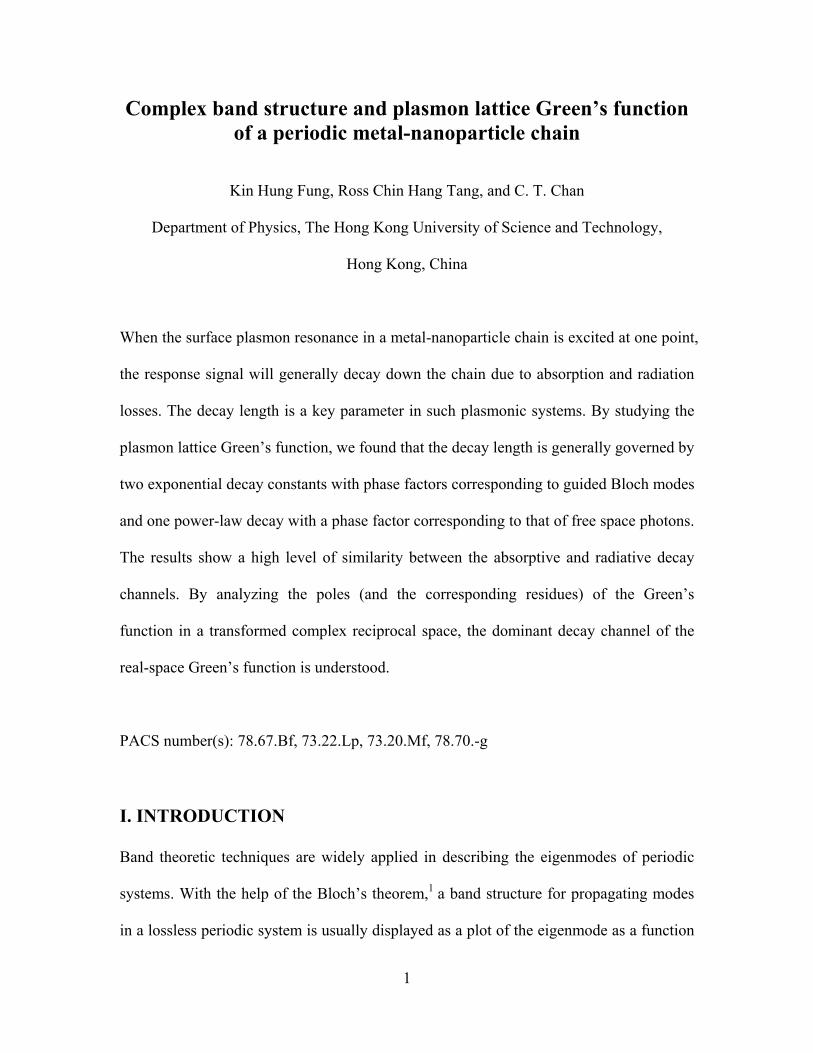
Fig. 2(a)]. In our calculations, we take N = 3001.

Here, we first briefly highlight some features of ( , )G mω . When there is no absorption

and radiation loss (i.e., γ = 0 and cω ω< ), ( , )G mω does not decay. As shown in Ref. 8,

the results are intuitively obvious and thus the results are not repeated here. However,

when the wave experience mainly absorption loss (i.e., γ = 0.02 eV and cω ω< ), the

Green’s function, ( , )G mω , has two short-range exponential decays (which dominates

8

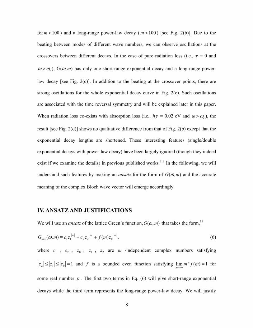
for 100m < ) and a long-range power-law decay ( 100m > ) [see Fig. 2(b)]. Due to the

beating between modes of different wave numbers, we can observe oscillations at the

crossovers between different decays. In the case of pure radiation loss (i.e., γ = 0 and

cω ω> ), ( , )G mω has only one short-range exponential decay and a long-range power-

law decay [see Fig. 2(c)]. In addition to the beating at the crossover points, there are

strong oscillations for the whole exponential decay curve in Fig. 2(c). Such oscillations

are associated with the time reversal symmetry and will be explained later in this paper.

When radiation loss co-exists with absorption loss (i.e., γ = 0.02 eV and cω ω> ), the

result [see Fig. 2(d)] shows no qualitative difference from that of Fig. 2(b) except that the

exponential decay lengths are shortened. These interesting features (single/double

exponential decays with power-law decay) have been largely ignored (though they indeed

exist if we examine the details) in previous published works.7 8 In the following, we will

understand such features by making an ansatz for the form of ( , )G mω and the accurate

meaning of the complex Bloch wave vector will emerge accordingly.

IV. ANSATZ AND JUSTIFICATIONS

We will use an ansatz of the lattice Green’s function, ),( mG ω that takes the form,19

mmmans zmfzczcmG 02211 )(),( ++≡ω , (6)

where 1c , 2c , 0z , 1z , 2z are m -independent complex numbers satisfying

1012 =≤≤ zzz and f is a bounded even function satisfying 1)(lim =∞→

mfm p

m for

some real number p . The first two terms in Eq. (6) will give short-range exponential

decays while the third term represents the long-range power-law decay. We will justify

9

the ansatz in the following, by comparing ),( mG ω and ),( mGans ω and their generating

functions in the complex number plane. By considering the generating functions, we will

get extremely accurate values of the complex quantities (including 1c , 2c , 0z , 1z , and 2z )

without using any function-fitting method.

To verify that ),( mG ω has to take the form as shown in Eq. (6), we consider the

generating function of ),( mG ω , defined as

∑∞

−∞=

≡m

mzmGzg ),(),( ωω , (7)

where z is a complex number. By multiplying mz to Eq. (4) and summing the equation

over the index m , one can show that the exact ),( zg ω reads

),(),( keg eigika ωαω = , (8)

for any complex number k by allowing analytic continuation (as in the usual definition

of the polylogorithm functions). Thus, we have a closed-from expression for ),( zg ω and

it has a one-to-one correspondence to ),( keig ωα , which is also the Green’s function in the

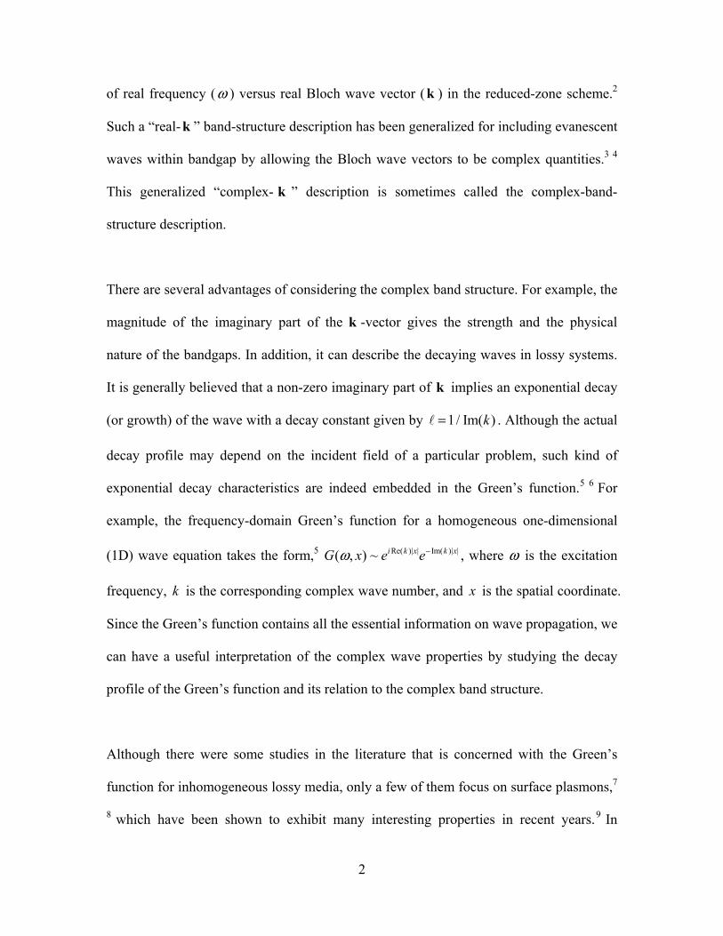
reciprocal space. To present a concrete picture, we plot ),( zg ω in the complex- z plane

(see Fig. 3) for various frequencies. From Fig. 3, we see that the exact generating

function, ),( zg ω , has 4 poles (at 1z z= , 11z− , 2z , and 1

2z − ) and two branch cuts for each

frequency. The poles are the solutions of Eq. (3) and the branch cuts, which show up as

straight line segments, are defined by, 0Arg( )z k a= for 0 1z< < and 0Arg( )z k a= − for

1z > . These branch cuts are the principle branch cuts of the polylogarithm functions.

The advantage of considering ),( zg ω as a function of z ( )ikae= instead of ),( keig ωα as

10

a function of k is that all the information are compressed within a finite unit circle,

1z ≤ , because of the mirror symmetry of the MNP chain [i.e., ),(),( 1−= zgzg ωω ]. In

Figs. 3(a) and 3(b), we see that all four poles lie on the unit circle when there is no loss,

i.e. cω ω< and 0γ = . As we increase ω (keeping 0γ = ), 1z moves towards 12z − while

2z moves towards 11z− , and all four poles remain on the unit circle. After the poles meet

at cω ω= (not shown), they leave the unit circle separately [see Fig. 3(c) and 3(d)],

keeping 1 2 1z z= < (due to radiation loss). It should be noted that we have 1 2z z ∗= (due

to time reversal symmetry) when 0γ = . When 0γ ≠ , the absorption breaks the time

reversal symmetry, leading to 1 2z z ∗≠ and smooth changes in the positions of the poles as

frequency changes [see Figs. 3(e)-3(h)]. All these results can be directly mapped into the

complex band structure and since each z can be mapped into a wave number, k , the

poles of the generating functions also give all the information required to produce the

complex band structure in Fig. 1.

Let us now consider the corresponding generating function for our ansatz Green’s

function in Eq. (6), ( , ) ( , ) mans ansm

g z G m zω ω∞

=−∞≡∑ . Using Eq. (6), we can write

1 11 1 2 2

1 2 01 11 1 2 2

( , ) ( ) m mans

m

z z z zg z c c f m z zz z z z z z z z

ω− − ∞

− −=−∞

⎛ ⎞ ⎛ ⎞= − + − +⎜ ⎟ ⎜ ⎟− − − −⎝ ⎠ ⎝ ⎠

∑ . (9)

It should be noted that, in writing Eq. (9), we have again used the analytic continuation as

in the polylogarithm functions. From Eq. (9), we see that the two short-range exponential

decays in ( , )ansG mω are associated with the four poles located at 1z z= , 11z− , 2z , and

12z − , which is consistent with ( , )g zω (as shown in Fig. 3). Here, we consider the exact

11

values of the poles and the corresponding residues of ( , )g zω . These quantities can be

found accurately as long as we have rough estimates for the poles (for example, finding

the poles from Fig. 3 by naked eye). With the estimated (and thus approximate) values of

the poles, we can calculate a simple contour integral ( , ) / 2C

R g z dz iω π= ∫ numerically

around a closed curve, C , that encloses the pole but not crossing the branch cuts. We

thus obtain the four residues (denoted by 1R , 2R , 3R , and 4R ) of ( , )g zω accordingly. It

is expected that these four residues should be consistent with that of ( , )ansg zω . By

equating the residues of ( , )g zω and ( , )ansg zω (i.e. 1 1 1R c z= , 12 1 1R c z −= − , 3 2 2R c z= ,

and 14 2 2R c z −= − ), we can solve for 1c , 2c , 1z , and 2z . The values of 1z and 2z obtained

in this way are surprisingly accurate in the sense that they pin the poles of ( , )g zω with a

relative error within 1010− even when the relative error of our initial estimated values is

about 0.1. This verifies that the form of the ansatz is essentially exact. To further make

sure that the complex quantities, 1c , 2c , 1z , and 2z , can describe the initial exponential

decays of ( , )G mω accurately, we also compare 1 1mc z and 2 2

mc z with ( , )G mω [see Figs.

2(b), 2(c), and 2(d)]. [We have 1 2c c ∗= and 1 2z z ∗= in the case without absorption loss

and thus 1 1mc z and 2 2

mc z overlap in Fig. 2(c).] The results deduced from the ansatz show

an exact agreement to ( , )G mω .

We note that in addition to the exponential decay(s), there are oscillations in the

magnitude of ( , )G mω . We mentioned that those features near the crossover points are

due to the beatings between different modes. Furthermore, there is an additional

12

oscillatory behavior for the whole range of exponential decay in the case of no absorption

because we have 1 1 2 2m mc z c z+ 1 12Re( )mc z= , which oscillates in its magnitude, when

0γ = . To verify these statements, we subtract both 1 1mc z and 2 2

mc z from ( , )G mω and

plot the remaining function, 1 1 2 2( , ) ( , ) m mremG m G m c z c zω ω≡ − − , (dashed lines) in Fig. 2.

We can see that the oscillatory features are immediately removed after the subtraction

and the remaining function is smooth in its magnitude. This is another evidence to show

that the ansatz gives the correct functional form of the Green’s function.

Finally, we have to check whether ( , )remG mω is of the form, 0( ) mf m z , with 0 1z = . The

verification of 0mz can be done by making a Fourier transform of the normalized function,

( , ) / ( , )rem remG m G mω ω . We take a finite list of ( , ) / ( , )rem remG m G mω ω for

0 1000m≤ ≤ to calculate the Fourier transform numerically and find that the Fourier

transform has only one single sharp peak located at hk k≈ (free-space wave number),

which means we have ( , ) / ( , ) hik marem remG m G m eω ω ∼ . This is consistent with fixing

0hik az e= in our ansatz. Furthermore, if 0( , ) ( ) m

remG m f m zω = , we will have

( , ) ( )remG m f mω = . We can see in the insets of Figs. 2(b)-2(d) that ( , )remG mω is a

smoothly decreasing function that behaves like 1/ pm for some constant p , manifesting

as straight lines in the log-log plots (except for 10m < ). Again, this verifies the form of

the ansatz. The long-range power-law decay has a wave number very close to that of the

free-space photons, suggesting that such portion of decaying wave is not confined within

the chain and is less related to the guided modes. The power factor, p , is found to be

13

close to 1.35, which is larger than the power factor for the Green’s function of photons in

free space.

V. DISCUSSION AND CONCLUSION

In summary, we have shown semi-analytically that the (transverse) lattice Green’s

function for a periodic metal nanoparticle chain is of the form ),( mG ω mzc 11= mzc 22+

amikhemf )(+ , which contains both exponential and power-law decays. This is

independent of whether the decay is due to radiation or absorption loss. Our results show

that a non-zero imaginary part of the Bloch wave number k in the complex band

structure only means an initial short-range exponential decay in the Green’s function for

such lossy system. There exists an additional power-law long-range decay that has no

apparent relation to the values of k of the guided mode. The existence of such power-law

region suggests that extra care must be taken when one try to obtain the decay length by

fitting the Green’s function with exponential function. Our results can be helpful in

understanding the wave propagation in lossy open systems. In addition, one interesting

and subtle feature is that there are two exponential decay constants in the transverse mode,

and it is true for frequencies that can excite guided modes or the leaky modes at the band

gap above guided mode frequencies. The existence of two (instead of one) decay

constants is due to the breaking of time reversal symmetry by absorptive dissipation. If

there is no absorption, the two decay lengths become equal, as required by time reversal

symmetry.

14

ACKNOWLEDGMENTS

This work was supported by the Central Allocation Grant from the Hong Kong RGC

through HKUST3/06C. Computation resources were supported by the Shun Hing

Education and Charity Fund. We thank Dr. Dezhuan Han, Dr. Yun Lai, and Prof.

Zhaoqing Zhang for comments and useful discussions.

15

REFERENCES

1 M. J. O. Strutt, Ann. d. Physik 85, 129 (1928); 86, 319 (1929); F. Bloch, Zeits. f. Physik

52, 555 (1928).

2 L. P. Bouckaert, R. Smoluchowski, and E. Wigner, Phys. Rev. 50, 58 (1936).

3 For photonic bands, see N. Stefanou, V. Karathanos, and A. Modinos, J. Phys.:

Condens. Matter 4, 7389 (1992) and T. Suzuki and K. L. Yu, J. Opt. Soc. Am. B 12, 804

(1995).

4 For electronic bands, see H. J. Choi and J. Ihm, Phys. Rev. B 59, 2267 (1999) and J. K.

Tomfohr and O. F. Sankey, Phys. Rev. B 65, 245105 (2002).

5 E. N. Economou, Green's Functions in Quantum Physics, 3rd ed. (Springer, Berlin,

2006).

6 P. Sheng, Introduction to Wave Scattering, Localization, and Mesoscopic Phenomena,

2nd ed. (Springer, Heidelberger, 2006).

7 W. H. Weber and G. W. Ford, Phys. Rev. B 70, 125429 (2004).

8 V. A. Markel and A. K. Sarychev, Phys. Rev. B 75, 085426 (2007).

9 See, e.g., W. L. Barnes, A. Dereux, and T. W. Ebbesen, Nature 424, 824 (2003).

10 The propagation of surface plasmon in a linear array of metal nanoparticles has been

studied experimentally in Ref. 11 and theoretically in Refs. 7, 8, 13, 14, and 15.

11 J.R. Krenn, A. Dereux, J.C. Weeber, E. Bourillot, Y. Lacroute, J.P. Goudonnet, G.

Schider, W. Gotschy, A. Leitner, F.R. Aussenegg, and C. Girard, Phys. Rev. Lett. 82,

2590 (1999); R. de Waele, A. F. Koenderink, and A. Polman, Nano Lett. 7, 2004 (2007);

A. F. Koenderink, R. de Waele, J. C. Prangsma, and A. Polman, Phys. Rev. B 76,

16

201403(R) (2007); K. B. Crozier, E. Togan, E. Simsek, and T. Yang, Opt. Express 15,

17482 (2007).

12 M. Quinten, A. Leitner, J. R. Krenn, and F. R. Aussenegg, Opt. Lett. 23, 1331 (1998);

M. L. Brongersma, J. W. Hartman, and H. A. Atwater, Phys. Rev. B 62, R16356 (2000);

Stefan A. Maier, Mark L. Brongersma, and Harry A. Atwater, Appl. Phys. Lett. 78, 16

(2001); S. Y. Park and D. Stroud, Phys. Rev. B 69, 125418 (2004); D. S. Citrin, Nano

Lett. 4, 1561 (2004); R. A. Shore and A. D. Yaghjian, Electron. Lett. 41, 578 (2005); J. J.

Xiao, K. Yakubo, and K. W. Yu, Appl. Phys. Lett. 88, 241111 (2006); A. F. Koenderink

and A. Polman, Phys. Rev. B 74, 033402 (2006); A. A. Govyadinov and V. A. Markel,

Phys. Rev. B 78, 035403 (2008); H. X. Zhang, Y. Gu, and Q. H. Gong, Chinese Phys. B

17, 2567 (2008).

13 C. R. Simovski, A. J. Viitanen, and S. A. Tretyakov, Phys. Rev. E 72, 066606 (2005).

14 A. Alù and N. Engheta, Phys. Rev. B 74, 205436 (2006).

15 K. H. Fung and C. T. Chan, Opt. Lett. 32, 973 (2007).

16 C. F. Bohren and D. R. Huffman, Absorption and Scattering of Light by Small

Particles (Wiley, New York, 1983).

17 V. A. Markel, J. Opt. Soc. Am. B 12, 1783 (1995).

18 The ),( keig ωα defined here is the same as the eigenpolarizability defined in Ref. 15.

19 The frequency dependence of every quantity (except m ) on the right-hand side of Eq.

(6) is not notated for the sake of a tidy expression.

17

FIG. 1: (Color online) Complex band structure for a 1D array of MNPs. Left (right)

panel show the real (imaginary) part of the wave number. The numbers inside the

square boxes indicate different non-degenerate modes when absorption is included.

18

FIG. 2: (Color online) Lattice Green’s function ( , )G mω . Panel (a) shows a

schematic diagram with a dipole source located at the center of the MNP chain.

Other panels show the values of ( , )G mω and the comparisons with the functions

making up the ansatz for the case when energy loss is (b) dominated by absorption

( ω = 3.260 eV and γ = 0.02 eV), (c) purely due to radiation ( ω = 3.275 eV and

γ = 0), and (d) contributed fairly by absorption and radiation ( ω = 3.275 eV and

γ = 0.02 eV), respectively. The insets show the same graphs but in log-log scale,

highlighting the long-range power law decay. Numbers with square boxes indicate

the corresponding plasmon modes shown in Fig. 1.

19

FIG. 3: (Color online) Contour plot of 30( , ) /g z rω at different frequencies. The

poles at 1z z= , 2z , 11z− , and 1

2z − of the function are labeled. Upper (lower) panels

show the results for the lossless (lossy) metal with γ = 0 ( γ = 0.02 eV). (a) and (e)

ω = 3.260 eV. (b) and (f) ω = 3.270 eV. (c) and (g) ω = 3.275 eV. (d) and (h)

ω = 3.280 eV.