ARTICLE IN PRESS

Engineering Analysis with Boundary Elements 33 (2009) 778–788

Contents lists available at ScienceDirect

Engineering Analysis with Boundary Elements

0955-79

doi:10.1

� Corr

E-m

URL

journal homepage: www.elsevier.com/locate/enganabound

Numerical Green’s functions for some electroelastic crack problems

L. Athanasius, W.T. Ang �, I. Sridhar

School of Mechanical and Aerospace Engineering, Nanyang Technological University, Republic of Singapore

a r t i c l e i n f o

Article history:

Received 7 October 2008

Accepted 15 January 2009Available online 23 February 2009

Keywords:

Numerical Green’s function

Boundary element method

Cracks

Piezoelectric solid

97/$ - see front matter & 2008 Elsevier Ltd. A

016/j.enganabound.2009.01.002

esponding author.

ail address: mwtang@ntu.edu.sg (W.T. Ang).

: http://www.ntu.edu.sg/home/mwtang (W.T.

a b s t r a c t

A plane electroelastic problem involving planar cracks in a piezoelectric body is considered. The

deformation of the body is assumed to be independent of time and one of the Cartesian coordinates. The

cracks are traction free and are electrically either permeable or impermeable. Numerical Green’s

functions which satisfy the boundary conditions on the cracks are derived using the hypersingular

integral approach and applied to obtain a boundary integral solution for the electroelastic crack

problem considered here. As the conditions on the cracks are built into the Green’s functions, the

boundary integral solution does not contain integrals over the cracks. It is used to derive a boundary

element procedure for computing the crack tip stress and electrical displacement intensity factors.

& 2008 Elsevier Ltd. All rights reserved.

1. Introduction

A well-established boundary element approach for solvingcrack problems is to use special Green’s functions (modifiedfundamental solutions) chosen to satisfy the boundary conditionson the cracks. With an appropriate Green’s function, the boundaryintegral formulation of the crack problem under considerationdoes not require integration over the crack faces. Consequently,difficulties associated with modeling the crack faces, such assingular stress at the crack tips and degenerate systems of linearalgebraic equations, may be neatly avoided.

Such an approach for solving crack problems numerically waspioneered by Snyder and Cruse [22] when they derived ananalytical Green’s function for a single planar crack in anorthotropic elastic space of infinite extent. Subsequently, Clem-ents and Haselgrove [10] extended the work in [22] to a generalanisotropic elastic space, and Ang and Clements [4] furthermodified the Green’s function to include the case of a fully closedplanar crack. Special Green’s functions for a planar crack and anarc crack in an isotropic elastic space were derived by Ang [2,3],respectively.

In general, it is difficult (if not impossible) to derive Green’sfunctions analytically for cracks with arbitrary geometries,configurations and boundary conditions. To solve a wider rangeof crack problems, Telles et al. [23] proposed to derive therequired Green’s function numerically based on the hypersingularintegral formulation of a suitable crack problem (see also [15]).(For some details on the hypersingular approach, one may refer to,

ll rights reserved.

Ang).

for example, [8].) More recently, Ang and Telles [6] extended thenumerical Green’s function approach in [23] to solve an elasto-static problem involving multiple interacting planar cracks in ananisotropic body.

During the last 10 years or so, there has been considerableinterest in the development of the boundary element method forfracture analysis of piezoelectric materials. Using Lekhnitskii’sformalism and dislocation modeling, Rajapakse and Xu [20]obtained an analytical Green’s function for a single traction freeand electrically impermeable crack in a piezoelectric space. Morerecently, Garcia-Sanchez et al. [13] and Groh and Kuna [14]presented boundary element procedures based on boundaryintegral equations derived by using fundamental solution whichdoes not satisfy the boundary conditions on the crack faces. In[14], opposite crack faces were modeled by using the so-calledsubdomain technique and quarter-point elements were employedto deal with the singular behaviors of the stress and electricdisplacement at the crack tips, while a dual (mixed) boundaryintegral formulation was used in [13] with the conditions on thecracks treated by a differentiated form of the usual boundaryintegral equations. Earlier works on boundary element methodsfor electroelastic crack problems include Xu and Rajapakse [25],Ding et al. [11] and Gao and Fan [12].

In the present paper, using the hypersingular integralapproach, we derive numerical Green’s functions for an arbitrarynumber of arbitrarily located planar cracks in an infinite piezo-electric space. The Green’s functions are chosen to satisfyparticular electroelastic boundary conditions on the cracks.Specifically, the boundary conditions are such that the cracksare traction free and electrically either permeable or imperme-able. The analysis in Ang and Telles [6], based on the Stroh’sformalism for anisotropic elasticity, serves as a useful guidehere for the derivation of the numerical Green’s functions, as

ARTICLE IN PRESS

L. Athanasius et al. / Engineering Analysis with Boundary Elements 33 (2009) 778–788 779

piezoelectric materials exhibit anisotropic behaviors when theydeform. With the use of the special Green’s functions, a boundaryintegral solution which does not require integration over the crackfaces is obtained for a plane electroelastic problem involvingplanar cracks in a piezoelectric body. A simple boundary elementprocedure is outlined for the numerical solution of the crackproblem. The displacement and electric potential jumps acrossopposite crack faces as well as the crack tip stress and electricdisplacement intensity factors may be readily and accuratelycomputed once the elastic displacements, tractions, electricpotential and electric displacement are all known on theboundary. To check the validity of the numerical Green’sfunctions, the boundary element procedure is applied to solvesome specific problems.

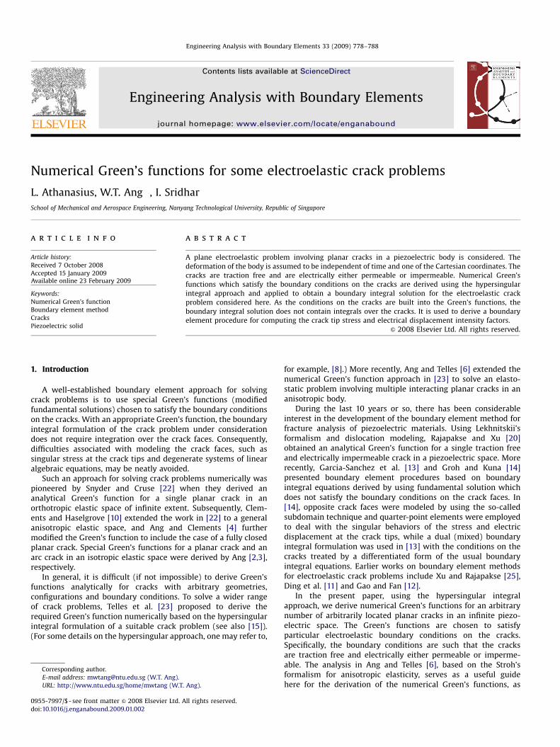
2. An electroelastic crack problem

With reference to a Cartesian co-ordinate frame denoted by0x1x2x3; consider a homogeneous piezoelectric solid whichcontains M arbitrarily orientated planar cracks. The geometriesof the solid and the cracks do not change along the x3 direction.The interior of the solid is denoted by R, the exterior boundary byB and the k-th crack by gðkÞ. It is assumed that the cracks do notintersect with one another or the exterior boundary B. On theplane x3 ¼ 0, the boundary B appears as a simple closed curve andthe crack gðkÞ as a straight cut with tips ðaðkÞ; bðkÞÞ and ðcðkÞ; dðkÞÞ.Refer to Fig. 1. For the purpose of the present paper, gðkÞ is taken tobe the directed straight line segment from ðaðkÞ; bðkÞÞ to ðcðkÞ; dðkÞÞ.

At each and every point on the boundary B, either thedisplacements or the tractions and either the electric potentialor the electric flux are prescribed. The prescribed conditions on B

are independent of the spatial coordinate x3 and time t and aresuch that the cracks become traction free. For the electricalconditions on the cracks, we consider separately two extremecases: (a) electrically impermeable cracks and (b) electricallypermeable cracks. Some discussions on electrically impermeablecracks versus permeable ones may be found in, for example,Shindo et al. [21] and Wang and Mai [24].

Mathematically, the boundary conditions on the cracks aregiven by

sijðx1; x2ÞmðkÞj ! 0 as ðx1; x2Þ ! ðy1; y2Þ 2 gðkÞ for k ¼ 1;2; . . . ;M,

(1)

x2 [n1, n2]

B

( c (k) , d (k))

γ (k)

( a (k) , b (k) )

R

0 x1

Fig. 1. A geometrical sketch of the problem.

and either

Djðx1; x2ÞmðkÞj ! 0 as ðx1; x2Þ ! ðy1; y2Þ 2 gðkÞ for k ¼ 1;2; . . . ;M

if the cracks are electrically impermeable, (2)

or

Dfðx1; x2Þ ! 0 and DDðx1; x2Þ ! 0 as ðx1; x2Þ ! ðy1; y2Þ 2 gðkÞ

for k ¼ 1;2; . . . ;M if the cracks are electricallypermeable, (3)

where sij and Di are, respectively, the stresses and the electricdisplacements, ½mðkÞ1 ;mðkÞ2 ;mðkÞ3 � ¼ ½ðd

ðkÞ� bðkÞÞ=‘ðkÞ; ðaðkÞ � cðkÞÞ=‘ðkÞ;0�

is a unit normal vector to the crack gðkÞ, ‘ðkÞ is the length of gðkÞ

(that is, ‘ðkÞ ¼ffiffiffiffiffiffiffiffiffiffiffiffiffiffiffiffiffiffiffiffiffiffiffiffiffiffiffiffiffiffiffiffiffiffiffiffiffiffiffiffiffiffiffiffiffiffiffiffiffiffiffiffiffiffiffiffiðdðkÞ � bðkÞÞ2 þ ðaðkÞ � cðkÞÞ2

q) and Df is the jump in

the electric potential f across opposite crack faces as defined by

Dfðx1; x2Þ ¼ lime!0½fðx1 � jejmðkÞ1 ; x2 � jejmðkÞ2 Þ

�fðx1 þ jejmðkÞ1 ; x2 þ jejmðkÞ2 Þ� for ðx1; x2Þ 2 gðkÞ, (4)

and DD is defined by

DDðx1; x2Þ ¼ lime!0½Djðx1 � jejmðkÞ1 ; x2 � jejmðkÞ2 Þ

� Djðx1 þ jejmðkÞ1 ; x2 þ jejmðkÞ2 Þ�mðkÞj

for ðx1; x2Þ 2 gðkÞ. (5)

To allow for antiplane deformations (that is, the case in whichu3a0), lowercase latin subscripts take the values of 1, 2 and 3. Theusual Einsteinian convention of summing a repeated index isassumed for lowercase latin subscripts. In general, the summation

over a repeated lowercase latin subscript (such as the subscript k

in (6) and (7)) runs from 1 to 3. Nevertheless, for some cases,the summation may run from 1 to 2 only. For example, the

summation over j in (1) and (2) is from 1 to 2 only as mðkÞ3 ¼ 0,

and so is the summation over j and p in (6) and (7) since thedisplacements uk are independent of x3.

The problem is to determine the displacements uk and theelectric potential f throughout the cracked piezoelectric solid.

3. Equations of electroelasticity

The governing equations for the displacements uk and theelectric potential f in the piezoelectric solid are given by

cijkpq2uk

qxjqxpþ epij

q2fqxjqxp

¼ 0,

ejkpq2uk

qxjqxp� kjp

q2fqxjqxp

¼ 0, (6)

where cijkp, epij and kjp are the constant elastic moduli, piezo-electric coefficients and dielectric coefficients, respectively.

The constitutive equations relating ðsij;DjÞ and ðuk;fÞ are givenby

sij ¼ cijkpquk

qxpþ epij

qfqxp

,

Dj ¼ ejkpquk

qxp� kjp

qfqxp

. (7)

Following closely the approach of Barnett and Lothe [7], we let

UJ ¼uj for J ¼ j ¼ 1;2;3;

f for J ¼ 4;

(

SIj ¼

sij for I ¼ i ¼ 1;2;3;

Dj for I ¼ 4;

(

ARTICLE IN PRESS

L. Athanasius et al. / Engineering Analysis with Boundary Elements 33 (2009) 778–788780

CIjKp ¼

cijkp for I ¼ i ¼ 1;2;3 and K ¼ k ¼ 1;2;3;

epij for I ¼ i ¼ 1;2;3 and K ¼ 4;

ejkp for I ¼ 4 and K ¼ k ¼ 1;2;3;

�kjp for I ¼ 4 and K ¼ 4;

8>>>><>>>>:

(8)

so that (6) and (7) may be written more compactly as

CIjKpq2UK

qxjqxp¼ 0 (9)

and

SIj ¼ CIjKpqUK

qxp, (10)

respectively. Note that uppercase latin subscripts have values 1–4.Summation is also implied for repeated uppercase latin subscriptsrunning from 1 to 4.

The general solution of (9) can be written as

UK ðx1; x2Þ ¼ ReX4

a¼1

AKaf aðzaÞ

( ), (11)

where Re denotes the real part of a complex number, f a areanalytic functions of za ¼ x1 þ tax2 in the domain of interest, taare the solutions, with positive imaginary parts, of the 8-th orderpolynomial (characteristic) equation

det½CI1K1 þ ðCI1K2 þ CI2K1Þtþ CI2K2t2� ¼ 0 (12)

and AKa are solutions of the homogeneous system

½CI1K1 þ ðCI1K2 þ CI2K1Þta þ CI2K2t2a�AKa ¼ 0. (13)

The characteristic equation (12) admits solutions which occur incomplex conjugate pairs [7]. It is assumed that we can find t1, t2,t3 and t4 such that an invertible 4� 4 matrix ½AKa� can beconstructed from (13).

The generalized stress functions SIj corresponding to (11) aregiven by

SIj ¼ ReX4

a¼1

LIjaf 0aðzaÞ

( ), (14)

where the prime denotes differentiation with respect to therelevant argument and

LIja ¼ ðCIjK1 þ taCIjK2ÞAKa. (15)

4. Numerical Green’s functions

For the crack problem stated in Section 2, we seek to derive afunction FKSðx1; x2; x1; x2Þ satisfying the system of partial differ-ential equations

CIjKpq2FKS

qxjqxp¼ dISdðx1 � x1; x2 � x2Þ, (16)

and the conditions on the cracks given by either

CIjSðx1; x2; x1; x2ÞmðkÞj ! 0 as ðx1; x2Þ ! ðy1; y2Þ 2 gðkÞ

for I ¼ 1;2;3;4 and k ¼ 1;2; . . . ;M

if the cracks are electrically impermeable (17)

or

CIjSðx1; x2; x1; x2ÞmðkÞj ! 0; Df4Sðx1; x2; x1;x2Þ ! 0

and DCSðx1; x2; x1; x2Þ ! 0 as ðx1; x2Þ ! ðy1; y2Þ 2 gðkÞ

for I ¼ i ¼ 1;2;3 and k ¼ 1;2; . . . ;M

if the cracks are electrically permeable, (18)

where dIS is the Kronecker-delta, d is the Dirac-delta function, CIjS

and DCS are defined by

CIjSðx1; x2; x1;x2Þ ¼ CIjRpqFRS

qxp,

DCSðx1; x2; x1;x2Þ ¼ lime!0½C4jSðx1 � jejmðkÞ1 ; x2 � jejmðkÞ2 ; x1; x2Þ

�C4jSðx1 þ jejmðkÞ1 ; x2 þ jejmðkÞ2 ; x1; x2Þ�mðkÞj

for ðx1; x2Þ 2 gðkÞ, (19)

and Df4S denotes the jump of F4S across opposite crack faces asdefined in (26).

Let FRSðx1; x2; x1; x2Þ be given by

FRSðx1; x2; x1; x2Þ ¼ F½1�RSðx1; x2; x1; x2Þ þF½2�RSðx1; x2; x1; x2Þ, (20)

F½1�RSðx1; x; x1; x2Þ ¼1

2pReX4

a¼1

fARaNaJ lnð½x1 � x1� þ ta½x2 � x2�ÞgdJS,

(21)

where ½NaJ � is the inverse of ½AKa�, dJS are real constants defined by

ImX4

a¼1

LI2aNaR

( )dRJ ¼ dIJ . (22)

Note that Im denotes the imaginary part of a complex number.The function F½1�RSðx1; x2; x1; x2Þ in (21) is a solution of (16) (see,

for example, [9]). It follows that F½2�RSðx1; x2; x1; x2Þ is required tosatisfy

cIjKp

q2F½2�KS

qxjqxp¼ 0 (23)

everywhere in the infinite piezoelectric space with the cracks gð1Þ,gð2Þ; . . . ; gðM�1Þ and gðMÞ.

Guided by the analysis in Ang and Park [5] and Ang and Telles[6], we take

F½2�RSðx1; x2; x1; x2Þ ¼XMk¼1

ZgðkÞ

DfPSðy1; y2; x1; x2Þ

�LðkÞPR ðx1; x2; y1; y2Þdsðy1; y2Þ, (24)

where

LðkÞIS ðx1; x2; y1; y2Þ ¼ �1

2pReX4

a¼1

TIjaSmðkÞj

½x1 � y1� þ ta½x2 � y2�

( ),

TIjaS ¼ LIjaNaRdRS, (25)

and

DfPSðx1; x2; x1; x2Þ ¼ lime!0½FPSðx1 � jejmðkÞ1 ; x2 � jejmðkÞ2 ;x1; x2Þ

�FPSðx1 þ jejmðkÞ1 ; x2 þ jejmðkÞ2 ; x1; x2Þ�

for ðx1; x2Þ 2 gðkÞ.(26)

Note that the integration over gðkÞ in (24) is one over a directedstraight line segment from ðaðkÞ; bðkÞÞ to ðcðkÞ; dðkÞÞ. It is assumed thatðx1; x2Þ does not lie on any of the cracks. The system in (23) issatisfied by (24).

4.1. Electrically impermeable cracks

Conditions (17) on the electrically impermeable cracks requirethat

CIjRpqF½2�RS

qxpmðkÞj ! LðkÞIS ðx1; x2; x1; x2Þ

as ðx1; x2Þ ! ðy1; y2Þ 2 gðkÞ for k ¼ 1;2; . . . ;M. (27)

ARTICLE IN PRESS

L. Athanasius et al. / Engineering Analysis with Boundary Elements 33 (2009) 778–788 781

From (24), conditions (27) for electrically impermeable cracksgive rise to the system of hypersingular integral equations

H

Z 1

�1

wðqÞPKDfðqÞPS ðv; x1;x2Þdv

ðt � vÞ2þXMn¼1naq

Z 1

�1DfðnÞPS ðv; x1;x2ÞY

ðnqÞPK ðv; tÞdv

¼ LðqÞKS ðXðqÞ1 ðtÞ;X

ðqÞ2 ðtÞ; x1; x2Þ

for � 1oto1; K ¼ 1;2;3;4; S ¼ 1;2;3;4 and q ¼ 1;2; . . . ;M,(28)

where H indicates that the integral is to be interpreted in theHadamard finite-part sense and

DfðnÞPS ðv; x1; x2Þ ¼ DfPSðXðnÞ1 ðvÞ;X

ðnÞ2 ðvÞ; x1; x2Þ,

wðqÞPK ¼1

pReX4

a¼1

‘ðqÞQPKrjamðqÞr mðqÞj

½ðcðqÞ � aðqÞÞ þ taðdðqÞ � bðqÞÞ�2

( ),

Y ðnqÞPK ðv; tÞ ¼

1

4pReX4

a¼1

‘ðnÞQPKrjamðqÞr mðnÞj

½XðnqÞðv; tÞ þ taYðnqÞ

ðv; tÞ�2

( ), (29)

where QPKrja ¼ ðcKrI1 þ tacKrI2ÞTPjaI , XðnqÞðv; tÞ ¼ XðnÞ1 ðvÞ � XðqÞ1 ðtÞ,

YðnqÞðv; tÞ ¼ XðnÞ2 ðvÞ � XðqÞ2 ðtÞ, 2XðnÞ1 ðtÞ ¼ ½c

ðnÞ þ aðnÞ� þ ½cðnÞ � aðnÞ�t and2XðnÞ2 ðtÞ ¼ ½d

ðnÞþ bðnÞ� þ ½dðnÞ � bðnÞ�t.

The method in Kaya and Erdogan [17] is chosen to solve (28)numerically for DfðnÞPS ðv; x1; x2Þ. Let DFðnÞPS ðv; x1; x2Þ be givenapproximately by

DfðnÞPS ðv; x1; x2Þ ’ffiffiffiffiffiffiffiffiffiffiffiffiffiffi1� v2

p XJ

j¼1

fðnjÞPS ðx1; x2ÞU

ðj�1ÞðvÞ, (30)

where UðjÞðxÞ ¼ sinð½jþ 1� arccosðxÞÞ= sinðarccosðxÞÞ ð�1oxo1Þ isthe j-th order Chebyshev polynomial of the second kind andfðnjÞ

PS ðx1; x2Þ are parameters to be determined.Through substituting (30) into (28) and collocating (28) by

letting t ¼ tðiÞ � cosð½2i� 1�p=½2J�Þ for i ¼ 1;2; . . . ; J, a system oflinear algebraic equations containing the unknowns fðniÞ

PS ðx1; x2Þ

can be obtained as follows:

�XJ

j¼1

jpfðqjÞPS ðx1; x2Þw

ðqÞPK Uðj�1Þ

ðtðiÞÞ

þXJ

j¼1

XMn¼1naq

fðnjÞPS ðx1; x2Þ

Z 1

�1

ffiffiffiffiffiffiffiffiffiffiffiffiffiffi1� v2

pUðj�1Þ

ðvÞY ðnqÞPK ðv; t

ðiÞÞdv

¼ LðqÞKS ðXðqÞ1 ðt

ðiÞÞ;XðqÞ2 ðtðiÞÞ; x1; x2Þ

for i ¼ 1;2; . . . ; J; K ¼ 1;2;3;4; S ¼ 1;2;3;4 and q ¼ 1;2; . . . ;M.

(31)

Once fðniÞPS ðx1;x2Þ are determined from (31), F½2�RSðx1; x2;x1; x2Þ can

be calculated approximately using

F½2�RSðx1; x2; x1; x2Þ ’1

2

XMn¼1

‘ðnÞXJ

j¼1

fðnjÞPS ðx1; x2Þ

Z 1

�1

ffiffiffiffiffiffiffiffiffiffiffiffiffi1� t2

p

� Uðj�1ÞðtÞLðnÞPR ðx1; x2;X

ðnÞ1 ðtÞ;X

ðnÞ2 ðtÞÞdt. (32)

If the points ðx1; x2Þ and ðx1; x2Þ do not lie on any of the cracks,the numerical evaluation of F½2�RSðx1; x2; x1; x2Þ as given by (32) doesnot pose any mathematical difficulties. The definite integrals overthe interval ½�1;1� in (31) and (32) can be easily and accuratelycomputed by using the numerical quadrature formula (25.4.40)listed in Abramowitz and Stegun [1].

Note that in (31) the coefficient of the unknown fðqjÞPS ðx1; x2Þ is

independent of the uppercase latin subscript S and the point ðx1; x2Þ.Thus, in solving (31) to determine fðqjÞ

PS ðx1;x2Þ for different values ofthe subscript S and for different points ðx1; x2Þ, the square matrixcontaining the coefficients of the unknowns has to be computed andprocessed only once. For example, if the LU decomposition techniquetogether with backward substitutions is used to solve (31), we haveto decompose the square matrix only once.

4.2. Electrically permeable cracks

Conditions (18) for electrically permeable cracks require thehypersingular integral equations (28) to be modified by takingDfðnÞ4S ðv;x1; x2Þ ¼ 0 and replacing K ¼ 1;2;3;4 with K ¼ k ¼ 1;2;3.Consequently, if the cracks are electrically permeable,

F½2�RSðx1; x2; x1; x2Þ can still be computed by using (32) but with

fðnjÞ4S ðx1; x2Þ ¼ 0. The remaining functions fðnjÞ

1S ðx1; x2Þ, fðnjÞ2S ðx1; x2Þ

and fðnjÞ3S ðx1; x2Þ required by (32) for computing F½2�RSðx1; x2; x1; x2Þ

are to be determined by solving (31) (with fðnjÞ4S ðx1; x2Þ ¼ 0) for

K ¼ k ¼ 1;2;3 (instead of K ¼ 1;2;3;4Þ.

5. A boundary element procedure

If Green’s function FIK ðx1; x2; x1; x2Þ satisfying either (17) or(18) (depending on the electrical boundary conditions on thecracks), as given in Section 4 is used, a direct boundary integralformulation for the crack problem in Section 2 is given by

lðx1; x2ÞUK ðx1; x2Þ ¼

ZB½UIðx1; x2ÞGIK ðx1; x2; x1; x2Þ

� PIðx1; x2ÞFIK ðx1; x2; x1; x2Þ�dsðx1; x2Þ, (33)

where lðx1; x2Þ ¼ 1 if ðx1; x2Þ lies in the interior of R and lðx1; x2Þ ¼12 if ðx1; x2Þ lies on a smooth part of B, PIðx1; x2Þ ¼ SIjðx1; x2Þnjðx1; x2Þ,nj are the components of the unit normal vector to the boundary B

(as shown in Fig. 1) and

GIK ðx1; x2; x1;x2Þ ¼ CIjRsnjðx1; x2Þqqxs½FRK ðx1; x2; x1; x2Þ�.

Note that the path of integration in (33) is over only the exteriorboundary B of the piezoelectric solid. To see how the boundaryintegral equations for system (9) may be derived, one may refer toClements [9].

From the boundary conditions on the exterior boundary B,either UI ¼ ui or PI ¼ pi for I ¼ i ¼ 1;2;3, and either U4 ¼ f or P4

are known at each and every point on B. The boundary B and theintegral equations in (33) can be discretized to determineapproximately the unknown generalized displacements UI

and/or tractions PI on B. To do this, the boundary B isapproximated using N straight line segments denoted by Bð1Þ,Bð2Þ; . . . ; BðN�1Þ and BðNÞ. Across the segment BðmÞ, the displacementsUI and the tractions PI are approximated by constants UðmÞI andPðmÞI , respectively. Through approximating (33), the unknownconstants on the boundary elements UðmÞI and/or tractions PðmÞI

can be determined from the system of linear algebraic equations:

1

2UðmÞK ¼

XN

n¼1

UðnÞI

ZBðnÞ

GIK ðx1; x2; xðmÞ1 ; xðmÞ2 Þdsðx1; x2Þ

�XN

n¼1

PðnÞI

ZBðnÞ

FIK ðx1; x2; xðmÞ1 ; xðmÞ2 Þdsðx1; x2Þ

for m ¼ 1;2; . . . ;N, (34)

where ðxðmÞ1 ; xðmÞ2 Þ is the midpoint of BðmÞ.Once UðmÞI and PðmÞI are all determined, the generalized

displacements UK (and hence the stresses SIj) at any interiorpoint ðx1; x2Þ in R can be computed approximately using

UK ðx1; x2Þ ¼XN

n¼1

UðnÞI

ZBðnÞ

GIK ðx1; x2;x1; x2Þdsðx1; x2Þ

�XN

n¼1

PðnÞI

ZBðnÞ

FIK ðx1; x2; x1; x2Þdsðx1; x2Þ. (35)

ARTICLE IN PRESS

L. Athanasius et al. / Engineering Analysis with Boundary Elements 33 (2009) 778–788782

The crack displacement jumps DUK ðx1; x2Þ defined by

DUK ðx1; x2Þ ¼ lime!0½UK ðx1 � jejmðkÞ1 ; x2 � jejmðkÞ2 Þ

� UK ðx1 þ jejmðkÞ1 ; x2 þ jejmðkÞ2 Þ�

for ðx1; x2Þ 2 gðkÞ (36)

can also be computed as explained below when UðmÞI and PðmÞI areall known.

5.1. Electrically impermeable cracks

If the cracks are electrically impermeable then DUK ðx1; x2Þ canbe determined by solving the hypersingular integral equations(see [6]):

H

Z 1

�1

wðqÞPKDUðqÞP ðvÞdv

ðt � vÞ2þXMn¼1naq

Z 1

�1DUðnÞP ðvÞY

ðnqÞPK ðv; tÞdv ¼ SðqÞK ðtÞ

for� 1oto1; K ¼ 1;2;3;4 and q ¼ 1;2; . . . ;M, (37)

where DUðqÞP ðvÞ ð�1ovo1Þ is a function that gives DUPðx1; x2Þ atthe point ðXðqÞ1 ðvÞ;X

ðqÞ2 ðvÞÞ of the crack gðqÞ, and

SðqÞK ðtÞ ¼XN

n¼1

CKjRsmðqÞj

�

ZBðnÞ�UðnÞI

qqxs½G½1�IR ðx1; x2; x1; x2Þ�

����ðx1 ;x2Þ¼ðX

ðqÞ1ðtÞ;XðqÞ

2ðtÞÞ

(

þPðnÞI

qqxs½F½1�IR ðx1; x2; x1; x2Þ�

����ðx1 ;x2Þ¼ðX

ðqÞ1ðtÞ;XðqÞ

2ðtÞÞ

)dsðx1; x2Þ.

(38)

Note that (37) is derived using the boundary conditions in (1) and(2) and SðqÞK ðtÞ is regarded as known after (34) is solved.

The system in (37) can be solved numerically using the samemethod for (28). The unknown functions DUðnÞP ðvÞ are approxi-mated using

DUðnÞP ðvÞ ’ffiffiffiffiffiffiffiffiffiffiffiffiffiffi1� v2

p XJ

j¼1

cðnjÞP Uðj�1Þ

ðvÞ, (39)

where cðnjÞP are constants determined by the system of linear

algebraic equations

�XJ

j¼1

jpcðqjÞP wðqÞPK Uðj�1Þ

ðtðiÞÞ

þXJ

j¼1

XMn¼1naq

cðnjÞP

Z 1

�1

ffiffiffiffiffiffiffiffiffiffiffiffiffiffi1� v2

pUðj�1Þ

ðvÞY ðnqÞPK ðv; t

ðiÞÞdv

¼ SðqÞK ðtðiÞÞ for i ¼ 1;2; . . . ; J;K ¼ 1;2;3;4 and q ¼ 1;2; . . . ;M,

(40)

where tðiÞ ¼ cosð½2i� 1�p=½2J�Þ as in (31).Note that the unknown cðqjÞ

p in (40) has the same coefficient asfðqjÞ

PS ðx1; x2Þ in (31). Thus, in solving (40) for the unknowns cðqjÞP , it

is not necessary to set up and process again the matrix containingthe coefficients of the unknowns.

Once the unknowns cðqjÞP are determined, DUK ðx1; x2Þ can be

approximately computed using (39) and crack parameters ofpractical interest, such as the stress and electric displacementintensity factors, can also be extracted.

5.2. Electrically permeable cracks

If the cracks are electrically permeable then (37) has to bemodified by setting DUðnÞ4 ðvÞ ¼ 0 and replacing K ¼ 1;2;3;4 by

K ¼ k ¼ 1;2;3. It follows that we can solve (40), with cðqjÞ4 ¼ 0 and

K ¼ k ¼ 1;2;3, for cðqjÞ1 , cðqjÞ

2 and cðqjÞ3 in order to determine

DUðnÞ1 ðvÞ, DUðnÞ2 ðvÞ and DUðnÞ3 ðvÞ.

6. Specific problems

In this section, the boundary element procedure together withthe numerical Green’s functions above is applied to solve somespecific problems involving a particular piezoelectric material.The piezoelectric material is such that it becomes elasticallytransversely isotropic under the action of the electric field, withthe transverse plane being perpendicular to the electrical polingdirection. The electroelastic properties of such a material arecharacterized by 10 independent constants denoted here by A, N,F, C, L, e1, e2, e3, �1 and �2.

Problem 1. The exterior boundary of the solution domain R (onthe plane x3 ¼ 0) is taken to be the sides of a square with verticesðh;hÞ, ð�h;hÞ, ð�h;�hÞ and ðh;�hÞ. The interior of R contains asingle electrically impermeable crack which occupies the region�aox1oa, x2 ¼ 0, where h and a are positive constants such thataoh. Here we take the crack tips to be ðað1Þ; bð1ÞÞ ¼ ð�a;0Þ andðcð1Þ; dð1ÞÞ ¼ ða;0Þ.

The electrical poling direction is taken to be along the x2

direction with the constitutive equations given by

s11

s22

s33

s32

s31

s12

0BBBBBBBBBBB@

1CCCCCCCCCCCA¼

A F N 0 0 0

F C F 0 0 0

N F A 0 0 0

0 0 0 L 0 0

0 0 0 0 12 ðA� NÞ 0

0 0 0 0 0 L

0BBBBBBBBBBB@

1CCCCCCCCCCCA

g11

g22

g33

2g32

2g31

2g12

0BBBBBBBBBBB@

1CCCCCCCCCCCA

�

0 e2 0

0 e3 0

0 e2 0

0 0 e1

0 0 0

e1 0 0

0BBBBBBBBBBB@

1CCCCCCCCCCCA

E1

E2

E3

0BB@

1CCA (41)

and

D1

D2

D3

0BB@

1CCA ¼

0 0 0 0 0 e1

e2 e3 e2 0 0 0

0 0 0 e1 0 0

0BB@

1CCA

g11

g22

g33

2g32

2g31

2g12

0BBBBBBBBBBB@

1CCCCCCCCCCCA

þ

�1 0 0

0 �2 0

0 0 �1

0BB@

1CCA

E1

E2

E3

0BB@

1CCA, (42)

where 2gkj ¼ quk=qxj þ quj=qxk and Ek ¼ �qf=qxk. Note that g33 ¼

0 and E3 ¼ 0 here since uk and f are independent of x3.

ARTICLE IN PRESS

L. Athanasius et al. / Engineering Analysis with Boundary Elements 33 (2009) 778–788 783

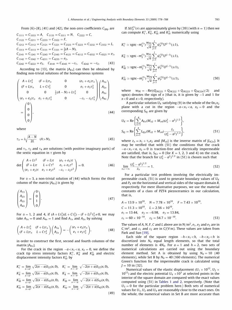
From (6)–(8), (41) and (42), the non-zero coefficients CIjKp are

C1111 ¼ C3333 ¼ A; C1133 ¼ C3311 ¼ N; C2222 ¼ C,

C1122 ¼ C2211 ¼ C2233 ¼ C3322 ¼ F,

C1212 ¼ C2112 ¼ C2121 ¼ C1221 ¼ C2323 ¼ C3223 ¼ C3232 ¼ C2332 ¼ L,

C1313 ¼ C3113 ¼ C3131 ¼ C1331 ¼12ðA� NÞ,

C2141 ¼ C1241 ¼ C3243 ¼ C2343 ¼ C4121 ¼ C4112 ¼ C4332 ¼ C4323 ¼ e1,

C1142 ¼ C3342 ¼ C4211 ¼ C4233 ¼ e2,

C2242 ¼ C4222 ¼ e3; C4141 ¼ C4343 ¼ ��1; C4242 ¼ ��2. (43)

According to (13), the matrix ½AKa� can then be obtained byfinding non-trivial solutions of the homogeneous systems

Aþ Lt2a ðF þ LÞta 0 ðe1 þ e2Þta

ðF þ LÞta Lþ Ct2a 0 e1 þ e3t2

a

0 0 12 ðA� NÞ þ Lt2

a 0

ðe1 þ e2Þta e1 þ e3t2a 0 ��1 � �2t2

a

0BBBBBB@

1CCCCCCA

A1a

A2a

A3a

A4a

0BBBBB@

1CCCCCA

¼

0

0

0

0

0BBBBB@

1CCCCCA, (44)

where

t3 ¼ i

ffiffiffiffiffiffiffiffiffiffiffiffiffiA� N

2L

rðA4NÞ, (45)

and t1, t2 and t4 are solutions (with positive imaginary parts) ofthe sextic equation in t given by

det

Aþ Lt2 ðF þ LÞt ðe1 þ e2ÞtðF þ LÞt Lþ Ct2 e1 þ e3t2

ðe1 þ e2Þt e1 þ e3t2 ��1 � �2t2

0B@

1CA ¼ 0. (46)

For a ¼ 3, a non-trivial solution of (44) which forms the thirdcolumn of the matrix ½AKa� is given by

A13

A23

A33

A43

0BBBB@

1CCCCA ¼

0

0

1

0

0BBB@

1CCCA. (47)

For a ¼ 1, 2 and 4, if ðAþ Lt2aÞðLþ Ct2

aÞ � ðF þ LÞ2t2aa0, we may

take A3a ¼ 0 and A4a ¼ 1 and find A1a and A2a by solving

Aþ Lt2a ðF þ LÞta

ðF þ LÞta Lþ Ct2a

!A1a

A2a

!¼ �

ðe1 þ e2Þtae1 þ e3t2

a

!, (48)

in order to construct the first, second and fourth columns of thematrix ½AKa�.

For the crack in the region �aox1oa, x2 ¼ 0, we define thecrack tip stress intensity factors K�I , K�II and K�III and electricdisplacement intensity factors K�IV by

KþI ¼ limx!aþ

ffiffiffiffiffiffiffiffiffiffiffiffiffiffiffiffiffi2ðx� aÞ

pS22ðx;0Þ; K�I ¼ lim

x!�a�

ffiffiffiffiffiffiffiffiffiffiffiffiffiffiffiffiffiffiffiffiffi�2ðxþ aÞ

pS22ðx;0Þ,

KþII ¼ limx!aþ

ffiffiffiffiffiffiffiffiffiffiffiffiffiffiffiffiffi2ðx� aÞ

pS12ðx;0Þ; K�II ¼ lim

x!�a�

ffiffiffiffiffiffiffiffiffiffiffiffiffiffiffiffiffiffiffiffiffi�2ðxþ aÞ

pS12ðx;0Þ,

KþIII ¼ limx!aþ

ffiffiffiffiffiffiffiffiffiffiffiffiffiffiffiffiffi2ðx� aÞ

pS32ðx;0Þ; K�III ¼ lim

x!�a�

ffiffiffiffiffiffiffiffiffiffiffiffiffiffiffiffiffiffiffiffiffi�2ðxþ aÞ

pS32ðx;0Þ,

KþIV ¼ limx!aþ

ffiffiffiffiffiffiffiffiffiffiffiffiffiffiffiffiffi2ðx� aÞ

pS42ðx;0Þ; K�IV ¼ lim

x!�a�

ffiffiffiffiffiffiffiffiffiffiffiffiffiffiffiffiffiffiffiffiffi�2ðxþ aÞ

pS42ðx;0Þ.

(49)

If DUð1ÞP ðvÞ are approximately given by (39) (with n ¼ 1) then wecan compute K�I , K�II , K�III and K�IV numerically using

K�I ’ sgnð�mð1Þ2 ÞwP2ffiffiffi

ap

XJ

j¼1

cð1jÞP Uðj�1Þ

ð�1Þ,

K�II ’ sgnð�mð1Þ2 ÞwP1ffiffiffi

ap

XJ

j¼1

cð1jÞP Uðj�1Þ

ð�1Þ,

K�III ’ sgnð�mð1Þ2 ÞwP3ffiffiffi

ap

XJ

j¼1

cð1jÞP Uðj�1Þ

ð�1Þ,

K�IV ’ sgnð�mð1Þ2 ÞwP4ffiffiffi

ap

XJ

j¼1

cð1jÞP Uðj�1Þ

ð�1Þ, (50)

where wPK ¼ �RefðQPK221 þ QPK222 þ QPK223 þ QPK224Þ=2g andsgnðxÞ denotes the sign of x (that is, it is given by �1 and 1 forxo0 and x40, respectively).

A particular solution UK satisfying (9) in the whole of the 0x1x2

plane with a cut in the region �aox1oa, x2 ¼ 0 and thecorresponding SKj are given by

UK ¼ ReX4

a¼1

AKaðMa2 þMa4Þðz2a � a2Þ

1=2

( ),

SKj ¼ ReX4

a¼1

LKjaðMa2 þMa4Þza

ðz2a � a2Þ

1=2

( ), (51)

where za ¼ x1 þ tax2 and ½MaS� is the inverse matrix of ½LK2a�. Itmay be verified that with (51) the conditions that the crack�aox1oa, x2 ¼ 0 is traction-free and electrically impermeableare satisfied, that is, SK2 ¼ 0 (for K ¼ 1, 2, 3 and 4) on the crack.Note that the branch for ðz2

a � a2Þ1=2 in (51) is chosen such that

limjza j!1

ðz2a � a2Þ

1=2

za¼ 1. (52)

For a particular test problem involving the electrically im-permeable crack, (51) is used to generate boundary values of UK

and PK on the horizontal and vertical sides of the square domain R,respectively. For mere illustrative purposes, we use the materialconstants of a class of PZT4 piezoceramics in our calculation,that is,

A ¼ 13:9� 1010; N ¼ 7:78� 1010; F ¼ 7:43� 1010,

C ¼ 11:3� 1010; L ¼ 2:56� 1010,

e1 ¼ 13:44; e2 ¼ �6:98; e3 ¼ 13:84,

�1 ¼ 60� 10�10; �2 ¼ 54:7� 10�10. (53)

The values of A, N, F, C and L above are in N=m2, e1, e2 and e3 are inC=m2, and �1 and �2 are in C/(V m). These values are taken fromPark and Sun [19].

Each side of the square region �hox1oh, �hox2oh isdiscretized into N0 equal length elements, so that the totalnumber of elements is 4N0. For a ¼ 1 and h ¼ 2, two sets ofnumerical calculations are carried out using the boundaryelement method. Set A is obtained by using N0 ¼ 10 (40elements), while Set B by N0 ¼ 40 (160 elements). The numericalGreen’s function for the impermeable crack is calculated usingJ ¼ 10 in (32).

Numerical values of the elastic displacement ðU1 � 1012, U2 �

1012Þ and the electric potential U4 �103 at selected points in the

interior of the square domain are compared with the exact valuescomputed using (51) in Tables 1 and 2, respectively. (Note thatU3 ¼ 0 for the particular problem here.) Both sets of numericalvalues for U1, U2 and U4 are reasonably close to the exact ones. Onthe whole, the numerical values in Set B are more accurate than

ARTICLE IN PRESS

Table 2

Numerical and exact values of U4 � 103 at selected interior points.

Point Set A Set B Exact

ðx1 ; x2Þ U4 � 103 U4 � 103 U4 � 103

ð1:10;0:00Þ 0.0000 0.0000 0.0000

ð0:50;0:80Þ 2.6621 2.7870 2.8228

ð0:10;0:70Þ 6.3796 6.4938 6.5263

ð1:90;0:10Þ �1.5416 �1.1523 �1.1403

ð0:90;0:20Þ 3.2009 3.2672 3.3500

ð1:05;1:05Þ �5.2272 �5.0658 �5.0197

0.400

0.300

0.200

0.100

0.0000 0.2 0.4 0.6 0.8 1

ν

ExactSet ASet B

ΔU2(1

) (ν) x

1010

Fig. 2. Plots of DUð1Þ2 ðvÞ �1010 over 0pvp1.

0.030

0.020

0.010

0.0000 0.2 0.4 0.6 0.8 1

ν

ExactSet ASet B

ΔU4(1

) (ν)

Fig. 3. Plots of DUð1Þ4 ðvÞ over 0pvp1.

Table 3Numerical and exact values of the stress and electric displacement intensity

factors.

Intensity factor Set A Set B Exact

KþI 1.00400 1.00102 1.00000

K�I 1.00400 1.00102 1.00000

KþIV � 1010 1.02638 1.00627 1.00000

K�IV � 1010 1.02638 1.00627 1.00000

Table 1

Numerical and exact values of ðU1 � 1012, U2 � 1012Þ at selected interior points.

Point Set A Set B Exact

ðx1 ; x2Þ ðU1 ;U2Þ � 1012ðU1;U2Þ � 1012

ðU1;U2Þ � 1012

ð1:10;0:00Þ ð2:5808;0:0000Þ ð2:6165;0:0000Þ ð2:6297;0:0000Þ

ð0:50;0:80Þ ð4:9294;15:936Þ ð4:9304;15:840Þ ð4:9312;15:807Þ

ð0:10;0:70Þ ð1:0309;17:915Þ ð1:0311;17:815Þ ð1:0312;17:780Þ

ð1:90;0:10Þ ð9:2099;0:82173Þ ð9:3035;0:74540Þ ð9:3331;0:74065Þ

ð0:90;0:20Þ ð5:8260;8:8090Þ ð5:8412;8:7584Þ ð5:8655;8:7773Þ

ð1:05;1:05Þ ð8:4852;12:839Þ ð8:4864;12:746Þ ð8:4887;12:716Þ

L. Athanasius et al. / Engineering Analysis with Boundary Elements 33 (2009) 778–788784

those in Set A and show significant convergence towards the exactvalues.

A graphical comparison between the numerical and the exactcrack-opening displacement DUð1Þ2 ðvÞ for the only crack here isgiven in Fig. 2 for 0pvp1. Similarly, plots of the numerical andthe exact electric potential jump DUð1Þ4 ðvÞ across opposite faces ofthe crack are given in Fig. 3. The graphs of the numerical DUð1Þ2 ðvÞ

and DUð1Þ4 ðvÞ are close to the exact ones. For the particular problemhere, note that DUð1Þ2 ðvÞ ¼ DUð1Þ2 ð�vÞ and DUð1Þ4 ðvÞ ¼ DUð1Þ4 ð�vÞ aswell as DUð1Þ1 ðvÞ ¼ 0 and DUð1Þ3 ðvÞ ¼ 0 for �1pvp1.

Note that KþII ¼ K�II ¼ 0 and KþIII ¼ K�III ¼ 0 for the particularproblem here. The numerically obtained values of K�II and K�III arenot exactly zero but extremely small in magnitude of the order10�15. A comparison of the numerical and exact values of only K�Iand K�IV are given in Table 3. The numerical values are in goodagreement with the exact ones, even for Set A in which thediscretization of the exterior boundary of the solution domain isrelatively crude.

Problem 2. The geometry of the solution domain and thedirection of the electrical poling are as in Problem 1. Here thecrack is, however, electrically permeable.

Take

UK ¼ ReX4

a¼1

AKaMa1ð1þ ðz2a � a2Þ

1=2Þ

( ),

SKj ¼ ReX4

a¼1

LKjaMa1za

ðz2a � a2Þ

1=2

( ), (54)

as a particular electroelastic solution of (9) in the whole of the0x1x2 plane with a cut in the region �aox1oa, x2 ¼ 0.

For the particular values of the constants A, N, F, C, L, e1, e2, e3,�1 and �2 used in Problem 1, as given in (53), the matrices ½AKa� and½MaS� are such that

ImX4

a¼1

A4aMa1

( )¼ 0. (55)

Because of (55), the electric potential U4 given by (54) satisfies

lime!0þ½U4ðx1; eÞ � U4ðx1;�eÞ� ¼ 0 for � aox1oa. (56)

With the material constants in (53), the functions UK and SKj in(54) satisfy the traction-free and electrically permeable conditionsðS12 ¼ S22 ¼ S32 ¼ 0 and DUð1Þ4 ¼ 0Þ on the crack �aox1oa, x2 ¼ 0.For a particular test problem to check the boundary elementprocedure and the numerical Green’s function for electricallypermeable cracks, we use (54) together with (53) to generateboundary values of UK and PK on the horizontal and vertical sidesof the square domain R, respectively.

To obtain some numerical results, we take a ¼ 1 and h ¼ 2,divide each side of the square domain into N0 of equal length andcarry out two sets of numerical calculations (Sets A and B as inProblem 1) using the boundary element method. The numericalGreen’s function for the permeable crack is computed using J ¼ 10in (32). In Tables 4 and 5 numerical values of U1 � 1012, U2 � 1012

and U4 at selected points in the interior of the solution domain arecompared with the exact values computed using (54). For theparticular problem here, KþII and K�II are the only intensity factorswhich have non-zero values. Table 6 compares the numerical and

ARTICLE IN PRESS

Table 4

Numerical and exact values of ðU1 � 1012, U2 � 1012Þ at selected interior points.

Point Set A Set B Exact

ðx1 ; x2Þ ðU1 ;U2Þ � 1012ðU1 ;U2Þ � 1012

ðU1 ;U2Þ � 1012

ð1:10;0:00Þ (0.00000,�10.926) (0.0000,�11.068) (0.0000,�11.111)

ð0:50;0:80Þ (32.931,�8.0315) (32.883,�8.0920) (32.893,�8.1062)

ð0:10;0:70Þ (29.721,�7.5773) (29.680,�7.5899) (29.691,�7.5928)

ð1:90;0:10Þ (5.7181,�19.721) (4.3235,�19.796) (4.3217,�19.899)

ð0:90;0:20Þ (13.742,�7.1452) (13.712,�7.2682) (13.688,�7.2885)

ð1:05;1:05Þ (41.822,�11.510) (41.739,�11.623) (41.746,�11.653)

Table 5Numerical and exact values of U4 at selected interior points.

Point Set A Set B Exact

ðx1 ; x2Þ U4 � 102 U4 � 102 U4 � 102

ð1:10;0:00Þ 2.7061 2.7330 2.7425

ð0:50;0:80Þ 2.8303 2.8399 2.8435

ð0:10;0:70Þ 2.0639 2.0659 2.0666

ð1:90;0:10Þ 4.8273 4.9076 4.9262

ð090;0:20Þ 2.8701 2.8906 2.9028

ð1:05;1:05Þ 3.8568 3.8776 3.8845

Table 6Numerical and exact values of the stress intensity factors.

Intensity factor Set A Set B Exact

KþII 1.00155 0.99962 1.00000

K�II 1.00155 0.99962 1.00000

1.200

1.000

0.800

0.600

0.400

0.200

BEM (for h/a = 30)Han and Wang (for h/a → ∞)

0 3 6 9 12 15d/a

Non

-dim

ensi

onal

ized

inte

nsity

fact

ors

Load ratios:

S0T0

T0

D0 =10-10 CN-1

=1

K / (S0 √a)+II

K / (T0 √a)+I

K / (D0 √a)+IV

Fig. 4. Plots of KþI =ðT0

ffiffiffiapÞ, KþII =ðS0

ffiffiffiapÞ and KþIV=ðD0

ffiffiffiapÞ against d=a.

L. Athanasius et al. / Engineering Analysis with Boundary Elements 33 (2009) 778–788 785

the exact values of KþII and K�II . The numerical values of KþII andK�II are in good agreement with the exact ones for both Sets Aand B.

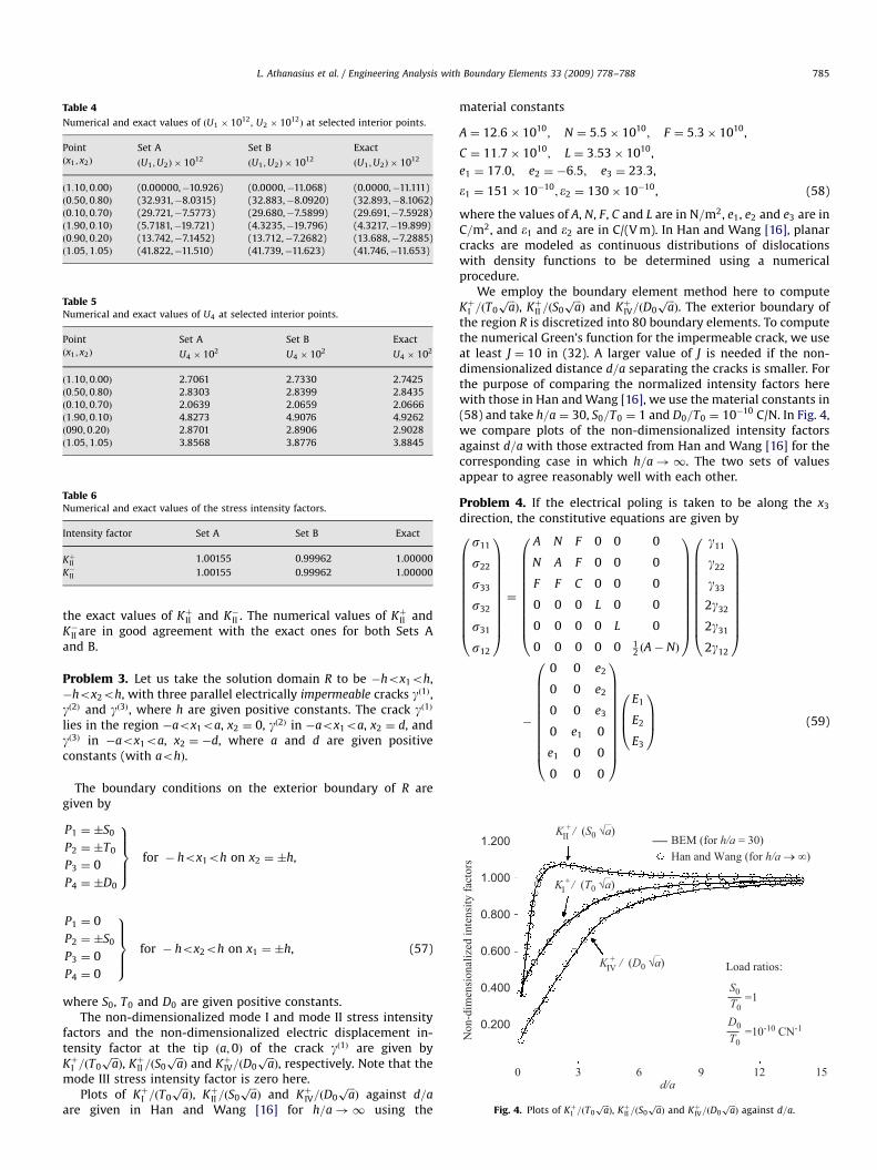
Problem 3. Let us take the solution domain R to be �hox1oh,�hox2oh, with three parallel electrically impermeable cracks gð1Þ,gð2Þ and gð3Þ, where h are given positive constants. The crack gð1Þlies in the region �aox1oa, x2 ¼ 0, gð2Þ in �aox1oa, x2 ¼ d, andgð3Þ in �aox1oa, x2 ¼ �d, where a and d are given positiveconstants (with aohÞ.

The boundary conditions on the exterior boundary of R aregiven by

P1 ¼ �S0

P2 ¼ �T0

P3 ¼ 0

P4 ¼ �D0

9>>>=>>>;

for � hox1oh on x2 ¼ �h,

P1 ¼ 0

P2 ¼ �S0

P3 ¼ 0

P4 ¼ 0

9>>>=>>>;

for � hox2oh on x1 ¼ �h, (57)

where S0, T0 and D0 are given positive constants.The non-dimensionalized mode I and mode II stress intensity

factors and the non-dimensionalized electric displacement in-tensity factor at the tip ða;0Þ of the crack gð1Þ are given byKþI =ðT0

ffiffiffiapÞ, KþII =ðS0

ffiffiffiapÞ and KþIV=ðD0

ffiffiffiapÞ, respectively. Note that the

mode III stress intensity factor is zero here.Plots of KþI =ðT0

ffiffiffiapÞ, KþII =ðS0

ffiffiffiapÞ and KþIV=ðD0

ffiffiffiapÞ against d=a

are given in Han and Wang [16] for h=a!1 using the

material constants

A ¼ 12:6� 1010; N ¼ 5:5� 1010; F ¼ 5:3� 1010,

C ¼ 11:7� 1010; L ¼ 3:53� 1010,

e1 ¼ 17:0; e2 ¼ �6:5; e3 ¼ 23:3,

�1 ¼ 151� 10�10; �2 ¼ 130� 10�10, (58)

where the values of A, N, F, C and L are in N=m2, e1, e2 and e3 are inC=m2, and �1 and �2 are in C/(V m). In Han and Wang [16], planarcracks are modeled as continuous distributions of dislocationswith density functions to be determined using a numericalprocedure.

We employ the boundary element method here to computeKþI =ðT0

ffiffiffiapÞ, KþII =ðS0

ffiffiffiapÞ and KþIV=ðD0

ffiffiffiapÞ. The exterior boundary of

the region R is discretized into 80 boundary elements. To computethe numerical Green’s function for the impermeable crack, we useat least J ¼ 10 in (32). A larger value of J is needed if the non-dimensionalized distance d=a separating the cracks is smaller. Forthe purpose of comparing the normalized intensity factors herewith those in Han and Wang [16], we use the material constants in(58) and take h=a ¼ 30, S0=T0 ¼ 1 and D0=T0 ¼ 10�10 C/N. In Fig. 4,we compare plots of the non-dimensionalized intensity factorsagainst d=a with those extracted from Han and Wang [16] for thecorresponding case in which h=a!1. The two sets of valuesappear to agree reasonably well with each other.

Problem 4. If the electrical poling is taken to be along the x3

direction, the constitutive equations are given by

s11

s22

s33

s32

s31

s12

0BBBBBBBBBBB@

1CCCCCCCCCCCA¼

A N F 0 0 0

N A F 0 0 0

F F C 0 0 0

0 0 0 L 0 0

0 0 0 0 L 0

0 0 0 0 0 12 ðA� NÞ

0BBBBBBBBBBB@

1CCCCCCCCCCCA

g11

g22

g33

2g32

2g31

2g12

0BBBBBBBBBBB@

1CCCCCCCCCCCA

�

0 0 e2

0 0 e2

0 0 e3

0 e1 0

e1 0 0

0 0 0

0BBBBBBBBBBB@

1CCCCCCCCCCCA

E1

E2

E3

0BB@

1CCA (59)

ARTICLE IN PRESS

L. Athanasius et al. / Engineering Analysis with Boundary Elements 33 (2009) 778–788786

and

D1

D2

D3

0BB@

1CCA ¼

0 0 0 0 e1 0

0 0 0 e1 0 0

e2 e2 e3 0 0 0

0BB@

1CCA

g11

g22

g33

2g32

2g31

2g12

0BBBBBBBBBBB@

1CCCCCCCCCCCA

þ

�1 0 0

0 �1 0

0 0 �2

0BB@

1CCA

E1

E2

E3

0BB@

1CCA. (60)

It follows that the non-zero coefficients CIjKp are

C1111 ¼ C2222 ¼ A; C1122 ¼ C2211 ¼ N; C3333 ¼ C,

C1133 ¼ C3311 ¼ C2233 ¼ C3322 ¼ F,

C1313 ¼ C3113 ¼ C3131 ¼ C1331 ¼ C2323 ¼ C3223 ¼ C3232 ¼ C2332 ¼ L,

C1212 ¼ C2112 ¼ C2121 ¼ C1221 ¼12ðA� NÞ,

C3141 ¼ C1341 ¼ C2342 ¼ C3242 ¼ C4131 ¼ C4113 ¼ C4223 ¼ C4232 ¼ e1,

C1143 ¼ C2243 ¼ C4311 ¼ C4322 ¼ e2,

C3343 ¼ C4333 ¼ e3; C4141 ¼ C4242 ¼ ��1; C4343 ¼ ��2. (61)

The homogeneous system of linear algebraic equations forworking out AKa is given by

Aþ 12 ðA� NÞt2

a ðN þ 12 ðA� NÞÞta 0 0

ðN þ 12 ðA� NÞÞta 1

2 ðA� NÞ þ At2a 0 0

0 0 Lþ Lt2a e1 þ e1t2

a

0 0 e1 þ e1t2a ��1 � �1t2

a

0BBBBBB@

1CCCCCCA

�

A1a

A2a

A3a

A4a

0BBBBB@

1CCCCCA ¼

0

0

0

0

0BBBBB@

1CCCCCA. (62)

If we use (62), we find that we cannot construct ½AKa� that isinvertible. To overcome this minor difficulty, a relatively smallamount of anisotropy is introduced into the equations governingu1 and u2. Specifically, we replace C1111 ¼ A in (61) byC1111 ¼ Aþ e, where e is a selected real number whose magnitudeis very small compared to A. It follows that we supercede (62) by

Aþ eþ 12 ðA� NÞt2

a ðN þ12 ðA� NÞÞta 0 0

ðN þ 12 ðA� NÞÞta 1

2 ðA� NÞ þ At2a 0 0

0 0 Lþ Lt2a e1 þ e1t2

a

0 0 e1 þ e1t2a ��1 � �1t2

a

0BBBBBB@

1CCCCCCA

�

A1a

A2a

A3a

A4a

0BBBBB@

1CCCCCA ¼

0

0

0

0

0BBBBB@

1CCCCCA. (63)

We can take t3 ¼ t4 ¼ i and t1 and t2 are two distinct solutionswith positive imaginary parts of the quartic equation

detAþ eþ 1

2 ðA� NÞt2 ðN þ 12 ðA� NÞÞt

ðN þ 12 ðA� NÞÞt 1

2 ðA� NÞ þ At2

!¼ 0. (64)

Note that (64) cannot yield two distinct solutions with positiveimaginary parts if e is zero.

From (62), we find that AKa may be chosen to be

A1a ¼ �ðN þ 1

2 ðA� NÞÞtaAþ eþ 1

2 ðA� NÞt2aðda1 þ da2Þ,

A2a ¼ da1 þ da2; A3a ¼ da3; A4a ¼ da4. (65)

The matrix ½AKa� as constructed in (65) is invertible if t1at2.For a particular problem in which the electrical poling is along

the x3 direction, let us take the solution domain R to be�hox1oh,�hox2oh, with two collinear permeable crack lying in the regions�box1o� a, x2 ¼ 0, and aox1ob, x2 ¼ 0,where a, b and h arepositive constants such that aoboh. The boundary conditions onthe exterior boundary of R are given by

P1 ¼ 0

P2 ¼ 0

P3 ¼ �S0

P4 ¼ �D0

9>>>=>>>;

for � hox1oh on x2 ¼ �h,

P1 ¼ 0

P2 ¼ 0

P3 ¼ 0

P4 ¼ 0

9>>>=>>>;

for � hox2oh on x1 ¼ �h, (66)

where S0 and D0 are non-negative constants.Let K inner

III and KouterIII , respectively, denote the mode III stress

intensity factor at the inner and outer tips of the collinear cracks.The crack energy release rates at the inner and outer tips are then,respectively, given by

Ginner¼

p2LðK inner

III Þ2 and Gouter

¼p2LðKouter

III Þ2. (67)

In Li [18], it is analytically given that

4LGinner

pðb� aÞS20

;4LGouter

pðb� aÞS20

!!

2½b2l� a2�2

aðb� aÞðb2� a2Þ

;2b3½1� l�2

ðb� aÞðb2� a2Þ

!

as 2h=ðb� aÞ ! 1, (68)

where

l ¼R p=2

0 ½1� ð1� ða=bÞ2Þsin2t�1=2 dtR p=20 ½1� ð1� ða=bÞ2Þsin2t��1=2 dt

. (69)

Using the material constants in (58) and taking 2h=ðb� aÞ ¼ 20,we use the boundary element method with Green’s function forthe permeable cracks to compute the crack energy release ratesGinner and Gouter according to (67) (after calculating numericallythe mode III stress intensity factors). In perturbing the elasticmodulus C1111 to construct an invertible matrix ½AKa�, we choosee ¼ 102, that is, we take C1111 to be given by ð12:6þ 10�8

Þ � 1010

N=m2 instead of 12:6� 108 N=m2. The outer boundary of thesolution domain is discretized into 160 elements. The numericalGreen’s function is calculated using at least J ¼ 10 in (32). If theinner tips of the cracks are close to each other then J ¼ 30 is used.If the outer tips are near the vertical sides, we use J ¼ 20 and addanother 40 elements on each of the vertical sides.

Plots of the non-dimensionalized crack energy release rates4LGinner=ðpðb� aÞS2

0Þ and 4LGouter=ðpðb� aÞS20Þ against 2a=ðb� aÞ

(for 0:50p2a=ðb� aÞp17:50Þ are given in Figs. 5 and 6, respec-tively. In the figures, we also compare the numerical crack energyrelease rates with the values calculated from (68) (given by Li [18]for 2h=ðb� aÞ ! 1). The numerical crack energy release rates arefound to agree very well with (68) for small values of 2a=ðb� aÞ.This is expected as (68) is valid only for 2h=ðb� aÞ ! 1 (that is,for an infinite piezoelectric material).

Note that the crack tip energy release rate G for thecorresponding problem involving only a single crack of length

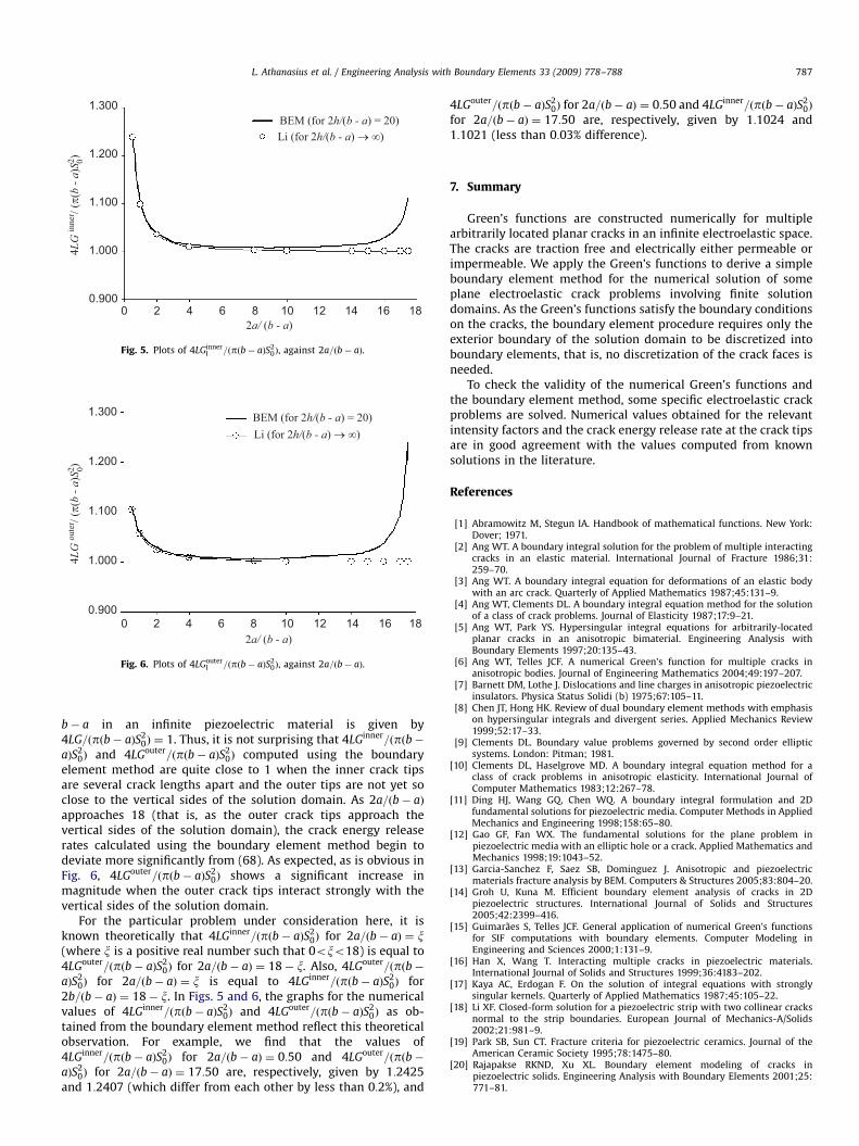
ARTICLE IN PRESS

1.300

1.200

1.100

1.000

0.900

BEM (for 2h/(b - a) = 20)Li (for 2h/(b - a) → ∞)

0 2 4 6 8 10 12 14 16 182a/ (b - a)

4LG

oute

r / (π(

b - a

)S2 ) 0

Fig. 6. Plots of 4LGouterI =ðpðb� aÞS2

0Þ, against 2a=ðb� aÞ.

1.300

1.200

1.100

1.000

0.900

BEM (for 2h/(b - a) = 20)Li (for 2h/(b - a) → ∞)

0 2 4 6 8 10 12 14 16 182a/ (b - a)

4LG

inne

r / (π(

b - a

)S2 ) 0

Fig. 5. Plots of 4LGinnerI =ðpðb� aÞS2

0Þ, against 2a=ðb� aÞ.

L. Athanasius et al. / Engineering Analysis with Boundary Elements 33 (2009) 778–788 787

b� a in an infinite piezoelectric material is given by4LG=ðpðb� aÞS2

0Þ ¼ 1. Thus, it is not surprising that 4LGinner=ðpðb�aÞS2

0Þ and 4LGouter=ðpðb� aÞS20Þ computed using the boundary

element method are quite close to 1 when the inner crack tipsare several crack lengths apart and the outer tips are not yet soclose to the vertical sides of the solution domain. As 2a=ðb� aÞ

approaches 18 (that is, as the outer crack tips approach thevertical sides of the solution domain), the crack energy releaserates calculated using the boundary element method begin todeviate more significantly from (68). As expected, as is obvious inFig. 6, 4LGouter=ðpðb� aÞS2

0Þ shows a significant increase inmagnitude when the outer crack tips interact strongly with thevertical sides of the solution domain.

For the particular problem under consideration here, it isknown theoretically that 4LGinner=ðpðb� aÞS2

0Þ for 2a=ðb� aÞ ¼ x(where x is a positive real number such that 0oxo18) is equal to4LGouter=ðpðb� aÞS2

0Þ for 2a=ðb� aÞ ¼ 18� x. Also, 4LGouter=ðpðb�aÞS2

0Þ for 2a=ðb� aÞ ¼ x is equal to 4LGinner=ðpðb� aÞS20Þ for

2b=ðb� aÞ ¼ 18� x. In Figs. 5 and 6, the graphs for the numericalvalues of 4LGinner=ðpðb� aÞS2

0Þ and 4LGouter=ðpðb� aÞS20Þ as ob-

tained from the boundary element method reflect this theoreticalobservation. For example, we find that the values of4LGinner=ðpðb� aÞS2

0Þ for 2a=ðb� aÞ ¼ 0:50 and 4LGouter=ðpðb�aÞS2

0Þ for 2a=ðb� aÞ ¼ 17:50 are, respectively, given by 1:2425and 1:2407 (which differ from each other by less than 0:2%), and

4LGouter=ðpðb� aÞS20Þ for 2a=ðb� aÞ ¼ 0:50 and 4LGinner=ðpðb� aÞS2

0Þ

for 2a=ðb� aÞ ¼ 17:50 are, respectively, given by 1:1024 and1:1021 (less than 0:03% difference).

7. Summary

Green’s functions are constructed numerically for multiplearbitrarily located planar cracks in an infinite electroelastic space.The cracks are traction free and electrically either permeable orimpermeable. We apply the Green’s functions to derive a simpleboundary element method for the numerical solution of someplane electroelastic crack problems involving finite solutiondomains. As the Green’s functions satisfy the boundary conditionson the cracks, the boundary element procedure requires only theexterior boundary of the solution domain to be discretized intoboundary elements, that is, no discretization of the crack faces isneeded.

To check the validity of the numerical Green’s functions andthe boundary element method, some specific electroelastic crackproblems are solved. Numerical values obtained for the relevantintensity factors and the crack energy release rate at the crack tipsare in good agreement with the values computed from knownsolutions in the literature.

References

[1] Abramowitz M, Stegun IA. Handbook of mathematical functions. New York:Dover; 1971.

[2] Ang WT. A boundary integral solution for the problem of multiple interactingcracks in an elastic material. International Journal of Fracture 1986;31:259–70.

[3] Ang WT. A boundary integral equation for deformations of an elastic bodywith an arc crack. Quarterly of Applied Mathematics 1987;45:131–9.

[4] Ang WT, Clements DL. A boundary integral equation method for the solutionof a class of crack problems. Journal of Elasticity 1987;17:9–21.

[5] Ang WT, Park YS. Hypersingular integral equations for arbitrarily-locatedplanar cracks in an anisotropic bimaterial. Engineering Analysis withBoundary Elements 1997;20:135–43.

[6] Ang WT, Telles JCF. A numerical Green’s function for multiple cracks inanisotropic bodies. Journal of Engineering Mathematics 2004;49:197–207.

[7] Barnett DM, Lothe J. Dislocations and line charges in anisotropic piezoelectricinsulators. Physica Status Solidi (b) 1975;67:105–11.

[8] Chen JT, Hong HK. Review of dual boundary element methods with emphasison hypersingular integrals and divergent series. Applied Mechanics Review1999;52:17–33.

[9] Clements DL. Boundary value problems governed by second order ellipticsystems. London: Pitman; 1981.

[10] Clements DL, Haselgrove MD. A boundary integral equation method for aclass of crack problems in anisotropic elasticity. International Journal ofComputer Mathematics 1983;12:267–78.

[11] Ding HJ, Wang GQ, Chen WQ. A boundary integral formulation and 2Dfundamental solutions for piezoelectric media. Computer Methods in AppliedMechanics and Engineering 1998;158:65–80.

[12] Gao GF, Fan WX. The fundamental solutions for the plane problem inpiezoelectric media with an elliptic hole or a crack. Applied Mathematics andMechanics 1998;19:1043–52.

[13] Garcia-Sanchez F, Saez SB, Dominguez J. Anisotropic and piezoelectricmaterials fracture analysis by BEM. Computers & Structures 2005;83:804–20.

[14] Groh U, Kuna M. Efficient boundary element analysis of cracks in 2Dpiezoelectric structures. International Journal of Solids and Structures2005;42:2399–416.

[15] Guimaraes S, Telles JCF. General application of numerical Green’s functionsfor SIF computations with boundary elements. Computer Modeling inEngineering and Sciences 2000;1:131–9.

[16] Han X, Wang T. Interacting multiple cracks in piezoelectric materials.International Journal of Solids and Structures 1999;36:4183–202.

[17] Kaya AC, Erdogan F. On the solution of integral equations with stronglysingular kernels. Quarterly of Applied Mathematics 1987;45:105–22.

[18] Li XF. Closed-form solution for a piezoelectric strip with two collinear cracksnormal to the strip boundaries. European Journal of Mechanics-A/Solids2002;21:981–9.

[19] Park SB, Sun CT. Fracture criteria for piezoelectric ceramics. Journal of theAmerican Ceramic Society 1995;78:1475–80.

[20] Rajapakse RKND, Xu XL. Boundary element modeling of cracks inpiezoelectric solids. Engineering Analysis with Boundary Elements 2001;25:771–81.

ARTICLE IN PRESS

L. Athanasius et al. / Engineering Analysis with Boundary Elements 33 (2009) 778–788788

[21] Shindo Y, Tanaka K, Narita F. Singular stress and electric fields of apiezoelectric ceramic strip with a finite crack under longitudinal stress. ActaMechanica 1997;120:31–45.

[22] Snyder MD, Cruse TA. Boundary integral analysis of cracked anisotropicplates. International Journal of Fracture 1975;11:315–28.

[23] Telles JCF, Castor GS, Guimaraes S. A numerical Green’s function approach forboundary elements applied to fracture mechanics. International Journal forNumerical Methods in Engineering 1995;38:3259–74.

[24] Wang BL, Mai YW. Impermeable crack and permeable crack assumptions,which one is more realistic? Journal of Applied Mechanics—Transactions ofASME 2004;71:575–8.

[25] Xu XL, Rajapakse RKND. Boundary element analysis of piezoelectric solidswith defects. Composites Part B: Engineering 1998;29:655–69.