Comparison of two wavelet transform coherence and cross-covariance functions applied on polar motion and atmospheric excitation W. Popiński Department of Standards, Central Statistical Office, Warsaw, Poland, e-mail: w.popinski@stat.gov.pl W. Kosek Space Research Centre, Polish Academy of Sciences, Warsaw, Poland, e-mail: kosek@cbk.waw.pl H. Schuh Institute of Geodesy and Geophysics, University of Technology, Wien, Austria, e-mail: hschuh@luna.tuwien.ac.at M. 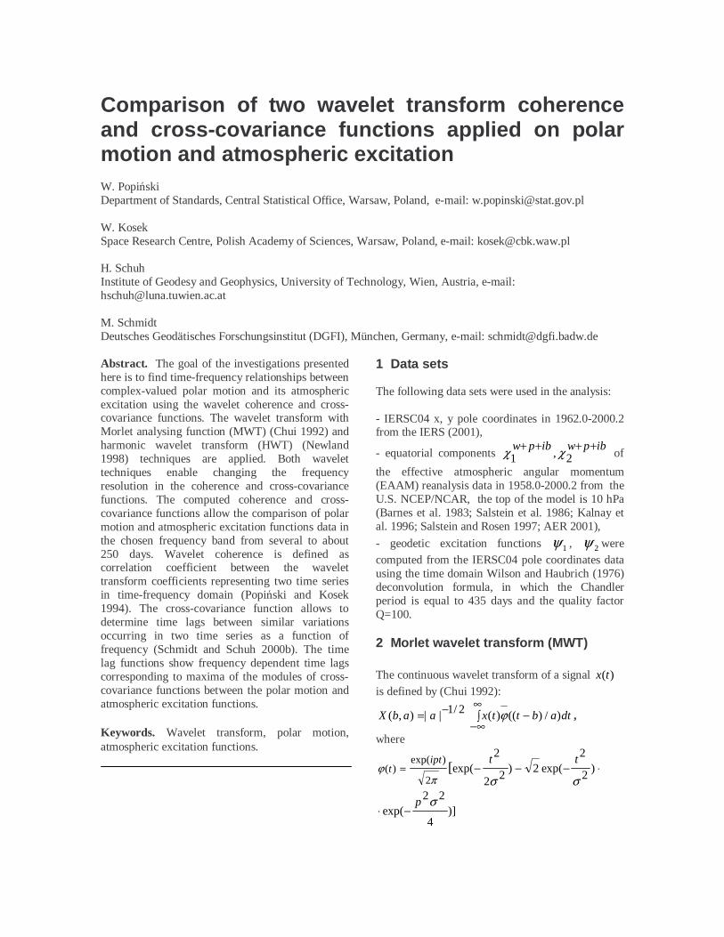Schmidt Deutsches Geodätisches Forschungsinstitut (DGFI), München, Germany, e-mail: schmidt@dgfi.badw.de Abstract. The goal of the investigations presented here is to find time-frequency relationships between complex-valued polar motion and its atmospheric excitation using the wavelet coherence and cross-covariance functions. The wavelet transform with Morlet analysing function (MWT) (Chui 1992) and harmonic wavelet transform (HWT) (Newland 1998) techniques are applied. Both wavelet techniques enable changing the frequency resolution in the coherence and cross-covariance functions. The computed coherence and cross-covariance functions allow the comparison of polar motion and atmospheric excitation functions data in the chosen frequency band from several to about 250 days. Wavelet coherence is defined as correlation coefficient between the wavelet transform coefficients representing two time series in time-frequency domain (Popiński and Kosek 1994). The cross-covariance function allows to determine time lags between similar variations occurring in two time series as a function of frequency (Schmidt and Schuh 2000b). The time lag functions show frequency dependent time lags corresponding to maxima of the modules of cross-covariance functions between the polar motion and atmospheric excitation functions.

Keywords. Wavelet transform, polar motion, atmospheric excitation functions.

1 Data sets The following data sets were used in the analysis: - IERSC04 x, y pole coordinates in 1962.0-2000.2 from the IERS (2001),

- equatorial components ibpwibpw ++++

2,1 χχ of

the effective atmospheric angular momentum (EAAM) reanalysis data in 1958.0-2000.2 from the U.S. NCEP/NCAR, the top of the model is 10 hPa (Barnes et al. 1983; Salstein et al. 1986; Kalnay et al. 1996; Salstein and Rosen 1997; AER 2001),

- geodetic excitation functions 1ψ , 2ψ were computed from the IERSC04 pole coordinates data using the time domain Wilson and Haubrich (1976) deconvolution formula, in which the Chandler period is equal to 435 days and the quality factor Q=100. 2 Morlet wavelet transform (MWT) The continuous wavelet transform of a signal )(tx is defined by (Chui 1992):

dtabttxaabX )/)(()(2/1||),( −∫∞

∞−−= ϕ ,

where

⋅−−−= )2

2exp(2)

22

2exp([

2

)exp()(

σσπϕ

ttiptt

)]4

22exp(

σp−⋅

is the Morlet wavelet function (Schmitz-Hübsch and Schuh 1999), 5>p - frequency parameter, σ

- decay parameter, b - translation parameter , 0≠a - dilation parameter.

For p =2π the dilated Morlet wavelet oscillation

period equals a (Popiński and Kosek 1994). The continuous Fourier transform (CFT) of the Morlet wavelet is given by the formula (Chui 1992):

−−

−= )2

22)([exp()(

σωσωϕ

p(

)]4

22exp()

4

22)(exp(

σσω pp−

−−−

so it has quasi-compact support both in time and frequency domain. The formula for coefficients ),( abX , which

involves CFT of the signal )(ωx(

and the wavelet

function )(ωϕ( reads

ωωωϕωπ

dibaxaabX )exp()()(2

1),(

2/1∫∞

∞−= ((

.

3 Harmonic wavelet transform (HWT) The harmonic wavelet transform (HWT) coefficients of a signal )(tx are defined by Newland (1998):

( ) ∫∞

∞−−= dttxbtwbH )(),(, µµ ,

where ),( µtw - the complex-valued harmonic wavelet function localised in frequency domain near some frequency µ , b - the translation parameter. The frequency domain formula reads (Newland 1998):

( ) ∫∞

∞−= ωωωµωµ dibxwbH )exp()(),(,

(( .

The CFT of the harmonic wavelet function is of boxcar type tapered by the Gaussian window for better frequency resolution (Newland 1998)

( )

≤−

−−

=

,0

22

2)(exp

,

otherwise

ifw

λωµσ

ωµµω(

where λ - window halfwidth, σ - smoothing parameter. 4 The wavelet transform cross-covariance and coherence functions

Analysing time series )(tx and )(ty ,

1,...,1,0 −= Nt , we compute the scale dependent cross-covariance and coherence estimates according to the formulae:

),(1

0),(),( akY

N

kakXaxyC ββ +∑

−

==

))),

)(2)(2

),0()(

ayax

axyCaxy

σσγ

))

)

) = ,

where 21

0),()(2 ∑

−

==

N

kakXax

))σ ,

21

0),()(2 ∑

−

==

N

kakYay

))σ .

Time lag function estimate )(aβ)

satisfies the condition:

),(maxarg)( axyCD

a ββ

β))

∈= ,

where the maximum is determined over some finite set },1,...,1,{ KKKKD −+−−= of integer time

shifts β .

Time-frequency coherence is computed as the running correlation coefficient of wavelet transform coefficients:

),(),(

),(),(

atyRatxR

atxyRatxy ))

)

) =κ ,

where

),(),(),( aktYM

MkaktXatxyR +∑

−=+=

))),

2),(),( ∑

−=+=

M

MkaktXatxR

)) ,

2),(),( ∑

−=+=

M

MkaktYatyR

)),

and M is a positive integer.

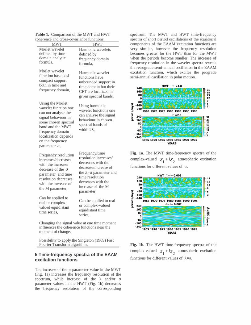
Table 1. Comparison of the MWT and HWT coherence and cross-covariance functions.

MWT HWT Morlet wavelet defined by time domain analytic formula, Morlet wavelet function has quasi-compact support both in time and frequency domain, Using the Morlet wavelet function one can not analyse the signal behaviour in some chosen spectral band and the MWT frequency domain localization depends on the frequency parameter a , Frequency resolution increases/decreases with the increase/ decrease of the σ parameter and time resolution decreases with the increase of the M parameter, Can be applied to real or complex-valued equidistant time series,

Harmonic wavelets defined by frequency domain formula, Harmonic wavelet functions have unbounded support in time domain but their CFT are localized in given spectral bands, Using harmonic wavelet functions one can analyse the signal behaviour in chosen spectral bands of width 2λ, Frequency/time resolution increases/ decreases with the decrease/increase of the λ=σ parameter and time resolution decreases with the increase of the M parameter, Can be applied to real or complex-valued equidistant time series,

Changing the signal value at one time moment influences the coherence functions near the moment of change, Possibility to apply the Singleton (1969) Fast Fourier Transform algorithm.

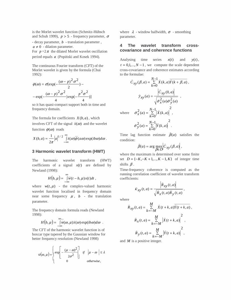
5 Time-frequency spectra of the EAAM excitation functions The increase of the σ parameter value in the MWT (Fig. 1a) increases the frequency resolution of the spectrum, while increase of the λ and/or σ parameter values in the HWT (Fig. 1b) decreases the frequency resolution of the corresponding

spectrum. The MWT and HWT time-frequency spectra of short period oscillations of the equatorial components of the EAAM excitation functions are very similar, however the frequency resolution becomes greater for the HWT than for the MWT when the periods become smaller. The increase of frequency resolution in the wavelet spectra reveals the retrograde semi-annual oscillation in the EAAM excitation function, which excites the prograde semi-annual oscillation in polar motion.

MWT =1.0

=2.01965 1970 1975 1980 1985 1990 1995

-240-160

-800

80160240

1965 1970 1975 1980 1985 1990 1995YEARS

-240-160

-800

80160240

per

iod

(da

ys)

36912151821

37111519232731

Fig. 1a. The MWT time-frequency spectra of the

complex-valued 21

χχ i+ atmospheric excitation

functions for different values of σ.

HWT = =0.005

1965 1970 1975 1980 1985 1990 1995-240-160

-800

80160240

= = 0.002

1965 1970 1975 1980 1985 1990 1995YEARS

-240-160

-800

80160240

per

iod

(day

s)

3691215182124

369121518

Fig. 1b. The HWT time-frequency spectra of the

complex-valued 21

χχ i+ atmospheric excitation

functions for different values of λ=σ.

6 Time-frequency relationship between the atmospheric and geodetic excitation functions 6.1 Coherences The MWT and HWT frequency dependent coherence functions are shown in Figure 2. It can be noticed that improved frequency resolution can be obtained by increasing the σ parameter value in the MWT and by decreasing the λ and/or σ parameter values in the HWT. The peaks of coherence functions computed by these two wavelet techniques correspond to similar prograde and retrograde oscillations, however, greater number of peaks can be noticed for the HWT coherence than for the MWT one in the shorter period band from –70 to 70 days.

-200 -100 0 100 2000.00.20.40.60.81.0

2.0

1.0

MWT1.5

-200 -100 0 100 200period (days)

0.00.20.40.60.81.0 0.010

0.015

=HWT

0.005

Fig. 2 The MWT and HWT coherence functions

between the complex-valued atmospheric 21

χχ i+

and geodetic 21 ψψ i+ excitation functions in

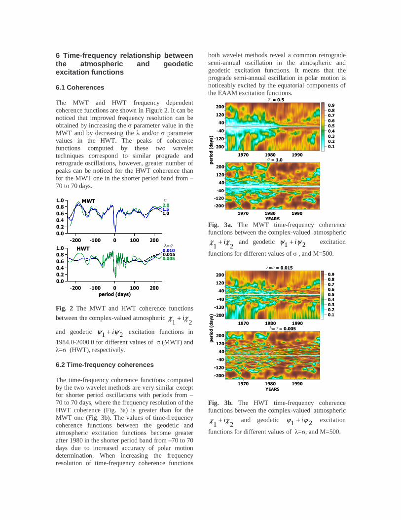
1984.0-2000.0 for different values of σ (MWT) and λ=σ (HWT), respectively. 6.2 Time-frequency coherences The time-frequency coherence functions computed by the two wavelet methods are very similar except for shorter period oscillations with periods from –70 to 70 days, where the frequency resolution of the HWT coherence (Fig. 3a) is greater than for the MWT one (Fig. 3b). The values of time-frequency coherence functions between the geodetic and atmospheric excitation functions become greater after 1980 in the shorter period band from –70 to 70 days due to increased accuracy of polar motion determination. When increasing the frequency resolution of time-frequency coherence functions

both wavelet methods reveal a common retrograde semi-annual oscillation in the atmospheric and geodetic excitation functions. It means that the prograde semi-annual oscillation in polar motion is noticeably excited by the equatorial components of the EAAM excitation functions.

1970 1980 1990

40

120

200

= 0.5

1970 1980 1990

40

120

200

pe

riod

(da

ys)

= 1.01970 1980 1990

-200

-120

-40

1970 1980 1990YEARS

-200

-120

-40

0.10.20.30.40.50.60.70.80.9

Fig. 3a. The MWT time-frequency coherence functions between the complex-valued atmospheric

21χχ i+ and geodetic 21 ψψ i+ excitation

functions for different values of σ , and M=500.

1970 1980 1990

40

120

200

= = 0.005

= = 0.015

1970 1980 1990YEARS

-200

-120

-40

1970 1980 1990

-200

-120

-40

0.10.20.30.40.50.60.70.80.9

1970 1980 1990

40

120

200

peri

od (

days

)

Fig. 3b. The HWT time-frequency coherence functions between the complex-valued atmospheric

21χχ i+ and geodetic 21 ψψ i+ excitation

functions for different values of λ=σ, and M=500.

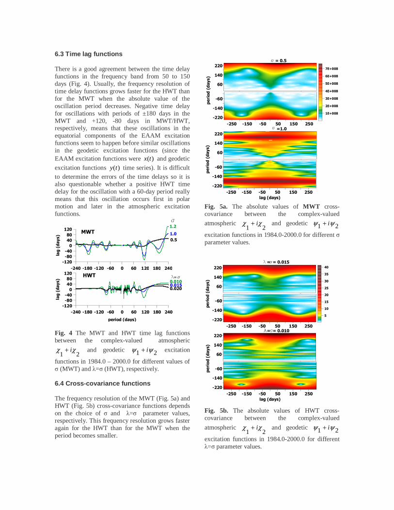
6.3 Time lag functions There is a good agreement between the time delay functions in the frequency band from 50 to 150 days (Fig. 4). Usually, the frequency resolution of time delay functions grows faster for the HWT than for the MWT when the absolute value of the oscillation period decreases. Negative time delay for oscillations with periods of ±180 days in the MWT and +120, -80 days in MWT/HWT, respectively, means that these oscillations in the equatorial components of the EAAM excitation functions seem to happen before similar oscillations in the geodetic excitation functions (since the EAAM excitation functions were )(tx and geodetic

excitation functions )(ty time series). It is difficult to determine the errors of the time delays so it is also questionable whether a positive HWT time delay for the oscillation with a 60-day period really means that this oscillation occurs first in polar motion and later in the atmospheric excitation functions.

-240 -180 -120 -60 0 60 120 180 240-120

-80-40

04080

120

lag

(day

s)

1.0

1.2MWT

0.5

-240 -180 -120 -60 0 60 120 180 240

period (days)

-120-80-40

04080

120

lag

(day

s) 0.010=

0.015

HWT

0.020

Fig. 4 The MWT and HWT time lag functions between the complex-valued atmospheric

21χχ i+ and geodetic 21 ψψ i+ excitation

functions in 1984.0 – 2000.0 for different values of σ (MWT) and λ=σ (HWT), respectively. 6.4 Cross-covariance functions The frequency resolution of the MWT (Fig. 5a) and HWT (Fig. 5b) cross-covariance functions depends on the choice of σ and λ=σ parameter values, respectively. This frequency resolution grows faster again for the HWT than for the MWT when the period becomes smaller.

-250 -150 -50 50 150 250lag (days)

-220

-140

-60

peri

od (

days

)

- 200 0 200

60

140

220

= 0.5

-200 0 200

60

140

220

=1.0-250 -150 -50 50 150 250

-220

-140

-60

per

iod

(da

ys)

1E+008

2E+008

3E+008

4E+008

5E+008

6E+008

7E+008

Fig. 5a. The absolute values of MWT cross-covariance between the complex-valued

atmospheric 21

χχ i+ and geodetic 21 ψψ i+

excitation functions in 1984.0-2000.0 for different σ parameter values.

-200 0 200

60

140

220

-250 -150 -50 50 150 250-220

-140

-60

p

erio

d (d

ays)

= = 0.015

-250 -150 -50 50 150 250lag (days)

-220

-140

-60

p

erio

d (d

ays)

-200 0 200

60

140

220= = 0.010

5

10

15

20

25

30

35

40

Fig. 5b. The absolute values of HWT cross-covariance between the complex-valued

atmospheric 21

χχ i+ and geodetic 21 ψψ i+

excitation functions in 1984.0-2000.0 for different λ=σ parameter values.

7 Conclusions The MWT and HWT techniques enable computation of time-frequency coherences and cross-covariance functions between two complex-valued time series. Time-frequency resolution of the spectra and coherence as well as the frequency resolution of the cross-covariance and time delay functions can be varied by changing the σ and λ and/or σ parameter values in the MWT and HWT, respectively. The spectra, coherence, cross-covariance and time delay functions are smoother and less noisy in high frequency band for the MWT than for the HWT, so it is advisable to use the MWT technique. The computed time delay depends on the choice of the σ and λ and/or σ parameter values in the MWT and HWT, respectively. A negative time delay for oscillations with periods of 180 days in the MWT and 120 days in the MWT/HWT seems to indicate that these oscillations in the equatorial components of the atmospheric excitation functions precede analogous oscillations in the geodetic excitation function by about 20 to 60 days. Results indicate that geophysical phenomena other than atmospheric excitation contribute to short period polar motion oscillations. Acknowlegement. This paper was supported by the Polish Committee of Scientific Research project No 8T12E 005 20 under the leadership of W. Kosek. References AER 2001, EAAM reanalysis data of the

NCEP/NCAR, anonymous ftp service: ftp aer.com/pub/sba

Barnes R.T.H., Hide R., White A.A., and Wilson C.A. 1983, Atmospheric Angular Momentum Fluctuations, length-of-day changes and polar motion, Proc. R. Soc. London, A387, 31-73.

Chui C.K. 1992, An Introduction to Wavelets, Wavelet Analysis and its Application Vol. 1, Academic Press, Boston-San Diego.

IERS 2001, The Earth Orientation Parameters, coordinates of the pole, http://www.iers.org/ iers/earth/rotation/eop/eop. html

Kalnay E. et al. 1996, The NCEP/NCAR 40-year reanalysis project, Bull. Amer. Meteor. Soc., 77, 437-471.

Liu P.C. 1994, Wavelet Spectrum Analysis and Ocean Wind Waves, in Wavelets in Geophysics, Wavelet Analysis and its Applications Vol. 4, E. Foufoula-Georgiou and P. Kumar (eds.), Academic Press, San Diego, 151-166.

Newland D.E. 1998, Time-Frequency and Time-Scale Signal Analysis by Harmonic Wavelets, in Signal Analysis and Prediction, A. Prohazka, J. Uhlir, P.J. Rayner, N.G. Kingsbury (eds), Birkhauser, Boston.

Popiński W., Kosek W. 1994, Wavelet Transform and Its Application for Short Period Earth Rotation Analysis, Artificial Satellites, Vol. 29, No 2, 75-83.

Salstein D.A., D.M. Kann, A.J. Miller, R.D. Rosen 1986, The Sub-bureau for Atmospheric Angular Momentum of the International Earth Rotation Service: A Meteorological Data Center with Geodetic Applications, Bull. Amer. Meteor. Soc., 74, 67-80.

Salstein D.A. and R.D. Rosen 1997, Global momentum and energy signals from reanalysis systems. Preprints of the 7th Conf. on Climate Variations, American Meteorological Society, Boston, MA, 344-348.

Schmidt M. and Schuh H. 2000a, Abilities of Wavelet Analysis for Investigating Short-Period Variations of Earth Rotation, IERS Technical Note No 28, Observatoire de Paris, 73-80.

Schmidt M. and Schuh H. 2000b, Frequency-dependent phase lags between LOD- and AAM-variations detected by wavelet analysis, poster presented at the EGS 25th General Assembly, Nice, France, 24-29 April 2000, http://www.dgfi.badw.de/dgfi/DOC/2000/schmidt_egs00.pdf

Schmitz-Hübsch H., Schuh H. 1999, Seasonal and Short-Period Fluctuations of Earth Rotation Investigated by Wavelet Analysis, Technical Report Nr. 1999.6-1, Department of Geodesy and Geoinformatics, Universität Stuttgart : ”Quo vadis Geodesia ...?”, Festschrift for Erik W. Grafarend on the occasion of his 60th birthday, F. Krumm, V.S. Schwarze (Eds), 421-431.

Singleton R.C. 1969, An Algorithm for Computing the Mixed Radix Fast Fourier Transform, IEEE Transactions on Audio and Electroacoustics, Vol. AU-17, No 2.

Wilson C.R. and Haubrich R.A. 1976, Meteorological Excitation of the Earth’s Wobble, Geophys. J. R. Astron. Soc., 46, 707-743.