Communications Source and Channel Coding with examples

Communications Source and ChannelCoding with examples

By:Peter Grant

Communications Source and ChannelCoding with examples

By:Peter Grant

Online:< http://cnx.org/content/col10601/1.3/ >

C O N N E X I O N S

Rice University, Houston, Texas

This selection and arrangement of content as a collection is copyrighted by Peter Grant. It is licensed under the

Creative Commons Attribution 2.0 license (http://creativecommons.org/licenses/by/2.0/).

Collection structure revised: May 7, 2009

PDF generated: October 26, 2012

For copyright and attribution information for the modules contained in this collection, see p. 43.

Table of Contents

1 Hu�man source coder . . . . . . . . . . . . . . . . . . . . . . . . . . . . . . . . . . . . . . . . . . . . . . . . . . . . . . . . . . . . . . . . . . . . . . . . . . . . 12 Block FECC coding . . . . . . . . . . . . . . . . . . . . . . . . . . . . . . . . . . . . . . . . . . . . . . . . . . . . . . . . . . . . . . . . . . . . . . . . . . . . . . . 73 Block code performance . . . . . . . . . . . . . . . . . . . . . . . . . . . . . . . . . . . . . . . . . . . . . . . . . . . . . . . . . . . . . . . . . . . . . . . . . 134 Convolutional FECC Encoder . . . . . . . . . . . . . . . . . . . . . . . . . . . . . . . . . . . . . . . . . . . . . . . . . . . . . . . . . . . . . . . . . . 255 Viterbi Decoder . . . . . . . . . . . . . . . . . . . . . . . . . . . . . . . . . . . . . . . . . . . . . . . . . . . . . . . . . . . . . . . . . . . . . . . . . . . . . . . . . . 316 Turbo Coding . . . . . . . . . . . . . . . . . . . . . . . . . . . . . . . . . . . . . . . . . . . . . . . . . . . . . . . . . . . . . . . . . . . . . . . . . . . . . . . . . . . . . 37Index . . . . . . . . . . . . . . . . . . . . . . . . . . . . . . . . . . . . . . . . . . . . . . . . . . . . . . . . . . . . . . . . . . . . . . . . . . . . . . . . . . . . . . . . . . . . . . . . 42Attributions . . . . . . . . . . . . . . . . . . . . . . . . . . . . . . . . . . . . . . . . . . . . . . . . . . . . . . . . . . . . . . . . . . . . . . . . . . . . . . . . . . . . . . . . . 43

iv

Available for free at Connexions <http://cnx.org/content/col10601/1.3>

Chapter 1

Hu�man source coder1

1.1 Source coding

Hu�man coding deploys variable length coding and then allocates the longer codewords to less frequentlyoccurring symbols and shorter codewords to more regularly occurring symbols. By using this techniqueit can minimize the overall transmission rate as the regularly occurring symbols are allocated the shortercodewords.

1.1.1 Simple source coding

Symbol Probability

A 0.10

B 0.18

C 0.40

D 0.05

E 0.06

F 0.10

G 0.07

H 0.04

Table 1.1: 8-symbol signal to be encoded

We have to start with knowledge of the probabilities of occurrence of all the symbols in the alphabet.The table above shows an example of an 8-symbol alphabet, A. . .H, with the associated probabilities foreach of the eight individual symbols.

1This content is available online at <http://cnx.org/content/m18172/1.4/>.


1

2 CHAPTER 1. HUFFMAN SOURCE CODER

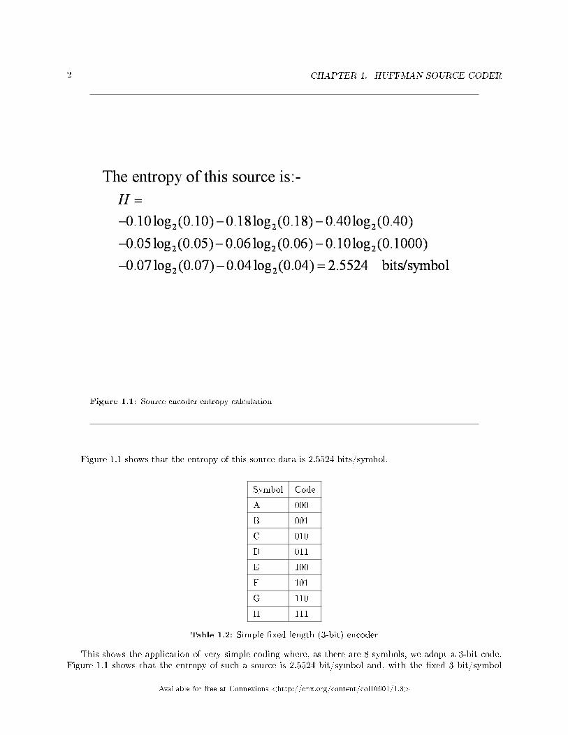
Figure 1.1: Source encoder entropy calculation

Figure 1.1 shows that the entropy of this source data is 2.5524 bits/symbol.

Symbol Code

A 000

B 001

C 010

D 011

E 100

F 101

G 110

H 111

Table 1.2: Simple �xed length (3-bit) encoder

This shows the application of very simple coding where, as there are 8 symbols, we adopt a 3-bit code.Figure 1.1 shows that the entropy of such a source is 2.5524 bit/symbol and, with the �xed 3 bit/symbol


3

length allocated codewords, the e�ciency of this simple coder would be only 2.5524/3.0 = 85.08%, which isa rather poor result.

1.1.2 Hu�man coding

This is a variable length coding technique which involves two processes, reduction and splitting.

1.1.2.1 Reduction

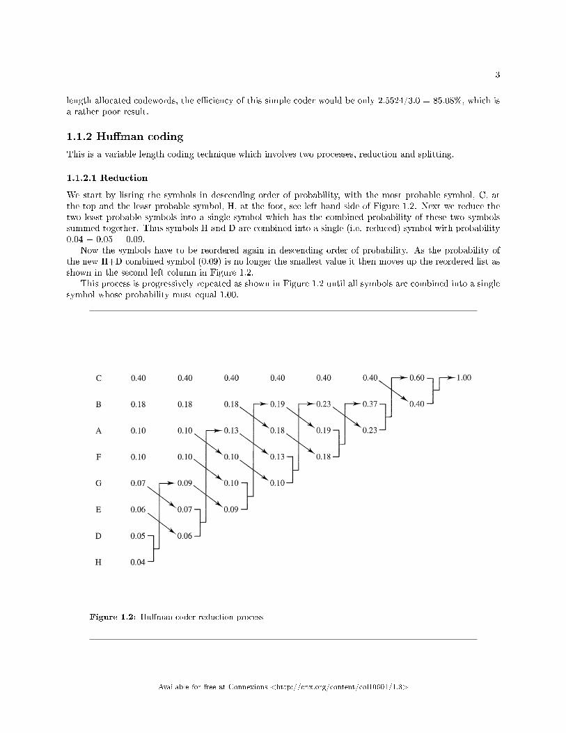
We start by listing the symbols in descending order of probability, with the most probable symbol, C, atthe top and the least probable symbol, H, at the foot, see left hand side of Figure 1.2. Next we reduce thetwo least probable symbols into a single symbol which has the combined probability of these two symbolssummed together. Thus symbols H and D are combined into a single (i.e. reduced) symbol with probability0.04 + 0.05 = 0.09.

Now the symbols have to be reordered again in descending order of probability. As the probability ofthe new H+D combined symbol (0.09) is no longer the smallest value it then moves up the reordered list asshown in the second left column in Figure 1.2.

This process is progressively repeated as shown in Figure 1.2 until all symbols are combined into a singlesymbol whose probability must equal 1.00.

Figure 1.2: Hu�man coder reduction process



1.1.2.2 Splitting

The variable length codewords for each transmitted symbol are now derived by working backwards (fromthe right) through the tree structure created in Figure 1.2, by assigning a 0 to the upper branch of eachcombining operation and a 1 to the lower branch.

The �nal �combined symbol� of probability 1.00 is thus split into two parts of probability 0.60 withassigned digit of 0 and another part with probability 0.40 with assigned digit of 1. This latter part withprobability 0.40 and assigned digit of 1 actually represents symbol C, Figure 1.3.

The �combined symbol� with probability 0.60 (and allocated �rst digit of 0) is now split into two furtherparts with probability 0.37 with an additional or second assigned digit of 0 (i.e. its code is now 00) andanother part with the remaining probability 0.23 where the additional assigned digit is 1 and associated codewill now be 01.

Figure 1.3: Hu�man coder splitting process to generate the variable length codewords and allocatethese depending on symbol probabilities.

This process is repeated by adding each new digit after the splitting operation to the right of the previousone. Note how this allocates short codes to the more probable symbols and longer codes to the less probablesymbols, which are transmitted less often.


5

Symbol Code

A 011

B 001

C 1

D 00010

E 0101

F 0000

G 0100

H 00011

Table 1.3: Hu�mann coded variable length symbols

1.1.3 Code e�ciency

Figure 1.3 summarises the codewords now allocated to each of the transmitted symbols A. . .H and alsocalculates the average length of this source coder as 2.61 bits/symbol. Note the considerable reduction fromthe �xed length of 3 in the simple 3-bit coder in earlier table.



Figure 1.4: Summary of allocated codewords for each symbol, A ...H, and calculation of average lengthof transmitted codeword.

Now recall from Figure 1.1 that the entropy of the source data was 2.5524 bits/symbol and the simple�xed length 3-bit code in the earlier table, with a length of 3.00 which gave an e�ciency of only 85.08%.

The e�ciency of the Hu�man coded data with its variable length codewords is therefore 2.5524/2.62 =97.7% which is a much more acceptable result.

If the symbol probabilities all have values 1/(2n) which are integer powers of 2 then Hu�mann codingwill result in 100% e�ciency.

note: This module has been created from lecture notes originated by P M Grant and DG M Cruickshank which are published in I A Glover and P M Grant, "Digital Communi-cations", Pearson Education, 2009, ISBN 978-0-273-71830-7. Powerpoint slides plus end ofchapter problem examples/solutions are available for instructor use via password access athttp://www.see.ed.ac.uk/∼pmg/DIGICOMMS/


Chapter 2

Block FECC coding1

2.1 Block FECC coding

2.1.1 Forward error correcting coding (FECC)

Block codes are one example of the forward error correcting coding (FECC) technique where we encodethe signal by adding additional bits or digits of redundant data so that the decoder is then able to correctmost of the errors which are introduced by transmission through a noisy channel. FECC was invented fordeep space probes where the extremely long transmission propagation path loss results in received data withparticularly low signal to noise ratio as the modest transmitter power is limited by the solar panel outputs.

As we are adding additional bits to generate each codeword this is a systematic encoder as the informationdata bits are included directly within the codewords. The additional bits required for the transmission of theredundant information increases the data rate which will consume more bandwidth if we wish to maintainthe same throughput, but, if we seek to obtain low error rates, then this trade-o� is usually acceptable.



7

8 CHAPTER 2. BLOCK FECC CODING

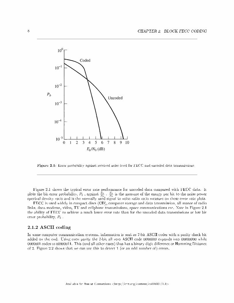
Figure 2.1: Error probability against received noise level for FECC and uncoded data transmissions

Figure 2.1 shows the typical error rate performance for uncoded data compared with FECC data. Itplots the bit error probability, Pb , against

Eb

N0. Eb

N0is the measure of the energy per bit to the noise power

spectral density ratio and is the normally used signal to noise ratio ratio measure on these error rate plots.FECC is used widely in compact discs (CD), computer storage and data transmission, all manor of radio

links, data modems, video, TV and cellphone transmissions, space communications etc. Note in Figure 2.1the ability of FECC to achieve a much lower error rate than for the uncoded data transmissions at low biterror probability, Pb .

2.1.2 ASCII coding

In some computer communication systems, information is sent as 7-bit ASCII codes with a parity check bitadded on the end. Using even parity the 7-bit all zero ASCII code 0000000 expands into 00000000 while0000001 codes to 00000011. This (and all other cases) thus has a binary digit di�erence or Hamming Distanceof 2. Figure 2.2 shows that we can use this to detect 1 (or an odd number of) errors.


9

Figure 2.2: ASCII code example where received codeword has single error in the 5th bit position

The block length is then n = 8 and the number of information bits k = 7. This generally assists witherror detection but is is insu�ciently robust or redundant to achieve an error correction capability as thecoding rate is only 7/8.

The minimum distance in binary digits between any two codewords is known as the minimum HammingDistance, Dmin , which is 2 for the case of odd or even parity check in ASCII data transmission. We canthen calculate the error detecting and correcting power of a code from the minimum distance in bits betweenerror free blocks or codewords, see error correction capability module.

Although we shall look exclusively at coding schemes for binary systems, error correcting and detectingcoding is not con�ned to binary digits. For example the ISBN numbers used on books have a checksumappended to them and these are calculated via modulo 11 arithmetic.

2.1.3 Block code construction

Block codes collect or arrange incoming information carrying data into groups of k binary digits and addcoding (i.e. parity) bits to increase the coded block length up to n bits, where n>k.



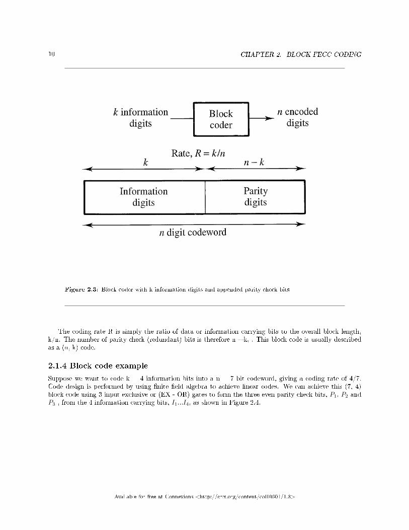
Figure 2.3: Block coder with k information digits and appended parity check bits

The coding rate R is simply the ratio of data or information carrying bits to the overall block length,k/n. The number of parity check (redundant) bits is therefore n � k, . This block code is usually describedas a (n, k) code.

2.1.4 Block code example

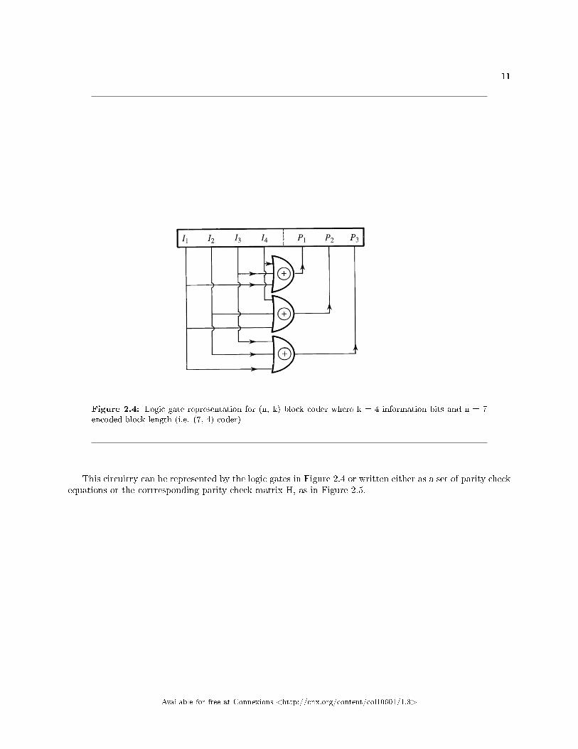
Suppose we want to code k = 4 information bits into a n = 7 bit codeword, giving a coding rate of 4/7.Code design is performed by using �nite �eld algebra to achieve linear codes. We can achieve this (7, 4)block code using 3 input exclusive or (EX - OR) gates to form the three even parity check bits, P1, P2 andP3 , from the 4 information carrying bits, I1...I4, as shown in Figure 2.4.


11

Figure 2.4: Logic gate representation for (n, k) block coder where k = 4 information bits and n = 7encoded block length (i.e. (7, 4) coder)

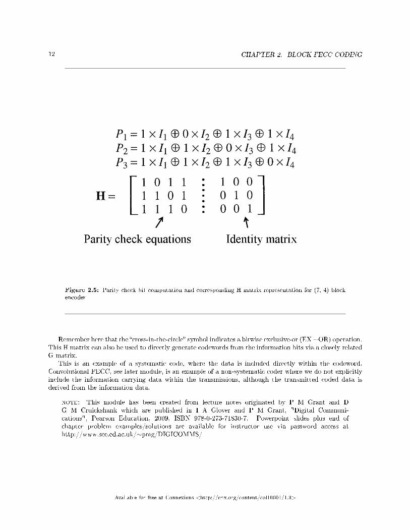
This circuitry can be represented by the logic gates in Figure 2.4 or written either as a set of parity checkequations or the corrresponding parity check matrix H, as in Figure 2.5.



Figure 2.5: Parity check bit computation and corresponding H matrix representation for (7, 4) blockencoder

Remember here that the �cross-in-the-circle� symbol indicates a bitwise exclusive-or (EX � OR) operation.This H matrix can also be used to directly generate codewords from the information bits via a closely relatedG matrix.

This is an example of a systematic code, where the data is included directly within the codeword.Convolutional FECC, see later module, is an example of a non-systematic coder where we do not explicitlyinclude the information carrying data within the transmissions, although the transmitted coded data isderived from the information data.



Chapter 3

Block code performance1

3.1 Block code error correction capability

3.1.1 Hamming distance

Consider two distinct �ve digit codewords C1 = 00000 and C2 = 00011. These have a binary digit di�erence(or Hamming distance) of 2 in the last two digits. The minimum distance in binary digits between any twocodewords is known as the minimum Hamming distance, Dmin

For block codes the minimum Hamming distance or the smallest di�erence between the digits for any twocodewords in the complete code set, Dmin , is the property which controls the error correction performance.We can thus calculate the error detecting and correcting power of a code from the minimum distance in bitsbetween the codewords.

Thus for a code with a minimum distance Dmin = 3 then this code can be used to correct:



13

14 CHAPTER 3. BLOCK CODE PERFORMANCE

Figure 3.1: Relationship between Dmin and error detection OR correction capability (but not bothsimultaneously)

Note in the earlier example of two �ve digit codewords C1 = 00000 and C2 = 00011 which had a Hammingdistance of 2 there is only one codeword (e.g. A = 00001 or B = 00010) which lies inbetween these twocodewords. Now if there was an error result (e.g. A = 00001) we cannot tell whether it came from C1 or C2so we can thus only used this to detect that an error has occurred.

If the two �ve digit codewords had been C1 = 00000 and C2 = 00111, which have a Hamming distanceof 3, there are then two words which lie inbetween these codewords (e.g. A = 00001 and B = 00011) andthese can thus be used EITHER to detect two errors without any correction capability OR if detection isnot required they can used to correct a single error (e.g. C1 = 00000 distorted into A = 00001 or C2 =00111 distorted into B = 00011), Figure 3.1.

When performing the correction operation we require to insert the decision boundary as shown in Example1 below. If in this example we had wished to perform detection only as shown in the lower part of Figure 3.1then we would ignore whether the received code A = 00001 resulted from a single error from a C1 transmissionor a double error from a C2 code transmission and only identify it as a detected error.

Example 1 � error correctionC1 = 00000A = 00001��B = 00011


15

C2 = 00111This explains further the detailed operation of the equations in Figure 3.1 where detection only operation

does not require the decision boundary to aid identi�cation of the origination of the error.

3.1.2 Block error probability and correction capability

If we have an error correcting code which can correct R' errors, than the probability of a codeword not beingcorrectable is the probability of having more than R' errors in n digits. The probability of having more thanR' errors is given in Figure 3.2. We can this calculate this probability by summing all the induvidual errorprobabilities up to and including R' errors in the block.

Figure 3.2: Correction of more than R' errors in an n digit block

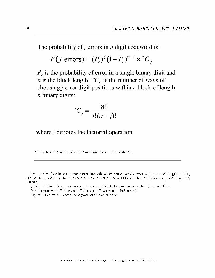
The probability of j errors occurring in an n digit codeword is given in Figure 3.3. Pe is the probabilityof error in a single binary digit and n is the block length. Figure 3.3 also shows how to calculate the nCjterm representing all the possible number of ways or error positions that j errors can occur within a blockof length n binary digits.



Figure 3.3: Probability of j errors occurring an an n-digit codeword

Example 2: If we have an error correcting code which can correct 3 errors within a block length n of 10,what is the probability that the code cannot correct a received block if the per digit error probability is Pe

= 0.01?Solution: The code cannot correct the received block if there are more than 3 errors. Thus:P > 3 errors = 1 - P(0 errors) - P(1 error) - P(2 errors) - P(3 errors).Figure 3.4 shows the component parts of this calculation.


17

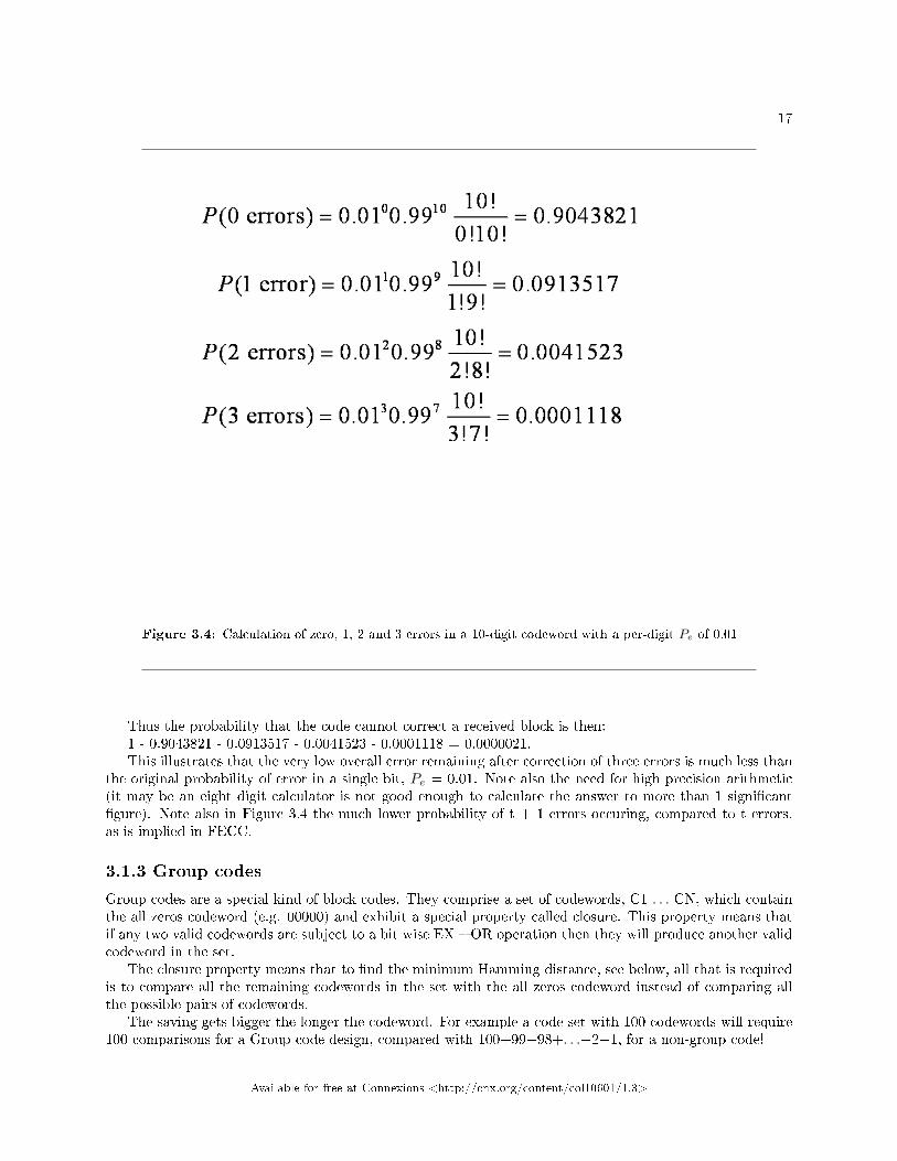
Figure 3.4: Calculation of zero, 1, 2 and 3 errors in a 10-digit codeword with a per-digit Pe of 0.01

Thus the probability that the code cannot correct a received block is then:1 - 0.9043821 - 0.0913517 - 0.0041523 - 0.0001118 = 0.0000021.This illustrates that the very low overall error remaining after correction of three errors is much less than

the original probability of error in a single bit, Pe = 0.01. Note also the need for high precision arithmetic(it may be an eight digit calculator is not good enough to calculate the answer to more than 1 signi�cant�gure). Note also in Figure 3.4 the much lower probability of t + 1 errors occuring, compared to t errors,as is implied in FECC.

3.1.3 Group codes

Group codes are a special kind of block codes. They comprise a set of codewords, C1 . . . CN, which containthe all zeros codeword (e.g. 00000) and exhibit a special property called closure. This property means thatif any two valid codewords are subject to a bit wise EX � OR operation then they will produce another validcodeword in the set.

The closure property means that to �nd the minimum Hamming distance, see below, all that is requiredis to compare all the remaining codewords in the set with the all zeros codeword instead of comparing allthe possible pairs of codewords.

The saving gets bigger the longer the codeword. For example a code set with 100 codewords will require100 comparisons for a Group code design, compared with 100+99+98+. . .+2+1, for a non-group code!



In Group codes the Dmin calculation is further simpli�ed into calculating the minimum codeword weightor minimum number of 1 digits in a codeword in the set.

3.1.4 Nearest neighbour decoding

Nearest neighbour decoding assumes that the codeword nearest in Hamming distance to the received wordis what was transmitted, as shown in Example 1 above. This inherently contains the assumption that theprobability of a small number of t errors is greater than the probability of the larger number of t+1 errors,i.e that Pe is small.

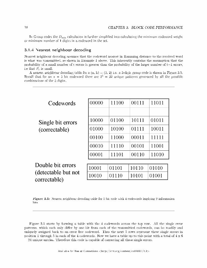
A nearest neighbour decoding table for a (n, k) = (5, 2) i.e. a 5-digit group code is shown in Figure 3.5.Recall that for an n = 5 bit codeword there are 25 = 32 unique patterns generated by all the possiblecombinations of the 5 digits.

Figure 3.5: Nearest neighbour decoding table for 5 bit code with 4 codewords implying 2 informationbits

Figure 3.5 starts by forming a table with the 4 codewords across the top row. All the single errorpatterns, which each only di�er by one bit from each of the transmitted codewords, can be readily anduniquely assigned back to an error free codeword. Thus the next 5 rows represent these single errors inposition 1 through 5 in each of the 4 codewords. Now we have a table up to this point with a total of 4 x 6= 24 unique entries. Therefore this code is capable of correcting all these single errors.


19

There are also eight remaining codes or table entries as 32 - 24 = 8 and these represent double errorpatterns which, as can be seen, lie an equal Hamming distance from at least 2 of the initial 4 codewordsin the top row. Note for example errors in the �rst two digits of the 00000 codeword result in us receiving11000. However data bit pattern is identi�ed here in Figure 3.5 as a single error from codeword 11100 as weassume that 1 error is a much more likely occurence than two errors!

These represent some of the double error patterns, which can thus be detected here, but they cannnotbe corrected as all the possible double error patterns do not have a unique representation in Figure 3.5.

3.1.5 Soft decision decoding

Nearest neighbour decoding can also be done on a soft decision basis, with real non-binary numbers fromthe receiver. The nearest Euclidean distance (nearest to these 5 codewords in terms of a 5-D geometry) isthen used and this gives a considerable performance increase over the hard decision decoding described here.

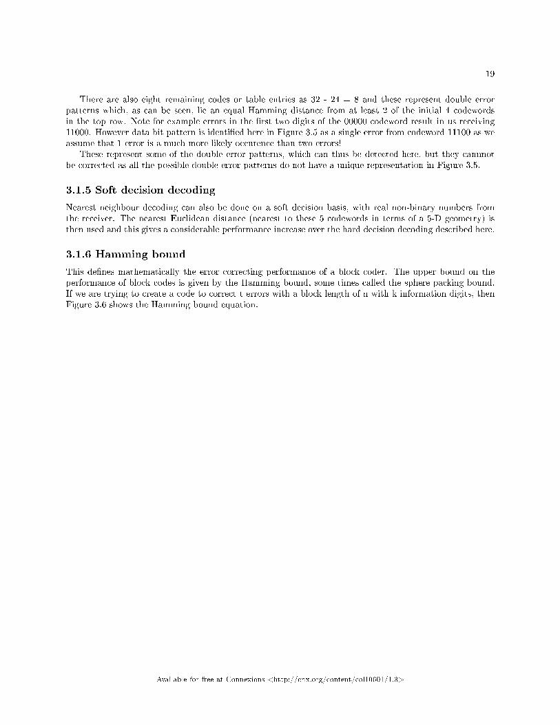
3.1.6 Hamming bound

This de�nes mathematically the error correcting performance of a block coder. The upper bound on theperformance of block codes is given by the Hamming bound, some times called the sphere packing bound.If we are trying to create a code to correct t errors with a block length of n with k information digits, thenFigure 3.6 shows the Hamming bound equation.



Figure 3.6: Hamming bound calculation for (n, k) block code to establish number of terms which canbe included in the denominator and hence arrive at the codes error correcting power t

Here the denominator terms, which are represented by the binomial coe�cients, represent the number ofpossible patterns or positions in which 1, 2, ..., t errors can occur in an n-bit codeword.

Note the relationship between the decoding table in Figure 3.5 and the Hamming Bound equation inFigure 3.6. The 2k = 4 left hand entry represents the number of transmitted codewords or columns in thetable. The numerator 2n = 32 represents the total possible number of unique entries in the table. Thedemoninator represents the number of rows which can be accommodated within the table. Here the �rstdenominator term (1) represents the �rst row (i.e. the transmitted codewords) and the second term (n) the5 single error patterns. Subsequent terms then represent all the possible double, triple error patterns, etc.The denominator has to be sized or restricted to t to ensure the inequality and this gives or de�nes the errorcorrection capability as t.

If the equation in Figure 3.6 is satis�ed then the design of suck an (n, k) code is possible with the errorcorrecting power of t. If the equation is not satis�ed, then we must be less ambitious by reducing t or k (forthe same block length n) or increasing n (while maintaining t and k).

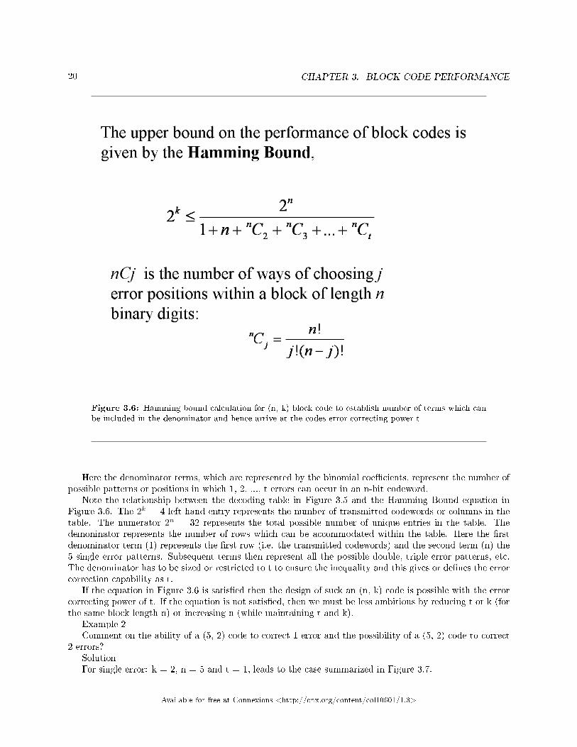
Example 2Comment on the ability of a (5, 2) code to correct 1 error and the possibility of a (5, 2) code to correct

2 errors?SolutionFor single error: k = 2, n = 5 and t = 1, leads to the case summarized in Figure 3.7.


21

Figure 3.7: Calculation to assess whether (5, 2) block code can correct t = 1 error - Answer yes

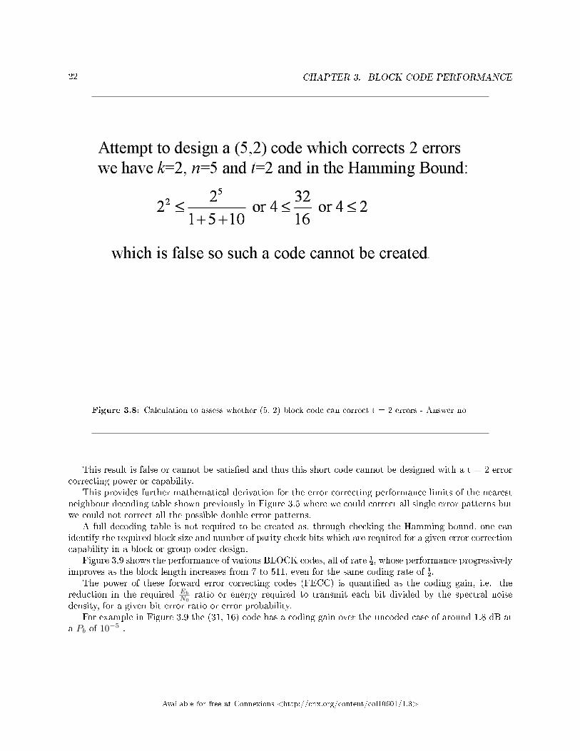
which is true so such a code design is possible.However if we try to design a (5, 2) code to correct 2 errors we have k = 2, n = 5 and t = 2, which is

summarized in Figure 3.8.



Figure 3.8: Calculation to assess whether (5, 2) block code can correct t = 2 errors - Answer no

This result is false or cannot be satis�ed and thus this short code cannot be designed with a t = 2 errorcorrecting power or capability.

This provides further mathematical derivation for the error correcting performance limits of the nearestneighbour decoding table shown previously in Figure 3.5 where we could correct all single error patterns butwe could not correct all the possible double error patterns.

A full decoding table is not required to be created as, through checking the Hamming bound, one canidentify the required block size and number of parity check bits which are required for a given error correctioncapability in a block or group coder design.

Figure 3.9 shows the performance of various BLOCK codes, all of rate ½, whose performance progressivelyimproves as the block length increases from 7 to 511, even for the same coding rate of ½.

The power of these forward error correcting codes (FECC) is quanti�ed as the coding gain, i.e. thereduction in the required Eb

N0ratio or energy required to transmit each bit divided by the spectral noise

density, for a given bit error ratio or error probability.For example in Figure 3.9 the (31, 16) code has a coding gain over the uncoded case of around 1.8 dB at

a Pb of 10−5 .


23

Figure 3.9: Error performance of 1/2 rate block coders with di�ering block lengths



Chapter 4

Convolutional FECC Encoder1

4.1 FECC � ½ Rate Convolutional Encoder Example

4.1.1 Convolutional coding

Convolutional codes are another type of forward error correcting coder (FECC) which are quite distinct fromblock codes. They are simpler to implement for longer codes than block coders and soft decision decodingcan be employed easily at the decoder.

Convolutional codes are non-systematic (i.e. the transmitted data bits do not appear directly in theoutput encoded data stream) and are generated by passing a data sequence through a transversal or �niteimpulse response (FIR) �lter. The coder output can be regarded as the convolution of the input sequencewith the impulse response of the coder, hence their name: convolutional codes.

4.1.2 Convolutional encoder

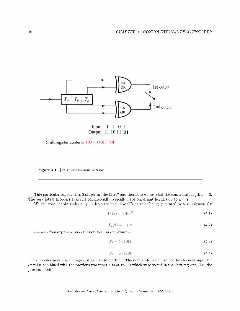
A simple example is shown in Figure 4.1. Here the encoder shift register starts with zeros at all three storedlocations (i.e. 0, 0, 0). The input data sequence to be encoded is 1, 1, 0, 1 in this example. The shift registercontents thus become, after each data bit arrives and propagates into the shift register: 100, 110, 011, 101.As there are two outputs for overy input bit the above encoder is rate ½.

The �rst output is obtained after arrival of a new data bit into the shift register when the switch is inthe upper position, the second with the switch in the lower position. Thus, in this example, the switch willgenerate, through the exclusive OR gates, from the four input data bits: 1, 1, 0, 1, the corresponding fouroutput digit pairs: 11, 10, 11, 01



25

26 CHAPTER 4. CONVOLUTIONAL FECC ENCODER

Figure 4.1: ½ rate convolutional encoder

This particular encoder has 3 stages in �the �lter� and therefore we say that the constraint length n = 3.The very latest encoders available commercially typically have constraint lengths up to n = 9.

We can consider the coder outputs from the exclusive OR gates as being generated by two polynomials:

P1(x) = 1 + x2 (4.1)

P2(x) = 1 + x (4.2)

These are often expressed in octal notation, in our example:

P1 = 5o(101) (4.3)

P2 = 6o(110) (4.4)

This encoder may also be regarded as a state machine. The next state is determined by the next input bitor value combined with the previous two input bits or values which were stored in the shift register, (i.e. theprevious state).


27

4.1.3 Tree state diagram

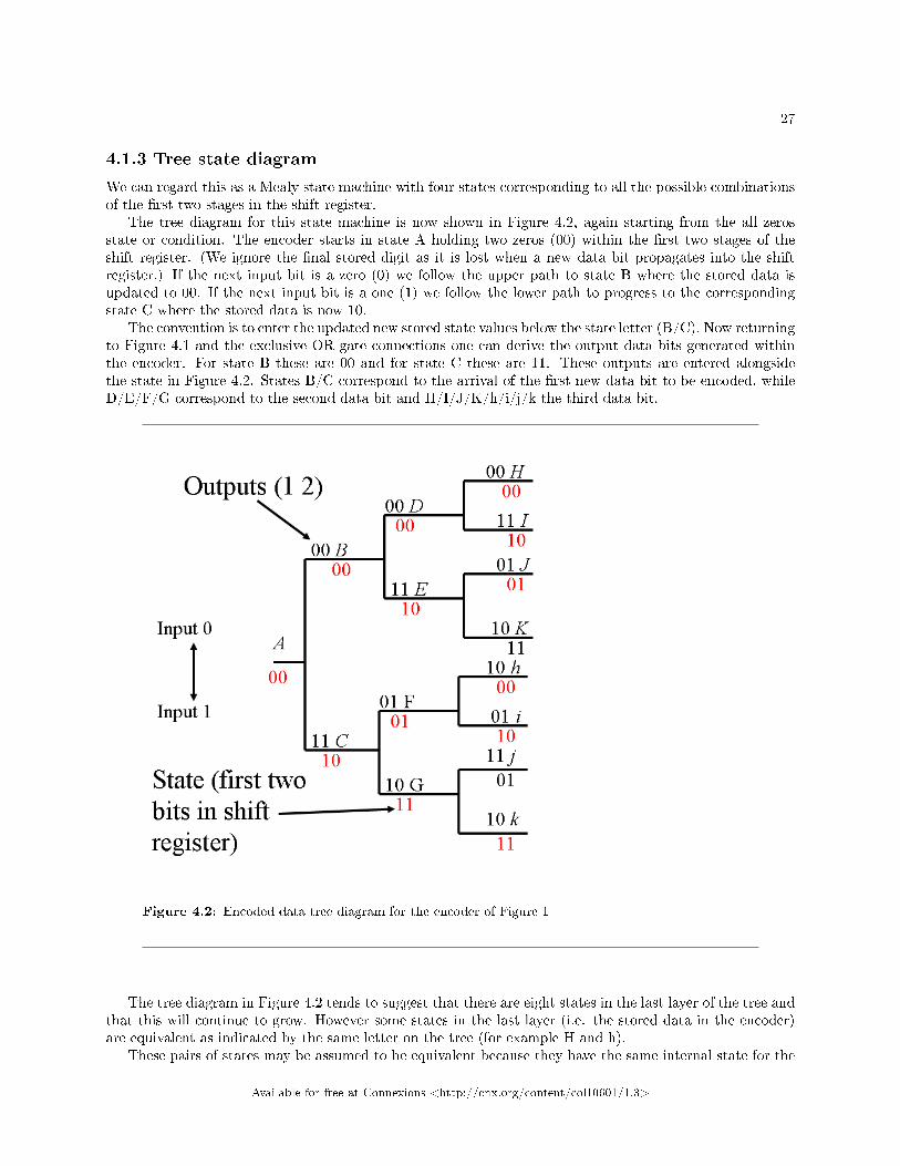
We can regard this as a Mealy state machine with four states corresponding to all the possible combinationsof the �rst two stages in the shift register.

The tree diagram for this state machine is now shown in Figure 4.2, again starting from the all zerosstate or condition. The encoder starts in state A holding two zeros (00) within the �rst two stages of theshift register. (We ignore the �nal stored digit as it is lost when a new data bit propagates into the shiftregister.) If the next input bit is a zero (0) we follow the upper path to state B where the stored data isupdated to 00. If the next input bit is a one (1) we follow the lower path to progress to the correspondingstate C where the stored data is now 10.

The convention is to enter the updated new stored state values below the state letter (B/C). Now returningto Figure 4.1 and the exclusive OR gate connections one can derive the output data bits generated withinthe encoder. For state B these are 00 and for state C these are 11. These outputs are entered alongsidethe state in Figure 4.2. States B/C correspond to the arrival of the �rst new data bit to be encoded, whileD/E/F/G correspond to the second data bit and H/I/J/K/h/i/j/k the third data bit.

Figure 4.2: Encoded data tree diagram for the encoder of Figure 1

The tree diagram in Figure 4.2 tends to suggest that there are eight states in the last layer of the tree andthat this will continue to grow. However some states in the last layer (i.e. the stored data in the encoder)are equivalent as indicated by the same letter on the tree (for example H and h).

These pairs of states may be assumed to be equivalent because they have the same internal state for the



�rst two stages of the shift register and therefore will behave exactly the same way to the receipt of a new(0 or 1) input data bit.

4.1.4 Trellis state diagram

Thus the tree can be folded into a trellis, as shown in , which is derived from the tree diagram of Figure 4.2and Figure 4.1 encoder. As the constraint length is n = 3 we have 2(3−1) = 4 unique states: 00, 01, 10, 11in Figure 4.2. In Figure 4.3 the states are shown as 00x to denote the third bit, x, which is lost or discardedfollowing the arrival of a new data bit.

Figure 4.3: Trellis Diagram corresponding to the Tree Diagram of Figure 2

Note in Figure 4.3 the horozontal arrangement of states A, B, D, H and L. The same applies to statesC, E, I and M etc. The horizontal direction corresponds to time (the whole diagram in Figure 4.3 nowcorresponds to encoding 4 input data bits). Here we have dropped the state information from Figure 4.2 asthe same states are all represented at the same horizontal level in Figure 4.3. The vertical direction herecorresponds to the stored state values a, b, c, d in the encoder shift register.

States along the time axis are thus equivalent, for example H is equivalent to L and C is equivalent toE etc. In fact all the states in a horizontal line are equivalent. Thus we can identify only four states in thiscoder: a, b, c and d and the related shift register stored values 00, 10, 01, 11 are shown in the left hand sideof Figure 4.3.


29

From any point, e.g. E, if the next input bit is a zero (0) we follow the upper path to state J where thestored data is updated to 01 and the output will be 01. If the next input bit is a one (1) we follow the lowerpath from E to progress to the next state K where the stored data is now 11 and the output will be 10 asindicated alongside the trellis path.

4.1.5 Transition state diagram

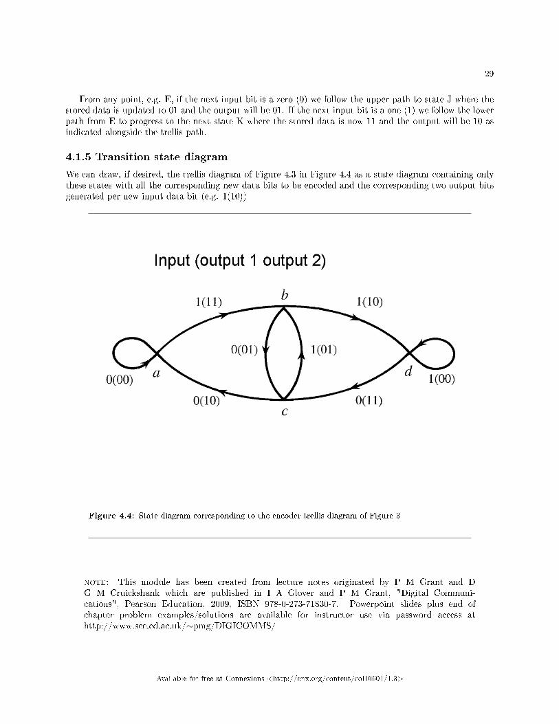
We can draw, if desired, the trellis diagram of Figure 4.3 in Figure 4.4 as a state diagram containing onlythese states with all the corresponding new data bits to be encoded and the corresponding two output bitsgenerated per new input data bit (e.g. 1(10))

Figure 4.4: State diagram corresponding to the encoder trellis diagram of Figure 3



Chapter 5

Viterbi Decoder1

5.1 Viterbi convolutional decoder

A convolutional code is not decoded in short blocks as in a block code. However, to simplify decoding,messages are arti�cially broken down into very long blocks by periodically �ushing the encoder with a stringof zeros, as in the example discussed here.

For illustration only this example here uses an unrealistically short block length of 5 data bits with thelast two �xed at 0 to �ush the encoder (remember that this is very ine�cient and, in practice, practicalblock lengths are very much longer, typically 1,000 to 10,000 bits in length).

Convolutional codes are always decoded using the Viterbi algorithm as this simpli�es the decoding op-eration. The algorithm is based on the nearest neighbour decoding scheme and, like the other algorithmswe have looked at, it relies on the assumption that the probability of t errors is much greater than theprobability of t+1 errors and it thus selects or chooses and retains only the paths which have fewer errors.

The decoding process is based on the previous decoding trellis. We will use the previous ½ rate encoderexample and assume that the received message is: 10 10 00 10 10, representing a total of �ve (unknown)transmitted data bits each encoded into �ve bit pairs, i.e. total of ten encoded data bits. We further assumein this simpli�ed example that the last 2 bits of the 5 data inputs were �ushing zeros to reset the encoderand decoder.

Starting (after �ushing) with the �rst received bit in position A in the encoder, we know that if a 1 hadbeen input, (lower path) from the encoder �gure the output should have been 11 as we moved to state C. Ifa 0 was input (upper path) we should have received 00 and moved to state B, see upper part of Figure 5.1.

What was actually received was 10, a Hamming distance of 1 from both these possibilities, so we drawthat in the lower part of Figure 5.1 onto the �rst stage of our decoding trellis.



31

32 CHAPTER 5. VITERBI DECODER

Figure 5.1: First stage of trellis after decoding �rst two received data bits

Instead of reporting the expected outputs we next annotate the lower part of Figure 5.1 with the separatedistances between the received data and the trellis encoder on each path. We then add the cumulativeHamming distance to the states (B, C) in square brackets above the states B and C

Now consider the second pair of received data bits. Consider �rst state B. As before, we should havereceived 00 for a 0 input and 11 for a 1 input, see left hand side of Figure 5.2. What we actually receivedwas 10, which is a Hamming distance of 1 from both possibilities so the right hand part of Figure 5.2 isannotated with the individual and cumulative distances to states D and E.

Then consider state C. For a 0 input, (upper part) we should have received 01, but what was actuallyreceived was 10, a Hamming distance of 2. For a 1 input (lower path) we should have received 10 and this isexactly what was received, corresponding to a Hamming distance of 0! Again the right part of Figure 5.2 isannotated with the individual distances on the paths and the new cumulative or summed distances to statesF and G.


33

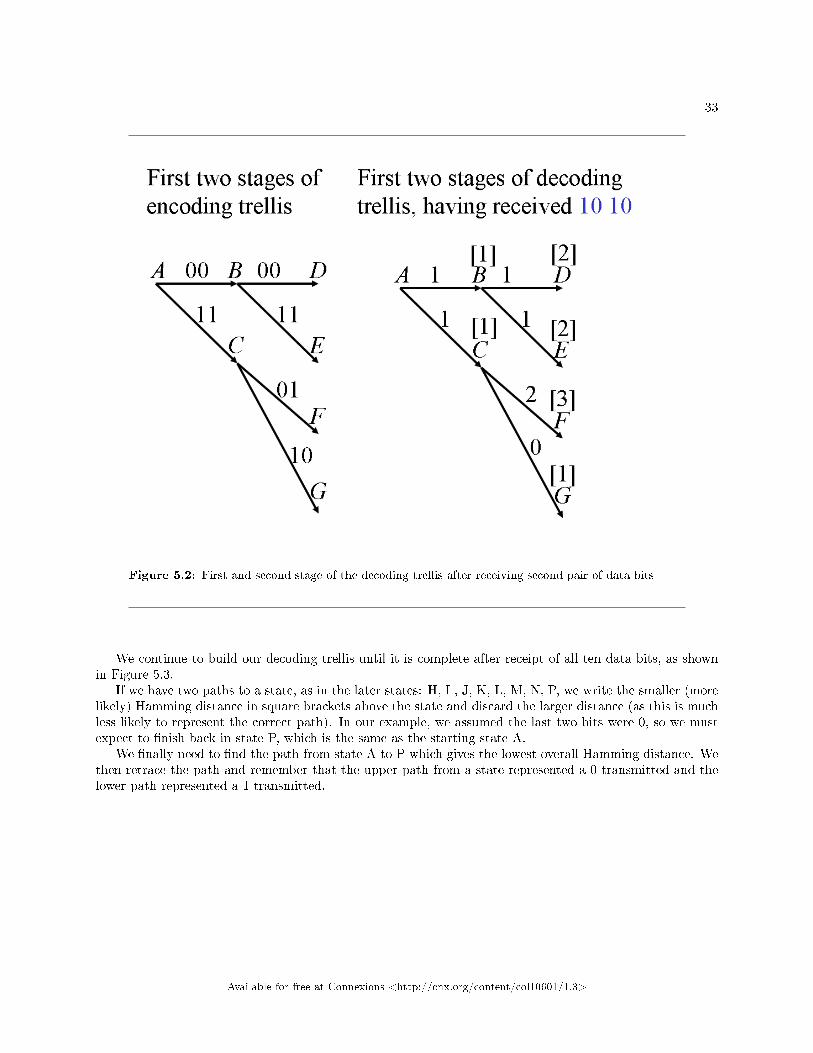
Figure 5.2: First and second stage of the decoding trellis after receiving second pair of data bits

We continue to build our decoding trellis until it is complete after receipt of all ten data bits, as shownin Figure 5.3.

If we have two paths to a state, as in the later states: H, I , J, K, L, M, N, P, we write the smaller (morelikely) Hamming distance in square brackets above the state and discard the larger distance (as this is muchless likely to represent the correct path). In our example, we assumed the last two bits were 0, so we mustexpect to �nish back in state P, which is the same as the starting state A.

We �nally need to �nd the path from state A to P which gives the lowest overall Hamming distance. Wethen retrace the path and remember that the upper path from a state represented a 0 transmitted and thelower path represented a 1 transmitted.



Figure 5.3: Full decoding trellis after receipt of all ten data bits

The reverse decoded data for this example is indicated by the dashed line in Figure 5.3.Leaving states A, C, G and K always in the lower of the two possible paths implies that a data bit 1 has

been received at these states and therefore this translates to 1, 1, 1 as the �rst three encoded data bits.The last two bits don't matter in this case as we have assumed they are 0, 0 and we can remove from

the docoding trellis all the states that don't support or contribute to this solution.Note that �nishing a block with n-1 zero input data bits is not compulsory. If you make a decision after

a delay of approximately �ve times the constraint length n, this makes little di�erence in code performancebut does limit the memory consumed by the process to a more sensible amount.

Figure 5.4 shows the performance of various BLOCK codes, all of rate ½, whose performance improves asthe block length increases, even for the same coding rate of ½.

The power of these forward error correcting codes (FECC) is quanti�ed as the coding gain, i.e. thereduction in the required Eb

N0ratio or energy required to transmit each bit divided by the spectral noise

density, for a given bit error ratio or error probability.For example in Figure 5.4 the (31, 16) code has a coding gain over the uncoded case of around 1.8 dB at

a Pb of 10−5 .


35

Figure 5.4: Error performance of 1/2 rate block coders with di�ering block lengths

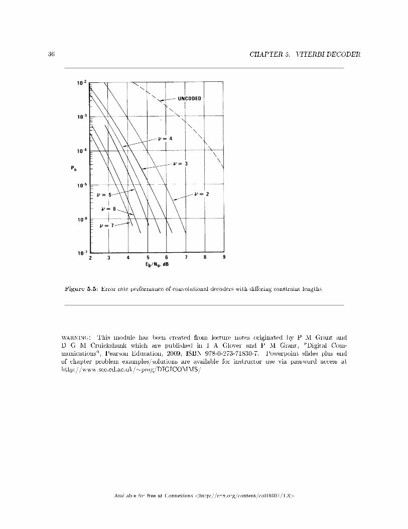
Figure 5.5 shows for comparison with the block codes of Figure 5.4 the performance of convolutionalcoders. The convolutional code initially provides very good performance at modest constraint length. Ashort constraint length of n = v = 3 is already superior to the 511 block length code of Figure 5.4. Theadditional attraction of the convolutional coder is its further improvement with the increase in constraintlength up to n = 7 or 9, as shown in Figure 5.5.

Unfortunately the coding and decoding process gets more complicated with larger block/constraint length.As shown here convolutional codes with Viterbi decoding are generally more powerful than block codes,especially for very low error rates, hence their wider use. Single chip constraint length 9 (512 state) encoderand decoders are now widely available as commercial products from many semiconductor vendors.



Figure 5.5: Error rate performance of convolutional decoders with di�ering constraint lengths

warning: This module has been created from lecture notes originated by P M Grant andD G M Cruickshank which are published in I A Glover and P M Grant, "Digital Com-munications", Pearson Education, 2009, ISBN 978-0-273-71830-7. Powerpoint slides plus endof chapter problem examples/solutions are available for instructor use via password access athttp://www.see.ed.ac.uk/∼pmg/DIGICOMMS/


Chapter 6

Turbo Coding1

6.1 Turbo encoding and decoding

6.1.1 Introduction

A paper was published by Claude Berrou and coauthors at the ICC conference in 1993 that rocked or shookthe �eld of forward error correction coding (FECC). This described a method of creating much more powerfulblock error correcting coding with only the minimum amount of e�ort. Its main features were two recursiveconvolutional encoders (RCE) interconnected via an interleaver. The data is fed into the �rst encoder directlyand into the second encoder after interleaving or reordereing of the input data.

6.1.2 Turbo encoding

The important features are the use of two recursive convolutional encoders and the design of the interleaverwhich gives a block code with the block size equal to the interleaver size, Figure 6.1. Random interleaverstend to work better than row and column interleavers. Note that recursive convolutional encoders wereknown about well before their use in turbo codes, but the di�culties in driving them into a known statemade them less popular than the non-recursive convolutional encoders described in the previous module.

The name turbo decoder came from the turbo charger in an automobile where the exhaust gasses areused to drive a compressor in a feedback loop to increase the input of fuel and hence the vehicles ultimateperformance.



37

38 CHAPTER 6. TURBO CODING

Figure 6.1: Turbo encoder with recursive encoding loops

The desired output rate was initially achieved by puncturing (ignoring every second output) from eachof the encoders.

6.1.3 Turbo decoding

Turbo decoding is iterative. The decoding is also soft, the values that �ow around the whole decoder arereal values and not binary representations (with the exception of the hard decisions taken at the end of thenumber of iterations you are prepared to perform). They are usually log likelihood ratios (LLRs), the log ofthe probability that a particular bit was a logic 1 divided by the probability the same bit was a logic 0.

Decoding is accomplished by �rst demultiplexing the incoming data stream into d, y1 , y2. d and y1 gointo the decoder for the �rst code, Figure 6.2. This gives an estimate of the extrinsic information from the�rst decoder which is interleaved and past on to the second decoder. The second decoder thus has threeinputs, the extrinsic information from the �rst decoder, the interleaved data d, and the received values fory2. It produces its extrinsic information and this is deinterleaved and passed back to the �rst encoder. Thisprocess is then repeated or iterated as required until the �nal solution is obtained from the second decoderinterleaver.


39

Figure 6.2: Turbo decoder

The decoders themselves generally use soft output Viterbi algorithm (SOVA) to decode the received data.However the preferred turbo decoding method is to use the maximum a-priori (MAP) algorithm but this istoo mathematical to discuss here!


40 CHAPTER 6. TURBO CODING

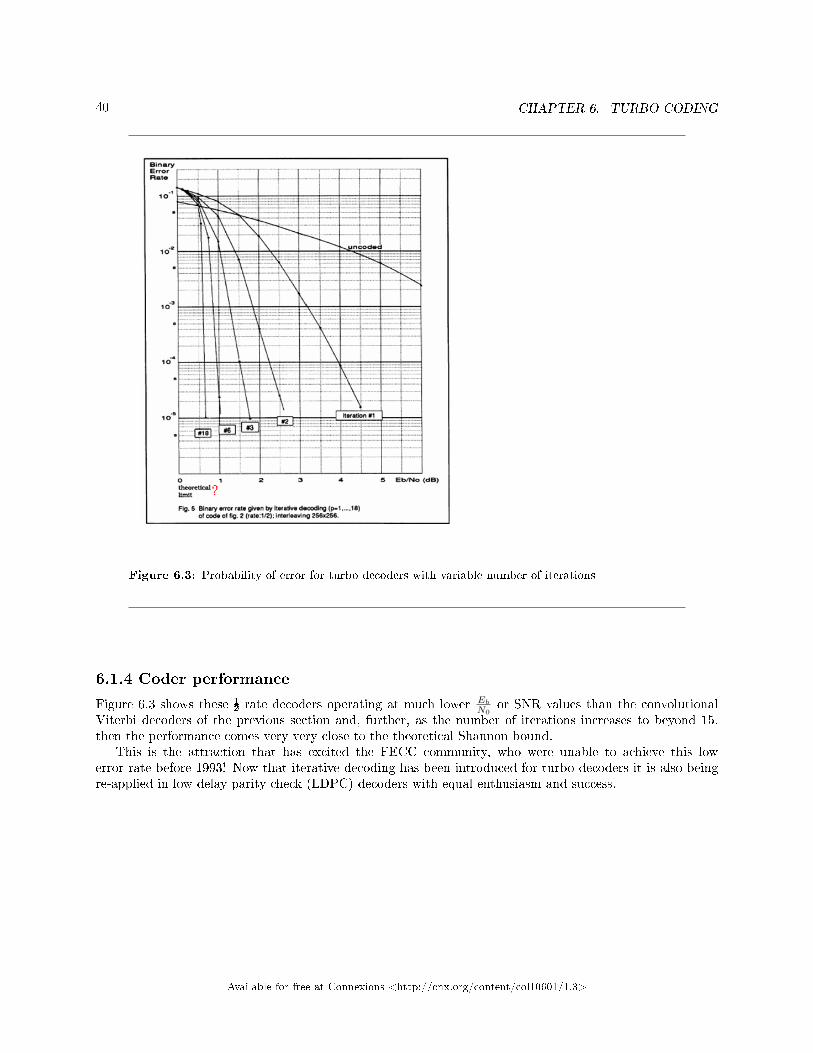
Figure 6.3: Probability of error for turbo decoders with variable number of iterations

6.1.4 Coder performance

Figure 6.3 shows these ½ rate decoders operating at much lower Eb

N0or SNR values than the convolutional

Viterbi decoders of the previous section and, further, as the number of iterations increases to beyond 15,then the performance comes very very close to the theoretical Shannon bound.

This is the attraction that has excited the FECC community, who were unable to achieve this lowerror rate before 1993! Now that iterative decoding has been introduced for turbo decoders it is also beingre-applied in low delay parity check (LDPC) decoders with equal enthusiasm and success.


41

Figure 6.4

Figure 6.4 includes a turbo decoding example (which as an animated power point slide) will show the blackdot noise induced errors being corrected on each subsequent iteration with the black dots being progressivelyreduced in the upper cartoon.



42 INDEX

Index of Keywords and Terms

Keywords are listed by the section with that keyword (page numbers are in parentheses). Keywordsdo not necessarily appear in the text of the page. They are merely associated with that section. Ex.apples, � 1.1 (1) Terms are referenced by the page they appear on. Ex. apples, 1

B Block codes, � 3(13)Block coding, � 2(7)

C Convolutional code, � 5(31)Convolutional coder, � 4(25)

F FECC, � 5(31), � 6(37)Forward Error Correcting Coder, � 4(25)

H Hamming bound, � 3(13)

hu�man coder, � 1(1)

N Nearest neighbour decoding, � 3(13)

P Parity check matrix, � 2(7)

S source coding, � 1(1)

T Turbo Decoders, � 6(37)

V Viterbi decoding, � 5(31)


ATTRIBUTIONS 43

Attributions

Collection: Communications Source and Channel Coding with examples

Edited by: Peter GrantURL: http://cnx.org/content/col10601/1.3/License: http://creativecommons.org/licenses/by/2.0/

Module: "Hu�man source coder"By: Peter GrantURL: http://cnx.org/content/m18172/1.4/Pages: 1-6Copyright: Peter GrantLicense: http://creativecommons.org/licenses/by/2.0/

Module: "Block FECC coding"By: Peter GrantURL: http://cnx.org/content/m18174/1.3/Pages: 7-12Copyright: Peter GrantLicense: http://creativecommons.org/licenses/by/2.0/

Module: "Block code performance"By: Peter GrantURL: http://cnx.org/content/m18175/1.7/Pages: 13-23Copyright: Peter GrantLicense: http://creativecommons.org/licenses/by/2.0/

Module: "Convolutional FECC Encoder"By: Peter GrantURL: http://cnx.org/content/m18176/1.3/Pages: 25-29Copyright: Peter GrantLicense: http://creativecommons.org/licenses/by/2.0/

Module: "Viterbi Decoder"By: Peter GrantURL: http://cnx.org/content/m18177/1.3/Pages: 31-36Copyright: Peter GrantLicense: http://creativecommons.org/licenses/by/2.0/

Module: "Turbo Coding"By: Peter GrantURL: http://cnx.org/content/m18178/1.3/Pages: 37-41Copyright: Peter GrantLicense: http://creativecommons.org/licenses/by/2.0/


Communications Source and Channel Coding with examples

Hu�man variable length source coder is �rst described then systematic channel coding block coder designis introduced for forward error correction coding (FECC). Nearest neighbour decoding and the Hammingbound is used to de�ne the performance of these block coders. Finally the nonsystematic convolutionalcoder, Viterbi decoder and turbo recursive coder designs are introduced with examples of the operation ofthese coders.

About Connexions

Since 1999, Connexions has been pioneering a global system where anyone can create course materials andmake them fully accessible and easily reusable free of charge. We are a Web-based authoring, teaching andlearning environment open to anyone interested in education, including students, teachers, professors andlifelong learners. We connect ideas and facilitate educational communities.

Connexions's modular, interactive courses are in use worldwide by universities, community colleges, K-12schools, distance learners, and lifelong learners. Connexions materials are in many languages, includingEnglish, Spanish, Chinese, Japanese, Italian, Vietnamese, French, Portuguese, and Thai. Connexions is partof an exciting new information distribution system that allows for Print on Demand Books. Connexionshas partnered with innovative on-demand publisher QOOP to accelerate the delivery of printed coursematerials and textbooks into classrooms worldwide at lower prices than traditional academic publishers.

Communications Source and Channel Coding with examples

Documents

Transcript of Communications Source and Channel Coding with examples