Combining Geoprocessing and Interregional Input-Output Systems:

An Application to the State of São Paulo in Brazil

Silvio Massaru Ichihara DERSA, Secretary of Transport - State of São Paulo

E-mail: ichihara@dersa.sp.gov.br

Joaquim José Martins Guilhoto1 Department of Economics, FEA - University of São Paulo

REAL, University of Illinois; and CNPq Scholar E-mail: guilhoto@usp.br

Denise Imori Department of Economics, FEA - University of São Paulo

E-mail: denise.imori@gmail.com

Paper Presented at 56th Annual North American Meetings of the Regional Science Association International

San Francisco, USA - November 18th - 21th, 2009

Abstract

This work develops a method for the construction of input-output systems capable of estimating the flows of goods and services among cities, having in view that the creation of accurate strategies depends on the regional peculiarities incorporated in the scope of the economic planning researches. The study innovates by combining geoprocessing with input-output theory elements, facilitating the interpretation of the information available on the extensive data set of interregional input-output systems. The analytical potential is showed through a panoramic evaluation of the São Paulo State supply and demand relations, and by the application of the estimated input-output system to a study of the regional impacts of the “Bolsa Familia” Program, an income transfer program from the Federal government. The results show that this program must be understood not only as a form of income transference, but also as a catalytic agent for decreasing the regional inequality inside the state.

Key words: Input-Output, Geoprocessing, Regional Development, Brazil, São Paulo State.

1 This author would like to thank FAPESP (Fundação de Amparo à Pesquisa do Estado de São Paulo) for the financial support that helped in the conduction of this study and made it possible to attend and to present this paper at “56th Annual North American Meetings of the Regional Science Association International”.

2

1. Introduction The input-output systems describe the flows of goods and services among the many sectors of

an economy, considering the characteristics of one or several regions. According to Leontief

(1965), its dimension can be large enough to represent the world economy or adequately small so

as to describe a metropolitan region.

When assuming a greater degree of geographical focalization, these models are able to

incorporate the regional peculiarities, enabling the elaboration of specific analysis and of urban

planning strategies (ISARD, 1998).

However, one of the greatest problems faced by these studies is the difficulty in obtaining the

appropriate data. Surveys with an adequate statistical relevance are expensive, demanding

significant time and dedication to be executed. Moreover, there is the need for secrecy,

aggravated when one analyses business data. In this way, the advantages of the regional analysis

collide with the insufficiency of information, so that the researcher is compelled to formulate

alternative methods for the estimation of nonexistent or unavailable data.

In this framework, the present work intends to formalize a procedure sequence that enables

the estimation of an interregional input-output system, considering a higher degree of regional

disaggregation, in order to achieve the municipal level.

Due to the unavailability of information on sectoral production in the municipal level, the

method developed by this study was applied only to the São Paulo State, Brazil, by way of

exemplifying the process of estimating an intermunicipal input-output table.

The following section presents the proposed method and, subsequently, the evaluation of the

results is done by means of the geographical representation of the main elements of the input-

output table. In order to do this, one utilizes geoprocessing techniques, in accordance with the

initial ideas exposed in Guilhoto et al (2003).

At last, a parallel analysis, conditioned to the geographical distribution of the “Bolsa

Família”, a federal income transfer program, in São Paulo State, intends to exemplify the

descriptive potential of these data as subsidies for planning strategies.

2.2 Methodology

Initially, this section presents the structure of the interregional input-output table and the

notation used to represent it. In the subsequent subsection, one briefly describes the main

3

methods utilized in the estimation of economic flows among regions, focusing the gravitational

input-output approach, which contains elements of the information theory and spatial variables.

At last, the variables needed for the implementation of the chosen method are calculated and the

proper adaptations and considerations on the modeling are characterized.

2.2.1 The interregional input-output model

The input-output model is composed by matrices and vectors based in the actual relations of

the economy, considering the logical and quantitative linkages among the productive sectors. Its

structure have to be in accordance with the international standards defined by the United Nations

- System of National Accounts - SNA (UNITED NATIONS, 2006).

In general lines, the system is characterized by two main tables: make and use matrices,

which describe the relations among the n productive sectors and the m commodities, but can be

summarized in a single matrix, considering either intersectoral relations (with dimensions: n rows

and n columns) or among commodities (dimensions: m rows and m columns.

This condition establishes that the ulterior analysis have to assume one of the two possible

hypotheses: industry-based (deciding for the relations among sectors) or commodity-based

technologies (deciding for the relations among commodities), according to Miller and Blair

(1985).

The two hypotheses are different alternatives to treat the same problem, but the choice for

either one or the other depends of several conditions (STONE, 1961). In general, many studies

adopt the industry-based technology hypothesis, because they focus the sectoral planning or

because this hypothesis can be easily interpreted, considering the economic circuit starting from

the demand. Mesnard (2004) demonstrated that the commodity-based theory cannot be

interpreted in the same way, since it would implicate in algebraic incoherencies when one

considers the economic circuit starting from the demand.

In the present study, one does not deepen the discussion about this question and opts for the

alternative of industry-based technology. From this point, all the concepts and considerations will

be based in this assumption.

In this way, the denomination “input-output table”, utilized in this study, corresponds to the

group composed by the use matrix (n sectors x n sectors) and the vectors of final demand

4

(investments, exports, inventory changes, households and government’s consumption), imports,

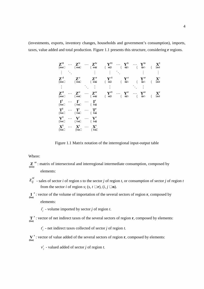
taxes, value added and total production. Figure 1.1 presents this structure, considering r regions.

( ) ( ) ( ) ( ) ( ) ( ) ( )

( ) ( ) ( ) ( ) ( ) ( ) ( )

( ) ( ) ( ) ( ) ( ) ( ) ( )

( ) ( ) ( )

( ) ( ) ( )

( ) ( ) ( )

( )

5 5 5

5 5 5

5 5 5

t t

s st s s st s s

t t

t

t

t

11 1 1r 11 1 1r 1

nxn nxn nxn nx nx nx nx1

1 r 1 r

nxn nxn nxn nx nx nx nx1

r1 r rr r1 r rr r

nxn nxn nxn nx nx nx nx1

1 r

1xn 1xn 1xn

1 r

1xn 1xn 1xn

1 r

1xn 1xn 1xn

1

1xn

Z Z Z Y Y Y X

Z Z Z Y Y Y X

Z Z Z Y Y Y X

I I I

T T T

V V V

X

L L L L

M O M M O M M

M O M M O M

L L L L

L L

L L

L L

( ) ( )t r

1xn 1xnX XL L

Figure 1.1 Matrix notation of the interregional input-output table

Where:

rr

(nxn)Z : matrix of intersectoral and interregional intermediate consumption, composed by

elements:

stijz - sales of sector i of region s to the sector j of region t, or consumption of sector j of region t

from the sector i of region s; (s, t ∈r ), (i, j ∈n).

r

(lxn)I : vector of the volume of importation of the several sectors of region r , composed by

elements:

tji - volume imported by sector j of region t.

r

(lxn)T : vector of net indirect taxes of the several sectors of region r , composed by elements:

tjt - net indirect taxes collected of sector j of region t.

r

(lxn)V : vector of value added of the several sectors of region r , composed by elements:

tjv - valued added of sector j of region t.

5

rr

(nxf)Y : matrix of final demand of region r for the production of s, composed by five columns (f =

5): a) households’ consumption; b) government’s consumption; c) gross fixed capital formation; d) exports; and e) inventory changes.

stiy - consumption of setor i of region s by the vectors of final demand of region t.

r

(lxn)X : vector of total production of the several sectors of region r , composed by elements:

tjx - total production of sector j of region t (total sum of the columns).

r

(nxl)X : vector of total production of the several sectors of region r , composed by elements:

six - total production of sector i of region s (total sum of the rows).

2.2.2 Estimation of the interregional flows

When one analyses a single region, the set r is unitary and the intermediate consumption is

composed by a single matrix Z, characterizing a structure very similar to that presented by

Leontief (1951) for the economy of United States. In Brazil, the national input-output table has

not been published by the Brazilian Institute of Geography and Statistics (IBGE) since 1996.

However, the information can be estimated by means of the system of national accounts, using

the methodology described by Guilhoto and Sesso Filho (2005b).

The inexistence of publications similar to the system of national accounts in the level of

regional administrations makes impossible to utilize the same method to construct municipal

tables. Even if this were possible, only the intersectoral relations of each region could be lonely

obtained, since the interregional relations depend also on the existence of data about the flows of

goods and services among the regions, characterizing the Zst (s ≠ t e s, t ∈ r ) matrices.

The efforts applied to estimate the flows of goods and services among regions and their

productive sectors are presented as a group of methods differently classified.

Algebraic techniques have been elaborated or adapted from other fields, in the attempt to

approximate the estimated interregional flows to the real ones. Round (1983) defines two main

classes of methods meant to update, organize or estimate the data of interregional tables: methods

with census data (“survey methods”) and methods with limited census data (partial-survey

methods” and “nonsurvey methods”).

Montoya (1999) presents a scheme in which the classification also departs from these two

main branches, in relation to the nature of data, making considerations about the reach and the

6

theoretical limitations of each group of interregional input-output model. The present work will

approach only the main mathematical techniques described in the literature that make use of

limited census data.

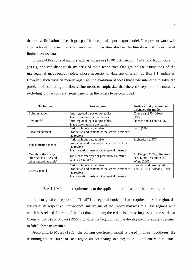
In the publications of authors such as Polenske (1970), Richardson (1972) and Robinson et al

(2001), one can distinguish six sorts of main techniques that ground the estimations of the

interregional input-output tables, whose necessity of data are different, as Box 1.1. indicates.

However, such division merely organizes the evolution of ideas that arose intending to solve the

problem of estimating the flows. One needs to emphasize that these concepts are not mutually

excluding, on the contrary, some depend on the others to be concluded.

Technique Data required Authors that proposed or discussed the model

Column model

• Intra-regional input-output tables • Trade flows among the regions

Chenery (1975); Moses (1955)

Row model

• Intra-regional input-output tables • Trade flows among the regions

Hansen and Tiebout (1963)

Location quotient • National input-output table • Production and demand of the several sectors of

the regions

Isard (1998)

Transportation model

• National input-output table • Production and demand of the several sectors of

the regions • Transportation costs or other spatial measure

Richardson (1972)

Models of the theory of information (RAS and other entropic models)

• Table of former year or previously estimated data to be adjusted

McDougall (1999); Robinson et al (2001); Canning and Wang (2005)

Gravity models

• National input-output table • Production and demand of the several sectors of

the regions • Transportation costs or other spatial measure

Leontief and Strout (1963); Theil (1967); Wilson (1970)

Box 1.1 Minimum requirements to the application of the approached techniques

In its original conception, the “ideal” interregional model of Isard requires, in each region, the

survey of its respective inter-sectoral matrix and of the import matrices of all the regions with

which it is related. In front of the fact that obtaining these data is almost impossible, the works of

Chenery (1975) and Moses (1955) signalize the beginning of the development of models destined

to fulfill these necessities.

According to Moses (1955), the column coefficient model is based in three hypotheses: the

technological structures of each region do not change in time; there is uniformity in the trade

7

relations of the productive sectors; and trade among regions is stable. In practice terms, the share

of a good that is demanded from a region by all sectors of the other one is considered to be

constant and is distributed to each of the productive sectors accordingly with the technical

coefficients (Chenery, 1975).

In order to apply the column model, or Chenery-Moses model, it is necessary to have the

intra-regional technical coefficients (intersectoral matrices of each region) and the coefficients of

trade of goods and services among the regions, but one does not need know about the

intersectoral flows among the regions. The proportions of demand obtained in the columns of

intra-regional tables are utilized to distribute the flows of goods, initially aggregated, in the

intersectoral flows among the regions.

Concerning the row coefficient model, presented by Hansen and Tiebout (1963), the same

idea is developed, but the difference consists in the fact that the shares are estimated from the

rows. In the row model, therefore, one fixes the proportions of sales and not those of the demand,

as the column model does.

Richardson (1972) evaluates that the Walrasian assumption, inherent to the input-output

models, can be disrespected if the sales proportion among regions of a certain sector remains

constant even if the demand level is modified in any region. This is an implication of the fact that

the Walrasian assumption presupposes that production variations are caused only by variations in

demand and changes in prices are provoked only by modifications in supply.

Polenske (1970) tested the column, row and gravity models; the results indicated that the

column model was superior to the row model, but there were no significant differences in relation

to the gravity model of Leontief and Strout (1963). Other authors, such as Ranco (1985), also

discuss the question of the possibility if theoretical incongruencies in the row model, indicating

the column model as preferable.

The assumption of the column model is that each region imports a fixed proportion of its

necessities for a commodity from a given exporting region, what is quite reasonable according to

many authors. However, given the difficulties in obtaining the data relative to the trade flows,

since this sort of information is not available in the accessible database, it is not possible to use

only these models (column and row models).

For this reason, the location quotient appears as a much less demanding technique, since it

does not require one to know neither the flows of goods among regions nor the input-output

8

tables of each region (intra-regional tables). Its central characteristic is determining the exporter

and importer sectors, without being calibrated by any additional criterion about the spatial

position of the sectors. Miller and Blair (1985) present the complete sequence of calculations

about the location quotient and its main variations: the purchases-only location quotient and the

cross-industry quotient.

Because it does not depend on the flows of goods among the regions, the location quotient

has been largely used in the practice, although with great restrictions. Isard (1998) mentions that

it is easy to observe errors in the use of location quotients, since the patterns of consumption and

income of households may cause the accumulation of production in some regions, which will not

necessarily be exporters of those commodities. Moreover, the estimation of the flows cannot be

independent of factors that restrict the interregional trade, such as distance and transportation

costs. Without this attrition, nothing would restrain the interaction between two regions in

opposite locations to be more intense than that between two complementary neighbors, where

one exports the commodities demanded by the other one.

Presently, setting aside the spatial question is not justifiable. The theory that comprehends the

concepts of economic and quantitative geography appears to be relevant in the recent studies.

Together with the evolution of the geoprocessing framework, the lines of thought such as that of

Von Thünen and Alfred Weber achieved an even greater importance by means of responding to

questions relative to rent (land use) and to the optimum localization of the productive activites,

respectively.

The Central Place Theory of Weber evidences the hierarchical relation among cities and is

based in scale economies and in the optimization of transportation costs (FUJITA, KRUGMAN E

VENABLES, 2002). In this way, the optimal localization of production in relation to demand is a

factor that justifies even more the utilization of models related to the transportation network in

the input-output analysis.

Allied to these theories, recent computational advances in the management of transportation

networks (engineering and logistics) were incorporated to the social sciences, facilitating the

practical utilization of transportation models in order to estimate the economic flows.

However, in the estimation of the interregional flows in the input-output table, although the

minimization of the transportation costs by linear programming is an interesting idea, it is not

9

applicable due to the number of null flows obtained, given the very essence of the optimization

process (RICHARDSON, 1972).

In this point, the gravity approach utilized in many fields, also incorporated to the modeling

of the distribution of demand for transportation (model of four stages), admits characteristics that

are very close to those required in the process of estimating the interregional flows. It is inspired

in the Newtonians observations about gravity, assuming that the movements of goods depend on

the levels of demand in the destination region and of supply in the origin, but are inhibited by the

attrition of distance.

In general, the gravity approach is not derived from a single technique and it can be obtained

from diverse concepts. The gravity input-output models can combine four important foundations:

the information theory, the optimization process, the Leontief-Strout model (presented farther on)

and the transportation costs.

In Theil (1967), the elements of the theory of information are developed together with several

economic issues, as: the mensuration of income inequality, problems in the allocation of

consumption and firms, and the question of the relation price-quantity. The author also proposes

ways of utilizing them in the input-output analysis, in order to respond to the problem of the bias

caused by sectoral aggregation, and to improve the estimation techniques for the international

trade flows.

The Theil’s ideas about the interregional relations, based in the use of the Shannon’s entropy

and in the model of Leontief-Strout, were even more improved by the optimization systems of

entropy, originating the gravity input-output model of Wilson (1970).

Initially, in Wilson (1969), the uncertainty about the probability distribution of the number of

interregional trips is maximized, being subject to the restrictions of supply and demand of trips in

each region. Subsequently, Wilson (1970) makes adaptations to this technique, replacing the

number of trips by the economic flows and constructing new restriction equations. In order to do

so, it makes use of the Leontief-Strout model and of considerations on transportation costs.

More recent works also apply concepts of entropic maximization or minimization and the

gravity model by way of estimating the flows of goods and services among the regions. As

example: Cho and Gordon (2001) make considerations about a model for determining economic

impacts in front of catastrophes, using transportation networks, information theory and input-

output models; Kim et al. (2002) evaluate the impacts in the transportation networks caused by

10

earthquakes, utilizing an algorithmic procedure that associates the optimization of flows in

stretches of roads with the entropy, the gravity model and the model of Leontief-Strout. However,

these methods demand specific data on transportation that are not easily obtained.

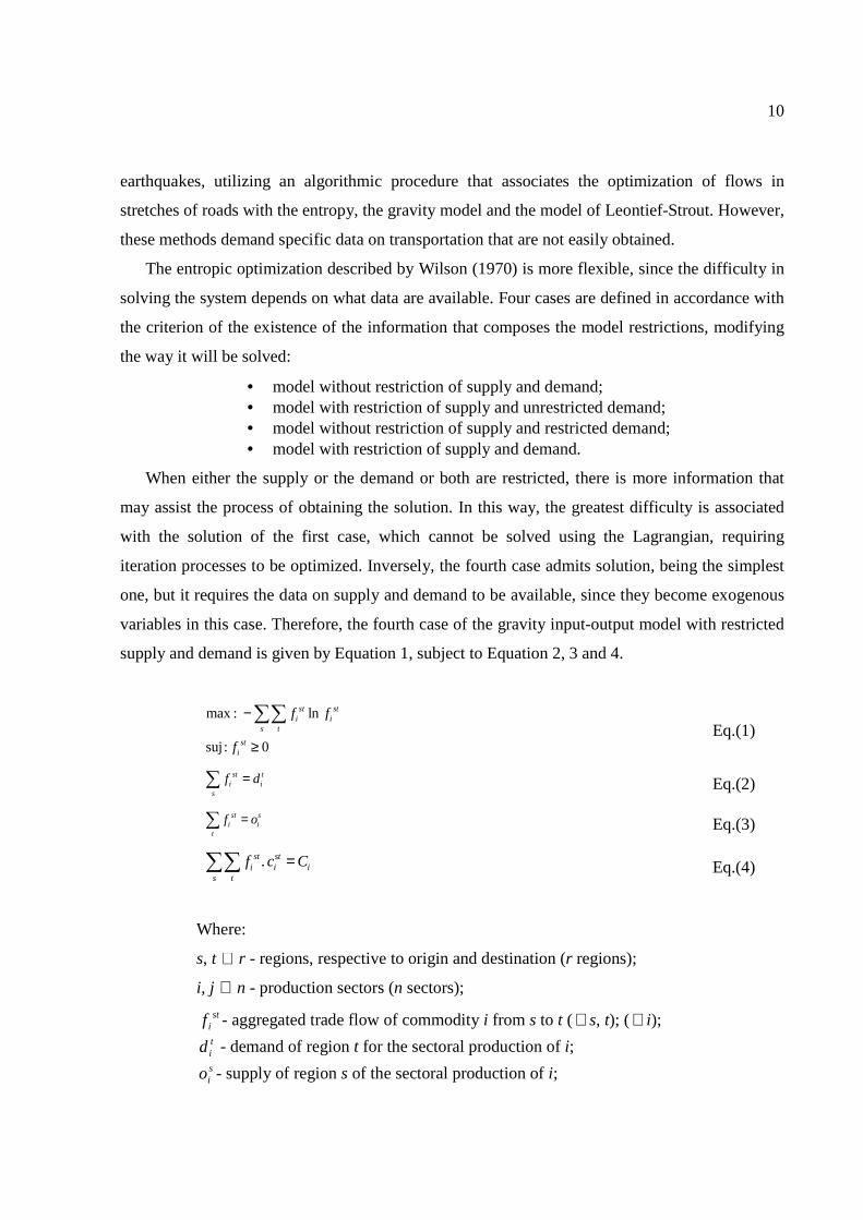
The entropic optimization described by Wilson (1970) is more flexible, since the difficulty in

solving the system depends on what data are available. Four cases are defined in accordance with

the criterion of the existence of the information that composes the model restrictions, modifying

the way it will be solved:

• model without restriction of supply and demand; • model with restriction of supply and unrestricted demand; • model without restriction of supply and restricted demand; • model with restriction of supply and demand.

When either the supply or the demand or both are restricted, there is more information that

may assist the process of obtaining the solution. In this way, the greatest difficulty is associated

with the solution of the first case, which cannot be solved using the Lagrangian, requiring

iteration processes to be optimized. Inversely, the fourth case admits solution, being the simplest

one, but it requires the data on supply and demand to be available, since they become exogenous

variables in this case. Therefore, the fourth case of the gravity input-output model with restricted

supply and demand is given by Equation 1, subject to Equation 2, 3 and 4.

max : ln

suj: 0

st sti i

s t

sti

f f

f

−

≥

∑∑ Eq.(1)

st ti i

s

f d=∑ Eq.(2)

st si i

t

f o=∑ Eq.(3)

.st sti i i

s t

f c C=∑∑ Eq.(4)

Where:

s, t ∈ r - regions, respective to origin and destination (r regions);

i, j ∈ n - production sectors (n sectors);

stif - aggregated trade flow of commodity i from s to t (∀ s, t); (∀ i);

tid - demand of region t for the sectoral production of i;

sio - supply of region s of the sectoral production of i;

11

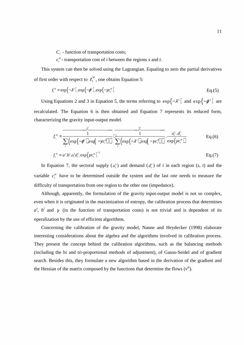
iC - function of transportation costs;

stic - transportation cost of i between the regions s and t.

This system can then be solved using the Lagrangian. Equaling to zero the partial derivatives

of first order with respect to stiz , one obtains Equation 5:

( ) ( ) ( )exp .exp .expst s t sti if cλ ϕ γ= − − − Eq.(5)

Using Equations 2 and 3 in Equation 5, the terms referring to ( )exp sλ− and ( )exp sϕ− are

recalculated. The Equation 6 is then obtained and Equation 7 represents its reduced form,

characterizing the gravity input-output model.

( ) ( )( ) ( ) ( )( ) ( ).1 1

.expexp .exp exp .exp

s ta b

s tst i i

istt st s stii i

t s

o df

cc c γϕ γ λ γ= ⋅

− − − −∑ ∑

6444447444448 6444447444448

Eq.(6)

( ) 1. . .expst s t s t st

i i i if a b o d cγ−

=

Eq.(7)

In Equation 7, the sectoral supply (sio ) and demand (t

id ) of i in each region (s, t) and the

variable stic have to be determined outside the system and the last one needs to measure the

difficulty of transportation from one region to the other one (impedance).

Although, apparently, the formulation of the gravity input-output model is not so complex,

even when it is originated in the maximization of entropy, the calibration process that determines

as, bt and γ (in the function of transportation costs) is not trivial and is dependent of its

operalization by the use of efficient algorithms.

Concerning the calibration of the gravity model, Nanne and Heydecker (1998) elaborate

interesting considerations about the algebra and the algorithms involved in calibration process.

They present the concept behind the calibration algorithms, such as the balancing methods

(including the bi and tri-proportional methods of adjustment), of Gauss-Seidel and of gradient

search. Besides this, they formulate a new algorithm based in the derivation of the gradient and

the Hessian of the matrix composed by the functions that determine the flows (vst).

12

2.2.3 Application of the gravity input-output model

Since it considers spatial elements, of information and of input-output theories, the present

work has elected the gravity input-output model, with restrictions of supply and demand, as the

theoretical basis of the calculations meant for estimating the interregional flows.

Intending that its considerations do not be merely theoretical, this work attempts to

effectively accomplish the estimation, applying the techniques in order to construct an

intermunicipal input-output table for the São Paulo State.

In this way, the following subsections make use of official statistics on the regional

economies of the São Paulo State. Important considerations based in the input-output theory have

to be made in order to enable the calculation of the variables of supply (sio ) and demand (tid ) that

are present in the Equation 7. In the sequence, the third subsection corresponds to the

considerations related to value of variable stic (impedance factor).

2.2.3.1 Regional supply and demand: utilized data

By means of the São Paulo Economic Activity Survey (PAEP), carried out by the State Data

Analysis System Foundation (SEADE, 2002), it is possible to analyze the main segments that

compose the economy of São Paulo State. The survey can be indicated as a powerful tool, able to

characterize the economic activity in regional level.

The most recent database of PAEP corresponds to the year 2001-02, being composed by

information obtained in questionnaires applied to the several economic sectors. It covers the

trade, the general industry (extractive and transformation industry), the construction industry, the

financial institutions and the services. In the present study, the PAEP microdata were consulted

and treated, having in view the respect for the rules of statistical secrecy and the sampling plan of

the survey.2

The fundamental contribution of PAEP is its effort to measure the Value Added (VA) of the

firms, obtaining it from the difference between the Gross Production Value (GPV) and the

2 Some flaws can be observed when one utilizes the PAEP in analysis at the municipal level, because the survey is not censual, adopting a sampling frame focused in the administrative regions of the State, not in its municipalities. In order to diminish this problem, other data banks, such as the Annual Report on Social Information (RAIS – BRASIL, 2006) and IBGE surveys as the Municipal Agricultural Production and the Municipal Livestock Production, were employed to improve the estimations of PAEP.

13

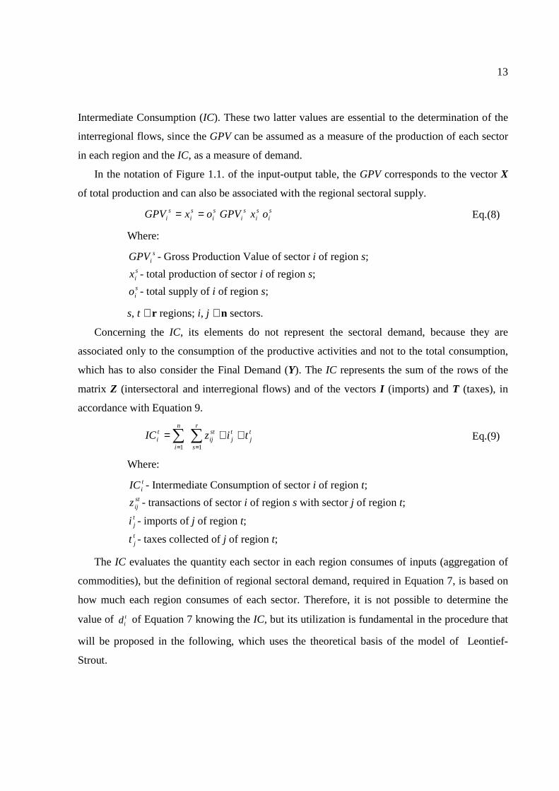
Intermediate Consumption (IC). These two latter values are essential to the determination of the

interregional flows, since the GPV can be assumed as a measure of the production of each sector

in each region and the IC, as a measure of demand.

In the notation of Figure 1.1. of the input-output table, the GPV corresponds to the vector X

of total production and can also be associated with the regional sectoral supply.

si

si

si oxGPV == s

iGPV six s

io Eq.(8)

Where:

siGPV - Gross Production Value of sector i of region s;

six - total production of sector i of region s;

sio - total supply of i of region s;

s, t ∈r regions; i, j ∈n sectors.

Concerning the IC, its elements do not represent the sectoral demand, because they are

associated only to the consumption of the productive activities and not to the total consumption,

which has to also consider the Final Demand (Y). The IC represents the sum of the rows of the

matrix Z (intersectoral and interregional flows) and of the vectors I (imports) and T (taxes), in

accordance with Equation 9.

tj

tj

r

s

stij

n

i

ti tizIC ++= ∑∑

== 11

Eq.(9)

Where:

tiIC - Intermediate Consumption of sector i of region t;

stijz - transactions of sector i of region s with sector j of region t;

tji - imports of j of region t;

tjt - taxes collected of j of region t;

The IC evaluates the quantity each sector in each region consumes of inputs (aggregation of

commodities), but the definition of regional sectoral demand, required in Equation 7, is based on

how much each region consumes of each sector. Therefore, it is not possible to determine the

value of tid of Equation 7 knowing the IC, but its utilization is fundamental in the procedure that

will be proposed in the following, which uses the theoretical basis of the model of Leontief-

Strout.

14

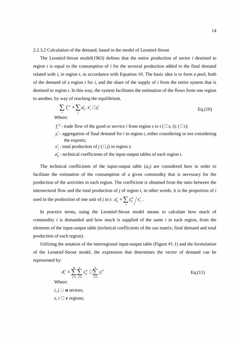
2.2.3.2 Calculation of the demand, based in the model of Leontief-Strout

The Leontief-Strout model(1963) defines that the entire production of sector i destined to

region t is equal to the consumption of i for the sectoral production added to the final demand

related with i, in region t, in accordance with Equation 10. The basic idea is to form a pool, both

of the demand of a region t for i, and the share of the supply of i from the entire system that is

destined to region t. In this way, the system facilitates the estimation of the flows from one region

to another, by way of reaching the equilibrium.

.st t t ti ij j i

s j

f a x y= +∑ ∑ Eq.(10)

Where:

stif - trade flow of the good or service i from region s to t (∀ s, t); (∀ i);

tiy - aggregation of final demand for i in region t, either considering or not considering

the exports; t

jx - total production of j (∀ j) in region t;

tija - technical coefficients of the input-output tables of each region t.

The technical coefficients of the input-output table (aij) are considered here in order to

facilitate the estimation of the consumption of a given commodity that is necessary for the

production of the activities in each region. The coefficient is obtained from the ratio between the

intersectoral flow and the total production of j of region t, in other words, it is the proportion of i

used in the production of one unit of j in t: t st tij ij j

s

a z x=∑ .

In practice terms, using the Leontief-Strout model means to calculate how much of

commodity i is demanded and how much is supplied of the same i in each region, from the

elements of the input-output table (technical coefficients of the use matrix, final demand and total

production of each region).

Utilizing the notation of the interregional input-output table (Figure #1.1) and the formulation

of the Leontief-Strout model, the expression that determines the vector of demand can be

represented by:

1 1 1

t st sti ij i

j s s

d z y= = =

= +∑∑ ∑n r r

Eq.(11)

Where:

i, j ∈ n sectors;

s, t ∈ r regions;

15

tid - total demand for i in region t;

iy - corresponds to the sum of the five vectors of final demand for i;

st in stz and sty - represents the destination of the production of region s, to the

intermediate consumption and the final demand of region t, respectively.

In Equation 9, if one separates taxes and imports, the value added of the intersectoral and

interregional transactions can be established by the IC, obtaining a value that, although

algebraically similar, is quite different from the element of the sum of z in Equation 11, since in

one of the cases there is row (i) sum and in the other, column (j) sum.

Although IC is not exactly what one is looking for, it can be used to estimate the intersectoral

matrices of aggregated intermediate consumption in each region ( st

s∑Z , with the notation of

Figure 1.1). By means of these matrices, one can obtain the column (j) sum of z (Equation 11).

In this point, the procedure requires an input-output table representing the totality of the

interregional system to be obtained ( st

t s∑∑Z , following the notation of Figure 1.1). In other

words, if the objective is estimating the relations among the municipalities, one needs to utilize a

state table; if the objective is obtaining an interstate system, one needs to already have a national

table, and so on. In the present work, in order to estimate a interregional system considering the

municipalities of São Paulo, it was necessary to utilize the data of the input-output table of this

State.3

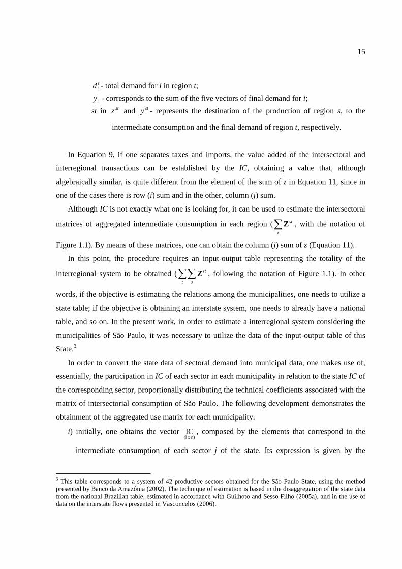
In order to convert the state data of sectoral demand into municipal data, one makes use of,

essentially, the participation in IC of each sector in each municipality in relation to the state IC of

the corresponding sector, proportionally distributing the technical coefficients associated with the

matrix of intersectorial consumption of São Paulo. The following development demonstrates the

obtainment of the aggregated use matrix for each municipality:

i) initially, one obtains the vector n) x (l

IC , composed by the elements that correspond to the

intermediate consumption of each sector j of the state. Its expression is given by the

3 This table corresponds to a system of 42 productive sectors obtained for the São Paulo State, using the method presented by Banco da Amazônia (2002). The technique of estimation is based in the disaggregation of the state data from the national Brazilian table, estimated in accordance with Guilhoto and Sesso Filho (2005a), and in the use of data on the interstate flows presented in Vasconcelos (2006).

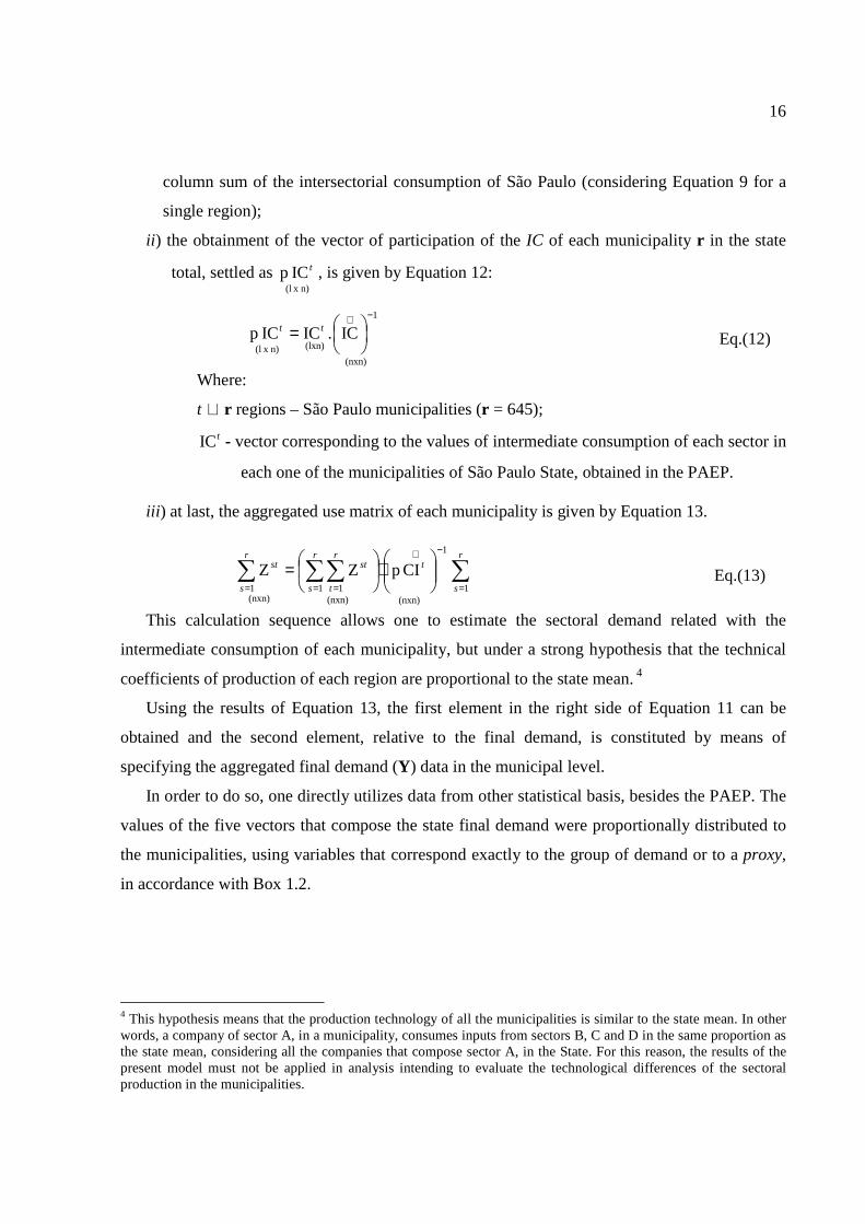
16

column sum of the intersectorial consumption of São Paulo (considering Equation 9 for a

single region);

ii ) the obtainment of the vector of participation of the IC of each municipality r in the state

total, settled as n) x (l

IC p t , is given by Equation 12:

(nxn)

1

(lxn)n) x (lIC.ICIC p

−∧

= tt Eq.(12)

Where:

t ∈ r regions – São Paulo municipalities (r = 645);

tIC - vector corresponding to the values of intermediate consumption of each sector in

each one of the municipalities of São Paulo State, obtained in the PAEP.

iii ) at last, the aggregated use matrix of each municipality is given by Equation 13.

∑∑∑∑=

−∧

= ==

⋅

=r

s

tr

s

r

t

str

s

st

1

1

(nxn)(nxn)1 1

(nxn)1

CIpZZ Eq.(13)

This calculation sequence allows one to estimate the sectoral demand related with the

intermediate consumption of each municipality, but under a strong hypothesis that the technical

coefficients of production of each region are proportional to the state mean. 4

Using the results of Equation 13, the first element in the right side of Equation 11 can be

obtained and the second element, relative to the final demand, is constituted by means of

specifying the aggregated final demand (Y) data in the municipal level.

In order to do so, one directly utilizes data from other statistical basis, besides the PAEP. The

values of the five vectors that compose the state final demand were proportionally distributed to

the municipalities, using variables that correspond exactly to the group of demand or to a proxy,

in accordance with Box 1.2.

4 This hypothesis means that the production technology of all the municipalities is similar to the state mean. In other words, a company of sector A, in a municipality, consumes inputs from sectors B, C and D in the same proportion as the state mean, considering all the companies that compose sector A, in the State. For this reason, the results of the present model must not be applied in analysis intending to evaluate the technological differences of the sectoral production in the municipalities.

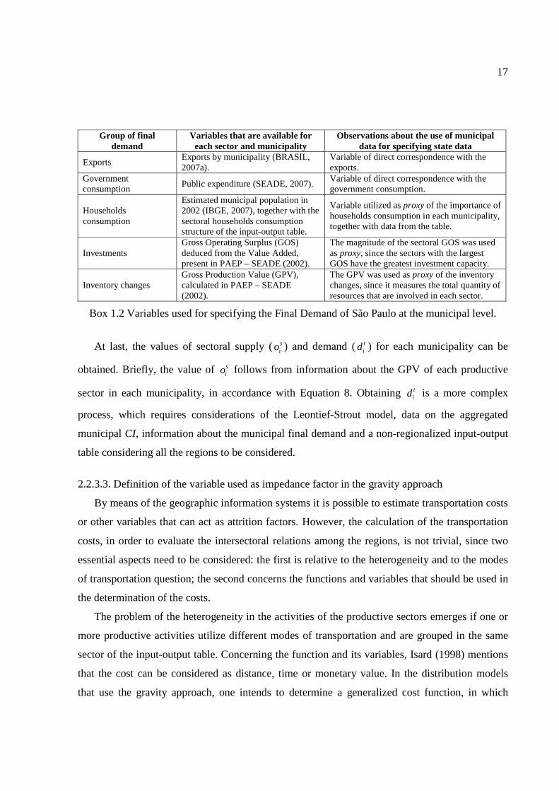
17

Group of final demand

Variables that are available for each sector and municipality

Observations about the use of municipal data for specifying state data

Exports Exports by municipality (BRASIL, 2007a).

Variable of direct correspondence with the exports.

Government consumption

Public expenditure (SEADE, 2007). Variable of direct correspondence with the government consumption.

Households consumption

Estimated municipal population in 2002 (IBGE, 2007), together with the sectoral households consumption structure of the input-output table.

Variable utilized as proxy of the importance of households consumption in each municipality, together with data from the table.

Investments Gross Operating Surplus (GOS) deduced from the Value Added, present in PAEP – SEADE (2002).

The magnitude of the sectoral GOS was used as proxy, since the sectors with the largest GOS have the greatest investment capacity.

Inventory changes Gross Production Value (GPV), calculated in PAEP – SEADE (2002).

The GPV was used as proxy of the inventory changes, since it measures the total quantity of resources that are involved in each sector.

Box 1.2 Variables used for specifying the Final Demand of São Paulo at the municipal level.

At last, the values of sectoral supply (sio ) and demand (t

id ) for each municipality can be

obtained. Briefly, the value of sio follows from information about the GPV of each productive

sector in each municipality, in accordance with Equation 8. Obtaining tid is a more complex

process, which requires considerations of the Leontief-Strout model, data on the aggregated

municipal CI, information about the municipal final demand and a non-regionalized input-output

table considering all the regions to be considered.

2.2.3.3. Definition of the variable used as impedance factor in the gravity approach

By means of the geographic information systems it is possible to estimate transportation costs

or other variables that can act as attrition factors. However, the calculation of the transportation

costs, in order to evaluate the intersectoral relations among the regions, is not trivial, since two

essential aspects need to be considered: the first is relative to the heterogeneity and to the modes

of transportation question; the second concerns the functions and variables that should be used in

the determination of the costs.

The problem of the heterogeneity in the activities of the productive sectors emerges if one or

more productive activities utilize different modes of transportation and are grouped in the same

sector of the input-output table. Concerning the function and its variables, Isard (1998) mentions

that the cost can be considered as distance, time or monetary value. In the distribution models

that use the gravity approach, one intends to determine a generalized cost function, in which

18

linear functions are recommended and that may incorporate a variable denominated modal

penalty. This parameter would be a form of considering all the variables that cannot be easily

dimensioned, and are relative to the modes of transportation that describe them.

In the present work, one has opted for considering only one transportation modality for the

majority of the productive sector: the road transportation. The sectoral productions of extraction

and refinery of oil and gas, and the iron and steel industries largely utilize other modes besides

the road transportation. However, these productions are concentrated in few localities in São

Paulo State, so that the relations of these sectors can be specifically treated.

In relation to the cost function, its measure is expressed in time, considering the road

distance, average velocity, kind of pavement and situation of the road stretch, obtained by means

of the software TransCad® - Caliper (Geographic Information System applied to transportation).

The georeferenced database, composed from the national road network, corresponds to the one of

the same company.

The differences in altitude between origin and destination are also utilized. In order to

calculate them, one uses interpolation techniques for treating the georeferenced altitude measures,

available in the Integrated Cartographic Digital Base of Brazil to the Millionth Scale (IBGE,

1997).

Using this group of information, the measures of the time consumed in covering the shortest

route between a municipality (s) and the other (t) are obtained and attributed as value of the

variable stic .

2.2.4 Estimation of the municipal interregional and intersectoral input-output table

After obtaining sio , t

id and stic , it is then possible to estimate the trade flows among the

regions ( stif ) by means of Equation 7. In this process, the balancing factors of the gravity model

( sa , tb and γ ) can be estimated through iteration and adjustment processes defined in Ortúzar

(2004) and Nanne and Heydecker (1998). The procedures are based in iteration methods for

searching the best values, and can be calibrated by auxiliary information about the distribution of

the interregional flows. In this study, the algorithms were implemented and executed through the

mathematical software Matlab® - MathWorks.

19

Having obtained the trade flows and the other data, it is possible to estimate the interregional

input-output table, considering the attributions of a multi-regional model. The following

development is based in the techniques presented in Miller and Blair (1985) for constructing the

interregional table and the Leontief inverse matrix from the trade flows among the regions, the

aggregated intermediate consumption and the aggregated final demand.

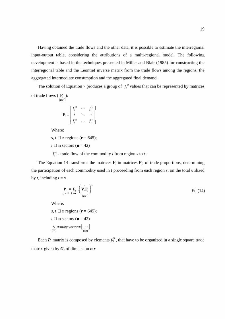
The solution of Equation 7 produces a group of stif values that can be represented by matrices

of trade flows (( )

irxr

F ):

11 1

1

ti i

is st

i i

f f

f f

=

F

L

M O M

L

Where:

s, t ∈ r regions (r = 645);

i ∈ n sectors (n = 42)

stif - trade flow of the commodity i from region s to t .

The Equation 14 transforms the matrices Fi in matrices Pi, of trade proportions, determining

the participation of each commodity used in t proceeding from each region s, on the total utilized

by t, including t = s.

( ) ( )( )

^

i i i

-1

rxr rxrrxr

P = F . V.F Eq.(14)

Where:

s, t ∈ r regions (r = 645);

i ∈ n sectors (n = 42)

[ ](lxr)(lxr)

1 ... 1or unity vect V ==

Each Pi matrix is composed by elementsstip , that have to be organized in a single square trade

matrix given by G, of dimension n.r.

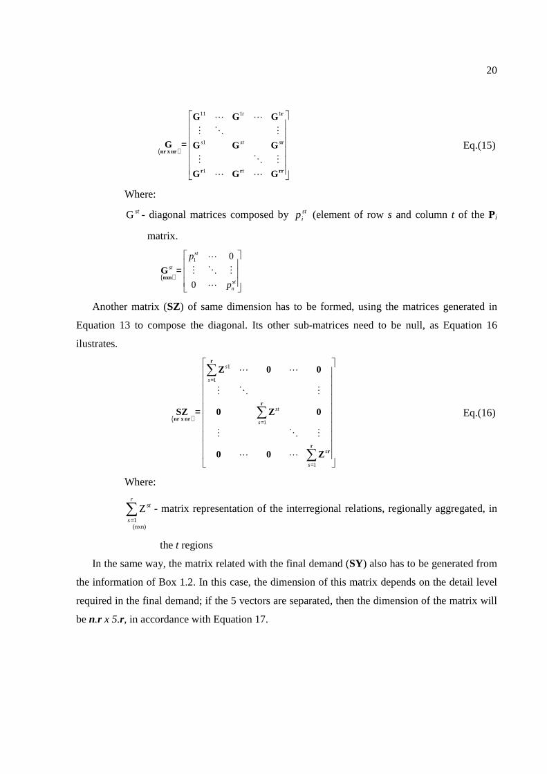
20

( )

11 1 1

1

1

t

s st s

t

=

r

r

nr x nr

r r rr

G G G

G G G G

G G G

L L

M O M

M O M

L L

Eq.(15)

Where:

stG - diagonal matrices composed by stip (element of row s and column t of the Pi

matrix.

( )

1 0

0

st

st

stn

p

p

=

nxnG

L

M O M

L

Another matrix (SZ) of same dimension has to be formed, using the matrices generated in

Equation 13 to compose the diagonal. Its other sub-matrices need to be null, as Equation 16

ilustrates.

( )

1

1

1

1

s

s

st

s

s

s

=

=

=

=

∑

∑

∑

r

r

nr x nr

rr

Z 0 0

SZ 0 Z 0

0 0 Z

L L

M O M

M O M

L L

Eq.(16)

Where:

(nxn)1

Z∑=

r

s

st - matrix representation of the interregional relations, regionally aggregated, in

the t regions

In the same way, the matrix related with the final demand (SY) also has to be generated from

the information of Box 1.2. In this case, the dimension of this matrix depends on the detail level

required in the final demand; if the 5 vectors are separated, then the dimension of the matrix will

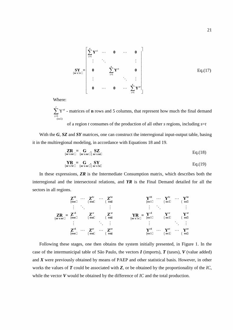
be n.r x 5.r, in accordance with Equation 17.

21

( )

1

1

51

1

s

s

st

s

s

s

=

=

=

=

∑

∑

∑

r

r

nr x r

rr

Y 0 0

SY 0 Y 0

0 0 Y

L L

M O M

M O M

L L

Eq.(17)

Where:

(nx5)1

Y∑=

r

s

st - matrices of n rows and 5 columns, that represent how much the final demand

of a region t consumes of the production of all other s regions, including s=t

With the G, SZ and SY matrices, one can construct the interregional input-output table, basing

it in the multiregional modeling, in accordance with Equations 18 and 19.

( ) ( ) ( )nr x nr nr x nr nr x nrZR = G . SZ Eq.(18)

( ) ( ) ( )nr x 5r nr x nr nr x 5rYR = G . SY Eq.(19)

In these expressions, ZR is the Intermediate Consumption matrix, which describes both the

interregional and the intersectoral relations, and YR is the Final Demand detailed for all the

sectors in all regions.

( )

( ) ( ) ( )

( ) ( ) ( )

( ) ( ) ( )

( )

( ) ( ) ( )

( ) ( ) ( )

( ) ( ) ( )

5 5 5

5 5 55

5 5 5

t t

s st s s st s

t t

11 1 1r 11 1 1r

nxn nxn nxn nx nx nx

1 r 1 r

nxn nxn nxn nx nx nxnr x nr nr x r

r1 r rr r1 r rr

nxn nxn nxn nx nx nx

Z Z Z Y Y Y

Z Z Z Y Y YZR = YR =

Z Z Z Y Y Y

L L L L

M O M M O M

M O M M O M

L L L L

Following these stages, one then obtains the system initially presented, in Figure 1. In the

case of the intermunicipal table of São Paulo, the vectors I (imports), T (taxes), V (value added)

and X were previously obtained by means of PAEP and other statistical basis. However, in other

works the values of T could be associated with Z, or be obtained by the proportionality of the IC,

while the vector V would be obtained by the difference of IC and the total production.

22

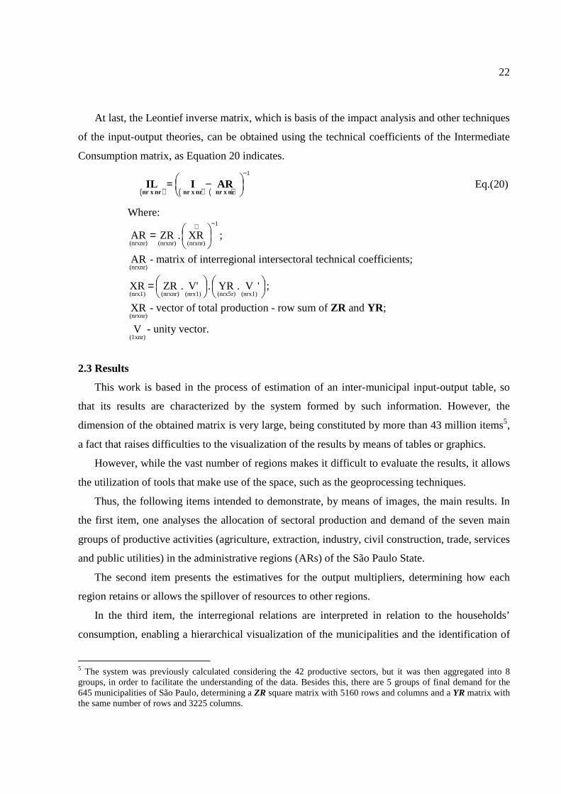
At last, the Leontief inverse matrix, which is basis of the impact analysis and other techniques

of the input-output theories, can be obtained using the technical coefficients of the Intermediate

Consumption matrix, as Equation 20 indicates.

( ) ( ) ( )

1− − nr x nr nr x nr nr x nr

IL = I AR Eq.(20)

Where:

1

(nrxnr)(nrxnr)(nrxnr)XR . ZR AR

−∧

= ;

(nrxnr)AR - matrix of interregional intersectoral technical coefficients;

= 'V . YR . V' . ZR XR

(nrx1)(nrx5r)(nrx1)(nrxnr)(nrx1);

(nrxnr)XR - vector of total production - row sum of ZR and YR;

(1xnr)V - unity vector.

2.3 Results

This work is based in the process of estimation of an inter-municipal input-output table, so

that its results are characterized by the system formed by such information. However, the

dimension of the obtained matrix is very large, being constituted by more than 43 million items5,

a fact that raises difficulties to the visualization of the results by means of tables or graphics.

However, while the vast number of regions makes it difficult to evaluate the results, it allows

the utilization of tools that make use of the space, such as the geoprocessing techniques.

Thus, the following items intended to demonstrate, by means of images, the main results. In

the first item, one analyses the allocation of sectoral production and demand of the seven main

groups of productive activities (agriculture, extraction, industry, civil construction, trade, services

and public utilities) in the administrative regions (ARs) of the São Paulo State.

The second item presents the estimatives for the output multipliers, determining how each

region retains or allows the spillover of resources to other regions.

In the third item, the interregional relations are interpreted in relation to the households’

consumption, enabling a hierarchical visualization of the municipalities and the identification of

5 The system was previously calculated considering the 42 productive sectors, but it was then aggregated into 8 groups, in order to facilitate the understanding of the data. Besides this, there are 5 groups of final demand for the 645 municipalities of São Paulo, determining a ZR square matrix with 5160 rows and columns and a YR matrix with the same number of rows and 3225 columns.

23

regional polarizing centres. Finally, the fourth item illustrates how these results can be used in the

definition of strategic plans for reducing the regional inequality, having in mind the spatial

distribution of the per capita amount of resources expended on the “Bolsa Família”, a federal

government transfer program, in the municipalities of São Paulo.

The four items do not exhaust the vast amount of information that can be extracted from an

intermunicipal georeferenced table, but by means of them is possible to discuss the quality of the

most important generated information.

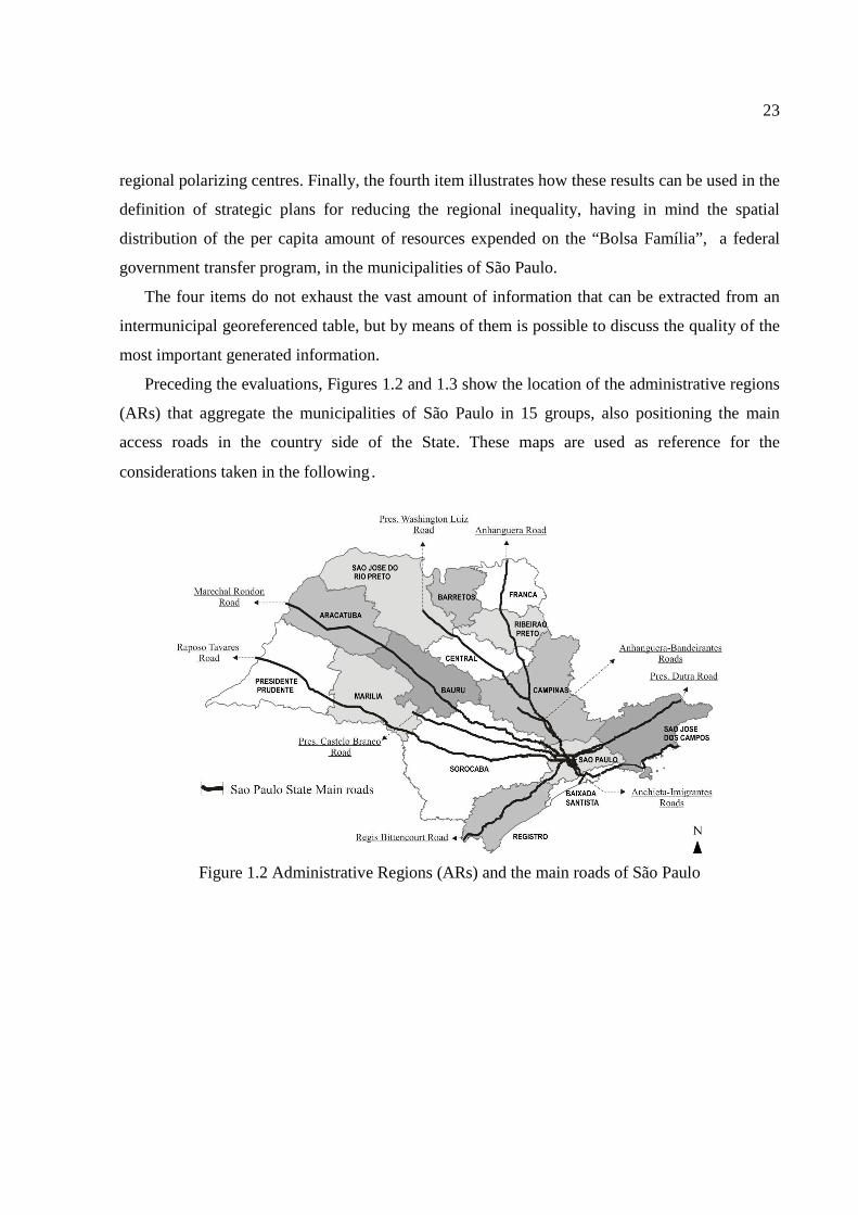
Preceding the evaluations, Figures 1.2 and 1.3 show the location of the administrative regions

(ARs) that aggregate the municipalities of São Paulo in 15 groups, also positioning the main

access roads in the country side of the State. These maps are used as reference for the

considerations taken in the following.

Figure 1.2 Administrative Regions (ARs) and the main roads of São Paulo

24

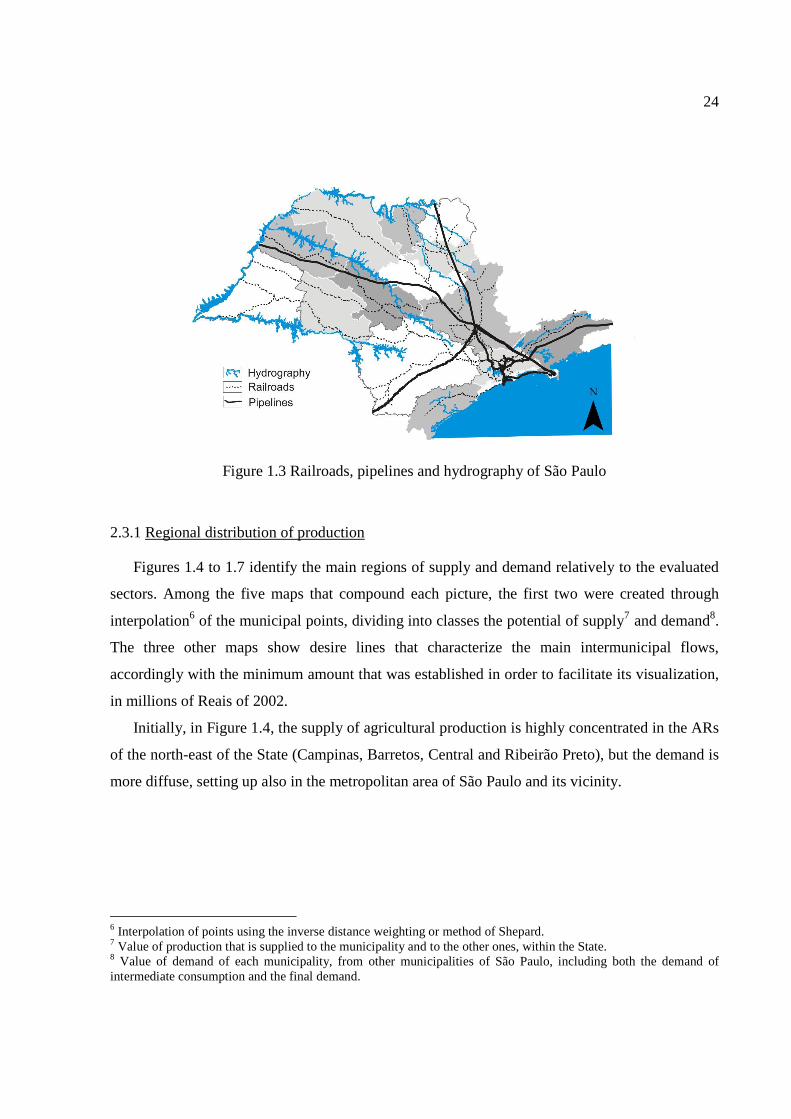
Figure 1.3 Railroads, pipelines and hydrography of São Paulo

2.3.1 Regional distribution of production

Figures 1.4 to 1.7 identify the main regions of supply and demand relatively to the evaluated

sectors. Among the five maps that compound each picture, the first two were created through

interpolation6 of the municipal points, dividing into classes the potential of supply7 and demand8.

The three other maps show desire lines that characterize the main intermunicipal flows,

accordingly with the minimum amount that was established in order to facilitate its visualization,

in millions of Reais of 2002.

Initially, in Figure 1.4, the supply of agricultural production is highly concentrated in the ARs

of the north-east of the State (Campinas, Barretos, Central and Ribeirão Preto), but the demand is

more diffuse, setting up also in the metropolitan area of São Paulo and its vicinity.

6 Interpolation of points using the inverse distance weighting or method of Shepard. 7 Value of production that is supplied to the municipality and to the other ones, within the State. 8 Value of demand of each municipality, from other municipalities of São Paulo, including both the demand of intermediate consumption and the final demand.

25

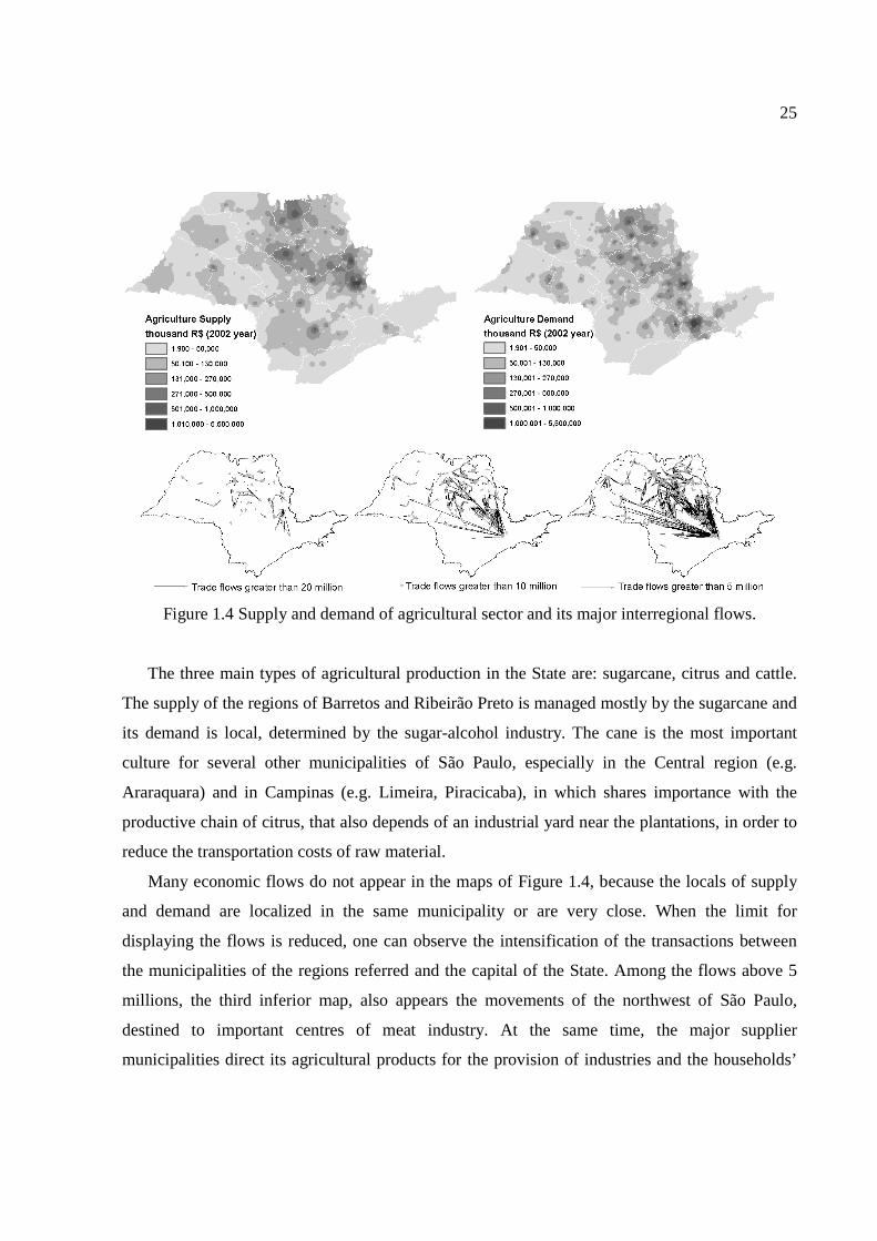
Figure 1.4 Supply and demand of agricultural sector and its major interregional flows.

The three main types of agricultural production in the State are: sugarcane, citrus and cattle.

The supply of the regions of Barretos and Ribeirão Preto is managed mostly by the sugarcane and

its demand is local, determined by the sugar-alcohol industry. The cane is the most important

culture for several other municipalities of São Paulo, especially in the Central region (e.g.

Araraquara) and in Campinas (e.g. Limeira, Piracicaba), in which shares importance with the

productive chain of citrus, that also depends of an industrial yard near the plantations, in order to

reduce the transportation costs of raw material.

Many economic flows do not appear in the maps of Figure 1.4, because the locals of supply

and demand are localized in the same municipality or are very close. When the limit for

displaying the flows is reduced, one can observe the intensification of the transactions between

the municipalities of the regions referred and the capital of the State. Among the flows above 5

millions, the third inferior map, also appears the movements of the northwest of São Paulo,

destined to important centres of meat industry. At the same time, the major supplier

municipalities direct its agricultural products for the provision of industries and the households’

26

consumption in the metropolitan area of São Paulo, whose supply is small in value terms and

focused on the production of farm products (fruits and vegetables).

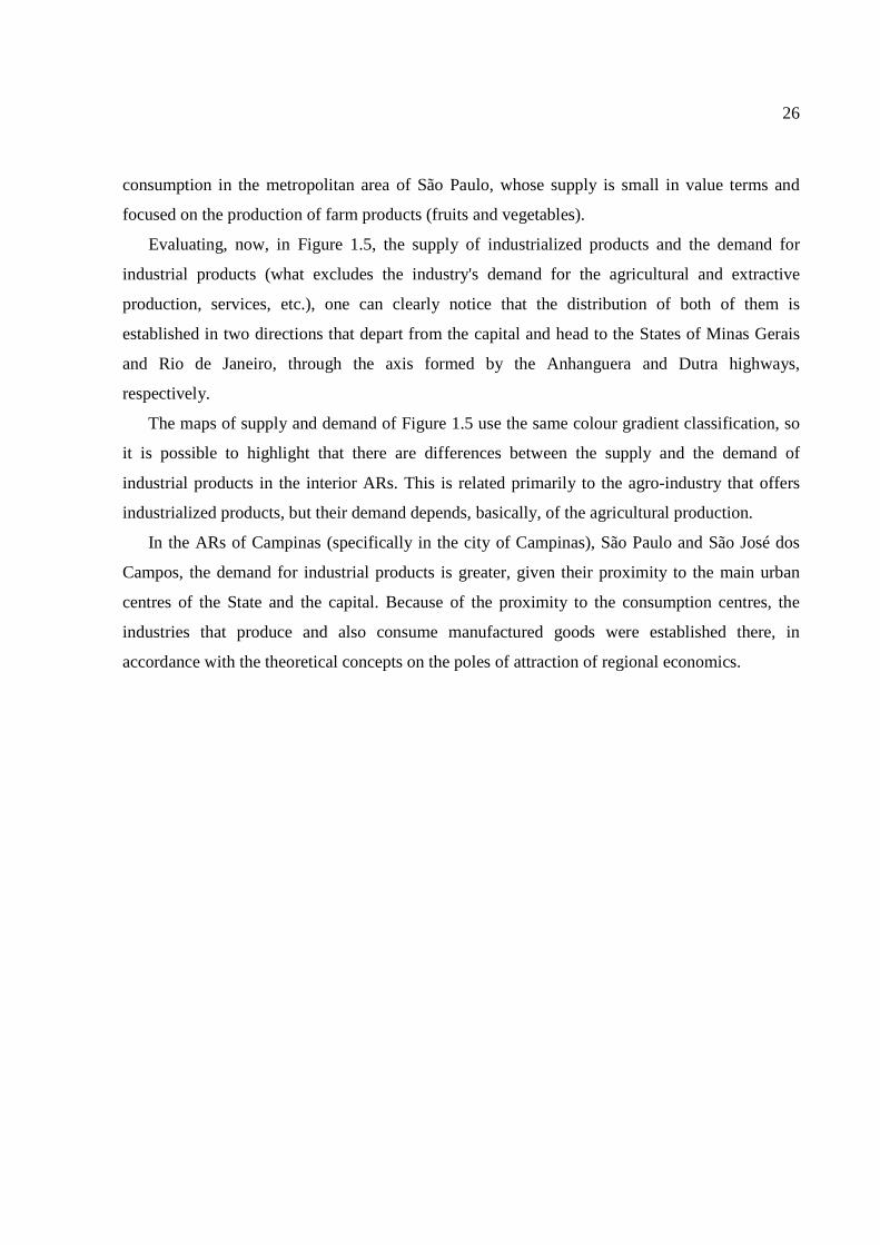
Evaluating, now, in Figure 1.5, the supply of industrialized products and the demand for

industrial products (what excludes the industry's demand for the agricultural and extractive

production, services, etc.), one can clearly notice that the distribution of both of them is

established in two directions that depart from the capital and head to the States of Minas Gerais

and Rio de Janeiro, through the axis formed by the Anhanguera and Dutra highways,

respectively.

The maps of supply and demand of Figure 1.5 use the same colour gradient classification, so

it is possible to highlight that there are differences between the supply and the demand of

industrial products in the interior ARs. This is related primarily to the agro-industry that offers

industrialized products, but their demand depends, basically, of the agricultural production.

In the ARs of Campinas (specifically in the city of Campinas), São Paulo and São José dos

Campos, the demand for industrial products is greater, given their proximity to the main urban

centres of the State and the capital. Because of the proximity to the consumption centres, the

industries that produce and also consume manufactured goods were established there, in

accordance with the theoretical concepts on the poles of attraction of regional economics.

27

Figure 1.5 Supply and demand of the industrial sector and its main interregional flows.

The first bottom map of Figure 1.5 presents only the largest transactions, demonstrating the

vast movement of industrial products between São Paulo and its neighbours (such as Osasco,

Guarulhos, Diadema and cities of the so-called ABC industrial pole – Santo André, São Bernardo

do Campo and São Caetano), as well as more distant municipalities (Campinas, Santos and São

José dos Campos). As the minimum limit of values decreases, it is observed an expressive

increase rate in the interaction of the municipalities in the axis of the road complex Anhanguera-

Bandeirantes with other municipalities throughout the State. The direction of these flows heads to

the country side, on the contrary to what has been shown for the flows of the agricultural sector

(third bottom map of the Figure 1.4).

It is important to emphasize that the flows with greater value represent the transactions

among the more industrialized and populous cities; in this way, the connections of smaller value

are basically determined by the provision of small towns with manufactured products. However,

these lines only establish the direct link between the initial seller and the final buyer, and do not

represent the towns in which the production actually pass through, i.e., the cities responsible for

the intermediate trade of these products are not represented.

28

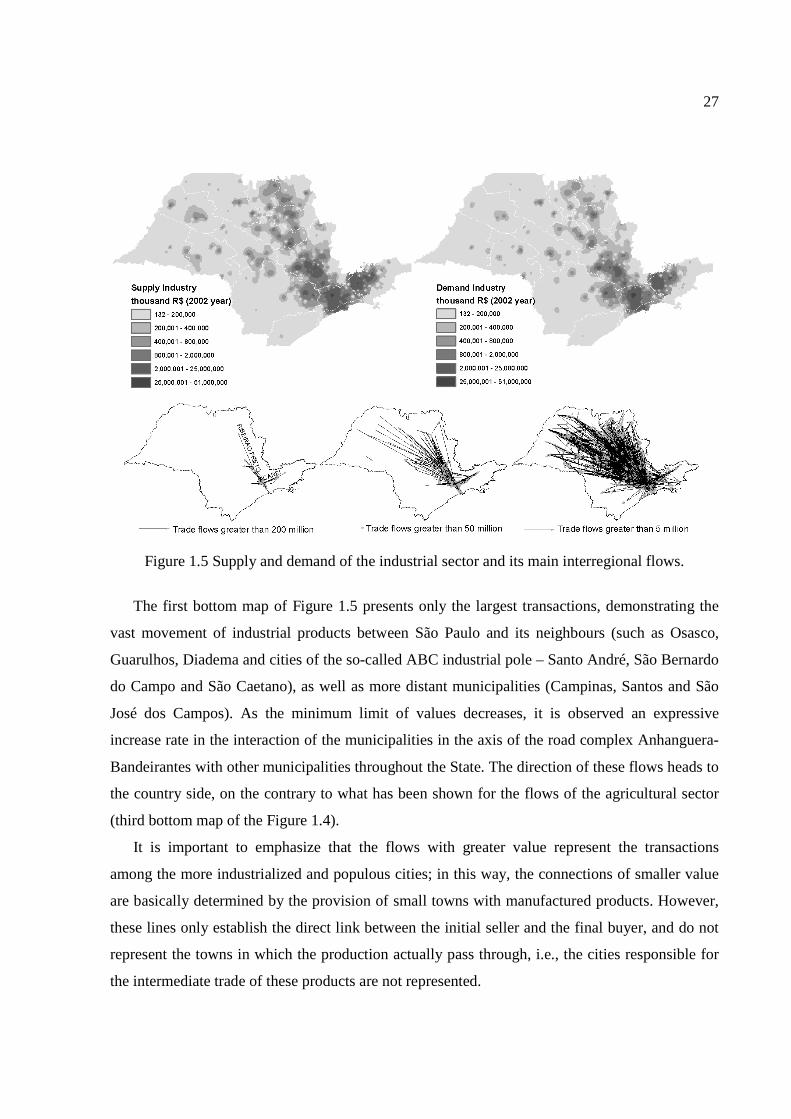
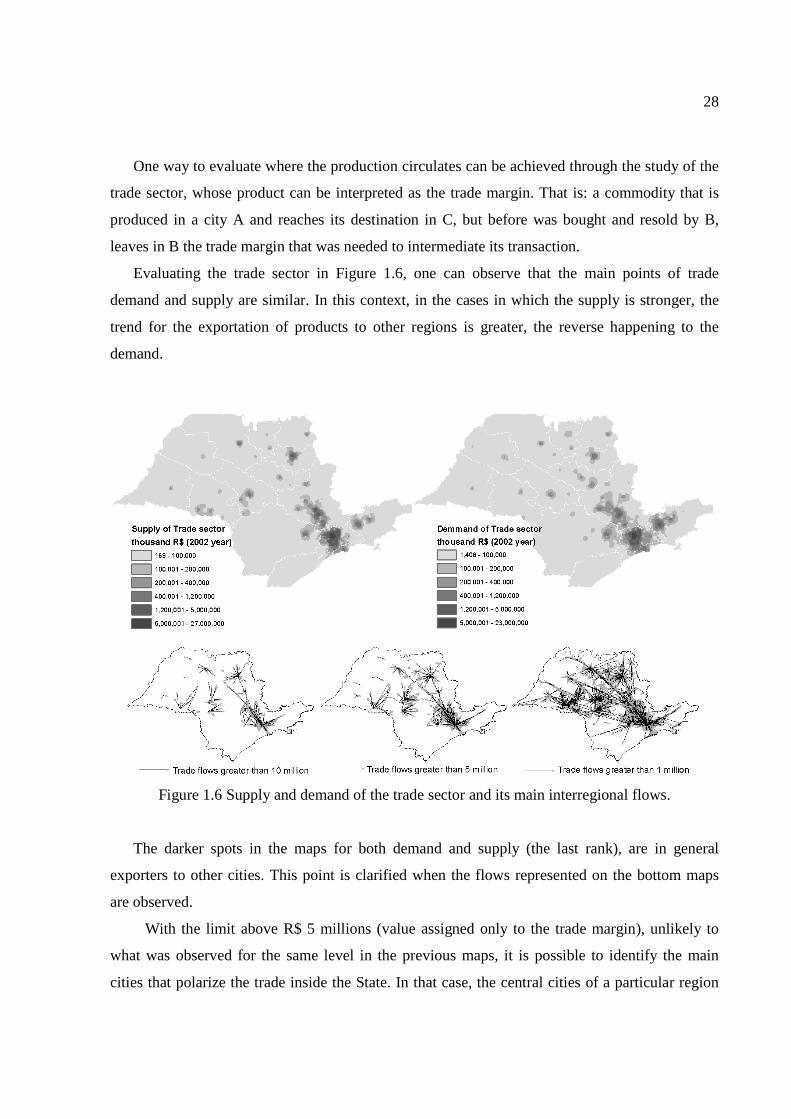
One way to evaluate where the production circulates can be achieved through the study of the

trade sector, whose product can be interpreted as the trade margin. That is: a commodity that is

produced in a city A and reaches its destination in C, but before was bought and resold by B,

leaves in B the trade margin that was needed to intermediate its transaction.

Evaluating the trade sector in Figure 1.6, one can observe that the main points of trade

demand and supply are similar. In this context, in the cases in which the supply is stronger, the

trend for the exportation of products to other regions is greater, the reverse happening to the

demand.

Figure 1.6 Supply and demand of the trade sector and its main interregional flows.

The darker spots in the maps for both demand and supply (the last rank), are in general

exporters to other cities. This point is clarified when the flows represented on the bottom maps

are observed.

With the limit above R$ 5 millions (value assigned only to the trade margin), unlikely to

what was observed for the same level in the previous maps, it is possible to identify the main

cities that polarize the trade inside the State. In that case, the central cities of a particular region

29

are identified by the quantity they trade and may not be representative in terms of industrial,

agriculture, extractive production or services, but in fact in terms of their strategic position for the

provision of less expressive cities that are distant of the major centres near the metropolitan area

of São Paulo.

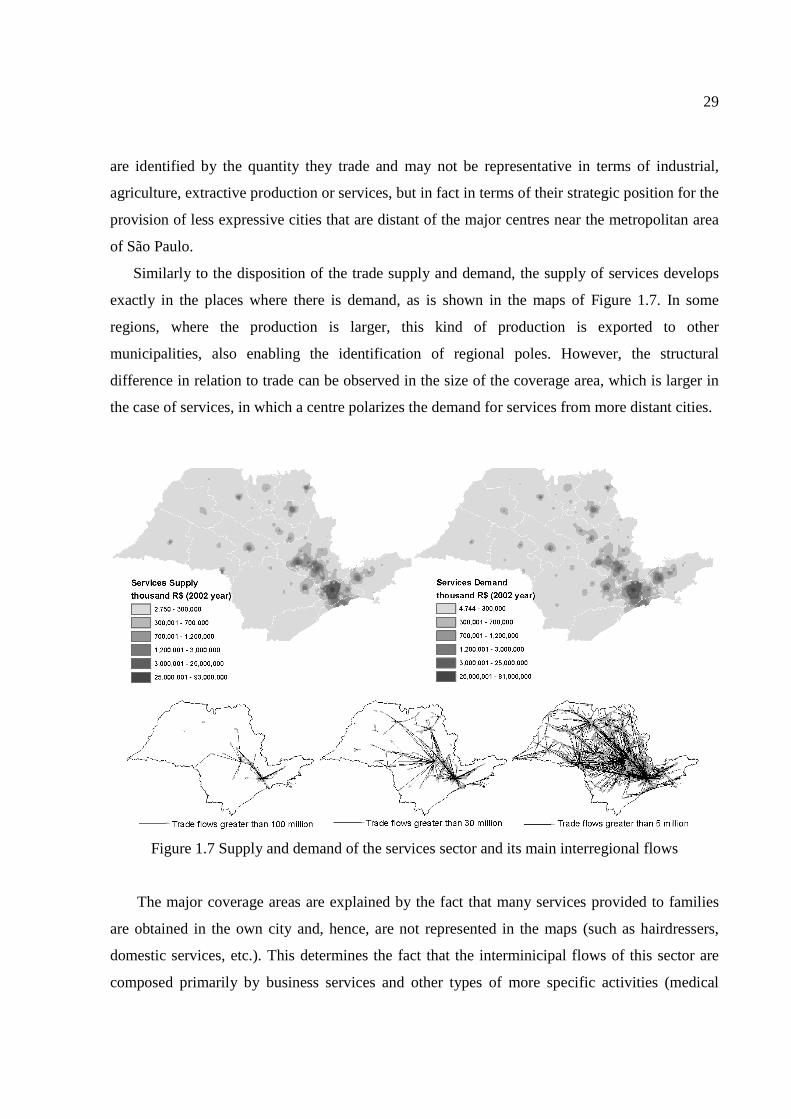
Similarly to the disposition of the trade supply and demand, the supply of services develops

exactly in the places where there is demand, as is shown in the maps of Figure 1.7. In some

regions, where the production is larger, this kind of production is exported to other

municipalities, also enabling the identification of regional poles. However, the structural

difference in relation to trade can be observed in the size of the coverage area, which is larger in

the case of services, in which a centre polarizes the demand for services from more distant cities.

Figure 1.7 Supply and demand of the services sector and its main interregional flows

The major coverage areas are explained by the fact that many services provided to families

are obtained in the own city and, hence, are not represented in the maps (such as hairdressers,

domestic services, etc.). This determines the fact that the interminicipal flows of this sector are

composed primarily by business services and other types of more specific activities (medical

30

specialties, higher education courses, authorized mechanic and electronic services), which cannot

exist in locations that do not present at least a minimum demand.

The four sectoral groups presented: industry, services, agriculture and trade cover most of the

economy of São Paulo State, while the other three groups that complement this analysis are more

succinctly presented by Figures 1.8 to 1.10, but with the same basic information of the previous

analyses.

The services of public utility are mainly composed by electric power supply, water and

sewage and gas services. Generally, the activities of water supply, sewage treatment, gas

distribution and electricity distribution are produced by the own municipality that consume them,

and are proportionately related to the size of the supplied economy.

The exploration and production of gas are components of the industrial sector of gas and oil

extraction, so that only the generation and transmission of electric energy have prominence in the

intermunicipal flows of the services of public utility sector.

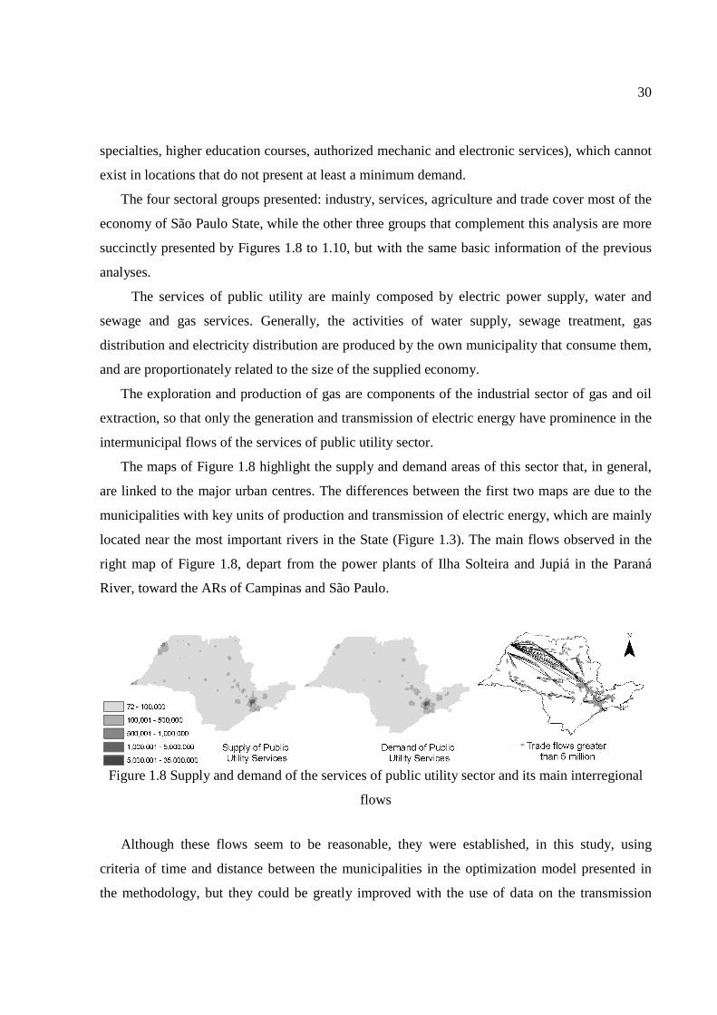
The maps of Figure 1.8 highlight the supply and demand areas of this sector that, in general,

are linked to the major urban centres. The differences between the first two maps are due to the

municipalities with key units of production and transmission of electric energy, which are mainly

located near the most important rivers in the State (Figure 1.3). The main flows observed in the

right map of Figure 1.8, depart from the power plants of Ilha Solteira and Jupiá in the Paraná

River, toward the ARs of Campinas and São Paulo.

Figure 1.8 Supply and demand of the services of public utility sector and its main interregional

flows

Although these flows seem to be reasonable, they were established, in this study, using

criteria of time and distance between the municipalities in the optimization model presented in

the methodology, but they could be greatly improved with the use of data on the transmission

31

lines. Since there are few companies operating in the energy sector, this sort of information can

be more easily reunited, but that depends on the policy that each company adopts in the provision

of such data.

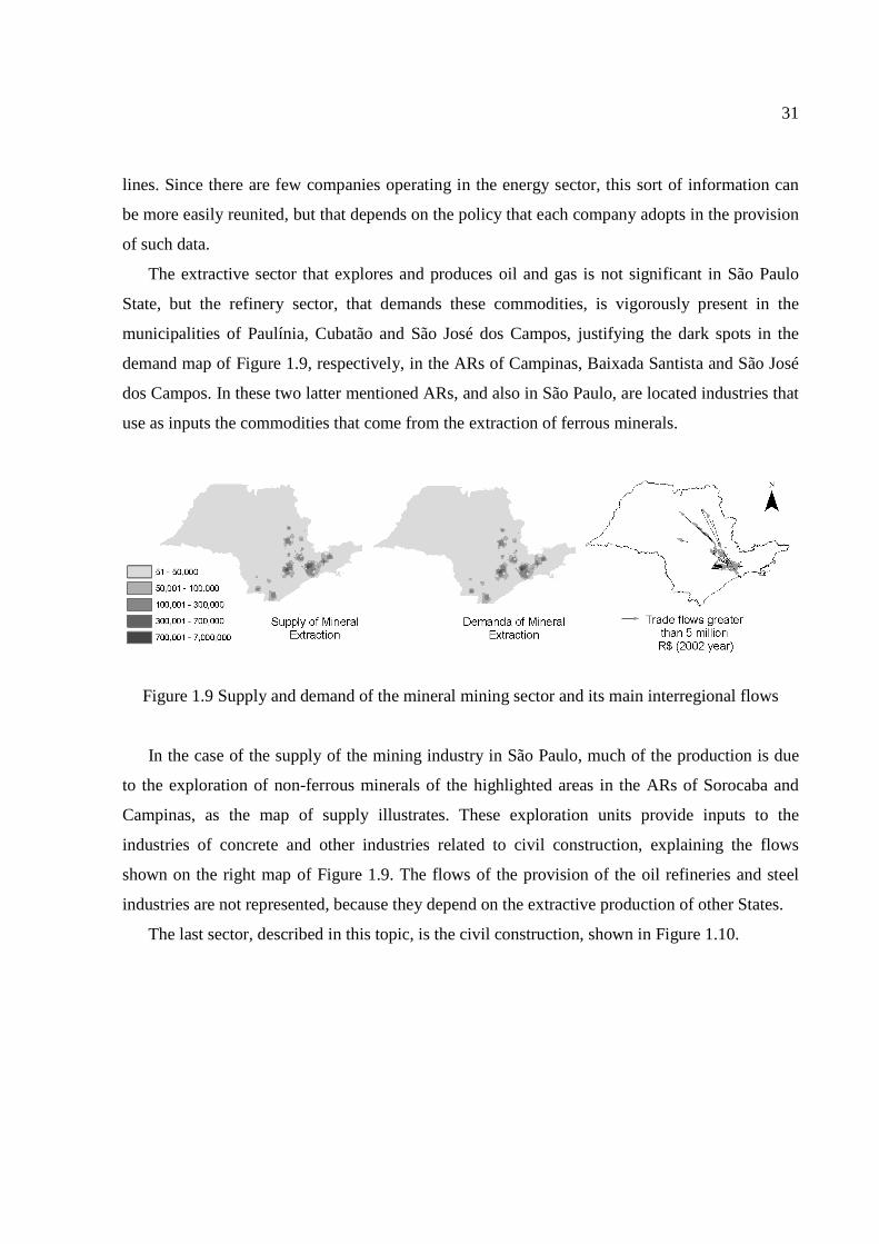
The extractive sector that explores and produces oil and gas is not significant in São Paulo

State, but the refinery sector, that demands these commodities, is vigorously present in the

municipalities of Paulínia, Cubatão and São José dos Campos, justifying the dark spots in the

demand map of Figure 1.9, respectively, in the ARs of Campinas, Baixada Santista and São José

dos Campos. In these two latter mentioned ARs, and also in São Paulo, are located industries that

use as inputs the commodities that come from the extraction of ferrous minerals.

Figure 1.9 Supply and demand of the mineral mining sector and its main interregional flows

In the case of the supply of the mining industry in São Paulo, much of the production is due

to the exploration of non-ferrous minerals of the highlighted areas in the ARs of Sorocaba and

Campinas, as the map of supply illustrates. These exploration units provide inputs to the

industries of concrete and other industries related to civil construction, explaining the flows

shown on the right map of Figure 1.9. The flows of the provision of the oil refineries and steel

industries are not represented, because they depend on the extractive production of other States.

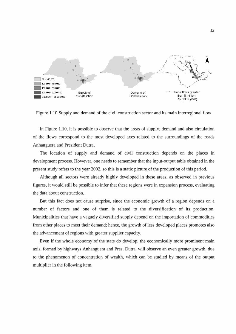
The last sector, described in this topic, is the civil construction, shown in Figure 1.10.

32

Figure 1.10 Supply and demand of the civil construction sector and its main interregional flow

In Figure 1.10, it is possible to observe that the areas of supply, demand and also circulation

of the flows correspond to the most developed axes related to the surroundings of the roads

Anhanguera and President Dutra.

The location of supply and demand of civil construction depends on the places in

development process. However, one needs to remember that the input-output table obtained in the

present study refers to the year 2002, so this is a static picture of the production of this period.

Although all sectors were already highly developed in these areas, as observed in previous

figures, it would still be possible to infer that these regions were in expansion process, evaluating

the data about construction.

But this fact does not cause surprise, since the economic growth of a region depends on a

number of factors and one of them is related to the diversification of its production.

Municipalities that have a vaguely diversified supply depend on the importation of commodities

from other places to meet their demand; hence, the growth of less developed places promotes also

the advancement of regions with greater supplier capacity.

Even if the whole economy of the state do develop, the economically more prominent main

axis, formed by highways Anhanguera and Pres. Dutra, will observe an even greater growth, due

to the phenomenon of concentration of wealth, which can be studied by means of the output

multiplier in the following item.

33

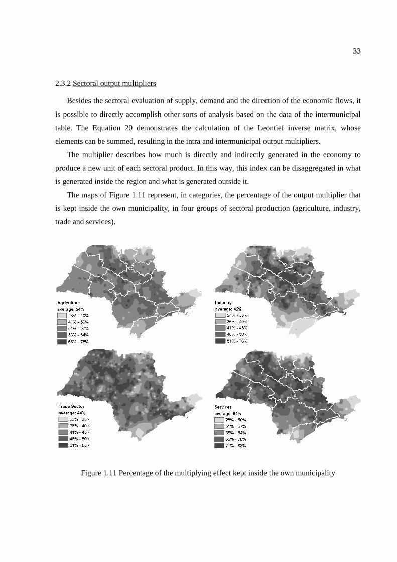
2.3.2 Sectoral output multipliers

Besides the sectoral evaluation of supply, demand and the direction of the economic flows, it

is possible to directly accomplish other sorts of analysis based on the data of the intermunicipal

table. The Equation 20 demonstrates the calculation of the Leontief inverse matrix, whose

elements can be summed, resulting in the intra and intermunicipal output multipliers.

The multiplier describes how much is directly and indirectly generated in the economy to

produce a new unit of each sectoral product. In this way, this index can be disaggregated in what

is generated inside the region and what is generated outside it.

The maps of Figure 1.11 represent, in categories, the percentage of the output multiplier that

is kept inside the own municipality, in four groups of sectoral production (agriculture, industry,

trade and services).

Figure 1.11 Percentage of the multiplying effect kept inside the own municipality

34

The regions with higher percentages represent economies that have a greater level of

interaction inside themselves. In general, they present more diversified productions, capable of

provisioning a great part of the demand with the local production. In this way, if economic

incentives are given to these municipalities, there is the tendency that a great part of the generated

wealth stay concentrated in themselves.

Oppositely, the municipalities in the areas represented with lighter colors have little internal

interaction (intraregional) and are strongly dependent of the interregional relations, since they

need the production of other localities to sustain their consumption.

Analyzing the Figure 1.11, one can observe that the sectoral groups of agriculture and

services have, in average, a greater capacity to keep the multiplying effect in the own

municipality. The industrial sector is much more dependent on the interregional transactions.

Especially in the map relative to the industry, there is a clear distinction of areas represented

with lighter colors, observed in the southeast9 and northeast10 of the State. More subtly, these

regions are also represented by lighter colored areas in the other maps, enhancing the great

spillover of the multiplying effect from their economies to other regions.

The multiplying effects do not depend, primordially, on the magnitude in value of the present

production in each municipality, because they are numbers derived from the technical

coefficients of production. However, as it is possible to observe in the Figures 1.4 to 1.10, these

regions also are little developed in all the sectors (except in the extractive activities). That is why

the potential of keeping the production multiplying effects is low, not only in these

municipalities, but also in the neighbor regions.

2.3.3 Polarizing centres for the households consumption

In the Figures 1.4 to 1.10, only the main flows (in value terms for the whole State) are

represented, excluding, thus, the flows of the less developed regions such as the Valley of

Ribeira, whose flows are extremely small in comparison to the flows of the more industrialized

regions.

9 Axis in the south direction of the Regis Bittencourt road heading to the countryside, Ribeira Valley region. 10 Axis in the direction of Presidente Dutra road, near to the Rio de Janeiro State, north part of the Paraíba Valley.

35

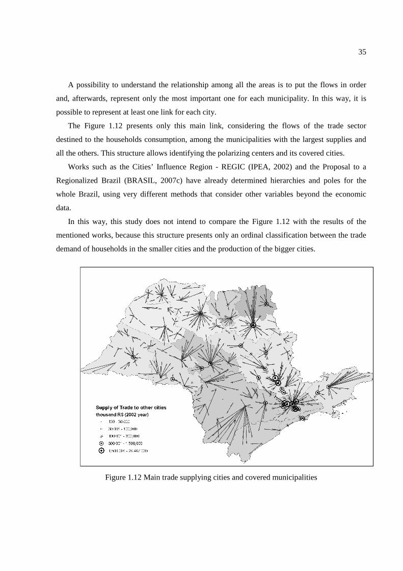
A possibility to understand the relationship among all the areas is to put the flows in order

and, afterwards, represent only the most important one for each municipality. In this way, it is

possible to represent at least one link for each city.

The Figure 1.12 presents only this main link, considering the flows of the trade sector

destined to the households consumption, among the municipalities with the largest supplies and

all the others. This structure allows identifying the polarizing centers and its covered cities.

Works such as the Cities’ Influence Region - REGIC (IPEA, 2002) and the Proposal to a

Regionalized Brazil (BRASIL, 2007c) have already determined hierarchies and poles for the

whole Brazil, using very different methods that consider other variables beyond the economic

data.

In this way, this study does not intend to compare the Figure 1.12 with the results of the

mentioned works, because this structure presents only an ordinal classification between the trade

demand of households in the smaller cities and the production of the bigger cities.

Figure 1.12 Main trade supplying cities and covered municipalities

36

However, is important to enhance that this type of information can be used in future studies

that intend to include the economic intersectoral relations of the input-output table in the

hierarchic definition among the cities, i.e., different presentations of polarizing cities can be

defined considering each type of production and/or sectoral demand.

2.3.4 Considerations on the reduction of the regional inequality

All the previous topics aim to describe the main results found through the estimation of the

input-output table for the São Paulo State, intending to evaluate aspects of the São Paulo

economic geography. Using the previous analysis, the objective of this topic is to suggest a

localized action capable of reducing the regional inequality, exemplifying a possible use to an

intermunicipal input-output table.

Many times, the regional inequality is associated with the social inequality, in a way that

regions with less developed economies have populations with smaller income.

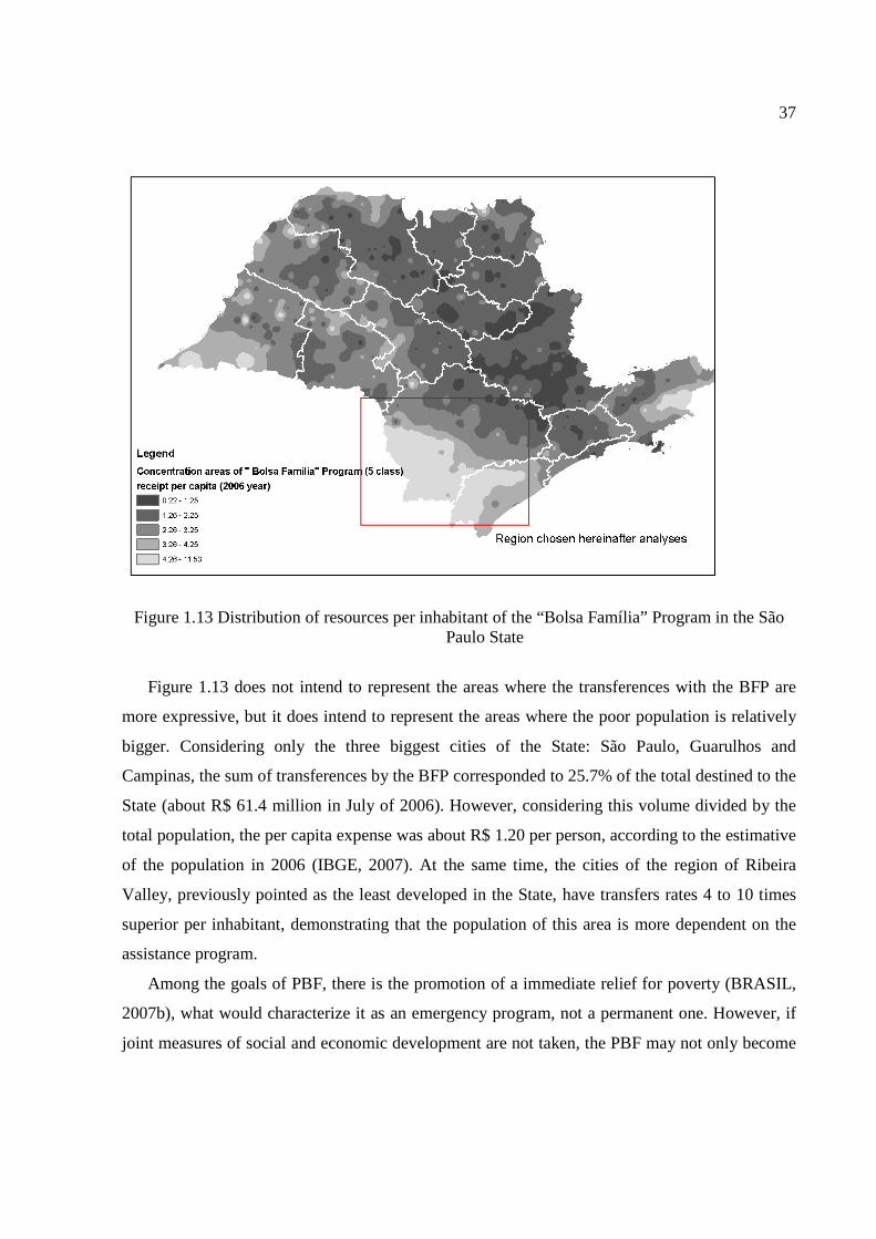
Using the data of the Ministry of Social Development (BRASIL, 2007b) about the municipal

distribution of the amount spent by the “Bolsa Família” Program (BFP)11, the Figure 1.13

illustrates the areas in relation to expenses per inhabitant. Once again, the areas that stand out are

the cities of the Ribeira Valley and some cities of the Paraíba Valley.

11 The “Bolsa Família” Program (BFP) is a conditional program of direct income transfers of the Federal Government. The objective of this program is to guarantee that “poor” (monthly income per person from R$ 60 to R$120) and “extremely poor “ (income per person lower than R$60) families receive a monthly benefit, according to BRASIL ( 2007b).

37

Figure 1.13 Distribution of resources per inhabitant of the “Bolsa Família” Program in the São Paulo State

Figure 1.13 does not intend to represent the areas where the transferences with the BFP are

more expressive, but it does intend to represent the areas where the poor population is relatively

bigger. Considering only the three biggest cities of the State: São Paulo, Guarulhos and

Campinas, the sum of transferences by the BFP corresponded to 25.7% of the total destined to the

State (about R$ 61.4 million in July of 2006). However, considering this volume divided by the

total population, the per capita expense was about R$ 1.20 per person, according to the estimative

of the population in 2006 (IBGE, 2007). At the same time, the cities of the region of Ribeira

Valley, previously pointed as the least developed in the State, have transfers rates 4 to 10 times

superior per inhabitant, demonstrating that the population of this area is more dependent on the

assistance program.

Among the goals of PBF, there is the promotion of a immediate relief for poverty (BRASIL,

2007b), what would characterize it as an emergency program, not a permanent one. However, if

joint measures of social and economic development are not taken, the PBF may not only become

38

a permanent program but may also have to be expanded, determining a larger public expense and

limiting the resources invested in infrastructure, what is essential for the economic growth.

It is expected that the solution is not to abruptly cut the funds for the program, but fortifying

the development and improving the income distribution, so that the poor and extremely poor

people no more receive the benefit because they no longer need it.

In this context, the concepts on the “spillover” of resources and the polarization centres can

be used to search strategies destined to reduce regional inequality and to eventually fortify the

cities of relatively more needy populations.

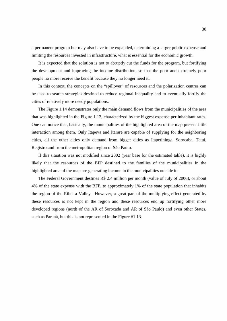
The Figure 1.14 demonstrates only the main demand flows from the municipalities of the area

that was highlighted in the Figure 1.13, characterized by the biggest expense per inhabitant rates.

One can notice that, basically, the municipalities of the highlighted area of the map present little

interaction among them. Only Itapeva and Itararé are capable of supplying for the neighboring

cities, all the other cities only demand from bigger cities as Itapetininga, Sorocaba, Tatuí,

Registro and from the metropolitan region of São Paulo.

If this situation was not modified since 2002 (year base for the estimated table), it is highly

likely that the resources of the BFP destined to the families of the municipalities in the

highlighted area of the map are generating income in the municipalities outside it.

The Federal Government destines R$ 2.4 million per month (value of July of 2006), or about

4% of the state expense with the BFP, to approximately 1% of the state population that inhabits

the region of the Ribeira Valley. However, a great part of the multiplying effect generated by

these resources is not kept in the region and these resources end up fortifying other more

developed regions (north of the AR of Sorocada and AR of São Paulo) and even other States,

such as Paraná, but this is not represented in the Figure #1.13.

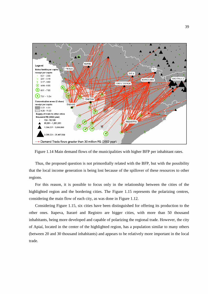
39

Figure 1.14 Main demand flows of the municipalities with higher BFP per inhabitant rates.

Thus, the proposed question is not primordially related with the BFP, but with the possibility

that the local income generation is being lost because of the spillover of these resources to other

regions.

For this reason, it is possible to focus only in the relationship between the cities of the

highlighted region and the bordering cities. The Figure 1.15 represents the polarizing centres,

considering the main flow of each city, as was done in Figure 1.12.

Considering Figure 1.15, six cities have been distinguished for offering its production to the

other ones. Itapeva, Itararé and Registro are bigger cities, with more than 50 thousand

inhabitants, being more developed and capable of polarizing the regional trade. However, the city

of Apiaí, located in the center of the highlighted region, has a population similar to many others

(between 20 and 30 thousand inhabitants) and appears to be relatively more important in the local

trade.

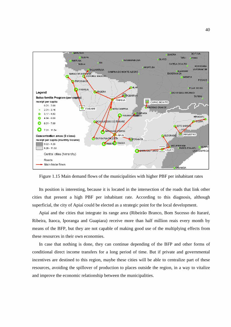
40

Figure 1.15 Main demand flows of the municipalities with higher PBF per inhabitant rates

Its position is interesting, because it is located in the intersection of the roads that link other

cities that present a high PBF per inhabitant rate. According to this diagnosis, although

superficial, the city of Apiaí could be elected as a strategic point for the local development.

Apiaí and the cities that integrate its range area (Ribeirão Branco, Bom Sucesso do Itararé,

Ribeira, Itaoca, Iporanga and Guapiara) receive more than half million reais every month by

means of the BFP, but they are not capable of making good use of the multiplying effects from

these resources in their own economies.

In case that nothing is done, they can continue depending of the BFP and other forms of

conditional direct income transfers for a long period of time. But if private and governmental

incentives are destined to this region, maybe these cities will be able to centralize part of these

resources, avoiding the spillover of production to places outside the region, in a way to vitalize

and improve the economic relationship between the municipalities.

41

Since the industrial potential of the region is weak and, at the same time, the agricultural

sector cannot expressively develop (this is an irregular terrain region, composed by areas of

environmental protection), it is necessary to investigate other activities. The activities of the

services sector can pointed for having, on average, a better capacity of fixing the multiplier effect

(Figure 1.11).

Although the table data does not demonstrate, the region can improve its economy through

the exploration of the adventure tourism, as it has already been done in areas next to Apiaí,

Iporanga and Eldorado, using the geological formation conserved by the Alto do Ribeira Tourist

Park (PETAR). The government can, for example: introduce superior courses in tourism, geology

and/or biology in the region and, at the same time, give incentives to the private initiative to

extend the tourist infrastructure.

Measures as these, unfortunately, do not mean reducing the social inequalities, but they can

reduce the regional inequalities.

This text does not have the intention of deeply exploring or offering a development plan for

the region, but with this considerations one intends to exemplify how the data of a regionalized

table in the municipal level can be useful for understanding the economic relationships among the

cities and how to use them to diagnose, direct or even recommend regional strategies with

politics that already exists, as the BFP.

2.4 Conclusions

The estimation of input-output tables with greater regional specification can proportionate

many benefits to regional studies. In this way, the present work proposes and evaluates a method

in order to accomplish this task.

Since the existing and available databases do not allow the construction of an intermunicipal

input-output matrix based on census data, this work tries to approach the reality by using a large

number of information, considering the production, the intermediate consumption and the final

demand of the main activity groups in each municipality.

However, as the intersectoral relations estimatives are derived from the technical coefficients

of a single table (São Paulo State table), it is not possible to use these results in studies whose

objective is making a technological confrontation among the regions.

42

Nevertheless, the method is capable of incorporating the input-output tables for each

municipality (intraregional tables), estimating only the tables of the relations among the regions,

i.e., the method admits that larger data be used in order to improve the estimations. It is important

to appoint that the greater the sectoral detailing, the better will be the interregional estimations.

Currently, the state Treasure Departments determine the flows of the interstate production,

due to a difference in the percentage used to calculate the Tax on Circulation of Goods and

Services (ICMS) in each state. These Departments also measure the municipal production to

calculate the value added and afterwards the Municipal Participation Index (IPM) for the

distribution of the share of the ICMS destined to the municipalities.

For this reason, the present work also tries to incentive these Departments to register and

make available this information to the scholars, not only in the case of the interstate transactions,

but also the intermunicipal ones, what would be enough to consolidate more reliable databases on

the economic flows.

This work presented an example of application of the input-output table, evaluating the

spillover of resources from less developed areas that are included in the “Bolsa Família”

Program, also demonstrating the possibility of identifying regional poles, to which one can

destine actions with the intention of vitalizing the local economies in a more precise way.

Anticipatively, one mentions that a similar study can be done for all the Brazilian

municipalities, what would make more sense, since the conditional direct income transfers is

much more important in many other regions of the country, where the underdevelopment and the

spillover of resources are even higher.

Finally, many other applications can use the data of the regionalized to the municipal level

input-output table data, specifying the results of the model. All these data can also be linked to

other methods, using the spatial variable as the linking element with other disciplines that use

geographic information systems, flow analysis, nets, geostatistics, geomarketing, among others,

allowing that new techniques be created or adapted.

References

BRASIL (2007a). Ministério do Desenvolvimento, Indústria e Comércio Exterior. Secretaria do Comércio Exterior. Disponível em: <http://aliceweb.desenvolvimento.gov.br>. Acesso em: 15 maio 2007.

43

BRASIL (2007b). Ministério do Desenvolvimento Social. Programa bolsa família. Disponível em: <http://www.mds.gov.br/programas/transferencia-de-renda/programa-bolsa-familia>. Acesso em: 27 ago. 2007.

BRASIL (2007c). Ministério Planejamento Orçamento e Gestão. Proposta de regionalização do Brasil - Ministério do Planejamento / Centro de Estudos de Gestão Estratégica - CCGE. Disponível em: <http://www.mp.gov.br>. Acesso em: 27 out. 2007.

BRASIL. Ministério do Trabalho e Emprego. Relação Anual de Informações Sociais – RAIS. Disponível em: <http://www.rais.gov.br>. Acesso em: 25 nov. 2006.

CANNING, P.; WANG, Z. A flexible mathematical programming model to estimate inter-regional input-output accounts. Journal of Regional Science, Oxford, v. 45, n. 3, p. 539-563, Aug. 2005.

CHENERY, H. Patterns of development, 1950-1970. London: Oxford University Press for the World Bank, 1975. 234 p.

CHO, J.E.; GORDON, P. Integrating Transportation Network and Regional Economic Models to Estimate the Costs of a Large Urban Earthquake. Journal of Regional Science, Oxford, v. 41, n. 1, p. 39-65, Feb. 2001.

FUJITA, M.; KRUGMAN, P.; VENABLES, A.J. Economia Espacial. São Paulo: Futura, 2002. 391p.

FUNDAÇÃO SISTEMA ESTADUAL DE ANÁLISE DE DADOS – SEADE. Informações sobre os municípios paulistas. Disponível em: <http://www.seade.gov.br>. Acesso em: 12 jan. 2007.

FUNDAÇÃO SISTEMA ESTADUAL DE ANÁLISE DE DADOS – SEADE. Pesquisa da Atividade Econômica Paulista – PAEP / Sala de acesso aos microdados. 2002.

GUILHOTO, J.J.M.; HEWINGS, G.J.D.; TAKASHIBA, E.H.; SILVA, L.M.S. Combining Geographical Information Systems and Input-Output Models: Concept and Initial Ideas. In: NORTH AMERICAN MEETING OF THE REGIONAL SCIENCE ASSOCIATION INTERNATIONAL, 50, 2003, Philadelphia. Papers... Illinois: REAL, 2003. 1 CD-ROM.

GUILHOTO, J.J.M.; SESSO FILHO, U.A. (2005a). Estrutura produtiva da Amazônia: uma análise de insumo-produto. Belém: Banco da Amazônia S.A. (BASA), 2005. 320 p.

GUILHOTO, J.J.M.; SESSO FILHO, U.A. (2005b). Estimação da Matriz Insumo-Produto a partir de Dados Preliminares das Contas Nacionais. Economia Aplicada, São Paulo, v. 9, n. 2, p. 277-299, abr. 2005.

HANSEN, L.; TIEBOUT, C. An Intersectoral Flows Analysis of the California Economy. The Review of Economics and Statistics, Cambridge, v. 45, n. 4. p. 409-418, Nov. 1963.

44

INSTITUTO BRASILEIRO DE GEOGRAFIA E ESTATÍSTICA - IBGE. Base Cartográfica Integrada do Brasil ao Milionésimo Digital – 1997 – IBGE / DGC / CCAR. 1 CD-ROM.

INSTITUTO BRASILEIRO DE GEOGRAFIA E ESTATÍSTICA - IBGE. Sistema IBGE de recuperação automática - SIDRA. Disponível em: <http://www.sidra.ibge.gov.br>. Acesso em: 25 maio 2007.

INSTITUTO DE PESQUISAS ECONÔMICAS - IPEA. Caracterização e Tendências da Rede Urbana do Brasil. Brasília: IPEA, 2002. 390 p. v. 2.

ISARD, W. et al. Methods of Inter-regional and Regional Analysis. Aldershot: Ashgate Publishing, 1998. 490 p.

ISARD, W. Inter-regional and regional input-output analysis: a model of a space-economy. The Review of Economics and Statistics, Cambridge, v. 33, n. 4, p. 319-328, Nov. 1951.

KIM, T.J.; HAM, H.; BOYCE, D.E. Economic impacts of transportation network changes: Implementation of a combined transportation network and input-output model. Papers Regional Science, Heidelberg, v. 81, n. 2, p. 223-246, Apr. 2002.

LEONTIEF, W.; STROUT, A. Multiregional Input-Output Analysis. In: BARNA T. (Ed.) Structural interdependence and economic development. New York: St. Martin’s Press, 1963. chap. 2, p.119-50

LEONTIEF, W. Input-Output Economics. 1 ed. New York: Oxford University Press, 1965. 257 p.

LEONTIEF, W. The Structure of the American Economy. 2 ed. New York: Oxford University Press, 1953. 561 p.

McDOUGALL, R.A. Entropy Theory and RAS are Friends. In: CONFERENCE OF GLOBAL ECONOMICAL ANALYSIS, 5, 1999, Copenhagen. Working Papers... Center for Global Trade Analysis, Department of Agricultural Economics, Purdue University. Disponível em: <http://ideas.repec.org/p/gta/workpp/300.html>. Acesso em: 10 maio 2006.

MESNARD, L. Understanding the shortcomings of commodity-based technology in input-output models: an economic-circuit approach. Journal of Regional Science, Oxford, v. 44, n. 1, p. 125-141, Feb. 2004.

MILLER, R.E.; BLAIR, P.D. Input-Output Analysis: Foundations and Extensions. 1 ed. New Jersey: Prentice Hall, 1985. 464 p.

MONTOYA, M.A. Análise insumo-produto internacional no Mercosul: desenvolvimento econômico e interdependência estrutural. Passo Fundo: EDIUPF, 1999. 208 p.

MOSES, L.N. The Stability of Inter-regional Trading Patterns and Input-Output Analysis. The American Economic Review, Nashville, v. 45, n. 5, p. 803-826, Dec. 1955.

45

NANNE, J.Z.; HEYDECKER, B.G. Improved algorithms for calibrating gravit models. IN: BELL, M. G. H. Transportation Networks: Recent Methodological Advances. Amsterdam, New York: Pergamon, 1998. 319 p.

ORTÚZAR, J.D.; WILLUMSEN, L.G. Modelling transport . 3 ed. New York: J. Wiley, 2004. 499 p.

POLENSKE, K.R. An Empirical Teste of Inter-regional Input-Output Models: Estimation of 1963 Japanese Production. The American Economic Review, Nashville, v. 60, n. 2, p. 76-82, May. 1970.

RANCO, B. Comparative stability analysis of multiregional input-output models: column, row and Leontief-Strout gravit coefficient models. The Quartely Journal of Economics, Cambridge, v. 99, n. 4, p. 791-815, Nov. 1984.

RICHARDSON, H.W. Input-output and regional economics. London: Weidenfeld and Nicolson, 1972. 267 p.

ROBINSON, S; CATTANEO, A; EL SAID, M. Updating and Estimating a Social Accounting Matrix Using Cross Entropy Methods. Economic Systems Research, London, v. 13, n. 1, Mar. 2001.

ROUND, J.I. Non-survey techniques: a critical review of the theory and evidence. International Regional Science Review, Thousand Oaks, v. 8, n. 3, p.189-212, Dec. 1983.

STONE, R. Input-output and national accounts. Paris: Organisation for European Economic Co-operation, 1961. 202 p.

THEIL, H. Economics and information theory. Amsterdam, Chicago: North-Holland Pub. Co.: Rand McNally, 1967. 488 p.

UNITED NATIONS. System of National Accounts - SNA - 1993. Disponível em. <http://unstats.un.org/unsd/sna1993/toctop.asp>. Acesso em: 10 jan. 2006.

VASCONCELOS, J.R.; OLIVEIRA, M.A. Análise da matriz por atividade econômica do comércio interestadual no Brasil - 1999. Texto para discussão n° 1159. Instituto de Pesquisa Econômica Aplicada – IPEA, 2006. Disponível em: <http://www.ipea.gov.br/pub>. Acesso em: 13 jun. 2007.

WILSON, A.G. Entropy in urban and regional modeling. Londres: Pion Limited, 1970. 166 p.

WILSON, A.G. The Use of Entropy Maximising Models in the Theory of Trip Distribution, Mode Split and Route Split. Journal of Transport Economics and Policy, Bath, v. 3, n. 1, p. 108-126, Jan. 1969.