Math GeosciDOI 10.1007/s11004-010-9286-5

S P E C I A L I S S U E

Combining Areal and Point Data in GeostatisticalInterpolation: Applications to Soil Science and MedicalGeography

Pierre Goovaerts

Received: 3 December 2009 / Accepted: 24 May 2010© International Association for Mathematical Geosciences 2010

Abstract A common issue in spatial interpolation is the combination of data mea-sured over different spatial supports. For example, information available for mappingdisease risk typically includes point data (e.g. patients’ and controls’ residence) andaggregated data (e.g. socio-demographic and economic attributes recorded at the cen-sus track level). Similarly, soil measurements at discrete locations in the field are of-ten supplemented with choropleth maps (e.g. soil or geological maps) that model thespatial distribution of soil attributes as the juxtaposition of polygons (areas) with con-stant values. This paper presents a general formulation of kriging that allows the com-bination of both point and areal data through the use of area-to-area, area-to-point,and point-to-point covariances in the kriging system. The procedure is illustrated us-ing two data sets: (1) geological map and heavy metal concentrations recorded in thetopsoil of the Swiss Jura, and (2) incidence rates of late-stage breast cancer diagnosisper census tract and location of patient residences for three counties in Michigan. Inthe second case, the kriging system includes an error variance term derived accordingto the binomial distribution to account for varying degree of reliability of incidencerates depending on the total number of cases recorded in those tracts. Except underthe binomial kriging framework, area-and-point (AAP) kriging ensures the coher-ence of the prediction so that the average of interpolated values within each mappingunit is equal to the original areal datum. The relationships between binomial krig-ing, Poisson kriging, and indicator kriging are discussed under different scenarios forthe population size and spatial support. Sensitivity analysis demonstrates the smallersmoothing and greater prediction accuracy of the new procedure over ordinary andtraditional residual kriging based on the assumption that the local mean is constantwithin each mapping unit.

P. Goovaerts (�)Biomedware, Inc., 3526 W Liberty, Suite 100, Ann Arbor, MI 48103, USAe-mail: goovaerts@biomedware.com

Math Geosci

Keywords Soil map · Cancer · Disaggregation · Change of support · Indicator ·Binomial

1 Introduction

Since its origin, geostatistics has been routinely used to predict block averages frompoint data. More recently, several authors (Gotway and Young 2002, 2005, 2007;Kyriakidis 2004; Goovaerts 2008) proposed the use of kriging to predict point valuesfrom areal data, an approach referred to as area-to-point (ATP) kriging, followingthe terminology in Kyriakidis (2004). This approach allows mapping the variabilitywithin geographical units while ensuring the coherence of the prediction so that thesum or average of disaggregated estimates is equal to the original areal datum. How-ever, looking at the general formulation of kriging (Journel and Huijbregts 1978), itis clear that this approach can accommodate different spatial supports for the data,such as a mixture of point data and irregular block values.

The issue of combining data measured on different spatial supports has been thetopic of much research in soil science. Indeed, the information available for mappingcontinuous soil attributes often includes point field data and choropleth maps (e.g.soil or geological maps) that model the spatial distribution of soil attributes as thejuxtaposition of polygons (areas) with constant values. One common approach is touse soil map information to inform the local mean of the random function (Goovaertsand Journel 1995; Hengl et al. 2004; Liu et al. 2006). Variography and kriging arethen conducted on the stationary residuals (that is, differences between point mea-surements and mapping units’ means) and results are combined to obtain the finalestimates. More recently, Goovaerts (2010) proposed to replace the choropleth mapof local means by an isopleth map created using ATP kriging to allow for smoothtransitions between units. In either case, because residual kriging proceeds in twosteps, there is no guarantee that the final map of kriging estimates will honor arealdata: the average of interpolated values within each area typically does not equal theareal datum.

Another field that is faced with the challenge of incorporating data measured overdifferent spatial supports is medical geography or spatial epidemiology, which is con-cerned with the study of spatial patterns of disease incidence and mortality and theidentification of potential causes of disease, such as environmental exposure or socio-demographic factors (Waller and Gotway 2004; Goovaerts 2007, 2009a). Maps ofhealth outcomes, such as cancer mortality or incidence of late-stage diagnosis, areused by public health officials to identify areas of excess and to guide surveillanceand control activities, including consideration of health services needs and resourceallocation for screening and diagnostic testing. Quality of decision-making thus re-lies on an accurate quantification of risks from observed rates which can be very un-reliable when computed from sparsely populated geographical units or recorded forminority populations. Data available for human health studies fall within two maincategories: individual-level data (e.g. location of patients’ residences) and aggregateddata (e.g. incidence rates of a disease computed within administrative entities). Formapping purposes, both types of data are typically processed independently using

Math Geosci

different sets of methods. For example, kernel density estimation is used to createisopleth risk maps from individual-level data, such as the risk of late-stage cancer di-agnosis computed from the location of residences of patients that were diagnosed lateor early (Talbot et al. 2000; Rushton et al. 2004). On the other hand, the noise attachedto unreliable rates recorded for sparsely populated areas is filtered using smoothingalgorithms to create reliable choropleth maps of health outcomes (Best et al. 2005;Goovaerts 2005). Recently, Goovaerts (2009a) proposed a two-step approach to com-bining individual-level data (e.g. patient residences) and area-based data (e.g. ratesrecorded at census tract level) into the mapping of late-stage cancer incidences, withan application to breast cancer in three Michigan counties. Spatial trends in cancerincidences are first estimated from census data using area-to-point binomial kriging.This prior model is then updated using residual indicator kriging and individual-leveldata. However, as discussed earlier for soil data, this form of residual kriging doesnot guarantee that the final map of kriging estimates will honor areal data, which isthe main focus of the present research.

This paper presents a general formulation of kriging that allows the combination ofboth point and areal data through the use of area-to-area, area-to-point, and point-to-point covariances in the kriging system. This approach capitalizes on the availabilityof GIS to discretize polygons of irregular shape and size and the knowledge of thepoint-support semivariogram model that can be inferred directly from point measure-ments, thereby eliminating the need for deconvolution procedure (Goovaerts 2008).A similar approach was recently implemented within a stochastic simulation frame-work by Liu and Journel (2009). Methodological developments are illustrated usingtwo data sets: the geological map and heavy metal concentrations recorded in thetopsoil of the Swiss Jura (Goovaerts 1997) and breast cancer cases diagnosed over17 years in three Michigan counties. Traditional ordinary kriging is introduced forthe mapping of soil properties, while a new formulation of binomial kriging (Websteret al. 1994a; Oliver et al. 1998; Walker et al. 2008) is used for the mapping of healthoutcomes. The performance of the proposed approaches, relative to ordinary krigingor a traditional residual kriging with choropleth trend model, is assessed using jack-knife. Performance criteria include the magnitude of prediction errors, the accuracyof the model of uncertainty, the smoothness of interpolated maps, and the ability todiscriminate between early- and late-stage cancer cases.

2 Setting the Problem

The combination of point field data and areal map data in spatial interpolation willfirst be illustrated using a case study related to heavy metal contamination of an areaof the Swiss Jura. In the spring of 1992, the Swiss Federal Institute of Technologysurveyed the topsoil of a 14.5 km2 region near La Chaux-de-Fonds and measured theconcentrations of seven trace metals at 359 locations (Atteia et al. 1994) (see Fig. 1A).Webster et al. (1994b) investigated the effect of geological formation and land use ontopsoil concentrations and found much smaller concentrations for most metals on theArgovian formation. The geological map displayed in Fig. 1C will thus act as oursource of areal information. This map includes 35 polygons that belong to one of the

Math Geosci

Fig. 1 Information available for mapping topsoil heavy metal concentration and late-stage breast cancerincidence. (A) Soil field measurements collected at 359 point locations. (B) Location of 937 patient resi-dences (data shuffled for confidentiality reasons). (C) Choropleth map of the main geological formations.(D) Choropleth map of late-stage breast-cancer incidence rate (age group 64–75 years) in three Michigancounties, by census tract, 1985–2002

five geological formations. In the present application, no independent calibration ofthe rock maps exists and, for the purpose of illustration, the mean chromium concen-tration within each formation was simply computed as the weighted average of allsamples collected on that formation. The weight is the area of influence of each sam-ple (that is, Thiessen polygon) in order to account for data clustering. In a situationwhere a soil map is available, areal data would simply be identified with concentra-tions recorded on representative profiles for each mapping unit (e.g. legacy soil data,see Kerry et al. 2010b).

The second case study is borrowed from the field of medical geography. Inva-sive breast cancer cases, diagnosed during the calendar years 1985 through 2002 inMichigan, were compiled by the Michigan Cancer Surveillance Program (MCSP)

Math Geosci

and successfully geocoded at residence at time of diagnosis. The current study fo-cuses on cases diagnosed for white women (age 65–74 years) in 83 census tracts ofthree counties in south-western Michigan (see Fig. 1B). Out of the 937 women di-agnosed with breast cancer during that time period, 18.46% of cases were definedas late-stage (that is, regional and distant metastatic cancer) according to the SEERGeneral Summary Stage classification (Young et al. 2001). Areal data are incidencerates computed from 937 cases at the level of census tracts (Fig. 1D) which are fre-quently used in the poverty literature as proxy for neighborhoods in which residentsare likely to face similar social and economic conditions (Barry and Breen 2005).

3 Methodology

3.1 Area-and-Point Kriging

Consider the problem of estimating the value of a continuous attribute z at any lo-cation u within a study area A. The information available consists of a set of pointdata collected at n discrete locations uα {z(uα);α = 1, . . . , n}, supplemented by a setof B areal data {z(vk); k = 1, . . . ,B} recorded for mapping units vk of various sizesand shapes. Both point and areal data can be simultaneously incorporated into theprediction using the area-and-point (AAP) kriging estimate, defined as

z∗AAP(u) =

n(u)∑

α=1

λα(u)z(uα) +n(u)+K∑

k=n(u)+1

λk(u)z(vk), (1)

where n(u) and K are the number of surrounding point and areal data, respectively.Point observations are typically selected based on their distance to the interpolationnode u while areal data are chosen according to adjacency rules; for example, allpolygons adjacent to the polygon including u are used in the estimation.

The kriging weights are the solution of the following ordinary kriging system

n(u)+K∑

j=1

λj (u)C̄(xi, xj ) + μ(u) = C̄(xi,u), i = 1, . . . , n(u) + K,

n(u)+K∑

j=1

λj (u) = 1,

(2)

where μ(u) is the Lagrange multiplier, xi = ui if i ≤ n(u) and xi = vi otherwise.The quantity C̄(xi, xj ) represents a point-to-point, point-to-block or block-to-blockcovariance depending on the indices i and j . Like in traditional block kriging, theblock-to-point covariance C̄(vk,u) is approximated by the average of the point sup-port covariance C(h) computed between the location u and a set of Pk points dis-cretizing the block vk . A similar procedure is used for the block-to-block covari-ance C̄(vk, vk′) = Cov{Z(vk),Z(vk′)} and involves averaging C(h) computed be-tween any two points discretizing the blocks vk and vk′ . A major difference between

Math Geosci

AAP kriging and the related algorithms (area-to-area and area-to-point kriging), in-troduced recently in the geostatistical literature, is the availability of point data here.Thus, the point support semivariogram can be inferred directly from the observationswithout any need for a deconvolution of the areal semivariogram (Goovaerts 2008).The prediction variance associated with the AAP kriging estimator is computed as

σ 2AAP(u) = C(0) −

n(u)∑

α=1

λα(u)C(uα,u) −n(u)+K∑

k=n(u)+1

λk(u)C̄(vk,u) − μ(u). (3)

3.2 Exactitude Property and Coherence Constraint

Because kriging is an exact interpolator, predicted values must honor both point andareal data. Prediction is typically conducted at the nodes of a regular grid for mappingpurposes, hence the exactitude property entails that the averaging point estimates atthe Pk nodes falling within any given entity vk must yield the areal data z(vk)

z(vk) = 1

Pk

Pk∑

s=1

z∗(us). (4)

Constraint (4) is satisfied if (1) the Pk interpolation nodes are also used as discretizingpoints for the area vk , and (2) the same K areal data and n(u) point data are used forthe estimation of each of the point us . This second condition is fulfilled by conductingthe search for closest areal and point neighbors based on the distance to the centroid ofthe unit vk . Beware that for small n(u) this search strategy can create discontinuitiesaway from the unit’s centroids (e.g. near the unit boundaries), since the interpolationmight not be based on the closest observations.

3.3 Binomial Kriging

The application of AAP kriging to the medical geography case study must account forthe fact that the K areal data have varying degrees of reliability. These observationsare incidence rates that tend to become unstable when the denominator (that is, thenumber of cancer cases in this particular example) is small. On the other hand, pointdata can be viewed as an extreme case where the population size is one (individual-level data). The information about each cancer case, referenced geographically byits residence’s spatial coordinates uα = (xα, yα), takes the form of an indicator ofearly/late-stage diagnosis

i(uα) ={

1 if late-stage diagnosis,

0 otherwise.(5)

Poisson kriging (Goovaerts 2005; Kerry et al. 2010a) was recently introduced toaccount for the population denominator in the geostatistical processing of rate data,such as cancer mortality or crime rates. To acknowledge the fact that late-stage cancerdiagnosis is not a rare event, the methodology was here modified by replacing the

Math Geosci

Poisson distribution by the binomial distribution in the derivation of the system ofequations (Webster et al. 1994a; Walker et al. 2008). Under this model, the numberof late-stage cases d(vi) is interpreted as a realization of a random variable D(vi)

that follows a binomial distribution with two parameters: the population size n(vi)

and the local risk Y(vi)

D(vi)|Y(vi) ∼ Bi[Y(vi), n(vi)

], i = 1, . . . ,N, (6)

where Y(vi) has a mean m and a variance σ 2Y = CY (0). Given the risk value Y(vi), the

count variables D(vi) are assumed to be conditionally independent. The conditionalmean and variance of the rate variable Z(vi) are defined as

E[Z(vi)|Y(vi)

] = Y(vi), (7)

Var[Z(vi)|Y(vi)

] = m(1 − m)/n(vi). (8)

Following Monestiez (personal communication) and Webster et al. (1994a), the un-conditional mean and variance are as follows

E[Z(vi)

] = m, (9)

Var[Z(vi)

] = m(1 − m) + (n(vi) − 1)σ 2Y

n(vi). (10)

In addition, CY (h) = CI (h) when individual-level indicator data (5) are available,which is the case here since the residence of all cancer patients is known.

The area-and-point (AAP) kriging estimate is now expressed as a linear combina-tion of point indicator data and areal incidence rates

z∗AAP(u) =

n(u)∑

α=1

λα(u)i(uα) +n(u)+K∑

k=n(u)+1

λk(u)z(vk). (11)

The kriging weights are the solution of the following system of linear equations(Webster et al. 1994a)

n(u)+K∑

j=1

λj (u)

[C̄I (xi, xj ) + δij

a

n(vi)

]+ μ(u) = C̄I (xi,u), i = 1, . . . , n(u) + K,

n(u)+K∑

j=1

λj (u) = 1.

(12)

where δij = 1 if i = j and 0 otherwise, a = m∗(1 − m∗) − C̄I (vi, vi), and m∗ is thepopulation-weighted mean of the N rates (N = 83 census tracts here). The additionof the error variance term a/n(vi) for a zero distance accounts for variability arisingfrom population size, leading to smaller weights for less reliable incidence rates basedon fewer cases. Note the following:

Math Geosci

(1) The error variance term a is zero for point indicator data; the number ofcases n(vi) is one, hence C̄I (vi, vi) = σ 2

Y = m∗(1 − m∗) and a = C̄I (vi, vi) −C̄I (vi, vi).

(2) Under the simplifying assumption that all census tracts have the same size andshape and C̄I (vi, vi) = σ 2

Y (Oliver et al. 1998), the term C̄I (vi, vi) + a/n(vi)

actually corresponds to the unconditional variance of the rate variable (10).(3) If all tracts can be assimilated with points and include only one case (that is,

individual-level indicator data), then the error variance term a is always zero(see item #1), making the binomial kriging system (12) identical to an indicatorkriging system (Journel 1983).

(4) If the proportion of late-stage cases m∗ becomes very small (i.e. rare disease) andthe number of cancer cases is much larger than 1 in every census tract, then thevariance (10) becomes σ 2

Y + m/n(vi), making the binomial and Poisson krigingsystems identical.

(5) The coherence constraint (4) is not satisfied by the binomial kriging estimatesbecause of the addition of the variance error term to the diagonal of the krigingmatrix. Indeed, binomial kriging aims to filter the noise attached to the areal data(that is, unstable incidence rates for census tracts with few cancer cases); hence,these areal data should not be reproduced. In other words, the exactitude propertyapplies to the point data for which the error variance term is zero but not to theareal data.

The prediction variance associated with the binomial kriging estimator is com-puted as

σ 2AAP(u) = C(0) −

n(u)∑

α=1

λα(u)CI (uα,u) −n(u)+K∑

k=n(u)+1

λk(u)C̄I (vk,u) − μ(u). (13)

4 Case Study

4.1 Mapping Chromium Concentrations and Late-Stage Cancer Incidence Rates

Figure 2 (left column) shows the maps of chromium concentration estimated on a25-meter spacing grid using alternative interpolation techniques. The reference ap-proach is ordinary kriging (OK) that uses only the 369 field data (Fig. 2A). The othertwo maps incorporate areal data that take the form of average chromium concentra-tion per geological mapping unit. These concentrations, ranging from 30.37 mg/kg(Argovian formation) to 39.25 mg/kg (Sequanian formation), were used either as lo-cal means in residual kriging or directly incorporated into the AAP estimator (1). Inthe first case, the average concentrations were subtracted from the 369 point data,and the residuals were interpolated using simple kriging and the residual semivari-ogram model of Fig. 3A. The final map (Fig. 2E) was obtained as the sum of thetrend model and the kriged residuals. In the second case, the estimation was based onthe 16 closest point data and the areal data that are first and second order neighborsof the kernel mapping unit vk that includes the estimation grid node. To compute the

Math Geosci

Fig. 2 Maps of chromium concentration and late-stage breast-cancer incidence rate created by alternativeinterpolation techniques. (A, B) Ordinary kriging. (C, D) Kriging that combines both point and areal data.(E, F) Residual kriging with a choropleth trend model. The same color scale is used for each series of threemaps

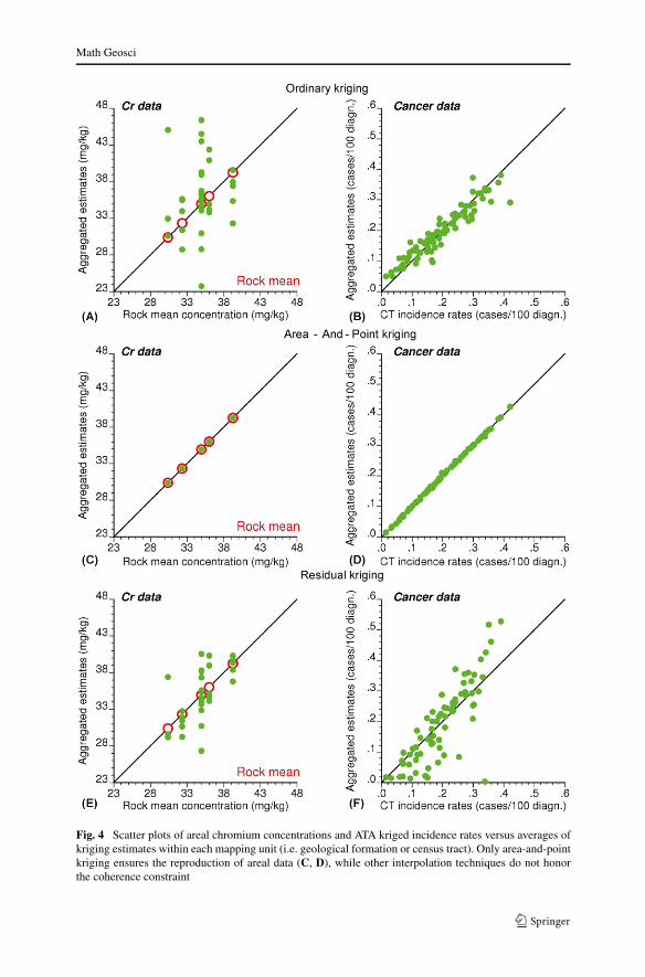
area-to-area and area-to-point covariances in AAP kriging system (2), each mappingunit was discretized using the interpolation grid nodes; this ensures that the krigedestimates in Fig. 2C honor the coherence constraint, as demonstrated by the scatterplot in Fig. 4C.

Math Geosci

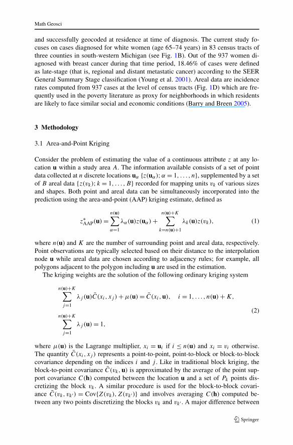
Fig. 3 Semivariogram modelsused for geostatisticalinterpolation. (A) Models fittedto semivariograms of chromiumconcentration before and aftersubtraction of trend estimates(i.e. residuals). Models fitted toindicator semivariograms ofhealth outcomes before and aftersubtraction of trend estimates:entire model (B) and detailedview of first few lags (C)

Math Geosci

Fig. 4 Scatter plots of areal chromium concentrations and ATA kriged incidence rates versus averages ofkriging estimates within each mapping unit (i.e. geological formation or census tract). Only area-and-pointkriging ensures the reproduction of areal data (C, D), while other interpolation techniques do not honorthe coherence constraint

Math Geosci

As expected, the Cr residual semivariogram has a lower sill than the original semi-variogram since a small part of the total variance is captured by the trend model. Theresidual semivariogram model has also a much shorter range, leading to bull’s-eyeeffect around sample points in the map created by residual kriging (Fig. 2E). In con-trast, the AAP map (Fig. 2C) is much smoother and clearly displays the lower concen-trations expected on the Argovian formation, in particular when compared with theordinary kriging map. Differences between the three maps are the largest in sparselysampled areas where the choice of a trend model becomes preponderant (Goovaerts1997). In particular, incorporating the geological information leads to smaller esti-mates on the section of Argovian formation where no sample was collected (dashedcircle in Fig. 2C) and in a small Argovian mapping unit that must satisfy the co-herence constraint despite the presence of larger concentrations recorded in the field(solid circle in Fig. 2C). The scatter plot in Fig. 4E indicates that residual kriging(RK) leads to a better reproduction of the areal data than ordinary kriging (Fig. 4A).Yet, there is no guarantee that the coherence constraint will be honored once thekriged residuals are added to the trend estimates. Such a constraint can only be im-posed through the joint incorporation of field point data and areal map data by AAPkriging (Fig. 4C). Although the map of AAP kriged estimates is smoother than theOK and RK maps when all 359 observations are used, cross-validation studies inFig. 7 will demonstrate the opposite for lower sampling densities.

A similar analysis was conducted for the health outcome data displayed inFigs. 1B–D. To account for the wide range of separation distances between cancercases (from a few metres to 112 km), the indicator semivariogram in Fig. 3B wascomputed using two series of lag classes: 37 lags of 30 metres to characterize thesmall-scale variation of the data and 37 lags of 800 metres to look at the regional pat-tern. The spatial variability is clearly nested: most of the variance occurs over shortdistances (first range = 397 metres, see detailed view in Fig. 3C) and is superimposedon a regional structure with a range of 19.57 km. Late detection cases do not occurrandomly in space, yet individual-level factors such as age or family history generatea large variability over short distances. Subtracting the census tract mean from indi-cator values slightly reduces the sill of the semivariogram, yet it has no impact overshorter distances (e.g. less than 1 km) which are smaller than the average dimensionof the tracts.

All incidence maps were created using the 32 closest point indicator data and,for AAP kriging, the rates recorded in census tracts that share a boundary or vertexwith the tract, including the interpolation node (first-order adjacency). Incorporat-ing census-tract information through residual kriging adds more details to the mapbut generates discontinuities at the tract boundaries. On the other hand, accountingfor adjacent areal data in AAP kriging leads to a map that has more compact spa-tial features, yet a larger variance, than the indicator kriging map. Scatter plots inFig. 4 (right column) compare the average of kriged estimates within each censustract with the incidence rates that were noise-filtered by area-to-area binomial krig-ing (Goovaerts 2009a). Unlike for the Jura data set, ordinary kriging of late-stagediagnosis indicators leads to a better reproduction of areal data than residual kriging.Because of the greater compactness of census tracts relative to the intricate arrange-ment of geological formations, point data used in ordinary kriging are more likely

Math Geosci

to belong to the same areal unit for the health data set than the soil data set. In ad-dition, the local means used in residual kriging ignore the small-number problem;differences displayed in Fig. 4F reflect the rate uncertainty.

4.2 Kriging Weights and Kriging Variances

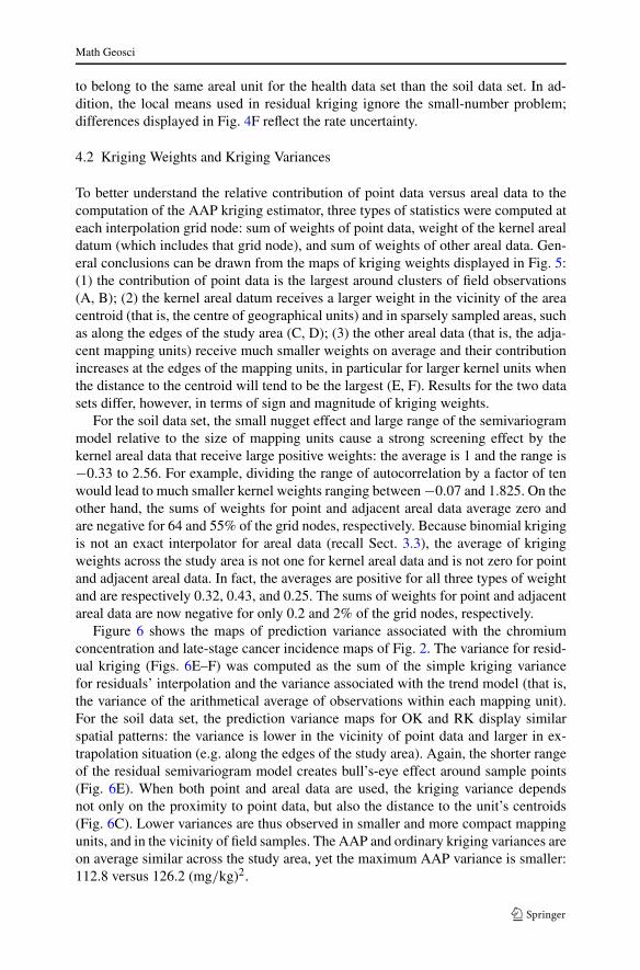
To better understand the relative contribution of point data versus areal data to thecomputation of the AAP kriging estimator, three types of statistics were computed ateach interpolation grid node: sum of weights of point data, weight of the kernel arealdatum (which includes that grid node), and sum of weights of other areal data. Gen-eral conclusions can be drawn from the maps of kriging weights displayed in Fig. 5:(1) the contribution of point data is the largest around clusters of field observations(A, B); (2) the kernel areal datum receives a larger weight in the vicinity of the areacentroid (that is, the centre of geographical units) and in sparsely sampled areas, suchas along the edges of the study area (C, D); (3) the other areal data (that is, the adja-cent mapping units) receive much smaller weights on average and their contributionincreases at the edges of the mapping units, in particular for larger kernel units whenthe distance to the centroid will tend to be the largest (E, F). Results for the two datasets differ, however, in terms of sign and magnitude of kriging weights.

For the soil data set, the small nugget effect and large range of the semivariogrammodel relative to the size of mapping units cause a strong screening effect by thekernel areal data that receive large positive weights: the average is 1 and the range is−0.33 to 2.56. For example, dividing the range of autocorrelation by a factor of tenwould lead to much smaller kernel weights ranging between −0.07 and 1.825. On theother hand, the sums of weights for point and adjacent areal data average zero andare negative for 64 and 55% of the grid nodes, respectively. Because binomial krigingis not an exact interpolator for areal data (recall Sect. 3.3), the average of krigingweights across the study area is not one for kernel areal data and is not zero for pointand adjacent areal data. In fact, the averages are positive for all three types of weightand are respectively 0.32, 0.43, and 0.25. The sums of weights for point and adjacentareal data are now negative for only 0.2 and 2% of the grid nodes, respectively.

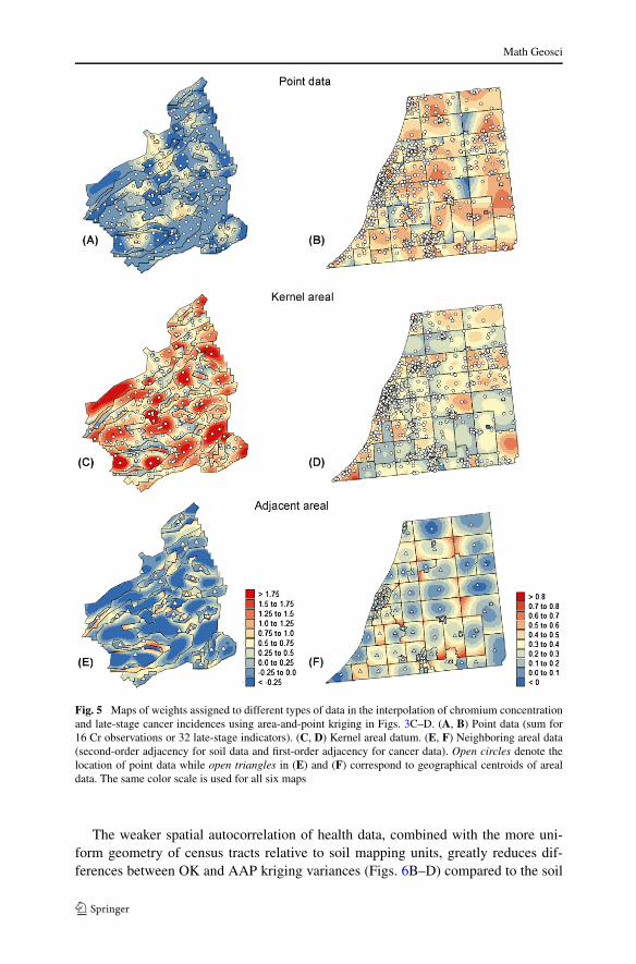
Figure 6 shows the maps of prediction variance associated with the chromiumconcentration and late-stage cancer incidence maps of Fig. 2. The variance for resid-ual kriging (Figs. 6E–F) was computed as the sum of the simple kriging variancefor residuals’ interpolation and the variance associated with the trend model (that is,the variance of the arithmetical average of observations within each mapping unit).For the soil data set, the prediction variance maps for OK and RK display similarspatial patterns: the variance is lower in the vicinity of point data and larger in ex-trapolation situation (e.g. along the edges of the study area). Again, the shorter rangeof the residual semivariogram model creates bull’s-eye effect around sample points(Fig. 6E). When both point and areal data are used, the kriging variance dependsnot only on the proximity to point data, but also the distance to the unit’s centroids(Fig. 6C). Lower variances are thus observed in smaller and more compact mappingunits, and in the vicinity of field samples. The AAP and ordinary kriging variances areon average similar across the study area, yet the maximum AAP variance is smaller:112.8 versus 126.2 (mg/kg)2.

Math Geosci

Fig. 5 Maps of weights assigned to different types of data in the interpolation of chromium concentrationand late-stage cancer incidences using area-and-point kriging in Figs. 3C–D. (A, B) Point data (sum for16 Cr observations or 32 late-stage indicators). (C, D) Kernel areal datum. (E, F) Neighboring areal data(second-order adjacency for soil data and first-order adjacency for cancer data). Open circles denote thelocation of point data while open triangles in (E) and (F) correspond to geographical centroids of arealdata. The same color scale is used for all six maps

The weaker spatial autocorrelation of health data, combined with the more uni-form geometry of census tracts relative to soil mapping units, greatly reduces dif-ferences between OK and AAP kriging variances (Figs. 6B–D) compared to the soil

Math Geosci

Fig. 6 Maps of prediction variance associated with the maps of Fig. 2. (A, B) Ordinary kriging. (C, D)Kriging that combines both point and areal data. (E, F) Residual kriging with a choropleth trend model.The same color scale is used for each series of three maps

data set (Figs. 6A–C). The two sets of kriging variances have the same magnitude,a smaller maximum for AAP kriging (0.138 versus 0.141), and they display a linearcorrelation coefficient of 0.93. The kriging variance is generally smaller in the prox-imity of cancer patients’ residences. Like the predicted values in Fig. 2F, the mapof residual kriging variance (Fig. 6F) shows strong discontinuities at the borders be-tween census tracts. In fact, unlike the two other algorithms, the RK estimates and

Math Geosci

variances are strongly correlated. The linear correlation coefficient of 0.52 reflectsthe relationship between the mean and variance of indicator data (8), which are usedas local trend in residual kriging.

4.3 Performance Comparison

Figures 2 through 6 provided useful information on the properties of the three typesof kriging estimator: ordinary kriging, AAP kriging and residual kriging. However,since the true chromium concentration and incidence rate are unknown, one cannotconclude that one estimator outperforms the others. The prediction performances ofthe different interpolation techniques with respect to sampling density were investi-gated using the following procedure:

1. Select a random subset (prediction set) of n field data with 30 ≤ n ≤ 255 forthe soil data set and 100 ≤ n ≤ 850 for the cancer data set. For each of the 16sampling intensities, 100 different random subsets were selected to account forsampling fluctuations.

2. For each random subset and sampling intensity,

• Predict the heavy metal concentration or risk of late-stage diagnosis at theN = 369 − n or N = 937 − n remaining locations (validation set) using eachof the three algorithms and the same search strategy applied in Fig. 2, exceptthat a minimum separation distance of 125 metres was imposed on neighboringfield data to avoid overly optimistic prediction accuracies for clustered obser-vations. A coarser discretization geography (100-m instead of 25-m grid) wasused for the soil data set to reduce the computational time required by each ofthe 1,600 simulation runs. In each case, the experimental semivariogram wascomputed and modeled using weighted least-square regression. For the cancerdata set, census-tract incidence rates are estimated for each simulation using then indicator data available.

• Compute the mean absolute error (MAE) of prediction as

MAE = 1

N

N∑

α=1

∣∣z∗(uα) − z(uα)∣∣. (14)

• Compute the mean square standardized residual (MSSR) as

MSSR = 1

N

N∑

α=1

[z∗(uα) − z(uα)

σK(uα)

]2

. (15)

If the actual estimation error is equal, on average, to the error predicted by themodel, the MSSR statistic should be about one (Wackernagel 1998). To penalizeequally the over- and under-estimation of the prediction errors by the krigingvariance, the inverse of MSSR was considered if the quantity (15) exceededone.

• Compute the variance of the set of N heavy metal concentration estimates toassess the magnitude of the smoothing effect caused by each type of krigingalgorithm.

Math Geosci

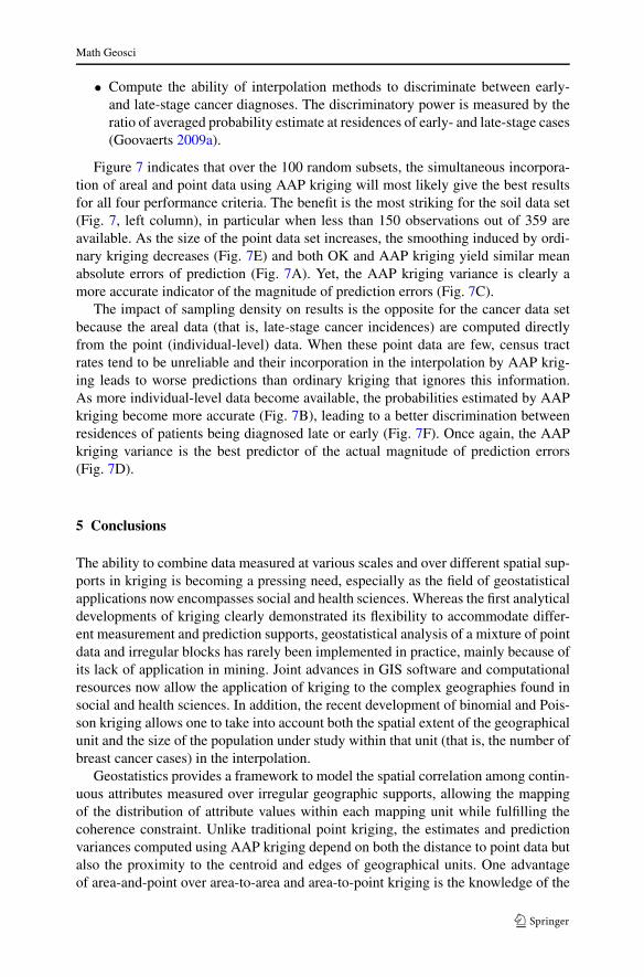
• Compute the ability of interpolation methods to discriminate between early-and late-stage cancer diagnoses. The discriminatory power is measured by theratio of averaged probability estimate at residences of early- and late-stage cases(Goovaerts 2009a).

Figure 7 indicates that over the 100 random subsets, the simultaneous incorpora-tion of areal and point data using AAP kriging will most likely give the best resultsfor all four performance criteria. The benefit is the most striking for the soil data set(Fig. 7, left column), in particular when less than 150 observations out of 359 areavailable. As the size of the point data set increases, the smoothing induced by ordi-nary kriging decreases (Fig. 7E) and both OK and AAP kriging yield similar meanabsolute errors of prediction (Fig. 7A). Yet, the AAP kriging variance is clearly amore accurate indicator of the magnitude of prediction errors (Fig. 7C).

The impact of sampling density on results is the opposite for the cancer data setbecause the areal data (that is, late-stage cancer incidences) are computed directlyfrom the point (individual-level) data. When these point data are few, census tractrates tend to be unreliable and their incorporation in the interpolation by AAP krig-ing leads to worse predictions than ordinary kriging that ignores this information.As more individual-level data become available, the probabilities estimated by AAPkriging become more accurate (Fig. 7B), leading to a better discrimination betweenresidences of patients being diagnosed late or early (Fig. 7F). Once again, the AAPkriging variance is the best predictor of the actual magnitude of prediction errors(Fig. 7D).

5 Conclusions

The ability to combine data measured at various scales and over different spatial sup-ports in kriging is becoming a pressing need, especially as the field of geostatisticalapplications now encompasses social and health sciences. Whereas the first analyticaldevelopments of kriging clearly demonstrated its flexibility to accommodate differ-ent measurement and prediction supports, geostatistical analysis of a mixture of pointdata and irregular blocks has rarely been implemented in practice, mainly because ofits lack of application in mining. Joint advances in GIS software and computationalresources now allow the application of kriging to the complex geographies found insocial and health sciences. In addition, the recent development of binomial and Pois-son kriging allows one to take into account both the spatial extent of the geographicalunit and the size of the population under study within that unit (that is, the number ofbreast cancer cases) in the interpolation.

Geostatistics provides a framework to model the spatial correlation among contin-uous attributes measured over irregular geographic supports, allowing the mappingof the distribution of attribute values within each mapping unit while fulfilling thecoherence constraint. Unlike traditional point kriging, the estimates and predictionvariances computed using AAP kriging depend on both the distance to point data butalso the proximity to the centroid and edges of geographical units. One advantageof area-and-point over area-to-area and area-to-point kriging is the knowledge of the

Math Geosci

Fig. 7 Impact of the sample size on the proportion of simulations for which an interpolation techniqueoutperforms the other two. Cross-validation statistics include: the mean absolute error of prediction, themean square standardized residual, the variance of the set of kriged estimates (smoothness), and the dis-criminatory power between early- and late-stage cases

point-support semivariogram model that can be inferred directly from point measure-ments, thereby eliminating the need for deconvolution procedures. This paper hasshown how to implement AAP kriging within the binomial framework and demon-strated its relationship with indicator kriging and Poisson kriging. Binomial kriging,

Math Geosci

like Poisson kriging, is a noise-filtering algorithm; hence, by construction, areal dataare not honored by kriging estimates.

Sensitivity analysis conducted for contrasted geographies (nested irregular geo-logical formations versus semi-regular polygonal census tracts) and types of kriging(traditional versus binomial) demonstrated the overall better prediction performanceof AAP kriging over ordinary kriging and residual kriging with the choropleth-maptrend model. In particular, when sampling is sparse, these two case studies indicatedthat incorporation of areal data tends to improve the prediction accuracy while theexactitude property of areal data decreases the smoothness of interpolated surfaces.Similar results were also obtained by Kerry et al. (2010b) using areal data that werederived independently of the point data.

This paper covered the situation where areal data provide a spatially exhaustivecoverage of the study area, for example, a map of soil classes or administrative units.However, the methodology is completely general and can be applied to a mixtureof point data and spatially disconnected areal data. The approach can also be imple-mented within a stochastic simulation framework. Liu and Journel (2009) recentlyintroduced a software package that uses either direct sequential simulation or errorsimulation to account for both point and block support data in stochastic simulation.Their algorithms are capable of handling different block geometries and differentlayouts of block data, including irregular-shaped and overlapping blocks.

Acknowledgements This research was funded by grants R43-CA135814-01 and R44-CA132347-02from the National Cancer Institute. The views stated in this publication are those of the author and do notnecessarily represent the official views of the NCI. The author thanks two anonymous reviewers for theirvery pertinent comments.

References

Atteia O, Dubois J-P, Webster R (1994) Geostatistical analysis of soil contamination in the Swiss Jura.Environ Pollut 86:315–327

Barry J, Breen N (2005) The importance of place of residence in predicting late-stage diagnosis of breastor cervical cancer. Heal Place 11:15–29

Best NG, Richardson S, Thomson A (2005) A comparison of Bayesian spatial models for disease mapping.Stat Meth Med Res 14:35–59

Goovaerts P (1997) Geostatistics for natural resources evaluation. Oxford University Press, New YorkGoovaerts P (2005) Geostatistical analysis of disease data: estimation of cancer mortality risk from empir-

ical frequencies using Poisson kriging. Int J Heal Geogr 4:31. doi:10.1186/1476-072X-4-31Goovaerts P (2007) Spatial uncertainty in medical geography: a geostatistical perspective. In: Shekhar S,

Xiong H (eds) Encyclopedia of GIS. Springer, Berlin, pp 1106–1112Goovaerts P (2008) Kriging and semivariogram deconvolution in presence of irregular geographical units.

Math Geosci 40:101–128Goovaerts P (2009a) Combining area-based and individual-level data in the geostatistical mapping of late-

stage cancer incidence. Spat Spatio-tempor Epidemiol 1:61–71Goovaerts P (2009b) Medical geography: a promising field of application for geostatistics. Math Geosci

41:243–264Goovaerts P (2010) A coherent geostatistical framework for combining choropleth map and field data in

the spatial interpolation of soil properties. Eur J Soil Sci (accepted)Goovaerts P, Journel AG (1995) Integrating soil map information in modeling the spatial variation of

continuous soil properties. Eur J Soil Sci 46:397–414Gotway CA, Young LJ (2002) Combining incompatible spatial data. J Am Stat Assoc 97(459):632–648

Math Geosci

Gotway CA, Young LJ (2005) Change of support: an interdisciplinary challenge. In: Renard Ph,Demougeot-Renard H, Froidevaux R (eds) geoENV V—Geostatistics for environmental applications.Springer, Berlin, pp 1–13

Gotway CA, Young LJ (2007) A geostatistical approach to linking geographically-aggregated data fromdifferent sources. J Comput Graph Stat 16(1):115–135

Hengl T, Heuvelink GBM, Stein A (2004) A generic framework for spatial prediction of soil variablesbased on regression-kriging. Geoderma 120:75–93

Journel AG (1983) Nonparametric estimation of spatial distributions. Math Geol 15(3):445–468Journel AG, Huijbregts CJ (1978) Mining geostatistics. Academic Press, LondonKerry R, Goovaerts P, Haining V, Ceccato RP (2010a) Applying geostatistical analysis to crime data:

car-related thefts in the Baltic States. Geogr Anal 42:53–75Kerry R, Rawlins BG, Goovaerts P (2010b) Area-to-point kriging of organic carbon and soil texture: an

efficient use of legacy soil data from polygon maps for regional or national scale digital soil mapping.In: Proceedings of 4th global workshop on digital soil mapping, Rome, Italy, May 24–26, 2010

Kyriakidis P (2004) A geostatistical framework for area-to-point spatial interpolation. Geogr Anal36(2):259–289

Liu Y, Journel AG (2009) A package for geostatistical integration of coarse and fine scale data. ComputGeosci 35(3):527–547

Liu TL, Juang KW, Lee DY (2006) Interpolating soil properties using kriging combined with categoricalinformation of soil maps. Soil Sci Soc Am J 70:1200–1209

Oliver MA, Webster R, Lajaunie C, Muir KR, Parkes SE, Cameron AH, Stevens MCG, Mann JR (1998)Binomial co-kriging for estimating and mapping the risk of childhood cancer. IMA J Math Appl Med15(3):279–297

Rushton G, Peleg I, Banerjee A, Smith G, West M (2004) Analyzing geographic patterns of disease inci-dence: Rates of late-stage colorectal cancer in Iowa. J Med Syst 28(3):223–236

Talbot TO, Kulldorff M, Forand SP, Haley VB (2000) Evaluation of spatial filters to create smoothed mapsof health data. Stat Med 19:2399–2408

Wackernagel H (1998) Multivariate geostatistics. Springer, Berlin. 2nd completely revised editionWalker E, Monestiez P, Renard D, Bez N (2008) Kriging of the latent probability of a binomial variable:

application to fish statistics. In: Ortiz J, Emery X (eds) Geostatistics 2008. GECAMIN, Santiago, pp981–990

Waller LA, Gotway CA (2004) Applied spatial statistics for public health data. Wiley, New JerseyWebster R, Oliver MA, Muir KR, Mann JR (1994a) Kriging the local risk of a rare disease from a register

of diagnoses. Geogr Anal 26:168–185Webster R, Atteia O, Dubois J-P (1994b) Co-regionalization of trace metals in the soil in the Swiss Jura.

Eur J Soil Sci 45:205–18Young JL Jr, Roffers SD, Ries LAG, Fritz AG, Hurlbut AA (eds) (2001) SEER summary staging manual—

2000: codes and coding instructions, National Cancer Institute. National Institutes of Health Pub# 01-4969, Bethesda, MD