Coexistence in Metacommunities: A discrete time, finite patch approach Vanessa M. Adams1, Chris Wilcox1,2, Phil Pollett3, Hugh P. Possingham1,3

1The Ecology Centre, The University of Queensland, Brisbane 4072, Australia 2CSIRO Marine and Atmospheric Research, Hobart 7001, Australia 3Department of Mathematics, The University of Queensland, Brisbane 4072, Australia Keywords: Metacommunity, Quasi-stationary distributions, Extinction, Competition, Coexistence, Vernal Pool, Fairy Shrimp, Branchinecta lynchi, Linderiella occidentalis Correspondence: The Ecology Centre, The University of Queensland, Brisbane, Queensland, 4072, Australia. Tel: +61 (0)7 3365 2709, Fax: +61 (0)7 3365 1655, v.adams@uq.edu.au Abstract:

Metapopulation theory has emerged as a popular paradigm for studying the abundance

and distribution of species in a fragmented landscape. A recent extension to

metapopulation theory has been the development of metacommunity theory, which

broadens the framework to incorporate the interacting dynamics of multiple species.

Much of the work using a metacommunity framework has focused on determining the

necessary conditions for species coexistence. Another fundamental but neglected

question is the distribution of communities in a landscape and what factors drive

occupancy patterns. We introduce a stochastic spatially implicit, discrete time, finite

patch metacommunity model to examine expected distributions of multiple species given

competition between species. We use the notion of quasi-stationarity to understand the

probability distribution of different patch occupancy patterns prior to extinction. We find

competition between species reduces the abundance of the lesser competitor. In addition,

our novel application of quasi-stationary probability distributions elucidates the relative

stability of the multiple species states and single species states. We contrast our model

1

with the more commonly used one-dimensional continuous-time competition models

which produce similar abundance predictions, but provide no information about the

stability of states or the variation about predicted averages. We illustrate the application

of our model by applying it to a system of vernal pool wetlands which support several

species of endangered crustaceans.

2

1. Introduction 1

2

3

4

5

6

7

8

9

10

11

12

13

14

15

16

17

18

19

20

21

22

The issue of how species coexist is a central question in community ecology. In short,

long-term coexistence of competitors using a single resource is almost impossible, and

life-history trade-offs are one of the primary mechanisms posited to allow co-existence of

competing species (Vance 1985). Much of community ecology has looked at local scale

phenomena, focusing coexistence predictions on limiting resources and trade-offs among

them (Chase and Leibold 2003). Recently, however, community ecology has shifted

focus from the local scale to examining trade-offs at broader scales (Kneitel and Chase

2004). Competition is traditionally characterized as either extinction competition, the

extinction of the lesser competitor, or migration competition, the migration of the lesser

competitor to alleviate competition (Levins and Culver 1971). In this context space is the

fundamental resource and trade-offs between dispersal and competitive ability can

mitigate competition and allow for coexistence.

A recent theoretical development that has allowed for a larger exploration of coexistence

is the metacommunity concept. A metacommunity is a set of communities, containing

potentially interacting species, occupying discrete patches linked by dispersal (Wilson

1992). Traditionally community theory has focused on a single scale, assuming that

communities were closed. Yet this approach fails to capture dynamic natural processes

such as dispersal and local extinction/colonization events which are likely to affect

coexistence.

3

23

24

25

26

Many metacommunity models (e.g. Shurin et al. 2004, Calcagno 2006, Yu 2001) use

extensions of the Levins and Culver (1971) model which may be summarized with two

simultaneous differential equations:

111111 )1( peppc

dtdp

−−= , 27

)1()1( 1201222222 ppeppeppc

dtdp

−−−−= , 28

29

30

31

32

33

34

35

36

37

38

39

40

41

42

43

44

where ci is the per patch colonization rate of species i, and pi is the proportion of sites

inhabited by species i. For species 1 local extinctions occur at per patch rate e1and are

assumed to be independent of species 2. In contrast it is assumed that local extinctions of

species 2 are influenced by the presence of species 1 such that, e0 is the per patch local

extinction rate for species 2 when species 1 is absent and , e2 is the per patch local

extinction rate when species 1 is present. These models, using differential equations,

implicitly assume continuous time processes and an infinite number of patches in order to

make conclusions about when coexistence may occur, and what values of the species

parameters will affect coexistence conditions (e.g., Amarasekare and Nisbet 2001,

Klausmeier 2001). In this paper we construct an equivalent model for the

presence/absence of each species in a patch using a discrete time, finite patch Markov

chain framework (see Day and Possingham 1995 for a single species version of the

approach). The discrete time parallel does not require assuming an infinite number of

patches and also forces colonization and extinction events to occur at discrete time steps

rather than instantaneously.

4

45

46

47

48

49

50

51

52

53

54

55

56

57

58

59

60

61

62

63

64

65

66

67

Much of the recent metacommunity work has been focused on extending the classical life

history trade-off framework, deducing which combinations of species parameters will

allow coexistence (Leibold et al. 2004, Yu et al. 2004, Yu 2001). However, the more

general question of the joint probability distributions of patch occupancy, which tells us

about the frequency and stability of various community types in a landscape, has been

relatively neglected. For instance, an important question that cannot be directly answered

by continuous time differential equation models is the effect of the number of available

patches in a landscape on the frequency of the potential community types. As landscapes

are becoming increasingly fragmented, and available habitat for species is decreasing, it

is important to be able to predict the effect of these changes on the distribution of species

in specific landscapes (Fahrig 1992). While continuous time differential equation models

cannot address these effects, a discrete time, finite patch model can as the number of

patches in a landscape can be directly manipulated.

In this paper we construct a stochastic discrete time, finite patch metacommunity model.

We develop summary measures of species and community distributions in the two

species case, and demonstrate how to extend this framework to an arbitrary number of

species. We apply our model to predict the persistence and community structure of two

species of crustaceans in a system of ephemeral wetlands in California, USA. These

wetland systems and their obligate fauna are of substantial conservation concern as the

majority of the habitat has been destroyed due to urban and agricultural development;

resulting in the listing of a number of the species under the US Endangered Species Act.

5

68

69

70

71

72

73

74

75

76

77

78

79

80

81

82

83

84

85

86

87

88

89

90

We address the effects of interspecific interactions in this posited metacommunity system

by comparing results with and without competitive interactions. We compare the

predicted distributions from the model with different assumptions with the observed

distribution, and draw conclusions regarding the conditions that allow for coexistence in

this wetland system. Additionally, we examine the influence of the number of patches in

the system, on the expected distribution of community types. We compare our results to

the results obtained using differential equations. Using these results we discuss the

implications of the model for the persistence of these kinds of communities, which are

significantly threatened by human development.

2. Methods

In this section we first describe the Markov chain model for a single species, then we

expand the model to any number of species, focusing on two species. Next we show how

to use the discrete-time Markov chain to predict the state of the metacommunity at any

time into the future and find the quasi-stationary equilibrium for the metacommunity.

Finally we parameterize the model for the Californian fairy-shrimp system.

2.1 A single species metapopulation model

6

91

92

93

94

95

96

97

98

99

100

101

102

103

104

105

106

107

108

109

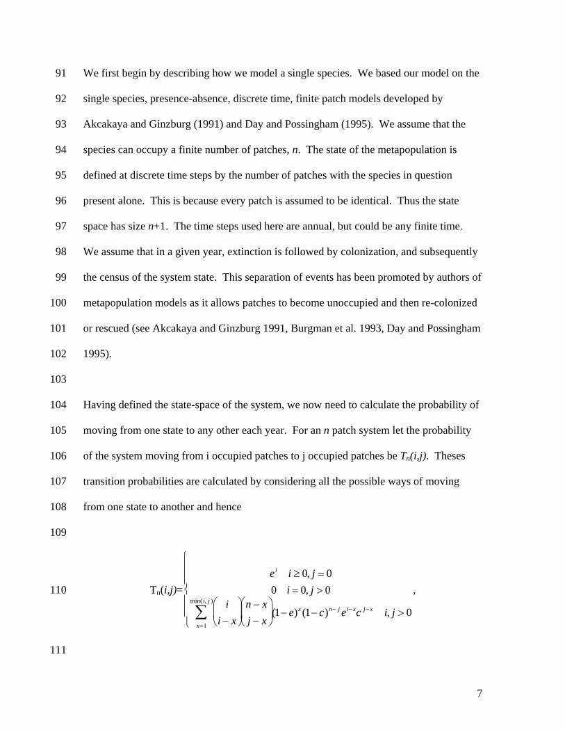
We first begin by describing how we model a single species. We based our model on the

single species, presence-absence, discrete time, finite patch models developed by

Akcakaya and Ginzburg (1991) and Day and Possingham (1995). We assume that the

species can occupy a finite number of patches, n. The state of the metapopulation is

defined at discrete time steps by the number of patches with the species in question

present alone. This is because every patch is assumed to be identical. Thus the state

space has size n+1. The time steps used here are annual, but could be any finite time.

We assume that in a given year, extinction is followed by colonization, and subsequently

the census of the system state. This separation of events has been promoted by authors of

metapopulation models as it allows patches to become unoccupied and then re-colonized

or rescued (see Akcakaya and Ginzburg 1991, Burgman et al. 1993, Day and Possingham

1995).

Having defined the state-space of the system, we now need to calculate the probability of

moving from one state to any other each year. For an n patch system let the probability

of the system moving from i occupied patches to j occupied patches be Tn(i,j). Theses

transition probabilities are calculated by considering all the possible ways of moving

from one state to another and hence

Tn(i,j)=ei i ≥ 0, j = 00 i = 0, j > 0

ii − x

⎛

⎝ ⎜

⎞

⎠ ⎟

n − xj − x

⎛

⎝ ⎜

⎞

⎠ ⎟

x=1

min( i, j )

∑ (1− e)x (1− c)n− j ei−xc j−x i, j > 0

⎧

⎨

⎪ ⎪

⎩

⎪ ⎪

, 110

111

7

where e is per patch local extinction probability and c is the probability per patch

probability any empty patch is colonized by an occupied patch. The transition

probabilities T

112

113

114

115

116

117

118

119

120

121

122

123

124

125

126

127

128

n(i,j) are conveniently stored in a matrix Tn.

2.2 Metacommunity model

We use this metapopulation model and extend it to a metacommunity model for two

species. The same approach can be used to extend the model to m species.

As with the one species model we assume there are n identical patches that may be

occupied at time t. The state of the system is described by the number of patches

occupied by each possible combination of species. For a system with two species

(species a and b) we have n0 + na + nb + nab = n, where n0 is the number of empty patches,

na is the number of patches occupied only by species a, nb is the number of patches

occupied only by species b, and nab is the number of patches occupied by both species a

and b. We will not keep explicit track of n0, because the number of completely empty

patches is simply the patches that are not in one of the other states. Thus our process may

take any one of the states in the set S = { }nnnnnn abba ≤++∈ :},...,1,0{ 3 . We note that S

has size |S| =

129

( )( )( 12361

33

+++=⎟⎟⎠

⎞⎜⎜⎝

⎛ +nnn

n )130

131

132

133

.

For a two patch, two species system there are ten possible states. Consider two possible

states in the full state space, Si , Sj ∈ S and let

8

134

135

136

137

138

139

140

141

142

143

144

145

146

147

148

149

150

151

152

153

154

s=na + nab for (na, nb, nab) = Si

t=na + nab for (na, nb, nab) = Sj

and

u=nb + nab for (na, nb, nab) = Si

v=nb + nab for (na, nb, nab) = Sj

Then the probability of the system moving from Si to Sj is given by T2,n(Si , Sj)

T2,n(Si ,

Sj)= ⎪⎩

⎪⎨⎧

>−−−−

∈⋅

∑ ∑= =

−−−−−− 0,,,)1()1()1()1(

},,,{0),(),(),min(

1

),min(

1, vutscecececeC

vutsvuTtsTts

x

vu

y

xtb

xsb

tna

xa

yvb

yub

vnb

ybyx

ba

(See appendix 1 for description of how coefficient Cx,y is determined) where and

are the single species transition matrices for species a and b respectively when

there are n patches. Predation and competition can be included in this model by using

conditional probabilities for extinction and colonization of a species given the presence of

another species. Using similar logic it is possible, but messy, to construct a general

transition matrix for m species in n identical patches, T

),( tsTa

),( tsTb

m,n. The transition matrix Tm,n can

be used to explore the dynamics of our metacommunity – however for the remainder of

this paper we will consider a two species metacommunity only.

2.3 Model analysis

9

155

156

157

158

159

160

161

162

163

164

165

166

167

168

169

170

In this section we describe methods used to analyze the discrete patch, finite time

metacommunity model. First we discuss the role of competition in long-term system

behavior. We then discuss the significance of the construction of the transition matrix

described above, and the how matrix math may be interpreted in the context of

metacommunity dynamics.

Given an initial metacommunity with a known number of patches in each of the four

possible combinations of which species are present (neither, species a, species b or both)

the metacommunity dynamics can be projected forward t time steps by raising the matrix

T2,n to the power of t. The initial state vector v(0), which will be a row vector with a

probability of 1 in one of the possible states and zeros in every other entry, may be

multiplied by (T2,n)t to give v(t). This gives the probability of being in any of the states in

S. To extract meaningful distributions from this vector we may sort and sum the

probabilities according to the number of patches where species a, species b, or both

species exist. For example if S1 is the set of all states with r patches containing both

species a and b we may find the probability of this state as

vu(t)u∈S1

∑ , where S1= u : nab = r{ }. 171

172

173

174

175

This gives us the fraction of sites occupied by species a, species b or both species a and b.

For the continuous case, if we assume that there are no interactions between species, the

expected equilibrium fraction (p) of patches occupied by a species not affected by

competition can be shown to be p1* =

c1

e1 + c 1

(similar to the incidence function described

by Hanski (1994)). Given coexistence, if competition affects the extinction probability,

176

177

10

the equilibrium fraction is p2* =

c2

c2 + e2 + eco p1* − e2 p1

* . We may use the expected fraction

to compare predicted number of patches occupied to observed number of patches

occupied. We will use this result to compare our discrete model to the continuous

differential equations model commonly used.

178

179

180

181

182

183

184

185

186

187

188

189

190

191

192

193

194

195

196

197

198

199

200

Quasi-Stationary Distributions

It is crucial to recognize that ecological systems are in a constant state of flux, but that

they may be described by an equilibrium distribution as they fluctuate through time

(Hastings 2003). In stochastic metapopulation models like this one, the only globally

stable state is extinction of both species. However, before that state is reached, the

system is very likely to occupy states according to a set of stable equilibria, the quasi-

stationary states. The quasi-stationary distribution is the average state of the system

conditioned on the species not having reached extinction. The rate of decay, or

movement out of this ‘averaged’ state towards extinction is given by the eigenvalue

associated with the quasi-stationary distribution (Darroch and Seneta 1965). The use of

quasi-stationarity has been applied to metapopulation theory to calculate the frequency of

patch occupancy in a landscape (e.g. Day and Possingham 1995, Pollett 1999). For a

community, interactions between species may effect the individual species distribution in

a landscape. In a system with multiple interacting species, as each species goes globally

extinct the system moves towards full extinction. Thus the stable distribution moves step

wise towards full extinction as different species leave the system. Therefore, there is not

a single quasi-stationary distribution, but rather a set of distributions, each corresponding

11

201

202

203

204

205

206

207

208

209

210

211

212

213

214

215

216

217

218

to a different number of extant species, that will fully describe the systems stable

equilibrium.

Our metapopulation model may be described as a Markov chain with a single absorption

state, extinction. Thus, the matrix, T, may be truncated such that the column and row

vectors corresponding to extinction are removed giving us matrix R. For a reduced

metapopulation matrix, R, the left eigenvector, ν, corresponding to the dominant

eigenvalue, λ, gives us the quasi-stationary distribution (Darroch and Seneta, 1965,

Gilpin and Taylor 1994, Day and Possingham 1995). The metacommunity matrix can

likewise be truncated by removing the absorption state (extinction). For this matrix, R,

the set of left vectors corresponding to the dominant eigenvalue deserves further

investigation.

First let us examine the nature of R. When the states are grouped properly, such that sets

of states are grouped together, we obtain sub-matrices along the diagonal of R

corresponding to transitions between states of the system for which there are only species

A, only species B, or species A and B both present.

R=[A] [0] [0][0] [B] [0][...] [...] [AB]

⎡

⎣

⎢ ⎢ ⎢

⎤

⎦

⎥ 219

220

221

222

⎥ ⎥

The sets of states where just one species is present (A and B, described by the sub-

matrices [A] and [B]) are irreducible. Once in one of these sets of states we may move

12

within the set but cannot move to other sets in the system. In ecological terms this means

that once one of the species A or B becomes extinct in our system we may there after

only have a single species system. A system composed solely of species A may not

suddenly have both species A and B, or just B. We may consider these states to be

pseudo-absorption states. Once we are in a pseudo-absorption state we may not leave it;

rather our system can only move towards the absorption state of extinction. Each of our

pseudo-absorption sub-matrices has a set of eigenvalues {ρ

223

224

225

226

227

228

229

230

231

232

233

234

235

236

237

238

239

240

241

242

243

244

245

n} and corresponding left

eigenvectors {υn} which are contained in the set of eigenvalues {ρ} and left eigenvectors

{υ} associated with matrix R.

Now consider the sub-matrix corresponding to the coexistence state in which we have

both species A and species B in the system. The set of states in which both species are

present is irreducible, but it may also lead to our other sets of states. This means that

state AB may lead to the set A or set B but set A and set B may not lead to set AB. For

this irreducible sub-matrix the quasi-stationary distribution of the set is the left

eigenvector of the sub-matrix.

Thus, for our metacommunity transition matrix, we have a matrix with one absorption

state (extinction), two pseudo-absorption states (sets A and B) and state AB. The sets of

states A, B, and AB are irreducible. Because there is more than one state which is

irreducible, the metacommunity exhibits a series of quasi-stationary states. Rather, we

have quasi-stationary distributions corresponding to our single species sets, and to our

coexistence set. In particular, we may calculate the probability of being in the coexistence

13

state conditioned on non-absorption into our single species states. The long-term limits

of these conditional probabilities are analogous to the quasi-stationary distribution in a

single species metapopulation. The coexistence state must eventually enter either of our

single species (pseudo-absorption) states. Once absorbed into a single species set the

probability of being anywhere in the single species set may be calculated conditional on

not being absorbed (extinction). The long-term limits of these probabilities compose the

quasi-stationary distribution for this set. Thus, to understand the composition of the

system we must look at the different quasi-stationary distributions and the associated

eigenvalues to evaluate how stable these states are relative to one another. For a two

species example we would then have three dominant eigenvalues corresponding to the

single species states (A, B) and the coexistence state (AB): λ

246

247

248

249

250

251

252

253

254

255

256

257

258

259

260

261

262

263

264

265

266

267

268

a, λb, λab. The relative size of

these eigenvalues tells us how quickly the system moves out of these states.

Additionally, 1/ λ provides an estimate of the time it takes to leave the state, or how long

the system remains in state A, B, or AB.

The state-space of a two species metacommunity requires three dimensions, which is

difficult to visualize. We can collapse the state-space into the Euclidean x-y plane by

summing na + nab and nb + nab to give total number of species a and b in the system.

While we lose some detail in this state space, it is more visually appealing. The axes

represent the pseudo-absorption states: when only one species is present (essentially the

metapopulation state space). All points in the interior of the x-y plane are points where

both species are present but not necessarily coexisting. The probability of being at any

point in the x-y plane is then the sum of all rows in the quasi-stationary distribution

14

corresponding to (na + nab, nb + nab). For any point (x,y) in our statespace, we may

examine the probability of species coexisting by creating a vector corresponding to all

states such that n

269

270

271

272

273

274

275

276

277

278

279

280

281

282

283

284

285

286

287

288

289

290

291

a + nab=x and nb + nab=y. The normalized vector then gives us the

relative probabilities of a,b being in the same patches for nab={0,…,min(na + nab, nb +

nab)}.

2.4 Vernal Pool Crustaceans: An Application

The vernal pool fairy shrimp (Branchiopoda: Anostraca, Branchinecta lynchi), a

federally threatened species, and the California linderiella (Linderiella occidentalis),

previously proposed for listing under the Endangered Species Act, inhabit seasonal

wetlands throughout the Central Valley of California (Eng et al. 1990). The seasonal

wetlands, or vernal pools, that the shrimp occupy are typical of Mediterranean climates,

with a summer dry phase and a winter wet phase. These habitats are separated by

uplands, giving them a patch and matrix structure typical of metapopulation systems.

Based on surveys, as detailed below, the species appear to have substantial turnover,

suggesting that they may have the colonization and extinction dynamics suggestive of

metapopulation dynamics. Moreover, based on preliminary experimental results the two

shrimp appear to have competitive interactions (Wilcox, unpublished data). Utilizing the

metacommunity framework to model this system allows us to capture those processes

which appear to be most important: competition between species, along with dispersal

and extinction/colonization events.

15

292

293

294

295

296

297

298

299

300

301

302

303

304

305

306

307

308

309

310

311

312

313

314

A discrete time stochastic model is a realistic framework for this particular system as the

vernal pools are seasonal, and thus the life cycle of the shrimp is annual, driven by

California’s Mediterranean climate. We include competition through conditional

colonization/extinction rates, parameterized as described below. We assume that all

patches are identical and equally related to each other in terms of colonization. We also

assume that local extinctions are independent events. Relaxing these assumptions is

mathematically possible, however the size of system state space may make numerical

work on systems with large number of patches intractable.

Species distribution data for these two species was collected from the vernal pools at the

1,575 hectare West Bear Creek Unit (WBC) of the San Luis National Wildlife Refuge,

Merced Co., California. All vernal pools (~122) were surveyed for macroinvertebrates

biweekly during the winters of 1997-1998 (5 surveys), 1998-1999 (8 surveys), and 1999-

2000 (4 surveys), beginning two weeks after the pools held water. Each pool was

sampled in a minimum of 3 random locations, with the constraint that the samples

covered the range of water depths in the pool. Samples were taken using 1.5 mm mesh

size handnets, varying in aperture from 25 x 47 cm to 10 x 20 cm. Nets were swept

through the water column horizontally in contact with the sediment for distances from 25

cm to 5.5 m, depending on pool size. Approximately 7% of the pool volume was

sampled. Branchiopod crustaceans were identified and counted in each sample.

Annual presence/absence data was calculated by aggregating data within each year. We

then used these annual values to estimate the frequency of changes in presence-absence

16

315

316

317

318

319

320

321

322

323

324

325

326

327

328

329

330

331

332

333

334

335

336

status, which we take as a proxy for extinction and colonization probabilities. While the

presence of dormant cysts makes estimation of colonization and extinction rates difficult,

the inaccuracies in estimated rates are predictable based on pool characteristics and

environmental conditions (Phillippi et al. 2004). The pools at the WBC site are relatively

similar in hydroperiod (Wilcox unpublished data), thus we expect that the observed

turnover rates are proportional to the actual rates (Phillippi et al. 2004), with relatively

little bias across pools due to differential selection for dormancy. Based on the raw

occupancy data, both species were widespread across the habitat and had substantial

turnover in occupancy (Figure 1a). B. lynchi (B) had a higher rate of turnover than L.

occidentalis (L) (Figure 1b).

We created our metacommunity matrix using the extinction and colonization variables

calculated based on the field data (Table 1). We estimated conditional extinction values

such that the extinction rate for species L increases when species B is present to reflect

the observed interactions between L and B (Wilcox unpublished data). We created a

metacommunity matrix in which no competition was included using the base extinction

and colonization variables, and one in which competition was included using the

conditional extinction values. The rows and columns of the transition matrix, T2,n, were

arranged such that when the absorption state was removed T2,n had the structure of R as

described in section 2.3. We calculated the stable distributions for the three state sets

(single species B, single species L, both B and L present) by finding the dominant

eigenvalue and corresponding left eigenvector for each of the sub-matrices. We repeated

17

this process for n=3, 5, 7 and 9 and compared the eigenvalues λB, λL, λBL for the different

systems (Table 4).

337

338

339

340

341

342

343

344

345

346

347

348

349

350

351

352

353

354

355

356

357

358

359

For the nine-patch system (n=9) we normalized the single species eigenvectors and each

probability corresponds directly to one of the nine possible states (0-9 patches occupied).

Points on the corresponding axis were plotted with size proportional to the probability in

the stable distribution. For both species present we reduced the state space to the x-y

plane as discussed in section 2.3, thus there were 81 possible states (nm where n is

number patches and m is number of species). The probability of being in any one of

these states is the sum of the rows of the quasi-stationary distribution corresponding to

the state. This probability distribution was calculated from the stable distribution and

plotted in the x-y plane with point size proportional to probability. Plots were created for

the metacommunity with no competition (Figure 2) and with competition (Figure 3). We

will denote the state of each point as we would a point on the X,Y plane: (B,L) being the

number of patches occupied by B and the number of patches occupied by L. For those

states with the greatest probability ((4,3), (4,4) (4,5), (5,3) (5,4), (5,5)) we determined the

probability of B and L being in the same patch by sorting the rows in the quasi-stationary

distribution corresponding to these states and plotting the normalized probabilities for

total possible number of BL (Figure 4). We used the quasi-stationary distributions of the

three states (B, L, and BL) to calculate the predicted percent composition of the system.

We did this for the model with and without competition. We compared our discrete time

model results with those of the continuous time model described in section 2.3, and with

the actual percent composition observed at the study site (Tables 2 and 3).

18

360

361

362

363

364

365

366

367

368

369

370

371

372

373

374

375

376

377

378

379

380

381

3. Results

When no competition was included in the metacommunity matrix the expected

metacommunity states are within the distributions of the two species (Figure 2a). The

probability distribution for the metacommunity falls within the probability distribution of

the independent species as would be expected, with the highest probabilities being (4,5),

(4,4), and (5,5) (probabilities 0.0693, 0.0607, 0.0601 respectively). When competition is

included in the metacommunity model the probability distribution for the

metacommunity remains the same for B, but is shifted downward (fewer patches

occupied) for L (Figure 2b). When the species compete, the most likely states are (4,4),

(5,4) and (4,3) (with probabilities 0.0725, 0.0628, 0.0613 respectively). The difference in

probabilities for the model with competition and without competition is shown in Figure

3.

The highest probability for coexistence (for the states (4,4), (4,5), (5,3) and (5,4)) is 2

patches (Figure 4). For the state (4,3) one patch containing both B and L has the highest

probability. For the state (5,5) the highest probability is for 3 patches coexisting. The

shape and center of the curves remain similar but are shifted by the presence of

competition (Figure 4).

19

382

383

384

385

386

387

388

389

390

391

392

393

394

395

396

397

398

399

400

401

402

403

404

Based on our metacommunity model, with competition incorporated, we would expect

the percent composition of the site to be 0.44 B (or 4 patches) and 0.44 L (or 4 patches).

We expect 1-2 of those patches to be co-occupied (or 0.16BL total in the system). The

observed composition of the site is given in Table 2. The predicted composition of the

site based on our models and differential equation models is given in Table 3. The

observed composition of the site is most closely predicted by our model with

competition.

To compare the relative stability of the states, B, L, and BL, we compare the dominant

eigenvalues. For all values of n λL is greater than λB which is greater than λBL. When the

number of patches is reduced λBL decreases at a much faster rate than λB and λL with λL

decreasing the slowest, and remaining larger than λB and λBL for all numbers of patches

(Table 4). The proportion of patches inhabited increases as number of patches in the

system decreases for both B and L. For a nine patch system the proportion patches

occupied for B is 0.44-0.55 and L is 0.33-0.44. For a three patch system proportion

patches occupied by both B and L is 0.66.

4. Discussion

The distribution of species is a central subject in theoretical and applied ecology.

Metapopulation theory allowed the advancement of prediction and understanding of the

distribution of a single species in a landscape (Hanski and Simberloff 1997).

Metacommunity theory allows us to extend this understanding by incorporating species

20

405

406

407

408

409

410

411

412

413

414

415

416

417

418

419

420

421

422

423

424

425

426

427

interactions (e.g. Roy 2004, Yu et al. 2004). The metacommunity concept thus extends

the metapopulation framework by more accurately describing the important ecological

processes that influence species distributions, such as competition and dispersal. Our

model specifically extends a discrete time, finite patch metapopulation framework to a

metacommunity framework. This allows for species interactions through conditional

probabilities of colonization and extinction given the presence of other species.

Our model demonstrates how competition effects the expected distribution of species.

When there is no competition, the expected distribution of a two species system is simply

the combined distributions of the two independent species’ distributions (Figure 2a).

Competition shifts the distribution of a two species system by decreasing the expected

number of patches occupied by the species which is negatively effected by the

competitive interaction (Figure 2b). Thus, in our system the expected distribution of the

two species system is shifted such that the probability distribution of L. occidentalis is

centered around a smaller proportion of patches occupied. The effect of competition is

displayed as a plot of the differences in probability for each state (Figure 3). This

demonstrates how competition shifts the distribution of L but not B. The model has

higher probability for states of 5 patches or more occupied by L. occidentalis when

competition is absent, while states with less than 5 occupied patches are more likely with

competition. This quantitatively shows the distribution shift when competition is

present. This result is in line with community ecology theory that the presence of a

better competitor decreases the likelihood of co-occurrence (Levins and Culver 1971).

21

Our model demonstrates that coexistence in the system is possible both regionally and

locally. This result is supported by the results of analogous continuous time models

which show that coexistence is still possible so long as the stronger competitor is below

an exclusion threshold abundance (Levins and Culver 1971). We expect coexistence as

the weaker competitor (L) has other life history traits that compensate (c

428

429

430

431

432

433

434

435

436

437

438

439

440

441

442

443

444

445

446

447

448

449

450

L/eL> cB/eB, e.g.

Nee and May 1992, Yu et al. 2004). The effects of competition on coexistence can be

seen in the shift of the distribution of number of patches co-occupied (Figure 4). The

center of the distributions, and the shape of the distributions are the same for competition

and no competition (Figure 4). Competition causes the probabilities below the median

(fewer BL) to be higher than those without competition, and the probabilities above the

median (more BL) to be lower than those without competition.

While coexistence occurs both locally and regionally in our model, we highlight that

coexistence in the landscape may be transient. The eigenvalue associated with the quasi-

stationary distribution for the coexistence state tells us how quickly the system is moving

out of this equilibrium and towards extinction (in this case via a single species system).

The proportion of sites occupied increases as number of patches decreases for both

species. This phenomenon is noted in a single species metapopulation by Hill and

Caswell (2001). This phenomenon can be attributed to the fact that the quasi-stationary

distribution is a measure of the proportion of patches occupied conditioned on the species

not having gone extinct. Thus, for systems with low numbers of patches, systems with

few occupied patches quickly go to extinction. For example in a one patch system we

must have both species present in that patch in order to not have the system extinct. Yet,

22

451

452

453

454

455

456

457

458

459

460

461

462

463

464

465

466

467

468

469

470

471

472

473

as we reduce the number of patches in the system, the eigenvalue associated with

coexistence in the two species system decreases at a much more rapid rate than the

eigenvalues for the single species states. Thus, while the proportion of sites occupied in a

3 patch system is higher than a 9 patch system, the eigenvalue is 0.619 compared to 0.919

for the 9 patch system. This indicates that for systems with fewer patches the two species

state is rapidly moving toward extinction. Thus, while coexistence may occur in our

system, we must recognize that this state may be quite transient.

Our metacommunity model is a novel approach to modeling multiple species in a

metapopulation framework. The incorporation of competition into our model has a very

clear effect on the expected fraction of patches occupied by our two species

metacommunity. The eigenvalues associated with the single species and two species

systems elucidate how the system composition may change through time, as well as with

number of patches. This mathematical exploration of the relative stability of the different

states of the system is a new application of quasi-stationary distributions. Quasi-

stationary distributions are a useful mathematical tool that has been relatively neglected

in ecological modeling (but see Day and Possingham 1995, Pollett 2001, Wilcox et al.

2006). As Hastings (2004) recently pointed out, transient dynamics probably drive most

ecological systems. All ecological communities are moving towards extinction, the key

is to capture the systems behavior before it reaches extinction.

Current mathematical approaches often focus on time to extinction. Yet, for many

systems, this value is very large. It is thus more relevant and important to ask what the

23

474

475

476

477

478

479

480

481

482

483

484

485

486

487

488

489

490

491

492

493

494

495

496

current state of the system is, and the stability of that state. Quasi-stationary distributions

and their associated decay rates provide us with this information. The need for a better

understanding of these dynamics prior to extinction has been recognized in

metapopulation theory both as fundamental to furthering ecological theory (Hanski,

2001) and for improved conservation and management of natural populations (Caughley

and Sinclair 1994). In our model the set of quasi-stationary distributions can tell us about

the long-term behavior of our system for the various possible states. When multiple

species are present a system will move towards full extinction in a stepwise fashion with

single species leaving the system (going extinct). Thus the long-term behavior of a two

species system may be described by the quasi-stationary distribution for the set of states

in which both species are present. This system, will however, move towards a single

species system over time. The method we present can also be used to test alternative

hypothesis regarding mechanisms structuring communities, as in our comparison of

predictions with and without the presence of interspecific competition.

While our model is simple, in that it does not account for patch quality or placement, it

captures the behavior of our system, accurately predicting the distribution of occupied

sites. However, the model can be extended to incorporate extinction and colonization

rates affected by the area of the patch and distance between patches following the

methods described by Day and Possingham (1995).

Metacommunity theory has focused on answering complex questions such as how

landscape heterogeneity effects local and regional composition of communities. The

24

497

498

499

500

501

502

503

504

505

506

507

508

509

510

511

512

basic distribution of populations in a landscape has been a focus of metapopulation

theory, but metacommunity theory has not experienced an analogous focus. Our

metacommunity model represents a simple framework to investigate this question for

communities. We examine the effects of reducing the number of patches in a landscape,

and show that this decreases the stability of the coexistence state, thus decreasing the

incidence of coexistence. The relative stability of all states conditional on not being

extinct significantly decreases as the number of patches decreases. This direct

examination of the effects of the number of patches in a landscape cannot be done using

continuous time differential equation models. Our mathematical methods represent a

novel and useful approach to modeling metacommunities that allows for analyses that

cannot be derived from continuous time differential equations. We argue that the use of

quasi-stationarity is an insightful mathematical approach that should be used in

ecological mathematics more regularly.

25

Appendix 513

514

515

516

517

518

519

520

Let E be the set of all possible extinction combinations. Let e ∈ E such that e=(mab⏐a,b,

mab⏐a, mab⏐b, ma⏐a, mb⏐b) where m is the number of patches in a specific state (ab, a, or

b) lost by extinction and ⏐indicates what combination of species went extinct from the

patches (a,b being both a and b, and a, or b being just a or b going extinct). For e ∈ E the

combination of ways e may happen is given by

ecoeff=nab

mab a ,b

⎛

⎝ ⎜

⎞

⎠ ⎟

nab − mab a ,b

mab a

⎛

⎝ ⎜

⎞

⎠ ⎟

nab − mab a,b −mab a

mab b

⎛

⎝ ⎜

⎞

⎠ ⎟

na

ma

⎛

⎝ ⎜

⎞

⎠ ⎟

nb

mb

⎛

⎝ ⎜

⎞

⎠ ⎟ . For every e ∈ E there are a

specific set of combinations in which colonization can occur to reach S

521

522

523

524

525

526

527

j. We notate the

set, C⏐e such that c ∈ C is given by c=(mab⏐a,b, mab⏐a, mab⏐b, ma⏐a, mb⏐b) where m is

the number of patches colonized such that a specific state (ab, a, or b) is reached by the

patch and ⏐ indicates which combination of species colonized the patch (a,b being both a

and b, and a, or b being just a or b colonizing). For c ∈ C⏐e the combination of ways c

may happen is given by

ccoeff=k0

mab a ,b

⎛

⎝ ⎜

⎞

⎠ ⎟

kb

mab a

⎛

⎝ ⎜

⎞

⎠ ⎟

ka

mab b

⎛

⎝ ⎜

⎞

⎠ ⎟

k0 − mab a,b

ma

⎛

⎝ ⎜

⎞

⎠ ⎟

k0 − mab a,b −ma

mb

⎛

⎝ ⎜

⎞

⎠ ⎟ , where K=(ka,kb,kab) is the

intermediate state after extinctions have occurred and k

528

529

530

531

0 is the number of empty patches

in the intermediate state.

Now, let E be the size of E and ej ∈ E. The total coefficient Cx,y is then given by 532

26

Cx,y= e j,coeff ccoeffC∑

⎛

⎝ ⎜

⎞

⎠ ⎟

27

j=1

E

∑533 .

28

References

Akcakaya, H. R., and L. R. Ginzburg. 1991. Ecological risk analysis for single and

multiple populations. Pages 78-87 in A. Seitz and V. Loescheke, editors. Species

Conservation: A population biological approach. Birkhauser, Basel.

Amarasekare, P., and R. M. Nisbet. 2001. Spatial Heterogeneity, source-sink dynamics,

and the local coexistence of competing species. The American Naturalist 158:572-584.

Burgman, M. A., S. Ferson, and H. R. Akcakaya. 1993. Risk Assessment in Conservation

Biology. Chapman & Hall, London, UK.

Calcagno V., N. Mouquet, P. Jarne, and P. David. 2006. Coexistence in a

metacommunity: the competition-colonization trade-off is not dead. Ecology Letters 9(8):

897-907.

Caughley, G., and A. R. E. Sinclair. 1994. Wildlife Ecology and Management. Blackwell,

Boston, Massachusetts, USA.

Chase, J.M. and M.A. Leibold. 2003. Ecological niches. University of Chicago Press,

Chicago, Illinois, USA.

Darroch, J. N., and E. Seneta. 1965. On quasi-stationary distributions in absorbing

discrete-time finite Markov chains. Journal of Applied Probability 2:88-100.

29

Day, J. R., and H. P. Possingham. 1995. A stochastic metapopulation model with

variability in patch size and position. Theoretical Population Biology 48:333-360.

Fahrig, L. and G. Merriam. 1992. Conservation of Fragmented Populations. Conservation

Biology 8 (1): 50-59.

Gilpin, M. 1992. Demographic stochasticity: A Markovian approach. Journal of

Theoretical Biology 154:1-8.

Gilpin, M., and B. L. Taylor. 1994. Reduced dimensional population transition matrices:

extinction distributions from Markovian dynamics. Theoretical Population Biology

46:121-130.

Hanski, I. A. 1994. A practical model of metapopulation dynamics. Journal of Animal

Ecology 63:151-162.

Hanski, I. A., and D. Simberloff. 1997. The metapopulation approach, its history,

conceptual domain and application to conservation. Pages 5-26 in I. A. Hanski and M. E.

Gilpin, editors. Metapopulation biology. Academic Press, London, UK.

Hanski, I. A. 2001. Spatially realistic theory of metapopulation ecology.

Naturwissenschaften 88:372-381.

30

Hastings, A. 2003. Metapopulation Persistence with Age-Dependent Disturbance or

Succession. Science 301: 1525 – 1526.

Hastings, A. 2004. Transients: the key to long term ecological understanding? TRENDS

in Ecology and Evoloution 19:39-45.

Hill, M.F. and H. Caswell. 2001. The effects of habitat destruction in finite landscapes: a

chain-binomial metapopulation model. OIKOS 93: 321-331.

Klausmeier, C. A. 2001. Habitat destruction and extinction in competitive and mutualistic

metacommunities. Ecology Letters 4:57-63.

Kneitel, J. M., and J. M. Chase. 2004. Trade-offs in community ecology: linking spatial

scales and species coexistence. Ecology Letters 7:69-80.

Leibold, M. A., M. Holyoak, N. Moquet, P. Amarasekare, J. M. Chase, M. F. Hoopes, R.

D. Holt, J. B. Shurin, R. Law, D. Tilman, M. Loreau, and A. Gonzalez. 2004. The

metacommunity concept: a framework for multi-scale community ecology. Ecology

Letters 7:601-613.

Levins, R., and D. Culver. 1971. Regional Coexistence of Species and Competition

between Rare species. Proceedings of the National Academy of Science, U.S.A. 68:1246-

1248.

31

Nee, S. and R.M. May. 1992. Dynamics of metapopulations: habitat destruction and

competitive coexistence. Journal of Animal Ecology 61: 37-40.

Pollett, P. K. 1999. Modeling quasi-stationary behavior in metapopulations. Mathematics

and Computers in Simulation 48:393-405.

Pollett, P. K. 2001. Quasi-stationarity in populations that are subject to large-scale

mortality or emigration. Environmental International 27:231-236.

Roy M., M. Pascual and S.A. Levin. 2004. Competitive coexistence in a dynamic

landscape. Theoretical Population Biology 66 (4): 341-353.

Shurin, J.B., P. Amarasekare, J.M. Chase, R.D. Holt, M.F. Hoopes, M.A. Leibold. 2004.

Alternative stable states and regional community structure. Journal of Theoretical

Biology, 227(3): 359-368.

Wilcox, C., B. Cairns, and H.P. Possingham. 2006. The role of habitat disturbance and

recovery in metapopulation persistence. Ecology 87:855-863.

Wilson, D. S. 1992. Complex interactions in metacommunities, with implications for

biodiversity and higher levels of selection. Ecology 73:1984-2000.

Yu D.W. and H.B. Wilson. 2001. The competition-colonization trade-off is dead; Long

live the competition-colonization trade-off. American Naturalist 158 (1): 49-63.

32

Yu D.W., H.B. Wilson, M.E. Frederickson W. Palominos, R. De La Colina, D.P Edwards

and A.A. Balareso. 2004. Experimental demonstration of species coexistence enabled by

dispersal limitation. Journal of animal ecology 73 (6): 1102-1114 .

33

Table 1. Extinction and Colonization values used.

Extinction

Probability (e)

Colonization

Probability (c)

Conditional Extinction

Probability (e|coexistence)

Branchinecta lynchi (B) 0.37 0.24 0.37

Linderiella occidentalis (L) 0.22 0.20 0.47

Table 2. Observed percent composition of sites in the field.

Percent of site in state

Empty 0.25

B 0.31

BL 0.17

L 0.28

Table 3. Predicted percent composition of sites in the field based on our model and

differential equation models solved at equilibrium.

Model

prediction

without

competition

Model

prediction with

competition

DE prediction

without

competition

DE prediction

with

competition

Empty 0.23 .28 0.32 0.38

B 0.22 .28 0.20 0.24

BL 0.22 .16 0.19 0.15

L 0.33 .28 0.29 0.23

34

Table 4. Values for the decay rate at which the system moves out of the quasi-stationary

state (λ), associated with different states (single species, B and L, and both species

present, BL) for a competitive metacommunity with varying numbers of patches

(3,5,7,9).

λL

λB

λBL

3 0.908 0.795 0.619

5 0.962 0.884 0.780

7 0.984 0.936 0.874

9 0.994 0.965 0.919

Figure 1. Relative turnover rates of Branchinecta lynchi and Linderiella occidentalis in

terms of A) presence/absence data and number of colonization/extinction events

observed. and B) comparison of colonization/extinction events observed in year 1 (1998)

and year 2 (1999).

A)

0

20

40

60

80

100

120

140

Bly Lo

Num

ber o

f obs

erva

tions

colonizationextinctionpresentabsent

B)

0

5

10

15

20

25

30

1998 1999

Bly ColonizationsBly ExtinctionsLo ColonizationsLo Extinctions

35

Figure 2. Stable Distributions of state classes in the metacommunity system with no

competition between species. Point size is weighted by probability of being in that state.

The x-axis and y-axis show the stable distributions for the pseudo-absorption, single

species states. The x-y plane shows the quasi-stationary distribution for a two species

system a) with no competition b) with competition.

a)

36

b)

37

Figure 3. Difference in probability of a particular state in a metacommunity with no

competition and a metacommunity with competition. Point size is proportional to the

difference. For differences in which the probability was greater for no competition, the

point is filled in. For difference in which the probability was greater for competition

present, the point is left open.

38

Figure 4. The distribution of the number of patches in which B and L coexist for a

metacommunity system with B=4,5 and L=3, 4, 5.

B=4, L=3 B=4, L=4 B=4, L=5

B=5, L=3 B=5, L=4 B=5, L=5

39