This article was published in an Elsevier journal. The attached copyis furnished to the author for non-commercial research and

education use, including for instruction at the author’s institution,sharing with colleagues and providing to institution administration.

Other uses, including reproduction and distribution, or selling orlicensing copies, or posting to personal, institutional or third party

websites are prohibited.

In most cases authors are permitted to post their version of thearticle (e.g. in Word or Tex form) to their personal website orinstitutional repository. Authors requiring further information

regarding Elsevier’s archiving and manuscript policies areencouraged to visit:

http://www.elsevier.com/copyright

Author's personal copy

C. R. Biologies 330 (2007) 845–854

http://france.elsevier.com/direct/CRASS3/

Biological modelling / Biomodélisation

Coexistence in competition models with density-dependent mortality

Shigui Ruan a,∗,1, Ada Ardito b,2, Paolo Ricciardi b,2, Don L. DeAngelis c

a Department of Mathematics, University of Miami, P.O. Box 249085, Coral Gables, FL 33124-4250, USAb Dipartimento di Matematica, Universitá di Roma “La Sapienza”, P. le Aldo Moro, 2, 00185 Roma, Italy

c Department of Biology, University of Miami, P.O. Box 249118, Coral Gables, FL 33124-0421, USA

Received 12 July 2007; accepted after revision 3 October 2007

Available online 7 November 2007

Presented by Pierre Auger

Abstract

We consider a two-competitor/one-prey model in which both competitors exhibit a general functional response and one of thecompetitors exhibits a density-dependent mortality rate. It is shown that the two competitors can coexist upon the single prey.As an example, we consider a two-competitor/one-prey model with a Holling II functional response. Our results demonstrate thatdensity-dependent mortality in one of the competitors can prevent competitive exclusion. Moreover, by constructing a Liapunovfunction, the system has a globally stable positive equilibrium. To cite this article: S. Ruan et al., C. R. Biologies 330 (2007).© 2007 Académie des sciences. Published by Elsevier Masson SAS. All rights reserved.

Résumé

Coexistence dans des modèles de compétition avec mortalité densité dépendante. Nous considérons un modèle à deuxcompétiteurs et une proie, dans lequel les deux compétiteurs ont une réponse fonctionnelle générale et un des compétiteurs pos-sède un taux de mortalité densité dépendant. Nous montrons que les deux compétiteurs peuvent coexister en présence d’une seuleproie. Pour illustrer nos résultats, nous considérons un modèle deux compétiteurs/une proie avec une réponse fonctionnelle detype Holling II. Ces résultats prouvent qu’un taux de mortalité densité dépendant chez un des compétiteurs peut empécher l’exclu-sion compétitive. De plus, en construisant une fonction de Lyapunov, nous montrons que le système possède un équilibre positifglobalement stable. Pour citer cet article : S. Ruan et al., C. R. Biologies 330 (2007).© 2007 Académie des sciences. Published by Elsevier Masson SAS. All rights reserved.

Keywords: Competition; Functional response; Density-dependent mortality; Competitive exclusion; Coexistence

Mots-clés : Compétition ; Réponse fonctionnelle ; Mortalité densité dépendante ; Exclusion compétitive ; Coexistence

* Corresponding author.E-mail address: ruan@math.miami.edu (S. Ruan).

1 Research was partially supported by NSF grants DMS-0412047and DMS-0715772.

2 Research was partially supported by Universitá di Roma “LaSapienza”.

1. Introduction

The principle of competitive exclusion [13,17,20,35,47] asserts that two or more competitors cannot coex-ist indefinitely on a single prey, which was supportedby experiments on Paramecium cultures by Gause [15](see also [28]). It was thought to hold in laboratory set-tings until Ayala [2] demonstrated experimentally that

1631-0691/$ – see front matter © 2007 Académie des sciences. Published by Elsevier Masson SAS. All rights reserved.doi:10.1016/j.crvi.2007.10.004

Author's personal copy

846 S. Ruan et al. / C. R. Biologies 330 (2007) 845–854

two species of Drosophila could coexist upon a singleprey.

In order to explain Ayala’s experiments, variouscompetition models have been proposed. For example,Armstrong and McGehee [1] considered the model:

du

dt= ru

(1 − u

K

)− auv − Auw

1 + Bu

(1.1)dv

dt= v(−d + eu)

dw

dt= w

(−D + Eu

1 + Bu

)

where v and w are the densities of the two competitorsand u is the density of the prey. In model (1.1) the con-tributions of the interaction between the competitor withdensity w and the prey u to the growth rates of thosespecies are described by Holling II functional responseterms. However, predation of a common prey is the onlyinteraction between species v and w that is represented.Armstrong and McGehee [1,36] found that, for appro-priate parameter values and suitable initial populationdensities (u(0), v(0),w(0)), system (1.1) does predictthe coexistence of the two competitors via a locally at-tracting periodic orbit. Hsu, Hubbell and Waltman [23,24] generalized this type of coexistence to the case whenboth competitors exhibit Holling II functional response(see also Butler and Waltman [4], Cushing [9], Farkas[12], Muratori and Rinaldi [37], Smith [41], etc.), i.e.,to a system of the form:

du

dt= ru

(1 − u

K

)− auv

1 + bu− Auw

1 + Bu

(1.2)dv

dt= v

(−d + eu

1 + bu

)dw

dt= w

(−D + Eu

1 + Bu

)

These studies support Hutchinson’s point [26] that thetwo competitive species “might oscillate in varyingnumbers, but persist almost indefinitely”. However, suchsystems do not possess a componentwise positive equi-librium [34] and thus no stable equilibrium is possi-ble [31]. Moreover, system (1.2), exhibiting Armstrong-and McGehee-type coexistence is only weakly persis-tent, but not persistent. Hence, it is not permanent, oth-erwise it would exhibit componentwise positive equilib-ria (see [27]).

Consider an ordinary differential equation model forn interacting biological species:

(1.3)dui

dt= uifi(u1, u2, . . . , un), i = 1,2, . . . , n

where ui(t) denotes the density of the ith species.Let (u1(t), u2(t), . . . , un(t)) denote the solution of sys-tem (1.3), with componentwise positive initial values.The system (1.3) is said to be weakly persistent if:

lim supt→∞

ui(t) > 0, i = 1,2, . . . , n

persistent if:

lim inft→∞ ui(t) > 0, i = 1,2, . . . , n

and uniformly persistent if there is an ε0 > 0 such that

lim inft→∞ ui(t) � ε0, i = 1,2, . . . , n

The system (1.3) is said to be permanent if, for eachi = 1,2, . . . , n, there are constants εi and Mi such that:

0 < εi � lim inft→∞ ui(t) � lim sup

t→∞ui(t) � Mi

Clearly, permanence implies uniform persistence, whichin turn implies persistence, and persistence impliesweak persistence; a dissipative uniformly persistent sys-tem is permanent. For further discussion about variousdefinitions of persistence and permanence and their con-nections, we refer to [14,27,43,48].

To have the strong version of coexistence, researchershave taken various other factors into account whenmodeling competition, such as interspecific interference[45,46], spatial heterogeneity [5], stoichiometric princi-ples [34], etc. Another important factor is intraspecificinterference within a population of competitors, whichincludes aggressive displays, posturing, fighting, infan-ticide, and cannibalism [30]. When the principal effectof the intraspecific interference is a reduced rate of feed-ing or resource intake, the effects can be modeled via analtered functional response for the consumer [8,10,40].Recently, Cantrell et al. [6] extended system (1.2) toincorporate conspecific feeding interference for one ofthe competitors. The functional responses for the com-petitor w and the prey u are now taken to have theBeddington–DeAngelis form:

Eu

1 + Bu + Cw

where Cw may be viewed as accounting for mutualfeeding interference among members of the competi-tors. It was demonstrated that two competitors not onlycoexist upon a single prey in the sense of uniform per-sistence, but also have a globally stable equilibrium.

On the other hand, when lethal fighting or cannibal-ism occurs, it is more appropriate to include a nonlin-ear (density-dependent) mortality term for the consumerinto the competition model [30]. In plant population,

Author's personal copy

S. Ruan et al. / C. R. Biologies 330 (2007) 845–854 847

density-dependent mortality is one of the three principaleffects resulting from intraspecific competition [38,49].To incorporate such intraspecific competition (as well asthe interspecific competition) into the model, Ruan andHe [39] studied the global stability of a chemostat-typecompetition model, Kuang et al. [30] investigated theglobal stability of a Lotka–Volterra competition model.See also [16,32,33] for persistence of n species on a sin-gle resource.

Notice that in Refs. [16,30,32,33,39] all competi-tors are assumed to have density-dependent mortal-ity rates. A very natural and very significant questionarises: If one of the competitors does not have a density-dependent mortality rate, does the model still exhibitcoexistence and have a stable componentwise positiveequilibrium? The numerical simulations of Kuang etal. [30] indicate that, even for a Lotka–Volterra model,a competitor without a density-dependent mortalityrate could eliminate another competitor with a density-dependent mortality rate if the first competitor has alower break-even prey biomass. The problem can bevery subtle.

Hixon and Jones [21] found that density-dependentmortality in demersal marine fishes is often causedby the interplay of predation and competition (seealso [22]). To study how the nonlinear mortality ratedetermines the dynamics of such competition modelsqualitatively, we consider a two-competitor/one-preymodel of the form:

du

dt= ru

(1 − u

K

)− avf (u) − Awg(u)

(1.4)dv

dt= v

(−d + ef (u))

dw

dt= w

(−D − Gw + Eg(u))

under the initial value conditions:

u(0) = u0 � 0, v(0) = v0 � 0,

(1.5)w(0) = w0 � 0

The functional responses for the predators v and w

are given by f (u) and g(u), respectively, which areincreasing and continuously differentiable functions,f (0) = g(0) = 0. The density-dependent mortality termfor the second species, Gw2, also referred to as a‘closure term’, describes either a self-limitation of theconsumers, w, or the influence of predation (see [42]and [29]). Self-limitation can occur if another factorbesides food can possibly become limiting at high pop-ulation densities. Predation on consumers can increaseas the w2 power if higher consumer densities attract

greater attention from predators or if consumers becomemore vulnerable at higher densities. Zooplankton, forexample, can experience density-dependent mortalitywhen population densities are high (see [7,11,39,42]).

We shall show that the two competitors can coex-ist upon the single prey. It demonstrates that density-dependent mortality in one of the competitors can pre-vent competitive exclusion.

As an example, we apply the obtained results to atwo-competitor/one-prey model with a Holling II func-tional response:

du

dt= ru

(1 − u

K

)− auv

1 + bu− Auw

1 + Bu

(1.6)dv

dt= v

(−d + eu

1 + bu

)dw

dt= w

(−D − Gw + Eu

1 + Bu

)More specific conditions on local and global stabilityare given in terms of the model parameters. Model (1.6)differs from model (1.2) in an important respect. Thegrowth of species w in (1.6) is strictly limited, due tothe Gw2 term, and can become non-positive for largeenough values of w, no matter what the size of its prey,u, is. In model (1.2), it is always possible for the preydensity, u, to be large enough for the growth rate of w tobe positive. Thus, model (1.6) differs significantly fromthe others and warrants separate investigation.

2. Mathematical analysis

2.1. General functional responses

First of all, we can see that the solutions to the initialvalue problem (1.4)–(1.5) are nonnegative.

Define U(t) = u + aev + A

Ew and denote d0 =

min{d,D}. We have:

dU

dt� (r + d0)(K + ε) − d0U

where ε > 0. The comparison principle implies that thesolutions of system (1.4) are bounded.

Next, we consider the existence of a positive equilib-rium. System (1.4) has a componentwise positive equi-librium E∗ = (u∗, v∗,w∗), where:

u∗ = f −1(

d

e

)

(2.1)v∗ = 1

af (u∗)

[ru∗

(1 − u∗

K

)− Aw∗g(u∗)

]

w∗ = 1

G

[Eg(u∗) − D

]

Author's personal copy

848 S. Ruan et al. / C. R. Biologies 330 (2007) 845–854

if:

(2.2)ru∗(

1 − u∗

K

)− Aw∗g(u∗) > 0

and

(2.3)G > 0, Eg(u∗) − D > 0

It is important to note that the key assumption forthe existence of the positive equilibrium E∗ is G > 0.If G = 0, then the positive equilibrium simply does notexist. To have w∗ > 0, we require Eg(u∗) > D, whichmeans that at the steady state the growth rate of thespecies w must be greater than the linear mortality rate.Notice that from the first equation, we have:

ru∗(

1 − u∗

K

)− av∗f (u∗) − Aw∗g(u∗) = 0

which gives:

av∗f (u∗) = ru∗(

1 − u∗

K

)− Aw∗g(u∗) > 0

so v∗ > 0 is well defined.Now we study the local stability of the positive equi-

librium E∗. Define:

(2.4)ρ(u) = r

K+ av∗

(f (u)

u

)′+ Aw∗

(g(u)

u

)′

The Jacobian matrix of system (1.4) at E∗ takes theform:

(2.5)J ∗ =[

j11 j12 j13j21 0 0j31 0 j33

]

where:

j11 = −u∗ρ(u∗)j12 = −af (u∗) < 0

j13 = −Ag(u∗) < 0

j21 = ev∗f ′(u∗) > 0

j31 = Ew∗g′(u∗) > 0

j33 = −Gw∗ < 0

The positive equilibrium E∗ is locally stable if all eigen-values of the Jacobian matrix J ∗ given by (2.5) havenegative real parts. The characteristic equation is givenby:

(2.6)λ3 + a1λ2 + a2λ + a3 = 0

where

a1 = −(j11 + j33) = u∗ρ(u∗) + Gw∗

a2 = j11j33 − j13j31 − j12j21

a3 = j12j21j33 = aeGv∗w∗f (u∗)f ′(u∗) > 0

Routh–Hurwitz criteria state that all roots of the charac-teristic equation (2.6) have negative real parts if:

a1 > 0, a3 > 0, a1a2 − a3 > 0

Since a3 > 0, the characteristic equation (2.6) alwayshas at least one negative real root. Notice that:

a1a2 − a3 = G(u∗)2w∗T(ρ(u∗)

)where:

T(ρ(u∗)

) = ρ(u∗)2 + ρ(u∗)[

aev∗

Gw∗f (u∗)

u∗ f ′(u∗)

+ AE

G

g(u∗)u∗ g′(u∗) + Gw∗

u∗

]

+ AEw∗

u∗g(u∗)u∗ g′(u∗)

Thus, we have

(i) a1 > 0 iff u∗ρ(u∗) + Gw∗ > 0(ii) a1a2 − a3 > 0 iff T (ρ(u∗)) > 0

Observe that for the quadratic form T (ρ(u∗)), we have

�T :=[

aev∗

Gw∗f (u∗)

u∗ f ′(u∗)]2

+ 2aev∗

Gw∗

× f (u∗)u∗ f ′(u∗)

[AE

G

g(u∗)u∗ g′(u∗) + Gw∗

u∗

]

(2.7)+[AEw∗

u∗g(u∗)u∗ g′(u∗) − Gw∗

u∗

]2

> 0

and

T

(−Gw∗

u∗

)= −aev∗

Gw∗f (u∗)

u∗ f ′(u∗) < 0

Thus

ρ∗+ > −Gw∗

u∗

where

ρ∗+ = 1

2

{−

[aev∗

Gw∗f (u∗)

u∗ f ′(u∗)

(2.8)+ AE

G

g(u∗)u∗ g′(u∗) + Gw∗

u∗

]+ √

�T

}

It follows that a1a2 − a3 > 0 iff ρ(u∗) > ρ∗+. We ob-serve that ρ∗+ < 0. Therefore, by Routh–Hurwitz criteriawe have the following result on the local stability of E∗.

Author's personal copy

S. Ruan et al. / C. R. Biologies 330 (2007) 845–854 849

Theorem 2.1. Assume that the positive equilibrium E∗exists. If

(2.9)u∗ρ(u∗) + Gw∗ > 0

and

(2.10)ρ(u∗) > ρ∗+then it is locally asymptotically stable.

Remark 2.2. The conditions (2.9) and (2.10) (cor-responding (2.17) and (2.18) in Proposition 2.4) aretechnical assumptions on parameters. For the specificHolling II functional response, these conditions willbe expressed explicitly, see Remark 2.7. Also, sinceρ∗+ < 0, we can see that ρ(u∗) > 0 implies both (2.9)and (2.10). Thus, conditions (2.9) and (2.10) can be re-placed by a stronger condition

ρ(u∗) > 0

Remark 2.3. Assume ρ(u∗) = ρ∗+ for certain parame-ter value, say a critical value of the carrying capacityof the prey population, K = Kc . Then the characteris-tic equation (2.6) has a pair of purely imaginary rootsgiven by λ2,3 = ±i

√a2. If, moreover, the transversality

condition

d

dKλ2,3(K)|K=Kc > 0

holds, then the positive equilibrium E∗ becomes unsta-ble and a Hopf bifurcation occurs at E∗ when K passesthrough Kc .

Finally, we discuss the global stability of the pos-itive equilibrium E∗. Choose a Liapunov function asfollows:

V (u, v,w) = α

u∫u∗

x − u∗

xdx + β

v∫v∗

y − v∗

ydy

(2.11)+ γ

w∫w∗

z − w∗

zdz,

where α, β , and γ are positive constants to be deter-mined. Along any trajectory of system (1.4), we have:

dV

dt= α(u − u∗)

[r

(1 − u

K

)− av

f (u)

u− Aw

g(u)

u

]

+ β(v − v∗)[−d + ef (u)

]+ γ (w − w∗)

[−D − Gw + Eg(u)]

= α(u − u∗)[− r(u − u∗)

K− av∗

(f (u)

u− f (u∗)

u∗

)

− Aw∗(

g(u)

u− g(u∗)

u∗

)

− af (u)

u(v − v∗) − A

g(u)

u(w − w∗)

]Define:

φ1(ξ1u) = d

du

(f (u)

u

)∣∣∣∣u=ξ1u

, 0 < ξ1 < 1

φ2(ξ2u) = d

du

(g(u)

u

)∣∣∣∣u=ξ2u

, 0 < ξ2 < 1

so that:

f (u)

u− f (u∗)

u∗ = φ1(ξ1u)(u − u∗)

g(u)

u− g(u∗)

u∗ = φ2(ξ2u)(u − u∗)

Also, denote:

f (u) − f (u∗) = f ′(ξ3u)(u − u∗), 0 < ξ3 < 1

g(u) − g(u∗) = g′(ξ4u)(u − u∗), 0 < ξ4 < 1

Therefore, we have:

dV

dt= α

[− r

K− av∗φ1(ξ1u) − Aw∗φ2(ξ2u)

](u − u∗)2

+[αa

f (u)

u+ βef ′(ξ3u)

](u − u∗)(v − v∗)

+[αA

g(u)

u+ γEg′(ξ4u)

](u − u∗)(w − w∗)

− γG(w − w∗)2

= zSzT

where

z = (u − v∗, v − v∗,w − w∗)

and the matrix S = (sij )3×3 is defined as

s11 = α

[− r

K− av∗φ1(ξ1u) − Aw∗φ2(ξ2u)

]

s12 = s21 = 1

2

[αa

f (u)

u+ βef ′(ξ3u)

]

s13 = s31 = 1

2

[αA

g(u)

u+ γEg′(ξ4u)

]s22 = s23 = s32 = 0, s33 = −γG

If α, β and γ can be chosen suitably such that S is neg-ative definite for all (u, v,w) ∈ R

3+, then dVdt

� 0 anddVdt

= 0 if and only if u = u∗, v = v∗, w = w∗. Thelargest invariant subset of the set of the points where

Author's personal copy

850 S. Ruan et al. / C. R. Biologies 330 (2007) 845–854

dVdt

= 0 is (u∗, v∗,w∗). Therefore, LaSalle’s InvariancePrinciple implies that E∗ = (u∗, v∗,w∗) is globally sta-ble.

In next subsection, for the model with Holling IIfunctional responses, we will choose proper α,β andγ to derive explicit sufficient conditions for the globalstability of the positive equilibrium.

2.2. Holling II functional responses

In this subsection we apply the above results to sys-tem (1.4) with Holling II functional responses, namelysystem (1.6). System (1.6) has a unique componentwisepositive equilibrium E∗ = (u∗, v∗,w∗) defined by:

(2.12)

u∗ = d

e − bd

v∗ = 1 + bu∗

a

[r

(1 − u∗

K

)− Aw∗

1 + Bu∗

]

w∗ = 1

G

(−D + Eu∗

1 + Bu∗

)

= 1

G

(−D + Ed

Bd + e − bd

)

provided

(2.13)r

(1 − u∗

K

)− Aw∗

1 + Bu∗ > 0

and

(2.14)G > 0,e

b> d,

Ed

Bd + e − bd> D

Note that the last two inequalities in (2.14) simply meanthat the death rates of the two competitors must besmaller than the corresponding growth rates, otherwisethe competing species cannot survive and the positivesteady state does not exist.

Define

ρ1(u) = r

K− abv∗

(1 + bu)(1 + bu∗)

(2.15)− ABw∗

(1 + Bu)(1 + Bu∗)We have:

T(ρ1(u

∗)) = ρ1(u

∗)2 + ρ1(u∗)

[eav∗

Gw∗(1 + bu∗)3

+ EA

G(1 + Bu∗)3+ Gw∗

u∗

]

+ EAw∗

u∗(1 + Bu∗)3

�T :=[

v∗

w∗ea

G(1 + bu∗)3

]2

+ 2eav∗

Gw∗(1 + bu∗)3

×[

EA

G(1 + Bu∗)3+ Gw∗

u∗

]

+[

EA

G(1 + Bu∗)3− Gw∗

u∗

]2

> 0

and

ρ∗1 = 1

2

{−

[eav∗

Gw∗(1 + bu∗)3+ EA

G(1 + Bu∗)3

(2.16)+ Gw∗

u∗

]+ √

�T

}

By Theorem 2.1, we have the following local stabil-ity result.

Proposition 2.4. Assume that the positive equilibriumE∗ of system (1.6) exists. If

(2.17)u∗ρ1(u∗) + Gw∗ > 0

and

(2.18)ρ1(u∗) > ρ∗

1

then it is locally stable.

Remark 2.5. Note that ρ(u∗), defined by Eq. (2.4), isfor general functional responses, while ρ1(u

∗), definedby Eq. (2.15), is for the specific Holling type-II func-tional response. They both are related to the derivativeof the right-hand side function of the prey equation, thatis, the growth of the prey population at the positive equi-librium.

Finally, we give a sufficient condition for the globalstability of the positive equilibrium E∗ for system (1.6).

Proposition 2.6. Assume that the positive equilibriumE∗ of system (1.6) is locally stable. If

(2.19)ρ1(0) > 0

then it is globally stable.

Proof. Let V (u, v,w) be the Liapunov function definedby (2.11), where α, β , and γ are positive constants tobe determined. Along any trajectory of system (1.6), wehave:

dV

dt= α

[− r

K+ abv∗

(1 + bu)(1 + bu∗)

+ ABw∗

(1 + Bu)(1 + Bu∗)

](u − u∗)2

Author's personal copy

S. Ruan et al. / C. R. Biologies 330 (2007) 845–854 851

+ 1

1 + bu

[−αa + βe − βbeu∗

1 + bu∗

]× (u − u∗)(v − v∗)

+ 1

1 + Bu∗

[−αA + γE − γBEu∗

1 + Bu∗

]× (u − u∗)(w − w∗)− γG(w − w∗)2

Choose

α = 1, β = a

e − bd

γ = A(e − bd + Bd)

E(e − bd)

Then we have

dV

dt=

[− r

K+ abv∗

(1 + bu)(1 + bu∗)

+ ABw∗

(1 + Bu)(1 + Bu∗)

](u − u∗)2

− AG(e − bd + Bd)

E(e − bd)(w − w∗)2

The coefficient for (w − w∗)2 is always negative. Thecoefficient for (u − u∗)2 is:

−ρ1(u) = − r

K+ abv∗

(1 + bu)(1 + bu∗)

+ ABw∗

(1 + Bu)(1 + Bu∗)

� − r

K+ abv∗

1 + bu∗ + ABw∗

1 + Bu∗� −ρ1(0)

Thus, if (2.19) is satisfied, then dVdt

� 0 and dVdt

= 0 ifand only if u = u∗, v = v∗, w = w∗. This completes theproof. �Remark 2.7. Using (2.12), (2.15) and (2.19), one of thelocal stability conditions (2.17) becomes:

(2.20)

u∗[

r

K− abv∗

(1 + bu∗)2− ABw∗

(1 + Bu∗)2

]+ Gw∗ > 0

and the global stability condition (2.19) reduces to

(2.21)K <d + e − bd

e − bd

We can see that G plays a role in the local stability con-dition (2.20). Once the positive equilibrium is locallystable, K, the carrying capacity of the prey, plays a rolein the global stability. If the value of K is increased sothat condition (2.21) is not satisfied, the positive equi-librium becomes unstable and a Hopf bifurcation canoccur (see Figs. 4 and 5).

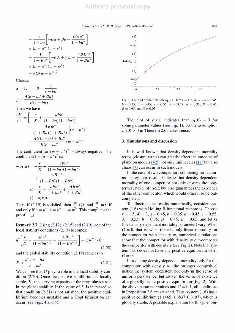
Fig. 1. The plot of the function ρ1(u). Here r = 1.5, K = 3, a = 0.45,b = 0.35, d = 0.45, e = 0.55, A = 0.55, B = 0.35, D = 0.45,E = 0.65, and G = 0.05.

The plot of ρ1(u) indicates that ρ1(0) > 0 forsome parameter values (see Fig. 1). So the assumptionρ1(0) > 0 in Theorem 2.6 makes sense.

3. Simulations and discussion

It is well known that density-dependent mortalityterms (closure terms) can greatly affect the outcome ofplankton models [42]: not only limit cycles [11] but alsochaos [7] can occur in such models.

In the case of two competitors competing for a com-mon prey, our results indicate that density-dependentmortality of one competitor not only ensures the long-term survival of itself, but also guarantees the existenceof the other competitor, which would otherwise be out-competed.

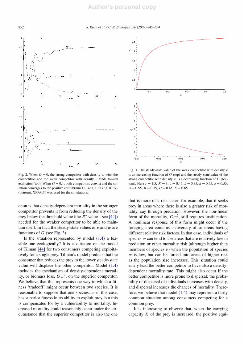
To illustrate the results numerically, consider sys-tem (1.6) with Holling II functional responses. Chooser = 1.5, K = 3, a = 0.45, b = 0.35, d = 0.45, e = 0.55,A = 0.55, B = 0.35, D = 0.45, E = 0.65, and let G

(the density-dependent mortality parameter) vary. WhenG = 0, that is, when there is only linear mortality forthe competitor with density w, numerical simulationsshow that the competitor with density w out-competesthe competitor with density v (see Fig. 2). Note that sys-tem (1.6) does not have any positive equilibrium whenG = 0.

Introducing density-dependent mortality only for thecompetitor with density w (the stronger competitor)makes the system coexistent not only in the sense ofuniform persistence, but also in the sense of existenceof a globally stable positive equilibrium (Fig. 2). Withthe above parameter values and G = 0.1, all conditionsin Proposition 2.6 are satisfied. Thus, system (1.6) has apositive equilibrium (1.1465,1.8837,0.8197), which isglobally stable. A possible explanation for this phenom-

Author's personal copy

852 S. Ruan et al. / C. R. Biologies 330 (2007) 845–854

Fig. 2. When G = 0, the strong competitor with density w wins thecompetition and the weak competitor with density v tends towardextinction (top). When G = 0.1, both competitors coexist and the so-lution converges to the positive equilibrium (1.1465,1.8837,0.8197)

(bottom). XPPAUT was used for the simulations.

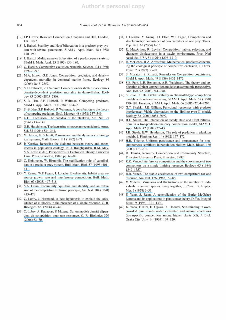
enon is that density-dependent mortality in the strongercompetitor prevents it from reducing the density of theprey below the threshold value (the R∗ value – see [44])needed for the weaker competitor to be able to main-tain itself. In fact, the steady-state values of v and w arefunctions of G (see Fig. 3).

Is the situation represented by model (1.4) a fea-sible one ecologically? It is a variation on the modelof Tilman [44] for two consumers competing exploita-tively for a single prey. Tilman’s model predicts that theconsumer that reduces the prey to the lower steady-statevalue will displace the other competitor. Model (1.4)includes the mechanism of density-dependent mortal-ity, or biomass loss, Gw2, on the superior competitor.We believe that this represents one way in which a fit-ness ‘tradeoff’ might occur between two species. It isreasonable to suppose that one species, w in this case,has superior fitness in its ability to exploit prey, but thisis compensated for by a vulnerability to mortality. In-creased mortality could reasonably occur under the cir-cumstance that the superior competitor is also the one

Fig. 3. The steady-state value of the weak competitor with density v

is an increasing function of G (top) and the steady-state value of thestrong competitor with density w is a decreasing function of G (bot-tom). Here r = 1.5, K = 3, a = 0.45, b = 0.35, d = 0.45, e = 0.55,A = 0.55, B = 0.35, D = 0.45, E = 0.65.

that is more of a risk taker; for example, that it seeksprey in areas where there is also a greater risk of mor-tality, say through predation. However, the non-linearform of the mortality, Gw2, still requires justification.A nonlinear response of this form might occur if theforaging area contains a diversity of subareas havingdifferent relative risk factors. In that case, individuals ofspecies w can tend to use areas that are relatively low inpredation or other mortality risk (although higher thanmembers of species v) when the population of speciesw is low, but can be forced into areas of higher riskas the population size increases. This situation couldeasily lead the better competitor to have also a density-dependent mortality rate. This might also occur if thebetter competitor is more prone to dispersal; the proba-bility of dispersal of individuals increases with density,and dispersal increases the chances of mortality. There-fore, we believe that model (1.4) may represent a fairlycommon situation among consumers competing for acommon prey.

It is interesting to observe that, when the carryingcapacity K of the prey is increased, the positive equi-

Author's personal copy

S. Ruan et al. / C. R. Biologies 330 (2007) 845–854 853

Fig. 4. The bifurcation diagram shows that the positive equilibrium isstable when K � 5.21. At K = 5.21, it loses its stability and a super-critical Hopf bifurcation occurs. Here r = 1.5, a = 0.45, b = 0.35,d = 0.45, e = 0.55, A = 0.55, B = 0.35, D = 0.45, E = 0.65,G = 0.1. XPPAUT was used for the simulations.

Fig. 5. When K = 6, there is a periodic orbit bifurcated from theinterior equilibrium in the three-dimensional space which is asymp-totically stable. Here r = 1.5, a = 0.45, b = 0.35, d = 0.45, e = 0.55,A = 0.55, B = 0.35, D = 0.45, E = 0.65, G = 0.1. XPPAUT wasused for the simulations.

librium loses its stability and a Hopf bifurcation occurswhen K passes a critical value. With parameters givenabove, a supercritical Hopf bifurcation occurs whenK = 5.21 (see Fig. 4). A three-dimensional positive pe-riodic solution bifurcates from the positive equilibriumvia a Hopf bifurcation with K = 6 (see Fig. 5). Thisis an example of the well-known paradox of enrich-ment [25].

It is also interesting to notice that, for the subsystemwithout the competitor v, that is, the predator-prey sys-tem with density-dependent mortality:

(3.1)

du

dt= ru

(1 − u

K

)− Auw

1 + Bu

dw

dt= w

(−D − Gw + Eu

1 + Bu

)

it is well known that (Bazykin [3], Hainzl [18,19]) verycomplex dynamics, such as the existence of multipleequilibria and multiple limit cycles, Hopf, homoclinc

and Bagdanov–Takens bifurcations, can occur. Note thatwhen system (1.6) has one positive equilibrium, it isunique. Thus, it does not exhibit complex dynamics asthe 2-dimensional system (3.1) has. Our results indicatethat introducing a weak competitor v (without density-dependent mortality) into the system has a stabilizingeffect on the system, since the competition model (1.6)either has a globally stable positive equilibrium undercertain conditions or exhibits the coexistence of bothcompetitors in terms of positive periodic solutions.

Acknowledgements

The authors are very grateful to the anonymous ref-eree for his careful reading, detailed comments, andhelpful suggestions. The first author would like to thankProf. G. Bard Ermentrout and Dr. Rongsong Liu fortheir help in using XPPAUT for the numerical simula-tions.

References

[1] R.A. Armstrong, R. McGehee, Competitive exclusion, Am. Nat.115 (1980) 151–170.

[2] F.J. Ayala, Experimental invalidation of the principle of compet-itive exclusion, Nature 224 (1969) 1076–1079.

[3] A.D. Bazykin, Nonlinear Dynamics of Interacting Populations,World Scientific, Singapore, 1998.

[4] G.J. Butler, P. Waltman, Bifurcation from a limit cycle in a twopredator-one prey ecosystem modeled on a chemostat, J. Math.Biol. 12 (1981) 295–310.

[5] R.S. Cantrell, C. Cosner, Spatial Ecology via Reaction–DiffusionEquations, Series in Math. Comput. Biol., John Wiley and Sons,Chichester, UK, 2003.

[6] R.S. Cantrell, C. Cosner, S. Ruan, Intraspecific interference andconsumer-resource dynamics, Dis. Con. Dynam. Syst. 4B (2004)527–546.

[7] H. Caswell, M.G. Neubert, Chaos and closure terms in planktonfood chain models, J. Plankton Res. 20 (1998) 1837–1845.

[8] C. Cosner, D.L. DeAngelis, J.S. Ault, D.B. Olson, A model fortrophic interaction, Theor. Pop. Biol. 56 (1999) 65–75.

[9] J.M. Cushing, Periodic two-predator, one-prey interactions andthe time sharing of a resource niche, SIAM J. Appl. Math. 44(1984) 392–410.

[10] D.L. DeAngelis, R.A. Goldstein, R.V. O’Neill, A model fortrophic interaction, Ecology 56 (1975) 881–892.

[11] A.M. Edwards, A. Yool, The role of higher predation in planktonpopulation models, J. Plankton Res. 22 (2000) 1085–1112.

[12] M. Farkas, Zip bifurcation in a competition model, NonlinearAnalysis – TMA 8 (1984) 1295–1309.

[13] H.I. Freedman, Deterministic Mathematical Models in Popula-tion Ecology, Marcel Dekker, New York, 1980.

[14] H.I. Freedman, P. Moson, Persistence definitions and their con-nections, Proc. Amer. Math. Soc. 109 (1990) 1025–1033.

[15] G.F. Gause, The Struggle for Existence, Williams and Wilkins,Baltimore, 1934.

[16] F. Grognard, F. Mazenc, A. Rapaport, Polytopic Lyapunov func-tions for persistence analysis of competing species, Dis. Con.Dynam. Syst. 8B (2007) 73–93.

Author's personal copy

854 S. Ruan et al. / C. R. Biologies 330 (2007) 845–854

[17] J.P. Grover, Resource Competition, Chapman and Hall, London,UK, 1997.

[18] J. Hainzl, Stability and Hopf bifurcation in a predator-prey sys-tem with several parameters, SIAM J. Appl. Math. 48 (1988)170–190.

[19] J. Hainzl, Multiparameter bifurcation of a predator-prey system,SIAM J. Math. Anal. 23 (1992) 150–180.

[20] G. Hardin, Competitive exclusion principle, Science 131 (1960)1292–1297.

[21] M.A. Hixon, G.P. Jones, Competition, predation, and density-dependent mortality in demersal marine fishes, Ecology 86(2005) 2847–2859.

[22] S.J. Holbrook, R.J. Schmitt, Competition for shelter space causesdensity-dependent predation mortality in damselfishes, Ecol-ogy 83 (2002) 2855–2868.

[23] S.-B. Hsu, S.P. Hubbell, P. Waltman, Competing predators,SIAM J. Appl. Math. 35 (1978) 617–625.

[24] S.-B. Hsu, S.P. Hubbell, P. Waltman, A contribution to the theoryof competing predators, Ecol. Monogr. 48 (1978) 337–349.

[25] G.E. Hutchinson, The paradox of the plankton, Am. Nat. 95(1961) 137–145.

[26] G.E. Hutchinson, The lacustrine microcosm reconsidered, Amer.Sci. 52 (1964) 334–341.

[27] V. Hutson, K. Schmitt, Permanence and the dynamics of biolog-ical systems, Math. Biosci. 111 (1992) 1–71.

[28] P. Kareiva, Renewing the dialogue between theory and exper-iments in population ecology, in: J. Roughgarden, R.M. May,S.A. Levin (Eds.), Perspectives in Ecological Theory, PrincetonUniv. Press, Princeton, 1989, pp. 68–88.

[29] C. Kohlmeier, W. Ebenhöh, The stabilization role of cannibal-ism in a predator-prey system, Bull. Math. Biol. 57 (1995) 401–411.

[30] Y. Kuang, W.F. Fagan, I. Loladze, Biodiversity, habitat area, re-source growth rate and interference competition, Bull. Math.Biol. 65 (2003) 497–518.

[31] S.A. Levin, Community equilibria and stability, and an exten-sion of the competitive exclusion principle, Am. Nat. 104 (1970)413–423.

[32] C. Lobry, J. Harmand, A new hypothesis to explain the coex-istence of n species in the presence of a single resource, C. R.Biologies 329 (2006) 40–46.

[33] C. Lobry, A. Rapaport, F. Mazenc, Sur un modèle densité dépen-dent de compétition pour une ressource, C. R. Biologies 329(2006) 63–70.

[34] I. Loladze, Y. Kuang, J.J. Elser, W.F. Fagan, Competition andstoichiometry: coexistence of two predators on one prey, Theor.Pop. Biol. 65 (2004) 1–15.

[35] R. MacArthur, R. Levins, Competition, habitat selection, andcharacter displacement in a patchy environment, Proc. NatlAcad. Sci. USA 51 (1964) 1207–1210.

[36] R. McGehee, R.A. Armstrong, Mathematical problems concern-ing the ecological principle of competitive exclusion, J. Differ.Equat. 23 (1977) 30–92.

[37] S. Muratori, S. Rinaldi, Remarks on Competition coexistence,SIAM J. Appl. Math. 49 (1989) 1462–1472.

[38] S.E. Park, L.R. Benjamin, A.R. Watkinson, The theory and ap-plication of plant competition models: an agronomic perspective,Ann. Bot. 92 (2003) 741–748.

[39] S. Ruan, X. He, Global stability in chemostat-type competitionmodels with nutrient recycling, SIAM J. Appl. Math. 58 (1998)170–192; Erratum, SIAM J. Appl. Math. 66 (2006) 2204–2205.

[40] G.T. Skalski, J.E. Gilliam, Functional responses with predatorinterference: Viable alternatives to the Holling type II model,Ecology 82 (2001) 3083–3092.

[41] H.L. Smith, The interaction of steady state and Hopf bifurca-tions in a two-predator–one-prey competition model, SIAM J.Appl. Math. 42 (1982) 27–43.

[42] J.H. Steele, E.W. Henderson, The role of predation in planktonmodels, J. Plankton Res. 14 (1992) 157–172.

[43] H.R. Thieme, Uniform persistence and permanence for non-autonomous semiflows in population biology, Math. Biosci. 166(2000) 173–201.

[44] D. Tilman, Resource Competition and Community Structure,Princeton University Press, Princeton, 1982.

[45] R.R. Vance, Interference competition and the coexistence of twocompetitors on a single limiting resource, Ecology 65 (1984)1349–1357.

[46] R.R. Vance, The stable coexistence of two competitors for oneresource, Am. Nat. 126 (1985) 72–86.

[47] V. Volterra, Variations and fluctuations of the number of indi-viduals in animal species living together, J. Cons. Int. Explor.Mer. 3 (1928) 3–51.

[48] F. Yang, S. Ruan, A generalization of the Butler–McGeheeLemma and its applications in persistence theory, Differ. IntegralEquat. 9 (1996) 1321–1330.

[49] K. Yoda, T. Kira, H. Ogawa, K. Hozumi, Self-thinning in over-crowded pure stands under cultivated and natural conditions(intraspecific competition among higher plants XI), J. Biol.Osaka City Univ. 14 (1963) 107–129.