Competition and Coexistence in anUnpredictable World

Alexander Douglas Washburne

A dissertation presented to the faculty of Princeton University in candidacy

for the degree of Doctor of Philosophy

Recommended for acceptance by the department of Quantitative and

Computational Biology

Adviser: Prof. Simon A. Levin

June, 2015

c© Copyright by Alexander Douglas Washburne, 2015. All rights reserved.

Abstract

All living things �struggle for existence� as they compete with other organ-

isms over limiting resources. Understanding how the diversity and dynamics

of living systems are shaped by competition can help us better understand

evolutionary problems of altruism, conservation management of competing

species, and even economic policy making to promote productive competition

in free markets. This thesis examines competition and its e�ects on diver-

sity and dynamics in four systems: the slime mold Dictyostelium discoideum,

predator-prey systems such as wolves in Yellowstone, the human microbiome

and the S&P 500. Diversity in slime molds may be maintained despite com-

petition for space in the spore capsules if the natural habitat of slime molds

is variable in space and time; resource availability might mediate quorum

sensing, and such molecular switches and bet-hedging can be advantageous

over competitors without such plasticity. Competition between prey can be

mediated by predators, but the ability of predators to stabilize prey com-

munities depends on the size of the community relative to the attack rate of

the predator, implying that some predators need especially large reserves to

exhibit their full ecological e�ects. Snapshots of the human microbiome and

the S&P 500 might suggest that they could arise from neutral competition,

but time-series analysis reveals that many seemingly neutral communities

may exhibit non-neutral dynamics. Understanding patterns of diversity and

dynamics of adaptive systems requires understanding competition and coex-

i

istence in an unpredictable world.

ii

Preface

The world is a �nite, unpredictable vat of resources. All living things try to

acquire resources and reproduce, but not all organisms will succeed. All of life

�nds itself in a �struggle for existence� [12] - competing with other members of

the same species or with other species in the same trophic guild. When Gause

grew mixed cultures of yeast in competition over the same resources, the �tter

variants competitively excluded the less �t variants; from these experiments,

Gause hypothesized that competition cleared communities of any overgrowth

of excessive diversity [13]. Lotka-Volterra style di�erential equation models

of organisms in competition over limiting resources con�rmed that species

coexistence is tenuous and competitive exclusion may be a likely outcome

of competition [14]. This led to the explicit statement of the competitive

exclusion principle in 1960 [15]: two species in competition over the same

limiting resource cannot coexist.

However, if competitive exclusion is so easily obtained in models, then

why do we see such a remarkable diversity of life?! In 1961, just one year

after the competitive exclusion principle was stated, Hutchinson [18] pointed

out that many species of plankton coexist over just a few limiting resources

- how is this possible? If tropical trees compete over just a few limiting

resources - space, water, nitrogen, phosphorus, and a few others - how over

220 species of trees coexist in the meager 50 ha plot of Barro Colorado Island?

How can 8 large ungulate species coexist in Yellowstone while competing

iii

over the same forage and through shared predators? How do hundreds of

operational taxonomic units of bacteria coexist on our body? Why have we

not seen competitive exclusion in these systems; why is there not one super-

tree that dominates Amazonia, a super-moose that dominates Yellowstone,

or a super-bug that dominates our large intestines?

In the years since Hutchinson's paradox of the plankton, ecologists have

carved out many mechanisms that maintain coexistence despite competi-

tion, mechanisms that range from MacArthur's niche partitioning in war-

blers [23, 22] or Janzen and Connell's suites of distant-dependent specialist

predators [19, 6] to Paine and Levin's rarefaction-like disturbances in inter-

tidal landscapes [21, 25] to spatial structure [1] and spatial and temporal

variation in environments [5], and more.

It's safe to say that the paradox of the plankton is no longer a para-

dox. Instead of being confused by the diversity of plankton or tropical trees,

ecologists now have the opposite problem: given the myriad possible mech-

anisms for coexistence and mediation of competition, which ones are most

important in our study system? How does the suite of stabilizing mecha-

nisms [4] at play in our system a�ect our management of natural systems?

In which other competitive systems are analogous stabilizing mechanisms at

play, and how can knowlege of stabilization in ecology inform our manage-

ment of other competitive systems? For instance, we �nd a suite of analogous

problems of competition and coexistence in human systems - of cultures in

sociology or companies in economics: since companies in a market compete

iv

over a �nite number of customers or a �nite amount of investment capital,

�tter companies can expand and advertise and, in theory, competitively ex-

clude less successful companies. How can insights from ecology of non-human

life generalize to our understanding of human competition? Such knowledge

of human competition would a�ect our economic policy making and portfo-

lio management - when human resources become limiting, shares might no

longer grow exponentially, and so principles of competition and evolution of

competitive systems may be needed to accurately price options and other

�nancial derivatives [2]. This thesis examines some of these modern ques-

tions of competition and coexistence in a �nite, stochastic world in systems

ranging from ungulates in yellowstone or arthropods on small islands in the

Bahamas, to slime molds, gut bacteria, and large cap companies in the S&P

500.

The �rst chapter explores a paradoxical coexistence of many genotypes of

the slime mold Dictyostelium discoideum in competition for limiting space in

the fruiting body. We show that multiple genotypes can coexist in a patchy

environment with spatial and temporal variation in the time between resource

replenishment; instead of a problem of altruism arising in competition over

space in the spore capsule, there may be dispersal-dormancy tradeo�s that

can explain the persistence of some so-called loner cells that �choose� not to

aggregate into the spore capsule but instead remain dormant; a mosaic of

environments that vary in their expected rate of resource arrival can explain

many genotypes with di�erent degrees of investment in dispersal vs. dor-

v

mancy. We �nish with a discussion of future empirical investigations that

can test our hypothesis and elucidate how exactly slime molds with the same

genotype might �choose� to aggregate or to ignore an autoinducing signal

from other cells hoping to form a quorum. If such conditional quorum acti-

vation does exist, which I hypothesize may be co-mediated by local resource

availability, it would have implications for the evolution of quorum sensing

in other model organisms such as Vibrio species.

The second chapter examines how stabilizing forces such as prey-switching

predation - which maintain coexistence in di�erential equation models - af-

fect small populations prone to �uctuations in population size from variation

in fecundity, lifespan, intraguild competitive interactions, and predatory en-

counters. Our main result is obvious in hindsight: by killing prey, predators

reduce mean population sizes of prey, and too high of attack rates - even

attack rates by �stabilizing� predators - can drive �nite prey populations to

rarity and eventually extinction. Because the probability of a species becom-

ing rare is directly related to prey community size, the e�ect of predation

on prey diversity depends on the habitat size and intensity of competition

among prey. A particular stabilizing predator may be bene�cial for diversity

at large spatial scales yet may clobber diversity at small scales. We show

that the impact of frequency-dependent killing of prey can be understood

through statistical properties of �uctuating prey communities: by suppress-

ing �uctuations in relative abundance, stabilizing forces reduce negative co-

variance that arises from direct competition and thereby reduce the risk of

vi

rarity of prey. High attack rates relative to community size can reduce the

mean abundance more than they increase the covariance in population size;

tension between increases in covariance and decreases in the mean abun-

dance of prey populations determines the observed e�ect of predation on

prey diversity. These results change our thinking about competition, sta-

bilizing forces, and coexistence in real study systems were populations are

�nite, moving us beyond systems of di�erential equations towards a broader,

trophic island-biogeographic perspective that considers the stochastic �uctu-

ations of communities in the presence of stabilizing interactions. This trophic

island biogeographic perspective and the scale-dependence of coexistence for

a given food web is especially relevant to modern conservation biology where

the trophic downgrading [7] and habitat fragmentation [8] are simultaneously

changing the stabilizing forces and the community sizes in natural systems.

The third and �nal chapter makes a solid epistemological stride by us-

ing time-series data for hypothesis-testing a particular model of competitive

dynamics - the Wright Fisher Process [11, 29], also known to ecologists and

population geneticists as Neutral Theory. The Wright-Fisher process has

been used as a null model for neutral competition in populations of genes

[20], communities of canopy trees [16], and even the market weights of com-

panies in competition over �nite investment capital [10, 26], and it's been

argued that neutrality may be a common occurrence in natural systems as

any large deviation from neutrality may likely result in quick competitive

exclusion [17]. From Tajima's D [28] to Fay & Wu's H [9] to tests of species-

vii

abundance distributions [24], hypothesis-tests of neutral competition are used

to uncover genes that have undergone selection, and similar tests in ecology

and economics may reveal niche structure within trophic guilds or economic

sectors. Existing hypothesis tests of neutral competition use static snapshots

of the frequencies of the di�erent competing species, alleles or companies; the

third chapter of my thesis presents tools for the hypothesis testing of neutral

competition with time-series datasets. The utility of the tools developed is

illustrated �rst by simulation and then by analyzing data from a time-series

dataset of the human microbiome [3] and the day-end prices for 451 compa-

nies in the S&P 500 from 2000 to 2005. These tests of real ecological and

economic time-series suggest that no one model can account for the stochastic

dynamics of real complex-adaptive systems: some communities are di�cult to

distinguish from a Wright-Fisher process, whereas others such as one male's

tongue microbiome and the S&P 500 market weights, exhibit markedly non-

neutral dynamics. Focusing on the example of the male's tongue microbiota,

I illustrate how the tools provided here for time-series analysis facilitate the

construction of suitable alternative models for the competitive dynamics of

these non-neutral systems.

Taken together, these chapters span a wide spectrum of competitive dy-

namics - resource competition in a patchy environment, apparent competition

of prey with a common generalist predator, and neutral competition in more

general competitive systems. At the heart of all of these studies is a limiting

resource - food for Dictyostelium; food, space, intraguild aggression and a

viii

shared, generalist predator for prey; or strict zero-sum competition for space

or investment capital - and these studies have examined various consequences

for the diversity, dynamics, and empirical studies of the organisms in com-

petition. Dictyostelium diversity can be stabilized by spatial and temporal

variability in resource pulses. Ungulates in Yellowstone can be stabilized by

wolves, but whether or not wolves increase the long-term persistence of un-

gulates depends crucially on the size of habitat - and it's possible that even

Yellowstone may not be big enough for wolves, but larger habitats or well-

connected blocks of habitat may be required. The failure of introduced anoles

on the Bahamas to maintain arthropod diversity could be due to the small

size of the islands to which they were introduced [27]. The S&P 500 and the

bacteria on the tongue of one particular male are in competition for limiting

resources, but evolution has not led to neutrality among competitors in these

systems over the timescales investigated; instead, there may be signatures of

trust-busting policies or incumbent e�ects or rare-species advantages in these

systems. Understanding the non-neutral competition in these systems has

implications ranging from economic policy making to portfolio management

and and probiotic pharmacokinetics.

Looking back, these projects are motivated by my interest in the assem-

bly of competitive systems over evolutionary timescales - how do slime molds

evolve under the tension between solitary life and cooperative dispersal? How

are food webs assembled - does evolution stabilize or destabilize food webs,

and, if so, how e�ective are these stabilizing forces for communities of di�er-

ix

ent size? Do species competitively exclude one another until they are e�ec-

tively neutral, as Hubbell hypothesized, or are general classes of non-neutral

competition underlying patterns of biogeography (species-abundance distri-

butions, species-area relationships, the distribution of times to most-recent

common ancestors of species in a region, etc.)?

Looking forward, this thesis is my �rst step in a long journey to under-

stand how competition structures natural systems, how our understanding

of evolution in competitive systems can be utilized to improve the com-

petitiveness of, say, a probiotic designed to establish a stable population

and deliver lactase to the host, and how we conceptualize evolution in this

world with Russian dolls of self-replicating things, with Dictyostelium strad-

dling the major evolutionary transition between single- and multi-cellularity,

with prey species in competition in a trophic guild (subjected to frequency-

dependent/apostatic selection from a predator), and with humans - walking

titans of 10 trillion cells harboring 100 trillion bacterial cells in their large

intestines, each cell containing its own lysogenic viruses or tranposable ele-

ments that self-replicate - all within a bustling (and currently growing but

eventually saturating and limiting) world of human groups (companies, cul-

tures, countries) and symbionts (crops, livestock, dogs) all struggling over

limiting resources for survival and replication. Some way, some how, out

of this struggle for existence over �nite, unpredictable resources, we see not

just many species of plankton or tropical trees, but a fractal symphony of

symphonies of competing, replicating things. Provided the broad impacts of

x

these ideas gives them some selective advantage in the community of human

ideas (in competition over limited publication space and professorships and

grants), or provided that I am fortunate in their neutral drift with equally

�t competitors, these three chapters will be just the �rst of many studies on

competition and coexistence in an unpredictable world.

Acknowledgments

�The enumeration in the Constitution, of certain rights, shall not be con-

strued to deny or disparage others retained by the people.�

-9th Amendment, U.S. Constitution.

The enumeration in these Acknowledgments of certain people, shall not

be construed to deny or disparage gratitude for other, unenumerated people.

I acknowledge support from an NSF Graduate Research Fellowship.

Dr. Alison E. Gammie was my Ms. Miyagi - this thesis would not have

been possible without her mentoring and both professional and personal sup-

port. Likewise, Prof. Henry Horn was my Mr. Miyagi, and a role model for

how to succeed as an academic generalist. My adviser, Prof. Simon Levin

cultivated an excellent community of collaborators and gave me full freedom

to pursue authentic academic work by saying, �Do what you want to do, I'll

xi

defend your work.� Those words gave me a personal responsibility for my

productivity and cultivated a stable, profound love of the science I'm doing.

Prof. Ned Wingreen was an invaluable member of my committee. Professor

Corina Tarnita and soon-to-be-Dr. Jacob B. Socolar are stellar collaborators

and co-�rst-authors - the time spent working with them added years of fuel

to the �re of my love of science.

The Princeton University Mountaineering Club deserves acknowledgment

for introducing me to many essential collaborators, especially its founder

Dr. Ben Safdi whose discussions about detecting dark matter while warm-

ing up on a V6 epitomized the academically productive culture of the club.

Dan Lacker taught me everything I know about stochastic calculus during

our drives to the Gunks and the New River Gorge. Emmanuel Shertzer

helped out with parameter estimation for the Wright-Fisher Process. Jono

Squire kept my sights (and psyche) high, motivating the use of Mathemat-

ica during our ascents of Moonlight Buttress, Half Dome, and other classic

climbs. Josh Burby's work in Hamiltonian mechanics was essential for �nding

variance-stabilizing transformations for the Wright-Fisher Process. Thomas

van Boeckel - also known as �Papa Thom�, �Brother Thom�, �Mr. Thom�,

�Admiral Thom�, and �El CapiThom� - fell from the sky and joined the

PUMC. We climbed together, drank together, explored the West together,

and solved damn near all of life's problems together. We started a group

called the IAS - the Institute for Actual Science - that met every Sunday

over bourbon to discuss where science will actually help solve the world's

xii

problems, helping us carve out our beliefs on the role of science in society.

I will be forever grateful for these exceptional collaborators and life-long

friends met through the PUMC.

Finally, I acknowledge an in�nite wellspring of support from my family.

My mom, Dr. Margaret Werner-Washburne is a molecular biologist and life-

coach - I wish everyone in grad school could have my mom as their mother,

mentor, and best friend. My dad, Bruce Washburne, taught me the im-

portance of saying �howdy� and being unconditionally nice to everyone, no

matter what New Jersey says. My brother, Gabe Washburne, has been a

life-long role model and a contagious source of enrichment and charisma. My

Uncle Paul Sullivan taught me the importance of loving everything - �Love

is everywhere you see it. You are all that you can be, so be it!� Last, but

certainly not least, is my dog, Dr. Jack Washburne, who supported me every

step of the way and taught me that all problems in life can be solved with a

su�ciently long walk through the woods.

And �nally, to future students who feel doubted and are told they can't

get a PhD with the amount of time they devote to living a good life outside

of work, I acknowledge you, support you in your own authentic career, and

encourage you to follow your heart (as my mom always told me) to �nd your

own calling. I leave you with an inspirational picture from an adventure

with colleagues/friends/partners-in-crime Jono Squire (photographer) and

Dan Lacker (belaying in the foreground).

xiii

References

[1] Priyanga Amarasekare. Competitive coexistence in spatially structured

environments: a synthesis. Ecology Letters, 6(12):1109�1122, 2003.

[2] Fischer Black and Myron Scholes. The pricing of options and corporate

liabilities. The journal of political economy, pages 637�654, 1973.

[3] J Gregory Caporaso, Christian L Lauber, Elizabeth K Costello, Donna

Berg-Lyons, Antonio Gonzalez, Jesse Stombaugh, Dan Knights, Pawel

xiv

Gajer, Jacques Ravel, Noah Fierer, et al. Moving pictures of the human

microbiome. Genome Biol, 12(5):R50, 2011.

[4] Peter Chesson. Mechanisms of maintenance of species diversity. Annual

review of Ecology and Systematics, pages 343�366, 2000.

[5] Peter L Chesson. Coexistence of competitors in spatially and temporally

varying environments: a look at the combined e�ects of di�erent sorts

of variability. Theoretical Population Biology, 28(3):263�287, 1985.

[6] Joseph H. Connell. On the role of natural enemies in preventing compet-

itive exclusion in some marine animals and in rain forest trees. In P. J.

den Boer and G. Gradwell, editors, Dynamics of Populations. Pudoc,

Washington, 1971.

[7] James A Estes, John Terborgh, Justin S Brashares, Mary E Power, Joel

Berger, William J Bond, Stephen R Carpenter, Timothy E Essington,

Robert D Holt, Jeremy BC Jackson, et al. Trophic downgrading of

planet earth. science, 333(6040):301�306, 2011.

[8] Lenore Fahrig. E�ects of habitat fragmentation on biodiversity. Annual

review of ecology, evolution, and systematics, pages 487�515, 2003.

[9] Justin C Fay and Chung-I Wu. Hitchhiking under positive darwinian

selection. Genetics, 155(3):1405�1413, 2000.

[10] Robert Fernholz and Ioannis Karatzas. Relative arbitrage in volatility-

stabilized markets. Annals of Finance, 1(2):149�177, 2005.

xv

[11] Ronald Aylmer Fisher. The genetical theory of natural selection. Claren-

don, 1930.

[12] George Francis Gause. The struggle for existence. Courier Corporation,

2003.

[13] Georgii Frantsevich Gause. Experimental studies on the struggle for

existence i. mixed population of two species of yeast. Journal of experi-

mental biology, 9(4):389�402, 1932.

[14] GF Gause and AAWitt. Behavior of mixed populations and the problem

of natural selection. American Naturalist, pages 596�609, 1935.

[15] Garrett Hardin et al. The competitive exclusion principle. science,

131(3409):1292�1297, 1960.

[16] Stephen P Hubbell. The uni�ed neutral theory of biodiversity and bio-

geography (MPB-32), volume 32. Princeton University Press, 2001.

[17] Stephen P Hubbell. Neutral theory in community ecology and the hy-

pothesis of functional equivalence. Functional ecology, 19(1):166�172,

2005.

[18] G Evelyn Hutchinson. The paradox of the plankton. American Natu-

ralist, pages 137�145, 1961.

[19] Daniel H. Janzen. Herbivores and the number of tree species in tropical

forests. The American Naturalist, 104(940):501�528, 1970.

xvi

[20] Motoo Kimura. The neutral theory of molecular evolution. Cambridge

University Press, 1985.

[21] Simon A Levin and Robert T Paine. Disturbance, patch formation, and

community structure. Proceedings of the National Academy of Sciences,

71(7):2744�2747, 1974.

[22] Robert MacArthur and Richard Levins. Competition, habitat selec-

tion, and character displacement in a patchy environment. Proceedings

of the National Academy of Sciences of the United States of America,

51(6):1207, 1964.

[23] Robert H MacArthur. Population ecology of some warblers of north-

eastern coniferous forests. Ecology, 39(4):599�619, 1958.

[24] Thomas J Matthews and Robert J Whittaker. Neutral theory and

the species abundance distribution: recent developments and prospects

for unifying niche and neutral perspectives. Ecology and evolution,

4(11):2263�2277, 2014.

[25] Robert T Paine and Simon A Levin. Intertidal landscapes: disturbance

and the dynamics of pattern. Ecological monographs, 51(2):145�178,

1981.

[26] Soumik Pal. Analysis of market weights under volatility-stabilized mar-

ket models. The Annals of Applied Probability, 21(3):1180�1213, 2011.

xvii

[27] David A Spiller and Thomas W Schoener. An experimental study of

the e�ect of lizards on web-spider communities. Ecological Monographs,

pages 58�77, 1988.

[28] Fumio Tajima. Statistical method for testing the neutral mutation hy-

pothesis by dna polymorphism. Genetics, 123(3):585�595, 1989.

[29] Sewall Wright. Evolution in mendelian populations. Genetics, 16(2):97,

1931.

xviii

Chapter 1: Spores and non-aggregating

cells can explain coexistence of

genotypes in Dictysotelium discoideum

Corina E. Tarnitaa,1, Alex D. Washburneb,1, Allyson E. Sgroc, Simon A. Levina

a - Department of Ecology and Evolutionary Biology

b - Lewis-Sigler Institute for Integrative Genomics

c - Joseph Henry Laboratories of Physics

1 - Joint �rst authors

Keywords: slime molds, cooperation, altruism, dispersal, genetic diver-

sity, multiple habitats, coexistence, chimeras, variable environments.

An expanded version was published as:

Tarnita, C. E., Washburne, A., Martinez-Garcia, R., Sgro, A. E., &

Levin, S. A. (2015). Fitness tradeo�s between spores and nonaggregating

cells can explain the coexistence of diverse genotypes in cellular slime molds.

Proceedings of the National Academy of Sciences, 201424242.

1

Abstract

Dictyostelium discoideum is a well-studied amoeba with a complex life cycle

that includes both a single-cellular and a multicellular stage. To achieve the

multicellular phase, individual amoebae aggregate upon starvation to form

a fruiting body made of stalk and spores. The amoebae that contribute to

stalk formation undergo apoptosis while those that become spores survive

and are able to reproduce, a behavior that has been described as altruism.

When amoebae aggregate they do not discriminate kin from non-kin, which

sometimes leads to chimeric fruiting bodies. Within chimeras, a linear hier-

archy of winning and losing genotypes has been documented, which suggests

that there should eventually be only one surviving genotype. This contra-

dicts however the great diversity of D. discoideum genotypes found in nature.

Here we suggest that a little-studied component of D. discoideum �tness �

the loner cells that stay behind and do not participate in the aggregate �

could be selected for and achieve di�erent abundances in environments with

di�erent food recovery properties, and that this could account for the ap-

parent contradiction. We show that if at least two environments exist that

are su�ciently di�erent in their food recovery characteristics, and if in addi-

tion they are connected via weak-to-moderate dispersal, then coexistence of

genotypes can occur. We further argue that the consideration of loners as a

component of D. discoideum �tness makes it hard to de�ne altruistic behav-

ior, winners or losers, without a clear description of the ecology encountered

2

by each genotype.

Signi�cance Statement

Dictyostelium discoideum is an amoeba whose life cycle includes both single-

cellular and multicellular stages, the latter achieved when individual amoebae

aggregate upon starvation. Because amoebae do not discriminate kin from

non-kin, chimeric aggregates can arise. Within chimeras, there is asymmetric

contribution to reproduction and, based on this, the co-existing genotypes

can be arrayed in a linear dominance hierarchy. This implies that only one

genotype can survive, contradicting the great diversity of strains found in na-

ture. We suggest that cells that fail to aggregate provide an additional �tness

component that, in a rich ecology with multiple environments connected via

dispersal, resolves the contradiction. The study of non-aggregators further

sheds light on the discussion of altruism in D. discoideum.

Introduction

Dictyostelium discoideum is a social amoeba (or cellular smile mold) native

to the upper layers of soil and leaf litter, where it feeds on bacteria (1-5).

Upon exhausting their local supply of food, the solitary starving amoebae

initiate a developmental program, joining with nearby amoebae to form an

aggregate that allows for facile transport to an area with more bacteria. Un-

3

der some environmental conditions, the aggregate initially forms a slug that

can migrate toward attractants such as light and heat that indicate a better

future environment; but the culmination of development, whether or not a

slug is formed, is ultimately a fruiting body. In this fruiting body, roughly

20% of the cells sacri�ce themselves, vacuolating and forming a cellulose wall

that provides a sturdy stalk to hold the remaining dormant spore cells o�

the ground so that they can more easily be dispersed to a new area. Since

the stalk cells die for the bene�t of the spore cells, this process is often

discussed in terms of altruism and cooperation (reviewed in (5)). In na-

ture, there is signi�cant diversity and coexistence of multiple strains of D.

discoideum (6). Moreover, chimeras (aggregates consisting of at least two

genotypes) occur naturally (6-8), which implies that D. discoideum amoebae

do not discriminate perfectly in the process of aggregation. These chimeras

are functional and viable in the sense that their aggregation results in a fruit-

ing body in which the multiple genotypes participate both in stalk formation

and in spore production. However, the genotypes are not necessarily equally

represented in the stalk and spores of the chimera (7). Through the mixing

of di�erent genotypes together into chimeras in the laboratory, linear hier-

archies of competitors have emerged (9,10), in which a stronger competitor

is a genotype that is disproportionately represented in the spores. From this

perspective, not all strains are equivalent, and hence chimeras are considered

suboptimal assemblages (10). In the absence of any additional information

on possible frequency-dependent processes that might maintain coexistence,

4

the existence of a linear competitive hierarchy suggests that there should be

only one winner. This raises a paradox � if there are clear winners within

chimeras, why is there so much diversity and coexistence among strains in na-

ture (9)? One possible resolution used to explain the absence of certain types

of cheaters in nature relies on spatial structure leading locally to a high degree

of relatedness that helps select against cheating genotypes (8, 11); however,

this is only the case for cheaters that are very harmful to group productivity

(including their own when clonal), and not for more `mild' cheaters that do

take advantage of others in chimeras but are still able to act cooperatively to

a certain extent, especially when clonal (8). The genotypes studied (10) �t

better with the latter category since they all contribute in some amount to

both spores and stalk, and therefore the high genetic relatedness mediated

by spatial structure is not an explanation (in this straightforward form, with-

out additional information about possible frequency dependent interactions

between strains) for the observed coexistence.

Another explanation for coexistence that was suggested but unexplored

both for D. discoideum (9) and for other cellular slime molds (12) is that

strains that are at a disadvantage in chimeras have an advantage at a di�er-

ent stage in their life cycle, i.e. that there is a tradeo� between sporulation

e�ciency and other �tness-related traits. To date, however, analyses of geno-

typical �tness have focused on spore contribution as the sole �tness indicator.

During the social phase however, not all cells aggregate; some cells stay be-

hind. We will refer to them as non-aggregators or loners. Loner cells have

5

been generally ignored so far; because D. discoideum do not make microcysts,

it was assumed that non-aggregating cells would simply die, which would be

�an unlikely strategy� (9). But recent results show that loner cells are viable,

meaning that they can eat and divide if food is replenished in the environ-

ment, and that therefore the loners can be an important component of D.

discoideum �tness (13). However, the authors also found that epigenetic dif-

ferences may lead to di�ering numbers of aggregating and non-aggregating

cells in a clonal population (13). We therefore performed experiments to

con�rm that there were no longer-term e�ects of starvation or an epigenetic

e�ect that prevented these non-aggregating �loner� cells from aggregating in

the future under starvation conditions. To test if such an e�ect exists, we

used cells left behind during the aggregation of starving D. discoideum from

a naturally isolated, clonal population that were allowed to form fruiting

bodies on non-nutrient agar (see SI for experimental details). The fruiting

bodies were then removed and fresh bacteria were added to the food source

facilitating the non-aggregating cells to re-grow and deplete the bacteria as

expected from (13) and re-aggregate and go on to form normal fruiting bod-

ies, leaving behind a population of non-aggregating cells themselves (see SI

Fig A.1). Therefore, we con�rm that the loners can be an important compo-

nent of D. discoideum �tness. Loner cells can act as a form of exploitation

strategy: certain environments may become advantageous quickly and, unlike

spores that take time to germinate, loner cells can begin to eat and divide

instantaneously. Thus, leaving behind some loner cells can give a geno-

6

type a head start in their home environment. Then, environments where

food replenishes faster (henceforth fast-recovery environments) will select for

genotypes that are more likely to invest in loners, while environments where

food replenishes slower (henceforth slow recovery environments) will select

for genotypes that are more likely to invest in spores. Stochastic (unpre-

dictable) environments potentially can select for mixed strategies (13). We

propose that, furthermore, if instead of focusing on one environment we con-

sider multiple environments connected via dispersal, the loners and spores

can play additional roles. The loners � an exploitation strategy � can also

be seen as ful�lling the role of local dispersal. By contrast, the spores � an

insurance against prolonged starvation � also ful�ll the role of global disper-

sal since they are more likely to be dispersed to other environments. The

spores will thus either survive until food is reintroduced, or they will get

dispersed to new environments, some of which can be food-rich. Since envi-

ronments with di�erent food-replenishment characteristics select for di�erent

investments in spores versus loners, we hypothesize that weak-to-moderate

dispersal between fast-recovery and slow-recovery environments can allow

for the coexistence of multiple genotypes. We explore the feasibility of this

notion through a model of resource competition that considers both loners

and spores as part of D. discoideum �tness, in one environment, and in two

environments connected by various degrees of dispersal.

7

Model and results

In our model, a D. discoideum genotype is characterized by a scalar α, which

represents the fraction of cells that aggregate; the remaining 1 − α is the

fraction of non-aggregating cells, or loners. Thus, a monoculture of genotype

α = 0 does not undergo an aggregation phase; a monoculture of α = 1 only

produces aggregates and leaves no loner cells behind. Intermediate α values

represent a mixed strategy, where some cells aggregate and others do not.

Out of the cells that aggregate, only a fraction will become spores (the re-

maining cells either commit suicide and contribute to the formation of stalk,

or get shed from the slug during migration). Since cells that are shed dur-

ing migration have also been proved to be viable (14), they may similarly

contribute to D. discoideum �tness; however, the number of cells left in the

trail is probably in�uenced by how far individual slugs migrate in di�erent

environments, which has not been quanti�ed in the wild. Similarly, di�erent

genotypes have di�erent investments in stalk versus spores (10); however,

in this paper we are not concerned with the selective forces that shape the

stalk-to-spore investment ratio. For these reasons and in order to simplify

our analysis, we will assume that the cell loss during migration and the in-

vestment in the stalk are �xed and identical for all genotypes so that we can

focus our analysis solely on the fraction of spores versus loner cells. The

model we describe will depend on the ecology that in�uences the lifecycle of

D. discoideum. For simplicity, we are not concerned with soil type, light or

8

moisture and assume those to be the same across environments; the property

of interest is the ability of food to replenish in a given environment, or in

other words, the starvation times experienced in that environment. One en-

vironment (patch). In the �rst part of the model we assume that the world

is comprised of a single environment, in which food replenishment can be

either deterministic (certain) or stochastic (uncertain). This model is simi-

lar to (13) but it is more general in that it explicitly accounts for resource

competition among di�erent genotypes. The amoebae consume resources,

reproduce freely and grow at a rate governed by Michaelis-Menten kinetics

(15). The di�erent genotypes compete indirectly through the existing re-

sources, but we assume no other frequency-dependence between types (i.e.

we assume that intrinsic parameters such as the growth and aggregation rates

of di�erent genotypes are independent of the composition of the population).

Since there is little-to-no information in the literature about growth rates of

di�erent genotypes, we make the simplifying assumption that di�erent geno-

types grow according to the same saturating functional form cR/(R1/2 + R)

where R is the amount of available resources, c is the consumption rate and

R1/2 is the concentration of resources at which the reaction rate is at half its

maximum. We further assume that amoebae die at rate µ.

We describe the dynamics of active amoebae of all genotypes α existing

in the same environment as resources are depleted by the growing amoebae

until they are no longer able to sustain growth, after which the amoebae

enter a starvation phase. During this phase, a fraction α of cells of genotype

9

α aggregate with the purpose of forming spores, while the remaining 1 − α

stay as starving loners. The non-aggregating (loner) cells stop consuming

resources, stop reproducing, and decay at rate until the next resource pulse.

Of the aggregating cells, a fraction s become viable spores; we assume that

spores are very resistant to environmental stress, but that they nevertheless

incur a small decay rate ; therefore, we assume that δ < µ. When the starva-

tion period is over, food is reintroduced in one resource pulse, R0. Then the

surviving loner cells start consuming resources and reproducing immediately,

while spores undergo a delay period , which is the time required to activate

the metabolic machinery necessary for resource consumption. The longer the

delay τ , the more cost will be incurred by spores in an environment where

loner cells are already consuming the resource while the spores undergo the

germination process. Therefore genotypes that can leave behind some loners

can have a head start and be favored. If resources get depleted before the ger-

mination period is over, we assume that spores return to dormancy, without

incurring any cost associated with the abortion of the germination process.

In reality, in addition to the costly delay of germination, D. discoideum also

experiences a costly delay of sporulation: after only 6 hours, just as individ-

ual amoeba are beginning to aggregate, they are irreversibly committed to

continuing with sporulation for the remaining 18 hours of the process (16).

Since we are trying to show that in certain environments loners can be se-

lected for, an additional cost for the spores will only make the selection for

loners stronger and reinforce our results. Therefore, for simplicity, we do

10

not include in our model the additional cost due to the irreversibility of the

sporulation process. The dynamic equations describing the spores and loners

are presented in the Supplementary Information. In a single environment as

described above, with competing D. discoideum genotypes and instantaneous

resource pulses arriving at random times, we explore how the lengths of the

starvation periods that a genotype experiences a�ect its investment in spores

and loners. Our results agree with (13). In a deterministic environment (i.e.

when the starvation times are always of the same length) there is selection

for one of the pure strategies: we �nd a critical threshold starvation time Tcr

such that for T < Tcr the winning genotype is one that never produces any

aggregates (α = 0) while for T > Tcr the winning genotype is one that always

aggregates to produce spores (α = 1). When the environment is stochastic

such that successive starvation times are independent and exponentially dis-

tributed with rate 1/λT , we �nd that mixed strategies can be selected for: if

on average the environment is a fast-recovery one (low λT ), then the mixed

strategy invests more in loners than in spores; indeed, for su�ciently low λT ,

only loners will survive. Conversely, if the environment is a slow-recovery one

(high λT ), then the mixed strategy invests more in spores (see Fig. 1A),

and for su�ciently high λT only spores will persist.

11

Figure 1: In one environment, deterministic (�xed) starvation times always select for pure strategies

while stochastic starvation times can select for mixed strategies. A. The corresponding to the evolutionarily

stable strategy (ESS) is shown as a function of average starvation time for both deterministic and stochastic

cases. In the deterministic case, if T is under a threshold (calculated in SI) then the all-loners strategy

wins; if T is above the threshold, then the all-spores strategy wins. In the stochastic case, extreme average

starvation times select for the corresponding pure strategies, but intermediate average starvation times

select for mixed strategies (intermediate ). B. The pairwise invasibility plot (PIP) for the stochastic case

with average starvation time λT = 1000. The ESS strategy is α= 0.63, which invests 63% in spores and

37% in loners.

The evolutionary stability (ESS) (17) of the mixed strategy is further

con�rmed by a pairwise invasibility analysis for a �xed stochastic environ-

ment with a given intermediate average starvation (see Fig. 1B). Here we

assume an exponential distribution of starvation times; assuming uniformly

distributed starvation times (13) leads to qualitatively similar results. In the

future it will be interesting to explore other distributions (e.g. normal); how-

ever, we generally expect similar results to hold. We next study the e�ects of

12

the model parameters on the evolutionarily stable genotype. The higher the

consumption rate c, and implicitly the reproductive rate of solitary amoebae,

the more likely it is to select for loners in the intermediate starvation regions;

this is intuitive since the more that loners can take advantage of new food,

the more advantage they will have over the spores. Similarly, the longer the

spore germination delay τ , the bigger the cost incurred by spores, which fa-

vors genotypes with more loners. Loners will also be more favored the higher

the death rate of spores, . Conversely, the higher the spore success rate s or

the death rate of single cells , the better it is for genotypes with more spores

(Fig 2A-E).

13

Figure 2: The sensitivity of the model to the parameters. A, B, C, F. Higher consumption rate (c),

spore death rate (δ), time needed for spore germination (τ) or resource input favor selection for loners. D,

E. Conversely, higher loner decay rate (µ) or higher spore survival and viable germination rate (s) favor

selection for spores. In all panels, the lowest value of the parameter is red, the intermediate is green and

the highest value is blue. Except for the parameter varied to perform the sensitivity analysis, all other

parameters are as in Table S1. Parameter values for the sensitivity analysis: c = 0.086, 0.173, 0.346; =

0.00004, 0.0002, 0.001; = 2, 4, 8; = 0.001, 0.002, 0.004; s = 0.25, 0.5, 0.75; R0 = 104, 108, 1012.

Finally, we treat the size of the resource pulse, R0, separately. If the

resource pulse is �xed, then the higher it is, the easier it is to select for lon-

ers. However, while varying R0 has a sigmoidal e�ect on Tcr for constant

T (SI Fig B.6), the bene�ts of varying R0 in a stochastic environment are

marginal and the resulting ESS α varies little with varying resource pulse

size (Fig 2F). This is because T is exponentially distributed and the e�ects

of R0 are sigmoidal, with only a small intermediate region in which the selec-

14

tion for spores or loners is sensitive to varying R0. Finally, a more realistic

scenario is that the resource pulse is stochastic. Our simulations suggest

that introducing stochasticity in the resource pulse size does not select for

mixed investment in loners and spores: if the starvation time T is �xed and

the only source of stochasticity comes from the resource pulse, it appears

that the only evolutionarily stable strategies are the pure strategies (see SI

Fig B.7). However, because this is only a simulation result, it is possible

that for di�erent parameter combinations resource stochasticity will result

in mixed investment. The relationship between the resource pulse and the

time to starvation is an interesting one and needs to be further explored,

for di�erent distributions of resources and stochastic times; however, since

our preliminary analysis suggests that the more interesting and rich behavior

seems to be induced by the starvation times, in this paper we choose to per-

form the entire analysis for a �xed resource input following every starvation

period.

Two environments (patches). Including the loners in the analysis already

produces interesting behavior (selection of mixed strategies) in one environ-

ment. In this second part however we explore whether the extension of our

model to a spatially heterogeneous environment connected via spore disper-

sal can, under certain conditions, favor the coexistence of genotypes, pure or

mixed. For simplicity, we consider exactly two environments characterized by

di�erent starvation times. Each environment is governed by the same dynam-

ics as above, but they receive and exhaust resources independently of each

15

Figure 3: In two environments, if food recovery is deterministic and the environments are su�ciently

di�erent, coexistence between the two pure strategies is possible in the faster environment. The more

di�erent the environments, the larger the dispersal range that allows coexistence � T = 1400, T = 500

allow coexistence for the entire dispersal range 0 < D < 1 while T = 850, T = 650 allow coexistence only

for D<0.5. The color scale, ranging from 0 (blue) to 1 (red), represents the average relative abundances

across 60 replicates at the end of 1500 growth/starvation cycles.

other (asynchronously); the only element that couples the dynamics in the

two environments is the dispersal of spores. When starvation occurs in one

environment, a fraction 1−D of the spores remain in their home environment

while a fraction D are moved to the other environment. Because the dynam-

ics in the two environments are desynchronized, when spores get moved to a

new environment they may immediately �nd food and start the germination

process, or they may be lying dormant until food gets introduced into that

environment. We consider two scenarios, depending on whether the starva-

tion times in the two environments are deterministic or stochastic. If the two

environments are deterministic, in the sense that environment i (for i = 1,2)

always has a starvation time of length Ti, then in the absence of dispersal

16

they each select for a pure strategy. Because we are interested in environ-

ments with di�erent starvation times, we study fast recovery environments,

which select for all loners ( = 0), paired with slow recovery environments,

which select for all spores ( = 1). When dispersal is allowed between the

two environments, coexistence of the two pure strategies can occur for weak

dispersal, such that each strategy will dominate in the environment in which

it is selected but, because of dispersal, spores will be present in both environ-

ments. As the dispersal fraction increases, however, two alternative outcomes

can occur depending on how di�erent the starvation times in the two envi-

ronments are: (i) If the two environments are very di�erent, coexistence in

the fast environment can be maintained for a large range of dispersal values.

This is because the very fast recovery of food allows the loners to grow quickly

and dominate their home environment. (ii) The more similar the environ-

ments however, only weaker dispersal can maintain coexistence. For stronger

dispersal the spores can easily start to dominate the loners in the fast envi-

ronment and eventually replace them (Fig 3). If the two environments are

stochastic, the behavior is richer. As in the deterministic case, each environ-

ment will have its winner in the absence of dispersal; and the more di�erent

the two environments, the more di�erent the respective winning genotypes.

When dispersal connects the two environments, for low-to-medium values of

D, both genotypes coexist in both environments, although, as in the deter-

ministic case, each environment is dominated by the genotype for which it

selects. Due to stochasticity, in the presence of new mutations, each of the

17

two coexisting genotypes is in fact likely to be a genotype surrounded by a

cloud of its very close relatives (similar to a quasispecies, (18)); in that case,

more than two genotypes might coexist due to dispersal and stochasticity in

starvation times. Although stochasticity does allow for a richer coexistence

than the one found in the deterministic case because mixed strategies coexist

in both environments, it does so for a narrower range of dispersal fractions

(weak-to-moderate dispersal). As dispersal increases, the two environments

become increasingly more connected and new winning strategies evolve that

are still dominating their home environments but are better able to deal with

the other environment as well. When dispersal becomes high enough there

is su�cient transfer between them for a new successful genotype to emerge

that is selected for the average of the two environments, and coexistence is

lost. As was the case in the deterministic scenario, the dispersal range for

which coexistence is maintained depends on how di�erent the two environ-

ments are, with more similar environments losing coexistence faster (Fig 4;

see also SI Fig B.8 and B.9).

Discussion

We argue that recognizing that loners (non-aggregating cells) contribute to

D. discoideum �tness and combining that with a richer ecology can explain

the observed coexistence of diverse genotypes, thus resolving the paradox

created by the linear competitive dominance in chimeras. The additional

18

Figure 4: In two environments, if food recovery is stochastic and the environments are su�ciently

di�erent, coexistence between two (possibly) mixed strategies is possible in both environments. The more

di�erent the environments, the larger the dispersal range that allows coexistence: T = 1400, T = 500

allow coexistence for approximately D < 0.6; T = 1200, T = 600 allow coexistence only for approximately

D < 0.1; T = 1000, T = 700 allow coexistence only for approximately D < 0.01. The color scale, ranging

from 0 (blue) to 1 (red), represents the average relative abundances across 60 replicates at the end of 1,500

growth/starvation cycles.

�tness component represented by the loner cells allows for mixed strategies

in variable environments; this, coupled with the existence of at least two

di�erent environments connected via weak-to-moderate dispersal ensures the

coexistence of at least two genotypes (Fig 5).

These ideas of spatially and/or temporally heterogeneous (variable) en-

vironments leading to risk-spreading or long-term optimization strategies in-

cluding dormancy versus dispersal, persistence versus normal growth versus

dormancy, and exploitation versus exploration are well established in ecol-

ogy from studies of plants (19-25) to those of bacteria (26), planktonic cope-

pods (27), and even social insects (28). Coupled with ideas of colonization-

competition tradeo�s (29-34), their e�ects on spatial coexistence of multiple

phenotypes or even species has been well studied. However, to the best of

19

Figure 5: Fast-recovery environments select for investment in loners; slow-recovery environments select

for investment in spores. Fast- and slow- recovery environments connected via weak-to-moderate dispersal

allow for coexistence of strategies � each strategy dominates its home environment but dispersal allows

for it to be present in the other environment as well.

our knowledge, they have never been suggested to explain coexistence in D.

discoideum. Furthermore, in the context of cooperation and altruism, our

loners have a strategy similar to the loner strategy described in the game-

theoretic literature (35). There, loners are individuals who choose to opt out

of the game or social contract. Because they cannot be exploited by defec-

tors, loners persist in the population and allow the recovery of cooperators

via rock-paper-scissors type dynamics. Due to their proven viability here and

elsewhere (13) and by analogy with the existing theoretical and empirical lit-

erature, it therefore makes sense to explore the possibility that the loners

contribute to D. discoideum �tness, and here we begin to show theoretically

the rich behavior that such an expanded strategy space would display.

Much remains to be done empirically before the non-aggregating cells

of D. discoideum are convincingly proven to be selected for, and before the

20

mechanisms by which a genotype mediates the amount of loner cells left be-

hind are understood. Because quorum sensing is instrumental in the decision

to aggregate in D. discoideum (reviewed in (5)), one possibility is to search

for mechanistic hypotheses there. We hypothesize two related mechanisms

by which a D. discoideum genotype could lead to mixed investment in loners

and spores when grown in a monoculture: (i) direct, signal-mediated quo-

rum activation, and (ii) indirect, resource co-mediated quorum activation.

The former posits the genotypes have varying and heritable sensitivities di-

rectly to the autoinducer; the latter posits that resource availability mediates

a cell's probability of responding to an autoinducer, and that the genotypes

have varying resource starvation tolerances (hence resource co-mediated quo-

rum activation). As resources are depleted, small-scale spatial heterogeneity

can lead to some cells of the same genotype sensing abundant resources in

their local environment and others sensing sparse resources. For a given

level of resources and a given degree of spatial heterogeneity, a fraction of

the cells may initiate their developmental program and move towards ag-

gregation, and that fraction can vary across genotypes due to variation in

the sensory and transcriptional machinery involved in detecting local resource

density. Recent work (13) supports the plausibility of such a mechanism, but

as loners still remain even in homogenous food conditions it is unresolved if

this is the only mechanism at work in loner formation. We suggest that

dose-response experiments examining di�erent genotypes' responsiveness to

the autoinducer at various resource concentrations could test this hypothesis

21

and assess the validity of our model.

It is furthermore important to note that the loners might not be the only

additional component of the amoeba �tness. Since the stalk is considered to

play an important role in dispersal, it is natural that stalk allocation would

also play an important role; similarly, since cells left behind in the trail of

the slug have been shown to remain viable (14), they too possibly need to be

included. But because slugs are not always formed and because they travel

di�erent distances depending on the environment (therefore shedding di�er-

ent amounts of cells), a more careful analysis and further experiments are

necessary to determine exactly how to include these additional components

into the D. discoideum �tness. Furthermore, our model assumes that di�er-

ent genotypes have identical growth rates both within the same environment

and across di�erent environments. Since empirical studies of growth rates

are lacking, it would have been arbitrary to posit di�erential growth. We ex-

pect however that, provided more empirical evidence, a further extension of

the model to include stalk- and trail-shedding allocations as well as possible

frequency-dependent interactions among genotypes could produce an even

richer set of predictions.

Here we have made a theoretical case for resolving the paradox of mul-

tiple genotype coexistence through considering non-aggregating cells as part

of the D. discoideum strategy. We further suggest however that, if the loners

are shown to be indeed selected for, other existing analyses of D. discoideum

need to be revisited. For example, because stalk cells undergo apoptosis,

22

D. discoideum has been used as a powerful model organism to explore the

evolution and maintenance of altruism (reviewed in (5)). But whereas be-

fore the �tness of a genotype was well-de�ned as the number of spores it

produced, because of the loners' contribution, �tness is a much more com-

plicated quantity that strongly depends on the environments that genotype

will encounter. The same is true for chimeras, where it is possible that a

genotype that is better represented in the spores is less represented in the

loners and vice versa, which makes the success of a genotype in a chimera

dependent on the environments in which the chimeras exist. Including the

loners in the analysis could also o�er very di�erent interpretations to the

stalk/spore measurements performed to evaluate dominance in chimeras (9).

Therefore, in this new context, a cheater, whether it be in a clonal or in

a chimeric context, is much more challenging to de�ne, motivating a com-

prehensive consideration of an organism's life history and ecological context

when looking for problems of altruism. Finally, we focused our analysis on

D. discoideum since it is the best studied of all cellular slime molds. How-

ever, similar diversity and coexistence has been identi�ed in the majority of

cellular slime molds (36) and both intra- and inter-speci�c chimeric fruiting

bodies have been found to occur (12, 37, 38), albeit the interspeci�c ones

are much rarer due to various interspecies barriers to mixing (37-39). As

is the case in D. discoideum, within chimeras there are asymmetries in the

contribution of the di�erent strains to the reproductive tissue (12, 38, 40).

Moreover, the social behavior of D. discoideum by no means exhausts the

23

enormous range of developmental strategies that are seen in the slime molds

(or even in the Dictyostelids). There are species in which a single amoeba can

sporulate, species in which the stalk is an extracellular product and species

in which cells die and produce a stalk continuously during the course of mi-

gration (2, 4, 41). We expect therefore that an extension of this analysis can

be performed for other species, which will allow us to explore meaningful the-

oretical and empirical comparisons between their di�erent social behaviors

as well as their abilities to coexist.

Acknowledgements

We thank J. Bonachela, J. Bonner, E. Cox, T. Gregor and P. Rainey for

many useful discussions that helped shape the manuscript and C. Nizak and

colleagues for generously sharing their work with us before publication. CET,

ADW and SAL acknowledge support from the Templeton Foundation FQEB

grant #RFP-12-14. AES acknowledges support from NIH through an NRSA

postdoctoral fellowship. ADW acknowledges support from the NSF through

a graduate fellowship, NSF DGE-1148900.

References

1. Bonner JT (1967) The Cellular Slime Molds, 2nd edn. Princeton Univ.

Press, Princeton, NJ. 2. Bonner JT (1982) Evolutionary strategies and de-

24

velopmental constraints in the cellular slime molds. Am Nat, 119(4):530-552.

3. Bonner JT (2009) The Social Amoebae. Princeton University Press,

Princeton, NJ. 4. Raper KB (1984) The Dictyostelids. Princeton: Princeton

University Press.

5. Strassmann JE, Zhu Y, Queller DC (2011) Evolution of cooperation

and control of cheating in a social microbe. Proc Natl Acad Sci 108:10855-

10862. 6. Fortunato A, Strassmann JE, Santorelli LA, Queller DC (2003)

Co-occurrence in nature of di�erent clones of the social amoeba, Dictyostelium

discoideum. Mol Ecol 12:1031�1038.

7. Strassmann JE, Zhu Y, Queller DC (2000). Altruism and social cheat-

ing in the social amoeba Dictyostelium discoideum. Nature 408:965-967.

8. Gilbert OM, Foster KR, Mehdiabadi NJ, Strassmann JE, Queller

DC (2007) High relatedness maintains multicellular cooperation in a social

amoeba by controlling cheater mutants. Proc Natl Acad Sci 104(21):8913-

8917. 9. Fortunato A, Queller DC, Strassmann JE (2003) A linear domi-

nance hierarchy among clones in chimeras of the social amoeba Dictyostelium

discoideum. J Evol Biol 16:438-445. 10. Buttery NJ, Rozen DE, Wolf JB,

Thompson CRL (2009) Quanti�cation of social behavior in D. discoideum

reveals complex �xed and facultative strategies. Curr Biol 19(16):1373-1377.

11. Buttery NJ, Jack CN, Adu-Oppong B, Snyder KT, Thompson CRL,

Queller DC, Strassmann JE (2012) Structured growth and genetic drift raise

relatedness in the social amoeba Dictyostelium discoideum. Biol Lett 8(5):794-

797.

25

12. Sathe S, Khetan N, Nanjundiah V (2013) Interspecies and intraspecies

interactions in social amoebae. J. Evol Biol 27:349-362.

13. Dubravcic D, van Baalen M, Nizak C (2014) An evolutionarily sig-

ni�cant unicellular strategy in response to starvation stress in Dictyostelium

social amoebae [v1; ref status: awaiting peer review, http://f1000r.es/3hg]

F1000Research 2014, 3:133.

14. Kuzdzal-Fick JJ, Foster KR, Queller DC, Strassmann JE (2007)

Exploiting new terrain: an advantage to sociality in the slime mold Dic-

tyostelium discoideum. Behav Ecol 18:433-437.

15. Michaelis L, Menten ML (1913) Die Kinetik der Invertinwirkung.

Biochem Z 49:333-369.

16. Katoh M, Chen G, Roberge E, Shaulsky G, Kupsa A (2007) Develop-

mental Commitment in Dictyostelium discoideum. Eukaryot Cell 6(11):2038-

2045.

17. Maynard Smith J, Price GR (1973). The logic of animal con�ict.

Nature 246:15-18.

18. Eigen M, Schuster P (1979) The Hypercycle: A Principle of Natural

Self-Organization. Berlin: Springer-Verlag.

19. Cohen D (1966) Optimizing reproduction in a randomly varying en-

vironment. J theor Biol 12: 119-129.

20. Hamilton WD, May RM (1977) Dispersal in stable habitats. Nature

269:578-581.

21. Levin SA, Cohen D, Hastings A (1984) Dispersal strategies in patchy

26

environments. Theor Pop Biol 26:165-191.

22. Cohen D, Levin SA (1987) The interaction between dispersal and

dormancy strategies in varying and heterogeneous environments. Mathemat-

ical Topics in Population Biology, Morphogenesis and Neurosciences, eds E.

Teramoto and M. Yamaguti (Springer-Verlag, Heidelberg), pp. 110-122.

23. Campbell BD, Grime JP, Mackey JML (1991) A trade-o� between

scale and precision in resource foraging. Oecologia 87:532-538.

24. Cohen D, Levin SA (1991) Dispersal in patchy environments: the

e�ects of temporal and spatial structure. Theor Pop Biol 39:63-99.

25. Ludwig D, Levin SA (1991) Evolutionary stability of plant communi-

ties and the maintenance of multiple dispersal types. Theor Pop Biol 40:285-

307.

26. Kussell E, Kishony R, Balaban NQ, Leibler S (2005) Bacterial persis-

tence: a model of survival in changing environments. Genetics 169(4):1807-

1814.

27. Hairston NG, Olds EJ (1984) Population di�erences in the timing

of diapause: adaptation in a spatially heterogeneous environment. Oecologia

61(1):42-48.

28. Hopper KR (1999) Risk-spreading and bet-hedging in insect popula-

tion biology. Annual Review of Entomology 44:535-560.

29. Levins R (1969) Some demographic and genetic consequences of envi-

ronmental heterogeneity for biological control. Bulletin of the Entomological

Society of America 15:237�240.

27

30. Levin SA (1974) Dispersion and population interactions. Am Nat

108:207-228. 31. Slatkin M (1974) Competition and regional coexistence.

Ecology 55:128�134. 32. Connell JH (1978) Diversity in tropical rain forests

and coral reefs. Science 199:1302�1310.

33. Tilman D (1994) Competition and biodiversity in spatially structured

habitats. Ecology 75(1):2-16.

34. Pacala SW, Rees M (1998) Models suggesting �eld experiments to

test two hypotheses explaining successional diversity. Am Nat 152:729�737.

35. Hauert C, De Monte S, Hofbauer J, Sigmund K (2002) Volunteering as

a Red Queen mechanism for cooperation. Science 296:1129-1132.

36. Sathe S, Kaushik S, Lalremruata A, Aggarwal RK, Cavender JC,

Nanjundiah V (2010) Genetic heterogeneity in wild isolates of cellular slime

mold social groups. Microb Ecol 60:137�148. 37. Bonner JT, Adams MS

(1958) Cell mixtures of di�erent species and strains of cellular slime moulds.

J Embryol Exp Morphol 6:346�356. 38. Kaushik S, Katoch B, Nanjundiah V

(2006) Social behaviour in genetically heterogeneous groups of Dictyostelium

giganteum. Behav Ecol Sociobiol 59:521�530. 39. Raper KB, Thom C (1941)

Interspeci�c mixtures in the Dictyosteliaceae. Am J Bot 28:69�78.

40. Khare A, Santorelli LA, Strassmann JE, Queller DC, Kuspa A,

Shaulsky G (2009) Cheater-resistance is not futile. Nature 461:980�982. 41.

Atzmony D, Zahavi A, Nanjundiah V (1997) Altruistic behaviour in Dic-

tyostelium discoideum explained on the basis of individual selection. Curr

Sci 72(2):142-145.

28

SUPPLEMENTAL

INFORMATION

1 Experimental con�rmation of loner viability

Clonal, natural strains NC34.1, NC105.1, and NC98.1 of Dictyostelium dis-

coideum, originally from Little Butt's Gap, North Carolina, USA (Francis

and Eisenberg 1993) were obtained from dictyBase (Fey, et al. 2013) and

maintained on Klebsiella aerogenes lawns grown on SM agar plates. For

growth of amoebae, spores of each strain were inoculated in SorMC bu�er(15

mM KH2PO4, 2 mM Na2HPO4, 50 µM MgCl2, and 50 µM CaCl2) supple-

mented with Klebsiella to an OD600 of 8 and shaken at 190 r.p.m. For starva-

tion experiments, vegetative cells were harvested from these shaking cultures,

washed, and resuspended at 1-2x107 cells/mL in developmental bu�er (DB;

10 nM K/Na2 phosphate bu�er, 2 mM MgSO4, 0.2 M CaCl2, pH 6.5). 1-2 µL

of this cell suspension was placed on a non-nutrient agar plate and allowed to

aggregate. To test the viability of cells left behind after aggregation, spores

were removed using an inoculation loop and 5 µL of Klebsiella at an OD600

of 8 in SorMC were added to the remaining cells.

We used cells left behind during the aggregation of starving D. discoideum

(Fig. 3A) that were allowed to form fruiting bodies on non-nutrient agar

(Fig. 3B,C). When these fruiting bodies are removed (Fig. 3D) and fresh

29

bacteria are added as a food source (Fig. 3E), the non-aggregating cells

re-grow and deplete the bacteria as expected from Dubravcic et al (2014)

and re-aggregate and go on to form normal fruiting bodies, leaving behind a

population of non-aggregating cells themselves (Fig. 3F).

2 Analytical results for one environment

The dynamics of free-living amoebae is described by:

dR

dt= − cR

R1/2 +R

∑α

Xα

dXα

dt=

cR

R1/2 +RXα − µXα

(1)

for all genotypes α. Here R is the available resource and Xα is the abundance

of amoebae of genotype α. Amoebae die at rate µ and reproduce and grow

following Michaelis-Menten kinetics (Michaelis & Menten 1913), where c is

chosen such that c > µ. When resources are no longer able to sustain the

growth of amoebae (i.e. when dXα/dt = 0 and R∗ = µR1/2/(c − µ)), these

enter a starvation phase. We let t∗X0;R0be the time to starvation when the

initial total amoeba population is X0 and the initial resource availability is

R0. For simplicity of exposition we will henceforth often use t∗ (unless other-

wise needed for disambiguation) but we will implicitly assume its dependence

on initial conditions.

We proceed to calculate the time to starvation t∗, the total abundance

30

of amoebae at time t, X(t) =∑

αXα(t) and the abundance of amoebae of

genotype α at time t, Xα(t). From equations (1) we obtain the change in

amoeba abundance X as a function of resources R:

dX/dR = −1 + µ

c+µR1/2

cR(2)

which allows us to �nd X as a function of R, and of the initial conditions:

X(R;X0;R0) =(− 1 +

µ

c

)R +

µR1/2

clogR + const.(X0, R0) (3)

Here the constant term is determined from the initial conditions. Plugging

(3) into the �rst equation in (1) we �nd

dR

dt= − cR

R1/2 +RX

= − cR

R1/2 +R

((− 1 +

µ

c

)R +

µR1/2

clogR + const.(X0, R0)

)=: − 1

f1(R;X0;R0)

(4)

where the last equality simply indicates notation. Here f1 is monotonic and

positive on the interval of interest. Then we obtain an expression for time as

a function of resources:

t(R;X0;R0) =

ˆ R

R0

(− f1(y)

)dy =

ˆ R0

R

f1(y)dy =: f2(R;X0;R0) (5)

where the last equality is again notation. From this equation, which we solve

31

via numerical integration, we obtain two key quantities. First, we �nd the

time to starvation t∗ simply as

t∗(X0;R0) =

ˆ R0

R∗X0,R0

f1(y)dy (6)

where R∗X0,R0is the equilibrium level of resources in equation (1) with initial

conditions X0, R0. Agreement between our formula (6) and simulations can

be see in Figure S3.

Second, by �nding the inverse of function f2, which exists since f1 and

hence f2 are strictly monotonic functions of R, we obtain R as a function of

t:

R(t;X0;R0) = f−12 (t(R;X0;R0)) (7)

Agreement between our analytical result (7) and simulations is shown in

Figure S4(a). From (4) we know that X = (R1/2 +R)/(cRf1(R;X0;R0)), so

substituting R(t) we �nd the abundance X as a function of time:

X(t;X0;R0) =R1/2 + f−12 (t)

cf−12 (t)

1

f1(f−12 (t))

(8)

Agreement between our result (8) and simulations is shown in Figure S4(b).

Because we assume that amoebae of di�erent genotypes have identical re-

productive and death rates, we can write the growth derived from one cell

32

during time t, starting with initial population size X0 and resources R0 as:

G(t;X0;R0) =X(t;X0;R0)

X0

(9)

Agreement between our result (7) and simulations is shown in Figure S5.

Then the abundance of amoebae of genotype α at time t is given byXα(t;X0;R0) =

Xα,0G(t;X0;R0), where Xα,0 is the initial abundance of genotype α.

We can now proceed to analyze the fate of a genotype when successive

periods of food and starvation occur. In what follows, to simplify our anal-

ysis, we assume that, after a starvation period, the same amount of initial

resources is introduced. Moreover, in order to simplify our notation we will

use t∗ (but implicitly assume that it depends on the initial resources as well

as the initial population size) to denote the time to starvation after all amoe-

bae are active. If the population has a non-zero number of spores, then from

the moment resources are introduced it will take time τ for all amoebae to

be active. It is at that point (after time τ) that we start to measure the

starvation time t∗ (see Fig 2). Because spores and loners have di�erent fates,

we keep track of each independently; furthermore, we keep track of the num-

ber and length of starvation periods that a genotype has experienced. We

consider a food period followed by a starvation period as one event and we

let Sα,k and Lα,k denote the abundance of spores, respectively of loners of

genotype α after the kth food phase (i.e. at the beginning of the starvation

phase of event k, see Fig 6).

33

Figure 6: Events k and k+1 with their food (growth) and starvation phases, showing where the spores

and loners are measured in our analytical description above.

We distinguish two cases:

• (i) the loners �nish the available food before the spores have had a

chance to germinate; this can only be the case when there are at least

some genotypes in the population that invest in loners. In this case we

can write

Sα,k+1 = e−δ(Tk+1+t∗k+1)Sα,k + αe−µTk+1Lα,kG(t

∗k+1)

Lα,k+1 = (1− α)e−µTk+1Lα,kG(t∗k+1)

(10)

where for simplicity of notation we usedG(t∗k+1) = G(t∗k+1; e−µTk+1Lk;R0),

which is the growth of a cell before the resources are depleted, given

that the initial number, e−µTk+1Lk, of cells is given by the number of

surviving loners after starvation time Tk, and that the initial resource

input is R0. Notice that for the growth function we do not use an index

34

α. This is because the initial conditions after starvation event k might

contain loners of many di�erent genotypes. Thus, when we say Lk we

mean all loners, of all possible genotypes, after phase k. Note that, as

mentioned above, t∗ also depends on the initial conditions � however,

to simplify the notation, since the initial conditions are the same as

those in the argument of G, we simply use t∗.

• (ii) the spores can complete their germination, in which case we can

write:

Sα,k+1 = α(e−δ(Tk+1+τ)sSα,k + e−µTk+1Lα,kG(τ)

)G(t∗k+1)

Lα,k+1 = (1− α)(e−δ(Tk+1+τ)sSα,k + e−µTk+1Lα,kG(τ)

)G(t∗k+1)

(11)

where as before, for simplicity, we denoteG(τ) = G(τ ; e−µTk+1Lk;R0) to

be the growth of a cell during time τ , given that the initial population is

made of the surviving loners and the initial resources are R0. Similarly,

G(t∗k+1) = G(t∗k+1; e

−δ(Tk+1+τ)sSk+e−µTk+1LkG(τ);R(τ ; e

−µTk+1Lk;R0))

is the growth of a cell in the time before resources are depleted, given

that the new initial population size is given by the active spores that

have survived starvation and successfully completed germination and

the loners which have grown for time τ ; the amount of resources avail-

able is that left from the initial R0, after the loners have consumed

food during time τ . Here, as well, the growth is determined by all

genotypes in the population; hence the growth term does not depend

35

on the genotype α. Note that, as mentioned above, t∗ also depends

on the initial conditions � however, to simplify the notation, since the

initial conditions are the same as those in the argument of G, we simply

use t∗.

For di�erent Tk this problem is hard (if not impossible) to solve analytically.

However, when the environment is entirely deterministic (i.e. all starvation

times have the same length) analytical results are possible. When all starva-

tion periods have the same length T , our simulations show that the system

converges to equilibrium values S∗α, L∗α and t∗. At this equilibrium, the sys-

tem will either be such that we are in case (i) (loners �nish the food before

spores can germinate) or in case (ii) (spores can complete the germination

process). If the former, then at equilibrium spores never get to germinate,

but simply decay at rate δ; so it is trivial that the winning genotype will be

one that does not invest in spores at all, i.e. α = 0. The more interesting

scenario occurs when at equilibrium we are in case (ii), so that genotypes that

invest in spores can potentially have a bene�t. In this case, we need to ex-

plore what strategies can be present at equilibrium. For this, we perform an

analysis to assess what strategies are evolutionarily stable. At equilibrium,

a resident monoculture population of type α will satisfy the following:

S∗α = α( A︷ ︸︸ ︷e−δ(T+τ)s S∗α +

Bα︷ ︸︸ ︷e−µTGα(τ)L

∗α

)Gα(t

∗)

L∗α = (1− α)(e−δ(T+τ)sS∗α + e−µTGα(τ)L

∗α

)Gα(t

∗)

(12)

36

where the subscript α in Gα(τ) and Gα(t∗) simply means that there is only

one type in the population and where we denote A = e−δ(T+τ)s and Bα =

e−µTGα(τ). The above equations imply that S∗α/L∗α = α/(1 − α) for α 6= 1.

When α = 1 then L∗α = 0, as expected. Then from (12) we obtain that the

growth of a cell before starvation in an environment where only type α is

present is given by

Gα(t∗) =

1

αA+ (1− α)Bα

(13)

This holds for α 6= 1; however, for α = 1 we conclude directly from (12) that

S∗1 = AG1(t∗)S∗1 , which implies that G1(t

∗) = 1/A. Thus, (13) holds for all

α ∈ [0, 1].

If we introduce a very small population of an invader β into a resident

population α 6= 1, then the growth of β is described by the equations

S ′β,α = β(ASβ,α +BαLβ,α

)Gα(t

∗)

L′β,α = (1− β)(ASβ,α +BαLβ,α

)Gα(t

∗)

(14)

The subscript α signi�es, as above, that the resident population is of type

α. Since the invader genotype is introduced at very low levels, its immediate

growth occurs in the environment where growth is still determined by the

resident genotype, such that Gα(t∗) is in fact given by (13). The only excep-

tion is when α = 1, i.e. the resident is all-spores. Then any genotype β 6= 1

will have loners that will be able to grow during time τ as if they were alone

in the environment; thus, in this case, the growth in time τ is in fact Gβ(τ)

37

and not G1(τ) and the matrix becomes

S ′β,1 = β(ASβ,1 +BβLβ,1

)G1(t

∗)

L′β,1 = (1− β)(ASβ,1 +BβLβ,1

)G1(t

∗)

(15)

Next we calculate in general the growth of genotype β in an α-monoculture;

for α 6= 1 this can be found from (14) to be λβ,α = βAGα(t∗) + (1 −

β)BαGα(t∗), which can be further written as:

λβ,α =βA+ (1− β)Bα

αA+ (1− α)Bα

(16)

for α 6= 1, while for α = 1 we obtain from (15)

λβ,1 =βA+ (1− β)Bβ

A(17)

We �rst explore when the pure strategies can invade or be invaded by other

strategies.

[noitemsep]

• (a) 0 is not invadable by strategy α 6= 0 if and only if λα,0 < 1, which

is equivalent to A < B0. Since this latter condition is independent of

α, we conclude that if A < B0, then 0 is not invadable by any strategy

α 6= 0. Conversely, if A > B0, then 0 is invadable by all strategies.

• (b) 0 can invade strategy α if and only if λ0,α > 1, which is equivalent

to A < Bα.

38

• (c) 1 is not invadable by strategy α 6= 1 if and only if λα,1 < 1, which

is equivalent to A > Bα.

• (d) 1 can invade α 6= 1 if and only if λ1,α > 1, which is equivalent to

A > Bα. If A = Bα then 1 and α are neutral with respect to each

other.

From these conditions we conclude that a strategy α can be invaded by

either strategy 0 (if A < Bα) or by strategy 1 (if A > Bα). Therefore, an

intermediate strategy α can never be an ESS and the only possible ESSes are

the pure strategies. (In the threshold case A = Bα, 1 and α are neutral, so α

is again not an ESS). Next we will show that there can be at most one ESS.

From (a) above, we know that 0 is ESS if A < B0; using (c) this also

means that 0 invades 1, which means that 1 cannot be an ESS. Similarly, if

1 is an ESS, then from (c) we know that A > Bα for all α 6= 0; this implies

that A > B0 as well, which means that 0 cannot be an ESS. Thus, there

can be at most one ESS for a given set of parameters. Finally, we explore

whether there can be no ESSes (i.e. whether neither of the pure strategies

is an ESS). One possibility occurs when 0 and 1 are neutral with each other,

i.e. A = B0. In that case we �nd the critical starvation time threshold

Tcr =log(G(τ))− log s+ δτ

µ− δ(18)

such that if T < Tcr then 0 is an ESS and if T > Tcr then 1 is an ESS (Fig.

??A).

39

Another possibility for there not to be any ESS is if A ≥ B0 (i.e. 0 is not

an ESS) and A < Bα for some α ∈ (0, 1) (i.e. 1 is not an ESS). However, we

conjecture and con�rm via simulations for the parameters of interest in this

paper that for biologically relevant parameter regimes either 0 or 1 will be

an ESS, except when these are neutral to each other. This last case is given

by (18).

From equation (18) it is also easy to see how the parameters of our model

a�ect the threshold Tcr: the right hand side of the above equation is decreas-

ing in s and µ and increasing in τ , δ and G(τ), the latter of which is an

increasing function of the resource input R0, an increasing function of the

consumption rate c and a decreasing function of R1/2. Thus, we conclude

that loners are favored for decreasing spore success rate s, decreasing loner

mortality rate µ, and decreasing R1/2 and for increasing time to germination

τ and increasing spore mortality rate δ. Finally, we treat the size of the

resource pulse, R0, separately. If the resource pulse is �xed, then the higher

it is, the easier it is to select for loners. Varying R0 has a sigmoidal e�ect on

Tcr for deterministic T (Fig 2), suggesting that for low and high values of the

resource pulse the bene�t of increasing R0 is only marginal. Thus, since T is

exponentially distributed, the bene�ts of varying R0 in a stochastic environ-

ment are marginal and the resulting ESS α varies little with varying resource

pulse size.

Finally, a more realistic scenario is that the resource pulse is stochas-

tic. Our simulations suggest that introducing stochasticity in the resource

40

pulse size does not select for mixed investment in loners and spores: if the

starvation time T is �xed and the only source of stochasticity comes from

the resource pulse, our simulations �nd that the only evolutionarily stable

strategies are the pure strategies. However, because this is only a simula-

tion result, it is possible that for di�erent parameter combinations resource

stochasticity will result in mixed investment. The relationship between the

resource pulse and the time to starvation is an interesting one and needs to be

further explored, for di�erent distributions of resources and stochastic times;

however, since our preliminary analysis suggests that the more interesting

and rich behavior seems to be induced by the starvation times, in this paper

we choose to perform the entire analysis for a �xed resource input following

every starvation period. A full sensitivity analysis for stochastic T is shown

in Fig. 2.

41

Figure 7: Varying R0 has a sigmoidal e�ect on the threshold Tcr: low values of R0 lead to low threshold

values and thus favor spores; high values of R0 lead to high threshold values and thus favor loners; in

between, for a narrow range of intermediate values, there is a sudden jump. Green = all-spores; red =

all-loners. All parameters are as in Table C.1.

42

Figure 8: Long-term simulations show that the coexistence of strategies for more similar environments

with stochastic starvation times is only possible for low values of dispersal. ForD = 0.1 there is coexistence

between strategies α = 0.35 and α = 0.7 while for D = 0.2 coexistence is lost. Green = strategies with

higher spore investment; red = strategies with higher loner investment.

43

Figure 9: Long-term simulations show that the coexistence of strategies for less similar environments

with stochastic starvation times is possible for low-to-medium values of dispersal. For both D = 0.4 and

D = 0.5 there is coexistence between strategies (α = 0.1 and α = 0.85 for the former; α = 0.5 and α = 0.9

for the latter). For higher values of D coexistence is lost. Green = strategies with higher spore investment;

red = strategies with higher loner investment.

44

3 Details of the simulations

All simulations were run using MATLAB R2013b. ode15s was used for nu-

merical integration of B1, and the parallel computing toolbox was used to

more rapidly sample replicates for trajectories, invasion analysis, and sensi-

tivity analysis.

One environment (patch). Populations were initialized with 21 geno-

types αi = 0.05i, i = 0, . . . , 21 whose initial abundances were independently

drawn from a standard log-normal distribution and subsequently normalized

so that the entire population contained 108 cells. The cells of the di�erent

genotypes were then split into spores with probability αi and loners with

probability 1− αi.

An initial resource pulse of magnitude 108 was added and the trajectories

governed by equation (1) were numerically integrated, with spores remaining

inactive until τ hours after the resource pulse. The simulation was stopped

when the resources could no longer sustain a growing population, that is,

when the resources crossed R∗. If the resources were consumed by the active

loners before the spores were able to activate, the spores remained dormant

and una�ected (i.e. there is no cost to spores aborting germination). After

the resources ran out, each subpopulation of genotype i split into spores

with probability αi and loners with probability 1 − αi. Only a fraction s

of spores were viable upon germination. Starvation times, Tk, were drawn

from an exponential distribution with mean λT . T is the time between the

45

end of growth (t∗) and the arrival of the following resource pulse. During

the starvation time, spore populations decayed exponentially at rate δ while

the loners decayed exponentially at rate µ > δ. At the end of the starvation

time, a new resource pulse of size 108 arrived.

Invasion Analysis. Residents were established at an initial abundance of

108 and invaders with initial abundance equal to a half that of the resident.

Single patch growth-starvation cycles were run for 1000 cycles and replicated

4 times. If the invader had, on average across replicates, a higher abundance

than the resident at the end of the 1000th growth phase, the corresponding

square in the pairwise invasibility plot (PIP) was colored black, otherwise

the corresponding square was colored white. The diagonal entries, where

residents and invaders were neutral, were not simulated but instead set to

black as a default.

Sensitivity analysis. Parameters c, µ, δ, τ , s and R0 were varied to study

their e�ects. Our estimates of αESS and α∗, were obtained by running 20

replicate single-patch simulations for 1000 growth/starvation cycles each, and

�nding the αi with the highest abundance, on average across replicates.

Multiple environments (patches). We ran simulations of two patches

undergoing desynchronized growth-starvation cycles, with dispersal from one

patch to the other happening during spore formation at the end of the dis-

persing patch's growth period. At the end of growth, a fraction D of the suc-

cessfully formed spores moved to the neighboring patch while 1−D stayed at

the home patch after which newly formed spores were governed by the same

46

delay assumptions as in the single patch. One patch was chosen as a Òslow-

recoveryÓ patch in which starvation times were drawn from an exponential

distribution with high average time λT , and the other patch was chosen to be

a Òfast-recoveryÓ patch with low λT . To explore the e�ect of the similarity

between patches, we varied the di�erence between the high and low λT 's.

Sampling Trajectories. In both single patch and 2-patch simulations,

trajectories were sub-sampled to reduce the memory costs of simulations and

interpolated at the same timepoints to allow averaging across replicates. Sub-

sampling of trajectories was performed by noting the time and population

vector for a patch at the end of that patch's growth phase. For the two

desynchronized patches, this means that the sampling times of each patch

di�er, as patch i was only sampled at the end of patch i's growth period. To

later obtain average trajectories such as those displayed in Fig C.1 and C.2,

the sampling times and population vectors of each patch were interpolated

at 1000 equally-spaced time points on the shortest time-interval of all the

replicates being averaged.

1cm

References

Dubravcic D, van Baalen M, Nizak C (2014). An evolutionarily signi�-

cant unicellular strategy in response to starvation stress in Dictyostelium

social amoebae [v1; ref status: awaiting peer review, http://f1000r.es/3hg]

47

Table of notation and parameter values

Parameter Use Value

c consumption rate 0.173 (4-hour doubling time)

R1/2 resource concentration at which 107

the reaction rate is at half-maximum

R0 resource input after starvation 108

s fraction of aggregating cells that become viable spores 0.504

τ time needed for spore germination 4 hours

µ death rate of amoebae 0.002

δ death rate of spores 0.0002

α, β fraction of aggregating amoebae variable

T length of starvation variable

λT average length of starvation variable

Table 1: Table of notations used in the text and the baseline parameter values used for simulations,

unless otherwise speci�ed in the �gure legends.

F1000Research 2014, 3:133 (doi: 10.12688/f1000research.4218.1)

Fey, P., Dodson, R., Basu, S., Chisholm, R. L. (2013). One Stop Shop

for Everything Dictyostelium: dictyBase and the Dicty Stock Center. Dic-

tyostelium discoideum Protocols. Methods Mol. Biol. 983:59-92, edited by

Ludwig Eichinger and Francisco Rivero.

Francis, D. and Eisenberg, R. (1993). Genetic structure of a natural popula-

tion of Dictyostelium discoideum, a cellular slime mould. Mol Ecol. 2(6):385-

391.

Michaelis, L, Menten, ML (1913). ÒDie Kinetik der InvertinwirkungÓ.

48

Biochem Z 49: 333-369.

49

Prey carrying capacity modulates the e�ect of

predation on prey diversity

Jacob Socolar1, Alex Washburne2

May 8, 2015

Author a�liations:

1Department of Ecology and Evolutionary Biology, Princeton University.

2Program for Quantitative and Computational Biology, Princeton University.

Author emails: 1jacob.socolar@gmail.com; 2awfour@princeton.edu

Both authors contributed equally to this work.

Keywords: Predator; Coexistence; Prey-switching; island biogeography;

stochastic dynamics

This paper is submitted as an �article� for The American Naturalist. All

elements contained in this pdf are intended for publication in print and the

expanded online edition. All �gures are to be printed in grayscale, but should

appear in color in the online edition.

1

50

Abstract

Understanding the role of predation in regulating prey diversity is a major2

goal in ecology, with profound consequences for community dynamics, ecosys-

tem structure, and conservation practice. Deterministic di�erential equation4

models predict that some predation regimes, such as prey-switching preda-

tion, should promote prey coexistence and increase prey diversity. However,6

such models do not capture stochastic population �uctuations that are ubiq-

uitous in empirical study sites and nature reserves. In this paper, we ex-8

amine the e�ects of prey-switching predation on the species richness of prey

communities with demographic noise. We show that in �nite, discrete prey10

populations, the ability of prey-switching predation to promote diversity de-

pends on the carrying capacity of the prey community and the richness of12

the source pool for prey. Identical predation regimes may have opposite ef-

fects on prey diversity depending on the size and productivity of the habitat14

or the metacommunity richness. Statistical properties of the �uctuations of

prey populations determine the e�ect of stabilizing mechanisms on species16

richness. We discuss the implications of this result for empirical studies of

predation in small study areas and for the management of small nature re-18

serves.

2

51

Introduction20

Predators in�uence numerous features of biological communities, including

the diversity of their prey (?). Intuitively, predators may reduce prey diver-22

sity by eating their prey into oblivion (??), but they also can promote prey di-

versity by reducing interspeci�c competition (??). This diversity-promoting24

e�ect occurs when predators consume a potentially dominant prey species

(?) or when specialist predators prevent any prey species from becoming26

abundant (???).

Much of the literature on predator-mediated coexistence has focused28

on di�erential equation models (??). In �nite populations, however, de-

mographic stochasticity may play a signi�cant role in observed community30

dynamics, especially when species are rare (???). Prey populations in a sin-

gle study area or nature reserve may be su�ciently small that stochastic32

processes in�uence important system properties, including species richness.

A nuanced understanding of predator-mediated coexistence in �nite popu-34

lations requires a trophic theory of island biogeography that explores how

predators in�uence inherently stochastic colonization/extinction dynamics36

and statistical patterns of richness in small prey communities (?).

Nascent trophic theories of island biogeography assume that �nite preda-38

tor and prey populations interact stochastically, but thus far have treated a

limited subset of predator-prey interactions, namely where predators do not40

a�ect prey populations, an assumption termed donor control (??). Contrary

3

52

to the assumption of donor control, predators generally reduce the mean42

population sizes of their prey, thereby increasing the probability of stochas-

tic extinction, all else being equal (?). Thus, when analyses of Lotka-Volterra44

style models predict that predation should promote diversity by increasing

the relative �tness of an invader, the actual impact of the predator on a �nite46

prey population is unclear. In very large prey populations, stabilizing pre-

dation regimes should reliably increase prey diversity. In su�ciently small48

prey populations, the elevated risk of stochastic extinction may outweigh the

stabilization a�orded by a particular predation regime.50

Elucidating the e�ects of predation on the diversity of �nite communities

has rami�cations for empirical studies of predation and for protected area52

management. Empirical studies of small populations may fail to detect a

diversity-promoting e�ect of predators even when that role indeed exists54

in larger natural communities. On the other hand, a predator's diversity-

promoting e�ect may vanish in small populations, leading theory and large-56

scale empirical studies to make perverse management recommendations for

small nature reserves.58

In this paper, we describe and implement a family of stochastic simu-

lations to elucidate the e�ects of stabilizing predation on the species rich-60

ness of �nite prey communities. We focus on prey-switching predators that

change their behavior through time to consistently target the most abundant62

prey (?????). In di�erential equation models, such predators stabilize prey

communities via negative frequency dependent selection, provided that the64

4

53

predator does not deterministically drive its prey extinct. This fact, coupled

with the simplicity of a single prey-switching predator (compared to myriad66

specialist predators), makes prey-switching predation an attractive regime

for investigating the tension between stabilizing ecological interactions and68

intensi�ed stochasticity resulting from predation. Furthermore, empirical ev-

idence documents prey-switching predators in nature: various predators form70

search images (?) or shift the timing (e.g. ?) and/or location (e.g. ?) of

foraging to better target abundant prey resources (?).72

In �nite prey populations with demographic variation in lifetime and fe-

cundity, we �nd that for a given prey-switching predation regime, there is74

a critical prey carrying capacity above which predation increases mean prey

richness relative to a zero-predation community, and below which predation76

depresses prey richness. This carrying capacity is determined by tension be-

tween the stabilizing e�ect of prey-switching predation and the destabilizing78

e�ect of reduced prey abundance. Increasing metacommunity species rich-

ness shrinks the region of parameter space where prey-switching predation80

increases diversity. These results can be understood in terms of the statistical

properties of colonization/extinction dynamics in the presence and absence82

of predators.

5

54

Methods84

We wish to investigate the dynamics of a community that is subject to both

stabilizing predator-prey interactions and demographic stochasticity. To do86

so, we use a simulation model that we describe and motivate in three steps.

First, we present a system of ordinary di�erential equations that captures88

the stabilizing predator-prey interaction in our model. Second, we build a

stochastic process that corresponds to the deterministic system with added90

demographic noise. By corresponds to, we mean that over in�nitesimal time

windows the expected change in the stochastic community (conditioned on92

its current state) equals the deterministic change of the system of di�erential

equations. Third, we supply the computational details of how we simulate94

the stochastic process (see supplemental material for computer code). We

summarize the simulations that we present in this paper, including sensi-96

tivity analysis and modi�cations to the model that we use to evaluate the

robustness of our results to relaxations of various model assumptions.98

The deterministic system

Predator-Prey Model100

Considerable work has been done in the analysis of prey-switching predators

in deterministic, continuous, well-mixed systems (e.g. see ????). To marry102

our study with their work, we construct a di�erential system similar to theirs

to govern the stabilizing dynamics in our simulations. We conceptualize a104

6

55

predator-prey community on a patch or island, where population dynamics

are the outcome of birth and death processes and a small immigration rate.106

We begin by writing general equations for a well-mixed, continuous-state

predator-prey system with one predator and one prey.108

dN

dt= rN

(1− N

K

)+m− ρP N

K(1)

dP

dt= αρP

N

K− δP.

The prey population N grows logistically with an intrinsic growth rate r,

a carrying capacityK, a small immigration ratem, and removal via a bilinear110

(Holling type I) predation term that depends on the predator population P

and the predation rate ρ. Eventually, we explore other functional forms for112

predation to assess the robustness of our results.

The predator population increases as it harvests prey, but decreases via114

a constant death rate δ. The paramter α−1 represents the average number

of prey that a predator must consume in order to replace itself. The model116

has a single non-trivial equilibrium at

N =δK

αρ(2)

P =rK

ρ

(1− δ

αρ

)+m.

7

56

The non-trivial equilibrium is stable when P > 0 or, for m ≈ 0, ρ > δα.118

Equilibrium prey populations decrease monotonically with ρ whereas P is

maximized when ρ ≈ 2 δα.120

We obtain a simple multi-species version of the system by assuming neu-

tral competition among prey:122

dNi

dt= rNi

(1−

∑Nj

K

)+m− ρP Ni

K(3)

dP

dt= αρP

∑Nj

K− δP.

These equations represent a mean-�eld neutral prey community subject to

nonselective predation.124

We assume neutrality in the prey community not because we believe prey

communities to be neutral in their dynamics, but as a parsimonious start-126

ing point. A neutral prey community allows us to explore the role of prey-

switching predators in maintaining prey diversity without being overwhelmed128

by the large space of particular assumptions about competitive interactions

between prey species. We break the neutral assumption when we incorpo-130

rate prey-switching, but the neutral prey community remains a benchmark

against which we compare communities containing prey-switching predators.132

Prey Switching

We now modify the predation term to incorporate prey-switching. We do so134

with a term that allows us to vary the strength of prey-switching independent

8

57

of the total amount of prey consumed. Thus, we retain the overall predation136

rate ρP∑

Nj

K, but we select which prey species is killed based on its rela-

tive abundance using a tunable parameter z that determines the strength of138

prey-switching. By de�nition, prey-switching predators preferentially target

more abundant prey, so that the diet ratio of species i and j, fi (N) /fj (N),140

increases more quickly than the ratio of those species' abundances, Ni/Nj.

Many functional forms of the species-speci�c predation rate have been im-142

plemented for prey-switching predators (reviewed by ??). For its algebraic

simplicity, we use the form144

fi (N) = ρP

∑Ni

K

(Ni)z∑

j (Nj)z (4)

with z ≥ 1. This yields identical diet ratios to the form used by ?, but the

community-wide predation rate remains ρP∑

Nj

Kregardless of the value of146

z. ? critique Elton & Greenwood's form and derive a more principled�but

more complex�alternative based on an individual-based encounter process.148

For our purposes, a critical advantage of our phenomenological functional

form is the ability to vary prey-switching independent of the overall preda-150

tion rate. This property allows us to develop intuition about our stochastic

system by decomposing a prey species' variance in abundance into the whole-152

community variance a�ected by ρ and the between-species covariance a�ected

by z. We later demonstrate that our results are robust to incorporating the154

functional form of prey-switching predation covered by van Leeuwen et al.

9

58

(see Robustness Checks, below).156

The full community dynamics are thus given by

dNj

dt= rNj

(1−

∑Nj

K

)+m− ρP

∑Nj

K

(Nj)z∑

(Ni)z (5)

dP

dt= αρP

∑Nj

K− δP.

This system of n species of prey and one predator has one predator-free158

�xed point where P = 0 and Ntot = K, and one predator-containing �xed

point where Ntot = δKαρ, where by symmetryNj = δK

αρnfor all prey species j160

and P = rK(1− ¯Ntot

K

). As for the 1-prey 1-predator system in equation 1,

the predators can persist when ρ > δα.162

The stochastic system

We construct a stochastic analog to equation 5 in a manner similar to ?.164

Populations are composed of discrete individuals, and populations increase

or decrease by one individual as a result of four fundamental events: prey166

birth/migration, natural prey death, predation, and predator death. We

assume that these events occur at exponentially distributed time intervals.168

We then construct a stochastic process by de�ning propensities of these four

events to ensure that over short (in�nitesimal) timescales the expected change170

in the stochastic system per unit time follows the trajectory de�ned by equa-

tion 5. We assume that prey competition results in a density-dependent birth172

process, while death is density-independent. Respectively, the propensities

10

59

are:174

n+j (N, P ) = max

{0, rNj

(1−

∑Nj

K

)+m+ γjNj

}(6)

n−j (N, P ) = γjNj

p+ (N, P ) = ρP

∑Nj

K

p− (N, P ) = δP

where n+j is the propensity of birth/migration events of species j, n−

j is the

propensity of natural death events of prey species j, p+ is the propensity176

of predation events community-wide, and p− is the propensity of predator

deaths. Each event has a speci�c impact on the community. Birth/migration178

in species j causes a unit increase in the population of species j (and con-

sequently in∑Nj), while a natural death causes a unit decrease. Predation180

causes a unit decrease in the prey community size∑Nj, and the decrease oc-

curs in species j with probability (Nj)z∑(Ni)

z . To account for the imperfect trophic182

e�ciency in our di�erential system (equation 5), each predation event has

a probability α < 1 of causing a unit increase in the predator population.184

Predator deaths cause a unit decrease in the predator population. To ensure

that predators don't go extinct, we set a re�ecting wall at P = 1, so the186

predators can never have fewer than one individual in the population.

The parameters γj allow the possibility that di�erent prey species have188

di�erent intrinsic per-capita death rates, and consequently di�erent aver-

age lifetimes, 1/γj. Allowing γj to vary by species enables us to change the190

11

60

generation times of prey independently without disrupting the mean-�eld

dynamics.192

To con�rm that this stochastic model produces trajectories over short

time intervals whose mean is given by equation 5, note that as long as∑Nj194

is not much larger than K (more precisely, as long as rNj

(1−

∑Nj

K

)+m+

γjNj > 0), the expected change in a prey species' abundance ∆Nj over a196

short time interval ∆t is

E [∆Nj|4t] = n+j − n−

j (7)

= rNj

(1−

∑Nj

K

)+m− ρP

∑Nj

K

(Nj)z∑

(Ni)z ,

and likewise the expected change in predator abundance in some small unit198

time is

E [∆P |4t] = αρP

∑Nj

K− δP. (8)

Note further that the model rarely attains value of∑Nj large enough to200

cause the mean trajectories to deviate from the deterministic expectation.

Birth rates drop to zero as the community approaches this value, and deaths202

are much more frequent than migrations.

One crucial di�erence between the stochastic model and its deterministic204

analog is the tendency for the stochastic model to display oscillatory dynam-

ics. In our model, such oscillations result from the resonant ampli�cation206

of demographic stochasticity (?); similar e�ects can also result from exoge-

nous environmental stochasticity ?. Below (see Robustness checks), we also208

12

61

consider a non-oscillatory system to con�rm that our main results are not

peculiarities related to quasicycles in stochastic Lotka-Volterra systems.210

Robustness checks

We wish to ensure that the species richness patterns predicted by our model212

are not artifacts peculiar to the Lotka-Volterra system that we implement.

Therefore, we also consider several related systems which serve as robustness214

checks for our general results.

Predator functional responses216

To begin, we consider deviations from the Holling Type I functional response

and the simple form of prey switching that we have discussed thus far. First,218

we replace the unbounded, linear predation term f (N) = ρ∑

Nj

Kwith a

saturating Holling type II term f (N) =ρ

∑Nj

K

1+ρh

∑Nj

K

where ρ is the attack rate220

and h is the handling time. Second, we consider a mechanistically justi�ed

functional form for prey-switching derived by ?. In their model, the per-222

predator rate of consumption of prey species i in an n-species prey community

is224

fi (N) =ρiNi

∑nk=1 sikρkNk∑n

k=1 ρkNk

(1 +

∑nj=1 skjTkjρjNj

) (9)

where ρi is the attack rate of predators on species i, sij is the similarity

of species i to species j, Tij is the handling time (the average time required226

between catching species i to attacking species j) and Ni = Ni

Kis the density

13

62

of species i (Figure S6). For our purposes, we set Tij = 0.5; sij = 0.5 for228

i 6= j and sij = 1 for i = j; and ρi = ρ constant for all species i.

Invariant and independently �uctuating predators230

In the presence of demographic stochasticity, Lotka-Volterra systems can

exhibit strong oscillatory behavior as a result of resonant ampli�cation of232

demographic stochasticity, and indeed our simulations exhibit strong oscilla-

tions (Figure S7). The resulting community-wide prey bottlenecks increase234

extinction rates, thereby reducing the likelihood that a prey-switching preda-

tor will increase diversity. Because oscillations are not ubiquitous in real-236

world predator-prey systems, we also examine a non-oscillatory system. To

do so, we replace the predator from the Holling type II di�erential system238

with a constant predator population P , equal to the equilibrium population

from that system. This invariant predator population consumes prey with a240

Holling type II functional response.

These systems produce predator-prey dynamics with considerably re-242

duced variance compared to the oscillatory cases. To increase the predator-

induced variance without producing quasicycles, we construct analogous sys-244

tems where the predator population is not constant, but instead varies ac-

cording to a discrete Ornstein-Uhlenbeck process with propensities246

p+ = λP + γP (10)

p− = (γ + λ)P

14

63

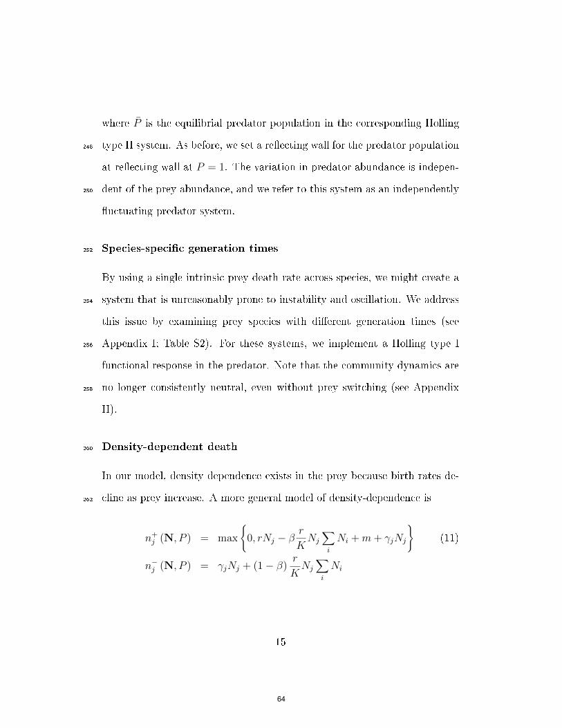
where P is the equilibrial predator population in the corresponding Holling

type II system. As before, we set a re�ecting wall for the predator population248

at re�ecting wall at P = 1. The variation in predator abundance is indepen-

dent of the prey abundance, and we refer to this system as an independently250

�uctuating predator system.

Species-speci�c generation times252

By using a single intrinsic prey death rate across species, we might create a

system that is unreasonably prone to instability and oscillation. We address254

this issue by examining prey species with di�erent generation times (see

Appendix I; Table S2). For these systems, we implement a Holling type I256

functional response in the predator. Note that the community dynamics are

no longer consistently neutral, even without prey switching (see Appendix258

II).

Density-dependent death260

In our model, density dependence exists in the prey because birth rates de-

cline as prey increase. A more general model of density-dependence is262

n+j (N, P ) = max

{0, rNj − β

r

KNj

∑i

Ni +m+ γjNj

}(11)

n−j (N, P ) = γjNj + (1− β)

r

KNj

∑i

Ni

15

64

where β = 1 is our density-dependent birth model. As a robustness check,

we consider a model of density-dependent death, β = 0. Populations with264

density-dependence entirely in death are more volatile and thus have higher

long-term variances in population size and qualitatively di�erent extinction-266

colonization dynamics following predator introduction (see Appendix II).

Metacommunity richness268

To investigate the in�uence of the metacommunity richness M on the ability

of predation to promote diversity, we simulate communities with Holling type270

I predation across the full range of values of ρ and K used in this paper for

M ∈ {10, 20, 40}. Additionally, for K = 1000 and M ranging from 10 to272

360, we determine the attack rate ρ∗ above which predators suppress diversity

below the neutral expectation (see Appendix II).274

Simulations

We simulate predator-prey communities using MATLAB R2013b. MATLAB276

code for simulation is available in the supplementary materials, described

in Appendix VI. We implement simulations using a Gillespie algorithm (?)278

in which timesteps are drawn from an exponential distribution whose rate

constant, η, is the inverse of the total propensity for events of any kind280

η =

(p+ + p−)

+∑j

(n+j + n−

j

)−1

. (12)

16

65

At the end of each timestep, a single event is selected with probability pro-

portional to the event's propensity. The time and state of the system are282

updated, and the process repeated for T time units.

Parameter choices and initial conditions284

To ensure biological realism in our simulations, we turn to the empirical lit-

erature to inform our parameterizations. Throughout this paper, we �x the286

prey death rate γ = 0.1. This is a free choice that speci�es the timescale, and

the remainder of the parameters are chosen relative to γ. Table 1 (Holling288

type I model) and Table S1 (all models) give the numerical values and biolog-

ical interpretations for all simulation parameters. We encourage the reader290

to visit Appendix I, where we outline parameter estimation for our model,

drawing on empirical investigations of demographic parameters, trophic e�-292

ciencies, predator-prey biomass ratios, trophic cascades, and so forth. Similar

measurements, if available, can be used to parameterize our model for any294

particular natural system. In each simulation, we initialize the community

near its equilibrium in the corresponding parameterization of the mean-�eld296

model, thus ensuring that transient dynamics alone cannot account for dif-

ferences between the stochastic system and the mean-�eld equilibrium.298

Stationarity check

We are interested in the asymptotic or stationary species-richness of com-300

munities at island-biogeographic equilibrium. To simulate this quantity, we

17

66

Table 1: Parameters for Holling type I model

Parameter units Value(s) Interpretation

δ time−1 0.1 Intrinsic prey deathrate;inverse prey lifespan

γ time−1 0.05 Intrinsic predator deathrate;inverse predator lifespan

r time−1 5 Maximum prey populationgrowth rate

K prey 200 � 2000 Carrying capacity; system size;inverse competition intensity

M species30;

10 � 360 (�g. 3)Metacommunity richness

m preytime

0.3 Migration rate

α predatorsprey

10−3 Ratio of predator birthsto predation events

ρ preypredators·time

0 � 500* Predator attack rate(prey deaths per predator)

z � 1 � 2 Prey-switching exponent

18

67

must determine the relaxation time required to ensure that the imprint of302

initial conditions fades and the system reaches dynamic equilibrium. For

every simulated result in this paper, we present a stationarity check in the304

supplement. Each �gure in the paper corresponds to an equivalently num-

bered supplementary �gure in Appendix III that presents the �nal result306

alongside results obtained by stopping the simulation after shorter time in-

tervals. These stationarity checks con�rm that even as we vary functional308

forms and parameters, simulations approximate the stationary species rich-

ness by T = 2000.310

Transient dynamics

Experimental manipulations of predation (???) result in transient dynamics.312

Experimenters might wish to know whether the dynamics observed follow-

ing a predator introduction provide reliable information about the eventual314

stationary state. To explore this question, we simulate predator introduc-

tions into a predator-free community. We consider the introduction of one316

individual predator with ordinary population dynamics and a Holling type I

functional response, and also of an invariant, equilibrium-sized predator pop-318

ulation with a Holling type II functional response (mimicking studies that

monitor an experimental predator introduction for less time than is typically320

required for predators to reproduce; e.g. ??). We monitor the dynamics by

examining the community state every 0.25 time units for 50 time units (5322

prey generations). Across the full range of values examined for ρ and K,

19

68

we simulate predator introductions into twenty independent replicate prey324

communities near stationarity (see Appendix II for details). We ask whether

the initial change in species richness is in the same direction as the �nal326

change, and we examine patterns in the time evolution of richness towards

stationarity.328

Results

Species richness landscapes330

As expected, predators that do not engage in prey-switching (z = 1) never

increase prey diversity for any value of the prey carrying capacity K. For332

such predators, any increase in predation intensity leads to a decrease in the

average prey species richness. Prey-switching predators, on the other hand,334

increase diversity at low attack rates and high values of K, and this e�ect

becomes more pronounced as z increases (Figure 1). These results are all in336

line with the predictions of the mean-�eld model.

20

69

Figure 1: Local prey species richness relative to metacommunity richness as a function of the carrying

capacity K, predator attack rate ρ, and prey-switching exponent z in a Holling type I predator-prey

community. Prey-switching predators increase prey diversity only when attack rates are su�ciently low,

and the range of diversity-promoting attack rates decreases as K gets small. All data points represent the

averaged richness of 4 communities simulated for T = 20000 time units. See Figure S1 for stationarity

checks.

However, for every value of z examined, su�ciently high predation rates338

lead to decreased diversity (Figure 1). For a particular value of K, the neu-

tral community at ρ = 0 serves as a baseline for species-richness in absence340

of predators. There always exists an attack rate ρ∗ above which even a

prey-switching predator depresses diversity below that of the predator-free342

community. The value of ρ∗ increases monotonically with K. Thus, the iden-

tical predation regime can promote diversity for large K and inhibit diversity344

for small K. The qualitative pattern in prey species-richness as a function of

ρ and K is robust to several variations in our model assumptions, including346

a saturating (Holling II) predation rate, invariant and independently �uc-

tuating predator populations, species-speci�c generation times for predators348

21

70

and prey, a di�erent functional form for prey-switching introduced by van

Leeuwen et al. (2013), and prey density dependence via death rates instead350

of birth rates (Figure 2).

22

71

Figure 2: The qualitative patterns evident in Figure 1 are preserved across a variety of alternative

models for predator-prey dynamics. All data points represent the relative richness of the local community

to the metacommunity richness averaged over 4 communities simulated for T = 2000 time units. Note the

di�erent scale for predator attack rates ρ for the van Leeuwen and Density dependent death simulations

(see appendices I & II for explanation). See Figure S2 for stationarity checks.

23

72

In all cases where z > 1, the prey species-richness isoclines are wedge-352

shaped contours that can be identi�ed either by their species richness or by

the carrying capacity K of the predator-free neutral community that yields354

the same average species richness. The lower boundaries of the species-

richness isoclines change only slightly with K and very rapidly with ρ, es-356

pecially around ρ = 50, which is the minimum value of ρ required for the

persistence of the predator in the mean-�eld model; these lower boundaries358

de�ne the region where increasing predation intensity will increase prey com-

munity diversity. The slope of the upper boundaries of the species-richness360

isoclines, and therefore the width of the wedge, increases as the amount of

prey switching increases. As expected, more strongly prey-switching preda-362

tors promote diversity across a broader region of parameter space.

The metacommunity richness M also plays a role in determining the364

attack rate ρ∗ above which prey richness decreases below the predator-free

average. Increases in M lead to decreases in ρ∗, meaning that predation is366

less likely to promote prey diversity in speciose metacommunities (Figure 3a).

However, even in highly speciose metacommunities, prey-switching predators368

promote diversity across a broad range of parameter space as long as K and

z are su�ciently high (Figure 3b).370

24

73

Figure 3: For constant K = 1000, increasing metacommunity richness decreases the range of predation

intensities over which prey-switching predation improves species richness. (A) ρ∗ decreases with increasing

metacommunity richness. (B) Prey switching increases species richness over a narrower range of ρ, K,

and z when prey metacommunities contain more species. See Figure S3 for stationarity checks.

Variance and quasicycles

Invariant or independently �uctuating predators tend to promote diversity372

over wider ranges of attack rates than predators with ordinary population

dynamics (Figures 1 & 2). These di�erences can be understood in terms374

of the e�ect of predators on prey population variance, which shapes the

diversity landscapes of Figures 1 & 2 because the likelihood of extinctions376

increases when the population size decreases to below-average values. For

all functional forms explored in this paper, predators increase the variance378

relative to the mean of the total prey population. Some functional forms,

including Holling types I and II with ordinary predator population dynamics,380

cause oscillatory behavior and especially large increases in relative variance.

25

74

Because the expected community size grows linearly with K, a system-382

size expansion in K (?) suggests that the variance in community size should

also grow linearly with K. The variances calculated from the replicate sim-384

ulations behind Figure 1 indeed show approximately linear increases (Figure

S7a). This trend becomes apparent only when communities with and with-386

out predators are disaggregated. Controlling for the expected community

size, communities with Holling type I predators have variances roughly one388

hundred times that of communities without predators (Figure S7a). This

massive increase in variance manifests as sustained periodic oscillations in390

the total community size (Figure S7b-d). These noise-induced oscillations,

referred to as quasicycles, result from the interaction of predator-prey feed-392

back and demographic stochasticity, and they persist even when the predator

and every prey species has a species-speci�c death rate. Quasicycles substan-394

tially increase the variance in prey population beyond what could be expected

without predator-prey feedback (??). The increase in variance is associated396

with bottlenecks in total prey abundance (Figure S7b).

Comparing the species richness plots (Figures 1 & 2) for Holling type I398

& II predators and invariant predators (which do not produce quasicycles),

we see that the increased variance associated with the quasicycle shrinks the400

region of parameter space where predators promote diversity. By comparing

the invariant and independently �uctuating predators, we see that varia-402

tion in predator populations reduces the ability of a prey-switching predator

to maintain diversity. However, we also see that prey population size still404

26

75

modulates the e�ect of predation on prey diversity, even in the absence of

quasicycles.406

Transience

Following the introduction of a predator to a predator-free community, the408

expected species richness of a community enters a transient period before

converging to the stationary expectation. For most parameter combinations,410

the initial change in species richness is in the same direction as the long-

term change. However, when predators weakly reduce prey richness in the412

long term (ρ is slightly greater than ρ∗), predator introduction may cause a

transitory increase in prey richness (Figures 4 & S14). This e�ect is most414

pronounced when the introduction involves a single individual predator. In

this case, the transient e�ect on species richness probably results from the416

transient growth of the predator population. Because the per-prey attack rate

is given by the product ρP , a predator population that has not yet reached418

its equilibrium abundance has exactly the same e�ect on prey dynamics as

a larger predator population with a lower attack rate. Even in the case420

of invariant predation, substantial time may pass before diversity begins to

decline, presumably because the predator initially targets abundant species422

and is unlikely to kill rare species until the relative abundance distribution

evens out (Figure 4).424

27

76

Figure 4: Predator introduction causes transient changes in prey richness generally in the same

direction as the long-term change. However, introducing predators that weakly suppress richness in the

long term can increase richness in the short term. The e�ect is most pronounced for introductions of

small (sub-equilibrial) predator populations that exhibit transient growth. Trajectories show the average

richness of twenty replicate communities (see Appendix II).

Extinctions and species richness

A formal treatment of species richness in our model requires an examination426

of prey extinction-colonization dynamics. In this section, we combine simula-

tions and analytic results to develop intuition for how prey-switching preda-428

tors increase or decrease prey diversity in an island biogeographic context,

where species richness is determined by a colonization-extinction equilibrium.430

Predators do not directly a�ect colonization rates; they a�ect species

richness entirely via extinctions. The propensity of extinctions at time t is432

ψ−(t) = n−1 (t)Ψ1(t) (13)

where n−1 (t) is the propensity for death of a singleton and Ψ1(t) the num-

28

77

ber of singletons in the community. The average rate of extinctions is the434

expectation of equation 13 over the stationary distribution of community

composition.436

E[ψ−]

= E[n−

1

]E [Ψ1] + Cov

[n−

1 ,Ψ1

]. (14)

To reduce extinction rates, a stabilizing mechanism must su�ciently decrease

the expectation of n−1 , the expectation of Ψ1, and/or the covariance between438

n−1 and Ψ1.

Therefore, to understand how the parameters ρ, z, and K a�ect species440

richness, we need to understand how they a�ect the means and covariance

on the right side of equation 14. We estimate analytically (Appendix V) and442

show by simulation (Figure 5a) that n−1 increases with ρ and decreases with

K and z. We show by simulation that for z > 1, the covariance Cov[n−

1 ,Ψ1

]444

increases with ρ, and that the e�ect is larger for small values of K and large

values of z (Figures 5a & S8). Analysis of the e�ect of model parameters on446

Ψ1 and the covariance Cov[n−

1 ,Ψ1

]is di�cult (Appendix V) but simulations

suggest that a U-shaped relationship between Ψ1 and ρ accounts for much of448

the humped relationship between ρ and species richness. The reduction in

Ψ1 for intermediate ρ is magni�ed by increasing K and/or z over the range450

of parameters we consider in this paper (Figures 5a & S8).

29

78

Figure 5: (A) Species richness in our model is controlled by the extinction rate. Based on equation 14,

the scaling of species richness with ρ and K can be understood in terms of the scaling of the expectation

of Ψ1, the expectation of n−1 , and the covariance between Ψ1 and n−

1 . (B) Prey switching can increase the

covariance between prey populations, pulling the distribution of the population of a given species away

from the boundaries where singletons occur and extinctions take place.

To understand the e�ect of z on Ψ1, we note that z does not a�ect the452

total community size or its variance. Instead, z increases the covariance

between species by suppressing �uctuations in relative abundance (Figure454

5b). We further note that the variance of population size of a particular

species, given that it is present in the community, relates to the variance in456

the total community size:

σ2C = Sσ2

N + S (S − 1)σi,j (15)

where σ2C is the variance in community size, σ2

N the variance in population458

30

79

size, and σi,j the covariance between populations of di�erent species. Sym-

metries in our model ensure that σi,j is constant for all pairs of prey species.460

The increased covariance σi,j necessarily entails a decrease in σ2N . Thus, in-

creasing z decreases Ψ1 by moving the multivariate prey densities away from462

the boundaries where singletons occur (Figures 5b, S9). Prey-switching pre-

dation of the van Leeuwen functional form similarly increases the covariance464

between prey populations (Figure S9). Since frequency-dependent stabiliz-

ing mechanisms like prey-switching predation dampen �uctuations in relative466

abundances, other statistics beyond σ2N and σi,j, such as the variance in rel-

ative abundance, σ2R, may yield useful scale-free proxies for extinction rates468

(Figure S13, Appendix V).

Discussion470

Whether in oceanic mesocosms, tropical islets, or remnant continental wild-

lands, a �eld biologist always encounters �nite, discrete populations with472

stochastic dynamics. Species appear and vanish from islands or study plots,

and these stochastic colonizations and extinctions are fundamental to meta-474

community theory and island biogeography. When di�erential equations ap-

proximate our study systems well, they provide profound mechanistic insight476

and predictive power (??). But some systems display important stochas-

tic dynamics that cannot be captured by di�erential equations alone. We478

have shown that when prey species richness is the variable of interest, some

31

80

predator-prey systems belong to this category across a range of parame-480

ters that the �eld biologist might encounter in nature, particularly where

the intensity of competition between prey is high (K is small). Di�erential482

equations continue to provide important insight, and indeed they form the

backbone of our simulation model, but they fail to predict key features of484

our system.

For all of our simulations, simple analysis of the corresponding di�er-486

ential equations suggests that the predator should stabilize the system and

promote prey diversity (????). By incorporating demographic stochasticity488

in �nite populations, we show that the e�ect of prey-switching predation de-

pends predictably not only on the predator's attack rate and degree of prey490

switching, but also on the prey carrying capacity and the prey metacommu-

nity richness. These variables together determine whether a given predation492

regime will increase or decrease the richness of an otherwise neutral prey

community.494

For a given prey carrying capacity K and prey-switching exponent z,

there is a critical predation intensity ρ∗ below which equilibrium prey rich-496

ness is increased relative to the predator-free community, and above which

equilibrium prey richness is reduced. Similarly, for a given attack rate ρ498

and prey-switching exponent z, there is a critical community size K∗ below

which equilibrium prey richness is reduced, and above which prey richness is500

increased. Increasing the metacommunity richness,M , decreases the relative

abundance of each prey species and consequently decreases ρ∗. This funda-502

32

81

mental result is robust to several important variations in model assumptions,

but it is invisible both to stability analysis of ordinary di�erential equations504

and to analysis of island-biogeographic communities which lack the niche

detail of predator-prey interactions.506

We suspect that the phenomena described here are not restricted to prey

communities regulated by a single prey-switching predator, but might also508

extend to communities regulated by a suite of specialist predators (??) or

generalist predators regulating hierarchically competitive prey (???). Any510

stabilizing predation regime that increases prey death rates will result in a

tension between stabilization and stochastic intensi�cation to determine prey512

diversity. We chose to consider prey-switching predators because simulations

of a single prey-switching predator are simple to implement, easy to interpret,514

and contain fewer parameters than simulations of an entire suite of specialist

predators.516

Empirical Consequences

We estimate our model parameters from the empirical literature (see Ap-518

pendix I). Doing so helps to ensure that the behavior we observe might exist

in nature, because it exists at reasonable values and combinations of pa-520

rameters. Moreover, our procedures for determining model parameters rely

on empirically available measurements from real-world systems. Our model522

can therefore be �t to a real world system using empirical data that might

reasonably be available.524

33

82

Scale-dependence of predator e�ects

Predators are known to regulate prey diversity in many systems, sometimes526

increasing prey diversity (??) and sometimes decreasing prey diversity (??).

Understanding the in�uence of predation on prey diversity is crucial for528

ecologists attempting to resolve the relative importance on top-down and

bottom-up processes as controls on ecosystems (?) because in some systems,530

predation is essential for the maintenance of species diversity (?). Empirical

observations of predation a�rm the theoretical notion that predators create532

a rare-species advantage by targeting abundant prey (??). Even when in-

dividual predators do not alter their preferences, the numerical response of534

specialist predators can produce a similar e�ect.

It is unsurprising that this rare species advantage is not always su�cient536

to ensure that predators increase prey diversity. With su�ciently large attack

rates (or numerical responses), predators increase the probability of prey538

extinction regardless of switching. This result is con�rmed by many recorded

instances of predators decimating prey diversity to such an extent that prey540

switching is unlikely to have ameliorated the consequences in any meaningful

way (??).542

The important insight from our models is that parameters other than

attack rates, such as the metacommunity richnessM or the carrying capacity544

K, can reverse the e�ect of predation on species richness. The carrying

capacity K is of considerable interest, because in nature it is controlled by546

factors such as productivity and area. In systems where prey communities

34

83

remain well-mixed and productivity-per-area remains constant across a range548

of spatial extents, horizontal slices of the plots in Figures 1 and 2 can be read

as species-area relationships (SARs; Figure S10). Many predation regimes550

that increase diversity at large spatial scales reduce prey diversity at small

scales. This possibility complicates the interpretation of empirical studies552

of the e�ects of predators on prey diversity. Landmark studies of predation

and prey diversity have occurred at very small spatial scales, in mesocosms554

or on small islands (???). For example, Spiller and Schoener's (?) seminal

work on Bahaman spider communities and their Anolis predators examined556

replicate communities with fewer than 300 spiders each in the absence of

predators, a value at the low-end of the range of the parameter space that558

we consider. These studies have done an admirable job elucidating the e�ects

of predation at small scales, but caution is warranted in applying the results560

to large blocks of continuous habitat.

Predators and prey frequently operate on di�erent spatial scales, with562

predators ranging across larger areas than their prey, and coupling spatially

distinct food webs (?). By con�ning both predators and prey to a single564

well-mixed patch, our models fail to account for this reality. However, our

model results hold for both invariant predator populations and independently566

�uctuating predator populations where predator dynamics are independent

of prey dynamics in the patch. Whereas the Holling type I model repre-568

sents a limiting case where predator populations respond strongly to prey

populations at the patch scale, these represent the opposite case, mimick-570

35

84

ing predators that range so widely that the dynamics at the patch scale

do not appreciably a�ect the amount of predation experienced at the patch572

scale. Furthermore, experimental manipulations of predation often com�ne

prey and predators to a single patch (?), or even restrict predator movement574

below that which is available to prey (?).

Conservation in habitat fragments576

Just as caution is warranted in extrapolating empirical results from small

scales to large, any empirical or theoretical understanding of the diversity-578

promoting e�ects of a predator in a large, intact system might not apply

in small isolates. Habitat fragmentation is a ubiquitous global process that580

creates such isolates (????). Increasingly, managing for predator persistence

or reintroduction is viewed as a tool to enhance conservation outcomes for582

species at lower trophic positions through top-down e�ects (?). However,

managing for predator persistence (or reintroduction) in fragmented habitats584

may negatively impact prey diversity even when the predator has unambigu-

ous positive impacts in intact systems. Note, however, that our results are586

relevant for cases when the focal species of conservation interest are poten-

tial prey. In some highly fragmented systems (e.g. Brazil's Atlantic forest),588

predators and prey alike are in serious danger of extinction (?). Our model

shows that managers cannot assume, based on the ability of prey to coexist590

with each other and with their predators in large landscapes, that such co-

existence will be maintained in small forest reserves; in the face of evidence592

36

85

that predators enhance prey coexistence in large blocks of habitat, our model

raises concern that fragmentation could reverse the predator's bene�cial ef-594

fect.

Coexistence in hyperdiverse communities596

Our model predicts that predators are more likely to increase species richness

on habitat patches subject to immigration from a depauperate metacommu-598

nity than on patches subject to immigration from a speciose metacommunity.

On its face, this result is contradicted by the mounting evidence that pre-600

dation plays a crucial role in the maintenance of diversity in hyperdiverse

communities, such as in humid tropical forests (???). However, at su�cient602

spatial scales switching predation continues to increase diversity across a rea-

sonably broad region of parameter space, even in hyperdiverse communities.604

Furthermore, our results apply exclusively to systems where predators reduce

the total density of their entire prey guild to substantially lower values than606

could be achieved in the absence of predation. Because tropical trees com-

pete ferociously for canopy space (?), our model assumptions are probably608

invalid for tropical trees.

More individuals hypothesis610

The tendency of predators to reduce diversity at small scales can be viewed as

a natural consequence of the more individuals hypothesis (?), which suggests612

that sites containing more individuals tend to contain more species and has

37

86

received substantial empirical support (?). Where prey-switching predation614

decreases species richness in our models, it does so partly by reducing the

density of individuals, so a focal patch contains fewer individuals and fewer616

total species. It is tempting to imagine that this sampling e�ect causes a

prey-switching predator to increase beta diversity, especially given a prey-618

switching predator's tendency to increase diversity at large scales, but to

reduce diversity at small scales (?). However, this presumption rests on a620

shaky premise, because our models of richness at small spatial scales represent

the richness of single small isolates, not of small patches integrated into a622

larger landscape and interconnected by migration. Such a model would be a

useful extension of our work.624

Extensions

Our investigations leave multiple open questions for future work. One inter-626

esting result from our simulations is that prey-switching predation increases

the covariance between time-series datasets of prey populations. The in-628

creased covariance in communities subjected to prey-switching predation is

due to prey-switching predation dampening stochastic �uctuations in relative630

abundances. Although the mean prey population sizes remain constant, the

increased correlation with increased prey-switching predation is a stochastic632

analog the observation that prey-switching predation can change apparent

competition to apparent mutualism between prey species (??): stochastic de-634

creases in the relative abundance of one species will lead to transient increases

38

87

in the death rates of other, more abundant species and so transient stochastic636

increases in harvesting of one of two equally abundant species should lead to

a transient decrease in the abundance of the other species. The prey popu-638

lations we've considered still satisfy Holt's notion of apparent competition in

the behavior of their means; this stochastic apparent mutualism exists only640

in species that stochastically �uctuate about their mean. This increase in

temporal covariance between prey populations under prey-switching preda-642

tion is empirically measurable - as is the hypothesized concomitant reduction

in variance of prey population size - and thus fruitful grounds for testing our644

hypotheses about predators' e�ects on statistical properties of prey popula-

tions.646

We hypothesize that the existence of ρ∗ and K∗ extend to more general

systems with frequency-dependent death in �nite, stochastic communities.648

This points the way to future studies of predator-prey communities with

multiple predators, specialist predators/pathogens, non-neutral niche struc-650

ture among the prey, and extrinsic environmental variability. The degree of

prey-switching could be in�uenced by population size (?), as well as patterns652

in spatial variation of prey relative to the home range of predators. Multi-

patch extensions of our model could shed new light on species persistence654

after habitat fragmentation (?), and could elucidate the potential stabilizing

and destabilizing impacts of predators that spatially couple local food webs656

(?).

If ρ∗ and K∗ generalize to a large class of realistic top-down mechanisms658

39

88

of biodiversity maintenance, then their scaling properties have major implica-

tions for our understanding of diversity in natural systems, the management660

of predators, and reserve design. For example, if top predators such as wolves

(?) or lions (?) exhibit very weak prey-switching, they may have bene�cial662

e�ects on species richness that are only apparent in large swaths of connected

habitat containing large prey populations. Contemporary management de-664

cisions about reserve size such as the range expansion of the Mexican Gray

Wolf (Canis lupus baileyi) are often motivated by arguments of population666

viability (?), but the diversity of the predators' diet (??) and the potential

scaling of the predators' impact on the robustness of prey populations with668

reserve size would motivate range expansions of prey-switching top predators

on the basis of the viability of the prey. The large historical ranges of these670

top predators compared to their smaller contemporary ranges mean that de-

spite the predators' persistence their full e�ects on ecosystem structure &672

function on the landscape scale are not currently realized (?).

Acknowledgements674

We thank our colleagues S. Levin, H. Horn, A. Dobson, J. Dusho�, A. Hein,

C. Torney, J.E.S. Socolar, and D. Wilcove for many useful discussions and676

feedback. Two anonymous reviewers provided comments that greatly im-

proved this manuscript. ADW and JBS both acknowledge support from678

NSF graduate research fellowships.

40

89

Supplemental information:

Appendices I-VI

1 Appendix I: Parameter Estimation

We turn to the empirical literature where possible (and the theoretical lit-

erature where necessary) to obtain realistic estimates for the parameters in

our models. Our goal is to ensure that our results of interest occur param-

eter values that correspond to realistic natural communities. Table S1, an

expanded version of table 1, includes every parameter used in our models.

Below, we explain our choices of values for each parameter in turn.

Lifespans: δ and γ

The choice of δ is an arbitrary free choice that speci�es the timescale in our

model. We use δ = 0.1, and thus the expected lifetime of a prey (given

that it does not succumb to predation) is Tprey = 10. Because predators are

generally longer-lived than their prey, we set the per-capita death rate of

predators γ = 0.05. Thus, predators have twice the average lifespan of their

prey.

This choice re�ects the average body mass ratio of predators to prey

(roughly 100 : 1; ??) and the allometric relationship between body size and

lifespan in mammals (log(lifespan) ≈ 0.2 log(body mass); ?). Note, however,

90

that the variance about both of these quantities is large, and a wide range

of ratios γδare reasonable. Note also that in our models, predators live on

average more than twice as long as prey, because prey lives are routinely cut

short by predation.

Population growth: r and K

When a (predator-free) community is nearly empty, the prey population

growth rate r is given by r = δ (r0 − 1), where r0 is the average lifetime re-

productive output of an individual under conditions of abundant resources,

and in the absence of predation. Thus we obtain an estimate of r by obtain-

ing values of r0 from the literature. r0 is variable across real-world systems,

and note that in sexually reproducing species, r0 is obtained by dividing by

two the average number of o�spring per individual. Below, we provide a

sampling of empirical values: In absence of predation, a North American

songbird might have a lifespan of four years (?) and a reproductive output

of perhaps 4 individuals per pair per year, given abundant resources (?).

In this case, r0 ≈ 8, and r ≈ 0.7 (in this example, one time unit is ≈ 0.4

years). A black-billed whistling-duck (Dendrocygna autumnalis) might have

a lifespan approaching eight years (?), and a reproductive output (under

abundant resources and no predation) as high as 14 individuals per pair per

year (?), yielding r ≈ 5.6 (in this example, one time unit is ≈ 0.8 years). A

female harbor seal (Phoca vitulina) might have a lifetime reproductive out-

put of roughly 25 pups, yielding r ≈ 1.2 (?). Female adders (Vipera berus)

91

Table S1: Parameters used in MATLAB simulations

Parameter matlab

Name Units Value(s) Interpretation

δ D time−1 0.1 Intrinsic prey deathrate;inverse prey lifespan

γ G time−1 0.05 Intrinsic predator deathrate;inverse predator lifespan

r r time−1 5 Maximum prey populationgrowth rate

K k prey 200 � 2000 Carrying capacity; system size;inverse competition intensity

M M species30;

10 � 360 (�g. 3)Metacommunity richness

m m preytime

0.3 Migration rate

α alpha predatorsprey

10−3 Ratio of predator birthsto predation events

ρ p preypredators·time

0 � 500∗ Predator attack rate(prey deaths per predator)

z z � 1 � 2 Prey-switching exponent

Additional Parameters used in Robustness Checks

h h predators·timeprey

10−3 Handling time(Holling Type II)

Tij h predators·timeprey

10−3 Handling time(van Leeuwen)

ρi p preypredators·time

0 � 1500 Attack rate(van Leeuwen)

sij s �1 if i = j

0.15 if i 6= jPrey similarity(van Leeuwen)

P P0 predatorsrKℵ (1− γ

αℵ)† Mean predator population;(Invariant and Indep. Fluctuating predators)

λ L time−1 10 Mean reversion(Independently Fluctuating predator pop.)

δi and γ′ D(i) time−1 See table S2 Species-speci�c death ratesfor prey and predator

* Note that in the density dependent death simulations, 0 ≤ ρ ≤ 1000. (Appendix II).

† Where ℵ = ρ(1− hγα ).

92

in �eld conditions might have a lifetime reproductive output of 10.5 o�spring

on average, so a lower bound on r in this system would be r = 0.43 (?),

while a female leatherback turtle (Dermochelys coriacea) might lay 60 eggs

every 5 years for 30 years after maturity, yielding r ≈ 17.9 (??). In insects,

documented lifetime fecundities range from 5.2 to 2469, yielding a range of r

from 0.16 to 123 (?). Among marine invertebrates, fecundity under optimal

conditions may be di�cult to estimate. For example, one sea hare (Tethys

californicus) can lay half a billion eggs in half a year, but an unknown frac-

tion (presumably very small) are fertilized and recruit into the population,

even under optimal conditions (?).

We pick r ≈ 5 as a reasonable ballpark value; similar values (6.0 ± 0.4)

have been found for meadow voles (Microtus pennsylvanicus) (?).

We examine several values ofK, all betweenK = 100 andK = 2000. The

upper bound corresponds roughly to, for example: the number of individual

birds breeding in one square kilometer of temperate or tropical forest (?);

the number of lizards in two square kilometers of dry Sonoran desert (?); one

tenth the number of �sh in a 3.8 hectare lake (average depth 8 m) in Michigan

(?); the number of trees > 10 cm diameter-at-breast-height in four hectares

of tropical forest (?); or the number of bacteria in 10−4 grams of dry soil

under maize cultivation in China (?). Note that in our model, K represents

the population density that would be realized in absence of predation, so the

densities mentioned above tend to be somewhat lower than the appropriate

densities for comparison. Counteracting this e�ect, population densities in

93

our model should be thought of as referring to one guild of competing species,

and so the densities mentioned above tend to be somewhat higher than the

appropriate densities for comparison.

As an aside, the web-spider communities studied by ? contained fewer

than 300 individuals per replicate in the absence of predators.

Colonizations: m and M

In our model, the colonization rate is determined by the migration rate m

and the number of species M − S present in the metacommunity but absent

in the local community. Realistic values for the metacommunity richness

M range from M = 1 (e.g. the richness of amphibians on Antigua and

Barbuda) to M > 600 (the number of breeding birds near Iquitos, Peru);

M > 2000 (the richness of reef �sh in the coral triangle�though some of

these are narrowly endemic to smaller sub-regions); or even M > 5000 (the

richness of freshwater �shes in the Amazon Basin�though again, many are

sub-regional endemics).

In most of our simulations (all �gures except Figure 3), we use M =

30, which approximates the richness of snakes in the coastal plain of North

Carolina, the richness of ungulates in the arid savanna of central Kenya, the

richness of ladybirds in England, or the richness of birds breeding in a New

England hardwood forest (?). We also test the e�ect of varying M , using

values ranging from 10 to 360.

In our model, m represents the rate at which immigrant individuals of

94

all species arrive in the focal patch. Realistic values for m in nature vary

tremendously, depending on the isolation of the focal patch and the biology of

the focal guild. On remote oceanic islands, immigrations of terrestrial mam-

mals and reptiles are rare indeed. In �ow-through mesocosms, immigrations

could account for a majority of the individuals present. We use m = 0.3.

Note that at equilibrium, prey have on average one o�spring per lifetime,

and in absence of predation, prey therefore have one o�spring per δ−1 = 10

timesteps, and the community produces K10

o�spring per timestep. Thus for

K = 2000, we expect that migrants account for roughly 0.1% of individuals

in the population, while for K = 200, that �gure rises to over 1%.

Our choices of m and M should be viewed as somewhat arbitrary, except

that we chose them intentionally to produce partly-�lled communities for the

range of values of K that we consider. This allows both diversity-promoting

and diversity-suppressing e�ects of predators to express themselves in simu-

lations.

Predator production: α

In our model, α represents the probability that a predation event will pro-

duce an additional predator, and α−1 is the average number of prey that

a predator must consume in order to reproduce once. Our functional form

assumes that the numerical response of the predator population is a linear

function of the number of prey consumed, an assumption that is valid in at

least some systems (?). Alpha depends on the e�ciency ε of biomass conver-

95

sion between trophic levels and on the biomass ratio τ of predators to prey:

α = ετ. In nature, the e�ciency of biomass conversion ε is variable because it

depends not only on the e�ciency of nutrient uptake in the digestive system

and the theoretical e�ciency of conversion by cells in culture, but also on the

metabolic costs associated with homeostasis and foraging (?). In a review of

invertebrates, Calow (1977) encountered minimum biomass conversion e�-

ciencies of 11% in leaf-eating lepidopteran larvae, and maximum e�ciencies

of ≈ 70% in the mite Steganacarus magnus (with an outlying e�ciency of

95% in the sea star Asterias rubens). Conversion e�ciencies in vertebrates

are lower (5-25% in juvenile salmon; Calow 1977), and as expected are lowest

in endotherms (4.6% in mice; ?). An absolute lower-bound to the e�ciency

of biomass conversion is the trophic e�ciency (the ratio of predator produc-

tion to prey production). In the North Sea, the estimated average trophic

e�ciency is 3.7%, while the estimated trophic e�ciency among organisms

with mass less than 256 g is 27% (?).

The ratio τ of individual predator mass to prey mass is similarly variable

in nature. Extremes exist in marine systems, where the black swallower

(Chiasmodon niger) takes prey more massive than itself (τ < 1; ?), while

a blue whale (Balaenoptera musculus) subsists on Antarctic krill (Euphasia

superba) 380 million times less massive than itself (τ = 3.8 ·108; ??). Average

biomass ratios of 100:1 appear to be typical in marine food webs (τ = 100;

??). This ratio is reasonable across a variety of systems (terrestrial and

aquatic) and taxa (endotherms and ectotherms), though endotherms tend to

96

have higher ratios while invertebrates tend to have lower ratios (?).

For our purposes, we �x α = 10−3, meaning that predators consume on

average 1000 prey to self-replace. This choice might re�ect, for example,

ε = 0.1 and τ = 100 (re�ecting the average predator-prey interaction in the

North Sea food web; ?); or ε = .05 and τ = 50; et cetera.

Predation: ρ and z

Determining an appropriate predation rate ρ is crucial to our results, because

the behavior we report is uninteresting if it occurs only for unrealistically

high values of ρ. Direct estimation is precluded by the dearth of empirical

studies that have succeeded in simultaneously measuring the total number

of individual prey, the total number of individual predators, and the total

rate of predation events in a natural system. However, in the context of our

model, we can derive an empirical estimate for ρ by noting that the expected

community size of prey without predators is x0 = K, whereas the expected

community size with predators is xρ = γKαρ

in the Holling Type I model.

Thus, ρ = γαx0xp. Following local predator extinctions, prey populations have

been observed to increase by as much as 10-fold or 100-fold ( x0xp∈ [10, 100];

?). Conservatively, we consider attack rates no higher than ρ = 10 γα

= 500.

There is also a lower bound for ρ, namely the minimum value required for

persistence of the predator population in the mean �eld model ρ > γα

= 50.

We consider no nonzero predation rates lower than this value.

Empirical estimates of the prey-switching parameter z exist for both

97

Minke Whales (Balenoptera acutorostrata) and the Hen Harrier (Circus cya-

neus) (??). In both of these studies, z is allowed to vary by prey species and

is parameterized in the context of a Holling Type II functional response for

three prey species. The studies �nd species-speci�c values ranging from 1 to

4, with values between 1 and 2 being typical across species. In our investiga-

tion, we consider no values for z less than one, as these would imply that the

predator preferentially targets rare species. When z = 2, our functional form

for prey switching is a special case of a general form derived from recent the-

oretical work on prey switching, suggesting that it is reasonable to consider

values as high as z = 2 (?). We therefore consider the range z ∈ [1, 2].

Additional parameters

Handling times: h and Tij Because these parameters serve as robustness

checks on our general results, we sought high-end estimates to demonstrate

that our qualitative results persist across a broad range of model assumptions.

We set the handling times at 10−3. Since a predator must consume on average

α−1 = 103 prey to self-replace, this means that a predator must spend on

average 1 time unit, or �ve percent its expected lifetime, handling prey just

to self-replace.

van Leeuwen predation: ρi and sij In van Leeuwen's functional form,

attack rates, prey similarity, and prey switching are intertwined. For i = j,

we set the similarity sij = 1, meaning that prey of the same species are

98

entirely self-similar. Otherwise, we set sij = 0.15, a low value that ensures

that signi�cant prey switching occurs in the functional response. For these

choices, it was necessary to examine higher values of ρi than the values of ρ

considered in other simulations in order to obtain a similar range of overall

attack rates.

Invariant and independently �uctuating predator populations: P

and λ In simulations with invariant predator populations, predator popu-

lations are �xed at the equilibrium predator population in the corresponding

Holling type II di�erential equation P = rKℵ (1− γ

αℵ), where ℵ = ρ(1− hγα

).

In simulations with independently �uctuating predator populations, preda-

tors �uctuate according to a discrete Ornstein-Uhlenbeck process with propen-

sities p+ = λP+γP and p− = (γ+λ)P . P de�nes the mean, and λ determines

the strength of mean reversion. We construct this model primarily to moti-

vate mathematical understanding of the system, and we do not attempt to

estimate λ from data. Instead, we examine λ = 0 (invariant predators) and

λ = 10, a value chosen because it produces variance in predator populations

similar to what we observe from the Holling type II predators with ordinary

population dynamics.

Note that because we set a re�ecting wall at P = 1, the process is not

truly an Ornstein-Uhlenbeck process, and the true mean is slightly greater

than P .

99

Species-speci�c death rates δi and γ′ In some simulations, we give

every prey species, plus the predator, a unique species-speci�c death rate.

We selected the death rates δi by drawing from a log-normal distribution

with E [log (δi)] = −2 and variance Var [log (δi)] = 1/4. Of the M + 1 death

rates drawn in this manner, we assign the minimum value to the predator

γ′ to ensure that it retains a longer average lifetime than its prey. The

generation times are drawn once and then are �xed through time and across

replicate communities. The randomly drawn generation times used in our

analyses are available in Table S2.

2 Appendix II: Supplementary methods

Non-neutrality with species-speci�c death rates

Although every species has the same expected per-capita growth rate at all

points in time, the model with species-speci�c death rates is not neutral in

the sense that two species with the same abundance but di�erent values of

δ will have di�erent propensities for birth & death despite having the same

average change in population size per unit time. This implies that individ-

uals belonging to these di�erent species will have di�erent birth and death

propensities, and that longer-lived species will tend to have higher lifetime

fecundity than shorter-lived species in growing communities and lower life-

time fecundity in shrinking communities. Furthermore, long-lived species

will have lifetime fecundities that integrate over longer timescales, and con-

100

Table S2: Species-speci�c death rates

Death rate (time−1)Predator 0.0311

Prey 0.0575

0.0738

0.0763

0.0776

0.0785

0.0793

0.0878

0.0879

0.0903

0.0921

0.0928

0.1199

0.1209

0.1246

0.1286

0.1333

0.1349

0.1376

0.1407

0.1583

0.1588

0.1592

0.1630

0.1852

0.2338

0.2357

0.2366

0.2685

0.2778

0.2912

101

sequently their fecundities may better approach the average fecundities of

organisms in the mean-�eld limit.

One surprising consequence of this non-neutrality is that species with

longer generation times outperform species with shorter generation times.

This hierarchical competition vanishes in the mean-�eld limit, but persists

in �nite communities, presumably due to �uctuations about the equilib-

rium community size that favor species with longer-generation times and less

volatile populations. A full analysis of this hierarchical competition would

distract from the focus of this paper; for now we present evidence for the

hierarchical competition in Figure S11.

Behavior of density-dependent death simulations

Prey communities with density-dependent death exhibit two major di�er-

ences in their island-biogeographic dynamics compared to prey-communities

with density-dependent birth: they are more volatile, and the death propen-

sity of a rare species does not necessarily increase with predator attack rate

ρ, owing to the reduction in the propensity of death due to intra-guild com-

petition. For the sake of contrast, we illustrate these e�ects by comparing

a single prey population N regulated by density-dependence that occurs ei-

ther entirely in the birth process, to a population ND regulated by density-

dependenc that occurs entirely in the death process. In the context of equa-

tion 11 of our main paper, these correspond to β = 1 and β = 0, respectively.

The increased volatility of communities with density-dependent death is

102

associated to higher rates of extinction due to higher stationary variance in

population size. Recall the propensities of a predator-free prey population

with density-dependence in birth and populations not much larger than K

are

n+ = rN

(1− N

K

)+ δN (S1)

n− = δN

and the propensities for a population with density dependence in death are

n+ = rND + δND (S2)

n− =r

KN2D + δND.

Over a short time-interval, the variance in the change of a population size is

Var [∆N ] = n+ + n− (S3)

which, for a predator-free prey community near its carrying capacity K, is

Var [∆N ] = 2δK (S4)

Var [∆ND] = 2 (r + δ)K.

It is clear that the populations with density-dependence in birth are less

volatile; Var [∆N ] < Var [∆ND]. This short-term volatility in ∆N is not

103

equivalent to the stationary variance in population size (and the associated

extinction rates), but since these processes have the same drift near their

mean, the near-equilibrium volatility of ∆N gives us the relative variance

of isolated populations with density-dependence entirely in birth or entirely

in death. Con�rmation of the stationary variance requires an appropriate

linear-noise approximation from either a martingale problem formalized by ?,

a Kramer-Moyal expansion, or a van Kampen system-size expansion. Because

of its rigor and direct relation to our problem - the dependence of predator-

mediated coexistence on system size - we choose to illustrate van Kampen's

method below.

The master equation specifying the time-evolution of the probability mass

function f(N, t) is

f =[(E1 − 1

)n− +

(E−1 − 1

)n+]f(N, t) (S5)

where Emf = f(N+m, t) is the step-operator de�ned by van Kampen (1981).

Decompose N into two variables at di�erent scales, K and K1/2:

N = Kx+K1/2ξ (S6)

f(N, t) = Π(ξ, t)

and substitute these into equation S5 to obtain

104

∂Π

∂t−K1/2∂Π

∂ξ

∂x

∂t=

(−K−1/2 ∂

∂ξ+

1

2K−1 ∂

2

∂ξ2+ ...

)(S7)

· (r + δ)(Kx+K

1/2ξ)

Π

+

(K−

1/2 ∂

∂ξ+

1

2K−1 ∂

2

∂ξ2+ ...

)·(Kx+K

1/2ξ) (δ + rx+K

−1/2rξ)

Π.

Collecting terms of order O(K1/2), we get

∂x

∂t= rx(1− x) (S8)

which de�nes the mean-�eld dynamics of the prey population relative to K.

Note the stationary solution to the normalized mean-�eld system is xs = 1.

Next, collect terms of order O(1), we get

∂Π

∂t= −(r + δ)

∂

∂ξξΠ +

1

2x (r + δ)

∂2Π

∂ξ2(S9)

+ (δ + 2rx)∂

∂ξξΠ +

1

2x (δ + rx)

∂2Π

∂ξ2

= −r(1− 2x)∂

∂ξξΠ +

1

2x(2δ + r + rx)

∂2Π

∂ξ2.

We note that the stationary solution to this Fokker-Plank equation will

be a Gaussian. We substitute in the stationary value of x = xs

∂Π

∂t= r

∂

∂ξξΠ +

1

2(2δ + 2r)

∂2Π

∂ξ2(S10)

105

and see that the stationary solution for �uctuations in density-dependent

death ξsD will be a Gaussian with mean 0 and variance

Var[ξsD] = 1 +δ

r. (S11)

In the model with density-dependent birth, we can follow the same steps

and obtain the Fokker-Plank equation

∂Π

∂t= −r (1− 2x)

∂

∂ξξΠ +

1

2x (2δ + r − rx)

∂2Π

∂ξ2(S12)

resulting in stationary variance

Var[ξs] =δ

r. (S13)

Thus, a Gaussian approximation for the stationary distributions of N and

ND yield

Var [N ] ≈ δ

rK (S14)

Var [ND] ≈(

1 +δ

r

)K.

Our instantaneous volatilities at N = ND = K calculated above give us the

same relative values of the stationary variances of N and ND due to their

having the same drift. Regardless, the result is clear: communities with

density-dependent death have higher variance in community size than com-

106

munities with density-dependent birth. For our choice of parameters, δ = 0.1

and r = 5, the stationary variance of communities with density-dependent

death is 51 times that of communities with density-dependent birth. Conse-

quently, the timescale of neutral drift to extinction will be much faster for

N than ND, and migration rates must be increased to obtain the same aver-

age species richness and realistic-looking species-abundance distributions in

absence of predators. To that end, all our simulations of density-dependent

death had migration rates that were 51 times that of the normal, density-

dependent birth migration rate, i.e. mD = 51m = 15.3.

Communities with density-dependent death have an additional feature

that causes qualitative di�erence in their extinction-colonization dynamics.

In our �Analytic Results� section, we assume that the death propensity for

a singleton invader, n−1 , should always increase with ρ. This is a reason-

able assumption for density dependent birth. Revisiting the singleton death

propensities for density-dependent birth,

n−1 = δ + ρ

∑iNi

K

P

1 +∑

iNzi

(S15)

we can make a conservative estimate that n−1 will increase under prey-switching

predation where ∂P∂ρ

> 0 since∑

iNzi will shrink faster than

∑iNi as ρ is

increased for z > 1. In equation 2 of the main paper we see that P is not

monotonic with ρ, but if �uctuations in n−1 are small we can approximate n−1

107

by substituting in P to get

n−1 ≈ δ +∑i

Ni

r(

1− γαρ

)1 +

∑iN

zi

(S16)

which increases with ρ for z > 1, since∑

iNzi will shrink faster than

∑iNi

as ρ increases. From this, we postulate that singleton death rate always

increases with increasing predation intensity for communities with density-

dependence entirely in birth.

However, for density-dependent death, this is not the case. The singleton

death propensity is

n−1 = δ +

∑iNi

K

(r +

ρP

1 +∑

iNzi

)(S17)

which can decrease with ρ if deaths due to intraguild competition rK

∑iNi

decrease faster than the increase in the death due to predation on singletons.

This leads to higher values of ρ necessary to obtain the same singleton death

propensity, and may yield a slower rate of increase in the extinction rate with

respect to ρ, and consequently a higher ρ∗ as observed in Figure 2. The death

rate of singletons in communities with density-dependence entirely in death

may decrease with increasing prey-switching predation intensity if intraguild

competition is a major cause of mortality.

When we simulated communities with density dependent death, we found

that predators increased prey diversity over a wide region of attack rates

108

ρ, and the breadth of this region increased rapidly with K. To present an

adequate picture of the changes in species richness with ρ and K, we found it

necessary to examine a wider range of values for ρ than in other simulations.

Calculation of ρ∗ for di�erent metacommunity richnesses (Figure

3)

To calculate ρ∗ for di�erent metacommunity richness M , 4 replicate commu-

nities were simulated from the standard, Holling I functional form of preda-

tion for K = 1, 000 and each value of ρ = [0, 50, 100, 150, 200, 250, 300],

M = [10, 20, 40, 80, 160, 320] and z = [1.1, 1.5]. Simulations ran for T =

3, 000 time units (300 prey generations) and species richnesses, Sρ, over the

last 2, 000 time units were averaged for more robust estimates. For each value

of M , the predator-free richness, S0, was obtained and then MATLAB's in-

terp1 function used to interpolate the species-richness curves, Sρ, and obtain

the value of ρ∗ > 0 such that Sρ∗ = S0.

Transient dynamics (Figure 4)

We wish to understand the transient dynamics of species richness following

predator introductions to neutral communities. To initialize the neutral com-

munities near the stationary distribution of the predator-free community for

a given value of K, we initialize four replicate communities near the mean-

�eld equilibrium and simulate the dynamics for T=20000 timesteps. We then

average the species-abundance distributions from these four replicates, and

109

we use this averaged distribution to initialize twenty new communities, each

of whose dynamics we simulate for T=1000 timesteps. We then simulate

predator introductions into each of these twenty replicate communities, and

we monitor the time-evolution of each replicate. We monitor the dynamics by

examining the community state every 0.25 timesteps for 50 timesteps (5 prey

generations). Finally, for each time point, we average the species-abundance

distributions across replicates to provide a general picture of the transient

dynamics.

Extinction & Species Richness Analysis

Prey communities were simulated for T = 40, 000 timesteps and sampled ev-

ery time unit for the last 39, 000 time units. The following parameters varied

factorially: K ∈ {500, 1000, 2000}, ρ ∈ {7nγ9α}n=9n=0, and z ∈ {1, 1.05, 1.1, 2}.

Average species richness, E[n−1 ], E[Ψ1], and Cov[n−1 ,Ψ1] were obtained by

taking the time-average of the respective quantity for each combination of

ρ, K and z, where

n−1 = δ + ρ

∑j Nj

K

P

1 +∑

j Nzj

(S18)

was the propensity of death for a singleton in the community calculated at

each time point.

110

3 Appendix III: Stationarity checks

We are interested in the asymptotic or stationary species-richness of com-

munities at island-biogeographic equilibrium. To simulate this quantity, we

must determine the relaxation time required to ensure that the imprint of

initial conditions fades and dynamic equilibrium is reached.

We �rst sought a conservative estimate of the relaxation time in the

Holling type I model as follows. We surmised that the community would

take longest to reach equilibrium at high carrying capacities and low pre-

dation rates. Since we explore parameter values where 0 ≤ ρ ≤ 500 and

100 ≤ K ≤ 2000, we used ten simulations with ρ = 0 and K = 2000,

initialized near the determinisitic equilibrium, to obtain estimates of the re-

laxation time for the species-abundance distribution. We estimate this time

to be T=20000 (approximately 2,000 prey generations, Figure S4). In per-

forming this stationarity check, we noted that species richness equilibrates

much faster than the entire species-abundance distribution, approximating

the long-term expectation by T=2000 (Figure S5). The qualitative response

of species richness to changes in model parameters is apparent even earlier,

by T=500. These observations allow us to perform many more simulations

than would be possible otherwise. We establish our principal results in Fig-

ure 1 by simulating communities to T=20000 timesteps, and we examine

species-abundance distributions only for communities simulated to T=20000

. Most other results are based on simulations to T=2000 timesteps.

111

Figure S1: Stationarity check for Figure 1. Note: all simulations began as communities �lled with all

M species. The simulations with the longest relaxation time are the bottom right pixels of these �gures

where ρ = 0 and K = 2, 000.

112

Figure S2: Stationarity check for Figure 2

113

Figure S3: Stationarity check for Figure 3. For simulations varying M , we were unsure whether

high or low values of M would have the longest relaxation times. We assumed that the relaxation time

would vary monotonically with M , if at all, and so chose values of M outside the range considered in the

corresponding �gure of the paper (M ∈ [10, 20, 40]). Here we have M ∈ [5, 45] and z ∈ [1.1, 2].

114

Figure S4: Stationarity of SAD over 10 replicates for K ∈ [1000, 2000] and ρ ∈ [0, 100], z = 1.5.

Prey-switching predation increases the evenness of the community by decreasing the individual �tness of

species with high relative abundances. The �nal SAD is determined by a balance of neutral drift yielding

log-series-like distributions in the top panel and deterministic forcing for evenness.

115

Figure S5: Relaxation of species richness over 10 replicates for K ∈ [1000, 2000] and ρ ∈ [0, 100],

z = 1.5. Error bars show ±2σ. The predator-free system has the longest relaxation time and thus sets

the lower bound on time needed for stationarity in species richness; for all simulations of species richness

in this paper, K ≤ 2, 000 and T = 2, 000.

116

4 Appendix IV: Additional supplementary �g-

ures

Figure S6: Prey-switching predators disproportionately consume the more abundant prey. (A) We

de�ne the per-capita rate of predation of species i as ρ∑

j Nj

K(Ni)

z∑j(Nj)z

, giving a diet ratio fi/fj =(

NiNj

)z.

(B) Van Leeuwen et al. (2013), derived a per-capita rate of predation based on individual-level assumptions

of attack rates, handling times, and the probability of switching from one prey species to another (see

Robustness Checks)

117

Figure S7: Demographic stochasticity causes sustained oscillations in prey community size which

increase the variance of prey populations over time. (A) Variance in community size vs. expected com-

munity size across replicate communities used to generate species richness plots in Figure 2. Black dots

represent communities where ρ = 0; red dots are communities with ordinary Holling I predators, and

blue dots are communities with independently �uctuating predators. All predator-containing communi-

ties plotted here fall within ρ ∈ [250, 350]. The variance increases approximately linearly with the mean:

Var[Ct] = const + E[Ct]. (B) A stacked time-series plot of prey abundances for a species-speci�c death

rates simulation. The prey and predator have generation times that are non-integer multiples of one an-

other, but oscillations nevertheless dominate the community dynamics. (C) The auto-covariance indicates

the existence of quasicycles. (D) An averaged power spectrum of prey community size over 42 replicate

simulations for K = 1000, T = 2000, and ρ = 250.

118

Figure S8: Extinction rates as a function of ρ, K and z. Breaking down the average rate of extinctions

into E[n−1 ], E[Ψ1], and Cov[n−

1 ,Ψ1] reveals that much of the gains in species richness for low values of ρ

are attributable to decreases in E[Ψ1], which we believe is related to decreases in the variance of relative

abundance that shrink the �uctuations of prey community composition away from the boundaries where

singletons occur. A major cause of increased extinction rates (and decreased species richness) for high

values of ρ is the increased covariance Cov[n−1 ,Ψ1], an e�ect that is pronounced for higher values of z and

lower values of K.

119

Figure S9: Van Leeuwen prey-switching predation does not separate the overall predation rate and

the degree of prey-switching due to the costs of switching between prey. Consequently, increasing s, the

similarity between prey (decreasing prey switching), leads to increasing rates of predation seen as the bulk

of the densities moving closer to the origin from the left-hand column to the right-hand column. Increasing

predation intensity has a similar e�ect of increasing the variance in community size while also increasing

the covariance between prey populations and decreasing the mean abundance of prey.

120

Figure S10: Cross-sections along lines of constant ρ in Figures 1-3 capture species-area relationships;

prey-switching predation increases the slope of SARs as plotted here for the average of 4 replicates sampled

at 4 time points, T ∈ [5000, 10, 000, 15, 000, 20, 000] and z = 1.5. K∗ is the value of K where SARs cross,

which requires that the species richness increase faster with K at ρ = ρ∗ than at ρ = 0.

121

Figure S11: Species-speci�c generation times yield non-neutral prey communities. (a) Stacked plots

of 2-species predator-free communities run for T=2000 shows that the species with longer generation times

have higher mean abundances. When δ1 = δ2, the communities are neutral (bottom panel of trajectory

plots) but as |δ1 − δ2| increases the competitive superiority of the longer-lived species becomes apparent

in a decreased mean abundance of the shorter-lived species (b).

122

Figure S12: θ is a good predictor of π1 (top panel), but both are poor predictors of Ψ1 (bottom

plots). Lines follow paths of increasing ρ for ρ ∈ [0, 350], with diamonds indicating the end where ρ = 0.

123

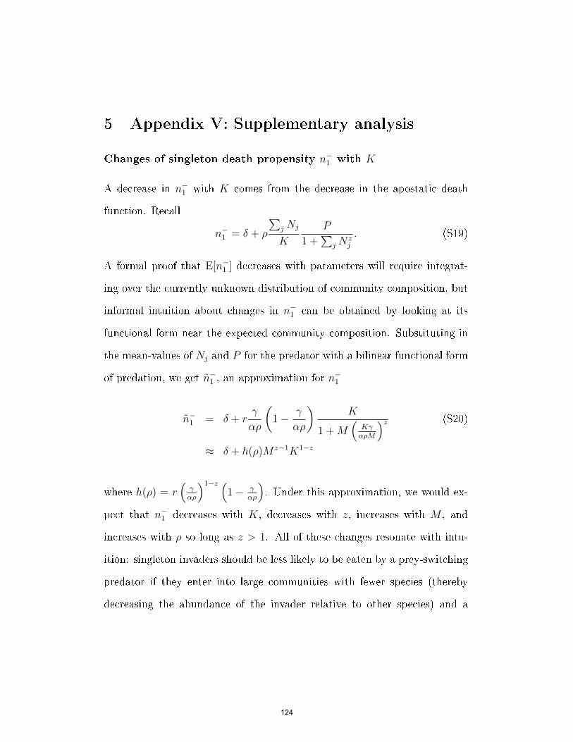
5 Appendix V: Supplementary analysis

Changes of singleton death propensity n−1 with K

A decrease in n−1 with K comes from the decrease in the apostatic death

function. Recall

n−1 = δ + ρ

∑j Nj

K

P

1 +∑

j Nzj

. (S19)

A formal proof that E[n−1 ] decreases with parameters will require integrat-

ing over the currently unknown distribution of community composition, but

informal intuition about changes in n−1 can be obtained by looking at its

functional form near the expected community composition. Substituting in

the mean-values of Nj and P for the predator with a bilinear functional form

of predation, we get n−1 , an approximation for n−1

n−1 = δ + rγ

αρ

(1− γ

αρ

)K

1 +M(

KγαρM

)z (S20)

≈ δ + h(ρ)M z−1K1−z

where h(ρ) = r(γαρ

)1−z (1− γ

αρ

). Under this approximation, we would ex-

pect that n−1 decreases with K, decreases with z, increases with M , and

increases with ρ so long as z > 1. All of these changes resonate with intu-

ition: singleton invaders should be less likely to be eaten by a prey-switching

predator if they enter into large communities with fewer species (thereby

decreasing the abundance of the invader relative to other species) and a

124

predator with low-attack rate that highly favors the more abundant species.

This calculation points to a useful quantity in the analysis of this system:

αργ, which is the expected number of o�spring, P0, produced by a single preda-

tor invading a community saturated with K prey. This quantity is also the

fold-decrease in prey populations observed following predator introduction,

an empirically tractable quantity that we used to estimate the parameter ρ.

We de�ne P0 = αργand rewrite equation S20

n−1 ≈ δ + rK1−z (MP0)z−1 (1− P−10

). (S21)

We see that for z > 1, n−1 is monotonically increasing with P0, and not just

ρ.

Investigating the number of singletons Ψ1

One may be able to compute Ψ1 through an iterative scheme but often such

schemes provide little intuition about Ψ1 and therefore leave us without rules-

of-thumb about how/why a prey-switching predator reduces the number of

singletons and how that scales with ρ and z (e.g. ?). We attempted to �nd

such rules of thumb by considering the probability that a species is a singleton

given that it is present in the community. We denote this probability π1. If

migrations are zero and if the propensity of singleton deaths were constant,

π1 is the quasistationary probability that an extant species is a singleton.

This quantity would be inversely related to the mean time to extinction, τE

125

(?):

τE =1

n−1 π1

. (S22)

In seeking an approximation for π1, we hypothesized that migration has a

negligible e�ect in our model, that n−1 approximately constant, and that we

could search for a reasonable approximation to π1 based on some function of

descriptive statistics of the distribution of prey population size such as the

mean, µN and variance, σ2N , conditioned on the prey species being present

in the community. In particular, decreases in the mean and increases in the

variance might be be tied to increases in π1. We developed these hypotheses

from the change in the probability density at x = 1 with changes in mean and

variance of a unimodal distribution with mean greater than 1, small relative

variance, and negligible skewness.

We explored various combinations of the mean and variances (e.g. the

coe�cient of variation θ = σNµN

) in search of a useful and empirically mea-

surable quantity that predicts π1, and consequently extinction rates, thus

yielding rules of thumb for the statistical signatures of prey communities

that would bene�t from prey-switching predation. Such a relationship be-

tween θ and extinction rates would open the door to incorporating known

scaling laws between the mean & variance (???) and might provide fruitful

discussion about the potential scaling of a prey-switching predator's e�ect

on prey diversity in natural systems.

However, although the coe�cient of variation was a good approximation

126

for π1 and both changed non-monotonically with ρ in much the same way

as the species richness, they provided a poor approximation of Ψ1 due to

the confounding and logically circular e�ect of the number of species in the

community at stationarity. Conditioned on there being fewer species, µN and

σ2N should rise, and in fact we see for high ρ an increase in the coe�cient

of variation of species conditioned on their being present in the community

(see Figure S12). It remains an open challenge to �nd heuristics and rules of

thumb based on measurable properties of prey populations that can predict

the e�ect of a predator on prey diversity given its attack rate and degree of

prey switching.

Investigating Cov[n−1 ,Ψ1]

Decreasing the variance in relative abundance of prey populations will change

the distribution of the number of singletons at any given point of time. For

example, consider a 2-species community. When the variance in relative

abundance is non-zero and variance in community size zero, the multivariate

prey density falls on the line Ni+Nj = C and there can be only one singleton

at any point in time. When a singleton is present in the community, Ψ1 = 0

or Ψ1 = 1 and thus n−1 takes on its second-lowest value

n−1 = δ + ρC

K

P

1 + (C − 1)z. (S23)

127

Therefore, when a singleton is present, Cov[n−1 ,Ψ1] < 0 when σ2R is large and

σ2C small. When the variance in relative abundance is zero, then N1 = N2

and the distribution of the number of singletons will fall entirely on either

Ψ1 = 0 or Ψ1 = 2, causing n−1 to take its highest value

n−1 = δ + ρP

K(S24)

when both species are singletons.

This analysis is complicated in multi-species communities with interme-

diate degrees of variance along and orthogonal to the simplex, but we suspect

that intuition from the 2-species case extends to multispecies communities.

For a given community size, C, n−1 is maximized when the community is per-

fectly even (Ni = Nj = N for all i, j), and for communities that are perfectly

even n−1 increases as the community gets small. We hypothesize that in gen-

eral n−1 increases monotonically along some direction of increasing evenness

and decreasing C. We hypothesize Cov[n−1 ,Ψ1] increases faster with ρ for

higher z because the predator decreases the variance in relative abundance

thereby increasing the variance of Ψ1, and this decrease in variance is greater

for a more e�ective prey-switcher (higher z). When there are above-average

numbers of singletons in a community with highly covarying populations,

we expect the total community size to be low, and the expected evenness

generated by a prey-switching predator will yield higher-than-average n−1 .

Increases in K will be tied to decreases in the variance of both n−1 (due to

128

the apostatic death function behaving like something between K−1 and K1−z

for z > 1; see equation S19) and Ψ1 (by moving the entire multivariate den-

sity away from the boundaries where singletons occur), and thus increases in

K should be associated with decreases in Cov[n−1 ,Ψ1].

Existence of ρ∗ and K∗

We are now equipped to see how K modulates the e�ect of predation on

species richness in our model. The existence of ρ∗ is ensured by su�ciently

large increases of E[n−1 ], E[Ψ1], and Cov[n−1 ,Ψ1] with ρ beyond the point of

maximal species richness. However, the existence of ρ∗ does not automat-

ically imply the existence of a critical carrying capacity K∗, above which

a prey-switching predator improves species richness and below which sup-

presses species richness relative to a predator free community. In order for

K∗ to exist, species richness must increase more rapidly withK in the vicinity

of ρ = ρ∗ than at ρ = 0.

To see why this occurs, we �rst note that for z > 1, n−1 decreases with

K for ρ > 0 but not for ρ = 0 since the singleton death rate in absence

of predation is simply δ. As long as Ψ1 and/or the covariance Cov[n−1 ,Ψ1

]do not increase with K, this result ensures that some predation regimes will

have opposite e�ects on richness depending on the value of K. In fact, in

our models Ψ1 and Cov[n−1 ,Ψ1

]enhance the e�ect further.

In our models, variation in n−1 is shallow over K ∈ [500, 2000] and cannot

account for the full e�ect (Figure S8). Instead, much of the e�ect can be at-

129

tributed to the decreasing of the number of singletons Ψ1 and the decreasing

covariance Cov[n−1 ,Ψ1

]with increasing K (Figure 5a). In the predator-free

communities (ρ = 0), Cov[n−1 ,Ψ1] = 0 since n−1 is independent of the com-

munity state, and Ψ1 varies little across the full range of carrying capacities

considered. However, in the presence of prey-switching predators (ρ > 0

and z > 1), smaller communities have higher covariance Cov[n−1 ,Ψ1

]. This

probably results from an increase in the between-prey covariance σi,j, which

causes singletons to occur when community sizes are below average and,

consequently, n−1 above average.

Variance in relative abundance as a measurable, heuristic tool for

assessing impacts of stabilizing forces on species richness

Rates of prey-switching predation on a focal species increase as a function

of that species' relative abundance, and thus �uctuations in relative abun-

dance may be more informative than �uctuations in numerical abundance for

understanding the impacts of a prey-switching predator (or other frequency-

dependent stabilizing mechanism) on the statistics of the population sizes

of its prey and community species richness. Fluctuations in community size

with �xed relative abundance are visualized as spread of the multivariate

prey distribution along the major axis of the ellipses pictured in Figure S9

(see also Figure 5b). Fluctuations in relative abundance in a �xed commu-

nity size, on the other hand, are �uctuations on a simplex (the minor axis of

the ellipses).

130

A Taylor expansion for the moments of the relative abundance yields

an approximation for the variance in relative abundance. This allows us to

appreciate the relationship between the relative abundance and statistics of

the distribution of prey population size. For a function f(X, Y ) of random

variables X and Y with well de�ned means and variance, its variance can

be approximated by performing a Taylor expansion about µX and µY , the

means of X and Y , respectively

Var [f(X, Y )] ≈ Var

[f(µX , µY ) + (X − µX)

∂f

∂X+ (Y − µY )

∂f

∂Y

](S25)

≈(∂f

∂X

)2

σ2X +

(∂f

∂Y

)2

σ2Y + 2

(∂f

∂X

)(∂f

∂Y

)Cov [X, Y ]

where the derivatives are evaluated at (X, Y ) = (µX , µY ). Performing this

expansion for the relative abundance R of some populationN in a community

of size C (R = N/C), we obtain

Var [R(N,C)] ≈ σ2N

µ2C

+µ2N

µ4C

σ2C − 2

µNµ3C

Cov [N,C] (S26)

where µN is the expected population size, µC the expected community size,

σ2N the variance of a prey species' population size, σ2

C the variance in com-

munity size, and Cov [N,C] the covariance between a focal prey population

and the community size. Assuming all M prey species are neutral, we have

that µC = MµN , Cov [N,C] = σ2N +(M − 1)σi,j, where σi,j is the covariance

between two populations. Substituting these into equation 25, we get an

131

expression for the variance in relative abundance, σ2R

σ2R ≈

σ2N

M2µ2N

+1

M4µ2N

[Mσ2

N +M (M − 1)σi,j]

− 2

M3µ2N

(σ2N + (M − 1)σi,j

).

(S27)

This simpli�es to

σ2R ≈

M − 1

M3

[(σNµN

)2

− σi,jµ2N

](S28)

or

σ2R ∝ θ2 − ζ2 (S29)

where θ = σNµN

is the coe�cient of variation and ζ =√σi,jµN

the coe�cient of

covariation. From this approximation, we see that changes in the variance

in relative abundance, the coe�cient of variation, and the covariance are

intimately tied. In the case where prey-switching is independent of over-

all predation rates (as in our models), prey-switching predators increase the

covariance between prey populations and decrease the variance within prey

populations. The overall e�ect is to decrease the variance in relative abun-

dance.

It turns out that this decomposition of population �uctuations in terms

of �uctuations in community size and �uctuations on simplices of constant

community size may lead scale-free statistics of population �uctuations that

132

are useful for understanding how stabilizing forces impact extinction risk.

Both the coe�cient of variation and the coe�cient of covariation scale with

K; we can approximate them as θ ≈ θK−12 and ζ ≈ ζK−

12 where θ and ζ

do not depend on K. We de�ning a re-scaled compositional variance σ2R =

σ2RK

−1, and we have

σ2R ∝

1

K2

[θ2 − ζ2

](S30)

which combines information from the means, variances and covariances in

prey populations to yield a useful metric of �uctuations in relative abun-

dance - precisely the �uctuations that are dampened by many stabilizing

mechanisms (including our prey-switching predators). We observe from our

models that for a given value of z, σ2R is a good metric of extinction rates

across a range of K and ρ (Figure S13). Note, however, that additional

information about z is necessary to predict species richness from empirical

measurements of σ2R, because systems without prey-switching predators (the

diamonds in Figure S13) or with di�erent values of z fall on a di�erent lines

from one another.

We do not know the exact reason for the close relationship between σ2R

and species richness, but it may be related to the relationship between σ2R and

the expected angular displacement of the community from its mean (Figure

S14). De�ning

φ = 2 cos−1

( ∑iNi√∑iN

2i

)

we can re-write φ as a function of relative abundances, Ri = Ni∑j Nj

and

133

perform a Taylor expansion of φ about the mean relative abundances E[R]

and note that all species are neutral to approximate

E[φ] ≈ Mσ2R

∂2

∂R2i

cos−1

(∑i

R2i

)− 12

E[R]

+2M(M − 1)Cov[Ri, Rj]

∂2

∂Ri∂Rj

cos−1

(∑i

R2i

)− 12

E[R]

and thus

E[φ] ∝ σ2R + aCov[Ri, Rj]

where a is some constant. In the special case of a 2-species community (or any

grouping of a community into two groups that are equivalent both in the eyes

of the researcher and of the predator) we have relative abundances R1 and

R2 = 1−R1, and Cov[Ri, Rj] = −σ2R thus our approximations imply a direct

proportionality between the expected angular deviation and the variance

in relative abundance E[φ] ∝ σ2R (Figure S14). Intuition for the utility of

the variance in relative abundance towards making scale-free statistic for

estimating extinction rates and equilibrium species richness comes from its

proportional relationship between the angular deviation of a community from

its mean, as these radial coordinates are closer to a scale-free indicator of

the proximity of a community to the edges where extinctions occur. More

thorough analysis is warranted, as are tests of whether or not the statistics

σ2R, σ

2R and φ are useful in asymmetric communities (perhaps with re-scaled

134

axes to ensure the central tendency of the rescaled community is centered in

the positive orthant).

Figure S13: Species richness vs. σ2R (equation S30) plotted for K ∈ {500, 1000, 2000}, along lines

of increasing ρ ∈ [0, 350]. σ2R may be a useful proxy for extinction risk given a particular mechanism of

stabilization. More information is required to predict species richness for di�erent stabilizing mechanisms,

as systems without prey-switching predators (solid diamonds) or systems with di�erent degrees of prey-

switching stabilization (the two subplots) appear to fall on signi�cantly di�erent curves.

135

Figure S14: The expected angular displacement of a community from its mean, φ, is linearly related

to the variance in relative abundance. Since the variance in relative abundance, σ2R, is dampened by

frequency-dependent stabilizing mechanisms, φ and σ2R may lead to useful scale-free statistics for assessing

extinction risk in �nite communities with frequency-dependent stabilization such as the prey-switching

predators we've considered.

6 Appendix VI: Guide to MATLAB simulation

code

We provide all of our MATLAB code for simulation in the online supplement.

The logic of the simulations is described in detail both in the main paper and

in annotations embedded within the attached MATLAB �les. Some minor

di�erences exist between the variable and parameter names used in our paper

136

and those used in the code. Where they involve parameters, these di�erences

are noted in Table S1. Where they involve variables, these di�erences are

noted in the annotated code.

The MATLAB �le PredSim.m, available with the online supplementary

materials, de�nes a function PredSim that takes as inputs the control param-

eters in our models, as well as a text string that speci�es the functional form

of predation to be used. PredSim provides as outputs snapshots of the preda-

tor/prey community after simulations have run for a user-speci�ed number

of timesteps. The �le PredSim_Demo.m contains the parameter values used

in our simulations, and a few short analyses that call PredSim and provide

outputs.

137

Chapter 3: Using Neutral Theory

(Wright-Fisher Process) As a Null

Model for Ecological and Economic

Time-Series

Alex Washburne

138

Introduction

Economies, ecosystems, and other complex-adaptive systems [11, 17, 1] change

with time as the relative abundances of various companies, species, or strate-

gies go up and down by a mix of forces we can predict and whose e�ects we

understand and forces we can't predict and/or whose e�ects we don't under-

stand. Reliable forecasts of these systems has implications for asset pricing,

investment, and the management of socio-ecological systems.

A large subset of complex-adaptive systems are constrained by �nite,

limiting resources that may create an approximately zero-sum game for the

agents (species, companies etc.) in competition over those resources. Ex-

amples are the cover of canopy trees on an island [12], the land owned by

various groups (e.g. Sunni, Shiite, Kurds & others in Iraq) or the market

share of companies in constant markets. For these zero-sum communities, the

Wright-Fisher Process (WFP) serves as a mechanistically-based null model

for time-series data against which one can look for competitively superior

trees, groups or companies, or more complicated features of the data such

as covariances between groups, clustering of di�erent groups, percent vari-

ance covered by the �rst principal component, etc. Rejection of the WFP

can motivate further construction of more detailed models for the stochastic

evolution of complex-adaptive systems.

The Wright-Fisher Process is an Ito stochastic di�erential equation (SDE)

originally proposed as a model for the neutral drift of alleles in a population

139

[10, 24]. It was later adapted by Kimura [16] as a null model for the distri-

bution of the frequency of molecular polymorphisms in a population, and ex-

tended by Hubbell [12] for species-abundance distributions and species-area

relationships. It has been shown that models of volatility-stabilized markets

[9] have market weights that follow the WFP [20]. The Wright-Fisher Process

has also been proposed as an approximation to the Langevin SDE for the

random opening and closing of ion channels in neurons [6]. Tests of neutrality

have become cornerstone in population genetics [22, 7] and making neutrality

tests available for time-series datasets may accelerate our understanding of

non-neutral patterns in ecological, economic, sociological and other systems

for which the WFP is a suitable null model.

The broad use of the Wright-Fisher process stems from its parsimonious

assumptions about the underlying mechanisms of random birth, death, and

dispersal. At each timestep, an organism is drawn at random to die. Im-

mediately after death, another organism is drawn at random to replace the

organism that died. With probability 1−m, an organism is randomly drawn

from the local community to reproduce otherwise, with probability m, an

organism is randomly drawn from an in�nitely large metacommunity to mi-

grate in, thereby maintaining a constant community size. This serves as

a useful null model of neutral competition as all species have the same per-

capita �tness - there are no niche di�erences, frequency-dependent stabilizing

mechanisms, or other trophic structure stabilizing competition. For time-

series datasets of communities of constant size, one might want to make a

140

solid epistemological statement that a feature observed in their model is not

explained by neutral birth, death and dispersal. Features of interest could

include the covariance between two species, the percent of variance explained

by the 3rd principal component, or some feature of the Fourier spectrum and

other complex features for which the null distributions of test statistics under

neutral competition are not known or for which statistical null hypotheses

detached from ecological mechanisms are less relevant and less conducive to

the construction of alternative models.

The combined broad applicability of the Wright-Fisher process and re-

cent emergence of long-term ecological research (LTER) datasets and other

longitudinal studies of fast-changing communities such as microbial commu-

nities on the surface of the skin or tongue [2] motivates making the WFP of

neutral competition accessible for hypothesis testing in time-series datasets.

Some recent work has tested some analytically tractable features of popula-

tions within a neutral community [3, 15], but neutrality is not a population-

level phenomenon: species are neutral with respect to one another, and so

community-based features such as covariances and other more global struc-

tures of the data may illuminate general stabilizing mechanisms or non-

neutral trophic structure in communities. The null distributions of such

features of interest may beyond the scope of current analytical tools; there is

a need for the ability to simulate surrogate datasets of neutral drift against

which features of time-series data can be compared. However, simulation of

the WFP is fraught with pitfalls in numerical stability and computational

141

speed; a fast, numerically stable method for accurate simulation of the WFP

would greatly enable hypothetico-deductive progress in our understanding of

the mechanisms underlying the dynamics of complex-adaptive systems.

In this chapter, I present a series of tools aimed at making the WFP

accessible as a null model for time-series datasets. The �rst tool presented

is a set of volatility-stabilizing transformations which can be combined with

constant-volatility tests to test the quadratic covariation of the WFP; these

multiple volatility-stabilizing transformations can be combined in a multiple-

hypothesis-testing framework for a global test of whether an entire commu-

nity is drifting according to a WFP. Second, I develop a numerically stable

and computationally e�cient scheme for simulating the WFP founded on two

key calculations: I �nd a numerically stable decomposition of the covariation

matrix which ensures a conservation of relative abundance and real-valued

output, and I use the invertible log-odds-ratio transform to simulate a WFP

on an unbounded state space which helps ensure trajectories don't hop out

of bounds. Third, I provide calculations for parameter estimation so one

can generate surrogate WFP datasets corresponding to their data. Finally,

to illustrate the utility of the tools developed here, I analyze datasets from

the human microbiome [2] and the S&P 500 and illustrate some ways for-

ward towards the construction of alternative models that explain non-neutral

phenomena in the data. I'm happy to make my MATLAB code available

to accelerate progress on inferring non-neutral features in the dynamics of

complex-adaptive systems.

142

The Model

The Wright-Fisher Process is derived as a continuous-state approximation

of an urn process where balls are drawn out at random for death and then

instantaneously replaced with either a birth from a randomly drawn member

of the urn or a migration from a randomly drawn member of an external,

in�nitely large metacommunity [10, 24]. For a community of size J , this

translates into the following transition probabilities for a population of size

N it at time t

P{N it → N i

t + 1} =

(J −N i

t

J

)(mp+ (1−m)

N it

J − 1

)P{N i

t → N it − 1} =

(N it

J

)(m(1− p) + (1−m)

J −N it

J − 1

)P{N i

t → N it} =

(J −N i

t

J

)(m(1− p) + (1−m)

J − 1−N it

J − 1

)+

(N it

J

)(mp+ (1−m)

N it − 1

J − 1

)

where P{N it → N i

t + 1} is the probability that the population size of

species i increases by 1 individual at time step t,m is the probability of migra-

tion and pi the metacommunity relative abundance of the species. The de�n-

ing assumptions of this one-step process are the random birth/death/migration

and the constant community size creating zero-sum neutral drift.

The discrete process can be simulated directly. However, many systems

are extremely large - there are 1014 bacteria in the gut, and 1012 − 1014 dol-

lars in some markets - and the simulation of WFP surrogate datasets for

143

these systems requires either computationally intensive direct simulation of

the discrete process or more computationally e�cient simulation of a simi-

lar, continuous process. This continuous process is obtained by considering

relative abundances, X it =

N it

C. In the limit of in�nitely large system size [23]

or by setting up a martingale problem and keeping constant the product of

the probability of migration and the community size [21] one arrives at the

Wright-Fisher SDE describing the trajectories of the relative abundances of

all n species in the community:

dXt = λ (p−Xt) dt+ σ (Xt) dWt (1)

where Xt ∈ ∆n ∀t is the vector of relative abundances at time t lying in

the n − 1 dimensional simplex, ∆n, in the positive orthant of Rn, p ∈ ∆n

is the relative abundance of the n species in the metacommunity, λ = mJ

is the rate of migration from the metacommunity into the local community,

and 12σσT = Σ is the covariation matrix where

Σij =

X it (1−X i

t) i = j

−X itX

jt i 6= j.

(2)

One can verify that the process stays in the simplex by con�rming that

dXTt 1 = 0.

144

Variance-Stabilizing Transformation

One promising avenue for hypothesis testing of the WFP is to �nd certain

features of the process in equation 1 which are invariant for the WFP but

need not be for other processes, allowing one to identify processes that are

not well described by the WFP. Since the mean-reverting drift of the WFP,

λ (p−Xt) dt, is linear, any process �uctuating about a stable node would

have qualitatively similar drift near its equilibrium. One could conceivably

test for whether di�erent variables, X it , have di�erent rates of reversion to-

wards their equilibrium, λi, by noting their autocorrelation time is τ i = 1λi.

Alternatively, one could look for systems reverting to a spiral node by look-

ing for periodic signals arising in the power spectrum or the autocovariance

function.

Another approach to identifying non-neutral features of data would be to

look at global features of the covariance structure and how they di�er from

that de�ned by Σ. There are many possibilities, but here we consider just

one: a volatility stabilizing transformation, g(Xt) such that the volatility of

g is constant, V[δg|δt] = δt. The SDE for g will be

dgt =

(λ∇gT (p−Xt) +

1

2∇gTHX∇g

)dt+∇gTσ(Xt)dWt (3)

and thus the volatility over some time, δt, will be

V[dgt] = δt(∇gTσσT∇g

)(4)

145

. Substituting σσT = 2Σ and setting the volatility V[dgt] = δt, we get that

a constant-volatility transformation, g, will satisfy

∇gTΣ∇g =1

2. (5)

Using equation 2, this can be can be expanded as

n−1∑i=1

n∑j=i+1

X iXj

(∂g

∂X i− ∂g

∂Xj

)2

=1

2(6)

.

In the 2-D case, this equation is solved by setting X1 = x and X2 = y

(for aesthetic purposes), yielding

xy

(∂g

∂x− ∂g

∂y

)2

=1

2(7)

and then making the substitution w = x− y and using y = 1− x to obtain

∂g

∂w=

1√2(1− w2)

(8)

which is solved by

g =1√2

sin−1(x− y) (9)

. An empiricist worried about reproducibility might prefer a symmetric func-

tion that doesn't require choosing which species is ′x′ and which species is ′y′.

This can be obtained by noting that (x−y)2 +4xy = 1 and so the symmetric

146

function

gsym =1√2

sin−1√

4xy (10)

is also a solution to equation 7 as both g and gsym can be interpreted as the

non-right angles of a right triangle with sides of length x− y and√

4xy, and,

since x + y = 1, a hypotenuse of length 1. Thus, since g = π2− gsym, if one

angle has constant volatility then so must the other.

By setting X3 = z, the n = 3 case for a constant-volatility transformation

can be written beautifully

xy

(∂g

∂x− ∂g

∂y

)2

+ xz

(∂g

∂x− ∂g

∂z

)2

+ yz

(∂g

∂y− ∂g

∂z

)2

= const. (11)

We see that the conditions for the constant-volatility transformation are al-

ways a special case of the Hamilton-Jacobi equation,

H(x,∇f(x)) = 0

whose solutions can be found by integrating the Hamilton equations

xi =∂H

∂qi

qi = −∂H∂xi

for i = 1, ..., n where qi = ∂g∂xi

. This connection to Hamilton-Jacobi theory

is not utilized in this chapter, but Burby & Washburne (in prep) have used

147

this approach to show that the equation de�nes a metric on the simplex

with constant Gaussian curvature, allowing one to �nd Killing vectors that

enable construction of a mapping of the simplex to the sphere that serves as

a constant-volatility transformation. For instance, note that for the 2-D case

setting u =√x and v =

√y, we have that u2 + v2 = 1 - a mapping from

the 2-simplex to the 2-sphere that then enables construction of a constant-

volatility transformation sin−1√4xy. In Burby & Washburne (in prep), we

found that there are uncountably many constant-volatility transformations.

Here, I present a small, intuitively useful subset of those solutions that were

found without the Hamilton-Jacobi theory.

Solution to equation 6: 2n volatility-stabilizing transfor-

mations for the WFP

One set of solutions to equation 6 is

g(Xt) = sin−1

(n∑i=1

aiXit

)(12)

where ai = ±1. The coe�cients {ai}ni=1 de�ne a �grouping� of species by

pooling the n species into two groups, those with ai = 1 and those with

ai = −1, and thus projects the n species WFP into a 2 species WFP

and exploits the solution given above in equation 9 (similarly, equation 10

can be used to de�ne another complimentary set of solutions). This de-

�nes 2n non-superimposable solutions, all of which have constant volatility,

148

limδt→0

V[gt+δt−gt]δt

= const. De�ning ∆g = gt+δt−gt, we can then test an arbitrary

time series dataset against a null hypothesis of neutral drift by testing het-

eroskedasticity of ∆g versus g, Xt, t, and other state variables of the system.

The utility of this method is illustrated below in the section �Application to

Real Data�.

Simulation of WFP

Many scientists confronted with a time-series of a complex adaptive system

may want to explore beyond a few simple, analytically tractable features of

the WFP such as the percent of variance accounted for by the nth principal

component, the distance between two clusters in a di�usion map, the cluster

validity index for a particular clustering algorithm, or myriad other features.

To enable these scientists to have a baseline for comparison, it would be

helpful to simulate surrogate datasets of a WFP such that the null distri-

butions of the scientists' feature of choice can be obtained from simulation.

Two obstacles prevent the trivial simulation of the WFP. First, derivation

of a matrix σ which is numerically stable (i.e. σ ∈ Rn×d and 1Tσ = 0) and

computationally e�cient - simply using numerical methods for computing

the Cholesky or eigen-decomposition of Σ yield complex-valued matrices σ

and do not reliably satisfy 1Tσ = 0. Second, ensuring that the simulations

remain within the state space, ∆n. In our paper, we overcome the �rst ob-

stacle with a decomposition of Σ which works for a large class of what we

149

call �zero-sum matrices�. We overcome the second obstacle by simulating the

log-odds-ratio transform of Xt which maps ∆n into an unbounded manifold

in Rn and which can be inverted to obtain trajectories of the Wright-Fisher

process.

Decomposition of Covariation Matrix

We note that the covariation matrix, Σ, can be decomposed as Σ = PV P T

where P is what we call a �zero-sum matrix� which ensures 1TΣ = 0, and V is

the �competition matrix� - a diagonal matrix whose diagonal elements denote

the nature of competition in a zero-sum community; in the case of the WFP

the diagonal elements of V are all possible unique pairwise combinations of

X itX

jt . For instance, let n = 3 and for easier notation set X1

t = x, X2t = y,

and X3t = z, the decomposition is

1 1 0

−1 0 1

0 −1 −1

xy

xz

yz

1 −1 0

1 0 −1

0 1 −1

= .

x(1− x) −xy −xz

−xy y(1− y) −yz

−xz −yz z(1− z)

(13)

For n = 4 we use the same notation as above in addition to X4t = w to

150

write the decomposition as

1 1 1 0 0 0

−1 0 0 1 1 0

0 −1 0 −1 0 1

0 0 −1 0 −1 −1

xy

xz

xw

yz

yw

zw

1 −1 0 0

1 0 −1 0

1 0 0 −1

0 1 −1 0

0 1 0 −1

0 0 1 −1

=

x(1− x) −xy −xz −xw

−xy y(1− y) −yz −yw

−xz −yz z(1− z) −zw

−xw −yw −zw w(1− w)

(14)

which makes it easy to see the generalization to n-species communities. For

an n-species community, P ∈ Rn×M and V ∈ RM×M where M = n(n−1)2

. P

can be constructed in blocks as

P =

1Tn−1 0Tn−2 · · · 0

1Tn−2. . .

...

. . . 0

1

−In−1 −In−2 · · · −1

(15)

where 1n ∈ Rn is the vector of all 1's, 0n ∈ Rn is the vector of all 0's, and

151

In ∈ Rn×n is the identity matrix. V is a diagonal matrix whose diagonal is

formed by vectorizing, row-by-row, the upper-triangular elements of XtXTt .

This factorization allows us to compute σ directly through σ =√

2PV 1/2

and thereby guarantee real-valued noise that could not be guaranteed by

numerical Cholesky or eigen-decomposition of Σ. Furthermore, analytically

the Wright-Fisher Process should have 1TXt = 1 ∀ t and the matrix P , which

clearly has 1TP = 0, may reduce the numerical error causing increases or

decreases in the total relative abundance.

We note that this factorization may be useful for other zero-sum covari-

ance matrices where 1TΣ = 0. In particular, this factorization works for any

covariance matrix of simplex-valued processes with non-positive quadratic

covariation, d[X it , X

jt ] ≤ 0 for i 6= j. This zero-sum decomposition of the co-

variance matrix decomposes the volatility of the WFP in a meaningful way,

where the columns of P containing a 1 and a −1 show that at every time

step, δt, the transfer of relative abundance (or acquisition of market share)

from species i to species j due to neutral drift is ∆ij =√

2 (δt)X itX

jtZ ,

where Z ∼ N(0, 1) is a standard normal random variable.

Log-odds-ratio transform

The next obstacle in simulating the WFP is the preservation of the boundary.

Some work has been done on the boundary preservation of Wright-Fisher Pro-

cesses: Milstein et al. [18] constructed a Balanced Implicit Method (BIM),

152

Moro & Schurz [19] constructed a split-step method, and Danger�eld et al.

[6] combined these two in a Balanced Implicit Split Step (BISS). The ap-

proach developed here seeks to use an invertible transformation to stretch

the bounded state space of the WFP onto an unbounded state space, elimi-

nating the need for the complex boundary-preserving numerical schemes.

For a process bounded on the simplex, we can use an invertible mapping of

the simplex into an unbounded n−1 dimensional manifold in Rn, simulating

the process on the unbounded manifold, and then inverting to obtain our

surrogate dataset. I de�ne a new vector Ito process, ft, de�ned as the log-

ratio transform of the WFP,

f it = log

(X it

1−X it

). (16)

Applying Ito's lemma, we get the SDE for ft

df it =(efit/2 + e−

fit/2)2[(λpi −

1

2

)+

(1− λ)

1 + e−fit

]dt+∇fTt σ (ft) dWt (17)

where σ (ft) is σ (Xt) = PV12 converted to a function of ft by substituting

X it =

(1 + e−f

it

)−1

for all i = 1, ..., n . However, the Euler-Maruyama in-

tegration and subsequent of inversion the process in equation 17 does not

preserve the simplex (Figure 1). The warping of trajectories - and the �nal

sum of relative abundances - is independent of the step-size of integration

(Figure 1), suggesting that the error is not due to numerical error from the

discretization of the continuous process. Interestingly, changing the number

153

Figure 1: Stacked plots of the relative abundances, Xit , obtained by inverting numerical solutions

of equation 17. The solutions leave the bounds of the simplex,∑iX

it = 1, not due to numerical error

(�rst row), but instead due to some anomalous drift associated with the dimensionality of the system.

Decreasing λ and increasing the number of species, n, increase the deviation of Xt from the simplex.

When n = 2,∑iX

it ≈ 1, but when n > 2

∑Xit & 1 and increasingly so for decreasing λ. Unless the

parameters are being varied as speci�ed in the �gure title, n = 5, p = 1n, λ = 10, and ∆t = 10−4.

of species changes the degree of warping, and decreasing λ causes increased

�uctuations about the long-term average of total relative abundance (Figure

1).

I found that incorporating a dimensionality correction, −12

(n−2n

) (efit/2 + e−f

it/2)2

dt,

improves the numerical stability of simulations in a reduced error of the total

relative abundance, ε = |∑

iXit − 1| without a�ecting the covariance matrix

of Xt obtained by inverting ft. (Figure 2). The SDE for f it becomes

df it =(efit/2 + e−

fit/2)2[(λpi −

1

2

)− 1

2

(n− 2

n

)+

(1− λ)

1 + e−fit

]dt+∇fTt σ (ft) dWt

(18)

154

Figure 2: Adding a dimensionality correction to the drift of f it decreases the error in total relative

abundance, ε = |∑iX

it−1|. It is not yet proven that the solutions of the dimensionality-corrected process

converge to solutions of the WFP.

Parameter Estimation

The parameters λ and p can be estimated by relating the mean and variance

of the WFP. Considering a single species whose dynamics are covered by the

univariate WFP

dXt = λ (p−Xt) dt+√

2Xt (1−Xt)dWt (19)

we can look at the dynamics of the �rst two moments, mt = E[Xt] and

st = E[X2t ]. Using Ito's lemma and the Ito Isometry one obtains the system

155

of ODEs

dmt

dt= λ (p−mt) (20)

dstdt

= 2 (1 + λp)mt − 2 (1 + λ) st

which yields the stationary mean, m∞ = limt→∞mt and second moment

s∞ = limt→∞st

m∞ = p

s∞ =1 + λp

1 + λm∞. (21)

Thus, the stationary mean is µ = p and the stationary variance is given by

v2 = s∞ −m2∞, yielding v

2 = p(1−p)1+λ

.

These two equations give one way of estimating λ and p from a time-

series dataset: calculate the sample mean of each species {µi}ni=1 and then

the sample variance of a focal species, v2i to get

pi = µi

λi =µi (1− µi)

v2i

− 1 (22)

or one can utilize their full data by getting the sample mean of each species

and sample variance of each species, v2i and use the full dataset to estimate

156

λ

λn =n∑i=1

λin

(23)

Other methods can be developed, such as pooling species until the pool has

an average relative abundance near 0.5, but for this paper I focus on pi = µi

and λn given in equation 23.

Figure 3: Parameter Estimation - plots of true values of the parameter versus their estimates for

700 solutions to equation 18 integrated over t ∈ [0, 2] and sub-sampled for T ∈ [10, 100, 1000] timesteps.

p = [1, 1.5, 3, 4.5] for every solution and each solution had a unique λ drawn from a uniform distribution

on [10, 50]. (A) The time-average provides an unbiased estimate of p, shown here as plots of the mean

estimator ±2 standard deviations over the 700 replicates. (B) Equations 22 and 23 provide estimates of

λ, but appear to be biased over-estimates of the true value of lambda, possibly due to the dimensionality-

correction factor introduced in equation 18.

The last parameter that remains to be estimated is the length of time,

Test, to simulate our surrogate datasets. This can be obtained by noting that

the true autocorrelation time of the WFP is τc = 1λ, i.e. the autocorrelation

C(Xt, Xt+τc) = e−1. For a dataset with M time points the autocorrelation

157

function can be interpolated to �nd the time lag, τ with 0 ≤ τ ≤ M , where

C(Xt, Xt+τ ) = e−1. We want a surrogate dataset to be simulated for the

same number of autocorrelation times as our empirical data, i.e. Testτc

= Mτ,

thus the time-length for the surrogate dataset will be

Test =M

λτ(24)

Figure 4 indicates that equation 24 produces a biased estimate of Test,

especially when using the true value of λ instead of its estimate λ1.

Figure 4: Estimating T and simultaneous inference of λ and T . 3000 values of T were drawn from a

log-uniform distribution, T ∈ [0.1, 10]. Equation 18 with λ = 20, n = 2 and p =

(1/21/2

)was numerically

integrated over [0, T ] for each value of T . The full trajectory was sub-sampled at M = 300 time points

equally spaced between 0 and T , and from that dataset λ1 was estimated through equation 22 and then

Test was obtained through equation 24.

158

Application to Real Data

To demonstrate a test of neutrality, I simulated a 15-species neutral commu-

nity using the method described below in equation 18, a set of 15 geometric

Brownian motions

d log Y it = µdt+ σdW i

t (25)

and a set of 15 mean-reverting geometric Brownian motions

d logZit = µ

(zi − Zi

t

)dt+ σdW i

t (26)

with µ = 15 and σ = 30. Solutions to these equation are later projected

onto the simplex, Y∆t = Yt

|Yt| , Z∆t = Zt

|Zt| . Sample trajectories for these three

simplex-valued Ito processes are plotted in �gure 5 below.

159

Figure 5: Testing Neutral Drift. The function g(Xt) : ∆n → R de�ned in equation 12 transforms a

Wright-Fisher trajectory from equation 1 into an Ito process with constant volatility seen in the Gaus-

sian distribution of ∆g and the homoskedasticity and absence of a trend in scatterplots of ∆g versus g.

Processes with di�erent covariance matrices, such as the simplex-projected geometric Brownian motion of

equation 25 or the simplex-projected mean-reverting geometric brownian motion of equation 26, may have

a combination of non-Gaussian distributions of ∆g and trends or heteroskedasticity in ∆g with respect to

other state variables, g, Xt, t. In the bottom panel, P-value distributions from White homoskedasticity

tests of ∆g vs. g are produced from 2,000 randomly drawn groupings, g. Tests of uniformity of this

P-value distribution provide a test of the WFP as a null model for time-series datasets. The P-values

are uniformly distributed when the process is a neutral community of size C = 10, 000 or a WFP, and

non-uniformly distributed (with many low P-values) for the geometric brownian motion and the mean-

reverting geometric brownian motions from �gure 1. The dependence of the P-values, however, causes a

high type 1 error rate for a standard Kolmogorov-Smirnov test; corrrecting for this dependence - either by

analytical calculation of the simulation of surrogate datasets to produce a null distribution of KS-statistics

- will allow for more accurate statements of the error rates in this test.

160

The fact that there are 2n solutions all with constant volatility can be

exploited to make a test of neutrality that does not require subjective choice

of grouping {ai}. If a process is a WFP and the time-points are equally

spaced, then the P-values for any test of normality or homoskedasticity or

trends of ∆g should be uniformly distributed. Thus, 2n P-values can be

generated from any test of constant volatility of the 2n variance-stabilizing

transformations and a uniform distribution of P-values fails to reject the null

hypothesis of neutral drift. A left-skewed P-value distribution leads to the

qualitative rejection of the WFP as a null model for the time series dataset.

The bottom panel of Figure 5 shows the resulting P-value distributions from

normality tests of ∆g for 2,000 randomly sampled groupings, g, indicating a

uniform distribution of P-values for the WFP and a correct rejection of the

non-neutral drifts plotted above.

Next, I apply these same ∆g homoskedasticity tests time-series datasets

from 372 time points of a male's palm, tongue and gut microbiomes, 130

time points of a female's palm, tongue and gut microbiomes [2] and 1256

day-end prices and market capitalization of all companies continuously in

the S&P 500 from January 1st 2000 to January 1st 2005 are tested for non-

neutral dynamics (data obtained from CRSP). For these datasets, one could

�t species-abundance distributions as in �gure 6, but I hope to show that

the species-abundance distribution �tting is a much weaker test than the

time-series analysis presented here and are summarized in �gure 7.

161

Figure 6: Species-abundance distributions for BCI [4], the male tongue and female gut metagenomes

[2] �t using the �untb� and �sads� packages in R. Species-abundance distributions are just snapshots

of communities �uctuating over time - the added information contained in time-series datasets can be

exploited to develop more powerful tests of Neutral Theory.

162

Figure 7: Testing neutral theory with ecological and economic time-series datasets. Time-series

datasets from 372 time points of the human microbiome [2] and 1256 time points of share prices and

market capitalization from all companies continuously in the S&P 500 from years 2000-2005 are tested

for non-neutral dynamics by White tests on g vs. ∆g for 4,000 randomly drawn variance-stabilizing

transformations, g (using function TestHet in MATLAB by pure quadratic regression of residuals, ε2 =

β0+β1gt+β2g2t +e, following linear regression of g on ∆g, ∆gt = γ0+γ1gt+ε). (A)Metagenomic samples

from a male's tongue qualitatively appear to have non-neutral dynamics based on the non-uniformity of the

P-value distribution from White tests also seen clearly in the CDF. Alternative models or explanations

for stochastic dynamics of this male's tongue microbiome may gain insight from inspection of scatter

plots of g versus ∆g and the coe�cients, β for auxillary regression in the signi�cantly heteroskedastic

cases (P < 0.05). The scatterplots of g versus ∆g indicate a clear negative slope that persists across many

choices of g (this is con�rmed by looking at the dominance of negative values for γ1) - it's possible that the

long time-intervals between samples require a drift-correction, a hypothesis investigated further in �gure 7

below. Looking for heteroskedasticity beyond the clear trend in ∆g, we see that for the male tongue, 751

out of the 4,000 choices of g (18%) had P < 0.05 from the White test. 513 out of the 751 cases of signi�cant

heteroskedasticity had β2 > 0, which correspond to a volatility smile of g - high variance of ∆g at the

extreme values of g. (B) Repeating a similar analysis for other microbiomes and for the S&P 500 data

lead to various qualitative results ranging from clear rejection of the WFP for the movement of market

weights and relative market cap to more uniformly-distributed P-values for a female's tongue microbiome.

The dependence of the P-values on each other invalidate a Kolmogorov-Smirnov goodness-of-�t test for

concise statements of acceptance/rejection of the WFP in these cases.

The microbiome datasets all appeared to yield a negative relationship

163

between gt and ∆gt. To test whether or not this could be caused by coarse

sampling of a Wright-Fisher process, values of λ and T were estimated for

the male tongue microbiome by grouping the �rst 200 operational taxonomic

units (OTUs), yielding a mean relative abundance µ = 0.5652, and then

applying equations 22 and 24 described above. This yielded λ = 18.0063

and interpolating the �rst 5 values of the autocovariance to �nd where τc (in

units days) such that C(Xt, Xt+τc) = e−1, we get an estimate τc = 1.5318 and

consequently Test = 13.4872. 1000 surrogate datasets corresponding to this

grouping of the �rst 200 OTUs was constructed by integrating the 2-species

equations 18 and 17 (which are identical for n = 2) over t ∈ [0, Test] using

the decomposed σ(ft) discussed in equations 12-14 and an Euler-Maruyama

integration scheme with ∆t = 10−5. No samples left the boundary of the

simplex, so there was no need to re-sample trajectories. The full surrogate

time-series was sub-sampled at 372 equally spaced time points and the results

are summarized below in �gure 8.

Discussion

Complex adaptive systems change with time and quantifying the uncertainty

of their future states has major implications for investment in and manage-

ment of these systems. Ecological communities are composed of many in-

dividual organisms competing over the same, �nite, limiting resources, and

these communities turn over as organisms reproduce, die, and migrate. Eco-

164

Figure 8: 1,000 surrogate trajectories were run using the parameter estimation and simulation tools

provided here to investigate whether the negative slope of ∆gt versus gt could arise in neutral simulations

with long time-intervals between samples. In the top-right sub-panel, I've plotted ∆g versus g for all 1,000

replicates (a total of 372, 000 points), from which we see that under the null hypothesis of a WFP we can

obtain a cloud of points with a negative slope of ∆g vs. g if the time between samples is long (black dots

are from surrogate datasets, red dots are from the grouping of the male tongue used to parameterize these

simulations). Thus, the negative slope of ∆g versus g seen in �gure 7a is not the noteworth departure from

neutrality. However, the P-values from White homoskedasticity tests are still uniformly distributed even

with longer time intervals between timepoints. Since the trajectories simulated here are independent, the

P-values in the White tests are also independent (since there is only one informative volatility-stabilizing

transformation for each trajectory), and a KS test can be used to suggest that the CDF is in fact uniformly

distributed with P = 0.3085. Further analysis of the auxillary regression shows that 20 out of 42 of the

trajectories yielding signi�cant heteroskedasticity had β2 > 0. The 20 out of 42 β2 > 0 in the WFP is

signi�cantly di�erent from the 513 out of 751 in the male tongue dataset (P = 9.9× 10−9). This provides

more evidence that the non-neutrality of the male tongue may come from a tendency for the community

to become more volatile when it is farther from its mean; this could be veri�ed by constructing alternative

models with hypervariable rare & abundant species or analogs of stochastic volatility models which try to

explain a similar volatility smile in �nancial data.

165

nomic markets are composed of many companies competing over a �nite

amount of capital - measured in human capital, number of loyal customers,

capital stock or investment capital - and the market shares of these compa-

nies changes with time. The birth & death process underlying the turnover

of these ecological and economic systems has led many authors to hypoth-

esize that ecosystems, economies, and other complex adaptive systems may

be qualitatively similar [11, 17, 1]. The Wright-Fisher Process is a null model

for the turnover of such systems with birth, death, dispersal, and zero-sum

competition over �nite resources. It can be used as a null model for popula-

tions of genes [16], communities of tropical trees [12] market weights [9, 20]

and other systems, and it is a compelling null hypothesis as neutrality may

be a likely occurrence because anything with a signi�cant competitive disad-

vantage will be quickly driven extinct, leading to an evening of competitive

abilities over evolutionary timescales [13].

In ecology and population genetics, Neutral Theory has been developed

for communities with zero-sum competition. Clear examples of a zero-sum

competition exist in nature, such as competition over limiting space - as in

percent cover of trees in the Amazon or the amount of land allocated to one

of a set of land uses such as agricultural, residential, open space, national

forest, etc. Some communities or markets may not be strictly zero-sum, but

their approximately constant size might warrant zero-sum competition as an

approximation. However, since Pal [20] has shown that one particular model

of market weights can still be a Wright-Fisher process in its relative abun-

166

dances despite not having zero-sum constraints on absolute abundances, the

rejection of zero-sum community dynamics does no reject the possible neu-

trality of the species in the community. Some authors use species-abundance

distributions to test for neutral drift, but since in�nitely many models have

the same stationary distributions such tests may not be the most powerful.

In the presence of time-series datasets for ecological or economic systems, one

might hope to use the added information from the time series to construct

stronger neutrality tests.

In this chapter, I provided two main tools for hypothesis-testing of neu-

tral drift in time-series ecological and economic datasets: volatility-stabilizing

transformations, and a means for the fast and reliable simulation of WFP

surrogate datasets whose parameters can be estimated from the data. How-

ever, more work needs to be done to make these tools accessible to researchers

as reliable and user-friendly packages in R and MATLAB. For the constant-

volatility tests, the multiple-hypothesis-testing framework of testing the uni-

formity of P-values from homoskedasticity/constant-volatility tests for the

multiple choices of g requires a test-statistic, such as the Kolmogorov-Smirnov

test statistic, whose null distribution is known. For the simulations, the vi-

ability of higher-order integration schemes and adaptive algorithms for ad-

justing the time-window of integration could be explored to develop more

reliable simulators. For parameter estimation, the clear bias in the estimates

of λ and T must be corrected, which may be resolved using techniques from

the literature on parameter estimation in stochastic di�erential equations.

167

Ultimately, though, the rejection of a null hypothesis is only as com-

pelling as the null hypothesis. The WFP has been proposed as a null model

for many systems, but repeated rejection of the WFP may render it obsolete.

Time-series datasets can provide more powerful tests and enable the swift

rejection of the WFP along with the construction of more suitable alterna-

tive models by careful assessment of how our data di�er from neutrality -

e.g. by having hyper- or hypo-variable rare species or particular taxonomic

groupings (e.g. C3 or C4 grasses) which yield particularly non-neutral dy-

namics. Some alternative models already exist or are in development, such

as the Atlas model [8] or urn processes with frequency-dependent stabilizing

mechanisms analogous to Janzen-Connell e�ects ([14, 5], Socolar & Wash-

burne, in prep), and comparison of patterns in gt vs. ∆gt plots like �gures

7 and 8 will be a stepping stone towards the development and motivation

of more compelling alternative models. The production of reliable models

of the stochastic evolution of complex-adaptive systems can enable better

forecasts of species richness and community viability in ecology to enable

better reserve design or �sheries management; it can enable the construction

of portfolios to achieve particular goals balancing risk and return [8]; it can

allow the development and clinical trial of more potent probiotics through a

better understanding of the pharmacokinetics of probiotics.

168

Acknowledgments

I thank my colleagues D. Lacker for his patient instruction in all things

stochastic and many interdisciplinary discussions on the interface between

ecology and economics, S. Pacala for introducing me to the problem and

for providing short but brilliant insights along the way, R. Chisholm for

many useful discussions and feedback, E. Shertzer for help with parameter

estimation, J. Burby and S. A. Levin for many hours of fun math working

towards the variance-stabilizing transformation, J. Squire for computational

support and inspirational badassedness, and J. O'Dwyer for his help with

species-abundance distributions and other null models for the dynamics of

gut biota.

References

[1] W Brian Arthur. Complexity and the economy. science, 284(5411):107�

109, 1999.

[2] J Gregory Caporaso, Christian L Lauber, Elizabeth K Costello, Donna

Berg-Lyons, Antonio Gonzalez, Jesse Stombaugh, Dan Knights, Pawel

Gajer, Jacques Ravel, Noah Fierer, et al. Moving pictures of the human

microbiome. Genome Biol, 12(5):R50, 2011.

[3] Ryan A Chisholm, Richard Condit, K Abd Rahman, Patrick J Baker,

Sarayudh Bunyavejchewin, Yu-Yun Chen, George Chuyong, HS Dat-

169

taraja, Stuart Davies, Corneille EN Ewango, et al. Temporal variability

of forest communities: empirical estimates of population change in 4000

tree species. Ecology letters, 17(7):855�865, 2014.

[4] Richard Condit. Tropical forest census plots: methods and results from

Barro Colorado Island, Panama and a comparison with other plots.

Springer Science & Business Media, 1998.

[5] Joseph H. Connell. On the role of natural enemies in preventing compet-

itive exclusion in some marine animals and in rain forest trees. In P. J.

den Boer and G. Gradwell, editors, Dynamics of Populations. Pudoc,

Washington, 1971.

[6] Ciara Danger�eld, David Kay, and Kevin Burrage. Stochastic models

and simulation of ion channel dynamics. Procedia Computer Science,

1(1):1587�1596, 2010.

[7] Justin C Fay and Chung-I Wu. Hitchhiking under positive darwinian

selection. Genetics, 155(3):1405�1413, 2000.

[8] E Robert Fernholz. Stochastic portfolio theory. Springer, 2002.

[9] Robert Fernholz and Ioannis Karatzas. Relative arbitrage in volatility-

stabilized markets. Annals of Finance, 1(2):149�177, 2005.

[10] Ronald Aylmer Fisher. The genetical theory of natural selection. Claren-

don, 1930.

170

[11] John H Holland. Complex adaptive systems. Daedalus, pages 17�30,

1992.

[12] Stephen P Hubbell. The uni�ed neutral theory of biodiversity and bio-

geography (MPB-32), volume 32. Princeton University Press, 2001.

[13] Stephen P Hubbell. Neutral theory in community ecology and the hy-

pothesis of functional equivalence. Functional ecology, 19(1):166�172,

2005.

[14] Daniel H. Janzen. Herbivores and the number of tree species in tropical

forests. The American Naturalist, 104(940):501�528, 1970.

[15] Michael Kalyuzhny, Efrat Seri, Rachel Chocron, Curtis H Flather, Ro-

nen Kadmon, and Nadav M Shnerb. Niche versus neutrality: A dynam-

ical analysis. The American Naturalist, 184(4):439�446, 2014.

[16] Motoo Kimura. The neutral theory of molecular evolution. Cambridge

University Press, 1985.

[17] Simon A Levin. Ecosystems and the biosphere as complex adaptive

systems. Ecosystems, 1(5):431�436, 1998.

[18] GN Milstein, Eckhard Platen, and Henri Schurz. Balanced implicit

methods for sti� stochastic systems. SIAM Journal on Numerical Anal-

ysis, 35(3):1010�1019, 1998.

171

[19] Esteban Moro and Henri Schurz. Boundary preserving semianalytic

numerical algorithms for stochastic di�erential equations. SIAM Journal

on Scienti�c Computing, 29(4):1525�1549, 2007.

[20] Soumik Pal. Analysis of market weights under volatility-stabilized mar-

ket models. The Annals of Applied Probability, 21(3):1180�1213, 2011.

[21] Daniel W Stroock and SR Srinivasa Varadhan. Multidimensional di�us-

sion processes, volume 233. Springer Science & Business Media, 1979.

[22] Fumio Tajima. Statistical method for testing the neutral mutation hy-

pothesis by dna polymorphism. Genetics, 123(3):585�595, 1989.

[23] N. G. van Kampen. Stochastic processes in physics and chemistry.

North-Holland, Amsterdam ; New York : New York, 1981.

[24] Sewall Wright. Evolution in mendelian populations. Genetics, 16(2):97,

1931.

172