Climatic changes in Eurasia and Africa at the last glacial maximum and mid-Holocene: reconstruction...
19
Climatic changes in Eurasia and Africa at the last glacial maximum and mid-Holocene: reconstruction from pollen data using inverse vegetation modelling Haibin Wu Joe ¨l Guiot Simon Brewer Zhengtang Guo Received: 26 June 2006 / Accepted: 11 January 2007 Ó Springer-Verlag 2007 Abstract In order to improve the reliability of climate reconstruction, especially the climatologies outside the modern observed climate space, an improved inverse vegetation model using a recent version of BIOME4 has been designed to quantitatively reconstruct past cli- mates, based on pollen biome scores from the BIOME6000 project. The method has been validated with surface pollen spectra from Eurasia and Africa, and applied to palaeoclimate reconstruction. At 6 cal ka BP (calendar years), the climate was generally wetter than today in southern Europe and northern Africa, espe- cially in the summer. Winter temperatures were higher (1–5°C) than present in southern Scandinavia, north- eastern Europe, and southern Africa, but cooler in southern Eurasia and in tropical Africa, especially in Mediterranean regions. Summer temperatures were generally higher than today in most of Eurasia and Africa, with a significant warming from ~3 to 5°C over northwestern and southern Europe, southern Africa, and eastern Africa. In contrast, summers were 1–3°C cooler than present in the Mediterranean lowlands and in a band from the eastern Black Sea to Siberia. At 21 cal ka BP, a marked hydrological change can be seen in the tropical zone, where annual precipitation was ~200–1,000 mm/year lower than today in equatorial East Africa compared to the present. A robust inverse relationship is shown between precipitation change and elevation in Africa. This relationship indicates that precipitation likely had an important role in controlling equilibrium-line altitudes (ELA) changes in the tropics during the LGM period. In Eurasia, hydrological de- creases follow a longitudinal gradient from Europe to Siberia. Winter temperatures were ~10–17°C lower than today in Eurasia with a more significant decrease in northern regions. In Africa, winter temperature was ~10–15°C lower than present in the south, while it was only reduced by ~0–3°C in the tropical zone. Compari- son of palaeoclimate reconstructions using LGM and modern CO 2 concentrations reveals that the effect of CO 2 on pollen-based LGM reconstructions differs by vegetation type. Reconstructions for pollen sites in steppic vegetation in Europe show warmer winter tem- peratures under LGM CO 2 concentrations than under modern concentrations, and reconstructions for sites in xerophytic woods/scrub in tropical high altitude regions of Africa are wetter for LGM CO 2 concentrations than for modern concentrations, because our reconstructions account for decreased plant water use efficiency. Keywords Palaeoclimatology Á Pollen Á Biome scores Á BIOME4 Á Atmospheric CO 2 Á LGM Á Mid-Holocene 1 Introduction Knowledge of palaeoclimates is crucial for the evalu- ation of climate model simulations, because such H. Wu Á Z. Guo SKLLQ, Institute of Earth Environment, Chinese Academy of Sciences, Xi’an 710075, China H. Wu Á J. Guiot (&) Á S. Brewer CEREGE, UMR 6635, CNRS/Universite ´ Paul Ce ´ zanne, CEREGE BP 80, Europole Mediterraneen de l’Arbois, 13545 Aix-en-Provence Cedex 4, France e-mail: [email protected] Z. Guo Institute of Geology and Geophysics, Chinese Academy of Sciences, P.O. Box 9825, Beijing 100029, China 123 Clim Dyn DOI 10.1007/s00382-007-0231-3
Transcript of Climatic changes in Eurasia and Africa at the last glacial maximum and mid-Holocene: reconstruction...

Climatic changes in Eurasia and Africa at the last glacialmaximum and mid-Holocene: reconstruction from pollendata using inverse vegetation modelling
Haibin Wu Æ Joel Guiot Æ Simon Brewer ÆZhengtang Guo
Received: 26 June 2006 / Accepted: 11 January 2007� Springer-Verlag 2007
Abstract In order to improve the reliability of climate
reconstruction, especially the climatologies outside the
modern observed climate space, an improved inverse
vegetation model using a recent version of BIOME4 has
been designed to quantitatively reconstruct past cli-
mates, based on pollen biome scores from the
BIOME6000 project. The method has been validated
with surface pollen spectra from Eurasia and Africa, and
applied to palaeoclimate reconstruction. At 6 cal ka BP
(calendar years), the climate was generally wetter than
today in southern Europe and northern Africa, espe-
cially in the summer. Winter temperatures were higher
(1–5�C) than present in southern Scandinavia, north-
eastern Europe, and southern Africa, but cooler in
southern Eurasia and in tropical Africa, especially in
Mediterranean regions. Summer temperatures were
generally higher than today in most of Eurasia and
Africa, with a significant warming from ~3 to 5�C over
northwestern and southern Europe, southern Africa,
and eastern Africa. In contrast, summers were 1–3�C
cooler than present in the Mediterranean lowlands and
in a band from the eastern Black Sea to Siberia. At
21 cal ka BP, a marked hydrological change can be seen
in the tropical zone, where annual precipitation was
~200–1,000 mm/year lower than today in equatorial
East Africa compared to the present. A robust inverse
relationship is shown between precipitation change and
elevation in Africa. This relationship indicates that
precipitation likely had an important role in controlling
equilibrium-line altitudes (ELA) changes in the tropics
during the LGM period. In Eurasia, hydrological de-
creases follow a longitudinal gradient from Europe to
Siberia. Winter temperatures were ~10–17�C lower than
today in Eurasia with a more significant decrease in
northern regions. In Africa, winter temperature was
~10–15�C lower than present in the south, while it was
only reduced by ~0–3�C in the tropical zone. Compari-
son of palaeoclimate reconstructions using LGM and
modern CO2 concentrations reveals that the effect of
CO2 on pollen-based LGM reconstructions differs by
vegetation type. Reconstructions for pollen sites in
steppic vegetation in Europe show warmer winter tem-
peratures under LGM CO2 concentrations than under
modern concentrations, and reconstructions for sites in
xerophytic woods/scrub in tropical high altitude regions
of Africa are wetter for LGM CO2 concentrations than
for modern concentrations, because our reconstructions
account for decreased plant water use efficiency.
Keywords Palaeoclimatology � Pollen � Biome scores �BIOME4 �Atmospheric CO2 � LGM �Mid-Holocene
1 Introduction
Knowledge of palaeoclimates is crucial for the evalu-
ation of climate model simulations, because such
H. Wu � Z. GuoSKLLQ, Institute of Earth Environment,Chinese Academy of Sciences, Xi’an 710075, China
H. Wu � J. Guiot (&) � S. BrewerCEREGE, UMR 6635, CNRS/Universite Paul Cezanne,CEREGE BP 80, Europole Mediterraneen de l’Arbois,13545 Aix-en-Provence Cedex 4, Francee-mail: [email protected]
Z. GuoInstitute of Geology and Geophysics,Chinese Academy of Sciences, P.O. Box 9825,Beijing 100029, China
123
Clim Dyn
DOI 10.1007/s00382-007-0231-3
evaluations can check the ability of model to simulate
future climates under changes in climate forcing
(COHMAP 1988; Kohfeld and Harrison 2000). Recent
reconstructions of the mid-Holocene and the last gla-
cial maximum (LGM) palaeoenvironments using pol-
len-based biome (Prentice et al. 2000) and lake-level
reconstructions (Kohfeld and Harrison 2000), have
been used as key benchmarks for model evaluation
(Joussaume et al. 1999; Liu et al. 2004). Quantitative
reconstructions of past climates offer a more directly
comparable and robust opportunity to evaluate climate
model sensitivities (Masson et al. 1999) than pollen-
biome and lake-level reconstructions, but require ro-
bust quantitative reconstructions of climate variables
from palaeoenvironmental data, especially at a conti-
nental scale (Masson et al. 1999).
Several recent large-scale quantitative palaeocli-
mate estimates, using the modern analog and plant
functional type (PFT) methods based on pollen data
from Eurasia (Guiot et al. 1993, 1999; Cheddadi et al.
1997; Peyron et al. 1998; Tarasov et al. 1999a, b; Davis
et al. 2003), East Africa (Peyron et al. 2000), and
North America (Sawada et al. 2004), have substantially
improved our knowledge of climates at the LGM and
the mid-Holocene. The reconstruction methods are
built upon the assumption that plant-climate interac-
tions remain the same through time, and implicitly
assume that these interactions are independent of
changes in atmospheric CO2 (Cowling and Sykes 1999;
Guiot et al. 1999, 2000). This assumption may lead to a
considerable bias, as polar ice core records show that
the atmospheric CO2 concentration has fluctuated
significantly over at least the past 740,000 year (EPICA
community members 2004). At the same time, a
number of physiological and palaeoecological studies
(Polley et al. 1993; Farquhar 1997; Jolly and Haxeltine
1997; Street-Perrott et al. 1997; Cowling 1999; Cowling
and Sykes 1999) have shown that plant-climate inter-
actions are sensitive to atmospheric CO2 concentra-
tion. Additionally, pollen assemblages lacking modern
analogs are well documented during glacial period in
Europe, eastern North America and other regions
(Peyron et al. 1998; Jackson and Williams 2004);
empirical palaeoclimatic reconstructions have higher
uncertainties when fossil pollen assemblages lack
modern analogues. Therefore, the use of mechanistic
vegetation models has been proposed to deal with
these problems (Guiot et al. 1999, 2000; Williams et al.
2000; Jackson and Williams 2004).
In this study, we have improved the approach using
a recent version of BIOME4 model and a new transfer
matrix between pollen biomes and BIOME4 output,
then extended its application to a wide variety of
vegetation types across three continents and two time
periods. The aim of this paper is to provide better
spatial and quantitative climate estimates from pollen
records and connect for CO2 bias to pollen-based cli-
mate reconstructions during the mid-Holocene and the
LGM periods in Eurasia and Africa, and thus improve
our understanding of the mechanisms of global palae-
oclimate changes since the LGM.
2 Data
A goal of the BIOME6000 project (Prentice et al.
2000) was the classification of pollen assemblages into
a set of vegetation types. Although biomes are rela-
tively crude climatic indices and mask internal varia-
tions in biome composition (Williams et al. 2004),
groups of taxa have a better-defined response to cli-
matic changes than individual taxa (Prentice et al.
1992), and using groups of taxa for palaeoclimate
reconstructions can obtain more accurate reconstruc-
tion when good analogs of fossil assemblages are
lacking (Peyron et al. 1998), especially during the gla-
cial periods. At the same time, the homogeneous
treatment applied here to the pollen data allows global
analysis of the response of a range of vegetation types
to climatic forcing since the LGM. The biome scores of
pollen data, on which the biome assignment is based,
are available for three key periods (0 k, 6 ± 0.5 k and
21 ± 2 k cal 14C BP) and for Africa and Eurasia
(Prentice et al. 1996; Jolly et al. 1998b; Tarasov et al.
1998; Elenga et al. 2000; Tarasov et al. 2000). The
dataset contains 1,491 samples for 0 ka BP, 635 sites
for 6 ka BP and 100 sites for 21 ka BP (see previous
references for citations).
Modern monthly mean climatic variables, including
temperature, precipitation and cloudiness, have been
spatially interpolated to each modern pollen site using
a global climate data set (Leemans and Cramer 1991).
The absolute minimum temperature is interpolated
from the dataset compiled by Spangler and Jenne
(1988). We used a 2-layer backpropagation (BP) arti-
ficial neural network technique as described by Guiot
et al. (1996) for the interpolation. Atmospheric CO2
concentration for the past was taken from ice core
records (EPICA community members 2004), and set to
200 ppmv for the LGM and 270 ppmv for the mid-
Holocene. The modern CO2 concentration was set to
340 ppmv, because the modern pollen samples were
collected in 1970s when the atmospheric CO2 was
about 340 ppmv. Soil properties were derived from the
FAO digital soil map of the world (FAO 1995). Due to
lack of paleosol data, we are obliged to assume that the
H. Wu et al.: Climatic changes in Eurasia and Africa
123
soil characteristics have not changed during the period
analyzed.
3 Method
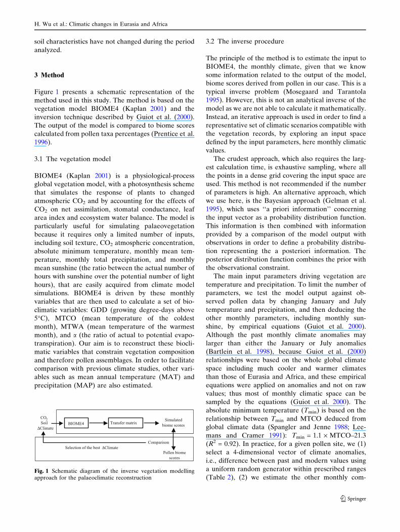
Figure 1 presents a schematic representation of the
method used in this study. The method is based on the
vegetation model BIOME4 (Kaplan 2001) and the
inversion technique described by Guiot et al. (2000).
The output of the model is compared to biome scores
calculated from pollen taxa percentages (Prentice et al.
1996).
3.1 The vegetation model
BIOME4 (Kaplan 2001) is a physiological-process
global vegetation model, with a photosynthesis scheme
that simulates the response of plants to changed
atmospheric CO2 and by accounting for the effects of
CO2 on net assimilation, stomatal conductance, leaf
area index and ecosystem water balance. The model is
particularly useful for simulating palaeovegetation
because it requires only a limited number of inputs,
including soil texture, CO2 atmospheric concentration,
absolute minimum temperature, monthly mean tem-
perature, monthly total precipitation, and monthly
mean sunshine (the ratio between the actual number of
hours with sunshine over the potential number of light
hours), that are easily acquired from climate model
simulations. BIOME4 is driven by these monthly
variables that are then used to calculate a set of bio-
climatic variables: GDD (growing degree-days above
5�C), MTCO (mean temperature of the coldest
month), MTWA (mean temperature of the warmest
month), and a (the ratio of actual to potential evapo-
transpiration). Our aim is to reconstruct these biocli-
matic variables that constrain vegetation composition
and therefore pollen assemblages. In order to facilitate
comparison with previous climate studies, other vari-
ables such as mean annual temperature (MAT) and
precipitation (MAP) are also estimated.
3.2 The inverse procedure
The principle of the method is to estimate the input to
BIOME4, the monthly climate, given that we know
some information related to the output of the model,
biome scores derived from pollen in our case. This is a
typical inverse problem (Mosegaard and Tarantola
1995). However, this is not an analytical inverse of the
model as we are not able to calculate it mathematically.
Instead, an iterative approach is used in order to find a
representative set of climatic scenarios compatible with
the vegetation records, by exploring an input space
defined by the input parameters, here monthly climatic
values.
The crudest approach, which also requires the larg-
est calculation time, is exhaustive sampling, where all
the points in a dense grid covering the input space are
used. This method is not recommended if the number
of parameters is high. An alternative approach, which
we use here, is the Bayesian approach (Gelman et al.
1995), which uses ‘‘a priori information’’ concerning
the input vector as a probability distribution function.
This information is then combined with information
provided by a comparison of the model output with
observations in order to define a probability distribu-
tion representing the a posteriori information. The
posterior distribution function combines the prior with
the observational constraint.
The main input parameters driving vegetation are
temperature and precipitation. To limit the number of
parameters, we test the model output against ob-
served pollen data by changing January and July
temperature and precipitation, and then deducing the
other monthly parameters, including monthly sun-
shine, by empirical equations (Guiot et al. 2000).
Although the past monthly climate anomalies may
larger than either the January or July anomalies
(Bartlein et al. 1998), because Guiot et al. (2000)
relationships were based on the whole global climate
space including much cooler and warmer climates
than those of Eurasia and Africa, and these empirical
equations were applied on anomalies and not on raw
values; thus most of monthly climatic space can be
sampled by the equations (Guiot et al. 2000). The
absolute minimum temperature (Tmin) is based on the
relationship between Tmin and MTCO deduced from
global climate data (Spangler and Jenne 1988; Lee-
mans and Cramer 1991): Tmin = 1.1 · MTCO–21.3
(R2 = 0.92). In practice, for a given pollen site, we (1)
select a 4-dimensional vector of climate anomalies,
i.e., difference between past and modern values using
a uniform random generator within prescribed ranges
(Table 2), (2) we estimate the other monthly com-
BIOME4 Transfer matrix
Pollen biome scores
Comparison
CO2Soil
∆Climate
Selection of the best
Simulated biome scores
∆Climate
Fig. 1 Schematic diagram of the inverse vegetation modellingapproach for the palaeoclimatic reconstruction
H. Wu et al.: Climatic changes in Eurasia and Africa
123
Ta
ble
1T
ran
sfe
rm
atr
ixfr
om
BIO
ME
4ty
po
log
yto
the
po
lle
nb
iom
esc
ore
s
BIO
ME
4ty
pe
Po
lle
nb
iom
ety
pe
CL
DE
CL
MX
CO
CO
CO
MX
DE
SE
ST
EP
TA
IGT
ED
ET
UN
DX
ER
OH
OD
ES
AV
AT
DF
OT
RF
OT
SF
OW
AM
XT
XW
S
TrE
gF
o0
00
00
00
00
00
05
15
10
00
TrS
eD
eF
o0
00
00
00
00
00
01
01
01
50
5T
rDe
Fo
00
00
00
00
00
05
15
51
00
0T
eD
eF
o0
55
10
00
01
50
00
00
00
10
0T
eC
oF
o0
01
51
00
00
50
00
00
00
00
Wa
Mx
Fo
00
00
00
01
00
10
00
00
01
50
Co
Mx
Fo
00
10
15
00
01
00
00
00
00
00
Co
Co
Fo
00
15
10
00
50
00
00
00
00
0C
lMx
Fo
10
15
00
00
10
00
00
00
00
00
Eg
Ta
ig5
10
50
00
15
00
00
00
00
00
De
Ta
ig1
05
00
00
15
05
00
00
00
00
TrS
av
00
00
05
00
00
01
55
00
01
0T
rXsS
l0
00
00
10
00
00
05
00
00
15
Te
XsS
l0
00
00
50
00
15
00
00
05
0T
eS
cWo
00
00
05
00
01
50
50
00
10
0T
eB
lSa
v0
00
00
50
50
50
15
00
05
0O
pC
oW
o0
01
00
05
00
00
00
00
00
0B
oP
rkl
00
50
01
01
00
05
00
00
00
0T
rGrl
00
00
01
50
00
05
50
00
01
0T
eG
rlc
00
00
51
50
05
00
00
00
00
Te
Grl
w0
00
05
15
00
05
05
00
00
0H
otD
ese
rt0
00
00
10
00
00
15
00
00
00
De
sert
00
00
15
10
00
00
00
00
00
0S
hT
un
d5
00
00
14
50
15
00
00
00
00
DS
hT
un
d0
00
00
50
01
50
00
00
00
0P
sSh
Tu
nd
00
00
05
00
15
00
00
00
00
Fo
LiM
oss
00
00
00
00
10
00
00
00
00
Ba
rre
n0
00
00
00
00
00
00
00
00
LIc
e0
00
00
00
00
00
00
00
00
We
div
ide
dte
mp
era
teg
rass
lan
din
toco
ol
tem
pe
rate
gra
ssla
nd
(Te
Grl
c)a
nd
wa
rmte
mp
era
teg
rass
lan
d(T
eG
rlw
),a
nd
de
sert
into
cold
de
sert
(De
sert
)an
dh
ot
de
sert
(Ho
tD
ese
rt),
ba
sed
on
the
min
imu
mte
mp
era
ture
(22
�C)
of
the
me
an
tem
pe
ratu
reo
fth
ew
arm
est
mo
nth
(Pre
nti
cee
ta
l.1
99
2)
Po
lle
nb
iom
ety
pe
s:C
LD
Eco
ldd
eci
du
ou
sfo
rest
;C
LM
Xco
ldm
ixe
dfo
rest
;C
OC
Oco
ol
con
ife
rou
sfo
rest
;C
OM
Xco
ol
mix
ed
fore
st;
DE
SE
de
sert
;H
OD
Eh
ot
de
sert
;S
AV
Asa
va
nn
a;
ST
EP
ste
pp
e;T
AIG
taig
a;T
DF
Otr
op
ica
ld
ryfo
rest
;T
ED
Ete
mp
era
ted
eci
du
ou
sfo
rest
;T
RF
Otr
op
ica
lra
info
rest
;T
SF
Otr
op
ica
lse
aso
na
lfo
rest
;T
UN
Dtu
nd
ra;
TX
WS
tro
pic
al
xe
rop
hy
tic
wo
od
s/sc
rub
;W
AM
Xb
roa
dle
av
ed
ev
erg
ree
n/w
arm
mix
ed
fore
st;
XE
RO
xe
rop
hy
tic
wo
od
s/sc
rub
BIO
ME
4ty
pe
s:B
arr
enb
arr
en
lan
d;
Bo
Prk
lb
ore
al
pa
rkla
nd
;C
lMx
Fo
cold
mix
ed
fore
st;
Co
Co
Fo
coo
le
ve
rgre
en
ne
ed
lele
af
fore
st;
Co
Mx
Fo
coo
lm
ixe
dfo
rest
;D
eser
td
ese
rt;
DeT
aig
cold
de
cid
uo
us
fore
st;
Dsh
Tu
nd
ere
ctd
wa
rf-s
hru
btu
nd
ra;
Eg
Ta
igco
lde
ve
rgre
en
ne
ed
lele
af
fore
st;
Fo
LiM
oss
cush
ion
-fo
rbli
che
n,
an
dm
oss
tun
dra
;H
otD
eser
th
ot
de
sert
;L
Ice
lan
dic
e;
Op
Co
Wo
tem
pe
rate
ev
erg
ree
nn
ee
dle
lea
fo
pe
nw
oo
dla
nd
;P
sSh
Tu
nd
pro
stra
ted
wa
rf-s
hru
btu
nd
ra.
Sh
Tu
nd
low
an
dh
igh
shru
btu
nd
ra;
TeB
lSa
vte
mp
era
ted
eci
du
ou
sb
roa
dle
av
ed
sav
an
na
;T
eCo
Fo
tem
pe
rate
ev
erg
ree
nn
ee
dle
lea
ffo
rest
;T
eDeF
ote
mp
era
ted
eci
du
ou
sb
roa
dle
af
fore
st;
TeG
rlc
coo
lte
mp
era
teg
rass
lan
d,
TeG
rlw
wa
rmte
mp
era
teg
rass
lan
d;
TeS
cWo
tem
pe
rate
scle
rop
hy
llw
oo
dla
nd
an
dsh
rub
lan
d;
TeX
sSl
tem
pe
rate
xe
rop
hy
tic
shru
bla
nd
;T
rDeF
otr
op
ica
ld
eci
du
ou
sb
roa
dle
af
fore
sta
nd
wo
od
lan
d;
TrE
gF
otr
op
ica
le
ve
rgre
en
bro
ad
lea
ffo
rest
;T
rGrl
tro
pic
al
gra
ssla
nd
;T
rSa
vtr
op
ica
lsa
va
nn
a;
TrS
eDeF
otr
op
ica
lse
mi-
ev
erg
ree
nb
roa
dle
af
fore
st;
TrX
sSl
tro
pic
al
xe
rop
hy
tic
shru
bla
nd
;W
aM
xF
ow
arm
-te
mp
era
tee
ve
rgre
en
bro
ad
lea
fa
nd
mix
ed
fore
st
H. Wu et al.: Climatic changes in Eurasia and Africa
123
ponents of the climate using the empirical equations,
(3) we add the anomalies to the modern climate and
run BIOME4, (4) we use a transfer matrix to convert
the BIOME4 biome to biome scores, compare the
simulated biome scores to the observed ones using a
Euclidian distance between observed and simulated
biome scores, then calculate the maximum likelihoods
(LH) which roughly measures the fit between ob-
served data and predicated data by the model, (5) we
accept or reject this climate vector based on its LH
relative to the criterion C (Fahmy 1997, please see the
Eq. (6) of Guiot et al. 2000), (6) we randomly select
another climate anomalies vector and go to (1). This
iterative process is stopped when we obtain a suffi-
cient number of valid scenarios to calculate the
a posteriori probability distributions, normally 200–
300 scenarios in 5,000 iterations or less. Finally, the
most probable climate, together with its confidence
intervals, is calculated from the a posteriori proba-
bilities.
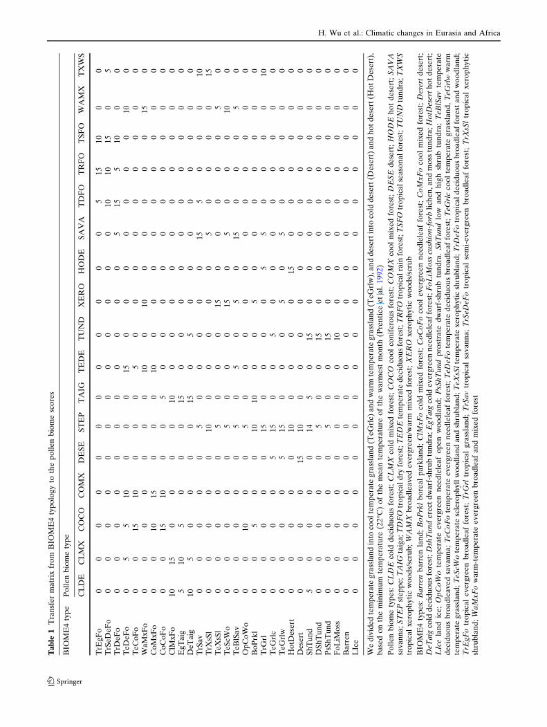
There is no full compatibility between the biome
typology of BIOME4 and the biome typology of
pollen data. We have therefore defined a transfer
matrix (Table 1) where each BIOME4 vegetation
type is assigned a vector of values, one for each
pollen vegetation type, ranging between 0 and 15, a
typical range of pollen-based biome scores. A value of
0 corresponds to an incompatibility between the
BIOME4 type and the pollen biome type, i.e., when
this type is simulated, pollen biomes with a value of
zero should not be present. A value of 15 corresponds
to a maximum correspondence. Some intermediate
values (5 or 10) are assigned to pollen biome, which,
despite not being fully compatible, can occupy a
common climatic space with the BIOME4 biome (e.g.
COCO pollen type in the simulated biome CoMxFo).
All these values have been set empirically by exami-
nation of the modern pollen biome score data and by
taking into account the theoretical definition of each
biome based on modern vegetation maps. The a priori
distribution of the input parameters is set between the
ranges given in Table 2.
Although the inverse procedure described above is
based on the paper of Guiot et al. (2000), two signifi-
cant differences must be noted. First, rather than using
a transfer function between modern pollen-derived
PFT scores and simulated net primary production
(NPP) values of the PFT to transform the model out-
put into values directly comparable with pollen-de-
rived PFT scores for the past, we have instead used the
transfer matrix between pollen biomes and BIOME4
output described above (Table 1). Second, a more re-
cent version of the vegetation model was used
(BIOME4 instead of BIOME3). The simulation of
arctic vegetation has been improved in the new version
(Kaplan 2001), and should give better results in an
inverse mode for the LGM vegetation at middle and
high latitudes.
3.3 Simulating CO2 effects on climate
reconstructions at the LGM
In order to improve palaeoclimate reconstructions
based on pollen data for glacial periods, it is necessary
to take into account the direct physiological impact of
low CO2 concentrations on vegetation (Guiot et al.
2000; Harrison and Prentice 2003). The inverse mod-
eling method enables us to solve part of this problem
by reconstructing the probability distribution of LGM
climates under different CO2 concentrations and to
identify potential climates that explain the occurrence
of a palaeoecosystem. This is a crucial departure from
classical statistical methods, as we accept the concept
of multi-equilibrium status between environmental
conditions (e.g. climate, CO2, soil) and the vegetation
(Guiot et al. 2000).
To evaluate the effects of CO2 concentrations on the
pollen-based palaeoclimate reconstructions, we have
devised two experiments:
• LGM340: an experiment with modern atmospheric
CO2 concentration (340 ppmv);
• LGM200: an experiment with LGM atmospheric
CO2 concentration (200 ppmv).
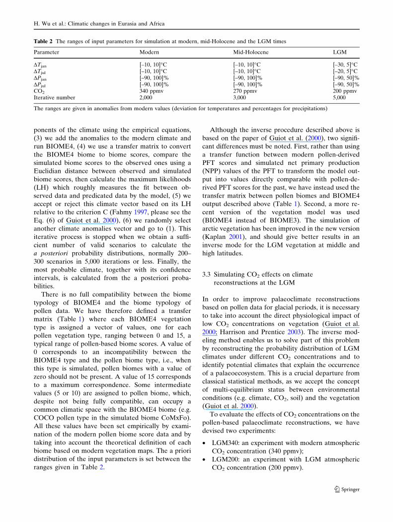
Table 2 The ranges of input parameters for simulation at modern, mid-Holocene and the LGM times
Parameter Modern Mid-Holocene LGM
DTjan [–10, 10]�C [–10, 10]�C [–30, 5]�CDTjul [–10, 10]�C [–10, 10]�C [–20, 5]�CDPjan [–90, 100]% [–90, 100]% [–90, 50]%DPjul [–90, 100]% [–90, 100]% [–90, 50]%CO2 340 ppmv 270 ppmv 200 ppmvIterative number 2,000 3,000 5,000
The ranges are given in anomalies from modern values (deviation for temperatures and percentages for precipitations)
H. Wu et al.: Climatic changes in Eurasia and Africa
123
4 Results
4.1 Validation with modern data
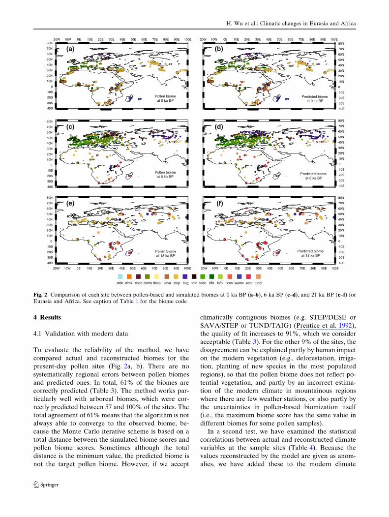
To evaluate the reliability of the method, we have
compared actual and reconstructed biomes for the
present-day pollen sites (Fig. 2a, b). There are no
systematically regional errors between pollen biomes
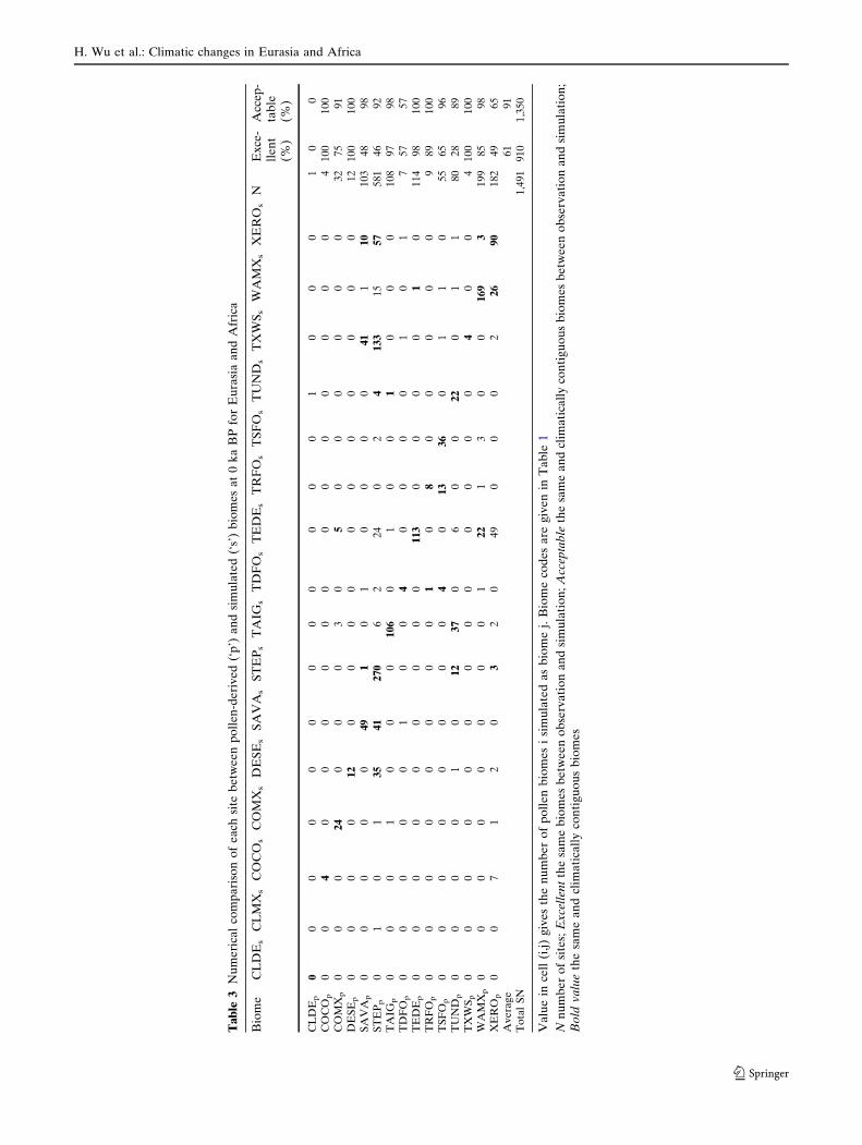
and predicted ones. In total, 61% of the biomes are
correctly predicted (Table 3). The method works par-
ticularly well with arboreal biomes, which were cor-
rectly predicted between 57 and 100% of the sites. The
total agreement of 61% means that the algorithm is not
always able to converge to the observed biome, be-
cause the Monte Carlo iterative scheme is based on a
total distance between the simulated biome scores and
pollen biome scores. Sometimes although the total
distance is the minimum value, the predicted biome is
not the target pollen biome. However, if we accept
climatically contiguous biomes (e.g. STEP/DESE or
SAVA/STEP or TUND/TAIG) (Prentice et al. 1992),
the quality of fit increases to 91%, which we consider
acceptable (Table 3). For the other 9% of the sites, the
disagreement can be explained partly by human impact
on the modern vegetation (e.g., deforestation, irriga-
tion, planting of new species in the most populated
regions), so that the pollen biome does not reflect po-
tential vegetation, and partly by an incorrect estima-
tion of the modern climate in mountainous regions
where there are few weather stations, or also partly by
the uncertainties in pollen-based biomization itself
(i.e., the maximum biome score has the same value in
different biomes for some pollen samples).
In a second test, we have examined the statistical
correlations between actual and reconstructed climate
variables at the sample sites (Table 4). Because the
values reconstructed by the model are given as anom-
alies, we have added these to the modern climate
20W 10W 0E 10E 20E 30E 40E 50E 60E 70E 80E 90E 100E
20W 10W 0E 10E 20E 30E 40E 50E 60E 70E 80E 90E 100E 20W 10W 0E 10E 20E 30E 40E 50E 60E 70E 80E 90E 100E
20W 10W 0E 10E 20E 30E 40E 50E 60E 70E 80E 90E 100E
40S
30S
20S
10S
0
10N
20N
30N
40N
50N
60N
70N
80N
40S
30S
20S
10S
0
10N
20N
30N
40N
50N
60N
70N
80N
40S
30S
20S
10S
0
10N
20N
30N
40N
50N
60N
70N
80N
40S
30S
20S
10S
0
10N
20N
30N
40N
50N
60N
70N
80N
40S
30S
20S
10S
0
10N
20N
30N
40N
50N
60N
70N
80N
40S
30S
20S
10S
0
10N
20N
30N
40N
50N
60N
70N
80N
(a) (b)
(c) (d)
(e) (f)
Pollen biome at 0 ka BP
Predicted biome at 0 ka BP
Predicted biome at 6 ka BP
Predicted biome at 18 ka BP
Pollen biome at 6 ka BP
Pollen biome at 18 ka BP
clde clmx coco comx dese sava step taig tdfo tede trfo tsfo txws wamx xero tund
Fig. 2 Comparison of each site between pollen-based and simulated biomes at 0 ka BP (a–b), 6 ka BP (c–d), and 21 ka BP (e–f) forEurasia and Africa. See caption of Table 1 for the biome code
H. Wu et al.: Climatic changes in Eurasia and Africa
123
Ta
ble
3N
um
eri
cal
com
pa
riso
no
fe
ach
site
be
twe
en
po
lle
n-d
eri
ve
d(‘
p’)
an
dsi
mu
late
d(‘
s’)
bio
me
sa
t0
ka
BP
for
Eu
rasi
aa
nd
Afr
ica
Bio
me
CL
DE
sC
LM
Xs
CO
CO
sC
OM
Xs
DE
SE
sS
AV
As
ST
EP
sT
AIG
sT
DF
Os
TE
DE
sT
RF
Os
TS
FO
sT
UN
Ds
TX
WS
sW
AM
Xs
XE
RO
sN
Ex
ce-
lle
nt
(%)
Acc
ep
-ta
ble
(%)
CL
DE
p0
00
00
00
00
00
01
00
01
00
CO
CO
p0
04
00
00
00
00
00
00
04
100
100
CO
MX
p0
00
24
00
03
05
00
00
00
32
75
91
DE
SE
p0
00
012
00
00
00
00
00
012
100
100
SA
VA
p0
00
00
49
10
10
00
041
110
103
48
98
ST
EP
p0
10
135
41
270
62
24
02
4133
15
57
581
46
92
TA
IGp
00
01
00
0106
01
00
10
00
108
97
98
TD
FO
p0
00
00
10
04
00
00
10
17
57
57
TE
DE
p0
00
00
00
00
113
00
00
10
114
98
100
TR
FO
p0
00
00
00
01
08
00
00
09
89
100
TS
FO
p0
00
00
00
04
013
36
01
10
55
65
96
TU
ND
p0
00
01
012
37
06
00
22
01
180
28
89
TX
WS
p0
00
00
00
00
00
00
40
04
100
100
WA
MX
p0
00
00
00
01
22
13
00
169
3199
85
98
XE
RO
p0
07
12
03
20
49
00
02
26
90
182
49
65
Avera
ge
61
91
To
tal
SN
1,4
91
910
1,3
50
Va
lue
ince
ll(i
,j)
giv
es
the
nu
mb
er
of
po
lle
nb
iom
es
isi
mu
late
da
sb
iom
ej.
Bio
me
cod
es
are
giv
en
inT
ab
le1
Nn
um
be
ro
fsi
tes;
Ex
cell
ent
the
sam
eb
iom
es
be
twe
en
ob
serv
ati
on
an
dsi
mu
lati
on
;A
ccep
tab
leth
esa
me
an
dcl
ima
tica
lly
con
tig
uo
us
bio
me
sb
etw
ee
no
bse
rva
tio
na
nd
sim
ula
tio
n;
Bo
ldv
alu
eth
esa
me
an
dcl
ima
tica
lly
con
tig
uo
us
bio
me
s
H. Wu et al.: Climatic changes in Eurasia and Africa
123
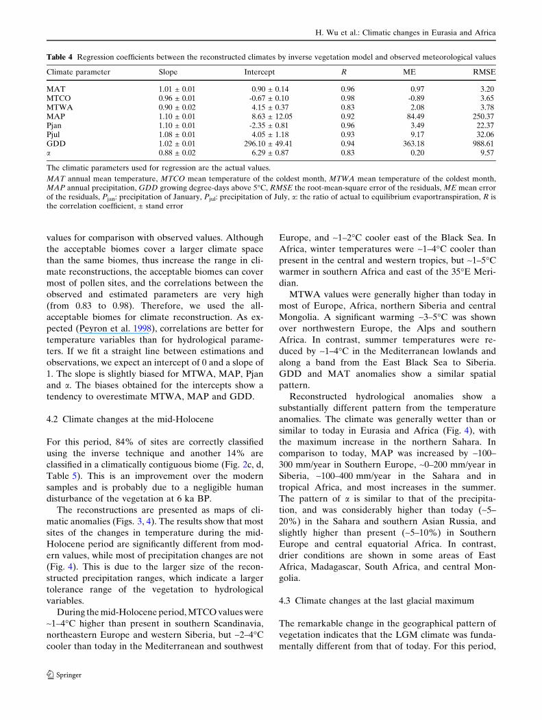
values for comparison with observed values. Although
the acceptable biomes cover a larger climate space
than the same biomes, thus increase the range in cli-
mate reconstructions, the acceptable biomes can cover
most of pollen sites, and the correlations between the
observed and estimated parameters are very high
(from 0.83 to 0.98). Therefore, we used the all-
acceptable biomes for climate reconstruction. As ex-
pected (Peyron et al. 1998), correlations are better for
temperature variables than for hydrological parame-
ters. If we fit a straight line between estimations and
observations, we expect an intercept of 0 and a slope of
1. The slope is slightly biased for MTWA, MAP, Pjan
and a. The biases obtained for the intercepts show a
tendency to overestimate MTWA, MAP and GDD.
4.2 Climate changes at the mid-Holocene
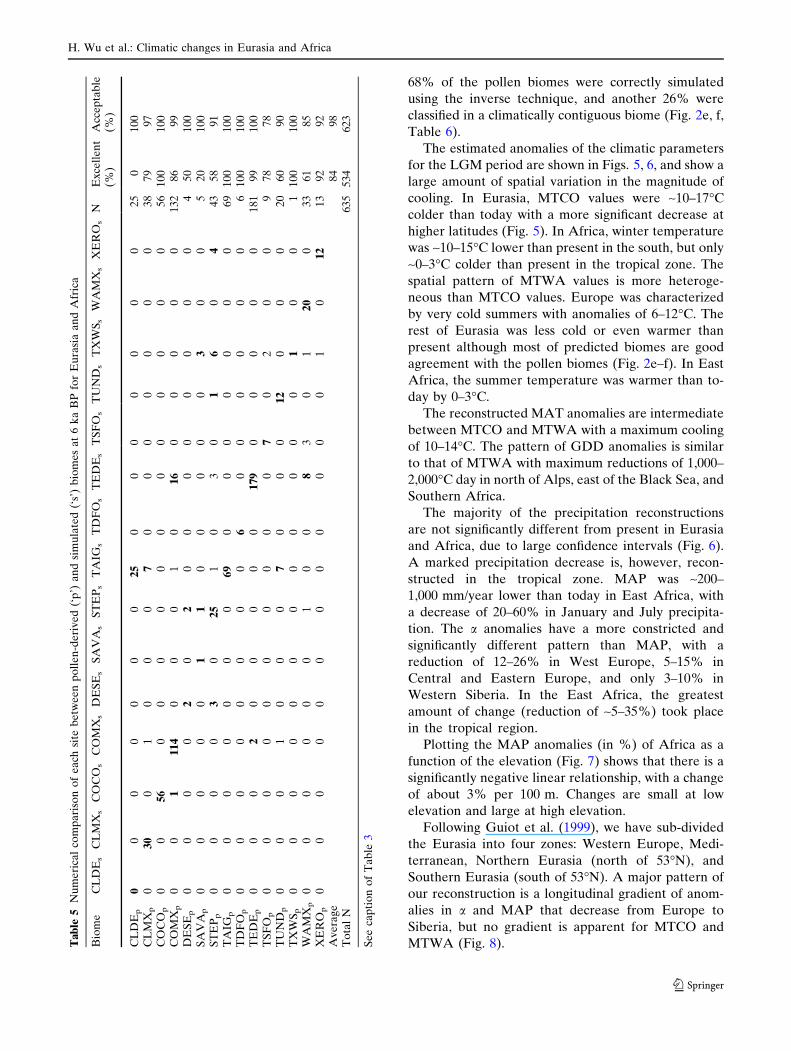
For this period, 84% of sites are correctly classified
using the inverse technique and another 14% are
classified in a climatically contiguous biome (Fig. 2c, d,
Table 5). This is an improvement over the modern
samples and is probably due to a negligible human
disturbance of the vegetation at 6 ka BP.
The reconstructions are presented as maps of cli-
matic anomalies (Figs. 3, 4). The results show that most
sites of the changes in temperature during the mid-
Holocene period are significantly different from mod-
ern values, while most of precipitation changes are not
(Fig. 4). This is due to the larger size of the recon-
structed precipitation ranges, which indicate a larger
tolerance range of the vegetation to hydrological
variables.
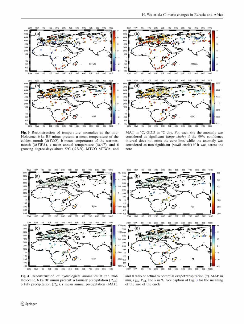
During the mid-Holocene period, MTCO values were
~1–4�C higher than present in southern Scandinavia,
northeastern Europe and western Siberia, but ~2–4�C
cooler than today in the Mediterranean and southwest
Europe, and ~1–2�C cooler east of the Black Sea. In
Africa, winter temperatures were ~1–4�C cooler than
present in the central and western tropics, but ~1–5�C
warmer in southern Africa and east of the 35�E Meri-
dian.
MTWA values were generally higher than today in
most of Europe, Africa, northern Siberia and central
Mongolia. A significant warming ~3–5�C was shown
over northwestern Europe, the Alps and southern
Africa. In contrast, summer temperatures were re-
duced by ~1–4�C in the Mediterranean lowlands and
along a band from the East Black Sea to Siberia.
GDD and MAT anomalies show a similar spatial
pattern.
Reconstructed hydrological anomalies show a
substantially different pattern from the temperature
anomalies. The climate was generally wetter than or
similar to today in Eurasia and Africa (Fig. 4), with
the maximum increase in the northern Sahara. In
comparison to today, MAP was increased by ~100–
300 mm/year in Southern Europe, ~0–200 mm/year in
Siberia, ~100–400 mm/year in the Sahara and in
tropical Africa, and most increases in the summer.
The pattern of a is similar to that of the precipita-
tion, and was considerably higher than today (~5–
20%) in the Sahara and southern Asian Russia, and
slightly higher than present (~5–10%) in Southern
Europe and central equatorial Africa. In contrast,
drier conditions are shown in some areas of East
Africa, Madagascar, South Africa, and central Mon-
golia.
4.3 Climate changes at the last glacial maximum
The remarkable change in the geographical pattern of
vegetation indicates that the LGM climate was funda-
mentally different from that of today. For this period,
Table 4 Regression coefficients between the reconstructed climates by inverse vegetation model and observed meteorological values
Climate parameter Slope Intercept R ME RMSE
MAT 1.01 ± 0.01 0.90 ± 0.14 0.96 0.97 3.20MTCO 0.96 ± 0.01 -0.67 ± 0.10 0.98 -0.89 3.65MTWA 0.90 ± 0.02 4.15 ± 0.37 0.83 2.08 3.78MAP 1.10 ± 0.01 8.63 ± 12.05 0.92 84.49 250.37Pjan 1.10 ± 0.01 -2.35 ± 0.81 0.96 3.49 22.37Pjul 1.08 ± 0.01 4.05 ± 1.18 0.93 9.17 32.06GDD 1.02 ± 0.01 296.10 ± 49.41 0.94 363.18 988.61a 0.88 ± 0.02 6.29 ± 0.87 0.83 0.20 9.57
The climatic parameters used for regression are the actual values.
MAT annual mean temperature, MTCO mean temperature of the coldest month, MTWA mean temperature of the coldest month,MAP annual precipitation, GDD growing degree-days above 5�C, RMSE the root-mean-square error of the residuals, ME mean errorof the residuals, Pjan: precipitation of January, Pjul: precipitation of July, a: the ratio of actual to equilibrium evaportranspiration, R isthe correlation coefficient, ± stand error
H. Wu et al.: Climatic changes in Eurasia and Africa
123
68% of the pollen biomes were correctly simulated
using the inverse technique, and another 26% were
classified in a climatically contiguous biome (Fig. 2e, f,
Table 6).
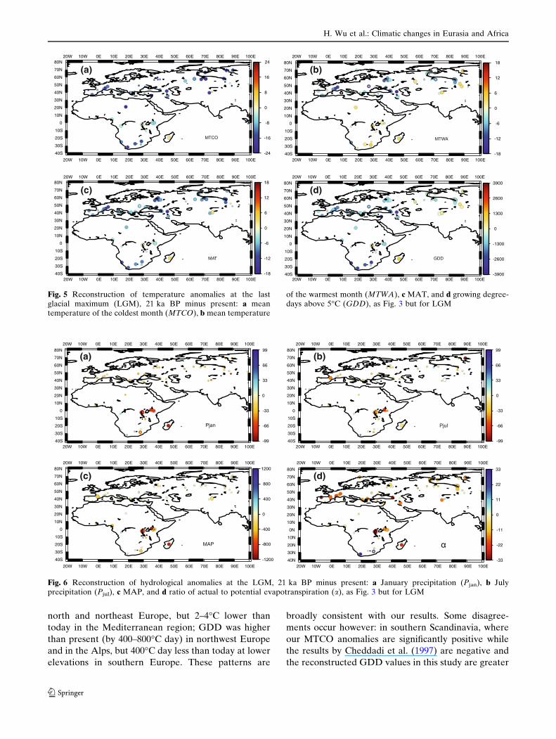
The estimated anomalies of the climatic parameters
for the LGM period are shown in Figs. 5, 6, and show a
large amount of spatial variation in the magnitude of
cooling. In Eurasia, MTCO values were ~10–17�C
colder than today with a more significant decrease at
higher latitudes (Fig. 5). In Africa, winter temperature
was ~10–15�C lower than present in the south, but only
~0–3�C colder than present in the tropical zone. The
spatial pattern of MTWA values is more heteroge-
neous than MTCO values. Europe was characterized
by very cold summers with anomalies of 6–12�C. The
rest of Eurasia was less cold or even warmer than
present although most of predicted biomes are good
agreement with the pollen biomes (Fig. 2e–f). In East
Africa, the summer temperature was warmer than to-
day by 0–3�C.
The reconstructed MAT anomalies are intermediate
between MTCO and MTWA with a maximum cooling
of 10–14�C. The pattern of GDD anomalies is similar
to that of MTWA with maximum reductions of 1,000–
2,000�C day in north of Alps, east of the Black Sea, and
Southern Africa.
The majority of the precipitation reconstructions
are not significantly different from present in Eurasia
and Africa, due to large confidence intervals (Fig. 6).
A marked precipitation decrease is, however, recon-
structed in the tropical zone. MAP was ~200–
1,000 mm/year lower than today in East Africa, with
a decrease of 20–60% in January and July precipita-
tion. The a anomalies have a more constricted and
significantly different pattern than MAP, with a
reduction of 12–26% in West Europe, 5–15% in
Central and Eastern Europe, and only 3–10% in
Western Siberia. In the East Africa, the greatest
amount of change (reduction of ~5–35%) took place
in the tropical region.
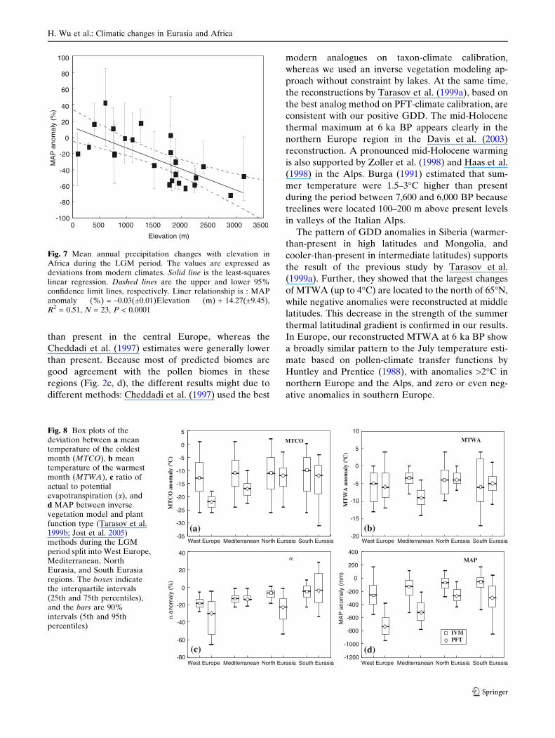
Plotting the MAP anomalies (in %) of Africa as a
function of the elevation (Fig. 7) shows that there is a
significantly negative linear relationship, with a change
of about 3% per 100 m. Changes are small at low
elevation and large at high elevation.
Following Guiot et al. (1999), we have sub-divided
the Eurasia into four zones: Western Europe, Medi-
terranean, Northern Eurasia (north of 53�N), and
Southern Eurasia (south of 53�N). A major pattern of
our reconstruction is a longitudinal gradient of anom-
alies in a and MAP that decrease from Europe to
Siberia, but no gradient is apparent for MTCO and
MTWA (Fig. 8).Ta
ble
5N
um
eri
cal
com
pa
riso
no
fe
ach
site
be
twe
en
po
lle
n-d
eri
ve
d(‘
p’)
an
dsi
mu
late
d(‘
s’)
bio
me
sa
t6
ka
BP
for
Eu
rasi
aa
nd
Afr
ica
Bio
me
CL
DE
sC
LM
Xs
CO
CO
sC
OM
Xs
DE
SE
sS
AV
As
ST
EP
sT
AIG
sT
DF
Os
TE
DE
sT
SF
Os
TU
ND
sT
XW
Ss
WA
MX
sX
ER
Os
NE
xce
lle
nt
(%)
Acc
ep
tab
le(%
)
CL
DE
p0
00
00
00
25
00
00
00
02
50
10
0C
LM
Xp
03
00
10
00
70
00
00
00
38
79
97
CO
CO
p0
05
60
00
00
00
00
00
05
61
00
10
0C
OM
Xp
00
11
14
00
01
01
60
00
00
13
28
69
9D
ES
Ep
00
00
20
20
00
00
00
04
50
10
0S
AV
Ap
00
00
01
10
00
00
30
05
20
10
0S
TE
Pp
00
00
30
25
10
30
16
04
43
58
91
TA
IGp
00
00
00
06
90
00
00
00
69
10
01
00
TD
FO
p0
00
00
00
06
00
00
00
61
00
10
0T
ED
Ep
00
02
00
00
01
79
00
00
01
81
99
10
0T
SF
Op
00
00
00
00
00
70
20
09
78
78
TU
ND
p0
00
10
00
70
00
12
00
02
06
09
0T
XW
Sp
00
00
00
00
00
00
10
01
10
01
00
WA
MX
p0
00
00
01
00
83
01
20
03
36
18
5X
ER
Op
00
00
00
00
00
00
10
12
13
92
92
Av
era
ge
84
98
To
tal
N6
35
53
46
23
Se
eca
pti
on
of
Ta
ble
3
H. Wu et al.: Climatic changes in Eurasia and Africa
123
20W
20W
10W
10W
0E
0E
10E
10E
20E
20E
30E
30E
40E
40E
50E
50E
60E
60E
70E
70E
80E
80E
90E
90E
100E
100E
40S
30S
20S
10S
0
10N
20N
30N
40N
50N
60N
70N
80N
-9
-6
-3
0
3
6
9
20W
20W
10W
10W
0E
0E
10E
10E
20E
20E
30E
30E
40E
40E
50E
50E
60E
60E
70E
70E
80E
80E
90E
90E
100E
100E
40S
30S
20S
10S
0
10N
20N
30N
40N
50N
60N
70N
80N
-9
-6
-3
0
3
6
9
20W
20W
10W
10W
0E
0E
10E
10E
20E
20E
30E
30E
40E
40E
50E
50E
60E
60E
70E
70E
80E
80E
90E
90E
100E
100E
40S
30S
20S
10S
0
10N
20N
30N
40N
50N
60N
70N
80N
-9
-6
-3
0
3
6
9
MTCO
20W
20W
10W
10W
0E
0E
10E
10E
20E
20E
30E
30E
40E
40E
50E
50E
60E
60E
70E
70E
80E
80E
90E
90E
100E
100E
40S
30S
20S
10S
0
10N
20N
30N
40N
50N
60N
70N
80N
-3000
-2000
-1000
0
1000
2000
3000
GDD
(d)
(a)
MTWA
(b)
MAT
(c)
Fig. 3 Reconstruction of temperature anomalies at the mid-Holocene, 6 ka BP minus present: a mean temperature of thecoldest month (MTCO), b mean temperature of the warmestmonth (MTWA), c mean annual temperature (MAT), and dgrowing degree-days above 5�C (GDD). MTCO MTWA, and
MAT in �C, GDD in �C day. For each site the anomaly wasconsidered as significant (large circle) if the 99% confidenceinterval does not cross the zero line, while the anomaly wasconsidered as non-significant (small circle) if it was across thezero
20W
20W
10W
10W
0E
0E
10E
10E
20E
20E
30E
30E
40E
40E
50E
50E
60E
60E
70E
70E
80E
80E
90E
90E
100E
100E
40S
30S
20S
10S
0
10N
20N
30N
40N
50N
60N
70N
80N
-150
-100
-50
50
100
150
0
-300
-200
-100
0
100
200
300
20W
20W
10W
10W
0E
0E
10E
10E
20E
20E
30E
30E
40E
40E
50E
50E
60E
60E
70E
70E
80E
80E
90E
90E
100E
100E
40S
30S
20S
10S
0
10N
20N
30N
40N
50N
60N
70N
80N
(b)
Pjul
20W
20W
10W
10W
0E
0E
10E
10E
20E
20E
30E
30E
40E
40E
50E
50E
60E
60E
70E
70E
80E
80E
90E
90E
100E
100E
40S
30S
20S
10S
0
10N
20N
30N
40N
50N
60N
70N
80N
0Ê
-1500
-1000
-500
0
500
1000
20W
20W
10W
10W
0E
0E
10E
10E
20E
20E
30E
30E
40E
40E
50E
50E
60E
60E
70E
70E
80E
80E
90E
90E
100E
100E
0
10N
20N
30N
40N
50N
60N
70N
80N
-45
-30
-15
0
15
30
45
40S
30S
20S
10S
(d)
Pjan
(a)
1500
MAP
(c)
Fig. 4 Reconstruction of hydrological anomalies at the mid-Holocene, 6 ka BP minus present: a January precipitation (Pjan),b July precipitation (Pjul), c mean annual precipitation (MAP),
and d ratio of actual to potential evapotranspiration (a). MAP inmm, Pjan, Pjul, and a in %. See caption of Fig. 3 for the meaningof the size of the circle
H. Wu et al.: Climatic changes in Eurasia and Africa
123
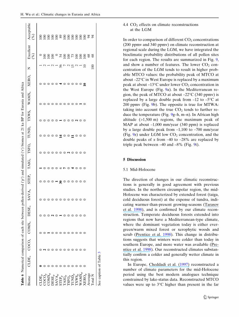
4.4 CO2 effects on climate reconstructions
at the LGM
In order to comparison of different CO2 concentrations
(200 ppmv and 340 ppmv) on climate reconstruction at
regional scale during the LGM, we have integrated the
bioclimatic probability distributions of all pollen sites
for each region. The results are summarized in Fig. 9,
and show a number of features. The lower CO2 con-
centration of the LGM tends to result in higher prob-
able MTCO values: the probability peak of MTCO at
about –22�C in West Europe is replaced by a maximum
peak at about –13�C under lower CO2 concentration in
the West Europe (Fig. 9a). In the Mediterranean re-
gion, the peak of MTCO at about –22�C (340 ppmv) is
replaced by a large double peak from –12 to –5�C at
200 ppmv (Fig. 9b). The opposite is true for MTWA:
taking into account the true CO2 tends to further re-
duce the temperature (Fig. 9g–h, m–n). In African high
altitude (>1,500 m) regions, the maximum peak of
MAP at about –1,000 mm/year (340 ppm) is replaced
by a large double peak from –1,100 to –700 mm/year
(Fig. 9z) under LGM low CO2 concentration, and the
double peaks of a from –40 to –28% are replaced by
triple peak between –40 and –8% (Fig. 9t).
5 Discussion
5.1 Mid-Holocene
The direction of changes in our climatic reconstruc-
tions is generally in good agreement with previous
studies. In the northern circumpolar region, the mid-
Holocene was characterized by extended forest (taiga,
cold deciduous forest) at the expense of tundra, indi-
cating warmer-than-present growing-seasons (Tarasov
et al. 1998), and is confirmed by our climate recon-
struction. Temperate deciduous forests extended into
regions that now have a Mediterranean-type climate,
where the dominant vegetation today is either ever-
green/warm mixed forest or xerophytic woods and
scrub (Prentice et al. 1998). This change in distribu-
tions suggests that winters were colder than today in
southern Europe, and more water was available (Pre-
ntice et al. 1998). Our reconstructed climates substan-
tially confirm a colder and generally wetter climate in
this region.
In Europe, Cheddadi et al. (1997) reconstructed a
number of climate parameters for the mid-Holocene
period using the best modern analogues technique
constrained by lake-status data. Reconstructed MTCO
values were up to 3�C higher than present in the farTa
ble
6N
um
eri
cal
com
pa
riso
no
fe
ach
site
be
twe
en
po
lle
n-d
eri
ve
d(‘
p’)
an
dsi
mu
late
d(‘
s’)
bio
me
sa
t2
1k
aB
Pfo
rE
ura
sia
an
dA
fric
a
Bio
me
CL
DE
sC
OC
Os
CO
MX
sD
ES
Es
SA
VA
sS
TE
Ps
TA
IGs
TS
FO
sT
UN
Ds
TX
WS
sW
AM
Xs
XE
RO
sN
Ex
cell
en
t(%
)A
cce
pta
ble
(%)
CL
DE
p0
00
00
01
00
00
01
01
00
CO
CO
p0
20
00
00
00
00
02
10
01
00
CO
MX
p0
01
00
00
00
00
01
10
01
00
DE
SE
p0
00
20
00
00
00
02
10
01
00
SA
VA
p0
00
00
10
00
00
01
01
00
ST
EP
p0
00
10
30
60
14
10
45
65
48
9T
AIG
p0
00
00
07
00
00
07
10
01
00
TS
FO
p0
00
00
00
20
00
02
10
01
00
TU
ND
p0
00
00
04
01
10
00
15
73
10
0T
XW
Sp
00
00
00
00
02
00
21
00
10
0W
AM
Xp
00
00
00
00
00
10
11
00
10
0X
ER
Op
00
00
00
00
00
01
01
01
00
10
0A
ve
rag
e6
89
4T
ota
lN
10
06
89
4
Se
eca
pti
on
of
Ta
ble
3
H. Wu et al.: Climatic changes in Eurasia and Africa
123
north and northeast Europe, but 2–4�C lower than
today in the Mediterranean region; GDD was higher
than present (by 400–800�C day) in northwest Europe
and in the Alps, but 400�C day less than today at lower
elevations in southern Europe. These patterns are
broadly consistent with our results. Some disagree-
ments occur however: in southern Scandinavia, where
our MTCO anomalies are significantly positive while
the results by Cheddadi et al. (1997) are negative and
the reconstructed GDD values in this study are greater
20W
20W
10W
10W
0E
0E
10E
10E
20E
20E
30E
30E
40E
40E
50E
50E
60E
60E
70E
70E
80E
80E
90E
90E
100E
100E
40S
30S
20S
10S
0
10N
20N
30N
40N
50N
60N
70N
80N
-24
-16
-8
0
8
16
24
20W
20W
10W
10W
0E
0E
10E
10E
20E
20E
30E
30E
40E
40E
50E
50E
60E
60E
70E
70E
80E
80E
90E
90E
100E
100E
40S
30S
20S
10S
0 0Ê
10N
20N
30N
40N
50N
60N
70N
80N
-18
-12
-6
0
6
12
18
20W
20W
10W
10W
0E
0E
10E
10E
20E
20E
30E
30E
40E
40E
50E
50E
60E
60E
70E
70E
80E
80E
90E
90E
100E
100E
40S
30S
20S
10S
0
10N
20N
30N
40N
50N
60N
70N
80N
-18
-12
-6
0
6
12
18
(c)
MAT
20W
20W
10W
10W
0E
0E
10E
10E
20E
20E
30E
30E
40E
40E
50E
50E
60E
60E
70E
70E
80E
80E
90E
90E
100E
100E
40S
30S
20S
10S
0
10N
20N
30N
40N
50N
60N
70N
80N
-3900
-2600
-1300
0
1300
2600
3900
MTCO
(a)
MTWA
(b)
GDD
(d)
Fig. 5 Reconstruction of temperature anomalies at the lastglacial maximum (LGM), 21 ka BP minus present: a meantemperature of the coldest month (MTCO), b mean temperature
of the warmest month (MTWA), c MAT, and d growing degree-days above 5�C (GDD), as Fig. 3 but for LGM
20W
20W
10W
10W
0E
0E
10E
10E
20E
20E
30E
30E
40E
40E
50E
50E
60E
60E
70E
70E
80E
80E
90E
90E
100E
100E
40S
30S
20S
10S
0
10N
20N
30N
40N
50N
60N
70N
80N
-99
-66
-33
0
33
66
99
20W
20W
10W
10W
0E
0E
10E
10E
20E
20E
30E
30E
40E
40E
50E
50E
60E
60E
70E
70E
80E
80E
90E
90E
100E
100E
40S
30S
20S
10S
0
10N
20N
30N
40N
50N
60N
70N
80N
-1200
-800
-400
0
400
800
1200
20W
20W
10W
10W
0E
0E
10E
10E
20E
20E
30E
30E
40E
40E
50E
50E
60E
60E
70E
70E
80E
80E
90E
90E
100E
100E
40S
30S
20S
10S
0
10N
20N
30N
40N
50N
60N
70N
80N
-99
-66
-33
0
33
66
99
20W
20W
10W
10W
0E
0E
10E
10E
20E
20E
30E
30E
40E
40E
50E
50E
60E
60E
70E
70E
80E
80E
90E
90E
100E
100E
40N
30N
20N
10N
0N
10N
20N
30N
40N
50N
60N
70N
80N
-33
-22
-11
0
11
22
33
(b)
Pjul
(c)
MAP
(d)
(a)
Pjan
Fig. 6 Reconstruction of hydrological anomalies at the LGM, 21 ka BP minus present: a January precipitation (Pjan), b Julyprecipitation (Pjul), c MAP, and d ratio of actual to potential evapotranspiration (a), as Fig. 3 but for LGM
H. Wu et al.: Climatic changes in Eurasia and Africa
123
than present in the central Europe, whereas the
Cheddadi et al. (1997) estimates were generally lower
than present. Because most of predicted biomes are
good agreement with the pollen biomes in these
regions (Fig. 2c, d), the different results might due to
different methods: Cheddadi et al. (1997) used the best
modern analogues on taxon-climate calibration,
whereas we used an inverse vegetation modeling ap-
proach without constraint by lakes. At the same time,
the reconstructions by Tarasov et al. (1999a), based on
the best analog method on PFT-climate calibration, are
consistent with our positive GDD. The mid-Holocene
thermal maximum at 6 ka BP appears clearly in the
northern Europe region in the Davis et al. (2003)
reconstruction. A pronounced mid-Holocene warming
is also supported by Zoller et al. (1998) and Haas et al.
(1998) in the Alps. Burga (1991) estimated that sum-
mer temperature were 1.5–3�C higher than present
during the period between 7,600 and 6,000 BP because
treelines were located 100–200 m above present levels
in valleys of the Italian Alps.
The pattern of GDD anomalies in Siberia (warmer-
than-present in high latitudes and Mongolia, and
cooler-than-present in intermediate latitudes) supports
the result of the previous study by Tarasov et al.
(1999a). Further, they showed that the largest changes
of MTWA (up to 4�C) are located to the north of 65�N,
while negative anomalies were reconstructed at middle
latitudes. This decrease in the strength of the summer
thermal latitudinal gradient is confirmed in our results.
In Europe, our reconstructed MTWA at 6 ka BP show
a broadly similar pattern to the July temperature esti-
mate based on pollen-climate transfer functions by
Huntley and Prentice (1988), with anomalies >2�C in
northern Europe and the Alps, and zero or even neg-
ative anomalies in southern Europe.
0 500 1000 1500 2000 2500 3000 3500
Elevation (m)
MA
P a
nom
aly
(%)
-100
-80
-60
-40
-20
0
20
40
60
80
100
Fig. 7 Mean annual precipitation changes with elevation inAfrica during the LGM period. The values are expressed asdeviations from modern climates. Solid line is the least-squareslinear regression. Dashed lines are the upper and lower 95%confidence limit lines, respectively. Liner relationship is : MAPanomaly (%) = –0.03(±0.01)Elevation (m) + 14.27(±9.45),R2 = 0.51, N = 23, P < 0.0001
-1200
-1000
-800
-600
-400
-200
0
200
400
MA
P a
nom
aly
(mm
)
West Europe Mediterranean North Eurasia South Eurasia
IVMPFT
(d)-80
-60
-40
-20
0
20
40
West Europe Mediterranean North Eurasia South Eurasia
(c)
-20
-15
-10
-5
0
5
10
West Europe Mediterranean North Eurasia South Eurasia
(b)-35
-30
-25
-20
-15
-10
-5
0
5
MT
CO
ano
mal
y (º
C)
West Europe Mediterranean North Eurasia South Eurasia
(a)
MTCO MTWA
MAP
MT
WA
ano
mal
y (º
C)
α an
omal
y (%
)
α
Fig. 8 Box plots of thedeviation between a meantemperature of the coldestmonth (MTCO), b meantemperature of the warmestmonth (MTWA), c ratio ofactual to potentialevapotranspiration (a), andd MAP between inversevegetation model and plantfunction type (Tarasov et al.1999b; Jost et al. 2005)methods during the LGMperiod split into West Europe,Mediterranean, NorthEurasia, and South Eurasiaregions. The boxes indicatethe interquartile intervals(25th and 75th percentiles),and the bars are 90%intervals (5th and 95thpercentiles)
H. Wu et al.: Climatic changes in Eurasia and Africa
123

Cheddadi et al. (1997) reconstructed wetter-than-
present conditions in eastern and southern Europe, and
drier conditions in northwest Europe. In our recon-
struction, the most marked feature is the increase in
moisture in the Mediterranean region consistent with
Cheddadi et al. (1997). However, previously recon-
structed drier conditions in the Alps (Cheddadi et al.
1997) are not confirmed in our reconstructions. Lake-
level data from the interior of northern Eurasia and
Mongolia indicate that conditions were wet or wetter
than present at 6 ka BP (Tarasov et al. 1999a), which
agree with our reconstructions.
During the mid-Holocene in Africa, the levels of
almost all Sahara lakes were high (Jolly et al. 1998a),
and the lakes and wetlands occupied ~7.5% of the total
area of the Sahara as compared with 0.5% today
(Hoelzmann et al. 1998). Recent water balance calcu-
lations yielded rainfall values of 100–600 mm/year in
the eastern Sahara (Pachur and Hoelzmann 1991;
Hoelzmann et al. 2001) and between 200 mm/year and
500 mm/year in the Western Sahara (Petit-Maire and
Riser 1988; Riser 1989). All these rainfall estimates are
consistent with our reconstruction for this region.
Between 10�N and 20�S, the results show a strong
contrast between east and west. Our reconstruction
indicates the mid-Holocene conditions in West and
Central Africa were generally wetter than today. In
western Central Africa, this pattern appears to dis-
agree with the occurrence of tropical seasonal forest in
almost all the sites that are occupied today by tropical
rain forest (Jolly et al. 1998b), suggesting that mid-
Holocene conditions were drier than today. However,
our results suggest that increased temperature sea-
sonality (colder winter and warmer summer) may also
∆T (ºC) ∆T (ºC) ∆T (ºC) ∆T (ºC) ∆T (ºC) ∆T (ºC)
∆T (ºC) ∆T (ºC) ∆T (ºC) ∆T (ºC) ∆T (ºC) ∆T (ºC)
MT
CO
rel
ativ
e fr
eque
ncy
(%)
CO2=200
CO2=340
CO2=200
CO2=340
MT
WA
rel
ativ
e fr
eque
ncy
(%)
0
5
10
15
20
25
30
35
∆α (%) ∆α (%) ∆α (%) ∆α (%) ∆α (%) ∆α (%)
0
5
10
15
20
25
30
35
40
MA
P r
elat
ive
freq
uenc
y (%
)α
rela
tive
freq
uenc
y (%
)
∆P (mm) ∆P (mm) ∆P (mm) ∆P (mm)Western Europe Mediterranean region Northern Eurasia Southern Eurasia
(b) (c) (d)
0
5
10
15
20
25
30
-40 -30 -20 -10 0 10
(a)
-40 -30 -20 -10 0 10 -40 -30 -20 -10 0 10 -40 -30 -20 -10 0 10 -40 -30 -20 -10 0 10 -40 -30 -20 -10 0 10
(e) (f)
0
10
20
30
40
50
-25 -20 -15 -10 -5 0 5 10
(g)
-25 -20 -15 -10 -5 0 5 10 -25 -20 -15 -10 -5 0 5 10 -25 -20 -15 -10 -5 0 5 10 -25 -20 -15 -10 -5 0 5 10 -25 -20 -15 -10 -5 0 5 10
-60 -40 -20 0 20 40 -60 -40 -20 0 20 40 -60 -40 -20 0 20 40 -60 -40 -20 0 20 40 -60 -40 -20 0 20 40 -60 -40 -20 0 20 40
-1600 -800 0 800 -1600 -800 0 800 -1600 -800 0 800 -1600 -800 0 800- -1600 -800 0 800 -1600 -800 0 800∆P (mm) ∆P (mm)
Africa (<1500m) Africa (>1500m)
(h) (i) (l) (m) (n)
(o) (p) (q) (r) (s) (t)
(u) (v) (w) (x) (y) (z)
Fig. 9 Probability distribution of four reconstructed bioclimaticparameters at LGM under 340 and 200 ppmv CO2 conditions inWest Europe (a, g, o, u), Mediterranean (b, h, p, v), NorthEurasia (c, i, q, w), South Eurasia (d, l, r, x), African altitude<1,500 m (e, m, s, y), and African altitude >1,500 m (f, n, t, z)
regions. Africa divided into low (<1,500 m) and high (>1,500 m)two regions, which is based on climate anomalies with theelevation. Mean temperature of the coldest month (MTCO):a–f mean temperature of the warmest month (MTWA): g–n ratioof actual to potential evaportranspiration (a): o–t and MAP: u–z
H. Wu et al.: Climatic changes in Eurasia and Africa
123
cause a change from tropical rain forest to tropical
seasonal forest. In northeastern Africa, the 6 ka BP
climate is slightly drier than today, in contrast with the
considerable precipitation increase over the Sahara.
Our results are in broad agreement with previous
climate reconstructions that show a negative MAT
anomaly at 6 ka BP of ~1–2�C in Burundi and a posi-
tive anomaly of approximately 2�C in north of the
equator, together with similar or wetter conditions
using PFT method (Peyron et al. 2000). The same au-
thors (Peyron et al. 2000) reconstructed cooler condi-
tions in southern Tanzania. In southern Africa, our
reconstruction of wetter conditions north of 25�S is
supported by lake-level data (Jolly et al. 1998a).
5.2 Last glacial maximum
The cold and dry conditions during the LGM favored
an extension of tundra in northern Eurasia (Tarasov
et al. 2000) and steppes around the Mediterranean
(Elenga et al. 2000), with a southward displacement of
northern hemisphere forest biomes. Boreal evergreen
forests (taiga) and temperature deciduous forests were
fragmented, while Eurasian steppes were greatly ex-
tended (Tarasov et al. 2000). In tropical Africa, tropi-
cal moist forest (i.e., tropical rain forest and tropical
seasonal forest) was reduced, and broadleaved ever-
green/warm mixed forests were shifted downward in
mountain regions (Elenga et al. 2000) where the
changes may also partly due to the low glacial CO2
concentration (Jolly and Haxeltine 1997; Street-Perrott
et al. 1997). In southern Africa, steppe replaced what is
presently xerophytic woods/scrub (Elenga et al. 2000).
We have compared our reconstructions to those of
Tarasov et al. (1999b), Jost et al. (2005), and Peyron
et al. (1998, 2005) who have covered the same areas
(Fig. 8). The major pattern of the PFT-based recon-
struction is a significantly longitudinal gradient of
anomalies for MTCO, a and MAP that decrease from
Europe to Siberia, and no gradient is apparent for
MTWA. However, both the gradient and the anoma-
lies are attenuated in our reconstructions by IVM ap-
proach (Fig. 8).
Peyron et al. (1998) reconstructed MTCO anomalies
of –30 ± 10�C over Western Europe. Our recon-
structed anomalies, whilst still showing a cooling of ~13
(–13/+14)�C, are smaller than these previous estimates.
Our anomalies are also smaller (warmer) than new
estimates calibrated on a better modern dataset by
Peyron et al. (2005), i.e., 17–26�C decrease (Jost et al.
2005). Although the average disagreement between the
two sets of results is as high as 9�C (Fig. 8a), the range
of our reconstructed temperatures encompasses those
estimated by Jost et al. (2005). In the Mediterranean
region, the PFT-based reconstructions are about 5�C
colder than our results, are, again, within our confi-
dence intervals. Our MTCO reconstructions agree well
with the previous work by Tarasov et al. (1999b) in
Northern and Southern Eurasia, as well as with the
reconstruction of –18�C for Eastern Europe by Peter-
son et al. (1979).
Our reconstructions of MTWA are coherent with
previous results (Fig. 8b), with the exception of the
Mediterranean region where the difference is ~5�C
warmer than the Jost et al. (2005) reconstructions. The
hydrological anomalies reconstructed in this study are
generally smaller (wetter) than previous estimates
(Fig. 8c, d), notably for MAP. The overall conclusion
of these results is that, in Europe, inverse modeling has
a tendency to reconstruct less-cold winters and less-dry
climates than statistical methods calibrated on modern
data. This is consistent with theoretical predictions
(Jolly and Haxeltine 1997; Street-Perrott et al. 1997;
Williams et al. 2000). In Eurasia, our reconstructions of
less-dry climates (Fig. 8d) and less-cold or even higher
than today in the summers (Fig. 5b) are consistent with
the evidence: there was no ice cap on northern Eurasia
at the LGM (Peltier 1994) because of the lack of pre-
cipitation in winter or/and warm summers.
In Africa, our results are comparable to the esti-
mates compiled by Farrera et al. (1999) showing that
low-elevation land temperatures in the tropics were on
average 2.5–3�C lower than present. They are also
consistent with the results (~2�C cooling) of recent
MARGO SST reconstructions from tropical oceans
(Rosell-Mele et al. 2004; Kucera et al. 2005; Barrows
and Juggins 2005). In the subtropical zone, our recon-
structed MAT show a cooling of ~7�C, similar to esti-
mates (~5.5�C cooling) from noble gases in
groundwater and d18O in speleothems in Namibia and
South Africa (Heaton et al. 1986; Talma and Vogel
1992; Stute and Talma 1997). The reconstructed dryer-
than-present conditions are consistent with the lowered
east African and northern west African lake-levels
(Jolly et al. 1998a; Barker and Gasse 2003), and with
studies by Bonnefille et al. (1990), Farrera et al.
(1999), and Bonnefille and Chalie (2000) based on
pollen data.
A new LGM snowline database for tropical and
subtropical regions has been compiled by Mark et al.
(2005), based on the data with the most reliable chro-
nologies. A significant negative relationship between
changes of equilibrium-line altitudes (ELA) and the
actual headwall altitude (HW) elevation was found:
glaciers originating at higher elevations did not display
a larger downslope shift in ELA at the LGM than
H. Wu et al.: Climatic changes in Eurasia and Africa
123

glaciers originating at lower elevations. Because glacier
mass balance is mainly controlled by surface energy
balance and precipitation (Hostetler and Clark 2000,
Mark et al. 2005), this relationship between HW and
ELA across the tropics suggests an underlying physical
mechanism related to climate. The relationship is dif-
ficult to explain by temperature changes, because it
requires smaller decrease in temperature with altitude
at the LGM than the decrease at present, which is an
opposite in direction to palaeoclimate data (Thompson
et al. 1995; Farrera et al. 1999; Pinot et al. 1999). Our
finding that the magnitude of LGM drying increased
with altitude during the LGM (Fig. 7) can reasonably
explain this relationship. Reduced precipitation at high
elevations would have hindered the down-valley
extension of glaciers, even though reductions in tem-
perature were larger at high elevations. This suggests
that precipitation was an important control of changes
in ELA during the LGM in the tropics.
5.3 CO2 effects on climate reconstructions
One major difference between the PFT and IVM ap-
proaches is that the statistical methods used in previous
studies are calibrated for pollen originating from plants
growing under modern levels of atmospheric CO2
whereas inverse modeling does not require such a
calibration. Instead the concentration of CO2 is a
model parameter. Physiological research has demon-
strated that the processes modifying carbon and water
uptake in plants are highly CO2-dependent (Polley
et al. 1993; Bert et al. 1997; Farquhar 1997; Cowling
and Sykes 1999), which indicates modern plant-climate
relationships are not representative of interactions
between plants and climate in the past. Jolly and
Haxeltine (1997) showed that a decrease in CO2 con-
centrations alone could explain the observed replace-
ment of tropical montane forest by xerophytic
vegetation in Burundi, and palaeoecological d13C re-
cords also suggest that low CO2 concentrations con-
tributed to the lowering of alpine tree lines in tropical
Africa at the LGM (Street-Perrott et al. 1997).
Reconstructions based on statistical methods will at-
tempt to attribute the changes caused by the lowered
CO2 level to one or all of the climate parameters,
biasing the results.
Although the contribution of CO2 fertilization to
terrestrial ecosystems has been uncertain based on
currently available data (Norby et al., 2005), Cowling
and Field (2003) have observed a good fit between
modeled and observed response of LAI to changes in
low CO2 for BIOME3, and the predictions of NPP
response to CO2 fertilization in the future using LPJ
model is also agreement with the experimental evi-
dences by Norby et al. (2005). Because the treatment
of CO2 fertilization in BIOME3 and LPJ is same as
BIOME4, these comparisons indicate that BIOME4
model can realistically predict the response to the CO2
fertilization.
Our results show that several solutions are possible
for the LGM climate in Mediterranean regions where
a mixture of steppes and tundra existed. As these
biomes have no clear analogues today, reconstructions
based on statistical methods will tend to choose the
least poor match, or fail to find a match. In the
dataset used by Peyron et al. (1998), these analogues
were located in tundra or very cold steppes, resulting
in very low reconstructed temperatures. In the im-
proved dataset of Jost et al. (2005), the analogues
selected were intermediate analogues in warmer
steppes. Our probability histograms (Fig. 9a, b) show
the differences of reconstructions by PFT (Jost et al.
2005) and IVM methods (Fig. 8a) are possible solu-
tions, and that these solutions are the most probable
if we consider the difference in CO2 concentration.
The inverse modeling method allows us to explore
other possible solutions at LGM CO2 levels that are
less cold in winter and slightly cooler in summer. As
these analogues do not currently exist, these solutions
can only be identified using a mechanistic approach
that allows random climate generator to sample out-
side the modern observed climate space. The results
indicate quite clearly that there is a CO2 bias in
previous LGM reconstructions based on cold steppe
vegetation (Fig. 8a, b).
In Africa, the results show that the arid conditions
reconstructed in tropical high altitude regions may be
overestimated for warm steppe and xerophytic woods/
scrub biomes if the reduction on CO2 concentrations is
not taken into account. This supports the result that
carbon limitation had a significant impact on the dis-
tribution of forest in tropical mountains at the LGM
(Jolly and Haxeltine 1997; Street-Perrott et al. 1997).
The bias can be explained by the fact that lower con-
centrations of CO2 amplify the effect of an arid climate
on the vegetation through its effect on leaf conduc-
tance and plant water use efficiency (Polley et al. 1993;
Bert et al. 1997; Cowling and Sykes 1999). Our results
show that reconstructed MTWA is reduced if the low
CO2 concentration is taken into account. The differ-
ence can also be explained by the effect of changes in
atmospheric CO2 on photosynthetic biochemistry, that
plant growth optima were lower at the LGM relative to
today (Polley et al. 1993; Cowling and Sykes 1999).
Therefore, the inverse modeling shows that although
significant CO2 biases occur, their effect on climate
H. Wu et al.: Climatic changes in Eurasia and Africa
123
reconstructions is not the same for vegetation in dif-
ferent climate zones.
However, the IVM approach is not a panacea. First,
because it is a model-based approach it is highly
dependent on the quality of the vegetation model.
Second, it requires a great deal of computation time,
which will increasingly become a problem in adapting
the technique to more sophisticated models. Third, the
algorithm used does not guarantee convergence toward
an optimal solution. Fourth, the output of the model is
not directly compared to the pollen data; the conver-
sion of BIOME4 biomes to pollen biomes by the
transfer matrix may add the source of uncertainty in
this analysis. Fifth, the input monthly climate for
BIOME4 using empirical equations from Guiot et al.
(2000) may not include all climatic space. Further
verification is required by adapting this approach to
other vegetation models and climate generators. It
remains important, however, to use this approach in
parallel with statistical approaches. The comparison of
different climate reconstructions can improve the
understanding on relationship between palaeoclimate
and palaeovegetation.
6 Conclusion
The quantitative reconstructions derived from pollen
data of Eurasia and Africa at the LGM and the mid-
Holocene, confirm the ability of the inverse vegetation
model (IVM) method to provide spatially coherent
patterns of palaeoclimate that are generally in agree-
ment with previous reconstructions from climate
proxies. However, the IVM approach allows differ-
ences in CO2 concentration between the modern cali-
bration period and the past to be taken into account as
well as climatic reconstructions from pollen assembles
with no modern analogue (Jackson and Williams 2004).
In western Europe and Mediterranean regions, the
method has led to improved results and helped to ex-
plain some of the discrepancies between data-based
climate reconstructions and model simulations, in
particular, the effect of changing atmospheric CO2
concentration.
Our continental-scale palaeoclimate reconstructions
are important for the ongoing validation of climate
models in the paleoclimate modelling intercomparsion
project (PMIP) (Joussaume and Taylor 2000), for the
LGM and mid-Holocene periods. Previous data-model
comparisons have shown regional disagreements be-
tween the PMIP models’ simulations and proxy-based
climate reconstructions. We show here that part of this
disagreement may be due to biases in previous pollen-
based reconstructions caused by the fact that modern
environments do not provide all the necessary ana-
logues for the past.
Acknowledgments This research was supported by a Europeanfunding in the frame of the EU Environment and SustainableDevelopment program (project MOTIF, EVK2-CT-2002-00153),NSFC Foundation (no. 40302021), NSFC key project (no.40231001), NSFC for Innovation Group project (no. 40121303),the National Basic Research Program of China (no.2004CB720203), as well as a grant of the French Ministry ofResearch to the first author. We are grateful to Dr. Odile Peyron(Laboratoire de Chrono-Ecologie, Universite de Franche-Com-te, France) for her contribution to the calibration data by PFTmethod based on an improved modern pollen dataset. Thanksare also extended to J-C Duplessy (editor) and the two anony-mous reviewers for their constructive suggestions and commentson the previous version of the manuscript.
References
Barker P, Gasse F (2003) New evidence for a reduced waterbalance in East Africa during the Last Glacial Maximum:implication for model-data comparison. Q Sci Rev 22:823–837
Barrows TT, Juggins S (2005) Sea-surface temperatures aroundthe Australian margin and Indian Ocean during the LastGlacial Maximum. Q Sci Rev 24:1017–1047
Bartlein PJ, Anderson KH, Anderson PM, Edeards ME, MockCJ, Thompson RS, Webb RS, Webb III T, Whitlock C(1998) Paleclimate simulations for North America over thepast 21,000 years: features of the simulated climate andcomparisons with paleoenvironmental data. Q Sci Rev17:547–585
Bert D, Leavitt SW, Dupouey JL (1997) Variations of wooddelta 13C and water-use efficiency of Abies alba during thelast century. Ecology 78:1588–1596
Bonnefille R, Chalie F (2000) Pollen-inferred precipitation time-series from equatorial mountains, Africa, the last 40 kyr BP.Global Planet Change 26:25–50
Bonnefille R, Chalie F, Guiot J, Vincens A (1992) Quantitativeestimates of full glacial temperatures in equatorial Africafrom palynological data. Clim Dyn 6:251–257
Bonnefille R, Roeland J C, Guiot J (1990) Temperature andrainfall estimates for the past 40,000 years in equatorialAfrica. Nature 346:347–349
Burga CA (1991) Vegetation history and paleoclimatology of themiddle Holocene-pollen analysis of Alpine peat bog sedi-ments, covered formerly by the Rutor Glacier, 2510 mAosta Valley, Italy. Global Ecol Biogeogr 1:143–150
Cheddadi R, Yu G, Guiot J, Harrison SP, Prentice IC (1997) Theclimate of Europe 6000 ago. Clim Dyn 13:1–9
COHMAP (1988) Climatic changes of the last 18,000 years:Observations and Model Simulations. Science 241:1043–1052
Cowling SA (1999) Simulated effects of low atmospheric CO2
on structure and compaosition of North American vegeta-tion at the Last Glacial Maximum. Global Ecol Biogeogr8:81–93
Cowling SA, Field CB (2003) Environmental control of leaf areaproduction: implications for vegetation and land-surfacemodeling. Global Biogeochem Cycl 17(1):1007, doi:10.1029/2002GB001915
H. Wu et al.: Climatic changes in Eurasia and Africa
123
Cowling SA, Sykes M (1999) Physiological significance of lowatmospheric CO2 for plant-climate interactions. Q Res52:237–242
Davis BAS, Brewer S, Stevenson AC, Guiot J, Data Contrib-utors (2003) The temperature of Europe during the Holo-cene reconstructed from pollen data. Q Sci Rev 22:1701–1716
Elenga H, Peyron O, Bonnefille R, Jolly D, Cheddadi R, Guiot J,Andrieu V, Bottema S, Buchet G, de Beaulieu JL, HamiltonAC, Maley J, Marchant R, Perez-Obiol R, Reille M, RiolletG, Scott L, Straka H, Taylor D, Van Campo E, Vincens A,Laarif F, Jonson H (2000) Pollen-based biome reconstruc-tions for southern Europe and Africa 18,000 yr BP. JBiogeogr 27:621–634
EPICA community members (2004) Eight glacial cycles from anAntarctic ice core. Nature 429:623–628
Fahmy T (1997) Modelisation de la qualite bacteriologique del’eau potable et optimization des procedures de controle.Doctorat, ENGREF, Paris, p 224
Farquhar GD (1997) Carbon dioxide and vegetation. Science278:1411
Farrera I, Harrison SP, Prentice IC, Ramstein G, Guiot J,Bartlein PJ, Bonnefille R, Bush M, Cramer W, vonGrafenstein U, Holmgren K, Hooghiemstra H, Hope G,Jolly D, Lauritzen SE, Ono Y, Point S, Stute M, Yu G(1999) Tropical climates at the Last Glacial Maximum: anew synthesis of terrestrial palaeoclimate data. I. Vegeta-tion, lake-levels and geochemistry. Clim Dyn 15:823–856
Food and Agriculture Organization (FAO) (1995) Soil map ofthe world 1:5,000,000. U.N. Educ., Sci., and Cult. Organ.,Paries
Gelman A, Carlin JB, Stein HS, Rubin DB (1995) Bayesian dataanalysis. Chapman and Hall, New York
Guiot J, Cheddadi R, Prentice IC, Jolly D (1996) A method ofbiome and land surface mapping from pollen data: applica-tion to Europe 6000 years ago. Palaeoclimates: Data Model1:311–324
Guiot J, Harrison SP, Prentice IC (1993) Reconstruction ofHolocene precipitation patterns in Europe using pollen andlake-level data. Quat Res 40:139–149
Guiot J, Torre F, Cheddadi R, Peyron O, Tarasov P, Jolly D,Kaplan JO (1999) The climate of the Mediterranean Basinand of Eurasia of the last glacial maximum as reconstructedby inverse vegetation modelling and pollen data. Ecol Medit25:193–204
Guiot J, Torre F, Jolly D, Peyron O, Boreux JJ, Cheddadi R(2000) Inverse vegetation modeling by Monte Carlo sam-pling to reconstruct palaeoclimate under changed precipi-tation seasonality and CO2 conditions: application to glacialclimate in Mediterranean region. Ecol Model 127:119–140
Haas JN, Rischoz I, Tinner W, Wick L (1998) SynchronousHolocene climate oscillations recorded on the Swiss Plateauand at the timberline in the Alps. Holocene 8:301–309
Harrison SP, Prentice CI (2003) Climate and CO2 controls onglobal vegetation distribution at the last glacial maximum:analysis based on palaeovegetation data, biome modelingand palaeoclimate simulations. Global Change Biol 9:983–1004
Heaton THE, Talma AS, Vogel JC (1986) Dissolved gaspaleotemperature and 18O varariations derived fromgroundwater near Uitenhage, South Africa. Q Res 25:79–88
Hoelzmann PD, Jolly D, Harrison SP, Laarif F, Bonnefille R,Pachur HJ (1998) Mid-Holocene land-surface conditions innorthern Africa and the Arabian peninsula: a data set forthe analysis of biogeophysical feedback in the climatesystem. Global Biogeochem Cycl 12:35–52
Hoelzmann P, Keding B, Berke H, Kropelin S, Kruse HJ (2001)Environmental change and archaeology: lake evolution andhuman occupation in the eastern Sahara during the Holo-cene. Palaeogeogr Palaeoclimatol Palaeoecol 169:193–217
Hostetler SW, Clark PU (2000) Tropical climate at the lastglacial maximum inferred from glacier mass-balance mod-eling. Science 290:1747–1750
Huntley B, Prentice IC (1988) July temperatures in Europe frompollen data, 6000 years before present. Science 241:687–690
Jackson ST, Williams JW (2004) Modern analogs in quaternarypaleoecology- Here Today, Gone Yesterday, Gone Tomor-row? Ann Rev Earth Plan Sci 32:495–537
Jolly D, Harrison S P, Damnai B, Bonnefille R (1998a)Simulated climate and biomes of Africa during the latequaternary: comparison with pollen and lake-status data. QSci Rev 17:629–657
Jolly D, Haxeltine A (1997) Effect of low glacial atmosphericCO2 on tropical African montane vegetation. Science276:786–788
Jolly D, Prentice I C, Bonnefille R, Ballouche A, Bengo M,Brenac P, Buchet G, Bureny D, Cazet JP, Cheddadi R,Edorh T, Elenga H, Elmoutaki S, Guiot J, Laarif F, LambH, Lezine AM, Maley J, Mbenza M, Peyron O, Reille M,Reynaud-Farrera I, Riollet G, Ritche JC, Roche E, Scott L,Ssemmanda I, Straka H, Umer M, Campo EV, VilimumbaloS, Vincens A, Waller M (1998b) Biome reconstruction frompollen and plant macrofossil data for Africa and theArabian Peninsula at 0 and 6 ka. J Biogeogr 25:1007–1028
Jost A, Lunt D, Kageyama M, Abe-Ouchi A, Pryron O, ValdesPJ, Ramstein G (2005) High-resolution simulations of thelast glacial maximum climate over Europe: a solution todiscrepancies with continental palaeoclimatic reconstruc-tions? Clim Dyn 24:577–590
Joussaume S, Taylor KE (2000) The paleoclimate modelingintercomparsion project. In: Braconnot P (ed) Paleoclimatemodeling intercomparsion project (PMIP). In: Proceedingsof 3rd PMIP workshop, vol WCRP-111, WMO/TD-no.1007,Canada, 4–8 October 1999, pp 9–24
Joussaume S, Tayler KE, Braconnot P, Mitchell JFB, KutzbachJE, Harrison SP, Prentice IC, Broccoli AJ, Abe-Ouchi A,Bartlein PJ, Bonfils C, Dong B, Guiot J, Herterich K,Hewitt CD, Jolly D, Kim JW, Kislov A, Kitoh A, LoutreMF, Masson V, McAvaney B, McFarlane N, de Noblet N,Peltier WR, Peterschmitt JY, Pollard D, Rind D, Royer JF,Schlesinger ME, Syktus J, Thompson S, Valdes P, VettorettG, Webb RS, Wyputta U (1999) Monsoon changes for6000 years ago: results of 18 simulations from the paleocli-mate modeling intercomparsion project (PMIP). GeophysRes Lett 26:859–862
Kaplan JO (2001) Geophysical applications of vegetation mod-eling. PhD Thesis, Lund University, Lund
Kohfeld KE, Harrison SP (2000) How well can we simulate pastclimate? Evaluating the models using global palaeoenviron-mental datasets. Q Sci Rev 19:321–346
Kucera M, Weinelt M, Kiefer T, Pflaumann U, Hayes A,Weinelt M, Chen MT, Mix AC, Barrows TT, Cortijo E,Duprat J, Juggins S, Waelbroec C (2005) Reconstruction ofsea-surface temperatures from assemblages of planktonicforaminifera: multi-technique approach based on geograph-ically constrained calibration data sets and its applicationto glacial Atlantic and Pacific Oceans. Q Sci Rev 24:951–998
Leemans R, Cramer W (1991) The IIASA Climate Database formean monthly values of temperature, precipitation andcloudiness on a global terrestrial grid. RR-91–81, Interna-tional Institute of Applied Systems Analysis, Laxenburg
H. Wu et al.: Climatic changes in Eurasia and Africa
123
Liu Z, Harrison SP, Kutzbach JE, Otto-Bliesner B (2004) Globalmonsoons in the mid-Holocene and oceanic feedback. ClimDyn 22:157–182
Mark BG, Harrison SP, Spessa A, New M, Evans DJA, HelmensKF (2005) Tropical snowline changes at the last glacialmaximum: a global assessment. Q Int 138–139:168–201
Masson V, Cheddadi R, Braconnot P, Joussaume S, Texier D,PMIP participants (1999) Mid-Holocene climate in Europe:what can we infer from PMIP model-data comparisons.Clim Dyn 15:163–182
Mosegaard K, Tarantola A (1995) Monte Carlo sampling ofsolutions to inverse problems. J Geophys Res100(B7):12431–12447
Norby RJ, DeLucia EH, Gielen B, Calfapietra C, Giardina CP,King JS, Ledford J, McCarthy HR, Moore DJP, CeulemansR, Angelis PD, Finzi AC, Karnosky DF, Kubiske ME, LukacM, Pregitzer KS, Scarascia-Mugnozza GE, Schlesinger WH,Oren R (2005) Forest response to elevated CO2 is consideredacross a broad range of productivity. PNAS 102:18052–18056
Pachur HJ, Hoelzmann P (1991) Paleoclimatic implications oflate quaternary lacustrine sediments in Western Nubia,Sudan. Q Res 36:257–276
Peltier WR (1994) Ice age paleotopography. Science 265:195–201Peterson G M, Webb III T, Kutzbach J E, Hammen T, Wijmstra
TA, Street FA (1979) The continental record of environ-mental conditions at 18,000 BP: an initial evaluation. Q Res49:183–196
Petit-Maire N, Riser J (1988) Le Sahara a l’Holocene: Mali.C.C.G.M., Paris., Institute Geographique National, 1 carte1/100000
Peyron O, Jolly D, Bonnefille R, Vincens A (2000) Climate ofEast Africa 6000 14C yr B.P. as inferred from pollen data.Quat Res 54:90–101
Peyron O, Begeot C, Brewer S, Heiri O, Magny M, Millet L,Ruffaldi P, Van Campo E, Yu G (2005) Late-Glacialclimatic changes in Eastern France (Lake Lautrey) frompollen, lake-levels, and chironomids. Q Res 64:197–211
Peyron O, Guiot J, Cheddadi R, Tarasov P, Reille M, Beaulieu JL,Bottema S, Andrieu V (1998) Climatic reconstruction inEurope for 18,000 yr B.P. from pollen data. Q Res 49:183–196
Pinot S, Ramstein G, Harrison SP, Prentice IC, Guiot J, Stute M,Joussaume S (1999) Tropical paleoclimates at the LastGlacial Maximum: comparison of Paleoclimate ModelingIntercomparsion Project (PMIP) simulations and paleodata.Clim Dyn 15:857–874
Polley HW, Johnson HB, Marino B, Mayeux HS (1993) Increasein C3 plant water-use efficiency and biomass over Glacial topresent CO2 concentrations. Nature 361:61–64
Prentice IC, Cramer W, Harrison SP, Leemans R, MonserudRA, Solomon AM (1992) A global biome model based onplant physiology and dominance, soil properties and climate.J Biogeogr 19:117–134
Prentice IC, Guiot J, Huntley B, Jolly D, Cheddadi R (1996)Reconstructing biomes from palaeoecological data: a gen-eral method and its application to European pollen data at 0and 6 ka. Clim Dyn 12:185–194
Prentice IC, Harrison SP, Jolly D, Guiot J (1998) The climateand biomes of Europe at 6000 yr BP: comparison of modelsimulations and pollen-based reconstructions. Q Sci Rev17:659–668
Prentice IC, Jolly D (2000) BIOME 6000 P, mid-Holocene andglacial-maximum vegetation geography of the northerncontinents and Africa. J Biogeogr 27(3):507–519
Riser J (1989) Modeles quaternaires et bilans d’erosion dansdeux plaines du basin de Taoudenni. Abstracts of IPCG 252,Jerba, Tunisia
Rosell-Mele A, Bard E, Emeis KC, Grieger B, Hewitt C, MullerPJ, Schneider RR (2004) Sea surface temperature anomaliesin the oceans at the LGM estimated from the alkenone-Uk
37
index: comparison with GCMs. Geophys Res Lett31:L03208, doi:10.1029/2003GL018151
Sawada M, Viau AE, Vettoretti G, Peltier WR, Gajewski K(2004) Comparison of Northern-American pollen-basedtemperature and global lake-status with CCCma AGCM2output at 6 ka. Q Sci Rev 23:225–244
Spangler WML, Jenne RL (1988) World monthly surface stationclimatology. NCAR, Scientific computing division, report6p + CDROM
Street-Perrott FA, Huang Y S, Perrott A, Eglinton G, Barker P,Khelifa LB, Harkness DD, Olago DO (1997) Impact oflower atmospheric carbon dioxide on tropical mountainecosystems. Science 278:1422–1426
Stute M, Talma AS (1997) Glacial temperatures and moistiuretransport regimes reconstructed from noble gases and 18O,Stampriet aquifer, Namibia. In: Isotope techniques in studingpast and current environmental changes in the hydroaphere
Talma AS, Vogel JC (1992) Late Quarternary paleotempera-tures derived from a speleothem from Congo caves, CapeProvence, South Africa. Q Res 37:203–213
Tarasov PE, Guiot J, Cheddadi R, Andreev AA, Bezusko LG,Blyakharchuk TA, Dorofeyuk NI, Filimonova LV, VolkovaVS, Zernitskaya VP (1999a) Climate in northern Eurasia6000 years ago reconstructed from pollen data. Earth PlanetSci Lett 171:635–645
Tarasov PE, Peyron O, Guiot J, Brewer S, Volkova VS, BezuskoLG, Dorofeyuk NI, Kvavadze EV, Osipova IM, Panova NK(1999b) Last Glacial Maximum climate of the former SovietUnion and Mongolia reconstructed from pollen and plantmacrofossil data. Clim Dyn 15:227–240
Tarasov PE, Volkova VS, Webb T III, Guiot J, Andreev AA,Bezusko LG, Bezusko TV, Bykova GV, Dorofeyuk NI,Kvavada EV, Osipova IM, Panova NK, Sevastyanov DV(2000) Last glacial maximum biomes reconstructed frompollen and plant macrofossil data from northern Eurasia. JBiogeogr 27:609–620
Tarasov PE, Webb TIII, Andreev A A, Andreev AA, AfanasevaNB, Berezina NA, Bezusko LG, Blyakharchuk TA, Bolik-hovskaya NS, Cheddadi R, Chernavskaya MM, ChernovaGM, Dorofeyuk NI, Dirksen VG, Elina GA, Filimonova LV,Glebov FZ, Guiot J, Gunova VS, Harrison SP, Jolly D,Khomutova VI, Kvavadze EV, Osipova IM, Panova NK,Prentice IC, Saarse L, Sevastyanov DV, Volkova VS, Zern-itskaya VP (1998) Present-day and mid-Holocene biomesreconstructed from pollen and plant macrofossil data from theformer Soviet Union and Mongolia. J Biogeogr 25:1029–1053
Thompson LG, Mosley-Thompson E, Davis IE, Lin PN, Hen-derson KA, Cole-Dai J, Bolzan JF, Liu KB (1995) Lateglacial stage and Holocene tropical ice core records fromHuascaran, Peru. Science 269:46–50
Williams JW, Shuman BN, Webb III T, Bartlein PJ, Leduc PL(2004) Late-quaternary vegetation dynamics in NorthAmerica: Scaling from taxa to biomes. Ecol Monogr74:309–334
Williams J W, Webb III T, Shurman B N, Bartlein P J (2000) Dolow CO2 concentrations affect pollen-based reconstructionsof LGM climates? a response to ‘‘physiological significanceof low atmospheric CO2 for plant–climate interactions’’ byCowling and Sykes. Q Res 53:402–404
Zoller H, Athanasiadis N, Heitz-Weniger A (1998) Late-glacialand Holocene vegetation and climate change at the Paluglacier, Bernina pass, Grisons canton, Switzerland. VegetHist Archaeobot 7:241–249
H. Wu et al.: Climatic changes in Eurasia and Africa
123