Civil Engineeri

İSTANBUL TECHNICAL UNIVERSITY INSTITUTE OF SCIENCE AND TECHNOLOGY

M.Sc. Thesis by Müge KULELI

Department : Civil Engineering

Programme : Structural Engineering

JUNE 2011

ANALYSIS AND DESIGN OF A LONG SPAN CABLE-STAYED BRIDGE

Thesis Supervisor: Assis. Prof. Dr. B. Ozden CAGLAYAN

İSTANBUL TECHNICAL UNIVERSITY INSTITUTE OF SCIENCE AND TECHNOLOGY

M.Sc. Thesis by Müge KULELİ

(501081091)

Date of submission : 06 May 2011 Date of defence examination: 10 June 2011

Supervisor (Chairman) : Assis.Prof.Dr.B. Ozden CAGLAYAN(ITU) Members of the Examining Committee : Prof. Dr. Zekai CELEP (ITU)

Prof. Dr. Faruk YÜKSELER (YTU)

JUNE 2011


HAZİRAN 2011

İSTANBUL TEKNİK ÜNİVERSİTESİ FEN BİLİMLERİ ENSTİTÜSÜ

YÜKSEK LİSANS TEZİ Müge KULELİ

(501081091)

Tezin Enstitüye Verildiği Tarih : 06 Mayıs 2011 Tezin Savunulduğu Tarih : 10 Haziran 2011

Tez Danışmanı : Yrd.Doç.Dr.B. Ozden ÇAĞLAYAN(İTÜ) Diğer Jüri Üyeleri : Prof. Dr. Zekai CELEP (İTÜ)

Prof. Dr. Faruk YÜKSELER (YTÜ)

KABLO ASKILI KÖPRÜLERİN ANALİZ VE TASARIMI

v

FOREWORD

I would like to express my special thanks to my advisor, Assist. Prof. Dr. Barlas Ozden Caglayan, for his guidance and encouragement throughout this work. This thesis would not be possible without his support for my academic goals.

I would also acknowledge the generous discussions and support provided by my experienced collegeue and friend, Mr. Ovunc Tezer.

I would also express my deepest gratitude to my dearest friend Mr. Berkin Ozgeneci for his enduring support, encouragement and patience during my academic studies.

Finally, I wish to dedicate this thesis to my mother, Belgin, my father, Teoman, and my brother, Mete, who have always stood by my side and given their unconditional love. I would not be able to achieve any of my goals without their encouragement and endless belief in me.

May 2011

Müge KULELİ

(Civil Engineer)

vii

TABLE OF CONTENTS

Page

TABLE OF CONTENTS ......................................................................................... viiABBREVIATIONS ................................................................................................... ixLIST OF TABLES .................................................................................................... xiLIST OF FIGURES ................................................................................................ xiiiSUMMARY .............................................................................................................. xvÖZET ....................................................................................................................... xvii1. INTRODUCTION.................................................................................................. 1 1.1 The Origin of the Thesis ........................................................................................ 1 1.1 Incheon Bridge, Korea ........................................................................................... 1 1.1 Tatara Bridge, Japan............................................................................................... 3 2. CABLE-STAYED BRIDGE CONFIGURATION.............................................. 5 2.1 Configuration of Cable-Stayed Bridges ................................................................ . 5

2.1.1 General Layout ............................................................................................. 5 2.1.2 Towers and Spatial Cable Layout ................................................................ 6 2.1.3 Stiffening Girder .......................................................................................... 8 2.1.4 Cables and Anchorages .............................................................................. 10 2.1.5 Foundations ................................................................................................ 12

3. STATE OF RESEARCH ON CABLE-STAYED BRIDGES .......................... 13 3.1 Nonlinearities in Cable-Stayed Bridges ............................................................ 13 3.2 Dynamic Characteristic and Response .............................................................. 15 3.3 Damping Characteristics ................................................................................... 18 4. BRIDGE CONFIGURATION ............................................................................ 23 4.1 Structure Description ........................................................................................ 23

4.1.1 The Deck .................................................................................................... 24 4.1.2 The Pylons and Piers .................................................................................. 26 4.1.3 The Stay Cables .......................................................................................... 26

5. FINITE ELEMENT OF THE BRIDGE ............................................................ 27 5.1 Introduction ...................................................................................................... 27 5.2 Description of The Finite Element Model........................................................ 27 5.2.1 The Deck .................................................................................................... 27 5.2.2 The Cables .................................................................................................. 31 5.2.3 The Pylons and Piers .................................................................................. 32 5.2.4 The Foundations ......................................................................................... 32 5.3 Static Loading Conditions ................................................................................ 33 5.3.1 Optimization of Cable Pretension .............................................................. 33 5.3.2 Vehicular Live Load ................................................................................... 37 5.4 Earthquake Records .......................................................................................... 38 5.5 Damping Characteristic .................................................................................... 45

6. CHARACTERISTICS OF THE BRIDGE ........................................................ 47 6.1 Static Characteristics of the Bridge ................................................................ .. 47 6.2 Dynamic Characteristics of the Bridge ............................................................ 47

viii

7. EARTHQUAKE RESPONSE............................................................................. 51 7.1 Introduction ...................................................................................................... 51 7.2 Nonlinear Time History Analysis..................................................................... 51 7.3 Results .............................................................................................................. 51

8. CONCLUSIONS................................................................................................ ... 61 REFERENCES......................................................................................................... 63 CURRICULUM VITAE.......................................................................................... 71

ix

ABBREVIATIONS

AASHTO : American Association of State Highway and Transportation Officials AISC : American Institute of Steel Construction

xi

LIST OF TABLES

Page

Table 3.1 : .............................................Natural Frequcies of Meiko-nishi Bridge 16 Table 4.1 : ................................................................................Material properties 24 Table 4.2 : ..................................................................Rib cross-section properties 25 Table 5.1 : ...................................................Stiffness properties of the box girder 28 Table 5.2 : ...............................................................Weight properties of the deck 29 Table 5.3 : ..........Distances between distributed lumped masses and shear centre 30 Table 5.4 : ..................................................................Mass properties of the deck 31 Table 5.5 : T ..............he calculated equivalent modulus of elasticity of the cables 32 Table 5.6 : ...............................................................................Loading Conditions 33 Table 5.7 : ....................................................Load Combinations and load factors 33 Table 5.8 : ....................................................Load factors for permanent loads, γp 33 Table 5.9 : ................................................................Multiple Presence Factors m . 37 Table 5.10 : .........................................................................PGA/PGV Ratio Range 40 Table 5.11 : .....................................................................Selected Ground Motions 41 Table 5.12 : ............................................................Fundamental Periods of IY 700 41 Table 6.1 : ............................................................................Boundary Conditions 47 Table 6.2 : .......................................................................................First 15 modes 48 Table 7.1 :

.................................................................................Comparison of moment values for element 134 between code specified load combinations 59

Table 7.2 : .................................................................................

Comparison of moment values for element 112 between code specified load combinations 59

Table 7.3 : ........................Increment ratio for rotational displacement of node 70 59

xiii

LIST OF FIGURES

Page

Figure 1.1 : ...............................................................The Expressway Link (Korea) 2 Figure 1.2 : ......................................................................Incheon Bridge Elevation 2 Figure 1.3 : .........................................................................Incheon Bridge (Korea) 2 Figure 1.4 : ............................................................................Tatara Bridge (Japan) 3 Figure 1.5 : .........................................................................Tatara Bridge Elevation 3 Figure 2.1 : ..........................................................Concept of a cable-stayed bridge 5 Figure 2.2 :

............................................................................Radial, harp and semi-fan (modified fan) arrangements for cable

stayed bridge systems 6 Figure 2.3 : 7 a) Two vertical plane b) Two inclined planes c) Single plane systems . Figure 2.4 : .......................................A, H and Diamond configurations of Towers 8 Figure 2.5 : ........................................................Cable span length – force relation 9 Figure 2.6 : ...............................................................................Parallel wire cable 10 Figure 2.7 : .......................................................................................Strand Cable. 10 Figure 2.8 : ................................................................................Locked-coil cable 11 Figure 2.9 : .......................Anchorage of mono-strand cables to a concrete pylon 12 Figure 2.10 : .................................................Overlapping of stay cable anchorages 12 Figure 3.1 : ...........................Nonlinear stress-strain relationship for a cable-stay 14 Figure 3.2 : ..................................................................Geometric hardeneing type 14 Figure 3.3 :

..............................................................................................................

Correspondence between modes from ambient vibration tests and from FE model 1C (linear analysis) and 17C (Geometric Nonlinear Analysis) 17

Figure 3.4 : .............Response comparison between linear and nonlinear analysis 18 Figure 3.5 : ................................................Meiko-nishi Bridge experiment model 20 Figure 3.6 :

.........................................................................Comparison of damping ratio versus oscillation amplitude relation for

longitudinal oscillation 21 Figure 3.7 :

.................................................................................Comparison of damping ratio versus oscillation amplitude relation for

vertical oscillation 21 Figure 4.1 : ................................................................Elevation of IY 700 Bridge . 23 Figure 4.2 : Cross-s ......................................ection of orthotropic steel box girder 24 Figure 4.3 : ............................................................................Cross-section of ribs 25 Figure 5.1 : ......................................................Finite element model of the bridge 27 Figure 5.2 : ..................................Finite element model of the deck cross-section 28 Figure 5.3 : ........................................................Finite element model of the deck 28 Figure 5.4 :

...................................................................................................Distribution of lumped masses used in calculating the total lumped

masses 29 Figure 5.5 : ........................................Force – displacement relationship of cables 31 Figure 5.6 : ..........................................................Finite element model of a pylon 32 Figure 5.7 : .............................Bending moment distribution in deck (dead load) 36 Figure 5.8 : .....................................................Dead load deformed shape (scaled) 36 Figure 5.9 : .......................................................................................Cable Groups 36

xiv

Figure 5.10 : .............................................................AASHTO-LRFD design truck 37 Figure 5.11 : ...........................Maximum and minimum bending moments in deck 38 Figure 5.12 : ..................................(a) Distribution of V/H Ratio; (b) time interval 41 Figure 5.13 : ...............Time – acceleration of Imperial Valley vertical component 42 Figure 5.14 : .........El Centro Array #6 – Vertical Component Response Spectrum 42 Figure 5.15 : ..................................El Centro Array #6 – Vertical Component FFT 42 Figure 5.16 : ............................Time – acceleration of Chi Chi vertical component 43 Figure 5.17 :

...............................................................................................................Chi Chi Taiwan, TCU068 – Vertical Component Response Spectrum

43 Figure 5.18 : .......................Chi Chi Taiwan, TCU068 – Vertical Component FFT 43 Figure 5.19 : ............................Time – acceleration of Kocaeli vertical component 44 Figure 5.20 : ............Kocaeli, Yarimca – Vertical Component Response Spectrum 44 Figure 5.21 : .....................................Kocaeli, Yarimca – Vertical Component FFT 44 Figure 6.1 : ....................................................................Fundamental Mode, TL 1 47 Figure 6.2 : .....................................................................................2nd Mode, V 1 48 Figure 6.3 : ....................................................................................4th Mode, TL 2 48 Figure 6.4 : ...............................................................................Period distribution 49 Figure 6.5 : .............................Modal mass participation in longitudinal direction 49 Figure 7.1 : ........Element and node of girder considered at midspan for response 52 Figure 7.2 : 52 Element and node considered at pylon section of girder for response Figure 7.3 : .............................................................................E134 – My Moment 52 Figure 7.4 : .......................................................................N94 – Ry Displacement 53 Figure 7.5 : .............................................................................E112 – My Moment 53 Figure 7.6 : .......................................................................N70 – Ry Displacement 54 Figure 7.7 : .............................................................................E134 – My Moment 54 Figure 7.8 : .......................................................................N94 – Ry Displacement 55 Figure 7.9 : .............................................................................E112 – My Moment 56 Figure 7.10 : .......................................................................N70 – Ry Displacement 56 Figure 7.11 : .............................................................................E134 – My Moment 57 Figure 7.12 : .......................................................................N94 – Ry Displacement 57 Figure 7.13 : .............................................................................E112 – My Moment 58 Figure 7.14 : .......................................................................N70 – Ry Displacement 58

xv


SUMMARY

In this study, the behaviour of long span cable-stayed bridges under the effect of

static and dynamic loads is investigated.

First, a cable-stayed bridge configuration with 105+245+700+245+105 m span

lengths is decided to represent today’s trend which based on the knowledge and

experience of the latest long span cable-stayed bridge projects. Preliminary design is

carried out, and then the bridge is analysed under its own weight with the effects of

the nonlinearities which cable-stayed bridges have inherently. Pretension

optimization of cables is carried out and then the bridge is analysed under the effect

of the vehicular live loads.

Near-fault ground motion datas are selected considering the appropriate criterias and

nonlinear time history analysis is carried out to obtain the response of the bridge

under the effects of only horizontal components of these selected ground motions.

Analyses with the contibution of the vertical components of the ground motions are

also carried out. Change of internal forces and the rotational displacements are

compared.

xvii

KABLO ASKILI KÖPRÜLERİN ANALİZ VE TASARIMI

ÖZET

Bu çalışmada, uzun açıklıklı kablo askılı köprülerin statik ve dinamik yükler etkisi

altında davranışı incelenmiştir.

Öncelikle, son yıllarda inşaa edilmiş uzun açıklıklı kablo askılı köprü projeleri ve

deneyimleri esas alınarak günümüz trendlerini temsil eden 105+245+750+245+105

açıklıklarına sahip bir köprü konfigürasyonuna karar verilmiştir. Köprünün ön

tasarımı yapılmış kendi ağırlığı etkisinde lineer olmayan analizi yapılmıştır. Kablo

ön çekme kuvvetlerinin optimizasyonu yapılmış ve hareketli araç yükleri etkisinde

analizi yapılarak statik yükler etkisindeki tasarımı tamamlanmıştır.

Statik yüler etkisi altında tasarımı yapılan köprünün, lineer olmayan zaman tanım

alanı yöntemi ile çeşitli deprem kayıtları kullanılarak yer hareketinin sadece yatay iki

bileşeni etkisi altında analizi yapılmıştır. Yatay bileşenlere düşey bileşen de katılarak

analiz tekrarlanmıştır. Yukarıda belirtilmiş olan iki dinamik etki altındaki iç kuvvet

ve dönme yerdeğiştirme değerlerindeki değişim karşılaştırılmıştır.

1

1. INTRODUCTION

1.1 The Origin of the Thesis

Cable-stayed bridges has been a research subject for about two decades. One of the

earlier research projects was conducted by Nazmy and Abdel-Ghaffar [1]. This

report comprised two different span lengths with same bridge configuration which

the shorter span was representing the 1980’s trend and longer span was representing

the future trend in design of cable-stayed bridges.

Multi-support excitation and the uniform excitation were considered. Nonlinearities

due to different types of sources are included in analysis. In addition, a comparison

between linear and nonlinear earthquake response analysis were carried out.

In this study, the configuration of the bridge is selected based on the latest long span

cable stayed bridge projects, Incheon Bridge (Korea) and Tatara Bridge (Japan) to

represent the current trend of long span cable stayed bridge projects.

The behavior of the bridges compared under the effects of only horizontal

component near field ground motions and with the contribution of the vertical

component to only horizontal case.

Especially the flexural moment and rotational displacement variations due to

contribution of the vertical component of near fault strong ground motions are

studied.

1.2 Incheon Bridge, Korea

Incheon Bridge is a long span cable stayed bridge with 80 + 260 + 800 + 260 + 80 m.

span lenghts which is a part of Korean Expressway Link as shown in Figure 1.1.

A streamlined orthotropic box girder was adopted. Y shape concrete pylons with

semi-fan type cable arrangement was employed. Cable stays were installed in two-

sided with the spacing of 15m. The supplementary piers are separate hollow section

twin columns and 58m in height. Counterweights are installed to resist the uplift

forces at the end piers. [2], [3]. The elevation of the bridge is shown in Figure 1.2.

2

Figure 1.1 : The Expressway Link (Korea) [2].

Figure 1.2 : Incheon Bridge Elevation [2].

Figure 1.3 : Incheon Bridge (Korea) [2].

3

1.3 Tatara Bridge, Japan

Tatara Bridge is linking Ikuchijima Island in Hiroshima Prefecture and Ohmishima

Island in Ehime Prefecture [4].

Figure 1.4 : Tatara Bridge (Japan) [4].

Its total lenght is 1480m with 50 + 50 + 170 + 890 + 270 + 50m span lenghts. Main

girder is a streamlined orthotropic boz girder. Y shape concrete pylons with semi-fan

type cable arrangement was employed [4]. The elevation of the bridge is shown in

Figure 1.5.

Figure 1.5 : Tatara Bridge Elevation [4].

5

2. CABLE-STAYED BRIDGES CONFIGURATION

2.1 Configuration of Cable Stayed Bridges

In this section the different structural configuration types of cable-stayed bridges and

their effect on structural behavior under static and dynamic loads with the long span

bridges perspective is given. Since all long span bridge projects are unique, their

solutions are unique. Hence, the full understanding and consideration should be

provided to choose the best solution for the specific configuration of these cable

systems.

2.1.1 General Layout

Cable stayed bridges are three dimensional structures that consist towers, cables,

girders. They primarly resist to vertical forces acting on the main girder and also to

earthquake and wind induced forces horizontally.

Figure 2.1 : Concept of a cable stayed bridge [5].

From Figure 2.1, it can be inferred that all structure parts are mainly under the effect

of axial force. Girders transfer the vertical load to cables and transfer carry them to

pylons. Inclination of the cables cause horizontal internal forces which are balanced

at the pylon section and axial compression at the girder section.

Three of the longitudinal cable arrangement types are depicted in Figure 2.2.

The anchorage detailing at the top of the pylon for radial arrangement is very

complex due to very large vertical axial force on the pylon. However, it is considered

as the best structural solution for girder and cables. Because the inclination to the

6

girder of cables are very high and the minimum horizontal component of the loads

are carried by the girders. [6]

Harp type arrangement cause bending moments in the pylon but the stiffness of the

main girder is improved in comparison with the radial type. [6]

Fan type longitudinal cable arrangement is the combination of other two types and

gives the optimum solution for the very long spans.

Figure 2.2 : Radial, harp and semi-fan (modified fan) arrangements for cable-stayed

bridge systems [7].

It should be noted that the cable arrangement has no significant effect on the bridge

structures except very long span bridges.

The superstructure transfers horizontal loads caused by ground motion and wind to

both pylons and piers by bending.

2.1.2 Towers and Spatial Cable Layout

Types of arrangements are shown in Figure 2.3. Among these types two inclined

plane arrangement is preferable for long span cable stayed bridges because of its

torsional rigidity against wind loads.

7

The role of the towers is to provide support for cables and transfer the loads on

bridge to its foundations. They are subjected to high axial forces. Also, bending

moment can arise as explained in harp type cable arrangement.

The shape of towers are mainly dependent on the cable arrangemet. H and I type

towers allow vertical planes of cables while the A and diamond shape towers provide

inclined cable planes.

For single plane system wider girder width is needed because of the position of

pylons at the centre of the roadway. In addition, the girder itself has to have the

adequate torsional rigidity to resist the eccentric live load loading within the

allowable limits. Besides, low fatigue loading on cables is achieved due to the load

transferring capability of the rigid girder. Also the second order moments are reduced

by the contribution of the rigid girder.

Figure 2.3 : a) Two vertical plane b) Two inclined planes c) Single plane systems[6].

Vertical lateral suspension as in H type pylons provide more rigid links between the

girder and the pylon.

8

Figure 2.4 : A, H and Diamond configurations of Towers.

A and diamond shaped towers provide better structural stiffness and stability. Under

the effect of bending moment the inclined cables and the girder behaves as a closed

rigid form. In addition, the rotations deformations are minimized which points out

better torsional rigidity in contrast with H and I shape pylons.These type of pylons

are especially employed when the aerodynamic effects are a concern as in very long

span bridges [8].

2.1.3 Stiffening Girder

The cable system introduces the considerable amount of axial compression forces to

the girder. Also, the vertical bending moment arise due to dead load and live load

acting on the girder.

The moment of inertia of the girder and the spacing between cables are the

controlling parameters of the vertical bending moment.

The girder is supported by cables, which provide longer spans to achieve and

minimum internal forces. It can be considered as an elastically supported beam. The

global component of this type girder moment is approximately [9]

𝑀 = 𝑎 × 𝑝 × �𝐼/𝑘 (2.1)

9

where

𝑎: a coefficient dependent to load type p

𝐼: moment of inertia of the girder

𝑘: elastic support constant derived from the cable stiffness

Figure 2.5 : Cable span length – force relation [5].

The relation between the span of cables and force acting on it is given by Figure 2.5.

the local bending moment of the girder is dependent to the square of spacing between

cables. [5]

According to above given information the smaller spacing between cables provide

smaller bending moments and so, slender girder sections.

Slender girder sections are susceptible for buckling phenomenon. However,

according to Tang [10].

Cable stiffness is more related to the buckling stability of the girder than the stiffness

of the girder itself. The formulation is given in Equation 2.2.

𝑃𝑐𝑟 = {∫𝐸𝐼𝑤 ′′2𝑑𝑠 + ∑𝐸𝐶 × 𝐴𝑐 × 𝐿𝑐} [∫(𝑃𝑠 𝑃𝑐⁄ )𝑤 ′2𝑑𝑠]⁄ (2.2)

A cable-stayed bridge is still can be stable even if the stiffness of the girder is not

considered. Experience shows that even for the most flexible girder, the

critical load against elastic buckling is well over 400% of the actual loads of the

bridge [5].

10

Prestressed concrete, composite, steel I girder are the most used girder types for

moderate span lenghts. Orthotropic steel girders are the most adopted type for long

span bridges.

2.1.4 Cables and Anchorages

Cables are the main structural elements that transfer the loads from main girder to

towers. Development of the stay cable technology leads to the successful long span

bridge projects.

Three categories of the cable types; paralel-wire cables, stranded cables and locked

coil strands. They are of high strength and have a satisfactory fatigue behavior.

Paralel wires consists of 50 to 350 number of 7 mm diameter wires and they are of

high strenght. Each strand consists of seven twisted wires and their quality is widely

varied.

Figure 2.6 : Parallel wire cable [8].

Figure 2.7 : Strand Cable [8].

Locked-coil cable consist a core of parallel wires and S and Z shaped elongated

sections which are overlapping outside of the core. Due to their %30 higher density

11

and slimmer sections may be achieved which lead to better aerodynamic behavior. In

addition, they are less susceptible to corrosion and their elasticity modulus is about

%50 higher than the other types of cables.

Figure 2.8 : Locked-coil cable [8].

To achieve the allowable stress of cables the capacity and fatigue are should be

significantly considered at the the weakest parts of the cables, anchorages.

Three solutions for acnhoring the cables to the concrete pylon is depicted in Figure

2.9. Cables anchored inside of the hollow concrete pylon section in (a) which the

forces transffering form the one face to another face of the pylon. In (b) the cable is

continous. The horizontal force can be transferred without any effect on pylon. In

figure (c) the cables cross through the pylon and mutual bearings sockets can be

achieved. Also the axial force arise from the horizontal component of cable. [7]

The torsion caused by the eccentric overlapping of cables (Figure 2.10 a) can be

avoided by the use of a detail shown in Figure 2.10 (b).

Fixed supports at the pylon may be provided by devices like pin or socket and

movable supports are provided by roller or rocker.

The configuration of deck anchorages depend on the type of cable used. Special

threaded sockets are used for connection and bolts are used to adjust the pretension

on cables. Further information can be found in literature [6], [7], [8], [11].

12

Figure 2.9 : anchoring of mono-strand cables to a concrete pylon [7].

(a) (b)

Figure 2.10 : Overlapping of stay cable anchorages with and without eccentricity[7].

2.1.5 Foundations

Foundations are the structural elements where the loads acting on bridge is

tranferred to ground. Pile foundations are the most utilized type of foundation for

cable stayed bridges. Also caissons are employed when the foundation is at the sea

level.

13

3. STATE OF THE RESEARCH ON CABLE-STAYED BRIDGES

3.1 Nonlinearities in Cable Stayed Bridges

Nonlinearities in cable-stayed bridges are identified by many investigators [12], [13],

[14], [15]. These are;

a) cable sag effect

b) Axial force and moment interaction in pylons and girders

c) The effect of relatively large deformations of whole system due to its flexibility –

P-∆ effects.

d) Material nonlinearity

Cable weight itself lead to sagging of a cable to a catenary shape, and the external

tension force results in a reduction of this out of plane deformation. Hence, the actual

stiffness of cable varies with the applied tension force and the total weight of the

cable as well as its cross-sectional area and inclination angle. Ernst has been the first

who explain this stiffness change with a nonlinear formulation [16].

𝐸𝑒𝑞 = 𝐸0

1+𝛾2×𝐿2×𝐸012×𝜎3

(3.1)

Formulation given in Eq. (3.1) represents the tangential value of the equivalent

modulus of elasticity when stress on the cable is equal to σ.

If the stress on cable is changing form an inital value of σi to a final value of σf

during an incremental loading, then the equivalent modulus of elasticity, which

represents the secantial value, is given by Eq (3.2).

𝐸𝑒𝑞 = 𝐸0

1+𝛾2×𝐿2×�𝜎𝑖+𝜎𝑓�𝐸0

24×𝜎𝑖2×𝜎𝑓

2

(3.2)

The stress-strain relationships in cases of tangential and secantial values of 𝐸𝑒𝑞 are

depicted in Figure 2.1.

14

Figure 3.1 : Nonlinear stress-strain relationship for a cable-stay [1].

Equivalent modulus of elasticity should be defined by using the cable pretresses

resulting from the nonlinear dead load analysis of the structure for accurate results in

dynamic analysis [13].

Since equivalent elasticity modulus approach is suggesting the stiffness of the

structure is increasing as tension forces increase, cable-stayed bridges are defined as

geometric-hardening type of structure. This behaviour is depicted in Figure 3.2 [17],

[18], [19].

Figure 3.2 : Geometric hardening type (adapted from [17]).

15

Nonlinear behaviour of bending members, towers and girders, caused by interaction

of axial and bending forces. [13] Flexural and axial stiffnesses of the members alter

under these combined effects and these nonlinear element formulations can be found

in [20].

The stiffness matrix of the structure should be updated due to deformed state of these

flexible bridges to represent the relatively large geometry changes in overall structure

[14], [15].

Material nonlinearity is not considered in this study. Information on this subject can

be found in literature.

2.2 Dynamic Characteristics and Response

Two major dynamic loads, aerodynamic and seismic, are in contradict when their

demands on structure is considered. Stiffer structures are better for stability of the

aerodynamic behavior and it is a well known fact that the seismic response will have

less demand when more flexible structure is considered.

It is essential to obtain natural periods, natural mode shapes and damping

characteristics accurately in seismic and aerodynamic analysis and design of cable-

stayed bridges.

3D modelling is mandatory to obtain reasonable and accurate results, since Abdel-

ghaffar and Nazmy found that there were significant coupling of modes in the three

orthogonal directions [1], [21].

Supporting conditions of the structure is an important consideration which affects the

dynamic response of the structure. Nazmy and Abdel-Ghaffar [22] investigated the

mode distribution depending on support conditions. The bridge with movable

supports have the longest period due to higher flexibility. Servicability limits should

also be taken into account to choose the supporting conditions.

Many full scale tests and numerical analysis were conducted to obtain accurate mode

shapes and natural frequencies of cable-stayed bridges. From these researches it can

be said that the linear analysis that assume appropriate mass and stiffness properties

16

distribution is capable of obtaining these results. [23] Eigen value analysis were

carried out to understand the dynamic response characteristics of cable-stayed

bridges by many researchers which will be given in this section. Many researchers

stated that the fundamental period of a cable-stayed bridge is very long compared

with other structures. First modes are usually deck modes, followed by coupled cable

and deck modes and coupled tower and deck modes [18].

Most of the excitation test were conducted by means of vertical flexural and torsional

ocsilaions to verify the aerodynamic stability of the cable-stayed bridges. Kawashima

and his co-workers were conducted several excitation tests on Meiko-nishi Bridge

not only for vertical flexural ocsillations but also for transverse flexural oscilations

which are as important as the vertical flexural and torsional oscillations. The cable

arrangement is fan type and the deck is a steel box girder. Obtained frequencies from

the excitation tests are depicted in Table 3.1 [24].

Table 3.1 : Natural Frequcies of Meiko-nishi Bridge (adapted from [24]).

Vertical Flexural Torsion Transverse

Flexure

1st 0.33 1.31 0.26 2nd 0.41

0.71

3rd 0.73

0.76 4th 0.81

1.01

5th 0.85

Daniell and MacDonald also conducted series of ambient vibration tests, among

other issues, to verify the natural frequencies which are computed by linear and

geometric nonlinear analysis procedures [25]. These values are depicted in Figure

3.3.

It is essential to perform a nonlinear dynamic analysis for spans longer than 450 m

[13]. For spans up to 450 m a linear dynamic analysis may be adequate to obtain

peak structural responses, but it must be preceeded by a nonlinear dead load analysis.

Linear and nonlinear analyses were also investigated by abdel-ghaffar [18] and three

analysis methods, which are explained below, were compared for dynamic anaylsis

of two bridges with center span lenghts 335 m (1100 ft) and 670 m (2200 ft).

17

Figure 3.3 : Correspondence between modes from ambient vibration tests and from

FE model 1C (linear analysis) and 17C (Geometric Nonlinear Analysis) [25].

L-L: Linear static analysis followed by linear earthquake analysis

NL-L: Nonlinear static analysis followed by linear earthquake analysis

NL-NL: Nonlinear static analysis followed by nonlinear earthquake analysis

Results suggested that for structure with 335 m center span (model 1), response

difference between the NL-L case and NL-NL case is small. However, L-L case was

considerably differ from the other two in response manner. The response

characteristics are depicted in Figure 3.4.

For the model with 670 m center span at the same study the nonlinear dynamic

analysis response was found more pronounced than model 1. Hence, geometric, as

well as general nonlinear dynamic analysis is necessary for calculating the response

of long span bridges subjected to strong ground excitation.

18

Figure 3.4 : Response comparison between linear and nonlinear analysis[18].

Multi support excitations should also be carried out in dynamic analysis of long span

bridges to take into account the spatial variability of the ground motion on the

structural response. They can have a significant effect on the response displacements

and member forces and these response quantities may be substantially increased by

non uniform ground motion [18], [26]. The authors also stated that at least three

diffrent types of ground motions consistent with the location of the bridge should be

considered in the calculation of the time history response to make realistic seismic

design.

Response characteristics under the effect of vertical component of ground motions

will be discussed in detail in Section 4.4.

3.3 Damping Characteristics

Cable-stayed bridges have inherently low values of damping and it is difficult to

generalize damping values because it varies significantly with the bridge

configuration as demonstrated by many field-forced vibration tests.

Kawashima stated that damping ratio of cable-stayed bridges is predominantly

dependent on material nonlinearity, structural damping mechanisms, radiation of

energy from foundation to ground and friction with air [27]

19

Fleming & Egeseli stated that the damping can have significant effect upon the

response of the bridge structures and should be considered and realistic values of

damping should be investigated for further analysis [13].

Two ways to consider damping in the analysis. First, material nonlinearity and

special energy dissipation devices may be included in the analysis with nonlinear,

elastic-plastic, hysteretic modeling of the elements. However, most commonly,

although the damping in cable-stayed bridges is not viscous; an equivalent viscous

damping can be utilized in the analysis. Rayleigh damping, which is a linear

combination of mass and stiffness matrix, is empoyed to form damping matrix. It

enables satisfying damping ratio exactly for 2 modes [28]. Damping ratios of 2-3%

have been employed by many researchers [29], [30].

Extensive experiments are carried out by Kawashima and his co-workers [27], [31],

[32]. A cable-stayed bridge is analysed with strong motion records and it was found

that the damping ratio is dependent on the mode shapes in [33] . For further research,

an analytical approach which consider several substructures to evaluate the damping

ration is adopted by Kawashima et al. in [27]. These could be cables, deck, bearing

supports and etc. The summation of the energy dissipation of each individual

substructure result in the total energy dissipation of the bridge structure. An

experimental model of Meiko-nishi Bridge, depicted in Figure 3.5, was fabricated

and model oscillation tests were made. Cable arrangement, amplitude of oscillation

and the mode shapes are the most significant factors that effect the damping values.

Damping values predicted by the derived enery dissipation functions and the

experimantal results are compared in [27]. These comparisons are depicted in figures

3.6 and 3.7.

Kawashima et al. [33] also investigated the damping values under the effect of real

strong motion excitation. Results suggested that the values were higher than values

resulted from forced vibration tests. %2 and 0-1% in both directions for towers and

%5 in both directions for deck are obtained when the strong ground motion was

considered.

20

Figure 3.5 : Meiko-nishi Bridge experiment model [27].

Figure 3.6 : Comparison of damping ratio versus oscillation amplitude relation for

longitudinal oscillation [27].

Wilson et al. [34] obtained %2-2.6 and %0.9-1.8 upper and lower bound damping

ratio values of Quincy Bayview Bridge were obtained for the first coupled

transverse/torsion mode.

21

Figure 3.7 : Comparison of damping ratio versus oscillation amplitude relation for

vertical oscillation [27].

23

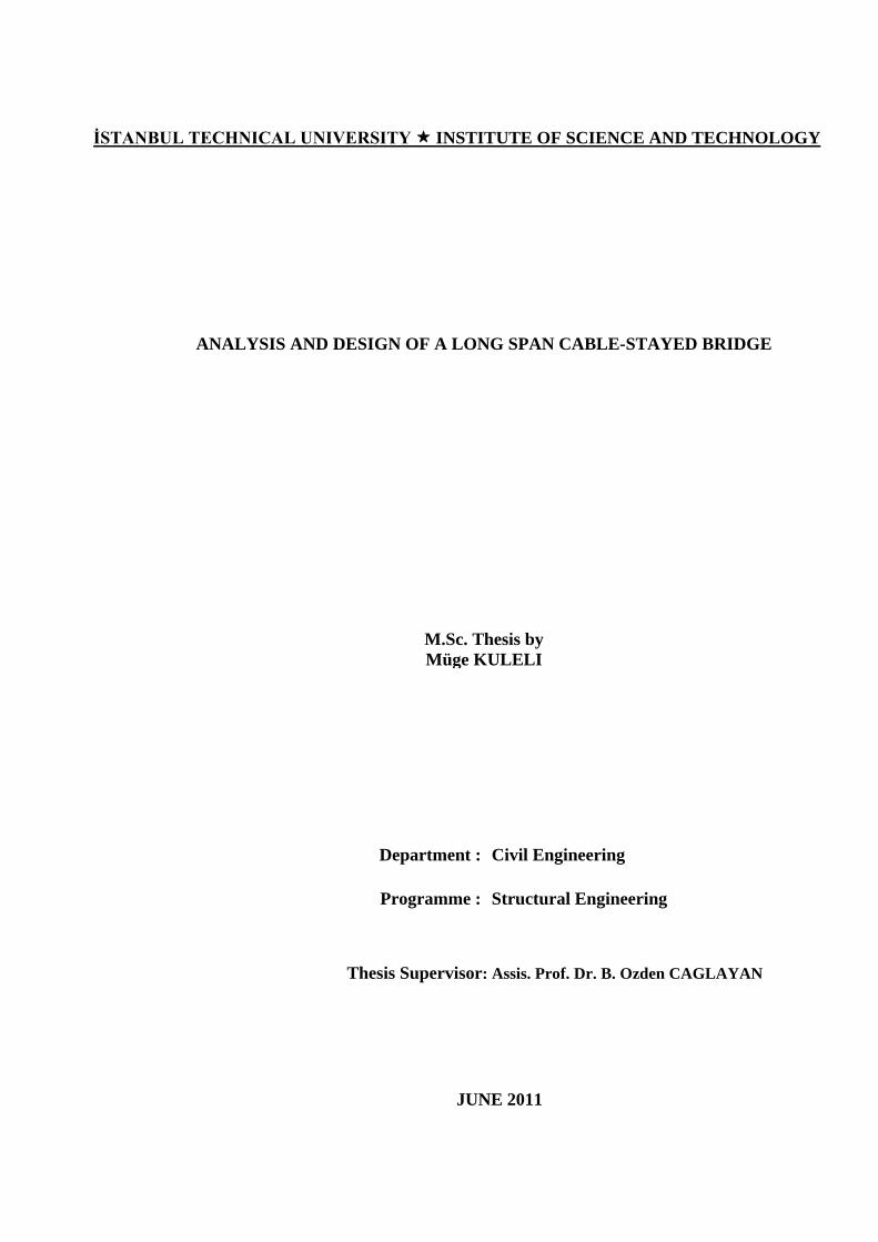
4. BRIDGE CONFIGURATION

4.1 Structure Description

The bridge considered in this study is a hypothetical example which reflects the

contemporary trend of long span cable-stayed bridges. The choice of structural

properties of the elements in the mathematical model was based on examining

several recently constructed long span cable-stayed bridges. [2], [3], [4].

A cable stayed bridge with the span arrangements 100+250+700+250+100, which

will be named as IY 700 here after, is considered to represent the current trend of

long span bridge projects. The preliminary analysis is carried out and design limit

states are checked. These calculation results will be given in Chapter 5.

Vertical profile of the bridge consists of a precamber with %1.5 vertical slope, to

compensate the dead and live load deflections. Also counterweights are arranged in

the back spans to resist uplift forces in the mid piers. Semi-fan arrangement of cables

is adopted. The general dimensions of IY 700 are depicted in Figure 4.1.

Figure 4.1 : Elevation of IY 700 Bridge.

Material Properties Table for the structural components is shown in Table 4.1.

24

Table 4.1 : Material properties

Material σy

(Mpa) σult. (Mpa) E (GPa)

Weigth Density (kN/m3)

Poisson's Ratio

Deck A572 Gr. 50 345 450 210 77.09 0.30

Cable ASTM - 1770 210 77.09 0.30 Pylon C70 - - 37 23.50 0.20 Cross Beam C70 - - 37 23.50 0.20

4.1.1 The Deck

As mentioned in Section 3.1.3, orthotropic steel box girders are preferable because of

their lightweight, torsional rigidity and streamlined cross section shapes. The box

girder is 14 m wide by 3 m deep and the central span is 700 m. The deck considered

in this study is depicted in Figure 4.2.

Figure 4.2 : Section of orthotropic steel box girder.

The proportions of the streamlined deck shape are decided based upon the given

experimental results by various authors [6], [7], [8], [11].

The torsional moments and lateral forces from box to the bearings are transferred by

provided external diaphragms at end and internal supports with a 1.875 m spacing.

Intermediate internal plate diaphragms are provided with 3.75 m spacing to ensure

the sufficient torsional rigidity and continuity of the stiffening girder. All diaphragms

are fully connected to top and bottom flanges and also webs.

Both inner and outer webs are adequately stiffened longitudinally. Access holes

within the diaphragms are not taken into consideration.

25

Since standardization of ribs is not available in AASHTO, the table provided by an

American steel company is used. [5]

Figure 4.3 : Section of ribs.

Table 4.2 : Rib cross-section properties

a (cm) d (cm) tf (cm) h' (cm) Yxx (cm) Ixx (cm4)

30.79 22.86 1.1 23.95 9.17 3612.9

Stiffening ribs are continous along the bridge. The deck plate is acting as the

common flange of both longitudinal ribs, diaphragms and webs.

Wheel load distribution on deck plate is calculated according to AASHTO-LRFD

[35]. The tire contact area is calculated as in Article 3.6.1.2.5.

Main girders of the steel orthotropic decks have been modelled either by using

equivalent beam elements or complete shell model and also by specific box girder

element formulations.

Equivalent beam element models consist beam elements with the actual stiffness

properties of the actual girder and fictitious rigid link elements are extended to cable

anchorage points which are eccentric to longitudinal center axis of the girder. This

model is named as “spine beam” and used effectively in many studies.

Complete shell model and specific box girder element formulation are the other

options to model girder which they could result in more accurate response

characteristics.

26

4.1.2 The Pylons and Piers

Diamond shape pylons are employed to improve the overall torsional stiffness of the

structure. The pylons are 208 m high with a 140 m height above the main span deck

elevation.

Beam elements are utilized to model the pylons, and piers are respresented by

supports. Solid elements may be used for more refined analysis to consider the shear

force effects accurately. These effects are not taken into account in this study for

simplicity.

4.1.3 The Stay Cables

Two inclined stay cable plane arrangement is of semi-fan type which is utilized.

There are total 184 units of cable with 92 units per each side. Cable spacing is small

in comparison with the length of the spans due to the considerations explained in

Section 3.1.3. The longest stay cable is about 360 m with an approximate weight of

300 kN.

Material properties of cables given in Table 4.1 are adopted from the VSL

International, Ltd. brochure to reflect the modern trend of the stay cable technology.

Parallel wire stand consisting of 7 mm diameter strands, each with a cross sectional

area of 38.48 mm2 is adopted for the analysis. Cables sizes range from a maximum of

0.0154 m2 for the back span cable to a minimum of 0.0054 m2 for the cables near the

pylons.

One straight chord truss element may be used to represent each cable only if the

equivalent elasticity modulus approach is utilized. Tangential modulus obtained as

explained in Section 3 is used for computing the tangent stiffness matrix of the stay

cable.

Multi element model is another option to represent cables to investigate the cable

vibration and its interaction with deck and tower modes which is not considered in

this study.

27

5. FINITE ELEMENT MODEL OF THE BRIDGE

5.1 Introduction

3D finite element model of IY 700 was set up with COSMOS-M [36] for the

purposes of static and dynamic analysis and it is depicted in Figure 5.1. In this

chapter, properties of the structural model of the bridge and assumptions made are

given in detail.

Figure 5.1 : Finite element model of the bridge.

5.2 Description of the finite element model

5.2.1 The deck

Since the dynamic behaviour of the bridge is considered, it is important to set up a

model to simulate the coupling of modes in the three orthogonal directions

accurately. Hence, 3D analysis is necessary [21].

The modelling approach given by Wilson and Gravelle [37], is adapted to model the

deck. The model consist a linear elastic beam elements which form the single central

spine and rigid links extending to the cable anchor and lumped mass points of the

deck. Mechanical properties of the equivalent beam is calculated by establishing an

exact cross section of the girder. The cross section is uniform along the bridge.

Also, a model which consist the exact shell representation of the girder to check the

accuracy of the equivalent beam model under static load conditions. Since the two

models are in good accordance by all means of deflections, moment distribution etc.,

28

the equivalent beam model is used for the rest of the analysis. The mechanical

properties of the cross section is depicted in Table 5.1.

Figure 5.2 : Finite element modelling of the cross section of the deck.

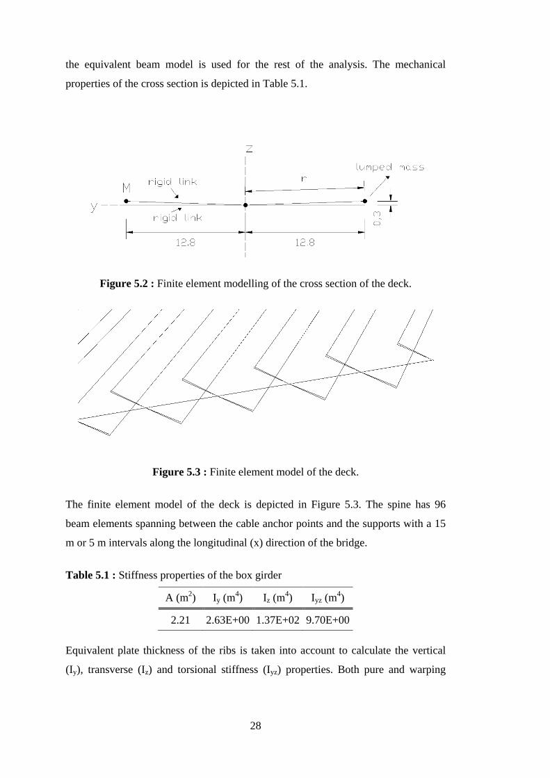
Figure 5.3 : Finite element model of the deck.

The finite element model of the deck is depicted in Figure 5.3. The spine has 96

beam elements spanning between the cable anchor points and the supports with a 15

m or 5 m intervals along the longitudinal (x) direction of the bridge.

Table 5.1 : Stiffness properties of the box girder

A (m2) Iy (m4) Iz (m4) Iyz (m4)

2.21 2.63E+00 1.37E+02 9.70E+00

Equivalent plate thickness of the ribs is taken into account to calculate the vertical

(Iy), transverse (Iz) and torsional stiffness (Iyz) properties. Both pure and warping

29

torsional stiffnesses are taken into account to calculate the overall torsional stiffness

of the cross section.

The mass of the deck consist both contribution from the cross section and the mass of

the utilities assumed distributed along the bridge. The weight properties are depicted

in Table 5.2.

Table 5.2 : Weight properties of the deck

Back Span (kN/m) Side Span (kN/m) Main Span

(kN/m)

189.08 169.08 169.08

Translational mass is calculated from the total weight of each segment either 15 m or

5 m including the contributions from ribs, plates, webs, and utilities assumed

distributed along the bridge. Total mass is divided into three concentrated masses and

allocated equally to the spine itself and points of rigid link extensions as can be seen

from Figure 5.2.

The distance between the shear center and the neutral axis of bending is taken into

account in the finite element model to allow torsional and coupled modes of

vibration.

The shear center of the cross section is 0.30 m below the centroid of the bridge which

is taken as the vertical distance between rigid links. In the finite element model the

spine is placed at the elevation of the roadway and at the shear center. Hence the

masses are placed 0.30 m above the spine and also the rotational mass properties are

calculated with the contributions of this assumption. The distance between the center

of rigidity and center of mass allows producing the coupling between the torsional

and transverse modes.

Figure 5.4 : Distribution of lumped masses used in calculating the total

lumped masses.

30

Table 5.3 : Distances between the distributed lumped masses and the shear centre

ri (m.)

m1 7.19

m2 14.60

m3 11.78

m4 4.29

m5 6.20

m6 12.93

The mass moments of inertia are calculated using the formula

𝐼𝑀𝑖 = 𝛴(𝐼𝑚𝑖 + 𝑚𝑖𝑟𝑖2) (5.1)

where;

𝐼𝑚𝑖: mass moment of inertia of the ith element about its own centroidal axis

𝑚: mass of ith element

𝑟𝑖: distance from centre of mass of ith element to the shear centre as depicted in

Figure 5.4.

The mass moment of inertia of the elements about their own centroidal axis are

calculated with the formulation given for plate elements (Eq. 5.3) and rod elements

(Eq. 5.4) where necessary.

𝐼𝑚𝑖 : 𝑚𝑖12

× �𝐿𝑥2 + 𝐿𝑦2 � (5.2)

𝐼𝑚𝑖 : 𝑚𝑖12

× �𝐿𝑦2 � (5.3)

Calculated mass properties are corrected to represent the actual mass moments of

inertia in the spine model as indicated in Wilson and Gravelle [37]. These corrected

values of translational and rotational mass are depicted in Table 5.4.

31

Table 5.4 : Mass properties of the deck

Mass Properties 15 m segment 7.5 m segment 12.5 m segment

Translational masses (kN/g) (kN/g) (kN/g)

Main Span 87.78 - 81.40

Side Span 87.78 - 81.40

Back Span 97.97 50.51961575 -

Rotational Inertia (kN/g x m2) (kN/g x m2) (kN/g x m2)

Main Span IMx 26641.92 - 17305.14

IMy 8991.99 - 4379.50

IMx 23273.65 - 15304.73

Side Span IMx 26641.92 - 17305.14

IMy 8991.99 - 4379.50

IMx 23273.65 - 15304.73

Back Span IMx 29984.03 12902.98 -

IMy 12334.10 5028.46 -

IMx 26615.76 12405.81 -

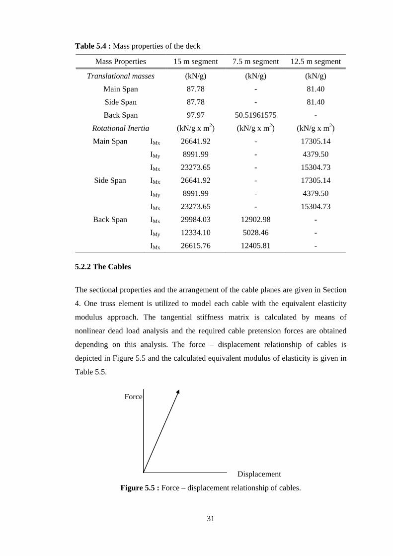
5.2.2 The Cables

The sectional properties and the arrangement of the cable planes are given in Section

4. One truss element is utilized to model each cable with the equivalent elasticity

modulus approach. The tangential stiffness matrix is calculated by means of

nonlinear dead load analysis and the required cable pretension forces are obtained

depending on this analysis. The force – displacement relationship of cables is

depicted in Figure 5.5 and the calculated equivalent modulus of elasticity is given in

Table 5.5.

Figure 5.5 : Force – displacement relationship of cables.

Force

Displacement

32

Table 5.5 : The calculated equivalent modulus of elasticity of the cables

Cable Group E (kN/m2)

1 1,55E+08 2 1,46E+08 3 1,71E+08 4 1,74E+08 5 1,84E+08 6 1,94E+08 7 1,79E+08 8 1,71E+08 9 1,60E+08

Ave. 1,70E+08

5.2.3 The Pylons and Piers

Beam elements are used to model pylons and finite element model of a pylon is

depicted in Figure 5.6. Intermediate and end piers are represented as supports since

the behaviour of these components is not a concern for this study.

5.2.4 The foundations

The interaction between soil and the structure is not taken into account.

Figure 5.6 : Finite element model of a pylon.

33

5.3 Static Loading Conditions

The loading conditions which are considered in this study are given in Table 5.6.

Table 5.6 : Loading Conditions

Load DC dead load of structural components and non-structural attachments DW dead load of wearing surfaces and utilities PS Cable prestress LL vehicular live load IM vehicular dynamic load allowance EQ earthquake

Load factors considered are given in Table 5.7.

Table 5.7 : Load Combinations and load factors

Limit State DC DD

LL IM EQ

STRENGTH I γp 1.75 STRENGTH II γp 1.35

EXTREME I γp γEQ 1 SERVICE II 1 1.3

Table 5.8 : Load factors for permanent loads, γp

Type of Load Maximum Minimum

DC: Component and Attachements 1.25 0.90 DW: Wearing Surfaces and Utilities 1.5 0.65

5.3.1 Optimization of Cable Pretension

There are infinite number of combinations concerning the pretension forces of any

cable stayed bridge. Obtaining the adequate and effective initial shape and internal

forces is the most significant task in the analysis of cable-stayed bridges since the

structure’s behaviour is dependent to it.

34

Although it is a well known fact that some of the cable pretension forces may differ

from the final form during the construction stage, in this study the final form of the

bridge is considered for the optimization process.

Three commonly used methods for obtaining the cable pretension forces have been

proposed to adjust the internal force and displacement conditions of cable-stayed

bridges. These methods are;

1. Optimization method

2. Zero displacement method

3. Force equilibrium method

There are many factors that affect the volume/cost and the safety of the structure

related to optimization process. Optimization method utilizes objective functions to

reach the ideal state of the bridge structure concerning the economy and the safety.

Deflection limits, material allowable stresses and the cost of the structure are the

primary objective function variables in this method. The constraints should be

selected very carefully or the result may be impractical.

Optimization Method

Negrao and Simoes [38] considered a multi objective function formulation consists

stress constraints on matearils used, concrete for pylons, and cost of materials.

Maximum/minimum stresses in stays, geometry control for box girder and

deflections under dead load are set as constraints by Simoes and Negrao [38], [39] to

optimize two cable-stayed bridges with box-girder decks.

The zero displacement method assumes that if the structure reaches the continuous

beam deflection after construction, the ideal state of is reached and the initial cable

forces are determined. The method is described by Wang et al. [40], [41]. The

straight and horizontal bridge decks are considered in this method, in which the

horizontal components of the cable forces will have no contribution on the bending

Zero Displacement Method

35

moment. Hence, the bending moment distribution of the structure with zero

displacements and the equivalent continuous beam will resemble each other.

According to Chen et al. [42], the bending moment distribution at the initial stage is

more important than the displacements whether zero or not as it affects the long term

behaviour of the bridge by the redistribution of internal forces.

Force Equilibrium Method

Since the method deal only with the force equilibrium, the nonlinearities arising

from cable sag does not need to be involved in the process. Hence, the cable weights

can be neglected. However, it is necessary take them into account to define the

appropriate final geometry and decide for an appropriate precamber.

Cable anchor points are involved in the calculation as control parameters which are

girder and tower anchor points. The bending moment distribution of the equivalent

continuous beam is the target for this method with zero bending moments at tower

section. [6], [7], [42].

Effective modulus of elasticity approach is utilized for the consideration of the

nonlinear cable sag effect. The stays are modelled by single truss elements.

Analysis Results

The followings are considered for the analysis to find the initial tension forces.

a. Excessive changes in cable forces should be avoided.

b. Bending moment of steel girders should be reduced and made uniform

c. The main tower should have little displacement in longitudinal direction

(bending moment of the main tower M → 0).

d. There should be no void of cable tension

e. Cable section should be uniform

The bending moments of the girder and the pylons are depicted in Figure 5.7.

36

Figure 5.7 : Bending moment distribution in deck (dead load).

The bending moment distribution of the final state of the bridge deck and pylons and

the equivalent continuous beam are in satisfactory accordance. The maximum

moment of the pylons is 16.3 MNm which is very small.

The deformed shape, Figure 5.8, under the effect of dead load and superimposed

dead load after applying the pretension forces on each cable. The maximum

deflection at the deck is 0.1405 m in vertical direction which is compensated by the

precamber. The maximum deflection of the pylons is 0.01 m in the longitudinal

direction of the bridge which is converging to zero as intended.

Figure 5.8: Dead load deformed shape (scaled).

Cables are grouped due to their installation order on the bridge. These are depicted in

Figure 5.9.

Figure 5.9 : Cable Groups.

37

5.3.2 Vehicular Live Load

There are six traffic lanes with 3600 mm width of each. Influence lines are obtained

to determine the live load forces.

AASHTO design vehicular live load, HL93, is a combination of a “design truck” or

“design tandem” and a “design lane”. A permit vehicle, P13 according to

CALTRANS, loading is also considered.

Simultaneous lane occupation of the live load is taken into account by multipresence

factors defined in AASHTO-LRFD [35] which are depicted in Table 5.9.

Application of the design vehicular live load is considered as in AASHTO-LRFD

Article 3.6.1.3 [35].

The maximum effect is resulted from the loading that considers the negative moment

between points of contraflexure under a uniform load on all spans and the reaction at

interior piers only.

Table 5.9 : Multiple Presence Factors m

Number of Loaded Lanes

Multiple Presence Factors m

1 1.20 2 1.00 3 0.85

> 3 0.65

Figure 5.10 : AASHTO-LRFD design truck.

38

Figure 5.11 : Maximum and minimum bending moments in deck.

Maximum moment in the deck under live load conditions is 276.5 MNm at

maximum and – 114.8 MNm which are depicted in Figure 5.11 for STRENGHT I

combinations.

Deflection criteria is checked according to the SERVICE I combination. The

maximum vertical deflection is 0.86 m. For most long-span cable-stayed bridges it is

acceptable limits for the deflection between 1/400 and 1/500 of the central span

length.

5.4 Earthquake Records

The effect of vertical component of ground motions on steel box girder of long span

cable-stayed bridges is the main objective of this study. Vertical component of

ground motions have been studied for two decades on the contrary of horizontal

component which is extensively studied by many researchers.

First research concerning the effects of vertical component on bridges was conducted

by Saadeghvaziri and Foutch [43]. They studied the inelastic behaviour of reinforced

concrete columns using artificial horizontal and vertical ground motion records. The

research showed that including vertical component in analysis resulted in

considerably more damage when effective peak accelerations of 0.7 g than

earthquake motions with effective peak acceleration equal to 0.4 g or less.

Some failure modes depending resulting from the vertical ground motion were

reported by Broderick and Elnashai [44] and Papazoglou and Elnashai [45].

Yu [46] and Yu et al. [47] conducted a research on the effects of vertical component

of ground motion on piers. Sylmar Hospital, Northridge record was used in analysis

and the results reported as %21 increase in axial force and a %7 increase in the

longitudinal moment on pier.

39

Button et al. [48], conducted a study with six different bridges covering variety of

structural system parameters subjected to several ground motions. However, these

studies were limited to linear response spectrum and linear time history analysis.

Veletzos et al. [49] investigated the effects of vertical component on precast

segmental superstructures and they concluded the average positive bending rotations

increase about 400% percent.

Recently Kunnath et al. [50], studied the effect of vertical component of several

configurations of typical highway overcrossing. They carried out nonlinear response

history analysis and concluded that the vertical component of ground motion cause

significant amplification in the axial force demand in the columns and moment

demands in the girder at both the midspan and at the face of the bent cap. Midspan

moments in the girder found to exceed the capacity which lead to severe damage.

S waves which are the main cause of horizontal components are longer than P waves

which cause propagation of the vertical component hence, vertical component has

much higher frequency content. In result, vertical component lead to large

amplifications in the short period range. [45], [51].

Unlike short-to-medium span bridges, there no code specified criteria to select

ground motions for long-span bridges. To obtain accurate and meaningful response,

selection of earthquake records for use of analysis is very important. Three criteria is

utilized as described below.

A selection criteria for the non-specific region applications suggested by Broderick

and Elnashai [44]. The ratio peak ground acceleration to peak ground velocity,

PGA/PGV (Zhu et.al) is employed for this study. Records will have high acceleration

peaks of short duration which cause low velocity cycles when they measured on rock

or resulted from near-source shallow earthquakes. This leads high values of

PGA/PGV ratios. On the contrary, records will have lower acceleration values, but

individual cycles are of longer duration which cause high velocity waves when they

measured on soft ground or resulted from deep earthquakes, and this leads low

values of PGA/PGV ratios. Hence, the records have high acceleration periods with

PGA/PGV Ratio:

40

longer duration periods tend to impose higher demand on long period structures [52].

The PGA/PGV ratio ranges are depicted in Table 5.10.

Table 5.10 : PGA/PGV Ratio Range (adapted from [52])

Range low PGA/PGV < 0.8

medium 0.8 ≤ PGA/PGV ≤ 1.2 high 1.2 < PGA/PGV

Many design codes using a 2/3 ratio of vertical component to horizontal component

of ground motion, which was first suggested by Newmark [53]. Studies conducted by

Abrahamson and Litehiser [54], Ambraseys and Simpson [55], Elgamal and He [56],

Bozorgnia and Campbell [57], showed that V/H ratio of 2/3 is an underestimated

value. In addition Elnashai and Papazoglou [45] stated that this value of V/H ratio is

unconservative in the near-field while it is overconservative in the far-field.

V / H (Peak Ground Acceleration Ratio):

Relationship between the timing of peak responses in the vertical and horizontal

components of ground motion is also have a significant effect on response of

structures in two ways. First, shakedown may be caused by earlier arrival of vertical

component than the horizontal component of ground motion. Secondly, coincidence

of these two components may cause significant amplification of the response of

structural elements [51].

Time interval between horizontal and vertical peak values:

A study including 452 earthquake records was carried out by Kim et al. [51] to

obtain the above mentioned V/H ratio and time interval characteristics with respect

to distance to source and earthquakes. The results of this study are depicted in Figure

5.12.

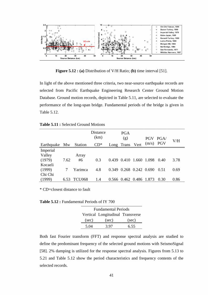
41

Figure 5.12 : (a) Distribution of V/H Ratio; (b) time interval [51].

In light of the above mentioned three criteria, two near-source earthquake records are

selected from Pacific Earthquake Engineering Research Center Ground Motion

Database. Ground motion records, depicted in Table 5.11, are selected to evaluate the

performance of the long-span bridge. Fundamental periods of the bridge is given in

Table 5.12.

Table 5.11 : Selected Ground Motions

Distance (km)

PGA (g)

PGV (m/s)

PGA/PGV V/H

Earthquake Mw Station CD* Long Trans Vert Imperial Valley (1979) 7.62

Array #6 0.3 0.439 0.410 1.660 1.098 0.40 3.78

Kocaeli (1999) 7 Yarimca 4.8 0.349 0.268 0.242 0.690 0.51 0.69 Chi Chi (1999) 6.53 TCU068 1.4 0.566 0.462 0.486 1.873 0.30 0.86

* CD=closest distance to fault

Table 5.12 : Fundamental Periods of IY 700

Fundamental Periods Vertical Longitudinal Transverse

(sec) (sec) (sec) 5.04 3.97 6.55

Both fast Fourier transform (FFT) and response spectral analysis are studied to

define the predominant frequency of the selected ground motions with SeismoSignal

[58]. 2% damping is utilized for the response spectral analysis. Figures from 5.13 to

5.21 and Table 5.12 show the period characteristics and frequency contents of the

selected records.

42

Figure 5.13 : Time – acceleration of Imperial Valley vertical component.

Figure 5.14 : El Centro Array #6 – Vertical Component Response Spectrum.

Figure 5.15 : El Centro Array #6 – Vertical Component FFT.

Time [sec]38363432302826242220181614121086420

Accele

ration [g]

1.5

1

0.5

0

-0.5

-1

-1.5

Damp. 2.0%

Period [sec]6543210

Res

pons

e Ac

cele

ratio

n [g

]

10.5109.5

98.5

87.5

76.5

65.5

54.5

43.5

32.5

21.5

10.5

0

43

Figure 5.16 : Time – acceleration of Chi Chi vertical component.

Figure 5.17 : Chi Chi Taiwan, TCU068 – Vertical Component Response Spectrum.

Figure 5.18 : Chi Chi Taiwan, TCU068 – Vertical Component FFT.

Time [sec]908580757065605550454035302520151050

Res

pons

e Ac

cele

ratio

n [g

]

0.5

0.4

0.3

0.2

0.1

0

-0.1

-0.2

-0.3

Damp. 2.0%

Period [sec]543210

Res

pons

e Ac

cele

ratio

n [g

]

10.95

0.90.85

0.80.75

0.70.65

0.60.55

0.50.45

0.40.35

0.30.25

0.20.15

0.10.05

0

44

Figure 5.19 : Time – acceleration of Kocaeli vertical component.

Figure 5.20 : Kocaeli, Yarimca – Vertical Component Response Spectrum.

Figure 5.21 : Kocaeli, Yarimca – Vertical Component FFT.

The rationale behind the selection of the above given ground motions can be stated

as;

Time [sec]3432302826242220181614121086420

Res

pons

e Ac

cele

ratio

n [g

]

0.2

0.15

0.1

0.05

0

-0.05

-0.1

-0.15

-0.2

-0.25

Damp. 2.0%

Period [sec]6543210

Res

pons

e Ac

cele

ratio

n [g

]

1.051

0.950.9

0.850.8

0.750.7

0.650.6

0.550.5

0.450.4

0.350.3

0.250.2

0.150.1

0.050

45

1 - El Centro Array #6 is the most commonly used earthquake record for the studies

of long-span cable-stayed bridges by many researchers.

2 - The Chi Chi ground motion is a not only near-fault but also pulse-type ground

motion. Pulse-type ground motions are not considered in any seismic codes except

UBC 1997.

3 - Kocaeli, Yarimca record is representing the mediocre ground motion event on the

basis of comparison of these selected ground motions.

5.5 Damping Characteristics

A structural damping of %2 is applied as Rayleigh damping and used for all analysis.

Damping characteristics of cable-stayed bridges were explained in extend in Section

2. Besides that, later Elnashai and Papazoglou [45] and Collier and Elnashai [59]

explained that the vertical component of ground motion is associated with higher

frequencies, hence suggested to limit the damping ratio of %2.

Rayleigh coefficients are computed depending on a deck mode and a tower mode

with high mass participation.

47

6.CHARACTERISTICS OF THE BRIDGE

6.1 Static Characteristics of the Bridge

Cable supported long span bridges are distinguished from most of the structures

because of their long spans and flexibility.

The bridge which is considered in this study found to satisfy all strength and service

limit states that considered among the relative displacements.

6.2 Dynamic Characteristics of the Bridge

The eigen value analysis is performed to obtain dynamic behaviour characteristics

with utilization of the tangent stiffness matrix of the dead load deformed state [4],

[24]. Boundary conditions considered for the modal analysis are given in Table 6.1.

Table 6.1 : Boundary Conditions

x - direction (longitudinal) y - direction (transverse) Deck - Pylon free fixed Intermediate Piers fixed fixed End Piers fixed fixed

First fifteen modes, their nature, periods, frequencies and mass participation ratios

are depicted in Table 6.2. First modes are all deck modes and first two mode shapes

are depicted in Figures 6.1 and 6.2.

The fundamental mode with period 6.55 s is a torsional lateral mode as depicted in

Figure 6.1.

Figure 6.1 : Fundamental Mode, TL 1

48

Table 6.2 : First 15 modes

Mode No

f [cyc/sec.] T [sec.]

Modal mass x

[%]

Modal mass y

[%]

Modal mass z

[%] Nature Dir.

1 0.15 6.55 0.00 20.20 0.00 TL 1 y 2 0.20 5.04 0.00 0.00 7.19 V 1 z 3 0.25 3.97 4.39 0.00 0.00 V 2 x 4 0.34 2.95 0.00 0.00 0.00 TL 2 y 5 0.35 2.90 0.00 1.80 0.00 TL 3 y 6 0.35 2.87 0.00 1.12 0.00 TL 4 y 7 0.36 2.78 0.00 0.00 0.00 TL 5 y 8 0.37 2.72 0.00 0.00 0.22 V 3 z 9 0.39 2.59 0.00 48.40 0.00 TL 6 y 10 0.43 2.34 19.96 0.00 0.00 V 4 x 11 0.48 2.07 0.00 0.00 0.00 TL 7 x 12 0.50 2.01 0.00 0.00 3.94 V 5 z 13 0.56 1.77 0.00 0.00 0.00 TL 8 y 14 0.58 1.73 6.75 0.00 0.00 V 6 x 15 0.62 1.62 6.41 0.00 3.63 TL 9 x

*TL identifies torsional lateral modes, V identifies vertical modes

Figure 6.2 : 2nd Mode, V 1.

Period distribution of the structure is depicted in Figure 6.4. First 11 modes have

periods above 2s and periods below 2s are closely spaced.

Figure 6.3 : 4th Mode, TL 2.

49

Figure 6.4 : Period distribution.

Figure 6.5 : Modal mass participation in longitudinal direction.

If model support conditions are selected as free in transverse (lateral) direction, then

the fundamental period of the bridge will result in the period of a pendulum which is

formulated by Galileo Galilei and the nature of this mode will be transverse sway.

𝑇𝑝𝑒𝑛𝑑𝑢𝑙𝑢𝑚 = 2𝜋�𝑙𝑔

(6.1)

Where,

0,00

1,00

2,00

3,00

4,00

5,00

6,00

7,00

1 51 101 151 201

Peri

od [s

]

Mode Number

0,0010,0020,0030,0040,0050,0060,0070,0080,0090,00

100,00

1 51 101 151 201

Acc

umul

ated

Mas

s [%

]

Mode Number

50

𝑙 ∶ the distance between pylon top and deck

𝑔 ∶ acceleration of gravity

𝑇𝑝𝑒𝑛𝑑𝑢𝑙𝑢𝑚 = 2𝜋�139𝑚𝑔

= 23.651 sec.

Since the period is calculated as 22.394 sec. by modal analysis, the deck is a bit

stiffer than the equivalent system.

51

7. EARTHQUAKE RESPONSE

7.1 Introduction

Nonlinear time history analysis is carried out, after a nonlinear static load analysis

under dead load, to obtain seismic response characteristics of the bridge.

Bending moment change at midspan, at the face of crossbeam of the pylon, and

intermediate pier are investigated among the rotation displacements.

7.2 Nonlinear Time History Analysis

Nonlinear direct integration method is adopted for dynamic analysis of the bridge.

• Newmark implicit integration sheme (δ = 0.5, α = 0.25)

• Time step, ∆t = 0.02 which allows high frequency modes to participate in

response. A sensitivity analysis should be carried out usually, however the

value suggested by many researchers is used in this study.

• Geometric nonlinearity is considered

7.3 Results

The results obtained by nonlinear time history analysis will be given in this section.

My refers to the longitudinal bending moment and Ry refers to rotational

deformations on the girder. Figure 7.1 showing elements and nodes in consideration.

H+L is representing values resulting from only horizontal ground motion excitation,

H+L+V is representing values obtained by including the vertical component of

ground motion to horizontal components in the following figures.

A parametric study is carried out depending upon PGA/PGV ratios and V/H ratios.

Response of bridge which is subjected to only horizontal components and both

horizontal and vertical components are given below in detail.

52

Figure 7.1 : Element and node of girder considered at midspan for response.

Figure 7.2 : Element and node considered at pylon section of girder for response.

Kocaeli, Yarimca:

Figure 7.3 : E134 – My Moment.

53

Figure 7.4 : N94 – Ry Displacement.


54


Moments resulting from the excitation of ground motion including vertical

component are seriously amplified when they compared with moments resulted from

only horizontal ground motion excitation at the midspan, Element 134. It is depicted

in Figure 7.3.

On the contrary, rotations about y axis of the bridge do not change due to

participation of the vertical component of earthquake at the midspan, Node 94. As

can be seen from Figure 7.4 change of rotation deformations in time resulting from

both cases are exactly same.

At the pylon section of stiffening girder, Element 112, moments resulting from the

excitation of ground motion including vertical component are also found to be

increased they compared with moments resulted from only horizontal ground motion.

The rate of amplification is depicted in Figure 7.5.

In addition, rotations about y axis of the girder are amplified by the contribution of

vertical component of earthquake.

55

ElCentro, Array # 6:



56



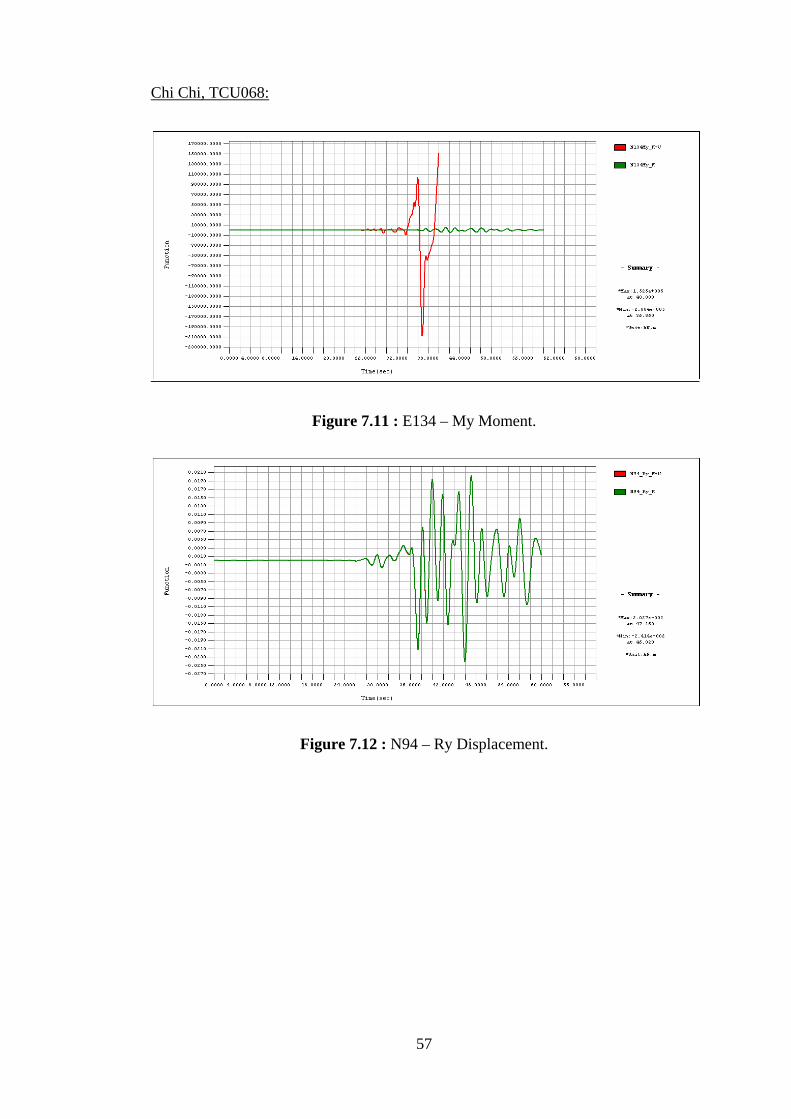
57

Chi Chi, TCU068:



58


Figure 7.14 : N70 – Ry Displacement .

Experience show that, seismic load seldom controls the design except in extremely

high seismic areas.

All results presented in Table 7.1 and Table 7.2 compare the code specified load

combinations for design and the internal forces obtained from the contribution of the

vertical component of the ground motions. The results in Table 7.1 and 7.2 are also

include the normalized values by the corresponding response of the live load and

dead load combination.

59

Table 7.1 : Comparison of moment values for element 134 between code specified

load combinations

Load Elem. No. Mmax. Mmin.

DL 134 (N94) 22677

DL + 1.75LL 137964 -2333

Kocaeli DL + (TH- H) 134 (N94) 27746 -2836

DL + (TH- HV) 85723 -91890 Imperial

Valley DL + (TH- H) 134 (N94)

27746 -3781 DL + (TH- HV) 93368 -64653

Chi Chi DL + (TH- H) 134 (N94) 27746 -4562

DL + (TH- HV) 152500 -208404

Table 7.2 : Comparison of moment values for element 112 between code specified

load combinations

Load Elem. No.

Mmax. Mmin. Mmax./DL Mmin./LL

DL 112 (N70)

22677 1,00

DL + 1.75LL -35079 -106726 -1,55 1,00

Kocaeli DL + (TH- H) 112

(N70) 10575 -49382 0,47 0,46

DL + (TH- HV) 46887 -49382 2,07 0,46 Imperial

Valley DL + (TH- H) 112

(N70) 8948 -49382 0,39 0,46

DL + (TH- HV) 92663 -49382 4,09 0,46

Chi Chi DL + (TH- H) 112

(N70) 17703 -49382 0,78 0,46

DL + (TH- HV) 68960 -90492 3,04 0,85

Table 7.3 : Increment ratio for rotational displacement of node 70.

N70 time (s.)

Kocaeli 71% 23

Imperial Valley 143% 31

Chi Chi 522% 40

61

8. CONCLUSIONS

Vertical component of ground motions and its effects on structures has not been

investigated in depth as much as the horizontal components. More research is needed

on the subject of vertical component of ground motions, especially for the near fault

strong motions.

Negative moment demand at the centre of the main span is considerably increased as

depicted in Table 7.1. No variation observed at the deck negative moment demand at

the face of pylon. Positive moment demand is increased as depicted in Table 7.2.

Rotational displacement demand of the deck at the face of the pylons is increased

with 71% ratio at least as depicted in Table 7.3. This may be further studied in

manner of ductility capacity of the deck.

These conclusions are in parallel manner with the conclusions derived by Kunnath et

al. [50] for short span crossover bridges. Also, it has been concluded that vertical

component effects may be uncoupled from the horizontal component effects as

depicted in Figures 7.3, 7.5, 7.7, 7.9, 7.11, 7.12.

In addition to above stated, it has been concluded that the impulse character of the

vertical component of ground motion, as in Chi Chi, Taiwan record, impose the most

demand on midspan deck negative moment and rotational displacement capacity of

the deck at the face of the pylon.

Selection of the ground motions by means of predominant frequency of the ground

motion is also an important criteria for obtaining effects of the vertical component.

Due to these results, the effect of the vertical component of the selected ground

motion should carefully examined, especially for the near fault ground motions.

62

Isolation devices may be used to reduce the response of cable-stayed bridges. In

addition support conditions may be revised to provide more flexible structure as

concluded by many researchers before.

It is obvious that due to exceptional and unique nature of each long span cable-stayed

project, a code specification is not possible. However, since the behaviour of the

structure in earthquake prone areas has been the major source of concern, guidance

for selection of ground motions is necessary for use of design firms.

As investigated by many researchers before, the effect of the vertical component of

the ground motion can cause severe amplification in the bridge response. Hence, it

should be included in dynamic analysis of long span bridges with appropriate

earthquake records selected to result in accurate and meaningful response

characteristics.

63

REFERENCES

[1] Nazmy, A. S., Abdel-Ghaffar, A. M., 1987 : Seismic Response Analysis of

Cable-Stayed Bridges Subjected to Uniform and Multi-Support

Excitations. Report No. 87-SM-1, Department of Civil Engineering,

Princeton University, Princeton, N.J.

[2] Cho, S., et al., 2009 : Incheon Bridge: Facts and the State of the Art,

International Commemorative Symposium for the Incheon Bridge,

Korea, pp. 18 – 29.

[3] Son, Y., et al., 2009 : Design & Construction of Incheon Bridge CSB Pylon,

International Commemorative Symposium for the Incheon Bridge,

Korea, pp. 120 – 133.

[4] Masashi, Y., et al., 2003 : Design of “Tatara Bridge”, IHI Engineering Review,

Vol. 36, No. 2, pp. 40 – 56.

[5] Chen, W. F., Duan, L., 2000 : Bridge Engineering Handbook. CRC Press LCC.

[6] Troitsky, M. S., 1988 : Cable-Stayed Bridges: Theory and Design. 2nd Edition.

[7] Gimsing, N. J., 1998 : Cable Supported Bridges – Concept & Desgin. John

Wiley, 2nd Edition.

[8] Walther, R. et al. 1999 : Cable Stayed Bridges. Thomas Telford, 2nd Edition.

[9] Tang, M. C., 1983 : Concrete cable-stayed bridges, presented at ACI

Convention, Kansas City.

[10] Tang, M. C., 1971 : Analysis of cable-stayed bridges, Journal of the Structural

Division ASCE.

64

[11] Podolny, N. J., Scalzi J. B., 1986 : Construction and Design of Cable-Stayed

Bridges. John Wiley & Sons, 2nd Edition.

[12] Ren, W. X., Obata, M., 1999 : Elastic-Plastic Seismic Response of Long Span

Cable-Stayed Bridges, Journal of Bridge Engineering, Vol. 4, pp.

194-203.

[13] Fleming, J. F., Egeseli, E. A., 1980 : Dynamic Behaviour of a Cable-Stayed

Bridge. Earthquake Engineering and Structural Dynamics, Vol. 8, pp.

1 – 16.

[14] Nazmy, A. S., Abdel-Ghaffar, A. M., 1990 : Non-linear earthquake response

analysis of long-span cable-stayed bridges: theory, Earthquake

Engineering and Structural Dynamics, Vol. 19, pp. 45 – 62.

[15] Nazmy, A. S., Abdel-Ghaffar, A. M., 1990 : Non-linear earthquake response

analysis of long-span cable-stayed bridges: applications, Earthquake


[16] Ernst, HJ., 1965 : Der E-Modul von Seilen unter Berücksichtingung des

Durchhangens. Bauingenieur, Vol. 40, pp. 52 – 55.

[17] Abdel-Ghaffar, A. M., Khalifa, M., 1991: Importance of Cable Vibration in

Dynamics of Cable-Stayed Bridges. Journal of Engineering

Mechanics, Vol. 117, pp. 2571 – 2589.

[18] Abdel-Ghaffar, A. M., A. S. Nazmy, 1991 : 3-D Nonlinear Seismic Behavior

of Cable-Stayed Bridges. Journal of Structural Engineering, Vol.

117, pp. 3456 – 3476.

[19] Abdel-Ghaffar, A. M., A. S. Nazmy, 1988 : Nonlinear Seismic Response of

Cable-Stayed Bridges Subjected to Nonsynchronous Motion.

Proceedings of 9th World Conference on earthquake Engineering,

Tokyo-Kyoto, Vol. 6, pp. 483 – 488.

[20] Zienkiewicz, O. C., Taylor, R. L., 1991 : The Finite Element Method. Mc

Graw Hill , 4th Edition, Vol. 1,2.

65

[21] Abdel-Ghaffar, A. M., A. S. Nazmy, 1986 : Seismic Behavior of Long-Span

Cable-Stayed Bridges. Dynamic Response of Structures, American

Society of Civil Engineers, New York, pp. 281-288.

[22] Ali, H. M., Abdel-Ghaffar, A. M., 1995 : Modelling the nonlinear seismic

behavior of cable-stayed bridges with passive control bearings.

Computers & Structures, Vol. 54, No. 3, pp. 461-492.

[23] Wilson, J. C., Liu, T., 1991: Ambient Vibration Measurements on a Cable-

Stayed Bridge. Earthquake Engineering and Structural Dynamics,

Vol. 20, pp. 723 – 747.

[24] Kawashima, K., 2011 : Seismic Design of Urban Infrastructure. Lecture Notes,

Tokyo Institute of Technology.

[25] Daniell, W. E., MacDonald, J. H. G., 2007: Improved Finite Element

Modelling of a Cable-Stayed Bridge Through Systematic Manual

Tuning. Engineering Structures, Vol. 29, pp. 358 – 371.

[26] Nazmy, A. S., Abdel-Ghaffar, A. M., 1992 : Effeccts of Ground Motion

Spatial Variabilty on the Response of Cable-Stayed Bridges.

Earthquake Engineering and Structural Dynamics, Vol. 21, pp. 1 –

20.

[27] Kawashima, K., Unjoh, S., Tunomoto, M., 1993 : Estimation of Damping

Ratio of Cable-Stayed Bridges for Seismic Design. Journal of

Structural Engineering, Vol. 119, pp. 1015 – 1031.

[28] Clough, R. W., Penzien, J. 1993 : Dynamics of Structures. McGraw-Hill, 2nd

Edition.

[29] Ali, H. M., Abdel-Ghaffar, A. M., 1995 : Modelling of Rubber and Lead

Passive-Control Bearings for Seismic Analysis. Journal of Structural

Engineering, Vol. 121, pp. 1134-1144.

66

[30] Ali, H. M., Abdel-Ghaffar, A. M., 1994 : Seismic Energy Dissipation for

Cable-Stayed Bridges Unsing Passive Devices. Earthquake


[31] Kawashima, K., Unjoh, S., 1992 : Damping Characteristics of Cable-Stayed

Bridges, Proceedings of the 10th World Conference on Earthquake

Engineering, Madrid, pp. 4803 – 4808.

[32] Kawashima, K., Unjoh, S., Azuta, Y.-I., 1988 : Damping Characteristics of

Cable-Stayed Bridges, Proceedings of the 9th World Conference on

Earthquake Engineering, Tokyo-Kyoto, Vol. 6, pp. 471 – 476.

[33] Kawashima, K., Unjoh, S., Azuta, Y.-I., 1990 : Analysis of Damping

Characteristics of a Cable-Stayed Bridge Based on Strong Motion

Records, Structural Engineering/Earthquake Engineering, Japan

Society of Civil Engineers, Vol. 6, No. 1, pp. 181 – 190.

[34] Wilson, J. C., Liu, T., Gravelle, W., 1991: Ambient Vibration and Seismic

Response of a Cable-Stayed Bridge. European Earthquake

Engineering, Vol. 5, pp. 9 – 15.

[35] AASHTO, LRFD Bridge Design Specifications, American Association of State

Highway and Transportation Officials, Washington, D. C., 2010.

[36] COSMOS/M, 2008: User’s Manual, Solidworks Corporation, Dassault

Systémes, Massachusetts, USA.

[37] Wilson, J. C., Gravelle, W., 1991: Modelling of a cable-stayed bridge for

dynamic analysis. Earthquake Engineering and Structural Dynamics,

Vol. 20, pp. 707 – 721.

[38] Negrao, J. H. O., Simoes, L. M. C., 1997 : Optimization of cable-stayed

bridges with three dimensional modelling, Computers and Structures,

Vol. 64, No. 1-4, pp. 741-758.

67

[39] Simoes, L. M. C., Negrao, J. H. O., 2000 : Optimization of cable-stayed

bridges with box-girder decks, Advances in Engineering Software,

Vol. 31, pp. 417-423.

[40] Wang, P.H., Lin, H. T., Tang, T. Y., 2002 : Study on nonlinear analysis of a

highly redundant cable-stayed bridge, Computers & Structures, Vol.

8, No. 2, pp. 165-182.

[41] Wang, P.H., Tang, T. Y., Zheng, H.N., 2004 : Analysis of Cable-Stayed

Bridges During Construction by cantilever methods, Computers &

Structures, Vol. 82, pp. 329-346.

[42] Chen, D. W., Au, F. T. K., Tham, L.G., Lee, P.K.K., 2000 : Determination of

initial cable forces in prestressed concrete cable-stayed bridges for

given design deck profiles using the force equilibrium method,

Computers & Structures, Vol. 74, pp. 1-9.

[43] Saadeghvaziri, M. A., Foutch, D. A., 1991 : Dynamic Behavior of R/C

highway bridges under the combined effect of vertical and horizontal

earthquake motions, Earthquake Engineering and Structural

Dynamics, Vol. 20, pp. 535 – 549.

[44] Broderick, B. M., Elnashai, A. S., 1995 : Analysis of the failure of the failure

of Interstate 10 freeqay ramp during the Northridge earthquake of 17

January 1994, Earthquake Engineering and Structural Dynamics, Vol.

24, No. 2, pp. 189 – 208.

[45] Papazoglou, A. J., Elnashai, A. S., 1996 : Analytical and field evidence of the

damaging effect of vertical earthquake ground motion, Earthquake


[46] Yu, C. P., 1996 : Effect of vertical earthquake componenets on bridge

responses, Ph.D. Thesis, University of Texas at Austin, Texas.

68

[47] Yu, C. P., Broekhuizen, D. S., Roesset, J. M., Breen, J. E., Kreger, M. E.,

1997 : Effect of vertical ground motion on bridge deck response,

Proceedings, Workshop on Earthquake Engineering Frontiers in

Transportation Facilities, Techical Report No. NCEER-97-0005,

National Center for Earthquake Engineering Research, State

Universtiy of New York at Buffalo, N. Y., 249 - 263.

[48] Button, M. R., Cronin, C. J., Mayes, R. L. 2002 : Effect of vertical motions on

seismic response of bridges, Earthquake Engineering and Structural

Dynamics, Vol. 25, pp. 1109 – 1137.

[49] Veletzos, M. J., Restrepo, J. I., Seible, F., 2006 : Response of precast

segmental bridge superstructures, Report submitted to Caltrans -

SSRP-06/18, University of California, San Diego, California.

[50] Kunnath, S. K., et al. 2008 : Development of guidelines for incorporation of

vertical ground motion effects in seismic design of highway bridges,

Report No. CA/UCD-SESM-08-01, University of California, San

Diego, California

[51] Kim, S. J., Curtis, J. H., Elnashai, A. S., 2011 : Analytical Assessment of the

Effect of Vertical Earthquake Motion on RC Bridge Piers, Journal of

Structural Engineering, Vol. 137, No. 2, pp. 252 – 260.

[52] Elnashai, A. S., Di Sarno, L., 2008 : Fundamentals of Earthquake Engineering:

Theory and Design. John Wiley & Sons, 2nd Edition.

[53] Newmark, N. M., Blume, J. A., Kapur, K. K., 1973 : Seismic Design Spectra

for Nuclear Power Plants, Journal of the Power Division, Vol. 99, pp.

287 – 303.

[54] Abrahamson, N. A., Lithesiher, J. J., 1989 : Attenuation of vertical peak

acceleration, Bulletin of the Seismological Society of America, Vol.

79, No. 3, pp. 549 – 580.

69

[55] Ambraseys, S. J., Simpson, K. A., 1996 : Prediction of vertical response

spectra in Europe, Earthquake Engineering & Strucutral Dynamics,

Vol. 25, No. 4, pp. 401 – 412.

[56] Elgamal, A., He, L., 2004 : Vertical earthquake ground motion records: An

overview, Journal of Earthquake Engineering, Vol. 8, No. 5, pp. 663

– 697.

[57] Bozorgnia, S. J., Campbell, K. W., 1995 : Analysis of the failure of Interstate

10 freeway ramp during the Northridge earthquake of 17 January

1994., Earthquake Engineering & Strucutral Dynamics, Vol. 24, No.

2, pp. 189 – 208.

[58] SeismoSignal, 2010: User’s Manual, SeismoSoft Ltd., Pavia, Italy.

[59] Collier, C. J., Elnashai, A. S., 2001 : A procedure for combining vertical and

horizontal seismic action effects, Journal of Earthquake Engineering,

Vol. 5, No. 4, pp. 521 – 539.

71

CURRICULUM VITAE

Candidate’s full name: Müge Kuleli

Place and date of birth: Tunceli, 09.07.1986

Permanent Address: Ismet Pasa Dist. Nusrat Mayın St. No:27 Çanakkale, Turkey

Universities and Colleges attended: 2004 - 2009 : Istanbul Technical University, Istanbul, Turkey Faculty of Civil Engineering BSc., Department: Civil Engineering 2001 - 2004 : Canakkale Science High School, Istanbul, Canakkale Science and Mathematics

Civil Engineeri

Documents

Transcript of Civil Engineeri