
chiversEtAl-supplementary material
88
Predator-prey systems depend on a prey refuge 1 — 2 Supplementary material 3 — 4 W. J. Chivers, W. Gladstone, R. D. Herbert and M. M. Fuller 5 1
Transcript of chiversEtAl-supplementary material

Predator-prey systems depend on a prey refuge1
—2
Supplementary material3
—4
W. J. Chivers, W. Gladstone, R. D. Herbert and M. M. Fuller5
1

Contents6
1 Model behaviour across initial condition and parameter value ranges 37
1.1 Method . . . . . . . . . . . . . . . . . . . . . . . . . . . . . . . . . . 48
1.2 Summary of results . . . . . . . . . . . . . . . . . . . . . . . . . . . . 69
1.3 Predator initial population . . . . . . . . . . . . . . . . . . . . . . . . 710
1.4 Predator initial resources . . . . . . . . . . . . . . . . . . . . . . . . . 1011
1.5 Predator metabolic cost per time step . . . . . . . . . . . . . . . . . . . 1312
1.6 Predator trophic efficiency . . . . . . . . . . . . . . . . . . . . . . . . 1613
1.7 Predator chances of eating . . . . . . . . . . . . . . . . . . . . . . . . 1914
1.8 Predator trapping rate . . . . . . . . . . . . . . . . . . . . . . . . . . . 2215
1.9 Predator generalist rate . . . . . . . . . . . . . . . . . . . . . . . . . . 2716
1.10 Predator generalist resources added . . . . . . . . . . . . . . . . . . . . 3417
1.11 Prey initial population . . . . . . . . . . . . . . . . . . . . . . . . . . . 4118
1.12 Prey initial resources . . . . . . . . . . . . . . . . . . . . . . . . . . . 4419
1.13 Prey metabolic cost per time step . . . . . . . . . . . . . . . . . . . . . 4720
1.14 Prey resource consumption per time step . . . . . . . . . . . . . . . . . 5021
1.15 Prey hidden . . . . . . . . . . . . . . . . . . . . . . . . . . . . . . . . 5322
2 Predator functional response 5623
3 Appendix 1: Model description in pseudo-code 5824
3.1 Initialisation and main loop . . . . . . . . . . . . . . . . . . . . . . . . 5825
3.2 Method definitions . . . . . . . . . . . . . . . . . . . . . . . . . . . . 5926
4 Appendix 2: The agent-based model implemented in the Python program-27
ming language 6128
4.1 Using the model graphical interface . . . . . . . . . . . . . . . . . . . 6129
4.2 Python version and additional packages . . . . . . . . . . . . . . . . . 6230
4.3 Running the ABM on Microsoft Windows . . . . . . . . . . . . . . . . 6231
4.4 Running the ABM on Linux or BSD . . . . . . . . . . . . . . . . . . . 6332
4.5 Running the ABM on Apple OSX . . . . . . . . . . . . . . . . . . . . 6333
4.6 The model code . . . . . . . . . . . . . . . . . . . . . . . . . . . . . . 6434
4.6.1 main.py . . . . . . . . . . . . . . . . . . . . . . . . . . . . . . 6435
4.6.2 gui.py . . . . . . . . . . . . . . . . . . . . . . . . . . . . . . . 6536
4.6.3 simulation.py . . . . . . . . . . . . . . . . . . . . . . . . . . . 7337
4.6.4 default_values.py . . . . . . . . . . . . . . . . . . . . . . . . . 8438
4.6.5 animal.py . . . . . . . . . . . . . . . . . . . . . . . . . . . . . 8539
4.6.6 predator.py . . . . . . . . . . . . . . . . . . . . . . . . . . . . 8740
4.6.7 prey.py . . . . . . . . . . . . . . . . . . . . . . . . . . . . . . 8841
2

1 Model behaviour across initial condition and param-42
eter value ranges43
This section presents an analysis of the sensitivity of the model to variation in the default44
initial condition and parameter values. The behaviour of the model with this parameter45
set is typical of all parameter sets observed.46
This analysis illustrates47
1. For all initial conditions or parameters:48
• the ranges over which each initial condition or parameter value can be ad-49
justed while maintaining population cycling,50
• the ranges over which each initial condition or parameter value can be ad-51
justed without causing extinctions,52
• suggested correlations between initial condition or parameter values and53
– population means,54
– population cycle period length and55
– population cycle amplitude.56
2. For the parameters predator trapping rate (ptr), predator generalist rate (pgrate)57
and predator generalist resources added (pgres) this analysis also illustrates58
• correlation between population amplitudes and the predator trapping rate,59
ptr and60
• correlations between population amplitudes and the generalist predator pa-61
rameters, pgrate and pgres.62
3

3. Finally for the parameters predator generalist rate (pgrate) and predator generalist63
resources added (pgres) this analysis illustrates the effects of these parameters on64
the predator functional response.65
1.1 Method66
The approach taken was to start with the default set of parameters (which usually results67
in the two populations reaching 1000 time steps without an extinction) and to vary each68
parameter while holding the others constant. The graphs produced were:69
1. For all initial condition or parameters:70
• mean populations and mean number of time steps before an extinction (up71
to 1000 time steps) graphed against the initial condition or parameter and72
• predator and prey populations per time step for eight executions of the model73
(up to 500 time steps) using different values of the initial condition or pa-74
rameter.75
2. For the parameters predator trapping rate (ptr), predator generalist rate (pgrate)76
and predator generalist resources added (pgres) the following are added:77
• mean predator population peaks graphed against the parameter and78
• mean prey population peaks and graphed against the parameter.79
3. Finally for the parameters predator generalist rate (pgrate) and predator generalist80
resources added (pgres) the functional response of the predators for eight execu-81
tions of the model using different values of the parameter are graphed and the82
intercepts and slopes of lines of best fit on these graphs are tabulated.83
4

For the purposes of this analysis the upper and lower limits for each initial condition84
or parameter were found by manual experimentation. These limits were identified by85
• increasing failure of one of the populations (usually the predator population) to86
reach 1000 time steps and/or87
• stabilisation of the apparent trend in the data.88
The ranges over which cycling populations were evident were judged by observation89
of the output of individual model executions.90
Population and time step mean graphs91
The data collected over 50 simulations at each initial condition or parameter value were92
• the mean populations over 1000 time steps,93
• the mean number of time steps (up to 1000) before extinction of either of the94
populations and95
• the mean maximum and minimum levels of each population.96
Individual simulations at selected parameter levels97
The data collected for each time step were98
• the time step,99
• the predator population and100
• the prey population.101
5

1.2 Summary of results102
Without formal statistical analysis, the graphs presented below suggest the following103
effects within parameter ranges which result in population cycling and few extinctions.104
Note: not tabulated was the observation that per capita predation rates may rise slightly105
as pgrate and/or pgres rise.106
SM Table 1: a) Ranges over which initial conditions and parameters produce popula-tion cycling and populations persistent to 1000 time steps and b) correlations betweeninitial condition or parameter levels and population means, population cycle periodlength and population cycle amplitude within these ranges. These correlations have notbeen formally tested—these results are suggested only by the trends evident in SM Fig-ures 1a to 13b.Key:— no correlation or no extinctions recorded? relationship not clear∗ positive correlation† negative correlation†? possible negative correlation, separates predator and prey resultsts: time steppop: population
Name Symbol Pop cycling Persistent Pop Pop cycle Pop cyclerange to 1000 ts means period amplitude
PredatorInitial population pn ≥ 0 — — — —Initial resources pir 20− 1700 ≥ 140 † ∗ ?Energy cost per ts pmc 14− 40 ≤ 37 ∗ † ∗Trophic efficiency pte 10− 40 ≥ 16 † — †Chance of eating pce 0.01− 0.06 ≥ 0.02 † — †Trapping rate ptr 0− 50 ≤ 25 ?,∗ †? ∗Generalist rate pgrate 0− 45 — † ∗ †Generalist resources pgres 0− 60 — † ∗ †PreyInitial population bn ≥ 0 — — — —Initial resources bir ≥ 60 ≥ 60 † ∗ †Energy cost per ts bmc 0− 70 ≤ 60 † ∗ †Resource consumption bminr,bmaxr 90− 700 ≥ 120 ∗,†? † †Prey hidden bph 5− 20 ≥ 6 † ∗ †
6

1.3 Predator initial population107
Summary108
The initial population of predators (pn) is the size of the population used to start a simu-109
lation. In the simulations reported in this parameter sensitivity analysis, this parameter110
has a default value of 35 individuals—this value chosen because it is the mean predator111
population level which emerges over many time steps with this parameter set.112
With the default parameter set, values of pn ≥ 0 individuals result in population cy-113
cling and no extinctions were observed while adjusting this parameter. Higher values of114
the parameter do result in transient dynamics at the start of a simulation as the predator115
population falls to a sustainable level. SM Figure 1a graphs mean population levels and116
mean time step reached over 50 simulations at each parameter level.117
Eight individual executions of the model are illustrated in SM Figure 1b at eight118
different parameter levels. These figures do not suggest any correlation between pn and119
population cycle period length or between the parameter and population cycle ampli-120
tudes.121
7

Predator initial population: Population levels, population persistence and range in122
which population cycling is evident123
0
20
40
60
80
100
120
0 100 200 300 400 500 0
200
400
600
800
1000
1200
Mean p
op
ula
tions
Mean tim
e s
teps
Predator initial population
Mean time stepsMean predator population
Mean prey population
SM Figure 1a: Mean populations and mean number of time steps before an extinctiongraphed against predator initial population (pn). To avoid any confounding effect ofincreasing the initial predator number, these data are from time steps 201–1000 only astransient dynamics at the start of a simulation very rarely persist for 200 time steps. Thedefault value for the simulations reported here was 35 individuals. The error bars repre-sent one standard deviation. No extinctions were observed and population cycling wasevident in the range 1 to > 500 individuals. This graph indicates the lack of importanceof the initial predator population size—the level of the predator initial population maycause transient dymanics at the start of a simulation, but the peaks, troughs and meanpopulations then settle to levels which are dependent on the model parameters.
8
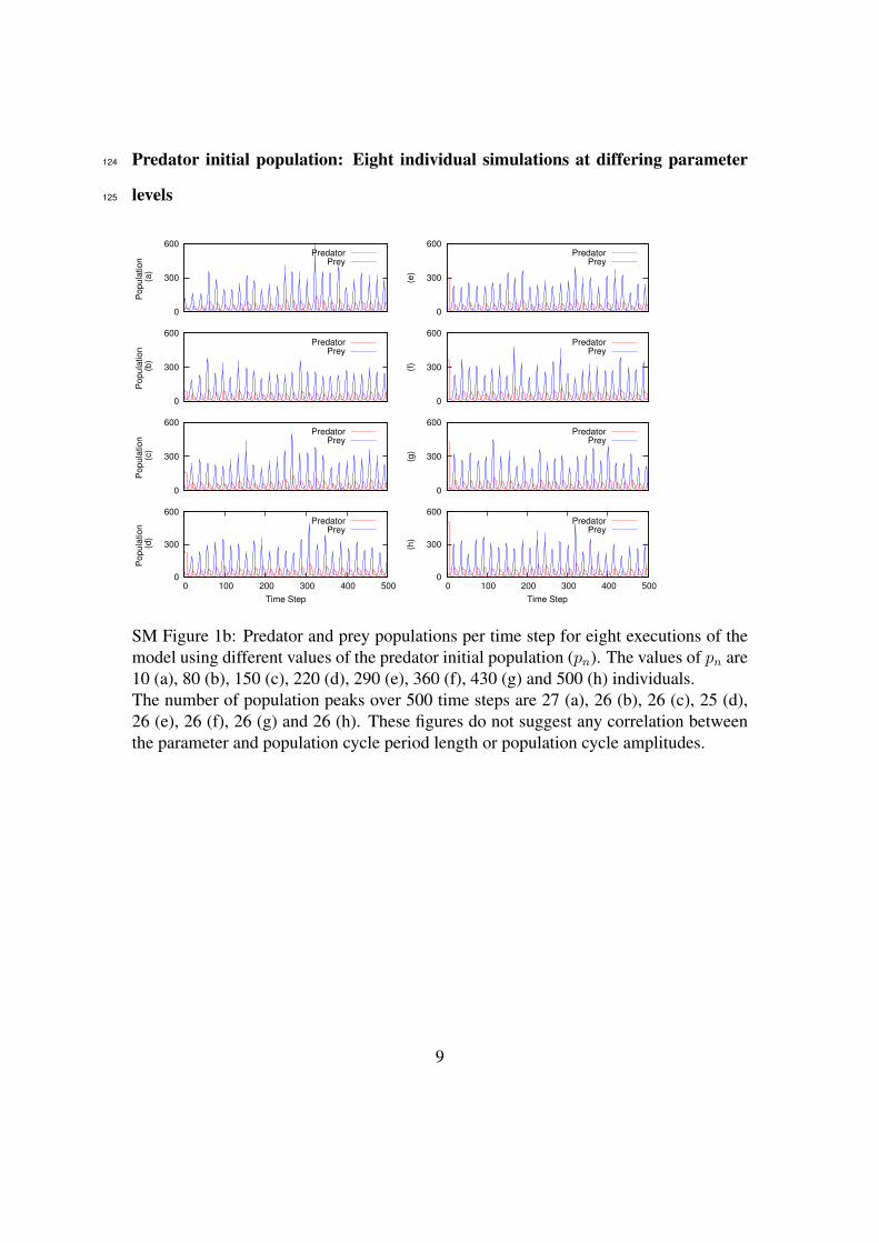
Predator initial population: Eight individual simulations at differing parameter124
levels125
0
300
600
Po
pu
lation
(a
)
PredatorPrey
0
300
600
Popula
tion
(b)
PredatorPrey
0
300
600
Popula
tion
(c)
PredatorPrey
0
300
600
0 100 200 300 400 500
Popula
tion
(d)
Time Step
PredatorPrey
0
300
600
(e)
PredatorPrey
0
300
600
(f)
PredatorPrey
0
300
600
(g)
PredatorPrey
0
300
600
0 100 200 300 400 500
(h)
Time Step
PredatorPrey
SM Figure 1b: Predator and prey populations per time step for eight executions of themodel using different values of the predator initial population (pn). The values of pn are10 (a), 80 (b), 150 (c), 220 (d), 290 (e), 360 (f), 430 (g) and 500 (h) individuals.The number of population peaks over 500 time steps are 27 (a), 26 (b), 26 (c), 25 (d),26 (e), 26 (f), 26 (g) and 26 (h). These figures do not suggest any correlation betweenthe parameter and population cycle period length or population cycle amplitudes.
9

1.4 Predator initial resources126
Summary127
The predator initial resources parameter (pir) represents the energy resources a predator128
individual is born with. At the start of a simulation all predators have this resource129
level and all individuals born during the simulation have the same resource level in their130
first time step. This parameter also specifies the cost of reproduction for a parent—it131
is the number of resources subtracted from a parent when it bears one offspring. In the132
simulations reported in this parameter sensitivity analysis, this parameter has a default133
value of 220.0 resource units.134
With the default parameter set, values of 20 ≤ pir ≤ 1700 resource units result in135
population cycling and extinctions are observed when pir ≤ 140 resource units. Mean136
populations of both species are negatively correlated with pir in this range of values, as137
illustrated by SM Figure 2a which graphs mean population levels and mean time step138
reached over 50 simulations at each parameter level.139
Eight individual executions of the model are illustrated in SM Figure 2b at eight140
different parameter levels. These figures suggest a positive correlation between pir and141
population cycle period length; the relationship between the parameter and population142
cycle amplitudes is not clear.143
10

Predator initial resources: Population levels, population persistence and range in144
which population cycling is evident145
0
50
100
150
200
250
0 500 1000 1500 2000 0
200
400
600
800
1000
1200
Mean p
op
ula
tions
Mean tim
e s
teps
Predator initial resources (resource units)
Mean time stepsMean predator population
Mean prey population
SM Figure 2a: Mean populations and mean number of time steps before an extinctiongraphed against predator initial resources (pir). The default value for the simulationsreported here was 220.0 resource units. The error bars represent one standard deviation.Extinctions were observed when pir <= 140 resource units and population cycling wasevident in the range 20(approx.) to 1700(approx.) resources (bounded by the dottedvertical lines).
11

Predator initial resources: Eight individual simulations at differing parameter lev-146
els147
0
300
600
Po
pu
lation
(a
)
PredatorPrey
0
300
600
Popula
tion
(b)
PredatorPrey
0
300
600
Popula
tion
(c)
PredatorPrey
0
300
600
0 100 200 300 400 500
Popula
tion
(d)
Time Step
PredatorPrey
0
300
600
(e)
PredatorPrey
0
300
600
(f)
PredatorPrey
0
300
600
(g)
PredatorPrey
0
300
600
0 100 200 300 400 500
(h)
Time Step
PredatorPrey
SM Figure 2b: Predator and prey populations per time step for eight executions of themodel using different values of the predator initial resources (pir). The values of pirare 40 (a), 320 (b), 600 (c), 880 (d), 1160 (e), 1440 (f), 1720 (g) and 2000 (h) resourceunits. Note the predator extinction at time step 467 in (a) and the breakdown of popula-tion cycling in (h).The number of population peaks over 500 time steps, where they can be visually iden-tified, are 20 (b), 13 (c), 10 (d), 7 (e), 6 (f) and 5 (g), suggesting a positive correlationbetween pir and population cycle period length. The relationship between the parameterand population cycle amplitudes is not clear from these figures
12

1.5 Predator metabolic cost per time step148
Summary149
The predator metabolic cost per time step parameter (pmc) represents the energy cost150
of metabolism in a living organism over time, this cost is subtracted from the resource151
total of each predator each time step. If after the subtraction a predator does not have152
enough resources to live another time step, it dies of starvation and is removed from153
the simulation. In the simulations reported in this parameter sensitivity analysis, this154
parameter has a default value of 30.0 resource units.155
With the default parameter set, values of 14 ≤ pmc ≤ 40 resource units result in156
population cycling and extinctions are observed when pmc ≥ 37 resource units. Mean157
populations of both species are positively correlated with pmc in this range of values, as158
illustrated by SM Figure 3a which graphs mean population levels and mean time step159
reached over 50 simulations at each parameter level.160
Eight individual executions of the model are illustrated in SM Figure 3b at eight161
different parameter levels. These figures suggest a negative correlation between pmc162
and population cycle period length and a positive correlation between the parameter and163
population cycle amplitudes.164
13

Predator metabolic cost per time step: Population levels, population persistence165
and range in which population cycling is evident166
0
50
100
150
200
250
5 10 15 20 25 30 35 40 0
200
400
600
800
1000
1200
Mean p
op
ula
tions
Mean tim
e s
teps
Predator metabolic cost per time step (resource units)
Mean time stepsMean predator population
Mean prey population
SM Figure 3a: Mean populations and mean number of time steps before an extinctiongraphed against predator metabolic cost per time step (pmc). The default value for thesimulations reported here was 30.0 resource units. The error bars represent one standarddeviation. Extinctions were observed when pmc => 37 resource units. Populationcycling was evident in the range 14(approx.) to > 40 resources (bounded by the dottedvertical line and the RH y-axis).
14

Predator metabolic cost per time step: Eight individual simulations at differing167
parameter levels168
0
100
200
Pop
ula
tion
(a)
PredatorPrey
0
100
200
Popula
tion
(b)
PredatorPrey
0
100
200
Popula
tion
(c)
PredatorPrey
0
100
200
0 100 200 300 400 500
Popula
tion
(d)
Time Step
PredatorPrey
0
600
1200
(e)
PredatorPrey
0
600
1200
(f)
PredatorPrey
0
600
1200
(g)
PredatorPrey
0
600
1200
0 100 200 300 400 500
(h)
Time Step
PredatorPrey
SM Figure 3b: Predator and prey populations per time step for eight executions of themodel using different values of the predator metabolic cost per time step (pmc). Thevalues of pmc are 5 (a), 10 (b), 15 (c), 20 (d), 25 (e), 30 (f), 35 (g) and 40 (h) resourceunits. Note the breakdown of population cycling at lower values of pmc and the differingy-axis scales.The number of population peaks over 500 time steps, where they can be visually iden-tified, are 20 (d), 23 (e), 26 (f), 28 (g) and 30 (h), suggesting a negative correlationbetween pmc and population cycle period length. A positive correlation between theparameter and population cycle amplitudes is also apparent in these figures.
15

1.6 Predator trophic efficiency169
Summary170
The predator trophic efficiency parameter (pte) is used to determine the proportion of171
the eaten prey individual’s resources to be added to the resources of the predator in a172
predation event. In the simulations reported in this parameter sensitivity analysis, this173
parameter has a default value of 20.0%.174
With the default parameter set, values of 10 ≤ pte ≤ 40% result in population cy-175
cling and extinctions are observed when pte ≤ 16%. Mean populations of both species176
are negatively correlated with pte in this range of values, as illustrated by SM Figure 4a177
which graphs mean population levels and mean time step reached over 50 simulations178
at each parameter level.179
Eight individual executions of the model are illustrated in SM Figure 4b at eight dif-180
ferent parameter levels. These figures suggest no correlation between pte and population181
cycle period length and a negative correlation between the parameter and population cy-182
cle amplitudes.183
16

Predator trophic efficiency: Population levels, population persistence and range in184
which population cycling is evident185
0
50
100
150
200
250
300
350
400
10 20 30 40 50 60 0
200
400
600
800
1000
1200
Mean p
op
ula
tions
Mean tim
e s
teps
Predator trophic efficiency (%)
Mean time stepsMean predator population
Mean prey population
SM Figure 4a: Mean populations and mean number of time steps before an extinctiongraphed against predator trophic efficiency (pte). The default value for the simulationsreported here was 20.0%. The error bars represent one standard deviation. Extinctionswere observed when pte < 16% and population cycling was evident in the range 10(ap-prox.) to 40(approx.)% (bounded by the LH y-axis and the dotted vertical line).
17

Predator trophic efficiency: Eight individual simulations at differing parameter186
levels187
0
1250
2500
Po
pu
lation
(a
)
PredatorPrey
0
600
1200
Popula
tion
(b)
PredatorPrey
0
300
600
Popula
tion
(c)
PredatorPrey
0
300
600
0 100 200 300 400 500
Popula
tion
(d)
Time Step
PredatorPrey
0
100
200
(e)
PredatorPrey
0
100
200
(f)
PredatorPrey
0
100
200
(g)
PredatorPrey
0
100
200
0 100 200 300 400 500
(h)
Time Step
PredatorPrey
SM Figure 4b: Predator and prey populations per time step for eight executions of themodel using different values of the predator trophic efficiency (pte). The values of pteare 12 (a), 17 (b), 22 (c), 27 (d), 32 (e), 37 (f), 42 (g) and 47% (h). Note the predatorextinction at time step 260 in (a), the breakdown of population cycling at higher valuesof pte and the differing y-axis scales.The number of population peaks over 500 time steps, where they can be visually iden-tified, are 26 (b), 26 (c), 25 (d), 26 (e) and 25 (f). These figures suggest no correlationbetween pte and population cycle period length and a negative correlation between theparameter and population cycle amplitudes.
18

1.7 Predator chances of eating188
Summary189
The predator chances of eating parameter (pce) is used in the decision whether each190
predator will eat during each time step. Predators may consume a small number of191
prey per time step, the number calculated as the product of pce and the current prey192
population. A result of 2.3, for example, would mean that the predator will eat two prey193
and have a 30% chance of eating a third—if the current prey population is greater than194
the size of the prey refuge (bph). In the simulations reported in this parameter sensitivity195
analysis, this parameter has a default value of 0.03.196
With the default parameter set, values of 0.01 ≤ pce ≤ 0.06 result in population197
cycling and extinctions are observed when pce ≤ 0.02. Mean populations of both species198
are negatively correlated with pce in this range of values, as illustrated by SM Figure 5a199
which graphs mean population levels and mean time step reached over 50 simulations200
at each parameter level.201
Eight individual executions of the model are illustrated in SM Figure 5b at eight dif-202
ferent parameter levels. These figures suggest no correlation between pce and population203
cycle period length and a negative correlation between the parameter and population cy-204
cle amplitudes.205
19

Predator chances of eating: Population levels, population persistence and range in206
which population cycling is evident207
0
100
200
300
400
500
600
0.01 0.02 0.03 0.04 0.05 0.06 0.07 0
200
400
600
800
1000
1200
Mean p
op
ula
tions
Mean tim
e s
teps
Predator eat chance
Mean time stepsMean predator population
Mean prey population
SM Figure 5a: Mean populations and mean number of time steps before an extinctiongraphed against predator chances of eating (pce). The default value for the simula-tions reported here was 0.03. The error bars represent one standard deviation. Extinc-tions were observed when pce ≤ 0.02 and population cycling was evident in the range0.01(approx.) to 0.06(approx.) (bounded by the LH y-axis and the dotted vertical line).
20

Predator chances of eating: Eight individual simulations at differing parameter208
levels209
0
2500
5000
Po
pu
lation
(a
)
PredatorPrey
0
1250
2500
Popula
tion
(b)
PredatorPrey
0
300
600
Popula
tion
(c)
PredatorPrey
0
300
600
0 100 200 300 400 500
Popula
tion
(d)
Time Step
PredatorPrey
0
100
200
(e)
PredatorPrey
0
100
200
(f)
PredatorPrey
0
100
200
(g)
PredatorPrey
0
100
200
0 100 200 300 400 500
(h)
Time Step
PredatorPrey
SM Figure 5b: Predator and prey populations per time step for eight executions of themodel using different values of the predator chances of eating (pce). The values of pceare 0.01 (a), 0.02 (b), 0.03 (c), 0.04 (d), 0.05 (e), 0.06 (f), 0.07 (g) and 0.08 (h). Notethe predator extinction at time step 278 in (a), the breakdown of population cycling athigher values of pce and the differing y-axis scales.The number of population peaks over 500 time steps, where they can be visually identi-fied, are 26 (b), 26 (c), 25 (d) and 25 (e). These figures suggest no correlation betweenpce and population cycle period length and a negative correlation between the parameterand population cycle amplitudes.
21

1.8 Predator trapping rate210
Summary211
The predator trapping rate parameter (ptr) specifies a percentage of predators to be se-212
lected randomly and removed from the simulation each time step to simulate the effect213
of human trappers. In the simulations reported in this parameter sensitivity analysis,214
this parameter has a default value of 0%.215
With the default parameter set, values of 0 ≤ ptr ≤ 50% result in population cycling216
and extinctions are observed when ptr ≥ 6% and more commonly when ptr ≥ 25%.217
The mean prey population is positively correlated with ptr in this range of values as218
illustrated by SM Figure 6a, however no correlation is detectable between the predator219
population and the parameter by visual inspection of the figure which graphs mean220
population levels and mean time step reached over 50 simulations at each parameter221
level.222
Eight individual executions of the model are illustrated in SM Figure 6b at eight223
different parameter levels. These figures suggest a negative correlation between ptr and224
population cycle period length and a positive correlation between the parameter and225
population cycle amplitudes.226
SM Figures 6c and 6d illustrate the effect of ptr on mean predator and prey pop-227
ulation peaks respectively. These figures indicate a positive correlation between the228
parameter and the population amplitudes of both species.229
22

Predator trapping rate: Population levels, population persistence and range in230
which population cycling is evident231
0
100
200
300
400
500
600
0 10 20 30 40 50 0
200
400
600
800
1000
1200
1400
Mean p
op
ula
tions
Mean tim
e s
teps
Predator trapping rate (%)
Mean time stepsMean predator population
Mean prey population
SM Figure 6a: Mean populations and mean number of time steps before an extinctiongraphed against predator trapping rate (ptr). The default value for the simulations re-ported here was 0%. The error bars represent one standard deviation. Extinctions wereobserved when ptr ≥ 6% and became more common when ptr ≥ 25%. At ptr >= 50%extinctions occurred within 25 time steps in each simulation, the trapping rate over-whelming the predator population. Population cycling was evident in the range 0 to50% (bounded by the LH y-axis and the dotted vertical line). The steps in the data,especially from ptr = 24 to 25, are a result of interaction with other parameters and areconsistently observed, albiet at different parameter levels for different parameter sets.
23

Predator trapping rate: Eight individual simulations at differing parameter levels232
0
500
1000
Po
pu
lation
(a
)
PredatorPrey
0
500
1000
Popula
tion
(b)
PredatorPrey
0
1000
2000
Popula
tion
(c)
PredatorPrey
0
1000
2000
0 100 200 300 400 500
Popula
tion
(d)
Time Step
PredatorPrey
0
2000
4000
(e)
PredatorPrey
0
2000
4000
(f)
PredatorPrey
0
2000
4000
(g)
PredatorPrey
0
2000
4000
0 100 200 300 400 500
(h)
Time Step
PredatorPrey
SM Figure 6b: Predator and prey populations per time step for eight executions of themodel using different values of the predator trapping rate (ptr). The values of ptr are 0(a), 8 (b), 16 (c), 24 (d), 32 (e), 40 (f), 48 (g) and 56% (h). Note the predator extinctionsat time step 261 in (e), 458 in (f) and 19 in (h) and the differing y-axis scales.The number of population peaks over 500 time steps, where there is no extinction, are26 (a), 27 (b), 27 (c), 27 (d) and 30 (g), suggesting a negative correlation between ptrand population cycle period length. A positive correlation between the parameter andpopulation cycle amplitudes is also apparent in these figures.
24

Predator trapping rate: Predator population maxima [6]233
0
50
100
150
200
250
300
350
400
0 10 20 30 40 50 0
1000
2000
3000
4000
Me
an
pre
dato
r p
op
ula
tion a
nd
mean p
redato
r popula
tion m
axim
um
Mean tim
e s
teps
Predator trapping rate (%)
Mean time stepsMean predator populationMean predator maximum
SM Figure 6c: Mean predator population, mean predator population peaks and meannumber of time steps before an extinction graphed against predator trapping rate (ptr).The default value for the simulations reported here was 0%. The error bars representone standard deviation. Population cycling was evident between the LH y-axis and thedotted vertical line. Please see Figure 6a caption for further comments.
Please see Figure 6b for eight executions of the model using different values ofthe predator trapping rate.
25

Predator trapping rate: Prey population maxima [7]234
0
100
200
300
400
500
600
0 10 20 30 40 50 0
1000
2000
3000
4000
5000
6000
Me
an
pre
y p
opula
tion
Mean p
rey p
opula
tion m
axim
um
and
mea
n t
ime s
teps
Predator trapping rate (%)
Mean time stepsMean prey populationMean prey maximum
SM Figure 6d: Mean prey population, mean prey population peaks and mean numberof time steps before an extinction graphed against predator trapping rate (ptr). Thedefault value for the simulations reported here was 0%. The error bars represent onestandard deviation. Population cycling was evident between the LH y-axis and thedotted vertical line. Please see Figure 6a caption for further comments.
Please see Figure 6b for eight executions of the model using different values ofthe predator trapping rate.
26
1.9 Predator generalist rate235
Summary236
The predator generalist rate parameter (pgrate) specifies a percentage of predators, se-237
lected randomly, to be given a number of resources (the latter number specified by pgres)238
each time step to simulate the predators’ consumption of a second prey species. In the239
simulations reported in this parameter sensitivity analysis, this parameter has a default240
value of 0%.241
With the default parameter set, values of 0 ≤ pgrate ≤ 45% result in popula-242
tion cycling (albeit with reduced amplitudes) and no extinctions were observed when243
pgrate ≤ 80%. Mean populations of both species are negatively correlated with pgrate244
in this range of values, as illustrated by SM Figure 7a which graphs mean population245
levels and mean time step reached over 50 simulations at each parameter level.246
Eight individual executions of the model are illustrated in SM Figure 7b at eight247
different parameter levels. These figures suggest a positive correlation between pgrate248
and population cycle period length and a negative correlation between the parameter249
and population cycle amplitudes.250
SM Figures 7c and 7d illustrate the effect of pgrate on mean predator and prey pop-251
ulation peaks respectively. These figures indicate a negative correlation between the252
parameter and the population amplitudes of both species.253
The predator functional response is illustrated for eight values of pgrate in SM Fig-254
ure 7e and SM Table 2. The figure and table indicate that the intercepts and slopes of the255
regression lines may have negative and positive correlations respectively with pgrate—256
this was not formally tested but it appears that predation rates may rise slightly as the257
generalist rate rises.258
27

Predator generalist rate: Population levels, population persistence and range in259
which population cycling is evident260
0
20
40
60
80
100
120
0 10 20 30 40 50 60 70 80 0
200
400
600
800
1000
1200
Mean p
op
ula
tions
Mean tim
e s
teps
Predator generalist rate (%)
Mean time stepsMean predator population
Mean prey population
SM Figure 7a: Mean populations and mean number of time steps before an extinctiongraphed against predator generalist rate (pgrate). The default value for the simulationsreported here was 0%. For all values of pgrate here 30.0 resource units were added tothe randomly selected predators each time step. The error bars represent one standarddeviation. No extinctions were observed and population cycling was evident in the range0 to 45(approx.)%, albeit with reduced amplitudes (bounded by the LH y-axis and thedotted vertical line).
28

Predator generalist rate: Eight individual simulations at differing parameter levels261
0
300
600
Po
pu
lation
(a
)
PredatorPrey
0
300
600
Popula
tion
(b)
PredatorPrey
0
300
600
Popula
tion
(c)
PredatorPrey
0
300
600
0 100 200 300 400 500
Popula
tion
(d)
Time Step
PredatorPrey
0
100
200
(e)
PredatorPrey
0
100
200
(f)
PredatorPrey
0
100
200
(g)
PredatorPrey
0
100
200
0 100 200 300 400 500
(h)
Time Step
PredatorPrey
SM Figure 7b: Predator and prey populations per time step for eight executions of themodel using different values of the predator generalist rate (pgrate). The values of pgrateare 0 (a), 7 (b), 14 (c), 21 (d), 28 (e), 35 (f), 42 (g) and 49% (h). For all values of pgratehere 30.0 resource units were added to the randomly selected predators each time step.Note the breakdown of population cycling in (h) and the differing y-axis scales.The number of population peaks over 500 time steps, where they can be visually iden-tified, are 26 (a), 24 (b), 23 (c), 22 (d), 21 (e), 19 (f) and 18 (g), suggesting a positivecorrelation between pgrate and population cycle period length. A negative correlationbetween the parameter and population cycle amplitudes is also apparent in these fig-ures.
29

Predator generalist rate: Predator population maxima [8]262
0
20
40
60
80
100
120
140
0 10 20 30 40 50 60 70 80 0
200
400
600
800
1000
1200
1400
Me
an
pre
dato
r p
op
ula
tion a
nd
mean p
reda
tor
popula
tion m
axim
um
Mean tim
e s
teps
Predator generalist rate (%)
Mean time stepsMean predator populationMean predator maximum
SM Figure 7c: Mean predator population, mean predator population peaks and meannumber of time steps before an extinction graphed against predator generalist rate(pgrate). The default value for the simulations reported here was 0%. The error barsrepresent one standard deviation. Population cycling was evident between the LHy-axis and the dotted vertical line. Please see Figure 7a caption for further comments.
Please see Figure 7b for eight executions of the model using different values ofthe predator generalist rate.
30

Predator generalist rate: Prey population maxima [9]263
0
100
200
300
400
500
600
700
0 10 20 30 40 50 60 70 80 0
200
400
600
800
1000
1200
1400
Mean p
rey p
op
ula
tion a
nd
mean p
rey p
opula
tion m
axim
um
Mea
n t
ime s
teps
Predator generalist rate (%)
Mean time stepsMean prey populationMean prey maximum
SM Figure 7d: Mean prey population, mean prey population peaks and mean numberof time steps before an extinction graphed against predator generalist rate (pgrate). Thedefault value for the simulations reported here was 0%. The error bars represent onestandard deviation. Population cycling was evident between the LH y-axis and thedotted vertical line. Please see Figure 7a caption for further comments.
Please see Figure 7b for eight executions of the model using different values ofthe predator generalist rate.
31

Predator generalist rate: Predator functional response264
0 100 200 300 400
02
46
8
Number of prey
Co
nsu
mp
tio
n r
ate
20 40 60 80 100 120 140
0.0
0.5
1.0
1.5
2.0
2.5
3.0
Number of prey
Co
nsu
mp
tio
n r
ate
(a) (e)
0 100 200 300 400
02
46
8
Number of prey
Co
nsu
mp
tio
n r
ate
20 40 60 80 100 120
0.0
0.5
1.0
1.5
2.0
2.5
3.0
Number of preyC
on
su
mp
tio
n r
ate
(b) (f)
50 100 150 200 250
01
23
45
6
Number of prey
Co
nsu
mp
tio
n r
ate
20 30 40 50 60 70 80
0.5
1.0
1.5
Number of prey
Co
nsu
mp
tio
n r
ate
(c) (g)
50 100 150 200
01
23
4
Number of prey
Co
nsu
mp
tio
n r
ate
20 30 40 50 60 70 80
0.5
1.0
1.5
Number of prey
Co
nsu
mp
tio
n r
ate
(d) (h)
SM Figure 7e: The predator per-capita consumption rate (y) plotted against the numberof prey (x) for each time step and for differing predator generalist rate (pgrate) values.The values of pgrate are 0 (a), 7 (b), 14 (c), 21 (d), 28 (e), 35 (f), 42 (g) and 49% (h).For all values of pgrate here 30.0 resource units were added to the randomly selectedpredators each time step. The data for each graph were collected from a single executionof the model of 1000 time steps. Please see SM Table 2 for the intercepts and slopes ofthe lines of best fit. Note the differing axis scales. Scatter plots and lines of best fit wereobtained using the R statistical environment (R Core Team, 2013).
32

Predator generalist rate: Predator functional response (continued)265
SM Table 2: Intercepts, slopes of lines of best fit and other descriptive statistics of thegraphs in SM Figure 7e.The intercepts and slopes may have negative and positive correlations respectively withpgrate, this was not formally tested. Descriptive statistics were obtained using the Rstatistical environment (R Core Team, 2013).
Prey populationpgrate Intercept Slope Min Median Max Mean SD R2 adj R2
0 -0.0453 0.0218 14.00 28.00 464.00 80.97 92.42 0.92 0.927 -0.0573 0.0220 15.00 25.00 403.00 68.01 75.42 0.93 0.93
14 -0.0749 0.0225 15.00 24.00 283.00 56.43 56.43 0.94 0.9421 -0.0837 0.0229 14.00 23.00 219.00 48.02 43.44 0.94 0.9428 -0.0915 0.0233 14.00 23.00 153.00 40.68 31.30 0.95 0.9535 -0.0804 0.0239 15.00 24.00 133.00 33.28 20.56 0.94 0.9442 -0.0857 0.0249 15.00 23.00 80.00 27.86 11.86 0.91 0.9149 -0.0995 0.0251 14.00 21.00 80.00 25.29 9.50 0.89 0.89
33

1.10 Predator generalist resources added266
Summary267
The predator generalist resources added per time step parameter (pgres) specifies the268
number of resources to be added to a percentage (pgrate) of randomly selected predators269
each time step to simulate the predators’ consumption of a second prey species. In the270
simulations reported in this parameter sensitivity analysis, this parameter has a default271
value of 0 resource units.272
With the default parameter set, values of 0 ≤ pgres ≤ 60 resource units result in pop-273
ulation cycling (albeit with reduced amplitudes) and no extinctions were observed when274
pgres ≤ 90 resource units. Mean populations of both species are negatively correlated275
with pgres in this range of values, as illustrated by SM Figure 8a which graphs mean276
population levels and mean time step reached over 50 simulations at each parameter277
level.278
Eight individual executions of the model are illustrated in SM Figure 8b at eight279
different parameter levels. These figures suggest a positive correlation between pgres280
and population cycle period length and a negative correlation between the parameter281
and population cycle amplitudes.282
SM Figures 8c and 8d illustrate the effect of pgres on mean predator and prey pop-283
ulation peaks respectively. These figures indicate a negative correlation between the284
parameter and the population amplitudes of both species.285
The predator functional response is illustrated for eight values of pgres in SM Fig-286
ure 8e and SM Table 3. These indicate that the intercepts and slopes of the regression287
lines may have negative and positive correlations respectively with pgres—this was not288
formally tested but it appears that predation rates may rise slightly as pgres rises.289
34

Predator generalist resources added: Population levels, population persistence and290
range in which population cycling is evident291
0
20
40
60
80
100
120
0 10 20 30 40 50 60 70 80 90 0
200
400
600
800
1000
1200
Mean p
op
ula
tions
Mean tim
e s
teps
Predator generalist resources added (resource units)
Mean time stepsMean predator population
Mean prey population
SM Figure 8a: Mean populations and mean number of time steps before an extinctiongraphed against predator generalist resources added per time step (pgres). The defaultvalue for the simulations reported here was 0 resource units. Resources were added to25% of the predators for all values of pgres here. The error bars represent one standarddeviation. No extinctions were observed and population cycling was evident in the range0 to 60 (approx.) resources, albeit with reduced amplitudes (bounded by the LH y-axisand the dotted vertical line).
35

Predator generalist resources added: Eight individual simulations at differing pa-292
rameter levels293
0
250
500
Po
pu
lation
(a
)
PredatorPrey
0
250
500
Popula
tion
(b)
PredatorPrey
0
250
500
Popula
tion
(c)
PredatorPrey
0
250
500
0 100 200 300 400 500
Popula
tion
(d)
Time Step
PredatorPrey
0
75
150
(e)
PredatorPrey
0
75
150
(f)
PredatorPrey
0
75
150
(g)
PredatorPrey
0
75
150
0 100 200 300 400 500
(h)
Time Step
PredatorPrey
SM Figure 8b: Predator and prey populations per time step for eight executions of themodel using different values of the predator generalist resources added per time step(pgres). The values of pgres are 0 (a), 10 (b), 20 (c), 30 (d), 40 (e), 50 (f), 60 (g) and70 (h) resource units. Resources were added to 25% of the randomly selected predatorsper time step for all values of pgres here. Note the breakdown of population cycling in(g) and (h) and the differing y-axis scales.The number of population peaks over 500 time steps, where they can be visually identi-fied, are 26 (a), 24 (b), 22 (c), 21 (d), 20 (e) and 18 (f), suggesting a positive correlationbetween pgres and population cycle period length. A negative correlation between theparameter and population cycle amplitudes is also apparent in these figures.
36

Predator generalist resources added: Predator population maxima [10]294
0
20
40
60
80
100
120
140
0 10 20 30 40 50 60 70 80 90 0
200
400
600
800
1000
1200
1400
Me
an
pre
dato
r p
op
ula
tion a
nd
mean p
reda
tor
popula
tion m
axim
um
Mean tim
e s
teps
Predator generalist resources added (resource units)
Mean time stepsMean predator populationMean predator maximum
SM Figure 8c: Mean predator population, mean predator population peaks and meannumber of time steps before an extinction graphed against predator generalist resourcesadded per time step (pgres). The default value for the simulations reported here was 0resource units. The error bars represent one standard deviation. Population cycling wasevident between the LH y-axis and the dotted vertical line. Please see Figure 8a captionfor further comments.
Please see Figure 8b for eight executions of the model using different values ofthe predator generalist resources added.
37
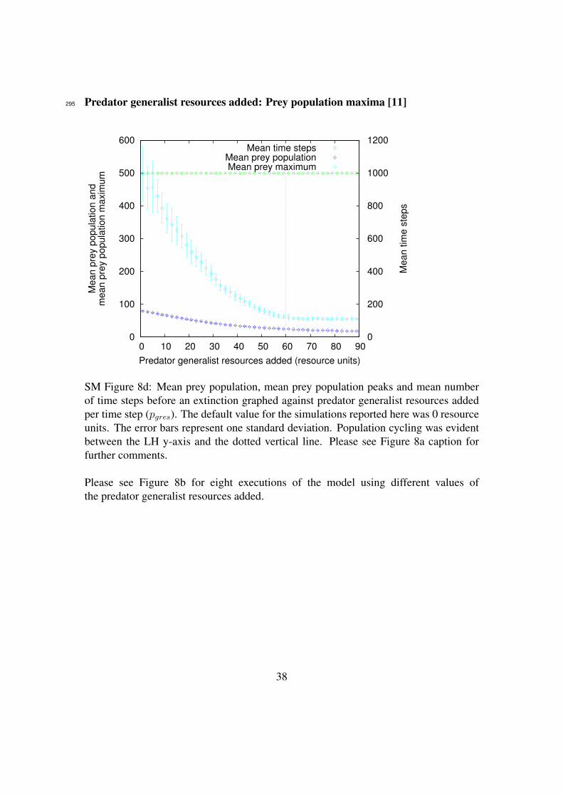
Predator generalist resources added: Prey population maxima [11]295
0
100
200
300
400
500
600
0 10 20 30 40 50 60 70 80 90 0
200
400
600
800
1000
1200
Mean p
rey p
op
ula
tion a
nd
mean p
rey p
opula
tion m
axim
um
Mea
n t
ime s
teps
Predator generalist resources added (resource units)
Mean time stepsMean prey populationMean prey maximum
SM Figure 8d: Mean prey population, mean prey population peaks and mean numberof time steps before an extinction graphed against predator generalist resources addedper time step (pgres). The default value for the simulations reported here was 0 resourceunits. The error bars represent one standard deviation. Population cycling was evidentbetween the LH y-axis and the dotted vertical line. Please see Figure 8a caption forfurther comments.
Please see Figure 8b for eight executions of the model using different values ofthe predator generalist resources added.
38

Predator generalist resources added: Predator functional response296
0 100 200 300 400 500
02
46
81
0
Number of prey
Co
nsu
mp
tio
n r
ate
20 40 60 80 100 120 140
0.0
0.5
1.0
1.5
2.0
2.5
3.0
Number of prey
Co
nsu
mp
tio
n r
ate
(a) (e)
0 100 200 300 400
02
46
8
Number of prey
Co
nsu
mp
tio
n r
ate
20 30 40 50 60 70 80
0.5
1.0
1.5
Number of preyC
on
su
mp
tio
n r
ate
(b) (f)
50 100 150 200 250
01
23
45
Number of prey
Co
nsu
mp
tio
n r
ate
20 30 40 50 60 70 80
0.2
0.4
0.6
0.8
1.0
1.2
1.4
Number of prey
Co
nsu
mp
tio
n r
ate
(c) (g)
50 100 150 200
01
23
4
Number of prey
Co
nsu
mp
tio
n r
ate
20 30 40 50 60 70 80
0.2
0.4
0.6
0.8
1.0
1.2
1.4
Number of prey
Co
nsu
mp
tio
n r
ate
(d) (h)
SM Figure 8e: The predator per-capita consumption rate (y) plotted against the numberof prey (x) for each time step and for differing predator generalist resources added(pgres) values. The values of pgres are 0 (a), 10 (b), 20 (c), 30 (d), 40 (e), 50 (f), 60 (g) and70 (h) resource units. Resources were added to 25% of the randomly selected predatorsper time step for all values of pgres here. The data for each graph were collected froma single execution of the model of 1000 time steps. Please see SM Table 3 for theintercepts and slopes of the lines of best fit. Note the differing axis scales. Scatter plotsand lines of best fit were obtained using the R statistical environment (R Core Team,2013).
39

Predator generalist resources added: Predator functional response (continued)297
SM Table 3: Intercepts, slopes of lines of best fit and other descriptive statistics of thegraphs in SM Figure 8e.The intercepts and slopes may have negative and positive correlations respectively withpgres, this was not formally tested. Descriptive statistics were obtained using the Rstatistical environment (R Core Team, 2013).
Prey populationpgres Intercept Slope Min Median Max Mean SD R2 adj R2
0 -0.0493 0.0217 15.00 28.00 535.00 83.45 96.72 0.92 0.9210 -0.0626 0.0221 14.00 25.00 424.00 65.98 71.13 0.93 0.9320 -0.0840 0.0228 14.00 24.00 241.00 51.74 48.15 0.94 0.9430 -0.0863 0.0231 15.00 24.00 199.00 42.85 34.30 0.95 0.9540 -0.0851 0.0240 14.00 24.00 136.00 33.92 20.37 0.94 0.9450 -0.0940 0.0246 14.00 23.00 80.00 28.39 12.22 0.92 0.9260 -0.1159 0.0260 15.00 22.00 80.00 24.03 7.28 0.85 0.8570 -0.1020 0.0254 15.00 19.00 80.00 20.75 4.67 0.75 0.75
40

1.11 Prey initial population298
Summary299
The initial population of prey (bn) is the size of the population used to start a simulation.300
In the simulations reported in this parameter sensitivity analysis, this parameter has a301
default value of 80 individuals—this value chosen because it is the mean prey population302
level which emerges over many time steps with this parameter set.303
With the default parameter set, values of bn ≥ 0 individuals result in population304
cycling and no extinctions were observed while adjusting this parameter. Higher values305
of the parameter do result in transient dynamics at the start of a simulation as the prey306
population falls to a sustainable level. SM Figure 9a graphs mean population levels and307
mean time step reached over 50 simulations at each parameter level.308
Eight individual executions of the model are illustrated in SM Figure 9b at eight309
different parameter levels. These figures do not suggest any correlation between bn and310
population cycle period length or between the parameter and population cycle ampli-311
tudes.312
41

Prey initial population: Population levels, population persistence and range in313
which population cycling is evident314
0
20
40
60
80
100
120
0 100 200 300 400 500 0
200
400
600
800
1000
1200
Mean p
op
ula
tions
Mean tim
e s
teps
Prey initial population
Mean time stepsMean predator population
Mean prey population
SM Figure 9a: Mean populations and mean number of time steps before an extinctiongraphed against prey initial population (bn). To avoid any confounding effect of increas-ing the initial prey number, these data are from time steps 201–1000 only as transientdynamics at the start of a simulation very rarely persist for 200 time steps. The defaultvalue for the simulations reported here was 80 individuals. The error bars represent onestandard deviation. Very few extinctions were observed and population cycling was ev-ident in the range 1 to > 500 individuals. This graph indicates the lack of importance ofinitial population numbers—the level of the prey initial population may cause transientdymanics at the start of a simulation and in extreme cases may cause extinctions, but ifthe latter does not occur the population means, peaks and troughs settle to levels whichare dependent on the model parameters.
42

Prey initial population: Eight individual simulations at differing parameter levels315
0
300
600
Po
pu
lation
(a
)
PredatorPrey
0
300
600
Popula
tion
(b)
PredatorPrey
0
300
600
Popula
tion
(c)
PredatorPrey
0
300
600
0 100 200 300 400 500
Popula
tion
(d)
Time Step
PredatorPrey
0
300
600
(e)
PredatorPrey
0
300
600
(f)
PredatorPrey
0
300
600
(g)
PredatorPrey
0
300
600
0 100 200 300 400 500
(h)
Time Step
PredatorPrey
SM Figure 9b: Predator and prey populations per time step for eight executions of themodel using different values of the prey initial population (bn). The values of bn are 10(a), 80 (b), 150 (c), 220 (d), 290 (e), 360 (f), 430 (g) and 500 (h) individuals.The number of population peaks over 500 time steps is 26 in each graph. These figuresdo not suggest any correlation between the parameter and population cycle period lengthor population cycle amplitudes.
43

1.12 Prey initial resources316
Summary317
The prey initial resources parameter (bir) represents the energy resources a prey indi-318
vidual is born with. At the start of a simulation all prey have this resource level and319
all individuals born during the simulation have the same resource level in their first320
time step. This parameter also specifies the cost of reproduction for a parent—it is the321
number of resources subtracted from a parent when it bears one offspring. In the simu-322
lations reported in this parameter sensitivity analysis, this parameter has a default value323
of 200.0 resource units.324
With the default parameter set, values of bir ≥ 60 resource units result in population325
cycling and extinctions are observed when bir ≤ 100 resource units. Mean populations326
of both species are negatively correlated with bir in this range of values, as illustrated by327
SM Figure 10a which graphs mean population levels and mean time step reached over328
50 simulations at each parameter level.329
Eight individual executions of the model are illustrated in SM Figure 10b at eight330
different parameter levels. These figures suggest a positive correlation between bir and331
population cycle period length and a negative correlation between the parameter and332
population cycle amplitudes.333
44

Prey initial resources: Population levels, population persistence and range in which334
population cycling is evident335
0
500
1000
1500
2000
2500
50 100 150 200 250 300 0
200
400
600
800
1000
1200
Mean p
op
ula
tions
Mean tim
e s
teps
Prey initial resources (resource units)
Mean time stepsMean predator population
Mean prey population
SM Figure 10a: Mean populations and mean number of time steps before an extinc-tion graphed against prey initial resources (bir). The default value for the simulationsreported here was 200.0 resource units. The error bars represent one standard devi-ation. Extinctions were observed when bir < 100, becoming more common whenbir <= 60 and population cycling was evident in the range 60(approx.) to > 300resources (bounded by the dotted vertical line and the RH y-axis).
45

Prey initial resources: Eight individual simulations at differing parameter levels336
0
6000
12000
Po
pu
lation
(a
)
PredatorPrey
0
2000
4000
Popula
tion
(b)
PredatorPrey
0
600
1200
Popula
tion
(c)
PredatorPrey
0
600
1200
0 100 200 300 400 500
Popula
tion
(d)
Time Step
PredatorPrey
0
300
600
(e)
PredatorPrey
0
300
600
(f)
PredatorPrey
0
300
600
(g)
PredatorPrey
0
300
600
0 100 200 300 400 500
(h)
Time Step
PredatorPrey
SM Figure 10b: Predator and prey populations per time step for eight executions of themodel using different values of the prey initial resources (bir). The values of bir are 60(a), 95 (b), 130 (c), 165 (d), 200 (e), 235 (f), 270 (g) and 305 (h) resource units. Notethe differing y-axis scales.The number of population peaks over 500 time steps are 32 (a), 30 (b), 27 (c), 26 (d), 26(e), 25 (f), 24 (g) and 24 (h), suggesting a positive correlation between bir and populationcycle period length. A negative correlation between the parameter and population cycleamplitudes is also suggested by these figures.
46

1.13 Prey metabolic cost per time step337
Summary338
The prey metabolic cost per time step parameter (bmc) represents the energy cost of339
metabolism in a living organism over time, this cost is subtracted from the resource340
total of each prey individual each time step. If after the subtraction the individual does341
not have enough resources to live another time step, it dies of starvation and is removed342
from the simulation. In the simulations reported in this parameter sensitivity analysis,343
this parameter has a default value of 25.0 resource units.344
With the default parameter set, values of 0 ≤ bmc ≤ 70 resource units result in345
population cycling and extinctions are observed when bmc ≥ 60 resource units. Mean346
populations of both species appear to be negatively correlated with bmc in this range of347
values, as illustrated by SM Figure 11a which graphs mean population levels and mean348
time step reached over 50 simulations at each parameter level.349
Eight individual executions of the model are illustrated in SM Figure 11b at eight350
different parameter levels. These figures suggest a positive correlation between bmc and351
population cycle period length and a negative correlation between the parameter and352
population cycle amplitudes.353
47

Prey metabolic cost per time step: Population levels, population persistence and354
range in which population cycling is evident355
0
20
40
60
80
100
120
0 10 20 30 40 50 60 70 0
200
400
600
800
1000
1200
Mean p
op
ula
tions
Mean tim
e s
teps
Prey metabolic cost per time step (resource units)
Mean time stepsMean predator population
Mean prey population
SM Figure 11a: Mean populations and mean number of time steps before an extinctiongraphed against prey metabolic cost per time step (bmc). The default value for the sim-ulations reported here was 25.0 resource units. The error bars represent one standarddeviation. Extinctions were observed when bmc >= 60 resource units and populationcycling was evident in the range 0 to 70(approx.) resources (bounded by the LH y-axisand the dotted vertical line).
48

Prey metabolic cost per time step: Eight individual simulations at differing param-356
eter levels357
0
300
600
Po
pu
lation
(a
)
PredatorPrey
0
300
600
Popula
tion
(b)
PredatorPrey
0
300
600
Popula
tion
(c)
PredatorPrey
0
300
600
0 100 200 300 400 500
Popula
tion
(d)
Time Step
PredatorPrey
0
300
600
(e)
PredatorPrey
0
300
600
(f)
PredatorPrey
0
300
600
(g)
PredatorPrey
0
300
600
0 100 200 300 400 500
(h)
Time Step
PredatorPrey
SM Figure 11b: Predator and prey populations per time step for eight executions of themodel using different values of the prey metabolic cost per time step (bmc). The valuesof bmc are 5 (a), 15 (b), 25 (c), 35 (d), 45 (e), 55 (f), 65 (g) and 75 (h) resource units.The number of population peaks over 500 time steps are 27 (a), 26 (b), 26 (c), 25(d), 24 (e), 24 (f), 23 (g) and 21 (h), suggesting a positive correlation between bmc
and population cycle period length. A negative correlation between the parameter andpopulation cycle amplitudes is also suggested by these figures.
49

1.14 Prey resource consumption per time step358
Summary359
The prey minimum resources per time step (bminr) and prey maximum resources per360
time step (bmaxr) parameters are the lower and upper bounds respectively of a random361
number of resources added to each prey individual each time step. In the simulations362
reported in this parameter sensitivity analysis these parameters have default values of363
bminr = 125.0 and bmaxr = 175.0 resource units, an assumed mean over the course of a364
simulation of x = 150 resource units.365
With the default parameter set, values of 90 ≤ x ≤ 700 resource units result in366
population cycling and extinctions are observed when x ≤ 120 resource units. The367
mean predator population is positively correlated with the mean resource consumption368
per time step as illustrated in SM Figure 12a and the mean prey population appears369
to be negatively correlated with resource input, although this has not been formally370
analysed. The figure illustrates mean population levels and mean time step reached over371
50 simulations at each parameter level.372
Eight individual executions of the model are illustrated in SM Figure 12b at eight373
different parameter levels. These figures suggest a negative correlation between prey374
resource consumption and population cycle period length and a negative correlation375
between the parameter and population cycle amplitudes.376
50
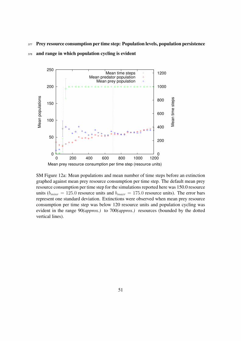
Prey resource consumption per time step: Population levels, population persistence377
and range in which population cycling is evident378
0
50
100
150
200
250
0 200 400 600 800 1000 1200 0
200
400
600
800
1000
1200
Mean p
op
ula
tions
Mean tim
e s
teps
Mean prey resource consumption per time step (resource units)
Mean time stepsMean predator population
Mean prey population
SM Figure 12a: Mean populations and mean number of time steps before an extinctiongraphed against mean prey resource consumption per time step. The default mean preyresource consumption per time step for the simulations reported here was 150.0 resourceunits (bminr = 125.0 resource units and bmaxr = 175.0 resource units). The error barsrepresent one standard deviation. Extinctions were observed when mean prey resourceconsumption per time step was below 120 resource units and population cycling wasevident in the range 90(approx.) to 700(approx.) resources (bounded by the dottedvertical lines).
51

Prey resource consumption per time step: Eight individual simulations at differing379
parameter levels380
0
300
600
Pop
ula
tion
(a)
PredatorPrey
0
300
600
Popula
tion
(b)
PredatorPrey
0
300
600
Popula
tion
(c)
PredatorPrey
0
300
600
0 100 200 300 400 500
Popula
tion
(d)
Time Step
PredatorPrey
0
150
300
(e)
PredatorPrey
0
150
300
(f)
PredatorPrey
0
150
300
(g)
PredatorPrey
0
150
300
0 100 200 300 400 500
(h)
Time Step
PredatorPrey
SM Figure 12b: Predator and prey populations per time step for eight executions of themodel using different values of the prey minimum resources per time step (bminr) andprey maximum resources per time step (bmaxr). The values of bminr,bmaxr are 75,125 (a),175,225 (b), 275,325 (c), 375,425 (d), 475,525 (e), 575,625 (f), 675,725 (g) and 775,825(h) resource units. Note the predator extinction at time step 59 in (a), the breakdown ofpopulation cycling in (h) and the differing y-axis scales.The number of population peaks over 500 time steps, where they can be visually identi-fied, are 26 (b), 30 (c), 29 (d), 30 (e), 30 (f) and 31 (g), suggesting a negative correlationbetween prey resource consumption and population cycle period length. These figuresalso suggest a negative correlation between the parameter and population cycle ampli-tudes.
52

1.15 Prey hidden381
Summary382
The prey hidden parameter (bph) specifies the number of prey “hidden” from the preda-383
tors in simulated prey refuges. The hidden prey are not identified—prey refuges are384
modelled simply as a number: if the prey population is below that number then preda-385
tion will not occur regardless of the value of the chance of eating parameter (pce). In the386
simulations reported in this parameter sensitivity analysis, this parameter has a default387
value of 10 individuals.388
With the default parameter set, values of 5 ≤ bph ≤ 20 individuals result in popula-389
tion cycling and extinctions are observed when bph ≤ 6 individuals. Mean populations390
of both species are negatively correlated with bph in this range of values, as illustrated391
by SM Figure 13a which graphs mean population levels and mean time step reached392
over 50 simulations at each parameter level.393
Eight individual executions of the model are illustrated in SM Figure 13b at eight394
different parameter levels. These figures suggest a positive correlation between bph and395
population cycle period length and a negative correlation between the parameter and396
population cycle amplitudes.397
53
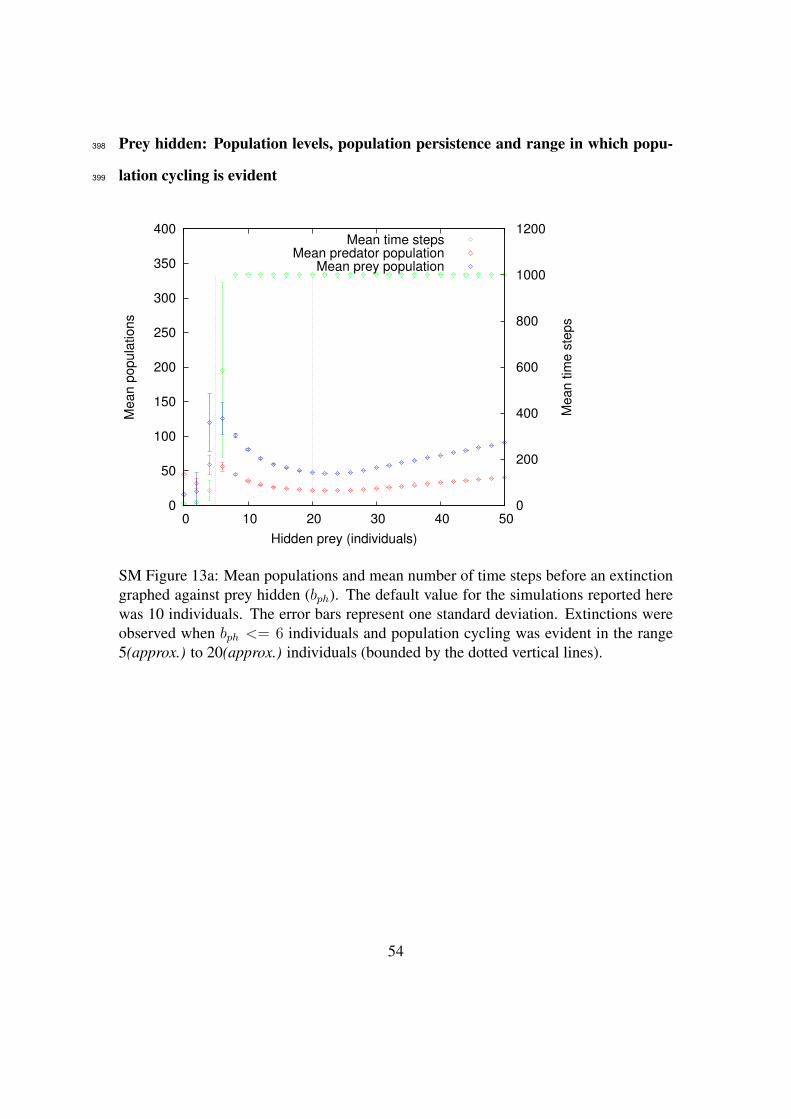
Prey hidden: Population levels, population persistence and range in which popu-398
lation cycling is evident399
0
50
100
150
200
250
300
350
400
0 10 20 30 40 50 0
200
400
600
800
1000
1200
Mean p
op
ula
tions
Mean tim
e s
teps
Hidden prey (individuals)
Mean time stepsMean predator population
Mean prey population
SM Figure 13a: Mean populations and mean number of time steps before an extinctiongraphed against prey hidden (bph). The default value for the simulations reported herewas 10 individuals. The error bars represent one standard deviation. Extinctions wereobserved when bph <= 6 individuals and population cycling was evident in the range5(approx.) to 20(approx.) individuals (bounded by the dotted vertical lines).
54

Prey hidden: Eight individual simulations at differing parameter levels400
0
750
1500
Po
pu
lation
(a
)
PredatorPrey
0
750
1500
Popula
tion
(b)
PredatorPrey
0
300
600
Popula
tion
(c)
PredatorPrey
0
300
600
0 100 200 300 400 500
Popula
tion
(d)
Time Step
PredatorPrey
0
150
300
(e)
PredatorPrey
0
150
300
(f)
PredatorPrey
0
150
300
(g)
PredatorPrey
0
150
300
0 100 200 300 400 500
(h)
Time Step
PredatorPrey
SM Figure 13b: Predator and prey populations per time step for eight executions of themodel using different values of the prey hidden (bph). The values of bph are 3 (a), 6 (b),9 (c), 12 (d), 15 (e), 18 (f), 21 (g) and 24 (h) individuals. Note the predator extinction attime step 52 in (a), the breakdown of population cycling at higher values of bph and thediffering y-axis scales.The number of population peaks over 500 time steps, where they can be visually identi-fied, are 26 (b), 26 (c), 25 (d), 25 (e), 23 (f) and 21 (g), suggesting a positive correlationbetween bph and population cycle period length. These figures also suggest a negativecorrelation between the parameter and population cycle amplitudes.
55
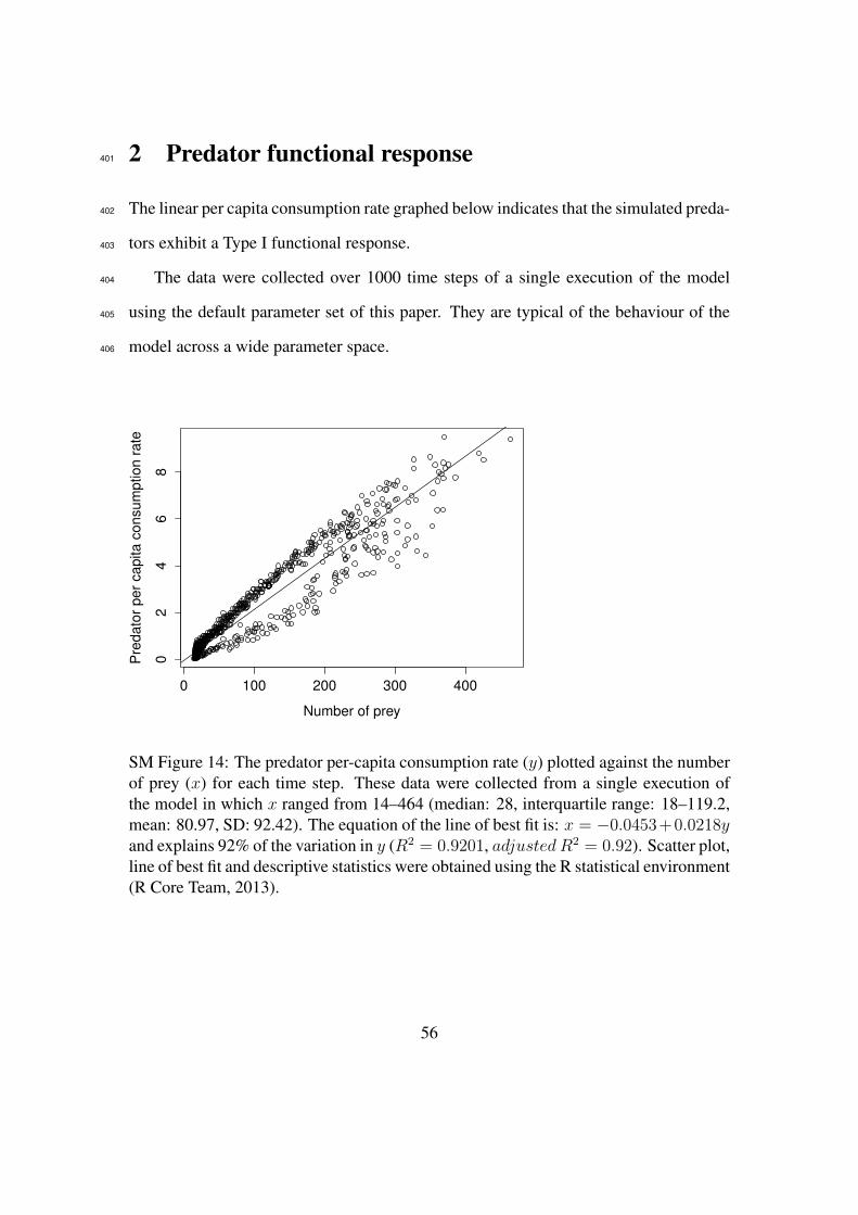
2 Predator functional response401
The linear per capita consumption rate graphed below indicates that the simulated preda-402
tors exhibit a Type I functional response.403
The data were collected over 1000 time steps of a single execution of the model404
using the default parameter set of this paper. They are typical of the behaviour of the405
model across a wide parameter space.406
0 100 200 300 400
02
46
8
Number of prey
Pre
da
tor
pe
r ca
pita
co
nsu
mp
tio
n r
ate
SM Figure 14: The predator per-capita consumption rate (y) plotted against the numberof prey (x) for each time step. These data were collected from a single execution ofthe model in which x ranged from 14–464 (median: 28, interquartile range: 18–119.2,mean: 80.97, SD: 92.42). The equation of the line of best fit is: x = −0.0453+0.0218yand explains 92% of the variation in y (R2 = 0.9201, adjusted R2 = 0.92). Scatter plot,line of best fit and descriptive statistics were obtained using the R statistical environment(R Core Team, 2013).
56

References407
Caron-Lormier G, Humphry RW, Bohan DA, Hawes C, Thorbek P. 2008. Asynchronous408
and synchronous updating in individual-based models. Ecol. Mod. 212: 522–527.409
Grimm V, Berger U, DeAngelis DL, Polhill JG, Giske J, Railsback SF. 2010. The ODD410
protocol: A review and first update. Ecol. Mod. 221: 2760–2768.411
Grimm V, Uchmanski J. 1994. Ecological systems are not dynamic systems: some con-412
sequences of individual variability. In Grasman J, van Straten G (eds.) Predictabil-413
ity and Nonlinear Modelling in Natural Sciences and Economics. Dordrecht, The414
Netherlands: Kluwer Academic Publishers, 248–259.415
Python Software Foundation. 2013. random — Generate pseudo-random numbers.416
Last accessed 20 June 2013.417
URL http://docs.python.org/2/library/random.html418
R Core Team. 2013. R: A language and environment for statistical computing. Last419
accessed 20 June 2013.420
URL http://www.R-project.org421
57

3 Appendix 1: Model description in pseudo-code422
The algorithm used in the ABM is described in this section using pseudo-code, a method423
of algorithm description intended for human reading.424
Programming control structures are written in upper case (for example FOR EACH),425
methods, functions or sub-programs which are further expanded in this model descrip-426
tion are written with parentheses as a suffix (for example process_predators()).427
3.1 Initialisation and main loop428
read initial conditions and parameter values429
create initial populations430
431
FOR EACH time step432
433
IF either population is extinct434
stop processing435
436
process_predators()437
process_prey()438
439
remove_starved_individuals()440
add newborn predator and prey objects to populations441
442
implement_trapping_rate()443
implement_generalist_predator()444
445
collect statistics446
Note: Referring to the Python implementation of the model included with this Sup-447
porting Information, the initial population sizes are read when the “Load” button is448
clicked—it can be clicked only once—and all parameter values are read each time the449
“Run” button is clicked.450
58

3.2 Method definitions451
process_predators()452
FOR EACH predator individual453
implement_predator_eating()454
apply_metabolic_cost()455
implement_reproduction()456
457
process_prey()458
FOR EACH prey individual459
add_prey_resources()460
apply_metabolic_cost()461
implement_reproduction()462
463
implement_predator_eating()464
number_to_eat_this_time_step = current_number_of_prey * pred_chances_of_eating465
WHILE number_to_eat_this_time_step >= 1466
implement_predation_event()467
subtract 1 from number_to_eat_this_time_step468
determine_whether_predator_eats()469
COMMENT note that number_to_eat_this_time_step now < 1470
IF predator is to eat471
implement_predation_event()472
473
determine_whether_predator_eats()474
calculate random_number between 0 and 1475
IF number_to_eat_this_time_step > random_number476
predator is to eat this time step477
478
implement_predation_event()479
IF number of prey > number of hidden prey480
select prey at random481
add (resource total of selected prey * trophic efficiency) to pred total482
remove prey individual from population483
484
add_prey_resources()485
select random number between upper and lower prey resource intake parameters486
add this number to prey resource total487
488
apply_metabolic_cost()489
subtract metabolic cost per time step from resource total490
IF new resource total < metabolic cost per time step491
flag individual for starvation492
493
implement_reproduction()494
IF NOT individual flagged for starvation495
WHILE resource total > (metabolic cost per time step + cost of reproduction)496
create new individual497
59

subtract cost of reproduction from resource total498
499
remove_starved_individuals()500
FOR EACH individual501
IF flagged for starvation502
remove from population503
504
implement_trapping_rate()505
FOR numberToRemove506
select random predator507
remove predator508
509
implement_generalist_predator()510
FOR numberOfGeneralists511
select random predator512
add resources to predator513
60

4 Appendix 2: The agent-based model implemented in514
the Python programming language515
The ABM code, written in the computer programming language Python, is reproduced516
following these instructions. This is the code used to generate all the data reported in517
this paper and Supporting Information.518
The Python source files (.py files) are available from the corresponding author.519
4.1 Using the model graphical interface520
Brief notes on installing Python and essential packages follow in the next sections. Once521
Python is installed and the model is started, the graphical interface contains additional522
notes. The populations should be loaded once before the ‘Run’ button is clicked. When523
the model completes the run, two graph windows will open—these can be closed before524
clicking the ‘Run’ button again.525
To see the six patterns discussed in this paper, the following sequence is suggested:526
• Click ‘Load’ then ‘Run’.527
• Close the two graph windows and set Trapping rate to 20. Click ‘Run’.528
• Close the two graph windows and set Trapping rate back to 0. Click ‘Run’.529
• Close the two graph windows and set Generalist rate to 25 and Generalist re-530
sources to 30. Click ‘Run’.531
• Close the two graph windows and set Generalist rate and Generalist resources532
back to 0. Click ‘Run’.533
61

The increased amplitudes associated with trapping rate and the decreased amplitudes534
associated with generalist predators should be evident.535
4.2 Python version and additional packages536
• This implementation of the ABM was written using Python 2.7.537
• The code uses the following Python packages:538
– Tkinter - for the user interface539
– numpy - for numerical computations540
– matplotlib - for graphs541
The Python language website, http://www.python.org, contains instructions on how542
to execute a Python program and could be consulted if the following notes are too brief.543
4.3 Running the ABM on Microsoft Windows544
These notes were tested on Windows version 7 (32bit).545
• Download the Windows installer from the Python site http://www.python.org.546
• Set the system PATH variable to include the Python directories:547
– Right-click ‘Computer’ and select ‘Properties’548
– In the dialogue box, select ‘Advanced System Settings’549
– In the next dialogue box, select ‘Environment Variables’550
– In the ‘User Variables’ section, add the following to the PATH statement:551
C:\Python27;C:\Python27\Lib\site-packages\;C:\Python27\Scripts\;552
62

• Download numpy from http://sourceforge.net/projects/numpy and install.553
• Download matplotlib from http://sourceforge.net/projects/matplotlib/ and install.554
When the above are installed and the code files created in an appropriate directory,555
the model can be executed from an integrated development environment such as Mi-556
crosoft Visual Studio or from the command line:557
python main.py558
4.4 Running the ABM on Linux or BSD559
Python is installed on most Linux distributions and on the BSD variants but you may560
need to install the additional packages listed above. When these packages are installed561
and the code files created in an appropriate directory, the model can be run from a562
terminal:563
python main.py564
4.5 Running the ABM on Apple OSX565
We suggest the use of a third party tool such as the Enthought Python Distribution,566
which is free of charge for academic purposes and is available at567
http://www.enthought.com/products/epd.php.568
63

4.6 The model code569
The model source code is written in in the following seven files:570
• main.py571
• gui.py572
• simulation.py573
• default_values.py574
• animal.py575
• predator.py576
• prey.py577
4.6.1 main.py578
#579
# Predator-prey individual-based model580
#581
# Dr William Chivers582
# Faculty of Science and Information Technology583
# University of Newcastle, PO Box 127, Ourimbah, NSW 2259, Australia584
# email: [email protected]
# alternative email: [email protected]
#587
# This file creates an instance of the graphical user interface to the model588
#589
590
from Tkinter import *591
from gui import *592
593
root = Tk()594
root.title("Predator-Prey ABM")595
596
app = gui(root)597
root.mainloop()598
64

4.6.2 gui.py599
#600
# Predator-prey individual-based model601
#602
# Dr William Chivers603
# Faculty of Science and Information Technology604
# University of Newcastle, PO Box 127, Ourimbah, NSW 2259, Australia605
# email: [email protected]
# alternative email: [email protected]
#608
# This file defines the gui class. One instance of this class is created. The609
# resulting graphical interface allows users to change initial populations,610
# parameter values and other simulation settings.611
#612
613
# -------------------------------------614
# Naming convention615
#616
# Attributes: aAttributeName617
# Local variable: lVariableName618
# Parameters: pParameterName619
# Classes: ClassName620
# Objects: aObjectName621
# Methods: methodName()622
#623
# Button: aBButtonName624
# Text field: aTFTextFieldName625
# Label: aLLabelName626
# Check box: aCBCheckBoxName627
# Radio button: aRBButtonName628
# -------------------------------------629
630
from Tkinter import *631
from simulation import *632
from default_values import *633
634
class gui:635
""" Creates the graphical interface to the model """636
637
# Constructor method reads default values and creates GUI638
def __init__(self, master):639
640
# Create default_values object641
self.aDefValue = DefaultValues()642
643
# Read default values from aDefValue object644
self.aPredInitialNo = self.aDefValue.aPredInitialNo # Pred initial population645
self.aPredInitialRes = self.aDefValue.aPredInitialRes # Pred initial resources646
self.aPredMetTax = self.aDefValue.aPredMetTax # Pred metabolic cost per time step647
self.aPredTrophicEff = self.aDefValue.aPredTrophicEff # Pred trophic efficiency648
65

self.aPredChEat = self.aDefValue.aPredChEat # Pred chances of eating649
650
self.aPredTrappingRate = self.aDefValue.aPredTrappingRate # Pred trapping rate651
self.aPredGenRate = self.aDefValue.aPredGenRate # Pred generalist rate652
self.aPredGenResources = self.aDefValue.aPredGenResources # Pred generalist resources added653
654
self.aPreyInitialNo = self.aDefValue.aPreyInitialNo # Prey initial population655
self.aPreyInitialRes = self.aDefValue.aPreyInitialRes # Prey initial resources656
self.aPreyMetTax = self.aDefValue.aPreyMetTax # Prey metabolic cost per time step657
self.aPreyMinRes = self.aDefValue.aPreyMinRes # Prey min resource consumption per time step658
self.aPreyMaxRes = self.aDefValue.aPreyMaxRes # Prey max resource consumption per time step659
self.aPreyHidden = self.aDefValue.aPreyHidden # Prey hidden660
661
self.aTimeStepsThisRun = self.aDefValue.aTimeStepsThisRun # Number of time steps on click of Run button662
self.aMaxPopulationSize = self.aDefValue.aMaxPopulationSize # Maximum population size663
664
self.aXTermDisplay = self.aDefValue.aXTermDisplay # Display time step levels on xterm?665
self.aShowStatistics = self.aDefValue.aShowStatistics # Display run statistics on xterm?666
self.aPlotPopGraph = self.aDefValue.aPlotPopGraph # Plot the populations per time step?667
self.aPlotPhaseGraph = self.aDefValue.aPlotPhaseGraph # Plot population phase graph?668
669
670
# Create GUI frame671
lFrame = Frame(master)672
lFrame.pack()673
674
# add left vertical spacer675
self.aLVSpacer00 = Label(lFrame, text="", width=1)676
self.aLVSpacer00.grid( row=0, column=0, sticky=W)677
678
679
# Instructions680
self.aLParameters = Label(lFrame, text="Notes", fg="blue")681
self.aLParameters.grid(columnspan=2, row=1, column=1, sticky=W)682
# Note 1683
self.aLParameters = Label(lFrame, text="1. Click ’Load’ then ’Run’.")684
self.aLParameters.grid(columnspan=1, row=2, column=1, sticky=W)685
# Note 2686
self.aLParameters = Label(lFrame, text="2. The ’Load’ button can be used only once.")687
self.aLParameters.grid(columnspan=1, row=3, column=1, sticky=W)688
self.aLParameters = Label(lFrame, text=" Initial populations can be adjusted")689
self.aLParameters.grid(columnspan=1, row=4, column=1, sticky=W)690
self.aLParameters = Label(lFrame, text=" before clicking ’Load’.")691
self.aLParameters.grid(columnspan=1, row=5, column=1, sticky=W)692
# Note 3693
self.aLParameters = Label(lFrame, text="4. The ’Run’ button can be used indefinitely.")694
self.aLParameters.grid(columnspan=1, row=6, column=1, sticky=W)695
self.aLParameters = Label(lFrame, text=" All values other than initial populations")696
self.aLParameters.grid(columnspan=1, row=7, column=1, sticky=W)697
self.aLParameters = Label(lFrame, text=" can be changed between ’Run’ clicks.")698
self.aLParameters.grid(columnspan=1, row=8, column=1, sticky=W)699
66

# Note 4700
self.aLParameters = Label(lFrame, text="3. No input values are tested: non-numeric")701
self.aLParameters.grid(columnspan=1, row=9, column=1, sticky=W)702
self.aLParameters = Label(lFrame, text=" input and other errors will be dealt")703
self.aLParameters.grid(columnspan=1, row=10, column=1, sticky=W)704
self.aLParameters = Label(lFrame, text=" with by the Python exception sub-system.")705
self.aLParameters.grid(columnspan=1, row=11, column=1, sticky=W)706
# Note 5707
self.aLParameters = Label(lFrame, text="5. The default values indicate whether the")708
self.aLParameters.grid(columnspan=1, row=12, column=1, sticky=W)709
self.aLParameters = Label(lFrame, text=" code expects an integer or a real number.")710
self.aLParameters.grid(columnspan=1, row=13, column=1, sticky=W)711
self.aLParameters = Label(lFrame, text=" Integers can be typed into real text boxes.")712
self.aLParameters.grid(columnspan=1, row=14, column=1, sticky=W)713
# Note 6714
self.aLParameters = Label(lFrame, text="6. The simulation stops if a population exceeds")715
self.aLParameters.grid(columnspan=1, row=15, column=1, sticky=W)716
self.aLParameters = Label(lFrame, text=" the ’Max population’. This is included only ")717
self.aLParameters.grid(columnspan=1, row=16, column=1, sticky=W)718
self.aLParameters = Label(lFrame, text=" to allow some user control over simulation")719
self.aLParameters.grid(columnspan=1, row=17, column=1, sticky=W)720
self.aLParameters = Label(lFrame, text=" run time in the absence of a ’Stop’ button.")721
self.aLParameters.grid(columnspan=1, row=18, column=1, sticky=W)722
# Note 7723
self.aLParameters = Label(lFrame, text="7. The simulation stops on the extinction")724
self.aLParameters.grid(columnspan=1, row=19, column=1, sticky=W)725
self.aLParameters = Label(lFrame, text=" of either population.")726
self.aLParameters.grid(columnspan=1, row=20, column=1, sticky=W)727
728
# add left vertical spacer729
self.aLVSpacer00 = Label(lFrame, text="", width=1)730
self.aLVSpacer00.grid( row=0, column=2, sticky=W)731
732
# Initial populations733
self.aLParameters = Label(lFrame, text="Initial populations", fg="blue")734
self.aLParameters.grid(columnspan=2, row=1, column=3, sticky=W)735
736
# create initial populations labels737
self.aLPredInitialNo = Label(lFrame, text="Predators")738
self.aLPredInitialNo.grid( row=2, column=3, sticky=W)739
self.aLPreyInitialNo = Label(lFrame, text="Prey")740
self.aLPreyInitialNo.grid( row=2, column=6, sticky=W)741
742
# create initial populations text boxes743
self.aTFPredInitialNo = Entry(lFrame, width=8)744
self.aTFPredInitialNo.grid( row=2, column=4, sticky=W)745
self.aTFPredInitialNo.insert(0, self.aPredInitialNo)746
self.aTFPreyInitialNo = Entry(lFrame, width=8)747
self.aTFPreyInitialNo.grid( row=2, column=7, sticky=W)748
self.aTFPreyInitialNo.insert(0, self.aPreyInitialNo)749
750
67

# add horizontal spacer between pred prey settings settings and simulation settings751
self.aLHSpacer02 = Label(lFrame, text="")752
self.aLHSpacer02.grid(columnspan=6, row=3, column=3, sticky=W)753
754
# Parameters755
self.aLParameters = Label(lFrame, text="Parameters", fg="blue")756
self.aLParameters.grid(columnspan=2, row=4, column=3, sticky=W)757
758
# create predator labels759
self.aLPredators = Label(lFrame, text="Predators")760
self.aLPredators.grid(columnspan=1, row=5, column=3, sticky=W)761
self.aLPredInitialRes = Label(lFrame, text="Initial resources")762
self.aLPredInitialRes.grid( row=6, column=3, sticky=W)763
self.aLPredMetTax = Label(lFrame, text="Metabolic cost")764
self.aLPredMetTax.grid( row=7, column=3, sticky=W)765
self.aLPredTrophicEff = Label(lFrame, text="Trophic efficiency (%)")766
self.aLPredTrophicEff.grid( row=8, column=3, sticky=W)767
self.aLPredChEat = Label(lFrame, text="Chance of eating")768
self.aLPredChEat.grid( row=9, column=3, sticky=W)769
self.aLPredTrappingRate = Label(lFrame, text="Trapping rate (%)")770
self.aLPredTrappingRate.grid( row=10, column=3, sticky=W)771
self.aLPredGenRate = Label(lFrame, text="Generalist rate (%)")772
self.aLPredGenRate.grid( row=11, column=3, sticky=W)773
self.aLPredGenResources = Label(lFrame, text="Generalist resources")774
self.aLPredGenResources.grid( row=12, column=3, sticky=W)775
776
# create predator text boxes777
self.aTFPredInitialRes = Entry(lFrame, width=8)778
self.aTFPredInitialRes.grid( row=6, column=4, sticky=W)779
self.aTFPredInitialRes.insert(0, self.aPredInitialRes)780
self.aTFPredMetTax = Entry(lFrame, width=8)781
self.aTFPredMetTax.grid( row=7, column=4, sticky=W)782
self.aTFPredMetTax.insert(0, self.aPredMetTax)783
self.aTFPredTrophicEff = Entry(lFrame, width=8)784
self.aTFPredTrophicEff.grid( row=8, column=4, sticky=W)785
self.aTFPredTrophicEff.insert(0, self.aPredTrophicEff)786
self.aTFPredChEat = Entry(lFrame, width=8)787
self.aTFPredChEat.grid( row=9, column=4, sticky=W)788
self.aTFPredChEat.insert(0, self.aPredChEat)789
self.aTFPredTrappingRate = Entry(lFrame, width=8)790
self.aTFPredTrappingRate.grid( row=10, column=4, sticky=W)791
self.aTFPredTrappingRate.insert(0, self.aPredTrappingRate)792
self.aTFPredGenRate = Entry(lFrame, width=8)793
self.aTFPredGenRate.grid( row=11, column=4, sticky=W)794
self.aTFPredGenRate.insert(0, self.aPredGenRate)795
self.aTFPredGenResources = Entry(lFrame, width=8)796
self.aTFPredGenResources.grid( row=12, column=4, sticky=W)797
self.aTFPredGenResources.insert(0, self.aPredGenResources)798
799
# add vertical spacer between predator and prey settings800
self.aLVSpacer01 = Label(lFrame, text="", width=3)801
68

self.aLVSpacer01.grid( row=0, column=5, sticky=W)802
803
# create prey labels804
self.aLPrey = Label(lFrame, text="Prey")805
self.aLPrey.grid(columnspan=1, row=5, column=6, sticky=W)806
self.aLPreyInitialRes = Label(lFrame, text="Initial resources")807
self.aLPreyInitialRes.grid( row=6, column=6, sticky=W)808
self.aLPreyMetTax = Label(lFrame, text="Metabolic cost")809
self.aLPreyMetTax.grid( row=7, column=6, sticky=W)810
self.aLPreyMinRes = Label(lFrame, text="Min. resources")811
self.aLPreyMinRes.grid( row=8, column=6, sticky=W)812
self.aLPreyMaxRes = Label(lFrame, text="Max. resources")813
self.aLPreyMaxRes.grid( row=9, column=6, sticky=W)814
self.aLPreyHidden = Label(lFrame, text="Number hidden")815
self.aLPreyHidden.grid( row=10, column=6, sticky=W)816
817
# create prey text boxes818
self.aTFPreyInitialRes = Entry(lFrame, width=8)819
self.aTFPreyInitialRes.grid( row=6, column=7, sticky=W)820
self.aTFPreyInitialRes.insert(0, self.aPreyInitialRes)821
self.aTFPreyMetTax = Entry(lFrame, width=8)822
self.aTFPreyMetTax.grid( row=7, column=7, sticky=W)823
self.aTFPreyMetTax.insert(0, self.aPreyMetTax)824
self.aTFPreyMinRes = Entry(lFrame, width=8)825
self.aTFPreyMinRes.grid( row=8, column=7, sticky=W)826
self.aTFPreyMinRes.insert(0, self.aPreyMinRes)827
self.aTFPreyMaxRes = Entry(lFrame, width=8)828
self.aTFPreyMaxRes.grid( row=9, column=7, sticky=W)829
self.aTFPreyMaxRes.insert(0, self.aPreyMaxRes)830
self.aTFPreyHidden = Entry(lFrame, width=8)831
self.aTFPreyHidden.grid( row=10, column=7, sticky=W)832
self.aTFPreyHidden.insert(0, self.aPreyHidden)833
834
# add horizontal spacer between pred prey settings settings and simulation settings835
self.aLHSpacer02 = Label(lFrame, text="")836
self.aLHSpacer02.grid(columnspan=6, row=13, column=3, sticky=W)837
838
# create simulation control labels839
self.aLSimulation = Label(lFrame, text="Simulation Settings", fg="blue")840
self.aLSimulation.grid(columnspan=2, row=14, column=3, sticky=W)841
self.aLTimeStepsThisRun = Label(lFrame, text="Time steps")842
self.aLTimeStepsThisRun.grid( row=15, column=3, sticky=W)843
844
self.aLMaxPopulationSize = Label(lFrame, text="Max. population")845
self.aLMaxPopulationSize.grid( row=16, column=3, sticky=W)846
847
# create simulation controls848
self.aTFTimeStepsThisRun = Entry(lFrame, width=9)849
self.aTFTimeStepsThisRun.grid( row=15, column=4, sticky=W)850
self.aTFTimeStepsThisRun.insert(0, self.aTimeStepsThisRun)851
852
69

self.aTFMaxPopulationSize = Entry(lFrame, width=9)853
self.aTFMaxPopulationSize.grid( row=16, column=4, sticky=W)854
self.aTFMaxPopulationSize.insert(0, self.aMaxPopulationSize)855
856
# output settings857
self.aLSimulation = Label(lFrame, text="Output Settings", fg="blue")858
self.aLSimulation.grid(columnspan=2, row=14, column=6, sticky=W)859
860
self.aXTermDisplayIV = IntVar() # Integer variable associated with check box861
self.aCBXTermDisplay = Checkbutton(lFrame, text="Time step levels on terminal?",862
variable=self.aXTermDisplayIV, onvalue=1, offvalue=0)863
self.aCBXTermDisplay.grid(columnspan=2, row=15, column=6, sticky=W)864
self.aXTermDisplayIV.set(self.aXTermDisplay)865
866
self.aShowStatisticsIV = IntVar() # Integer variable associated with check box867
self.aCBShowStatistics = Checkbutton(lFrame, text="Overall means on terminal?",868
variable=self.aShowStatisticsIV, onvalue=1, offvalue=0)869
self.aCBShowStatistics.grid(columnspan=2, row=16, column=6, sticky=W)870
self.aShowStatisticsIV.set(self.aShowStatistics)871
872
self.aPlotPopGraphIV = IntVar() # Integer variable associated with check box873
self.aCBPlotPopGraph = Checkbutton(lFrame, text="Plot populations per time step?",874
variable=self.aPlotPopGraphIV, onvalue=1, offvalue=0)875
self.aCBPlotPopGraph.grid(columnspan=2, row=17, column=6, sticky=W)876
self.aPlotPopGraphIV.set(self.aPlotPopGraph)877
878
self.aPlotPhaseGraphIV = IntVar() # Integer variable associated with check box879
self.aCBPlotPhaseGraph = Checkbutton(lFrame, text="Plot population phase graph?",880
variable=self.aPlotPhaseGraphIV, onvalue=1, offvalue=0)881
self.aCBPlotPhaseGraph.grid(columnspan=2, row=18, column=6, sticky=W)882
self.aPlotPhaseGraphIV.set(self.aPlotPhaseGraph)883
884
# add horizontal spacers between simulation settings and control buttons885
self.aLHSpacer02 = Label(lFrame, text="")886
self.aLHSpacer02.grid(columnspan=6, row=19, column=3, sticky=W)887
self.aLHSpacer02 = Label(lFrame, text="")888
self.aLHSpacer02.grid(columnspan=6, row=20, column=3, sticky=W)889
890
# Button: load populations - executed only once891
self.aBLoad = Button(lFrame, text="Load", command=self.createInitialPopulations)892
self.aBLoad.grid( row=21, column=3, sticky=W)893
# Button: run simulation - executed indefinitely894
self.aBRun = Button(lFrame, text="Run", command=self.runSimulation)895
self.aBRun.grid( row=21, column=4, sticky=W)896
self.aBRun[’state’] = DISABLED # initially disable Run button897
# Button: close GUI898
self.aBClose = Button(lFrame, text="Close", command=lFrame.quit)899
self.aBClose.grid( row=21, column=7, sticky=W)900
901
# add horizontal spacer between control buttons and bottom of window902
self.aLHSpacer02 = Label(lFrame, text="")903
70

self.aLHSpacer02.grid(columnspan=6, row=22, column=3, sticky=W)904
905
# add left vertical spacer906
self.aLVSpacer02 = Label(lFrame, text="", width=1)907
self.aLVSpacer02.grid( row=0, column=8, sticky=W)908
# end constructor909
910
911
# implementor methods912
913
# create initial populations914
def createInitialPopulations(self):915
""" Create initial populations - executed only once on first click of Run button """916
917
# create simulation control object918
self.aSimulation = Simulation()919
920
# create predator list921
self.aSimulation.initPredators(int(self.aTFPredInitialNo.get()), # Pred initial population922
float(self.aTFPredInitialRes.get())) # Pred initial resources923
924
# create prey list925
self.aSimulation.initPrey(int(self.aTFPreyInitialNo.get()), # Prey initial population926
float(self.aTFPreyInitialRes.get())) # Prey initial resources927
928
# disable Load button and initial population text fields929
self.aTFPredInitialNo[’state’] = DISABLED930
self.aTFPreyInitialNo[’state’] = DISABLED931
self.aBLoad[’state’] = DISABLED932
# enable Run button933
self.aBRun[’state’] = NORMAL934
935
# end createInitialPopulations()936
937
# run simulation938
def runSimulation(self):939
""" Run simulation - executed any number of times """940
941
# run the simulation942
self.aSimulation.runSimulation(int(self.aTFPredInitialNo.get()), # Pred initial population943
float(self.aTFPredInitialRes.get()), # Pred initial resources944
float(self.aTFPredMetTax.get()), # Pred metabolic cost per time step945
float(self.aTFPredTrophicEff.get()), # Pred trophic efficiency946
float(self.aTFPredChEat.get()), # Pred chances of eating947
948
float(self.aTFPredTrappingRate.get()), # Pred trapping rate949
float(self.aTFPredGenRate.get()), # Pred generalist rate950
float(self.aTFPredGenResources.get()), # Pred generalist resources added951
952
int(self.aTFPreyInitialNo.get()), # Prey initial population953
float(self.aTFPreyInitialRes.get()), # Prey initial resources954
71

float(self.aTFPreyMetTax.get()), # Prey metabolic cost per time step955
float(self.aTFPreyMinRes.get()), # Prey min res cons per time step956
float(self.aTFPreyMaxRes.get()), # Prey max res cons per time step957
int(self.aTFPreyHidden.get()), # Prey hidden958
959
int(self.aTFTimeStepsThisRun.get()), # Number of ts on click of Run button960
int(self.aTFMaxPopulationSize.get()), # Maximum population size961
962
int(self.aXTermDisplayIV.get()), # Display time step levels on xterm?963
int(self.aShowStatisticsIV.get()), # Display run statistics on xterm?964
int(self.aPlotPopGraphIV.get()), # Plot the populations per time step?965
int(self.aPlotPhaseGraphIV.get()) # Plot population phase graph?966
)967
# end runSimulation()968
72

4.6.3 simulation.py969
#970
# Predator-prey individual-based model971
#972
# Dr William Chivers973
# Faculty of Science and Information Technology974
# University of Newcastle, PO Box 127, Ourimbah, NSW 2259, Australia975
# email: [email protected]
# alternative email: [email protected]
#978
# This file defines the simulation class. One instance of this class is created by the gui object.979
# The Simulation class has methods to create initial predator and prey populations and to execute980
# the model algorithm each time step. It also collects and displays statistics and creates the981
# graphs.982
#983
984
import sys985
import tkMessageBox986
import random987
import numpy988
import matplotlib.pyplot as aPlot989
990
from prey import *991
from predator import *992
993
994
class Simulation:995
""" Creates initial populations, runs the model, collects and displays statistics996
and creates graphs """997
998
# instance attributes - values read from gui in the methods below999
aPredInitialNo = 0 # Pred initial population1000
aPredInitialRes = 0.0 # Pred initial resources1001
aPredMetTax = 0.0 # Pred metabolic cost per time step1002
aPredTrophicEff = 0.0 # Pred trophic efficiency1003
aPredChEat = 0.0 # Pred chances of eating1004
1005
aPredTrappingRate = 0.0 # Pred trapping rate1006
aPredGenRate = 0.0 # Pred generalist rate1007
aPredGenResources = 0.0 # Pred generalist resources added1008
1009
aPreyInitialNo = 0 # Prey initial population1010
aPreyInitialRes = 0.0 # Prey initial resources1011
aPreyMetTax = 0.0 # Prey metabolic cost per time step1012
aPreyMinRes = 0.0 # Prey min resource consumption per time step1013
aPreyMaxRes = 0.0 # Prey max resource consumption per time step1014
aPreyHidden = 0 # Prey hidden1015
1016
aTimeStepsThisRun = 0 # Number of time steps on click of Run button1017
aMaxPopulationSize = 0 # Maximum population size1018
73
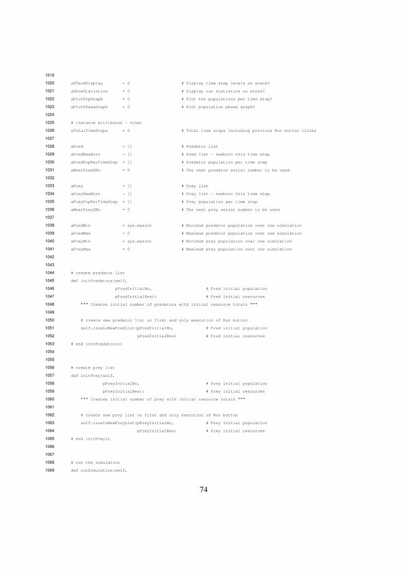
1019
aXTermDisplay = 0 # Display time step levels on xterm?1020
aShowStatistics = 0 # Display run statistics on xterm?1021
aPlotPopGraph = 0 # Plot the populations per time step?1022
aPlotPhaseGraph = 0 # Plot population phase graph?1023
1024
# instance attributes - other1025
aTotalTimeSteps = 0 # Total time steps including previous Run button clicks1026
1027
aPred = [] # Predator list1028
aPredNewBorn = [] # Pred list - newborn this time step1029
aPredPopPerTimeStep = [] # Predator population per time step1030
aNextPredSNo = 0 # The next predator serial number to be used1031
1032
aPrey = [] # Prey list1033
aPreyNewBorn = [] # Prey list - newborn this time step1034
aPreyPopPerTimeStep = [] # Prey population per time step1035
aNextPreySNo = 0 # The next prey serial number to be used1036
1037
aPredMin = sys.maxint # Minimum predator population over one simulation1038
aPredMax = 0 # Maximum predator population over one simulation1039
aPreyMin = sys.maxint # Minimum prey population over one simulation1040
aPreyMax = 0 # Maximum prey population over one simulation1041
1042
1043
# create predator list1044
def initPredators(self,1045
pPredInitialNo, # Pred initial population1046
pPredInitialRes): # Pred initial resources1047
""" Creates initial number of predators with initial resource totals """1048
1049
# create new predator list on first and only execution of Run button1050
self.createNewPredList(pPredInitialNo, # Pred initial population1051
pPredInitialRes) # Pred initial resources1052
# end initPredators()1053
1054
1055
# create prey list1056
def initPrey(self,1057
pPreyInitialNo, # Prey initial population1058
pPreyInitialRes): # Prey initial resources1059
""" Creates initial number of prey with initial resource totals """1060
1061
# create new prey list on first and only execution of Run button1062
self.createNewPreyList(pPreyInitialNo, # Prey initial population1063
pPreyInitialRes) # Prey initial resources1064
# end initPrey()1065
1066
1067
# run the simulation1068
def runSimulation(self,1069
74
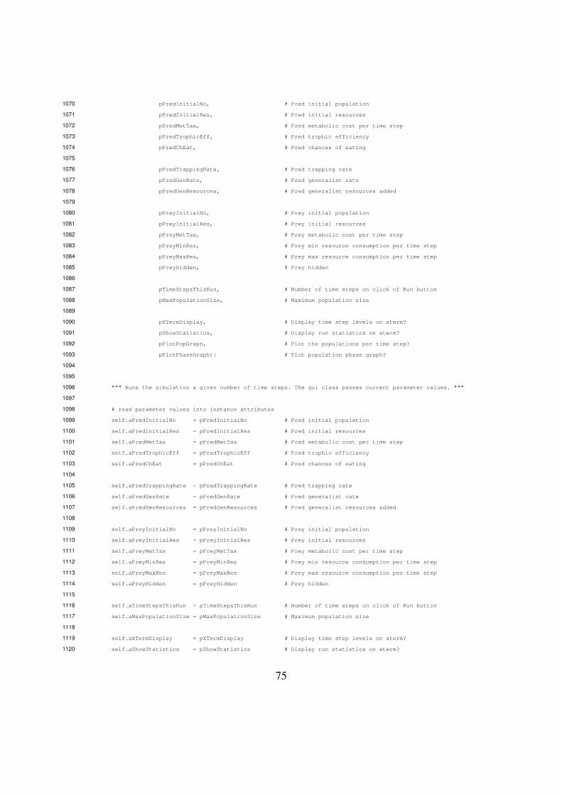
pPredInitialNo, # Pred initial population1070
pPredInitialRes, # Pred initial resources1071
pPredMetTax, # Pred metabolic cost per time step1072
pPredTrophicEff, # Pred trophic efficiency1073
pPredChEat, # Pred chances of eating1074
1075
pPredTrappingRate, # Pred trapping rate1076
pPredGenRate, # Pred generalist rate1077
pPredGenResources, # Pred generalist resources added1078
1079
pPreyInitialNo, # Prey initial population1080
pPreyInitialRes, # Prey initial resources1081
pPreyMetTax, # Prey metabolic cost per time step1082
pPreyMinRes, # Prey min resource consumption per time step1083
pPreyMaxRes, # Prey max resource consumption per time step1084
pPreyHidden, # Prey hidden1085
1086
pTimeStepsThisRun, # Number of time steps on click of Run button1087
pMaxPopulationSize, # Maximum population size1088
1089
pXTermDisplay, # Display time step levels on xterm?1090
pShowStatistics, # Display run statistics on xterm?1091
pPlotPopGraph, # Plot the populations per time step?1092
pPlotPhaseGraph): # Plot population phase graph?1093
1094
1095
""" Runs the simulation a given number of time steps. The gui class passes current parameter values. """1096
1097
# read parameter values into instance attributes1098
self.aPredInitialNo = pPredInitialNo # Pred initial population1099
self.aPredInitialRes = pPredInitialRes # Pred initial resources1100
self.aPredMetTax = pPredMetTax # Pred metabolic cost per time step1101
self.aPredTrophicEff = pPredTrophicEff # Pred trophic efficiency1102
self.aPredChEat = pPredChEat # Pred chances of eating1103
1104
self.aPredTrappingRate = pPredTrappingRate # Pred trapping rate1105
self.aPredGenRate = pPredGenRate # Pred generalist rate1106
self.aPredGenResources = pPredGenResources # Pred generalist resources added1107
1108
self.aPreyInitialNo = pPreyInitialNo # Prey initial population1109
self.aPreyInitialRes = pPreyInitialRes # Prey initial resources1110
self.aPreyMetTax = pPreyMetTax # Prey metabolic cost per time step1111
self.aPreyMinRes = pPreyMinRes # Prey min resource consumption per time step1112
self.aPreyMaxRes = pPreyMaxRes # Prey max resource consumption per time step1113
self.aPreyHidden = pPreyHidden # Prey hidden1114
1115
self.aTimeStepsThisRun = pTimeStepsThisRun # Number of time steps on click of Run button1116
self.aMaxPopulationSize = pMaxPopulationSize # Maximum population size1117
1118
self.aXTermDisplay = pXTermDisplay # Display time step levels on xterm?1119
self.aShowStatistics = pShowStatistics # Display run statistics on xterm?1120
75

self.aPlotPopGraph = pPlotPopGraph # Plot the populations per time step?1121
self.aPlotPhaseGraph = pPlotPhaseGraph # Plot population phase graph?1122
1123
1124
# main simulation loop (aTimeStepsThisRun) on each execution of Run button1125
for i in range(self.aTimeStepsThisRun):1126
1127
# stop simulation if predators are extinct1128
if len(self.aPred) < 1:1129
print "Predator extinction at time step", self.aTotalTimeSteps1130
tkMessageBox.showwarning("Simulation stopped",1131
"Predator extinction at time step %d" % self.aTotalTimeSteps)1132
break1133
1134
# stop simulation if prey are extinct1135
if len(self.aPrey) < 1:1136
print "Prey extinction at time step", self.aTotalTimeSteps1137
tkMessageBox.showwarning("Simulation stopped",1138
"Prey extinction at time step %d" % self.aTotalTimeSteps)1139
break1140
1141
# stop simulation if predator population exceeds aMaxPopulationSize1142
if len(self.aPred) > self.aMaxPopulationSize:1143
print "Predator population exceeded max. size at time step", self.aTotalTimeSteps1144
tkMessageBox.showwarning("Simulation stopped",1145
"Predator population exceeded max. size at time step %d" % self.aTotalTimeSteps)1146
break1147
1148
# stop simulation if prey population exceeds aMaxPopulationSize1149
if len(self.aPrey) > self.aMaxPopulationSize:1150
print "Prey population exceeded max. size at time step", self.aTotalTimeSteps1151
tkMessageBox.showwarning("Simulation stopped",1152
"Prey population exceeded max. size at time step %d" % self.aTotalTimeSteps)1153
break1154
1155
1156
# display levels per time step on xterm?1157
if self.aXTermDisplay:1158
# output has the following columns:1159
print self.aTotalTimeSteps, # 1. time step1160
print len(self.aPred), # 2. pred population1161
print len(self.aPrey) # 3. prey population1162
1163
1164
# Increment aTotalTimeSteps - total time steps including previous Run button clicks1165
self.aTotalTimeSteps += 11166
1167
# process predators1168
for j in range(len(self.aPred)):1169
1170
# implement predator eating1171
76

1172
# Determine chance of eating or number of prey to eat this time step by this predator1173
lNumOfPreyToEat = len(self.aPrey) * self.aPredChEat # current number of prey1174
# * pred chances of eating1175
1176
# The random.random() method returns a pseudorandom1177
# number between 0.0000000000000 and 0.99999999999991178
lRandomNum = random.random()1179
1180
# If lNumOfPreyToEat >= 1 the predator eats one or more1181
# prey objects (if prey population > number hidden)1182
while lNumOfPreyToEat >= 1:1183
if(len(self.aPrey) > self.aPreyHidden):1184
self.eatPrey(self.aPred[j])1185
lNumOfPreyToEat -= 11186
1187
# If lNumOfPreyToEat < 1 the predators might eat a1188
# prey object - note lNumOfPreyToEat is now < 11189
if lNumOfPreyToEat > lRandomNum:1190
if(len(self.aPrey) > self.aPreyHidden):1191
self.eatPrey(self.aPred[j])1192
1193
1194
# apply metabolic cost1195
1196
self.aPred[j].applyMetTax(self.aPredMetTax) # Predator metabolic cost per time step1197
1198
1199
# implement reproduction1200
1201
# set/reset counter1202
lNumOfPredToAdd = 0 # Count the number of offspring this time step for this predator1203
1204
if (not self.aPred[j].getDiedThisTimeStep()):1205
while (self.aPred[j].getResourceTotal() >= (self.aPredInitialRes + self.aPredMetTax)):1206
1207
# add new predator object to new predators list1208
lNumOfPredToAdd += 1 # Number of predators to add this time step1209
1210
# subtract current aPredInitialRes from resource total1211
self.aPred[j].setResourceTotal(self.aPred[j].getResourceTotal() - self.aPredInitialRes)1212
1213
# create the new born predators1214
self.createNewBornPred(lNumOfPredToAdd)1215
1216
1217
# process prey1218
for j in range(len(self.aPrey)):1219
1220
# add resources to prey objects1221
1222
77

self.aPrey[j].addResources(self.aPreyMinRes, # Prey min resource consumption per time step1223
self.aPreyMaxRes) # Prey max resource consumption per time step1224
1225
# apply metabolic cost1226
1227
self.aPrey[j].applyMetTax(self.aPreyMetTax) # Prey metabolic cost per time step1228
1229
# implement reproduction1230
1231
# set/reset counter1232
lNumOfPreyToAdd = 0 # Count the number of offspring this time step for this prey1233
1234
if (not self.aPrey[j].getDiedThisTimeStep()):1235
while (self.aPrey[j].getResourceTotal() >= (self.aPreyInitialRes + self.aPreyMetTax)):1236
1237
# add new prey object to new prey linked list1238
lNumOfPreyToAdd += 1 # Number of prey to add this time step1239
1240
# subtract current aPreyInitialRes from resource total1241
self.aPrey[j].setResourceTotal(self.aPrey[j].getResourceTotal() - self.aPreyInitialRes)1242
1243
# create the new born prey1244
self.createNewBornPrey(lNumOfPreyToAdd)1245
1246
1247
# remove predator and prey objects which have starved1248
self.removeDeadPredators()1249
self.removeDeadPrey()1250
1251
# add newborn predator and prey objects to lists1252
self.aPred.extend(self.aPredNewBorn) # add new predators to main list, to be processed next time step1253
del self.aPredNewBorn[:] # empty new predators list1254
self.aPrey.extend(self.aPreyNewBorn) # add new prey to main list, to be processed next time step1255
del self.aPreyNewBorn[:] # empty new prey list1256
1257
# simulate trapping by removing a percentage of the predator population1258
self.implementTrappingRate()1259
1260
# simulate generalist predator by adding resources1261
self.implementGeneralistPredator()1262
1263
# update population levels1264
self.aPredPopPerTimeStep.append(len(self.aPred)) # collect predator population each time step1265
self.aPreyPopPerTimeStep.append(len(self.aPrey)) # collect prey population each time step1266
1267
# update maxima and minima1268
if self.aPredMin > len(self.aPred): # Minimum predator population over one simulation1269
self.aPredMin = len(self.aPred)1270
if self.aPredMax < len(self.aPred): # Maximum predator population over one simulation1271
self.aPredMax = len(self.aPred)1272
if self.aPreyMin > len(self.aPrey): # Minimum prey population over one simulation1273
78
self.aPreyMin = len(self.aPrey)1274
if self.aPreyMax < len(self.aPrey): # Maximum prey population over one simulation1275
self.aPreyMax = len(self.aPrey)1276
1277
1278
# end main simulation loop (aTimeStepsThisRun) on each execution of Run button1279
1280
# print run statistics?1281
if self.aShowStatistics:1282
self.showStats()1283
1284
# plot the populations per time step and/or the phase graph1285
self.plotGraphs()1286
1287
# end runSimulation()1288
1289
1290
# display simulation statistics1291
def showStats(self):1292
""" Displays mean predator and prey populations for all time steps completed """1293
1294
print ""1295
print "Pred mean", numpy.mean(self.aPredPopPerTimeStep),1296
print "SD", numpy.std(self.aPredPopPerTimeStep, ddof=0), # ddof: degrees of freedom1297
print "range", self.aPredMin, "to", self.aPredMax # Min to max predator population1298
1299
print "Prey mean", numpy.mean(self.aPreyPopPerTimeStep),1300
print "SD", numpy.std(self.aPreyPopPerTimeStep, ddof=0), # ddof: degrees of freedom1301
print "range", self.aPreyMin, "to", self.aPreyMax # Min to max prey population1302
1303
# end showStats()1304
1305
1306
# createNewPredList1307
def createNewPredList(self,1308
pPredInitialNo, # Pred initial population1309
pPredInitialRes): # Pred initial resources1310
""" Creates a new predator list at the start of the simulation """1311
1312
for i in range(pPredInitialNo):1313
lPred = {}1314
# create predator object1315
lPred[i] = Pred(i)1316
# set resource total to aPredInitialRes1317
lPred[i].setResourceTotal(pPredInitialRes)1318
# add predator object to main predator linked list1319
self.aPred.append(lPred[i])1320
1321
self.aNextPredSNo = pPredInitialNo # the next predator serial number to be used1322
# end createNewPredList()1323
1324
79
1325
# createNewPreyList1326
def createNewPreyList(self,1327
pPreyInitialNo, # Prey initial population1328
pPreyInitialRes): # Prey initial resources1329
""" Creates a new prey list at the start of the simulation """1330
1331
for i in range(pPreyInitialNo):1332
lPrey = {}1333
# create prey object1334
lPrey[i] = Prey(i)1335
# set resource total to aPreyInitialRes1336
lPrey[i].setResourceTotal(pPreyInitialRes)1337
# add prey object to main prey linked list1338
self.aPrey.append(lPrey[i])1339
1340
self.aNextPreySNo = pPreyInitialNo # the next prey serial number to be used1341
# end createNewPreyList()1342
1343
1344
# createNewBornPred1345
def createNewBornPred(self,1346
pNumberToAdd): # number of predators to add1347
""" Creates individual predator objects during execution of the simulation """1348
1349
for i in range(pNumberToAdd):1350
lNewPred = {}1351
# create predator object1352
lNewPred[i] = Pred(self.aNextPredSNo)1353
# set resource total to aPredInitialRes1354
lNewPred[i].setResourceTotal(self.aPredInitialRes)1355
# add predator object to temporary newborn linked list1356
self.aPredNewBorn.append(lNewPred[i])1357
# increment the next predator serial number to be used1358
self.aNextPredSNo += 11359
# end createNewBornPred()1360
1361
1362
# createNewBornPrey1363
def createNewBornPrey(self,1364
pNumberToAdd): # number of prey to add1365
""" Creates individual prey objects during execution of the simulation """1366
1367
for i in range(pNumberToAdd):1368
lNewPrey = {}1369
# create prey object1370
lNewPrey[i] = Prey(self.aNextPreySNo)1371
# set resource total to aPreyInitialRes1372
lNewPrey[i].setResourceTotal(self.aPreyInitialRes)1373
# add prey object to temporary newborn linked list1374
self.aPreyNewBorn.append(lNewPrey[i])1375
80

# increment the next prey serial number to be used1376
self.aNextPreySNo += 11377
# end createNewBornPrey()1378
1379
1380
# implement predator eating1381
def eatPrey(self,1382
lPred): # current predator object1383
1384
# select random prey:1385
# The random.randint() method returns a pseudorandom integer1386
# between the lower and upper parameters inclusively1387
lPreyToBeEaten = random.randint(0, len(self.aPrey)-1)1388
1389
# aquire resources of prey object1390
lPred.eatPrey(self.aPrey[lPreyToBeEaten].getResourceTotal(), # resource total of prey1391
self.aPredTrophicEff) # Pred trophic efficiency1392
1393
# remove prey object1394
del self.aPrey[lPreyToBeEaten]1395
1396
1397
# remove predator objects which have starved1398
def removeDeadPredators(self):1399
""" Removes individual predator objects during execution of the simulation """1400
1401
lLivingPred = []1402
for i in range(len(self.aPred)):1403
if not (self.aPred[i].getDiedThisTimeStep()):1404
lLivingPred.append(self.aPred[i])1405
self.aPred = lLivingPred1406
# end removeDeadPredators()1407
1408
1409
# remove prey objects which have starved1410
def removeDeadPrey(self):1411
""" Removes individual prey objects during execution of the simulation """1412
1413
lLivingPrey = []1414
for i in range(len(self.aPrey)):1415
if not (self.aPrey[i].getDiedThisTimeStep()):1416
lLivingPrey.append(self.aPrey[i])1417
self.aPrey = lLivingPrey1418
# end removeDeadPrey()1419
1420
# simulate trapping by removing a percentage of the predator population1421
def implementTrappingRate(self):1422
""" Remove a percentage of the predator population. Called each time step. """1423
1424
lNumberToRemove = int( round( len(self.aPred) * (self.aPredTrappingRate / 100) ) )1425
1426
81
for i in range(lNumberToRemove):1427
# select random predator1428
# The random.randint() method returns a pseudorandom integer1429
# between the lower and upper parameters inclusively1430
lPredToBeEaten = random.randint(0, len(self.aPred)-1)1431
1432
# remove predator object1433
del self.aPred[lPredToBeEaten]1434
# end implementTrappingRate()1435
1436
# simulate generalist predator by adding resources1437
def implementGeneralistPredator(self):1438
""" Add resources to a percentage of the predator population. Called each time step. """1439
1440
lNumberOfGeneralists = int(round(len(self.aPred) * (self.aPredGenRate / 100)))1441
1442
for i in range(lNumberOfGeneralists):1443
# select random predator1444
# The random.randint() method returns a pseudorandom integer1445
# between the lower and upper parameters inclusively1446
lPredToBeGeneralist = random.randint(0, len(self.aPred)-1)1447
1448
# add resources to predator1449
self.aPred[lPredToBeGeneralist].setResourceTotal(self.aPred[lPredToBeGeneralist].getResourceTotal()1450
+ self.aPredGenResources)1451
# end implementGeneralistPredator()1452
1453
# plot the populations per time step and/or the phase graph1454
def plotGraphs(self):1455
""" Plot population and phase graphs after the specified number of time steps. """1456
1457
# plot population phase graph?1458
if self.aPlotPhaseGraph:1459
lPlot2 = aPlot.figure()1460
self.plotPhaseGraph()1461
1462
# plot the populations per time step?1463
if self.aPlotPopGraph:1464
lPlot1 = aPlot.figure()1465
self.plotPredPreyInteraction()1466
1467
aPlot.show()1468
1469
def plotPhaseGraph(self):1470
aPlot.plot(self.aPreyPopPerTimeStep, self.aPredPopPerTimeStep, ’b’)1471
aPlot.grid()1472
# set label names1473
aPlot.ylabel(’Predators’)1474
aPlot.xlabel(’Prey’)1475
1476
def plotPredPreyInteraction(self):1477
82

aPlot.plot(self.aPreyPopPerTimeStep, ’b’, self.aPredPopPerTimeStep, ’r’)1478
aPlot.legend(["Prey", "Predators"])1479
aPlot.grid()1480
# set label names1481
aPlot.ylabel(’Population’)1482
aPlot.xlabel(’Time step’)1483
1484
# end plot the populations per time step and/or the phase graph1485
# end class Simulation1486
83

4.6.4 default_values.py1487
#1488
# Predator-prey individual-based model1489
#1490
# Dr William Chivers1491
# Faculty of Science and Information Technology1492
# University of Newcastle, PO Box 127, Ourimbah, NSW 2259, Australia1493
# email: [email protected]
# alternative email: [email protected]
#1496
# This file lists the default values for initial populations, parameters and other simulation settings1497
#1498
1499
class DefaultValues:1500
""" Default values for initial populations, parameters and other simulation settings """1501
1502
# constructor method1503
def __init__(self):1504
1505
self.aPredInitialNo = 35 # Pred initial population1506
self.aPredInitialRes = 220.0 # Pred initial resources1507
self.aPredMetTax = 30.0 # Pred metabolic cost per time step1508
self.aPredTrophicEff = 20.0 # Pred trophic efficiency1509
self.aPredChEat = 0.03 # Pred chances of eating1510
1511
self.aPredTrappingRate = 0.0 # Pred trapping rate1512
self.aPredGenRate = 0.0 # Pred generalist rate1513
self.aPredGenResources = 0.0 # Pred generalist resources added1514
1515
self.aPreyInitialNo = 80 # Prey initial population1516
self.aPreyInitialRes = 200.0 # Prey initial resources1517
self.aPreyMetTax = 25.0 # Prey metabolic cost per time step1518
self.aPreyMinRes = 125.0 # Prey min resource consumption per time step1519
self.aPreyMaxRes = 175.0 # Prey max resource consumption per time step1520
self.aPreyHidden = 10 # Prey hidden1521
1522
self.aTimeStepsThisRun = 200 # Number of time steps on click of Run button1523
self.aMaxPopulationSize = 10000 # Maximum population size1524
1525
self.aXTermDisplay = 1 # Display time step levels on xterm?1526
self.aShowStatistics = 1 # Display run statistics on xterm?1527
self.aPlotPopGraph = 1 # Plot the populations per time step?1528
self.aPlotPhaseGraph = 1 # Plot population phase graph?1529
1530
# end constructor1531
84
4.6.5 animal.py1532
#1533
# Predator-prey individual-based model1534
#1535
# Dr William Chivers1536
# Faculty of Science and Information Technology1537
# University of Newcastle, PO Box 127, Ourimbah, NSW 2259, Australia1538
# email: [email protected]
# alternative email: [email protected]
#1541
# This file defines the Animal class which is used as an abstract class from which the1542
# Pred and Prey classes inherit the attributes and methods below.1543
#1544
1545
class Animal():1546
""" Represents a generic animal """1547
1548
# instance attributes1549
aSNo = 0 # Serial number1550
aResourceTotal = 0.0 # Resource total of individual1551
aDiedThisTimeStep = 0 # Flags the individual for removal1552
1553
1554
# constructor method1555
def __init__(self,1556
pSNo): # Serial number1557
self.aSNo = pSNo # Serial number1558
# end constructor1559
1560
1561
# getter methods1562
def getSNo(self):1563
return self.aSNo1564
1565
def getResourceTotal(self):1566
return self.aResourceTotal1567
1568
def getDiedThisTimeStep(self):1569
if self.aDiedThisTimeStep == 0:1570
return False1571
else:1572
return True1573
1574
1575
# setter methods1576
def setResourceTotal(self,1577
pResourceTotal): # Resource total of individual1578
self.aResourceTotal = pResourceTotal1579
1580
def setDiedThisTimeStep(self):1581
85

self.aDiedThisTimeStep = 11582
1583
1584
# implementor methods1585
1586
# apply metabolic tax1587
def applyMetTax(self,1588
pMetTax): # metabolic cost per time step1589
""" Subtract the metabolic cost per time step from the object’s resource total and1590
set the Boolean aDiedThisTimeStep if the subsequent resource total is now1591
below the metabolic cost. """1592
1593
self.setResourceTotal(self.getResourceTotal() - pMetTax)1594
1595
if (self.getResourceTotal() < pMetTax):1596
self.setDiedThisTimeStep()1597
# end applyMetTax()1598
86

4.6.6 predator.py1599
#1600
# Predator-prey individual-based model1601
#1602
# Dr William Chivers1603
# Faculty of Science and Information Technology1604
# University of Newcastle, PO Box 127, Ourimbah, NSW 2259, Australia1605
# email: [email protected]
# alternative email: [email protected]
#1608
# This file defines the Pred (predator) class. It inherits attributes and1609
# methods from the Animal class.1610
#1611
1612
import random1613
from animal import *1614
1615
class Pred(Animal):1616
""" Defines the predator class. Inherits from Animal """1617
1618
# constructor method1619
def __init__(self,1620
pSNo): # Serial number1621
Animal.__init__(self,1622
pSNo) # Serial number1623
# end constructor1624
1625
1626
# implementor methods1627
1628
# aquire resources of prey object1629
def eatPrey(self,1630
pResourceTotal, # resource total of prey object to be eaten1631
pPredTrophicEff): # Pred trophic efficiency1632
""" Uses resource total of the selected prey object and the ’trophic efficiency’ parameter1633
to add resources to predator object """1634
1635
lNewResourceTotal = self.getResourceTotal() + (pResourceTotal * (float(pPredTrophicEff) / 100))1636
self.setResourceTotal(lNewResourceTotal)1637
# end eatPrey()1638
87

4.6.7 prey.py1639
#1640
# Predator-prey individual-based model1641
#1642
# Dr William Chivers1643
# Faculty of Science and Information Technology1644
# University of Newcastle, PO Box 127, Ourimbah, NSW 2259, Australia1645
# email: [email protected]
# alternative email: [email protected]
#1648
# This file defines the Prey class. It inherits attributes and1649
# methods from the Animal class.1650
#1651
1652
import random1653
from animal import *1654
1655
class Prey(Animal):1656
""" Defines the prey class. Inherits from Animal """1657
1658
# constructor method1659
def __init__(self,1660
pSNo): # Serial number1661
Animal.__init__(self,1662
pSNo) # Serial number1663
# end constructor1664
1665
1666
# implementor methods1667
1668
# add resources1669
def addResources(self,1670
pPreyMinRes, # Prey min resource consumption per time step1671
pPreyMaxRes): # Prey max resource consumption per time step1672
""" Selects a random number between the two parameters and adds this to resource total """1673
1674
# The random.randint() method returns a pseudorandom integer between1675
# the lower and upper parameters inclusively1676
lNewResources = random.randint(pPreyMinRes, pPreyMaxRes)1677
self.setResourceTotal(self.getResourceTotal() + lNewResources)1678
# end addResources()1679
88