Chau K.T. (1999) "Onset of natural terrain landslides modeled by linear stability analysis of...

INTERNATIONAL JOURNAL FOR NUMERICAL AND ANALYTICAL METHODS IN GEOMECHANICS

Int. J. Numer. Anal. Meth. Geomech., 23, 1835}1855 (1999)

ONSET OF NATURAL TERRAIN LANDSLIDES MODELLEDBY LINEAR STABILITY ANALYSIS OF CREEPING SLOPES

WITH A TWO-STATE VARIABLE FRICTION LAW

K. T. CHAU*

Department of Civil and Structural Engineering, The Hong Kong Polytechnic University, Hung Hom, Hong Kong, China

SUMMARY

This paper further examines the possibility of modelling landslide as a consequence of the unstable slip ina steadily creeping slope when it is subject to perturbations, such as those induced by rainfall andearthquakes. In particular, the one-state variable friction law used in the landslide analysis by Chau isextended to a two-state variable friction law. According to this state variable friction law, the shear strength(q) along the slip surface depends on the creeping velocity (< ) as well as the two state variables (h

1and h

2),

which evolve with the ongoing slip. For translational slides, a system of three coupled non-linear "rst-orderordinary di!erential equations is formulated, and a linear stability analysis is applied to study the stability inthe neighbourhood of the equilibrium solution of the system. By employing the stability classi"cation ofReyn for three-dimensional space, it is found that equilibrium state (or critical point) of a slope may changefrom a &stable spiral' to a &saddle spiral with unstable plane focus' through a transitional state called&converging vortex spiral' (i.e. bifurcation occurs), as the non-linear parameters of the slip surface evolve withits environmental changes (such as those induced by rainfall or human activities). If the one-state variablefriction law is used in landslide modelling, velocity strengthening (i.e. dq

44/d<'0, where q

44is the steady-

state shear stress) in the laboratory always implies the stability of a creeping slope containing the same slipsurface under gravitational pull. This conclusion, however, does not apply if a two-state variable friction lawis employed to model the sliding along the slip surface. In particular, neither the region of stable creepingslopes in the non-linear parameter space can be inferred by that of velocity strengthening, nor the unstableregion by that of velocity weakening. Copyright ( 1999 John Wiley & Sons, Ltd.

KEY WORDS: natural terrain landslides; stability analysis; creeping slopes; friction law

1. INTRODUCTION

Landslides are exceedingly wide spread geologically and frequent in occurrence. They poseserious threats to highway, railway and residential areas on mountainous terrain. The traditionalway to assess whether a slope is safe or not relies mainly on the use of factor of safety by applyinga limit equilibrium of the soil or rock mass.1

Recently, Chau2 proposed that landslide can be understood as a consequence of the unstableslip of a creeping slope when it is subject to small external perturbation, such as the e!ect ofrainfall. Although the idea of modelling landslides as unstable creeping of slopes is not new,3}5 the

*Correspondence to: K. T. Chau, Department of Civil and Structural Engineering, The Hong Kong PolytechnicUniversity, Hung Hom, Hong Kong, China. E-mail: [email protected]

Contract/grant sponsor: RGC and HKPolyU

CCC 0363}9061/99/151835}21$17.50 Received 30 March 1998Copyright ( 1999 John Wiley & Sons, Ltd. Revised 15 July 1998

application of one-state variable friction law by Chau2 to landslide modelling appears to beoriginal. Motivated by the experimental observations by Ruina6 for dry rock surfaces and bySkempton7 for fully saturated clay layers, Chau2 suggested that the one-state variable friction lawproposed by Ruina6 can be used to model landslides that occur in natural in"nite slope alonga plane of weak surface, such as a persistent rock joint, a rock joint "lled with wet gouge or soil ora soil interface. The non-linear parameters involved in the formulation by Chau2 may evolve dueto environmental impact (e.g. rainfall) such that a previously stable slope may become unstable(i.e. bifurcation occurs) when a small perturbation is imposed. Therefore, the bifurcation analysisof Chau2 provides a plausible explanation to why slope failure may occur during a particularrainfall or earthquake, which is not the largest in the history of the slope.

The main limitation of Chau's analysis is that progressive process of failure8}11 is notincorporated. To model the failure of slopes subject to frequent rainfall, progressive failure in#uid-in"ltrated solids needs to be considered. The pore water pressure #uctuation during theshear zone propagation or shear sliding may have signi"cant e!ects on the failure process and thisremains an area for active research.12}20 These analyses are, however, out of the scope of thepresent study.

More speci"cally, it is assumed here that a pre-existing weak plane exists within the slope. It isprobably not the case in man-made "ll slopes but it is common in the cases of natural slopes. Forexample, many recent fatal landslides in Hong Kong were caused by the existence of a weak layerof soils within the slope. The &Cheung Shan Estate Landslide' on 16 June 1993,21 which killed onewoman and injured "ve others at the Cheung Shan Estate bus stop, was caused by landslip alonga soil interface between a layer of loose colluvium and a layer of partially weathered granodiorite.The &Shum Wan Road Landslide' on 13 August 1995,22 which damaged three shipyards anda factory, killed two people, and injured "ve others, was caused by sliding along the joints "lledwith clay seam within a natural hillside of partially weathered tu!. The &Fei Tsui Road Landslide'on the same day,23 which buried one person and injured one other, was again caused by a slidingalong a weak layer of kaolinite-rich altered tu! within the slope.

For the sake of simplicity, only one state variable friction law is assumed in the formulation ofChau;2 but experiments on quartzite,6 dolomite24 and granite25 have demonstrated that twostate variables are often needed for a more complete description of the shear stress evolution withdeformation. The two-state variable frictional law, which is to be discussed in the next section, is"rst proposed by Ruina6 and has mainly been applied to earthquake modelling.26}29

Therefore, in this paper, the one-state variable friction law used by Chau2 is replaced bya two-state variable friction law, in modelling slip surface within creeping slopes. Similar to thediscussion by Chau,2 only shallow landslides or failure of in"nite slopes that mostly occur innatural slopes are considered. Therefore, the present analysis is more relevant to the onset ofnatural terrain landslides. In particular, driven by the gravitational pull, the sliding soil or rockmass is mathematically equivalent to a single sliding block with a frictional surface at the bottom.By the force equilibrium parallel to the slope surface, a system of three coupled nonlinear "rstorder di!erential equations is formulated. Linear stability analysis by Reyn30 is then applied tostudy the possible stability behaviour of any equilibrium state when small perturbation isimposed to a creeping slope.

It should be emphasized here that although the stability of a spring-slider system witha two-state variable friction law has been well studied,26}27,29 the present stability analysis isdi!erent from these works since the present non-linear system is formulated by consideringgravitational pull instead of by spring}slider system. That is, a non-linear system di!erent from

1836 K. T. CHAU

Copyright ( 1999 John Wiley & Sons, Ltd. Int. J. Numer. Anal. Meth. Geomech., 23, 1835}1855 (1999)

the spring}slider system is considered here, and thus direct comparison of the present stabilityanalysis and theirs cannot be made despite the same friction law is used.

As remarked by Chau,2 many landslides around the world were triggered by rainfall;21,22,31}37there are also many landslides triggered by earthquakes.38}41 In the present context of analysis,the e!ect of rainfall and earthquakes enters the present analysis only through the imposition ofa sudden jump in either the friction stress or the creeping velocity, as discussed by Chau42 andChau and Chan.43

2. TWO-STATE VARIABLE FRICTION LAW

As suggested by Chau,2 the state variable approach to be discussed here applies equally to wetslip surfaces containing saturated clay or dry rock joints. The two-state variable friction law isused to describe the memory dependence and the constitutive response of the slip surface as6,26

q"q0#h

1#h

2#A ln(</<

0) (1)

dh1

dt"!A

<

¸1B [h

1#B

1ln(</<

0)] (2)

dh2

dt"!A

<

¸2B [h

2#B

2ln(</<

0)] (3)

where < is the slip velocity, <0

is the reference velocity (which is somewhat arbitrary), A, B1

andB2

are empirical constants, q0

is the threshold stress level, t is the time variable and ¸1

and ¸2

arethe characteristic decay length scales for the state variables h

1and h

2, respectively. Both of these

current state variables (h1

and h2) evolve with ongoing slip and are introduced to characterize the

current mechanical state of the slip surface. The parameters, A, B1

and B2, indicate the amount of

immediate increase in shear resistance after a velocity increase along the slip surface, and thesubsequent drops in shear resistance due to the "rst and second state variables, respectively. Inparticular, equations (1)}(3) predict that the shear stress along the slip surface increases byA when the sliding velocity jumps from<

0to e<

0(e+2.71828), then decreases exponentially with

ongoing slip by an amount of B1#B

2, with characteristic delay lengths of ¸

1and ¸

2for h

1and

h2, respectively. The scenario of such stress evolution is depicted in Figure 1. The shear stress

evolution shown in Figure 1(c) closely resembles some of the experimental observations bySkempton7 and by Ruina,6 which are also reported in Figures 1(a) and 1(c) of Chau.2

To compare and contrast (1) with the traditional Coulomb-type friction law, one can dividethrough (1) by the e!ective stress p6 on the slip surface as

k"k0#

h1p6#

h2p6#

A

pNln(</<

0) (4)

where k and k0

are the current and threshold coe$cients of friction, respectively. If there is nocreeping on the slip surface, one can set the state variables h

1and h

2and A to zero; thus, the

Coulomb-type friction law can be recovered. That is, the mechanical state of the slip surface willnot change since there is no ongoing slip. If there is no pre-existing slip surface within the slope,one should have k

0#c/pN instead of k

0in (4), where c is the cohesion of the intact soil slope. Thus,

the traditional approach on estimating the shear resistance within the slope can be considered asthe stationary limit (i.e. no creeping) of (1).

MODELLING OF LANDSLIDES 1837


Figure 1. The responses in shear stress q with sliding displacement u predicted by the two-state variable friction law whena uniform sliding velocity <

0is suddenly increased to e<

0(e+2.71828). Part (c) is the "nal prediction of the stress

evolution with the sliding displacement and is the sum of: (a) the term A in equation (1); and (b) the terms B1

and B2

givenin equations (2) and (3) due to the evolutions of the state variables h

1and h

2

As h1

and h2

evolve with ongoing slip, the new steady-state values !B1ln(</<

0) and

!B2ln(</<

0) will be approached respectively, and, consequently, the new steady-state shear

stress becomes

q44(<)"q

0#(A!B

1!B

2) ln(</<

0) (5)

However, how the microstructural change a!ect the state variables and what controls thecharacteristic lengths of evolution of these variables are intriguing questions that remain to beanswered.44 Dieterich45 suggested that the characteristic decay lengths appear to be independentof the normal pressure on the sliding surfaces, but seem to be correlated to the surface roughness.

Di!erentiating (5) with respect to <, one has the following velocity dependency of q44:

dq44

d<"

1

<(A!B

1!B

2) (6)

The slip surface is velocity strengthening if A!B1!B

2'0 (i.e. dq

44/d<'0), and is velocity

weakening if A!B1!B

2(0 (i.e. dq

44/d<(0). As illustrated in Figure 2 of Reference 6, the

constitutive response of (1)}(3) predicts the shear stress evolution with the sliding displacementmuch better than that by the one-state variable friction law. In fact, in many cases, theexperimental data clearly indicate that the two-state variable friction law is needed in describing

1838 K. T. CHAU


the shear stress evolution after a sudden increase in the sliding velocity.6,24,25 However, to date,most of the stability analyses were done using the one-state variable friction law, for the two-statevariable friction law the only available stability analyses are for the case of spring-slidersystem.24,26,27,29

The values of A, B1

and B2

as well as the combination A}B1}B

2are of profound importance in

landslide prediction, as both Chau,2 using the one-state variable friction law, and Davis et al.5concluded that a velocity strengthening behaviour in the friction law also implies a stable slidingof creeping slope. (As it will be shown in later section, such conclusion does not apply to thetwo-state variable friction law employed here.)

For sliding experiments on geomaterials, both velocity strengthening7,46,47 and weaken-ing6,24,28 have been observed. Generally speaking, sliding surfaces with little or no developmentof gouge are commonly characterized by velocity weakening while the presence of substantialthickness of gouge will normally induce velocity strengthening behaviour along the slidingsurfaces.49 For clay-like materials in granite joints, both velocity strengthening and weakeningare possible.47 There is also evidence that A}B

1}B

2may change sign at various sliding rates for

halite sliding on sandstone50 and that the amount of velocity strengthening seems to increasewith temperature.51

Based upon the experimental observation on saturated clay and siltstone with low clayfraction,7 Chau2 suggested that the state variable friction law applies equally to the modelling ofwater-saturated or wet sliding surfaces. In fact, a more thorough literature search showsexperimental evidence supporting the use of state variable friction law for water-saturated slipsurfaces. When triaxial tests are employed, the jump phenomenon shown in Figure 1 was alsoobserved for a saturated gouge layer in a sample of saw-cut Westerly granite47,52 and for a layerof Ottawa sand in saw-cut Westerly granites53 when di!erent strain rates are suddenly applied.Similar constitutive response was also observed in pure sand subject to various rates of shear-ing.54,55

Recently, Lockner and Byerlee56 examined the e!ect of dilatancy of #uid-saturated gougeunder undrained condition and proposed the following one-state variable law:

k"qp6"k

0#(a#a

$) lnA

<

<0B#b lnA

hh0B (7)

where k is the current coe$cient of friction along the slip surface, h the history-dependent statevariable and < the velocity; k

0, h

0and <

0are the corresponding values at the reference state. The

constants a and b bear similar signi"cance of A, B1

and B2in (5) with an additional term a

$which

is de"ned as

a$"

k0a

b (p!p0)/

0

(8)

where a is a constant relating linearly the change in porosity and the change in velocity, b the #uidcompressibility in the gouge, p the normal stress, p

0the reference #uid pressure and /

0the

porosity at p0. They concluded that the e!ect of dilatancy is velocity strengthening due to the

inclusion of the additional term a$, and Lockner and Byerlee's experiments suggest that dilatancy

strengthening may even be greater than the intrinsic velocity strengthening for dry gouge.56However, there is no overwhelming evidence at the moment that dilatancy strengthening willalways override the intrinsic velocity weakening of the slip surface when it is dry. As shown in



later section, even slip surface with overall velocity strengthening may cause slope insta-bility if two-state variable friction law is used and if the slip surface is driven by gravitationalpull.

Based upon the two-state variable friction law given in (1)}(3), the special case of a translationalslide or in"nite slope problem is formulated next.

3. FORMULATION FOR CREEPING SLOPES

To investigate the e!ect of two-state variable friction law in a reasonably simple way and tocompare and contrast the results obtained by Chau,2 it is assumed that the failure of a real slopecan be modelled as the stability problem of an in"nite slope with a pre-existing slip surface, suchas a soil interface "lled with softer clay or a rock joint "lled with gouge. A slope at equilibrium isconsidered as steadily creeping. When a perturbation in either shear stress or velocity is imposed,the force equilibrium will be the balance of the gravitational pull, the self-weight of the overlyingrock or soil mass and the inertia force along the direction parallel to the slope surface. Therefore,as discussed by Chau,2 the landslide problem can mathematically be modelled by a single slidingblock as shown in Figure 2. Consequently, the acceleration of the sliding mass is

d<

dt"gAsin i!

qc.h cos iB (9)

where g is the gravitational constant (+9)81m/s2), i the slope angle, c.

and h the unit weight andthickness of the overlying soil or rock, mass, respectively. Di!erentiating (1) with respect to time,one obtains

dqdt

"

dh1

dt#

dh2

dt#

A

<

d<

dt(10)

Figure 2. The idealization of an in"nite slope by a sliding mass with velocity< (t) along the pre-existing slip surface undergravitational pull

1840 K. T. CHAU


Substitution of (2), (3) and (9) into (10) leads to

dqdt

"!

<

¸1

[h1#B

1ln(</<

0)]!

<

¸2

[h2#B

2ln(</<

0)]#

Ag

c.

h< cos i(c

.h sin i cos i!q)

(11)

Equations (11), (2), (3) and (9) form a system of four "rst-order ordinary di!erential equations forq, <, h

1and h

2. Note that once < (t) is known the sliding displacement u can also be found by

integrating du/dt"<. Either h1or h

2can be eliminated by using (1); thus, the system of equations

can be reduced to

dqdt

"!

<

¸1

[h1#B

1ln(</<

0)]!

<

¸2

[q!q0!h

1#(B

2!A) ln(</<

0)]

#

Ag

c.h<Ac.h sin i!

qcos iB (12)

d<

dt"

g

c.h cos i

(c.h cos i sin i!q) (13)

dh1

dt"!A

<

¸1B [h

1#B

1ln(</<

0)] (14)

if h2

is eliminated. The solution of (12)}(14) gives q(t), <(t) and h1(t); then h

2(t) can be found by

using (1). Before proceeding to consider the possible behaviour of this non-linear system, it isconvenient to introduce the following dimensionless shear stress (s), velocity (v), state variable (#)and time (¹):

s"q/A, v"ln(</<0), #"h

1/A, ¹"<

0t/h (15)

The non-linear system (12)}(14) can then be rewritten as

ds

d¹"!je vM(1#o)##v[b

1#o (b

2!1)]#o (s!s

0)N#

e~v

i(c!s) (16)

dv

d¹"

e~v

i(c!s) (17)

d#d¹

"!jev (##b1v) (18)

where s0"q

0/A, i"c

.cos i<2

0/(Ag), c"c

.h sin i cos i/A, b

1"B

1/A, b

2"B

2/A, o"¸

1/¸

2and

j"h/¸1. Note that the system is autonomous, since the rates of s, v and # do not contain the time

variable (¹ ) explicitly. Because the system (16)}(18) is non-linear, exact solutions for s, v and# are, in general, not possible. Therefore, it will be informative to "rst consider the qualitativestability behaviour in the vicinity of the equilibrium solution, before numerical techniques areused to solve the system.



4. LINEAR STABILITY ANALYSIS OF THE SYSTEM

The equilibrium or so-called critical point of the system can be obtained by settingds/d¹"dv/d¹"d#/d¹"0.57,58 The critical point in the s}v}# phase space is

s"sN"c, #"#1 "!

b1(c!s

0)

1!b2#b

1

, v"vN"c!s

01!b

2#b

1

(19)

This solution corresponds to the rate of changes of s, # and v to vanish simultaneously; or, inother words, it is the steady-state solution since all the involved variables remain constant withthe change of time. Thus, a steadily sliding slope is always possible if force equilibrium is satis"ed(i.e. sN"c). Similar to the case of one-state variable friction law,2 the solutions s(¹ ), v(¹ ) and #(¹)will form trajectories in the s}v}# phase space.

The main question is what will be the stability of a steadily sliding slope when it is subject toa small perturbation, such as a sudden change in both s and v resulting from either a heavyrainfall or an earthquake. As time evolves, to see whether the disturbed slope will becomeunstable or remain stable, one has to examine whether vPR as ¹PR or vPvN as ¹PR?

Following the procedure by Chau,2 a linear stability analysis is employed here in obtaining thequalitative information about the equilibrium solution when it is subject to a small perturbation.For two-dimensional system (such as the case considered by Chau2) the linear stability analysishas been well documented in standard textbooks on di!erential equations.57}59 However, for thecases of three-dimensional system the discussion on the stability classi"cation is rather incom-plete in most of the books on stability analysis of di!erential equations.60,61 To my bestknowledge, the most exhaustive classi"cation of the stability behaviour around a equilibriumsolution of a linearized system of three "rst-order ordinary di!erential equations is probably theone given by Reyn;30 therefore, his classi"cation of stability will be adopted here.

First, the following new variables are introduced:

/"s!sN , t"v!vN , s"#!#1 (20)

which correspond to the perturbations about the equilibrium point or the critical point (sN , vN , #1 ),and the critical point becomes the origin in the /}t}s space. Substitution of (20) into (16)}(18)leads to the following system of equations for /, t and s:

d/d¹

"!jevN M (1#o)s#[b1#o(b

2!1)]tN!AojevN

#

e~vN

i B /#g1(/, t, s) (21)

dtd¹

"!

e~vN

i/#g

2(/, t, s) (22)

dsd¹

"!jevN (s#b1t)#g

3(/, t, s) (23)

where g1(/, t, s), g

2(/, t, s) and g

3(/, t, s) are the non-linear terms in the series expansion about

the point (sN , vN , #1 ). It can be shown that g1(/, t, s), g

2(/, t, s) and g

3(/, t, s) decay much faster

than the distance from the critical point in the sense that

g1(/, t, s)/rP0, g

2(/, t, s)/rP0, g

3(/, t, s)/rP0 as rP0 (24)

1842 K. T. CHAU


where r"(/2#t2#s2)1@2 is the distance from the origin. Consequently, (21)}(23) are almostlinear near the critical point. Therefore, a linear stability analysis for the critical point should bemeaningful as in the case of one-state variable friction law.2 In particular, by linearization of(21)}(23) by dropping g

1, g

2and g

3, and by introduction of the following solution form,

/"c1euT, t"c

2euT, s"c

3euT, (25)

where c1, c

2and c

3are arbitrary constants, it is straightforward to see that the eigenvalue u of the

linearized system satis"es the following cubic equation:

u3!s1u2#s

2u!s

3"0 (26)

in which si(i"1, 2, 3) are the invariants of the coe$cients of the linearized system of (21)}(23) and

are given by

s1"!GjevN (1#o)#

e~vN

i H (27)

s2"jevN GojevN

#

e~vN

i[1!b

1!o (b

2!1)]H (28)

s3"!

oj2

ievN (1!b

2#b

1) (29)

The nature of the eigenvalue for u controls the asymptotic stability of the system near theequilibrium solution. In general, if the real part of the root u is positive [i.e. Re(u)'0, whereRe(u) stands for the real part of u], the critical point is asymptotically unstable; if all the realparts of u are negative [i.e. Re(u)(0], the equilibrium solution is asymptotically stable.

The problem of determining the roots of cubic equations was "rst solved more than fourhundred years ago and the solution is known as Cardano's solution, although there is a dispute ofwho actually solved the cubic equation "rst.62 It is interesting to note that the introduction ofcomplex number was actually motivated by Cardano's solution when mathematicians tried toexamine the validity of Cardano's solution.62 More speci"cally, the roots of (26) are given by63}65

u1"1

3s1#[!Q/2#D1@2]1@3#[!Q/2!D1@2]1@3 (30)

u2"1

3s1#)[!Q/2#D1@2]1@3#)2[!Q/2!D1@2]1@3 (31)

u3"1

3s1#)2[!Q/2#D1@2]1@3#)[!Q/2!D1@2]1@3 (32)

where ) satis"es )3"1 and )O1 [i.e. )"(!1#iJ3)/2 and )2"(!1!iJ3)/2 withi"(!1)1@2 being the imaginary constant] and

Q"

9s1s2!27s

3!2s3

127

, D" 127

(s2!1

3s21)3#1

4(! 2

27s31#1

3s1s2!s

3)2. (33)

Note that there is a printing error in the D given by Reyn.30 Substitution of (27)}(29) into (33)gives the expressions of Q and D in terms of o, b

1, b

2, i and vN , which are given in the Appendix for

the sake of completeness.



Reyn30 compiled a total of 27 possible scenarios for the roots of u. In general, there are one realand two complex roots for u when D'0, there are three distinct roots when D(0, and at leasttwo roots coincide when D"0. In addition, on the surface D"0 there exists a curve: s

2"s2

1/3

and s3"s3

1/27, on which all three roots coincide.

For the cases of D'0, the complex roots become purely imaginary when they are on thesurface E"0, which separates a region (E(0) with complex roots having a positive real part [i.e.Re(u)'0] from a region (E'0) with complex roots having a negative real part [i.e. Re(u)(0].This surface is de"ned as E"s

3!s

1s2"0, or in terms of the physical parameters as

E"(1#o)Coj3e3vN#(1#o)

j2

ievN#

ji2

e~vND!j2

ievN [b

1(1#2o)#o2b

2]!(b

1#ob

2)

ji2

e!vN

(34)

For this special case, the expression for D given in (41) of the appendix can be simpli"ed to

D"

jevN

27 GojevN#

e!vN

i[1!b

1!o (b

2!1)]HGoj2e2vN

#

ji

[1!b1!o (b

2!1)]

#CjevN (1#o)#e~vN

i D2

H2

(35)

To simplify the discussion here, the typical ranges of parameters are assumed to be restricted bythose data observed in experiments. In particular, experimental results show that all of j, b

1, b

2, i

and v6 are positive; thus, by virtue of (27), one must have s1(0. Calibration of the characteristic

decay lengths ¸1

and ¸2

for quartzite surfaces by Gu et al.26 suggested that 1#b1'b

2;

consequently, (29) shows that s3

must also be negative. The three-dimensional parametricclassi"cations given in Figure 1 of Reyn30 can now be simpli"ed to a two-dimensional plot in thes2}s

3plane as shown in Figure 3 for a "xed value of negative s

1.

In particular, only seven possible scenarios out of the original 27 possibilities remain (as shownin Figure 3). More speci"cally, there are four di!erent regions: Region I: ¹hree branched saddlenode with unstable two branched plane node; Region II: Saddle spiral with unstable plane focus;

Figure 3. Regime classi"cation for seven possible types of equilibrium solution in the s2}s

3parameter space for a "xed

and negative value of s1. Region I is de"ned by s

2(0 and D(0, region II by E(0 and D'0, region III by E'0 and

D'0, region IV by D(0 and s2'0. The I-II, II-III, and III-IV boundaries are de"ned by D"0 with s

2(0, E"0, and

D"0 with s2'0, respectively. The terms D and E are given in equations (33) and (34), respectively

1844 K. T. CHAU


Region III: Stable pointed, conical or blunt spiral; and Region IV: Stable three branched node.Between these regions are the three boundaries: I}II boundary: Saddle star with unstable planestar; II}III boundary: Converging vortex spiral; and III}IV boundary: Stable wide or slender twobranched node.

As discussed by Reyn,30 there are three real and distinct roots in regions I and IV; there arethree real roots and two of them coincide on boundaries I}II and III}IV; and two of the threeroots are complex conjugates in regions II and III and on boundary II}III. The typical stabilitybehaviour, the nature of roots and the corresponding conditions to be satis"ed by D, E, s

1, s

2and

s3

are summarized separately next.

4.1. Region 1: three branched saddle node with unstable two branched plane node

There are three real and distinct roots in Region I or, u1(0(u

2(u

3, and the physical

parameters satisfy D(0, s1(0, s

2(0, and s

3(0 (see Figure 3). The linearized system for /,

t and s can "rst be transformed into the following canonical form:

d/1

dt"u

1/

1,

dt1

dt"u

2t1,

ds1

dt"u

3s1

(36)

where /1"c

1exp(u

1t), t

1"c

2exp(u

2t) and s

1"c

3exp(u

3t) with c

i(i"1, 2, 3) being

constants.The solution trajectories in the vicinity of the origin is sketched in Figure 4. The arrows are

used to indicate the directions of the trajectories with increasing t. The trajectories in the t1}s

1plane are tangent to the t

1-axis at the origin, except for the solution trajectory coincides with the

s1-axis. Therefore, these trajectories form an unstable two branched plane node in the t

1}s

1plane. The only stable solution trajectory is along either the negative or the positive /

1-axis. It

should be emphasized here that only a very slight deviation from the /1-axis will cause an

eventual departure of the solution to in"nity. All other solution curves in the space approachthe t

1}s

1plane as the distance from the origin, that is (t2

1#s2

1)1@2, becomes in"nity. When

these solution curves are projected onto the /1}s

1and /

1}t

1planes, a plane of saddle point is

formed.

Figure 4. The solution trajectories in the vicinity of the equilibrium state (the origin) for region I: three branched saddlenode with unstable two branched plane node (after Reference 30)



Figure 5. The solution trajectories in the vicinity of the equilibrium state (the origin) for region II: saddle spiral withunstable plane focus (after Reference 30)

4.2. Region II: saddle spiral and unstable plane focus

In this region, there are one real and two complex conjugates roots, or u1(0 and Re(u

2)'0,

while the parameters satisfy D'0, E(0, and s3(0 (see Figure 3). The linearized system for /,

t and s can "rst be transformed into the following canonical form:

d/1

dt"u

1/1,

dr

dt"Re(u

2)r,

dudt

"Im(u2) (37)

where /1"c

1exp(u

1t), t

1"r sinu, and s

1"r cos u with r"c

2exp[Re(u

2)t] and

u"Im(u2) (t#c

3) and c

i(i"1, 2, 3) are constants. Note that Im(u

2) is, as usual, the imaginary

part of u2.

The unstable spiral solution curves about the /1-axis are sketched in Figure 5. The only stable

solution path is along either the positive or negative /1-axis. On the r}u or t

1}s

1plane, all

solution curves form a unstable plane focus. The spatial curves are travelling on surfaces ofrevolution with the /

1-axis being the axis of revolution before they approach in"nity (rPR) on

/1"0 at tPR. The projections of these spatial curves coincide with the solution curves on the

r}u plane.

4.3. Region III: stable pointed, conical or blunt spiral

The roots in this region are: u1(0 and Re(u

2)(0. The stable spiral in this region can further

be classi"ed as pointed, conical and blunt if u1/Re(u

2) is greater than, equal to or smaller than one,

respectively. The parameters of the problem should satisfy D'0, E'0, s1(0, s

2'0 and

s3(0. Again the system of equations can be transformed into the canonical form of (37). Figure

6 shows a sketch for the case of a stable pointed spiral [i.e. u1/Re(u

2)'1], on which all the

solution trajectories converge to the origin as tPR. At the origin, the only solution curves therehaving a tangent are the curves coinciding with the /

1axis. On the r}u plane, the solution curves,

which coincide with the projections of the spatial spirals travelling on the conical surfaces withthe /-axis as the axis of revolution, form a stable plane focus. For the cases of stable conical spiral[i.e. u

1/Re(u

2)"1], the conical surfaces shown in Figure 6 are simply replaced by circular cones

1846 K. T. CHAU


Figure 6. The solution trajectories in the vicinity of the equilibrium state (the origin) for region III: stable pointed, conicalor blunt spiral (after Reference 30)

Figure 7. The solution trajectories in the vicinity of the equilibrium state (the origin) for region IV: stable three branchednode (after Reference 30)

with the /1-axis as the axis of revolution. When u

1/Re(u

2)(1 or when the equilibrium solution

is a stable blunt spiral, the description for the stable pointed spiral shown in Figure 6 remainsvalid except that the conical surfaces are now perpendicular to the /

1-axis at the origin, instead of

forming a cusp at the origin.

4.4. Region IV: stable three branched node

In this region, all of roots for u are real negative (i.e. u3(u

2(u

1(0) and the parameters

satisfy D(0, s1(0, s

2'0, and s

3(0, after correcting a typo in Reyn.30 The system can be

transformed into the canonical form of (36). The typical solution trajectories around the criticalpoint are sketched in Figure 7. All perturbed states in the neighbourhood of the equilibrium statemove toward the origin as tPR. All trajectories, except those on the t

1}s

1plane, move

tangentially to the /1-axis near the origin. As shown in the "gure, all solution states on the t

1}s

1plane approach the origin and become tangent to the t

1-axis at the origin, except for the solution

curves which are initially on the s1-axis. Thus, a stable two branched plane node is formed on the

t1}s

1plane. The projections of the spatial curves on the /

1}t

1and /

1}s

1planes again form

a stable two branched plane node on the corresponding plane. Therefore, this stable equilibriumstate is called a stable three branched node.



Figure 8. The solution trajectories in the vicinity of the equilibrium state (the origin) for boundary I}II: saddle star withunstable plane star (after Reference 30)

4.5. Boundary I}II: saddle star with unstable plane star

As remarked earlier, one of the roots for u is negative and the other two are equal and negative,i.e. u

1(0 and u

2'0, and the conditions for this region are D"0, s

1(0, s

2(0, and s

3(0. On

this boundary, the system can "rst be transformed into the following canonical form:

d/1

dt"u

1/

1,

dt1

dt"u

2t1,

ds1

dt"u

2s1

(38)

where /1"c

1exp(u

1t), t

1"c

2exp(u

2t) and s

1"c

3exp(u

2t) with c

i(i"1, 2, 3) being constants.

Figure 8 shows the typical solution trajectories around the critical point, which are, in essence,the same as those given in Figure 4 for the three branched saddle node with unstable twobranched plane node except that the unstable two branched plane node on the t

1}s

1plane

becomes an unstable plane star.

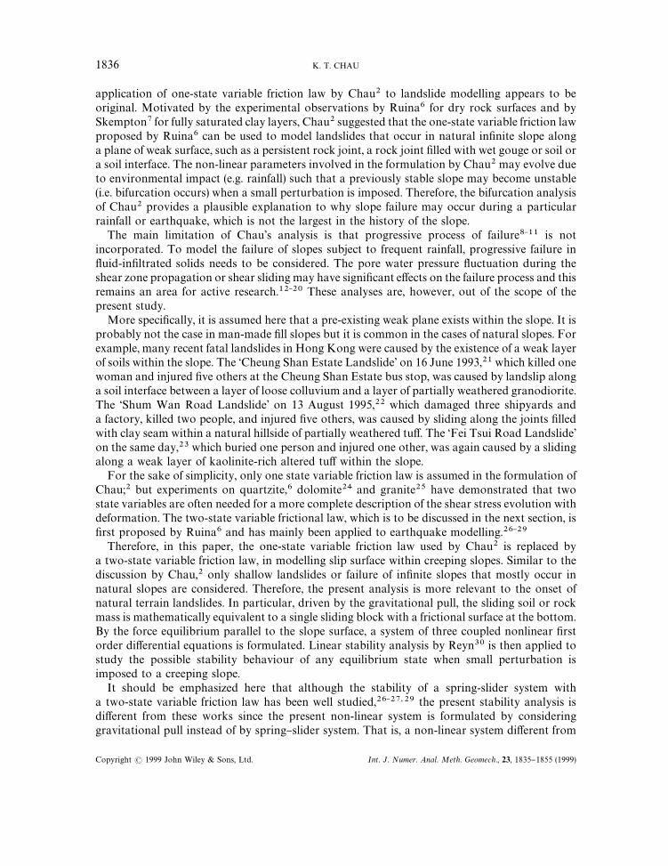
4.6. Boundary II}III: converging vortex spiral

In this region, the real root is negative and the complex roots are purely imaginary, or u1(0

and Re(u2)"0. The canonical form of the system is the same as those of (37). The situation

occurs when D'0, E"0, s1(0, s

2'0 and s

3(0. The converging vortex spiral approaches the

t1}s

1plane as tPR and travels on a cylindrical surface with the /

1axis as the axis of

axisymmetry, as shown in Figure 9. Therefore, the projections of the solution curves form a circle(the centreline) or a plane centre on the t

1}s

1plane. The only perturbed states that move toward

the origin are those initially situated on the /1-axis.

4.7. Boundary III}IV: stable wide or slender two branched node

All of the three real roots are negative, or u1(0 and u

2(0. This stable two branched node

occurs when D"0, s1(0, s

2'0, and s

3(0 (see Figure 3 and note that there is a typo in

Reference 30). The linearized system for /, t and s can "rst be transformed into the following

1848 K. T. CHAU


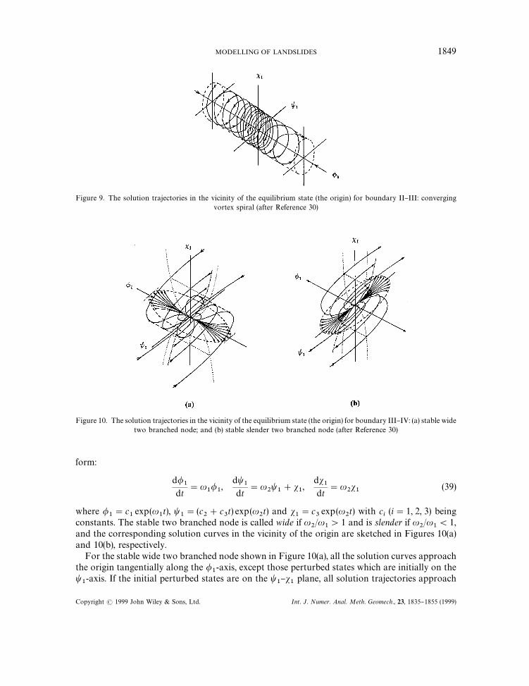
Figure 9. The solution trajectories in the vicinity of the equilibrium state (the origin) for boundary II}III: convergingvortex spiral (after Reference 30)

Figure 10. The solution trajectories in the vicinity of the equilibrium state (the origin) for boundary III}IV: (a) stable widetwo branched node; and (b) stable slender two branched node (after Reference 30)

form:

d/1

dt"u

1/1,

dt1

dt"u

2t1#s

1,

ds1

dt"u

2s1

(39)

where /1"c

1exp(u

1t), t

1"(c

2#c

3t) exp(u

2t) and s

1"c

3exp(u

2t) with c

i(i"1, 2, 3) being

constants. The stable two branched node is called wide if u2/u

1'1 and is slender if u

2/u

1(1,

and the corresponding solution curves in the vicinity of the origin are sketched in Figures 10(a)and 10(b), respectively.

For the stable wide two branched node shown in Figure 10(a), all the solution curves approachthe origin tangentially along the /

1-axis, except those perturbed states which are initially on the

t1-axis. If the initial perturbed states are on the t

1}s

1plane, all solution trajectories approach



the origin along a path which is tangential to the t1-axis at the origin (see the curves passing

through the centreline). Therefore, a stable one branched plane node locates on the t1}s

1plane.

On the /1}t

1plane, all solution curves approach the origin along the /

1-axis except those on the

t1-axis; thus, a stable two branched plane node is formed on that plane.For the stable slender two branched node shown in Figure 10(b), the solution behaviour

around the origin is similar to the case of stable wide two branched node shown in Figure 10(a),except that all solution trajectories on /

1}t

1plane approach the origin along a path which is

tangential to the t1

axis (instead of the /1

axis) at the origin.Strictly speaking, linear stability analysis is only valid for in"nitesimal perturbations when the

non-linear terms can be neglected. However, as illustrated by Chau2 for the one state variablecase, for almost linear system, such as (21)}(23), the linear stability analysis indeed providesqualitative and useful information on stability of the equilibrium state.

5. INSTABILITY REGION IN THE b1}b

2PARAMETER PLANE

From the classi"cation given in Figure 3, it is clear that the boundary between the stable andunstable regions in the s

2}s

3parameter space is the surface E"0. That is, the regions on the left

of the surface E"0 are unstable and those on the right of E"0 are stable, while the solution onE"0 is neutrally stable in the form of converging vortex spiral shown in Figure 9. It isstraightforward to show that this condition for stability agrees with the Routh}Hurwitz criteriagiven by Levinson and Redhe!er.66

So far, it has been assumed that the non-linear system (16)}(18) is autonomous (or physically theparameters along the sliding surface are time-independent). However, if the parameters on thesliding surface, such as b

1and b

2, evolve with the environmental impacts, such as erosion due to

rainfall and permanent change in surrounding stress "elds due to human activities near the slope,an initially stable slope may become unstable. Therefore, the non-linear parameters of the systemmay change such that an initially positive E may become negative, then bifurcation occurs in thesense that a perturbation imposed on the equilibrium solution will cause a catastrophic increasein sliding velocity or landslide results. Thus, it is of importance to study how the bifurcationcondition E"0 varies with the parameters on the sliding surface.

Presuming that both b1and b

2can change with time, Figure 11 plots the bifurcation condition

E"0 (solid lines) for various values of o in the b1}b

2parameter space. The following values are

used for the plot: with i"0)01, j"100, and c!s0"0)2. The boundary between the regions for

velocity strengthening and velocity weakening (b1#b

2"1) is plotted as dotted line for compari-

son. In contrast to the conclusion obtained by Chau, using one-state variable friction law,2 thebifurcation in creeping slope does not, in general, coincide with the onset of velocity weakening(i.e. dq

44/d<(0). In particular, Figure 11 shows that: if b

2'0, the region for unstable creeping

slope can be much smaller than the region of velocity weakening; if b2(0, the regime for

unstable slip for slopes can also occur in the velocity strengthening regime. In addition, the regimefor unstable slip decreases with the increase of o, which is the ratio between the characteristiclengths for the "rst and second state variables h

1and h

2. That is, observation of velocity

weakening in the laboratory does not necessarily imply an unstable creeping slope along the sameslip surface in the "eld even though the exact slip surface is duplicated in the laboratory. Similarly,velocity strengthening observed for a slip surface in the laboratory does not preclude the onset ofunstable slip for the same surface in the "eld under gravitational pull. The region of unstablecreeping slopes, in general, decreases with the increase of o.

1850 K. T. CHAU


Figure 11. Stability regime classi"cation on the b1}b

2parameter space for various values of a creeping slope. The solid

lines are the bifurcation condition E"0 (the solid lines) for various values of o together with the boundary betweenvelocity strengthening and velocity weakening regimes (the dotted line). The other parameters used in these plots are:

i"0)01, j"100, c!s0"0)2

Figure 12. Stability regime classi"cation on the b1}b

2parameter space for a creeping slope. The solid lines are the

bifurcation condition E"0 (the solid lines) for various values of c!s0

together with the boundary between velocitystrengthening and velocity weakening regimes (the dotted line). The other parameters used in these plots are: i: 0)01,

j"100, o"0)05 and c"1)1



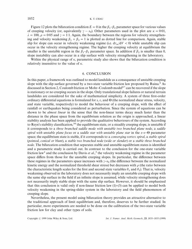
Figure 12 plots the bifurcation condition E"0 in the b1}b

2parameter space for various values

of creeping velocity (or, equivalently c!s0). Other parameters used in the plot are i"0)01,

j"100, o"0)05 and c"1)1. Again, the boundary between the regions for velocity strengthen-ing and velocity weakening b

1#b

2"1 is plotted as dotted line for comparison. Again, stable

slip for slope can occur in velocity weakening regime (i.e. dq44/d<(0) while unstable slip can

occur in the velocity strengthening regime. The higher the creeping velocity at equilibrium thesmaller is the unstable region in the b

1}b

2parameter space. In addition if b

2is smaller than 0,

slope instability can also occur in a slip surface with velocity strengthening in the laboratory.Within the physical range of i, parametric study also shows that the bifurcation condition is

relatively insensitive to the value of i.

6. CONCLUSION

In this paper, a framework was outlined to model landslide as a consequence of unstable creepingslope with the slip surface governed by a two-state variable friction law proposed by Ruina.6 Asdiscussed in Section 2, Coulomb friction or Mohr}Coulomb model67 can be recovered if the slopeis stationary or no creeping occurs in the slope. Only translational slope failures or natural terrainlandslides are considered for the sake of mathematical simplicity. A system of three "rst-orderordinary di!erential equations is formulated for s, v, and # (the normalized shear stress, velocity,and state variable, respectively) to model the behaviour of a creeping slope, with the e!ect ofrainfall or earthquakes being considered as perturbation. Since the system of equations can beshown to be almost linear in the sense that the non-linear terms decay much faster than thedistance in the phase space from the equilibrium solution as the origin is approached, a linearstability analysis has been applied to provide the qualitative behaviours of the system. Accordingto Reyn's stability classi"cation,30 the equilibrium state, or a steadily creeping slope, is unstable ifit corresponds to a three branched saddle mode with unstable two branched plane node, a saddlespiral with unstable plane focus or a saddle star with unstable plane star in the s}v}# parameterspace; the equilibrium state is stable, if it corresponds to a converging vortex spiral, a stable spiral(pointed, conical or blunt), a stable two branched node (wide or slender) or a stable three branchednode. The bifurcation condition that separates stable and unstable equilibrium states is identi"edand a parametric study is carried out. In contrast to the conclusion for the one-state variablefriction law2 and the conclusion by Davis et al.,5 the velocity weakening regime in the parameterspace di!ers from those for the unstable creeping slopes. In particular, the di!erence betweenthese regimes in the parameters space increases with c}s

0(the di!erence between the normalized

kinetic energy and the normalized threshold shear stress) but decreases with o (the ratio betweenthe characteristic length scales for the "rst and second state variables h

1and h

2). That is, velocity

weakening observed in the laboratory does not necessarily imply an unstable creeping slope withthe same slip surface in the "eld if an in"nite slope is assumed, while velocity strengthening doesnot necessarily imply stable slope with the same slip surface. However, it should be emphasizedthat this conclusion is valid only if non-linear friction law (1)}(3) can be applied to model bothvelocity weakening in the spring-slider system in the laboratory and the "eld phenomenon ofcreeping slope.

Nevertheless, the present model using bifurcation theory provides an attractive alternative tothe traditional approach of limit equilibrium and, therefore, deserves to be further studied. Inparticular, more experiments are needed to be done on the calibration of the two-state variablefriction law for clay and other types of soils.

1852 K. T. CHAU


ACKNOWLEDGEMENT

I am grateful to the support from the RGC and HKPolyU when this paper was written. Thiswork was originally inspired by a term project and a series of lectures on the &Mechanics ofEarthquake' given by Prof. John Rudnicki of Northwestern University. The discussion with Dr.Rob Davis of University of Canterbury, New Zealand on landslides has been helpful. Analgebraic mistake in the formulation was corrected by an anonymous reviewer.

APPENDIX

Substitution of (27)}(29) into (33) gives the following expressions of Q and D in terms of o, b1, b

2,

i and vN :

Q"

1

27G[3o(1#o)!2(1#o3)]j3e3vN#3[1!4o#o2!3b

1(1#4o)#3ob

2(2!o)]

j2

ievN

#3[1!3b1#o(1!3b

2)]

ji2

e~vN!

2e~3vN

i3 H (40)

D"a1e6vN

#a2e4vN

#a3e2vN

#a4#a

5e!2vN (41)

where

a1"!

o2j6

108(1!o)2 (42)

a2"

oj5

54i[(1!o) (1!o2)#b

1(3!7o!2o2#2o3)#b

2(!2#4o!o2!o3)] (43)

a3"

j4

108i2[!(1#2o!6o2#2o3#o4)#2b

1(1!o#14o2!2o3)

#2b2o(4!10o#5o2#o3)

#2ob1b2(!10!17o#8o2)#b2

1(!1#28o#44o2)#o2b2

2(8!8o!o2)] (44)

a4"

j3

54i3M(1!o) (1!o2)#b

1[!(4#o#7o2)#b

1(5#14o)!2b2

1]

!ob2[1!5o#4o2#ob

2(4!5o)#2o2b2

2]#ob

1b2[(1#19o)!6(b

1#ob

2)]N (45)

a5"

j2

108i4[4b

1(1#o)!(1!o#b

1#ob

2)2] (46)

REFERENCES

1. A. W. Skempton, &Long-term stability of clay slopes', Geotechnique, 14, 77}102 (1964).2. K. T. Chau, &Landslides modeled as bifurcations of creeping slopes with nonlinear friction law', Int. J. Solids Struct.,

32, 3451}3464 (1995).3. W. Z. Savage and A. F. Chleborad, &A model for creeping #ow in landslides', Bull. Assoc. Engng Geol., 19, 333}338

(1982).



4. R. O. Davis, N. R. Smith and G. Salt, &Pore #uid frictional heating and stability of creeping landslides', Int. J. Numer.Anal. Meth. Geomech., 14, 427}443 (1990).

5. R. O. Davis, C. S. Desai and N. R. Smith, &Stability of motion of translational landslides', J. Geot. Engng, ASCE, 119,420}432 (1993).

6. A. Ruina, &Slip instability and state variable friction laws', J. Geophys. Res., 88, 10 359}10370 (1983).7. A. W. Skempton, &Residual strength of clays in landslides, folded strata and the laboratory', Geotechnique, 35, 3}18

(1985).8. L. Bjerrum, &Progressive failure in slopes of overconsolidated plastic clay and clay shales', J. Soil Mech. Found. Div.

Proc., ASCE, 93, 1}49 (1967).9. A. W. Bishop, &The in#uence of progressive failure on the choice of the method of stability analysis', Geotechnique, 21,

168}172 (1971).10. A. C. Palmer and J. R. Rice, &The growth of slip surfaces in the progressive failure of over-consolidated clay', Proc.

Roy. Soc. ¸ond. A, 332, 527}548 (1973).11. J. R. Rice, &The initiation and growth of shear bands', in A. C. Palmer (ed.), Proc. Symp. on the Role of Plasticity in Soil

Mechanics, Cambridge, 1973, pp. 263}278.12. J. R. Rice and D. A. Simons, &The stabilization of spreading shear faults by coupled deformation}di!usion e!ects in#uid-in"ltrated porous materials', J. Geophys. Res., 81, 5322}5334 (1976).

13. J. W. Rudnicki, &E!ect of pore #uid di!usion on deformation and failure of rock', in Z. Bazant (ed.), Mechanics ofGeomaterials. Wiley, New York, 1985, pp. 315}347.

14. J. W. Rudnicki, &Slip on an impermeable fault in a saturated rock mass', Earthquake Source Mechanics, GeophysicalMonograph, Vol. 37, AGU, Washington, DC, 1986, pp. 81}89.

15. J. W. Rudnicki, &Plane strain dislocations in linear elastic di!usive solids', J. Appl. Mech., ASME, 54, 545}552(1987).

16. J. W. Rudnicki, &Boundary layer analysis of plane strain shear cracks propagating steadily on an impermeable plane inan elastic di!usive solid', J. Mech. Phys. Solids, 39, 201}221 (1991).

17. J. W. Rudnicki and C.-H. Chen, &Stabilization of rapid frictional slip on a weakening fault by dilatant hardening',J. Geophys. Res., 93, 3275}3285 (1988).

18. J. W. Rudnicki and T.-C. Hsu, &Pore pressure changes induced by slip on permeable and impermeable faults',J. Geophys. Res., 93, 3275}3285 (1988).

19. R. M. Iverson and R. G. LaHusen, &Dynamic pore-pressure #uctuations in rapidly shearing granular materials',Science 246, 796}799 (1989).

20. R. O. Davis and M. D. Bolton, &Strength post-liquefaction #ows-A speculative velocity dependent model', in J. X.Yuan (ed.), Comp. Methods & Advances in Geomech., Balkema, Rotterdam, 1997, pp. 115}121.

21. W. K. Pun and A. C. O. Li, &Report on the investigation of the 16 June 1993 landslip at Cheung Shan Estate',Investigation of Some Major Slope Failures Between 1992 and 1995, GEO Report No. 52, Sect. 3, Hong KongGovernment, HK, 1996, pp. 44}57.

22. Geotechnical Engineering O$ce (GEO), Report on the Shum =an Road ¸andslide of 13 August, 1995. GEO, HongKong Government, Hong Kong, 1996.

23. Geotechnical Engineering O$ce (GEO), Report on the Fei ¹sui Road ¸andslide of 13 August, 1995. GEO, Hong KongGovernment, Hong Kong, 1996.

24. J. D. Weeks and T. E. Tullis, &Frictional sliding of dolomite: a variation in constitutive behavior', J. Geophys. Res., 90,7821}7826 (1985).

25. T. E. Tullis and J. D. Weeks, &Constitutive behaviour and stability of frictional sliding of granite', Pure Appl. Geophys.(PAGEOPH), 124, 383}414 (1986).

26. J.-C. Gu, J. R. Rice, A. L. Ruina and S. T. Tse, &Slip motion and stability of a single degree of freedom elastic systemwith rate and state dependent friction', J. Mech. Phys. Solids, 32, 167}196 (1984).

27. M. L. Blanpied and T. E. Tullis, &The stability and behavior of a frictional system with a two state variable constitutivelaw', Pure Appl. Geophys. (PAGEOPH), 124, 415}444 (1986).

28. J. R. Rice, &Constitutive relations for fault slip and earthquake instabilities', Pure Appl. Geophys. (PAGEOPH), 121,443}475 (1983).

29. Y. Gu and T.-F. Wong, &Nonlinear dynamics of the transition from stable sliding to cyclic stick-slip in rock', NonlinearDynamics and Predictability of Geophysical Phenomena, Geophysical Monograph, vol. 83, IUUG Vol. 18, IUGG andAGU, 1994.

30. J. W. Reyn, &Classi"cation and description of the singular points of a system of three linear di!erential equations',J. Appl. Math. Phys. (ZAMP), 15, 540}557 (1964).

31. D. K. Keefer, C. S. Alger, E. E. Brabb, W. M. Brown, S. D. Ellen, E. L. Harp, R. K. Mark, G. F. Wieczorek,R. C. Wilson and R. S. Zatkin, &Real-time landslide warning during heavy rainfall', Science, 238, 921}925 (1987).

32. R. M. Iverson and J. J. Major, &Rainfall, groundwater-#ow, and seasonal movement at Minor Creek landslide,Northwestern California-Physical interpretation of empirical relations', Geol. Soc. Am. Bull., 99, 579}594 (1987).

33. K. Kashiwaya, T. Kawatani and T. Okimura, &Tree-ring information and rainfall characteristic for landslide in theKobe district, Japan', Earth Surface Processes ¸andforms, 14, 63}71 (1989).

1854 K. T. CHAU


34. S. K. Kim, W. P. Hong and Y. M. Kim, &Prediction of rainfall-triggered landslides in Korea', in D. H. Bell (ed.),¸andslides, Balkema, Rotterdam, 1991, pp. 989}994.

35. T. C. Pierson, R. M. Iverson and S. D. Ellen, &Spatial and temporal distribution of shallow landsliding during intenserainfall, southeastern Oahu, Hawaii', in D. H. Bell (ed.), ¸andslides. Balkema, Rotterdam, 1991, pp. 1393}1398.

36. G. Polloni, M. Ceriani, S. Lauzi, N. Padovan and G. Crosta, &Rainfall and soil slipping events in Valtellina', in D. H.Bell (ed.), ¸andslides. Balkema, Rotterdam, 1991, pp. 183}188.

37. J. Premchitt, E. W. Brand and P. Y. M. Chen, &Rain-induced landslides in Hong Kong, 1972}1992', Asia Engineer43}51 (1994).

38. G. E. Ladd, &Landslides, subsidences and rockfalls', Am. Railway Eng. Asso. Proc. 36, 1091}1162 (1935).39. A. J. Pearce and A. J. Watson, &E!ects of earthquake-induced landslides on sediment budget and transport over

a 50-year period', Geology 14, 52}55 (1986).40. R. G. Updike, J. A. Egan, I. M. Idriss, Y. Moriwaki and T. L. Moses, &A model for earthquake-induced translatory

landslides in Quaternary sediments', Geol. Soc. Am. Bull. 100, 783}792 (1988).41. R. F. Madole, R. L. Schuster and A. M. Sarnawojcicki, &Ribbon-Cli! landslide, Washington, and the Earthquake of 14

December 1872', Bull Seism. Soc. Am. 86, 544}545 (1996).42. K. T. Chau, &Failure of slopes modelled as bifurcation', Int. Conf. on Comp. Meth. Struct. Geot. Eng., Vol. 2, Hong

Kong, 1994, pp. 500}505.43. K. T. Chau and C. H. Chan, &E!ect of pore pressure on slope failure modelled as bifurcation', Int. Conf. on ¸andslides,

Slope Stability & the Safety of Infra-structures, Kuala Lumpur, Malaysia, 1994, pp. 97}104.44. J. W. Rudnicki, &Physical models of earthquake instability and precursory processes', Pure Appl. Geophys. (PAG-

EOPH), 126, 531}554 (1988).45. J. H. Dieterich, &Modeling of rock friction 1. Experimental results and constitutive equations', J. Geophys. Res., 84,

2161}2168 (1979).46. P. Solberg and J. D. Byerlee, &A note on the rate sensitivity of frictional sliding of Westerly granite', J. Geophys. Res.,

89, 4203}4205 (1984).47. D. A. Lockner, R. Summers and J. D. Byerlee, &E!ects of temperature and sliding rate on frictional strength of granite',

Pure Appl. Geophys. (PAGEOPH), 124, 445}469 (1986).48. J. H. Dieterich, &Constitutive properties of faults with simulated gouge', in N. L. Carter, M. Friedman, J. M. Logan

and D. W. Stearns (eds), Mechanical Behaviour of Crustal Rocks, Geophys. Monograph, Am. Geophys. Union,Washington, DC, 1981.

49. B. E. Hobbs, A. Ord and C. Marone, &Dynamic behaviour of rock joints', in N. Barton and O. Stephansson (eds), RockJoints: Proc. Int. Symp. Rock Joints, Balkema, Rotterdam, 1990.

50. T. Shimamoto, &Transition between frictional slip and ductile #ow for halite shear zones at room temperature',Science, 231, 711}714 (1986).

51. R. M. Stesky, &The mechanical behaviour of faulted rock at high temperature and pressure', Ph.D. ¹hesis, Mass-achusetts Institute of Technology, Cambridge, 1975.

52. J. D. Byerlee and P. Vaughan, &Dependence of friction on slip velocity in water saturated granite with added gouge',¹rans. Amer. Geophys. ;nion, EOS, 65, 1078 (1984).

53. C. Morrow and J. D. Byerlee, &A physical explanation for transient behavior during shearing of fault gouge at variablestrain rates (Abstract)', ¹rans. Amer. Geophys. ;nion, EOS, 66, 1100 (1985).

54. K. A. Healy, &The dependency of dilation in sand on rate of shear strain', Ph.D. ¹hesis, Massachusetts Institute ofTechnology, Cambridge, 1959.

55. O. Hungr and N. B. Morgenstern, &High velocity ring shear tests on sand', Geotechnique, 34, 415}421 (1984).56. D. A. Lockner and J. D. Byerlee, &Dilatancy in hydraulically isolated faults and the suppression of instability',

Geophys. Res. ¸ett., 21, 2353}2356 (1994).57. N. Minorsky, Nonlinear Oscillations, van Nostrand, Princeton, 1962.58. W. E. Boyce and R. C. DiPrima, Elementary Di+erential Equations and Boundary<alue Problems, 5th edn, Wiley, New

York, 1992.59. C. G. Cullen, ¸inear Algebra and Di+erential Equations, 2nd edn, PWS-Kent Publishing Co., Boston, 1991.60. V. I. Arnold, Ordinary Di+erential Equations (Translated from the Russian by R. A. Silverman). MIT Press,

Cambridge, MA, 1973.61. J. M. T. Thompson and H. B. Steward, Nonlinear Dynamics and Chaos, Wiley, Chichester, 1986.62. J.-P. Tignol, Galois1 ¹heory of Algebraic Equations. Longman Scienti"c & Technical, Essex, England, 1988.63. M. Abramowitz and I. A. Stegun (eds), Handbook of Mathematical Functions, Dover, New York, 1965.64. I. Stewart, Galois ¹heory, 2nd edn, Chapman & Hall, London, 1989.65. C. J. Tranter, ¹echniques of Mathematical Analysis. Hodder and Stoughton, London, 1957.66. N. Levinson and R. M. Redhe!er, Complex <ariables, Holden-Day, San Fransico, 1970.67. B. Voight (ed.), Rockslides and Avalanches, Vols. 1 and 2, Elsevier, New York, 1978.



Chau K.T. (1999) "Onset of natural terrain landslides modeled by linear stability analysis of...

Documents

Transcript of Chau K.T. (1999) "Onset of natural terrain landslides modeled by linear stability analysis of...