Charge Transport in amorphous organic semiconductors
140
Charge Transport in amorphous organic semiconductors Dissertation zur Erlangung des Grades “Doktor der Naturwissenschaften” am Fachbereich Physik der Johannes Gutenberg-Universit¨at Mainz Alexander Lukyanov geb. in Glasow, Russland Max-Planck-Institut f¨ ur Polymerforschung Mainz, M¨arz 2011
-
Upload
khangminh22 -
Category
Documents
-
view
1 -
download
0
Transcript of Charge Transport in amorphous organic semiconductors

Charge Transport
in amorphous
organic semiconductors
Dissertation
zur Erlangung des Grades
“Doktor der Naturwissenschaften”
am Fachbereich Physikder Johannes Gutenberg-Universitat Mainz
Alexander Lukyanovgeb. in Glasow, Russland
Max-Planck-Institut fur PolymerforschungMainz, Marz 2011


Abstract
Organic semiconductors with the unique combination of electronic and me-chanical properties may offer cost-effective ways of realizing many electronicapplications, e. g. large-area flexible displays, printed integrated circuits andplastic solar cells. In order to facilitate the rational compound design oforganic semiconductors, it is essential to understand relevant physical prop-erties e. g. charge transport. This, however, is not straightforward, sincephysical models operating on different time and length scales need to becombined. First, the material morphology has to be known at an atom-istic scale. For this atomistic molecular dynamics simulations can be em-ployed, provided that an atomistic force field is available. Otherwise it hasto be developed based on the existing force fields and first principle calcula-tions. However, atomistic simulations are typically limited to the nanometerlength- and nanosecond time-scales. To overcome these limitations, system-atic coarse-graining techniques can be used.
In the first part of this thesis, it is demonstrated how a force field can beparameterized for a typical organic molecule. Then different coarse-grainingapproaches are introduced together with the analysis of their advantages andproblems. When atomistic morphology is available, charge transport canbe studied by combining the high-temperature Marcus theory with kineticMonte Carlo simulations.
The approach is applied to the hole transport in amorphous films of tris(8-hydroxyquinoline)aluminium (Alq3). First the influence of the force fieldparameters and the corresponding morphological changes on charge transportis studied. It is shown that the energetic disorder plays an important role foramorphous Alq3, defining charge carrier dynamics. Its spatial correlationsgovern the Poole-Frenkel behavior of the charge carrier mobility. It is foundthat hole transport is dispersive for system sizes accessible to simulations,meaning that calculated mobilities depend strongly on the system size. Amethod for extrapolating calculated mobilities to the infinite system size isproposed, allowing direct comparison of simulation results and time-of-flightexperiments. The extracted value of the nondispersive hole mobility and itselectric field dependence for amorphous Alq3 agree well with the experimentalresults.
III

IV

Zusammenfassung
Organische Halbleiter weisen eine Kombination von elektronischen undmechanischen Eigenschaften auf, die eine kostengunstige Realisierung vielerelektronischen Anwendungen, z. B. großflachige flexible Displays, gedruckteintegrierte Schaltungen oder Kunststoff-Solarzellen ermoglichen konnen. ImZuge des Entwurfs neuer organischer Halbleiter ist es wichtig, relevante physi–kalische Eigenschaften zu verstehen, z. B. Ladungstransport. Dies ist jedochmit Schwierigkeiten verbunden, da mehrere Modelle, die Effekte auf unter-schiedlichen Zeit- und Langenskalen beschreiben, kombiniert werden mussen.Zunachst muss die Materialmorphologie mit atomistischer Auflosung bekanntsein. Diese kann durch Molekulardynamik-Simulationen generiert werden,unter der Voraussetzung, dass ein atomistisches Kraftfeld zur Verfugungsteht, welches auf der Basis bestehender Kraftfelder und ab-initio Rech-nungen entwickelt werden kann. Allerdings sind atomistische Simulationenauf Langen- und Zeitskalen beschrankt, die in der Großenordnung einigerNanometer bzw. Nanosekunden liegen. Um großere Skalen zu erschließenkonnen systematische Vergroberungstechniken (Coarse-Graining) verwendetwerden.
Im ersten Teil dieser Arbeit wird gezeigt, wie ein Kraftfeld fur ein typ-isches organisches Molekul parametrisiert werden kann. Dann werden ver-schiedene Vergroberungsansatze eingefuhrt und deren Vorteile und Problemediskutiert. Sobald eine atomistische Morphologie zur Verfugung steht, kannder Ladungstransport durch eine Kombination der Hochtemperatur-Marcus-Theorie mit der kinetischen Monte-Carlo-Methode simuliert werden.
Dieser Ansatz wird verwendet, um den Lochertransport in amorphenSchichten von Tris-(8-Hydroxychinolin)-Aluminium zu simulieren. Zunachstwird der Einfluss der Kraftfeldparameter und der entsprechenden morpholo-gischen Veranderungen auf den Ladungstransport untersucht. Es wird gezeigt,dass die energetische Unordnung im System eine wichtige Rolle spielt. Diesebeeinflusst die Ladungstragerdynamik erheblich, entsprechende raumlicheKorrelationen beeinflussen das Poole-Frenkel-Verhalten der Ladungstrager–mobilitat. Es ist zu beobachten, dass Lochertransport dispersiven Charak-ter besitzt, d. h. berechnete Beweglichkeiten hangen stark von der Sys-temgroße ab. Es wird ein Verfahren zur Extrapolation der berechnetenBeweglichkeiten zur unendlichen Systemgroße vorgeschlagen, das einen di-rekten Vergleich der Simulationsergebnisse zu Time-Of-Flight-Experimentenermoglicht. Die extrahierten Werte der nichtdispersiven Lochermobilitat undihre Abhangigkeit vom elektrischen Feld stimmen fur amorphes Alq3 gut mitden experimentellen Ergebnissen uberein.
V

VI

Contents
Related Publications 1
1 Organic electronics 3
1.1 Devices . . . . . . . . . . . . . . . . . . . . . . . . . . . . . . 41.1.1 Organic light emitting diodes . . . . . . . . . . . . . . 41.1.2 Organic field effect transistors . . . . . . . . . . . . . . 51.1.3 Organic solar cells . . . . . . . . . . . . . . . . . . . . 6
1.2 Mobility measurements . . . . . . . . . . . . . . . . . . . . . . 71.2.1 Time-of-flight measurements . . . . . . . . . . . . . . . 81.2.2 Diode and transistor measurements . . . . . . . . . . . 91.2.3 Summary: mobility measurements . . . . . . . . . . . . 10
1.3 Importance of theory and simulation . . . . . . . . . . . . . . 10
2 Theoretical description of charge transport 13
2.1 High temperature semi-classical Marcus theory . . . . . . . . . 142.2 Reorganization energy . . . . . . . . . . . . . . . . . . . . . . 162.3 Transfer integrals . . . . . . . . . . . . . . . . . . . . . . . . . 182.4 Free energy difference . . . . . . . . . . . . . . . . . . . . . . . 192.5 Gaussian disorder model . . . . . . . . . . . . . . . . . . . . . 19
2.5.1 Temperature dependence . . . . . . . . . . . . . . . . . 212.5.2 Field dependence . . . . . . . . . . . . . . . . . . . . . 212.5.3 The nondispersive to dispersive transition . . . . . . . 212.5.4 Expression for the mobility . . . . . . . . . . . . . . . . 22
2.6 Role of site energy spatial correlations . . . . . . . . . . . . . 222.7 Charge transport in realistic morphologies . . . . . . . . . . . 23
3 Morphology simulations 27
3.1 Molecular dynamics simulations . . . . . . . . . . . . . . . . . 273.2 Force field development . . . . . . . . . . . . . . . . . . . . . . 28
3.2.1 DP-PPV force field as an example . . . . . . . . . . . . 283.2.1.1 Parametrization of backbone dihedrals . . . . 30
VII

3.2.1.2 Force-field validation . . . . . . . . . . . . . . 323.2.1.3 DP-PPV force-field . . . . . . . . . . . . . . . 34
3.3 Limitations of MD simulations . . . . . . . . . . . . . . . . . . 34
4 Coarse-graining techniques 37
4.1 Introduction . . . . . . . . . . . . . . . . . . . . . . . . . . . . 374.2 Boltzmann inversion . . . . . . . . . . . . . . . . . . . . . . . 394.3 Iterative Boltzmann inversion . . . . . . . . . . . . . . . . . . 414.4 Inverse Monte Carlo . . . . . . . . . . . . . . . . . . . . . . . 424.5 Force matching . . . . . . . . . . . . . . . . . . . . . . . . . . 45
4.5.1 FM method: formal statistical mechanical derivation . 464.5.2 FM method: connections to the liquid state theory . . 48
4.6 Relationship between CG methods . . . . . . . . . . . . . . . 49
5 Comparison of coarse-graining techniques 51
5.1 Coarse-graining of water . . . . . . . . . . . . . . . . . . . . . 515.2 Coarse-graining of methanol . . . . . . . . . . . . . . . . . . . 545.3 Liquid propane: from an all- to an united-atom description . . 575.4 Angular potential of a hexane molecule . . . . . . . . . . . . . 59
6 Conformational structure of PPV derivatives 63
6.1 Atomistic molecular dynamics . . . . . . . . . . . . . . . . . . 656.1.1 Alkyl side chain stretching in solvated DP-PPV . . . . 656.1.2 Orientational correlations in solvated DP-PPV . . . . . 666.1.3 Planarity and tacticity of solvated DP-PPV . . . . . . 676.1.4 DP-PPV melt . . . . . . . . . . . . . . . . . . . . . . . 706.1.5 Atomistic molecular dynamics: summary . . . . . . . . 71
6.2 A coarse-grained model for DP10-PPV . . . . . . . . . . . . . 716.2.1 Bonded interaction potentials . . . . . . . . . . . . . . 726.2.2 Non-bonded interaction potentials . . . . . . . . . . . . 726.2.3 Coarse-grained simulations of DP10-PPV in chloroform 74
6.3 Discussion . . . . . . . . . . . . . . . . . . . . . . . . . . . . . 75
7 Morphology and charge transport in amorphous Alq3 77
7.1 Introduction . . . . . . . . . . . . . . . . . . . . . . . . . . . . 777.2 Force-field parameters . . . . . . . . . . . . . . . . . . . . . . 787.3 Relationship between morphology and charge transport . . . . 857.4 Role of energetic disorder . . . . . . . . . . . . . . . . . . . . . 87
7.4.1 Computational details . . . . . . . . . . . . . . . . . . 877.4.2 Poole-Frenkel behavior . . . . . . . . . . . . . . . . . . 887.4.3 Charge dynamics visualization . . . . . . . . . . . . . . 89
VIII

7.4.4 Spatial correlations of energetic disorder . . . . . . . . 92
8 Extracting nondispersive mobilities 95
8.1 Mean carrier energy in a finite system . . . . . . . . . . . . . . 968.2 Temperature extrapolation . . . . . . . . . . . . . . . . . . . . 98
A Force matching using cubic splines 105
B Yvon-Born-Green equations for a homogeneous liquid 109
C Validation of the Alq3 force field 111
Bibliography 113
IX

X

Related Publications
[1] A. Lukyanov, C. Lennartz, and D. Andrienko. Amorphous filmsof tris(8-hydroxyquinolinato)aluminium: Force-field, morphology, andcharge transport. Phys. Stat. Sol.(a), 206:2737–2742, 2009.
[2] V. Ruhle, C. Junghans, A. Lukyanov, K. Kremer, and D. Andrienko.Versatile object-oriented toolkit for coarse-graining applications. J.Chem. Theory Comput., 5(12):3211–3223, 2009.
[3] A. Lukyanov, A. Malafeev, V. Ivanov, H.-L. Chen, K. Kremer, andD. Andrienko. Solvated poly-(phenylene vinylene) derivatives: conforma-tional structure and aggregation behavior. J. Mater. Chem., 20:10475–10485, 2010.
[4] A. Lukyanov and D. Andrienko. Extracting nondispersive charge carriermobilities of organic semiconductors from simulations of small systems.Phys. Rev. B., 82(19):193202, 2010.
1

2

Chapter 1
Organic electronics
When the first transistor was invented in the middle of 20th century [5],inorganic semiconductors such as silicon and germanium began to play adominating role in electronics, where metals were prevailing before. To-day science and industry are working on a new class of materials, knownas organic semiconductors, which promise to revolutionize electronics again.Organic semiconductors have electronic properties approaching those of inor-ganic counterparts combined with mechanical properties of plastic materials,offering low-cost processing and a possibility to realize new applications, suchas large-area flexible displays, low-cost printed integrated circuits and plasticsolar cells [6]. Moreover, by varying the chemistry slightly, it is possible tomodify material properties of interest (e.g. band gap), to achieve the desireddevice performance.
There are two major classes of organic semiconductors: low molecularweight materials (usually processed in vacuum) and polymers (usually pro-cessed by wet chemical techniques). Typical examples are shown in Fig. 1.1.Both have in common a conjugated π-electron system, which is responsiblefor their semiconducting properties. Thin films of organic semiconductorsare typically used in three types of devices: (1) Organic light emitting diodes(OLED), (2) Organic field-effect transistors (OFET), (3) organic photovoltaiccells (OPVC). Typical structures of these devices are depicted in Fig. 1.2 andFig. 1.3. An organic light emitting diode (OLED) emits light in response toan electric current [7]. Solar cell does the opposite: it converts the energyof sunlight directly into electricity [8]. Organic field-effect transistor controlsthe conductivity of a channel, made of organic semiconductor, by applyingelectric field [9].
In the following section we will discuss operation principles of the organicelectronics devices in detail.
3

CHAPTER 1. ORGANIC ELECTRONICS
O
O
S
S
S**
*
*
poly(phenylene vinylene)
PCBM
hexabenzocoronene
poly(3−hexylthiophene) (P3HT)
tris(8−hydroxyquinoline) aluminium (Alq3)
Figure 1.1: Typical compounds used in organic electronics applications.
1.1 Devices
1.1.1 Organic light emitting diodes
A typical OLED is composed of several layers of organic materials sand-wiched between two electrodes. Charge carriers of both signs are injectedfrom the electrodes and recombine, forming a neutral exciton, a bound stateof an electron-hole pair. The decay of an exciton results in the emissionof radiation whose frequency is in the visible range. The frequency of thisradiation depends on the optical band gap of the material.1 For the opera-tion of the device, charge carriers must be efficiently injected to the organicfilm from the electrodes. This requires low energetic barriers at the metal-organic interfaces for both contacts in order to inject equally high amountsof electrons and holes and to provide a balanced charge carrier flow. In sin-gle layer devices hole and electron concentrations might be imbalanced, forexample due to different electron and hole mobilities, which leads to low ef-ficiency. Better efficiency is obtained if additional layers are added to thedevice. The hole (electron) transporting layer is used to provide intermedi-ate energy states to allow holes (electrons) to cascade through smaller gaps
1Optical band gap is related to the exciton binding energy and the energy differencebetween the highest occupied molecular orbital (HOMO) and lowest unoccupied molecularorbital (LUMO).
4Rev. 117(e1a68f80ce2b) from 2011-03-08

1.1. DEVICES
(a) (b)
Figure 1.2: Organic light emitting diode. (a) Typical device consists of the followinglayers: electron transporting layer (ETL), hole blocking layer (HBL), emission layer (EL),electron blocking layer (EBL), hole transporting layer (HTL). Adapted from [6]; (b) Energylevels in OLED layers.
in case there is a barrier between the metal work function and the HOMO(LUMO) of the emission layer. Hole (electron) blocking layers have verydeep HOMO (or high LUMO) levels which help to prevent holes (electrons)from passing through the device to the opposite electrode without formingan exciton. Typical OLED structure is shown in Fig. 1.2.
The first high-performance OLED was reported in 1987 [10]. These firstdevices used tris(8-hydroxyquinoline)aluminium (Alq3) (see Fig. 1.1) as anelectron transporting layer. After more than two decades of intensive re-search and development of OLEDs, Alq3 continues to be the workhorse inlow-molecular weight materials for these devices. It is used as an electron-transporting layer, as well as an emission layer where green light emission isgenerated by the electron-hole recombination in Alq3. It also serves as a hostmaterial for various dyes, helping to tune the emission color from green tored [11]. Many studies have been focused on the optimization of OLED effi-ciency and long-term stability, by means of the understanding of charge trans-port properties of amorphous thin films, see e.g. Refs. [12, 13, 14, 15, 16, 17].
Understanding microscopic mechanisms of charge transport in amorphousAlq3 is one of the topics of this thesis. It is covered in detail in Chapter 8.
1.1.2 Organic field effect transistors
Organic field effect transistors (OFETs) are the basic building blocks for flex-ible integrated circuits and displays. An OFET can be viewed as a resistor,that can be adjusted by applying external voltage. A typical OFET struc-ture is shown in Fig. 1.3a. The current between the source and the drain
Rev. 117(e1a68f80ce2b) from 2011-03-085

CHAPTER 1. ORGANIC ELECTRONICS
(b)(a)
Figure 1.3: Organic electronics devices (a) field effect transistor; (b) organic solarcell. Adapted from [6].
electrodes is modulated by applying voltage to the gate electrode, which isseparated from the transporting layer by a dielectric. Application of volt-age to the gate electrode changes the charge carrier density in the organicsemiconductor, thus modifying the resistance. In an ideal device there is noconductance without the application of the gate voltage (“off” state). Whenthe gate voltage is applied, current between source and drain appears (“on”state). The on-off current ratio characterizes the ability of the device to“switch off”. Currently values up to 108 can be achieved [18]. Device perfor-mance also critically depends on charge carrier mobility, which must be highenough in order to obtain source-drain currents, which can be modulated bya reasonable gate voltage. Therefore, designing materials with high chargecarrier mobilities is a key to high-performance OFETs.
1.1.3 Organic solar cells
Organic solar cells convert sunlight into electric current. This process can beschematically described by the following steps: (1) absorption of a photonleading to the formation of a bound electron-hole pair (exciton); (2) excitondiffusion to a region where exciton dissociation (charge separation) occurs;and (3) charge transport within the organic semiconductor to the respectiveelectrodes [19].
The large optical band gap in organic materials (normally higher than2 eV) limits light harvesting to 30 % [19], reducing the device efficiency. Toovercome this problem, low band gap polymers must be designed [20, 21].Another problem is that primary photoexcitations do not lead directly to freecharge carriers, but to coulomb-bound electron-hole pairs (excitons). Sinceexciton binding in organic semiconductors is of the order of 10 − 50 kBT ,thermal energy can not drive charge separation, as it would happen in inor-
6Rev. 117(e1a68f80ce2b) from 2011-03-08

1.2. MOBILITY MEASUREMENTS
ganic materials. Instead, an additional mechanism is required for the chargeseparation to occur [22]. One way to achieve this is to use a mixture ofdonor and acceptor compounds (e.g. conjugated polymers with fullerenes).By tuning the difference between the lowest unoccupied molecular orbitals(LUMO) of a donor and an acceptor it is possible to compensate for the exci-ton binding energy. In this case, electron transfers to the acceptor, leaving ahole in the donor. After the separation, free carriers diffuse to the electrodesand generate electric current in the external circuit.
Since the typical exciton diffusion length in organic materials is of theorder of 10 − 20 nm, only excitons created within this distance from theinterface can reach it. This leads to the loss of absorbed photons furtheraway from the interface and results in low efficiencies [23]. One way to solvethis problem is to use bulk heterojunctions - blends of the donor and acceptorcomponents in a bulk volume, which exhibit phase separation in a 10−20 nmlength scale (see Fig. 1.3b). In such a nanoscale interpenetrating network,each interface is within a distance less than the exciton diffusion length fromthe absorbing site. By using the bulk heterojunction concept it is possibleto increase the interfacial area between the donor and acceptor phases byorders of magnitude, significantly improving the solar cell efficiency [19].
1.2 Mobility measurements
The devices mentioned above share one common feature: their performancecritically depends on the efficiency with which charge carriers move withinthe π-conjugated materials. The physical quantity which describes this ef-ficiency is charge carrier mobility. Mobility is one of the key parameters ofinterest - both towards realizing improved device performance, as well asunderstanding the underlying semiconductor physics in these materials. Itis in particular important for the efficiency of transistors (how fast they canswitch) and solar cells (how fast the separated charges can “run away” fromeach other). Mobility strongly depends on the processing, chemical struc-ture and purity of a material. Organic semiconductors have lower mobilitiescompared to their inorganic counterparts2: values of 0.1 − 1.0 cm2/Vs areconsidered to be good for organic semiconductors. Most materials have mo-bilities which are orders of magnitude smaller. For example, hole mobilitiesin amorphous Alq3 are of the order 10−9 − 10−8 cm2/Vs [26].
A number of techniques was designed in order to measure charge carriermobility experimentally. An extensive review is given in Ref. [27]. Here we
2Typical electron mobility for crystalline silicon at room temperature (300 K) is1400 cm2/Vs and the hole mobility is around 450 cm2/Vs [24, 25].
Rev. 117(e1a68f80ce2b) from 2011-03-087

CHAPTER 1. ORGANIC ELECTRONICS
Figure 1.4: Typical transient photocurrents (a) non-dispersive; (b) dispersive. Inset:double logarithmic plot. Taken from [27].
will briefly describe the time-of-flight, diode and transistor measurements.
1.2.1 Time-of-flight measurements
The time-of-flight (TOF) method is based on the measurement of the carriertransit time τ , namely, the time required for a packet of carriers to driftacross the organic semiconducting layer. In the TOF setup the material ofinterest is sandwiched between two electrodes, one of which is transparent.Charges are generated by photo-excitation of the film through irradiationwith a short laser pulse. Subsequently, carriers propagate along the electricfield and generate a displacement current, which flows until charge carriersarrive at the other electrode. Typical photocurrents are shown in Fig. 1.4.From the cusp of the non-dispersive photocurrent (Fig. 1.4a) the transit timeτ can be determined. Then the charge carrier mobility is calculated as
µ =v
E=
d
Eτ=
d2
V τ(1.1)
where V is the applied voltage, E = V/d is the electric field, and d is thesample thickness.
Polymers and amorphous glasses often exhibit dispersive photocurrents,without any definite cusp, as shown in Fig. 1.4b. In this case, τ can stillbe determined from the double logarithmic plot. Although mobilities deter-mined from dispersive transients are thickness-dependent. This means thatthe dispersive mobility is not a material constant, but depends on the systemsize. First microscopic statistical model of dispersive transport was proposedin Ref. [28]. As opposed to the Gaussian packet (nondispersive transport),where the peak and the mean are located at the same position and move
8Rev. 117(e1a68f80ce2b) from 2011-03-08

1.2. MOBILITY MEASUREMENTS
with the same velocity, the mean carrier of a “dispersive” packet propagateswith a velocity which decreases with time as it separates from the peak whichremains nearly fixed at the point of origin of the carriers.
Due to the requirement that the absorption depth of the laser excitationmust be much smaller than the sample thickness, TOF method requires thicksamples (usually in the range from 4 to 20 µm). Thus, the measured bulkmobilities are sensitive to the positional and orientational disorder and de-fects in the sample [29]. Note that a typical TOF setup has very low chargecarrier densities, meaning that single carrier mobilities are measured. Anadvantage of the time-of-flight method is that hole and electron mobilitiescan be studied separately.
1.2.2 Diode and transistor measurements
An alternative approach to measure the mobility of an organic material isto embed it as a functional layer into a device and extract the mobilityfrom the device characteristics [30]. In an OLED, the material of interestis sandwiched between two electrodes, which are chosen in such a way thatonly holes or electrons are injected at low voltage. In the absence of trapsand at low electric fields, current-voltage characteristics may be expressedas [27]:
I =9
8ǫ0ǫrµ
U2
L3(1.2)
Here ǫ0 (ǫr) is dielectric permittivity of free space (of the semiconductinglayer) and L is the device thickness. µ is charge carrier mobility, whichis assumed to be constant throughout the sample. The prefactor 9/8 comesfrom the assumption that the diode has a rectangular geometry. Dependence(1.2) is characteristic of a space-charge limited current (SCLC). Space-chargelimitation of the current means that the number of charge carriers in thematerial is not limited by the injection but by the amount of the carriersalready present in the sample. Their electrostatic potential prevents injectionof the additional charges [31]. In the SCLC scheme, the charge density is notuniform across the material and is the largest close to the injecting electrode.In the presence of traps and at high fields, Eq. 1.2 must be modified [27].
Similarly, carrier mobilities can be extracted from the electrical charac-teristics measured in a field-effect transistor (FET) configuration. The I −V(current-voltage) expression in a linear regime is given by
ISD =W
Lµ (VG − VT ) VSD (1.3)
Rev. 117(e1a68f80ce2b) from 2011-03-089

CHAPTER 1. ORGANIC ELECTRONICS
and in a saturated regime by
ISD =W
2LµC (VG − VT )2 (1.4)
Here, ISD and VSD are the current and the voltage bias between source anddrain, respectively, VG denotes the gate voltage, VT is the threshold voltageat which the current starts to rise, C is the capacitance of the gate dielectric,and W and L are the width and the length of the conducting channel.
In a FET setup mobilities are measured at high charge carrier densities.Since charge transport occurs in a narrow channel, it is affected by structuraldefects at the interface, surface topology, or polarity of the dielectric. This in-fluence might be irrelevant for amorphous materials, but becomes importantfor crystalline or liquid-crystalline materials.
1.2.3 Summary: mobility measurements
Different techniques discussed above operate at different conditions: singlecarrier bulk mobilities are measured by the time-of-flight technique, whereasinterface mobilities at high charge carrier densities are extracted from OFETcharacteristics. Other techniques exist, such as Pulse Radiolysis - Time Re-solved Microwave Conductivity (PR-TRMC) [32], which measure local mo-bilities of small well-ordered domains. As a result, mobility values obtainedby different methods for the same material can differ by orders of magni-tude [27]. This should be kept in mind when comparing simulations withexperimental data. Single carrier kinetic Monte Carlo simulations describedin the next Chapter mimic time-of-flight experiments and thus must be com-pared to them. Nevertheless care must be taken when the simulation boxcontains only a few hopping sites as explained in detail in Chapter 8.
1.3 Importance of theory and simulation
Organic electronic devices presented in this chapter are promising candidatesto replace (at least for some applications) their silicon-based analogues. Thiswould simplify the production process, since cost-efficient techniques such asspin coating and ink-jet printing can be employed. Combination of mechan-ical and semiconducting properties of conjugated polymers allows design offlexible electronics, such as bendable solar cells, rollable light sources anddisplays.
In order to be competitive on the market, organic electronic devices mustpossess high enough efficiency and stability. At the moment only OLEDs are
10Rev. 117(e1a68f80ce2b) from 2011-03-08

1.3. IMPORTANCE OF THEORY AND SIMULATION
routinely used in commercial applications: Samsung, Sony and HTC fabri-cate TV and smartphone devices with OLED displays [33]. However, solarcells reported so far show very low power conversion efficiency (about 5% [20])and are not stable long enough under ambient conditions. To systematicallyimprove the device performance and stability, fundamental understandingof the underlying physical and chemical processes is required. It is impor-tant to understand the relationships between the chemical structure of thecompound, its morphology and finally the properties of the resulting thinfilm or device. In order to achieve this understanding, models and methods,applicable on different length- and time scales should be combined. In thepast decades methods were developed to describe charge transport in organicmaterials on microscopic, mesoscopic and macroscopic levels. On a micro-scopic level Marcus theory is normally used (see Chapter 2), which providesrates for the charge hopping between neighboring molecules based on firstprinciples calculations. On the mesoscopic level charge carrier mobilities canbe calculated by solving a master equation for a system of hopping sites,given some assumptions about the charge hopping rates. This approach isusually called the Gaussian disorder model and it is described in detail inChapter 2. On the macroscopic level device characteristics can be calculatedusing drift-diffusion equations, given charge carrier mobility is known as afunction of temperature, electric field and charge carrier density [34].
In this thesis microscopic and mesoscopic levels of description are com-bined to calculate charge carrier mobilities in amorphous films of tris(8-hydroxyquinoline)aluminium (Alq3). To model amorphous films classicalmolecular dynamics simulations are used. The approach works as follows:first, an atomistic force-field for Alq3 is developed and validated, based onexisting force-fields, first principle calculations and experimental data. Sec-ond, realistic material morphologies are obtained using molecular dynamicssimulations. Semi-classical Marcus theory is then used to calculate chargehopping rates between all neighboring molecules in the amorphous morphol-ogy. Finally, kinetic Monte Carlo simulations are used to calculate chargecarrier mobilities.
The above mentioned techniques are used to study how non-bonded force-field parameters affect the morphology of amorphous Alq3 and how sensitivecharge transport properties are to the corresponding morphological changes.It is shown that in the particular case of Alq3, the energetic disorder playsan important role, defining charge carrier dynamics, and its spatial corre-lations govern the Poole-Frenkel behavior of the charge carrier mobility. Itis found that hole transport in amorphous Alq3 is dispersive for the systemsizes accessible to simulations, meaning that calculated mobilities dependstrongly on the system size. A method for extrapolating calculated mobil-
Rev. 117(e1a68f80ce2b) from 2011-03-0811

CHAPTER 1. ORGANIC ELECTRONICS
ities to the infinite system size is proposed, allowing direct comparison ofsimulation results and time-of-flight experiments. The extracted value of thenon-dispersive hole mobility and its electric field dependence for amorphousAlq3 agree well with the experimental results.
12Rev. 117(e1a68f80ce2b) from 2011-03-08

Chapter 2
Theoretical description of
charge transport
Charge transport mechanisms and their descriptions in organic semiconduc-tors can vary significantly depending on the degree of structural order. Inthe extreme case of highly purified molecular crystals at low temperaturesband transport is observed [35]. This means that charge carriers are delo-calized and their mobility is determined from their effective mass and themean relaxation time of the band states [30]. However, electronic delocaliza-tion is weak compared to inorganic semiconductors (typically only a few kBTat room temperature). Therefore room temperature mobilities in molecularcrystals only reach values in the range from 1 to 10 cm2/Vs [36]. A powerlaw temperature dependence of charge mobility is a characteristic feature ofband transport:
µ ∝ T−n with n = 1 . . . 3 (2.1)
and mobility decreases with increasing the temperature.The other extreme case is an amorphous solid, where charge carriers are
strongly localized. In this case charge transport can be described by hoppingof charge carriers between localized states, which can be entire moleculesor conjugated segments in case of polymers. Charge localization results inmuch lower mobility values (around 10−3 cm2/Vs, and lower). In the hoppingregime the temperature dependence shows an activated behavior and dependson the applied electric field E:
µ(E, T ) ∝ exp[
(−α/kBT )2]
· exp(β√
E) (2.2)
where α and β are numerical constants, kBT is a thermal energy. Typicalvalue of α is of the order of 0.1 eV. For β values of the order of 10−3 (cm/V)0.5
are observed [26]. Electric field and temperature dependence of the chargecarrier mobility in the hopping regime are discussed later in this chapter.
13

CHAPTER 2. THEORETICAL DESCRIPTION OF CHARGETRANSPORT
An intermediate between the band and the hopping transport regimes cor-responds to the situation when a charge carrier is spread over several neigh-boring molecules. In this case semi-classical dynamics (for details see [37, 38])is a suitable method of description.
In this thesis the focus is on amorphous highly disordered materials(Alq3), where charge transport occurs by thermally activated hopping. Inorder to better understand the microscopic picture of charge transport, thederivation of the Marcus rate equation in the high-temperature limit is out-lined in the next section.
2.1 High temperature semi-classical Marcus
theory
Let us consider a single electron hop from a molecule D (donor) to a moleculeA (acceptor), which can be viewed as an electron transfer reaction:
D−A → DA− (2.3)
where D and A denote donor and acceptor states respectively. D− denotesthe reactant state with an excess electron localized on the donor. After theelectron has moved to the acceptor the product state is formed.
Taking into account that in organic semiconductors the intermolecularinteractions are weak, the donor |D〉 and acceptor |A〉 states can be approx-imated by the non-interacting molecular orbitals, or diabatic states, and theelectronic Hamiltonian takes its tight-binding form [39]:
Hel = ED |D〉 〈D| + EA |A〉 〈A| + J (|D〉 〈A| + |A〉 〈D|) (2.4)
where ED, EA are the energies of the individual states (sometimes referredto as site energies), and J is the electronic coupling (transfer integral) forthe two states.
In order to describe charge transfer reactions which are coupled to thenuclear motion, it is helpful to introduce a reaction coordinate q, related tothe actual positions of the nuclei, which connects the donor and acceptorstates (see Fig. 2.1).
To simplify the derivation, all nuclear motions are treated classically. Wealso assume that the potential energy surfaces for the initial and final statesare harmonic with identical curvature.1 The Hamiltonian of Eq. 2.4 can then
1A more general treatment, where different curvatures of the initial and final states areallowed is also possible [41]
14Rev. 117(e1a68f80ce2b) from 2011-03-08

2.1. HIGH TEMPERATURE SEMI-CLASSICAL MARCUS THEORY
qD q∗ qA
energy
q
UD UA
∆G
λ
Figure 2.1: Potential energy surfaces for a DA complex in a harmonic approx-
imation. The driving force (free energy difference) ∆G and the reorganization energy λare indicated. Adapted from [40].
be rewritten as:
Hel = |D〉 〈D|{
ED +1
2ω2
q (q − qD)2
}
+ |A〉 〈A|{
EA +1
2ω2
q (q − qA)2
}
+ J (|D〉 〈A| + |A〉 〈D|) (2.5)
where ωq is the vibrational frequency of the mode promoting the chargetransfer. Taking into account that the coupling J is small, it is possible todescribe the electron transfer reaction within the framework of the pertur-bation expansion with respect to J where diabatic states (non-interactingdonor and acceptor molecules) represent the zeroth-order Hamiltonian [42].The first-order correction is then given by the Fermi’s Golden Rule [43]:
kDA =2π
~
∫
dq p(q)|J2|δ (UD(q) − UA(q)) (2.6)
where
UD(q) = ED +1
2ω2
q (q − qD)2
UA(q) = EA +1
2ω2
q (q − qA)2 (2.7)
and the averaging is weighted by the canonical distribution of the nuclearpositions:
p(q) ∝ exp [−UD(q)/kBT ] (2.8)
Rev. 117(e1a68f80ce2b) from 2011-03-0815

CHAPTER 2. THEORETICAL DESCRIPTION OF CHARGETRANSPORT
In the approximation of parabolic potential energy surfaces (PES), the in-tegration can be carried out analytically, providing the expression for thecharge transfer rate [44, 45, 46]:
kDA =2π
~|J |2
√
1
4πkBTλexp[−(∆G + λ)2/4λkBT ] (2.9)
where λ is the so-called reorganization energy and it is related to the cur-vature of the parabolic PES. ∆G is the reaction driving force and is givenby the difference of the PES minima (see Fig. 2.1). In a more general case,when the number of vibrational degrees of freedom is macroscopic, ∆G hasto be understood as a free energy difference during the reaction. Eq. 2.9 isoften referred to as a Marcus rate in the high-temperature limit.
From Eq. 2.9 it is clear that in order to calculate the charge hoppingrate, one has to know several parameters: (1) electronic coupling element ortransfer integral J , (2) reorganization energy λ and (3) ∆G = ED − EA -free energy difference between reactant and product states. ED and EA arenormally referred to as site energies. Below we discuss how to extract theseparameters from quantum chemical/classical calculations.
2.2 Reorganization energy
The reorganization energy is one of the key quantities that controls the ratesfor charge transfer. From Eq. 2.9 one can see, that in the normal regime(|∆G| < λ) the rate decreases exponentially with the increase of λ. Therefore,if high mobility is required for a particular application, compounds with lowreorganization energies should be used.
Usually the reorganization energy is divided into two parts: inner andouter contributions. The inner (intramolecular) contribution arises from thechange in the equilibrium geometry of the donor and acceptor molecules inthe charge transfer reaction. The outer reorganization energy is due to theelectronic and nuclear polarization/relaxation of the surrounding medium.In many cases these contributions are of the same order of magnitude [47].Methods to estimate the outer reorganization energy were mainly developedto describe charge transfer in solutions [40], so it is desirable to extend thesestandard models to be able to calculate outer reorganization energy for awide range of organic materials. In our calculations presented in Chapters 7and 8 we neglected the outer reorganization energy.
Below, the intramolecular reorganization energy is defined in terms ofvibronic modes. In order to understand separate contributions to λ, it isconvenient to switch to a “monomer” picture. The PES of the donor and
16Rev. 117(e1a68f80ce2b) from 2011-03-08

2.2. REORGANIZATION ENERGY
Figure 2.2: Potential energy surfaces of a donor and an acceptor molecules
related to charge transfer. See text for details. Taken from [47].
acceptor molecules, involved in a transfer reaction D + A+ → D+ + A (holetransport) are shown separately in Fig. 2.2. Electronic states A1(D1) andA2(D2) correspond to the neutral and cationic states of the acceptor (donor),respectively. Charge transfer process can be formally divided into two steps:(1) simultaneous reduction of A+ and oxidation of D at frozen reactant ge-ometries, corresponding to the vertical transition from the minimum of D1surface to D2 and a similar A2 to A1 transition; (2) relaxation of the productnuclear geometries.
Thus, the intramolecular reorganization energy consists of two terms [47](see Fig. 2.2):
λi = λ(A1)i + λ
(D2)i (2.10)
with λ(A1)i = E(A1)(A+)−E(A1)(A) and λ
(D2)i = E(D2)(D)−E(D2)(D+). Here
E(A1)(A+) and E(A1)(A) are the energies of the neutral acceptor A at thecation geometry and optimal ground-state geometry, respectively. E(D2)(D)and E(D2)(D+) are the energies of the cation D+ at the neutral geometryand optimal cation geometry.
Formula 2.10 allows to compute the reorganization energy of a cation (holetransport) based on four quantum chemical calculations. Similar procedurecan be used to calculate the reorganization energy for an electron transport.
Rev. 117(e1a68f80ce2b) from 2011-03-0817

CHAPTER 2. THEORETICAL DESCRIPTION OF CHARGETRANSPORT
2.3 Transfer integrals
A number of computational techniques has been developed for calculation ofelectronic couplings, or transfer integrals, Jij [48]. A widely used approachis to use Koopmans’ theorem and to estimate the transfer integrals for holes(electrons) as half the splitting of the HOMO (LUMO) levels in a systemmade of two molecules in the neutral state [47]. In this approach a quan-tum chemical calculation has to be performed for each pair of neighboringmolecules, making it computationally demanding for big systems. Also caremust be taken, when splitting approach is used for asymmetric dimers. Insuch a situation, a part of the electronic splitting can simply arise from thedifferent local environments experienced by the two interacting molecules, soadditional correction terms are required [49].
Another approach, often called a projective method, relies on the projec-tion of molecular orbitals of monomers onto the manifold of the molecularorbitals of the dimer within a Counterpoise basis set [50, 51]. Recently therelation between calculation parameters, (e.g. basis set, model chemistry)and associated computational costs for the projective method were system-atically evaluated, finding that systems up to several thousand molecules canbe treated on a DFT level [52].
An alternative approach to evaluate transfer integrals was reported byJ. Kirkpatrick [53]. It is based on Zerner’s Independent Neglect of Differ-ential Overlap (ZINDO) Hamiltonian [54], which requires only a single self-consistent field calculation on an isolated molecule to be performed in orderto determine the transfer integral for all pairs of molecules. The advantageof this method is that the density matrix for a pair of molecules is not cal-culated explicitly, but constructed based on the relative geometry of the twomolecules and the transporting orbitals of the isolated molecules. Therefore,only a single ZINDO calculation for each type of molecule is needed for allpairs. Additionally, overlap integrals for atomic orbitals can be precalculatedand stored, which further improves performance of the method. In this workthe ZINDO method was used to calculate transfer integrals for systems con-taining up to 14.000 molecules, which is beyond the capabilities of the othermethods.2
2It is practically impossible to estimate the accurracy of the ZINDO method a priori.In practice one can compare the results obtained by different levels of theory for a specificsystem to judge, whether the most efficient method still provides a reasonable accuracy.
18Rev. 117(e1a68f80ce2b) from 2011-03-08

2.4. FREE ENERGY DIFFERENCE
2.4 Free energy difference
Hopping from a molecule i to another molecule j is driven by the free en-ergy difference ∆G. One can see from Eq. 2.9, that the charge transferrate depends exponentially on ∆Gij, which makes the free energy term veryimportant, especially in the case of materials with large energetic disorder,where the width of the distribution of site energies Ei can be of the order of0.1 eV.
In general ∆Gij can have several contributions. If charge transport isstudied under the externally applied electric field E, the corresponding con-tribution reads ∆Gext
ij = eErij where e is elementary charge and rij is thedistance between molecules i and j.
If molecules have large dipole moments, the electrostatic contributionto ∆G might be significant [55]. The corresponding ∆Gel
ij arises from theinteraction of the charge carrier with the surrounding dipoles. It can becalculated classically using partial charges for charged and neutral moleculesin the ground state obtained from density functional theory calculations asdescribed in [56].
Finally, if molecules are highly polarizable, electronic polarization mustbe taken into account in addition to the simple electrostatic picture. Elec-trostatic interactions between molecules induce dipole moments on them,which in turn produce an electric field, so the problem must be treated self-consistently [57].
When polymers are studied, charge carriers are localized not on the wholepolymer chains, but on the so-called conjugated segments, which can havedifferent lengths [58]. If the hopping occurs between conjugated segments ofdifferent lengths, the difference in HOMO (LUMO) levels must be also takeninto account. Another term accounts for the energetic difference when thehopping occurs between chemically identical molecules with different confor-mations at finite temperatures, if the conformational disorder is significant.This contribution is ignored in this thesis.
2.5 Gaussian disorder model
Using Eq. 2.9 together with the techniques to calculate charge transport pa-rameters (e.g. transfer integrals) mentioned in the previous sections, it is pos-sible to study charge transport in realistic morphologies (based on moleculardynamics simulations) without any fitting parameters [59]. Before describingthis type of simulations in detail it is useful to discuss the so-called Gaussiandisorder model (GDM), in which charge transport parameters are not calcu-
Rev. 117(e1a68f80ce2b) from 2011-03-0819

CHAPTER 2. THEORETICAL DESCRIPTION OF CHARGETRANSPORT
lated, but obtained by fitting experimental data, or simply prescribed [60].The Gaussian disorder model is a generic model for hopping transport. GDM(or its minor modifications) can explain experimentally observed transportcharacteristics, such as field and temperature dependence of charge carriermobility, dispersive/non-dispersive transport. It captures all the relevantphysics of hopping transport, that is why it is essential to understand GDMbefore performing simulations based on realistic morphologies.
In GDM charge carriers are assumed to be localized on the sites of a cubiclattice. Instead of Marcus rates (Eq. 2.9) the Gaussian disorder model usesMiller-Abrahams rates, originally used for inorganic semiconductors [61]:
kij = ν0 exp(−2γRij)
exp
(
−ǫj − ǫi
kBT
)
for ǫj > ǫi
1 for ǫj < ǫi
(2.11)
Here ν0 is a material-specific prefactor, Rij is the separation between sites iand j, γ is the overlap factor, and ǫi and ǫj are the site energies. The firstexponential term describes the decrease in electronic coupling with molecularseparation, thus modelling the decay of the overlap of the wave functions ofneighbors. The obvious simplification here is that it does not depend onthe relative orientations of the molecules. The last term is the Boltzmannfactor for an upward jump and is equal to 1 for a jump downward in energy.Energetic disorder is simulated by assigning site energies taken from theGaussian distribution with variance σ:
p(ǫ) =1√
2πσ2exp
(
− ǫ2
2σ2
)
(2.12)
The “degree” of energetic disorder in the system is characterized by thedimensionless parameter σ = σ/kBT . Positional disorder is modelled byallowing the wave function overlap parameter, Γij = 2γRij, to fluctuatein a random manner. It is done by considering Γij = Γi + Γj, each varyingrandomly according to the Gaussian probability density of standard deviationδΓ. The variance of Γij is Σ =
√2δΓ. It characterizes the “amount” of
positional disorder in the system.
GDM was extensively studied by Bassler and coworkers using time-of-flight type (see Sec. 1.2.1) kinetic Monte Carlo simulations [60, 62, 63]. Inthe following, their main findings are briefly summarized.
20Rev. 117(e1a68f80ce2b) from 2011-03-08

2.5. GAUSSIAN DISORDER MODEL
2.5.1 Temperature dependence
At low electric fields, charge carrier mobilities were found to depend on tem-perature in a non-Arrhenius fashion:3
µ(T ) = µ0 exp
[
−(
2σ
3kBT
)2]
= µ0 exp
[
−(
T0
T
)2]
(2.13)
with σ representing the standard deviation of the site energy distributionfrom Eq. 2.12. This expression provides a way to extract the energetic disor-der parameter σ from an experimentally measured temperature dependence.Note that positional disorder Σ does not affect temperature dependence ofcharge mobility. It is solely defined by the energetic disorder parameter σ.
2.5.2 Field dependence
When energetic disorder is not present or very small (σ . 2), charge mobilitydecreases with the increase of electric field. For (σ & 2) the opposite behavioris observed. In all cases, the field dependence of the mobility approaches alog µ ∝ βE1/2 law at moderately high fields (& 7 × 10⁵ V/cm), known asPoole-Frenkel behavior [65]. Poole-Frenkel dependence is routinely observedin time-of-flight measurements for amorphous organic compounds. However,experimentally it is also observed at lower electric fields. To obtain Poole-Frenkel behavior at low fields, site energy spatial correlations must be takeninto account [55, 66]. Fundamental question about the origin of Poole-Frenkelbehavior in general is still open [67, 34, 68].
2.5.3 The nondispersive to dispersive transition
As already discussed in Sec. 1.2.1, charge transport becomes dispersive whenthe time required for a packet of carriers to reach the dynamic equilibriumbecomes comparable to the transient time. Under these conditions currenttransients do not show a plateau region and extracted carrier mobilities de-pend on the system size. A dispersive - nondispersive transition was observedin GDM simulations, in agreement with the experimental data [69]. An em-pirical relationship between the critical temperature Tc (equivalent to thecritical disorder parameter σc) and the sample thickness was also established:
σ2c = 44.8 + 6.7 log L (2.14)
3This formula was obtained by fitting the experimental data. Analytical results for one-dimensional system show that the real dependence is slightly more complicated, although
the leading term exp[
−(
T0
T
)2]
is correct [64].
Rev. 117(e1a68f80ce2b) from 2011-03-0821

CHAPTER 2. THEORETICAL DESCRIPTION OF CHARGETRANSPORT
with L being the sample length (in dimensionless cm). For a given samplethickness L, transport is dispersive for σ > σc and nondispersive otherwise.
2.5.4 Expression for the mobility
From the results of Monte Carlo simulations, the general behavior of themobility as a function of both temperature and electric field in the presenceof both positional and energetic disorder is given by:
µ(σ, Σ, E) = µ0 exp
[
−(
2
3σ
)2]
×{
exp[C(σ2 − Σ2)E1/2] Σ ≥ 1.5
exp[C(σ2 − 2.25)E1/2] Σ < 1.5
(2.15)
where C is an empirical constant. This formula is obtained by analyzing thesimulation data and is widely used to analyze experimental results.
2.6 Role of site energy spatial correlations
As already mentioned in Sec. 2.5.2, GDM fails to reproduce Poole-Frenkelbehavior of charge carrier mobility at low fields (. 7× 10⁵ V/cm), routinelyobserved in experiments [70]. The reason is that site energies in GDM arefully random and uncorrelated, which appears to be too severe an approxima-tion for many systems, especially in the case when molecules have permanentdipole moments. The physical reason for spatial correlations is the long-rangenature of the dipole’s electrostatic potential. It was shown by S. Novikov andV. Vannikov, that the electrostatic potential in a system of randomly orienteddipoles is strongly correlated [71] , see Fig. 2.3(a). This holds true even whenthe dipoles are orientationally uncorrelated. As a consequence, site energiesfor this system are also correlated and the correlation function decays slowlywith the intersite separation r [55]:
C(r) = 〈ǫ(0)ǫ(r)〉 ∼ σ2da/r (2.16)
where a is a minimal charge-dipole separation and σd is the rms width ofthe dipolar energetic disorder. An empirical relation was obtained for thefield dependence of the non-dispersive mobility in correlated (e.g. dipolar)media [66]:
µ = µ0 exp
[
−(
3σd
5
)2
+ C0
(
σ3/2d − Γ
)
√
eaE
σd
]
(2.17)
22Rev. 117(e1a68f80ce2b) from 2011-03-08

2.7. CHARGE TRANSPORT IN REALISTIC MORPHOLOGIES
(b)(a)
Figure 2.3: Role of site energy correlations. (a) Distribution of electrostatic potentialin a finite sample (31 × 31 × 31) of point dipoles. Black and white spheres represent siteswith positive and negative values of electrostatic potential φ respectively. Taken from [71];(b) Results of the correlated disorder model (CDM) simulations for different σd (from topcurve downward). The lowest curve is the mobility for the GDM for σ = 5.10. Takenfrom [66].
where σd = σd/kBT , C0 = 0.78, and Γ = 2. Analogous to the Gaussiandisorder model, this model is usually referred to as correlated disorder model(CDM). The difference in field dependence of charge mobility between GDMand CDM is illustrated in Fig. 2.3(b).
One can understand without complicated calculations why spatial correla-tions of site energies enhance Poole-Frenkel behavior at low fields. Physically,a strong field dependence should occur when the potential drop δU = eElacross a relevant length of the system is comparable to kBT . With uncor-related energies the only length scale in the problem is the average distancebetween the hopping sites. Correlations introduce a new length scale, namely,the correlation length associated with energetic disorder, thereby decreasingthe critical field [55].
2.7 Charge transport in realistic morpholo-
gies
In spite of the success of the GDM (and similar models) in describing hop-ping transport, this model does not have predictive power. In order to studya specific material, parameters for the model (e.g. energetic disorder param-eter σ) must be obtained by fitting experimental data. In that sense, they
Rev. 117(e1a68f80ce2b) from 2011-03-0823

CHAPTER 2. THEORETICAL DESCRIPTION OF CHARGETRANSPORT
molecular
dynamics coarse−graining
Coarse−grained modelAtomistic morphologyForce field
back−mapping
MOO
Marcus theory
kinetic Monte
Carlo
Molecular orbitals Rate equations Charge mobility
Mapping to qm segments
Figure 2.4: Outline of the multiscale methodology.
are merely adjustable parameters, without any microscopic meaning. Miller-Abrahams rates used in the GDM only depend on the distance between twomolecules, but not on their mutual orientation, making it impossible to studyhow the morphology of material affects charge transport. In order to under-stand the effect of morphology and to relate charge transport properties tothe underlying chemical structure, a multiscale approach should be used,where charge hopping rates are calculated based on the realistic morpholo-gies. In this thesis the methodology is used, which was initially developedto study charge transport in discotic liquid crystals and avoids using fittingparameters and regular grids [59, 72, 56, 73, 74].
Realistic morphologies are obtained by means of atomistic molecular dy-namics simulations [75]. Since for organic molecules force-fields are not read-ily available, force-field parameterization should be done starting from theforce-field parameters for similar compounds and quantum chemical calcula-tions [1, 76, 77]. The developed force-field must be validated, for example,by comparing structural and thermodynamical properties extracted from thesimulations to experimental data [3]. This is illustrated in Chapter 3. In somecases, length- and time-scales of atomistic simulations are not sufficient toequilibrate the system. For example, this is the case for polymer melts, whereequilibration time scales with the third power of the chain length τ ∝ N3 [78].Coarse-graining techniques help to overcome length- and time-scale limita-tions of atomistic simulations by reducing the number of degrees of freedomrepresenting a system of interest [79]. Coarse-graining methods and theirlimitations are covered in detail in Chapters 4 and 5, where we also com-pare the performance of different coarse-graining techniques for the model
24Rev. 117(e1a68f80ce2b) from 2011-03-08

2.7. CHARGE TRANSPORT IN REALISTIC MORPHOLOGIES
systems.When a realistic morphology is available, parameters required to obtain
Marcus hopping rates (transfer integrals, site energies) can be calculated asdescribed in Sec. 2.3 and Sec. 2.4. Together with reorganization energies fromDFT calculations (Sec. 2.2), these parameters are used to obtain charge hop-ping rates for each pair of neighboring molecules, using semiclassical Marcustheory (Eq. 2.9). Once the hopping rates are known, one can treat eachmolecule as a structureless hopping site, located at the molecule’s center ofmass.
Finally, a kinetic Monte Carlo algorithm is used to simulate charge dy-namics and calculate charge carrier mobilities. An outline of the methodologyis given in Fig. 2.4.
Rev. 117(e1a68f80ce2b) from 2011-03-0825

CHAPTER 2. THEORETICAL DESCRIPTION OF CHARGETRANSPORT
26Rev. 117(e1a68f80ce2b) from 2011-03-08

Chapter 3
Morphology simulations
3.1 Molecular dynamics simulations
Molecular dynamics (MD) simulations describe evolution of molecular sys-tems in a classical limit, meaning that atomic nuclei are treated as pointparticles, while electronic degrees of freedom are not taken into account ex-plicitly. Instead interactions between nuclei are described by a potential en-ergy function (usually referred to as a force field), which implicitly representsforces arising from electronic degrees of freedom.
The basic functional form of a force field encapsulates both bonded termsrelating to atoms that are linked by covalent bonds, and nonbonded (alsocalled “noncovalent”) terms describing the long-range electrostatic and vander Waals forces. All atomistic simulations in this work are based on all-atomOPLS force field [80], which has the following form:
U ({~ri}) =∑
bonds
1
2kb (r − r0)
2 +1
2
∑
angles
kθ (θ − θ0)2
+∑
torsions
{
V1
2[1 + cos(ϕ)] +
V2
2[1 − cos(2ϕ)]
+V3
2[1 + cos(3ϕ)]
}
+∑
impropers
kγ (γ − γ0)2
+N
∑
i=1
N∑
j=i+1
{
4ǫij
[
(
σij
rij
)12
−(
σij
rij
)6]
+qiqj
rij
}
, (3.1)
First two sums in this expression account for the bond stretching (2-particleinteractions) and angle bending (3-particles). The third sum represents tor-sion angles (4-particles), which are modeled by the first four terms of Fourier
27

CHAPTER 3. MORPHOLOGY SIMULATIONS
series. Torsions are periodic functions of the angle and are used to describerotation around the chemical bonds. The fourth sum represents improperdihedral angles (4-particles), which are introduced to keep atoms in a plane(e. g. aromatic rings), or to prevent molecules from flipping over to theirmirror images. The last sum over all pairs represents non-bonded interac-tions, which are modeled by Lennard-Jones (steric repulsion and Londondispersion) and Coulomb (electrostatics) terms.
To propagate the system in the phase-space, Newton’s equations of mo-tions are integrated numerically. From the point of view of statistical me-chanics, this corresponds to the microcanonical ensemble, since total energyof the system is conserved. It is possible, however, to simulate other ensem-bles of statistical mechanics, for example, NV T or NPT [81, 82, 83, 84, 85].
For more information about molecular dynamics simulations the readeris referred to the textbooks [86, 75, 87].
In this thesis molecular dynamics simulations are used to obtain realisticmorphologies of organic materials. In the following section we will discusshow such force field can be obtained for a typical organic molecule.
3.2 Force field development
Since force fields for novel organic compounds are generally not available,they must be developed for every compound of interest. Force field develop-ment is an area of research in itself, and many efforts have been undertaken toautomate the parameterization procedure [80, 88, 89]. In this section a sim-plified procedure is described, which was used in the course of this thesis toparameterize force fields for conjugated polymers poly(2,3-diphenylphenylenevinylene)(DP-PPV) [3], poly[2,6-(4,4-bis-(2-ethylhexyl)-4H -cyclopenta[2,1-b;3,4-b ]-dithiophene)-alt -4,7-(2,1,3-benzothiadiazole)](PCPDTBT) as well as for tris(8-hydroxyquinoline)aluminium(Alq3) [1].
3.2.1 DP-PPV force field as an example
In this section a typical parameterization procedure is described using DP-PPV as an example. DP-PPVs have been considered as a family of green-emitting materials for polymer LED applications due to their good mechan-ical and optical properties [90, 91, 92]. Chemical structure of DP-PPV isshown in Fig. 3.1a.
As a starting point, we use the OPLS all-atom force-field [80]. Parametersfor bonds, angles as well as van der Waals parameters for non-bonded inter-actions are taken from this force-field. Partial charges and missing bonded
28Rev. 117(e1a68f80ce2b) from 2011-03-08

3.2. FORCE FIELD DEVELOPMENT
R
H
H
H
H
H
H
HH
H
H
H
H
12
3 4 5
6
7
8
9
10
1115
13
23
24
25
2622
12
1416
17
19202118
(a) (b)
Figure 3.1: (a) Chemical structure of DP-PPV derivatives. R = C6H13 correspondsto DP6-PPV and R = C10H21 to DP10-PPV. (b) Trans-stilbene - a monomer of poly-(phenylene vinylene) used to validate the re-parametrized atomistic force-field.
Level of theory atom No. 6 atom No. 12B3LYP 6-31G(d,p) 0.227 -0.187B3LYP 6-311G 0.278 -0.241B3LYP 6-311G(d) 0.295 -0.248B3LYP 6-311G(d,p) 0.283 -0.237B3LYP 6-311+G(d,p) 0.294 -0.243B3LYP 6-311++G(d,p) 0.301 -0.241B3LYP 6-311++G(2d,2p) 0.264 -0.216B3LYP 6-311G(2df,2pd) 0.254 -0.210MP2 6-31G(d,p) 0.259 -0.222
Table 3.1: Partial charges of atoms 6 and 12 as a function of the basis set size. Atomlabeling is shown in Fig. 3.1b.
interactions are determined using first principles calculations [1, 77, 72].The force-field parametrization is then verified by simulating several ther-modynamic properties of trans-stilbene, whose chemical structure is shownin Fig. 3.1b.
Partial atomic charges were calculated using the CHELPG procedure [93].For geometry optimization we used hybrid DFT functional B3LYP [94] aswell as Møller-Plesset second order perturbation theory (MP2). To illustratethe basis set convergence, the charges of the atoms 6 and 12 (see Fig. 3.1b)are listed in Table 3.1 as a function of the basis set. One can see that forsmall basis sets, the variation is about 20%. Saturation is achieved for arather large basis set, 6-311G++(2d,2p). The DFT values agree well withMP2 calculations, especially for large basis sets. To assess the values ofpartial charges in a polymer, we have also performed calculations for tetra-and octamers. No significant variations were found.
Rev. 117(e1a68f80ce2b) from 2011-03-0829

CHAPTER 3. MORPHOLOGY SIMULATIONS
dihedral φ0, deg kφ, kJ/mol1-6-12-14 0 76-12-14-16 0 306-1-5-12 0 270
Table 3.2: Dihedral parameters. See Fig. 3.1b and Fig. 3.2 for notations.
3.2.1.1 Parametrization of backbone dihedrals
To refine the force-field parameters for dihedral angles, we first consideredthe backbone without the side chains as shown in Fig. 3.1b. Three dihe-dral potentials, which are not present in the OPLS force-field, determine therigidity and conformation of the backbone. To obtain parameters for thesepotentials, the angle of interest was scanned by optimizing the molecular ge-ometry for a fixed value of the dihedral. The scan provides a set of optimizedmolecular structures and total energies for each angle value. Subsequently,the energy of each optimized conformation was evaluated with the help of theforce-field, where the dihedral of interest was switched off. To do this, themolecular geometry was again optimized for each value of the constrained di-hedral angle and the difference between the two energies was fitted, providingthe desired dihedral parameters [95].
For the dihedrals (1-6-12-14) and (6-12-14-16), which describe rotationaround the bonds (see Fig. 3.1b), the functional form given by Eq. (3.2) wasused, while for the improper dihedral (6-1-5-12), which keeps the atoms inplane, the functional form given by Eq. (3.3) was used
V = kφ [1 + cos(2φ − φ0)] , (3.2)
V =1
2kφ (φ − φ0)
2 , (3.3)
where φ0 is the equilibrium angle and kφ is the fitted force constant.
The results of fitting are shown in Fig. 3.2. For the first dihedral, (1-6-12-14), different levels of theory provide different equilibrium values of thedihedral angle. MP2 calculations suggest that the ground state of trans-stilbene is nonplanar contrary to the DFT calculations. In fact, the discrep-ancy between these methods is a known issue. A more detailed study oftrans-stilbene shows that it is planar and the value of the torsional barrieris 14.3 kJ/mol [96]. This value was used for fitting. The results for all threedihedrals are summarized in Table 3.2.
30Rev. 117(e1a68f80ce2b) from 2011-03-08

3.2. FORCE FIELD DEVELOPMENT
-30 -20 -10 0 10 20 30Angle, deg
0
5
10
15
20
25
30
Ene
rgy,
kJ/
mol
B3LYP 6-31G*B3LYP 6-31G**B3LYP 6-311GB3LYP 6-311G*B3LYP 6-311G**MP2 6-31G*MP2 6-311Gforce field fit
-30 -20 -10 0Angle, deg
0
5
10
15
20
25
Ene
rgy,
kJ/
mol
B3LYP 6-31G**B3LYP 6-311GB3LYP 6-311G*B3LYP 6-311G**force field fit
0 50 100 150Angle, deg
0
5
10
15
20
Ene
rgy,
kJ/
mol
B3LYP 6-31G*B3LYP 6-31G**B3LYP 6-311GB3LYP 6-311G*B3LYP 6-311G**MP2 6-31G*MP2 6-311Gforce field fit
(b)
(a)
(c)
Figure 3.2: Energies calculated using first principle methods as well as fitted force-field po-tentials for the dihedrals: (a) 1-6-12-14 (b) 6-12-14-16 (c) 6-1-5-12. The scanned dihedralsare depicted in the insets. Different methods and basis sets are shown.
Rev. 117(e1a68f80ce2b) from 2011-03-0831

CHAPTER 3. MORPHOLOGY SIMULATIONS
Experiment [97] MD simulationsa 12.287 ± 0.003 12.09 ± 0.06b 5.660 ± 0.003 5.38 ± 0.06c 15.478 ± 0.005 16.9 ± 0.2
β, deg 112.03 ± 0.1 110.0 ± 0.2
Table 3.3: Monoclinic unit cell parameters of trans-stilbene. All distances are given in A.
C0 C1 C2 C3 C4 C5
(i) 8.60 0.0 -30.81 0.0 21.66 0.0(ii) -4.22 -0.027 9.44 0.48 -5.15 -0.47
Table 3.4: Ryckaert-Belleman parameters for (i) the dihedral linking two phenyl ringsand (ii) the dihedral connecting the backbone phenyl ring with the alkyl side chain. Allconstants are in kJ/mol.
3.2.1.2 Force-field validation
To validate the force-field, we compared the dimensions of the simulated andexperimentally measured unit cell of trans-stilbene crystal and its meltingtemperature.
The monoclinic unit cell of trans-stilbene [97] was multiplied as 2a×4b×2cto be able to use 0.9A cutoff distance for van der Waals interactions. Af-ter energy minimization with the conjugate gradient method [98], a 200 psmolecular dynamics run in the NPT ensemble (anisotropic Berendsen ther-mostat [81], P = 1 bar, T = −160◦C) was performed. After equilibration,an NPT production run of 600 ps was performed. The simulated density oftrans-stilbene was 1161 kg/m3, which is in a good agreement with the exper-imental value of 1200 kg/m3 as well as the crystallographic parameters givenin Table 3.3.
To simulate the crystal melting, we performed a simulated annealing run,increasing the temperature from −160◦C to 180◦C during 1200 ps (heatingrate 0.283◦C/ps). While monitoring the mean squared displacement anddensity of the compound, as shown in Fig. 3.3. We concluded the meltingpoint to be 127±25◦C. To reduce the error bars, a set of 200 ps NPT simula-tions at 102◦C, 112◦C, 122◦C, and 132◦C were performed. Up to 122◦C, thesystem remains in the crystalline state, melting completely at 132◦C. Ourpredicted melting point of 127± 5◦C agrees well with the experimental valueof 124 ± 1◦C. To ensure that the system size and the heating rate do notaffect the results, we also annealed a 4a× 6b× 4c cell. The results are shownin Fig. 3.3, indicating that there are no significant finite size effects. Within
32Rev. 117(e1a68f80ce2b) from 2011-03-08

3.2. FORCE FIELD DEVELOPMENT
900
950
1000
1050
1100
1150
Den
sity
, kg
/ m3
2 4 24 6 4
-50 0 50 100 150 200Temperature, deg
0
0.1
0.2
0.3
0.4
RM
SD
, nm
(a)
(b)
Figure 3.3: (a) Density as a function of temperature during a 1200 ps simulated annealingrun. Two system sizes are shown: 2a × 4b × 2c and 4a × 6b × 4c. The results suggestthat the melting point of trans-stilbene is 127 ± 25◦C. (b) Root mean square deviationfrom the equilibrium crystalline structure as a function of temperature. 1200 ps simulatedannealing. Melting occurs at 1020 ± 80 ps, which corresponds to 127 ± 25◦C.
Rev. 117(e1a68f80ce2b) from 2011-03-0833

CHAPTER 3. MORPHOLOGY SIMULATIONS
the range of 0.07 − 0.3 deg/ps, we did not observe any dependence on theheating rate.
In summary, we can conclude that the performance of our force-field fortrans-stilbene is adequate.
3.2.1.3 DP-PPV force-field
To derive the force-field for DP6-PPV and DP10-PPV, we followed the samestrategy. We first calculated the partial charges of a DP-PPV monomerunit and then parametrized two additional dihedral potentials. The firstone, linking phenyl rings to the backbone and the second one, connectingthe backbone phenyl ring and the alkyl side chain. The Ryckaert-Bellemanfunctional form [99] was used to parametrize these two dihedrals
Vrb(φ) =5
∑
n=0
Cn cosn φ, (3.4)
where φ = 0 corresponds to the trans-conformation. The obtained constants,Cn, are given in Table 3.4. For the alkyl side chains, we used the OPLS unitedatom force-field [80].1
Derived force field was used to study conformational properties and ag-gregation behavior of DP-PPV in organic solutions [3].
3.3 Limitations of MD simulations
All-atom molecular dynamics simulations provide key insight into the struc-ture and dynamics of soft matter systems by providing a model of molecularmotion with angstrom level detail and femtosecond resolution. However,all-atom simulations are limited to the nanometer length- and nanosecondtime-scales, even for the most powerful modern hard- and software [100].This limitation may be crucial, for example if one wants to simulate an equi-librium morphology of a polymer melt. Equilibration time for a melt scaleswith τ ∝ N3, where N is the backbone length [78]. To access larger simu-lated time scales and system sizes, a further simplification of the molecularmodel is needed. Systematic coarse-graining methods, which are discussedin the next chapter, help to overcome these limitations. Combined with ef-ficient backmapping procedures [101, 102], which allow to reintroduce back
1Since the side chains are practically neutral, this approximation should not affect theconformational structure of the backbone significantly. If charge transport is studied,side chains can also be neglected, because the charge is normally delocalized over theconjugated backbone [59].
34Rev. 117(e1a68f80ce2b) from 2011-03-08

3.3. LIMITATIONS OF MD SIMULATIONS
the atomistic details, coarse-graining methods can be used to simulate largescale morphologies [101, 103, 104].
Rev. 117(e1a68f80ce2b) from 2011-03-0835

CHAPTER 3. MORPHOLOGY SIMULATIONS
36Rev. 117(e1a68f80ce2b) from 2011-03-08

Chapter 4
Coarse-graining techniques
4.1 Introduction
Computational materials science deals with phenomena covering a wide rangeof length- and time-scales, from Angstrøms (typical bond lengths) and femto-seconds (bond vibrations) to micrometers (crack propagation) and millisec-onds (a single polymer chain relaxation). Depending on the characteristictime- and length-scales involved, the system description can vary from firstprinciples and atomistic force-fields to coarse-grained models and continuummechanics. The role of bottom-up coarse-graining, in a broad sense, is toprovide a systematic link between these levels of description.
This chapter is focused on coarse-graining techniques that link two particle-based descriptions with a different number of degrees of freedom. The systemwith the larger number of degrees of freedom is denoted as the reference sys-tem. The system with the reduced number of the degrees of freedom isreferred to as the coarse-grained system. An example is an all-atom (refer-ence) and a united atom (coarse-grained) molecular representations, wherethe number of the degrees of freedom is reduced by embedding hydrogensinto heavier atoms. Another example, which is treated in detail here, is anall-atom (three sites) and a single site model of water. Other examples canbe readily found in the literature [103, 105, 106, 107, 108, 109, 110, 111, 112,113, 114, 115].
It is assumed that the following prerequisites are satisfied:
• Both the reference and the coarse-grained descriptions are representedby a set of point sites, r = {ri}, i = 1, 2, . . . , n in case of the referencesystem, and R = {Rj}, j = 1, 2, . . . , N in case of the coarse-grainedsystem.
37

CHAPTER 4. COARSE-GRAINING TECHNIQUES
• A mapping scheme, i.e. a relation between r and R, can be expressedas R = Mr, where M is an n × N matrix.
• For the reference system, trajectory that samples a canonical ensembleis available.
Then the prime task of systematic coarse-graining is to derive a potentialenergy function of the coarse-grained system, U(R).
To do this, one can use several coarse-graining approaches. From thepoint of view of implementation, these approaches can be divided in iterativeand non-iterative methods. Boltzmann inversion is a typical example of anon-iterative method [103]. In this method, which is exact for independentdegrees of freedom, coarse-grained interaction potentials are calculated byinverting the distribution functions of the coarse-grained system. Anotherexample of a non-iterative method is force matching, where the coarse-grainedpotential is chosen in such a way that it reproduces the forces on the coarse-grained beads [116, 108]. Configurational sampling [117], which matches thepotential of mean force, also belongs to this category. Boltzmann inversionand force matching only require a trajectory for a reference system. Oncethat is known, coarse-grained potentials can be calculated for any mappingmatrix M . Note that this is often a “special” trajectory which is designedto decouple the degrees of freedom of interest, e. g. a single polymer chainin vacuum with appropriate exclusions [103].
Iterative methods refine the coarse-grained potential U(R) by re-iteratingcoarse-grained simulations and calculating corrections to the potential on thebasis of the reference and coarse-grained observables (e. g. radial distribu-tion function or pressure). The simplest example is the iterative Boltzmanninversion method [118], which is an iterative analogue of the Boltzmann in-version method. More sophisticated (in terms of the update function) is theinverse Monte Carlo approach [119].
One can also classify systematic coarse-graining approaches by micro- andmacroscopic observables used to derive the coarse-grained potential, such asstructure-based [119, 120, 103], force-based [116, 121, 108], and potential-based approaches [122], where the name identifies the quantities used forcoarse-graining. Note that hybrids of these methods are also possible [106,115].
With a rich zoo of methods plus their combinations available at hand,it is natural to ask about an optimal method for a specific class of systems.On a more fundamental level one might question whether the different meth-ods provide the same coarse-grained potential and whether it is possible toformulate a set of (even empirical) rules favoring one method with respect
38Rev. 117(e1a68f80ce2b) from 2011-03-08

4.2. BOLTZMANN INVERSION
to another. It is obvious this is a difficult task to be treated analytically,especially for realistic systems. To assess the quality of a particular coarse-graining technique one needs to apply all available methods to a certainnumber of systems and to compare and quantify the degree of discrepancybetween the coarse-grained and reference descriptions.
This is, however, cumbersome due to the absence of a single packagewhere all these methods are implemented with the same accuracy and samelevel of technical detail. That is why we started to implement such a pack-age, the Versatile Object-oriented Toolkit for Coarse-graining Applications(VOTCA) [2] in collaboration with V. Ruhle and C. Junghans. The authorof this thesis was focused on implementation of the force matching method.
In the following sections the basic ideas behind each method are described,paying special attention to the technical issues one has to overcome when im-plementing them. Then the methods are illustrated by coarse-graining sys-tems of different complexity: a three-site SPC/E water, methanol, propane,and hexane.
For more information the reader is referred to a (far from complete) listof reviews which cover various aspects of generating coarse-grained poten-tials [123, 124, 125, 126, 79, 127, 102].
4.2 Boltzmann inversion
Boltzmann inversion is the simplest method one can use to obtain coarse-grained potentials [103]. It can only be used for bonded potentials, such asbonds, angles, and torsions. Boltzmann inversion is structure-based and onlyrequires positions of atoms.
The idea of Boltzmann inversion stems from the fact that in a canonicalensemble independent degrees of freedom q obey the Boltzmann distribution,i. e.
P (q) = Z−1 exp [−βU(q)] , (4.1)
where Z =∫
exp [−βU(q)] dq is a partition function, β = 1/kBT . Once P (q)is known one can invert eq. 4.1 and obtain the coarse-grained potential, whichin this case is a potential of mean force:
U(q) = −kBT ln P (q) (4.2)
Note that the normalization factor Z is not important since it would onlyenter the coarse-grained potential U(q) as an irrelevant additive constant.
In practice, P (q) is computed from the trajectory of the reference systemwhich is sampled either by Monte Carlo, molecular dynamics, stochastic
Rev. 117(e1a68f80ce2b) from 2011-03-0839

CHAPTER 4. COARSE-GRAINING TECHNIQUES
dynamics, or any other integrator that ensures a canonical distribution ofstates.
Boltzmann inversion is simple to implement, however one has to be carefulwith the rescaling of the probability P due to orientational entropy as wellas computational issues. The probability rescaling can be explained on aparticular example of coarse-graining of a single polymer chain by beads withbond, angle and torsion potentials. In this case the coarse-grained potentialU depends on three variables, bond length r, angle θ and torsion angle ϕ.
Assuming, as before, a canonical distribution and independence of thecoarse-grained degrees of freedom, one can write
P (r, θ, ϕ) = exp [−βU (r, θ, ϕ)] , (4.3)
P (r, θ, ϕ) = Pr(r)Pθ(θ)Pϕ(ϕ) . (4.4)
If now the histograms for the bonds Hr(r), angle Hθ(θ), and torsion angleHϕ(ϕ) are computed, they must be rescaled in order to obtain the volumenormalized distribution functions:
Pr(r) =Hr(r)
4πr2, Pθ(θ) =
Hθ(θ)
sin θ, Pϕ(ϕ) = Hϕ(ϕ) . (4.5)
The coarse-grained potential can then be calculated by Boltzmann inversionof the distribution functions:
U(r, θ, ϕ) = Ur(r) + Uθ(θ) + Uϕ(ϕ) , (4.6)
Uq(q) = −kBT ln Pq(q), q = r, θ, ϕ .
On the technical side, the implementation of the Boltzmann inversionmethod requires smoothing of U(q) to provide a continuous force. Splinescan be used for this purpose. Poorly and unsampled regions, that is regionswith high U(q), shall be extrapolated. Since the contribution of these regionsto the canonical density of states is small the exact shape of the extrapolationis less important.
Another crucial issue is the cross-correlation of the coarse-grained de-grees of freedom. Independence of the coarse-grained degrees of freedom isthe main assumption that allows factorization of the probability distribu-tion, eq. 4.4, and the potential, eq. 4.6, hence, one has to carefully checkwhether this assumption holds in practice. This can be done by perform-ing coarse-grained simulations and comparing cross-correlations for all pairsof degrees of freedom in atomistic and coarse-grained resolution, e. g. us-ing a two-dimensional histogram, analogous to a Ramachandran plot. Note,that checking the linear correlation coefficient does not guarantee statisti-cal independence of variables, for example c(x, x2) = 0 if x has a symmetric
40Rev. 117(e1a68f80ce2b) from 2011-03-08

4.3. ITERATIVE BOLTZMANN INVERSION
probability density P (x) = P (−x). This case is often encountered in systemsused for coarse-graining [128, 129]. The concept is illustrated in sections 5.3and 5.4 for liquid propane and a single molecule of hexane.
4.3 Iterative Boltzmann inversion
Iterative Boltzmann inversion (IBI) is a natural extension of the Boltzmanninversion method. Since the goal of the coarse-grained model is to reproducethe distribution functions of the reference system as accurately as possible,one can also iteratively refine the coarse-grained potentials using some nu-merical scheme. Depending on the update function, this can be done eitherby using iterative Boltzmann inversion [118] or inverse Monte Carlo [119, 120]method.
In the iterative Boltzmann inversion, the coarse-grained potential is re-fined according to the following scheme:
U (n+1) = U (n) + ∆U (n) , (4.7)
∆U (n) = kBT lnP (n)
Pref
= U refPMF − U
(n)PMF .
One can easily see that convergence is reached as soon as the distributionfunction P (n) matches the reference distribution function Pref , or, in otherwords, the potential of mean force, U
(n)PMF converges to the reference potential
of mean force.
Note that eq. 4.7 is nothing else but a numerical scheme that allowsone to match the coarse-grained and the reference distribution functions.It can be seen as a first-order correction to the interaction potential withrespect to a gas of non-interacting particles. Indeed, in an ideal gas, theprobability of finding two particles at a distance r is P (0) ∝ 4πr2, whichis equivalent to the statement that the radial distribution function of anideal gas is 1. Substituting P (0) into eq. 4.7 one obtains the first iterationU (1) = −kBT ln(Pref/4πr2), which is the potential of mean force, eq. 4.2.
IBI can be used to refine both bonded and non-bonded potentials. Itis primarily used for simple fluids with the aim of reproducing the radialdistribution function of the reference system in order to obtain non-bondedinteractions [118]. It can have convergence problems for multicomponent sys-tems, since it does not account for cross-correlation correction terms, that isthe updates for PAA, PAB, and PBB are not coupled (the subscript enumer-ates a single component in a multicomponent system). For such systems, the
Rev. 117(e1a68f80ce2b) from 2011-03-0841

CHAPTER 4. COARSE-GRAINING TECHNIQUES
inverse Monte Carlo method works better. The scheme can be stabilized bymultiplying the update function, ∆U (n), by a factor η ∈ [0..1].
On the implementation side, IBI has the same issues as the inverse Boltz-mann method, i. e. smoothing and extrapolation of the potential must beimplemented.
One should also mention that, according to the Henderson theorem [130,127], which is a classical analogue of the Hohenberg-Kohn theorem, the pair-wise coarse-grained potential U(r) is unique up to an additive constant andexists [131, 132], which, in principle, states that all structure-based iterativemethods must converge to the same coarse-grained potential, provided thattheir aim is to exactly reproduce pair correlation functions of the referencesystem. However, this is often not the case in practice (see Sec. 5.2), sincesmall changes in the radial distribution function often lead to big changes inthe pair potential, i. e. it is difficult to control systematic errors during thecalculation of the potential update.
Another issue of coarse-graining is that coarse-grained models cannotreproduce all the statistical or thermodynamic properties of the referencesystem. Pressure, compressibility, or viscosity [133] are often very differentfrom those of the reference system. In some cases, however, one can correctfor some of these. For example, the viscosity can be adjusted by tuningthe parameters of the thermostat [85] and the pressure can be correctediteratively by adding a linear term to the non-bonded potential:
∆Upressure = A
(
1 − r
rcut
)
, (4.8)
where A is either a constant, e. g. −0.1 kBT [118], or can be estimated fromthe virial expansion [134]. Compressibility and pressure, however, cannot becorrected simultaneously.
4.4 Inverse Monte Carlo
Inverse Monte Carlo (IMC) is another iterative procedure that refines thecoarse-grained potentials until the coarse-grained model reproduces a set ofreference distribution functions. It is very similar to IBI except that theupdate of the potential, ∆U , is calculated using rigorous thermodynamicarguments.
The name “inverse Monte Carlo” is somehow confusing and is due to thefact that the original algorithm was combined with Monte Carlo samplingof the phase space [119]. However, practically any sampling method can be
42Rev. 117(e1a68f80ce2b) from 2011-03-08

4.4. INVERSE MONTE CARLO
used (e.g. molecular dynamics or stochastic dynamics) as long as it providesa canonical sampling of the phase space.
A detailed derivation of the IMC method can be found in Ref. [119].Here a brief recapitulation of the more compact version for non-bonded in-teractions is given (Ref. [127]), with the emphasis on technical problemsencountered during implementation and application of the method.
The idea of IMC is to express the potential update ∆U in a thermody-namically consistent way in terms of measurable statistical properties, e. g.radial distribution function g(r). Considering a single-component system asan example one can write the Hamiltonian of the system as:
H =∑
i,j
U(rij) , (4.9)
where U(rij) is the pair potential and we assume that all interactions dependonly on the distance, rij, between particles i and j. It is further assumedthat this potential is short-ranged, i.e. U(rij) = 0 if rij ≥ rcut.
The next step is to tabulate the potential U(r) on a grid of M points,rα = α∆r, where α = 0, 1, . . . ,M , and ∆r = rcut/M is the grid spacing.Then the Hamiltonian, eq. 4.9, can be rewritten as:
H =∑
α
UαSα , (4.10)
where Sα is the number of particle pairs with interparticle distances rij = rα
which correspond to the tabulated value of the potential Uα.
On one hand, the average value of Sα is related to the radial distributionfunction g(r):
〈Sα〉 =N(N − 1)
2
4πr2α∆r
Vg(rα) , (4.11)
where N is the number of atoms in the system (12N(N−1) is then the number
of all pairs) and ∆r is the grid spacing, rcut/M , V is the total volume of thesystem.
On the other hand, 〈Sα〉 is a function of the potential Uα and hence canbe expanded in a Taylor series with respect to small perturbations of Uα,∆Uα:
∆ 〈Sα〉 =∑
γ
∂ 〈Sα〉∂Uγ
∆Uγ + O(∆U2) . (4.12)
Rev. 117(e1a68f80ce2b) from 2011-03-0843

CHAPTER 4. COARSE-GRAINING TECHNIQUES
The derivatives ∂ 〈Sα〉/∂Uγ can be obtained by using the chain rule:
Aαγ =∂ 〈Sα〉∂Uγ
(4.13)
=∂
∂Uγ
∫
dqSα(q) exp [−β∑
λ UλSλ(q)]∫
dq exp [−β∑
λ UλSλ(q)]
= β (〈Sα〉 〈Sγ〉 − 〈SαSγ〉) .
Using equations 4.11, 4.12, and 4.13 one can calculate the correction forthe potential by solving a set of linear equations:
〈Sα〉 − Srefα = Aαγ∆Uγ , (4.14)
where Srefα is given by the target radial distribution function. The procedure
is then repeated until convergence is reached.A clear advantage of the IMC compared to the IBI method is that the
update of the potential is rigorously derived using statistical mechanics andhence the iterative procedure shall converge faster with the IMC update thanwith the empirical IBI update. Another advantage is that, in the case of mul-ticomponent mixtures, IMC takes into account correlations of observables,that is updates for UAA, UAB, and UBB are interdependent (A and B denotedifferent particle types). In the IBI method these updates are independentwhich may lead to convergence problems for multicomponent systems.
The advantages come, of course, at a computational cost. As it is clearfrom eq. 4.13, one has to calculate cross-correlations of Sα. This requiresmuch longer runs to get statistics that is good enough to calculate the po-tential update to a similar accuracy as IBI. The accuracies of the updatefunctions of IMC and IBI methods are compared in section 5.1 for the caseof a coarse-grained model of water.
Another issue of the IMC method is the stability of the scheme. Severalfactors can influence it: the first, and rather technical, point is that gref(rα)has to be calculated using exactly the same convention for the grid as Sα (e.g.the function value should be assigned to the middle of the interval), otherwisethe scheme becomes unstable. Second, inversion of Aαγ requires that it shallbe well defined. This means that one has to remove the regions which are notsampled, such as those at the beginning of the radial distribution function.The convergence can be significantly improved if a smoothing of the potentialupdate ∆U is used. Note that it is better to do smoothing of the updatefunction, not the potential itself, since the latter has more features whichcan be lost due to too aggressive smoothing. The convergence can also beimproved by introducing a multiplicative prefactor for the update function orusing a regularization procedure by adding thermodynamic constraints [135].
44Rev. 117(e1a68f80ce2b) from 2011-03-08

4.5. FORCE MATCHING
Finally, it was also noticed that the systematic error in 〈SαSγ〉 is alwayshigher in the vicinity of the cutoff, which leads to a shift in the tail of theinteraction potential and, as a result, to a large offset of pressure. The cross-correlation term 〈SαSγ〉 is also very sensitive to the box size, and special caremust be taken in order to converge the results with respect to system size.Finite size effects are discussed in detail in section 5.2, where liquid methanolis coarse-grained.
4.5 Force matching
Force matching (FM) is another approach to evaluate corse-grained poten-tials [116, 108, 136]. In contrast to the structure-based approaches, its aimis not to reproduce various distribution functions, but instead try to matchforces on coarse-grained beads as closely as possible. FM is a non-iterativemethod and hence is less computationally demanding.
The method works as follows. The first assumption is that the coarse-grained force-field (and hence the forces) depends on M parameters g1, ..., gM .These parameters can be prefactors of analytical functions, tabulated valuesof the interaction potentials, or coefficients of splines used to describe thesepotentials.
In order to determine these parameters, the reference forces on coarse-grained beads are calculated by properly re-weighting the forces on the atoms:
~f refi = Mi
∑
α
wα~fα
mα
, (4.15)
where Mi = (∑
α w2α/mα)
−1is the mass of the bead i, index α numbers all
atoms belonging to this bead, ~fα is the force on the atom α, mα is its mass,wα are mapping coefficients used to obtain the position of the coarse-grainedbead, ~Ri =
∑
α wαrα. If the center of mass is used in the mapping, eq. 4.15simplifies to the sum of the forces.
By calculating the reference forces for L snapshots one can write downN × L equations:
~f cgil (g1, ..., gM) = ~f ref
il , i = 1, . . . , N, l = 1, . . . , L . (4.16)
Here ~f refil is the force on the bead i, ~f cg
il is the coarse-grained representationof this force. Index l enumerates snapshots picked for coarse-graining. Byrunning the simulations long enough one can always ensure that M < N ×L.In this case the set of equations 4.16 is overdetermined and can be solved ina least-squares sense.
Rev. 117(e1a68f80ce2b) from 2011-03-0845

CHAPTER 4. COARSE-GRAINING TECHNIQUES
Though the underlying idea of FM is very simple, implementation wiseit is the most complicated method. Here we briefly outline the problems,which are then discussed in more detail in Appendix A.
Going back to the set of equations 4.16 one can see that fcgil is, in prin-
ciple, a non-linear function of its parameters {gi}. It is, therefore, useful torepresent the coarse-grained force-field in such a way that equations (4.16)become linear functions of {gi}. This can be done using splines to describethe functional form of the forces [108].
An adequate sampling of the system requires a large number of snapshotsL. Hence, the applicability of the method is often constrained by the amountof available memory. To remedy the situation, one can split the trajectoryinto blocks, find the coarse-grained potential for each block and then performaveraging over the blocks. More details on the technical implementation offorce matching using cubic splines is given in Appendix A.
4.5.1 FM method: formal statistical mechanical deriva-
tion
In the classification of CG methods given in Sec. 4.1, FM method was definedas force-based as opposed to structure-based methods, such as iterative Boltz-mann inversion and inverse Monte Carlo. In this section it is shown that FMequations follow from the requirement that the ensemble of low resolutionstructures observed with a CG model is a low resolution representation ofthe ensemble that would be observed using an atomistically detailed system.This fact shows, that the classification given above is purely nomenclaturaland that the force matching may be attributed to the structure-based meth-ods as well. In order to show this mathematically, one has to introduce somenotations. Description in this section follows the derivation given in [137].
It is assumed that the instantaneous state of the atomistic system isdescribed by specifying the values of the Cartesian coordinates and momenta:
rn = {r1, . . . , rn}, (4.17)
pn = {p1, . . . ,pn}. (4.18)
of the n atoms in the system. The atomistic hamiltonian is:
h(rn,pn) =n
∑
i=1
1
2mi
p2i + u(rn) (4.19)
In the canonical ensemble, positions and momenta are distributed accordingto:
prp(rn,pn) = pr(r
n)pp(pn) (4.20)
46Rev. 117(e1a68f80ce2b) from 2011-03-08

4.5. FORCE MATCHING
where
pr(rn) ∝ exp(−u(rn)/kBT ) (4.21)
pp(pn) ∝ exp(−
n∑
i=1
p2i /2mikBT ) (4.22)
Similarly, on a coarse-grained level, the coordinates and momenta arespecified by the positions and momenta of CG sites:
RN = {R1, . . . ,RN}, (4.23)
P N = {P1, . . . ,PN}. (4.24)
Hamiltonian and canonical distributions of CG system can be obtained byformally substituting lower case letters with the capital ones in Eq. 4.19-4.22.
The physical meaning of the positions of the CG sites is specified by alinear mapping operator MN
R(rn) = {MN
R1(rn), ...,MN
RN (rn)} of the form
MNRI(r
n) =n
∑
i=1
cIiri for I = 1,. . . ,N (4.25)
Thus MNRI(r
n) is the physical meaning of RI in terms of an atomistic model.Similarly, physical meaning of the CG momentum PI is
MNPI(p
n) = MI
n∑
i=1
cIiri = MI
n∑
i=1
cIi
mi
pi for I = 1,. . . ,N (4.26)
Coefficients cIi are usually called a mapping scheme. For any reasonablemapping scheme translational invariance should be satisfied. That is, if anatomistic system is translated by a constant vector, the corresponding coarse-grained system is also translated by the same vector. This implies that, forall I:
n∑
i=1
cIi = 1. (4.27)
Atomistic equilibrium probability distributions in Eq. 4.20 together withthe mapping operators in eqns. 4.25 and 4.26 imply the following equilibriumdistribution for the CG positions and momenta:
pR(RN) =
∫
drnpr(rn)δ(MN
R(rn) − RN) (4.28)
pP (P N) =
∫
dpnpp(pn)δ(MN
P(pn) − P N) (4.29)
Rev. 117(e1a68f80ce2b) from 2011-03-0847

CHAPTER 4. COARSE-GRAINING TECHNIQUES
The requirement pR(RN) = PR(RN), pP (P N) = PP (P N) is equivalent tothe following equations:
exp(−U(RN)/kBT ) ∝∫
drn exp(−u(rn)/kBT )
×δ(MNR
(rn) − RN) (4.30)
exp
(
−N
∑
I=1
P 2I /2MIkBT
)
∝∫
dpn exp
(
−n
∑
i=1
p2i /2mikBT
)
×δ(MNP
(pn) − P N) (4.31)
Equations 4.30 and 4.31 are the consistency conditions for the CG model. Ifthey are satisfied, the CG model will generate the same statistical ensembleas the low resolution representation of the underlying atomistic model. Belowsuch CG models are referred to as consistent CG models.
Equation 4.30 implies, that the coarse-grained force-field for a consistentCG model U(RN) is completely determined by the atomistic force-field u(rn)and the mapping scheme MN
R(rn). Consistent CG force-field is a many-body
potential of mean force (PMF), which is a conditional free energy surfacein the coordinate space of the CG variables. In general U(RN) does notfactorize, and contains 2-body, 3-body, . . . , interactions.
It can be shown, that equation 4.30 is equivalent to the force-matchingequations 4.16 for the broad range of mapping operators [137]. Thus, FMequations can be obtained by requiring that structural properties of the atom-istic model are reproduced. In practice, however, FM method rarely repro-duces structural properties, such as radial distribution functions (see chapter5), because the basis set used to represent the CG force-field is not complete.Due to efficiency reasons, most modern MD codes use only pairwise spherical-symmetric nonbonded potentials. Thus, CG force field is an effective pairpotential, that represents an approximate decomposition of the many-bodyinteraction obtained from a formal integration over uninteresting degrees offreedom. For many cases this is not enough to represent many-body potentialof mean force U(RN) (see Sec. 5.1).
4.5.2 FM method: connections to the liquid state the-
ory
Structure-based coarse-grained modeling is similar to the “inverse problem”of liquid-state theory [138]. Both attempt to determine an interaction poten-tial reproducing an observed structure. The theory of the Yvon-Born-Green
48Rev. 117(e1a68f80ce2b) from 2011-03-08

4.6. RELATIONSHIP BETWEEN CG METHODS
(YBG) equations provides a direct solution to this inverse problem [138],given that such an interaction potential exists. The YBG equation pro-vides an exact relation between a given two-body interaction potential andthe n- and (n + 1)-particle distribution functions obtained from equilibriumsimulations employing this potential.1 Therefore, a CG pair potential maybe determined by inverting the YBG equation for the observed two- andthree-particle CG distribution functions. This relationship shows a role ofhigh-order correlations in deducing a pair potential that will reproduce theobserved CG structure.
It was recently shown by W. Noid et al [136] that for homogeneousisotropic systems force matching equations 4.16 are equivalent to the gen-eralized Yvon-Born-Green equations [138]. For such systems, FM procedureexplicitly considers the two- and three-particle correlations between CG siteswithin an atomistic MD simulation, assumes, that these distributions weregenerated by a pairwise decomposable force field, and then inverts the re-sulting YBG equation to determine this force field.
4.6 Relationship between CG methods
In this section a comparison of force matching and RDF-based methods (IBI,IMC) is given for one-component homogeneous isotropic systems.
Iterative Boltzmann inversion and Inverse Monte Carlo methods deter-mine CG potentials, which reproduce a given radial distribution functions(RDF). However, these potentials are not guaranteed to reproduce higher-order correlation functions. For example, it is known that IBI and IMCpotentials for water do not reproduce three-particle correlations, althoughthe RDF is quantitatively accurate [134, 139]. In contrast, force matchingmethod is able to reproduce both RDF and 3-body correlations, if 3-bodyinteractions are included in the coarse-grained force field [140].
As discussed in Sec. 4.5.2, force matching method implicitly measurestwo- and three-body correlation functions describing CG beads within anatomistic MD simulation and then directly inverts the YBG equation to de-termine a 2-body central CG potential that would generate these distributionfunctions, if such a potential exists. In general such a potential may not exist,and consequently, simulations with the resulting FM potential will not repro-duce either the two- or the three-particle distributions exactly. Nevertheless,FM method clearly takes three-particle correlations into account. Since FMdoes not necessarily reproduce the pair correlation functions, comparison of
1YBG equations for a homogeneous liquid are presented in Appendix B.
Rev. 117(e1a68f80ce2b) from 2011-03-0849

CHAPTER 4. COARSE-GRAINING TECHNIQUES
atomistic and CG RDFs is a useful measure of the validity of the CG model(see Chapter 5).
In contrast, IBI and IMC methods only consider the two-particle cor-relations and attempt to solve the YBG equation for the pair interactionthat reproduces the target RDF while allowing the three-particle correlationfunctions to vary as necessary [136]. Succesive Molecular Dynamics or MonteCarlo simulations used for iteratively updating the pair potential may be con-sidered as a nonlinear regression algorithm that solves the YBG equation fora pair potential reproducing a fixed RDF. If three-body correlations were notsignificant in the YBG equation, then the pair potential would be simply thetwo-body PMF, which is often implemented as an initial guess in IBI andIMC. During successive iterations the simulated RDF converges to the targetRDF, measured from atomistic simulations. IBI and IMC implicitly incor-porate information regarding three-body correlations by updating the forcefield to improve agreement between the measured and the target RDF, but inthe iterative simulations the three-body correlations may change. The YBGequation that is implicitly solved through the IBI or IMC method incorpo-rates the target RDF and is guaranteed to reproduce this RDF. However, thethree-particle correlations in the final YBG equation may be different thanthose in the original atomistic representation of the system.
50Rev. 117(e1a68f80ce2b) from 2011-03-08

Chapter 5
Comparison of coarse-graining
techniques
After the discussion of coarse-graining techniques in detail in Chapter 4 itis useful to consider practical examples. In this chapter iterative Boltzmanninversion, inverse Monte Carlo and force matching are applied to model sys-tems of different complexity: a three-site SPC/E water, methanol, propane,and a single chain of hexane. Strengths and drawbacks of different methodsare discussed for every example. This study was done together with V. Ruhleand C. Junghans within the VOTCA project [2].
5.1 Coarse-graining of water
Water is one of the most studied liquids, both from the point of view of all-atom representations and coarse-grained models [141, 142]. In this sectioncoarse-graining of the all-atom SPC/E water model [143, 144] is presented.The corresponding parameters of this 3-site model are given in the captionto Fig. 5.1. Note that this is a rigid model, i. e. the distances betweentwo hydrogens as well as oxygen and hydrogens are constrained during themolecular dynamics runs. For coarse-graining one-site representation with apair potential U(Rij) is used, where Rij connects the centers of mass of watermolecules i and j.
The all-atom system consisting of 2180 water molecules was first equili-brated in the NPT ensemble at 300 K and 1 bar for 100 ns using the Berendsenthermostat and barostat [81]. The last 80 ns were used to determine the equi-librium box size of 4.031 nm, which was then fixed during the 45 ns productionrun in the NVT ensemble using a stochastic dynamics algorithm [145]. Forall further analysis, only the last 40 ns were used. The radial distribution
51

CHAPTER 5. COMPARISON OF COARSE-GRAINING TECHNIQUES
-1.0
-0.5
0.0
0.5
1.0
1.5
2.0
2.5
3.0
0.2 0.3 0.4 0.5 0.6 0.7 0.8 0.9
U(k
J/m
ol)
r (nm)
(a)
θHH
qH
qOσ
lOH
0.50
1.00
1.50
2.00
2.50
0.2 0.3 0.4 0.5 0.6 0.7 0.8 0.9
g(r
)
r (nm)
(b)
0.01
0.1
1
100 1000
erro
r,ǫ ∆
U
number of snapshots, L
(c)
0.001
0.01
0.1
1 10 100
conve
rgen
ce,∆
g n
number of iterations, n
(d)
iterative Boltzmann inversioninverse Monte Carlo
force matching
referenceiterative Boltzmann inversion
inverse Monte Carloforce matching
iterative Boltzmann inversioninverse Monte Carlo
1/√
L
iterative Boltzmann inversioninverse Monte Carlo
Figure 5.1: Water (a) Coarse-grained potentials for SPC/E water obtained using differentcoarse-graining techniques. (b) Corresponding radial distribution functions. (c) Averageerror of the potential update function versus number of snapshots used for calculatingthe update function. (d) Root mean square deviation of reference and current radialdistribution function versus iteration step. One can see that IMC converges faster thanIBI. Inset of (a) shows Van der Waals excluded volume and coarse-grained representationsof a single water molecule, as well as parameters used: σ = 3.166 A, ǫ = 0.650 kJ mol−1,lOH = 1.0000 A, qH = +0.4238 e, qO = −0.8476 e, θHH = 109.47◦.
52Rev. 117(e1a68f80ce2b) from 2011-03-08

5.1. COARSE-GRAINING OF WATER
function was calculated using a 0.01 nm grid spacing. The snapshots wereoutput every 0.4 ps.
Force matching potentials were calculated using blocks of 6 snapshotseach. Spline grid spacing of 0.02 nm was used in the interval from 0.24 to1 nm. For the iterative procedures, the potential of mean force was takenas an initial guess for the interaction potential. The coarse-grained box hadthe same system size as in the atomistic simulations. Simulations of thecoarse-grained liquid were done using a stochastic dynamics algorithm. [145]300 iterations of 100 ps each were performed when using IBI. For IMC weused 10 iterations of 500 ps each. Additionally, two iterations of triangularsmoothing were applied to the IMC potential update, ∆U . The cut-off waschosen at 0.9 nm with a grid spacing of 0.01 nm.
The reference radial distribution function, gref(r), coarse-grained poten-tials and corresponding radial distribution functions are shown in fig. 5.1a,b.IBI and IMC give practically the same interaction potential. Although theforce-matched potential has a very similar structure with two minima, thecorresponding radial distribution function is very different from the targetone. Reasons for these discrepancies are discussed in Refs. [136, 126, 127]and in Chapter 4 and stem from the fact that FM aims to reproduce themany-body potential of mean force, which does not necessarily guaranteeperfect pairwise distribution functions, considering the fact that the basissets in the coarse-grained force field may be limited. It is worth mentioning,that inclusion of 3-body interactions into the coarse-grained force field rem-edy the situation for the FM method: in this case both radial distributionfunction and 3-particle correlations are reproduced [140].
Note that all three methods lead to a different pressure of the coarse-grained system: 8000 bar (IBI), 9300 bar (IMC), and 6500 bar (FM). Differ-ent pressures for the iterative methods is due to different accuracy of thepotential update. Indeed, small changes of pressure can significantly affectthe potential, especially its long tail [118, 146, 134]. However, they hardlychange the radial distribution function due to small compressibility of water.One can improve the agreement between the iterative methods on the cost ofthe compressibility by using pressure correction terms for the update [134].
The performance of the iterative methods depends on two factors: (i) theaverage (over all bins) error of the potential update ǫ∆U and (ii) the numberof iterations required for convergence. We define the average error as:
ǫ∆U =1
N
N∑
i=0
ǫ(∆U(ri)) , (5.1)
where N is the number of bins and ǫ(∆U(ri)) is the error of the update
Rev. 117(e1a68f80ce2b) from 2011-03-0853

CHAPTER 5. COMPARISON OF COARSE-GRAINING TECHNIQUES
function at a separation ri. ǫ(∆U(ri)) was calculated using a Jackknife anal-ysis [147].
The average error of the potential update is shown in Fig. 5.1c as afunction of the run length. One can see that, for both methods, the errordecreases as 1/
√L, where L is the number of snapshots used for averaging.
However the prefactor for the IBI update error, which is based on the radialdistribution function, is at least ten times smaller than for the IMC updateerror, which makes use of cross-correlations of Sα. This observation impliesthat, in order to have the same accuracy of the update function, IMC needssignificantly longer sampling.
This disadvantage is of course compensated by the efficiency of the updatefunction, which is assessed by computing the root mean square deviation,∆gn, of the current and target radial distribution functions:
∆g2n =
∫
[
gref(r) − g(n)(r)]2
dr . (5.2)
∆gn is plotted as a function of the number of iterations, n, in Fig. 5.1d. It isclear that IMC converges much faster than IBI, though the root mean squaredeviation saturates after some number of iterations.
5.2 Coarse-graining of methanol
Liquid methanol (see the inset in Fig. 5.2) is the second example of coarse-graining of non-bonded interactions that is presented here. In fact, FM hasalready been used to coarse-grain this system [146] and, contrary to water,the liquid structure (radial distribution function) is well reproduced by theFM coarse-grained potential. In addition, the excluded volume of methanolis larger than that of water and the undulations of the radial distributionfunction extend up to 1.5 nm. As will be shown, this leads to pronouncedfinite size effects for IMC, since it has a non-local potential update. FM andIBI do not have this problem, since the IBI potential energy update is localand FM is based on pair forces. The range of the latter is much shorter thanthe correlation length of structural properties (such as undulations of theradial distribution function), which may propagate over the boundaries forsmall boxes.
Simulation parameters were taken from ref. [146] and OPLS [148, 149] all-atom force field was used. Atomistic simulations were performed with 1000methanol molecules in a cubic box (4.09 nm box size) at 300 K using the Nose-Hoover thermostat [82, 83]. The system was equilibrated for 2 ns followed
54Rev. 117(e1a68f80ce2b) from 2011-03-08

5.2. COARSE-GRAINING OF METHANOL
-1.0
0.0
1.0
2.0
3.0
4.0
5.0
0.2 0.4 0.6 0.8 1.0 1.2 1.4
U(k
J/m
ol)
r (nm)
(a)
0.6
0.8
1.0
1.2
1.4
1.6
0.2 0.4 0.6 0.8 1.0 1.2 1.4
g(r
)
r (nm)
(b)
-1.0
0.0
1.0
2.0
3.0
4.0
5.0
6.0
0.2 0.4 0.6 0.8 1.0 1.2 1.4
U(k
J/m
ol)
r (nm)
(c)
0.001
0.01
0.1
1 10 100
conve
rgen
ce,∆
g n
number of iterations, n
(d)
iterative Boltzmann inversioniterative Monte Carlo
force matching
referenceiterative Boltzmann inversion
inverse Monte Carloforce matching
1000 molecules2000 molecules8000 molecules
1000 molecules2000 molecules8000 molecules
iterative Boltzmann inversion
Figure 5.2: Methanol (a) Coarse-grained potentials. (b) Corresponding radial distri-bution functions. (c) coarse-grained potentials using 10 IMC iterations for simulationboxes with 1000, 2000 and 8000 methanol molecules (box size 4.09 nm, 5.15308 nm, and8.18 nm) equilibrated at the same density. (d) Root mean square deviation of referenceand the current radial distribution function versus number of iterations. Similar to liquidwater, IMC converges faster than IBI. The convergence saturates and the saturation errorstrongly depends on the system size. The inset of (a) shows the Van der Waals excludedvolume and coarse-grained representations of a methanol molecule.
Rev. 117(e1a68f80ce2b) from 2011-03-0855

CHAPTER 5. COMPARISON OF COARSE-GRAINING TECHNIQUES
by a production run of 18 ns. The reference radial distribution function wascalculated using snapshots every 0.5 ps and is shown in Fig. 5.2b.
The FM potential was calculated using blocks of 6 frames each and aspline grid of 0.02 nm. With this potential, coarse-grained simulations wereperformed using a stochastic dynamics integrator, 1000 beads and with thesame box size and the same temperature as in the atomistic simulations.The system was equilibrated for 40 ps followed by a production run of 160 ps.Snapshots were stored every 5 ps and used to calculate the radial distributionfunction.
For the iterative procedures, the potential of mean force was taken as aninitial guess. The cutoff was chosen at 1.54 nm with a grid spacing of 0.01 nm.For IBI, 300 iterations were performed using stochastic dynamics with thesame parameters used in the FM-based procedure. The IMC iterations wereperformed with 8000 molecules and a box size of 8.18 nm. The total lengthof the run was 1 ns and snapshots were stored every 0.2 ps. Two smoothingsteps were used at each iteration for the potential update, ∆U .
The coarse-grained potentials for all methods are shown in Fig. 5.2a. Inspite of small differences between the coarse-grained potentials, the agree-ment between the reference and coarse-grained radial distribution functionsis excellent, as can be seen from Fig. 5.2b.
It is important to mention that the IMC method, which has a non-localupdate, is prone to systematic errors due to finite size effects and hencerequires much larger simulation boxes in order to calculate the potential up-date. This is due to artificial cross-correlations of Sα at large distances, whichlead to a small difference of tails between the coarse-grained and the referenceradial distribution functions, and, as a consequence, to a much higher pres-sure of the coarse-grained system and a significantly different coarse-grainedpotential. In contrast, IBI and FM work well with system sizes of the orderof two radial distribution function cutoff lengths.
To illustrate this point, simulation boxes of three different sizes wereprepared, with 1000, 2000 and 8000 methanol molecules (box size of 4.09 nm,5.15308 nm and 8.18 nm, simulation times of 3 ns, 2 ns and 1 ns respectively).The IMC iterative procedure was repeated until the potentials converged, andthese are shown in Fig. 5.2c. One can see that the potentials significantlydiffer from each other. These differences lead to small deviations in the tailof the radial distribution function, which, however, vanish, in a systematicway, for bigger boxes, as illustrated in Fig. 5.2d, where the integral of thedifference of the reference and current distribution functions is plotted. Moredetailed analysis have shown that, for small boxes, an additional linear termin the potential update at large separations appear. To determine the originof this term, ∆U was calculated using the full matrix Aαβ as well as only
56Rev. 117(e1a68f80ce2b) from 2011-03-08

5.3. LIQUID PROPANE: FROM AN ALL- TO AN UNITED-ATOMDESCRIPTION
its diagonal elements. The potential after 50 IBI iterations was taken asan initial guess. Without the off-diagonal elements ∆U was small once thereference and coarse-grained radial distribution functions were matching eachother. Inclusion of the off-diagonals elements always resulted in an additional,practically linear, term in the potential update which became smaller forlarge boxes. Based on this observation is was concluded that the off-diagonalelements of the matrix Aαβ systematically change with the box size.
To summarize, IMC should be used with care for small systems. Thepotential update (or the coarse-grained potential) must be converged withrespect to the simulation box size. In the case of methanol coarse-graining, abox of size three times the radial distribution function cut-off was not enoughto achieve the converged potential for IMC, even though this is sufficient forIBI and FM methods.
5.3 Liquid propane: from an all- to an united-
atom description
So far coarse-graining of non-bonded degrees of freedom was illustrated usingliquid water and methanol as examples. In this section it is shown howbonded interactions can be coarse-grained by deriving a united atom model(i.e. hydrogens embedded into heavier atoms) from an all-atom model ofliquid propane.1 The mapping scheme, as well as the bonded coarse-grainedvariables (two bonds, b, and one angle, θ) are shown in the inset of Fig. 5.3.Note that this coarse-graining scheme has two different bead types: an innerbead, of type B, with two hydrogens, and two outer beads, of type A, withthree hydrogens. As a result, three types of non-bonded interactions, UAA,UBB, and UAB must be determined.
As before, atomistic simulations were performed using the OPLS all atomforce field [148, 149]. A box of liquid propane was first equilibrated at 200 Kand 1 bar in the NPT ensemble for 10 ns using the Berendsen thermostat andbarostat [81]. The equilibrated box of the size 4.96337×5.13917×4.52386 nm3
was then simulated for 10 ns in the NVT ensemble at 200 K using velocityrescaling with a stochastic term [84]. No bond constraints were used during
1The united atom model we use here shall not be confused with the united atommodels commonly used in the atomistic force-field community, for example OPLS-UAforce-field [148, 149]. The latter models map the potentials, which are analytical functionsof bonds, angles, and dihedral angles, onto thermodynamic properties of the correspondingsubstances. In our case coarse-grained potentials are tabulated functions of coarse-grainedvariables and only the mapping (hydrogens embedded into heavier atoms) is similar to thatof the united atom force-fields.
Rev. 117(e1a68f80ce2b) from 2011-03-0857

CHAPTER 5. COMPARISON OF COARSE-GRAINING TECHNIQUES
-0.8
-0.6
-0.4
-0.2
0.0
0.2
0.4
0.4 0.6 0.8 1.0
Uα
β(k
J/m
ol)
r (nm)
(a)
0.8
1.0
1.2
1.4
1.6
0.4 0.6 0.8 1.0 1.2 1.4
g(r
)
r (nm)
(b)
0.0
5.0
10.0
15.0
20.0
1.7 1.8 1.9 2.0 2.1
Uθ
(kJ/m
ol)
θ (rad)
(d)
A
B
θ
bA
0.0
5.0
10.0
15.0
20.0
0.16 0.16 0.17 0.17 0.18
Ub
(kJ/m
ol)
b (nm)
(c)
IBI: AAABBB
FM: AAABBB
reference: AAABBB
IBI: AAABBB
FM: AAABBB
Boltzmann inversionforce matching
force matching, liquid
Boltzmann inversionforce matching
force matching, liquid
1.7 1.8 1.9 2.0 2.1
θ (rad)
0.15
0.16
0.17
0.18
b(n
m)
Figure 5.3: Propane (a) Non-bonded interaction potentials UAA, UBB, and UAB ob-tained with IBI and FM methods. For clarity, FM potentials are offset along the y axis.(b) Corresponding radial distribution functions, plotted together with the atomistic ra-dial distribution function. (c) Bond potential obtained for a single molecule in vacuumby Boltzmann-inverting the corresponding distribution function, using FM for a singlepropane molecule in vacuum and force matching for liquid propane. (d) Angular coarse-grained potentials. FM-based distributions for a single molecule and the liquid are ontop of each other. The inset of (c) shows the correlations of b and θ. The inset of (d)shows all-atom and coarse-grained representations of a propane molecule, bead types, andcoarse-grained bonded degrees of freedom (bond b and angle θ).
58Rev. 117(e1a68f80ce2b) from 2011-03-08

5.4. ANGULAR POTENTIAL OF A HEXANE MOLECULE
the simulations and hence the integration timestep was 1 fs. Snapshots werewritten every 1 ps.
In the case of iterative methods, the bonded potentials (bond and an-gle) were calculated by Boltzmann-inverting the corresponding distributionfunctions of a single molecule in vacuum, according to eq. 4.5. The propanemolecule in vacuum was simulated in an stochastic dynamics run [145] for100 ns with snapshots stored every 2 ps. Non-bonded potentials were iter-atively refined by using IBI with a grid spacing of 0.01 nm and a cutoff of1.36 nm (1.38 nm) for A-A, A-B (B-B) interaction types, respectively. Therun length for each iteration was 50 ps with snapshots written every 0.5 ps.At every iteration step only one interaction type was corrected. When usingthe FM method, both bonded and non-bonded potentials were obtained atthe same time, since FM does not require the explicit separation of bondedand non-bonded interactions.
The obtained potentials are shown in Fig. 5.3a,c,d. FM and Boltzmanninversion-derived bond and angle potentials (Fig. 5.3c,d) perfectly agree witheach other. The non-bonded potentials, shown in Fig. 5.3a, are not com-pletely identical, but have similar shapes and barrier heights. This of courseresults in a good reproducibility of the propane liquid structure by the FM-based coarse-grained potentials, as can bee seen from the radial distributionfunctions shown in figure Fig. 5.3b. Again, as expected, IBI reproduces thereference radial distribution functions exactly.
To summarize, the united atom model of liquid propane is an ideal exam-ple of coarse-graining where the structure- and force-based methods resultin similar bonded and non-bonded interaction potentials. As will be shownlater, this is due to (i) the completeness of the basis set used to constructthe coarse-grained force-field; and (ii) independence of bond and angular de-grees of freedom. The latter can be understood with the help of a histogramshowing the correlation of b and θ, depicted in the inset of Fig. 5.3c.
In the next section coarse-graining of a single molecule of hexane is con-sidered, for which this is not the case.
5.4 Angular potential of a hexane molecule
The last example discussed here is the angular potential of a hexane coarse-grained into a three-bead chain, with two carbon atoms per bead (see theinset in Fig. 5.4a). Atomistic simulations of a single hexane molecule invacuum were performed using the all-atom OPLS force field and a stochasticdynamics integrator [145]. The run length was 1000 ns and snapshots werestored every 2 ps.
Rev. 117(e1a68f80ce2b) from 2011-03-0859

CHAPTER 5. COMPARISON OF COARSE-GRAINING TECHNIQUES
0.0
5.0
10.0
15.0
20.0
25.0
1.6 1.8 2.0 2.2 2.4 2.6 2.8 3.0 3.2
U(k
J/m
ol)
θ (rad)
(a)
θ
f1
ff3
2
0.0
1.0
2.0
3.0
1.6 1.8 2.0 2.2 2.4 2.6 2.8 3.0 3.2
p(θ
)
θ (rad)
(b)
Boltzmann inversionforce matching
atomisticBoltzmann inversion
force matching
2.0 2.5 3.0
θ (rad)
0.24
0.26
0.28
b(n
m)
Figure 5.4: Hexane (a) Coarse-grained angular potentials obtained using Boltzmanninversion (no iterations) and FM for a single hexane molecule in vacuum. The inset of(a) shows hexane molecule and its coarse-grained representation. Arrows indicate thedirections of the forces on three beads for a specific snapshot. (b) Probability density(probability distribution normalized by the interval) obtained from the atomistic run aswell as from the runs using coarse-grained angular potentials. The inset of (b) shows thecorrelation of b and θ).
The coarse-grained angular potential was again obtained by Boltzmann-inverting the angular distribution function or by using the FM method (blocksof 50000 frames each, a spline grid of 0.05 nm, sampling in the θ ∈ [1.6, 3.14]interval). Both coarse-grained potentials are shown in Fig. 5.4a. The cor-responding distribution functions, together with the reference function ob-tained from the atomistic simulations, are shown in Fig. 5.4b.
It is obvious that the distribution which corresponds to simple Boltzmanninversion is practically identical to the reference distribution, while the FM-based distribution samples small angles much more often, which is a directconsequence of a very deep local minimum in the angular potential at theseangles. It is easy to understand why FM fails to predict the relative heightof this minimum. On a coarse-grained level the change of the angle fromlarge to small values corresponds to the reorientation of the dihedral anglesat the atomistic level. This reorientation results in instantaneous forces, f1,f2, f3, on the beads which have an out of plane component, where the planeis defined by the centers of the beads (see also the inset of Fig. 5.4a). Thecoarse-grained potential, however, has only an angular term, Uθ, and hencecan only capture forces which lie in the plane in which the angle θ is defined.Hence, only the projections of the forces on this plane are used in FM, andthis clearly leads to underestimation of the position of the second minimum,since the work conducted by the out-of-plane forces is completely ignored.
Additionally, this mapping scheme does not have independent variables,
60Rev. 117(e1a68f80ce2b) from 2011-03-08

5.4. ANGULAR POTENTIAL OF A HEXANE MOLECULE
e. g. bond and angle degrees of freedom are coupled, as can be seen from theRamachandran plot shown in the inset of Fig. 5.4(b). This means that, eventhough Boltzmann inversion reproduces correct distributions, sampling ofthe configurational space is incorrect because of the lack of cross-correlationterms in the coarse-grained potential.
This example clearly shows that coarse-graining shall be used with un-derstanding and caution, the methods should be cross-checked with respectto each other, as well as with respect to the reference system. In thenext Chapter a more complicated example is considered, namely a solvent-free coarse-grained model of poly(2,3-diphenylphenylene vinylene) with hexyl(DP6-PPV) and decyl side chains (DP10-PPV) in chloroform.
Rev. 117(e1a68f80ce2b) from 2011-03-0861

CHAPTER 5. COMPARISON OF COARSE-GRAINING TECHNIQUES
62Rev. 117(e1a68f80ce2b) from 2011-03-08

Chapter 6
Conformational structure of
PPV derivatives
After introducing different coarse-graining techniques in Chapter 4 and dis-cussing their strengths and weaknesses in Chapter 5 we will consider a morecomplicated example, namely a coarse-grained model for the dilute solutionsof conjugated polymer poly(2,3-diphenyl phenylene vinylene).
Conjugated polymers have attracted much interest due to their uniqueoptical and semiconducting properties, making them the materials of choicefor opto-electronic applications, e.g. polymer light emitting diodes and plas-tic conductive layers [150, 151, 152].
Even in the early stages of the design of polymeric optoelectronic de-vices, it already became clear that the electronic properties of thin films ofconjugated polymers are extremely sensitive to the global as well as the lo-cal arrangement of chains. By choosing different processing techniques, e.g.spin-coating or drop-casting, and processing conditions, such as solvent andtemperature, it is possible to obtain different morphologies and hence controlthe electronic properties of the film.
The generic molecular architecture of conjugated polymers is comprised ofa semi-rigid conjugated backbone, responsible for charge conductance, andflexible side chains that insure solubility and facilitate processing. Whendrop-casted or spin-coated from solution, the resulting film morphology de-pends on the chain conformation in dilute solution. Hence, understanding ofthe conformational structure of conjugated polymers in solutions is necessaryin order to control the morphology of a thin organic semiconducting layer.
Experimentally, techniques such as light or neutron scattering are usedto study structural properties of polymer solutions. These properties areextracted by fitting scattering profiles to predefined analytical models [153].However, even an excellent fit alone can not guarantee that the underlying
63

CHAPTER 6. CONFORMATIONAL STRUCTURE OF PPVDERIVATIVES
analytical model is valid. In this situation, computer simulations may beemployed to validate the conclusions of experimental studies and help tolink morphology and electronic structure to charge or exciton mobility (seeChapter 2). In order to do this, one first has to be able to generate large-scale material morphologies at an atomistic scale resolution. This involves (a)parametrization of atomistic force-fields, since these are not readily availablefor most organic compounds (Chapter 3) and (b) development of solvent-freecoarse-grained models, capable of back-mapping (Chapters 4 and 5). Thelatter is essential for extending time- and length-scales accessible to those ofclassical molecular dynamics simulations.
In this chapter, we illustrate how the latter task may be tackled for dilutesolutions of conjugated polymers.1 Specifically, we study two derivativesof poly(2,3-diphenylphenylene vinylene) (DP-PPV) with hexyl (DP6-PPV)and decyl (DP10-PPV) side chains, which were presented in Chapter 3 (seeFig. 3.1).
DP-PPVs have been considered as a family of green-emitting materialsfor LED applications due to their high glass transition temperature, high flu-orescence efficiency, and ease of monomer and polymer synthesis [90, 91, 92].Conformational structure and aggregation behavior of DP6-PPV have beenstudied by means of small angle neutron scattering (SANS) and dynamiclight scattering (DLS) [154]. It could be shown that DP6-PPV tends toaggregate in chloroform and toluene, yielding network aggregates whose in-ternal structure can be characterized by a certain fractal dimension. Twotypes of segmental association with distinct stability were identified for thetoluene solution. The highly stable segmental association was attributed tothe π − π complex already present in the DP6-PPV powder, while the labilesegmental association was ascribed to the poor affinity of the aliphatic sidechains of DP6-PPV to toluene. An analogous study for DP10-PPV showedthat only a minor fraction of the polymer undergoes segmental association inchloroform, whereas in toluene disk-like clusters are formed [155]. The differ-ence in aggregation behavior between DP6- and DP10-PPV was attributedto the more pronounced steric repulsion of the longer side-chains in the latterpolymer.
This chapter is organized as follows. First the results of the atomistic sim-ulations of dilute DP-PPV solutions are presented. Special attention is paidto side-chain stretching, backbone orientational correlations, chain tacticity,and the influence of side groups on the backbone planarity. Subsequently,atomistic trajectories of a single chain in a solvent in combination with thepotential of mean force calculations are used to parametrize a coarse-grained
1The former task is considered in Chapter 3.
64Rev. 117(e1a68f80ce2b) from 2011-03-08

6.1. ATOMISTIC MOLECULAR DYNAMICS
model with two repeat units per bead and coarse-grained simulations areperformed. These then serve to study large-scale systems and to determinehow static structure factors and persistence length change as a function ofpolymer concentration. The work is summarized by comparing simulationresults to experimental data and by commenting on the limitations of ourmultiscale approach.
6.1 Atomistic molecular dynamics
In this section, we present results of our atomistic molecular dynamics sim-ulations such as side chain stretching, planarity of the backbone, and chainpersistence length in two solvents. Throughout the text, we use the follow-ing abbreviations for different polymer derivatives, solvents, and backbonelengths: each system name begins either with D6 or D10, corresponding toDP6-PPV or DP10-PPV respectively. An additional letter denotes the sol-vent: “c” is for chloroform and “t” for toluene. Finally, a number for thebackbone chain length, in repeat units, is added. For example, D6c20 is a20 monomer units long DP6-PPV derivative in chloroform. Unless otherwisestated, all simulations were performed at 300 K.
6.1.1 Alkyl side chain stretching in solvated DP-PPV
Experimentally, chloroform is considered to be a relatively good solvent forboth DP6- and DP10-PPV derivatives, whereas toluene is a relatively poorone. Additional segmental aggregation in toluene relative to chloroform isoften ascribed to the poor affinity of the aliphatic side chains of DP-PPV fortoluene [154, 155]. To check this, we analyzed alkyl side chain stretching inboth solvents.
A 10-mer of DP6- or DP10-PPV was simulated in chloroform and toluenefor 40 ns and the corresponding distributions of the side chain end-to-enddistances are shown in Fig. 6.1. As one can see, the distributions are identicalfor both solvents, i.e. the difference in solvent quality does not affect the sidechain conformations, at least in our atomistic model. The same conclusioncould be made when simulating an all-atom hexane chain (which correspondsto a side chain of DP6-PPV) in chloroform and toluene, where again, no effectof solvent quality on chain conformations was detected.
Experimentally, solvent quality can be characterized via the second virialcoefficient A2, which can be determined from static light scattering exper-iments [155]. A2 = 6.7 × 10⁻⁶mol dm3 g−2 was reported for chloroformand 3.7 × 10⁻⁶ mol dm3 g−2 for toluene. This difference is rather small and
Rev. 117(e1a68f80ce2b) from 2011-03-0865
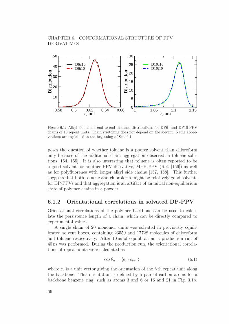
CHAPTER 6. CONFORMATIONAL STRUCTURE OF PPVDERIVATIVES
0.58 0.6 0.62 0.64 0.66r, nm
10
20
30
40
50
Dis
trib
utio
n
D6c10D6t10
1 1.05 1.1 1.15r, nm
0
5
10
15
20
25
30
Dis
trib
utio
n
D10c10D10t10
Figure 6.1: Alkyl side chain end-to-end distance distributions for DP6- and DP10-PPVchains of 10 repeat units. Chain stretching does not depend on the solvent. Name abbre-viations are explained in the beginning of Sec. 6.1
poses the question of whether toluene is a poorer solvent than chloroformonly because of the additional chain aggregation observed in toluene solu-tions [154, 155]. It is also interesting that toluene is often reported to bea good solvent for another PPV derivative, MEH-PPV (Ref. [156]) as wellas for polyfluorenes with longer alkyl side chains [157, 158]. This furthersuggests that both toluene and chloroform might be relatively good solventsfor DP-PPVs and that aggregation is an artifact of an initial non-equilibriumstate of polymer chains in a powder.
6.1.2 Orientational correlations in solvated DP-PPV
Orientational correlations of the polymer backbone can be used to calcu-late the persistence length of a chain, which can be directly compared toexperimental values.
A single chain of 20 monomer units was solvated in previously equili-brated solvent boxes, containing 23550 and 17728 molecules of chloroformand toluene respectively. After 10 ns of equilibration, a production run of40 ns was performed. During the production run, the orientational correla-tions of repeat units were calculated as
cos θn = 〈ei · ei+n〉 , (6.1)
where ei is a unit vector giving the orientation of the i-th repeat unit alongthe backbone. This orientation is defined by a pair of carbon atoms for abackbone benzene ring, such as atoms 3 and 6 or 16 and 21 in Fig. 3.1b.
66Rev. 117(e1a68f80ce2b) from 2011-03-08

6.1. ATOMISTIC MOLECULAR DYNAMICS
0 5 10 15 20n, monomer units
0.4
0.6
0.8
1
cos θ
n
D6c20D10c20D6t20D10t20
(a) (b)
Figure 6.2: (a) Orientational correlations for 20 repeat unit chains of DP6- and DP10-PPV in chloroform and toluene. 40 ns run, average of 20000 configurations. (b) Typicalconformation of a DP10-PPV chain in chloroform.
〈· · · 〉 denotes the time average and the average over all pairs, i, i + n, alongthe chain. The persistence length, lp, can be estimated as log(cos θn) ∝−nl/lp, where l is the length of the repeat unit. Note, that this is onlypossible if correlations decay exponentially, which might not necessarily bethe case [159, 160, 161].
Orientational correlations for different solvents and different side-chainlengths are shown in Fig. 6.2a. It is clear that the backbone is quite rigid(see also Fig. 6.2b, where a typical conformation of a DP10-PPV chain inchloroform is shown). Moreover, within available accuracy, the decay of thecorrelation function does not depend on the side-chain length or solvent. Afit yields a rough estimate of the persistence length, lp ∼ 17−25 A. Improvedstatistical averages are needed for more accurate estimates of lp, which can beobtained by using solvent-free coarse-grained models, as described in Sec. 6.2.
6.1.3 Planarity and tacticity of solvated DP-PPV
To facilitate charge transport along a conjugated chain, planarity of thebackbone is required [162]. In principle, conjugation already enforces a planarbackbone conformation. However, non-bonded (Coulomb and van der Waals)contributions can favor twists in the backbone. Here, we study how thechemical structure of a repeat unit, in particular the side chain groups, affectsthe planarity and tacticity of the backbone.
A PPV repeat unit has two dihedral angles which control its planarity,as depicted in the inset of Fig. 6.3a. In Fig. 3.2a the dihedral potential oftrans-stilbene, corresponding to these angles is shown. It has two minimaseparated by a barrier significantly higher than kBT . Since both minima arerather shallow, thermal fluctuations can easily lead to a 45 degree twist in
Rev. 117(e1a68f80ce2b) from 2011-03-0867

CHAPTER 6. CONFORMATIONAL STRUCTURE OF PPVDERIVATIVES
-180 -90 0 90 180φ, deg
Dis
trib
utio
n
φ1
φ2
-180 -90 0 90 180φ, deg
Dis
trib
utio
n
φ1
φ2
-180 -90 0 90 180φ, deg
Dis
trib
utio
n φ1
φ2
-180 -90 0 90 180φ, deg
Dis
trib
utio
n φ1
φ2
φ2, DP10
n
n
C6H13
C6H13
n
C6H13
C6H13
n
(b)
(d)
(a)
(c)
φ1
φ2
φ1
φ2
φ1
φ2
φ1
φ2
Figure 6.3: Distributions of dihedral angles controlling planarity of the PPV unit. (a)Bare PPV, without the side chains and phenyl rings. (b) Phenyl rings only. (c) Sidechains only. (d) DP6-PPV. All results stem from a single chain in vacuum. Insets depictthe chemical structure of the corresponding compounds.
the backbone, breaking the conjugation.
To study the effect of varying side chains on the dihedral distributions,we simulated three model systems, all based on a DP6-PPV trimer. The firstone, referred to as a “bare backbone” system, had both alkyl side chains andphenyl rings (not belonging to the backbone) substituted with hydrogens.The second system did not have aliphatic side chains, while the last systemhad the non-bonded interactions of the phenyl rings not belonging to thebackbone switched off.
The distributions of the dihedral angles for these three cases are shownin Fig. 6.3. The distributions for a backbone without any side groups,Fig. 6.3a, are rather broad with the maxima located at 0 and ±180 deg.Due to the symmetry of the “bare backbone” PPV, both distributions are
68Rev. 117(e1a68f80ce2b) from 2011-03-08

6.1. ATOMISTIC MOLECULAR DYNAMICS
0 2 4 6 8 10n, monomer units
-0.5
0
0.5
1co
s θn
D6c20D10c20D6t20D10t20
Figure 6.4: Orientational correlations of neighboring monomer units. Correlation functionsshow that DP-PPV polymers are syndiotactic.
identical and probabilities of finding the system with angles of 0 deg and±180 deg are the same. The distributions became asymmetric for the sys-tems with the alkyl side chains, as shown in Fig. 6.3c. Here, one of thedihedral angles samples conformations around 0 deg and the other those ofaround 180 deg. This reflects the fact that the alkyl side chains repel eachother and are attached in an asymmetric way with respect to the two dihe-drals. Hence, the symmetry of the distributions with respect to the angles isbroken. If instead, only the phenyl rings are attached, the cis conformationbecomes improbable, as can be seen in Fig. 6.3b. In this case, the φ = 0 degconformation is more preferable than the φ = ±180 deg one. Both effects addup in the distributions of DP6-PPV, which are shown in Fig. 6.3d. Here, theheights of the distributions of the dihedral angles φ1 and φ2 are different atφ = 0 deg, which is due to alkyl side chains. Additionally, conformationswith φ = ±180 deg are strongly suppressed due to the presence of the phenylrings. For the DP10-PPV derivative, the situation is qualitatively similar.Namely, longer alkyl side chains lead to an even broader distribution of thedihedral angle φ2.
The final issue we would like to address here is the tacticity of a DP-PPVpolymer chain. It is important for choosing an appropriate mapping for acoarse-grained model, as discussed in Sec. 6.2. By analyzing the distributionsof the backbone dihedral angles, we have concluded that the presence of thephenyl side groups leads to chain conformations with opposite orientationsof alkyl side chains of neighboring repeat units, i.e. DP-PPV is a syndio-
Rev. 117(e1a68f80ce2b) from 2011-03-0869

CHAPTER 6. CONFORMATIONAL STRUCTURE OF PPVDERIVATIVES
0.5 1 1.5 2r, nm
0
0.2
0.4
0.6
0.8
1
RD
FDP6-PPVDP10-PPV
Figure 6.5: Intermolecular radial distribution function for phenyl rings in the melt ofDP-PPV oligomers.
tactic polymer. In order to see the effect of solvent and side chain lengthon correlations of monomer orientations, we calculated the correlation func-tion of a cross product of vectors connecting the atoms 2-4 and 18-19 (seeFig. 3.1b for atom designations). This cross-product, which is a measure of achain deviation from planarity, is shown in Fig. 6.4. Again, within availableaccuracy, our model cannot differentiate between toluene and chloroform orhexyl and decyl side chains.
6.1.4 DP-PPV melt
An interesting observation made on the basis of WAXS experiments is that,in a powder, DP6-PPV forms a π−π complex but DP10-PPV does not [154].This conclusion was made by analyzing WAXS profiles, which have a sharpmaximum at 3 A in the case of DP6-PPV, and ascribed to the distance be-tween the π-stacked phenyl rings. This maximum was absent in the DP10-PPV powder. The difference in ring packing was explained in terms of thebulkier side chains of DP10-PPV as compared to those of DP6-PPV.
The radial distribution function of the centers of mass of the phenyl ringsis shown in Fig. 6.5. As one can see, it is practically identical for the meltsof DP6- and DP10 oligomers. Hence, in a melt of oligomers, the averagedistance between phenyl rings is not sensitive to the length of side chains.Of course, the melt morphology might differ from the non-equilibrium semi-crystalline morphology of a polymer powder. Nevertheless, some π − π com-
70Rev. 117(e1a68f80ce2b) from 2011-03-08

6.2. A COARSE-GRAINED MODEL FOR DP10-PPV
plexes should also appear in the melt and their amount and the π−π distanceshould depend on the length of the side chains. Since this is not the case,atomistic models hint that the absence of π − π complexes in DP10-PPVpowder is due to the non-equilibrium state of the polymer.
Another interesting experimental observation is the crystallization of poly-mer backbones upon annealing of a spin-coated film. Crystallization leads toa significantly more pronounced X-ray diffraction peak at a π − π stackingdistance, which is reported to be 3 A [154]. Fig. 6.5 indeed shows that afterannealing, the first maximum of the radial distribution function is located ata separation of about 6 A. In fact, this separation corresponds to the mini-mum of the potential of mean force of two coarse-grained beads in vacuumas shown in Fig. 6.6c. It obviously overestimates the π − π staking distancesince the system is in a non-equilibrium state. However, the reported inexperiments separation of 3 A is too small and already in the range of therepulsion of two cofacially aligned repeat units, even without any side chainsattached to them [163].
6.1.5 Atomistic molecular dynamics: summary
In summary, the all-atom molecular dynamics simulations give similar andoften identical results for DP6-PPV and DP10-PPV in both solvents, i.e.we could not capture the difference in solvent quality. Longer side chains ofDP10-PPV as compared to DP6-PPV do neither affect phenyl ring packingin a melt nor dimer-dimer interactions in vacuum and solution, as will beshown in Sec. 6.2.2. Hence, experimentally observed fractal aggregates ofDP6-PPV in chloroform or disk-like aggregates of DP10-PPV in toluene, cannot be rationalized by atomistic models. However, reasonable agreement withexperiments can be expected for a dilute solution of DP10-PPV in chloroform,since in this case no aggregation occurs. In the following section, we willdevelop a solvent-free coarse-grained model of DP10-PPV in chloroform.
6.2 A coarse-grained model for DP10-PPV
As has already been pointed out in Sec. 6.1, atomistic simulations do notallow an accurate estimation of polymer persistence lengths. Moreover, forstudying dilute solutions of DP-PPV in chloroform or toluene, systems withmany chains have to be simulated at different concentrations, which is prac-tically impossible at the atomistic level of detail.
In this section, we develop a solvent-free coarse-grained model for DP10-PPV in chloroform and use it to calculate persistence length and static struc-
Rev. 117(e1a68f80ce2b) from 2011-03-0871

CHAPTER 6. CONFORMATIONAL STRUCTURE OF PPVDERIVATIVES
ture factor as a function of polymer concentration. Both are then comparedto the experiment.
To represent a DP-PPV chain on a coarse-grained level, we mapped twomonomer units onto one spherical bead, as illustrated in Fig. 6.6d. Two (in-stead of one) monomer units per bead were used because PPV is syndiotactic(see Sec. 6.1.3). Hence, a coarse-grained representation with one bead perrepeat unit is problematic, since repeat units are asymmetric and cannot beproperly described by spherically-symmetric pair potentials.
6.2.1 Bonded interaction potentials
The next step of systematic coarse-graining is to determine bonded and non-bonded potentials. Here, only two types of bonded interactions, are included,namely a bond stretching potential between two successive beads and anangle potential between three successive beads. Dihedral potentials are notincluded as DP-PPVs have a rigid backbone which can be accounted for bythe angular potential only. To parametrize the bonded potential, an approachwas used in which bonded interactions are obtained from canonical samplingof a single chain in a solvent. The potentials are then obtain by simpleBoltzmann inversion. Specifically, a single chain of 20 repeat units of DP10-PPV in chloroform was used. Resulting distributions for both atomistic andcoarse-grained sampling are in perfect agreement with each other as shownin Fig. 6.6a,b.
6.2.2 Non-bonded interaction potentials
For non-bonded coarse-grained interaction potentials we used the potentialof mean force (PMF) between dimers. In this case, PMF is a free energyof a dimer pair at a specific separation, averaged over all possible mutualorientations of the dimers, as well as positions and orientations of solventmolecules, if present.
Note that non-bonded potentials can not be obtained by IBI or IMC inthis case, because it is practically impossible to obtain accurate RDFs fora dilute solution. Hence, to simulate dilute solutions, we used PMF in asolvent as a non-bonded potential.
PMFs for both DP6- and DP10-PPV were calculated in vacuum andsolvents, using configurational sampling [117]. Results are shown in Fig. 6.6c.In vacuum, PMF predicts strong dimer-dimer attraction, which might leadto polymer aggregation. On the other hand, fully solvated dimers have apurely repulsive interaction. Calculated PMFs, and hence the coarse-grainednon-bonded potentials, correspond to infinitely dilute systems. In practice,
72Rev. 117(e1a68f80ce2b) from 2011-03-08

6.2. A COARSE-GRAINED MODEL FOR DP10-PPV
1.15 1.2 1.25 1.3 1.35bond length, nm
Dis
trib
utio
n
atomisticCG
100 120 140 160 180angle, deg
Dis
trib
utio
n
0 0.5 1 1.5 2r, nm
-50
0
50
100
150
PM
F, k
J/m
ol
DP6-PPVDP10-PPVDP6-PPV/chloroformDP10-PPV/chloroform
C6H13
C6H13
C6H13
C6H13
(a) (b)
(d)(c)
Figure 6.6: Coarse-grained bond (a) and angle (b) distribution functions as obtained fromatomistic and coarse-grained MD simulations. A chain of 20 monomers of DP10-PPV inchloroform was used for sampling. Potentials are obtained by Boltzmann-inverting thedistributions. (c) Dimer-dimer potential of mean force (PMF), calculated using configu-rational sampling. PMFs in toluene are identical to those in chloroform. (d) Mappingscheme for the coarse-grained model. When determining centers of coarse-grained beads,no alkyl side chains were included.
Rev. 117(e1a68f80ce2b) from 2011-03-0873

CHAPTER 6. CONFORMATIONAL STRUCTURE OF PPVDERIVATIVES
0.1 1
q, nm-1
1
10
S (q
)
0.1 wt%0.5 wt%1.0 wt%1/q
0 10 20 30 40 50 60 70l, nm
0.1
1
cos
θ n
0.1 wt%0.5 wt%1.0 wt%atomistic
Figure 6.7: Backbone orientational correlations for DP10-PPV/chloroform solutions fordifferent concentrations. Results from atomistic simulations are shown for comparison.
potentials might depend on polymer concentration. However, for systems ofup to 1 wt% this dependence may be neglected. In addition, PMFs in bothsolvents are purely repulsive and only ensure that coarse-grained beads havea certain excluded volume. Hence, simulation results should not be sensitiveto the actual functional form of the potential.
6.2.3 Coarse-grained simulations of DP10-PPV in chlo-
roform
Experimentally, three different concentrations of DP10-PPV/chloroform so-lutions were studied: 0.1, 0.5, and 1.0 wt% [155]. We used the same con-centrations as in experiment and compared simulated and measured polymerpersistence lengths and static structure factors.
The systems consisted of 512 polymer chains, 50 beads each, which corre-sponds to 100 monomer units. NVT simulations were performed for 16 ns and800 frames were used to compute static structure factors. All coarse-grainedsimulations were performed at 300 K.
The calculated structure factors, S(q), for different polymer concentra-tions are shown in Fig. 6.7a. One can see that S(q) scales as q−1 in the high-qregion, irrespective of concentration. This is due to the rod-like nature ofthe segments constituting the DP10-PPV chains [164]. In the low-q region,intensity decreases with an increase of concentration. This dependence is de-termined by the dynamic network structure formed by the interchain overlapin the semidilute solution [165].
74Rev. 117(e1a68f80ce2b) from 2011-03-08

6.3. DISCUSSION
concentration, wt% lp, nm0.1 6.40.5 13.31.0 23.0MD 25.0 ± 0.5
Table 6.1: Estimations of persistence length from SANS experiments [155] and coarse-grained MD simulations. MD predicts the same value for all three concentrations.
Backbone orientational correlations are shown in Fig. 6.7b. These cor-relations decay exponentially on the accessible length scale, which allowsestimations of polymer persistence lengths as discussed in Sec. 6.1.2. Thecalculated persistence length of 25± 0.5 nm is independent of concentration,contrary to experimental findings summarized in Table. 6.1. In experiments,persistence length was extracted by fitting SANS profiles to the wormlikechain model with excluded-volume interactions [155].
The increase with concentration can be attributed to chain aggregation.At low concentrations, chains do not interact and there is no aggregation.Upon increasing the concentration, aggregates start to form and inside thoseaggregates, chains become locally more extended which increases their per-sistence length. Our model can not capture this effect since we have repulsiveeffective potentials. Hence, no driving force is present, which might lead topolymer aggregation at higher concentrations.
6.3 Discussion
Our simulations confirm experimental evidence that both chloroform andtoluene are good solvents for DP-PPVs. This is based on alkyl side chainstretching, backbone orientational correlations, and the potential of meanforce (PMF) of DP-PPV dimers in the solvent. However, the experimentallyreported quantitative results on solvent quality could not be reproduced.
Atomistic simulations show that the difference in side chain lengths ofDP6- and DP10-PPV does not affect chain packing in a melt of oligomers,which is practically identical for both DP6- and DP10-PPV. Interdimer in-teractions in solutions are also not strongly affected by the difference in sidechain lengths, namely the interdimer PMF is repulsive for both DP6- andDP10-PPV. This seems to contradict experimental observations which findthat DP6-PPV forms aggregates in solution, whereas DP10-PPV does not.A possible reason for this inconsistency might be that in experiments, thesystem is in its non-equilibrium state, since powder, in which polymer chains
Rev. 117(e1a68f80ce2b) from 2011-03-0875

CHAPTER 6. CONFORMATIONAL STRUCTURE OF PPVDERIVATIVES
are semicrystalline, was used to prepare the solution. Furthermore, as can befound in Ref. [155], DP10-PPV does aggregate in toluene solutions. However,if the system is heated up to 85◦C and then cooled down, these aggregatestend to disappear. Recently, an alternative explanation of anomalous aggre-gation in good polymer solutions has been proposed [166]. This mechanism isapplicable to stereoregular polymers, such as DP-PPV, which indeed shownto be syndiotactic in our simulations.
Coarse-grained simulations show that, for very low polymer concentra-tions (0.1 – 1.0 wt%), polymer persistence length does not depend on polymerconcentration. This again contradicts the experimental picture, where theincrease of persistence length at 1.0 wt% is rationalized as chain aggregation.The overestimation of the polymer persistence length in simulations mightbe due to the presence of tetrahedral chemical defects in real samples [167].In these defects conjugated carbon-carbon bonds are replaced by tetrahedralones. They divide polymer chains into structurally identifiable quasi-straightsegments and reduce orientational correlations, which leads to a decrease inpersistence length.
Finally, we should mention that various approximations in our simulationmodels might also lead to a disagreement between experiments and simula-tions. For example, as experimental data for conjugated compounds is rathersparse, force-field validation becomes problematic. To this end, although wehave reproduced density, melting temperature, and crystal structure of stil-bene, this is no guaranty that thermodynamic properties such as solvationfree energy are correctly reproduced. Other issue can be limited accessiblelength- and time-scales. Explicit solvents and rather stiff polymer backbonesprohibit the study of global chain conformations and chain self-interactionsvia atomistic molecular dynamics. Solvent-free coarse-grained models are ca-pable of simulating bigger boxes on longer timescales. These, however, leadto additional approximations, which cannot be easily controlled.
76Rev. 117(e1a68f80ce2b) from 2011-03-08

Chapter 7
Morphology and charge
transport in amorphous Alq3
7.1 Introduction
Tris(8-hydroxyquinoline)aluminium (Alq3, Fig. 7.1a) is a commonly used or-ganic semiconductor with a higher electron than hole mobility [168]. Thefirst organic light emitting diodes were made with Alq3 and since then it hasplayed the role of a “guinea pig” compound in organic electronics [6]. Thedistinctive properties of Alq3 are its green light emission and good electronmobility. It is also used as a host material for emissive dopants of loweremission energy.
In organic semiconductors both emission and charge transport proper-ties are extremely sensitive to the material morphology. The latter can becontrolled by an appropriate processing or compound derivatization. Un-derstanding the link between the structure, morphology, and macroscopicproperties of organic compounds is the first step towards their rational de-
N
O
Al
3
ba c
Oa
Na
Al
ObCa1
Ca2
Oc
Ca3
Figure 7.1: (a) Chemical structure of tris-8(hydroxyquinoline aluminium) (Alq3). (b)Meridional isomer of Alq3. (c) Atom labeling used to show the distributions of angles anddihedrals. Largest linear dimension of the molecule is ≈ 1 nm.
77

CHAPTER 7. MORPHOLOGY AND CHARGE TRANSPORT INAMORPHOUS ALQ3
sign [74].
In spite of numerous experimental studies, there were only two theoreti-cal/computational attempts to relate the morphology of amorphous Alq3 toits charge carrier mobility [169, 68]. In Ref. [169] the rigid-body approxima-tion for the intramolecular structure was used together with the non-bondedparameters taken from the Dreiding force field. Approximate force constantsfor bonded parameters and non-bonded parameters of the Williams 99 forcefield were used in Ref. [68]. In both cases neither the force field nor the gen-erated amorphous morphology was checked against the experimental data,and its characterization was reduced to pair correlation functions and densityat ambient conditions.
In this chapter, we first derive bonded parameters for the Alq3 moleculeusing first-principles potential energy scans. Second, we compare OPLS andWilliams 99 force fields to each other as well as to the available experimen-tal data. We further assess how the morphological difference, resulting fromusing different force field parameters, affects charge transport. Finally, wedemonstrate that the dipolar energetic disorder (see Sec. 2.4) must be takeninto account in order to describe charge dynamics correctly. We analyze theinfluence of energetic disorder in terms of pathways and occupation proba-bilities and show that the spatial correlations of site energies must be takeninto account in order to reproduce Poole-Frenkel behavior (see Sec. 2.6) ofthe charge carrier mobility.
7.2 Force-field parameters
As already explained in Chapter 3, force field refinement can be split intoseveral steps: (i) determination of partial charges; (ii) calculation of theforce field parameters for the bonded interactions; (iii) parameterization ofthe non-bonded interactions.
Partial charges were obtained from electrostatic potentials using a gridbased method (CHELPG) [93] after the geometry optimization of a merid-ional Alq3 isomer1 in vacuum (see Fig. 7.1b) using the B3LYP functionaland 6-311g(d) basis set. The corresponding molecular dipole moment wasd = 4.4 D. The DFT results were checked against MP2 calculations with6-311g(d) basis set, for which the dipole moment is 5.4 D. No substantialdifferences were noticed with either B3LYP or MP2 charges used. All results
1Another isomer which is commonly observed in the octahedral complexes of the typeMN3O3, where M is a trivalent metal, namely the facial isomer, has not been experimen-tally identified for amorphous Alq3 [170].
78Rev. 117(e1a68f80ce2b) from 2011-03-08
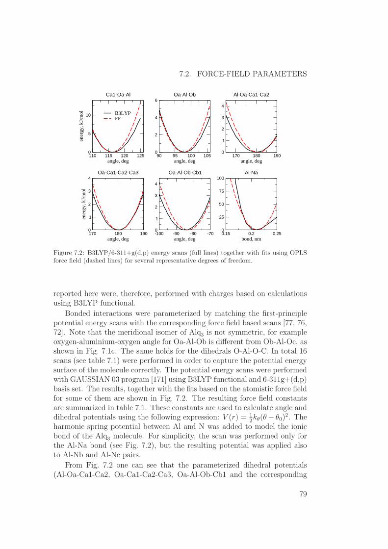
7.2. FORCE-FIELD PARAMETERS
110 115 120 125angle, deg
0
5
10
ener
gy, k
J/m
ol
B3LYPFF
Ca1-Oa-Al
90 95 100 105angle, deg
0
2
4
6Oa-Al-Ob
170 180 190angle, deg
0
1
2
3
4
Al-Oa-Ca1-Ca2
170 180 190angle, deg
0
1
2
3
4
ener
gy, k
J/m
ol
Oa-Ca1-Ca2-Ca3
-100 -90 -80 -70angle, deg
0
1
2
3
4
Oa-Al-Ob-Cb1
0.15 0.2 0.25bond, nm
0
25
50
75
100Al-Na
Figure 7.2: B3LYP/6-311+g(d,p) energy scans (full lines) together with fits using OPLSforce field (dashed lines) for several representative degrees of freedom.
reported here were, therefore, performed with charges based on calculationsusing B3LYP functional.
Bonded interactions were parameterized by matching the first-principlepotential energy scans with the corresponding force field based scans [77, 76,72]. Note that the meridional isomer of Alq3 is not symmetric, for exampleoxygen-aluminium-oxygen angle for Oa-Al-Ob is different from Ob-Al-Oc, asshown in Fig. 7.1c. The same holds for the dihedrals O-Al-O-C. In total 16scans (see table 7.1) were performed in order to capture the potential energysurface of the molecule correctly. The potential energy scans were performedwith GAUSSIAN 03 program [171] using B3LYP functional and 6-311g+(d,p)basis set. The results, together with the fits based on the atomistic force fieldfor some of them are shown in Fig. 7.2. The resulting force field constantsare summarized in table 7.1. These constants are used to calculate angle anddihedral potentials using the following expression: V (r) = 1
2kθ(θ− θ0)
2. Theharmonic spring potential between Al and N was added to model the ionicbond of the Alq3 molecule. For simplicity, the scan was performed only forthe Al-Na bond (see Fig. 7.2), but the resulting potential was applied alsoto Al-Nb and Al-Nc pairs.
From Fig. 7.2 one can see that the parameterized dihedral potentials(Al-Oa-Ca1-Ca2, Oa-Ca1-Ca2-Ca3, Oa-Al-Ob-Cb1 and the corresponding
Rev. 117(e1a68f80ce2b) from 2011-03-0879

CHAPTER 7. MORPHOLOGY AND CHARGE TRANSPORT INAMORPHOUS ALQ3
Degree of freedom Constant kθ, kJmol−1rad−2
Ca1-Oa-Al 600Cb1-Ob-Al 500Cc1-Oc-Al 400Oa-Al-Ob 320Ob-Al-Oc 200Oc-Al-Oa 420
Al-Oa-Ca1-Ca2 55Al-Ob-Cb1-Cb2 50Al-Oc-Cc1-Cc2 50
Oa-Ca1-Ca2-Ca3 200Ob-Cb1-Cb2-Cb3 200Oc-Cc1-Cc2-Cc3 200Oa-Al-Ob-Cb1 50Oa-Al-Oc-Cc1 30Oc-Al-Oa-Ca1 20
bond Al-Na 62459, kJmol−1nm−2
Table 7.1: Bonded interactions parameters, obtained using the fitting described in thetext.
0.4 0.6 0.8r, nm
-0.8
-0.6
-0.4
-0.2
0
0.2
Ene
rgy,
kJ
/ mol
O OPLS-AA
O Williams 99
N OPLS-AA
N Williams 99
C OPLS-AA
C Williams 99
H OPLS-AA
H Williams 99
Figure 7.3: Non-bonded O-O, N-N, C-C and H-H interactions for the OPLS and Williams99 force fields. OPLS force field has bigger binding energies for N and O. Note thatinteractions between different atom types, e. g. N and O are calculated using the OPLSmixing rules [80].
80Rev. 117(e1a68f80ce2b) from 2011-03-08

7.2. FORCE-FIELD PARAMETERS
atom OPLS W99 fittedσ, nm ǫ, kJ/mol σ, nm ǫ, kJ/mol
Carbon 0.355 0.29288 0.348873 0.263802Hydrogen 0.242 0.12552 0.277899 0.107032Oxygen 0.296 0.87864 0.305762 0.428992Nitrogen 0.325 0.71128 0.327197 0.282361
Table 7.2: Non-bonded parameters of OPLS and Williams 99 force fields used in oursimulations. For Williams 99, effective Lennard-Jones parameters obtained by fittingBuckingham potential are given (W99 fitted).
potentials for the other ligands) are quite soft. This is consistent with thefact that the Al-N bonds can be characterized as ionic rather than covalent.Consequently the angle values we used for parametrization do not cover thewhole region of the dihedral angles, which can be sampled at 300K during theMD simulation. However, the extension of the scans beyond those values isproblematic, because at large deviations from an equilibrium geometry van-der-Waals non-bonded interactions between ligands start to play a significantrole, which can not be correctly described by the density functional theory.Instead of extending the region of the scans we verified that the potentialof mean force (PMF) of the dihedral distributions for amorphous morphol-ogy (see below) reproduces the scans obtained from the DFT. Additionallywe compared the distributions of the representative degrees of freedom ob-tained from the force field simulations with the results of ab-initio moleculardynamics (see Appendix C).
The Lennard-Jones parameters for all atoms were taken either from theOPLS [80] or Williams 99 [172] force field. Note that the OPLS force fielduses the Lennard-Jones (12-6) potential while Williams 99 is based on theBuckingham potential, V (r) = A exp(−Br)− C
r6 . The only difference betweenthe two functional forms is the repulsive part, and one can refit the Buck-ingham potential with the Lennard-Jones one, which also results in a speedup of about 2.5. The non-bonded force field parameters are summarized intable 7.2.
The two force fields are compared in Fig. 7.3. One can see that thebinding energy for nitrogen and oxygen is much bigger for the OPLS thanWilliams 99 force field and should result in a more dense molecular packing.Aromatic carbons have similar parameters.
To verify the derived force field, we studied amorphous morphologies ofAlq3. The systems were prepared by first arranging the molecules on a cubiclattice with the density adjusted in order to avoid molecular overlaps and
Rev. 117(e1a68f80ce2b) from 2011-03-0881

CHAPTER 7. MORPHOLOGY AND CHARGE TRANSPORT INAMORPHOUS ALQ3
10 100 1000Time, ps
0.01
1
100
MS
D, n
m2
300K500K700K
10 100 1000Time, ps
0.2
0.4
0.6
0.8
1
C (
t)
a b
Figure 7.4: (a) Log-log plot of the mean squared displacement of the center of mass ofAlq3 molecules for a set of temperatures. (b) Correlation function of a Alq3 molecularorientation, defined as a normal vector to the plane containing the three oxygens. Solidline: OPLS force field. Dashed line: Williams 99 force field.
then equilibrating at 700 K in an NPT ensemble, with a stochastic velocityrescaling thermostat [84] and the Berendsen barostat [81], and finally coolingdown to room temperature. All simulations were performed using the GRO-MACS package [173]. Note that two alternative ways of system preparationwere reported previously. The first one, based on the Monte Carlo algorithmmimicking the film deposition process [169], is limited to rigid molecules. Thesecond, based on a compression of a simulation box of a randomly positionedmolecules at low density [68] is sensitive to the compression rate and oftenresults in voids.
To monitor the equilibration dynamics we calculated relaxation timesfrom the correlation functions for the rotational molecular motion as well asmean squared displacement (MSD) of their translational motion. Both areshown in figs. 7.4a,b for a set of temperatures. Figs. 7.4a,b indicate thatsystems can be equilibrated at 700 K after about 1 ns run, which is the timeneeded for the center of mass of a molecule to travel a distance comparable toits size. In addition, after this period of time molecular orientations are fullyuncorrelated. At lower temperatures significantly longer runs are required.Therefore, to prepare large-scale morphologies, we annealed our systems at700 K and then cooled them down to the desired temperature with the coolingrate 0.2 ps/K.
To compare molecular packing in amorphous morphologies generated with
82Rev. 117(e1a68f80ce2b) from 2011-03-08

7.2. FORCE-FIELD PARAMETERS
0 1 2r, nm
0
0.5
1
1.5
gA
l-A
l (r)
Williams 99 (Nagata et al)Williams 99, NVTOPLS, NPTWilliams 99, NPT
0 1 2r, nm
0
0.5
1
1.5
gC
-C (
r)a b
Figure 7.5: (a) Al-Al and (b) C-C radial distribution functions for OPLS and Williams99 force fields obtained after equilibration in NPT ensemble at 300K. For comparison,results of NVT simulations (note different density) of Ref. [68] are also shown.
the OPLS and Williams 99 force fields, we calculated two radial distributionfunctions, which are shown in figs. 7.5a,b. One can see that different bondedparameters used in this work and Ref. [68] do not significantly change theradial distribution function. Note, however, that these two curves are com-pared for a fixed density of Ref. [68]. On the other hand, if the systemsare equilibrated in the NPT ensemble (which results in higher density), ra-dial distribution functions have a more pronounced structure (better resolvedpeaks) for both OPLS- and Williams 99 based force fields. The differencebetween the two force fields is small, however. One can conclude that theradial distribution function is not an optimal measure of molecular packing,due to its limited sensitivity.
Other two macroscopic quantities are known from experiments: the den-sity of amorphous Alq3 at ambient conditions and its glass transition temper-ature [174, 176]. The density versus temperature plot is shown in Fig. 7.6a.One can see that the system density strongly depends on the Lennard-Jonesparameters (and does not change if we substitute ESP charges derived fromthe B3LYP- with MP2-based electron density). One can see that OPLSpredicts a higher density than Williams 99 and it is also closer to the experi-mental values.2 Densities used in previous simulation studies by Y. Nagata et
2Note, that we intentionally did not try to reproduce the experimental density of theamorphous Alq3 from Ref. [174] exactly. In Sec. 7.3 it is demonstrated, that the differencein density does not influence charge transport properties significantly.
Rev. 117(e1a68f80ce2b) from 2011-03-0883

CHAPTER 7. MORPHOLOGY AND CHARGE TRANSPORT INAMORPHOUS ALQ3
300 400 500 600 700temperature, K
800
1000
1200
1400
1600
dens
ity, g
/ cm
3
alpha phase (exp)amorphous phase (exp)OPLSWilliams 99Y. Nagata et al. (sim)J. Kwiatkowski et al. (sim)
300 350 400 450 500 550temperature, K
300
320
340
360
380
400
box
volu
me,
nm3
OPLSWilliams 99
Tg = 425 K
Tg = 455 K
Figure 7.6: (a) Density versus temperature for OPLS and Williams 99-based force fieldstogether with experimental results: amorphous density is taken from [174], alpha-phasedensity is taken from [175]. Density used in previous studies by Y. Nagata et al. [68]and J. Kwiatkowski et. al [169] are also shown. (b) Volume of the simulation box versustemperature for amorphous Alq3. Intersection of two fitting lines is used to predict glasstransition temperature, which is estimated to be 455 K for OPLS and 425 K for Williams99 force field. Experimental value is 448 K [176].
al. [68] (density is mentioned in the paper) and J. Kwiatkowski et. al. [169](density is calculated using number of molecules and the box size specifiedin the paper) are also shown for comparison.
To estimate the glass transition temperature we calculated the volumeof the simulation box as a function of temperature. These dependencies areshown in Fig. 7.6b. By performing a linear fit of the low and high temperatureparts of the curves one can find the intersection point which provides anestimate of the glass transition temperature [177]. The latter is estimatedto be 455 K for OPLS and 425 K for Williams 99 force field. Experimentalvalue is 448 K [176], which is again closer to the OPLS-predicted value.
Summarizing, we can conclude that the OPLS-based force field performsbetter for the amorphous Alq3 films than the Williams 99 force field bypredicting closer to the experimental values of density and glass transitiontemperature.
84Rev. 117(e1a68f80ce2b) from 2011-03-08

7.3. RELATIONSHIP BETWEEN MORPHOLOGY AND CHARGETRANSPORT
7.3 Relationship between morphology and charge
transport
In this section we use the multiscale approach presented in Sec. 2.7 to sim-ulate charge dynamics in two different morphologies described above and tounderstand how the change in morphology influences charge carrier mobil-ity. For simplicity we ignore the energetic disorder in these considerations,but the more detailed analysis shows, that the conclusions drawn from thesimplified picture stay valid also if electrostatic contribution to the energeticdisorder is taken into account.
Within the Marcus theory under the assumption that energetic disorder isnegligible, charge transport is governed only by two parameters: the reorga-nization energy and the transfer integral (see Chapter 2). The reorganizationenergy λ was computed as discussed in Sec. 2.2 using B3LYP functional witha triple zeta split basis set, 6-311g+(d,p), using the GAUSSIAN 03 [171] pro-gram. The computed values for the reorganization energies are λh = 0.23 eVand λe = 0.28 eV. The transfer integrals J were computed using the inter-mediate neglect of differential overlap level of theory (ZINDO) as describedin Sec. 2.3. Molecular orbitals are calculated using the GAUSSIAN 98 pack-age [178]. Since the transfer integral is related to the molecular overlap, itis very sensitive to relative orientations and positions of the neighbors. Thecorresponding HOMO and LUMO orbitals are shown in Fig. 7.7a. Note thatZINDO predicts that the LUMO is localized on one of the arms, while DFTcalculations of Ref. [169], as well as our MP2 calculations (see Fig. 7.7a) showthat the LUMO is delocalized over two of them. Different localization mayaffect charge dynamics, especially the ratio between the hole and electronmobilities, since the delocalization leads to the less pronounced dependenceof transfer integrals on the mutual orientation of neighbors.
However, here we do not aim at a quantitative description of charge dy-namics, since we anyway ignore several essential ingredients required for itscorrect description, such as energetic disorder as well as electrostatic and po-larization contributions to it. Our main goal is to understand how the changeof morphology influences charge carrier mobility.3 Hence, here we analyzeonly the hole transport, since all three first-principles methods predict similarlocalization pattern for HOMO.
For charge dynamics simulations amorphous morphologies containing 4096molecules in a cubic box were prepared using both OPLS and Williams 99force fields and the aforementioned equilibration procedure. The size of the
3Of course one has to keep in mind that the energetic disorder might also be sensitiveto the underlying morphology.
Rev. 117(e1a68f80ce2b) from 2011-03-0885

CHAPTER 7. MORPHOLOGY AND CHARGE TRANSPORT INAMORPHOUS ALQ3
10 12 14
log (total hopping rate / s-1
)
0
0.1
0.2
0.3
0.4
Prob
abili
ty D
ensi
ty
OPLSW99
ZINDO MP2
LUMO
HOMO
a b
Figure 7.7: (a) HOMO and LUMO orbitals of a meridional isomer of Alq3 calculated withZINDO and Hartree-Fock (using MP2-optimized geometry) methods. (b) Probability dis-tribution of the total hopping rate away from the molecule for OPLS and Williams 99 forcefields. Only hole transport was considered. ZINDO orbitals were used for calculations.
cubic box was 13.4263 nm, the length of the KMC run was 10−5 sec, and themobilities were averaged over 10 starting points. A cutoff of 15 A was usedto calculate the hopping rates between neighboring molecules.
We first have a look at the probability distributions of the total hoppingrate away from a molecule:
ωtotali =
∑
j
ωij (7.1)
where the sum is taken over all neighbors of the molecule i.
The result is shown in Fig. 7.7b. One can notice that the distribution thatcorresponds to the OPLS force field is shifted to higher values of outgoinghopping rates compared to the Williams 99 force field. This is expected,since the OPLS force field predicts more dense molecular packing.
Charge carrier mobilities were calculated by monitoring the projectionof the charge velocity on the field direction. The simulations were done fora single charge diffusing in an external field through the configuration ofone molecular dynamics snapshot with periodic boundary conditions appliedin all directions. The mobility was calculated as µ = v/E, where v is theaveraged over a hundred different starting positions for every frame velocityof the charge carrier along the field E.
The calculated hole mobilities are µhOPLS = (3.7 ± 0.1) × 10−3 cm2V−1s−1
and µhW99 = (1.7 ± 0.1) × 10−3 cm2V−1s−1. Both values are several orders of
86Rev. 117(e1a68f80ce2b) from 2011-03-08

7.4. ROLE OF ENERGETIC DISORDER
magnitude higher than the experimentally measured ones: electron mobili-ties of amorphous Alq3 are of the order of 10−5 − 10−6 cm2V−1s−1 [168, 179]while hole mobilities are of the order of 10−8 cm2V−1s−1 [168]. The discrep-ancy between the experimental and calculated values is due to the fact thatwe ignore the energetic disorder, which can significantly influence resultingmobilities [169, 68]. The effect of energetic disorder is discussed in the nextsection.
To conclude, the difference in density and packing induced by differentforce field parameters does not significantly affect the charge dynamics, lead-ing to slightly higher mobilities in case of a more dense system (OPLS-basedmorphology).
7.4 Role of energetic disorder
Considerations of the Sec. 7.3 ignore energetic disorder. However, the dipolemoment of an Alq3 molecule is rather large (d = 4.4 D, see Sec. 7.2). Hence,dipolar disorder cannot be neglected (see Chapter 2). In this section we studythe influence of energetic disorder on charge dynamics in amorphous Alq3
by comparing carrier mobilities calculated with and without the disorder.Visualization of hopping site occupation probabilities and current filamentsfurther suggests the important role of energetic disorder.
7.4.1 Computational details
We assume that there are two contributions to the free energy difference∆Gij (see Eq. 2.9): one due to an externally applied electric field and theother one due to different electrostatic interactions of the excess charge withthe surrounding neutral molecules: ∆Gij = eEr + ∆Gel. The electrostaticcontribution, ∆Gel = Ei − Ej, is calculated classically as it is describedin Ref. [56] using CHELPG-fitted partial charges for a charged and neutralAlq3 molecule in the ground state obtained from DFT calculations using theB3LYP hybrid functional and the 6-311g(d) basis set. We denote the partialcharge of the atom a in the molecule i as qa
i if the molecule is neutral and asqai∗ if the molecule is charged. ∆Gel
ij is then given by [56]:
∆Gelij =
∑
c
∑
k 6=i
∑
n
qci∗qn
k
4πǫ0ǫrcn
−∑
c
∑
k 6=j
∑
n
qcj∗qn
k
4πǫ0ǫrcn
, (7.2)
with the permittivity of free space ǫ0 and a relative macroscopic dielectricconstant ǫ. The distance between two atoms is given by rcn. The first
Rev. 117(e1a68f80ce2b) from 2011-03-0887

CHAPTER 7. MORPHOLOGY AND CHARGE TRANSPORT INAMORPHOUS ALQ3
sum runs over all partial charges qci∗ of the initially charged molecule i that
interact with all partial charges qnk in all other k 6= i neutral molecules. It
represents the energy of the system if the molecule i is charged. Second termis the energy of the system when the molecule j is charged. This procedure isexact in the limit of an infinite system. We use no spherical cutoff but applythe nearest image convention, and have checked that this converges alreadyfor a few hundered molecules in the simulation box.
Polarization effects are treated phenomenologically by using a distance-dependent dielectric constant [180]:
ǫ = ǫ(rcn) = ǫ∞ − (ǫ∞ − 1)e−srcn(1 + srcn + 1/2s2r2cn). (7.3)
where ǫ∞ = 3.0 (experimental value) [181] and s = 0.3 A−1 [68]. Effectively,atoms that are close in space feel the unscreened Coulomb interaction withǫ = 1 which is then screened to the bulk value ǫ∞ at larger distances.
Charge dynamics is simulated using the kinetic Monte Carlo techniqueusing the (extended) VOTCA package [2]. We use periodic boundary condi-tions and calculate charge carrier mobility as
µ =〈vE〉E
(7.4)
where 〈vE〉 is the averaged projection of carrier velocity on the direction ofthe applied electric field E.
7.4.2 Poole-Frenkel behavior
Mobilities with and without disorder, for different values of an applied electricfield are shown in Fig. 7.8. One can see that taking energetic disorder intoaccount leads to significantly lower mobilities. More important, it resultsin the correct electric field dependence of the mobility: µ ∝ exp(βE1/2)which is known as a Poole-Frenkel behavior (see Chapter 2) and was observedexperimentally for amorphous Alq3 [168, 26, 179]. The distribution of siteenergies resulting from electrostatic interactions is shown on the inset ofFig. 7.8. It has a Gaussian shape with a standard deviation of σ = 0.14 eV.
Another important observation is that, when energetic disorder is takeninto account, charge carrier mobilities are system-size dependent. This in-dicates that charge transport becomes dispersive, as was discussed in Chap-ter 2. As a consequence, calculated dispersive mobilities disagree with theexperimental reference data that is obtained in the nondispersive regime (seeFig. 7.8). A way of extracting the absolute value of nondispersive mobilityfrom simulations of small systems is addressed in Chapter 8.
88Rev. 117(e1a68f80ce2b) from 2011-03-08

7.4. ROLE OF ENERGETIC DISORDER
1e-10
1e-09
1e-08
1e-07
1e-06
1e-05
0.0001
0.001
0.01
300 400 500 600 700 800 900 1000
mobility,
cm2/V
s
E1/2, (V/cm)1/2
0
1
2
3
-0.4 0 0.4
dis
trib
ution
energy, [eV]
no disorderwith disorder
TOF experiment
Figure 7.8: Hole mobility as a function of applied electric field of a system with 13824 Alq3
molecules with and without energetic disorder. Results of the time-of-flight experimentare taken from Ref. [26]. Inset shows the site energy distribution. It is Gaussian withσ = 0.14 eV.
7.4.3 Charge dynamics visualization
In the previous section it was shown that energetic disorder significantlyaffects charge dynamics. Taking energetic disorder into account lowers cal-culated mobilities and changes its electric field dependence. Here we visualizethe difference between the systems with and without disorder using chargecarrier pathways and site occupations.
Occupation probability of a hopping site is defined as a fraction of timea charge carrier spends on it. It is normalized in a sense that the sum of allthe occupation probabilities over all hopping sites is 1. Here we present theresults for an amorphous morphology of 512 Alq3 molecules.
Fig. 7.9 compares the distributions of occupation probabilities calculatedwith and without energetic disorder. When energetic disorder is ignored, thedistribution of occupation probabilities is narrow, since all probabilities areof the same order of magnitude. When energetic disorder is taken into ac-count, the distribution broadens, spanning several orders of magnitude. Thisis illustrated in the inset of Fig. 7.9, where hopping sites are shown with col-ored spheres. Each color corresponds to a particular order of magnitude ofthe occupation probability. The radius of a sphere is proportional to thelog10 of the occupation probability. When energetic disorder is ignored, allspheres have the same color, meaning that each site has the same order of
Rev. 117(e1a68f80ce2b) from 2011-03-0889

CHAPTER 7. MORPHOLOGY AND CHARGE TRANSPORT INAMORPHOUS ALQ3
0
10
20
30
40
50
60
70
80
-12 -10 -8 -6 -4 -2 0
dis
trib
ution
occupation probability, log10(Pocc)
no disorderwith disorder
Figure 7.9: Distribution of occupation probabilities with and without energetic disorder.Insets show the occupation probabilities of the same order of magnitude with the samecolor. Occupation probabilities were calculated for one trajectory snapshot in a 10−3 secKMC simulation
(a) (b) (c)
Figure 7.10: (a) Probability current graph. Without (a) and with (b) energetic disorder;(c) The same graph as in (b), but with occupation probabilities as in Fig. 7.9
90Rev. 117(e1a68f80ce2b) from 2011-03-08

7.4. ROLE OF ENERGETIC DISORDER
magnitude for the occupation probability. When energetic disorder is takeninto account, a colorful picture is obtained instead, which allows to identifyhopping sites with the highest occupation probabilities. These sites, whichalso have the largest radius, are shown in cyan and pink. One can see that thesites with the largest occupation probability are not randomly distributed inspace. They form percolating pathways, which span the simulation box frombottom to top, see Fig. 7.9. The use of percolation theory seems appealingfor analyzing the finite-size effects in such a system [182]. If energetic disor-der is small cluster analysis approach of Ref. [58] can be used to relate the“effective” transfer integral in the system with the charge carrier mobility. Inour case energetic disorder is significant and transfer integral Jij alone doesnot determine the charge carrier mobility. The use of the charge transferrate ωij instead is also problematic, because of its asymmetry: ωij 6= ωji.Influence of the finite system size on the charge carrier dynamics is analyzedin Chapter 8.
To quantify the spatial distribution of occupation probabilities, we alsocalculated the probability current. It is defined by each pair of neighboringhopping sites i and j as follows:
Jvij =
∣
∣
∣
∣
∣
∑
hops i→j
dij
τi
−∑
hops j→i
dij
τj
∣
∣
∣
∣
∣
. (7.5)
Here the first sum goes over all hops from i to j observed in a kinetic MonteCarlo run. The second sum is over all backward hops. τi and τj are thecorresponding waiting times, dij is the distance between the sites i and j. Alarge value of the probability current for a particular pair of sites means thatthis pair considerably contributes to the probability current. A collection ofsuch pairs thus represents most favorable pathways.
In order to visualize the probability current we show the bonds between200 pairs with the highest value of the current in Fig. 7.10. Without theenergetic disorder, the most favorable pathways are uniformly distributedin space and a charge carrier is equally likely to take any of the pathways.When the energetic disorder is taken into account, a charge carrier moveson a very rough energy landscape, and some pathways are sampled morefrequently than the others. The distribution of the most favorable pathways,Fig. 7.10(b), clearly correlates with the occupation probabilities, Fig. 7.9(c).To emphasize the correlation they are shown together in Fig. 7.10(c).
Rev. 117(e1a68f80ce2b) from 2011-03-0891

CHAPTER 7. MORPHOLOGY AND CHARGE TRANSPORT INAMORPHOUS ALQ3
0
0.2
0.4
0.6
0.8
1
0 0.5 1 1.5 2 2.5
C(r
)
r, nm
0
4
8
12
16
0.8 1.2 1.6 2 2.4 2.8
1/C
(r)
r, nm
C(r)
c0/(r − r0)
c0 = 0.15 ± 0.01
r0 = 0.67 ± 0.07 nm
Figure 7.11: Reduced site energy correlation function calculated for the system containing13824 Alq3 molecules. Inset illustrates the linear fit.
7.4.4 Spatial correlations of energetic disorder
It is interesting to note that there is a direct relationship between the en-ergy and occupation probability of a hopping site. Indeed, in the canonicalensemble occupation probabilities are Boltzmann-distributed:
pi ∝ exp [−Ei/kBT ] (7.6)
Thus, the sites with high occupation probabilities are those with the lowestenergies. We have already mentioned that the sites with the highest occupa-tion probabilities are not randomly distributed in space (Sec. 7.4.3) but formpathways. Keeping in mind that these sites have the lowest energies, onemay conclude that site energies are correlated in space. In fact, this resultmight be anticipated, since the Alq3 molecule has a large dipole moment (seeSec. 7.2), which is known to lead to the spatial correlations in the site ener-gies and to often affect the field dependence of the mobility (see Sec. 2.6).
Site energy correlations can be characterized by the following function:
C(r) =〈(Ei − 〈E〉)(Ej − 〈E〉)〉
〈(Ei − 〈E〉)2〉 , (7.7)
which shows the “degree” of energetic correlation of two sites, separatedby the distance r. For the system of randomly oriented point dipoles, the
92Rev. 117(e1a68f80ce2b) from 2011-03-08

7.4. ROLE OF ENERGETIC DISORDER
1e-07
1e-06
1e-05
0.0001
500 1000 1500 2000 2500 3000
mobility,
cm2/V
s
E1/2, (V/cm)1/2
experimentallyrelevant range
proper correlationsno correlations
Figure 7.12: Poole-Frenkel plot for a system with 4096 molecules: (a) site energies arespatially correlated; (b) site energy correlation is removed by a random shuffling of thesite energies.
correlation function decays as 1/r at large distances (see Sec. 2.6). Since Alq3
molecules have a finite size (linear dimensions around 1 nm), the correlationfunction should be at least corrected for this:4
C(r) =c0
r − r0
, (7.8)
where r0 represents the characteristic length-scale, which corresponds to themolecule size. The calculated correlation function for amorphous Alq3 is pre-sented in Fig. 7.11 together with the fitting to the functional form of Eq. 7.8.Fitting yields satisfactory results in the range of 1.0− 2.5 nm. Apparent de-viation in the range from 0 to 1.0 nm can be explained by the fact that thereare no molecule pairs in this region due to the excluded volume interactions.Parameters extracted by fitting are: c0 = 0.15±0.01 and r0 = 0.67±0.07 nm.The value of r0 gives a reasonable estimation of the linear size of an Alq3
molecule.5
4Of course, Alq3 molecules are not point dipoles, so higher multipole moments alsoexist, which poses a question, whether the 1/r form is applicable at all.
5 The radius of gyration of a single Alq3 molecule at 300K is Rg = 0.378 ± 0.001 nm.Another estimation of the molecular linear size can be obtained by dividing the volume ofthe equilibrated simulation box by the number of molecules, thus obtaining the effectivevolume of one molecule, which can be used to obtain molecular radius, assuming that themolecule is spherical. This “effective” radius is Reff = 0.53 ± 0.01 nm.
Rev. 117(e1a68f80ce2b) from 2011-03-0893

CHAPTER 7. MORPHOLOGY AND CHARGE TRANSPORT INAMORPHOUS ALQ3
To study how site energy spatial correlations affect the Poole-Frenkelbehavior of the charge mobility (see Sec. 2.5.2) we performed simulations,in which site energies are not correlated. Correlations were removed byrandom shuffling of the site energies, which does not change the site en-ergy distribution. Results are shown in Fig. 7.12. One can see that in therange of fields which is typically used in time-of-flight experiments (300 −1300 (V/cm)1/2) [168, 26, 179] only the model with proper correlations repro-duces the correct Poole-Frenkel behavior. If site energies are uncorrelated,the mobility has a plateau at low fields. At higher fields, however, bothmodels give PF behavior log µ ∝ βE1/2 with the same slope β. This isconsistent with the more general study of the effects of spatially correlateddisorder on charge carrier mobility (Sec. 2.6). At even higher fields, chargecarrier mobility reaches its maximum and then decreases. This is known asan inverted region [40]. Our results also explain the fact that in the pre-vious study field-independent mobilities were observed [169]. In this studythe dipolar energetic disorder was ignored and therefore site energies werespatially uncorrelated.
To conclude, Poole-Frenkel behavior of the charge carrier mobility inamorphous Alq3 is governed by the site energy spatial correlations in therange of fields which is relevant for the time-of-flight experiments.
94Rev. 117(e1a68f80ce2b) from 2011-03-08

Chapter 8
Extracting nondispersive
mobilities
Bottom-up multiscale approach discussed in Sec. 2.7 allows, in principle,to study transport without fitting parameters. However, its bottleneck isthe computationally demanding evaluation of hopping rates for each pair ofneighboring molecules, in particular intermolecular transfer integrals [52].1
If density functional theory is employed, systems of up to several thousandmolecules can be treated. As discussed in Chapter 2, semi-empirical meth-ods, such as ZINDO, are more efficient since they require only precomputedmonomer orbitals [53]. These methods are, however, not applicable for alarge class of, e. g. metal-coordinated, compounds. As a result, simulatedsystems are normally only several nanometers thick, and charge transportis dispersive at room temperature for many amorphous materials, where en-ergetic disorder is significant [28, 62]. Hence, simulated mobility will besystem-size dependent.
In simulations, the box is often duplicated in the direction of the fieldbefore charge dynamics is studied. This seemingly straightforward increaseof the system size will indeed result in non-dispersive transients, but is stillincorrect since all periodically duplicated boxes have exactly the same (small)number of site energies, defining the equilibrium energy of a charge. Hence,charge carriers would traverse the sample at a different (higher) temperaturethan in an infinitely large system. On the other hand, in time-of-flight (TOF)experiments, a typical sample thickness is in the µm range and transportis often non-dispersive. To link simulation and experiment, one needs toextract the non-dispersive mobility from the simulations of small systems,
1The number of molecule pairs for which transfer integrals have to be evaluated can beof the order of 105(−106) for a single trajectory snapshot, making these calculations verytime-consuming, even if parallelization is used.
95

CHAPTER 8. EXTRACTING NONDISPERSIVE MOBILITIES
where charge transport is dispersive.
8.1 Mean carrier energy in a finite system
To address this problem, we first consider the Gaussian density of states(GDOS), where the site energies ǫi are distributed according to p(ǫ) =1/√
2πσ2 exp(−ǫ2/2σ2). For a finite number of hopping sites, the carriermean energy in canonical ensemble reads:
EN =
⟨
1
ZN
N∑
n=1
ǫne−βǫn
⟩
, (8.1)
where ZN =∑N
n=1 e−βǫn , 〈· · · 〉 denotes the average over all realizations ofN site energies, β = 1/kBT . In a system with an infinite number of sites,N = ∞, the mean energy is proportional to inverse temperature [183, 184]:
E∞ =1
Z
∫ ∞
−∞
ǫp(ǫ)e−βǫ dǫ = −σ2/kBT, (8.2)
where Z =∫ ∞
−∞p(ǫ)e−βǫ dǫ.
The dependencies of EN/σ versus the number of sites, N , and the inversetemperature, σ/kBT , are shown in Fig. 8.1. One can see that the carriermean energies in finite size systems are systematically higher than E∞. Thisimplies that mobility simulations in a small box would be effectively per-formed at a higher temperature. Hence, one might expect that the mobilitywill decrease with the increase of system size.2 A similar trend is observed forthe temperature dependence of EN/σ, where mean energies are higher thanE∞ for small temperatures and large values of energetic disorder. Analysis ofthese dependencies yields an empirical expression for the transition betweenthe dispersive and non-dispersive transport for large N , similar to [62]:
(σ/kBT )2 = −5.7 + 1.05 log N (8.3)
For σ/kBT = 2.7, the asymptotic value E∞ is achieved for N > 105. Forσ/kBT = 5.4, EN is well above E∞, even for N > 105, i.e. significantly
2In experiments, temporal relaxation is normally discussed [183, 184], where meanenergy is a function of time and E(t → ∞) = E∞. While this approach is suitable for theinterpretation of experimental data and time-of-flight type simulations, where charges areinjected on one and collected on the other side of the sample, in simulations with periodicboundary conditions it is more appropriate to consider mean carrier energy as a functionof the total number of hopping sites N .
96Rev. 117(e1a68f80ce2b) from 2011-03-08

8.1. MEAN CARRIER ENERGY IN A FINITE SYSTEM
EN
/σ
Number of sites, N
EN
/σ
σ/kBT
σ/kBT = 2.0σ/kBT = 2.7σ/kBT = 5.4
-6
-5
-4
-3
-2
-1
0
103
104
105
dispersive
non-dispersive
512
2000
4096
13824
N = ∞
0 1 2 3 4 5 6-6
-5
-4
-3
-2
-1
0
GDOS
Figure 8.1: EN (symbols) and E∞ (solid lines) as a function of number of sites N (left)and inverse temperature (right). EN is calculated by choosing N random numbers fromthe Gaussian distribution and evaluating the sum in Eq. (8.1). σ/kBT = 5.4 correspondsto 300K for Alq3, which has an energetic disorder of σ = 0.14 eV. The grey area on theleft plot (small N , large σ) defines the parameter space of the dispersive transport. GDOSis shown on the right plot.
bigger systems are required to equilibrate a charge carrier in the GDOS withσ = 0.14 eV at 300 K, which is a typical value of the energetic disorderof Alq3. Note that much smaller systems are often used, N = 294 [68],N = 1137 [169], N = 320 [185] but the results are still compared directly toexperiments.
There is a very simple mathematical argument, behind the fact that EN
is always larger than E∞. Site energies ǫn contribute to the average EN
with the weight e−βǫn . Roughly speaking, low-lying energies ǫn give thebiggest contribution to the average EN , whereas the highest energies canbe neglected. However, for small N there is only a very small probability,that those low-lying ǫn are encountered. When increasing N , more and morelow-lying energies are sampled, thus decreasing the EN .
Rev. 117(e1a68f80ce2b) from 2011-03-0897

CHAPTER 8. EXTRACTING NONDISPERSIVE MOBILITIES
10−10
10−9
10−8
10−7
10−6
10−5
400 600 800 1000
µ,c
m2/V
s
F 1/2, (V/cm)1/2
N
O
Al
3
512, sim2000, sim4096, sim
13824, sim2000, ext4096, ext
13824, extexperiment
Figure 8.2: Chemical structure of Alq3, simulated (sim) and extrapolated (ext) Alq3 holemobilities as a function of electric field for a set of box sizes (number of hopping sites,N). Strong variation of simulated mobilities with system size is typical for dispersivetransport. Simulated values collapse on a single curve (in a zero field limit) after extrap-olation. Experimental mobilities are taken from Ref. [26]. Poole-Frenkel behavior of themobility [26, 16, 168], µ = µ0 exp (γ
√F ), is also reproduced.
8.2 Temperature extrapolation
Eq. (8.3) predicts that a brute-force increase of the number of sites N cannotresolve the problem for compounds with large energetic disorder, since Nincreases exponentially with σ2. Eq. (8.3) also hints at a possible solution.Indeed, the relevant dimensionless parameter is the half width of GDOSdivided by temperature, σ/kBT . Hence, the transition between dispersiveand non-dispersive transport can be shifted to lower values of N by simplyincreasing the temperature. At some elevated temperature, transport willeventually become non-dispersive even for small box sizes. Provided thetemperature dependence of the non-dispersive mobility is known, its valuecan then be extrapolated to experimentally relevant temperatures.
Two prerequisites are needed to perform such an extrapolation. First,the simulation temperatures should be high enough for transport to be non-dispersive for a given size of the simulation box. To do this, the transitiontemperature TND, can be estimated via Eq. (8.3) from the value of energeticdisorder σ (which can be obtained from the site energy distribution even insmall systems) and the number of hopping sites, N . Non-dispersive mobili-ties can then be calculated for a set of temperatures above TND. Second, anexplicit temperature dependence of charge carrier mobility is needed. In one
98Rev. 117(e1a68f80ce2b) from 2011-03-08

8.2. TEMPERATURE EXTRAPOLATION
0
1
2
3
4
5
0 0.0005 0.001 0.0015
50000 1500 1000 600
log
[
T3/2µ(T
)]
1/T, K−1
T, K
-12
-10
-8
0 1 2 3
10000 700 600
log
[µ(T
)]
1/T 2 × 10⁻⁶ K−2
T, K
512
2000
4096
13824
Figure 8.3: Temperature dependence of non-dispersive hole mobility. F = 105 V/cm.Points correspond to the simulation results, lines to fittings to Eq. (8.4). Inset shows thatwidely used GDM temperature dependence [60, 62], µ(T ) = µ0 exp[−(T0/T )2], can onlybe used in a limited temperature range, failing at high temperatures [64].
dimension, the exact analytical expression for mobility is known for an arbi-trary set of rates [186, 64, 187]. In the case of Marcus rates, the temperaturedependence of the non-dispersive mobility at zero field reads [187]:
µ(T ) =µ0
T 3/2exp
[
−( a
T
)2
−(
b
T
)]
, (8.4)
where a, b, and µ0 are material constants. Strictly speaking, this tempera-ture dependence is valid in one dimension only. As we will see, it can still beused in a three-dimensional case in a very broad temperature range. A fitto Eq. (8.4) allows for the parameters µ0, a, and b to be extracted. Finally,the same expression is used to obtain the mobility at a desired tempera-ture. Since the actual temperature dependence of mobility is not of interest,the morphology equilibrated at room temperature is kept fixed. To studytemperature dependence, e.g. an effect of a glass transition [62], the proce-dure should be repeated for several, equilibrated at different temperatures,morphologies.
To illustrate and test the extraction of non-dispersive mobilities, we con-sider hole transport in amorphous films of tris(8-hydroxyquinoline) aluminum
Rev. 117(e1a68f80ce2b) from 2011-03-0899

CHAPTER 8. EXTRACTING NONDISPERSIVE MOBILITIES
10−9
10−8
10−7
10−6
10−5
10−4
10−3
10−2
3 6 9 12
700 500 400 300
µ,cm
2/V
s
1/T 2 × 10⁻⁶, K−2
T, K
non-d
isper
sive
dispersive
kinetic Monte Carlo, N = 4096
µ0
T 3/2exp
[
−(
aT
)2 −(
bT
)]
µ0 exp[
−(T0
T )2]
experiment
Figure 8.4: Alq3 hole mobility as a function of temperature. F = 105 V/cm. In thedispersive regime, mobility deviates from Eq. (8.4) as well as from a GDM-based low fieldlimit temperature dependence of charge carrier mobility. As long as high temperatures arenot required (for fitting), the difference between the GDM-based and Eq. (8.4) functionalforms is small.
(Alq3). Hole mobilities in amorphous Alq3 are known to be non-dispersivefor a µm range thickness [26, 168, 16].
The Poole-Frenkel plot, namely, room temperature mobility as a functionof the square-root of an applied electric field, is shown in Fig. 8.2 for simula-tion boxes of 512, 2000, 4096, and 13824 molecules. Details of the simulationsare described in Sec. 7.4.1. The mobility is clearly system size dependent andis several orders of magnitude larger than the experimentally reported value.After estimating TND for each N (for example, TND(N = 4096) ≈ 600 K), themobility was calculated for a broad temperature range from 700 K to 50000 Kfor T > TND(N). Simulation results together with the fit to Eq. (8.4) areshown in Fig. 8.3. The agreement is excellent and validates the ansatz usedfor the temperature dependence. A small deviation exists only for N = 512,which is due to the limited accuracy of the fit since there are only a few pointsavailable above TND. One should note that this is an additional limitation inthe case of too small system sizes.
The results of the extrapolation are illustrated in Fig. 8.4, where both sim-ulated and extrapolated mobilities are shown. At low temperatures, when
100Rev. 117(e1a68f80ce2b) from 2011-03-08

8.2. TEMPERATURE EXTRAPOLATION
transport is dispersive, mobility is systematically higher than the value pre-scribed by Eq. (8.4). In this region, carrier mobility is system-size dependent.Above TND, mobility does not depend on the system size and its temperaturedependence agrees well with Eq. (8.4).
Finally, we calculated the non-dispersive mobility at 290 K for two lowvalues of the electric field, F = 105 V/cm and 2 × 10⁵ V/cm. The resultsare shown in Fig. 8.2 together with the TOF results obtained at 290 K [26].One can see that both absolute values as well as the Poole-Frenkel behaviorare very well reproduced. Given systematic errors of transfer integrals andsite energies and the fact that TOF experiments provide slightly differentmobilities depending on the coating rate for the amorphous film prepara-tion [26, 16, 168], the agreement between simulated and experimental valuesis excellent.
To summarize, an approach was proposed which can be used to obtainnon-dispersive charge carrier mobilities from simulations in small systems,which provides a way to bridge length-scales with different carrier dynamics.
Rev. 117(e1a68f80ce2b) from 2011-03-08101

CHAPTER 8. EXTRACTING NONDISPERSIVE MOBILITIES
102Rev. 117(e1a68f80ce2b) from 2011-03-08

Conclusion and Outlook
In this thesis a multiscale approach which combines molecular dynamicssimulations for generating material morphologies, electronic-structure cal-culations for determining charge hopping rates and kinetic Monte Carlo forsimulating charge dynamics was applied to study charge transport in amor-phous films of tris(8-hydroxyquinoline) aluminium (Alq3). First, an atomisticforce field was parameterized by matching the first-principles potential en-ergy scans with the corresponding force field based scans. The resulting forcefield was then validated against available experimental data, reproducing thedensity and glass transition temperature. It was also shown that the mor-phological changes caused by the slight variation of the nonbonded force fieldparameters do not significantly affect charge dynamics.
Amorphous morphologies of Alq3 were then used to simulate the chargecarrier dynamics. It was demonstrated that the large molecular dipole mo-ment is responsible for the energetic disorder, which significantly affects thecharge transport. Spatial correlations of the site energies are shown to gov-ern the Poole-Frenkel behavior of the charge mobility. It was also found thatthe hole transport is dispersive for system sizes accessible to simulations,implying that simulated mobilities are system size dependent. A method forextrapolating simulated mobilities to the infinite system size was proposed,which allows to compare calculated mobilities directly to the time-of-flightexperiments. The extracted value of the nondispersive hole mobility and itselectric field dependence were found to be in agreement with the experimentalresults.
As a natural extension of this work, the techniques must be developed tocalculate different contributions to the energetic disorder in organic materi-als, since those can significantly affect the carrier dynamics. For example,the explicit treatment of the atomic polarization might lead to a significantsource of disorder, which was only phenomenologically taken into account inthis work. Another possible contribution is related to the fact, that everymolecule in the amorphous morphology has a different conformation, whichis different from its ground state. Thus, apart from the corresponding ener-
103

CHAPTER 8. EXTRACTING NONDISPERSIVE MOBILITIES
getic difference, reorganization energies must be explicitly calculated for eachmolecule instead of using the value obtained for the ground state geometry.
Taking these additional sources of disorder into account will provide adeeper microscopic understanding of the charge transport in amorphous ma-terials. Specifically, it might help to understand why electron mobilities inamorophous Alq3 are two orders of magnitude higher than the hole mobilitiesand why electron transport is reported to be dispersive in most time-of-flightstudies, while showing higher mobilities than the nondispersive hole trans-port. In the long run microscopic understanding of the structure-propertyrelationships in organic semiconductors will help to design more efficient de-vices with improved stability.
For amorphous Alq3 large scale morphologies can be generated solely us-ing atomistic molecular dynamics. However, atomistic simulations can onlycover nanometer length- and nanosecond time-scales, which might be notenough to equilibrate a system with long relaxation times (e. g. polymericsystems). In order to overcome this limitation, systematic coarse-grainingmethods can be used. Iterative Boltzmann inversion (IBI), inverse MonteCarlo (IMC) and force matching (FM) were applied to parameterize coarse-grained models for the SPC/E water, methanol, propane and the singlemolecule of hexane. It was demonstrated that, while IMC has a more ef-ficient update than IBI, it sometimes suffers from finite-size effects. It wasshown that force matching is a very efficient method, but in many cases itfails to reproduce the reference distributions, because the basis set used torepresent the coarse-grained force field is not complete. However, if 3-bodyinteraction terms are included in the coarse-grained force field, FM would re-produce both 2-body and 3-body correlation functions, which is not possibleto achieve with IBI or IMC. As an extension of this work, the development ofthe “hybrid” coarse-graining techniques is needed. One can think of a schemewhich combines the strength of both IBI and IMC. This scheme must havean efficient update, comparable to that of IMC, combined with the stabilityof IBI. Another possibility is a combination of IBI for bonded interactions(since in this case the iterative procedure is rarely required) and FM for thenonbonded interactions (since FM reproduces nonbonded reference distribu-tions in many cases). Computational cost of this “hybrid” scheme will benegligible compared to the pure IBI, since iterative CG simulations are notrequired.
104Rev. 117(e1a68f80ce2b) from 2011-03-08

Appendix A
Force matching using cubic
splines
Implementations of force matching using different basis functions (linearsplines, cubic splines, step functions) and different methods for solving theleast-squares problem (QR decomposition, singular value decomposition, it-erative techniques, normal matrix approach) are discussed in detail in Ref. [146].
Here the outline is given for the implementation which uses cubic splinesas basis functions, QR-decomposition for solving the least-squares problem,and block averaging to sample large trajectories.
In this case the force ~fγi({rk}) acting on bead i due to an interaction γi
with the potential Uγican be written as
~fγi({rk}) = −~∇iU (κ ({~rk})) (A.1)
= −∂U
∂κ~∇iκ ({~rk})
= −fγi~∇iκ ({~rk}) ,
where κ = r, b, θ, ϕ denotes the type of interaction, and ~∇i the gradient withrespect to the coordinates ~ri of bead i. The variable κ can label non-bondedinteractions, bonds, angles or dihedral angles, which are given by the distancebetween two beads, the bond length, the angle which depends on 3 beadsor the dihedral angle defined using 4 beads, respectively. Now, the totalforce ~f cg
i acting on coarse-grained bead i can be expressed in terms of thecoarse-grained interactions and equation 4.16 can be rewritten as
∑
γi
fγi(κ) ~∇iκ ({~rkl}) = ~f ref
il , (A.2)
where γi enumerates all interactions acting on bead i.
105

APPENDIX A. FORCE MATCHING USING CUBIC SPLINES
f(κ) is interpolated using cubic splines connecting a set of points {κk}
Sn(κ, {κk}, {fk}, {f′′
k }) = An (κ) fn (A.3)
+ Bn (κ) fn+1
+ Cn (κ) f′′
n
+ Dn (κ) f′′
n+1 .
where {fk}, {f ′′
k } are tabulations of f(κ) and its second derivative on the grid{κk}, the parameters {fk}, {f ′′
k } are obtained from the fit, κ ∈ [κn, κn+1], andthe coefficients An, Bn, Cn, and Dn have the following form
An(κ) = 1 − κ − κn
hn+1
, (A.4)
Bn(κ) =κ − κn
hn+1
,
Cn(κ) =1
2(κ − κn)2 − 1
6
(κ − κn)3
hn+1
− 1
3hn+1(κ − κn) ,
Dn(κ) =1
6
(κ − κn)3
hn+1
− 1
6hn+1(κ − κn) ,
where hn = κn+1 − κn.An additional requirement on the spline coefficients is the continuity of
the first derivatives
An(κn+1)′fn + Bn(κn+1)
′fn+1+ (A.5)
Cn(κn+1)′f ′′
n + Dn(κn+1)′f ′′
n+1 =
An+1(κn+1)′fn+1 + Bn+1(κn+1)
′fn+2+
Cn+1(κn+1)′f ′′
n+1 + Dn+1(κn+1)′f ′′
n+2 .
If the total number of grid points is N + 1 (n = 0, 1, . . . , N) then theseconditions are specified for the points n = 0, 1, . . . , N − 1. For non-periodicpotentials the end points are treated using normal boundary conditions, i. e.f ′′
0 = 0, f ′′N = 0.
Due to the spline interpolation, equation A.2 simplifies to a set of linearequations with respect to the fitting parameters fn, f
′′
n . The complete set ofequations to solve therefore consists of equations A.2 and constraints A.5.Strictly speaking, this set of equations cannot be solved in a least-squaressense using simple QR decomposition. The reason is that the constraintsshall be satisfied exactly to ensure the continuity of the first derivative of thepotential, which is not the case if they are treated in a least-squares sense.To solve the problem, one, in principle, has to use a constrained least-squares
106Rev. 117(e1a68f80ce2b) from 2011-03-08

solver [188]. From a practical point of view, however, it is simpler to treatthe constraints in a least-squares sense for each block. This will only leadto a piecewise-smooth potential, but the smoothness can be “recovered” byaveraging over the blocks.
Rev. 117(e1a68f80ce2b) from 2011-03-08107

APPENDIX A. FORCE MATCHING USING CUBIC SPLINES
108Rev. 117(e1a68f80ce2b) from 2011-03-08

Appendix B
Yvon-Born-Green equations for
a homogeneous liquid
Consider a system, consisting of N identical beads. The hamiltonian is de-fined as:
H(RN ,PN) =N
∑
i
1
2MP 2
i + V N(RN) (B.1)
Assuming that the potential function V N is pairwise decomposable, the totalforce on each bead Fi = −∂V N/∂Ri arises from a sum of pair interactions:
Fi =∑
j
Fij(Ri,Rj) (B.2)
For a homogeneous system with ρ(Ri) = ρ = const, the following Yvon-Born-Green (YBG) equation holds, which relates the equilibrium two- andthree-particle distribution functions to the pairwise decomposable force fieldFij [138]:
(
kBT∂
∂Ri
− Fij(Ri,Rj)
)
g(2)(Ri,Rj) = ρ
∫
dRk Fik g(3)(Ri,Rj,Rk)
(B.3)
109

APPENDIX B. YVON-BORN-GREEN EQUATIONS FOR AHOMOGENEOUS LIQUID
110Rev. 117(e1a68f80ce2b) from 2011-03-08

Appendix C
Validation of the Alq3 force field
To assess the quality of the developed Alq3 force field we compare the distri-bution of the selected degrees of freedom obtained in different simulations:(1) Car-Parrinello molecular dynamics simulations [189] with the dispersion-corrected BLYP functional [190]; (2) Classical MD for a single molecule;(3) Classical MD of the amorphous morphology consisting of 512 molecules.Force field parameterization described in Chapter 7 was done on a singlemolecule using B3LYP scans. That implies that nonbonded dispersion forceswere not properly taken into account. To check whether this introduces a se-rious mistake we performed CPMD simulations with the dispersion-correctedfunctional. To quantify how the molecular packing in the amorphous mor-phology affects the molecule shape we also added MD simulations of theamorphous morphology for comparison. Resulting distributions are shownin Fig. C.1.
The results of both classical simulations are practically identical, showingthat packing does not play an important role. On the other hand, CPMDresults1 show deviations for some of the degrees of freedom (angle Ca1-Oa-Al, dihedral Oa-Al-Ob-Cb1). These deviations might be due to the use ofdifferent functionals (BLYP for the CPMD run, B3LYP for the force fieldparameterization) or due to the fact that dispersion forces were not takeninto account properly during the parameterization. Nevertheless, the qualityof the resulting force field is sufficient for the type of calculations performedin this thesis.
1Since CPMD simulations are limited to the picosecond time scales even for a singlemolecule, only very poor statistics was obtained.
111

APPENDIX C. VALIDATION OF THE ALQ3 FORCE FIELD
100 110 120 130 140angle, deg
0
0.05
0.1
0.15
0.2
Dis
trib
utio
n
CPMDFF morphFF single
Ca1-Oa-Al
80 100 120angle, deg
0
0.02
0.04
0.06
0.08
0.1Oa-Al-Ob
140 160 180 200 220angle, deg
0
0.02
0.04
0.06
0.08Al-Oa-Ca1-Ca2
160 180 200angle, deg
0
0.02
0.04
0.06
0.08
Dis
trib
utio
n
Oa-Ca1-Ca2-Ca3
-120 -80 -40angle, deg
0
0.01
0.02
0.03
0.04
0.05
0.06Oa-Al-Ob-Cb1
0.18 0.2 0.22 0.24bond, nm
0
20
40
60
80Al-Na
Figure C.1: Distributions of the several representative degrees of freedom of an Alq3
molecule obtained using Car-Parrinello MD (dispersion-corrected BLYP) (full lines), clas-sical MD with the developed force field for an amorphous morphology (dashed lines) andfor a single molecule in vacuum (dots).
112Rev. 117(e1a68f80ce2b) from 2011-03-08

Bibliography
[1] A. Lukyanov, C. Lennartz, and D. Andrienko. Amorphous filmsof tris(8-hydroxyquinolinato)aluminium: Force-field, morphology, andcharge transport. Phys. Stat. Sol.(a), 206:2737–2742, 2009.
[2] V. Ruhle, C. Junghans, A. Lukyanov, K. Kremer, and D. Andrienko.Versatile object-oriented toolkit for coarse-graining applications. J.Chem. Theory Comput., 5(12):3211–3223, 2009.
[3] A. Lukyanov, A. Malafeev, V. Ivanov, H.-L. Chen, K. Kremer, andD. Andrienko. Solvated poly-(phenylene vinylene) derivatives: con-formational structure and aggregation behavior. J. Mater. Chem.,20:10475–10485, 2010.
[4] A. Lukyanov and D. Andrienko. Extracting nondispersive chargecarrier mobilities of organic semiconductors from simulations of smallsystems. Phys. Rev. B., 82(19):193202, 2010.
[5] J. Bardeen and W. H. Brattain. The transistor, a semi-conductor tri-ode. Phys. Rev., 74(2):230–231, 1948.
[6] W. Brutting. Physics of Organic Semiconductors. Wiley-VCH, Berlin,2005.
[7] J. Kalinowski. Organic Light-Emitting Diodes: Principles, Character-istics & Processes. Marcel Dekker Inc, collectors ed/. edition, 2004.
[8] C. Brabec, U. Scherf, and V. Dyakonov. Organic Photovoltaics: Ma-terials, Device Physics, and Manufacturing Technologies. Wiley-VCHVerlag GmbH & Co. KGaA, 1. auflage edition, 2008.
[9] I. Kymissis. Organic Field Effect Transistors: Theory, Fabrication andCharacterization. Springer-Verlag Gmbh, 1 edition, 2009.
[10] C. Tang and S. VanSylke. Organic electroluminescent diodes. Appl.Phys. Lett., 51:913, 1987.
113

BIBLIOGRAPHY
[11] C. Tang and S. VanSlyke. Electroluminescence of doped organic thinfilms. J. Appl. Phys., 65:3610, 1989.
[12] J. Shi and C. Tang. Doped organic electroluminescent devices withimproved stability. Appl. Phys. Lett., 70:1665, 1997.
[13] L. S. Hung, C. W. Tang, and M. G. Mason. Enhanced electron injectionin organic electroluminescence devices using an al/lif electrode. Appl.Phys. Lett., 70:152–154, 1997.
[14] H. Aziz, Z. D. Popovic, N.-X. Hu, A.-M. Hor, and G. Xu. DegradationMechanism of Small Molecule-Based Organic Light-Emitting Devices.Science, 283:1900–1902, 1999.
[15] M. Stossel, J. Staudigel, F. Steuber, J. Blassing, J. Simmerer,and A. Winnacker. Space-charge-limited electron currents in 8-hydroxyquinoline aluminum. Appl. Phys. Lett., 76:115–117, 2000.
[16] W. Brutting, S. Berleb, and A. G. Muckl. Device physics of organiclight-emitting diodes based on molecular materials. Organic Electron-ics, 2:1–36, 2001.
[17] S. Berleb and W. Brutting. Dispersive electron transport in tris(8-hydroxyquinoline)aluminum(alq3) probed by impedance spectroscopy.Phys. Rev. Lett., 89:286601, 2002.
[18] T. P. Saragi, T. Fuhrmann-Lieker, and J. Salbeck. High on/off ratio andstability of amorphous organic field-effect transistors based on spiro-linked compounds. Synthetic Metals, 148(3):267 – 270, 2005.
[19] S. Gunes, H. Neugebauer, and N. S. Sariciftci. Conjugated polymer-based organic solar cells. Chem. Rev., 107(4):1324–1338, 2007.
[20] J. Peet, J. Kim, N. Coates, W. Ma, D. Moses, A. Heeger, and G. Bazan.Efficiency enhancement in low-bandgap polymer solar cells by process-ing with alkane dithiols. Nature Materials, 6:497, 2007.
[21] M. Schraber, M. Koppe, J. Gao, F. Cordella, M. Loi, P. Denk,M. Morana, H.-J. Egelhaaf, K. Forberich, G. Dennler, R. Gaudiana,D. Waller, Z. Zhu, X. Shi, and C. Brabec. Influence of the bridgingatom on the performance of a low-bandgap bulk heterojunction solarcell. Adv. Mater., 22:367–370, 2010.
114Rev. 117(e1a68f80ce2b) from 2011-03-08

BIBLIOGRAPHY
[22] X. Yang and J. Loos. Toward High-Performance polymer solar cells:The importance of morphology control. Macromolecules, 40(5):1353–1362, 2007.
[23] C. Winder and N. Sariciftci. Low bandgap polymers for photon harvest-ing in bulk heterojunction solar cells. J. Mater. Chem., 14:1077–1086,2004.
[24] C. Canali, C. Jacoboni, F. Nava, G. Ottaviani, and A. Alberigi-Quaranta. Electron drift velocity in silicon. Phys. Rev. B, 12(6):2265–2284, 1975.
[25] G. Ottaviani, L. Reggiani, C. Canali, F. Nava, and A. Alberigi-Quaranta. Hole drift velocity in silicon. Phys. Rev. B, 12(8):3318–3329,1975.
[26] H. Fong and S. So. Hole transporting properties of tris(8-hydroxyquinoline) aluminum (alq3). J. App. Phys., 100:094502, 2006.
[27] S. Tiwari and N. Greenham. Charge mobility measurement techniquesin organic semiconductors. Optical and Quantum Electronics, 41:69–89,2009.
[28] H. Scher and E. W. Montroll. Anomalous transit-time dispersion inamorphous solids. Phys. Rev. B, 12:2455, 1975.
[29] F. Laquai, G. Wegner, C. Im, H. Bassler, and S. Heun. Comparativestudy of hole transport in polyspirobifluorene polymers measured bythe charge-generation layer time-of-flight technique. J. Appl. Phys.,99:023712, 2006.
[30] V. Coropceanu, J. Cornil, D. A. da Silva Filho, Y. Olivier, R. Silbey,and J.-L. Bredas. Charge transport in organic semiconductors. Chem.Rev., 107(4):926–952, 2007.
[31] P. W. M. Blom, M. J. M. de Jong, and J. J. M. Vleggaar. Electronand hole transport in poly(p-phenylene vinylene) devices. Appl. Phys.Lett., 68:3308–3310, 1996.
[32] P. P. Infelta, M. P. de Haas, and J. M. Warman. The study of the tran-sient conductivity of pulse irradiated dielectric liquids on a nanosecondtimescale using microwaves. Radiation Physics and Chemistry, 10(5-6):353 – 365, 1977.
Rev. 117(e1a68f80ce2b) from 2011-03-08115

BIBLIOGRAPHY
[33] http://en.wikipedia.org/wiki/Organic light-emitting diode.
[34] W. F. Pasveer, J. Cottaar, C. Tanase, R. Coehoorn, P. A. Bobbert,P. W. M. Blom, D. M. de Leeuw, and M. A. J. Michels. Unifieddescription of charge-carrier mobilities in disordered semiconductingpolymers. Phys. Rev. Lett., 94(20):206601, 2005.
[35] N. Karl. Charge carrier transport in organic semiconductors. Syn-thetic Metals, 133-134:649 – 657, 2003. Proceedings of the YamadaConference LVI. The Fourth International.
[36] N. Karl and J. Marktanner. Electron and hole mobilities in high purityanthracene single crystals. Mol. Cryst. Liq. Cryst., 355:149, 2001.
[37] A. Troisi and G. Orlandi. Charge-transport regime of crystalline or-ganic semiconductors: Diffusion limited by thermal off-diagonal elec-tronic disorder. Phys. Rev. Lett., 96(8):086601, 2006.
[38] A. Troisi, D. L. Cheung, and D. Andrienko. Charge transport in semi-conductors with multiscale conformational dynamics. Phys. Rev. Lett.,102:116602, 2009.
[39] J. C. Slater and G. F. Koster. Simplified lcao method for the periodicpotential problem. Phys. Rev., 94(6):1498–1524, 1954.
[40] V. May and O. Kuhn. Charge and Energy Transfer Dynamics in Molec-ular Systems. Second, revised and enlarged edition. Wiley-Vch, 2004.
[41] T. Kakitani and N. Mataga. Comprehensive study on the role of co-ordinated solvent mode played in electron-transfer reactions in polarsolutions. J. Phys. Chem., 91(24):6277–6285, 1987.
[42] V. Balzani. Electron Transfer in Chemistry. Wiley-VCH, Weinheim,2001.
[43] L. Landau and L. Lifshitz. Quantum Mechanics: Non-relativistic the-ory. Butterworth-Heinemann, 3 edition, 1981.
[44] K. F. Freed and J. Jortner. Multiphonon processes in the nonradiativedecay of large molecules. J. Chem. Phys., 52(12):6272–6291, 1970.
[45] R. A. Marcus. On the theory of oxidation-reduction reactions involvingelectron transfer. i. J. Chem. Phys., 24(5):966–978, 1956.
116Rev. 117(e1a68f80ce2b) from 2011-03-08

BIBLIOGRAPHY
[46] R. A. Marcus. Electron transfer reactions in chemistry: Theory andexperiment. Rev. Mod. Phys., 65(3):599–610, 1993.
[47] J.-L. Bredas, D. Beljonne, V. Coropceanu, and J. Cornil. Charge-transfer and energy-transfer processes in pi-conjugated oligomers andpolymers: A molecular picture. Chem. Rev., 104(11):4971–5004, 2004.
[48] M. D. Newton. Quantum chemical probes of electron-transfer kinetics:the nature of donor-acceptor interactions. Chem. Rev., 91(5):767–792,1991.
[49] E. F. Valeev, V. Coropceanu, D. A. da Silva Filho, S. Salman, andJ. Bredas. Effect of electronic polarization on Charge-Transport pa-rameters in molecular organic semiconductors. J. Am. Chem. Soc.,128(30):9882–9886, 2006.
[50] S. Boys and F. Bernardi. The calculation of small molecular interac-tions by the differences of separate total energies: Some procedureswith reduced errors. Mol. Phys., 19, 1970.
[51] S. Simon, M. Duran, and J. J. Dannenberg. How does basis set su-perposition error change the potential surfaces for hydrogen-bondeddimers? J. Chem. Phys., 105, 1996.
[52] B. Baumeier, J. Kirkpatrick, and D. Andrienko. Density-functionalbased determination of intermolecular charge transfer properties forlarge-scale morphologies. Phys. Chem. Chem. Phys., 12:11103–11113,2010.
[53] J. Kirkpatrick. An approximate method for calculating transfer inte-grals based on the zindo hamiltonian. Int. J. Quant. Chem., 108:51,2008.
[54] J. Ridley and M. Zerner. An intermediate neglect of differential overlaptechnique for spectroscopy: Pyrrole and the azines. Theoretica ChimicaActa, 32(2):111–134, 1973.
[55] D. H. Dunlap, P. E. Parris, and V. M. Kenkre. Charge-dipole modelfor the universal field dependence of mobilities in molecularly dopedpolymers. Phys. Rev. Lett., 77(3):542–545, 1996.
[56] J. Kirkpatrick, V. Marcon, K. Kremer, J. Nelson, and D. Andrienko.Columnar mesophases of hexabenzocoronene derivatives: Ii. charge car-rier mobility. J. Chem. Phys., 129:094506, 2008.
Rev. 117(e1a68f80ce2b) from 2011-03-08117

BIBLIOGRAPHY
[57] S. Verlaak and P. Heremans. Molecular microelectrostatic view onelectronic states near pentacene grain boundaries. Phys. Rev. B,75(11):115127, 2007.
[58] V. Ruhle, J. Kirkpatrick, and D. Andrienko. A multiscale descrip-tion of charge transport in conjugated oligomers. J. Chem. Phys.,132(13):134103, 2010.
[59] J. Kirkpatrick, V. Marcon, J. Nelson, K. Kremer, and D. Andrienko.Charge mobility of discotic mesophases: A multiscale quantum andclassical study. Phys. Rev. Lett., 98(22):227402, 2007.
[60] P. M. Borsenberger, L. Pautmeier, and H. Bassler. Charge transportin disordered molecular solids. J. Chem. Phys., 94:5447, 1991.
[61] A. Miller and E. Abrahams. Impurity conduction at low concentrations.Phys. Rev., 120(3):745–755, 1960.
[62] P. Borsenberger, E. Magin, M. van der Auweraer, and F. de Schryver.The role of disorder on charge transport in molecularly doped polymersand related materials. Phys. Stat. Sol.(a), 140:9, 1993.
[63] H. Bassler. Charge transport in disordered organic photoconductors -a monte carlo simulation study. Phys. Stat. Sol. B, 175(1):15–56, 1993.
[64] H. Cordes, S. D. Baranovskii, K. Kohary, P. Thomas, S. Yamasaki,F. Hensel, and J. Wendorff. One-dimensional hopping transportin disordered organic solids. i. analytic calculations. Phys. Rev. B,63(9):094201, 2001.
[65] W. D. Gill. Drift mobilities in amorphous charge-transfer com-plexes of trinitrofluorenone and poly-n-vinylcarbazole. J. Appl. Phys.,43(12):5033–5040, 1972.
[66] S. Novikov, D. Dunlap, V. Kenkre, P. Parris, and A. Vannikov. Es-sential role of correlations in governing charge transport in disorderedorganic materials. Phys. Rev. Lett., 81:4472, 1998.
[67] A. Ohno and J. Hanna. Simulated carrier transport in smecticmesophase and its comparison with experimental result. Appl. Phys.Lett., 82(5):751–753, 2003.
[68] Y. Nagata and C. Lennartz. Atomistic simulation on charge mobility ofamorphous tris(8-hydroxyquinoline) aluminum (alq3): Origin of poole-frenkel-type behavior. J. Chem. Phys., 129:034709, 2008.
118Rev. 117(e1a68f80ce2b) from 2011-03-08

BIBLIOGRAPHY
[69] P. M. Borsenberger, L. T. Pautmeier, and H. Bassler. Nondispersive-to-dispersive charge-transport transition in disordered molecular solids.Phys. Rev. B, 46(19):12145–12153, 1992.
[70] Y. Gartstein and E. Conwell. High-field hopping mobility in molecularsystems with spatially correlated energetic disorder. Chem. Phys. Lett.,245:351–358, 1995.
[71] S. Novikov and A. Vannikov. Cluster structure in the distribution ofthe electrostatic potential in a lattice of randomly oriented dipoles. J.Phys. Chem., 99:14573, 1995.
[72] V. Marcon, V. T., J. Kirkpatrick, C. Jeong, D. Y. Yoon, K. Kremer,and D. Andrienko. Columnar mesophases of hexabenzocoronene deriva-tives. 1. phase transitions. J. Chem. Phys., 129:094505, 2008.
[73] V. Marcon, W. Pisula, J. Dahl, D. W. Breiby, J. Kirkpatrick, S. Pat-wardhan, F. Grozema, and D. Andrienko. Understanding structure-mobility relations for perylene tetracarboxdiimide derivatives. J. Am.Chem. Soc., 131:11426–11432, 2009.
[74] X. Feng, V. Marcon, W. Pisula, M. Hansen, J. Kirkpatrick,F. Grozema, D. Andrienko, K. Kremer, and K. Mullen. Towards highcharge-carrier mobilities by rational design of the shape and peripheryof discotics. Nature Materials, 8(5):421–426, 2009.
[75] D. C. Rapaport. The Art of Molecular Dynamics Simulation. Cam-bridge University Press, 2 edition, 2004.
[76] T. Vehoff, J. Kirkpatrick, K. Kremer, and D. Andrienko. Atomisticforce field and electronic properties of carbazole: from monomer tomacrocycle. Phys. Status Solidi B, 245:839, 2008.
[77] V. Ruhle, J. Kirkpatrick, K. Kremer, and D. Andrienko. Coarse-grained modelling of polypyrrole morphologies. Phys. Status SolidiB, 245:844, 2008.
[78] A. Grosberg and A. Khokhlov. Statistical Physics of Macromolecules.American Institute of Physics, 2002.
[79] G. A. Voth, editor. Coarse-Graining of Condensed Phase andBiomolecular Systems. Taylor and Francis, 2008.
Rev. 117(e1a68f80ce2b) from 2011-03-08119

BIBLIOGRAPHY
[80] W. Jorgensen and J. Tirado-Rives. The opls [optimized potentials forliquid simulations] potential functions for proteins, energy minimiza-tions for crystals of cyclic peptides and crambin. J. Am. Chem. Soc.,110:1657, 1988.
[81] H. J. C. Berendsen, J. P. M. Postma, W. F. Vangunsteren, A. Dinola,and J. R. Haak. Molecular-dynamics with coupling to an external bath.J. Chem. Phys., 81:3684–3690, 1984.
[82] S. Nose. A molecular dynamics method for simulations in the canonicalensemble. Mol. Phys., 52:255–268, 1984.
[83] W. G. Hoover. Canonical dynamics: Equilibrium phase-space distri-butions. Phys. Rev. A, 31(3):1695, 1985.
[84] G. Bussi, D. Donadio, and M. Parrinello. Canonical sampling throughvelocity rescaling. J. Chem. Phys., 126:014101, 2007.
[85] C. Junghans, M. Praprotnik, and K. Kremer. Transport propertiescontrolled by a thermostat: An extended dissipative particle dynamicsthermostat. Soft Matter, 4(1):156–161, 2008.
[86] M. Allen and D. Tildesley. Computer simulations of liquids. Oxfordscience publications, 1989.
[87] D. Frenkel and B. Smit. Understanding molecular simulation: Fromalgorithms to applications. Academic Press, 2 edition, 2002.
[88] R. Faller, H. Schmitz, O. Biermann, and F. Muller-Plathe. Automaticparameterization of force fields for liquids by simplex optimization. J.Comp. Chem., 20(10):1009–1017, 1999.
[89] M. Hulsmann, T. Koddermann, J. Vrabec, and D. Reith. Grow: agradient-based optimization workflow for the automated developmentof molecular models. Comp. Phys. Commun., 181:499–513, 2010.
[90] B. Hsieh, H. Antoniadis, D. Bland, and W. Feld. Chlorine precursorroute (cpr) chemistry to poly(p-phenylene vinylene)-based light emit-ting diodes. Adv. Mater., 7:36, 1995.
[91] B. Hsieh, Y. Yu, E. Forsythe, G. Schaaf, and W. Feld. A new family ofhighly emissive soluble poly(p-phenylene vinylene) derivatives. a steptoward fully conjugated blue-emitting poly(p-phenylene vinylenes). J.Am. Chem. Soc., 120:231, 1998.
120Rev. 117(e1a68f80ce2b) from 2011-03-08

BIBLIOGRAPHY
[92] W. Wan, H. Antoniadis, V. Choong, H. Razafitrimo, Y. Gao, W. Feld,and B. Hsieh. Halogen precursor route to poly[(2,3-diphenyl-p-phenylene)vinylene] (dp-ppv): Synthesis, photoluminescence, electro-luminescence, and photoconductivity. Macromolecules, 30:6567, 1997.
[93] C. Breneman and K. Wiberg. Determining atom-centered monopolesfrom molecular electrostatic potentials. the need for high sampling den-sity in formamide conformational analysis. J. Comp. Chem., 11:361,1990.
[94] U. von Barth. Basic density functional theory - an overview. PhysicaScripta, T109:9–39, 2004.
[95] W. L. Jorgensen, D. S. Maxwell, and J. Tirado-Rives. Development andtesting of the opls all-atom force field on conformational energetics andproperties of organic liquids. J. Am. Chem. Soc., 118:11225, 1996.
[96] S. Kwasniewski, L. Claes, J.-P. Francois, and M. Deleuze. High leveltheoretical study of the structure and rotational barriers of trans-stilbene. J. Chem. Phys., 118:7823, 2003.
[97] A. Hoekstra, P. Meertens, and A. Vos. Refinement of the crystal struc-ture of trans-stilbene (tsb). the molecular structure in the crystallineand gaseous phases. Acta Cryst. B, 31:2813, 1975.
[98] K. Zimmerman. Oral: All purpose molecular mechanics simulator andenergy minimizer. J. Comp. Chem., 12:310–319, 1991.
[99] J. P. Ryckaert and A. Bellemans. Molecular dynamics of liquid alkanes.Far. Disc. Chem. Soc., 66:95–106, 1978.
[100] B. J. Peter, H. M. Kent, I. G. Mills, Y. Vallis, P. J. G. Butler, P. R.Evans, and H. T. McMahon. BAR Domains as Sensors of MembraneCurvature: The Amphiphysin BAR Structure. Science, 303(5657):495–499, 2004.
[101] W. Tschop, K. Kremer, O. Hahn, J. Batoulis, and T. Burger. Simula-tion of polymer melts. ii. from coarse-grained models back to atomisticdescription. Acta Polymerica, 49:75–79, 1998.
[102] C. Peter and K. Kremer. Multiscale simulation of soft matter systems– from the atomistic to the coarse grained level and back. Soft Matter,5:4357–4366, 2009.
Rev. 117(e1a68f80ce2b) from 2011-03-08121

BIBLIOGRAPHY
[103] W. Tschop, K. Kremer, J. Batoulis, T. Burger, and O. Hahn. Simula-tion of polymer melts. i. coarse-graining procedure for polycarbonates.Acta Polymerica, 49:61–74, 1998.
[104] D. Fritz, V. A. Harmandaris, K. Kremer, and N. F. A. van derVegt. Coarse-grained polymer melts based on isolated atomistic chains:Simulation of polystyrene of different tacticities. Macromolecules,42(19):7579–7588, 2009.
[105] J. Shelley, M. Shelley, R. Reeder, S. Bandyopadhyay, and M. Klein. Acoarse grain model for phospholipid simulations. J. Phys. Chem. B,105(19):4464–4470, 2001.
[106] C. Abrams and K. Kremer. Combined coarse-grained and atomisticsimulation of liquid bisphenol a-polycarbonate: Liquid packing andintramolecular structure. Macromolecules, 36(1):260–267, 2003.
[107] T. Murtola, E. Falck, M. Patra, M. Karttunen, and I. Vattulainen.Coarse-grained model for phospholipid/cholesterol bilayer. J. Chem.Phys., 121(18):9156–9165, 2004.
[108] S. Izvekov and G. Voth. Multiscale coarse graining of liquid-state sys-tems. J. Chem. Phys., 123(13):134105, 2005.
[109] Q. Sun and R. Faller. Systematic coarse-graining of a polymer blend:Polyisoprene and polystyrene. J.Chem. Theo. Comp., 2(3):607–615,2006.
[110] V. Harmandaris, N. Adhikari, N. van der Vegt, and K. Kremer. Hi-erarchical modeling of polystyrene: From atomistic to coarse-grainedsimulations. Macromolecules, 39(19):6708–6719, 2006.
[111] L. Yelash, M. Muller, P. Wolfgang, and K. Binder. How well can coarse-grained models of real polymers describe their structure? the case ofpolybutadiene. J. Chem. Theor. Comp., 2(3):588–597, 2006.
[112] A. Shih, A. Arkhipov, P. Freddolino, and K. Schulten. Coarse grainedprotein-lipid model with application to lipoprotein particles. J. Phys.Chem. B, 110(8):3674–3684, 2006.
[113] A. Lyubartsev. Multiscale modeling of lipids and lipid bilayers. Eur.Biophys. J., 35(1):53–61, 2005.
122Rev. 117(e1a68f80ce2b) from 2011-03-08

BIBLIOGRAPHY
[114] J. Zhou, I. Thorpe, S. Izvekov, and G. Voth. Coarse-grained pep-tide modeling using a systematic multiscale approach. Biophys. J.,92(12):4289–4303, 2007.
[115] A. Villa, N. van der Vegt, and C. Peter. Self-assembling dipeptides:including solvent degrees of freedom in a coarse-grained model. Phys.Chem. Chem. Phys., 11(12):2068–2076, 2009.
[116] F. Ercolessi and J. B. Adams. Interatomic potentials from 1st-principlescalculations - the force-matching method. Europhys. Lett., 26(8):583–588, 1994.
[117] B. Hess, C. Holm, and N. van der Vegt. Modeling multibody effects inionic solutions with a concentration dependent dielectric permittivity.Phys. Rev. Lett., 96:147801, 2006.
[118] D. Reith, M. Putz, and F. Muller-Plathe. Deriving effective mesoscalepotentials from atomistic simulations. J. Comp. Chem., 24(13):1624–1636, 2003.
[119] A. Lyubartsev and A. Laaksonen. Calculation of effective interactionpotentials from radial-distribution functions - a reverse monte-carloapproach. Phys. Rev. E, 52(4):3730–3737, 1995.
[120] A. Soper. Empirical potential monte carlo simulation of fluid structure.Chem. Phys., 202:295–306, 1996.
[121] S. Izvekov, M. Parrinello, C. J. Burnham, and G. A. Voth. Effectiveforce fields for condensed phase systems from ab initio molecular dy-namics simulation: A new method for force-matching. J. Chem. Phys.,120(23):10896–10913, 2004.
[122] G. Toth. Effective potentials from complex simulations: a potential-matching algorithm and remarks on coarse-grained potentials. J. Phys.Cond. Mat., 19(33):335222, 2007.
[123] J. Baschnagel, K. Binder, P. Doruker, A. A. Gusev, O. Hahn, K. Kre-mer, W. L. Mattice, F. Muller-Plathe, M. Murat, W. Paul, S. Santos,U. W. Suter, and V. Tries. Advances in Polymer Science: Viscoelas-ticity, Atomistic Models, Statistical Chemistry. Springer Verlag, Hei-delberg, 2000.
[124] K. Kremer. In M. E. Cates and M. R. Evans, editors, Soft and fragilematter, nonequilibrium dynamics, metastability and flow, Proceedings
Rev. 117(e1a68f80ce2b) from 2011-03-08123

BIBLIOGRAPHY
of NATO ASI Workshop, pages 423–445, Bristol, UK, 2000. Instituteof Physics.
[125] F. Muller-Plathe. Coarse-graining in polymer simulation: From theatomistic to the mesoscopic scale and back. Chem. Phys. Phys. Chem.,3(9):754–769, 2002.
[126] M. Johnson, T. Head-Gordon, and A. Louis. Representability problemsfor coarse-grained water potentials. J. Chem. Phys., 126(14):144509,2007.
[127] T. Murtola, A. Bunker, I. Vattulainen, M. Deserno, and M. Karttunen.Multiscale modeling of emergent materials: biological and soft matter.Phys. Chem. Chem. Phys., 11(12):1869–1892, 2009.
[128] V. A. Harmandaris, D. Reith, N. F. A. Van der Vegt, and K. Kremer.Comparison between coarse-graining models for polymer systems: Twomapping schemes for polystyrene. Macromol. Chem. Phys., 208(19-20):2109–2120, 2007.
[129] A. Villa, C. Peter, and N. F. A. van der Vegt. Self-assembling dipep-tides: conformational sampling in solvent-free coarse-grained simula-tion. Phys. Chem. Chem. Phys., 11(12):2077–2086, 2009.
[130] R. Henderson. Uniqueness theorem for fluid pair correlation-functions.Phys. Lett. A, A 49(3):197–198, 1974.
[131] J. Chayes and L. Chayes. On the validity of the inverse conjecture inclassical density functional theory. J. Stat. Phys., 36:471–488, 1984.
[132] J. Chayes, L. Chayes, and E. Lieb. The inverse problem in classicalstatistical-mechanics. Comm. Math. Phys., 93(1):57–121, 1984.
[133] S. Leon, N. van der Vegt, L. Delle Site, and K. Kremer. Bisphenol apolycarbonate: Entanglement analysis from coarse-grained md simula-tions. Macromolecules, 38(19):8078–8092, 2005.
[134] H. Wang, C. Junghans, and K. Kremer. Comparative atomistic andcoarse-grained study of water: What do we lose by coarse-graining?Eur. Phys. J. E, 28(2):221–229, 2009.
[135] T. Murtola, E. Falck, M. Karttunen, and I. Vattulainen. Coarse-grainedmodel for phospholipid/cholesterol bilayer employing inverse montecarlo with thermodynamic constraints. J. Chem. Phys., 126(7):075101,2007.
124Rev. 117(e1a68f80ce2b) from 2011-03-08

BIBLIOGRAPHY
[136] W. G. Noid, J. W. Chu, G. S. Ayton, and G. A. Voth. Multiscalecoarse-graining and structural correlations: Connections to liquid-statetheory. J. Phys. Chem. B, 111(16):4116–4127, 2007.
[137] W. G. Noid, J. Chu, G. S. Ayton, V. Krishna, S. Izvekov, G. A. Voth,A. Das, and H. C. Andersen. The multiscale coarse graining method.1. a rigorous bridge between atomistic and coarse-grained models. J.Chem. Phys., 128:244114, 2008.
[138] J. Hansen and I. McDonald. Theory of simple liquids. Academic Press,San Diego, CA, 1990.
[139] P. Jedlovszky, I. Bako, G. Palinkas, T. Radnai, and A. K. Soper. Inves-tigation of the uniqueness of the reverse monte carlo method: Studieson liquid water. J. Chem. Phys., 105(1):245–254, 1996.
[140] L. Larini, L. Lu, and G. A. Voth. The multiscale coarse-grainingmethod. 6. implementation of three-body coarse-grained potentials. J.Chem. Phys., 132(16):164107, 2010.
[141] I. Nezbeda and J. Slovak. A family of primitive models of water: Three-, four and five-site models. Mol. Phys., 90(3):353–372, 1997.
[142] A. Wallqvist and R. D. Mountain. Molecular models of water: Deriva-tion and description. Rev. Comp. Chem., 13:183–247, 2007.
[143] P. G. Kusalik and I. M. Svishchev. The spatial structure in liquidwater. Science, 65:1219–1221, 1994.
[144] H. J. C. Berendsen, J. R. Grigera, and T. P. Straatsma. The missingterm in effective pair potentials. J. Phys. Chem., 91:6269–6271, 1987.
[145] W. F. V. Gunsteren and H. J. C. Berendsen. A leap-frog algorithm forstochastic dynamics. Mol. Sim., 1(3):173, 1988.
[146] W. G. Noid, P. Liu, Y. Wang, J. Chu, G. Ayton, S. Izvekov, H. C.Andersen, and G. Voth. The multiscale coarse-graining method. 2. nu-merical implementation for coarse-grained molecular models. J. Chem.Phys., 128:244115, 2008.
[147] W. Janke. Statistical Analysis of Simulations: Data Correlations andError Estimation, volume 10 of NIC Series, From Theory to Algo-rithms, Lecture Notes. 2002.
Rev. 117(e1a68f80ce2b) from 2011-03-08125

BIBLIOGRAPHY
[148] W. L. Jorgensen and J. Tirado-Rives. Development of the opls-aaforce field for organic and biomolecular systems. J. Chem. Soc., Abstr.,216:U696–U696, 23 1998.
[149] W. L. Jorgensen and J. Tirado-Rives. Potential energy functions foratomic-level simulations of water and organic and biomolecular sys-tems. Proc. Natl. Acad. Sci., 102(19):6665–6670, 2005.
[150] J. H. Burroughes, D. D. C. Bradly, A. R. Brown, R. N. Marks,K. Mackay, R. H. Friend, P. L. Burns, and A. B. Holmes. Light-emittingdiodes based on conjugated polymers. Nature, 347:539, 1990.
[151] R. H. Friend, R. W. Gymer, A. B. Holmes, J. H. Burroughes, R. N.Marks, C. Taliani, D. D. C. Bradley, D. A. dos Santos, J. L. Bredas,M. Loglund, and W. R. Salaneck. Electroluminiscence in conjugatedpolymers. Nature, 397:121, 1999.
[152] H. Spreitzer, H. Becker, E. Kluge, W. Kreuder, H. Schenk, R. Demandt,and H. Schoo. Soluble phenyl-substituted ppvs - new efficient materialsfor highly efficient polymer leds. Adv. Mater., 10:1340, 1998.
[153] J. Pedersen and P. Schurtenberger. Scattering functions of semiflexiblepolymers with and without excluded volume effects. Macromolecules,29:7602–7612, 1996.
[154] Y. C. Li, K. B. Chen, H. L. Chen, C. S. Hsu, C. S. Tsao, J. H. Chen,and S. A. Chen. Fractal aggregates of conjugated polymer in solutionstate. Langmuir, 22:11009, 2006.
[155] Y.-C. Li, C.-Y. Chen, Y.-X. Chang, P.-Y. Chuang, C. J-H, H.-L. Chen,C.-S. Hsu, V. Ivanov, P. Khalatur, and S.-A. Chen. Scattering study ofthe conformational structure and aggregation behavior of a conjugatedpolymer solution. Langmuir, 25:4668–4677, 2009.
[156] C. Collison, L. Rothberg, V. Treemaneekarn, and L. Y. Conformationaleffects on the photophysics of conjugated polymers: A two speciesmodel for meh-ppv spectroscopy and dynamics. Macromolecules,34:2346–2352, 2001.
[157] M. Knaapila, V. Garamus, L. Dias, F.B. Almasy, F. Galbrecht, A. Cha-ras, J. Morgado, H. Burrows, U. Scherf, and A. Monkman. Influenceof solvent quality on the self-organization of archetypical hairy rods-branched and linear side chain polyfluorenes: Rodlike chains versusbeta-sheets in solution. Macromolecules, 39:6505–6512, 2006.
126Rev. 117(e1a68f80ce2b) from 2011-03-08

BIBLIOGRAPHY
[158] M. Grell, D. Bradley, G. Ungar, J. Hill, and K. Whitehead. Interplayof physical structure and photophysics for a liquid crystalline polyflu-orene. Macromolecules, 32:5810–5817, 1999.
[159] H.-P. Hsu, W. Paul, and K. Binder. Standard definitions of persistencelength do not describe the local ”intrinsic” stiffness of real polymerchains. Macromolecules, 43:3094, 2010.
[160] L. Schafer, A. Ostendorf, and J. Hager. Scaling of the correlationsamong segment directions of a self-repelling polymer chain. J. Phys.A: Math. Gen., 32:7875, 1999.
[161] L. Schafer and K. Elsner. Calculation of the persistence length of aflexible polymer chain with short-range self-repulsion. Eur. Phys. J E,13:225, 2004.
[162] L. Siebbeles, F. Grozema, M. de Haas, and J. Warman. Effect of back-bone structure on charge transport along isolated conjugated polymerchains. Rad. Phys. Chem., 72:85–91, 2005.
[163] O. A. von Lilienfeld and D. Andrienko. Coarse-grained interaction po-tentials for polyaromatic hydrocarbons. J. Chem. Phys., 124(5):054307,2006.
[164] R. Roe. Methods of X-ray and Neutron Scattering in Polymer Science.Oxford: New York, 2000.
[165] M. Rubinstein and R. Colby. Polymer Physics. Oxford: New York,2003.
[166] A. Semenov. Theory of cluster formation in homopolymer melts.Macromolecules, 42:6761–6776, 2009.
[167] D. Hu, J. Yu, K. Wong, B. Bagchi, P. Rossky, and P. Barbara. Col-lapse of stiff conjugated polymers with chemical defects into ordered,cylindrical conformations. Nature, 405:1030, 2000.
[168] S. Naka, H. Okada, Y. Onnagawa, T. Yamaguchi, and T. Tsutsui.Carrier transport properties of organic materials for el device operation.Synth. Met., 111-112:331–333, 2000.
[169] J. J. Kwiatkowski, J. Nelson, H. Li, J.-L. Bredas, W. Wenzel, andC. Lennartz. Simulating charge transport in tris(8-hydroxyquinoline)aluminium (alq3). PCCP, 10:1852, 2008.
Rev. 117(e1a68f80ce2b) from 2011-03-08127

BIBLIOGRAPHY
[170] M. Colle and W. Brutting. Thermal, structural and photophysicalproperties of the organic semiconductor alq3. Phys. Stat. Sol. (a),201:1095, 2004.
[171] M. Frisch et al. Gaussian 03, Revision C.02, 2004. Gaussian, Inc.,Wallingford, CT, 2004.
[172] D. Williams. Improved intermolecular force field for molecules contain-ing h, c, n, and o atoms, with application to nucleoside and peptidecrystals. J. Comput. Chem., 22:1154, 2001.
[173] B. Hess, C. Kutzner, D. van der Spoel, and E. Lindahl. Gromacs 4:Algorithms for highly-efficient, load-balanced and scalable molecularsimulation. J. Chem. Theory Comput., 4:435, 2008.
[174] C. Maree, R. Weller, L. Feldman, K. Pakbaz, and H. Lee. Accuratethickness/density measurements of organic light-emitting diodes. J.Appl. Phys., 84:4013, 1998.
[175] M. Brinkmann, G. Gadret, M. Muccini, C. Taliani, N. Masciocchi, andA. Sironi. Correlation between molecular packing and optical propertiesin different crystalline polymorphs and amorphous thin films of mer-tris(8-hydroxyquinoline)aluminum(iii). J. Am. Chem. Soc., 122:5147,2000.
[176] K. Naito and A. Miura. Molecular design for nonpolymeric organicdye glasses with thermal stability: ralations between thermodynamicparameters and amorphous properties. J. Phys. Chem., 97:6240, 1993.
[177] S. W. Watt, J. Chisholm, W. Jones, and S. Motherwell. A moleculardynamics simulation of the melting points and glass transition temper-atures of myo-and neo-inositol. J. Chem. Phys., 121:9565, 2004.
[178] M. Frisch et al. Gaussian 98, 1998. Gaussian, Inc., Pittsburgh, PA,1998.
[179] H. Murata, G. Malliaras, M. Uchida, Y. Shen, and Z. Kafafi. Non-dispersive and air-stable electron transport in an amorphous organicsemiconductor. Chem. Phys. Lett., 339:161–166, 2001.
[180] V. Daggett, P. A. Kollman, and I. D. Kuntz. Molecular dynamicssimulations of small peptides: Dependence on dielectric model and ph.Biopolymers, 31(3):285–304, 1991.
128Rev. 117(e1a68f80ce2b) from 2011-03-08

BIBLIOGRAPHY
[181] R. Martin, J. Kress, I. Campbell, and D. Smith. Molecular and solid-state properties of tris-(8-hydroxyquinolate)-aluminum. Phys. Rev. B,61:15804, 2000.
[182] D. Stauffer. Scaling theory of percolation clusters. Phys. Rep., 54:1–74,1979.
[183] M. Grunewald, B. Pohlmann, B. Movaghar, and D. Wurtz. Theoryof non-equilibrium diffusive transport in disordered materials. Philos.Mag. B., 49:341–356, 1984.
[184] B. Movaghar, M. Grunewald, B. Ries, H. Bassler, and D. Wurtz. Dif-fusion and relaxation of energy in disordered organic and inorganicmaterials. Phys. Rev. B., 33:5545, 1986.
[185] N. G. Martinelli, M. Savini, L. Muccioli, Y. Olivier, F. Castet,C. Zannoni, D. Beljonne, and J. Cornil. Modeling polymer dielec-tric/pentacene interfaces: On the role of electrostatic energy disorderon charge carrier mobility. Adv. Funct. Mat., 19(20):3254–3261, 2009.
[186] B. Derrida. Velocity and diffusion constant of a periodic one-dimensional hopping model. J. Stat. Phys., 31(3):433–450, 1983.
[187] K. Seki and M. Tachiya. Electric field dependence of charge mobilityin energetically disordered materials: Polaron aspects. Phys. Rev. B,65(1):014305, 2001.
[188] G. H. Golub and C. F. Van Loan. Matrix Computations, 3rd Edition.Johns Hopkins University Press, Baltimore, 1996.
[189] R. Car and M. Parrinello. Unified approach for molecular dynamicsand density-functional theory. Phys. Rev. Lett., 55:2471, 1985.
[190] O. von Lilienfeld, I. Tavernelli, U. Rothlisberger, and D. Sebastiani.Optimization of effective atom centered potentials for london dispersionforces in density functional theory. Phys. Rev. Lett., 93:153004, 2004.
Rev. 117(e1a68f80ce2b) from 2011-03-08129

BIBLIOGRAPHY
130Rev. 117(e1a68f80ce2b) from 2011-03-08