Evaluation of fracture resistance of ceramics: Edge fracture tests
Upload
khangminh22Category
view
0download
0
Characterization of fracture behaviour of Indianreduced activation Ferritic/Martensitic steel inductile to brittle transition region using master
curve approach
By
ABHISHEK TIWARI
ENROLMENT NO. ENGG01201304015
A thesis submitted to the
Board of studies in engineering sciences
in partial fulfilment of requirements
for the degree of
DOCTOR OF PHILOSOPHY
of
HOMI BHABHA NATIONAL INSTITUTE
Oct., 2017

Homi Bhabha National Institute
Recommendations of the Viva Voce Committee
As members of the Viva Voce Committee, we certify that we have read the dissertation prepared
by Abhishek Tiwari entitled Characterization of fracture behaviour of Indian reduced ac-tivation ferritic/martensitic steels in ductile to brittle transition region using master curveapproach and recommend that it may be accepted as fulfilling the thesis requirement for the
award of Degree of Doctor of Philosophy.
Chairman Dr. Dinesh Srivastava Date:
Guide/convenor Dr. R. N. Singh Date:
Co-guide Dr. J Chattopadhyay Date:
Examiner Date:
Member-1 Dr. K. B. Khan Date:
Member-2 Dr. A. K. Arya Date:
I/We hereby certify that I/we have read this thesis prepared under my/our direction and recom-
mend that it may be accepted as fulfilling the thesis requirement.
Date:
Place : Signature Signature
Guide-1 Guide-2
i

STATEMENT BY AUTHOR
This dissertation has been submitted in partial fulfillment of requirements for an ad-
vanced degree at Homi Bhabha National Institute (HBNI) and is deposited in the Li-
brary to be made available to borrowers under rules of the HBNI.
Brief quotations from this dissertation are allowable without special permission, pro-
vided that accurate acknowledgement of source is made. Requests for permission for
extended quotation from or reproduction of this manuscript in whole or in part may be
granted by the Competent Authority of HBNI when in his or her judgment the proposed
use of the material is in the interests of scholarship. In all other instances, however,
permission must be obtained from the author.
(ABHISHEK TIWARI)
ii Fracture behaviour of In-RAFMS in DBT

Declaration
I, hereby declare that the investigation presented in the thesis has been carried out by
me. The work is original and has not been submitted earlier as a whole or in part for a
degree / diploma at this or any other Institution / University.
(ABHISHEK TIWARI)
Fracture behaviour of In-RAFMS in DBT iii


List of publications arising from the thesis
Journals/Published and under review
1. Tiwari, Abhishek, R. N. Singh, Per Stahle, (2017) “Assessment of effect of duc-
tile tearing on cleavage failure probability in ductile to brittle transition region” ,
International Journal of Fracture. pp. 1-24
2. Tiwari A, Gopalan A., Shokry A., Singh R. N., Stahle P. (2017) “Fracture study of
ferritic/ martensitic steels using weibull stress analysis at quasi-static and higher
loading rates.” International Journal of Fracture pp. 17, DOI 10.1007/s10704-017-
0184-4
3. “Determination of reference transition temperature of In-RAFMS in ductile brittle
transition regime using numerically corrected Master Curve approach.” , Tiwari,
Abhishek, G. Avinash, Saurav Sunil, R. N. Singh, Per Sthle, J. Chattopadhyay,
and J. K. Chakravartty, Engineering Fracture Mechanics 142 (2015): 79-92.
4. “Assessment of constraint difference in CT and SE(B) specimens using a novel
Weibull triaxiality method on ferritic/martensitic steels in DBT region” , Tiwari,
Abhishek, R. N. Singh, Per Stahle, Fracture and Fatigue of Engineering Materials.
Under review
5. “Fracture behaviour of ferritic/martensitic steels in DBT region characterized us-
ing CT and TPB specimen geometries” , Tiwari, A, R. N. Singh, International
Journal of Fracture. Under review
Proceedings/International Conference
1. Tiwari, Abhishek, R. N. Singh, Per Sthle, and J. K. Chakravartty. “A loss of
constraint assessment using σ?−V ? approach to describe the effect of crack depth
on reference transition temperature T 0.” Procedia Structural Integrity 2 (2016):
690-696.
v

2. Tiwari, Abhishek, Ram Niwas Singh, Per Sthle, and J. K. Chakravartty. “Master
curve in upper region of ductile brittle transition: a modification based on local
damage approach.” Procedia Structural Integrity 2 (2016): 1553-1560.
vi Fracture behaviour of In-RAFMS in DBT

Dedication
to
my mom
and
my dear wife
vii

Acknowledgement
This thesis is the final stamp on the ticket which has taken this me to different states
of mind and when I look back at this point I find this thesis to be a memoir of all the
stepping and stopping stones which shaped the work as well as myself. In the words of
Robert Frost I can describe this journey as ”Two roads diverged from the woods and I,
I took the one less travelled by..” , however, any of two roads would have ended at some
place giving me some character. So, the important part is the journey and therefore my
greatest regards, and gratitude undoubtedly is to the work of this PhD.
Then I would like to thank my guide Dr. R N Singh and Dr. J Chattopadhyay for
their continuous guidance and support. I remember the questions they asked to justify
the results and to which I had no answer. Those questions turned to sleepless nights
and pushed me toward understanding and seeing things beyond the results, interpreting
the results and finding a reason which can explain it and then to prove that explanation
further by repeating it. All this probably started when my guide Dr. R N Singh said
”..No matter how weird they look, results are the facts”
Many a times, my guide Dr. R N Singh made me realize the importance of others’
perspectives. Also his reply, when I shared my disgust towards Feudalistic behaviour of
system, that “not all fingers in one’s hand are of same length”, made me think about the
limitations of people scissored by their capabilities, social constraint, responsibility, and
most importantly adaptability in a situation. I also learnt from him that every situation
is a learning opportunity, irrespective of how ecstatic or painful it is.
I would also like to extend my gratitude to the doctoral committee members Dr. Di-
nesh Srivastava, Dr. Ashok K Arya, Dr. K B Khan and the ex committee members
Dr. R Tewari and Dr. R C Hubli. Their constant reviews on the work expanded the
understanding and troubleshot many problems.
I would also like to thank the reviewers of the journals who reviewed my manuscripts
and asked questions which many a times changed the perspective of the work. They
ix

Acknowledgement
helped not only in making the work presentable but also especially the negative ones
which were adequate in amount, helped in giving the work altogether a different di-
rection. I would like to especially acknowledge an anonymous reviewer who actually
in one sentence described a function which opposed the ideas presented in my work.
Without these reviewers this work would not have reached the conclusions it has.
The friendly and very supportive environment created by all the labmates especially,
Mr. Avinash Gopalan, Mr. Saurav Sunil and Mr. A K Bind made the job easier and
technical discussions with them improved the learning part. I would also like to thank
Mr. R K Choudhary for helping me in the experimental analyses of dilatation strain
analysis.
I am also very thankful to laboratories and researchers around the world who has pre-
viously worked on the subject especially J Heerens and D Hellmann from Institute of
Materials Research, GKSS Research Centre Geesthacht and Dr. Enrico Lucon from
Belgium Nuclear Research Centre, SCK-CEN, NMS, Mol, Belgium who made approx-
imately 800 fracture data available for free which helped a lot in this research work.
The work of Dr. Kim Wallin also inspired a great deal and helped when outcome of
my work was not that great. It gave a sense of aspiration to know that Wallin started on
the subject in 1964 pursued it till his method was standardized as ASTM E1921 which
came to me as a readily available tool for analysis. Also the technical discussions online
with very simple and extremely helpful expert of the subject of fracture mechanics Dr.
Robert O. Ritchie helped me in improving my understanding of the subject and I shall
always be grateful for his answers.
Another and perhaps most strong support in terms of technical understanding was of-
fered by Prof. Per Stahle. I am thankful for his kindness, teachings and support which
not only helped this work but also taught me many fundamental concepts of fracture
mechanics and finite element analysis.
I would also like to thank my friend Dr. Dominic Olveda from Technical University
Darmstadt, Germany who taught me finite element analysis from scratch without any
x Fracture behaviour of In-RAFMS in DBT

Acknowledgement
expectation and I shall always be indebted for his kindness and the initiative taken by
him to help me. I have been lucky to get friends like him.
I am also thankful to Bhabha Atomic Research Centre, Mumbai and Board of Research
in Nuclear Sciences, India for my fellowship to make my PhD financially stable.
The biggest support without any doubt came from my wife Dr. Sudha Bind who has
tolerated all the undocumented events of impatience, pressure, frustrations and yet held
me together, supported and made me strong and motivated me by being strong while
struggling in her own field. Last but surely not the least to be thanked is my mother
Mrs. Saroj Tiwari who must be very proud of me for completing this work and who
has always been supportive towards my studies. Without her it would not have been
possible.
(ABHISHEK TIWARI)
Fracture behaviour of In-RAFMS in DBT xi


Contents
Title 1
Front matter i
List of publication v
Dedication vii
Acknowledgement ix
Contents xvii
Abstract xvii
List of Figures xix
List of Tables xxvii
Abbreviation xxix
List of Symbols xxxi
Synopsis 19
1 Introduction 201.1 A brief history of fusion reactor & challenges to structural integrity . . . 201.2 Objectives . . . . . . . . . . . . . . . . . . . . . . . . . . . . . . . . . 271.3 Structure of thesis . . . . . . . . . . . . . . . . . . . . . . . . . . . . . 28
2 Literature Review 312.1 An Introduction to ductile to brittle transition of fracture mode . . . . . 312.2 Probabilistic approach towards scatter in ductile to brittle transition . . . 322.2.1 Master curve: a global approach . . . . . . . . . . . . . . . . . . . . 352.2.2 Censoring of dataset for maximum likelihood analysis . . . . . . . . 392.2.3 Advanced master curve approaches: SINTAP, Bimodal and Multi-
modal master curves . . . . . . . . . . . . . . . . . . . . . . . . . . 412.2.4 Modifications of master curve approach: Case studies . . . . . . . . 432.2.5 Cleavage fracture: local approaches . . . . . . . . . . . . . . . . . . 46
2.3 Reduced activation ferritic/martensitic steels: An Overview . . . . . . . 49
3 Problem formulation 543.1 Test matrix . . . . . . . . . . . . . . . . . . . . . . . . . . . . . . . . 56
4 Material 584.1 Material: Ferritic/Maretensitic steels . . . . . . . . . . . . . . . . . . . 58
xiii

Contents
4.2 Microstructural characterization of In-RAFMS . . . . . . . . . . . . . 594.2.1 Phase transformation and heat treatment . . . . . . . . . . . . . . . 594.2.2 Microscopy: precipitates and micro-structure . . . . . . . . . . . . . 65
4.3 Summary . . . . . . . . . . . . . . . . . . . . . . . . . . . . . . . . . 69
5 Experimental and Numerical methods 705.1 Experimental set-up . . . . . . . . . . . . . . . . . . . . . . . . . . . . 705.1.1 Metallographic studies . . . . . . . . . . . . . . . . . . . . . . . . . 765.1.2 Tensile and Charpy testing . . . . . . . . . . . . . . . . . . . . . . . 775.1.3 Fracture toughness testing and measurement in DBT region . . . . . 77
5.2 Finite element analysis . . . . . . . . . . . . . . . . . . . . . . . . . . 795.2.1 Continuum FEM . . . . . . . . . . . . . . . . . . . . . . . . . . . . 805.2.2 Ductile damage implementation . . . . . . . . . . . . . . . . . . . . 83
5.3 Solver, mesh and sensitivity analyses . . . . . . . . . . . . . . . . . . . 84
6 In-RAFMS: Mechanical behaviour in DBT & conventional master curve 866.1 Impact toughness, damage in DBTT and Tensile properties . . . . . . . 866.1.1 Brittle fracture in DBT region . . . . . . . . . . . . . . . . . . . . . 876.1.2 Intermediate fracture in DBT region . . . . . . . . . . . . . . . . . . 896.1.3 Tensile properties . . . . . . . . . . . . . . . . . . . . . . . . . . . 91
6.2 Conventional master curve analysis of In-RAFMS . . . . . . . . . . . . 966.2.1 Single and multi-temperature master curves . . . . . . . . . . . . . . 976.2.2 Strict censoring . . . . . . . . . . . . . . . . . . . . . . . . . . . . 100
6.3 Conclusions . . . . . . . . . . . . . . . . . . . . . . . . . . . . . . . . 101
7 Master curve: effect of out of plane constraint loss 1037.1 Introduction . . . . . . . . . . . . . . . . . . . . . . . . . . . . . . . . 1047.2 Fracture dataset . . . . . . . . . . . . . . . . . . . . . . . . . . . . . . 1057.3 Numerical assessment of constraint loss . . . . . . . . . . . . . . . . . 1067.3.1 Numerical correction of Sokolov’s Work . . . . . . . . . . . . . . . 1077.3.2 Pre processing . . . . . . . . . . . . . . . . . . . . . . . . . . . . . 1087.3.3 Post processing . . . . . . . . . . . . . . . . . . . . . . . . . . . . 1097.3.4 Numerical correction on Euro dataset . . . . . . . . . . . . . . . . . 1137.3.5 Numerical Correction on In-RAFMS . . . . . . . . . . . . . . . . . 1157.3.6 Pre-processing . . . . . . . . . . . . . . . . . . . . . . . . . . . . . 1157.3.7 Post Processing . . . . . . . . . . . . . . . . . . . . . . . . . . . . 115
7.4 Results and Discussion . . . . . . . . . . . . . . . . . . . . . . . . . . 1177.4.1 Master Curve from uncorrected experimental data . . . . . . . . . . 1177.4.2 Numerical correction of In-RAFMS dataset . . . . . . . . . . . . . . 117
7.5 Conclusions . . . . . . . . . . . . . . . . . . . . . . . . . . . . . . . . 121
8 Master curve: effect of in plane constraint loss 1228.1 Introduction . . . . . . . . . . . . . . . . . . . . . . . . . . . . . . . . 1228.2 Experimental dataset . . . . . . . . . . . . . . . . . . . . . . . . . . . 1248.3 Numerical Analysis . . . . . . . . . . . . . . . . . . . . . . . . . . . . 1248.4 Results . . . . . . . . . . . . . . . . . . . . . . . . . . . . . . . . . . . 125
xiv Fracture behaviour of In-RAFMS in DBT

Contents
8.5 Discussion . . . . . . . . . . . . . . . . . . . . . . . . . . . . . . . . . 1278.6 Conclusions . . . . . . . . . . . . . . . . . . . . . . . . . . . . . . . . 134
9 Master curve: effect of specimen geometry (CT and SE(B)) 1359.1 Introduction . . . . . . . . . . . . . . . . . . . . . . . . . . . . . . . . 1369.2 Material and Experimental Details . . . . . . . . . . . . . . . . . . . . 1389.3 Cleavage failure probability, Weibull Triaxiality . . . . . . . . . . . . . 1389.3.1 Weibull Triaxiality . . . . . . . . . . . . . . . . . . . . . . . . . . 141
9.4 Finite element analysis . . . . . . . . . . . . . . . . . . . . . . . . . . 1429.5 Results . . . . . . . . . . . . . . . . . . . . . . . . . . . . . . . . . . . 1439.6 Discussions . . . . . . . . . . . . . . . . . . . . . . . . . . . . . . . . 1469.6.1 Effect of CT and SE(B) geometries on To . . . . . . . . . . . . . . . 1469.6.2 Constraint differences in CT and SE(B) and numerical prediction of
cleavage failure probability . . . . . . . . . . . . . . . . . . . . . . 1499.7 Conclusions . . . . . . . . . . . . . . . . . . . . . . . . . . . . . . . . 153
10 Master curve: effect of loading rate 15510.1 Introduction . . . . . . . . . . . . . . . . . . . . . . . . . . . . . . . . 15510.1.1 Master Curve Methodology and effect of loading rate . . . . . . . . 15610.1.2 Cleavage failure probability, Weibull stress and loading rate . . . . . 15710.1.3 Calibration of Weibull parameters . . . . . . . . . . . . . . . . . . . 157
10.2 Experimental dataset . . . . . . . . . . . . . . . . . . . . . . . . . . . 16210.3 Finite element analysis . . . . . . . . . . . . . . . . . . . . . . . . . . 16310.3.1 Finite element analysis of In-RAFMS . . . . . . . . . . . . . . . . . 16410.3.2 Finite element analysis of F82H . . . . . . . . . . . . . . . . . . . . 16610.3.3 Finite element analysis of Mod-9Cr-1Mo steels . . . . . . . . . . . . 167
10.4 Results . . . . . . . . . . . . . . . . . . . . . . . . . . . . . . . . . . . 16810.4.1 Calibration of Weibull slope:In-RAFMS . . . . . . . . . . . . . . . 16810.4.2 Calibration of Weibull slope:F82H . . . . . . . . . . . . . . . . . . 17110.4.3 Calibration of Weibull slope:Mod-9Cr-1Mo . . . . . . . . . . . . . 17210.4.4 Master Curve analysis of In-RAFMS at different loading rates . . . . 172
10.5 Discussions . . . . . . . . . . . . . . . . . . . . . . . . . . . . . . . . 17410.5.1 Calibrated cleavage failure probability distribution for ferritic/marten-
sitic steels . . . . . . . . . . . . . . . . . . . . . . . . . . . . . . . 17410.5.2 Effect of loading rate on fracture behaviour . . . . . . . . . . . . . . 176
10.6 Conclusions . . . . . . . . . . . . . . . . . . . . . . . . . . . . . . . . 181
11 Master curve in upper region of DBT 18311.1 Introduction . . . . . . . . . . . . . . . . . . . . . . . . . . . . . . . . 18411.1.1 Cleavage fracture in upper region of ductile to brittle transition . . . 184
11.2 Material datasets . . . . . . . . . . . . . . . . . . . . . . . . . . . . . 18811.3 Cleavage with prior DCG . . . . . . . . . . . . . . . . . . . . . . . . . 18911.3.1 Increasing active volume with DCG . . . . . . . . . . . . . . . . . . 18911.3.2 Change in constraint with DCG . . . . . . . . . . . . . . . . . . . . 191
11.4 Numerical analyses . . . . . . . . . . . . . . . . . . . . . . . . . . . . 19511.4.1 Ductile damage implementation . . . . . . . . . . . . . . . . . . . . 196
Fracture behaviour of In-RAFMS in DBT xv

Contents
11.4.2 Calibration of GTN parameters . . . . . . . . . . . . . . . . . . . . 19611.4.3 Finite element models of CT and TPB geometries . . . . . . . . . . 197
11.5 Results . . . . . . . . . . . . . . . . . . . . . . . . . . . . . . . . . . . 20211.5.1 Euro fracture data . . . . . . . . . . . . . . . . . . . . . . . . . . . 20411.5.2 In-RAFMS data . . . . . . . . . . . . . . . . . . . . . . . . . . . . 205
11.6 Discussion . . . . . . . . . . . . . . . . . . . . . . . . . . . . . . . . . 20811.6.1 Effect of plastic strain and embrittlement . . . . . . . . . . . . . . . 211
11.7 Conclusions . . . . . . . . . . . . . . . . . . . . . . . . . . . . . . . . 213
12 Summary and conclusions 214
13 Future scope of work 218
A Appendix-A 219A.1 Maximum likelihood analysis: conventional master curve . . . . . . . . 219A.2 Maximum likelihood analysis: Bimodal master curve master curve for
upper DBT . . . . . . . . . . . . . . . . . . . . . . . . . . . . . . . . 221A.3 Maximum likelihood analysis: Modified master curve for upper DBT . 222
B Appendix-B 223B.1 Fracture data of 0.4T SEB specimen of In-RAFMS . . . . . . . . . . . 224B.2 Fracture data of 0.4T CT specimens of In-RAFMS . . . . . . . . . . . 228B.3 Fracture data of 0.4T SEB specimens of In-RAFMS at different loading
rates . . . . . . . . . . . . . . . . . . . . . . . . . . . . . . . . . . . . 229B.4 Fracture data of 0.2T SEB specimens of In-RAFMS at different crack
depths . . . . . . . . . . . . . . . . . . . . . . . . . . . . . . . . . . . 231B.5 Fracture data of 1T CT specimens of P91 steel . . . . . . . . . . . . . 235B.6 Fracture data of 0.4T standard charpy specimens of P91 steel . . . . . . 236
C Appendix-C 237
Bibliography 251
xvi Fracture behaviour of In-RAFMS in DBT

Abstract
The ductile to brittle transition temperature of high Chromium ferritic/martensitic steel
used in first wall blanket module in fusion reactor is prone to the damage imposed on
the component by high energy neutrons (14.1 MeV) at high temperature (350-500oC).
The structural material of fusion reactor, therefore, is designed to have better swelling
resistance and creep strength. The structural material for first wall were derived from
modified 9Cr-1Mo grade steels due to its proven creep and swelling strength. For the
concerns related to radioactivity of the structural material, the transmutable elements of
modified 9Cr-1Mo grade steels such as Mo, Nb were replaced by low activity elements
such as W and Ta.
The He flow for heat extraction from the test blanket module provides a temperature
window of 350-480oC. In this range of temperature with 14.1 MeV neutron irradiation,
the possibility of transition of fracture mode from ductile to brittle is high. The irradi-
ation causing structure defects and clusters of defects with added effect on dislocation
loops density and mobility, results in hardening of the material. Studies have shown that
an upward shift of 100oC and more can be realized in ferritic/martensitic steels in the
mentioned temperature window at a dose of 2-2.5 dpa only Kytka et al. (2011). Further,
the pulse mode operation of fusion reactor imposes the condition of higher loading rates
on the blanket structure. The possibility of ductile to brittle transition in the operational
condition and higher risk of catastrophical fracture due to higher loading rates, make it
very important to study the fracture behaviour of blanket material in ductile to brittle
transition range.
In the process of material development starting from Optifier and Manet grades , the first
generation of candidate material was F82H steel developed by Japan Atomic Energy
Association and JLF by Japan. The next grade was more advanced Eurofer97, which
showed greater potential towards fracture resistance due to smaller carbides (100 µm)
of Ta, which helped in grain size refinement, unlike oxides of Ta, which were found
in F82H (30µm) and showed detrimental behaviour by assisting in originating failure
xvii
Abstract
nuclei (void and microcrack nuclei). In this lineage of material development extensive
study of creep, tensile and fatigue properties helped in developing the first candidate
structural material from India known as Indian Reduced Activation Ferritic Martensitic
Steel (In-RAFMS).
To characterize the fracture behaviour of In-RAFMS, the probabilistic approach of mas-
ter curve is used. The approach, however, have limitations on the test conditions to be
applicable to statistical maximum likelihood analysis. Study the effect of irradiation
on mechanical behaviour of ferritic/martensitic grade of steel requires small specimens
to be tested for mechanical behaviour studies, which puts constraint loss as the ma-
jor obstacle toward the fracture mechanics single parameter based approach of master
curve.
In this work the master curve approach is corrected numerically by finite element method
using σ?−V ? approach for both out of plane and in-plane constraint loss. The local
approach of Weibull stress is applied using finite element method and the changes in
reference transition temperatures occurring due to change in loading rates are exam-
ined. The Weibull stress based cleavage failure probability is calculated by calibrating
Weibull modulus for In-RAFMS as well as mod-9Cr-1Mo steel. The calibration was
carried out by generating datasets at two different constraint level and transforming the
data at Small Scale Yielding (SSY) condition by modelling modified boundary layer
formulation using finite element method.
The first novel outcome of this work is a finite element analysis based new constraint
parameter named Weibull Triaxiality. The nomenclature is based on its mathematical
expression, which is similar to Weibull stress. Second novel outcome is an analytical
extension of master curve approach, which is applicable in upper region of DBT where
so far no approach has shown potential to estimate a reference transition temperature,
which can be compared with conventional master curve results.
The fracture toughness tests in DBT region were performed on In-RAFMS as well as
modified 9Cr-1Mo steel, which is the reference material for all RAFM grades. The tests
were carried out in the range of -150oC to -50oC on both Compact Tension (CT) and
xviii Fracture behaviour of In-RAFMS in DBT

List of Figures
Three Point Bend (TPB) geometries at three different loading rates. The parametric
study of effect of crack depth in the range of 0.2≤ a/W ≤ 0.7 was also performed. The
effects of changing crack depths, loading rate, size and type of loading were studied and
assisting numerical analyses for each subject were performed to better understand and
interpret the experimental behaviour. Also, the numerical results helped in correcting
the probabilistic master curve approach applicability. The results obtained for different
studies (loading rate, size, crack depth) were similar to other popular grades of RAFMS.
The micro-structural studies on In-RAFMS were carried out to examine the phase trans-
formation temperatures, which were supported by numerical predictions. The Scanning
Electron Microscopy (SEM) micro-structural studies and fractographic studies helped
in characterization of cleavage initiators and also in understanding the role of ductile
tearing on cleavage fracture. The overall behaviour of In-RAFMS, for all affecting pa-
rameters, studied in this work were compared with the results of other popular RAFM
grades and it was found that In-RAFMS is comparable to Eurofer97. Although, unlike
for the case of Eurofer97, where a modification of master curve’s athermal parame-
ter was required, for In-RAFMS conventional master curve was found applicable with
numerical corrections.
The applicability of master curve approach in upper region of DBT was an untouched
field, which was explored in this work and a modified master curve approach was pro-
posed, tested with existing and newly developed experimental dataset and justified.
Keywords Master Curve, Ductile brittle transition, cleavage fracture, In-RAFMS
Fracture behaviour of In-RAFMS in DBT xix


List of Figures1 (a) Active volume V ? versus KJC and (b) master curve of In-RAFMS
with untransformed and transformed datasets based on Active volumeV ? versus KJC behaviour under non-SSY condition with loss of con-straint . . . . . . . . . . . . . . . . . . . . . . . . . . . . . . . . . . . 11
2 Master curve of data transferred at a/W of 0.5 using σ?−V ? approachshowing (a) Shift in To with a/W and (b) KJC transformed to a/W = 0.5 12
3 The Weibull triaxiality qW compared for different specimens at -120oCwith In-RAFMS tensile response as FEA input . . . . . . . . . . . . . 13
4 Master curves at different loading rates and ∆To of In-RAFMS withincreasing loading rate . . . . . . . . . . . . . . . . . . . . . . . . . . 14
5 Numerical prediction and experimental rank probabilities for fracturetests performed at (a) 100 mm/min and (b) 1000 mm/min actuator speed.
. . . . . . . . . . . . . . . . . . . . . . . . . . . . . . . . . . . . . . 146 (a) Modified master curve and conventional master curve comparison
for Euro 0.5TCT dataset and (b) comparison of mdofied master curveresults with one obtained from mean approximation of KJC−∆a . . . . 16
1.1 Computer simulation of nuclear fusion reaction in a tokamak (a) D-Treaction (b) Plasma generation (Daniel, 2012) . . . . . . . . . . . . . . 23
1.2 Test blanket module . . . . . . . . . . . . . . . . . . . . . . . . . . . . 24
2.1 ASME K1C Curve for SA533 steel base and weld datasets . . . . . . . 332.2 ASME K1C Curve for SA533 steel incoparison with master curve and
RT10 . . . . . . . . . . . . . . . . . . . . . . . . . . . . . . . . . . . 352.3 Schematic of fracture surface with shaded fatigue pre-cracked and cracked
areas . . . . . . . . . . . . . . . . . . . . . . . . . . . . . . . . . . . . 372.4 Crack tip defining probability of cleavage failure according to Eq.(2.24) 482.5 Participation of alloying elements in (a) M23C6 carbides and in (b) MX
precipitates in 10%Cr steel obtained from JMat-Pro . . . . . . . . . . . 51
4.1 Dilatometer response of In-RAFMS and P91 steels (a) while solution-izing and aircooling and (b) tempering . . . . . . . . . . . . . . . . . . 61
4.2 Phase diagram of (a) In-RAFMS and (b) P91 calculated with chemicalcomposition estimated from Optical Emission Spectroscopy . . . . . . 62
4.3 Optical Microstructure of In-RAFMS and P91 taken after etching thepolished specimens with 5% Nital for 30 seconds . . . . . . . . . . . . 66
4.4 EDXS intensities and respective thresholds for image analysis . . . . . 674.5 EDXs intensity threshold prediction of distribution of carbides . . . . . 68
5.1 Engineering drawing of tensile specimens . . . . . . . . . . . . . . . . 715.2 Engineering drawings of fracture speicmens (a) 0.4T CT specimen draw-
ing and (b) 0.4T TPB specimen drawing . . . . . . . . . . . . . . . . . 725.3 0.4T CT specimen tested at sub-zero temperature in environmental cham-
ber using UTM . . . . . . . . . . . . . . . . . . . . . . . . . . . . . . 73
xxi

List of Figures
5.4 0.4T TPB specimen tested at sub-zero temperature in environmentalchamber using UTM . . . . . . . . . . . . . . . . . . . . . . . . . . . 73
5.5 Schematic of Modified Boundary Layer model showing boundary con-ditions . . . . . . . . . . . . . . . . . . . . . . . . . . . . . . . . . . . 82
6.1 Impact energy variation in DBT region for In-RAFMS and P91 steels . 876.2 Fracture surface of broken charpy specimens of In-RAFMS in DBT re-
gion with ductile fracture at (a) -30oC (b) -50oC, (c) intermediate frac-ture at -85oC and (d) complete cleavage at -100oC . . . . . . . . . . . 88
6.3 SEM image of near crack tip region of In-RAFMS broken specimen at-70oC showing ductile damage signatures along with microcracks . . . 89
6.4 SEM image of near crack tip region of P91 broken specimen at -70oCshowing ductile damage signatures along with micro-cracks . . . . . . 90
6.5 EDXs mapping of surface near micro-crack of In-RAFMs showing chem-ical composition . . . . . . . . . . . . . . . . . . . . . . . . . . . . . 91
6.6 Engineering stress-plastic strain (εT −σ/Eo) response of In-RAFMS inDBT region . . . . . . . . . . . . . . . . . . . . . . . . . . . . . . . . 92
6.7 Yield strength, UTS responses at (a) different temperatures and harden-ing behaviour in form of σo/σUT S at (b) different strain rates . . . . . . 94
6.8 Conventional master curve of In-RAFMS . . . . . . . . . . . . . . . . 986.9 Effect of single and multi-temperature analyses on conventional master
curve of 0.2T TPB dataset of In-RAFMS . . . . . . . . . . . . . . . . . 996.10 Effect of strict censoring on master curve of 0.4T TPB dataset of In-
RAFMS . . . . . . . . . . . . . . . . . . . . . . . . . . . . . . . . . . 100
7.1 Extrapolated yield strengths for fracture toughness measurements in therange of test temepratures . . . . . . . . . . . . . . . . . . . . . . . . 106
7.2 Dimensions of CT specimen geometry . . . . . . . . . . . . . . . . . . 1087.3 Boundary condition and mesh of 0.4T CT geometry of Sokolov’s work
(Sokolov and Tanigawa, 2007) . . . . . . . . . . . . . . . . . . . . . . 1097.4 K2D'SSY and K3D'non−SSY obtained from FEA of Sokolov’s geometry . 1107.5 Comparative master curve of Sokolov’s dataset . . . . . . . . . . . . . 1127.6 Comparison of master curves obtained from Euro data transformed to
SSY and untransformed conditions . . . . . . . . . . . . . . . . . . . 1147.7 Boundary conditions imposed and mesh of 0.2T TPB specimen of In-
RAFMS . . . . . . . . . . . . . . . . . . . . . . . . . . . . . . . . . . 1167.8 Active volume V ? under non-SSY condition with loss of constraint . . 1177.9 Active volume V ? versus KJC under non-SSY condition with loss of
constraint . . . . . . . . . . . . . . . . . . . . . . . . . . . . . . . . . 1187.10 Master curve of In-RAFMS with untransformed and transformed datasets
. . . . . . . . . . . . . . . . . . . . . . . . . . . . . . . . . . . . . . 119
8.1 Experimental analyses of Sumpter showing effect of crack depth onfracture toughness . . . . . . . . . . . . . . . . . . . . . . . . . . . . . 123
8.2 Quarter symmetric charpy geometry with active volume at crack front . 1258.3 Master curves showing data outside tolerance bounds for shallower crack
datasets and workable scatter for deeper crack datasets . . . . . . . . . 1268.4 Shift in transition temperatures with increasing crack depth . . . . . . . 127
xxii Fracture behaviour of In-RAFMS in DBT

List of Figures
8.5 Curve fitting of active volume calculated according to Eq.(8.1) . . . . . 1288.6 Master curve plot of all KJC transformed to a/W = 0.5 . . . . . . . . . 1308.7 Correlation of fitting parameters of Eq.(8.1) with (a) change in con-
straint parameter ∆Tstress and (b) Tstress with a/W . . . . . . . . . . . 132
9.1 Mesh of (a) side grooved 0.4T-CT specimen (RP represents a ReferencePoint which is kinematically coupled with the pin hole surface) and (b)0.2T SE(B) specimen . . . . . . . . . . . . . . . . . . . . . . . . . . . 143
9.2 Comparison of master curves for (a) In-RAFMS 0.4T-CT specimenswith the TPB dataset (b) In-RAFMS 0.2T TPB specimens with 0.4T-CTdatasets (c) P91 1T-CT specimens with 0.4T standard charpy datasetand (d) P91 0.4T standard charpy specimens with 1T-CT dataset forcomparison . . . . . . . . . . . . . . . . . . . . . . . . . . . . . . . . 145
9.3 Master Curves of the combined dataset of P91 standard charpy speci-mens and 1T-CT specimens . . . . . . . . . . . . . . . . . . . . . . . 148
9.4 (a) The stress field near crack tip in visualization mode of ABAQUS andthe (b) normalized stress profile along crack front in 0.4T-CT geometrymodel . . . . . . . . . . . . . . . . . . . . . . . . . . . . . . . . . . . 150
9.5 Weibull triaxiality qW for P91 steel calculated at -60oC and -110oC forCT and SE(B) geometries . . . . . . . . . . . . . . . . . . . . . . . . 150
9.6 Weibull triaxiality qW for In-RAFMS steel calculated at -120oC for CTand SE(B) geometries . . . . . . . . . . . . . . . . . . . . . . . . . . 150
9.7 Numerical and experimental cleavage failure probabilities comparisonat -110oC for P91 . . . . . . . . . . . . . . . . . . . . . . . . . . . . . 151
9.8 Numerical and experimental cleavage failure probabilities comparisonat -60oC for 1T CT dataset of P91 steel . . . . . . . . . . . . . . . . . 152
9.9 Numerical and experimental cleavage failure probabilities comparisonat -120oC for In-RAFMS . . . . . . . . . . . . . . . . . . . . . . . . . 152
10.1 (a) Two dimensional MBL model quarter symmetric geometry mesh,(b) magnified crack tip root radius . . . . . . . . . . . . . . . . . . . . 165
10.2 Quarter symmetric models of (a) 0.4T CT geometry for LC conditionand (b) CT 1T geometry modelled for F82H steel as HC condition . . . 167
10.3 Tensile behaviour of In-RAFMS at -120oC, F82H at -100oC and P91at -110oC extrapolated to 2.0 strain used for FE modelling. (The ten-sile property of F82H at -100oC is generated using the yield strengthreported in literature and tensile property of In-RAFMS at -120oC.) . . 168
10.4 Rank probability of HC (0.4T CT side grooved) and LC (0.2T TPB)datasets of In-RAFMS . . . . . . . . . . . . . . . . . . . . . . . . . . 169
10.5 Error calculated using Eq.(10.5) for trial values of m and Kmin used onfracture data of In-RAFMS . . . . . . . . . . . . . . . . . . . . . . . . 169
10.6 (a) The behaviour of g-function for HC and LC models at different mvalues and (b) σW behaviour for HC and LC dataset of In-RAFMS at m= 9 . . . . . . . . . . . . . . . . . . . . . . . . . . . . . . . . . . . . 170
10.7 Rank probability of HC (1T CT) and LC (0.4T CT) dataset for F82H-IEA showing no constraint difference . . . . . . . . . . . . . . . . . . 171
10.8 Error values obtained for trial values of m and Kmin for F82H-IEA . . . 172
Fracture behaviour of In-RAFMS in DBT xxiii

List of Figures
10.9 Rank probabilities of test data obtained on P91 steel for 10×10 standardcharpy as HC and 0.16T CT as LC conditions . . . . . . . . . . . . . . 173
10.10Error values obtained for trial values of m and Kmin for Mod-9Cr-1Mosteel . . . . . . . . . . . . . . . . . . . . . . . . . . . . . . . . . . . . 173
10.11Master curve of In-RAFMS with To = -120oC with scatter of 0.2T TPBand 0.4T CT datasets . . . . . . . . . . . . . . . . . . . . . . . . . . . 174
10.12Master curves of 0.4T standard charpy specimens dataset of In-RAFMStested at (a) 100 mm/min and (b) 1000 mm/min of actuator speed . . . 175
10.13Shift in reference transition temperature To of In-RAFMS with increas-ing loading rate with the prediction of Wallin according to Eq.(10.1)
. . . . . . . . . . . . . . . . . . . . . . . . . . . . . . . . . . . . . . 17610.14Cleavage failure probability with HC and LC datasets of (a) In-RAFMS
(b) Mod-9Cr-1Mo and (c) F82H steels . . . . . . . . . . . . . . . . . . 17810.15Numerical prediction and experimental rank probabilities for fracture
tests performed at (a) 100 mm/min and (b) 1000 mm/min actuator speed 179
11.1 Schematic of validity criteria of datasets used in master curve method . 18711.2 Schematic of increasing active volume with ductile tearing . . . . . . . 18911.3 Implementation of ductile damage in FEM using VUMAT subroutine;
(a) Geometry of quarter symmetric tensile specimen (b) Calibration ofGTN paratemeters (c) Comparison of calibrated VUMAT with Abaqusporous plasticity . . . . . . . . . . . . . . . . . . . . . . . . . . . . . 197
11.4 Psuedo-randomly distributed elastic elements showing effect of con-straint on criticality of carbides (a) Onset of DCG and carbides, (b)∆a = 0.2mm, (c) ∆a = 0.4mm . . . . . . . . . . . . . . . . . . . . . . 200
11.5 True stress plastic strain response extrapolated to 2 for (a) 22NiMoCr37and (b) In-RAFM steel . . . . . . . . . . . . . . . . . . . . . . . . . . 201
11.6 Triaxiality ratio q f /qi at different temperatures for (a) 0.5 T CT 22NiMoCr37steel, (b) 0.4 T CT In-RAFM steel . . . . . . . . . . . . . . . . . . . . 202
11.7 Ductile tearing based on GTN ductile damage in 0.4T CT side groovedand 0.2T TPB geometries modelled with material parameters corre-sponding to -110oC for In-RAFMS . . . . . . . . . . . . . . . . . . . 203
11.8 (a) Engineering Stress-strain response 22NiMoCr37 steel tensile speci-mens and (b) KJC−∆a response of 0.5T CT Euro data . . . . . . . . . 205
11.9 (a) Modified master curve and conventional master curve for 0.5T CTEuro fracture dataset and (b) comarison with predictions obtained fromEq. (31) . . . . . . . . . . . . . . . . . . . . . . . . . . . . . . . . . . 206
11.10(a) Engineering stress strain response In-RAFMS and (b) KJC versus∆a behavior of In-RAFMS obtained from experimental CT and TPBdatasets and finite element analyses . . . . . . . . . . . . . . . . . . . 207
11.11(a) Conventional and modified master curves 0.4T CT and (b) 0.2T TPBdatasets of In-RAFM steel . . . . . . . . . . . . . . . . . . . . . . . . 208
11.12Comparison of conventional, Wallin’s and proposed formulation withrank probability obtained for 0.5T CT Euro fracture data at -40oC . . . 209
11.13Comparison of scaling of Active volume with conventional, Wallin’scorrection and proposed model of this work for (a) -110oC and (b) -130oC . . . . . . . . . . . . . . . . . . . . . . . . . . . . . . . . . . . 210
xxiv Fracture behaviour of In-RAFMS in DBT

List of Figures
C.1 Fabrication drawing of M6 tensile specimens) . . . . . . . . . . . . . . 238C.2 Fabrication drawing of 0.5T-CT specimen) . . . . . . . . . . . . . . . . 239C.3 Notch dimension of SE(B) 0.4T specimen) . . . . . . . . . . . . . . . . 240C.4 Fabrication drawing of 0.4T SE(B) specimen . . . . . . . . . . . . . . 240C.5 Fabrication drawing of 0.2T SE(B) specimen . . . . . . . . . . . . . . 240C.6 Notch dimension of 0.4T SE(B) specimen . . . . . . . . . . . . . . . . 240
Fracture behaviour of In-RAFMS in DBT xxv


List of Tables1 Experimental and numerical methodologies used in this work . . . . . . 5
3.1 Test matrix for fracture property assessment . . . . . . . . . . . . . . . 57
4.1 Chemical composition of ferritic/martensitic steels investigated . . . . . 604.2 Comparison of various ferritic/martensitic grade steels . . . . . . . . . 64
5.1 Datasets generated for different parametric studies . . . . . . . . . . . . 755.2 All type of tests with experimental conditions performed in this work . . 76
6.1 Summary of microstructural and mechanical properties of In-RAFMS . 956.2 Single and Multi-temperature analysis of 0.4T and 0.2T SEB datasets
of In-RAFMS . . . . . . . . . . . . . . . . . . . . . . . . . . . . . . . 99
7.1 Fracture toughness dataset obtained using 0.4T CT specimen at -100oCin Sokolov’s work used for validation of numerical modelling performedin this work (σo at -100oC = 575 MPa) . . . . . . . . . . . . . . . . . 112
7.2 Comparison of reference transition temperatures of popular RAFM steels 120
8.1 Statistical details of MC analysis of grouped datasets . . . . . . . . . . 131
9.1 Statistical parameters of In-RAFMS and P91 Master Curve analysis 1 ni
is the weight factor used according to ASTM E1921-13a for validity criteria . . . . 146
10.1 Dataset from Sokolov and Tanigawa (2007) used for Weibull calibration. 17110.2 Numerical and statistical parameters of fracture test datasets. . . . . . . 180
11.1 Trials used for GTN parameter calibration for In-RAFMS tensile re-sponse at -110oC . . . . . . . . . . . . . . . . . . . . . . . . . . . . . 198
11.2 Calibrated GTN parameters used for ductile crack growth modelling forIn-RAFMS and 22NiMoCr37 steels . . . . . . . . . . . . . . . . . . . 201
11.3 Comparison of To obtained from modified and conventional MC fordifferent datasets . . . . . . . . . . . . . . . . . . . . . . . . . . . . . 213
B.1 Fracture data of 0.4T SEB specimen of In-RAFMS . . . . . . . . . . . 224B.2 Fracture data of 0.4T CT specimens of In-RAFMS . . . . . . . . . . . 228B.3 Fracture data at 100 mmpm actuator speed . . . . . . . . . . . . . . . 229B.4 Fracture data at 1000 mmpm actuator speed . . . . . . . . . . . . . . . 230B.5 Fracture data with a/W in range of 0.29 to 0.34 . . . . . . . . . . . . . 231B.6 Fracture data with a/W in range of 0.35 to 0.44 . . . . . . . . . . . . . 232B.7 Fracture data with a/W in range of 0.46 to 0.55 . . . . . . . . . . . . . 233B.8 Fracture data with a/W in range of 0.56 to 0.69 . . . . . . . . . . . . . 234B.9 Fracture data of 1T CT specimens of P91 steel . . . . . . . . . . . . . 235B.10 Fracture data of 0.4T standard charpy specimens of P91 steel . . . . . . 236
xxvii


Abbreviation
Abbreviations Full form
DBT ductile to brittle transition
MC Master Curve
WST Wallin Saario Torrengornen
MLE maximum likelihood estima-
tion
UTS Ultimate tensile strength
YS yield strength
GTN Gurson Tvergaard Neddle-
man
SDV4 state dependent variable num-
ber 4
CT compact tension
TPB three point bend
DCG ductile crack growth
FEA finite element analysis
xxix


List of Symbols
SYMBOL Description
α Threshold of colour in image analysis
β constant in DCG modified cleavage failure probability by Wallin
γS surface energy of material
γP plastic work required for crack propagation
ψ yield function in numerical analysis for an incremental plastic loading
φ constant in DCG modified cleavage failure probability by Wallin
Ω constant in DCG modified cleavage failure probability by Wallin
ω an assumed constant resulting on integration of probability density of
finding critical cleavage initiator in active volume ahead of crack tip
δ Kronecker delta
εpeq equivalent plastic strain
εpeq equivalent plastic strain rate
εpkk volumetric plastic strain rate
λ degree of Tstress function used for Master Curve modification
µ mean of distribution of voids nucleation
τ curve fitting parameter
ν Poissons ratio
σeq equivalent stress component
σh hydrostatic stress component
σ1 maximum principal stress
xxxi

List of Symbols
σ f low average of yield strength and ultimate tensile strength
σo yield strength
σyy stress applied normal to the crack plane
σstd Standard deviation of distribution of void nucleation sites
Θ angle from the crack plane measured counter clock wise
a crack length
∆a ductile crack growth prior to cleavage in ductile to brittle transition re-
gion
fi probability density function of KJC
f ? void volume fraction at current time increment in numerical analysis
f cumulative void volume fraction
fM a constant in GTN theory
f ?U a constant in GTN theory
fC critical value of void volume fraction
fN nucleation rate if voids
fG growth rate if voids
r radius of spherical cleavage initiator
rC radius of spherical cleavage initiator responsible for fracture
r f low radius of zone encompassed by flow stress locus ahead of crack tip
m Constant in DCG modified cleavage failure probability by Wallin
nT thickness of specimen in terms of n/25 inch
q1 a constant in GTN theory
q2 a constant in GTN theory
A Athermal toughness contribution in 100 MPa.m1/2 toughness at refer-
ence transition temperature
B thickness of fracture specimen
C empirical constant in exponential variation of thermal part of 100
MPa.m1/2 toughness at reference transition temperature
CT compact tension
xxxii Fracture behaviour of In-RAFMS in DBT

List of Symbols
D constant in DCG modified cleavage failure probability
E elastic modulus
F fraction of cleavage trigger sites taking part in fracture
Ko fracture toughness at 63.2% cleavage probability
K1 opening mode stress intensity factor
KJC elastic plastic fracture toughness based on J-integral
KJC,1T elastic plastic fracture toughness based on J-integral for specimen of
thickness 1 inch
Kmin threshold fracture toughness below which cleavage cannot occur
KJC,medianmedian of elastic plastic fracture toughness data generated in transition
region
KJC,nT elastic plastic fracture toughness based on J-integral for specimen of
thickness (n/25) inch
KJC,limit limit of fracture toughness defined in ASTM E1921-13a
KJC,exp elastic plastic fracture toughness value obtained by testing a sample
Fracture behaviour of In-RAFMS in DBT xxxiii

List of Symbols
L maximum likelihood parameter
M constraint parameter in validity criteria of Master Curve approach
N numbers of cleavage initiators’ sites
Pf probability of cleavage failure
Q Non-dimensional parameter as a measure of distance under SSY condi-
tion
Si survival function of KJC
To reference transition temperature defined by ASTM E1921-13a
To,est estimated value of reference transition temperature from Charpy test
data
Tstress second term of Williams stress function
∆Tstress Change in Tstress as a function of increasing crack length
W width of a fracture specimen defined in ASTM E1820
W1 constant in DCG modified cleavage failure probability
X distance from the crack tip
Z parameter describing the nucleation rate multiplier in GTN model
Z′ power law fitting parameter of σ?−V ? approach
Fracture behaviour of In-RAFMS in DBT 1

Synopsis
Introduction
The Test Blanket Module (TBM) of thermo nuclear fusion reactor is the component
which will face drastic irradiation by high energy (14.1 MeV) neutrons (IAEA, 2001a,b).
The heat from the high energy neutron will be extracted by flowing Lead-Lithium eutec-
tic and highly pressurized He separately passing through the Lithium titanate ceramic
breeder. Flowing He for the heat extraction provides a temperature window of 350-
480oC for the structural material.
The structural integrity of the test blanket module first wall material is decided by the
material’s performance under irradiation, at high temperature and in accidental condi-
tions such as, loss of coolant and/or loss of flow (LOCA/LOFA). The irradiation induced
safety measures impose further the condition of low activity on the material. The candi-
date structural material for the first wall of TBM is developed world wide. Extensively
studied creep and irradiation induced mechanical properties put modified 9Cr-1Mo steel
2 Fracture behaviour of In-RAFMS in DBT

Synopsis
as the reference material for the development of first wall material. The safety concern
related to radioactive waste is ensured by replacement of transmutable long duration ac-
tive elements from the precursor 9Cr-1Mo steel (P91) with low activity elements. The
high activity Mo was replaced by W and Nb by Ta. The first generation of structural
first wall material were MANET, OPTIFIER and F82H. The steel developed by Japan
in this series of first generation to be the potential candidate for first wall TBM is known
as F82H. This grade was extensively studied for creep, swelling resistance, irradiation
damage and Ductile to Brittle Transition (DBT) behaviour. The second in this series
of fusion grade structural material which became most popular is Eurofer97. A sim-
ilar grade by examining for the better creep resistance was developed by India (Laha
et al., 2013; Chaudhuri et al., 2012; Jayakumar et al., 2013) which is referred as Indian
Reduced Activation Ferritic/Martensitic Steel (In-RAFMS).
Studies to assess structural integrity of RAFMS under high irradiation by Kytka et al.
(2011) showed that the shift in Ductile to Brittle Transition Temperature (DBTT) results
in an increase in DBTT by 100oC or more. It was also found that the maximum shift
in DBTT for 2.43 dpa of irradiation occurred at 300oC. These and similar observations
made the fracture behaviour of RAFMS in DBT region a major safety concern.
The existing method to characterize fracture behaviour in DBT region is more advanced
in comparison to older yet in practise Impact and drop weight energy measurement
methods. The master curve method (E1921, 2013) which statistically describes the
fracture behaviour determines a material property known as reference transition tem-
perature To. This temperature can be obtained by testing smaller specimens and using
the size adjustment method of master curve (Donald E. McCabe, 2005; E1921, 2013),
however, the basic assumption of master curve methodology which requires Small Scale
Yielding (SSY) at the crack tip prohibits and also counters the size adjustment method.
Additionally, irradiation studies demand smaller specimen characterization due to their
ease in dosing the specimens with irradiation. The structure of the component i.e. TBM
comprises many slots and channels for coolant passage where the thickness of the wall
is smaller than the reference thickness of 1 inch (1T) used in master curve methodol-
ogy. The smaller dimension structural components and ease in irradiation studies with
smaller specimens require a method which can accurately transfer the fracture tough-
ness from one dimension to another. In other words, the independence of master curve
Fracture behaviour of In-RAFMS in DBT 3

Synopsis
method with parameters which may vary in application such as size, crack depth, load-
ing rate is to be investigated extensively. Other major concern is the transferability of To
obtained from laboratory specimen to structural component. The master curve method
as mentioned before may be affected by loss of constraint due to non self similarity
of the stress field at the crack tip. Further the methodology of master curve used in
analysing the fracture behaviour in DBT region suffers from a drawback of its inappli-
cability in the upper region of DBT. The true behaviour of fracture in the upper region
of DBT is mostly censored by the master curve method due to significantly large duc-
tile tearing preceding cleavage fracture. The censoring cuts off the true behaviour at
maximum valid (i.e. fracture toughness without ductile tearing) KJC. Moreover, for a
dataset where all of the tests correspond to cleavage fracture with prior DCG cannot
be used for To estimation at all. The need to either extended or modified master curve
method for its applicability in the upper region of DBT was realized. The approxima-
tion of master curve, mathematically modelled for lower region of DBT, cannot simply
be extended in upper region of DBT due to significant amount of ductile tearing prior
to cleavage. The real fracture behaviour in upper DBT is generally censored in master
curve methodology due to the violation of its assumptions. Therefore, upper region of
DBT where cleavage fracture is a possibility is yet to be investigated for accurate and
complete assessment of fracture behaviour.
Objectives
The characterization of fracture behaviour of In-RAFMS in DBT region for the as-
sessment of its structural integrity is the prime objective of this work. To understand
the probability of catastrophic failure by cleavage fracture the statistical approach of
master curve methodology is used as the tool to characterize the fracture behaviour of
Indian RAFM steel in DBT region. The effect of both out of plane and in plane loss
of constraint, effect of elevated loading rate and transferability of fracture toughness to
different geometry are the domains explored in this work to meet the prime objective.
It is also a major concern of this work to analyse and include the cleavage fracture
possibilities which occurs in the upper region of DBT and which is generally avoided
with almost all the established fracture toughness characterizing methodologies.
4 Fracture behaviour of In-RAFMS in DBT

Synopsis
TABLE 1: Experimental and numerical methodologies used in this workSubject Specimen
GeometryLoading rate a/W Material Methodology
Conventional 0.2T SE(B)
0.5 mmpm 0.5 In-RAFMS, P91Conventional
master curve0.4T SE(B)0.4T CT0.4T Charpy master curve
Loss of 0.2T SE(B)0.4T SE(B) 0.5 In-RAFMS,
P91σ?−V ? model
constraint 0.2T SE(B) 0.3-0.7 In-RAFMS
Loading rate0.2T SE(B) 0.5 mmpm 0.5 In-RAFMS Beremin’s0.4T Charpy 100 mmpm 0.5 In-RAFMS
model0.4T Charpy 1000 mmpm 0.5 In-RAFMS
CT and TPB
0.2T SE(B)0.4T CT
0.5 mmpm 0.5 In-RAFMS, P91Weibull
0.4T CharpyTriaxiality
1T CT
Upper DBT 0.4T CT Modified0.2T SE(B) 0.5vmmpm 0.5 In-RAFMS master curve
Methodology
To characterize the fracture behaviour of In-RAFM steel in DBT region and to under-
stand the effect of loss of constraint, type of specimen and loading rate, extensive frac-
ture and tensile tests were performed on Compact Tension (CT), Single Edge Notched
Bend (SENB/SE(B)), standard Charpy, Pre-cracked V Notch Charpy (PCVN) and sub-
sized Charpy specimens in the range of -150oC to -50oC on In-RAFMS and P91 steels.
The experimentally measured fracture toughness data were analysed using master curve
approach which is described subsequently. The transferability of fracture toughness
from one crack tip condition (level of constraint, loading rate, e.t.c.) to another, was
examined by modified Ricthie Knott Rice (RKR) model. This methodology which is
developed by Bonade et al. (2008) is referred as σ?−V ? approach.
The numerical prediction of cleavage failure probability is generally determined by
Beremin’s model (Beremin et al., 1983b), which is also used in this work after cali-
bration of Weibull parameters. The test matrix and analyses performed in this work are
summarized in Table 1. The methodologies used and developed in this work are briefed
below.
Fracture behaviour of In-RAFMS in DBT 5
Synopsis
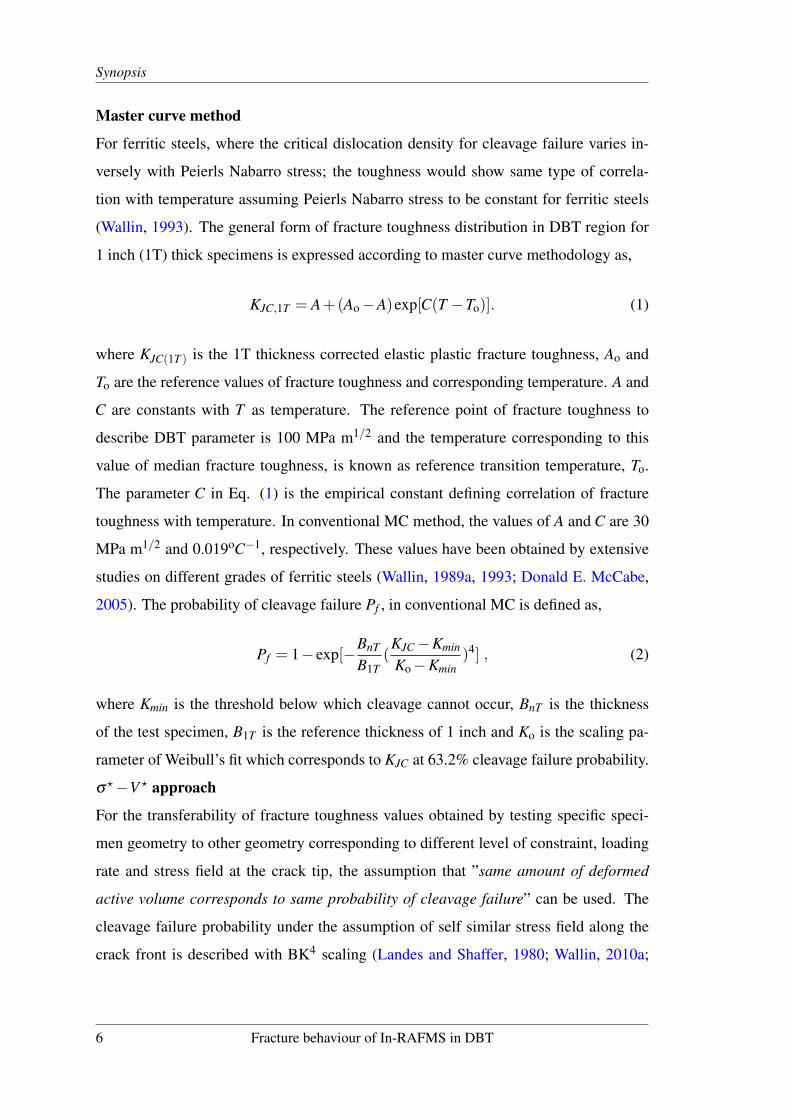
Master curve method
For ferritic steels, where the critical dislocation density for cleavage failure varies in-
versely with Peierls Nabarro stress; the toughness would show same type of correla-
tion with temperature assuming Peierls Nabarro stress to be constant for ferritic steels
(Wallin, 1993). The general form of fracture toughness distribution in DBT region for
1 inch (1T) thick specimens is expressed according to master curve methodology as,
KJC,1T = A+(Ao−A)exp[C(T −To)]. (1)
where KJC(1T ) is the 1T thickness corrected elastic plastic fracture toughness, Ao and
To are the reference values of fracture toughness and corresponding temperature. A and
C are constants with T as temperature. The reference point of fracture toughness to
describe DBT parameter is 100 MPa m1/2 and the temperature corresponding to this
value of median fracture toughness, is known as reference transition temperature, To.
The parameter C in Eq. (1) is the empirical constant defining correlation of fracture
toughness with temperature. In conventional MC method, the values of A and C are 30
MPa m1/2 and 0.019oC−1, respectively. These values have been obtained by extensive
studies on different grades of ferritic steels (Wallin, 1989a, 1993; Donald E. McCabe,
2005). The probability of cleavage failure Pf , in conventional MC is defined as,
Pf = 1− exp[−BnT
B1T(KJC−Kmin
Ko−Kmin)4] , (2)
where Kmin is the threshold below which cleavage cannot occur, BnT is the thickness
of the test specimen, B1T is the reference thickness of 1 inch and Ko is the scaling pa-
rameter of Weibull’s fit which corresponds to KJC at 63.2% cleavage failure probability.
σ?−V ? approach
For the transferability of fracture toughness values obtained by testing specific speci-
men geometry to other geometry corresponding to different level of constraint, loading
rate and stress field at the crack tip, the assumption that ”same amount of deformed
active volume corresponds to same probability of cleavage failure” can be used. The
cleavage failure probability under the assumption of self similar stress field along the
crack front is described with BK4 scaling (Landes and Shaffer, 1980; Wallin, 2010a;
6 Fracture behaviour of In-RAFMS in DBT

Synopsis
Donald E. McCabe, 2005) as,
Pf = 1− exp[−BK4] . (3)
For small specimen when self similarity of crack tip stress field is lost, one of the pos-
sible cleavage failure probability description is,
Pf = 1− exp[−BKλ ] . (4)
The size adjustment of master curve methodology uses Eq.(3) for specimens of any
thickness, however due to the break down of self-similarity of the stress field along the
crack front the volume ahead of crack tip does not scale with a power 4 and therefore to
find the true scaling a modified RKR model which utilizes the fact that cleavage occurs
when a threshold tensile stress is reached at a characteristic distance from the crack tip.
The characteristic distance may vary along the crack front as stress field may not be self
similar and therefore, this criteria requires a volume to be considered which ends at the
boundary where σ1 ≥ σth. The volume for a specimen geometry or for any crack front
can be obtained by finite element analysis which then can be correlated to the fracture
toughness KJC or J to determine the true scaling parameter λ .
Beremin’s model
A similar local approach of cleavage failure modelling numerically in DBT region
started with the pioneer study of Beremin’s group (Beremin et al., 1983b) on cleav-
age failure probability based on Weibull stress which is described as,
Pf = 1− exp[−(σW
σu)m], (5)
where Pf is the numerical probability of cleavage failure, σu is the scaling parameter
and m is the Weibull slope. σW is the Weibull stress defined as,
σW = [1
Vo
∫V ∗
σm1 dV ]1/m, (6)
where Vo is the reference volume not too big to have significant stress gradient nor too
small to violate the characteristic length of RKR model (Ritchie et al., 1973) which is a
few grains. Maximum principal stress, σ1, is integrated in the volume V ∗. The volume
Fracture behaviour of In-RAFMS in DBT 7
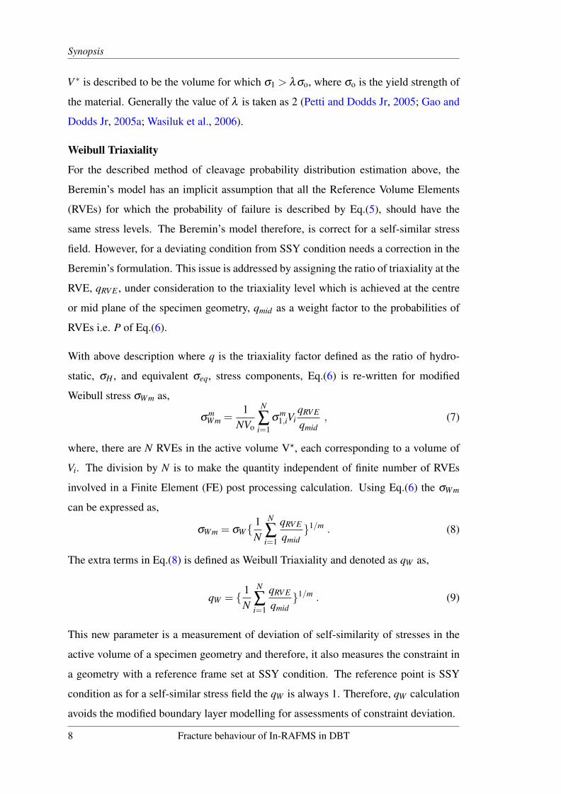
Synopsis
V ∗ is described to be the volume for which σ1 > λσo, where σo is the yield strength of
the material. Generally the value of λ is taken as 2 (Petti and Dodds Jr, 2005; Gao and
Dodds Jr, 2005a; Wasiluk et al., 2006).
Weibull Triaxiality
For the described method of cleavage probability distribution estimation above, the
Beremin’s model has an implicit assumption that all the Reference Volume Elements
(RVEs) for which the probability of failure is described by Eq.(5), should have the
same stress levels. The Beremin’s model therefore, is correct for a self-similar stress
field. However, for a deviating condition from SSY condition needs a correction in the
Beremin’s formulation. This issue is addressed by assigning the ratio of triaxiality at the
RVE, qRV E , under consideration to the triaxiality level which is achieved at the centre
or mid plane of the specimen geometry, qmid as a weight factor to the probabilities of
RVEs i.e. P of Eq.(6).
With above description where q is the triaxiality factor defined as the ratio of hydro-
static, σH , and equivalent σeq, stress components, Eq.(6) is re-written for modified
Weibull stress σWm as,
σmWm =
1NVo
N
∑i=1
σm1,iVi
qRV E
qmid, (7)
where, there are N RVEs in the active volume V?, each corresponding to a volume of
Vi. The division by N is to make the quantity independent of finite number of RVEs
involved in a Finite Element (FE) post processing calculation. Using Eq.(6) the σWm
can be expressed as,
σWm = σW1N
N
∑i=1
qRV E
qmid1/m . (8)
The extra terms in Eq.(8) is defined as Weibull Triaxiality and denoted as qW as,
qW = 1N
N
∑i=1
qRV E
qmid1/m . (9)
This new parameter is a measurement of deviation of self-similarity of stresses in the
active volume of a specimen geometry and therefore, it also measures the constraint in
a geometry with a reference frame set at SSY condition. The reference point is SSY
condition as for a self-similar stress field the qW is always 1. Therefore, qW calculation
avoids the modified boundary layer modelling for assessments of constraint deviation.
8 Fracture behaviour of In-RAFMS in DBT

Synopsis
Due to the modifications described here, the probability of cleavage failure can be re-
defined as,
Pf = 1− exp[−(σ
m/4Wm −σ
m/4Wm−min
σm/4Um −σ
m/4Wm−min
)4] , (10)
where σWm−min and σUm are the minimum modified Weibull stress and modified scaling
parameter. The values of σWm−min and σUm are obtained from the history of σWm−KJC.
Structure of the thesis and results
The thesis starts by highlighting the challenges of fusion reactor technology with a mo-
tivation towards cheaper, safer and cleaner energy source. The history of the concept
and the practical aspects of the ITER program and its design activities are outlined in
brief in Chapter 1, which converges towards the development of structural component
of fusion reactor, especially first wall blanket component. With In-RAFMS developed
in our country this work of investigation finds its objective to examine the fracture be-
haviour of In-RAFMS in DBT region and to investigate, extend and possibly correct
the existing probabilistic approach of master curve to the domains of practical/opera-
tional importances but beyond the scope of conventional master curve methodology in
Chapter 1.
The methodology is reviewed in depth and its applicability on similar grades of ma-
terials are documented in Chapter 2, which helps in formulating the test matrix and
numerical program for understanding and characterizing the fracture behaviour in DBT
region. The detailed formulation of the problem addressed in this work and proposed
test matrix is described in Chapter 3.
The details of microstructure, phase transformation and precipitates in In-RAFMS and
mod-9Cr-1Mo steels with comparison to other popular grades of ferritic/martensitic
steels are provides in Chapter 4.
The experimental set-up, standards, test specimen geometries, temperature set up, pro-
cedure of fracture toughness measurements along with details of impact energy mea-
surement, microstructural examinations are described in the first part of Chapter 5. The
Fracture behaviour of In-RAFMS in DBT 9

Synopsis
finite element analyses pre and post processing methods with formulation and mesh-
ing schemes used for standard calculations such as modified boundary layer model are
provides in second part of Chapter 5.
Chapter 6 titled ”In-RAFMS mechanical behaviour in DBT & conventional master
curve” describes the impact toughness and uniaxial tensile behaviour in DBT region.
The second part of the chapter comprises conventional master curve, comparison of
single and multi-temperature methods, and the effect of valid data/censoring on uncer-
tainty in estimation of reference transition temperature.
Chapter 7 & 8 describe loss of constraint both out of plane and In-plane, respectively.
The chapter on Out of plane constraint loss details the conventional master curve anal-
ysis of 0.2T TPB specimens of In-RAFMS which resulted in a To of -123oC. In this
analyses the small specimen do not show a self similar stress field at crack front and
therefore the master curve assumption of BK4 scaling does not work. This violation
of SSY condition is corrected numerically by transforming the volume deformed under
a non-SSY condition to an equivalent SSY condition which is described as σ?−V ?
approach. The numerical correction based on σ?−V ? approach resulted in a To of
-109oC.
The active volume V? dependencies on KJC,2D obtained by integrating the area under
maximum principal stress at mid plane along thickness and on KJC,3D by calculating
the volume with non-self similarity of stress field are shown in Figure 1(a) and the SSY
corrected master curve obtained by testing 0.2T SE(B) specimens is shown in Figure
1(b).
Chapter 8 describes in-plane constraint loss by analysing the results obtained by testing
specimen of same dimension as for out of plane constraint loss study in chapter 7, with
varying crack depths showed an expected behaviour of increasing To from lowest value
of -125oC for crack depth of 0.3 to 0.44 to highest of -99oC for crack depth of 0.65
to 0.7. The approach of σ?−V ? again showed good potential to scale the differently
constrained conditions to SSY condition and a To of -100oC was obtained for all data
transformed to a/W of 0.5. The in plane change in constraint also showed that the stan-
dard deviation increased for shallower crack depths which indicated that as the dataset
10 Fracture behaviour of In-RAFMS in DBT

Synopsis
(a)
(b)
FIGURE 1: (a) Active volume V ? versus KJC and (b) master curve of In-RAFMS with un-transformed and transformed datasets based on Active volume V ? versus KJC behaviour under
non-SSY condition with loss of constraint
moves away from high constraint condition more uncertainty is induced in the estima-
tion of To. The To obtained with KJC,med and master curve obtained by transferring all
the data to an a/W of 0.5 is shown in Figure 2.
Fracture behaviour of In-RAFMS in DBT 11

Synopsis
(a)
(b)
FIGURE 2: Master curve of data transferred at a/W of 0.5 using σ?−V ? approach showing (a)Shift in To with a/W and (b) KJC transformed to a/W = 0.5
Chapter 9 describes the two popular loading schemes of fracture mechanics which im-
pose different amount of triaxiality along the crack front. The effect is further compli-
cated with the in plane and/or out of plane constraint effects as discussed above. CT and
TPB specimens of In-RAFMS as well as P91 steels re-confirmed the effect and proved
once again that CT specimens should be preferred for To estimation as it always shows
more triaxiality in comparison to bending for identical a/W and thickness. The bending
scheme may have other benefits such as quick setting up while testing and advantage
of using load line displacement for KJC measurement but it also induces errors associ-
ated with the misalignment while fixing the specimens. The side grooved specimens of
In-RAFMS showed the constraint level reaches high enough to ensure self similarity of
stress field. The Weibull Triaxiality developed as an independent constraint assessment
parameter is shown in Figure 3 comparing different specimens tested for To determina-
tion of In-RAFMS and P91 steels.
12 Fracture behaviour of In-RAFMS in DBT

Synopsis
FIGURE 3: The Weibull triaxiality qW compared for different specimens at -120oC with In-RAFMS tensile response as FEA input
The effect of loading rate on reference transition temperature is described in Chapter
10. The experimental results on the dataset of In-RAFMS at three different loading
rates showed an expected systematic increase in To with increasing loading rate. The
Weibull stress analysis was used to predict the cleavage failure probability numerically.
This method required a numerical parameter which is also a material property to be
calibrated. For In-RAFMS this material property known as Weibull modulus was found
to be 9. The Weibull modulus for P91 was also calibrated for the first time and was
found to be 15. The numerical prediction of Weibull stress analysis does not show very
good agreement with the experimental results. This behaviour is attributed to the effect
of plastic strain which causes violation of constant numbers of cleavage initiators in the
active volume. The reasoning is in support of experimental results as for higher loading
rate datasets the Weibull stress based numerical predictions were better than that for
quasi-static condition. As higher strain rate imposes more triaxiality, the possibility of
cleavage initiators turning into void nucleation cites decreases. The master curves at
different loading rates and the comparison of shift in To with Wallin’s correlation is
shown in Figure 4. The Beremin’s model used for numerical predictions of cleavage
failure probability at different loading rates are shown in Figure 5.
Fracture behaviour of In-RAFMS in DBT 13

Synopsis
Temperature (oC)
-140 -120 -100 -80 -60 -40
KJC
at 1
T (
MP
a m
1/2 )
0
100
200
300
Valid and Censored dataInvalid and Uncensored data
50% Median
95% Tolerance
5% Tolerance
dK/dt = 250-370 MPa m 1/2 s-1
To= -95 oC
(a)
Temperature (oC)
-140 -120 -100 -80 -60 -40
KJC
at 1
T (
MP
a m
1/2 )
0
50
100
150
200
250
300
350Valid and Censored dataInvalid Uncensored data
dK/dt = 650-1450 MPa m 1/2s-1
To= -90 oC
95% Tolerance
5% Tolerance
(b) (c)
FIGURE 4: Master curves at different loading rates and ∆To of In-RAFMS with increasing
loading rate
(a) (b)
FIGURE 5: Numerical prediction and experimental rank probabilities for fracture tests per-
formed at (a) 100 mm/min and (b) 1000 mm/min actuator speed.
14 Fracture behaviour of In-RAFMS in DBT

Synopsis
Chapter 11 describes the effect of ductile tearing on cleavage fracture. The event of
cleavage fracture preceded by ductile tearing is analytically modelled and a contribution
due to change in constraint with ductile tearing which was mostly ignored by previous
researchers is considered in the mathematical model. The change in triaxiality measured
as q f /qo where q is the ratio of hydrostatic and Mises stress components for final and
initial conditions, when incorporated with correction of increasing active volume with
ductile tearing, the probability of cleavage failure resulted in a form shown as,
ln(1
1−Pf) = (
BnT
B1T)(
q f
qi) · ( K−Kmin
Ko−Kmin)4 · [1+2
(∆K)2
K2 ] , (11)
where ∆K is the change in KJC with amount of ductile tearing ∆a. The triaxiality and
active volume were calculated by modelling ductile crack growth using GTN model
with VUMAT subroutine.
It was found that this modification expands the validity window of master curve ap-
proach and predicts To in very close range to one obtained by conventional method
when the dataset contains only few cleavage fracture events with prior ductile tearing.
Moreover, the To was also obtained for the dataset where no valid data according ASTM
E1921 was available and no To could have been obtained by using conventional mas-
ter curve method. The modified method was used and justified on Euro fracture data
(Heerens and Hellmann, 1999), and on the dataset CT and SE(B) geometries of In-
RAFMS. The modified master curve in comparison with conventional master curve for
Euro 0.5T CT dataset is shown in Figure 6 (a). The prediction based on mean approx-
imation of KJC−∆a is compared with the results obtained by using modified master
curve in Figure 6 (b)
Fracture behaviour of In-RAFMS in DBT 15

Synopsis
(a)
(b)
FIGURE 6: (a) Modified master curve and conventional master curve comparison for Euro
0.5TCT dataset and (b) comparison of mdofied master curve results with one obtained from
mean approximation of KJC−∆a
Conclusions
The conventional master curve was used for the determination of To of fusion re-
actor test blanket structural In-RAFM steel using smaller CT and Bend specimens.
The To for In-RAFMS was -120oC. The loss of constraint for smaller specimens
was studied using σ?−V ? approach extensively for both in plane and out of plane
16 Fracture behaviour of In-RAFMS in DBT

Synopsis
loss of constraint. The σ?−V ? approach was found accurate enough for trans-
ferring the fracture toughness to SSY condition and estimated conservative To for
smaller In-RAFMS specimens was found to be -109oC.
The in plane constraint loss study using test specimens with crack depth from
a/W of 0.3 to 0.7, showed that in this range of crack depth , To shows consistent
correlation with constraint and σ?−V ? approach can be used for estimation of To
for any a/W in the investigated range.
The differences of constraint between CT and TPB geometries were analysed us-
ing a novel Weibull Traixiality method which was found to correct Beremin’s
model for constraint. The numerical predictions based on corrected Beremin’s
model shows the potential of Weibull Traixiality.
The assessment of loading rate effect on To was found to follow Wallin’s corre-
lation based on Zener-Holoomon strain rate parameter. The numerical prediction
based on Beremin’s model showed good accuracy and Weibull slopes were cal-
ibrated for the first time for In-RAFMS, P91 and F82H steels which were 9, 15
and 11, respectively.
The master curve validity window was expanded by modifying the cleavage fail-
ure probability when cleavage is preceded by significant amount of ductile tear-
ing. The increasing active volume, increasing triaxiality and criticality of carbides
were taken care of in the modified master curve with the help of constraint as-
sessment by triaxiality factor q and re-derivation of increasing active volume. The
modified master curve was found to estimate To for a dataset where no To estima-
tion was possible using conventional master curve approach. This modification
was found applicable in upper region of DBT where cleavage in followed by sig-
nificantly large amount of ductile tearing of the order of 2.5 mm.
Fracture behaviour of In-RAFMS in DBT 17

ReferencesASTM E. (1921) E 1921 standard test method for determination of reference tempera-
ture. T0, for ferritic steels in the transition range
Beremin F. M., Pineau A., Mudry F., Devaux J.-C., D’Escatha Y., Ledermann P. (1983)A local criterion for cleavage fracture of a nuclear pressure vessel steel. MetallurgicalTransactions A 14(11):2277–2287, doi10.1007/BF02663302
Bonade R., Mueller P., Spatig P. (2008) Fracture toughness behavior in the ductile–brittle transition region of the tempered martensitic eurofer97 steel: Experiments andmodeling. Engineering fracture mechanics 75(13):3985–4000
Chaudhuri P., Kumar E. R., Sircar A., Ranjithkumar S., Chaudhari V., Danani C., YadavB., Bhattacharyay R., Mehta V., Patel R., Vyas K., Singh R., Sarkar M., SrivastavaR., Mohan S., Bhanja K., Suri A. (2012) Status and progress of indian LLCB testblanket systems for ITER. Fusion Engineering and Design 87(78):1009 – 1013,doihttp://dx.doi.org/10.1016/j.fusengdes.2012.02.062,
Donald E. McCabe K. W. John G. Merkle (2005) An Introduction to the Developmentand Use of the Master Curve Method.
Gao X., Dodds Jr R. H. (2005) Loading rate effects on parameters of the weibull stressmodel for ferritic steels. Engineering Fracture Mechanics 72(15):2416 – 2425, doi-http://dx.doi.org/10.1016/j.engfracmech.2005.03.001
Heerens J., Hellmann D. (1999) Fracture toughness of steel in the ductile to brittle tran-sition regime. Final Report, Measurement and Testing Programme Contract MAT1-CT-940080
IAEA (2001a) Final Report of the ITER EDA. No. 21 in ITER EDA DocumentationSeries, INTERNATIONAL ATOMIC ENERGY AGENCY, Vienna,
IAEA (2001b) Summary of the ITER Final Design Report. No. 22 in ITER EDA Doc-umentation Series, INTERNATIONAL ATOMIC ENERGY AGENCY, Vienna,
Jayakumar T., Mathew M., Laha K. (2013) High temperature materials for nuclear fastfission and fusion reactors and advanced fossil power plants. Procedia Engineering55:259 – 270, doihttp://dx.doi.org/10.1016/j.proeng.2013.03.252,
Kytka M., Brumovsky M., Falcnik M. (2011) Irradiation embrittlement characterizationof the eurofer 97 material. Journal of Nuclear Materials 409(2):147–152
Laha K., Saroja S., Moitra A., Sandhya R., Mathew M., Jayakumar T., Kumar E. R.(2013) Development of india-specific RAFM steel through optimization of tung-sten and tantalum contents for better combination of impact, tensile, low cyclefatigue and creep properties. Journal of Nuclear Materials 439(13):41 – 50, doi-http://dx.doi.org/10.1016/j.jnucmat.2013.03.073
Landes J., Shaffer D. (1980) Statistical characterization of fracture in the transitionregion. In: Fracture Mechanics, ASTM International
18

Synopsis
Petti J. P., Dodds Jr R. H. (2005) Calibration of the weibull stress scale parameter,u, using the master curve. Engineering Fracture Mechanics 72(1):91 – 120, doi-http://dx.doi.org/10.1016/j.engfracmech.2004.03.009
Ritchie R. O., Knott J. F., Rice J. (1973) On the relationship between critical tensilestress and fracture toughness in mild steel. Journal of the Mechanics and Physics ofSolids 21(6):395–410
Tagawa T., Kayamori Y., Hira H. (2010) Statistical scatter of fracture toughness inthe ductile–brittle transition of a structural steel. Engineering Fracture Mechanics77(16):3077–3086
Wallin K. (1989) The effect of ductile tearing on cleavage fracture probability in fracturetoughness testing. Engineering Fracture Mechanics 32(4):523–531
Wallin K. (1993) Irradiation damage effects on the fracture toughness transition curveshape for reactor pressure vessel steels. International journal of pressure vessels andpiping 55(1):61–79
Wallin K. (2010) Structural integrity assessment aspects of the master curvemethodology. Engineering Fracture Mechanics 77(2):285 – 292, doi-http://dx.doi.org/10.1016/j.engfracmech.2009.02.010
Wasiluk B., Petti J. P., Jr. R. H. D. (2006) Temperature dependence of weibullstress parameters: Studies using the euro-material. Engineering Fracture Mechanics73(8):1046 – 1069, doihttp://dx.doi.org/10.1016/j.engfracmech.2005.11.006
Fracture behaviour of In-RAFMS in DBT 19

Chapter 1
Introduction
In this chapter, the background of fusion reactor technology is briefed and motivationsare drawn for the dissertation work. The objectives of the work is followed subse-quently.
1.1 A brief history of fusion reactor & challenges to structural in-tegrity
The worldwide energy demand with an estimated increase of electricity production by
at least a factor of two in the second half of this century, fading resources of raw mate-
rials and a growing concern about global warming require innovative solutions (Kytka
et al., 2011). The concept of producing efficient energy at low cost to make energy
available for everything and everyone gave motivation for the nuclear power produc-
tion and resulted in large scale power production units through nuclear fission reactors
world wide. The technology of fission reactor is well established, in-depth studied, and
worked upon. However, the huge radioactive waste and nuclear accidents such as, Three
miles island, Chernobyl and Fukushima raise concerns regarding the safety and environ-
mental effects of nuclear power (Oughton, 2016). With the added benefit of being even
cheaper and non-fossil source of power, fusion power production is highly appreciated
by the world and the first largest international collaboration currently including India,
Russian Federation, China, South Korea, Japan, European Union and USA came under
the umbrella of International Thermonuclear Experimental Reactor (ITER) program to
establish this technology.
The power production from fusion of two light elements such as Deuterium (D) and
Tritium (T) is not practically very easy. The first device to magnetically confine plasma
as a pre-requisite for this reactor started in 1950 with the tokamak creation credited
20

Chapter 1: Introduction
to Andrei Sakharov and Igor Kurchatov (Bromberg, 1982; Wikipedia, 2004). For the
fusion reaction i.e. the fusion of D and T, it requires a very high temperature (gas
temperature approx. 5×10⁷ K) for the fusion reaction rate to attain its peak (Bromberg,
1982; Stacey, 2010). Other possibilities such as fusion of D-D and D-He require further
higher temperatures. To generate this amount of temperature the concept of Z-pinch
is used (Miernik et al., 2013). The first nuclear fusion registered in 1948 was also the
first detailed examination of this concept which was patented by the United Kingdom
Atomic Energy Authority. The invention of this reactor with Z-pinch is credited to Sir
George Paget Thomson and Moses Blackman.
The principle of Z-pinch is that a current passing through plasma generates a magnetic
field around it which according to Lenz’s law causes an inward force for plasma to col-
lapse in. This results in a dense plasma, which further increases the inward force. This
chain reaction in controlled manner can reach the density and temperature required for
D-T reaction to occur. However, the challenge is to have an electrode which can pass
current to this plasma at the temperature of as high as million K. The possibility is ex-
plored by inducing current by magnetic fields around plasma. Because the plasma is
charged and thus reacts to electrical and magnetic field the plasma is also controlled by
these fields. The practicality of the idea of harnessing energy with a safer and cheaper
means motivated towards the first international project in 1985 when European commu-
nity, Soviet Union, Japan and United States were invited to conceptualize by IAEA the
terms and conditions of engineering and design activities of an International Thermo-
nuclear Experimental Reactor (ITER). The acceptance of IAEA invitation was realized
in 1988 and in 1990 first conceptual design activity was completed. Further progress in
terms and conditions of Engineering Design and Activity (EDA) resulted in IAEA-EDA
agreement in 1992. In 1998, at the end of the six years of joint work originally foreseen
under the ITER EDA agreement, a design for ITER was developed which fulfilled the
overall programmatic objectives and complied with the detailed technical objectives,
technical approaches, and the cost target adopted by the ITER Parties in 1992 at the
start of the EDA (IAEA, 2001a)
Fracture behaviour of In-RAFMS in DBT 21

Chapter 1: Introduction
Due to huge financial requirements, safety concerns and challenges of practicality, the
formation of Special Working Group (SWG) lead to divide the full-fledged reactor es-
tablishment to smaller steps or phases of fusion reactor technology (IAEA, 2001b).
• H-phase This is a non-nuclear phase using only hydrogen or helium plasmas,
planned mainly for complete commissioning of the tokamak system in a non-
nuclear environment where remote handling maintenance is not mandatory.
• D-phase The characteristics of deuterium plasma are very similar to those of DT
plasma except for the amount of alpha heating. Therefore, the reference DT oper-
ational scenarios, i.e., high Q, inductive operation and non-inductive steady state
operation, can be simulated further. Since some tritium will be generated in the
plasma, fusion power production for short periods of time without fully imple-
menting the cooling and tritium-recycle systems could therefore also be demon-
strated. By using limited amounts of tritium in a deuterium plasma, the integrated
nuclear commissioning of the device will be possible. In particular, the shielding
performance will be tested.
• D-T Phase During the first phase of DT operation the fusion power and burn
pulse length will be gradually increased until the inductive operational goal is
reached. Non-inductive, steady state operation will also be developed. DEMO
reactor relevant test blanket modules will also be tested whenever significant neu-
tron fluxes will be available, and a reference mode of operation for that testing will
be established. The second phase of full DT operation, beginning after a total of
about ten years of previous operation, will emphasise improvement of the overall
performance and the testing of components and materials with a higher neutron
fluence. This phase will address the issues of higher availability and further im-
proved modes of plasma operation. The implementation and the programme for
this phase will be decided following a review of the results from the preceding
three operational phases and an assessment of the merits and priorities of pro-
grammatic proposals. A decision on incorporating in the vessel a tritium breeding
blanket during the course of the second D-T phase will be taken on the basis of
22 Fracture behaviour of In-RAFMS in DBT
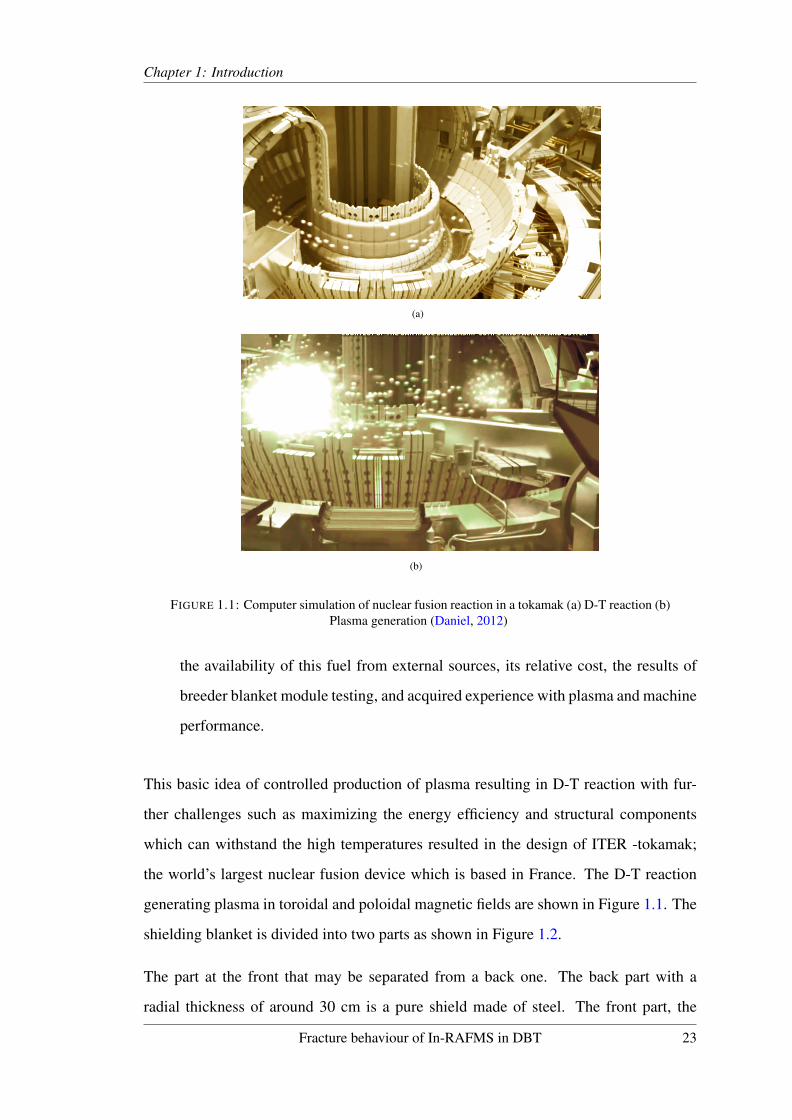
Chapter 1: Introduction
(a)
(b)
FIGURE 1.1: Computer simulation of nuclear fusion reaction in a tokamak (a) D-T reaction (b)Plasma generation (Daniel, 2012)
the availability of this fuel from external sources, its relative cost, the results of
breeder blanket module testing, and acquired experience with plasma and machine
performance.
This basic idea of controlled production of plasma resulting in D-T reaction with fur-
ther challenges such as maximizing the energy efficiency and structural components
which can withstand the high temperatures resulted in the design of ITER -tokamak;
the world’s largest nuclear fusion device which is based in France. The D-T reaction
generating plasma in toroidal and poloidal magnetic fields are shown in Figure 1.1. The
shielding blanket is divided into two parts as shown in Figure 1.2.
The part at the front that may be separated from a back one. The back part with a
radial thickness of around 30 cm is a pure shield made of steel. The front part, the
Fracture behaviour of In-RAFMS in DBT 23

Chapter 1: Introduction
FIGURE 1.2: Test blanket module
first wall, includes various different class of materials which are l cm thick Beryllium
armour protection, l cm thick copper to diffuse the heat load as much as possible, and
around 10 cm of steel structure. This component will become the most activated and
tritium-contaminated component in the entire ITER device. It could be in contact with
the plasma in off normal conditions, and thus can suffer damage from the large heat
locally deposited, and may have to be repaired or possibly changed.
The operational pulsating mode due to non-availability of longer duration plasma, high
temperature and high energy neutrons demand the first wall blanket material to have
enough structural strength to withstand these conditions. The first wall blanket is also
the component which is used for flowing lead-lithium eutectic which works as Tritium
breeder and coolant. Due to such operational conditions the first reference taken for
structural material came from the extensively researched fission reactor. The initial
studies for fast breeder reactors conditions showed that the austenitic stainless steels
were prone to swelling resulting from irradiation induced vacancy-interstitial creations.
The fusion reactor condition therefore would magnify this effect due to even higher
24 Fracture behaviour of In-RAFMS in DBT

Chapter 1: Introduction
energy irradiation caused by 14MeV neutrons in comparison to 2MeV neutrons of fis-
sion reactors. The tempered martensitic steels showed good swelling resistance and
therefore the reference material for fusion reactor test blanket material converged on
modified 9%Cr−1%Mo steels (Banerjee, 2014; Mathew et al., 2011; Jayakumar et al.,
2013).
Due to the high energy irradiation the safe waste management of radioactive materials
requires the activity of nuclear components to be controlled. The low activity therefore
was achieved by replacing the active elements of modified 9%Cr−1%Mo steels with
low activity W, Ta and Mn.
In the process of establishing fusion reactor technology, Pb-Li eutectic is to be used as
tritium breeder (Lead-lithium ceramic breeder/LLCB) and helium to be used for cool-
ing. The test blanket module which consists of U-shaped first wall with helium cooling
system has inlet at 350oC and outlet at 480oC, helium pressure of 8 MPa and pressure
drop of 0.3 MPa. With 9%Cr−1%Mo steels as reference material the proposed mate-
rial for U-shaped first wall structure evolved as Reduced Activation Ferritic Martensitic
steel (RAFMs). Many such steels such as EUROFER-97, F82H, JLF, Optifier and In-
RAFMs are proposed by different parts of world. First generation of RAFMS, however,
were OPTIFIER, MANET and F82H. The more improved version of Eurofer97 was
developed after F82H which was followed by other grades from different part of the
world. Research activities on the future generation of RAFMS which is oxide strength-
ened grades mainly by oxides of Yitrium has also started world wide (Banerjee, 2014;
Jayakumar et al., 2013).
Being a ferritic martensitic steel, RAFMs undergoes a transition from ductile to brittle
failure at lower temperature. Transition temperature of steels, also known as reference
temperature (To) shifts upward under the influence of irradiation. Both for quasi-static
and dynamic loading rates the transition temperature can shift by 100oC with an irra-
diation dose of 2dpa (Kytka et al., 2011). The irradiation studies, on various grades of
RAFMs, further show that for damage induced at 250-300oC the shift in transition tem-
perature is maximum. Therefore, in order to assure the structural safety and integrity
Fracture behaviour of In-RAFMS in DBT 25

Chapter 1: Introduction
of the test blanket module, it becomes utmost important to understand the behaviour of
fracture toughness in DBT region for RAFM grade steels and effect if irradiation on it.
At present, the transition temperatures of steels are characterized by impact toughness,
RTNDT ASME approach and recently developed Master Curve approach (Wallin, 1984;
Yoon et al., 2001a). Out of these, impact test method suffers with huge scatter and
requires large number of samples. Additionally for testing and measurement of me-
chanical responses of nuclear grade materials, the conventional standard size impact
specimens are too big and sub-sized and miniature specimens which are best for irradi-
ation studied do not show a single correlation with standard size specimens.
On the other hand RTNDT approach of ASME uses the data from impact tests and drop
weight tear tests and takes the lowest values to determine reference temperature. This
approach does not deal with the scatter of data and results in an over-conservative esti-
mate in many cases.
Master Curve (MC) approach is the only approach which works on the concept of
stochastic nature of cleavage initiators’ distribution in DBT regime; making it the most
efficient method for transition behaviour characterization (Slatcher, 1986).
The extensive research on Indian RAFMS started with reference composition of Eu-
rofer97 and four different compositional variation were studied exhaustively for creep
deformation strength, low cycle fatigue properties, tensile and impact properties. The
chemical composition of elements driving these properties in steels i.e. W and Ta were
studied with four basic variation in compositions of W and Ta. The four alloys com-
prises 1%W-0.06%, 1.4%W-0.06%, 2%W-0.06% and 1%W-0.14% Laha et al. (2013).
The higher activity elements such as Mo, Nb, B, Cu, Ni, Al, Co, Ti and embrittling
elements such as S, P, As, Sb, Sn, Zr and O are kept in ppm levels. After the extensive
studies on mechanical behaviour the second composition was declared as In-RAFMS
Laha et al. (2013), with the understanding that 1.4%W results in the best creep rupture
strength and creep deformation resistance and 0.06%Ta with 9%Cr gives the lowest pos-
sible Ductile to Brittle Transition Temperature (DBTT) obtained from 68 Joule criteria
26 Fracture behaviour of In-RAFMS in DBT

Chapter 1: Introduction
of impact toughness. The heat treatment of In-RAFMS is fixed to be solutionized at
1263±10K for 30 minutes per 25 mm. After solutionizing and normalizing the plates
are to be tempered at 1038±5K for 90 minutes per 25 mm thickness.
1.2 Objectives
The structural material for the fusion reactor test blanket developed in India which is
designated as Indian reduced activation ferritic martensitic steel (In-RAFMS) is de-
signed by its creep and fatigue properties with swelling resistance against irradiation.
Further understanding of effect of irradiation on transition behaviour and mechanical
behaviour under liquid metal embrittling environment of Pb-Li eutectic is required. The
objective of work presented here is to study extensively the fracture behaviour of Indian
RAFMS in DBT region with the help of probabilistic master curve approach.
With the broad objective to characterize the fracture behaviour of In-RAFMS in DBT
region following objectives were derived.
To determine the conventional reference transition temperature for In-RAFM and
modified 9Cr-1Mo steels and also to examine the effect of censoring of dataset
and censoring parameter.
To establish a method of transforming the fracture toughness obtained from smaller
specimen to SSY and other non-SSY scales.
To understand the effect of size and specimen geoemtries, such as CT and SE(B)
on reference transition temperature.
To understand the effect of loading rate on reference transition temperature.
To establish numerical methods of predicting cleavage fracture probability for
different sizes and loading rates.
To determine reference transition temperature from cleavage fracture with prior
ductile tearing.
Fracture behaviour of In-RAFMS in DBT 27

Chapter 1: Introduction
The scope of the work, therefore, includes the parametric study of loading rate, speci-
men geometry type (CT and SE(B)), and the fracture behaviour in full domain of DBT.
To attain this material based understanding, the scope of this work also includes the
modification in the existing methodology of master curve in the DBT region where
applicable.
1.3 Structure of thesis
The thesis starts by highlighting the challenges of fusion reactor technology with a mo-
tivation towards cheaper, safer and cleaner energy source. The history of the concept
and the practical aspects of the ITER program and its design activities are outlined in
brief in Chapter 1. With In-RAFMS developed in our country as structural first wall
blanket material, this work of investigation finds its objective to examine the fracture
behaviour of In-RAFMS in DBT region and to investigate, extend and possibly correct
the existing probabilistic approach of master curve to the domains of practical/opera-
tional importances but beyond the scope of conventional master curve methodology in
Chapter 1.
The methodology is reviewed in depth and its applicability on similar grades of ma-
terials are documented in Chapter 2 which helps in formulating the test matrix and
numerical program for understanding and characterizing the fracture behaviour in DBT
region. The detailed formulation of the problem addressed in this work and proposed
test matrix is described in Chapter 3.
The details of microstructure, phase transformation and precipitates in In-RAFMS and
mod-9Cr-1Mo steels with comparison to other popular grades of ferritic/martensitic
steels are provides in Chapter 4.
The experimental set-up, standards, test specimen geometries, temperature set up, pro-
cedure of fracture toughness measurements along with details of impact energy mea-
surement, microstructural examinations are described in the first part of Chapter 5. The
28 Fracture behaviour of In-RAFMS in DBT

Chapter 1: Introduction
finite element analyses pre and post processing methods with formulation and mesh-
ing schemes used for standard calculations such as modified boundary layer model are
provides in second part of Chapter 5.
Chapter 6 titled ”In-RAFMS mechanical behaviour in DBT & conventional master
curve” describes the impact toughness and uniaxial tensile behaviour in DBT region.
The second part of the chapter comprises conventional master curve, comparison of
single and multi-temperature methods, and the effect of valid data/censoring on uncer-
tainty in estimation of reference transition temperature.
The loss of constraint occurring due to out of plane dimension is dealt in Chapter 7,
where the effect is analysed and corrected numerically with a thickness scaling or con-
straint transformation method developed developed as an outcome of this work. The
same approach was proven to be applicable to solve the problem of loss of constraint
resulting from in-plane changes in crack tip stresses due to different crack depths. The
approach also is claimed and justified as a tool of constraint measurement as detailed in
Chapter 8.
The persistent problem of bending and tension loading in fracture mechanics is taken
care off in Chapter 9. The problem is analysed using the dataset generated on CT and
TPB geometries of P91 and In-RAFM steels and a novel method of constraint measure-
ment is developed. The importance of simple side-grooving method which appears to
solve the large scale yielding problem for smaller specimens is discussed in this chapter.
The effect of loading rate at three different actuator speeds is studied in Chapter 10. To
examine this aspect a numerical property which is presumably a signature of material
and also known as Weibull modulus is calculated for In-RAFMS in this Chapter by
calibrating it on the dataset created for high constraint and low constraint conditions
which is analysed in previous chapters.
The master curve methodology is re-defined for its application to the region of DBT
which has been more or less untouched so far by the fracture mechanics community.
Fracture behaviour of In-RAFMS in DBT 29

Chapter 1: Introduction
The modified method is assessed numerically and on the existing as well as newly de-
veloped dataset of In-RAFMS in Chapter 11.
The different aspects of aforementioned parameters are collectively interpreted and crit-
ically summarized in Chapter 12 and the outcome of the work are concluded.
The fracture dataset created in this work is tabulated in Appendix-A. The maximum
likelihood estimation method for conventional and modified master curve methodolo-
gies are explained mathematically in Appendix-B. The different types of test speci-
mens used to generate the fracture, tensile and impact toughness dataset are detailed in
Appendix-C. The complete bibliography is provided on page numbers 240 to 250. The
list of figures, tables and symbols are provided on page number xxi to xxxiii.
30 Fracture behaviour of In-RAFMS in DBT

Chapter 2
Literature Review
In this chapter, various problems, shortcomings and existing methodologies of mechan-
ical behaviour in ductile to brittle transition region are briefed. The developments of
probabilistic approach to solve the scatter of DBT region is then explained subsequently.
The global as well as local approaches to model cleavage fracture, their applicability
and developments of master curve method , which is used in the work of dissertation
is explained. Later, the modifications in master curve method, advanced master curve
methods to study inhomogeneities and case studied on ferritic martenistic steels are dis-
cussed.
2.1 An Introduction to ductile to brittle transition of fracture mode
Nuclear fusion reactor is one promising future solution to replace fossil fuel for power
production. In the process of establishing fusion reactor technology, Pb-Li eutectic is
to be used as tritium breeder (Lead-lithium ceramic breeder/LLCB) and helium to be
used for cooling. The test blanket module , which consists of U-shaped first wall with
helium cooling system has inlet outlet at 350-480oC, helium pressure of 8 MPa and
pressure drop of 0.3 MPa. The proposed material for U-shaped first wall structure is
Reduced Activation Ferritic Martensitic steel (RAFMs). The RAFMs has been derived
from Mod-9Cr-1Mo steel with elements having half life more than 100 years replaced
with those having less than 100 years, for instance Mo is replaced by W and Nb by
Tantalum. Properties , which make RAFMs challenging candidate material for structure
are its low swelling property and improved creep resistance. Many such steels such as
31

Chapter 2: Literature Review
EUROFER-97, F82H, JLF, Optifier and In-RAFMs are proposed by different parts of
world.
Being a ferritic martensitic steel, RAFMs undergoes a transition from ductile to brittle
failure at lower temperature. Transition temperature of steels, also known as reference
emperature (To) shifts upward under the influence of irradiation. Therefore, it becomes
important to investigate the fracture behaviour of Indian RAFMs (In-RAFMs) in DBT
regime. At present, the transition temperatures of steels are characterized by impact
toughness, RTNDT ASME approach and Master Curve approach. Out of these, impact
test method suffers with huge scatter and requires large number of samples (Wallin,
1984). On the other hand RTNDT approach uses the data from impact tests and drop
weight tear tests and takes the lowest values to determine reference temperature. This
approach does not deal with the scatter of data and results in an over-conservative es-
timate in many cases. Master Curve (MC) approach is the only approach utilizing the
fact of stochastic nature of cleavage initiators’ distribution in DBT regime; making it the
most efficient method for transition behaviour characterization. Master curve method
was established initially for Reactor Pressure Vessel steels , which was ferritic in nature.
The approach is discussed in detail in following section.
2.2 Probabilistic approach towards scatter in ductile to brittle tran-
sition
The ductile to brittle transition region is usually characterized industrially by Charpy
test (ASTM E23). The specimens used in this method are 10×10×55 mm3 rectangular
bars with V notch. There are generally three parameters resulting from Charpy tests ,
which are used for indexing the ductile the brittle transition. The first parameter is the
impact energy (in Joules). There are several reference points to define a transition tem-
perature such as 28 J, 41J and 68J reference points. The second parameter is the fracture
surface showing a mixture of flat and rough surfaces in correspondence to brittle and
ductile fracture zones, respectively. The percentage area on fracture surface is defined
32 Fracture behaviour of In-RAFMS in DBT

Chapter 2: Literature Review
as Fracture Appearance Transition Temperature (FATT) where 50% area is rough and
rest is flat. The third parameter is the lateral strain measured in perpendicular to the
plane of notch. Despite of aforementioned criteria huge scatter in DBT region makes
the result only useful for qualitative purpose.
To deal with the problem of scatter the ASME provided a method known as RTNDT
approach and was given in form of ASME K1C Curve in ASME Pressure Vessel Code
Section III. The Japanese Research Program , which re-analysed the dataset including
655 static fracture toughness data of SA533 steel including data from Weld specimens,
also compared the results of ASME K1C Curve with a statistical approach of master
curve. The details of the categorical datasets used in the analysis is provided in (Yoon
et al., 2001b). The temperature axis normalized with RTNDT for the datasets are shown
in Figure 2.1.
FIGURE 2.1: ASME K1C Curve for SA533 steel base and weld datasets
Fracture behaviour of In-RAFMS in DBT 33

Chapter 2: Literature Review
It is evident from Figure 2.1 that the RTNDT is a lower bound curve , which is over
conservative to the true fracture behaviour of material, as it can be realized that the
RTNDT for weld as well as base metal shows same profile in form of ASME K1C Curve,
even after scaling the temperature axis to T-RTNDT . The RTNDT temperature is obtained
by analysing Charpy and drop weight test data following the rules given below.
• Charpy and Drop Weight tests are performed on the material with the intention
that a conservative value from either of the test is obtained.
• The crack plane in the test specimen is oriented to coincide with the plane of
maximum primary membrane stress.
• The Nil Ductility Temperature (TNDT ) is obtained by following ASTM E208 at
quarter thickness (0.25T) location.
• At least three Charpy V Notch (CVN) at TNDT + 33.3oC using specimens from
quarter thickness location.
• If all thee of the CVN tests show a lateral strain of 1mm or more then RTNDT =
TNDT .
• If above criteria is not met then find the temperature T40, where lateral strain is 40
mils (1mm) and then RTNDT = T40 +33.3oC.
A modification in ASME K1C Curve was performed in Code Case 610 by analysis
the data generated by performing Drop Weight tests on specimens made by one-pass
welding unlike double pass. Further, in Code case - 629, the RTNDT is referred as RT10
, which is To− 33.3oC. The dataset analysed using master curve method is compared
with ASME K1C Curve and RT10 in Figure 2.2. The potential of master curve is evident
from Figure 2.2 and the motivation to use master curve approach for characterization of
fracture behaviour is realized.
34 Fracture behaviour of In-RAFMS in DBT

Chapter 2: Literature Review
FIGURE 2.2: ASME K1C Curve for SA533 steel incoparison with master curve and RT10
2.2.1 Master curve: a global approach
The fracture behaviour of ferritic steels in the Ductile to Brittle Transition (DBT) re-
gion is known for its inherent huge scatter (Wallin, 1984). There have been various
methodologies developed to assess this scatter ranging from impact energy measure-
ment to elasto-plastic fracture toughness correlation with temperature known as Master
Curve approach. The development of master curve , which takes probabilistic behaviour
of cleavage fracture into consideration exploits the weakest link theory of Weibull
(Weibull, 1951). It is unsure about the time the terms of master curve equations started
emerging in engineering fracture mechanics but it won’t be wrong to say that the most
important tool to analyse DBT regime started with the Weibull’s model of weakest link
in 1951, , which is described in brief here .
Fracture behaviour of In-RAFMS in DBT 35

Chapter 2: Literature Review
Weakest Link Theory
A chain made by joining n number of links will fail if one link fails, thus the weakest of
all links will describe the failure probability of the chain, which is expressed as,
P = 1− exp−φ(x) , (2.1)
where P defines the probability of failure of one link in the sense that it can be written as
probability of x having a value less than a property of link , which in this case is failure.
Extending the concept, for n links the failure probability of a chain can be written as,
1− (1−P)n = 1− exp−nφ(x) . (2.2)
Weibull in his theory (Weibull, 1951) also gave the simplest function φ(x) in the form
as,
φ(x) =(x− xU)
m
xo, (2.3)
considering the necessary conditions of the function to be positive, non-decreasing and
vanishing at a value xU . The value xo is called the scaling parameter and m is known as
Weibull’s coefficient or Weibull slope. Weibull also demonstrated by giving examples
for the application of the theory of weakest link in variety of fields, such as yield strength
of Bofors, Fiber strength of Indian cotton, fatigue behaviour and few more.
In the field of fracture mechanics, especially in DBT regime one can realize the effect of
Weibull’s equation together with probabilistic fracture mechanics analysis of Stephan
Slatcher (Slatcher, 1986). Slatcher not only explored the probabilistic approach in DBT
regime but also found theoretically the Weibull’s slope parameter to be 4. Slatcher in
his theoretical model, assumed that the elemental initiation can be considered as the
event to define fracture in DBT regime , which depends on the proportion of crack front
in elements ahead of crack tip and the probability of failure can be described as,
Pf = 1− exp(−BϕJ2) , (2.4)
36 Fracture behaviour of In-RAFMS in DBT

Chapter 2: Literature Review
FIGURE 2.3: Schematic of fracture surface with shaded fatigue pre-cracked and cracked areas
where B is the thickness of specimen and ϕ is defined as,
ϕ =∫
θ=π
θ=−π
∫ u=h(θ)
u=g(θ)u f (u,θ ,η1,η2 · · ·)du ·dθ . (2.5)
In his first assumption, the elemental homogeneity is of crucial importance and for a
material where the elemental homogeneity is questionable, the model cannot be benefi-
cial. The second assumption considers the stresses and strains to be dependent on J/r
ratio, which comes from the assumption that the stress strain ahead of crack front is fully
characterized by J value. The functions g(θ) and h(θ) describe the annular domain that
uses r to define the element area under consideration. In Eq.( 2.5), parameter u is a
function of J/r ratio. In the review of Slatcher the master curve equation was already
clear but before going any further, a briefing of the classic work of Landes and Shaffer
is necessary. Landes and Shaffer (1980) in their work in DBT regime found a charac-
teristic microstructural feature shown in Figure 2.3. The figure schematically shows the
initiation points ahead of pre-cracked region, from where the specimen cleaved. Some-
times, there were more than one initiation points, and this feature reported by Landes
and Shaffer was documented to be the evidence of materials following weakest link the-
ory in DBT regime by Wallin (Donald E. McCabe, 2005). Landes and Shaffer brought
an important aspect of cleavage fracture that it was dependent on the points of mini-
mum toughness across the crack tip and the scatter in smaller specimens were found
to be lower due to the scarcity of these points of minimum toughness, which are also
Fracture behaviour of In-RAFMS in DBT 37

Chapter 2: Literature Review
referred to as cleavage triggers. Since then, it was concluded that the cleavage failure in
DBT regime is a stochastic process and should be treated with probabilistic approach.
For ferritic steels, where the critical dislocation density for cleavage failure varies in-
versely with Peierls Nabarro stress; the toughness would show same type of correla-
tion with temperature assuming Peierls Nabarro stress to be constant for ferritic steels
(Wallin, 1993). The general form of fracture toughness distribution in DBT region for
1 inch (1T) thick specimens is expressed according to master curve methodology as,
KJC,1T = A+(Ao−A)exp[C(T −To)]. (2.6)
where KJC(1T ) is the 1 inch (1T) thickness corrected elastic plastic fracture toughness,
Ao and To are the reference values of fracture toughness and corresponding temperature.
A and C are constants with T as temperature. The reference point of fracture toughness
to describe DBT parameter is 100 MPa m1/2 and the temperature corresponding to this
value of median fracture toughness, is known as reference transition temperature, To.
The parameter C in Eq. (2.6) is the empirical constant defining correlation of fracture
toughness with temperature. In conventional MC method, the values of A and C are 30
MPa m1/2 and 0.019oC−1, respectively. These values have been obtained by extensive
studies on different grades of ferritic steels (Wallin, 1989a, 1993; Donald E. McCabe,
2005). The probability of cleavage failure Pf , in conventional MC is defined as,
Pf = 1− exp[−BnT
B1T(KJC−Kmin
Ko−Kmin)4] , (2.7)
where Kmin is the threshold below , which cleavage cannot occur, BnT is the thickness of
the test specimen, B1T is the reference thickness of 1 inch and Ko is the scaling param-
eter of Weibull’s fit , which corresponds to KJC at 63.2% cleavage failure probability.
The fracture data obtained by testing the specimens in DBT region undergo Maximum
Likelihood (ML) analysis after size adjusting the dataset to 1 inch thickness. The ML
38 Fracture behaviour of In-RAFMS in DBT

Chapter 2: Literature Review
parameter L is defined by finding the probability density function ( fi) and survival func-
tion (Si)
fi =dPf
dKJC, (2.8)
Si = exp[−(KJC(i)−Kmin
Ko−Kmin)1/4] , (2.9)
where index i refers to the individual data analysed at each test temperature. The maxi-
mum likelihood parameter is described as
L =N
∏i=1
f δii ·S
1−δii . (2.10)
The maximization of ML parameter is carried out for master curve method by satisfying
set of equations,∂L∂A
=∂L∂C
=∂L∂To
= 0 . (2.11)
Apart from aforementioned three equations, the ML analysis is solved by using the
relation of Ko with reference transition temperature To described as
Ko = Kmin +1
(ln2)1/4 (A−Kmin)+(Ao−A)exp[C(T −To)] . (2.12)
The relation in Eq.(2.12) is obtained using the fact that Ko is KJC at 63.2% probability
of cleavage failure.
2.2.2 Censoring of dataset for maximum likelihood analysis
The reference transition temperature can be obtained by two methods; one of which uti-
lizes experimental fracture toughness values at different temperatures to create the sam-
ple space (multi-temperature master curve), whereas other simplifies the method by us-
ing experimental data at single temperature (Single temperature master curve method).
The fracture dataset , which is used for maximum likelihood analyses is right censored
Fracture behaviour of In-RAFMS in DBT 39

Chapter 2: Literature Review
before analyses. There are various levels of censoring in master curve methodology ,
which are,
• Any fracture toughness value KJC > KJC,limit is replaced with the KJC,limit value
where KJC,limit is obtained by measuring initial ligament length bo, Elastic mod-
ulus, E, constraint parameter M , which is generally = 30, yield strength σo and
Poisson’s ratio ν as,
KJC,limit =
√Eboσo
M(1−µ2). (2.13)
• Any fracture toughness value KJC , which is accompanied by ductile tearing >
minimum of 5%bo and 1 mm, is replaced by the maximum value of valid KJC
according to first validity criteria obtained experimentally or KJ1C at same test
temperature.
The aforementioned are the two censoring criteria according to ASTM E1921. Apart
from these, there are few validity requirements , which put further constraint on usage
of experimental dataset for maximum likelihood analyses according to master curve
approach , which are,
• The crack depth for the all the fracture toughness dataset should be in the range
of 0.45 ≤ (a/W ) ≤ 0.55. This criteria is imposed to ensure homogeneity of the
dataset as much variation in crack depth may cause difference in stress field at the
crack tips , which may not be adjusted by the homogeneity assumption of master
curve methodology.
• The product of statistical validity factor ri and the number of valid tests ni should
always be greater than 1.
• If KJC,median of a data set is lower than 58 MPa m1/2, then the maximum likelihood
analyses using that dataset is not allowed. This criteria eliminates the chances
of increased uncertainty , which may be imparted due to nearing lower shelf for
smaller specimens where nucleation controlled cleavage based master curve is not
valid.
40 Fracture behaviour of In-RAFMS in DBT

Chapter 2: Literature Review
• The rate of loading defined in terms of rate of change of stress intensity factordKdT
should be in the range of 0.2≤ dKdT≤ 2MPa m1/2. This criteria justifies the quasi-
static assumption of master curve micro-mechanics (Wallin et al., 1986; Wallin
and Laukkanen, 2008).
• The test temperature should be in the range of To± 50. However, this range is
changed to mitigate the effect of nearing lower shelf by redefining it as −14 ≤
(T −To)≤+50.
2.2.3 Advanced master curve approaches: SINTAP, Bimodal and Multi-modal
master curves
The datasets , which do not respond accurately to conventional master curve method-
ology can be analysed by advanced statistical algorithms of inhomogeneity analysis
methods. There are three different approaches , which are SINTAP, Bi-modal and Multi-
modal master curve approaches. The Bi-modal master curve , which is generally used
for dissimilar welded materials and materials showing clear evidence of two types of
distribution in the fracture dataset. The details of Bi-modal master curve is described in
next section with the example of Sokolov and Tanigawa (2007)’s work on F82H steel.
The inhomogeneity in a dataset is expected when the cleavage triggering sites show seg-
regation or the initial conditions of few of the data in the dataset are different. For ex-
ample if some of the specimens had different crack depths or suffered from prior DCG.
Two differently sized specimen’s dataset can also show bi-modality to certain extent, if
the difference of the size is huge and one shows loss of constraint while other complies
with the thickness scaling of conventional master curve method. The approaches of
dealing with inhomogeneous datasets are described below.
SINTAP lower tail estimation
The SINTAP method takes its name from Structural INTegrity Assessment Procedure ,
which was proposed in 1999 (SINTAP, 1999; Wallin, 2010b). The procedure works for
Fracture behaviour of In-RAFMS in DBT 41

Chapter 2: Literature Review
a smaller datasets unlike Bi-modal or Multi-modal master curves for , which a minimum
of 15 valid data are required (SINTAP, 1999; Wallin, 2010b; Wallin et al., 2004). This
procedure not only gives a lower bound To but also works as an algorithm to check the
inhomogeneity of a dataset.
The SINTAP lower tail estimation method has three steps of analysis , which are
• STEP-1 The first step is the conventional master curve approach where first es-
timate of To or KJC,median is found using Eq.(2.8) to Eq.(2.11) with conventional
censoring.
• STEP-2 In the second step all the data with KJC,1T > KJC,median are censored with
δ = 0 in Eq.(2.10). The To obtained after this is referred here as To,2 and the
first estimate as To,1. The method concludes the To,SINTAP = To,1 if To,1 > To,2,
otherwise when To,1 < To,2, To,2 is used as To,1 and Step-2 is repeated until a
constant estimate of To,adjusted is obtained. The only condition is that minimum
valid data should not be less than 10 at any point of calculation.
• STEP-3 If valid data are less than 10 then in step-3 each KJC value is converted
to corresponding To, i.e. To,i. The maximum value of To,i is designated as To,max.
If To,max > To,adjusted + 8oC then the dataset is inhomogeneous and the lower tail
estimate i.e. To,SINTAP = To,max, otherwise To,SINTAP = To,adjusted
Random inhomogeneity analysis: Multi-modality
To analyse a dataset where inhomogeneity is observed but Bi-modality cannot describe
it accurately; a random inhomogeneity is assumed in the form of Gaussian distribution
of To, with ToMML as the mean of the distribution and σoMML as standard deviation. The
distribution of To in a dataset, then, can be described as,
fT =1
σoMML√
2πexp[−(To−ToMML)
2
2σoMML] . (2.14)
42 Fracture behaviour of In-RAFMS in DBT

Chapter 2: Literature Review
The probability density function obtained by using Eq.(2.8) is referred here as fTo and
the total survival factor SMML and probability density fMML is then obtained as,
SMML =∫
∞
−∞
fT ·STodTo , (2.15)
and
fMML =∫
∞
−∞
fT · fTodTo . (2.16)
2.2.4 Modifications of master curve approach: Case studies
The conventional master curve methodology has been proven accurate by using ex-
tensively on many huge datasets (Wallin, 1993) such as, Euro fracture data on reactor
pressure vessel steel. The method however is rarely used on tempered martensitic steels
, which is the material of investigation in this work. There have been, however, sev-
eral studies after master curve standardization on tempered martensitic fusion reactor
grade steels such as Eurofer97 and F82H. The master curve application on these mate-
rials have shown some differences from conventional approach , which are discussed in
brief, subsequently.
Case 1: Master curve analyses of Eurofer97: strict censoring
The approach however for the first time was used for the analysis of ferritic martensitic
steels , which are micro-structurally tempered martensite with precipitates of chromium,
by Odette’s group (Mueller et al., 2009; Lucas et al., 2007; Spatig et al., 2007). In
their work, it was found that the fracture dataset obtained from 0.5T CT and 0.25T CT
specimens were not following the trend of conventional master curve. The important
fact to note is that in conventional master curve methodology the maximum likelihood
analysis is performed by maximizing the ML parameter only with respect to To, , which
means that only last part of Eq.(2.11) is used. However, it has been suggested in many
studies on constraint effect on fracture behaviour that the basic assumption of self-
similar stress field along the crack front is violated for smaller specimens. The same was
Fracture behaviour of In-RAFMS in DBT 43
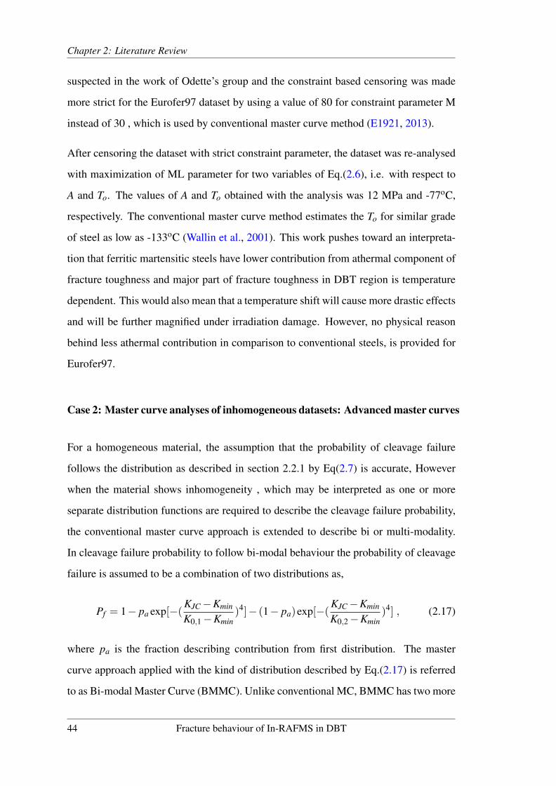
Chapter 2: Literature Review
suspected in the work of Odette’s group and the constraint based censoring was made
more strict for the Eurofer97 dataset by using a value of 80 for constraint parameter M
instead of 30 , which is used by conventional master curve method (E1921, 2013).
After censoring the dataset with strict constraint parameter, the dataset was re-analysed
with maximization of ML parameter for two variables of Eq.(2.6), i.e. with respect to
A and To. The values of A and To obtained with the analysis was 12 MPa and -77oC,
respectively. The conventional master curve method estimates the To for similar grade
of steel as low as -133oC (Wallin et al., 2001). This work pushes toward an interpreta-
tion that ferritic martensitic steels have lower contribution from athermal component of
fracture toughness and major part of fracture toughness in DBT region is temperature
dependent. This would also mean that a temperature shift will cause more drastic effects
and will be further magnified under irradiation damage. However, no physical reason
behind less athermal contribution in comparison to conventional steels, is provided for
Eurofer97.
Case 2: Master curve analyses of inhomogeneous datasets: Advanced master curves
For a homogeneous material, the assumption that the probability of cleavage failure
follows the distribution as described in section 2.2.1 by Eq(2.7) is accurate, However
when the material shows inhomogeneity , which may be interpreted as one or more
separate distribution functions are required to describe the cleavage failure probability,
the conventional master curve approach is extended to describe bi or multi-modality.
In cleavage failure probability to follow bi-modal behaviour the probability of cleavage
failure is assumed to be a combination of two distributions as,
Pf = 1− pa exp[−(KJC−Kmin
K0,1−Kmin)4]− (1− pa)exp[−(KJC−Kmin
K0,2−Kmin)4] , (2.17)
where pa is the fraction describing contribution from first distribution. The master
curve approach applied with the kind of distribution described by Eq.(2.17) is referred
to as Bi-modal Master Curve (BMMC). Unlike conventional MC, BMMC has two more
44 Fracture behaviour of In-RAFMS in DBT

Chapter 2: Literature Review
unknown parameters in comparison to conventional MC , which are the respective Kos
corresponding to 63.2% probabilities of respective distributions, namely, K0,1 and K0,2.
These two parameters are changed in terms of temperatures, T0,1 and T0,2, , which are the
respective reference transition temperatures. The relation describing the dependencies
of scaling parameters with reference transition temperatures are described as,
K0,1 =1
ln(2)1/4 (A+(100−A)exp[C(T −T0,1)] , (2.18)
K0,2 =1
ln(2)1/4 (A+(100−A)exp[C(T −T0,2)] . (2.19)
For BMMC analyses, there are 5 unknown parameters to be solved for, , which are T0,1
or K0,1, T0,2 or K0,2, pa, C and A.
The multi-model master curve or random inhomogeneity approach was applied on Euro
fracture dataset as well as ferritic/martensitic grade steel known as F82H by Lucon
and Scibetta (2011) and Sokolov and Tanigawa (2007). For F82H dataset of Sokolov
and Tanigawa (2007) the 50% median KJC predicted from conventional master curve
method did not describe the experimental fracture behaviour at lower temperatures for
the dataset of F82H , which resulted in inhomogeneity analysis of the dataset. How-
ever, instead of bimodal a multi-modal approach was applied by Sokolov and Tanigawa
(2007) , which then was found to be reciprocating the dataset behaviour accurately.
It was noticed, in both the cases presented here, that the deviation from the conventional
method , which was suspected, and also justified for both the datasets comprised two
or more differently sized specimens. In case of F82H (Sokolov and Tanigawa, 2007),
the 0.25T CT specimens were fabricated from 0.5T CT tested specimens and in Euro
fracture data the dataset contained 0.5T CT to 1T CT datasets.
In the case of Eurofer97 (Case 1), the loss of constraint was given importance and the
criteria of validity was made more strict with M of 80 and in case of F82H this was
ignored and inhomogeneity appeared to solve the problem. This observation suggests
that a dataset with a large thickness specimen having higher constraint and a very small
Fracture behaviour of In-RAFMS in DBT 45

Chapter 2: Literature Review
thickness specimen with greater loss of constraint may behave as two different mate-
rials, if proper constraint corrections are not applied, and therefore any non-identical
condition in a dataset may be statistically dealt by assuming different probability dis-
tribution assigned to those datasets. However, this kind of approach does not guarantee
any physical reasoning of the results, neither it ensures reproducibility and repeatability
of the results.
Similar material effect on dataset inhomogeneity was found in the analyses of Euro
fracture data, where a set of specimens made from a block (plate SX9) , which had a
different material history than other parts of the ring segment of RPV steel supplied by
Siemens from which the whole Euro fracture data was created. It was found that the
degree of inhomogeneity was more, if the dataset of SX9 was included in the master
curve analysis. The dataset was analysed by SINTAP, conventional Bimodal as well as
multi-modal methods and its was found that the overall variation in estimated To was
6oC and the scatter increased by including the dataset of SX9. The inhomogeneity was
confirmed by the fact that BMMC analysis resulted in pa of 0.91 , which was also the
percentage share of the data not coming from SX9 dataset ( the ratio of numbers of data
after excluding SX9 , which is 698 and complete dataset of 734 tests gives a ratio of
0.95 , which is close to pa).
2.2.5 Cleavage fracture: local approaches
The cleavage fracture event is modelled micro-mechanically by taking into considera-
tion the micro-crack generation in the vicinity of the volume ahead of the crack tip and
unstable propagation of the same. The micro-cracks, generated under opening mode,
may be parallel to the crack plane and therefore can have an angular distribution associ-
ated with the distribution of micro-cracks. The probability of non-failure event, Pn f for
a unit volume can be described as,
Pn f =∫
VP(a)g(θ)dadθ . (2.20)
46 Fracture behaviour of In-RAFMS in DBT

Chapter 2: Literature Review
where P(a)da describes the probability of finding a micro-crack oriented in single di-
rection of size between a and (a+da) in the volume V , which has suitable stress condi-
tions to be eligible to influence cleavage fracture directly. The function g(θ)dθ together
with P(a)da describes this probability for micro-cracks in all possible orientations. The
definition of this volume, sometimes referred as active volume or critical volume or V?
(Bonade et al., 2008; Ritchie et al., 1973; Tiwari et al., 2015), is a function of maximum
principal stresses both first and second (Mudry, 1987). If micro-cracks are assumed to
nucleate only at carbides for specific case of a steel such as low impurity ferritic steel
most micro-cracks will nucleate parallel to principal loading direction (Smith, 1966).
Additionally, assuming the volume V? to be divided into smaller volumes independent
of each other, the Pn f can be described as,
Pn f = exp[−φ(σ1) ·V ] , (2.21)
where φ(σ1) is the function of first principal stress. The effect of second principal
stress is neglected assuming planar micro-crack nucleation. The effect of second prin-
cipal stress is dominant for an angular distribution of micro-cracks and become more
predominant under pre-straining on both tensile and compressive kinds (Smith, 1966;
Beremin et al., 1983a; Mudry, 1987).
With Eq.(2.21) describing non failure event, the probability of cleavage fracture can be
described as,
Pf = 1− exp[−φ(σ1) ·V ] . (2.22)
The cleavage failure probability model as described by the probabilistic local approach
of WST (Wallin et al., 1986; Wallin and Laukkanen, 2008) assumes the Small Scale
Yielding (SSY) condition at the crack tip, , which in fact is also the basic assumption of
MC approach developed with active volume responsible for cleavage to be scaling with
BK4. The critical size of cleavage initiators (assumed to be spherical) responsible for
unstable failure in DBT region is assessed from Griffith’s instability criteria described
as,
rC =πE(γS + γP)
2(1−υ2)σ2yy
, (2.23)
Fracture behaviour of In-RAFMS in DBT 47

Chapter 2: Literature Review
where, E is elastic modulus, υ is Poisson’s ratio, γS is the surface energy of the matrix,
γP is the plastic work required for crack propagation and σyy is the applied mode-I stress
ahead of the crack tip. The probability of cleavage failure is then defined as,
Pf = 1−X=rpl
∏X=0
(1−P(r ≥ rC))NFBdXX sinθ , (2.24)
where X is the distance ahead of crack tip, r is the radius of a cleavage crack initiator,
rpl is the distance from the crack tip to the elasto-plastic interface, N is the number of
cleavage initiators, F is the fraction of N taking part in fracture process and θ is the
angle measured counter clockwise from the crack plane and P(r≥ rC) is the probability
of in-homogeneities such as carbides being critical in size to initiate cleavage. The
variables can be visualized in Figure 2.4.
FIGURE 2.4: Crack tip defining probability of cleavage failure according to Eq.(2.24)
Using non-dimensional parameter Q as,
Q =X
( Kσo)2
, (2.25)
and assuming self-similarity of stress fields or SSY condition, the integration otherwise
required in thickness direction can be avoided and the probability of cleavage failure
can be then written as,
Pf ∝ 1− exp−NFBsinθ
∫ Q=Qpl
Q=0P(r ≥ rC)QdQ , (2.26)
48 Fracture behaviour of In-RAFMS in DBT

Chapter 2: Literature Review
where Qpl is the value of Q at r = rpl . By assuming the integration part to be a constant
say ω (although it may not always be constant as discussed in next section) Eq.(2.27)
can be re-written as,
Pf = 1− exp(−ωBK4) , (2.27)
, which is the basis of size adjustment equation given in ASTM E1921. The size adjust-
ment equation used in MC method is described as,
KJC,1T = Kmin +(KJC,nT −Kmin) · (BnT
B1T)1/4 , (2.28)
where KJC,nT is the measured experimental fracture toughness of BnT inch thick speci-
men and B1T corresponds to 1 inch or 25 mm.
The stress dependence of reference unit volume and resulting probability of cleavage
failure of active volume ahead of crack tip results in similar expression as in Eq.(2.22)
and Eq.(2.26). For more details on the subject of local approaches towards cleavage
fracture is reviewed in great detail by Mudry (Mudry, 1987).
2.3 Reduced activation ferritic/martensitic steels: An Overview
The steels with high Cr content are known for its application in boilers, steam pipelines
and turbines of ultra-supercritical fossil power plants where the operating temperature
can result the structure to go up to 650oC (Abe et al., 2008). High Cr steels are also very
popular in power industry due to excellent creep properties, high thermal conductivity
and low thermal expansion coefficient (Klueh, 2005). Recently, the ferritic/martensitic
steels being the primary candidate material for fusion reactor first wall blanket appli-
cation have attracted attention across the globe (Moslang et al., 2005; Banerjee, 2014;
Odette and He, 2000; Yu et al., 2007; Sokolov and Tanigawa, 2007). Also due the ap-
plication of ferritic/martensitic steels in super critical water cooled reactors in cladding
and core components (Li et al., 2010), RAFM grade steels have been studied extensively
in the last decade.
Fracture behaviour of In-RAFMS in DBT 49

Chapter 2: Literature Review
The operational requirement of DEMO reactor requires the material to perform in the
temperature window of 350-550oC. The material is also required to have good resistance
against irradiation damage. The steels developed under the category of Reduced/Low
Activation Ferritic/Martensitic steels (RAFM/LAFM) are Eurofer97, F82H, JLF and
few older versions such as MANET and OPTIFIER . These fusion reactor grade steels
were developed with 9%Cr and 12% Cr steels as reference materials due to their already
proven creep strength and swelling resistance. In the series of RAFM grade steels men-
tioned before, the basic chemical composition follow that of Mod-9Cr-1Mo steel also
known as P91/T91 steels.
The RAFM differs from P91 steels in the chemistry due to the replaced high activity
(half-life>100Years) elements from Mod-9Cr-1Mo with elements of low activity but
same effect such as, W for Mo and Ta for Nb. Other transmutable elements are removed
by expensive vacuum arc melting process making this grade of steel most clean and low
activation.
Due to the wide spectrum of applicability of high Cr content tempered martensitic
steels, several studies have been carried out in all the dimensions, including microstruc-
tural, mechanical, irradiation, welding, ductile to brittle transition, tempering, thermo-
mechanical treatments, liquid metal embrittlement, electrical and magnetic aspects.
The most important property of steels having 9% Cr (unless otherwise mentioned the
percentage in this work refers to weight percentage) is its creep resistance , which is
attributed to its tempered martensitic lath structure. The microstructural aspects, how-
ever, remain dependent on the tempering temperature and duration. It has been found,
recently, by Mishnev et al. (2016), that in the range of 600-650oC the tempered marten-
sitic lath structure changes to sub-grain structure of low angle grain boundaries , which
results in lower density of dislocation. On the other hand, Sandim et al. (2015) on
his work on Eurofer97 steel, has revealed softening in hardness, drop in coercive field,
Vickers micro-hardness and increase in residual electrical resistivity at tempering tem-
perature approaching 500oC. These phenomena show the importance of precipitation
sequence of carbides, carbo-nitrides, and in few cases where boron is experimented,
50 Fracture behaviour of In-RAFMS in DBT

Chapter 2: Literature Review
nitrides play important role in the resulting properties. Besides the sequence of pre-
cipitation, the size distribution, preferable sites of carbides/carbo-nitrides/nitrides (Kli-
menkov et al., 2015) are also important. The elements taking part in these precipitates
are also given importance and have been investigated in several studies (Laha et al.,
2013; Moitra et al., 2014; Mythili et al., 2013; Vanaja et al., 2012; Rosenwasser et al.,
1979).
Abe et al. (2008), have investigated the coarsening of M23C6 carbides in 9Cr-W steels
where the effect of W on the creep property was studied. It was shown in his work that
W reduces the coarsening of M23C6 carbides at 600oC. Long term ageing of 10%Cr
tempered F/M steel showed that Cr and Mo content increases in M23C6 carbides at the
expense of Fe up to 51,072 h of creep exposure (Xu et al., 2016). Xu et al. (2016), very
recently, did systematic study of 10%Cr F/M steels under long term ageing to study the
kinetics of M23C6 carbides, and found that V starts diffusing in M23C6 at 650oC for
12,000 h to 25000 h. Additionally, interesting finding was also that V not only replaces
Fe but also W and Mo from M23C6 carbides.
The involvement of Cr, Mn, Mo, Nb, Ni, V along with Fe and C in M23C6 for 10%Cr
steel during tempering is shown in Figure 2.5. The plot shows results obtained from
JMat-pro software package (Saunders et al., 2003).
(a) Participation in M23C6 (b) Participation in MX
FIGURE 2.5: Participation of alloying elements in (a) M23C6 carbides and in (b) MX precipi-tates in 10%Cr steel obtained from JMat-Pro
The composition of M23C6 in Fig. 2.5 (a), shows clearly the continuous replacement of
Cr and Mo by Fe above 600oC. In Fig. 2.5 (b) the compositional changes in MX type
Fracture behaviour of In-RAFMS in DBT 51

Chapter 2: Literature Review
precipitates are shown, where it is clear that around 870oC, Nb starts replacing V. The
reason P91 steel was chosen to be the reference material for RAFM grade was not only
the creep strength but also the swelling resistance (Rosenwasser et al., 1979). On the
other hand, 12%Cr steels also showed similar properties under creep and irradiation.
The study of Ioltukhovsky et al. (1998) showed that 12%Cr steels were not susceptible
to swelling till 100-110 dpa of irradiation. At 120-142 dpa of irradiation swelling was
prominent at 400oC. The steel was also found not to be prone to irradiation embrittle-
ment at high temperature. The work of Danon and Alamo (2002) on Eurofer97 shows
prior austenitic grain boundary to be another important parameter , which affects the
performance of high Cr steels. The prior austenitic grain boundary was found not to
change till 1050oC and further was found to coarsen till 1200oC. The importance lies in
the fact that the martensite growth depends on the pre-austenitic grain boundaries and
martensite cannot continue to grow after it hits a pre-austenitic grain boundary. There-
fore, a coarser pre-austenitic grain boundary will result in larger laths of martensite
, which in turn will affect the creep, as well as fracture behaviour in ductile to brittle
transition due to the large inhomogeneity and associated weakest links for cleavage frac-
ture. In the recent work of Klimenkov et al. (2015), where B effect on micro-structural
aspects were studied, showed that B by forming BN, decreases the spatial distribution
of VN. This results in V enrichment in the matrix. The V enriched matrix makes it
preferable for V to replace Ta from TaC and also finds place in M23C6. Ta as a replace-
ment finds its place in VN by replacing V. The overall effect is the increment in width
of laths and thus micro-structural instability.
In the study of RAFM grade steel developed in India (In-RAFMS), four different combi-
nations of compositions by varying W and Ta content in close range with other alloying
elements similar in amount to popular RAFM steels were studied by Laha et al. (2013).
It was found in the study that the low cycle fatigue life increased with W and Ta con-
tent, however, tensile properties were not affected. The most sensitive property to the
content of W and Ta investigated was creep rupture strength. Furthermore, it was also
discovered that W and Ta affected the Ductile to Brittle Transition (DBT) behaviour.
52 Fracture behaviour of In-RAFMS in DBT

Chapter 2: Literature Review
In a different study on 9%Cr RAFM grade steels, Tan et al. (2013) discovered that
thermo-mechanical treatment comprising hot rolling after normalizing and before tem-
pering to the extent of 60% thickness reduction, resulted in superior tensile strength
with negligible loss in ductility to oxide dispersion strengthen RAFM grade steels. The
reason was attributed to the refinement of subgrains and M23C6 and MX type precipi-
tates.
The effect of V and Ta on Ferritic/Martensitic steel has been extensively studied by
Xiao et al. (2013) on 12%Cr steel recently developed for application upto 650oC with
better creep properties than conventional 9%Cr RAFM grade (Murty and Charit, 2008).
The effect of delta ferrite the shape of MX type precipitates was investigated and it was
found that there are TaC rich MX type precipitates and V-N-rich MX type precipitates.
The Ta-C rich precipitates do not dissolve in the solutionizing stage and while temper-
ing, new precipitates of this type also add up. On the other hand, V-N-rich precipitates
only show up while tempering. In the study of steels without V and Ta, with V ,and with
both V and Ta, micro-alloyed in Cr-W based steel, Xiao et al. confirmed that M2X type
precipitate form in first type of allow in absence of V and Ta. In presence of V only, V-
rich carbo-nitrides take over M2X and in presence of both V and Ta, both V-N rich and
Ta-C rich precipitates form. The shape of MX precipitates were observed to be planar
within delta ferrite and it was concluded that V and Ta stabilize the MX precipitate in
comparison to detrimental M2X phase.
Summarizing the investigations carried out on 12%Cr-steels, 9%Cr steels, and RAFMS,
it can be concluded that major properties of high chromium tempered martensitic steels
are delineated by the kinetics and spatial distribution of M23C6 and MX precipitates,
pre-austenitic grain size and lath structure of martensite. The precipitate size distribu-
tion and morphology with its influence on DBT fracture behaviour of In-RAFMS is
further discussed in Chapter 4. The major features of RAFM grade , which makes it
the structural material are good swelling resistance and creep strength. The crucial as-
pect of probability of catastrophic fracture remains open for In-RAFMS in DBT region,
which is explored in depth in this work.
Fracture behaviour of In-RAFMS in DBT 53

Chapter 3
Problem formulation
In this chapter, the methodology to meet the objectives described in Chapter 1 are dis-
cussed. The test matrix is then sketched to address the formulated problem. Subse-
quently the structure of the thesis is described.
For the fail-safe design approach, the characterization of fracture behaviour of In-
RAFMS, requires the understanding of micro-mechanical aspects of cleavage failure
probability, in DBT region. Additionally, the probabilistic distribution of cleavage frac-
ture event and effects of parameters such as loading rate, loading type and loss of con-
straint (out of plane-thickness and in-plane-crack depth) on cleavage fracture, also need
extensive understanding for qualification of the structural component and its safety.
As discussed in Chapter 1 and Chapter 2, the structural integrity of first wall blanket is
crucial as this part faces most of the irradiation. The transmutation safety requirements
control the activity issue, and the engineering of material can focus on the damage which
may be induced by high energy neutron irradiation. The operational conditions demand
avoiding catastrophic failure of the component, which may be caused by upward shift
in ductile to brittle transition temperature due to irradiation. The fast fracture mode of
cleavage makes the DBTT an important parameter to examine in comparison to creep
and swelling. Owing to the component’s importance in structural integrity of fusion
reactor, not only the material but also the approach or methodology which described the
probability of catastrophic failure event, is under scrutiny.
The most promising methodology which has come up to the standard of analysing cru-
cial components structural integrity is the master curve methodology as discussed in
54

Chapter 3: Problem formulation
Chapter 2. It has also been reviewed in Chapter 2 that RAFM grade has shown devia-
tion from the conventional approaches of this methodology with Eurofer97 and F82H
as examples.
The methodology of master curve like any other standard analysis method is based on
certain assumptions as discussed in Chapter 2. The cleavage event formulation under
self-similar stress field at the crack tip is generally a condition which is often violated
in fracture mechanics. Moreover, the future objective of fusion reactor components’
structural integrity needs irradiation studies on the mechanical behaviour of component
materials, which in turn imposes small specimen testing requirement. Therefore, it
becomes important to understand, the extent to which the conventional approach can
handle the loss of constraint associated with small specimens. Further, it is required to
explore the possibilities for correcting the effects of loss of constraint.
In order to meet the objective of this work, the formulated area of studies are discussed
below describing also the scope of this work.
Categorizing aforementioned requirements helps in formulating the studies of this work.
The loss of constraint and corrections, which can make the conventional master curve
approach usable for probabilistic analysis of cleavage fracture, includes examination of
master curve approach due to loss of inplane as well as out of plane constraint. The
tests on smaller specimens and shallow and deep cracks are performed and numerical
approaches are used to investigate the problems of both types of constraint loss phe-
nomena.
The pulse mode operation of ITER also imposes the condition of sudden change in
loading rate, which may cause an added upward shift in DBTT in addition to that caused
by irradiation. Therefore, a study of master curve approach at higher loading rate is also
carried out using Indian RAFMS small specimens. Additionally, the fracture behaviour
in upper DBT region is studied in greater detail with an objective to explore the domain,
where no standard fracture mechanics or probabilistic approach exists at present. The
upper region of of DBT is one such regime where a strong methodology, such as master
curve method, does not exist. The cleavage fracture in this region of DBT is so far not
Fracture behaviour of In-RAFMS in DBT 55
Chapter 3: Problem formulation
characterized by any global approach which can estimate a parameter such as reference
transition temperature. It is required, therefore, to establish a method, which combines
ductile tearing and cleavage fracture together to examine the probability of catastrophic
fracture after ductile tearing.
The understanding of size effect on fracture behaviour requires the assessment of both
out of plane and in-plane constraint loss in three dimension. Therefore, the finite ele-
ment study for assessment of constraint change with the variation in size, type of load-
ing, and ductile tearing prior to cleavage is required. The micro-mechanical aspects of
cleavage fracture mechanisms are pre-requisite to the understanding of cleavage frac-
ture probability distribution in DBT region, which is also included in the scope of this
work. To meet the objectives of this work as defined in Chapter 1, the modified 9%Cr-
1%Mo steel which is the reference material for RAFM grade steels is also examined
and compared with responses of In-RAFMS.
3.1 Test matrix
With the above discussion on the salient desirable outcomes of this investigation, the
extensive testing program for characterization of fracture behaviour of In-RAFMS in
DBT region is categorized as given below.
1. Tensile testing as pre-requisite for fracture toughness measurements
2. Fracture testing for assessment of loss of constraint ( both out of plane and in
plane)
3. Fracture testing for assessment of loading rate effect
4. Fracture testing for assessment of loading type
5. Fracture testing for assessment of fracture behaviour on upper region of DBT
Different geometries under three point bending and tension were tested under different
loading rates and test temperatures. The detailed test matrix is described in Table 3.1.
56 Fracture behaviour of In-RAFMS in DBT

Chapter 3: Problem formulation
TABLE 3.1: Test matrix for fracture property assessmentTest conditions Test Temperatures Tesnile tests Fracture tests Material
Quasi-static0.5 mm.min
-110oC, -120oC, -130oC,-140oC, -150o
2 specimenper temperature
TPB , CT In-RAFMS, P91
100 mm/min-80oC,-100oC
2 specimenper temperature
Standard charpyTPB
In-RAFMS
1000 mm/min-80oC,-100oC
In-RAFMS
Impact toughness27oC, -30oC, -50oC,
-85oC, -100oC, -115oC-130oC, -170oC, -196oC
In-RAFMS, P91
Fracture behaviour of In-RAFMS in DBT 57

Chapter 4
Material
In this chapter the micro-structural aspects, phases and their transformation kinetics,
heat treatment, and the properties, distributions, and types of precipitates in In-RAFMS
are discussed. With the objective to characterize the fracture behaviour of In-RAFMS,
more focus is given to In-RAFMS and only necessary and relevant studies are performed
on mod-9Cr-1Mo steel as and when required.
4.1 Material: Ferritic/Maretensitic steels
To correlate the structure and property of ferritic/martensitic steels, firstly, it is important
to understand the system of ferritic/martensitic steels and changes occurring by small
differences in amount of alloying elements and heat treatment dictating pre-austenitic
grain boundaries, transformation temperatures and carbides structures. Secondly the
importance of micro-structure and its effect on fracture is required.
In this work of investigation, to understand the fracture behaviour in DBT region two
grades of ferritic/martensitic steels are studied, which are In-RAFMS and P91 or Mod-
9%Cr−1Mo steels.
The fusion reactor grade In-RAFMS, as discussed in Chapter 1, is derived from P91
grade and is made cleaner by removing the transmutable and tramp elements by vacuum
remelting. The two grades therefore differ in the amount of tramp elements. The heat
treatment given to these grades are close and the micro-structure for both the steels
show tempered martensite with precipitates of Chromium, Tungsten/Molybdenum and
58

Chapter 4: Material
Vanadium/Tantalum located at inter lath and pre-austenitic grain boundaries as well as
inside laths of martenstites.
The heat treatment of both grades are designed for better creep strength and weldability.
Both of the grades are air-cooled after tempering to avoid Z and Lave phases which are
detrimental both for creep as well as DBTT.
4.2 Microstructural characterization of In-RAFMS
Both grades of ferritic/martensitic steels studied in this work, namely In-RAFMS and
mod-9Cr-1Mo, show tempered martensitic microstructure. The carbides of Cr are found
on the pre-austenitic grain boundaries and Ta/V carbides are dominantly present inside
laths. The two grades show similar phases with close range of equilibrium and non-
equilibrium phase transformation temperatures. The details of the equilibrium phases
and microstructural features are discussed in detail below.
4.2.1 Phase transformation and heat treatment
The shape and size of precipitates, homogeneities and temperature dependencies of pre-
cipitates dictate the crack direction, cleavage failure initiation, propagation and driving
force for fracture to occur and therefore, it is necessary to understand this system before
characterization of fracture behaviour statistically.
The spatial distribution of precipitates, and its effect on Ductile to Brittle Transition
(DBT), as well as phase transformation are studied for two grades of ferritic/martensitic
steels. More focus is given to In-RAFMS and the properties are compared with other
popular RAFMS as well as high Cr tempered martensitic steels. The chemical composi-
tion and heat treatment given to In-RAFMS and P91 steels are shown in Table 4.1. The
phase transformation for isothermal conditions for P91 and In-RAFMS are calculated
using ThermoCalc software (Andersson et al., 2002) package as well as experimentally
from dilatometry analyses. The non-isothermal martensitic transformation temperatures
Fracture behaviour of In-RAFMS in DBT 59

Chapter 4: Material
TABLE 4.1: Chemical composition of ferritic/martensitic steels investigatedMod-9Cr-1Mo
Solutionized at 1050oCTempered at 770oC, 1hr
C Cr Mo V Nb Si Mn S N Al Ni0.104 8.76 0.98 0.2 0.08 0.9 0.49 0.002 0.02 0.002 0.28
In-RAFMSSolutionized at 977oC
Tempered at 760oC, 1hrC Cr W V Ta Si Mn S N Al Ni
0.08 9.15 1.37 0.24 0.08 0.026 0.53 0.002 0.02 0.004 0.004
are calculated using empirical correlations available in literature. The dilatometry re-
sults for mod-9Cr-1Mo as well as In-RAFMS are shown in Figure 4.1. It is evident
that the phase transformation behaviour of both mod-9Cr-1Mo and In-RAFMS is sim-
ilar except in the tempering region where strain gradient against temperature increases
for mod-9Cr-1Mo. The austenitic start (As) and finish (A f ) as well as martensitic start
(Ms) and (M f ) temperatures of both steels are very close. As visible in Figure 4.1, the
solutionizing behaviour for In-RAFMS and mod-9Cr-1Mo is similar. Whereas, during
tempering, unlike the slope of In-RAFMS which remains unchanged, mod-9Cr-1Mo
steel shows a significant change in slope. This difference in tempering region may be
attributed to Z and Lave phases formation which differs in two grades. In-RAFMS lacks
the tramp elements which form these precipitates. The Lave and Z phases formation is
avoided in manufacturing process by air-cooling the plates of steels after tempering. In
dilatometer, however, the cooling rate was slow enough to cause the precipitation of
undesirable Z and Lave phases. The transformation temperatures are shown in Table
4.2 along with the basic chemical compositions of different ferritic/martensitic grade
steels.
The operational parameters of DEMO fusion reactor, as discussed in Chapter 1 and
3, may cause microstructural changes during service. To understand this scenario the
equilibrium phase diagram was calculated for P91 as well as In-RAFMS. The two phase
diagrams are shown in Figure 4.2.
60 Fracture behaviour of In-RAFMS in DBT

Chapter 4: Material
(a) Solutionizing and Air cooling
(b) Tempering
FIGURE 4.1: Dilatometer response of In-RAFMS and P91 steels (a) while solutionizing andaircooling and (b) tempering
Fracture behaviour of In-RAFMS in DBT 61

Chapter
4:M
aterial
(a) (b)
FIGURE 4.2: Phase diagram of (a) In-RAFMS and (b) P91 calculated with chemical composition estimated from Optical Emission Spectroscopy
62Fracture
behaviourofIn-RA
FMS
inD
BT

Chapter 4: Material
The maximum temperature under operation is 500oC which is much lower than the As
temperature of all popular grades of RAFMS as shown in Table 4.2. It is realized from
the equilibrium phase diagram that the inter-critical region, of ferrite and Austenite
phases, is ≈ 50oC.
The critical issue might be, therefore, the close values of tempering temperature which
is 760-780oC and As temperature for RAFM grade steel falling in range of 770oC to
890oC. Any tempering process depending on its accuracy might cause some Austenite
transformation.For better view and comparison of various popular grades of RAFM
steels Table 4.2 is referred. The Ms temperatures, for all grade of steels in Table 4.2 are
calculated using different empirical equations available in literature (Andrews, 1965;
Steven and Haynes, 1956; Kunitake and Ohtani, 1969; Kunitake, 2001; Tamura, 1970;
Eldis, 1977; Kung and Rayment, 1982; Andersson et al., 2002; Xu et al., 2016; Danon
and Alamo, 2002; Zilnyk et al., 2015).
From above discussion, and Table 4.2, it becomes clear that for the grades of steels
compared with basic composition of 9-12%Cr-W/Mo-Ta/Nb-V, the transformation tem-
peratures are in very close range. Therefore, depending on the tempering process the
pre-austenitic grain structure, and size and distribution of carbides, can be monitored.
Therefore, the fracture of these steels are dictated by the structure of pre-austenitic grain
boundaries and carbides type, size and its distribution.
Fracture behaviour of In-RAFMS in DBT 63

Chapter
4:M
aterial
TABLE 4.2: Comparison of various ferritic/martensitic grade steelsMaterial C (Wt%) Mn (Wt%) Cr (Wt%) Ni (Wt%) Mo/W (Wt%) Nb/Ta (Wt%) V (Wt%) Si (Wt%) Ms−1 (oC) Ms−2 (oC) Ms−3 (oC)10Cr steel 0.11 0.5 10.22 0.55 1.42 0.5 0.2 332.9 288.8 333.2F82H-Mod 0.09 0.156 7.68 0.021 1.04 0.1 0.162 395.7 364.9 396optifier-736 0.1 0.38 8.46 0.076 0.21 384.6 340.3 384.9optifier-734 0.13 0.61 9.41 0.095 0.277 351.2 301.3 351.6optifier-735 0.13 0.55 9.48 0.065 0.245 354.3 304.7 354.7In-RAFM 0.08 0.53 9.15 0.004 1.37 0.08 0.24 0.01 367.7 328.4 367.9P91 0.1 0.49 8.76 0.28 0.98 0.08 0.2 0.19 361.5 321.1 360.4Eurofer97 0.11 0.56 9.08 1.07 0.125 0.235 359.4 318.6 359.7ODS Eurofer 0.07 0.408 8.92 1.11 0.081 0.193 0.11 380 341.1 379.5JLF 0.1 0.64 8.93 0.49 1.96 0.1 0.21 345.6 308.8 345.8La12LC 0.09 1.13 8.92 0.73 0.1 0.3 0.03 353.3 302.8 353.4LA12TALC 0.1 1.13 9 0.73 0.1 0.3 0.03 347.7 297.2 347.79.15Cr-0.08C 0.08 9.15 394.1 351.5 394.4
Ms−4 (oC) Ms−5 (oC) Ms−6 (oC) Ms−7 (oC) Ms−8 (oC) Ms−9 (oC) As(oC) Af(oC) Ms(oC) Mf(oC)Cooling
rate (K/s)10Cr steel 453 462.3 276.8 243 262.9 256.6 312 193F82H-Mod 492 492.1 361 323 347.3 342.9 850* 1 910* 430* 60optifier-736 503 503.2 339.4 328.5 324.3 325optifier-734 479 479 297.7 293.7 281.4 282.2optifier-735 483 483.4 300.6 295.7 285.3 286.1In-RAFM 477 476.7 319.9 282.3 302.1 295.6 778 875P91 469 474.7 314.4 283 301.5 297.2Eurofer97 470 470.1 311.5 282 295.1 290.3 820-860 † 2 880-970 360 † 0.1-1000ODS Eurofer 490 490.4 333.2 297.1 317.8 312.6 835-875 † 915-985 † 380 † 1/∞-30JLF 443 451.1 299.9 253 284.9 275.5 842 † 895 † 380 † 200 † 160.0La12LC 466 466 300.9 284.7 281.3 277.5 807 † 875 † 375 † 200 † 45.0LA12TALC 461 460.8 294.9 279.4 275.7 272 820 † 940 † 402 † 200 † 90.09.15Cr-0.08C 523 522.9 346.2 330.8 338.1 339
1*Obtained from ThermoCalc/Jmat or experimentally2† Obtained from literature
64Fracture
behaviourofIn-RA
FMS
inD
BT

Chapter 4: Material
4.2.2 Microscopy: precipitates and micro-structure
The micro-structure of ferritic/martensitic grade steels is typical tempered martensite
structure. The tempering, as can be seen in Table 4.1, is performed at relatively higher
temperature, in order to avoid any in-service shape/ size change of precipitates, or phase
transformation. The optical image of the microstructure is shown in Figure 4.3. The
optical image of the microstructure shows the pre-austenitic grain boundaries decorated
with carbides in dark. The lath structures are also visible in the microstructure for both
the steels.
The microstructural analysis and distribution of carbides are also studied using Scanning
Electron Microscopy (SEM) for ductile failure, brittle failure and for the intermediate
zone of combined ductile and brittle failure. The optical microstructure shows that the
pre-austenitic grain size for both the steels are close which is reportedly 15 µm (Laha
et al., 2013). A ductile to brittle transition may occur in a specimen where the initial
crack starts propagating in ductile manner and due to changing crack tip stress fields the
fracture mode can change to cleavage. The distribution of carbides as visible in Figure
4.3 shows that the random distribution of carbides as assumed in the formulation of
master curve (Chapter 2) may not be very accurate. The carbides of larger sizes as will
be discussed more based on the SEM images in this chapter, are dominantly present at
the pre-austenitic grain boundaries. This local segregation of more potential cleavage
initiators in comparison to the smaller carbides present elsewhere may be quantified as
a function of grain size and/or lath size.
Spatial distribution of carbides; Image analyses
The fracture in complete cleavage fashion found at -120oC was used for EDXs mapping
at the area near secondary crack and was analysed for Cr, V and Ta. The intensities of
Cr, V and Ta as shown in Figure 4.4 (a), Figure 4.4 (c) and Figure 4.4 (e) were altered
by changing the threshold limits of intensities by shrinking the band to the spectrum
of pixels of the image. The image intensity shows a Gaussian distribution. To find
Fracture behaviour of In-RAFMS in DBT 65

Chapter 4: Material
(a) Mod-9Cr-1Mo
(b) In-RAFMS micro-structure
FIGURE 4.3: Optical Microstructure of In-RAFMS and P91 taken after etching the polishedspecimens with 5% Nital for 30 seconds
the maximum frequency intensities this distribution of imgae intensity, for all three
elements (Cr, V, Ta), were filtered with the limits (α) as 52(≤ α ≤)172 (α is the filter-
ing parameter), so that the intensity spectrum lies in twice of standard deviation range.
These images are shown in Figure 4.4 (b), Figure 4.4 (d) and Figure 4.4 (f). The image
in Figure 4.4 (g) was also altered in order to visualize the white precipitates decorating
lath and pre-austenitic grain boundaries clearly as shown in Figure 4.4 (h). The altered
pictures were then stacked over on the mapped area image shown in Figure 4.4 (h). The
stacked image containing Cr, V, Ta intensities over micro-structure is shown in Figure
4.5. The carbides as discussed earlier in Chapter 2 are generally M23C6 type and MX
type. From the phase diagram, it is also evident that M23C6 is highly stable for In-
RAFMS till As. The precipitates of M2X are ignored due to the presence of V and Ta as
66 Fracture behaviour of In-RAFMS in DBT

Chapter 4: Material
(a) Chromium (b) Chromium thresheld
(c) Vanadium (d) Vanadium thresheld
(e) Tantalum (f) Tantalum thresheld
(g) Fracture surface (h) Fracture surface recolored
FIGURE 4.4: EDXS intensities and respective thresholds for image analysis
Fracture behaviour of In-RAFMS in DBT 67

Chapter 4: Material
FIGURE 4.5: EDXs intensity threshold prediction of distribution of carbides
discussed earlier. The lave phases in In-RAFMS are avoided by air cooling the ferritic/-
martensitic steels after tempering. Therefore, the microstructure of In-RAFMS contains
mainly M23C6 carbides which are larger in size in comparison to MX precipitates, and
are located at the boundaries unlike MX precipitates of V and Ta, which are located in-
side the grains as visible in Figure 4.5. The M23C6 precipitates, as can be inferred from
Figure 2.5 would contain around 58% of Cr, 17% of Fe and W/Mo and insignificant
amount of V and Ta/Nb for 10% Cr ferritic/martensitic steel at 740oC. The enriched V,
Ta matrix will cause MX type carbides inside grains and sub-grains for RAFMS grade
owing to its less N2 content. The size of carbides of M23C6 type has been reported to
be 200 nm (Vanaja et al., 2013), which is also evident from Figure 4.4(g).
The SEM image of crack area after etching as shown in Figure 4.4(g) clearly reveals the
carbides decorating lath interfaces and pre-austenitic grain boundaries. The carbides
on pre-austenitic grain boundaries are also visible in the optical micro-graph shown in
Figure 4.3. The carbide precipitates were also observed within pre-austenitic grains on
the lath interfaces.
Although, in the Figure 4.5, it seems that the prediction by the image analyses matches
the spatial location of precipitates; it is also observed that many of the points fall on
the area (very small) where no precipitates are visible in the SEM image. The reason is
that the EDXs signals of the elements are not very strong in the raw form i.e. in Figure
68 Fracture behaviour of In-RAFMS in DBT

Chapter 4: Material
4.4. Therefore, the stacking procedure though is proven to be promising, depends on
the initial signal of the elements scanned for.
4.3 Summary
The microstructure, equilibrium phases and transformation temperatures of phases, car-
bides and spatial distribution of carbides qualitatively were studied for In-RAFM and
mod-9Cr-1Mo steels. The phase transformation for the two steels were studied by
measuring unidirectional expansion/contraction in dilatometry test. The microstructure,
phase transformation (both equilibrium and non-equilibrium) were compared with other
popular grades of steels with similar composition and application. The comparison was
made with the help of available literature data and emprical correlations.
The equilibrium phase calculations using numerical methods showed that the austenitic
and ferritic transformation temperatures for the two steels very close. Similar is the
observation for non-equilibrium phase transformation of martensite. The kinetics of
phase transformation differs in the tempering region for P91, due to the precipitation of
undesired Z and Lave phases.
The microstructure of two steels shows pre-austenitic grain boundaries and lath inter-
faces decorated with M23C6 carbides (M is a combination of Cr, W, Fe) and intra lath
regions with MC type carbides of Ta/V. The reported size of M23C6 carbides are in the
range of 100-300 nm with average size of 200 nm. The average size of MC carbides are
20 nm.
In case of P91 steel, the carbides were larger in size. The segregation of larger car-
bides on pre-austenitic grain boundaries makes the P91 steel inferior in comparison to
In-RAFMS. The clean grade of In-RAFMS is expected to be free of detrimental precip-
itates of P, which are generally the weak links in P91 steels.
Fracture behaviour of In-RAFMS in DBT 69

Chapter 5
Experimental and Numerical methods
In this chapter, the detailed description of the tensile and fracture tests, temperature
control and test fixtures are described. In the second part of the chapter the descriptions
of finite element models used for different studies such as effect of loading rate, size of
specimens, type of specimens (CT and SE(B)) are detailed. The finite element analyses
to model boundary layer formulation, ductile damage for simulating cleavage with prior
DCG are also described.
5.1 Experimental set-up
The fracture tests as well as tensile tests were performed on servo-hydraulic universal
testing machine at sub-zero temperatures. The cylindrical specimen of 4 mm diameter
and 20 mm parallel length were used for measurement of tensile properties. The fracture
specimen of different size and dimensions were tested using Compact Tension (CT) and
Single Edge cracked Bend (SE(B)) specimens. The details of the specimen geometries
used for different purpose are described in corresponding chapters. The In-RAFMS
was obtained in hot rolled and tempered condition from Mishra Dhatu Nigam Ltd.,
Hyderabad, India in the form of 12 mm, 8 mm and 6 mm thick plates. The tensile
specimens were fabricated from 6 mm thick plate. The fracture specimen of both CT
and TPB geometries were fabricated from 12 mm thick plates. The engineering drawing
of tensile specimen is shown in Figure 5.1.
70

Chapter 5: Experimental and Numerical methods
FIGURE 5.1: Engineering drawing of tensile specimens
The SE(B) specimen drawing is shown in Figure 5.2. The first lot of fracture specimens
were fabricated with a thickness of 10 mm for both Three Point Bend (TPB) and CT
geometries. The CT specimens were scaled for 0.5T CT according to ASTM E1921,
although the thickness of the specimens were 10 mm. Therefore, the CT specimens are
referred in this document as 0.4T CT and TPB as 0.4T TPB or 0.4T SE(B) specimens.
The drawing of 0.4T CT specimens are shown in Figure 5.2. The TPB specimen were
scaled in all directions according to ASTM E1921, as shown in Figure 5.2.
For assessment of effect of size, broken 0.4T TPB specimens were used and 0.2T spec-
imen of 5×5×27 mm3 were fabricated. Standard and sub-sized Charpy specimens of
10 mm and 5 mm thickness were also fabricated as discussed in corresponding chapters.
Fracture behaviour of In-RAFMS in DBT 71

Chapter
5:E
xperimentaland
Num
ericalmethods
(a)
(b)
FIGURE 5.2: Engineering drawings of fracture speicmens (a) 0.4T CT specimen drawing and (b) 0.4T TPB specimen drawing
72Fracture
behaviourofIn-RA
FMS
inD
BT

Chapter 5: Experimental and Numerical methods
FIGURE 5.3: 0.4T CT specimen tested at sub-zero temperature in environmental chamber usingUTM
The fracture tests were performed after pre-cracking the specimens to desired crack-
depths using RUMUL resonent fatigue testing machine at R = 0.1 with decreasing load
algorithm to ensure Kmin , which is 20 MPa is never exceeded to avoid warm pre stress-
ing at sub-zero temperatures (E1921, 2013; Wallin, 2004, 2003).
The fracture as well as tensile testing was performed for different parametric studies
by placing those in an environmental chamber and the test temperature was maintained
with an accuracy of ±1oC by re-circulating liquid N2 in the chamber. The CT and TPB
tests performed in environmental chamber at sub-zero temperatures. Image showing the
test fixture and environmental chamber is shown in Figure 5.3 and Figure 5.4 for CT
and SE(B) specimens, respectively.
The similar test specimens were tested for P91 grade steel and the details of the spec-
imen geometries of both the grades are described in Appendix-C. The complete test
FIGURE 5.4: 0.4T TPB specimen tested at sub-zero temperature in environmental chamberusing UTM
Fracture behaviour of In-RAFMS in DBT 73

Chapter 5: Experimental and Numerical methods
matrix of tensile tests, fracture tests, impact tests performed on In-RAFMs and P91
steels specimens is provided in Table 5.2.
74 Fracture behaviour of In-RAFMS in DBT

Chapter
5:E
xperimentaland
Num
ericalmethods
TABLE 5.1: Datasets generated for different parametric studiesObjective Test Temperature loading rate No. of Tests Specimen geometry Specimen size a/W
Assessment ofconstraint loss (out of plane)
-110oC, -120oC, -130oC,0.5 mm/min 29 TPB
0.2T (5×5×27) 0.5-140oC -150o 0.2T (5×10×55) 0.5
Assessment ofconstraint loss (in plane)
-110oC, -120oC, -130oC,0.5 mm/min 29 TPB
0.2T (5×5×27)0.3-0.7
-140oC -150o 0.2T (5×10×55)
Assessment ofloading rate
-80oC, -100oC0.5 mm/min
29 TPB0.4T (W = 25,B = 10mm)
0.5100 mm/min1000 mm/min
Assessment ofloading type
-110oC, -120oC, -130oC,0.5 mm/min 29
TPB 0.2T (5×10×55) 0.5-140oC -150o CT 0.4T (10×10×55) 0.5
Assessment of prior ductile tearing on cleavage 1
1Dataset of 0.2T TPB for MC analysis was used for upper DBT region
FracturebehaviourofIn-R
AFM
Sin
DB
T75

Chapter 5: Experimental and Numerical methods
TABLE 5.2: All type of tests with experimental conditions performed in this work
Type of Test No of tests Material Test temp (oC) Loading rate Specimen Type
Tensile 2 per tempIn-RAFMs
300, 200, 100,RT,-50, -70,
-110, -120, -130,-140 , -150, -196
0.5mmpm
M6 Tensile-80,-100 100 mmpm
-80,-100 1000 mmpm
P91-60,-70,
-100,-1100.5mmpm
Impact5 per temp In-RAFMs
RT ,-30,-50,-85,-100,115,
-133,-177,-189 Standard Charpy
5 per temp P91RT, 0, -30, -50,
-77, -89, 95, -190
Fracture tests
26
In-RAFMs
-50, -70, -110, -120,-130 , -140 , -150
0.5mmpm
CT
33 TPB (0.4T TPB)
39 TPB (0.2T TPB)
10 -80,-100100 mmpm
TPB (0.4T TPB)
18 -80,-100 TPB (0.4T TPB)
12
P91
-60,-70
0.5mmpm
CT (1T)
15 -100,-110 TPB
20 -110 CT (0.16 T)
5.1.1 Metallographic studies
The In-RAFMS and P91 steel specimens were used for the study of phases, grain size
and carbides’ spatial distribution. For these studies and also for the damage study by
observation of voids steel specimens of both grades, metallographic specimens were
obtained from broken fracture test specimens. The specimens were polished on SiC pa-
pers followed by suspension polishing. The polished specimens were etched by dipping
the specimens in 5% and 10% Nital (mixture of HNO3 and H2O). The metallographic
studies were performed under both optical as well as scanning electron microscopy. The
76 Fracture behaviour of In-RAFMS in DBT

Chapter 5: Experimental and Numerical methods
broken specimen used for study of ductile damage were cut normal to the crack plane
and polished.
5.1.2 Tensile and Charpy testing
The tensile tests were performed on the specimens described in section 5.1. The speci-
mens were tested in the environmental chamber as discussed in section 5.1. The tensile
tests were performed in the range of -50oC to -150oC. The load displacement record
obtained from the UTM were used for calculation of engineering stress and strain. The
elastic modulus was calculated at room temperature by testing the tensile specimen with
extensometer. The Elastic modulus measured at room temperature was 207 GPa. The
elastic modulus variation with temperature used for fracture toughness measurement
followed the correlation given by Moattari et al. (2016).
The charpy tests were performed in a CEAST impact testing machine of 300 Joules
capacity. The standard charpy specimens were soaked in cooling bath for 30 minutes.
At each temperature five specimens were tested and average was used for the sigmoidal
fitting as described in Chapter 6. The cooling bath were made by cooling ethyl alco-
hol with the help of liquid nitrogen and dry ice. The temperatures below -60oC were
achieved by cooling the alcohol with liquid nitrogen only. Temperature below -100oC
were achieved by cooling a bath of isopentane. The results of charpy tests are provided
in Chapter 6.
5.1.3 Fracture toughness testing and measurement in DBT region
Before performing the fracture tests the specimens of different geometries were pre-
cracked under cyclic loading. The fatigue precracking was performed on RUMUL res-
onant fatigue testing machine. The precracking followed a decreasing load algorithm
with the intention to have maximum K less than 20 MPa m1/2 in all cases.
The fracture tests were performed on the UTM in environmental chamber as described
in section 5.1. The load load line displacement record was used for fracture toughness
Fracture behaviour of In-RAFMS in DBT 77
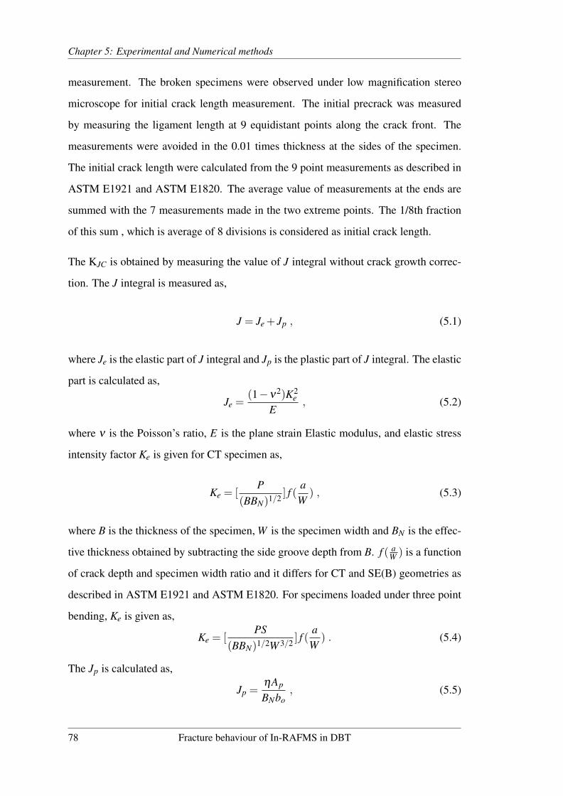
Chapter 5: Experimental and Numerical methods
measurement. The broken specimens were observed under low magnification stereo
microscope for initial crack length measurement. The initial precrack was measured
by measuring the ligament length at 9 equidistant points along the crack front. The
measurements were avoided in the 0.01 times thickness at the sides of the specimen.
The initial crack length were calculated from the 9 point measurements as described in
ASTM E1921 and ASTM E1820. The average value of measurements at the ends are
summed with the 7 measurements made in the two extreme points. The 1/8th fraction
of this sum , which is average of 8 divisions is considered as initial crack length.
The KJC is obtained by measuring the value of J integral without crack growth correc-
tion. The J integral is measured as,
J = Je + Jp , (5.1)
where Je is the elastic part of J integral and Jp is the plastic part of J integral. The elastic
part is calculated as,
Je =(1−ν2)K2
eE
, (5.2)
where ν is the Poisson’s ratio, E is the plane strain Elastic modulus, and elastic stress
intensity factor Ke is given for CT specimen as,
Ke = [P
(BBN)1/2 ] f (a
W) , (5.3)
where B is the thickness of the specimen, W is the specimen width and BN is the effec-
tive thickness obtained by subtracting the side groove depth from B. f ( aW ) is a function
of crack depth and specimen width ratio and it differs for CT and SE(B) geometries as
described in ASTM E1921 and ASTM E1820. For specimens loaded under three point
bending, Ke is given as,
Ke = [PS
(BBN)1/2W 3/2 ] f (a
W) . (5.4)
The Jp is calculated as,
Jp =ηAp
BNbo, (5.5)
78 Fracture behaviour of In-RAFMS in DBT
Chapter 5: Experimental and Numerical methods
where bo is the initial ligament length. The plastic part of area under load displacement
curve is obtained as,
Ap = A− 12
CoP2 , (5.6)
where A is the area under the load displacement curve , which is calculated in this
work by applying Simpson’s trapezoidal rule to the load displacement data points.Co is
the reciprocal of the initial elastic slope. P is the force at the end. For more detailed
description of the area under load displacement curve and calculations pertaining to
load displacement with multiple pop-ins, ASTM E1921 is referred. The η factor for Jp
calculation using Clip on Gauge (COD) response, is given as,
η = 2+0.522(bo
W) , (5.7)
for CT specimens. For specimens tested in three point bending scheme, the η is de-
scribed as,
η = 3.667−2.199ao
W+0.4376(
ao
W)2 . (5.8)
For three point bend tests in this work load line displacement is used for Jp calculation
with a value of η = 1.9. For CT specimens, however, COD response is use for Jp
calculation and η from Eq.(5.7) is used.
The JC is then obtained by adding the Je and Jp and KJC is calculated as,
KJC =
√JC
E(1−ν2)
. (5.9)
5.2 Finite element analysis
The Finite Element Analysis (FEA) method is used in this work throughout for assess-
ment of loss of constraint, effect of loading rate, ductile crack growth prior to cleavage,
and for calculation of micro-mechanical Weibull stress. The FEA is implemented in all
these application using ABAQUS commercial package (Hibbitt et al., 1998). There are
two types of simulations performed in this work. First being the continuum FEA where
Fracture behaviour of In-RAFMS in DBT 79

Chapter 5: Experimental and Numerical methods
damage in material is not incorporated and second where damage is considered. The
micro-crack nucleation and effect of micro-cracks on cleavage failure mechanism is
not implemented using any damage parameter in conventional or modern FEA methods
anywhere. The cleavage fracture is assessed using micro-mechanical parameter known
as Weibull stress , which is defined later in Chapter 9 and 10. The micro-mechanical
condition to define cleavage follows generally the stress based criteria (Ritchie et al.,
1973) and modern approaches including Weibull stress and WST approach is based on
this idea. The ductile damage on the other hand is a strain based phenomena, and is
taken care of by means of continuum damage mechanics. The two types of FEA im-
plemented in this work is explained in a generic way for all the numerical analyses
performed in this work. Case specific details are described in corresponding chapters.
5.2.1 Continuum FEM
The continuum finite element analyses without damage was performed using incremen-
tal plasticity for assessment of micro-mechanical parameters for cleavage failure prob-
ability measurement. The material behaviour in terms of mechanical response obtained
experimentally was used as input. The material behaviour followed J2 flow theory with
incremental plasticity and complete linear pre-plastic behaviour. The true stress (σ )
logarithmic strain (ε) curve follows a power law hardening plastic behaviour as,
ε
εo=
σ
σofor ε < εo (5.10)
ε
εo= (
σ
σo)n for ε ≥ εo (5.11)
where σo and εo are the yield strength and corresponding strain. The non-linear be-
haviour starts after the plastic strain reaches εo. The hardening non-linearity is described
by the hardening coefficient n.
The crack tip modelled for different geometries were generally used for J−Integral
calculation by means of domain integral (Parks, 1992; Anderson, 2005) and the element
type in all the three dimensional models was 20 noded brick elements.
80 Fracture behaviour of In-RAFMS in DBT

Chapter 5: Experimental and Numerical methods
A very specific two dimensional modelling approach is applied for measurement of cru-
cial parameters and highly accurate crack tip stress-strain analyses, known as boundary
layer model. In this scheme, the crack tip region encircled at a radius where the material
remains elastic is scooped out and loading is applied at this circular boundary following
set of equations given as,
ux =K(1+ν)
E·√
r2π·cos(
φ
2) · (3−4ν−cos(φ))+Tstress ·
1−ν2
E· r ·cos(φ) , (5.12)
uy =K(1+ν)
E·√
r2π·sin(
φ
2) ·(3−4ν−cos(φ))−Tstress ·
ν(1+ν)
E·r ·sin(φ) . (5.13)
The scooped out region given displacements according to Eq.(5.12) and Eq.(5.13) with
second order stress function of William’s expansion (Williams, 1961) is referred as
Modified Boundary Layer (MBL) model.
In Eq.(5.12) and Eq.(5.13), ux and uy are the displacements in Cartesian coordinates x
and y as shown in the schematic Fig. 2. r, is the radius of the scooped out region, E is
Young’s modulus, Tstress is the elastic stress of the second term of William’s crack tip
stress expansion series, ν is Poisson’s ratio, K is the stress intensity factor in opening
mode and φ is the angle from crack surface.
The meshing of MBL has also been studied extensively with 20 noded serendipity el-
ements. The mesh size is refined from the outer to inner layers. As the mesh refine-
ment, in three dimensional problems, causes longer durations for analysis; many time
saving practices has been used. In WARP 3D FEA open source package, the plane
strain elements formulation is absent , which demands a 3D model to have imposed a
boundary condition of zero displacement in thickness direction. Nevalainen and Dodds
(Nevalainen and Dodds Jr, 1996) have used linear pre-conditioned conjugate gradient
(LPCG) method that avoids assembling large stiffness matrices, thereby decreasing both
the solution runtime as well as the physical memory in comparison to direct solvers. On
the other hand computations by Delorenzi and Shih (1983); Koers et al. (2013) with
Fracture behaviour of In-RAFMS in DBT 81

Chapter 5: Experimental and Numerical methods
FIGURE 5.5: Schematic of Modified Boundary Layer model showing boundary conditions
moderate meshing has shown satisfying results of J variation along three dimensional
crack fronts. The MBL model has been used by Nevalinen and Dodds for the assessment
of CT and SE(B) geometries with shallow and deep notch for strong, moderate and low
hardening materials in comparison with small scale semi-infinite solutions. The model
by Nevalainen has also used hexahedral elements with 14 layers along the thickness
direction.
In another study by Dodds Jr et al. (1991) investigating effect of crack depth on crack
tip stress field it was emphasized that reduced integration 2×2 Gauss quadrature elimi-
nates locking of arbitrarily shaped elements once the incompressible conditions of fully
plastic deformation constrain volumetric changes in the displacement gradients. The
importance of crack tip blunting has also been recommended in the study of Petti and
Dodds Jr (2005), where it was found that the smaller root radius helps in convergence of
the finite element analysis for boundary layer model. The root radius of MBL analysed
by Petti and Dodds was 2.5µm.
Based on above works, the MBL modelled in this work has 40 layers of concentric
circles of elements surrounding the region near the crack tip , which was meshed with
82 Fracture behaviour of In-RAFMS in DBT

Chapter 5: Experimental and Numerical methods
constant mesh size of 3µm.
5.2.2 Ductile damage implementation
The numerical analysis to simulate prior ductile crack growth to cleavage, was car-
ried out with ductile damage. The failure criteria of elements were ductile damage
dependent. The load displacement response of the model was used to calculate KJC by
assuming cleavage to occur at each increment of crack. The finite element analyses of
both CT and TPB geometries were performed for measurement of change in constraint
with ductile tearing. The ductile damage was introduced in the finite element analy-
ses using Gurson, Trevergaard and Needleman (GTN) (Gurson, 1977; Tvergaard, 1981;
Tvergaard and Needleman, 1984) model. The GTN model describes the yield function
Ψ as,
Ψ = (σeq
σo)2 +2q1 f ? cosh(q2
3σh
2σo)− (1+q2
1 f ?2) , (5.14)
where σeq, is the equivalent stress, σo is the yield strength of the material, σh is the
hydrostatic stress, q1, q2 are the GTN models fitting parameters and f ? is the void
volume fraction in the material.
The plastic behaviour of the model according to GTN theory is described by the void
volume fraction in the material. The ductile damage occurs due to nucleation, growth
and coalescence of voids in the material. The nucleation and growth according to GTN
theory is dependent on the equivalent and hydrostatic components of the stresses. The
coalescence is taken care of by giving a steep increment to f ? after a threshold value of
fC. The nucleation rate, fN for a GTN type damage is described as,
fN = Z · ε peq , (5.15)
and the void growth rate is described as,
fG = (1− f ) · ε pkk , (5.16)
Fracture behaviour of In-RAFMS in DBT 83

Chapter 5: Experimental and Numerical methods
where εpeq, is the equivalent plastic strain rate,ε p
kk is the volumetric strain rate, f is the
instantaneous void volume fraction at the step increment in finite element calculation
and Z is a parameter , which describes the probability density of nucleation of voids as,
Z =fM
σstd√
2π[−1
2(ε
peq−µ
σstd)2] , (5.17)
where, fM is a constant, σstd is the standard deviation of distribution of nucleation sites,
εpeq is the equivalent plastic strain and µ is the mean of the distribution. The rate of
increment of the void volume fraction at any stage of the loading (time increment of
simulation) is sum of nucleation and growth rate. The ductile damage is implemented
in the finite element analyses by deleting the elements following fracture criteria defined
as,
f ? = f when f < fC (5.18)
f ? = fC +f ?U − fCfF − fC
· ( f − fC) when f > fC (5.19)
In this work, to introduce the ductile crack growth prior to cleavage, a user material
program VUMAT , which can be coupled with ABAQUS FEA software was written
(Hibbitt et al., 1998). The VUMAT subroutine used here, calculated the yield function
and void volume fraction in each elements locally. The element deletion option was
used with VUMAT to induce ductile crack growth.
5.3 Solver, mesh and sensitivity analyses
The finite element analyses used incremental plasticity with full Newtonian solution
method, in which each increment is approximated by remaking the Jacobian matrix to
capture the non-linear load displacement response. This method is better for accurate
solutions and also economical for not very large number of elements (Hibbitt et al.,
1998). For ductile damage simulations, deletion of elements based on failure criteria
was applied following explicit solution technique. The rest were solved using implicit
displacement increment. The details of implicit and explicit algorithms of boundary
84 Fracture behaviour of In-RAFMS in DBT

Chapter 5: Experimental and Numerical methods
condition application can be found in user manual of Abaqus package (Hibbitt et al.,
1998).
For In-RAFMS CT as well as bend geometries the models were tested for sensitivity
analyses of mesh size. The mesh independent values of crack tip features were found
for an element size of 0.2 mm 3. Therefore, all the FEA analyses has been performed
with elements of size 0.2 mm 3 or less.
Fracture behaviour of In-RAFMS in DBT 85
Chapter 6
In-RAFMS: Mechanical behaviour in
DBT & conventional master curve
In this chapter, the first part details the tensile and impact properties of Indian Reduced
Activation Ferritic/Martensitic Steels (In-RAFMS) in DBT region. The DBT behaviour
of In-RAFMS is discussed with the fractographic observations. The second part of this
chapter presents the conventional master curve results of In-RAFMS. The conventional
master curve approach using single and multi-temperature methods are compared and
it’s advantages and disadvantages are discussed.
6.1 Impact toughness, damage in DBTT and Tensile properties
The operational condition of fusion reactor demands the first wall blanket to perform in
the temperature range of 350-500oC. As described earlier, high chromium steels due to
its better creep properties are best suitable for this application. However, it has shown
by Kytka et al. (2011) that the shift in quasi-static DBT temperature after 2.43 dpa of
irradiation damage shifts upward by 110oC. Therefore, the fracture behaviour in DBT
region becomes a huge liability on the RAFM steels for these to perform in fusion
reactors with irradiation damage induced by high energy (≈ 14.1 MeV) neutrons.
The Charpy impact test energy can be used to estimate the reference transition temper-
ature as described by Wallin (Donald E. McCabe, 2005). The impact energy behaviour
of In-RAFMS and P91 steels, investigated in this work, are shown in Figure 6.1 with a
sigmoidal fit showing differences in transition behaviour of the two grades.
86

Chapter 6: In-RAFMS: Mechanical behaviour in DBT & conventional master curve
FIGURE 6.1: Impact energy variation in DBT region for In-RAFMS and P91 steels
The damage mechanisms in SEM fractographs for In-RAFMS is shown in Figure 6.1.
The Charpy test result behaviour makes it evident that the P91 steel is inferior in impact
toughness to In-RAFMS. The transition temperature DBTT obtained by averaging the
upper and lower shelf of the sigmoidal fit in Figure 6.2, shows that P91 has a DBTT
70oC higher than that for In-RAFMS. Figure 6.2 shows the signatures of dimples at
higher temperatures and cleavage facets at lower temperatures showing a typical ductile
to brittle transition. In the SEM image of fracture specimen broken under quasi-static
loading at -70oC shown in Figure 6.3, the fracture is clearly followed by void coales-
cence as can be seen in Figure 6.3(c).
6.1.1 Brittle fracture in DBT region
The brittle fracture was examined using fracture specimen broken at -120oC which was
used for image analyses in Chapter 4 (Section 4.2.2). It is found in this work, by testing
in lower shelf, that secondary crack formation is almost 100% for specimens tested
in lower shelf. The SEM image was also taken at the secondary crack, however, the
specimen analysed did not belong to lower shelf.
In the region of DBT or in lower shelf the fracture is well known to be by microcrack
formation in the volume encompassed by a critical value of maximum principal stress
Nevalainen and Dodds Jr (1996); Ritchie et al. (1973). This volume is also known as
Fracture behaviour of In-RAFMS in DBT 87

Chapter 6: In-RAFMS: Mechanical behaviour in DBT & conventional master curve
(a) (b)
(c) (d)
FIGURE 6.2: Fracture surface of broken charpy specimens of In-RAFMS in DBT region withductile fracture at (a) -30oC (b) -50oC, (c) intermediate fracture at -85oC and (d) complete
cleavage at -100oC
active sampled volume and is the same volume which is used by master curve method-
ology for modelling cleavage failure as discussed in Chapter 2. The micro-cracks form
due to failure of carbides or inhomogeneities. Inclusions in steels not fail but debond.
RAFMS is a cleaner grade of steels, free of inclusion and hence does not show any
debonding. This failed carbide acts as a micro penny shaped crack, which requires en-
ergy to propagate to the matrix grain and then to cross the grain boundary. This requires
dynamic propagation of microcrack as steady growth is not energetically sufficient for
the microcrack to cross the boundary. This results in a competition of two mechanisms;
one which defines the propagation of microcrack resulting in catastrophic failure by
88 Fracture behaviour of In-RAFMS in DBT

Chapter 6: In-RAFMS: Mechanical behaviour in DBT & conventional master curve
(a) micro cracks expanded in right (b) micro cracks
(c) voids expanded from (a) (d) voids expanded from (c)
FIGURE 6.3: SEM image of near crack tip region of In-RAFMS broken specimen at -70oCshowing ductile damage signatures along with microcracks
cleavage, and another which is caused by plastic strain if the tensile stress does not
provide sufficient energy for dynamic propagation of the crack. These behaviours are
visible in Figures 6.3 and 6.4.
6.1.2 Intermediate fracture in DBT region
The intermediate region is described where fracture is found to be a mixture of trans-
granular and intergranular fracture. The plastic strain criteria is met and the micro-void
coalescence as shown in Figures 6.3 and 6.4 for both In-RAFMS and P91, causes steady
ductile tearing. The crack starts with blunting the crack tip followed by ductile tearing.
This process as the ligament length decreases results in increase in constraint which then
makes cleavage to occur. The combination of ductile and brittle fracture is observed as
intergranular fracture followed by transgranular fracture.
Fracture behaviour of In-RAFMS in DBT 89

Chapter 6: In-RAFMS: Mechanical behaviour in DBT & conventional master curve
(a) voids and microcracks (b) failed carbides as nucleation cites of voids
(c) micro cracks propagated and arrested (d) voids from differently sized precipitates
FIGURE 6.4: SEM image of near crack tip region of P91 broken specimen at -70oC showingductile damage signatures along with micro-cracks
On the right side in Figure 6.3(d) the magnified view of the ductile damage area encir-
cled in Figure 6.3(c) shows the trail of larger voids at the pre-austenitic grain boundaries
which is accompanied by smaller size voids following the smaller carbides inside the
grains. This is due to the higher stress concentration and higher strain incompatibility
associated with larger carbides at the pre-austenitic grain boundaries. Moreover, as the
carbides at the boundaries are generally larger in size, the coalescence of the voids are
also easier. This is also revealed in the Figure 6.3(c). The void coalescence is also
largely visible at the pre-austenitic grain structure. Similar is the finding for P91 grade
as shown in Figure 6.4.
Tan et al. (2013) has shown that the triggering particles in Ta alloyed ferritic/martensitic
steels of similar composition, as discussed in this work, are oxides of Mn-rich particles
in ductile tearing and smaller dimples were formed at Ta-rich oxides.
90 Fracture behaviour of In-RAFMS in DBT
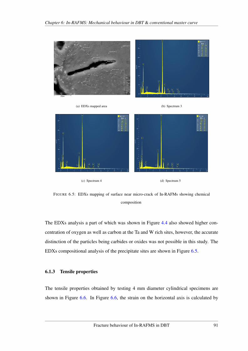
Chapter 6: In-RAFMS: Mechanical behaviour in DBT & conventional master curve
(a) EDXs mapped area (b) Spectrum 3
(c) Spectrum 4 (d) Spectrum 5
FIGURE 6.5: EDXs mapping of surface near micro-crack of In-RAFMs showing chemical
composition
The EDXs analysis a part of which was shown in Figure 4.4 also showed higher con-
centration of oxygen as well as carbon at the Ta and W rich sites, however, the accurate
distinction of the particles being carbides or oxides was not possible in this study. The
EDXs compositional analysis of the precipitate sites are shown in Figure 6.5.
6.1.3 Tensile properties
The tensile properties obtained by testing 4 mm diameter cylindrical specimens are
shown in Figure 6.6. In Figure 6.6, the strain on the horizontal axis is calculated by
Fracture behaviour of In-RAFMS in DBT 91

Chapter 6: In-RAFMS: Mechanical behaviour in DBT & conventional master curve
subtracting the elastic strain based on the initial Elastic modulus. The values are qual-
itative only after necking and are shown for the differentiation in failure points of the
specimens at different temperatures.
FIGURE 6.6: Engineering stress-plastic strain (εT −σ/Eo) response of In-RAFMS in DBT
region
The trend of yield strength and Ultimate Tensile Strength (UTS) as appearing in Figure
6.6 shows conventional behaviour except at -50oC. Due to this discrepancy and also due
to the expected transition temperature (with the help of Charpy Impact toughness) to be
lower than -50oC, fracture tests were avoided in the temperature range more than -50oC.
Only exception was 0.4T CT specimen, some of which were tested at -50oC to examine
the effect of prior ductile tearing on cleavage fracture.
The tensile behaviour in Figure 6.6 also shows an upward jump for temperatures more
than -110oC. The post necking strain decreases significantly after -140oC. The be-
haviour of YS and UTS is also shown in Figure 6.7, where it is clear that with decreasing
92 Fracture behaviour of In-RAFMS in DBT

Chapter 6: In-RAFMS: Mechanical behaviour in DBT & conventional master curve
temperature the YS and UTS tend to converge, showing difficulty in dislocation move-
ment due to less slip systems and converges at -196oC, where apparently the lower shelf
fracture without any work hardening occurs.
The tensile behaviour of ferritic/martensitic grade steel (Eurofer97) has been studied
in great detail by Bonad et al. (2008); Bonade (2006). For the constitutive relation-
ship of true stress and logarithmic strain, to be used for finite element analyses it has
been a trend to linearly extrapolate the behaviour till UTS beyond necking. The post
necking extrapolation of logarithm of true stress and strain has been discussed in de-
tail by Hasegawa et al. (2009). It should however not be ignored that the post necking
behaviour might be completely different from the pre-necking tensile behaviour due to
the damage kinetics. Still, in this work the linear extrapolation of logarithm of true
stress strain has been followed. The reason for the extrapolated tensile behaviour is to
simulate the crack front which generally strains beyond uniform strain. In the work of
Bonad et al. (2008), where fracture behaviour of Eurofer97 is studied, similar approach
is applied.
The tensile properties in form of true stress and logarithmic plastic strain were obtained
till Ultimate Tensile Strength (UTS) from the raw data in form of load and load-line
displacement. The natural logarithm of true stress-logarithmic strain behaviour obtained
for In-RAFMS as well as P91 when plotted till UTS showed a linear behaviour. The
finite element analyses of crack tip elements requires the material’s tensile response
beyond UTS and therefore, this linear logarithmic response was extrapolated by fitting
the behaviour as,
ln(σtrue) = a1 ln(εp)+ao , (6.1)
where ao and a1 are fitting parameter. The tensile properties extrapolated to a plastic
strain of 2 were used in numerical calculation. The details of extrapolated tensile re-
sponses are detained in corresponding chapters. Similarly the tensile response of P91
were also extrapolated.
The yield strength (σo) and UTS is shown in Figure 6.7 for In-RAFMS tested at quasi-
static loading rate of 0.5 mm/min. The ratio σUT Sσo is shown in Figure 6.7 for quasi-static
Fracture behaviour of In-RAFMS in DBT 93

Chapter 6: In-RAFMS: Mechanical behaviour in DBT & conventional master curve
FIGURE 6.7: Yield strength, UTS responses at (a) different temperatures and hardening be-haviour in form of σo/σUT S at (b) different strain rates
(0.5 mm.min) as well as for higher actuator (Cross Head Speeds) speeds, such as 100
mm/min and 1000 mm/min corresponding to strain rates of 0.083 s−1 and 0.83 s−1,
respectively.
After studying the micro-structure, phase transformation, precipitate size and distribu-
tions, and tensile behaviour of In-RAFMS, a detailed property chart of In-RAFMS is
enlisted in Table 6.1.
94 Fracture behaviour of In-RAFMS in DBT

Chapter
6:In-R
AF
MS:M
echanicalbehaviourin
DB
T&
conventionalmaster
curve
TABLE 6.1: Summary of microstructural and mechanical properties of In-RAFMSChemical composition (Wt %)
C Cr W V Ta Si Mn S, N Al, Ni0.08 9.15 1.37 0.24 0.08 0.026 0.53 < 0.002 < 0.004Hardness 220 HVC at RT (Microhardness 253 tempered martensite/207 ferrite and carbide (Raju et al., 2009))Heat Treatment Solutionizing | 977oC for 0.5 hr | normalizing & Tempering | 760oC for 1hr | air cooledMicrostructure Tempered marteniste | Cr23C6 (100-300 nm) at pre-austenitic & interlath boundaries | (Ta/V)C carbides inside laths of 20 nm size.|Phase and transformation temperatures DSC ThermoCalcCurie Temperature 745oC M23C6 dissolution 1277oCAc1 832oC 778oC Delta ferrite start 1302oCAc3 867oC 875oC MX compete dissoultion 1408oCMartensite to ferrite + M23C6 664oC Liquid start 1457oCMs 441oC 302-477 oC (Table 4.2) Complete melting 1532
Mf 345oCH alpha-gamma 13-14 J/gEnthalpy of Melting 364 J/g
Heat capacity Cp Cp = AT + BT2 + CT3 + D/T +E ln(| T−TCTC|)
10.64 -0.018 8.57×10⁻⁶ -760670.77 -30653.01Tenisle behaviourTemperature (oC) YS (MPa) UTS (MPa) DBTT
300 418 485 68J criteria -85oC200 436 570 DBTT -95oC100 430 609 (Average of upper
RT 410 637 & lower shelf)
-70 560 636.4-80 564 650.2
-110 587 708.7-120 765 800.2-130 845 928.5-140 878 956.4-150 957.51 978-196 1086 1096
FracturebehaviourofIn-R
AFM
Sin
DB
T95

Chapter 6: In-RAFMS: Mechanical behaviour in DBT & conventional master curve
6.2 Conventional master curve analysis of In-RAFMS
The conventional master curve analysis was performed on the fracture dataset of stan-
dard Single Edge Notched Bend specimens (SENB) with specimen width W being twice
of thickness. The specimen dimension is shown in Appendix-C with the geometry of
knife edges and notch root radius. The conventional master curve as discussed in Chap-
ter 2 can be performed on the fracture dataset generated at different temperatures which
is known as multi-temperature master curve method . A special and simpler case when
the dataset generated at single temperature is analysed is referred as single-temperature
master curve . The conventional master curve takes the athermal part of fracture tough-
ness as 30 MPa m1/2 and thermal part takes the value of 70 MPa m1/2 in Eq.(2.6).
The conventional master curve involves certain validity criteria as discussed in section
2.2.2. As the assumption of master curve methodology demands single parameter char-
acterization of crack tip stress field either by J or KJ , the self-similarity of the stress
field becomes an implicit requirement. For smaller specimens this is almost impossible
which results in non-uniformity of the To assessment by single and multi-temperature
master curve methods.
The extensive study to assess the uncertainty involved in examined on the 0.4T SEB
dataset as well as 0.2T TPB dataset as shown in Table 6.2.
It has also been discussed earlier that various studies such as Joyce and Tregoning
(2005a); Nevalainen and Dodds Jr (1996) has shown both experimentally and by finite
element analyses results that for SEB type specimens loaded under three point bend-
ing the constraint parameter for censoring should be made more strict. The study by
Faleskog et al. (1998) suggests the M parameter in Eq.(2.13) should be as high as 70,
however on the other hand earlier study by Joyce and Tregoning (2005a) recommends it
to be as high as 200 for smaller SEB specimens to achieve SSY conditions. To study the
effect of strict censoring 0.4T SEB dataset was used as 0.2T dataset had less valid data
for maximum likelihood analysis. The conventional multi-temperature master curve
96 Fracture behaviour of In-RAFMS in DBT

Chapter 6: In-RAFMS: Mechanical behaviour in DBT & conventional master curve
analysis of 0.4T SEB, 0.2T TPB and 0.4T CT specimens of In-RAFMS are shown in
Figure 6.8.
6.2.1 Single and multi-temperature master curves
The single temperature master curve analysis estimates the behaviour of fracture tough-
ness dependence with temperature using dataset only at one test temperature. This
inherently restricts involvement of fracture toughness thermal dependence and forces
maximum likelihood to result to follow the empirical thermal dependence of master
curve. The trend of fracture toughness w.r.t. temperature, therefore, is decided by the
median found at single temperature as shown in Figure 6.9. The effect however is miti-
gated as the master curve assumes a standard shape and the dependence is not generally
altered for ferritic and ferritic martensitic steel. A case study on Eurofer97 is discussed
in Chapter 2, where this conventional dependence was challenged and thermal athermal
part of master curve were re-analysed. Statistical analysis of same dataset may show
variation in result to different degrees due to many reasons. Every specimen has its
own reference transition temperature, which is decided by its unique geometry and the
alignment while testing, considering all other affecting parameters such as constraint,
loading rate e.t.c. The actual temperature felt by the specimen at the crack tip while
testing is decided by the micro-mechanism which may change the temperature felt by
specimen such as adiabatic heating at elevated loading rates, distribution of cleavage
initiators and the degree of triaxiality at the crack tip.
The general effect of single and multi-temperature analyses does not show a correla-
tion as shown in Figure 6.9 as well as in Figure 6.10. The 0.2T, 0.4T TPB and 0.4T
CT dataset multi-temperature analyses results in a To of -120oC. The effect of strict
censoring and single temperature master curve analysis are discussed in the following
section.
The differences in reference transition temperature To obtained by performing single
temperature maximum likelihood analyses are shown in Table 6.2.
Fracture behaviour of In-RAFMS in DBT 97

Chapter 6: In-RAFMS: Mechanical behaviour in DBT & conventional master curve
(a) 0.2T TPB dataset (To = -123oC)
(b) 0.4T TPB dataset (To = -120oC)
(c) 0.4T CT dataset (To = -129oC)
FIGURE 6.8: Conventional master curve of In-RAFMS
98 Fracture behaviour of In-RAFMS in DBT

Chapter 6: In-RAFMS: Mechanical behaviour in DBT & conventional master curve
TABLE 6.2: Single and Multi-temperature analysis of 0.4T and 0.2T SEB datasets of In-RAFMS
SpecimenGeometry
TotalTests
ValidTests
TestTemp.
MLEMethod
ValidityParameter ‘M’ To (oC)
0.2T TPB(5×5×27) 7 7 -140 ST 30 -91
0.2T TPB(5×10×55)
7 6 -120 ST 30 -104.514 10 -130 ST 30 -120
39 26-110,-120,-130,
-140,-150MT 30 -123.5
0.2T TPB(10×20×90)
14 9 -110 ST 30 -132.712 12 -120 ST 30 -129.27 7 -130 ST 30 -12633 26 -110,-120,-130 MT 30 -129.833 26 -110,-120,-130 MT 40 -127.733 21 -110,-120,-130 MT 50 -125.333 19 -110,-120,-130 MT 60 -123.333 17 -110,-120,-130 MT 80 -126.7333 16 -110,-120,-130 MT 100 -122.3
The estimated To can be much away from the more reliable To estimated by multi-
temperature master curve on a bigger dataset. It can be higher or lower than the To
estimated by multi-temperature master curve and can show variation for dataset be-
longing to test temperature falling below actual To or above it. The ASTM standard
E1921 dictates the reproducibility limit to show a half standard deviation of 20o which
is huge for design aspects. However, in general the difference found is not that great if
the analysis contains more valid data and a large dataset of 20 or more valid data.
FIGURE 6.9: Effect of single and multi-temperature analyses on conventional master curve of0.2T TPB dataset of In-RAFMS
Fracture behaviour of In-RAFMS in DBT 99

Chapter 6: In-RAFMS: Mechanical behaviour in DBT & conventional master curve
FIGURE 6.10: Effect of strict censoring on master curve of 0.4T TPB dataset of In-RAFMS
6.2.2 Strict censoring
The increment in constraint parameter which becomes a function of temperature follow-
ing the dependence of Yield strength as evident from Eq.(2.13) invalidates many data
points and makes the certainty of To compromise on the conservative approach towards
To estimation.
In Figure 6.10 the dataset of 0.4T SEB specimens have been analysed with increasing
M parameter starting from conventional value of 30 to a very strict value of 100. As
the validity criteria gets tough the number of valid data decreases and censored values
start taking over the results. However the result does not change much in the case of
In-RAFMS as the number of valid data even at M = 100 are 16 out of 33, which is more
than 50% of the data. However the drastic effect of data points getting invalidated as M
increase is clear from Figure 6.10.
The method of making validity tough by increasing M parameter is one way to address
the problem of non self similar stress field in small specimens. There can be various
other ways to solve the problem without making experimental data invalid. Some of
the methods such as side grooving the specimen, numerical correction and thickness
scaling, triaxiality measurements are examined in this work which will be discussed in
forthcoming chapters.
100 Fracture behaviour of In-RAFMS in DBT
Chapter 6: In-RAFMS: Mechanical behaviour in DBT & conventional master curve
6.3 Conclusions
The tensile, impact, and fracture properties of In-RAFMS were studied in DBT region.
The competing ductile and microcrack based damage is measured and fractographic ex-
amination is used for understanding the DBT region. At higher temperature the larger
dimple size showed the dominance of ductile behaviour in Charpy specimens. It is note-
worthy that higher temperature do promote ductile tearing however this does not mean
that the cleavage failure probability decreases. The reality is actually quite contrary and
results in increased probability of cleavage failure with ductile tearing. This is discussed
in Chapter 11. The distribution of carbides and absence of inclusions imposes the un-
derstanding that the cracking of carbides is one of major parameters which describes
the cleavage event, apart from the availability of energy/stresses for dynamic propaga-
tion/arrest of microcracks and number of carbides taking part in microcrack nucleation.
The distribution of carbide is found to be homogeneous for both the steels with bigger
size of carbides in P91 in comparison to In-RAFMS which results in higher DBTT for
P91 as reflected in the impact toughness response depicted in Figure 6.1.
The master curve assumes homogeneous distribution of second phase particles in the
matrix for assessment of fracture behaviour. An advance approach may incorporate
the certainty of finding bigger inhomogeneities at the pre-austenitic grain boundaries,
which can be quantified as a function of pre-austenitic grain size. However, this would
complicate the simple engineering approach of master curve and maximum likelihood
analysis to a great extent. Therefore, unnecessary complications are avoided by ruling
out the approach to quantify distribution of carbides and a simple and effective Gaussian
distribution of carbides embedded into master curve methodology is followed. Never-
theless, for a crystal plasticity based understanding of local cleavage failure probability,
quantifying secondary phase distribution may be helpful.
The conventional master curve analysis resulted in a To of -120oC. The To obtained
from differently sized and shaped specimens differed at most by 9oC, with 0.4T SE(B)
Fracture behaviour of In-RAFMS in DBT 101

Chapter 6: In-RAFMS: Mechanical behaviour in DBT & conventional master curve
specimen to have a To of -129oC. The conventional master curve analyses appear to con-
verge for different dataset and with different levels of constrained maximum likelihood
analysis for In-RAFMS.
102 Fracture behaviour of In-RAFMS in DBT

Chapter 7
Master curve: effect of out of plane
constraint loss
This chapter deals with the out of plane constraint loss assessment in small three point
bend specimens. Fracture behaviour of In-RAFMS is investigated using small speci-
mens in three point bend loading in subzero temperature range of -110oC to -150oC.
The transition reference temperature, To, is calculated using Master Curve approach.
The small specimens resulted in a non-conservative To, due to Large Scale Yielding
(LSY) condition near crack tip. A numerical correction method is described in this
chapter, which is used to transform LSY fracture toughness to equivalent Small Scale
Yielding (SSY) value. The numerical correction method simulated using commercial
FEM package is validated on two datasets, 1) given by Sokolov et.al and 2) by Euro
Fracture Data. The methodology is then applied on the In-RAFMS data and used for
estimation of conservative To value corresponding to specimen’s crack tip under SSY
condition.
The results and findings presented in this chapter are published in:
Tiwari A., Avinash G., Sunil S., Singh R., Stahle P., Chattopadhyay J., Chakravartty
J. (2015) Determination of reference transition temperature of in-rafms in ductile brit-
tle transition regime using numerically corrected master curve approach. Engineering
Fracture Mechanics 142:79 92
103

Chapter 7: Out of plane constraint loss
7.1 Introduction
The fracture behaviour of steels in transition regime shows huge scatter and master
curve approach deals with this phenomenon by identifying the scatter as stochastic
effect and solves it using Weakest Link Theory (Weibull, 1951). The foundation of
MC methodology, which is developed largely by Wallin (Wallin, 1993, 1989a, 1999),
requires small scale yielding (SSY) condition to be met by the specimen. In reality
however, this condition of SSY is hardly reached for small and miniature specimens
(Landes and Shaffer, 1980). Moreover, the thickness scaling method of master curve
approach (also referred as size adjustment ), which scales the KJC to an equivalent 1T
SSY condition, described in ASTM E1921 (E1921, 2013) does not completely trans-
form the original experimental value to the equivalent SSY value of KJC at 1T, This is
due to the fact that the existing thickness correction of ASTM E1921 does not take care
of non-SSY condition of stresses in small specimens.
Many researchers, including Wallin, such as Wallin et al. (2001); Wallin (2001); Gao
and Dodds Jr (2000); Dodds Jr et al. (1991) have discovered various correction methods
to resolve the problem due to out of plane constraint loss. In order to understand the
cleavage phenomenon using a statistical approach, many analytical models have been
proposed, such as the classic work of Landes and Shaffer (1980). Another approach
to model cleavage phenomenon is established by Wallin, Saario, To rr o nen, which
is known as WST (Wallin et al., 1986; Wallin and Laukkanen, 2008) model. In WST
approach, Griffith instability criteria is used to identify the critical cleavage initiator size
as described earlier in Chapter 2 by Eq.(2.23). The implicit assumption in Eq.(2.23) is
the spherical shape of crack initiator. The idea of size adjustment equation in MC
methodology originates from Eq.(2.18), described in Chapter 2, where assumption of
SSY condition helps to use a non-dimensional scale Q as in Eq.(2.16), and simplifies
the probability of failure expression to be written in integration form as in Eq.(2.19).
The use of non-dimensional parameter Q assumes the self-similarity of stress fields.
The problem in the size adjustment equation lies in the concept of volume responsible
for cleavage trigger. The methodology assumes that the volume responsible for cleavage
104 Fracture behaviour of In-RAFMS in DBT

Chapter 7: Out of plane constraint loss
in 3 dimension (3D) can be obtained by extruding the 2 dimensional (2D) area along
the thickness, which is only realistic when the stress distribution is self-similar along
the crack front. This assumption is valid for SSY condition but questionable in the
case of small or miniature specimens especially for specimens to be tested in bending
(Joyce and Tregoning, 2005a). The problem of transformation of a non-SSY value
of KJC to an equivalent SSY value is addressed in this study numerically using finite
element analysis. The numerical correction is validated with the experimental data
of Sokolov and Tanigawa (2007) work and a part of dataset provided in the report of
Belgian Nuclear Research Centre, which is also known as Euro fracture data (Heerens
and Hellmann, 2002; Lucon and Scibetta, 2011; Heerens and Hellmann, 1999). The
same correction has been used in this work to find reference transition temperature for
In-RAFMS.
7.2 Fracture dataset
The test and experimental details are described in Chapter 5. The dataset used for the
analysis of out of plane constraint loss belongs to quasi-static 0.2T TPB dataset as de-
scribed in Chapter 2. The yield strength at test temperature of -70, -80 and -110oC
were linearly extrapolated. The complete tensile dataset was not generated during the
assessment of constraint loss, therefore, the tensile behaviour was assumed linear and
extrapolated. Though, as shown in Chapter 5 that this extrapolation does not follow the
true behaviour of yield strength for In-RAFMs, the linear extrapolation remains con-
servative to -150oC. The temperature dependence of yield strength behaviour is shown
in Figure 7.1. The tensile properties at -110oC was used as input data in finite element
simulation.
Fracture toughness testing of In-RAFMS
From the Charpy impact toughness work on In-RAFMs by Laha et al. (2013), the es-
timated transition temperature To,est was found to be -108oC obtained using 41 Joule
Fracture behaviour of In-RAFMS in DBT 105

Chapter 7: Out of plane constraint loss
FIGURE 7.1: Extrapolated yield strengths for fracture toughness measurements in the range oftest temepratures
criteria following Wallin’s method (Donald E. McCabe, 2005). The fracture toughness
tests, in this work, were carried out using 0.2T single edge notched bend or SE (B)
type samples at temperatures of -110oC,-130oC, -140oC and -150oC at a loading rate
of 0.5 mm/min on the same servo-hydraulic machine used for tensile testing, which is
described in Chapter 5.
After test completion, the broken samples were examined under low magnification
stereo microscope for measurement of initial crack length. The method of crack length
measurement and testing scheme is described in Chapter 5. The fractographic mea-
surement confirmed that none of the specimens had stable crack growth more than 0.05
times of the ligament. None of the tests completed failure without cleavage.
7.3 Numerical assessment of constraint loss
In Finite Element Analysis (FEA) the major aim was to find a method, which can cor-
rectly transform the experimental KJC value to an equivalent SSY value. The classical
model of Ritchie, Knott and Rice (RKR) (Ritchie et al., 1973) defines cleavage to occur
at a characteristic length ahead of crack tip where maximum principal stress surpasses
106 Fracture behaviour of In-RAFMS in DBT

Chapter 7: Out of plane constraint loss
a critical amount. This characteristic length in annular stress field is an area and in 3
dimension becomes a volume. Therefore, cleavage is said to occur if the maximum prin-
ciple stress σ1 goes beyond a critical value σ? in a critical volume V ?. This approach of
defining cleavage fracture is referred as σ?−V ? model. The same approach was used
by Mueller et al. (2009) to investigate the non-SSY condition effect on sampled volume
ahead of crack tip. Although V ? variation is explored by Odette and He (Odette and He,
2000), in this work it is assumed that V ? is independent of temperature.
The WST model is also based on extrusion of 2 dimensional area along the thickness,
which is erroneous to various degrees depending on the size of the sample as the fraction
of the sample thickness exhibiting SSY condition depends on its size . Therefore, to
address the aforementioned issue, numerical analysis using finite element method was
performed and the results were validated with the work of Sokolov and Tanigawa (2007)
on F82H steel. Same numerical correction was also applied on a part of Euro fracture
toughness dataset and the reference transition temperature, To, was validated against
that obtained from the complete dataset.
7.3.1 Numerical correction of Sokolov’s Work
Sokolov and Tanigawa (2007) performed tests using 1T, 0.4T and 0.16T CT samples
machined from F82H steel plates. The steel plates were Electron Beam and Tungsten
Inert Gas welded and further post weld heat treated. The To found by conventional
multi-temperature MC was -105oC (Sokolov and Tanigawa, 2007). In the present work,
only 0.4T CT sample data has been used for application of numerical correction, as
most of the data at single temperature were available only for this geometry. Finite ele-
ment analysis was performed on 0.4T CT geometry using FEM package. The specimen
geometry is shown in Figure 7.2.
The Sokolov’s dataset for 0.4T CT geometry is reproduced in Table 7.1. Experimental
KJC corresponding to serial no. 6 in Table 7.1 was invalid due to excessive stable crack
growth (KJC,∆a criteria of ASTM E1921-13a). Therefore, to find reference temperature
by single temperature MC approach 1 data of size 1T (Serial No.7) was included. Data
Fracture behaviour of In-RAFMS in DBT 107

Chapter 7: Out of plane constraint loss
FIGURE 7.2: Dimensions of CT specimen geometry
corresponding to serial no. 6 was replaced by maximum valid fracture toughness of
173.4 MPam1/2 from dataset of Sokolov following ASTM E1921-13a. The 1T data was
assumed to be in SSY condition and was not therefore corrected numerically in this
study. The transition temperature obtained by using the dataset shown in Table 7.1, by
single temperature approach comes out to be -115oC.
7.3.2 Pre processing
In order to apply numerical correction, 0.4 CT geometry was modelled with isotropic
incremental plasticity. Modelling of 0.4CT geometry was carried out in both 2 and 3
dimension. Only quarter of the specimen volume was modelled due to symmetry and
the load was applied on the reference point RP-1 as shown in Figure 7.3.
In case of 3D modelling, due to the two-fold symmetry of the problem only a quarter
(x1 ≥ 0 , (x2 ≥ 0) of the body was modelled with boundary condition as follows: 1.
X-axis symmetry along the ligament (u1 = ur2 = ur3 = 0) 2. Z-axis symmetry along
thickness ((u3 = ur1 = ur2 = 0) where u denotes displacement and ur rotation with
1(x), 2(y) and 3(z) as Cartesian coordinate axes. The reference point as shown in Figure
7.3(a) was kinematically coupled with the pinhole surface of CT specimen. The load
and displacement in mode 1 direction was extracted as reaction force and displacement
at reference point RP-1. The load was multiplied by 2 in case of 3D model and dis-
placement was multiplied by 2 to get the load displacement response of a full sample.
108 Fracture behaviour of In-RAFMS in DBT

Chapter 7: Out of plane constraint loss
(a) Boundary conditions (b) Mesh features
FIGURE 7.3: Boundary condition and mesh of 0.4T CT geometry of Sokolov’s work (Sokolovand Tanigawa, 2007)
In case of 2D model, the load per unit thickness was multiplied by twice of thickness
of the sample and displacement was multiplied by 2. Three dimensional model was
meshed with 20 noded brick elements whereas 2D was meshed with 8 noded quadrilat-
eral plane strain elements. The computation was carried out using reduced integration
full Newtonian non-linear analysis. Meshed geometry is shown in Figure 7.3(b). The
element size was kept constant near crack tip to facilitate ease of V ? calculation.
7.3.3 Post processing
In order to find the volume surrounded by critical maximum principal stress, guidelines
of IAEA project CRP-8 (IAEA, 2009) used for finite element round robin analyses was
followed. The volume ahead of crack tip containing the region surrounded by maximum
principal stress, was calculated by extracting all the nodes enduring σ1 ≥ 1.7σo and
εp ≥ 0.001. In case of 3D analysis the volume V ? was calculated as,
V? =Nodes enduring σ1 ≥ 1.7σo
Nodes per unit element·Volume o f an element . (7.1)
The critical volume calculated by Eq.(7.1) was also re-calculated by counting elements
for, which the maximum principal stress at the centroid of the element endured 1.7
times of yield strength (σo). The numbers of elements found in this way multiplied
Fracture behaviour of In-RAFMS in DBT 109

Chapter 7: Out of plane constraint loss
FIGURE 7.4: K2D'SSY and K3D'non−SSY obtained from FEA of Sokolov’s geometry
with elemental volume resulted in values close to the result found by using Eq. (7.1).
Therefore, for all further analyses Eq. (7.1) was used for V ? calculation. In case of 2D
analyses, areas under critical maximum principal stress were calculated by Eq. (7.1),
after replacing the elemental volume term with elemental area. After the calculation of
critical area, the value was multiplied by thickness. Therefore, the volume in case of 2D
was an extrusion of area along the thickness. The total volume obtained from quarter
symmetric 3D model was multiplied with 4. In 2 dimensional analysis, the total volume
was found by multiplying the area enduring σ1 ≥ 1.7σo with twice the thickness. From
the load displacement values extracted from 2D and 3D FEM model, KJC was calculated
following ASTM E1921-13a method from load and load line displacement. The KJC
versus Critical volume plots for 2D model and 3D model calculations is shown in Figure
7.4.
In the local approach to analyse cleavage phenomena numerically, σ?−V ? approach de-
fines cleavage with bi-parametric criterion. For the same material at same temperature,
attainment of equivalent amount of critical volume V ? in samples implies same proba-
bility of cleavage failure(Nevalainen and Dodds Jr, 1996). Therefore, the experimental
KJC obtained from the experimental load displacement response should correspond to a
110 Fracture behaviour of In-RAFMS in DBT

Chapter 7: Out of plane constraint loss
3D model and whereas the 2D model KJC corresponding to equally stressed volume in
3D will represent SSY equivalent value of KJC.
In order to simulate the SSY condition, a boundary layer model can be solved, however
the boundary layer model results are independent of loading conditions i.e. tension
or bending. In specimens of any size/thickness the constraint is always highest at the
centre and the specimen remains in plane stress at the surface.
The SSY condition is achieved when Tstress = 0, however, at the mid plane the Tstress
is generally > 0, resulting in high constraint by compressive hydrostatic stress field.
Wallin (Wallin et al., 2001) has shown that, this compressive Tstress has insignificant
effect on fracture parameters such as KJC in comparison to SSY (Tstress = 0) condition.
Therefore, in order to capture the effect of loading type the 2D geometry was modelled.
The area confined by maximum principal stress in a 2D model when extrapolated for
a thickness gives the volume under high constraint. Taking into consideration, the in-
significant effect of compressive Tstress in comparison to SSY condition, this volume
represents the equivalent SSY sampled volume.
The σ?−V ? plots for 2D and 3D models were fitted in two parameter power law as it is
well known that the stressed volume scales with KJC following power law. From these
power law fitted plots the equivalent SSY KJC was obtained for each experimental value.
The power law fitting was chosen by taking the inspiration from the fact that the volume
scales with a power of 4, which comes from the area integration along crack front. The
area of stressed volume is proportional to the stressed zone radius, which scales with
K2, K being mode 1 stress intensity factor. Therefore, area will be proportional to K4.
The lacking information here is that K varies along the thickness on non-SSY condition
due to constraint loss and therefore, K4 relation with stressed volume in LSY condition
remains questionable. After fitting the σ?−V ? plots the relation of equivalent SSY KJC
was found as,
K2d,SSY = 13.86(Kexp
7.272)0.7298 . (7.2)
Fracture behaviour of In-RAFMS in DBT 111
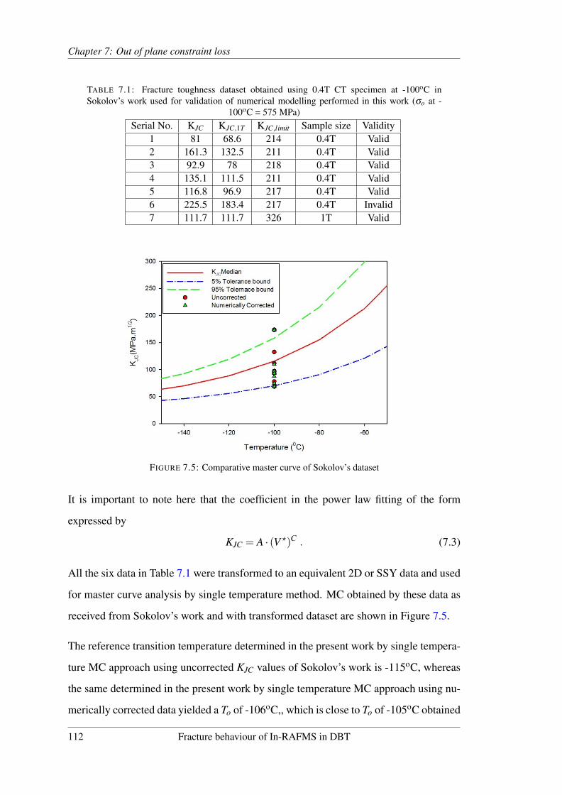
Chapter 7: Out of plane constraint loss
TABLE 7.1: Fracture toughness dataset obtained using 0.4T CT specimen at -100oC inSokolov’s work used for validation of numerical modelling performed in this work (σo at -
100oC = 575 MPa)Serial No. KJC KJC,1T KJC,limit Sample size Validity
1 81 68.6 214 0.4T Valid2 161.3 132.5 211 0.4T Valid3 92.9 78 218 0.4T Valid4 135.1 111.5 211 0.4T Valid5 116.8 96.9 217 0.4T Valid6 225.5 183.4 217 0.4T Invalid7 111.7 111.7 326 1T Valid
FIGURE 7.5: Comparative master curve of Sokolov’s dataset
It is important to note here that the coefficient in the power law fitting of the form
expressed by
KJC = A · (V ?)C . (7.3)
All the six data in Table 7.1 were transformed to an equivalent 2D or SSY data and used
for master curve analysis by single temperature method. MC obtained by these data as
received from Sokolov’s work and with transformed dataset are shown in Figure 7.5.
The reference transition temperature determined in the present work by single tempera-
ture MC approach using uncorrected KJC values of Sokolov’s work is -115oC, whereas
the same determined in the present work by single temperature MC approach using nu-
merically corrected data yielded a To of -106oC,, which is close to To of -105oC obtained
112 Fracture behaviour of In-RAFMS in DBT

Chapter 7: Out of plane constraint loss
by Sokolov using multi-temperature MC approach. Noticeable observation is that ma-
jor part of data is on lower side of the median curve, which is similar to the findings of
Kim et al. (Kim et al., 2013) indicating inhomogeneity.
7.3.4 Numerical correction on Euro dataset
The Euro fracture toughness dataset is one of the biggest dataset ever created for frac-
ture toughness investigation of reactor pressure vessel steel in ductile brittle transition
regime. In the present work only one part of the dataset i.e. the dataset of block SX9
was used. In the documented work, the fracture toughness tests were carried out on
2T and 0.5T CT specimens at -60oC. Total number of tests were 36 out of, which 30
tests were valid according to ASTM E1921-05. The Euro dataset reports the reference
temperature obtained by MC, multi-modal master curve, bi-modal master curve, Single
point estimate and SINTAP lower tail method.
In order to apply numerical correction, 0.5T CT geometry was modelled in the present
work in a similar way as for Sokolov’s work using material properties of 22NiMoCr37
Reactor Pressure Vessel steel. The reason to model 0.5T CT geometry was that this
geometry was the smallest size tested in the Euro fracture dataset. Specimen of thick-
ness 1T or higher would probably not suffer from constraint loss in lower DBT region.
The KJC−V ? plot obtained from the FE analysis is shown in Figure 7.6. The reference
temperature obtained using 30 valid data out of 36 tests performed at -60oC reported
by Belgian Nuclear Research Centre is -107oC by conventional single temperature MC,
-104oC by Multi-modal MC. The Bi-modal MC approach yielded To,1 and To,2 values
of -93oC and -115oC, respectively.
The master curve obtained in the present work after applying numerical correction on
12 data of 0.5T-CT samples KJC values, is shown in Figure 7.6(a). The master curve
obtained by SCK.CEN for SX-9 block with all 30 valid data is also shown along with
numerically corrected MC in Figure 7.6 (b) for comparison.
Fracture behaviour of In-RAFMS in DBT 113

Chapter 7: Out of plane constraint loss
(a) Transformed and untransformed dataset To = -104oC
(b) Transformed dataset with rest of SX9 and Euro data at single temperature
FIGURE 7.6: Comparison of master curves obtained from Euro data transformed to SSY anduntransformed conditions
From Figure 7.6 (a) it seems that the numerically corrected MC does not follow the
median and many data falls in 50% to 2% probability range, however in Figure 7.6 (b)
it can be seen that numerically corrected MC does pass through the median. Notice-
able observation is that few tests values used after numerical correction could predict a
reference temperature value close to that obtained using larger dataset.
114 Fracture behaviour of In-RAFMS in DBT

Chapter 7: Out of plane constraint loss
7.3.5 Numerical Correction on In-RAFMS
In order to apply the same numerical correction on experimental data obtained using
0.2T SE(B) sample geometry were modelled in both 2D and 3D with plastic behaviour
of material given in form of stresses and plastic strains obtained from tensile behaviour
of In-RAFMS.
Elastic modulus of In-RAFMS was obtained from tensile test at room temperature using
extensometer.
7.3.6 Pre-processing
The 0.2T SE(B) geometry was modelled in ABAQUS FEM package (Hibbitt et al.,
1998) similar to CT geometry models. The solutions for FE analysis was obtained by
2× 2× 2 reduced integration. The area ahead of crack tip was refined with element
volume of 0.1× 0.1× 0.2 mm3 and 1r singularity at the crack tip was imposed. In
case of 2D model except the elements (8 noded quadrilateral plane strain elements) and
elemental area (0.1×0.1 mm2) all other parameters were kept same.
The boundary condition of application of load and extraction of load and displacement
was done by following guidelines of IAEA CRP-8 (TECDOC 1631) project finite ele-
ment round robin program. The boundary conditions and the mesh is shown in Figure
7.7.
7.3.7 Post Processing
In a 3D quarter symmetric model of a CT geometry, the reaction force is calculated
at the reference point which is kinematically coupled with the pinhole surface. The
surface is half of the full thickness and reaction force includes the effect of symmetry
on the crack plane. Thus a multiplication factor of 2 to reaction force is required for load
calculation. The displacement in a CT specimen model only counts for half symmetry
and therefore, displacement also requires a multiplication factor of 2.
Fracture behaviour of In-RAFMS in DBT 115

Chapter 7: Out of plane constraint loss
FIGURE 7.7: Boundary conditions imposed and mesh of 0.2T TPB specimen of In-RAFMS
For a TPB model, when the reaction forces are extracted at pin loading point, the quarter
symmetry effect comes in. This requires a multiplication factor of 4. On the other hand,
the TPB model displacement does not require any multiplication factor. This is evident
as the quarter symmetric TPB model does not have any symmetric boundary condition
on the constrained points (roller pin locations) in the direction of displacement.
In 3D analysis, the load was extracted on the part shown in Figure 7.7 as reaction force
in Y-direction and was multiplied by 4 to get response of full geometry. In case of
2D model, the load per unit thickness was extracted and was multiplied by 2 times of
thickness. This was required as the load values without assigning any plane strain thick-
ness in ABAQUS corresponds to a unit dimension thick strip. The load for full specimen
geometry thus requires a multiplication factor of 2× thickness of the specimen. The dis-
placement would represent value for full geometry unlike CT quarter symmetric model
and thus was used as extracted.
Load line displacement was obtained by subtracting the displacement data in Y direc-
tion, extracted at edge AB and line from point P in 3D model as shown in Figure 7.7(b).
In 2D model the same procedure was applied at points instead of lines.
116 Fracture behaviour of In-RAFMS in DBT

Chapter 7: Out of plane constraint loss
FIGURE 7.8: Active volume V ? under non-SSY condition with loss of constraint
7.4 Results and Discussion
7.4.1 Master Curve from uncorrected experimental data
The fracture toughness data of 0.2T SE(B) after applying censoring with KJC limit were
used for obtaining reference transition temperature with multi-temperature MC. The
master curve plot is shown in Figure 7.10 with 0.2T data size adjusted to 1T using
ASTM E1921-13a.
The transition temperature found from test data of 0.2T SE(B) was -123.5oC, which
is close to the reported values (T0 = -119oC) obtained for F82H (Wallin et al., 2001).
However, this temperature is non-conservative as it has been obtained from non-SSY
condition test data.
7.4.2 Numerical correction of In-RAFMS dataset
From the 2D and 3D modelling of 0.2T SE(B) specimen, critical volume V ? and KJC
values were calculated. In the simulated result it was found that the 3D volume sur-
rounded by a critical maximum principal stress is not same throughout the thickness.
The volume surrounded under critical maximum principal stresses can be seen in Figure
7.8.
The plot of KJC vs. critical volume contained in maximum principal stress more than
1.7 times Yield strength obtained from FE analysis is presented in Figure 7.9. The
effect of size on stressed volume is governed by two parameters. The first parameter
Fracture behaviour of In-RAFMS in DBT 117

Chapter 7: Out of plane constraint loss
FIGURE 7.9: Active volume V ? versus KJC under non-SSY condition with loss of constraint
being thickness and other in plane constraint. The V ? behaviour with KJC for 0.2T
SE(B) geometry shows that the difference of volume obtained from 3D and 2D model
is higher than that obtained in case of CT geometry of 0.4T and 0.5T analysis. The
difference is an evidence of high constraint in case of higher thickness specimens in
comparison to 0.2T SE(B) samples.
Similar to the analysis performed on Sokolov’s data, KJC−V ? plots were fitted in power
law
K2d,SSY = 58.15 · (Kexp
127.7)1.4483 , (7.4)
which was used to transform KJC experimental to equivalent SSY values.
The reference transition temperature obtained from numerically corrected MC for In-
RAFMS is -109oC. The Master Curve plot of numerically corrected data can be seen
in Figure 7.10. The reference transition temperatures of Eurofer 97, F82H and Modi-
fied 9Cr-1Mo steels, which are similar to In-RAFMS in composition and heat treatment
are shown in Table 7.2 for comparison. It can be realized from Table 7.2 that the nu-
merically corrected To estimate of -109oC for In-RAFMS is close to the other RAFMs
reference temperatures obtained by various methods of constraint correction [18, 28-
30]. The uncorrected data are labelled LSY. It can be seen in Figure 7.10 that many
118 Fracture behaviour of In-RAFMS in DBT

Chapter 7: Out of plane constraint loss
FIGURE 7.10: Master curve of In-RAFMS with untransformed and transformed datasets
of corrected data are outside the 5% tolerance bound, which was also the case with
uncorrected MC shown in Figure 7.5.
Fracture behaviour of In-RAFMS in DBT 119

Chapter
7:O
utofplaneconstraintloss
TABLE 7.2: Comparison of reference transition temperatures of popular RAFM steelsChemical composition (Wt %)
C Cr W/Mo V Nb/Ta Si Ni Mn
Eurofer97 0.14 8.94 1.07 0.2 0.15F82H Mod 0.09 8 1.88 0.19 0.02 0.11 0.16Modified 9Cr 1Mo 0.085 9.37 0.911 0.189 0.08 0.336 0.097In-RAFMS 0.08 9.15 1.37 0.24 0.08 0.026 0.004 0.53
Heat Treatment
Austenitizing Tempering after normalizing
Eurofer97 980 oC for 0.5 hrs 760 oC 1.5 hrsF82H Mod 1040 oC for 0.67 hrs 960 oC for 0.5 hrsModified 9Cr 1Mo 1050 oC for 1 hr 770 oC for 0.5 hrIn-RAFMS 977 oC for 0.5 hr 760 oC for 1 hr
Reference transition temperature, To (oC)
Uncorrected SSY corrected
Eurofer97 -77F82H Mod -133 to -137 -103 to -105Modified 9Cr 1Mo -67.7 to -72.4In-RAFMS -123 -109
120Fracture
behaviourofIn-RA
FMS
inD
BT

Chapter 7: Out of plane constraint loss
This particular outlier behaviour has been also found with Sokolov’s data analysis. The
inference from this behaviour suggests that much of effect on mean value estimation
comes from the censored data. Sokolov and Tanigawa (2007) solved this problem by
random inhomogeneity analysis of the data. It might also occur, if a significant amount
of ductile crack growth occurs during the test. Ductile crack growth (DCG) may cause
the fracture toughness to increase and get censored, due to KJC limit criteria. Moreover,
the numerical correction method will not be valid for DCG effect in fracture tests.
It can be concluded that uncorrected reference transition temperature of -123.5oC for
In-RAFMS is applicable to miniature specimens with very small thickness whereas,
reference temperature of -109oC obtained by analysing numerically corrected data re-
semble the behaviour of structure loaded in SSY condition.
7.5 Conclusions
The fracture behaviour of In-RAFM steel is investigated in ductile brittle transition
regime using 0.2T three point bend samples. The transition temperature estimated to
be -123.5oC from conventional multi-temperature master curve methodology is non-
conservative.
The constraint loss at smaller dimensions invalidates the SSY assumption of MC method-
ology. Numerical analyses was used to obtain an equivalent SSY value. The numerical
approach was validated on test data of Sokolov and Euro fracture datasets. Predicted
reference temperature from multi temperature MC approach on In-RAFMS using nu-
merically corrected MC yields a reference temperature of -109oC, which is more conser-
vative and close to the transition temperatures obtained by applying different constraint
correction methods to steels belonging to RAFMS family.
Fracture behaviour of In-RAFMS in DBT 121

Chapter 8
Master curve: effect of in plane
constraint loss
In this chapter, the fracture behaviour of In-RAFM steels is investigated with system-
atically varying a/W using Master Curve approach. This a/W effect is investigated
using σ?−V ? approach by calculating the active volume at simulated crack front. The
fitting parameter of σ?−V ? approach is compared with changing constraint parameter
∆Tstress.
The results and findings presented in this chapter are published in:
Tiwari, Abhishek, R. N. Singh, Per Stahle, and J. K. Chakravartty. “A loss of constraint
assessment using σ?−V ? approach to describe the effect of crack depth on reference
transition temperature To. Procedia Structural Integrity 2 (2016): 690-696
8.1 Introduction
The conventional Master Curve approach, which is used to characterize the fracture
behaviour of ferritic and ferritic/martensitic steels, restricts the crack depth to be in
the range of 0.45 ≤ a/W ≤ 0.55. The reference transition temperature is known to
increase with increasing crack depth owing to increase in constraint. Despite the fact
that the fracture parameters corresponding to shallower crack depth are unconventional
due to its non-conservative values, in transition region a correlation to assess the shift
in reference transition temperature with different crack depth is of great importance.
122

Chapter 8: In plane constraint loss
FIGURE 8.1: Experimental analyses of Sumpter showing effect of crack depth on fracturetoughness
Additionally the experimental work of Sumpter and Forbes (1993) shows that the va-
lidity window of master curve can easily be extended to atleast from 0.3 ≤ a/W ≤ 0.6
as shown from Figure 8.1. It is clear from Sumpter’s work that the loss of constraint
dominates for a/W ≤ 0.3 where SSY assumption is completely unreliable due to plastic
hinge formation and single parameter description of crack tip stress field is impossible.
However for deeper cracks there is no violation of SSY condition as long as bo > B.
Therefore, to figure out whether master curve approach can be extended in the range
of crack depth, the experimental as well as numerical analyses are performed on the
dataset of In-RAFMS.
The fracture toughness of ferritic and ferritic/martensitic steels having BCC structure,
generally shows a transition not only with temperature, but also with crack depth be-
ing tougher for shallower crack and brittle for deeper crack in DBT region. This is
attributed to constraint loss for shallow cracks. In this work, the MC methodology is
used to estimate reference transition temperature for different crack depths and the loss
of constraint is examined numerically.
Fracture behaviour of In-RAFMS in DBT 123

Chapter 8: In plane constraint loss
8.2 Experimental dataset
The fracture specimens pre-cracked to obtain width normalized crack length in the range
of 0.2 to 0.6 were used for this analyses. The specimens after measurement of pre-
crack length, were categorized according to their a/W values in ranges of 0.2-0.3±0.04,
0.4±0.04, 0.5±0.04, 0.6±0.09, as shown below. The details of the experimental meth-
ods and set-ups are described in Chapter 3.
• Group 1 (Gr-1) = 0.29-0.34
• Group 2 (Gr-2) = 0.35-0.44
• Group 3 (Gr-3) = 0.45-0.54
• Group 4 (Gr-4) = 0.55-0.69
8.3 Numerical Analysis
To understand the effect of crack depth on the volume sampled ahead of the crack tip
under the maximum principal stress dominance, numerical analyses were performed on
a/W of 0.3, 0.4, 0.5, 0.6 and 0.7. The geometry used for modelling was 5×10×55 mm3
sub-size charpy specimen with 2× 2× 2 reduced integration and incremental loading
algorithm. The tensile properties were used for -110oC obtained from 4 mm diameter
and 20 mm gauge length round bar tensile specimen. The quarter symmetric geometry
modelled is shown in Figure 8.2.
The numerical analysis was post processed for the σ?−V ? approach as described in
previous chapter (Chapter 4) behavior investigation. The cleavage failure is described
in this approach by the volume ahead of the crack tip encompassed under maximum
principal stress σ1 higher than a threshold. The threshold value is generally taken to be
twice of yield strength σo. The details of calculation involved in σ?−V ? approach can
be found in earlier work by Tiwari et al. (Tiwari et al., 2015) as well as in Chapter 4.
124 Fracture behaviour of In-RAFMS in DBT

Chapter 8: In plane constraint loss
FIGURE 8.2: Quarter symmetric charpy geometry with active volume at crack front
8.4 Results
The Master Curves for test data categorized in four groups are shown in Figure 8.3.
The cumulative plot of median curves for all categories is shown in Figure 8.4, with re-
spective reference transition temperatures To obtained according to conventional master
curve approach described by E1921 (2013). The effect of crack depth is evident from
Figure 8.4 showing an increasing To with increasing crack depth.
The master curve analyses of the four grouped dataset shows a systematically increasing
To with increasing crack depth. The increasing constraint, which causes otherwise non-
critical cleavage initiators such as carbides to trigger cleavage by developing high stress
field explains the result. Also the matrix helps under higher constraint by allowing
micro-crack formation in the active volume ahead of crack tip.
Fracture behaviour of In-RAFMS in DBT 125

Chapter
8:In
planeconstraintloss
(a) Gr-1 master curve To = -125oC (b) Gr-2 master curve To = -115oC
(c) Gr-3 master curve To = -105oC (d) Gr-4 master curve To = -99oC
FIGURE 8.3: Master curves showing data outside tolerance bounds for shallower crack datasets and workable scatter for deeper crack datasets
126Fracture
behaviourofIn-RA
FMS
inD
BT

Chapter 8: In plane constraint loss
FIGURE 8.4: Shift in transition temperatures with increasing crack depth
The constraint due to changing crack depth is measured by calculating Weibull traixial-
ity as explained earlier. The active sampled volume is calculated for a/W ratio of 0.3,
0.4, 0.5, 0.6 and 0.7. The behaviour of active volume is plotted against KJC calculated
from load-load line displacment response of simulated model. The KJC vs. V ? is fitted
using power relation as,
KJC = Z(V −Vo)β . (8.1)
It can be seen in Figure 8.5 that the fitting parameters of Eq.(8.1) show a systematic
trend with crack depth.
8.5 Discussion
The active volume under SSY condition of stresses at crack front can be estimated as
BK4, as discussed in Chapter 1. The active volume correlates plastic zone radius to the
radius of area under maximum principal stress dominance. Under non-SSY condition
where the stress field is not self-similar along the crack front the volume will not scale
with BK4. Under the circumstances where loss of constraint occurs there can be three
approaches, which can be applied to understand the generic cleavage failure probability
Fracture behaviour of In-RAFMS in DBT 127

Chapter 8: In plane constraint loss
FIGURE 8.5: Curve fitting of active volume calculated according to Eq.(8.1)
as described earlier in Eq.(2.18) in Chapter 2. The three possibility which emerge for
non-SSY conditions are as follows.
1. In this approach, described by Anderson (2005) the active volume is equated with
a volume where SSY condition would exist and cleavage failure probability will
scale with BK4. The cleavage failure probability in this case is described as,
Pf = 1− exp(−ω ·Be f f K4) . (8.2)
2. In second approach which was first given by Wang and Parks (1992) in his doc-
toral thesis and was later developed by Gao and Dodds Jr (2000) describes the
cleavage failure probability with a constraint parameter known as g-function. The
cleavage failure probability in this case is described as,
Pf = 1− exp(−ω ·gBK4) . (8.3)
3. The third approach assumes that the effect of loss of constraint results in a scaling
128 Fracture behaviour of In-RAFMS in DBT

Chapter 8: In plane constraint loss
with volume which does not obey power 4 scaling with cleavage failure probabil-
ity. The cleavage failure probability in this case is described as,
Pf = 1− exp(−ω ·BKλ ) . (8.4)
The third approach can be used for scaling the non-SSY conditions to SSY condition.
The approach of σ?−V ? is basically equating the third approach with Eq.(2.27). The
second approach is cumbersome due to the pre-requisite finite element analysis of mod-
ified boundary layer formulation. The detailed calculation of second approach is used
in calibration of Weibull slope in Chapter 10. The first approach is also comparatively
easier in comparison to second approach in calculation. However, in this work, third ap-
proach is used due to its applicability in transformation of non-SSY fracture toughness
to SSY condition in both out of plane and in plane cases of constraint loss.
It is also assumed that the same deformed volume for any two condition would result
in same probability of cleavage failure. This assumption gives a benefit of transforming
the non-SSY condition to SSY condition as described in Chapter 7.
By equalizing the sampled active volume for two different crack depth specimens,
namely A and B, the transformation of KJC,B to KJC,A can be expressed as,
KJC,A = Z[(Vo,B−Vo,A)+(KJC,B
ZB)1/βB]βA . (8.5)
Using Eq. (8.5), the transformed data at 0.5 a/W were analyzed using MC method
which is shown in Figure 8.6.
The Master curve plot with different a/W shows the expected effect on reference tran-
sition temperature. The shift in temperature with a/W increment is shown in Figure
8.4. The KJC,median calculated at -110oC and the standard deviation of the Weibull fit
calculated using ASTM E1921-14a is shown in Table 8.1.
Fracture behaviour of In-RAFMS in DBT 129

Chapter 8: In plane constraint loss
FIGURE 8.6: Master curve plot of all KJC transformed to a/W = 0.5
The standard deviation of fitted Weibull distribution in master curve approach is de-
scribed in ASTM E1921 as,
σd,1 = 0.28KJC,med(1−20
KJC,med) . (8.6)
The standard deviation of estimation of To, is described in ASTM E1921 as,
σd,2 =
√β 2
r+σ2
exp , (8.7)
where β is the sample size uncertainty factor which is obtained from ASTM E1921-13a
section (10). r is the number of valid tests, and σexp is taken as 4oC as recommended
in ASTM E1921-13a. For β factor to be obtained, an equivalent fracture toughness
KEqJC,med is calculated as,
KEqJC,med =
1r
r
∑i=1
30+70exp0.019(Ti−To) , (8.8)
where To is the test temperature of individual tests.
The shift in transition temperature To was found to be increasing by 10oC with incre-
ment in a/W . This however may change as the increment value depends on number of
130 Fracture behaviour of In-RAFMS in DBT

Chapter 8: In plane constraint loss
TABLE 8.1: Statistical details of MC analysis of grouped datasets
Total no. r Valid KEqJC To σd,1 σd,2
of tests tests (MPa m1/2) (Eq.(8.8)) (oC) (Eq.(8.6)) (Eq.(8.7))Gr-1 15 9 80.62 -125 28.86 43.27Gr-2 15 9 81.22 -115 24.35 43.27Gr-3 12 8 75.8 -105 20.62 48.18Gr-4 12 8 67.33 -99 18.7 48.18
data used for analysis and also on the number of censored data.
The numerical analysis of 0.2T geometry for different crack depths were fitted accord-
ing to Eq.(8.1) and shown in Figure 8.5. The coefficient Z and the degree β of Eq.(8.1)
shows a trend with changing crack depth. As discussed earlier the power 4 scaling of
KJC with active volume V , is not followed under LSY conditions. The fitting parameters
Z and β are plotted with increasing a/W in Figure 8.7. Unlike the constant increment in
To found experimentally these parameters show a transition from shallow to deep crack
with a minimum slope in the a/W range of 0.4 to 0.6.
Fracture behaviour of In-RAFMS in DBT 131

Chapter
8:In
planeconstraintloss
FIGURE 8.7: Correlation of fitting parameters of Eq.(8.1) with (a) change in constraint parameter ∆Tstress and (b) Tstress with a/W
132Fracture
behaviourofIn-RA
FMS
inD
BT

Chapter 8: In plane constraint loss
To understand whether these parameters have ability to quantify constraint, standard
constraint parameter Tstress was calculated using the fifth degree polynomial used by
Wallin (Wallin et al., 2001) for bend geometry as
Tstress,T PB
σo=−1.13+5.96(
aW
)12.68(a
W)2+18.31(
aW
)315.7(a
W)4+5.6(
aW
)5 . (8.9)
The difference in normalized Tstress with a/W is also calculated as
∆Tstress,T PB
σo= 5.96(
∆aW
)12.68(∆a2 +2ao∆a
W 2 )+18.31(∆a3 +3a2
o∆a+3ao∆a2
W 3 ) .
(8.10)
where a0 is the crack length for 0.5 a/W if the normalized ∆Tstress is being calculated
for a/W of 0.6 a/W . The difference ∆a
W is 0.1 for the calculation in this case.
The plot of normalized Tstress and ∆Tstress is shown in Figure 8.7 in comparison with
fitting parameters. It is evident from the figure that the fitting parameter Z shows a
one to one correlation with normalized ∆Tstress. However, fitting parameter β shows
although an increasing trend as shown by normalized Tstress but the differs in slope
with normalized Tstress as shown in Figure 8.7 (b). Reciprocal of β shows a unique
correlation with normalized ∆Tstress as shown in Figure 8.7 (a). On the other hand,
β shows a cubic polynomial behaviour, whereas, normalized Tstress shows a parabolic
trend in Figure 8.7 (b). The behaviour of 1/β as well as Z varies in correspondence to
normalized ∆Tstress, uniquely. From this it becomes evident that the fitting parameters
of σ?−V ? have the potential to be used as a constraint measurement parameter.
By equalizing the sampled active volume for two different crack depth specimens,
namely A and B, the transformation of KJC,B to KJC,A can be expressed as,
KJC,A = Z′[(Vo,B−Vo,A)+(KJC,B
Z′B)1/βB]βA . (8.11)
Fracture behaviour of In-RAFMS in DBT 133

Chapter 8: In plane constraint loss
8.6 Conclusions
Master curve fracture toughness analysis was carried out on 0.2T specimen in the range
of 0.2 to 0.7 a/W . The dataset were categorized based on a/W and analysed for ref-
erence transition temperature determination. The To was found to be increasing for
higher a/W . The numerical analysis showed that under non-SSY stress field condi-
tion for both constraint loss and high constraint specimens the active volume scaling
with KJC changes drastically and cannot be analysed using conventional master curve
method. On the other hand in the range of 0.37≤ a/W ≤ 0.7, the data can be analysed
using master curve by transforming the dataset to a single a/W scale. The numerical
analysis of active volume ahead of crack front showed a good correlation with change
in Tstress. The fitting parameters Z′ was found to follow one on one correlation with
∆Tstressand therefore this parameter can be used as a measure of constraint for cleavage
fracture.
134 Fracture behaviour of In-RAFMS in DBT
Chapter 9
Master curve: effect of specimen
geometry (CT and SE(B))
The fracture behaviour of steels are generally studied by testing Compact Tension (CT)
and Single Edge cracked Bend (SE(B)) specimens. The CT specimen data results in a
conservative reference transition temperature. On the other hand, small SE(B) speci-
mens are of great importance for irradiation studies. However, these small SE(B) speci-
mens suffer from greater loss of constraint in comparison to CT geometry. In this chap-
ter, CT and SE(B) specimens response in DBT region are studied using Master Curve
method and loss of constraint between CT and SE(B) specimens is examined by a novel
constraint parameter, Weibull Triaxiality (qW ). qW is developed as a micro-mechanical
tool to understand the distribution of the ratio of hydrostatic stress (σh) and equivalent
stress (σeq) components, in the volume directly influencing the cleavage phenomena.
The qW parameter is used to modify Beremin’s model. The cleavage failure probabil-
ity predicted using modified Beremin’s model shows better accuracy when compared
to experimental results. Also master curve results are examined for two grades of fer-
ritic/martensitic steels namely, Mod-9Cr-1Mo and Indian Reduced Activation Ferritic/-
Martensitic Steel (In-RAFMS).
135

Chapter 9: Master curve: CT and SE(B)
9.1 Introduction
In DBT region, a single specimen can show all the features of ductile to brittle transition,
starting with blunting of the tip to ductile tearing which accelerates the crack propaga-
tion and increases the triaxiality, which later causes the specimen to fail in cleavage
fashion (Knott, 1995). The scatter in the fracture toughness behaviour in the region of
DBT for general purpose conventional BCC steels can be attributed to following param-
eters.
1. Experimental errors
2. Constraint loss and distribution of cleavage initiators
3. Ductile tearing
4. Thickness/size of the sample
The constraint level describing the intensity of stress field at the crack tip differs for dif-
ferent geometries used for fracture toughness measurement. There have been studies on
fracture toughness with many geometries of specimens, such as Single Edge Notched
in Tension (SENT) and in Bending (SENB or SE(B)), Double Edge Notched Tension
(DENT), Centre Cracked specimen (MT) and Compact Tension (CT) specimens. The
most commonly used specimens out of the aforementioned are SE(B) and CT. The frac-
ture toughness measurement standards for general testing (E1820) and testing in DBT
regions using master curve approach (E1921, 2013) focus on SENB and CT specimens
with or without side grooving. CT specimens in a context of fracture testing at sub-zero
temperatures for fracture assessment shows less scatter of fracture data in comparison to
the specimens tested in bending. The specimens in bending are rectangular bar geome-
tries with fracture specimen’s width to thickness ratio (W/B) = 1 or 2. These specimens
can have misalignment issues while testing in the plane normal to the crack path as well
as along the load axis, where as in CT specimens the alignment is assured by the test
fixtures. The alignment issues can be resolved by fixture modifications, but even so, it
remains difficult to use miniature specimens and therefore the usage imposes challenges
towards the reproducibility of the fracture parameters. The fatigue pre-cracking prior to
fracture testing also plays an important role in deciding the stress profile near the crack
136 Fracture behaviour of In-RAFMS in DBT
Chapter 9: Master curve: CT and SE(B)
tip. Any misalignment of the pre-crack not visible from surface will also contribute to
the scatter.
Apart from the type of loading and geometry, the assessment of fracture toughness based
on load Crack Mouth Opening Displacement (CMOD) or on load-Load Line Displace-
ment (LLD) also causes scatter (Nevalainen and Dodds Jr, 1996) to the order of 20-25%
for fracture toughness measured using LLD. The most important parameter to model
scatter in cleavage fracture in DBT regime is the distribution of cleavage initiators. The
spatial distribution of the cleavage initiators vary depending on the size of precipitates,
phase distribution, number of phases present in the microstructure and grain size. In
general purpose conventional ferritic steels, the cleavage initiates from secondary phase
particles due to their bigger size and stress raising shapes unless the shapes are modi-
fied by metal working. In steels, the cleavage is caused by microcracks originating from
carbides. In general, any second phase having different plasticity may lead to micro-
crack generation and further to cleavage if the micro-crack is generated before the peak
stress is reached making the dynamic propagation possible for the micro-crack from
the secondary phase to the grain and beyond (Neville, 1988; Nevalainen and Dodds Jr,
1996).
In cleavage fracture the effect of size is prominent as assessed in the pioneer work of
Landes and Shaffer (Landes and Shaffer, 1980). The thickness of test specimens affect
the fracture toughness first by increasing the constraint and secondly by increasing the
probability of initiation of catastrophic failure. The reason for the latter is the increased
number of cleavage initiators that fall in the active volume of maximum principal stress
exceeding the threshold for cleavage fracture (Ritchie et al., 1973). The active volume
in case of cleavage fracture phenomena is referred to the volume ahead of crack tip
under the maximum principal stress (σ1) larger than a threshold value of (σ1) which is
defined in proportion to yield strength (σo) (Bonade et al., 2008).
The objective of this part of the work is to experimentally investigate the DBT re-
gion fracture behaviour of In-RAFMS and P91 steels using CT and TPB specimens.
The difference of constraint is studied using Beremin’s model and a novel method or
Fracture behaviour of In-RAFMS in DBT 137

Chapter 9: Master curve: CT and SE(B)
Weibull Triaxiality, qW , is developed to correct the numerical predictions obtained using
Beremin’s model.
9.2 Material and Experimental Details
The fracture behaviour of ferritic/martensitic steels of two different grades namely,
Mod-9Cr-1Mo and Indian Reduced Activation Ferritic/Martensitic Steels (In-RAFMS)
are investigated in DBT region using both CT and SENB geometries.
The details of the material differences and similarities of the two grades are described
in Chapter 4. As the master curve approach sets its reference thickness at 1 inch i.e. 1T,
the testing on P91 steel was carried out on 1T CT specimens with 10% side grooves.
For TPB, the tests were performed on widely used specimen geometry of full sized
standard charpy. Due to the scarcity of the RAFM grade steel, the fracture testing on
In-RAFMS was carried out on 55×10×5 mm3 sub-size charpy geometry and 0.4T-CT
specimens with W/B = 2.5. The CT specimens were side-grooved unlike Pre-cracked
V notch sub-size Charpy (PCVN) specimens. The tests were conducted in accordance
with ASTM E1921-13a, in DBT region for both the steels. The details of the experi-
ments are discussed in Chapter 4 and the specimen geometries used for experimental
and numerical analyses are detailed in Appendix-C.
9.3 Cleavage failure probability, Weibull Triaxiality
The approach used generally for understanding the cleavage failure mechanism numer-
ically in DBT region started with the pioneer study of Beremin’s group (Beremin et al.,
1983b). The detailed method of cleavage fracture prediction based on Beremin’s model
is described in Chapter 10. The cleavage failure probability based on Weibull stress is
described as
Pf = 1− exp[−(σW
σu)m], (9.1)
138 Fracture behaviour of In-RAFMS in DBT

Chapter 9: Master curve: CT and SE(B)
where Pf is the numerical probability of cleavage failure, σu is the scaling parameter
and m is the Weibull slope. For a Griffith crack, in a crack tip volume actively taking
part in cleavage phenomena (Active Volume), the probability, P to find a micro-crack of
size in the range of lo to lo+dlo in a small fraction of active volume, VS can be described
as,
P =∫
∞
lco
P(lo)dlo = (σ1
σU)m , (9.2)
where σU is a constant and σ1 is maximum principal stress. Using Eq. (9.2), the cumu-
lative probability of cleavage fracture of active volume can be described by integrating
P for all VS in active volume V as,
Pf = 1− exp[− 1Vo
∫V(
σ1
σU)m] , (9.3)
where the integration is defined in a volume which is dominated by maximum principal
stress surpassing a threshold value. The general trend is to define the boundary of the
active volume where σ1 is twice of σo. Defining Weibull stress, σW , as
σW = [1
Vo
∫V ∗
σm1 dV ]1/m, (9.4)
where Vo is the reference volume not too big to have significant stress gradient nor too
small to violate the characteristic length of RKR model (Ritchie et al., 1973) which is a
few grains. Maximum principal stress, σ1, is integrated in the volume V ∗. The volume
V ∗ is described to be the volume for which σ1 > λσo, where σo is the yield strength of
the material. Generally the value of λ is taken as 2 (Petti and Dodds Jr, 2005; Gao and
Dodds Jr, 2005a; Wasiluk et al., 2006).
For the importance of reference volume, Vo, it is reviewed by Dowling and Lidbury
(2000) that relatively larger elements in finite element analyses gives accurate results
for Weibull stress calculations and it is not obligatory to refine mesh in order to have
single element size equal to be in exact correspondance to Vo. Dowling and Lidbury
(2000) showed, by studying the element size equal to Vo (which was of dimension 50
Fracture behaviour of In-RAFMS in DBT 139

Chapter 9: Master curve: CT and SE(B)
µm) and greater, that the important aspect was to capture the stress strain field at the
crack tip accurately.
The relation of σW with fracture parameter J or K for self similar stress field at the crack
tip is described by Beremin et al. (1983b); Wasiluk et al. (2006) as,
σmW = ζ BJ2 = ζ BK4 , (9.5)
where ζ = ζ [ (1−ν2)E ]2, varies with change in temperature and flow properties. Using
Eq.(9.5), the cleavage failure probability in three parameter Weibull distribution is de-
scribed as,
Pf = 1− exp[−(σ
m/4W −σ
m/4W−min
σm/4U −σ
m/4W−min
)4] , (9.6)
which is obtained by finding a corresponding Weibull stress to the fracture parameter
KJC used in the description of master curve approach according to Eq.(2.7). The thresh-
old of cleavage initiation , σW−min corresponds to Kmin and σU corresponds to Ko.
For the numerical prediction of cleavage failure probability, it is a pre-requisite to cal-
ibrate the Weibull slope m. The scaling parameter σU is then the σW corresponding to
Ko. The history of Weibull stress based cleavage failure probability starts as discussed
earlier with the work of Beremin’s group (Beremin et al., 1983b), which was then a
two parameter Weibull analysis. The calibration procedure for two parameter as well
as three parameter Weibull cleavage failure probability was developed mostly by Gao
and Dodds Jr (2005a), Petti and Dodds Jr (2005), Wasiluk et al. (2006) and Ruggieri
et al. (1998). The approach in these works brought cleavage failure probability very
close to the master curve methodology. In other words, the stress based cleavage failure
probability was coupled with master curve methodology, especially with three param-
eter Weibull probability distribution function as described in Eq. (9.6). Simultaneous
efforts were also made to introduce plastic strain factor in the cleavage failure probabil-
ity. The plastic strain correction and evolution of Weibull stress based cleavage failure
probability is recently reviewed in the work of Ruggieri and Dodds Jr (2015).
140 Fracture behaviour of In-RAFMS in DBT
Chapter 9: Master curve: CT and SE(B)
The calibration procedure following the procedure suggested by Wasiluk et al. (2006)
which is similar to one used by Gao et al. (2006) is detailed in Chapter 10.
9.3.1 Weibull Triaxiality
For the described method of cleavage probability distribution estimation above, the
Beremin’s model has an implicit assumption to arrive at Eq.(9.2) to Eq.(9.3). The as-
sumption which is crucial for Beremin’s model formulation is that all the Reference
Volume Elements (RVEs) for which the probability of failure is described by Eq.(9.2),
should have the same stress levels. The Beremin’s model therefore, is correct for a self-
similar stress field. However, the case deviating from SSY condition needs a correction
in the Beremin’s formulation. This issue is addressed by assigning the ratio of triax-
iality at the RVE, qRV E , under consideration to the triaxiality level which is achieved
at the centre or mid plane of the specimen geometry, qmid as a weight factor to the
probabilities of RVEs i.e. P of Eq.(9.2).
With above description where q is the triaxiality factor defined as the ratio of hydro-
static, σH , and equivalent σeq, stress components, Eq.(9.5) is re-written for modified
Weibull stress σWm as,
σmWm =
1NVo
N
∑i=1
σm1,iVi
qRV E
qmid, (9.7)
where, there are N RVEs in the active volume V?, each corresponding to a volume of
Vi. The division by N is to make the quantity independent of finite number of RVEs
involved in a Finite Element (FE) post processing calculation. Using Eq.(9.4) the σWm
can be expressed as,
σWm = σW1N
N
∑i=1
qRV E
qmid1/m . (9.8)
The extra terms in Eq.(9.8) is defined as Weibull Triaxiality and denoted as qW as,
qW = 1N
N
∑i=1
qRV E
qmid1/m . (9.9)
This new parameter is a measurement of deviation of self-similarity in a specimen ge-
ometry and therefore, it also measures the constraint in a geometry with a reference
Fracture behaviour of In-RAFMS in DBT 141

Chapter 9: Master curve: CT and SE(B)
frame set at SSY condition. The reference point is SSY condition as for a self-similar
stress field the qW is always 1. Therefore, qW calculation avoids the modified boundary
layer modelling for assessments of constraint deviation.
Due to the modifications described here, the probability of cleavage failure can be re-
defined as,
Pf = 1− exp[−(σ
m/4Wm −σ
m/4Wm−min
σm/4Um −σ
m/4Wm−min
)4] , (9.10)
where σWm−min and σUm are the minimum modified Weibull stress and modified scaling
parameter. The values of σWm−min and σUm are obtained from the history of σWm−KJC.
9.4 Finite element analysis
The test geometries of 5×10×55 mm3 SE(B) specimen was modelled in three dimen-
sion with 31 layers of elements of uniform meshing along thickness. The CT geometry
of W = 25 and B = 10 mm was modelled with 10% side grooved quarter symmetric ge-
ometry. The mesh of both CT side grooved and SE(B) geometries are shown in Figure
9.1(a) and 9.1(b), respectively. The mesh in these geometries at the crack tip were kept
constant in size for the volume calculation in post processing.
In Figure 9.1 uri refers to the rotation along the axis defined by i direction. The method
of Weibull Triaxiality is applied in this work to the tested geometries. The Weibull
slope calibration mentioned in detail in section 10.1.3 used the high constraint and low
constraint datasets for minimizing the differences between SSY, high constraint and low
constraint datasets (Wasiluk et al., 2006). The Weibull slope obtained using the method
of Wasiluk et al. (2006) for In-RAFMS and P91 were found to be 9 and 15, respectively.
The Weibull Triaxiality was checked for its dependency on number of elements involved
in the calculation. The sensitivity analysis showed accurate results for more than 800
elements in the active volume.
142 Fracture behaviour of In-RAFMS in DBT

Chapter 9: Master curve: CT and SE(B)
(a) 0.4 T CT side grooved geometry mesh
(b) 0.2T TPB geometry mesh
FIGURE 9.1: Mesh of (a) side grooved 0.4T-CT specimen (RP represents a Reference Pointwhich is kinematically coupled with the pin hole surface) and (b) 0.2T SE(B) specimen
9.5 Results
The charpy results, as shown in Figure 6.6 in Chapter 6, were used to estimate the To
according to the criteria suggested by Donald E. McCabe (2005). The estimated To
was found to be -130oC for In-RAFMS and -110oC for P91. The fracture tests for
In-RAFMS were performed at -110oC, -120oC, -130oC, -140oC and -150oC, whereas
P91 was tested at -60oC, -70oC, -100oC and -110oC. The 1T-CT specimens of P91
steel were tested at higher (-60oC and -70oC) temperatures due to the expected high
constraint, whereas the SE(B) specimens of P91 were tested at relatively lower (-100oC
and -110oC) temperatures.
The Master Curves of 0.4T-CT side grooved specimens and 0.2T SE(B) specimens
of In-RAFMS are shown in Figures 9.2(a) and 9.2(b) with the scatter shown for both
datasets for comparison. The To for 0.4T-CT dataset and 0.2T TPB dataset were found
Fracture behaviour of In-RAFMS in DBT 143

Chapter 9: Master curve: CT and SE(B)
to be -120oC and -123oC. Similarly the Master Curves for P91 steel 1T-CT side grooved
specimens giving a To of -103oC and 0.4T-standard charpy specimen resulting in To of
-132oC , are shown in Figures 9.2(c) and 9.2(d). In Figures 9.2(c) and 9.2(d), for the
comparison, alternate geometry dataset is also shown.
Apart from aforementioned test conditions a dataset of fracture tests following ASTM
E1921 which was used as low constraint condition for Weibull slope calibration is also
included in this work for the assessment of constraint loss and for comparison with
experimental behaviour at test temperature of -110oC. As the 1T CT dataset of P91 is
tested at -60oC and -70oC, it cannot be compared with 10×10 SE(B) dataset which is
obtained at -110oC. This dataset which was created on specimens of 4 mm thickness
and other dimensions of 1T CT could not be used for To estimation due to less numbers
of valid data, nevertheless, it is used for the rank probability calculation and comparison
with the numerical predictions based on Beremin’s model.
144 Fracture behaviour of In-RAFMS in DBT

Chapter
9:M
astercurve:
CT
andSE
(B)
FIGURE 9.2: Comparison of master curves for (a) In-RAFMS 0.4T-CT specimens with the TPB dataset (b) In-RAFMS 0.2T TPB specimens with 0.4T-CTdatasets (c) P91 1T-CT specimens with 0.4T standard charpy dataset and (d) P91 0.4T standard charpy specimens with 1T-CT dataset for comparison
FracturebehaviourofIn-R
AFM
Sin
DB
T145
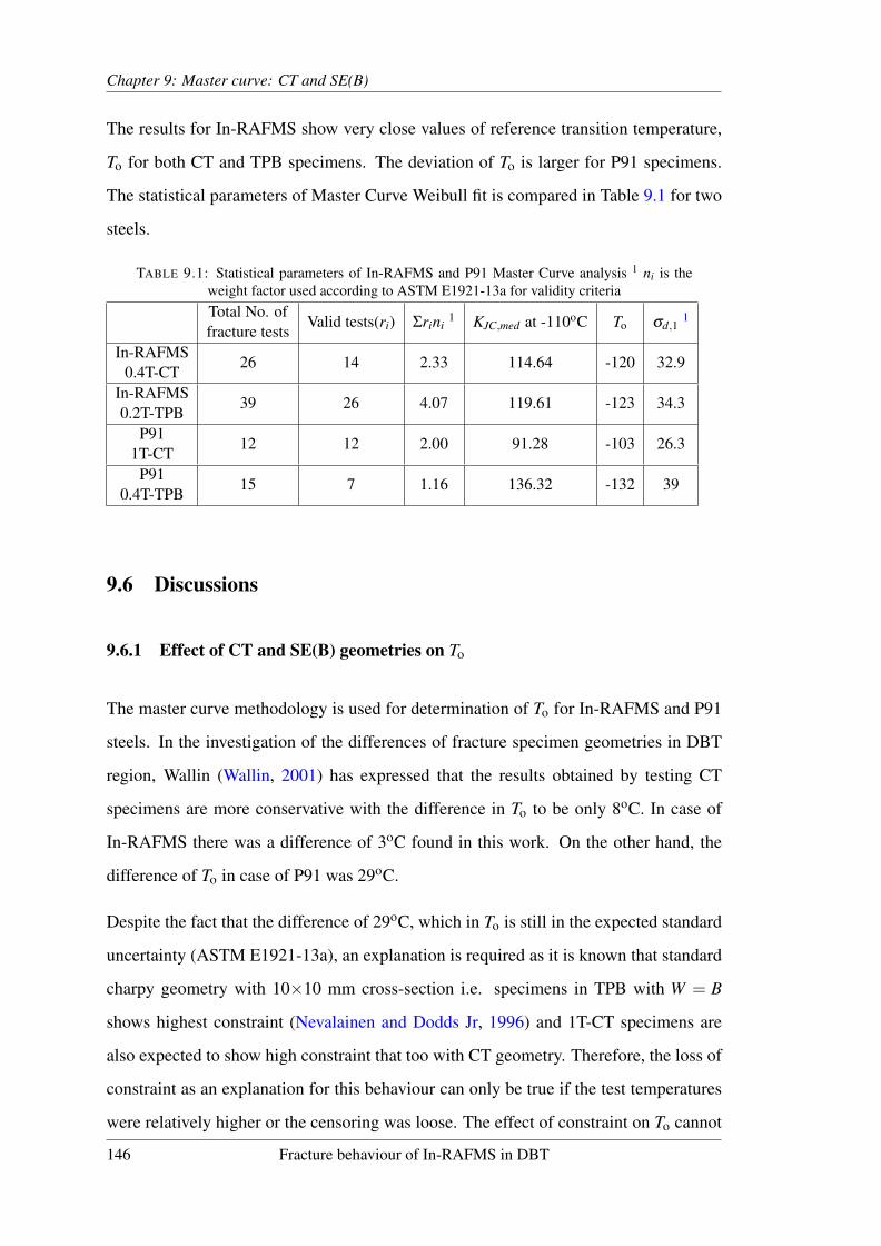
Chapter 9: Master curve: CT and SE(B)
The results for In-RAFMS show very close values of reference transition temperature,
To for both CT and TPB specimens. The deviation of To is larger for P91 specimens.
The statistical parameters of Master Curve Weibull fit is compared in Table 9.1 for two
steels.
TABLE 9.1: Statistical parameters of In-RAFMS and P91 Master Curve analysis 1 ni is theweight factor used according to ASTM E1921-13a for validity criteriaTotal No. offracture tests
Valid tests(ri) Σrini1 KJC,med at -110oC To σd,1
1
In-RAFMS0.4T-CT
26 14 2.33 114.64 -120 32.9
In-RAFMS0.2T-TPB
39 26 4.07 119.61 -123 34.3
P911T-CT
12 12 2.00 91.28 -103 26.3
P910.4T-TPB
15 7 1.16 136.32 -132 39
9.6 Discussions
9.6.1 Effect of CT and SE(B) geometries on To
The master curve methodology is used for determination of To for In-RAFMS and P91
steels. In the investigation of the differences of fracture specimen geometries in DBT
region, Wallin (Wallin, 2001) has expressed that the results obtained by testing CT
specimens are more conservative with the difference in To to be only 8oC. In case of
In-RAFMS there was a difference of 3oC found in this work. On the other hand, the
difference of To in case of P91 was 29oC.
Despite the fact that the difference of 29oC, which in To is still in the expected standard
uncertainty (ASTM E1921-13a), an explanation is required as it is known that standard
charpy geometry with 10×10 mm cross-section i.e. specimens in TPB with W = B
shows highest constraint (Nevalainen and Dodds Jr, 1996) and 1T-CT specimens are
also expected to show high constraint that too with CT geometry. Therefore, the loss of
constraint as an explanation for this behaviour can only be true if the test temperatures
were relatively higher or the censoring was loose. The effect of constraint on To cannot
146 Fracture behaviour of In-RAFMS in DBT

Chapter 9: Master curve: CT and SE(B)
be verified by making more strict censoring as increasing censoring parameter M from
conventional value of 30, results in less number of available valid tests than required for
determination of To.
The reference transition temperature estimate depends on statistical dataset available
and also on the amount of censoring. Apart from these, the To estimation is also known
to be affected by the test temperature (Bhowmik et al., 2015, 2012; Lucon and Scibetta,
2011). The To estimation is generally lower if obtained by analysing fracture tough-
ness data generated at higher temperatures. The reason is that as the test temperature
increases, the material’s flow becomes easier making the material more ductile in com-
parison to one at lower temperature. This results in greater non-linearity in the load
displacement behaviour due to loss of constraint. On the other hand choosing compara-
tively lower test temperatures with a controlled estimation of not falling into lower shelf,
may also result in lower To estimation as the yield strength of the material increases with
lowering of the temperature. This increase in yield strength results in loose censoring
limit by increasing KJC,limit , resulting further in lower To estimation due to involvement
of loss of constraints validated by censoring method. An approach to vary censoring
parameter M instead of keeping it independent of test temperature may be explored
especially for specimens loading in three point bending as for this type of loading, it
is suggested by many researchers (Joyce and Tregoning, 2005b; Rathbun et al., 2006;
Nevalainen and Dodds Jr, 1996) to increase censoring limits. Rathbun et al. (2006)
states in his extensive work by studying the effect of constraint loss for both change in
crack depth and thickness that the loss of constraint for TPB starts very early at M≈ 200
and that the BK4 scaling is also not very accurate for both very high thickness and very
small thickness specimens. However, the approximation of power 4 scaling of master
curve method remains close to the experimental results and gives a good estimation of
To. The master curve analysis of a combined dataset of CT and SE(B) specimens of
P91 steel results in a To of -108oC which is close to one obtained by analysing 1T CT
dataset alone (-103oC). The master curve for combined dataset is shown in Figure 9.3.
Figure 9.3 in comparison to Figure 9.2(c) and (d) shows that the the estimated To by
1T CT and combined dataset captures the experimental behaviour in the 5% and 95%
Fracture behaviour of In-RAFMS in DBT 147

Chapter 9: Master curve: CT and SE(B)
FIGURE 9.3: Master Curves of the combined dataset of P91 standard charpy specimens and1T-CT specimens
tolerance bounds. This estimate is more reliable statistically as the combined dataset
has more valid tests than SE(B) dataset alone. The P91 steel is known to show infe-
rior fracture resistance owing to the phosphorus content and tramp elements (Bhowmik
et al., 2012). The carbides’ clusters are also found to add to its inferiority in comparison
to In-RAFMS. The voids and microcrack formations in In-RAFMS and P91 steels were
shown in Chapter 6 in Figures 6.3 and 6.4, respectively.
It is evident from Figure 6.3 (c) and (d) and from Figure 6.4(a),(b) and (d) that the
number density of damage emanating sites are more in P91. Moreover, in case of In-
RAFMS microcracks are less in number at -70oC in comparison to P91, which shows
that P91 steel’s tendency to show catastrophic failure at comparatively higher temper-
ature is more. The same behaviour was expected from the Impact energy transition
shown in Figure 6.6.
It was found by FE analysis that CT specimens show higher constraint and with side
grooving the self-similarity of stresses are achieved to considerable amount in smaller
specimens. The 0.4T CT side grooved specimen crack tip stress field is shown in Figure
9.4. Therefore, the close value of To obtained from 0.2T TPB to that obtained from 0.4T
CT specimen dataset, leads to the understanding that the loss of constraint effect com-
ing in 0.2T TPB dataset of In-RAFMS were taken care off by the censoring and large
148 Fracture behaviour of In-RAFMS in DBT

Chapter 9: Master curve: CT and SE(B)
number of valid data as shown in Table 9.1. This is proven by the standard deviation
shown in Table 9.1 and also by the validity index rini.
The In-RAFMS data of both geometries were statistically large and thus the close values
of To is expected. The difference in To for P91 CT and TPB datasets is due to less
(though sufficient for To estimation (E1921, 2013)) number of valid data, which is again
reflected in standard deviation in Table 9.1. The 1T CT dataset of is more reliable as
it has the highest amount of constraint at the test temperatures and more number of
valid test data in comparison to SE(B) dataset which may also have maintained higher
constraint but for which the number of valid test data is less.
9.6.2 Constraint differences in CT and SE(B) and numerical prediction of cleav-
age failure probability
The qW values for CT and SE(B) geometries of P91 at -110oC and -60oC, as shown in
Figure 9.5 indicates that the level of constraint remains unchanged at these test tempera-
tures. Therefore, the To difference cannot be explained by differences in constraint with
the fact in consideration that for W =B the constraint is generally higher. The constraint
measured in form of qW shows expected behaviour for In-RAFMS as well. The qW for
CT and SE(B) test geometries of In-RAFMS are compared at -120oC in Figure 9.6. The
qW behaviour should not be compared for In-RAFMS and P91 as the tensile properties
for both the steels as well as the test temperatures are different. However, it is evident
by comparing Figure 9.5 and 9.6, that the level of self-similarity or constraint differs for
0.2T SE(B) and other geometries by a significant amount. The qW values for 0.4T CT
specimens as well as for 1T CT speicmen were much closer to SSY value of 1. This be-
haviour was also reflected in numerical probability prediction as the modified Weibull
stresses were decreased by 15% approximately for these geometries in comparison to
conventional Weibull stresses due to qW . The close to SSY stress fields observed in FE
analysis for 0.4T CT specimen is shown in Figure 9.4.
Fracture behaviour of In-RAFMS in DBT 149

Chapter 9: Master curve: CT and SE(B)
FIGURE 9.4: (a) The stress field near crack tip in visualization mode of ABAQUS and the (b)normalized stress profile along crack front in 0.4T-CT geometry model
FIGURE 9.5: Weibull triaxiality qW for P91 steel calculated at -60oC and -110oC for CT andSE(B) geometries
FIGURE 9.6: Weibull triaxiality qW for In-RAFMS steel calculated at -120oC for CT and SE(B)geometries
150 Fracture behaviour of In-RAFMS in DBT

Chapter 9: Master curve: CT and SE(B)
The predictions based on modification brought to cleavage failure probability by qW
appears to be not very different from conventional Beremin’s model predictions. How-
ever, the modified predictions are better as compared with experimental behaviour. For
the comparison of qW effect on P91, the test data of 0.16 T CT specimens, which were
used for calibration of P91 Weibull slope, were used. The cleavage failure probability
studied at -110oC for standard charpy dataset and 0.16 T CT dataset are shown in Figure
9.7(a) and 9.7(b).
(a) 10×10 Charpy P91 (b) 0.16T CT P91
FIGURE 9.7: Numerical and experimental cleavage failure probabilities comparison at -110oC
for P91
It is evident from Figure 9.7 that the qW corrected cleavage fracture probability follows
the experimental behaviour closely in comparison to uncorrected prediction. Although,
it was found that qW does not change by any significant amount for both Charpy and 1T
CT specimens at -110oC and -60oC, yet the probability distribution would differ for as-
sessment using rank probability method which was used for cleavage failure probability
estimation for experimental data. The cleavage failure probability for 1T CT dataset of
P91 steel at -60oC and for 0.4T CT and 0.2T SE(B) datasets of In-RAFMS at -120oC
are shown in Figures 9.8, 9.9(a) and 9.9(b), respectively.
In all the cases, the modification due to qW results in better approximation of experi-
mental behaviour. It is also anticipated that for a non-self similar stress condition the
Fracture behaviour of In-RAFMS in DBT 151

Chapter 9: Master curve: CT and SE(B)
FIGURE 9.8: Numerical and experimental cleavage failure probabilities comparison at -60oCfor 1T CT dataset of P91 steel
(a) 0.4T CT side grooved In-RAFMS (b) 0.2T SE(B) In-RAFMS
FIGURE 9.9: Numerical and experimental cleavage failure probabilities comparison at -120oCfor In-RAFMS
scaling should be at lower levels. This is seen by modification due to qW as the σUm is
decreased in comparison to conventional scaling parameter σU . The σW−min does not
change the probability estimation significantly and can be kept as obtained from conven-
tional Beremin’s model. The close behaviour of corrected cleavage fracture probability
and conventional cleavage fracture probability for specimen geometries showing higher
constraint, is due to the higher constraint coming from their virtue of geometry, such as
CT, and TPB specimens with W = B. As explained in the section 9.3, the Beremin’s
model assumes all the RVEs to be under same stress conditions which is accurate for
SSY condition. For any deviation from SSY condition especially for loss of constraint,
this assumption is inaccurate and the correction is provided by qW . For over constrained
152 Fracture behaviour of In-RAFMS in DBT

Chapter 9: Master curve: CT and SE(B)
conditions stresses remain close to SSY conditions (Parks, 1992), and correction may
not be required. It is evident from the experimental behaviour and numerical predic-
tions shown in these figures that the Beremin’s model in its conventional form results
in a conservative predictions. The modified probability predictions using qW shows ac-
curate estimates for all the experimental datasets, leading to the understanding that qW
correction has the potential to solve for the violation of the assumptions that all RVEs
in the active volume remain at self-similar stress conditions.
9.7 Conclusions
Two different grades of ferritic/martensitic steels with similar composition, heat treat-
ment and microstructure were tested in DBT regime and the fracture behaviour is anal-
ysed using master curve approach. The experimental investigation included two popular
fracture test geometries, namely CT and SE(B)/TPB. The reference transition tempera-
ture, To of In-RAFMS obtained for both type of tested specimen geometries, was found
to be almost equal, whereas, for Mod-9Cr-1Mo, the SE(B) specimens in three point
bending showed a To, 29oC lower than that for CT geometry. The differences in To
obtained on CT and TPB specimens showed, a conservative value for CT geometry, for
both steels supporting the earlier studies. The large difference in To obtained using CT
and TPB specimens of Mod-9Cr-1Mo steel is attributed to the small dataset of TPB
specimens tested at lower temperatures. The results, however, are under the expected
reproducibility limit. The inferior DBT transition behaviour in terms of DBTT or To is
due to the larger carbides and more impurities in comparison to In-RAFMS which is a
cleaner steel grade, with detrimental elements P, As, Sb etc. reduced to ppm levels.
The novel method of Weibull Triaxiality, qW is developed and applied using Beremin’s
model for numerical prediction of cleavage failure probability. The qW showed the
potential to correct the predictions without performing SSY calculation. The numerical
probability prediction were found more accurate with qW formulation. The effect of qW
was found more prominent on scaling parameter σU .
Fracture behaviour of In-RAFMS in DBT 153

Chapter 9: Master curve: CT and SE(B)
The constraint differences between CT and TPB geometries were examined using qW .
The parameter qW , shows the level of non-self similarity with a reference frame set at
SSY condition. It was also brought out, as expected, using qW that the level of constraint
is always higher in CT geometry and for SE(B) type specimens the constraint is higher
when W = B.
154 Fracture behaviour of In-RAFMS in DBT

Chapter 10
Master curve: effect of loading rate
In this chapter, effect of loading rate on cleavage failure probability for ferritic/marten-
sitic steels using Weibull stress analysis is studied. Calibration of Weibull slope for
two grades of fusion reactor blanket steels namely, Indian Reduced Activation Fer-
ritic/Martensitic Steel referred as In-RAFMS, F82H and a non fusion grade modified
9Cr-1Mo steel (P91) are performed for the first time. The calibrated values of Weibull
slope is used to predict the fracture behaviour of In-RAFMS at three different loading
rates. The effect of loading rate is also examined on reference transition temperature
using Wallin’s correlation based on Zener-Hollomon strain rate parameter.
The results and findings presented in this chapter are published in:
Tiwari A, Gopalan A., Shokry A., Singh R. N., Stahle P. (2017) “Fracture study of fer-
ritic/ martensitic steels using weibull stress analysis at quasi-static and higher loading
rates. International Journal of Fracture pp. 17, DOI 10.1007/s10704-017- 0184-4
10.1 Introduction
The fracture behaviour of ferritic steels in DBT region have been extensively investi-
gated using probabilistic master curve approach in last two decades. The extensive ex-
perimental work of Heerens and Hellmann (2002); Lucon and Scibetta (2011); Heerens
and Hellmann (1999), which resulted in the largest dataset (Euro Fracture data) along
with statistical analysis of Wallin (Wallin, 2013, 2002, 2010a, 2004, 2003; Wallin et al.,
2001; Wallin, 2001, 1989a,b; Wallin et al., 2015, 2004) have contributed significantly
155

Chapter 10: Master curve: effect of loading rate
in standardization of master curve methodology (ASTM E1921). A similar approach
in understanding the cleavage failure mechanism numerically in DBT region started
with the pioneer study of Beremin’s group (Beremin et al., 1983b) on cleavage failure
probability based on Weibull stress, which is described in Chapter 9. The two parame-
ter Weibull distribution of cleavage fracture probability is described in Eq.(9.2). The
Weibull stress approach later developed into a numerical methodology, which recipro-
cates the master curve methodology in numerical or Weibull stress form. The master
curve methodology and cleavage failure probability assessment using Weibull stress
approach to investigate effects of change in loading rates, are explained briefly in fol-
lowing sections.
10.1.1 Master Curve Methodology and effect of loading rate
The general variation of fracture toughness measured according to ASTM E1921 with
temperature in transition region is explained in detail in Chapter 2. The loading rate
effect on reference transition temperature To was studied by Wallin (1997) and a corre-
lation of shift in reference transition , To was suggested by Wallin, which is described
as,
∆To =(To,1−273)ln(
dKdt
)
Γ− ln(dKdt
), (10.1)
where dK/dt is the rate of change of opening mode stress intensity factor in terms of
MPa m1/2 s−1, Γ is the Zener-Hollomon strain rate sensitivity parameter (Zener and
Hollomon, 1944), To,1 is the quasi-static reference transition temperature in oC and ∆To
is the shift in reference transition temperature from the value obtained at quasi-static
loading. The Zener-Hollomon strain rate parameter is described as,
Γ = 100.9exp[((To,1−273)
190)1.66 +(
σo,1
722)1.09] , (10.2)
where σo,1 is the yield strength of the material in MPa at quasi-static reference transition
temperature, To,1. The loading rate correlation is derived from the fact that the the
156 Fracture behaviour of In-RAFMS in DBT

Chapter 10: Master curve: effect of loading rate
effect of loading rate resulting in intertia of the material is anulled by diffusion causing
relaxation of material as described in the pioneer work of Zener and Hollomon (1944).
10.1.2 Cleavage failure probability, Weibull stress and loading rate
The Weibull stress analysis as a tool to predict cleavage failure probability started with
the pioneer work of Beremin et al. (1983b). For a Griffith crack, in a crack tip volume
actively taking part in cleavage phenomena (Active Volume), the probability, P to find
a micro-crack of size in the range of lo to lo +dlo in a small fraction of active volume,
VS was described in Chapter 9, in Eq.(9.2). Using Eq. (9.2), the cumulative probability
of cleavage fracture of active volume can be described by integrating P for all VS , as
shown in Eq.(9.3). The Weibull stress then takes the form shown in Eq.(9.4). The three
parameter cleavage failure probability involves an extra term, σW−min, which is similar
to Kmin in master curve methodology, as described in Eq.(9.6).
10.1.3 Calibration of Weibull parameters
For the numerical prediction of cleavage failure probability, it is a pre-requisite to cal-
ibrate the Weibull slope m. The scaling parameter σU is then the σW corresponding to
Ko. The history of Weibull stress based cleavage failure probability starts as discussed
earlier with the work of Beremin’s group (Beremin et al., 1983b), which was then a
two parameter Weibull analysis. The calibration procedure for two parameter as well
as three parameter Weibull cleavage failure probability was developed mostly by Gao
and Dodds Jr (2005a), Petti and Dodds Jr (2005), Wasiluk et al. (2006) and Ruggieri
et al. (1998). The approach in these works brought cleavage failure probability very
close to the master curve methodology. In other words, the stress based cleavage failure
probability was coupled with master curve methodology, especially with three param-
eter Weibull probability distribution function as described in Eq. (9.6). Simultaneous
efforts were also made to introduce plastic strain factor in the cleavage failure probabil-
ity. The plastic strain correction and evolution of Weibull stress based cleavage failure
probability is recently reviewed in the work of Ruggieri and Dodds Jr (2015).
Fracture behaviour of In-RAFMS in DBT 157

Chapter 10: Master curve: effect of loading rate
The calibration of Weibull slope is described and used by many researchers such as Gao
et al. (2006); Wasiluk et al. (2006); Qian et al. (2011, 2015); Petti and Dodds Jr (2005);
Dowling and Lidbury (2000). The calibration procedure used in this work follows the
procedure suggested by Wasiluk et al. (2006), which is similar to one used by Gao et al.
(2006). The g-function used as calibration procedure in the work of Gao et al. (2006)
and Petti and Dodds Jr (2005) is a measure of differences in stress fields under Small
Scale Yielding (SSY) and real crack tip conditions. For detailed description of the g-
function, readers are referred to the work of Gao et al. (2006), Petti and Dodds Jr (2005)
and Wasiluk et al. (2006). The relation of σW with fracture parameter J or K for self
similar stress field at the crack tip was described in Eq.(9.5), in Chapter 9. For real
crack tip conditions, which are non-SSY conditions, Eq. (9.5) is modified (Gao and
Dodds Jr, 2000) with a dimensionless parameter known as g-function. The modified
form of Eq.(9.5) with K as fracture parameter is
σmW = ζ g(M)BK4 . (10.3)
The calibration of Weibull modulus procedure has been described by many researchers
in different ways (Dowling and Lidbury, 2000; Beremin et al., 1983b; Wasiluk et al.,
2006; Petti and Dodds Jr, 2005). In the work of Dowling and Lidbury (2000), the cal-
ibration process is described in, which the data is generated in psuedo-random fashion
and the ML analysis is carried out on these data. The procedures described by Wasiluk
et al. (2006) and Gao et al. (2006) differs from the earlier procedures with an addition
of SSY correction and calibration with real test data. The SSY correction’s importance
is based on the fact that the Weibull stress analysis model stands on the assumption of
Griffith type micro-cracks in a unit cell volume of Vo. It thus becomes a pre-requisite to
transform the σW −K history to SSY condition before attempting calibration of Weibull
slope.
The calibration procedure requires two datasets of fracture specimens, one of which
shows significant loss of constraint without significant ductile crack growth, and other
158 Fracture behaviour of In-RAFMS in DBT

Chapter 10: Master curve: effect of loading rate
shows high constraint. In the work of Gao et al. (2006) the high constraint (HC) is ob-
tained on Compact Tension (CT) specimens with crack length to specimen width ratio
(a/W ) = 0.6 and the low constraint (LC) is obtained by Three Point Bend (TPB) spec-
imens with (a/W ) = 0.2. The choice of LC and HC may differ and can be achieved by
changing the thickness of specimen as well. However, for calibration of Weibull slope
the dataset should be obtained at single temperature. Further the process of calibration
described by Wasiluk et al. (2006) follows stepwise.
1. The HC experimental dataset is assured to have high constraint i.e. M ≥ 100, and
LC dataset is assured to have no significant ductile crack growth. Here M = bJ/σo is a
dimensionless parameter with b as ligament length.
2. The two dataset are created at single temperature suggested (Wasiluk et al., 2006) to
be above reference transition temperature To.
3. The tensile response at this test temperature say Ttest is extrapolated to a plastic strain
of 2.0 and is used for Finite Element (FE) modelling of HC and LC test geometries.
4. A Modified Boundary Layer (MBL) Small Scale Yielding (SSY) condition represent-
ing plane strain 1T SSY crack tip stress field, which is obtained by applying boundary
conditions with zero Tstress is modelled with tensile behaviour, i.e. true stress and plastic
strain at Ttest extrapolated to plastic strain of 2.0. The details of boundary layer mod-
elling is given in Chapter 6. The finite element analyses in this work follow incremental
plasticity with quadratic elements and reduced integration for MBL model.
5. In FE analyses of HC, LC and SSY MBL conditions, Weibull stress can be com-
puted using WSTRESS algorithm from WARP 3D software (Koppenhoefer et al., 1994).
In this work a different post processing method is used for Weibull stress calculation
based on the active volume calculation method described by Tiwari et al. (2015) us-
ing ABAQUS FE software package (Hibbitt et al., 1998). The history of σW and J is
recorded for three models with trial values of m and Kmin. From the assumed value of
Kmin, value of σW−min is set.
6. The HC and LC experimental fracture toughness values, i.e. K(HC/LC)JC are corrected
Fracture behaviour of In-RAFMS in DBT 159

Chapter 10: Master curve: effect of loading rate
to 1T SSY condition i.e. KSSY (1T )JC following the correction as,
KSSY (1T )JC = Kmin +[g(M(HC/LC))1/4K(HC/LC)
JC −
g(M(HC/LC)min )1/4Kmin](
B(HC/LC)
B1T)1/4 , (10.4)
where g(M(HC/LC)) is a function describing the difference in level of constraint (Gao
et al., 2006) for HC and LC geometries and B(HC/LC) and B1T are the thickness of the
modelled HC or LC and 1T SSY conditions respectively. The 1T SSY corrected datasets
are referred here as KHC/LC−1T,SSYJC .
7. Using single temperature master curve methodology, parameter KHC−1T,SSYo is calcu-
lated from the corrected HC dataset. The KHC−1T,SSYo and trial Kmin values are used
to define a continuous, cumulative probability distribution function referred here as
Pf ,1T−SSY vs K1T−SSYJC .
8. The error is calculated in two parts. First part of the error comprises the summed dif-
ferences of KHC/LC−1T,SSYJC and K1T−SSY
JC and the second part comprises of the difference
of KHC/LC−1T,SSYJC i.e. the differences in corrected KJC values of HC and LC datasets,
which is referred here as ∆KHC/LC−1T,SSYJC . The error for trial values of m and Kmin is
described as
Error =(nLC+nHC)
∑i=1
|KHC/LC−1T,SSYJC(i) −KSSY (1T )
JC(i) |WF(i)+min(nLC+nHC)
∑i=1
|∆KHC/LC−1T,SSYJC |WF(i) , (10.5)
where WF denotes the Weight Factor, which is explained in detail in the work of
Wasiluk et al. (2006).
The procedure described above is repeated for a range of trial values of m and Kmin and
the calibrated pair of values of m and Kmin are obtained for which the Error defined in
Eq.(10.5) is minimum. The scaling parameter σU for different conditions are obtained
160 Fracture behaviour of In-RAFMS in DBT

Chapter 10: Master curve: effect of loading rate
from σ1T,SSYU , which corresponds to σW at KJC = K1T,SSY
o as
σ(HC/LC)U = [(σ1T,SSY
W )m4 − (σ1T,SSY
W−min)m4 +(σ
HC/LCW−min)
m4 ] , (10.6)
where σW−min for 1T,SSY and HC/LC conditions corresponds to σW at KJC = Kmin.
Eq.(10.6) is based on the fact that the denominator in Eq.(9.6) does not change for
different conditions (Wasiluk et al., 2006). In the pioneer work of (Beremin et al.,
1983b), as described in Eq.(9.1), the scaling parameter σU is described as a material
property independent of temperature, and level of constraint. In Beremin’s work the
model was 2 parameter as shown in Eq.(9.1). In three parameter description of cleavage
failure probability which follows Eq.(9.6), the value of σU cannot remain constant as it
has to compensate for the changes brought in due to change in σW−min.
Koppenhoefer and Dodds Jr (1997) studied numerically the effect of loading rate on
Weibull stress based cleavage failure probability using pre-cracked charpy V notch frac-
ture specimen geometry. In their study the parameter m was assumed to be invariant and
it was suggested to generate experimental data to investigate further. The loading rate
effect on Weibull stress based cleavage failure probability is assessed extensively in the
work of Gao and Dodds Jr (2005a,b); Gao et al. (2008, 2001). Initially, in the work
of Gao et al. (2001), the Weibull parameter was investigated on A-515-70 strongly rate
sensitive steel where the range of loading rate investigated was in the range of 0.8 MPa
m1/2s−1 to 3200 MPa m1/2s−1. In their work, the calibrated value of m was 11.2 and
it was found that the m value remained fixed for quasi-static to elevated loading rates.
On the same material in other work, where the range of loading rate was ≤ 2200 MPa
m1/2s−1, it was re-confirmed that the m is invariant with loading rate. σU was found to
be decreasing with increasing loading rate and σW−min was found to be increasing with
increasing loading rate.
In the work of Gao et al. (2008) on 22NiMoCr37 pressure vessel grade steel, the vari-
ation of m parameter was studied in the range of loading rate from quasi-static to 3000
MPa m1/2s−1. In this work also it was proven that the value of m remains invariant with
Fracture behaviour of In-RAFMS in DBT 161

Chapter 10: Master curve: effect of loading rate
change in loading rate in the investigated range and σU decreases and σW−min increases
with increase in loading rate.
The objective of present work is to investigate the effect of loading rate experimentally
on Indian Reduced Activation Ferritic/Martensitic Steels (In-RAFMS) and to analyse
the fracture behaviour using master curve method with numerical prediction of cleav-
age failure probability. As the Weibull stress analysis is not carried out on fusion reactor
grade material till date, the second objective of this work was to calibrate the Weibull
slope for In-RAFMS, which also is a pre-requisite for the first objective. Further the cal-
ibrated Weibull slope is used here to understand whether the cleavage failure probability
reciprocates the experimental behaviour.
With the support of the extensive work by Gao and Dodds Jr (2005b); Gao et al. (2008,
2001), it will be reasonable to assume calibrated value of m to be invariant in the range
of loading rate examined in this work. Some of the concerns related to plastic strain in
Weibull stress analysis are also discussed in this work. Although, the effect of plastic
strain on cleavage failure probability is not studied in this work.
10.2 Experimental dataset
For the assurance that the calibrated value of m obtained in this work for In-RAFMS
is justifiable, another fusion reactor grade steel known as F82H is also investigated
using the fracture data from the work of Sokolov and Tanigawa (2007). The material
tested by Sokolov and Tanigawa (2007) was produced for International Energy Agency
(IEA) round robin tests and is also referred as F82H-IEA. In the work of Sokolov and
Tanigawa (2007), fracture tests were conducted on 1T, 0.4T and 0.16T CT specimens
in DBT region. The dataset was reported to be inhomogeneous, however, due to the
lack of available dataset on RAFM grade steel, this dataset was chosen. Apart from
F82H, Mod-9Cr-1Mo or P91 steel is also calibrated for, which the data is generated
and analysed in this work only for quasi-static loading condition. The details about
differences and similarities of these steels are already discussed in Chapter 4.
162 Fracture behaviour of In-RAFMS in DBT

Chapter 10: Master curve: effect of loading rate
It is important to bring forward the fact that the F82H dataset is only used to find whether
the calibrated m value falls close to one calibrated for In-RAFMS. The details of mate-
rials and experiments are provided in Chapter 4.
The fracture toughness tests were carried out at test temperatures of -110 oC,-120oC,
-130oC, -140oC and -150oC for quasi-static condition. The tests were performed on
standard charpy specimens at -80oC and -100oC for higher displacement rates of 100
and 1000 mm/min. These actuator speeds corresponded to dK/dt in range of 250 MPa
m1/2s−1 to 370 MPa m1/2s−1 for 100 mm/min and 650 to 1450 MPa m1/2s−1 for 1000
mm/min. The dK/dt was calculated as the ratio of KJC and the time of fracture t f for
each test.
For calibration purpose, the P91 standard charpy specimens were tested at -100oC and
-110oC. This dataset was used as HC dataset as from the work of Nevalainen and
Dodds Jr (1996) it is clear that the standard Charpy geometry shows highest constraint
with respect to other geometries tested in TPB. For the LC dataset 4 mm thick spec-
imens with specimen width W = 50 were tested. This dataset is a part of undergoing
study where the effect of thickness without changing the ligament length is being inves-
tigated on Mod-9Cr-1Mo steels.
10.3 Finite element analysis
The finite element analysis for In-RAFMS, P91 and F82H steels were carried out using
ABAQUS FE software package with incremental plasticity and 20 noded serendipity
elements. For HC, LC and SSY conditions the J was stored as history output by defining
contour integral at the crack front. Except the SSY condition for both the steels, the FE
modelling was carried out in three dimension. The SSY models were meshed with 8
noded reduced integration quadrilateral elements. The detailed FE analysis is explained
for both the dataset is discussed below.
Fracture behaviour of In-RAFMS in DBT 163

Chapter 10: Master curve: effect of loading rate
10.3.1 Finite element analysis of In-RAFMS
Finite element analysis was carried out on In-RAFMS dataset for quasi-static condition
for calibration of Weibull slope. The dataset chosen for calibration was 0.4T CT side
grooved specimen geometry for HC and TPB 0.2T geometry for LC model. The fracture
tests corresponding to -120oC was selected at, which the number of HC data were 8
and LC were 18. The true stress plastic strain response recorded at -120oC was used
for FE modelling of HC, LC and SSY conditions for In-RAFMS. The mesh for 0.4T
CT side groove geometry and 0.2T TPB geometry modelled as HC and LC conditions
respectively are discussed in Figure 9.1 in Chapter 9.
The specimens tested at higher loading rates i.e. at 100 mm/min and 1000 mm/min
were standard full size charpy specimens in TPB, therefore, for Weibull calculation
at elevated loading rates quarter symmetric standard charpy geometry was modelled
with tensile response obtained at test temperature of -100 oC. As it is assumed based
on the work of Gao and Dodds Jr (2005b); Gao et al. (2001) that the Weibull slope
m remains invariant with loading rate, the Weibull stress for elevated rate assessments
were calculated for tensile input corresponding to the tensile test response at -100oC.
The meshing of MBL has also been studied extensively using 20 noded serendipity
elements with layered meshing of 20 or more layers. The mesh is refined from the
outer to inner layers. As the mesh refinement in three dimensional problems causes
longer durations in CPU time for analysis, many time saving practices have been used.
Nevalainen and Dodds Jr (1996) have used linear pre-conditioned conjugate gradient
(LPCG) method that avoids assembling large stiffness matrices, thereby decreasing both
the solution runtime as well as the physical memory in comparison to direct solvers.
On the other hand quantitative assessments of (Delorenzi and Shih, 1983; Koers et al.,
2013) with moderate meshing has shown satisfying results of J variation along three
dimensional crack fronts.
The meshing scheme of MBL model is described in detail in Chapter 5, section 5.2.1.
The MBL is solved in two dimension with reduced integration full Newtonian solution
164 Fracture behaviour of In-RAFMS in DBT

Chapter 10: Master curve: effect of loading rate
procedure following incremental plasticity. The mesh of the MBL model is shown in
Figure 10.1.
(a)
(b)
FIGURE 10.1: (a) Two dimensional MBL model quarter symmetric geometry mesh, (b) mag-nified crack tip root radius
In the similar study on cleavage failure probability by Gao and Dodds Jr (2000), the
MBL was modelled by a crack tip root radius of 2.5 µm and 0.25 µm. It was found
that the model with 0.25 µm root radius resulted in unacceptable crack tip element
distortion at higher J values. On the other hand the model with larger crack tip root
radius of 2.5 µm permitted deformation at higher J values. The crack tip root radius in
the work of Petti and Dodds Jr (2005); Gao and Dodds Jr (2000) was also modelled for
easy convergence.
The post processing method used for Weibull calculation in this work is carried out
extracting maximum principal stress σ1 and maximum principal strain εp,1. The process
is described below.
Step 1. Extraction of σ1 and Maximum Principal Strain εp,1 at nodes where σ1 ≥ 2σo
in the model.
Fracture behaviour of In-RAFMS in DBT 165
Chapter 10: Master curve: effect of loading rate
Step 2. Counting the number of nodes in each increment for stresses starting from 2 σo
to maximum value of σ1 , i.e. σ1,max in the model.
Step 3. For each increment and each value of σ1 in range of (2 σo to σ1,max) calculating
the volume using method described in Chapter 7 (Tiwari et al., 2015).
Step 4. Multiplying the volume with σ1 corresponding to each stress level and adding
the products at the end.
For example, starting from σ1 = σ1,ini to σ1 = σ1,max, where σ1,ini is the starting value
for each step of calculation.
Start a for loop as For j = σ1,ini to σ1,max with an interval of δσ1
Vj = Volume of nodes having σ1,ini ≤ σ1 ≤ σ1 +δσ1 with assumed value of m.
End the for loop
This results in σmWVo = ∑
j=σ1,maxj=σ1,ini
Vj · (σ1 +δσ1)m
It was studied earlier by Rice et al. (1970) and explained by McMeeking (1977) that
an initial root radius in a plane strain MBL analysis is expected to attain a steady state
solution for contained yielding, which is independent of initial notch geometry. The
steady state in terms of stress field at crack tip is attained when the deformed root
radius is much larger than the initial root radius. To reduce the effect of initial crack
tip root radius the MBL results were extracted after the deformed crack tip root radius
exceeded thrice of initial crack tip root radius. Further the results were limited till the
plastic zone size was significantly smaller in comparison to the remote boundary. The
results were extracted till the plastic zone radius rp was less than r/20 where r is the
radius of the remote boundary. Similar approach was applied in the work of Gao and
Dodds Jr (2000) for MBL modelling.
10.3.2 Finite element analysis of F82H
The F82H dataset from the work of Sokolov and Tanigawa (2007) comprises fracture
data of 1T, 0.4T and 0.16 CT specimens. Out of these, 1T dataset was chosen to simulate
HC and 0.4T CT dataset was chosen to simulate LC condition as 0.16 CT dataset was
very small. The maximum number of fracture data were available for -100 oC, which
166 Fracture behaviour of In-RAFMS in DBT

Chapter 10: Master curve: effect of loading rate
therefore was chosen to model the HC, LC and SSY conditions. The yield strength
at this temperature for F82H is reported to be 575 MPa and the closest value of yield
strength for In-RAFMS is at -120oC. Thus, the tensile response for F82H at -100oC
was generated with the tensile response of In-RAFM at -120oC with σo = 575 MPa for
F82H. The mesh of 1T and 0.4T CT geometries are shown in Figure 10.2.
FIGURE 10.2: Quarter symmetric models of (a) 0.4T CT geometry for LC condition and (b)CT 1T geometry modelled for F82H steel as HC condition
The Weibull stress was calculated with the same post processing method described in
Section 3.1. Both HC and LC conditions were meshed with 20 noded serendipity ele-
ments and the FE analysis was carried out using incremental plasticity.
10.3.3 Finite element analysis of Mod-9Cr-1Mo steels
The HC dataset of P91 corresponded to 10×10 standard charpy geometry and LC to
0.16 T CT with dimensions of 1T CT geometry and thickness of 4mm. The HC dataset
Fracture behaviour of In-RAFMS in DBT 167

Chapter 10: Master curve: effect of loading rate
comprised 15 data and LC comprised 20 data. The calibration temperature was chosen
to be -110oC. Few of the tests, which were carried out at -100oC were also used for
calibration. The mesh technique for 0.16 T CT and 10×10 standard charpy specimen
were similar to the meshes for F82H and In-RAFMS with quarter symmetry.
The tensile data used for FE analysis for In-RAFMS, F82H and P91 steel models are
shown in Figure 10.3.
FIGURE 10.3: Tensile behaviour of In-RAFMS at -120oC, F82H at -100oC and P91 at -110oCextrapolated to 2.0 strain used for FE modelling. (The tensile property of F82H at -100oC isgenerated using the yield strength reported in literature and tensile property of In-RAFMS at
-120oC.)
10.4 Results
10.4.1 Calibration of Weibull slope:In-RAFMS
The dataset obtained by quasi-static fracture tests using ASTM E1921 used for Weibull
calibration are shown in Figure 10.4 with the rank probabilities. The LC dataset corre-
sponds to 0.2T TPB specimens and HC corresponds to 0.4T CT side grooved specimens.
The difference in constraint can be easily realized from Figure 10.4. The dataset was
filtered to assure M ≥ 100 for HC dataset. It has been suggested that calibration of
Weibull slope with trial values of m and Kmin should be done only with huge dataset by
168 Fracture behaviour of In-RAFMS in DBT

Chapter 10: Master curve: effect of loading rate
FIGURE 10.4: Rank probability of HC (0.4T CT side grooved) and LC (0.2T TPB) datasets ofIn-RAFMS
Gao et al. (2006), however, in this work m and Kmin both calibration is attempted and m
at Kmin = 20 is used as calibrated value of m. The error obtained against trial value of
m and Kmin is shown in Figure 10.5.
FIGURE 10.5: Error calculated using Eq.(10.5) for trial values of m and Kmin used on fracturedata of In-RAFMS
It can be visualized from Figure 10.5 that the error defined by Eq.(10.5) gets minimized
for all trial values of Kmin at m = 9. The minimum error was found at Kmin = 60 MPa
m1/2, however, as discussed earlier due to the smaller dataset, the Kmin of 20 MPa m1/2
is used in the investigations on In-RAFMS further. The g-function for increasing m
Fracture behaviour of In-RAFMS in DBT 169

Chapter 10: Master curve: effect of loading rate
values for HC and LC models are shown in Figure 10.6(a). The increasing Weibull
slope appears to increase the g-function for both HC and LC models. It can be inferred
from Eq.(10.4)) that the g-function apart from the specimen thickness B is a direct
function of σW . Therefore, for LC model due to the relaxation of stresses at the crack
tip resulting from loss of constraint, the g-function is usually lower than that for HC
model at same KJC. The smaller σW resulting in smaller g-function can be realized for
m of 9 in Figure 10.6(b).
(a)
(b)
FIGURE 10.6: (a) The behaviour of g-function for HC and LC models at different m valuesand (b) σW behaviour for HC and LC dataset of In-RAFMS at m = 9
170 Fracture behaviour of In-RAFMS in DBT

Chapter 10: Master curve: effect of loading rate
10.4.2 Calibration of Weibull slope:F82H
The dataset of F82H from the work of Sokolov and Tanigawa (2007) has very few
data at single temperature for both 1T CT and 0.4T CT. Maximum number of data are
available at -100oC. Five data for 1T CT specimen geometry and 6 data for 0.4T CT
geometry were selected for calibration of Weibull slope. The dataset is shown in Table
10.1. The rank probability for the HC and LC datasets are shown in Figure 10.7
TABLE 10.1: Dataset from Sokolov and Tanigawa (2007) used for Weibull calibration.KJC,HC 1T CT Validity KJC,LC 0.4T CT Validity
111.7 1 81 196.6 1 161.3 1173.4 1 92.9 196.4 1 135.1 1131.5 1 116.8 1
25.5 0
FIGURE 10.7: Rank probability of HC (1T CT) and LC (0.4T CT) dataset for F82H-IEAshowing no constraint difference
The dataset shows almost no constraint difference as appearing from Figure 10.7. Also,
the dataset is too small for calibration of Weibull slope. Nevertheless, this dataset was
used for calibration of Weibull slope for F82H, just to know if it falls close to the one
obtained for In-RAFMS. The error obtained by attempting Weibull slope calibration for
F82H is shown in Figure 10.8 for same range of trial values of m and Kmin.
Fracture behaviour of In-RAFMS in DBT 171

Chapter 10: Master curve: effect of loading rate
FIGURE 10.8: Error values obtained for trial values of m and Kmin for F82H-IEA
In case of F82H as shown in Figure 10.8, the error minimizes for higher values of m
when Kmin is higher. The minimum error of all is obtained at Kmin = 20 MPa m1/2 and
m = 11. Although, it would be too erroneous to conclude that m for F82H is 11, still
the certainty for calibrated m for In-RAFMS can be said to be obtained due to the close
value with that of F82H.
10.4.3 Calibration of Weibull slope:Mod-9Cr-1Mo
The dataset of P91 fracture tests for HC and LC conditions consist of 15 data and 20 data
respectively as shown in Figure 10.9 with the rank probabilities. For P91 HC and LC
conditions the error minimization calculations were performed with a narrower range
of trial values of m ( in the range of 5 to 35) and Kmin (in the range of 20 to 60). The
error values are plotted in Figure 10.10.
10.4.4 Master Curve analysis of In-RAFMS at different loading rates
The multi-temperature MC analysis of In-RAFMS specimens tested in quasi-static con-
dition resulted in To of -123oC by 0.2T TPB dataset and -120oC by 0.4T CT dataset .
The Master Curve plot for quasi-static condition is shown in Figure 10.11.
172 Fracture behaviour of In-RAFMS in DBT

Chapter 10: Master curve: effect of loading rate
FIGURE 10.9: Rank probabilities of test data obtained on P91 steel for 10×10 standard charpyas HC and 0.16T CT as LC conditions
FIGURE 10.10: Error values obtained for trial values of m and Kmin for Mod-9Cr-1Mo steel
At the higher actuator speeds, i.e. at dK/dt in range of 250 MPa m1/2s−1 to 370 MPa
m1/2s−1 for 100 mm/min and 650 to 1450 MPa m1/2s−1 for 1000 mm/min, the To was
found to be -95oC and -90oC, respectively. The Master Curve plots corresponding to
tests carried out at higher loading rates are shown in Figure 10.12.
The effect of loading rate described by Wallin (1997) on To, estimates the shift ∆To as
shown in Figure 10.13 in, which the variation of To obtained in this work is compared
with the prediction obtained by correlation given by Wallin as in Eq.(10.1).
Fracture behaviour of In-RAFMS in DBT 173
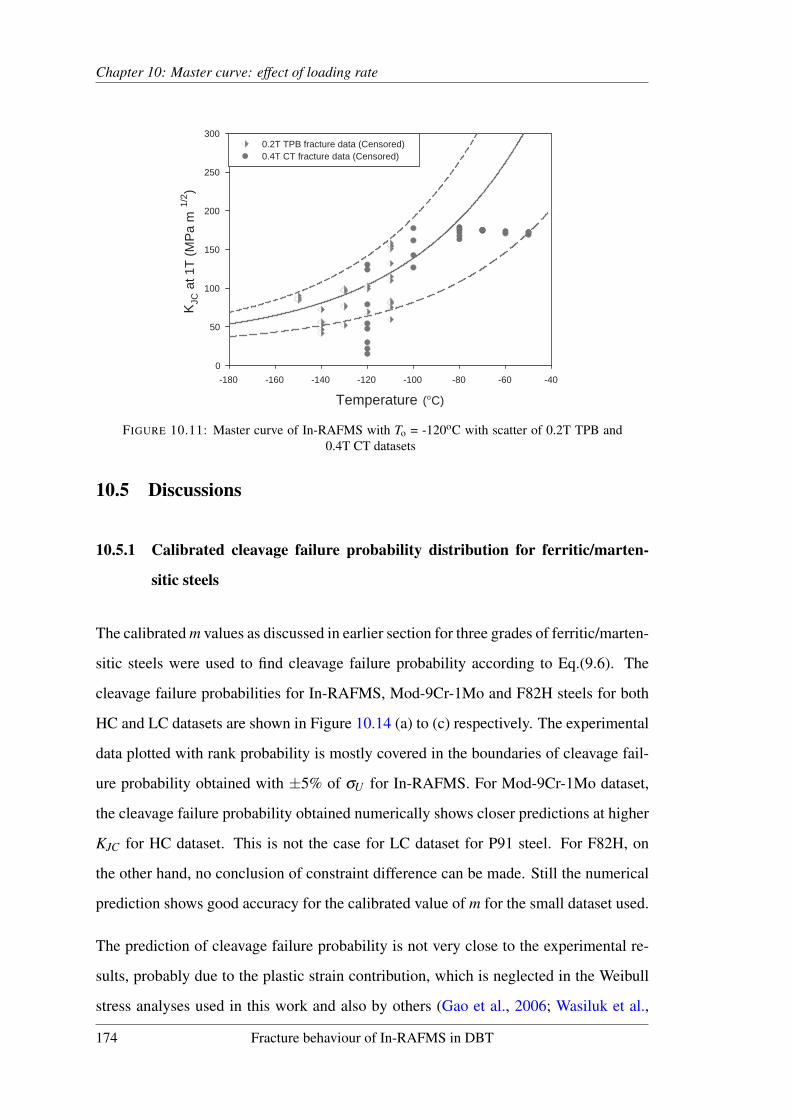
Chapter 10: Master curve: effect of loading rate
Temperature (oC)
-180 -160 -140 -120 -100 -80 -60 -40
KJC
at 1
T (
MP
a m
1/2 )
0
50
100
150
200
250
3000.2T TPB fracture data (Censored)0.4T CT fracture data (Censored)
FIGURE 10.11: Master curve of In-RAFMS with To = -120oC with scatter of 0.2T TPB and0.4T CT datasets
10.5 Discussions
10.5.1 Calibrated cleavage failure probability distribution for ferritic/marten-
sitic steels
The calibrated m values as discussed in earlier section for three grades of ferritic/marten-
sitic steels were used to find cleavage failure probability according to Eq.(9.6). The
cleavage failure probabilities for In-RAFMS, Mod-9Cr-1Mo and F82H steels for both
HC and LC datasets are shown in Figure 10.14 (a) to (c) respectively. The experimental
data plotted with rank probability is mostly covered in the boundaries of cleavage fail-
ure probability obtained with ±5% of σU for In-RAFMS. For Mod-9Cr-1Mo dataset,
the cleavage failure probability obtained numerically shows closer predictions at higher
KJC for HC dataset. This is not the case for LC dataset for P91 steel. For F82H, on
the other hand, no conclusion of constraint difference can be made. Still the numerical
prediction shows good accuracy for the calibrated value of m for the small dataset used.
The prediction of cleavage failure probability is not very close to the experimental re-
sults, probably due to the plastic strain contribution, which is neglected in the Weibull
stress analyses used in this work and also by others (Gao et al., 2006; Wasiluk et al.,
174 Fracture behaviour of In-RAFMS in DBT

Chapter 10: Master curve: effect of loading rate
Temperature (oC)
-140 -120 -100 -80 -60 -40
KJC
at 1
T (
MP
a m
1/2 )
0
100
200
300
Valid and Censored dataInvalid and Uncensored data
50% Median
95% Tolerance
5% Tolerance
dK/dt = 250-370 MPa m 1/2 s-1
To= -95 oC
Temperature (oC)
-140 -120 -100 -80 -60 -40
KJC
at 1
T (
MP
a m
1/2 )
0
50
100
150
200
250
300
350Valid and Censored dataInvalid Uncensored data
dK/dt = 650-1450 MPa m 1/2s-1
To= -90 oC
95% Tolerance
5% Tolerance
FIGURE 10.12: Master curves of 0.4T standard charpy specimens dataset of In-RAFMS testedat (a) 100 mm/min and (b) 1000 mm/min of actuator speed
2006). In the pioneer work by Beremin et al. (1983b), the effect of plastic strain was
studied on the cleavage failure probability. The formation of micro-cracks in reference
volume Vo must vary for different geometry of specimens, size and temperature, which
contributes to the sluggishness or abrupt initiations of micro-cracks. For the same ge-
ometry of notched tensile specimens at -196oC, (Beremin et al., 1983b) has reported a
rupture strain of 15% and 69%, which resulted in average rupture stress of 1127 and
1485 MPa, respectively.
Fracture behaviour of In-RAFMS in DBT 175

Chapter 10: Master curve: effect of loading rate
FIGURE 10.13: Shift in reference transition temperature To of In-RAFMS with increasingloading rate with the prediction of Wallin according to Eq.(10.1)
In the recent work by Ruggieri et al. (2015), the impact of plastic strain on cleavage fail-
ure probability is extensively studied with different form of functions used for inserting
the effect of plastic strain in Beremin’s model (Chapter 2). Though, with different forms
of plastic strain functions, close values of results can be obtained, the development of an
unequivocal form of function needs both more experimental studies with larger datasets
as well as analytical or empirical support. The investigation on contribution of plastic
strain function on cleavage failure probability distribution remains the scope for our
future study. With the observations made in this study, it can be concluded that the ex-
perimental behaviour supports the numerical predictions for the calibrated values of m
for In-RAFMS and P91 steels.
10.5.2 Effect of loading rate on fracture behaviour
The experimental results obtained from the fracture tests conducted on In-RAFMS
shows that the To obtained at various strain rates were in accordance with Wallins pre-
diction. The Zener-Hollomon parameter based correlation suggested by Wallin is based
on the heat of activation associated with the stress relaxation on loading at higher rates.
Zener and Hollomon, in their work used the indirect method of measurement of effects
176 Fracture behaviour of In-RAFMS in DBT

Chapter 10: Master curve: effect of loading rate
of loading rates on isothermal stress-strain response of the material, by accounting for
the changes due to loading rate with that due to temperature.
It is well known that the effect of strain rate on plastic flow of material is equivalent to
that induced by change in temperature (Zener and Hollomon, 1944). The same was ob-
served in the tensile behaviour of In-RAFMS, as shown in the σUT S/σo versus temper-
ature plot for quasi-static loading shown in Figure 6.6 (b) in Chapter 6. The equivalent
effect of decreasing σUT S/σo with increasing strain rate is also shown for In-RAFMS
in Figure 6.6 (b). The Zener-Hollomon strain rate parameter based correlation given
by Wallin for shift in To captures efficiently the experimental results for In-RAFMS.
This also implies that the activation energy defined by Zener and Hollomon, remains
constant in the range of loading rate investigated in this work. As the strain rate in-
creases the macroscopic toughness for cleavage decreases causing the To to shift at
higher values. This can be explained further using dislocation mobility as the effects
of decreasing temperature and increasing loading rate are equivalent. The toughness of
steels is demonstrated by the mobility of dislocations in lattice, which decreases with
decreasing temperature and increasing loading rate. The flow behaviour of BCC al-
loys has been found to have thermal and athermal part (Zerilli and Armstrong, 1987;
EricksonKirk and EricksonKirk, 2006). Additionally, if the thermal activation energy
described by Zener and Hollomon (1944) assumed to be constant in the tested con-
ditions, the increase in loading rate would result in decreased dislocation movement,
which in turn will decrease the toughness of the material. The effect of loading rate
on cleavage failure probability comparison with experimental rank probability for 100
mm/min and 1000 mm/min actuator speeds are shown in Figure 10.15(a) and Figure
10.15(b) respectively.
The fracture tests data, statistical and Weibull analysis parameters are noted in Table
10.2.
Fracture behaviour of In-RAFMS in DBT 177

Chapter 10: Master curve: effect of loading rate
(a)
(b)
(c)
FIGURE 10.14: Cleavage failure probability with HC and LC datasets of (a) In-RAFMS (b)Mod-9Cr-1Mo and (c) F82H steels
178 Fracture behaviour of In-RAFMS in DBT

Chapter 10: Master curve: effect of loading rate
(a)
(b)
FIGURE 10.15: Numerical prediction and experimental rank probabilities for fracture testsperformed at (a) 100 mm/min and (b) 1000 mm/min actuator speed
Fracture behaviour of In-RAFMS in DBT 179
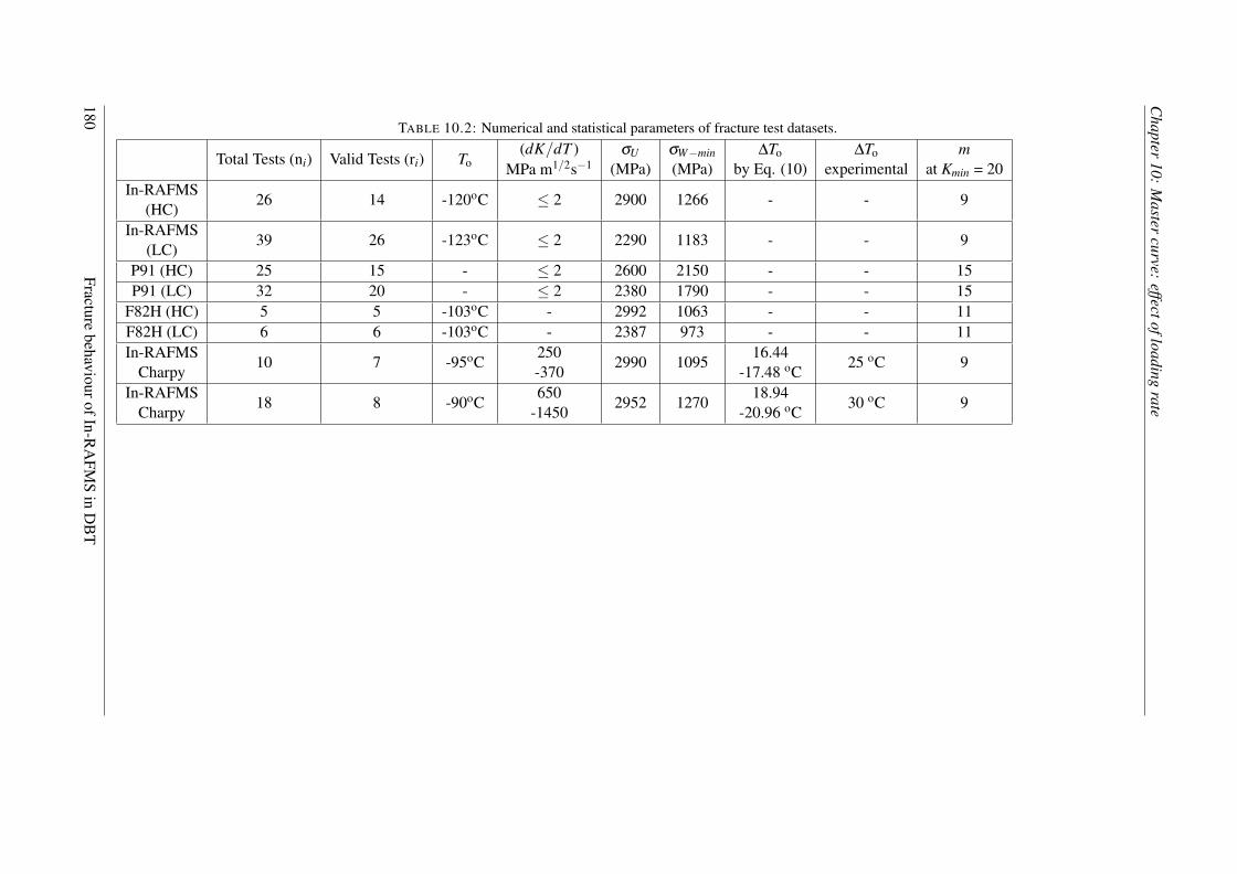
Chapter
10:M
astercurve:
effectofloadingrate
TABLE 10.2: Numerical and statistical parameters of fracture test datasets.
Total Tests (ni) Valid Tests (ri) To(dK/dT )
MPa m1/2s−1σU
(MPa)σW−min
(MPa)∆To
by Eq. (10)∆To
experimentalm
at Kmin = 20In-RAFMS
(HC)26 14 -120oC ≤ 2 2900 1266 - - 9
In-RAFMS(LC)
39 26 -123oC ≤ 2 2290 1183 - - 9
P91 (HC) 25 15 - ≤ 2 2600 2150 - - 15P91 (LC) 32 20 - ≤ 2 2380 1790 - - 15
F82H (HC) 5 5 -103oC - 2992 1063 - - 11F82H (LC) 6 6 -103oC - 2387 973 - - 11In-RAFMS
Charpy10 7 -95oC
250-370
2990 109516.44
-17.48 oC25 oC 9
In-RAFMSCharpy
18 8 -90oC650
-14502952 1270
18.94-20.96 oC
30 oC 9
180Fracture
behaviourofIn-RA
FMS
inD
BT

Chapter 10: Master curve: effect of loading rate
The scaling parameter of Weibull’s fit, σU , was found to be decreasing with the increase
in loading rate. The shift in To as well as in σU was larger when changing dK/dt from
quasi-static loading rate of 2 MPa m1/2s−1 to 250-370 MPa m1/2s−1 in comparison to
that for a change from 250-370 to 650-1450 MPa m1/2s−1. The result therefore pre-
dicts that the σU behaviour is also similar to the behaviour of To. Similar behaviour
of σU was found by Gao and Dodds Jr (2005b); Gao et al. (2008, 2001). The scaling
parameter decreased with increasing loading rate as the overall toughness of the mate-
rial decreased. The load carrying capacity of the material is hampered as dislocation
movement becomes difficult with increase in loading rate.
Another observation, which can be made from Figure 10.14(a), Figure 10.15(a) and
Figure 10.15(b) that as the material toughness decreases with increase in loading rate
the plastic strain impact appears to decrease. The numerical prediction comes closer to
the experimental rank probability distribution from Figure 10.14(a) to Figure 10.15(b)
with increasing loading rate. It can therefore be realized that the importance of plastic
strain factor to assess the effect of loading rate also needs to be studied in detail to
strengthen the cleavage failure probability predictions.
10.6 Conclusions
For the assessment of cleavage failure probability of ferritic/martensitic steels and to
investigate the effect of loading rate on reference transition temperature To along with
cleavage failure probability, two grades of ferritic/martensitic steel using CT and TPB
specimens were tested in DBT region. For the numerical prediction of cleavage fail-
ure probability, calibration of Weibull slope was carried out on HC and LC datasets
of the two steels. Calibration of Weibull slope was also attempted on fusion reactor
grade F82H steel, however, due to the reported inhomogeneity of the F82H dataset, the
calibrated m may lack in accuracy.
The cleavage failure probability for In-RAFMS and P91 steels datasets, captures the
experimental fracture behaviour to satisfactory extent. The prediction can be made
Fracture behaviour of In-RAFMS in DBT 181
Chapter 10: Master curve: effect of loading rate
more accurate with an established plastic strain embedded in the calculation of cleavage
failure numerical probability. The calibrated m value for In-RAFMS is found to be 9,
and close in the range with other ferritic/martensitic steels analysed in this work and
reported in Table 10.2.
The calibrated m value of In-RAFMS was used for assessment of fracture behaviour in
DBT region at elevated loading rates. At 0.5 mm/min, 100 mm/min and 1000 mm/min
of crosshead speeds the To estimated are -120oC, -95oC and -90oC, respectively. It is
found in the assessment that the probability of cleavage failure increases for a KJC at
higher loading rate and the shift in reference transition temperature To is in accordance
with correlation suggested by Wallin in Eq. (10.1).
182 Fracture behaviour of In-RAFMS in DBT

Chapter 11
Master curve in upper region of DBT
The fracture behaviour of ferritic and ferritic martensitic steels in Ductile to Brittle
Transition (DBT) region has been extensively studied in recent years and a probabilistic
approach of master curve method is generally used to describe the fracture toughness
of BCC steels in DBT region as a function of temperature. The assessment of cleavage
failure probability however is still untouched in the upper region of ductile to brittle
transition, although various extensions of master curve approach and various local ap-
proaches has been explored. Additionally, the geometry of specimens (CT and SE(B))
also adds up to the difficulties when cleavage failure is assisted with prior ductile tear-
ing. In this chapter, the cleavage fracture is investigated in upper region of DBT and
a modified master curve approach is presented, which can satisfactorily describe the
fracture toughness as a function of temperature as well as amount of ductile tearing pre-
ceding cleavage. The methodology is explored for both CT and SE(B) geometries.
The results and findings presented in this chapter are published in:
Tiwari, Abhishek, R. N. Singh, and Per Stahle. “Assessment of effect of ductile tearing
on cleavage failure probability in ductile to brittle transition region.” International Jour-
nal of Fracture (2017): 1-24.
and
Tiwari, Abhishek, R. N. Singh, Per Stahle, and J. K. Chakravartty. “Master curve in up-
per region of ductile brittle transition: a modification based on local damage approach.
Procedia Structural Integrity 2 (2016): 1553-1560.
183

Chapter 11: Master curve in upper region of DBT
11.1 Introduction
The approach of master curve and local approaches towards cleavage micro-mechanics
has already been discussed earlier. The subject, which has remained untouched in this
work is also the problem, which is not yet solved by the researchers of fracture com-
munity, is the problem of cleavage fracture in upper region of DBT. The phenomena of
cleavage when associates itself with significant amount of DCG prior to it, the fracture
toughness load-line displacement behaviour shows significant non-linearity violating
SSY domain and therefore remains isolated from the conventional master curve ap-
proach or any other probabilistic approach to described cleavage failure probability.
The dataset, which comprises cleavage fracture with significant amount of prior DCG
cannot be used for estimation of To. The fracture behaviour therefore in upper region
of DBT, which is a major part of DBT regime remains unanalysed and indescribable so
far. In this Chapter the approach towards this part of DBT is dealt with.
11.1.1 Cleavage fracture in upper region of ductile to brittle transition
Margolin et al. (2003) has discussed this issue in detail by discussing three possibilities,
which are
• Condition of cleavage fracture toughness measured at no prior ductile tearing to
be equal to cleavage fracture toughness with prior DCG, which means there is no
effect of prior DCG,
• Condition of cleavage fracture toughness at no prior ductile tearing to be > cleav-
age fracture toughness with prior DCG, i.e. fracture toughness increases more
steeply in upper DBT than master curve and
• Condition of cleavage fracture toughness no prior ductile tearing to be < cleavage
fracture toughness with prior DCG, i.e. fracture toughness increases less steeply
in upper DBT than master curve.
184 Fracture behaviour of In-RAFMS in DBT

Chapter 11: Master curve in upper region of DBT
In the work of Margolin et al. it was noticed that for general grade of ferritic steels the
fracture toughness in upper DBT is much by the plastic strain and the third condition is
observed. The same was experimentally observed by Tagawa et al. (2010), where the
specimens of two different thickness to width ratios (B/W ) were tested. Tagawa et al.
concluded in their work that in upper region of DBT the cleavage failure probability
scales with BK2 rather than the master curve scaling of BK4.
Scibetta (Scibetta, 2010) brought out that for very low toughness materials the onset of
DCG resulting in cleavage can occur prior to out of plane loss of constraint. It was also
re-confirmed in the same study that the crack growth effectively increases the cleavage
failure probability by resharpening the crack tip and lower bound of DBT region is
unaffected by such mechanisms.
The phenomena of cleavage failure with prior DCG has also been investigated by Moskovic
(Doig and Moskovic, 1993; Moskovic, 2002; Burdekin et al., 1999) using log-normal
distributions. The analytical contribution of sampled volume in case of prior DCG is
studied by Bruckner and Munz (Bruckner and Munz, 1984). The study of Bruckner and
Munz and Wallin Wallin (1989a) on the probability of cleavage failure with prior DCG
shows similar expressions as,
ln(1
1−Pf) = (
KKo
)4 · DK4
o
∫∆a
0( f (∆a)m)∂ (∆a) , (11.1)
where f (∆a) is a function of ∆a and m has a value of 2 in Wallin’s work and 4 in
the work of Bruckner and Munz. The parameter D is a function dependent on flow
behaviour of the material and the position of maximum value of tensile stress ahead
of crack tip. Wallin’s expression of the form as shown in Eq.(11.1) assumes that the
effective active volume grows with increased loading, whereas Bruckner and Munzs
expression assumes the active volume to be constant with crack growth. Wallin (Wallin,
1989a) simplified the probability of failure for very small prior DCG by a modified
probability distribution as,
Fracture behaviour of In-RAFMS in DBT 185

Chapter 11: Master curve in upper region of DBT
ln(1
1−Pf)1/4 = (
BnT
B1T)1/4(
K−Kmin
Ko−Kmin) · (1+2
∆aσ2f low
K2β)1/4 , (11.2)
where β = 3.5(KJCσo
)2, is the distance from the crack tip to the boundary of the active
volume and σ f low is the average of ultimate tensile strength and Yield strength (σo),
The simplification in the form of Eq.(11.2) was given by Wallin to avoid cumbersome
integration of function of ∆a and this form of equation was suggested to be valid for a
small amount of ∆a where KJC versus ∆a behaviour is flat.
With the discussion on master curve methodology and process of cleavage fracture in
upper region of DBT, it is observed that the cleavage is generally preceded by significant
amount of ductile tearing in upper region of DBT. The KJC inevitably fails to single
handedly describe the fracture toughness and master curve methodology cannot be used
for describing the correlation of fracture toughness with temperature. The problem
therefore arises with the dataset, which shows cleavage fracture and yet cannot be used
straight away for probabilistic determination of its correlation with temperature. The
conventional master curve methodology censors the dataset generated in upper DBT.
Censoring the dataset in DBT region is a powerful tool to utilize the data, which do not
fall into the validity window of the statistical model of master curve. The censoring
scheme is schematically shown in Figure (11.1).
In case of MC approach another censoring method for loss of constraint is applied,
which uses the ligament length and the flow properties of the tested sample and limits
the toughness by a constraint parameter M is described in Chapter 2, Eq.(2.13). The
value of KJC,limit is, according to Eq.(2.13), the fracture toughness, which sample would
have achieved in SSY condition. The tested toughness value, i.e. KJC,exp is discarded
from the analysis. This part of censoring is appreciated by the authors for constraint
loss, however constraint correction methods (Tiwari et al., 2015; Gao and Dodds Jr,
2000) can be used to transform the invalid toughness values to a SSY equivalent values.
The numerical correction and MC censoring are similar in nature and any of the method
can be used.
186 Fracture behaviour of In-RAFMS in DBT

Chapter 11: Master curve in upper region of DBT
FIGURE 11.1: Schematic of validity criteria of datasets used in master curve method
The censoring where the data corresponding to cleavage failure with significant amount
of ductile tearing is also appreciated as long as the analysis method is master curve
approach. The real behaviour of upper region of DBT and utilization of dataset be-
longing to upper region of DBT in assessment of a transition temperature is missed by
conventional methods. The question arises that whether the dataset in upper region of
DBT can be dealt in a similar way and whether it would be possible to elevate the struc-
tural potential of a material, which might be under utilized by conventional conservative
approaches.
The fracture toughness with temperature changes in upper DBT drastically due to the
significant changes at the crack tip activities due to prior ductile tearing. Whether or
not the master curve methodology holds good to certain extent is one of the question
being investigated in this study. The answer to the question imposed by the event of
cleavage preceded by ductile tearing is not very simple, however it is certain that the
fracture toughness is not dependent on temperature only. The amount of ductile tearing
significantly alters the behaviour of fracture toughness with temperature.
The objective of this work is to answer some of the questions if not all. The upper
region of DBT is examined using existing approaches and works of other researchers
and an important factor of constraint increment with DCG, which is missing in earlier
studies of this subject, is incorporated.
Fracture behaviour of In-RAFMS in DBT 187

Chapter 11: Master curve in upper region of DBT
In our approach, the cumbersome integration part of Eq.(11.1) is solved with an as-
sumption that the materials resistance curve remains unchanged in the DBT region.
This assumption is not far from reality for many of the tested materials. The approach
to study the upper region of DBT is studied in this work by extending the master curve
concept and incorporating the changes occurring due to prior ductile tearing. The con-
ventional master curve is an extensively studied subject and has been proven to be a
strong tool to measure reference transition temperature as a global parameter indepen-
dent of specimen geometry, loading rate and type of loading. The analysis of upper
region of DBT ought to complicate the simple master curve methodology but it is justi-
fiable for the complex nature of fracture behaviour in this region of transition. It is not
the objective of this work to create a cumbersome methodology. The work presented
explores the upper region of DBT and efforts are made to make the fracture data avail-
able in upper region of DBT potent enough to determine To, which otherwise may not
be determined for a completely or partially invalid dataset.
11.2 Material datasets
For the assessment of effect of fracture behaviour in DBT region, the largest dataset
is the Euro Fracture dataset. This dataset was created by testing 0.5T, 1T, 2T and
4T thick Compact Tension (CT) specimens at various laboratories across Europe on
22NiMoCr37 steel. The cumulative dataset contains test results conducted over many
years. For the assessment of modification proposed in this work on cleavage failure
probability, the dataset of 0.5T specimens are used as the dataset of 0.5T specimens
contain most of the cleavage data affected by prior DCG.
Apart from Euro dataset, 0.4T CT specimen dataset and 0.2T SE(B) dataset of In-
RAFMS were also used for assessment of effect of prior ductile tearing on cleavage
fracture. The material and experimental details are provided in Chapter 4 and 5, respec-
tively.
188 Fracture behaviour of In-RAFMS in DBT

Chapter 11: Master curve in upper region of DBT
11.3 Cleavage with prior DCG
11.3.1 Increasing active volume with DCG
The volume as discussed above, which influences the cleavage event is the volume,
which is under sufficient tensile stress and, which has deformed plastically. This volume
is shown schematically in two dimension for a crack growth of ∆a in Figure 11.2. It
FIGURE 11.2: Schematic of increasing active volume with ductile tearing
is well studied that the maximum first principal stress is achieved at a distance of 2-4
times of Crack Tip Opening Displacement (CTOD) symbolized as δ . For a material this
value of proportionality is constant in the range of 2-4 and therefore, for our calculation
of increasing active volume it is assumed that the maximum first principal stress is
achieved at a distance of λ times of CTOD. Similar to the derivation of Wallin, an
arbitrary triangular area is considered as shown in Figure 11.2 for derivation. It is also
assumed here that the stress field remains self-similar along the thickness. For initial
condition of no crack growth, the active volume for the half symmetric crack tip as in
Figure 11.2 would be
V =12
λδi ·λδi ·B tanθ , (11.3)
Fracture behaviour of In-RAFMS in DBT 189
Chapter 11: Master curve in upper region of DBT
where B is the specimen thickness and δi is the initiation CTOD. It is a valid assumption
made here that the scaling of the perpendicular and the base of the triangular region in
Figure 11.2 remains unchanged with DCG (Wallin, 1989a). Thus, after a ductile through
thickness crack growth of ∆a the active volume would be
V =12
λ (δ +∆δ ) ·λ (δ +∆δ ) ·B tanθ , (11.4)
The scaling volume Vo as described by Wallin can be defined by the argument of BK4
scaling with Vi as the active volume at the CTOD of δi as
Vo =Viδo
δi. (11.5)
The cleavage failure probability as a function of active volume can be described as
Pf = 1− exp[− ρ
ρo· V −Vmin
Vo−Vmin] . (11.6)
where ρ defines the number density of critical cleavage initiators taking part in micro-
crack generation. Under the assumption of homogeneous distribution of cleavage ini-
tiators it is not unwise to state that ρ at any point of applied K will be same as ρo, only
if there is no crack growth. The effect of crack growth on Pf will be discussed in section
11.3.2. For through thickness self similarity and for Vmin to be zero, the cleavage failure
probability can be simply defined as
Pf = 1− exp[−VVo
] . (11.7)
Using the expressions of V and Vo from Eq.(11.4) and Eq.(11.5) and ignoring the higher
order terms, the probability of cleavage failure can be re-written as,
ln(1
1−Pf) =
δ 2
δ 2o· (1+2
∆δ
δ) . (11.8)
190 Fracture behaviour of In-RAFMS in DBT

Chapter 11: Master curve in upper region of DBT
By using the fact that CTOD is directly correlated to J and again transforming J to K,
Eq.(11.5) can be re-written as,
ln(1
1−Pf) =
K4
K4o· (1+2
(∆K)2
K2 ) . (11.9)
The derivation of increment in active volume is similar to that of Wallin and for more
details the readers are referred to the work of Wallin (1989a). The expression how-
ever differs and is more simple in this case. Another simplification is incorporated by
describing the K versus ∆a correlation with Ki as the initiation fracture toughness as,
K = Ki +φ(∆a)m) . (11.10)
The K correlation with ∆a as described above is used to replace ∆K from Eq.(11.9),
which results in cleavage failure probability as,
ln(1
1−Pf) =
BnT
B1T
K4
K4o· [1+2
(φ(∆a)m)2
K2 ] . (11.11)
11.3.2 Change in constraint with DCG
In the assessment of effect of ductile tearing on cleavage failure probability by Wallin
as well as Bruckner and Munz, the change in constraint associated with ductile crack
growth was ignored. For a significantly smaller crack growth, this assumption does not
result in much error, however, for a significant amount of ductile tearing as observed
in upper region of DBT, the change in constraint needs to be addressed in the cleavage
failure probability calculation.
As the crack grows, the sampled volume increases and the probability of cleavage fail-
ure increases. The initial ductile tearing may occur due to the overall increase in plas-
ticity of material matrix or due to the constraint loss. Both result in increase in tough-
ness values. As the crack advances, the constraint increases due to decreasing ligament
length. In other words, the ductile tearing may start due to constraint loss or higher test
temperature, which makes carbides less critical for unstable crack growth and tries to
Fracture behaviour of In-RAFMS in DBT 191

Chapter 11: Master curve in upper region of DBT
achieve higher constraint by increasing a/W . However, if the carbide becomes critical
for instability, cleavage occurs.
It is many a times doubted whether the change in constraint with advancing crack is
positive i.e. constraint increases or negative i.e decreases, despite numerous works in
literature on both CT and SE(B) geometries in support of increment in constraint with
DCG (Moattari et al., 2016; Varias, 1998; Yan and Mai, 1997; Ruggieri and Dodds Jr,
1996). The increment in constraint is attributed to the decreasing ligament length and
to understand the effect in a very simple way one can take an imaginary ligament to be
the reference frame. This imaginary ligament is assumed to be constant with growing
crack. In reality however, the ligament will decrease and so will the ratio of ligament and
thickness of the specimen. To keep this ratio same for imaginary ligament the thickness
should increase. Therefore, a crack growth process can be viewed as a transition from a
thinner to thicker specimen with decreasing ligament to thickness ratio. The importance
of ρ in Eq.(11.6) is readily brought out as the change in constraint will change the
effective distribution of imhomogeneities/carbides, which become critical for micro-
crack initiation. Thus, the probability of cleavage fracture needs further modification
to incorporate the changes occurring in ρ
ρowith increasing constraint. It is already
discussed by many researchers that for α number of carbides taking part in cleavage
fracture directly, the condition of ductile tearing i.e. increasing plastic strain imposes
a few of these carbides say αo to participate in micro-void coalescence. Therefore,
only α −αo number of carbides remain available for next active volume for cleavage
initiation as those taking part in micro-void coalescence cannot contribute to micro-
crack nucleation and its dynamic propagation. The number of carbides taking part in
micro-void coalescence depends on amount of plastic strain. The events taking place at
the crack tip for a ductile matrix chronologically can be described as below.
• With applied loading the stresses at the crack tip increases and the crack tip de-
forms plastically. If the carbides in the active volume do not initiate micro-cracks
the plastic strain continues to increase and the micro-void coalescence occurs as
192 Fracture behaviour of In-RAFMS in DBT

Chapter 11: Master curve in upper region of DBT
it becomes difficult for the micro-crack generated by failed carbide to move into
the matrix at lower stresses.
• The micro-voids subsequently grow and coalesce further to promote ductile tear-
ing. Statistically it can be visualized that all the carbides may not participate in
micro-void coalescence and some may participate in micro-cracks propagation
into the matrix, which locally escalates the probability of cleavage according to
Eq.(11.6).
• As the crack grows the volume ahead of crack tip consists of a region, which is
elastically unloaded followed by a new active volume, which may take part in
cleavage fracture and a region between these two where plastic strain is higher
to promote nucleation, growth and coalescence of voids (Ruggieri and Dodds Jr,
1996).
• With the crack growth, the constraint ahead of the crack tip increases and the
chances for carbides to contribute in micro-void coalescence decreases.
With the above discussion, it can be concluded that the increasing constraint can be used
as a measure of change in ρ with respect to the initial distribution density of carbides.
Generally for a growing crack the constraint is measured by a factor q also known as
triaxiality parameter, which is defined as the ratio of hydrostatic stress component, σh
and equivalent stress σeq (Ruggieri and Dodds Jr, 1996; Yan and Mai, 1997; Moattari
et al., 2016)
As the constraint increases the material flow is restricted and the material around the
carbide cannot increase its plastic strain easily in comparison to the matrix where con-
straint is less. With triaxiality ratio q as a measurement of constraint, a simple function
can be defined to accommodate the effective increment in potential cleavage initiators.
This increment should have a reference frame set at the initial testing condition and
the number density of potential cleavage initiators should increase with increasing con-
straint due to ∆a. This function is defined here by assuming a linear proportionality
Fracture behaviour of In-RAFMS in DBT 193

Chapter 11: Master curve in upper region of DBT
between ρ
ρoand corresponding triaxialities as,
ϕ =q f
qi, (11.12)
where q f is the final triaxiality factor and qi is the triaxiality factor before the ductile
tearing starts. The linear approximation is inspired from the pioneer work of Argon
et al. (Argon et al., 1975) and Beremin et al. (Beremin, 1981) where the stress based
criteria for debonding of inclusions to form cavities is a function of σh+σeq, which can
be rearranged to be a function of q as σeq(1+q). As the debonding of the inclusion is
accelerated with increasing constraint for a system of carbides it would assist in dynamic
propagation of micro-cracks into matrix and from one grain to another before the plastic
strain limit for micro-void coalescence is reached.
With earlier discussion on increasing active volume calculation and triaxiality function
, the cleavage failure probability can now be redefined with the increment in active
volume and cleavage initiators with a function of q as,
ln(1
1−Pf) =
BnT
B1T(q f
qi) · ( K−Kmin
Ko−Kmin)4 · [1+2
(φ(∆a)m)2
K2 ] . (11.13)
The maximum likelihood analysis of Eq.(11.13) is carried out using Eq.(2.10) and
Eq.(2.11). The maximization of maximum likelihood parameter L is performed only
with respect to To as other variables of Eq.(11.13) are kept as in ASTM E1921, with
Kmin = 20 MPa m1/2. Detailed maximum likelihood analysis procedure for Eq.(11.13)
is provided in Appendix A.3.
The temperature dependence of KJC in modified master curve follows same behaviour
as in conventional master curve described in Eq.(2.6). For a mean approximation of KJC
behaviour with ductile crack growth ∆a, the dependency of KJC with ductile tearing can
be described as,
KJC,med = A+(100−A)exp0.019(T −To)= KJC,ini +φ(∆a)m . (11.14)
where KJC,ini is the initiation fracture toughness and φ and m are the power law fitting
194 Fracture behaviour of In-RAFMS in DBT

Chapter 11: Master curve in upper region of DBT
constants. The modified master curve therefore follows the correlation with ∆a either
coming out as a mean approximation from the experimental data or from the numerical
prediction based on finite element analysis.
With the cleavage failure probability described in the form of Eq.(11.13), one can ex-
press the cleavage failure probability for two differently sized specimens, say of thick-
ness nT and 1T where T denotes thickness in inches, with same amount of cleavage
fracture probability as,
BnT ·K4
nTK4
o· f (∆a) = B1T ·
K41T
K4o· f (∆a) . (11.15)
It is required here to have a mean approximation of size independent KJC −∆a or a
KJC−∆a correlation obtained by numerically analysing 1T reference thickness geome-
try. In this case the function dependent on DCG cancels out and size adjustment scheme
of conventional master curve can be used for the proposed modification. In the formu-
lation of Eq.(11.13) there is a function dependent on triaxiality also included in the
probability expression. This function assuming it to be independent of other parameters
will also cancel out for a size independent behaviour for same amount of DCG. The
effect of plastic strain embrittlment on the triaxiality function is discussed in section 6,
which supports the unchanged size adjustment scheme.
11.4 Numerical analyses
The numerical analysis to simulate prior ductile crack growth to cleavage, was car-
ried out with ductile damage. The failure criteria of elements were ductile damage
dependent. The load displacement response of the model was used to calculate KJC by
assuming cleavage to occur at each increment of crack. The finite element analyses of
both CT and TPB geometries were performed for measurement of change in constraint
with ductile tearing.
Fracture behaviour of In-RAFMS in DBT 195

Chapter 11: Master curve in upper region of DBT
The plastic behaviour, using isotropic hardening following the true stress plastic strain
response used as input, was implemented in VUMAT subroutine. The numerical so-
lution followed full Newtonian non linear algorithm using explicit scheme. The mesh
size was kept constant in the area of interest near the crack tip for volume calculation as
the post processing for active volume calculation requires the elemental volume to be
constant in the crack tip region (Tiwari et al., 2015). Twenty noded brick elements were
used for both tensile specimen models as well as CT and TPB fracture models. The
element size near crack tip was 0.15 mm in thickness direction and 0.2 mm in plane
normal to crack front.
11.4.1 Ductile damage implementation
The ductile damage was introduced in the finite element analyses using Gurson, Trever-
gaard and Needleman (GTN) (Gurson, 1977; Tvergaard, 1982; Tvergaard and Needle-
man, 1984) model. The details of the ductile damage implementation is given in Chapter
5, section 5.2.2.
11.4.2 Calibration of GTN parameters
Initially it was required to justify that the user subroutine VUMAT was coded correctly.
Therefore, the subroutine was compared with the ductile damage porous plasticity in-
built in ABAQUS FEA package. The geometry of the tensile specimen modelled is
shown in Figure 11.3(a) In Figure 11.3(b), the comparison of the engineering stress
strain response of quarter symmetric three dimensional (3D) model of tensile specimen
is shown. The calibration of GTN parameter and VUMAT with calibrated parameter is
compared in Figure 11.3(b). The void volume fraction f ? at the centre of the quarter
symmetric tensile model is also compared in Figure 11.3(c).
It can be realized from Figure 11.3(c) that the VUMAT coded was reasonably accurate.
The reason for coding of ductile damage using VUMAT subroutine was preferred on
196 Fracture behaviour of In-RAFMS in DBT

Chapter 11: Master curve in upper region of DBT
(a) (b)
(c)
FIGURE 11.3: Implementation of ductile damage in FEM using VUMAT subroutine; (a) Ge-ometry of quarter symmetric tensile specimen (b) Calibration of GTN paratemeters (c) Com-
parison of calibrated VUMAT with Abaqus porous plasticity
ABAQUS in-built porous plasticity, to have freedom in changing or removing nucle-
ation or growth rate calculations if needed.
11.4.3 Finite element models of CT and TPB geometries
The GTN parameter calibration was carried out using ABAQUS in-built porous plastic-
ity algorithm using 3D explicit 8 noded brick elements with 2×2×2 Gaussian points.
The initial trial of GTN parameters were taken from the work of Stratil et al. (2014)
on Eurofer 97. The plasticity data were given in form of true stress-true plastic strain
Fracture behaviour of In-RAFMS in DBT 197

Chapter 11: Master curve in upper region of DBT
extrapolated to a final plastic strain of 2. The plastic data used for modelling, corre-
sponded to In-RAFMS tensile data tested at -110oC and -130oC. At these temperature
many fracture specimens tested in three point bending revealed significant ductile crack
growth prior to cleavage failure.
The mesh and boundary conditions with quarter symmetric specimen dimensions for
CT and TPB geometries are discussed in Chapter 5. The GTN parameters for porous
plasticity and VUMAT subroutine models used for calibration of -110oC tensile speci-
men response for In-RAFMS is shown in Table 11.1.
TABLE 11.1: Trials used for GTN parameter calibration for In-RAFMS tensile response at-110oC
Tensile models GTN Parametersq1 q2 fF fC µ σstd fo
Abaqus porousplasticity-1
1.26 0.931 0.1 0.02 0.3 0.1 0.00088
Abaqus porousplasticity-2
1.26 0.931 0.17 0.01 0.3 0.1 0.00088
Abaqus porousplasticity-3
1.26 0.931 0.1 0.01 0.3 0.1 0.00088
Abaqus porousplasticity-4
1.06 0.931 0.29 0.1 0.3 0.1 0.00088
Abaqus porousplasticity-5
1.06 0.931 0.35 0.1 0.3 0.1 0.00088
Apart from the objective of obtaining change in constraint and fracture responses from
the finite element models a qualitative study of increasing number density of carbides
taking part in cleavage fracture with increasing DCG was also performed on SE(B)
geometry by assigning linear elastic properties for small number of elements, chosen
psuedo-randomly using computer code. The increasing stresses on these elements sim-
ulating elastic response while matrix deforms plastically confirms increasing ρ
ρoas de-
picted with continuous crack growth in Figure 11.4.
For the application of modified master curve formulation on Euro fracture data, three
test temperatures were chosen to investigate the effect of plastic strain in terms of void
volume fraction at failure and embrittlement in terms of true stress logarithmic strain
response. The three test temperatures, 0oC, -20oC and -60oC were chosen as at 0oC and
198 Fracture behaviour of In-RAFMS in DBT

Chapter 11: Master curve in upper region of DBT
-20oC, most of the data were affected by prior DCG and at -60oC many conventionally
valid data were available for comparison of conventional and modified master curve.
The 22NiMoCr37 steel tensile data were obtained from Heerens and Hellmann (2002).
The true stress strain behaviour of 22NiMoCr37 steel used for FE analyses is shown in
Figure 11.5 (a).
Fracture behaviour of In-RAFMS in DBT 199

Chapter 11: Master curve in upper region of DBT
(a)
(b)
(c)
FIGURE 11.4: Psuedo-randomly distributed elastic elements showing effect of constraint on
criticality of carbides (a) Onset of DCG and carbides, (b) ∆a = 0.2mm, (c) ∆a = 0.4mm
200 Fracture behaviour of In-RAFMS in DBT

Chapter 11: Master curve in upper region of DBT
(a) (b)
FIGURE 11.5: True stress plastic strain response extrapolated to 2 for (a) 22NiMoCr37 and (b)
In-RAFM steel
The true stress plastic strain response used for finite element analyses of In-RAFMS at
-110 and -130oC are shown in Figure 11.5 (b). The GTN parameters for 22NiMoCr37
steel used for modelling ductile crack growth were calibrated using load displacement
response. The tensile load displacement reponse for 22NiMoCr37 steel was obtained
from ftp://ftp.gkss.de/pub/eurodataset and the final point was assumed to be the fail-
ure point. The calibrated GTN parameters for 22NiMoCr37 steels and In-RAFMS are
shown in Table 11.2.
TABLE 11.2: Calibrated GTN parameters used for ductile crack growth modelling for In-RAFMS and 22NiMoCr37 steels
Euro Fracture Data Material (22NiMoCr37 Steel)GTN parameters
Test Temperature YS UTS fo σstd µ q1 q2 fC fF
0 470 621 0.009 0.1 0.3 1.35 0.931 0.08 0.12-20 476 640 0.008 0.1 0.3 1.05 0.78 0.1 0.15-60 509 670 0.008 0.15 0.3 1.35 0.931 0.08 0.12
In-RAFMSTest Temperature YS UTS GTN parameters
-110 560 710 0.00088 0.1 0.3 1.06 0.931 0.1 0.1-130 790 951 0.00088 0.1 0.3 1.01 0.95 0.1 0.15
Fracture behaviour of In-RAFMS in DBT 201

Chapter 11: Master curve in upper region of DBT
11.5 Results
Finite element modelling of CT and TPB geometries with GTN damage made it possible
to calculate the change in triaxiality factor q with ∆a. The behaviour of changing q with
crack length to specimen width ratio for the CT and TPB models are shown in Figure
11.6 (b).
(a) (b)
FIGURE 11.6: Triaxiality ratio q f /qi at different temperatures for (a) 0.5 T CT 22NiMoCr37
steel, (b) 0.4 T CT In-RAFM steel
Similar behaviour was observed for the material of Euro fracture data, i.e. DIN 22NiMoCr37.
The behaviour of traixiality function for 22NiMoCr37 steel at three different tempera-
ture obtained by modelling 0.5T CT geometry is shown in Figure 11.6 (a).
The qualitative finite element results to visualize effect of increment in potential cleav-
age initiators is shown in Figure 11.4, where as the ductile crack grows more numbers
of psuedo-randomly selected elements feel higher stresses, confirming the effect of in-
creasing constraint on ρ
ρo.
The increasing active volume with ductile tearing for TPB and CT side grooved models
are shown in Figure 11.7.
202 Fracture behaviour of In-RAFMS in DBT

Chapter 11: Master curve in upper region of DBT
(a) TPB-SDV4 (Void volume fraction)with fF crite-ria at ∆a = 0.67 mm
(b) Active volume at ∆a = 0.67 mm
(c) CT- SDV4 (Void volume fraction)with fF criteriaat ∆a = 0.5 mm
(d) Active volume at ∆a = 0.5 mm
(e) CT- SDV4 (Void volume fraction)with fF criteriaat ∆a = 1.3 mm
(f) Active volume at ∆a = 1.3 mm
(g) CT- SDV4 (Void volume fraction)with fF criteriaat ∆a = 1.7 mm
(h) Active volume at ∆a = 1.7 mm
FIGURE 11.7: Ductile tearing based on GTN ductile damage in 0.4T CT side grooved and 0.2TTPB geometries modelled with material parameters corresponding to -110oC for In-RAFMS
The modified master curve analyses were performed on different datasets as discussed
earlier using Eq.(11.13) with a partial censoring approach. As discussed in section
Chapter 2, the conventional master curve applies two fold of censoring on the frac-
ture data. The censoring to avoid contribution in non-linearity of load-displacement
behaviour due to ductile tearing is avoided in modified master curve analysis. Any data
showing ductile tearing is treated valid and only those data, which showed no DCG and
Fracture behaviour of In-RAFMS in DBT 203

Chapter 11: Master curve in upper region of DBT
crossed the criteria of KJC,limit based on out of plane constraint loss, were censored. This
approach of single fold censoring increases the validity window of conventional master
curve and expands it to upper region of DBT. The results of master curve analyses on
different datasets are discussed below.
11.5.1 Euro fracture data
The Euro fracture dataset of 0.5T CT specimen shows ductile crack growth as high as
2.54 mm. The KJC versus ∆a behaviour for 0.5T CT dataset and one obtained at 0oC,
-20oC and -60oC by finite element analyses are shown in Figure 11.8 (b).
The dataset does not show much variation in the behaviour in the temperature region of
-60oC to 0oC for 0.5T CT specimens. The correlations obtained in form of Eq.(11.10)
were used for maximum likelihood analysis of modified master curve.
The reference transition temperatures for dataset affected by ∆a is analysed using Eq.(11.13)
is expected to shift lower due to increasing KJC,med . This behaviour as a result of mod-
ified master curve analysis is shown in Figure 11.9 (a). The comparison is shown by
further categorizing the dataset in three sections. The first section includes dataset with
∆a < 1 mm, the second section with ∆a varying in range of 1.2 mm to 1.45 mm and
the third section with ∆a > 1.45 mm. The change in To, as discussed earlier can be
predicted by Eq.(11.14), which is compared with the modified master curve results in
Figure 11.9 (b).
204 Fracture behaviour of In-RAFMS in DBT

Chapter 11: Master curve in upper region of DBT
(a)
(b)
FIGURE 11.8: (a) Engineering Stress-strain response 22NiMoCr37 steel tensile specimens
and (b) KJC−∆a response of 0.5T CT Euro data
11.5.2 In-RAFMS data
The fracture tests performed on In-RAFMS comprised 26 tests on 0.4T CT specimens
and 39 tests on 0.2T TPB specimens in the range of test temperature from -50oC to -
150oC. The finite element based KJC versus ∆a behaviour calculation was carried out for
Fracture behaviour of In-RAFMS in DBT 205

Chapter 11: Master curve in upper region of DBT
(a)
(b) Modified master curve
FIGURE 11.9: (a) Modified master curve and conventional master curve for 0.5T CT Eurofracture dataset and (b) comarison with predictions obtained from Eq. (31)
-110oC and -130oC. The engineering stress-strain behaviour is shown in Figure 11.10
(a). The KJC versus ∆a behaviour of In-RAFMS dataset is shown in Figure 11.10 (b),
where finite element results obtained at -110oC and -130oC are also compared. The
TPB specimen experimental data was inconclusive to give a KJC versus ∆a correlation.
Therefore, the correlation obtained from CT specimen dataset was used for modified
master curve analysis.
The modified and conventional master curve results for In-RAFMS are shown in Figure
11.11 (a) and Figure 11.11 (b) for CT and TPB datasets, respectively. The To values
obtained from conventional and modified master curve methods for CT dataset are -
120oC and -123.5oC respectively. On the other hand for TPB dataset the conventional
and modified master curve analyses resulted in To values of -123oC and -140oC.
206 Fracture behaviour of In-RAFMS in DBT

Chapter 11: Master curve in upper region of DBT
(a)
(b)
FIGURE 11.10: (a) Engineering stress strain response In-RAFMS and (b) KJC versus ∆a behav-ior of In-RAFMS obtained from experimental CT and TPB datasets and finite element analyses
The larger difference in the results of TPB dataset is attributed to the fact that more
number of data in case of TPB were affected by prior DCG in comparison to CT dataset.
Although the amount of ductile tearing was more in case of CT specimens due to the
higher test temperatures but more datasets with smaller amount of DCG were involved
in the TPB dataset. Another reason, which had an effect on modified master curve
analysis was the differences in triaxiality function in comparison to CT.
Fracture behaviour of In-RAFMS in DBT 207

Chapter 11: Master curve in upper region of DBT
(a)
(b)
FIGURE 11.11: (a) Conventional and modified master curves 0.4T CT and (b) 0.2T TPBdatasets of In-RAFM steel
11.6 Discussion
The modified cleavage failure probability derived from conventional master curve method-
ology when applied on selected datasets shows a greater potential of utilizing the cleav-
age data with prior DCG. The modification based on incremental active volume and
constraint helps in estimation of reference transition temperature, To from the conven-
tionally invalid dataset. The approach described to incorporate the effect of prior DCG
208 Fracture behaviour of In-RAFMS in DBT

Chapter 11: Master curve in upper region of DBT
on cleavage failure probability by Wallin is compared with the rank probability and
proposed correction by present authors in Figure 11.12.
FIGURE 11.12: Comparison of conventional, Wallin’s and proposed formulation with rankprobability obtained for 0.5T CT Euro fracture data at -40oC
The unique correlation of active volume scaling with functions of KJC, ∆a, and triax-
iality is shown in Figure 11.13. It can be seen from Figure 11.13 that on a semi-log
scale for functions of KJC, ∆a, and triaxiality, the volume shows two different depen-
dencies for proposed formulation described by Eq.(11.13). The slope changes a little
later from the initiation of DCG and follows the scaling to the maximum DCG simu-
lated at -110oC and -130oC. Wallin’s DCG correction also shows similar trend but the
behaviour changes at larger DCG.
Fracture behaviour of In-RAFMS in DBT 209

Chapter
11:M
astercurve
inupper
regionofD
BT
(a) (b)
FIGURE 11.13: Comparison of scaling of Active volume with conventional, Wallin’s correction and proposed model of this work for (a) -110oC and (b) -130oC
210Fracture
behaviourofIn-RA
FMS
inD
BT

Chapter 11: Master curve in upper region of DBT
11.6.1 Effect of plastic strain and embrittlement
Various investigations on the effect of prior DCG on cleavage fracture probability,
exploring the subject using local approaches (Moattari et al., 2016; Margolin et al.,
2003; Ruggieri and Dodds Jr, 1996; Sobotka and Dodds, 2014) as well as global ap-
proaches (Bruckner and Munz, 1984; Moskovic, 2002; Tagawa et al., 2010; Scibetta,
2010; Wallin, 1989a) converge to demonstrate that the probability of cleavage fracture
increases with increasing amount of prior ductile tearing in a cleavage fracture, except
Margolin et al. (2003). In Margolin et al. (2003) work a heat treated condition simu-
lating irradiation hardening was analysed using local approach and it was demonstrated
that for embrittled condition the probability of cleavage fracture decreased. The increas-
ing probability of cleavage fracture originates from the facts such as increasing active
volume and constraint causing increasing numbers of potential cleavage initiators as
discussed in sections 3.1 and 3.2. However, a decreasing cleavage fracture probabil-
ity needs mechanism based explanation as it seems difficult that for a work hardening
material the cleavage failure probability will decrease.
In the formulation proposed in this work in form of Eq.(11.13), scope of decreasing frac-
ture probability exists if a decreasing constraint is realized with ductile tearing. The ef-
fect of embrittlement as well as plastic strain defining ductile failure is analysed by sim-
ulating -110oC and -130oC conditions on In-RAFMS and 0oC, -20oC and -60oC con-
ditions on 22NiMoCr37 steel. The engineering stress strain behaviour of 22NiMoCr37
steel shown in Figure 11.8 (a) when compared to the behaviour of KJC−∆a response in
Figure 11.8 (b), it is revealed that the initiation of ductile tearing depends on the failure
strain. The failure strain visible from the engineering stress strain behaviour predicts
that the failure void volume fraction will be achieved for 0oC and -60oC earlier to that
for -20oC. The effect of work hardening is also reflected in the KJC−∆a response. Sim-
ilar behaviour can be observed for In-RAFMS in Figure 11.10. It is evident, therefore,
that the effect of differences in work hardening and plastic failure strain is taken care
for by including the KJC−∆a in form of Eq.(11.10).
Fracture behaviour of In-RAFMS in DBT 211

Chapter 11: Master curve in upper region of DBT
To study the effect of plastic failure strain and embrittlement on triaxiality function,
the q f /qi response for In-RAFMS and 22NiMoCr37 steels at different temperatures is
shown in Figure 11.6 (a) and Figure 11.6 (b), respectively. For CT geometry the q f /qi
ratio was not found to change much except in the initiation point, which is dependent
on failure void volume fraction. However, sub-sized TPB showed a different response
for q f /qi ratio in comparison to CT specimens. This behaviour was expected due to
different amount of constraints associated with the geometries.
For 22NiMoCr37 the q f /qi ratio was found to be similar for 0oC and -60oC and differs
at higher amount of DCG for -20oC. The failure void volume fraction does not have an
effect on the amplitude of q f /qi ratio rather the effect is realized in the position of onset
of ductile tearing. The work hardening also does not change the q f /qi ratio for smaller
amount of DCG but appears to cause differences at larger DCG. This behaviour may be
attributed to the increasing qi for materials or conditions with higher work hardening.
The comparison of conventional master curve with modified master curve for all the
datasets shows that the two approaches give same result at no ductile crack growth. As
the ductile tearing increases the transition temperature realized from that dataset goes
lower, which thereby increases the KJC,med . This is due to the fact that for more numbers
of data showing significant DCG the probability of cleavage failure shifts towards lower
temperatures.
The potential of modification made for master curve to be applicable in upper region of
DBT can be realized in Table 11.3.
The modification in cleavage failure probability proposed in this work does not take care
of the change in constraint due to thickness i.e. out of plane loss of constraint, which
may increase the KJC,med significantly. Therefore, the approach of partial censoring is
applied, which is to censor the datasets having KJC,1T > KJC,limit . Any data showing
any measurable amount of DCG is treated valid.
212 Fracture behaviour of In-RAFMS in DBT

Chapter 11: Master curve in upper region of DBT
TABLE 11.3: Comparison of To obtained from modified and conventional MC for differentdatasets
Datasets No. of Tests Test temperatures To Conventional To ModifiedIn-RAFMS(0.5T CT)
2614 valid
-50,-60,-70,-80,-100, -120oC -120oC -131oC
In-RAFMS(0.2T TPB)
3926 valid
-110,-120,-130,-140,-150oC -123oC -146oC
Euro data 0.5T CT∆a = 0
53 -60oC -85oC -85oC
Euro data 0.5T CT∆a < 1 mm
5953 valid
-40,-60oC -85oC -89oC
Euro data 0.5T CT∆a 1.2-1.45 mm
6153 valid
-20, -40,-60oC -85oC -127oC
Euro data 0.5T CT∆a 2±0.5 mm
580 valid
-40,-60oC To Not possible -128oC
11.7 Conclusions
The phenomena of cleavage fracture preceded by ductile tearing is studied in detail and
investigated by a proposed modification of the master curve method, which is based
on the increasing active volume and constraint with ductile tearing. The methodol-
ogy analyses the cleavage fracture data with single fold censoring unlike conventional
master curve by revalidating the data showing any significant amount of ductile crack
growth in the DBT region and ending in cleavage fracture mode. The modified master
curve method is applied on existing databases and also on the dataset of newly devel-
oped In-RAFM steel for its applicability in upper region of DBT. The question raised
in the introductory section to understand the complex behaviour of cleavage fracture in
upper region of DBT where preceding ∆a alters the conventionally modelled behaviour
of fracture toughness with temperature is answered to certain extent by the proposed
methodology. The fracture toughness is described as a function of temperature as well
as the ductile crack growth. The modified master curve estimates the To for a dataset in
upper DBT and the estimated To lowers as the amount of DCG and number data affected
by DCG increases.
Fracture behaviour of In-RAFMS in DBT 213

Chapter 12
Summary and conclusions
In this work, the master curve methodology was used to investigate and characterize
the fracture behaviour of In-RAFMS in DBT region. Simultaneous efforts were made
to not only characterize the fracture behaviour of In-RAFMS but also to challenge the
approach itself beyond the limits of validity and assumptions. Required corrections
based on numerical calculations as well as analytical understanding were implemented
on the probabilistic approach to address the problem of DBT where competing failure
mechanisms decide the fracture mode. More than the material aspect, it may seem in
this work that the approach is challenged, however the compatibility of the approach
beyond its limits are judged by the dataset of the material in question.
The master curve method inherently suffers with the evergreen constraint loss problem
of fracture mechanics due to its assumption of self-similar stress field at the crack tip.
The problem is magnified owing to involvement of statistical analyses as individual data
shows variation in constraint at crack tip. This difference causes a variation in local
temperature felt by the specimen, local strain rate as well as local micro-mechanisms.
It also comes out as a known fact and an observation in this work that changes in param-
eters such as loading rate, thickness, type of loading and material properties all result in
changes in crack tip stress fields, which can be quantified as a change in temperature or
loading rate or constraint. The effect of changing any parameter is equivalent to change
in other. The parametric studies in this work was carried out with In-RAFMS as the
main material of investigation with comparative studies on similar grade of P91 steel.
The study included the effect of loss of constraint due to change in size of the specimen
with constant crack depth and also due to change in crack depth with constant size of
the specimens. The effect of loading rate and effect of specimen geometry (CT and
SE(B)) were also examined on both In-RAFMS and P91 steels.
214

Chapter 12: Summary and conclusions
A novel method of constraint quantification using triaxiality ratio was studied both
experimentally and numerically using finite element calculations. This was named
Weibull Triaxiality. Another novel approach towards assessment of probability of
cleavage failure in upper region of DBT, was established by extending the conventional
master curve method. The mechanisms, which were not included in conventional mas-
ter curve approach were analytically examined and included in modified master curve
approach proposed in this work. The method was justified on existing largest dataset of
Euro Fracture data as well as on the newly developed dataset of In-RAFMS.
The constraint assessment on both out of plane constraint loss as well as in plane con-
straint loss, using finite element method and experimental justification showed that the
active volume ahead of the crack tip can be used efficiently to describe the loss of
constraint. The method not only quantifies the loss of constraint but also comes out
to be a tool to correct the lower constraint fracture toughness value to an equivalent
SSY condition. Although, active volume does not describe the micro-mechanical stress
concentration in the specimen like Weibull stress does, yet it clearly separates the differ-
ences, which occur due to dimension or crack depth. This method of constraint scaling
is pronounced in this work as σ?−V ? approach.
Another type of constraint quantification pronounced as Weibull Triaxiality is developed
in this work. It has been shown that Weibull Triaxiality (qW ) efficiently captures the
micro-mechanical constraint distribution in active volume and thus it is ranked higher
than Weibull stress as well as active volume. A proposal to embed (qW ) in the cleavage
failure probability is also discussed however complete understanding of this parameter
remains in the scope in future.
The Weibull stress (σW ) method is used to calibrate the Weibull modulus m as a material
property and later it has been used for assessment of loading rate on the master curve
methodology and reference transition temperature To. The conclusions from the work
are summarized as following.
Loss of constraint The conventional master curve analysis of 0.2T TPB speci-
mens of In-RAFMS resulted in a To of -123oC. The small specimen do not show
Fracture behaviour of In-RAFMS in DBT 215

Chapter 12: Summary and conclusions
a self similar stress field at crack front and therefore the master curve assumption
of BK4 scaling does not work. This violation of SSY condition can be corrected
numerically by transforming the volume deformed under a non-SSY condition
to an equivalent SSY condition, which is described as σ?−V ? approach. The
numerical correction based on σ?−V ? approach resulted in a To of -123oC of
-109oC.
The in plane constraint loss assessment by testing specimen of same dimension
with varying crack depths showed an expected behaviour of increasing To from
lowest value of -125oC for crack depth of 0.3 to 0.44 to highest of -99oC for crack
depth of 0.65 to 0.7. The approach of σ?−V ? again showed good potential to
scale the differently constrained conditions to SSY condition and a To of -100oC
was obtained for all data transformed to a/W of 0.5. The in plane change in
constraint also showed that the standard deviation increased for shallower crack
depths, which indicated that as the dataset moves away from high constraint con-
dition more uncertainity is induced in the estimation of To.
Tension vs Bending The two popular loading schemes of fracture mechanics im-
pose different amount of triaxiality along the crack front. This is then magnified
with the in plane or out of plane constraint effects as discussed above. CT and
TPB specimens of In-RAFMS as well as P91 steels re-confirmed the effect and
proved once again that CT specimens should be preferred for To estimation as
it always shows more triaxiality in comparison to bending. The bending scheme
may have other benefits such as quick setting up while testing and advantage of
using loado line displacement for KJC measurement but it also induces errors as-
sociated with the benefits. The side grooved CT specimens of In-RAFMS showed
the constraint to be higher than not only 0.4T TPB but also 0.2T TPB specimens.
The 10% side grooving shows added benefit of self-similar stress field, which
was proven by FEA and use of novel constraint measurement tool developed as
Weibull Triaxiality.
216 Fracture behaviour of In-RAFMS in DBT

Chapter 12: Summary and conclusions
Loading rate The experimental results on the dataset of In-RAFMS at three dif-
ferent loading rates showed an expected systematic increase in To with increasing
loading rate. The Weibull stress analysis was used to predict the cleavage failure
probability numerically. This method required a numerical parameter, which is
also a material property to be calibrated. For In-RAFMS this material property
known as Weibull modulus was found to be 9. The Weibull modulus for P91 was
also calibrated for the first time and was found to be 15. The numerical prediction
of Weibull stress analysis does not show very good agreement with the experi-
mental results. This behaviour is attributed to the effect of plastic strain, which
causes violation of constant numbers of cleavage initiators in the active volume.
The reasoning is supported experimentally as for higher loading rate datasets the
Weibull stress based numerical predictions were better than that for quasi-static
condition. As a higher strain imposes more triaxiality the possibility of cleavage
initiators turning into void nucleation cites decreases.
The changes in To with loading rate was in accord with Zener-Hollomon based
loading rate correction proposed by Wallin. The correlation is accurate enough to
predict the shift in To in the tested range of loading rate.
Cleavage preceded by ductile tearing The event was analytically modelled and
a contribution due to change in constraint with ductile tearing, mostly ignored by
previous researchers, was considered in the mathematical model. It was found
that this modification expands the validity window of master curve approach and
predicts To for a dataset completely invalid for conventional method.
The modified master curve shows that by discarding/censoring the cleavage events
with prior DCG, conventional master curve is unable to estimate the true potential
of the material and over conservative results are obtained by following conven-
tional master curve with censoring of DCG affected cleavage events.
Fracture behaviour of In-RAFMS in DBT 217

Chapter 13
Future scope of work
The event of cleavage fracture is modelled in this work using Beremin’s model, σ?−
V ?, and Weibull triaxiality corrected Beremin’s model. All these models and also the
concept of master curve is based on the assumption of randomly distributed cleavage
initiators. However, it was shown in the SEM micrographs in Chapter 6, in Figures
6.3 and 6.4 that ferritic/martensitic grade steels show a quantifiable pattern of cleavage
initiating carbides. Therefore, it seems appealing to develop a mathematical model of
cleavage fracture which can utilize the information of carbide position. The method
based on specific distribution of carbides can also be used for next generation RAFM
grade, in which oxides are being used for strengthening the alloy.
A recent study by Lei (2016a,b); Qian et al. (2017), has shown that the axioms of prob-
ability theory are violated in the basic formulation of Beremin’s model. By the same
researchers new local approach is developed and calibrated for ferritic steels. Simul-
taneously, effect of plastic strain which was a part of initial works of Beremin was
neglected by major research groups across the globe while modelling cleavage fracture.
Therefore, a systematic study on the effect of plastic strain with a new local or non-local
approach towards cleavage fracture may be interesting.
To make the numerical prediction closer to the mesoscale material response, a crystal
plasticity based formulation for prediction of cleavage failure probability may prove to
be better than the conventional local approaches. Further, it is a real concern that a
non-local approach towards cleavage fracture formulation does not exist and any work
in this direction would surely be appreciated.
218

Appendix A
Appendix-A
A.1 Maximum likelihood analysis: conventional master curve
As described in Chapter 2, the probability of cleavage fracture is described as,
Pf = 1− exp[−BnT
B1T(KJC−Kmin
Ko−Kmin)4] , (A.1)
The probability density function and survival function to find maximum likelihood pa-
rameters are described as,
fi =dPf
dKJC, (A.2)
Si = exp[−(KJC(i)−Kmin
Ko−Kmin)1/4] , (A.3)
where index i refers to the individual data analysed at each test temperature. The maxi-
mum likelihood parameter is described as
L =N
∏i=1
f δii ·S
1−δii . (A.4)
For conventional master curve the maximization of ML parameter is obtained only with
respect to reference transition temperature To, which gives fi as,
∂Pf
dKJC= 4
(KJC−Kmin)3
(Ko−Kmin)4 exp[−(KJC−Kmin
Ko−Kmin)4] , (A.5)
and survival function Si as,
Si = exp[−(KJC−Kmin
Ko−Kmin)4] . (A.6)
219

Appendix A: Fracture datasets
The maximum likelihood parameter is then described as,
L =N
∏i=1
(4(KJC−Kmin)
3
(Ko−Kmin)4 )exp[−(KJC−Kmin
Ko−Kmin)4])δi · (exp[−(KJC−Kmin
Ko−Kmin)4])1−δi , (A.7)
which simply becomes,
L =N
∏i=1
(4(KJC−Kmin)
3
(Ko−Kmin)4 )δi exp[−(KJC−Kmin
Ko−Kmin)4]) , (A.8)
The maximization of L with respect to To is easier when Eq.(A.7) is changed to loga-
rithmic form as ∂ (lnL)∂To
. As the only function which is dependent on To in Eq.(A.8) is Ko
by the relation given as,
Ko−Kmin =1
(ln2)1/4(30−Kmin)+70exp[C(T −To)] . (A.9)
The partial derivative is first obtained w.r.t. Ko as,
∂ (lnL)∂Ko
= (4(KJC−Kmin)
4
(Ko−Kmin)5 −4
(Ko−Kmin)) · ∂Ko
∂To. (A.10)
The partial derivative w.r.t. Ko is ,
∂Ko
∂To=
1(ln2)1/4(−C×70exp[C(T −To)] . (A.11)
Replacing∂Ko
∂Toand Ko from Eq.(A.10) with ln(2)1/4 as 0.9124, Kmin as 20 MPa m1/2
and C as 0.019oC−1 gives ,
∂ (lnL)∂To
= 0 =
∂Ko∂To
(11+77exp[0.019(T −To)])5 +
∂Ko∂To
(KJC−Kmin)4
(11+77exp[0.019(T −To)])5 .
(A.12)
Eq.(A.12) has to be performed for each experimental value after censoring and it takes
the summation as described in Eq.(A.6). The To is obtained by trial of different values
which results in summation of Eq.(A.12) as zero.
220 Fracture behaviour of In-RAFMS in DBT

Appendix A: Fracture datasets
A.2 Maximum likelihood analysis: Bimodal master curve master
curve for upper DBT
The maximum likelihood analysis of bimodal master curve is more complicated in com-
parison to conventional as apart from two reference transition temperatures another un-
known parameter pa exists. The probability of cleavage fracture for a bimodal distribu-
tion is described as,
Pf = 1− pa exp[−(KJC−Kmin
K0,1−Kmin)4]− (1− pa)exp[−(KJC−Kmin
K0,2−Kmin)4] , (A.13)
The probability density function as ∂Pf∂KJC
takes the form,
∂Pf
∂KJC= 4pa
(KJC−Kmin)3
(Ko,1−Kmin)4 exp[−(KJC−Kmin
Ko,1−Kmin)4]+
4(1− pa)(KJC−Kmin)
3
(Ko,2−Kmin)4 exp[−(KJC−Kmin
Ko,2−Kmin)4] , (A.14)
and the survival function is described as,
Si = pa exp[−(KJC−Kmin
Ko,1−Kmin)4]+ (1− pa)exp[−(KJC−Kmin
Ko,2−Kmin)4] , (A.15)
The rest of the procedure remains same as for conventional master curve except that,
instead of one equation for one reference transition temperature two equations for To,1
and To,2 are solved for. The dependence of To,1 and To,2 on Ko,1 and Ko,2 is described
as,
Ko,1 =1
ln(2)1/4 (A+(100−A)exp[C(T −To1)] , (A.16)
Ko,2 =1
ln(2)1/4 (A+(100−A)exp[C(T −To2)] . (A.17)
Fracture behaviour of In-RAFMS in DBT 221

Appendix A: Fracture datasets
A.3 Maximum likelihood analysis: Modified master curve for up-
per DBT
The modified master curve as described in Chapter 11 describes the cleavage failure
probability as,
ln(1
1−Pf) = (
q f
qi) · ( K−Kmin
Ko−Kmin)4 · [1+2
(φ(∆a)m)2
K2 ] . (A.18)
In the present form the maximum likelihood analysis is more complicated and therefore,
a simple assumption that the initiation fracture toughness is a constant 1 is applied and
the probability can then be re-written as,
ln(1
1−Pf) = (
q f
qi) · ( K−Kmin
Ko−Kmin)4 · [1+2
(φ(∆a)m)2
K2i
] . (A.19)
After this simplification the probability density function becomes,
∂Pf
dKJC= 4
(KJC−Kmin)3
(Ko−Kmin)4 exp[−(KJC−Kmin
Ko−Kmin)4](
q f
qi)[1+2
(φ(∆a)m)2
K2i
] , (A.20)
and the survival function becomes,
Si = exp[−(KJC−Kmin
Ko−Kmin)4](
q f
qi)[1+2
(φ(∆a)m)2
K2i
] . (A.21)
The triaxiality function and function dependent on DCG which describes the increasing
active volume remain independent of Ko and To and therefore, the rest of the procedure
for To determination is same as that for conventional master curve.1The details about importance of initiation fracture toughness in modified master curve is detailed in Chapter 11
222 Fracture behaviour of In-RAFMS in DBT

Appendix B
Appendix-B
All the fracture data generated in this thesis are listed in this section. The unit of fracture
toughness parameter KJC and all other forms of this parameter is MPa m0.5, and the unit
of temperature is always oC.
223

Appendix
B:M
aximum
likelihoodanalyses
B.1 Fracture data of 0.4T SEB specimen of In-RAFMS
TABLE B.1: Fracture data of 0.4T SEB specimen of In-RAFMS
SampleId.
bo(mm)
∆a(mm)
a/WTemp(oC)
YS(MPa)
KJC
(MPa m0.5)KJC,limit
(MPa m0.5)validity Censored KJC,1T
(MPa m0.5)
HS-1 7.64 4.72 0.62 -100 490 191.98 168.47 1 Non-Test
HS-5 9.5 0.99 0.52 -100 490 96.59 187.91 1 96.58 80.91
K-4 10.87 0 0.46 -110 507 69.86 204.43 1 69.86 59.65
K-6 10.97 0 0.45 -110 507 187.9 205.35 1 187.9 153.53
K-9 10.56 0 0.47 -110 507 96.68 201.44 1 96.68 80.98
1 8.93 0 0.55 -110 507 139.24 185.29 1 139.24 114.83
6 9.14 0 0.54 -110 507 161.02 187.47 1 161.02 132.15
2 9.01 0 0.55 -110 507 133.23 186.09 1 133.24 110.05
4 8.91 0 0.55 -110 507 209.53 185.08 0 185.08 151.29
7 9.36 0 0.53 -110 507 272.87 189.7 0 189.7 154.96
10 9.25 0 0.54 -110 507 323.52 188.59 0 188.59 154.08
3 9.79 0 0.51 -110 507 394.08 194.05 0 194.05 158.42
5 9.45 0 0.53 -110 507 408.26 190.6 0 190.6 155.67
8 9.45 0 0.53 -110 507 166.37 190.6 1 166.37 136.4
9 9.45 0 0.53 -110 507 96.25 190.6 1 96.25 80.64
224Fracture
behaviourofIn-RA
FMS
inD
BT

Appendix
B:M
aximum
likelihoodanalyses
FracturebehaviourofIn-R
AFM
Sin
DB
T225

Appendix
B:M
aximum
likelihoodanalyses
Sample bo ∆a a/W Temp YS KJC KJC,Limit validity Censored KJC,1T
id (mm) (mm) (oC) (MPa) (MPa m0.5) (MPa m0.5) at M = 30 censored
10 9.25 0 0.54 -110 507 323.52 188.59 0 188.59 154.08
3 9.79 0 0.51 -110 507 394.08 194.05 0 194.05 158.42
5 9.45 0 0.53 -110 507 408.26 190.6 0 190.6 155.67
8 9.45 0 0.53 -110 507 166.37 190.6 1 166.37 136.4
9 9.45 0 0.53 -110 507 96.25 190.6 1 96.25 80.64
I-9 11.1 0 0.45 -120 675.4 124.02 238.47 1 124.02 102.72
J-9 10.48 0 0.47 -120 675.4 82.07 231.62 1 82.07 69.36
K-10 10.47 0 0.47 -120 675.4 120.23 231.61 1 120.23 99.71
K-7 11.15 0 0.44 -120 675.4 119.68 239.01 1 119.68 99.27
E1 9.99 0.01 0.5 -120 675.4 116.11 226.24 1 116.11 96.43
E2 10.57 1.13 0.47 -120 675.4 144.84 232.61 1 144.84 119.28
E3 9.88 0.23 0.51 -120 675.4 221.34 224.99 1 221.34 180.12
E4 9.51 0.98 0.52 -120 675.4 101.92 220.64 1 101.92 85.15
E13 9.77 0.45 0.51 -130 750 84.58 235.79 1 84.58 71.36
E21 9.76 0.49 0.51 -130 750 114.22 235.54 1 114.22 94.93
226Fracture
behaviourofIn-RA
FMS
inD
BT
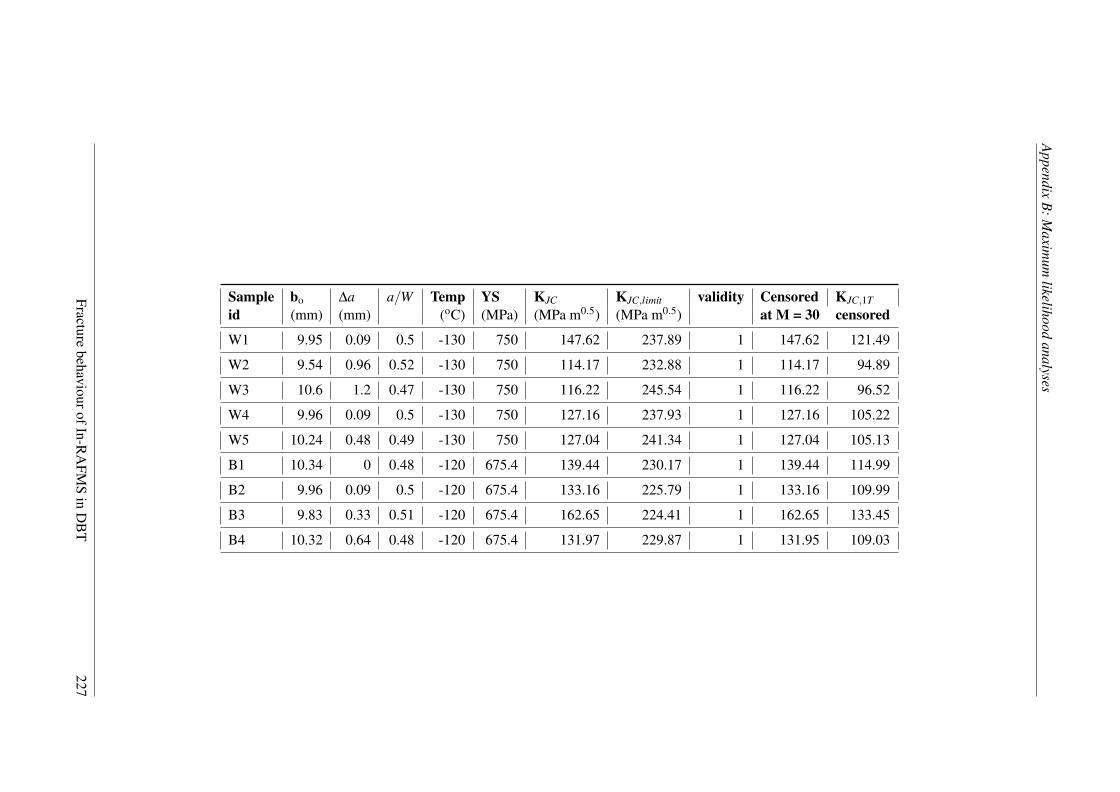
Appendix
B:M
aximum
likelihoodanalyses
Sample bo ∆a a/W Temp YS KJC KJC,limit validity Censored KJC,1T
id (mm) (mm) (oC) (MPa) (MPa m0.5) (MPa m0.5) at M = 30 censored
W1 9.95 0.09 0.5 -130 750 147.62 237.89 1 147.62 121.49
W2 9.54 0.96 0.52 -130 750 114.17 232.88 1 114.17 94.89
W3 10.6 1.2 0.47 -130 750 116.22 245.54 1 116.22 96.52
W4 9.96 0.09 0.5 -130 750 127.16 237.93 1 127.16 105.22
W5 10.24 0.48 0.49 -130 750 127.04 241.34 1 127.04 105.13
B1 10.34 0 0.48 -120 675.4 139.44 230.17 1 139.44 114.99
B2 9.96 0.09 0.5 -120 675.4 133.16 225.79 1 133.16 109.99
B3 9.83 0.33 0.51 -120 675.4 162.65 224.41 1 162.65 133.45
B4 10.32 0.64 0.48 -120 675.4 131.97 229.87 1 131.95 109.03
FracturebehaviourofIn-R
AFM
Sin
DB
T227

Appendix B: Maximum likelihood analyses
B.2 Fracture data of 0.4T CT specimens of In-RAFMS
TABLE B.2: Fracture data of 0.4T CT specimens of In-RAFMS
Sample bo ∆a Temp YS KJC KJC,limit Validity Censored Censoredid oC MPa MPa m0.5 KJC,xT KJC,1T
507S B5 10.9 2.06 -50 413 560.97 184.75 0 211.77 172.51
50B8 13.75 0.22 -50 413 356 207.51 0 207.51 169.12
60B3 13.56 0.35 -60 428 435.34 209.75 0 209.75 170.9
60D0 14.04 0.16 -60 428 295.4 213.43 0 213.43 173.83
70B2 13.54 0.28 -70 447 292.4 214.22 0 214.22 174.46
70B7 13.61 0.41 -70 447 350.29 214.78 0 214.78 174.9
70D1 13.7 0.21 -70 447 233.89 215.48 0 215.48 175.46
50D2C1 11.64 0.93 -50 413 435.09 190.93 0 211.77 172.51
70D4 13.69 0.37 -70 447 336.36 215.37 0 215.37 175.37
120B4 14.27 0 -120 765 22.51 270.37 1 22.51 22
100B6 13.79 0 -100 490 154.41 226.37 1 154.41 126.89
100B9 12.82 0.24 -100 490 223.72 218.23 0 218.23 177.65
100D7 13.71 0 -100 490 174.38 225.69 1 174.38 142.77
120S0 13.07 0 -120 765 54.75 258.67 1 54.75 47.63
80c2 14.05 0 -80 454 295.37 219.96 0 219.96 179.02
80d8 13.45 0 -80 454 200.24 215.21 1 200.24 163.34
120c4 13.08 0 -120 765 158.95 258.79 1 158.95 130.5
s1-120 14.91 0 -120 765 63.42 276.34 1 63.42 54.53
120s3 14.03 0 -120 765 150.88 268.05 1 150.88 124.08
120s2 13.98 0 -120 765 94.46 267.59 1 94.47 79.22
5s 120 14.23 0 -120 765 32.73 269.91 1 32.73 30.13
120s50 14.51 0 -120 765 14.01 272.56 1 14.01 15.24
80-C5 13.57 0 -80 454 218.52 216.13 0 216.13 175.98
80S4 13.4 0.22 -80 454 211.77 214.77 1 211.77 172.51
S8 14.55 0 -80 454 205.62 223.77 1 205.62 167.62
228 Fracture behaviour of In-RAFMS in DBT

Appendix B: Maximum likelihood analyses
B.3 Fracture data of 0.4T SEB specimens of In-RAFMS at different
loading rates
TABLE B.3: Fracture data at 100 mmpm actuator speed
100mmpm
0.2T(5×10) ao a/W KJC Temp KJC,1T KJC,limit Validity
Specimen Id (mm) (MPa m0.5) oC (MPa m0.5) (MPa m0.5)
s1 4.96 0.50 310.20 -80.00 214.07 166.95 0
s2/s7 5.31 0.53 36.30 -100.00 30.90 164.12 1
s4 5.23 0.52 450.99 -80.00 308.22 162.41 0
s5 5.67 0.57 123.30 -100.00 89.08 157.72 1
x6 5.50 0.55 357.70 -80.00 245.83 157.64 0
x2 5.77 0.58 143.44 -80.00 102.55 152.86 1
1 4.37 0.44 70.25 -100.00 53.60 179.69 1
s10 4.21 0.42 67.20 -100.00 51.56 182.33 1
u2 4.55 0.46 101.13 -100.00 74.25 176.86 1
u10 4.24 0.42 21.61 -100.00 21.08 181.80 1
Fracture behaviour of In-RAFMS in DBT 229

Appendix B: Maximum likelihood analyses
TABLE B.4: Fracture data at 1000 mmpm actuator speed
1000mmpm
0.4T(10x10) ao a/W KJC Temp KJC,1T KJC,Limit Validity
Specimen Id (mm) (MPa m0.5) oC (MPa m0.5) (MPa m0.5)
R29 4.52 0.45 98.32 -80 172.69 141.43 1
R30 4.54 0.45 206.2 -80 172.44 141.23 0
R32 4.07 0.4 106.54 -80 179.69 146.99 1
R33 4.63 0.46 113.55 -80 171.03 140.11 1
R34 4.69 0.46 106.49 -80 170.12 139.38 1
R35 4.97 0.49 307.51 -80 165.55 135.75 0
R48 4.61 0.46 170.77 -80 171.36 140.37 1
RR1 4.42 0.44 103.8 -80 174.32 142.73 1
RR2 4.56 0.45 148.14 -80 172.13 140.98 1
R26 4.48 0.44 81.89 -100 185.08 151.28 1
R31 4.52 0.45 48.82 -100 184.34 150.69 1
R38 4.47 0.44 50.24 -100 185.23 151.4 1
R39 3.84 0.38 70.17 -100 195.43 159.51 1
R42 4.56 0.45 70.66 -100 183.74 150.22 1
R43 4.58 0.45 269.53 -100 183.45 149.99 0
R46 4.55 0.45 64.61 -100 183.95 150.38 1
R47 4.38 0.43 65.27 -100 186.66 152.54 1
R49 4.99 0.49 58.07 -100 176.24 144.26 1
230 Fracture behaviour of In-RAFMS in DBT

Appendix B: Maximum likelihood analyses
B.4 Fracture data of 0.2T SEB specimens of In-RAFMS at different
crack depths
TABLE B.5: Fracture data with a/W in range of 0.29 to 0.34
Sr No a/W Temp KJC KJC,1T YS KJC,Limit KJC,1T,Limit Validity
Gr-1
(oC) (MPa m0.5) (MPa m0.5) (MPa) (MPa m0.5) (MPa m0.5)
1 0.19 -140 98.21 72.30 871 163.97 116.28 1
3 0.32 -140 95.94 70.78 871 150.30 107.13 1
4 0.29 -140 52.83 41.96 871 152.96 108.91 1
5 0.25 -140 369.66 253.83 871 157.43 111.91 0
6 0.35 -110 376.34 258.30 506 111.71 81.33 0
7 0.32 -110 334.38 230.24 506 114.14 82.96 0
8 0.35 -110 266.94 185.14 506 112.09 81.58 0
9 0.34 -130 158.92 112.90 750 137.37 98.49 0
10 0.32 -140 73.05 55.48 871 150.25 107.10 1
11 0.33 -140 59.97 46.73 871 148.39 105.86 1
12 0.33 -140 68.83 52.65 871 148.31 105.80 1
13 0.31 -140 52.74 41.90 871 151.30 107.81 1
14 0.32 -150 116.45 84.50 891 151.42 107.89 1
15 0.32 -150 118.73 86.02 891 151.36 107.84 1
Fracture behaviour of In-RAFMS in DBT 231

Appendix B: Maximum likelihood analyses
TABLE B.6: Fracture data with a/W in range of 0.35 to 0.44
Gr-2
Sr No a/W Temp KJC KJC,1T YS KJC,Limit KJC,Limit,1T Validity
(oC) (MPa m0.5) (MPa m0.5) (MPa) (MPa m0.5) (MPa m0.5)
1 0.42 120 82.57 61.85 675.4 121.72 88.03 1
2 0.43 120 63.54 49.12 675.4 120.67 87.32 1
3 0.39 130 96.54 71.19 750 131.19 94.36 1
4 0.43 130 78.03 58.81 750 127.38 91.81 1
5 0.40 130 82.97 62.11 750 130.78 94.08 1
6 0.37 -110 323.58 223.01 506 109.72 80.00 0
7 0.39 -130 103.75 76.01 750 131.83 94.79 1
8 0.37 -130 139.92 100.19 750 134.19 96.36 0
9 0.39 -130 208.05 145.75 750 132.04 94.93 0
10 0.37 -130 188.02 132.36 750 134.29 96.43 0
11 0.39 -140 74.64 56.54 871 142.24 101.75 1
12 0.37 -140 98.78 72.68 871 144.80 103.46 1
13 0.41 -150 118.97 86.19 891.4 141.04 100.95 1
14 0.44 -110 131.66 94.67 506 103.42 75.78 0
15 0.45 -110 293.20 202.70 506 102.81 75.38 0
232 Fracture behaviour of In-RAFMS in DBT

Appendix B: Maximum likelihood analyses
TABLE B.7: Fracture data with a/W in range of 0.46 to 0.55
Gr-3
Sr No a/W Temp KJC KJC,1T YS KJC,Limit KJC,Limit,1T Validity
(oC) (MPa m0.5) (MPa m0.5) (MPa) (MPa m0.5) (MPa m0.5)
1 0.51 120 119.87 86.78 675.4 112.09 81.59 0
2 0.52 120 93.70 69.29 675.4 110.52 80.54 1
3 0.52 120 294.56 203.61 675.4 111.10 80.92 0
4 0.52 120 127.78 92.08 675.4 111.21 80.99 0
5 0.52 130 331.35 228.21 750 117.19 84.99 0
6 0.51 130 106.29 77.71 750 118.51 85.88 1
7 0.49 130 105.28 77.03 750 120.35 87.11 1
8 0.48 130 87.99 65.47 750 121.13 87.63 1
9 0.53 -120 104.33 76.39 675.4 109.52 79.87 1
10 0.49 -130 68.11 52.17 750 120.26 87.04 1
11 0.54 -130 106.14 77.60 750 114.39 83.12 1
12 0.54 -130 89.90 66.74 750 114.39 83.12 1
Fracture behaviour of In-RAFMS in DBT 233

Appendix B: Maximum likelihood analyses
TABLE B.8: Fracture data with a/W in range of 0.56 to 0.69
Gr-4
Sr No a/W Temp KJC KJC,1T YS KJC,Limit KJC,1T,Limit Validity
(oC) (MPa m0.5) (MPa m0.5) (MPa) (MPa m0.5) (MPa m0.5)
1 0.60 -120 281.19 194.67 675.4 100.87 74.08 0
2 0.60 -120 278.57 192.92 675.4 101.43 74.46 0
3 0.59 -120 69.69 53.23 675.4 103.02 75.52 1
4 0.63 -120 115.27 83.71 675.4 97.82 72.04 0
5 0.59 -110 264.03 183.19 508 88.90 66.08 0
6 0.62 -130 108.84 79.41 750 104.48 76.49 0
7 0.62 -130 139.30 99.78 750 103.44 75.80 0
8 0.56 -130 120.09 86.94 750 111.46 81.16 0
9 0.55 -150 153.81 109.48 891.4 123.27 89.06 0
10 0.55 -110 318.77 219.80 508 93.59 69.21 0
1 0.67 -110 320.44 220.91 508 79.80 59.99 0
2 0.65 -120 307.98 212.58 675.4 94.26 69.66 0
3 0.65 -130 135.22 97.05 750 99.65 73.27 0
4 0.67 -110 390.87 268.02 506 79.84 60.02 0
5 0.65 -110 94.96 70.13 506 81.67 61.24 0
6 0.64 -130 81.63 61.22 750 101.36 74.41 1
7 0.64 -110 102.99 75.50 506 82.94 62.09 0
8 0.64 -110 250.45 174.11 506 83.66 62.57 0
9 0.64 -130 240.38 167.38 750 100.96 74.14 01 0.58 -120 357.69 245.82 675.4 103.24 75.67 0
2 0.64 -110 272.01 188.53 506 82.80 62.00 0
3 0.61 -110 176.25 124.49 506 86.63 64.56 0
4 0.63 -110 244.45 170.10 506 83.80 62.67 0
5 0.59 -130 52.02 41.41 750 107.51 78.52 1
6 0.56 -120 108.25 79.01 690 107.04 78.21 0
7 0.60 -130 27.34 24.91 750 107.23 78.34 1
8 0.69 -110 157.23 111.77 506 77.57 58.50 0
9 0.63 -110 248.61 172.88 506 83.69 62.59 0
B1 0.53 -140 93.99 69.48 871 124.22 89.70 1
B2 0.55 -140 103.31 75.71 871 121.84 88.10 1
B3 0.59 -130 157.90 112.22 750 107.35 78.41 0
E4 0.58 -130 90.17 66.93 750 109.71 79.99 1
M7 0.61 -140 79.96 60.10 871 114.02 82.87 1
234 Fracture behaviour of In-RAFMS in DBT

Appendix B: Maximum likelihood analyses
B.5 Fracture data of 1T CT specimens of P91 steel
TABLE B.9: Fracture data of 1T CT specimens of P91 steel
Sample id bo ∆a ao a/W KJC KJC,Limit Temp
(mm) (mm) (mm) (MPa m0.5) (MPa m0.5) (oC)
P4 21.49 0.34 28.51 0.57 278.17 362.81 -60
P7 22.90 27.10 0.54 193.87 378.18 -70
P9 23.61 26.39 0.53 149.69 384.05 -70
P15 24.10 25.90 0.52 136.80 387.99 -70
P16 23.41 26.59 0.53 184.83 378.67 -60
P18 23.20 0.37 26.80 0.54 229.90 376.97 -60
P19 24.22 25.78 0.52 212.37 385.12 -60
P1 26.95 23.05 0.46 29.27 406.28 -60
P2 25.62 24.38 0.49 180.67 396.13 -60
P3 26.28 23.72 0.47 213.78 401.21 -60
P11 26.35 23.65 0.47 192.25 405.73 -70
P5 26.82 23.18 0.46 73.11 409.32 -70
P6 25.35 24.65 0.49 34.41 397.88 -70
P8 25.30 24.70 0.49 201.57 393.65 -60
Fracture behaviour of In-RAFMS in DBT 235

Appendix B: Maximum likelihood analyses
B.6 Fracture data of 0.4T standard charpy specimens of P91 steel
TABLE B.10: Fracture data of 0.4T standard charpy specimens of P91 steel
Sample id bo ∆a ao a/W KJC KJC,Limit Temp
(mm) (mm) (mm) (MPa m0.5) (MPa m0.5) (oC)
A1 4.82 5.18 0.52 225.93 170.42 -100
A2 5.00 0.10 5.00 0.50 241.97 173.47 -100
A3 4.92 5.08 0.51 145.09 174.50 -110
A6 5.03 0.09 4.97 0.50 219.42 176.33 -110
K4 4.98 5.02 0.50 84.56 175.48 -110
P1 4.95 5.05 0.51 200.54 174.94 -110
P2 5.08 4.92 0.49 141.37 177.18 -110
R1 4.67 0.33 5.33 0.53 332.35 167.76 -100
R2 4.84 0.11 5.16 0.52 237.77 170.65 -100
R4 5.00 5.00 0.50 190.43 175.78 -100
R6 4.88 0.35 5.12 0.51 135.66 171.35 -100
T3 4.93 5.07 0.51 179.56 174.71 -110
T4 4.70 0.26 5.30 0.53 314.85 168.16 -100
T21 4.82 5.18 0.52 195.83 170.32 -100
P3 5.07 4.93 0.49 120.26 177.05 -110
R3 4.89 5.11 0.51 175.37 173.93 -110
B4 4.89 5.11 0.51 182.79 171.60 -100
236 Fracture behaviour of In-RAFMS in DBT

Appendix C
Appendix-C
Engineering drawing of test specimens
237

Appendix
C:D
rawings
oftestspecimens
FIGURE C.1: Fabrication drawing of M6 tensile specimens)
238Fracture
behaviourofIn-RA
FMS
inD
BT

Appendix
C:D
rawings
oftestspecimens
FIGURE C.2: Fabrication drawing of 0.5T-CT specimen)
FracturebehaviourofIn-R
AFM
Sin
DB
T239

Bibliography Appendix C Appendix-C Appendix C Appendix-C
FIGURE C.3: Notch dimension of SE(B) 0.4T specimen)
FIGURE C.4: Fabrication drawing of 0.4T SE(B) specimen
FIGURE C.5: Fabrication drawing of 0.2T SE(B) specimen
FIGURE C.6: Notch dimension of 0.4T SE(B) specimen
240 Fracture behaviour of In-RAFMS in DBT

BibliographyAbe F., Kern T.-U., Viswanathan R. (2008) Creep-resistant steels. Elsevier
Anderson T. L. (2005) Fracture Mechanics: Fundamentals and Applications, Third Edi-tion. Taylor & Francis, New York, NY
Andersson J.-O., Helander T., Hoglund L., Shi P., Sundman B. (2002) Thermo-calc &dictra, computational tools for materials science. Calphad 26(2):273–312
Andrews K. (1965) Empirical formulae for the calculation of some transformation tem-peratures. J Iron Steel Inst 203(7):721–727
Argon A., Im J., Safoglu R. (1975) Cavity formation from inclusions in ductile fracture.Metallurgical Transactions A 6(4):825–837
Banerjee S. (2014) Overview of indian activities on fusion reactor materials. Journal ofNuclear Materials 455(13):217 – 224, DOI http://dx.doi.org/10.1016/j.jnucmat.2014.06.009, proceedings of the 16th International Conference on Fusion Reactor Materi-als (ICFRM-16)
Beremin F. (1981) Cavity formation from inclusions in ductile fracture of a508 steel.Metallurgical Transactions A 12(5):723–731
Beremin F., Pineau A., Mudry F., Devaux J.-C., DEscatha Y., Ledermann P. (1983a) Alocal criterion for cleavage fracture of a nuclear pressure vessel steel. Metallurgicaltransactions A 14(11):2277–2287
Beremin F. M., Pineau A., Mudry F., Devaux J.-C., D’Escatha Y., Ledermann P. (1983b)A local criterion for cleavage fracture of a nuclear pressure vessel steel. MetallurgicalTransactions A 14(11):2277–2287, DOI 10.1007/BF02663302
Bhowmik S., Sahoo P., Acharyya S., Chattopadhyay J., Dhar S. (2012) Applica-tion and comparative study of the master curve methodology for fracture toughnesscharacterization of 20mnmoni55 steel. Materials and Design 39:309 – 317, DOIhttp://dx.doi.org/10.1016/j.matdes.2012.02.050
Bhowmik S., Sahoo P., Acharyya S. K., Dhar S., Chattopadhyay J. (2015) Evaluationand effect of loss of constraint on master curve reference temperature of 20mnmoni55steel. Engineering Fracture Mechanics 136:142 – 157, DOI http://dx.doi.org/10.1016/j.engfracmech.2015.01.022
Bonad R., Mueller P., Sptig P. (2008) Fracture toughness behavior in the ductilebrittletransition region of the tempered martensitic eurofer97 steel: Experiments and mod-eling. Engineering Fracture Mechanics 75(13):3985 – 4000, DOI https://doi.org/10.1016/j.engfracmech.2008.01.016
Bonade R., Mueller P., Spatig P. (2008) Fracture toughness behavior in the ductile–brittle transition region of the tempered martensitic eurofer97 steel: Experiments andmodeling. Engineering fracture mechanics 75(13):3985–4000
Bonade R. A. (2006) Constitutive behavior and fracture properties of tempered marten-sitic steels for nuclear applications
241

Bibliography BIBLIOGRAPHY BIBLIOGRAPHY
Bromberg J. (1982) Fusion: Science, Politics, and the Invention of a New EnergySource. MIT Press
Bruckner A., Munz D. (1984) Scatter of fracture toughness in the brittle-ductile transi-tion region of a ferritic steel. ASME, PVP 92:105–113
Burdekin F., Lidbury D., Moskovic R. (1999) On the onset of upper shelf transitiontemperature behaviour in ferritic steels. International journal of pressure vessels andpiping 76(13):875–877
Chaudhuri P., Kumar E. R., Sircar A., Ranjithkumar S., Chaudhari V., Danani C., YadavB., Bhattacharyay R., Mehta V., Patel R., Vyas K., Singh R., Sarkar M., SrivastavaR., Mohan S., Bhanja K., Suri A. (2012) Status and progress of indian LLCB testblanket systems for ITER. Fusion Engineering and Design 87(78):1009 – 1013,DOI http://dx.doi.org/10.1016/j.fusengdes.2012.02.062, tenth International Sympo-sium on Fusion Nuclear Technology (ISFNT-10)
Daniel J. (2012) Fusion energy production by deuterium particle injection
Danon A., Alamo A. (2002) Behavior of eurofer97 reduced activation martensitic steelupon heating and continuous cooling. Journal of nuclear materials 307:479–483
Daum E., Ehrlich K., Schirra M. (1997) Proceedings of the second milestone meetingof European laboratories on the development of ferritic/martensitic steels for fusiontechnology. Tech. rep., FIZ Karlsruhe
Delorenzi H., Shih C. (1983) 3-d elastic-plastic investigation of fracture parameters inside-grooved compact specimen. International Journal of Fracture 21(3):195–220
Dodds Jr R. H., Anderson T. L., Kirk M. T. (1991) A framework to correlate a/w ratioeffects on elastic-plastic fracture toughness (j c). International Journal of Fracture48(1):1–22
Doig P., Moskovic R. (1993) The influence of competing fracture mode on the ductileto brittle transition temperature. Engineering fracture mechanics 46(3):529–535
Donald E. McCabe K. W. John G. Merkle (2005) An Introduction to the Developmentand Use of the Master Curve Method. ASTM International
Dowling A. R., Lidbury D. P. G. (2000) Local approach modelling of constraint con-tributions to the ductile to brittle transition. In: Hirsch P., Lidbury D. (eds) Fracture,Plastic Flow and Structural Integrity, Proceedings of the 7th Symposium, TechnicalAdvisory Group on Structural Integrity of Nuclear Plant
E1921 A. (2013) E 1921 standard test method for determination of reference tempera-ture. T0, for ferritic steels in the transition range
Eldis G. T. (1977) A critical review of data sources for isothermal transformation andcontinuous cooling transformation diagrams. Hardenability Concepts with Applica-tions to Steel pp. 126–157
EricksonKirk M., EricksonKirk M. (2006) An upper-shelf fracture toughness mastercurve for ferritic steels. International Journal of Pressure Vessels and Piping 83(8):571– 583, DOI http://dx.doi.org/10.1016/j.ijpvp.2006.05.001
242 Fracture behaviour of In-RAFMS in DBT

Bibliography BIBLIOGRAPHY BIBLIOGRAPHY
Faleskog J., Gao X., Shih C. F. (1998) Cell model for nonlinear fracture analysis–i.micromechanics calibration. International Journal of Fracture 89(4):355–373
Gao X., Dodds Jr R. H. (2000) Constraint effects on the ductile-to-brittle transitiontemperature of ferritic steels: a weibull stress model. International Journal of Fracture102(1):43–69
Gao X., Dodds Jr R. H. (2005a) Loading rate effects on parameters of the weibull stressmodel for ferritic steels. Engineering Fracture Mechanics 72(15):2416 – 2425, DOIhttp://dx.doi.org/10.1016/j.engfracmech.2005.03.001
Gao X., Dodds Jr R. H. (2005b) Loading rate effects on parameters of the weibull stressmodel for ferritic steels. Engineering Fracture Mechanics 72(15):2416 – 2425, DOIhttp://dx.doi.org/10.1016/j.engfracmech.2005.03.001
Gao X., Dodds Jr R. H., Tregoning R., Joyce J. A. (2001) Weibull stress model for cleav-age fracture under high-rate loading. Fatigue & Fracture of Engineering Materials &Structures 24(8):551–564
Gao X., Zhang G., Srivatsan T. (2006) A probabilistic model for prediction of cleavagefracture in the ductile-to-brittle transition region and the effect of temperature onmodel parameters. Materials Science and Engineering: A 415(12):264 – 272, DOIhttp://dx.doi.org/10.1016/j.msea.2005.09.098
Gao X., Joyce J. A., Roe C. (2008) An investigation of the loading rate dependence ofthe weibull stress parameters. Engineering Fracture Mechanics 75(6):1451 – 1467,DOI http://dx.doi.org/10.1016/j.engfracmech.2007.07.007
Gurson A. L. (1977) Continuum theory of ductile rupture by void nucleation andgrowth: Part iyield criteria and flow rules for porous ductile media. Journal of en-gineering materials and technology 99(1):2–15
Hasegawa K., Chen Z.-C., Nishimura K., Ikeda K. (2009) Determination of true stress-ndash;strain curves of sheet metals in post-uniform elongation range. MATERIALSTRANSACTIONS 50(1):138–144, DOI 10.2320/matertrans.P-MRA2008838
Heerens J., Hellmann D. (1999) Fracture toughness of steel in the ductile to brittle tran-sition regime. Final Report, Measurement and Testing Programme Contract MAT1-CT-940080
Heerens J., Hellmann D. (2002) Development of the euro fracture toughness dataset.Engineering Fracture Mechanics 69(4):421–449
Hibbitt, Karlsson, Sorensen (1998) ABAQUS/standard: User’s Manual, vol 1. Hibbitt,Karlsson & Sorensen
IAEA (2001a) Final Report of the ITER EDA. No. 21 in ITER EDA DocumentationSeries, INTERNATIONAL ATOMIC ENERGY AGENCY, Vienna
IAEA (2001b) Summary of the ITER Final Design Report. No. 22 in ITER EDA Doc-umentation Series, INTERNATIONAL ATOMIC ENERGY AGENCY, Vienna
IAEA (2009) 1631. master curve approach to monitor fracture toughness of reactorpressure vessels in nuclear power plants. International Atomic Energy Agency
Fracture behaviour of In-RAFMS in DBT 243

Bibliography BIBLIOGRAPHY BIBLIOGRAPHY
Ioltukhovsky A., Leontyeva-Smirnova M., Kazennov Y., Medvedeva E., Tselishchev A.,Shamardin V., Povstyanko A., Ostrovsky S., Dvoryashin A., Porollo S., et al. (1998)Influence of operation conditions on structure and properties of 12% cr steels as can-didate structural materials for fusion reactor. Journal of nuclear materials 258:1312–1318
Jayakumar T., Mathew M., Laha K. (2013) High temperature materials for nuclear fastfission and fusion reactors and advanced fossil power plants. Procedia Engineering55:259 – 270, DOI http://dx.doi.org/10.1016/j.proeng.2013.03.252, 6th InternationalConference on Creep, Fatigue and Creep-Fatigue Interaction
Joyce J., Tregoning R. (2005a) Determination of constraint limits for cleavage initiatedtoughness data. Engineering fracture mechanics 72(10):1559–1579
Joyce J., Tregoning R. (2005b) Determination of constraint limits for cleavage initiatedtoughness data. Engineering fracture mechanics 72(10):1559–1579
Kim B. J., Kasada R., Kimura A., Wakai E., Tanigawa H. (2013) Application of mastercurve method to the evaluation of fracture toughness of f82h steels. Journal of NuclearMaterials 442(1):S38–S42
Klimenkov M., Materna-Morris E., Moslang A. (2015) Boron effect on the microstruc-ture of 9% cr ferritic–martensitic steels. Journal of Nuclear Materials 462:280–288
Klueh R. (2005) Elevated temperature ferritic and martensitic steels and their applica-tion to future nuclear reactors. International Materials Reviews 50(5):287–310
Knott J. (1995) The transition from fibrous fracture to cleavage fracture. Internationaljournal of pressure vessels and piping 64(3):225–234
Koers R. W., Braam H., Bakker A. (2013) Investigation into the effect of thicknesson three-and four-point single edge notch bend specimens using two-and three-dimensional elastic-plastic stress analyses. In: ICF7, Houston (USA) 1989
Koppenhoefer K. C., Dodds Jr R. H. (1997) Loading rate effects on cleavage fracture ofpre-cracked CVN specimens: 3-d studies. Engineering Fracture Mechanics 58(3):249– 270, DOI http://dx.doi.org/10.1016/S0013-7944(97)00076-3
Koppenhoefer K. C., Gullerud A. S., Ruggieri C., Dodds Jr R. H., Healey B. (1994)WARP3D: dynamic nonlinear analysis of solids using a preconditioned conju-gate gradient software architecture. Tech. rep., University of Illinois at Urbana–]Champaign
Kung C., Rayment J. (1982) Examination of the validity of existing empirical formulaefor the calculation of m/sub s/temperature. Metall Trans, A;(United States) 13(2)
Kunitake T. (2001) Prediction of ac sub 1, ac sub 3 and ms temperatures of steel by em-pirical formulas. Netsu Shori(Journal of the Japan Society for Heat Treatment)(Japan)41(3):164–169
Kunitake T., Ohtani H. (1969) Calculating the continuous cooling transformation char-acteristics of steel from its chemical composition. SUMITOMO SEARCH, NOV1969,–2–, 18-21
244 Fracture behaviour of In-RAFMS in DBT

Bibliography BIBLIOGRAPHY BIBLIOGRAPHY
Kytka M., Brumovsky M., Falcnik M. (2011) Irradiation embrittlement characterizationof the eurofer 97 material. Journal of Nuclear Materials 409(2):147–152
Laha K., Saroja S., Moitra A., Sandhya R., Mathew M., Jayakumar T., Kumar E. R.(2013) Development of india-specific RAFM steel through optimization of tungstenand tantalum contents for better combination of impact, tensile, low cycle fatigue andcreep properties. Journal of Nuclear Materials 439(1):41 – 50, DOI http://dx.doi.org/10.1016/j.jnucmat.2013.03.073
Landes J., Shaffer D. (1980) Statistical characterization of fracture in the transitionregion. In: Fracture Mechanics, ASTM International
Lei W.-S. (2016a) A cumulative failure probability model for cleavage fracture in fer-ritic steels. Mechanics of Materials 93:184–198
Lei W.-S. (2016b) A statistical model of cleavage fracture in structural steelswith power-law distribution of microcrack size. Philosophical Magazine Letters96(3):101–111
Li X.-G., Yan Q.-Z., Rong M., Wang H.-Q., Ge C.-C. (2010) First results of charac-terization of 9cr-3wvtitan low activation ferritic/martensitic steel. Journal of Iron andSteel Research, International 17(5):57–62
Lucas G., Odette G., Matsui H., Mslang A., Spatig P., Rensman J., Yamamoto T. (2007)The role of small specimen test technology in fusion materials development. Journalof Nuclear Materials 367370, Part B:1549 – 1556, DOI http://dx.doi.org/10.1016/j.jnucmat.2007.04.034, proceedings of the Twelfth International Conference on FusionReactor Materials (ICFRM-12)Proceedings of the Twelfth International Conferenceon Fusion Reactor Materials (ICFRM-12)
Lucon E., Scibetta M. (2011) Application of advanced master curve approaches to theeuro fracture toughness data set. In: Fatigue and Fracture Mechanics: 37th Volume,ASTM International
Margolin B., Kostylev V., Minkin A. (2003) The effect of ductile crack growth on thetemperature dependence of cleavage fracture toughness for a rpv steel with vari-ous degrees of embrittlement. International journal of pressure vessels and piping80(5):285–296
Mathew M., Vanaja J., Laha K., Reddy G. V., Chandravathi K., Rao K. B. S. (2011)Tensile and creep properties of reduced activation ferriticmartensitic steel for fusionenergy application. Journal of Nuclear Materials 417(13):77 – 80, DOI http://dx.doi.org/10.1016/j.jnucmat.2011.01.058, proceedings of ICFRM-14
McMeeking R. (1977) Finite deformation analysis of crack-tip opening in elastic-plasticmaterials and implications for fracture. Journal of the Mechanics and Physics ofSolids 25(5):357 – 381, DOI http://dx.doi.org/10.1016/0022-5096(77)90003-5
Miernik J., Statham G., Fabisinski L., Maples C., Adams R., Polsgrove T., FincherS., Cassibry J., Cortez R., Turner M., Percy T. (2013) Z-pinch fusion-based nu-clear propulsion. Acta Astronautica 82(2):173 – 182, DOI http://dx.doi.org/10.1016/j.actaastro.2012.02.012, 7th IAA Symposium on Realistic Advanced ScientificSpace MissionsAosta, Italy, July 2011
Fracture behaviour of In-RAFMS in DBT 245
Bibliography BIBLIOGRAPHY BIBLIOGRAPHY
Mishnev R., Dudova N., Kaibyshev R. (2016) Low cycle fatigue behavior of a 10cr–2w–mo–3co–nbv steel. International Journal of Fatigue 83:344–355
Moattari M., Sattari-Far I., Bonora N. (2016) The effect of subcritical ductile crackgrowth on cleavage fracture probability in the transition regime using continuumdamage mechanics simulation. Theoretical and Applied Fracture Mechanics 82:125–135
Moitra A., Dasgupta A., Sathyanarayanan S., Sasikala G., Albert S., Saroja S., BhaduriA., Kumar E. R., Jayakumar T. (2014) A study of fracture mechanisms in rafm steel inthe ductile to brittle transition temperature regime. Procedia Engineering 86:258–263
Moskovic R. (2002) Modelling of fracture toughness data in the ductile to brittletransition temperature region by statistical analysis. Engineering fracture mechanics69(4):511–530
Moslang A., Diegele E., Klimiankou M., Lasser R., Lindau R., Lucon E., Materna-Morris E., Petersen C., Pippan R., Rensman J., et al. (2005) Towards reduced activa-tion structural materials data for fusion demo reactors. Nuclear fusion 45(7):649
Mudry F. (1987) A local approach to cleavage fracture. Nuclear Engineering and design105(1):65–76
Mueller P., Spatig P., Bonad R., Odette G., Gragg D. (2009) Fracture toughness master-curve analysis of the tempered martensitic steel eurofer97. Journal of Nuclear Mate-rials 386388:323 – 327, DOI http://dx.doi.org/10.1016/j.jnucmat.2008.12.122, fusionReactor MaterialsProceedings of the Thirteenth International Conference on FusionReactor Materials
Murty K., Charit I. (2008) Structural materials for gen-iv nuclear reactors: Challengesand opportunities. Journal of Nuclear Materials 383(1):189–195
Mythili R., Vanaja J., Laha K., Saroja S., Jayakumar T., Mathew M., RajendrakumarE., et al. (2013) Microstructural modifications due to tungsten and tantalum in 9crreduced activation ferritic martensitic steels on creep exposure. Procedia Engineering55:295–299
Nevalainen M., Dodds Jr R. H. (1996) Numerical investigation of 3-d constraint effectson brittle fracture in se (b) and c (t) specimens. International Journal of Fracture74(2):131–161
Neville D. (1988) On the distance criterion for failure at the tips of cracks, minimumfracture toughness, and non-dimensional toughness parameters. Journal of the Me-chanics and Physics of Solids 36(4):443–457
Odette G., He M. Y. (2000) A cleavage toughness master curve model. Journal of nu-clear materials 283:120–127
Oughton D. (2016) Societal and ethical aspects of the fukushima accident. IntegratedEnvironmental Assessment and Management 12(4):651–653
Parks D. (1992) Advances in characterization of elastic-plastic crack-tip fields. In: Top-ics in Fracture and Fatigue, Springer, pp. 59–98
246 Fracture behaviour of In-RAFMS in DBT

Bibliography BIBLIOGRAPHY BIBLIOGRAPHY
Petti J. P., Dodds Jr R. H. (2005) Calibration of the weibull stress scale parameter,u, using the master curve. Engineering Fracture Mechanics 72(1):91 – 120, DOIhttp://dx.doi.org/10.1016/j.engfracmech.2004.03.009
Qian G., Gonzlez-Albuixech V., Niffenegger M. (2015) Calibration of beremin modelwith the master curve. Engineering Fracture Mechanics 136:15 – 25, DOI http://dx.doi.org/10.1016/j.engfracmech.2015.02.003
Qian G., Lei W.-S., Niffenegger M. (2017) Calibration of a new local approach to cleav-age fracture of ferritic steels. Materials Science and Engineering: A 694:10–12
Qian X., Zhang S., Swaddiwudhipong S. (2011) Calibration of weibull parameters us-ing the conventional mechanism-based strain gradient plasticity. Engineering FractureMechanics 78(9):1928 – 1944, DOI http://dx.doi.org/10.1016/j.engfracmech.2011.03.010
Raju S., Ganesh B. J., Rai A. K., Mythili R., Saroja S., Mohandas E., VijayalakshmiM., Rao K., Raj B. (2009) Measurement of transformation temperatures and specificheat capacity of tungsten added reduced activation ferriticmartensitic steel. Journal ofNuclear Materials 389(3):385 – 393, DOI http://dx.doi.org/10.1016/j.jnucmat.2009.02.030
Rathbun H., Odette G., Yamamoto T., Lucas G. (2006) Influence of statistical andconstraint loss size effects on cleavage fracture toughness in the transitiona singlevariable experiment and database. Engineering Fracture Mechanics 73(1):134 – 158,DOI http://dx.doi.org/10.1016/j.engfracmech.2005.07.008
Rice J., Johnson M., Kanninen M., et al. (1970) Inelastic behavior of solids. McGraw-Hill, New York 641
Ritchie R. O., Knott J. F., Rice J. (1973) On the relationship between critical tensilestress and fracture toughness in mild steel. Journal of the Mechanics and Physics ofSolids 21(6):395–410
Rosenwasser S., Miller P., Dalessandro J., Rawls J., Toffolo W., Chen W. (1979) Theapplication of martensitic stainless steels in long lifetime fusion first wall/blankets.Journal of Nuclear Materials 85:177–182
Ruggieri C., Dodds Jr R. H. (1996) A transferability model for brittle fracture includingconstraint and ductile tearing effects: a probabilistic approach. International Journalof Fracture 79(4):309–340
Ruggieri C., Dodds Jr R. H. (2015) An engineering methodology for constraint correc-tions of elasticplastic fracture toughness part i: A review on probabilistic models andexploration of plastic strain effects. Engineering Fracture Mechanics 134:368 – 390,DOI http://dx.doi.org/10.1016/j.engfracmech.2014.12.015
Ruggieri C., Jr R. D., Wallin K. (1998) Constraint effects on reference temperature, t0,for ferritic steels in the transition region. Engineering Fracture Mechanics 60(1):19 –36, DOI http://dx.doi.org/10.1016/S0013-7944(98)00001-0
Ruggieri C., Savioli R. G., Dodds Jr R. H. (2015) An engineering methodology forconstraint corrections of elasticplastic fracture toughness part ii: Effects of specimen
Fracture behaviour of In-RAFMS in DBT 247

Bibliography BIBLIOGRAPHY BIBLIOGRAPHY
geometry and plastic strain on cleavage fracture predictions. Engineering FractureMechanics 146:185 – 209, DOI http://dx.doi.org/10.1016/j.engfracmech.2015.06.087
Sandim M., Farrao F., Oliveira V., Bredda E., Santos A., dos Santos C., Sandim H.(2015) Effect of tempering on the microstructure, electrical, and magnetic propertiesof eurofer-97 steel. Journal of Nuclear Materials 461:265–270
Saunders N., Guo U., Li X., Miodownik A., Schille J.-P. (2003) Using jmatpro to modelmaterials properties and behavior. JOM 55(12):60–65
Scibetta M. (2010) Effect of prior crack growth on cleavage fracture of low toughnessprecracked charpy specimens. Journal of Nuclear Materials 406(1):113–118
SINTAP S. I. A. P. (1999) Final revision. EU-Brite Euram-Project, BE pp. 95–1462
Slatcher S. (1986) A probabilistic model for lower-shelf fracture toughnesstheory andapplication. Fatigue & Fracture of Engineering Materials & Structures 9(4):275–289
Smith E. (1966) Physical basis of yield and fracture. In: Proc. Conf., Institute of Physicsand Physical Society, Oxford, United Kingdom, p. 36
Sobotka J., Dodds R. (2014) Effects of steady ductile crack growth on cleavage frac-ture from three-dimensional, small-scale yielding simulations. Engineering FractureMechanics 127:211–225
Sokolov M., Tanigawa H. (2007) Application of the master curve to inhomogeneousferritic/martensitic steel. Journal of Nuclear Materials 367:587–592
Spatig P., Bonad R., Odette G., Rensman J., Campitelli E., Mueller P. (2007) Plasticflow properties and fracture toughness characterization of unirradiated and irradiatedtempered martensitic steels. Journal of Nuclear Materials 367370, Part A:527 – 538,DOI http://dx.doi.org/10.1016/j.jnucmat.2007.03.038, proceedings of the Twelfth In-ternational Conference on Fusion Reactor Materials (ICFRM-12)Proceedings of theTwelfth International Conference on Fusion Reactor Materials (ICFRM-12)
Stacey W. (2010) Fusion: An Introduction to the Physics and Technology of MagneticConfinement Fusion. Wiley
Steven W., Haynes A. (1956) The temperature of formation of martensite and bainite inlow-alloy steels. Journal of the Iron and Steel Institute 183(8):349–359
Stratil L., Siska F., Hadraba H., Dlouhy I. (2014) Modeling of ductile tearing for rafmsteel eurofer97. Procedia Materials Science 3:1155–1160
Sumpter J., Forbes A. (1993) Constraint based analysis of shallow cracks in mild steel.Abington Publishing(UK), p. 7
T. M. (1972) Tekko-zairyo-gaku, chapter martensite. JikkyoSyuppan Corp in Japanese43(1):4–11
Tagawa T., Kayamori Y., Hira H. (2010) Statistical scatter of fracture toughness inthe ductile–brittle transition of a structural steel. Engineering Fracture Mechanics77(16):3077–3086
248 Fracture behaviour of In-RAFMS in DBT

Bibliography BIBLIOGRAPHY BIBLIOGRAPHY
Tamura I. (1970) Steel material study on the strength. Nikkan Kogyo Shinbun Ltd,Tokyo 40
Tan L., Yang Y., Busby J. T. (2013) Effects of alloying elements and thermomechani-cal treatment on 9cr reduced activation ferritic–martensitic (rafm) steels. Journal ofNuclear Materials 442(1):S13–S17
Tiwari A., Avinash G., Sunil S., Singh R., Stahle P., Chattopadhyay J., Chakravartty J.(2015) Determination of reference transition temperature of in-rafms in ductile brittletransition regime using numerically corrected master curve approach. EngineeringFracture Mechanics 142:79 – 92, DOI http://dx.doi.org/10.1016/j.engfracmech.2015.05.041
Tvergaard V. (1981) Influence of voids on shear band instabilities under plane strainconditions. International Journal of Fracture 17(4):389–407
Tvergaard V. (1982) Influence of void nucleation on ductile shear fracture at a freesurface. Journal of the Mechanics and Physics of Solids 30(6):399–425
Tvergaard V., Needleman A. (1984) Analysis of the cup-cone fracture in a round tensilebar. Acta metallurgica 32(1):157–169
Vanaja J., Laha K., Mythili R., Chandravathi K., Saroja S., Mathew M. (2012) Creep de-formation and rupture behaviour of 9cr–1w–0.2 v–0.06 ta reduced activation ferritic–martensitic steel. Materials Science and Engineering: A 533:17–25
Vanaja J., Laha K., Nandagopal M., Sam S., Mathew M., Jayakumar T., Kumar E. R.(2013) Effect of tungsten on tensile properties and flow behaviour of rafm steel. Jour-nal of Nuclear Materials 433(1):412–418
Varias A. (1998) Constraint effects during stable transient crack growth. ComputationalMechanics 21(4-5):316–329
Wallin K. (1984) The scatter in KIC-results. Engineering Fracture Mechanics19(6):1085 – 1093, DOI http://dx.doi.org/10.1016/0013-7944(84)90153-X
Wallin K. (1989a) The effect of ductile tearing on cleavage fracture probability infracture toughness testing. Engineering Fracture Mechanics 32(4):523 – 531, DOIhttp://dx.doi.org/10.1016/0013-7944(89)90186-0
Wallin K. (1989b) The effect of ligament size on cleavage fracture toughness. En-gineering Fracture Mechanics 32(3):449 – 457, DOI http://dx.doi.org/10.1016/0013-7944(89)90316-0
Wallin K. (1993) Irradiation damage effects on the fracture toughness transition curveshape for reactor pressure vessel steels. International journal of pressure vessels andpiping 55(1):61–79
Wallin K. (1997) Proc. conf. ’Recent Advances in Fracture’(R K Mahidhara, Ed). TheMinerals, Metal and Materials Society of AIME pp. 171 – 181
Wallin K. (1999) The master curve method: a new concept for brittle fracture. Interna-tional Journal of Materials and Product Technology 14(2-4):342–354
Fracture behaviour of In-RAFMS in DBT 249

Bibliography BIBLIOGRAPHY BIBLIOGRAPHY
Wallin K. (2001) Quantifying tstress controlled constraint by the master curve transitiontemperature To. Engineering Fracture Mechanics 68(3):303 – 328, DOI http://dx.doi.org/10.1016/S0013-7944(00)00067-9
Wallin K. (2002) Master curve analysis of the euro fracture toughness dataset.Engineering Fracture Mechanics 69(4):451 – 481, DOI http://dx.doi.org/10.1016/S0013-7944(01)00071-6
Wallin K. (2003) Master curve implementation of the warm pre-stress effect. En-gineering Fracture Mechanics 70(18):2587 – 2602, DOI http://dx.doi.org/10.1016/S0013-7944(03)00064-X
Wallin K. (2004) Warm pre-stress based pre-cracking criteria for fracture toughnesstesting. Engineering Fracture Mechanics 71(12):1737 – 1750, DOI http://dx.doi.org/10.1016/S0013-7944(03)00245-5
Wallin K. (2010a) Structural integrity assessment aspects of the master curve method-ology. Engineering Fracture Mechanics 77(2):285 – 292, DOI http://dx.doi.org/10.1016/j.engfracmech.2009.02.010
Wallin K. (2010b) Structural integrity assessment aspects of the master curve method-ology. Engineering Fracture Mechanics 77(2):285–292
Wallin K., Laukkanen A. (2008) New developments of the wallin, saario, torronencleavage fracture model. Engineering Fracture Mechanics 75(11):3367–3377
Wallin K., Saario T., Torronen K., Forsten J., Torronen K., Aho-Mantila I. (1986) Brittlefracture theory (wst model). Reliability of Reactor Materials Fracture Mechanics
Wallin K., Planman T., Valo M., Rintamaa R. (2001) Applicability of miniaturesize bend specimens to determine the master curve reference temperature To. En-gineering Fracture Mechanics 68(11):1265 – 1296, DOI http://dx.doi.org/10.1016/S0013-7944(01)00020-0
Wallin K., Nevasmaa P., Laukkanen A., Planman T. (2004) Master curve analysis of in-homogeneous ferritic steels. Engineering Fracture Mechanics 71(1617):2329 – 2346,DOI http://dx.doi.org/10.1016/j.engfracmech.2004.01.010
Wallin K., Pallaspuro S., Valkonen I., Karjalainen-Roikonen P., Suikkanen P. (2015)Fracture properties of high performance steels and their welds. Engineering FractureMechanics 135:219 – 231, DOI http://dx.doi.org/10.1016/j.engfracmech.2015.01.007
Wallin K. R. (2013) Distribution free statistical assessment of scatter and size effectsin the euro fracture toughness data set. Engineering Fracture Mechanics 103:69 – 78,DOI http://dx.doi.org/10.1016/j.engfracmech.2012.05.018, advances in Failure As-sessment Using Fracture and Damage Mechanics.
Wang Y., Parks D. (1992) Evaluation of the elastic t-stress in surface-cracked platesusing the line-spring method. International Journal of fracture 56(1):25–40
Wasiluk B., Petti J. P., Jr. R. H. D. (2006) Temperature dependence of weibullstress parameters: Studies using the euro-material. Engineering Fracture Mechanics73(8):1046 – 1069, DOI http://dx.doi.org/10.1016/j.engfracmech.2005.11.006
250 Fracture behaviour of In-RAFMS in DBT

Bibliography BIBLIOGRAPHY BIBLIOGRAPHY
Weibull W. (1951) Wide applicability. Journal of applied mechanics 103:293–297
Wikipedia (2004) Fusion power — Wikipedia, the free encyclopedia. [Online; modified17 October 2016,]
Williams M. (1961) The bending stress distribution at the base of a stationary crack.Journal of applied mechanics 28(1):78–82
Xiao X., Liu G., Hu B., Wang J., Ullah A. (2013) Effect of v and ta on the precipitationbehavior of 12% cr reduced activation ferrite/martensite steel. Materials Characteri-zation 82:130–139
Xu Y., Zhang X., Tian Y., Chen C., Nan Y., He H., Wang M. (2016) Study on thenucleation and growth of m 23 c 6 carbides in a 10% cr martensite ferritic steel afterlong-term aging. Materials Characterization 111:122–127
Yan C., Mai Y. (1997) Effect of constraint on ductile crack growth and ductile-brittlefracture transition of a carbon steel. International journal of pressure vessels and pip-ing 73(3):167–173
Yoon K., Hall J., Van Der Sluys W., Higuchi M., Iida K. (2001a) Japanese fracturetoughness data analysis using the master curve method. ASME-PUBLICATIONS-PVP 423:167–178
Yoon K., Hall J., Van Der Sluys W., Higuchi M., Iida K. (2001b) Japanese fracturetoughness data analysis using the master curve method. ASME-PUBLICATIONS-PVP 423:167–178
Yu J., Huang Q., Wan F. (2007) Research and development on the china low activationmartensitic steel (clam). Journal of Nuclear Materials 367:97–101
Zener C., Hollomon J. (1944) Effect of strain rate upon plastic flow of steel. Journal ofApplied physics 15(1):22–32
Zerilli F. J., Armstrong R. W. (1987) Dislocation-mechanics-based constitutive relationsfor material dynamics calculations. Journal of Applied Physics 61(5):1816–1825
Zilnyk K., Oliveira V. B., Sandim H. R. Z., Moslang A., Raabe D. (2015) Martensitictransformation in eurofer-97 and ods-eurofer steels: A comparative study. Journal ofNuclear Materials 462:360–367
Fracture behaviour of In-RAFMS in DBT 251
Indexσ?−V ? approach, 107σ?−V ? approach, 215
Beremin’s Model, 48Beremin’s model, 156, 157Bimodal master curve, 41
Calibration of Weibull parameters, 157, 159Cleavage failure probability, numerical pre-
dictions, 157Cleavage failure probability, Weibull stress
, 156Cleavage, local approach, 46Constitutive equations of finite element anal-
yses, 80Constraint loss, in plane, 122Constraint loss, out of plane, 104
Euro fracture data, 113
Fatigue pre cracking of fracture specimens,73
Ferritic/Martensitic steels, 49First wall, 24Fracture toughness measurement, 78
Griffith’s criteria, 47Griffith’s criteria of cleavage fracture, 104Griffith’s micro-cracks, 47GTN damage, 83
Impact test, 77In-RAFMS, 49, 52ITER, 21ITER, phases of fusion reaction, 22
MANET, 50Master Curve, 35Maximum likelihood analysis, 6, 38Mesh, finite element, 82mesh, finite element, 84Metallography, etchant, 77Micro-mechanics of cleavage fracture, 47Modified 9%Cr-1%Mo steels, 49Modified boundary layer model, 81Multi-modal master curve, 41Multi-temperature master curve, 96
Objectives of the work, 27
OPTIFIER, 50
P91 steel, 49Phase diagram, In-RAFMS, 59Phase diagram, P91, 59
Quarter symmetric boundary conditions, 108
RAFMS, carbide fracture, 87RAFMS, comparison of different grades,
63RAFMS, damage, 87RAFMS, effect of alloying elements, 51RAFMS, heat treatment, 59RAFMS, Impact toughness, 86RAFMS, Lave phases, 65RAFMS, Ludwig fit, 93RAFMS, M23C6 and MX carbides, 65RAFMS, micro structure, 59, 65RAFMS, micro-cracks, 87RAFMS, Phase transformation, 59RAFMS, precipitates, 65RAFMS, tensile behaviour, 93RAFMS, voids, 87Random inhomogeneity analysis, 41RKR model, 48
sensitivity analysis, 84Single-temperature master curve, 96SINTAP lower tail estimate, 41solver, finite element, 84SSY corrected To, 121
Tstress, modifed boundary layer model, 81
Validity criteria, master curve, 35Void growth, 84Void nucleation, 84Void volume fraction, GTN model,porous
plasticity, 84
Weakest link theory, 36Weibull stress, 157, 158Weibull stress calculation, 165Weibull Triaxiality, 141, 215WST model, 48, 107
Zener-Hollomon strain rate function, 156Zeta pinch, 21
252
Copyright © 2022 FDOKUMEN