at SciVerse ScienceDirect

Environmental Modelling & Software 40 (2013) 1e20

Contents lists available

Environmental Modelling & Software

journal homepage: www.elsevier .com/locate/envsoft

Position paper

Characterising performance of environmental modelsq

Neil D. Bennett a, Barry F.W. Croke a, Giorgio Guariso b, Joseph H.A. Guillaume a, Serena H. Hamilton a,Anthony J. Jakeman a,*, Stefano Marsili-Libelli c, Lachlan T.H. Newhama, John P. Norton a, Charles Perrin d,Suzanne A. Pierce e, Barbara Robson f, Ralf Seppelt g, Alexey A. Voinov h, Brian D. Fath i, j,Vazken Andreassian d

a Fenner School of Environment and Society, National Centre for Groundwater Research and Training, The Australian National University, Australiab Politecnico di Milano, ItalycDepartment of Systems and Computers, University of Florence, Italyd IRSTEA, FranceeCenter for International Energy and Environmental Policy, Jackson School of Geosciences, The University of Texas at Austin, USAfCSIRO Land and Water, AustraliagUFZ e Helmholtz Centre for Environment Research, Department of Computational Landscape Ecology, Leipzig, Germanyh ITC, Twente University, The NetherlandsiDepartment of Biological Sciences, Towson University, USAjAdvanced Systems Analysis Program, International Institute for Applied Systems Analysis, Austria

a r t i c l e i n f o

Article history:Received 17 July 2012Received in revised form25 September 2012Accepted 25 September 2012Available online 6 November 2012

Keywords:Model developmentModel evaluationPerformance indicatorsModel testingSensitivity analysis

q Position papers aim to synthesise some key aspefor environmental modelling and software issues. Thea normal external review process followed by extemembers. See the Editorial in Volume 21 (2006).* Corresponding author.

E-mail address: tony.jakeman@anu.edu.au (A.J. Jak

1364-8152/$ e see front matter � 2012 Elsevier Ltd.http://dx.doi.org/10.1016/j.envsoft.2012.09.011

a b s t r a c t

In order to use environmental models effectively for management and decision-making, it is vital toestablish an appropriate level of confidence in their performance. This paper reviews techniques avail-able across various fields for characterising the performance of environmental models with focus onnumerical, graphical and qualitative methods. General classes of direct value comparison, coupling realand modelled values, preserving data patterns, indirect metrics based on parameter values, and datatransformations are discussed. In practice environmental modelling requires the use and implementationof workflows that combine several methods, tailored to the model purpose and dependent upon the dataand information available. A five-step procedure for performance evaluation of models is suggested, withthe key elements including: (i) (re)assessment of the model’s aim, scale and scope; (ii) characterisation ofthe data for calibration and testing; (iii) visual and other analysis to detect under- or non-modelledbehaviour and to gain an overview of overall performance; (iv) selection of basic performance criteria;and (v) consideration of more advanced methods to handle problems such as systematic divergencebetween modelled and observed values.

� 2012 Elsevier Ltd. All rights reserved.

1. Introduction

Quantitative environmental models are extensively used inresearch, management and decision-making. Establishing ourconfidence in the outputs of such models is crucial in justifyingtheir continuing use while also recognizing limitations. The ques-tion of evaluating a model’s performance relative to our

ct of the knowledge platformreview process is twofold e

nsive review by EMS Board

eman).

All rights reserved.

understanding and observations of the system has resulted inmanydifferent approaches and much debate on the identification ofa most appropriate technique (Alexandrov et al., 2011; McIntoshet al., 2011). One reason for continued debate is that performancemeasurement is intrinsically case-dependent. In particular, themanner inwhich performance is characterised depends on the fieldof application, characteristics of the model, data, information andknowledge that we have at our disposal, and the specific objectivesof the modelling exercise (Jakeman et al., 2006; Matthews et al.,2011).

Modelling is used across many environmental fields: hydrology,air pollution, ecology, hazard assessment, and climate dynamics,to name a few. In each of these fields, many different types ofmodels are available, each incorporating a range of characteristicsto measure and represent the natural system behaviours.

N.D. Bennett et al. / Environmental Modelling & Software 40 (2013) 1e202

Environmental models for management typically consist ofmultiple interacting components with errors that do not exhibitpredictable properties. This makes the traditional hypothesis-testing associated with statistical modelling less suitable, at leaston its own, because of the strong assumptions generally required,and the difficulty (sometimes impossibility) of testing hypothesesseparately. Additionally if a single performance criterion is used, itgenerally measures only specific aspects of a model’s performance,which may lead to counterproductive results such as favouringmodels that do not reproduce important features of a system (e.g.,Krause et al., 2005; Hejazi and Moglen, 2008). Consequently,systems of metrics focussing on several aspects may be needed fora comprehensive evaluation of models, as advocated e.g., by Guptaet al. (2012).

It is generally accepted that the appropriate form of a model willdepend on its specific objectives (Jakeman et al., 2006), which oftenfall in the broad categories of improved understanding of naturalprocesses or response to management questions. The appropriatetype of performance evaluation clearly depends on the modelobjectives as well. Additionally, theremay be several views as to thepurpose of a model, and multiple performance approaches mayhave to be used simultaneously to meet the multi-objectiverequirements for a given problem. In the end, the modeller mustbe confident that a model will fulfil its purpose, and that a ‘better’model could not have been selected given the available resources.These decisions are a complex mixture of objectively identifiedcriteria and subjective judgements that represent essential steps inthe cyclic process of model development and adoption. In addition,the end-users of a model must also be satisfied, and may not becomfortable using the same performance measures as the expertmodeller (e.g., Miles et al., 2000). It is clear that in this context,a modeller must be eclectic in choice of methods for characterisingthe performance of models.

Regardless, assessing model performance with quantitativetools is found to be useful, indeed most often necessary, and it isimportant that the modeller be aware of available tools. Quantita-tive tools allow comparison of models, point out where modelsdiffer from one another, and provide somemeasure of objectivity inestablishing the credibility and limitations of a model. Quantitativetesting involves the calculation of suitable numerical metrics tocharacterise model performance. Calculating a metric valueprovides a single common point of comparison between modelsand offers great benefits in terms of automation, for exampleautomatic calibration and selection of models. The use of metricvalues alsominimises potential inconsistencies arising from humanjudgement. Because of the expert knowledge often required to usethese tools, the methods discussed in this paper are intended foruse primarily by modellers, but they may also be useful to informend-users or stakeholders about aspects of model performance.

This paper reviews methods for quantitatively characterisingmodel performance, identifying key features so that modellers canmake an informed choice suitable for their situation. A classifica-tion is used that cuts across a variety of fields. Methods withdifferent names or developed for different applications aresometimes more similar than they at first appear. Studies in onedomain can take advantage of developments in others. Althoughthe primary applications under consideration are environmental,methods developed in other fields are also included in this review.We assume that a model is available, along with data representingobservations from a real system, that preferably have not beenused at any stage during model development and that can becompared with the model output. This dataset should be repre-sentative of the model aims; for instance it should contain floodepisodes or pollution peaks if the model is to be used in suchcircumstances.

The following section provides a brief view of how character-isation of model performance fits into the broader literature on themodelling process. Section 3 reviews selection of a so-called ‘vali-dation’ dataset. In Section 4, quantitative methods for character-ising performance are summarized, within the broad categories ofdirect value comparison, coupling real and modelled values,preserving data patterns, indirect metrics based on parametervalues, and data transformations. Section 5 discusses how quali-tative and subjective considerations enter into adoption of themodel in combination with quantitative methods. Section 6 pres-ents an approach to selecting performance criteria for environ-mental modelling. Note that a shorter and less comprehensiveversion of this paper was published as Bennett et al. (2010).

2. Performance characterisation in context

With characterisation of model performance being a core part ofmodel development and testing, there is naturally a substantialbody of related work. This section presents some key links betweensimilar methods that have developed separately in different fields.In many of the fields of environmental modelling, methods andcriteria to judge the performance of models have been consideredin the context of model development. Examples include workcompleted for hydrological models (Krause et al., 2005; Jakemanet al., 2006; Moriasi et al., 2007; Reusser et al., 2009), ecologicalmodels (Rykiel, 1996) and air quality models (Fox, 1981; Thuniset al., 2012). The history of methods to characterise performancedates back at least a few decades (see, for instance Fox, 1981;Willmott, 1981) and makes use of artificial intelligence (Liu et al.,2005) and statistical models (Kleijnen, 1999), while efforts tostandardise them extensively and include them in a coherentmodel-development chain are more recent. For instance, inhydrology, previous work has been completed on general model-ling frameworks that consider performance criteria as part of theiterative modelling process (Jakeman et al., 2006; Refsgaard et al.,2005; Wagener et al., 2001). Stow et al. (2009) presenta summary of metrics that have been used for skill assessment ofcoupled biological and physical models of marine systems. Studieshave also focused explicitly on performance criteria, such asMoriasi et al. (2007) and Dawson et al. (2007, 2010), who producedguidelines for systematic model evaluation, including a list of rec-ommended evaluation techniques and performance metrics. Beck(2006) provides a survey of key issues related to performanceevaluation. And Matott et al. (2009) reviewed model evaluationconcepts in the context of integrated environmental models anddiscussed several relevant software-based tools.

Some official documents on model evaluation have also beenproduced by governing agencies. Among these, some are particu-larly detailed, e.g., “Guidance on the use of models for the EuropeanAir Quality Directive” (FAIRMODE, 2010), the “Guidance for QualityAssurance Project Plans for Modelling” (USEPA, 2002) and the“Guidance on the Development, Evaluation, and Application ofEnvironmental Models” (USEPA, 2009). This paper, by contrast,focuses on graphical and numerical methods to characterise modelperformance. The domain-specific reviews are synthesised fora broader audience. Use of these methods within the modellingprocess is only briefly discussed, and the reader is directed to otherreferences for more detail. Finally, a philosophical debate has aimedto differentiate verification from validation (Jakeman et al., 2006;Oreskes et al., 1994; Refsgaard and Henriksen, 2004). We, however,focus on summarizing methods to characterise performance ofenvironmental models, whether these methods and criteria areused for verification, validation or calibration instead of continuingthis debate.

N.D. Bennett et al. / Environmental Modelling & Software 40 (2013) 1e20 3

While this paper focuses mainly on model evaluation bycomparison to data, the reader should be aware of cases where thisis not possible due to the nature of the analysis or the stage ofmodelling. For example, such evaluation techniques are notpossible for qualitative conceptual models built in participatorymodelling frameworks to establish a common understanding of thesystem. The methods presented may not be sufficient for complexsituations, for example where the identification of feedbacks andrelationships between different environmental processes acrossspatial and temporal scales is of specific interest. Untanglingfeedbacks, especially in highly complex and spatially interrelatedsystems, remains a big challenge (Seppelt et al., 2009). Also,performance in future conditions cannot be directly assessed asavailable data may not be representative; this is particularly thecase where the model includes an intervention that will change thebehaviour of the system.

Data-based performance measures are only a small part ofquality assurance (QA) in modelling (Refsgaard et al., 2005).Guidelines and tools such as those produced by RIVM/MNP (van derSluijs et al., 2004), the HarmoniQuA project (Henriksen et al., 2009)and Matott et al. (2009) generally cover the qualitative definition ofthe model requirements and stakeholder engagement, in additionto the quantitative measures discussed in this paper. A consistentprocedure for characterising performance over the entiremodel lifecycle can facilitate QA by providing clarity, and hence increasedknowledge and confidence in developing and selecting the mostappropriate model to suit particular goals. This can also benefitfuture model reuse and application.

The paper will not discuss formal methods for sensitivity oruncertainty analysis, though these aspects are recognised as centralin the modelling process. Sensitivity analysis assesses how varia-tions in input parameters, model parameters or boundary condi-tions affect the model output. For more information on sensitivityanalysis, see Saltelli et al. (2000), Norton (2008), Frey and Patil(2002), Saltelli and Annoni (2010), Shahsavani and Grimvall(2011), Makler-Pick et al. (2011), Yang (2011), Nossent et al.(2011), Ratto et al. (2012) and Ravalico et al. (2010). Uncertaintyanalysis as generally understood is concerned with establishingbounds around point predictions, from either deterministic anal-ysis based on model-output error bounds or probabilistic analysisyielding confidence intervals. While this is often a useful measureof model performance, related methods have already beenreviewed elsewhere (e.g., Beven, 2008; Keesman et al., 2011; Vrugt

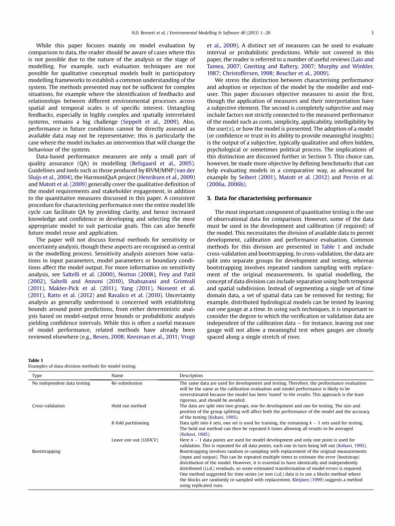
Table 1Examples of data-division methods for model testing.

Type Name Description

No independent data testing Re-substitution The same datwill be the saoverestimaterigorous, and

Cross-validation Hold out method The data areposition of thof the testing

K-fold partitioning Data split intThe hold out(Kohavi, 1995

Leave one out (LOOCV) Here n � 1 dvalidation. Th

Bootstrapping Bootstrappin(input and oudistribution odistributed (iOne methodthe blocks arusing replica

et al., 2009). A distinct set of measures can be used to evaluateinterval or probabilistic predictions. While not covered in thispaper, the reader is referred to a number of useful reviews (Laio andTamea, 2007; Gneiting and Raftery, 2007; Murphy and Winkler,1987; Christoffersen, 1998; Boucher et al., 2009).

We stress the distinction between characterising performanceand adoption or rejection of the model by the modeller and end-user. This paper discusses objective measures to assist the first,though the application of measures and their interpretation havea subjective element. The second is completely subjective and mayinclude factors not strictly connected to the measured performanceof the model such as costs, simplicity, applicability, intelligibility bythe user(s), or how the model is presented. The adoption of a model(or confidence or trust in its ability to provide meaningful insights)is the output of a subjective, typically qualitative and often hidden,psychological or sometimes political process. The implications ofthis distinction are discussed further in Section 5. This choice can,however, be made more objective by defining benchmarks that canhelp evaluating models in a comparative way, as advocated forexample by Seibert (2001), Matott et al. (2012) and Perrin et al.(2006a, 2006b).

3. Data for characterising performance

Themost important component of quantitative testing is the useof observational data for comparison. However, some of the datamust be used in the development and calibration (if required) ofthe model. This necessitates the division of available data to permitdevelopment, calibration and performance evaluation. Commonmethods for this division are presented in Table 1 and includecross-validation and bootstrapping. In cross-validation, the data aresplit into separate groups for development and testing, whereasbootstrapping involves repeated random sampling with replace-ment of the original measurements. In spatial modelling, theconcept of data division can include separation using both temporaland spatial subdivision. Instead of segmenting a single set of timedomain data, a set of spatial data can be removed for testing; forexample, distributed hydrological models can be tested by leavingout one gauge at a time. In using such techniques, it is important toconsider the degree to which the verification or validation data areindependent of the calibration data e for instance, leaving out onegauge will not allow a meaningful test when gauges are closelyspaced along a single stretch of river.

a are used for development and testing. Therefore, the performance evaluationme as the calibration evaluation and model performance is likely to bed because the model has been ‘tuned’ to the results. This approach is the leastshould be avoided.split into two groups, one for development and one for testing. The size ande group splitting will affect both the performance of the model and the accuracy(Kohavi, 1995).o k sets, one set is used for training, the remaining k � 1 sets used for testing.method can then be repeated k times allowing all results to be averaged).ata points are used for model development and only one point is used foris is repeated for all data points, each one in turn being left out (Kohavi, 1995).g involves random re-sampling with replacement of the original measurementstput). This can be repeated multiple times to estimate the error (bootstrap)f the model. However, it is essential to have identically and independently.i.d.) residuals, so some estimated transformation of model errors is required.suggested for time series (or non i.i.d.) data is to use a blocks method wheree randomly re-sampled with replacement. Kleijnen (1999) suggests a methodted runs.

N.D. Bennett et al. / Environmental Modelling & Software 40 (2013) 1e204

Selecting a “representative” set of data that sufficientlycaptures the key patterns in the data involves many consider-ations, for example, the sampling method, the heterogeneity of themeasure, and sources of sampling errors; for further discussionsee Cochran (1977), Gy (1998) and Nocerino et al. (2005). One maywant to test the ability of the model to generalise, i.e. its ability topredict sufficiently accurately for a given purpose, even in condi-tions that were not observed during model development. Ideally,model results are compared to unseen data from the past thatcapture the conditions that the model will be used to predict.Models are often used to simulate extreme conditions; for suchcases the testing data should include the relevant conditions, forexample, data that covers a particularly warm or wet period.Models are more likely to fail against such testing data if calibratedprimarily over less extreme periods, but will provide greaterconfidence if successful (e.g., Robson and Hamilton, 2004;Andréassian et al., 2009; Coron et al., 2012; Seiller et al., 2012). Inother cases, however, the data available do not sufficiently coverthe prediction conditions, so confidence in the model performanceshould instead be built by looking at components of the overallmodel or generating suitable artificial “data” sequences. Suchartificial data sequences may be generated with a more sophisti-cated (and more expensive or difficult to use) model in whichconfidence has already been established through other means(e.g., Raick et al., 2006; Littlewood and Croke, 2008); for example,a flow-routing model may be tested against output from a detailedcomputational fluid dynamics model. Whatever the case, thedecision of what is representative is subjective and strongly linkedto the final aim of the model.

Metrics typically calculate a single value for the whole dataset,which can disguise significant divergent behaviour over the timeintervals or spatial fields (see for example Berthet et al., 2010;Moussa, 2010). To prevent this, evaluation can instead be on a localbasis (e.g., pixel to pixel or event to event). Data may be partitioneda priori, using some external information about, for instance, theseason or the specific spatial domain, or they can be separated intolow, medium, and high events (Yilmaz et al., 2008) or, in hydrology,into rising-hydrograph and falling-hydrograph components, eachwith its own performance criteria. A more complex partitioningscheme in hydrology suggested by Boyle et al. (2000) involvessplitting the data into components driven by rainfall, interflow andbaseflow components. As another alternative, Choi and Beven(2007) use a multi-period framework, where a moving windowof thirty days is used to classify periods into dry, wetting, wet anddrying climate states.

Automatic grouping methods may be used to select approxi-mately homogeneous regions or regions of interest from the orig-inal data to assess model performance under different conditions.Wealands et al. (2005) studied the methods used in image pro-cessing, landscape ecology and content-based image retrievalamong others, and recommended several methods as potentiallyuseful for application to spatial hydrological models. They recom-mend a clustering method that starts with all the pixels as separateregions, which are then merged wherever the gradient in thevariable of interest is below a threshold. Merging is continued in aniterative process until no neighbouring regions satisfy the criteriafor merging. Further control of the regions can be achieved byimposing additional criteria, for example criteria on the desiredshape, size and roundness of the regions (Wealands et al., 2005).

Evidently any of these methods can be used in both the time andspatial domains, but sometimes it is necessary to consider bothspatial and temporal performance, which may require the selectionof a 4-dimensional dataset to allow a combination of spatialmapping of temporally averaged metrics and time-series repre-sentation of spatially averaged metrics (e.g., Robson et al., 2010).

It is important to realise that, just as the model output is not thesame as the true state of the environmental system, neither is theobservational dataset. Rather, the observational data provide(imperfect) evidence regarding the true state of the system.Measurement errors, spatial and temporal heterogeneity at scalesbelow the resolution of measurements, and the distinctionbetweenwhat is measured (e.g., chlorophyll a or even fluorescence)and what is modelled (e.g., phytoplankton concentrations con-verted to approximate chlorophyll concentration for comparisonpurposes) all contribute to the error and uncertainty in the degreeto which the observational data reflect reality. What this means forassessing model performance is that not only is it almost impos-sible to achieve an exact match betweenmodel and data, it may noteven be desirable. Bayesian techniques for parameter estimationand data assimilation can allow for this by treating both the modeland the data as priors with different degrees of uncertainty (Pooleand Raftery, 2000). When using non-Bayesian approaches, a mod-eller should aim to understand the degree of error inherent in thedata before setting performance criteria for the model.

4. Methods for measuring quantitative performance

Quantitative testing methods can be classified in many ways.We use a convenient grouping based on common characteristics.Direct value comparison methods directly compare model outputto observed data as a whole (4.1). These contrast with methods thatcombine individual observed and modelled values in some way(4.2). Within this category, values can be compared point-by-pointconcurrently (4.2.1), by calculating the residual error (4.2.2), or bytransforming the error in some way (4.2.3). The relationshipbetween points is considered in methods that preserve the datapattern (4.3). Two completely different approaches measureperformance according to parameter values (4.4), and by trans-formation of the data to a different domain (4.5), a key examplebeing the use of Fourier transforms.

4.1. Direct value comparison

The purpose of direct value comparison methods is to testwhether the model output y (the elements of an array of dimension1e4 depending on the number of independent variables: time and/or one or more spatial coordinates) shows similar characteristics asawhole to the setof comparisondata by (having the samedimensionsbut not necessarily the same granularity). The simplest directcomparison methods are standard summary statistics of both yand by shown in Table 2. Clearly, one would like the summarystatistics computed on y to be very close in value to those computedon by. Common statistical metrics that can be used for the directcomparisonofmodels and testdata include themean,mode,medianand range of the data. The variance, a measure of the spread of thedata, is often computed. Higher-order moments, such as kurtosisand skew, could also potentially be used for comparison.Note that incomparing model and observation, statistical properties may becomplicated by different support scales: for instance, if the modelresolution means that it is averaging over a 1 km grid and a 1 daytime-step, whereas observations depend on instantaneous 100 mLwater samples, a lower variance might legitimately be expected inthe model results, without invalidating the model.

A related method involves comparison of empirical distributionfunctions, plotted as continuous functions or arranged as histo-grams. Often the cumulative distributions of the modelled outputand the observed data are estimated according to Equation (2.9) inTable 2. The two distributions can then be directly compared. Whentime is the only independent variable, the cumulative distributioncan be interpreted as a “duration curve” showing the fraction of

Fig. 1. Empirical cumulative distribution function used for model validation. The flowduration curve is calculated for a rainfallerunoff model, IHACRES (Jakeman et al.,1990). In a standard plot (top) it is difficult to distinguish between results. By usinga log transform on the y-axis (bottom) significant divergent behaviour can be observedby Model 3 at low flow levels.

Table 2Details of methods for direct comparison of models, where n is the number of observations of y and yi is the ith observation.

ID Name Formula Notes

2.1 Comparison of scatter plots w Look for curvature and dispersion of plots (Figs. 2 and 3).

2.2 Mean y ¼ 1n

Xni¼1

yi Calculation of the expected values of modelled and measured data. Need toconsider the effect of outliers on each calculation.

2.3 Mode w Calculation of most common value in both modelled and measured data.2.4 Median w Unbiased calculation of ‘middle’ value in both modelled and measured data.2.5 Range max(y)emin(y) Calculates the maximum spread of data, may be heavily affected by outliers.

2.6 Variance s21n

Xni¼1

ðyi � yÞ2 Provides a measure of how spread out the data are.

2.7 Skew

1n

Xni¼1

ðyi � yÞ3

1n

Xni¼1

ðyi � yÞ2!3=2 A measure of the asymmetry of the data, skew indicates if the mean of the data

is further out than the median. A negative skew (left) has fewer low values anda positive skew (right) has fewer large values.

2.8 Kurtosis

1n

Xni¼1

ðyi � yÞ4

1n

Xni¼1

ðyi � yÞ2!2 � 3 Kurtosis is a measure of how peaked the data is. A high kurtosis value indicates

that the distribution has a sharp peak with long and fat tails.

2.9 Cumulative distribution Fn�x� ¼ 1

n

Xni¼1

Iðyi � xÞ Empirical distribution of data, compare graphically on normal or logarithmic axis(Fig. 1). Or create a simple error metric.

2.10 Frequency distribution plot, histogram w Separate the data into classes, and count the number or percentage of data pointsin each class.

2.11 Comparison of autocorrelation andcross-correlation plots

w Graphically compare correlation functions derived from observed and modelleddata (or create simple error metrics) to establish whether the model systemaccurately reflects patterns in the expected direction of change.

N.D. Bennett et al. / Environmental Modelling & Software 40 (2013) 1e20 5

time for which the variable exceeds a given value. This interpre-tation is often useful when the modelled system is going to be usedfor production (e.g., river flow for water supply, wind speedfor a wind generator). Fig. 1 shows the use of a floweduration curvein hydrological modelling. A logarithmic transformation can beused to highlight the behaviour of the data for smaller events.Yilmaz et al. (2008) present a number of hydrological “signaturemeasures” making use of the floweduration curve. Simple metricscan be calculated by sampling the curve at specific points ofinterest. For instance, the duration of time below a certain waterlevel may help in evaluation of model behaviour in low-flowconditions, or the interval above a certain pollution concentrationto evaluate performance for dangerous pollution episodes. Theintegral of the cumulative distribution between two pointsprovides another potential metric. SOMO 35 (sum of dailymaximum 8-h values exceeding 35 ppb) and AOT40 (sum of thepositive differences between hourly concentration and 40 ppb) areexamples of this metric for ozone air pollution.

To generalise from these common examples, many summarymeasures can be calculated from a given dataset. Comparing themto the same summary measures calculated from the model outputprovides a (possibly graphical) measure of performance. Forexample, an autocorrelation or cross-correlation plot of a timeseries provides information about the relation between points overtime within the dataset, whereas box (or box-and-whisker) plotsprovide a convenient visual summary of several statistical proper-ties of a dataset as they vary over time or space. We expect that theplots from the modelled and observed datasets would be similar,and differences may help identify error in the model or data. Cross-correlations will be discussed again later in the context of residuals.There is an important distinction between the two applications.The methods in this section do not directly compare individualobserved and modelled data points. They are therefore suited toevaluate properties and behaviours of the whole dataset (or chosensubsets).

Fig. 3. Scatter plots can reveal underlying behaviour of the model, including bias ornon-constant variance. Data in this example were from a random number generatorwith appropriate relations to introduce bias.

N.D. Bennett et al. / Environmental Modelling & Software 40 (2013) 1e206

4.2. Coupling real and modelled values

These methods consider the pairs of values yi and byi for thesame point in time or space, i, where yi is the observed value and byiis the modelled value. These methods often explicitly computetheir difference, the residual or error.

4.2.1. Concurrent comparisonThe simplest method is the scatter plot (Figs. 2 and 3), where the

modelled output values are plotted against the correspondingmeasured data. An ideal, unbiased model would yield a unity-slopeline through the origin; the scatter of the points about the linerepresents the discrepancy between data and model. Systematicdivergence from the line indicates unmodelled behaviour. Thisgraph (with arithmetic or logarithmic scales) is ideal for comparingmodel performance at low, medium, and high magnitudes, andmay well reveal that the model underestimates or overestimates ina certain range if most points lie below or above the line.

The scatter plot can be analysed by computing the statisticalproperties of the observed data/model data regression line, throughan F-statistic function of the regression line coefficients (slope andintercept in ID 3.10, Table 3). This function provides a way ofchecking whether the regression line is statistically similar to the1:1 line (perfect agreement) (Haefner, 2005). A drawback of thismethod is that the time-indexing of the data is lost.

An additional test is linear regression analysis on the measureddata and model output (Table 3, ID 3.10). When used for hypothesistesting, there are strict requirements for the residuals to be iden-tically and independently (normally) distributed (i.i.n.d). The zerointercept and unit slope of a perfect model can be contrasted withthe actual intercept and slope to check if the difference is statisti-cally significant (e.g., with Student’s t-statistic) or to evaluate thesignificance of any bias. In hypothesis testing, this significance testis often found to be inadequate, resulting in incorrect acceptance orrejection. However, even if these requirements are not met, it maystill be informative for model performance comparison. Kleijnenet al. (1998) proposed a new test where two new time series arecreated: the difference and the sum of the model and observedvalues (Table 3, ID 3.12). A regression model is fitted between thesenew time series; an ideal model has zero intercept and unit slope,since the variables will have equal variances only if their sum andvariance are uncorrelated.

Fig. 2. Scatter plot used for model verification. Modelled and observed data are plottedagainst each other, residual standard deviation (red) or percentage variance (blue)lines can be plotted to assist in interpretation of the results. Data in this example werefrom a random number generator. (For interpretation of the references to colour in thisfigure legend, the reader is referred to the web version of this article.)

Among the methods coupling real and modelled values, manyare based on a table reporting their behaviour in important casesor events, typically passing a specified threshold (commonlyreferred to as an “alarm” or “trigger” value representing, forinstance, a flood level or a high pollution episode). The contin-gency table (Fig. 4) reports the number of occurrences in whichreal data and model output were both above the threshold (hits),the number in which they were both below (correct negative), thenumber of alarms missed by the model (misses) and that of falsealarms. A perfect model would have data only on the maindiagonal. The numbers in the other two cells are already possiblemetrics for evaluating model under-estimation (high misses) orover-estimation (high false alarms). Many other metrics can bederived from the contingency table (see Ghelli and Ebert, 2008);some are summarized in Table 3. The main purpose of thesemetrics is to condense into a single number the overall behaviourof the model in terms of critical conditions. If one wants to workon single events, then a quantitative measure of the differencebetween model and data can also be measured, such as metricsPDIFF and PEP (defined in Table 3, ID 3.8 and 3.9, respectively).

Consideringmore categories beyond simple occurrence or not ofan event can extend this approach. This is so when more than onethreshold is defined (e.g., attention and alarm levels) or in spatialproblems where points can belong to several different classes. Thematrix built in these cases is often termed the “confusion matrix”(Congalton, 1991), comparing the observed and modelled data(Fig. 5) in each category. From the matrix, the percentage of correctidentification for one or all categories or other indices in Table 3 canbe calculated.

A criticism of these methods is that they do not account forrandom agreement. A simple metric that tries to account forpredictions that are correct by chance is the Kappa statistic (Table 3,ID 3.13). It compares the agreement between the model andobserved data against chance agreement (the probability that themodel and data would randomly agree). The statistic can confirm ifthe percentage correct exceeds that obtained by chance. However,the chance percentage can provide misleading results as a lowkappa (i.e. 0) could result for a model with good agreement if onecategory dominates the data. For example, if there are few obser-vations in one category, then the model may completely fail toidentify this category while maintaining a high number of correctidentifications for the others.

Originally used in image processing, the ‘Information’ MSE(IMSE) aims at accounting for a subset of data that is more signif-icant, for example, special areas which have higher environmental

Table 3Details of metrics that compare real and modelled values concurrently.

ID Name Formula Range Idealvalue

Notes

3.1 Accuracy(fraction correct)

hitsþ correct negativestotal

(0, 1) 1 It is heavily influenced by the most common category,usually “no event”.

3.2 Bias score(frequency bias)

hitsþ false alarmshitsþmisses

(0,N) 1 Measures the ratio of the frequency of modelled events tothat of observed events. Indicates whether the model hasa tendency to underestimate (BIAS < 1) or overestimate(BIAS > 1).

3.3 Probability ofdetection (hit rate)

hitshitsþmisses

(0, 1) 1 Sensitive to hits, but ignores false alarms. Good for rareevents.

3.4 False alarm ratiofalse alarms

hitsþ false alarms(0, 1) 0 Sensitive to false alarms, but ignores misses.

3.5 Probability of falsedetection (falsealarm rate)

false alarmscorrect negativesþ false alarms

(0, 1) 0 Sensitive to false alarms, but ignores misses.

3.6 Threat score (criticalsuccess index, CSI)

hitshitsþmissesþ false alarms

(0, 1) 1 Measures the fraction of observed cases that were correctlymodelled. It penalizes both misses and false alarms.

3.7 Success index12

�hits

hitsþmissesþ correct negatives

observed no

�(0, 1) 1 Weights equally the ability of the model to detect correctly

occurrences and non-occurrences of events.

3.8 PDIFF Peak Difference maxðyiÞ �maxðbyiÞ e 0 Compares the two largest values from each set, should berestricted to single event comparisons (Dawson et al., 2007).

3.9 PEP Percent Error inPeak

maxðyiÞ �maxðbyiÞmaxðyiÞ

*100 (0, 100) 0 Percent error in peak is similar to the PDIFF (3.8) calculationexcept it is divided by the maximum measured value. Onlysuitable for single events (Dawson et al., 2007).

3.10 F-statistic of theregression line

F2;n�2;a ¼ na2 þ 2aðb� 1ÞPni¼1 xi þ ðb� 1Þ2Pn

i¼1 x2i

2S2yxAnalyse the coefficients (a,b) of the data/model outputregression line at the a level of confidence.

3.11 Regression analysis(basic)

y ¼ b0 þ b1by (�1, 1) 1 Perform a simple linear regression to calculate b0 and b.Ideal values are b0 ¼ 0 and b1 ¼ 1.

3.12 Regression analysis(novel)

di ¼ yi � byiui ¼ yi þ byidi ¼ g0 þ g1ui

e e Perform a simple linear regression to calculate g0 and g1.Ideal values are g0 ¼ 0 and g1 ¼ 0 (Kleijnen et al., 1998).

3.13 Kappa statistic kPrðaÞ � PrðcÞ1� PrðcÞ (�1, 1) 1 Pr(a) is the relative agreement and Pr(c) is the hypothetical

probability that both would randomly agree. A value closeto zero indicates that the majority of agreement may be dueto chance.

3.14 Information MeanSquare Error (IMSE)

1N

Xx;y

ðAðx; yÞIðx; yÞ � bAðx; yÞbIðx; yÞÞ2I�i� ¼ logn

1PðiÞ; P

�i� ¼ ni

N

(0,N) 0 A is the spatial field, I is the information weighting fieldcalculated from a single event grid, P is the probability ofoccurrence of a given value bin, i is the bin number, ni isthe total number of grid values in the bin and N is the totalnumber of pixels.

3.15 Fuzzy maps e e e Use of fuzzy relational characteristics to evaluatecategorisation models. Different categories and locationsare weighted by their relationship.

N.D. Bennett et al. / Environmental Modelling & Software 40 (2013) 1e20 7

importance. Tompa et al. (2000) select the weighting of the MSEfrom an ‘event of importance’. Spatial results are split into groupsfrom which weighting according to the probability of the event(pixel value) occurring is calculated. Here, pixels with a low prob-ability of occurrence receive higher weighting (e.g., peak or verylow events). The ‘event of importance’ will significantly affect theoutcome and must be chosen with care.

For some categorical models, some categories may be morestrongly related than others, representing a smaller error. Similarly

a small position error may not be very significant and should not betreated as total disagreement. Fuzzy sets allow the expression ofa degree of membership of a category. A common application is theuse of fuzzy maps, with special relationship weights defined forlocations and categories (Wealands et al., 2005).

Traditionally, the Kappa statistic has been a standard forcomparison in spatial models. It has been criticized for inability totrack the location of error (Kuhnert et al., 2006), and more recentlyPontius and Millones (2010) have pronounced “death to Kappa”

Fig. 4. Standard structure of a contingency table.

Fig. 6. Residual plot showing the residuals of the model plotted against the descriptorvariable (time). A uniform spread of residuals is expected (top), and systematic changesover time indicate unmodelled behaviour (bottom). Data in this example wereartificial.

N.D. Bennett et al. / Environmental Modelling & Software 40 (2013) 1e208

and declared the “birth of Quantity Disagreement and AllocationDisagreement for Accuracy”. Kuhnert et al. (2006), and earlierCostanza (1989), also insisted that comparisons based on visualproximity, using a sliding window or expanding windowapproaches, are more reliable for estimating allocation errors (seeSeppelt and Voinov, 2003 for applications).

As a further extension, it may be possible to remove the effect ofa well-understood error, to allow errors of different origins to bequantified. Pontius (2004) presents a method for spatially explicitland-change models. Once an initial error calculation has beencompleted, the maps are adjusted to remove location and magni-tude errors.

4.2.2. Key residual methodsBy far the most prevalent methods for model evaluation are

residual methods, which calculate the difference between observedand modelled data points. The residual plot (Fig. 6) and the QQ plot(Fig. 7) are two simple graphical methods to analyse modelresiduals.

The residual plot is a plot of residual error as dependent variableand a chosen descriptor variable (e.g., time or location). The plotreveals unmodelled behaviour when there is systematic divergencefrom zero. For instance, high density of negative values indicatesthat the model tends to underestimate correct values (in that timeor place). If residuals are due to unsystematic measurement erroralone, thenwemay expect them to be normally distributed. The QQplot (Fig. 7) tests whether or not the distribution of residualsapproximates normality. The quantiles of the residuals are plottedagainst the Gaussian quantiles. Deviations from a straight lineindicate the distribution of residuals is skewed towards larger orsmaller values and whether it has a relatively ‘peaky’ or flatdistribution.

The statistical significance of the QQ plot derived from a givencumulative distribution can be assessed with the KolmogoroveSmirnov (KS) or the Lilliefors tests for a given level of confidence.The KS test checks the hypothesis that the two datasets come fromthe same distribution, whatever it is, whereas the Lilliefors testdoes the same, but is limited to the Gaussian distribution. This

Fig. 5. Example of confusion matrix where categorical results are tabulated.

latter test is particularly robust because it does not require one toestimate the null distribution, whereas in the KS test the referencedistribution must be provided.

Of the many possible numerical calculations on model residuals,by far themost common are bias andMean Square Error (MSE). Bias(Table 4, ID 4.3) is simply the mean of the residuals, indicating

Fig. 7. QQ plot of model residuals. The residuals are compared against the normaldistribution and deviation from the line indicates different distribution properties.Data in these examples were from random number generators with the skew anddistribution modified to show the different behaviours.

Table 4Key residual criteria.

ID Name Formula Range Ideal value Notes

4.1 Residual plot w e e Plot residuals against the predictor variable(s), look for curvature orchanges in magnitude as the predictor variable changes.

4.2 QQ plot w e e Plots the inverse distribution (quantile) function of residuals againstnormal distribution quantile function. Look for curvature and divergenceaway from the mean diagonal (Fig. 7).

4.3 Bias1n

Xni¼1

ðyi � byiÞ (�N, þN) 0 Calculates the mean error. Result of zero does not necessarily indicatelow error due to cancellation.

4.4 Mean Square Error (MSE)1n

Xni¼1

ðyi � byiÞ2 (0, N) 0 Calculates a mean error (in data units squared), which is not effected bycancellation. Squaring the data may cause bias towards large events.

4.5 Root Mean Square Error (RMSE)

ffiffiffiffiffiffiffiffiffiffiffiffiffiffiffiffiffiffiffiffiffiffiffiffiffiffiffiffiffiffiffiffi1n

Xni¼1

ðyi � byiÞ2vuut (0, N) 0 MSE error (4.4) except result is returned in the same units as model, which

is useful for interpretation.

4.6 Mean Absolute Error (MAE)1n

Xni¼1

����yi � byi���� (0, N) 0 Similar to RMSE (4.5) except absolute value is used instead. This reducesthe bias towards large events; however, it also produces a non-smooth operatorwhen used in optimisation.

4.7 Absolute Maximum Error (AME) max���yi � byi��� e e Records the maximum absolute error.

N.D. Bennett et al. / Environmental Modelling & Software 40 (2013) 1e20 9

whether the model tends to under- or over-estimate the measureddata, with an ideal value zero. However, positive and negativeerrors tend to cancel each other out. To prevent such cancellation,the Mean Square Error (Table 4, ID 4.4) criterion squares theresiduals before calculating the mean, making all contributionspositive and penalizing greater errors more heavily, perhapsreflecting the concerns of the user. The Root Mean Square Error(RMSE, Table 4, ID 4.5) takes the square root of the MSE to expressthe error metric in the same units as the original data. A similarlymotivated measure is the Mean Absolute Error (MAE, Table 4, ID4.6), but MSE and RMSE are usually preferred because they aresmooth functions of the residuals, a requirement for many opti-misation methods, whereas MAE has a kink at zero.

A complementary test, preserving the time dependence of thedata is residual autocorrelation analysis. Assuming that any deter-ministic behaviour in the data is explained by the model, theremaining residuals should consist of white noise, i.e. with zeroautocorrelation. So if the model “whitens” the residuals it can bereasonably assumed that all the deterministic behaviours have

Fig. 8. Iterative process aimed at the whitening of the residuals. Autocorrelograms of white

zero if its samples lie in the statistically zero band with limits �1:96ffiffiffiffiN

p where N is the numb

been included in the model. Conversely, a statistically non-zeroautocorrelation for any lag >0 or a periodic behaviour (see Fig. 6)indicates non-white residuals induced by unmodelled behaviours.This reasoning can be summarized in Fig. 8.

4.2.3. Relative error and error transformationsIn some studies, all events are not equally relevant for use as

information to support decisions, designs, or interpretation; forexample, in hydrologic modelling, one may be interested in eitherlow-flow or high-flow conditions. Extremes may be of particularinterest or of none, and may well dominate computed measures.Transforming the data or errors allows a focus on the aspects ofinterest.

Relative errors, error/measured value, weight the metrictowards smaller values since larger ones may only have smallrelative error. The majority of metrics already defined can becalculated on relative errors, as in Table 5. Another option is totransform the residuals with a standard mathematical function toaccentuate aspects of interest. For example, instead of squaring in

and coloured residuals are shown in the lower part. Autocorrelation is considered to be

er of experimental data points.

Table 5Residual methods that use data transformations.

ID Name Formula Notes

5.1 Relative bias 1n

Xni¼1

ððyi þ 3Þ � ðbyi þ 3ÞÞðyi þ 3Þ

1n

Xni¼1

yi � byiyi

Relative equivalent of ID 4.3, which increases the weighting of errors relating to lowmeasurement values (e.g., low flow conditions in hydrological modelling). Ideal valueis z0 and range �N. 3is a small value required in the event of yi ¼ 0.

5.2 Relative MSE (MSRE)1n

Xni¼1

0@ðyi þ 3Þ � ðbyi þ 3Þðyi þ 3Þ

1A2 Relative equivalent of 4.4, Calculates the mean of the relative squareerrors. Ideal value is z0 and range [0, N).

5.3 Fourth Root Mean Quadrupled(Fourth Power) Error (R4MS4E) 4

ffiffiffiffiffiffiffiffiffiffiffiffiffiffiffiffiffiffiffiffiffiffiffiffiffiffiffiffiffiffiffiffi1n

Xni¼ 1

ðyi � byiÞ4vuut This approach modifies the RMSE by using the fourth power. This weights the error

calculation towards large events within the record. Ideal value is 0 and range (0, N).

5.4 Square-Root Transformed RootMean Square Error (RTRMSE)

ffiffiffiffiffiffiffiffiffiffiffiffiffiffiffiffiffiffiffiffiffiffiffiffiffiffiffiffiffiffiffiffiffiffiffiffiffiffiffiffiffi1n

Xni¼ 1

ð ffiffiffiffiyi

p �ffiffiffiffiffibyiqÞ2

vuut RTRMSE uses the RMSE method (4.5), but in this case the data is pre-transformed bythe square root function, to weight the error function towards lower values. Theideal value is still 0 and range [0, N).

5.5 Log Transformed Root MeanSquare Error (LTRMSE)

ffiffiffiffiffiffiffiffiffiffiffiffiffiffiffiffiffiffiffiffiffiffiffiffiffiffiffiffiffiffiffiffiffiffiffiffiffiffiffiffiffiffiffiffiffiffiffiffiffiffiffiffiffiffiffiffiffiffiffiffiffiffiffiffiffiffiffiffiffi1n

Xni¼ 1

ðlogðyi þ 3Þ � logðbyi þ 3ÞÞ2vuut In a similar fashion the data in this case are pre-transformed by taking the logarithm

of the data, which increases the weighting towards small values. It is important tonote that this does not handle zero data well. The easiest way to overcome this is toadd a very small ( 3¼ 1e � 6) value to each data point. Due to offset, ideal valueis ¼ 0 and range (0, N).

5.6 Inverse Transformed RootMean Square Error (ITRMSE)

ffiffiffiffiffiffiffiffiffiffiffiffiffiffiffiffiffiffiffiffiffiffiffiffiffiffiffiffiffiffiffiffiffiffiffiffiffiffiffiffiffiffiffiffiffiffiffiffiffiffiffiffiffiffiffiffiffiffiffiffiffiffiffiffiffiffi1n

Xni¼ 1

ððyi þ 3Þ�1 � ðbyi þ 3Þ�1Þ2vuut The Inverse transform operates in a similar method to those previously mentioned.

This method has the largest weighting towards small values and as in 5.5 it needszero elements to be dealt with.

5.7 Relative MAE (MARE) 1n

Xni¼1

������ðyi þ 3Þ � ðbyi þ 3Þðbyi þ 3Þ

������Relative equivalent of the mean absolute error (4.6) Due to offset, ideal valueis ¼ 0 and range (0, N).

5.8 MdAREMedian Absolute PercentageError

median

0@������ðyi þ 3Þ � ðbyi þ 3Þðbyi þ 3Þ

������1A� 100

This approach is similar to 5.7 but it uses the median to reduce the possibleeffect of outliers.

5.9 RVERelative Volume Error

1n

Xni¼1

ðyi � byiÞ1n

Xni¼1

ðyiÞ

The relative volume error compares the total error to the total measurementrecord. Similar to bias measurements, a low value does not mean low errors, justbalanced errors.

5.10 Heteroscedastic MaximumLikelihood Estimator (HMLE)

1n

Xni¼1

wiðlÞ½byi � yi�2"Yni¼1

wtðlÞ#1

n

Where the weights are typically calculated by wi ¼ f 2ðl�1Þi with fi the expected value

of yi (either yi or byi can be used). l is an a priori unknown shaping parameter necessaryto stabilise the variance and is often adjusted along with the parameters(Sorooshian and Dracup, 1980).

N.D. Bennett et al. / Environmental Modelling & Software 40 (2013) 1e2010

RMSE, the fourth power could be used to accentuate large events,while the square root, logarithm and inverse functions could beused to accentuate small values. Formulae are presented formodifications to the RMSE (Table 5), applicable also to othercriteria. For a discussion on the impact of transformations seePushpalatha et al. (2012).

Another criterion weighting the residuals is maximum likeli-hood. Maximum-likelihood estimation (MLE) relies on assump-tions about the distribution of the residuals, often that they arenormally distributed, zero-mean and constant-variance. Whenassuming a heteroscedastic variance (proportional to the magni-tude of events) this criterion becomes the HMLE proposed bySorooshian and Dracup (1980). This reduces the influence of largeevents and provides more consistent performance over all eventranges. A formal likelihood function for correlated, hetero-scedastic and non-Gaussian errors was recently proposed bySchoups and Vrugt (2010).

Relative (e.g., volume) error or relative bias of a predictedattribute compares the total error to the sum of the observations ofthe attribute over the time period or spatial extent of interest.Median absolute percentage error (Table 5, ID 5.8) modifies themean absolute relative error (MARE) (Table 5, ID 5.7) by using themedian instead of the mean.

4.3. Preserving the data pattern

Methods that consider each event in time or space as a sepa-rate item subsequently lose the evident patterns that often exist

in time- and space-dependent environmental data. Adjacentvalues can tend to be strongly correlated, in which case thisstructure should be taken into account in the model. To test theability of the model to preserve the pattern of data, performancemetrics must include consideration of how data points and howtheir errors relate to each other.

A simple quantitative and graphical measure is the cross-corre-lation between measured and calculated values. It measures howthe similarity of the two series varies with delay along onedimension (usually time). A simple standard deviation test iscalculated to determine if behaviours are significantly similar. Inaddition, the cross-correlation can be computed between inputdata and residuals (Fig. 9); if a significant correlation is detected,then it will indicate that some behaviour of the system is not beingaccurately represented by the model. For some models (in partic-ular statistical or regression-based), it is also appropriate to calcu-late the autocorrelation of the residuals. Significant autocorrelationmay indicate unmodelled behaviour.

Perhaps the best known item in this category is the correlationcoefficient. It is used to indicate how variation of one variable isexplained by a second variable, but it is important to remember itdoes not indicate causal dependence. The Pearson Product-Moment Correlation Coefficient (PMCC), which calculates thecorrelation between two series of sampled data and lies between�1 and 1, is commonly used for model evaluation. Coefficient ofDetermination (r2) is a squared version of PMCC that is alsocommonly used to measure the efficiency of a model, but onlyvaries between 0 and 1 (Table 6).

Fig. 9. Cross-correlation function (CCF) plot between effective rainfall and the modelresiduals for a hydrological model. Model A shows a significantly larger correlationbetween the residuals and input indicating there is more unmodelled behaviour inModel A. Data were generated from the IHACRES model.

N.D. Bennett et al. / Environmental Modelling & Software 40 (2013) 1e20 11

In hydrologic modelling, the Coefficient of Determination iscommonly known as the NasheSutcliffe efficiency coefficient (NSEor R2; we use the former notation in this paper to avoid confusionwith r2) (Table 6, ID 6.1) (Nash and Sutcliffe, 1970). It indicates howwell the model explains the variance in the observations, compared

Table 6Correlation and model efficiency performance measures.

ID Name Formula Ran

6.1 Coefficient of determination/NasheSutcliffe Model Efficiency (NSE)

1�

1n

Xni¼1

ðyi � byiÞ21n

Xni¼ 1

ðyi � yÞ2

(�N

6.2 Cross-Correlation Function (CCF) ccf at lag n :PNi¼ 1

uiðyiþn � byiþnÞPNi¼ 1

yiðyiþn � byiþnÞacf at lag n :PNi¼ 1

ðyi � byiÞðyiþn � byiþnÞ

6.3 PPMCPn

i¼1ðyi � yÞðbyi � ~yÞffiffiffiffiffiffiffiffiffiffiffiffiffiffiffiffiffiffiffiffiffiffiffiffiffiffiffiffiffiffiffiPni¼1ðyi � yÞ2

q ffiffiffiffiffiffiffiffiffiffiffiffiffiffiffiffiffiffiffiffiffiffiffiffiffiffiffiffiffiffiffiffiPni¼1ðbyi � ~yÞ2

q (�1

6.4 RSqr (r2)Coefficient of determination

0BBBB@Pn

i¼ 1ðyi � yÞðbyi � ~yÞffiffiffiffiffiffiffiffiffiffiffiffiffiffiffiffiffiffiffiffiffiffiffiffiffiffiffiffiffiffiffiPni¼1ðyi � yÞ2

q ffiffiffiffiffiffiffiffiffiffiffiffiffiffiffiffiffiffiffiffiffiffiffiffiffiffiffiffiffiffiffiffiPni¼ 1ðbyi � ~yÞ2

q1CCCCA

2 (0, 1

6.5 IoAdIndex of Agreement 1�

Pni¼1ðyi � byiÞ2Pn

i¼1ð��byi � y

��þ jyi þ yjÞ2(0, 1

6.6 PIPersistence Index

1�

1n

Xni¼1

ðyi � byiÞ21n

Xni¼1

ðyi � yi�1Þ2

e

6.7 RAERelative Absolute Error

1n

Xni¼1

����yi � byi����1n

Xni¼1

����yi � y����

(0, N

6.8 RSRRMSE e Standard deviation ratio

ffiffiffiffiffiffiffiffiffiffiffiffiffiffiffiffiffiffiffiffiffiffiffiffiffiffiffiffiffiffiffiffiffiPni¼1ðyi � byiÞ2q

ffiffiffiffiffiffiffiffiffiffiffiffiffiffiffiffiffiffiffiffiffiffiffiffiffiffiffiffiffiffiffiPni¼1ðyi � yÞ2

q (0, N

with using their mean as the prediction. A value of unity indicatesa perfect model, while a value below zero indicates performanceworse than simply using the mean. This criterion was shown to bea combination of other simple metrics (observed and simulatedmeans and standard deviations (Table 2, ID 2.2 and 2.6) and thecorrelation coefficient (Table 6, ID 6.3)) by Gupta et al. (2009). Thepersistence index (e.g., Kitanidis and Bras, 1980) is similar to NSE,but instead of using the mean as the predictor variable, it uses theprevious observed value as the predictor and is therefore wellsuited in a forecasting context.

Another criterion similar to NSE is the RMSE-standard deviationratio (RSR), which weights the standard RMSE by the standarddeviation of the observed values and is equivalent to the rootsquare of 1 minus NSE. This standardises the criterion, allowingconsistent evaluation of models when applied to systems withdifferent variance inherent in the observed data (Moriasi et al.,2007).

All the evaluation methods mentioned above suffer potentialbias. A model may have a significant offset and still yield idealvalues of these metrics. The Index of Agreement (IoAD) comparesthe sum of squared error to the potential error. Potential error is thesum of squared absolute values of the differences between thepredicted values and the mean observed value and between theobserved values and themean observed value. IoAD is similar to thecoefficient of determination, but is designed to handle differencesin modelled and observed means and variances.

ge Idealvalue

Notes

, 1) 1 This method compares the performance of the model to a model thatonly uses the mean of the observed data. A value of 1 would indicatea perfect model, while a value of zero indicates performance nobetter than simply using the mean. A negative value indicateseven worse performance.Cross-correlation plots (Fig. 9) plot the cross correlation as a functionof lag, including significance lines. Note that the correct formula forthe cross correlation includes the complex conjugate of the firstterm, but this is not needed here as the quantities are real.In the first case look for any relationship between input (u) andresiduals (there should be none), in the second case look for a shiftbetween the modelled and measured CCF peaks(there should be none).

, 1) 1 The Pearson Product moment correlation measures the correlationof the measured and modelled values. Negatives to this model arelinear model assumptions and the fact it can return an ideal resultfor a model with constant offset.

) 1 Squared version of 6.3, with the same interpretation of results,except range is now (0, 1).

) 1 This method compares the sum of squared error to the potentialerror. This method is similar to 6.4 however it is designed to bebetter at handling differences in modelled and observed meansand variances. Squared differences may add bias to large data valueevents (Willmott, 1981).

e The persistence index compares the sum of squared error to theerror that would occur if the value was forecast as the previousobserved value. Similar to 6.1 except the performance of themodel is being compared to the previous value.

) 0 This compares the total error relative to what the total error wouldbe if the mean was used for the model. A lower value indicates abetter performance, while a score greater than one indicates themodel is outperformed by using the mean as the prediction.

) 0 The traditional RMSE method weighted by the standard deviationof the observed values (Moriasi et al., 2007).

N.D. Bennett et al. / Environmental Modelling & Software 40 (2013) 1e2012

When modelling a chaotic system, it may be impossible toreproduce an observed time-series, but still possible and desirableto reproduce observed data patterns. In this case, none of the errormetrics presented in Table 6 will be appropriate. However, most ofthe direct value comparisons presented in Table 2 are still relevant.In addition, graphical comparisons of data patterns, such as auto-correlation plots and phase space plots may be useful in comparingthe model with observations. In recent years, some authors haveproposed a new family of visual performance measures that arebased on attempts to mimic how the eye evaluates proximitybetween curves (Ewen, 2011; Ehret and Zehe, 2011). These criteriaseem very promising, as they avoid traducing model errors simplyin terms of difference of magnitude, and also include time shifts.

4.4. Indirect metrics based on parameter values

Model identification techniques (Ljung, 1999; Walter andPronzato, 1997; Norton, 2009) deal with, among other things,how well the model parameters are identified in calibration. Thesetechniques help to judge whether a model is over-fitted, i.e. has toomany parameters relative to observed behaviour (e.g., Jakeman andHornberger, 1993), and consequently how reliable is the computedvalue of the parameters. Attention to model identification is animportant consideration in performance evaluation.

Some of these techniques, especially for models that are linearin the parameters, give the estimated variance of each parametervalue, and more generally their joint covariance. Although esti-mated variance is a tempting indicator of the quality of a parameterestimate, it has to be treated with care. Low estimated parametervariance signifies only that estimates obtained in an ensemble ofexperiments using data with identical statistical properties wouldhave small scatter. It is only as reliable as the estimates of thoseproperties are. Moreover, variance alone says nothing aboutpossible bias; mean-square error is variance plus bias squared.There is also a risk that, although all parameter variance estimatesare small, high covariance exists between the estimates of two ormore parameters, so their errors are far from independent. Hencesome parameter combinations may be poorly estimated. Thecovariance matrix shows directly the correlations between all pairsof parameter estimates, but eigen-analysis of the covariance matrixis necessary to check for high estimated scatter of linear combi-nations of three or more parameter estimates. Keeping theselimitations in mind, high estimated covariance may suggest thatthe model has too many parameters or that the parameters cannotbe well identified from the available data. Uncertainty in theparameters, indicated by high covariance, may translate tohigh uncertainty in model-based predictions. In one example,instantaneous-unit-hydrograph parameters (in modelling of linear

Table 7Some metrics based on model parameters.

ID Name Formula Description

7.1 ARPEAverage Relative Parameter Error

1n

Xni¼1

bs2iai

bs2i is the estimat

are identified and

7.2 DYNIADynamic Identifiability Analysis

e Localised sensitivfunctions. Determ

7.3 AICAkaike Information Criterion

mlognðRMSEÞ þ 2p This metric weigthe number of freand prevent over

7.4 BICBayesian Information Criterion

mlognðRMSEÞ þ plognðmÞ A modification of

7.5 YICYoung Information Criterion YIC ¼ loge

s2

s2yþ logeEVN

EVN ¼ 1nr

Xi¼nr

i¼1

bs2piibr2i

Where nr is the nP(N) matrix obtamodel and param

dynamics from effective rainfall to observed flow) are estimated byan automatic procedure from the data and have standard errorswhich can be used to estimate prediction variance (Young et al.,1980). This applies to any identification procedure which esti-mates parameter covariance. If this is not possible, then it isnecessary to estimate the variance in other ways such as bootstrapor sensitivity analysis, which over a given parameter range willobserve the changes in the objective function, from which theparameter variance can be estimated.

Other examples of parameter-based metrics are the AkaikeInformation Criterion (AIC) (Akaike, 1974), the similar BayesianInformation Criteria (Schwarz, 1978), originally designed for linear-in-parameters models to prevent over-fitting with too manyparameters, and the Young Information Criterion (YIC; Young,2011) (see Table 7). They allow determination of relative rankingbetween models, but cannot be used to evaluate how well themodel approximates data in absolute terms. Weijs et al. (2010)endorse the use of information theory and corresponding scoresfor evaluating models, arguing that such approaches maximise theinformation extracted from observations.

The Dynamic Identifiability Analysis (DYNIA) approach devel-oped byWagener et al. (2003) is another parameter-based method.It uses a Monte Carlo approach to examine the relation betweenmodel parameters and multiple objective functions over time.Uncertainty analysis is performed over a moving time window todetermine the posterior distributions of the parameters, allowingfor the identification of ‘informative regions’ (Fig. 10) or potentialstructural errors in the model. Different optimal parameters atdifferent times might indicate the model is failing to represent allmodes of behaviour of the system.

Identifiability is a joint property of the model and the input/output data, concerning whether its parameters can be found withacceptable uncertainty (Norton, 2009, Section 8.2). Its analysisposes two questions. First, is the model identifiable in the sensethat all the desired parameters would be found uniquely fromnoise-free data by error-free estimation? It would not be if, forinstance, a transfer-function model could be identified but did notuniquely determine the physically meaningful parameters. Thatcould be due to it having too few parameters or due to ambiguity,with no way to decide e.g., which of its poles related to whichphysical process. Bellman and Astrom (1970) introduced the idea asstructural identifiability, although a better name is deterministicidentifiability, as it depends on the data as well as the modelstructure. Walter (1982) gives an approach for comprehensiveanalysis of deterministic identifiability of models linear in theirparameters. Analysis for non-linear models is much harder(Pohjanpalo, 1978; Holmberg, 1982; Chapman and Godfrey, 1996;Evans et al., 2002). Tests linking identifiability with noisy data to

ed variance of parameter, ai. Gives an indication of how well model parameterswhether there is over-fitting. Range is (0, N) and ideal value is 0.

ity analysis to determine parameter identifiability by multiple objectiveines optimal parameter sets and parameter identifiability (Wagener et al., 2003)

hts the RMSE error based on the number of points used in calibration, m, ande parameters, p. The aim of this metric is to find the simplest model possible-fitting (Akaike, 1974).AIC (7.3) (Schwarz, 1978)

umber of parameters in the r vector, pii is the ith diagonal element of theined from the estimation analysis. YIC combines the residual variance of theeter efficiency (Young, 2011).

Fig. 10. Example DYNIA plots. The top plot shows for a parameter (b), the temporalchange of the marginal posterior distribution against the observed stream flow. Thebottom plot shows the temporal variation of data information content with respect toone of the model parameters. Taken from Wagener and Kollat (2007).

N.D. Bennett et al. / Environmental Modelling & Software 40 (2013) 1e20 13

sensitivity in Monod-like kinetics were presented by Vanrolleghemand Keesman (1996), Dochain and Vanrolleghem (2001), Petersenet al. (2003) and Gernaey et al. (2004).

The second question in testing identifiability is whether theuncertainties in the data allow adequate estimation of the param-eters. The properties of the input are crucial here, in particularwhether persistency-of-excitation conditions are met (Ljung, 1999;Norton, 2009, Section 8.3), ensuring that the system behaviourrepresented by the model is fully excited. A further critical aspect isthe sampling scheme for the input and output, as a too-lowsampling rate may prevent identification of rapid dynamics or,through aliasing, lead to them beingmisidentified, while a too-highsampling rate may result in avoidable numerical ill-conditioning inthe estimator. Finally, the presence of feedback may determineidentifiability (Norton, 2009, Section 8.4).

The relationship between identifiability and sensitivity throughthe Fisher Information Matrix (FIM) was explored in depth byPetersen (2000) and De Pauw (2005), and later applied to river-quality models by Marsili-Libelli and Giusti (2008).

Confidence Region Analysis is a very effective tool for assessingthe reliability of parametric identification. It is based on the

Table 8Details of transformation methods.

ID Name Formula Description

8.1 Fourier transform andpower spectral density Yk ¼ 1

n

Xni¼ 1

yie�2pj

n ki

IðukÞ ¼ 1njYkj2

Where Y isMany algorcompared bas I(uk) (Fig

8.2 Continuous wavelet transformCyi

�s� ¼ Pn�1

i0 ¼0 yi0J*�i0 � is

�dt

Where Jisplace paramis complete

8.3 Discrete wavelet transform Y½n� ¼ ðyi*gÞ½n�¼ Pk¼N

k¼�N

yi0gn�i

Where n is(note that tEach resolu

8.4 EOFEmpirical Orthogonal Functions

Aðt; sÞ ¼ PMk¼1 CkðtÞukðsÞ EOF analysi

of a spatialTypically anmost varianSee Hannac

computation of the covariance matrix of the estimated parameters(Bates and Watts, 1988; Seber and Wild, 1989; Marsili-Libelli, 1992;Dochain and Vanrolleghem, 2001) by differing means and oninferring the model consistency by their agreement or divergence(Marsili-Libelli et al., 2003; Checchi and Marsili-Libelli, 2005;Marsili-Libelli and Checchi, 2005). The divergence between theestimated confidence regions computed in the exact way (Hessianmatrix) and through a linear approximation (FIM matrix) indicatespoor parameter identification.

4.5. Data transformation methods

The transformation of data into different domains is anothertechnique that can be used for performance evaluation. Trans-formation can often highlight aspects of a model’s behaviour thatwere not clear in the original time or space domain.

4.5.1. Fourier transformationThe most common and best-known transformation is the

Fourier transform which converts data into the frequency domain(Table 8, ID 8.1). The Fourier transform represents the originaldomain vector as a series of complex exponentials, where eachcomplex exponential can be interpreted as representinga frequency of the signal (variable) with a magnitude and phase.Results can be plotted (Fig.11) to allowmodelled and observed datato be directly compared in the frequency domain. Here, trans-forming the data can give insights into model performance thatmight not be obvious in untransformed data e for instance, themodel may be accurately representing seasonal transitions butmissing some effect that occurs on monthly time-scales. Anotheroption is to sample model output and observed data at specificfrequencies and calculate their differences. The Fourier transform iscommonly evaluated in terms of the power spectrum, whichsquares the magnitude of the transform; the power spectrum is theFourier transform of the autocorrelation function (Ebisuzaki, 1997).

4.5.2. WaveletsAn extension of the Fourier transformation uses wavelets.

Unlike the Fourier transform, which uses complex exponentialsdefined over the entire original domain (time or space), wavelettransforms use functions with a finite energy, allowing the trans-formation to be localised in frequency and temporal or spatiallocation (Table 8, ID 8.2 and 8.3) adapting the resolution of theanalysis, both in time and scale, to each portion of the signal. Asa result, model performance can be quantitatively assessed ondifferent temporal and spatial scales, using wavelets to separate

the Fourier transform, the same length as sequence y and j is the imaginary unit.ithms are available to calculate the Fourier transform. Signals are commonlyased on their power spectral density function, which can be estimated. 11).

the mother wavelet function, dt is the time step, i and s are the scale andeters. Many possible calculations can be made once the transformation, please see Lane (2007) for complete details.the resolution level, g is the filter coefficients from the discrete wavelethere will be two sets, one for the high pass and one for low pass filter).tion level can then have performance criteria applied separately (Chou, 2007).s produces a result which specifies the spaceetime field as a linear combinationbasis function, uk, with expansion functions of time ck, over multiple modes (M).alysis will be completed for only the first couple of modes which explain thece. Need to compare both uk and ck to evaluate model performance.hi et al. (2007) for more details.

Fig. 11. Power spectral density graph of climate model global mean temperatures. Thegraph compares the frequency response of different climate models against observa-tions, taken from IPCC (2001).

N.D. Bennett et al. / Environmental Modelling & Software 40 (2013) 1e2014

signals and remove interference across scales or between locations.Wavelet transforms are apt for assessing the temporal and spatialvariability of high-frequency data, such as in situ automated sensordata or remote sensing data (Kara et al., 2012).

Wavelet analysis (Strang and Nguyen, 1996; Torrence andCompo, 1998) is based on adapting a set of replicas of an initialfunction (mother wavelet) of finite duration and energy by adapt-ing it to the data through shifting (change of time origin) andscaling (change of amplitude). The use of wavelet-based transformsto analyse model performance will be highlighted using two con-trasting examples. In the first, Lane (2007) uses a discreteapproximation of the Continuous Wavelet Transform (CWT) toanalyse performance of rainfallerunoff model results. In particular,the localisation feature allows the models to be analysed for errorsthat appear at certain times and locations. Once the CWT has beencalculated, several types of analysis can be performed. For example,the spectrum of the CWT can be calculated (similar to the Fouriertransform PSD), fromwhich error metrics or cross-correlations canbe calculated between the modelled and observed data (Fig. 12).Errors and potential time lags can be found from the power andphase data.

Continuous Wavelet Analysis involves analysing a huge numberof coefficients and this redundancy is often confusing. By contrast, ifthe wavelet replicas by shifting and scaling are constrained topowers of 2 (dyadic decomposition), then the original time-seriescan be neatly split into low-frequency components (approxima-tions) and high-frequency details, still retaining the double time-scale representation. Chou (2007) implements the stationarywavelet transform, a variant of the discrete wavelet transform(DWT), to perform multi-resolution analysis. At each step, the

Fig. 12. Example of error plots created using the CWT contour plots of power error (the diffe(left) and phase difference for simulations (right). The plots show model performance varcaptures this internal variability. Taken from Lane (2007).

signal (the discrete wavelet in this case) is passed through speciallydesigned high-pass and low-pass filters. Through a cascade offilters, the signal can be decomposed into multiple resolutionlevels. Chou (2007) decomposed the calculated and observedvalues into different time-scales; model performance could bequantitatively evaluated at each level. Examples of DWT for signalsmoothing and denoising can be found in Marsili-Libelli andArrigucci (2004) and Marsili-Libelli (2006).

4.5.3. Empirical orthogonal functionsAnother approach to data transformation is to use Empirical

Orthogonal Functions (EOF), which has been extensively used, forinstance, for analysis of spatial models in meteorology, climatologyand atmospheric science (see Hannachi et al., 2007 for a thoroughreview). EOF analysis extends principal-component analysis. Fora spaceetime field, EOF analysis finds a set of orthogonal spatialpatterns and an associated uncorrelated time series (or principalcomponents). This allows the model to be judged on a spatial aswell as temporal basis (Doney et al., 2007). The orthogonal spatialpatterns explain the variance in the spatial model, allowing iden-tification of the pattern that explains the most variance, which canbe compared between modelled and measured values. It is alsoimportant to observe how well the model calculates the temporal(principal) components of the data. Methods have been developedfor various model types and studies, including variations focussingsolely on spatial resolution or patterns correlated in time.

5. Qualitative model evaluation

Despite the power of quantitative comparisons, model accep-tance and adoption depend in the end strongly on qualitative, andoften subjective, considerations. There may be even moresubjectivity in considering the results of quantitative testing.Suppose onemodel is superior to another according to one metric,while it is the reverse according to another metric. What is theweight to be assigned to individual quantitative criteria in theoverall assessment? How are these weights decided and bywhom? Qualitative assessments may become essential in highlycomplex or data-poor situations, when data are scarce or unreli-able. In such cases, we may be more interested in qualitativemodel behaviour that can sketch out trends and system behav-iour, than in quantitative output that produces actual values forvariables. These qualitative assessments typically involve experts,defined as those with appropriate extensive or in-depth experi-ence in the domain, including non-professionals (Krueger et al.,2012).

Expert opinion can be elicited to provide endpoint estimates tocompare against model results (Rowan et al., 2012; Giordano andLiersch, 2012), or estimates of uncertainty associated with modelcomponents (Page et al., 2012). A common form of expert evalua-tion involves peer review of the conceptual model to assesswhether the logic and details of the model matches its intended

rence between wavelet power spectra with simulated error and the original data series)ying through the dataset and thus an appropriate performance indicator is one that

N.D. Bennett et al. / Environmental Modelling & Software 40 (2013) 1e20 15

purpose (Nguyen et al., 2007; Krueger et al., 2012). Expert opinionis inherently uncertain and experts even from the same domainmay hold diverse, possibly opposing, viewpoints. Methods areavailable for aggregating or finding consensus among multipleopinions, for example, through evaluating the level of mutualagreement between opinions (Vrana et al., 2012). However thereare cases where consensus is not the objective, and rather, impor-tant information lies within the disagreement among experts (Knolet al., 2010).

In some cases a model is valued not for the accuracy of itspredictive power, but by other outcomes, including community-and capacity-building, and the ontological and educational func-tionality that it brings to groups of stakeholders or users who gainfrom being part of modelling process (Voinov and Bousquet, 2010;Krueger et al., 2012). There have been various attempts to evaluatethe modelling process and its usefulness for stakeholders (Campoet al., 2010). Questions of construction, operation and output ofthe model that may be relevant to its adoption cover a number ofissues (Robson et al., 2008; Parker et al., 2002; Risbey et al., 1996),ranging from uncertainty in model components to unexpectedbehaviour and to how it is presented to users. Relevant questionsare:

� Has the user community been clearly identified?� Does the model meet its specified purpose?� How reliable are the input data (e.g., measurement error,sampling rate)? How might this affect model output?

� Does the model behave as expected? How is the modelbehaviour affected by assumptions required in development ofthe model?

� Is the model structure plausible? Have alternative modelstructures/types been tested?

� Has the model been calibrated satisfactorily?� Is the model flexible/transparent enough for the intendedusers?

� Does the model improve users’ ability to understand systembehaviour (compared with nomodel or with a simpler model)?

� Is the model useful as a co-learning tool and can it helpreconcile or synchronize knowledge between various users orstakeholders?

� Does the model tell us anything new about the system? Arethere any emergent properties that deserve further attention orthat explain known phenomena?

Many of these questions can be answered only qualitatively, buttheir answers may be more important in practice than quantitativeperformance evaluation. In some modelling communities, this hasled to the development of systematic protocols to ensure

Fig. 13. Results from the NUSAP system. Numerical values are assigned to qualitative fields a2005).

consideration of both factors. The Good Modelling Practice Hand-book (STOWA/RIZA, 1999) for deterministic, numerical models andguidelines for groundwater modelling by the Murray-Darling BasinCommission (2000) are two examples of checklists developed toevaluate models systematically.

As demonstrated by Seppelt and Richter (2005, 2006), it ispossible for a particular numerical procedure to produce differentsolutions with different modelling packages due to internal coding.This highlights the importance of careful treatment of modelresults and qualitative forms of evaluation. Sometimes it is useful toassign numerical values to the qualitative answer of each question,allowing the models to be evaluated numerically or graphically.One system using this approach is the Numerical Unit SpreadAssessment Pedigree (NUSAP) system (van der Sluijs et al., 2004).This system combines derived numerical metrics (including someform of error calculation and spread calculation) with more quali-tative approaches to assess the performance of the model and theprocess generating the model. The results from these multi-criteriatests are combined onto a single kite-diagram allowing easycomparison of performance for multiple models (Fig. 13). A similarmethodology was adopted by Devisscher et al. (2006) to assess themodel performance of differing wastewater treatment controlschemes.

6. Performance evaluation in practice: a suggested generalprocedure

As pointed out by many authors (e.g., Jakeman et al., 2006),performance evaluation is just one step of iterative model devel-opment. Evaluation results may indicate whether additional studyis necessary. If performance is unsatisfactory, then different data,calibration procedures and/or model structures should be consid-ered. With satisfactory performance, one may also evaluatewhether simplification or other modification would entail signifi-cant performance loss. Modelling is an iterative process and modelevaluation is as well. Model evaluation occurs repeatedly at variousstages, helping themodel developers to keep themodelling process‘in check’ and ‘under control’.

A question that must be addressed when using any of theperformance metrics discussed in Section 4 is: what constitutesa “good” or “acceptable” match? During parameter estimation, theaim may be simply to select the model with the lowest error,whatever its value, but for final evaluation it is often desirable tohave some more objective criterion. This may be a pre-determinedvalue that an end-user has determined will allow confidentdecision-making, or it may be derived by comparison with theaccuracy of other models in a similar setting, such as the statisticspresented by Arhonditsis and Brett (2004) for aquatic

nd a simple kite diagram is used for multi-criteria evaluation (van der Sluijs et al., 2004,

N.D. Bennett et al. / Environmental Modelling & Software 40 (2013) 1e2016

biogeochemical models. A few authors have attempted to relateexpert judgement and numerical criteria (e.g., Chiew andMcMahon, 1993; Houghton-Carr, 1999; Crochemore, 2011).

Every modelling endeavour has unique goals and challenges, sothere is no ideal or standard technique for evaluation that can beapplied for all models. Even so, it is possible to suggest somegeneral elements that are beneficial in modelling processes assummarised in the five steps below. This procedure assumes thatthe model is already built. Also, the steps can be linked to existingmodelling guidelines (e.g., Henriksen et al., 2009; Hutchins et al.,2006; Piuleac et al., 2010; Blocken and Gualtieri, 2012).

Step 1. Reassess the model’s aim, scale, resolution and scopeThemost important step is to have a clear idea of themodelling

purpose: what the model is used for, the decision to be taken, theunderstanding we want to improve. This means in turn havinga clear idea of what conditions are being modelled and deter-mining what constitutes a ‘good’model. In a hydrologic modellingexample, is the modelling objective to reproduce high-magnitudeevents or the entire range of events? Is it more important for themodel to replicate aggregated (e.g., monthly, seasonal, annual)behaviour or individual, perhaps critical, events? Having a clearidea of the model’s purpose allows a first selection of errormetrics. It helps ensure the metrics are suited to the context of themodel construction, including its assumptions, scales and reso-lution. Often the model’s aim and scope changes during the modellife cycle and evaluation of performance metrics can sometimesguide the study in other directions. In order to keep track of modelchanges, reflect on its context and communicate its purpose tonew users, it may help to document the model description ina standardised way, such as that described by Grimm et al. (2006,2010).

Step 2. Check the dataThe second step determines whether sufficient data are avail-

able and how they can be split between calibration and perfor-mance evaluation. For initial data analysis, a graphical procedure issuggested to examine the general behaviour of the data. For timeseries data, autocorrelation will detect any periodicity or drift,while calculating the empirical distribution function will givea better impression of the magnitude of events. It is desirable toexamine a timeedomain plot of events to detect periods in whichevents and outliers occur. Autocorrelation can also be applied tospatial datasets to identify spatial periodicity (e.g., turbulenteddies) or inhomogeneity. After these tests, the data pattern andsubsets for calibration and testing can be selected with higherconfidence. Subsequent model evaluations must balance the limitsof computing resources and time. For example, a modeller maydecide to reshuffle the data and increase the calibration domain,often times at the expense of the quality of further performanceevaluations that will be possible.

Step 3. Visual performance analysisThe third step entails visual analysis to judge the model

performance, using graphics, maps, animations and other digitalmethods for viewing patterns in data (see Kelleher and Wagener,2011). There are two main goals: the detection of under- or non-modelled behaviour and gaining an overview of the overallperformance.

Unmodelled behaviour can be detected by means such as theresidual plot, QQ plot and cross-correlation between the input dataand residuals, all capable of indicating when a model is not rep-resenting a system’s behaviour adequately. These results can beused to help refine the model before further evaluation.

In some contexts, simple graphical representation of modeloutput is sufficient. The great strength of visualisation is that

details can be observed in the results which would have remainedhidden in a quantitative evaluation, or which can help to directthe tools used for quantitative evaluation. Visualisation takesadvantage of the strong human capacity for pattern detection andmay allow model acceptance or rejection without determiningstrict formal criteria in advance. Kuhnert et al. (2006), forinstance, explore the output of a visual comparison in a websurvey of 100 people, together with a variety of algorithms ofspatial comparison.

Step 4. Select basic performance criteriaRMSE or r2 are good initial candidates for a metric as their wide

usage aids communication of the model performance. Thoroughunderstanding of any weakness of the metric for the particularpurpose is essential.

Even in initial model evaluation, multiple metrics should beconsidered in view of the weaknesses of individual metrics (e.g.,Carpentieri et al., 2012; Smiatek et al., 2012). For example, thecoefficient of determination r2, which can suffer significant offseterror, should be paired with bias. RMSE (or again r2) can be pairedwith a selected data transformation to reduce the bias that someconditions (e.g., large events) introduce into the evaluation. A moreelegant approach would be to use the KGE criterion proposed byGupta et al. (2009), in which the bias is an explicit component.

Step 5. Refinements (and back to model improvements andeventually Step 1 at the next stage)

Once analysis has been completed, it is possible to consider howexhaustive the evaluation has been. The first set of metrics adoptedis judged against the knowledge gained from visual analysis in Step3, as well as howwell the current evaluation differentiates betweencompeting models or interpretations. Depending on the problemsidentified, for example, if changes in model divergence over time/space are not captured by the metrics, then a windowed metric ora more advanced wavelet analysis may be needed. When a signifi-cant difference between calibration and testingmodel performanceis detected, calibration data/procedures may have been inadequate,and sensitivity analysis may help determine which parameters arecausing problems. If significant divergences, for example betweenlow/high-magnitude events, are not captured by metrics, then datatransformations or multi-resolution methods to highlight thedifferences may be adopted. As already pointed out, these refine-mentsmay entail revision of themodel structure and/or data, so theprocedure may require additional cycle(s).

It is crucial to engage the user community in all these five stepsto the extent possible. Even without the users understanding themethods in detail, dialogue maintained with users may help themodeller identify the most suitable performance metrics (Kämäriet al., 2006). In the end, the user or stakeholder determineswhether model performance is acceptable and the choice of metricshould capture the users’ expectations.

As shown in the previous sections, methods developed indifferent application areas can inform practice across disciplines.More broadly, methodological knowledge from environmentalmodelling may benefit from a common classification to reconcilequantitative approaches to performance evaluation. Additionally,modern computer software tools allow incremental construction ofa common repository of implemented methods to support perfor-mance evaluation of a large class of environmental models. Atpresent, discipline specific examples are emerging (e.g., Olesen,2005; Gilliam et al., 2005; Dawson et al., 2007, 2010), but a gener-alised repository of evaluation approaches is needed across thespectrum of environmental modelling communities. Such a repos-itory should allow users to select only the methods that are ofinterest for their case (avoiding overload from redundant

N.D. Bennett et al. / Environmental Modelling & Software 40 (2013) 1e20 17

information), should allow references to case studies on theapplication of different methods, and should be open to additionsand discussion. Given the subjective and qualitative aspects ofmodel evaluation alluded to above, it may constitute a real“community” tool for environmental modellers. It would be amajorstep in improving the characterisation of model performance sothat we as a community can enunciatemore explicitly the strengthsand limitations of our models.

7. Conclusions

This paper provides an overview of qualitative and quantitativemethods of characterising performance of environmental models.Qualitative issues are crucial to address. Not everything can bemeasured. However, quantitative methods that make use of datawere emphasised as they are somewhat more objective and can begeneralised across model applications. This includes not justmethods that couple real and modelled values point by point, butalso methods that involve direct value comparison, preserving datapatterns, indirect metrics based on parameter values, and datatransformations. We also stress that observed data are the result ofselection and interpretation. Data for modelling should be assessedcritically in terms of its information content, reliability andgenerality.

We proposed a structured workflow to characterise the perfor-mance of environmental models. The modeller critically assessesthe model scope and purpose, and the quality of the data. Apreliminary performance analysis with visual and other techniquesprovides an overview that leads to the selection of simple, generalperformance criteria. Appraisal of intermediate results may identifythe need to revisit the previous steps and use more advancedmethods, depending on model aims and scope.

The overview of methods and the suggested structured work-flow address the growing demand for more standardisation inevaluation of environmental models (Alexandrov et al., 2011;Bellochi et al., 2009). This paper aims to provide a common base ofmethods with a supporting workflow, rather than a more detailedevaluation standard. It would be difficult to come up with suchstandards given that models are built for various purposes, and thegoals of the modelling effort very much determine the character-isation of a model. What is good for one application may turn out tobe inadequate for another. For example, a model that is performingquite poorly in terms of simulating daily dynamics can do a verygood job in describing the annual trends, which could be exactlywhat is needed for a particular decision analysis. In principle anevaluation standard should then contain both a characterisation ofa model and a description of the case study, the goal of the model.

No matter how the model is used, it is still always good to knowhow it performs compared to the datasets that are available. Ourmain message is that characterising model performance should beconsidered an iterative process of craftsmanship. The selection oftools for a given context requires both expertise and creative skill.To produce a model that fulfils both modeller and stakeholderexpectations, cooperative dialogue is needed, perhaps crossingmultiple disciplines or areas of knowledge. In order to guide thisprocess, a modeller cannot afford to restrict themselves to onestandard recipe. “If all you have is a hammer, everything looks likea nail”. A modeller needs to have a firm grasp of the broad range ofavailable methods for characterising model performance. We hopethat this paper will be a useful contribution and reference.

References

Akaike, H., 1974. A new look at the statistical model identification. IEEE Transactionson Automatic Control 19 (6), 716e723.

Alexandrov, G.A., Ames, D., Bellocchi, G., Bruen, M., Crout, N., Erechtchoukova, M.,Hildebrandt, A., Hoffman, F., Jackisch, C., Khaiter, P., Mannina, G., Mathunaga, T.,Purucker, S.T., Rivington, M., Samaniego, L., 2011. Technical assessment andevaluation of environmental models and software: letter to the Editor. Envi-ronmental Modelling and Software 26 (3), 328e336.

Andréassian, V., Perrin, C., Berthet, L., Le Moine, N., Lerat, J., Loumagne, C., Oudin, L.,Mathevet, T., Ramos, M.H., Valéry, A., 2009. Crash tests for a standardizedevaluation of hydrological models. Hydrology and Earth System Sciences 13,1757e1764. http://dx.doi.org/10.5194/hess-13-1757-2009.

Arhonditsis, G.B., Brett, M.T., 2004. Evaluation of the current state of mechanisticaquatic biogeochemical modeling. Marine Ecology-Progress Series 271, 13e26.

Bates, D., Watts, D., 1988. Nonlinear Regression Analysis and its Applications. JohnWiley & Sons, New York.

Beck, B., 2006. Model Evaluation and Performance. In: Encyclopedia of Environ-metrics. John Wiley & Sons, Ltd.

Bellman, R., Astrom, K.J., 1970. On structural identifiability. Mathematical Biosci-ences 7, 329e339.

Bellochi, G., Rivington, M., Donatelli, M., Matthews, K., 2009. Validation ofbiophysical models: issues and methodologies. A Review. Agronomy forSustainable Development. http://dx.doi.org/10.1051/agro/2009001.

Bennett, N., Croke, B.F.W., Jakeman, A.J., Newham, L.T.H., Norton, J.P., 2010. Perfor-mance evaluation of environmental models. In: Swayne, D.A., Yang, W.,Voinov, A.A., Rizzoli, A., Filatova, T. (Eds.), Proceedings of 2010 InternationalCongress on Environmental Modelling and Software. iEMSs, Ottawa, Canada.

Berthet, L., Andréassian, V., Perrin, C., Loumagne, C., 2010. How significant arequadratic criteria? Part 2. On the relative contribution of large flood eventsto the value of a quadratic criterion. Hydrological Sciences Journal 55 (6),1063e1073.

Beven, K.J., 2008. Environmental Modelling: an Uncertain Future? An Introductionto Techniques for Uncertainty Estimation in Environmental Prediction. Taylorand Francis.

Blocken, B., Gualtieri, C., 2012. Ten iterative steps for model development andevaluation applied to Computational Fluid Dynamics for Environmental FluidMechanics. Environmental Modelling and Software 33, 1e22.

Boucher, M.A., Perreault, L., Anctil, F., 2009. Tools for the assessment of hydrologicalensemble forecasts obtained by neural networks. Journal of Hydroinformatics11 (3e4), 297e307.

Boyle, D.P., Gupta, H.V., Sorooshian, S., 2000. Toward improved calibration ofhydrologic models: combining the strengths of manual and automatic methods.Water Resources Research 36 (12), 3663e3674.

Campo, P.C., Bousquet, F., Villanueva, T.R., 2010. Modelling with stakeholderswithin a development project. Environmental Modelling and Software 25(11), 1302e1321.

Carpentieri, M., Salizzoni, P., Robins, A., Soulhac, L., 2012. Evaluation of a neigh-bourhood scale, street network dispersion model through comparison withwind tunnel data. Environmental Modelling and Software 37, 110e124.

Chapman, M.J., Godfrey, K.R., 1996. Nonlinear compartmental model indistin-guishability. Automatica 32 (3), 419e422.

Checchi, N., Marsili-Libelli, S., 2005. Reliability of parameter estimation in respi-rometric models. Water Research 39, 3686e3696.

Chiew, F.H.S., McMahon, T.A., 1993. Assessing the adequacy of catchment stream-flow yield estimates. Australian Journal of Soil Research 31, 665e680.

Choi, H., Beven, K., 2007. Multi-period and multi-criteria model conditioning toreduce prediction uncertainty in an application of topmodel within the GLUEframework. Journal of Hydrology 332 (3e4), 316e336.

Chou, C.-M., 2007. Applying multi-resolution analysis to differential hydrologicalgrey models with dual series. Journal of Hydrology 332 (1e2), 174e186.

Christoffersen, P., 1998. Evaluating intervals forecasts. International EconomicReview 39, 841e862.

Cochran, W.G., 1977. Sampling Techniques, third ed. Wiley.Congalton, R.G., 1991. A review of assessing the accuracy of classifications of

remotely sensed data. Remote Sensing of Environment 37, 35e46.Coron, L., Andréassian, V., Perrin, C., Lerat, J., Vaze, J., Bourqui, M., Hendrickx, F.,

2012. Crash testing hydrological models in contrasted climate conditions: anexperiment on 216 Australian catchments. Water Resources Research 48 (5),W05552. http://dx.doi.org/10.1029/2011WR011721.

Costanza, R., 1989. Model goodness of fit: a multiple resolution procedure.Ecological Modelling 47, 199e215.

Crochemore, L., 2011. Evaluation of Hydrological Models: expert Judgement vsNumerical Criteria. Master thesis, Université Pierre et Marie Curie, PolyTechParis, France, 54 pp.

Dawson, C., Abrahart, R., See, L., 2007. HydroTest: a web-based toolbox of evaluationmetrics for the standardised assessment of hydrological forecasts. Environ-mental Modelling and Software 22 (7), 1034e1052.

Dawson, C., Abrahart, R., See, L., 2010. HydroTest: further development of a webresource for the standardised assessment of hydrological models. Environ-mental Modelling and Software 25 (11), 1481e1482.

De Pauw, D.J.W., 2005. Optimal Experimental Design for Calibration of BioprocessModels: a Validated Software Toolbox. PhD thesis in Applied Biological Sciences,BIOMATH, University of Gent. URL: http://biomath.ugent.be/publications/download/.

Devisscher, M., Ciacci, G., Fé, L., Benedetti, L., Bixio, D., Thoeye, C., De Gueldre, G.,Marsili-Libelli, S., Vanrolleghem, P.A., 2006. Estimating costs and benefits ofadvanced control for wastewater treatment plants e the MAgIC methodology.Water Science and Technology 53 (4e5), 215e223.

N.D. Bennett et al. / Environmental Modelling & Software 40 (2013) 1e2018

Dochain, D., Vanrolleghem, P.A., 2001. Dynamical Modelling and Estimation inWastewater Treatment Processes. IWA Publishing, London.

Doney, S.C., Yeager, S.G., Danabasoglu, G., Large, W.G., McWilliams, J.C., 2007.Mechanisms governing interannual variability of upper ocean temperature ina global ocean hindcast simulation. Journal of Physical Oceanography 37 (7),1918e1938.

Ebisuzaki, W., 1997. A method to estimate the statistical significance of a correlationwhen the data are serially correlated. Journal of Climate 10, 2147e2153.

Ehret, U., Zehe, E., 2011. Series distance e an intuitive metric to quantify hydrographsimilarity in terms of occurrence, amplitude and timing of hydrological events.Hydrology and Earth System Sciences 15 (3), 877e896.

Evans, N.D., Chapman, M.J., Chappell, M.J., Godfrey, K.R., 2002. Identifiability ofuncontrolled nonlinear rational systems. Automatica 38 (10), 1799e1805.

Ewen, J., 2011. Hydrograph matching method for measuring model performance.Journal of Hydrology 408 (1e2), 178e187.

FAIRMODE, 2010. Guidance on the Use of Models for the European Air QualityDirective. Working Document of the Forum for Air Quality Modelling in EuropeFAIRMODE. Version 6.2.

Fox, D.G., 1981. Judging air quality model performance. Bulletin of the AmericanMeteorological Society 62 (5), 599e609.

Frey, C.H., Patil, S.R., 2002. Identification and review of sensitivity analysis methods.Risk Analysis 22 (3), 553e578. http://dx.doi.org/10.1111/0272-4332.00039.

Gernaey, K.V., van Loosdrecht, M.C.M., Henze, M., Lind, M., Jørgensen, S.B., 2004.Activated sludge wastewater treatment plant modelling and simulation: stateof the art. Environmental Modelling and Software 19, 763e783.

Ghelli, A., Ebert, E., March 2008. Meteorological applications. Special Issue: ForecastVerification 15 (1).

Gilliam, R.C., Appel, W., Phillips, S., 2005. The atmospheric model evaluation tool:meteorology module. In: Proc. 4th Annual CMAS Models-3 Users’ Conference,September 26e28, 2005, Chapel Hill, NC.

Giordano, R., Liersch, S., 2012. A fuzzy GIS-based system to integrate local andtechnical knowledge in soil salinity monitoring. Environmental Modelling andSoftware 36, 49e63.

Gneiting, T., Raftery, A.E., 2007. Strictly proper scoring rules, prediction, and esti-mation. Journal of the American Statistical Association 102, 359e378.

Grimm, V., Berger, U., Bastiansen, F., Eliassen, S., Ginot, V., Giske, J., Goss-Custard, J.,Grand, T., Heinz, S.K., Huse, G., Huth, A., Jepsen, J.U., Jørgensen, C., Mooij, W.M.,Müller, M., Pe’er, G., Pioub, C., Railsback, S.F., Robbins, A.M., Robbins, M.M.,Rossmanith, E., Rüger, N., Strand, E., Souissi, S., Stillman, R.A., Vabø, R., Visser, U.,DeAngelis, D.L., 2006. A standard protocol for describing individual-based andagent-based models. Ecological Modelling 198 (1e2), 115e126. http://dx.doi.org/10.1016/j.ecolmodel.2006.04.023.

Grimm, V., Berger, U., DeAngelis, D.L., Polhill, J.G., Giske, J., Railsback, S.F., 2010. TheODD protocol: a review and first update. Ecological Modelling 221 (23), 2760e2768. http://dx.doi.org/10.1016/j.ecolmodel.2010.08.019.

Gupta, H.V., Kling, H., Yilmaz, K.K., Martinez, G.F., 2009. Decomposition of the meansquared error and NSE performance criteria: implications for improvinghydrological modelling. Journal of Hydrology 377 (1e2), 80e91.

Gupta, H.V., Clark, M.P., Vrugt, V.A., Abramowitz, G., Ye, M., 2012. Towardsa comprehensive assessment of model structural adequacy. Water ResourcesResearch W08301. http://dx.doi.org/10.1029/2011WR011044.

Gy, P., 1998. Sampling for Analytical Purposes. Wiley, New York.Haefner, J.W., 2005. Modeling Biological Systems, Principles and Applications.

Springer, New York, 475 pp.Hannachi, A., Jolliffe, I.T., Stephenson, D.B., 2007. Empirical orthogonal functions

and related techniques in atmospheric science: a review. International Journalof Climatology 27 (9), 1119e1152.

Hejazi, M.I., Moglen, G.E., 2008. The effect of climate and land use change on flowduration in the Maryland Piedmont region. Hydrological Processes 22 (24),4710e4722.

Henriksen, H., Refsgaard, J., Højberg, A., Ferrand, N., Gijsbers, P., Scholten, H., 2009.Harmonised principles for public participation in quality assurance of inte-grated water resources modelling. Water Resources Management 23 (12),2539e2554.

Holmberg, A., 1982. On the practical identifiability of microbial models incorpo-rating MichaeliseMenten-type nonlinearities. Mathematical Biosciences 62,23e43.

Houghton-Carr, H.A., 1999. Assessment criteria for simple conceptual daily rainfallerunoff models. Hydrological Sciences Journal 44 (2), 237e261.

Hutchins, M., Urama, K., Penning, E., Icke, J., Dilks, C., Bakken, T., Perrin, C.,Saloranta, T., Candela, L., Kämäri, J., 2006. The model evaluation tool: guidancefor applying benchmark criteria for models to be used in river basin manage-ment. Large Rivers 17 (1e2), 23e48.

IPCC, 2001. In: Houghton, J.T., Ding, Y., Griggs, D.J., Noguer, M., van der Linden, P.J.,Xiaosu, D. (Eds.), Contribution of Working Group I to the Third AssessmentReport of the Intergovernmental Panel on Climate Change (IPCC). CambridgeUniversity Press, UK, p. 944.

Jakeman, A.J., Hornberger, G.M., 1993. How much complexity is warranted ina rainfallerunoff model? Water Resources Research 29 (8), 2637e2649.

Jakeman, A.J., Littlewood, I.G., Whitehead, P.G., 1990. Computation of the instan-taneous unit hydrograph and identifiable component flows with application totwo small upland catchments. Journal of Hydrology 117, 275e300.

Jakeman, A.J., Letcher, R.A., Norton, J.P., 2006. Ten iterative steps in developmentand evaluation of environmental models. Environmental Modelling and Soft-ware 21 (5), 602e614.

Kämäri, J., Boorman, D., Icke, J., Perrin, C., Candela, L., Elorza, F.J., Ferrier, R.C.,Bakken, T.H., Hutchins, M., 2006. Process for benchmarking models: dialoguebetween water managers and modellers. Large Rivers 17 (1e2), 3e21.

Kara, E.L., Hanson, P., Hamilton, D., Hipsey, M.R., McMahon, K.D., Read, J.S.,Winslow, L., Dedrick, J., Rose, K., Carey, C.C., Bertilsson, S., da Motta Marques, D.,Beversdorf, L., Miller, T., Wu, C., Hsieh, Y.-F., Gaiser, E., 2012. Time-scaledependence in numerical simulations: assessment of physical, chemical, andbiological predictions in a stratified lake at temporal scales of hours to months.Environmental Modelling and Software 35, 104e121.

Keesman, K.J., Koskela, J., Guillaume, J.H., Norton, J.P., Croke, B., Jakeman, A., 2011.Uncertainty modelling and analysis of environmental systems: a river sedimentyield example. In: Proceedings of MODSIM2011 International Congress onModelling, Perth, Australia, 2011.

Kelleher, C., Wagener, T., 2011. Ten guidelines for effective data visualization inscientific publications. Environmental Modelling and Software 26 (6), 822e827.

Kitanidis, P.K., Bras, R.L., 1980. Real-time forecasting with a conceptual hydrologicmodel. 2. Application and results. Water Resources Research 16 (6), 1034e1044.

Kleijnen, J.P.C., Bettonvil, B., Van Groenendaal, W., 1998. Validation of trace-driven simulation models: a novel regression test. Management Science 44(6), 812e819.

Kleijnen, J.P.C., 1999. Validation of models: statistical techniques and data avail-ability. In: Proceedings of the 31st Conference on Winter Simulation, WSC ’99.ACM, New York, NY, USA, pp. 647e654.

Knol, A.B., Slottje, P., van der Sluijs, J.P., Lebret, E., 2010. The use of expert elicitationin environmental health impact assessment: a seven step procedure. Environ-mental Health 9, 19.

Kohavi, R., 1995. A study of cross-validation and bootstrap for accuracy estimationand model selection. In: Proceedings of the Fourteenth International JointConference on Artificial Intelligence, vol. 2, pp. 1137e1143.

Krause, P., Boyle, D.P., Bäse, F., 2005. Comparison of different efficiency criteria forhydrological model assessment. Advances in Geosciences 5, 89e97.

Krueger, T., Page, T., Hubacek, K., Smith, L., Hiscock, K., 2012. The role of expertopinion in environmental modelling. Environmental Modelling and Software36, 4e18.

Kuhnert, M., Voinov, A., Seppelt, R., 2006. Comparing raster map comparisonalgorithms for spatial modeling and analysis. Photogrammetric Engineeringand Remote Sensing 71 (8), 975e984.

Laio, F., Tamea, S., 2007. Verification tools for probabilistic forecasts of continuoushydrological variables. Hydrology and Earth System Sciences 11 (4), 1267e1277.

Lane, S.N., 2007. Assessment of rainfallerunoff models based upon wavelet analysis.Hydrological Processes 21 (5), 586e607.

Littlewood, I.G., Croke, B.F.W., 2008. Data time-step dependency of conceptualrainfall streamflowmodel parameters: an empirical study with implications forregionalisation. Hydrological Sciences Journal 53 (4), 685e695.

Liu, F., Ma, P., Yang, M., 2005. A validation methodology for AI simulation models. In:Machine Learning and Cybernetics, 2005. Proceedings of 2005 InternationalConference on, vol. 7, pp. 4083e4088.

Ljung, L., 1999. System Identification e Theory For the User, second ed. PrenticeHall, Upper Saddle River, NJ, USA.

Makler-Pick, V., Gal, G., Gorfine, M., Hipsey, M.R., Carmel, Y., 2011. Sensitivityanalysis for complex ecological models e a new approach. EnvironmentalModelling and Software 26, 124e134.

Marsili-Libelli, S., Arrigucci, S., 2004. Circadian patterns recognition in ecosystemsby wavelet filtering and fuzzy clustering. In: Pahl, C., Schmidt, S., Jakeman, A.(Eds.), Proceedings of 2004 International Congress on Complexity and Inte-grated Resources Management. iEMSs, Osnabrück, Germany.

Marsili-Libelli, S., Checchi, N., 2005. Identification of dynamic models for horizontalsubsurface constructed wetlands. Ecological Modelling 187, 201e218.

Marsili-Libelli, S., Giusti, E., 2008. Water quality modelling for small river basins.Environmental Modelling and Software 23, 451e463.

Marsili-Libelli, S., Guerrizio, S., Checchi, N., 2003. Confidence regions of estimatedparameters for ecological systems. Ecological Modelling 165, 127e146.

Marsili-Libelli, S., 1992. Parameter estimation of ecological models. EcologicalModelling 62, 233e258.

Marsili-Libelli, S., 2006. Control of SBR switching by fuzzy pattern recognition.Water Research 40, 1095e1107.

Matott, L.S., Babendreier, J.E., Purucker, S.T., 2009. Evaluating uncertainty in inte-grated environmental models: a review of concepts and tools. Water ResourcesResearch 45. http://dx.doi.org/10.1029/2008wr007301.

Matott, L.S., Tolson, B.A., Asadzadeh, M., 2012. A benchmarking framework forsimulation-based optimization of environmental models. EnvironmentalModelling and Software 35, 19e30.

Matthews, K.B., Rivington, M., Blackstock, K., McCrum, G., Buchan, K., Miller, D.G.,2011. Raising the bar? e the challenges of evaluating the outcomes of envi-ronmental modelling and software. Environmental Modelling and Software 26(3), 247e257.

McIntosh, B., Alexandrov, S.G., Matthews, K., Mysiak, J., van Ittersum, M. (Eds.), 2011.Thematic issue on the assessment and evaluation of environmental models andsoftware. Environmental Modelling and Software, vol. 26 (3), pp. 245e336.

Miles, J.C., Moore, C.J., Kotb, A.S.M., Jaberian-Hamedani, A., 2000. End user evalu-ation of engineering knowledge based systems. Civil Engineering and Envi-ronmental Systems 17 (4), 293e317.

Moriasi, D.N., Arnold, J.G., Van Liew, M.W., Bingner, R.L., Harmel, R.D., Veith, T.L.,2007. Model evaluation guidelines for systematic quantification of accuracy inwatershed simulations. Transactions of the ASABE 50 (3), 885e900.

N.D. Bennett et al. / Environmental Modelling & Software 40 (2013) 1e20 19

Moussa, R., 2010. When monstrosity can be beautiful while normality can be ugly:assessing the performance of event-based flood models. Hydrological SciencesJournal 55 (6), 1074e1084.

Murphy, A.H., Winkler, R.L., 1987. A general framework for forecast verification.Monthly Weather Review 115 (7), 1330e1338.

MurrayeDarling Basin Commission, 2000. Groundwater Flow Modelling Guideline.MurrayeDarling Basin Commission, Canberra. Project No. 125.

Nash, J., Sutcliffe, J., 1970. River flow forecasting through conceptual models part i ea discussion of principles. Journal of Hydrology 10 (3), 282e290.

Nguyen, T.G., de Kok, J.L., Titus, M.J., 2007. A new approach to testing an integratedwater systems model using qualitative scenarios. Environmental Modelling andSoftware 22 (11), 1557e1571.

Nocerino, J.M., Schumacher, B.A., Dary, C.C., 2005. Role of sampling devices andlaboratory subsampling methods in representative sampling strategies. Envi-ronmental Forensics 6 (14), 35e44.

Norton, J.P., 2008. Algebraic sensitivity analysis of environmental models. Envi-ronmental Modelling and Software 23 (8), 963e972.

Norton, J.P., 2009. An Introduction to Identification. Dover Publications, Mineola, NY(Reprinted from Academic Press, London and New York, 1986).

Nossent, J., Elsen, P., Bauwens, W., 2011. Sobol’ sensitivity analysis of a complexenvironmental model. Environmental Modelling and Software 26 (12),1515e1525.

Olesen, H.R., 2005. User’s Guide to the Model Validation Kit, Research Notes. NERINo. 226. Ministry of the Environment, Denmark.

Oreskes, N., Shrader-Frechette, K., Belitz, K., 1994. Verification, validation, andconfirmation of numerical models in the earth sciences. Science 263 (5147),641e646.

Page, T., Heathwaite, A.L., Thompson, L.J., Pope, L., Willows, R., 2012. Eliciting fuzzydistributions from experts for ranking conceptual risk model components.Environmental Modelling and Software 36, 19e34.

Parker, P., Letcher, R., Jakeman, A., Beck, M., Harris, G., Argent, R., Hare, M., Pahl-Wostl, C., Voinov, A., Janssen, M., 2002. Progress in integrated assessment andmodelling. Environmental Modelling and Software 17 (3), 209e217.

Perrin, C., Andréassian, V., Michel, C., 2006a. Simple benchmark models as a basisfor criteria of model efficiency. Archiv für Hydrobiologie Supplement 161/1e2,Large Rivers 17 (1e2), 221e244.

Perrin, C., Dilks, C., Bärlund, I., Payan, J.L., Andréassian, V., 2006b. Use of simplerainfallerunoff models as a baseline for the benchmarking of the hydrologicalcomponent of complex catchment models. Archiv für Hydrobiologie Supple-ment 161/1e2, Large Rivers 17 (1e2), 75e96.

Petersen, B., Gernaey, K., Devisscher, M., Dochain, D., Vanrolleghem, P.A., 2003.A simplified method to assess structurally identifiable parameters in Monod-based activated sludge models. Water Research 3, 2893e2904.

Petersen, B., 2000. Calibration, Identifiability and Optimal Experimental Design ofActivated Sludge Models. PhD thesis in Applied Biological Sciences, BIOMATH,University of Gent. URL: http://biomath.ugent.be/publications/download/.

Piuleac, C.G., Rodrigo, M.A., Cañizares, P., Curteanu, S., Sáez, C., 2010. Ten steps ofelectrolysis processes by using neural networks. Environmental Modelling andSoftware 25, 74e81.

Pohjanpalo, H., 1978. System identifiability based on the power series expansion ofthe solution. Mathematical Biosciences 41, 21e33.

Pontius, R., Millones, M., 2010. Death to kappa: birth of quantity disagreement andallocation disagreement for accuracy assessment. International Journal ofRemote Sensing 32 (15), 4407e4429.

Pontius, R., 2004. Useful techniques of validation for spatially explicit land-changemodels. Ecological Modelling 179 (4), 445e461.

Poole, D., Raftery, A.E., 2000. Inference for deterministic simulation models: theBayesian melding approach. Journal of the American Statistical Association 95(452), 1244e1255.

Pushpalatha, R., Perrin, C., Le Moine, N., Andréassian, V., 2012. A review of efficiencycriteria suitable for evaluating low-flow simulations. Journal of Hydrology 420e421, 171e182.

Raick, C., Soetaert, K., Gregoire, M., 2006. Model complexity and performance: howfar can we simplify? Progress in Oceanography 70 (1), 27e57.

Ratto, M., Castelletti, A., Pagano, A., 2012. Emulation techniques for the reductionand sensitivity analysis of complex environmental models. EnvironmentalModelling and Software 34, 1e116.

Ravalico, J.K., Dandy, G.C., Maier, H.R., 2010. Management Option Rank Equivalence(MORE) e a new method of sensitivity analysis for decision-making. Environ-mental Modelling and Software 26, 171e181.

Refsgaard, J.C., Henriksen, H.J., 2004. Modelling guidelines e terminology andguiding principles. Advances in Water Resources 27 (1), 71e82. http://dx.doi.org/10.1016/j.advwatres.2003.08.006.

Refsgaard, J.C., Henriksen, H.J., Harrar, W.G., Scholten, H., Kassahun, A., 2005. Qualityassurance in model based water management e review of existing practice andoutline of new approaches. Environmental Modelling and Software 20 (10),1201e1215.

Reusser, D.E., Blume, T., Schaefli, B., Zehe, E., 2009. Analysing the temporal dynamicsof model performance for hydrological models. Hydrology and Earth SystemSciences 13 (7), 999e1018.

Risbey, J., Kandlikar, M., Patwardhan, A., 1996. Assessing integrated assessments.Climatic Change 34 (3), 369e395.

Robson, B.J., Hamilton, D.P., 2004. Three-dimensional modelling of a Microcystisbloom event in the Swan River estuary, Western Australia. Ecological Modelling174 (1e2), 203e222.

Robson, B.J., Hamilton, D.P., Webster, I.T., Chan, T., 2008. Ten steps applied todevelopment and evaluation of process-based biogeochemical models ofestuaries. Environmental Modelling and Software 23 (4), 367e384.

Robson, B., Cherukuru, N., Brando, V., 2010. Using satellite-derived optical data toimprove simulation of the 3D light field in a biogeochemical model. In:Swayne, D.A., Yang, W., Voinov, A.A., Rizzoli, A., Filatova, T. (Eds.), Proceedings of2010 International Congress on Environmental Modelling and Software. iEMSs,Ottawa, Canada.

Rowan, J.S., Greig, S.J., Armstrong, C.T., Smith, D.C., Tierney, D., 2012. Development ofa classification and decision-support tool for assessing lake hydromorphology.Environmental Modelling and Software 36, 86e98.

Rykiel, E.J., 1996. Testing ecological models: the meaning of validation. EcologicalModelling 90 (3), 229e244.

Saltelli, A., Annoni, P., 2010. How to avoid a perfunctory sensitivity analysis. Envi-ronmental Modelling and Software 25 (12), 1508e1517.

Saltelli, A., Chan, K., Scott, E.M., 2000. Sensitivity Analysis. In: Wiley Series inProbability and Statistics. Wiley.

Schoups, G., Vrugt, J.A., 2010. A formal likelihood function for parameter andpredictive inference of hydrologic models with correlated, heteroscedastic, andnon-Gaussian errors. Water Resources Research 46, W10531. http://dx.doi.org/10.1029/2009WR008933.

Schwarz, G.E., 1978. Estimating the dimension of a model. Annals of Statistics 6 (2),461e464.

Seber, G.A.F., Wild, C.J., 1989. Nonlinear Regression. John Wiley & Sons, New York.Seibert, J., 2001. On the need for benchmarks in hydrological modelling. Hydro-

logical Processes 15 (6), 1063e1064.Seiller, G., Anctil, F., Perrin, C., 2012. Multimodel evaluation of twenty lumped

hydrological models under contrasted climate conditions. Hydrology and EarthSystem Sciences 16 (4), 1171e1189.

Seppelt, R., Richter, O., 2005. “It was an artefact not the result”: a note on systemsdynamic model development tools. Environmental Modelling and Software 20(12), 1543e1548.

Seppelt, R., Richter, O., 2006. Corrigendum to “It was an artefact not the result:a note on systems dynamic (Environ. Model. Softw. 20 (2005) 1543e1548).Environmental Modelling and Software 21, 756e758.

Seppelt, R., Voinov, A.A., 2003. Optimization methodology for land use pat-ternsdevaluation based on multiscale habitat pattern comparison. EcologicalModelling 168 (3), 217e231.

Seppelt, R., Müller, F., Schröder, B., Volk, M., 2009. Challenges of simulating complexenvironmental systems at the landscape scale: a controversial dialoguebetween two cups of espresso. Ecological Modelling 220 (24), 3481e3489.

Shahsavani, D., Grimvall, A., 2011. Variance-based sensitivity analysis of modeloutputs using surrogate models. Environmental Modelling and Software 26,723e730.

Smiatek, G., Kuntsmann, H., Werhahn, J., 2012. Implementation and performanceanalysis of a high resolution coupled numerical weather and river runoffprediction model system for an Alpine catchment. Environmental Modellingand Software 38, 231e243.

Sorooshian, S., Dracup, J.A., 1980. Stochastic parameter estimation procedures forhydrologic rainfallerunoff models: correlated and heteroscedastic error cases.Water Resources Research 16 (2), 430e442.

Stow, C.A., Joliff, J., McGillicuddy, D.J., Doney, S.C., Allen, J.I., Friedrichs, M.A.M.,Rose, K.A., Wallhead, P., 2009. Skill assessment for coupled biological/physicalmodels of marine systems. Journal of Marine Systems 76 (1e2), 4e15.

STOWA/RIZA, 1999. Smooth Modelling in Water Management, Good ModellingPractice Handbook. STOWA Report 99e05. Dutch Department of Public Works,Institute for Inland Water Management and Waste Water Treatment, ISBN 90-5773-056-1. Report 99.036.

Strang, G., Nguyen, T., 1996. Wavelets and Filter Banks. Wellesley-Cambridge Press.Thunis, P., Georgieva, E., Pederzoli, A., 2012. A tool to evaluate air quality model

performances in regulatory applications. Environmental Modelling and Soft-ware 38, 220e230.

Tompa, D., Morton, J., Jernigan, E., 2000. Perceptually based image comparison. In:Proceedings of the IEEE International Conference on Image Processing, Van-couver, BC, Canada, 2000, pp. 489e492.

Torrence, C., Compo, A., 1998. A practical guide to wavelet analysis. Bulletin of theAmerican Meteorological Society 79, 61e78.

USEPA, 2002. Guidance for Quality Assurance Project Plans for Modeling. EPA QA/G-5M. United States Environmental Protection Agency, Office of EnvironmentalInformation, Washington DC.

USEPA, 2009. Guidance on the Development, Evaluation, and Application of Envi-ronmental Models. EPA/100/K-09/003. Office of the Science Advisor, Council forRegulatory Environmental Modeling. United States Environmental ProtectionAgency.

van der Sluijs, J., Janssen, P., Petersen, A., Kloprogge, P., Risbey, J., Tuinstra, W.,Ravetz, J., 2004. RIVM/MNP Guidance for Uncertainty Assessment andCommunication: Tool Catalogue for Uncertainty Assessment. Utrecht Univer-sity. Retrieved 27th April 2011, from: http://www.nusap.net/sections.php.

van der Sluijs, J.P., Cray, M., Funtowicz, S., Kloprogge, P., Risbey, J., 2005. Combiningquantitative and qualitative measures of uncertainty in model-based environ-mental assessment: the NUSAP system. Risk Analysis 25 (2), 481e492.

Vanrolleghem, P.A., Keesman, K.J., 1996. Identification of biodegradation modelsunder model and data uncertainty. Water Science and Technology 33, 91e105.

Voinov, A., Bousquet, F., 2010. Modelling with stakeholders. EnvironmentalModelling and Software 25, 1268e1281.

N.D. Bennett et al. / Environmental Modelling & Software 40 (2013) 1e2020

Vrana, I., Vaní�cek, J., Ková�r, P., Bro�zek, J., Alya, S., 2012. A group agreement-basedapproach for decision making in environmental issues. Environmental Model-ling and Software 36, 99e110.

Vrugt, J., ter Braak, C., Gupta, H., Robinson, B., 2009. Equifinality of formal (DREAM)and informal (GLUE) Bayesian approaches in hydrologic modeling? StochasticEnvironmental Research and Risk Assessment 23 (7), 1011e1026. http://dx.doi.org/10.1007/s00477-008-0274-y.

Wagener, T., Kollat, J., 2007. Numerical and visual evaluation of hydrological andenvironmental models using the Monte Carlo analysis toolbox. EnvironmentalModelling and Software 22 (7), 1021e1033.

Wagener, T., Boyle, D., Lees, M., Wheater, H., Gupta, H., Sorooshian, S., 2001.A framework for development and application of hydrological models.Hydrology and Earth System Sciences 5 (1), 13e26.

Wagener, T., Mcintyre, N., Lees, M.J., Wheater, H.S., Gupta, H.V., 2003. Towardsreduced uncertainty in conceptual rainfallerunoff modelling: dynamic identi-fiability analysis. Hydrological Processes 17 (2), 455e476.

Walter, E., Pronzato, L., 1997. Identification of Parametric Models from ExperimentalData. In: Communications and Control Engineering Series. Springer, London.

Walter, E., 1982. Identifiability of State Space Models, with Applications to Trans-formation Systems. Springer, Berlin and New York, 202 pp.

Wealands, S., Grayson, R., Walker, J., 2005. Quantitative comparison of spatial fieldsfor hydrological model assessment e some promising approaches. Advances inWater Resources 28 (1), 15e32.

Weijs, S.V., Schoups, G., van de Giesen, N., 2010. Why hydrological predictionsshould be evaluated using information theory. Hydrology and Earth SystemSciences 14 (12), 2545e2558.

Willmott, C.J., 1981. On the validation of models. Physical Geography 2 (2), 184e194.Yang, J., 2011. Convergence and uncertainty analyses in Monte-Carlo based sensi-

tivity analysis. Environmental Modelling and Software 26 (4), 444e457.Yilmaz, K.K., Gupta, H.V., Wagener, T., 2008. A process-based diagnostic approach to

model evaluation: application to the NWS distributed hydrologic model. WaterResources Research 44 (9), W09417. http://dx.doi.org/10.1029/2007wr006716.

Young, P.C., Jakeman, A.J., McMurtrie, R.E., 1980. An instrumental variable methodfor model order identification. Automatica 16, 281e294.

Young, P.C., 2011. Recursive Estimation and Time-series Analysis: an Introductionfor the Student and Practitioner, second ed. Springer, New York.