Characterising and quantifying vegetative drought in East Africa using fuzzy modelling and NDVI data

at SciVerse ScienceDirect

Journal of Arid Environments xxx (2011) 1e10

Contents lists available

Journal of Arid Environments

journal homepage: www.elsevier .com/locate/ jar idenv

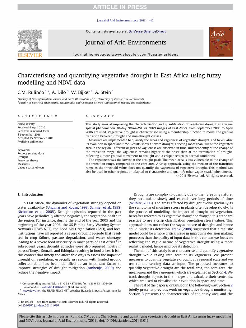
Characterising and quantifying vegetative drought in East Africa using fuzzymodelling and NDVI data

C.M. Rulinda a,*, A. Dilo b, W. Bijker a, A. Stein a

a Faculty of Geo-information Science and Earth Observation (ITC), University of Twente, The Netherlandsb Faculty of Electrical Engineering, Mathematics and Computer Science, University of Twente, The Netherlands

a r t i c l e i n f o

Article history:Received 4 April 2010Received in revised form8 September 2011Accepted 15 November 2011Available online xxx

Keywords:Remote sensing dataDroughtFuzzy set theoryMeasuresVague spatial objects

* Corresponding author. Tel.: þ31 0 53 4874559; faE-mail address: [email protected] (C.M. Rulinda

1 www.fews.net: the USAID FEWS NET Weather HaAfrica.

0140-1963/$ e see front matter � 2011 Elsevier Ltd.doi:10.1016/j.jaridenv.2011.11.016

Please cite this article in press as: Rulinda, Cand NDVI data, Journal of Arid Environment

a b s t r a c t

This study aims at improving the characterisation and quantification of vegetative drought as a vaguespatial phenomenon. 10-day NOAA-AVHRR NDVI images of East Africa from September 2005 to April2006 are used. Vegetative drought is characterised using a membership function to model the gradualtransition between drought and non-drought classes.

Measures are implemented to quantify the areas and vagueness of vegetative drought, and to visualiseits evolution in space and time. Results show a severe drought, affecting more than 60% of the vegetatedarea in the region. Different degrees of vagueness are observed in time, independently of the change ofthe transition range; the vagueness remains higher at the onset than at the termination of drought,reflecting a more gradual movement to drought and a crisper return to normal conditions.

The vagueness was the lowest at the drought peak. The mean-area is less vulnerable to the change ofthe transition range, compared to the core-area. A Crisp approach, using the median of the transitionrange as the threshold value, does not quantify the vagueness of vegetative drought. This method canalso be used in other regions, or adapted to characterise and quantify other vague spatial phenomena.

� 2011 Elsevier Ltd. All rights reserved.

1. Introduction

In East Africa, the dynamics of vegetation strongly depend onwater availability (Unganai and Kogan, 1998; Sannier et al., 1998;Nicholson et al., 2005). Drought episodes reported in the pastyears have periodically affected negatively the vegetation health inthe region. For instance, during the end of the year 2005 and thebeginning of the year 2006, the US Famine Early Warning SystemNetwork (FEWS NET), the Food Aid Organization (FAO), and localinstitutions have all reported a severe drought episode that resul-ted in crop failure, pasture degradation, and water shortage,leading to a severe food insecurity in most parts of East Africa.1 Insubsequent years, drought episodes were also reported mostly inparts of Kenya, Somalia and Ethiopia, resulting in food crises. It is inthis context that timely and affordable ways to assess the impact ofdrought on vegetation, especially in regions with limited groundcollected data, has been identified as an important factor toimprove strategies of drought mitigation (Ambenje, 2000) andreduce the negative impact.

x: þ31 0 53 4874400.).zards Impacts Assessment for

All rights reserved.

.M., et al., Characterising ands (2011), doi:10.1016/j.jariden

Droughts are complex to quantify due to their creeping nature;they accumulate slowly and extend over long periods of time(Wilhite, 2005). The areas affected by drought evolve gradually asthe symptoms of moisture stress in plants often develop slowly. Inthe process of modelling the impact of drought on vegetation,hereafter referred to as vegetative drought or drought, it is standardpractice to use a crisp classification vegetation stress values. Thisapproach does not reflect the vague nature of drought, and hencecould hinder its detection. Frank (2008) suggested that a realisticmodel could be a more critical issue in improving decision makingprocesses than the quality of input data. In this context we focus onreflecting the vague nature of vegetative drought using a morerealistic model, hence improve its detection.

The aim of this study is to characterise and quantify vegetativedrought while taking into account its vagueness. We presentmeasures to quantify vegetative drought at a regional scale and weuse remote sensing data as input. The proposed measures toquantify vegetative drought are the total-area, the core-area, themean-area and the vagueness, which are explained in Section 4.Wetrack drought objects in the images and calculate their centroids,which are used to visualise their evolution in space and time.

The rest of the paper is organised in the followingway: Section 2briefly presents previous work on vegetative drought monitoring;Section 3 presents the characteristics of the study area and the

quantifying vegetative drought in East Africa using fuzzy modellingv.2011.11.016

mailto:[email protected]

http://www.fews.net/

www.sciencedirect.com/science/journal/01401963

http://www.elsevier.com/locate/jaridenv

http://dx.doi.org/10.1016/j.jaridenv.2011.11.016



C.M. Rulinda et al. / Journal of Arid Environments xxx (2011) 1e102

data; Section 4 details the methods; Section 5 presents and discussthe results, and is followed by a conclusion in Section 6.

2. Previous work

Remote sensing data proved to be of a significant value inmonitoring vegetation (Sannier et al., 1998; Diouf and Lambini,2001) and more specifically drought (Tucker and Choudhury,1987; Liu and Kogan, 1996; Ambenje, 2000; Peters et al., 2002;Quan and Tenhunen, 2004; Song et al., 2004; Lacaze and Bergés,2005; Gouvia et al., 2009) using multi-temporal data (Kogan,2001). Although vegetative drought is difficult to identify, it canbe measured using various indicators which provide means ofmonitoring (Dracup et al., 1980). In this context, the NormalizedDifference Vegetation Index (NDVI) (Tucker, 1979) is often used(Tucker and Choudhury, 1987; Ji and Peters, 2003).

Among the NDVI-based approach studies, Song et al. (2004)produced 10-day (dekad) classified drought risk maps using thedifference between the current NDVI and the corresponding 3-yearaverage from the National Oceanic and AtmosphericAdministration-Advanced Very High Resolution Radiometer(NOAA-AVHRR). Pixels with difference NDVI values below�0.1 wereconsidered as drought risk areas, while pixels with difference NDVIvalues below �0.25 were considered as severe drought areas. Ona monthly basis and using the Satéllite Pour l’Observation de laTerre (SPOT)-Vegetation NDVI data, Gouvia et al. (2009) estimatedthe area of stressed vegetation in Portugal based on the number ofpixels with NDVI anomalies lower than �0.025. These NDVIanomalies were computed as the departure from the median ofthat month calculated for 8 years. Generally speaking, theNDVI-based approaches (Sannier et al., 1998; Gouvia et al., 2009;Leelaruban et al., 2010), although characterising and quantifyingvegetative drought, are limited in the way that they use the crispclassification method, hence do not account for the vague nature ofvegetative drought.

Fig. 1. Subset of East Africa (so

Please cite this article in press as: Rulinda, C.M., et al., Characterising andand NDVI data, Journal of Arid Environments (2011), doi:10.1016/j.jariden

Significant progress has been made, using the fuzzy set theory(Zadeh, 1965), to describe, store, process, and display vague objects(Schneider, 1999; Dilo et al., 2007b; Cheng et al., 2009; Kanjilalet al., 2010; Pauly and Schneider, 2010). Methods were also devel-oped in this perspective to characterise vague spatial entities suchas soil types (Burrough,1989), forests types (Brown,1998), and landuse (Cheng et al., 2001). In this paper we use a fuzzy approach tomodel the gradual transition between non-drought and drought.We use measures developed for vague objects (Dilo et al., 2007a)and modified them for raster images. To visualise the evolution ofdrought in time and space, dynomap, a software developed byTurdukulov et al. (2005) to track and visualise the evolution ofimage features in time-series, is used.

3. Study area and data

3.1. East Africa

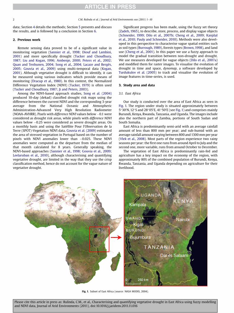
Our study is conducted over the area of East Africa as seen inFig. 1. The region under study is situated approximately between5�300N,12�S and 28�050E, 41�500E (see Fig. 1) and comprises mainlyBurundi, Kenya, Rwanda, Tanzania, and Uganda. The images includealso the northern part of Zambia, portions of South Sudan andSouth Somalia.

East Africa is predominantly semi-arid with an average rainfallamount of less than 800 mm per year; and sub-humid with anaverage rainfall amount varying between800 and1300mmper year(Vlek et al., 2008). Most parts of the region experience two rainyseasons per year: the first one runs fromaround April to July and thesecond one, more variable, runs from around October to December.

The vegetation of East Africa is predominantly rain-fed andagriculture has a key impact on the economy of the region, withapproximately 80% of the combined population of Burundi, Kenya,Rwanda, Tanzania, and Uganda depending on agriculture for theirlivelihood.

urce: NASA MODIS, 2004).


C.M. Rulinda et al. / Journal of Arid Environments xxx (2011) 1e10 3

3.2. Drought in East Africa

In January 2006, the US National Aeronautics and SpaceAdministration (NASA) Earth Observatory2 reported that the failureof the short-season rains left large sections of East Africa in severedrought at the end of the year 2005 and early 2006. In a normalyear, most of these affected regions experience rainfall from MarchtoMay during the long rainy season, and fromOctober to Decemberduring the short rainy season. In 2005, the long rainy seasonproduced little rain while the short rainy season failed. The FEWSNET reported that as a result, the rainfall totals for the year wereonly 20e60 percent of normal, depending on the region.

The FEWS NET reported that the impact of the drought has beensevere, resulting in crop failures, pasture degradation, watershortages, and has raised serious food security concerns for theregion. By the end of January 2006, millions were in need of foodaid, particularly pastoralists who depend on rain-fed pasture landsto maintain their livestock.

3.3. Data

The data used in this study is composed of AVHRR-based NDVIimages. These images are processed by the Global InventoryMonitoring and Modelling Systems (GIMMS) group (Pinzón et al.,2005; Tucker et al., 2005) at the US National Aeronautic SpaceAgency (NASA/GSFC). They are freely available from the FamineEarlyWarning System/Africa Data Dissemination Service.3 They areselected as they cover our area of interest and the long-term meanNDVI data for the same area is also available. Data from the firstdekad of September 2005 to the last dekad of April 2006, and long-term mean NDVI data for the same dekads are used. This multi-temporal dataset covers the drought period under study. Thelong-term mean NDVI are calculated from the year 1982 throughthe year 2008. From the original images, subsets covering theregion under study (see Fig. 1) are extracted.

In these original images, NDVI values in the range [0,1] arelinearly stretched to [0,250]. Missing and erroneous values areassigned to the value 253 and water to the value 250. A total of 42AVHRR-NDVI images for 21 dekads are used. Three dekads, namelythe 2nd dekad of February 2006, the 2nd dekad of March 2006 andthe 1st dekad of April 2006 only contain the value 0. The pixelresolution of the images is 8 km, which we consider acceptable formonitoring vegetative drought at the regional scale of East Africa.

4. Methodology

Our methodology consists of using the difference between thecurrent (i.e. from September 2005 to April 2006) and the long-termmean NDVI of the same period to characterise the state of vegeta-tion, similar to Song et al. (2004) and Anyamba and Tucker (2005b).Amembership function is then applied to the difference NDVI valuesto model vegetative drought. The proposed measures of vegetativedrought are calculated for all the dekads and the evolution ofdrought areas is visualised using the Dynomap space-time cube.The subsequent sections detail our methodology.

4.1. Characterising vegetative drought

To characterise vegetative drought, a membership function isapplied on NDVI anomaly images, called difference NDVI. Thefollowing subsections explain the process.

2 http://earthobservatory.nasa.gov/IOTD/view.php?id¼6246.3 FEWS/ADDS, earlywarning.usgs.gov/adds/.


4.1.1. Generating the difference NDVI mapsNDVI is the most commonly used vegetation index and it is

related to vegetation vigor, percentage green cover and biomass(Anyamba and Tucker, 2005a). It is calculated as the normalizeddifference of the spectral reflectance of the near infrared lNIR(0.73e1.1 mm for NOAA-AVHRR channels) and red lRED(0.55e0.68 mm for NOAA-AVHRR channels):

NDVI ¼ lNIR � lREDlNIR þ lRED

(1)

NDVI values vary between �1 and þ1, and are undefined whenboth lNIR and lRED are zero. NDVI values for vegetated land areasgenerally range from approximately 0.1 to 0.7, with values greaterthan 0.5 indicating dense vegetation. Values less than 0.1 indicateno vegetation, e.g. barren area, rock, sand or snow (Tucker, 1979).

As NDVI itself does not reflect drought or non-drought condi-tions, the difference between the current NDVI, i.e. measuredduring the period of interest, and the long-term mean of the sameperiod is considered. The intensity of vegetative drought can thenbe defined from the deviation of the current NDVI from itslong-term average (Anyamba and Tucker, 2005b). Positive NDVIdifference values indicate above normal vegetation conditions, zerovalues indicate no change and negative NDVI difference valuesindicate below normal vegetation conditions, which suggest pre-vailing drought conditions. The larger the negative departure, thehigher the intensity of vegetative drought. This NDVI deviationfrom the long-term mean values, called here difference NDVI andwritten difNDVI, is obtained by subtracting the long-term averagefrom the current NDVI value for each dekad from September 2005to April 2006, excluding water, missing and erroneous values. Foreach dekad i˛ (1,.,21), the difference NDVI is calculated from theraster subtraction

difNDVIi ¼ NDVIi �NDVIi (2)

The difNDVI values range between �250 and 250. PositivedifNDVI values indicate either above normal conditions, missingvalues, erroneous values or water all assigned to value 250. Nega-tive values indicate below normal conditions. We characterisevegetation stress using negative difNDVI values.

4.1.2. Defining the membership functionIn this study we assume vegetation stress being caused by

drought conditions. A membership function, which accounts forthe gradual transition between non-drought to drought classes, isproposed. The proposed membership function, drought:[�250,250] / [0,1], calculates drought from the negative difNDVIvalues. We selected two types of functions, a linear one anda sigmoidal one to assess the impact of the shape of the function onthe results. The linear (semi-trapezoidal) membership function (seeFig. 2(a)) drought, noted below as d, is built over difNDVI values by:

cx˛½�250;250�; dðxÞ ¼

8><>:

1 cx : x � ab� xb� a

cx : a < x < b

0 cx : x � b

(3)

Where a and b are respectively the lower (start) and upper (end)limits of the transition range (TR) [a,b].

4.1.3. Selecting the transition range of the drought membershipfunction

The limits of the transition range are selected as follow: b, beingthe end of the transition range, is set to difNDVI value zero, whichcorresponds to the end of drought possibility. From 0 and above,


http://earthobservatory.nasa.gov/IOTD/view.php%3fid=6246

http://earthobservatory.nasa.gov/IOTD/view.php%3fid=6246

http://earlywarning.usgs.gov/adds/

Fig. 2. (a) Linear drought membership function applied to difNDVI images, with thetransition range TR ¼ [�14,0]; (b) Sigmoidal drought membership function applied todifNDVI images, with TR ¼ [�14,0]; (c) Linear drought membership function applied todifNDVI images, with TR ¼ [�7,0].


there is certainly no drought. a being the start of the transitionrange, is set in the following way:

� As drought was reported to occur in November 2005 throughMarch 2006, we assume drought to be “certain” at thesemonths and “possible” during the other months.

� As such, the difNDVI images of September, October and Aprilare combined into a single “possible” drought image and basicstatistics of this combined image are calculated on thehistogram.

Min Max Mean Stdev

�225 207 4.397862 9.339158

� Assuming a 95% confidence of possible drought, b is calculatedas: Mean � 2 Stdev, hence assigned to the difNDVI value �14.

In order to understand the impact of the shape of the function onthe results, a sigmoidal function (Fig. 2(b)) is used and calculated by:

cx˛½�250;250�; dðxÞ ¼ 1� 2

1þ exp��2x

3� 5

� (4)


In order to assess the impact of the change of the TR on theresults, the transition range was also reduced. By drawing a corre-spondence between with what Gouvia et al. (2009) call severedrought, and what we call “certain” drought, the TR was reducedfrom [�14, 0[ to ]�7, 0], as shown on Fig. 2 (c). �7 in the range[�250,0] being an approximation of �0.025 in the range [�1,0].

These membership functions are applied to difNDVI images toproduce drought maps D for each dekad i.

4.2. Quantifying vegetative drought

Quantifying vegetative drought involves using measuresadapted from the ones proposed by Dilo (2006), Dilo et al. (2007a)for continuous space. These measures are modified for rasterimages. Visualising the evolution of vegetative drought area inspace and time is done using a tracking software developed byTurdukulov et al. (2005) and modified to use the proposedmeasures. The following sections paragraphs details.

4.2.1. Drought measuresThe measures proposed to quantify drought are: the total size of

the areas possibly covered by drought, called total-area; the totalsize of the areas certainly covered by drought, called the core-area;and an average of the area sizes of drought with the different certaintydegrees, called mean-area. We also quantify the degree of uncer-tainty in our description of drought with a measure called vague-ness. These drought measures are built on measures proposed forvague objects in the continuous space IR2 (Dilo, 2006; Dilo et al.,2007a), and are adapted to raster data. The following paragraphsdetail the process of building these measures.

The total-area of drought is the area size of the possible droughtlocations, i.e. locationswithpositivemembership values. Foravagueregion m:IR2 / [0,1], the total-area is Areaðfðx; yÞ˛IR2jmðx; yÞ > 0gÞ.Our data composed of raster images, Di for each dekad, which areproduced from the data processing of the previous step. In thefollowing equationswe useD to notate the set of pixels in the image,and d(j) to indicate the value of drought in pixel j. The D total-area iscalculated by:

total-area ¼X

fj˛DjdðjÞ>0gpixel-size: (5)

Thus, the total-area is equal to the pixel-size multiplied by thenumber of positive pixels.

The core-area is the area size of the certain drought locations.Drought can be described in different levels of certainty using theconcept of a-cuts (Klir and Yuan, 1995): ma ¼ fðx; yÞ˛IR2��mðx; yÞ �ag, where a˛½0;1�. The certain drought region is the 1-cut, whicharea size is the core-area:

Areaðfðx; yÞ˛IR2��mðx; yÞ ¼ 1gÞ. For a raster image D, thecore-area is calculated by:

core-area ¼X

fj˛DjdðjÞ¼1gpixel-size: (6)

Thus, the core-area of drought is equal to the pixel-size multi-plied by the number of 1-valued pixels in D.

The different a-cuts produce different description of drought,each associated with a different certainty level, a. To get an esti-mation of the area size that accounts for all the different descrip-tions based on a values, we calculate the arithmetic mean of areasizes of a-cuts. This measure is the mean-area. For a vague region m

in IR2 the mean-area(m) is equal toR R

mðx; yÞdx dy (Dilo, 2006; Diloet al., 2007a). For a raster image D, the mean-area is calculated byreplacing the integral with the sum:


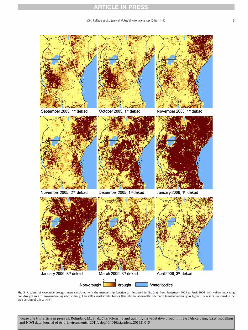
Fig. 3. A subset of vegetative drought maps calculated with the membership function as illustrated in Fig. 2(a), from September 2005 to April 2006, with yellow indicatingnon-drought area to brown indicating intense drought area. Blue masks water bodies. (For interpretation of the references to colour in this figure legend, the reader is referred to theweb version of this article.)


Please cite this article in press as: Rulinda, C.M., et al., Characterising and quantifying vegetative drought in East Africa using fuzzy modellingand NDVI data, Journal of Arid Environments (2011), doi:10.1016/j.jaridenv.2011.11.016

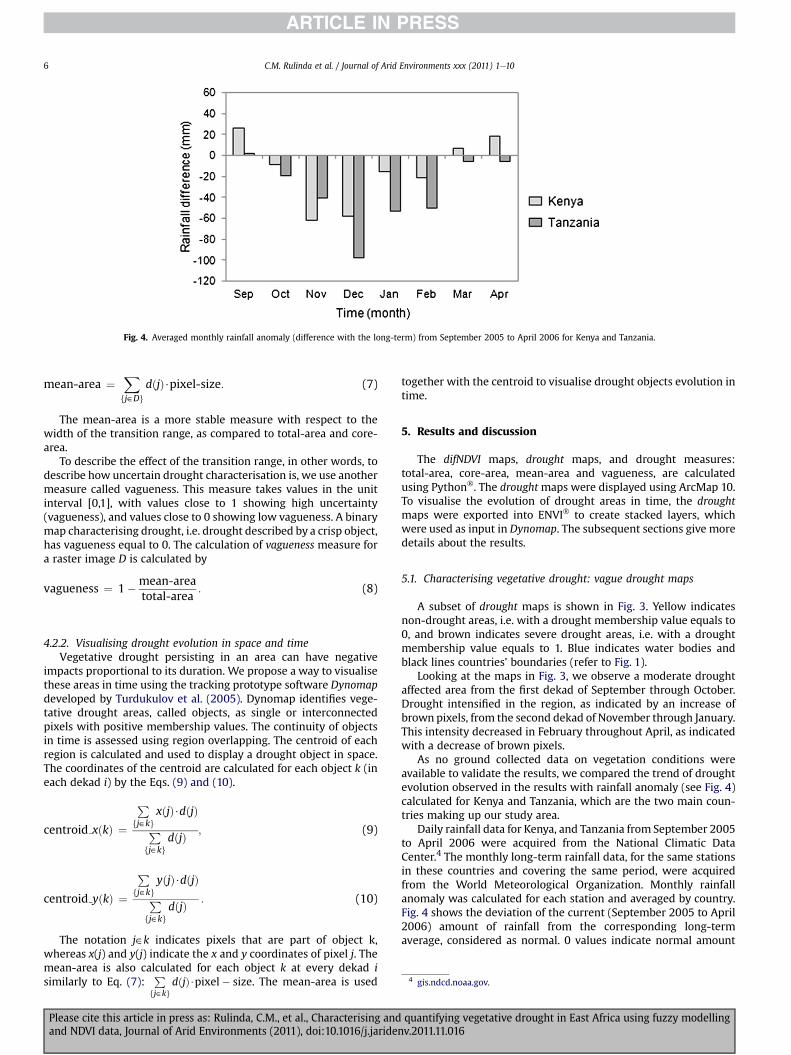
Fig. 4. Averaged monthly rainfall anomaly (difference with the long-term) from September 2005 to April 2006 for Kenya and Tanzania.


mean-area ¼ dðjÞ$pixel-size: (7)

4 gis.ndcd.noaa.gov.

Xfj˛Dg

The mean-area is a more stable measure with respect to thewidth of the transition range, as compared to total-area and core-area.

To describe the effect of the transition range, in other words, todescribe how uncertain drought characterisation is, we use anothermeasure called vagueness. This measure takes values in the unitinterval [0,1], with values close to 1 showing high uncertainty(vagueness), and values close to 0 showing low vagueness. A binarymap characterising drought, i.e. drought described by a crisp object,has vagueness equal to 0. The calculation of vagueness measure fora raster image D is calculated by

vagueness ¼ 1�mean-areatotal-area

: (8)

4.2.2. Visualising drought evolution in space and timeVegetative drought persisting in an area can have negative

impacts proportional to its duration. We propose a way to visualisethese areas in time using the tracking prototype software Dynomapdeveloped by Turdukulov et al. (2005). Dynomap identifies vege-tative drought areas, called objects, as single or interconnectedpixels with positive membership values. The continuity of objectsin time is assessed using region overlapping. The centroid of eachregion is calculated and used to display a drought object in space.The coordinates of the centroid are calculated for each object k (ineach dekad i) by the Eqs. (9) and (10).

centroid xðkÞ ¼

Pfj˛kg

xðjÞ$dðjÞP

fj˛kgdðjÞ ; (9)

centroid yðkÞ ¼

Pfj˛kg

yðjÞ$dðjÞP

fj˛kgdðjÞ : (10)

The notation j˛k indicates pixels that are part of object k,whereas x(j) and y(j) indicate the x and y coordinates of pixel j. Themean-area is also calculated for each object k at every dekad isimilarly to Eq. (7):

Pfj˛kg

dðjÞ$pixel� size. The mean-area is used


together with the centroid to visualise drought objects evolution intime.

5. Results and discussion

The difNDVI maps, drought maps, and drought measures:total-area, core-area, mean-area and vagueness, are calculatedusing Python�. The droughtmaps were displayed using ArcMap 10.To visualise the evolution of drought areas in time, the droughtmaps were exported into ENVI� to create stacked layers, whichwere used as input in Dynomap. The subsequent sections give moredetails about the results.

5.1. Characterising vegetative drought: vague drought maps

A subset of drought maps is shown in Fig. 3. Yellow indicatesnon-drought areas, i.e. with a drought membership value equals to0, and brown indicates severe drought areas, i.e. with a droughtmembership value equals to 1. Blue indicates water bodies andblack lines countries’ boundaries (refer to Fig. 1).

Looking at the maps in Fig. 3, we observe a moderate droughtaffected area from the first dekad of September through October.Drought intensified in the region, as indicated by an increase ofbrown pixels, from the second dekad of November through January.This intensity decreased in February throughout April, as indicatedwith a decrease of brown pixels.

As no ground collected data on vegetation conditions wereavailable to validate the results, we compared the trend of droughtevolution observed in the results with rainfall anomaly (see Fig. 4)calculated for Kenya and Tanzania, which are the two main coun-tries making up our study area.

Daily rainfall data for Kenya, and Tanzania from September 2005to April 2006 were acquired from the National Climatic DataCenter.4 The monthly long-term rainfall data, for the same stationsin these countries and covering the same period, were acquiredfrom the World Meteorological Organization. Monthly rainfallanomaly was calculated for each station and averaged by country.Fig. 4 shows the deviation of the current (September 2005 to April2006) amount of rainfall from the corresponding long-termaverage, considered as normal. 0 values indicate normal amount


http://gis.ndcd.noaa.gov/

Fig. 5. Total-area, core-area and mean-area: (a) calculated as illustrated in Fig. 3(a) and(b) calculated as illustrated in Fig. 3(b) and (c) calculated as illustrated in Fig. 3(c).


of rainfall, negative values indicate below normal amount of rainfalland positive values indicate above normal amount of rainfall.

We observe on Fig. 4 a below average condition of rainfall fromOctober 2005 through February 2006, with a severe lack of rainfalloccurring between November and February, as for drought as seenon (Fig. 3). The lack of rainfall observed in October 2005 worsenedthrough December and can explain the level of drought intensifi-cation observed in January 2006. In April 2006 drought conditionsstarted fading, which can be explained by the slow return to normalrainfall condition observed in March.

5.2. Quantifying vegetative drought: vague drought measures

Vegetative drought area for the region is measured using thetotal-area, core-area, and the mean-area. Fig. 5 shows the areas,expressed in sq. km, calculated per dekad and plotted against eachother.

In all figures the total-area remains the same as we kept thesame end for the TR, 0. These values vary between a minimum of656,448 sq. km and a maximum of 1,870,080 sq. km. The core-areavalues does not significantly change after changing the shape of thefunction, however it changes drastically after reducing the transi-tion range, and affects the mean-areas in Fig. 5(c). In Fig. 5(a) and(b), the core-area varies between a minimum of 60,096 sq. km anda maximum of 1,424,448 sq. km, while in Fig. 5(c) it varies between296,640 sq. km and 1,647,104 sq. km. The mean-area variesbetween a minimum of 358 560 and a maximum of1,637,344 sq. km in Fig. 5(a) and (b), while it varies between502,198 sq. km and 1,756,525 sq. km in Fig. 5(c).

With the difference of the core-area minimum values being236,544 sq. km, and of the mean-area minimum values being143,636 sq. km, we can say that the mean-area measure is morestable measure of vegetative drought area, i.e. its values are lessaffected from the change of TR than the core.

The difference between the total-area and the core-area valuesvary for each dekad. The magnitude of this difference is reduced inFig. 5(c), as the transition range was reduced. In all the casesthough, the difference remains higher at the beginning of droughtthan at the end, and was the smallest at the peak of the droughtevent in January 2006. This variation shows that vegetative droughtis more spatially vague at its beginning than at its end, and lessvague at its peak.

The degree of vagueness of vegetative drought characterisationis also quantified. This uncertainty is quantified using the vague-ness measure, as shown in Fig. 6.

The degree of vagueness of vegetative drought is plotted for allthe dekads, for both TR. By defining the severity of vegetativedrought as the percentage of drought affected vegetation, weobserve in both figures a severe drought event in January withmore than 60% of the vegetation affected by drought. The onset ofthe drought severity corresponds to a higher degree of vaguenesscompared to its end in both figures, however the magnitude ofvagueness changes with the width of the transition zone. Thehighest severity of vegetative drought corresponds to the lowestvagueness of vegetative drought.

5.3. Comparison with a traditional crisp approach

Traditional approaches usually characterise vegetative droughtfrom difNDVI images using a binary function. In order to comparethe two approaches, the crisp threshold of 50%, or a-cut ¼ 0.5, isused. This value is a good threshold as it is the mean the transitionrange. Drought area calculated using that crisp threshold, calledhere crisp-area, and the mean-area calculated using a membershipfunction are plotted together in Fig. 7.


From Fig. 7 it can be observed that

� The creeping nature of drought is observed from bothmeasures.

� The crisp approach with a threshold of a-cut ¼ 0.5 givesa smaller size of vegetative drought area.

We can conclude from the comparison that

� The vagueness of the drought can only be observed andquantified with the use of a drought membership function, i.e.it equals to 0 with a crisp threshold.


Fig. 6. Degree of vagueness of vegetative drought for all dekads with TR ¼ [�14,0[ and ]�7,0], plotted against the percentage of mean-area of drought and non-drought arearespectively.

Fig. 7. Mean-area, calculated with the membership function as illustrated in Fig. 3(a),and crisp-area, calculated with a crisp function with a threshold of a-cut ¼ 0.5.


� The Fuzzy-based modelling allows us also to quantify vegeta-tive drought for any given threshold value within the transitionrange, meaning we can map drought at different levels ofcertainty. The certainty level however depends on how good isthe membership function.

5.4. Visualising drought evolution in space and time

To detect drought objects, we have set the minimum droughtobject to be of 1 pixel, due to the low spatial resolution of theimages, where a pixel area equivalent to 64 km2, is a large area. Aswe are interested in visualising persistent drought objects, we onlydisplay objects existing during all the 21 dekads (see Fig. 8). Thesize of the objects are proportional to the mean-area size. Thevariation of the size of objects during their lifetime indicates thatthe mean-area of these objects changes over time, as can also beobserved in Fig. 5(a).

Please cite this article in press as: Rulinda, C.M., et al., Characterising and quantifying vegetative drought in East Africa using fuzzy modellingand NDVI data, Journal of Arid Environments (2011), doi:10.1016/j.jaridenv.2011.11.016

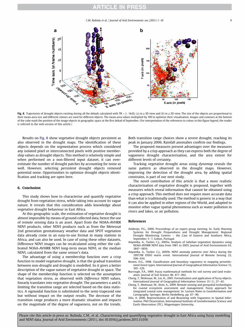
Fig. 8. Trajectories of drought objects existing during all the dekads calculated with TR ¼ [�14,0]; (a) in a 3D view and (b) in a 2D view. The size of the objects are proportional totheir mean-area size and different colours are used for different objects. The mean-area values multiplied by 100 to optimize their visualisation. Images and contours at the bottomof the cube mark the position of the image objects in geographic space at the first dekad of September. (For interpretation of the references to colour in this figure legend, the readeris referred to the web version of this article.)


Results on Fig. 8 show vegetative drought objects persistent asalso observed in the drought maps. The identification of theseobjects depends on the segmentation process which consideredany isolated pixel or interconnected pixels with positive member-ship values as drought objects. This method is relatively simple andwhen performed on a non-filtered input dataset, it can over-estimate the number of drought patches by accounting for noise aswell. However, selecting persistent drought objects removedpotential noise. Opportunities to optimize drought objects identi-fication and tracking are open here.

6. Conclusion

This study shows how to characterise and quantify vegetativedrought from vegetation stress, while taking into account its vaguenature. It reveals that this consideration adds knowledge aboutvegetative drought behaviour in East Africa.

At this geographic scale, the estimation of vegetative drought isalmost impossible bymeans of ground collected data, hence the useof remote sensing data is an asset. Apart from the NOAA-AVHRRNDVI products, other NDVI products such as from the Meteosat2nd generation geostationary weather data and SPOT vegetationdata already come in an easy-to-use format in many stations inAfrica, and can also be used. In case of using these other datasets,Difference NDVI images can be recalculated using either the cali-brated NOAA-AVHRR NDVI long-term mean NDVI, or the medianNDVI, calculated from the same sensor’s data.

The advantage of using a membership function over a crispfunction to model vegetative drought, is that the gradual transitionbetween non-drought and drought is modelled. So it gives a betterdescription of the vague nature of vegetative drought in space. Theshape of the membership function is selected on the assumptionthat vegetation stress, as observed with Difference NDVI values,linearly translates into vegetative drought. The parameters a and b,limiting the transition range are selected based on the data statis-tics. A sigmoidal function is substituted to the semi-trapezoid onebut without impact on the output results. The decrease of thetransition range produces a more dramatic situation and impactson the magnitude of the degree of vagueness, not on the trends.


Both transition range choices show a severe drought, reaching itspeak in January 2006. Rainfall anomalies confirm our findings.

The proposed measures present advantages over the measuresprovided by a crisp approach as they can express both the degree ofvagueness drought characterisation, and the area extent fordifferent levels of certainty.

Tracking vegetative drought areas using dynomap reveals thesame pattern as observed in the drought maps. However,improving the detection of the drought area, by adding spatialconstrains, is part of our next study.

The novel contribution of this article is that a more realisticcharacterisation of vegetative drought is proposed, together withmeasures which reveal information that cannot be obtained usinga crisp approach. This method does not require more accurate datathanwhat is traditionally used. The method is generic in a way thatit can also be applied in other regions of the World, and adapted tomonitor other vague spatial phenomena such as water pollution inrivers and lakes, or air pollution.

References

Ambenje, P.G., 2000. Proceedings of an expert group meeting. In: Early WarningSystems for Drought Preparedness and Drought Management: RegionalDrought Monitoring Centres e the Case of Eastern and Southern Africa,September 5e7, Lisbon, Portugal.

Anyamba, A., Tucker, C.J., 2005a. Analysis of Sahelian vegetation dynamics usingNOAA-AVHRR NDVI data from 1981 to 2003. Journal of Arid Environments 63,1847e1859.

Anyamba, A., Tucker, C.J., 2005b. NDVI anomaly patterns over Africa during the1997/98 ENSO warm event. International Journal of Remote Sensing 22,596e614.

Brown, D.G., 1998. Classification and boundary vagueness in mapping presettle-ment forest types. International Journal of Geographical Information Science 12,105e129.

Burrough, P.A., 1989. Fuzzy mathematical methods for soil survey and land evalu-ation. Journal of Soil Science 40, 477e492.

Cheng, T., Molenaar, M., Lin, H., 2001. Formalization and application of fuzzy objects.International Journal of Geographical Information Science 15 (1), 27e42.

Cheng, T., Molenaar, M., Stein, A., 2009. Remote sensing and geospatial technologiesfor coastal ecosystem assessment and management. Fuzzy approach forintegrated coastal zone management. In: Lecture Notes in Geoinformation andCartography. Springer, Berlin Heidelberg, pp. 67e90.

Dilo, A. 2006. Representation of and Reasoning with Vagueness in Spatial Infor-mation. PhD Dissertation, International Institute of Geoinformation Science andEarth Observation (ITC), Wageningen University.



Dilo, A., de By, R.A., Stein, A., 2007a. Metrics for vague spatial objects based on theconcept of mass. In: Proceedings of 2007 IEEE International Conference onFuzzy Systems, pp. 804e809.

Dilo, A., de By, R.A., Stein, A., 2007b. A system of types and operators for handlingvague spatial objects. International Journal of Geographical Information Science21 (4), 397e426.

Diouf, A., Lambini, E.F., 2001. Monitoring land-cover changes in semi-arid regions:remote sensing data and field observations in the Ferlo, Senegal. Journal of AridEnvironments 48, 129e148.

Dracup, A., Lee, K.S., Paulson, E.G., 1980. On the definition of droughts. WaterResources Research 16 (2), 291e302.

Frank, A.U., 2008. Analysis of dependence of decision quality on data quality.Journal of Geographical Systems 10 (1), 71e88.

Gouvia, C., Trigo, R.M., DaCamara, C.C., 2009. Drought and vegetation stressmonitoring in Portugal using satellite data. Natural Hazards and Earth SystemSciences 9 (9), 185e195.

Ji, L., Peters, A., 2003. Assessing vegetation response to drought in the northernGreat Plains using vegetation and drought indices. Remote Sensing of Envi-ronment 87, 85e98.

Kanjilal, V., Liu, H., Schneider, M., 2010. Plateau regions: an implementation conceptfor fuzzy regions in spatial databases and GIS. In: Proceedings: 13th Interna-tional Conference on Information Processing and Management of Uncertainty,IPMU 2010. Lecture Notes in Computer Science, 6178 LNAI.

Klir, G.J., Yuan, B., 1995. Fuzzy Sets and Fuzzy Logic: Theory and Application.Prentice-Hall.

Kogan, F.N., 2001. Operational space technology for global vegetation assessment.Remote Sensing of Environment 82, 1949e1964.

Lacaze, B., Bergés, J.C., 2005. Contribution of Meteosat Second Generation (MSG) todrought early warning. In: Proceedings: 13th International Conference: RemoteSensing and Geoinformation Processing in the Assessment and Monitoring ofLand Degradation and Desertification: State of the Art and OperationalPerspectives, Sept 7e9, Trier, Germany.

Leelaruban, N., Akyuz, A., Oduor, P., Padmanabhan, G., 2010. Geospatial analysis ofdrought impact and severity in North Dakota, USA using remote sensing andGIS. In: American Meteorological Society: 18th Conference on AppliedClimatology.

Liu, W.T., Kogan, F.N., 1996. Monitoring regional drought using the vegetationcondition index. International Journal of Remote Sensing 17 (14), 2761e2782.

Nicholson, S.E., Davenport, M.L., Malo, A.R., 2005. A comparison of the vegetationresponse to rainfall in the Sahel and East Africa, using normalized differencevegetation index from NOAA-AVHRR. Climatic Change 17, 209e241.


Pauly, A., Schneider, M., 2010. VASA: an algebra for vague spatial data in databases.Information Systems 35, 111e138.

Peters, A.J., WalterShea, E.A., JI, L., Viña, A., Hayes, M., Svoboda, M.D., 2002. Droughtmonitoring with NDVI-based standardized vegetation index. PhotogrammetricEngineering & Remote Sensing 68 (1), 71e75.

Pinzón, J., Brown, M.E., Tucker, C.J., 2005. Satellite time series correction of orbitaldrift artifacts using empirical mode decomposition. In: Hilbert-HuangTransform: Introduction and Applications, World Scientific, pp. 167e186.

Quan, W., Tenhunen, J.D., 2004. Vegetation mapping with multitemporal NDVI inNorth Eastern China Transect (NECT). International Journal of Applied EarthObservation and Geoinformation 6 (1), 17e31.

Sannier, C.A.D., Taylor, J.C., Du Plessis, W., Campbell, K., 1998. Real time vegetationmonitoring with NOAA-AVHRR in Southern Africa for wildlife management andfood securityassessment. International Journal of Remote Sensing19 (4), 621e639.

Schneider, M., 1999. Uncertainty management for spatial data in databases: fuzzyspatial data types. In: Advances in Spatial Databases, SSD’99, Lecture Notes inComputer Science, 1651. Springer, pp. 330e351.

Song, X., Saito, G., Kodama, M., Sawada, H., 2004. Early detection system of droughtin East Asia using NDVI from NOAA/AVHRR data. International Journal ofRemote Sensing 25 (16), 3105e3111.

Tucker, C.J., 1979. Red and photographic infrared linear combinations formonitoring vegetation. Remote Sensing of Environment 8, 127e150.

Tucker, C.J., Choudhury, B.J., 1987. Satellite remote sensing of drought conditions.Remote Sensing of Environment 23, 243e251.

Tucker, C.J., Pinzón, J.E., Brown, M.E., Slayback, D., Pak, E.W., Mahoney, R.,Vermote, E., El Saleous, N., 2005. An Extended AVHRR 8-km NDVI data setcompatible with MODIS and SPOT vegetation NDVI data. International Journalof Remote Sensing 26 (20), 4485e4498.

Turdukulov, U.D., Tolpekin, V., Kraak, M.-J., 2005. Visual exploration of time series ofremote sensing data. In: Proceedings of: Spatial-temporal Modeling, SpatialReasoning, Analysis, Data Mining and Data Fusion (ISPRS-WG/II), Beijing, China27e29 August, 2005.

Unganai, L.S., Kogan, F.N., 1998. Drought monitoring and corn yield estimation inSouthern Africa from AVHRR data. Remote Sensing of Environment 63 (3),219e232.

Vlek, P.L.G., Le, Q.B., Tamene, L., 2008. Land Decline in Land-Rich Africa e a CreepingDisaster in the Making. Technical Report. CGIAR Science Council Secretariat,Rome, Italy.

Wilhite, D.A., 2005. Drought and Water Crisis: Science, Technology and Manage-ment Issues. Taylor & Francis Group.

Zadeh, L.A., 1965. Fuzzy sets. Information and Control 8 (3), 338e353.


Characterising and quantifying vegetative drought in East Africa using fuzzy modelling and NDVI data

Documents

Transcript of Characterising and quantifying vegetative drought in East Africa using fuzzy modelling and NDVI data