Characterising the Optical Response of the SNO+ Detector - LIP
298
University of Liverpool Characterising the Optical Response of the SNO+ Detector Author: Robert Stainforth Supervisor: Dr. Neil McCauley Thesis submitted in accordance with the requirements of the University of Liverpool for the degree of Doctor in Philosophy in the Faculty of Science and Engineering Department of High Energy Particle Physics March 2016
-
Upload
khangminh22 -
Category
Documents
-
view
0 -
download
0
Transcript of Characterising the Optical Response of the SNO+ Detector - LIP

University of Liverpool
Characterising the OpticalResponse of the SNO+ Detector
Author:
Robert Stainforth
Supervisor:
Dr. Neil McCauley
Thesis submitted in accordance with the requirements of the
University of Liverpool for the degree of Doctor in Philosophy
in the
Faculty of Science and Engineering
Department of High Energy Particle Physics
March 2016

UNIVERSITY OF LIVERPOOL
AbstractFaculty of Science and Engineering
Department of High Energy Particle Physics
Characterising the Optical Response of the SNO+ Detector
by Robert Stainforth
SNO+ is a liquid scintillator based neutrino experiment located 2039 m under-
ground in VALE’s Creighton mine, Lively, Ontario, CA. It is a re-purposing of the
original Cherenkov detector used in the SNO experiment to study neutrino oscilla-
tions. The advent of neutrino oscillations has revealed that neutrinos have a small
yet non-zero mass. However, the nature of this mass has yet to be determined. It
is possible that the neutrino is its own anti-particle, a Majorana fermion. If so,
such particles necessitate lepton number violating processes such as neutrinoless
double beta decay. SNO+ intends to search for the neutrinoless double beta decay
of 130Te. Other physics objectives include the study of low-energy solar neutrinos,
reactor anti-neutrinos, geo-neutrinos and sensitivity to nucleon decay and super-
nova neutrinos. To fulfil these objectives, SNO+ will operate over three detector
phases; water, scintillator and tellurium (loading of the scintillator with tellurium).
Prior to each phase, the experiment will undergo a full detector calibration. This
includes an optical calibration that seeks to characterise the optical response of the
detector using two types of in-situ light sources; one of these is called the laserball.
The laserball provides a pulsed, near-isotropic light distribution throughout the
detector. Laserball data is used in conjunction with a parameterised model that
characterises the optical response; the parameters are determined using a statis-
tical fit. This thesis presents an implementation of said model to all three phases
of the SNO+ experiment. A characterisation of the optical response in water is
presented using a combination of original laserball data from SNO and MC data
of the SNO+ detector. Thereafter, the two scintillator based phases are consid-
ered, wherein the increased attenuation of light due to absorption and reemission
introduced by the scintillator is addressed alongside a model of the scintillation
time profile.

Acknowledgements
There are numerous people I would like to thank for their help throughout my
time as a PhD student. Indeed, the words herein are my own, but only through
the insight of others have they been conceived. Firstly, I would like to thank my
supervisor Neil McCauley for his continual support, enthusiasm and time. He has
always made time for me, and will never cease to impress me with his knowledge
of neutrino physics and experimental practices. As my time at Liverpool ends, I
attribute a lot of my understanding to him for which I will always be thankful.
I hope we are able to work again sometime in the future. For now though I am
glad to be rid of his weekly reminders concerning the status of my football team,
Aston Villa relative to the mighty West Bromwich Albion.
I would also like to extend many thanks to Jose Maneira at LIP. Since joining
the SNO+ optics group, Jose has provided invaluable knowledge concerning the
laserball and the optical model discussed in this work. He has been an excellent
mentor and friend. I would also like to thank other members of the optics group;
Gersende Prior, Nuno Baros and Phil Jones for their help.
I feel very fortunate to have worked on SNO+ at Liverpool alongside my colleague,
and fellow PhD student John Walker. Seemingly in tandem1, John and I began and
concluded our work on SNO+ side by side. From summer schools and conferences
to a thoroughly enjoyable eight months living together in Sudbury, there is no one
I would have rather shared these memories with.
I have made many good friends without whom my time on SNO+ would have
been less enjoyable. I would like to thank fellow SNO+ UK students; Evelina
Arushanova, Ashley Back, Jack Dunger, Chris Jones, Stefanie Langrock and James
Waterfield and Sudbury locales Aleksandra Bialek, Caitlyn Darrach, Janet Rum-
leskie and Andy Stripay. I would also like to thank those all important non-
physicists in my life; Maike Potschulat, Emily Hole and Jenna Hinds as well as
Linda Fielding and Angie Reid at Liverpool for their help in assisting with my
travel arrangements.
Finally, thanks to my parents and sister for their support and love throughout
both this and all moments in my life; you couldn’t have given more.
1We did in fact once ride a tandem bike over the golden gate bridge. . .
ii

iii
Statement of Originality
All the work, analysis and discussion presented in this thesis is that of the author
unless otherwise stated.
The SNO+ collaboration is composed of approximately 100 members from var-
ious institutions in Europe and North America. As such, the individual tasks
required to run the experiment are split between working groups of 10-15 people.
Calculations or features of the SNO+ MC, RAT are therefore the result of iter-
ative improvements authored by several people from different groups. Relevant
to this work is the implementation of the different scintillator mixtures into RAT
by L. Segui of Oxford and spectrometer measurements of the laser-dye profiles by
J. Maneira of LIP. Past characterisations of the laserball light distribution obtained
from several optical calibrations in SNO were provided by N. Baros, after which
the author implemented these into RAT for use in the MC laserball data sets.
The laserball generator used to produce MC data was co-authored by the author
and J. Maneira. The calculation of refracted light paths discussed here originally
featured in the optical calibration software used in SNO, LOCAS. This calculation
has been revised and as such the mathematical derivation of this calculation has
been re-performed by the author and implemented into RAT. Similarly, the opti-
cal model and occupancy ratio method have previously been applied to laserball
data in SNO through LOCAS. LOCAS has now been replaced by a completely new
software utility for SNO+, OCA. OCA intends to serve the same purpose and as
such shares similarities to LOCAS. OCA was written entirely by the author in C++.
The time profile model presented as part of the discussion of laserball simulations
in scintillator was conceived by the author.

Contents
1 Searching for a Neutrino Mass 1
1.1 The Neutrino . . . . . . . . . . . . . . . . . . . . . . . . . . . . . . 1
1.2 Neutrino Oscillations . . . . . . . . . . . . . . . . . . . . . . . . . . 3
1.2.1 The Solar Neutrino Problem . . . . . . . . . . . . . . . . . . 4
1.2.1.1 Cherenkov Detectors . . . . . . . . . . . . . . . . . 8
1.2.1.2 The Kamiokande Experiment . . . . . . . . . . . . 10
1.2.1.3 The Sudbury Neutrino Observatory . . . . . . . . . 12
1.2.1.4 KamLAND . . . . . . . . . . . . . . . . . . . . . . 16
1.2.2 Atmospheric Neutrino Anomaly . . . . . . . . . . . . . . . . 17
1.2.3 Neutrino Mixing and Oscillations . . . . . . . . . . . . . . . 18
1.2.4 Neutrino Oscillations in Matter . . . . . . . . . . . . . . . . 21
1.2.5 Neutrino Oscillation Experiments . . . . . . . . . . . . . . . 23
1.3 Nature of the Neutrino Mass . . . . . . . . . . . . . . . . . . . . . . 27
1.3.1 Dirac Neutrino Masses . . . . . . . . . . . . . . . . . . . . . 27
1.3.2 Majorana Neutrino Masses . . . . . . . . . . . . . . . . . . . 28
1.3.3 Lepton Number Violation . . . . . . . . . . . . . . . . . . . 30
1.4 Detection of the Neutrino Mass . . . . . . . . . . . . . . . . . . . . 31
1.4.1 Neutrinoless Double β-Decay . . . . . . . . . . . . . . . . . 33
1.4.2 Neutrinoless Double β-Decay Experiments . . . . . . . . . . 36
1.4.2.1 Detector Technologies . . . . . . . . . . . . . . . . 37
2 The SNO+ Experiment 45
2.1 Detector Components and Materials . . . . . . . . . . . . . . . . . 45
2.1.1 PMTs & Electronics . . . . . . . . . . . . . . . . . . . . . . 47
2.2 Operating Phases & Backgrounds . . . . . . . . . . . . . . . . . . . 50
2.3 Detector Calibration . . . . . . . . . . . . . . . . . . . . . . . . . . 53
2.3.1 Optical Sources . . . . . . . . . . . . . . . . . . . . . . . . . 54
2.3.2 LED/Laser Light Injection System . . . . . . . . . . . . . . 55
2.3.3 The Laser System and Laserball . . . . . . . . . . . . . . . . 56
2.4 SNO+ Monte-Carlo: RAT . . . . . . . . . . . . . . . . . . . . . . . 60
3 Scintillators in SNO+ 61
3.1 Scintillator Structure . . . . . . . . . . . . . . . . . . . . . . . . . . 63
iv

Contents v
3.2 The SNO+ Scintillator . . . . . . . . . . . . . . . . . . . . . . . . . 66
3.3 Excitation & Attenuation . . . . . . . . . . . . . . . . . . . . . . . 68
3.4 De-Excitation & Luminescence . . . . . . . . . . . . . . . . . . . . 72
3.4.1 Fluorescence . . . . . . . . . . . . . . . . . . . . . . . . . . . 72
3.4.2 Phosphorescence & Delayed-Fluorescence . . . . . . . . . . . 73
3.4.3 Energy Migration . . . . . . . . . . . . . . . . . . . . . . . . 74
3.4.4 Wavelength Shifters . . . . . . . . . . . . . . . . . . . . . . . 74
3.4.5 Scintillation Time Profile . . . . . . . . . . . . . . . . . . . . 77
3.5 Quenching . . . . . . . . . . . . . . . . . . . . . . . . . . . . . . . . 79
3.6 The SNO+ Scintillator Plant . . . . . . . . . . . . . . . . . . . . . 81
3.7 A Deep Rooted Plant . . . . . . . . . . . . . . . . . . . . . . . . . . 82
3.7.1 Transportation & Storage of LAB . . . . . . . . . . . . . . . 83
3.7.2 Construction of the Plant . . . . . . . . . . . . . . . . . . . 84
3.7.3 Helium Leak Checking . . . . . . . . . . . . . . . . . . . . . 86
4 Characterising Optical Response 91
4.1 Optical Response . . . . . . . . . . . . . . . . . . . . . . . . . . . . 92
4.1.1 Energy & Physics Sensitivty to Optical Effects . . . . . . . . 93
4.2 Optical Response Model . . . . . . . . . . . . . . . . . . . . . . . . 95
4.2.1 Calculation of a Light Path . . . . . . . . . . . . . . . . . . 97
4.2.1.1 Mathematical Description of a Path . . . . . . . . 97
4.2.2 Time Residuals & Group Velocity . . . . . . . . . . . . . . . 101
4.2.3 Prompt Peak Count Calculation . . . . . . . . . . . . . . . . 102
4.2.4 PMT Angular Response . . . . . . . . . . . . . . . . . . . . 105
4.2.5 Laserball Light Distribution . . . . . . . . . . . . . . . . . . 108
4.2.6 Solid Angle . . . . . . . . . . . . . . . . . . . . . . . . . . . 112
4.2.7 Fresnel Transmission Coefficient . . . . . . . . . . . . . . . . 112
4.3 Implementation of the Optical Model . . . . . . . . . . . . . . . . . 113
4.3.1 Occupancy Ratio Method . . . . . . . . . . . . . . . . . . . 117
4.3.2 PMT Variability . . . . . . . . . . . . . . . . . . . . . . . . 117
4.4 Data Selection . . . . . . . . . . . . . . . . . . . . . . . . . . . . . . 119
4.4.1 PMT Shadowing . . . . . . . . . . . . . . . . . . . . . . . . 120
4.4.2 Chi-Square Selection Cuts . . . . . . . . . . . . . . . . . . . 122
4.5 Scintillator Response . . . . . . . . . . . . . . . . . . . . . . . . . . 127
4.5.1 In-situ Scintillator Time Profile . . . . . . . . . . . . . . . . 127
4.5.2 Scintillator Time Profile Model . . . . . . . . . . . . . . . . 128
4.5.3 Scintillator Time Profile Model Log-Likelihood . . . . . . . . 132
4.6 Conclusion on Optical Response . . . . . . . . . . . . . . . . . . . . 133
5 Production and Processing of Data 136
5.1 Monte-Carlo Production . . . . . . . . . . . . . . . . . . . . . . . . 136
5.1.1 Selection of Laser Intensity & Wavelength . . . . . . . . . . 139
5.1.1.1 Average Reemitted Wavelengths . . . . . . . . . . 142
5.1.2 Laserball Scan Positions . . . . . . . . . . . . . . . . . . . . 145

Contents vi
5.2 Processing . . . . . . . . . . . . . . . . . . . . . . . . . . . . . . . . 147
5.2.1 The SOC-run File . . . . . . . . . . . . . . . . . . . . . . . . 148
5.2.2 RAT’s SOCFitter Processor . . . . . . . . . . . . . . . . . . 151
5.2.3 OCA Processors . . . . . . . . . . . . . . . . . . . . . . . . . 153
5.2.3.1 soc2oca . . . . . . . . . . . . . . . . . . . . . . . . 154
5.2.3.2 oca2fit . . . . . . . . . . . . . . . . . . . . . . . . . 155
5.2.3.3 rdt2soc . . . . . . . . . . . . . . . . . . . . . . . . 156
5.3 Summary of Data Production . . . . . . . . . . . . . . . . . . . . . 156
6 Optical Fit in Water 158
6.1 Data Selection . . . . . . . . . . . . . . . . . . . . . . . . . . . . . . 159
6.1.1 Chi-Square Cuts . . . . . . . . . . . . . . . . . . . . . . . . 162
6.2 Optical Fit Results: Data & Monte-Carlo . . . . . . . . . . . . . . . 164
6.2.1 Attenuation Coefficients . . . . . . . . . . . . . . . . . . . . 167
6.2.2 PMT Angular Response . . . . . . . . . . . . . . . . . . . . 176
6.2.2.1 Discrepancies between Data & Monte-Carlo . . . . 180
6.2.3 PMT Variability . . . . . . . . . . . . . . . . . . . . . . . . 181
6.2.4 Laserball Light Distribution . . . . . . . . . . . . . . . . . . 183
6.2.4.1 Laserball Mask Function . . . . . . . . . . . . . . . 184
6.2.4.2 Laserball Angular Distribution . . . . . . . . . . . 186
6.2.5 Covariance Matrix & Parameter Correlations . . . . . . . . . 191
6.2.5.1 Correlation Matrices . . . . . . . . . . . . . . . . . 192
6.2.6 Systematic Errors . . . . . . . . . . . . . . . . . . . . . . . . 196
6.2.6.1 Systematic Variations . . . . . . . . . . . . . . . . 199
6.3 Laserball Water Phase Prospects . . . . . . . . . . . . . . . . . . . 204
7 Optical Fit in Scintillator 206
7.1 Optical Fit Results:LABPPO(+0.3%Te+Bis-MSB/Perylene) . . . . . . . . . . . . . . . 207
7.1.1 Attenuation Coefficients . . . . . . . . . . . . . . . . . . . . 208
7.1.2 PMT Angular Response . . . . . . . . . . . . . . . . . . . . 217
7.1.3 Laserball Light Distribution . . . . . . . . . . . . . . . . . . 219
7.1.4 Covariance Matrix & Parameter Correlations . . . . . . . . . 225
7.1.5 Systematic Errors . . . . . . . . . . . . . . . . . . . . . . . . 226
7.1.6 Conclusion on Optical Fit in Scintillator . . . . . . . . . . . 231
7.2 Scintillator Timing . . . . . . . . . . . . . . . . . . . . . . . . . . . 232
7.2.1 Scintillator Time Model Results . . . . . . . . . . . . . . . . 234
7.2.2 Shape Comparison . . . . . . . . . . . . . . . . . . . . . . . 240
7.2.3 Statistical and Systematic Uncertainties . . . . . . . . . . . 242
7.2.4 Conclusion on Scintillator Time Profile Model . . . . . . . . 245
8 Conclusions 247

Contents vii
A Optical Response Calculations 252
A.1 Light Path Derivation . . . . . . . . . . . . . . . . . . . . . . . . . 252
A.2 PMT Bucket Time . . . . . . . . . . . . . . . . . . . . . . . . . . . 255
A.3 Fresnel Transmission Coefficient Calculation . . . . . . . . . . . . . 256
A.4 Scintillator Time Profile Model Timings . . . . . . . . . . . . . . . 257
B Monte-Carlo Data Production:Extended 259
B.1 KITON-RED Laser-Dye for Monte-Carlo Production . . . . . . . . 259
C Optical Model Fits:Extended Results 261
C.1 Attenuation Coefficient Systematics:Water & D2O . . . . . . . . . . . . . . . . . . . . . . . . . . . . . . 261
C.2 Attenuation Coefficient Systematics:Scintillator . . . . . . . . . . . . . . . . . . . . . . . . . . . . . . . . 268
Bibliography 278

For my sister, Liz, my father, Mel, and my mother, Lindsey.
viii

1
Searching for a Neutrino Mass
I’m not quite sure what my son does, I think he chases neutrinos down a hole...
Melvin Stainforth
1.1 The Neutrino
The neutrino was postulated by W. Pauli, who in 1930 predicted the existence of a
light, neutrally charged elementary particle as a means to retain the conservation of
momentum, energy and spin in β-decay; Pauli believed that such a particle could
not be experimentally observed [1]. However, in 1956 the neutrino was indeed
detected after C. Cowan and F. Reines observed anti-neutrinos from a nuclear
reactor through β-capture [2]. This later became known as the Reines-Cowan
experiment for which F. Reines was awarded the 1995 Nobel prize [3] 1.
Within the same year as the Reines-Cowan result, work by T. Lee, C. Yang and
C. Wu [4, 5] respectively predicted and experimentally confirmed parity violation
in weak interactions, noting that all observed neutrinos and anti-neutrinos have
respectively, left- and right-handed helicity states. This motivated a phenomeno-
logical description of the neutrino, whereby it is considered the electro-weak part-
ner of the charged lepton, `αL. Collectively, both particles form components of
1By this time C. Cowan had unfortunately passed away (dec. 1974).
1

Chapter 1: Searching for a Neutrino Mass 2
the SU(2)L lepton doublet, LαL of the Standard Model (SM). Alongside the right-
handed charged lepton field, `αR the SM picture of leptons is as follows;
LαL =
(ναL
`αL
), `αR, α = e, µ, τ. (1.1)
Here, the `αR field is considered a singlet due to the absence of right-handed
neutrinos in the SM. The neutrino is a spin-half particle and carries zero electrical
or coloured charge. There are three flavours of neutrino, να, α = e, µ, τ . A
constraint on the number of light neutrino flavours was found to be Nα,ν = 2.981±0.012 following precision electro-weak measurements of the Z0 boson decay width
at LEP [6]. More recently, cosmological studies from recent Planck data have
provided a result consistent with LEP, Nα,ν = 3.36+0.68−0.64 [7].
Neutrinos interact through charged-current (CC) and neutral-current (NC) electro-
weak interactions, coupling to charged and neutral leptons of the same flavour as
well as W± and Z0 bosons. At the tree level, there exist no flavour changing
neutral currents in the SM.
e, µ, τ νe, νµ, ντ
W ±
νe, νµ, ντνe, νµ, ντ
Z0
Figure 1.1: Left: The charged-current interaction vertex involving a neutrino,a charged lepton and a W± boson. Right: The neutral current interaction
vertex involving a neutrino with a Z0 boson.
The neutrino is described as a massless particle in the SM. However, this has
been disproved following various neutrino experiments conducted within the last
half-century. These experiments have highlighted and confirmed the existence of
a phenomena known as neutrino oscillations. This arises from neutrinos having
a small but non-zero mass; a mass unaccounted for by the SM. At present, the

Chapter 1: Searching for a Neutrino Mass 3
origin of the neutrino mass is unknown - it is a known-unknown, prompting three
important questions:
Q1. What is the absolute mass scale of the neutrino?
Q2. What is the nature of the neutrino mass?
Q3. Through what mechanism does the neutrino mass arise?
The answers to these questions could be intrinsically linked, and any one solution
to these questions has implications in answering the questions which remain. For
example, neutrino masses under a Dirac formalism - like other SM particle masses
- could possibly be obtained through the Higgs mechanism. This assumption is
problematic, and as will be discussed, motivates an alternative consideration that
the neutrino is a Majorana particle; its own anti-particle which necessitates new
physics. However, the mechanisms through which Dirac and Majorana neutrino
masses are produced may be constrained by different symmetries that produce
masses on different scales.
In order to solve all three of these questions, it is arguably best to answer the
second question first. A verification of the Majorana nature of neutrinos would
point to new mechanisms beyond the standard model (BSM) (question 3) which
would be constrained by some new energy scale (question 1). Therefore, two
further questions should be considered;
QA. How does the physics associated with Majorana particles manifest?
QB. Through what experimental study could this physics be probed?
These two questions, and the pursuit of their answers, provide the phenomenolog-
ical motivation for the experimental method and objectives discussed henceforth.
1.2 Neutrino Oscillations
Neutrino oscillations exhibit lepton flavour violation. Phenomenologically, neu-
trinos oscillate between flavour eigenstates as they propagate. The first, albeit
then unbeknownst evidence of this phenomena followed investigations of the so-
lar neutrino flux which began in the 1960s by R. Davis and J. Bachall. At the

Chapter 1: Searching for a Neutrino Mass 4
time, Bachall was interested in the underlying reactions that drive the produc-
tion of thermonuclear energy inside the Sun. The Sun produces energy through a
series of nuclear fusion reactions and decays, converting protons (hydrogen) into
α-particles (helium ions), positrons and neutrinos. The overall reaction can be
written as follows;
4p→ 4He2+ + 2e+ + 2νe +Q [26.731 MeV], (1.2)
where Q is the release of thermal energy which escapes the Sun as light, attributing
to its luminosity. Positrons annihilate with nearby electrons producing photons
which are subject to intense scattering. The neutrinos escape the Sun quickly with
an energy spectrum reflective of the reaction that produced them. The objective
for Davis was to build a detector that could detect these neutrinos and to confirm
whether, at the time, the assumption in Equation 1.2 was correct. The detec-
tor Davis built became known as the Homestake experiment [8]. However, upon
measuring the solar neutrino flux, Davis measured a deficit when compared to
Bachall’s predictions. As far as neutrinos were understood at the time, neutrinos
from the Sun appeared to be missing when they arrived at Earth. This anomaly
became known as the Solar Neutrino Problem and marked the epoch of neutrino
spectroscopy in the decades and experiments that followed.
1.2.1 The Solar Neutrino Problem
The Homestake experiment was built by Davis in the period 1965-67. The name
Homestake derives from the location of the experiment in the Homestake gold
mine 1478 m below the surface of Lead, South Dakota, USA [9]. Homestake
collected initial data in 1968-70 and thereafter ran continuously until 1994 [8].
The detector consisted of a single large cylindrical tank filled with 615 tonnes of
tetrachloroethylene, C2Cl4. The experiment was designed to be sensitive to the
inverse β-decay process;
νe + 37Cl→ 37Ar + e−, Eν ≥ 0.814 MeV, (1.3)
where Eν is the neutrino energy threshold for the capture of the neutrino on the
chlorine nucleus. Davis was able to count the number of argon atoms produced
and subsequently make a calculation of the solar neutrino flux. The neutrino

Chapter 1: Searching for a Neutrino Mass 5
capture rate was measured in solar neutrino units (SNU) which is equivalent to
the number of neutrino interactions on 1036 37Cl atoms s−1. Initial findings of
the solar-neutrino induced capture rate set an upper limit that was less than a
third of that predicted by Bachall and collaborators [10, 11]. With 25 subsequent
years worth of data and reduced uncertainties the final Homestake measurement
supported the deficit originally reported [9];
Homestake [1968]: R37Cl ≤ 3.0 SNU, (1.4)
Bachall et al. [1968]: R37Cl = 7.5+3.0−3.0 SNU, (1.5)
Homestake25yr.: R37Cl = 2.56± 0.16 (stat.)± 0.16 (sys.) SNU, (1.6)
Bachall et al. [1995]: R37Cl = 9.3+1.3−1.3 SNU. (1.7)
Bachall’s prediction was based on a mathematical treatment of the Sun that was
parameterised to fit measurements of the Sun’s luminosity, radius and the ratio
of heavy-elements to hydrogen, known as the metallicity, on its surface. This is
now commonly known as the standard solar model (SSM). The SSM describes the
evolution of a star as its composition changes over time. Beginning with a high
abundance of hydrogen, larger elements are created through fusion reactions. The
increase in the abundance of these heavier elements causes the core to contract
under gravity. As part of this contraction, gravitational potential energy is released
in the form of radiation to the outer layer of the star, increasing the pressure
and hence the temperature. Consequently, this increase in temperature increases
the rate of further nuclear reactions and the overall luminosity. The outer layer
compensates for this increase in pressure and temperature by expanding, increasing
the radius of the star. This repeated process of core-contraction and energy release
continues to keep the star in a near-steady equilibrium state until the hydrogen is
ultimately consumed. The SSM is updated as relevant measurements and theories
of the Sun’s composition and mechanisms develop.
In reality, the process of nuclear fusion outlined in Equation 1.2 is driven by a
chain and cycle of several intermediate reactions that contribute to the overall
neutrino output of the Sun. The dominant series is known as the pp-chain which
begins as the fusion of two protons. There is also the pep-chain, but this is less
common. Figure 1.2 illustrates the steps involved in the pp- and pep-chains.
In addition to the pp- and pep-chains is the CNO-cycle, a cycle of fusion reactions
between carbon, nitrogen, oxygen and protons as shown in Figure 1.3. These

Chapter 1: Searching for a Neutrino Mass 6
Figure 1.2: [12] The pp- and pep-chains. Reactions marked with red denotethose which emit neutrinos. The majority of neutrinos emitted by the Sun are
from the initial pp-reaction.
reactions also produce neutrinos. A complete table of the solar neutrino types and
their respective energies is shown in Table 1.1.
It is of note that all solar neutrinos emitted as part of the reactions outlined here
are electron-neutrinos. This removed at least some of the uncertainty as to what
Homestake had actually measured, but further enforced the anomalous result. Due
to the 0.814 MeV energy threshold on the chlorine nucleus, Homestake was limited
to neutrino capture from primarily 8B-neutrinos. These constitute only a small
fraction of neutrinos emitted by the Sun. This prompted further measurements
by similar radiochemical experiments such as SAGE [14], GALLEX [15] and GNO
[16] in the period 1970-90s. These experiments used gallium instead of chlorine to

Chapter 1: Searching for a Neutrino Mass 7
Figure 1.3: [12] The series of fusion reactions between carbon, nitrogen andoxygen in the CNO-cycle. Reactions marked with red denote those which emit
neutrinos.
Solar Neutrino Types
Source Process 〈Eν〉 [MeV] Emaxν [MeV] 〈Qν〉 [MeV]
pp p+ p→ 2H + e+ + νe 0.2668 0.423±0.03 13.0987pep p+ e− + p→ 2H + νe 1.445 1.445 11.9193hep 3He + p→ 4He + e+ + νe 9.628 18.778 3.73707Be 7Be + e− → 7Li + νe 0.3855 (10%) 0.3855 12.6008
0.8631 (90%) 0.8631 12.60088B 8B→ 8B∗ + e+ + νe 6.735±0.036 15±0.090 6.6305
13N 13N→ 13C + e+ + νe 0.7063 1.1982±0.0003 3.457715O 15O→ 15N + e+ + νe 0.9964 1.7317±0.0005 21.570617F 17F→ 17O + e+ + νe 0.9977 1.7364±0.0003 2.363
Table 1.1: Solar neutrino types as produced by the pp- and pep-chains. Shownalso are the neutrinos produced as part of the CNO-cycle. 〈Eν〉 denotes themean neutrino energy, Emax
ν denotes the maximum and 〈Qν〉 denotes the averagethermal energy released alongside a neutrino. Values of the 8B-neutrino energies
are from [13], all others are from [12].
observe the following inverse β-decay reaction;
νe + 71Ga→ 71Ge + e−, Eν ≥ 0.233 MeV. (1.8)
The lower energy threshold of 0.233 MeV made these experiments sensitive to the

Chapter 1: Searching for a Neutrino Mass 8
more abundant pp-neutrinos, 〈Eν〉 = 0.2668 MeV. A combined analysis of the
SAGE, GALLEX and GNO results [17] further confirmed the Homestake result
reporting a deficit around one half of that theoretically predicted [12];
SAGE+GALLEX+GNO: R71Ge = 66.1± 3.1 (stat.+sys.) SNU, (1.9)
SSM [2004]: R71Ge = 131+12−10 SNU. (1.10)
The main disadvantage of Homestake and the gallium experiments was that they
could only count neutrino interactions; they did not provide information on the
neutrino energy or direction; one interaction was indistinguishable from another.
In order to observe the real-time information of neutrinos on a per-interaction
basis, a different type of detector technology known as Cherenkov detectors would
need to be used. It would be through measurements made by Cherenkov detector
experiments that the observed solar neutrino deficit would be explained alongside
the first measurements of their energy spectra.
1.2.1.1 Cherenkov Detectors
Cherenkov detectors are designed to detect Cherenkov radiation; the emission of
photons when a charged particle travels faster than the local phase velocity of light
through a medium. This phenomena was first observed by P. Cherenkov in 1934
for which he later received the Nobel prize in 1958 [18]. Cherenkov radiation is
produced inside detectors by the tracks of relativistically charged particles arising
from some interaction. In the context of neutrino studies, one such example is the
elastic scattering of a neutrino off of an electron;
να + e− → να + e−, α = e, µ, τ. (1.11)
For all three flavours this process can be mediated by a neutral-current interac-
tion (Z0-boson exchange). However, the νe + e− → νe + e− cross-section also
receives contributions from charged-current interactions (W±-boson exchange).
From electro-weak calculations, the cross-section for this process is therefore 6.43
times larger for electron-neutrinos, νe than for non-electron type neutrinos, νµ,τ
[12].

Chapter 1: Searching for a Neutrino Mass 9
As the neutrino scatters, it transfers a fraction of its momentum to the electron.
For a sufficiently energetic neutrino, the recoiled electron will begin to travel rel-
ativistically; emitting Cherenkov radiation along its path (often referred to as a
track). The electron is scattered through an angle θν with respect to the original
direction of the neutrino. The kinetic energy of the recoiled electron, Te is related
to θν through the following expression [19];
Te = Eν − E ′ν = Eν
(1− 1
1 + Eνmec2
(1− cos θν)
), (1.12)
where Eν and E ′ν are the respective initial and recoiled neutrino energies and me is
the electron mass. The electron target in Cherenkov detectors is typically water.
The number of Cherenkov photons emitted is given by the following expression
[20];
d2N
dxdλ=
2παZ2
λ2
(1− 1
(nβ)2
), (1.13)
where x is the distance travelled by the charged particle, λ is the wavelength of the
photon, Z is the charge of the particle, α the fine structure constant (= 1/137),
β = v/c and n is the refractive index of the medium. In water, approximately
340 photons cm−1 are emitted within a wavelength range between 300 and 600 nm
[12]. The photons are emitted at a characteristic angle about the axis defined by
the track of the charged particle, forming a cone of light [18];
cos θC =1
nβ, (1.14)
θC ∼ 41o for n = 1.33 [Water] .
The above expression can be used to derive the energy threshold, Ec for Cherenkov
radiation to be produced [21];
Ec ≥ m
1√1− 1
n2
− 1
, (1.15)
where m is the mass of the charged particle. The energy threshold for electrons
in water is Eec = 260 keV.

Chapter 1: Searching for a Neutrino Mass 10
In order to observe Cherenkov radiation, detectors make use of highly sensitive
photo-detectors called photo-multiplier tubes (PMTs). PMTs provide informa-
tion on the amount of light produced within the detector, as well as its arrival
time at the PMT itself. PMTs therefore make detectors sensitive not only to the
particle momentum, type and direction, but also the location of the original inter-
action point from where the charged track began. In the case of elastic scattering,
momentum information of the charged track is related to the original neutrino
momentum through the expression in Equation 1.12.
1.2.1.2 The Kamiokande Experiment
One of the first Cherenkov detectors to study neutrinos was the Kamiokande
experiment. Kamiokande started running in 1983 and was originally built to search
for proton decay. The detector consisted of approximately 3000 tonnes of water
surrounded by ∼1000 PMTs in a cylindrical cavity 1 km underground in the
Kamioka mine, Japan. After several years the detector was upgraded to study
solar neutrinos through the elastic scattering process outlined in Expression 1.11.
Despite an energy threshold of 260 keV for electron recoils in water, Kamiokande
was limited to energies Te ≥ 6.6 (8.8) MeV at 50% (90%) efficiency [22]. This
was because of radioactive nuclei - predominantly radon, which emanated from
the rock that surrounded the detector - which decayed to produce backgrounds.
Kamiokande was therefore particularly sensitive to the solar 8B-neutrino spectrum,
〈Eν〉 = 6.735 MeV. A comparison of the sensitivity of Cherenkov detectors to
solar neutrinos compared to Homestake and the gallium experiments is shown in
Figure 1.4.
Kamiokande published its first measurements of the solar 8B-neutrino flux in 1989
after collecting data for 450 live days [22]. Again, the same anomalous deficit as
originally reported by Homestake was observed. Kamiokande measured less than
one half of the flux that Bachall had predicted a year before [24];
φ(Kamiokande450 d.
)φ (SSM [1988])
= 0.46± 0.13 (stat.)± 0.08 (syst.) . (1.16)
Although Kamiokande was unable to account for the missing solar electron-neutrinos,
it was able to provide important energy and directional information, see Figure 1.5.
Kamiokande provided the first real-time detection of neutrino interactions and

Chapter 1: Searching for a Neutrino Mass 11
Figure 1.4: Shown are the different types of solar neutrino flux as detailedin Table 1.1. Dashed lines for the 13N, 15O and 17F fluxes represent modelpredictions [23]. Overlaid are the sensitivies of the Homestake experiment,37Cl:Eν ≥ 0.814 MeV, the gallium experiments, 71Ga:Eν ≥ 0.233 MeV andwater Cherenkov detectors, Eν & 5 MeV; the sensitivity of which is subject to
background rejection.
Figure 1.5: [22] Kamiokande solar 8B-neutrino results. (a) The recordeddirections of recoiled electrons with a kinetic energy ≥ 10.1 MeV. (b) Therecorded number of solar 8B-neutrino induced electron recoils with energies≥ 9.3 MeV. The dotted line is the best fit to the data which lies at 46% of the
theoretically predicted value (based on solar models).

Chapter 1: Searching for a Neutrino Mass 12
continued to have a central role in an era of neutrino spectroscopy; providing
measurements of neutrinos from sources aside from the Sun. These included neu-
trinos produced in the Earth’s atmosphere and supernova 1987A. Kamiokande left
a lasting legacy of neutrino studies in Japan which continues today through its
successor, the Super-Kamiokande (SK) experiment. An order of magnitude larger
than Kamiokande (50,000 tonnes of water and over 11,000 PMTs) the experiment
began in 1996 and provided precision measurements on the solar 8B-neutrino flux
[25].
By 1999, the anomalous solar electron-neutrino deficit had been reinforced by a
series of experiments spanning three decades since the original Homestake result.
Despite using several detector technologies across different experiments, the solar
neutrino problem remained unsolved. The strongest hypothesis at the time was
that neutrinos were subject to some type of time or energy variation. This meant
that a fraction of electron-neutrinos were not missing, but had reached detectors
as a different type, oscillating to different flavour eigenstates such as muon- or tau-
neutrinos. Measurements of elastic scattering up until this point had been flavour
independent. Consequently, to test the theory of neutrino oscillations, an experi-
ment was required that could distinguish between electron and non-electron type
neutrino interactions. The experiment to do this was called the Sudbury Neutrino
Observatory. By accounting for these missing neutrinos this experiment would
provide conclusive evidence that supported neutrino oscillations as a solution to
the solar neutrino problem.
1.2.1.3 The Sudbury Neutrino Observatory
The Sudbury Neutrino Observatory (SNO) was a second generation Cherenkov
detector experiment located 2039 m underground in the Creighton mine in Lively
near Sudbury, Ontario, CA. It was built in the 1990s and began collecting data
in 1999. The detector was spherically shaped, featuring a 12 m diameter acrylic
vessel surrounded by ∼9000 inward looking PMTs. The PMTs were held in place
by a steel geodesic sphere 17.8 m in diameter [26]. Many of these original detector
components are to be reused for SNO+. A detailed description of the original
SNO detector and the upgrades made for SNO+ are outlined in Chapter 2.
A unique feature of SNO was that it used D2O, heavy water, as the target mate-
rial to study Cherenkov radiation. Heavy water features a deuterium atom (2H)

Chapter 1: Searching for a Neutrino Mass 13
on each water molecule. This is in contrast to the conventional water which had
previously been used in Cherenkov detectors (featuring the naturally abundant 1H
atom). By using D2O, SNO was able to measure the following neutrino interac-
tions;
Charged-Current (CC) : νe + 2H→ p+ p+ e−, (1.17)
Neutral-Current (NC) : να + 2H→ p+ n+ να,
→ n+ 2H→ 3H + γ [6.25 MeV] , (1.18)
Elastic Scattering (ES) : να + e− → να + e−. (1.19)
SNO resolved measurements into contributions from CC, ES and NC interactions
using probability distribution functions (PDFs) parameterised by the kinetic en-
ergy of the electron, Te, the electron deflection angle, θν and a fiducial volume cut.
An energy threshold of Te ≥ 5.0 MeV meant that SNO was sensitive primarily to
solar 8B-neutrinos.
It is the inclusion of the CC and NC interactions for the disintegration of deu-
terium that is important to note. The CC interaction is sensitive only to electron-
neutrinos, whereas the NC interaction is sensitive to all three neutrino flavours.
Measuring the rate of CC and NC interactions therefore allows flux contributions
from electron and non-electron neutrino types to be separated. Assuming appro-
priate normalisation, the NC contributions to the flux can thus be considered to be
a measure of the effective total flux of all neutrino types; electron and non-electron
types;
φNC = φe + φµ,τ , where φe = φCC. (1.20)
The contributions to the ES flux follow the ratio of 6.43 : 1 for electron to non-
electron neutrino types;
φES = φe +1
6.43φµ,τ . (1.21)
Assuming no distortions of the solar 8B-neutrino energy spectrum, SNO tested
a no-oscillation hypothesis of the 8B-neutrino flux, publishing its first combined
measurements of the flux contributions to all three CC, NC and ES interactions

Chapter 1: Searching for a Neutrino Mass 14
in 2002 [27];
φCC = 1.76+0.06−0.05 (stat.)+0.09
−0.09 (syst.) 106 cm−2 s−1, (1.22)
φNC = 5.09+0.44−0.43 (stat.)+0.46
−0.43 (syst.) 106 cm−2 s−1, (1.23)
φES = 2.39+0.24−0.23 (stat.)+0.12
−0.12 (syst.) 106 cm−2 s−1. (1.24)
As an example, the NC measurement can be expressed in terms of the electron
and non-electron neutrino components by use of Equation 1.20;
φe = 1.76+0.05−0.05 (stat.)+0.09
−0.09 (syst.) 106 cm−2 s−1, (1.25)
φNCµ,τ = 3.41+0.45
−0.45 (stat.)+0.48−0.45 (syst.) 106 cm−2 s−1. (1.26)
The measured rate for the NC reaction is shown to be in good agreement with the
SSM, see Figure 1.6.
0 1 2 3 4 5 6012345678
)-1 s-2 cm6 (10eφ
)-1 s-2 cm6
(10
τµφ SNONCφ
SSMφ
SNOCCφSNO
ESφ
Figure 1.6: [27] The flux of solar 8B-neutrinos detected as electron, φe ornon-electron, φµ,τ types. The width of the coloured bands represent ±1σ errorsin the measured flux. The measured values of φe and φµ,τ intersect at the pointshown. The dashed line represents the SSM predicted value of which the φNC
flux is consistent.
This was a pioneering result. The ratio φe/φµ,τ = 0.52 strongly refutes the no-
oscillation hypothesis at 5.3σ with close to 50% of the total flux being contributions
from non-electron neutrino types [27]. SNO had provided conclusive evidence

Chapter 1: Searching for a Neutrino Mass 15
supporting the theory of neutrino oscillations as a solution to the solar neutrino
problem.
SNO continued to run until 2006, operating over three phases. The first was the
deuterium phase as described, ending in June 2001. The second involved adding 2
tonnes of NaCl to the D2O. The idea being to use chlorine to capture the thermal
neutrons produced by deuterium disintegration through the NC interaction;
Neutral-Current (NC) : να + 2H→ p+ n+ να,
→ n+ 35Cl→ 36Cl + γ′s [Σγ = 8.57 MeV] . (1.27)
The thermal neutron capture cross-section on chlorine is larger than deuterium
(σ (35Cl) ' 44 b, σ (2H) ' 0.5 b) [28]. This subsequently gave improved statistics
for the measurements of the NC interaction. The capture on chlorine also emits
several gammas with a distinctive isotropy. When compared to the distribution
of Cherenkov light, this allows for better discrimination between the NC and CC
interactions. The salt phase ran for 391 live days, ending in October 2003.
The third and final phase of SNO saw the deployment of 36 vertical strings of3He counters; an array of neutral current detectors (NCDs) into the detector.
Each string was 9-11 m in length. The NCD phase ran for 385 live days between
November 2004 and November 2006. By this time neutrino studies were concerned
with precision measurements in order to obtain values of the parameters which
characterised neutrino oscillations, see Section 1.2.3. The use of NCDs allowed
SNO to make measurements of the NC interactions using a method independent
to that from the previous two phases. Neutrons from the NC interactions were
detected in an NCD as follows [29];
n+ 3He→ p+ 3H + 0.764 MeV. (1.28)
The wire in each 3He counter was kept at a high voltage meaning the energetic
proton and tritium pair induced an avalanche of secondary ionisation whose current
could be read out as a signal.
Support for neutrino oscillations as a solution to the solar neutrino problem was
strong. However, several other theories to explain it remained in contention [30].
As will be discussed, the theory of oscillations is parameterised by mixing angles,

Chapter 1: Searching for a Neutrino Mass 16
θ that characterise the amplitude of the oscillation between neutrino flavours, and
phases, ∆m2 that control the rate at which this oscillation occurs. In addition,
neutrinos travelling through matter, such as the Sun, are subject to resonant os-
cillation effects (discussed in Section 1.2.4). At the time, one hypothesis was that
solar neutrinos underwent matter effects in the Sun that were subject to a large
mixing angle (LMA). To test the LMA-matter solution, information about the
phase, ∆m2 was required. Given the naturally large distance over which solar
studies had detected neutrinos, they were only sensitive to the mixing angle; the
phase was effectively averaged over. It was therefore desirable to design an exper-
iment that was sensitive to this phase in order to test the LMA-matter solution
to the solar neutrino problem.
1.2.1.4 KamLAND
KamLAND was designed to specifically test the LMA-matter solution using a ter-
restrial source of neutrinos. Located in the Kamioka mine, the detector consisted
of a 6.5 m radius vinyl balloon filled with 1000 tonnes of liquid scintillator sur-
rounded by ∼1900 PMTs in an 18 m diameter steel spherical support sphere [31].
KamLAND studied anti-neutrinos produced in a variety of nuclear reactors in
Japan over an average distance of 180 km from the detector. By using scintillator
as its target material, the energy of the analysis threshold was lower than that of
water Cherenkov experiments, Te ≥ 2.6 MeV. KamLAND observed anti-neutrino
interactions through the inverse β-decay process;
νe + p→n+ e+,
→ n+ p→ 2H + γ [2.22 MeV]. (1.29)
Coincidence detection of both the e+ and the 2.22 MeV γ allowed KamLAND
to significantly reduce background contributions. Given the energy of the reac-
tor anti-neutrinos, ∼3-5 MeV and the shorter distance from which the detector
was situated to the source, KamLAND was sensitive to the cyclic nature of the
oscillation as determined by the phase, ∆m2, see Figure 1.7. After 145.1 live
days between March and October 2002, KamLAND observed a deficit in electron

Chapter 1: Searching for a Neutrino Mass 17
anti-neutrinos above 3.4 MeV, refuting a no-oscillation hypothesis [32];
φνe [Measured]
φνe [No Oscillation]= 0.611± 0.085 (stat.)± 0.041 (sys.) . (1.30)
As KamLAND collected further data, the uncertainties on the spectral information
of the oscillation were reduced, and hence values of ∆m2 were determined with
better precision.
the expected no-oscillation !e flux by more than a factor of2. In Fig. 1(b) the signal counts are plotted in bins ofapproximately equal !e flux corresponding to total reactorpower. For !m2 and tan2" determined below and theknown distributions of reactor power level and distance,the expected oscillated !e rate is well approximated by astraight line. The slope can be interpreted as the !e ratesuppression factor and the intercept as the reactor-independent constant background rate. Figure 1(b) showsthe linear fit and its 90% C.L. region. The intercept isconsistent with known backgrounds, but substantiallylarger backgrounds cannot be excluded; hence this fitdoes not usefully constrain speculative sources of antineu-trinos such as a nuclear reactor at the Earth’s core [6]. Thepredicted KamLAND rate for typical 3 TW geo-reactorscenarios is comparable to the expected 17:8! 7:3 eventbackground and would have minimal impact on the analy-sis of the reactor power dependence signal. In the follow-ing we consider contributions only from knownantineutrino sources.
Figure 2(a) shows the correlation of the prompt anddelayed event energy after all selection cuts except forthe Edelayed cut. The prompt energy spectrum above2.6 MeV is shown in Fig. 2(b). The data evaluation methodwith an unbinned maximum likelihood fit to two-flavorneutrino oscillation is similar to the method used previ-ously [1]. In the present analysis, we account for the 9Li,accidental, and the 13C"#; n#16O, background, rates. Forthe (#,n) background, the contribution around 6 MeV isallowed to float because of uncertainty in the cross section,
while the contributions around 2.6 and 4.4 MeV are con-strained to within 32% of the estimated rate. We allow for a10% energy scale uncertainty for the 2.6 MeV contributiondue to neutron quenching uncertainty. The best-fit spec-trum together with the backgrounds is shown in Fig. 2(b);the best fit for the rate-and-shape analysis is !m2 $7:9%0:6
&0:5 ' 10&5 eV2 and tan2" $ 0:46, with a large uncer-tainty on tan2". A shape-only analysis gives!m2 $ "8:0!0:5# ' 10&5 eV2 and tan2" $ 0:76.
Taking account of the backgrounds, the Baker-Cousins$2 for the best fit is 13.1 (11 d.o.f.). To test the goodness offit we follow the statistical techniques in Ref. [7]. First, thedata are fit to a hypothesis to find the best-fit parameters.Next, we bin the energy spectrum of the data into 20 equal-probability bins and calculate the Pearson $2 statistic ($2
p)for the data. Based on the particular hypothesis 10 000spectra were generated using the parameters obtainedfrom the data and $2
p was determined for each spectrum.The confidence level of the data is the fraction of simulatedspectra with a higher $2
p. For the best-fit oscillation pa-rameters and the a priori choice of 20 bins, the goodness offit is 11.1% with $2
p=d:o:f: $ 24:2=17. The goodness of fitof the scaled no-oscillation spectrum where the normaliza-tion was fit to the data is 0.4% ($2
p=d:o:f: $ 37:3=18). Wenote that the $2
p and goodness-of-fit results are sensitive tothe choice of binning.
To illustrate oscillatory behavior of the data, we plot inFig. 3 the L0=E distribution, where the data and the best-fitspectra are divided by the expected no-oscillation spec-trum. Two alternative hypotheses for neutrino disappear-ance, neutrino decay [8] and decoherence [9], givedifferent L0=E dependences. As in the oscillation analysis,we survey the parameter spaces and find the best-fit points
(MeV
)de
laye
dE 2
3
4
5
(MeV)promptE0 1 2 3 4 5 6 7 8
Eve
nts
/ 0.4
25 M
eV
0
20
40
60
80no-oscillationaccidentals
O16,n)αC(13
spallationbest-fit oscillation + BGKamLAND data
FIG. 2 (color). (a) The correlation between the prompt anddelayed event energies after cuts. The three events withEdelayed ( 5 MeV are consistent with neutron capture on carbon.(b) Prompt event energy spectrum of !e candidate events withassociated background spectra. The shaded band indicates thesystematic error in the best-fit reactor spectrum above 2.6 MeV.The first bin in the accidentals histogram contains (113 events.
20 30 40 50 60 70 800
0.2
0.4
0.6
0.8
1
1.2
1.4
(km/MeV)eν/E0L
Rat
io
2.6 MeV promptanalysis threshold
KamLAND databest-fit oscillationbest-fit decaybest-fit decoherence
FIG. 3 (color). Ratio of the observed !e spectrum to theexpectation for no-oscillation versus L0=E. The curves showthe expectation for the best-fit oscillation, best-fit decay, andbest-fit decoherence models taking into account the individualtime-dependent flux variations of all reactors and detector ef-fects. The data points and models are plotted with L0 $ 180 km,as if all antineutrinos detected in KamLAND were due to asingle reactor at this distance.
PRL 94, 081801 (2005) P H Y S I C A L R E V I E W L E T T E R S week ending4 MARCH 2005
081801-4
Figure 1.7: [33] The oscillation spectra of electron anti-neutrinos in Kam-LAND. The data (black) is in agreement with an oscillation spectrum generated,
at the time, using the best-fit parameters available.
1.2.2 Atmospheric Neutrino Anomaly
Another early indicator of neutrino oscillations came from the Kamiokande exper-
iment in 1988. When studying the flux of atmospheric neutrinos produced in the
Earth’s atmosphere (discussed in Section 1.2.5) Kamiokande observed electron-like
events consistent with predictions, but a deficit in muon-like events, detecting only
59 ±7% of what was expected [34]; this became known as the atmospheric neutrino
anomaly. Further studies by Kamiokande suggested that such an anomaly could
not be described by oscillation between electron and muon neutrinos (νe ↔ νµ),
and so an alternative channel, νµ ↔ ντ,x was investigated [35, 36]. The larger scale
of the Super-Kamiokande experiment increased the statistical significance of this

Chapter 1: Searching for a Neutrino Mass 18
original result, demonstrating that the deficit in the atmospheric muon neutrino
flux was consistent with neutrino oscillations, see Figure 1.8.VOLUME 81, NUMBER 8 PHY S I CA L R EV I EW LE T T ER S 24 AUGUST 1998
FIG. 4. The ratio of the number of FC data events to FCMonte Carlo events versus reconstructed L!En . The pointsshow the ratio of observed data to MC expectation in theabsence of oscillations. The dashed lines show the expectedshape for nm $ nt at Dm2 ! 2.2 3 1023 eV2 and sin2 2u !1. The slight L!En dependence for e-like events is due tocontamination (2–7%) of nm CC interactions.
experiment [4]. The Super-Kamiokande region favorslower values of Dm2 than allowed by the Kamiokandeexperiment; however the 90% contours from both ex-periments have a region of overlap. Preliminary stud-ies of upward-going stopping and through-going muonsin Super-Kamiokande [24] give allowed regions consis-tent with the FC and PC event analysis reported in thispaper.Both the zenith angle distribution of m-like events
and the value of R observed in this experiment signifi-cantly differ from the best predictions in the absenceof neutrino oscillations. While uncertainties in the fluxprediction, cross sections, and experimental biases areruled out as explanations of the observations, the presentdata are in good agreement with two-flavor nm $ nt
oscillations with sin2 2u . 0.82 and 5 3 1024 , Dm2 ,6 3 1023 eV2 at a 90% confidence level. We con-clude that the present data give evidence for neutrinooscillations.We gratefully acknowledge the cooperation of the
Kamioka Mining and Smelting Company. The Super-Kamiokande experiment was built and has been operatedwith funding from the Japanese Ministry of Education,Science, Sports and Culture, and the United States De-partment of Energy.
*Present address: NASA, JPL, Pasadena, CA 91109.†Present address: High Energy Accelerator ResearchOrganization (KEK), Accelerator Laboratory, Tsukuba,Ibaraki 305-0801, Japan.‡Present address: University of Chicago, Enrico FermiInstitute, Chicago, IL 60637.§Present address: Institute of Particle and NuclearStudies, High Energy Accelerator Research Organization(KEK), Tsukuba, Ibaraki 305-0801, Japan.Present address: Stanford University, Department ofPhysics, Stanford, CA 94305.
[1] G. Barr et al., Phys. Rev. D 39, 3532 (1998); V. Agrawalet al., Phys. Ref. D 53, 1314 (1996); T.K. Gaisser andT. Stanev, in Proceedings of the International CosmicRay Conference, Rome, Italy, 1995 (Arti Grafiche, Urbino,1995), Vol. 1, p. 694.
[2] M. Honda et al., Phys. Lett. B 248, 193 (1990); M. Hondaet al., Phys. Rev. D 52, 4985 (1995).
[3] K. S. Hirata et al., Phys. Lett. B 205, 416 (1988); K. S.Hirata et al., Phys. Lett. B 280, 146 (1992).
[4] Y. Fukuda et al., Phys. Lett. B 335, 237 (1994).[5] D. Casper et al., Phys. Rev. Lett. 66, 2561 (1991);
R. Becker-Szendy et al., Phys. Rev. D 46, 3720 (1992).[6] Super-Kamiokande Collaboration, Y. Fukuda et al., hep-
ex/9803006.[7] Super-Kamiokande Collaboration, Y. Fukuda, et al., hep-
ex/9805006.[8] K. Daum et al., Z. Phys. C 66, 417 (1995).[9] M. Aglietta et al., Europhys. Lett. 8, 611 (1989).[10] W.W.M. Allison et al., Phys. Lett. B 391, 491 (1997);
T. Kafka, inProceedings of the 5th International Workshopon Topics in Astroparticle and Underground Physics, GranSasso, Italy, 1997 (to be published).
[11] O.G. Ryazhskaya, JETP Lett. 60, 617 (1994); JETP Lett.61, 237 (1995).
[12] Y. Fukuda et al., Phys. Lett. B 388, 397 (1996).[13] T.K. Gaisser et al., Phys. Rev. D 54, 5578 (1996).[14] J. Engel et al., Phys. Rev. D 48, 3048 (1993).[15] S. Kasuga et al., Phys. Lett. B 374, 238 (1996).[16] W.A. Mann, T. Kafka, and W. Leeson, Phys. Lett. B 291,
200 (1992).[17] This represents an improvement from Refs. [6,7] due to
improved calibration.[18] T.K. Gaisser and T. Stanev, Phys. Rev. D 57, 1977
(1998).[19] L. Wolfenstein, Phys. Rev. D 17, 2369 (1978).[20] S. P. Mikheyev and A.Y. Smirnov, Sov. J. Nucl. Phys. 42,
1441 (1985); S. P. Mikheyev and A.Y. Smirnov, NuovoCimento Soc. Ital. Fis. 9C, 17 (1986); S. P. Mikheyev andA.Y. Smirnov, Sov. Phys.-Usp. 30, 759 (1987).
[21] Based on a two-dimensional extension of the method fromthe Particle Data Group, R.M. Barnett et al., Phys. Rev.D 54, 1 (1996); see sec. 28.6, p. 162.
[22] M. Apollonio et al., Phys. Lett. B 420, 397 (1998).[23] C. Athanassopoulos et al., Phys. Rev. C 54, 2685 (1996);
Phys. Rev. Lett. 77, 3082 (1996).[24] T. Kajita, in Proceedings of the XVIIIth International Con-
ference on Neutrino Physics and Astrophysics, Takayama,Japan, 1998 (to be published).
1567
Figure 1.8: [37] Results from Super-Kamiokande: The points shown denotethe ratio of observed electron- and muon-like events to the MC prediction as-suming no oscillations. The dashed line denotes the value from a two-neutrino
mixing scenario, νµ ↔ ντ,x, to which the data agrees well.
1.2.3 Neutrino Mixing and Oscillations
B. Pontecorvo first discussed the possibility of neutrino oscillations in 1957 [38].
Pontecorvo proposed that each neutrino flavour state is a linear superposition of
three light neutrino mass states, each with a different mass (eigenvalue);
|να〉 =3∑
k=1
U∗αk|νk〉, α = e, µ, τ. (1.31)
The coefficients Uαk are elements of a unitary matrix, U known as the Pontecorvo-
Maki-Nakagawa-Sakata (PMNS) mixing matrix, the structure of which is anal-
ogous to the CKM mixing matrix between the three quark generations. U is
parameterised by three mixing angles, θ12, θ23, θ13 and a charge-parity (CP) phase,

Chapter 1: Searching for a Neutrino Mass 19
δCP;
U =
c12c13 s12c13 s13e
−iδCP
−s12c23 − c12s23s13eiδCP c12c23 − s12s23s13e
iδCP s23c13
s12s23 − c12c23s13eiδCP −c12s23 − s12c23s13e
iδCP c23c13
, (1.32)
where cij ≡ cos θij and sij ≡ sin θij [39]. In vacuum, the temporal evolution of the
mass states is governed by the time-dependent Shrodindger equation;
H0|νk〉 ≡ id
dt|νk〉 = Ek|νk〉. (1.33)
As each mass is different, these states evolve in time with varying phases, leading
to transitions between flavour states with a non-zero probability. The general form
of the neutrino oscillation probability can be written as follows;
Pνα→νβ(L,Eν) =3∑
k,j=1
U∗αkUβkUαjU∗βj exp
(−i
∆m2kjL
2Eν
), (1.34)
where Eν is the neutrino energy and L is the propagation distance, often referred
to as the baseline. The probability depends on θ12, θ23, θ13, δCP and two linearly
independent mass-squared differences;
∆m221 = m2
2 −m21, (1.35)
∆m231 = m2
3 −m21. (1.36)
In the context of neutrino oscillation experiments, the phenomena is best illus-
trated by considering mixing between just two neutrino generations. In such a
scenario, the flavour eigenstates are related to the mass eigenstates by the follow-
ing unitary transformation;(|να〉|νβ〉
)=
(cos θ sin θ
− sin θ cos θ
)(|νi〉|νj〉
). (1.37)

Chapter 1: Searching for a Neutrino Mass 20
By use of Equation 1.34, an expression for the neutrino disappearance probability,
Pνα→νβ in vacuum can be obtained;
Pνα→νβ (L,Eν) = sin2 (2θ) sin2
(∆m2L
4Eν
), (1.38)
where the complementary survival probability is simply Pνα→να = 1−Pνα→νβ . The
disappearance probability therefore has a maximum amplitude of sin2 (2θ) which
completes one full oscillation over a length;
Losc =4πEν∆m2
. (1.39)
This implies that for an appropriate neutrino energy, experiments observing neu-
trino oscillations over different baselines will be sensitive to different values of
∆m2. In general, long baseline experiments are sensitive to small values of ∆m2,
and short baselines are sensitive to larger values of ∆m2. If the baseline of an
experiment is much greater than the oscillation length, the total probability will
be averaged over the oscillating phase characterised by ∆m2, see Figure 1.9.
Figure 1.9: [12] The averaging of the neutrino oscillation probability, Pα→β(solid line) over the ∆m2 phase (dashed line) with L/Eν .
From the above formalism it is clear that neutrino oscillations in vacuum are
sensitive to only the mass squared differences, and hence do not reveal an absolute
mass scale of the three neutrino masses, m1,m2 and m3. As determined by the
solar experiments, ∆m221 is positive definite through confirmation of the matter
effects in the sun. The sign of ∆m231 has not yet been determined to a sufficient

Chapter 1: Searching for a Neutrino Mass 21
level of significance, so far only the relative sizes of the two parameters has been
deduced; |∆m231| |∆m2
21|. This means that two mass hierarchies are possible;
Normal Hierarchy (NH): ∆m231 > 0 : m3 m2,m1, (1.40)
Inverted Hierarchy (IH): ∆m231 < 0 : m3 m2,m1. (1.41)
The values of all six parameters θ12, θ23, θ13,∆m221,∆m
231 and δCP are determined
by experiment. Experiments are designed with the ratio L/Eν in mind, strate-
gically situating their sensitivities to oscillation maxima and minima in order to
probe the parameter space.
1.2.4 Neutrino Oscillations in Matter
Within ten years of the Homsestake result a theory of neutrino oscillations in mat-
ter had been developed, later known as the Mikheyev-Smirnov-Wolfenstein (MSW)
effect. First introduced by L. Wolfenstein in 1978, the MSW effect describes the
resonance enhancement of neutrino oscillations involving electron-neutrino states
in matter [40]. This arises because matter is composed of atoms; nuclei and
electrons, rather than nuclei and muon or tau particles. As a result, electron-
neutrinos are subject to both charged- as well as neutral-current interactions when
propagating through matter; muon- and tau-neutrinos are restricted to only the
neutral-current interaction. The charged-current interaction therefore subjects the
electron-neutrino to an additional non-zero potential, ACC which contributes to
the Hamiltonian as expressed in Equation 1.33;
ACC = ±2√
2EνGFNe, (1.42)
where GF is the Fermi constant and Ne is the electron density of the matter.
The value of ACC is positive for electron-neutrinos and negative for electron-anti-
neutrinos. This potential term manifests as a new mass-squared difference, ∆m2M
and mixing angle, θM, different to those in vacuum, which control the evolution
of the oscillating neutrino state in matter. For the case of two-neutrino mixing as

Chapter 1: Searching for a Neutrino Mass 22
previously discussed, these can be written as follows;
∆m221,M =
√(∆m2
21 cos (2θ12 − ACC))2
+ (∆m221 sin (2θ12))
2, (1.43)
tan (2θ12,M) =tan (2θ12)
1− (ACC/∆m221 cos (2θ12))
. (1.44)
An interesting scenario is when,
ACC → ∆m221 cos (2θ12)⇒ tan (2θ12,M)→∞, (1.45)
giving rise to a resonance in the mixing which corresponds to complete transitions
of the initial flavour states 2. This is equivalent to the following electron number
density of the matter;
Ne =∆m2
21 cos (2θ12)
2√
2EνGF
. (1.46)
It is of experimental interest that the potential is reversed for electron anti-
neutrinos (ACC → −ACC), leading to different values of ∆m221,M and θ12,M. In
a full three-flavour mixing paradigm, the transition probability between any two
flavour states is dependent on all six of the neutrino oscillation parameters: θ12,
θ23, θ13, ∆m221, ∆m2
31 and δCP. Two outstanding issues which have yet to be
experimentally determined are the mass hierarchy i.e. the sign of ∆m231 as pre-
viously mentioned, and the value of δCP. By studying the neutrino oscillation
channels νµ → νe and νµ → νe at the ∆m231 baseline, experiments are sensitive to
a residual probability difference between these two channels which is attributed to
sub-leading matter effects and CP-violation. This residual term being proportional
to ∆m231 and δCP [41, 42];
Pνµ→νe − Pνµ→νe =16 |ACC|∆m2
31
sin2
(∆m2
31L
4Eν
)c2
13s213s
223
(1− 2s2
13
)− 2 |ACC|L
Eνsin
(∆m2
31L
4Eν
)c2
13s213s
223
(1− 2s2
13
)− 4∆m2
21L
Eνsin2
(∆m2
31L
4Eν
)sin δCPs13c
213c23s23c12s12. (1.47)
2This is effectively what happens to neutrinos produced in the Sun.

Chapter 1: Searching for a Neutrino Mass 23
As the complexity of the above expression suggests, resolving the sign of ∆m231
and the value of δCP is difficult. However, for a sufficiently long baseline, L the
above expression becomes more sensitive to the value of δCP. Next generation
experiments such as DUNE/LBNF [43] and Hyper-Kamiokande [44] have been
proposed to make this measurement.
1.2.5 Neutrino Oscillation Experiments
As mentioned, neutrino oscillation experiments are attuned to the ratio L/Eν in
order to probe the oscillation parameter space which controls the rate of neutrino
appearance and disappearance. This is done either by controlling the baseline, L,
the neutrino energy, Eν or both. For studies of natural neutrino sources e.g. solar
and atmospheric neutrinos, this ratio is effectively fixed and the measured flux
is relatively small. Instead, by using an artificially intense neutrino source e.g.
nuclear reactors or an accelerator based neutrino beam, a category of experiments
known as baseline experiments are able to situate their detectors at a fixed short-
or long-baseline from the source. Through a combination of solar, atmospheric,
short- and long-baseline experiments, a complete determination of the neutrino
oscillation parameters is possible.
Determination of θ12 and ∆m221
Solar and short-baseline reactor neutrino studies (Eν ∼ O(MeV)) are sensitive to
the mass squared difference ∆m221 and the mixing angle θ12. Studies of electron-
neutrino disappearance of the solar 8B-neutrino flux by SK and SNO provide
accurate measurements for θ12. In addition, KamLAND has contributed to this
solar parameter space with precision measurements of ∆m221 by looking at electron
anti-neutrino disappearance.
Determination of θ23 and ∆m231
Early values of ∆m231 and θ23 originally came from measurements of νµ-disappearance
in atmospheric data by SK [37]. This was itself prompted by the earlier indication
of a missing atmospheric neutrino flux by Kamiokande as discussed in Section 1.2.2.
Neutrinos are produced in the atmosphere as the result of hadronic interactions

Chapter 1: Searching for a Neutrino Mass 24
of cosmic rays (mostly protons) with nuclei in the Earth’s atmosphere e.g.
p+X → Y + π±,
→ π± → µ+ νµ, (1.48)
→ µ→ e+ νe + νµ, (1.49)
where X and Y are nuclei. The charge conjugated versions of the above in-
teractions occur with equal frequency, providing an atmospheric flux ratio of(φνµ + φνµ
)/ (φνe + φνe) ' 2. These atmospheric neutrinos are produced over
a broad energy spectrum between 0.1-100 GeV, that peaks around 1 GeV. To
leading order, the atmospheric parameters ∆m231 and θ23 characterise the proba-
bility of νµ-disappearance. The SK result was obtained by observing νµ and νe
quasi-elastic scattering off of nuclei (e.g. oxygen) through charged-current inter-
actions, categorising events as either muon-like or electron-like. By demonstrating
that a two neutrino mixing hypothesis for the νµ ↔ νe channel was incompat-
ible with data, SK inferred the νµ ↔ ντ channel as the cause for the observed
νµ-disappearance.
Currently, the most precise measurements of the atmospheric parameters are from
accelerator based long-baseline experiments. These experiments use accelerator
facilities to artificially create an intense beam of νµ or νµ. The accelerator collides
protons into a target (e.g. graphite or beryllium), producing many mesons, mostly
pions (and some kaons). The pions are focussed into a beam directed at the far de-
tector using strong magnets, and proceed to decay as in expressions 1.48 and 1.49.
By using magnets to focus either particles or anti-particles, accelerator baseline
experiments can be ran in neutrino or anti-neutrino modes. The leading mea-
surements of ∆m331 come from two recent accelerator long-baseline experiments,
MINOS and T2K [45, 46]. The latter of these two has also provided the current
best measurement of θ23 [47].
An outstanding issue with the measurement of θ23 is which octant its value is
in. In a two-neutrino mixing picture, the measurement of the νµ ↔ ντ channel
is actually sensitive to sin2 (2θ23); it is surjective in θ23. Consequently there are
two qualifying values of θ23, see Figure 1.10. Current data favours different octant
values based on the nature of the neutrino mass hierarchy.

Chapter 1: Searching for a Neutrino Mass 25
Determination of θ13
Until relatively recently, the value of θ13 was the least well known of the mixing
angles, some theories even considered it to be zero (θ13, δCP = 0, see tri-bimaximal
mixing [48]). This changed however in the years 2010-11 as the T2K experiment
reported six events in the νµ → νe channel after its first two runs of collecting
physics data. The electron-neutrino appearance was an indication of θ13 6= 0 and
as such T2K provided an early indication to the value of θ13 at a 90% confidence
level; 0.03(0.04) < sin2 (2θ13) < 0.28(0.34) for normal (inverted) hierarchies [49].
A statistically more significant result followed with the advent of the Daya-Bay
experiment; a short baseline experiment studying reactor anti-neutrinos. Daya-
Bay provided evidence for θ13 6= 0 at 5.2σ after collecting 55 live days worth of
data between the end of 2011 and early 2012. Daya-Bay probed the νe survival
probability which for short baselines can be approximated as follows;
Pνe→νe ' 1− sin2 (2θ13) sin2
(∆m2
13L
4Eν
). (1.50)
Note that the structure of this expression is simply the complement of the oscil-
lation probability in Equation 1.38. Further to the Daya-Bay result, not only was
θ13 non-zero, but it was also larger than originally anticipated, θ13 ∼ 9o. Given
the relationship between θ13 and δCP in the PMNS matrix, the size of θ13 provides
a good opportunity to probe δCP in future long-baseline experiments. Current
values for the neutrino oscillation parameters (including primitive esitmates for
δCP) from a combined global analysis are shown in Figure 1.10.
Three decades after the original Homestake result, experiments have ultimately
confirmed flavour transmutation in the neutrino sector. Through various tech-
nique, and by studying neutrino fluxes from different sources, a more complete
understanding of neutrino oscillations as well as the eponymous particle itself has
been revealed. Most prominently, these studies have led to the conclusion that
the neutrino has a small but non-zero mass i.e. mν 6= 0. Neutrino oscillations
therefore provide evidence of physics beyond the standard model. This is a pio-
neering discovery that has led to the recognition of the original work done by R.
Davis at Homestake and M. Koshiba at Kamiokande. In 2002, they were awarded
the Nobel prize for the detection of cosmic neutrinos; those from the Sun and
supernova 1987A [52]. More recently, A. McDonald and T. Kajita received the

Chapter 1: Searching for a Neutrino Mass 26
0.2 0.25 0.3 0.35 0.4
sin2
θ12
0
5
10
15
∆χ
2
6.5 7 7.5 8 8.5
∆m2
21 [10
-5 eV
2]
0.3 0.4 0.5 0.6 0.7
sin2
θ23
0
5
10
15
∆χ
2
-2.6 -2.4 -2.2
∆m2
32 [10
-3 eV
2] ∆m
2
31
2.2 2.4 2.6 2.8
0.015 0.02 0.025 0.03
sin2
θ13
0
5
10
15
∆χ
2
0 90 180 270 360
δCP
NO, IO (Huber)
NO, IO (Free + RSBL)
NuFIT 2.0 (2014)
Figure 2. Global 3ν oscillation analysis. The red (blue) curves are for Normal (Inverted) Ordering.
For solid curves the normalization of reactor fluxes is left free and data from short-baseline (less than
100 m) reactor experiments are included. For dashed curves short-baseline data are not included
but reactor fluxes as predicted in [45] are assumed. Note that as atmospheric mass-squared splitting
we use ∆m231 for NO and ∆m2
32 for IO.
– 5 –
Figure 1.10: [50] Current estimates for the neutrino mixing oscillation pa-rameters. Values are taken from [51]. The estimates include those with, andwithout short baseline reactor (RSBL) neutrino data. Values are shown for both
currently possible mass hierarchies; normal (red) and inverted (blue).
same accolade in 2015 for their respective work on the SNO and T2K experiments
which contributed to the discovery of neutrino oscillations.

Chapter 1: Searching for a Neutrino Mass 27
1.3 Nature of the Neutrino Mass
The existence of a neutrino mass provides ample motivation to conjecture the
mechanism by which this mass arises, and to search for any inherent new physics
that manifest. However, before such searches begin, determining the nature of the
neutrino itself is essential. Nature being the phenomenological description of the
neutrino, either as a Dirac or Majorana particle.
1.3.1 Dirac Neutrino Masses
SM neutrinos are members of an SU(2)L doublet, LαL (as in Expression 1.1), whose
massless states are described by single left-handed chiral fields, ναL. These fields
satisfy the Weyl equation;
iγµ∂µναL = 0. (1.51)
In order to obtain a mass one can treat neutrinos as Dirac particles alongside
the other SM fermions whose masses are obtained through the Higgs mechanism.
These Dirac masses require couplings of both left- and right-handed fields in the
Lagrangian mass term, L DMν of the form;
−L DMν = mναLναR, α = e, µ, τ ναL = ν†αLγ
0. (1.52)
Consequently, for such field couplings to be possible for neutrinos, an extension
to the SM is required in the form of additional right handed neutrino fields, ναR.
These fields are singlets under SU(2)L ×U(1)Y and are often referred to as sterile
as they do not participate in weak interactions and have zero isospin (I = 0) and
hypercharge (Y = 0). The SM can be arbitrarily extended by any number of
sterile fields. In the natural extension with three additional right-handed fields,
ναR (α = e, µ, τ) the diagonalised Higgs-lepton Lagrangian reads;
−L DMHiggs-lepton =
(v +H√
2
)[ ∑α=e,µ,τ
y`α`αL`αR +3∑
k=1
yνkνkLνkR
]+ H.c. , (1.53)

Chapter 1: Searching for a Neutrino Mass 28
where H is the Higgs field, v is the Higgs vacuum expectation value (VEV), ∼246
GeV and H.c. is the hermitian conjugate term. The y`α and yνk terms are real
and positive elements of two separate diagonalised matrices of Yukawa couplings.
Here, νk are the massive neutrino fields which are related to να by the unitary
transformation in Equation 1.31. The following neutrino masses arise from the
Higgs mechanism following electro-weak symmetry breaking;
mk =yνkv√
2, k = 1, 2, 3. (1.54)
These masses are proportional to the Higgs VEV, as are the charged lepton masses.
However, limits on the neutrino mass bound its size to no more than 2 eV [53].
Given the size of the Higgs VEV, yνk is thus required to be O(10−12) GeV. This is
problematic since the SM does not account for the size of the Yukawa couplings.
Other than convenience, there is no just cause for including such small values
of yνk . The Higgs mechanism then is unsatisfactory in explaining the source of
the neutrino mass. If instead the neutrino is assumed to behave as a Majorana
particle, then the origin of its mass may become closer to being understood.
1.3.2 Majorana Neutrino Masses
The motivation behind Majorana particles lies in considering the following ques-
tion:
Q. What is the smallest component formalism required
to describe a massive fermion?
In 1937, E. Majorana looked to answer this question in response to P. Dirac’s four
component spinor theory of electrons and positrons [54]. Majorana devised that
massive fermions could in fact be described by two-component spinors, alleviating
the constraint of two additional negative energy states present in Dirac’s theory.
This is achieved provided the fermion field, ψ = ψL + ψR satisfies the Majorana
condition;
ψ = ψc with ψc = CψT, C = iγ0γ2, (1.55)

Chapter 1: Searching for a Neutrino Mass 29
where ψc is the charge conjugated field and C is the charge conjugate operator.
The reduction of four component Dirac spinors into the two component theory
proposed by Majorana requires that the left- and right-handed fields, ψL and ψR,
be somehow related. In fact, it can be shown that ψcL is right handed and ψcR is
left handed, i.e.
PLψcL = 0, PRψ
cR = 0, PR
L=
1
2(1± γ5) . (1.56)
Equation 1.55 manifestly imposes equality between particles and anti-particles,
meaning physically, Majorana particles must be neutrally charged. With a non-
zero mass inferred by neutrino oscillations, and being the only known neutral
fermion, the neutrino is the best current candidate for being a Majorana particle
and provides reason to consider Majorana mass terms.
Similarly to Dirac mass terms, Majorana masses arise from the coupling of left-
and right-handed fields,
−LMMν =
1
2m(ναLν
cαL + νcαLναL
)
=1
2m(ναLCναL
T − νTαLC†ναL), (1.57)
where the factor of 1/2 is to avoid double counting, as the left- and right-handed
fields are related. However, these ναL fields are members of an SM doublet, LαL.
Hence, each mass term behaves as an isospin triplet (I3 = 1) with hypercharge Y =
−2. Consequently, the above mass term does not leave the Lagrangian invariant.
In fact, construction of a Majorana mass using only SM fields requires two Higgs
doublets, Φ forming the non-renormalisable dimension-5 operator, (LH)2 [55];
(LH)2 =g
M
(LTαLτ2Φ
)C†(ΦT τ2LαL
)+ H.c. . (1.58)
Here, τ2 is the Pauli matrix and g/M is a new coupling of dimension E−1 which
is required to maintain the correct dimensions of the Lagrangian. The following
Majorana mass is generated,
mν =gv2
M. (1.59)

Chapter 1: Searching for a Neutrino Mass 30
To be in agreement with the current bounds on the neutrino mass, the coupling
g/M must be O(10−15) GeV), suppressed by some large mass, M existing near
the energy scale of Grand Unification Theories (GUT), ∼1015 GeV. However, it
should also be acknowledged that this is the only Majorana mass which can be con-
structed using the low-energy theory that the Standard Model outlines. Therefore,
there is no reason to exclude similar masses from a possible BSM source existing
at higher energies. In many phenomenological models, Majorana contributions
to the neutrino mass of the form in Equation 1.57 come from sterile fields, ναR
whose Majorana mass terms behave as singlets of the SM symmetries, leaving the
Lagrangian invariant. These Majorana contributions feature in what are known as
type-I see-saw mechanisms, in which the smallness of the neutrino mass is resolved
through the existence of heavy sterile neutrinos [56]. This is of particular interest
to phenomenologists, as these heavy neutrinos can be used propagate leptogenesis
and subsequently CP violation in cool-down models of the early universe [57].
1.3.3 Lepton Number Violation
A Majorana neutrino will interact differently than a Dirac neutrino. Specifically, a
particle being its own anti-particle will mediate new physics such as lepton number
violation (LNV). The concept of lepton number is illustrated by considering the
following local U(1) gauge transformations of the lepton fields [12];
νkL → eiφνkL, νkR → eiφνkR, k = 1, 2, 3, (1.60)
`αL → eiφ`αL, `αR → eiφ`αR, α = e, µ, τ. (1.61)
Invariance of the Lagrangian under these transformations conserves lepton num-
ber. Leptons have a lepton number of L = +1 and anti-leptons have a lepton
number of L = −1. By considering the behaviour of the left-right field cou-
plings in the Dirac and Majorana mass terms of equations 1.52 and 1.57 under
these transformations, it is observed that Dirac neutrinos conserve lepton number
whereas Majorana neutrinos do not;
Dirac : νkLνkR −→ νkLe−iφνkRe
iφ = νkLνkR, (1.62)
Majorana : νcαRναR = −νTαRC†ναR −→ −ei2φνTαRC†ναR. (1.63)

Chapter 1: Searching for a Neutrino Mass 31
Phenomenologically, Majorana masses would modify the PMNS matrix. Mathe-
matically, an n × n unitary matrix (such as the PMNS matrix) is parameterised
by n(n− 1)/2 mixing angles and n(n+ 1)/2 complex phases. For n = 3 this leads
to three mixing angles and six phases. However, in the case of Dirac particles
five of these phases can be eliminated through a rephasing of the lepton fields,
and thus reduce the parameterisation to three mixing angles and just one phase,
δCP. However, it is clear that a rephasing of the Majorana fields as above can-
not be performed to the same extent. Consequently, if neutrinos are Majorana
particles there can exist additional Majorana CP-violating phases in the mixing
matrix. These are associated with the neutrino masses, modifying the PMNS by
multiplying it with a diagonal matrix of Majorana phases, D = diag(1, eiα1 , eiα2)
i.e. U → UD.
All SM interactions conserve lepton number, however, it is only an accidental
symmetry of the theory. Due to the construction of the Majorana fields presented
here, wherein the left- and right-handed fields are related to one another, the field
transformations leave an overall residual phase. Majorana particles then mediate
lepton number violation. One LNV process is called neutrinoless double β-decay
(0νββ-decay). Yet to be experimentally observed, verification of such a process
would further elucidate the nature of the neutrino and its mass. This is discussed
in Section 1.4.1.
1.4 Detection of the Neutrino Mass
The study of atmospheric, solar, reactor and accelerator based neutrino sources has
provided sufficient evidence of at least three neutrino mass eigenstates. However,
the study of oscillations does not discern the nature, Dirac or Majorana or the
absolute scale at which these eigenstates exist. In general, there are three methods
through which the neutrino mass scale can be inferred; cosmological studies, direct
detection and 0νββ-decay.
The neutrino mass scale is of interest in cosmological models in the form of the
neutrino eigenstate mass sum, Σνimi. The sum is often used as a parameter which
drives structure formation in the early universe from which a large abundance of
relic neutrinos were left over. Current models combined with recent Planck data
constrain Σνimi ≤ 0.23 eV [7]. Similar to the relic photons of the cosmic microwave

Chapter 1: Searching for a Neutrino Mass 32
background, relic neutrinos are expected to constitute a similar cosmic neutrino
background (CNB). The CNB has yet to be experimentally verified, although its
existence has been inferred through several other cosmological observables [58].
The PTOLEMY experiment, currently in a prototype phase intends to search for
relic neutrinos through neutrino capture on tritium [59].
Interpretation of a neutrino mass through cosmological data is highly analysis and
model dependent, and ultimately only provides an upper-bound on the sum of the
masses. An alternative route is through direct mass detection by studying weak
decays of the form;
X → Y + e− + νe. (1.64)
Here, the determination of the mass is purely kinematic and model independent.
Relative to the recoiling nucleus, the electron and neutrino share the majority
of the energy released; the Q-value. The energy is distributed between the two
particles statistically, characterised by the distribution of emitted electron energies
known as the β-spectrum. Even if the electron takes all of the available energy,
some residual energy must remain for the rest mass of the neutrino and hence
the end-point of the β-spectrum should have a well defined cut-off. This was
originally noted by Fermi [60]. Naturally, the frequency of electrons with such
high energies is small, and hence detection through this method requires equisite
energy resolution. From end-point measurements, the average squared neutrino
mass is determined [53];
m2 (νe) =3∑i=1
|Uei|2m2i . (1.65)
As the particles are released in their flavour eigenstates (i.e. electron), the ob-
served mass is the coherent sum of the electron anti-neutrino mass eigenstates.
Figure 1.11 illustrates the differences in the β-spectrum endpoint region between
a massive and massless neutrino scenario. It is important to note that for mas-
sive neutrinos, there is both an end-point cut-off and a distortion in the overall
spectrum itself. The KATRIN experiment plans to perform an end-point study
of tritium. Tritium is ideal for such studies because of its small Q-value = 18.58
keV, meaning that distortions from massive neutrinos are a larger fraction of the

Chapter 1: Searching for a Neutrino Mass 33
total spectrum. KATRIN is expected to have a sensitivtiy to a neutrino mass of
200 meV (90% C.L.) [61].
Figure 1.11: Illustrative diagram of the β-spectrum for electron energies, Erelative to the Q-value, E0 in two neutrino mass scenarios; massless (red) andmassive (blue). In the massive regime there is a well defined cut-off 1eV fromE0. In the massless case the spectrum is continous up to E0. Plot is a modified
version of that originally appearing in [62].
1.4.1 Neutrinoless Double β-Decay
Neutrinoless double beta decay is a hypothesised lepton number violating process
mediated by BSM physics; this includes Majorana neutrinos. 0νββ-decay involves
the emission of two electrons following the decay of a parent nuclei;
0νββ : (A,Z)→ (A,Z + 2) + 2e−, (1.66)
with atomic mass, A and proton number, Z. This process violates lepton number,
∆L = +2. This is in contrast to conventional double β-decay (2νββ-decay) in
which two electron anti-neutrinos and two electrons are emitted;
2νββ : (A,Z)→ (A,Z + 2) + 2e− + 2νe, (1.67)
for which lepton number is conserved, ∆L = 0. 2νββ-decay occurs in isotopes
where it is energetically more favourable for two nucleons within the nuclei to
decay rather than one (standard β-decay). If neutrinos are indeed Majorana in

Chapter 1: Searching for a Neutrino Mass 34
nature, a small branching fraction of the decays of these isotopes should be through
0νββ-decay. The tree-level Feynman diagrams for 2νββ-decay and 0νββ-decay are
shown in Figure 1.12. In 0νββ-decay the neutrino acts as a fermionic propagator
between the two electron vertices. This is only possible if the neutrino is a Majo-
rana fermion; the two anti-neutrino vertices of the 2νββ-decay process are joined,
where an anti-neutrino emitted from one vertex is absorbed as a neutrino with
matching helicity by the other i.e. νe = νe. This is prohibited by the massless de-
scription of neutrinos in the SM, νe 6= νe whose purely left- and right-handed fields
result in a mismatch between positive and negative helicities. Both these issues are
resolved by a massive Majorana neutrino, mν 6= 0, νe = νe. The helicity matching
is made possible only through suppression of the state by a factor of mν/E at
one of the vertices. This description of 0νββ-decay, mediated by a light Majorana
neutrino, is known as the light neutrino exchange model. Ultimately, 0νββ-decay
is a process in which only two electrons are emitted; a different, perhaps more ex-
otic, BSM theory could similarly mediate the process. Hence 0νββ-decay studies
are not technically a neutrino mass experiment in the same vein as experiments
such as KATRIN are.
The 0νββ-decay rate is as follows [56];
Γ0νββ = G0νββ (Q,Z)∣∣∣M 0νββ
A,Z
∣∣∣ 〈mββ〉2, (1.68)
where G0νββ (Q,Z) is the phase space factor which describes the physics of the final
emitted states; it is proportional to Q5.∣∣∣M 0νββ
A,Z
∣∣∣ is the nuclear matrix element
(NME), describing the energetic transition of the nuclei between its initial and
final state, and 〈mee〉 is the effective neutrino mass;
〈mββ〉 =3∑i=1
|Uei|2mi =∣∣|Ue1|2m1 + |Ue2|2m2e
i2α1 + |Ue3|2m3ei2α2∣∣ , (1.69)
where the above assumes the light neutrino exchange model as described. In this
scenario the effective mass is dependent on the parameters of neutrino oscillation
physics, where α1 and α2 are the additional Majorana phases. Note the additional
dependency on α1 and α2 in comparison to Equation 1.65. Whilst end-point studies
are not sensitive to a Majorana phase, they provide constraints on measurements of
the effective Majorana neutrino mass from 0νββ-decay experiments. As illustrated
in Figure 1.13 the 〈mββ〉 parameter space is different for either normal or inverted

Chapter 1: Searching for a Neutrino Mass 35
Figure 1.12: Top: tree level Feynman diagram of 2νββ-decay allowed withinthe SM framework. Bottom: lepton number violating, 0νββ-decay permitted bythe Majorana neutrino acting as a propagator between the two leptonic vertices.
hierarchies. Furthermore, from Equation 1.68 it is evident that the half-life of the
process is also related to the effective mass of the neutrino, t0νββ1/2 ∝ 1/Γ0νββ ∝〈mββ〉−2. Therefore an experimental observation of 0νββ-decay probes both the
nature and (effective) mass scale of the neutrino. Depending on the true state of
the mass hierarchy, and assuming a lightest neutrino mass of 0.01-0.05 eV, the
half-life can range from 1026−27 years for IH, and 1028−29 years for NH based on
the isotope [63].
It is important to emphasise the uncertainty inherent to the expression in Equa-
tion 1.68. The NME is obtained from nuclear physics calculations. These are
many body calculations in which the wavefunctions of the decaying nucleons can
be configured into one of many states. The NME is calculated by solving the Dirac
equation for these wavefunctions in a mean background field (the local potential

Chapter 1: Searching for a Neutrino Mass 36
within the nuclei). The small overlapping of these wavefunctions induce large
changes in the Hamiltonian and hence the NME. Subsequently, the uncertainties
on the NME can have a factor 2-3 uncertainty, which is itself different depending
on the nuclear model assumed [56].
Figure 1.13: The 〈mββ〉 parameter space with lightest neutrino mass. Plot isa modified version of that originally appearing in [56].
As with standard β-decay, the electrons emitted in 2νββ decay are similarly dis-
tributed according to a ββ-spectrum, where some of the energy is taken by the
two neutrinos. Experimentally then, the signature of 0νββ-decay is the recon-
structed sum of the emitted electrons being close to the Q-value of the decay i.e.
(T1 + T2)/Q ' 1, this is shown illustratively in Figure 1.14.
1.4.2 Neutrinoless Double β-Decay Experiments
Previous searches for 0νββ-decay have provided no tangible evidence for it, al-
though some claims have been made [64]. Currently, the best results are based
on putting limits on the isotope 0νββ-decay half-life, t0νββ1/2 and the effective Ma-
jorana neutrino mass, 〈mββ〉. A summary of the most recent limits are given in
Table 1.3. The large uncertainties associated with the values of 〈mββ〉 shown are
related to the discrepancies between the NME assumed. The current generation
of experiments make use of a variety of detector technologies using different candi-
date isotopes; a summary is provided in Table 1.2. There is no single ideal isotope

Chapter 1: Searching for a Neutrino Mass 37
Figure 1.14: The distribution of electron energies in 2νββ- and 0νββ-decay.In 0νββ-decay the electrons share the total available phase space energy (Q-
value). The size of the 0νββ peak is exaggerated for illustrative purposes.
for 0νββ-decay experiments. Rather, the choice of isotope is informed by the ex-
perimental set-up3. Idealistically, an experiment seeks to maximise the sensitivity,
S0νββ through a combination of source mass M , exposure time, texp., detector ef-
ficiency, ε and energy resolution, σE whilst minimising possible backgrounds, B
[65, 66];
S0νββ ∝ εNatoms
A
(Mtexp.
BσE
)1/2
, (1.70)
where Natoms is the number of atoms of the isotope and A is the atomic number.
1.4.2.1 Detector Technologies
A variety of experimental methods have been, or are currently considered, to
search for 0νββ-decay. A brief overview of recent experiments that have either
finished, continue to run, or are to begin shortly is now given alongside the exper-
imental method they employ. The current generation of experiments have used
an isotope mass on the order of 10-102 kg, demonstrating a technique that could
potentially be scaled to a larger version as part of a next-generation of 0νββ-decay
experiments using 102-103 kg mass. The sensitivities of such future experiments
3. . . and financial resources available i.e. cost of isotope enrichment.

Chapter 1: Searching for a Neutrino Mass 38
0νββ-decay Isotope Candidates and Experiments
Isotope Nat. Abd. % Q-Value [MeV] Experiment48Ca 0.187 4.27 CANDLES [67], SuperNEMO [68]76Ge 7.8 2.04 GERDA [69], MAJORANA [70]82Se 9.2 2.99 NEMO-3 [71], SuperNEMO [68]96Zr 2.8 3.35 NEMO-3 [72]
100Mo 9.6 3.04 NEMO-3 [73]116Cd 7.6 2.81 NEMO-3 [71]130Te 34.5 2.53 SNO+ [74], CUORE [75]136Xe 8.9 2.46 EXO-200 [76], KamLAND-Zen [77]150Nd 5.6 3.37 NEMO-3 [78], SuperNEMO [68]
Table 1.2: [56] Summary of candidate 0νββ-decay isotopes with correspondingnatural abundances and Q-values. Shown also are recent experiments whichhave either previously, intend to, or are currently studying these isotopes for
evidence of 0νββ-decay.
Current Limits on t0νββ1/2 and 〈mββ〉
Isotope Experiment t0νββ1/2 [yr] 〈mββ〉 [meV]76Ge GERDA > 2.1× 1025 <200-400 [79]82Se NEMO-3 > 3.2× 10²³ <940-2500 [80]
100Mo NEMO-3 > 1.0× 1024 <470-960 [80]130Te CUORICINO > 2.8× 1024 <300-710 [81]136Xe EXO-200 > 1.1× 1025 <190-450 [76]136Xe KamLAND-Zen > 1.3× 1025 <140-280 [77]
Table 1.3: The current respective lower and upper limits on isotope half-lives,t0νββ1/2 and the effective Majorana neutrino mass, 〈mββ〉 from recent 0νββ-decay
experiments.
is also discussed, and illustrated in Figure 1.15 in terms of the effective Majorana
neutrino mass 〈mββ〉.
High Purity Gemanium Detectors - GERDA & MAJORANA
The principle behind high purity germanium (HPGe) detector based experiments
is that the isotope (76Ge) is both the source and detection medium. A conventional
Ge-detector consists of a cylindrical configuration of germanium crystals that are
coaxial (i.e. annular in cross-section) to electrical readouts on the inner and outer
surfaces. Germanium is a semi-conductor with an electron-band structure such
that excited electrons can induce a current. Doping of the germanium accordingly
allows for the formation of n-p junctions; an interface between electron-rich and
electron-deficient forms of germanium in which the transport of charge takes place.

Chapter 1: Searching for a Neutrino Mass 39
Figure 1.15: Current and future sensitivities of experiments to 0νββ-decay.Values are based on 5 years worth of running with the respective experimentisotope. Sensitivities are subject to change based on the detector efficiency and
the nuclear model assumed.
The nature of this transportation - and hence the detector read-out - varies based
on the type incident ionising radiation which excited the electrons e.g. light/heavy
charged particles or photons. Given this, pulse-shape discrimination of the read-
out can be performed for particle identification [82].
HPGe detectors are suited to 0νββ-decay experiments for a variety of reasons; the
germanium source is intrinsically low in backgrounds, the detector construction
allows for excellent energy resolution (∼2-5 keV) and the industrial production
of Ge-detectors is well established. Indeed, some of the current most stringent
limits on 0νββ-decay are from 76Ge experiments that have, or continue to make
use of HPGe detectors. The most recent being from the GERDA experiment [83],
located at Laboratori Nazionali del Gran Sasso (LNGS). During its first phase,
GERDA reused a combination of enriched and natural HPGe detectors from the
Heidelberg-Moscow, ANG and IGEX collaborations, totalling a source mass of
17.7 kg of 76Ge. The GERDA HPGe detectors were bathed in a cryostat of liquid
argon. The first phase lasted for an exposure time of 21.6 kg yr. GERDA is
currently being refurbished for a second phase, which aims to run at an exposure
time of 100 kg yr with a source mass of 20.8 kg [83].

Chapter 1: Searching for a Neutrino Mass 40
The upcoming MAJORANA experiment also plans to use HPGe detectors to study
0νββ-decay. It is currently at the demonstrator stage, using 29 kg of enriched
∼87% 76Ge and 15 kg of natural germanium [84]. It plans to run for an exposure
time of 100 kg yr. A novel feature of MAJORANA over GERDA is that the
HPGe detectors are stored in a vacuum in order to reduce the background rate.
The MAJORANA and GERDA collaboration intend to work cooperatively in a
future tonne scale 76Ge experiment with an expected sensitivity to an effective
Majorana neutrino mass of 〈mββ〉 ' 20 meV [70].
Cryostat Bolometers - CUORICINO & CUORE(-0)
Bolometers are used to measure the change in temperature of a material. Under
ideal conditions, a bolometer can in principle be made such that it is sensitive
to the small changes in temperature arising from the radioactive decay of nuclei
in a material. This was the principle of the CUORICINO experiment, located at
LNGS.
CUORICINO ran from 2003-08, and studied the decay of 130Te. The CUORICINO
bolometers consisted of TeO2 crystals cooled in a cryostat to 8-10 mK; at this
temperature, the Debye law predicts a specific heat capacity in the crystals of
cQ = 2.3 × 10⁻⁹ J K−1. Given this, an energy deposition of a few keV results
in a measurable temperature difference. Such a measurement requires excellent
resolution; CUORICINO was able to achieve a resolution of 7 keV at the 130Te
Q-value. The detector consisted of a stacked tower of 44 125 cm3 and 18 54 cm3
crystals arranged in arrays over 13 planes. Most of these crystals contained natural
tellurium except four; two enriched at 75% 130Te and another two at 82.3% 130Te
[81]. CUORICINO collected data over an exposure time of 19.6 kg yr with 40.7 kg
of tellurium equivalent to 11.6 kg 130Te.
CUORICINO was a prototype for a larger scale experiment, CUORE. CUORE
intends to use 988 TeO2 crystal bolometers arranged into 19 CUORICINO-type
towers with a total source mass of 750 kg of tellurium which is equivalent to
∼200 kg of 130Te. One of the largest challenges is to keep ∼1000 bolometers at
a temperature of 10 mK, for which a cryostat has been specially constructed.
Assuming optimal background rejection, CUORE is sensitive to an effective Ma-
jorana neutrino mass of 〈mββ〉 = 26-40 meV [75]. Prior to CUORE, between
2013-2015, a single CUORE-style tower, CUORE-0 collected data in order to test

Chapter 1: Searching for a Neutrino Mass 41
the background reduction techniques envisioned for CUORE [85]. CUORE-0 had
a comparable source mass as CUORICINO.
Time Projection Chamber - EXO-200
Time projection chambers (TPC) are particle detectors that make use of electric
and magnetic fields in order to drift charge induced by ionising radiation passing
through a liquid or gas. TPCs allow for a fully three-dimensional reconstruction
of a particle track, and have been used in previous neutrino experiments, such as
ICARUS [86] and the T2K near-detector, ND280 [87].
The EXO-200 experiment is an example of a liquid xenon TPC used to search for
the 0νββ-decay of 136Xe, located at the waste isolation pilot plant in New Mexico.
EXO-200 makes use of 110 kg of liquid xenon enriched to 80.6% 136Xe inside of a
40 cm diameter, 44 cm long cylindrical TPC separated into two drift regions by a
cathode at the centre. The TPC provides good trajectory information, collecting
both charge and scintillation light simultaneously [88]. In doing so, the detector
is able to distinguish tracks separated by more than ∼1 cm, with an individual
position resolution of ∼1 mm. At the 136Xe Q-value the energy resolution is 1.53%
[76]. The experiment recently published results after an exposure time of 100 kg yr
in the period 2011-13 providing the most stringent limits on the 0νββ-decay half-
life of 136Xe, see Table 1.3.
EXO-200 is itself a proof of concept for a larger liquid xenon based experiment,
nEXO. The current proposal for nEXO is to use 5000 kg of 90% enriched liq-
uid Xe136 in a large single-drift region TPC. After five years at optimal running,
nEXO’s sensitivity to an effective Majorana neutrino mass would be in the region
〈mββ〉 ' 7-18 meV [89].
Tracking & Calorimetry - NEMO-3 & SuperNEMO
A unique approach to a 0νββ-decay search came in the form of the NEMO-3
experiment. NEMO-3 ran between 2003-10 and was located in the Modane under-
ground laboratory in France. The detector consisted of a cylindrical configuration
of gaseous drift cells and plastic scintillator blocks interlaced with foils of the can-
didate isotope. Surrounding this were PMTs connected to the scintillator blocks
by light guides [90]. The foils were distinctly modular to the surrounding detection
medium. This allowed for simple installation and replacement of the foils meaning
multiple isotopes could be deployed. The combination of tracking and calorimetry

Chapter 1: Searching for a Neutrino Mass 42
enabled NEMO-3 not only to measure the energy deposits of radioactive decays in
the detector, but also the event topology by measuring the angular distribution of
the emitted particles. NEMO-3 deployed multiple isotopes including; 48Ca, 82Se,96Zr, 100Mo, 116Cd, 130Te, and 150Nd. The majority of these were for 2νββ-decay
measurements. The most used for a 0νββ-decay search was 100Mo at 6.92 kg,
running for a live time of 4.96 yr to an exposure time of 34.3 kg yr [73].
The next generation version of NEMO-3, superNEMO is currently being con-
structed and intends to make use of the same tracking and calorimetry principles
used by its predecessor. SuperNEMO plans to deploy multiple isotopes as 20 5 kg
foils. As an example, with 150Nd, SuperNEMO will be sensitive to an effective
Majorana neutrino mass of 〈mββ〉 ' 70 meV after an exposure time of 500 kg yr
(5 years live time). Assuming a successful 0νββ-decay signature, the event topol-
ogy information of the events can be studied to test for exotic physics beyond the
standard light neutrino exchange interpretation of 0νββ-decay [68].
Liquid Scintillator - KamLAND-Zen & SNO+
Liquid scintillator has previously been used as a detection medium for neutrino
oscillation studies, examples include; KamLAND [32], Borexino [91], LSND [92],
MiniBooNE [93] and Daya-Bay [94]. Given its relatively cheap availability and
high light yield, it is also suited for use in 0νββ-decay searches.
Prior to EXO-200, the best limits on the 0νββ-decay half-life using 136Xe came
from KamLAND-Zen. KamLAND-Zen was a re-purposing of the short-baseline
reactor anti-neutrino detector used in KamLAND (see Section 1.2.1.4). Inside of
KamLAND’s liquid scintillator filled vinyl balloon, a smaller 1.54 m radius balloon
containing 320 kg of enriched Xe136 gas dissolved in scintillator was deployed [77].
KamLAND-Zen ran for a live time 114.8 days between December 2013 and May
2014, equivalent to an exposure time of 108.8 kg yr of 136Xe. To date, KamLAND-
Zen is the largest 0νββ-decay search (by source mass) to have been conducted.
SNO+ is another liquid scintillator based 0νββ-decay experiment. It intends to
take advantage of the naturally high abundance of 130Te and exploit the large
pre-existing SNO Cherenkov detector. SNO+ plans to load 780 tonnes of liquid
scintillator with 0.3% natural tellurium, corresponding to ∼800 kg of 130Te. One
disadvantage of 130Te is that the Q-value coincides with several backgrounds (see
Section 2.2). However, through characterisation of the scintillator emission profile,

Chapter 1: Searching for a Neutrino Mass 43
most of this background can be rejected. The hypothetical sensitivity to the 0νββ-
decay of 130Te for an effective Majorana neutrino mass of 〈mββ〉 = 200 meV is
shown in Figure 1.16 with a region of interest (ROI) of 2.47-2.70 MeV.
One advantage of the loading technique employed by SNO+ is that it can be scaled
to a higher loading-%. A second phase of SNO+ with upgraded high quantum-
efficiency PMTs and a 3% loading of natural tellurium would increase sensitivity
to an effective Majorana neutrino mass in the region 〈mββ〉 ' 19-46 meV [74].Advances in High Energy Physics 13
Tββ (MeV)
2.2 2.3 2.4 2.5 2.6 2.7 2.8 2.9 3
Counts
/5
yr/
20
keV
bin
0
10
20
30
40
50
Tββ (MeV)
2.2 2.4 2.6 2.8Cts
/5
yr/
122
keV
020406080
100120 0νββ (200 meV)
2νββ
U Chain
Th Chain
(α, n)
External8B ν ES
Cosmogenic
Residuals
Figure 6: Summary stacked plot of all backgroundsand a hypothetical 0νββ signal corresponding to a massmββ = 200 meV for 5 years data taking. Events areshown in the FV of 3.5 m, for 0.3% natural telluriumloading and 200 Nhits/MeV light yield. Tββ is the effec-tive kinetic energy.
a Bayesian or a frequentist definition of 90% confidencelevel. With the natural tellurium concentration of 0.3%(by weight) in Phase I, corresponding to about 800 kg of130Te, a 20% FV cut, and five years of data taking, SNO+can set a lower limit on the half-life of T0νββ
1/2 > 9×1025 yr
(90% CL). This corresponds to a limit on the effectiveMajorana neutrino mass, mββ , of 55 – 133meV, usinga phase space factor G = 3.69 × 10⁻¹⁴ yr−1 [45] andgA = 1.269; the range is due to differences in nuclearmatrix element calculation methods [44, 46, 47, 48, 49].
5.3. Higher tellurium concentration in the future. Oneof the main advantages of the SNO+ technique is thepossibility of moving toward higher sensitivities by in-creasing the loading. R&D efforts have demonstratedthat with 3% (by weight) tellurium loading, a light yieldof 150Nhits/MeV can be achieved using perylene as asecondary wavelength shifter. In SNO+ Phase II, thisloss in light yield will be compensated by an upgradeto high quantum efficiency PMTs and improvements toPMT concentrators. These improvements will increasethe light yield by a factor of ∼ 3. A preliminary studyshows that SNO+ Phase II can set a lower limit on the0νββ half-life of T 0νββ
1/2 > 7 × 1026 years (90% C.L.), for
a mββ range of 19–46meV [43].
6. Solar Neutrino Physics
SNO+ has the opportunity to measure low energy solarneutrinos with unprecedented sensitivity. This is due tothe reduced production rate of cosmogenic isotopes at
the SNOLAB depth and requires that the intrinsic back-ground sources are low enough.
At scintillator purity levels similar to that of Borex-ino Phase I [21, 27], the unloaded scintillator phase ofSNO+ provides excellent sensitivity to CNO, pep, andlow-energy 8B neutrinos. With the scintillator sourcedfrom a supply low in 14C, SNO+ could also measure ppneutrinos with a sensitivity of a few percent. Due tothe relatively high end-point of the spectrum, 8B νs withenergy above the 130Te end-point can also be measuredduring the 0νββ-decay phase.
The first measurement of the flux of neutrinos fromthe sub-dominant CNO fusion cycle would constrain themetallicity of the solar interior, and thus provide criti-cal input to the so-called solar metallicity problem: thecurrent disagreement between helioseismological observa-tions of the speed of sound and model predictions, dueto uncertainties in the heavy element (metal) content ofthe Sun. Historically, model predictions for the speed ofsound were in excellent agreement with observation – oneof the primary reasons for confidence in the Standard So-lar Model during the period of uncertainty surroundingthe solar neutrino problem. However, recent improve-ments in solar atmospheric modeling – including transi-tioning from one-dimensional to fully three-dimensionalmodels, and including effects such as stratification andinhomogeneities [50] – produced a lower value for theheavy element abundance of the photosphere and, thus,changed the prediction for the speed of sound. The the-oretical prediction for the CNO flux depends linearly onthe core metallicity, and can be further constrained by aprecision measurement of the 8B flux, due to their similardependence on environmental factors. A measurement ofCNO neutrinos would thus resolve this uncertainty, andalso advance our understanding of heavier mass main-sequence stars, in which the CNO cycle dominates overthe pp fusion chain.
Precision measurements of the pep flux and the low-energy 8B spectrum offer a unique opportunity to probethe interaction of neutrinos with matter, and to searchfor new physics. The shape of the νe survival probabil-ity in the transition region between vacuum oscillation(≤ 1 MeV) and matter-enhanced oscillation (≥ 5 MeV)is particularly sensitive to new physics effects, such asflavor-changing neutral currents or mass-varying neutri-nos, due to the resonant nature of the MSW interaction.The pep neutrinos are a line source at 1.44MeV, thus of-fering the potential for a direct disappearance measure-ment partway into this vacuum-matter transition region.However, due to their production region closer into thecore of the Sun, the effect of new physics on the 8B neu-trino spectrum is significantly more pronounced. Thus,the most powerful search combines a precision measure-ment of the pep flux with a 8B spectral measurement.
Borexino has published the first evidence for pep neu-trinos [35], with a significance of just over 2σ from zero.
Figure 1.16: [74] SNO+ sensitivity for a hypothetical 0νββ-decay signal (red)at 〈mββ〉 = 200 meV for five years worth of data taking with 0.3% loadingof natural tellurium in liquid scintillator. Tββ is the sum of the reconstructedelectron energies. Shown also are a variety of backgrounds which SNO+ must
address, including the tail of the 2νββ spectrum (grey).
As is evident in Figure 1.16, the 0νββ-decay ROI is populated by a number of
background processes, including the tail of the 2νββ-decay spectrum. The 0νββ-
decay is less of a well defined peak (as in Figure 1.14) and is smeared due to the
anticipated energy resolution of the detector. Given the sensitivity required to
detect a positive signal, which could possibly be smaller than that in Figure 1.16,
an accurate understanding of the detector and its materials is required; a full de-
tector calibration. One component of the calibration is determining the optical
response of the detector. This is the focus of the work discussed here. Chapter 2
provides a summary of the SNO+ detector and experimental objectives, introduc-
ing a calibration hardware system called the laserball. Chapter 3 discusses the

Chapter 1: Searching for a Neutrino Mass 44
use of scintillator in SNO+; its intrinsic, chemical and optical properties. Using
laserball data, a model which characterises the optical response of the detector and
the scintillator timing profile is introduced in Chapter 4. Chapter 5 follows with
an outline of the production and processing of SNO and simulated SNO+ laser-
ball data discussed under the context of RAT; the SNO+ Monte-Carlo, and OCA;
the software implementation of the optical response model written by the author.
Chapters 6 and 7 discuss the results of a statistical fit of the optical model to data
in water (Chapter 6) and scintillator (Chapter 7). This body of work concludes in
Chapter 8 with a summary of the work presented.

2
The SNO+ Experiment
The scientist begins by carrying out experiments whose aim is to make carefully
controlled and meticulously measured observations at some point on the frontier
between our knowledge and our ignorance.
Popper, Bryan Magee
2.1 Detector Components and Materials
The SNO+ detector is a re-purposing of the original Cherenkov detector used in
the SNO experiment, and is located 2039 m underground in VALE’s Creighton
mine, Lively, Ontario, CA. A cross-sectional diagram of the original SNO detector
is shown in Figure 2.1. The detector is comprised of the following features:
• Cavity: The cavity is a barrel shaped 22 m wide by 34 m high recess in the
mine rock in which the SNO+ detector is contained [95]. The cavity walls
and floor consist of shotcrete coated with nine layers of a urylon liner with
a total thickness of 8 mm [96]. The cavity is filled with ∼7000 tonnes of
ultra-pure water.
• PMT support sphere (PSUP): The PMT support sphere is a geodesic
steel sphere approximately 17.8 m in diameter. It is designed to hold ∼9000
PMTs and encapsulate all the other detector components. The PSUP is
supported by cables connected to bolts on the ceiling and walls of the cavity.
45

Chapter 2: The SNO+ Experiment 46
• Acrylic vessel (AV): The acrylic vessel is a thin, 55 mm thick, 12 m
diameter spherical volume. In SNO, the AV contained D2O, in SNO+ it will
be filled with liquid scintillator. The vessel is constructed out of a series
of acrylic tiles/panels bonded together as shown in Figure 2.3. The AV
is positioned concentrically inside the PSUP. At the top of the vessel is a
cylindrical neck that reaches a deck level above the cavity containing a clean
room area.
• Support ropes: The AV is suspended inside the PSUP with the use of
support ropes. These consist of 10 U-shaped loops of 3/4′′ tensylon rope that
are threaded through the equator of the AV to the outside the PSUP where
they are connected to the cavity ceiling.
• Belly plates: The support ropes are threaded through 10 square acrylic
layers that are located around the equator, the ‘belly ’ of the AV. The plates
are bevelled, and curved to match the spherical shape of the AV.
Figure 2.1: Cross sectional diagram of the original SNO detector. Shown isthe PSUP inside the cavity. Inside the PSUP is the acrylic vessel.
Not shown in Figure 2.1 is a recently installed AV hold-down rope net. The main
difference between SNO+ and SNO is the deployment of liquid scintillator instead
of D2O inside the AV. Liquid scintillator is less dense than water with a density
of 0.865 g cm−3 [97]. As a consequence, once filled with scintillator the AV will
have a buoyant tendency against the surrounding water in the outer AV region.
The AV hold-down rope net is an interwoven basket of 20 11/4′′ tensylon ropes laid
across the top of the AV and anchored to the floor of the cavity to keep the AV
in position [98]. A schematic diagram of the rope net is shown in Figure 2.2.

Chapter 2: The SNO+ Experiment 47
Figure 2.2: Wireframe diagram of the SNO+ detector. Shown is the locationof the AV hold-down rope net (red) relative to the AV (blue) and PSUP (green).
Figure is a modified version of that originally appearing in [74].
In addition to several detector upgrades, the original D2O purification facility from
SNO has been replaced with a scintillator plant for SNO+. The construction of
the scintillator plant is discussed in Section 3.6.
2.1.1 PMTs & Electronics
SNO+ contains approximately 9000 inward looking, 8′′ diameter Hamamatsu R1408
PMTs. These are the same PMTs as used in SNO. SNO+ has repaired or replaced
those which have since broken. The original choice for this model of PMT was
based primarily on the fast rise and fall time of the PMT pulse with a single
photoelectron timing resolution of ∼1.70 ns [26]. The PMTs are held within the
PSUP and centred towards the middle of the AV. These PMTs measure the re-
sultant light from particle interactions of interest inside the detector. In addition,
there are PMTs about the neck of the AV and 91 outward looking PMTs (OWLs)
located on the outer surface of the PSUP; these are used to detect light from
exterior sources such as cosmogenic muons travelling through the cavity.

Chapter 2: The SNO+ Experiment 48
Figure 2.3: Technical drawing of the AV. Shown are the support ropes andbelly plates about the equator. The spherical vessel is constructed out of acrylicpanels that are bonded together. In reality there exist seven pipes which termi-nate at different heights along the vessel, only three are shown for illustrativepurposes. Figure is a modified version of that originally appearing here [26].
The inward looking PMTs are surrounded by a series of concave petal-like reflectors
formed into a Winston cone. These reflectors act to collect light, redirecting it
onto the PMT face. A technical drawing of a PMT and it’s surrounding reflector
assembly is shown in Figure 2.4. The reflector assembly is an important component
which is the subject of an investigation and characterisation that is discussed in
Chapter 4.
The PMTs read out time and charge values that are used to identify physics events
in SNO+. Each individual PMT is connected to a channel with 16 12-bit analog-
to-digital converter (ADC) cells. Each channel is connected to a PMT interface
card (PMTIC). Each PMTIC contains eight channels which are connected to a
daughter board (DB). Each set of four DBs are connected to a mother board,

Chapter 2: The SNO+ Experiment 49
PMT
Reflector assembly
Figure 2.4: [26] Technical drawing of a PMT and its surrounding reflectorassembly. Measurement units are in cm.
known as a front end card (FEC). Therefore each FEC interfaces with 8× 4 = 32
PMTs. There are approximately 300 FECs. Physically, the FECs are stacked into
19 crates on the deck level. Each crate interfaces with a centralised master trigger
card (MTC) via a crate trigger card (CTC) [99].
Light incident at a PMT will create a photoelectron at the PMT cathode. Under
a strong electric field this electron is accelerated through a stack of nine anodes
creating an electron shower that accumulates as charge, interpreted as a pulse.
As charge accumulates, the time-to-amplitude (TAC) slope of the pulse is used
to convert the ADC counts into a time value. If the pulse passes a discriminator
threshold value, it is known as a PMT hit. The accumulated charge (Q) values
under high-gain (H) over short (S) and long (L) integration times are known
as QHS and QHL respectively. Another value is also calculated over the long
integration time using low-gain (X) known as QLX.
Each DB performs an initial sum of the number of PMTs that pass their discrim-
inator threshold. The information from all DBs in a crate is sent to the CTC
where it is summed and subsequently sent to the analogue MTC (MTCA). The
MTCA performs a total sum of the number of hit PMTs across all crates. The
MTCA interfaces with a digital MTC (MTCD) that compares the total sum with
the trigger requirements for a global trigger (GT) e.g. Nhit threshold in a 100 ns

Chapter 2: The SNO+ Experiment 50
window. If a GT is declared then the hit information of each PMT contributes
to the event. If no GT is declared within a nominal window (∼400 ns) then the
PMT time and charge information is reset.
The use of scintillator not only requires physical modifications to the detector, but
due to the increased light output of scintillation light compared to Cherenkov light
(factor of ∼50), the electronics have also been upgraded to handle the expected
increased event rate.
2.2 Operating Phases & Backgrounds
The SNO+ experiment will operate throughout three planned phases :
• Water phase: In this phase, water will fill both the inner and outer AV
regions. This phase allows for a first complete calibration of the detector
since the end of SNO in 2006. In addition, it also provides an opportunity
to search for nucleon decay through invisible decay modes [100].
• Scintillator phase: The water in the inner AV region will be replaced with
liquid scintillator. Once scintillator is in the detector, the energy threshold is
reduced. At this stage, SNO+ becomes a multi-purpose experiment, sensitive
to the following types of low-energy neutrinos;
– Solar neutrinos:
∗ pep-chain neutrinos, Eν = 1.44 MeV
∗ CNO-cycle neutrinos, Eν ∼ 0.7-1.7 MeV
– Geo-neutrinos: Eν ∼ 1.8-3.5 MeV
– Reactor anti-neutrinos: Eν ≥ 1.8 MeV
– Supernova neutrinos: Eν ≥ 0.2 MeV
• Tellurium phase: The tellurium phase is the primary phase of the SNO+
experiment. Natural tellurium (∼34% 130Te) will be loaded into the scin-
tillator in order to search for 0νββ-decay with a 2.47-2.70 MeV ROI. The
tellurium phase will begin with an initial loading of 0.3%, ∼800 kg of 130Te,
with the possibility to increase the loading-% in the future.

Chapter 2: The SNO+ Experiment 51
The use of scintillator not only increases the detector sensitivity to physics of
interest, but also a sensitivity to a variety of background processes. In SNO, the
analysis threshold of Cherenkov events was greater than 4.5 MeV largely due to
an irreducible background wall of β- and γ-particles (α-particles also arose from
background processes, but did not directly produce Cherenkov light). This was
sufficient for the study of solar 8B-neutrinos, Eν ≥ 6 MeV. However, given that
the physics of interest in SNO+ is within the 1-3 MeV range, the processes that
contribute to this background wall need to be identified and removed. Unwanted
physics interactions that produce these β-, α- and γ-particles in the ROI are mostly
due to the decay of radioactive isotopes. They can be found within the materials
from which the detector was constructed e.g. PMTs, PSUP, cavity rock and the
acrylic vessel. These are known as external backgrounds. Alternatively they can
also be found within the detector media itself e.g. water and scintillator. These
types are known as internal backgrounds. The isotopes are predominantly the
daughter nuclei of the uranium-238 (238U) and thorium-232 (232Th) chains. 238U
and 232Th are long lived isotopes that occur naturally in almost all materials.
The decay chains of 238U and 232Th are shown in Figure 2.5. In both cases the
background problem arises once the chain reaches radon-222/210 (222/210Rn) which
is a gas at 12o (the expected water temperature inside the cavity). Radon therefore
emanates into the detector; it is short-lived (tRn-2201/2 = 55.6 sec, tRn-222
1/2 = 3.82 days)
and proceeds to decay further through a series of β, γ and α emissions until ter-
minating at lead-206/208 (206/208Pb). Of primary concern is bismuth-212 (212Bi),
which has a half-life of tBi-2121/2 = 60.6 mins, decaying 36% of the time into thallium-
208 (208Tl) by α emission. 208Tl proceeds to decay to 208Pb through the emission
of a 2.61 MeV γ that falls within the 0νββ-decay ROI. The other 64% of the time,212Bi decays to polonium-212 (212Po) through β emission. Background events of
this type can be rejected through tagging of the subsequent 212Po decay to 208Pb
by α emission using particle identification of the scintillator timing profile. This
is discussed in Section 3.4.5.
Other radioactive backgrounds not part of the 238U and 232Th chains include 40K,85Kr and 14C. In addition, the 2039 m rock overburden provides a shielding of 6010
metres of water equivalent (m.w.e), reducing the through going rate of cosmogenic
muons to about three per hour (0.27 µ m−2 [95]). Ultimately, for SNO+ to be
sensitive to any of the objective physics events, it needs to operate in a sufficiently
background free environment. For 238U and 232Th chains the target purity levels of

Chapter 2: The SNO+ Experiment 52
Figure 2.5: [101] The decay chains of 238U (left) and 232Th (right). Once eachof the chains reaches 222/210Rn it decays through a series of β, γ and α emissionsinto daughter nuclei, terminating at 206/208Pb which is stable. Energies areshown in MeV for β- and α-particles and in keV for γ-particles. The emissionof β-, α- and γ-particles contribute towards the background event rate in SNO+.
the scintillator are 1.6×10⁻¹⁷ g/g and 6.8×10⁻¹⁸ g/g respectively [102]. To ensure
these targets are met, a strict procedure to all commissioning work associated with
the scintillator circulation and purification has been enforced. This includes the
construction of the scintillator plant which is discussed in Section 3.6.
Outside of radioactive backgrounds, another type of background are instrumental
backgrounds. Instrumental backgrounds are interferences or characteristics of the
detector electronics that reduce the efficiency of interpreting event information;
they are non-physics related. There are a variety of instrumental backgrounds,
but static discharge and breakdowns in the electronics are most common [103].

Chapter 2: The SNO+ Experiment 53
2.3 Detector Calibration
Prior to collecting physics data a full calibration of the detector is required. The
calibration is divided into four main procedures that collectively calculate the
necessary offsets associated with the detector electronics and PMTs, as well as
characterise the response of the detector to different energy and light sources;
• Electronics calibration (ECA): The ECA is the first necessary calibration
step in order to convert PMT information into physics information. When a
PMT is not hit, the ADC information can be read out to provide the zero-hit
value for the channel. In general the ADC read-out will vary from PMT to
PMT. The ECA therefore calculates the pedestal values of the ADC counts
for each of the charge integrations; QHS, QHL and QLX for when the PMT
is not hit. PMTs whose pedestal values vary frequently between calibrations
can subsequently be flagged as unreliable. The ECA also determines the
TAC which is used to convert the pulse shape into a time value [104].
• PMT calibration (PCA): The PCA calibrates the walk and gain at each
PMT;
– Walk calibration: The PMT walk is the rise time of the leading edge of
the pulse between the creation of the photoelectron at the photocathode
and the time at which the pulse passes the discriminator threshold. The
walk is unique to each PMT.
– Gain calibration: The purpose of the gain calibration is to charac-
terise each PMT’s single photoelectron charge spectrum in units of ADC
counts above the pedestal values determined by the ECA [105]. This
standardises the charge read out across all PMTs.
• Optical calibration: SNO+ will make use of scintillator which will emit
over a broad wavelength spectra. As this light is produced it becomes sub-
ject to a number of optical effects such as absorption, scattering, reflection
and refraction as it propagates through the detector to the PMTs. The op-
tical calibration therefore characterises the response of the detector to light
produced in different locations inside the detector and across different wave-
lengths. Optical calibration is sought using two systems; the laserball and
a light injection system consisting of several optical fibres installed on the
PSUP.

Chapter 2: The SNO+ Experiment 54
• Energy calibration: A variety of radioactive sources are deployed into
the detector to probe its energy response between 0.1-10 MeV. The energy
calibration also characterises the response to different types of particle inter-
actions based on the source. This can be used to inform the reconstruction
of physics events and the rejection of unwanted backgrounds. Of particu-
lar interest in SNO+ is the response to β-particles in the energy region of
the 2νββ end-point spectrum of 130Te E2νββ ' 2.5 MeV. A summary of the
planned radioactive sources to be deployed in SNO+ is shown in Table 2.1.
SNO+ Radioactive Sources
Source Particle & Energy [MeV]AmBe n, γ = 2.2, 4.4 MeV
8Li β = 10.0 MeV16N γ = 6.1 MeV
24Na γ (sum) = 4.1 MeV48Sc γ (sum) = 3.3 MeV57Co γ = 0.122 MeV60Co γ (sum) = 2.5 MeV65Zn γ = 1.1 MeV90Y β = 2.2 MeV
Cherenkov γ Spectrum
Table 2.1: [106] Radioactive sources planned for deployment in SNO+.
2.3.1 Optical Sources
Two calibration systems are used to characterise the optical response of the detec-
tor; the laserball, which is the focus of the work presented here, and a fibre based
light injection system. Collectively, these quantify various optical effects such as
scattering, attenuation and reflections. Using these systems the timing uncertainty
of the PMTs is reduced such that the sensitivity to the temporal distribution of
physics events is increased. This is important as the timing information of the
PMTs is the most precise source of information in SNO+ and is used for the
reconstruction of both physics and background events.

Chapter 2: The SNO+ Experiment 55
2.3.2 LED/Laser Light Injection System
The stringent radiopurity requirements in SNO+ make it is undesirable to regu-
larly deploy calibration sources stored externally. The idea of the light injection
system is to mount optical fibres onto the PSUP which are connected to an LED
or laser source in the clean room on the deck level above the cavity. The fibres
are installed as part of the detector construction, and hence do not need to be
adjusted once the experiment begins. Furthermore, the fibres are installed in the
water region of the detector, and hence the sensitive scintillator region in the in-
ner AV can remain sealed. A diagram of the fibre injection system is shown in
Figure 2.6.
!
!"#$%&%'()*+,'-
.&%/+$)**0
1%%23(4)*5647*8$9*)$9,7%)-
1,7)%75+2&%-
1,7%)$(%)0,+/(,*+
-5::*)(
;<4*&232*=+)*:%-
;<4*&235:)*:%-
>?@>4*&235:)*:%-
Figure 1. Sketch of the SNO+ detector showing the calibration hardware on the deck above the acrylicvessel, as well as an example of the light injection points.
1. Introduction
In SNO+ [2, 3] liquid scintillator replaces the heavy water previously used in the SNO (SudburyNeutrino Observatory) experiment [1] with the primary aim of searching for neutrinoless double-beta decay, and measuring neutrinos from nuclear reactors, the Earth, the Sun and supernovae.
The central elements of the SNO+ detector are a 12 meter diameter spherical acrylic vessel(AV) with a 5 cm thick wall surrounded by an array of about 9500 photomultiplier tubes (PMTs)mounted in a 17.8 meter diameter steel geodesic PMT support structure (PSUP). Each PMT ismounted inside a reflector to increase its optical coverage. The detector is located at a depth of2092 meters, at SNOLAB, in the Vale Creighton Mine near Sudbury, Canada, providing effec-tive shielding against cosmic ray muons and the neutron flux resulting from muon interactions.The inner-most detector volume is shielded from neutrons and gamma rays produced by naturalradioactivity in the PMTs and surrounding rock, by about 7 kilotonnes of ultra-pure water (bet-ter than ppt level for 238U and 232Th contamination), contained in a 34 m-high cylindrical cavitycovered with a radon-barrier. A system of field-compensation coils embedded in the cavity wallcancels the vertical component of the earth’s magnetic field, such that the remaining effect is a2.5 % reduction in photon detection efficiency [1]. No preferential direction of the first dynode waschosen when mounting the PMTs in their structure. Detector electronics, as well as the calibrationsystems hardware, are located on the deck within the top part of the cavity. A sketch of the SNO+experimental setup is shown in Figure 1. The liquid scintillator, Linear Alkylbenzene (LAB) with2 gL−1 of PPO (2,5-diphenyloxazole), was chosen because of good optical properties – high light
– 2 –
Figure 2.6: [107] Cross-sectional diagram of the SNO+ detector. The fibresinstalled on the PSUP pulse light across the detector.
The fibres pulse light across the detector that scatters or reflects based on the
fibre position and beam direction. In using many fibres installed on the PSUP,
the overlapping beam profiles of neighbouring fibres ensure a sufficient coverage of
light to all the PMTs. A full description of the light injection system is given in
[107].

Chapter 2: The SNO+ Experiment 56
2.3.3 The Laser System and Laserball
The laserball is designed to produce an isotropic, point-like source of laser light
throughout the detector. The laserball was originally designed by R. Ford whilst
working on the SNO experiment [108], and was deployed into the detector during
several calibration phases of the SNO experiment between September 2000 and
August 2006. SNO+ will make use of the original laserball used in SNO during
the water phase. For the scintillator phase, a new laserball has been made by
the University of Sussex that is designed to be compatible with scintillator, using
materials with a low background emanation rate [109].
The principle of the laserball is to connect a laser source to a light diffusing sphere
inside the detector. This diffusing sphere is a quartz flask 10.9 cm in diameter
that is filled with 2 g of small air-filled glass beads 50 µm in diameter [110]. The
beads are suspended in 0.5 kg of silicone gel and scatter light injected into the flask
through a fibre guide inserted in through its neck. The flask is held from above by
stainless steel mounting hardware that contains the connection between the fibre
guide to the flask, and the end of a bundle of 20 optical fibres connected to the
laser. The mounting hardware is connected to the manipulator rope guide system
through a mating flange. Shown in Figure 2.7 is a technical drawing of the laserball
flask and the mounting hardware of the SNO laserball to be deployed in the water
phase. Also shown is the redesigned SNO+ laserball flask and neck intended for
use in the scintillator phase. A significant improvement of this redesign is the
reduced shadowing about the neck, ∼7.3o. This improves on the larger shadowing
∼30o of the original SNO laserball design. The shadowing of upward light from
the flask by the mounting hardware is the main cause of light anisotropy. For this
reason the laserball is only near -isotropic. As will be discussed in Section 4.2.5,
the overall anisotropy of the laserball is important to consider when interpreting
laserball data.

Chapter 2: The SNO+ Experiment 57
Figure 2.7: The SNO and SNO+ laserball flask and light shield designs. Di-agram is a combination of modified versions originally appearing in [109, 110].
The laser system is located inside a clean room on the deck level. It consists of a
nitrogen based laser, λ = 337.1 nm with a 1-45 Hz pulse rate of 100 µJ per pulse.
The laser is mounted to a table. Down the beam-line of the laser is a movable
mirror that moves along the table parallel to the beam-line, redirecting the beam
into one of four dye resonators. Within these resonators are cell cuvettes containing
dyes. These dyes change the wavelength of the incident laser light, resulting in
an outgoing beam with an approximate energy of 10-30 µJ per pulse [110]. The
original wavelengths and dyes used in SNO are as follows:
• Nitrogen laser, λLB = 337 nm, σλLB= 0.1 nm

Chapter 2: The SNO+ Experiment 58
• PBD dye, λLB = 369 nm, σλLB= 10.0 nm
• BBQ dye, λLB = 385 nm, σλLB= 8.0 nm
• Bis-MSB dye, λLB = 420 nm, σλLB= 8.0 nm
• COUMARIN-500 dye, λLB = 505 nm, σλLB= 14.0 nm
• KITON-RED Dye, λLB = 620 nm, σλLB= 10.0 nm
These dyes were chosen to probe the Cherenkov wavelength profile which was
relevant to the solar neutrino studies of SNO. For SNO+, scintillation light will
provide the relevant wavelength profile; therefore a selection of different dyes may
be considered, this will be discussed in Section 5.1.1. Finally, before leaving the
deck level, and entering the optical fibres connected to the laserball, the resulting
laser beam intensity is controlled by the use of two successive attenuator wheels;
the first containing six course adjustment neutral density (ND) filters, and a second
with six fine adjustment filters. For a full description of the laser system see [110].
The optical fibres which transport light from the laser system on the deck level
to the laserball flask inside the detector are protected inside a triple membraned
cable known as the umbilical. The umbilical is ∼30 m long and is stored and
deployed using a pulley system inside what is known as an umbilical retrieval
mechanism (URM). The deployment of the laserball with the umbilical and URM
is shown in Figure 2.8. In SNO, the umbilical consisted of an inner Teflon tube
in which the 20 optical fibres were located. The Teflon tube was protected by
an outer polyethylene tube which itself was surrounded by an outer silicone tube.
This triple membraned design was both impermeable to water once deployed and
had a low background count, with an emanation rate less than 10% of the D2O
used in SNO [110]. For SNO+ the use of scintillator introduces three key points
of concern. Once the umbilical is deployed and retracted, it will be drenched
in scintillator; the stringent low background requirements of the scintillator and
tellurium phases mean the umbilical will need to be made from materials with a
low background count. Second, the storage of the umbilical in the URM when not
in use needs to be in a low background environment; the pulley motors need to use
little oil and operate under a nitrogen bath to avoid contaminating the scintillator
with oxygen. Finally, scintillator has a small coefficient of friction, and therefore
the pulley system of the URM needs to be robust against slippage of the umbilical

Chapter 2: The SNO+ Experiment 59
when deploying and retracting it. A new URM and umbilical is being designed by
LIP and Queen’s University for use with scintillator [111, 112].
Figure 2.8: Deployment of the laserball inside the SNO+ detector. The laser-ball is attached to a motor-driven rope guide system via a manipulator assem-bly which holds the laserball flask. Diagram is a modification to that originally
found in [110].
For the purposes of the work presented here, it is useful to define two sets of
coordinate systems. One is the detector coordinate system whose origin is at the
centre of the AV, with the z-axis pointing along the vertical, from the top of
the cavity to the bottom through the neck of the AV. The (x, y)-plane points in
four compass directions north (+y), east (+x), south (−y) and west (−x). The
laserball flask and mounting hardware share a similar spherical symmetry with
the AV, the local angular coordinate frame, (cos θLB, φLB) of the laserball is thus

Chapter 2: The SNO+ Experiment 60
chosen to share a 1:1 mapping with the PSUP coordinates, north (φLB = π/2),
east (φLB = 0), south (φLB = −π/2) and west (φLB = π). The PSUP and laserball
coordinate systems are illustrated in Figure 2.9.
Figure 2.9: Illustrative diagram of the laserball coordinate system with refer-ence to the detector coordinate system of the PSUP. The origin of the detectorcoordinates is located at the centre of the AV. Both the laserball and PSUPshare a spherical symmetry, therefore the local (cos θLB, φLB) coordinates of the
laserball share a 1:1 mapping with the detector (cos θ, φ) coordinates.
2.4 SNO+ Monte-Carlo: RAT
Monte-Carlo simulations of the SNO+ detector are produced using reactor analysis
tools (RAT) [113]. Originally developed by the Braidwood collaboration, versions
of RAT have been adopted by other experiments in addition to SNO+, including
MINI-CLEAN and DEAP-3600. RAT uses both Geant4 [114] and GLG4Scint [115]
libraries to simulate scintillator properties. The MC data produced by RAT uses
a data structure based on ROOT [116] libraries written in C++.

3
Scintillators in SNO+
Life seems to me like a long, weary night that would be intolerable if there were not
occasionally flashes of light, the sudden brightness of which is so comforting and
wonderful, that the moments of their appearance cancel out and justify the years
of darkness.
Gertrude, Hermann Hesse
The use of liquid scintillator is common-place in large scale neutrino experiments
such as SNO+. Recent examples of other scintillator based neutrino experiments
include; KamLAND, Borexino, Double-Chooz and Daya-Bay [91, 94, 117, 118].
Scintillator is used because it produces luminescence in response to ionising radia-
tion (IR) propagating through it. This luminescence is also known as scintillation
light. Types of IR which induce scintillation light include;
• Electrons and positrons (β-particles); e±
• Heavy charged particles such as protons, α-particles, muons, charged mesons
and heavy ions; p, α, µ±, qq, AZX±.
In SNO+, these types of IR will originate from a combination of interesting and
unwanted physics events inside the detector, produced over a broad range of ener-
gies, 0.1-10 MeV. Along their path, these ionising particles deposit energy in the
scintillator, exciting and ionising atoms in the scintillator molecules. The rates
at which an IR induces excitation and ionisation in the scintillator are known as
61

Chapter 3: Scintillators in SNO+ 62
the excitation and ionisation densities, which vary based on the energy and IR
type. As will be discussed in sections 3.4.5 and 3.5, the excitation and ionisation
densities affect the time profile of the scintillation light, as well as the intensity of
the light itself. Based on the physics objectives and backgrounds in SNO+, the
most frequent types of IR are expected to be β-, α- and γ-particles. Using PMT
information, the objective is to reconstruct scintillation light from processes of in-
terest e.g. 0νββ-decay (β-particles), and distinguish it from that associated with
background processes such as the daughter nuclei of the 238U and 232Th chains
(β-, α- and γ-particles).
In comparison to SNO, scintillator provides an increased sensitivity to low-energy
neutrino interactions over D2O, for which the intensity of the Cherenkov light is
indistinguishable to that from backgrounds at energies ≤ 4.5 MeV [103]. Types
of low-energy neutrinos include solar neutrinos produced via the CNO-cycle, pp-
and pep-chains, geo-neutrinos produced within the Earth’s mantle, reactor anti-
neutrinos and supernova neutrinos [19, 119]. Unlike Cherenkov radiation, scin-
tillation light is produced isotropically, and is not correlated with the direction
of the ionising radiation which induced it. Therefore, direction reconstruction is
more challenging in scintillator than in water.
The energy sensitivity of SNO+ with respect to scintillator is dependent on three
factors;
• Scintillator light yield, L: The light yield is a measure of the number
of produced photons per quanta of energy absorbed by the scintillator; it is
the effective intensity of the scintillation light. Here, the empirical unit of
Hits MeV−1 is used to quantify the expected amount of scintillation light in
terms of the number of PMTs registering a hit in response to its production
per MeV of the incident IR. As will be discussed in Section 3.5, the light yield
is non-linear at higher energies due to a phenomena known as quenching.
• Scintillator emission profile: Scintillation light is produced with a char-
acteristic time and wavelength profile. Depending on the wavelength of the
produced scintillation light, there is an associated likelihood of light being
lost in the scintillator due to absorption or scattering; the effects of which
are collectively known as attenuation.

Chapter 3: Scintillators in SNO+ 63
• Detector optical response: In addition to attenuation, the PMTs them-
selves are more efficient at different wavelengths. The optical response of
the detector is then a characterisation of the combined effect of both the
attenuating processes and the PMT efficiencies.
The ideal scintillator for SNO+ should therefore produce a high light yield (espe-
cially in the 0νββ-decay ROI ∼2.5 MeV) over an emission spectrum whose light is
subject to minimal attenuation, but that also coincides with the optimal efficiency
of the PMTs. The physics of scintillation light and its attenuating properties is to
be discussed here. Aspects concerning the detector optical response are discussed
in Chapter 4.
Finally, the use of liquid scintillator in SNO+ requires not only changes to the
original SNO detector design, but also the associated infrastructure and systems
which neighbour the SNO+ cavity. In particular, the D2O purification facility used
in SNO has been removed and replaced with a scintillator plant for use in SNO+.
A brief description of the scintillator plant, its construction and commissioning at
SNOLAB is presented in Section 3.6.
3.1 Scintillator Structure
A variety of scintillator types exist, including; organic crystals and liquids, inor-
ganic crystals, plastics, gases and glasses. In particular, organic liquid compounds
are ideal candidates for use as scintillators as they contain carbon 12C atoms. It is
the electron configuration of carbon which gives rise to luminescence; the emission
of light associated with these types of scintillators.
12C [Z = 6] : 1s22s22p2 Ground State,
1s22s12p3 Binding State.
Figure 3.1: The electronic configuration of orbitals in a carbon 12C atom forthe ground and binding states.
When a carbon atom features in a compound the electronic structure of the ground
state is re-ordered into a binding state wherein one of the 2s electrons is excited to

Chapter 3: Scintillators in SNO+ 64
the 2p orbital, see Figure 3.1. The four electrons in the valence orbitals (2s12p3)
can orientate themselves in one of three ways [120];
• Tetrahedral, sp3: All four of the valence electrons align to form a tetrahe-
dral shape with a separation angle of ∼109o, each electron contributing to a
bond. This is the configuration exhibited by carbon in saturated hydrocar-
bons such as methane, CH4 and crystal lattice structures such as diamond.
• Trigonal, sp2: Three of the valence electrons separate in a two-dimensional
plane about, and perpendicular to a common axis forming a triangular shape
with a separation angle of 120o. These three electrons contribute to bonds
leaving a remaining valence electron in the 2p orbital, along the common
axis. This is the configuration exhibited by carbon in aromatic compounds
containing one or more ring-like benzene or toluene structures.
• Digonal, sp: Two of the valence electrons separate linearly back-to-back
with a separation angle of 180o along a common axis. These two electrons
contribute to bonds leaving two remaining valence electrons in the 2p orbital.
This is the configuration exhibited by linear compounds such as acetylene,
C2H2 and carbon dioxide, CO2.
The electrons that contribute towards bonds are called σ-electrons, the bonds
being σ-bonds. The orientation of σ-electrons in benzene, C6H6 is shown in Fig-
ure 3.2. In both trigonal and digonal configurations, one or more electrons remain
valent within the 2p orbital. These valent electrons are less tightly bound to their
parent carbon nuclei and are known as π-electrons. These π-electrons may also
form similar π-bonds in certain compounds depending on the orientation of their
respective orbitals. In ring-like structures such as benzene, the π-electrons form
a cloud of delocalised charge in parallel planes above and below the plane of the
ring, see Figure 3.3. In general, a molecule containing n benzene rings will con-
tribute 2(2n + 1) π-electrons, one from each carbon atom. The delocalisation of
the π-electrons means they require less energy than σ-electrons to be excited. It is
the excitation and subsequent de-excitation of π-electrons that is responsible for
the production of luminescence, scintillation light, in organic liquid scintillators.

Chapter 3: Scintillators in SNO+ 65
Figure 3.2: Two-dimensional plane perspective of the electron orbitals in ben-zene (C6H6). Shown are six carbon atoms (red) with trigonal orbital orientations(black). The σ-electrons form bonds with adjacent carbon and hydrogen atoms
(blue).
Figure 3.3: Three-dimensional perspective of the electron orbitals in benzene(C6H6). Shown are the six valent π-electron orbitals which are directed out ofthe plane of the ring structure. Collectively these form rings of positive and
negative delocalised charge above and below the plane of the ring.

Chapter 3: Scintillators in SNO+ 66
3.2 The SNO+ Scintillator
The primary scintillator used in SNO+ is LABPPO; a combination of an aromatic
compound called linear alkyl-benzene (LAB) at a concentration of 825.0 g L−1
and 2,5-diphenyloxazole (PPO) at a concentration of 2.0 g L−1. LABPPO is an
example of a binary liquid scintillator; a two component mixture containing a
solvent (LAB) and a fluor (PPO). The role of the solvent is to absorb energy
deposited by ionising radiation and transfer it to the fluor molecules, thus exciting
them. Whilst LAB will naturally scintillate, it is preferable to use a secondary
component which has a higher quantum efficiency (photons emitted per quanta of
energy absorbed). The fluor should also have an absorption spectrum coincident
with the emission profile of the solvent. The absorption of scintillation light from
the solvent by the fluor is known as radiative transfer. The fluor is often referred
to as being a wavelength shifter (WLS). As will be discussed in Section 3.4.3,
the mechanism for energy migration between the solvent and the WLS can be
radiative or non-radiative. Primarily, it is the emission of light following excitation
and de-excitation of the WLS which is associated with the scintillation light of a
binary liquid scintillator. LABPPO is to be used during the scintillator phase
of SNO+. At time of writing there are also two candidate ternary mixtures,
containing two fluors, for use in the tellurium phase; LABPPO+0.3%Te+bis-MSB
and LABPPO+0.3%Te+perylene. The chemical structures of LAB, PPO, bis-
MSB and perylene are shown in Figure 3.4.
Figure 3.4: Chemical structures of LAB, PPO, bis-MSB and perylene. Allfour of these molecules contain benezene rings (red) which contribute valentπ-electrons. It is within these regions that scintillation light is produced.

Chapter 3: Scintillators in SNO+ 67
Tellurium is prone to precipitating in liquids [121]. Subsequently, an LAB based
surfactant, PRS is used to maintain suspension of the tellurium in the scintillator.
Unfortunately, the PPO emission spectrum coincides where the PRS is highly ab-
sorbing. As will be discussed, to avoid this problem, either bis-MSB or perylene
can be added as a secondary WLS to catch the PPO emission and shift the wave-
length away from the PRS absorption peaks. The concentrations of LAB, PPO,
PRS, bis-MSB and perylene are shown in Table 3.1. The side-effect of adding
PRS is that the light yield of the base mixture, LABPPO is decreased. The light
yields of the three different scintillator mixtures are shown in Table 3.2. For com-
parison, the light yield of Cherenkov radiation in water is included also. It is
the increased light yield with scintillator that allows SNO+ to probe low-energy
neutrino interactions, 1-3 MeV.
SNO+ Scintillator Component Concentrations
Scintillator Component Conc. [g L−1]
LABPPOLAB 825.0PPO 2.0
LABPPO+0.3%Te+Bis-MSB
LAB 825.0PPO 2.0
PRS+0.3%Te 43.43Bis-MSB 0.015
LABPPO+0.3%Te+Perylene
LAB 825.0PPO 2.0
PRS+0.3%Te 43.43Perylene 0.015
Table 3.1: Concentrations of LAB, PPO, PRS+0.3%Te, bis-MSB and pery-lene in different scintillator mixtures for use in the scintillator and telluriumphases of SNO+. There are currently two candidates for the tellurium phase;
LABPPO+0.3%Te+bis-MSB and LABPPO+0.3%Te+perylene.
Light Yields, L
Material L [Hits MeV−1]LABPPO 520
LABPPO+0.3%Te+Bis-MSB 240LABPPO+0.3%Te+Perylene 312
H2O/D2O (Cherenkov) 8-9
Table 3.2: The light yield of the three scintillator mixtures considered here.The light yield of water from Cherenkov radiation is included for comparison.

Chapter 3: Scintillators in SNO+ 68
3.3 Excitation & Attenuation
The excitation and subsequent de-excitation of π-electrons in the fluor give rise to
absorption and luminescence. Ionising radiation loses energy as it passes through
a scintillator, depositing it in the material. A fraction of this energy is absorbed by
the material, thus exciting the molecules in it. Because of the low concentration of
the fluor, the solvent molecules typically absorb the energy and migrate it to the
fluor either radiatively and non-radiatively. Once energy is absorbed by the fluor,
excitation occurs rapidly 1-10 ps. Excitation of π-electrons occurs between the
singlet ground state, S0 and higher singlet states; S1, S2, S3. . . etc. The electrons
will also couple to the different vibrational modes of the molecule, dividing each
singlet state into further sub-levels.
The π-electrons may also exist in triplet states, T1, T2, T3 . . . etc. which exist
at a slightly lower energy than the equivalent singlet state. Direct excitation
from S0 → T1 is spin-forbidden. However, excited singlet states can transition
to their equivalent triplet state via spin-orbit coupling, often referred to as inter-
system crossing. As will be discussed in Section 3.4, this leads to different types
of luminescence. An example of the energy levels for π-electron singlet and triplet
states is shown in Figure 3.5.
The transitions between singlet states, S0 → S1, S0 → S2, S0 → S3. . . etc give
rise to the observed absorption of light in organic compounds across different
wavelengths. The absorption of a component can be measured in terms of the
molar extinction coefficient, ε a measure of the transition probability. This governs
the transmittance; the fraction of energy transmitted, as light, through a material
as defined by the Beer-Lambert law:
Transmittance = 10−A, A = εcd, (3.1)
where c is the concentration of the component in the medium and d is the path
length travelled by the light. The molar extinction coefficients for LAB, PPO,
PRS, bis-MSB and perylene from measurements made by L. Segui at Brookhaven
National Laboratory (BNL) are shown in Figure 3.6. The fluors; PPO, bis-MSB
and perylene all have much larger extinction coefficients than LAB. This is in-
dicative of the fluors higher quantum efficiency over the solvent to absorb energy
and emit light. PRS also has a larger extinction coefficient than LAB; although

Chapter 3: Scintillators in SNO+ 69
Figure 3.5: Energy level diagram for π-electrons. Shown are the singlet, Siand triplet, Ti states. Dashed lines represent vibrational sub-levels of each state.
it is not a fluor, it only absorbs light. It is then important to note that PRS
absorbs more than PPO in the ∼370-500 nm region. This leads to absorption of
the PPO emission by PRS. It is for this reason that mixtures containing PRS also
contain bis-MSB or perylene as a secondary WLS. This is because they are more
absorbing than PRS in this region, and therefore are more likely to absorb light
and subsequently emit it at higher wavelengths away from the regions where the
PRS is strongly absorbing.
In addition to absorption, light travelling through the detector will be subject to a
variety of scattering effects; Mie, Compton and Rayleigh scattering. Rayleigh scat-
tering is the most prominent because the wavelength of optical photons O(102) nm
is larger than the water or scintillator molecules (for comparison, the diameter of
a benzene ring is ∼0.28 nm [123]). In scintillator specifically, it is the solvent
molecules (LAB) which provide the scattering media because of their large con-
centration; scattering from the WLS and PRS is negligible. Therefore, for all three
scintillator mixtures considered here, the scattering lengths are similar. Measure-
ments of the scattering lengths for each of the scintillator mixtures were com-
bined; the average scattering length of LABPPO, LABPPO+0.3%Te+bis-MSB

Chapter 3: Scintillators in SNO+ 70
1
Lext=
1
Labs+
1
Lscatt(2)
In Figure 9 (a) the original data for each component is shown , i.e., the
molar extinction coefficient and in 9 (b) the extinction length is shown after
multiplied by the concentration and applied Equation 2. When we first obtained
the absorption lengths, we compared them with the old model observing some
differences, as was presented in the CM in August 2014 [2]. Since then, the PRS
scattering was measured as we will see later. In addition, each component is
discussed independently in the following sections trying to decide which data set
to use in our model. When possible I have compared with data from literature.
(a) (b)
Figure 9: (a) Original data from measurements as molar extinction coefficient.
(b) Converted to extinction length using expression 1
3.1 Study of component by component
In order to get a clear idea why the differences observed between old and new
data a detailed study component by component has been made, comparing with
extra data from literature when possible.
10
Figure 3.6: Molar extinction coefficients for LAB, PPO, PRS, bis-MSB andperylene. Measurements made at BNL by L. Segui [122].
and LABPPO+0.3%Te+perylene is shown in Figure 3.7. The Rayleigh scattering
length increases quarticly with wavelength ∝ λ4.
Figure 3.7: Average scattering length for LABPPO(+0.3%Te+bis-MSB/perylene). Measurements are fitted to a quartic function in wavelength.
Measurements made at BNL by L. Segui [122].

Chapter 3: Scintillators in SNO+ 71
The quantity A in Equation 3.1 is the absorbance, a decadic quantity that is related
to the naperian attenuation coefficient of the component, α as follows:
Transmittance = 10−A = e−αd,
⇒ α =A
dln(10) = εc ln(10). (3.2)
Attenuation is the measure of the total extinction of light as it passes through a
medium due to absorption and scattering. The attenuation coefficient is the sum
of the absorption and scattering coefficients;
α = αabs + αscat =1
Labs
+1
Lscat
=1
Lattn
, (3.3)
where Labs, Lscat and Lattn are the respective absorption, scattering and attenua-
tion lengths. Using equations 3.2 and 3.3, measurements of the molar extinction
coefficient can be related to the attenuation lengths, see Figure 3.8.
Figure 3.8: [122] Attenuation lengths for LAB, PPO, PRS, bis-MSB andperylene.
For a multi-component material such as the SNO+ scintillator the total attenua-
tion coefficient is given as the sum of the individual coefficients:
α =∑i
αi = ln(10)∑i
εici. (3.4)

Chapter 3: Scintillators in SNO+ 72
Based on the scintillator mixture, the attenuation in scintillator will be domi-
nated by either scattering or absorption. For example, in the 375-450 nm region
in LABPPO, both the LAB and PPO molar extinction coefficients are small,
≤ 10−2 dm3 mol−1 cm−1 (weakly absorbing). Therefore, the majority of the at-
tenuation will be due to Rayleigh scattering. However, in the same wavelength
region for LABPPO+0.3%Te+perylene, the molar extinction coefficient of pery-
lene is large, and hence the majority of the light will be absorbed and reemitted
to longer wavelengths. The same applies for LABPPO+0.3%Te+bis-MSB in the
375-400 nm region. In all three of the mixtures light < 400 nm is subject to both
high levels of absorption and scattering; the scattering length is shorter than the
AV radius, Lscat < 6 m. Light in this region is therefore strongly attenuated.
Consequently, it is preferable to select a scintillation emission profile which emits
at longer wavelengths where there is less attenuation.
3.4 De-Excitation & Luminescence
The de-excitation of π-electrons to the S0 state gives rise to luminescence. De-
pending on the transition between states, the luminescence will be produced with
both a different emission and timing profile. There are three types of luminescence;
fluorescence, phosphorescence and delayed-fluorescence.
3.4.1 Fluorescence
Fluorescence is the emission of light associated with the transition of π-electrons
between S1 → S0. The majority of light produced by scintillators is through
fluorescence. The lifetime, τs of the S1 states is typically 1-10 ns. Fluorescence
is therefore considered a fast process. The intensity of the fluorescence decays
exponentially in time;
I = I0 exp (−t/τs) , (3.5)
where I0 is the initial fluorescence intensity and I is the intensity at a time t
following population of the excited states. The π-electrons which are initially
excited into higher states, S2, S3 . . . etc. quickly (∼0.01 ns) thermalise into S1 via
non-radiative internal conversion, thereafter transitioning via S1 → S0.

Chapter 3: Scintillators in SNO+ 73
It is important to note that there is also a finite time associated with the population
of excited singlet states. The length of this time depends on the nature of the
incident ionising radiation. In the case of electromagnetic radiation, the fluor can
be directly excited based on the absorption length at a particular wavelength,
whereas with charged particles the fluor is excited by the energy transfer from the
solvent molecules. The cumulative effect of these different energy transfers is a
time spread for the population of excited states. This is often referred to as the
rise-time, τr the mean time taken to populate excited states of the fluor, either
radiatively or non-radiatively. Equation 3.5 can be modified to account for the
rise time;
I = I0 (exp (−t/τs)− exp (−t/τr)) . (3.6)
The rise time is typically no greater than 1 ns but can increase as additional
components are added to the scintillator, increasing variations in energy migrations
prior to excitation and emission [124]. The rise time can therefore be alternatively
characterised as the photon-walk length, αw; the average displacement (not time)
of energy migration between components prior to emission of the final scintillation
light. This is discussed in Section 4.5.2.
3.4.2 Phosphorescence & Delayed-Fluorescence
Excited singlet states may transition to a triplet state, and vice-versa through
inter-system crossing. Inter-system crossing arises from the spin-orbit coupling of
excited π-electrons to their parent nuclei. Inter-system crossing is more favourable
when the vibrational sub-levels of the singlet and triplet states overlap. Once in
a triplet state, the molecule may acquire further energy allowing for the electron
to return to the singlet state and decay radiatively via fluorescence. Due to inter-
system crossing, this process is slower than standard fluorescence ∼10−4 s, it is
delayed and decays non-exponentially in time. Alternatively, the triplet state may
return to S0 radiatively with a similarly long life-time; this is known as phospho-
rescence. The energy level transitions for fluorescence and phosphorescence are
illustrated in Figure 3.9.

Chapter 3: Scintillators in SNO+ 74
Figure 3.9: Energy level diagram for the required transitions between singletand triplet states for phosphorescence and delayed fluorescence.
3.4.3 Energy Migration
Due to small concentrations of the fluor, the majority of the energy deposited by
the IR is absorbed by the solvent molecules. Once this occurs, there are several
mechanisms between the scintillator components that compete for this energy. For
example, the energy could be transferred to the fluor, or another solvent molecule
either radiatively, e.g. emission followed by absorption, or non-radiatively e.g.
vibrational collisions. Alternatively, energy may be lost within the molecule it-
self through internal conversion. Figure 3.10 outlines the different mechanisms
in a binary system such as LABPPO. The complexity of the competing pro-
cesses is compounded for ternary systems, e.g. LABPPO+0.3%Te+bis-MSB and
LABPPO+0.3%Te+perylene, which contain two types of fluor in addition to PRS.
3.4.4 Wavelength Shifters
As outlined in Section 3.3, the use of a secondary WLS is necessary during the
tellurium phase to avoid absorption of the PPO emission by the surfactant, PRS.
The current candidates for this secondary WLS are bis-MSB and perylene. As
shown in Figure 3.11, both absorb relatively strongly in the primary PPO emission
region 350-370 nm. Bis-MSB emits in a region of 390-450 nm whilst perylene emits
at longer wavelengths, 450-500 nm.

Chapter 3: Scintillators in SNO+ 75
Figure 3.10: Flow diagram of the processes competing for energy in a binaryscintillator. Energy can be transferred from the initially excited molecule to thesolvent or fluor either radiatively or non-radiatively. It is also possible for the
energy of the excited molecule to be lost through internal conversion.
Emission followed by immediate absorption is known as reabsorption. When the
molecules emitting and absorbing are of the same type, it is called self-absorption.
Reabsorption and self-absorption arise from overlaps in the absorption and emis-
sion spectra. As will be discussed in Section 7.1.1, the level of reabsorption or
self-absorption is geometrically constrained by the size of the bulk liquid. As gov-
erned by the absorption lengths of the individual components, the longer light
must travel through the scintillator, the more likely it is to be reabsorbed.
It is important to note that at wavelengths . 400 nm and . 450 nm in the bis-MSB
and perylene scenarios respectively, regardless of the type of incident IR, the emis-
sion spectra of the scintillator will closely match that of the secondary wavelength
shifter. An example using 400 nm photons in LABPPO+0.3%+perylene is shown
in Figure 3.12, in which none of the original 400 nm is detected at the PMTs; it
is absorbed and reemitted at longer wavelengths. For this reason, the emission
spectra of the secondary WLS must also coincide with the quantum efficiency of
the PMTs to detect light of a particular wavelength. In addition, scintillation

Chapter 3: Scintillators in SNO+ 76
Figure 3.11: The absorption lengths of LAB, PPO and (top) bis-MSB and(bottom) perylene. Shown also are the respective emission spectra for PPO,bis-MSB and perylene. Bis-MSB and perylene absorbs the PPO emission 350-370 nm, reemitting at longer wavelengths; predominantly 390-450 nm (bis-MSB)
and 450-500 (perylene).
light produced in the inner AV region will also need to pass through the acrylic
of the AV itself, which is absorbing at shorter wavelengths. Figure 3.13 illustrates
how the emission of the different wavelength shifters relates to the efficiency of the
PMTs and the absorption length of the acrylic across different wavelengths.
The final choice of the secondary WLS to be used needs to account for the above
factors. For example, the higher wavelengths of the perylene emission favours
less scattering, less overall attenuation and higher transparency in the acrylic.
However, the shorter wavelengths of the bis-MSB spectrum favour a higher PMT

Chapter 3: Scintillators in SNO+ 77
Wavelength [nm]300 350 400 450 500 550 600 650 700
Cou
nts
/ 4.0
nm
210
310
410
510Reemitted LambdaDetected Lambda
400nm Photons from AV Centre, LABPPO+0.3%Te+Perylene
Figure 3.12: The emitted (black) and detected (red) emission profilefrom simulations of 400 nm photons at the centre of the detector inLABPPO+0.3%Te+perylene. At its maximum, the detected spectrum is ∼22%of the emitted spectrum at∼475 nm. This corresponds to the approximate PMTefficiency of 21-22% in this region, see Figure 3.13. Above 550 nm the PMTefficiency is very small, this is reflected in the suppressed tail of the detected
spectrum.
efficiency. Alongside the optical properties of the WLS, other factors include;
compatibility with expected reconstruction techniques, cost, chemical compati-
bility with the other detector materials and the techniques used to purify the
scintillator.
3.4.5 Scintillation Time Profile
Depending on the nature of the incident radiation, the timing of the scintilla-
tion profile will be different. This is particularly important when discriminating
between β- and α-particles passing through the scintillator. α-particles have a
greater excitation density than β-particles, meaning that excitations of the singlet
states become saturated, increasing the likelihood of populating additional triplet
states. The saturation of excited states increases the overall light yield of the
scintillation process. However, the triplet states lead to a longer effective lifetime
of the scintillation intensity due to delayed fluorescence. Reconstruction exploits
this phenomena in order to identify different particles based on the scintillation

Chapter 3: Scintillators in SNO+ 78
Figure 3.13: The quantum efficiency of the SNO+ PMTs alongside the emis-sion spectra of PPO, bis-MSB and perylene. Shown also is the absorption lengthof the acrylic of the AV itself which absorbs light at shorter wavelengths. ThePMT efficiency curves comes from measurements originally made in the SNO
design phase [125].
time profile. In particular, this can be combined with coincidence timing to re-
move Bi-Po background events; the decay of 212Bi (α/β emission, t1/2 ∼60 mins)
followed by 212Po decay (α/β, tβ1/2 ∼3 mins, tα1/2 ∼0.30 µs). An example of the
scintillation time profiles for β- and α-particles is shown in Figure 3.14.
Past studies of the scintillator mixtures for SNO+ [126, 127] have found that the
scintillation timing profile for β- and α-particles can be well characterised as a
linear combination of three exponential decay profiles;
I = I0
3∑i=1
Ni exp (−t/τi) ,3∑i=1
Ni = 1, (3.7)
where Ni are normalisation constants.

Chapter 3: Scintillators in SNO+ 79
Figure 3.14: The scintillation time profiles for β- and α-particles inLABPPO+perylene (blue) and LAB+perylene+0.3% tellurium (red). In bothmixtures, the α-particle profile has a longer and larger tail following the mainpeak due to increased delayed fluorescence. Measurements made at the Univer-
sity of Pennsylvania by S. Grullon [126].
3.5 Quenching
Following prolonged exposure to ionising radiation, the efficiency of a scintilla-
tor will deteriorate. Degradation is due to ionisation; the liberation of electrons
from the bound states with their parent nuclei. Highly energetic particles such
as cosmogenic muons and α-particles ionise atoms in the scintillator as they pass
through it. The ionisation density associated with these particles is enough to tem-
porarily or permanently damage the molecules. Recovery from temporary damage
is via ion-recombination. Studies suggest that ∼75 % of ion-recombination is into
triplet states, thus slowing the fluorescence process; the fast component of the
scintillator. Permanent damage results in impurities in the scintillator, making
the affected molecules unavailable for the production of luminescence [120]. Col-
lectively these effects are known as quenching. For sufficiently energetic ionising
radiation, quenching limits the increase in light yield of a scintillator.
Experimental evidence suggests that as the energy of the incident IR increases,
the change in light yield of the scintillator becomes non-linear and approaches a
constant, maximum value. The quenching curve for anthracene; a scintillating

Chapter 3: Scintillators in SNO+ 80
aromatic compound is shown in Figure 3.15. In this example, protons, β- and α-
particles reach an energy at which the increase in the light yield begins to plateau.
Figure 3.15: [120] The quenching of the scintillating compound, anthracene.As the incident energy of the IR increases (∝dE/dx) the change in the light
yield (dL/dx) becomes non-linear and plateaus due to quenching.
It is useful to define two quantities which relate the change in light yield, dL/dx
of the scintillator to the change in energy of the ionising radiation along its path,
dE/dx. At low energies the scintillator response is linear;
dL
dx= S
dE
dx, (3.8)
where S is the efficiency of the scintillator to convert energy into luminescence. A
relation known as Birk’s law characterises the non-linear response of the scintillator
at higher energies [120];
dL
dx=
S dEdx
1 + kBdEdx
, (3.9)
where kB is an IR and material specific quantity known at Birk’s constant or
quenching factor. This characterises the rate of plateau of the scintillator response
at higher energies. At low energies (dE/dx 1) Equation 3.9 returns to the
expression in Equation 3.8. At high energies (dE/dx 1) the change in light

Chapter 3: Scintillators in SNO+ 81
yield approaches a constant value;
dL
dx' S
kB= const. (3.10)
Members of the SNO+ collaboration recently published measurements of kB for
α-particles in LAB obtained using three independent methods [128];
[LAB, α] : 0.0066± 0.0016 < kB < 0.0076± 0.0003 cm MeV−1. (3.11)
These results provided the first accurate account of quenching for α-particles in
LAB. This is of use to not only SNO+, but also other LAB based experiments
who hope to use the discriminating power of scintillator to identify particle types.
3.6 The SNO+ Scintillator Plant
The D2O purification facility used in SNO has been removed and replaced with
a scintillator plant for use in SNO+, located in an adjacent drift to the detector
cavity as shown in Figure 3.16. This facility consists of 39 volumes varying between
0.5-4 m3 : 13 vessels, 17 kettles and 9 columns. These are all interconnected with
approximately 2 km of pipeline. The main function of the plant is to purify and
mix the various scintillator components; the solvent (LAB), the fluors/WLS (PPO
and bis-MSB/perylene), the surfactant (PRS) and the tellurium.
After contractual work to assemble the scintillator plant itself was completed, the
plant entered a phase of stringent assessments and post processing in order to
comply with the strict background requirements of the experiment. This involved
helium leak checking of all volumes and pipelines. This is discussed in Section 3.7.3.
Starting in January 2013, construction and assessment of the plant took approx-
imately two and a half years to complete. Given the associated logistical and
engineering constraints, the strict safety regulations imposed by VALE and the
cleanliness standards of SNOLAB itself, the construction of an industrial sized
scintillator plant 2 km underground is one of greatest achievements of the SNO+
commissioning phase.

Chapter 3: Scintillators in SNO+ 82
Figure 3.16: Three-dimensional plan layout of SNOLAB. Shown are the lo-cations of the SNO+ detector cavity and the approximate location of the scin-
tillator plant in the adjacent drift.
3.7 A Deep Rooted Plant
The scintillator plant is central to the overall strategy of processing LAB at SNO-
LAB; transporting it underground, purifying it, putting it into the AV and ulti-
mately returning it to the surface once SNO+ completes collecting data. It is lo-
cated as close to the detector as possible in order to minimise backgrounds induced
by exposing the LAB to cosmogenic activity which would otherwise accumulate at
a higher rate through surface storage. In addition, once the individual scintillator
components arrive underground, the plant applies various purifying techniques to
ensure the final mixture is compliant with the background requirements of the
experiment itself.
A consequence of the plant location highlights several associated logistical and
technical considerations; the safety regulations imposed by VALE on the trans-
portation and storage of chemicals underground, and the highly constrained con-
tainment area available for construction of the plant inside SNOLAB itself.

Chapter 3: Scintillators in SNO+ 83
3.7.1 Transportation & Storage of LAB
The main task when transporting and storing LAB is to minimise its exposure
to cosmogenic activity on the surface. Consequently, the available infrastructure
available to SNOLAB has been maximised in order to transport as much LAB as
possible in a working day whilst maintaining cleanliness requirements.
LAB is sourced from CEPSA Quımica SA who deliver to SNOLAB three times
a week using road tankers with a capacity of 22 tonnes each, 66 tonnes week−1.
Once delivered, the LAB is temporarily stored in the surface transfer facility, a
70 m3 holding tank which acts as the loading terminal for six rail tanker trucks,
each with a capacity of 3 m3, equivalent to 2.2 tonnes of LAB, see Figure 3.17. The
rail tankers transport the LAB underground and return once a day. This equates
to approximately 13 tonnes day−1 of LAB. Assuming a 5-day weekly working
schedule, the rail tankers are able to deliver 66 tonnes week−1 underground. The
1000 kg hr−1 flow rate of the scintillator plant is therefore sufficient to process all
the LAB arriving underground within the week of its arrival [97]. Ultimately, the
rate of LAB transported underground is limited only by the capacity and number
of rail tankers.
Figure 3.17: The surface rail tankers (left) used to transport the LAB fromthe SNOLAB surface transfer facility (right).

Chapter 3: Scintillators in SNO+ 84
3.7.2 Construction of the Plant
The scintillator plant occupies the same area as the D2O processing facility previ-
ously used in SNO, situated within a 15.3 m × 4.6 m containment area. The plant
exists on two levels that are separated by a grated steel mezzanine floor [129]. The
first and second levels have overhead clearances of 3 m and 2-3 m respectively (the
ceiling height on the second level varies due to the cavernous nature of the rock
in the drift ceiling). An additional 2 m pit was excavated from the drift floor on
the first level to make room for the larger columns as shown in Figure 3.18.

Chapter 3: Scintillators in SNO+ 85
Figure3.18:
An
exam
ple
cross
sect
ion
alte
chn
ical
dra
win
gby
Koch
Mod
ula
rP
roce
ssSyst
ems
LL
Cof
the
SN
O+
scin
till
ator
pla
nt.
Lab
elle
dar
eth
eve
ssel
s(V
-XX
X),
ket
tles
(E-X
XX
)an
dco
lum
ns
(C-X
XX
).T
he
pla
nt
span
sth
ree
level
sw
ith
anu
pp
eran
dlo
wer
level
and
anad
dit
ion
al,
new
lyex
cava
ted
pit
area
inor
der
tofi
tla
rge
stri
pp
ing
and
scav
enge
rco
lum
ns.

Chapter 3: Scintillators in SNO+ 86
Figure 3.19: The lower (left) and upper (right) levels of the scintillator plant.
3.7.3 Helium Leak Checking
The scintillator plant must operate in compliance with the stringent radiopurity
levels required by the experiment. The mine rock from which the lab is excavated
regularly emanates radon, and hence the operating components of the plant must
be sealed to prevent the accumulation of backgrounds in the scintillator prior to
deployment into the AV. The seal integrity of all the vessels and pipelines were
checked using a helium leak detector. For the target levels of 238U = 1.6×10⁻¹⁷ g/g
and 232Th = 6.8× 10⁻¹⁸ g/g in LABPPO, the equivalent leak rate (LR) for each
connection between every component is required to be ≤ 1 × 10⁻⁹ mBar L s−1
[102, 129]. The author spent eight months helium leak checking between March
- December 2014 with a team of other collaborators. An overview of the leak
checking procedure is now given.
The scintillator plant is designed to act as a single operating entity, in which scin-
tillator is continuoisly processed, flowing through the plant whilst being stripped
of backgrounds and mixed with other components. Leak checking the entire plant
in a single pass is infeasible, and therefore the plant was leaked checked systemat-
ically by identifying subsets of components e.g. vessels and interconnected pipes,
and isolating them from the rest of the plant to form a closed loop or spool.
Leak checking of a loop/spool is composed of four steps;

Chapter 3: Scintillators in SNO+ 87
• Loop isolation: The isolation of a vessel or pipeline involves the installa-
tion of blind flanges or caps onto one or several of its ports. The interface of
these blinds can vary from 1/4′′-1′′ VCR Swagelock gaskets to 1′′-12′′ diam-
eter conflat flanges. Hand-valves located on the pipes can also be closed to
provide a termination point. One port in the loop is then selected to attach
a KF adapter to which a vacuum pump can be attached. Aluminium tape
is applied around all joints, seals and welds that are to be tested.
• Achieving vacuum in the vessel: An Edwards nXDS6i or XDS-5 [130]
scroll pump is attached to the KF adapter and used to evacuate the loop,
reducing the internal pressure from an initial 1000 mBar to 0.1 mBar. In
achieving this level of vacuum, any traces dust or water vapour are removed
from inside the loop. Dust and water vapour is damaging to the pump and
spectrometer contained in the helium leak detector. It is for this reason a
scroll pump that is more robust to particulates is used first. Next, the loop is
sealed off temporarily by use of a needle valve such that the scroll pump can
be replaced with a helium leak detector (model: Leybold INFICON UL 200
[131]). The leak detector also features a vacuum pump which is used to
further increase the vacuum inside the loop from 0.1 to 10−3 mBar [132].
• Helium injection: The helium leak detector is switched into detect mode.
Inside the helium leak detector is a helium-calibrated mass spectrometer. In
detect mode a small internal inlet valve is opened exposing the spectrometer
to the vacuum of the loop. A small hole is then pierced through the alu-
minium tape on one of the testing locations on the loop, and using a helium
cannister attached to a probe a short injection of helium is sprayed into the
hole. A waiting period ensues in order to see if any helium is registered at
the leak detector (i.e. to see if the testing location leaks). Based on the
proximity of the injection point to the detector, the waiting period can vary
between 1-60 mins.
• Vessel reconnection: If the LR at each of the testing locations meets or is
below the required 10−9 mBar L s−1 threshold then the loop is disassembled
and final connections are made to reintegrate the loop into the rest of the
plant. If any of the tests fail then the problem is diagnosed and fixed before
testing again. A commonly encountered problem was misalignment of the
gasket between two components. Before retesting a further waiting period
is required to evacuate all the helium from the loop. For this reason, testing

Chapter 3: Scintillators in SNO+ 88
locations closest to the pump were checked first such that in the case of a
leak any residual helium could be quickly removed from the loop.
In practice, the procedure is complicated for a number of reasons. For exam-
ple, some hand-valves use a Teflon diaphragm which is not sufficient to use as a
termination point along a pipeline. In addition, some valves were actuated, and
could only be opened with an air supply; a series of airlines needed to be installed
in such cases. Also, many of the flow-valves, by design, restrict back pressure
meaning they can only be evacuated from one direction. The most important
consideration is the making of final connections, once a connection was tested as
part of one loop, it could not be disassembled in preparation for another. This ul-
timately constrained the choice of loops, making some large. Large loops required
both morning and night shifts to prepare and pump down in order to achieve
a vacuum. An illustrative summary of the leak checking procedure is shown in
Figure 3.20. Photos of the components which have been described are shown in
Figure 3.21.
Figure 3.20: Illustrative diagram of helium leak checking. A vessel and itsconnecting pipelines and ports are blinded or terminated and sealed with alu-minium tape. The helium leak detector ensures a vacuum of 10−3 mBar L s−1.Helium is injected at one of the seals. If helium enters the vacuum it is eventu-
ally detected by the leak detector.

Chapter 3: Scintillators in SNO+ 89
Figure 3.21: Top-left: helium leak detector and vacuum pump. Top-right:scroll vacuum pump. Middle-left: needle valve. Middle-right: pipelines andhand-valves. Bottom-left: author beside vessel. Bottom-right: join sealed with
aluminium tape, a hole is pierced in order to inject helium.

Chapter 3: Scintillators in SNO+ 90
Following completion of helium leak checking. The plant underwent cleaning and
passivation in which water and acid was forced through the plant to clean the
inner surfaces of the vessels and pipes. Cleaning and passivation was completed
in 2015. As of 2016, the final work has begun on integrating the electronics and
power systems to the instruments in the plant that will monitor the purification
chain of the final scintillator mixture. As discussed, the final composition of this
mixture has yet to be decided upon, and therefore some operational aspects of
the plant may be subject to change once a final decision has been made. The
scintillator plant will be operated for a first time during the initial scintillator
phase some time in 2017.

4
Characterising Optical Response
These things move within you as lights and shadows in pairs that cling.
And when the shadow fades and is no more, the light that lingers becomes
a shadow to another light.
The Prophet, Kahlil Gibran
Thus far, chapters 2 and 3 provided individual descriptions of the SNO+ detector
and the principle fiducial material; scintillator. However, in practice both need to
be combined and understood as a coherent entity - how do the characteristics of
one affect the other? Indeed, the PMT efficiency can be accurately measured in
a lab; similarly, the emission profile of the scintillator can be well characterised
under the same conditions. But what if there are ∼9000 PMTs? What if there
is ∼780 tonnes of scintillator? Do all PMTs to behave the same? Does a small
sample of scintillator reflect the characteristics of a bulk quantity at the tonne
scale? The answer is no, and although this may appear obvious, it motivates a
further and ultimately more crucial consideration; how does the large scale nature
of the SNO+ detector in its many components and bulk materials impinge upon
the sensitivity to a physics event, and in the case of 0νββ-decay, an event whose
ROI is narrow, 2.47-2.70 MeV [74]. And, given all this, does the detector correctly
interpret the true energy of these physics events? These are the questions to
be answered by a full detector calibration, a component of which is the optical
calibration; a measurement of the detector response using controlled light sources
deployed in-situ: inside the detector.
91

Chapter 4: Characterising Optical Response 92
As described in Chapter 2, there are two optical calibration sources. The focus of
the discussion presented here is under the context of one of these, the laserball.
Henceforth, this chapter and those which follow seek to address and characterise
the optical response of the SNO+ detector in both the water and scintillator phases
of the experiment using laserball data.
4.1 Optical Response
In the planned water and scintillator (with or without tellurium) phases, the scin-
tillator or water will be sensitive to ionising radiation within the detector. This
radiation will arise from both physics events of interest and undesired background
events. The scintillation or Cherenkov light produced from these events subse-
quently propagates through the detector and is the messenger of the physics event
information. It is important to understand the behaviour of this light as it reaches
the PMT. In characterising the optical response of the detector, an understanding
of the following aspects is required;
• Optical effects: As photons propagate through the detector it will be sub-
ject to optical processes such as refraction, reflection, absorption and a va-
riety of energy dependent scattering interactions; Rayleigh, Compton and
Mie. The prominence of these effects is governed by the material properties
of the detector; the water or scintillator in the inner AV region, the acrylic
of the AV itself and the outer AV water region in the cavity. In particular, it
is of interest to measure the combined effect of the absorption and scattering
effects, collectively known as attenuation, as described in Section 3.3.
• Detector components: The measurement of a physics event rate involves
summing reconstructed events in a variety of locations throughout the de-
tector. The PMTs then need to be sensitive to light from these different
positions. Therefore, it is important to determine the combined efficiency of
the PMTs and their surrounding reflectors across the different wavelengths
and incident angles that light is expected to reach them. In practice the
AV is not only a spherical vessel surrounded by PMTs, but it is also sur-
rounded by several structures that support the AV itself. For a given source
of light inside the AV, these structures will obstruct light reaching certain

Chapter 4: Characterising Optical Response 93
PMTs, effectively shadowing them from the light source. This also needs to
be accounted for.
• Intrinsic scintillator properties: Based on the scintillator composition,
certain wavelengths of light will be absorbed and reemitted by wavelength
shifters. Probing this process and the time period over which it occurs
is necessary as it will manifest changes in the timing distribution of light
detected at PMTs.
The characterisation of these three items will be discussed here alongside their
implementation into a parameterised model that can be used with laserball data.
In addition, it is also important to consider the effect these aspects have on the
overall physics objectives of SNO+ in searching for physics events at the 1-3 MeV
scale.
4.1.1 Energy & Physics Sensitivty to Optical Effects
To understand physics in SNO+ is to understand the energy response of the de-
tector; to understand this response is to understand the optical effects that un-
derpin them. The expected energy resolution in scintillator is several hundreds
of keV, which translates to a ∼4-8% uncertainty in the 0νββ-decay ROI. Back-
ground events are the main challenge in achieving this target sensitivity to possible
0νββ-decay events. A variety of background sources cumulatively provide a near
diffuse source of β-, α- and γ-particles in the detector across a range of energies,
0.1-10.0 MeV. These backgrounds need to be well understood, and through appro-
priate techniques rejected to a high degree of efficiency e.g. > 99.99% for Bi−Po
[74]. The success of these rejection techniques relies on the accuracy of the PMT
hit distributions to reflect not only the true temporal and spacial nature of an
event, but also the energy scale at which it occurred. The success of background
rejection is therefore directly related to the response of the detector to light; later
interpreted as the energy of an event.
The energy reconstruction of an event is strongly related to the detector response
which is itself dependent on attenuation and the PMT response. To illustrate
this, shown in Figure 4.1 are two MC examples of the reconstructed energies of
2.0 MeV electrons distributed uniformly throughout the inner AV region filled with

Chapter 4: Characterising Optical Response 94
LABPPO scintillator. The top figure shows the reconstructed energy for different
scalings of the scintillilator attenuation length; scaling both the absorption and
Rayleigh scattering lengths by a given percentage. Similarly, the bottom plot
highlights the change in the reconstructed energy for different values of the PMT
reflector reflectivity. As one would expect, both shorter attenuation lengths and
smaller reflectivity decrease the reconstructed energy; the light information has
been lost.
[MeV]-eReconstructed E1.6 1.8 2 2.2 2.4 2.6
Cou
nts
/ 15
keV
0
50
100
150
200
250
300
350
400
450
500 in LABPPO - Varying Attenuation Length-e Reconstructed E-MC 2.0 MeV e
= 1.95 MeV, -2.41%µ80% Attn. Len., = 2.00 MeVµ100% Attn. Len., = 2.03 MeV, +1.82%µ120% Attn. Len.,
[MeV]-eReconstructed E1 1.2 1.4 1.6 1.8 2 2.2 2.4 2.6 2.8 3
Cou
nts
/ 25
keV
0
50
100
150
200
250
300
350
400
450
500 in LABPPO - Varying PMT Reflector Reflectivity-e Reconstructed E-MC 2.0 MeV e
= 1.37 MeV, -31.2%µ50% Refl.,
= 1.49 MeV, -25.3%µ60% Refl.,
= 1.6 MeV, -19.5%µ70% Refl.,
= 1.73 MeV, -13.2%µ80% Refl.,
= 1.86 MeV, -6.84%µ90% Refl.,
= 2.00 MeVµ100% Refl.,
Figure 4.1: Reconstructed energies of MC 2.0 MeV electrons distributed uni-formly throughout the inner AV region in LABPPO scintillator with differentscalings of the attenuation length (top) and PMT reflector reflectivity (bottom).The smaller the scaling-%, the larger the rate of attenuation or loss of light re-spectively. Deviations from the expected mean of each distribution, µ are shown
in the legend.

Chapter 4: Characterising Optical Response 95
It is reasonable to expect changes in attenuation and the reflector reflectivity; over
time contaminants may leech from the detector components or cavity walls causing
an increase in attenuation; the PMT reflectors may degrade and lose reflectivity.
A characterisation of the optical response allows these properties to not only be
measured, but also monitored over time such that any drift in the optical response
can be quantified. The following description of the optical model is based on the
same model as studied in successive optical calibrations in all three phases of the
original SNO experiment [133, 134].
4.2 Optical Response Model
Optical calibration with the laserball is sought by collecting individual PMT in-
formation over the course of a laserball run. A run consists of the laserball being
moved to a specific position inside the inner AV region and triggered, pulsing near-
isotropic light at a fixed wavelength. For a laser pulse rate of 28-40 Hz, the run will
last ∼20-30 minutes. Many laserball runs are performed at the same wavelength
in different positions, some in central positions (where the laserball is positioned
at the centre of the AV) and some off-axis (not at the centre). Collectively, this
forms a complete set of runs known as a laserball scan. A complete laserball data
set consists of several scans at different wavelengths.
For a given laserball run i, the number of photons expected at PMT j, Nij can be
modelled (Nmodelij ) as the product of the following terms;
Nmodelij = NiεjΩijTijRijLij exp
(−∑k
dij,kαk
), (4.1)
where the sum over the index k denotes the different regions of the detector, k =
inner AV, AV and outer AV regions. Each term in this expression is as follows:
• Laserball intensity normalisation, Ni: The number of photons emitted
by the laserball and detected at all PMTs within a prompt time window
(described in Section 4.2.3) throughout the run.

Chapter 4: Characterising Optical Response 96
• PMT efficiency, εj : The intrinsic efficiency of PMT j and its associated
electronics. This is the combined efficiency of the PMT to convert incident
light to a photoelectron, and for the subsequent accumulation of charge at
the PMT anode to pass the discriminator threshold, registering a hit.
• PMT solid angle, Ωij : The solid angle subtended by PMT j from the
laserball position in run i.
• Fresnel transmission coefficient, Tij : For a laserball deployed in the
inner AV region, this is the combined transmission probability necessary for
light crossing two detector media boundaries in order to reach the PMT; the
inner AV/AV and AV/outer AV interface boundaries.
• PMT angular response, Rij : The efficiency of the PMT reflectors to
redirect light entering the PMT bucket onto the PMT face, specifically light
entering the PMT bucket beyond the solid angle area subtended by the PMT
face. This is a function of the incident angle at which light enters the bucket,
θγ i.e. Rij (θγ,ij).
• Laserball light distribution, Lij : This is the relative intensity of the
laserball based on the predicted direction at which light leaves the laser-
ball surface to reach a PMT. This is typically parameterised using the local
angular coordinate frame of the laserball i.e. Lij(cos θijLB, φ
ijLB
).
• Distance through detector region, dij,k: This is the calculated distance
that light travels through each of the inner AV, acrylic and outer AV regions
to reach the PMT.
• Detector region attenuation coefficient, αk: The attenuation coeffi-
cient (the reciprocal of the attenuation length, αk = L−1k,attn) of each of the
inner AV, acrylic and outer AV regions.
The product of these terms describe an effective probability for light emitted by
the laserball to be converted into PMT hits. Based simply on the relative position
between a PMT and the laserball, some of these terms can be directly calcu-
lated analytically; Ωij, Tij, dij,k. And, as will be discussed, other terms such as

Chapter 4: Characterising Optical Response 97
Ni, Rij, Lij and αk are calculated using a statistical fit of the model over laser-
ball data. However, in both instances these parameters require the information
contained in a vector description of the light path between the laserball and the
PMT in order to provide θγ,ij, dij,k, cos θijLB and φijLB. It is therefore important to
calculate this description of the light path as it travels through the detector.
4.2.1 Calculation of a Light Path
A light path can be characterised by a starting and finishing location within the
detector. In the context of a physics event, these two locations would be a re-
constructed event vertex and a PMT position. For laserball studies, the laserball
position replaces the event vertex. In general, a solution for a light path between
these two points is non-unique. There can exist several physically plausible paths
between these two points, each with different path lengths. Therefore, a third con-
straint, the initial direction vector from the laserball, is required to ensure that the
shortest of these possible paths is calculated. In terms of a likelihood, the shortest
path is the most probable, and best represents the average distance travelled by
photons contributing to the prompt signal recorded by the PMT.
What follows is a calculation of the light path that approximates the path through
the detector between any two given points. These points are defined in the global
detector coordinates, with the origin located at the centre of the AV, as shown
in Figure 4.2. This calculation was implemented into RAT’s light path calculator
utility [135].
4.2.1.1 Mathematical Description of a Path
As an example, let ~ri be the starting position of the light path somewhere inside
the scintillator region and let ~rj be the position of some PMT, j in the PSUP. Let
~r1 and ~r2 be the locations, respectively on the inner and outer surface of the AV
where the path transitions between the inner AV/AV and AV/outer AV regions;
~ri := Path start position,
~rj := Path end position (PMT position).

Chapter 4: Characterising Optical Response 98
The above definitions of ~ri and ~rj can be used to define a set of coordinates
(x′, y′, z′) that determine the geometric plane containing both ~ri and ~rj and the
connecting path between them;
x′ = ~ri, z′ = x′ × ~rj, y′ = z′ × x′. (4.2)
• x′-direction : The direction defined by the radial vector pointing from the
origin (centre of the AV) to the starting position i.e. x′ = ~ri.
• z′-direction : The direction perpendicular to both the radial vector from the
origin to the starting position and the radial vector from the origin to the
PMT position. Mathematically, the z′-direction unit vector defines the plane
in which the path is calculated.
• y′-direction : The direction defined by the cross product of the x′- and z′-
directions: y′ = z′ × x′. The y′-direction is therefore perpendicular to both
the x′- and z′-directions, but lies in the same plane as the x′-direction.
As shown in Figure 4.2, in the plane as defined above, the angles between subse-
quent vector pairs;
~ri, ~r1 : θi1, ~r1, ~r2 : θ12, ~r2, ~rj : θ2j, (4.3)
collectively define the required angular displacement between the start and PMT
position i.e.
θi1 + θ12 + θ2j = θij = cos−1(~ri · ~rj
). (4.4)
Using Snell’s law of refraction for light passing through material A (refractive
index nA) to material B (refractive index nB);
nA sin θA = nB sin θB, (4.5)

Chapter 4: Characterising Optical Response 99
ri
r1
rj
r2
0
z
y
x
z′y′
x′
dH2O
dAV
dScint
θi1
θ12
θ2j
Inner − AV
WaterAV
rγ
θγ
Figure 4.2: Shown is an example illustration of a refracted light path betweenthe start position, ~ri and the PMT position, ~rj in the plane as defined by z′ (outof the page). The vectors ~r1 and ~r2 are the respective vectors to the intersectionpoints of the path with the inner AV/AV and AV/outer AV interfaces. Theangles θi1, θ12 and θ2j are the respective angles between ~ri and ~r1, ~r1 and ~r2 and~r2 and ~rj . The global coordinate frame is denoted by the red axes, the path
coordinate frame is in turquoise.

Chapter 4: Characterising Optical Response 100
and a combination of sine and cosine rules (see Appendix A.1 for a full derivation),
these three angles can be analytically described as a function of the angle between
the radial starting position vector, ~ri and the initial photon direction, ~rγ:
θγ = cos−1(~ri · ~rγ
), (4.6)
cos θi1 (θγ) =|~ri||~r1|
sin2 θγ + cos θγ
√√√√(1−( |~ri||~r1|
sin θγ
)2), (4.7)
cos θ12 (θγ) =1
|~r1| |~r2|
(nScint
nAV
ri sin θγ
)2
+
√1−( |~ri||~r1|
nScint
nAV
sin θγ
)2
×√
1−( |~ri||~r2|
nScint
nAV
sin θγ
)2 , (4.8)
cos θ2j (θγ) =1
|~r2| |~rj|
(nScint
nH2O
|~ri| sin θγ)2
+
√1−( |~ri||~r2|
nScint
nH2O
sin θγ
)2
×√
1−( |~ri||~rj|
nScint
nH2O
sin θγ
)2 . (4.9)
Using equations 4.7 - 4.9 an expression for θij (θγ) is thus obtained;
θij (θγ) = cos−1 (cos θi1 (θγ)) + cos−1 (cos θ12 (θγ)) + cos−1 (cos θ2j (θγ)) . (4.10)
Based on the initial event position, ~ri and the position of the hit PMT, ~rj, the
calculation of a path between these two points, dPath should provide the individ-
ual distances - assumed straight lines themselves - through the scintillator, dScint,
acrylic, dAV and water, dH2O such that;
dpath = dScint + dAV + dH2O ≥ |~rj − ~ri| , (4.11)
where equality holds only for cases of normal incidence i.e. |~ ir · ~ jr| = 1.

Chapter 4: Characterising Optical Response 101
4.2.2 Time Residuals & Group Velocity
The distance information provided by a path can be combined with additional
information, such as the photon group velocity in each material to calculate what
is known as the time residual, tres;
tres + t0 = tPMT − tToF = tPMT −∑k
dkvg,k− tbucket (θγ) , (4.12)
where values of dk and vg,k denote the distances and group velocities of the pho-
ton in the respective detector regions as before. The value tbucket (θγ) is a small
correction ∼0.45-0.7 ns to account for the fact that the path is calculated to the
entrance of the PMT bucket, not the face of the PMT itself. tbucket (θγ) therefore
accounts for the time spent inside the bucket region of the PMT prior to hitting
the PMT face; it is related to the incident angle and discussed here [136] and in
Appendix A.2. The time residual, tres can be thought of as the corrected, instant-
neous event time which accounts for the light propagation time to the PMT, tToF
relative to the time of an event epoch, t0 and a PMT hit time, tPMT. Calculation of
the time residuals from the PMT hit times are used for reconstruction e.g. event
identification. The distributions are themselves interesting, as they reveal both
detector reflections and PMT characteristics, an example is shown in Figure 4.4.
Both the distances and group velocities are wavelength dependent. The distances
are governed by the level of refraction between each material interface and thus
the refractive index, n (λ). The group velocity is related to the refractive index
(and hence the wavelength) through the following relation;
vg (λ) =c
n (λ)− λ∂n(λ)∂λ
, (4.13)
where c = 3× 10⁸ m s−1. The refractive indices and group velocities for LABPPO
scintillator, acrylic and water are shown in Figure 4.3.
With a treatment of the light path now presented, it may be used to provide the
necessary values of the distances dScint, dAV and dH2O and the angular information;
(cos θLB, φLB), obtained from ~rγ and the incident angle at the PMT using ~r2 and
~rj.

Chapter 4: Characterising Optical Response 102
Wavelength [nm]200 300 400 500 600 700 800
Ref
ract
ive
Inde
x
1.35
1.4
1.45
1.5
1.55
1.6
1.65
1.7
1.75 LABPPO ScintillatorAV AcrylicWater
Detector Material Refractive Indices
Wavelength [nm]300 350 400 450 500 550 600 650 700
Gro
up V
eloc
ity [m
m/n
s]
170
180
190
200
210
220
230
LABPPO ScintillatorAV AcrylicWater
Detector Material Group Velocities
Figure 4.3: The dependency of the refractive indices (top) and group velocities(bottom) with wavelength. Shown are the refractive indices and group velocitiesfor LABPPO scintillator (black), the acrylic of the AV (red) and the outer AV
water (green).
4.2.3 Prompt Peak Count Calculation
In the model description, the calculation of the light path assumes no reflections
or perturbations to the path distance or direction due to reflections or scattering;
it therefore only describes the path of the prompt light, identified as the global
peak of the time residual distribution. Similarly then, the observed number of
prompt counts, Ndataij is calculated by integrating the number of counts within a

Chapter 4: Characterising Optical Response 103
Figure 4.4: Shown is the laserball time residual distribution across all PMTs inLABPPO at 420 nm simulated in RAT with the laserball positioned at the centreof the AV. The distribution reveals populations of reflected light from variousdetector components (the 35o PMT reflection is described in Section 4.2.4).Revealed also are the intrinsic properties of the PMTs themselves, with both
pre- and late-pulsing populations either side of the prompt peak.
time window about the prompt peak. First, the global time residual distribution
across all PMTs is calculated as in Equation 4.12. A peak finding routine is used
to identify the central time value of the global peak, which is known as the global
time offset (GTO); it is the approximate time that the laserball was triggered,
t0 within a nominal time window. An example of the time residual distribution
and global time offset are shown in Figure 4.5 for an MC simulation of a central
laserball run in LABPPO at 505 nm.
The global time offset is subtracted from the time residual distribution of each
PMT such that its prompt peak is centred about t = 0. The value of Ndataij is
then the total number of counts ±4 ns either side of the central peak value. The
value of 4 ns is chosen to maximise the prompt light without including tails from
the pre- or late-pulsing of the PMTs. This value was used previously in SNO
[133, 134, 137]. The integration of the prompt peak at an example PMT is shown
in Figure 4.6.

Chapter 4: Characterising Optical Response 104
Time [ns]320 340 360 380 400 420 440
Cou
nts
/ 0.2
5 ns
310
410
510
610
Time Residual and Global Time Offset - SNO+ MC, LABPPO, 505 nm
Global Time Offset
Figure 4.5: Shown is the time residual distribution for a SNO+ MC centrallaserball run in LABPPO at 505 nm. The central value of the global peak is
identified as the global time offset for the event window.
Time Residual [ns]5− 0 5 10 15 20 25 30
Cou
nts
/ 0.2
5 ns
0
20
40
60
80
100
120
140
160
180
200
220
PMT Time Residual and Prompt Peak Integration - SNO+ MC, LABPPO, 505 nm
PMT Time Residual
Prompt Peak Integration
Figure 4.6: Shown is the individual time residual distribution for a PMT ina SNO+ MC central laserball run in LABPPO at 505 nm. The time residual iscentred about zero following subtraction of the global time offset. The promptpeak count of the PMT, Ndata
ij is the integrated number of counts in a window±4 ns either side of the peak centre.

Chapter 4: Characterising Optical Response 105
The central time value of the peak, tpeak is used to calculate what is known as the
PMT time centroid, the average PMT time;
tcentroid = tpeak + tToF (~rmanip.) + tGTO, (4.14)
where tpeak is the central time value of the peak, tToF is the time of flight as in
Equation 4.12 and tGTO is the global time offset. One technicality is that the
time of flight is calculated from the manipulator position, ~rmanip. not the laserball
position, ~rLB. However, the time centroid can be used to fit for the laserball
position as will be discussed in Section 5.2.2. The error on the centroid is taken
as the RMS of the peak, δtcentroid = σcentroidRMS .
4.2.4 PMT Angular Response
Each of the inward facing PMTs in the detector are surrounded by a circular series
of concave petal-like reflectors shaped into a Winston cone [125]. A Winston cone
acts to concentrate light from a large opening aperture e.g. the PMT bucket
entrance, and focus it onto a smaller area such as the PMT face. The reflectors
effectively increase the PMT sensitivity to light by a factor of 1.74 [133]. The PMT
angular response is the efficiency of these reflectors and is related to the incident
angle that light enters the PMT bucket, θγ which is defined as the angle to the
normal of the entrance plane as shown in Figure 4.7. The Winston cone design
of the PMT bucket and reflector assembly was subject to a detailed study in the
pre-production phase of SNO [125]. For light at normal incidence, the position of
the PMT face with respect to the reflectors means that light can be back-reflected
out of the PMT bucket at a characteristic angle of 35o, see Figure 4.7. Light is also
reflected out of the bucket at large incident angles as well. Back-reflected light is
eventually received at other PMTs on the far side of the PSUP, leading to a peak
that can be identified in time residual distributions such as that which was shown
in Figure 4.4.
A photo of a PMT and its reflectors is shown in Figure 4.8. As suggested by
the photo, the complete removal of a reflector reduces its efficiency to collect light.
SNO+ uses the same reflectors as those in SNO which are now ∼20 years old. Over
this time the reflectors have been exposed to a variation in the cavity environment
between experiments. As a consequence the reflectors have begun to degrade.

Chapter 4: Characterising Optical Response 106
Two examples of degraded reflectors are shown in Figure 4.9. The rate and type
of reflector degradation does not follow a standardised pattern between PMTs.
Regardless, in all cases the efficiency of the reflectors, the angular response, is
reduced.
Figure 4.7: Shown are two side-on technical diagrams of the PMT and thereflector assembly. Top: The definition of the incident angle, θγ is given as theincident angle into the plane of the bucket entrance, defined by a normal vector(blue). Bottom: In certain instances, light is back-reflected out of the PMT at
a characteristic 35o angle.
For a given laserball position inside the detector, the range of incident angles which
can be probed is fixed. This range increases as the laserball moves closer to the
PMTs as illustrated in Figure 4.10. For laserball deployment in the inner AV region
|~rLB| ∈ (0.0, 5500) mm, the range of sampled incident angles is approximately

Chapter 4: Characterising Optical Response 107
Figure 4.8: Photo of a PMT, its surrounding reflectors and the bucket inwhich they are contained.
Figure 4.9: [138] Shown are two sets of reflectors previously used in the SNOdetector. Either set show signs of degradation. The left set appears to showsigns of reduced reflectivity which resemble that found on the surface of a thinfilm. The right set show specular flaking of the mirrored surface revealing white,
non-reflective plastic underneath.
θγ ∈ (0o, 50o). As indicated by the z-axis of Figure 4.10 the sampling of incident
angles is non-uniform. This motivates the deployment of the laserball at a range
of different position radii, |~rLB| for a given scan.
For the purposes of the optical model, it is useful to define the relative PMT
angular response; the response of the PMT to light at a given value of θγ relative

Chapter 4: Characterising Optical Response 108
Incident Angle at PMT [degrees]0 10 20 30 40 50 60 70 80 90
Lase
rbal
l Pos
ition
Rad
ius
[mm
]
0
1000
2000
3000
4000
5000
6000
7000
8000
PMT
Hits
1
10
210
310
410
Incident Angles at PMT probed by Laserball Position Radius
Figure 4.10: The variation in the range of incident angles which can be probedat different laserball position radii. As the laserball moves closer to the PMTs
the range of sampled angles broadens.
to the response at normal incidence, θγ = 0o. The reason for this is that a central
laserball run will typically only probe a small range of angles close to normal
incidence; these central runs are important and will feature as part of the statistical
fit which is discussed in Section 4.3.
The relative PMT response varies with the incident angle and wavelength (as does
the standard response in general), this variation is shown in Figure 4.11 for an
example MC data set. The angular response is binned per degree of incident angle.
In the range θγ ∈ (0o, 30o) the response is quasi-linear and thereafter decreases
based on the wavelength. At higher incident angles, θγ & 45o the relative response
becomes less than 1, as light is reflected back out of the PMT bucket.
4.2.5 Laserball Light Distribution
For a given light path to a PMT, the initial photon direction provides the local an-
gular (cos θLB, φLB) coordinates on the laserball where the light was emitted. The
laserball is designed to provide an isotropic distribution of light. In practice, it is
only near-isotropic, and some anisotropies are present. For example, the mounting
hardware that supports the laserball flask from above introduces shadowing; the

Chapter 4: Characterising Optical Response 109
Incident Angle at PMT [degrees]0 10 20 30 40 50
Rel
ativ
e PM
T A
ngul
ar R
espo
nse
0.92
0.94
0.96
0.98
1
1.02
1.04
1.06
1.08
1.1
1.12
PMT Angular Response Relative to Normal Incidence by Wavelength
337 nm369 nm385 nm420 nm505 nm
Figure 4.11: Shown is the angular response relative to normal incidence (θγ =0o) across different wavelengths. The relative response drops below 1 at large
incident angles, where light is reflected back out of the PMT bucket.
intensity of light emitted upwards, cos θLB ' 1 is generally smaller than that emit-
ted downwards, cos θLB ' −1. This characteristic is visible when comparing the
relative number of PMT hits by PMT position in cos θPMT for a central laserball
run as shown in Figure 4.12. A laserball mask function, P4 (cos θLB) is used to
describe this variation;
P4 (cos θLB) = 1 +4∑
k=1
ak (1 + cos θLB)k , (4.15)
where the coefficients in the sum, ak are determined by a statistical fit and the
variation is described about a fixed normalised value, a0 = 1. Prior studies in SNO
identified that a polynomial mask function of order four (1 + 4 parameters) was
the minimum order degree polynomial required to accurately describe the relative
intensity variation in cos θLB of the laserball [139].
Given the spherical symmetry shared by both the PSUP and the laserball, the
PMT and laserball coordinate systems share a 1:1 mapping; they are coincident.
Therefore observations in the PMT hits by PMT position provide information on
the relative intensity of the laserball in (cos θLB, φLB) (≡ (cos θPMT, φPMT)).
In addition, small irregularities in the distribution of the glass beads inside the

Chapter 4: Characterising Optical Response 110
PMTθPMT Position cos1− 0.5− 0 0.5 1
Rel
ativ
e PM
T H
its
0.2
0.4
0.6
0.8
1
1.2
1.4
1.6
1.8Relative PMT Hits with PMT Position - Central Laserball Run, SNO Oct’03, 505 nm
Laserball Mask Function
Figure 4.12: Shown is the relative change in the number of PMT hits withthe PMT position cos θPMT coordinate from a central laserball run at 505 nm.The decrease in PMT hits with increasing cos θPMT is indicative of the intensityvariation of the laserball in cos θLB. The mask function, P4 that describes thisvariation is shown in red. Data is from the original SNO experiment in October
2003.
laserball flask lead to both cos θLB and φLB angular anisotropies in the light in-
tensity. This is observed by comparing the ratio of PMT hits by PMT position
in φPMT for two central laserball runs at different orientations. An example is
shown for the laserball used in an optical calibration of SNO in August 2006 in
Figure 4.13. This angular distribution can be characterised in one of two ways:
• Binned angular distribution Hbin (cos θLB, φLB): The angular distribu-
tion in (cos θLB, φLB) is divided into (12, 36) corresponding bins, each of
which becomes an independent parameter in the optical model. This ap-
proximation is good if there is no prior assumption on the nature of the
angular anisotropy. However, one disadvantage of this method is that it
introduces many parameters (12× 36 = 432) into the model.
• Sinusoidal angular distribution, Hsin (cos θLB, φLB): Prior observations
of the laserball in SNO describe a sinusoidal variation in φLB of the angular
anisotropy [134, 137, 139]. This is evident in the SNO August 2006 measure-
ment of the laserball angular isotropy in Figure 4.13. The sinusoidal model
splits the angular distribution into several cos θLB slices, typically 24. For

Chapter 4: Characterising Optical Response 111
each cos θLB slice the relative intensity of the laserball is described as follows:
Hksin (φLB) = 1 + Ak sin (φLB + δk) , k = [1, 24], (4.16)
where Ak controls the amplitude of the anisotropy and δk provides an overall
phase shift in φLB for the k-th cos θLB slice. This model introduces 24×2 = 48
parameters in total.
The total laserball light distribution L (cos θLB, φLB) is therefore a composite value
consisting of the two-dimensional angular distribution, H (cos θLB, φLB) multiplied
by the mask function, P4 (cos θLB);
L (cos θLB, φLB) = P4 (cos θLB)×H (cos θLB, φLB) . (4.17)
PMTφPMT Position
3− 2− 1− 0 1 2 3
PMT
Hit
Rat
io
0.94
0.96
0.98
1
1.02
1.04
1.06
1.08 < 0.17PMTθ0.0 < cos < -0.33PMTθ-0.5 < cos
< 0.67PMTθ0.5 < cos
PMT Hit Ratio - Laserball Orientation 2 / Orientation 0, SNO Aug’06, 505 nm
Figure 4.13: Shown is the ratio of PMT hits between two central laserball runsat different orientations: 0 ≡ φLB = 0 and 2 ≡ φLB = π. The ratio is plottedagainst the PMT φPMT coordinate which shares a 1:1 mapping with φLB. ThePMT ratios relate to an intensity anisotropy of ±6% in φLB. The angularanisotropy is not necessarily constant in cos θLB (≡ cos θPMT) and therefore thePMTs are grouped into cos θPMT slices. Three examples are shown. The plotsshown are from SNO+ MC data generated using the SNO August 2006 laserball
anisotropies.

Chapter 4: Characterising Optical Response 112
4.2.6 Solid Angle
The solid angle is the area subtended by the face of the PMT from the laserball
position. Specifically it is the subtended area of the PMT face projected onto
the inner AV surface as illustrated in Figure 4.14. The calculation procedure is
to define four points (P1, P2, P3 and P4 in Figure 4.14) along the perimeter of
the PMT face, and calculate the light path to each of these points, using the four
intersection points on the inner AV surface to define an ellipse. The four points
form pairs that define the major and minor axes of the ellipse. The angles α and
β between the points of each pair are used to calculate the solid angle, Ω on the
unit sphere, centred about the laserball;
Ω ' π × αβ
4, (4.18)
where the equality is sufficient for small angles α and β.
The nominal solid angle of a PMT from the centre of the AV is 8.8 × 10⁻³ and
overall follows an inverse square relation between the laserball position and the
PMT. The relative change in the solid angle with respect to the centre of the AV
is therefore non-negligible as shown in Figure 4.15.
4.2.7 Fresnel Transmission Coefficient
The Fresnel transmission coefficient is a second-order effect on the optical model
and denotes the probability of light traversing across a material interface. This
probability is calculated for each interface the light path encounters. For a laserball
position in the inner AV region these interfaces are between the inner AV/AV and
AV/outer AV regions. The transmission coefficient relies on the calculated light
path information for the incident and refracted angles at each interface as well
as the refractive indices of both media. The explicit formulae used can be found
in Appendix A.3. Given the wavelength dependence of the refractive indices, the
Fresnel transmission coefficient also varies slightly with wavelength as shown in
Figure 4.16.

Chapter 4: Characterising Optical Response 113
Figure 4.14: Illustrative diagram of the solid angle area subtended by thePMT face relative to the laserball position. The solid angle is the projectionof the subtended area onto the inner surface of the AV. Figure is a modified
version from that originally appearing in [133].
4.3 Implementation of the Optical Model
In order to constrain the parameter space the model prediction for the number of
photons at a PMT, Nmodelij for a given run is divided by the expected value from
a run with the laserball located at the centre of the detector, Nmodel0j :
Nmodelij
Nmodel0j
=NiΩijTijRijLijN0Ω0jT0jR0jL0j
exp
(−∑k
(dij,k − d0j,k)αk
). (4.19)
By taking the ratio between an off-axis (i.e. not in the centre of the AV) and
a central laserball run, the dependency on the PMT efficiency, εj is removed,

Chapter 4: Characterising Optical Response 114
Figure 4.15: Shown is the variation in the relative solid angle with the distancefrom the laserball to the PMT. Here, relative denotes the comparison with thecalculated solid angle to that at the centre of the AV, corresponding to a distance
of ∼8500 mm.
Figure 4.16: Shown is the Fresnel transmission coefficient for light paths inLABPPO in the inner AV region. The coefficient varies based on the incidentangle at the first material interface; the inner AV/AV interface. The value of thecoefficient varies slightly with wavelength due to a dependency on the refractive
indices, n (λ) at each boundary.

Chapter 4: Characterising Optical Response 115
eliminating about 9000 parameters from the model. With respect to the equivalent
observed ratio in data i.e. Ndataij /Ndata
0j , it is useful to first define what is known
as the occupancy, which is related to Ndataij as follows;
Odataij =
Ndataij
Npulsesi
, (4.20)
where Npulsesi is the number of laserball pulses triggered in run i. In general, the
collection of hits at a PMT follow Poisson counting statistics. Multiple photoelec-
trons (MPEs) produced in the same time window at a PMT will only be registered
as a single hit. This effectively underestimates the intensity of the laserball. As-
suming the mean of the Poisson distribution, ξij reflects the true occupancy of
the PMT, this can be used to determine the multiple photoelectron corrected
occupancy, OMPEij ;
Prob.(≥ 1 Hit|Odata
ij
)= 1− Prob.
(0 Hits|Odata
ij
), Odata
ij ∼ Poisson (ξij) ,
⇒ Odataij = 1− (ξij)
0 e−ξij
0!= 1− e−ξij ,
⇒ ξij = − ln(1−Odata
ij
)= OMPE
ij . (4.21)
Note that the model does not account for MPE effects, and therefore this is a cor-
rection that is only applied to the data. For sake of notation, henceforth references
to Odataij imply OMPE
ij .
The number of pulses Npulsesi is known exactly as it is purposefully triggered, the
error in Odataij is therefore only attributed to the uncertainty in Ndata
ij ;
δNdataij =
√Ndataij . (4.22)
Using equations 4.20, 4.21 and 4.22 the uncertainty on Odataij is thus obtained;
δOdataij =
∂(Odataij
)∂Ndata
ij
δNdataij =
√Ndataij
Npulsesi −Ndata
ij
. (4.23)

Chapter 4: Characterising Optical Response 116
Following the definition of the occupancy, the occupancy ratio, ORdataij is therefore
the ratio of the PMT occupancy from the off-axis run relative to the central run;
ORdataij =
Odataij
Odata0j
. (4.24)
Given that the solid angles, Ωij,Ω0j and Fresnel transmission coefficients Tij, T0j
can be directly calculated, and are implicit to the data values, they can be used
to correct the ratio;
ORdataij =
Odataij
Odata0j
→ Odataij
Odata0j
×(
Ω0jT0j
ΩijTij
). (4.25)
The uncertainty on ORdataij follows;
δORdataij = ORdata
ij
√√√√(δOdataij
Odataij
)2
+
(δOdata
0j
Odata0j
)2
. (4.26)
Applying the same correction to the model (multiplying by Ω0jT0j/ΩijTij) the
model prediction can similarly be written in terms of an occupancy ratio, ORmodelij :
ORmodelij =
Omodelij
Omodel0j
=OiRijLijO0R0jL0j
exp
(−∑k
(dij,k − d0j,k)αk
), (4.27)
where the intensity normalisations Ni, N0 → Oi, O0 become occupancy normalisa-
tions and denote the total occupancy of all PMTs within a prompt timing window.
Apart from the distances, dij,k the model occupancy ratio is now an expression
that is entirely characterised by parameters that can be determined by a statistical
fit. This is now discussed.

Chapter 4: Characterising Optical Response 117
4.3.1 Occupancy Ratio Method
The quantities ORmodelij and ORdata
ij are used as the respective predictions and
observations for a goodness of fit test using a chi-square (χ2) test statistic;
χ2 =Nruns∑i
NPMTs∑j
(ORdata
ij −ORmodelij
)2
σ2stat.,ij + σ2
PMT (θγ,ij), (4.28)
where σstat.,ij = δORdataij as given in Equation 4.26. The term σPMT,ij (θγ,ij) is an
additional correction that accounts for a residual uncertainty in the PMT efficiency
based on the incident angle light enters the PMT bucket, θγ. The calculation of
this uncertainty is discussed in Section 4.3.2.
The minimisation of χ2 in Equation 4.28 is a non-linear least squares problem.
The non-linear component is the ORmodelij parameter space and for this reason the
Levenberg-Marquardt (LM) [140] algorithm is used to perform the minimisation.
The LM algorithm is an adaptive technique which behaves as two methods based
on the proximity of its current guess for the solution to the minimum. At large
distances from the minimum it employs a gradient descent method that generally
performs well in a many parameter problem such as this. Closer to the minimum
the algorithm uses the Gauss-Newton method of minimisation which converges
quicker than the gradient descent method. The LM algorithm is implemented into
the SNO+ optical fit software, OCA which is discussed in Section 5.2.3.
4.3.2 PMT Variability
The physical interpretation of the PMT variability is likely due to a combination
of performance and irregularities between PMTs. For example, the photocathode
thickness about the PMT face may not be entirely uniform [133]. Similarly, the
degradation, if at all, of the PMT reflectors such as those in Figure 4.9 are unique
to each set of reflectors. Both of these features act to affect the PMT efficiency
at different incident angles. To quantify this effect, the PMT variability can be
understood by considering the estimator of the PMT efficiency, εij that appears
in Equation 4.1. This is initially removed as part of the occupancy ratio method
but can be retrieved once the optical fit has been minimised as in Section 4.3.1
with σPMT (θγ,ij) = 0. εij represents the PMT efficiency of the model predicted

Chapter 4: Characterising Optical Response 118
occupancy in relation to that observed in data;
εij ×Omodelij |χ2
min= Odata
ij
⇒ εij =Odataij
Omodelij
∣∣∣∣χ2min
. (4.29)
The individual PMT efficiencies can be compared between runs through normali-
sation;
εij → εij =εij/εjε
, (4.30)
where εj is the average efficiency of PMT j across all runs and ε is the average
efficiency of all PMTs across all runs;
εj =1
Nruns
Nruns∑i
εij, ε =1
NPMTs
NPMTs∑j
εj. (4.31)
Past studies from SNO note an overall variation in the spread of the normalised
efficiencies with incident angle, θγ [137]. This can be observed by computing the
normalised efficiency for each PMT j, εij and binning it by its associated incident
angle, θγ,ij into a histogram, one-degree per bin. The coefficient of variation, cv
for the resulting distribution formed in each bin, θγ = t is calculated as follows;
cv (θγ = t) =σRMSt
µt, (4.32)
where σRMSt and µt are the respective RMS and mean of the distribution in the
t-th bin. The coefficient value varies across different incident angles. An example
is shown in Figure 4.17 for the 505 nm wavelength scan from SNO in October
2003. As shown in the figure, the coefficient values are in excess of the statistical
uncertainty on the occupancy, δOdataij . It is this excess variation in incident angle
that is known as the PMT variability, δvij (θγ,ij). The variability is a systematic
that contributes an excess uncertainty beyond that associated with the statistical
uncertainty. The variability is therefore defined as the residual of the coefficient
of variation once this statistical uncertainty has been subtracted;
δvij (θγ,ij) =
√c2v (θγ,ij)−
(δOdata
ij
)2. (4.33)

Chapter 4: Characterising Optical Response 119
As also shown in Figure 4.17, a fitted linear or polynomial function can be used
to parameterise an estimator function for the coefficient of variation. Using Equa-
tion 4.33 this can subsequently be used to estimate the PMT variability. This is
discussed in the results of the optical fit on original SNO data in Section 6.2.3.
The final variability error term, σPMT (θγ,ij) featured in Equation 4.28 is related
to δvij (θγ,ij) by a multiplicative factor of the occupancy ratio;
σPMT (θγ,ij) = ORdataij × δvij (θγ,ij) . (4.34)
Indicent Angle at PMT [degrees]0 5 10 15 20 25 30 35 40 45 50
( Var
iatio
n or
Unc
erta
inty
) / d
egre
e
0.02
0.025
0.03
0.035
0.04
Statistical Uncertainty and Coefficient of Variation, SNO October 2003, 505 nm
Coefficient of VariationStatistical UncertaintyCoefficient Polynominal Fit
Figure 4.17: The coefficient of variation (red) and mean statistical uncertainty(black) on the occupancy binned by incident angle, θγ for the SNO October 2003laserball scan at 505 nm. A fitted polynomial function (blue) is used to providean estimator of the coefficient of variation. The PMT variability is the excess
contribution to the coefficient of variation above the statistical uncertainty.
4.4 Data Selection
Prior to the minimisation of χ2, three selection criteria are applied to each of the
PMTs in every run. Only PMTs that pass all three of these selection criteria are
chosen. The three criteria are as follows:

Chapter 4: Characterising Optical Response 120
• PMT type and hardware status: The channel hardware status of the
PMT is checked to ensure it was operating during the time of the laserball
run. Only the normal inward facing PMTs are selected for the data sample.
Special PMT types e.g. PMTs in the neck of the AV and the OWL PMTs
on the outer PSUP are not included.
• Prompt peak counts: For a given PMT, j a minimum number of prompt
counts from the off-axis run, i and central run, i = 0 is imposed;
Ndataij ≥ 1000⇒ δOdata
ij ≤ 3%,
Ndata0j ≥ 4000⇒ δOdata
ij ≤ 1%. (4.35)
A typical laserball scan at a given wavelength consists of 39 runs, of which
only four are central runs. However, the occupancy of each PMT is paired
with the value from a central run as required by the occupancy ratio method
described in Section 4.3. Therefore, the error on each data point can be
reduced by imposing a more stringent error requirement of ≤ 1% on the
occupancy values of PMTs from central runs. It is for this reason that the
central laserball runs contain approximately quadruple the statistics (see
Table 5.3). In practice, the additional running time of a central laserball run
in order to achieve such an increase in statistics is reasonable 1-1.5 hours.
• PMT shadowing: Detector components located between the AV and the
PSUP intercept light from the laserball reaching certain PMTs. Over the
duration of a run this reduces the PMT occupancy. For each PMT in a run,
the calculated light path from the laserball to the PMT is checked to see if
it intersects, to within a given tolerance, with the known location of a piece
of detector geometry. If so, the PMT is removed from the data sample.
4.4.1 PMT Shadowing
The predominant source of low occupancy PMTs is from the shadowing of PMTs
by various detector components that are located between the AV and the PSUP.
Such components include; support ropes, AV hold-down ropes, belly plates, NCD
anchors, the AV neck boss and AV pipes. For a given laserball position, the

Chapter 4: Characterising Optical Response 121
exposure of some PMTs to the laserball light is obscured by such components.
Over the duration of the laserball run this effectively shadows the PMTs resulting
in a reduced occupancy. Given the location of the laserball for a particular run
and the known locations of the detector geometry, the light path to each PMT
is tested for shadowing. A PMT is removed from the fit if the closest point of
approach of the light path is within 150.0 mm of an obscuring piece of the detector
geometry. The associated light path for each PMT in both its off-axis and central
run representations are tested for shadowing. An example of the PMT shadowing
in SNO and SNO+ for a central and off-axis run is shown in figures 4.18 and 4.19.
Due to the addition of the AV hold-down ropes, more PMTs will be shadowed in
SNO+ than in SNO.
Across different laserball positions, the AV hold-down ropes have the potential to
shadow most of the PMTs as the ropes cover almost the entire range of cos θPMT
positions. Shown in Figure 4.20 is the relative number of PMT hits for a central
laserball run with PMT position in cos θPMT. Below the main distribution are
a series of scattered points. In the approximate range cos θPMT ∈ (−0.8, 1.0) a
fraction of these points denote PMTs shadowed by the AV hold-down ropes (in
comparison to the less scattered distribution in SNO, see Figure 4.12). Shown also
are those shadowed by the NCD anchors, cos θPMT ∈ (−1,−0.8) and the AV neck
boss, cos θPMT ∈ (0.9, 1). In the case of the belly plates, cos θPMT ∈ (−0.1, 0.1),
the curved and bevelled nature of the plates act as an acrylic lens, focussing the
light and increasing the occupancy of some PMTs above average.
Table 4.1 provides a breakdown of the percentage of PMTs shadowed by each
detector component for two example laserball positions at 420 nm. The percentage
value given for each component is independent to that of another. In general, two
components may shadow the same PMT meaning the total percentage of shadowed
PMTs is less than the sum of the individual percentages. The shadowing cuts are
therefore applied sequentially, one detector component at a time to ensure the true
total is calculated e.g if a PMT is shadowed by both a belly plate and support
rope and the belly plate cut is applied first, it won’t be considered by the support
rope cut. The values given in figures 4.19 and 4.18 reflect the true total percentage
of shadowed PMTs.

Chapter 4: Characterising Optical Response 122
[degrees]φPMT Position 200− 150− 100− 50− 0 50 100 150 200
)θPM
T Po
sitio
n C
os(
1−
0.5−
0
0.5
1
Belly Plates [2.7 %]Hold-Down Ropes [0 %]
Support Ropes [8.5 %]NCD Anchors [1.7 %]
AV Pipes [5 %]Neck Boss [1.7 %]
Total PMT Shadowing: 20 %
= 13.24 mmLB
Shadowed PMTs: Central Run-34707, SNO Oct’03, D2O, 420 nm, r
[degrees]φPMT Position 200− 150− 100− 50− 0 50 100 150 200
)θPM
T Po
sitio
n C
os(
1−
0.5−
0
0.5
1
Belly Plates [2.8 %]Hold-Down Ropes [0 %]
Support Ropes [5.6 %]NCD Anchors [2.6 %]
AV Pipes [4 %]Neck Boss [1.2 %]
Total PMT Shadowing: 16 %
= 5568.18 mmLBShadowed PMTs: Off-Axis Run-34875, SNO Oct’03, D2O, 420 nm, r
Figure 4.18: PMT shadowing for a central and off-axis laserball run at 420 nmfrom SNO, October 2003. Each point on the graph represents a PMT and itsposition, (φPMT, cos θPMT) in the detector coordinate system. PMTs are colourcoded based on the geometry which shadows its associated light path from the
laserball.
4.4.2 Chi-Square Selection Cuts
A selection of χ2 cuts are applied to remove data points from the sample. In gen-
eral, it is perhaps bad practice to use such a cut, eliminating data from the sample
which doesn’t agree with the hypothesised model. However, given the number of

Chapter 4: Characterising Optical Response 123
[degrees]φPMT Position 200− 150− 100− 50− 0 50 100 150 200
)θPM
T Po
sitio
n C
os(
1−
0.5−
0
0.5
1
Belly Plates [2.8 %]Hold-Down Ropes [22 %]
Support Ropes [7.1 %]NCD Anchors [1.4 %]
AV Pipes [3.5 %]Neck Boss [0.55 %]
Total PMT Shadowing: 37 %
= 1.17 mmLB
Shadowed PMTs: Central Run-2420038, SNO+ MC, H2O, 420 nm, r
[degrees]φPMT Position 200− 150− 100− 50− 0 50 100 150 200
)θPM
T Po
sitio
n C
os(
1−
0.5−
0
0.5
1
Belly Plates [2.5 %]Hold-Down Ropes [20 %]
Support Ropes [4.2 %]NCD Anchors [1.9 %]
AV Pipes [2.8 %]Neck Boss [0.38 %]
Total PMT Shadowing: 32 %
= 5544.35 mmLBShadowed PMTs: Off-Axis Run-2420032, SNO+ MC, H2O, 420 nm, r
Figure 4.19: PMT shadowing for an MC central and off-axis laserball runat 420 nm in the SNO+ detector. Each point on the graph represents a PMTand its position, (φPMT, cos θPMT) in the detector coordinate system. PMTsare colour coded based on the geometry which shadows its associated light path
from the laserball.
data points and many configurations of the laserball run position contained within
the sample, it is not unreasonable to expect some PMTs to undergo irregular ex-
posure to the light which is unaccounted for by the model. The model essentially
assumes near-uniform efficient PMTs surrounding a perfectly smooth and trans-
parent vessel. However, the AV is not perfectly smooth, it contains tile bonds

Chapter 4: Characterising Optical Response 124
Figure 4.20: Shown is the relative change in the number of PMT hits with thePMT position cos θPMT coordinate from a central laserball run at 505 nm. Datais from SNO+ MC. In different ranges of cos θPMT some PMTs have a reduced
relative number of hits due to shadowing by different detector components.
PMT Shadowing by Individual Components, 420 nm
DetectorComponent
PMTs Shadowed %|~rLB| = 0.0 mm
PMTs Shadowed %|~rLB| = 5500.0 mm
Belly Plates 2.98% 6.56%AV Hold-Down Ropes 21.53% 20.10%
Support Ropes 10.75% 8.32%NCD Anchors 6.93% 5.76%
AV Pipes 5.10% 3.71%Neck Boss 2.32% 1.92%
Table 4.1: Shown are the percentages of PMTs shadowed by each type ofdetector component. The amount of shadowing varies according to the laserballposition in the AV. Two examples are shown for a central laserball position,|~rLB| = 0.0 mm and an off-axis position, |~rLB| = 5500.0 mm. The total shad-owing is less than the sum of the individual contributions as some components
may shadow the same PMT e.g. a belly plate and a support rope.
whose surface, in practice, is blemished. In addition, some detector components
may deflect light to certain PMTs which aren’t considered shadowed. The use
of a prompt time window intends to suppress this. Ultimately, PMTs subject to
irregular reflections or scattering of the light will contribute to populations of the

Chapter 4: Characterising Optical Response 125
sample that do not reflect the underlying physics of the model, and as such they
are removed for this reason.
Following the initial selection cuts, the optical fit proceeds by minimising the
optical model over the data throughout several iterations. For each iteration PMTs
whose χ2 value exceeds a given upper limit are removed. An initial upper limit
of χ2lim = 1000 is chosen as it is sufficiently large to include almost all the PMTs
which pass the aforementioned selection criteria. Minimisation is then repeated
using the following upper χ2 limits for each iteration:
χ2lim =
100, 50, 25, 16, χ2
lim,f, χ2lim,f
, (4.36)
where χ2lim,f is the final upper χ2 limit which is nominally repeated to ensure
stability of the fit. The progressive sequence of decreasing upper limits is used to
avoid the introduction of any initial bias into the data sample and the minimisation
about local minima in the parameter space. To avoid a sequential minimisation
over the same subset of the sample, all PMTs, even those previously removed, are
reconsidered in each iteration. The purpose of this is to re-include previously cut
PMTs whose χ2 may have peripherally exceeded a prior limit, but for which a
more recent parameter state produces a χ2 value within the current limit.
The value of χ2lim,f is informed by studying the distribution of the data point pull ;
Data Point Pull =ORmodel
ij −ORdataij
σstat,ij
, (4.37)
which is a measure of the deviation between the model predicted and measured
value of the occupancy ratio; it is the square-root of the argument that is summed
over to calculate χ2 as in Equation 4.28. By sampling data points one effectively
samples a parent distribution that has a mean and variance but whose form cannot
be assumed. However, provided the model prediction of the occupancy ratio is a
good approximation of the data, the pulls should follow a known distribution type,
which in this case is expected to be Gaussian. Figure 4.21 shows the data point
pull distribution for an example SNO+ MC laserball scan in water at 420 nm.
The final upper χ2 limits were determined by first fitting a Gaussian function to
the pull distribution in a narrow range between (−1, 1), after which this range
was gradually extended. It was found that for both the data and MC data sets,

Chapter 4: Characterising Optical Response 126
the pull distribution became non-Gaussian at a distance of ∼2σ from the mean,
µ (' 0); beyond this distance the goodness of fit deteriorated. It is in this non-
Gaussian region that the model prediction no longer provides a good description
of the data. Therefore, the distance of 2σ can be used to define an upper limit.
To be consistent across all wavelengths, the average width across all wavelength
scans in a particular data set is used to define the final upper χ2 limit as follows:
χ2lim,f = (2〈σλ〉)2 , 〈σλ〉 =
1
nλ
∑λ
σi, nλ = No. wavelength scans. (4.38)
Figure 4.21: The data point pull distributions for a SNO+ MC laserball scanin water at 420 nm. The pull values are normally distributed about zero in therange (−2.6, 2.6) for the SNO+ MC scan. This range is equivalent to a distanceof ∼2σ either side of the origin based on the sigma value of the associatedGaussian fit (red) in the respective range. Beyond these ranges the distribution
becomes non-Gaussian as shown.
As will be discussed in Section 6.1.1, given the small variation in the Gaussian
widths between different wavelength scans of the same data set, the value of the
final upper χ2 value is conservatively rounded to the nearest whole integer, i.e.
χ2lim,f →
⌈χ2
lim,f
⌋=⌈(2〈σλ〉)2⌋ . (4.39)

Chapter 4: Characterising Optical Response 127
4.5 Scintillator Response
One of the new phenomena introduced into SNO+ by the use of scintillator is that
of absorption and reemission. As discussed in Chapter 3, based on the scintillator
mixture, certain wavelengths of light will be prone to being absorbed and reemitted
at a wavelength according to the respective WLS. The optical model as expressed
in Equation 4.1 does not directly account for absorption and reemission1. In
the context of laserball studies, these effects do not impact the intensity of the
prompt light significantly; it merely scales it by the reemission probability, εp
of the scintillator. Ultimately, this is a scaling factor which becomes part of the
normalisation terms, Oi and O0 in Equation 4.27. Rather, the impact of absorption
and reemission is characterised by the time profile of the scintillator, which is
driven by the exponential nature of fluorescence as in Equation 3.5. Here, the
optical model is instead used to seed a new type of model that aims to characterise
absorption and reemission through the extraction of an in-situ time profile from
the time residual distribution.
4.5.1 In-situ Scintillator Time Profile
To demonstrate the impact of absorption and reemission it is useful to compare the
time residual distributions from a central laserball run between two wavelengths;
one at a short wavelength for which the light is entirely absorbed and remitted,
and another at a wavelength that matches the peak of the reemission profile. For
example, in LABPPO at 337 nm the absorption length is small, ∼100 mm (see
Figure 3.11). For a central laserball run, the minimum distance through the inner
AV region is 6000 mm (the radius of the AV) which guarantees that the majority
of the 337 nm light will be absorbed. As will be discussed in Section 5.1.1, at
337 nm in LABPPO, the average wavelength of the reemitted light is ∼400 nm.
Therefore, a comparison of the time residual distributions in LABPPO at 337 nm
and 400 nm illustrate the impact of absorption and reemission. An example using
this comparison is shown in Figure 4.22. Two distinct features are present:
• Scintillation emission time: Between 337 nm and 400 nm there is an
overall shift in the time residual distribution by +1.35 ns, identified as the
1It will be discussed in Chapter 7 that although the model does not parameterise absorptionor reemission, the other optical parameters are directly affected by these effects.

Chapter 4: Characterising Optical Response 128
difference between the central values of the respective prompt peaks. This
overall shift is driven by the delay associated with the fluorescence of the
wavelength shifter (PPO), characterised by an exponential decay with time
constant, τs.
• Photon walk: In addition to the convolved emission delay, the smearing
of the time residuals and the reduced prominence of the smaller peaks; the
pre- and late-pulsing either side of the prompt peak and the populations of
reflected light in the range 415-435 ns is due to photon walk. Photon walk is
the random displacement between the initial position of the laser light and
the final position of the remitted light that leaves the AV. Depending on
the scintillator mixture, the light may be absorbed and reemitted multiple
times as part of general radiative transfer between the solvent and wave-
length shifters. The random element of this walk arises from the nature of
scintillation light, whose emitted direction is random. The effective emission
point of the resulting scintillation light is therefore displaced from the ini-
tial position in the centre of the detector, broadening the range of possible
reflections.
4.5.2 Scintillator Time Profile Model
Taking into account the scintillator emission time and the photon walk, the arrival
time at the PMT can be expressed as follows;
tPMT =
Nabs∑n=1
[dn,walk (αw (λn−1) , ~rn−1, ~rn)
vg,Scint (λn−1)+ temit (τs)
]∣∣∣∣|~rn|<RAV
+∑k
dk (~rn)
vg,k (λemit)
∣∣∣∣n=Nabs.
+ tbucket (θγ|~rn) , (4.40)
where
λn =
λLB if n = 0
λemit if n ≥ 1, and ~r0 ≡ ~rLB. (4.41)
Here, the sum over the index n denotes the number of absorptions and reemissions,
Nabs.. λLB and λemit are the respective wavelengths of the laserball and the reemit-
ted light. The value temit is the emission time of the scintillator parameterised by

Chapter 4: Characterising Optical Response 129
Time [ns]320 340 360 380 400 420 440
Cou
nts
/ 0.2
5 ns
310
410
510
610
Time Residuals for Central Laserball Run at Short and Reemitted Wavelengths, LABPPO
337 nm400 nm
Time [ns]320 325 330 335 340 345 350 355 360 365 370
Cou
nts
/ 0.2
5 ns
310
410
510
610
Time Residuals for Central Laserball Run at Short and Reemitted Wavelengths, LABPPO
337 nm400 nm
GT Offset = 1.35001 ns∆
Figure 4.22: The time residual distributions for SNO+ MC central laserballruns in LABPPO at 337 (red) and 400 nm (black). Shown are the global dis-tributions (top) and the distributions about the prompt peak (bottom). InLABPPO, at 337 nm the light is absorbed and reemitted at an average wave-length of 400 nm. At 400 nm the light is not absorbed to the same extent, incomparison the result is a +1.35 ns change in the global time offset (∆ GT) at
337 nm due to absorption and reemission.
the exponential time constant, τs. The value dn,walk is the distance between the

Chapter 4: Characterising Optical Response 130
current absorption position, ~rn and the prior emission point ~rn−1, i.e.
dn,walk = |~rn − ~rn−1| , (4.42)
where the magnitude of dn,walk is dependent on the mean photon walk length for
the previously emitted wavelength, αw (λn−1).
Absorption and reemission only occurs in the scintillator region, and thus |~rn| <RAV. As in Equation 4.12, the index k is summed over the three detector regions;
inner AV, AV and outer AV, where the distances dk are calculated from the final
emission position before light escapes the scintillator region, ~rn for n = Nabs.
Figure 4.23 illustrates the process behind the model expression in Equation 4.40.
At each absorption point (denoted by encircled nodes) the new direction of the
reemitted photon is determined at random over a uniform distribution.
From this the time residual is the PMT hit time, tPMT corrected for the (assumed)
time of flight from the initial laserball position to the PMT as follows;
t0 + tres = tPMT −∑k
dk (~rLB)
vg,k (λemit)− tbucket (θγ) , (4.43)
where it is important to emphasise the difference between the time of flight over
the distances dk (~rLB) that are calculated from the initial laserball position unlike
those in Equation 4.40. Indeed setting n = 0 in Equation 4.40 returns the standard
time residual relation.
The values of dn,walk and temit cannot be analytically resolved for a specific PMT.
However, their values are related to the respective absorption/scattering lengths
and time decay constants of the scintillator which are naturally described by expo-
nential relations as in equations 3.3 and 3.5. Therefore, for many photons arriving
at a PMT, the values of dn,walk and temit are also distributed exponentially;
dn,walk ∼ Exp (1/αw (λn−1)) , temit ∼ Exp (1/τs) . (4.44)

Chapter 4: Characterising Optical Response 131
Figure 4.23: Illustrative diagram of the path taken by light initially emittedat the centre of the detector which undergoes absorption and reemission. Twoexamples are shown, one where the light is absorbed twice (red) and anotheronce (green). At each absorption point (circles) the direction of the reemittedphoton can be in any direction, and is chosen at random. This is the random
walk of the photon.
One point to note is that the reemission times are sampled over the following
reemission window;
Reemission Time Window : (τs, 3τs) , (4.45)
This is the window used by GLGScint in MC simulations (RAT) to model the
emission of light by the scintillator. There is also a subtlety associated with αw.
From one PMT time calculation to the next, the number of absorptions may be
different, and in practice, the absorptions may be between different components
of the scintillator itself e.g. radiative transfers: LAB → PPO, LAB → bis-MSB,
PPO→ perylene etc. Each of these components will have its own emission profile

Chapter 4: Characterising Optical Response 132
for which the photon walk length prior to the next absorption (if at all) will be
different. αw is therefore an effective attenuation length that encapsulates a variety
of micro-physical processes occurring within the scintillator prior to the emission of
light. Therefore, to avoid over parameterisation of the model, the implementation
presented here will assume the following;
dn,walk ∼
Exp (1/αw (λLB)) if n = 0
Exp(1/α
(λemit
))if n ≥ 1
, (4.46)
where α(λemit
)is the attenuation length of the scintillator at the mean emitted
wavelength, λemit. It will be shown in Chapter 7 that α(λemit
)can be determined
using the optical response model described in Section 4.2 and therefore be used as
an input.
Following a description of the scintillator time profile model, the objective is to
parameterise the observed time residuals in scintillator according to αw (λLB) and
τs.
4.5.3 Scintillator Time Profile Model Log-Likelihood
A log-likelihood method is used to fit for the optimum values of αw (λLB) and τs.
In practice, the form of a time residual distribution in scintillator is the result of
several physical and instrumental effects which are convolved together; the PMT
response, the time profile of the laser emittance, the absorption of photons and the
isotropic emission of scintillation photons. Subsequently, an analytical probability
distribution function (PDF) involves multiple integrals over all physically possible
paths and detector responses such that it coincides with an observed PMT hit time.
Such calculations are computationally exhaustive. Instead, the forward problem
is considered whereby the parameter space is mapped to the data-space using an
MC technique to produce a time residual distribution that is used to produce a
PDF.
Using equations 4.40 and 4.43, the time residual distribution for given values of
αw (λLB) and τs is generated by calculating the PMT hit time tPMT for all PMTs
in the detector from the centre of the AV many times ∼5×10⁶. For simplicity,
the centre is chosen to be the starting position in order to preserve the symmetry
about the detector.

Chapter 4: Characterising Optical Response 133
For each calculation, the values of dn,walk and temit are randomly sampled according
to their respective exponential distributions. Values are sampled until the path
leaves the AV region. The initial and remitted direction of the light is chosen
randomly each time. The final direction of the light is that of the last reemission
whose following sample length took the path outside of the inner AV region. To
emulate the laser emission and detector response, randomly sampled times from
the laser emission profile, tσ,LB and the PMT response, tσ,PMT are included (see
Appendix A.4);
tPMT → tPMT + tσ,LB + tσ,PMT,
tσ,LB ∼ Gaus (µ = 0.0, σ = 0.7) ns, (4.47)
tσ,PMT ∼ Gaus (µ = 0.0, σ = 1.7) ns.
The MC time residuals are stored in histograms using a 0.25 ns binning, and then
interpolated between to produce a PDF, P (tres|αw (λLB) , τs). These PDFs are
used in the log-likelihood fit over the observed time residuals, minimising over the
function, L ;
L = −Ndata∑q=0
ln (P (tq,res|αw (λLB) , τs)) , (4.48)
where Ndata is the total number of PMT hit times in the data sample.
Examples of MC generated distributions for different values of αw (λLB) and τs
are shown in Figure 4.24 for a laser wavelength λLB = 337 nm in LABPPO with
an average reemitted wavelength λemit = 400 nm. Variations in both αw (λLB)
and τs characterise the shape of the time residual distribution. In particular,
changes in αw (λLB) introduce minor shifts in the prompt peak location whereas
τs characterises the tail of the distribution.
4.6 Conclusion on Optical Response
A model that characterises the optical response of the detector has been presented
within the context of the laserball calibration hardware. The laserball is to be
deployed in both the water, scintillator and tellurium phases of SNO+. Using

Chapter 4: Characterising Optical Response 134
Time Residual [ns]345 350 355 360 365 370
Cou
nts
/ 0.2
5 ns
[a.u
.]
0
0.005
0.01
0.015
0.02
0.025
0.03
0.035
0.04
Time Residual with Varying Photon Walk Length
= 0 mmwα
= 600 mmwα
= 1200 mmwα
= 1800 mmwα
= 2400 mmwα
Time Residual [ns]345 350 355 360 365 370
Cou
nts
/ 0.2
5 ns
[a.u
.]
0
0.005
0.01
0.015
0.02
0.025
0.03
0.035
0.04
Time Residual with Varying Time Decay Constants
= 0 nssτ = 2 nssτ = 4 nssτ = 6 nssτ = 8 nssτ = 10 nssτ
Figure 4.24: Generated time residual distributions for variations in αw (λLB)(top) and in τs in LABPPO for a laser wavelength of λLB = 337 nm (λemit =400 nm). For the variations in αw (λLB) a small value of τs = 0.01 ns wasused with a nominal attenuation length value of αw
(λemit
)= 106 mm for the
reemitted light. Similarly, for the plots describing the variations in τs valuesof αw (λLB) = 0.1 mm and αw
(λemit
)= 106 mm was used. For the plotted
distributions at αw (λLB) = 0 and τs = 0, no random sampling was performed.
laserball data the attenuation and PMT response can be characterised. This can be
combined with the output of other calibration systems as part of the full detector
calibration. The optical model does not explicitly account for the absorption
and reemission expected in scintillator. Therefore, a second model that aims
to characterise the time profile of the scintillation light has also been presented.

Chapter 4: Characterising Optical Response 135
Collectively, both the optical and time profile model can be used to characterise
the behaviour of the scintillator in SNO+, and its impact on the optical response.
As discussed in Chapter 3, SNO+ is currently considering two candidate fluors
to be used as a secondary WLS in the tellurium phase; bis-MSB and pery-
lene. The results of the optical fit and time profile model over laserball scans
in scintillator are discussed in Chapter 7, and consider the base LABPPO mix-
ture and those containing bis-MSB (LABPPO+0.3%Te+bis-MSB) and perylene
(LABPPO+0.3%Te+perylene). The data used for this analysis are produced us-
ing simulations of the laserball in RAT. RAT is also used to produce laserball scan
simulations of the water phase. The results of which are discussed in Chapter 6.
The production of this SNO+ MC laserball data is now discussed.

5
Production and Processing of
Data
Holmes: Ah, I have no data. I cannot tell.
Watson: Well, there seems to me to be only one possible solution. . .
The Adventure of the Copper Beeches, Arthur Conan Doyle
5.1 Monte-Carlo Production
Prior to collecting laserball data, preliminary studies make use of simulated data
generated by RAT; the SNO+ MC software. RAT features a laserball generator
that emulates the in-situ action of the laserball in an MC representation of the
detector. The laserball generator is characterised by sampling a combination of
lab-based measurements and parameters obtained from laserball scans during the
SNO experiment. This includes:
• The wavelength distributions, see Figure 5.1, of the N2 laser and the laser-
dyes:
– N2 laser, λLB = 337 nm
– PBD dye, λLB = 369 nm
– BBQ dye, λLB = 385 nm
136

Chapter 5: Production and Processing of Data 137
– Bis-MSB dye, λLB = 420 nm
– COUMARIN-500 dye, λLB = 505 nm
– KITON-RED dye, λLB = 620 nm
• The laserball angular distribution, H (cos θLB, φLB) and mask function, P4 (cos θLB)
obtained from the laserball scan of each previous calibration period in SNO
between September 2000 and August 2006. An example of the COUMARIN-
500 sinusoidal angular distribution is shown in Figure 5.2. Examples of the
mask function are shown in Figure 5.3.
• The timing information of the laser pulse. This is modelled as a Gaussian
function with (µ, σ) = (0.0, 0.7) ns that is truncated with minimum and
maximum time values, (tlow, thigh) = (−1.5, 10.0) ns (see Appendix A.4).
The 0.7 ns width is attributed to the dispersion of the laser pulse in the
40 m long optical fibres between the laser source and the laserball.
Wavelength [nm]350 400 450 500 550 600 650
Inte
nsity
[a.u
.]
0
0.02
0.04
0.06
0.08
0.1
0.12
Dye Wavelength Distributions
PBD: 369 nmBBQ: 385 nmBIS-MSB: 420 nmCOUMARIN-500: 505 nmKITON-RED: 620 nm
PBD: 369 nmBBQ: 385 nmBIS-MSB: 420 nmCOUMARIN-500: 505 nmKITON-RED: 620 nm
Figure 5.1: The wavelength distributions of the five different laser-dyes stim-ulated by an N2 (λLB = 337 nm) laser. Values are obtained from ex-situ mea-
surements made by J. Maneira at Queen’s University [141].
In effect, the laserball as understood during SNO, in-situ, is being convolved with
the RAT Monte-Carlo in order to understand how the physical and material prop-
erties of the detector affect the optical response. Of particular interest in SNO+
is how the inclusion of the new AV hold-down rope net and the use of scintillator
reduce or enhance this response.

Chapter 5: Production and Processing of Data 138
[rad]LB
φLaserball 3− 2− 1− 0 1 2 3
LBθLa
serb
all C
os
1−
0.8−
0.6−
0.4−
0.2−
0
0.2
0.4
0.6
0.8
1
Rel
ativ
e In
tens
ity
0.97
0.98
0.99
1
1.01
1.02
1.03
Sinusoidal Laserball Angular Distribution, August 2006, COUMARIN-500, 505nm, MC-Input
Figure 5.2: The relative sinusoidal laserball angular distribution as measuredin SNO for the COUMARIN-500 dye during the August 2006 calibration period.This is used as an input to the laserball angular distribution in RAT at this
wavelength.
LBθLaserball Cos1− 0.5− 0 0.5 1
Rel
ativ
e La
serb
all I
nten
sity
0.5
0.6
0.7
0.8
0.9
1
337 nm369 nm385 nm420 nm505 nm
Laserball Masks, August 2006, MC-Input
Figure 5.3: The laserball mask functions as fitted in SNO during the August2006 calibration period. These are used as inputs for the relative laserball
intensity distributions in RAT at the respective wavelengths shown.

Chapter 5: Production and Processing of Data 139
5.1.1 Selection of Laser Intensity & Wavelength
Laserball data was simulated using the SNO August 2006 laserball light distribu-
tion (angular distribution and mask function) in RAT v.5.2.2 for all four target
materials; water, LABPPO,
LABPPO+0.3%Te+bis-MSB and LABPPO+0.3%Te+perylene. Data was gener-
ated such that the average occupancy per pulse was 3%. As shown in figures 5.4
and 5.5, the required intensity to achieve this target occupancy is different across
different wavelengths and materials. This is due to varying PMT efficiencies (both
in angular response and quantum efficiency) and attenuation across different wave-
lengths. The target level of 3% occupancy is chosen such that the PMTs are in a
single photoelectron regime. As described in Section 4.3, multiple photoelectrons
produced in the same time window at the same PMT will only be registered under
a single PMT hit. The probability of multiple photoelectrons increases as the laser-
ball intensity increases, but in only registering single hits the effect underestimates
the intensity of the laserball. Therefore, the target occupancy of the laserball runs
needs to be great enough such that as many PMTs as possible register hits, but
do so with only single photoelectrons. Any possible corrections are made through
Equation 4.21. In practice, the ND filters are used to limit the intensity of the
laser light for each wavelength scan. In RAT, the number of photons emitted per
pulse of the laserball is adjusted. The intensity chosen for each MC wavelength
scan in the target materials is shown in Table 5.11.
Laserball Photons Per Pulse for 3% Detector Occupancy
Wavelength [nm] Water LABPPOLABPPO+0.3%Te
+Bis-MSBLABPPO+0.3%Te
+PeryleneN2 : 337 8,200γ 8,400γ 18,050γ 12,400γPBD: 369 6,300γ 7,400γ 13,750γ 10,000γBBQ: 385 6,950γ 6,400γ 14,150γ 9,400γ
Bis-MSB: 420 5,750γ 5,500γ 20,700γ 9,250γCOUMARIN: 505 9,950γ 7,300γ 7,600γ 7,700γ
Table 5.1: The required intensities, γ pulse−1 in RAT for the simulation of a3% occupancy run in each of the four target materials.
1The omission of the KITON-RED dye, λLB = 620 nm was due to simulation reasons. At620 nm the efficiencies of the PMTs are very small, and hence few hits are registered. Tocompensate, this would require many more photons per pulse to be computed by RAT, > 106γpulse−1 which is computer exhaustive, see appendix B.1. Further, for the scintillation profiles ofinterest here, none emit at 620 nm.

Chapter 5: Production and Processing of Data 140
]3Photons Per Pulse [100 2 4 6 8 10 12 14 16 18 20
Ave
rage
Occ
upan
cy P
er P
ulse
[%]
2
4
6
8
10
12
337 nm369 nm385 nm420 nm505 nm
Water
]3Photons Per Pulse [100 2 4 6 8 10 12 14 16 18 20
Ave
rage
Occ
upan
cy P
er P
ulse
[%]
0
2
4
6
8
10
12
14
337 nm369 nm
385 nm420 nm
505 nm
LABPPO
Figure 5.4: Values for the average occupancy (%) per pulse for the laserballat wavelengths 337, 369, 385, 420 and 505 nm in water (top) and LABPPO(bottom). Here, the average occupancy is the ratio of the mean number ofhits, NHits to the total number of PMTs, nPMT = 9728. Errors are statistical,
±√NHits. Photon units are in photons ×103 as simulated in RAT.

Chapter 5: Production and Processing of Data 141
]3Photons Per Pulse [100 2 4 6 8 10 12 14 16 18 20
Ave
rage
Occ
upan
cy P
er P
ulse
[%]
1
2
3
4
5
6
7
8
9
337 nm369 nm385 nm420 nm505 nm
LABPPO + 0.3%Te + BisMSB
]3Photons Per Pulse [100 2 4 6 8 10 12 14 16 18 20
Ave
rage
Occ
upan
cy P
er P
ulse
[%]
0
1
2
3
4
5
6
7
8
9
337 nm369 nm385 nm420 nm505 nm
LABPPO + 0.3%Te + Perylene
Figure 5.5: Values for the average occupancy per pulse for the laserball atwavelengths 337, 369, 385, 420 and 505 nm in LABPPO+0.3%Te+bis-MSB(top)/perylene (bottom). Here, the average occupancy is the ratio of the meannumber of hits, NHits to the total number of PMTs, nPMT = 9728. Errors are
statistical, ±√NHits. Photon units are in photons ×103 as simulated in RAT.

Chapter 5: Production and Processing of Data 142
5.1.1.1 Average Reemitted Wavelengths
As described in Section 3.4.4, the action of absorption and reemission by the scin-
tillator changes the detected spectrum of wavelengths at the PMT; this spectrum
being characteristic of the active wavelength shifting components in the scintilla-
tor. For example, as shown in Figure 5.6 at 337 nm, the detected wavelengths
in LABPPO, LABPPO+0.3%Te+bis-MSB/perylene all vary based on the active
wavelength shifting component; PPO, bis-MSB and perylene. The mean wave-
length, µλ and width, σλ of the wavelengths detected at the PMTs in each of
the four materials considered here is shown in Table 5.2. The values obtained in
water reflect the convolution of the PMT efficiencies with the intrinsic widths of
the laser-dyes. In the three scintillator mixtures they reflect the convolution of the
PMT efficiencies with the respective emission spectra of the wavelength shifters 2.
Wavelength [nm]300 350 400 450 500 550
Cou
nts
/ 2.0
nm
0
0.01
0.02
0.03
0.04
0.05
337 nm, LABPPO
337 nm, LABPPO + 0.3%Te + Bis-MSB
337 nm, LABPPO + 0.3%Te + Perylene
Detected Wavelength at PMTs [nm]
Figure 5.6: The reemission profile detected at PMTs for light gener-ated at 337 nm inside one of three scintillator mixtures; LABPPO (red),LABPPO+0.3%Te+bis-MSB (green) and LABPPO+0.3%Te+perylene (black).None of the initial 337 nm light is detected because it is absorbed and reemitedby the scintillator. The detected profiles therefore reflect the active wavelengthshifters in each of the scintillator mixtures. The distributions do not reflectthe true reemission profile of the wavelength shifters entirely as the distribu-tion becomes convolved with the wavelength dependence of the PMT detection
efficiency.
2In addition, for all materials considered some attenuative effects will also be present basedon the distribution width.

Chapter 5: Production and Processing of Data 143
Detected Wavelength Distributions at PMTsMean & RMS (µλ, σλ,RMS) nm
Wavelength [nm] Water LABPPO
N2 : 337 (337.10, 0.02) (398.75, 25.51)PBD: 369 (369.30, 9.55) (388.64, 22.92)BBQ: 385 (384.60, 6.97) (391.87 16.98)
Bis-MSB: 420 (418.99, 6.02) (420.75, 9.76)COUMARIN-500: 505 (500.76, 11.80) (501.87, 12.25)
Wavelength [nm]LABPPO+0.3%Te
+Bis-MSBLABPPO+0.3%Te
+PeryleneN2 : 337 (452.55, 27.45) (489.67, 18.73)PBD: 369 (453.95, 27.40) (489.79, 18.70)BBQ: 385 (453.70, 27.53) (489.81, 18.71)
Bis-MSB: 420 (424.78, 14.42) (489.76, 18.69)COUMARIN-500: 505 (502.42, 11.90) (503.01, 11.52 )
Table 5.2: The respective mean and RMS values for the wavelength distri-bution detected across all PMTs from a central laserball run using differentlaser-dyes. Values are obtained from MC information in RAT and are repre-sentative of photons that led to the creation of a photoelectron at the PMT
photocathode.
The selection of the five laser-dyes considered thus far was based on the intention
of probing the Cherenkov light distribution in SNO. In SNO+, the scintillator
reemission spectrum is instead of interest. For this reason, an additional wave-
length scan in each of the scintillator mixtures is used. The wavelength chosen for
each mixture is intended to coincide with the mean wavelength of the scintillation
spectrum detected by the PMTs. Three commercial laser-dyes are available whose
emission peak coincide in the region of these mean values [142];
• LABPPO:
– α-NPO, λ ∈ (391-425) nm, λpeak = 400 nm
• LABPPO+0.3%Te+Bis-MSB:
– COUMARIN-440, λ ∈ (420-475) nm, λpeak = 446 nm
• LABPPO+0.3%Te+Perylene:
– COUMARIN-481, λ ∈ (461-549) nm, λpeak = 490 nm
Hence, for each scintillator mixture, an additional scan was simulated at the peak
wavelength of these three dyes; 400 nm, 446 nm and 490 nm. Similarly to scans at

Chapter 5: Production and Processing of Data 144
other wavelengths, these runs target a 3% detector occupancy with the following
intensities; 5750 (400 nm), 9750 (446 nm) and 7050 (490 nm) γ pulse−1.

Chapter 5: Production and Processing of Data 145
5.1.2 Laserball Scan Positions
Monte-Carlo data is simulated using detector settings that are as close to those
which will be enforced during the actual calibration phase. Most notably, this
means generating laserball data in a series of positions that are realistically obtain-
able by the detector rope manipulator system, see Figure 5.7. At each wavelength
in each of the four materials 39 laserball runs, each with a different position or ori-
entation of the laserball was performed, see Table 5.3. As described in Section 4.4,
given the nature of the occupancy ratio method, central runs contain quadruple
the statistics of off-axis runs.
Figure 5.7: Laserball deployment in the inner AV region. Shown are thelaserball positions in the xz-plane (the positions are the same in the yz-plane,x→ y). Each run position is shown as a red dot. The shaded inner AV regions
denote where the rope guide system is unable to reach.

Chapter 5: Production and Processing of Data 146
Laserball Scan Positions
Orientation(θLB, φLB) [rad.]
x [cm] y [cm] z [cm] |~rLB| [cm]No.
Pulses [103](0, π) -150.0 0.0 -150.0 212.13 50(0, π) -150.0 0.0 150.0 212.13 50(0, π) -190.0 0.0 -460.0 497.70 50(0, π) -230.0 0.0 -230.0 325.27 50(0, π) -230.0 0.0 -500.0 550.36 50(0, π) -230.0 0.0 230.0 325.27 50(0, π) -320.0 0.0 -320.0 452.54 50
(0, π/2) 0.0 -150.0 -150.0 212.13 50(0, π/2) 0.0 -150.0 150.0 212.13 50(0, π/2) 0.0 -190.0 -460.0 497.70 50(0, π/2) 0.0 -230.0 -230.0 325.27 50(0, π/2) 0.0 -230.0 -500.0 550.36 50(0, π/2) 0.0 -230.0 230.0 325.27 50(0, π/2) 0.0 -320.0 -320.0 452.54 50(0, π) 0.0 0.0 -230.0 230.0 50(0, π) 0.0 0.0 -450.0 450.0 50(0, π) 0.0 0.0 -500.0 500.0 50(0, π) 0.0 0.0 -550.0 550.0 50(0, 0) 0.0 0.0 0.0 0.0 200
(0, π/2) 0.0 0.0 0.0 0.0 200(0, π) 0.0 0.0 0.0 0.0 200
(0,−π/2) 0.0 0.0 0.0 0.0 200(0, π) 0.0 0.0 230.0 230.0 50(0, π) 0.0 0.0 450.0 450.0 50
(0, π/2) 0.0 0.0 500.0 500.0 50(0, π/2) 0.0 150.0 -150.0 212.13 50(0, π/2) 0.0 150.0 150.0 212.13 50(0, π/2) 0.0 190.0 -460.0 497.70 50(0, π/2) 0.0 230.0 -230.0 325.27 50(0, π/2) 0.0 230.0 -500.0 550.36 50(0, π/2) 0.0 230.0 230.0 325.27 50(0, π/2) 0.0 320.0 -320.0 452.54 50(0, π) 150.0 0.0 -150.0 212.13 50(0, π) 150.0 0.0 150.0 212.13 50(0, π) 190.0 0.0 -460.0 497.70 50(0, π) 230.0 0.0 -230.0 325.27 50(0, π) 230.0 0.0 -500.0 550.36 50(0, π) 230.0 0.0 230.0 325.27 50(0, π) 320.0 0.0 -320.0 452.54 50
Table 5.3: Positions of the laserball for each wavelength scan. The orientationis defined as the azimuthal angle of the laserball, φLB about its local z-axiswhich points vertically upwards through the laserball manipulator with φLB =
0 ≡ PSUP-East and φLB ∈ (−π, π).

Chapter 5: Production and Processing of Data 147
5.2 Processing
The processing chain for laserball data is handled by RAT and OCA. OCA is a
suite of optical calibration (OCA) software utilities that performs a statistical
fit of the optical model presented in Section 4.2 over laserball data. The OCA
fit routine is comprised of two programs; soc2oca and oca2fit. The procedure
begins by converting laserball run data, initially handled by RAT in the form of
SNO+ Optical Calibration (SOC) files into a format used by OCA. OCA converts
the SOC-run files into OCA-run files (soc2oca) and uses these to perform a fit
(oca2fit) that returns the parameters of the optical model. These parameters
can then be used to monitor the detector response and be reimplemented into
RAT for future simulations. An additional OCA program, rdt2soc allows for the
conversion of original SNO RDT-run laserball files into SOC-run files. This enables
OCA to fit optical parameters across both SNO and SNO+ scans. The RAT and
OCA processing chain is outlined in Figure 5.8.
Figure 5.8: Flow diagram illustrating the chain of processes involved in con-verting SNO and SNO+ data into the required OCA-run format prior to anoptical fit. Entities in black denote a data structure of stored information. La-belled in red are the names of the programs used to convert and or extractone data structure into another. The SOCFitter processor (blue) is the RATprocessor used to calculate additional information required for the fit, see Sec-
tion 5.2.2.

Chapter 5: Production and Processing of Data 148
5.2.1 The SOC-run File
The SOC-run file is a ROOT structured file produced by RAT (either through MC
or from the detector) that stores information about a single laserball run. The
information is stored at the run level such that all the hit times for a single PMT
in the run are stored as a single array and not divided event-by-event i.e. pulse-
by-pulse. Each SOC-run file is structured in the form of a RAT::DS::SOC C++
object that contains the following daughter objects and information;
• RAT::DS::Calib: The configuration settings of the laser for the run:
– The source identifier (source ID) which is either the laserball or one of
the other deployed sources.
– The laserball intensity and wavelength (dye name). For MC the in-
tensity is the simulated number of photons per pulse. For data it is
defined by the neutral density (ND) filter used to limit the intensity of
the laser.
– The position and orientation/direction of the manipulator as measured
by the rope guide system. The orientation of the manipulator (and
hence laserball) is given as the slot number, 0, 1, 2 or 3, that the
laserball was connected to the manipulator side ropes (0: φLB = 0, 1:
φLB = π/2, 2: φLB = π, 3: φLB = −π/2).
– The trigger time, as determined by the detector clock (50 Mhz) of each
laser pulse in a nominal 500 ns time window.
• RAT::DS::FitResult: The fitted vertex (position and trigger time) of the
laserball.
• RAT::DS::SOCPMT: A collection of SOCPMT objects, one per PMT as featured
in the run. Each SOCPMT object contains the following run-level information:
– The ID of the PMT. This can be used to query the database for the
PMT bucket position and orientation.
– The time for each registered hit at the PMT within the run.
– The value of the associated short- and long-time integration charge
values for each hit; QHS and QHL.

Chapter 5: Production and Processing of Data 149
In addition, both the SOC and SOCPMT objects each contain fields that store values
calculated using a RAT processor (see Figure 5.9). A processor is a RAT function
that acts on the raw run-level information (e.g. hit times) to calculate fitted
information such as the laserball position on the FitResult object. The position
is required for the light path calculation in order to produce the time residual
distribution from which the prompt peak integration is performed. For laserball
runs, RAT’s SOCFitter processor is used to calculate values for the following fields
on the SOC and SOCPMT objects:
• SOC
– Global Time Offset: The central time value of the prompt peak in the
global time residual distribution across all PMTs (see Figure 4.5).
• SOCPMT
– Time of Flight: The estimated time of flight for light to reach the PMT
from the laserball position.
– Prompt Peak Time: The central time value of the prompt peak in the
time residual distribution of the PMT (see Section 4.2.3).
– Prompt Peak Counts: The integrated number of counts ±4 ns either
side of the prompt peak time (see Figure 4.6).

Chapter 5: Production and Processing of Data 150
Figure
5.9:
Th
eRAT::DS::SOC
ob
ject
dat
ast
ruct
ure
.E
ach
SO
C-r
un
file
conta
ins
aRAT::DS::SOC
ob
ject
that
conta
ins
aSOCPMT
rep
rese
nta
tion
for
ever
yP
MT
feat
ure
din
the
run
.It
also
conta
ins
the
lase
rca
lib
rati
onse
ttin
gs
(Calib),
the
fitt
edla
serb
all
pos
itio
n(FitResult)
an
dth
egl
obal
tim
eoff
set.
Th
ese
latt
ertw
oar
eca
lcu
late
du
sin
gth
eSOCFitter
pro
cess
or
inRAT
,as
are
the
tim
eof
flig
ht
and
pro
mp
tp
eak
cou
nts
and
tim
efo
rea
chSOCPMT.

Chapter 5: Production and Processing of Data 151
5.2.2 RAT’s SOCFitter Processor
The purpose of the SOCFitter processor is to fit for the laserball position, ~rLB and
trigger time, t0 using the PMT information. In practice only the coordinates of
the manipulator are known, not the laserball flask itself which is held tens of cen-
timetres below the manipulator. Similarly, the 50 MHz clock used by the detector
provides insufficient time resolution to determine when in the event window the
laser was triggered. The 1.7 ns resolution of the PMTs therefore provide the most
precise source of available information in the detector and are used to determine
the laserball position and trigger time. The SOCFitter performs a minimisation
of the χ2 statistic;
χ2LB =
NPMTs∑j
(tcentroidj − tToF,j (~rLB)− t0
)2(σcentroid
RMS
)2 , (5.1)
where tcentroidj is the PMT centroid time as in Equation 4.14. Here, the time of
flight, tToF,j generates the dependency of χ2 on the current guess of the laserball
position.
In calculating the time centroid, the SOCFitter processor performs the prerequi-
site calculations of the global time offset and the individual PMT prompt peak
integrations as described in Section 4.2.3. The difference between the true and fit-
ted laserball position coordinates in all x-, y- and z-directions from MC data sets
in water and the three scintillator mixtures at 505 nm are shown in figures 5.10
and 5.11. Overall, the average uncertainty in the x- and y- directions of the laser-
ball is ∼10 mm, but can be larger, 20-30 mm in the z-direction. In particular, the
uncertainty in the laserball z-direction increases slightly as the laserball position
radius approaches the AV radius at 6 m. The uncertainties in the laserball posi-
tion introduce systematics into the optical model that are discussed as part of the
results in Section 6.2.6 for water and Section 7.1.5 for scintillator. In addition, it
is important to note that the trigger time, t0 is essentially the global time offset
calculated using the fitted laserball position. It will be shown in Section 7.2 that
in scintillator this value contains information about absorption and reemission,
and therefore doesn’t reflect the true trigger time.

Chapter 5: Production and Processing of Data 152
Laserball Position Radius [mm]0 1000 2000 3000 4000 5000 6000
-Las
erba
ll Po
sitio
n, (x
,y,z
) [m
m]
∆
50−
40−
30−
20−
10−
0
10
20
30
40
50x-directiony-directionz-direction
Laserball Position Fits - Water, 505 nm
Laserball Position Radius [mm]0 1000 2000 3000 4000 5000 6000
-Las
erba
ll Po
sitio
n, (x
,y,z
) [m
m]
∆
50−
40−
30−
20−
10−
0
10
20
30
40
50x-directiony-directionz-direction
Laserball Position Fits - LABPPO, 505 nm
Figure 5.10: Shown are the uncertainties in each of the x-, y- and z-directionsof the fitted laserball position with respect to the true known position in MC
in water (top) and LABPPO (bottom) at 505 nm.

Chapter 5: Production and Processing of Data 153
Laserball Position Radius [mm]0 1000 2000 3000 4000 5000 6000
-Las
erba
ll Po
sitio
n, (x
,y,z
) [m
m]
∆
50−
40−
30−
20−
10−
0
10
20
30
40
50x-directiony-directionz-direction
Laserball Position Fits - LABPPO+0.3%Te+Bis-MSB, 505 nm
Laserball Position Radius [mm]0 1000 2000 3000 4000 5000 6000
-Las
erba
ll Po
sitio
n, (x
,y,z
) [m
m]
∆
50−
40−
30−
20−
10−
0
10
20
30
40
50x-directiony-directionz-direction
Laserball Position Fits - LABPPO+0.3%Te+Perylene, 505 nm
Figure 5.11: Shown are the uncertainties in each of the x-, y- and z-directionsof the fitted laserball position with respect to the true known position in MC inLABPPO+0.3%Te+bis-MSB (top) and LABPPO+0.3%Te+perylene (bottom)
at 505 nm.
5.2.3 OCA Processors
The SOC-run file is the standardised file format for an optical calibration run in
SNO+, be it with the laserball or any other deployed source. The OCA-run file is
a bespoke structure for the optical model as presented in Chapter 4 using laserball
data. It therefore requires further information such as the light path information

Chapter 5: Production and Processing of Data 154
and the values of the solid angle and Fresnel transmission coefficients. In addition,
given that the model uses the occupancy ratio, information from both the off-axis
and central runs need to be brought together such that they can be stored in a
single file. The conversion of off-axis and central SOC-run files into an OCA-run
file is performed by the soc2oca program. Once all the neccessary OCA-run files
have been created for a particular laserball scan, the optical fit is performed by
oca2fit.
5.2.3.1 soc2oca
An OCA-run file representation of a laserball run at a wavelength λLB is stored in
an OCA::OCARun object created by the soc2oca utility as follows;
SOC [off-axis, λLB]
SOC [central, λLB]
SOC [off-axis, λLB = 505 nm]
soc2oca−−−−→ OCA [off-axis, λLB]. (5.2)
The off-axis and central run files at λLB are used to calculate the occupancy ratio
and the necessary model parameters which at this stage can be done analytically.
Similarly to the SOC-run files, the relevant off-axis and central information for
each PMT on an OCA-run file is held within an OCA::OCAPMT object stored in
the OCARun object. An OCAPMT object stores the observed occupancy ratio and
the following model parameters from both off-axis and central runs; solid angle,
Fresnel transmission coefficient, distances through the detector, incident angle at
the PMT bucket and the initial path direction. The data structure of the OCARun
and OCAPMT objects is shown in Figure 5.12. In the case where the required OCA-
run file is that of a central run, a central run using a different laserball orientation
(φLB) is used e.g.
SOC [central, φLB = 0, λLB]
SOC [central, φLB = π/2, λLB]
SOC [central, φLB = 0, λLB = 505 nm]
soc2oca−−−−→ OCA [central, φLB = 0, λLB],
(5.3)
these types of OCA-run files are important for determining the angular anisotropy
of the laserball as discussed in Section 4.2.5.

Chapter 5: Production and Processing of Data 155
Of note in this process is the inclusion of the third file featured as an input; the
equivalent run at λLB = 505 nm. As will be presented in Chapter 6, at 505 nm the
acrylic of the AV is optically transparent and the light is subject to less attenuation.
In practice, laserball runs are performed across all wavelengths at a given position
before moving the laserball to the next. Given this, the fitted position of the
laserball at λLB = 505 nm is used as the best estimate of the location from which
light path calculations are made in order to calculate the necessary values to be
stored on the OCA-run file.
Figure 5.12: The OCA::OCARun object data structure. Each OCA-run filecontains an OCA::OCARun object which contains an OCAPMT representation foreach PMT featuring in the run. Each OCAPMT contains an occupancy value fromboth the off-axis and central runs. Contained also are the model values fromboth runs used to calculate the predicted occupancy ratio. These model valuesare calculated by the light path calculator in RAT which calculates light paths
from the laserball to all PMT positions as discussed in Section 4.2.1.1.
5.2.3.2 oca2fit
Once all the necessary OCA-run files for a laserball scan have been created, they
are used as inputs to the oca2fit routine;
OCA [off-axis, λLB]...
OCA [central, λLB]...
Nruns
oca2fit−−−−→ αk, R (θγ) , L (cos θLB, φLB) , (5.4)
Chapter 5: Production and Processing of Data 156
where the output is the set of optical model parameters determined by a statistical
fit over χ2 as in Equation 4.28. Namely, these parameters are the attenuation coef-
ficients, αk, the PMT angular response, R (θγ) and the laserball light distribution,
L (cos θLB, φLB).
The optical fit performed by oca2fit is a reimplementation of the Fitmrq numer-
ical routine originally featuring in [143], and as previously implemented in LOCAS;
the software used in SNO to perform a fit of the optical model to laserball data.
The routine makes use of the LM algorithm in order to minimise the non-linear
least squares problem posed by the optical model.
5.2.3.3 rdt2soc
An additional routine, rdt2soc provides backwards compatibility with SNO laser-
ball data. The original processing chain of laserball data in SNO involved several
file formats (see [133]), one of which was a root delta time (RDT) file, one RDT file
per laserball run. One disadvantage is that the RDT files are summary files; the
full PMT hit information is no longer present. However, it was verified that the
prompt hit and time information pre-exisiting on the files was calculated using the
same methods as discussed in this work. Given this, rdt2soc converts the RDT
file to a SOC-run file, but does not subject it to the calculations performed by the
SOCFitter processor.
Using original SNO data also requires the PMT channel hardware status flags for
each of the laserball runs. These were made available in the form of DQXX files
which are the SNO equivalent to the channel hardware status (CHS) files used in
SNO+.
5.3 Summary of Data Production
The SNO+ MC software, RAT provides the opportunity to produce an MC laser-
ball data set that aims to resemble - as best possible - the expected data collected
during laserball deployment in the SNO+ water, scintillator and tellurium phases.
Combined with OCA, the model of the detector optical response can be fitted to
either this MC data or original SNO data in order to quantify the optical proper-
ties of the detector. Fitting to MC data allows for tuning of the software and the

Chapter 5: Production and Processing of Data 157
optical model. Comparisons with original SNO data provides insight into optical
effects which are not accounted for by RAT, but that can be expected in future
calibrations with the laserball in SNO+. A discussion of the results obtained from
a fit of the optical model to both SNO+ MC and original SNO data using OCA
is now presented over the next two chapters; first in water using a combination of
SNO+ MC and SNO data and then in scintillator using SNO+ MC data only.

6
Optical Fit in Water
Water, water, every where,
And all the boards did shrink;
Water, water, every where,
Nor any drop to drink.
The Rime of the Ancient Mariner, Samuel Taylor Coleridge
The first phase of SNO+ will be a water phase, where water (H2O) will occupy
both the inner and outer AV regions of the detector. Prior to this it is useful to
compare MC predictions of the expected detector optical response with an example
of the true response. As SNO+ has yet to collect data, this is done by comparing
SNO+ MC data with SNO data. Presented here are the results from two sets of
laserball scans; one produced in RAT using the SNO+ MC geometry for the water
phase, and another from SNO in October 2003 where heavy water (D2O) occupied
the inner AV region:
• SNO laserball scans, data in D2O, October 2003
– Laser wavelengths [nm]: 337, 369, 385, 420, 505, 620.
• SNO+ laserball scans, MC Data in H2O
– Laser wavelengths [nm]: 337, 369, 385, 420, 505.
A comparison between MC and real data are of interest for two reasons:
158

Chapter 6: Optical Fit in Water 159
• Verification of new OCA software: Values of the heavy water and wa-
ter attenuation coefficients in RAT were obtained from SNO data using the
original optical fit software, LOCAS. These values therefore characterise any
subsequent MC data RAT produces. By using OCA to re-perform the op-
tical fit of the attenuation coefficients from original SNO data, the values
obtained through OCA can be verified against the MC-inputs in RAT.
• Comparison between data and MC-data of the PMT response: Pre-
vious studies of the PMT angular response from SNO suggest several dis-
crepancies in the PMT efficiencies that are unaccounted for in RAT. These
irregularities primarily concern the progressive degradation of the PMT re-
flectors as well as the non-uniformity of the PMT efficiencies. This will be
discussed in Section 6.2.2.
6.1 Data Selection
For a single wavelength, a typical laserball scan consists of 39 runs each with
around 9000 calibrated normal-type PMTs. Each PMT from each run is a candi-
date data point for the optical fit. This means approximately 351,000 data points
enter the fit at the top-level, the stage prior to minimisation of the model over
the data. The three selection criteria as discussed in Section 4.4 are applied se-
quentially to the data set to remove PMTs from runs which may be uncalibrated,
subject to a low number of prompt counts or shadowed by detector geometry.
For a nominal laserball run, the total PMT shadowing in the SNO+ detector
fluctuates between 30-40% with the main contribution being from the AV hold-
down rope net which shadows 18-22% of the PMTs. The AV hold-down net
was not present in SNO and therefore the total PMT shadowing is less for the
heavy water data set, 15-20%. A combination of the prompt count cut and the
PMT shadowing removes at least 35-40% of the calibrated PMTs from each run.
The total number of PMTs removed is largest for laserball runs in the near AV
region, rLB ' 5500.0 mm where as many as ∼67% of the PMTs are removed. The
percentage per run is large, and therefore motivates the need for laserball runs in
as many different locations inside the detector as possible. The main constraint
in this selection process is the removal of PMTs based on their central run status.
PMTs removed based on insufficient statistics from the central run, or shadowing

Chapter 6: Optical Fit in Water 160
from the central position will effectively remove their PMT off-axis counterparts
from being included in the fit. A breakdown of the number of PMTs removed per
cut is shown in Table 6.1 for two example runs from each of the data and MC data
sets.

Chapter 6: Optical Fit in Water 161
Sequential Data Selection Cuts
Central Run-34707, SNO Oct’03, D2O, 420 nm, rLB = 13.24 mm
Selection Cut No. PMTs Pass : Fail PMTs Removed (%)
1) Noff-axisprompt > 1000 8013 : 764 8.70%
2) N centralprompt > 4000 6461 : 1552 17.68%
3) Central PMT Shadowing 5470 : 991 11.29%4) Off-Axis PMT Shadowing 5451 : 19 0.22%
Total PMTs: 8777 5451 : 3326 37.89%
Off-Axis Run-34875, SNO Oct’03, D2O, 420 nm, rLB = 5568.18 mm
Selection Cut No. PMTs Pass : Fail PMTs Removed (%)
1) Noff-axisprompt > 1000 3402 : 5375 61.24%
2) N centralprompt > 4000 3361 : 41 0.47%
3) Central PMT Shadowing 3008 : 338 3.85%4) Off-Axis PMT Shadowing 2790 : 218 2.48%
Total PMTs: 8777 2790 : 5972 68.04%
Central Run-2420038, SNO+ MC, H2O, 420 nm, rLB = 1.17 mm
Selection Cut No. PMTs Pass : Fail PMTs Removed (%)
1) Noff-axisprompt > 1000 8976 : 266 2.88%
2) N centralprompt > 4000 8458 : 518 5.60%
3) Central PMT Shadowing 5434 : 3024 32.72%4) Off-Axis PMT Shadowing 5433 : 1 0.01%
Total PMTs: 9242 5433 : 3809 41.13%
Off-Axis Run-2420032, SNO+ MC, H2O, 420 nm, rLB = 5544.35 mm
Selection Cut No. PMTs Pass : Fail PMTs Removed (%)
1) Noff-axisprompt > 1000 5661 : 3581 38.75%
2) N centralprompt > 4000 5620 : 41 0.44%
3) Central PMT Shadowing 3915 : 1705 18.45%4) Off-Axis PMT Shadowing 3117 : 798 8.63%
Total PMTs: 9242 3117 : 6125 66.27%
Table 6.1: Example of the sequential data selection cuts made across all nor-mal type PMTs for two given laserball runs in the central and near AV regionsin D2O (SNO) and H2O (SNO+ MC). Cuts are applied at the top-level and se-quentially (1)-(4) prior to the minimisation of the optical model over the data.Here sequentially denotes that the sum of the pass-to-fail ratio for cuts (2)-(4)is equal to the number of PMTs which passed the preceding cut. The number
of PMTs removed for a given cut is shown as a percentage.

Chapter 6: Optical Fit in Water 162
6.1.1 Chi-Square Cuts
Using the definition of the data point pull as in Equation 4.37, the individual pull
distributions for each wavelength scan was studied. Figure 6.2 shows two examples
of these pull distributions for the 505 nm scan from the SNO and SNO+ MC data
sets. The widths, σλ for all wavelengths in each of the data sets are shown in
Figure 6.1. From this, the method described in Section 4.4.2 was applied, using
the rounded average value,⌈(2× 〈σλ〉)2⌋ as an estimator of the final upper χ2
limit for each data set:
〈σMCλ 〉 = 1.32⇒ χ2,MC
lim,f =⌈(2× 1.32)2⌋ = 7, (6.1)
〈σDataλ 〉 = 1.53⇒ χ2,Data
lim,f =⌈(2× 1.53)2⌋ = 9. (6.2)
Laser Wavelength [nm]350 400 450 500 550 600
Dat
a Po
int P
ull W
idth
1.25
1.3
1.35
1.4
1.45
1.5
1.55
1.6
1.65
Data Point Pull Widths
D2O (SNO)H2O (SNO+ MC)
Figure 6.1: The fitted values of the Gaussian width, σλ for each of the datapoint pull distributions from each laserball scan in the SNO (red) and SNO+
MC (black) data sets.
Although the two are not directly comparable, the pull widths of the SNO scans
are larger in comparison to the SNO+ MC data set. This is likely to be reflective
of a discrepancy between the modelling of the PMT efficiencies in RAT and the
actual PMTs themselves; the PMT variability. This is discussed in Section 6.2.2.

Chapter 6: Optical Fit in Water 163
Figure 6.2: The data point pull distributions for a SNO (top) and SNO+ MC(bottom) laserball scan at 505 nm. In both cases the pull values are normallydistributed about zero in the ranges (−3.0, 3.0) for the SNO scan and (−2.6, 2.6)for the SNO+ MC scan. These ranges are equivalent to a distance of ∼2σ eitherside of the origin based on the sigma value of the associated Gaussian fit (red)in the respective range. Beyond these ranges the distribution becomes non-
Gaussian as shown.

Chapter 6: Optical Fit in Water 164
It is clear that the size of the data sample, and hence the final result of the fit
is informed by the choice of the final upper χ2 limit. Although the choice of this
final limit has been reasoned in the above, it is important to test the sensitivity
of the final fit result to different final limits. This can therefore be considered a
systematic for which a treatment is presented in Section 6.2.6.
6.2 Optical Fit Results: Data & Monte-Carlo
The water phase of SNO+ provides a unique opportunity to improve the measure-
ments of two of the optical parameters:
• Improved sensitivity to the water attenuation coefficient, αH2O:
Due to the nature of the detector geometry, the distance travelled by light
in the outer water region between the AV and the PMTs is restricted to
an approximate range of (2.2, 4.0) m. This range is small in comparison to
the range of distances that light can travel inside the AV (0.5, 11.5) m; the
only limitation being the placement of the laserball in the near AV region,
rLB ≥ 5.5 m. Consequently, values of the inner AV attenuation coefficient are
known to a better degree of statistical certainty, and are more robust against
systematic variations given that path lengths in this region are sampled over
a broader range. For a water filled detector, both the inner and outer AV
regions may be treated as the same material. By considering the maximum
and minimum path lengths, the sampled range is broadened to (2.7, 12.0) m,
over which to fit for a combined water attenuation coefficient, αcomb.H2O with
improved sensitivity. The original SNO experiment did not have a water
phase; the SNO+ water phase will be the first opportunity to fit for such a
combined attenuation coefficient over the inner and outer AV regions.
• In-situ measurement of the acrylic attenuation coefficient, αAV:
Light emitted inside the AV will only travel a small distance, between a
range of (55.0, 98.0) mm through the 55.0 mm thick acrylic vessel. For a
nominal light path from the centre of the detector, this distance accounts
for <1% of the total path length. Furthermore, the distance of light through
the acrylic and outer AV water regions are strongly correlated as shown
in Figure 6.3. This correlation is present in all scenarios where the inner

Chapter 6: Optical Fit in Water 165
and outer AV materials are different e.g. D2O (SNO), LABPPO (SNO+),
LABPPO+0.3%Te+bis-MSB/perylene (SNO+). This makes an in-situ mea-
surement of the acrylic attenuation coefficient, αAV difficult. As a result, pre-
vious studies during SNO would typically fix this parameter in the fit to an
ex-situ lab measurement. As shown in Figure 6.3, for a water phase scenario,
by combining the path lengths in the inner and outer AV water regions as
described above, the direct correlation between the distances in acrylic and
water may be broken. In doing this, the acrylic attenuation coefficient be-
comes parametrically unconstrained, making an in-situ measurement more
feasible.
To summarise, the SNO heavy water data was used to fit for the D2O and H2O at-
tenuation coefficients, αD2O and αH2O with the acrylic attenuation coefficient fixed
to ex-situ measurements. The SNO+ MC water data was used to fit for a com-
bined H2O attenuation coefficient, αcomb.H2O and the acrylic attenuation coefficient,
αAV. In both instances all other parameters in the model were allowed to vary; the
laserball light distribution, the PMT angular response and the laserball intensity
normalisation (in the form of the occupancy normalisation as in Equation 4.27).

Chapter 6: Optical Fit in Water 166
Figure 6.3: Top: The correlation between the distance through the acrylicand outer AV water regions in SNO at 420 nm. The banding of the distributionis due to PMTs housed in the PSUP at different radii from the centre of thedetector. Bottom: The relation between the distance through the acrylic andthe combined distance through the inner and outer AV water regions for theSNO+ water phase. The direct correlation is broken. The individual curvesremain locally banded as above; the global separation in the curves is due to
different laserball positions at different radii, rLB ∈ (0, 5500.0) mm.

Chapter 6: Optical Fit in Water 167
6.2.1 Attenuation Coefficients
Fitted values of the attenuation coefficients for the SNO and SNO+ MC data
sets alongside their associated reduced χ2 value are shown in Table 6.2. Both the
statistical and systematic errors are shown. The statistical error is extracted from
the parameter covariance matrix, and the systematic error represents the combined
uncertainty due to a variety of systematic contributions that are discussed in
Section 6.2.6. These systematic uncertainties contribute most to the uncertainty
on each attenuation coefficient, in particular for the outer water, αH2O and acrylic,
αAV regions. Given the sufficient size of the data samples in each scan, &100,000
data points, the statistical uncertainty is generally small in the inner AV region
0.23-2.7%. The statistical uncertainty associated with the acrylic and outer water
regions can be larger, ranging from 0.6-10.7% and 0.73-14% respectively based on
the wavelength. As discussed previously, this is reflective of the narrow range of
paths lengths over which these materials are sampled.
SNO October 2003, α± stat.± sys.
λ [nm] αD2O [10−5 mm−1] αH2O [10−5 mm−1] χ2/d.o.f. [2 d.p.]
337 1.44± 0.01± 0.01 3.89± 0.26± 2.60 157259 / 129600 = 1.21369 0.93± 0.01± 0.12 2.78± 0.25± 1.49 116568 / 117717 = 0.99385 0.80± 0.01± 0.12 3.90± 0.23± 1.88 115150 / 117197 = 0.98420 0.59± 0.01± 0.14 1.77± 0.22± 2.15 101370 / 98689 = 1.03505 0.31± 0.01± 0.09 4.87± 0.17± 1.92 170710 / 165044 = 1.03620 0.37± 0.01± 0.06 32.68± 0.24± 1.57 147591 / 148257 = 0.99
SNO+ MC, α± stat.± sys.
λ [nm] αcomb.H2O [10−5 mm−1] αAV [10−3 mm−1] χ2/d.o.f [2 d.p.]
337 2.70± 0.01± 0.21 4.81± 0.03± 0.49 128303 / 128040 = 1.00369 2.05± 0.01± 0.21 1.39± 0.04± 0.41 118928 / 118929 = 1.00385 1.88± 0.01± 0.21 0.64± 0.03± 0.41 126743 / 126378 = 1.00420 2.05± 0.01± 0.22 0.29± 0.04± 0.41 122996 / 121078 = 1.02505 4.30± 0.01± 0.22 0.28± 0.03± 0.39 129906 / 128132 = 1.01
Table 6.2: Top: Attenuation coefficients of the inner AV D2O and outer AVH2O regions from the SNO data set. Bottom: The combined inner and outerAV water regions and the acrylic of the AV from the SNO+ MC water phase
data set.

Chapter 6: Optical Fit in Water 168
SNO October 2003 - D2O & H2O
Values of αD2O and αH2O are shown in Figure 6.4. The fitted D2O attenuation
coefficients are consistent with those obtained in SNO, and which are present in
RAT. Also shown are the ex-situ attenuation coefficients measured by Boivin et al.
using a long-path-length transmittance method [144]. These measurements were
made in 1986 following the initial proposal of the SNO experiment. The fitted
D2O attenuation coefficients from the October 2003 laserball scans are found to
be smaller than those obtained by Boivin et al.; this has similarly been observed
in previous studies of SNO laserball data [133]. This discrepancy is likely due to
a limitation of the Boivin et al. technique which used a relatively short 50.3 cm
water-cell, and improvements in the purification techniques of heavy water between
1986 and the start date of SNO in 2000. Variations in the D2O attenuation
coefficient across all three phases of the SNO experiment have also been previously
noted, observing a drift in αD2O between optical calibration runs that took place
between September 2000 and August 2006 [134].
Values of αH2O obtained for the outer water region are also consistent with original
measurements made in SNO (and included in RAT). Again, measurements of the
attenuation coefficients by Boivin et al. are shown for consistency. Included also
are measurements by Pope et al. [145] of the water absorption coefficient between
348-700 nm. The values of αH2O are consistent and within systematic uncertainty
of those reported by Boivin et al. in the 310-440 nm region. Beyond this, in
the λ ≥ 500 nm region, the fitted values agree very well with the previous SNO
result, whereas the lab measurements by Boivin et al. coincide with the absorption
spectrum in the 540-580 nm region. This particular measurement illustrates the
importance of an in-situ characterisation of the attenuation coefficients. Despite
a relative consistency within the two types of in-situ and ex-situ data, the types
themselves exhibit non-negligible variations in different regions of the wavelength
spectrum.
The obtained values of αD2O and αH2O occupy a minimum in a smooth parameter
space. A scan of the reduced χ2 for the surrounding parameter space in the physical
regions of this minimum are shown for the 385 and 505 nm scan in Figure 6.5 and
suggests that the minimum identified by the OCA fit is both global and unique.

Chapter 6: Optical Fit in Water 169
Laser Wavelength [nm]300 350 400 450 500 550 600 650 700
]-1
Opt
ical
Coe
ffici
ent [
mm
6−10
5−10
D2O Attenuation, SNO Oct 2003 (OCA-Fit)D2O Attenuation (RAT/SNO)D2O Attenuation, Ex-situ (Boivin et al.)D2O Rayleigh Scattering (RAT/SNO)
D2O Attenuation, SNO Oct 2003 (OCA-Fit)D2O Attenuation (RAT/SNO)D2O Attenuation, Ex-situ (Boivin et al.)D2O Rayleigh Scattering (RAT/SNO)
D2O, SNO October 2003
Laser Wavelength [nm]300 350 400 450 500 550 600 650 700
]-1
Opt
ical
Coe
ffici
ent [
mm
6−10
5−10
4−10
3−10H2O Attenuation, SNO Oct 2003 (OCA-Fit)H2O Attenuation (RAT/SNO)H2O Attenuation, Ex-situ (Boivin et al.)H2O Rayleigh Scattering (RAT/SNO)H2O Absorption, Ex-situ (Pope et al.)
H2O Attenuation, SNO Oct 2003 (OCA-Fit)H2O Attenuation (RAT/SNO)H2O Attenuation, Ex-situ (Boivin et al.)H2O Rayleigh Scattering (RAT/SNO)H2O Absorption, Ex-situ (Pope et al.)
H2O - Outer AV Region, SNO October 2003
Figure 6.4: The fitted attenuation coefficients for D2O (top) and H2O in theouter AV region (bottom) obtained from the SNO October 2003 data set. Errorsshown are both statistical and systematic. Shown in each respective plot are theattenuation coefficients obtained by Boivin et al. [144] (blue) and the currentRAT Rayleigh scattering (green) and attenuation coefficients (red) which arebased on measurements from SNO. Shown also on the bottom plot is the water
absorption spectrum (dashed line) as measured by Pope et al. [145].

Chapter 6: Optical Fit in Water 170
]-1 mm-5 [10D2OαInner AV: D2O, 0.6 0.65 0.7 0.75 0.8 0.85 0.9 0.95
]-1
mm
-5 [1
0H2
Oα
Out
er A
V: W
ater
,
2
2.5
3
3.5
4
4.5
5
5.5 / d.
o.f
2χ
Redu
ced
Chi-S
quar
e,
0.995
0.9955
0.996
0.9965
0.997
0.9975
0.998
Attenuation Coefficient Chi-Square Surface - SNO October 2003, 385 nm
]-1 mm-5 [10D2OαInner AV: D2O, 0.1 0.2 0.3 0.4 0.5 0.6 0.7 0.8 0.9
]-1
mm
-5 [1
0H
2Oα
Out
er A
V: W
ater
,
1
2
3
4
5
6
7
8
9 / d.
o.f
2χ
Red
uced
Chi
-Squ
are,
1.03
1.035
1.04
1.045
1.05
1.055
1.06
1.065
1.07
Attenuation Coefficient Chi-Square Surface - SNO October 2003, 505 nm
Figure 6.5: The reduced χ2 surface between the inner and outer AV waterattenuation coefficients for the 385 and 505 nm laserball scan in D2O from SNOOctober 2003. The contours are smooth, with a colour scale that represents the
minimised reduced χ2 value at each combination of αD2O and αH2O.

Chapter 6: Optical Fit in Water 171
SNO+ MC - H2O & Acrylic
The attenuation coefficient of water for the combined inner and outer AV regions,
αcomb.H2O from the SNO+ MC data set are shown in Figure 6.6. In comparison
with the values of αH2O obtained from the SNO data set, the values here are
identified with improved statistical uncertainty, <1%. In addition, by combining
the inner and outer regions into a single effective material, the values are more
robust against systematic changes that introduce uncertainties in the range 5-12%
based on wavelength.
Laser Wavelength [nm]300 350 400 450 500 550 600
]-1
Opt
ical
Coe
ffici
ent [
mm
5−10
4−10
H2O Attenuation, SNO+ MC (OCA-Fit)H2O Attenuation (RAT/SNO)H2O Rayleigh Scattering (RAT/SNO)H2O Absorption, Ex-situ (Pope et al.)
H2O Attenuation, SNO+ MC (OCA-Fit)H2O Attenuation (RAT/SNO)H2O Rayleigh Scattering (RAT/SNO)H2O Absorption, Ex-situ (Pope et al.)
H2O - Inner & Outer AV Regions, SNO+ MC
Figure 6.6: Shown in black are the fitted attenuation coefficients of the com-bined inner and outer AV water regions, αcomb.
H2O obtained from the SNO+ MCdata set. Errors shown are both statistical and systematic. Shown also arethe current RAT Rayleigh scattering (green) and attenuation coefficients (red).Points along the black dashed line represent absorption measurements made by
Pope et al. [145].
It is also of interest to consider the inner and outer AV water regions as different
materials and test for equivalence of the attenuation coefficients either side of
the acrylic boundary imposed by the AV. For MC data, it is expected that the
attenuation coefficients are equivalent. However, in practice the inner and outer
AV water regions are exposed to different environments, particularly in the outer
region where slight impurities may leech into the water from detector components
and the cavity liner. Subsequently, any contamination of the water - for which
there is precedent [134, 146] - may alter the attenuating properties of the water.

Chapter 6: Optical Fit in Water 172
For this reason a control fit was performed on the data wherein the inner and
outer AV water regions were treated as different materials to test the ability of
the fit to identify equivalence between the two. The values of αH2O in the outer
AV region from the control fit are shown in Figure 6.7. As expected, the values
are equivalent to those obtained in the inner AV region, but are subject to the
larger systematic uncertainties associated with the outer AV region. The ratio of
the attenuation coefficients, αH2O obtained for the separate treatment of the inner
and outer AV regions as part of the control fit are shown in Figure 6.8 and are
consistent with unity.
Laser Wavelength [nm]300 350 400 450 500 550 600
]-1
Opt
ical
Coe
ffici
ent [
mm
5−10
4−10
H2O Attenuation, SNO+ MC (OCA-Fit)H2O Attenuation (RAT/SNO)H2O Rayleigh Scattering (RAT/SNO)H2O Absorption, Ex-situ (Pope et al.)
H2O Attenuation, SNO+ MC (OCA-Fit)H2O Attenuation (RAT/SNO)H2O Rayleigh Scattering (RAT/SNO)H2O Absorption, Ex-situ (Pope et al.)
H2O - Outer AV Region, SNO+ MC
Figure 6.7: Shown in black are the fitted attenuation coefficients of the outerAV water region, αH2O obtained from the SNO+ MC data set. Errors shownare both statistical and systematic. Shown also are the current RAT Rayleighscattering (green) and attenuation coefficients (red). Points along the blackdashed line represent absorption measurements made by Pope et al. [145]. Thevalues obtained in the outer water region are consistent with those obtained inthe inner AV region, but are subject to a larger degree of systematic uncertainty.
The obtained values of the acrylic attenuation coefficient, αAV are shown in Fig-
ure 6.9. The values of the acrylic in RAT come from ex-situ measurements made
prior to SNO [147]. Despite probing only a very narrow range of path lengths
through the acrylic region, the fit performs well, matching the expected shape of
the attenuation curve between 337-505 nm. However, the values themselves are
slightly underestimated and are generally smaller than the ex-situ measurements.

Chapter 6: Optical Fit in Water 173
Laser Wavelength [nm]320 340 360 380 400 420 440 460 480 500 520
-H2O
-Out
er [a
.u.]
α-H
2O-In
ner /
α
0.4
0.6
0.8
1
1.2
1.4
1.6Systematic ErrorStatistical Error
Attenuation Coefficient Ratio (Inner-AV/Outer-AV) - SNO+ MC, H2O
Figure 6.8: The ratio of the water attenuation coefficients, αH2O for the innerand outer AV water regions from the SNO+ MC data set. The ratio is con-sistent with unity, illustrating the ability of the fit to find equivalence betweentwo detector regions that are made of the same material. Larger systematiccontributions (black) come from the outer region values. Shown also in red is
the statistical uncertainty.
In-situ measurements of the acrylic may be improved by performing laserball scans
outside of the AV. This would further separate the correlation between the water
and acrylic path lengths by sampling two new light path types; paths wherein
the light only travels through the nearside water region directly to the PSUP and
paths that intersect the AV twice. At time of writing, the possibility of such
laserball deployment is currently being explored by members of the SNO+ optics
group.
As before, the attenuation coefficients αcomb.H2O and αAV are parameters in a very
smooth parameter space. Example projections of the reduced χ2 surface for the 337
and 369 nm scans are shown in Figure 6.10. The smooth parabolic nature of these
surfaces is contoured by the parameter covariances, which is ultimately reflective
of the statistical uncertainties in the single parameter values. However, these type
of plots do not illustrate the relationship between the parameter space and the
various systematic effects that drive the dominant uncertainties (see Section 6.2.6)
in the parameter values.

Chapter 6: Optical Fit in Water 174
Laser Wavelength [nm]300 350 400 450 500 550 600
]-1
Opt
ical
Coe
ffici
ent [
mm
6−10
5−10
4−10
3−10
2−10
Acrylic Attenuation, SNO+ MC (OCA-Fit)
Acrylic Attenuation (RAT/SNO)
Acrylic Rayleigh Scattering (RAT/SNO)
Acrylic Attenuation, SNO+ MC (OCA-Fit)
Acrylic Attenuation (RAT/SNO)
Acrylic Rayleigh Scattering (RAT/SNO)
Acrylic - AV, SNO+ MC
Figure 6.9: Shown in black are the fitted attenuation coefficients of the AVacrylic obtained from the SNO MC+ data set. Errors shown are both statisticaland systematic. Show also are the current RAT Rayleigh scattering (green) andattenuation coefficients (red) for acrylic which are based on ex-situ measure-
ments from SNO.

Chapter 6: Optical Fit in Water 175
]-1 mm-5 [10H2Ocomb.αInner & Outer AV: H2O,
1 1.5 2 2.5 3 3.5
]-1
mm
-3 [1
0A
Vα
AV:
Acr
ylic
,
1
2
3
4
5
6
7
8
9 / d.
o.f
2χ
Red
uced
Chi
-Squ
are,
1.1
1.2
1.3
1.4
1.5
Attenuation Coefficient Chi-Square Surface - SNO+ MC, 337 nm
]-1 mm-5 [10H2Ocomb.αInner & Outer AV: H2O,
1 1.2 1.4 1.6 1.8 2 2.2 2.4 2.6 2.8
]-1
mm
-3 [1
0A
Vα
AV:
Acr
ylic
,
0.5
1
1.5
2
2.5
3
3.5
4
4.5 / d.
o.f
2χ
Red
uced
Chi
-Squ
are,
1
1.05
1.1
1.15
1.2
Attenuation Coefficient Chi-Square Surface - SNO+ MC, 369 nm
Figure 6.10: The reduced χ2 surface between the combined inner and outer AVwater and AV acrylic attenuation coefficients for the 337 and 369 nm laserballscans produced by RAT. The contours are smooth, with a colour scale thatrepresents the minimised reduced χ2 value at each combination of αcomb.
H2O andαAV.

Chapter 6: Optical Fit in Water 176
6.2.2 PMT Angular Response
The fitted relative PMT angular response obtained from the SNO heavy water
and SNO+ MC water phase data sets are shown for all associated wavelengths in
figures 6.11 and 6.13 respectively. In general, this angular response distribution
varies across different wavelengths and incident angles. This is indicative of the
effective response of the PMT reflector assembly and the intrinsic efficiency of the
PMT itself to light at different wavelengths and incident angles.
In comparing different wavelength scans from the SNO data in Figure 6.11, the
θPMT ∈ (0o, 30o) range of the distributions are generally consistent and near-linear,
increasing with slight variations in the gradient as the incident angle becomes
larger. Thereafter, at incident angles θPMT ∈ (30o, 42o) the distributions deviate
and increase or decrease based on the wavelength. For all wavelengths the response
decreases at θPMT ≥ 42o. The results obtained for this data set using the OCA fit
procedure are consistent with those obtained through the original SNO software
equivalent, LOCAS. An example comparison between the fitted angular response
from OCA and LOCAS is shown for the 420 nm scan in Figure 6.12.
Incident Angle at PMT [degrees]0 5 10 15 20 25 30 35 40 45
Rel
ativ
e PM
T A
ngul
ar R
espo
nse
[a.u
.]
0.95
1
1.05
1.1
1.15
1.2337 nm369 nm385 nm420 nm505 nm620 nm
Relative PMT Angular Response - SNO October 2003
Figure 6.11: The fitted relative PMT angular response for the SNO October2003 heavy water data set. Errors are both statistical and systematic.

Chapter 6: Optical Fit in Water 177
Incident Angle at PMT [degrees]0 5 10 15 20 25 30 35 40 45
Rel
ativ
e PM
T A
ngul
ar R
espo
nse
[a.u
.]
1
1.02
1.04
1.06
1.08
1.1
1.12PMT Angular Response Comparison: OCA-Fit and LOCAS, SNO October 2003, 420 nm
LOCAS-Fit PMT Angular Response, 420 nm
OCA-Fit PMT Angular Response, 420 nm
Figure 6.12: A comparison of the fitted relative PMT angular response at420 nm for the SNO October 2003 heavy water data set as calculated by OCAand the original LOCAS fit procedure. Errors are both statistical and systematic.
Incident Angle at PMT [degrees]0 5 10 15 20 25 30 35 40 45
Rel
ativ
e PM
T A
ngul
ar R
espo
nse
[a.u
.]
1
1.02
1.04
1.06
1.08
1.1 337 nm369 nm385 nm420 nm505 nm
Relative PMT Angular Response - SNO+ MC
Figure 6.13: The fitted relative PMT angular response for the SNO+ MCwater phase data set. Errors are both statistical and systematic.

Chapter 6: Optical Fit in Water 178
The angular response distributions obtained from the SNO+ MC data set share
similar features to the SNO response in the region θPMT ∈ (0o, 27o), exhibiting
a consistent near-linear increase across all wavelengths. However, the peak of
the response across all wavelengths resides in the range θPMT ∈ (27o, 30o) and
thereafter decreases for incident angles θPMT ≥ 300. In the case of the 337 and
505 nm scans, the decrease of the relative response at these larger angles becomes
less than 1. This is an effect that is induced by the geometry of the PMT reflector,
which is, in part, determined by both its length and radius of curvature. Based on
the entry of light into the plane of the PMT bucket, there will be a limiting angle
above which light that enters is reflected back out and away from the face of the
PMT, subsequently reducing the PMT response. This effect was observed in pre-
production studies of the PMT geometry for SNO [125]. As shown in Figure 6.14,
the fitted angular response spectrum obtained from this MC data set is consistent
with the expected angular response shape present in RAT. Variations in the size
of the spectra are maximal about the peak, 2-3% and overall are attributed to
correlations between the response and the laserball intensity which is discussed in
Section 6.2.5.
Incident Angle at PMT [degrees]0 5 10 15 20 25 30 35 40 45
Rel
ativ
e PM
T A
ngul
ar R
espo
nse
[a.u
.]
0.98
1
1.02
1.04
1.06
1.08
1.1
1.12
1.14
PMT Angular Response Comparison: OCA-Fit and RAT, 505 nm
RAT PMT Angular Response, 505 nmOCA-Fit PMT Angular Response, 505 nm
Figure 6.14: A comparison of the fitted relative PMT angular response at505 nm for the SNO+ MC data set as calculated by the OCA fit procedure andfrom MC studies in RAT. Errors are both statistical and systematic for the OCA
fit distribution and only statistical for the RAT distribution.
The PMT angular response is robust to systematic uncertainties associated with
the laserball position. The fitted angular response and that obtained from a sys-
tematic fit in which the laserball position radius is increased by 1% is shown

Chapter 6: Optical Fit in Water 179
Figure 6.15 for both SNO and SNO+ MC data sets at 420 nm. The fractional
change in the response is small, and in most cases < 0.1%, only increasing above
∼1% for θPMT ≥ 400 where the sampling of the response is statistically limited.
Incident Angle at PMT [degrees]0 5 10 15 20 25 30 35 40 45
Rel
ativ
e PM
T A
ngul
ar R
espo
nse
[a.u
.]
1
1.02
1.04
1.06
1.08
1.1
1.12 Nominal FitLaserball R*1.01 Systematic FitSystematic / Nominal Ratio
Systematic Comparison of PMT Angular Response - SNO, October 2003, 420 nm
Incident Angle at PMT [degrees]0 5 10 15 20 25 30 35 40 45
Rel
ativ
e PM
T A
ngul
ar R
espo
nse
[a.u
.]
1
1.02
1.04
1.06
1.08
1.1
1.12 Nominal FitLaserball R*1.01 Systematic FitSystematic / Nominal Ratio
Systematic Comparison of PMT Angular Response - SNO+ MC, 420 nm
Figure 6.15: Comparison of the fitted relative PMT angular response at420 nm (black) from the SNO (top) and SNO+ MC (bottom) data sets withthose obtained from a systematic fit (red) wherein the laserball position radiusis increased by 1%. Only statistical errors are shown. The blue dashed-line
represents the systematic-to-nominal ratio of the two distributions.

Chapter 6: Optical Fit in Water 180
6.2.2.1 Discrepancies between Data & Monte-Carlo
It is clear by direct comparison of the angular response from both data sets that
there are discrepancies between the real and MC performance of the PMTs and
their reflectors. This is particularly evident at larger incident angles, and is illus-
trated by the data-to-MC ratio of the response as shown in Figure 6.16. Across
all wavelengths the fractional changes between data and MC can vary at the very
most between (−4%,+12%) in the region θPMT ≥ 300.
Incident Angle at PMT [degrees]0 5 10 15 20 25 30 35 40 45 50
Ang
ular
Res
pons
e R
atio
( D
ata
/ MC
)
0.96
0.98
1
1.02
1.04
1.06
1.08
1.1
1.12 337 nm369 nm385 nm420 nm505 nm
PMT Angular Response Ratio: SNO / SNO+ MC
Figure 6.16: The data-to-MC ratio of the relative PMT angular responseparameters obtained from the SNO and SNO+ MC data sets.
The relative PMT angular response is an effective treatment designed to charac-
terise the response of all normal-type PMTs and their reflectors. For MC studies,
this is reasonable as RAT assumes that all PMTs have the same efficiency and
are surrounded with as-new reflectors. However, in practice each individual PMT
will have its own intrinsic efficiency, and each set of reflectors will have its own
collection efficiency; a measure of the effectiveness of the reflectors to redirect light
onto the PMT face. These efficiencies are in part eliminated from the optical fit
by using the occupancy ratio method. Despite this there are two main in-situ phe-
nomena which affect the PMT response that are not yet accounted for by RAT.
As discussed in Section 4.2.4, one of these is the degradation of the reflectors over
time. At time of writing, a full ageing model of the PMT concentrators is not
currently implemented in RAT, but is the subject of an ongoing investigation at
UC Berkeley [104, 148].

Chapter 6: Optical Fit in Water 181
6.2.3 PMT Variability
In addition to the ageing of the reflectors, the other effect unaccounted for by
RAT is the PMT variability, δv (θγ). As discussed in Section 4.3.2, the PMT
variability characterises the observed correlation of increasing width in the effective
PMT efficiencies at larger incident angles; this increase being beyond that of the
counting statistics associated with the occupancies of the PMTs. The measure
of this width is given by the coefficient of variation, of which the variability is
the residual uncertainty once the statistical uncertainty has been subtracted (see
Equation 4.33). Shown in Figure 6.17 is an example comparison of the coefficient
of variation between the SNO and SNO+ MC data sets for a scan at 420 nm.
For the SNO+ MC data set, the variation is relatively constant with values in the
range 0.023-0.027, which are consistent with the uncertainty on the occupancy,
. 3%. There are therefore no contributions from the variability based on the
incident angle in MC data produced by RAT. The variation in the SNO data is
larger, and increases at larger incident angles i.e. δv (θγ) 6= 0. In both data sets,
the coefficient of variation is suppressed at small incident angles, θPMT ∈ (00, 50)
due to the improved statistics of the central runs (×4 those of off-axis runs) for
which all incident angles are small. It is the overall smaller variation in the SNO+
MC data which results in the narrower data point pull distributions (and hence
smaller final χ2 limits) which were discussed in Section 6.1.1.
As shown in Figure 6.18 the trend of increasing variation with incident angle is
similar across all wavelengths in the SNO scans. To account for this at each
PMT in the sample of the fit, linear and second-order degree polynomial functions
are fitted to the coefficient of variation distribution, two examples are shown in
Figure 6.19 for scans at 337 and 420 nm. This can then be used to estimate the
individual PMT variability in a given run, δvij (θγ,ij) using Equation 4.33. The
fitted functions are only intended to be an approximation to the coefficient of
variation, which can be parameterised by only two or three parameters based on
the order of the polynomial1.
The optics fit for the SNO data set is corrected for by introducing the PMT
variability term. A full fit without consideration for this effect yields reduced χ2
1In practice, there is nothing to stop one from using the individual variability values at eachincident angle. However, this introduces around 45 new parameters into the fit. It was verifiedthat this approach did not change the overall fit result compared to using two or three parameterto define a function.

Chapter 6: Optical Fit in Water 182
Incident Angle at PMT [degrees]0 5 10 15 20 25 30 35 40 45 50
Coe
ffici
ent o
f Var
iatio
n / d
egre
e
0.015
0.02
0.025
0.03
0.035
0.04
0.045Coefficient of Variation - SNO & SNO+ MC, 420 nm
SNO, Oct 2003SNO+ MCSNO, Oct 2003SNO+ MCSNO, Oct 2003SNO+ MC
Figure 6.17: Comparison between the calculated coefficient of variation forSNO (red) and SNO+ MC data (blue) at 420 nm. The variation of the SNO dataincreases with incident angle (δv (θγ) 6= 0) whereas little variability is exhibited
by the MC data.
Incident Angle at PMT [degrees]0 5 10 15 20 25 30 35 40 45 50
Coe
ffici
ent o
f Var
iatio
n / d
egre
e
0.025
0.03
0.035
0.04
0.045
0.05
0.055
0.06337 nm369 nm385 nm420 nm505 nm620 nm
Coefficient of Variation - SNO October 2003
Figure 6.18: The coefficient of variation across all wavelengths of the SNOOctober 2003 data set.
values ∼1.6-1.8, this is unreasonable given a fit consists of &100,000 data points.
Including the variability term restores the values of the reduced χ2 to ∼ 1.

Chapter 6: Optical Fit in Water 183
Incident Angle at PMT [degrees]0 5 10 15 20 25 30 35 40 45 50
Coe
ffici
ent o
f Var
iatio
n / d
egre
e
0.03
0.035
0.04
0.045
0.05
0.055
0.06 Coefficient of VariationCoefficient Function
Coefficient of Variation - SNO October 2003, 337 nm
Incident Angle at PMT [degrees]0 5 10 15 20 25 30 35 40 45 50
Coe
ffici
ent o
f Var
iatio
n / d
egre
e
0.025
0.03
0.035
0.04
0.045Coefficient of Variation
Coefficient Function
Coefficient of Variation - SNO October 2003, 420 nm
Figure 6.19: The coefficient of variation for the SNO October 2003 data setat 337 nm (top) and 420 nm (bottom). Shown is the calculated coefficient ofvariation for each 1o of the incident angle (black). The fitted polynomials (red)are used to estimate the coefficient of variation from which the PMT variability
can be calculated.
6.2.4 Laserball Light Distribution
The total light distribution of the laserball, L (cos θLB, φLB) is a composite value
consisting of a two-dimensional angular distribution, H (cos θLB, φLB) multiplied

Chapter 6: Optical Fit in Water 184
by a degree-four polynomial mask function, P4 (cos θLB);
L (cos θLB, φLB) = P4 (cos θLB)×H (cos θLB, φLB) . (6.3)
Here, H (cos θLB, φLB) characterises the relative angular anisotropy in the local
(cos θLB, φLB) coordinate frame of the laserball. P4 (cos θ) characterises the overall
intensity of the laserball, which is generally smaller near the mounting hardware at
the top of the flask (cos θLB ' 1), and maximal near the bottom (cos θLB ' −1).
As discussed in Section 4.2.5, the angular distribution can either be defined as
a two-dimensional histogram with (12, 36) binning in (cos θLB, φLB); a total of
12 × 36 = 432 parameters, or alternatively as a sinusoidal distribution binned in
24 cos θLB slices, each with its own relative amplitude, Ak and sinusoidal phase,
δk; a total of 24× 2 = 48 parameters. Given the fewer parameters required by the
sinusoidal model this was chosen to be the distribution used in the fit. However,
as will be discussed, the binned distribution is useful to verify the sinusoidal input
used by RAT as the input for the SNO+ MC data set.
6.2.4.1 Laserball Mask Function
The laserball mask function, P4 (cos θLB) for each wavelength scan obtained from
both SNO and SNO+ MC data sets are shown in Figure 6.20. The function is
normalised to unity at the expected maximum, cos θ ' −1. In the high cos θLB
region the intensity decreases as a result of intrinsic shadowing introduced by the
mounting hardware which holds the laserball flask from directly above, cosLB θ ' 1.
In the case of the SNO+ MC data set, this data was produced by RAT which uses
a known form of the laserball mask obtained from measurements in SNO during
the August 2006 calibration period (see Section 5.1, Figure 5.3). Therefore, the
mask function obtained through the OCA fit procedure can be directly compared
to the MC-input used in simulations of the laserball. This provides a good test of
the OCA fit convergence to the true MC-inputs. The ratio of the fitted and MC-
input of the laserball mask function, P4 (cos θLB) for each comparable wavelength
is shown in Figure 6.21. In general, the fitted mask function is in good agreement
with the RAT input, with a fractional difference of at most 4.7% which occurs
for the 420 nm wavelength scan. For all wavelengths the fractional difference
is greatest near the very top of the laserball, cos θLB ' 1. This discrepancy is

Chapter 6: Optical Fit in Water 185
LBθLaserball Cos1− 0.5− 0 0.5 1
Rel
ativ
e La
serb
all I
nten
sity
0
0.1
0.2
0.3
0.4
0.5
0.6
0.7
0.8
0.9
1
337 nm369 nm385 nm420 nm505 nm620 nm
- SNO October 20034Laserball Mask Function, P
LBθLaserball Cos1− 0.5− 0 0.5 1
Rel
ativ
e La
serb
all I
nten
sity
0.5
0.6
0.7
0.8
0.9
1
337 nm369 nm385 nm420 nm505 nm
- SNO+ MC4Laserball Mask Function, P
Figure 6.20: Shown are the fitted laserball distribution mask functions ob-tained from the SNO (top) and SNO+ MC (bottom) data sets. The maskfunction is normalised near the expected maximum intensity region, cos θLB '
−1, θLB ' π.
reasonable to expect as it is an unphysical region in which to expect light output
due to the shadowing caused by the mounting hardware.

Chapter 6: Optical Fit in Water 186
LBθLaserball Cos1− 0.5− 0 0.5 1
Lase
rbal
l Mas
k R
atio
( Fi
tted
/ MC
-Inpu
t )
0.99
1
1.01
1.02
1.03
1.04
1.05337 nm369 nm
385 nm420 nm
505 nm
Laserball Mask Function Ratios ( Fitted / MC-Input ) - SNO+ MC
Figure 6.21: The fitted-to-MC-input ratio of the fitted laserball mask obtainedthrough OCA to that which is used by RAT to simulate the laserball. Thefractional differences are shown for all wavelengths of the SNO+ MC data set.
6.2.4.2 Laserball Angular Distribution
The fitted sinusoidal forms of the laserball angular distributions from the SNO and
SNO+ MC data sets are shown in figures 6.22 and 6.23 respectively. In both cases
the sinusoidal variation of 3-4% in the relative intensity about φLB is evident. The
clarity of this sinusoidal form is particularly clear in the SNO+ MC data set, as
this data was simulated using a sinusoidal characterisation of the laserball obtained
from SNO (see Section 5.1).
One feature to note about the angular distributions from the SNO data set is that
there are artefacts of the fitting procedure in the 337, 369, 385 and 420 nm data
sets at cos θLB ' 1. In this region, the anisotropy is discontinuous. Similarly to
the laserball mask functions in this region of cos θLB, the parameters are sampled
less by the data as they define the very top of the laserball flask which is shadowed
by the mounting hardware. There is no laserball geometry included in RAT and
therefore this feature does not appear in the distributions obtained from the SNO+
MC data set.

Chapter 6: Optical Fit in Water 187
Ultimately, the strength of the OCA fit to identify any intrinsic angular anisotropy
of the laserball distribution is governed by the inclusion of runs wherein the laser-
ball is positioned at one of the four different orientations inside the detector. In
doing this, any correlations between the angular distribution and mask function
is broken; this is illustrated in Section 6.2.5 by studying the covariance matrix
returned by the fitting procedure.
One final verification of the OCA fit procedure on the angular distribution is to
assume the SNO+ MC data was not produced with a sinusoidal model (even
though it was) and to fit for the angular distribution using the aforementioned
binned distribution, H (cos θLB, φLB) ≡ 12 × 36 bins. The advantage of a binned
distribution is that each of the 432 parameters are independent of one another,
and not characterised by any functional form as in the sinusoidal model. In doing
this, no prior bias is assumed on the form of the angular distribution. An example
of a fit using a binned distribution is shown for the 505 nm scan in Figure 6.24.
Comparing with the true input (see Section 5.1, Figure 5.2) the OCA procedure is
able to successfully identify the true sinusoidal nature of the RAT input to within
1%.

Chapter 6: Optical Fit in Water 188
Figure 6.22: The fitted laserball angular distributions from the SNO October2003 data set. Distributions were fitted using a sinusoidal model composed of
24 cos θLB slices.

Chapter 6: Optical Fit in Water 189
Figure 6.23: The fitted laserball angular distributions from the SNO+ MCdata set. Distributions were fitted using a sinusoidal model composed of 24
cos θLB slices.

Chapter 6: Optical Fit in Water 190
[rad]LBφLaserball
3− 2− 1− 0 1 2 3
LBθLa
serb
all C
os
1−
0.8−
0.6−
0.4−
0.2−
0
0.2
0.4
0.6
0.8
1
Rel
ativ
e In
tens
ity
0.97
0.98
0.99
1
1.01
1.02
1.03
Laserball Distribution (Binned) - SNO+ MC October 2015, 505 nm
[rad]LB
φLaserball 3− 2− 1− 0 1 2 3
LBθLa
serb
all C
os
1−
0.8−
0.6−
0.4−
0.2−
0
0.2
0.4
0.6
0.8
1
Rel
ativ
e In
tens
ity R
atio
0.992
0.994
0.996
0.998
1
1.002
1.004
1.006
1.008
1.01
Laserball Distribution Ratio ( Fitted / MC-Input ) - SNO+ MC October 2015, 505 nm, H2O
Figure 6.24: Shown is the fitted laserball angular distribution from the 505 nmscan of the SNO+ MC data set (top). This distribution was obtained using abinned approximation to the angular anisotropy. Shown also (bottom) is theratio of this distribution to the true MC-input distribution used by RAT. TheOCA fitting procedure obtains a fitted distribution to within 1% of the true
MC-input distribution.

Chapter 6: Optical Fit in Water 191
6.2.5 Covariance Matrix & Parameter Correlations
The covariance matrix is returned at the end of each fit. It is an Npar × Npar-
dimensional matrix, where Npar is the number of the parameters in the fit. The
specific ordering of the parameters is as follows;
• Index [1] - Inner AV region attenuation coefficient.
• Index [2] - AV acrylic attenuation coefficient.
• Index [3] - Outer AV region H2O attenuation coefficient.
• Indices [4 : 8] - Laserball mask function, P4 (cos θLB). Polynomial of order
four → 4 + 1 parameters.
• Indices [9 : 89] - Relative PMT angular response, R (θPMT). Incident angles
between 0 - 90 degrees, with one parameter per degree.
• Indices [90 : 137] - Laserball light distribution, L (cos θLB, φLB). Sinusoidal
model with 24 cos θLB slices, with two parameters per slice→ 48 parameters.
• Indices: [138 : (137 +Nruns)] - Nruns occupancy normalisations, one per
run.
A typical fit therefore returns a covariance matrix for 176 parameters (a typical
SNO+ MC wavelength scan contains Nruns = 39 runs). However, not all the
parameters vary in the fit, and in most cases some are fixed for which there is no
meaningful covariance information. The following subsets of parameters are fixed:
• Fixing of attenuation coefficients: For the SNO October 2003 data set,
the acrylic attenuation coefficient, αAV is fixed to ex-situ measurements. For
the SNO+ MC data set, the inner and outer AV regions are combined, αcomb.H2O
as explained in Section 6.2, requiring one less parameter.
• Fixing of relative PMT angular response: For most laserball scans, the
range of incident angles probed at the PMTs is in the range θPMT ∈ [0o, 50o].
Therefore, approximately 40 parameters corresponding to the θPMT ∈ (50o, 90o]
range are not sampled and subsequently fixed.

Chapter 6: Optical Fit in Water 192
As a result of this parameter fixing, the subset of parameters which are of interest
(those which are not fixed) form a covariance matrix featuring 130-140 parame-
ters. In the following discussion, the covariance matrices, from which correlation
matrices are obtained, represent these subsets of varying parameters.
6.2.5.1 Correlation Matrices
The covariance matrix, CV consists of covariance values between parameters which
all vary based on the overall magnitude of the parameter value itself; this can be
between 10−6-102 depending on the particular parameter. It is therefore useful
to define a correlation matrix, CR which normalises the relationship between the
parameters to the range [−1, 1]; where values close to -1 or +1 denote a respective
tendency towards negative or positive correlation;
CR = D−1V CVD
−1V , where DV =
√Diag. (CV ). (6.4)
In general, all equivalent parameters share the same correlations across both SNO
and SNO+ MC data sets and the different wavelength scans therein. An example
of the global parameter correlation space is shown in Figure 6.25 for the SNO+
MC data set at 420 nm. In particular it is interesting to note the correlations,
if any, between the three main composite subsets of parameters in the optical
model; the relative PMT angular response, the laserball angular distribution and
the intensity normalisations. The most prominent feature here is the slight neg-
ative correlation between the PMT angular response and the laserball intensity.
This is reasonable to expect as there is a slight positive correlation between both
the laserball intensity and the PMT angular response with the laserball position
radius; specifically in the |z|-coordinate direction. An example of this relationship
is shown in Figure 6.26 for a scan at 505 nm. The negative correlation between
the angular response and the laserball intensity can then be reasoned by consid-
ering that for a given number of hits, Nhit at a single PMT, this value will be
directly proportional to both the efficiency of the PMT (itself related to the an-
gular response i.e. ε (R (θPMT))) and the amount of light emitted by the laserball,
Nγ;
Nhit ∝ ε (R (θPMT))×Nγ. (6.5)

Chapter 6: Optical Fit in Water 193
Therefore, increases in one of either the angular response or the intensity are
compensated for by decreases in the other, thus resulting in a negative correlation.
Figure 6.25: The global correlation space for the varying parameters from theSNO+ MC data set at 420 nm. Shown are the three main composite parametersubsets; the relative PMT angular response, the laserball angular distributionand the intensity normalisations. In the case of the PMT angular response, only
the correlations for the parameters in the range θPMT ∈ (0o, 50o) are shown.
As expected, the intrinsic laserball anisotropy characterised by the angular re-
sponse is not correlated to either the intensity of the laserball or the response of
the PMTs. More importantly however, and as shown in Figure 6.27, is that the
angular distribution does not share any correlations with the parameters that de-
fine the mask function which characterises the cos θLB dependence of the laserball
intensity. This supports the use of multiple laserball runs in the same position, but
at different angular orientations as it ensures that the fit can dissociate separate
φLB and cos θLB dependencies in the overall laserball light distribution.
The attenuation coefficients of the optical model only share correlations with the
PMT angular response. Specifically, it is only the attenuation coefficient of the
outer most region which shares a strong correlation; αH2O in the case of the SNO
data set and αAV in the case of the SNO+ MC data set (the outer water region
is combined with the inner region as part of αcomb.H2O ). As shown in Figure 6.28,
the correlation is greatest in the high incident angle region, θPMT ∈ (30o, 45o).
The increase in the correlation is reflective of the quadratic relationship between

Chapter 6: Optical Fit in Water 194
Figure 6.26: Shown is the correlation in the fitted intensity normalisations(black, left-axis) and the incident PMT angles (magenta, right-axis) at differentlaserball positions in the |z|-direction. Data is taken from the SNO+ MC data
set at 505 nm.
Figure 6.27: The correlation matrix for the laserball intensity mask and an-gular distribution parameters. No correlation is exhibited between these two
sets of parameters.
the path lengths in the outer most region, from which the attenuation coefficient

Chapter 6: Optical Fit in Water 195
is sampled, and the incident angle of the light at the PMT. An example of this
quadratic form is shown in Figure 6.29.
Parameters within the angular response distribution are themselves correlated
with other parameters within the distribution. This arises as a consequence of the
interpolation between neighbouring parameters performed for the evaluation of
each θPMT value in the fit. For example, in Figure 6.28 there is a particularly strong
correlation shared between the parameters with indices 3-6 ≡ θPMT ∈ (0o, 3o).
This occurs as a result of the fixing of the zeroth-degree parameter to 1 and
the aforementioned effects introduced by interpolation which propagate to the
neighbouring parameters θPMT ∈ (0o, 3o) thereafter.
Figure 6.28: The correlation matrix for the fitted attenuation coefficients,αD2O and αH2O with the relative PMT angular response for the SNO October2003 data set at 420 nm. The angular response is shown for values θPMT ∈(0o, 45o). A strong correlation arises between αH2O and the angular response in
the θPMT ∈ (30o, 45o) region.

Chapter 6: Optical Fit in Water 196
Figure 6.29: Shown is the incident angle and the corresponding distance trav-elled in the outer AV water region (red) for each PMT featured in the SNOOctober 2003 fit at 420 nm. Overlaid is a fit of a quadratic function (black)with corresponding coefficients p0, p1 and p2. Overall, the distance through the
water region increases quadratically with increasing incident angle.
6.2.6 Systematic Errors
Systematic errors are introduced through uncertainties in the calibration variables,
in particular those related to the laserball e.g. position, light distribution and
wavelength. In addition, and as discussed in Section 6.2.3, the PMT variability
which features in the SNO data set is also a systematic that needs to be accounted
for. The overall objective is to understand how robust the optical parameters are
- in particular the attenuation coefficients - to these systematic changes. The
following systematics were investigated:
• (1) Laserball radial 1% shift, |rLB| × 1.01: The radius of the laser-
ball position in each run is moved outward by 1%. This effectively reduces
the average time of flight for light to reach the PMTs from the laserball.
This therefore accounts for uncertainties related to the group velocity of the
detector materials and the timing of individual PMTs.
• (2) Laserball (x, y, z)-coordinate discrete shift, rx,y,z ± 50.0 mm:
Based on the uncertainties of the fitted laserball position in the x-, y- and

Chapter 6: Optical Fit in Water 197
z-coordinates from Figure 5.10 the position of the laserball is shifted by an
exaggerated value of 50.0 mm in either the positive or negative x-, y- or
z-directions.
• (3) Laserball wavelength shift, λ ± λRMS: From MC studies of the
detected wavelength distributions at PMTs for each of the laser dyes as
reported in Table 5.2, the wavelength is both increased and decreased by
the associated RMS value of its respective distribution. This small change
in wavelength is designed to test the change in the refractive indices and
consequently the related incident angles at the PMTs, θγ.
• (4) Squared laserball angular anisotropy, H2 (cosLB, φLB): The laser-
ball angular anisotropy is squared in order to probe the effect of the angular
distribution on the optical parameters. This increases the maximal nominal
laserball anisotropy in φLB from 4% to 8%.
• (5) Flat laserball angular anisotropy, H (cosLB, φLB) = 1.0: Similar
to the above, the assumption of a perfectly flat i.e. isotropic laserball angular
distribution is enforced in order to gauge its effect on the optical parameters.
• (6) Final upper χ2 limit, χ2lim,f = 16,9: As discussed in Section 6.1.1,
the choice of the final upper χ2 limit determines the size of the data sample
over which the fit is performed. The upper limit is relaxed to χ2lim,f = 16
in the case of the SNO and SNO+ MC data sets. An additional final limit
of χ2lim,f = 9 is also imposed on the SNO+ MC data for which the nominal
limit is smaller (χ2lim,f = 7).
• (7) Zero PMT variability, σPMT = 0: The PMT variability term, σPMT
which was observed for the SNO data set is removed from the calculation
of the χ2. This systematic is not applied for the SNO+ MC data set as no
variation was implemented into RAT.
• (8) Laserball flask radius, d−50.0mminnerAV : The distance in the inner AV,
dinnerAV region is reduced by 50.0 mm (the approximate radius of the laserball
flask) to account for the fact that light will be emitted at the flask surface,
not the centre. This systematic is only applied to the SNO data set (the
SNO+ MC data set was not produced using a laserball geometry).

Chapter 6: Optical Fit in Water 198
For each systematic featured above, the systematic change was applied to the
associated variable and the entire optical fit was repeated. The subsequent out-
put parameters were then used to calculate the systematic change in the nominal
attenuation coefficient values. This systematic change was calculated by multiply-
ing the fractional difference in the two parameter values by a scaling factor, si. In
some cases, the systematic is applied to an exaggerated degree to ensure that the
change probes any sensitivity of the optical parameters to a significant extent. In
these cases the change is thereafter scaled down i.e. si < 1. The scaling factor
used for each systematic is shown in Table 6.3.
Systematic Scaling Factors
No. Systematic Scaling Factor, si1 |rLB| × 1.01 0.22 rx,y,z ± 50.0 mm rx,y = 0.2, rz = 0.53 λ± λRMS nm 1.04 H2 (cos θLB, φLB) 0.055 H (cos θLB, φLB) = 1.0 0.056 χ2
lim,f = 16, 9 1.07 σPMT = 0 1.08 d−50.0mm
innerAV 1.0
Table 6.3: Systematic scaling factors.
The scaling factors, si are determined by the uncertainty on the aspect of the
optical response they affect. For example, the scaling of the laserball radius by
1% is multiplied by a factor of s1 = 0.2 to 0.2% in order to coincide with the
approximate uncertainty associated with the material group velocities and PMT
timings. Shifts in the laserball position by ±50.0 mm in the x- and y- directions are
scaled by a factor of s2 = 0.2 to approximate the 10.0 mm uncertainty associated
with the laserball position in these directions. As shown in Figure 5.10, the z-
coordinate is known to a lesser degree of accuracy, for which a larger scaling factor
of s2 = 0.5 is enforced. Variations in the laser wavelengths λ ± λRMS, used to
calculate the light paths and subsequent incident angles at the PMTs are expected
to be small, for this reason the systematic changes remain unscaled (s3 = 1.0).
Modifications to the laserball angular distribution (systematics 4 and 5) are scaled
by a value of s4,5 = 0.05 to reflect what is, at most, a ∼5% uncertainty associated
with variations in the angular distribution. Changes in the final upper χ2 limit,
χ2lim,f remain unscaled (s6 = 1.0) as a change in this limit does not reflect any
physical uncertainties associated with the detector. Systematic 7 is also unscaled

Chapter 6: Optical Fit in Water 199
(s7 = 1.0) as a conservative measure to test the full effect of the PMT variability
being included as a systematic correction to the overall calculation of the χ2.
Finally, systematic 8 is unscaled (s8 = 1.0) as the shift enforced is equal to a well
known measurement of the laserball flask radius.
6.2.6.1 Systematic Variations
The range of uncertainties in the fitted attenuation coefficients for both the SNO
and SNO+ MC data sets across all wavelengths for each systematic are shown in
Table 6.4. The corresponding range of reduced χ2 values for each of the fits wherein
the systematic was applied for each data set is shown in Table 6.52. Examples of
the individual systematic contributions to the total uncertainty in αD2O and αH2O
for the SNO data set is shown in tables 6.6 and 6.7 for two wavelength scans at
369 and 505 nm. Similarly, tables 6.8 and 6.9 provide the same information on the
systematics for αcomb.H2O and αAV obtained from the SNO+ MC data set in water at
369 and 505 nm. Information for all wavelengths scans in both data sets can be
found in Appendix C.1.
Attenuation Coefficient Uncertainties by Systematic
Systematic SNO, Oct’03, D2O SNO+ MC, H2OαD2O αH2O αcomb.
H2O αAV
|rLB| × 1.01 3.58-16.85% 2.51-32.41% 1.39-2.90% 4.85-68.04%rx,y,z ± 50.0 mm 0.04-7.69% 0.06-30.57% 0-1.09% 0.02-69.88%λ± λRMS nm 0.02-1.11% 0.04-4.23% 0-0.01% 0.01-1.49%
H2 (cos θLB, φLB) 0-0.03% 0-0.16% 0-0.01% 0.01-0.07%H (cos θLB, φLB) = 1.0 0.04-0.68% 0.09-0.89% 4.71-10.82% 0.36-7.47%
χ2lim,f = 16 0.02-11.50% 1.24-74.52% 0.29-0.96% 4.66-66.74%χ2
lim,f = 9 N/A N/A 0.03-0.29% 1.14-12.98%σPMT = 0 2.79-18.86% 1.29-78.34% N/A N/Ad−50.0mm
innerAV 0-0.19% 0.01-1.50% N/A N/ATotal 6.21-29.24% 4.8-121.21% 5.01-11.42% 10.30-141.84%
Table 6.4: Shown is the range of systematic uncertainties across all wavelengthscans in the SNO and SNO+ MC data sets for their respective fitted attenuation
coefficients; αD2O, αH2O (SNO) and αcomb.H2O , αAV (SNO+ MC).
2It was observed that the reduced χ2 of the SNO 337 nm scan was large for both nominal andsystematic fits, χ2/No.Dof ≥ 1.2, these values are not included in Table 6.5. This has previouslybeen observed and is possibly related to fluorescence in the optic fibre at this short wavelength[133].

Chapter 6: Optical Fit in Water 200
Reduced χ2 by Systematic
Systematic Reduced χ2, χ2/No.DofSNO, Oct’03, D2O SNO+ MC, H2O
|rLB| × 1.01 0.97-1.02 1-1.02rx,y,z ± 50.0 mm 0.97-1.03 1.02-1.04λ± λRMS nm 0.98-1.02 1-1.02
H2 (cos θLB, φLB) 0.98-1.03 1-1.02H (cos θLB, φLB) = 1.0 1.02-1.08 1.44-1.46
χ2lim,f = 16 1.15-1.24 1.19-1.24χ2
lim,f = 9 N/A 1.07-1.09σPMT = 0 1.63-1.67 N/Ad−50.0mm
innerAV 0.98-1.02 N/A
Table 6.5: Shown is the range of reduced χ2 values across all wavelength scansin the SNO and SNO+ MC data sets.
From the SNO data set, the combined systematic uncertainty of αD2O is ∼6-30%
in the 337-620 nm region. The largest contributions to this uncertainty come
from the radial laserball position shift, |rLB| × 1.01 and the removal of the PMT
variability, σPMT = 0. Respectively, both these systematics contribute between
∼4-17% and ∼3-19% based on the wavelength. Similarly, the radial shift in the
laserball position impacts the values of αH2O by up to ∼33%. However the largest
contributions to the uncertainty on αH2O comes from relaxing the final upper χ2
limit of the optical fit, χ2lim,f = 16 leading to an uncertainty of up to ∼75% and
the removal of the PMT variability, ∼79%. Overall then, the value of αH2O varies
between ∼5-122%. It is clear that the systematic uncertainties in the attenuation
coefficients are non-negligible, especially in the case of αH2O where the uncertainty
can exceed 100%. However, it is important to remember that these systematics
are conservatively applied. Indeed, as shown in Table 6.5 the reduced χ2 values of
these larger contributions to the uncertainty are large χ2/No.Dof ≥ 1.15, and it is
arguable that these should be removed. In such cases the systematic uncertainty
is reduced.
The SNO+ MC data set theoretically provides a better measurement of αH2O than
the SNO data set as it combines the inner and outer AV regions. Values of αcomb.H2O
are obtained with a systematic uncertainty in the range ∼5-12%. However, it is
likely that in practice this uncertainty will be larger, as it would receive contribu-
tions from the PMT variability which is not currently modelled in RAT. For this
MC data set, the largest contribution is from assuming a flat laserball angular

Chapter 6: Optical Fit in Water 201
anisotropy; L (cos θLB, φLB) = 1.0 which contributes ∼5-11% uncertainty. Given
that this data set was simulated with a known, non-flat distribution, removing
this systematic from consideration reduces the overall uncertainty on αcomb.H2O to the
order of 1-3%. A measurement of the acrylic attenuation length is very difficult
overall. Values of αAV are heavily affected by systematic changes in the laserball
position, both by radial and linear shifts in the z-direction where the uncertainty
can reach ∼70%. Overall the acrylic uncertainties range between 10-142%.

Chapter 6: Optical Fit in Water 202
Attenuation Systematics - SNO October 2003, D2O, 369 nm
SystematicαD2O
10−5 mm−1 si ×∆α/ααH2O
10−5 mm−1 si ×∆α/α χ2/No.Dof
Nominal 0.93 0.00% 2.78 0.00% 0.98|rLB| × 1.01 0.67 −5.58% −0.30 −22.16% 0.98rx − 50.0 mm 0.93 0.14% 2.73 −0.40% 0.99rx + 50.0 mm 0.91 −0.32% 2.71 −0.53% 0.99ry − 50.0 mm 0.91 −0.40% 2.58 −1.49% 0.98ry + 50.0 mm 0.94 0.30% 2.64 −1.00% 0.99rz − 50.0 mm 0.98 2.89% 1.59 −21.44% 0.98rz + 50.0 mm 0.87 −3.13% 3.79 17.97% 0.98λ− λRMS nm 0.92 −0.34% 2.74 −1.62% 0.98λ+ λRMS nm 0.93 0.33% 2.83 1.71% 0.98
H2 0.93 0.01% 2.78 −0.01% 0.98H = 1.0 0.99 0.34% 3.16 0.68% 1.02χ2
lim,f = 16 0.90 −2.62% 3.64 30.79% 1.16σPMT = 0 1.03 10.76% 2.09 −24.93% 1.63d-50.0mm
innerAV 0.93 0.04% 2.80 0.40% 0.98Total 13.14% 53.41%
Table 6.6: Systematic contributions to αD2O and αH2O from the SNO October2003 data set with heavywater at 369 nm.
Attenuation Systematics - SNO October 2003, D2O, 505 nm
SystematicαD2O
10−5 mm−1 si ×∆α/ααH2O
10−5 mm−1 si ×∆α/α χ2/No.Dof
Nominal 0.31 0.00% 4.87 0.00% 1.02|rLB| × 1.01 0.05 −16.85% 1.86 −12.36% 1.02rx − 50.0 mm 0.31 −0.22% 4.71 −0.65% 1.03rx + 50.0 mm 0.31 −0.13% 5.01 0.56% 1.03ry − 50.0 mm 0.28 −2.03% 4.67 −0.81% 1.02ry + 50.0 mm 0.34 1.97% 4.73 −0.58% 1.03rz − 50.0 mm 0.35 6.67% 3.64 −12.61% 1.02rz + 50.0 mm 0.26 −7.69% 6.14 13.03% 1.02λ− λRMS nm 0.31 −1.11% 4.80 −1.57% 1.02λ+ λRMS nm 0.31 0.71% 5.08 4.23% 1.02
H2 0.31 −0.01% 4.89 0.02% 1.03H = 1.0 0.35 0.68% 4.96 0.09% 1.08χ2
lim,f = 16 0.28 −10.07% 5.78 18.72% 1.24σPMT = 0 0.37 18.86% 3.59 −26.41% 1.65d-50.0mm
innerAV 0.31 −0.01% 4.87 0.02% 1.02Total 29.24% 39.39%
Table 6.7: Systematic contributions to αD2O and αH2O from the SNO October2003 data set with heavywater at 505 nm.

Chapter 6: Optical Fit in Water 203
Attenuation Systematics - SNO+ MC, H2O, 369 nm
SystematicαH2O
10−5 mm−1 si ×∆α/ααAV
10−3 mm−1 si ×∆α/α χ2/No.Dof
Nominal 2.05 0.00% 1.39 0.00% 1.00|rLB| × 1.01 1.78 −2.61% 0.35 −14.96% 1.00rx − 50.0 mm 2.05 −0.05% 1.39 −0.09% 1.02rx + 50.0 mm 2.05 −0.03% 1.43 0.53% 1.02ry − 50.0 mm 2.01 −0.43% 1.23 −2.30% 1.02ry + 50.0 mm 2.09 0.36% 1.55 2.31% 1.02rz − 50.0 mm 2.09 0.91% 0.90 −17.65% 1.00rz + 50.0 mm 2.01 −1.09% 1.82 15.36% 1.00λ− λRMS nm 2.05 −0.01% 1.39 −0.01% 1.00λ+ λRMS nm 2.05 −0.01% 1.40 0.31% 1.00
H2 2.05 0.01% 1.39 −0.03% 1.00H = 1.0 −2.11 −10.13% 1.66 0.97% 1.44χ2
lim,f = 16 2.05 −0.29% 1.52 9.28% 1.19χ2
lim,f = 9 2.05 0.06% 1.43 2.40% 1.07
Total 10.58% 29.58%
Table 6.8: Systematic contributions to αH2O and αAV from the SNO+ MCdata set with water at 369 nm.
Attenuation Systematics - SNO+ MC, H2O, 505 nm
SystematicαH2O
10−5 mm−1 si ×∆α/ααAV
10−3 mm−1 si ×∆α/α χ2/No.Dof
Nominal 4.31 0.00% 0.29 0.00% 1.01|rLB| × 1.01 4.01 −1.39% −0.69 −68.03% 1.02rx − 50.0 mm 4.31 0.01% 0.33 3.41% 1.04rx + 50.0 mm 4.31 0.00% 0.35 4.37% 1.03ry − 50.0 mm 4.27 −0.19% 0.14 −10.42% 1.03ry + 50.0 mm 4.35 0.18% 0.45 11.47% 1.03rz − 50.0 mm 4.34 0.34% −0.13 −72.97% 1.02rz + 50.0 mm 4.27 −0.41% 0.67 68.11% 1.01λ− λRMS nm 4.31 0.00% 0.28 −1.49% 1.01λ+ λRMS nm 4.31 0.00% 0.29 1.03% 1.01
H2 4.31 0.00% 0.28 −0.07% 1.01H = 1.0 0.25 −4.71% 0.57 4.99% 1.46χ2
lim,f = 16 4.27 −0.79% 0.47 64.05% 1.24χ2
lim,f = 9 4.30 −0.20% 0.32 12.98% 1.09
Total 5.01% 138.43%
Table 6.9: Systematic contributions to αH2O and αAV from the SNO+ MCdata set with water at 505 nm.

Chapter 6: Optical Fit in Water 204
6.3 Laserball Water Phase Prospects
The water phase of SNO+ will allow for the first full calibration of the detector
since the end of SNO in 2006. This will provide clarification on any discrepancies in
the modelling of the optical response between RAT and the true detector response.
Most notably, the largest of these discrepancies is expected to be revealed by the
true state of the PMT reflectors and their efficiencies. In the context of the optical
model presented here, this will manifest in the PMT angular response. Indeed, a
discrepancy in the angular response between RAT and original SNO data is already
evident, with variations of up to 12% at large incident angles (θγ ≥ 30o) between
the MC and true response. This is largely due to the absence of an accurate PMT
ageing model in RAT. Work on such a model is ongoing.
The advantage of a water phase is that, of all three phases, it allows for the
most precise in-situ measurement of the water attenuation coefficient and the AV
acrylic attenuation coefficient. Using the configuration of runs considered here, a
combined treatment of the inner and outer AV water region has demonstrated that
the maximum uncertainty on the attenuation coefficient is reduced from ∼120%
to ∼12%. In addition, this treatment of combining the inner and outer AV regions
breaks the correlation between the acrylic and outer AV water regions. Despite
being a very thin region of the detector volume, it has been demonstrated that such
as treatment allows for the attenuation coefficient of the AV acrylic to be obtained.
However, its value is subject to large systematic errors between 10-142% based on
wavelength. In principle a scan consisting of laserball positions both inside and
outside the AV should constrain and therefore reduce these uncertainties. The
full, quantifiable extent of using laserball runs outside the AV is left for a future
study.
Most importantly, and as will be discussed next, it should be emphasised that a
determination of the water attenuation coefficient in the outer AV region during a
scintillator-based phase is difficult with laserball data alone (similarly, measuring
the AV acrylic attenuation is near impossible with scintillator in the detector).
This is largely because the scintillator is more attenuating than water, and in
cases of absorption and reemission the scintillation light is emitted isotropically.
In addition, the isotropic and longer wavelength nature of this emitted light masks
the PMT response at lower wavelengths. The water phase is therefore a critical pre-
requisite to the phases which will follow; it is the only opportunity to accurately

Chapter 6: Optical Fit in Water 205
understand the optical properties which determine a significant component of the
detector energy response; the attenuation coefficient of water and the PMT angular
response (as illustrated by Figure 4.1). Such measurements are also important as
they will be implemented into RAT for better tuning of MC data to that collected
during the scintillator-based phases.
The significance of the proposed measurements described above should also be
independently verified using data collected from the deployment of radioactive
sources during the energy calibration. This will help to discriminate correlations
associated with the model-dependent expectation of parameters presented here
from the intrinsic values of the parameters themselves. Specifically, in this anal-
ysis neighbouring parameters in some regions of the PMT angular response are
strongly correlated due to interpolation. This correlation is especially strong at
low incident angles, θγ ∈ (0o, 5o). Furthermore, the angular response itself is
negatively correlated to the intensity normalisations of individual laserball runs.
Finally, it is clear that further run positions may also be required in the inner AV
to compensate for the increased shadowing of PMTs. For a nominal central run
the shadowing is expected to increase from ∼11% (SNO) to ∼33% (SNO+) due
to the AV hold-down ropes.

7
Optical Fit in Scintillator
Constant new discoveries in chemistry and optics are widening our field consider-
ably and it is up to us to apply them to our technique; a technique that communi-
cates what we see.
The Mind’s Eye, Henri Cartier-Bresson
Presented in this chapter are the results from laserball scans in three different
scintillator mixtures;
• SNO+ MC laserball scans in LABPPO
– Laser wavelengths [nm]: 337, 369, 385, 400, 420, 505.
• SNO+ MC laserball scans in LABPPO+0.3%Te+bis-MSB
– Laser wavelengths [nm]: 337, 369, 385, 420, 446, 505.
• SNO+ MC laserball scans in LABPPO+0.3%Te+perylene
– Laser wavelengths [nm]: 337, 369, 385, 420, 490, 505.
All three data sets were produced in RAT, each containing scans at five of the orig-
inal laser wavelengths from SNO. The wavelength listed in bold is an additional
wavelength designed to match the reemission peak of the wavelength shifting com-
ponent of each mixture as described in Section 5.1.1.1. For brevity, henceforth and
where not explicitly stated, the three data sets will be referred to by the wavelength
206

Chapter 7: Optical Fit in Scintillator 207
shifting component that characterises its scintillation profile, PPO (LABPPO),
bis-MSB (LABPPO + 0.3%Te + bis-MSB) and perylene (LABPPO + 0.3%Te +
perylene).
7.1 Optical Fit Results:
LABPPO(+0.3%Te+Bis-MSB/Perylene)
The approach taken to perform the OCA-fit procedure on MC scintillator laserball
data is no different to that used for the MC water laserball data as presented
in Chapter 6. Subsequently, the same data selection criteria - cuts based on the
prompt counts and PMT shadowing - as described in Section 4.4 are applied. The
MC scintillator data also exhibits statistical characteristics similar to that of the
MC water data; the data point pulls follow a Gaussian distribution with widths
of a comparable size, see Figure 7.1. Therefore, the same final χ2 upper limit
(χ2lim,f = 7) is used in the fitting procedure.
Laser Wavelength [nm]340 360 380 400 420 440 460 480 500 520
Dat
a Po
int P
ull W
idth
1.16
1.18
1.2
1.22
1.24
1.26
1.28
1.3
1.32
1.34 LABPPOLABPPO+0.3%Te+Bis-MSBLABPPO+0.3%Te+Perylene
Data Point Pull Widths
Figure 7.1: The fitted values of the Gaussian width, σλ for each of the datapoint pull distributions across all laserball scans in the three scintillator data
sets.

Chapter 7: Optical Fit in Scintillator 208
7.1.1 Attenuation Coefficients
Values of the fitted attenuation coefficients, αpposcint α
bis.scint and αpery.
scint alongside their
respective statistical and systematic uncertainties are shown in Table 7.1. Also
shown are the corresponding values of the water attenuation coefficients in the
outer AV region, αppoH2O αbis.
H2O and αpery.H2O as well as the reduced χ2 values.
SNO+ MC - LABPPO, α± stat.± sys.
λ [nm] αpposcint [10−5 mm−1] αppo
H2O [10−5 mm−1] χ2/d.o.f. [2 d.p.]
337 10.66± 0.01± 0.22 9.21± 0.10± 2.02 137160 / 134109 = 1.02369 15.04± 0.01± 0.25 9.81± 0.10± 1.98 121028 / 118564 = 1.02385 10.22± 0.01± 0.22 5.06± 0.08± 1.82 131021 / 132776 = 0.99400 6.88± 0.01± 0.26 4.96± 0.08± 1.48 115706 / 118545 = 0.98420 5.06± 0.01± 0.24 4.86± 0.08± 1.56 117871 / 117670 = 1.00505 2.37± 0.01± 0.24 6.65± 0.09± 1.55 114114 / 116871 = 0.98
SNO+ MC - LABPPO+0.3%Te+Bis-MSB, α± stat.± sys.
λ [nm] αbis.scint [10−5 mm−1] αbis.
H2O [10−5 mm−1] χ2/d.o.f. [2 d.p.]
337 20.23± 0.01± 0.21 14.03± 0.10± 1.56 153472 / 132675 = 1.16369 19.46± 0.01± 0.21 13.02± 0.10± 1.69 137958 / 122322 = 1.13385 19.72± 0.01± 0.21 14.25± 0.10± 1.70 135668 / 119331 = 1.14420 31.96± 0.01± 0.22 7.39± 0.08± 1.51 132680 / 127631 = 1.04446 17.68± 0.01± 0.23 5.31± 0.08± 1.67 122536 / 123089 = 1.00505 5.65± 0.01± 0.22 6.58± 0.09± 1.57 119010 / 120955 = 0.98
SNO+ MC - LABPPO+0.3%Te+Perylene, α± stat.± sys.
λ [nm] αpery.scint [10−5 mm−1] αpery.
H2O [10−5 mm−1] χ2/d.o.f. [2 d.p.]
337 10.94± 0.01± 0.19 13.02± 0.13± 2.10 129457 / 121436 = 1.07369 10.91± 0.01± 0.19 13.67± 0.12± 1.71 136878 / 127090 = 1.08385 10.92± 0.01± 0.19 13.51± 0.12± 2.05 136771 / 128242 = 1.07420 10.93± 0.01± 0.19 13.45± 0.12± 2.10 139176 / 128462 = 1.08490 7.21± 0.01± 0.24 5.89± 0.09± 1.60 113591 / 115617 = 0.98505 5.98± 0.01± 0.23 6.79± 0.09± 1.54 118106 / 119556 = 0.99
Table 7.1: Attenuation coefficients of the inner AV scintillator and outer AVH2O regions of the PPO (top), bis-MSB (middle) and perylene (bottom) data
sets.
Across all data sets, each wavelength scan is fitted with a sample size consisting
of > 110, 000 data points. The statistical errors of the scintillator attenuation co-
efficients are therefore consistent with those obtained from studies of water data,
≤ 0.01 × 10⁻⁵ mm−1 ∼ 0.03-0.17%. However, the systematic uncertainties are
much smaller; the uncertainty on the scintillator attenuation coefficients is at

Chapter 7: Optical Fit in Scintillator 209
most ∼10%. As will be discussed, the absorption and reemission properties of the
scintillator, and the overall higher attenuation in comparison to water reduces the
impact of the systematic uncertainties. Using the reduced χ2 as a measure of the
fit, the optical model generally performs best in regions where the laser wavelength
coincides, or is longer than the reemission peak of the wavelength shifting com-
ponent. In these regions, the reduced χ2 is close to 1, χ2/d.o.f. ∼ 1. Therefore,
absorption and reemission at shorter wavelengths reduces the accuracy to which
the model can describe the data; the effectiveness of which varies based on the
scintillator composition. This is related to the impact of absorption and reemis-
sion on the other parameters in the optical model; the PMT angular response
and the laserball light distribution. A discussion of this impact is discussed in
sections 7.1.2 and 7.1.3.
Shown for the PPO, bis-MSB and perylene data sets in figures 7.2 and 7.3 are
the fitted attenuation coefficients (black) plotted against the expected total atten-
uation of the scintillator (red), and the absorption and reemission profiles of the
relevant wavelength shifter (blue). Also shown for the bis-MSB and perylene data
is the absorption spectrum for the tellurium surfactant, PRS.
Laser Wavelength [nm]300 350 400 450 500 550 600
]-1
Opt
ical
Coe
ffici
ent [
mm
5−10
4−10
3−10
Scintillator Attenuation (OCA-Fit)Scintillator Attenuation (RAT)PPO Absorption (RAT)PPO Emission (RAT)
Scintillator Attenuation (OCA-Fit)Scintillator Attenuation (RAT)PPO Absorption (RAT)PPO Emission (RAT)
LABPPO [Scintillator] - SNO+ MC
Figure 7.2: Shown are the fitted attenuation coefficient values for LABPPO(black). The expected attenuation of the scintillator as used by RAT is shown inred. In solid and dashed blue are the respective PPO absorption and reemission
profiles. Both statistical and systematic errors are shown but are small.
Figures 7.2 and 7.3 illustrate three important and interesting characteristics that
scintillator and the action of absorption and reemission has on the optical model.

Chapter 7: Optical Fit in Scintillator 210
Laser Wavelength [nm]300 350 400 450 500 550 600
]-1
Opt
ical
Coe
ffici
ent [
mm
5−10
4−10
3−10
2−10Scintillator Attenuation (OCA-Fit)Scintillator Attenuation (RAT)Bis-MSB Absorption (RAT)Bis-MSB Emission (RAT)PRS Absorption (RAT)
Scintillator Attenuation (OCA-Fit)Scintillator Attenuation (RAT)Bis-MSB Absorption (RAT)Bis-MSB Emission (RAT)PRS Absorption (RAT)
LABPPO+0.3%Te+Bis-MSB [Scintillator] - SNO+ MC
Laser Wavelength [nm]300 350 400 450 500 550 600
]-1
Opt
ical
Coe
ffici
ent [
mm
5−10
4−10
3−10
2−10
1−10Scintillator Attenuation (OCA-Fit)Scintillator Attenuation (RAT)Perylene Absorption (RAT)Perylene Emission (RAT)PRS Absorption (RAT)
Scintillator Attenuation (OCA-Fit)Scintillator Attenuation (RAT)Perylene Absorption (RAT)Perylene Emission (RAT)PRS Absorption (RAT)
LABPPO+0.3%Te+Perylene [Scintillator] - SNO+ MC
Figure 7.3: Shown are the fitted attenuation coefficient values for the bis-MSB (top) and perylene (bottom) data sets. The expected attenuation of thescintillator as used by RAT is shown in red. In solid and dashed blue are therespective bis-MSB/perylene absorption and reemission profiles. The absorptioncoefficient spectrum of PRS is shown in green. Both statistical and systematic
errors are shown but are small.
The first feature of note is that for a given scintillator mixture, the effective atten-
uation coefficient at wavelengths for which light is absorbed and reemitted is the
same, regardless of the initial laser wavelength - it is wavelength independent. This
can be seen for the scans in bis-MSB at 368 and 385 nm, αbis.scint ∼ 20×10−5 mm−1,

Chapter 7: Optical Fit in Scintillator 211
and in perylene at 337, 369, 385 and 420 nm, αpery.scint ∼ 10 × 10−5 mm−1,1. Con-
sequently, and as shown in Figure 7.3, the fitted attenuation coefficients appear
to flat-line in these wavelength regions. This flat distribution coincides where the
absorption length of the wavelength shifter is very small, ∼1-100 mm. It is rea-
sonable to expect; chemically, the wavelength shifter is blind to the specific energy
of an absorbed photon provided it is sufficient to excite electrons through which a
new reemission photon can be created.
The second important feature follows on from the first, and is related to the com-
posite nature of the scintillator mixtures themselves. As described in Chapter 3,
the emission of light by the scintillator is the result of an initial absorption by
the solvent (LAB) followed by a series of radiative or non-radiative energy trans-
fers that ultimately lead to the excitement of the wavelength shifter, emitting a
characteristic scintillation profile. Therefore, to ensure a sufficient light yield, the
wavelength shifter needs to be the most active, absorbing component during this
energy transfer prior to emission. This is especially true for the bis-MSB and pery-
lene mixtures which are required to shift the PPO emission spectrum to longer
wavelengths. Subsequently, the effective attenuation of reemitted light should co-
incide with the attenuation of the most absorbing scintillator component in the
reemission region. This is demonstrated well in the PPO data set for the 337 nm
scan, for which the attenuation coefficient, αpposcint ' 10 × 10−5 mm−1, coincides
with the attenuation at ∼385 nm, which resides within the main reemission region
340-400 nm.
This characteristic is made more complex in the bis-MSB and perylene data sets
due to the presence of PRS. In the perylene data set, the perylene is far more
absorbing than either the LAB or the PRS in the 340-465 nm region, and approx-
imately equal to LAB at 337 nm. In the main reemission region 470-500 nm, the
absorption lengths of LAB, perylene and PRS are sufficiently long (≥ 10 m) that
the reemitted light can escape the AV without being reabsorbed. PRS becomes
problematic within the main reemission region of the bis-MSB data set at around
420 nm where the absorption length is approximately 5 m; less than the radius
of the AV. However, the fitted attenuations at 337, 369 and 385 nm for which
light is absorbed and remitted is less than that at 420 nm. This suggests that the
bis-MSB, on average, emits above 420 nm, which was indeed confirmed by MC
1Light is only absorbed and reemitted for one wavelength in the PPO data set at 337 nm.However, more scans close to this wavelength would expect to reveal the same feature.

Chapter 7: Optical Fit in Scintillator 212
studies in Section 5.1.1.1, and which motivated the additional scan in bis-MSB at
446 nm. Ultimately, in bis-MSB shorter wavelength light circumvent the higher
absorption regions of PRS, λ ∼ 390-430 nm by being absorbed and reemitted at
longer wavelengths, λ ≥ 430 nm where the PRS is sufficiently transparent for it
not to be reabsorbed.
The overall attenuation coefficient of the scintillator is determined by the individ-
ual properties of its constituent components. However, what is being measured
here is an effective in-situ attenuation that is not only determined by the scin-
tillator, but also the dimensions of the detector itself, specifically the radius of
the AV. This is the third and final notable feature. As described in the previous
paragraph, reemitted light is able leave the AV provided the absorption lengths
of the individual scintillator components are sufficiently large. This explains why
the fitted attenuation coefficient of reemitted light in the PPO and perylene data
sets are roughly equivalent, αscint ' 10 × 10−5 mm−1, corresponding to an atten-
uation length of ∼10 m. Despite using different wavelength shifters the data sets
are constrained by a fixed AV radius, whose dimensions ultimately impinge upon
the final fitted value. The PPO and perylene are similar in that their respective
wavelength shifters are the most absorbing components prior to reemission. This
is not shared with the bis-MSB data, where instead the PRS is the most absorbing
component in the reemission region. PRS does not reemit any light it absorbs,
and as a result, the fitted attenuation coefficient of reemitted light in this data
set is approximately twice as large, αbis.scint ' 20× 10−5 mm−1 corresponding to an
attenuation length of ∼5 m.
Shown in Figure 7.4 is a comparison of the effective attenuation lengths of the
three scintillator mixtures. Also shown, and in relation to these are the geometric
aspects of the AV; its diameter, dAV = 12 m and the range of mean light path
lengths through the inner AV region, 〈dinnerAV〉 ∈ (5.2, 5.8) m. This illustrates the
similarities between the attenuation lengths and the dimensions of the AV. In the
337-390 nm region, the attenuation lengths are less than the diameter of the AV,
and as has been discussed, light is prone to being absorbed and reemitted (PPO,
perylene) and/or lost (bis-MSB) in this region depending on the scintillator. All
three scintillators are relatively transparent at long wavelengths, λ ≥ 480 nm.
This constraint of the detector geometry on the attenuation is perhaps the most
important of the three discussed here. The perylene and bis-MSB are currently

Chapter 7: Optical Fit in Scintillator 213
candidate mixtures, and the loss of light through PRS absorption disfavours the
bis-MSB mixture from being selected.
Laser Wavelength [nm]320 340 360 380 400 420 440 460 480 500 520
Atte
nuat
ion
Leng
th [m
]
10
210Scintillator Attenuation [PPO] (OCA-Fit)Scintillator Attenuation [Bis-MSB] (OCA-Fit)Scintillator Attenuation [Perylene] (OCA-Fit)AV Diameter (=12 m)Range of Average Path Lengths
Scintillator Attenuation Length Comparison
Figure 7.4: The effective attenuation lengths in the three different scintillatormixtures; PPO, bis-MSB and perylene. Values are based on the fitted attenua-tion coefficients obtained from the optical fit. The error on each point is bothstatistical and systematic. Shown also for comparison is the diameter of the AV(dAV = 12 m) and the range of average light path lengths through the inner AV
(scintillator) region for a wavelength scan, 〈dinnerAV〉 ∈ (5.2, 5.8) m.
The fitted values of the water attenuations, αppoH2O, αbis.
H2O and αpery.H2O are inconsistent
with the expected values used in RAT. As shown in Figure 7.5, the values are much
larger, and at wavelengths that are absorbed and reemitted consistent with the
attenuation of the scintillator itself, αH2O ' 10× 10−5 mm−1. The only region for
which the fit provides near-consistent results is in the optically transparent region
at wavelengths 490 nm in perylene and at 505 nm in all three data sets. At 505 nm
the values obtained are all consistent with one another, but still out of systematic
uncertainty with the expected value.
A fit of the water region is therefore at a two-fold disadvantage in scintillator.
First, the water region is only probed by light after it has passed through a more
attenuating medium. Comparing the attenuation in scintillator with the water val-
ues obtained in Chapter 6, the attenuation in scintillator is up to 5 times stronger
than in water. This is compounded further by the fact that, on average, ∼63% of
the path length is through this more attenuating medium. The strong attenuation

Chapter 7: Optical Fit in Scintillator 214
Laser Wavelength [nm]320 340 360 380 400 420 440 460 480 500 520
]-1
Opt
ical
Coe
ffici
ent [
mm
5−10
4−10
Water Attenuation [PPO] (OCA-Fit)Water Attenuation [Bis-MSB] (OCA-Fit)Water Attenuation [Perylene] (OCA-Fit)Water Attenuation (RAT)
Water Attenuation [PPO] (OCA-Fit)Water Attenuation [Bis-MSB] (OCA-Fit)Water Attenuation [Perylene] (OCA-Fit)Water Attenuation (RAT)
Outer AV Water Region [Inner AV: Scintillator] - SNO+ MC
Figure 7.5: The fitted attenuations in the outer AV water region from the PPO(blue), bis-MSB (green) and perylene (black) scintillator data sets. Shown inred is the expected attenuation length used in RAT. Errors shown are bothstatistical and systematic. Overall, the values of the water attenuation areaffected by absorption and reemission of light in the scintillator prior to leavingthe inner AV region. The attenuation lengths therefore do not coincide with
the expected value.
of the scintillator therefore biases the fitted values of the water attenuation coef-
ficients. This can be illustrated by considering the attenuation weighted by path
length;
αpathtotal =
path∑i
fiαi, fi = 〈di〉 /path∑i
〈di〉 , (7.1)
where i denotes the different components of the path length through the scintil-
lator, acrylic and water, 〈di〉 denotes the average path length over all laserball
positions in each of these regions and fi denotes the weight of this distance as a
fraction of the average total path length. A plot of this total attenuation is shown
in Figure 7.6 for the PPO data set. At 337, 369, 385, 400 and 420 nm the water
attenuations become biased by the strong attenuation of the scintillator. This
effect is inverted at longer wavelengths such as 505 nm where the water is more
attenuating.
The OCA-fit identifies the global χ2 minimum of the scintillator and water at-
tenuation coefficients. A χ2 scan about the minimum is shown in Figure 7.7 for

Chapter 7: Optical Fit in Scintillator 215
Laser Wavelength [nm]300 350 400 450 500 550 600
]-1
Opt
ical
Coe
ffici
ent [
mm
5−10
4−10
Scintillator Attenuation [PPO] (RAT)Water Attenuation (RAT)Total Path Attenuation [Weighted] (RAT)Water Attenuation [PPO] (OCA-Fit)
Scintillator, Water and Total Path Attenuation - LABPPO
Figure 7.6: Shown in green is the weighted path attenuation in LABPPO asdescribed by Equation 7.1. Shown in black and red are the attenuations of waterand scintillator in RAT. The points plotted in blue are the fitted attenuationsin the water regions obtained from an optical fit of laserball scans in LABPPO.
Errors are both statistical and systematic.
the PPO and perylene data set at 385 nm. As shown, the parameter space is
very steep in αpposcint and αpery.
scint and broad in αppoH2O and αpery.
H2O . This is reflective of
the aforementioned weakness of the fit to idenfity the expected attenuation in the
water region due to the attenuating strength of the scintillator.
Aside from long wavelength regions where the scintillator is relatively transparent,
both the attenuating strength of the scintillator and the action of absorption and
reemission affect the OCA-fit description of the other optical parameters. Its im-
pact on the water attenuation coefficient has been presented; what follows now is a
summary of the impact it has on the other parameters; the relative PMT angular
response and the laserball light distribution.

Chapter 7: Optical Fit in Scintillator 216
]-1 mm-5 [10ScintαInner AV: Scintillator [PPO], 9.6 9.8 10 10.2 10.4 10.6 10.8
]-1
mm
-5 [1
0H
2Oα
Out
er A
V: W
ater
,
1
2
3
4
5
6
7
8 / d.
o.f
2χ
Red
uced
Chi
-Squ
are,
0.99
1
1.01
1.02
1.03
1.04
1.05
1.06
1.07
1.08
Attenuation Coefficient Chi-Square Surface - Scintillator [PPO], 385 nm
]-1 mm-5 [10ScintαInner AV: Scintillator [Perylene], 10 10.2 10.4 10.6 10.8 11 11.2 11.4 11.6 11.8
]-1
mm
-5 [1
0H
2Oα
Out
er A
V: W
ater
,
10
11
12
13
14
15
16 / d.
o.f
2χ
Red
uced
Chi
-Squ
are,
1.07
1.08
1.09
1.1
1.11
1.12
1.13
1.14
1.15
1.16
Attenuation Coefficient Chi-Square Surface - Scintillator [Perylene], 385 nm
Figure 7.7: The reduced χ2 surface between the inner scintillator and outerAV water attenuation coefficients for the 385 nm laserball scans in LABPPO(top) and LABPPO+0.3%Te+perylene (bottom). The surfaces are smooth with
the fitted values identified by the OCA fit residing in a global minimum.

Chapter 7: Optical Fit in Scintillator 217
7.1.2 PMT Angular Response
The fitted relative PMT angular response distributions are shown in figures 7.8
and 7.9. These reflect the response at the wavelength at which light leaves the AV.
Consequently, at wavelengths that are absorbed and reemitted, the distributions
are equivalent, and reflect the response at the average reemission wavelength of
the respective wavelength shifter. The equivalence of distributions at reemitted
wavelengths is most prominent in the perylene data set, in which four of the six
wavelengths are absorbed and reemitted; 337, 369, 385 and 420 nm. Similarly,
the effect of absorption and reemission is exhibited in bis-MSB at 337, 369, and
385 nm and in PPO at 337 nm.
Incident Angle at PMT [degrees]0 5 10 15 20 25 30 35 40 45
Rel
ativ
e PM
T A
ngul
ar R
espo
nse
[a.u
.]
0.96
0.98
1
1.02
1.04
1.06
1.08
1.1
1.12
1.14337 nm369 nm
385 nm400 nm
420 nm505 nm
Relative PMT Angular Response - LABPPO
Figure 7.8: The fitted relative PMT angular response for the LABPPO dataset. Errors are both statistical and systematic.
As expected, the PMT response is robust to systematic changes to the same extent
as those obtained from MC water data discussed in Section 6.2.2. The combined
statistical and systematic error on each parameter per degree of incident angle is
small, ∼ 0.1-1% in the range θPMT ∈ (0o, 42o) and at most ∼3% at higher angles
θPMT ≥ 42o.

Chapter 7: Optical Fit in Scintillator 218
Incident Angle at PMT [degrees]0 5 10 15 20 25 30 35 40 45
Rel
ativ
e PM
T A
ngul
ar R
espo
nse
[a.u
.]
0.96
0.98
1
1.02
1.04
1.06
1.08
1.1
1.12337 nm
369 nm385 nm420 nm446 nm505 nm
Relative PMT Angular Response - LABPPO+0.3%Te+Bis-MSB
Incident Angle at PMT [degrees]0 5 10 15 20 25 30 35 40 45
Rel
ativ
e PM
T A
ngul
ar R
espo
nse
[a.u
.]
0.96
0.98
1
1.02
1.04
1.06
1.08
1.1
1.12 337 nm369 nm385 nm420 nm490 nm505 nm
Relative PMT Angular Response - LABPPO+0.3%Te+Perylene
Figure 7.9: The fitted relative PMT angular response for the bis-MSB (top)and perylene (bottom) data sets. Errors are both statistical and systematic.

Chapter 7: Optical Fit in Scintillator 219
7.1.3 Laserball Light Distribution
At wavelengths that are absorbed, the isotropic nature of the subsequent scin-
tillation light suppresses the directional information of the laserball anisotropy.
Ultimately, this directional information is not preserved. This impacts the in-
terpretation of the optical model to the laserball mask and angular distribution.
The fitted laserball masks across all wavelengths of the PPO, bis-MSB and pery-
lene data sets are shown in Figure 7.10. The angular distributions are shown in
figures 7.11, 7.12 and 7.13. In the transparent wavelength regions the expected
form of the mask is returned. At absorbed wavelengths the mask functions are
relatively flat compared to the expected form. These flat distributions increase by
at most ∼10% above the normalisation value (P4 = 1, cos θLB = −1) as cos θLB
increases. This behaviour is counter-intuitive; increasing in intensity towards the
(known) shadowed regions of the laserball. This effect does not have a physical
interpretation; rather it is likely to compensate for fluctuations in the effectively
flat angular distributions at absorbed wavelengths.
Absorption and reemission mask the intrinsic ±4% angular anisotropy of the laser-
ball distribution which is only preserved at wavelengths where the scintillator is
optically transparent. This fact can be exploited to allow for a model-independent
test of the optical transparency of the scintillator along the wavelength spectrum
337-505 nm. In general, the anisotropy of the laserball is revealed by calculating
the ratio of PMT hits, NHit per PMT from two central laserball runs at differ-
ent orientations (where the laserball is rotated about φLB). If the scintillator is
strongly absorbing, this ratio is reduced to unity by the isotropic action of the
reemission. This ratio can therefore be used as a measure of where along the
wavelength spectrum a particular scintillator mixture transitions from being pre-
dominantly absorbing to relatively transparent. An example of these NHit ratios
at five wavelengths are shown in Figure 7.14 for the PPO and bis-MSB data sets.
Particularly in the case of the bis-MSB data set, this representation of the PMT
Nhit ratios provides further evidence that the source of the high attenuation in
the 390-430 nm region of this data set (see Section 7.1.1) is caused by the PRS
(the laserball anisotropy is preserved at 420 nm) and not the reemission following
absorption by the bis-MSB wavelength shifter.

Chapter 7: Optical Fit in Scintillator 220
LBθLaserball Cos1− 0.5− 0 0.5 1
Rel
ativ
e La
serb
all I
nten
sity
0.6
0.7
0.8
0.9
1
337 nm369 nm385 nm400 nm420 nm505 nm
- LABPPO4Laserball Mask Function, P
LBθLaserball Cos1− 0.5− 0 0.5 1
Rel
ativ
e La
serb
all I
nten
sity
0.6
0.7
0.8
0.9
1
1.1
337 nm369 nm385 nm420 nm446 nm505 nm
- LABPPO+0.3%Te+Bis-MSB4
Laserball Mask Function, P
LBθLaserball Cos1− 0.5− 0 0.5 1
Rel
ativ
e La
serb
all I
nten
sity
0.6
0.7
0.8
0.9
1
1.1
337 nm
369 nm
385 nm
420 nm
490 nm
505 nm
- LABPPO+0.3%Te+Perylene4
Laserball Mask Function, P
Figure 7.10: Shown are the fitted laserball masks at different wavelengths foreach of the PPO (top), bis-MSB (middle) and perylene (bottom) data sets.

Chapter 7: Optical Fit in Scintillator 221
Figure 7.11: The fitted laserball angular distributions from the PPO data set.Distributions were fitted using a sinusoidal model composed of 24 cos θLB slices.At 337 nm the angular distribution is reduced to being relatively flat as a result
of absorption and reemission.

Chapter 7: Optical Fit in Scintillator 222
Figure 7.12: The fitted laserball angular distributions from the bis-MSB dataset. Distributions were fitted using a sinusoidal model composed of 24 cos θLB
slices. At 337, 369 and 385 nm the angular distribution is reduced to beingrelatively flat as a result of absorption and reemission.

Chapter 7: Optical Fit in Scintillator 223
Figure 7.13: The fitted laserball angular distributions from the perylene dataset. Distributions were fitted using a sinusoidal model composed of 24 cos θLB
slices. At 337, 369, 385 and 420 nm the angular distribution is reduced to beingrelatively flat as a result of absorption and reemission.

Chapter 7: Optical Fit in Scintillator 224
Figure 7.14: The distribution of the NHit ratios for the PPO and bis-MSBdata sets at 337, 369, 385, 420 and 505 nm from central runs at two different
orientations: orientation-0: φLB = 0 and orientation-2: φLB = π.

Chapter 7: Optical Fit in Scintillator 225
7.1.4 Covariance Matrix & Parameter Correlations
The optical model does not directly account for the action of absorption and
reemission on the detector response; these effects are only interpreted through
the parameter values and not the physics they describe. Therefore, the same
calculations of the optical model in scintillator as in water leave the correlations
largely the same. In the transparent regions of the scintillator they are no different
to water; an example of the correlations in the bis-MSB data set at 420 nm is shown
in Figure 7.15.
Figure 7.15: The global correlation space for the varying parameters from thebis-MSB data set at 420 nm. Shown are the three main composite parametersubsets; the relative PMT angular response, the laserball angular distributionand the laserball intensity normalisations. In the case of the PMT angularresponse, only the correlations for the parameters in the range θPMT ∈ (0o, 50o)
are shown.
Similarly, absorption of the light does not affect the known correlation between
the outer AV water attenuation coefficient, αH2O and the PMT angular response.
An example is shown in Figure 7.16 for the 369 nm scan (a short wavelength which
is absorbed and reemitted) from the perylene data set.

Chapter 7: Optical Fit in Scintillator 226
Figure 7.16: The correlation matrix for the fitted attenuation coefficients,αpery.
scint and αpery.H2O with the relative PMT angular response for the perylene data
set at 369 nm. The angular response is shown for values θPMT ∈ (0o, 45o). Astrong correlation arises between αH2O and the angular response in the θPMT ∈
(30o, 45o) region.
7.1.5 Systematic Errors
The systematic uncertainties applied are the same as those applied to the SNO+
MC water data in Section 6.2.6. The uncertainties that each systematic contributes
to the attenuation coefficient values are shown in Table 7.2. The range shown for
the outer AV water region attenuation is representative of all three data sets.
Table 7.3 provides a summary of the reduced χ2 ranges for each systematic.
Overall, the impact of the systematic uncertainties on the optical model and the
attenuation coefficients is smaller in scintillator than in water. The uncertainty
on the scintillator attenuation varies between 1-10% in the PPO data set, and is
smaller for the bis-MSB and perylene data sets, 1-4%. The action of absorption and
reemission affects the model to a greater extent as it readjusts the transit of light
more so than any small changes in the laserball position. Therefore, this effectively
reduces the systematic impact of the uncertainties related to the laserball position.
The systematic uncertainties are most pronounced in the transparent wavelength
regions of each mixture where the data is subject to systematic changes in a
similar fashion to measurements in water. The increased uncertainty at longer
wavelengths is evident by comparing the systematic contributions between short

Chapter 7: Optical Fit in Scintillator 227
(absorbed) and long (not absorbed) wavelengths. Examples are shown in tables 7.4
and 7.5 for PPO at 337 and 420 nm, tables 7.6 and 7.7 for bis-MSB at 337 and
420 nm and tables 7.8 and 7.9 for perylene at 385 and 505 nm. The tables for
each wavelength scan of each data set can be found in Appendix C.2.
Attenuation Coefficient Uncertainties by Systematic
Systematic PPO Bis-MSB Perylene Water
αpposcint αbis.
scint αpery.scint α
ppo/bis/peryH2O
|rLB| × 1.01 0.33-0.67% 0.30-0.49% 0.35-0.50% 2.21-6.9%rx,y,z ± 50.0 mm 0-4.24% 0-1.70% 0-1.64% 0-26.17%λ± λRMS nm 0.53-1.17% 0.11-0.28% 0.17-0.75% 0.12-4.50%
H2 (cos θLB, φLB) < 0.01% < 0.01% < 0.01% 0-0.02%H (cos θLB, φLB) = 1.0 1.17-8.07% 0.55-3.24% 1.42-3.10% 1.66-5.16%
χ2lim,f = 16 0.01-0.51% 0.06-0.29% 0.01-0.26% 7.18-17.70%χ2
lim,f = 9 0-0.23% 0.01-0.12% 0-0.15% 0.15-4.36%
Total 1.69-9.97% 0.70-3.95% 1.73-3.80% 12.52-35.97%
Table 7.2: Shown is the range of systematic uncertainties across all wavelengthscans in the three different scintillator mixtures for their respective fitted at-tenuation coefficients; αppo
scint, αbis.scint and αpery.
scint . Alongside this is the range ofuncertainty associated with the water region attenuation coefficient across all
data sets, αppo/bis./pery.H2O .
Reduced Chi-Square by Systematic
Systematic Reduced Chi-Square, χ2/No.DofPPO Bis-MSB Perylene
|rLB| × 1.01 0.99-1.06 1-1.19 1-1.11rx,y,z ± 50.0 mm 0.97-1.05 0.97-1.18 0.97-1.10λ± λRMS nm 0.97-1.03 0.98-1.17 0.98-1.08
H2 (cos θLB, φLB) 0.98-1.02 0.98-1.16 0.98-1.08H (cos θLB, φLB) = 1.0 1.40-1.43 1.41-1.48 1.41-1.45
χ2lim,f = 16 1.15-1.24 1.16-1.48 1.15-1.34χ2
lim,f = 9 1.04-1.10 1.05-1.26 1.04-1.17
Table 7.3: Shown is the range of reduced χ2 values across all wavelength scansin the PPO, bis-MSB and perylene data sets.

Chapter 7: Optical Fit in Scintillator 228
Attenuation Systematics - SNO+ MC, LABPPO, 337 nm
Systematicα ppo
Scint
10−5 mm−1 si ×∆α/αα ppo
H2O
10−5 mm−1 si ×∆α/α χ2/No.Dof
Nominal 10.67 0.00% 9.21 0.00% 1.02|rLB| × 1.01 10.40 −0.50% 7.02 −4.75% 1.05rx − 50.0 mm 10.66 −0.01% 8.57 −1.38% 1.03rx + 50.0 mm 10.66 −0.01% 8.53 −1.47% 1.03ry − 50.0 mm 10.65 −0.04% 8.50 −1.54% 1.03ry + 50.0 mm 10.69 0.03% 8.72 −1.06% 1.03rz − 50.0 mm 10.75 0.37% 7.95 −6.85% 1.05rz + 50.0 mm 10.53 −0.64% 7.21 −10.84% 1.00λ− λRMS nm 10.74 0.66% 8.80 −4.44% 1.03λ+ λRMS nm 10.60 −0.63% 8.20 −10.91% 1.01
H2 10.67 0.00% 9.20 −0.00% 1.02H = 1.0 7.23 −1.61% 4.30 −2.66% 1.43χ2
lim,f = 16 10.66 −0.07% 10.25 11.29% 1.24χ2
lim,f = 9 10.67 0.04% 9.57 3.98% 1.10
Total 2.05% 21.99%
Table 7.4: Systematic contributions to α ppoScint and α ppo
H2O from the SNO+ MCdata set with PPO at 337 nm.
Attenuation Systematics - SNO+ MC, LABPPO, 420 nm
Systematicα ppo
Scint
10−5 mm−1 si ×∆α/αα ppo
H2O
10−5 mm−1 si ×∆α/α χ2/No.Dof
Nominal 5.07 0.00% 4.86 0.00% 1.00|rLB| × 1.01 4.96 −0.41% 3.18 −6.90% 1.01rx − 50.0 mm 5.07 0.03% 4.67 −0.75% 1.02rx + 50.0 mm 5.06 −0.02% 4.50 −1.48% 1.01ry − 50.0 mm 5.05 −0.05% 4.40 −1.89% 1.01ry + 50.0 mm 5.09 0.10% 4.48 −1.57% 1.01rz − 50.0 mm 5.25 1.80% 4.11 −7.69% 1.02rz + 50.0 mm 4.85 −2.11% 2.43 −25.01% 1.00λ− λRMS nm 5.10 0.61% 4.90 0.94% 1.00λ+ λRMS nm 5.04 −0.53% 4.85 −0.18% 1.00
H2 5.07 0.00% 4.86 0.01% 1.00H = 1.0 1.25 −3.77% 0.35 −4.64% 1.41χ2
lim,f = 16 5.06 −0.02% 5.64 16.18% 1.18χ2
lim,f = 9 5.06 −0.06% 5.00 3.01% 1.07
Total 4.76% 32.16%
Table 7.5: Systematic contributions to α ppoScint and α ppo
H2O from the SNO+ MCdata set with PPO at 420 nm.

Chapter 7: Optical Fit in Scintillator 229
Attenuation Systematics - SNO+ MCLABPPO + 0.3%Te + Bis-MSB, 337 nm
Systematicα bis.
Scint
10−5 mm−1 si ×∆α/αα bis.
H2O
10−5 mm−1 si ×∆α/α χ2/No.Dof
Nominal 20.23 0.00% 14.03 0.00% 1.16|rLB| × 1.01 19.81 −0.41% 11.84 −3.13% 1.19rx − 50.0 mm 20.23 −0.00% 13.58 −0.63% 1.16rx + 50.0 mm 20.22 −0.01% 13.41 −0.88% 1.16ry − 50.0 mm 20.20 −0.02% 13.66 −0.53% 1.16ry + 50.0 mm 20.25 0.02% 13.87 −0.23% 1.16rz − 50.0 mm 20.25 0.05% 12.74 −4.60% 1.18rz + 50.0 mm 20.15 −0.20% 12.88 −4.11% 1.12λ− λRMS nm 20.27 0.19% 13.40 −4.50% 1.16λ+ λRMS nm 20.21 −0.12% 14.00 −0.19% 1.15
H2 20.23 0.00% 14.01 −0.01% 1.16H = 1.0 16.90 −0.82% 9.03 −1.78% 1.47χ2
lim,f = 16 20.28 0.27% 15.04 7.18% 1.48χ2
lim,f = 9 20.25 0.12% 14.01 −0.15% 1.26
Total 1.02% 11.15%
Table 7.6: Systematic contributions to α bis.Scint and α bis.
H2O from the SNO+ MCdata set with bis-MSB at 337 nm.
Attenuation Systematics - SNO+ MCLABPPO + 0.3%Te + Bis-MSB, 420 nm
Systematicα bis.
Scint
10−5 mm−1 si ×∆α/αα bis.
H2O
10−5 mm−1 si ×∆α/α χ2/No.Dof
Nominal 31.96 0.00% 7.39 0.00% 1.04|rLB| × 1.01 31.48 −0.30% 6.57 −2.21% 1.07rx − 50.0 mm 31.96 0.00% 7.27 −0.33% 1.05rx + 50.0 mm 31.95 −0.00% 7.03 −0.96% 1.05ry − 50.0 mm 31.93 −0.01% 7.23 −0.43% 1.05ry + 50.0 mm 31.98 0.02% 7.49 0.29% 1.05rz − 50.0 mm 32.04 0.13% 7.41 0.15% 1.07rz + 50.0 mm 31.82 −0.22% 5.20 −14.82% 1.01λ− λRMS nm 31.99 0.11% 7.35 −0.46% 1.04λ+ λRMS nm 31.92 −0.12% 7.29 −1.39% 1.04
H2 31.96 0.00% 7.37 −0.01% 1.04H = 1.0 28.44 −0.55% 1.98 −3.66% 1.41χ2
lim,f = 16 31.98 0.06% 8.34 12.86% 1.24χ2
lim,f = 9 31.96 0.02% 7.64 3.44% 1.11
Total 0.70% 20.46%
Table 7.7: Systematic contributions to α bis.Scint and α bis.
H2O from the SNO+ MCdata set with bis-MSB at 420 nm.

Chapter 7: Optical Fit in Scintillator 230
Attenuation Systematics - SNO+ MCLABPPO + 0.3%Te + Perylene, 385 nm
Systematicα pery.
Scint
10−5 mm−1 si ×∆α/αα pery.
H2O
10−5 mm−1 si ×∆α/α χ2/No.Dof
Nominal 10.92 0.00% 13.51 0.00% 1.07|rLB| × 1.01 10.64 −0.50% 10.69 −4.17% 1.09rx − 50.0 mm 10.92 0.00% 13.32 −0.29% 1.07rx + 50.0 mm 10.91 −0.02% 13.14 −0.56% 1.07ry − 50.0 mm 10.90 −0.04% 13.22 −0.44% 1.07ry + 50.0 mm 10.94 0.03% 13.44 −0.11% 1.07rz − 50.0 mm 10.99 0.33% 11.80 −6.33% 1.09rz + 50.0 mm 10.77 −0.69% 11.08 −9.01% 1.04λ− λRMS nm 10.94 0.17% 13.45 −0.45% 1.07λ+ λRMS nm 10.90 −0.20% 13.54 0.19% 1.06
H2 10.92 −0.00% 13.51 −0.00% 1.07H = 1.0 7.80 −1.43% 8.71 −1.78% 1.45χ2
lim,f = 16 10.93 0.11% 14.73 8.97% 1.32χ2
lim,f = 9 10.93 0.13% 13.84 2.38% 1.15
Total 1.73% 15.13%
Table 7.8: Systematic contributions to α pery.Scint and α pery.
H2O from the SNO+ MCdata set with perylene at 385 nm.
Attenuation Systematics - SNO+ MCLABPPO + 0.3%Te + Perylene, 505 nm
Systematicα pery.
Scint
10−5 mm−1 si ×∆α/αα pery.
H2O
10−5 mm−1 si ×∆α/α χ2/No.Dof
Nominal 5.98 0.00% 6.79 0.00% 0.99|rLB| × 1.01 5.85 −0.46% 5.19 −4.73% 1.01rx − 50.0 mm 5.99 0.02% 6.83 0.12% 1.00rx + 50.0 mm 5.98 −0.00% 6.60 −0.55% 1.00ry − 50.0 mm 5.96 −0.07% 6.64 −0.43% 1.00ry + 50.0 mm 6.01 0.09% 6.79 −0.01% 1.00rz − 50.0 mm 6.14 1.33% 6.15 −4.70% 1.01rz + 50.0 mm 5.79 −1.64% 4.81 −14.58% 0.98λ− λRMS nm 5.99 0.22% 6.82 0.44% 0.99λ+ λRMS nm 5.97 −0.25% 6.82 0.41% 0.99
H2 5.98 0.00% 6.78 −0.01% 0.99H = 1.0 2.27 −3.10% 2.59 −3.09% 1.41χ2
lim,f = 16 5.98 0.05% 7.82 15.13% 1.17χ2
lim,f = 9 5.98 0.03% 7.09 4.36% 1.06
Total 3.80% 22.70%
Table 7.9: Systematic contributions to α pery.Scint and α pery.
H2O from the SNO+ MCdata set with perylene at 505 nm.

Chapter 7: Optical Fit in Scintillator 231
7.1.6 Conclusion on Optical Fit in Scintillator
Overall, the optical model performs well in identifying the attenuation coefficient
of the candidate scintillator mixtures to a good degree of accuracy. The small
systematic uncertainties on the coefficients is reflective of the fact that the scintil-
lator is strongly attenuating, but also that the model does not explicitly account
for absorption and reemission2. This is evident by the overall larger reduced χ2
at shorter wavelengths. However, it is clear that absorption and reemission affects
the other parameters in the model. In the case of the laserball light distribution
and the PMT angular response, the fitted values are not necessary wrong, indeed,
they are as expected and imply absorption and reemission. Rather it is that these
processes are unquantified. This is because the model only describes the response
of the detector to the effective intensity of laser/scintillation light emitted, whether
or not it was absorbed. Better understanding of the absorption and reemission is
obtained by studying its impact on the timing at PMTs; an aspect to which the
optical model is not directly sensitive to. Using the scintillation time profile model
presented in Section 4.5.2, an approach to quantify the absorption and reemission
is discussed in the next.
Of the parameters in the model, the uncertainty on the water attenuation coef-
ficient is of most concern and remains largely unaccounted for (see Figure 7.5).
As demonstrated by Figure 7.6 it is clear that the larger and more attenuating
medium of the scintillator region biases the overall attenuation of light in the
detector. This makes an accurate measurement of the water attenuation with
laserball data in scintillator very difficult. Combined with absorption and reemis-
sion at shorter wavelengths, the optical model ultimately loses all sensitivity to
such a measurement. As discussed in Chapter 6 this reinforces the importance of
a water phase prior to the deployment of scintillator in SNO+; it is the only phase
in which an accurate characterisation of water in the detector can be made. In
general, for physics events in scintillator the light will be shifted to longer wave-
lengths where water is more attenuating. This presents uncertainties related to the
expected light yield of physics events if light is attenuated to an unknown extent
once it escapes the AV region. This subsequently manifests as uncertainties in the
reconstructed energy of all physics events.
2The only systematic to account for the absorption and reemission is the λ±λRMS systematicwhich probes the change in wavelength due to reemission. However, its effect on the opticalparameters is small ∼1%

Chapter 7: Optical Fit in Scintillator 232
Failing an accurate measurement of the water attenuation, this poses the question
of how the water attenuation could be regularly monitored during the scintillator
phases. In conclusion, it is clear that scintillator should not be deployed into the
detector until the optical properties of the water region is fully understood.
7.2 Scintillator Timing
Thus far it has been shown that the action of absorption and reemission of the
three scintillator mixtures can only be identified, not characterised, by studying
its effect on the output parameters of the optical model. An understanding of
absorption and reemission is instead developed through the timing information.
The scintillator time profile model as presented in Section 4.5.2 is designed to
characterise the effective absorption and reemission properties of the scintillator
components at specific wavelengths in terms of two parameters; the photon walk,
αw(λLB) and the scintillator emission time constant, τs.
The different wavelength shifting properties of PPO, bis-MSB and perylene is
exhibited by the time residual distributions from the central laserball runs in each
respective data set, see Figure 7.17. The most prominent feature of these plots is
the shift in the central value of the prompt peaks. The central value of the prompt
peak can be determined by the laserball position fit as described in Section 5.2.2;
it is the global time offset and is an estimator of the trigger time of the laser,
t0. However, in scintillator the value obtained from this fit is not the true trigger
time because it contains information about the absorption and reemission of the
initial laser light as shown. For example, at wavelengths that are absorbed and
reemitted in perylene; 337, 369, 385 and 420 nm the peak is shifted by ∼5 ns. At
larger residual values in the 410-440 ns region, any evidence of AV, PMT or PSUP
reflections is smeared completely. Evidence for absorption and reemission is also
evident in the PPO and bis-MSB data sets, but these effects are less pronounced
than in perylene.

Chapter 7: Optical Fit in Scintillator 233
Time Residual [ns]320 340 360 380 400 420 440
Cou
nts
[a.u
.]
5−10
4−10
3−10
2−10
1−10Time Residuals - SNO+ MC, LABPPO
337 nm369 nm385 nm400 nm420 nm505 nm
Time Residual [ns]320 340 360 380 400 420 440
Cou
nts
[a.u
.]
5−10
4−10
3−10
2−10
Time Residuals - SNO+ MC, LABPPO + 0.3%Te + Bis-MSB
337 nm369 nm385 nm420 nm446 nm505 nm
Time Residual [ns]320 340 360 380 400 420 440
Cou
nts
[a.u
.]
5−10
4−10
3−10
2−10
Time Residuals - SNO+ MC, October 2015, LABPPO + 0.3%Te + Perylene
337 nm369 nm385 nm420 nm490 nm505 nm
Figure 7.17: Shown are the time residual distributions from central laserballruns at diffferent wavelengths for each of the PPO (top), bis-MSB (middle) and
perylene (bottom) data sets.

Chapter 7: Optical Fit in Scintillator 234
The time profile model was implemented according to the time residual expression
in Equation 4.43;
t0 + tres = tPMT (αw(λLB), τs)−∑k
dk (~rLB)
vg,k (λemit)− tbucket (θγ) , (7.2)
where tPMT (αw, τs) is the arrival time of the light at the PMT, as generated itera-
tively through MC according to Equation 4.40. It is the MC generated distribution
of t0 + tres that is used as the model prediction to the observed time residual dis-
tribution over which the minimisation of the log-likelihood (see Equation 4.48) is
performed. Here, t0 is the true time in the event window when the laserball was
triggered; it is a constant. This is known precisely in MC data as presented here,
with a nominal value of t0 = 350.0 ns. However, it may not be precisely known in
data and can be considered as a third parameter in addition to αw (λLB) and τs.
As will be discussed, this offset ultimately impacts the value of αw(λLB) as both
parameters characterise a shift in the central value of the prompt peak. Two fits
are therefore considered;
• t0-Fixed: The trigger time is set to the MC value, t0 = 350.0 ns and is
considered a systematic of the floating parameters αw(λLB) and τs.
• t0-Float: The trigger time is allowed to float and the fit is performed over
three parameters; αw(λLB), τs and t0.
Henceforth these fits will be referred to as t0-fixed and t0-float respectively.
7.2.1 Scintillator Time Model Results
The fits are performed using the central laserball runs at absorbed and reemitted
wavelengths as discussed in Section 7.1.1; these include PPO : 337 nm, bis-
MSB : 337, 369, 385 nm and perylene : 337, 369, 385, 420 nm. Based on the
distributions in Figure 7.17, for the PPO and bis-MSB runs the time residual
distribution is restricted to a range of (345, 360) ns about the prompt peak. Due
to the larger offset of the prompt peak in the perylene data set, a wider range of
(345, 370) ns is selected. The choice of these time windows are made such that the
peak information, characterised by αw, and the immediate tail, characterised by
τs are both included in the fit. Beyond this, the true distributions begin to include

Chapter 7: Optical Fit in Scintillator 235
reflection and PMT pulsing effects that are not included in the model. Both the
model predicted and observed time residual distributions use 0.25 ns binning.
The obtained values of αw(λLB) and τs for the t0-fixed fit are shown in Table 7.10.
The values of αw(λLB), τs and t0 from the t0-float fit are shown in Table 7.11. Both
parameter sets are presented alongside their respective statistical and systematic
uncertainties. The calculation of these uncertainties is discussed in Section 7.2.3.
t0-Fixed Parameters ±stat.± sys.
Data : λLB
[nm]αw (λLB) [mm] τs [ns]
PPO : 337 1.00± 0.71± 144.46 1.47±< 0.01± 0.29Bis. : 337 454.71± 0.35± 164.97 2.11±< 0.01± 0.32Bis. : 369 125.10± 2.84± 115.58 1.15±< 0.01± 0.23Bis. : 385 285.24± 1.90± 107.67 1.15±< 0.01± 0.27Pery. : 337 875.07± 0.79± 221.60 9.88± 0.01± 1.07Pery. : 369 187.59± 9.37± 736.31 8.11±< 0.01± 0.74Pery. : 385 18.45± 0.86± 854.08 7.75± 0.01± 0.62Pery. : 420 35.95± 1.06± 887.60 7.39±< 0.01± 0.61
Table 7.10: Fitted values of the photon walk, αw(λLB) and the emission timeconstant, τs for absorbed wavelengths in the PPO, bis-MSB and perylene data
sets. Errors less than 2 d.p. are quoted as ±<0.01.
t0-Float Parameters ±stat.± sys.
Data : λLB
[nm]αw (λLB) [mm] τs [ns] t0 [ns]
PPO : 337 1.00± 9.09± 9.00 1.47±< 0.01±< 0.01 350.05±< 0.01± 0.02
Bis. : 337 105.85± 1.02± 24.71 2.01±< 0.01±< 0.01 350.42±< 0.01± 0.02
Bis. : 369 123.32± 7.41± 150.33 1.15±< 0.01±< 0.01 350.03±< 0.01± 0.13
Bis. : 385 62.60± 0.94± 9.17 1.15±< 0.01±< 0.01 350.22± 0.01± 0.25
Pery. : 337 88.34± 2.82± 36.45 8.96± 0.01± 0.04 350.95±< 0.01± 0.05
Pery. : 369 1.00± 2.62± 104.85 7.91±< 0.01± 0.19 350.2±< 0.01± 0.10
Pery. : 385 1.00± 1..54± 52.42 7.75± 0.04± 0.20 350.00±< 0.01± 0.05
Pery. : 420 1.00± 1.70± 17.47 7.58± 0.02± 0.11 350.1±< 0.01±< 0.01
Table 7.11: Fitted values of the photon walk, αw(λLB) emission time constant,τs and the laser trigger time, t0 for absorbed wavelengths in the PPO, bis-MSB
and perylene data sets. Errors less than 2 d.p. are quoted as ±<0.01.
Examples of the generated time residuals using the fitted values are shown in com-
parison to the observed distributions in Figure 7.18. Shown are the distributions
for the 337 nm runs in PPO, bis-MSB and perylene.

Chapter 7: Optical Fit in Scintillator 236
Time Residual [ns]346 348 350 352 354 356 358 360
Cou
nts
/ 0.2
5 ns
[a.u
.]
0
200
400
600
800
1000
1200
1400
310×Time Residuals - PPO, 337 nm
SNO+ MC Data
-Fixed0Model - t
-Float0Model - t
Time Residual [ns]346 348 350 352 354 356 358 360
Cou
nts
/ 0.2
5 ns
[a.u
.]
0
200
400
600
800
1000
1200
1400
310×Time Residuals - Bis-MSB, 337 nm
SNO+ MC Data
-Fixed0Model - t
-Float0Model - t
Time Residual [ns]345 350 355 360 365 370
Cou
nts
/ 0.2
5 ns
[a.u
.]
0
100
200
300
400
500
600
700
310×Time Residuals - Perylene, 337 nm
SNO+ MC Data
-Fixed0Model - t
-Float0Model - t
Figure 7.18: Shown are the fitted model time residual distributions for the337 nm runs in PPO (top), bis-MSB (middle) and perylene (bottom). Theobserved residual distribution from the MC data is shown in black. The t0-
fixed and t0-float results are shown in red and green respectively

Chapter 7: Optical Fit in Scintillator 237
The obtained values of αw(λLB) from the t0-fixed fit are generally larger in com-
parison to those obtained in the t0-float fit, for which values of t0 reside up to 0.95
ns above the true MC value of t0 = 350.0 ns. This slight shift in t0 is largest at
337 nm in the bis-MSB and perylene run. By allowing t0 to float, and increase,
it constrains αw(λLB) to be small . 125.0 mm; t0 and αw(λLB) are negatively
correlated. As the constraint on αw(λLB) is not present in the t0-fixed fit, it has
more resolving power to characterise shifts in the prompt peak and hence values of
αw(λLB) are larger. However, by including variations in t0 as a systematic, these
values of αw(λLB) carry a large uncertainty, and at the lower limits are close to,
if not consistent with, those obtained in the t0-float fit. For PPO at 337 nm and
perylene at 369, 385 and 420 nm these large uncertainties in αw(λLB) exceed the
parameter values, forcing the respective values of αw(λLB) to be consistent with
zero. The systematic uncertainties in the t0-float fit are smaller, but similarly the
values of αw(λLB) are consistent with zero across the same set of runs. As shown
in Figure 7.18 the large value of αw(λLB) in the t0-fixed fit slightly suppresses the
prompt peak in comparison to the small values in the t0-float fit.
The values of τs are more robust to changes in t0, and hence the values between
the two fits are relatively consistent, particularly at longer wavelengths in bis-MSB
and perylene. In both fits, these values of the time constant vary as the wave-
length probes different components in the scintillator. The complexity of this is
compounded for the bis-MSB and perylene runs, where the initial laser light is
absorbed by a first component, for which the reemitted light is then absorbed by
a second i.e. λLB → PPO→ perylene/bis-MSB. The values of the time constant
obtained are therefore effective values that encapsulate the total action of succes-
sive absorptions and reemissions between different components. It was discussed
in Section 7.1.1 that at absorbed wavelengths, the attenuation coefficient of the
scintillator is geometrically constrained by the dimensions of the detector, with
values of the attenuation coefficients ∼ 10−4 mm−1. It was shown that these val-
ues coincided in the region where the absorption length of the active wavelength
shifting component is ∼10 m. In absorption regions below this length, the size of
the detector gives the wavelength shifter enough space to reabsorb again. Subse-
quently, the time profile also contains information about the elastic behaviour of
the wavelength shifters that self-absorb their own, or another component’s emis-
sion spectrum. Using a value of 10 m as a threshold value for the absorption length,
the percentage of the reemission spectrum that is subject to elastic scattering can
be estimated, see Figure 7.19.

Chapter 7: Optical Fit in Scintillator 238
Wavelength [nm]300 350 400 450 500 550 600
Cou
nts
[a.u
.]
02468
1012141618202224
610×
PPO, 33.16 % OverlapBis-MSB, 21.85 % Overlap
Perylene, 38.40 % Overlap
Emission Overlap: Absorption Length < 10 m
Figure 7.19: Shown are the overlap regions for the PPO, bis-MSB and peryleneemission spectra when the absorption length of the respective wavelength shifteris < 10 m, the approximate value of the absorption length beyond which light
is able to escape the inner AV region.
Given this behaviour, in order to interpret these effective time constants, τs it is
useful to discuss them relative to the individual time constants of the components
used in the MC; LAB, PPO, bis-MSB and perylene. These are shown in Table 7.12.
SNO+ MC Time Constant Values
Component τMCs [ns]
LAB 5.80PPO 1.60
Bis-MSB 1.40Perylene 6.40
Table 7.12: The individual reemission time constant values for LAB, PPO,bis-MSB and perylene. These are used in the MC scintillator mixtures in RAT.
The simplest of the values to interpret is that from the PPO data set, where there
is only one wavelength shifter. In both fits, the obtained value of τs = 1.47 ns for
the PPO run at 337 nm is within 10% of the true MC input, τMCs = 1.60 ns. For
the t0-fixed fit it is within systematic uncertainty; τs = 1.47±< 0.01± 0.29 ns.

Chapter 7: Optical Fit in Scintillator 239
For the ternary mixtures, it is useful to define the fraction of the the total absorp-
tion coefficient of the two wavelength shifting components at a given wavelength;
f absi = αabs
i /
Ncomp.∑i
αabsi , (7.3)
where αabsi is the absorption coefficient for the i-th component. For the bis-MSB
and perylene mixtures considered here, Ncomp. = 2,3. The values of f abs.i are
shown for these mixtures in Figure 7.20 as fractional percentages. These provide
a visual illustration to the competing nature of the wavelength shifters across
different wavelengths. For example, in the 337 nm run in perylene, the PPO
absorbs the initial laser light and reemits according to its emission spectrum; this
is then absorbed by the perylene. From Figure 7.20, at 337 nm the two successive
absorptions are equally separated between where the PPO is highly absorbing, and
where the perylene is highly absorbing. Therefore, the emission distribution in
time should be distributed as the equal sum of the PPO and perylene components
i.e.
e−t/τs ∼(e−t/τ
MC, ppos + e−t/τ
MC, pery.s
). (7.4)
Using the values from Table 7.12, one can calculate the mean of this distribu-
tion over the reemission time window (τMC, pery.s , 3τMC, pery.
s ) (as discussed in Sec-
tion 4.5.2, Equation 4.45);
〈t〉 =
∫ 3τMC, pery.s
τMC, pery.s
t(e−t/1.60 + e−t/6.40
)dt = 10.76 ns. (7.5)
This is within uncertainty of the fitted values of τs at this wavelength in perylene
for the t0-fixed fit; τs = 9.88± 0.01± 1.07 ns. The value obtained by the t0-float
fit generally underestimates this value; τs = 8.96±0.01±0.04 ns. This calculation
can be similarly be applied to the 337 nm run in bis-MSB;
〈t〉 =
∫ 3τMC, bis.s
τMC, bis.s
t(e−t/1.60 + e−t/1.40
)dt = 2.39 ns, (7.6)
3Technically the LAB does have its own emission spectrum, however, it is has a small emissionprobability, εp ∼ 0.5. In addition, in the MC the LAB emission spectrum is set to match that ofPPO.

Chapter 7: Optical Fit in Scintillator 240
which is consistent with the obtained value, τs = 2.11 ±< 0.01 ± 0.32 ns from
the t0-fixed fit. Similarly to perylene, the t0-float fit underestimates the value
with bis-MSB; τs = 2.01 ±< 0.01 ±< 0.01. Therefore, whilst the time constant is
generally robust to changes in t0, at smaller wavelengths it shares a slight negative
correlation with t0.
At longer wavelengths e.g. 369 and 385 nm the picture becomes more complicated.
The laser light is emitted over a broader wavelength spectrum (see Figure 5.1) be-
cause it is produced by a chemical compound in the laser-dye. In comparison, the
intrinsic spectrum of the N2 laser at 337 nm is near-monochromatic. As a result,
in both bis-MSB and perylene, the initial laser-dye spectrum overlaps the tran-
sition between regions of absorption dominated by PPO and bis-MSB/perylene,
350-370 nm. This region is shown in Figure 7.20. Consequently, some of the light
is directly absorbed by the secondary wavelength shifter and hence the values of
τs are smaller.
7.2.2 Shape Comparison
Beyond visual inspection, a quantifiable shape comparison between the model pre-
dicted and observed time residual distributions is done by computing the Bhat-
tacharyya distance measure (BDM) [149]. The BDM between two histograms, u
and v is computed as follows;
TBDM =
√~u
Nu
· ~vNv
=
(k∑i=1
uiviNuNv
)1/2
, (7.7)
where k is the number of histogram bins and ~u and ~v are vectors of the normalised
histogram bin entries;
~u =
(u1
Nu
,u1
Nu
, . . .ukNu
), Nu =
k∑i=1
ui, (7.8)
~v =
(v1
Nv
,v1
Nv
, . . .vkNv
), Nv =
k∑i=1
vi. (7.9)
The BDM is analogous to the dot product of two vectors; if identical, the two vec-
tors point in the same direction i.e. if the shapes of the histograms are identical

Chapter 7: Optical Fit in Scintillator 241
Wavelength [nm]300 350 400 450 500 550 600
Abs
orpt
ion
Coe
ffici
ent F
ranc
tiona
l Per
cent
age
[%]
0
20
40
60
80
100
120
140PPOBis-MSBPPO EmissionBis-MSB Emission
Absorption Coefficient Fractional Percentage - PPO & Bis-MSB
Wavelength [nm]300 350 400 450 500 550 600
Abs
orpt
ion
Coe
ffici
ent F
ranc
tiona
l Per
cent
age
[%]
0
20
40
60
80
100
120
140PPOPerylenePPO EmissionPerylene Emission
Absorption Coefficient Fractional Percentage - PPO & Perylene
Figure 7.20: Shown are the fractional percentages of the total absorption co-efficients for each of the wavelength shifting components; PPO and bis-MSB(top) and PPO and perylene (bottom). The fractional percentages are cal-culated using Equation 7.3. The emission spectra of each component is also
shown.
TBDM = 1. The BDM was computed between each fitted model distribution and
the observed distribution; the values are shown in Table 7.13. Overall, the values
are small, which is due to discrepancies about the peak or in the tail of the distri-
bution as evident in Figure 7.18. In addition, the variation in the BDM measure
between t0-fixed and t0-float distributions is itself small, with the shape of the t0-
float distributions marginally favoured. This is consistent with a visual inspection

Chapter 7: Optical Fit in Scintillator 242
of the distributions in Figure 7.18 which suggests that the t0-float distributions
are in better agreement with observations over the t0-fixed model. Ultimately,
the BDM values suggest that there are discrepancies in the model, especially for
bis-MSB which appear inconsistent both in the peak and tail shape.
BDM Measure Comparison
Data : λ [nm] t0-Fixed BDM t0-Float BDMPPO : 337 0.15888 0.15896Bis. : 337 0.15694 0.15799Bis. : 369 0.16258 0.16258Bis. : 385 0.16223 0.16241Pery. : 337 0.11324 0.11427Pery. : 369 0.11335 0.11341Pery. : 385 0.11333 0.11329Pery. : 420 0.11357 0.11345
Table 7.13: BDM measure for shape comparison for each run. The BDMmeasure is computed for each model predicted distribution from each fit type
against the observed distribution.
7.2.3 Statistical and Systematic Uncertainties
Globally, the log-likelihood in each of the parameter directions has a well defined
form such that the minimum can be identified. An example of this is given in the
form of the log-likelihood (αw, τs)-plane in bis-MSB at 369 nm, and perylene at
337 nm as shown in Figure 7.21 for the t0-fixed fits. Shown also are the t0-float
slices in the t0-direction. However, given that the PDFs are generated through
binned MC distributions, not analytically, the log-likelihood is not locally smooth
and is limited by statistical fluctuations, 0.3-0.7% per bin. Although this fluc-
tuation is small, for a given parameter, pi it makes the log-likelihood difficult to
double-differentiate in order to estimate the parameter error, δpi = ∂2L /∂2pi4.
Instead, as discussed in [150], it is appropriate to approximate the error as the
change in pi such that the difference in the log-likelihood changes by 0.5;
δpi = |pi,min − p∗i | s.t. L (pi,min ± p∗i )−L (pi,min) = 0.5, (7.10)
4This is the classical approximation to an error that is Gaussian about the minimum, whichis not guaranteed for the scenario considered here. Most textbooks quote the error as δpi =−∂2L /∂2pi where the negative sign is due to the fact that it is most often a maximum of thelog-likelihood which is discussed. Here, the negative sign is implicit to the definition of L asdefined in chapter 4.
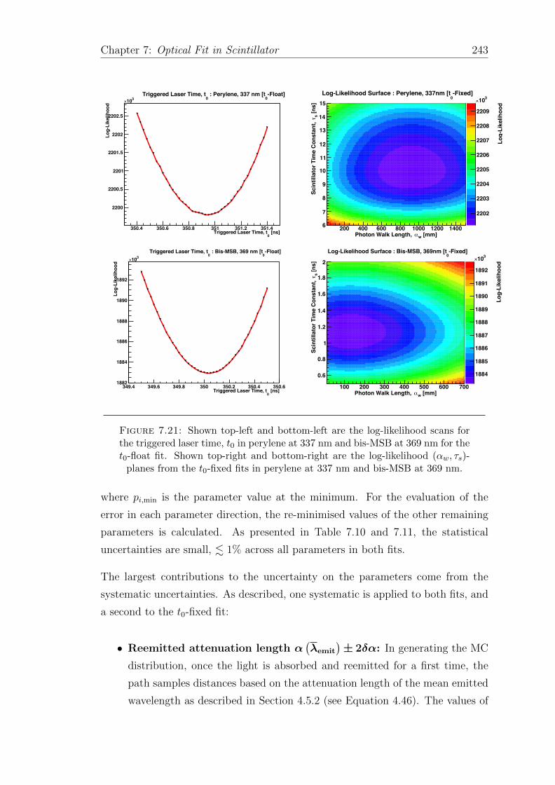
Chapter 7: Optical Fit in Scintillator 243
[ns]0
Triggered Laser Time, t350.4 350.6 350.8 351 351.2 351.4
Log-
Like
lihoo
d
2200
2200.5
2201
2201.5
2202
2202.5
310×-Float]
0 : Perylene, 337 nm [t
0Triggered Laser Time, t
[mm]wαPhoton Walk Length, 200 400 600 800 1000 1200 1400
[ns]
sτSc
intil
lato
r Tim
e C
onst
ant,
6
7
8
9
10
11
12
13
14
15
Log-
Like
lihoo
d
2202
2203
2204
2205
2206
2207
2208
2209
310×-Fixed]
0Log-Likelihood Surface : Perylene, 337nm [t
[ns]0
Triggered Laser Time, t349.4 349.6 349.8 350 350.2 350.4 350.6
Log-
Like
lihoo
d
1882
1884
1886
1888
1890
1892
310×
-Float]0
: Bis-MSB, 369 nm [t0
Triggered Laser Time, t
[mm]wαPhoton Walk Length, 100 200 300 400 500 600 700
[ns]
sτSc
intil
lato
r Tim
e C
onst
ant,
0.6
0.8
1
1.2
1.4
1.6
1.8
2
Log-
Like
lihoo
d
1884
1885
1886
1887
1888
1889
1890
1891
1892
310×-Fixed]
0Log-Likelihood Surface : Bis-MSB, 369nm [t
Figure 7.21: Shown top-left and bottom-left are the log-likelihood scans forthe triggered laser time, t0 in perylene at 337 nm and bis-MSB at 369 nm for thet0-float fit. Shown top-right and bottom-right are the log-likelihood (αw, τs)-
planes from the t0-fixed fits in perylene at 337 nm and bis-MSB at 369 nm.
where pi,min is the parameter value at the minimum. For the evaluation of the
error in each parameter direction, the re-minimised values of the other remaining
parameters is calculated. As presented in Table 7.10 and 7.11, the statistical
uncertainties are small, . 1% across all parameters in both fits.
The largest contributions to the uncertainty on the parameters come from the
systematic uncertainties. As described, one systematic is applied to both fits, and
a second to the t0-fixed fit:
• Reemitted attenuation length α(λemit
)± 2δα: In generating the MC
distribution, once the light is absorbed and reemitted for a first time, the
path samples distances based on the attenuation length of the mean emitted
wavelength as described in Section 4.5.2 (see Equation 4.46). The values of

Chapter 7: Optical Fit in Scintillator 244
α(λemit
)used are the attenuation lengths obtained from the optical model
fit in Section 7.1.1. The fit is performed using values α(λemit
)± 2δα where
δα is the systematic error. Twice the error value is used to exaggerate the
effect of changing the attenuation length to ±10-20% of the original value.
The error in the fitted parameter is then rescaled by a factor of s1 = 0.5.
• Triggered laser time, t0±1.0 ns: The triggered laser time in the t0-float
fit is varied by 1.0 ns either side of the MC time, t0 = 350.0 ns. The error is
scaled by a factor of s2 = 0.25, such that it is equivalent to the 0.25 ns bin
width.
Scintillator Time Profile Model - Systematic Uncertainties
Data : λ [nm] Parametert0-Fixed t0-Float
αw(λemit
)± 2δα t0 ± 1.0 ns α
(λemit
)± 2δα
PPO : 337αw (λLB) 1746% 14381% 899.33%
τs < 0.01% 19.74% < 0.01%t0 - - < 0.01%
Bis. : 337αw (λLB) 13.68% 33.60% 23.35%
τs < 0.01% 15.04% < 0.01%t0 - - < 0.01%
Bis. : 369αw (λLB) 1.41% 92.38% 121.90%
τs < 0.01% 19.98% < 0.01%t0 - - 0.04%
Bis. : 385αw (λLB) 12.32% 35.68% 14.65%
τs < 0.01% 23.48% < 0.01%t0 - - 0.01%
Pery. : 337αw (λLB) 2.23% 25.22% 41.25%
τs 2.61% 10.52% 0.42%t0 - - 0.01%
Pery. : 369αw (λLB) 25.73% 391.66% 10447.9%
τs 1.23% 9.04% 2.41%t0 - - 0.02%
Pery. : 385αw (λLB) 299.11% 4613.19% 5238.9%
τs 2.58% 7.55% 2.58%t0 - - 0.01%
Pery. : 420αw (λLB) 68.74% 2468.02% 1746.27%
τs 2.20% 8.02% 1.41%t0 - - 0.0%
Table 7.14: Shown are the systematic uncertainties as percentages of theparameter values obtained for the t0-fixed and t0-float fits.

Chapter 7: Optical Fit in Scintillator 245
The systematic contributions to each parameter are shown in Table 7.14. Overall,
the parameters in the t0-fixed fit are subject to large uncertainties due to the
inclusion of t0 as a systematic, producing variations of 25-35% in αw(λLB) for
values inconsistent with zero. In cases where the fitted value αw(λLB) is small or
consistent with zero, the systematic uncertainties, ≥ 100% are redundant. The
variations in t0 for the t0-fixed fit induce a 7-25% uncertainty in τs. In comparison,
the systematic uncertainty in α(λemit
)give rise to small uncertainties, < 2.6% in
both fits.
7.2.4 Conclusion on Scintillator Time Profile Model
The time profile model provides sensitivity to the absorbing and reemitting action
of the scintillator. However, the model is largely dominated by uncertainties as-
sociated with the trigger time of the laser, t0. In practice, the trigger time cannot
be guaranteed to a sufficient degree of accuracy. One idea to partially resolve this
could be to calculate the global time offset as an estimator for t0 for a run close
to the reemitted wavelength i.e. PPO: 400 nm, bis-MSB: 446 nm and perylene:
490 nm, and use this value as the fixed trigger time at shorter wavelengths in
the model. However, again, this would require performing two successive laserball
runs in which only the dye is changed; even then it cannot be guaranteed that the
detector state would otherwise remain unchanged between these two runs.
A further problem is that the model assumes characteristics of the laser emission,
(σLB = 0.7 ns) and the PMT time response (σPMT = 1.7 ns). Again, in practice
these values cannot be assumed. In principle these could be added as additional
parameters into the fit, although this would ultimately over constrain the model
as presented here; a model that uses only one central run per wavelength, of which
a relatively small time residual window of 15-20 ns is used.
Despite these issues, the most interesting result from studying this model comes
from the emission time value, τs which is sensitive to the multi-component nature
of the ternary mixtures, identifying the variation in absorption strengths of the
different wavelength shifters across short wavelengths. Furthermore, the sensitivity
of τs is reasonably robust to changes in the trigger time depending on whether
it varies (or is fixed) in the fit with uncertainties ranging from 0.01-2.6% (8.0-
23.5%). To this extent, the model is in principle able to quantify the micro-physical
processes within the bulk liquid scintillator.

Chapter 7: Optical Fit in Scintillator 246
The photon walk ultimately appears to be a minor effect in the model whose
systematic uncertainties ( > 1000% in perylene) are dominated by variations t0.
A re-parameterisation of the model could replace αw(λLB) with the rise-time of
the scintillator, τr as in Equation 3.6. Although the sensitivity to time would
remain; the rise time of most scintillators is typically no larger than 1 ns. The
value would therefore be minor in comparison to variations in t0 and the combined
uncertainties in the laser emission time and the PMT timing.

8
Conclusions
It’s a great thing when you realise you still have the ability to surprise yourself.
Makes you wonder what else you can do that you’ve forgotten about.
Lester Burnham (American Beauty), Alan Ball
The SNO+ experiment is a liquid scintillator based neutrino experiment. It is
a re-purposing of the original Cherenkov detector used to study solar neutrinos
in the SNO experiment. The experiment is sensitive to a variety of interesting
physics that include; invisible nucleon decay modes, pep-chain and CNO-cycle solar
neutrinos, geo-neutrinos, reactor anti-neutrinos, supernova neutrinos and 0νββ-
decay. To study these processes the experiment will operate over three phases;
water, scintillator and tellurium (loading of the scintillator with tellurium). The
primary objective is during the tellurium phase, in which SNO+ will search for
the 0νββ-decay of 130Te. This phase will begin by loading 780 tonnes of liquid
scintillator with 0.3% natural tellurium that has an abundance of ∼34% 130Te. At
0.3% loading this is equivalent to ∼800 kg of 130Te. Several upgrades have been
made to the detector to ensure it is compatible with scintillator. This includes the
installation of AV hold-down ropes and a variety of electronics upgrades to handle
the increased light yield, a factor of 50 times larger than that of the D2O used in
SNO.
The base scintillator mixture used is LABPPO, which consists of an LAB solvent
containing a PPO fluor. As part of the loading procedure for the tellurium phase, a
surfactant, PRS is added to the LABPPO to keep the tellurium in suspension. PRS
247

Chapter 8: Conclusions 248
is highly absorbing over the PPO emission spectrum and therefore a secondary
wavelength shifter is required. There are currently two candidates, bis-MSB and
perylene;
• Scintillator Phase: LABPPO
• Tellurium Phase - Candidate A: LABPPO+0.3%Te+Bis-MSB
• Tellurium Phase - Candidate B: LABPPO+0.3%Te+Perylene
The use of scintillator increases sensitivity to physics in a 1-3 MeV ROI. A variety
of internal and external backgrounds coincide with this ROI, contaminating the
signal region with unwanted physics events. The source of these backgrounds is
predominately from the radioactive decay of daughter nuclei from the 238U and232Th chains. SNO+ has therefore imposed stringent radiopurity levels throughout
its commissioning which has included the construction of a scintillator plant. The
plant must be sealed from contaminants in the lab atmosphere such as radon
that emanates from the surrounding mine rock. To prevent such contaminants
entering the detector, the facility has been constructed with a per-component leak
rate ≤ 10−9 mBar L s−1.
Prior to collecting physics data in each of the three phases, a full detector calibra-
tion is required. This is further warranted by the fact that the original components
of the SNO detector, including the PMTs, are now ∼20 years old. The calibration
can be divided up into four procedures;
• Calibration of the electronic systems.
• Calibration of the PMTs.
• Calibration of the detector optical response.
• Calibration of the detector energy response.
The optical calibration aims to characterise optical effects in the detector such
as reflections, refraction and attenuation; the combined effect of scattering and
absorption. In addition, the optical calibration determines both the angular and
timing response of the ∼9000 PMTs in the detector. The overall objective of such
a calibration is to minimise the uncertainties associated with the PMT response

Chapter 8: Conclusions 249
such that the meaningful behaviour of physical interactions inside the detector can
be resolved i.e. the scintillation time profile.
Optical calibration is sought through two hardware systems, a fibre based laser/LED
injection system installed into the PSUP [107] and the laserball, a light diffusing
sphere [110]. The laserball, as discussed in this thesis can be used to collect data
over which a parameterisation of the detector optical response can be modelled.
This model characterises the PMT angular response and the attenuation of the
three main detector media; the inner AV region, the acrylic of the AV itself, and
the outer AV water region. The model can be applied to data collected in all three
detector phases.
In the water phase, a comparison between original SNO data and SNO+ MC
highlights differences between the ideal scenario as assumed in MC, and the reality
of the true detector state as in SNO. Most notably, the reflectors which surround
each PMT are not perfectly reflecting, and have been subject to degradation over
time. This introduces an additional systematic to the optical model known as the
PMT variability. The degradation of the PMT reflectors is important to monitor,
as it affects the overall optical response and the energy response that it underpins.
The water phase will be the first time that the inner AV and outer AV regions
have been occupied by the same material. This provides a good opportunity to
break the correlation between the attenuation coefficients of the AV acrylic and
the water of the outer AV region as observed in SNO. In doing so, the systematic
uncertainties on the water attenuation coefficient can be significantly reduced from
> 100% to < 12%. In addition, the broken correlation between the acrylic and
the water regions allows for an in-situ measurement of the acrylic attenuation
coefficient. However, given the thin 55.0 mm nature of the acrylic, these values of
the attenuation coefficient are subject to large systematic variations in the region
of 10-140%.
The scintillator phase presents a new phenomena which is observed in the detec-
tor; absorption and reemission. This impacts the optical response of the detector
as light that is emitted inside the detector at short wavelengths is absorbed and
reemitted at longer wavelengths. At these longer wavelengths the scintillator is rel-
atively transparent. The wavelength regions in which the scintillator is absorbing
varies based on the composition of the scintillator mixture; λ . 360 nm (PPO),
. 400 nm (bis-MSB) and . 450 nm (perylene). The attenuation of the scintillator

Chapter 8: Conclusions 250
has a strong resolving power in the fit of the optical model, and values are obtained
with relatively small systematic uncertainties, 1-10% for PPO, and < 4% for the
mixtures containing either bis-MSB or perylene. It is found that the values of the
attenuation coefficients at absorbing regions is constrained by the dimensions of
the detector; the inner AV radius. In cases where light is absorbed and reemitted,
the obtained attenuation coefficient coincides in the region where the absorption
length of the active wavelength shifting component is ∼10 m.
A scintillator time profile model can be used on central runs in scintillator to
quantify the multi-component nature of the scintillator. This is particularly inter-
esting for the ternary mixtures proposed for the tellurium phase. Through timing
information the model is able to quantify the different wavelength regions in which
the different components are most absorbing. However, the model is subject to
non-negligible systematic errors associated with the timing of the laserball trigger
time.
The laserball data presented in scintillator use five of the laser/dye profiles from
SNO; 337 nm (N2), 369 nm (PBD), 385 nm (BBQ), 420 nm (bis-MSB) and 505 nm
(COUMARIN-500). In addition, MC studies of the scintillator mixtures can be
used to inform the wavelength of an additional laser-dye whose peak emission value
coincides with the average reemitted wavelength of the scintillator. For the three
mixtures considered here, these are as follows:
• LABPPO:
– α-NPO, λ ∈ (391-425) nm, λpeak = 400 nm
• LABPPO+0.3%Te+Bis-MSB:
– COUMARIN-440, λ ∈ (420-475) nm, λpeak = 446 nm
• LABPPO+0.3%Te+Perylene:
– COUMARIN-481, λ ∈ (461-549) nm, λpeak = 490 nm
Probing the optical response at these wavelengths is of interest as they are located
at the transition boundary between the absorbing and transparent regimes of the
scintillator in the detector. It would be interesting to further probe this transition
region either side of the boundary at different wavelengths. However, this would
require near-monochromatic light sources; the distributions for the proposed dyes

Chapter 8: Conclusions 251
above are broad. This may be resolved through using an LED source, either as a
modification to the laserball or as part of the fibre based light injection system.
At time of writing, no final decision has been made for the scintillator mixture to be
used in the tellurium phase. However, the current consensus amongst the SNO+
collaboration favours bis-MSB over perylene due to its short mean emission time
(1.4 ns: bis-MSB, 6.4 ns: perylene) and an emission profile that coincides more so
with the optimal quantum efficiency of the PMTs than perylene. Most notably, the
shorter emission time is conducive to more accurate position reconstruction and
efficient background rejection through α-β discrimination. However, as discussed
here the bis-MSB emission competes with the PRS absorption around 420 nm.
Therefore further developments have been made recently to investigate the use
of an alternative loading technique that makes use 1,2 butanediol to molecularly
suspend the tellurium, forming an organometallic complex, in the liquid scintillator
[151]. Early indications are promising, but a final decision to implement this
technique is subject to tests of the complex stability over 6-12 months.
Given the above, deployment of the laserball is critical in SNO+. It is an im-
portant component of the detector calibration, and alongside data collected with
a complementary fibre-based LED system characterises the detector optical re-
sponse. This is required to interpret physics events, specifically the expected light
detected from candidate 0νββ-decay events and associated backgrounds in the
tellurium phase. However, given that these levels of detection, such as the PMT
response or attenuation of the detector regions may change over time, the optical
response will also change. Repeated deployment of the laserball therefore allows
for regular monitoring of the optical response ensuring data sets collected over
time are consistent with one another. Although the scintillator mixtures discussed
here are not finalised, the approach and analysis of laserball data presented here
outline the principle technique for which regular monitoring of the optical response
can be achieved.

Appendix A
Optical Response Calculations
A.1 Light Path Derivation
Suppose there is a light path with a starting position inside the AV, ~ri and a
finishing position at PMT j, ~rj. In a coordinate frame whose origin is at the
centre of the AV, and using a combination of Snell’s law of refraction and sine and
cosine rules, one may derive the values of cos θ1, cos θ2 and cos θ3 as illustrated in
figure (4.2). The vectors ~r1 and ~r2 are the intersection points of the path between
the inner AV/AV and AV/outer AV regions respectively.
cos θ1: With reference to figure (4.2) and by using the cosine rule, a formula for
the distance through the scintillator region, dScint is obtained;
d2Scint = |~ri|2 + |~r1|2 − 2 |~ri| |~r1| cos θ1. (A.1)
Using the sine rule;
dScint
sin θ1
=|~r1|
sin (π − θγ)=|~r1|
sin θγ. (A.2)
Rearranging for dScint in the above expression and substituting into equation (A.1),
with some trigonometric manipulation, the following expression is obtained;
cos2 θ1 − 2|~ri||~r1|
sin2 θγ cos θ1 + sin2 θγ
(( |~ri||~r1|
)2
+ 1
)− 1 = 0, (A.3)
252

Appendix A: Optical Response Calculations 253
where the identitiy sin2 θ1 + cos2 θ1 = 1 has been used. Equation (A.3) is a
quadratic in cos θ1 and can therefore be solved using the standard quadratic for-
mula;
cos θ1 = − b
2a± 1
2a
√b2 − 4ac, (A.4)
where
a = 1, b = −2|~ri||~r1|
sin2 θγ and c = sin2 θγ
(( |~ri||~r1|
)2
+ 1
)− 1. (A.5)
Thus the expression for cos θ1 follows;
⇒ cos θ1 =|~ri||~r1|
sin2 θγ
± 1
2
√4
( |~ri||~r1|
)2
sin4 θγ − 4
( |~ri||~r1|
)2
sin2 θγ − 4 sin2 θγ + 4,
=|~ri||~r1|
sin2 θγ
±√( |~ri||~r1|
)2
sin2 θγ(sin2 θγ − 1
)+ cos2 θγ,
=|~ri||~r1|
sin2 θγ ± cos θγ
√1−
( |~ri||~r1|
sin θγ
)2
. (A.6)
Similarly, an expression for cos θ2 can be obtained by transforming the points
which define the triangle for cos θ1 to those which define that for cos θ2 i.e.
~ri → ~r1, ~r1 → ~r2, and θγ → θb. (A.7)
This gives an expression for cos θ2;
cos θ2 =|~r1||~r2|
sin2 θb ± cos θb
√1−
( |~r1||~r2|
sin θb
)2
. (A.8)
Using Snell’s law of refraction for light passing from material a to material b with
respective refractive indices of na and nb (in this case from the scintillator region

Appendix A: Optical Response Calculations 254
to the acrylic of the AV), sin θb can be expressed as follows;
sin θasin θb
=nbna
(Snell’s Law)
⇒ sin θb =nanb
sin θa. (A.9)
sin θb can subsequently be expressed in terms of θγ by use of the sine rule and
again, Snell’s law;
|~ri|sin θa
=|~r1|
sin (π − θγ)=|~r1|
sin θγ
⇒ sin θa =|~ri||~r1|
sin θγ,
|~r2|sin (π − θb)
=|~r2|
sin θb=nbna
|~r2|sin θa
⇒ sin θb =nanb
sin θa =nanb
|~ri||~r1|
sin θγ. (A.10)
Using the above result and the transformations as in expression (A.7) one obtains
the final result for cos θ2;
cos θ2 =1
|~r1| |~r2|
(nanb|~ri| sin θγ
)2
±
√1−(nanb
|~ri||~r1|
sin θγ
)2
×√
1−(nanb
|~ri||~r2|
sin θγ
)2 . (A.11)
Finally, an expression for cos θ3 can be obtained using the same principle by a
transformation of variables;
~ri → ~r2, ~r1 → ~rj, and θγ → θd. (A.12)
This gives an expression for cos θ3;
cos θ3 =|~r2||~rj|
sin2 θd ± cos θd
√1−
( |~r2||~rj|
sin θd
)2
. (A.13)

Appendix A: Optical Response Calculations 255
Using Snell’s law sin θd can be expressed as follows;
sin θd =nbnc
sin θc. (A.14)
By applying the sine rule, a relation between sin θc and sin θb can be obtained;
sin θc =|~r1||~r2|
sin θb. (A.15)
Finally, using this and equation (A.10), sin θd can be expressed in terms of sin θγ
as follows;
sin θd =nbnc
|~r1||~r2|
sin θb =nanb
nbnc
|~r1||~r2||~ri||~r1|
sin θγ =nanc
|~ri||~r2|
sin θγ. (A.16)
cos θ3 in terms of θγ is thus;
cos θ3 =1
|~r2| |~rj|
(nanc|~ri| sin θγ
)2
+
√1−( |~ri||~r2|
nanc
sin θγ
)2
×√
1−( |~ri||~rj|
nanc
sin θγ
)2 . (A.17)
A.2 PMT Bucket Time
As discussed in section (4.2.2), the light path calculation is calculated up to the
entrance of the PMT bucket. The time spent inside the bucket prior to the creation
of the photoelectron, tbucket (θγ) is an additional time discussed by the author here
[136]. Overall, the bucket time is a 0.45-0.7 ns correction, which can be assumed
wavelength independent given its size. The time is related to the incident angle of
the light entering the PMT bucket as shown in figure (A.1). It is calculated using
MC simulations.

Appendix A: Optical Response Calculations 256
Incident PMT Angle [degrees]0 10 20 30 40 50
Tim
e sp
ent i
n PM
T B
ucke
t [ns
]
0.1
0.2
0.3
0.4
0.5
0.6
0.7
/ ndf 2χ 43.84 / 43p0 0.002276± 0.4543 p1 0.0002659± 0.003148 p2 4.873e-06± -0.0002565 p3 2.838e-07± 9.626e-06 p4 6.38e-09± -6.865e-08
/ ndf 2χ 43.84 / 43p0 0.002276± 0.4543 p1 0.0002659± 0.003148 p2 4.873e-06± -0.0002565 p3 2.838e-07± 9.626e-06 p4 6.38e-09± -6.865e-08
PMT Peak Bucket Time at 504nm
Figure A.1: The time spent inside the PMT bucket. This is measured as thetime spent between the photon entering the PMT bucket, and the creation ofthe photoelectron at the PMT photocathode. The example above is shown for
504 nm, and is consistent with that observed for all wavelengths.
A.3 Fresnel Transmission Coefficient Calculation
The calculation of the Fresnel transmission coefficient assumes equal polarisation
of the laserlight; half perpendicular to the plane of incidence and half parallel.
The coefficient is calculated for both these components - perpendicular, T⊥ and
parallel, T‖ - at each material interface of the path between the laserball position
and the PMT; the inner AV/AV and AV/outer AV regions. For a light path
passing from material A to material B with refractive indices nA and nB at an
incident angle, θinc, the perpendicular and parallel components are calculated as
follows;
T⊥ =4nA cos θincR (nA, nB, θinc)
(nA cos θinc +R (nA, nB, θinc))2 , (A.18)
T‖ =4nAn
2B cos θincR (nA, nB, θinc)
(n2B cos θinc + nAR (nA, nB, θinc))
2 , (A.19)

Appendix A: Optical Response Calculations 257
where,
R (nA, nB, θinc) =
√n2B − n2
A sin2 θinc if nB > nA sin θinc
0 if nB < nA sin θinc
. (A.20)
In the case of R (nA, nB, θinc) = 0, this is equivalent to total internal reflection.
For the light path as described in section (A.1), from position ~ri to PMT j with
position, ~rj the total transmission coefficient, Tij is the product of these terms;
Tij =1
2
(T IA⊥ T
OA⊥ + T IA
‖ TOA‖), (A.21)
where T IA⊥ , T
OA⊥ and T IA
‖ , TOA‖ are the respective transmission coefficients from
the inner AV/AV (IA) and AV/outer AV (OA) material interfaces for the perpen-
dicular and parallel components. The factor of 1/2 is due to the equal polarisation
in both components as assumed. The value of θinc used in the calculations of the
coefficients is obtained from the vector description of the light path;
θIAinc = cos−1
(~r1 · ~rγ
), θOA
inc = cos−1
(~r2 − ~r1
)√
2· ~r2
, (A.22)
where ~rγ is the initial photon direction from the laserball, ~r1 is the intersection
point on the inner AV surface and ~r2 is the intersection point on the outer AV
surface. The refractive indices are functions of the wavelength i.e. nA (λ) , nB (λ),
whose values are obtained from the forms given in figure (4.3).
A.4 Scintillator Time Profile Model Timings
The scintillator time profile model as described in section (4.5.3) (see expres-
sion (4.47)) samples times according to the laserball pulse and PMT timing widths;
tσ,LB = 0.7 ns and tσ,PMT = 1.7 ns. These distributions are shown in figure (A.2),
and are the same time distributions implemented into RAT for the generation of
MC data.

Appendix A: Optical Response Calculations 258
Time [ns]2− 1− 0 1 2 3
Cou
nts
[a.u
.]
00.0020.0040.0060.008
0.010.0120.0140.0160.0180.02
0.0220.024
Laserball Pulse Width
Time [ns]10− 8− 6− 4− 2− 0 2 4 6 8 10
Cou
nts
[a.u
.]
0
0.002
0.004
0.006
0.008
0.01
PMT Time Width
Figure A.2: Top: The laserball emission time. The distribution is truncated at-1.5 ns. The width of the distribution (σ = 0.7 ns) is due to the light dispersionin the ∼40 m optical fibres from the laser system on the upper deck above thecavity to the laserball. Bottom: The time transit spread of the PMTs. Thetime transit spread is the distribution in times over which a photoelectron isaccelerated through the PMT dynode stack. The spread of this distribution is
σ ' 1.7 ns.

Appendix B
Monte-Carlo Data Production:
Extended
B.1 KITON-RED Laser-Dye for Monte-Carlo Pro-
duction
As stated in section (5.1.1), the KITON-RED laser-dye is omitted from the SNO+
MC data production. This is due to a combination of high attenuation in water at
long wavelengths, α ∼ 3× 10⁻⁴ mm−1 (see table (6.2)) and low PMT efficiency, <
2.5% (see figure (3.13)). Shown in figure (B.1) are the average detector occupancies
with varying intensities at 620 nm in water. Even at high intensities, the occupancy
is small, ≤ 0.2%. Extrapolating the linear response as shown, a target occupancy
of 3% would require 1236 × 103 photons pulse−1. This is computer intensive. In
principle, the PMT efficiencies could be scaled up, or the attenuation coefficient
could be scaled down. However, this is undesired given the aim of the optical model
is to directly probe the expected value of these properties across all wavelengths.
259

Appendix B: Monte-Carlo Data Production: Extended 260
]3Photons Per Pulse [100 5 10 15 20 25 30
Ave
rage
Occ
upan
cy P
er P
ulse
[%]
0.1
0.2
0.3
0.4
0.5
0.6
0.7
0.8
0.9
1
620 nm
Water
Figure B.1: Values for the average occupancy per pulse for the laserball at 620nm in water. Here, the average occupancy is the ratio of the mean number ofhits, NHits to the total number of PMTs, nPMT = 9728. Errors are statistical,
±√NHits. Photon units are in photons ×103 as simulated in RAT.

Appendix C
Optical Model Fits:
Extended Results
C.1 Attenuation Coefficient Systematics:
Water & D2O
The following are the full systematic contributions to the attenuation coefficients
for each of the wavelengths scans form the SNO October 2003 (D2O) and SNO+
MC data sets (H2O). The SNO data set used a fixed value of the AV acrylic, αAV
based on ex-situ measurements from SNO. The SNO+ MC data combined the
inner and outer AV water regions to fit for αcomb.H2O and αAV.
261

Appendix C: Optical Model Fits: Extended Results 262
Attenuation Systematics - SNO October 2003, D2O, 337 nm
SystematicαD2O
10−5 mm−1 si ×∆α/ααH2O
10−5 mm−1 si ×∆α/α χ2/No.Dof
Nominal 1.44 0.00% 3.89 0.00% 1.20|rLB| × 1.01 1.18 −3.58% 0.71 −16.38% 1.20rx − 50.0 mm 1.43 −0.12% 3.55 −1.79% 1.21rx + 50.0 mm 1.44 −0.04% 3.94 0.26% 1.21ry − 50.0 mm 1.41 −0.45% 4.24 1.77% 1.20ry + 50.0 mm 1.47 0.36% 3.47 −2.20% 1.21rz − 50.0 mm 1.50 2.18% 2.89 −12.89% 1.20rz + 50.0 mm 1.37 −2.49% 5.12 15.78% 1.20λ− λRMS nm 1.44 0.02% 3.92 0.81% 1.20λ+ λRMS nm 1.45 0.24% 4.00 2.62% 1.20
H2 1.44 −0.00% 4.02 0.16% 1.21H = 1.0 1.43 −0.04% 4.31 0.53% 1.24χ2
lim,f = 16 1.40 −2.57% 5.59 43.53% 1.47σPMT = 0 1.48 2.79% 2.22 −43.09% 1.84d-50.0mm
innerAV 1.44 0.19% 3.95 1.50% 1.20Total 6.21% 66.76%
Table C.1: Systematic contributions to αD2O and αH2O from the SNO October2003 data set with heavywater at 337 nm.
Attenuation Systematics - SNO October 2003, D2O, 369 nm
SystematicαD2O
10−5 mm−1 si ×∆α/ααH2O
10−5 mm−1 si ×∆α/α χ2/No.Dof
Nominal 0.93 0.00% 2.78 0.00% 0.98|rLB| × 1.01 0.67 −5.58% −0.30 −22.16% 0.98rx − 50.0 mm 0.93 0.14% 2.73 −0.40% 0.99rx + 50.0 mm 0.91 −0.32% 2.71 −0.53% 0.99ry − 50.0 mm 0.91 −0.40% 2.58 −1.49% 0.98ry + 50.0 mm 0.94 0.30% 2.64 −1.00% 0.99rz − 50.0 mm 0.98 2.89% 1.59 −21.44% 0.98rz + 50.0 mm 0.87 −3.13% 3.79 17.97% 0.98λ− λRMS nm 0.92 −0.34% 2.74 −1.62% 0.98λ+ λRMS nm 0.93 0.33% 2.83 1.71% 0.98
H2 0.93 0.01% 2.78 −0.01% 0.98H = 1.0 0.99 0.34% 3.16 0.68% 1.02χ2
lim,f = 16 0.90 −2.62% 3.64 30.79% 1.16σPMT = 0 1.03 10.76% 2.09 −24.93% 1.63d-50.0mm
innerAV 0.93 0.04% 2.80 0.40% 0.98Total 13.14% 53.41%
Table C.2: Systematic contributions to αD2O and αH2O from the SNO October2003 data set with heavywater at 369 nm.

Appendix C: Optical Model Fits: Extended Results 263
Attenuation Systematics - SNO October 2003, D2O, 385 nm
SystematicαD2O
10−5 mm−1 si ×∆α/ααH2O
10−5 mm−1 si ×∆α/α χ2/No.Dof
Nominal 0.80 0.00% 3.90 0.00% 0.98|rLB| × 1.01 0.54 −6.55% 0.55 −17.17% 0.97rx − 50.0 mm 0.80 0.00% 3.87 −0.14% 0.98rx + 50.0 mm 0.80 −0.22% 3.73 −0.87% 0.98ry − 50.0 mm 0.78 −0.71% 3.67 −1.18% 0.97ry + 50.0 mm 0.83 0.59% 3.70 −1.03% 0.98rz − 50.0 mm 0.86 3.29% 2.57 −17.01% 0.98rz + 50.0 mm 0.75 −3.48% 4.84 12.00% 0.97λ− λRMS nm 0.80 −0.21% 3.87 −0.78% 0.98λ+ λRMS nm 0.81 0.20% 3.91 0.18% 0.98
H2 0.81 0.00% 3.89 −0.01% 0.98H = 1.0 0.89 0.52% 4.27 0.48% 1.01χ2
lim,f = 16 0.78 −3.27% 4.74 21.38% 1.15σPMT = 0 0.91 12.54% 2.58 −33.81% 1.63d-50.0mm
innerAV 0.80 −0.01% 3.90 −0.14% 0.98Total 15.33% 48.30%
Table C.3: Systematic contributions to αD2O and αH2O from the SNO October2003 data set with heavywater at 385 nm.
Attenuation Systematics - SNO October 2003, D2O, 420 nm
SystematicαD2O
10−5 mm−1 si ×∆α/ααH2O
10−5 mm−1 si ×∆α/α χ2/No.Dof
Nominal 0.60 0.00% 1.78 0.00% 1.02|rLB| × 1.01 0.35 −8.34% −1.10 −32.41% 1.01rx − 50.0 mm 0.60 0.04% 1.82 0.55% 1.02rx + 50.0 mm 0.59 −0.24% 1.76 −0.21% 1.02ry − 50.0 mm 0.56 −1.35% 1.55 −2.52% 1.02ry + 50.0 mm 0.63 1.15% 1.68 −1.09% 1.03rz − 50.0 mm 0.66 5.27% 0.65 −31.67% 1.02rz + 50.0 mm 0.53 −5.41% 2.86 30.57% 1.02λ− λRMS nm 0.59 −0.61% 1.74 −2.06% 1.02λ+ λRMS nm 0.60 0.18% 1.79 1.08% 1.02
H2 0.59 −0.03% 1.78 0.00% 1.02H = 1.0 0.67 0.65% 2.09 0.89% 1.06χ2
lim,f = 16 0.53 −11.50% 3.10 74.52% 1.23σPMT = 0 0.69 16.03% 0.38 −78.34% 1.63d-50.0mm
innerAV 0.60 −0.00% 1.78 0.01% 1.02Total 22.80% 121.21%
Table C.4: Systematic contributions to αD2O and αH2O from the SNO October2003 data set with heavywater at 420 nm.

Appendix C: Optical Model Fits: Extended Results 264
Attenuation Systematics - SNO October 2003, D2O, 505 nm
SystematicαD2O
10−5 mm−1 si ×∆α/ααH2O
10−5 mm−1 si ×∆α/α χ2/No.Dof
Nominal 0.31 0.00% 4.87 0.00% 1.02|rLB| × 1.01 0.05 −16.85% 1.86 −12.36% 1.02rx − 50.0 mm 0.31 −0.22% 4.71 −0.65% 1.03rx + 50.0 mm 0.31 −0.13% 5.01 0.56% 1.03ry − 50.0 mm 0.28 −2.03% 4.67 −0.81% 1.02ry + 50.0 mm 0.34 1.97% 4.73 −0.58% 1.03rz − 50.0 mm 0.35 6.67% 3.64 −12.61% 1.02rz + 50.0 mm 0.26 −7.69% 6.14 13.03% 1.02λ− λRMS nm 0.31 −1.11% 4.80 −1.57% 1.02λ+ λRMS nm 0.31 0.71% 5.08 4.23% 1.02
H2 0.31 −0.01% 4.89 0.02% 1.03H = 1.0 0.35 0.68% 4.96 0.09% 1.08χ2
lim,f = 16 0.28 −10.07% 5.78 18.72% 1.24σPMT = 0 0.37 18.86% 3.59 −26.41% 1.65d-50.0mm
innerAV 0.31 −0.01% 4.87 0.02% 1.02Total 29.24% 39.39%
Table C.5: Systematic contributions to αD2O and αH2O from the SNO October2003 data set with heavywater at 505 nm.
Attenuation Systematics - SNO October 2003, D2O, 620 nm
SystematicαD2O
10−5 mm−1 si ×∆α/ααH2O
10−5 mm−1 si ×∆α/α χ2/No.Dof
Nominal 0.37 0.00% 32.68 0.00% 0.98|rLB| × 1.01 0.10 −14.44% 28.59 −2.51% 0.98rx − 50.0 mm 0.37 −0.28% 32.57 −0.07% 0.99rx + 50.0 mm 0.37 0.02% 32.74 0.04% 0.99ry − 50.0 mm 0.34 −1.52% 32.98 0.18% 0.99ry + 50.0 mm 0.40 1.44% 32.39 −0.18% 0.99rz − 50.0 mm 0.38 1.57% 31.04 −2.51% 0.98rz + 50.0 mm 0.36 −2.31% 34.43 2.67% 0.98λ− λRMS nm 0.37 −0.63% 32.65 −0.09% 0.99λ+ λRMS nm 0.37 0.25% 32.69 0.04% 0.99
H2 0.37 0.00% 32.75 0.01% 0.99H = 1.0 0.42 0.58% 33.42 0.11% 1.02χ2
lim,f = 16 0.37 0.02% 33.09 1.24% 1.16σPMT = 0 0.39 5.57% 32.26 −1.29% 1.67d-50.0mm
innerAV 0.37 −0.11% 32.69 0.01% 0.99Total 15.90% 4.80%
Table C.6: Systematic contributions to αD2O and αH2O from the SNO October2003 data set with heavywater at 620 nm.

Appendix C: Optical Model Fits: Extended Results 265
Attenuation Systematics - SNO+ MC, H2O, 337 nm
Systematicαcomb.
H2O
10−5 mm−1 si ×∆α/ααAV
10−3 mm−1 si ×∆α/α χ2/No.Dof
Nominal 2.70 0.00% 4.82 0.00% 1.00|rLB| × 1.01 2.44 −1.95% 3.65 −4.85% 1.00rx − 50.0 mm 2.70 0.02% 4.87 0.23% 1.02rx + 50.0 mm 2.70 −0.03% 4.90 0.36% 1.02ry − 50.0 mm 2.66 −0.29% 4.68 −0.56% 1.02ry + 50.0 mm 2.74 0.29% 5.00 0.76% 1.02rz − 50.0 mm 2.75 0.85% 4.29 −5.46% 1.01rz + 50.0 mm 2.65 −0.90% 5.33 5.34% 1.00λ− λRMS nm 2.70 0.00% 4.81 −0.01% 1.00λ+ λRMS nm 2.70 0.01% 4.81 −0.04% 1.00
H2 2.70 0.01% 4.81 −0.01% 1.00H = 1.0 −1.29 −7.38% 5.16 0.36% 1.46χ2
lim,f = 16 2.68 −0.82% 5.04 4.66% 1.20χ2
lim,f = 9 2.69 −0.29% 4.87 1.14% 1.07
Total 7.79% 10.30%
Table C.7: Systematic contributions to αH2O and αAV from the SNO+ MCdata set with water at 337 nm.
Attenuation Systematics - SNO+ MC, H2O, 369 nm
Systematicαcomb.
H2O
10−5 mm−1 si ×∆α/ααAV
10−3 mm−1 si ×∆α/α χ2/No.Dof
Nominal 2.05 0.00% 1.39 0.00% 1.00|rLB| × 1.01 1.78 −2.61% 0.35 −14.96% 1.00rx − 50.0 mm 2.05 −0.05% 1.39 −0.09% 1.02rx + 50.0 mm 2.05 −0.03% 1.43 0.53% 1.02ry − 50.0 mm 2.01 −0.43% 1.23 −2.30% 1.02ry + 50.0 mm 2.09 0.36% 1.55 2.31% 1.02rz − 50.0 mm 2.09 0.91% 0.90 −17.65% 1.00rz + 50.0 mm 2.01 −1.09% 1.82 15.36% 1.00λ− λRMS nm 2.05 −0.01% 1.39 −0.01% 1.00λ+ λRMS nm 2.05 −0.01% 1.40 0.31% 1.00
H2 2.05 0.01% 1.39 −0.03% 1.00H = 1.0 −2.11 −10.13% 1.66 0.97% 1.44χ2
lim,f = 16 2.05 −0.29% 1.52 9.28% 1.19χ2
lim,f = 9 2.05 0.06% 1.43 2.40% 1.07
Total 10.58% 29.58%
Table C.8: Systematic contributions to αH2O and αAV from the SNO+ MCdata set with water at 369 nm.

Appendix C: Optical Model Fits: Extended Results 266
Attenuation Systematics - SNO+ MC, H2O, 385 nm
Systematicαcomb.
H2O
10−5 mm−1 si ×∆α/ααAV
10−3 mm−1 si ×∆α/α χ2/No.Dof
Nominal 1.88 0.00% 0.65 0.00% 1.00|rLB| × 1.01 1.61 −2.90% −0.31 −29.67% 1.00rx − 50.0 mm 1.88 −0.02% 0.69 1.25% 1.02rx + 50.0 mm 1.88 −0.02% 0.68 1.00% 1.02ry − 50.0 mm 1.84 −0.42% 0.52 −3.97% 1.02ry + 50.0 mm 1.92 0.38% 0.83 5.46% 1.02rz − 50.0 mm 1.91 0.80% 0.22 −32.85% 1.01rz + 50.0 mm 1.85 −0.91% 1.04 30.35% 1.00λ− λRMS nm 1.88 −0.01% 0.65 −0.18% 1.00λ+ λRMS nm 1.88 −0.01% 0.65 0.31% 1.00
H2 1.88 0.00% 0.65 −0.01% 1.00H = 1.0 −2.19 −10.82% 1.14 3.81% 1.46χ2
lim,f = 16 1.85 −1.75% 0.85 30.32% 1.22χ2
lim,f = 9 1.88 −0.28% 0.70 7.32% 1.07
Total 11.42% 62.58%
Table C.9: Systematic contributions to αH2O and αAV from the SNO+ MCdata set with water at 385 nm.
Attenuation Systematics - SNO+ MC, H2O, 420 nm
Systematicαcomb.
H2O
10−5 mm−1 si ×∆α/ααAV
10−3 mm−1 si ×∆α/α χ2/No.Dof
Nominal 2.05 0.00% 0.29 0.00% 1.02|rLB| × 1.01 1.78 −2.63% −0.69 −68.04% 1.02rx − 50.0 mm 2.05 −0.02% 0.29 0.02% 1.04rx + 50.0 mm 2.05 0.02% 0.34 3.49% 1.03ry − 50.0 mm 2.01 −0.39% 0.16 −8.76% 1.03ry + 50.0 mm 2.09 0.35% 0.39 7.11% 1.03rz − 50.0 mm 2.08 0.81% −0.15 −76.78% 1.02rz + 50.0 mm 2.01 −0.95% 0.69 69.88% 1.01λ− λRMS nm 2.05 −0.01% 0.28 −1.31% 1.02λ+ λRMS nm 2.05 −0.00% 0.29 −0.26% 1.02
H2 2.05 0.00% 0.29 −0.04% 1.02H = 1.0 −2.11 −10.15% 0.72 7.47% 1.45χ2
lim,f = 16 2.03 −0.96% 0.48 66.74% 1.23χ2
lim,f = 9 2.05 0.03% 0.31 7.81% 1.09
Total 10.62% 141.84%
Table C.10: Systematic contributions to αH2O and αAV from the SNO+ MCdata set with water at 420 nm.

Appendix C: Optical Model Fits: Extended Results 267
Attenuation Systematics - SNO+ MC, H2O, 505 nm
Systematicαcomb.
H2O
10−5 mm−1 si ×∆α/ααAV
10−3 mm−1 si ×∆α/α χ2/No.Dof
Nominal 4.31 0.00% 0.29 0.00% 1.01|rLB| × 1.01 4.01 −1.39% −0.69 −68.03% 1.02rx − 50.0 mm 4.31 0.01% 0.33 3.41% 1.04rx + 50.0 mm 4.31 0.00% 0.35 4.37% 1.03ry − 50.0 mm 4.27 −0.19% 0.14 −10.42% 1.03ry + 50.0 mm 4.35 0.18% 0.45 11.47% 1.03rz − 50.0 mm 4.34 0.34% −0.13 −72.97% 1.02rz + 50.0 mm 4.27 −0.41% 0.67 68.11% 1.01λ− λRMS nm 4.31 0.00% 0.28 −1.49% 1.01λ+ λRMS nm 4.31 0.00% 0.29 1.03% 1.01
H2 4.31 0.00% 0.28 −0.07% 1.01H = 1.0 0.25 −4.71% 0.57 4.99% 1.46χ2
lim,f = 16 4.27 −0.79% 0.47 64.05% 1.24χ2
lim,f = 9 4.30 −0.20% 0.32 12.98% 1.09
Total 5.01% 138.43%
Table C.11: Systematic contributions to αH2O and αAV from the SNO+ MCdata set with water at 505 nm.

Appendix C: Optical Model Fits: Extended Results 268
C.2 Attenuation Coefficient Systematics:
Scintillator
The following are the full systematic contributions to the attenuation coefficients
for each of the wavelengths scans form the SNO+ MC data sets in LABPPO,
LABPPO+0.3%Te+bis-MSB and LABPPO+0.3%Te+perylene.
Attenuation Systematics - SNO+ MC, LABPPO, 337 nm
Systematicα ppo
Scint
10−5 mm−1 si ×∆α/αα ppo
H2O
10−5 mm−1 si ×∆α/α χ2/No.Dof
Nominal 10.67 0.00% 9.21 0.00% 1.02|rLB| × 1.01 10.40 −0.50% 7.02 −4.75% 1.05rx − 50.0 mm 10.66 −0.01% 8.57 −1.38% 1.03rx + 50.0 mm 10.66 −0.01% 8.53 −1.47% 1.03ry − 50.0 mm 10.65 −0.04% 8.50 −1.54% 1.03ry + 50.0 mm 10.69 0.03% 8.72 −1.06% 1.03rz − 50.0 mm 10.75 0.37% 7.95 −6.85% 1.05rz + 50.0 mm 10.53 −0.64% 7.21 −10.84% 1.00λ− λRMS nm 10.74 0.66% 8.80 −4.44% 1.03λ+ λRMS nm 10.60 −0.63% 8.20 −10.91% 1.01
H2 10.67 0.00% 9.20 −0.00% 1.02H = 1.0 7.23 −1.61% 4.30 −2.66% 1.43χ2
lim,f = 16 10.66 −0.07% 10.25 11.29% 1.24χ2
lim,f = 9 10.67 0.04% 9.57 3.98% 1.10
Total 2.05% 21.99%
Table C.12: Systematic contributions to α ppoScint and α ppo
H2O from the SNO+ MCdata set with ppo at 337 nm.

Appendix C: Optical Model Fits: Extended Results 269
Attenuation Systematics - SNO+ MC, LABPPO, 369 nm
Systematicα ppo
Scint
10−5 mm−1 si ×∆α/αα ppo
H2O
10−5 mm−1 si ×∆α/α χ2/No.Dof
Nominal 15.04 0.00% 9.81 0.00% 1.02|rLB| × 1.01 14.79 −0.33% 8.01 −3.68% 1.06rx − 50.0 mm 15.04 −0.01% 9.31 −1.01% 1.03rx + 50.0 mm 15.03 −0.02% 9.02 −1.62% 1.03ry − 50.0 mm 15.01 −0.04% 9.21 −1.22% 1.03ry + 50.0 mm 15.05 0.01% 9.35 −0.93% 1.03rz − 50.0 mm 15.17 0.42% 8.67 −5.81% 1.05rz + 50.0 mm 14.83 −0.72% 7.87 −9.91% 0.99λ− λRMS nm 15.13 0.56% 9.48 −3.41% 1.03λ+ λRMS nm 14.95 −0.59% 8.70 −11.32% 1.01
H2 15.04 0.00% 9.82 0.00% 1.02H = 1.0 11.53 −1.17% 4.76 −2.57% 1.40χ2
lim,f = 16 15.06 0.08% 10.82 10.25% 1.21χ2
lim,f = 9 15.05 0.04% 10.05 2.48% 1.09
Total 1.69% 20.23%
Table C.13: Systematic contributions to α ppoScint and α ppo
H2O from the SNO+ MCdata set with ppo at 369 nm.

Appendix C: Optical Model Fits: Extended Results 270
Attenuation Systematics - SNO+ MC, LABPPO, 385 nm
Systematicα ppo
Scint
10−5 mm−1 si ×∆α/αα ppo
H2O
10−5 mm−1 si ×∆α/α χ2/No.Dof
Nominal 10.23 0.00% 5.06 0.00% 0.99|rLB| × 1.01 10.02 −0.41% 3.53 −6.02% 1.00rx − 50.0 mm 10.23 0.00% 4.69 −1.45% 1.00rx + 50.0 mm 10.22 −0.01% 4.40 −2.60% 1.00ry − 50.0 mm 10.21 −0.03% 4.41 −2.57% 0.99ry + 50.0 mm 10.24 0.04% 4.49 −2.24% 1.00rz − 50.0 mm 10.35 0.62% 4.36 −6.91% 1.00rz + 50.0 mm 10.06 −0.82% 2.41 −26.17% 0.98λ− λRMS nm 10.29 0.59% 5.15 1.78% 0.99λ+ λRMS nm 10.17 −0.54% 4.33 −14.36% 0.98
H2 10.23 0.00% 5.06 0.00% 0.99H = 1.0 6.74 −1.71% 0.20 −4.80% 1.42χ2
lim,f = 16 10.21 −0.18% 5.87 16.12% 1.17χ2
lim,f = 9 10.22 −0.03% 5.23 3.49% 1.05
Total 2.19% 35.97%
Table C.14: Systematic contributions to α ppoScint and α ppo
H2O from the SNO+ MCdata set with ppo at 385 nm.
Attenuation Systematics - SNO+ MC, LABPPO, 400 nm
Systematicα ppo
Scint
10−5 mm−1 si ×∆α/αα ppo
H2O
10−5 mm−1 si ×∆α/α χ2/No.Dof
Nominal 6.88 0.00% 4.96 0.00% 0.98|rLB| × 1.01 6.77 −0.34% 3.40 −6.27% 0.99rx − 50.0 mm 6.89 0.01% 4.67 −1.15% 0.99rx + 50.0 mm 6.88 −0.01% 4.57 −1.57% 0.99ry − 50.0 mm 6.87 −0.04% 4.51 −1.80% 0.99ry + 50.0 mm 6.90 0.05% 4.66 −1.18% 0.99rz − 50.0 mm 7.07 1.33% 4.30 −6.63% 1.00rz + 50.0 mm 6.67 −1.58% 2.63 −23.48% 0.97λ− λRMS nm 6.96 1.17% 4.90 −1.15% 0.98λ+ λRMS nm 6.82 −0.99% 4.54 −8.51% 0.97
H2 6.88 0.00% 4.96 −0.00% 0.98H = 1.0 3.07 −2.77% −0.16 −5.16% 1.41χ2
lim,f = 16 6.88 0.01% 5.55 11.91% 1.15χ2
lim,f = 9 6.88 −0.00% 5.08 2.46% 1.04
Total 3.79% 29.86%
Table C.15: Systematic contributions to α ppoScint and α ppo
H2O from the SNO+ MCdata set with ppo at 400 nm.

Appendix C: Optical Model Fits: Extended Results 271
Attenuation Systematics - SNO+ MC, LABPPO, 420 nm
Systematicα ppo
Scint
10−5 mm−1 si ×∆α/αα ppo
H2O
10−5 mm−1 si ×∆α/α χ2/No.Dof
Nominal 5.07 0.00% 4.86 0.00% 1.00|rLB| × 1.01 4.96 −0.41% 3.18 −6.90% 1.01rx − 50.0 mm 5.07 0.03% 4.67 −0.75% 1.02rx + 50.0 mm 5.06 −0.02% 4.50 −1.48% 1.01ry − 50.0 mm 5.05 −0.05% 4.40 −1.89% 1.01ry + 50.0 mm 5.09 0.10% 4.48 −1.57% 1.01rz − 50.0 mm 5.25 1.80% 4.11 −7.69% 1.02rz + 50.0 mm 4.85 −2.11% 2.43 −25.01% 1.00λ− λRMS nm 5.10 0.61% 4.90 0.94% 1.00λ+ λRMS nm 5.04 −0.53% 4.85 −0.18% 1.00
H2 5.07 0.00% 4.86 0.01% 1.00H = 1.0 1.25 −3.77% 0.35 −4.64% 1.41χ2
lim,f = 16 5.06 −0.02% 5.64 16.18% 1.18χ2
lim,f = 9 5.06 −0.06% 5.00 3.01% 1.07
Total 4.76% 32.16%
Table C.16: Systematic contributions to α ppoScint and α ppo
H2O from the SNO+ MCdata set with ppo at 420 nm.
Attenuation Systematics - SNO+ MC, LABPPO, 505 nm
Systematicα ppo
Scint
10−5 mm−1 si ×∆α/αα ppo
H2O
10−5 mm−1 si ×∆α/α χ2/No.Dof
Nominal 2.37 0.00% 6.65 0.00% 0.98|rLB| × 1.01 2.29 −0.67% 5.05 −4.81% 0.99rx − 50.0 mm 2.37 0.03% 6.50 −0.44% 0.99rx + 50.0 mm 2.37 0.00% 6.51 −0.42% 0.99ry − 50.0 mm 2.36 −0.09% 6.38 −0.80% 0.99ry + 50.0 mm 2.39 0.18% 6.49 −0.47% 0.99rz − 50.0 mm 2.55 3.79% 6.06 −4.43% 0.99rz + 50.0 mm 2.17 −4.24% 4.28 −17.79% 0.98λ− λRMS nm 2.39 0.75% 6.66 0.16% 0.98λ+ λRMS nm 2.35 −0.69% 6.65 0.04% 0.98
H2 2.37 0.00% 6.65 0.00% 0.98H = 1.0 −1.45 −8.07% 2.31 −3.26% 1.41χ2
lim,f = 16 2.36 −0.51% 7.48 12.54% 1.15χ2
lim,f = 9 2.36 −0.23% 6.92 4.19% 1.04
Total 9.97% 23.37%
Table C.17: Systematic contributions to α ppoScint and α ppo
H2O from the SNO+ MCdata set with ppo at 505 nm.

Appendix C: Optical Model Fits: Extended Results 272
Attenuation Systematics - SNO+ MCLABPPO + 0.3%Te + Bis-MSB, 337 nm
Systematicα bis.
Scint
10−5 mm−1 si ×∆α/αα bis.
H2O
10−5 mm−1 si ×∆α/α χ2/No.Dof
Nominal 20.23 0.00% 14.03 0.00% 1.16|rLB| × 1.01 19.81 −0.41% 11.84 −3.13% 1.19rx − 50.0 mm 20.23 −0.00% 13.58 −0.63% 1.16rx + 50.0 mm 20.22 −0.01% 13.41 −0.88% 1.16ry − 50.0 mm 20.20 −0.02% 13.66 −0.53% 1.16ry + 50.0 mm 20.25 0.02% 13.87 −0.23% 1.16rz − 50.0 mm 20.25 0.05% 12.74 −4.60% 1.18rz + 50.0 mm 20.15 −0.20% 12.88 −4.11% 1.12λ− λRMS nm 20.27 0.19% 13.40 −4.50% 1.16λ+ λRMS nm 20.21 −0.12% 14.00 −0.19% 1.15
H2 20.23 0.00% 14.01 −0.01% 1.16H = 1.0 16.90 −0.82% 9.03 −1.78% 1.47χ2
lim,f = 16 20.28 0.27% 15.04 7.18% 1.48χ2
lim,f = 9 20.25 0.12% 14.01 −0.15% 1.26
Total 1.02% 11.15%
Table C.18: Systematic contributions to α bis.Scint and α bis.
H2O from the SNO+ MCdata set with bis-MSB at 337 nm.
Attenuation Systematics - SNO+ MCLABPPO + 0.3%Te + Bis-MSB, 369 nm
Systematicα bis.
Scint
10−5 mm−1 si ×∆α/αα bis.
H2O
10−5 mm−1 si ×∆α/α χ2/No.Dof
Nominal 19.46 0.00% 13.02 0.00% 1.13|rLB| × 1.01 19.05 −0.42% 10.94 −3.20% 1.16rx − 50.0 mm 19.46 −0.00% 12.85 −0.26% 1.13rx + 50.0 mm 19.47 0.00% 12.65 −0.57% 1.13ry − 50.0 mm 19.44 −0.02% 12.62 −0.63% 1.13ry + 50.0 mm 19.49 0.03% 12.99 −0.05% 1.13rz − 50.0 mm 19.48 0.05% 11.88 −4.38% 1.16rz + 50.0 mm 19.39 −0.18% 11.39 −6.29% 1.09λ− λRMS nm 19.50 0.18% 12.48 −4.21% 1.14λ+ λRMS nm 19.44 −0.13% 13.06 0.31% 1.12
H2 19.46 0.00% 13.00 −0.01% 1.13H = 1.0 16.02 −0.88% 7.20 −2.24% 1.46χ2
lim,f = 16 19.52 0.29% 14.09 8.20% 1.41χ2
lim,f = 9 19.49 0.11% 13.41 2.97% 1.23
Total 1.07% 12.99%
Table C.19: Systematic contributions to α bis.Scint and α bis.
H2O from the SNO+ MCdata set with bis-MSB at 369 nm.

Appendix C: Optical Model Fits: Extended Results 273
Attenuation Systematics - SNO+ MCLABPPO + 0.3%Te + Bis-MSB, 385 nm
Systematicα bis.
Scint
10−5 mm−1 si ×∆α/αα bis.
H2O
10−5 mm−1 si ×∆α/α χ2/No.Dof
Nominal 19.73 0.00% 14.22 0.00% 1.14|rLB| × 1.01 19.31 −0.43% 12.06 −3.05% 1.17rx − 50.0 mm 19.72 −0.01% 14.23 0.00% 1.14rx + 50.0 mm 19.73 −0.00% 13.91 −0.45% 1.14ry − 50.0 mm 19.70 −0.03% 13.98 −0.34% 1.14ry + 50.0 mm 19.75 0.02% 14.02 −0.29% 1.14rz − 50.0 mm 19.74 0.03% 12.99 −4.35% 1.17rz + 50.0 mm 19.65 −0.20% 12.24 −6.99% 1.10λ− λRMS nm 19.76 0.16% 13.93 −2.09% 1.15λ+ λRMS nm 19.70 −0.13% 14.14 −0.62% 1.13
H2 19.73 0.00% 14.22 −0.00% 1.14H = 1.0 16.35 −0.86% 8.58 −1.98% 1.48χ2
lim,f = 16 19.78 0.28% 15.26 7.26% 1.42χ2
lim,f = 9 19.75 0.10% 14.52 2.05% 1.24
Total 1.04% 11.96%
Table C.20: Systematic contributions to α bis.Scint and α bis.
H2O from the SNO+ MCdata set with bis-MSB at 385 nm.
Attenuation Systematics - SNO+ MCLABPPO + 0.3%Te + Bis-MSB, 420 nm
Systematicα bis.
Scint
10−5 mm−1 si ×∆α/αα bis.
H2O
10−5 mm−1 si ×∆α/α χ2/No.Dof
Nominal 31.96 0.00% 7.39 0.00% 1.04|rLB| × 1.01 31.48 −0.30% 6.57 −2.21% 1.07rx − 50.0 mm 31.96 0.00% 7.27 −0.33% 1.05rx + 50.0 mm 31.95 −0.00% 7.03 −0.96% 1.05ry − 50.0 mm 31.93 −0.01% 7.23 −0.43% 1.05ry + 50.0 mm 31.98 0.02% 7.49 0.29% 1.05rz − 50.0 mm 32.04 0.13% 7.41 0.15% 1.07rz + 50.0 mm 31.82 −0.22% 5.20 −14.82% 1.01λ− λRMS nm 31.99 0.11% 7.35 −0.46% 1.04λ+ λRMS nm 31.92 −0.12% 7.29 −1.39% 1.04
H2 31.96 0.00% 7.37 −0.01% 1.04H = 1.0 28.44 −0.55% 1.98 −3.66% 1.41χ2
lim,f = 16 31.98 0.06% 8.34 12.86% 1.24χ2
lim,f = 9 31.96 0.02% 7.64 3.44% 1.11
Total 0.70% 20.46%
Table C.21: Systematic contributions to α bis.Scint and α bis.
H2O from the SNO+ MCdata set with bis-MSB at 420 nm.

Appendix C: Optical Model Fits: Extended Results 274
Attenuation Systematics - SNO+ MCLABPPO + 0.3%Te + Bis-MSB, 446 nm
Systematicα bis.
Scint
10−5 mm−1 si ×∆α/αα bis.
H2O
10−5 mm−1 si ×∆α/α χ2/No.Dof
Nominal 17.68 0.00% 5.31 0.00% 1.00|rLB| × 1.01 17.41 −0.31% 4.07 −4.66% 1.01rx − 50.0 mm 17.69 0.00% 5.14 −0.65% 1.01rx + 50.0 mm 17.69 0.01% 5.29 −0.07% 1.01ry − 50.0 mm 17.67 −0.01% 5.06 −0.96% 1.01ry + 50.0 mm 17.71 0.03% 5.57 0.99% 1.01rz − 50.0 mm 17.83 0.41% 5.00 −2.93% 1.01rz + 50.0 mm 17.51 −0.48% 2.71 −24.45% 0.98λ− λRMS nm 17.73 0.27% 5.40 1.64% 1.00λ+ λRMS nm 17.64 −0.22% 5.25 −1.18% 1.00
H2 17.68 0.00% 5.31 −0.00% 1.00H = 1.0 14.06 −1.02% 0.71 −4.33% 1.41χ2
lim,f = 16 17.70 0.07% 6.25 17.70% 1.18χ2
lim,f = 9 17.69 0.04% 5.54 4.27% 1.06
Total 1.29% 31.38%
Table C.22: Systematic contributions to α bis.Scint and α bis.
H2O from the SNO+ MCdata set with bis-MSB at 446 nm.
Attenuation Systematics - SNO+ MCLABPPO + 0.3%Te + Bis-MSB, 505 nm
Systematicα bis.
Scint
10−5 mm−1 si ×∆α/αα bis.
H2O
10−5 mm−1 si ×∆α/α χ2/No.Dof
Nominal 5.65 0.00% 6.58 0.00% 0.98|rLB| × 1.01 5.51 −0.49% 4.83 −5.32% 1.00rx − 50.0 mm 5.65 −0.00% 6.38 −0.60% 1.00rx + 50.0 mm 5.64 −0.02% 6.34 −0.72% 1.00ry − 50.0 mm 5.63 −0.07% 6.25 −0.98% 1.00ry + 50.0 mm 5.66 0.06% 6.51 −0.19% 1.00rz − 50.0 mm 5.80 1.34% 5.80 −5.88% 1.00rz + 50.0 mm 5.45 −1.70% 4.37 −16.80% 0.97λ− λRMS nm 5.66 0.29% 6.59 0.27% 0.99λ+ λRMS nm 5.63 −0.28% 6.51 −0.97% 0.98
H2 5.65 0.00% 6.57 −0.00% 0.98H = 1.0 1.98 −3.24% 2.31 −3.24% 1.42χ2
lim,f = 16 5.65 0.09% 7.50 14.02% 1.16χ2
lim,f = 9 5.65 0.01% 6.82 3.76% 1.05
Total 3.95% 23.85%
Table C.23: Systematic contributions to α bis.Scint and α bis.
H2O from the SNO+ MCdata set with bis-MSB at 505 nm.

Appendix C: Optical Model Fits: Extended Results 275
Attenuation Systematics - SNO+ MCLABPPO + 0.3%Te + Perylene, 337 nm
Systematicα pery.
Scint
10−5 mm−1 si ×∆α/αα pery.
H2O
10−5 mm−1 si ×∆α/α χ2/No.Dof
Nominal 10.94 0.00% 13.02 0.00% 1.07|rLB| × 1.01 10.69 −0.46% 10.41 −4.02% 1.09rx − 50.0 mm 10.94 0.00% 13.06 0.06% 1.07rx + 50.0 mm 10.93 −0.01% 12.64 −0.59% 1.07ry − 50.0 mm 10.92 −0.04% 12.81 −0.33% 1.07ry + 50.0 mm 10.96 0.04% 12.97 −0.09% 1.07rz − 50.0 mm 11.03 0.43% 11.57 −5.60% 1.09rz + 50.0 mm 10.77 −0.78% 11.17 −7.10% 1.03λ− λRMS nm 10.96 0.18% 12.92 −0.82% 1.07λ+ λRMS nm 10.92 −0.19% 13.04 0.12% 1.06
H2 10.94 0.00% 13.02 −0.00% 1.07H = 1.0 7.81 −1.43% 8.15 −1.87% 1.45χ2
lim,f = 16 10.95 0.09% 14.57 11.86% 1.32χ2
lim,f = 9 10.94 0.05% 13.52 3.85% 1.15
Total 1.77% 16.06%
Table C.24: Systematic contributions to α pery.Scint and α pery.
H2O from the SNO+MC data set with perylene at 337 nm.
Attenuation Systematics - SNO+ MCLABPPO + 0.3%Te + Perylene, 369 nm
Systematicα pery.
Scint
10−5 mm−1 si ×∆α/αα pery.
H2O
10−5 mm−1 si ×∆α/α χ2/No.Dof
Nominal 10.91 0.00% 13.67 0.00% 1.08|rLB| × 1.01 10.65 −0.48% 11.10 −3.76% 1.10rx − 50.0 mm 10.91 −0.00% 13.47 −0.30% 1.08rx + 50.0 mm 10.91 0.00% 13.26 −0.61% 1.08ry − 50.0 mm 10.90 −0.03% 13.31 −0.53% 1.08ry + 50.0 mm 10.93 0.03% 13.60 −0.11% 1.08rz − 50.0 mm 10.99 0.38% 12.16 −5.54% 1.10rz + 50.0 mm 10.75 −0.72% 11.83 −6.74% 1.05λ− λRMS nm 10.93 0.19% 13.60 −0.52% 1.08λ+ λRMS nm 10.89 −0.20% 13.51 −1.17% 1.07
H2 10.91 −0.00% 13.64 −0.01% 1.08H = 1.0 7.82 −1.42% 9.13 −1.66% 1.45χ2
lim,f = 16 10.91 0.01% 14.70 7.56% 1.32χ2
lim,f = 9 10.91 0.00% 13.95 2.03% 1.16
Total 1.73% 12.52%
Table C.25: Systematic contributions to α pery.Scint and α pery.
H2O from the SNO+MC data set with perylene at 369 nm.

Appendix C: Optical Model Fits: Extended Results 276
Attenuation Systematics - SNO+ MCLABPPO + 0.3%Te + Perylene, 385 nm
Systematicα pery.
Scint
10−5 mm−1 si ×∆α/αα pery.
H2O
10−5 mm−1 si ×∆α/α χ2/No.Dof
Nominal 10.92 0.00% 13.51 0.00% 1.07|rLB| × 1.01 10.64 −0.50% 10.69 −4.17% 1.09rx − 50.0 mm 10.92 0.00% 13.32 −0.29% 1.07rx + 50.0 mm 10.91 −0.02% 13.14 −0.56% 1.07ry − 50.0 mm 10.90 −0.04% 13.22 −0.44% 1.07ry + 50.0 mm 10.94 0.03% 13.44 −0.11% 1.07rz − 50.0 mm 10.99 0.33% 11.80 −6.33% 1.09rz + 50.0 mm 10.77 −0.69% 11.08 −9.01% 1.04λ− λRMS nm 10.94 0.17% 13.45 −0.45% 1.07λ+ λRMS nm 10.90 −0.20% 13.54 0.19% 1.06
H2 10.92 −0.00% 13.51 −0.00% 1.07H = 1.0 7.80 −1.43% 8.71 −1.78% 1.45χ2
lim,f = 16 10.93 0.11% 14.73 8.97% 1.32χ2
lim,f = 9 10.93 0.13% 13.84 2.38% 1.15
Total 1.73% 15.13%
Table C.26: Systematic contributions to α pery.Scint and α pery.
H2O from the SNO+MC data set with perylene at 385 nm.
Attenuation Systematics - SNO+ MCLABPPO + 0.3%Te + Perylene, 420 nm
Systematicα pery.
Scint
10−5 mm−1 si ×∆α/αα pery.
H2O
10−5 mm−1 si ×∆α/α χ2/No.Dof
Nominal 10.93 0.00% 13.45 0.00% 1.08|rLB| × 1.01 10.65 −0.50% 10.66 −4.15% 1.11rx − 50.0 mm 10.92 −0.01% 13.37 −0.12% 1.09rx + 50.0 mm 10.92 −0.01% 13.25 −0.30% 1.09ry − 50.0 mm 10.90 −0.04% 13.28 −0.26% 1.08ry + 50.0 mm 10.94 0.03% 13.45 0.00% 1.09rz − 50.0 mm 11.00 0.32% 11.88 −5.82% 1.11rz + 50.0 mm 10.78 −0.67% 11.60 −6.86% 1.05λ− λRMS nm 10.95 0.19% 13.32 −0.95% 1.09λ+ λRMS nm 10.90 −0.19% 13.60 1.11% 1.08
H2 10.92 −0.00% 13.47 0.01% 1.08H = 1.0 7.79 −1.43% 8.62 −1.80% 1.44χ2
lim,f = 16 10.95 0.26% 14.95 11.18% 1.34χ2
lim,f = 9 10.94 0.15% 13.89 3.24% 1.17
Total 1.74% 15.47%
Table C.27: Systematic contributions to α pery.Scint and α pery.
H2O from the SNO+MC data set with perylene at 420 nm.

Appendix C: Optical Model Fits: Extended Results 277
Attenuation Systematics - SNO+ MCLABPPO + 0.3%Te + Perylene, 490 nm
Systematicα pery.
Scint
10−5 mm−1 si ×∆α/αα pery.
H2O
10−5 mm−1 si ×∆α/α χ2/No.Dof
Nominal 7.21 0.00% 5.90 0.00% 0.98|rLB| × 1.01 7.08 −0.35% 4.10 −6.10% 1.00rx − 50.0 mm 7.21 0.02% 5.74 −0.54% 0.99rx + 50.0 mm 7.20 −0.02% 5.46 −1.48% 0.99ry − 50.0 mm 7.19 −0.05% 5.51 −1.31% 0.99ry + 50.0 mm 7.23 0.07% 5.82 −0.25% 0.99rz − 50.0 mm 7.38 1.22% 5.09 −6.83% 1.00rz + 50.0 mm 6.99 −1.47% 3.58 −19.67% 0.97λ− λRMS nm 7.26 0.75% 6.03 2.28% 0.98λ+ λRMS nm 7.16 −0.58% 5.92 0.46% 0.98
H2 7.20 −0.00% 5.88 −0.02% 0.98H = 1.0 3.46 −2.60% 1.09 −4.08% 1.41χ2
lim,f = 16 7.21 0.09% 6.80 15.28% 1.15χ2
lim,f = 9 7.21 0.02% 6.11 3.54% 1.04
Total 3.38% 27.26%
Table C.28: Systematic contributions to α pery.Scint and α pery.
H2O from the SNO+MC data set with perylene at 490 nm.
Attenuation Systematics - SNO+ MCLABPPO + 0.3%Te + Perylene, 505 nm
Systematicα pery.
Scint
10−5 mm−1 si ×∆α/αα pery.
H2O
10−5 mm−1 si ×∆α/α χ2/No.Dof
Nominal 5.98 0.00% 6.79 0.00% 0.99|rLB| × 1.01 5.85 −0.46% 5.19 −4.73% 1.01rx − 50.0 mm 5.99 0.02% 6.83 0.12% 1.00rx + 50.0 mm 5.98 −0.00% 6.60 −0.55% 1.00ry − 50.0 mm 5.96 −0.07% 6.64 −0.43% 1.00ry + 50.0 mm 6.01 0.09% 6.79 −0.01% 1.00rz − 50.0 mm 6.14 1.33% 6.15 −4.70% 1.01rz + 50.0 mm 5.79 −1.64% 4.81 −14.58% 0.98λ− λRMS nm 5.99 0.22% 6.82 0.44% 0.99λ+ λRMS nm 5.97 −0.25% 6.82 0.41% 0.99
H2 5.98 0.00% 6.78 −0.01% 0.99H = 1.0 2.27 −3.10% 2.59 −3.09% 1.41χ2
lim,f = 16 5.98 0.05% 7.82 15.13% 1.17χ2
lim,f = 9 5.98 0.03% 7.09 4.36% 1.06
Total 3.80% 22.70%
Table C.29: Systematic contributions to α pery.Scint and α pery.
H2O from the SNO+MC data set with perylene at 505 nm.

Bibliography
[1] W. Pauli. Open Letter to the Group of Radioactive People at the Gauverein
meeting in Tubingen. Letter, December 1930.
[2] C. Cowan et al. Detection of the Free Neutrino: A Confirmation. Science,
124:103–104, July 1956.
[3] NobelPrize.org. The Nobel Prize in Physics 1995. Press Release, Oc-
tober 1995. URL http://www.nobelprize.org/nobel_prizes/physics/
laureates/1995/.
[4] T. Lee and C. Yang. Parity Nonconservation and a Two-Component Theory
of the Neutrino. Phys. Rev., 105:1671–1675, March 1957.
[5] C. Wu et al. Experimental Test of Parity Conservation in Beta Decay. Phys.
Rev. Lett., 105:1413–1415, February 1957.
[6] K. Monig. Recent Results from LEP at the Z0 on Electroweak and
Heavy Flavour Physics. CERN, URL: http://www.slac.stanford.edu/
cgi-wrap/getdoc/ssi96-020.pdf, 5-6, 1990-1995.
[7] J. Lesgourgues et al. Neutrino Cosmology and Planck. New J. Phys., 16,
June 2014.
[8] R. Davis. A Review of the Homestake Solar Neutrino Experiment. Prog.
Part. Nucl. Phys., 32:13–32, January 1994.
[9] R. Davis et al. Measurement of the Solar Electron Neutrino Flux with
the Homestake Chlorine Detector. The Astrophysical Journal, (496), March
1998.
[10] J. Bachall et al. Present Status of the Theoretical Predictions for the Cl-37
Solar-Neutrino Experiment. Phys. Rev. Lett., 20(1209), May 1968.
278

Bibliography 279
[11] R. Davis et al. Search for Neutrinos from the Sun. Phys. Rev. Lett., 20
(1205), May 1968.
[12] C. Giunti and C. Kim. Fundamentals of Neutrino Physics and Astrophysics.
Oxford University Press, 2007.
[13] J. Bachall et al. Standard neutrino spectrum from 8B decay. Phys. Rev. C,
54(411), July 1996.
[14] J. Abdurashitov et al. Results from SAGE (The Russian-American gallium
solar neutrino experiment. Phys. Lett. B, 328(1-2):234–248, May 1994.
[15] P. Anselmann et al. Solar Neutrinos observed by GALLEX at Gran Sasso.
Phys. Lett. B, 285(4):376–389, July 1992.
[16] M. Altmann et al. Complete results for five years of GNO solar neutrino
observations. Phys. Lett. B, 618(3-4):174–190, June 2005.
[17] J. Abdurashitov et al. Measurement of the solar neutrino capture rate with
gallium metal. III. Results for the 2002-2007 data-taking period. Phys. Rev.
C, 80(1), July 2009.
[18] P. Cerenkov. Visible Radiation Produced by Electrons Moving in a Medium
with Velocities Exceeding that of Light. Phys. Rev., 52:378, June 1937.
[19] S. Davini. Measurement of the pep and CNO Solar Neutrino Interaction
rates in Borexino. PhD thesis, Universita Degli Studi di Genova, 2012.
[20] I. Tamm. Radiation Emitted by Uniformly Moving Electrons. J. Phys.
(USSR), 1, 1939.
[21] L. Radel and C. Wiebusch. Calculation of the Cerenkov light yield from low
energetic secondary particles accompanying high-energy muons in ice and
water with Geant4 simulations. Astrophys.J., 38:53–67, June 2012.
[22] K. Hirata et al. Observation of 8B solar neutrinos in the Kamiokande-II
detector. Phys. Rev. Lett., 63(1), July 1989.
[23] J. Bachall and A. Serenelli. New Solar Opacities, Abundances, Helioseismol-
ogy, and Neutrino Fluxes. Astrophys.J., (621), January 2005.
[24] J. Bachall and R. Ulrich. Solar Models, Neutrino Experiments, and Helio-
seismology. Rev. Mod. Phys., 60(2):297, April 1988.

Bibliography 280
[25] Y. Fukuda et. al. Measurements of the Solar Neutrino Flux from Super-
Kamiokande’s First 300 Days. Phys. Rev. Lett., 81(1):1158–1162, May 1998.
[26] Q. Ahmad et al. The Sudbury Neutrino Observatory. Nuclear Instruments
and Methods in Physics Research A, 449:172–207, 2000.
[27] Q. Ahmad et al. Direct Evidence for Neutrino Flavour Transformation from
Neutral-Current Interactions in the Sudbury Neutrino Observatory. Phys.
Rev. Lett., 89(1), July 2002.
[28] B. Aharmin et al. Electron energy spectra, fluxes, and day-night asymmetries
of 8B solar neutrinos from measurements with NaCl dissolved in the heavy-
water detector at the Sudbury Neutrino Observatory. Phys. Rev. C, 72(5),
November 2005.
[29] B. Aharmin et al. Independent Measurement of the Total Active 8B Solar
Neutrino Flux Using an Array of 3He Proportional Counters at the Sudbury
Neutrino Observatory. Phys. Rev. Lett., 101(11-12), September 2008.
[30] A. Bandyopadhyay et al. On the measurement of solar neutrino oscillation
parameters with KamLAND. Phys. Lett. B, 581(1-2):62–74, February 2004.
[31] F. Suekane et al. An Overview of the KamLAND 1-kiloton Liquid Scintilla-
tor. arXiv:physics/0404071 [physics.ins-det], 2004.
[32] K. Eguchi et al. First Results from KamLAND: Evidence for Reactor An-
tineutrino Disappearance. Phys. Rev. Lett., 90(2):021802, January 2003.
[33] T. Araki et al. Measurement of Neutrino Oscillation with KamLAND: Evi-
dence of Spectral Distortion. Phys. Rev. Lett., 94(081801), March 2005.
[34] K. Hirata et al. Experimental study of the atmospheric neutrino flux. Phys.
Lett. B, 205(2-3):416–420, April 1988.
[35] K. Hidaka et al. Neutrino Oscillations and the Anomalous Atmospheric
Neutrino Flux. Phys. Rev. Lett., 61(14):1537–1540, October 1988.
[36] K. Hirata et al. Observation of a small atmospheric νµ/νe ratio in
Kamiokande. Phys. Lett. B, 280(1-2):146–152, April 1992.
[37] Y. Fukuda et al. Evidence for Oscillation of Atmospheric Neutrinos. Phys.
Rev. Lett., 81:1562–1567, August 1998.

Bibliography 281
[38] B. Pontecorvo. Mesonium and Anti-Mesonium. J. Exptl. Theoret. Phys.
(U.S.S.R.), 33:549–551, August 1957.
[39] W. Rodejohann. The See-Saw Mechanism: Neutrino Mixing, Leptogenesis
and Lepton Flavour Violation. Pramana - J. Phys., 72:217–227, January
2009.
[40] L. Wolfenstein. Neutrino Oscillations in Matter. Phys. Rev. D, 17(9):2369–
2374, May 1978.
[41] M. Thompson. Future Neutrino Facilities. In SLAC Summer Institute: The
Universe of Neutrinos, page 16, August 2015.
[42] K. Kimura et al. Exact formulas and simple CP dependence of Neutrino
Oscillation Probabilities in Matter with Constant Density. Phys. Rev. D, 66
(7), October 2002.
[43] M. Goodman. The Deep Underground Neutrino Experiment. Advances in
High Energy Physics, (256351), 2015.
[44] M. Nakahata. Future Prospects of Super-kamiokande and Hyper-
kamiokande. Physics Procedia, 61:568–575, 2015.
[45] P. Adamson et al. Combined Analysis of νµ Disappearance and νµ → νe
Appearance in MINOS Using Accelerator and Atmospheric Neutrinos. Phys.
Rev. Lett., 112(19), May 2014.
[46] K. Abe et al. Evidence of electron neutrino appearance in a muon neutrino
beam. Phys. Rev. D, 88:032002, August 2013.
[47] K. Abe et al. Measurements of Neutrino Oscillations in Appearance and
Disappearance Channels by the T2K Experiment with 6.6×10²⁰ Protons on
Target. Phys. Rev. D, 91(7), April 2015.
[48] P. Harrison et al. Tri-Bimaximal Mixing and the Neutrino Oscillation Data.
Phys. Lett. B, 530(1-4):167–173, March 2002.
[49] K. Abe et al. Indication fo Electron Neutrino Appearance from an Accelera-
tor Produced Off-Axis Muon Neutrino Beam. Phys. Rev. Lett., 107(041801),
July 2011.
[50] M. Gonzalex-Garcia et al. Updated Fit to Three Neutrino Mixing: Status
of Leptonic CP Violation. J. HEP, 52, November 2014.

Bibliography 282
[51] P. Huber. Determination of Antineutrino Spectra from Nuclear Reactors.
Phys. Rev. C, 84(2), August 2011.
[52] NobelPrize.org. The Nobel Prize in Physics 2002. Press Release, Oc-
tober 2002. URL http://www.nobelprize.org/nobel_prizes/physics/
laureates/2002/.
[53] E. Otten et al. Neutrino Mass Limit from Tritium Beta Decay. Reports on
Progress in Physics, 71(8), July 2008.
[54] E. Majorana. A Symmetric Theory of Electrons and Positrons. Il Nuovo
Cimento, 14:171–184, 1937.
[55] G. Altarelli. The Mystery of Neutrino Mixings. arXiv:1111.6421 [hep-ph]:2,
November 2011.
[56] W. Rodejohann. Neutrino-less Double Beta Decay and Particle Physics. J.
Modern Physics E, October 2011.
[57] W. Buchmuller. Leptogenesis: Theory & Neutrino Masses. Nuclear Physics
B, 235-236:329–335, March 2012.
[58] J. Lesgourgues et al. Neutrino Mass from Cosmology. Advances in High
Energy Physics, 2012(608515), October 2012.
[59] S. Betts et al. Development of a Relic Neutrino Detection Experiment
at PTOLEMY: Princeton Tritium Observatory for Light, Early-Universe,
Massive-Neutrino Yield. arXiv:1307.4738v2 [astro-ph.IM], July 2013.
[60] E. Fermi. Nuovo Cim., 11:1–19, 1934.
[61] R. Robertson. KATRIN: An experiment to Determine the Neutrino Mass.
Journal of Physics: Conference Series, 120(5), 2008.
[62] C. Weinheimer. Neutrino Masses. Annalen der Physik, 525:565–575, Septem-
ber 2013.
[63] W. Rodejohann. Neutrinoless Double Beta Decay: Theory. In SLAC Sum-
mer Institute: The Universe of Neutrinos, page 104, 2015.
[64] H. Klapdor-Kleingrothaus et al. Evidence for Neutrinoless Double Beta
Decay. Mod. Phys. Lett. A, 16:2409–2420, December 2001.

Bibliography 283
[65] L. Kaufman. Neutrinoless Double Beta Decay: Experiments. In SLAC
Summer Institute: The Universe of Neutrinos, page 50, 2015.
[66] J. Gomez-Cadenas et al. Sense and sensitivity of double beta decay experi-
ments. JCAP, 1106(007), 2011.
[67] T. Iida et al. Search for Neutrino-less Double Beta Decay with CANDLES.
Physics Procedia, 61(1-3):283–288, 2015.
[68] R. Arnold et al. Probing New Physics Models of Neutrinoless Double Beta
Decay with SuperNEMO. Eur. Phys. J. C., 70:927–943, May 2010.
[69] GERDA Collaboration. 2νββ decay of 76Ge into excited states with GERDA
Phase I. J. Phys. G: Nucl. Part. Phys., 24(115201), 2015.
[70] N. Abgrall et al. The MAJORANA DEMONSTRATOR Neutrinoless
Double-Beta Decay Experiment. Advances in High Energy Physics, (365432),
2014.
[71] A. Barabash. NEMO 3 double beta decay experiment: latest results. J.
Phys. Conf. Ser., 173(1), 2009.
[72] J. Argyriades et al. Measurement of the two neutrino double beta decay
half-life of Zr-96 with the NEMO-3 detector. Nuclear Physics A, 847(3-4):
168–179, December 2010.
[73] R. Arnold et al. Result of the search for neutrinoless double-β decay in
100Mo with the NEMO-3 experiment. Phys. Rev. D, 92(072011), 2015.
[74] V. Lozza et al. Current Status and Future Prospects of the SNO+ Experi-
ment. Advances in High Energy Physics, Neutrino Masses and Oscillations,
Special Issue 2015.
[75] C. Arnaboldi et al. Results from a search for the 0νββ-decay of 130Te. Phys.
Rev. C, 78(035502), 2008.
[76] The EXO-200 Collaboration. Search for Majorana neutrinos with the first
two years of EXO-200 data. Nature, 510, June 2014.
[77] The KamLAND-Zen Collaboration. Results from KamLAND-Zen. In Neu-
trino 2014 Proceedings, 2014.

Bibliography 284
[78] J. Argyriades et al. Measurement of the Double Beta Decay Half-life of 150-
Nd and Search for Neutrinoless Decay Modes with the NEMO-3 Detector.
Phys. Rev. C, 80(032501), 2009.
[79] M. Agostini et al. Results on Neutrinoless Double-β Decay of 76Ge from
Phase I of the GERDA Experiment. Phys. Rev. Lett., 111(122503), Septem-
ber 2013.
[80] M. Bongrand et al. Results of the NEMO-3 Double Beta Decay Experiment.
In 22nd Recontres de Blois, 2010.
[81] C. Bucci et al. Final results of CUORICINO and status of CUORE. Nuclear
Physics B, 217(1):41–43, August 2011.
[82] A. Kirsch. Search for Neutrinoless Double β-decay in GERDA Phase I us-
ing a Pulse Shape Discrimination technique. PhD thesis, Ruperto-Carola
University of Heidelberg, July 2014.
[83] K. Ackermann et al. The GERDA experiment for the search of 0νββ-decay
in 76Ge. Eur. Phys. J. C., 73(2330), March 2013.
[84] C. O’Shaughnessy. The MAJORANA DEMONSTRATOR search for neu-
trinoless double beta decay. In Invisibles Conf., June 2015.
[85] C. Alduino et al. Analysis Techniques for the Evaluation of the Neutrinoless
Double-Beta Decay Lifetime in 130Te with CUORE-0. PRC, January 2016.
[86] C. Rubbia et al. Underground operation of the ICARUS T600 LAr-TPC:
first results. J. INST, 6, July 2011.
[87] N. Abgrall et al. Time projection chambers for the T2K near detectors.
Nuclear Instruments and Methods in Physics Research A, 637(1):25–46, May
2011.
[88] M. Auger et al. The EXO-200 detector, part I: Detector Design and Con-
struction. J. INST, 7, May 2012.
[89] nEXO Collaboration. nEXO Proposal - Position Paper. Fundamental Sym-
metries and Neutrinos 2014 Town Meeting, 2014.
[90] J. Argyriades et al. Spectral modelling of scintillator for the NEMO-3 and
SuperNEMO detectors. Phys. Res. A, 625(1):20–28, January 2011.

Bibliography 285
[91] G. Alimonti et al. The Borexino detector at the Laboratori Nazionali del
Gran Sasso. Nuclear Instruments and Methods in Physics Research A, 600
(3):568–593, March 2009.
[92] A. Aguilar et al. Evidence for Neutrino Oscillations from the Observation
of Electron Anti-neutrinos in a Muon Anti-Neutrino Beam. Phys. Rev. D,
64(112007), November 2001.
[93] A. Aguilar et al. Improved Search for νµ → νe Oscillation in the MiniBooNE
Experiment. Phys. Rev. Lett., 110(161801), April 2013.
[94] X. Guo et al. A Precision measurement of the neutrino mixing angle θ13 us-
ing reactor anti-neutrinos at Daya-Bay. BNL-77369-2006-IR, LBNL-62137,
TUHEP-EX-06-003, October 2007.
[95] SNOLAB. SNOLAB User’s Handbook Rev 2. June 2008.
[96] D. Hallman. Liners & Seals: The SNO(+) Experience. Advances in Neutrino
Technology 2011, October 2011.
[97] R. Ford. SNO+ Scintillator Operating Modes and Liquid Handling System
Specifications and Process Descriptions. Internal document: SLDO-SNP-
TR-5003 Rev 1, March 2013.
[98] K. Singh et al. The Expected Performance and Motion of the Upward and
Downward Ropes in the SNO+ Rope Net. SNO+ Document 1872-v1, April
2013.
[99] J. Klein et al. The SNO Trigger System. SNO+ Document 827-v1, February
2011.
[100] I. Coulter. Modelling and reconstruction of events in SNO+ related to future
searches for lepton and baryon number violation. PhD Thesis, University of
Oxford, Denys Wilkinson Building, Keble Rd, Oxford, May 2013.
[101] H. O’Keeffe. Low Energy Background in the NCD Phase of the Sudbury
Neutrino Observatory. PhD Thesis, University of Oxford, Denys Wilkinson
Building, Keble Rd, Oxford, 2008.
[102] V. Lozza. Background Table. SNO+ Document 1981-v18, August 2015.

Bibliography 286
[103] N. McCauley. Producing a Background Free Data Set for Measurement of
the Charge Current Flux and Day-Night Asymmetry at the Sudbury Neutrino
Observatory. PhD thesis, University of Oxford, October 2001.
[104] K. Kamdin. Understanding the SNO+ Detector. SNO+ Document 2504-v2,
April 2014.
[105] F. Deschamps. PCA Calibration. SNO+ Document 1081-v3, January 2016.
[106] M. Mottram. Deployed Calibration Sources in SNO+. SNO+ Document
1832-v3, April 2013.
[107] R. Alves et al. The calibration system for the photomultiplier array of the
SNO+ experiment. J. INST, 10, March 2015.
[108] R. Ford. SNO N2/Dye Laser System Manual. SNO-STR-96-056, January
1998.
[109] J. Sinclair. Scintillator Phase Laserball hardware Status. SNO+ Document
2901-v1, January 2015.
[110] B. A. Moffat et al. Optical calibration hardware for the Sudbury Neutrino
Observatory. Nuclear Instruments and Methods in Physics Research A, 554
(1-3):255–265, December 2005.
[111] J. Maneira et al. URM Status. SNO+ Document 2740-v1, August 2014.
[112] S. Manecki et al. Umbilical Log. SNO+ Document 2820-v2, August 2015.
[113] S. Steibert et al. RAT: Reactor Analysis Tools, 2014. URL http://rat.
readthedocs.org/en/latest/index.html.
[114] S. Agostinelli et al. GEAT4: A Simulation toolkit. Nuclear Instruments and
Methods in Physics Research A, 506:250–303, 2003.
[115] G. Horton-Smith et al. GLG4Sim - An adaptation of KamLAND’s
KGL4Sim, 2005. URL http://neutrino.phys.ksu.edu/~GLG4sim/.
[116] R. Brun et al. ROOT - An Object Orientated Data Analysis Framework.
Nuclear Instruments and Methods in Physics Research A, 389:81–86, 1997.
[117] The KamLAND Collaboration. A high sensitivity search for electron anti-
neutrinos from the Sun and other sources at KamLAND. Phys. Rev. Lett.,
92(071301), 2004.

Bibliography 287
[118] Y. Abe et al. Indication for the disappearance of reactor electron anti-
neutrinos in the Double Chooz experiment. Phys. Rev. Lett., 108(131801),
March 2012.
[119] G. Bellini et al. Measurement of geo-neutrinos from 1353 days of Borexino.
Phys. Lett. B, 722:295–300, 2013.
[120] J. Birks. The Theory and Practice of Scintillation Counting. Pergamon
Press, Second edition, 1967.
[121] S. Maguire (SNOLAB Chemist). Discussion of tellurium in scintillator. Pri-
vate correspondence, October 2014.
[122] L. Segui. Scintillator Model: Comparison between new data and old model.
SNO+ Document 2774-v3, February 2015.
[123] J. Morse. The Structure and Dimensions of the Benzene Ring. Proc. Natl
Acad Sci U.S.A., 12:789–793, December 1927.
[124] G. Knoll. Introduction to Radiation Detectors and Electronics - III Scintil-
lation Detectors. page 4, 1998.
[125] M. Moorhead. Reflectors in Cerenkov Detectors. PhD thesis, University of
Oxford, February 1992.
[126] S. Grullon et al. Time Profiles and Scintillation Decay Times for Tellurium-
loaded LAB. SNO+ Document 2249-v2, January 2014.
[127] H. O’Keeffe et al. Scintillation Decay Time and Pulse Shape Discrimination
in Oxygenated and Deoxygenated Solutions of Linear Alkylbenzene for the
SNO+ Experiment. Nuclear Instruments and Methods in Physics Research
A, 640(1), June 2011.
[128] B. von Krosigk et al. Measurement of α-particle quenching in LAB based
scintillator in independent small-scale experiments. Eur. Phys. J. C., 76
(109), March 2016.
[129] R. Ford et al. SNO+ Scintillator Purification and Assay. In LRT2010
Sudbury, August 2010.
[130] Edwards. Instruction Manual. nXDS6i Scroll Pump, July 2013.

Bibliography 288
[131] Leybold Inficon. Technical Handbook. UL 200 Helium Leak Detector, De-
cember 1997.
[132] A. Bialek. He-leak Check Documentation Package. SNO+ Document 2799-
v1, October 2014.
[133] B. Moffat. The Optical Calibration of the Sudbury Neutrino Observatory.
PhD thesis, Queen’s University, Kingston, Ontario, Canada, July 2001.
[134] N. Baros. Precision Measurements of Neutrino Oscillation Parameters:
Combined Three-Phase Results of the Sudbury Neutrino Observatory. PhD
thesis, Universidade de Lisboa, December 2011.
[135] R.P. Stainforth. LightPathCalculator Documentation. SNO+ Document
1700-v8, February 2015.
[136] R. Stainforth. PMT Bucket Time. SNO+ Document 3138-v6, May 2015.
[137] O. Simard. Measurement of the Survival Probability and Determination of
the Three-Flavour Neutrino Oscillation Parameters at the Sudbury Neutrino
Observatory. PhD thesis, Ottawa-Carleton Institute for Physics, Carleton
University, Ottawa, Ontario, Canada, September 2009.
[138] C. Jackson. Photographs of aged concentrators. SNO+ Document 3518-v1,
January 2016.
[139] O. Simard. A New Laserball Model for the Optics in the NCD Phase. Internal
SNO Optics Note, July 2008.
[140] H. Gavin. The Levenberg-Marquardt method for nonlinear least squares
curve-fitting problems. September 2015.
[141] J. Maneira. Measurement of the Wavelength Spectra of the SNO Laser Dyes.
Internal SNO+ Document, March 2004.
[142] Exciton. α-NPO Dye, COUMARIN-400, COUMARIN-481. Laser Dye
Sheet, Accessed: January 2015 .
[143] W. Press et al. Numerical Recipes: The Art of Scientific Computing. Cam-
bridge University Press, Third Edition edition, 2007.

Bibliography 289
[144] L. Boivin et al. Determination of the attenuation coefficients of visible and
ultraviolet radiation in heavy water. Applied Optics, 25(6):877–882, March
1986.
[145] R. Pope et al. Absorption spectrum (380-700 nm) of pure water II: Inte-
grating cavity measurements. Applied Optics, 36(33):8710–8723, November
1997.
[146] SNO E&O Working Group. Tech. Rep. MANN-5M6QZ3. Energy and Optics
Measurements for the Salt Phase of SNO, 2003.
[147] S. Grullon. Optical Properties Task Force Investigative Summary. SNO+
Document 1531-v3, February 2013.
[148] C Jackson. Angular Response and Concentrator Ageing. SNO+ Document
3130-v1, April 2015.
[149] F. Porter. Testing Consistency of Two Histograms. Cal. Tech, March 2008.
[150] L. Lyons. Statistics for nuclear and particle physicists. Cambridge University
Press, 1999.
[151] S. Biller et al. Tellurium Loading Downselect Background Information Doc-
ument. SNO+ Document 3505-v1, December 2015.