1

Characterisation of efficiency losses in ground source heat 1

pump systems equipped with a double parallel stage. A case 2

study 3

J. García-Céspedesa*, G. Arnób, I. Hermsb, J. J. de Felipec 4

a Energía Coherente, C/Nord 2, Bj. C, E-08004 Barcelona. Spain 5 b Area of Geological Resources, Institut Cartogràfic i Geològic de Catalunya, Parc de Montjuïc, E-08038 6 Barcelona. Spain 7 c Departament of Mining, Industrial and ICT Engineering. Universitat Politècnica de Catalunya. 8 Av/ Bases de Manresa 61, E-08242 Manresa. Barcelona. Spain 9 * Corresponding author. Tel.: +34625592448; e-mail address: Jordi.garcia@energiacoherente.com 10

ABSTRACT 11

This work focuses on methods to characterise the efficiency losses in existing ground-source 12 heat pump (GSHP) installations under part-load conditions. Efficiency losses were identified 13 and quantified in a GSHP by analysing key parameters measured and recorded by its monitoring 14 system. The heating/cooling production facility comprises a vertical borehole heat exchanger 15 field and a GSHP equipped with a double parallel stage and fixed-speed compressors within. 16 The methodology was based on the EN-14825 standard and other recent works. However, the 17 particularity of having two parallel stages motivated the creation of a modified theoretical 18 approach, since the original methodology was only applicable to single-stage heat pumps. To 19 obtain significant results, minute-resolved data acquired over time periods with almost constant 20 thermal load (quasi-steady state conditions) proved necessary. The study concluded that the 21 coefficient of performance can suffer reductions as high as 9% exclusively due to part-load 22 operation. Most importantly, it demonstrated that the actual capacity of the GSHP as a whole 23 shows an effective reduction ranging between 20% and 24% with respect to the declared 24 capacity of the heat pump alone. Moreover, weekly-averaged data collected during 3 complete 25 cool and warm seasons point to a progressive degradation from the date of commissioning. 26 Finally, Ground Loop Design software (v2016) was used to validate the methodology. 27 Consistent agreement was found between simulated and measured seasonal performance. 28

Keywords: Ground source heat pump, Partialisation losses, Seasonal performance, Parallel 29 stages, Part-load factor, Part-load ratio 30

2

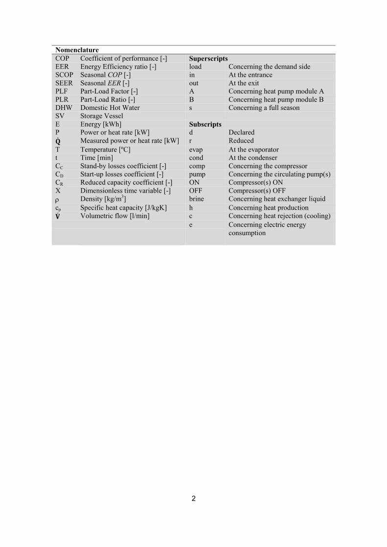
Nomenclature COP Coefficient of performance [-] Superscripts EER Energy Efficiency ratio [-] load Concerning the demand side SCOP Seasonal COP [-] in At the entrance SEER Seasonal EER [-] out At the exit PLF Part-Load Factor [-] A Concerning heat pump module A PLR Part-Load Ratio [-] B Concerning heat pump module B DHW Domestic Hot Water s Concerning a full season SV Storage Vessel E Energy [kWh] Subscripts P Power or heat rate [kW] d Declared �̇� Measured power or heat rate [kW] r Reduced T Temperature [ºC] evap At the evaporator t Time [min] cond At the condenser CC Stand-by losses coefficient [-] comp Concerning the compressor CD Start-up losses coefficient [-] pump Concerning the circulating pump(s) CR Reduced capacity coefficient [-] ON Compressor(s) ON X Dimensionless time variable [-] OFF Compressor(s) OFF Density [kg/m3] brine Concerning heat exchanger liquid cp Specific heat capacity [J/kgK] h Concerning heat production �̇� Volumetric flow [l/min] c Concerning heat rejection (cooling) e Concerning electric energy

consumption

3

1. INTRODUCTION 31

Ground-source heat pumps (GSHPs) represent undoubtedly one of the most important 32 low-carbon technologies for heating and cooling in the residential and non-residential sectors 33 [1, 2]. Utilization of shallow geothermal energy (SGE) mitigates carbon dioxide emissions 34 because GSHPs require less electrical energy to produce (or reject) the same amount of heat as 35 analogous technologies such as air-to-air or air-to-water heat pumps. For each kWh electric, 36 GSHPs can produce (or remove) over 50% more thermal energy than aerothermal systems [3–37 7]. 38

Heat pump performance is inherently dependent on the temperature of the fluids exchanging 39 heat at the evaporator and the condenser stages. Therefore, different climatic conditions and 40 demand patterns over a season can lead to large variations in the overall efficiency of the 41 machine. But despite the influence of the climate and demand, there are other aspects affecting 42 heat pump performance that can go unnoticed without a proper and accurate analysis. Most of 43 them are related to technological and operational issues, such as compressor aging, leaking 44 refrigerant fluid, fouling generation at the heat exchanger pipe internal walls [8] or the operation 45 under part-load regimes (partialisation losses) with fixed-speed compressors [9–11]. All of them 46 contribute to an overall reduction of the efficiency. Therefore, real-time performance 47 monitoring is a valuable tool to distinguish between external and internal factors influencing 48 seasonal performance. Moreover, the use of common methodologies, international standard 49 procedures and harmonised metrics contribute to a fair and rigorous comparison between 50 different installations [12]. 51

F. Ruiz-Calvo and C. Montagud presented a work where five years of performance data were 52 recorded and processed to characterise an existing GSHP located in Valencia (Spain) [13]. 53 Nonetheless, the information was limited to the seasonal performance of the GSHP and the 54 ground temperature evolution, without assessing any possible performance degradation. 55 J. Corberán et al. [14] published an excellent analysis of water-to-water heat pumps. It was 56 focused on the partialisation losses due to operation under cycling conditions, although the 57 study was carried out on a laboratory setup. Similarly, E. Fuentes et al. [15] established a 58 correlation between efficiency losses and part-load operation by taking into account the extra 59 power consumption during compressor start-up as well as during stand-by mode. Even though 60 this work presented useful and rigorous results, the data used for the analysis were also obtained 61 in a laboratory environment under steady state conditions. 62

The aim of this work is to identify and quantify any degradation in efficiency of an existing 63 GSHP and to characterise partialisation losses. The research is approached both from practical 64 and theoretical points of view. As a result, a new methodology is proposed. The analysis is 65 based on data recorded strictly under real conditions and taking into account relevant 66 particularities of the GSHP configuration. The validity of the methodology is tested by means of 67 Ground Loop Design software (GLD, version 2016) [16]. 68

Through the study of a particular installation, the authors intend to demonstrate the potential of 69 the monitoring systems to provide detailed characterisation of GSHPs. Moreover, this study 70 aims to contribute to new regulatory frames for real-time monitoring of GSHPs and other 71 heating/cooling systems. 72

4

2. DESCRIPTION OF THE GSHP SYSTEM 73

2.1. Climatic and geological setting 74

The GSHP under study is placed in the basement of a three-floor office building with a total 75 living area of 800 m2. The building is located at 470 m above the sea level in the city of Tremp, 76 NW of Catalonia (NE of Spain). According to the Köppen-Geiger climatic classification [17], 77 the climate in this region is humid warm temperate, with warm summers (Cfb type). The annual 78 average temperature is 12-13 ºC. The winter lasts from December to February next year with 79 minimum average air temperature of -1.2 °C. Besides, the summer lasts from June to September 80 with maximum average air temperature of 28.5 °C. Due to its high annual thermal amplitude, 81 Tremp is an ideal location to exploit SGE. 82

Regarding the Geology of the site, Tremp is situated on alternating layers of shales and fine to 83 medium grain sandstones (Garumnian facies). The regional groundwater level is rather deep, but 84 there is a perched water table above it, between 3 to 10 m depth. 85

2.2. Description of the closed-loop shallow geothermal system 86

A preliminary analytical design determined a total vertical borehole field length of 1400 m. On 87 this basis, a closed-loop system was designed with 10 vertical borehole heat exchangers (BHEs) 88 with an average drilling depth of 140 m and 130 mm in diameter. 89

All boreholes were equipped with a single U-tube (40 mm outer diameter, SDR11), and 90 backfilled with grout to secure good thermal contact between the heat exchanger and the 91 surrounding ground. The distance between boreholes ranges between 5 and 6 m. The heat 92 exchanging fluid is pure water. 93

In order to determine the thermal properties of the ground, a thermal response test was executed 94 in one of the boreholes that would later be part of the installation. A mean ground thermal 95 conductivity of 2.1 W/mK and a thermal diffusivity of 5.03·10-7 m2/s were obtained, and an 96 undisturbed ground temperature value of 14.9 ºC was measured. 97

2.3. Design and actual thermal loads 98

Initially, the production facility was planned to meet a heating demand of 43720 kWh and a 99 cooling demand of 45890 kWh. The design capacities were calculated as 50 kW for the cool 100 season (heating) and 60 kW for the warm season (cooling). Therefore, the expected equivalent 101 number of operating hours at full power was 874 h in heating mode and 765 h in cooling mode. 102 If the total number of hours in a year (8760 h) is considered, then the yearly utilization factor 103 (equivalent hours / total hours) is 18.7 %. However it must be borne in mind that this is an 104 office building, not a residential one. This means that the building is operative only about 230 105 days a year with a maximum of 10 h opening hours per day (~ 2300 h). Although this is a 106 simplistic approximation, it is relevant from the sizing perspective to see that the total number 107 of equivalent hours represents about 70 % of the total opening hours. Interestingly, the actual 108 thermal loads differ substantially from the planned ones (see table 1). 109

5

Period Cooling load (kWhc) Heating load (kWhh) 2015-2016 33883 85254 2016-2017 39613 83440 2017-2018 - 89007

Table 1. Seasonal thermal loads from April 2015 to May 2018. 110

2.4. GSHP characteristics 111

The heat pump was acquired from the Swedish company Nibe Industrier AB (model 112 Fighter 1330). It has a nominal overall heating capacity of 60 kW generated by two twin heat 113 pump modules (a double parallel stage) of 30 kW each. Both modules are equipped with 114 fixed-speed compressors and share the same circulation pump at the evaporator side (nominal 115 consumption: 1.3 kW), while at the condenser each module has its own pump (nominal 116 consumption: 0.17 + 0.17 kW) (see figure 1). Module A acts as the master stage while 117 module B acts as the slave. This means that module B produces or rejects heat if module A 118 cannot meet the demand by itself. Besides, domestic hot water (DHW) is produced exclusively 119 by module B. It is important to distinguish between two parallel stages and two parallel 120 compressors. The latter is also known as “tandem compressors”. Under the tandem 121 configuration, the two compressors do work in parallel at full capacity, although they share the 122 same evaporator and condenser. A representative set of the heat pump performance data 123 (declared values) is presented in table 2. 124

𝐓𝐞𝐯𝐚𝐩𝐢𝐧 (ºC) 𝐓𝐜𝐨𝐧𝐝

𝐢𝐧 (ºC) Heating capacity Ph (kW)

Cooling capacity Pc (kW)

Electric power Pe

(kW) COPd EERd

-5 35 52,58 39,40 13,18 3,53 2,64 0 35 60,68 46,84 13,84 3,90 3,01 5 35 70,10 55,46 14,64 4,28 3,39 10 35 80,62 64,95 15,67 4,63 3,73 10 45 76,73 59,08 17,65 3,96 3,05 10 55 73,16 52,99 20,17 3,34 2,42 10 65 69,92 46,68 23,24 2,80 1,87

Table 2. Nominal performance data of the heat pump provided by the manufacturer, for a set of representative values of 125 T and T . The column “Electric power” accounts only for the consumption of the compressors. However, the 126 values of COPd and EERd include the consumption of the circulation pumps in their calculation. 127

Nominal stand-by consumption of the heat pump is 110W. A storage vessel of 750 l is used to 128 provide thermal inertia to the installation, which reduces the number of start-stop cycles of the 129 compressors within the GSHP. In fact, the heat produced or rejected from the building is 130 measured as the heat supplied or removed to/from the storage vessel. On the other side, an 131 accumulator tank of 1000 l of capacity is used for DHW. Inside the DHW vessel, the tap water 132 from the building flows through an isolated zigzag pipe, exchanging heat with the water in the 133 vessel. This way, the drinking water is not mixed with the water flowing from and to the BHE 134 field, which is an adequate solution for the sake of hygiene and safety. This is not the case of the 135 storage vessel, because the water contained within flows through both the distribution system 136 and the BHE field. 137

The GSHP shifts from heating to cooling mode (and vice versa) through a climate exchange 138 module (CEM). The CEM (model HPAC 42, also from Nibe) is basically a set of four 3-way 139 valves connecting the storage and DHW vessels, the BHEs and the heat pump. Whenever the 140

6

GSHP is operating under heating mode, the CEM connects the water circulation between the 141 BHEs and the evaporator(s) on the one hand (through the evaporator pump), and between the 142 storage/DHW vessel and the condenser(s) on the other (through the condenser pumps(s)). Under 143 cooling mode, the water now circulates between the BHEs and the condenser(s) (now the 144 condenser pump(s) does the job) and between the storage vessel and the evaporator(s) (using the 145 evaporator pump). 146

147

Figure 1. Basic scheme of the heating/cooling production facility under study. The numbered labels indicate the location of 148 the sensors measuring the key parameters of the installation, which are recorded by the monitoring system: 1.-Upper 149 temperature sensor; 2.-Volumetric flow sensor; 3.- Lower temperature sensor (these 3 sensors account for thermal energy 150 measurement at the storage vessel); 4.- Storage vessel temperature sensor; 5.- Temperature sensor for brine (water) going 151 to the ground; 6.- Temperature sensor for brine (water) coming from the ground; 7.- Upper temperature sensor; 152 8.- Volumetric flow sensor; 9.- Lower temperature sensor (these 3 sensors account for thermal energy measurement at the 153 DHW vessel). 154

The GSHP contains a set of temperature and water flow sensors, integrated as part of two 155 thermal energy meters in order to measure the thermal energy produced/rejected in the system 156 (model MULTICAL 601, from Kamstrup A/S, with a typical error < 0.6 %). It also has an 157 electric energy meter (model 382 from Kamstrup A/S, with a typical error < 0.5 %) and three 158 independent temperature sensors (#4, #5 and #6 shown in figure 1 are Pt100 sensors with 159 typical absolute error of < 0.5 ºC). The electrical energy meter measures strictly the energy 160 consumed by the compressors and the circulation pumps, leaving stand-by consumption 161 unmeasured. Finally, there is a monitoring system that periodically reads the values of several 162 key parameters of the GSHP. Some of these parameters can be recorded remotely as text files, 163 allowing the generation of the data sets used for the performance analysis of this work. 164

7

3. METHODOLOGY 165

The methodology developed in this project is mainly based on a previous work of E.Fuentes et 166 al. [15]. It aims to be applied to a particular GSHP operating under real conditions taking into 167 consideration its specific architecture (double parallel stage with fixed-speed compressors). The 168 steps carried out are summarized in the following sequence: 169

1. - Identification of all the parameters recorded by the monitoring system and their limitations. 170 It is necessary to record performance data at least for one year (two complete seasons) with the 171 highest time resolution available (1 minute). 172

2. - Adoption of the most suitable theoretical approach to characterise efficiency losses. This 173 will be addressed by correlating the part-load factor (PLF) and the part-load ratio (PLR), which 174 are related through specific degradation coefficients. Previous works are based on GSHPs with 175 a single stage; hence a new relationship must be developed to account for the double parallel 176 stage configuration. 177

3. - Definition and/or adoption of specific metrics to process the raw data from the monitoring 178 system. Obtain the values of the characterisation parameters according the metrics. Analyse the 179 limitations and any approximations that might be necessary. 180

4. - Generation of significant data sets of (PLF, PLR) pairs from data corresponding to the 181 whole period of study. 182

5. - Implementation of a minimum square fitting of the curves defined by PLF and PLR values 183 using the degradation coefficients as the fitting parameters. The values obtained for the fitting 184 parameters will constitute the quantification of the efficiency degradation. 185

6. - Creation of a model in GLD resembling the GSHP under study. The key point here is to find 186 the way to implement the degradation in performance of the heat pump. The declared data from 187 the manufacturer (see table 2) must be modified in order to carry implicitly the degradation in 188 efficiency quantified in the previous step. 189

7. - Simulation under GLD environment and comparison between the seasonal performance and 190 that obtained empirically (from the monitoring data). The degree of agreement between 191 measured and simulated values will account for both the validation of the model built in GLD 192 and the methodology itself. 193

Hereafter, the methodology is described in 5 detailed blocks, from sections 3.1 to 3.5. 194

3.1. Data collection 195

The information recorded remotely by the monitoring system accounts for minute-resolved 196 values of Ee, Eh (calculated through temperature sensors #1 and #3 and flow sensor #2 in 197 figure 1), Ec (same as for Eh), EDHW (calculated through temperature sensors #7 and #9 and flow 198 sensor #8 in figure 1), TSV (temperature sensor #4 in figure 1), T (temperature sensor #5 in 199 figure 1), T (temperature sensor #6 in figure 1), t and t . Apart from it, there are other 200 parameters that can be accessed in-place, like V̇ , V̇ , T , T , T and T . The 201 flow values can be checked at the display of the thermal energy meters, while the temperature 202 values are displayed by the heat pump. Although T and T are especially relevant for the 203 performance analysis, these parameters are not included in the automatic data acquisition 204 system. To overcome this, TSV and T were used instead. 205

8

The relationship between the readouts of T and T with T and T was found 206 experimentally, depending on the operating mode (heating or cooling): 207

T

= T + 0.6ºC = T

(1)

T

= T + 1.7ºC = T

(2)

Figure 2 illustrates the minute-resolved data recorded by the monitoring system, after being 208 processed and plotted together. Energy measurements are presented as cumulative values within 209 a single day. A binomial function represents the time periods whenever a compressor is ON 210 (value = 1) or OFF (value = 0). It is worth to mention that during the periods when the 211 compressors are in OFF mode, the values of T and T do not coincide. A test was 212 carried out in place to check the temperature readouts when the circulation pumps were forced 213 to operate while the compressors were in OFF mode. In that case it was observed a coincident 214 value for T and T . This implies that these temperature readouts are simply not trustable 215 when water is not circulating within the pipes. The reason for this is still unknown, although 216 from a practical point of view it cannot be considered a relevant issue. 217

218

Figure 2. Parameters recorded by the monitoring system. The data shown correspond to the 27th of November, 2017 219 between 8am and 8pm. The heat pump was operating under heating mode. 220

3.2. Performance characterisation at part-load 221

In water-to-water heat pumps with fixed-speed compressors, part-load operation is an inherent 222 source of performance degradation. The two main factors responsible for this are: on one side, 223 the extra power consumption of the compressors at start and re-balance of refrigerant pressures 224

0

1

0

100

200

300

400

500

600

8,00 10,00 12,00 14,00 16,00 18,00 20,00t O

N(0

/1)

En

erg

y (k

Wh

)

Daytime (h)

E(heat) E(DHW) E(e) t ON (A) t ON (B)

0

10

20

30

40

50

8 10 12 14 16 18 20

T (º

C)

Daytime (h)

T(SV) T(brine in) T(brine out)

Eh EDHW Ee tONA tON

B

TSV Tbrinein Tbrine

out

9

within the refrigerant circuit (start-up losses); on another side, the power consumption of the 225 machine whenever the heat pump is switched on but inactive (stand-by losses) [15]. 226

Additionally, it is common to switch on the circulation pumps before the compressors start to 227 operate, and they are switched off after the compressors stop. This would be also contributing to 228 the start-up losses. Of course, all these performance degradation mechanisms are relevant to a 229 greater or lesser extent depending on the cycling characteristics. The shorter and the more 230 frequent cycling periods are, the higher partialisation losses will be [14,18]. 231

The analysis of the partialisation losses is commonly carried out through two indicators: the 232 PLR and the PLF. PLR expresses the ratio between the thermal load of the building and the 233 rated/declared heating and cooling capacity of the heat pump. This parameter is also known as 234 capacity ratio (CR) and is also denoted by the Greek letter . On the other hand, PLF is defined 235 as the ratio between the coefficient of performance under cyclic conditions and its declared 236 value. These two terms are related through a set of dimensionless coefficients (ranging from 237 0 to 1) which account for the degradation losses when operating at part-load. 238

According to the EN-14825 standard [19], stand-by losses represent the only relevant source of 239 performance degradation in water-to-water heat pumps under part-load conditions, and therefore 240 PLF and PLR show the following relationship: 241

PLF =PLR

C PLR + (1 − C ) (3)

Where CC is the stand-by losses coefficient. Its value would reach 1 if there was no 242 consumption under stand-by mode (so PLF=1 at all times), and at the other extreme, CC = 0 243 would mean that the stand-by consumption is way higher than that of the compressors, which 244 obviously makes no sense. In fact, CC is requested to be equal to 0.9 by default when no 245 empirical data is available. This norm considers that start-up losses are negligible in air-to-water 246 and water-to-water systems. 247

In the literature, there are examples of water-to-water characterisation where start-up losses are 248 not negligible, in contrast to EN-14825. This is the case of the work done by E. Fuentes et 249 al. [15]. This team found that the partialisation losses due to cycling operation in water-to-water 250 heat pumps might not be negligible at all. Particularly, it was found a correlation between the 251 thermal inertia introduced by storage vessels at the demand side and the partialisation losses, so 252 the higher the tank volume to capacity ratio (l/kW) is, the lower the losses are. Indeed, storage 253 vessels are commonly installed in facilities equipped with water-to-water heat pumps to avoid 254 excessive cycling of the compressors [20], so this result could be somehow anticipated. The 255 authors derived a new equation based on the work published previously by J. M. Corberán et 256 al. [14]. In this new expression, the CC coefficient was combined with another one associated to 257 start-up losses (CD): 258

PLF =1

1 +C (1 − PLR)

1 − C (1 − PLR)+ (1 − C )

(1 − PLR)PLR

(4)

In this case, CD also varies between 0 and 1, but when CD = 0, it means that no start-up losses 259 take place, and the above expression coincides with eq.3. 260

In our particular case, since the measured electrical energy does not include stand-by 261 consumption (see section 2.4), any empirical value of PLF cannot account for partialisation 262 losses attributed to stand-by operation. Therefore the theoretical expression relating PLF and 263 PLR will be a simplified version of eq.4, where CC can be considered equal to 1: 264

10

PLF = 1 − C (1 − PLR) (5)

This expression coincides with the ARI standard [21], which only accounts for start-up losses. At 265 this point, additional considerations must be taken into account. The expected or ideal 266 performance under steady state conditions is determined by the capacity and power 267 consumption values provided by the manufacturer (see table 2). Nevertheless, this would imply 268 that every machine manufactured shows exactly the same performance, which might not be 269 realistic. In fact, the declared performance data can be understood as a reference based on the 270 manufacturer’s own statistical sample among the units tested at their factory [23]. Hence it 271 should be admitted a certain deviation, which can be easily in the range of +/-5%. Besides, in 272 real system, the performance of the heat pump alone cannot be analysed separately from the rest 273 of the installation because other external factors come into play (linked to the BHEs or to the 274 CEM, for example) [23]. In order to include this aspect into calculations, a new coefficient is 275 proposed. CR (reduced capacity coefficient) is defined as a constant value ranging from 0 to 1. It 276 introduces a proportional reduction in the capacity of the GSHP with respect to the declared 277 value: 278

P = (1 − C )P (6)

So when CR = 0, then Pr = Pd = P. As a result, eq.5 is modified in the following manner: 279

PLF = (1 − C )[1 − C (1 − PLR)] (7)

Notice that the deviation from declared performance in eq.6 is strictly attributed to an effective 280 reduction of the heating or cooling capacity, not an increase in the electrical power consumption 281 of the compressors. The reason for this is purely empirical. Significant deviations were observed 282 only in the heating or cooling capacity, but not in the power consumption of the compressors, 283 compared to the GSHP performance data (table 2). 284

The aim is to obtain as many PLR and PLF values as possible after processing the data gathered 285 by the monitoring system. Then it will be possible to determine the partialisation losses under 286 cyclic-real conditions and the mismatch between the declared capacity of the heat pump and that 287 of the entire GSHP. However, since the data is obtained out of laboratory conditions and the 288 heat pump contains a double parallel stage, several assumptions and approximations must be 289 taken into consideration in order to apply eq.7 to the system under analysis. 290

3.2.1. Part-load ratio evaluation 291

When Q̇ and Q̇ are constant during a certain period Δt (steady state conditions), it can be 292 demonstrated [14] that for fixed-speed compressors, PLR is equivalent to: 293

PLR =t

∆t=

t

t + t (8)

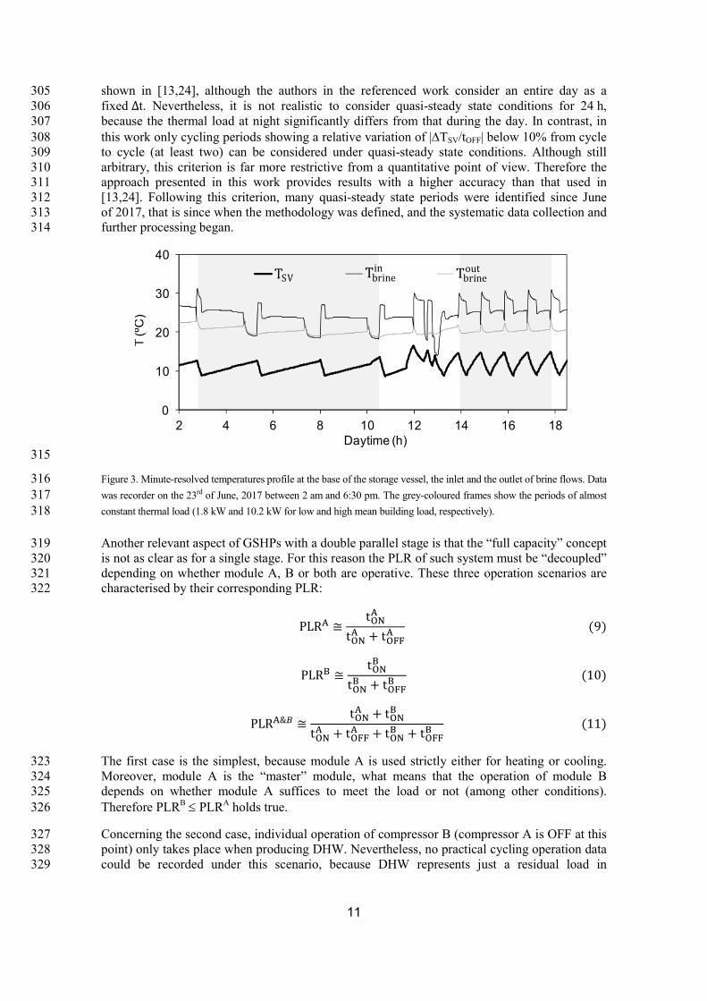
Where t is the total time when the compressor is ON during Δt. In contrast to a laboratory 294 setup, in real systems thermal load varies during the day, so prolonged periods (>1h) presenting 295 constant load are rarely identified through the recorded data. However, the eq.8 can be 296 considered still valid for real systems when the temperature profile of the storage vessel reveals 297 an almost constant load (quasi-steady state conditions). This is one of the most important 298 assumptions of this work, and it is illustrated by figure 3, where concatenated, almost identical 299 ON/OFF cycles (cooling mode) are identified within a reasonably large period (few hours). 300 Notice that during the time periods when dTSV/dtOFF > 0 (increase of TSV when compressors 301 are OFF), higher TSV gradients are a consequence of higher loads. Similarly under heating 302 mode, the OFF periods are characterised by dTSV/dtOFF < 0, so the lower the TSV gradient is, the 303 higher the load will be. From a methodological point of view, this criterion is similar to that 304

11

shown in [13,24], although the authors in the referenced work consider an entire day as a 305 fixed Δt. Nevertheless, it is not realistic to consider quasi-steady state conditions for 24 h, 306 because the thermal load at night significantly differs from that during the day. In contrast, in 307 this work only cycling periods showing a relative variation of |TSV/tOFF| below 10% from cycle 308 to cycle (at least two) can be considered under quasi-steady state conditions. Although still 309 arbitrary, this criterion is far more restrictive from a quantitative point of view. Therefore the 310 approach presented in this work provides results with a higher accuracy than that used in 311 [13,24]. Following this criterion, many quasi-steady state periods were identified since June 312 of 2017, that is since when the methodology was defined, and the systematic data collection and 313 further processing began. 314

315

Figure 3. Minute-resolved temperatures profile at the base of the storage vessel, the inlet and the outlet of brine flows. Data 316 was recorder on the 23rd of June, 2017 between 2 am and 6:30 pm. The grey-coloured frames show the periods of almost 317 constant thermal load (1.8 kW and 10.2 kW for low and high mean building load, respectively). 318

Another relevant aspect of GSHPs with a double parallel stage is that the “full capacity” concept 319 is not as clear as for a single stage. For this reason the PLR of such system must be “decoupled” 320 depending on whether module A, B or both are operative. These three operation scenarios are 321 characterised by their corresponding PLR: 322

PLR ≅t

t + t (9)

PLR ≅t

t + t (10)

PLR & ≅t + t

t + t + t + t (11)

The first case is the simplest, because module A is used strictly either for heating or cooling. 323 Moreover, module A is the “master” module, what means that the operation of module B 324 depends on whether module A suffices to meet the load or not (among other conditions). 325 Therefore PLRB PLRA holds true. 326

Concerning the second case, individual operation of compressor B (compressor A is OFF at this 327 point) only takes place when producing DHW. Nevertheless, no practical cycling operation data 328 could be recorded under this scenario, because DHW represents just a residual load in 329

0

10

20

30

40

2 4 6 8 10 12 14 16 18

T (º

C)

Daytime (h)

TSV Tbrinein Tbrine

out

12

comparison with heating or cooling. Therefore, this scenario was far from resembling a steady 330 or quasi-steady state load. 331

The last case is the most complex. The definition provided here for PLRA&B might look 332 somehow arbitrary, but it is not. Since module B acts as the slave module (PLRB PLRA), the 333 same total cycling period must be considered for both modules: 334

t + t = t + t = ∆t (12)

Hence: 335

PLR & ≅t + t

2∆t (13)

Therefore, PLRA and PLRB are related through: 336

PLR & =1

2PLR + PLR (14)

It is straightforward to check the validity and consistency of the eq. 14. For instance, if 337 compressor A is OFF, the value of PLRA&B equals to ½PLRB. On the other hand, if both 338 compressors are 100% operative, then PLRA&B = 1. 339

3.2.2. Part-load factor evaluation 340

For PLF assessment it is necessary to distinguish between different possible scenarios that can 341 take place. For instance, when a single compressor is ON, the capacity considered as declared is 342 simply ½Pd(h) or ½Pd(c). Analogously, the declared power consumption of the compressor would 343 be ½Pd(e), but the electrical power consumed by the circulation pumps would involve the use of 344 just one condenser pump instead of two. This means that for a given pair of values 345 (T , T ), COPd and EERd would show higher values when both compressors are operative 346 compared to single compressor operation. Nevertheless, it is desired that the PLF represents an 347 overall ratio between actual and declared performance, irrespective of the operating number of 348 compressors. For this reason, given a cycling period Δt and quasi-steady state load conditions, it 349 is proposed that PLF is evaluated as: 350

PLF ≅1

t

COP

COPdt ≅

1

t

COP

COP (15)

PLF ≅1

t

EER

EERdt ≅

1

t

EER

EER (16)

3.2.3. PLF vs. PLR adapted to a double parallel stage 351

Double parallel stage complicates the theoretical expression relating PLFA&B and PLRA&B. As 352 for PLRA&B, the behaviour of modules A and B must be decoupled as well. Separate PLF (PLR) 353 curves should be considered as if two separate heat pumps are under analysis: 354

PLF = 1 − C 1 − C 1 − PLR (17)

PLF = 1 − C 1 − C 1 − PLR (18)

The purpose of this methodology is to treat the GSHP as a whole, and for this reason a single 355 expression must be developed to allow a reliable characterisation of the entire system. In this 356

13

sense, the contribution of each stage to the global PLF is directly related to the time that the 357 corresponding compressors are operative during Δt. So this demands a time-weighted (and 358 normalized) contribution of modules A and B: 359

PLF & =t

t + tPLF +

t

t + tPLF (19)

As for eq.14, the validity and consistency of eq.19 can be checked through extreme case 360 examples. If only one compressor is ON, then the value of the effective PLFA&B coincides with 361 that of the individual stage, and if t = t then PLFA&B is the arithmetic mean of PLFA and 362 PLFB. Therefore, by inserting eq.7 in eq.19, the most general expression that relates PLFA&B 363 with PLRA and PLRB is: 364

PLF & =t 1 − C 1 − C 1 − PLR + t 1 − C 1 − C 1 − PLR

t + t (20)

For the sake of simplicity, let’s first assume that modules A and B are effectively “twins” in all 365 senses, so C = C = C and C = C = C . Then, by considering the definitions of PLRA and 366 PLRB in terms of t , and Δt, it can be demonstrated that: 367

PLF & = (1 − C ) 1 − C 1 − 2PLR & +2t t

∆t(t + t ) (21)

Eq.21 accounts for the influence of having both modules A and B with different part-load 368 operation conditions within the same cycling period Δt. Again, notice that when one of the 369 compressors is OFF, PLFA&B coincides with that of a single module. 370

3.3. System metrics and definition of characterisation parameters 371

There are different metrics to characterise the efficiency of a heating/cooling system along the 372 cool/warm season, always depending on the boundaries taken into consideration. Besides, an 373 important distinction must be made between laboratory testing and actual performance. The first 374 case invokes the norm EN-14825 and the parameters SCOPnet and SEERON. These indicators are 375 obtained by taking into account several reference climatic conditions and the corresponding 376 declared heating/cooling capacity and electric power consumption of the heat pump, all 377 measured under normalized steady state conditions. In the second case, actual performance 378 characterisation demands the use of indicators such as the seasonal performance factor, or SPFn. 379 This indicator is the result of dividing the total thermal energy (supplied or extracted) measured 380 in a real building, divided by the electrical energy consumption along a complete seasonal 381 period. The subscript n accounts for the different elements of the system consuming electrical 382 power included in the calculation [12]. 383

The characterisation metrics used in this work are closely related to the SPF2 parameter. The 384 main difference is that the actual electrical energy consumption only accounts for the 385 compressors and circulation pumps, but not for stand-by operation. This is just a question of 386 which equipment in the facility is being accounted by the electric energy meter (see section 2.4). 387 Therefore, the characterisation parameters (not to confuse with similar nomenclatures contained 388 in EN-14825) are defined and obtained from the collected data as follows: 389

COPd: Declared coefficient of performance (in kW/kW units) at certain temperature conditions: 390

14

COP T , T =P T , T

P T , T + P (22)

EERd: Declared energy efficiency ratio (in kW/kW units) at a certain temperature conditions: 391

EER T , T = P T , T

P T , T + P (23)

COP: Averaged coefficient of performance integrated over a certain period of time under active 392 mode (possibly including ON/OFF cycles) (in kWh/kWh units): 393

COP =∫ V̇ ρc (T − T )dt + ∫ V̇ ρc (T − T )dt

∫ Q̇ + Q̇ dt=

394

= ∫ Q̇ dt + ∫ Q̇ dt

∫(Q̇ + Q̇ )dt=

E + E

E (24)

EER: Averaged energy efficiency ratio (in kWh/kWh units) analogous to the COP: 395

EER =∫ V̇ ρc (T − T )dt

∫ Q̇ + Q̇ dt=

396

=∫ Q̇ dt

∫ Q̇ + Q̇ dt=

E

E (25)

It is worth mentioning that the average COP (eq.24) and EER (eq.25) can be assimilated as 397 instant values within a minute-resolved time scale. Experimentally, it has been determined that a 398 maximum temperature variation of 0.8ºC/min in the storage vessel is reached when the GSHP 399 operates at full capacity, so it is an appropriate approximation to assume quasi-steady state 400 conditions over such a short time period. Hence it is valid to compare COPd and COP values 401 based on a minute-resolved temporal frame. This is an important point to stress out, especially 402 when it comes to evaluate the PLF at a particular set of temperatures (T , T ) in eq.15 and 403 eq.16. 404

SCOP: Coefficient of performance under active mode (possibly including ON/OFF cycles) 405 integrated over 1 year (in kWh/kWh units): 406

SCOP =∫ Q̇ dt

∫(Q̇ + Q̇ )dt=

E + E

E (26)

SEER: Seasonal energy efficiency ratio (kWh/kWh units), analogous to the SCOP: 407

SEER =∫ Q̇ dt

∫(Q̇ + Q̇ )dt=

E

E (27)

PLR: Part-load ratio. It is defined as the ratio between the heating/cooling load rate (demand 408 side), and the rated capacity at a certain pair (T , T ) (in kW/kW units), and approximated 409 as in section 3.2.1 under quasi-steady state conditions: 410

15

PLR T , T =Q̇ T , T

P T , T≅

t + t

2∆t (28)

PLR T , T =Q̇ T , T

P T , T ≅

t + t

2∆t (29)

PLF: Part-load factor. As mentioned above, steady state conditions can be assumed under a 411 minute-resolved time scale, so it is equivalent to compare power and energy ratios. Therefore: 412

PLF T , T =COP T , T

COP T , T (30)

PLF T , T =EER T , T

EER T , T (31)

3.4. Determination of the degradation coefficients 413

Once the theoretical approach has been defined and the values of (PLF, PLR) pairs can be 414 obtained considering all the particularities of the system, it is time for the determination of the 415 degradation loss coefficients. Prior to this, it is important to analyse the behaviour that should be 416 expected from of eq.21. First of all, it is helpful to rearrange eq.21 in order to visualize its linear 417 behaviour. In fact, it is a linear relationship containing two dimensionless variables, which 418 geometrically is represented by a plane in a Cartesian 3-axis system: 419

PLF & = a · PLR & + b · X + c (32)

Where: 420

X =t t

∆t t + t (33)

a = 2C (1 − C ) (34)

b = −a (35)

c = (1 − C )(1 − C ) (36)

The variable X accounts for the dependence of PLF with the multiple combinations of ∆t, t 421 and t , and it is exclusively attributed to the double parallel stage. Having in mind the 422 constraint imposed by eq.12, it can be demonstrated that X[0, 0.5]. When t or t equals 423 zero (only one compressor in operation), then X = 0 and the eq.32 is reduced to a single variable 424 linear expression: 425

PLF & = a · PLR & + c (37)

It is important to highlight that PLR & and X are not independent variables, since they both 426 depend on t and t . Indeed, t and t are the only true independent variables of the 427 analysed system, as denoted by eq.19. In order to visualize the dependence between PLFA&B and 428 PLRA&B, Monte Carlo simulations were generated. 1000 random values of PLRA&B were built 429 from independent pair values of t and t . The only constraint was to keep valid the 430 inequality t + t ≤ 2∆t. In figure 4, two different scenarios defined by CR and CD are 431

16

depicted. The resulting values of PLF appear between upper and lower limits defined by two 432 extreme cases. The upper limit corresponds to the case when only one compressor is operative 433 (t = 0 or t = 0) and the lower limit stands for the cases when t = t . Geometrically, 434 the representation provided by the plots in figure 4 is the 2-D projection of the plane defined by 435 eq.32 over the plane defined by the PLF and PLR axes. The most important conclusion from 436 this preliminary simulation is that the methodology presented is especially relevant when having 437 heat pump equipped with a double parallel stage and PLRA&B ~ 0.5. Under this situation, 438 treating the same heat pump as if it had an effective single stage would maximize the error in 439 the analysis. On the contrary, for average values of PLRA&B ≳ 0.8 and PLRA&B ~ 0, the proposed 440 approach would be rather unnecessary. The same holds true when start-up losses are negligible 441 (CD → 0), because then PLF would be constant and independent from PLR. 442

443

444

Figure 4. Monte Carlo simulations of PLF (PLR), illustrating the influence of CD and CR through 2 different scenarios: 445 (A): high start-up losses and capacity reduction; (B): same as A, but lower start-up losses. Grey continuous curves 446 represent upper and lower limits delimitating the possible scenarios of operation. 447

0.0

0.2

0.4

0.6

0.8

1.0

0.0 0.2 0.4 0.6 0.8 1.0

PLF

PLR

0.0

0.2

0.4

0.6

0.8

1.0

0.0 0.2 0.4 0.6 0.8 1.0

PLF

PLR

CD = 0.25 CR = 0.25 (A)

CD = 0.10 CR = 0.25 (B)

CD = 0.10 CR = 0.25 (B)

17

In order to determine the coefficients CD and CR, it is necessary to perform a two-variable linear 448 regression of the data sets (PLF, PLR), assuming eq.32 as the expression relating PLF and PLR, 449 and further processing the values obtained for the linear coefficients a, b and c (expressions 34, 450 35 and 36). This must be performed separately for the cool and warm seasons. 451

3.5. Simulation with GLD 452

The next objective is to construct a model of the analysed GSHP under GLD environment. This 453 model must be accurate enough so it matches the measured SCOP and SEER for the time period 454 under analysis. GLD is usually used to provide borehole field sizing, prediction of seasonal 455 performance and time evolution of the ground temperature. Nevertheless, the case under study 456 starts from a different scenario, since now the main objective is to replicate the performance of 457 an existing facility. The key is to implement the degradation losses determined for the GSHP in 458 a quantitative way, and see whether this allows the software to match the measured values of 459 SCOP and SEER. If so, this method would provide a double validation, i.e. one for the 460 methodology determining the efficiency degradation, and the other for the construction of the 461 model itself under GLD environment. Indeed, this method exploits new capabilities of the 462 software. 463

The modelling procedure is divided into three main blocks. The first one defines borehole field 464 (soil types, borehole geometry and physical characteristics of the ground and brine). The second 465 block stands for monthly thermal loads, and the third block defines the heat pump. 466

GLD contains a database of water-to-water manufacturers and models, but it is also possible to 467 include your own heat pump. To do so, the edit/add heat pump module of the software demands 468 a set of discrete heating and cooling capacity and electrical power consumption data, for various 469 temperature conditions ( T , T ). Quadratic interpolation curves from these reference 470 conditions are automatically generated, so the software can estimate the actual capacity at any 471 temperature of the brine at the inlet of the evaporator and the condenser. 472

Default options are limited to heat pumps equipped with single stages. There is not any field or 473 panel to introduce partialisation losses due to cycling operation or any kind of efficiency 474 degradation. So this must be carried out implicitly. Declared capacity values (according to table 475 2) need to be substituted by their reduced counterparts at the edit/add heat pump module, 476 according to the following expression: 477

P = P PLF (38)

Notice that the above expression is only valid as long as the declared electrical power 478 consumption remains unaltered, which is actually the case. However, it is difficult to choose a 479 single and representative PLFs value that is valid both for the cool and the warm seasons. As 480 part of the proposed methodology, PLF and PLF values have been estimated by inserting 481 global seasonal PLR values in eq.21 along with CD and CR values previously obtained from the 482 linear regression. In this case, global PLR and PLR values can be estimated just by counting 483 the total t , and t , along the whole season, which is represented by the total seasonal 484 collection time Δ𝑡 and Δ𝑡 , regardless of any quasi-steady state consideration, therefore: 485

PLF = 1 − C ( ) 1 − C ( ) 1 − 2PLR +2t , t ,

∆t t , + t , (39)

PLF = 1 − C ( ) 1 − C ( ) 1 − 2PLR +2t , t ,

∆t (t , + t , ) (40)

18

In this sense, seasonal PLRs values represent less accurate figures than PLRA&B values, which 486 are obtained from quasi-steady state periods comprising just a few hours. Nevertheless, it 487 accounts for the whole seasonal period. This way GLD will simulate seasonal performance 488 considering a modified heat pump showing reduced cooling and heating capacities. 489

Furthermore, extra power consumed by the GSHP has to be considered as well. In the borehole 490 field module it is possible to attribute a value for electrical consumption of the circulation 491 pumps. Under GLD environment, these pumps are considered to operate synchronized with the 492 compressors. However, it is not possible to establish a continuous stand-by power consumption 493 base level. For this reason, the metric used by GLD and that selected in this work for SCOP and 494 SEER calculations are exactly the same. Therefore the comparison between simulated and 495 measured values is consistent (“apples compared to apples”). 496

19

4. RESULTS AND DISCUSSION 497

Data in Table 3. Monthly loads for the period of time under analysis. The values of SEER and 498 table 3 correspond to the thermal energy measured as heat production (heating) and heat 499 rejection (cooling), as well as the electrical energy consumed by the compressors and the 500 circulation pumps. A remarkable unbalance is observed between the actual total heating and 501 cooling loads, so it can be anticipated that a progressive cooling of the ground might be taking 502 place. The obtained SEER and SCOP are 3.14 and 3.09, respectively. These values are below 503 what is expected in such heating/cooling facilities, where SEER and SCOP can easily exceed a 504 value of 3.5 [25, 26]. This fact motivates by its own the search for the identification of any 505 possible source of performance degradation. 506

Month Heat rejection

(Ec)

(kWhc)

Electrical energy (Ee(c))

(kWhe)

Heat production +

DHW (Eh+EDHW)

(kWhh)

Electrical energy (Ee(h))

(kWhe)

April 2017

4051.5 1275.6 May 2017 1454.0 566.2 2460.0 980.3 Jun 2017 9933.3 3014.1 509.2 157.2

July 2017 10564.3 3310.5 407.4 125.4 August 2017 11542.6 3708.9 417.8 137.6

September 2017 4204.2 1332.2 739.7 229.9 October 2017 1915.0 669.9 1006.2 339.0

November 2017

11689.1 3663.6 December 2017

22885.5 7295.7

January 2018

14533.8 4678.6 February 2018

16416.0 5349.2

March 2018

13891.1 4532.7 TOTAL 39613.2 12601.8 89007.3 28764.7

SEER = 3.14 SCOP = 3.09

Table 3. Monthly loads for the period of time under analysis. The values of SEER and SCOP are shown at the bottom. 507

Figure 5Figure 5 shows two different data sets (PLF, PLR) corresponding to warm and cool 508 seasons. Empirical points are represented by grey circles, while expected theoretical points are 509 represented by black triangles. The theoretical values of PLF were obtained after the linear 510 regression process detailed in section 3.4. The correlation coefficients show values around 0.7, 511 what cannot be taken as a strong degree of correlation yet. Despite this, p-values are lower than 512 0.01, so the null hypothesis should be discarded. Actually this indicates that the correlation is 513 significant after all, thus a consistent interpretation of the results is allowed, even though a 514 larger sampling is required. It is noticed that in the data set from warm season (plot A in 515 figure 5) PLRA&B < 0.5, which indicates that the linear regression could be implemented by 516 using eq.37 instead of eq.32. 517

CD is found to be the same for the warm and cool seasons within a 5% error margin, while CR is 518 clearly different from one season to another (> 15% discrepancy). Although the causes behind 519 the seasonal similarities or differences of CD and CR are not yet clear, a thorough analysis of the 520 PRL can bring some light to this. During the warm season, the cooling load hardly requires 521 more than one module operating at the same time for heat rejection, leading to a residual use of 522 module B, so predominantly module A is the one doing the job and therefore PLRA&B < 0.5. On 523 the contrary, during the cool season the use of module B is way higher. Since CR(h) < CR(c), it is 524

20

reasonable to think that module B is actually performing better than module A, so when both are 525 being used, the resulting energy efficiency is better than if only module A operates. The reason 526 would lay on the fact that module A accumulates a larger operation time. In other words, 527 module A would be degrading at a faster rate than module B due to its more intense use. 528

This result contradicts a previously stated assumption (see section 3.2.1), where modules A 529 and B are considered effectively identical. This implies that a more general expression (like 530 eq.20), should be considered for the minimum square fitting, resulting in separate estimations 531 for C , C , C and C . However, this procedure is impractical. In order to obtain univocal 532 results, a minimum square fitting with 4 adjusting parameters requires a much larger data set 533 than those presented in figure 5. But despite the possible physical differences between modules 534 A and B, it would be inaccurate to attribute this reduction in heating or cooling capacity just to 535 the heat pump machine. 536

537

538

0.5

0.6

0.7

0.8

0.9

1

0.0 0.2 0.4 0.6 0.8 1.0

PL

FcA

&B

PLRA&B

PLF(c) empirical

PLF(c) theoretical

0.5

0.6

0.7

0.8

0.9

1

0.0 0.2 0.4 0.6 0.8 1.0

PL

Fh

A&

B

PLRA&B

PLF(h) empirical

PLF(h) theoretical

CD(h) = 0.084 CR(h) = 0.204 r = 0.68 p-value(PLR) = 1.06·10-6 (B)

p-value (X) = 2.16·10-3

CD(c) = 0.088 CR(c) = 0.244 r = 0.73 p-value = 1.41·10-3 (A)

21

Figure 5.Theoretical (according to eq.32) and empirical (PLF, PLR) data sets employed in the performance analysis. The 539 upper plot (A) corresponds to the warm season (cooling) and the bottom plot (B) corresponds to the cool one (heating) 540

In fact, there is no doubt about the progressive degradation in performance of the GSHP. Figure 541 6 6 demonstrate that COP and EER decreased since systematic data collection started almost 542 three years ago (weekly-averaged values). Linear fit indicate yearly performance decrease of 543 COP and EER by 1.6% and 4.0%, respectively. If the trend is extrapolated back to July of 2012 544 (the date of commissioning), it can be estimated that EER value at that time was around 3.8. 545

After these results were obtained, a physical inspection was undertaken by the engineering and 546 maintenance service of the heating/cooling facility (August of 2018). It was found that one of 547 the 3-way valves in the CEM module showed deficient performance (incomplete closing). This 548 caused an unwanted connection between the evaporator and the condenser water circuits. 549 Additionally, the water filter at the evaporator side had a significant amount of dirt, which 550 contributes to a decreased V̇ through the pipes. These physical mechanisms contribute to an 551 effective capacity reduction, although it is not possible to identify them as the only ones yet. 552 New data must be gathered and analysed in order to quantify the effect of the intervention 553 performed on the GSHP after the inspection (valve repair and water filter replacement). 554

Finally, it must be emphasized that the consistency of the results relies on the assumption that 555 the gathered data is reliable within the error range provided by the manufacturers at each of the 556 measuring components (see section 2.4). 557

558

Figure 6. Weekly-averaged COP and EER values recorded for almost a 3-year period. A linear fit is shown in order to 559 illustrate the decreasing trend of these parameters through time. COP and EER values in the vicinity of change of seasons 560 distort the observations and have been removed from this plot. 561

Regarding simulations carried out under GLD environment, the calculated PLFh and PLFc 562 (according to eq.39 and eq.40, respectively) are shown in table 4. These values have been used 563

2.0

2.2

2.4

2.6

2.8

3.0

3.2

3.4

3.6

3.8

4.0

CO

P &

EE

R (w

ee

kly-

ave

rage

d)

Date

COP

EER

COP linear trend

EER linear trend

22

to modify Pd(h) and Pd(c) values in the edit/add heat pump module from GLD, according to the 564 procedure described in section 3.5 (eq.38). The new capacity values represent an effective 565 reduction with respect to the nominal ones (table 2). 566

PLRs CD CR PLFs

Effective capacity

reduction (%)

Warm season 0.198 0.087 0.244 0.703 29.7% Cool season 0.344 0.084 0.204 0.752 24.8%

Table 4. Resulting averaged seasonal PLR and PLF used for the modification of Pd in the edit/add heat pump module 567 from GLD. 568

The main results of the simulations are shown in table 5, where an excellent agreement between 569 empirical and simulated SCOP and SEER is shown (discrepancy lower than 2%). In 570 comparison, a different simulation was run in GLD, where the heat pump input in the edit/add 571 heat pump module corresponded to the declared performance shown in table 2. According to 572 this, the SCOP and SEER would reach values around 4 if the capacity of the GSHP was that 573 corresponding to the declared performance (and no partialisation losses were taken into account) 574

SCOP SEER

Simulated with Pd 3.9 4.1 Simulated with Pr 3.1 3.1

Measured 3.1 3.1

Table 5. Seasonal performance results of the simulated GSHP, considering declared and reduced capacity 575 (Pr(c) = Pd(c)·[1 - 0.30] and Pr (h) = Pd(h)·[1 - 0.25]), and compared to the measured values. 576

23

5. CONCLUSIONS 577

This work shows a reliable methodology for the characterisation of partialisation losses and 578 other degradation factors on GSHPs operating under real conditions. This is done through the 579 use of minute-resolved recorded data concerning a few key parameters, namely E , E , E , 580 E , T , T , T , t and t . The identification of time periods with almost constant 581 building loads (quasi-steady state conditions) is crucial to obtain useful and representative PLF 582 and PLR values. 583

A new expression has been deduced (eq.21) based on previous research carried out by different 584 teams. It successfully represents the influence of part-load operation on the efficiency of GSHPs 585 equipped with a double parallel stage and fixed-speed compressors within. Furthermore, an 586 additional coefficient has been presented (CR), accounting for an effective capacity reduction of 587 the heat pump. Monte Carlo simulations helped to visualize the influence of the different 588 coefficients on the (PLF, PLR) distribution, and justified the need of this new methodological 589 analysis approach especially when the overall PLR is around 0.5. 590

The analysis yielded a value around 9% for the maximum partialisation losses (when PLR → 0) 591 due to cycling operation. On the other hand, it has been demonstrated an overall heating and 592 cooling capacity reduction in the GSHP. An overall 20% reduction has been determined for the 593 cool season (heating) and a 24% for the warm season (cooling). Although the determination of 594 CR does not provide any direct information about the physical mechanisms behind efficiency 595 degradation, it is a useful tool to identify and quantify their effects. Moreover, the obtained 596 results could fully justify a deep maintenance revision of the GSHP, since these levels of 597 efficiency reduction (around 20%) result in a significant (and quantifiable) rise in the electricity 598 bill. The difference in CR between seasons is not yet clear, although it has been observed a more 599 intense utilisation of module A compared to module B along the year, suggesting a higher 600 degradation related to usage. It is emphasized the importance of rigorous data analysis as a tool 601 to successfully identify and quantify energy efficiency degradation phenomena on GSHPs. 602

New and indirect capabilities of the GLD software have been demonstrated. By determining CD, 603 CR and by estimating the mean seasonal values of PLR, it has been possible to replicate the 604 same seasonal performance as the ones measured (discrepancy in SCOP and SEER < 2%) for a 605 given time period. The key step has been to modify the declared heating and cooling capacity 606 data corresponding at the edit/add heat pump module in GLD. Consequently, the information 607 about any degradation in performance is implicitly contained in the GSHP model. However, this 608 is just one-case statistics, so it is mandatory to extend this approach to other installations and 609 other data in order to obtain a fair and solid quantification of its reliability and robustness. 610

At the time of writing this article, it was not possible to extract data from the monitoring system 611 after the physical inspection of the GSHP. As a consequence, there has been no chance to 612 analyse the performance of the installation afterwards. This is the next mandatory step in order 613 to bring further evidence and consistency to the analysis. 614

24

6. ACKNOWLEDGEMENTS 615

This work was supported by a grant from the Institut Cartogràfic i Geològic de Catalunya 616 (ICGC) in the framework of the general research line on shallow geothermal energy. The 617 authors wish to thank Bartomeu Casals (Middle Orient Geothermal Energy Consultant) and 618 Jordi Espiell (expert in Ground Source Heat Pump installations) who provided valuable input in 619 the fieldwork and useful information about the system and regarding the measurements. Special 620 thanks to Vaiva Cypatie from the Geothermal and Hydrogeology Team (Geological Resources 621 Area, ICGC) for her invaluable contribution to the quality of the writing. Finally, thanks to the 622 Ground Loop Design software team at Thermal Dynamics Incorporated for their support and 623 advice. 624

25

7. REFERENCES 625

[1] J. Gao, A. Li, X. Xu, W. Gang, T. Yan, Ground Heat Exchangers : Applications, 626 Technology Integration, Renew. Energy. (2018). doi:10.1016/j.renene.2018.05.089. 627

[2] A.D. Carvalho, P. Moura, G.C. Vaz, A.T. De Almeida, Ground source heat pumps as 628 high efficient solutions for building space conditioning and for integration in smart grids, 629 Energy Convers. Manag. 103 (2015) 991–1007. doi:10.1016/j.enconman.2015.07.032. 630

[3] Q. Lu, G.A. Narsilio, G.R. Aditya, I.W. Johnston, Economic analysis of vertical ground 631 source heat pump systems in Melbourne, Energy. 125 (2017) 107–117. 632 doi:10.1016/j.energy.2017.02.082. 633

[4] W. Yang, H. Zhang, X. Liang, Experimental performance evaluation and parametric 634 study of a solar-ground source heat pump system operated in heating modes, Energy. 635 149 (2018) 173–189. doi:10.1016/j.energy.2018.02.043. 636

[5] L. Zhang, G. Huang, Q. Zhang, J. Wang, An hourly simulation method for the energy 637 performance of an office building served by a ground-coupled heat pump system, 638 Renew. Energy. 126 (2018) 495–508. doi:10.1016/j.renene.2018.03.082. 639

[6] N. Zhu, P. Hu, W. Wang, J. Yu, F. Lei, Performance analysis of ground water-source 640 heat pump system with improved control strategies for building retrofit, Renew. Energy. 641 80 (2015) 324–330. doi:10.1016/j.renene.2015.02.021. 642

[7] A. Franco, F. Fantozzi, Experimental analysis of a self consumption strategy for 643 residential building: The integration of PV system and geothermal heat pump, Renew. 644 Energy. 86 (2016) 1075–1085. doi:10.1016/j.renene.2015.09.030. 645

[8] J. Song, Z. Liu, Z. Ma, J. Zhang, Experimental investigation of convective heat transfer 646 from sewage in heat exchange pipes and the construction of a fouling resistance-based 647 mathematical model, Energy Build. 150 (2017) 412–420. 648 doi:10.1016/j.enbuild.2017.06.025. 649

[9] M.J. Kim, B.M. Seo, J.M. Lee, J.M. Choi, K.H. Lee, Operational behavior 650 characteristicsand energy saving potential of vertical closed loop ground source heat 651 pump system combined with storage tank in an office building, Energy Build. 179 652 (2018) 239–252. doi:10.1016/j.enbuild.2018.09.025. 653

[10] K.C. Edwards, D.P. Finn, Generalised water flow rate control strategy for optimal part 654 load operation of ground source heat pump systems, Appl. Energy. 150 (2015) 50–60. 655 doi:10.1016/j.apenergy.2015.03.134. 656

[11] A. Capozza, A. Zarrella, M. De Carli, Long-term analysis of two GSHP systems using 657 validated numerical models and proposals to optimize the operating parameters, Energy 658 Build. 93 (2015) 50–64. doi:10.1016/j.enbuild.2015.02.005. 659

[12] R. Nordman, O. Kleefkens, P. Riviere, T. Nowak, A. Zottl, C. Arzano-Daurelle, A. 660 Lehmann, O. Polyzou, K. Karytsas, P. Riederer, M. Miara, M. Lindahl, K. Andersson, 661 M. Olsson, R. Nordman, SEasonal PErformance factor and MOnitoring for heat pump 662 systems in the building sector SEPEMO-Build: FINAL REPORT, 2012. 663 https://ec.europa.eu/energy/intelligent/projects/sites/iee-664 projects/files/projects/documents/sepemo-build_final_report_sepemo_build_en.pdf. 665

[13] F. Ruiz-Calvo, C. Montagud, Geothermics Reference data sets for validating GSHP 666

26

system models and analyzing performance parameters based on a five-year operation 667 period, Geothermics. 51 (2014) 417–428. doi:10.1016/j.geothermics.2014.03.010. 668

[14] J.M. Corberán, D. Donadello, I. Martínez-Galván, C. Montagud, Partialization losses of 669 ON/OFF operation of water-to-water refrigeration/heat-pump units, Int. J. Refrig. 36 670 (2013) 2251–2261. doi:10.1016/j.ijrefrig.2013.07.002. 671

[15] E. Fuentes, D.A. Waddicor, J. Salom, Improvements in the characterization of the 672 efficiency degradation of water-to-water heat pumps under cyclic conditions, Appl. 673 Energy. 179 (2016) 778–789. doi:10.1016/j.apenergy.2016.07.047. 674

[16] Thermal dynamics Inc., Ground loop design, version 2016. 675

[17] F. Kottek, M., Grieser, J., Beck, C., Rudolf, B., Rubel, World Map of the Koppen-Geiger 676 climate classification updated, Meteorol. Zeitschrift. 15 (2006) 259–263. 677 doi:10.1127/0941-2948/2006/0130. 678

[18] D.A. Waddicor, E. Fuentes, M. Azar, J. Salom, Partial load efficiency degradation of a 679 water-to-water heat pump under fixed set-point control, Appl. Therm. Eng. 106 (2016) 680 275–285. doi:10.1016/j.applthermaleng.2016.05.193. 681

[19] EN 14825, 2010. Air Conditioners, Liquid Chilling Packages and Heat Pumps, with 682 Electrically Driven Compressors, for Space Heating and Cooling d Testing and Rating at 683 Part Load Conditions and Calculation of Seasonal Performance. 684

[20] G.T. Kim, Y.U. Choi, Y. Chunh, M.S. Kim, K.W. Park, M.S. Kim, Experimental study 685 on the performance of multi-split heat pump system with thermal energy storage, Int. J. 686 Refrig. 88 (2018) 523–537. doi:10.1016/j.ijrefrig.2018.01.021. 687

[21] A.C.& R. Institute, ARI Standard 210/240, USA, 1989. 688

[22] F. Simon, J. Ordoñez, T.A. Reddy, A. Girard, T. Muneer, Developing multiple 689 regression models from the manufacturer’s ground-source heat pump catalogue data, 690 Renew. Energy. 95 (2016) 413–421. doi:10.1016/j.renene.2016.04.045. 691

[23] S.K. Kim, G.O. Bae, K.K. Lee, Y. Song, Field-scale evaluation of the design of borehole 692 heat exchangers for the use of shallow geothermal energy, Energy. 35 (2010) 491–500. 693 doi:10.1016/j.energy.2009.10.003. 694

[24] F. Ruiz-Calvo, J. Cervera-Vázquez, C. Montagud, J.M. Corberán, Reference data sets for 695 validating and analyzing GSHP systems based on an eleven-year operation period, 696 Geothermics. 64 (2016) 538–550. doi:10.1016/j.geothermics.2016.08.004. 697

[25] J. Pospísil, M. Spilácek, L. Kudela, Potential of predictive control for improvement of 698 seasonal coefficient of performance of air source heat pump in central european climate 699 zone, 154 (2018) 415–423. doi:10.1016/j.energy.2018.04.131. 700

[26] E. Kim, J. Lee, Y. Jeong, Y. Hwang, S. Lee, N. Park, Performance evaluation under the 701 actual operating condition of a vertical ground source heat pump system in a school 702 building, Energy Build. 50 (2012) 1–6. doi:10.1016/j.enbuild.2012.02.006. 703