sustainability

Article

Free Riding without Dead Weight Losses

Kwon-Sik Kim 1 and Seong-ho Jeong 2,*1 Korea Small Business Institute, Seoul 07074, Korea; kskim@kosbi.re.kr2 Korea Public Finance Information Service, Seoul 04637, Korea* Correspondence: jazzsh@kpfis.kr; Tel.: +82-10-7475-3724

Received: 5 August 2019; Accepted: 19 September 2019; Published: 20 September 2019�����������������

Abstract: Traditional economic theory assumes that dead weight loss due to free riding on public goodsis inevitable. This study demonstrates that free riding without dead weight losses can theoreticallyexist through Bowen’s model. To this end, this study uses the consumer surplus analysis to presentthe conditions for free-riding that do not involve dead weight losses, as well as to demonstrate thatpolicy choices that satisfy both the value of efficiency and equity in the supply of public goods arepossible. This article formularizes the conditions under which such exceptional cases occur andexamines what policy implications the presence of such conditions have in making decisions aboutthe provision of public goods. The discussion of possibility and conditions for free-riding withoutdead weight losses is significant in that it suggests theoretical and policy implications for policies toraise equity as another important value, not just providing a solution to market failure.

Keywords: free-riding; dead weight losses; public good; market failure; non-excludable and non-rival

1. Introduction

It is a common conclusion of conventional economic analysis that the free-rider problem that iscommon with public goods leads to social inefficiency (i.e. dead weight loss). According to the approachof classical welfare economics, public goods, which are both non-excludable and non-rivalrous, cannotrealize the optimum production where social welfare is maximized [1–3]. Such market failure in publicgoods is generally explained by the opportunistic behavior of free riders. Assuming that free-ridingcauses dead weight losses, the government’s role in solving the free rider problem, one that hasplagued the market for years, is important to the efficient use of public goods. Many theoreticaldiscussions have been raised to resolve this. A few examples of such discussions have been suggestedby Hirschman, such as the role of an activist [4], government provision [5], voluntary negotiatedsettlement [6], and settlement by assurance contract. On the other hand, if there are conditions inwhich free-riding does not result in social inefficiency, the government needs to take on a new role.

However, what if there are exceptional cases in which there is no dead weight loss even if freeriding is allowed? If such cases do exist, it would be possible to achieve social equity without a loss ofeconomic efficiency. Is this really possible, and if so, what are the political implications of this scenario?

Mainstream economics has been consistent in concluding that the free-rider problem causes deadweight loss in the provision of public goods [2,7,8]. The fundamental purpose of this study is todemonstrate, through the Bowen’s model based upon the consumer surplus analysis approach, thatfree-riding without incurring social inefficiency theoretically exists. It also discusses the possibility of apolicy choice that satisfies both efficiency and equity, two conflicting values in the supply of publicgoods, by presenting the conditions for free riding without the dead weight loss.

We explored the tendencies which can appear between the two desirable values, equity andefficiency. And the case of free-riding without dead weight loss can help promote social equity in publicgoods supply, without causing the hindrance of economic efficiency. Through this, a desirable social

Sustainability 2019, 11, 5168; doi:10.3390/su11195168 www.mdpi.com/journal/sustainability

Sustainability 2019, 11, 5168 2 of 15

value, equity can be achieved without the additional consumption of economic resources. And this,ultimately, can contribute to the “sustainability” of national finances and the whole community’seconomic resources.

This study is organized as follows: Chapter 2 is the literature review; Chapter 3 examines theconditions for the formation of free-riding that do not involve dead weight losses; Chapter 4 looks atthe possibility of free-riding that exists without social inefficiency as well as the policy implicationsthat can be selected for supplying public goods; and Chapter 5 concludes this study as a whole.

2. Literature Review

2.1. Theoretical Scope

Economists generally believe that the pareto optimality of resources in relation to public goods isincompatible with the underlying incentive of private ownership [3]. In this regard, many scholars havediscussed alternatives to solve the problem of free riding in the supply of public goods. Hirschman [4]argues that individuals in fierce competition for survival in the private sector cannot afford to devotetheir resources to solving problems in the public domain, so they benefit from an activist who organizescollective action and solves public problems. Meanwhile, political entrepreneurs or leaders believe thatindividuals can address the problem of public goods by appealing to their own altruism. However,Friedman and other economists argue that the government should find a solution to the problemof public goods in other areas and not rely on calls for altruism. For example, Friedman insists onsupporting a legal monopoly while excluding a technical monopoly (natural monopoly) since it mightbe more efficient for the government to provide services that cannot be provided directly by the privatesector, although some among these can be provided more efficiently by the private sector as well [9].

Tabarrok [10] presents a solution through the assurance contract. When a certain quorum isreached in a manner that forms public goods through binding pledges, the public goods are suppliedthrough a collection fee gathered from the participants, which in turn ultimately becomes a profitof the public good supplier. Coase [6] argues that if these are no transaction costs, it becomeseasier for the beneficiaries of the public good to negotiate and resolve the public good problem byexchanging resources (Coase Theorem). In reality, transaction costs do exist, so the legal system orthe government’s role in reducing them plays a key role. In addition, to address the problem offree-riding inherent in the supply of public goods, the government can use taxes to secure funds anduse government provision [10] or prevent free-riding entirely by making them mandatory throughunfunded mandates [11]. Also, the government can subsidize the private sector to produce publicgoods [12]. All these classical theoretical discussions raise various solutions to the free-riding problem,but have the same major premise: free-riding harms pareto optimum of free-market.

2.2. Review of Recent Studies

Recent studies have primarily dealt with themes on the behavioral pattern and features throughcase studies or experimental methods. To begin with, some research has been conducted concerningthe free-riding actors through case studies. Jordahl et al. [13] published the strategic behavior inthe Swedish municipal amalgamation case, where each municipality had incentives to free-ride ontheir partners by increasing debt prior to amalgamation. Nordhaus [14] referred to internationalclimate agreement (for example, Kyoto Protocol), in that a Climate Club with small trade penaltieson non-participants can incur a large scale of stable coalition. Thielemann [15] argued, from theperspective of public goods theory, that some significant insights can be found in the effectiveness ofEU refugee burden-sharing instruments.

In addition, there are many studies using the public goods game approach, mainly in economics.According to Fischbacher et al. [16], public goods experiments showed that many people contributemore to the public good than was previously thought by the pure self-interest assumption. But undercertain conditions, free-riding still appears because of other-regarding preferences; for example,

Sustainability 2019, 11, 5168 3 of 15

frustrated attempts at kindness, learning the free-riding incentives, etc. Nielsen et al. [17] show bypublic goods game, that free-riders spend much time deliberating whether to break a social norm ofconditional cooperation or not, so-called second thinking. Ellingsen et al. [18] maintained that in acontracting game of public goods supply, collective ownership enables more efficient consequencesthan individual asset ownership, due to contract negotiations.

Some sequential studies have been conducted on the free-riding behavior with other kinds ofsocial experiment methodology. Bonroy et al. [19] argued the free-ride problem depends on the qualityamong members of a marketing cooperative, where the average quality provided by members of thecooperative results in a collective rent. Bucciol et al. [20] contended that peer monitoring could promotevirtuous behavior when monetary incentives cannot be used to solve social dilemmas, in the case offree riding around household waste sorting. Iida et al. [21] argued that there is a general differencebetween a decision made as an individual and as a representative of a group in the context of a publicgood game, representatives contributed less than individuals when they could not communicate withtheir constituency. McDougal [22] studied the effect of social status on perceptions of, and reactions to,free riders.

As shown above, recent studies mainly focus on researching the behavioral pattern of free-ridersthrough experiments or case study, and do not explore questions on the consequences of resourceallocation in case free-riding.

2.3. The Distinction of This Study from Existing Studies

Existing discussions, whether classical or recent, mentioned above, are an attempt to find anexogenous solution (i.e. activist, administration provision, administration mandate, etc.) to thetheoretical model, assuming that free riding of public goods is an inevitable phenomenon. This studyverifies that there are circumstances in which the problem of free-riding can be solved endogenouslythrough the unusual case inherent in a partial equilibrium model [1,23] on the supply of public goods.Additionally, this research poses the formularized conditions on that case and their policy implications.From these points, we can find the originality of this research. In the next chapter, we verify theexistence and conditions of the case where free-riding does not incur dead weight loss in publicgoods supply.

3. Free Ride Cases without Market Failure

3.1. Free-Riders’ Influence on the Public Goods

In case of market failure, the balance of the perfect market cannot maximize social welfare anylonger. As for public goods, a kind of market failure, there will be losses of welfare (dead weight loss)because its non-rivalry and non-excludability makes it difficult for a market to form, and even if thereis a market, there will be under-production due to the free-rider problem causing welfare losses, asproduction would not reach the optimal level.

The perfectly competitive market equilibrium achieved by the price mechanism maximizes socialwelfare. This can be demonstrated by showing that social welfare decreases when actual production isless than or exceeds the production Q* in perfect competition equilibrium. Figure 1 shows the situationin which social welfare loss occurs when the production in the actual market falls below the productionQ*, maximizing social welfare due to market failure. Production Q* in perfect competition equilibriummaximizes consumer and producer surplus, and consequently, social welfare. If actual productionbecomes Q1, less than Q* due to market failure, consumer and producer surplus will decrease andthere will be social welfare loss of 4ABC. This loss of welfare is referred to as “dead weight loss” [24].

Sustainability 2019, 11, 5168 4 of 15Sustainability 2017, 9, x FOR PEER REVIEW 4 of 15

Figure 1. Social welfare loss due to market failure [24]. Note: * means equilibrium.

In the theory of finance, non-rivalry and non-excludability are cited as major characteristics of

public goods as opposed to private goods [2,8,25]. Due to non-rivalry of the public goods, meaning

use by one individual does not reduce its availability to others, these goods can be effectively

consumed simultaneously by more than one person within the range of the benefits. Also, public

goods have non-excludability, meaning individuals cannot be excluded from use for not paying for

them, so the so-called free-rider problem occurs when individuals free ride on the contribution of

others to enjoy benefits. Due to these characteristics, if the provision of public goods is at the hand of

the free market, efficient allocation of resources cannot be achieved, and the more free-riders, the

more distorted social decision making is, which causes inefficiency of resource allocation (dead

weight loss) and, consequently, market failure. There have been a number of scholars who proved

the existence of this free-ride phenomenon with various methodologies. Recently, the focus has been

on confirming the possibility of free-riding through mathematical induction or social experiments

[16,26–29].

Out of many theories and models which analyze market failure due to the free-rider problem,

the four representative models are the prisoners' dilemma model by the same utility functions;

prisoners' dilemma model by the different utility functions; public goods game social experiment

based on prisoner’s dilemma model; and analysis of consumer surplus of free-riding [30]. Consumer

surplus analysis explains market failure due to free-riding well by introducing realistic assumptions

that individuals have different utility functions, supply and demand of public goods are not fixed

and divided, and marginal benefits vary depending on changes in supply and demand [30]. In this

chapter, we analyze the case of free-riding without dead weight losses through consumer surplus

analysis in contrast with prior research on free-riding with public goods.

3.2. Welfare Economics Perspective of Free-Riding

Private goods do not have non-rivalry or non-excludability as factors, and their consumption by

one consumer prevents simultaneous consumption by other consumers, which means an individual

cannot free ride on the consumption of these goods to enjoy their benefits. Therefore, market demand

at a given price is the sum of consumption by individual consumers. Market demand would be the

horizontal summation of all the market participants' individual demand while the market demand

curve is represented by the horizontal summation of all the individual demand curves.

On the other hand, as presented in Figure 2, the relationship between individual demand curves

and the market demand curve of public goods is different from that of private goods. As previously

Figure 1. Social welfare loss due to market failure [24]. Note: * means equilibrium.

In the theory of finance, non-rivalry and non-excludability are cited as major characteristics ofpublic goods as opposed to private goods [2,8,25]. Due to non-rivalry of the public goods, meaning useby one individual does not reduce its availability to others, these goods can be effectively consumedsimultaneously by more than one person within the range of the benefits. Also, public goods havenon-excludability, meaning individuals cannot be excluded from use for not paying for them, sothe so-called free-rider problem occurs when individuals free ride on the contribution of others toenjoy benefits. Due to these characteristics, if the provision of public goods is at the hand of thefree market, efficient allocation of resources cannot be achieved, and the more free-riders, the moredistorted social decision making is, which causes inefficiency of resource allocation (dead weight loss)and, consequently, market failure. There have been a number of scholars who proved the existence ofthis free-ride phenomenon with various methodologies. Recently, the focus has been on confirmingthe possibility of free-riding through mathematical induction or social experiments [16,26–29].

Out of many theories and models which analyze market failure due to the free-rider problem,the four representative models are the prisoners' dilemma model by the same utility functions;prisoners' dilemma model by the different utility functions; public goods game social experimentbased on prisoner’s dilemma model; and analysis of consumer surplus of free-riding [30]. Consumersurplus analysis explains market failure due to free-riding well by introducing realistic assumptionsthat individuals have different utility functions, supply and demand of public goods are not fixed anddivided, and marginal benefits vary depending on changes in supply and demand [30]. In this chapter,we analyze the case of free-riding without dead weight losses through consumer surplus analysis incontrast with prior research on free-riding with public goods.

3.2. Welfare Economics Perspective of Free-Riding

Private goods do not have non-rivalry or non-excludability as factors, and their consumption byone consumer prevents simultaneous consumption by other consumers, which means an individualcannot free ride on the consumption of these goods to enjoy their benefits. Therefore, market demandat a given price is the sum of consumption by individual consumers. Market demand would be thehorizontal summation of all the market participants' individual demand while the market demandcurve is represented by the horizontal summation of all the individual demand curves.

On the other hand, as presented in Figure 2, the relationship between individual demand curvesand the market demand curve of public goods is different from that of private goods. As previouslymentioned, the consumption of public goods are non-rivalrous, and it is possible for different consumers

Sustainability 2019, 11, 5168 5 of 15

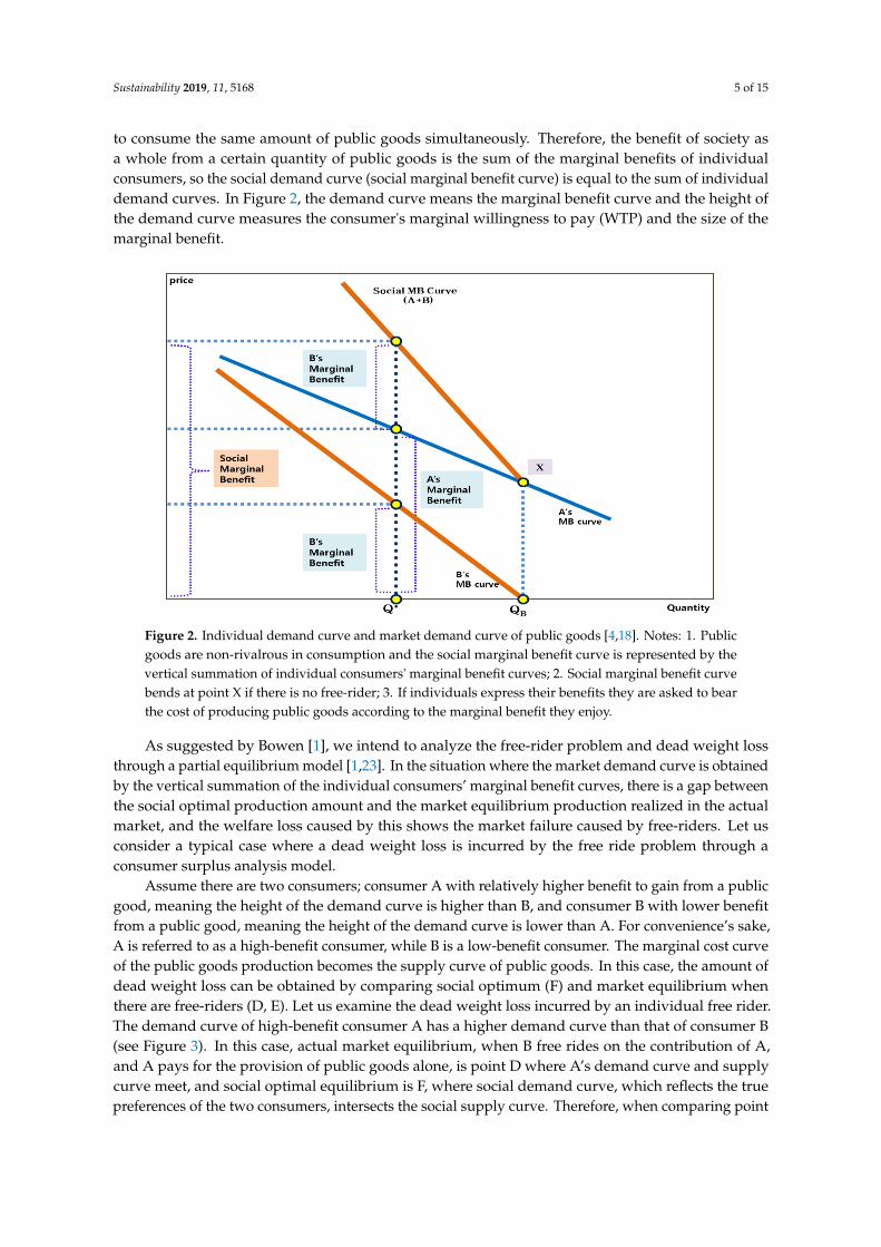
to consume the same amount of public goods simultaneously. Therefore, the benefit of society asa whole from a certain quantity of public goods is the sum of the marginal benefits of individualconsumers, so the social demand curve (social marginal benefit curve) is equal to the sum of individualdemand curves. In Figure 2, the demand curve means the marginal benefit curve and the height ofthe demand curve measures the consumer's marginal willingness to pay (WTP) and the size of themarginal benefit.

Sustainability 2017, 9, x FOR PEER REVIEW 5 of 15

mentioned, the consumption of public goods are non-rivalrous, and it is possible for different

consumers to consume the same amount of public goods simultaneously. Therefore, the benefit of

society as a whole from a certain quantity of public goods is the sum of the marginal benefits of

individual consumers, so the social demand curve (social marginal benefit curve) is equal to the sum

of individual demand curves. In Figure 2, the demand curve means the marginal benefit curve and

the height of the demand curve measures the consumer's marginal willingness to pay (WTP) and the

size of the marginal benefit.

As suggested by Bowen [1], we intend to analyze the free-rider problem and dead weight loss

through a partial equilibrium model [1,23]. In the situation where the market demand curve is

obtained by the vertical summation of the individual consumers’ marginal benefit curves, there is a

gap between the social optimal production amount and the market equilibrium production realized

in the actual market, and the welfare loss caused by this shows the market failure caused by free-

riders. Let us consider a typical case where a dead weight loss is incurred by the free ride problem

through a consumer surplus analysis model.

Figure 2. Individual demand curve and market demand curve of public goods [4,18]. Notes: 1. Public

goods are non-rivalrous in consumption and the social marginal benefit curve is represented by the

vertical summation of individual consumers' marginal benefit curves; 2. Social marginal benefit curve

bends at point X if there is no free-rider; 3. If individuals express their benefits they are asked to bear

the cost of producing public goods according to the marginal benefit they enjoy.

Assume there are two consumers; consumer A with relatively higher benefit to gain from a

public good, meaning the height of the demand curve is higher than B, and consumer B with lower

benefit from a public good, meaning the height of the demand curve is lower than A. For

convenience’s sake, A is referred to as a high-benefit consumer, while B is a low-benefit consumer.

The marginal cost curve of the public goods production becomes the supply curve of public goods.

In this case, the amount of dead weight loss can be obtained by comparing social optimum (F) and

market equilibrium when there are free-riders (D, E). Let us examine the dead weight loss incurred

by an individual free rider. The demand curve of high-benefit consumer A has a higher demand

curve than that of consumer B (see Figure 3). In this case, actual market equilibrium, when B free

rides on the contribution of A, and A pays for the provision of public goods alone, is point D where

A’s demand curve and supply curve meet, and social optimal equilibrium is F, where social demand

curve, which reflects the true preferences of the two consumers, intersects the social supply curve.

Figure 2. Individual demand curve and market demand curve of public goods [4,18]. Notes: 1. Publicgoods are non-rivalrous in consumption and the social marginal benefit curve is represented by thevertical summation of individual consumers' marginal benefit curves; 2. Social marginal benefit curvebends at point X if there is no free-rider; 3. If individuals express their benefits they are asked to bearthe cost of producing public goods according to the marginal benefit they enjoy.

As suggested by Bowen [1], we intend to analyze the free-rider problem and dead weight lossthrough a partial equilibrium model [1,23]. In the situation where the market demand curve is obtainedby the vertical summation of the individual consumers’ marginal benefit curves, there is a gap betweenthe social optimal production amount and the market equilibrium production realized in the actualmarket, and the welfare loss caused by this shows the market failure caused by free-riders. Let usconsider a typical case where a dead weight loss is incurred by the free ride problem through aconsumer surplus analysis model.

Assume there are two consumers; consumer A with relatively higher benefit to gain from a publicgood, meaning the height of the demand curve is higher than B, and consumer B with lower benefitfrom a public good, meaning the height of the demand curve is lower than A. For convenience’s sake,A is referred to as a high-benefit consumer, while B is a low-benefit consumer. The marginal cost curveof the public goods production becomes the supply curve of public goods. In this case, the amount ofdead weight loss can be obtained by comparing social optimum (F) and market equilibrium whenthere are free-riders (D, E). Let us examine the dead weight loss incurred by an individual free rider.The demand curve of high-benefit consumer A has a higher demand curve than that of consumer B(see Figure 3). In this case, actual market equilibrium, when B free rides on the contribution of A,and A pays for the provision of public goods alone, is point D where A’s demand curve and supplycurve meet, and social optimal equilibrium is F, where social demand curve, which reflects the truepreferences of the two consumers, intersects the social supply curve. Therefore, when comparing point

Sustainability 2019, 11, 5168 6 of 15

F, where social welfare is maximized, and the actual market equilibrium D, it is evident that socialwelfare decreases by 4ADF at point D.

Sustainability 2017, 9, x FOR PEER REVIEW 6 of 15

Therefore, when comparing point F, where social welfare is maximized, and the actual market

equilibrium D, it is evident that social welfare decreases by △ADF at point D.

On the other hand, when A free-rides on B’s contribution and B pays for all the provision cost

of the public good, actual market equilibrium is point E, where B’s demand curve and supply curve

meet. Thus, comparison of point F, where social welfare is maximized, and the actual market

equilibrium E, shows that social welfare decreases △HEF at point E due to B’s free ride. In this case,

the dead weight loss incurred when a high-benefit consumer A free rides is greater than that of a low-

benefit consumer B (△ADF＞△HEF).

Figure 3. Market failure and dead weight loss by the free-rider. Notes: 1. Point B is production when

Consumer B’s benefit is zero; 2. Point D is Market equilibrium reached when A free-rides and B pays

for all the cost; 3. Point E is Market equilibrium reached when B free-rides and A pays for all the cost;

4. Point F is Social welfare that is maximized when there is no free-rider.

In short, classical welfare economics conclude that when a consumer free-rides, concealing his

or her benefit and distorting social benefits, it leads to under-provision of public goods at the level

lower than is required to maximize social welfare, incurring dead weight losses. This result justifies

the argument of the traditional public economics that the government should intervene with policy

measures to reach the optimal social welfare level (point F in the figure) to address dead weight losses

associated with the free-rider problem [2,7,31]. However, further research is required to understand

if free-riding always incurs dead weight losses, or, in other words, causes undesirable results in terms

of economic efficiency. The next section examines the cases of free-riding, where there is no loss in

economic efficiency or dead weight losses, from the perspective of welfare economics.

3.3. Why Does Free-Riding Incur Dead Weight Losses?

To begin with, why does a free rider generate dead weight losses? In this example, the reason is

that the actual market equilibrium (point D and E) is positioned to the left of the bending point (point

X) of the social marginal benefit curve. A closer look at Figure 4 reveals that in the section where there

is a gap between the height of the social marginal benefit curve and that of Consumer A’s marginal

benefit curve (left of point X), optimum balance, or maximum social welfare (point F) is reached at

the intersection of the supply curve, and the provision of public goods differ between optimum

Figure 3. Market failure and dead weight loss by the free-rider. Notes: 1. Point B is production whenConsumer B’s benefit is zero; 2. Point D is Market equilibrium reached when A free-rides and B paysfor all the cost; 3. Point E is Market equilibrium reached when B free-rides and A pays for all the cost; 4.Point F is Social welfare that is maximized when there is no free-rider.

On the other hand, when A free-rides on B’s contribution and B pays for all the provision cost ofthe public good, actual market equilibrium is point E, where B’s demand curve and supply curve meet.Thus, comparison of point F, where social welfare is maximized, and the actual market equilibrium E,shows that social welfare decreases 4HEF at point E due to B’s free ride. In this case, the dead weightloss incurred when a high-benefit consumer A free rides is greater than that of a low-benefit consumerB (∆ADF > ∆HEF).

In short, classical welfare economics conclude that when a consumer free-rides, concealing hisor her benefit and distorting social benefits, it leads to under-provision of public goods at the levellower than is required to maximize social welfare, incurring dead weight losses. This result justifiesthe argument of the traditional public economics that the government should intervene with policymeasures to reach the optimal social welfare level (point F in the figure) to address dead weight lossesassociated with the free-rider problem [2,7,31]. However, further research is required to understand iffree-riding always incurs dead weight losses, or, in other words, causes undesirable results in termsof economic efficiency. The next section examines the cases of free-riding, where there is no loss ineconomic efficiency or dead weight losses, from the perspective of welfare economics.

3.3. Why Does Free-Riding Incur Dead Weight Losses?

To begin with, why does a free rider generate dead weight losses? In this example, the reason isthat the actual market equilibrium (point D and E) is positioned to the left of the bending point (point X)of the social marginal benefit curve. A closer look at Figure 4 reveals that in the section where thereis a gap between the height of the social marginal benefit curve and that of Consumer A’s marginal

Sustainability 2019, 11, 5168 7 of 15

benefit curve (left of point X), optimum balance, or maximum social welfare (point F) is reached at theintersection of the supply curve, and the provision of public goods differ between optimum balance Fand actual market equilibrium D and E, generating dead weight losses. In other words, social welfare,the sum of consumer surplus and producer surplus, is maximized at optimum balance point F wherethe supply is QF, due to the free-rider problem, production is determined at actual market equilibriumD and E, where production QD and QE are lower than social optimal production quantity. Therefore,the size of social welfare through the market equilibrium (D, E) is smaller than the maximized socialwelfare at point F, by 4ADF and 4HEF, respectively (see Figure 3).

Sustainability 2017, 9, x FOR PEER REVIEW 7 of 15

balance F and actual market equilibrium D and E, generating dead weight losses. In other words,

social welfare, the sum of consumer surplus and producer surplus, is maximized at optimum balance

point F where the supply is QF, due to the free-rider problem, production is determined at actual

market equilibrium D and E, where production QD and QE are lower than social optimal production

quantity. Therefore, the size of social welfare through the market equilibrium (D, E) is smaller than

the maximized social welfare at point F, by △ADF and △HEF, respectively (see Figure 3).

3.4. Possibility of Free Riding without Dead Weight Losses

Shin [12] suggests that there are cases in which free-riding does not lead to dead weight loss,

unlike the conventional argument. Let us assume that low-benefit consumer C free-rides on the

contribution of high-benefit consumer A, who pays for all the provisional costs of a public good (see

Figure 4). In this case, the bending point of the social benefit curve (point Y) is located to the right of

market equilibrium and is reached when there is free-riding (point E) and the location and shape of

demand-supply curves for the public good becomes different than usual. When point E, where public

goods supply curve intersects with high-benefit consumer A’s demand curve, is located to the right

of the bending point (Y), point E becomes the actual market equilibrium1 and social optimum (welfare

maximization), simultaneously, although low-benefit consumer C free-rides. Unlike the case

explored in Figure 4, social welfare can be maximized at the market equilibrium where consumer C

free-rides and only consumer A’s demand is expressed. That is, as social welfare is maximized at the

actual market equilibrium, there are no dead weight losses.

Figure 4. Free-riding without dead weight losses. Notes: 1. Point C is production when Consumer C’s

benefit is zero; 2. Point E is Market equilibrium reached when C free-rides and A pays for all the cost;

3. Point G is Market equilibrium reached when A free-rides and Consumer C pays for all the cost.

Figure 4 shows that the actual market equilibrium E, where demand curve for A—whose

demand is expressed—and public goods supply curve meet when C free-rides, is located to the right

of the bending point Y of the social marginal benefit curve. In this case, unlike in the case illustrated

in Figure 3, the social benefit curve bends in the left of market equilibrium E and there is no gap

between the actual market equilibrium and social optimum welfare, the two points are identical

because high-benefit consumer A’s demand curve corresponds to the social demand curve to the

right of the bending point Y.

Figure 4. Free-riding without dead weight losses. Notes: 1. Point C is production when Consumer C’sbenefit is zero; 2. Point E is Market equilibrium reached when C free-rides and A pays for all the cost; 3.Point G is Market equilibrium reached when A free-rides and Consumer C pays for all the cost.

3.4. Possibility of Free Riding without Dead Weight Losses

Shin [12] suggests that there are cases in which free-riding does not lead to dead weight loss,unlike the conventional argument. Let us assume that low-benefit consumer C free-rides on thecontribution of high-benefit consumer A, who pays for all the provisional costs of a public good(see Figure 4). In this case, the bending point of the social benefit curve (point Y) is located to the rightof market equilibrium and is reached when there is free-riding (point E) and the location and shape ofdemand-supply curves for the public good becomes different than usual. When point E, where publicgoods supply curve intersects with high-benefit consumer A’s demand curve, is located to the right ofthe bending point (Y), point E becomes the actual market equilibrium1 and social optimum (welfaremaximization), simultaneously, although low-benefit consumer C free-rides. Unlike the case exploredin Figure 4, social welfare can be maximized at the market equilibrium where consumer C free-ridesand only consumer A’s demand is expressed. That is, as social welfare is maximized at the actualmarket equilibrium, there are no dead weight losses.

Figure 4 shows that the actual market equilibrium E, where demand curve for A—whose demandis expressed—and public goods supply curve meet when C free-rides, is located to the right of thebending point Y of the social marginal benefit curve. In this case, unlike in the case illustrated inFigure 3, the social benefit curve bends in the left of market equilibrium E and there is no gap betweenthe actual market equilibrium and social optimum welfare, the two points are identical because

Sustainability 2019, 11, 5168 8 of 15

high-benefit consumer A’s demand curve corresponds to the social demand curve to the right of thebending point Y.

On the other hand, in the case where low-benefit consumer C’s demand is expressed andhigh-benefit consumer A free-rides, social welfare loss becomes larger than that of Figure 4. This isbecause when high-benefit consumers free-ride, there is a gap between the actual market equilibriumG and social optimum E, and production of public goods at point G does not reach that of the socialoptimum point E (See notes in Figure 5 for the size of dead weight loss).

Sustainability 2017, 9, x FOR PEER REVIEW 8 of 15

On the other hand, in the case where low-benefit consumer C’s demand is expressed and high-

benefit consumer A free-rides, social welfare loss becomes larger than that of Figure 4. This is because

when high-benefit consumers free-ride, there is a gap between the actual market equilibrium G and

social optimum E, and production of public goods at point G does not reach that of the social

optimum point E (See notes in Figure 5 for the size of dead weight loss).

Figure 5. Relationship between free-riding and dead weight loss. Notes: 1. Point C is production when

Consumer C’s benefit is zero; 2. Point D is Market equilibrium reached when A free-rides and B pays

for all the cost; 3. Point G is Market equilibrium reached when A free-rides and C pays for all the cost;

4. Point F is Social welfare is maximized and there is no free ride for A or B; 5. Point E is Low-benefit

consumer B and C free-ride and A pays for all the cost. Dead weight loss incurs (△EFH) when

Consumer B free-rides, but not at point E where Consumer C free-rides.

Figure 5 shows Figure 3, where free-riding incurs dead weight loss, and Figure 4, the case of

free-riding without dead weight loss, simultaneously. If a high-benefit consumer is A and low-benefit

consumer who free-rides is B, the social marginal benefit curve bends at point X. Therefore, actual

market equilibrium is inconsistent with social optimum (E ≠ F), and the production of public goods

at the actual market equilibrium QE is smaller than social optimum production QF, creating dead

weight loss of △EFH. On the other hand, when low-benefit consumer C free-rides, the social marginal

benefit curve bends at point Y. Therefore, social welfare is at its maximum at the actual market

equilibrium (E) where only A’s demand curve is considered, because social marginal benefit curve is

the same as high-benefit consumer A’s demand curve on the right of point Y. In other words, if the

low-benefit consumer who free-rides is C, rather than B, the QE that is supplied from the actual market

equilibrium becomes the production maximizing the social welfare immediately. Thus, dead weight

loss is not incurred. On the other hand, if A free-rides on C, a larger dead weight loss is incurred than

when A free-rides on B, which has already been explained in Figure 4.

In conclusion, whether dead weight loss will be created due to free-riding or not, depends on

the relative position of the bending point on the social marginal benefit curve (demand curve for the

public good), whether it is located to the left or right of the actual market equilibrium E. Given this,

what are the conditions for low-benefit consumers’ free-riding not to incur social welfare loss? X-

coordinate for bending points (Y, X) on the social marginal benefit curve means demand where low-

Figure 5. Relationship between free-riding and dead weight loss. Notes: 1. Point C is productionwhen Consumer C’s benefit is zero; 2. Point D is Market equilibrium reached when A free-rides and Bpays for all the cost; 3. Point G is Market equilibrium reached when A free-rides and C pays for allthe cost; 4. Point F is Social welfare is maximized and there is no free ride for A or B; 5. Point E isLow-benefit consumer B and C free-ride and A pays for all the cost. Dead weight loss incurs (4EFH)when Consumer B free-rides, but not at point E where Consumer C free-rides.

Figure 5 shows Figure 3, where free-riding incurs dead weight loss, and Figure 4, the case offree-riding without dead weight loss, simultaneously. If a high-benefit consumer is A and low-benefitconsumer who free-rides is B, the social marginal benefit curve bends at point X. Therefore, actualmarket equilibrium is inconsistent with social optimum (E , F), and the production of public goods atthe actual market equilibrium QE is smaller than social optimum production QF, creating dead weightloss of 4EFH. On the other hand, when low-benefit consumer C free-rides, the social marginal benefitcurve bends at point Y. Therefore, social welfare is at its maximum at the actual market equilibrium(E) where only A’s demand curve is considered, because social marginal benefit curve is the same ashigh-benefit consumer A’s demand curve on the right of point Y. In other words, if the low-benefitconsumer who free-rides is C, rather than B, the QE that is supplied from the actual market equilibriumbecomes the production maximizing the social welfare immediately. Thus, dead weight loss is notincurred. On the other hand, if A free-rides on C, a larger dead weight loss is incurred than when Afree-rides on B, which has already been explained in Figure 4.

In conclusion, whether dead weight loss will be created due to free-riding or not, depends onthe relative position of the bending point on the social marginal benefit curve (demand curve for

Sustainability 2019, 11, 5168 9 of 15

the public good), whether it is located to the left or right of the actual market equilibrium E. Giventhis, what are the conditions for low-benefit consumers’ free-riding not to incur social welfare loss?X-coordinate for bending points (Y, X) on the social marginal benefit curve means demand wherelow-benefit consumers’ marginal benefit (or WTP) becomes 0 (QC, QB), F means social optimum wheresocial marginal benefit curve intersects marginal cost curve and the social optimum production is QF.Under the circumstances, the conditions for low-benefit consumer C’s free-riding not to incur deadweight loss, can be formulated as discussed below.

Let’s assume the marginal benefit curve of consumer A enjoying a relatively high benefit from acertain public good, consumer C enjoying a relatively low benefit, and producer, as MBA = MBA(Q),MBC = MBC(Q), MC = MC(Q), respectively. Market equilibrium E satisfies MBA(Q) = MC(Q). Andwhere low-benefit consumer C free-rides without dead weight loss and high-benefit consumer A bearsall the cost, the production at market equilibrium E is QE. Meanwhile, production where low-benefitconsumer C’s marginal benefit becomes 0 (MBC(Q) = 0), is QC, which is also production at point Ywhere the social marginal benefit curve bends.

As mentioned above, when low-benefit group C free-rides on the contribution of high-benefitgroup A and there is no dead weight loss, point E corresponds to the actual market equilibrium andsocial optimum for maximization of social welfare and should be located to the right of bending pointY on the social benefit curve. This means the production that makes low-benefit consumer C’s marginalbenefit 0, needs to be the same as social optimum production or smaller, as represented as QC ≤ QE.From the discussion above, it is evident that the incurring of dead weight loss is determined by therelative position of demand (X-intercept on the demand curve) making low-benefit consumer’s WTP0, which is the shape of the demand curve (marginal benefit curve) of low-benefit consumer, ratherthan supply side factors such as the slope or position of the supply curve (marginal cost curve) for thepublic good. And the Condition for free-riding without dead weight losses is as follows.

Sustainability 2017, 9, x FOR PEER REVIEW 9 of 15

benefit consumers’ marginal benefit (or WTP) becomes 0 (QC, QB), F means social optimum where

social marginal benefit curve intersects marginal cost curve and the social optimum production is QF.

Under the circumstances, the conditions for low-benefit consumer C’s free-riding not to incur dead

weight loss, can be formulated as discussed below.

Let’s assume the marginal benefit curve of consumer A enjoying a relatively high benefit from a

certain public good, consumer C enjoying a relatively low benefit, and producer, as MBA = MBA(Q),

MBC = MBC(Q), MC = MC(Q), respectively. Market equilibrium E satisfies MBA(Q) = MC(Q). And

where low-benefit consumer C free-rides without dead weight loss and high-benefit consumer A

bears all the cost, the production at market equilibrium E is QE. Meanwhile, production where low-

benefit consumer C’s marginal benefit becomes 0 (MBC(Q) = 0), is QC, which is also production at

point Y where the social marginal benefit curve bends.

As mentioned above, when low-benefit group C free-rides on the contribution of high-benefit

group A and there is no dead weight loss, point E corresponds to the actual market equilibrium and

social optimum for maximization of social welfare and should be located to the right of bending point

Y on the social benefit curve. This means the production that makes low-benefit consumer C’s

marginal benefit 0, needs to be the same as social optimum production or smaller, as represented as

QC ≤ QE. From the discussion above, it is evident that the incurring of dead weight loss is determined

by the relative position of demand (X-intercept on the demand curve) making low-benefit consumer’s

WTP 0, which is the shape of the demand curve (marginal benefit curve) of low-benefit consumer,

rather than supply side factors such as the slope or position of the supply curve (marginal cost curve)

for the public good. And the Condition for free-riding without dead weight losses is as follows.

3.5. Free-Rider Problem in the Relationship between Consumer Groups

We assumed the existence of two consumers above and examined the special case where free-

riding with public goods does not incur a dead weight loss. If this is applied to the relationship

between the two groups of consumers, such an analysis will be able to provide practical implications

for creating and implementing public policies. For the convenience of analysis, let us introduce the

following assumptions.

3.5.1. Assumption 1: Divisibility of Consumer Groups

It is assumed that the consumers of a public good can be divided into two groups by the size of

benefits from consuming the public good. In this case, the demand curve of each group becomes a

collective demand curve that combines the marginal benefits of the individuals in the group.

3.5.2. Assumption 2: Linear Demand Function Moving Down and Right

It is assumed the demand function is a linear function moving down and to the right. Also, it is

supposed that the demand curves of different groups do not intersect. In other words, the demand

of the low-benefit group is always lower than that of the high-benefit group in all sections of demand

for the public good. As before, groups which enjoy relatively high or low benefits, are referred to as

the high-benefit group and the low-benefit group, respectively.

Condition for free-riding that do not involve deadweight losses MBA = MBA(Q), MBC = MBC(Q), MC = MC(Q), where consumer A and C exist.

Point E: Production at market equilibrium, where low-benefit consumer C free-riding without

dead weight loss

QE: high-benefit consumer A bears all the cost, which satisfies MBA(Q) = MC(Q)

QC: production where low-benefit consumer C’s marginal benefit becomes 0,

i.e. MBC (Q) = 0, Then the Condition where free-riding of low-benefit consumer does not

cause dead weight loss, can be formulated as [QC ≤ QE ]

3.5. Free-Rider Problem in the Relationship between Consumer Groups

We assumed the existence of two consumers above and examined the special case where free-ridingwith public goods does not incur a dead weight loss. If this is applied to the relationship betweenthe two groups of consumers, such an analysis will be able to provide practical implications forcreating and implementing public policies. For the convenience of analysis, let us introduce thefollowing assumptions.

3.5.1. Assumption 1: Divisibility of Consumer Groups

It is assumed that the consumers of a public good can be divided into two groups by the size ofbenefits from consuming the public good. In this case, the demand curve of each group becomes acollective demand curve that combines the marginal benefits of the individuals in the group.

Sustainability 2019, 11, 5168 10 of 15

3.5.2. Assumption 2: Linear Demand Function Moving Down and Right

It is assumed the demand function is a linear function moving down and to the right. Also, it issupposed that the demand curves of different groups do not intersect. In other words, the demand ofthe low-benefit group is always lower than that of the high-benefit group in all sections of demand forthe public good. As before, groups which enjoy relatively high or low benefits, are referred to as thehigh-benefit group and the low-benefit group, respectively.

3.5.3. Assumption 3: Possibility of Allowing Free-Riding by Expressed Preferencesand Policy Selection

It is assumed that the preferences of the two groups can be learned accurately. And intentionalfree-riding is impossible while free riding is possible only by government’s public policy choice orsocial agreement.

Under these assumptions, previous discussions about free-riding between two consumers, can beapplied to the relationship between two groups. As shown in Figure 5, the social marginal benefitcurve bends at the point of public goods production where the low-benefit group C’s marginal benefit(or WTP) becomes 0, and optimum balance E is positioned on the right of the bending point whichintersects the marginal cost curve. Therefore, there is no gap between social optimum and the actualmarket equilibrium, and no dead weight loss incurred despite the free-riding of group C.

As demonstrated in Figure 6, let’s assume the existence of two consumer groups, A and C. And themarginal benefit curve of consumer group A enjoying a relatively high benefit from a certain publicgood, consumer group C enjoys a relatively low benefit, and producer, as MBA = MBA(Q), MBC =

MBC(Q), MC = MC(Q), respectively.

Sustainability 2017, 9, x FOR PEER REVIEW 10 of 15

3.5.3. Assumption 3: Possibility of Allowing Free-Riding by Expressed Preferences and Policy

Selection

It is assumed that the preferences of the two groups can be learned accurately. And intentional

free-riding is impossible while free riding is possible only by government’s public policy choice or

social agreement.

Under these assumptions, previous discussions about free-riding between two consumers, can

be applied to the relationship between two groups. As shown in Figure 5, the social marginal benefit

curve bends at the point of public goods production where the low-benefit group C’s marginal benefit

(or WTP) becomes 0, and optimum balance E is positioned on the right of the bending point which

intersects the marginal cost curve. Therefore, there is no gap between social optimum and the actual

market equilibrium, and no dead weight loss incurred despite the free-riding of group C.

As demonstrated in Figure 6, let’s assume the existence of two consumer groups, A and C. And

the marginal benefit curve of consumer group A enjoying a relatively high benefit from a certain

public good, consumer group C enjoys a relatively low benefit, and producer, as MBA = MBA(Q), MBC

= MBC(Q), MC = MC(Q), respectively.

Figure 6. Cases of free-riding between groups with no dead weight loss. Notes: There is no dead

weight loss at point E where low-benefit Group C free-rides and high-benefit Group A pays for all

the cost. In contrast, there is considerably large dead weight loss incurred at point G where high-

benefit Group A free-rides and low-benefit Group C pays for all the cost.

As explained in section 3.4., at point E, where low-benefit consumer group C free-rides without

dead weight loss, high-benefit consumer group A bears all the cost. At point QE, the condition,

MBA(Q) = MC(Q) is satisfied. Meanwhile, the production where low-benefit consumer group C’s

marginal benefit becomes 0 (MBC(Q) = 0), is QC, which is also production at point Y where social

marginal benefit curve is refracted. When low-benefit group C free-rides on the contribution of high-

benefit group A and there is no dead weight loss, point E equals the actual market equilibrium (i.e.

social optimum), and should be located to the right-side of bending point Y on the social benefit

curve. As mentioned above, the production where low-benefit consumer group C’s marginal benefit

equal zero, meets the condition of QC ≤ QE. And this condition [QC ≤ QE] is the same as that of section

3.4.

Figure 6. Cases of free-riding between groups with no dead weight loss. Notes: There is no deadweight loss at point E where low-benefit Group C free-rides and high-benefit Group A pays for all thecost. In contrast, there is considerably large dead weight loss incurred at point G where high-benefitGroup A free-rides and low-benefit Group C pays for all the cost.

Sustainability 2019, 11, 5168 11 of 15

As explained in Section 3.4, at point E, where low-benefit consumer group C free-rides withoutdead weight loss, high-benefit consumer group A bears all the cost. At point QE, the condition, MBA(Q)= MC(Q) is satisfied. Meanwhile, the production where low-benefit consumer group C’s marginalbenefit becomes 0 (MBC(Q) = 0), is QC, which is also production at point Y where social marginalbenefit curve is refracted. When low-benefit group C free-rides on the contribution of high-benefitgroup A and there is no dead weight loss, point E equals the actual market equilibrium (i.e. socialoptimum), and should be located to the right-side of bending point Y on the social benefit curve. Asmentioned above, the production where low-benefit consumer group C’s marginal benefit equal zero,meets the condition of QC ≤ QE. And this condition [QC ≤ QE] is the same as that of Section 3.4.

As demonstrated in Figure 5, whether dead weight loss will be created between groups, is alsodetermined by the relative positions of bending points (X, Y) on the social marginal benefit curveand the actual market equilibrium E. Not only that, the difference in marginal benefits between thetwo groups is bigger in the case where there is no dead weight loss than where the low-benefit groupfree-rides and incurs a dead weight loss. In Figure 5, comparing low-benefit group C (no dead weightloss) and low-benefit group B, shows that the height difference in demand curves between A andC, is larger than that between A and B; indicating that whether dead weight loss will be created isdetermined by the relative positions of the demand curve of the low-benefit groups and resultant heightdifference between high-benefit group A and low-benefit group B, C. It is also clear that the differencein height of the demand curves between the two groups is much bigger when there is no dead weightloss. This means that the height difference in the demand curves between A and C, is much largerthan that between A and B when the free-rider problem does not cause losses in economic efficiency.Given that the height of the demand curves of the two groups is more different when there is no deadweight loss, it is plausible to think that the higher the difference in benefits between the two groupswith different income levels, the higher the possibility of free-riding not causing dead weight losses.

4. Discussion

As mentioned before, conventional economics assumes that free-riding incurs social inefficiency(dead weight loss) and several economists focused on the exogenous solutions based under this veryassumption. As opposed to the conventional belief, this study proposes the possibility, formularizedconditions and policy implications of the case on free-riding with no dead weight loss.

4.1. Possibility of Pursuing the Conflicting Values, Equity and Efficiency, at the Same Time

When a consumer free-rides on the contribution of others to use public goods, it leads tounder-provision of public goods at the level lower than is required to maximize social welfare,incurring dead weight losses. However, there are cases where free-riding does not cause a dead weightloss. This was confirmed through the consumer surplus analysis above; if the production at the pointwhere the benefit of a consumer group which enjoys relatively low benefit, becomes 0,2 is the sameas that of market equilibrium (QE), or smaller, social optimum balance is identical with the actualmarket equilibrium. Then what are the public policy implications of this situation where free-ridersdo not cause dead weight losses and can be justified in terms of economic efficiency? If free-ridersdo not inflict losses in social welfare, it is possible to produce and provide public goods to reachsocial optimum where all consumers can enjoy benefits without burdening every consumer with theproduction cost of the public goods. To be brief, it is possible to maximize economic efficiency ofcreating a maximum benefit at minimum cost.

On the other hand, there would be a problem of social equity or fairness for those consumingpublic goods without paying for them. Furthermore, we cannot rule out the possibility that somemay conceal their preferences for public goods strategically causing dead weight losses, which cannegatively influence the general public goods market.

Lakner and Milanovic [32] stated that the inequality of global income distribution gradually rosebetween 1988 and 2008, showing a pattern of polarization between the rich and the lower-income group.

Sustainability 2019, 11, 5168 12 of 15

Furthermore, this trend is becoming increasingly serious. Supply of public goods has a big impact onincome distribution. Governments can spend income redistribution to strengthen social equity, butthey can consider particular consumer groups by controlling the types and amounts of public goodsthat finance them. Given the worsening income polarization, it is all the more important to pursuemeasures to enhance social (distributional) equality between groups and classes by implementingpublic policies for fair distribution without hampering economic efficiency. It is the same for the supplyof public goods. If consumers with lower income level are allowed to benefit from free riding on thecost burden of those with higher income, desirable allocation of resources from the perspective ofsocial equity may be the result. Nevertheless, in terms of economic efficiency, free riding causes adead weight loss and wasted resources. In this case, if the underprivileged is allowed to free ridein the name of social equity to justify the loss of economic efficiency, it will be very unlikely to beimplemented as a policy because of many controversies and conflicts it will spark.

4.2. Relationship between Income Levels and the Size of Benefits from Public Goods

Then what determines the difference in marginal benefit between groups in relation to theconditions for not causing dead weight loss? This can be primarily seen as the standard to divide theconsumers into two groups. If the two groups are divided by the income levels, government needsto identify the influences of the income level on marginal benefits gained from public goods. It isnecessary to consider if the public goods’ demand curve is higher, in other words, the benefit frompublic goods is bigger as the income level becomes higher.

A higher income level means higher benefit from public goods where those with higher incomelevels can get more help than those with lower incomes, from the services of public goods in protectingand managing their assets or income, or in consuming and enjoying them. On the other hand, having alower income level means benefitting more from public goods, when those with lower income levelsuse their income to buy quality private goods as a substitute for public goods. For instance, there ispublic transportation service (although it is not a pure public good, but a quasi-public good chargingfare) [30]. High-income earners are likely to benefit less from public transportation as they possess theirown cars while low-income earners are likely to benefit relatively more from the public transportationservice as they do not possess their own cars or do not use them as frequently. If it is true that thosewith higher income levels are more likely to enjoy greater benefits, it is more likely for those withlower income level to form a low-benefit group. This means more room for [i]considering those in thelow-income bracket while achieving economic efficiency, in other words, allowing them to free ridewhen using public goods.

Table 1 presents the result of the analysis of actual data.3 In 2016 Korean General Social Survey(KGSS), items asking the perception about the government performance by functions, were used.Government activities can be seen as police services provided by the government and the degree ofperformance was set as a proxy variable to represent the level of satisfaction with the public service.Government performance in the function of crime control (security) is shown in Table 1. The resultshows that the higher the income level the higher the benefit from the police services and the coefficientis significant (0.016).

Sustainability 2019, 11, 5168 13 of 15

Table 1. Evaluation of government performance in police services.

Independent Variables Regression Coefficient t-Value Significance Probability(P > t)

Gender (male = 1) 0.315 *** 4.650 0.000

Age 0.009 *** 3.390 0.001

Marital status (married = 1) 0.031 0.420 0.675

Job (employed = 1) −0.161 ** −2.330 0.020

Middle school graduate 0.101 0.680 0.498

High school graduate −0.111 −0.920 0.357

College graduate −0.272 * −1.730 0.085

University or higher −0.076 −0.580 0.562

Self-reported income level 0.049 ** 2.410 0.016

_cons 2.003 9.250 0.000

Note: * p < 0.1, ** p < 0.05, *** p < 0.01.

The findings indicate that the income gap is likely to be greater as the gap between benefits isbigger, which means that low-benefit groups may free ride without causing market failure. Not onlythat, if the condition of [QC ≤ QE] is satisfied and the low-benefit group has lower income than thehigh-benefit group, it is possible to reach a conclusion that allowing free-rider may help promote socialequity without reducing economic efficiency.

4.3. Contribution to the Academic Literature and Further Study

This study expands the existing economic analysis model (Bowen’s Model) to validate thatthere are cases for which conventional theories are unable to account (i.e. free-riding case withoutmarket failure). Furthermore, those exceptional cases and their conditions grant us some significantimplications, which can help us with pursuing the two conflicting values, equity and efficiencysimultaneously in public goods supply, considering that most of social policies require a huge amountof government expenditure.

On the other hand, this study constructed an analytical model under strict assumptions: divisibilityof consumer groups, linear demand function, allowing free-riding by expressed preferences and policyselection. Thus, future study based on less strict assumptions is needed to derive generalizedconclusions. Furthermore, specific analysis was not carried out to reflect differences in characteristicsof individual public goods, such as whether they are public goods provided by the central governmentor those provided by local governments, and whether the source of resources is national or local taxes.Considering these problems, empirical studies of estimating demand for public goods through the useof contingent valuation method (CVM) are left for future studies.

5. Conclusions

Previously or currently, most studies and arguments adhere to the assumption that free-ridingcauses market failure in public goods supply. But this study took the possibility of free-ridingwithout dead weight loss as the starting point for research. Based on our results, we can suggest away of promoting social equity without hindering economic progress, setting this study apart fromprevious ones.

We demonstrated there are cases where free-riding in public goods does not cause a dead weightloss, unlike the conventional argument that free-riding leads to market failure by creating dead weightlosses, and formulated the conditions. We confirmed that to prevent the incurring of dead weightloss with free-riders, the difference in the demand curve height between high-benefit and low-benefitgroups should be big enough, and the production quantity where marginal benefit of low-benefit

Sustainability 2019, 11, 5168 14 of 15

group becomes 0, should be less than the social optimum. Additionally, it was found that in applyingthis conclusion in implementing public polices, an analytical framework can be provided to seekdesirable public policy alternatives in terms of economic efficiency and fair distribution when thebenefit difference as the criteria for dividing groups is consistent with the income level. In short,the higher the difference in benefits between the two groups with different income levels, the higher thepossibility of free-riding not causing dead weight losses. In this case, we can allow the lower-incomeand lower benefit group to free-ride the other group, thus realizing the value of equity withoutmarket failure.

Social equality is one of the most important values for public policies to pursue. To achieve thisgoal, it should be sometimes inevitable to compromise economic efficiency to a certain degree. In thissense, the research here has a significant implication as it suggests the possibility of satisfying the twoapparently conflicting values, efficiency and equity, simultaneously if there is a way to accomplishsocial equity without reducing economic efficiency.

Notes:1. Since C free-rides without expressing his or her demand, the market equilibrium is formed at

the intersection of the marginal benefit curve of public goods and A’s demand curve.2. This means quantity Qc, which corresponds to the bending point of the social marginal

benefit curve.3. For analysis, 2016 data from Korean General Social Survey by Sungkyunkwan University in

South Korea was used. The survey data is freely available (accumulated data, 2003-2016).

Author Contributions: Conceptualization, K-S.K. and S.J.; Methodology, S.J.; Writing-Original Draft Preparation,K-S.K.; Writing-Review and Editing, S.J.; Validation, S.J.

Funding: This research received no external funding.

Conflicts of Interest: The authors declare no conflicts of interest.

References

1. Bowen, H.R. Toward Social Economy; Rinchart: New York, NY, USA, 1948; pp. 176–195.2. Case, K.E. Musgrave’s Vision of the Public Sector: The Complex Relationship between Individual, Society

and State in Public Good Theory. J. Econ. Financ. 2008, 32, 348–355. [CrossRef]3. Groves, T.; Ledyard, J. Optimal Allocation of Public Goods: A Solution to the “Free-Rider” Problem.

Econometrica 1977, 45, 783–809. [CrossRef]4. Hirschman, A.O. Shifting Involvements: Private Interest and Public Action; Princeton University Press: Princeton,

NJ, USA, 2002.5. Thompson, D. The Proper Role of Government: Considering Public Goods and Private Goods; The Pennsylvania

State University: State College, PA, USA, 2015.6. Coase, R. The Problem of Social Cost. J. Law Econ. 1960, 3, 1–44. [CrossRef]7. Musgrave, R.A. The Theory of Public Finance: A Study in Public Economy; McGraw-Hill: New York, NY, USA,

1959.8. Banzhaf, H.S. The Market for Local Public Goods. Case West. Reserve Law Rev. 2014, 64, 1441–1480.9. Friedman, M.; Rose, D. Capitalism and Freedom; University of Chicago Press: Chicago, Illinois, United States,

1982.10. Tabarrok, A. The private provision of public goods via dominant assurance contracts. Public Choice 1998, 96,

345–362. [CrossRef]11. Dilger, R.J.; Beth, R.S. Unfunded Mandate Reform Act: History, Impact, and Issues; Federal Publications:

Washington, USA, 2013.12. Shin, H.G. Consumer Surplus Analysis for the ‘Tragedy of Free-riding? ’ Korean Policy Stud. Rev. 2016, 25,

221–236.13. Jordahl, H.; Liang, C.Y. Merged municipalities, higher debt: on free-riding and the common pool problem in

politics. Public Choice 2010, 143, 157–172. [CrossRef]

Sustainability 2019, 11, 5168 15 of 15

14. Nordhaus, W. Climate Clubs: Overcoming Free-riding in International Climate Policy. Am. Econ. Rev. 2015,105, 1339–1370. [CrossRef]

15. Thielemann, E. Why Refugee Burden-Sharing Initiatives Fail: Public Goods, Free-Riding and SymbolicSolidarity in the EU. J. Common Mark. Stud. 2018, 56, 63–82. [CrossRef]

16. Fischbacher, U.; Gachter, S. Social Preferences, Beliefs, and the Dynamics of Free Riding in Public GoodsExperiments. Am. Econ. Rev. 2010, 100, 541–556. [CrossRef]

17. Nielsen, U.H.; Tyran, J.-R.; Wengström, E. Second thoughts on free riding. Econ. Lett. 2014, 122, 136–139.[CrossRef]

18. Ellingsen, T.; Paltseva, E. Confining the Coase Theorem: Contracting, Ownership, and Free-Riding.Rev. Econ. Stud. 2016, 83, 547–586. [CrossRef]

19. Bonroy, O.; Garapin, A.; Hamilton, S.F.; Monteiro, D.M.S. Free-riding on product quality in cooperatives:Lessons from an experiment. Am. J. Agric. Econ. 2019, 101, 89–108. [CrossRef]

20. Bucciol, A.; Montinari, N.; Piovesan, M. It Wasn't Me! Visibility and Free Riding in Waste Disposal. Ecol. Econ.2019, 157, 394–401. [CrossRef]

21. Iida, Y.; Schwieren, C. Contributing for Myself, but Free riding for My Group? Ger. Econ. Rev. 2015, 17, 36–47.[CrossRef]

22. McDougal, M.K. Unequal and Unfair: Free Riding in One-Shot Interactions. Sociol. Inq. 2018, 88, 494–509.[CrossRef]

23. Kennedy, M.M.J. Public Finance; PHI Learning Pvt. Ltd.: Delhi, India, 2012; pp. 62–63.24. Mankiw, N.G. Principles of Economics, 6th ed.; Cengage Learning: Boston, MA, USA, 2008; pp. 311–313.25. Rodrigues, J. Where to Draw the Line between the State and Markets? Institutionalist Elements in Hayek’s

Neoliberal Political Economy. J. Econ. Issues 2012, 46, 1007–1033. [CrossRef]26. Baron, D. Morally Motivated Self-regulation. Am. Econ. Rev. 2010, 100, 1299–1329. [CrossRef]27. Bracht, J.; Figuieres, C.; Ratto, M. Relative Performance of Two Simple Incentive Mechanisms in a Public

Goods Experiment. J. Public Econ. 2008, 92, 54–90. [CrossRef]28. Burlando, R.; Guala, F. Heterogeneous Agents in Public Goods Experiments. Exp. Econ. 2005, 8, 35–54.

[CrossRef]29. Nikiforakis, N.; Normann, H. A Comparative Statics Analysis of Punishment in Public-Good Experiments.

Exp. Econ. 2008, 11, 358–369. [CrossRef]30. Shin, H.G. ‘Prisoner’s Dilemma’ vs. ‘Consumer Surplus’ As an Analysis of Free-riding. Korean Assoc.

Policy Dev. 2016, 16, 1–23.31. Samuelson, P.A. The Pure Theory of Public Expenditure. Rev. Econ. Stat. 1954, 36, 387–389. [CrossRef]32. Lakner, C.; Milanovic, B. Global Income Distribution from the Fall of the Berlin Wall to the Great Recession; Policy

Research Working Paper 6719; Oxford University Press: Oxford, UK, 2013.

© 2019 by the authors. Licensee MDPI, Basel, Switzerland. This article is an open accessarticle distributed under the terms and conditions of the Creative Commons Attribution(CC BY) license (http://creativecommons.org/licenses/by/4.0/).