Paleodemography: “Not quite dead

92 Evolutionary Anthropology ARTICLES

32 Dausset J, Colombani J (eds) ( I 972) Histo- compatibilitv Testing 1972. Copenhagen: Munksgaard. 33 Terasaki PI (ed) ( 1 980) Histoconipatibilir.y Testing 1980. Los Angeles: UCLA Tissue Typing Laboratory. 34 Albert ED, Baur MP, Mayr WR (eds) ( 1 984) Histocompatibility Testing 1984. Berlin: Sprin- ger-Verlag. 35 Tsuji K, Aizawa M, Sasazuki T (eds) (1 992) HLA 1991, Proceedings ofrlz Eleverith Interna- t io nal Histocompat ih ility Workshop and Con - ference, Volume 1. Oxford: Oxford University Press. 36 Baur MP. Neugebauer M, Albert ED (1984) Reference tablesof two-locus haplotype frequen- cies for all MHC marker loci. In Albert ED, Baur MI: Mayr WR (eds), Histocompatibilitv Testing 1984, pp 677-755. Berlin: Springer-Verlag. 37 Williams RC, Chen SN, Gill DK, Lane JTL,

McAuley JE, Strothman R, Mittal KK (1 989) Antigen Society #6 Report (B21, B49, Bw50, BN21, B12, B44, B45) In Dupont B (ed), Im- munobiology of‘HLA, Volume I , Histocompati- bility Tesrirzg 1987, pp 133-147. New York: Springer-Verlag. 38 Will iams RC, Chen S N , McAuley J E , Richiardi P, D’Alfonso S, Mehra N, McCalmon RT, Tardif G, Strothman R, Knowler WC, Pet- titt DJ (1992) Report of the Antigen Society 106,B21, B49, Bw50.BN21, B12,B44, B45. In TsujiK,AizawaM,SasazukiT(eds), HLA 1991 Proceedings of‘the Eleventh International His- tocompatibilitv Workshop and Conference, Vol- ume 1, pp 305-307. Oxford: Oxford University Press. 39 Hildebrand WH, Madrigal JA, Belich MP, Zemmour J , Ward FE, Williams RC, Parham P (1 992) Serologic cross-reactivities poorly re- flect allelic relationships in the HLA-BIZ and

HLA-B21 groups. J Immunol 149:3563-3568. 40 Kawaguchi G, Hildebrand WH, Hiraiwa M, Karaki S, Nagao T, Akiyama N, Uchida H, Kashiwase K, Akaza T, Williams RC, Juji T, Parham P, Takiguchi M (1992) Two subtypes of HLA-BS/ differing by substitution at posi- t ion 171 of t h e a2 helix. lmmunogenetics 3757-63. 41 Hill AVS, Allsopp CEM, Kwiatkowski D, Anstey NM, Twumasi P, Rowe PA, Bennett S, Brewstcr D, McMichael AJ, Greenwood BM (1991) Common West African HLA antigens a re associated with protection from severe malaria. Nature 352:595400. 42 Tiwari JL, Terasaki PI (1 985) HLA and Dis- eare Associations. New York: Springer-Verlag.

0 1994 Wiley-Liss. Inc

Paleodemography: “Not Quite Dead” LYLE W. KONIGSBERG AND SUSAN R. FRANKENBERG

As Kim Hill’ recently noted in Evolutionary Anthropologj humans are unique among the hominoids with regard to the length of their lives, as well as other ele- ments in the individual life histories. The evolutionary details that modified a basic pongid life history into a hominid one remain obscure, but aspects of recent human demographic history are assailable. Study of the last 10,000 years or so is an important part of ongoing anthropological discourse, for demographic changes may be intimately linked to such major developments as agriculture and Whether demographicchanges are antecedents for or consequences of these major developments is a matter of great contention, but at the least we should attempt to document the nature of human demographic changes in the recent past. Although this documentation can take different forms, the principal sources are archeological information on past settlement patterns and analyses of prehistoric human skeletal material.

Lyle Konigsberg and Susan Frankenberg are, respectively, Assistant Professor and Research Assistant Professor in the Department of Anthropology at the University of Tennessee, Knoxville In addi t ion to paleodemography, their research interests include historical demography U S Eastern Woodland archeology, quantitative genetic analysis, and human skeletal biology Konigsberg is an associate editor for the Amencan Journal of Physlcal Anthropology, the biological/physical anthropology editor for the Journal of Quanttatwe Anfhropology, and the associate editor for physical anthropology for the Tennessee Anthropolog/st

In a scene from the film “Monty Py- thon and the Holy Grail,” a mortally wounded squire to one of King Ar- thur’s knights remarks that he is “not quite dead.” This statement is followed by other comments from the squire: “I think I could pull through” and “Actu- ally, I think I’m all right.” Similar state- ments might be made concerning the general health of paleodemography. Having sustained some crushing blows from various protagonists (see Box l), paleodemography has begun

history, and, indeed, is stronger now for having weathered the criticisms. Rather than having died at the hands of its critics, paleodemography is, like the wounded squire, “not quite dead.” But we should not follow the example of the Black Knight in the same film, who cavalierly dismisses the loss of both arms as “just a flesh wound.” We should not belittle the problems that still lie ahead to be solved in paleode- mograph y.

THE NATURE OF ARCHEOLOGICAL SKELETAL

SAMPLES

In a Panglossian world, all past members of a population could be recovered in archeological samples. In the real world, this probably is never the case. Instead, a number of natural and cultural filters conspire to produce archeological skeletal samples that cannot be considered as random samples of all members of a population who died within a certain period. Natural filters consist of taphonomic processes, which may differentiallv af-

to re-emerge as a vital field that can inform us about human evolutionary

fect the recovery of skeletons by age and ~ex.~.’O Cultural filters include a di-

Key words: Age estimation, hazards analysis, maximum likelihood

ARTICLES Evolutionary Anthropology 93

GLOSSARY Bayes’ Theorem-A classic theorem in

probability theory first published in 1763 by the Reverend Thomas B a y e ~ , ~ ~ which states that the posterior probability is proportional to the product of the prior probability and the likelihood.

Conditional probability-The probability that an event (Ei) will occur if some previous event (E;) has already occurred. Usually written as p(Ei I Ej) and read as “the probability of Ei given El” or “the probability of E, conditional on E;.”

Gompertz function-One of the many distribution functions used to represent continuous age-at-death distributions. It is a special case of the Weibull distribution (see below) with theshape parameter equal to one.

Hazards analysis-The study of hazards functions (instantaneous conditional failure rates). In demography, a hazard function is the probability that an individual a t a particular age will die within an infinitesimally small period. The age-specific probability of death from traditional life-table analysis is analogous to the hazard function, although the time intervals in alife tableare discrete, and the approach is nonpara- metric. As applied in demography, hazards analysis generally approximates the continuously distributed variable “age” with discrete, short time intervals such as weeks, months, or years.

Likelihood-The likelihood of a set of parameters conditional on the observed data, which is usually written as L(8 I x), is proportional to the probability of obtaining the observed data conditional on fixed values for the parameters. Thus, L(8 1 x)-p(x 18. Because likelihoods are used relative to one another (in the sense that we talk about certain values of parameters being more likely than others), the arbitrary constant of proportionality is of no immediate concern.

Joint probability density function, or joint density-The probability of ob-

taining particular values for two or more variables. In the case of age and an indicator, the joint density is the probability that an individual will be a particular age and have a particular value of the indicator.

Logit regression-A particular type of nonlinear regression in which the dependent variable is a probability or rate; therefore, its estimate from the regression must be constrained between zero and one.

Marginal probability density function, o r marginal density-The probability of obtaining particular values of a single variable across all the values of one or more other variables. In the case of age and an indicator, the marginal density of age is simply the probability that an individual will be any particular age.

Prior probability-The unconditional probability of an event, hypothesis, or set of parameters. For example, in paleodemography the prior probability that a randomly selected individual from the reference sample died at a particular age is given by the marginal density of age.

Posterior probability-The conditional probability of an event, hypothesis, or set of parameters. For example, in paleodemography the posterior probability that a randomly selected individual from the target sample died at a particular age is proportional to the product of the prior probability of the age with the likelihood (from the reference sample) that an individual with the observed indicator data would be that particular age.

Rayleigh function-One of many distribution functions used to represent continuous age-at-death distributions. It is a special case of the Weibull distribution (see below) with the shape parameter equal to two.

Weibull function-A general distribution function used to represent continuous age-at-death distributions. It is characterized by both shape and scale parameters (see Hastings and Peacock96).

verse array of factors that can affect the representativeness of skeletal samples. Chief among these factors is dif- ferential mortuary treatment. Biased sex ratios may arise in skeletal samples because one sex is most likely to enter the archeological record in a place or manner that increases its chances of recovery. Similarly, certain age groups may have been treated dif- ferently with respect to interment. Skeletons of infants frequently are under-represented in cemetery samples,‘ either because the bodies were placed elsewhere or because they are

less likely to have been preserved. In rare instances, two or more spatially separate mortuary tracts may be recovered that are patterned by age or sex. This was true, for example at the Averbuch site near Nashville, Tennes- see. Excavation of the three cemeteries associated with the village (Fig. 1A) produced 852 skeletons, among which infants up to the age of one year were subs t a n t i a1 1 y under- represented , whereas excavation of house floors in the village (Fig. 1B) produced 35 skeletons, of which 27 were less than one year old.I2 Figure 1C shows the two

age-at-death distributions for the Averbuch samples (data from Berry- man12) and how the distribution of one sample appears to complement that of the other. Unfortunately, in many archeological cases, we are left with only one segment of the burial population and the knowledge that some people must be missing.

In addition to the cultural factors active at the time of corpse disposal, many other cultural factors can filter the archeological record at later times. Indeed, archeological methods them- selves can substantially alter skeletal samples. For example, archeologists may neglect to locate and recover burials completely or may choose to leave material in situ. Other cultural practices that can have nonrandom effects on skeletal samples are repatria- tion and reburial. The effects of the latter can be expected to increase in the ensuing years, given the current political and legal climate surrounding the excavation and curation of archeologically recovered human skeletal material.

Because of the myriad factors that can affect and ultimately distort the demographic profile of archeological skeletal samples, biological anthropologists who work with this material should be conversant in archeological method and theory, cultural anthropological theory, and such diverse areas as taphonomy and soil science. This directive is hardly novel, emanating as it does from the articulation between the “new archeology” of the 1960s and the developing methods of human skeletal biology.’3 Unfortunately, there are no “magic bullets” that can be uniformly applied to remove the biases caused by biological and cultural filters. Each case is unique and needs to be treated as such. However, if we can assume that these myriad filters on the archeological record can, to some extent, be controlled, at least in a statistical sense, then the next task of paleodemography is to establish the ages-at-death of skeletal remains.

DEATH AND THE SINGLE SKELETON

In a typical forensic anthropology setting, the skeletal remains of a single individual are presented to an expert, whose task is to describe the remains


C

Figure 1 . Photographs of excavations at the Averbuch site and comparison of age-at-death distributions. The site was excavated in 1977 and 1978 by the Department of Anthropology at the University of Tennessee under compliance with the Archaeological and Historic Preservation Act of 1974. Mitigation was necessary because of the impact of housing construction on the site, which was located in a suburban subdivision near Nashville, Tennessee. Averbuch was a large palisaded Mississippian village. the excavation of which revealed three cemetery areas with stone box graves and 22 domestic structures. A) Photograph of one of the burials from a domestic structure. This burial contained the remains of an individual who died within the first half year of life. B) Photograph of cemetery 1 . C) Comparison of age-at-death profiles for skeletons from Averbuch cemeteries (n = 852) and village structures (n = 35). Data are taken from Berryman.12


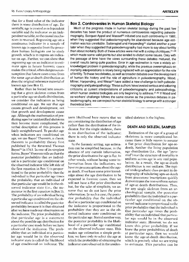
Box 1. Assumptions in Age Estimation Regressing age on an indicator to estimate the age-at-death in aforensiccase

requires the assumption that the forensic sample comes from the same age-at- death distribution as does the reference sample. We prove this here, although we warn readers that some cumbersome notation is necessary, as is a basic

, knowledge of probability theory, calculus, and statistics. A number of the terms used here are defined in the glossary. In this proof, we wish to find the continuous distribution of age (x) for a single skeleton conditional on the observation that the skeleton has a value of yi for a continuous indicator. Using Bayes’ Theorem, this conditional distribution is:

(1 1

j [ f ( K I x) 9 (4 1 dx x=o

where f(y, I x) is the conditional probability from the reference sample that an individual who is age x will have an indicator value of y,, g(x) is the probability density function for age for the forensic skeleton, and the integration is across age until the maximum attainable age of w. Equation 1 can be expanded to:

where f(x) and g(x) are the respective probability density functions for age in the reference sample and for the forensic skeleton, and f(x,y,) is the joint density for age and indicator in the reference sample. In this context, g(x) represents the prior density for age; it is our best guess at the distribution of possible ages from which the individual was selected. This is the prior probability, with our guess made independent of any information about the indicator value.

If we assume that the population from which the forensic skeleton is derived has the same age-at-death distribution as the reference sample, then g(x) = f(x), so that these terms cancel in both the numerator and denominator. The integration in the denominator is then for a joint density across a marginal density, so x integrates out and the denominator is simply f(y,). This leaves us with p(Ny,) = f(x, y,)/f(y,), which is equal to f(xly,); that is, the distribution of age for a single skeleton equals the distribution from the regression of age on indicator in the reference sample. Thus, use of the regression of age on indicator in a reference sample to estimate the age-at-death of a forensic case makes the implicit assumption that the forensic case comes from the same age-at-death distribution as that represented by the reference sample.

If, instead, we assume that the forensic case comes from a uniform age-at- death distribution, then g(x) can be replaced with a constant (such as 7 4 , which can be factored out of the integral and then will cancel with this same constant in the numerator. This leaves the conditional distribution of age on indicator in the target sample as:

(3)

X=O

The denominator represents a “normalizing” factorz3 that makes equation 3 a true density function. Because f(L; 1 x) is the regression of indicator on age, use of this second method to estimate ages only makes the assumption that ages are uniformly distributed. This is a much weaker assumption, for it really is a statement of ignorance. We are saying that without recourse to information from the indicator we cannot make any statement about the age-at-death.

so that they can be matched to a missing individual. In addition to stature and “race,” age and sex are distin- guishing characteristics that limit the number of potential matches. Even though forensic anthropologists are not inherently interested in the demographic structure of their case loads, researchers will estimate the age-at- death and sex of remains to aid in identification. Determining the sex for adult remains is not particularly prob- lematic. In the absence of any external information such as age-at-death or circumstances of death, the odds of a correct determination are 1 : 1. Further, the development of new techniques for sexing skeletal material from the presence of Y-chromosome mark- e r ~ ~ ~ , ~ ~ may provide near certainty in sex assessment for all individuals, regardless of age-at-death. Determina- tion of age-at-death is an entirely different matter. There is considerable variation, not only in how individual researchers determine age, but in how they choose to report it. Some give a simple point estimate (e.g., the remains are those of a 47-year-old), some give a range (e.g., the individual was between 45 and 50 years old), and some give a standard error (e.g., the individual was 47 f 2.59 years old).

First consider how a forensic an- thropologist arrives at a point estimate or range of ages for individual remains. Usually, the researcher will use information on one or more age indicators relative to a reference sample of skeletons of known age in order to determine the age of the unknown skeleton. If the indicator is discontinu- ous, as is the case for cranial suture closure,16 the development of joint surfaces such as the auricular surface or pubic s y m p h y s i ~ , ~ ~ , ~ ~ or dental formation and eruption,19 then an age range can be given for each stage in the sample of known age. This range can then be applied to the skeleton under study. For continuous indicators, such as the transparency of dentin in

or the development of histological features in bone,22 it is usual to regress age on the indicator in the reference sample, then predict the age of the skeleton being studied. In either case, the researcher considers the distribution of age to be conditional on the indicator information, assuming

96 Evolutionary Anthropology

that for a fixed value of the indicator there is some distribution of age. Es- sentially, age is treated as a dependent variable and the indicator as an independent variable, so thecausal mecha- nism is reversed. Regressing age on a continuous indicator in a sample of known age is opposite from the procedure human biologists use to study growth, which is to regress an indicator on age. Further, we can show that regressing age on an indicator to estimate ages in future forensic cases makes the critical, often dangerous assumption that future cases come from the same age-at-death distribution as does the original reference material of known age (see Box 1).

Rather than be forced into assuming that a given skeleton comes from a particular age-at-death distribution, we consider the indicators as being conditional on age. We say that age causes growth and development, not that growth and development cause age. Although the mathematics of pre- dicting ages for unidentified skeletons then become more complicated, the verbal description of this process is fairly straightforward. To predict age when indicators are conditional on age, we use Bayes’ Theorem, a classic theorem in probability theory first published by the Reverend Thomas B a y e ~ * ~ in 1763. In one of its simplest forms, Bayes’ Theorem tells us that the posterior probability that an individual is a particular age conditional on the observed indicator (the left side of the first equation in Box 1) is proportional to the prior probability that the individual is that particular age times the probability that an individual of that particular age would be in the observed indicator state (i.e., the numerator in the first equation in Box 1). The probability of an individual being a particular age conditional on the observed indicator is called the posterior probability because it is that obtained after we have made our observation on the indicator. The prior probability of that particular age is a statement about the possible age distribution for a particular case made before we have observed the indicator. The probability that an individual at a particular age would be in the observed indicator state is called the likelihood of age conditional on indicator. The

ARTICLES

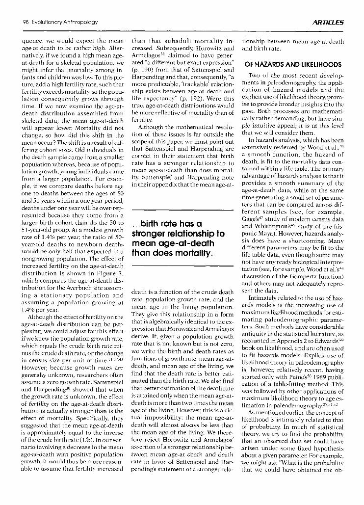
Box 2. Controversies in Human Skeletal Biology Much of the progress made in human skeletal biology during the past few

decades has been the product of numerous controversies regarding paleodemography. Bocquet-Appel and Massetz6 initiated one such controversy in 1982, when they suggested that paleodemography be abandoned because age estimation was too unreliable. Sattenspiel and Harpending30 started another a year later when they suggested that paleodemography had more to say about fertility than about mortality. Both of these articles were met with avolleyof critiques,31-39 which made some valid points but also tended to distort some issues. Only with the passage of time have the views surrounding these debates matured, the overall results being quite positive. Error in age estimation is now a widely ac- knowledged problem in paleodemography, while the previous overemphasis on mortality interpretations is slowly being replaced with an appreciation for the role of fertility. To these two debates, as well as broaderdebates over the development of human life history and the role of agriculture in paleodemography, Wood, Milner, Harpending, and Weiss40 have added a new challenge to both paleodemography and paleopathology. These authors have leveled serious and sobering criticisms at current interpretations of paleodemography and paleopathology, which human skeletal biologists are only beginning to a d d r e s ~ . ~ ~ ~ ~ ~ If Wood and co-workers’ challenge follows the same course as the previous debates in paleodemography, we can expect human skeletal biology to emerge with a stronger theore tical bent.

term likelihood here means that we are considering the distribution of age rather than the distribution of the indicator. For the single skeleton, there is no distribution of the indicator; there is only the observed indicator state.

In the forensic setting, age estimation can be simplified because, in the absence of any outside information, the prior distribution for age is flat. In other words, without having some information from the indicators, we have no preconceptions about the age- at-death. If we have some prior knowledge about the age distribution to be expected in forensic cases, then we will not have a flat prior distribution but, for the sake of simplicity, we assume that we do not have the prior information. In such a case, the posterior probability that the individual died at a particular age conditional on the indicator is proportional to the probability that they are in the observed indicator state conditional on the particular age. Stated another way, the posterior probability is the likelihood of a particular age conditional on the observed indicator state. This makes age estimation a simple problem; we have only to select the age at which the probability of obtaining the indicator state observed in the uniden-

tified skeleton is the highest.

DEATH AND SKELETAL SAMPLES

Estimation of the age of a group of skeletons is more complicated because there is little reason to assume a flat prior distribution for age-at- death. Neither the living population age distribution (i.e., the age “pyra- m i d ) nor the structure of mortality is uniform across age in any real population. As a result, the age-at-death distribution is not uniform. The typical undergraduate class project in demography of tabulating ages-at-death from gravestone inscriptions quickly demonstrates the non-uniform nature of age-at-death distributions. Thus, for any single skeleton from an archeological sample, the posterior probability that the individual is a particular age conditional on the observed indicator is proportional to the prior probability that the individual is that particular age times the probability that an individual that particular age would be in the observed indicator state. However, we do not know this prior probability. If we knew the prior probabilities of death at particular ages, then we would know the age-at-death distribution, which is precisely what we are trying to estimate. This paradox can be


Figure 2. Ageat-death distributions in weeks since the last menstrual period (LMP) for a large collection of prehistoric and protohistoric fetal and neonatal Arikara Indians. The gray bars in the background give the age-at-death distribution from Owsley and Jantz?B derived by using published regressions of age on long bone length.97 The white bars in the foreground give the age- at-death distribution derived by the maximum likelihood method, using a regression of femur length on gestational age from a large uitrasound study.29 Forty weeks represent a term infant. Note that the original age distribution from Owsley and Jantz appears to underestimate ages substantially when compared to the maximum likelihood method.

solved by using a common statistical method known as maximum likelihood estimation. Just as we can write the posterior probability of age conditional on indicator for a single skeleton, we can write the joint probability of ages for a group of skeletons. This joint probability is the likelihood of the age-at-death distribution conditional on the observed indicator information from all skeletons in the group.

The maneuvers we have described are admittedly more complicated than the methods of age estimation typi- cally used in paleodemography Tradi- tionally, one would assign a point estimate or range for the age-at-death for each skeleton based on the conditional distribution of age on indicators in a reference sample, then tabulate these deaths into a life table. Unfortu- nately, this form of age determination almost always leads to biased estimates of the age-at-death distribution, as was pointed out first in the fisheries literatureZ5 and later in the human paleodemography l i te ra t~re*~,~ ' (see Box 2). This bias occurs because if we make age conditional on indicators, then we make the a priori assumption that skeletons in the archeological

distributions for almost 500 perinatal skeletons originally reported by Owsley and JantzZs and our analysis of the same sample. Owsley and Jantz used a regression of age in weeks on long bone length to estimate ages, whereas we calculated the age-at- death structure using maximum likelihood and a regression of femur length on age.29 The differences between the distributions are marked. Owsley and Jantz's study suggests that 88% of the remains are of preterm or term infants (usually defined as 40 weeks postmenstruation); our analysis indicates that only 17% are term or preterm infants. The average age-at- death in the Owsley and Jantz study (38.5 weeks) is consequently about a month lower than in our study (42 weeks).

BIRTH, DEATH, AND SKELETAL SAMPLES

An additional complication in estimating the age-at-death distribution - - of a skeletal sample is that the age structure represented in a cemetery is affected by both deaths and births. For example, suppose that the idants and

adequate nutrition so that their mar-

the Same age-at-death distribution as does the reference

ple of the bias that can arise, Figure 2 sample (see Box 1. a simp1e exam- children in a population had generally

presents the estimated age-at-death tality rate was very low. As a conse-

Figure 3. Comparison of age-atdeath distributions for the Averbuch site under different fertility rates. The gray ribbon in the background shows the age-at-death distribution assuming that the birth and death rates were equal (i.e., population growth rate was zero). The white ribbon in the foreground shows the ageat-death distribution assuming that fertility had increased to the extent that population growth was 1.4% per year. It appears that the proportion of individuals who die at young ages has increased and the proportion dying at old ages has decreased in the higher fertility population, even though mortality has remained unchanged.


quence, we would expect the mean age-at-death to be rather high. Alter- natively, if we found a high mean age- at-death for a skeletal population, we might infer that mortality among infants and children was low. To this pic- ture, add a high fertility rate, such that fertility exceeds mortality, so the population consequently grows through time. If we now examine the age-at- death distribution assembled from skeletal data, the mean age-at-death will appear lower. Mortality did not change, so how did this shift in the mean occur? The shift is a result of differing cohort sizes. Old individuals in the death sample came from a smaller population whereas, because of population growth, young individuals came from a larger population. For example, if we compare deaths before age one to deaths between the ages of 50 and 5 1 years within a one year period, deaths under one year will be over-represented because they come from a larger birth cohort than do the 50 to 5 1 -year-old group. At a modest growth rate of 1.4% per year, the ratio of 50- year-old deaths to newborn deaths would be only half that expected in a nongrowing population. The effect of increased fertility on the age-at-death distribution is shown in Figure 3 , which compares the age-at-death distribution for the Averbuch site assuming a stationary population and assuming a population growing at 1.4% per year.

Although the effect of fertilityon the age-at-death distribution can be perplexing, we could adjust for this effect if we knew the population growth rate, which equals the crude birth rate minus the crude death rate, or the change in census size per unit of time.lI.37.43 However, because growth rates are generally unknown, researchers often assume a zero growth rate. Sattenspiel and Harpending30 showed that when the growth rate is unknown, the effect of fertility on the age-at-death distribution is actually stronger than is the effect of mortality. Specifically, they suggested that the mean age-at-death is approximately equal to the inverse of the crude birth rate ( 1 /b). In our sce- nario involving a decrease in the mean age-at-death with positive population growth, it would thus be more reasonable to assume that fertility increased

than that subadult mortality increased. Subsequently, Horowitz and Armelagos3* claimed to have generated “a different but exact expression” (p. 190) from that of Sattenspiel and Harpending and that, consequently, “a more predictable, ‘trackable’ relationship exists between age at death and life expectancy” (p. 192). Were this true, age-at-death distributions would be more reflective of mortality than of fertility.

Although the mathematical resolu- tion of these issues is far outside the scope of this paper, we must point out that Sattenspiel and Harpending are correct in their statement that birth rate has a stronger relationship to mean age-at-death than does mortality. Sattenspiel and Harpending note in their appendix that the mean age-at-

... birth rate has a stronger relationship to mean age-at-death than does mortality.

death is a function of the crude death rate, population growth rate, and the mean age in the living population. They give this relationship in a form that is algebraically identical to the expression that Horowitz and Armelagos derive. If, given a population growth rate that is not known but is not zero, we write the birth and death rates as functions of growth rate, mean age-at- death, and mean age of the living, we find that the death rate is better estimated than the birth rate. We also find that better estimation of the death rate is attained only when the mean age-at- death is more than two times the mean age of the living. However, this is a vir- tual impossibility: the mean age-at- death will almost always be less than the mean age of the living. We therefore reject Horowitz and Armelagos’ assertion of a stronger relationship between mean age-at-death and death rate in favor of Sattenspiel and Har- pending’s statement of a stronger rela-

tionship between mean age-at-death and birth rate.

OF HAZARDS AND LIKELIHOODS

Two of the most recent developments in paleodemography, the appli- cation of hazard models and the explicit use of likelihood theory, prom- ise to provide broader insights into the past. Both processes are mathemati- cally rather demanding, but have simple intuitive appeal; it is at this level that we will consider them.

In hazards analysis, which has been extensively reviewed by Wood et al.,44 a smooth function, the hazard of death, is fit to the mortality data contained within a life table. The primary advantage of hazards analysis is that it provides a smooth summary of the age-at-death data, while at the same time generating a small set of parameters that can be compared across different samples (see, for example, Gage’s4’ study of modern census data and Whittington’sA6 study of pre-his- panic Maya). However, hazards analysis does have a shortcoming. Many different parameters may be fit to the life table data, even though some may not have any ready biological interpretation (see, for example, Wood et a l . ’ ~ ~ ~ discussion of the Gompertz function) and others may not adequately represent the data.

Intimately related to the use of hazards models is the increasing use of maximum likelihood methods for estimating paleodemographic parameters. Such methods have considerable antiquity in the statistical literature, as recounted in Appendix 2 to Edwards’4Y book on likelihood, and are often used to fit hazards models. Explicit use of likelihood theory in paleodemography is, however, relatively recent, having started only with Paine’sso 1989 publi- cation of a table-fitting method. This was followed by other applications of maximum likelihood theory to age estimation in paleodeniography.*7,51~’*

As mentioned earlier, the concept of likelihood is intimately related to that of probability. In much of statistical theory, we try to find the probability that an observed data set could have arisen under some fixed hypothesis about a given parameter. For example, we might ask “What is the probability that we could have obtained the ob-


lel to the axis for crude death rate, the peak of the ridge viewed across crude birth rate does not move much. Thus, if we did not know the growth rate (or, for that matter, crude death rate) we

, could estimate the crude birth rate. The converse is not true. If we look at the ridge across crude death rate, the ridge is flat at the top, slightly convex in the foreground, and slightly con- cave in the background. We therefore could not interpret the age-at-death distribution with respect to changes in the crude death rate. This, which is precisely the point made by Satten- spiel and H a r ~ e n d i n g , ~ ~ is borne out again here by the likelihood analysis.

WHAT DO WE KNOW ABOUT PALEODEMOGRAPHY?

0

Qz

If our samples, our age estimates, and OUT demographic reconstructions are also biased, what do we know about past human demography? The

Figure4 Log-Ilkellhood surface against crude death rate and crude blrth rate for the Libben site 53 The log-likelihood is the log of the probability of obtaining the observed age-at death distribuhon from Libben conditional on the crude birth and death rates

served difference between two means if the true difference between the means was zero?” In this case, we consider the hypothesis as fixed and the observed data as variable. In the likelihood approach, we similarly deal with the probability that we would have obtained the observed data under a given hypothesis, but now consider the data as fixed and the hypothesis as variable. For example, we could ask “What is the probability of obtaining the observed age-at-death data if the crude death rate was 0.05 and the crude birth rate 0.04?” We can then consider a multitude of alternative hypotheses about what the birth and death rates might have been. When comparing alternative hypotheses, it would be reasonable to choose the hypothesiLed rates at which the observed data are most likely or, in other words, the parameters at which the probability of obtaining the observed data is highest. We would then have found the maximum likelihood estimates of the parameters. Because the probabilities are often very small, and because it simplifies the mathematics, we usually search across likelihoods in a logarithmic scale and thus try to find the maximum log-likelihood. The parameter values at the maximum likelihood on the log scale

will correspond to the parameter values at the maximum likelihood on the original scale. Figure 4 shows an example of a log-likelihood surface for the Libben sitej3 plotted against crude birth and death rates. The log-likelihoods were calculated as in Paine50 although, rather than using model life tables, we used the observed mortality profile for Libben (assuming zero population growth), then adjusted birth and death rates. The death rates were adjusted by a logit regre~si0n. j~

Figure 4 shows that the fertility rate has a greater effect on the age-at-death profile than does the mortality rate. If a likelihood or log-likelihood surface is very flat, this tells us that we are having difficulty estimating a parameter. Intuitively, this makes sense-a completely flat surface tells us that the data are equally likely to have been generated by different values across the parameter space. Therefore, we want to find the maximum likelihood estimates of parameters (as the highest point in the log-likelihood surface); we also want the likelihood surface to fall rapidly from the maximum in all directions. The surface in Figure 4 looks much like a long east Tennessee mountain ridge, with the ridge run- ning parallel to the crude death rate. Because the ridge runs roughly paral-

answer is that although there is little that we know with certainty, there is much that we can infer from the archeological record. Considerable ef- fort in paleodemographic research has focused myopically on the details of individual sites or small groups of sites, often attempting to relate small changes in life-table parameters to changing subsistence or health. These individual case histories are interesting in their own right, but it is at broader levels of analysis that we can begin to see paleodemographic generalities.

Three far-reaching questions have emerged within the paleodemographic literature over the years. The first is whether human life-span has increased; the second is whether life expectancy at birth has increased; and the third is whether demographic consequences or antecedents are related to the origins of food production. An initial problem with the concept of life-span is its definition. Olshansky et al.5” define it as “the genetically en- dowed limit to life for a single individual if free of all exogenous risk factors” (p. 635) . However, current empirical results make a unitary genetic basis for longevity highly ~ n l i k e l y . ~ ~ , ~ ~ De- spite difficulties in defining life-span, the term is conceptually ingrained in both the popular and scientific presses. We can assume that the limit


of human life-span, however defined, was a subject for debate even before the written word. Because the literature on life-span is voluminous, we touch only tangentially on the paleodemographic evidence.

During the last 20 years, the question of the evolution of life-span has been addressed sporadically in the paleodemographic literature, but the main evidence has been rather indirect. Both Cutler58 and Sachers’ argued that the maximum human life-span has remained fairly constant for at least the last 100,000 years. Their arguments were based on the empirical relationship between increased brain size and life-span across many modern mammalian taxa, to- gether with the observation that the size of the human brain has not changed since the appearance of our species. More recently, Allman et have noted a strong relationship between the brain weight and life-span of hominoids, again suggesting that modern human life-span was attained at the same point that modern brain size was attained.

Smith6’ has reviewed evidence that the rate of maturation and life-span in Austvafopithecus were probably more ape-like than human-like. She suggests that the modern human life-span was established only on the order of tens of thousands of years ago. Her research on the Nariokotome Homo evectus skeleton,62 which had a pattern of dental emergence that was still ape- like in some respects, but was closer to that of humans, supports her argument that the pattern of human life history was established by the emergence of Homo sapiens.

David Smith63 summarizes the arguments on this subject, suggesting that the life-span of Australopithecus africanus was probably similar to that of modern apes-that is, about 50 years-and that life-span gradually doubled by the establishment of modern Homo sapiens approximately 100,000 years ago. Estimated life-span for humans now is between 80 to 100 years; the oldest verified age is slightly in excess of 120 years.55 The evolutionary causes for increases in life-span remain obscure, although methods as diverse as biochemistry, cell biology, and computer simulation of the de-

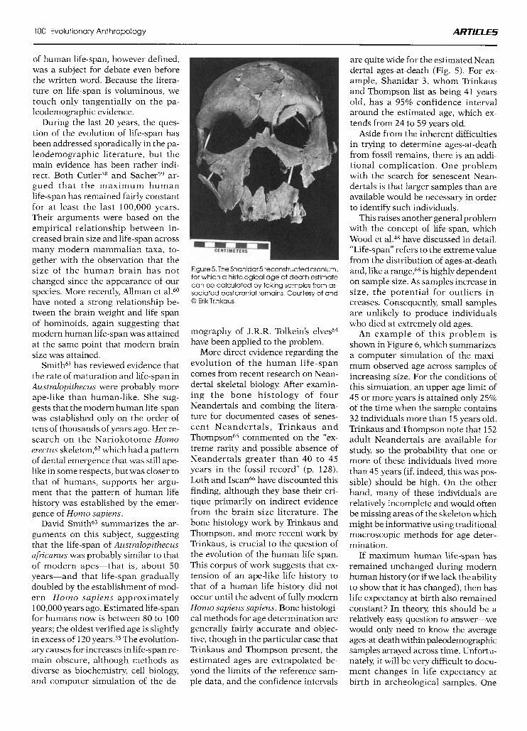
Figure 5. The Shanidar5 reconstructed cranium, for which a histological age at death estimate c a n be calculated by taking samples from associated postcranial remains. Courtesy of and 0 Erik Trinkaus.

mography of J.R.R. Tolkein’s e l ~ e s 6 ~ have been applied to the problem.

More direct evidence regarding the evolution of the human life-span comes from recent research on Nean- dertal skeletal biology. After examin- ing the bone histology of four Neandertals and combing the literature for documented cases of senescent Neandertals, Trinkaus and Thompson65 commented on the “extreme rarity and possible absence of Neandertals greater than 40 to 45 years in the fossil record (p. 128). Loth and Iscad6 have discounted this finding, although they base their critique primarily on indirect evidence from the brain size literature. The bone histology work by Trinkaus and Thompson, and more recent work by Trinkaus, is crucial to the question of the evolution of the human life span. This corpus of work suggests that ex- tension of an ape-like life history to that of a human life history did not occur until the advent of fully modern Homo sapiens sapiens. Bone histological methods for age determination are generally fairly accurate and objec- tive, though in the particular case that Trinkaus and Thompson present, the estimated ages are extrapolated beyond the limits of the reference sample data, and the confidence intervals

are quite wide for the estimated Nean- dertal ages-at-death (Fig. 5). For example, Shanidar 3, whom Trinkaus and Thompson list as being 41 years old, has a 95% confidence interval around the estimated age, which ex- tends from 24 to 59 years old.

Aside from the inherent difficulties in trying to determine ages-at-death from fossil remains, there is an additional complication. One problem with the search for senescent Nean- dertals is that larger samples than are available would be necessary in order to identify such individuals.

This raises another general problem with the concept of life-span, which Wood et al.48 have discussed in detail. “Life-span’’ refers to the extreme value from the distribution of ages-at-death and, like a range,bs is highly dependent on sample size. As samples increase in size, the potential for outliers increases. consequently, small samples are unlikely to produce individuals who died at extremely old ages.

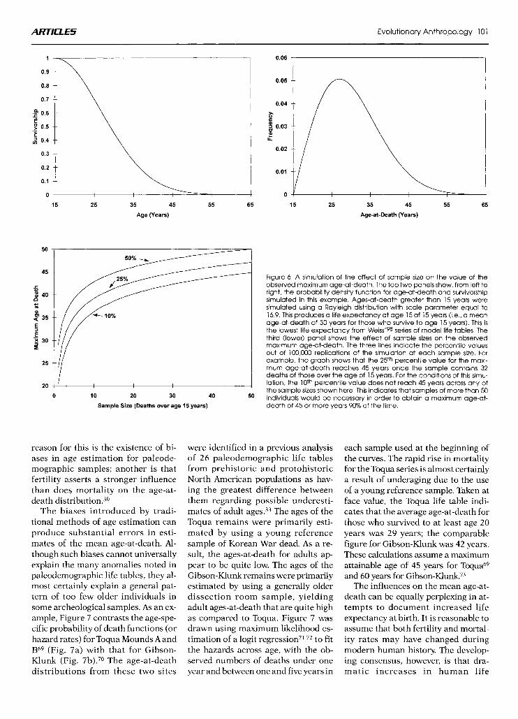
An example of this problem is shown in Figure 6, which summarizes a computer simulation of the maximum observed age across samples of increasing size. For the conditions of this simulation, an upper age limit of 45 or more years is attained only 25% of the time when the sample contains 32 individuals more than 15 years old. Trinkaus and Thompson note that 152 adult Neandertals are available for study, so the probability that one or more of these individuals lived more than 45 years (if, indeed, this was possible) should be high. On the other hand, many of these individuals are relatively incomplete and would often be missing areas of the skeleton which might be informative using traditional macroscopic methods for age determination.

If maximum human life-span has remained unchanged during modern human history (or if we lack the ability to show that it has changed), then has life expectancy at birth also remained constant? In theory, this should be a relatively easy question to answer-we would only need to know the average ages-at-death within paleodemogaphic samples arrayed across time. Unfortu- nately, it will be very difficult to document changes in life expectancy at birth in archeological samples. One

ARTICL E5 Evolutionary Anthropology 101

50

45

5 40

0

0

L

p 35

: ’8 30 I

25

0.06 1

15 25 35 45 55 65

Age (Years)

15 25 35 45 55 65

Age-at-Death (Years)

20 1 ’ 0 10 20 30 40 50

Sample Size (Deaths over age 15 years)

Figure 6. A simulation of the effect of sample size on the value of the observed maximum age-at-death. The top two panels show, from left to right, the probability density function for age-atdeath and survivorship simulated in this example. Ages-at-death greater than 15 years were simulated using a Rayleigh distribution with scale parameter equal to 16.9. This produces a life expectancy at age 15 of 15 years (i.e.. a mean age-at-death of 30 years for those who survive to age 15 years). This is the lowest life expectancy from Wei~s’~8 series of model life tables. The third (lower) panel shows the effect of sample sizes on the observed maximum aged-death. The three lines indicate the percentile values out of 100,000 replications of the simulation at each sample size. For example, the graph shows that the 25th percentile value for the maximum age-at-death reaches 45 years once the sample contains 32 deaths of those over the age of 15 years. For the conditions of this simulation, the 10th percentile value does not reach 45 years across any of the sample sizes shown here. This indicates that samples of more than 50 individuals would be necessary in order to obtain a maximum age-at- death of 45 or more years 90% of the time.

reason for this is the existence of biases in age estimation for paleodemographic samples; another is that fertility asserts a stronger influence than does mortality on the age-at- death di~tribution.3~

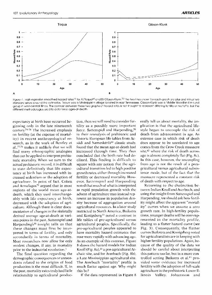
The biases introduced by traditional methods of age estimation can produce substantial errors in estimates of the mean age-at-death. Al- though such biases cannot universally explain the many anomalies noted in paleodemographic life tables, they almost certainly explain a general pattern of too few older individuals in some archeological samples. As an example, Figure 7 contrasts the age-specific probability of death functions (or hazard rates) for Toqua Mounds A and B69 (Fig. 7a) with that for Gibson- Hunk (Fig. 7b).’O The age-at-death distributions from these two sites

were identified in a previous analysis of 26 paleodemographic life tables from prehistoric and protohistoric North American populations as having the greatest difference between them regarding possible underesti- mates of adult ages.33 The ages of the Toqua remains were primarily estimated by using a young reference sample of Korean War dead. As a result, the ages-at-death for adults appear to be quite low. The ages of the Gibson-Hunk remains were primarily estimated by using a generally older dissection room sample, yielding adult ages-at-death that are quite high as compared to Toqua. Figure 7 was drawn using maximum likelihood estimation of a logit regression71J2 to fit the hazards across age, with the observed numbers of deaths under one year and between one and five years in

each sample used at the beginning of the curves. The rapid rise in mortality for the Toqua series is almost certainly a result of underaging due to the use of a young reference sample. Taken at face value, the Toqua life table indicates that the average age-at-death for those who survived to at least age 20 years was 29 years; the comparable figure for Gibson-Hunk was 42 years. These calculations assume a maximum attainable age of 45 years for T ~ q u a ~ ~ and 60 years for Gibson-Hunk.73

The influences on the mean age-at- death can be equally perplexing in at- tempts to document increased life expectancy at birth. It is reasonable to assume that both fertility and mortality rates may have changed during modern human history. The developing consensus, however, is that dra- matic increases in human life


$ 0.6 a: $ 0.5 N

1

0.9

0.8

0.7

$ 0.6 K E 0.5 m 4 0.4

0.3

0.2

0.1

0

Toqua Gibson-Klunk

1 I ::: 1 0.7 I

0 10 20 30 40 50 0 10 20 30 40 50

Age Age

A B

Figure 7. Logit regression smoothed hazard rates71 for A) Toqua69 and B) Gib~on-Klunk.~o The two lines shown for each graph are plus and minus two standard errors around the estimates. Toqua was a Mississippian village located in east Tennessee; Gibson-Klunk was a Middle Woodland mound group in west-central Illinois. The contrast between these two graphs of hazard rates is not thought to represent differing fertility or mortality, but the different methodologies used to determine ages-at-death.

expectancy at birth have occurred beginning only in the late nineteenth ~ e n t u r y . ~ ~ - ~ ~ The increased emphasis on fertility (at the expense of mortality) in recent anthropological research, as in the work of Bentley et a1.,77,78 makes it unlikely that we will find many ethnographic analogies that can be applied to interpret prehistoric mortality. When we turn to the actual prehistoric record, it is difficult to state definitively that life expectancy at birth has increased with increased sedentism or the adoption of agriculture. In point of fact, Cohen and arm el ago^^^ argued that in most regions of the world mean age-at- death, which they used interchange- ably with life expectancy at birth, decreased with the adoption of agriculture. Although there is clear documentation of changes in the skeletally derived average age-at-death at various points in the past, Sattenspiel and Harpending’s30 insight tells us that these changes must first be interpreted in terms of fertility, and only secondarily in terms of mortality. Most researchers now allow for only modest changes, if any, in mortality prior to the industrial rev~lut ion.~

The final question regarding the demographic consequences or antecedents related to the origins of food production is the most difficult. I f , in the past, mortality rates truly had little relationship to agricultural produc-

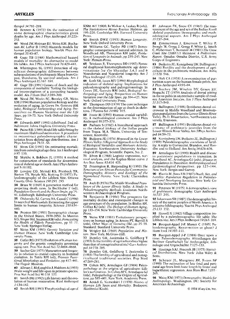
tion, then we will need to consider fertility as a possibly more important force. Sattenspiel and H a r ~ e n d i n g , ~ ~ in their reanalysis of prehistoric and historic European life tables from Ac- sadi and Nemeskeri’sBo classic study, found that the mean age-at-death had increased through time. They thus concluded that the birth rate had de- clined. This finding is difficult to square with any notion that the agricultural transition led to high positive growth rates, either through increased fertility or decreased mortality. How- ever, Sattenspiel and Harpending noted that much of what is interpreted as rapid population growth with the advent of agriculture may instead represent an increase in population density because of aggregation around agricultural resources. In a later study restricted to North America, Buikstra and K~nigsberg’~ noted a contrast in life tables of pre-agricultural versus agricultural peoples. Specifically, the pre-agricultural peoples appeared to have mortality hazard estimates that rose more rapidly with advancing age. As an example of this contrast, Figure 8 shows the hazard models for Indian Knoll (Fig. 8a),81 a pre-agricultural Ar- chaic site, and for Averbuch (Fig. 8b), a Late Mississippian agricultural site. The Averbuch “mortality” profile is much flatter against age. Why might this be?

If the data represented in Figure 8

really tell us about mortality, the im- plication is that the agricultural life- style began to uncouple the risk of death from advancement in age. An extreme case in which risk of death does appear to be unrelated to age comes from the Crow Creek massacre site,82 where the risk of death across age is almost completely flat (Fig. 8c). In this case, however, the uncoupling from age is not the result of a prea- gricultural versus agricultural subsistence mode, but of the fact that the massacre represented a constant risk of death with respect to age.

Returning to the distinction between Indian Knoll and Averbuch, and using the insight from Sattenspiel and Harpending, we should ask how fertility might affect the apparent “mortality” curves when we assume a zero growth rate. In high-fertility populations, younger deaths will be over-represented in the mortality profile, leading to a flatter hazard curve (see Fig. 3 ) . Consequently, the flatter curves Buikstra and Konigsberg noted for agriculturalists are in keeping with higher fertility populations. Again, because of the quality of the data we should be careful about interpreting this pattern too far, but in a more controlled setting Buikstra et al.83 provided some evidence for increased fertility with the adoption of full-scale agriculture in the prehistoric Lower 11- linois Valley. Johansson and


0.7

5 0.6 z 7 0.5 m

1

0.9

0.8

0.7

3 0.6 LL 7 0.5 m p 0.4

0.3

0.2

0.1

0

--

--

--

Indian Knoll

0 10 20 30 40 50

Age

A

Crow Creek

1 , I 0.9

0.7

O Y 0 10 20 30

Age

C

H o r ~ w i t z ~ ~ also suggested that for a diachronic series from a single site in Central Illinois, Dickson Mounds, the decreasing mean age-at-death with the adoption of maize agriculture indicates an increasing birth rate.

An increase in average number of “birth scars” on the pubic bones or at the pre-auricular sulci in adult females would be a useful corollary to the inferred increased fertility rates mentioned earlier. Unfortunately, the relationship between such osseous marks and parity among documented skeletal remains is weak at best,g4,85 so an analysis of prehistoric skeletal remains would be quite tenuous. More promising are studies that focus on the age of infants at weaning or the nature of the weaning process, which may serve as indirect measure of past fertility. For example, B u l l i n g t ~ n ~ ~ , ~ ~

40 50

Averbuch

I

0.8 0.9 1

0 10 20 30 40 50

Age

B

Figure 8. Logit regression smoothed hazard rates for A) Indian Knoli, an Archaic cemetery in Kentucky 81; B) Averbuch Cemeteries, from a Late Mississippian village in central Tennessee ’2 (see Figure 1 ); C) Crow Creek, the site of a fourteenth century massacre of a South Dakota Initial Coa- lescent village.82The contrast between hazard rates for Indian Knoll and Averbuch is thought to be a product of the higher fertility rates at Aver- buch. Crow Creek contrasts with all previous graphs in having a hazard rate that is virtually unrelated to age, presumably as a result of massacre victims dying regardless of their ages.

based on a study of microwear on the deciduous dentition, has suggested that the shift to agriculture in the prehistoric Lower Illinois Valley occurred at the same time as the introduction of a softer weaning diet. This possibility reinforces previous suggestions83,88 that a technological change in ceramic production concident with the development of agriculture in this region may have provided an easy means of cooking weaning gruels made from soft, starchy seeds. More rapid and easier weaning may have led to shorter interbirth intervals, and thus to increased fertility. This argument remains quite speculative; the relationship between weaning and fertility is complicated.

The relationship that the adoption or intensification of agriculture has to population pressure, fertility, mortal-

ity, and pathology is obviously also quite complicated. We need to be es- pecially careful of attempting to paint the broad history of humanity with the fine brush strokes provided by regional histories and prehistories.88 We should expect that the generalities will be few and the exceptions great. What does seem to emerge repeatedly from the archeological record is a slight decrease in the skeletally derived mean- age-at-death with the adoption or intensification of agriculture.79 The former dogma was that such a decrease was a signal mark of decreasing quality of life and increasing mortality rate^.^^,^^ This view is now being par- tially challenged by one that replaces the emphasis on increased mortality with an emphasis on increased fertility.37,83,88,W In coming years, we must be careful not to subscribe to the


wholesale adoption of a new dogma. A challenge to the prevailing view that agriculture necessarily leads to poorer quality of life has also recently been presented40 (see Box 2 ) . In this in- stance, there seems little chance of a paradigm shift in the near future, for the challenge appears to have been dismissed by a few and ignored by many.

The swirl of activity, uncertainty, and controversy that now surrounds paleodemography is a sign that the field is undergoing a healthy maturation. With the relatively new appreciation of the problems of age estimation, sample bias, and the complexity of relationships among fertility, mortality, population growth, and life table analysis, we see paleodemography as just beginning to embark on what should be a truly productive phase of research. The addition of analytical techniques such as maximum likelihood estimation and hazards analysis to the traditional paleodemographic arsenal can only strengthen our ability to make inferences about past human life. Although we well appreciate the critical comments directed towards paleodemographic research,26,y1-y5 we believe that it is time to move beyond the methodological problems and re- turn to answering the interesting larger issues.

ACKNOWLEDGMENTS

We thank Jane Buikstra, John Fleagle, and Henry Harpending for their constructive and copious comments on a previous draft of this paper. We also thank Richard Jantz for pro- viding us with the original Owsley and Jantz data in machine-readable form, for commenting on a previous draft, and for encouraging us even when our results deviated from some previous findings. The photographs of the Aver- buch site were provided by the McClung Museum (Fig. 1B) and Wal- ter Klippel (Fig. lA) , whom we grate- fully acknowledge. The Neandertal photograph (Fig. 5) was provided by Erik Trinkaus, who also kindly provided a galley copy of his article on Neandertal mortality, which will appear (undoubtedly prior to this article) in the Journal of Archaeological Science. We thank him for his help, and strongly encourage readers of

this article to refer to his Journal of Archaeological Science article as the definitive source on Neandertal paleodemography.

REFERENCES 1 Hill K (1993) Life history theory and evolutionary anthropology. Evol Anthropol 2:78- 89. 2 Dumond DE (1975) The limitation of human population: A natural history. Science /87:713-721. 3 Cohen MN (1 989) Health and the Rise o f Civilization. New Haven: Yale University. 4 Boserup E (1965) The Conditions of Agri- cultural Growth. Chicago: Aldine Press. 5 Boserup E (1990) Economic and Demo- graphic Relationships in Development. Balti- more: Johns Hopkins University Press. 6 Handwerker WP (ed) (1986) Culture and Reproduction: An Anthropological Critique of Demographic Transition Theory. Boulder: Westview Press. 7 Coale AJ (1974) The history of human population. Sci Am 23/:40-51. 8 Frisch RE (1978) Population, food intake, and fertility. Science 199:22-30. 9 Gordon CC, Buikstra JE (1981) Soil pH, bone preservation, and sampling bias a t mor- tuaiy sites. Am Antiq 46566-571. 10 Walker PL, Johnson JR, Lambert PM (1 988) Age and sex biases in the preservation of human skeletal remains. Am J Phys Anthro- pol 76:183-188. 1 1 Moore JA, Swedlund AC, Armelagos GJ (1975) The use of life tables in paleodemography. In Swedlund AC (ed), Population Studies in Archaeology and Biological Anrhropologv: A Symposium, pp 57-70. Washington DC: Soci- ety for American Archaeology. 12 Berryman HE (1981) The Averbuch skeletal series: A study of biological and social stress at a Late Mississippian Period Site from Middle Tennessee. Ph.D. Dissertation, Univer- sity of Tennessee, Knoxville. 13 Buikstra JE (1977) Biocultural dimen- sions of archaeological study: A regional per- spect ive. In Blakey RL (ed) , Biocultural Adaptation in Prehistoric America, pp 67-84. Athens GA: University of Georgia Press. 14 Hummel S, Hexmann B (1991) Y-chromosome-specific DNA amplified in ancient human bone. Naturwissenschaften 78:266- 267. 15 Stone AC, Milner GR, Paabo S (1994) Sex determination of prehistoric human remains using DNA analysis. Am J Phys Anthropol (Suppl) 18:188. 16 Masset C (1989) Age estimation on the basis of cranial sutures. In Iscan MY (ed), Age Markers in the Human Skeleton, pp 71-103. Springfield: Charles C. Thomas. 17 Katz D, Suchey JM (1986) Age determina- tionofthemaleospubis. Am JPhys Anthropol 69:237-244. 18 Meindl RS, Lovejoy CO (1989) Age changes in the pelvis: Implications for pa- Ieodemography. In Iscan MY (ed),Age Markers in the Human Skeleton, pp 137-168. Spring- field: Charles C. Thomas. 19 Saunders SR (1992) Subadult skeletons and growth related studies. In Saunders SR, Katzenberg MA (eds), Skeletal Biology of Past Peoples: Research Methods, pp 1-20. New York: John Wiley & Sons, Inc. 20 Drusini AG (1991) Age-related changes in root transparency of teeth in males and females. Am J Hum Biol3:629-637.

21 DrusiniAG,CalliariI,VolpeA(1991)Root dentine transparency: Age determination of human teeth using computerized densitomet- ric analysis. Am J Phys Anthropol 85:25-30. 22 Stout SD (1992) Methods of determining age at death using bone microstructure. In Saunders SR, Katzenberg MA (eds), Skeletal Biologv o f Past Peoples: Research Methods, pp 21-35. New York: John Wiley & Sons, Inc. 23 Box GEP, Tiao GC ( I 992) Bayesian Infer- ence in Statistical Aizalvsis. New York: John Wiley & Sons. 24 Bayes TR (1763) An essay towards solving a problem in the doctrine of chances. Phil Trans Roy SOC London 53:370418. 25 Westrheim SJ, Ricker WE ( 1 978) Bias in using an age-length key to estimate age-fre- quency distributions. J Fish Res Board Can 35:184-189. 26 Bocquet-Appel J-P, Masset C (1982) Fare- well topaleodemography. J H u m Evol11:321- 333. 27 Konigsberg LW, Frankenberg SR (1992) Estimation of age structure in anthropological demography. Am J Phys Anthropol 89:235- 256. 28 Owsley DW, Jantz RL (1985) Long bone lengths and gestational age distributions of Post-contact Period Arikara Indian perinatal infant skeletons. Am J Phys Anthropol68:321- 328. 29 Oman SD, Wax Y (1984) Estimating fetal age by ultrasound measurements: An example of mul t ivar ia te ca l ibra t ion . Biometr ics 40:947-960. 30 Sattenspiel L, Harpending H ( 1 983) Sta- ble populations and skeletal age. Am Antiq 48:489498. 31 Van Gerven DP, Armelagos GJ (1983) “Farewell to paleodemography?” Rumors of its death have been greatly exaggerated. J Hum Evol 12:353-360. 32 Greene DL, Van Gerven DP, Armelagos GJ ( I 986) Life and death in ancient populations: Bones of contention in paleodemographv. Hum Evol /:193-207. 33 Buikstra JE, Konigsberg LW (1985) Pa- leodemography: Critiques and controversies. Am Anthropol87:316-333. 34 Lanphear KM (1989) Testing the value of skeletal samples in demographic research: A comparison with vital registration samples. Int J Anthropol4:185-193. 35 Mensforth RP (1990) Paleodemography of the Carlston Annis (Bt-5) Late Archaic skeletal population. Am J Phys Anthropol 8223-99 36 Piontek J , Weber A ( I 990) Controversy on paleodemography. Int J Anthropol5:71-83. 37 Johansson SR, Horowitz S (1986) Esti- mating mortality in skeletal populations: In- f luence of t h e growth ra te o n the interpretation of levels and trends during the transition to agriculture. Am J Phys Anthropol 71 :233-250. 38 Horowitz S, Armelagos G (1 988) On generating birth rates from skeletal populations. Am J Phys Anthropol 76:189-196. 39 Jackes M (1992) Paleodemography: Prob- lems and techniques. In Saunders SR, Katzen- berg MA (eds), Skeletal Biologv ofpast Peoples: Research Methods, pp 189-224. New York: John Wiley & Sons, Inc. 40 Wood JM, Milner GR, Harpending HC, Weiss KM (1992) The osteological paradox: Problems of inferring prehistoric health from skelctal samples. Curr Anthropol 33:343-370. 41 Jackes M (1993) On paradox and osteol- ogy. Cum Anthropol34:434439. 42 Goodman AH (1993) On the interpretation of health From skeletal remains. Curr An-


thropol34:281-288. 43 Bennett K (1973) On the estimation of some demographic characteristics given deaths by age. Am J Phys Anthropol 39:223- 232. 44 Wood JW, Holman DJ, Weiss KM, Bucha- nan AV, LeFor B (1992) Hazards models for human population biology. Yearbk Phys An- thropol35:43-87. 45 Gage TB (1988) Mathematical hazard models of mortality: An alternative to model life tables. Am J Phys Anthropol 76:429-441. 46 Whittington SL (1991) Detection of sig- nificant demographic differences between subpopulations of prehispanic Maya from Co- pan, Honduras, by survival analysis. Am J Phys Anthropol85:167-184. 47 Gage TB (1991) Causes of death and the components of mortality: Testing the biological interpretations of a competing hazards model. Am J Hum Biol3:289-300. 48 Wood JW, Weeks SC, Bentley GR, Weiss KM (1994) Human population biology and the evolution of aging. In Crews De, Garruto RM (eds), Biological Anthropology and Aging: Per- spectives on Human Variation over the Life Span, pp 19-75. New York: Oxford University Press. 49 Edwards AWF (1992) Likelihood. 2nd ed. Baltimore: Johns Hopkins University Press. 50 Paine RR (1 989) Model life table fitting by maximum likelihood estimation: A procedure to reconstruct paleodemographic characteristics from skeletal age distributions. Am J Phys Anthropol 79:51-56. 51 Siven CH (1991) On estimating mortali- ties from osteological agedata. Int J Anthropol 6:97-110. 52 Skytthe A, Boldsen JL (1993) A method for construction of standards for determination of skeletal age at death. Am J Phys Anthro- pol S 16:182. 53 Lovejoy CO, Meindl RS, Pryzbeck TR, Barton TS, Heiple KG, Kotting D (1977) Pa- leodemography of the Libben Site, Ottawa County, Ohio. Science 198:291-293. 54 Brass W (1969) A generation method for projecting death rates. In Bechhofer F (ed), Population Growth and the Brain Drain, pp 75- 91. Edinburgh: Edinburgh University Press. 55 Olshansky SJ, Carnes BA, Cassel C (1 990) In search of Methuselah: Estimating theupper limits to human longevity. Science 250:634- 640. 56 Preston SH (1993) Demographic change in the United States, 1970-2050. In Manton KG, Singer BH, Suzman RM (eds), Forecasting the Health of Elderly Populations, pp 51-77. New York: Springer-Verlag. 57 Weiss KM (1 993) Genetic Variation and Human Disease. New York Cambridge Uni- versity Press. 58 Cutler RG ( 1 975) Evolution of human longevity and the genetic complexity governing aging rate. Proc Nat Acad Sci 72:46644668. 59 Sacher GA (1975) Maturation and longevity in relation to cranial capacity in hominid evolution. In Tuttle RH (ed), Primate Func- tional Morphology and Evolution, pp 417-441. The Hague: Mouton. 60 Allman J, McLaughlin J, Hakkem A (1 993) Brain weight and life-span in primate species. Proc Nat Acad Sci 90:118-122. 61 Smith BH (1992) Life history and the evolution of human maturation. Evol Anthropol J:134-142. 62 Smith BH (1993) The physiological age of

KNM-WT 15000. In Walker A, Leakey R (eds), The Nariokotome Homo Erectus Skeleton, pp 195-220. Cambridge MA: Harvard University Press. 63 Smith DWE (1993) Human Longevity. New York: Oxford University Press. 64 Williams GC, Taylor PD (1987) Demo- graphic consequences of natural selection. In Woodhead AD, Thompson KH (eds), Evolu- tion oflongevity in Animals. pp 235-245. New York: Plenum Press. 65 Trinkaus E, Thompson DD (1987) Femo- ral diaphyseal histomorphometric age deter- minations for the Shanidar 3,4,5 and 6 Neandertals and Neandertal longevity. Am J Phys Anthropol 72:123-129. 66 Loth SR, Iscan MY (1994) Morphological indicators of skeletal aging: Implications for paleodemography and paleogerontology. In Crews DE, Garruto RM (eds), Biological An- thropology and Aging: Perspectives on Human Variation over the Life Span, pp 394425. New York: Oxford University Press. 67 Thompson DD (1979) The core technique in the determination of age at death in skeletons. J Forens Sci 24:902-915. 68 Foote M (1993) Human cranial variability: A methodological comment. Am J Phys Anthropol 90:377-379. 69 Parham S (1982) A biocultural approach to the skeletal biology of the Dallas people from Toqua. M.A. Thesis, University of Ten- nessee, Knoxville. 70 Buikstra JE (1976) Hopewell in the Lower Illinois Va1ley:A Regional Approach to the Study of Biological Variability and Mortuary Activity. Evanston: Northwestern University Archae- ological Program, Scientific Papers, No. 2. 71 Efron B (1988) Logistic regression, survival analysis, and the Kaplan-Meier curve. J Am Stat Assoc 83:414-425. 72 Pennington R, Harpending H (1 993) The Structure ofan African Pastoralist Community: Demography, History, and Ecology o f the Ngamiland Herero. New York: Clarendon Press. 73 Asch D ( I 976) The Middle Woodland Popu- lation of the Lower Illinois Valley: A Study in Paleodemographic Methods. Evanston: North- western Archaeological Program. 74 Benjamin B (1986) The prospects for mortality decline and consequent changes in age structure of the population. In Bittles AH, Collins KJ (eds), The Biology of Human Aging, pp 133-154. New York Cambridge University Press. 75 Weiss KM (198 1) Evolutionary perspectives on human aging. In Amoss PT, Harrell S (eds), Other Ways o f Growing Old, pp 25-58. Stanford: Stanford University Press. 76 Wrigley EA (1969) Population and His- tory. New York: McGraw-Hill. 77 Bentley GR, Jasienska G, Goldberg T (1 993) Is the fertility of agriculturalists higher than that of nonagriculturalists? Curr Anthro- pol 34:778-785. 78 Bentley GR, Goldberg T, Jasienska G (1 993) The fertility of agricultural and nonag- ricultural traditional societies. Pop Stud 47:269-28 1. 79 Cohen MN, Armelagos GJ (1984) Paleo- pathology at the origins of agriculture: Edi- tor’s summation. In Cohen MN, Armelagos GJ (eds), Paleopathology at the Origins of Agricul- ture, pp 585-601. New York: Academic Press. 80 Acsadi G, NemeskCri J (1970) History of Human Life Span and Mortality. Budapest: Akademiai Kiad6.

81 Johnston FE, Snow CE (1961) The reas- sessment of the age and sex of the Indian Knoll skeletal population: Demographic and methodological aspects. Am J Phys Anthropol I9:237-244. 82 Zimmerman J, Emerson T, Willey P, Swegle M, Gregg J, Gregg P, White E, Smith C, Haberman T, Bumsted M (1981) The Crow Creek Site (39BF11) Massacre: A Preliminaty Report. Omaha: Omaha District, U.S. Army Corps of Engineers. 83 Buikstra JE, Konigsberg LW, Bullington J (1986) Fertility and the development of agriculture in the prehistoric midwest. Am Antiq 5J:528-546. 84 Holt CA (1978) A re-examination of par- turition scars on the human female pelvis. Am J Phys Anthropol49:91-94. 85 Suchey JM, Wiseley DV, Green RF, Noguchi TT (1 979) Analysis of dorsal pitting in the 0s pubis in an extensive sample of modern American females. Am J Phys Anthropol 51:s 17-540. 86 Bullington J (1 988) Deciduous dental microwear in Middle Woodland and Mississip- pian populations from the Lower Illinois River Valley. Ph.D. Dissertation, Northwestern Uni- versity, Evanston. 87 Bullington J (1991) Deciduous dental microwear of prehistoric juveniles from the Lower Illinois River Valley. Am J Phys Anthro- pol 84:59-73. 88 Konigsberg LW, Buikstra JE, Bullington J (1 989) Paleodemographic correlates of fertility: A reply to Corruccini, Brandon, and Han- dler and to Holland. Am Antiq 54:626436. 89 Armelagos GJ (1990) Health and disease in prehistoric populations in transition. In Swedlund AC, Armelagos GJ (eds), Diseuse in Populations in Transition: Anthropological and Epidemiological Perspectives, pp 127- 144. New York: Bergin and Garvey. 90 Harris M, Ross EB (1987) Death, Sex, and Fertility: Population Regulation in Preindus- trial and Developing Societies. New York: Co- lumbia University Press. 91 Petersen W (1975) A demographer’s view of prehistoric demography. Curr Anthropol 16:227-245. 92 JohanssonSR( 1982)Thedemographichis- t o n of the native ueoules of North America: A selective bibliography. Yearbk Phys Anthropol 25: 133-1 52. 93 Howell N (1982) Village composition im- plied by a paleodemographic life table: The Libben site. Am J Phys Anthropol59:263-269. 94 Bocquet-Appel J-P, Masset C (1985) Pa- leodemography: Resurrection or ghost? J Hum Evol J4:107-111. 95 Bocquet-Appel J-P (1986) Once upon a time: Palaeodemography. Mitteilungen der Berliner Gesellschaft fur Anthropolgic, Eth- nologie und Urgeschichte 7127-133. 96 Hastings NAJ, Peacock JB (1975) Statisti- cal Distributions. New York: John Wiley & Sons. 97 Scheuer JL, Musgrave JH, Evans SP (1980) The estimation of late fetal and perinatal age from limb bone length by linear and logarithmic regression. Ann Hum Biol 7257- 265. 98 Weiss KM (1973) Demographic Models for Anthropology. Washington, DC: Society for American Archaeology.

0 1994 Wiley-Liss. Inc.

Paleodemography: “Not quite dead

Documents

Transcript of Paleodemography: “Not quite dead