Chapter 2 Introduction to Spread Spectrum Communications

Tan F. Wong:Spread Spectrum & CDMA 2. Intro. Spread Spectrum

Chapter 2

Introduction to Spread Spectrum

Communications

As discussed in Chapter 0, a spread spectrum modulation produces a transmitted spectrum much wider

than the minimum bandwidth required. There are many ways to generate spread spectrum signals. We

are going to introduce some of the most common spread spectrum techniques such as direct sequence

(DS), frequency hop (FH), time hop (TH), and multicarrier (MC). Of course, one can also mix these

spread spectrum techniques to form hybrids which have the advantages of different techniques.

Spread spectrum originates from military needs and finds most applications in hostile communi-

cation environments. We will start by briefly looking at the advantage of spreading the spectrum in

the presence of a Gaussian jammer as our motivation to study spread spectrum communications. To-

ward the end of the chapter, we will also state some common spread spectrum applications. Detailed

treatments of some of these applications are left for the coming chapters.

2.1 Motivation—a jamming analysis

Consider the transmission of a bit streamfbkg1k=�1 (bk = �1) through an AWGN channel. We employ

BSPK modulation at the carrier frequency! . The channel is also corrupted by an intentional jammer.

The received signalr(t), in complex envelope representation, is given byr(t) = s(t) + j(t) + n(t); (2.1)

2.1


kb̂r(t)=s(t)+j(t)+n(t)

k

p (T-t)Tc

@ t=(k+1)T+ ∆

sgn(Re[ ])r = s + j + nk k k

Figure 2.1: Matched filter receiver for BPSK data with jammer

where s(t) = s2PTT 1Xk=�1 bkpT (t� kT ��) (2.2)

is the transmitted signal,n(t) is the AWGN with power spectrum�n(!) = N0, andj(t) is the jamming

signal. In (2.2),T is the symbol duration,T is the symbol pulse width, andP is the average transmitted

power. From Section 1.7, we know that the spectrum of the transmitted signals(t) is given by�s(!) = PT sin2(!T =2)(!T =2)2 (2.3)

if we model the bits as iid random variables and� as a uniform random variable on[0; T ). By exam-

ining the spectrum of the transmitted signal, a reasonable jamming strategy is to put all the jamming

powerPJ into the band coincides with the main lobe of the signal spectrum, i.e., from�2�=T to2�=T rad/sec. For simplicity, we assume thatj(t) is a zero-mean WSS Gaussian random process with

power spectrum�j(!) = PJT for j!j < 2�=T , and�j(!) = 0 otherwise. Moreover,n(t) andj(t)are independent.

Neglecting the jamming signal, the ML receiver is the matched filter receiver developed in Sec-

tion 1.2. We redraw the matched filter receiver in Figure 2.1 here for convenience. Let us consider

the performance of the matched filter when the jamming signalis present. Conditioning on�1, the

sampled output of the matched filter corresponding to thekth symbol isrk = sk + jk + nk; (2.4)

where sk = Z 1�1 s(�)pT (� � kT ��)d�1We will see that the conditional error probability does not depend on�. Hence the unconditional error probability

(averaged over�) is the same as the conditional error probability.

2.2

Tan F. Wong:Spread Spectrum & CDMA 2. Intro. Spread Spectrum= Z kT+�+T kT+� s(�)d�= q2PTT bk; (2.5)jk = Z 1�1 j(�)pT (� � kT ��)d�; (2.6)

and nk = Z 1�1 n(�)pT (� � kT ��)d�: (2.7)

From the assumptions above, we know thatjk andnk are independent zero-mean Gaussian random

variables. It remains to determine their variances. The variance ofnk is�2nk = 12E[n�knk℄ = N0T : (2.8)

Forjk, we note that its variance is equal to the value of the autocorrelation function of the matched filter

output component due toj(t) at 0. Using the Fourier relationship between autocorrelation function

and power spectral density, we have�2jk = 12E[j�kjk℄= 12� Z 1�1 T 2 sin2(!T =2)(!T =2)2 �j(!)d!= PJT 2 � Z �� sin2 !!2 d!= 0:9028PJT 2 : (2.9)

Now, we can calculate the symbol (bit) error probability of the communication system described

above. By symmetry, we know that the average symbol error probability is equal to the conditional

symbol error probability given that, say,bk = 1. Under the condition thatbk = 1, the decision statistic

Re[rk] is a Gaussian random variable with meanp2PTT and variance�2jk + �2nk . Therefore, the

symbol error probability is Ps = Q0�vuut 2PTT �2jk + �2nk1A= Q0�vuut 2E=N01 + 0:9028PJT =N01A ; (2.10)

whereE = PT is the symbol energy. Comparing (2.10) to (1.22), we suffer aloss in SNR by a factor

of 1 + 0:9028PJT =N0 with respect to the case where the jammer is not present.

2.3


There are two ways to reduce the loss in SNR. For a bandwidth limited channel, we can increase

the transmitted powerP of the signal. If power is the main constraint, we can reduce the pulse widthT . This corresponds to spreading the spectrum of the transmitted signal. In military applications, one

consideration is that we do not want our enemies to interceptor detect our transmission. The higher the

transmission power the more susceptible is the transmission being intercepted. Therefore, we usually

resort to spreading the spectrum of the transmitted signal instead of raising the transmission power.

This is the reason why spread spectrum is originally considered for military communications.

In terms of jamming immunity, the spreading method described above is far from desirable. Simply

reducingT is effective only for the continuous Gaussian jammer assumed above. Since the continuous

Gaussian jammer spreads its power across the whole symbol period, for a smallT , we only need to

integrate a small fraction of the symbol duration and, hence, pick up a small jamming energy. However,

because of the regularity of the transmitted signal, it is easy for the enemies to determine when the

pulses are sent. Hence, they can switch to a pulse jammer which outputs high power jamming pulses

coincide with our transmission pulses. By doing so, the jammer can cause maximum degradation to

our transmission without increasing the average jamming power. In this case, reducingT will not

help to combat the pulse jammer. To tackle the pulse jammer, we can randomize the transmission

time of the pulse within the symbol duration to make the detection of the transmission times of the

pulses difficult. Without the knowledge of the transmissiontimes of the pulses, the pulse jammer

becomes ineffective. We once again force our enemies to spread the jamming power both in time and

in frequency. As a result, we arrive back at the case of continuous Gaussian jammer, and we can spread

the spectrum to combat the jammer. The spreading technique just described is known astime hopping.

The discussion above brings out an important characteristic of spread spectrum communications.

In order for the receiver to perform properly, it has to know the transmission times of the pulses. This

means that the transmission times cannot be truely random. Instead, a sequence of pseudo-random

transmission times is pre-assigned to both the transmitterand the receiver. This sequence is generally

referred to as acode. We will see that all spread spectrum techniques contain some forms of pseudo-

random codes. In fact, we usually do not classify a spectral spreading technique, which does not

employ any form of codes (like the one in (2.2)), as a spread spectrum modulation.

2.4


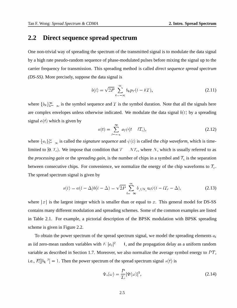
2.2 Direct sequence spread spectrum

One non-trivial way of spreading the spectrum of the transmitted signal is to modulate the data signal

by a high rate pseudo-random sequence of phase-modulated pulses before mixing the signal up to the

carrier frequency for transmission. This spreading methodis calleddirect sequence spread spectrum

(DS-SS). More precisely, suppose the data signal isb(t) = p2P 1Xk=�1 bkpT (t� kT ); (2.11)

wherefbkg1k=�1 is the symbol sequence andT is the symbol duration. Note that all the signals here

are complex envelopes unless otherwise indicated. We modulate the data signalb(t) by a spreading

signala(t) which is given by a(t) = 1Xl=�1 al (t� lT ); (2.12)

wherefalg1l=�1 is called thesignature sequence and (t) is called thechip waveform, which is time-

limited to [0; T ). We impose that condition thatT = NT , whereN , which is usually referred to as

theprocessing gain or thespreading gain, is the number of chips in a symbol andT is the separation

between consecutive chips. For convenience, we normalize the energy of the chip waveforms toT .The spread spectrum signal is given bys(t) = a(t��)b(t��) = p2P 1Xl=�1 bbl=N al (t� lT ��); (2.13)

wherebx is the largest integer which is smaller than or equal tox. This general model for DS-SS

contains many different modulation and spreading schemes.Some of the common examples are listed

in Table 2.1. For example, a pictorial description of the BPSK modulation with BPSK spreading

scheme is given in Figure 2.2.

To obtain the power spectrum of the spread spectrum signal, we model the spreading elementsalas iid zero-mean random variables withE[jalj2℄ = 1, and the propagation delay as a uniform random

variable as described in Section 1.7. Moreover, we also normalize the average symbol energy toPT ,

i.e.,E[jbkj2℄ = 1. Then the power spectrum of the spread spectrum signals(t) is�s(!) = PT j(!)j2; (2.14)

2.5


BPSK modulation QPSK modulation

BPSK (t) = pT (t) (t) = pT (t)spreading bk 2 f�1g bk 2 f� 1p2 � j 1p2gal 2 f�1g al 2 f�1g

QPSK (t) = pT (t) (t) = pT (t)spreading bk 2 f�1g bk 2 f� 1p2 � j 1p2gal 2 f� 1p2 � j 1p2g al 2 f�1;�jg

Table 2.1: Common spreading schemes

b(t)

s(t)

a(t)

Figure 2.2: BPSK modulation and BPSK spreading scheme

2.6


devicedecision

@ t=(k+1)T+∆

r(t) h (t)zk b̂kk

Figure 2.3: Matched filter receiver for thekth symbol of the DS-SS signal

where(!) is the Fourier transform of the chip waveform (t). The power spectra of the spread

signals for the four schemes shown in Table 2.1 are all given by�s(!) = PT sin2(!T =2)(!T =2)2 : (2.15)

Comparing this to the power spectrum of the original data signal�b(!) = PT sin2(!T=2)(!T=2)2 ; (2.16)

we see that the spectrum is spreadN times wider by the direct sequence technique in (2.13). In

practice, the spreading sequences are pseudo-random. We will discuss, in Chapter 3, different ways to

generate sequences which have properties close to those of random sequences.

In an AWGN channel, the ML receiver for the spread spectrum signal is the matched filter receiver

shown in Figure 2.3. We note that the matched filter is time-varying unless the spreading sequencefalg1l=�1 is periodic with periodN . For thekth symbol, the impulse response of the matched filterhk(t) is given by hk(t) = N�1Xl=0 a�l+kN �(T � lT � t): (2.17)

For BPSK modulation, the decision device gives decisionb̂k = sgn(Re[zk℄). For QPSK modulation,

the decision device gives decisionb̂k = 1p2sgn(Re[zk℄) + j 1p2sgn(Im[zk℄). The general case is left as

an exercise. Alternatively, we can implement (see Homework2) the matched filter receiver as shown

in Figure 2.4.

The spreading method described in (2.13) is by no mean the only possible DS-SS technique. For

example, one can spread the in-phase and quadrature channels independently instead of spreading the

complex channel as in (2.13). Suppose the complex data signal isb(t) = bx(t) + jby(t); (2.18)

2.7


devicezk

c(T -t)

@ t=(l+1)T +∆c

decision(k+1)N-1

b̂kr(t) ψ*

a*l

Σl=kN

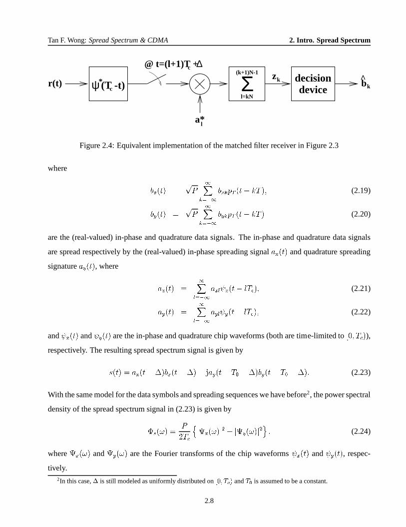
Figure 2.4: Equivalent implementation of the matched filterreceiver in Figure 2.3

where bx(t) = pP 1Xk=�1 bxkpT (t� kT ); (2.19)by(t) = pP 1Xk=�1 bykpT (t� kT ) (2.20)

are the (real-valued) in-phase and quadrature data signals. The in-phase and quadrature data signals

are spread respectively by the (real-valued) in-phase spreading signalax(t) and quadrature spreading

signatureay(t), where ax(t) = 1Xl=�1axl x(t� lT ); (2.21)ay(t) = 1Xl=�1ayl y(t� lT ); (2.22)

and x(t) and y(t) are the in-phase and quadrature chip waveforms (both are time-limited to[0; T )),respectively. The resulting spread spectrum signal is given bys(t) = ax(t��)bx(t��) + jay(t� T0 ��)by(t� T0 ��): (2.23)

With the same model for the data symbols and spreading sequences we have before2, the power spectral

density of the spread spectrum signal in (2.23) is given by�s(!) = P2T njx(!)j2 + jy(!)j2o ; (2.24)

wherex(!) andy(!) are the Fourier transforms of the chip waveforms x(t) and y(t), respec-

tively.2In this case,� is still modeled as uniformly distributed on[0; T ) andT0 is assumed to be a constant.

2.8


devicec(T -t)

decisiondevicec(T -t)r (t)

x

r (t)y

r (t)x

r (t)y

r(t) = + j

decision∆

b̂ykψ

ayl

Σl=kN

(k+1)N-1

y

@ t=(l+1)T +T +c 0

b̂xkψ

axl

Σl=kN

(k+1)N-1

x

@ t=(l+1)T +c ∆

Figure 2.5: Matched filter receiver for independent-channel-spreading DS-SS

This DS-SS model includes offset QPSK spreading and serial-MSK spreading, which we are not

going to discuss in detail. The matched filter receiver for this form of DS-SS is shown in Figure 2.5.

We note that the two different forms of DS-SS described in (2.13) and (2.23) overlap, but they are not

subsets of each other.

In order to implement the matched filter receivers shown above, we need to achieve timing and

phase synchronization which will be discussed in Chapter 5.

2.3 Frequency hop spread spectrum

Another common method to spread the transmission spectrum of a data signal is to (pseudo) randomly

hop the data signal over different carrier frequencies. This spreading method is calledfrequency hop

spread spectrum (FH-SS). Usually, the available band is divided into non-overlapping frequencybins.

The data signal occupies one and only one bin for a durationT and hops to another bin afterward.

When the hopping rate is faster than the symbol rate (i.e.,T > T ), the FH scheme is referred to

as fast hopping. Otherwise, it is referred to asslow hopping. A typical FH-SS transmitter and the

corresponding receiver are shown in Figures 2.6 and 2.7, respectively.

Because it is practically difficult to build coherent frequency synthesizers, modulation schemes,

2.9


Modulator FilterHighpass

SynthesizerFrequency

CodeGenerator

FH codeclock

Data s(t)data

a(t)

b(t)

Figure 2.6: Transmitter for FH-SS

Frequency

CodeGenerator

FH codeclock

RejectionImage

Filter

DataDemodulator

Synthesizer

estimated

a(t)

FilterBandpass data

Figure 2.7: Receiver for FH-SS

2.10


such asM -ary FSK, which allow noncoherent detection are usually employed for the data signal. ForM -ary FSK, the data signal3 can be expressed asb(t) = p2P 1Xk=�1 pT (t� kT ) os(!kt+ �k); (2.25)

where!k 2 f!s0; !s1; : : : ; !sM�1g. The frequency synthesizer outputs a hopping signala(t) = 2 1Xl=�1 pT (t� lT ) os(!0lt + �0l); (2.26)

where!0k 2 f! 0; ! 1; : : : ; ! L�1g. This means that there areL frequency bins in the FH-SS system.

We impose the constraint thatT = NT for fast hopping, orT = NT for slow hopping. The FH-SS

signal is given bys(t) = p2P 1Xl=�1 pT (t� lT ��) os h(!bl=N + !0l)(t��) + �bl=N + �0li (2.27)

for the case of fast hopping (T > T ), ors(t) = p2P 1Xk=�1 pT (t� kT ��) os h(!k + !0bk=N )(t��) + �k + �0bk=N i (2.28)

for the case of slow hopping (T < T ). The orthogonality requirement for the FSK signals forcesthe

separation between adjacent FSK symbol frequencies be at least2�=T for fast hopping, or2�=T for

slow hopping. Hence, the minimum separation between adjacent hopping frequencies is2M�=T for

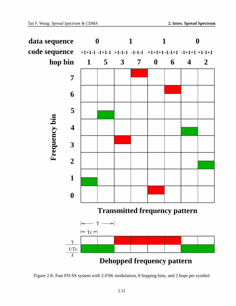
fast hopping, or2M�=T for slow hopping. For example, Figure 2.8 depicts the operation of a fast

FH-SS system with2-FSK modulation (M = 2), 8 hopping bins (L = 8), and2 hops per symbol

(T = 2T ,N = 2).

To obtain the power spectrum of theM -ary FH-SS signal, we model the phases�k and�0l as iid

random variables uniformly distributed on[0; 2�). The hopping frequencies!0l are modelled as iid

random variables taking values from the setf! 0; ! 1; : : : ; ! L�1g with equal probabilities. The FSK

symbol frequencies!k are iid random variables taking values from the setf!s0; !s1; : : : ; !sM�1g with

equal probabilities. The delay� is assumed to be uniformly distributed on[0; T ) for fast hopping, or[0; T ) for slow hopping. We also assume that all the random variables mentioned above are indepen-

dent. With these assumptions, we can show (see Homework 2) that the power spectrum of the FH-SS3All the signals in this section are real bandpass signals

2.11


4607351

T

2

1/Tc

6

3

1

0

5

7

2

4

Fre

quen

cy b

in

data sequence 00 1 1+1+1-1 -1+1-1 +1-1-1 -1-1-1 +1+1+1-1-1+1 -1+1+1 +1-1+1

hop bincode sequence

Transmitted frequency pattern

Dehopped frequency pattern

Tc

Figure 2.8: Fast FH-SS system with 2-FSK modulation, 8 hopping bins, and 2 hops per symbol

2.12


signals(t) is given by�s(!) = PT 2ML L�1Xl=0 M�1Xm=0 8<:"sin(! � ! l � !sm)T =2(! � ! l � !sm)T =2 #2 + "sin(! + ! l + !sm)T =2(! + ! l + !sm)T =2 #29=; (2.29)

for fast hopping, or�s(!) = PT2ML L�1Xl=0 M�1Xm=0 8<:"sin(! � ! l � !sm)T=2(! � ! l � !sm)T=2 #2 + "sin(! + ! l + !sm)T=2(! + ! l + !sm)T=2 #29=; (2.30)

for slow hopping. Therefore, the spectrum of the original data signalb(t) is approximately spread by

a factor ofLN for fast hopping, or by a factor ofL for slow hopping.

2.4 Time hop spread spectrum

In time hop spread spectrum (TH-SS), we spread the spectrum by modulating the data signal by a

pseudo-random pulse-position-modulated spreading signal. We have described the general idea in

Section 2.1. Here, we give the precise definition. Suppose the data signalb(t) isb(t) = p2P 1Xk=�1 bkpT (t� kT ): (2.31)

We modulate the data signal by the spreading signala(t) = s TT 1Xk=�1 pT (t� kT � akT ); (2.32)

whereak 2 f0; 1; : : : ; N � 1g andT = NT . The resulting spread spectrum signals(t) is given bys(t) = a(t��)b(t��) = s2PTT 1Xk=�1 bkpT (t� kT � akT ��): (2.33)

To obtain the power spectrum of the TH-SS signals(t), we model the data symbolsbk as iid zero-

mean random variables withE[jbkj2℄ = 1. The pulse location indicesak are assumed to be iid random

variables taking values fromf0; 1; : : : ; N � 1g with equal probabilities. The propagation delay� is

modelled as a uniform random variable on[0; T ) as usual. It can be shown (see Homework 2) that the

power spectral density of the spread spectrum signals(t) is the same as the one obtained in Section 2.1,

i.e., �s(!) = PT sin2(!T =2)(!T =2)2 : (2.34)

2.13


deviceTcp (T-t)

CodeGenerator

TH codeclock

decision

Circuit

@ t=(k+1)T+a T +

Timing

b̂kr(t)

∆k c

Figure 2.9: Matched filter receiver for TH-SS

The matched filter receiver for this spreading method is shown in Figure 2.9. It is the same as the

receiver in Figure 2.1 except that the sampler is controlledby a timing circuit which is in turn driven

by the pseudo-random pulse-location code.

We note that there are other types of TH-SS techniques. For example, one can use pulse-position

modulation for the data signal. As a result, the spread spectrum signal will be purely pulse-position

modulated. The hopping scheme is similar to theM -ary FSK FH-SS system described in Figure 2.8

with frequency bins replaced by time bins.

2.5 Multicarrier spread spectrum

In FH-SS, only one of many possible frequencies is transmitted at a time. The other extreme is that

we transmit all the possible frequencies simultaneously. The resulting spreading method is called

multicarrier spread spectrum (MC-SS). More precisely, suppose the data signalb(t) is given byb(t) = p2P 1Xk=�1 bkpT (t� kT ): (2.35)

2.14


We modulate the data signal by the spreading signala(t) = 1pN 1Xk=�1N�1Xn=0 an;kej!ntpT (t� kT ): (2.36)

The resulting spread spectrum signal iss(t) = a(t��)b(t��) = s2PN 1Xk=�1N�1Xn=0 bkan;kej!n(t��)pT (t� kT ��): (2.37)

The data and spreading sequences are phase-modulated as in the case of DS-SS. The carrier frequencies!n should be chosen so that signals at different frequencies donot interfere each other. The minimum

frequency separation is2�=T . To obtain the power spectrum of the spread spectrum signal,we model

the spreading elementsan;k as iid zero-mean random variables withE[jan;kj2℄ = 1, and the propagation

delay as a uniform random variable on[0; T ). Moreover, we also normalize the average symbol energy

to PT by settingE[jbkj2℄ = 1. Then the power spectrum of the spread spectrum signals(t) is (see

Homework 2) �s(!) = PTN N�1Xn=0 "sin(! � !n)T=2(! � !n)T=2 #2 : (2.38)

The matched filter receiver for MC-SS is shown in Figure 2.10.When!n = 2n�=T , the operation

of the correlator branches in Figure 2.10 can be approximately performed by a single FFT. Hence the

matched filter receiver can be implemented very efficiently.To see this, consider the output of thenth

correlator for thekth symbol in Figure 2.10 and denote it byzn;k. Then,zn;k = Z (k+1)T+�kT+� r(t)e�j 2n�tT +�dt= N�1Xl=0 Z kT+�+(l+1)T kT+�+lT r(t)e�j 2n�tT +�dt: (2.39)

In above, we divide the interval[kT +�; (k + 1)T +�) intoN sub-intervals of lengthT . In thelthsub-interval, forl = 0; 1; : : : ; N � 1, we approximate4 the integralZ kT+�+(l+1)T kT+�+lT r(t)e�j 2n�tT +�dt � T r(kT +�+ lT )e�j 2n�lT T : (2.40)

Hence, zn;k � T N�1Xl=0 r(kT +�+ lT )e�j 2nl�N : (2.41)

4Better approximations can be made, say, by using the trapezoidal and Simpson’s methods instead. We still get similar

FFT implementation of the correlator branches by using these approximations.

2.15


a0,k*

(k+1)T+ ∆

kT+ ∆

( ) dt

(k+1)T+ ∆

kT+ ∆

( ) dt

decisiondevicea1,k

*bk^

(k+1)T+ ∆

r(t)

aN-1,k*

eΣ

e

( ) dtkT+ ∆

-jw t+

-jw t+∆

1 ∆

e-jw t+N-1

0

∆

Figure 2.10: Matched filter receiver for MC-SS

2.16


We note that (2.41) says that for eachk, the sequencefzn;kgN�1n=0 is approximately the DFT (scaled)

of the sequencefr(kT + � + lT )gN�1l=0 . Therefore, we can implement the correlator branches ap-

proximately by samplingr(t) at the chip rate and passing the samples through an FFT circuit. Similar

approximations can also be applied on the transmitter side.

2.6 Applications

As discussed in Section 2.1, anti-jamming is an important application for spread spectrum modula-

tions. In addition to anti-jamming, we will briefly introduce several other spread spectrum applica-

tions in this section. In describing these applications, wefocus on DS-SS systems. One should note

that other spread spectrum techniques also have similar applications since the main idea behind these

applications is the spreading of the spectrum.

2.6.1 Anti-jamming

We know that we can combat a wide-band Gaussian jammer by spreading the spectrum of the data

signal. Here we consider another kind of jammers—the continuous wave (CW) jammers. Suppose

the spread spectrum signal is given by (2.13) and it is jammedby a sinusoidal signal with frequency! + !0 and powerPJ . The received signal is given byr(t) = s(t) +q2PJej!0t + n(t); (2.42)

wheren(t) represents the AWGN. When one of the four DS-SS schemes in Table 2.1 is used, we can

easily see that the power spectrum of the received signalr(t) is given by�r(!) = PT sin2(!T =2)(!T =2)2 + PJÆ(! � !0) +N0: (2.43)

We consider the matched filter receiver in Figure 2.3. For convenience, we redraw the receiver in

the equivalent correlator form in Figure 2.11. At the outputof the despreader, the signalz(t) can be

expressed as z(t) = r(t)a�(t��)= s(t)a�(t��) +q2PJej!0ta�(t��) + n(t)a�(t��)= b(t��) +q2PJej!0ta�(t��) + n(t)a�(t��): (2.44)

2.17


device bk^

(k+1)T+ ∆

kT+ ∆

( ) dt decisionz(t)r(t)

* ∆a (t- )

Figure 2.11: Matched filter receiver (correlator form) for DS-SS

It can be shown (see Homework 2) that the power spectrum of thedespread signalz(t) is�z(!) = PT sin2(!T=2)(!T=2)2 + PJT "sin(! � !0)T =2(! � !0)T =2 #2 +N0: (2.45)

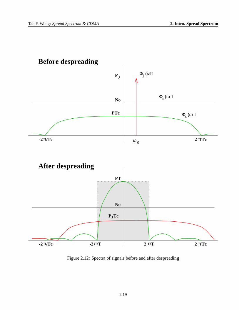
Now the anti-jamming property of the spread spectrum modulation can be explained by comparing

the spectra of the signals before and after despreading in Figure 2.12. Before despreading, the jam-

mer power is concentrated at frequency!0 and the signal power is spread across a wide frequency

band ([�2�=T ; 2�=T ℄). The despreader spreads the jammer power into a wide frequency band

([�2�=T ; 2�=T ℄) while concentrates the signal power into a much narrower band ([�2�=T; 2�=T ℄).The integrator acts like a low-pass filter to collect power ofthe despread signal over the frequency

band[�2�=T; 2�=T ℄. As a result, almost all of the signal power is collected, butonly 1=N th of the

jammer power is collected. The effective power of the jammeris reduced by a factor ofN . This is the

reason whyN is called the spreading gain.

2.6.2 Low probability of detection

Another military-oriented application for spread spectrum is low probability of detection (LPD), which

means that it is hard for an unintentional receiver to detectthe presence of the signal. The idea behind

this can be readily seen from Figure 2.12. When the processing gain is large enough, the spread

spectrum signal hides below the white noise level. Without knowledge of the signature sequences, an

unintentional receiver cannot despread the received signal. Therefore, it is hard for the unintentional

receiver to detect the presence of the spread spectrum. We are not going to treat the subject of LPD

any further than the intuition just given. A more detailed treatment can be found in [1, Ch. 10].

2.18


Φ (ω)s

Φ (ω)jPJ

TcPJ

ω 0π

2 /Tcπ

Before despreading

2 /Tc

No

No

PTc

Φ (ω)n

π π 2 /T

PT

π

π

-2 /Tc

-2 /Tc

-2 /T

After despreading

Figure 2.12: Spectra of signals before and after despreading

2.19


2.6.3 Multipath combining

Another advantage of spreading the spectrum is frequency diversity, which is a desirable property

when the channel is fading. Fading is caused by destructive interference between time-delayed replica

of the transmitted signal arise from different transmission paths (multipaths). The wider the transmitted

spectrum, the finer are we able to resolve multipaths at the receiver. Loosely speaking, we can resolve

multipaths with path-delay differences larger than1=W seconds when the transmission bandwidth isWHz. Therefore, spreading the spectrum helps to resolve multipaths and, hence, combats fading.

The best way to explain multipath fading is to go through the following simple example. Suppose

the transmitter sends a bit with the value “+1” in the BPSK format, i.e., the transmitted signal envelope

is pT (t), whereT is the symbol duration. Assume that there are two transmission paths leading from

the transmitter to the receiver. The first path is the direct line-of-sight path which arrives at a delay

of 0 seconds and has a unity gain. The second path is a reflected path which arrives at a delay of2T seconds and has a gain of�0:8, whereT = T=10 is the chip duration of the DS-SS system we are

going to introduce in a moment. The overall received signal can be written asr(t) = pT (t)� 0:8pT (t� 2T ) + n(t); (2.46)

wheren(t) is AWGN. To demodulate the received signal, we employ the matched filter receiver,

which is matched to the direct line-of-sight signal, i.e.,h(t) = pT (T � t). The output of the matched

filter is plotted in Figure 2.13. We can see from the figure thatthe contribution from the second path

partially cancels that from the first path. We sample the matched filter output at timet = T . The

signal contribution in the sample is0:36T and the noise contribution is a zero-mean Gaussian random

variable with varianceN0T . Compared to the case where only the direct line-of-sight path is present,

the signal energy is reduced by87%, while the noise energy is the same. Therefore, the bit error

probability is greatly increased.

Now, let us spread the spectrum by the spreading signala(t) = 9Xl=0 akpT (t� lT ); (2.47)

wherefa0; a1; : : : ; a9g = f+1;�1;+1;+1;+1;�1;�1;�1;+1;�1g. The received signal for this

DS-SS system is r(t) = a(t)� 0:8a(t� 2T ) + n(t): (2.48)

2.20


0 0.5 1 1.5 2 2.5−1

−0.8

−0.6

−0.4

−0.2

0

0.2

0.4

0.6

0.8

1

time (T sec)

mat

ched

filte

r ou

tput

(T

)

1st path

2nd path

overall

Figure 2.13: Matched filter output for the two-path channel without spreading

2.21


0 0.5 1 1.5 2 2.5−1

−0.8

−0.6

−0.4

−0.2

0

0.2

0.4

0.6

0.8

1

time (T sec)

mat

ched

filte

r ou

tput

(T

)

1st path2nd pathoverall

Figure 2.14: Matched filter output for the two-path channel with spreading

Again, we consider using the matched filter receiver, which is matched toa(t). The output of the

matched filter is shown in Figure 2.14. We can clearly see fromthe figure that the contributions from

the two paths are separated since the resolution of the spread system is ten times finer than that of

the unspread system. If we sample att = T , we get a signal contribution ofT , which is the same as

what we would get if there was only a single path. Hence, unlike what we saw in the unspread system,

multipath fading does not have a detrimental effect on the error probability. In fact, we will show in

Chapter 4 that we can do better by taking one more sample att = T + 2T to collect the energy of the

second path. If we know the channel gain of the second path, wecan combine the paths coherently.

Otherwise we can perform equal-gain noncoherent combining. This ability of the spread spectrum

2.22


modulation to collect energies from different paths is calledmultipath combining.

2.6.4 Code division multiple access

We end our survey of spread spectrum applications by introducing the most investigated application

of spread spectrum techniques—code division multiple access (CDMA). For simplicity, let us focus on

DS-SS. We can allow different users to use the channel simultaneously by assigning different spread-

ing code sequences to them. Thus there is no physical separation in time or in frequency between

signals from different users. The physical channel is divided into many logical channels by the spread-

ing codes. Different from TDMA and FDMA, spread signals fromdifferent users do interfere each

other unless the transmissions from all users are perfectlysynchronized and orthogonal codes are used.

The interference from other users is known asmulitple access intereference (MAI). In general, syn-

chronization across users is hard to achieve in the uplinks of most practical wireless systems. In some

situations, we may not want to restrict ourselves to orthogonal codes. Therefore, we are interested in

investigating how MAI affect the performance of the system and how we can eliminate the effect of

MAI. Detailed discussions on these two issues will be provided in Chapters 6 and 7. Here we present

a crude analysis on how MAI affect the bit error probability performance of the system.

Suppose we employ DS-SS with BPSK modulation and BPSK spreading. There areK simul-

taneous users, each having a distinct pseudo-random sequence, in the system. We select one of the

users, call it the desired user, and try to determine the bit error probability for this user. We assume

that the desired user employs the correlator receiver, which is matched to the spreading code of the

desired user. To simplify the discussion, we assume that thereceived powers of signals from all the

users are identical. Recall from the discussion in Section 2.6.1 that the despreader removes the effect

of spreading from the desired signal. Since the despreader is not matched to the signals from other

users, it cannot remove the effect of spreading for those signals. As a result, the signals from other

users remain wideband after despreading, while the despread desired signal is the same as the original

unspread narrowband data signal. Since the integrator following the despreader acts like a lowpass

filter collecting power from the passband of the data signal,a crude but reasonable approximation is to

assume the signals from other users are independent and identical white Gaussian random processes

2.23


with power spectral densityPT 5, whereP is the received power andT is the chip duration. Thus

the combined effect of the MAI and AWGN is the same as that of the AWGN with power spectral

density raised fromN0 to (K � 1)PT + N0. Substituting this back into (1.22), we see that the bit

error probability is given by Ps = Q s 2PT(K � 1)PT +N0!= Q0�vuut 2E=N01 + (K � 1)E=NN01A ; (2.49)

whereT = NT is the symbol duration andE = PT is the symbol energy. We suffer a loss in SNR

by a factor of1+ (K � 1)E=NN0 with respect to the single-user system. If the number of users in the

system is fixed, we can reduce the loss in SNR by increasing theprocessing gain, i.e., the bandwidth

of the system. Unlike the case of anti-jamming, we cannot reduce the loss by merely increasing the

signal power.

Using (2.49), we can have a preliminary estimate on the capacity of a DS-SS CDMA system. First,

we note that the signal-energy-to-white-noise ratioE=N0 is large in most practical situations. Hence,

we can further approximate the error probability byPs = Q0�s 2NK � 11A : (2.50)

For example, a bit error probability of10�3 is considered sufficient in voice communications. Using

the result in (2.50), we see that the CDMA system with processing gainN can accommodate aboutN=5 users without using any error-correcting code. With a powerful error-correcting code, we expect

this number to increase.

2.7 References

[1] R. L. Peterson, R. E. Ziemer, and D. E. Borth,Introduction to Spread Spectrum Communications,

Prentice Hall, Inc., 1995.5The reason we set the power spectral density toPT is that the power spectra of the DS-SS signals are squared “sinc”

functions which peak at! = 0 with the valuePT .2.24


[2] M. B. Pursley, “Performance evaluation for phase-codedspread-spectrum multiple-access com-

munication — Part I: System analysis,”IEEE Trans. Commun., vol. 25, no. 8, pp. 795–799,

Aug. 1977.

[3] R. A. Scholtz, “Multiple access with time-hopping impulse modulation,”Proc. MILCOM ’93,

pp. 11-14, Boston, MA, Oct. 1993.

[4] N. Yee, J. M. G. Linnartz, and G. Fettweis, “Multi-carrier CDMA in indoor wireless radio

networks,”IEICE Trans. Commun., vol. E77-B, no. 7, pp. 900–904, Jul. 1994.

[5] S. Kondo and L. B. Milstein, “Performance of multicarrier DS CDMA systems,”IEEE Trans.

Commun., vol. 44, no. 2, pp. 238–246, Feb. 1996.

[6] R. L. Pickholtz, L. B. Milstein, and D. L. Schilling, “Spread spectrum for mobile communica-

tions,” IEEE Trans. Veh. Technol., vol. 40, no. 2, pp. 313–321, May 1991.

2.25

Chapter 2 Introduction to Spread Spectrum Communications

Documents

Transcript of Chapter 2 Introduction to Spread Spectrum Communications