Chapter 11. problems in radiation detection and measurement
33
-
Upload
khangminh22 -
Category
Documents
-
view
0 -
download
0
Transcript of Chapter 11. problems in radiation detection and measurement
Introduction All instruments designed for a specific purpose require
several considerations of design characteristics and performance limitations in common Detection efficiency Counting rate limitations Detecting and counting problems for non-penetrating radiations
발표자
프레젠테이션 노트
모든 radiation을 측정하는 장비들은 각각의 특성과 사용목적에 따라 다르게 디자인되어지는데 공통적으로 디자인 특성과 performance의 한계에 관련하여 고려해야할점이 대표적으로 세가지 있습니다 최소한의 방사능양으로 최대치의 정보를 얻어내기위하여 instrument 의 detection efficiency를 고려해야하고 counting rate 의 limit을 넘어서게되면 data loss나 data distortion으로 인해 부정확한 결과를 얻게되기때문에 counting rate limitation을 고려해야합니다. 마지막으로 베타입자와 같은 non-penetrating radiation particles을 측정하는데 생기는 문제점또한 고려해야합니다.
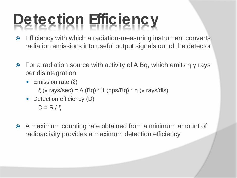
Detection Efficiency Efficiency with which a radiation-measuring instrument converts
radiation emissions into useful output signals out of the detector
For a radiation source with activity of A Bq, which emits η γ rays per disintegration Emission rate (ξ)
ξ (γ rays/sec) = A (Bq) * 1 (dps/Bq) * η (γ rays/dis) Detection efficiency (D)
D = R / ξ
A maximum counting rate obtained from a minimum amount of radioactivity provides a maximum detection efficiency
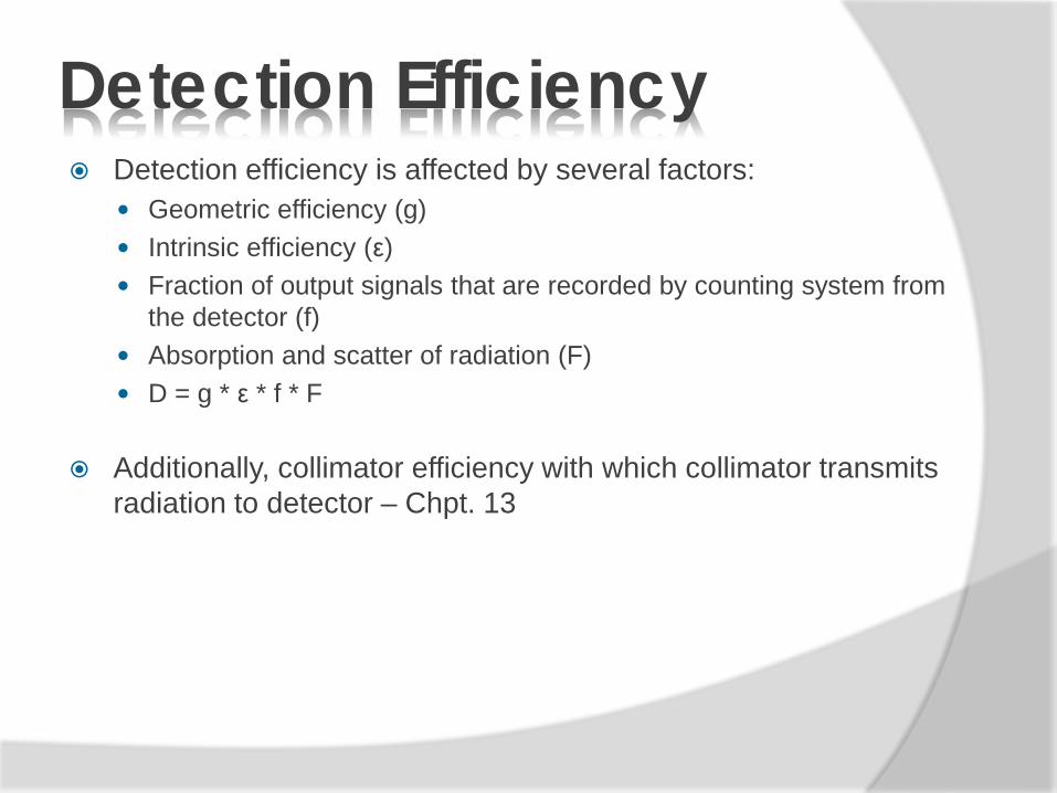
Detection Efficiency Detection efficiency is affected by several factors:
Geometric efficiency (g) Intrinsic efficiency (ε) Fraction of output signals that are recorded by counting system from
the detector (f) Absorption and scatter of radiation (F) D = g * ε * f * F
Additionally, collimator efficiency with which collimator transmits radiation to detector – Chpt. 13
Detection Efficiency A. Geometric Efficiency
A measure of how the detector intercepts radiation emitted from the source
Isotropic emission of a radioactive source – equal intensity of radiation in all directions
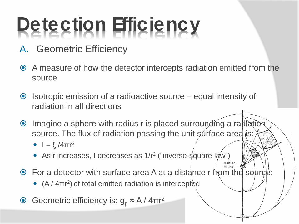
Imagine a sphere with radius r is placed surrounding a radiation source. The flux of radiation passing the unit surface area is: I = ξ /4πr2 As r increases, I decreases as 1/r2 (“inverse-square law”)
For a detector with surface area A at a distance r from the source: (A / 4πr2) of total emitted radiation is intercepted
Geometric efficiency is: gp ≈ A / 4πr2
Detection Efficiency A. Geometric Efficiency
EXAMPLE: Q. Calculate the geometric efficiency for a detector of diameter d = 7.5cm at a distance r = 20 cm from a point source. A. Surface area of the detector, A = π*3.752=44.179cm2 Surface area of the sphere, A’ = 4*π*202=5026.548cm2 gp ≈ A / A’
≈ 44.179 / 5026.548 ≈ 0.00879
A. Geometric Efficiency
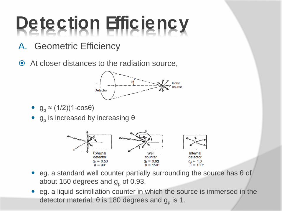
At closer distances to the radiation source,
gp ≈ (1/2)(1-cosθ) gp is increased by increasing θ
eg. a standard well counter partially surrounding the source has θ of about 150 degrees and gp of 0.93.
eg. a liquid scintillation counter in which the source is immersed in the detector material, θ is 180 degrees and gp is 1.
Detection Efficiency
A. Geometric Efficiency
Approximations for the geometric efficiency presented so far are valid for: Point sources of radiation Distributed sources of small dimensions in relative to the source-to-
detector distance (eg. source diameter ≥ 0.3r)
Detection Efficiency
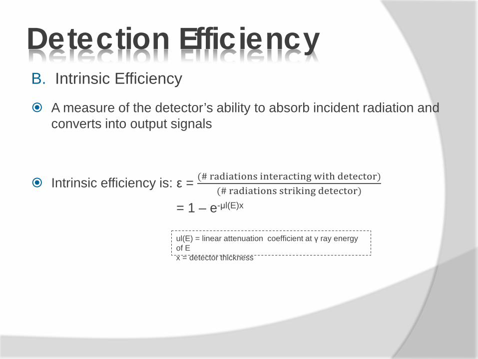
B. Intrinsic Efficiency
A measure of the detector’s ability to absorb incident radiation and converts into output signals
Intrinsic efficiency is: ε = (# radiations interacting with detector)(# radiations striking detector)
= 1 – e-μl(E)x
Detection Efficiency
ul(E) = linear attenuation coefficient at γ ray energy of E x = detector thickness
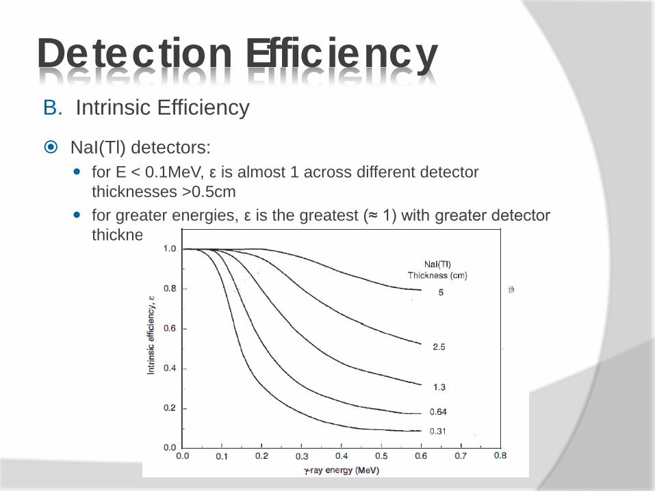
B. Intrinsic Efficiency
NaI(Tl) detectors: for E < 0.1MeV, ε is almost 1 across different detector
thicknesses >0.5cm for greater energies, ε is the greatest (≈ 1) with greater detector
thickness
Detection Efficiency
B. Intrinsic Efficiency
Semiconductor detectors: Si(Li) detectors (Z=14) used for low-energy γ rays and x rays Ge(Li) detectors (Z=32) used for high energies higher density than NaI(Tl) with higher Z for E≤ 250keV, μl is greater. However, at greater E, NaI(Tl) is more efficient
CdTe and CZT detectors
Z similar to NaI(Tl), higher densities Greater intrinsic detection efficiencies than NaI(Tl), but difficult to
fabricate in great thicknesses Limited to low energy applications
Detection Efficiency
B. Intrinsic Efficiency
Gas-filled detectors good intrinsic efficiency for particle radiations only due to low density ~1% intrinsic efficiency for γ ray detection for GM tubes, proportional
counters and ionisation chambers in nuclear medicine Xenon gas filled counters at high pressures, lead/leaded glass γ ray
converters display higher efficiencies, but mostly useful for low energies only
Detection Efficiency
C. Energy-Selective Counting
The fraction of output signals from the detector falling within the pulse-height analyser window (denoted as f) is considered
Photofraction, fp, is the fraction within the photopeak is dependent on detector material γ ray energy crystal size
If full spectrum is used (no selective counting), f ≈ 1 maximum counting rate is provided advantageous when a single radionuclide is counted with little
interference from scattered radiation
Detection Efficiency
Pr (photoelectric absorption)
Complicating Factors
Present when idealised conditions for NaI(Tl) detection system are not met
Nonuniform detection efficiency Detection of simultaneously emitted radiations in coincidence Attenuation and scatter of radiation outside the detector
Detection Efficiency
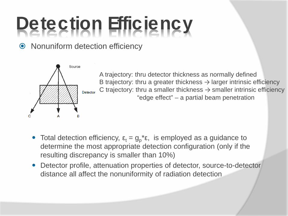
Nonuniform detection efficiency
Total detection efficiency, εt = gp*ε, is employed as a guidance to determine the most appropriate detection configuration (only if the resulting discrepancy is smaller than 10%)
Detector profile, attenuation properties of detector, source-to-detector distance all affect the nonuniformity of radiation detection
Detection Efficiency
A trajectory: thru detector thickness as normally defined B trajectory: thru a greater thickness → larger intrinsic efficiency C trajectory: thru a smaller thickness → smaller intrinsic efficiency “edge effect” – a partial beam penetration
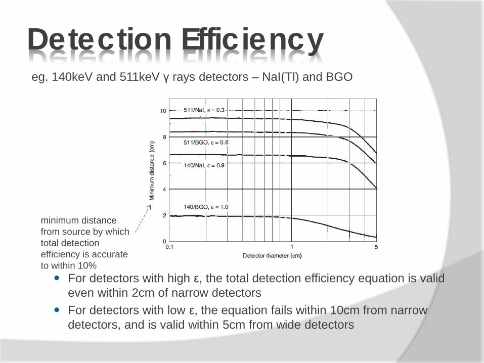
eg. 140keV and 511keV γ rays detectors – NaI(Tl) and BGO
For detectors with high ε, the total detection efficiency equation is valid even within 2cm of narrow detectors
For detectors with low ε, the equation fails within 10cm from narrow detectors, and is valid within 5cm from wide detectors
Detection Efficiency
minimum distance from source by which total detection efficiency is accurate to within 10%
Simultaneously emitted radiations in coincidence
Suppose γ1 and γ2 are emitted simultaneously with relative frequencies of η1 and η2, and total detection efficiencies of D1 and D2, respectively. Probability (γ1 detected following a single disintegration), p1 = η1D1 In the absence of coincidence detection, counting rate for γ1, R1 = p1 * A(Bq) In the presence of coincidence detection, Pr (both γ1 and γ2 detected simultaneously), p12 = η1D1 * η2D2 Counting rate for simultaneously detected events, R12 = p12 * A Recorded full-spectrum counting rate, R1 + R2 – R12
Detection Efficiency
Attenuation and scatter of radiation before the detector
in vivo measurements
Absorption effects decrease the counting rate, whereas scattering causes either a decrease or increase, depending on the direction of scattered rays
Corrections for the effects depend on a number of factors incld: γ ray energy, depth of source in medium, use of energy-selective counting etc eg. counting rate for a source may be greater in scattering medium at a
shallow depth due to the presence of backscattering, and smaller at deeper depths because the absorption effects predominate
Detection Efficiency
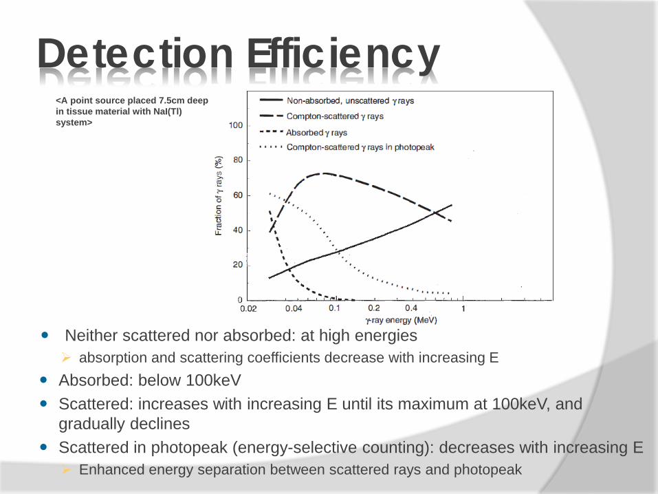
Neither scattered nor absorbed: at high energies absorption and scattering coefficients decrease with increasing E
Absorbed: below 100keV Scattered: increases with increasing E until its maximum at 100keV, and
gradually declines Scattered in photopeak (energy-selective counting): decreases with increasing E Enhanced energy separation between scattered rays and photopeak
Detection Efficiency <A point source placed 7.5cm deep in tissue material with NaI(Tl) system>
Attenuation by housing material of detector Very thin layers of material such as aluminum or beryllium (depending on
the energy of a source of interest) form the entrance windows of detectors in order to minimise attenuation effects
If detectors are used outside the range of its intended applications, attenuation effects become non-negligible
Can be severe in β-particle counting measurements
Detection Efficiency
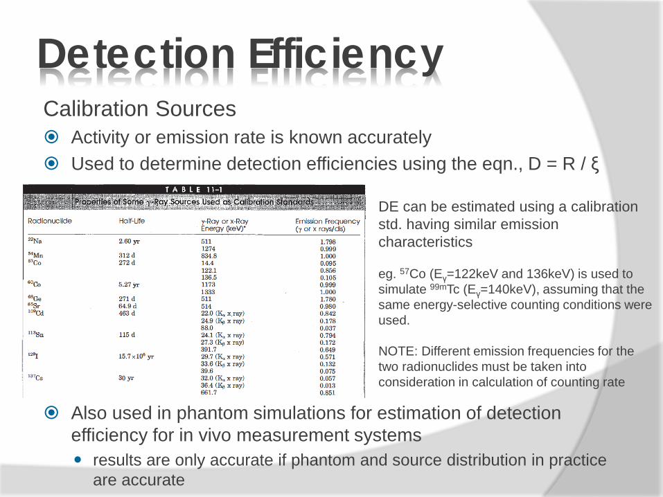
Calibration Sources Activity or emission rate is known accurately Used to determine detection efficiencies using the eqn., D = R / ξ
Also used in phantom simulations for estimation of detection efficiency for in vivo measurement systems results are only accurate if phantom and source distribution in practice
are accurate
Detection Efficiency
DE can be estimated using a calibration std. having similar emission characteristics eg. 57Co (Eγ=122keV and 136keV) is used to simulate 99mTc (Eγ=140keV), assuming that the same energy-selective counting conditions were used. NOTE: Different emission frequencies for the two radionuclides must be taken into consideration in calculation of counting rate
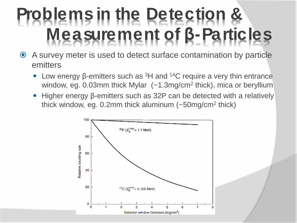
A survey meter is used to detect surface contamination by particle emitters Low energy β-emitters such as 3H and 14C require a very thin entrance
window, eg. 0.03mm thick Mylar (~1.3mg/cm2 thick), mica or beryllium Higher energy β-emitters such as 32P can be detected with a relatively
thick window, eg. 0.2mm thick aluminum (~50mg/cm2 thick)
Problems in the Detection & Measurement of β-Particles
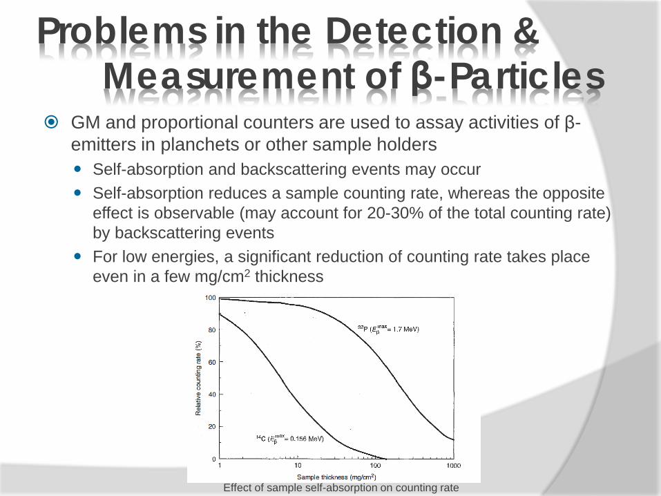
GM and proportional counters are used to assay activities of β-emitters in planchets or other sample holders Self-absorption and backscattering events may occur Self-absorption reduces a sample counting rate, whereas the opposite
effect is observable (may account for 20-30% of the total counting rate) by backscattering events
For low energies, a significant reduction of counting rate takes place even in a few mg/cm2 thickness
Problems in the Detection & Measurement of β-Particles
Effect of sample self-absorption on counting rate
Careful sample preparation skills are necessary for external particle-counting measurements
Bremsstrahlung counting can be used as an indirect method for β particle detection using penetrating radiation detectors such as a NaI well counter Available only for relatively energetic β particles, eg. 32P Requires a very high activity to be detectable
Problems in the Detection & Measurement of β-Particles
Dead Time Causes of Dead Time Dead time/pulse resolving time (τ) = the time required to process
individual detected events
With GM detectors, the overlap of two pulses may occur in the detector itself The second pulse is not detected
With energy-sensitive detectors, eg. scintillation, semiconductor, proportional counters, overlap occurs in the pulse amplifier Baseline shift and pulse pileup If fall outside the analyser window, valid events are lost
The shorter the dead time, the smaller the dead time losses
Dead Time Causes of Dead Time GM tubes: τ~ 500-200 usec
NaI and semiconductor detectors: τ~ 0.5-5 usec Liquid scintillation systems: τ~ 0.1-1 usec Gas proportional counters: τ~ 0.1-1 usec
Dead time losses also occur in pulse-height analysers, scalers, computer interfaces etc while processing pulse signals Scalers and single-channel analysers: τ~ <1 usec Multichannel analysers and computer interface : τ~ a few usec Normally given as whole
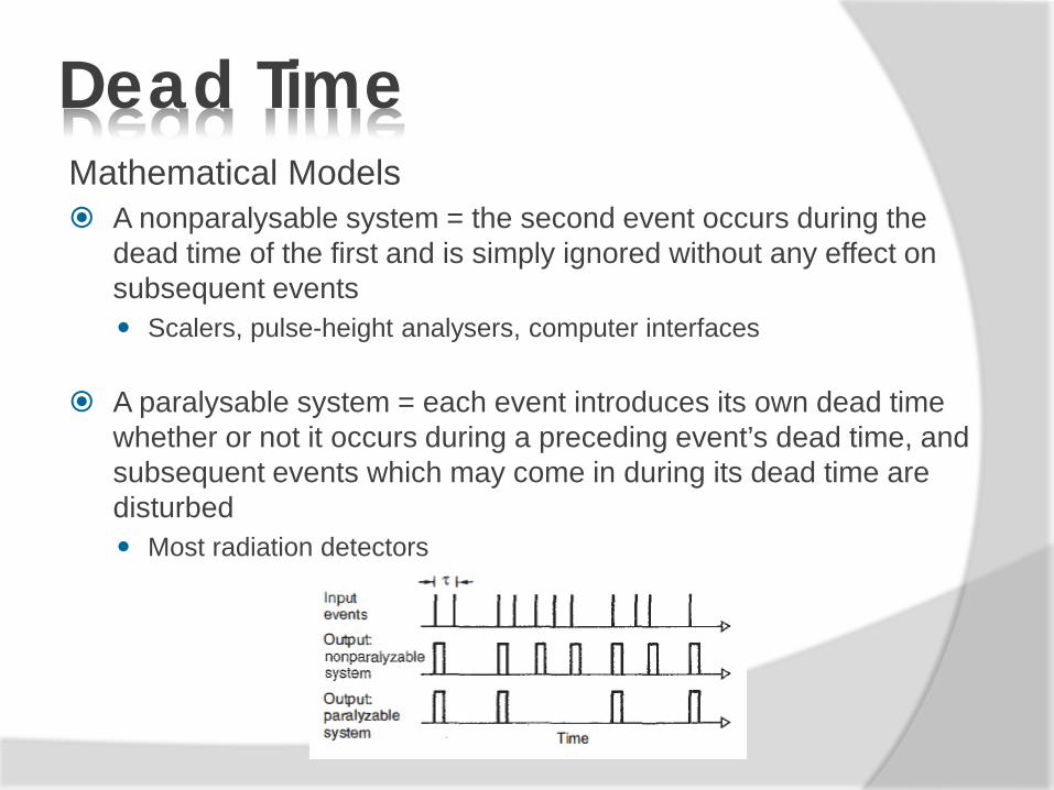
Dead Time Mathematical Models A nonparalysable system = the second event occurs during the
dead time of the first and is simply ignored without any effect on subsequent events Scalers, pulse-height analysers, computer interfaces
A paralysable system = each event introduces its own dead time whether or not it occurs during a preceding event’s dead time, and subsequent events which may come in during its dead time are disturbed Most radiation detectors
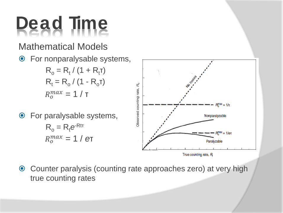
Dead Time Mathematical Models For nonparalysable systems, Ro = Rt / (1 + Rtτ) Rt = Ro / (1 - Roτ)
For paralysable systems, Ro = Rte-Rtτ
Counter paralysis (counting rate approaches zero) at very high true counting rates
𝑅𝑜𝑚𝑚𝑚 = 1 / τ
𝑅𝑜𝑚𝑚𝑚 = 1 / eτ
Dead Time Mathematical Models Dead time losses are expressed as % losses % losses = [(Rt-Ro)/Rt]*100% When Rtτ is small (<0.1), the percentage losses are small (<10%),
and the following equation can be applied for both paralysable and nonparalysable systems
% losses = (Rtτ)*100% In multiple component systems (mixed paralysable and
nonparalysable components), mostly one component dominates and its behaviour describes the system behaviour.
If both paralysable and nonparalysable systems have similar dead times, the behaviour is a hybrid of the two
Dead Time Window Fraction Effects In cases of pileup effects in pulse-height spectrum, the total-
spectrum counting rate needs to be taken into account, as well as the counting rate within the selected window, to determine dead time losses.
Apparent dead time (τa) = τ / wf
eg. NaI(Tl) detector system with τ of 1usec used with a narrow
window within which 25% of total events are detected (wf = 0.25). Then, τa = 1/0.25 = 4 usec
Window fractions are affected by amount of scattering events
wf = The fraction of detected events occurring within the selected analyser window
Dead Time Dead Time Correction Methods The mathematical models described till this point can be used as
dead time correction for most of the systems with a standardised measuring configuration with little or no window fraction variations
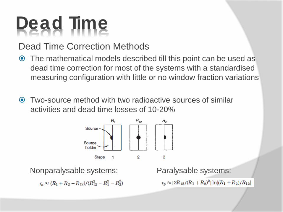
Two-source method with two radioactive sources of similar activities and dead time losses of 10-20%
Nonparalysable systems: Paralysable systems:
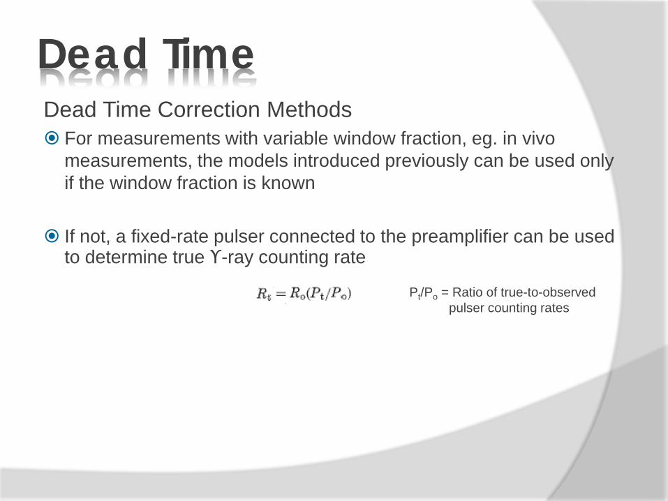
Dead Time Dead Time Correction Methods For measurements with variable window fraction, eg. in vivo
measurements, the models introduced previously can be used only if the window fraction is known
If not, a fixed-rate pulser connected to the preamplifier can be used to determine true ϒ-ray counting rate
Pt/Po = Ratio of true-to-observed pulser counting rates
Quality Assurance for Radiation Measurement Systems Radiation measurement systems are subject to malfunctions
leading to changes in detection efficiency, increased background etc
To assure system consistency, quality assurance procedures are necessary Daily measurement of the system’s response to a standard radiation source Daily measurement of background levels A periodic measurement of system energy resolution for systems with pulse-
height analysis capabilities
Statistical tests, eg X2 test, can be used to assist to detect subtle changes in performance P < 0.01 or P > 0.99, evidence of a system problem 0.05 < P < 0.95, acceptable in between, equivocal and test needs to be repeated