
CHAPTER 1 INTRODUCTION - CORE
338
WWW.BROOKES.AC.UK/GO/RADAR RADAR Research Archive and Digital Asset Repository Assessing the potential of heat pumps to reduce energy-related carbon emissions from UK housing in a changing climate Robert W Irving (2013) https://radar.brookes.ac.uk/radar/items/9e311425-0948-4390-bbeb-4da569dc9fa7/1/ Copyright © and Moral Rights for this thesis are retained by the author and/or other copyright owners. A copy can be downloaded for personal non-commercial research or study, without prior permission or charge. This thesis cannot be reproduced or quoted extensively from without first obtaining permission in writing from the copyright holder(s). The content must not be changed in any way or sold commercially in any format or medium without the formal permission of the copyright holders. When referring to this work, the full bibliographic details must be given as follows: Irving, R W (2013) Assessing the potential of heat pumps to reduce energy-related carbon emissions from UK housing in a changing climate PhD, Oxford Brookes University
-
Upload
khangminh22 -
Category
Documents
-
view
1 -
download
0
Transcript of CHAPTER 1 INTRODUCTION - CORE

WWW.BROOKES.AC.UK/GO/RADAR
RADAR
Research Archive and Digital Asset Repository
Assessing the potential of heat pumps to reduce energy-related carbon emissions from UK housing in a changing climate
Robert W Irving (2013)
https://radar.brookes.ac.uk/radar/items/9e311425-0948-4390-bbeb-4da569dc9fa7/1/
Copyright © and Moral Rights for this thesis are retained by the author and/or other copyright owners. A copy can be downloaded for personal non-commercial research or study, without prior permission or charge. This thesis cannot be reproduced or quoted extensively from without first obtaining permission in writing from the copyright holder(s). The content must not be changed in any way or sold commercially in any format or medium without the formal permission of the copyright holders.
When referring to this work, the full bibliographic details must be given as follows:
Irving, R W (2013) Assessing the potential of heat pumps to reduce energy-related carbon emissions from UK housing in a changing climate PhD, Oxford Brookes University
Assessing the potential of heat pumps to reduce energy-related carbon emissions from UK housing in a changing climate
Robert Irving BA(hons) MSc
A thesis submitted in partial fulfilment of the requirement of the School of Architecture, Faculty of Technology, Design & Environment,
Oxford Brookes University, Oxford, UK for the degree of Doctor of Philosophy
Oxford September 2013

ii
ABSTRACT
This thesis describes three connected stages of development and analysis of residential heat pump energy use: firstly, the analysis of heat pump performance data from a monitoring study of ground source heat pumps; secondly, the definition and development of a generalised residential heat pump energy model embedded within an enhanced dwelling energy model; finally, the analysis of the effects of possible residential heat pump installation scenarios on the UK energy supply and carbon emissions.
The monitoring study involved three ground source heat pump installations. The data collected consisted of heat output, electric power input, system temperatures and system status indicators. Analysis indicated that these systems showed reductions in carbon emissions from homes ranging from 18% to 37% compared with their counterfactual fuel-burning systems.
The monitoring study provided empirical values to parameterise the heat pump model which was built around a linear regression relationship of heat pump COP to source / sink temperature differential based on heat pump performance data from standard laboratory test results. This model was added in a new module to enhance the BRE domestic energy model, BREDEM-8, which provides monthly estimates. Estimating rules were included for energy use from bivalent alternate, bivalent parallel operation and space cooling.
The enhanced BREDEM-8 model was used to analyse the effects of possible residential heat pump installations within a housing stock energy model developed using the English Housing Survey datasets as a data source. Baseline estimates for the current stock were created using data reduction techniques to provide parameters (u-values, glazing details) for the enhanced BREDEM-8 model.
Scenarios for heat pump deployments were created for the periods up to 2020 and 2050, selecting dwellings for heat pump application according to scenarios reflecting the perceived needs of the period, ie. the likely reduction in UK generating capacity up to 2020 and CO2 emissions reduction targets to 2050. Results showed that up to 2020, a policy of targeting dwellings with the highest overall emissions for replacement would reduce carbon emissions by 7.6%, at the expense of a 12% increase in electricity consumption. Targeting dwellings with the highest emitting existing systems caused a smaller increase in electricity consumption of about 6.5% with carbon emissions reduced by about 6.8%.
The scenarios for the period to 2050, including 80% replacement of gas systems with heat pumps, gave an estimated 80% reduction in carbon emissions, when accompanied by an similar reduction in the carbon intensity of electricity generation and bringing about an increase in electricity consumption of somewhat over 40%. The effect of the more extreme scenario is to replace all but a small proportion of the energy used for heating and hot water with standard rate electricity, in 84.6% of the dwellings, and retaining gas in the remainder, 15.2%, bringing about a radical shift to electric heating throughout the housing stock.

iii
DECLARATION
The candidate, Robert Irving, while registered for the Degree of Doctor of Philosophy, was not registered for any other award of a university during the programme
Robert Irving, September 2013

iv
ACKNOWLEDGEMENTS
The author would like to thank: my supervisor, Professor Rajat Gupta, without whose assistance this project would not have happened, for putting up with my vicissitudes and finally navigating me through the project; my second supervisor, Dr Nicholas Walliman, for his helpful comments on my work; Dr David Atkins, of ICE Energy, for setting up the data monitoring section of the project and providing advice on the internals of heat pumps and their controllers; Steve Ingram for building the dataloggers and Richard Cartwright for installing them; Mr & Mrs Bufton and family, Mr & Mrs Richards and family, Mr and Mrs Oliver for the use of their heat pump systems for the monitoring study and tolerating my fortnightly visits; their neighbours for ignoring my hanging around outside their houses with a laptop for no apparent reason; my wife Joy for her support and tolerance throughout the project and for allowing me to take over a whole room for the whole time; and my son and occasional daughter for studiously ignoring me at the right times. Other entities that deserve a mention for providing various sources of distraction are a small cat that came to sexual maturity and learnt keyboard and other office skills during my write-up; the pilots and lawn-mowers of the Cotswolds; and the MicroSoft Excel and Word development teams who could have helped more. This research was carried out as part of a 3.5 year project funded by the Engineering and Physical
Science Research Council (Grant no. CASE/CNA/06/82) to assess the potential of ground source
heat pumps in reducing energy-related carbon emissions from UK housing in a changing climate.

v
TABLE OF CONTENTS
ABSTRACT.................................................................................................................................ii
DECLARATION........................................................................................................................iii
ACKNOWLEDGEMENTS........................................................................................................iv TABLE OF CONTENTS ............................................................................................................v
Chapter 1 Introduction ................................................................................................................1 1.1 Introduction ..................................................................................................................................... 2 1.2 Heating systems in UK dwellings ................................................................................................... 2
1.2.1 History and current status .......................................................................................................... 2 1.2.2 Domestic energy use for heating................................................................................................ 5 1.2.3 Carbon emissions from domestic energy use ............................................................................. 7 1.2.4 Effect of the dominance of gas central heating .......................................................................... 7 1.2.5 Heat pump heating systems ....................................................................................................... 8
1.3 Drivers for change ........................................................................................................................... 9 1.3.1 ‘Peak Oil / Gas’ ......................................................................................................................... 9 1.3.2 Reduction of greenhouse gas emissions .................................................................................. 11
1.4 UK Government policies on carbon emission reduction in dwellings ....................................... 11 1.4.1 Carbon Emission Reduction Targets (CERT)(UK Parliament, 2008b) ................................... 12 1.4.2 Code for Sustainable Homes (CSH) (DCLG, 2008a) .............................................................. 12 1.4.3 UK Renewable Heat Incentive ................................................................................................ 15 1.4.4 'Green Investment Bank', 'Green Deal' scheme ....................................................................... 16
1.5 Research aims and objectives ....................................................................................................... 17 1.6 Thesis structure ............................................................................................................................. 18 1.7 Summary ........................................................................................................................................ 20
Chapter 2 Technical aspects of heat pump systems ................................................................22 2.1 Introduction ................................................................................................................................... 23 2.2 Basis in thermodynamics .............................................................................................................. 23 2.3 Heat pump / refrigeration cycle types .......................................................................................... 24 2.4 Theoretical Heat Pump Cycle ....................................................................................................... 24
2.4.1 Carnot Cycle ............................................................................................................................ 26 2.4.2 Coefficient of Performance ...................................................................................................... 27
2.5 The vapour compression heat pump cycle .................................................................................. 28 2.6 Heat pump system components .................................................................................................... 30
2.6.1 Sources and collectors ............................................................................................................. 30 2.6.2 Source and collector characteristics ......................................................................................... 31 2.6.3 Heat pump configurations ........................................................................................................ 34 2.6.4 Compressors ............................................................................................................................ 35 2.6.5 ‘Soft start’ power supply.......................................................................................................... 36 2.6.6 Additions to the basic compressed vapour heat pump cycle .................................................... 36 2.6.7 Controls ................................................................................................................................... 37 2.6.8 Refrigerants ............................................................................................................................. 38 2.6.9 Distribution System ................................................................................................................. 39
2.7 Environmental credentials of heat pump systems ...................................................................... 41 2.7.1 Heat pump space heating as renewable energy ........................................................................ 41 2.7.2 Carbon dioxide emissions reduction ........................................................................................ 42
2.8 Barriers and drivers to the take-up of domestic heat pumps .................................................... 44 2.8.1 Barriers .................................................................................................................................... 44 2.8.2 Drivers ..................................................................................................................................... 47
2.9 Distinctive characteristics of heat pump systems over ‘fuelled’ systems .................................. 48 2.10 Summary ...................................................................................................................................... 50
Chapter 3 Modelling of domestic heat pump energy consumption .......................................51 3.1 Introduction ................................................................................................................................... 52

vi
3.2 Heat pump modelling studies in research ................................................................................... 52 3.2.1 Aims of this thesis and filtering of model descriptions............................................................ 52 3.2.2 'Filtration' of research papers ................................................................................................... 54 3.2.3 Relevant heat pump models in research ................................................................................... 56
3.3 Models in standards ...................................................................................................................... 77 3.3.1 British Standard EN15316-4-2 (British Standards Institution, 2008a) .................................... 77 3.3.2 Calculation Rules ..................................................................................................................... 82 3.3.3 Discussion ................................................................................................................................ 85 3.3.4 BREDEM/SAP models ............................................................................................................ 88
3.4 Publicly-available software models .............................................................................................. 94 3.4.1 Encraft heat pump calculator ................................................................................................... 94 3.4.2 Heat pump energy efficiency evaluator ................................................................................... 97 3.4.3 RETScreen ............................................................................................................................. 100 3.4.4 Summary of findings ............................................................................................................. 109
3.5 Discussion ..................................................................................................................................... 110 3.5.1 General relationships within a heat pump model ................................................................... 110 3.5.2 Additional or back-up heating ............................................................................................... 111
3.6 Final conclusions for this chapter .............................................................................................. 112
Chapter 4 Domestic energy models for the UK .....................................................................113 4.1 Introduction ................................................................................................................................. 114 4.2 Model Requirements ................................................................................................................... 114 4.3 Model types .................................................................................................................................. 115 4.4 MARKAL model family .............................................................................................................. 116
4.4.1 End-use/demand technologies ............................................................................................... 119 4.5 Disaggregated (bottom-up) models ............................................................................................ 120
4.5.1 General characteristics ........................................................................................................... 120 4.6 Model details ................................................................................................................................ 125 4.7 Review of models ......................................................................................................................... 125
4.7.1 Modelled scenarios ................................................................................................................ 125 4.7.2 Availability and suitability of model software ....................................................................... 126 4.7.3 Routines ................................................................................................................................. 126 4.7.4 Additional data ...................................................................................................................... 127
4.8 Summary and Conclusions ......................................................................................................... 127
Chapter 5 Methodology ...........................................................................................................129 5.1 Introduction ................................................................................................................................. 130 5.2 Aims of the research .................................................................................................................... 130 5.3 Stages of the research .................................................................................................................. 133 5.4 Heat pump data collection and analysis .................................................................................... 134
5.4.1 Collection and analysis of energy data from dwellings with heat pump systems .................. 134 5.4.2 Acquisition and transformation of heat pump performance data ........................................... 135
5.5 Development of an enhanced building energy computer model .............................................. 136 5.5.1 Requirements ......................................................................................................................... 136 5.5.2 Domestic heat pump model development .............................................................................. 136 5.5.3 Heat pump model rules .......................................................................................................... 138 5.5.4 Enhanced dwelling energy model .......................................................................................... 140 5.5.5 Model validation .................................................................................................................... 142
5.6 EHS / BREDEM domestic energy model ................................................................................... 142 5.6.1 Development process ............................................................................................................. 142 5.6.2 EHS Survey data .................................................................................................................... 144 5.6.3 EHS Sampling method .......................................................................................................... 145 5.6.4 Sample bias ............................................................................................................................ 145 5.6.7 Extraction of model variables from EHS datasets and creation of main data table ............... 150 5.6.8 Creation of baseline energy estimates for samples in the EHS extract .................................. 151 5.6.9 Estimation of possible solar photovoltaic output ................................................................... 155 5.6.10 Scenarios for future UK electricity consumption ................................................................ 157
5.7 Summary ...................................................................................................................................... 159
Chapter 6 Primary and secondary data collection................................................................161 6.1 Introduction ................................................................................................................................. 162 6.2 Collection of energy and temperature data from residential heat pumps .............................. 162
6.2.1 Approach ............................................................................................................................... 162

vii
6.2.2 Monitored dwellings and heat pump installations ................................................................. 162 6.2.3 Data collected ........................................................................................................................ 165 6.2.4 Data summarisation and analysis ........................................................................................... 165 6.2.5 Results ................................................................................................................................... 173 6.2.6 Discussion .............................................................................................................................. 181
6.3 Secondary data acquisition ......................................................................................................... 184 6.3.1 Heat pump performance data ................................................................................................. 184
6.4 Summary and conclusions .......................................................................................................... 187
Chapter 7 Development of an enhanced standard RESIDENTIAL building energy model ...................................................................................................................................................190
7.1 Introduction ................................................................................................................................. 191 7.2 Objectives ..................................................................................................................................... 191 7.3 BREDEM/SAP estimation .......................................................................................................... 191 7.4 Comparison of heat pump characteristics with BREDEM / SAP heat pump-specific parameters ......................................................................................................................................... 193
7.4.1 Heat pump system characteristics .......................................................................................... 193 7.4.2 Lower temperature output ...................................................................................................... 194 7.4.3 Reduction of source energy over the heating season ............................................................. 195 7.4.4 CO2 emissions dependent on the method of electricity generation ........................................ 196 7.4.5 Size-dependent cost of installation of GSHP systems ........................................................... 196 7.4.6 Non-uniform increase in operating cost and CO2 emissions with increase in load ................ 197 7.4.7 Cooling energy consumption ................................................................................................. 197
7.5 Replacement estimation methods ............................................................................................... 198 7.5.1 Objectives .............................................................................................................................. 198 7.5.2 Approach ............................................................................................................................... 198 7.5.3 Determining heat pump system efficiency............................................................................. 198 7.5.4 Numerical relationship between COP and ‘lift’ ..................................................................... 199 7.5.5 Estimation methods for ‘lift’ .................................................................................................. 200 7.5.6 Estimation methods for source temperature........................................................................... 201 7.5.7 Estimating methods for sink temperature .............................................................................. 207 7.5.8 Energy use for secondary heating – bivalent operation ......................................................... 212 7.5.9 Estimation of cooling energy consumption ........................................................................... 219
7.6 Validation ..................................................................................................................................... 220 7.6.1 Comparison with standard BREDEM estimate for dwelling with heat pump ....................... 220 7.6.2 Seasonal performance factor (SPF) ....................................................................................... 221
7.7 Discussion ..................................................................................................................................... 222 7.7.1 Deficiencies of revised heat pump system energy model ...................................................... 222
7.8 Summary ...................................................................................................................................... 224 7.8.1 Completion of Objective 4 ..................................................................................................... 224 7.8.2 Summary of BREDEM / SAP heat pump parameters and replacement estimation methods 224
Chapter 8 Future energy consumption effects of residential heat pump deployment .......226 8.1 Introduction ................................................................................................................................. 227 8.2 Initial processing of English House Condition Survey data ..................................................... 227
8.2.1 Extraction and building of sample data table ......................................................................... 227 8.2.2 Additional variables created on the extract table ................................................................... 229 8.2.3 Assignment of heat pump configurations to dwelling samples.............................................. 237 8.2.4 Heating system and fuel type mappings ................................................................................ 238 8.2.5 Dwelling orientation .............................................................................................................. 241 8.2.6 Linkage of BREDEM model to EHS data ............................................................................. 241 8.2.7 DECC / BREDEM-8 variations ............................................................................................. 244
8.3 Scenario creation ......................................................................................................................... 247 8.3.1 Scenarios for 2020 ................................................................................................................. 248 8.3.2 Application scenarios ............................................................................................................. 249 8.3.3 Scenario results ...................................................................................................................... 252 8.3.4 Scenarios for 2050 ................................................................................................................. 260 8.3.5 2050 Scenario results ............................................................................................................. 263
8.4 Discussion ..................................................................................................................................... 273 8.4.1 Sample weights ...................................................................................................................... 273 8.4.2 Reliability of estimates .......................................................................................................... 273 8.4.3 Scenarios for domestic heat-pump take-up ............................................................................ 274

viii
8.4.4 Openness, robustness and integrity of modelling .................................................................. 275 8.4.5 Allocation of heat pump sources and bivalent operating modes ............................................ 276
8.5 Summary and conclusions ......................................................................................................... 277
Chapter 9 Conclusions and recommendations ......................................................................280 9.1 Final conclusions .......................................................................................................................... 281
9.1.1 Fulfilment of objectives ......................................................................................................... 281 9.1.2 Overview of research methodology - chapter 5 ..................................................................... 282 9.1.3 Overview of heat pump energy data collection and analysis ................................................ 283 9.1.4 Overview of secondary data acquisition ................................................................................ 285 9.1.5 Overview of heat pump model and enhanced building energy model development ............. 285 9.1.6 Overview of future energy mix and carbon emission reduction scenarios ............................ 287
9.2 Contributions to the field ............................................................................................................ 293 9.2.1 Heat pump and dwelling energy models ............................................................................... 293 9.2.2 Domestic energy model ......................................................................................................... 294
9.3 Scope and limitations of the research ........................................................................................ 295 9.4 Recommendations for further research ..................................................................................... 296
9.4.1 Coefficient of performance / Season Performance Factor measurement ............................... 296 9.4.2 Heat pump performance......................................................................................................... 296 9.4.3 Take-up of heat pump heating systems .................................................................................. 297 9.4.4 Heat pump performance testing ............................................................................................. 297 9.4.5 Heat pump module and associated database in SAP .............................................................. 298

ix
FIGURES
Figure 1.1 Central Heating ownership by tenure 1977 - 200 ....................................................................... 3
Figure 1.2 Domestic consumption by fuel, UK (1970-2012) ....................................................................... 6
Figure 1.3 Domestic final energy consumption by end use, UK (1970-2012) ............................................. 6
Figure 1.4. The development in net energy exports and imports split on energy sources for UK for the years 1981 - 2007 in MTOE. ............................................................................................................ 10
Figure 1.5 The 'Zero Carbon Policy Triangle' ............................................................................................ 14
Figure 2.1 European heat pump sales to 2009 ............................................................................................ 24
Figure 2.2. Schematic representations of a heat engine and a heat pump - ................................................ 25
Figure 2.3 Temperature - Entropy (TS) diagram ........................................................................................ 26
Figure 2.4 Equipment required to create ideal Carnot Cycle heat pump .................................................... 27
Figure 2.5 Detailed schematic of an air source heat pump showing temperatures and pressures. ............. 29
Figure 2.6. Averaged maximum and minimum temperatures for 1991 - 2000 from Lyneham weather station ............................................................................................................................................... 32
Figure 2.7. Scroll compressor cycle ........................................................................................................... 36
Figure 2.8. Size of radiator as a function of supply temperature. ............................................................... 41
Figure 2.9 Relative energy use of different heating systems ...................................................................... 43
Figure 2.10. Ground-to-water heat pump systems: CO2 emissions and fuel use efficency ...................... 43
Figure 3.1 Comparison of model results with monitoring data .................................................................. 58
Figure 3.2 Validation of heat pump model ................................................................................................. 59
Figure 3.3 Performance diagram for Viessmann Vitocal 300 .................................................................... 65
Figure 3.4 Measured and predicted temperatures from Equation 3.14 ....................................................... 66
Figure 3.5 Effect of heat pump size on predicted carbon emissions savings ............................................. 68
Figure 3.6 Effect of GSHP size on predicted running cost savings ............................................................ 68
Figure 3.7 Effects of grid CO2 intensity on annual CO2 savings ................................................................ 69
Figure 3.8 Diagrammatic representation of the heat pump model ............................................................. 70
Figure 3.9 Test results for COP vs temperature 'lift' compared with estimates from model ...................... 71
Figure 3.10 (a) Predicted COP vs. monitoring average COP and (b) predicted COP (no temperature compensation) vs. monitoring average COP. ................................................................................... 72
Figure 3.11 SPF vs 'lift' (Miara, 2007, p. 13) ........................................................................................... 74
Figure 3.12 Heat pump system boundaries ................................................................................................ 78
Figure 3.13 Energy balance of EN15316-4-2 generation system ............................................................... 79
Figure 3.14 Flowchart of detailed process (British Standards Institute, 2008) Captions inserted from key by author ........................................................................................................................................... 81
Figure 3.15 Encraft heat pump calculator: sample input ............................................................................ 95
Figure 3.16 Encraft heat pump calculator - sample output ......................................................................... 95
Figure 3.17 Sample of Evaluator output .................................................................................................... 97
Figure 3.18 RETScreen GSHP energy model system flow ...................................................................... 102
Figure 4.1. Top-down and bottom-up modelling techniques for estimating the regional or national residential energy consumption (Figure 2 from Swan & Ugursal, 2009) ....................................... 115
Figure 4.2 MARKAL energy system ....................................................................................................... 117

x
Figure 4.3 Structure of residential sector in UK MARKAL .................................................................... 118
Figure 4.4 Parameters specified for demand technologies ....................................................................... 119
Figure 4.5 Energy conservation versus energy efficiency in MARKAL ................................................. 120
Figure 5.1 Summary flowchart of development ....................................................................................... 133
Figure 6.1 Frequency distribution of electricity consumption for samples when only pumps operating . 169
Figure 6.2 Monthly average external temperature at all 3 sites ................................................................ 172
Figure 6.3 Electricity consumption vs heating degree days - all three sites ............................................. 172
Figure 6.4 Electricity consumption for all three systems ......................................................................... 176
Figure 6.5 Monthly output from all three systems ................................................................................... 178
Figure 6.6 Monthly SPF by dwelling ....................................................................................................... 179
Figure 7.1 Extract from EN 13516-2-4 which illustrates the relationship between CoP and source/delivery temperature ..................................................................................................................................... 195
Figure 7.2. Dwelling 2: Coefficient of Performance against Lift ............................................................. 199
Figure 7.3. COP to 'lift' data points from one week's test results from WPZ for air source and ground source heat pump system, with trend lines ..................................................................................... 200
Figure 7.4. Soil temperature estimated from Equation 6.1 for different values of soil thermal diffusivity ........................................................................................................................................................ 203
Figure 7.5. Monitored dwelling 1 - Comparison of predicted weekly soil temperatures at 1.2m depth with day's average of return temperatures from ground loop to heat pump at seven day intervals ........ 205
Figure 7.6. Monitored dwelling 2 - Comparison of predicted weekly soil temperatures at 1.2m depth with day's average of return temperatures from ground loop to heat pump at seven day intervals ........ 206
Figure 7.7. Monitored dwelling 3 - Comparison of predicted weekly soil temperatures at 1.2m depth with day's average of return temperatures from ground loop to heat pump at seven day intervals ........ 206
Figure 7.8 Weather compensation temperature curves for Rego 600-series controller fitted to IVT heat pumps. ............................................................................................................................................ 208
Figure 7.9 Weather compensation heat curves from NIBE Energy Systems SMO 10 system ................. 208
Figure 7.10. Dwelling 1 - Distribution system temperatures against external temperatures .................... 209
Figure 7.11. Dwelling 2 - Distribution system temperatures against external temperatures .................... 210
Figure 7.12. Dwelling 3 - Distribution system temperatures against external temperatures .................... 210
Figure 7.13. Dwelling 1 - Distribution supply and return temperature differential .................................. 211
Figure 7.14. Dwelling 2 - Distribution supply and return temperature differential .................................. 211
Figure 7.15. Dwelling 3 - Distribution supply and return temperature differential .................................. 212
Figure 7.16. Percentage frequencies of bivalent operating temperatures ................................................. 213
Figure 7.17 Comparison between BREDEM-8 energy consumption estimates, original & enhanced .... 221
Figure 7.18 Effects of space cooling load on heat pump SPF, combined with external temperatures 'morphed' to 2050 values. ............................................................................................................... 222
Figure 8.1 BRE HDD Regions and GO Regions ..................................................................................... 231
Figure 8.2 Plot of embodied carbon in ASHP systems against "Standard House Set" floor areas - from Johnson 2011 Table 11 ................................................................................................................... 237
Figure 8.3 Overall electricity consumption to 2020 ................................................................................. 255
Figure 8.4 Peak rate electricity consumption to 2020 .............................................................................. 256
Figure 8.5 Carbon dioxide emission reductions for 2015 & 2020 policy scenarios ................................. 256
Figure 8.6 Percentage change in energy mix due to Policy Scenario 4 .................................................... 257
Figure 8.7 Energy consumption for Policy Scenario 4 - Fuel / technology replacement ......................... 258

xi
Figure 8.8 Relative emissions of heat pump systems at different carbon intensities of electricity generation compared with fuel-burning systems ............................................................................ 260
Figure 8.9 Primary energy consumption to 2050: Fuel / technology replace ........................................... 265
Figure 8.10 Up to 2050 - percentage change in energy consumption ...................................................... 266
Figure 8.11 Primary energy consumption for electricity: scenarios up to 2050, including space cooling and output from photovoltaics ........................................................................................................ 266
Figure 8.12 2050 Central - Monthly total effects of Fuel / Technology Change scenario ....................... 269
Figure 8.13 2050 Stretch - Monthly total effects of Fuel / Technology Change scenario ....................... 269
Figure 8.14 Change in CO2 emissions due to 2050 scenarios ................................................................. 271
Figure 8.15 UK house prices, retail price index, earnings 1953 - 2010 ................................................... 275

xii
TABLES
Table 1.1 Carbon dioxide emissions due to domestic energy use ................................................................ 7
Table 1.2 Energy and Carbon dioxide emission Assessment Criteria ....................................................... 13
Table 2.1. Space heating heat pump sources and collectors ....................................................................... 30
Table 2.2 Indicative capital costs* for individual ground-to-water heat pump systems............................. 44
Table 3.1 Total annual energy consumption for a ‘‘current’’ four-storey office for ‘‘baseline’’ and ASHPs
scenario ............................................................................................................................................. 63
Table 3.2 Total annual energy consumption for a ‘‘2030’’ four-storey office for ‘‘baseline’’ and ASHPs
scenario ............................................................................................................................................. 63
Table 3.3 Emissions and savings associated with different office scenarios .............................................. 64
Table 3.4 Comparison of ASHP, gas condensing boiler & direct electric space heating systems. ............ 72
Table 3.5 (a) ASHP detailed simulation results; (b) boiler detailed simulation results; (c) direct electrical heating annual simulation results. ..................................................................................................... 73
Table 3.6 Heat pump system parameters in BREDEM-8 ........................................................................... 89
Table 3.7. Summary of heat pump system-related parameters (additional to SPF tables) extracted from SAP 2005, 2008 update specification(BRE,2008) ............................................................................ 90
Table 3.8. Table N1 from BRE (2010) ....................................................................................................... 92
Table 3.9. Table N2 from BRE (2010) ...................................................................................................... 93
Table 3.10 Effects of controls on COP in Heat pump energy efficiency evaluator .................................... 97
Table 4.1 Energy demand services for MARKAL residential energy module in base year 2000 ............ 118
Table 4.2 Disaggregated domestic energy models - summary of features ............................................... 124
Table 5.1 Estimating methods for heat pumps in BREDEM / SAP ......................................................... 137
Table 5.2 Sample bias towards social housing ......................................................................................... 146
Table 5.3 EHS Primary data captured from questionnaire ............................................................... 147
Table 5.4 EHS derived data variables by data file .............................................................................. 148
Table 5.5 EHS tables used in main extract ............................................................................................... 150
Table 5.6 Summary of additional variables .............................................................................................. 152
Table 6.1 Summary of characteristics of dwellings and monitored heat pump systems .......................... 163
Table 6.2 Electricity consumption totals .................................................................................................. 170
Table 6.3 Summary results table for all dwellings ................................................................................... 175
Table 6.4 Distribution, internal and external temperatures for all three systems ..................................... 180
Table 6.5 Proportion of EHS stock sample having had substantial work (extension or refurbishment) by age of work. .................................................................................................................................... 183
Table 6.6 Analysis of window construction types from EHS .................................................................. 183
Table 6.7 Summary table for WPZ heat pump test conditions ................................................................. 185
Table 6.8 Variables in heat pump test results database ............................................................................ 186
Table 7.1 Heat pump system parameters in BREDEM-8 ......................................................................... 192
Table 7.2. Summary of heat pump system-related parameters (additional to SPF tables) extracted from SAP 2005, 2008 update specification (BRE,2008) ......................................................................... 193
Table 7.3. Typical thermal properties of soils (Table 2.1 from Rawlings(1999) with addition) .............. 202
Table 7.4. Summary of changes to SAP / BREDEM for this study ......................................................... 225
Table 8.1 EHS tables used in building main extract................................................................................. 228
xiii
Table 8.2 Variables extracted to build model ........................................................................................... 228
Table 8.3 GO to BRE Region cross-reference with allocations ............................................................... 232
Table 8.4 "Standard set" of dwellings defined by BRE for RHI consultations, with additions by Johnson (DECC, 2010f; Johnson, 2011) ...................................................................................................... 234
Table 8.5 Heat pump foot prints, cavity wall dwellings, 15 year lifetime - Johnson, 2011, additions by author .............................................................................................................................................. 235
Table 8.6 Heat pump footprints, solid wall dwelling, 15 year lifetimes - Johnson, 2011, additions by author .............................................................................................................................................. 236
Table 8.7 Assignment rules for heat pump source ................................................................................... 237
Table 8.8 Assignment rules for heat pump operating mode ..................................................................... 238
Table 8.9 Percentage split of heat pump system operating mode ............................................................. 238
Table 8.10 EHS variables and corresponding BREDEM-8 primary heating system characteristics ....... 239
Table 8.11 Built form related parameters for BREDEM-8 ...................................................................... 242
Table 8.12 BREDEM-8 parameters related to date of construction ......................................................... 243
Table 8.13 Comparison between grossed-up enhanced BREDEM estimates and Table 3.7 (DECC, 2010c) ........................................................................................................................................................ 245
Table 8.14 Adjustment factors to be applied to EHS / Enhanced BREDEM-8 energy consumption estimates ......................................................................................................................................... 245
Table 8.15 EHS SAP2005 vs enhanced BREDEM-8 estimated energy consumption for EHS samples . 246
Table 8.16 Costs. CO2 emissions and primary energy conversion factors ............................................... 247
Table 8.17 NERA scenarios for heat pump installations 2015, 2020 ...................................................... 248
Table 8.18 Predictions and targets for carbon intensity of electricity generation (Fawcett, 2011) .......... 250
Table 8.19 Outflow temperatures to distribution system for monitored heat pumps ............................... 251
Table 8.20 Sample sizes of dwellings affected by insulation improvements. .......................................... 252
Table 8.21 Summary of application scenario / dwelling assignments ...................................................... 253
Table 8.22 Summary of results for 2020 Scenarios ................................................................................. 254
Table 8.23 Effects of Scenarios 1, 2, & 4 on primary energy consumption and load for month of January ........................................................................................................................................................ 259
Table 8.24 Installation scenarios for 2050 ............................................................................................... 261
Table 8.25 Summary of dwelling / heat pump assignments for 2050 scenarios....................................... 264
Table 8.26 Estimated primary energy consumption and loads for January and July ............................... 268
Table 8.27 Estimated carbon emissions to 2050 ...................................................................................... 270
Table 8.28 Carbon emissions from operation 2020, 2050 ....................................................................... 271
Table 8.29 Annualised cost of carbon emissions reduction ..................................................................... 272
Table 9.1 NERA Scenarios for residential heat pump installations 2015, 2020 (taken from Tables C.5 & C.8) ................................................................................................................................................. 289
Table 9.2 Summary of results for 2020 Scenarios ................................................................................... 290
Table 9.3 Installation scenarios for 2050 (also Table 8.25) ..................................................................... 292

xiv
ABBREVIATIONS
AD Approved Document (part of the UK Building Regulations) ASHP Air source heat pump ASHRAE American Society of Heating, Refrigerating & Air conditioning
Engineers BRE Building Research Establishment BREDEM BRE Domestic Energy Model CAT Carbon Abatement Technologies CCS Carbon Capture & Storage CERT Carbon Emission Reduction Targets CFC Chlorofluorocarbon CHP Combined heat and power CIBSE Chartered Institute of Building Services Engineers CO2 Carbon dioxide COP Coefficient of performance CORGI Confederation of Registered Gas Installers CSH Code for Sustainable Homes DCLG Department of Communities & Local Government DECC Department of Energy & Climate Change DER Dwelling emission rate DHW Domestic hot water DUKES Digest of UK Energy Statistics EAHP Exhaust air heat pump ECO Energy Company Obligation EER Energy efficiency ratio EHCS English House Condition Survey EST Energy Saving Trust EU European Union FiT Feed-in tariff GFA Ground floor area GHG Green house gas GIS Geographical information system GJ Giga (109) Joules GO Government Office GSHP Ground source heat pump GWh Giga(109) watt hours GWP Global warming potential HCFC Hydrochlorofluorocarbon HDD Heating degree days HFC Hydrofluorocarbon kWh kilowatt hour(s) kWth kilowatt hours thermal LCBP Low Carbon Buildings Programme LZC Low and zero carbon MtC Million tonnes of carbon MTOE Million Ton Oil Equivalents NHER National Home Energy Rating ODP Ozone depletion potential RHI Renewable Heat Incentive RHPP Renewable Heat Premium Payment

xv
SAP Standard Assessment Procedure SEDBUK Seasonal Efficiency of Domestic Boilers in the UK SEER Seasonal energy efficiency ratio SHW Solar hot water SPF Seasonal performance factor TER Target emission rate TFA Total floor area TRY Test Reference Year TWh Tera(1012) watt hours UFH Under floor heating

1
CHAPTER 1 INTRODUCTION

Chapter 1: Introduction
2
1.1 Introduction
As a introduction to this thesis, this chapter contains an examination of the current
position of heating systems in the the UK housing stock, a brief history of how this
situation has arisen and an indication of its effect on UK energy consumption. It also
contains description of the drivers for change in this field and their origins, and details
of the policies and regulations that will influence the direction of this change.
As a result of the issues raised, the research aims and objectives are defined and a
summary of the thesis chapter structure and contents follows.
1.2 Heating systems in UK dwellings
1.2.1 History and current status
In research for this section, this writer has come across only one author, Lawrence
Wright, who has chronicled the history of heating in British homes in ‘Home Fires
Burning’ (Wright, 1964). This reveals the convoluted and eccentric ways in which we
in Britain have struggled over many centuries to re-attain the heights of domestic
convenience which the Romans had already reached back at the beginning of the
Christian era. Nothing as sophisticated as the Roman hypocaust was installed in
buildings in Britain until the 18th century and this later equivalent remained largely the
preserve of public buildings, factories and stately homes when Wright was writing in
1964. At that time, the author wrote “Only about 10 per cent of existing owner-
occupied houses, and not many more of those being built, have central
heating.”(Wright, 1964, p200) and thought that the equipment was far too expensive
for home-owners to consider installing it. However, by 1970, the proportion of
households with central heating had risen to over 30% and has continued to rise
steeply over the following three decades to almost saturation levels in privately-owned
houses, as reflected by the following two graphs:

Chapter 1: Introduction
3
Figure 1.1 Central Heating ownership by tenure 1977 - 2004
(Utley & Shorrock, 2006)
Figure 1.2 Main form of heating in centrally heated dwellings (Utley & Shorrock, 2006)
These graphs reflect the rapid take-up of central heating, especially gas central
heating, throughout the UK housing stock, and leaves the reader slightly puzzled as to
what had changed between Wright’s pessimistic comments in 1964 and 1970, when
Chapter 1: Introduction
4
the percentage had tripled. The answer to this question, while somewhat historic in
context, is germane to this study because of some parallels between the current
situation and that of 1964 which, this author considers, are as follows:
in 1964, there existed a substantial section of the UK housing stock that lacked
basic amenities, viz. bathrooms, hot water supply, heating other than coal fires
(Wright, 1964); this could be considered to have a parallel in the lack of sufficient
thermal insulation, draught-proofing and of sustainable, low or zero-carbon
heating systems in our current stock;
as ‘work in progress’ from the late 1940’s and 1950’s, the mechanisms of the
Clean Air Act (1956), designed to eliminate the smog caused by coal-fired heating
and power generation, has an parallel in the Climate Change Act (UK Parliament,
2008a), in bringing about a change of heating systems and fuels.
The up-rating of the housing stock, especially the privately-owned dwellings, appears
to have been achieved by two mechanisms: firstly, the system of Improvement Grants
whereby householders could claim a grant of 50% of the cost of installing the
conveniences mentioned above; secondly, by the simpler mechanism of house-owners’
adding the cost of the upgrades on to their mortgages (house loans), mostly by re-
mortgaging, but sometimes while buying a new house (Smith, 2003, page 59). This
second option allowed the spreading of the repayment over a long period at the
comparatively low rates of interest charged by lenders on loans secured on property.
The ability to finance house improvements in this way is dependent on the house-
buyer’s excess of earnings over and above that necessary to make the repayments on
the basic home loan; and on the lender's confidence that the dwelling’s value will
continue to rise, maintaining security for the loan. These two factors are, to some
extent, in opposition, in that with the continued rise in house prices, the proportion of
each new buyer’s income consumed by servicing the loan rises correspondingly. Only
those house-owners who have been ‘on the housing ladder’ long enough for the
process of income inflation to reduce this proportion will be able to take advantage of
financing improvements in this way.

Chapter 1: Introduction
5
Figure 1.3 UK price and earnings index, earnings - 1953 - 2010 (Nationwide Building Soc, 2011; Office of National Statistics, 2010; Officer, 2011)
Moreover, average UK house prices have risen very substantially between 1997 and
2008, much faster than average income, increasing the level of income required to
make an initial first house purchase and of those who would want to finance
improvements by additional mortgage commitments.
1.2.2 Domestic energy use for heating
Domestic energy use for the period 1970 - 2012 in the UK is illustrated by Figure 1.2,
Figure 1.3 which show an analysis of fuel consumption and of end use of energy
(DECC, 2013), of which the source data values in the latter figure are the results of
modelling rather than empirical data. The first figure shows the predominance of
natural gas as a domestic energy source which, until the start of the current century,
largely displaced all the solid fuels and a small proportion of petroleum-based fuel, ie.
oil. In percentage terms, in 1970, 39% of consumption was coal, 24% natural gas and
9% oil; this changed to 8% coal, 63% gas and 6% oil in 1990; and to 1% coal, 68%
gas and 6% oil in 2012. In terms of end use, over the period, the main relative changes
have been increases of 8% in energy use for space heating and for appliances and
lighting, and falls of 13% and 3% for water heating and cooking. Further modelled
values indicate that in 2012, heat energy use was 14% solid fuel, 7.2% oil, 74% gas
and 4.1% electricity. Gas use appears to have been at a high-point in 2008 at 83%,

Chapter 1: Introduction
6
while solid fuel was at a low point at 7.5%. These relative changes appear to be due to
a reduction in gas consumption, brought about by long-term trends to reduced heat
Figure 1.2 Domestic consumption by fuel, UK (1970-2012)
Figure 1.3 Domestic final energy consumption by end use, UK (1970-2012)
loss, increased boiler efficiency and increasing average external temperature (DECC,
2013, Tables 3.33, 3.34, 3.06). Regardless of the slow downward trend, the high gas
consumption from non-renewable sources is incompatible with UK targets for CO2
emissions.

Chapter 1: Introduction
7
1.2.3 Carbon emissions from domestic energy use
In carbon emission terms, the effect of the large numbers of gas central heating systems is systems is substantial, as can be seen in the following Table 1.1 extracted from the Great Britain’s Housing Energy Fact file (Palmer & Cooper, 2011), though their emissions appear to be reducing. Conversely, emissions due to electricity consumption are increasing, though this would appear to be from appliance use rather than space heating, since the numbers of electrically-heated dwellings are reducing (
Figure 1.1).
Table 1.1 Carbon dioxide emissions due to domestic energy use
Year Gas Solid Electric Oil GB total
Emission factor
Electricity
(kgCO2/kWh)
2000 65.3 6.3 55.3 9.6 136.5 0.518
2001 67.0 6.0 59.4 10.5 142.9 0.540
2002 66.4 4.7 59.9 9.2 140.2 0.523
2003 68.2 3.8 64.2 9.1 145.3 0.547
2004 70.0 3.3 64.3 9.7 147.3 0.543
2005 67.4 2.3 65.7 9.2 144.6 0.548
2006 64.8 2.1 64.6 9.7 141.1 0.543
2007 62.3 2.2 63.1 8.5 136.1 0.537
2008 63.5 2.5 60.7 9.0 135.6 0.531
2009 58.7 2.4 59.4 9.0 129.4 0.525
Extract from Table 3a: CO2 Emissions from Housing Energy (MtCO2) Palmer &
Cooper, 2011)
1.2.4 Effect of the dominance of gas central heating
The dominance of gas central heating has had the effect of embedding this form of
heating in standards and regulations. Thus, the Government’s main tool for assessing
the thermal efficiency of buildings, the Standard Assessment Procedure (SAP) (BRE,
2008) relies heavily on the SEDBUK (Seasonal Efficiency of Domestic Boilers in the
UK) database (BRECSU, 2011) of gas-fired (and, admittedly, some oil) boilers, with
an entry for each boiler make and model, to provide a basis for calculation. The
Chapter 1: Introduction
8
SEDBUK database is compiled from the results of manufacturers’ testing under legal
requirements to demonstrate compliance with the European Boiler Efficiency
Directive. In comparison, it is only in the last few years that the specification of a heat
pump in SAP has gone beyond a simple ‘yes/no’ selection and been replaced by a sub-
section of the SAP Appendix Q process (BRE, 2010b). The gas installers’ trade is also
quite heavily regulated by the Confederation of Registered Gas Installers. (CORGI)
(CORGI, 2008)
The above implies that the gas-fired condensing boiler will be ‘a hard act to follow’
and that there is little motivation for householders or installers to change away from
them.
1.2.5 Heat pump heating systems
The basic function of a heat pump heating system as applied in a building of any sort
is to acquire energy from the virtually infinite volume of its environment in the form
of low-temperature heat, and 'concentrate' it at substantially higher temperature to pass
into the smaller volume of the building's heat distribution system.
The source of the low-temperature heat may be either the air surrounding the building,
or the top few metres of soil on the land surrounding the building, or the sub-soil
below the building, or any neighbouring body of water, a lake, river or the sea, of
sufficiently large size.
Currently, the acquisition of heat by the majority of heat pump systems is achieved by
the vapour compression cycle, in which the heat is acquired by the evaporation of a
refrigerant at the system collector, the temperature of the resultant gas is raised by a
compressor, and the resultant heat is released to the distribution system by the
condenser.
The majority of compressors are driven by electric motors, and can therefore employ
low or zero-carbon electricity supplies, giving them their credentials as low-carbon
heat supplies. If sized, installed and operated correctly, these systems will acquire at
least twice as much heat energy from the environment as is required to drive them,
thereby achieving a notional efficiency of 200%, which is more customarily termed a
Coefficient of Performance (COP) of 2.0. That the heat collected from the
environment originates from the sun gives some grounds for regarding these systems
as a form of renewable energy.

Chapter 1: Introduction
9
The theoretical and physical basis of heat pump technology are further detailed in
Chapter 2.
1.3 Drivers for change
Currently, the most significant drivers for moving away from gas central heating
originate in the twin forces of the need to reduce greenhouse gas emissions to mitigate
against anthropogenic climate change and that of the imminent reaching of the point
where the maximum world production of both oil and natural gas is reached, called
‘Peak Oil’. These have translated into more direct drivers, firstly, policies and legal
frameworks instituted by the UK government to reduce carbon emissions in response
to its obligations under the main international treaty on greenhouse gas emissions, the
Kyoto Protocol, and, secondly, substantial rises in the prices of oil and, consequently,
natural gas.
1.3.1 ‘Peak Oil / Gas’
The dependence of virtually the whole world on the easy and cheap availability of
fossil-based fuels started to become a source of concern when oil production in the
USA peaked in 1970 (BP, 2008) as predicted by Hubbert (Hubbert, 1956). In the last
few years, the point at which the world oil production reaches its maximum - has
become widely, but not totally accepted. Opinions on when it will be or has been
reached differ fairly widely (Hirsch, 2007, pp 10-12), ranging from sometime in the
past few years through to 2020. Given these divergent opinions on the future oil
supplies, forecasts of future natural gas supplies are even less certain. Currently the
UK imports natural gas by pipeline from Norway, the Netherlands, Belgium, and
Germany and limited quantities of liquid natural gas (LNG) from around the world
(BP, 2008). Of these sources, Norway and the Netherlands have reserves estimated to
last in the region of 19 and 33 years respectively at the current rate of production;
whilst, on the same basis, the Russian Federation has reserves estimated to last some
73 years and world reserves excluding Russia have an estimated life of 60 years. Over
the period since 1970 which is covered by the BP (2008) statistics, world natural gas
production has increased by 192% and consumption by 287%. However, since
estimating the size of the Russia Federation’s reserves is as much a political process as
a physical one and the ‘current rate of production’ method of estimating the lifetime of
Chapter 1: Introduction
10
reserves does not allow for any future increases in production, there is little to cling to
in the way of certainty.
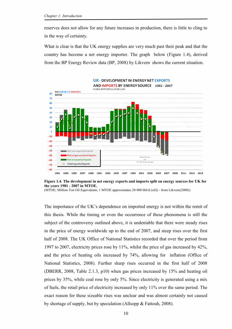
What is clear is that the UK energy supplies are very much past their peak and that the
country has become a net energy importer. The graph below (Figure 1.4), derived
from the BP Energy Review data (BP, 2008) by Likvern shows the current situation.
Figure 1.4. The development in net energy exports and imports split on energy sources for UK for the years 1981 - 2007 in MTOE. (MTOE; Million Ton Oil Equivalents; 1 MTOE approximates 20 000 bbl/d (oil)) - from Likvern(2008))
The importance of the UK’s dependence on imported energy is not within the remit of
this thesis. While the timing or even the occurrence of these phenomena is still the
subject of the controversy outlined above, it is undeniable that there were steady rises
in the price of energy worldwide up to the end of 2007, and steep rises over the first
half of 2008. The UK Office of National Statistics recorded that over the period from
1997 to 2007, electricity prices rose by 11%, whilst the price of gas increased by 42%,
and the price of heating oils increased by 74%, allowing for inflation (Office of
National Statistics, 2008). Further sharp rises occurred in the first half of 2008
(DBERR, 2008, Table 2.1.3, p10) when gas prices increased by 15% and heating oil
prices by 35%, while coal rose by only 5%. Since electricity is generated using a mix
of fuels, the retail price of electricity increased by only 11% over the same period. The
exact reason for these sizeable rises was unclear and was almost certainly not caused
by shortage of supply, but by speculation (Allsopp & Fattouh, 2008).

Chapter 1: Introduction
11
1.3.2 Reduction of greenhouse gas emissions
Some efforts are being made by governments to take mitigating action against climate
change, of which the major international action is the Kyoto Protocol, which has
allocated various carbon emission reduction targets to the ratifying countries
(UNFCCC, 2008). These targets are based on 1990 levels and are due to be met by
2012. The international carbon emissions trading system (ETS) through which these
reductions are to be delivered in the European Union (EU) came into force in 2005
(Pearce, 2006). The EU ETS was introduced to meet the EU’s greenhouse gas
emissions reduction target under the Kyoto Protocol, which is an 8 per cent reduction
in emissions compared to 1990 levels in the first Kyoto Protocol period of 2008 to
2012. The UK’s commitment under the Burden Sharing Agreement is to reduce its
emissions of greenhouse gases by 12.5% below base year levels by 2012. The UK’s
target annual level of emissions implied by the Burden Sharing Agreement is 682
million tonnes of carbon dioxide (MtCO2) equivalent calculated from data in the UK’s
2004 inventory submission (DEFRA, 2007, p5).
In the UK, the government White Paper 'Our Energy Future – Creating a Low Carbon
Economy' (DBERR, 2003), targeted a further cut in UK carbon emissions of 60% by
2050 and this target was set in a legal framework through the Climate Change Act
(UK Parliament, 2008a). The 60% target was subsequently increased to 80%, which is
the current objective for the UK.
1.4 UK Government policies on carbon emission reduction in
dwellings
These operate at three levels: at nationwide level in the form of legal obligations on
energy companies to reduce carbon emissions by reducing energy use by their
customers via the Carbon Emission Reduction Targets (CERT), now being replaced by
the Energy Company Obligation; at the design and specification level for dwellings
via the Code for Sustainable Homes (CSH); and at the level of individual households,
groups or organizations, via the UK Renewable Heat Incentive (RHI).
These three initiatives all have or may have some effect on the take-up of heat pump
systems. All three are comparatively recent in their implementations, so that while
their workings and limitations can be described here, their effects have yet to be seen.

Chapter 1: Introduction
12
1.4.1 Carbon Emission Reduction Targets (CERT)(UK Parliament,
2008b)
This initiative replaces two ‘rounds’ of a similar process, called the Energy Efficiency
Commitment (EEC1 & EEC2). CERT and its predecessors function by placing legal
obligations on energy suppliers to reduce their customers’ carbon emissions by
providing them with subsidized or even free energy-saving equipment or house
improvements. The provision of these measures is financed by a levy on each of the
energy suppliers’ customers and is biased toward householders on lower incomes and/
or who are receiving social security benefits or tax credits. The majority of the
measures taken so far have been to provide subsidized or free insulation and free
compact fluorescent light bulbs. In the context of this thesis, the main (limited) interest
is that the Statutory Instrument for CERT allows for the ‘promotion to a householder
…… of ground source heat pumps in respect of a property which does not have a
mains gas supply’ (UK Parliament, 2008b, page 4). The CERT scheme was replaced
by the Energy Company Obligation (ECO) associated with the Green Deal scheme and
finished at the end of 2012.
1.4.2 Code for Sustainable Homes (CSH) (DCLG, 2008a)
This design code has been created by the UK Government’s Department of
Communities and Local Government to replace previous voluntary design codes for
dwellings. The Code lays down standards for all aspects of a dwelling with the
intention of reducing the environmental impact of its construction and operation. The
main aspects of its standards that concern this thesis are those defining carbon
emissions for the dwelling. These take as the basis for the standard a value known as
the Target Emission Rate, which is the maximum emission rate permitted by the
Approved Document (AD) Part L1A of the Building Regulations (DCLG, 2006),
which are the statutory regulations applying to energy use in new-build dwellings. The
CSH rating process, at the design stage, calculates carbon emission estimates for the
dwelling as designed, by the Government’s Standard Assessment Procedure (SAP)
and a second estimate for a similar building which just meets the standards for
insulation and heating in AD Part L1A. The first estimate is known as the ‘Dwelling
Emission Rate’ (DER), the second as the previously-mentioned ‘Target Emission
Rate’ (TER). The rating for the design for the dwelling depends on the percentage
reduction of the DER against the TER as given by the formula:

Chapter 1: Introduction
13
(1.1)
The CSH Level corresponding to percentage reduction achieved is given by the
following Table 1.2:
Table 1.2 Energy and Carbon dioxide emission Assessment Criteria
It should be noted that even if a particular level of carbon emission reduction is
achieved, then the dwelling will not necessarily attain that CSH level, since the other
criteria in the CSH must be taken into consideration. However, to qualify for a given
overall CSH Level, the dwelling must achieve that Level of carbon emissions
reduction.
Originally, Levels 5 and 6 were highly challenging for the developer or designer, since
the only method of achieving these levels was to provide on-site generation of energy
either within the boundary of the house itself or on the site from a source which is
directly wired to the houses, precluding the delivery of power from the grid. The
higher level of 'Zero Carbon Home' was defined as one in which all the energy for
cooking, DHW and powering appliances was generated by on-site renewables as well
as that for heating or cooling. However, this requirement has been reduced
substantially under the current government, while still being referred to as 'zero
carbon', as being too restrictive for commercial housing development in the UK,
raising costs and restricting sites suitable for house-building by requiring higher build

Chapter 1: Introduction
14
and insulation standards and reducing the number of houses any site could
accommodate. The degradation of the standard was made in two ways. An initial step
was to consider only carbon emissions from 'regulated energy use' - use for space
heating and cooling, hot water and most lighting which are subject to Part L1A of the
UK Building Regulations. The second was to change the requirement from on-site
renewable generation to off-site renewables from so-called 'Allowable Solutions',
defined as 'forms of carbon abatement delivered off-site which mitigate any residual
carbon emissions from a building once onsite requirements have been met'. Also
included in this volte-face is a requirement that, from 2016, the 'built performance'
emissions for detached houses should not exceed 10kg CO2(eq)/m2/year, for other house
types should not exceed 11kg CO2(eq)/m2/year, and for low rise apartment blocks, 14kg
CO2(eq)/m2/year, again including emissions only from energy from 'regulated' sources,
ie. space heating, DHW generation, and lighting. It is these built performance
emissions that are be off-set by the carbon emission abatements provided by
'Allowable Solutions'. A 'Fabric Energy Efficiency Standard' of 39 kWh/m2/yr for
apartment blocks and mid-terrace houses and 46 kWh/m2/yr is to be required (Carbon
Compliance Task Group, 2011; Zero Carbon Hub, 2011a, 2011b, 2011c).
Figure 1.5 The 'Zero Carbon Policy Triangle'
(Carbon Compliance Task Group, 2011; Zero Carbon Hub, 2011b).
The built performance allowances are based an estimate of the LZC energy that can be
generated on site, which is taken to be the output from an area of photovoltaic panels
equal to 40% of the ground floor area of the dwelling, where the photovoltaic system
is assumed to be rated at 7m2/kWp (ZCH, 2011), with assumed ground floor areas for
each dwelling built form.

Chapter 1: Introduction
15
The effects of this change in policy in terms of energy consumption and carbon
emissions are not easy to estimate when taken in combination with unknown increases
in the housing stock. It is possible that the original 'zero-carbon' policy was not
implementable, in any case.
1.4.3 UK Renewable Heat Incentive
The Renewable Heat Incentive (RHI) is a system for the subsidy of what are deemed
to be renewable heating systems, aimed at encouraging their installation in either
domestic or commercial situations. For domestic systems, this involves ground source
heat pumps, biomass boilers, and solar thermal hot water systems. The subsidy entails
a payment per kilowatt hour of heat generated, which may be either metered or
'deemed', ie. calculated according to a rule depending on the size and type of
installation, made to the householder, on similar lines to the Feed-in Tariff (FiT)
scheme for electricity generated from renewable sources.
The RHI scheme has had a checkered history. It was originally proposed by the
Labour government in 2009 to be available for any dwelling and for either ground
source or air source heat pump systems. However, with a change of government in
May 2010, this scheme was suspended for review, and the resultant scheme is
considerably different and much more restricted. The RHI process started in July 2011
for domestic systems with subsidising payments, referred to as the "RHI Premium
Payment", of a total of £15 million to support the installation of 25,000 systems. These
payments were for solar thermal hot water, air source heat pumps, ground source heat
pumps and biomass boilers. Eligibility depends on the house being insulated to a
minimum level (but only if this is possible) and the householder being prepared to
provide feedback on the performance of the equipment. The payment is aimed at
dwellings without gas-fired central heating systems (DECC, 2011e) and amounts to
£1250 for GSHP installations and £850 for ASHPs. Sometime after this, the main
domestic RHI payments will commence, with per kilowatt-thermal payments being
made for solar thermal, ground source heat pumps, and biomass boilers (but not air
source heat pumps). Currently, the DECC proposal is that the output heat from these
systems will be metered to calculate the payments due.
No indication has been given as to what proportion of the 25,000 planned domestic
RHI installations are to be heat pump systems or whether, and by how much, this total

Chapter 1: Introduction
16
may grow over the 20 year lifetime of the RHI. Since the UK’s target is to obtain 15%
of energy from renewable sources, of which the ‘illustrative mix’ contains 12% of heat
by 2020 (DECC, 2010d; House of Lords : European Union Committee, 2008) and, in
the longer term, to fulfill the legally binding requirement in the UK’s Climate Change
Act ("Climate Change and Sustainable Energy Act," 2006) to reduce greenhouse gas
emissions by 80% by 2050, the lack of information on how these targets, (especially
the short-term one for 2020) are to be reached, must be a source of concern. It is not
known whether the installation scenarios proposed in the earlier background studies
(NERA Economic Consulting, 2008, 2009) made by NERA for the DECC “Heat and
Energy Saving Strategy Consultation Document” (DECC, 2009a) of the possible
contributions that various technologies could make in reaching UK targets, are still
under consideration.
1.4.4 'Green Investment Bank', 'Green Deal' scheme
Over the period 2012 to 2015, the 'Green Investment Bank', set up by the UK
Government, will commence operation as an investment fund to support investment in
projects to encourage 'green' growth, defined as ‘environmentally sustainable,
biodiverse, low-carbon and climate-resilient growth in human prosperity’
(:vivideconomics, 2011). Amongst its initial priorities is said to be support for the
Green Deal scheme (DBIS, 2011). The Green Deal is a complex mechanism which is
designed to allow a housholder to improve the energy efficiency of their property
without any initial payment on their part. It is intended that the cost of energy
efficiency measures implemented under this scheme will be recouped via the
householder's electricity bills and it is one of the scheme's defining principles - 'The
Golden Rule' - that this cost should be no greater than the savings made by the energy
efficiency measures. However, if significant energy savings cannot be made without
measures for which the cost exceeds this level, then a subsidy may be paid via a
second scheme, the 'Energy Company Obligation' (ECO), a scheme replacing CERT.
(para 1.4.1 above). The whole mechanism has not been in operation long enough to
judge its effectiveness.

Chapter 1: Introduction
17
1.5 Research aims and objectives
The previous sections indicate the forces and policies affecting domestic heating in the
UK at present and in the future, with the take-up of heat pumps apparently being
necessary to meet carbon emission reduction targets and being encouraged through
regulation and incentives, but being counteracted by the domination of gas heating,
apparent shortfall in electricity generation capacity and poor energy-efficiency of the
UK housing stock.
To give clarity to the future of domestic heat pump systems, the main aim of this study
is to estimate the potential of heat pumps to meet both the heating and cooling
requirements of UK dwellings in a changing climate up to 2050, and to forecast the
effect of possible take-up of heat pumps on the UK electricity demand and carbon
emissions.
To meet this aim, the subsidiary objectives are to:
1. Review the theoretical and physical characteristics of heat pump systems and
identify those that are most significant in the estimation of the energy use of
these systems; examine currently-available models and modelling routines for
estimating heating pump energy use for their inclusion of the these
characteristics, their relevance to the requirements of this study, including their
capability for incorporation in a building energy model;
2. Identify and review literature on the modelling approaches that could be used
to forecast energy use and CO2 emissions, and undertake a critical analysis of
models that have been built to predict the future energy use and CO2 emissions
of the UK housing stock. Examine whether any of the models are both suitable
and available for use in this study; whether their routines can be employed
even if no model could be utilised directly and whether the scenarios were
appropriate to this current study.
3. Monitor how current owners of ground source heat pumps (GSHPs) utilise this
equipment, i.e. to record their use of the equipment for heating, cooling and
domestic hot water provision, and the consequent energy consumption and
system temperatures.
4. Develop a computer model to estimate the energy produced from, and
consumed by, residential-scale heat pumps in meeting domestic heating and

Chapter 1: Introduction
18
cooling demands for different UK house types. Validate and calibrate the
model as appropriate.
5. Extend the model to include potential future take-up of domestic heat pump
equipment in order to assess:
The likely effects of various scenarios for the deployment and application
of replacement heat pump installations in the medium and long-term (2020,
2050) on the consumption of electricity and other forms of energy, in
particular natural gas.
Their effect on consequent carbon emissions for the UK both in their
manufacture (embodied carbon) and operation.
the extent to which increases in electricity consumption by heat pumps due
to summertime cooling are offset by reductions caused by temperature
increases envisaged by the prediction of climate change from UKCIP09
scenarios.
the extent to which increases in electricity consumption by heat pumps
might be offset by the output from building-mounted solar photo-voltaic
systems.
1.6 Thesis structure
Chapter 2 contains an examination of the technical aspects of heat pump heating
systems and the implications of these for the modelling of such systems. Chapter 3 and
4 review current literature, with Chapter 3 examining dwelling-level heat pump
modelling studies and Chapter 4 studies of stock-level dwelling energy models.
Chapter 5 describes the methodology of the study. Chapter 6 describes the heat pump
monitoring study and its results, Chapter 7 the development of the heat pump model,
Chapter 8 the development of the stock-level model and the results thereof. Chapter 9
contains the conclusions of the research.
Chapter 2 describes the theoretical background for heat pumps in thermodynamics, the
detail of the heat pump cycle and of its components indicating the implications of
these for domestic (and other) installations. It reviews the environmental credentials of
heat pump systems, in terms of their status as renewable energy systems and claims of

Chapter 1: Introduction
19
carbon emission reductions. It evaluates those factors presenting barriers to and those
driving on the installation of heat pumps.
Chapter 3 presents a review of recent studies presenting research in the modelling of
domestic (and where appropriate, non-domestic) heat pump systems, evaluating these
in terms of how they address the main characteristic of these systems. It also details
the routines contained in the heat pump model in EN15316-4-2 document which
defines the main European Standard for modelling heat pump systems in buildings and
considers its suitability for implementation within a computer model outside the
complex overall model contained in the overall EN15316 standard. It further examines
the limited set of publicly-available software tools that provide estimating facilities for
heat pump systems. All these are evaluated in terms of their utility in improving the
detailed modelling of heat pump systems and their possible implementation in a
housing stock energy model, which confirms the requirement to develop a new heat
pump energy model within a modified version of the BREDEM-8 standard dwelling
energy model.
Chapter 4 initially reviews the classification of housing stock energy models,
examining the applicability of the different types to the current study. It then reviews
those that are most relevant to the current study, being UK-based.
Chapter 5 describes the methodology of the study. The data collection and analysis
stage consists of the collection of heat pump energy and temperature data through a
year-long monitoring study and the further analysis of secondary data. The initial
development stage consists of the selection and enhancement of a dwelling energy
model and the development of a heat pump energy model based on both primary and
secondary data. The second development stage consists of the development of a
housing stock level model with the third the analysis of results from this model based
on scenarios of the numbers of domestic heat pump systems deployed and the
dwellings chosen for the application of these systems.
Chapter 6 documents the heat pump monitoring study carried out for this study and
also the extraction processes to acquire data for the heat pump regression model. The
heat pump monitoring study was carried out over a 12 month period, capturing input
and output energy, temperature and status data from three IVT ground source heat
pump systems. The energy data is analysed to provide monthly energy and SPF
values to illustrate the characteristics of these systems. Temperature data, particularly
that from ground loop and distribution sensors, is analysed to provide values for the
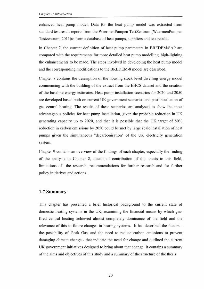
Chapter 1: Introduction
20
enhanced heat pump model. Data for the heat pump model was extracted from
standard test result reports from the WaermenPumpen TestZentrum (WaermenPumpen
Testzentrum, 2011)to form a database of heat pumps, suppliers and test results.
In Chapter 7, the current definition of heat pump parameters in BREDEM/SAP are
compared with the requirements for more detailed heat pump modelling, high-lighting
the enhancements to be made. The steps involved in developing the heat pump model
and the corresponding modifications to the BREDEM-8 model are described.
Chapter 8 contains the description of the housing stock level dwelling energy model
commencing with the building of the extract from the EHCS dataset and the creation
of the baseline energy estimates. Heat pump installation scenarios for 2020 and 2050
are developed based both on current UK government scenarios and past installation of
gas central heating. The results of these scenarios are analysed to show the most
advantageous policies for heat pump installation, given the probable reduction in UK
generating capacity up to 2020, and that it is possible that the UK target of 80%
reduction in carbon emissions by 2050 could be met by large scale installation of heat
pumps given the simultaneous "decarbonisation" of the UK electricity generation
system.
Chapter 9 contains an overview of the findings of each chapter, especially the finding
of the analysis in Chapter 8, details of contribution of this thesis to this field,
limitations of the research, recommendations for further research and for further
policy initiatives and actions.
1.7 Summary
This chapter has presented a brief historical background to the current state of
domestic heating systems in the UK, examining the financial means by which gas-
fired central heating achieved almost completely dominance of the field and the
relevance of this to future changes in heating systems. It has described the factors -
the possibility of 'Peak Gas' and the need to reduce carbon emissions to prevent
damaging climate change - that indicate the need for change and outlined the current
UK government initiatives designed to bring about that change. It contains a summary
of the aims and objectives of this study and a summary of the structure of the thesis.

21
CHAPTER 2 TECHNICAL ASPECTS OF HEAT PUMP SYSTEMS

Chapter 2: Technical Aspects of Heat Pump Systems
22
2.1 Introduction
The contents of this section are as follows:
an outline of the fundamental principles behind heat pump technology;
a review of the key components of current domestic heat pump systems;
a review of different applications, operation modes and heat distribution
systems; the potential for CO2 savings.
While this Chapter covers a wider range of topics, its primary purpose is to meet
Objective 1 of this study, that of identifying the those characteristics of heat pump
systems which are most significant in estimating energy consumption.
2.2 Basis in thermodynamics
Superficially, the heat pump defies the simplest statement of the Second Law of
Thermodynamics viz.
Heat can never pass from a colder to a warmer body without some other change,
connected therewith, occurring at the same time.
as stated by Clausius (Clausius, 1856). However, in 1852, William Thomson (later Lord
Kelvin) designed a ‘heat multiplier’, a device which uses energy to transfer heat from
the surroundings to an enclosed space, thereby maintaining that space at a higher
temperature, which is the basic concept of the heat pump. However, the earliest
application of these principles was an ice maker, designed and built by Dr John Gorrie
in 1851 (Chapel, 2001) in attempt to cure, or reduce the symptoms of, yellow fever. In
the UK, J G N Haldane built what was deemed to be the first heat pump for use in his
house in 1930 and this remained the only one until the 1940’s when J A Sumner built
some test units, following them with one for his own home in 1950 (Neal, 1978). In the
UK, some interest was generated in domestic heat pump heating systems between the
mid-1970's and early 1980's after the sudden rise in oil, and consequently gas, prices as
a result of the Arab-Israeli wars, indicated by publication of books such as Neal (1978),
Sumner (1980), McMullan & Morgan (1981) and Armor (1981). However, concerns
were raised over their efficiency and cost-effectiveness when installed compared with
gas-fired heating, triggering reports like Grigg & McCall (1988). In consequence, the
use of heat pumps for domestic heating applications in the UK is substantially less

Chapter 2: Technical Aspects of Heat Pump Systems
23
common than in the rest of Western Europe (Curtis, 2001). Recent sales of heat pumps
in the UK (Figure 2.1) are increasing but continue to be much lower than in the other
major states of Europe.
Figure 2.1 European heat pump sales to 2009
(Fors n Nowak, 2010) 2.3 Heat pump / refrigeration cycle types
Heppenstall (2000) distinguishes several refrigeration cycle types - absorption cycle,
gas cycle, stirling cycle, thermionic, magnetic, Gifford-McMahon, pulse tube, optical,
vortex tubes, Vuilleumier, Malone – apart from the vapour compression cycle which is
most common in space heating applications. While these other cycles have niches in
various applications or show promise for the future, this study will describe the working
of the vapour compression cycle, as this is used to the exclusion of all others in
domestic space heating systems.
2.4 Theoretical Heat Pump Cycle
In terms of thermodynamic theory, the heat pump cycle is almost the exact opposite of
that of the heat engine. In the heat engine, high temperature heat is supplied to perform
work as output and residual heat is rejected at low temperature. In a heat pump, the heat
supply is at low temperature and is transferred to a higher temperature by means of an
input of mechanical work (McMullan & Morgan, 1981, p3-4). The two systems can be
shown in schematic as follows (Figure 2.2).

Chapter 2: Technical Aspects of Heat Pump Systems
24
Figure 2.2. Schematic representations of a heat engine and a heat pump - (McMullan & Morgan, 1981, Fig 1.1, p4)
The energy use for either mechanism can be described (McMullan & Morgan, 1981, p. 3)
by an equation of the form:
(2.1)
where Qh is the heat flow from the source, Qc is the heat flow to the sink, and W is work
input. For a heat pump the flows are reversed, but the equation remains the same. For a
heat engine, the efficiency, η, is fairly simply calculated as the ratio of the work produced
to the heat input:
η = W/Qh (2.2)
However, since a heat pump can be used for either heating or cooling, calculation of its
efficiency must be in terms of the application, either heat rejected, Qh, to the sink for
heating, or heat absorbed Qc from the source for cooling. This gives two ratios: for
heating, of Qh/W, the amount of heat rejected for unit work; and for cooling, of Qc/W,
the amount of heat absorbed for unit work. Rather than ‘efficiency’, these values are
known respectively as ‘Coefficient of Performance’ (COP):
COP = Qh / W (2.3)
and ‘Energy Efficiency Ratio’ (EER):
EER = Qc / W (2.4)
Applying the original equation, 2.1, this gives the relationship:
COP = EER + 1 (2.5)
showing that for cooling, it might be expected that a given, reversible (ie. capable of both
heating and cooling) heat pump might be less effective at cooling than heating.
Chapter 2: Technical Aspects of Heat Pump Systems
25
2.4.1 Carnot Cycle
The heat engine as described in the previous section is referred to as a ‘Carnot Engine’,
and the process by which it functions as the Carnot Cycle or the ‘reversed Carnot Cycle’
for refrigeration. This cycle forms a basis for understanding the mechanism and
limitations of the vapour compression heat pump cycle. It represents the most efficient
heat engine cycle allowed by physical laws and consists of two isothermal processes
(where there is a change of temperature, but not of pressure) and two adiabatic
processes (where there is change of pressure but not of temperature). These processes
are assumed to be reversible. The Carnot cycle for a heat pump can be seen in terms of
the following figures (.
Figure 2.3 & 2.4).
Figure 2.3 Temperature - Entropy (TS) diagram
(reproduced from fig. 2a LeFeuvre(2007))

Chapter 2: Technical Aspects of Heat Pump Systems
26
Figure 2.4 Equipment required to create ideal Carnot Cycle heat pump
(source : fig 2b, LeFeuvre(2007))
.
Figure 2.3, A→B and C→D represent idealized versions of the condenser and
evaporator, where there is a change in energy level but no change in temperature, and
B→C and D→A represent idealized versions of the compressor and expander, where
there is a change in temperature but no change in energy level.
2.4.2 Coefficient of Performance
The value for every heat pump that is most significant is that which reflects the amount
of energy that is passed to the sink as a proportion of that which is input to the pump.

Chapter 2: Technical Aspects of Heat Pump Systems
27
This value is known as the Coefficient of Performance (COP) and is calculated by the
following:
COP = Delivered heat energy (kW) (2.6)
Electrical input to the compressor(kW)
Thus a COP of 4.0 implies that the heat pump is delivering four times the energy to the
sink as is being input to the system. For the Carnot Cycle heat pump above, where there
are no heat losses, the COP can be calculated from the temperature difference between
the heat source and the heat sink – again the evaporator and the condenser – as follows:
εc = T / (T – Tu ) (2.7)
where εc = COP from the Carnot Engine
T = temperature at the condenser
TU = temperature.at the evaporator
Temperatures are given in degrees Kelvin(ºK)
Thus a Carnot Engine heat pump raising the temperature of a source from 0 ºC (273 ºK)
to 60 ºC (333 ºK) would be working at a COP of 5.55 (Ochsner, 2007). While it is
impossible for a heat pump to operate at its Carnot COP, this value gives an upper
bound for the actual COP for a given temperature difference and also indicates that, for
an actual heat pump, the COP will be largely determined by the temperature increase
(known as the “lift”) required between source and sink. The significance of this for a
domestic heat pump system is that the system will be required to work harder, ie. will
require increased input of energy, to maintain any given temperature if the source
temperature falls. This reduction of source temperatures as the heating season
progresses in parallel with the requirement to balance the lower winter temperatures
constitutes a significant difference between a ground source system and a fuel-burning
one.
2.5 The vapour compression heat pump cycle
This heat pump cycle is illustrated below (Figure 2.5)

Chapter 2: Technical Aspects of Heat Pump Systems
28
Figure 2.5 Detailed schematic of an air source heat pump showing temperatures and pressures.
Source (Ochsner, 2007)
The heat pump cycle is as follows:
a) the cooled, low pressure refrigerant arrives at the evaporator (Figure 2.5, right hand
side) which is a heat exchanger. It is warmed by the heat from the source to 3 ºC (in
this case, air at 7 ºC) and evaporates.
b) The refrigerant then passes to the compressor, where it rises in temperature under
compression to approximately 73 ºC;
c) In second heat exchanger, the condenser, it is cooled by the ‘sink’ (internal air from
the house at 45 ºC) to 48 ºC while the temperature of the air is raised to 50 ºC.
d) Still under pressure, the refrigerant passes through a pressure relief valve, where
both its pressure and temperature fall and it returns at low temperature and pressure
to the evaporator.
Thus the refrigerant has to be able to tolerate continuous heating and cooling from 3ºC
to 73ºC or possibly more and back, and continual compression and de-compression.

Chapter 2: Technical Aspects of Heat Pump Systems
29
2.6 Heat pump system components
The components of a heat pump system are as follows:
1. the heat source as indicated above;
2. the collector;
3. the heat pump itself, consisting of evaporator, compressor, condenser and pressure
relief valve, refrigerant, control system, and, optionally, an accumulator and
reversing and check valves;
4. the distribution system, consisting either of fan / coil unit or units for air distribution
or under-floor heating piping or low temperature radiators for water distribution.
2.6.1 Sources and collectors
The choice of source largely determines the choice of collector, as per Table 2.1:
Table 2.1. Space heating heat pump sources and collectors
(modified from Table 1 (Heat Pump Centre(2008)) Heat source Temperature Range (°C) Most common collector Ambient air -10 to 15 Fan Exhaust air 15 to 25 Fan Ground water 4 to 10 Borehole Lake water 0 to 10 Pipe loop River water 0 to 10 Pipe loop Sea water 3 to 8 Pipe loop Rock 0 to 5 Borehole Ground 0 to 10 Pipe loops Waste water and effluent >10 Pipe loop
In general, the source to be used is determined by location – particularly, the size of the
site - and cost. To quote the IEA Heat Pump Centre (2008b),
An ideal heat source for heat pumps in buildings has a high and stable temperature
during the heating season, is abundantly available, is not corrosive or polluted, has
favourable thermo-physical properties, and its utilisation requires low investment and
operational costs.
They then comment that availability is the main determinant in choice of source. This is
primarily determined by location, as, for example, it is necessary to be close to the sea
to use that as a heat source. However, availability and cost are not inseparable. For
example, while ground water is more desirable than soil as a source on the basis of
steady temperature, its availability is restricted by the increased cost of drilling the

Chapter 2: Technical Aspects of Heat Pump Systems
30
necessary borehole to reach it. Similarly, air is much more available than either ground
water or ground, but carries with it the energy penalties of a lower specific heat and the
need to defrost of the collector at low temperatures. Somewhat less inevitably, it also
carries a noise penalty from the collector fan. Thus, availability of funds and of space
form the main determinants of the choice of source. If sufficient space is available (a
rule of thumb is 1.5 to 2 times the dwelling floor area) then a horizontal ground loop is
preferable. If sufficient space is not available but funds are, then a borehole may be
preferred. If both funds and space are lacking, then it is necessary to use air as a source.
The IEA Heat Pump Centre website (2008b) also makes reference to temperature
stability as a consideration. This cannot be such a major factor as the size of the site or
cost in choosing a source, but having chosen the source, its temperature stability
becomes a major factor in designing the heat pump system.
2.6.2 Source and collector characteristics
Two basic types of collection exist, those using pumped fluid to transfer the heat from
the source and those using air. Again, pumped fluid sources can have three different
forms, using either a mixture (conventionally known as a brine) of water and an anti-
freeze such as glycol in an indirect transfer, using a warm fluid source directly, or using
the heat pump’s own refrigerant to absorb heat from the source, a configuration termed
'direct expansion'.
Ambient air
The standard collector type for air source heat pumps is a fan drawing or blowing air
directly across the evaporator of the pump. The collector can be a separate unit,
positioned outside the dwelling and pumping refrigerant to the heat pump inside (a split
unit), or part of a single unit, positioned outside and blowing heated air in or positioned
inside and drawing ambient air in (compact units).
Using ambient air as a source in this way has a number of features. Firstly, as noted
before, when the ambient temperature falls toward 0ºC, condensation or frost will form
on the collector, severely reducing its efficiency. This condensation is removed by
various means, including reversing the heat pump process for a short time so that it
heats the collector or by directing hot refrigerant gas from the high pressure side of the
compressor through the evaporator for short period of time (hot gas defrost). While

Chapter 2: Technical Aspects of Heat Pump Systems
31
maintaining the efficiency of the evaporator, these processes reduce the overall
efficiency of the system. Secondly, an external collector has a reduced life-span due to
weathering. Thirdly, an external fan can be noisy in operation, especially if positioned
too close to a wall. Taken together, these factors can make an air source heat pump
inherently less desirable despite its lower capital cost and the reduced disruption
involved in its installation.
The energy available from air is, of course, determined by its temperature which, in a
typical UK location (Figure 2.6), has a more or less symmetric pattern either side of the
summer and winter solstices.
Figure 2.6. Averaged maximum and minimum temperatures for 1991 - 2000 from Lyneham weather station (Met Office, 2008)
Assuming that the volumetric specific heat capacity of air is 1300 J/m3K and that it is
undesirable to reduce the temperature at the collector by much more than 5 °C to avoid
its temperature going below 0 °C, then in order to acquire a Kilowatt-hour of energy
from the air, it will be necessary to collect heat from at least 554 m3 of air per hour.
Exhaust air
The collectors used in this application are similar to those for ambient air. While
exhaust air is mostly used as a heat source in industrial and agricultural applications
since these are the most common sources of waste heat, it may also be included in
mechanical ventilation with heat recovery (MVHR) systems in domestic applications
(Total Home Environment Ltd, 2012) where smaller heat pumps are utilised to recover
heat from extracted air to heat the incoming supply or to generate DHW.

Chapter 2: Technical Aspects of Heat Pump Systems
32
Ground water
Ground water can be used in either an open loop system, where the water itself is
pumped up pipes in one borehole, through the evaporator, and returned through a
second, in a closed system, where a borehole closed loop heat exchanger consisting of
polyethylene pipe, grouted into the borehole with bentonite clay, is used. As the
geology in the UK varies considerably over quite small areas, the amount of heat to be
sourced from ground water in any location is not readily determinable, though around
75% of the UK has quite a shallow water table. The variations in geology make the
effort involved in drilling boreholes unpredictable (Curtis, 2001). Extraction of ground
water in the UK is subject to a licensing system with a possible extraction charge
(Brown, 2009, pp. 28-29).
The energy available from ground water, particularly flowing water, is more or less
constant throughout the year.
River and lake water
As noted by the IEA (2008b), this “has the major disadvantage of low temperature in
winter (close to 0°C)”, requiring care over the brine content of the heat exchanger fluid
to avoid freezing. Its availability is also location-dependent and its extraction to an
open-loop system is subject to the same licensing system as ground water.
Sea water
Since sea temperature is high and constant (5-8°C) at a depth of 25-50 metres, and its
freezing point at -1°C to -2°C) is low, sea water can be a useful heat source, especially
for larger systems. Its use in open systems requires corrosion-resistant equipment with
filtering to avoid organic fouling.
Rock (geothermal heat)
Since this is used where there is little ground water, it is not often required in the UK. It
requires bore holes in the region of 100 to 200 metres in depth and uses a brine system
with welded plastic pipes. Some rock-coupled systems in commercial buildings use the
rock for heat and cold storage. The deep boreholes make this source economically
unattractive for domestic use. Where the application is dominated by either heating or
cooling, then careful sizing is required to reduce the possibility of long-term
‘exhaustion’ of the source. Borehole heat exchanger sizing has been much researched,
notably by (Eskilson, 1987; Fisher, Daniel E., Rees, Padhmanabhan, & Murugappan,

Chapter 2: Technical Aspects of Heat Pump Systems
33
2006; Kummert & Bernier, 2008; Kyriakis, Michopoulos, & Pattas, 2006; Sanner,
Karytsas, Mendrinos, & Rybach, 2003) and others.
Ground source systems
These are currently the most common systems in the UK in both residential and
commercial applications. As a collector of solar energy, the ground has similar
advantages to a ground-water source with relatively high annual temperatures. Heat is
extracted from horizontal ground coils, mostly in spread out coils known as ‘slinkies’
and both direct expansion and brine systems can be used, though brine systems are most
common. Direct expansion systems are more efficient as they avoid the need to transfer
heat from the soil to brine, and hence can work with a shorter ground loop. Conversely,
the pipework required is more expensive (currently copper) and has to be carefully
designed to avoid leakage of refrigerant into the soil.
The thermal capacity of the soil varies with the moisture content and the climatic
conditions. Because of the extraction of heat, the soil temperature around the ground
loop will fall during the heating season and may freeze around an undersized loop,
causing frost heave. However, in summer the sun will raise the ground temperature, and
complete temperature recovery should be possible if the loop has been correctly sized.
2.6.3 Heat pump configurations
Space heating heat pump units come in a range of configurations depending on
application, ranging from very small units of ~2 kW output rating judged suitable for
very low energy demand houses ie. German ‘passivhaus’ standard, to commercial units
of ~1300 kW, which have multiple compressors and are capable of simultaneous heat
and cooling (Calorex Heat Pumps ltd, 2008; Dimplex UK, 2007, and others; Kensa
Engineering, 2007d; Ochsner Wärmepumpen Gmbh, 2007), with a corresponding range
of physical size. In the domestic context, some contain dedicated domestic hot water
(DHW) tanks as buffer store for the distribution system, for others, this is a separation
installation. Air source systems are substantially different in external appearance from
ground source, due to their fans and associated grilles and the need for waterproof
casings.
While all, apparently, contain the same basic components, some variation is present in
choice of compressor and of refrigerant, for which some analysis is required since these
are the areas in which most performance improvements has been made in the recent
past.

Chapter 2: Technical Aspects of Heat Pump Systems
34
2.6.4 Compressors
The most recent improvement in heat pump performance has come from the
introduction of scroll compressors, currently fitted to the majority of domestic heat
pumps, replacing, in most cases, reciprocating ones (Bachman, 2012).(Wikipedia,
2008). This type of compressor, at its most basic level, consists of two interleaved scroll
castings, one of which moves eccentrically with respect to the other. See Figure 2.7.
The scroll compressor has fewer moving parts and its casing does not have to cope with
stress due to reciprocating parts. The basic mechanism of a reciprocating compressor
consists of a piston moving in a cylinder, in the head of which are valves controlling the
air flow. This must be designed such that space always remains above the top of the
piston at the top of its stroke, to avoid a clash with the valves. Thus the complete
volume of the cylinder is never emptied. This restriction does not apply to the scroll
compressor where virtually 100% of the volume may be compressed. Discharge and
suction processes in scroll compressors occur for a full rotation whereas a reciprocating
compressor's compression cycle may be as little as 25% of its rotation, producing
strongly pulsed output which places stress on the rest of the system. Without the noise
and impact of opening and closing valves, the scroll compressor is quieter and
vibration-free. While the scroll compressor is therefore more efficient, the same traits
that bring the increase in efficiency can also make it less robust. Since the refrigerant is
rarely completely evaporated before entering the compressor, the present of fluid in the
compression chamber can cause stress on the scroll mechanism avoided by the
reciprocating one. An accumulator tank is therefore added to the heat pump system to
trap fluid before it enters the compressor. Since the direct of scroll compressor’s
rotation cannot be reversed, reversible heat pumps (those designed for cooling as well
as heating) achieve the required change of direction by a four-way valve in the
refrigerant flow.

Chapter 2: Technical Aspects of Heat Pump Systems
35
Figure 2.7. Scroll compressor cycle (Air Compressor Equipment (2008)) 2.6.5 ‘Soft start’ power supply
These are required to prevent surges in the mains electricity circuits when larger heat
pumps are started. This is particularly important because of the single-phase, lower
voltage supply that is the norm in the UK, which currently (2008) restricts the
maximum size of domestic heat pumps to around 11 kW (Curtis, 2001; Energy Saving
Trust, 2007).
2.6.6 Additions to the basic compressed vapour heat pump cycle
Because no evaporation process is complete, a vapour-liquid separator known as a
“suction-line accumulator” is added to the system to trap low pressure liquid before it
reaches the compressor since this can only compress vapour. Such liquid would also
wash out the layer of lubricating oil which the compressor relies on as a sealant
(Danfoss Refrigeration & Air Conditioning, 2008). A second, possible, addition to the
basic cycle is called an ‘economizer’ which is used to improve the performance of scroll
compressors at low temperatures (Ma & Chai, 2004), and a third is an ‘intercooler’,
which performs a heat exchange between the output of the condenser and the input to
the compressor to assist with superheating (Reay & Macmichael, 1988, p 21). Not all
of these can be present in every heat pump design.
Where the main use of the system is for cooling, then an additional bleed, referred to as
a ‘desuperheater’ may be taken from the refrigeration circuit immediately after the
compressor to provide heat to generate domestic hot water.
Chapter 2: Technical Aspects of Heat Pump Systems
36
2.6.7 Controls
Most heat pumps have comprehensive, programmable micro-processor controls which
allow for their operating times to be co-ordinated with periods when cheaper, ‘off-peak’
charging rates are applied by electricity suppliers or for any other pattern of operation
required by the householder. Controllers can also provide diagnostic data for solving
performance problems via an interface to a computer (Ochsner, 2007, p23).
Control system characteristics that are, to a degree, specific to heat pumps consist of the
following:
‘weather compensation’ controls
auxiliary heating controls
Weather compensation
To operate a heat pump system in as efficient a manner as possible, it is necessary to
employ only the minimum amount of temperature “lift” necessary to maintain the
desired indoor temperature. This is ensured by using “weather compensation”, where
changes in ambient temperature are detected by an external sensor which then causes
the heat pump controller to vary the output temperature of the heat pump according to a
factory set curve of the relationship between this and external temperature. Thus the
output of the heat pump is increased before the temperature inside the dwelling falls in
response to the external temperature, rather than delaying the increase until the internal
temperature has fallen, thereby allowing a reduced “lift” (Energy Saving Trust, 2007).
However, where the prevailing electricity pricing system has reduced rates for ‘off-
peak’ periods, then the advantages of weather compensation are less clear, as it is
financially beneficial to run the system at maximum output (while avoiding
overheating) during the cheaper rate period (Kensa Engineering, 2007a).
Auxiliary heating
Where it is not financially viable for the main heat pump system to be sized to fulfill the
entire demand for space heating in what is referred to as a ‘monovalent’ system, then
additional heating (usually direct electric) is provided in a ‘bivalent’ system. This can
be controlled in two ways: either as a ‘bivalent parallel’ system where both forms of
heating function simultaneously or as a ‘bivalent alternate’ system, where only one form
of heating is used at a time. The former system is deemed capable of attaining a

Chapter 2: Technical Aspects of Heat Pump Systems
37
temperature of 65ºC, whilst the latter can attain 90ºC according to Ochsner(2007),
making both types of system suitable for retro-fitting to older houses, with the ‘bivalent-
alternate’ operation being particularly suitable where the existing boiler is still
functional. Careful specification and use of auxiliary heating is necessary to avoid
reduction in efficiency and increases in heating bills. Further analysis of the system
sizing and set-points for the different types of operation will be described in the chapter
on heat pump modelling.
2.6.8 Refrigerants
The working fluid for a heat pump must absorb heat by evaporation and release it by
condensation and is therefore required to change phase at ‘useful’ temperatures and
pressures. The evaporation cycle is particularly important since incomplete evaporation
can cause ingress of fluid into the compressor which is undesirable mechanically (Reay
& Macmichael, 1988, p 16). The refrigeration fluid must therefore be heated beyond the
normal evaporation temperature (superheated) to achieve a safety margin. However,
beyond this, the choice of fluid is not limited through thermodynamic considerations.
To quote Reay(1988, p 49), “Any fluid which can be made to evaporate between 1 bar
and 20 bar at useful temperatures is interesting”. Refrigerants in heat pumps have been
selected for:
their ability to withstand the higher temperatures present, especially at the
compressor discharge port;
low toxicity for ease of handling;
low flammability for safety in domestic situations; and
low costs.
The list of refrigerants used in heat pumps has been subject to considerable change over
the last 20 years, largely for external reasons rather than for technological reasons. The
substances chosen have more or less come full-circle from commonly-available,
relatively natural fluids through various types of hydrocarbon only to return to the initial
list of 'natural' fluids (IEA Heat Pump Centre, 2008a).
Initially, basic substances such as ammonia, carbon dioxide, propane were used, which
were disadvantageous in that carbon doxide required higher pressures than were easily
maintainable in a refrigeration circuit at the time and ammonia and propane are highly
inflammable (IEA Heat Pump Centre, 2008a).
Chapter 2: Technical Aspects of Heat Pump Systems
38
In the early 1930's, the freon ‘family’ of refrigerants, composed of chlorofluorocarbons
(CFCs), were developed and were, for a long time, considered to be ideal refrigerants,
being chemically stable, of low toxicity and fairly inexpensive. However, with the
discovery in 1974 of the environmental damage – the destruction of the Earth’s ozone
layer - caused by the reaction of the chlorine content of the chlorofluorocarbons with
atmospheric ozone at high altitudes, production of these was phased out by 1995, under
the Montreal Protocol, within the developed countries of the world and being totally
banned in 1996 (IEA Heat Pump Centre, 2008a).
To avoid the wholesale replacement of refrigeration equipment, CFCs have been
replaced on a transitional basis by hydrochlorofluorocarbons (HCFCs), which have a
lower global warming potential (GWP) and ozone depletion potential (ODP) and are
able to act as a direct replacement for CFCs. HCFCs are being further replaced over the
period up to 2020 by mixtures of hydrofluorocarbons (HFC)s which, though not
presenting problems due to ODP, have been found to possess high global warming
potential. The need to phase out all these substances has been the motivation behind the
European SHERHPA project to develop heat pumps using so-called ‘natural’
refrigerants including carbon dioxide, hydrocarbons such as propane, and ammonia.
(SHERHPA, 2007). However, most current heat pumps use R-407C, R-404 or R-410
HFC mixtures (IEA Heat Pump Centre, 2008a).
The ‘R’ (for refrigerant) numbers used to designate these fluids are determined by their
molecular composition, with numbers determined by (starting from the right) the
number of fluorine atoms; the number of hydrogen atoms plus 1; the number of carbon
atoms minus 1; and the number of unsaturated carbon-carbon bonds in the molecule.
When the third or fourth numbers are zero, then they are omitted. Mixtures are
allocated numbers in the 400 or 500 series, 400 if they are zeotropic (evaporating over a
temperature range), 500 if they are azeotropic, with a capital letter distinguishing
between mixtures in different proportions of the same substances. Non-fluorocarbon
organic substances are numbered in the 600 range and inorganic substances in the 700
range (IIFIIR, 2001).
2.6.9 Distribution System
The choice of distribution system, ie. the means by which the heat collected by the heat
pump is used in heating the dwelling, is very much determined by whether an existing
dwelling or a new build is being considered. Available systems are ducted air, direct air,
wet radiant underfloor, wall or even ceiling systems, or wet radiators.
Chapter 2: Technical Aspects of Heat Pump Systems
39
Ducted Air
This type of system is not popular in the UK, probably because heating systems have
customarily been used to provide hot water as well as heating, thereby making the
whole task part of the plumber’s remit. Building-in ducts occupies a considerable
amount of space, but could have advantages in providing ventilation in well-sealed
dwellings, particularly with heat recovery. Since the output temperature from a heat
pump is on the low side, large volumes of air must be moved to provide sufficient
warmth and this can cause draughts. Other potential problems and hazards include the
spreading of smells and noise and the feeding of air to fires. The use of air distribution
also has advantages. Importantly it provides a much more rapid heating
response(Armor, 1981, p14). It facilitates the reverse use of the system to provide
cooling and the incorporation of air filters to reduce dust and humidifiers (McMullan &
Morgan, 1981, p108). Air outlet grilles occupy less space compared with radiators,
allowing more flexible placing of furniture (Armor, 1981, p14).
Direct air
Used by standalone units – usually ASHPs. The output from a fan blown over the
condenser is passed straight into the house, directed by louvres.
Wet radiant systems (floor, wall or ceiling)
Because these systems do not rely on convection air circulation to warm the room, they
can provide sufficient warmth at much lower temperatures (30 – 35°c) than radiator
systems. The lower temperatures allow the efficient operation of heat pumps, since this
is a much lower ‘lift’ than the 80°C required to warm a room using radiators. The
difference in efficiency is illustrated by Kensa Engineering’s sizing tables for radiator-
coupled and under-floor coupled heat pumps where the heat pump current usages for
typical running conditions are reduced by about 25% for UFH and Kensa claim a COP
of 4 when operating with an underfloor system and 3 with radiators (Kensa Engineering,
2007b, 2007c) McMullan and Morgan (1981, pp106-107) show that an under-floor
system at 30°C with air temperature at 20°C can provide a heat transfer by convection
and radiation of 70 W/m-2, which was deemed adequate even at the time they were
writing. Unfortunately, retro-fitting of this form of heat distribution is not easy to
achieve. Additionally, use of UFH conflicts with the customary use in the UK of
wooden floors and carpets, which act as good insulators and require special fittings in
suspended floors to ensure that heat is reflected upwards.

Chapter 2: Technical Aspects of Heat Pump Systems
40
While reversible heat pumps (those that can provide cooling) are available, their use for
cooling in such systems is not recommended without protection against condensation
(Energy Saving Trust, 2007).
Wet radiator systems
These are the most common systems to be found in centrally-heated dwellings in the
UK and throughout the EU (Iles, 2002). They are, in general, sized to suit the higher
temperatures (80°C) generated by fossil-fuel boilers and therefore do not provide
sufficient heat output at the lower temperatures at which heat pumps are most efficient.
Ochsner (2007, p87) states that radiator “supply temperatures should be limited to 55
°C” or 65 °C for renovations. He provides a graph (Figure 2.8) from standard DIN
EN442 relating the increase in radiator size to the required reduction in temperature.
Figure 2.8. Size of radiator as a function of supply temperature. Source DIN EN442 reproduced from (Ochsner, 2007)
Practical experience seems to indicate that a significant proportion of radiators in UK
dwellings are already oversized because of the fitting of oversized boilers(McMullan &
Morgan, 1981), leading Peapell(2007, pp300-301) to suggest that existing radiators
should be left in place until found wanting in cold weather.
2.7 Environmental credentials of heat pump systems
2.7.1 Heat pump space heating as renewable energy
The basic function of a heat pump is to transfer heat from one body to another. The
most everyday version of this function is that of transferring the small amount of heat

Chapter 2: Technical Aspects of Heat Pump Systems
41
inside a domestic refrigerator to the outside world, thereby making the inside desirably
cooler and the outside a little, probably irrelevantly, warmer. A heat pump space-
heating system has almost the reverse function, taking the low temperature heat energy
from a large body and ‘compressing’ it into higher temperature heat in a smaller body.
The ‘large body’ can be either the surrounding air, a layer of surrounding earth down to
about 1.2 metres, the body surrounding a borehole, a river or a lake, or any combination
of these as available. The smaller body is usually the distribution fluid in a hot water
central heating system or the air in a house. The warmth in the large body is, more or
less, solar gain, so that the heat pump is using its source as an inter-seasonal store,
which is being ‘filled’ in the summer by solar energy and ‘emptied’ during the winter
by the heat pump (Ochsner, 2007; Peapell, 2007). Using a reversible heat pump, the
heat source can be re-charged by cooling the dwelling during the summer, if necessary.
In making use of this solar energy, these types of heat pump systems are judged to be
utilizing renewable energy.
2.7.2 Carbon dioxide emissions reduction
The main objective in installing a heat pump is to provide a low-carbon heat source
which can either replace existing heat sources or take advantage of new-build, highly-
insulated homes. Figure 2.9 shows that, given a heat pump of a sufficiently high COP(ε
= 3.0), the use of heat pump heat systems can balance out generation and transmission
losses, allowing the available energy delivered to a household to equal primary energy,
unlike the other forms of heating shown. Of course, this 'balancing out' is not truly
saving energy, merely the acquisition of extra energy to replace the system losses as the
additional flow of energy into the heat pump system in the bottom row of Figure 2.9
indicates.
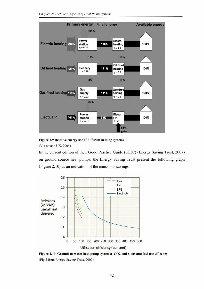
Chapter 2: Technical Aspects of Heat Pump Systems
42
Figure 2.9 Relative energy use of different heating systems
(Viessmann UK, 2004)
In the current edition of their Good Practice Guide (CE82) (Energy Saving Trust, 2007)
on ground source heat pumps, the Energy Saving Trust present the following graph
(Figure 2.10) as an indication of the emissions savings.
Figure 2.10. Ground-to-water heat pump systems: CO2 emissions and fuel use efficency
(Fig 2 from Energy Saving Trust, 2007)

Chapter 2: Technical Aspects of Heat Pump Systems
43
This graph is based on the CO2 emission factors used in the current version of the UK
government Standard Assessment Procedure (SAP, 2005) (BRE, 2008) viz. Electricity =
0.422kg/kWh delivered, gas = 0.194 kg/kWh, LPG = 0.234 kg/kWh, oil = 0.265
kg/kWh. Using these values, they quote that a condensing gas boiler at a seasonal
efficiency of 85% would emit 0.23 kg CO2 for every kilowatt-hour of output, whilst a
ground source heat pump with a seasonal efficiency of 350% would emit 0.12 kg CO2
for every kilowatt-hour of useful output, claiming an almost 50% reduction in emissions
for the GSHP (Energy Saving Trust, 2007, p4). This also implies that the Seasonal
Performance Factor for the heat pump need only exceed 1.8 to provide CO2 emission
savings. However, the validity of this claim is highly dependent on the CO2 emission
factor for grid-supplied electricity which is again highly dependent of the fuel mix used
in generation. Since the value used by BRE (2008) is now some several years old,
recent recalculation (Mackay, 2008) based on the DBERR Energy Trends for March
2008 gave a value of 0.554 kg/kWh, some 31% higher. This has the effect of shifting
the Energy Saving Trust curve for emissions for electricity upwards in Figure 2.10,
giving emissions of almost 0.16 kg CO2 for every kilowatt-hour for a GSHP at 350%
efficiency and a ‘break-even’ point against the gas boiler of 240%.
2.8 Barriers and drivers to the take-up of domestic heat pumps
2.8.1 Barriers
Some of these points have been included in previous sections but are included here for
completeness.
Capital Cost
The main barrier against the adoption of heat pumps, particularly GSHPs, is the initial
cost of the equipment and its installation as illustrated by Table 2.2 below.
Table 2.2 Indicative capital costs* for individual ground-to-water heat pump systems
System type Ground coil costs (£/kW)
Heat pump cost (£/kW) Total system costs (£/kW)
Horizontal 250 - 400 350 - 750 600 - 1150 Vertical 550 - 750 350 - 750 800 – 1500
*Costs include installation and commissioning of the heat pump and ground loop but exclude costs for the heat distribution system.
(Energy Saving Trust, 2007. p17)

Chapter 2: Technical Aspects of Heat Pump Systems
44
This gives a cost of £4,800 - £9,200 for a typical 8kW system with a horizontal collector
and £6,400 - £12,000 for one with a vertical borehole. Even with a maximum grant from
the RHPP of £1250 (EST, 2012), this represents a sizeable extra cost against a
condensing gas-fired system. The costing issue is compounded by the complexity of
design decisions to be made: the use of borehole or horizontal collector; different
horizontal collector types; the sizing of the collector according to the heat load of the
dwelling and the soil type; the requirement for, or suitability of the distribution system
for cooling; the provision made for generation of domestic hot water (DHW). Bigger
systems (> 11Kw) bring additional problems with the need to uprate the power supply
to the house from single phase to three phase.
Since the size of the collector represents 35-40% of the system cost, accurate calculation
of the heat load required and consequent sizing of the system and its collector is crucial
to minimise costs. Methods of reducing ground collector size by means such as re-
charging soil temperature from solar thermal collectors in the system can be considered,
but bring their own increases in complexity and cost (Harrogate Borough Council,
2007).
Plot size
This is mainly a concern with GSHPs using a horizontal collector, since a ‘rule of
thumb’ is that these will occupy 1.5 to 2 times the floor area of the building.
Consequently, for a building of 150m2, a horizontal collector will occupy between
225m2 and 300m2. Further, the collector must be 2m. from trees, 1.5m from cables and
3m from septic tanks, water, waste and sewage pipes because of possible freezing
(Nottingham Energy Partnership, 2006). As the average plot size for new UK houses is
89m2 (Wolsey Securities, 2006), the current generation of GSHPs in individual homes
is restricted to the upper end of the housing market or to country properties. In the retro-
fit applications which concern this study, digging of the collector trenches is severely
disruptive to the garden of an existing house. 'Split' ASHP systems also require some
external space for the collector unit which is judged to be 4 m2 (Energy Saving Trust,
2011). Borehole collectors can be accommodated on much smaller sites, but carry the
cost penalty indicated above in Table 2.2.
Expertise
Because heat pumps of all kinds are still unfamiliar to designers in the UK, it is likely
that they will be unwilling to specify them unless specifically requested by the client.
Chapter 2: Technical Aspects of Heat Pump Systems
45
Equally, the installation of the systems is unfamiliar to the construction industry, which
may cause problems, particularly with collector installation (Harrogate Borough
Council, 2007).
With the lack of expertise in installation, there is a possibility that poor installation may
cause systems not to meet manufacturers' standards for performance. This appears to be
an implication of the findings of the EST heat pump monitoring study (Bradford, 2009;
Bradford, Carmichael, & Bean, 2011) where the performance of heat pumps in UK
dwellings was found to be significantly poorer than the equivalent European systems.
Electricity supply
One of the problems highlighted in heat pump installations is the low capacity of the
power supply to UK homes, which is usually only 230v 50 Hz, single-phase, which is
sufficient only for heat pumps up to 11kw (unless fitted with a ‘soft start’). This is
especially true of country areas, off the gas grid, where the difficulty and expense of
upgrading the power supplies are greatest, but the potential improvement in comfort and
well-being for the occupants from pump installations is greatest. The conversion of a
single domestic power supply to three-phase power by Eon distribution company costs
around £1000 plus the cable burial costs of about £70 / metre (E-ON Energy Services,
2008). The original connection to the electricity supply may have been made to such an
inferior standard that the supply capacity for a community is only sufficient for the
installation of a heat pump in only one house in two, as was found in the village of
North Blyth (Lacey, 2010).
Heat distribution systems
As heat pump systems operate more efficiently at lower temperatures, they are most
frequently coupled to underfloor heating systems (UFH) or to low-temperature radiators
that appear over-sized to those accustomed to gas or oil-fired systems (Butcher, 2007).
Standards
The standards for calculating energy requirements for heat pump heating systems –
EN15316-4-2 - had draft status from 2005 until consultation ended in January 2006 and
were only given approved status in August 2008. Butcher (2007) in his paper for NHBC
Foundation describes it as “complex and difficult to interpret” which might go some

Chapter 2: Technical Aspects of Heat Pump Systems
46
way to explain this position. There are, as yet, no standards for the required efficiency
of heat pumps similar to the SEDBUK ratings for gas or oil-fire boilers, which renders
their specification for dwellings more complex.
External Collectors
Air source heat pumps, while not requiring underground collectors, do require external
fan-driven collectors, which can be noisy if incorrectly positioned. Because these are
largely exposed to the weather, their life expectancy is much reduced compared with
GSHP collector loops.
Geology
Britain has an extensive range of geology. To quote Curtis (2001), ‘almost all known
geological sequences exist within the UK’. This causes difficulties both with drilling
boreholes, but also with calculating ground loop sizes because of the wide variation in
thermal conductivity that occurs over quite small areas.
2.8.2 Drivers
Renewable Heat Premium Payment / Renewable Heat Incentive
As previously stated, heat pump systems are classified as renewable energy devices and
their installation is eligible for the Renewable Heat Premium Payment payments of
£1250 for a GSHP or £850 for an ASHP in single homes without mains gas heating,
providing that the house has the basic measures of cavity wall insulation (where
appropriate) and 250 mm of loft insulation (EST, 2012). This provides only a limited
incentive, as it does not reflect the cost differential between conventional heating and a
heat pump installation. However, the future implementation of the Renewable Heat
Incentive, which will probably make 4.7p per kilowatt hour payments for ground source
systems, may constitute more of an incentive to householders despite the "off the gas
grid" restriction (Ofgem, 2011).
Operating Costs
At July, 2008 prices, energy costs for GSHPs are estimated to be similar to gas-fired
heating. Costing for ASHPs are about 60% higher. The only cheaper form of heating is
unseasoned wood (Nottingham Energy Partnership, 2008). The major cost advantage of

Chapter 2: Technical Aspects of Heat Pump Systems
47
heat pump equipment is its apparent low maintenance requirement, with suppliers
claiming that heat pumps do not require the annual inspection required by gas or oil-
fired equipment.
Convenience
Of the ‘low carbon’ technologies currently available, heat pumps are the only type that
approaches or possibly exceeds the level of convenience of gas central heating. They
require no fuel storage facilities or delivery, do not suffer from variations in fuel quality,
do not require flues or airflows and are completely electronically controlled, requiring
minimal interference from their owners (Energy Saving Trust, 2007, p5.).
Obviating the need for a mains gas connection in new developments
The installation of a heat pump system obviates the need for the developers of new
housing to provide (and pay for) the connection of a mains gas supply for the site,
reducing their costs, though the lack of gas provision may make those dwellings less
attractive to buyers.
2.9 Distinctive characteristics of heat pump systems over ‘fuelled’
systems
Of the characteristics of heat pump systems, those that are distinctive from gas and oil
systems are as follows:
a) Heat pump systems have lower temperature output due to the characteristics of the
vapour compression cycle, especially that of degradation of refrigerants at higher
temperatures. Higher temperatures are only possible with multi-stage compressors
or additional heaters.
Output temperature is very significant in radiator systems because the heat
transfer by radiation is approximately proportional to the fourth power of the
temperature difference between the emitter and the surroundings.
Because of their lower output temperatures, heat pump systems require a control
system based on weather compensation rather than internal temperature in order to
Chapter 2: Technical Aspects of Heat Pump Systems
48
reduce the size of temperature ‘lift’ required to match a fall in outside
temperature. This is not necessary for fuel burning systems.
b) For fuel burning systems, the energy available is dependent only on the fuel
supply. For ground source heat pumps, there is a reduction in source energy over
the heating season due to depletion of the ground as an inter-seasonable store. For
air source heat pumps, there is a reduction in source energy from October –
February with the fall in air temperature due to reduced solar gain.
c) CO2 emissions from operating electric heat pumps are almost solely due to the
carbon intensity of electricity generation, not of the fuel itself.
d) The cost of installation of GSHP systems is highly dependent on the size of the
system, especially of the collector, so it is important to ensure that system is not
oversized. However systems are even more expensive to uprate once installed as it
is not possible just to fit a more powerful boiler.
e) The cost of operating an oil/gas fire system probably increases uniformly with the
size of the inside / outside temperature differential to be maintained. Additional
heat (above balance temperature) with a heat pump system is at a COP < 1.0.
f) Heat pump systems are capable of providing cooling as well as heating, either in
the form of air cooled directly from a ground loop collector or by reversing the heat
pump to cool the distribution system. While these both can have the effect of re-
charging the source, providing more heat in the winter, they can also imply an
increase in domestic electricity use during the summer.

Chapter 2: Technical Aspects of Heat Pump Systems
49
2.10 Summary
This chapter has examined information on the following:
an outline of the fundamental principles behind heat pump technology;
a review of the key components of current domestic heat pump systems;
a review of different applications, operation modes and heat distribution systems;
the potential for CO2 savings.
a review of the drivers for and the barriers against the mass take-up of domestic
heat pump systems.
the significant differences between heat pump heating systems and fuel burning
heating systems.
The chapter has necessarily limited its scope to consideration of heat pump technology
as used in the UK, both because of particular circumstances in the UK and also to limit
the volume of information to be considered.
In terms of the study Objective 1, the following issues are raised by this chapter:
The important relationship, shown in Section 2.4, in estimating heat pump energy
use is that between efficiency (COP) and the "lift" - the difference between the
source and sink temperatures required from the system - as expressed by Equation
2.6.
The construction of a model of this relationship, therefore, will rely on the estimation
of the source and sink temperatures appropriate for the dwelling and site involved,
requiring rules determining the source and sink types, based on detail of outside
space and of the heat distribution system.
Where a heat pump system is sized such that it cannot balance the heat load of winter
temperatures, then additional heat is required, from either a parallel or alternate
system. At a dwelling level, the desired model must encompass the sizing of the
system, the degree to which it balances the system loads and the resultant use of
additional heat.
To include the above factors, modelling for this study must therefore be based at
dwelling level, with sufficient detail of built form and surroundings. However, this
raises problems of creating dwelling-level estimates within a data structure which will
allow their grossing up to stock-level estimates.

50
CHAPTER 3 MODELLING OF DOMESTIC HEAT PUMP ENERGY
CONSUMPTION

Chapter 3: Modelling of domestic heat pump energy consumption
51
3.1 Introduction
The previous section identified the technical characteristics of the heat pump heating
systems designed for use in domestic situations and the incentives and barriers to their
take-up in the UK. A substantial proportion of the barriers involve the questions
surrounding the performance of the systems, which is a crucial determinant of their
status as low-carbon heating systems and positions them as "follower" technology
behind the de-carbonisation of the electricity supply. For the first part of Objective 1 of
this study, it identified the theoretical and physical characteristics of heat pump systems
that are most significant in the estimation of the energy use of these systems.
For the second part of Objective 1, this section examines the models which have been
developed for the estimation of heat pump performance under categories covering
research studies, official standards and freely-available software.
3.2 Heat pump modelling studies in research
3.2.1 Aims of this thesis and filtering of model descriptions
The main aim of this thesis is predict and understand the effects of a substantial take-up
of heat pump heating and DHW systems in dwellings in the UK on that country's
electricity supply on a monthly and yearly basis. As part of this estimation process, it is
required to improve upon the current implementations of the modelling of heat pump
characteristics in dwelling energy models, which generally mask the differences
between heat pump systems and fuel-burning systems. Hence this chapter examines
studies of heat pump models, which are based either on thermodynamic theory or
statistical analysis of the results from monitoring studies, standard models of heat pump
energy use, and software packages for estimation of heat pump energy use. However,
because it is not required to analyse the performance of these systems for engineering
improvement, the papers reviewed have been restricted to those relating to unmodified,
"off-the-shelf" systems and to studies of generic systems.
The annual and monthly timescale implies that any modelling studies need not operate
at time intervals outside this range, on the assumption that any performance variations
within shorter periods will not be significant over a longer period, while longer term

Chapter 3: Modelling of domestic heat pump energy consumption
52
variations appropriate for borehole heat sources do not register either. The study will
also assume that systems, especially ground source heat collectors, have been sized
correctly, that only readily available sources are employed and that no additional
equipment has been incorporated into the heating and DHW system beyond a standard
heat pump, either ASHP or GSHP as appropriate, thereby excluding prototype or one-
off systems. So that the process should be as transparent as possible, a further
requirement is that any modelling should avoid proprietary software models of HVAC
equipment.
The characteristics of heat pump systems for dwellings, particularly in temperate
climates such as the UK, differ significantly from commercial systems, in that
commercial systems are frequently required to provide cooling as well as heating, and
sometimes both at the same time, especially for a high density of computer equipment
in a server room operating in mid-winter in an office block. The UK's particular housing
stock, with its characteristic of large numbers of old, much extended houses with poor
energy efficiency, also brings its own flavour to the analysis, as does the widely varying
geology in the UK, making the installation of ground heat exchangers 'a minor
nightmare for ground coupled installers' (Curtis, 2001).
This study will not include detailed thermal modelling of ground loops in the analysis
and will assume that ground loops are correctly sized for the heating load of the system.
While the sizing of ground source heat collectors is crucial both to the efficiency of
GSHPs and to the cost of these systems, and widespread under-sizing could cause
excess electricity consumption, it is not possible to allow for any mis-sizing of
collectors without conducting a long-term study of collector sizes and loads to ascertain
the size and variation of discrepancies.
analysis of heat sources other than air and soil using closed, indirect ground loops is not
thought to be appropriate for this study. A generalised housing stock sample does not
provide exact location data and therefore it is not possible to identify whether a house is
close to a suitable, available body of water or another less conventional source. Open
ground loop systems involving the extraction of ground water are subject to a licensing
system in the UK and possibly to an extraction charge, which might be tolerated in a
commercial situation, but the increased expense and bureaucracy are likely to deter a
private householder (Brown, 2009, pp. 28-29). Currently, direct evaporation systems, ie.
those where the collection fluid is evaporated in the ground collector and passes directly
Chapter 3: Modelling of domestic heat pump energy consumption
53
to the compressor without the use of a separate evaporating heat exchanger, are
uncommon in the UK, probably due to the requirement for a expensive corrosion-
resistant, copper ground loop capable of maintaining the necessary high pressure
(Brown, 2009, pp. 27-28; Ochsner, 2007, pp. 21-22, 58-62).
Eschewal of studies involving systems that incorporate other equipment - examples
being solar collectors to provide additional heat for the system source, or buffer storage
to avoid short-cycling of the system due to the lack of thermal mass in a radiator
system - is based on the necessity to reduce complexity in modelling and to reflect the
need to keep down the capital cost of and space requirement for the system modelled.
While studies involving prototype systems may provide indications of future
performance levels, prototypes are not necessarily configured optimally and
specifications will change with manufacture.
The requirement to ensure transparency through use of available software has the effect
of eliminating some studies from this review, since these employ pre-compiled modules
within their models for which the source code is not available and the software
environment itself is only available at a price unrealistic for individual users.
3.2.2 'Filtration' of research papers
The definition of the above criteria allows the 'filtering' of the not-inconsiderable
number of publications on the subject of heat pump heating systems, necessary because
these are fairly numerous, with a search of "Web of Science" (Thomson Reuters, 2012)
with key words "building", "heat", "pump", "model" returning 440 entries. The same
search using "Google Scholar" (Google, 2012) returned some 25,700 entries. The
extent to which it is necessary to examine the full gamut of literature on this subject is
not clear. In the basic structure of a heat pump system, there are a limited number of
variables and therefore a limited number of relationships which require to be reflected
in a model.
Using the criteria above in 3.2.1 it is possible to filter this substantial volume of papers
somewhat, excluding the following:
Detailed modelling:
Exergy and energy analysis of individual heat pump components and system (Hepbasli
& Tolga Balta, 2007); modelling of the internal components of the heat pump system,

Chapter 3: Modelling of domestic heat pump energy consumption
54
particularly those with scroll compressors (Jin & Spitler, 2002); modelling of systems
which provide DHW only (Bourke & Bansal, 2010); thermo-economic optimisation of
heat pump system and ground-coupled heat exchanger (Sanaye & Niroomand, 2010);
Ground loop modelling:
modelling of energy flows in ground loops (particularly vertical boreholes) in detail
over short timescales (Parker, 1985; Spitler, Liu, Rees, & Yavuzturk, 2003), (Yavuzturk
& Spitler, 1999), (Bai, Zhang, Zheng, Zhang, & He, 2009); studies of the optimisation
of borehole ground loops using artificial neural network techniques (Esen & Inalli,
2009; Esen, Inalli, Sengur, & Esen, 2008c), or adaptive neuro-fuzzy inference systems
(Esen, Inalli, Sengur, & Esen, 2008a, 2008b); detailed modelling over annual and multi-
year timescales using EnergyPlus software (Fisher, Daniel E. & Rees, 2005; Fisher,
Daniel E., et al., 2006), using HVACSIM+ in optimisation (Haider Khan, 2004); a study
comparing results from TRNSYS simulations of dynamic and steady state simulation of
ground loops and heating systems (Kummert & Bernier, 2008); long-term (10 years)
modelling of vertical ground source collectors for commercial buildings using
HVACSIM+ (Underwood & Spitler, 2007); modelling of vertical GLHEs with variable
convective resistance and thermal mass of the fluid (Xu & Spitler, 2006); simulation
using finite element modelling of temperature distribution development around the
boreholes of ground-coupled heat pump systems over a 48 hour time interval (Esen,
Inalli, & Esen, 2009);
Modelling using proprietary software:
modelling, using the proprietary software TRNSYS, of a larger than residential size
system capable of simultaneous heating and cooling through the addition of extra
buffers (Byrne, Miriel, & Lenat, 2009);
modelling of the use of ground water and road pavements, both as heat sources and for
heat rejection (Chiasson, 1999); a study of the issues surrounding the retro-fit of direct
expansion ground loops (Bangheri, 1994); a comparative study by simulation of
different forms of heating and cooling including both compressor and adsorption heat
pumps (Bolling & Mathias, 2008); an hourly simulation model within the HVACSIM+
environment of a GSHP system with hot water heating using a desuperheater for a small
residential apartment in Hong Kong (Cui, Yang, Spitler, & Fang, 2008); energy analysis
of a vertical ground source heat system with Matlab (Michopoulos & Kyriakis, 2009);

Chapter 3: Modelling of domestic heat pump energy consumption
55
comparison between design and actual energy performance of a ground source and air
source heat pump system in cooling and heating operation using TRNSYS(TESS, 2012)
simulation (Magraner, Montero, Quilis, & UrchueguÌa, 2010);
Systems using additional components:
evaluation of a low energy home with a GSHP used for space heating and cooling,
photovoltaic modules, wind power and solar collectors (Hamada, Nakamura, Ochifuji,
Nagano, & Yokoyama, 2001); modelling and energy evaluation of a GSHP system
incorporating a solar collector (Ozgener & Hepbasli, 2007); modelling and evaluation
of an experimental CO2 heat pump with a counter-flow tripartite gas cooler (Stene,
2005).
3.2.3 Relevant heat pump models in research
The following works have been found relevant to this study:
3.2.3.1 Boait, Fan, & Stafford (2011)
The objective of this study is to examine the effects of modifications to the operation of
the weather compensated control algorithm for a heat pump controller to overcome
characteristics which have been found unsatisfactory in use. These systems appear to
have a slow response to user control, causing dwellings to be excessively warm at night
and to be more costly to operate than expected. This is apparently caused by the
unmodified system's continuous operation without any 'set-back' (off or reduced
temperature) period and the lack of influence of the internal temperature sensor on the
operating temperature. The control mechanism relates the return temperature from the
distribution system to the set point temperature and the external temperature by the
following equation:
( )
( ) (3.1)

Chapter 3: Modelling of domestic heat pump energy consumption
56
where
Tr = distribution return temperature
Te external ambient temperature
Ts = set-point temperature
K = constant set by user, know as the 'controller slope'
To examine the effects of changes to the configuration of the system controller, Boait,
Fan, & Stafford (2011) initially define a simple model for the dwelling temperatures as
follows:
( )
(3.2)
where
Tr = room temperature
Te external ambient temperature
𝝉 = thermal time constant of the dwelling (thermal capacity / heat
loss rate)
and a heat pump model based on the following relationships:
( )
(3.3)
where
μ = multiplier representing mechanical and other losses in the heat
pump system
TL = temperature lift between the heat pump output to the radiator circuit
and the ground loop output temperature
Tg = difference between the external ambient temperature and the ground
loop exit temperature.
Te external ambient temperature

Chapter 3: Modelling of domestic heat pump energy consumption
57
The multiplier, μ, is estimated from data collected from a monitoring project in the
dwellings in which the issues with control were found and is, apparently, estimated by a
linear regression of the form:
(3.4) where
W = heat pump output power (Watts)
(W)
thereby calculating the system COP as a proportion of the Carnot COP, according to
the system output. Thus, according to Boait, Fan, & Stafford (2011), though the
system COP reduces as heat output increases with the increase in TL, it is partly offset
by an increase in μ, as the mechanical and electrical losses reduce as a proportion of
overall output. Boait, Fan, & Stafford (2011) validate the model from Equation 3.2 by
comparing the internal temperature results from the model with results from their
monitoring study using the following equation:
( ) ( )
(3.5)
where
C = thermal capacity (kWh/ºC)
Wh = Power output from heat pump (W)
Wa = Casual gains from appliance use(W)
Wo Gains from occupancy (100w assumed from a single occupant)
L = Specific heat loss (kW/ºC)
and provide an example of the comparison:
Figure 3.1 Comparison of model results with monitoring data

Chapter 3: Modelling of domestic heat pump energy consumption
58
(Fig. 5 from Boait, et al., 2011)
and the heat pump model is validated by comparing the actual electricity consumed
over a 24 hour period with the model's prediction based on the actual output and
temperature lift values. For Equation 3.4, values for a and b of 0.2 and 0.033 were
used to compute μ, giving the following results in Figure 3.2:
Figure 3.2 Validation of heat pump model
(Fig. 6 from Boait, et al., 2011)
which show that the predicted results correlate well with the actual consumption of the
system.
The remaining part of this study uses these models to compare the effects of a night-
time setback of the system with those of continuous running which is set as a default.
3.2.3.2 Jenkins, Tucker, Ahadzi, & Rawlings (2008)
This study modelled the effects of replacing gas boilers and conventional air
conditioning in a four storey office block, 4000 m2 in floor area, with air source heat
pumps used for both heating and cooling. The objective of the study was to indicate the
possibilities for carbon savings with heat pump systems, given improvements to the
energy efficiency of the building fabric, reduction in internal gains due to the energy use
of office equipment and the increases in external temperature due to climate change.
Two scenarios were used for the building modelled, the first with 2005 fabric, internal
gains in terms of computer equipment and lighting, and climate, the second for 2030
with U-values for walls, roof & floor improved from 0.65, 0.87 and 0.27 to 0.15, 0.14

Chapter 3: Modelling of domestic heat pump energy consumption
59
and 0.22 W/m2 K respectively, windows with standard double-glazing with U-value of
2.75 W/m2 K improved to triple-glazed argon-filled with reduced solar transmission (U-
value = 0.78 W/m2 K), lower-energy computer hardware and lighting, and climate
'morphed' to temperatures deemed possible for 2010-2040. For gas heating, the
efficiency of the boiler was increased by about 5% for 2030, to simulate a condensing
boiler. The effect of the second scenario on annual energy loads is to reduce the heating
load from 173 to 199 kW and the cooling load from 272 to 177 kW, leading to the
comment that "the 2030 office is more heating-dominated than the 2005 office, which
has very large cooling loads".
To provide a heat pump model, the authors calculate two factors, fCOP and fQH against
test reference values:
quation 3.1
(3.6)
where:
COPRef = the nominal value of the system COP at reference conditions
(outdoor dry-bulb temperature = 7 ºC, wet-bulb temperature = 6 ºC, indoor
dry-bulb temperature = 20 ºC.) and fCOP is given by the following expression:
External wet-bulb temperature (degC) fCOP
Twb>11 = 1.056 11> Twb > 6 = 0.0112 x (Twb-6)+1 6 > Twb > 4 = 0.075 x (Twb-4)+0.85 4 > Twb > 1 = 0.017 x (Twb-1)+0.799 1 > Twb > -1 = -0.0405 x (Twb+1)+0.88 -1 > Twb > -4 = 0.88
T <wb -4 = 0.0257 x (Twb+4)+0.88
Equation 3.2
(3.7)
where QH and QHref are the calculated and reference heating capacities.
From external data sources, Jenkins, et al.(2008) have calculated fQH as follows:
3.3
(3.8)
for -6ºC< Twb < 12ºC

Chapter 3: Modelling of domestic heat pump energy consumption
60
where Twb = external wet-bulb temperature, fQH = heating capacity factor.
with the relationship between -6ºC and 12ºC allowing for the reduced capacity because
of the defrost cycle (though the temperature range for this relationship would appear
somewhat extended, since the defrost requirement above 5ºC should surely be minimal).
Similar factors are calculated for cooling:
on 3.4 (3.9)
where:
EERRef = the nominal value of the system EER at reference conditions
(outdoor dry-bulb temperature = 35 ºC, indoor wet-bulb temperature = 19 ºC,
indoor dry-bulb temperature = 27 ºC.
quation 3.5 (3.10)
The cooling capacity factor, fQC, is defined as:
Equation 3.6 (3.11)
where QC and QCref are the calculated and reference cooling capacities.
Again, Jenkins, et al. (2008) have calculated QQC from external data sources as follows:
Eqtion 3.7
(3.12)
where Tdb = external wet-bulb temperature, fQc = cooling capacity factor.
Jenkins, et al. (2008) also calculate a part-load factor, which attempts to allow for the
reduction in the efficiency due to the on and off cycling of the system when the demand
for heating or cooling is low. This is defined as a function of the part-load capacity, the
ratio between the current load at any one time and the system capacity, with Jenkins, et
al. (2008) employing a curvilinear equation derived from a set of curves specified by the
US Department of Energy for residential air-conditioning plant (Henderson, H., Huang,
& Parker, 1999). The formula derived is as follows:

Chapter 3: Modelling of domestic heat pump energy consumption
61
( )
Equation 3.8
(3.13)
where:
PLF = part load factor and PLC = part load capacity.
The above equations are used with heating and cooling loads and associated climate
data in calculations on an hourly basis as follows:
a 'baseline' heating and cooling system, sized according to CIBSE calculations for
HVAC (CIBSE, 2005), consisting of a gas boiler and chillers, is assigned to the
2005 version of the building, with a higher efficiency boiler and the same chillers
assigned to the 2030 version.
Given the wet (or dry) bulb temperature for the current hour, the current capacity
and nominal rated heating capacity of the ASHPs is calculated for heating or
cooling as appropriate.
The actual heating or cooling supplied over the current hour is determined from the
minimum of the predicted demand and the available capacity of the machine.
The part-load factor is then calculated using the ratio of actual to current capacity
(heating or cooling as appropriate) of the ASHPs.
Depending on whether the system is in heating or cooling mode, the current COP or
EER is calculated using the wet (heating) or dry (cooling) bulb temperatures for the
current hour, and the nominal rated value for COP or EER. This value is multiplied by
the part-load factor to determine actual current COP or EER which is then divided into
the actual heating or cooling energy supplied to give the power consumption for the
current hour. The hourly values are totalled over all hours and converted to an
equivalent annual CO2 emissions.
The energy consumption values for space heating and cooling are then combined with
consumption for DHW generation, 'small power' (energy consumed by office
equipment), and lighting to analyse the two scenarios for the office building. The effects
of the change from gas heating to the ASHP system in the 2005 office are, firstly, to
reduce the energy consumption for cooling somewhat, due to the improved efficiency of
the modern heat pump system over what is assumed to be an older air conditioning

Chapter 3: Modelling of domestic heat pump energy consumption
62
system, and, secondly, to substantially reduce space heating energy, because of the
much improved COP of the heat pump system over an older gas system.
Table 3.1 Total annual energy consumption for a ‘‘current’’ four-storey office for ‘‘baseline’’ and
ASHPs scenario
Annual energy consumption (kWh/year) Heating Cooling Fans/pumps/ventilation Small power Lighting Hot water Electrical total Gas total Baseline 55,319 34,071 11,760 235,784 213,800 48,000 495,415 103,319 ASHPs 4,514 27,874 9,141 235,784 213,800 48,000 501,113 48,000
(Jenkins, D., et al., 2008, Table 3)
In the equivalent table for the "2030" office, the results for the "baseline' version show
an increase in space heating energy use over the "2005" office, which is assumed to be
due to the reduction in internal gains from office equipment and, possibly, to a reduction
in solar gains because of the change in glazing, both of which are also responsible for
the reduction in cooling demand. The major part of the energy savings between the
"2005" and "2030" scenarios are substantially due to the improvements in efficiency of
office equipment and lighting.
Table 3.2 Total annual energy consumption for a ‘‘2030’’ four-storey office for ‘‘baseline’’ and
ASHPs scenario
Annual energy consumption (kW h/year) Heating Cooling Fans/pumps/ventilation Small power Lighting Hot water Electrical total Gas total Baseline 87,439 17,808 11,779 93,465 50,777 41,532 173,829 128,971 ASHPs 23,347 15,946 9,141 93,465 50,777 41,532 192,676 41,532
(Jenkins, D., et al., 2008, Table 4)
Table 3.3 contains estimates of CO2 emissions for the different scenarios. Within the
"2005" and "2030" scenarios, alternative methods of generating DHW are included,
either by direct electric heating or by gas. The effect of electric heating of DHW has the
effect of considerably reducing CO2 emission savings due to the conversion to the heat
pump system, from savings in the region of 20% to virtually zero. This is, of course,
due to the much higher carbon intensity of electricity generation, quoted in Jenkins, et
al.(2008) at 0.43 kg CO2/kWh compared with gas heating at 0.19 kg CO2/kWh.
The basic difference between this modelling study and the work for this thesis is, of
course, the application to a commercial building. The larger size of such a building in
proportion to the size of the heating equipment allows for a more complex system
involving, for example, more than one heat pump unit or systems of more than one type.
The authors also assume the use of heat distribution by air, a method which is employed
in just over 1% of UK dwellings (DCLG, 2010c), as opposed to 'wet radiator' systems

Chapter 3: Modelling of domestic heat pump energy consumption
63
used in about 92%. For these reasons, the study is less than applicable to the current
thesis.
The results and inferences from Jenkins, et al. (2008) are somewhat unhelpful to the
study of the effectiveness of heat pump systems as low carbon systems. The main point
being made appears to be that reductions in heating and cooling loads due to
improvements in the efficiency of building fabric and office equipment make other
energy loads more significant and that without due attention being paid to these, the
carbon advantage of the main system will be reduced or disappear altogether.
While the assumptions made in the study about the means of supplying DHW to the
"2030" office block are, of course, viable, consideration could easily have been given to
including solar thermal heating, possibly bringing a significant reduction in the CO2
emissions over the gas system. Another alternative would have been to provide DHW
from a subsidiary heat pump system, which might have also provided a lower carbon
supply.
Table 3.3 Emissions and savings associated with different office scenarios
2005 office emissions (tCO2/year)
2030 office emissions (tCO2/year)
HVACa only Total for office
HVACa only
Total for office
Gas HW Elec. HW Gas HW Elec. HW Gas HW Elec. HW Gas HW Elec. HW
Baseline 35 35 233 233 33 33 99 99
ASHPs 27 35 225 232 25 33 83 99
Savings (%) 22.8 1.9 3.5 0.3 25.7 0.3 16.5 -0.1 a Refers to heating, cooling, ventilating and hot water (Jenkins, D., et al., 2008, Table 6)
3.2.3.3 Jenkins, Tucker, & Rawlings (2009)
This study assesses the effects of replacing a domestic gas boiler system with a GSHP
system in terms of energy, carbon dioxide emissions and costs by the creation of a
GSHP model. Within this scenario, it further examines the effects of varying some of
the factors significant in heat pump performance, such as output temperature to the
distribution system or the ground depth of the system collector.

Chapter 3: Modelling of domestic heat pump energy consumption
64
Figure 3.3 Performance diagram for Viessmann Vitocal 300
(Fig. 2 from Jenkins, D. P., et al., 2009)
The starting point for the model described is a set of performance curves for a specific
heat pump product, Figure 3.3, showing electricity consumption and heating and
cooling output related to the temperature of the brine returning from the ground loop or
source. Each set contains a curve for the values corresponding to system output
temperatures from 35ºC to 55ºC, with intermediate curves at 5ºC intervals. The curve
range covers a source range of -5ºC to 15ºC. A "Reference" value for each of the
graphed values is defined at a source value of 0ºC and sink value of 35ºC. Relationships
for COP with source and sink temperatures, and heat capacity with source and sink
temperatures are then derived from the performance curves, again in terms of fCOP and
fQ as per the previous paper, relating these factors to the COP and capacity at the
reference temperatures. For the given heat pump, this provides equations from which
COP and capacity values can be calculated for a given source temperature and any of

Chapter 3: Modelling of domestic heat pump energy consumption
65
35ºC, 45ºC or 55ºC sink temperatures according to the distribution system in the
dwelling.
Jenks et al.(2009) starting position for determining source temperature is defined in
Equation 3.14 (Labs, 1979) which relates soil temperature to collector depth, soil type
and surface (air) temperatures as follows:
Equation 3.9
(3.14)
where T(xs, t) is the temperature at soil depth xs on day t (in Julian day format, where 1st
January = 0, 31st December = 364 in a non-leap year and t0 is the day when the
minimum soil surface temperature occurs), Tm is mean soil temperature, As is annual
surface temperature amplitude (maximum temperature – minimum temperature divided
by 2), α is the soil thermal diffusivity in m2/day. Thermal diffusivity = k / (ρ.cp ), where
k is thermal conductivity (W/(m·K)), ρ is density (kg/m³), cp is specific heat capacity
(J/(kg·K)) and is a measure of "thermal inertia" (Venkanna, 2010, p. 38). This model of
soil temperature is verified against data from the Environmental Change Network's site
at Rothamsted, using values of mean soil temperature of 10 ºC, annual surface
temperature amplitude of 8ºC, minimum temperature occurring at 24 days and soil
diffusivity of 0.05 m2/day, with comparative results from actual and predicted data
shown in Figure 3.4.
Figure 3.4 Measured and predicted temperatures from Equation 3.14
T xs,t( ) = Tm - As exp -xsp
365a
æ è ç
ö ø ÷
12ì
í ï
î ï
ü ý ï
þ ï cos 2p
365t - t0 -
xs
2365pa
æ è ç
ö ø ÷
1 2é
ë ê
ù
û ú
ì í ï
î ï
ü ý ï
þ ï

Chapter 3: Modelling of domestic heat pump energy consumption
66
(Fig 3 from Jenkins, D. P., et al., 2009)
Given the soil temperature, Jenkins, et al. (2009) adjust this value by the addition of
6ºC to give a source ("brine") temperature returning from the ground loop, when the
heat pump is operating at its rated capacity, and state that this value will reduce in
proportion to the ratio of heating demand to GSHP rated capacity, such that as the heat
output from the system falls, then the difference between soil temperature and the return
temperature from the ground loop will decrease.
With the adjusted ground loop temperatures from Equation 3.14, and a dataset of hourly
thermal loads for a year for an existing house, Jenkins et al. (2009) calculate energy
consumption, overall SPF and CO2 savings for that dwelling on an hourly basis, then
perform analyses to observe the effects of varying the system output temperature and
the ground loop depth on the system performance, carbon dioxide emissions and
running costs.
Further analyses are carried out to determine the optimum sizing of the heat pump
system with respect both to carbon emissions and cost savings. Figure 3.5 indicates that
maximum carbon emission reductions of 44% are realised when the heat pump system
meets 100% of the peak load of the dwelling, with substantial savings of around 38% at
60% of peak load, at which level about 95% of the total annual heating load will still be
met. From Figure 3.6, Jenkins et al. (2009) infer that 80% of peak load will achieve very
close to the maximum cost savings of about 30%, and that therefore the replacement
heat pump system should be sized between 60% and 80% of peak load.
Finally, Jenkins et al. (2009) examine the effects of the carbon intensity of electricity
generation, shown

Chapter 3: Modelling of domestic heat pump energy consumption
67
Figure 3.5 Effect of heat pump size on predicted carbon emissions savings
(Fig 9 from Jenkins, D. P., et al., 2009)
Figure 3.6 Effect of GSHP size on predicted running cost savings
(Fig. 10 from Jenkins, D. P., et al., 2009)
in Figure 3.7 that the carbon reducing potential of heat pump systems is strongly
dependent on grid carbon intensity, with the currently-accepted values indicating that
the lower level of system performance at higher temperature not unexpectedly produces
lower levels of reduction.

Chapter 3: Modelling of domestic heat pump energy consumption
68
Figure 3.7 Effects of grid CO2 intensity on annual CO2 savings (Fig 11 from Jenkins, D. P., et al., 2009)
The Jenkins et al. (2009) study raises questions as to whether the adjustment to soil
temperature to obtain a return temperature from the system ground loop will decrease
according to the ratio of the system output to the heat pump capacity and also as to
whether the use of a single constant value for the distribution temperature is valid. The
validity of the first of these assumption must be dependent on the variation of the speed
of the ground loop pump with output. A constant speed pump would, presumably,
maintain the same temperature difference throughout. A variable speed pump will cause
the output temperature from the ground loop to rise with an increase in flow rate,
thereby reducing the differential between the soil temperature and the output
temperature and increasing the temperature differential across the ground loop.
The use of a single output temperature is questionable because the model treats the
generation of DHW as part of the normal heating load, ignoring the requirement that
water should be heated to 60ºC to prevent the growth of Legionnella bacteria. This is
particularly significant if the output temperature for estimating is at the lowest value of
35ºC.
3.2.3.4 Kelly & Cockroft (2010)
This study examines the effectiveness of retro-fit domestic ASHP systems in reducing
costs and carbon emissions via a performance monitoring and modelling process as
follows:
a model of an ASHP system was developed and calibrated using laboratory test
data;

Chapter 3: Modelling of domestic heat pump energy consumption
69
this model was integrated into a whole-building simulation model of a house in a
field trial;
the predictions of the whole-building model were validated against data from the
field trial; and
after being reconfigured to reflect the actual characteristics of the heat pump system
as installed, the model was used in estimating the annual energy and economic
performance of the ASHP compared with alternative heating systems.
The modelling of the ASHP in this study is described by the authors as ‘grey-box’, in
that it reflects the underlying physical features of the device but with characteristics
approximated using empirically derived expressions. Thus, for the heat pump itself, the
model contains one module representing the system collector and compressor,
modelling the acquisition of heat from the environment, and modules representing either
side of the system condenser, modelling the passing of heat to the distribution system
Figure 3.8.
Figure 3.8 Diagrammatic representation of the heat pump model
(Fig. 2 from Kelly & Cockroft, 2010)
The equations for the collector and compressor calculate the COP and heat output Q at
each time-step as a 2nd-order polynomial function of the heat pump 'lift', ie. the
difference between the output temperature to the distribution system and the
temperature at the collector, with the polynomial coefficients derived from the heat
pump performance test results. A comparison of the model output and the test results is
shown in Figure 3.9.

Chapter 3: Modelling of domestic heat pump energy consumption
70
Figure 3.9 Test results for COP vs temperature 'lift' compared with estimates from model
(Fig. 3 from Kelly & Cockroft, 2010)
The resultant heat pump model was then integrated into a dynamic simulation model
reproducing one of the dwellings in the ASHP trial in room layout, constructions,
distribution system and air-tightness, with occupancy assumed from current practice.
Inconsistency between the results from this model and data collected from the field trial
showed that the system as installed had been configured incorrectly, and therefore the
model was amended to match the actual configuration. The two set of results, before
and after the change, are shown in Figure 3.10 (a) and (b), indicating the much
improved fit obtained by the modification.
Further detailed simulation was carried out comparing the ASHP with a condensing gas boiler boiler rated at an efficiency of 88% and a direct electric radiator system rated at 100% efficiency, efficiency, with results as per
Table 3.4 &

Chapter 3: Modelling of domestic heat pump energy consumption
71
Table 3.5. Similarly to the previous studies, these indicate the potential for carbon
emission reductions but with higher running costs of heat pump installations over gas
boilers, contrasting with substantial carbon emissions and cost reductions compared
with direct electric heating. The carbon dioxide emissions estimates are based on 0.54
kg/kWh for grid electricity and 0.19 kg/kWh for natural gas.
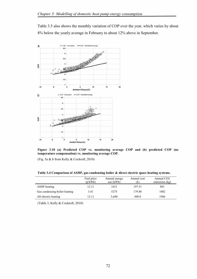
Chapter 3: Modelling of domestic heat pump energy consumption
72
Table 3.5 also shows the monthly variation of COP over the year, which varies by about
8% below the yearly average in February to about 12% above in September.
Figure 3.10 (a) Predicted COP vs. monitoring average COP and (b) predicted COP (no temperature compensation) vs. monitoring average COP.
(Fig. 5a & b from Kelly & Cockroft, 2010)
Table 3.4 Comparison of ASHP, gas condensing boiler & direct electric space heating systems.
Fuel price (p/kWh)
Annual energy use (kWh)
Annual cost (£)
Annual CO2 emissions (kg)
ASHP heating 12.11 1631 197.51 881
Gas condensing boiler heating 3.41 5275 179.88 1002
All-electric heating 12.11 3,640 440.8 1966
(Table 3, Kelly & Cockroft, 2010)

Chapter 3: Modelling of domestic heat pump energy consumption
73
Table 3.5 (a) ASHP detailed simulation results; (b) boiler detailed simulation results; (c) direct electrical heating annual simulation results.
January February March April May June July August September October November December Year
(a) Actual COP 2.58 2.55 2.71 2.77 2.9 3.1 2.91 2.78 2.67 2.77
Electrical (kWh) 308 261 219 113 57 37 143 221 272 1631
ASHP heat out (kWh) 793 667 593 314 164 113 418 613 727 4403
System heat loss (kWh) 46 44 41 35 30 22 37 39 42 335 Total system heat out (kWh) 747 623 552 279 134 91 381 574 685 4067
ON/OFF cycles 459 456 477 301 166 116 388 478 470 3311
(b) Efficiency 0.88 0.88 0.88 0.88 0.89 0.89 0.88 0.88 0.88 0.88
Gas (kWh) 937 788 701 385 203 144 521 732 865 5275
Boiler heat out (kWh) 821 691 617 341 180 128 459 643 759 4638
System heat loss (kWh) 34 40 45 47 41 38 56 42 36 379
Total System Heat Out (kWh) 787 652 571 294 139 91 403 601 722 4259
ON/OFF cycles 1087 932 911 528 282 206 758 964 1044 6712
(c) Total system heat
out (kWh) 692 572 496 250 116 69 320 505 620 3640
(Table 2, Kelly & Cockroft, 2010)
3.2.3.5 Staffel (2009)
This paper is a review of a large number of data sources for heat pump performance
data, with samples from laboratory testing to EN14511 and EN255 by the
Wärmepumpen-Testzentrum (WPZ) for both ASHPs and GSHPs, from manufacturers'
data sheets for ASHPs and GSHPs (Nibe, Calorex, Ciat, Thermia, Nordic, Daikin,
Hitachi, IVT, Viessmann, Worcester Bosch), from independent testing by BRE of a
Mitsubishi ASHP system, and from field trials of ASHPs in Slovenia, Belgium, Japan
(2 trials), Germany, and of GSHPs in Slovenia, UK, Germany and Japan. Of the field
trials, the German trials by the Fraunhofer Institute for Solar Energy Systems are the
most significant, consisting of some 110 systems from 7 manufacturers.(Miara, 2007)
The main analyses in this review are plots of COP against 'lift' - difference between
input temperature and output temperature - for the WPZ data and SPF against lift for
the Fraunhofer Institute trial data in Figure 3.11. This last figure is not that used by
Staffel(2009), but another in the same source document using monthly rather than daily
values.

Chapter 3: Modelling of domestic heat pump energy consumption
74
Staffel(2009)'s analyses of the test results appear to show a simple, linear relationship
between COP and 'lift', with the parameters of this relationship varying depending on
system type (ASHP or GSHP). Unfortunately the originals are of too poor quality to
include here. The plot of the field trial is much less clearly linear, a result which may be
caused by the inclusion of electricity for back-up heating within the system boundary
for the electricity consumption data collected(Miara, 2007, p. 11).
Figure 3.11 SPF vs 'lift' (Miara, 2007, p. 13)
3.2.3.6 Westergren(2000)
This paper details an approach to modelling energy consumption in a single family
home using a GSHP system as part of a larger project to estimate the total energy need
in such houses in Sweden. The estimation for this type of system has been separated
into a separate paper and method because of the relation of the performance of GSHP
systems to the temperature difference between the heat pump source and the dwelling
interior, rather than simply to the difference between internal and external temperature;

Chapter 3: Modelling of domestic heat pump energy consumption
75
and because of the requirement to estimate the energy consumption of an additional
backup heating system.
From a conventional heat balance model for the energy requirement of the dwelling, the
procedure starts from an approximation of average daily temperature over the heating
season (≤ 10ºC) based on a sinusoidal inequality as follows:
(
) 3.3-1Equation 3.10 (3.15)
where
aq = Annual average temperature
A = Daily average temperature amplitude
t = Day no. starting from 1st January
Phase shift to day of minimum temperature correct.
= Limit temperature for meteorological summer (≤ 10ºC) or set-point
for the additional heating system (not given in paper)
Given the equation defining the surface temperature, Westergren(2000) gives the
equation for the temperature amplitude at depth d, which is reduced in range and lagged
behind that at the surface, as follows:
( 3.3-2Equation 3.11 (3.16)
where Ad = Temperature amplitude at depth d A = Temperature amplitude at surface D = Damping depth.
The 'damping depth' is a constant measuring the decrease in temperature amplitude with
soil depth and is a function of soil thermal diffusivity.
The lag at depth d is assumed to be proportional to the distance below the surface,
giving the phase shift as:
( 3.3-3Equation 3.12 (3.17)

Chapter 3: Modelling of domestic heat pump energy consumption
76
where
= Phase shift (in days)
d = Collector depth
D = Damping depth.
Westergren(2000) then derives a formula for the COP of a generalised heat pump based
on the assumption that this is directly proportional to the Carnot COP for the system
given by ⁄ where TH and TC = the system output and input temperatures, both
in degrees K. Given a fixed output temperature, denoted by θ, and substituting the
previous equations in the Carnot COP calculation, the following equation is given for
heat pump performance:
The remaining section of the Westergren (2000) paper describes the details of
regression-based dwelling energy models, both static and dynamic, utilising this
expression for the heat pump COP, which also include estimation of the energy
( )
(
)
(3.18)
where
k = a constant representing the actual COP of the heat pump system as a
proportion of the theoretical maximum COP at the given input and output
temperatures
a = Annual average temperature
A = Daily average temperature amplitude
t = Day no. starting from 1st January
Phase shift to day of minimum temperature
Phase shift to day t
= System output temperature
Chapter 3: Modelling of domestic heat pump energy consumption
77
consumption of a secondary, back-up system. The data on which these model are based
was collected from Swedish dwellings in a monitoring study.
3.3 Models in standards
3.3.1 British Standard EN15316-4-2 (British Standards Institution, 2008a)
3.3.1.1 General
BS EN 15316-4-2 (hereinafter referred to as 'The Standard') is a long (130 pages
including annexes) and complex set of standards that applies not only to the electrically-
driven, vapour-compression heat pumps which are the subject of this thesis but also to
combustion engine driven vapour compression and thermally driven absorption cycle
heat pumps. It also defines two forms of model to estimate heat pump energy
consumption and efficiencies, of which the simpler, the 'system typology' method, is
defined only in general terms in the standard, while the more complex, 'component
efficiency' or 'bin-method' method is defined at length, with a worked example in Annex
D. The Standard states that the detail of the simpler method should be defined in a
national annex for each country, which has not been specified for England and Wales,
apart from the heat pump-related parameters in SAP. The Standard was developed
through the International Energy Agency Heat Pump Programme Annex 28 (Wemhöner
& Afjei, 2006a, 2006b).
The heat pump system configuration to which this Standard relates is shown in Figure
3.12. This differs from those in the monitoring study in this thesis in that it allows for a
buffer store associated with the distribution system, with corresponding heat losses. The
effects of this buffer can, presumably, be nullified in calculations by zeroising the
parameters for the buffer and pipework.

Chapter 3: Modelling of domestic heat pump energy consumption
78
Figure 3.12 Heat pump system boundaries
(Fig. 1 from British Standards Institution, 2008a)

Chapter 3: Modelling of domestic heat pump energy consumption
79
Figure 3.13 Energy balance of EN15316-4-2 generation system
(Fig. 2 from British Standards Institute, 2008 - colouring additions by author)
.
1 driving energy input to cover the heat requirement (e.g. electricity, fuel) EHW,gen,in
8 generation subsystem total auxiliary energy WHW,gen,aux
2 ambient heat used as heat source of the heat pump QHW,gen,in
9 generation subsystem recovered auxiliary energy QHW,gen,aux,ls,rvd
3 heat output of the generation subsystem corresponding to the heat requirement of the distribution sub- system(s) QHW,gen,out = QHW,dis,in
10 generation subsystem unrecovered auxiliary energy QHW,gen,aux,ls
4 generation subsystem thermal losses QHW,gen,ls
11 generation subsystem recoverable auxiliary energy QHW,gen,aux,ls,rbl
5 generation subsystem thermal loss (thermal part) recoverable for space heating QHW,gen,ls,rbl
12 generation subsystem non-recoverable auxiliary energy QHW,gen,aux,ls,nrbl
6 generation subsystem thermal loss (thermal part) non-recoverable QHW,gen,ls,nrbl
13 generation subsystem
7 generation subsystem thermal loss recoverable for space heating QHW,gen,ls,rbl,tot

Chapter 3: Modelling of domestic heat pump energy consumption
80
The energy flows included in this Standard are shown in Figure 3.13, of which the
percentage values 'are intended to give an idea of the size of the respective energy flows'
and are therefore not definitive.
The Standard states that the method is based on standard test results (British Standards
Institution, 2007) and is to be carried out with the heat capacity and COP data for a
specific system. The procedures in the Standard revolve around the partitioning of the
calculation period (which may be a month or a year) into 'bins'. In this context, the
meaning of a 'bin' is a division of the calculation period into temperature intervals for
which are accumulated the hourly averaged frequency values for temperatures in the bin
range. Thus, if a bin is defined as the interval from 0ºC to 10ºC, then a total for this bin
is the number of hours during which the external average temperature was in this range.
Within each bin, the operating conditions are assumed to be those of the central value,
the 'operating point', in the example 5ºC.
According to the Standard, bins should be chosen to have an even spread of operating
points across the temperature range, where possible with operating points coinciding
with the test points at which the performance results were measured and bin limits half-
way between operating points. It is unclear as to how overlapping source/sink ranges
should be handled. As an alternative to bins determined by test points, bins can be
defined as 1 K only in size, with COP values interpolated between test results.
3.3.1.2 'Detailed case specific calculation based on component efficiency data'
method
The flow of this procedure is shown in Figure 3.14.
After initial configuration, the procedure allows for the two operating modes:
monovalent and bivalent. Estimating methods for the bivalent mode are defined at two
levels of complexity, of which the simpler level requires the knowledge (or assumption)
of a value for the system balance point, which is not required for the more complex one.
A further high-level decision point is made depending on whether the heat pump system
is capable of simultaneous space heating and hot water generation, which introduces an
extra level of complexity into the system running time calculations.

Chapter 3: Modelling of domestic heat pump energy consumption
81
Figure 3.14 Flowchart of detailed process (British Standards Institute, 2008) Captions inserted from key by author
The main steps of the estimating procedure appear as follows:
a) definition of the calculation periods (month, year) and bins
b) calculation of energy requirements for each bin

Chapter 3: Modelling of domestic heat pump energy consumption
82
c) correction of the system's heating capacity and COP according to the operating
conditions, ie. source and sink temperatures, for each bin;
d) if the results of part-load testing on the system are available, the COP value is
corrected for the effects of part-load running;
e) calculation of heat losses from the system, particularly from a buffer tank and
associated pipework if present;
f) the previous steps establish the total energy consumption in each bin directly for
space heating or hot water generation, allowing the calculation of back-up
energy use for either of these functions where such back-up is included in the
configuration;
g) calculation of the heat pump running time in providing the required energy;
h) calculation of auxiliary energy, i.e. that consumed by the system pumps, not
only in the main operation of importing heat from the source and distributing it
to the sink, but also in stand-by operation while the system controller is
monitoring temperatures for weather compensation control.
i) estimation of thermal losses from the system which are recoverable via the
ambient - either inside the casing of the system itself or the dwelling.
j) final calculations total the energy output and the losses from the system for
space heating and hot water generation and divide by the system COP to obtain
estimates for the electricity consumed for these purposes by the heat pump.
3.3.2 Calculation Rules
These are lengthy as is may be judged by the flowchart in Figure 3.14, involving the
evaluation of a table of bin entries (containing the number of hours during which the
ambient temperature lies between an upper and lower value), with options for more or
less complex computation methods. The detail of the computation rules is described in
Appendix I.
3.3.2.1 Boundary conditions
The Standard has the following data parameter requirements (also known as boundary
conditions):

Chapter 3: Modelling of domestic heat pump energy consumption
83
Boundary conditions
Meteorological data:
frequency of the outdoor air temperature of the site at 1 K resolution or hourly
average values of the outdoor air temperature for an entire year;
outdoor design temperature of the site.
Space heating (SH) mode:
indoor design temperature;
heat energy requirement of the space heating distribution subsystem according
to EN 15316-2-3;
type and controller setting of the heat emission subsystem (flow temperature of
the heating system dependent on the outdoor air temperature, e.g. heating
characteristic curve or characteristic of room thermostat), temperature spread
at design conditions, upper temperature limit for heating;
heat pump characteristics for heating capacity and COP according to product
test standards (e.g. according to EN 14511 for electrically-driven heat pumps)
and guaranteed temperature level that can be produced with the heat pump;
results for part load operation, e.g. according to CEN/TS 14825 for electrically-
driven heat pumps, if available;
for the simplified calculation method of the back-up energy, the balance point;
system configuration:
installed back-up heater: operation mode, efficiency (fuel back-up heater
according to EN 15316-4-1);
installed heating buffer storage: stand-by loss value, flow temperature
requirements;
power of auxiliary components (source pump, storage loading pump,
primary pump, stand-by consumption).
Domestic hot water (DHW) mode:

Chapter 3: Modelling of domestic heat pump energy consumption
84
heat energy requirement of domestic hot water distribution subsystem according
to EN 15316-3-2;
temperature requirements of DHW operation: cold water inlet temperature (e.g.
15 °C), DHW design temperature (e.g. 60 °C);
heat pump characteristics for DHW heating capacity and COP according to
product test standards (e.g. according to EN 255-3 for electrically-driven heat
pumps);
set temperature for the energy delivery by the heat pump (e.g. at 55 °C due to
heat pump operating limit);
parameters of the domestic hot water storage (stand-by loss value);
installed back-up heater: operation mode, efficiency (fuel back-up heaters are
calculated according to EN 15316-4-1).
This is a considerable number of data items, particularly for the controller settings,
rendering it almost impossible to use this routine for sizing a heat pump.
3.3.2.2 Overall totals
The Standard requires the following overall totals to be calculated:
a) Electricity input to the heat pump for space heating operation
b) Electricity input to the heat pump for domestic hot water operation
c) Energy input to back-up system, for either of
Electrical back-up heater
Fuel back-up heater
d) Total driving and back-up energy input to cover the heat requirement
e) Seasonal performance factor and expenditure factor of the generation subsystem
f) Total heat produced by the heat pump and the back-up heater

Chapter 3: Modelling of domestic heat pump energy consumption
85
3.3.3 Discussion
3.3.3.1 UK approval of the overall EN 15316 Standard
Neither the Standard being discussed here nor any of the other Standards in this series
have been accepted by the UK government. In the National Foreword to the document,
it is stated that "the UK voted against this standard on the grounds that it was
considered disproportionate to the essential requirements of the EU Energy
Performance of Buildings Directive (2002/91/EC), which it supports. In the opinion of
the UK committee, EN 15316[sub-section number] is regarded as unsuitable for
existing buildings where the data required are unlikely to be available." Amongst other
provisions, the Directive (EU Parliament, 2002) requires member countries to provide a
method for the assessment of the energy performance of buildings, the output from
which is an Energy Performance Rating and associated Certificate which must be made
available to a prospective purchaser or tenant at the initial handover of a new building
and whenever a building is to be sold or rented out. For the purpose of this Certificate,
the method currently used for rating dwellings in the UK is the Reduced Data SAP
(RdSAP) procedure, a version of the main SAP routine employing parameter reduction
techniques to estimate the values of lower level construction parameters (BRE, 2010a).
Many other Standards are involved in the definition of the Energy Performance Rating
assessment process and therefore the failure to endorse the EN 15316 series of
Standards does not appear to have much effect. Some parts of the EN 15316-4-2
Standard have been invoked in the full SAP assessment in the generalised estimation of
heat pump energy consumption and also in the Appendix Q process (BRE, 2009b;
Hayton, 2010).
3.3.3.2 Data availability
The initial values used in the Standard's calculations are listed in section 3.3.2.1. To
create a generalised model from the equations in the Standard to meet the objectives of
this research, it is necessary to examine how these values might be derived for this
general case. For the conditions listed above, the following comments apply:
a) Meteorological data at the level of detail required by the routines is not currently
used by any of the standard UK domestic energy models. Weather data in
BREDEM-8 (Anderson et al., 2001) and BREDEM-12 (Anderson et al., 2002)

Chapter 3: Modelling of domestic heat pump energy consumption
86
consists of average monthly temperatures for each of 21 UK regions which are
defined by similar heating degree day values, whilst in SAP 9-90 (BRE, 2010a),
meteorological data is limited to one set of monthly average temperatures based on
a single UK location. Within these routines, values for heating design days are
calculated by a standard equation, with the monthly average temperature and month
length in days as parameters.
To generalise the meteorological data, it would be necessary to create a table of
outdoor air temperature frequencies for each month in each degree-day region.
b) A suitable default value would be required for the outdoor design temperature, as
this is not explicitly specified for any of the current UK standard models.
c) Details of the type and settings of the system controller are not available in the UK
standard models. The Standard provides an equation (Section B.1, page 70) to
describe the relationship between external temperature and the distribution flow
temperature, which is the value required in computation, but this requires
knowledge of further parameters, the design flow and return temperature to the
distribution system, for which general values are not available in the UK standard
models. This equation also requires an outdoor design temperature value.
d) Heat pump performance test results are available from the Wärmenpumpen
Testzentrum (WaermenPumpen Testzentrum, 2011) for individual heat pumps. A
guaranteed temperature level value is usually only available in manufacturer's
documentation (IVT Industrier AB, 2004).
e) Performance test results according to CEN/TS 14825 for part-load operation are
not, to the author's knowledge, available in significant numbers comparable with
the EN14511 and EN255 results published by WPZ.
f) House balance point temperatures are not usually available for existing houses,
requiring analysis to obtain a suitable general value.
g) The parameters required for estimation of the energy use of domestic hot water
generation and storage would appear to raise the same issues as space heating.
3.3.3.3 Complexity and interconnectivity of Standards documents
As a somewhat crude measure of complexity, the Standard under consideration contains
some 58 equations to estimate the energy use of a heat pump heating system alone

Chapter 3: Modelling of domestic heat pump energy consumption
87
whereas the BREDEM-12 specification (Anderson, et al., 2002) contains about 70
equations in its dwelling energy model, including some calculations of heating system
energy use which would be included within the EN 15316-4 series of Standards. The
calculations example in Annex D of the Standard contains 47 steps for 4 bins, but
covers one calculation period only, ie. a month, requiring 12 repetitions for a complete
year of estimates which equates to about 2250 calculations. The method used in Annex
D is the 'simplified' method and the 'detailed' method would require perhaps the same
number of calculations again, depending on the temperature range of the climate at the
site.
The Standard under consideration is one of a set of 14 parts in BS EN 15316. It also
references eight other Standards which themselves reference further Standards and so
on. Since these are all part of a structure aimed at the "European harmonisation of the
methodology for the calculation of the energy performance of buildings", to quote the
Foreword of BS EN 13790 (British Standards Institution, 2008b), then it is to be hoped
that, as far as possible, the estimating methods defined in the Standards in this series are
in step. It is however, another matter as whether the heat pump model as defined in this
Standard can be employed in a domestic energy model that is not part of the structure,
since the available standard UK dwelling energy models pre-date these European
Standards, and SAP (BRE, 2005, 2010a) makes reference to a single Standard, BS
EN13790 (British Standards Institution, 2008b).
3.3.3.4 Computer processing
While the author has no definite evidence, his impression is that reproducing the BS
15316-4-2 routines in a spreadsheet routine, especially one which analysed many
dwelling samples, would require excessively lengthy processing times. The detailed
method, particularly the estimation of back-up energy, would require the processing of a
table of 9 bins (rows) times 14 columns for each period (eg. a month) for each sample, a
total of 1512 cells per sample to provide a year's estimate.

Chapter 3: Modelling of domestic heat pump energy consumption
88
3.3.4 BREDEM/SAP models
3.3.4.1 General
The BREDEM series of models have been used by BRE as their main means of
estimating the energy use of dwellings since the inception of the basic energy model,
named BREDEM-1, as documented by Christine Uglow in 1981 (Uglow, 1981). Since
then, BREDEM has been developed through versions 2 to 12 and adopted as the basis of
commercial energy assessment software, with BREDEM-9 being spun off as the basis
for SAP (Shorrock & Anderson, 1995). BREDEM-8 and 12 models form the basis of
the BREHOMES modelling at national level of domestic energy use (Henderson &
Shorrock, 1988; L D Shorrock, Henderson, & Bown, 1991(Shorrock & Dunster, 1997)
providing analyses of energy consumption for the English House Condition Survey
(Utley & Shorrock, 2008) and SAP forms the basis of the system for approving the
design of new dwellings laid down by the Approved Documents of Part L1 of the UK
Building Regulations (BRE, 2008). These are, therefore, accepted standard models for
the estimation of energy consumption and carbon emissions in the UK.
The BREDEM models (Anderson, et al., 2001) are based on a static space heating
equation, in which the heating requirement is determined by the difference between
internal and external temperatures and by the specific heat loss coefficient for the
building, as calculated from the resistivity of its construction elements and its
ventilation losses. The various heat gains, ie. solar gain, casual gains from occupants,
from hot water generation and cooking, etc. that also determine the heating requirement
are estimated using empirical relationships based on appropriate characterising data, viz.
window area, location and orientation, floor area etc. The dwelling is divided into two
heating zones, each with its own heat loss coefficient, with the transmission of heat
between zones estimated by the definition of an interzonal heat loss coefficient.
External temperatures are determined from a table of average monthly temperatures
according to the building’s location. Mean internal temperatures are determined from
the demand temperature required by the occupants, conventionally set to 21°C; from a
‘responsiveness’ parameter determined by the type of heat distribution system and its
controls; from the heating pattern adopted by the occupants; and from the heat loss
coefficient. The responsiveness parameter indicates how long the heating system takes
to return to background temperature after it has been turned off and varies from 1.0 for a
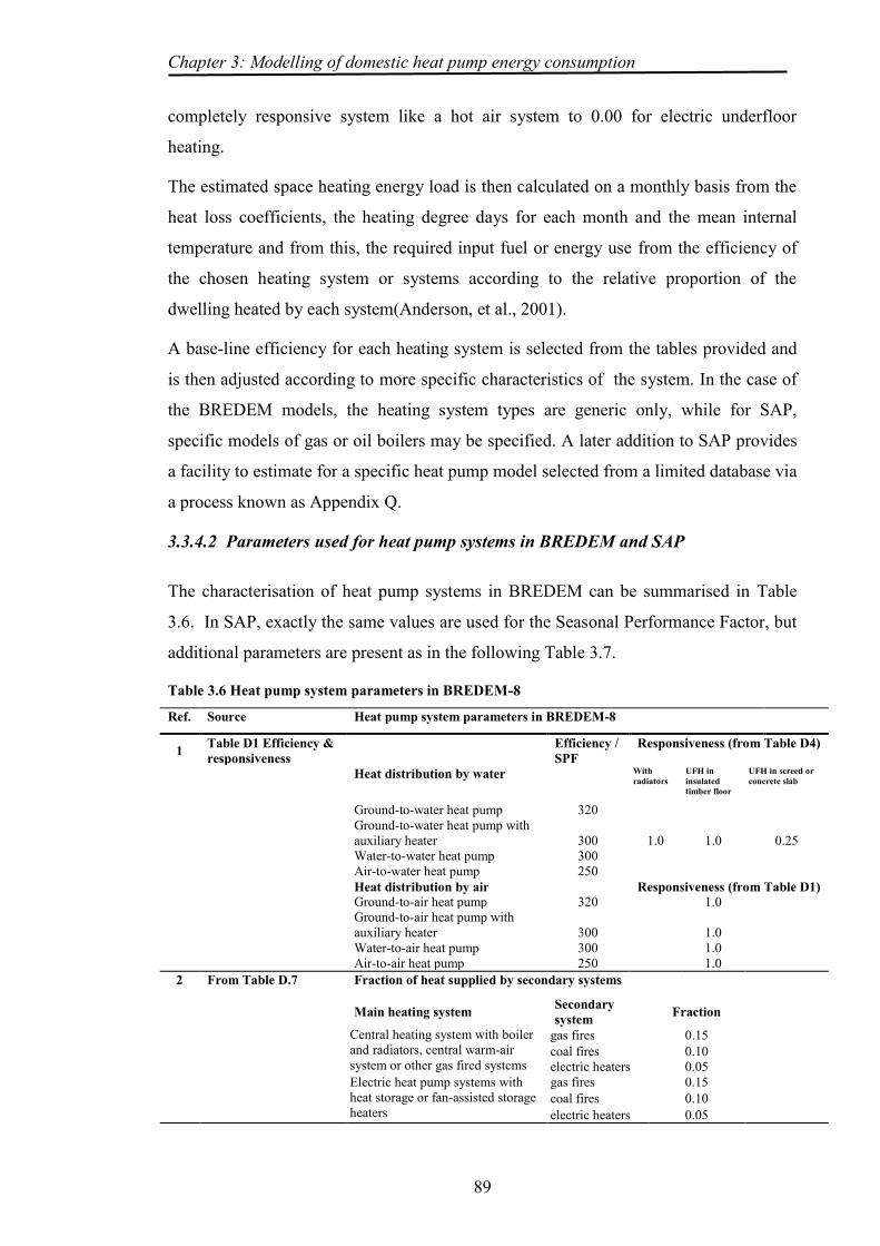
Chapter 3: Modelling of domestic heat pump energy consumption
89
completely responsive system like a hot air system to 0.00 for electric underfloor
heating.
The estimated space heating energy load is then calculated on a monthly basis from the
heat loss coefficients, the heating degree days for each month and the mean internal
temperature and from this, the required input fuel or energy use from the efficiency of
the chosen heating system or systems according to the relative proportion of the
dwelling heated by each system(Anderson, et al., 2001).
A base-line efficiency for each heating system is selected from the tables provided and
is then adjusted according to more specific characteristics of the system. In the case of
the BREDEM models, the heating system types are generic only, while for SAP,
specific models of gas or oil boilers may be specified. A later addition to SAP provides
a facility to estimate for a specific heat pump model selected from a limited database via
a process known as Appendix Q.
3.3.4.2 Parameters used for heat pump systems in BREDEM and SAP
The characterisation of heat pump systems in BREDEM can be summarised in Table
3.6. In SAP, exactly the same values are used for the Seasonal Performance Factor, but
additional parameters are present as in the following Table 3.7.
Table 3.6 Heat pump system parameters in BREDEM-8
Ref. Source Heat pump system parameters in BREDEM-8
1 Table D1 Efficiency & responsiveness
Efficiency / SPF
Responsiveness (from Table D4)
Heat distribution by water With
radiators UFH in insulated timber floor
UFH in screed or concrete slab
Ground-to-water heat pump 320
1.0 1.0 0.25 Ground-to-water heat pump with auxiliary heater 300
Water-to-water heat pump 300 Air-to-water heat pump 250 Heat distribution by air Responsiveness (from Table D1) Ground-to-air heat pump 320 1.0
Ground-to-air heat pump with auxiliary heater 300
1.0
Water-to-air heat pump 300 1.0 Air-to-air heat pump 250 1.0
2 From Table D.7 Fraction of heat supplied by secondary systems
Main heating system Secondary system Fraction
Central heating system with boiler
and radiators, central warm-air system or other gas fired systems
gas fires 0.15 coal fires 0.10 electric heaters 0.05
Electric heat pump systems with
heat storage or fan-assisted storage heaters
gas fires 0.15 coal fires 0.10 electric heaters 0.05
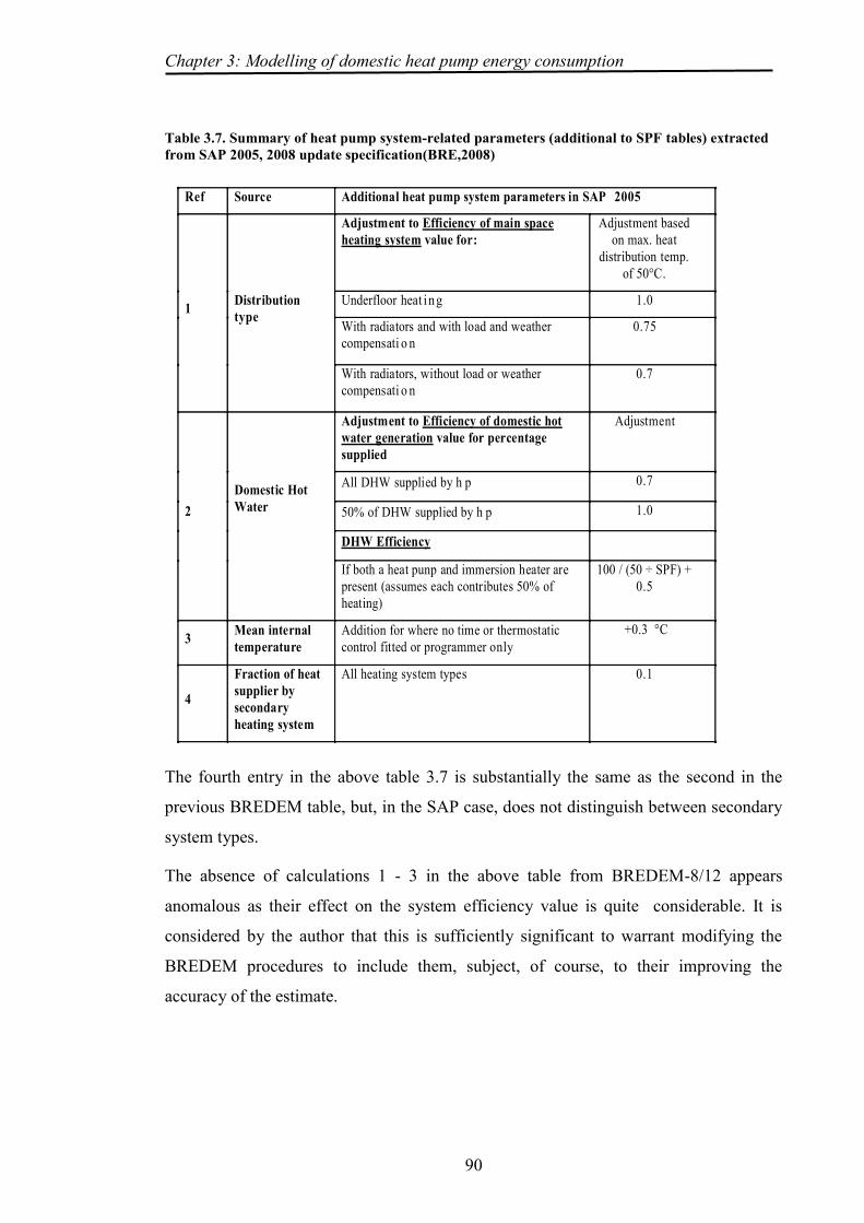
Chapter 3: Modelling of domestic heat pump energy consumption
90
Table 3.7. Summary of heat pump system-related parameters (additional to SPF tables) extracted from SAP 2005, 2008 update specification(BRE,2008)
The fourth entry in the above table 3.7 is substantially the same as the second in the
previous BREDEM table, but, in the SAP case, does not distinguish between secondary
system types.
The absence of calculations 1 - 3 in the above table from BREDEM-8/12 appears
anomalous as their effect on the system efficiency value is quite considerable. It is
considered by the author that this is sufficiently significant to warrant modifying the
BREDEM procedures to include them, subject, of course, to their improving the
accuracy of the estimate.
Ref Source Additional heat pump system parameters in SAP 2005
Adjustment to Efficiency of main space
heating system value for:
Adjustment based on max. heat
distribution temp. of 50°C.
Underfloor heat i n g 1.0
With radiators and with load and weather compensati o n
0.75 1
Distribution
type
With radiators, without load or weather compensati o n
0.7
Adjustment to Efficiency of domestic hot
water generation value for percentage supplied
Adjustment
All DHW supplied by h p 0.7
50% of DHW supplied by h p 1.0
DHW Efficiency
2
Domestic Hot
Water
If both a heat punp and immersion heater are present (assumes each contributes 50% of heating)
100 / (50 ÷ SPF) + 0.5
3 Mean internal
temperature
Addition for where no time or thermostatic control fitted or programmer only
+0.3 °C
4
Fraction of heat
supplier by
secondary
heating system
All heating system types 0.1

Chapter 3: Modelling of domestic heat pump energy consumption
91
3.3.4.3 SAP Appendix N/Q process
This was introduced in SAP version 9.82 as an 'add-on' to the UK Standard Assessment
Procedure (SAP) for assessing the energy performance of dwellings (BRE, 2009b,
2010a, 2010c). The objective of the procedure is to estimate the carbon dioxide and
energy consumption savings for the installation of a selected specific heat pump model
in the dwelling being assessed, replacing the generic heat pump system for which
standard parameters are provided in SAP. The calculation process is documented both
in Appendix N of the SAP specification and in a separate document (Hayton, 2010)
available from the Appendix Q website (BRE, 2009b). The accompanying database of
thermal performance data for heat pump systems which have been verified by testing to
EN14511-2 or prEN255-3 standards is contained in a spreadsheet containing an
implementation of the calculation method and is available for download from the
Appendix Q website. The database is updated with data provided by suppliers or
manufacturers. The Appendix Q calculation is additional to and separate from the SAP
calculations in that it uses some intermediate results from the SAP calculations,
returning results for input at a later step in the SAP calculation. The Appendix Q
specification (Hayton, 2010) is said to be based on the British Standard BS EN 15316-
4-2 (British Standards Institution, 2008a) document and therefore the test result data
values in the database are those required for this calculation. The Appendix Q method
largely replaces the parameters as specified in Tables 3.6 and 3.7 when a specific heat
pump ‘package’ is selected from the database. However, an initial comment in the
attached documentation in the Appendix Q calculations spreadsheet states '[the
procedure] is only valid for the carbon dioxide calculations and shows additional
energy saved (or consumed) compared to the default heat pump specified in the SAP
calculator; calculations for consumption and costs are invalid' (BRE, 2010b).
3.3.4.4 SAP Appendix Q database
As stated above, the test results data stored in this database are those generated by the
EN14511-2/EN255 test procedures and required as input to the EN 15316-4-2
calculation. The range of equipment for which the database is designed is not limited to
the ‘classic’ ASHP or GSHP systems but also allows for test results for exhaust air
source equipment with different heat recovery options. Hence some data items are
irrelevant to the simpler configurations.

Chapter 3: Modelling of domestic heat pump energy consumption
92
The data consists of a set of items which apply to each heat pump (unique identifier,
make, model name, data source, heat source, etc.), followed by two sets of test results
for that heat pump, the first of which is the heat recovery results for results containing a
group for each emitter type (UFH, radiators or convectors), within which there are
results for each of a list of plant size ratios (ratio of system output to design heat loss).
The full list of the data items is shown below in Tables 3.8 & 3.9.
Table 3.8. Table N1 from BRE (2010)
SAP 2009 version 9.90 (March 2010)
84
b) If the throughput lies within the range of values in the database record use the intermediate results for the applicable throughput by linear interpolation.
c) If the throughput is less than the lowest value in the database record calculate a heat pump
over-ventilation ratio (Rhp) as the lowest rate in the database record in the database record (l/s) divided by the required dwelling rate (l/s); otherwise set the ratio to 1. When the ratio exceeds 2 the data are invalid for the dwelling and when it is above 1 but less than or equal to 2 use the intermediate results for the lowest value in the database record. Further calculations are required using the over-ventilation ratio as set out in N3.1.1.
The interpolation for PSR should be done first, followed by the interpolation for air flow rate.
Table N1: Package general information
Data item Unit
Package main fuel (see Table 12) -
For heat pumps, the heat pump source, one of: - ground - water - air - exhaust air MEV - exhaust air MVHR - exhaust air mixed
-
Service provision, one of - space and hot water all year - space and hot water in heating season only - space heating only - water heating only
-
Product index number for MEV/MVHR (for exhaust air MEV, exhaust air MVHR or exhaust air mixed)
-
Hot water vessel, one of - integral to package - separate, specified cylinder - separate but unspecified cylinder - none (DHW not provided by package)
-
Hot water vessel volume (where relevant) litres
Hot water vessel loss (where relevant) kWh/day
Hot water vessel volume heat transfer area (where relevant) m!

Chapter 3: Modelling of domestic heat pump energy consumption
93
Table 3.9. Table N2 from BRE (2010)
The Appendix Q data most relevant to this study is the table of entries for each plant
size ratio/emitter type combination which consists of:
heating capacity (maximum space heating output for this emitter type);
heating seasonal performance factor (SPF);
heat pump running hours per year.
3.3.4.5 Appendix N/Q calculation process
A large section of the Appendix N/Q process involves the derivation of an estimate for
the effect of a possible difference between the standard SAP assumptions for dwelling

Chapter 3: Modelling of domestic heat pump energy consumption
94
occupancy – 9 hours on weekdays, 16 hours on Saturday and Sunday - and the heat
pump system operating hours – up to 24 hours every day. This creates a replacement
equation with which to estimate the Mean Internal Temperature for the dwelling living
area in Table 9c. For Section 9a, Energy Requirements, of the main SAP process, a
value for the Secondary Fraction (fraction of the heat energy provided by a secondary
system) is obtained from reference table N8 according to the PSR and this value is used
in field 201 in the SAP worksheet. A value for space heating thermal efficiency is
obtained from the Appendix Q database entry for the heat pump, PSR, and emitter type
used by the system.
3.3.4.6 Discussion
The characteristics and deficiencies of the BREDEM/SAP heat pump parameters are
discussed in Chapter 7.
3.4 Publicly-available software models
These are limited in number. Most publicly-available calculators for heat pump sizing
consist only of limited web-based facilities (Encraft Ltd, 2012; Nu-Heat Ltd, 2011;
Vaillant Ltd, 2011). A limited, educational spreadsheet tool is available from John
Cantor, a UK heat pump expert(Cantor, 2008). A package known as RETScreen is the
only reputable and professionally-supported software tool that the author has found.
3.4.1 Encraft heat pump calculator
3.4.1.1 Description
The Encraft heat pump calculator (Encraft Ltd, 2012) is a web-based tool which can be
accessed freely by registered users under restricted conditions and embedded in a user's
own website if required. Paid versions allow programming access to the tool so that the
user can pass parameters avoiding the standard interface.
Samples of the input and output web pages are shown in Figure 3.15 and Figure 3.16.
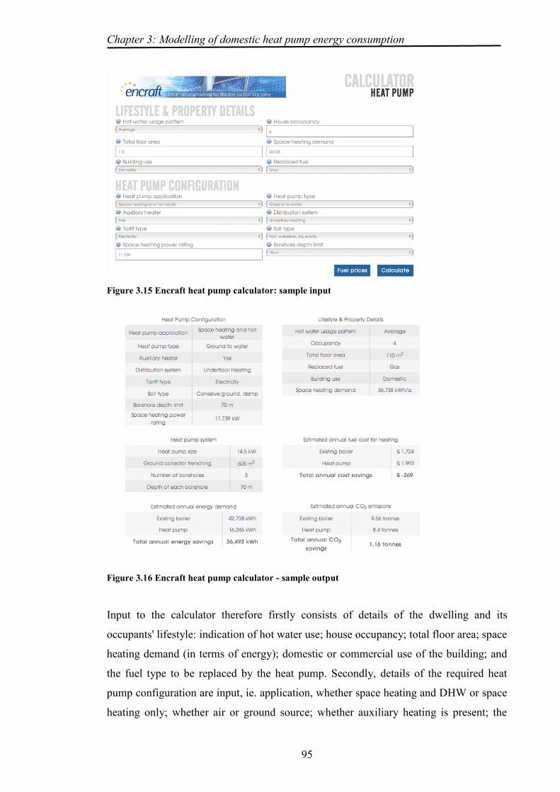
Chapter 3: Modelling of domestic heat pump energy consumption
95
Figure 3.15 Encraft heat pump calculator: sample input
Figure 3.16 Encraft heat pump calculator - sample output
Input to the calculator therefore firstly consists of details of the dwelling and its
occupants' lifestyle: indication of hot water use; house occupancy; total floor area; space
heating demand (in terms of energy); domestic or commercial use of the building; and
the fuel type to be replaced by the heat pump. Secondly, details of the required heat
pump configuration are input, ie. application, whether space heating and DHW or space
heating only; whether air or ground source; whether auxiliary heating is present; the

Chapter 3: Modelling of domestic heat pump energy consumption
96
type of distribution system; the soil type for a ground collector, the depth limit for
borehole collectors and the heat pump power rating. Either of two tariffs for electricity
supply are permitted, green (ie. zero-carbon) or conventional. The calculator responds
with output of: sizing for the heat pump and ground collector trenching, the number and
depth of boreholes; estimated annual energy demand, energy cost and CO2 emissions
for existing system and the heat pump. Only annual values are computed.
Using the output Energy Demand and input Space Heating values to calculate the
effective SPF for the systems, it was found that the SPF values assumed by the
Calculator are basically those in SAP/BREDEM with a maximum value of 3.2 for a
GSHP and 2.50 for an ASHP when used for space heating only with distribution by
UFH. The effect of replacing "UFH" with "Radiators" or "Space heating only" with
"Space heating and hot water" is to reduce the SPF, with the lowest values being 1.57
and 1.84 for ASHP and GSHP respectively. The effect of changing the soil type from
the more useful type of "Saturated ground" to "Non-cohesive, dry, sandy" is to increase
the "Ground collector trenching" value, rather to effect the SPF in any way.
3.4.1.2 Discussion
The main restriction in this calculator is that it is only available as a web page requiring
a user login and interaction to trigger each calculation. Its heat pump model is restricted
to a single, annual SPF value, which would not be affected by changes to ambient
temperature and the relationship of SPF to the various input parameters is not publicly
available.

Chapter 3: Modelling of domestic heat pump energy consumption
97
3.4.2 Heat pump energy efficiency evaluator
3.4.2.1 Description
A typical evaluation from this facility (Cantor, 2008) is shown in Fig 3.17.
Figure 3.17 Sample of Evaluator output
The output from the spreadsheet is a COP value, shown on the lefthand side, towards
the top. This is calculated from a relationship with the Working Temperature Difference
value (in red, below the COP value) shown by the values indicated by the dotted red
lines on the chart. The Working Temperature Difference is calculated from the
difference between the heat pump refrigerant evaporation and condensation
temperatures with the values for these temperatures set by 11 controls as per the
following table:
Table 3.10 Effects of controls on COP in Heat pump energy efficiency evaluator
Ref. Control Setting
1 Type of heat pump Refers to the type of ground source collector, with
values of "ground source", "spring source indirect",
& "spring source - direct". Varies the evapotion
temperature, with "ground source" giving the lowest

Chapter 3: Modelling of domestic heat pump energy consumption
98
value and "spring source - direct" the highest.
2 Type of house Refers to the energy efficiency of the house, varying
the condensation temperature from the highest for
"Old building, solid walls, badly insulated house"
down to the lowest for "Super insulated eco-home"
3 Type of emitter Refers to the output of the distribution system,
varying the condensation temperature from the
highest for "Radiators" down to the lowest for
"Underfloor screed with solid / tiles covering"
4 Emitter pipework
design
Refers to the output of the distribution system,
varying the condensation temperature from the
higher value for "Standard (as used for boilers)"
down to the lower for "Low temperature design (for
heat pump)"
5 Geographical location Refers to the Ground temperature value, with "North
East, Scotland" being the lowest at 9ºC and "South
West" the highest at 11ºC.
6 Heat pump efficiency Allows two values, "High quality, optimised for
heating" and "Lower quality (cheaper)". The first
value both increases the evaporation temperature and
decreases the condensing temperature compared with
the second.
7 Ground collector area Affects the evaporating temperature value, with the
"Small area" setting reducing its value and "Large
area" increasing it.
8 Ground conditions Again, affects evaporating temperature value, with
the "Dry ground" setting reducing its value and "Wet
ground" increasing it.

Chapter 3: Modelling of domestic heat pump energy consumption
99
9 Required room
temperature
The three values for this control have the obvious
effect of changing the Room Temperature value, but
also have the effect of changing all the temperatures
back to the condensing temperatures.
10 Backup electric
heating?
The effect of this control are different from those of
the others. The "Electric back-up (small heat pump)"
value apparently sets a value for energy use from
back-up of 20% of energy consumption, regardless
of other parameters. The "Electric back-up (if max.
temperature exceeded)" adds that percentage on to
the energy consumption value depending on how
much the Working Temperature Difference exceeds
60ºC.
11 Heat pump run-hours The three values allowed for this control have the
effect of changing the Evaporation temperature
value, with the "Light use..." value causing an
increase and the "High run hours..." causing a
decrease.
The effects of these controls are cumulative. Thus, the effect of specifying values of
"Old building...", "Radiators" and "Standard (as used with boilers)" for controls 2, 3 and
4 increases the refrigerant condensing temperature up to 72.4ºC, whereas the same
values of controls 3 and 4 result in a temperature of 50.5ºC when 2 is set to "Super-
insulated eco-home". Similar effects are observed in setting those controls affecting the
condensing temperature.
3.4.2.2 Discussion
The major consideration concerning this software is that details of its relationships and
of the values of the parameters corresponding to the various control settings are not
available for incorporation into another model. By sampling values of COP for different
values of Working Temperature Difference, it is possible to obtain a relationship for
these two variables. However, it is still unclear what the characteristics of a dwelling are

Chapter 3: Modelling of domestic heat pump energy consumption
100
represented by, for example, parameter 2 and a similar lack of clarity applies to most of
the other parameters. Hence, as the author indicates, the tool is useful for illustrating the
characteristics effecting the efficiency of a heat pump system, but does not allow the
specification of a system based on any description of a dwelling built form.
3.4.3 RETScreen
This section describes the heat pump project estimating facility within the RETScreen
(Renewable Energy Technology Screen[ing?]) software developed by, and available
freely from, Natural Resources Canada (Minister of Natural Resources Canada, 2005b,
2011). It is written in Microsoft Excel but has a facility to save project files in its own
format. The software contains facilities for examining the feasibility in terms of costs
and GHG emissions of different forms of renewable energy and energy efficiency
measures for new-build and retro-fit, domestic and non-domestic buildings and, where
required, comparing the new measures with the existing provisions. The RETScreen
software currently available brings together modules for each project type, of which one
was for estimating energy and costs for GSHP projects (Minister of Natural Resources
Canada, 2005b). Further documentation is provided by a second manual (Minister of
Natural Resources Canada, 2005a)
The measures for which estimates can be prepared include energy efficiency
improvements to the fabric of the building (or buildings), effects of various renewable
and non-renewable methods of electricity generation and of the replacement of heating
and cooling systems. Electricity generation methods include fuel cells, wind,
hydroelectric, solar thermal and PV, landfill gas, biomass, biodiesel, biogas, hydrogen,
natural gas, oil/diesel, coal, and municipal waste. Heating systems include biomass,
solar air and water, gas and oil boilers and heat pumps. Cooling system types include
vapour compression (conventional air conditioning) adsorption, desiccant, heat pump
and 'free'.
The RETScreen software has two analysis levels, denoted Method 1 and Method 2 of
which Method 2 provides a greater level of information and therefore has greater data
requirements which depend on the type of project concerned. Use of Method 2 inserts
additional worksheets into the spreadsheet for data input for cost, emission, financial
and risk analysis and for tools relevant to the type of project involved. The 'Tools'

Chapter 3: Modelling of domestic heat pump energy consumption
101
worksheet is used to acquire the more detailed data required to size the heat pump and
its ground loop.
To analyse the feasibility of the proposed project, the RETScreen model requires
definition of existing energy consumption and climate for the location. From the climate
data, temperature bin values and ground temperatures are calculated. The heating and
cooling loads and balance point temperatures are calculated from the built form data for
each temperature bin. An initial estimate of the system capacity is calculated with the
size of the ground heat exchanger, from which the system COP and capacity by
temperature bin is estimated, which allows the need for additional heating to be
evaluated and the annual system energy consumption to be calculated. This flow is
illustrated in Figure 3.18.

Chapter 3: Modelling of domestic heat pump energy consumption
102
Figure 3.18 RETScreen GSHP energy model system flow
(Fig 17 from Minister of Natural Resources Canada. (2005a))
3.4.3.1 Data requirements for RETScreen
Climate data for the model is set by the user choosing a location from a list within the
model data. The locations available for the UK are at UK airports and RAF airbases, not
all coinciding with those in the CIBSE datasets used in UK standard models (CIBSE,
2007). In a similar way to the EN 15316-4-2 model documented above, the weather data
is 'binned' by degree hours, ie, a 'bin' is defined by an external temperature and is

Chapter 3: Modelling of domestic heat pump energy consumption
103
allocated the number of hours during which the temperature was in the range halfway
between the bin temperature below and that halfway between the bin temperature
above, eg, if bin temperatures were -10, -8, -6, etc. then the value assigned to the bin
with temperature -8ºC would be the number of hours during which the temperature was
between -9ºc and -7ºC. RETScreen uses separate degree hours binning for day-time and
night-time and for the coldest month and warmest month, but because of the substantial
volume of data that would be involved holding such data for all regions of the world,
the software uses a generator routine to create the hourly temperature values, based on
design temperatures and latitude values for the location.
The next stage of the calculation is to estimate the source temperature for the heat
pump. For a vertical borehole this is assumed to be the annual average surface soil
temperature. For horizontal ground loops, the RETScreen routine calculates the
maximum and minimum ground temperature, Tg,max and Tg,min, based on annual average
surface soil temperature, , the surface temperature amplitude AS, the given heat
exchanger depth XS, the soil thermal diffusivity, α, from equations 3.19 and 3.20:
( √
)
(3.19)
and
( √
)
(3.20)
3.4.3.2 Building load calculation
RETScreen contains two methods for calculating the building energy load: the
descriptive data method, for which the details of the built form and thermal
characteristic of the building elements are entered; or the energy use method for which
summary energy load and use values are entered, for which knowledge of an existing
building is required. For the descriptive method, the relationship between external
temperature and the different building heating and cooling loads is calculated, with the
loads involved being as follows (Minister of Natural Resources Canada, 2005b, p.
GSHP.30):
Transmission losses (conductive and convective)
Solar gains (sensible)

Chapter 3: Modelling of domestic heat pump energy consumption
104
Internal gains (sensible)
Fresh air load (sensible)
Fresh air load (latent)
Internal gains (latent)
The descriptive data input allows the relationships between the above loads and external
temperature to be calculated, which, combined with the bin degree hours, enables total
load values to be calculated for each bin.
The data required for the descriptive method does not differ substantially from data used
in other models and therefore will not be described in detail here. The assumptions
made about the built form by the RETScreen model are more significant. The building
load calculation makes assumptions about the built form, viz. the building is assumed to
have a square built form, with windows evenly distributed across its aspects and
orientations. Dwellings are all assumed to have a single heating zone and identical
occupation of two adults and two children for the whole day, while occupancy in
commercial building is assumed to be 5 persons per 100m2 for 24 hours, though this is
not stated (Minister of Natural Resources Canada, 2005a). It is assumed that ventilation
losses for dwellings are related to insulation levels, but these are defined only as "high",
"medium" and "low", rather any specific values. The actual insulation values associated
with these levels are defined in a Canadian source (Hydro-Quebec, 1994).
The results of the descriptive method input are used to form a quadratic equation,
relating energy load to external temperature. Used with the bin temperature hours, this
is used to calculate energy consumption for each bin. It is also solved to find a balance
point temperature.
The energy load method relies on detailed data having been collected from an existing
building, a method which is not available when estimating for the entire housing stock.
3.4.3.3 Heat pump ground loop sizing
Two formulae are given for the collector length, one for heating, one for cooling, which
are basically similar in structure. For heating, the formula for the length is as follows:
[
( )]
(3.21)
where:

Chapter 3: Modelling of domestic heat pump energy consumption
105
qd,heat = design heating load
COPh = the design COP for heating of the system
Rp = the pipe thermal resistance,
Rs = soil/field resistance
Fh = heat exchanger part load factor for heating
Tg,min = minimum undisturbed ground temperature
Tewt, min = minimum design entering water temperature
[
( )]
(3.22)
where:
qd,cool = design cooling load
COPc = the design COP for cooling of the system
Rp = the pipe thermal resistance,
Rs = soil/field resistance
Fc = heat exchanger part load factor for cooling
Tg,max = maximum undisturbed ground temperature
Tewt, max = maximum design entering water temperature
Units for these variables are determined by user preferences for SI or Imperial units.
Choice of which of the two possible sizes of heat exchanger will be determined by user
input deciding the priority of heating or cooling. Where either length is insufficient for
its function, then the system indicates that additional heating or additional heat rejection
is required. Of the variables in equations 3.42 and 3.43, Tg,min and Tg,max are calculated
as per equations 3.40 and 3.41 above, Tewt, min is calculated as Tg,min - 8.3 K (stated as
15ºF in (Minister of Natural Resources Canada, 2005a) section 2.6.2), Tewt, max is
calculated as the minimum of Tg,max+ 11 K and 43.3 ºC (again, temperature values
stated as 20ºF and 110ºF in section 2.6.2), the part load factors Fh and Fc are calculated
as the ratio between the average load and the peak load for the months of January for
heating and July for cooling using the values calculated from the appropriate bin. The
methods of determining Rp and Rs are stated as coming from the IGSHPA 'Installation
Guide' (IGSHPA, 1988) without further details.
A further of section of the RETScreen manual (Minister of Natural Resources Canada,
2005a) details calculations for sizing open loop groundwater heat exchangers. These are
not often used in the UK in residential applications because of the requirement to

Chapter 3: Modelling of domestic heat pump energy consumption
106
license the extraction of the ground water from the appropriate authority and the
possible cost of the extraction (Brown, 2009, p. 34). Consequently this the calculations
for this source type will not be examined here.
3.4.3.4 Heat pump system
The RETScreen model relates heat pump COP and capacity to entering fluid
temperature by two equations:
( ) (3.23)
( ) (3.24)
where:
COPactual = COP of the heat pump at Tewt, the given entering fluid temperature
COPbaseline = system COP under test conditions (RETScreen assumes 0ºC and 25ºC for
heating and cooling respectively)
Tewt = entering fluid temperature
, k are regression coefficients for which RETScreen provides a table of values.
= heat exchanger part load factor for heating or cooling
The value of is determined by whether heating or cooling is prioritised by the design
criteria, ie. whether the heat pump system is chosen to match the cooling or the heating
load. It is defined by two further equations:
( )
(3.25)
where:
qd,cool = design cooling load
Tewt,max = maximum entering fluid temperature as above
( )
(3.26)
where:
qd,heat = design heating load
Tewt,min = minimum entering fluid temperature as above
For cooling-based priority, is calculated from Equation 3.47, while for heating-based
priority, it is calculated from the maximum of the results of Equations 3.46 and 3.47.

Chapter 3: Modelling of domestic heat pump energy consumption
107
The next stage is that of calculating the value of the entering water temperature for each
bin which is assumed to be a linear function of external temperature, given by the
formula:
(
) ( ) (3.27)
where:
Tmin = the soil temperature when air temperature = 0ºC and other variables are
as previously defined.
This formula applies to closed loop collectors with the open loop collector calculation
again omitted.
In the final stages, the system run-time for each bin is calculated by dividing the load by
the heat pump capacity and a part load factor, F, is calculated as follows:
( )
(3.28)
where:
cd = degradation coefficient, set to 0.15
and the electricity consumption of the heat pump as follows:
(3.29)
where:
Q = heat pump capacity
For the electricity consumption of auxiliary equipment, auxiliary building loop pumping
power is assumed to be 17 W per kW of installed cooling capacity. The supplementary
heating or cooling needs for each temperature bin are calculated by the building load
minus the capacity of the heat pump. The total electricity consumption, Qe, of the
system in each bin is calculated as:
( )[( ) ] (3.30)
where:
Bin(h) = the number of hours in the bin
F = the part load factor calculated in equation 3.49 above.
AUXe = Electricity demand for all auxiliary loads
The design auxiliary loads for heating and for cooling are calculated differently since
additional cooling capacity is required if sufficient heat to meet the cooling load cannot

Chapter 3: Modelling of domestic heat pump energy consumption
108
be rejected via the ground loop, whereas additional heating is required if the heat pump
capacity is insufficient to meet the heating load. Thus the additional heat requirement is
calculated by subtracting the system’s heating capacity at minimum entering water
temperature - the lowest value - from the building design load, while the additional heat
rejector load is calculated by subtracting the GHX capacity at maximum entering water
temperature from the building design cooling load.
3.4.3.5 Discussion
Software characteristics
While the RETScreen software is written using Microsoft Excel as a platform, it is
highly 'packaged' and providing interfaces to pass data into its spreadsheets is only
possible to a limited extent. While, for example, it is possible to add an additional
worksheet into the RETScreen workbook and link data from that worksheet into the
RETScreen ones, it does not appear possible to set the control required to make the
building element data variables available for input.
Assumptions
The assumption within the descriptive dwelling energy load model that glazing is
assigned to all four aspects of the building implies that all dwellings are detached
houses, which, applied to the UK housing stock, would exclude the most common built
forms since detached houses form only about 16% of the English stock (Utley &
Shorrock, 2008, p. 75). The assumed occupancy levels for houses, being two adults and
two children for 24 hours per day, differ from those used in UK standard models both in
people and in duration. The gains per person at 76.6 W/person differ somewhat from
UK standards at 60w/person (Anderson, et al., 2002; BRE, 2009a). Calculations
regarding heat losses from cellars, which, while they may be disregarded, form a
distraction as cellars are not particularly common in the UK, being present in only
slightly over 1% of dwellings in the English housing stock (DCLG, 2010c). The
building energy model uses a set point of 23ºC for both heating and cooling, which is 2
K higher than that for heating in the standard UK models.
Integrity of model description

Chapter 3: Modelling of domestic heat pump energy consumption
109
Though it was found not to be possible to incorporate the RETScreen Excel spreadsheet
itself into a heat pump model, the possible use of the documented routines as the basis
of a new model was considered. This raised the following points:
some references in Minister of Natural Resources Canada (2005a) are missing or
outdated and no longer contained the information referenced; in section 2.6.2,
describing the heat pump system calculations, there is a citation of
"Tarnawski(1990)" which has no corresponding entry in the reference list at the
end of the document. Unfortunately this reference forms the basis of the approach
used for the relationships determining COP values in RETScreen; in section 2.9.1,
a document "Standard for Ground-source Closed-Loop Heat Pump Equipment,
ARI 330-93" is cited as a source for a constant value in Equation 81, for which no
information was found in the ARI 330-98 Standard which replaced that
cited(AHRI, 1998).
the documentation of these routines is unclear, failing to differentiate clearly
between "load", "capacity", and containing a number of definitions of a part load
factor, F, without distinguishing subscripts;
the value of the part load factor, F, from equation 3.46 seems excessive or even
erroneous; calculated for values of the variable RunTime, it varies from 0 for
RunTime = 0, continuously increasing to a limiting value of 6.666 (recurring) as
RunTime tends to very large numbers. The comment in this document that "The
smaller the values of RunTime, the greater the penalty due to the degradation
coefficient" is not reconcilable with these results;
the system configuration assumed is a water-to-air system, whereas the most
common distribution system in the UK is a wet radiator system; the model does
not allow for air source heat pumps in any configuration;
the assumptions detailed above in section 3.4.3.2 are unsuitable for a UK
environment and would be inconsistent with standard UK model studies.
3.4.4 Summary of findings
In this section, the examination of the models has shown that:

Chapter 3: Modelling of domestic heat pump energy consumption
110
The RETScreen model, while comprehensively documented and freely available, does
not attempt to address the seasonal character of heat pump energy use. Its software is
packaged such that it cannot be used in other applications. It does provide comparative
values for energy consumption, costs and carbon dioxide emissions. Since it is designed
as an interactive tool with facilities to select parameter values from lists and with
internal routines that create or delete worksheets according to user input, the package
would appear to be too complex to link to other routines.
European Standard EN15316 is complex and relies on the knowledge of many
parameters that are not available without reference to a particular heat pump system in a
particular dwelling. Thus it has not been accepted as a standard for the UK since it
requires data which is not usually obtainable for existing buildings. Its many rules
would be computationally demanding and hence not suitable for a large number of
executions in a disaggregated housing stock model.
3.5 Discussion
From the review of heat pump models and modelling tools above, it would appear that
no software is readily available for utilisation within an overall dwelling energy model
and that it is necessary for such a model to be developed based on the general physical
characteristics of a heat pump system.
3.5.1 General relationships within a heat pump model
The analysis performed by Staffel (2009) shows a substantial degree of correlation
between temperature 'lift' ('heating amount') across a heat pump system and COP
(Figure 3.11), particularly within the data for systems with the same source type, as do
the results of the comparison between Kelly & Cockroft (2010)'s model estimates and
heat pump test results in Figure 3.9. These three set of results all show a significant
negative relationship between COP and 'lift' which is substantially linear in nature.
Conversely, Figure 3.10 (b) shows a significant positive linear relationship between
ambient temperature and the COP of the ASHP systems in the monitored data.
Given the significance of this temperature difference, some consideration has to be
given to the temperature values employed in estimation. For an air source system,
Jenkins, Tucker, Ahadzi, & Rawlings (2008) use external wet-bulb temperature and

Chapter 3: Modelling of domestic heat pump energy consumption
111
appear to assume a fixed system output temperature of 20ºC. Jenkins et al. (2009)
estimate soil source temperature from external surface temperature using equation 3.9
and create estimates for output temperatures of 35ºC, 45ºC and 55ºC, apparently
assuming that these temperatures are fixed for each distribution type. Kelly & Cockroft
(2010), with ASHPs, take the source temperature from climate data, and use a set point
of 45ºC for the sink temperature, with the output from their simulation showing
temperatures between 30 & 50ºC for the return from the distribution system. The
derivation of source temperature in the Westergren(2000) study uses much the same
sinusoidal function as that in Jenkins et al. (2009) and this is conjoined with the Carnot
COP equation to provide an estimate for actual COP, on the basis of a fixed, but
unknown, sink value.
Whilst all these models allow variation of source temperature to affect the system COP,
there appears to be an assumption that, for estimating purposes, the system sink
temperature is not deemed to vary other than between the requirements of different
distribution systems. Since a high proportion of heat pump systems are controlled by
weather compensation controllers, as detailed by Boait, Fan, & Stafford (2011), which
monitor external temperatures in order to reduce the system output temperature required
to meet an increase in system load by anticipating the internal temperature fall, some
investigation of this assumption is required, which will emerge from the monitoring
study documented later on in this thesis.
3.5.2 Additional or back-up heating
This use of energy is estimated in two ways in the models examined. One, in Jenkins et
al. (2009), is by subtraction of the capacity of the heat pump system from the heating
load of the house. The second, included in BS EN15316-4-2(British Standards
Institution, 2008a) is by determining an external balance point temperature below which
the additional heating facility is switched on and estimating energy use according to
degree hours or days above and below that temperature, further allocating these energy
estimates according to whether the additional system replaces the heat pump system
(bivalent alternate) or operates in parallel (bivalent parallel). This refinement in
estimation is not possible with the first method, which is only able to estimate for a 'top
up' configuration. Whether it is necessary for a model to estimate energy use for
bivalent alternate operation is not entirely clear. Ochsner (2007, p. 40) states that

Chapter 3: Modelling of domestic heat pump energy consumption
112
bivalent alternate operation is necessary for "renovations", while Brown (2009) only
states that it is inefficient and undesirable.
3.6 Final conclusions for this chapter
For the second part of Objective 1 of the study, this Chapter has analysed studies and
models of heat pump energy use in buildings as documented in research studies,
standards and available software for the main determinants and characteristics of heat
pump energy use. The main intention of these models is to estimate the effect on
energy use and carbon emissions of various measures to improve the energy efficiency
of dwellings. Of these, it was found that the research studies lacked generality in one
aspect or another, particularly in climate data and the heat pump systems modelled. The
model embedded in the British and European Standard was found to be very complex,
requiring the estimation or defaulting of many parameters. Freely-available software
was found to be restricted to interactive use and hence not available to be embedded in
another model. No simple routines were found for the calculation of energy used in
bivalent operation in either mode. However, the basis for a comparatively simple
regression model relating heat pump COP to source - sink temperature differential
("lift") was shown to be a valid approach as discused in section 3.5.1 . Within the
research papers, the routine for estimation of soil temperature (Jenkins, D. P., et al.,
2009) and the generalised relationship between COP and 'lift' (Staffel, 2009) were found
to be applicable to the current study.
Having examined the models of individual heat pump systems, the next Chapter
examines the significant work in the field of housing stock-level domestic energy
models, which is the next logical level above.

113
CHAPTER 4 DOMESTIC ENERGY MODELS FOR THE UK

Chapter 4: Domestic energy models for the UK
114
4.1 Introduction
To meet Objective 2 of this study, this section contains:
a review of the accepted classifications of energy models for the domestic sector,
the techniques involved and their applicability for use in the current study;
a review of the significant models and studies which are most directly applicable
to this study, ie. domestic sector energy models for the UK;
The aspects of these models to be considered are: firstly, the studies for which they
are employed; secondly, the estimating methods that they use; thirdly, the data on
which they are based; fourthly, the degree to which their estimating methods,
assumptions and data are open and available to scrutiny.
The review of these models will examine:
whether the actual software is both available and suitable for use in the current
study, either 'as is' or modified as necessary;
if the software is unavailable, whether the estimating techniques involved are
available and suitable for use in the current study.
From this review, the requirements, both for estimating methods and additional data,
for the current study will be identified.
4.2 Model Requirements
In the context of the current study, the following criteria will be used in the
evaluation of the models and modelling systems reviewed:
because one of the aims of this study is to examine the variation of heat pump
systems' energy consumption across the year, largely ignored by other
modelling, it is essential that any model involved accepts monthly external
temperature data and can produce estimates on a monthly basis;
since both air and ground source heat pump systems typically require external
space for installation beside a dwelling, it would be desirable if this plot size
requirement was reflected in the relationship between heat pump installations
and the housing stock;
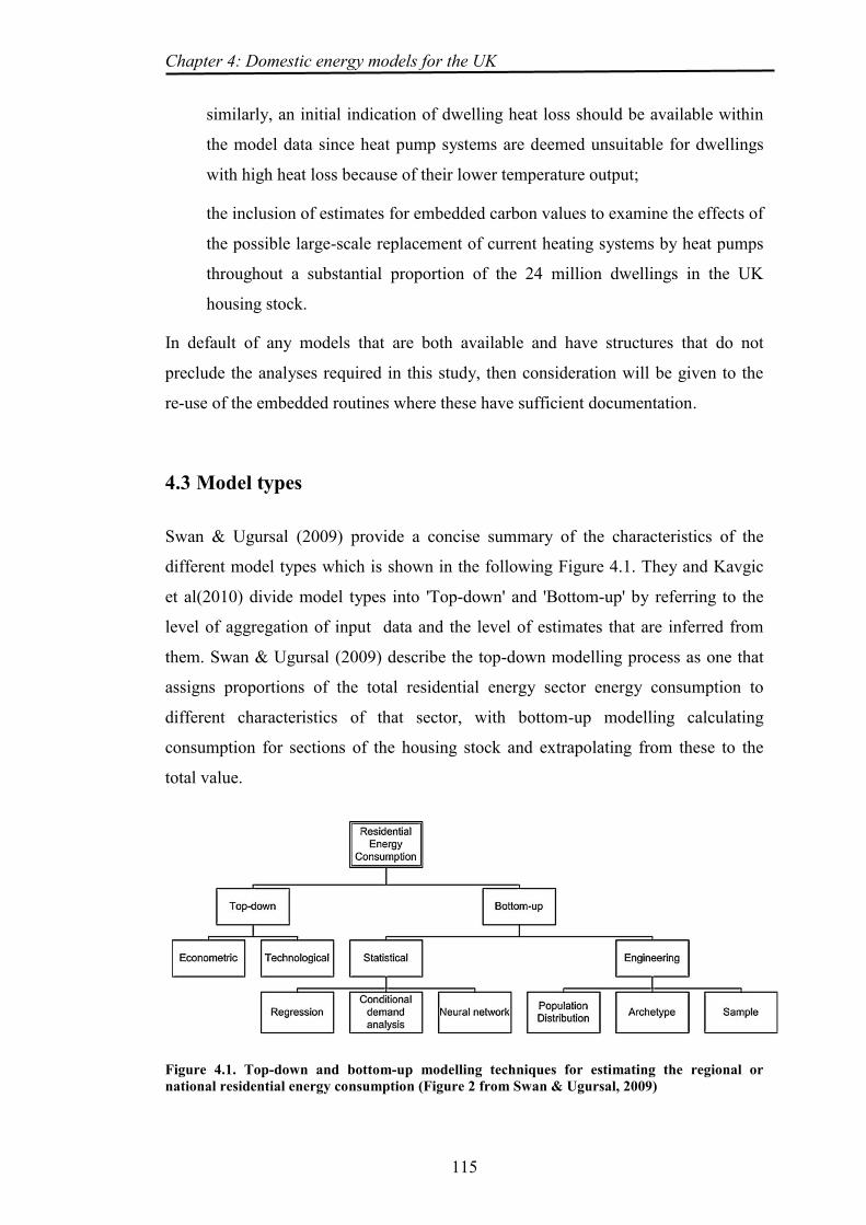
Chapter 4: Domestic energy models for the UK
115
similarly, an initial indication of dwelling heat loss should be available within
the model data since heat pump systems are deemed unsuitable for dwellings
with high heat loss because of their lower temperature output;
the inclusion of estimates for embedded carbon values to examine the effects of
the possible large-scale replacement of current heating systems by heat pumps
throughout a substantial proportion of the 24 million dwellings in the UK
housing stock.
In default of any models that are both available and have structures that do not
preclude the analyses required in this study, then consideration will be given to the
re-use of the embedded routines where these have sufficient documentation.
4.3 Model types
Swan & Ugursal (2009) provide a concise summary of the characteristics of the
different model types which is shown in the following Figure 4.1. They and Kavgic
et al(2010) divide model types into 'Top-down' and 'Bottom-up' by referring to the
level of aggregation of input data and the level of estimates that are inferred from
them. Swan & Ugursal (2009) describe the top-down modelling process as one that
assigns proportions of the total residential energy sector energy consumption to
different characteristics of that sector, with bottom-up modelling calculating
consumption for sections of the housing stock and extrapolating from these to the
total value.
Figure 4.1. Top-down and bottom-up modelling techniques for estimating the regional or national residential energy consumption (Figure 2 from Swan & Ugursal, 2009)

Chapter 4: Domestic energy models for the UK
116
Thus, in the 'econometric' pathway in Figure 4.1, the expected change in energy use
in the sector is related, for estimation, to changes in gross domestic product, rates of
employment, income and fuel prices, and rates of house construction and demolition,
while in the 'technological' pathway it is related to changes in appliance ownership
estimates or population-weighted changes in temperature.
Relationships in these type of models are estimated from historical data and,
consequently, are only valid for existing, installed technology and, therefore, reduce
in validity as time passes after their creation and the further forward they are required
to predict. This also implies that they are unlikely to provide accurate predictions of
the effects of new technology, though because these paradigm shifts occur
infrequently in housing, they remain effective at predicting in the shorter term and
for smaller variations (Swan & Ugursal, 2009).
4.4 MARKAL model family
Of this 'top-down' type, the most significant system involved in UK energy
modelling is the MARKAL (MARKet ALlocation) family of models (ETSAP, 2008)
which has a lengthy history dating back to 1976 (Fishbone & Abilock, 1981). This
set of models is the basis of major UK energy studies - Energy White Papers in 2003
and 2007, Carbon Abatement Technology strategy, Climate Change Bill, Carbon
Budgets - by the UK government (Strachan, Anandarajah, Pye, & Usher, 2010),
including the Departments of the Environment, Food and Rural Affairs (DEFRA),
for Trade and Industry, and latterly the Department for Energy and Climate Change
and the Committee on Climate Change (Committee on Climate Change, 2010).
Strachan, Anandarajah, Pye, & Usher (2010) list seven named variants of the UK
MARKAL model and indicate that others exist for specific projects.
The MARKAL models differ from conventional, predictive modelling in that they
focus on optimisation of energy characteristics over the modelling period, with the
standard MARKAL minimising discounted total energy system cost and MARKAL-
Macro maximising discounted total welfare through energy use, both with

Chapter 4: Domestic energy models for the UK
117
optimisation performed by linear programming. Based on a start year of 2000, a pass
by the model performs optimisation every 5 years for the period up to 2070.
A simplified MARKAL structure is illustrated by Figure 4.2, showing the
relationships which form its basis, starting from supply curves for fuel resources
(energy against price), fuel processing and energy conversion, transmission and
distribution, through to end energy use. Since MARKAL models the entire energy
system, the residential energy end use forms only one module within it, for which the
relationships are as shown in Figure 4.3. In this figure, the left-hand energy inputs
are linked to other modules defining the resource levels, generation processes,
infrastructure, and electricity and heat generation,
Figure 4.2 MARKAL energy system
(Strachan, et al., 2010, p. 5)

Chapter 4: Domestic energy models for the UK
118
Figure 4.3 Structure of residential sector in UK MARKAL
(Fig R-1 from UKERC, 2007)
Within the module, energy service demand types are shown in the right-hand column
of Figure 4.3. These energy demands may be met by various end-use technologies,
as in the second column of Figure 4.3. As the MARKALL models operate at a
sectoral level, all these characteristics are aggregated values across the whole
housing stock (UKERC, 2007). Thus, initialisation of the MARKAL system at its
base date of the year 2000 is in terms of the single values for each of the main energy
service demand types as follows (Table 4.1):
Table 4.1 Energy demand services for MARKAL residential energy module in base year 2000
Type of residential energy demand services Units Space heating 827.5 PJ Space cooling - PJ Hot-water 336.9 PJ Lighting 63.8 PJ Other electrical appliances 114.7 PJ Hob 25.3 Million units Oven 25.3 Million units Refrigerators 12.6 Million units Fridge freezer 15.9 Million units Chest freezer 4.4 Million units Upright freezer 6.6 Million units
(UKERC, 2007, Table R-1)
These are the initial variables for which values are set for the existing housing stock
in 2000 based on the actual final energy use for 2000 from DUKES (DECC, 2010b),

Chapter 4: Domestic energy models for the UK
119
with new values being assigned for each 5-year period of a MARKAL pass, and a
separate set of the same variables being maintained for houses constructed post-
2000. Energy efficiency measures are applied by modifying only the values for the
existing housing stock. Apart from the single values in Table 4.1, each energy
service demand can have an option to specify variable demand in terms of seasonal
or diurnal fractions, corresponding to the real demands for space heat and cooling or
for lighting. The correct definition of these fractional demands is apparently
important for the accuracy of the output estimates (UKERC, 2007, p. 4).
4.4.1 End-use/demand technologies
Various demand technologies may be specified to meet each energy demand, of
which the most obvious example is the meeting of space heating by a boiler fuelled
by either gas, electricity or other fuel or directly by radiators heated by a district
heating system. Demand technologies are defined in terms of several parameters, as
per Figure 4.4.
Figure 4.4 Parameters specified for demand technologies
(Fig. R-2 from UKERC, 2007)
Of these, efficiency, existing capacity, capacity constraints, lifetime, year of
available (availability?) capital and operating and maintenance (O & M) costs are

Chapter 4: Domestic energy models for the UK
120
mandatory to define a demand technology. To model improvements in efficiency
over time, variants of a technology are defined with applicable availability dates,
with conservation measures applied as dummy energy technologies which require no
input. As an example, Figure 4.5 indicates that gas condensing boilers become
available in 2005 and improved heat pumps from 2010.
Figure 4.5 Energy conservation versus energy efficiency in MARKAL
(Fig. R-3 from UKERC, 2007)
Despite its fitting the criteria as a 'top-down' model, it would appear that, to some
extent, the MARKAL model is able to estimate for scenarios involving technological
change, though the mechanism does not provide for any element of selectivity across
the housing stock for the installation of new technology. As the MARKAL system
models the entire energy system including transportation, industry, electricity
generation, etc. for a nation, it does not fit the criteria for this study.
4.5 Disaggregated (bottom-up) models
4.5.1 General characteristics
Models of this type estimate energy consumption of individual end-uses, individual
houses, or groups of houses which are then grossed-up to provide estimates for the
required section of the housing stock, for example a region or nation, based on the
representative weights of the modelled sample.
The sub-division of this type in Figure 4.1 from Swan & Ugursal (2009) into
'statistical' and 'engineering' depends on the type of sub-model utilised, with an
engineering model employing physically-derived relationships, ie. heat loss
calculations based on the thermal properties of construction elements, internal and
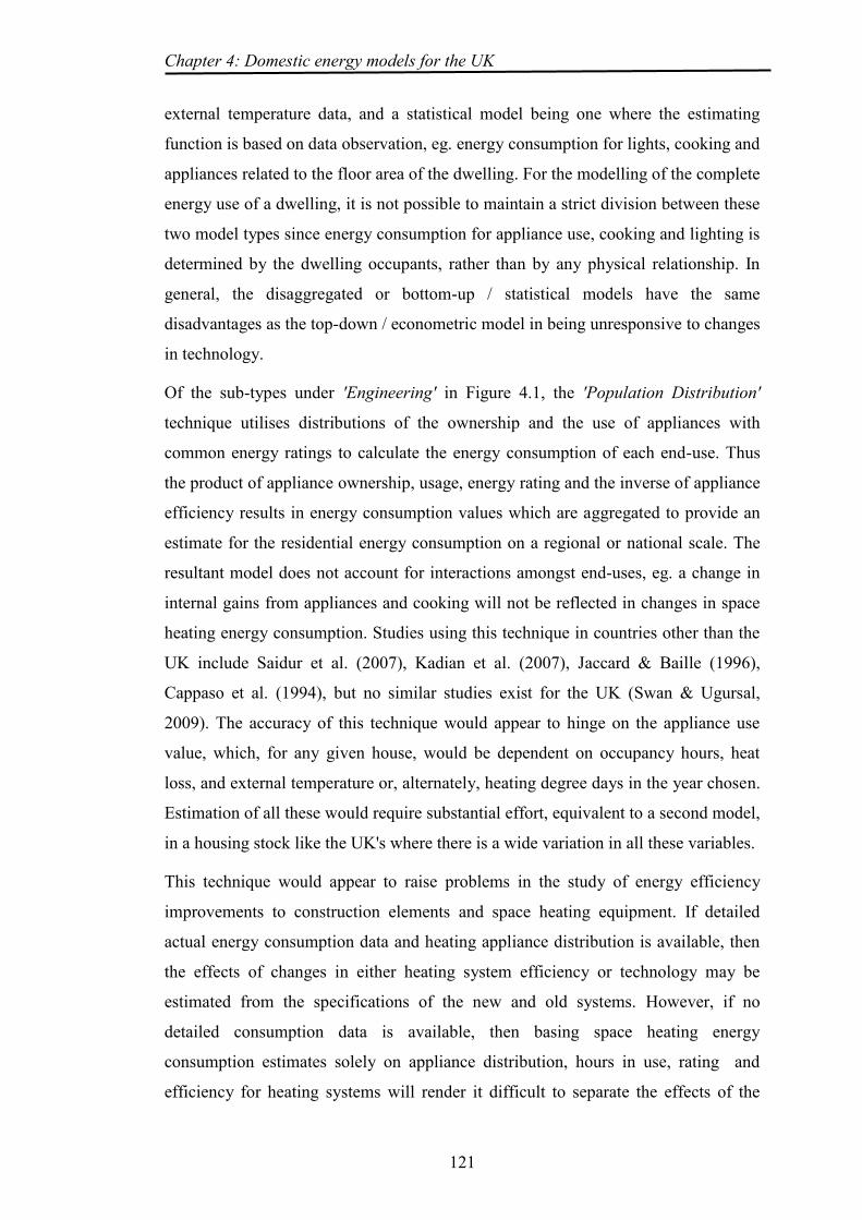
Chapter 4: Domestic energy models for the UK
121
external temperature data, and a statistical model being one where the estimating
function is based on data observation, eg. energy consumption for lights, cooking and
appliances related to the floor area of the dwelling. For the modelling of the complete
energy use of a dwelling, it is not possible to maintain a strict division between these
two model types since energy consumption for appliance use, cooking and lighting is
determined by the dwelling occupants, rather than by any physical relationship. In
general, the disaggregated or bottom-up / statistical models have the same
disadvantages as the top-down / econometric model in being unresponsive to changes
in technology.
Of the sub-types under 'Engineering' in Figure 4.1, the 'Population Distribution'
technique utilises distributions of the ownership and the use of appliances with
common energy ratings to calculate the energy consumption of each end-use. Thus
the product of appliance ownership, usage, energy rating and the inverse of appliance
efficiency results in energy consumption values which are aggregated to provide an
estimate for the residential energy consumption on a regional or national scale. The
resultant model does not account for interactions amongst end-uses, eg. a change in
internal gains from appliances and cooking will not be reflected in changes in space
heating energy consumption. Studies using this technique in countries other than the
UK include Saidur et al. (2007), Kadian et al. (2007), Jaccard & Baille (1996),
Cappaso et al. (1994), but no similar studies exist for the UK (Swan & Ugursal,
2009). The accuracy of this technique would appear to hinge on the appliance use
value, which, for any given house, would be dependent on occupancy hours, heat
loss, and external temperature or, alternately, heating degree days in the year chosen.
Estimation of all these would require substantial effort, equivalent to a second model,
in a housing stock like the UK's where there is a wide variation in all these variables.
This technique would appear to raise problems in the study of energy efficiency
improvements to construction elements and space heating equipment. If detailed
actual energy consumption data and heating appliance distribution is available, then
the effects of changes in either heating system efficiency or technology may be
estimated from the specifications of the new and old systems. However, if no
detailed consumption data is available, then basing space heating energy
consumption estimates solely on appliance distribution, hours in use, rating and
efficiency for heating systems will render it difficult to separate the effects of the

Chapter 4: Domestic energy models for the UK
122
different efficiencies of construction elements. It is noticeable that the studies cited
(Jaccard & Baille, 1996; Kadian, et al., 2007) do not provide estimates for space
heating or are from locations where space heating is un-necessary.
The 'Archetype' technique
This technique involves the creation of a dataset of archetype dwellings to be
representative of the housing stock, in which the number of members are determined
by the dwelling characteristics most significant in the estimation of energy
consumption, and the categories into which these characteristics are appropriately
divided. To be representative, the values assigned to each characteristic of each
archetype must be derived from survey data from the actual housing stock and a
weight must be calculated for each archetype to gross any estimates up to values for
that stock. The archetypes in the model dataset are then utilised to generate estimates
for energy consumption and carbon emissions for the whole stock. Kavgic, et al.
(2010) provide a summary table of five residential energy models of this type for the
UK which vary in the numbers of archetypes used from 2 in the Johnston model up
to 20,000 in the Environmental Change Institute's UK Domestic Carbon Model and
these are reviewed below. An additional model by Fawcett (2005), reviewed by
Kannan & Strachan (2009), uses the same mechanisms as Johnston (2003), with
slightly different initial assumptions, to examine the possibilities of reducing carbon
emissions through carbon rationing. Insufficient information was available to
complete a table entry for this model.
The 'Samples' technique
This technique is a variation of the 'archetypes' technique substituting sample data
from housing surveys for archetypes to provide a higher degree of variation in the
built form / construction types / heating system configurations included in the model.
Again, to provide stock level estimates, weighting factors must be calculated to gross
up individual dwelling estimates, and this represents only a variation of the issue
inherent in the 'archetypes' technique. Models of this type for countries other than the
UK have been developed by Farahbakhsh, Ugursal, & Fung (1998) and Larsen &
Nesbakken (2004).
While the 'samples' technique has not been employed to create a UK housing stock
energy and emissions model, use (Jones, Lannon, & Williams, 2001) has been made

Chapter 4: Domestic energy models for the UK
123
of sampling to improve archetypes in the domestic sub-model in the Energy and
Environmental Prediction (EEP) model developed by Cardiff University, in which
data for archetype dwellings was enhanced with that collected from surveying to
allow energy consumption estimates to be created for a UK post code area. This was
further developed in the Solar Energy Planning (SEP) system (Gadsden, 2001;
Gadsden, Rylatt, & Lomas, 2003a, 2003b; Rylatt, Gadsden, & Lomas, 2003a, 2003b)
to estimate the potential for solar design in new dwellings and for solar thermal and
solar photo-voltaics more generally from GIS data; and in DECoRuM (Gupta,
2005a, 2009a, 2009b) which considers the feasibility of a complete package of
energy efficiency and LZC measures for individual dwellings cased on a
combination of a "walk-past" survey and GIS measurement. This system is further
examined in Section A.7 of the appendices.

Chapter 4: Domestic energy models for the UK
124
Table 4.2 Disaggregated domestic energy models - summary of features
Name BREHOMES Johnston UKDCM DECarb CDEM DECORuM
Developer Building
Research
Establishment
(BRE)
PhD thesis
(Leeds
University)
Environmental
Change Institute,
Oxford
University
University of
Bath,
University of
Manchester
Loughboroug
h University,
Loughboroug
h, UK
Gupta, Oxford
Brookes
University, UK
Year Early 1990s 2003 2006 2007 2009 2005
Embedded
calculation
model
BREDEM-12 BREDEM-9
(modified
version)
BREDEM-8 BREDEM-8 BREDEM-8 BREDEM-12 /
SAP
Data output &
temporal
resolution
Annual energy
consumption Annual
energy
consumption
& CO2
emissions
Monthly energy
consumption &
CO2
Monthly
energy
consumption
Monthly
energy
consumption
& CO2
emissions
Annual energy
consumption &
CO2 emissions.
Installation,
operating costs
Level of
disaggregation
(spatial
resolution)
1008 dwelling
types (defined
by age group,
built form,
tenure type and
the ownership
of central
heating)
Two dwelling
types (pre-
and post-
1996)
20000 dwelling
types by 2050
8064 unique
combinations
for 6 age
bands
47 house
archetypes,
derived from
unique
combinations
of built form
type and
dwelling age
Dwelling level
within selected
area
Level of data
input
requirement
Medium
(national
statistics)
Medium
(national
statistics)
Medium (national
statistics)
Low (defaults
from national
statistics)
Medium
(national
statistics)
High (dwelling
level by survey)
Time
dimension
(projections to
the future)
Two scenarios
until 2020:
(a) reference
(business-as-
usual),
(b) efficiency
Three
scenarios
until 2050:
(a) business-
as- usual, (b)
demand side,
(c) integrated
Three scenarios
until 2050:
(a) business-as-
usual, (b) 44%
emission
reduction,
(c) 25% emission
reduction below
1990 levels
Back-cast
scenario from
1970 to 1996
and UKCIP02
climate
change
scenarios and
additional
runs to test
the
BREHOMES,
Johnston and
UKDCM
scenarios
Predictions
only for one
point in time
(2001
housing
stock)
Predictions
only for current
housing stock
Aggregation
level of data
output (spatial
coverage)
National National National National National,
City,
Neighbourho
od
Neighbourhood
Inter-model
comparison
Extensive Comparison
with results
obtained from
BREHOME
Comparison with
regional statistics
provided by
BERR
Comparison
with results
obtained from
BREHOMES
Local
sensitivity
analysis,
linearity and
superimpositi
on tests to
quantify the
impact of
input
parameters on
output
uncertainties
Comparison
with other
dwelling-level
models

Chapter 4: Domestic energy models for the UK
125
Empirical
validation
with existing
data
Extensive Comparison
with
empirical data
from the BRE
Domestic
Energy Fact
File
Comparison with
regional statistics
provided by
BERR
Comparison
with DUKES
provided by
BERR and
the BRE
Domestic
Energy Fact
File
Comparison
with DEFRA
aggregate
domestic
space heating
consumption
figure for
2001
Not applicable
Application Policy advice
tool (used by
DEFRA
Policy advice
tool
Policy advice tool
(Oxford)
Policy advice
tool Policy advice
tool
Local authority
policy &
intervention
tool
Current
availability Used only by
the developer Freely available Open
framework
Open
structure
Uses available
BREDEM
model with
commercial
GIS
(Kavgic, et al., 2010)
DECORuM details added by author.
4.6 Model details
The models from Table 4.2 are described in Appendix A.
4.7 Review of models
4.7.1 Modelled scenarios
With the exception of one, CDEM (Firth, Lomas, & Wright, 2010), which was
designed and developed to examine the results from previous studies, the objectives
of all the studies are to examine the effects on the UK carbon emissions of the
implementation of a range of measures to reduce energy consumption by improving
dwelling fabric, by improvements to heating systems, and by installing low and zero
carbon technologies, improved lighting and appliances. On the supply side, studies
employing reduced carbon intensity of electricity generation included BREDEM
[down to 0.29 CO2/kWh (Shorrock, Henderson, & Utley, 2005)], Johnston (2003)
(reduce to the same intensity as gas (0.184 kg CO2/kWh). In DECARB, the value is
variable across the modelling period, while in UKDCM and CDEM it is allowed to
remain unchanged from the value of 0.43 kg CO2/kWh used in SAP at the time those
models were developed. As DECoRuM (Gupta, 2005b, 2009a, 2009b) is aimed at
planning for energy efficiency upgrades, it automatically uses the current value.

Chapter 4: Domestic energy models for the UK
126
The modelling studies reviewed here were mostly developed before the passing of
the Climate Change (UK Parliament, 2008a) and hence before the target of 80%
reduction in carbon emissions was in place in the UK. Following the setting of this
target, it is now more realistic to include such a reduction in the carbon intensity of
electricity generation in scenarios.
The scenarios also tend to suggest a range of heating system technologies in future,
particularly micro- and community CHP and fuel cells apart from heat pumps and the
current gas boilers. As the UK housing stock has been tending towards a
monoculture of gas-fired central heating since the early 1970's, with central heating
in 96% of dwellings and 80% of central heating using gas (Palmer & Cooper, 2011,
pp. 36-37), all using conventional gas boilers, it would seem more plausible that if a
new generation of heating system is to take over, this could be equally uniform in its
make-up.
4.7.2 Availability and suitability of model software
Of the models reviewed in this chapter, the UKDCM model is the only one that is
available currently (2011) for download from the Environmental Change Institute's
website. The DECARB model is, apparently, also available from its author.
However it would appear from their basic structures that neither model would allow
the allocation of heat pump systems to a specified selection from their datasets of
archetypal dwellings as heating system types are allocated on a percentage basis
across the housing stock in both systems. Moreover, attempting to restrict heat pump
assignments to dwellings by, say, heat loss parameter, would require an addition pass
at that part of the model.
Neither model has any routines associated with embedded carbon or life-cycle
analysis, and creation of these would require additional development.
4.7.3 Routines
Of the 5 models reviewed by Kavgic et al (2010), all use a variant of the BREDEM
routines, with some modification, as the central dwelling-level energy model in the
model, as does Gupta (2005b, 2009a, 2009b), though in conjunction with SAP
routines for carbon emission estimates, thereby making the use of the BREDEM
routine at least acceptable for this type of study.

Chapter 4: Domestic energy models for the UK
127
Where the information is available or appropriate, an equal degree of unanimity
occurs in the techniques used to populate the parameters required for the BREDEM
model. The three latter models reviewed by Kavgic plus Gupta rely upon the age of
construction bands to provide a set of u-values for the construction elements, for
heating system efficiency, ceiling heights, presence / absence of chimneys and fans
and DHW system characteristics. They similarly relate built form type to other
characteristics, in particular the division of floor, exposed wall, and roof areas
between heating zones, the proportion of window to wall areas. The prevalence and
acceptance of these relationships, all of which are based upon the same original
research and survey work, in these models provides confidence of their validity.
The appropriate tables from the DECoRuM model are available to the author.
4.7.4 Additional data
Reference to the documentation of the version of the English Housing Survey current
at the time of commencing the modelling section of this study showed that dwelling
plot size data (widths, depth of front and rear plots) was present amongst the survey
data and a SAP rating was present in the calculated variables.
4.8 Summary and Conclusions
To meet Object 2 for this study, this chapter has reviewed a wide range of different
domestic energy models, the structures of which have basic similarity but which vary
in detail according to their studies' objectives and the software environment espoused
by their developers. The objective of this review was to examine whether any of the
models were both suitable and available for use in this study; whether their routines
could be employed even if no model could be utilised directly and whether the
scenarios were appropriate to this current study.
It was found that, of the available models, those that were publicly available were not
structured in a way that allowed the desired method of allocating new heating
systems, since both required allocation across the housing stock by percentage
distribution and neither had the ability to filter by dwelling plot size or heat loss
coefficient. These omissions are significant and need to be remedied to meet the
objectives of this study in modelling the effects of air and ground source heat pump

Chapter 4: Domestic energy models for the UK
128
installations, which require some outdoor space for installation and are deemed
unsuitable for high heat loss dwellings. The source of suitable data was found to be
the English Housing Survey (previously the English House Condition Survey) and
the use of this data will be described in a later chapter.
The following chapter describes the methodology to be used in this study.

129
CHAPTER 5 METHODOLOGY

Chapter 5 : Methodology
130
5.1 Introduction
Previous chapters have reviewed relevant energy models at two levels; at individual
dwelling / heat pump system level and at housing stock level. The perspective of the
former models has been found to range between a simplistic view of heat pump
characteristics, which fail to reflect the characteristics of these systems, and a complex
view demanding more parameters than are generally available. The housing stock
models present problems of open-ness, of comprehensiveness and of structure. Of those
reviewed, BREHOMES references data and uses rules which are not publically
available, while others define the housing stock in terms of a very limited number of
dwelling types. Those for which the software is freely available appeared to present
problems of structure, whereby it was not possible to make assignments of heat pump
installation to a specified segment of the dwelling stock without considerable alteration
of the structure of the model.
From the review of individual dwelling / heat pump system modeling, it was concluded
that the requirement for a model of residential heat pump energy performance that
reflects these systems' characteristics while retaining simplicity could be fulfilled by a
linear regression model using heat pump performance test results from WPZ
(WaermenPumpen Testzentrum, 2011) as base data.
From the review of disaggregated housing stock energy models, it was concluded that
the requirement to examine the future effects of heat pump adoption on the UK energy
mix would be best answered by building a 'bottom-up' domestic energy model with the
freely-available English Housing Survey dataset. A BREDEM-style model provides
dwelling-level estimates obtaining the majority of the necessary parameters from the
EHS data, answering the open-ness criticism made by Kavgic, et al (Kavgic, et al.,
2010). This will further be answered by developing the required models in Microsoft
Excel, since this software is reasonably widely known and available.
This chapter contains a description of the methodology to be used in meeting these
requirements and details of the reasoning behind its use.
5.2 Aims of the research
To re-cap, the aims of this research are as follows:

Chapter 5 : Methodology
131
the overall aim of the study is to estimate the potential of heat pumps to meet both the
heating and cooling requirements of UK dwellings in a changing climate, and to
forecast the effects of possible take-up of heat pumps on the UK electricity demand.
To meet this aim, the subsidiary objectives are to:
1. Review the theoretical and physical characteristics of heat pump systems and
identify those that are most significant in the estimation of the energy use of
these systems; examine currently-available models and modelling routines for
estimating heating pump energy use for their inclusion of the these
characteristics, their relevance to the requirements of this study, including their
capability for incorporation in a building energy model; this objective was
fulfilled in Chapters 2 and 3;
2. Identify and review literature on the modelling approaches that could be used to
forecast energy use and CO2 emissions, and undertake a critical analysis of the
work that has been undertaken to predict the future energy use and CO2
emissions of the UK housing stock; examine whether any of the models are both
suitable and available for use in this study; whether their routines can be
employed even if no model could be utilised directly and whether the scenarios
were appropriate to this current study.this objective was fulfilled in Chapter 4;
3. Monitor how current owners of ground source heat pumps (GSHPs) utilise this
equipment, i.e. to record their use of the equipment for heating, cooling and
domestic hot water provision, and the consequent energy consumption and
system temperatures.
4. Develop a building energy computer model to estimate the energy produced
from, and consumed by, heat pumps in meeting domestic heating and cooling
demands for different UK house types. Validate and calibrate the model as
appropriate.
5. Extend the model to include potential future take-up of domestic heat pump
equipment in order to assess:
The likely effects of various scenarios for the deployment and application of
replacement heat pump installations in the medium and long-term (2020,

Chapter 5 : Methodology
132
2050) on the consumption of electricity and other forms of energy, in
particular natural gas.
Their effect on consequent carbon emissions for the UK both in their
manufacture (embodied carbon) and operation.
the extent to which increases in electricity consumption by heat pumps due
to summertime cooling are offset by reductions caused by temperature
increases envisaged by the prediction of climate change from UKCIP09
scenarios.
the extent to which increases in electricity consumption by heat pumps due
might be offset by the output from building mounted photo-voltaic systems.

Chapter 5 : Methodology
133
Figure 5.1 Summary flowchart of development
5.3 Stages of the research
The aims of this research are fulfilled by the following stages of the development,
illustrated in Figure 5.1:
a) over a 12-month period, the collection and analysis of energy consumption and
output and system temperatures from ground source heat pump systems installed in
typical UK dwellings; this step is Stage 1 of the development and fulfills Objective 3 of
the research;

Chapter 5 : Methodology
134
b) the definition and development, using primary and secondary data, of a model of heat
pump energy consumption reflecting the required improvements identified from the
review in Chapter 2 and 3;
c) the incorporation of the heat pump model into an existing dwelling energy
consumption model, including estimating rules for energy use from bivalent operation
and space cooling; this step and step (b) make up Stage 2 of the development which
fulfills Objective 4 of the research;
d) the definition and development of an energy and carbon dioxide emissions model for
the English housing stock based on the dwelling energy model from (c) using the data
reduction techniques employed by the DECORuM system to estimate for each of a
reduced dataset of dwellings extracted from the English Housing Survey data. This
forms Stage 3 of the development;
e) the building of forecasts for future UK electricity consumption, both in terms of
annual and peak monthly loads, based on different scenarios for the level of take-up of
heat pump systems and for the replacement of existing heating systems. For the longer-
term, these forecasts would include allowance for the predicted effects of climate
change and for the parallel installation of roof-mounted solar photovoltaic systems to
counterbalance the increase in electricity consumption. This forms Stage 4 of the
development and Objective 5.
5.4 Heat pump data collection and analysis
This constitutes Stage 1 from Figure 5.1.
5.4.1 Collection and analysis of energy data from dwellings with heat pump
systems
This section of the study is intended to provide empirical data to estimate relationships
between variables for which simple theoretical relationships are not available, but which
are required to complete the model.
Data for the monitoring study was collected by a datalogging unit which acquires and
stores the temperature and status data using an existing diagnostic facility. Additionally,
heat output and electricity consumption data is collected by dedicated meters in the

Chapter 5 : Methodology
135
distribution and DHW circuit and the electricity mains connection, respectively, and
passed to the datalogger. Data values were stored at 15 minute intervals, tagged with a
collection date and time stamp. The stored data is down-loaded in batches to a personal
computer via a wireless connection.
The data batches from the datalogger for each system were combined into an overall
spreadsheet for each heat pump system to create a dataset for the whole logging period.
Editing functions within the spreadsheet software were used to cleanse the data of
erroneous values. The sample-level data was summarised by day and then by month.
Where data samples were missing due to faults in the dataloggers, the summarised
energy values were adjusted according to either the heating degree hours or the
operating hours in the period lost. Using the sub-system statuses recorded with each
sample, the energy data was analysed into categories: space heating or DHW
generation, with or without the use of auxiliary heaters, energy use for distribution
system pumps.
The following analyses were performed to obtain values for the enhance heat pump
model:
Analysis of ground loop return temperatures was performed to obtain a
relationship between these and the values calculated by the sinusoidal function
estimated by Kusuda & Achenbach (1965) for soil temperature as a function of
air temperature.
A frequency analysis of external temperature and energy use by the system
auxiliary heaters was performed to calculate a balance point for the systems.
Monthly average and maximum space heating distribution system temperatures
were compared with the conventional values.
5.4.2 Acquisition and transformation of heat pump performance data
The objective of this part of the study is to provide performance data for a wide range of
heat pump systems from an authoritative source (WaermenPumpen Testzentrum, 2011).
As this information is only available in report format, it was transformed into look-up
tables using software to convert it into an initial Excel spreadsheet. This initial

Chapter 5 : Methodology
136
spreadsheet was further edited to create tables of heat pump suppliers and heat pump
systems, and two tables of heat pump test results, one for air/water systems, the other
for soil/water systems. A set of linear regression parameters were calculated for each
heat pump system based on the lift and COP values from the test values for that system
and an overall set of linear regression parameters are calculated for each of the two test
results tables.
This completes Stage 1 from Figure 5.1.
5.5 Development of an enhanced building energy computer model
This constitutes Stage 2 from Figure 5.1.
5.5.1 Requirements
The development of the enhanced building energy computer model for this study has
two purposes, firstly, to provide an estimate of energy use for a single dwelling, with
the intention that the characteristics of the new model will feed into the current UK
building energy regulatory process, and, secondly, as part of a mechanism to estimate
UK-wide energy use. Thus it is necessary for the new computer model to function on
both these levels, requiring that default values are available for its parameters in the
UK-wide use while allowing individual values for individual dwellings.
As the model is also required to provide estimates of energy use under conditions of
climate change as predicted in the UK Climate Projection , it must also be capable of a)
creating estimates using different weather datasets; b) estimating cooling loads as well
as heating loads.
Because the main focus of this research is on the effects of domestic heat pump
deployment, the aim of the first part of this stage is to develop a heat pump model to
provide estimates that reflect the effect of the changing climate and of cooling loads,
given the set of characteristics described in Section 2.9 and the performance -
temperature relationship documented in Section 3.5.1 .
5.5.2 Domestic heat pump model development
The development is in three parts:

Chapter 5 : Methodology
137
The first part of this process is to examine the estimation methods for the energy use of
the different types of heat pump systems in the BREDEM/SAP models used in the UK
domestic energy model and in Standards for energy efficiency.
The second part is to identify where these methods are substantially deficient in
modelling the characteristics of heat pump systems.
Thirdly, more appropriate methods are identified for characterizing heat pump systems
within an improved BREDEM-style model and to specify the equations and processing
involved.
5.5.2.1 Original methods for estimating heat pump energy use in BREDEM / SAP
These were described in Section 3.3.4 in which the following were found:
Table 5.1 Estimating methods for heat pumps in BREDEM / SAP
Ref Parameter / variable BREDEM /SAP version
1 Space heating COP/SPF
Single annual value dependent on source type, reduced if system is fitted with auxiliary electric heaters.
2 Water heating COP/SPF
As above
3 Additional heating Allowed for in reduction in COP
4 Cooling load Not estimated in BREDEM. Single annual value for EER in SAP
5.5.2.2 Heat pump system characteristics
These were identified in detail in section 2.9, viz.
a) lower temperature output due to the characteristics of the vapour compression cycle
heat pump;
b) variation of source energy over the heating season due to depletion of the ground as
an inter-seasonable store or to the fall in air temperature;
c) CO2 emissions from operating electric heat pumps are due to the carbon intensity of
electricity generation rather than the fuel it consumes;

Chapter 5 : Methodology
138
d) cost of installation of GSHP systems is highly dependent on the size of the system,
especially of the collector;
e) Non-uniform increase in operating cost and CO2 emissions with increase in
indoor/outdoor temperature differential when outside temperature falls below the
system balance point temperature; this being due to the use of additional heat at a COP
< 1.0;
f) Heat pump systems are capable of providing cooling as well as heating.
5.5.3 Heat pump model rules
In Section 3.5.1 , it was determined that the COP of a heat pump system was related to
the source-sink temperature differential or 'lift' in an inverse linear relationship which
differs between system source types, specifically between air source and all the water
source types (horizontal ground loop or vertical bore hole). Data to estimate coefficients
for the COP / lift relationships for air and water source systems was obtained from the
Swiss testing laboratory WPZ (WaermenPumpen Testzentrum, 2011).
Having built relationships from this data, rules had then to be developed to relate the lift
value to the available parameters of a dwelling energy model such that a suitable COP
value can be obtained for the estimation of monthly energy consumption. In the case of
the BREDEM-8 model, this parameter is the monthly average external temperature,
from which values for the source and sink temperatures at the heat pump system
boundaries must be computed.
Given a monthly average external temperature, different relationships are defined to
estimate the source temperature at the system boundary for each of the three different
source types, as follows:
for an air source heat pump, then the source temperature can be assumed to
coincide with the external monthly average temperature;
for a GSHP system linked to a borehole heat exchanger, the soil temperature is
judged to be equal to the annual average air temperature (Ochsner, 2007);

Chapter 5 : Methodology
139
for a GSHP linked to a horizontal ground loop or similar, then the soil
temperature for an air temperature value may be estimated from the sinusoidal
equation 3.14 defined by Labs (1979) (Section 3.2.3.3), for appropriate values of
its parameters;
a relationship can then be derived between the estimated soil temperature from
this equation and the source temperature by comparing the output values from
that equation with the ground loop return temperature values from the
monitoring study.
In estimating sink temperature values, the main determining factors are:
the presence or absence of weather compensation control within the system
controller, since this varies the system output temperature with variations in
external temperature;
the choice of heat distribution by radiators or UFH as the latter conventionally
require a lower temperature flow for a given room temperature.
Conventionally, temperatures of 35ºC and 55ºC are used in calculations for heat pump
output to UFH and to radiators, respectively (Ochsner, 2007), while weather-
compensated control utilises a 'curve' relating the target distribution temperature to the
current external temperature, with the gradient of this curve being set to a higher value
for radiator distribution than for UFH. Thus the estimating mechanism for a sink
temperature may be defined from the graph of the controller curve provided by the heat
pump supplier, if weather compensation is installed, or the conventional values used if
not.
The final stage steps of the heat pump model are to calculate a 'lift' value from the
source and sink temperatures and, thence, a COP value from the regression function for
the heat pump type.

Chapter 5 : Methodology
140
5.5.4 Enhanced dwelling energy model
5.5.4.1 Choice of energy model
As the major focus of this thesis is to measure the impact of domestic heat pump
systems on the UK energy supply, it is therefore appropriate to choose a version of
BREDEM as a basis for this enhanced model. While other building energy models
which include heat pump system calculations exist and were presented in Chapter 3,
they do not have the particular relevance of the BREDEM models in the assessment of
the UK situation.
As indicated in Section 3.3.4.1, three versions of BREDEM exist. BREDEM-8,
BREDEM-12 and SAP (being in effect, BREDEM-9). Of these, the most regularly
updated has been SAP, which has been through several versions since its inception.
Since the SAP calculations are the basis for pass/fail decisions for the energy efficiency
of the dwelling design (DCLG, 2006) according to Part L1A of the UK Building
Regulations, they contain additional complexity, of which the most obvious is the
calculation of a SAP rating for a dwelling of identical built form which meets the
minimum standard of the Regulations for comparison with that of the design dwelling
to determine a pass or fail. In compiling an energy rating for a dwelling, it has
previously been deemed that this should be unaffected by its geographic location and
therefore this element has been omitted from SAP up to now, rendering the energy
consumption estimates from SAP insensitive to change of climate across the country or
across time. The SAP procedures also now include procedures for evaluating
community schemes, for evaluating a dwelling as built, and for proposing energy saving
measures for existing dwellings, though the latter are not included in the energy
calculations. In mid-2009, further substantial revisions were proposed, including the
monthly calculation of space and water heating loads, and of space cooling, the explicit
calculation of the effects of thermal mass, revisions to the carbon dioxide emissions
factors, boiler efficiency and the calculation of internal heat gains.
A version with fewer input parameters, known as “Reduced data SAP” (RD SAP), has
been created to create Energy Performance Certificates to conform with the European
Energy Performance of Buildings directive. RD SAP has a preliminary process which
expands the reduced set of parameters into the full set required for the full SAP
assessment to be performed.

Chapter 5 : Methodology
141
While the current version of SAP contains relevant methods for the estimation of
elements that concern this study, the added complexity of the calculations for regulatory
purposes makes it unwieldy for the current purpose, implying that a version of
BREDEM would be more suitable. A distinction must be made between the different
BREDEM models, since two main versions, BREDEM-8 and BREDEM-12, exist.
These have different emphases, BREDEM-8 calculating monthly estimates for 12
months of the year based on monthly average external temperatures, while BREDEM-
12 calculates a year’s estimate only using heating degree days. BREDEM-8 contains
different calculation modules for the effects of different heat system types. As this
thesis concerns itself with the effects of changes in energy available to heat pump
heating systems across the year, BREDEM-8 appears to be the appropriate choice as the
baseline version for modification.
5.5.4.2 Enhancements to BREDEM-8
These consist of the following:
the insertion of an additional module to provide estimates for energy
consumption by an appropriately sized heat pump; processing within this
module is controlled by parameters as follows:
a) bivalent operating mode - either monovalent, bivalent parallel or alternate
parallel;
b) balance point temperature: the temperature below which auxiliary heating
is switched in;
c) the system source type: air, vertical borehole, horizontal ground loop;
d) the distribution type: radiators, underfloor heating;
e) presence/absence of weather compensation control.
within this module, the heat pump model is invoked for each month of the year
with the appropriate monthly average temperature, returning a corresponding
COP value.
Chapter 5 : Methodology
142
routines are added to the heat pump module to estimate the effect on energy
consumption of each of the three operating modes based on the balance point
parameter;
a separate module is added to the overall BREDEM-8 to estimate space cooling
loads employing either the installed heat pump system in reverse or a stand-
alone air-conditioning unit;
A routine is added to calculate CO2 emissions for all the energy consumed in the
dwelling, depending on the type of fuel consumed and the overall model is modified to
provide a comparison between the energy use of an existing heating system and a
comparable heat pump system.
5.5.5 Model validation
This consists of comparing the energy loads of a dwelling or dwellings using both the
new software, the current version of the same software and the data collected from the
monitored installations.
5.6 EHS / BREDEM domestic energy model
This constitutes Stage 3 from Figure 5.1.
5.6.1 Development process
Following on from the enhanced dwelling energy model development, this section
describes that model's use in the development of a domestic energy model for England
based on the dwelling sample data from the English Housing Survey.
The initial steps in this development are as follows:
a) the extraction of the relevant data, both in terms of samples and of variables,
from the EHS data tables held in SPSS format and the compilation of these
extracts into a single MicroSoft Excel table;
b) the creation of additional variables required by the enhanced BREDEM model,
including plot size variables;

Chapter 5 : Methodology
143
c) the addition of versions of the DECORuM reference tables relating the values of
common, built form and construction date variables from EHS to parameters
required by the BREDEM-8 model;
d) the definition of rules for the configuration of heat pump installations for
dwelling;
Following on from these steps, a pass of the extract table is made to create estimates for
both the existing system and a putative heat pump system:
energy consumption for primary and second space heating, space cooling,
DHW, heat distribution, appliances and cooking;
CO2 emissions;
energy cost.
The estimates for each sample are grossed-up by the sample weight to obtain their effect
within the whole housing stock and the grossed-up values totalled to form estimates for
the entire stock.
After the creation of this baseline model, future scenarios for heat pump energy use in
2020 and 2050 are developed as follows:
a) the definition of scenario tables of possible heat pump installations for 2020;
conventionally other research and reports have divided the installations between
air and ground source systems without further division;
b) definition of application scenario rules for the installation of heat pump systems
in dwelling samples;
c) translation of each of these rules into model processing and execution of the
required model runs to create energy consumption and CO2 emission estimates
for these scenarios;
d) summarisation and analysis of results from these runs;
e) estimation of electricity output from roof-mounted photovoltaic systems for each
sample in the EHS extract, based on roof areas derived from the survey
variables, assigned values for the system characteristics and dwelling
orientation;
f) the creation of scenario data for temperature changes under conditions of
climate change in 2050 based on UKCP09 predictions;
Chapter 5 : Methodology
144
Repeat of steps (b) to (d) for the 2050 scenarios.
The following sections describe this methodology in greater detail.
5.6.2 EHS Survey data
The EHS survey and its database is described in detail in the survey User Guide
(DCLG, 2010b). It is a continuous survey of virtually all aspects of a sample of English
dwellings, carried out for the UK Department of Communities and Local Government
(DCLG) and was formed in 2008 as a merger between the English House Condition
Survey (EHCS), and the Survey of English Housing (SEH). As this merger occurred
during the compilation of the dataset used in this survey, the previous names
(particularly the EHCS name) were still in use in sections of the survey documentation.
The data is freely available from the Office of National Statistics in two data formats, of
which the SPSS format (SPSS Inc, 2010) was used as the basis for this study. It has
been chosen for this study as it is a definitive source for all reporting for the English
housing stock (DCLG, 2011).
Three types of data are collected:
household data concerning their tenure, composition, occupations and income;
physical data concerning the dwellings’ location, built form and services, state
of repair, surroundings, disabled access, health hazards;
valuation data concerning the dwellings’ market value.
Management of the Survey is conducted by the Office of National Statistics whose
researchers conduct household interviews while a firm of chartered surveyors perform
the physical surveys using questionnaires developed by the Building Research
Establishment (BRE). The property valuations, based on the physical surveys and
photographs, are made by the government Valuation Office Agency, the property
valuation agency for the UK Revenue and Customs department (DCLG, 2010b).
The sample size for the survey is approximately 8000 dwellings each year, with the
current '2007' release consisting of data collected between in the two years between
April 2006 and March 2008, a total of 16,217 dwellings and 15,604 households (the
sample includes vacant properties) (DCLG, 2010b). The data as obtainable from the
Chapter 5 : Methodology
145
Economic and Social Data Service (DCLG, 2010b) is spread over some 29 primary
data tables and 14 derived tables. These tables are linked by a unique identifier for each
sample with the 'general' table forming a starting point from which to link to all the
others. Entries in the tables mostly form a one-to-one relationship with the 'general'
table entries, ie. there is one entry in the 'firstimp' table for each entry in the 'general'
table, but in tables such as 'windows', there are entries for each window type / material
combination for each sample dwelling.
Each sample carries a weight estimated according to the probability of the dwelling
being selected from the UK housing stock, adjusted for bias created by non-response to
the survey, then scaled such that the grossed-up number of dwellings by tenure and GO
Region in the sample equals that of control totals from Census values for the same
partitioning of the housing stock. The implication of the weighting is that a value
calculated from an EHCS sample can be grossed up to an estimate for the whole English
housing stock using the sample dwelling weight. This extends to the estimation of
dwelling energy use with SAP and BREDEM routines, with such calculations being
included in the EHCS Technical Guide Chapter 7 'Using EHCS data to model Decent
Homes Thermal Comfort' (DCLG, 2010a, p47).
5.6.3 EHS Sampling method
The EHS is described as 'a multi-stage clustered sample stratified by tenure' (DCLG,
2010a, p. 9). For this sampling method, the total population is divided into the groups
(or clusters) and a sample selected from these groups. The required data is collected
from the elements within each selected group, either from the totality of the elements or
from a sub-sample. The 'multi-stage' element implies that there are layers of grouping in
the sample. ie. groups within groups. In the case of the EHS sampling process, the
clusters are based on tenure (owner-occupied, privately-rented etc.) within Government
Region. The objective of this strategy is to allow sample bias towards social housing to
provide more accurate results for this sector. See section 8.2.2.
To provide information on building condition, some additional longitudinal sampling
was introduced from 2005-2006, whereby successful sample addresses from the three-
year previous survey were included (DCLG, 2010b).
5.6.4 Sample bias
Because the survey is commissioned by central government, which is concerned with

Chapter 5 : Methodology
146
the meeting of targets for the reduction in numbers of social housing which are unfit for
habitation or which fail to meet standards for the cost of heating, social housing is
deliberately over-represented in the sampling process as indicated in Table 5.2, where
owner-occupied dwellings are reduced to 50% of the sample, with the equivalent value
for the whole housing stock being 70%. This, according to the EHS Technical Report,
ensures that the Survey provides information about “rarer tenures” (DCLG, 2010b, p.
7). Table 5.2 Sample bias towards social housing
Table 5.2 indicates that owner-occupied housing is deliberately under-represented in the
sample by 50% as against 70% with local authority housing stocking comprising 25%
of the sample while being less than 1% of the UK housing stock.
5.6.5 Primary Survey data
This is of two types: household data and dwelling data. Data for dwellings vacant at the
time is also treated as household data but recorded separately. Household data is based
on an interview with the householder and consists of details of: the individuals in the
household including ages, relationships, work status; amounts and sources of income,
including benefit payments; attitudes to the dwelling and surroundings; occupants' type
of tenure; disabilities (if any). For the dwelling, it also collects details of: adaptations to
the dwelling to assist with disabilities; which rooms are occupied or shared;
responsibility for repairs and repairs done; damp problems in the dwelling fabric;
improvements or significant maintenance done by occupants or landlord.
Dwelling data is based on a lengthy questionnaire (Appendix I) and collects data on
many aspects of the dwelling which increase in number and complexity depending on
the type of dwelling with a single, detached house as the most simple and flats as the
most complex.

Chapter 5 : Methodology
147
Table 5.3 EHS Primary data captured from questionnaire
a) interior Presence/absence, condition / safety of facilities including cold &
hot water supplies, waste outflows, kitchen cooking facilities,
cupboards, work top, facilities for food preparation, appliances,
bathroom, shower room, wc's.
Presence / absence of gas / electricity supply, normal or off-peak;
condition of electrical system, type, fuel, age, safety etc of space
and water heating systems; loft condition and insulation.
b) shared facilities Presence/absence/condition of shared facilities, eg. common rooms,
stores, laundries, drying rooms, offices, parking or garages,
communal heating, alarms systems, external lighting, lifts, refuse
chutes, security systems, fire safety systems, balconies, decks,
corridors, lobbies.
Condition of building elements - damp, stability, drainage, lighting
etc.
c) external Dimensions, built form, materials and finished for dwelling plus
details of defects, alterations, improvements, including type of
accommodation and date of construction; presence/ absence/
condition of chimneys, bays, dormers, porches, conservatories,
balconies, roof features; presence / absence / condition of a damp
proof course; type / position / age / condition of doors and
windows. Additionally for flats: numbers of flats in module, non-
residential uses within module, details of wall exposures (external/
internal / accesses).
d) surroundings Presence / absence / condition / size / positioning / fences or walls
of external plot. Accessibility of dwelling entrance; condition of
plot drainage; details of parking provision; exposure of dwelling
position; characteristics of surrounding housing - density, built
form, construction data, tenure; social character of neighbourhood -
incidence of vandalism, graffiti, intrusive industry, empty

Chapter 5 : Methodology
148
While it is possible that not all sections of the survey for a sample dwelling are
completed, eg. the surveyor may not be able to arrange an interview or the householder
may refuse to participate, these 'unsuccessful' samples are not included in the version of
the database on public release.
5.6.6 Derived/computed data
This is of two categories: firstly, data summarised up from the individual questionnaire
variables; secondly, data estimated using modelling techniques, specifically SAP 2005,
and the values used as input parameters to that model. A summary of the data types is in
Table 5.4.
Table 5.4 EHS derived data variables by data file
Data file Content type
general Tenure, categorised in different ways
Government Office Region (GOR)
Surroundings, categorised in different ways
Environment: upkeep, traffic, utilisation, liveability, quality
assessments;
Valuation of dwelling
Assessed demand in area
Nation Regeneration Fund (NRF) status of district
Index of Multiple Deprivation (IMD) ranking
Market area factor score for housing demand, number of
properties on market plus ranking of score
Rural / urban morphology
Dwelling weight for grossing-up
Household weight for grossing-up
physical Dwelling type, categorised in different ways
Construction date, banded in different ways
Summarised dwelling dimensions: floor area, number of floors
Predominant types of : roof covering and structure, wall finish
and structure, windows.
buildings, noise etc.
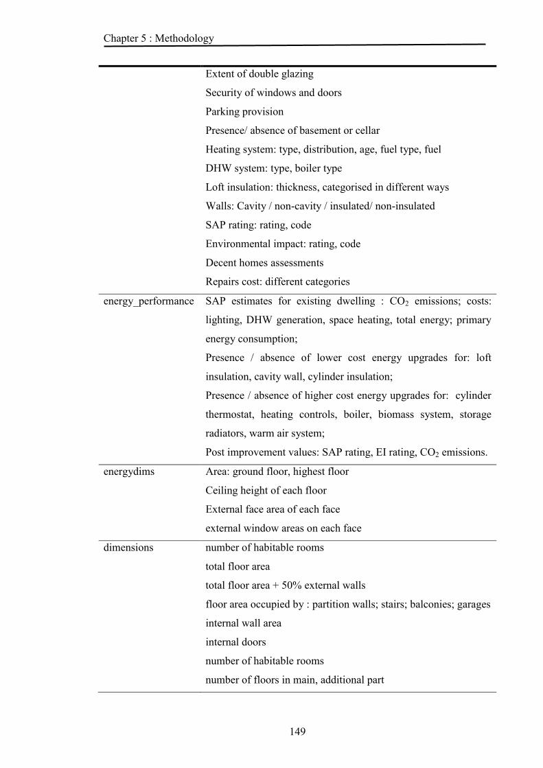
Chapter 5 : Methodology
149
Extent of double glazing
Security of windows and doors
Parking provision
Presence/ absence of basement or cellar
Heating system: type, distribution, age, fuel type, fuel
DHW system: type, boiler type
Loft insulation: thickness, categorised in different ways
Walls: Cavity / non-cavity / insulated/ non-insulated
SAP rating: rating, code
Environmental impact: rating, code
Decent homes assessments
Repairs cost: different categories
energy_performance SAP estimates for existing dwelling : CO2 emissions; costs:
lighting, DHW generation, space heating, total energy; primary
energy consumption;
Presence / absence of lower cost energy upgrades for: loft
insulation, cavity wall, cylinder insulation;
Presence / absence of higher cost energy upgrades for: cylinder
thermostat, heating controls, boiler, biomass system, storage
radiators, warm air system;
Post improvement values: SAP rating, EI rating, CO2 emissions.
energydims Area: ground floor, highest floor
Ceiling height of each floor
External face area of each face
external window areas on each face
dimensions number of habitable rooms
total floor area
total floor area + 50% external walls
floor area occupied by : partition walls; stairs; balconies; garages
internal wall area
internal doors
number of habitable rooms
number of floors in main, additional part

Chapter 5 : Methodology
150
Lowest, highest floors in main, additional part
External front, back wall areas
Front, back window areas
Damp proof course perimeter, front, back
External front, back roof plan area
External front, back roof slope area
External front, back eaves perimeter
External main, back eaves height
5.6.7 Extraction of model variables from EHS datasets and creation of
main data table
Since the BREDEM-8 model is not capable of providing estimates for flats or
apartments (Anderson, et al., 2001), the initial entry point for the extract was the
derived dataset (file name 'physical.sav') for the physical survey, which contains several
variables containing codes indicating the built form of the dwelling, of which the
variable 'housex' has the simplest coding - either "flat" or "house". The resultant extract
table was then cross-referenced by the Sample ID (variable name 'aacode') to further
EHS tables to extract the variables required. The tables referenced are listed in Table
5.5.
Table 5.5 EHS tables used in main extract
File name Description of file around Dwelling surroundings: dimensions of plot, relative
location of plot dimensions Number of rooms, wall and floor areas energy_performance SAP ratings, energy efficiency ratings, light, water and
space heating costs, energy upgrade costs energydims Area of ground and highest floor, ceiling heights, external
wall and window areas. firstimp Key information on the first impressions of the dwelling
and neighbourhood as recorded by interviewer general Tenure, dwelling condition, location, housing market in
locality physical Built form, date of construction, construction details,
heating system, SAP rating. services Details of heating systems shape Dwelling shape: external dimension of dwelling; material
and construction of dwelling.

Chapter 5 : Methodology
151
Thus the data collected in the EHS provides the majority of the conventionally-collected
built form and services data, i.e. dwelling type, i.e. detached, semi-detached, end/mid
terrace, bungalow, purpose-built/converted flat, dwelling age in 11 bands from ‘post
1850’ to ‘post 2002’, floor area, ceiling height, main and secondary heating system type
and fuel, DHW generation system and fuel, glazing area and type, plot size and a
limited amount of insulation information.
5.6.8 Creation of baseline energy estimates for samples in the EHS extract
5.6.8.1 Additional variables for main EHS extract
Based on variables from the 'around' table, two new variables are calculated for the
useable plot size - that available for the installation of a GSHP ground loop, and the rear
plot size - that area assumed to be sufficiently secure for an ASHP installation, which
are deemed prone to vandalism. The value for the useable area of the dwelling plot is
calculated as the greater of the front or rear sections, ie. plot width times plot depth,
assuming that either the rear or front section, but not both, can be used for the burial of
a ground source collector, with the latter applying to the rear plot only.
A new variable is created for the heating degree region appropriate to the Government
Office Region code value for each sample. BREDEM-8 utilises a table of external
temperatures with entries for 21 heating degree day regions to determine heating load
whereas location data on the EHS samples is limited to a variable for the 8 Government
Office Regions. As one GO Region can encompass more than one heating degree day
region, and a heating degree day region may overlap GO Regions, a routine was written
that randomly assigned each sample to a heating degree day region according to the
relative numbers of houses in each county or other administrative area in its GO Region.
To provide estimates of embodied CO2, a value is calculated based on the Total Floor
Area, the built form type (detached, semi-detached, terraced) and the wall construction
type (cavity wall, sold wall) of the sample using the relationships defined by Johnson
(2011).

Chapter 5 : Methodology
152
Table 5.6 Summary of additional variables
Variable Source and derivation
Useable plot area Calculated from plot depth times width
Rear plot area Calculated from rear plot depth times width
Heating degree day region Derived from Government Office Region, randomly
assigned according to proportion of housing stock in
constituent counties.
Embodied carbon dioxide Calculated from dwelling total floor area using
relationships from Johnson (2011).
5.6.8.2 Assignment of heat pump configurations to dwelling samples
The characteristics of the dwelling sample are used to determine the configuration of the
putative heat pump system in terms of the source and the mode of operation assigned.
Initially, the source type is determined according to the sample plot size calculated
above, with a horizontal ground loop source being selected if plot size is at least twice
the dwelling total floor area, an air source if the rear plot area is greater than 4 m2,
defaulting to a vertical bore hole for smaller areas of plot (Energy Saving Trust, 2011;
Nottingham Energy Partnership, 2006).
The second configuration variable is the operating mode which is set according to the a)
contruction date of the dwelling; b) its SAP rating; and c) whether it currently has an
installed central heating system; and has possible values of monovalent, bivalent
parallel or bivalent alternate.
5.6.8.3 Heating systems and fuel type mappings
Each sample has variables containing details of heating system types, fuels used and age
for a Primary and 'other' heating systems, plus hot water generation system, allowing
that these may be the same items of equipment. To provide energy consumption
estimates in the BREDEM model, it is necessary to create tables cross-referencing
combinations of the EHS variables to the BREDEM efficiency and other parameter
values. Thus, to determine the efficiency, responsiveness, BREDEM heating type, and

Chapter 5 : Methodology
153
fuel type of the primary heating system, a table was constructed relating all these values
to the 'primary heating system - type of system', Main fuel type', 'main heating fuel',
'Boiler group' variables from the EHS Extract. A second table was constructed for the
efficiency and responsiveness of the secondary heating system and a third relating the
primary heating type, fuel type and secondary heating type to the proportion of primary
system energy consumed by the secondary system.
5.6.8.4 Linkage of EHS sample table to the enhanced BREDEM-8 model
After the addition of the additional variables to each sample and the construction of the
heating system tables as indicated above, each EHS Extract sample is used as input to
the enhanced BREDEM model to create energy, carbon dioxide and cost estimates. The
building elements data collected in the Survey are not sufficient to provide all the
parameters required for the BREDEM model and therefore recourse must be made to
techniques of data reduction, i.e. the inference of multiple parameter values from a
single value, being 'data reduction' in the sense that the technique reduces the data
required to be collected by surveying to populate the model parameters. Because of
good access to the techniques in this process, the author opted to use the data reduction
techniques from DECoRuM (Gupta, 2005a, 2009a, 2009b), derived from Rylatt (Rylatt,
et al., 2003a, 2003b) in which date of construction and the built form of the dwelling are
proxies to set the values of lower level parameters in BREDEM-8.
Built form, ie. detached, semi-detached, mid-terrace etc., is used to specify the
following:
a) the proportion of the dwelling surface areas (roof, ground floor, total floor area,
external walls) assigned to each of the two heating zones;
b) the proportion of window area assigned to front and rear walls, and also between
zones;
c) the number and type (inside, outside) of exterior wall corners forming thermal
bridges.
d) number of sheltered walls which varies between zero for a detached house and 2
for a mid-terrace.
The values chosen by Gupta (2005a) for c) above effectively simplify the floor-plan of
each sample dwelling to a simple rectangle. The actual floor-plan of each dwelling is

Chapter 5 : Methodology
154
collected in the EHS physical survey, but does not appear to be encoded in the survey
variables in a way that permits any improvement on Gupta's (2005a) assumption.
Date of construction, for which the EHS variable has 9 ranges, from 'Pre 1850' to 'Post
1990', determines:
a) u-values of opaque construction elements, ie. walls, ground floor and roof
b) Thickness of wall construction (solid/cavity)
c) Tightness of windows and doors
d) Draught stripping on doors
e) Tightness of doors
f) Type of hot water tank insulation
g) Thickness of hot water tank insulation
h) Insulation of primary pipe-work
i) Presence of hot water cylinder thermostat
j) Sealing of loft hatch
k) Number and type of extractor fans
Further values are assumed to be identical for all houses:
a) Control of primary space heating system
b) Off peak tariff for hot water
c) Single outlet for hot water
d) Floor type (suspended timber unsealed=0.2, sealed=0.1; other floor=0)
5.6.8.5 Processing of EHS Extract to create baseline estimates table
A Excel routine is then required which loads the required parameters into the enhanced
BREDEM model, executes its processing, and then extracts the required estimates into a
new table of results for use in the development of scenarios. In each table, the sample-
level estimates are grossed-up by the sample weights for the stock-level effect of this
sample.

Chapter 5 : Methodology
155
To implement the requirement to prepare a set of estimates under conditions of climate
change, an suitably-amended table of monthly average temperatures is loaded over the
original and the Excel process re-run to create a new output table.
5.6.8.6 Validation and adjustment of model estimates against DECC (2010c) data
To verify and adjust the total estimates calculated by the baseline model, these are
compared with the actual values for domestic energy consumption from the 2010 update
of 'Energy Consumption in the UK: Domestic data tables: Table 3.7: Domestic energy
consumption by end use and fuel 1990 to 2008', using data for the central year of the
EHS survey, 2007, making a necessary conversion from energy values in thousands of
tonnes equivalent to Gigawatt hours. This provided adjustment factors for each of the
main fuel types (solid fuel, natural gas, heating oil and electricity) to be applied to the
estimates from the model.
5.6.9 Estimation of possible solar photovoltaic output
To estimate the possible power output from roof-mounted photovoltaic systems on
sample dwellings, a separate table of monthly estimates was created, with one entry for
each sample, keyed with the EHS Sample Number. The maximum output value (0.193
kWp/m2) from the RenSMART comparison table of photovoltaic modules (RenSMART
Ltd, 2013) provided a standard value for the per-area output of the modules, assuming
that this maximum value will become a typical value by 2050. A value for the monthly
output of the system was derived using the methods from the current draft SAP 2012
calculation (BRE, 2011, pp. 81-82) and accompanying supporting Technical Paper
(Henderson, J., 2011).
Equations relating solar output to annual solar radiation, peak output of the modules and
overshading are provided by the Appendix M of SAP 2012:
( 5.1)
where kWp is the peak output of the system, S is the annual solar radiation in kWh/m2
and ZPV is the overshading factor.
Appendix U of SAP 2012 relates S, solar radiation, to orientation, tilt and month of the
year, based on a factor converting horizontal radiation values to a given inclination,
again for a given orientation and tilt, as follows:
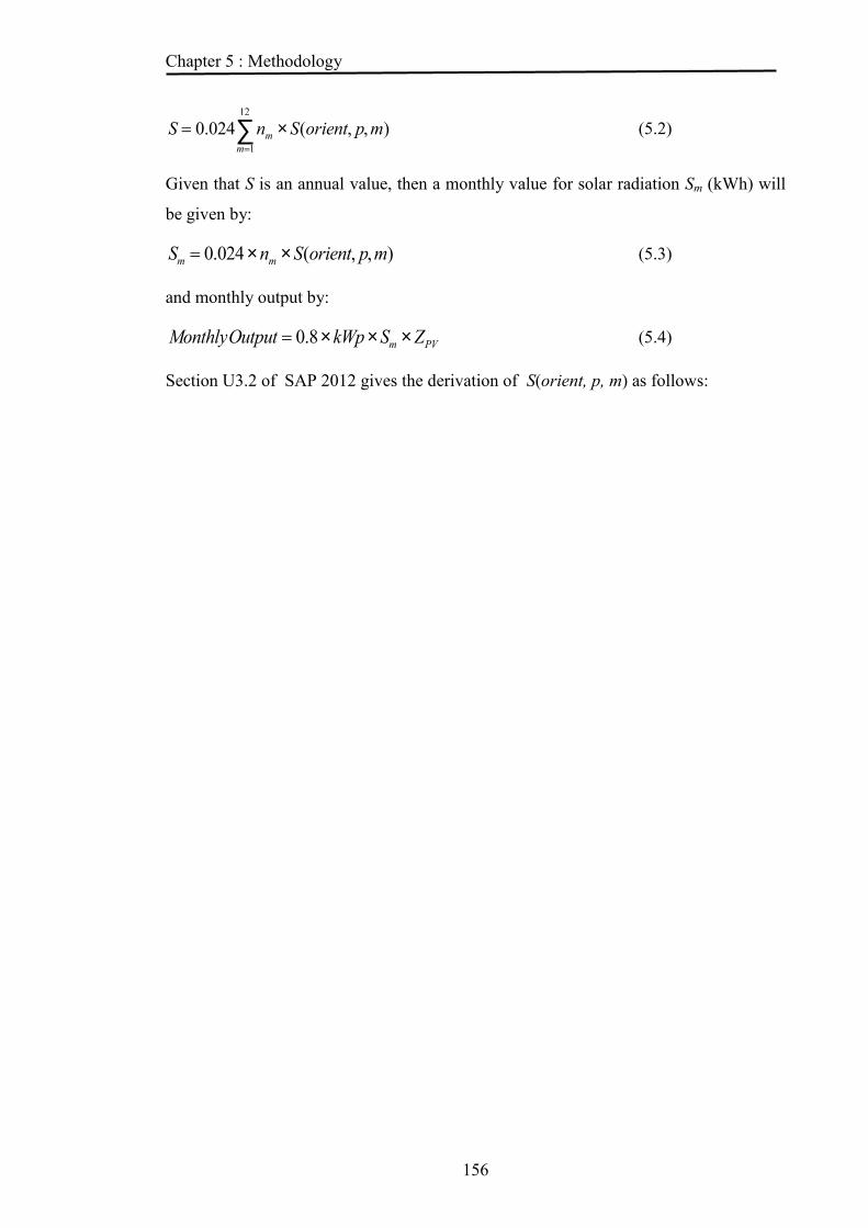
Chapter 5 : Methodology
156
S = 0.024 nm ´ S(orient, p,m)m=1
12
å (5.2)
Given that S is an annual value, then a monthly value for solar radiation Sm (kWh) will
be given by:
Sm = 0.024 ´ nm ´ S(orient, p,m) (5.3)
and monthly output by:
MonthlyOutput = 0.8´ kWp´ Sm ´ ZPV (5.4)
Section U3.2 of SAP 2012 gives the derivation of S(orient, p, m) as follows:

Chapter 5 : Methodology
157
S(orient, p,m) = Sh,m ´Rh-inc(orient, p,m) (5.5)
and
(5.6)
where:
nm = number of days in month m;
orient = orientation of the roof surface (N, NE, E, SE, S, SW, W or NW)
p = tilt of the surface in degrees from horizontal (e.g. 0° is horizontal, 90° is vertical),
30º assumed;
Sh,m = horizontal solar flux (W/m2) for the month and heating degree days region.
Rh-inc(orient, p, m) = factor for converting from horizontal to vertical or inclined solar
flux in month m for a given orientation orient and tilt p;
𝜙 = representative latitude in degrees N for the heating degree region of the sample
dwelling;
= solar declination for the applicable month in degrees;
A, B and C are further determined by a set of quadratic expressions in the sine of the tilt
angle with coefficients determined by orientation (BRE, 2011, Table U5).
The area of photovoltaic modules used to estimate output is determined by the area of
uppermost floor of the dwelling (SPSS variable 'higharea' from table 'energydims'), of
which an arbitrary fraction (0.33) is deemed available for this purpose.
5.6.10 Scenarios for future UK electricity consumption
This section constitutes Stage 4 from Figure 5.1.
5.6.10.1 Objectives
There are two objectives for this section of the study. One is to examine the effects on
the UK energy "mix" - and in particular electricity demands - of the current UK
Government initiative, the Renewable Heat Incentive, to encourage the take-up of
renewable heating devices to meet European Union targets over the period to 2020 and

Chapter 5 : Methodology
158
to examine alternative application of these systems. The second is to examine the
electricity demand effects of much wider deployment of domestic heat pumps in order
to meet the UK's target for 80% reduction in carbon emissions by 2050, including the
possibility of substantial cooling loads from reversible heat pumps under conditions of
climate change.
5.6.10.2 Structure of scenarios
Scenarios for heat pump installations are defined in two levels: firstly, the number of
systems that may be deployed by the end of the scenario period, termed here as
'deployment scenarios'; secondly, the selection of dwelling samples to which these
systems are to be applied, termed 'application scenarios'. The application scenarios, in
terms of installation numbers, are translated into weights on each sample assigned to the
scenario to accrue the sample estimates for a scenario.
5.6.10.3 Temperature data for climate change condition in 2050
The table of monthly average temperatures for each Heating Degree Day region is
'morphed' by temperature increase estimates taken from the UK Climate Projection
(DEFRA, 2011) “high emission”, ‘central estimate” data for GO Regions.
5.6.10.4 Application scenario rules
These define which samples are selected for each scenario by setting a value for the
weighting to be applied to the samples, zero weighting implying that the sample is
excluded from the scenario and the maximum value equalling to the EHS sample
weight. Samples are selected by the selection routine until the total of the weights
assigned for each system type exceeds the total number of systems for the scenario.
The rules utilised for 2020 application scenarios were as follows:
a) samples were selected by a pseudo-random process - one that allows for the
process to be repeated - and the weighting applied to the selected sample also
assigned by a similar pseudo-random process;
b) an identical sample set to that in (a) but with a limited set of energy efficiency
measures applied to the samples;
c) samples are selected according to the total carbon emissions of the dwellings
starting from the highest;

Chapter 5 : Methodology
159
d) samples are selected according to the carbon emissions of heating system fuel,
starting from the highest.
5.6.10.5 Model processing
Two methods of processing were used. For scenarios (a) and (b), rows were selected
from the Output estimates table by a randomly-generated row number. Each selected
row was then assigned weight values for each scenario by generating a second random
number with a maximum value of the Sample Weight. This process was repeated for
each deployment scenario until the total of the weights assigned exceeded the value for
the scenario at which point no further assignments were made. When the highest
deployment scenario value - the 'Stretch' scenario - was exceeded, then the assignment
routine was terminated. As the scenario values are divided between ASHPs and GSHPs,
separate totals are maintained for each type during the assignment process with the
appropriate total being incremented according to the heat pump type allocated to the
sample in Section 0.
For scenarios (c) and (d), rows were processed according to the appropriate CO2
emission value, either the dwelling value or that for the primary heating fuel, in
descending order of magnitude. In this case, the entire sample weight is assigned to the
scenario weight for each sample selected, rather than a proportion. Again, weights are
assigned for each scenario until the total scenario is exceeded, with the process
continuing until the 'Stretch' values are reached.
5.6.10.6 Analysis of results
Results from the assignment process for the scenarios are summarised by fuel type and
by total emissions between existing heating systems and heat pump systems on an
annual and monthly basis to provide appropriate tables and charts to observe the
scenario effects.
5.7 Summary
This chapter has reviewed the requirements for fulfilling the study objectives and
specified the methodological steps required to achieve those objectives. The salient
points of these steps are:

Chapter 5 : Methodology
160
a long-term monitoring study of domestic heat pumps for collection of detailed
performance data with the objective of informing the development of a heat pump
model;
the development of an enhanced BREDEM-8 dwelling energy model, at the kernel of
which is a regression-based heat pump model, which will provide energy consumption
and carbon emission estimates both for an existing system and for a heat pump system;
and the linking of this BREDEM-8 model to the English Housing Survey extract using
parameter reduction techniques; the creation of sample energy consumption and
emissions estimates for both existing heating systems and putative heat pump systems;
creation of housing stock consumption and emission estimates for installation and
policy scenarios for 2020 and 2050;
analysis of these final estimates against the UK electricity generation capacity and
carbon emissions reduction targets.
BREDEM-8 was chosen as a starting point because of its position as an accepted
standard for dwelling energy modelling and for its ability to provide monthly estimates.
It is also capable of being implemented in the chosen platform of MicroSoft Excel.
The English Housing Survey data was chosen because of its completeness and public
availability and the presence of sample weights which allow sample estimates to be
grossed-up to housing stock values.
The following chapter describes the monitoring study for domestic heat pumps and the
analysis of the output data to provide empirical values as parameters for the heat pump
model.

161
CHAPTER 6 PRIMARY AND SECONDARY DATA COLLECTION

Chapter 6 : Primary and secondary data collection
162
6.1 Introduction
Chapter 5 described the methodological approach to be taken in this study. This chapter
describes the initial stage in that methodology, the collection of data, both primary and
secondary. Apart from forming a basis for this study, the primary data collection had the
additional objective of providing independent verification of the performance of the
industrial partner's heat pump products. This stage meets Objective 3 of this study.
6.2 Collection of energy and temperature data from residential heat
pumps
6.2.1 Approach
The approach used in building the monitoring system for the heat pumps was
determined by the requirements of the industry partner, who required a datalogging unit
to acquire diagnostic data for heating systems whose performance was unsatisfactory.
The datalogging unit replaces an existing facility by which data is output via a
diagnostic socket on the heat pump controller to a computer for monitoring by a
maintenance technician. The unit is plugged into the same diagnostic socket and
acquires the same diagnostic data as the existing facility plus the additional energy data
for this research. The data values are stored every 15 mins and the unit (known as a
SPIE box) has a capacity of 1638 samples, slightly over 17 days’ worth of data.
6.2.2 Monitored dwellings and heat pump installations
6.2.2.1 Selection of dwellings for the study
The number of installations involved in this study was restricted to three by the lack of
availability of the custom-made logging equipment, due to circumstances outwith the
control of the author.
In selecting dwellings for this study, the intention was to include a range of different
built forms and ages of dwelling as possible. This intention was difficult to fulfill
because of the current state of the GSHP market in the UK, where, due to their high
capital cost compared to almost all other types of heating systems, to their comparative
novelty, and requirement for a reasonably large garden in which to install the ground
loop, installations have largely been restricted to larger, detached, new-build houses in
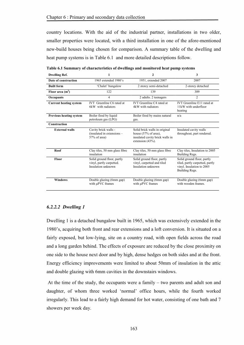
Chapter 6 : Primary and secondary data collection
163
country locations. With the aid of the industrial partner, installations in two older,
smaller properties were located, with a third installation in one of the afore-mentioned
new-build houses being chosen for comparison. A summary table of the dwelling and
heat pump systems is in Table 6.1 and more detailed descriptions follow.
Table 6.1 Summary of characteristics of dwellings and monitored heat pump systems Dwelling Ref. 1 2 3
Date of construction 1965 extended 1980’s 1951, extended 2007 2007
Built form ‘Chalet’ bungalow 2 storey semi-detached 2-storey detached
Floor area (m2) 122 139 309
Occupants 4 2 adults. 2 teenagers 2
Current heating system IVT Greenline C6 rated at 6kW with radiators
IVT Greenline C4 rated at 4kW with radiators
IVT Greenline E11 rated at 11kW with underfloor
heating Previous heating system Boiler fired by liquid
petroleum gas (LPG) Boiler fired by mains natural
gas. n/a
Construction
External walls Cavity brick walls -
(insulated in extensions –
57% of area)
Solid brick walls in original
house (57% of area),
insulated cavity brick walls in extension (43%).
Insulated cavity walls
throughout, part rendered.
Roof Clay tiles, 50 mm glass fibre
insulation Clay tiles, 50 mm glass fibre
insulation Clay tiles, Insulation to 2005
Building Regs. Floor Solid ground floor, partly
vinyl, partly carpetted.
Insulation unknown
Solid ground floor, partly
vinyl, carpetted and tiled
Insulation unknown
Solid ground floor, partly
tiled, partly carpetted, partly
vinyl. Insulation to 2005 Building Regs.
Windows Double glazing (6mm gap)
with μPVC frames Double glazing (6mm gap)
with μPVC frames Double glazing (6mm gap)
with wooden frames.
6.2.2.2 Dwelling 1
Dwelling 1 is a detached bungalow built in 1965, which was extensively extended in the
1980’s, acquiring both front and rear extensions and a loft conversion. It is situated on a
fairly exposed, but low-lying, site on a country road, with open fields across the road
and a long garden behind. The effects of exposure are reduced by the close proximity on
one side to the house next door and by high, dense hedges on both sides and at the front.
Energy efficiency improvements were limited to about 50mm of insulation in the attic
and double glazing with 6mm cavities in the downstairs windows.
At the time of the study, the occupants were a family – two parents and adult son and
daughter, of whom three worked ‘normal’ office hours, while the fourth worked
irregularly. This lead to a fairly high demand for hot water, consisting of one bath and 7
showers per week day.

Chapter 6 : Primary and secondary data collection
164
The heat pump system is installed in a garage beside the house and distributes heat via
the original radiators used with the previous LPG system. The installation in this
location is somewhat disadvantageous as any faults in the equipment can go un-noticed.
The heat pump is rated at an output of 5.9kW (0ºC source/ 35ºC sink) by the
manufacturers.
6.2.2.3 Dwelling 2
Dwelling 2 is a semi-detached, 2 storey house built in 1951, which was extended at the
rear in 2006-2007 by a substantial kitchen dining room on the ground floor and extra
bedroom on the first floor. Replacement, double-glazed windows with μpvc frames
were fitted around the same time, though these were not of good quality since the trickle
vents on some had failed, no longer closing properly. The house is situated on a village
road on an exposed corner, facing due south. To the rear, the lawn under which the heat
pump collectors had been installed is sheltered by hedges.
At the time of the study, the occupants were a family, two adults and two teenage
daughters, of whom the daughters were at school and further education college, one
adult worked both a 12-hour shift pattern and at a part-time building job and the other
worked from 9 am. to 5 pm. in a local shop. With teenage daughters, the hot water
demand was thought to be fairly high but irregular.
The heat pump is installed in the former kitchen in the middle of the house and
distributes heat via the original radiators used with the previous mains gas system.
Additional heating is available from a solid fuel stove in the sitting room. The heat
pump is an older model no longer sold by the manufacturer, rated at 3.9kW.
During the course of the monitoring period, the external temperature sensor, GT2,
which provides the main influence over the heat pump controller weather compensation
algorithm was moved from a position where it received undesirable, direct sunlight to a
shaded location, but there was no apparent effect on the monitored values.
6.2.2.4 Dwelling 3
Dwelling 3 is a detached, 5 bedroom, 5 bathroom house built in 2007 to replace an
older, smaller house. It is on a fairly sheltered site, facing north, with a garden rising
slightly to the rear. Though it is detached, it is quite close to the neighbouring houses
and surrounded by mature trees.

Chapter 6 : Primary and secondary data collection
165
The occupants at the time of the study were a married couple, of whom the wife worked
conventional office hours four days / week and the husband, a consultant, either worked
at home or made long-ish day trips on business. Relative to the house size, the hot water
demand was quite low, mostly running at 4 showers / day, except during family visits.
The heat pump system is installed in a utility room inside the house and distributes heat
via underfloor heating. The installation configuration was slightly unconventional in
that the weather-compensated control had been configured to ignore the internal sensor,
so any casual gains from activity inside the house did not effect the system's operation.
The system was the largest one in the study, rated at 11kW and the only one to have a
separate DHW storage tank.
6.2.3 Data collected
Four types of data are collected for the full analysis of the operation of the heat pump
system:
a) data from the energy input and output from the system;
b) temperature data at the significant points of the system;
c) data for the operational status of the system,
d) data of the current status of the interval timers maintained by the controller.
The characteristics of the different types of data, acquisition method, cleansing and
accuracy are detailed in appendix B.
6.2.4 Data summarisation and analysis
6.2.4.1 General
Data was stored in a separate MicroSoft Excel spreadsheet for each location, with each
sample being stored in a separate row of the spreadsheet. The sample-level data was
then summarised by day, week and month, with temperature values averaged over the
summary period and energy values totaled. Values from samples when the compressor
was not operating were not included in the average temperature values.

Chapter 6 : Primary and secondary data collection
166
6.2.4.2 Analysis for SAP / BREDEM comparison
The SAP/BREDEM routines (Anderson, et al., 2001; BRE, 2008) estimate values for
primary and secondary heating loads, requirements for DHW generation and energy
used for heating system pumps and fans. Actual values for these were calculated using
an analysis based on the Status indicators in the data.
Using the cumulative electricity consumption and heat output values from each sample,
a value was calculated for the consumption and output in each 15 minute period by
simple subtraction from the values for the previous sample. This was then analysed
according to the Status Indicators set on the current sample. Totals were accrued for all
combinations of the following indicators.
a) Compressor
b) Additional heating element 1
c) Additional heating element 2
d) Heat carrier pump
e) Radiator pump
f) Three-way valve
g) Alarm
It was found that the Ground Loop Pump status rarely, if ever, differed from
Compressor status and therefore this was omitted. The indicators for the ‘Mixing Valve’
status were irrelevant for the heating systems under consideration, since these indicators
are used only when the heating system contains both radiators and underfloor heating,
which requires that cooler water is mixed into the floor system water to prevent this
becoming excessively hot.
Of the selected indicators, those for ‘Additional heating’ were treated as one. Any
samples where the ‘Alarm’ indicator was set were included in a separate total as this is
an indication that the pump was not operating correctly. This left thirty-two status
combinations, of which ‘all off’ does not occur, since the heat pump controller defaults
to setting the three-way valve to ‘DHW generation’ status during periods when the
external temperature exceeds 18 ºC.

Chapter 6 : Primary and secondary data collection
167
It was, however, realised that where more than one status was set, the consumption and
output values will consist of contributions from each sub-system within the heat pump.
Moreover, because the various sub-systems of the heat pump may switch in or out
between the logging of samples, the consumption and output values might be made up
of indeterminate contributions from these sub-systems due to the change of
circumstances in the 15 minute period between samples. It was therefore necessary to
estimate the contributions of the less variable sub-systems - additional heating and
system pumps - using other methods detailed in the following paragraphs.
6.2.4.3 Additional heating
The IVT heat pump models which are the subject of this part of the study contain two
additional heaters, the first rated at 3 kw and the second at 6 kw, which are switched in
either separately or together, depending on the heating load that must be balanced and
the controller settings. If the status for either is set on for a given sample, it can be
assumed that its load will be present for at least part of the period between the samples
before and after the current one, but no other assumptions can be made. For the benefit
of this exercise, it will be assumed that if the status is set, then the heaters will operate
for a standard duration of 7.5 minutes (half the interval between samples). Thus a value
for the electricity consumption, EAdd, in kWH, by the additional heaters is given by the
formula:
( ) (6.2)
where SH1, SH2 are the statuses of heater 1 and heater 2 respectively. This consumption
value is then further analysed by means of the ‘Three-way Valve’ status, which if set,
indicates that DHW is being generated, otherwise the system is providing space heating.
6.2.4.4 Distribution system
For the IVT heat pumps, this consists of two pumps, one, P1, for circulation of heating
water specifically around a radiator or underfloor heat distribution system, and another,
P2, for circulating water around the DHW system and as a return from the distribution
system. These pumps appear to operate in tandem since an analysis of their status
indicators for Dwelling 1 showed that, of 21972 samples, 18403 samples had the P1
status set, 18737 had the P2 status set and 18379 had both statuses set. Inspection of the
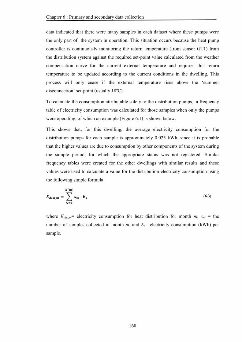
Chapter 6 : Primary and secondary data collection
168
data indicated that there were many samples in each dataset where these pumps were
the only part of the system in operation. This situation occurs because the heat pump
controller is continuously monitoring the return temperature (from sensor GT1) from
the distribution system against the required set-point value calculated from the weather
compensation curve for the current external temperature and requires this return
temperature to be updated according to the current conditions in the dwelling. This
process will only cease if the external temperature rises above the ‘summer
disconnection’ set-point (usually 18ºC).
To calculate the consumption attributable solely to the distribution pumps, a frequency
table of electricity consumption was calculated for those samples when only the pumps
were operating, of which an example (Figure 6.1) is shown below.
This shows that, for this dwelling, the average electricity consumption for the
distribution pumps for each sample is approximately 0.025 kWh, since it is probable
that the higher values are due to consumption by other components of the system during
the sample period, for which the appropriate status was not registered. Similar
frequency tables were created for the other dwellings with similar results and these
values were used to calculate a value for the distribution electricity consumption using
the following simple formula:
∑
( )
(6.3)
where Edist,m= electricity consumption for heat distribution for month m, sm = the
number of samples collected in month m, and Es= electricity consumption (kWh) per
sample.

Chapter 6 : Primary and secondary data collection
169
Figure 6.1 Frequency distribution of electricity consumption for samples when only pumps operating
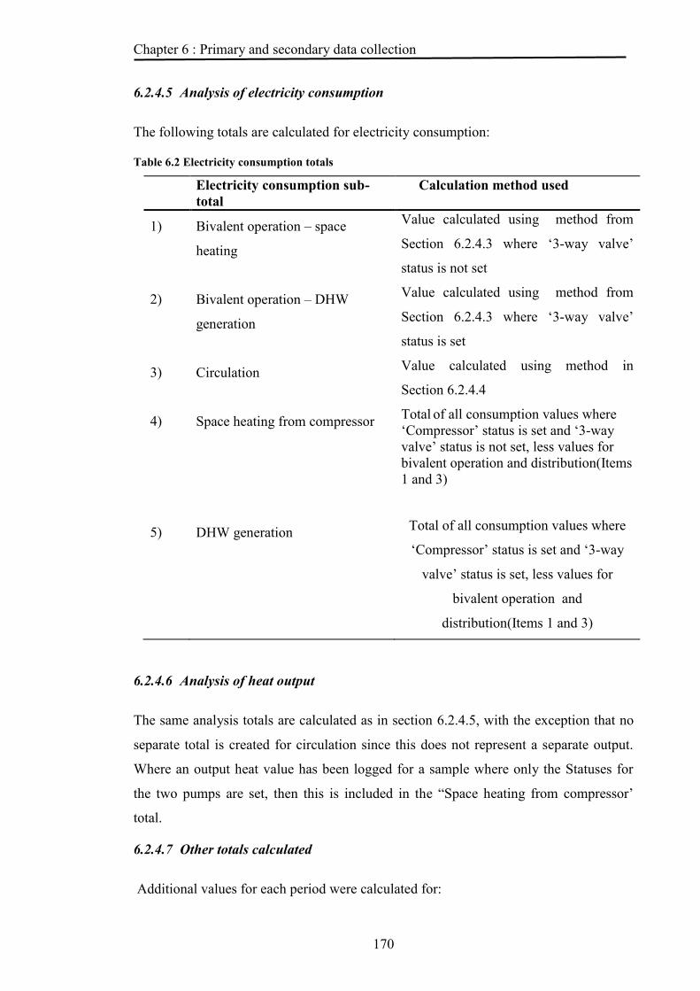
Chapter 6 : Primary and secondary data collection
170
6.2.4.5 Analysis of electricity consumption
The following totals are calculated for electricity consumption:
Table 6.2 Electricity consumption totals
Electricity consumption sub-total
Calculation method used
1) Bivalent operation – space
heating
Value calculated using method from
Section 6.2.4.3 where ‘3-way valve’
status is not set
2) Bivalent operation – DHW
generation
Value calculated using method from
Section 6.2.4.3 where ‘3-way valve’
status is set
3) Circulation Value calculated using method in
Section 6.2.4.4
4) Space heating from compressor Total of all consumption values where ‘Compressor’ status is set and ‘3-way valve’ status is not set, less values for bivalent operation and distribution(Items 1 and 3)
5) DHW generation Total of all consumption values where
‘Compressor’ status is set and ‘3-way
valve’ status is set, less values for
bivalent operation and
distribution(Items 1 and 3)
6.2.4.6 Analysis of heat output
The same analysis totals are calculated as in section 6.2.4.5, with the exception that no
separate total is created for circulation since this does not represent a separate output.
Where an output heat value has been logged for a sample where only the Statuses for
the two pumps are set, then this is included in the “Space heating from compressor’
total.
6.2.4.7 Other totals calculated
Additional values for each period were calculated for:

Chapter 6 : Primary and secondary data collection
171
total heating degree days, based on 15 ºC – calculated, initially as degree hours, by
interval length (0.25 hrs) times base temperature minus sample external temperature,
then divided by 24.
total logged hours, based on 15 min. per sample.
6.2.4.8 Adjustment of results
Because of faults in the datalogging equipment, a considerable proportion of the
possible data was not captured during the collection period. This amounted to
approximately 37% of the possible data for dwelling 1, 19% for dwelling 2 and 1.35%
for dwelling 3. In order to allow more useful comparison between the data, adjustments
were applied to the monthly totals for dwellings 1 and 2 as follows:
Use was made of the fairly close proximity of all three dwellings – dwelling 1 is
about 7 km from dwelling 3, dwelling 2 is about 34 km away. On this basis, it was
judged there would be only minor differences between the average temperatures at
the sites and hence only minor differences between the degree days experienced at
the three sites. This was found to be a reasonably correct assumption from the data
as shown by the following Figure 6.2 & Figure 6.3, which indicate that i) that the
temperatures at all three sites were closely related, and ii) there is a strong
correlation between heating degree days and electricity consumption for space
heating.
It was therefore deemed reasonable to adjust those values largely determined by
temperature, viz. electricity consumption and heat output for space heating, in
proportion to the monthly heating degree days. Those values which are related to
occupancy, viz. electricity consumption and heat output for DHW generation, and
those which are simply related to operating hours, were adjusted according in
proportion to the hours of data collected against the monthly hours.

Chapter 6 : Primary and secondary data collection
172
Figure 6.2 Monthly average external temperature at all 3 sites
Figure 6.3 Electricity consumption vs heating degree days - all three sites

Chapter 6 : Primary and secondary data collection
173
6.2.5 Results
6.2.5.1 General results
Energy and performance results for all three dwellings are summarised in the following
Table 6.3. Apart from the collected data, an additional value is included for the heat
load for each of the houses as estimated by the Apache dynamic simulation program
within the IES Virtual Environment system (IES, 2012). This value was included for
comparison because of the author's reduced confidence in the measurement of output by
the heat meter installed. The two values for heat output, line 11 in Table 6.3, are, headed
'Heat meter', that measured by the afore-mentioned meter, and, headed 'From temp
calculation', that calculated using Equation 6.1.
Notable in these results are the following:
a) the exceedingly high space heating consumption per unit area of dwelling 1
compared with the other two;
b) the absence of direct electric heating in dwelling 3; possibly indicating that the
system is over-sized;
c) the significantly higher consumption for distribution in dwelling 3 - more than
twice either of the others as a percentage of electricity consumption; due to the
second pump in the distribution system required for the upper floor;
d) the inconsistent results for dwelling 2, for which the SPF of the heat pump
calculated on the data from the heat meter is implausibly high, but the heat load per
unit area is comparable with dwelling 1;
e) the SPF of the heat pump in dwelling 3 is similar to that in dwelling 2 despite the
use of underfloor heating for distribution which is claimed to improve performance
by allowing a lower distribution temperature; this appears to be a consequence of
the high consumption of the distribution pumps.
f) A general, fairly predictable, point that emerges from this table is that dwelling 3,
being of more modern construction, has significantly lower energy use per unit area
for space heating compared with the other two.

Chapter 6 : Primary and secondary data collection
174
6.2.5.2 Monthly electricity consumption
Figure 6.4 provides a chart of the electricity consumption of all three systems. As
indicated, it analyses consumption by the two functions of the heat pump, those of space
heating and DHW generation and by circulation, the power used by the system pumps.
Within the functions, a further separation is made into consumption by the compressor
and that by the additional direct electric heaters for bivalent operation. Within the
distribution electricity consumption, the separation is between the use of pumps when
heat is being supplied to the house or the hot water reservoir, and that when the pumps
are maintaining circulation to provide temperature feedback to the controller. A trend
line indicates the heating degree days for each month - the values are based on the
temperatures recorded at dwelling 3. The values for dwelling 1 and 2 have been
adjusted for missing data as per section 6.2.4.8.
The significant points of these results, for this study, are as follows:
a) for dwellings 1 and 2, the proportion of consumption for bivalent operation for
space heating is very small except in January and February; this implies that a
significant rise in average temperatures or fabric improvements for energy
efficiency might eliminate the requirement for bivalent operation; results for
dwelling 3 contained almost no bivalent operation at all, raising a question as
to whether the heat pump system is oversized.
b) reflecting the lower source temperatures in January and February, energy
consumption for DHW generation rises in these months, despite the demand
probably being similar throughout the year.
c) as noted in section 6.2.5.1, dwelling 3 has significantly higher energy
consumption for distribution than the other two, of which a substantial
proportion occurs during the summer months and consists largely of circulation
for temperature monitoring.

Chapter 6 : Primary and secondary data collection
175
Table 6.3 Summary results table for all dwellings
Dwelling 1
2
3
1) Floor area (m2) 122 139 309 2) Occupants 4
4
2
Annual energy consumption (kWh) Space heating 3) Compressor 5,815 71.7%
3,275 68.1%
4,334 59.1%
4) Direct electric 188 2.3% 107 2.2%
11 0.1% 5) = (3)+(4) Total space heating 6,002 74.0%
3,382 70.3% 4,345 59.2%
per unit area 49
24
14
DWH generation 6) Compressor 1,577 19.5%
854 17.8%
2,070 28.2%
7) Direct electric 62 0.8% 90 1.9%
48 0.6% 8) Total DHW 1,640 20.2%
945 19.6% 2,118 28.9%
per occupant 410
236
1,059
9) Heat distribution 230 2.8%
203 4.2% 255 3.5% 10) Circulation for control 235 2.9%
277 5.8% 616 8.4%
Total energy consumption 11)=(10)+(9)+(8)+(5) 8,107
4,807
7,333
Annual heat load (kWh) Heat meter
From temp calculation
From dynamic simulation Heat meter
From temp calculation
From dynamic simulation
From temp calculation
From dynamic simulation
12) Annual heat load 16,809 77.1% 15,236 19,716 18,339 67.4% 11,509 13,550 14,686 70.0% 11,302 13) per unit area 138
125 161 132
83 97 49
38
Annual energy output from DHW usage (kWh) 14) Total 4,989 22.9% 4,205
8,890 32.6% 8,787
6,304 30.0%
15) Per occupant 1,247
1,051
2,222
2,197
3,152 Total output (kWh)
16)=(12)+(14) 21,798
19,441 27,228
20,296 20,991
17) = (12)/(5) SPF (Heating only) 2.80
2.54
5.42
3.40
3.38
18) = (16)/(11) SPF (Heating & DHW) 2.69
2.40 5.66
4.22 2.86
Estimated CO2 emissions (kg)
(assumed)
Original system fuel Bottled LPG (0.234 kg/kWh)
Mains gas (0.194 kg / kWh)
Heating oil ( 0.265 kg / kWH)
19) from (16) Original system 5,101
4,549
5,282
3,937
5,563
20) from (11) Heat pump system (0.517 kg/kWh) 4,191 2,485 3,791
21) Emission reduction 18%
8%
53%
37%
32%

Chapter 6 : Primary and secondary data collection
176
Figure 6.4 Electricity consumption for all three systems

Chapter 6 : Primary and secondary data collection
177
6.2.5.3 Monthly output
The monthly output for all three systems, with systems 1 and 2 again adjusted for
missing data is shown in Figure 6.5. A notable anomaly in these charts is the high
value for bivalent energy output for dwelling 1 in month 2009/6. This was due to the
failure of the compressor which caused the system to use the additional heaters to
generate DHW for a substantial part of that month.

Chapter 6 : Primary and secondary data collection
178
Figure 6.5 Monthly output from all three systems
83% 78%
78% 83% 77% 71%
28% 30% 60%
79% 80%
16% 18%
17% 16%
23% 29%
71% 69%
39%
21%
20%
0
50
100
150
200
250
300
350
0
500
1000
1500
2000
2500
3000
3500
4000
4500
5000
2008-122009-012009-022009-032009-042009-052009-062009-072009-082009-092009-102009-11
kWh
Dwelling 1 - Monthly output
88% 85% 86% 83%
67% 52% 33% 26% 32% 41% 77% 78%
12% 14%
12% 17%
32% 48%
65% 73% 66% 58%
23% 22%
0
50
100
150
200
250
300
350
0
500
1000
1500
2000
2500
3000
3500
4000
4500
5000
2008-122009-012009-022009-032009-042009-052009-062009-072009-082009-092009-102009-11
kWh
Dwelling 2 - Monthly output
83% 85% 85%
79%
64% 39% 42%
72%
17% 14%
14%
20%
36%
61% 58%
28%
0
50
100
150
200
250
300
350
0
500
1000
1500
2000
2500
3000
3500
4000
4500
5000
2008-12
2009-01
2009-02
2009-03
2009-04
2009-05
2009-06
2009-07
2009-08
2009-09
2009-10
2009-11
kWh
Dwelling 3 - Monthly output
Compressor space heating Compressor DHW generation Bivalent operation - DHW generation
Bivalent operation - space heating Heating degree days

Chapter 6 : Primary and secondary data collection
179
6.2.5.4 Monthly SPF values
These are shown in Figure 6.6. Again, this figure shows a divergence between the
performance of the two radiator/retro-fit systems and the UFH/new build system.
Performance of the former two systems has twin peaks in early and late summer,
falling off sharply at either end of the year, while the latter system varies only
slightly throughout the year with a single peak in August. The former set of curves
appears to reflect the improvement in performance due to the reduction in lift for
heating required as both the ground temperature and the air temperature increase in
spring / early summer, then, when heating is no longer required, a reduction in
performance due to the requirement for DHW generation at a higher lift in mid-
summer. The curve for the UFH system appears to reflect both its possible over-size,
noted in 6.2.5.2 paragraph (a) and also the comparatively low demand for hot water,
noted in 6.2.2.4.
Figure 6.6 Monthly SPF by dwelling
6.2.5.5 Output temperatures to distribution (Sink temperature)
Table 6.4 shows that the distribution temperatures in the three dwellings differ
substantially, in the same way as the SPF values. Distribution temperatures for the
0
1
2
3
4
5
6
7
8
9
2008-12 2009-01 2009-02 2009-03 2009-04 2009-05 2009-06 2009-07 2009-08 2009-09 2009-10 2009-11
SP
F(-)
Month
Monthly SPF by dwelling
Dwelling
1
Dwelling
2
Dwelling
3

Chapter 6 : Primary and secondary data collection
180
dwelling 2 system are considerably lower than the 55ºC that might be expected
(Ochsner, 2007, p. 87), lower than those in the dwelling 3, yet the internal
temperatures in dwelling 2 are maintained at or above 22 ºC. This reduction is
presumably due to the effect of the weather compensation control (Cantor, 2011, p.
13), with distribution temperatures being reduced in response to higher external
temperatures during the heating season.
Table 6.4 Distribution, internal and external temperatures for all three systems
Month 2008 2009
All temps in ºC 12 1 2 3 4 5 6 7 8 9 10 11
Dwelling 1
Distribution outflow 47.0 48.5 51.6 46.8 46.4 44.5 56.8 - - 46.8 43.9 44.9
Hot water
54.9 54.7 55.4 55.3 55.2 55.3 52.2 52.1 52.5 52.3 52.5 52.4
Internal
19.9 19.7 19.7 20.2 20.5 20.6 21.7 22.9 22.2 21.1 20.6 20.0
External
4.9 3.6 2.8 8.1 11.3 12.8 16.1 18.4 17.4 15.1 11.9 8.3
Max distr
61.9 67.9 69.2 63.7 64.1 63.9 66.9 59.8 60.2 59.2 59.1 58.9
Dwelling 2 Distribution outflow 37.8 36.8 37.5 37.1 38.6 41.6 45.0 - 44.7 43.1 38.2 36.7
Hot water
46.1 47.0 46.3 45.9 45.7 45.8 45.4 45.7 45.4 45.5 48.1 47.1
Internal
22.4 22.4 22.3 22.5 22.8 23.1 24.8 25.1 25.0 23.4 22.5 22.4
External
4.6 6.0 5.9 10.8 13.4 15.6 19.3 18.8 19.5 16.5 12.7 9.6
Max distr
49.1 66.7 49.0 47.8 49.0 49.3 49.4 50.3 49.9 49.0 48.4 49.3
Dwelling 3 Distribution outflow 41.4 40.8 41.2 42.0 44.4 47.0 50.0 50.9 51.9 47.9 47.1 43.3
Hot water
47.5 47.4 46.9 46.9 46.7 46.5 46.6 46.9 46.9 43.0 44.4 45.9
Internal
21.1 20.3 21.4 20.9 21.1 21.6 23.1 23.1 23.0 21.7 20.5 19.6 External
4.4 3.3 5.0 8.0 12.1 15.0 18.0 18.8 18.9 15.8 12.2 9.3
Max distr 52.0 66.7 49.8 51.4 50.4 41.8 44.0 - - 45.6 45.6 52.0
Further analysis of output temperatures and flow / return differentials was carried out
to establish characteristics for estimating and these results are also presented in
context in Chapter 7.
6.2.5.1 Temperatures returned from ground loop
An analysis was made to provide an estimate of the differential between soil
temperature and the ground loop temperature. This is presented later in this
document in Chapter 7 as being clearer in that context.

Chapter 6 : Primary and secondary data collection
181
6.2.6 Discussion
6.2.6.1 Datalogging equipment
For datalogging, this research brought out two points. Firstly, the custom datalogging
equipment, designed and built in a comparatively short time, was not a reliable
solution to this problem and should have been avoided, with other solutions being
explored such as the use of dedicated personal computers for data storage. Secondly,
the heat meters employed for measuring the system output were too complex,
requiring additional temperature sensors which were awkward to fit and which
duplicated some already present in the heat pump system. Reference to the relevant
data sheet (Sontex, 2004) shows that the flow meter within the Supercal 539 employs
a magnetic sensor, which the author considers could have been disrupted by electro-
magnetic interference within the heat pump, possibly from the compressor.
6.2.6.2 Heat pump systems and dwelling energy efficiency
The results of the data analysis confirm the relationship between output temperature
and heat pump SPF, in that the average monthly distribution temperatures in the
monitored systems form one progression from low (~ 37 ºC) to high (~ 45ºC),
(Table 6.4) with the SPF values forming a second from high (~ 4.0) to low (~2.6)
(Table 6.3) across the systems. However, the fact that the central pair of SPF and
distribution temperature values is from Dwelling 3, a new-build house with a UFH
distribution system, is anomalous in that UFH is deemed to require lower distribution
temperatures to achieve the same heat output, allowing a higher SPF. Equally
anomalous are the comparatively low distribution temperatures found in the
Dwelling 2 system, thereby raising some queries about how much the energy
efficiency of dwellings and their heat distribution systems should be regarded as
barriers to the future take-up of heat pumps.
Because heat pump systems can achieve a higher COP whilst operating at lower
temperatures, it is asserted that this necessitates both a low temperature distribution
system and a high level of energy efficiency in a dwelling to provide an acceptable
level of thermal comfort while still operating the system at a sufficiently high COP
(Cantor, 2011; EST, 2011). The need to replace existing radiators with new, much
larger ones and to upgrade insulation and draught-proofing is therefore seen as a

Chapter 6 : Primary and secondary data collection
182
barrier in the transition to heat pump systems, certainly by Fawcett (Fawcett, 2011).
However, the degree to which the building fabric must be improved is unclear and
there is some dispute - admittedly from some years previously (McMullan &
Morgan, 1981, p108) - about the absolute necessity for replacing radiators on the
basis that existing radiators are likely already to be oversized for fuel-fired systems.
McMullan & Morgan contend that, in order to raise dwelling temperature quickly, it
was the practise of heating engineers to install boilers and radiators which were as
much as 250% larger than required which is in the region of the increase in size
required to match the reduced temperature economically provided by a heat pump
system. To some extent, the two retro-fit dwellings in the current study support
McMullan & Morgan (1981), in that there was no change to the existing radiators
when the heat pump systems were installed. In Dwelling 1, no additional efficiency
measures were installed with the heat pump systems though double-glazing had been
installed previously, but in Dwelling 2, double-glazing was installed and a substantial
extension added at about the same time as the heat pump was installed, reducing the
proportion of the external wall composed of the original single brick skin by about
one third. The earlier improvements to Dwelling 1, though probably to a lower
energy efficiency standard, have also somewhat improved that house but with a
substantial increase in external surface area. With these improvements, the heating
systems in both dwellings maintained an SPF sufficient to achieved some reductions
in carbon emissions, as has been said above.
Given the above, found in what is, admittedly, a very small sample of dwellings, it
would appear that double glazing and extensions to houses, made to contemporary
standards, have the potential to improve the housing stock such that heat pump
systems would be found to be viable for retro-fit, even without the additional
improvement of larger radiators. Analysis of the relevant EHS file('shape') showed
that about 13% of the English stock had been either refurbished completely, an
extension added, or a loft extension built and approximately 82% had double glazing
(Tables 6.5 & 6.6).

Chapter 6 : Primary and secondary data collection
183
Table 6.5 Proportion of EHS stock sample having had substantial work (extension or refurbishment) by age of work.
Sample total grossed-up
Percentage of stock
None 11499270 62.4%
Pre 1945 114769 0.6% 1945 - 1964 240564 1.3% 1965 - 1984 1703283 9.2% 1985 - 1990 1342562 7.3% 1991 - 1995 993906 5.4% 1996 - 2005 2243984 12.2% Unknown 47492 0.3% In progress 232350 1.3% Since 1996 13.45%
Table 6.6 Analysis of window construction types from EHS
Construction Grossed-up total
Percentage
double-glazed, UPVC 12663464 68.8% single-glazed, wood sash 570848 3.1% single-glazed, wood casement 1781376 9.7% double-glazed, wood 1743240 9.5% double-glazed, metal 797007 4.3% single-glazed, UPVC 171448 0.9% single-glazed, metal 280272 1.5% mixed types 410525 2.2%
6.2.6.3 Monitoring of performance
Given a modest additional amount of computing capability and provided the problem
identified in 6.2.6.1 can be solved, it would be possible to measure both the
electricity consumption and heat output to provide real-time monitoring of a heat
pump's performance, particularly of its COP, using the data from the heat and
electricity meters used. In addition, though it is not immediately obvious from this
study, the main indicators of the state of health of a heat pump system would appear
to be the flow rate for the distribution system, indicating the proportion of the heat
output that is reaching the distribution, and the relationship between the output
temperature from the compressor and that to the distribution system, indicating the
proportion of the compressor heat output that is being output via the condenser.

Chapter 6 : Primary and secondary data collection
184
6.3 Secondary data acquisition
6.3.1 Heat pump performance data
As data for this study had been collected from only three installations of one type of
heat pump, it was by no means possible to make any statistically-valid estimates of
heat pump performance from this data. It was therefore necessary to acquire a larger
volume of data for this purpose. Following on from Staffel (Staffel, 2009), test
results from the Wärmenpumpen TestZentrum (WPZ) (WaermenPumpen
Testzentrum, 2009) were employed for the purpose of this study.
6.3.1.1 Description
The WPZ tests used in this study are both air-to-water and soil-to-water systems,
both to European Standard EN14511(British Standards Institution, 2007) and to
EN255(British Standards Institution, 1997). Water-to-water heat pump test results
are included with those for soil-to-water systems, and a separate set of results are
included for water heating heat pump systems which are not required for this study.
Samples of the test result documents are included as Appendix B & C of this thesis.
The data provided in the test results is as follows:
a) The system supplier
b) The supplier's model number for the system;
c) the test reference
d) the type and weight in kilogrammes of the refrigerant used in the system;
e) the performance test results in the form of energy input, energy output and COP
for each source/sink temperature combination as specified in the test schedule for the
Standard.
f) system flow rate used in testing (nominal - from manufacturer) in m3/hour;
g) Temperature differential (K) between outflow and return from the heat pump sink;
Other data is present but is not deemed relevant to this study.
For the purpose of the current study, the substantive difference between the EN255
and the EN14511 standards is in the definition of the 'boundary' for a heat pump

Chapter 6 : Primary and secondary data collection
185
system, which, for EN14511, includes distribution pumps which are excluded from
EN255 (British Standards Institution, 1997, 2007). The test values for each standard
are summarised in Table 6.7. For each heat pump tested to EN14511, this means that
10 data points are available for a regression model for COP against 'lift', while for
EN255, 10 data points are available for air / water heat pumps but only 6 for soil /
water systems.
Table 6.7 Summary table for WPZ heat pump test conditions
Heat pump type : Air to water Standard: EN14511
Source / sink temps LiftA10/W35 25A7 /W30 - W35 28A2/ W35 33A2/W35-25 23A-7/W35 42A-15/W35 50A7/W45 38A20/W55 35A7/W55 48 A-7/W55 62
Heat pump type : Soil to water Standard: EN14511Source / sink temps LiftB5/W35 25B0/W35 35B0/W35-25 25B5/W45 35B0/W45 45B-5/W45 55B5/W55 45B0/W55 55
Standard: EN255
Source / sink temps LiftA20/W35 15A10/W35 25A7/W35 28A2/W35 33A-7/W35 42A20/W50 30A15/W50 35A7/W50 43A2/W50 48A-7/W50 57
Standard: EN255Source / sink temps LiftB5/W35 30B0/W35 35B-5/W35 40B5/W50 45B0/W50 50B-5/W50 55
6.3.1.2 Development of database
The database of heat pump test results was created as follows:
The print format from WPZ was imported into an Excel spreadsheet, using
"PDF2Office" (Recosoft, 2010) software which partially converted the data, leaving
some items, particularly numeric values, to be formatted manually.

Chapter 6 : Primary and secondary data collection
186
Further manual editing was performed to create: a) a table of all the heat pump
suppliers present; a table of heat pump systems containing a row for each system;
and two tables of heat pump test results, one for air/water systems, the other for
soil/water systems, each containing one row for each test result, viz. source
temperature, sink temperature, resultant lift , electricity input, heat output, resultant
COP. For each heat pump row, a set of linear regression parameters were calculated,
based on the lift and COP values from the test values for that system. A detailed list
of the variables present in each table is shown in Table 6.8. An overall set of linear
regression parameters are calculated for each of the two tables of test results.
Table 6.8 Variables in heat pump test results database
Table Variable Meaning / use Supplier Supplier ID Unique identifier for supplier providing sample system for test
Name Allows selection of a list of systems by supplier
Address For confirmation of selection
Heat pump system HP ID Unique identifier for system
Model number Supplier's identification for system
Supplier ID Link to supplier entry
Type ="AW" for air / water ="SW" for soil / water for choice of table for the location of test results.
First entry First row number of batch of test results data for current heat pump system.
Count of following entries Count of rows of test results for the current heat pump system.
Regression parameters Two parameters - results of linear regression of COP against lift value from the test results for the current heat pump system
Date of test
Test results HP model number Link to Heat Pump table entry
Test ID Unique identifier for test result entry
Source temperature Value prefixed by "A" in Test Conditions for air source systems or by "B" in those for ground source systems. (ºC)
Sink temperature Value prefixed by "W" in Test Conditions for both air source systems and ground source systems. (ºC).
Input Value in kW for electricity input during test
Output Value in kW for heat output during test
COP Output value ÷ input value.
Lift Sink temperature - source temperature (K)
Date published As stated.
Carnot COP = (Source temp + 273) / (Source - sink)
Carnot efficiency = actual COP / Carnot COP
Chapter 6 : Primary and secondary data collection
187
6.3.1.3 Discussion
It should be noted from the above that a considerable amount of 'manual'
manipulation of data was involved in the creating of this database rendering it
somewhat impractical for regular usage. When last asked, WPZ responded that the
information was not available in any other form (Nani, 2009), though recently the
results files are being provided in English.
It would be useful if the test results data was available for the heat pump systems
from UK suppliers so that this database was more applicable to this current study.
6.4 Summary and conclusions
This chapter described the primary and secondary data collection processes for this
research, detailing the monitoring study of ground source heat pumps and analysis of
its results, and the creation of a database of heat pump performance data from
standard test results.
For the monitoring study of IVT ground source heat pumps, data for electricity input
and heat output, system temperature values and statuses was collected from three
installations using a custom datalogger over a period of 12 months starting in
December 2008 and ending in November 2009. The monitoring study was hampered
by lack of cases and by faults in the dataloggers, the root cause of which was a
financial dispute between the industrial partner and the developer for the datalogger,
which effectively prevented any more than three sets of equipment being built and
faults in those three being cured.
The data was analysed to provide monthly totals for: electricity consumption by
space heating, DHW generation and heat distribution, distinguishing where
consumption was by the heat pump compressor or by the additional, direct electric
heaters; heat output for space heating and DHW generation, again making the same
distinction. Because of faults in the data loggers causing the loss of data samples,
particularly for dwellings 1 and 2, it was necessary to adjust the results from the
electricity input and heat output analysis to compensate for this loss, based on the
heating degree days measured at Dwelling 3. An apparent failure of the heat meter on
the system output for Dwelling 3 also made it necessary to base the heat output from

Chapter 6 : Primary and secondary data collection
188
that system on a calculated value. For comparison, values for heat output for
dwellings 1 and 2 were calculated using the same method.
A monthly Seasonal Performance Factor (SPF) was calculated for each system to
observe the pattern of its fluctuation. Return temperatures from the ground loop
collector and output temperatures to the distribution system were analysed for use in
the latter part of the study.
Results from the monitoring study indicated that:
while the heat pump systems in the two retro-fit installations appeared to be
subject to more variable heating loads, it is still possible for such installations to
reach a reasonably high Seasonable Performance Factor, albeit on the basis of a
very small sample;
a penalty of using underfloor heating continues to be substantial consumption of
electricity (~900 kWh annually, approx. 12%) by pumps for distribution, in
particular for monitoring internal temperatures, as has been noted previously
(BRECSU, 2000);
the distribution temperatures - both average and maximum - registered for one of
the retro-fit installations, Dwelling 2, and for the new-build installation,
Dwelling 3, did not differ substantially, with those from the retro-fit being
considerably below the conventional value for radiator systems (average 38 ºC
as opposed to 55 ºC) and those from the new-build similarly above that for
underfloor heating (average 42 ºC as opposed to 35 ºC); distribution
temperatures in Dwelling 1 were higher than in the others, but still lower than
the conventional 55 ºC value. As the average internal temperature in all three
dwellings is close to the required norm, this might indicate that the systems'
weather compensation controls are effective in maintaining lower operating
temperatures and that the heat transfer rate of the radiator distribution systems is
adequate to maintain the required temperature, despite the lower operating
temperatures.
One of the main points arising from the study was that the data collected did not
provide an indication of the health and efficiency of the heat pump installations
without considerable computation and that there is a need for research into diagnostic
methods for this purpose.

Chapter 6 : Primary and secondary data collection
189
To build a database of heat pump system performance data, the required data was
extracted from print image files available from the Wärmenpumpen TestZentrum
(WaermenPumpen Testzentrum, 2009) and formatted into separate spreadsheet tables
for each of supplier details, heat pump system details and test result values.
The next chapter presents the details of a development of a simple regression model
for heat pump energy use based on the data documented in the first two sections of
this chapter, and its embedding in a building energy model.

190
CHAPTER 7 DEVELOPMENT OF AN ENHANCED STANDARD
RESIDENTIAL BUILDING ENERGY MODEL

Chapter 7 : Development of an enhanced standard residential building energy model
191
7.1 Introduction
This section contains details of the development of the building energy computer
model in achieving Objective 4 of this study and consists of:
an analysis of the calculation methods used in the current UK standard procedures
for assessing residential energy use, SAP/BREDEM, and the possible deficiencies
of these methods in the handling of heat pump systems;
details of replacement methods for estimating the energy use of heat pump heating
systems, including their theoretical basis, data sources and the equations required.
7.2 Objectives
The initial objective of this section is to detail the methods used to calculate the
contribution made by the different types of heat pump systems to residential energy
use in the BREDEM/SAP models used in the UK domestic energy model and
standards for energy efficiency and for gaining Building Regulations approval under
the Building Regulations Approved Documents: Part L1A applicable to new houses.
The second objective is to identify where these methods are substantially deficient in
modelling the characteristics of heat pump systems.
A third objective is to identify more appropriate methods for characterizing heat
pump systems, to provide an improved BREDEM-style model and to specify the
equations and processing involved.
7.3 BREDEM/SAP estimation
The principles behind the BREDEM/SAP models have been described in Section
3.3.4.1. The BREDEM heat pump parameters are reproduced in Table 7.1, with those
from SAP in Table 7.2.

Chapter 7 : Development of an enhanced standard residential building energy model
192
Table 7.1 Heat pump system parameters in BREDEM-8
Ref. Source Heat pump system parameters in BREDEM-8
1 Table D1 Efficiency & responsiveness
Efficiency / SPF
Responsiveness (from Table D4)
Heat distribution by water With
radiators UFH in insulated timber floor
UFH in screed or concrete slab
Ground-to-water heat pump 320
1.0 1.0 0.25 Ground-to-water heat pump with auxiliary heater 300
Water-to-water heat pump 300 Air-to-water heat pump 250 Heat distribution by air Responsiveness (from Table D1) Ground-to-air heat pump 320 1.0
Ground-to-air heat pump with auxiliary heater 300
1.0
Water-to-air heat pump 300 1.0 Air-to-air heat pump 250 1.0
2 From Table D.7 Fraction of heat supplied by secondary systems
Main heating system Secondary system Fraction
Central heating system with boiler
and radiators, central warm-air system or other gas fired systems
gas fires 0.15 coal fires 0.10 electric heaters 0.05
Electric heat pump systems with
heat storage or fan-assisted storage heaters
gas fires 0.15 coal fires 0.10 electric heaters 0.05
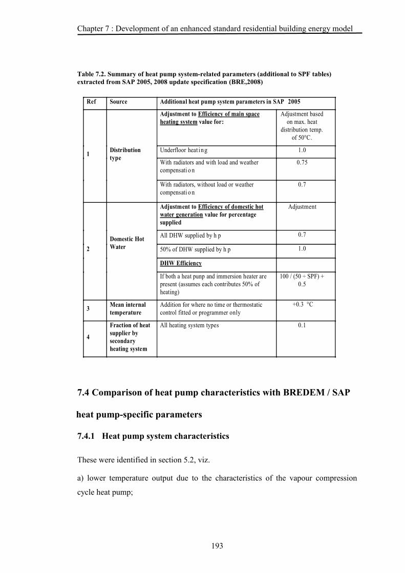
Chapter 7 : Development of an enhanced standard residential building energy model
193
Table 7.2. Summary of heat pump system-related parameters (additional to SPF tables) extracted from SAP 2005, 2008 update specification (BRE,2008)
7.4 Comparison of heat pump characteristics with BREDEM / SAP
heat pump-specific parameters
7.4.1 Heat pump system characteristics
These were identified in section 5.2, viz.
a) lower temperature output due to the characteristics of the vapour compression
cycle heat pump;
Ref Source Additional heat pump system parameters in SAP 2005
Adjustment to Efficiency of main space
heating system value for:
Adjustment based on max. heat
distribution temp. of 50°C.
Underfloor heat i n g 1.0
With radiators and with load and weather compensati o n
0.75 1
Distribution
type
With radiators, without load or weather compensati o n
0.7
Adjustment to Efficiency of domestic hot
water generation value for percentage supplied
Adjustment
All DHW supplied by h p 0.7
50% of DHW supplied by h p 1.0
DHW Efficiency
2
Domestic Hot
Water
If both a heat punp and immersion heater are present (assumes each contributes 50% of heating)
100 / (50 ÷ SPF) + 0.5
3 Mean internal
temperature
Addition for where no time or thermostatic control fitted or programmer only
+0.3 °C
4
Fraction of heat
supplier by
secondary
heating system
All heating system types 0.1

Chapter 7 : Development of an enhanced standard residential building energy model
194
b) variation of source energy over the heating season due to depletion of the ground
as an inter-seasonable store or to the fall in air temperature;
c) CO2 emissions from operating electric heat pumps are due to the carbon intensity
of electricity generation rather than the fuel it consumes;
d) cost of installation of GSHP systems is highly dependent on the size of the system,
especially of the collector;
e) Non-uniform increase in operating cost and CO2 emissions with increase in
indoor/outdoor temperature differential when outside temperature falls below the
system balance point temperature; this being due to the use of additional heat at a
COP < 1.0;
f) Heat pump systems are capable of providing cooling as well as heating.
In this section, each of these characteristics will be examined in turn as to whether or
how they are dealt with by SAP / BREDEM.
7.4.2 Lower temperature output
The temperature of hot water output from fuel burning central heating systems is at
least 80 °C. while the maximum from heat pump systems is around 55-65°C
(McMullan & Morgan, 1981; Ochsner, 2007, p. p37). This characteristic of heat
pump systems is reproduced in the factors dependent on Distribution Type (Ref. 1,
Table 7.2) which reduce the efficiency value used in calculating energy use by a
factor of 0.75 where distribution is by radiators with load and weather compensating
controls and by 0.7 where radiators are used without these controls, basing these
factors on a maximum distribution temperature of 50ºC. This implies that, in the
first case, one third more and in the second, 43% more energy is necessary to
maintain a given temperature with radiator distribution as against underfloor heating.
According to Anderson (Anderson, 2009b) the factors were derived empirically from
statistics of heat pump tests carried out by the Wärmpumpen Testzentrum (WPZ)
(WaermenPumpen Testzentrum, 2011) and are based on the ratio between the
average COP of the systems tested at sink temperatures of 35ºC and 50ºC for both
system types and source temperatures of 0ºC and 7ºC for GSHPs and ASHPs
respectively as shown in the following Figure 7.1, graphically, from experimental

Chapter 7 : Development of an enhanced standard residential building energy model
195
results in the British Standard EN 13516-2-4 (British Standards Institution, 2008a, p.
p115).
The validity of the values derived by this graphical method can be confirmed by
calculating the ratio between the Carnot COP of the perfect heat pump at 0ºC source/
35ºC sink and that at 50ºC sink which gives a value of 0.734, fairly close to the SAP
value; and the same calculation for an ASHP using a source temperature of 7ºC
which gives a value of 0.68. Since this latter calculation is based upon
thermodynamic theory, it could be a better basis for the SAP parameters.
Figure 7.1 Extract from EN 13516-2-4 which illustrates the relationship between CoP and source/delivery temperature
7.4.3 Reduction of source energy over the heating season
The reduction of the energy available from the system source, either by the
extraction of heat from the soil surrounding the collector of a GSHP over the course
of a winter or the reduction of air temperature during the winter for an ASHP,
represents a similar process to the calculations involved in estimating the fall in
efficiency due to raising the sink temperature to that required by radiator distribution
from that required by underfloor heating. They both represent a change in ‘lift’, since
the heat pump has to cope with a fall in sink temperature while maintaining a similar
or higher output temperature.

Chapter 7 : Development of an enhanced standard residential building energy model
196
No attempt is made in BREDEM to estimate this effect since a single COP value is
used throughout the year, despite the introduction of monthly calculations with SAP
2009. In SAP 2009, Appendix N (BRE, 2010a, p. p89), there is the following note
“In reality the space heating efficiency varies through the year according to the
source temperature. The value used in this procedure is adjusted to the total annual
space heating requirement so as to give the correct total fuel use but the monthly
values of fuel use will not be correctly indicated”.
7.4.4 CO2 emissions dependent on the method of electricity generation
Fixed values (Table 12 of SAP 2009) are used in SAP calculations for calculating the
Dwelling and Target Emission Rates of carbon dioxide emissions based on the
‘fuel’ used by the heating system. Up until SAP 2009, the value for carbon emissions
due to electricity generation had been unchanged since the SAP process was
formulated and, at 0.422 KgCO2/kWh, was considerably lower than that obtained
from current official statistics, for which 0.53702 KgCO2/kWh was quoted as a
rolling average (DEFRA, 2008 Annex 3, p4). In this publication, a value of 0.43
KgCO2/kWh is quoted as the marginal rate of emission to be used in calculating CO2
savings. This rate corresponds to the savings due to the ‘non-construction’ of a
combined-cycle gas-turbine power station and is the value used “when appraising
policies that reduce electricity consumption or encourage the use of renewable
electricity” to quote this document. As the calculations in SAP reflect additional
electricity consumption in a new building, the use of a similar value in SAP does not
seem particularly logical and it would be more appropriate to use the rolling average
figure of 0.517 KgCO2/kWh , which now appears to be used in SAP 2009.
7.4.5 Size-dependent cost of installation of GSHP systems
While this particular characteristic is highly significant to the purchaser of a GSHP
system and implies that the sizing of the system warrants considerably more care
than that of a fuel-burning system, it is not germane to an energy model and so is not
included in either the original or the improved version.

Chapter 7 : Development of an enhanced standard residential building energy model
197
7.4.6 Non-uniform increase in operating cost and CO2 emissions with
increase in load
To allow for the energy use of auxiliary electric heating in bivalent parallel
operation, SAP/BREDEM reduces the fixed COP values used from 320% to 300%,
i.e. by about 6.3%, for GSHPs, giving a corresponding increase in the energy use for
the dwelling. This value is based on the performance of the system documented in
the GIR 72 monitoring report produced by BRECSU (Anderson, 2009a; BRECSU,
2000). Since the additional heaters do not operate continuously, but only when the
main heat pump is unable to balance the energy load below a design external
temperature, this method of estimation does not reflect correctly the heat pump’s
change in energy consumption in response to an overall rise in ambient temperature.
To allow SAP/BREDEM to be used under conditions of climate change, a
calculation method is required for the energy contribution of the additional heating
that relates directly to ambient temperature.
The above fixed parameters are improved upon by the SAP 2009 Appendix N/Q
calculations, which derive a Secondary Heating Fraction value which relates to the
Plant Size Ratio (ratio of the heat pump rated output to the dwelling design heat loss)
but this is limited to those heat pumps for which there are data base entries, and no
attempt is made to generalise the calculation.
7.4.7 Cooling energy consumption
Provision has been made in the latest version of SAP 2009 for the estimation of
cooling loads and consequent energy consumption and costs. These are estimated
according to the heat transfer coefficient, total gains, external temperature for the
region and month concerned, based on a standard internal temperature of 25°C,
reduced according to the fraction of the dwelling cooled and by an intermittency
factor based on the Thermal Mass Parameter and Heat Loss Parameter for the
dwelling. The cooling load equations used are detailed in Tables 10, 10a, 10b of the
SAP 2009 document (BRE, 2010a) with the method for estimating energy
consumption in Table 10c and the fuel cost, CO2 emission factor and primary
emission factor values are those for electricity in Table 12 .

Chapter 7 : Development of an enhanced standard residential building energy model
198
7.5 Replacement estimation methods
7.5.1 Objectives
In the previous section, the following deficiencies were identified in the BREDEM-8
estimation process and this study will endeavour to provide solutions for them:
a) use of a fixed value for system efficiency, thereby ignoring any variations between
heat pump systems from different manufacturers and neglecting the variation in
system efficiency over seasons due to variation in source temperatures;
b) the use of an empirically-estimated variation to this fixed system efficiency value
to adjust for the different temperatures required for different distribution systems
rather than basing the variation on thermodynamic theory; even this limited
estimating process is absent from BREDEM-8, which ignores the distribution type
altogether;
c) estimating the energy consumption of additional heaters in bivalent parallel
operation by a reduction of the value of the fixed system efficiency; this would over-
estimate the value of this reduction if there was a substantial overall rise in ambient
temperature. The use of a single value for the year for the Secondary Heat Fraction
has an identical disadvantage.
d) omission of an estimate of energy use for space cooling.
7.5.2 Approach
Rather than approach these in a piecemeal approach, it is considered by the author
that it is better to document all the replacement methods together, then indicate
which deficiencies have been addressed. It is thought that this provides a clearer
exposition of the topic.
7.5.3 Determining heat pump system efficiency
In Section 2.4.2 of this study, the calculation of the Carnot COP for a heat pump was
described in Equation 2.6. This relates the theoretical maximum COP of the heat
pump to the temperature differential between the source temperature (external air or
soil) and the sink temperature (the temperature output to the distribution). As this
differential increases, the value of the Carnot COP falls towards unity, and, as a real

Chapter 7 : Development of an enhanced standard residential building energy model
199
heat pump system can achieve a COP of only a fraction of this ideal value, the COP
of a real system will fall in the same way. Thus the COP of a heat pump system is
heavily dependent on the source / sink temperature differential – commonly known
as the ‘lift’ – required for the given heating load. Combining the objectives stated in
paragraph 7.5.1 (a) and (b) of estimating the effect of variations of source
temperature and of the different requirements of different distribution systems, the
net effect of these variations is to change the lift required of the system. If the
numerical relationship between the COP and the ‘lift’ is known, then a value for the
COP may be estimated that reflects both changes in source and sink temperatures.
7.5.4 Numerical relationship between COP and ‘lift’
While, in theory, it would be possible to estimate parameters for this relationship
using the data collected for this study, the resultant analysis showed only a small
degree of correlation, of which Figure 7.2 below is typical. Analysis for the data
from the Wärmpumpentestzentrum heat pump tests provided better results as per
Figure 7.3.
Figure 7.2. Dwelling 2: Coefficient of Performance against Lift

Chapter 7 : Development of an enhanced standard residential building energy model
200
Figure 7.3. COP to 'lift' data points from one week's test results from WPZ for air source and ground source heat pump system, with trend lines
The results in the above graph come from 200 samples from 22 ground source heat
pumps and 497 samples from 92 air source heat pumps. This data shows a reasonably
high degree of negative correlation between ‘lift’ and COP as would be expected
from theory. Thus, it would seem appropriate to use the equations derived from this
data to estimate COP values from estimates of lift values.
7.5.5 Estimation methods for ‘lift’
7.5.5.1 Source and sink temperature estimation
Because of the different ways by which they are determined, different estimation
methods are required for each of these temperature values. Further, different methods
are required for the different source types.
For the purposes of this study, it is considered that estimation methods for three
source types, air, borehole, and ground loop, are required. The various other sources
in use – surface water (lake, river or sea), ground water, exhaust air - have been
omitted as they are mostly used only in commercial buildings.
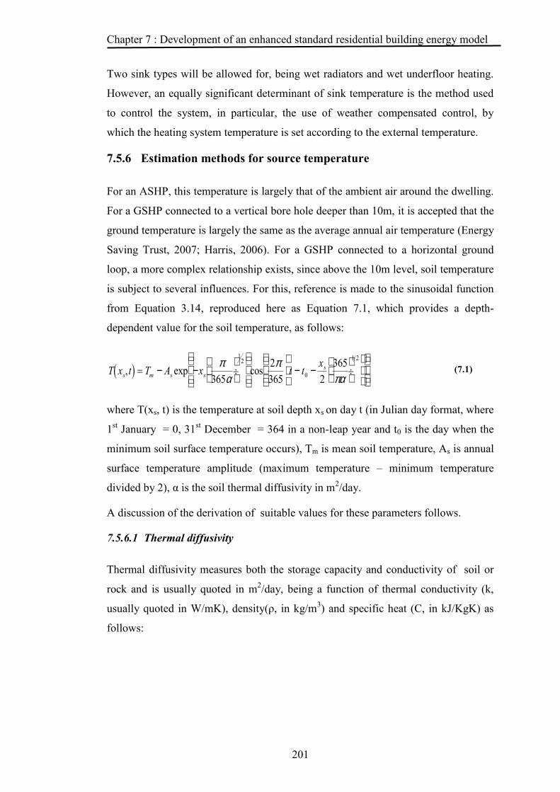
Chapter 7 : Development of an enhanced standard residential building energy model
201
Two sink types will be allowed for, being wet radiators and wet underfloor heating.
However, an equally significant determinant of sink temperature is the method used
to control the system, in particular, the use of weather compensated control, by
which the heating system temperature is set according to the external temperature.
7.5.6 Estimation methods for source temperature
For an ASHP, this temperature is largely that of the ambient air around the dwelling.
For a GSHP connected to a vertical bore hole deeper than 10m, it is accepted that the
ground temperature is largely the same as the average annual air temperature (Energy
Saving Trust, 2007; Harris, 2006). For a GSHP connected to a horizontal ground
loop, a more complex relationship exists, since above the 10m level, soil temperature
is subject to several influences. For this, reference is made to the sinusoidal function
from Equation 3.14, reproduced here as Equation 7.1, which provides a depth-
dependent value for the soil temperature, as follows:
T xs,t( ) = Tm - As exp -xsp
365a
æ è ç
ö ø ÷
12ì
í ï
î ï
ü ý ï
þ ï cos
2p
365t - t0 -
xs
2365pa
æ è ç
ö ø ÷
1 2é
ë ê
ù
û ú
ì í ï
î ï
ü ý ï
þ ï (7.1)
where T(xs, t) is the temperature at soil depth xs on day t (in Julian day format, where
1st January = 0, 31st December = 364 in a non-leap year and t0 is the day when the
minimum soil surface temperature occurs), Tm is mean soil temperature, As is annual
surface temperature amplitude (maximum temperature – minimum temperature
divided by 2), α is the soil thermal diffusivity in m2/day.
A discussion of the derivation of suitable values for these parameters follows.
7.5.6.1 Thermal diffusivity
Thermal diffusivity measures both the storage capacity and conductivity of soil or
rock and is usually quoted in m2/day, being a function of thermal conductivity (k,
usually quoted in W/mK), density(ρ, in kg/m3) and specific heat (C, in kJ/KgK) as
follows:
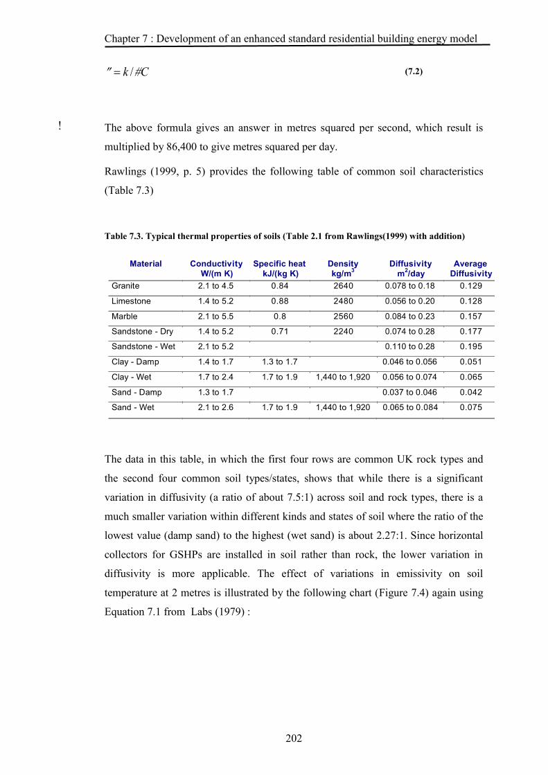
Chapter 7 : Development of an enhanced standard residential building energy model
202
!
² = k /#C (7.2)
The above formula gives an answer in metres squared per second, which result is
multiplied by 86,400 to give metres squared per day.
Rawlings (1999, p. 5) provides the following table of common soil characteristics
(Table 7.3)
Table 7.3. Typical thermal properties of soils (Table 2.1 from Rawlings(1999) with addition)
The data in this table, in which the first four rows are common UK rock types and
the second four common soil types/states, shows that while there is a significant
variation in diffusivity (a ratio of about 7.5:1) across soil and rock types, there is a
much smaller variation within different kinds and states of soil where the ratio of the
lowest value (damp sand) to the highest (wet sand) is about 2.27:1. Since horizontal
collectors for GSHPs are installed in soil rather than rock, the lower variation in
diffusivity is more applicable. The effect of variations in emissivity on soil
temperature at 2 metres is illustrated by the following chart (Figure 7.4) again using
Equation 7.1 from Labs (1979) :

Chapter 7 : Development of an enhanced standard residential building energy model
203
Figure 7.4. Soil temperature estimated from Equation 6.1 for different values of soil thermal diffusivity
The above curves are calculated using fairly typical values for the variables, viz.
mean soil temperature = 10ºC, annual surface temperature amplitude of 13ºC, soil
depth of 2m, Julian day of minimum soil surface temperature = 24. Jenkins et al
(2009), in simulating the variations in soil diffusivity, found that ‘changing the soil
type only affects the system COP by 1 – 2%’. This finding does not entirely gel with
the approximately 2.5ºC difference between the estimates for the highest and lowest
diffusivities in the above figure, particularly since these values coincide with the
coldest and hottest parts of the year. Harris (2006) comments that “soil types, and
thermal properties, may vary with depth” and that “variation in soil type may lead to
differences in the way moisture percolates through the layers”. While such
complexities may be included in models, the level of uncertainty in knowledge of
soil properties means that this may not lead to any measurable improvement in
accuracy. As can be seen from Table 7.3, thermal diffusivity also varies with soil
moisture content, and it may differ radically for ‘made ground’ at brown field sites
(Harris, 2006). Thus, it is probably necessary to make an arbitrary choice, the mean
value, 0.058 m2/day, from Table 7.3 being appropriate.
7.5.6.2 Mean soil temperature
This has been taken by other researchers (Zogou & Stamatelos, 1998) and
practitioners (BSRIA, 2004; Rawlings, 1999; Viessmann UK, 2004) to be the so-

Chapter 7 : Development of an enhanced standard residential building energy model
204
called ‘far field’ temperature (that of the soil below the influence of air temperature –
about 10m down) which again is equal to the mean air temperature - between 10 –
14 ºC, depending on location. Jenkins et al (2009) found the value to be 10 ºC at
Rothamsted. Annual average soil temperature at 10 cm and 30 cm depths is available
from the ten other sites in the Environmental Change Network (2009). Harris (2006)
quotes Labs (1979) that the mean soil temperature can be calculated by adding 1.7 ºC
to the mean air annual air temperature, but adds that this should be lower in the UK,
failing to add how much lower.
7.5.6.3 Day number for minimum soil surface temperature
Values for this in the UK are obtainable from the Environmental Change Network
summary data but only to the nearest month. Raw, daily data could be acquired to
ascertain an exact Julian day, although interpolation between the monthly values
might probably be accurate enough. From physical geography, Harris (2006)
calculates a value of day 36, based on the 46 day lag of the surface temperature wave
behind the solar radiation wave, which has its minimum at the winter solstice, Julian
day 355. Jenkins et al (2009) use day 24 in their Rothamsted comparison.
7.5.6.4 Annual surface temperature amplitude
Values for this in the UK may be calculated from the Environmental Change
Network summary data. Labs (1979) states that a suitable value can be estimated by
dividing the difference between the July and January monthly average temperature
and adding 1.1 ºC.
7.5.6.5 Soil – ground loop return temperature differential
While equation (7.1 provides an estimate of soil temperature, for GSHPs, this does
not equate to the temperature of the fluid return from the ground loop required to
calculate the heat pump lift since the acquisition of heat can never be perfect.
In order to estimate a relationship between soil temperature and the return
temperature from the ground loop, the following was carried out:
a) the day’s average of the return temperature from the ground loop to the heat
pump was calculated at seven-day intervals for the each set of heat pump data for

Chapter 7 : Development of an enhanced standard residential building energy model
205
the monitored dwellings and plotted against Julian day within the year. A second
order polynomial trend line was calculated by the software for the resultant plot.
b) a curve was plotted using Equation 7.1 using the same Julian day values for the
variable t, with mean soil temperature, Tm = 10 ºC, As = 13ºC, α = 0.061 m2/day
and t0 = 5.
For the three dwellings being monitored, this produced the following three figures
(Figure 7.5, Figure 7.6 & Figure 7.7)
Figure 7.5. Monitored dwelling 1 - Comparison of predicted weekly soil temperatures at 1.2m depth with day's average of return temperatures from ground loop to heat pump at seven day intervals

Chapter 7 : Development of an enhanced standard residential building energy model
206
Figure 7.6. Monitored dwelling 2 - Comparison of predicted weekly soil temperatures at 1.2m depth with day's average of return temperatures from ground loop to heat pump at seven day intervals
Figure 7.7. Monitored dwelling 3 - Comparison of predicted weekly soil temperatures at 1.2m depth with day's average of return temperatures from ground loop to heat pump at seven day intervals
This shows an average difference of about 3.5 ºC between estimated soil temperature
and the trend values for the return temperature from the ground loop over much of
the heating season, about the first 80 days of the year.

Chapter 7 : Development of an enhanced standard residential building energy model
207
7.5.7 Estimating methods for sink temperature
The other value which must be estimated for the system ‘lift’ is the required output
temperature to the system sink, that is, the dwelling distribution system. This value is
determined by the type of distribution system and the type of control system
installed.
7.5.7.1 Distribution systems
The main type of distribution system to be found in existing UK homes is a wet
radiator system. With a fuel-fired boiler, this has a usual operating temperature of 80-
90 ºC and the radiators will be sized to provide sufficient heat at this temperature.
Thus if a heat pump system is retro-fitted to a radiator system, its operating
temperature is deemed to be the highest economic for a heat pump, around 50 ºC.
The alternative to wet radiators, wet underfloor heating, is judged to operate at the
lower temperature of 35 ºC because of the much large surface area available. While
this lower temperature is not explicitly stated in SAP, the effect of the relative
temperatures is used to modify the value of the fixed value used for the system COP.
See Table 7.2, Item 1.
7.5.7.2 Control system
In the SAP calculations, the presence or absence of load or weather compensation
controls is also used in determining the value of any adjustment applied to the system
COP, also without noting the relationship with operating temperature.
For the purposes of this study, the most relevant form of the control is that of weather
compensation, the effect of which is to adjust the target temperature within the
distribution system according to the external temperature. This adjustment is made
according to a function within the controller which calculates a target temperature for
the heat pump from the current external temperature based on a so-called heating
curve, examples of which follow (Figures 7.8 & 7.9).
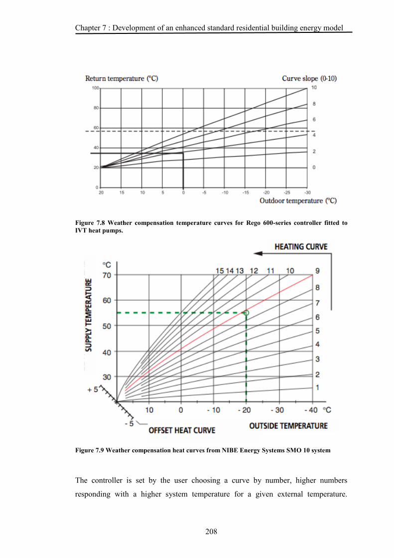
Chapter 7 : Development of an enhanced standard residential building energy model
208
Figure 7.8 Weather compensation temperature curves for Rego 600-series controller fitted to IVT heat pumps.
Figure 7.9 Weather compensation heat curves from NIBE Energy Systems SMO 10 system
The controller is set by the user choosing a curve by number, higher numbers
responding with a higher system temperature for a given external temperature.

Chapter 7 : Development of an enhanced standard residential building energy model
209
Higher curves are recommended for radiator systems, lower for UFH. Thus, if the
function to calculate the target temperature for the heat pump output is known or can
be determined, this can be used to estimate a value for the sink temperature from the
external temperature. However, as might be expected, weather compensation
functions are not uniform across heat pumps, either in their slopes or their
configuration within the system. The two examples above differ in that the first is
configured to use the return temperature from the distribution system as a target, the
second to use the supply temperature, the first set of functions are simple linear
relationships, the second slightly more complex curves. However, since, in practice,
the effect of one weather compensation function set should be largely similar to any
other, and greater variation in temperature conditions will be provided by the
dwellings in which they are installed and by the usage of their inhabitants, the choice
of an arbitrary but known set of functions would appear justifiable.
For the purposes of the current study, it is disadvantageous that the controller in the
monitored IVT heat pumps tracks the distribution return temperature in comparison
with the target output from the weather compensation algorithm, since the return
temperature to the heat pump does not provide a particularly useful basis from which
to estimate the supply temperature as indicated by the following figures (Figure 7.10,
Figure 7.11 & Figure 7.12) which plot daily averages of these temperatures against
external temperature:
Figure 7.10. Dwelling 1 - Distribution system temperatures against external temperatures

Chapter 7 : Development of an enhanced standard residential building energy model
210
Figure 7.11. Dwelling 2 - Distribution system temperatures against external temperatures
Figure 7.12. Dwelling 3 - Distribution system temperatures against external temperatures
Applying a different analysis provides some clarification. By looking at a single
day’s worth of data, in particular one when the heat pump was in operation, if not the
whole day, at least a very large proportion thereof, then the following set of graphs
can be derived (Figures 7.13, 7.14 & 7.15):

Chapter 7 : Development of an enhanced standard residential building energy model
211
Figure 7.13. Dwelling 1 - Distribution supply and return temperature differential
Figure 7.14. Dwelling 2 - Distribution supply and return temperature differential

Chapter 7 : Development of an enhanced standard residential building energy model
212
Figure 7.15. Dwelling 3 - Distribution supply and return temperature differential
The figures all contain curves for five quantities: the supply and return temperatures
to the distribution system (either UFH or radiators, depending on the dwelling) and
the difference between these two; and the temperatures at the internal and external
sensors. Where appropriate, other quantities are included: an estimate of the target
temperature being applied by the weather compensation algorithm; an estimate of the
energy use for additional heat to maintain the temperature when the heat pump
cannot; an indication of when DHW was being generated.
Of these figures, Figure 7.15 is by the simplest and provides a value of 10ºC for the
supply / return differential for an underfloor heating system. The other two are are
more complex, since the supply temperature over the day selected is influenced by
the operation of the additional heating in Figure 7.13 and by hot water generation in
Figure 7.14. However, it would appear that, in a ‘steady state’, the value for the
difference between supply and return temperatures is approximately 7 ºC in dwelling
1 and approximately 4ºC in dwelling 2.
7.5.8 Energy use for secondary heating – bivalent operation
7.5.8.1 General characteristics
Bivalent operation is employed to allow the installation of a heat pump system of
smaller capacity than would be necessary to balance the heat load of the dwelling at
the lowest occurring external temperature. A design decision is made as to the lowest

Chapter 7 : Development of an enhanced standard residential building energy model
213
external temperature which will be balanced by the main system – the balance point -
with a form of auxiliary heating being switched in when the external temperature
falls below this value, either as a boost to the heat pump which continues operating
or as a replacement for the heat pump, which is turned off. Thus, the energy
consumption of additional heaters or a secondary system is dependent on the the
heating degree days of the periods during which the external temperature is below
the balance point temperature (CIBSE, 2006).
7.5.8.2 Balance point temperature
A value for the balance point temperature was obtained empirically from the
monitored data as follows:
a) selecting all those samples where i) the heat pump compressor was operating;
ii) one or other of the additional heaters was switched on; iii) the three-way valve
was directing the output to the distribution system, rather than the hot water tank.
b) creating a histogram of the percentage frequencies (Figure 7.16) of the external
temperatures from each of these samples.
Figure 7.16. Percentage frequencies of bivalent operating temperatures

Chapter 7 : Development of an enhanced standard residential building energy model
214
From Figure 7.16, it can be observed that the additional heaters are most likely to
start operating at approximately 3ºC or below and this value has been used by the
author in calculations.
7.5.8.3 Heating degree days
Hitchin (Hitchin, 1983, 1990) provides an equation which estimates the number of
heating degree days which will occur in a month as follows:
DD(tb ) = N(tb - t0 ) / 1- exp -k tb - t0( )( )( ), tb ¹ t0
= N /k, tb = t0 (7.2)
where tb = base temperature, t0 = monthly mean external temperature, N is the
number of days in the month, DD(tb) is the conventional notation for the number of
heating degree days to the base tb and k is a constant for which Hitchen recommends
a value of 0.71 although BREDEM-8 uses 1.1. This allows the calculation of both the
heat output required at the balance point temperature and that required at the lowest
temperature expected, given the average monthly temperature, which is the value of
tb for which DD(tb) = 0, using an equation of the form:
Qt =H.DD t( ) (7.3)
where Qt is the heat required to maintain internal temperature t, H is the heat loss
parameter for the building in W/ºC, DD(t) is the number of heating degree-days for a
base temperature t.
7.5.8.4 Choice of estimating methods
For the purpose of this study it was decided that where possible any additional
estimation methods should use the same or similar methods as those already present
in BREDEM-8. It was identified that a) the characteristics of the energy consumption
of electric boiler systems are analogous to those of a heat pump system operating in
bivalent parallel mode; b) those of heat storage radiators are analogous to those of
bivalent alternate mode operation, so these methods were adapted for these purposes.

Chapter 7 : Development of an enhanced standard residential building energy model
215
7.5.8.5 Bivalent parallel operation
The distinguishing characteristic of this mode of operation is that when the external
temperature drops below the balance point temperature, the secondary heating
system cuts in to ‘top up’ the output from heat pump to maintain the internal
temperature and both systems will operate simultaneously. Section 11.2.5 of the
BREDEM-8 document provides a method for estimating the energy use of an electric
boiler system, operating using off-peak electricity to store heat in a buffer tank. It is
assumed that if the capacity of the buffer tank is insufficient to balance the heating
load for the external temperature during peak time, then on-peak electricity is used to
maintain the demand by reheating the tank.
The steps in this method estimate, first, the quantity of heat that such a system can
store given its rated energy output and the duration for which electricity is available
at reduced, ‘off-peak’ rates, assuming that all the heat generated can be stored;
secondly, an estimate is calculated for the ‘saturation’ temperature which is the
lowest external temperature for which the stored heat can maintain the required
indoor temperature.
From the value of the saturation temperature, the additional heat required to ‘top up’
the output from the stored heat may be calculated using the dwelling heat loss
parameter and the degree-days value for the saturation temperature. TSat is calculated
as follows:
(7.4)
where H1 & H2 are the heat loss parameters, T1 & T2 are mean internal temperatures,
G2 & G2 are the useful gains for the two zones defined in the BREDEM-8 model and
Cmax is the average heat output of the boiler. The next step in BREDEM-8 is to
calculate the additional heat required to heat the house to TSat, which is given by the
standard degree days formula:
(7.5)
If the initial calculation of Tsat is omitted and replaced by a balance point temperature
value of 3ºC as per para 7.5.8.2, then this method corresponds to that required to

Chapter 7 : Development of an enhanced standard residential building energy model
216
estimate the energy (Qon) required to ‘top up’ the output of a heat pump system to
maintain the demand temperatures at external temperatures below the balance point
temperature as follows:
Qon = H .DD Tbp{ } (7.6)
where H is the heat loss parameter in W/K, DD{Tbp} is the monthly degree-days for
base temperature Tbp. The portion of the heat output generated by the main heat pump
system, QHP, is then estimated by simple subtraction from the total heating load on
the dwelling, viz.
QHP =Qh -Qon (7.7)
where Qh = monthly space heating energy requirement as defined in the BREDEM-8
document, and Qon = the additional heat requirement.
7.5.8.6 Bivalent alternate operation
As indicated above in Section 7.5.8.1, this mode is characterised by the secondary
heating system cutting in to replace the heat pump system at the balance point
temperature. This is not a situation with which the BREDEM-8 routines cope
explicitly. However, examination of the routines to estimate the energy use of
storage heater systems shows that these systems have characteristics similar to
bivalent alternate operation, in that once their relatively fixed heat capacity has been
exhausted, further heat cannot be generated immediately and a second system must
be brought into operation to maintain the demand temperature. The equations used in
the routines for storage heaters are complicated by allowances for the characteristics
of these devices and some of these can be removed for simplification. The most
significant of these is the allowance for the lack of controllability of the storage
heaters which allows heat to ‘leak’ out from them during the periods when the
heating system would normally be switched off, contributing to the background
temperature. For the purpose of this current routine, this assumption will be omitted.
The steps involved in this method in BREDEM again involve the calculation of a
saturation temperature, TSat , with the same meaning as above. This is then used with
the base temperature for the dwelling to calculate the average rate of off-peak
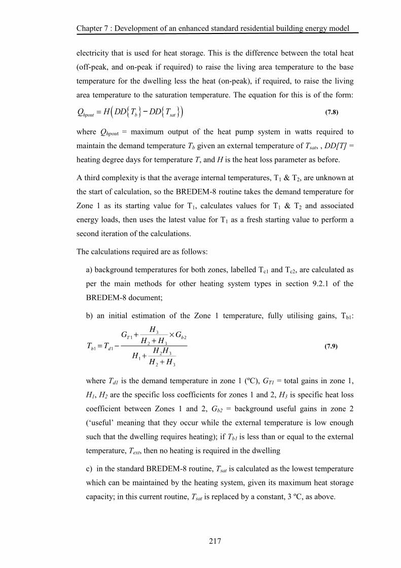
Chapter 7 : Development of an enhanced standard residential building energy model
217
electricity that is used for heat storage. This is the difference between the total heat
(off-peak, and on-peak if required) to raise the living area temperature to the base
temperature for the dwelling less the heat (on-peak), if required, to raise the living
area temperature to the saturation temperature. The equation for this is of the form:
Qhpout = H DD Tb{ } -DD Tsat{ }( ) (7.8)
where Qhpout = maximum output of the heat pump system in watts required to
maintain the demand temperature Tb given an external temperature of Tsat, , DD[T] =
heating degree days for temperature T, and H is the heat loss parameter as before.
A third complexity is that the average internal temperatures, T1 & T2, are unknown at
the start of calculation, so the BREDEM-8 routine takes the demand temperature for
Zone 1 as its starting value for T1, calculates values for T1 & T2 and associated
energy loads, then uses the latest value for T1 as a fresh starting value to perform a
second iteration of the calculations.
The calculations required are as follows:
a) background temperatures for both zones, labelled Tc1 and Tc2, are calculated as
per the main methods for other heating system types in section 9.2.1 of the
BREDEM-8 document;
b) an initial estimation of the Zone 1 temperature, fully utilising gains, Tb1:
(7.9)
where Td1 is the demand temperature in zone 1 (ºC), GT1 = total gains in zone 1,
H1, H2 are the specific loss coefficients for zones 1 and 2, H3 is specific heat loss
coefficient between Zones 1 and 2, Gb2 = background useful gains in zone 2
(‘useful’ meaning that they occur while the external temperature is low enough
such that the dwelling requires heating); if Tb1 is less than or equal to the external
temperature, Text, then no heating is required in the dwelling
c) in the standard BREDEM-8 routine, Tsat is calculated as the lowest temperature
which can be maintained by the heating system, given its maximum heat storage
capacity; in this current routine, Tsat is replaced by a constant, 3 ºC, as above.

Chapter 7 : Development of an enhanced standard residential building energy model
218
d) a first value for the required output from heat pump, which corresponds to the
stored heat energy generated using off-peak electricity in the original routine, is
calculated as follows:
(7.10)
where Qhpout= maximum output of the heat pump system in watts required to
maintain the demand temperature Tb1 given an external temperature of Tsat, d is
the number of days in the current month, DD{T} = heating degree days for
temperature T, and H1, H2 and H3 are as before;
e) the standard BREDEM routine next calculates a value for the rise in
temperature in both zones due to the uncontrolled heat output from the storage
heaters, which will be omitted from this routine, as detailed above,
f) mean internal temperatures, T1 and T2, are calculated using the standard
BREDEM-8 methods in section 9.3 of the BREDEM document, from which
heating loads (in GJ) for each month for both zones are calculated as follows:
(7.11)
in which values are as before with the exception of G1 and G2 which are the
average daily heat gains in zones 1 and 2 respectively; and the total monthly
heating (also in GJ) allowing for savings due to a conservatory as follows;
(7.12)
f) the demand temperature for zone 1, Td1, was used as starting value for the
internal average temperature (normally T1) in this zone. From this, a new, more
accurate value for T1 has been calculated as per paragraph (e) above. A second
iteration is then performed replacing Td1 in Equations 13 and 14 to obtain a new
value for Qhpout.
g) values for the main heat pump system (Qprim) and the secondary system (Qsec )
energy in GJ are calculated as follows:

Chapter 7 : Development of an enhanced standard residential building energy model
219
(7.13)
and
(7.14)
where εhp and εsec are the COP of the heat pump and the efficiency of the
secondary system, respectively.
7.5.9 Estimation of cooling energy consumption
A routine based on that used in SAP version 9.90 (BRE, 2009a, Tables 10, 10a, 10b)
is used to estimate energy requirements for space cooling. This has the following
parameters, with the defaults used in parentheses:
a) type of cooling equipment (0 = none, 1 = reversible heat pump system, 2 =
dedicated air conditioner)
b) thermal mass parameter for the dwelling (250 kJ/m2K – median value from
SAP 9.90 Table 1d)
c) internal temperature at which cooling starts (25ºC)
d) cooling temperature (18ºC)
e) fraction of total floor area cooled (100%)
f) Seasonal Energy Efficiency Ratio (SEER) for a dedicated air conditioning
system (2.0 – assumed Energy Label class G from SAP 9.90, table 10c)
The routine follows SAP 9.90 (BRE, 2010a), tables 10, 10a, 10b & 10c. It returns the
following values:
the annual cooling energy requirement (kWh);
the annual cooling energy use (kWh, GJ).
The SAP calculation is itself based on the similar calculation method in the BS EN
ISO 13790 standard for estimating on a monthly basis (British Standards Institution,
2008b, pp. 64 - 68,).

Chapter 7 : Development of an enhanced standard residential building energy model
220
7.6 Validation
7.6.1 Comparison with standard BREDEM estimate for dwelling with
heat pump
Figure 7.17 shows the difference between energy consumption estimates using
identical parameters for the built form of the dwelling, with the upper graph using the
original BREDEM heat pump parameters and the lower using the enhanced
BREDEM model, both with a GSHP using a soil collector. The lower figure
indicates that the enhanced model is much more responsive to variation in ambient
temperature since no energy is used by secondary space heating (additional heaters)
outside the heating season, with heating coming from the main system only ie.
relying totally on the heat pump compressor. The response to the change in ambient
temperature throughout the year indicates that the model will respond correctly to the
overall changes occurring under conditions of climate change.

Chapter 7 : Development of an enhanced standard residential building energy model
221
Figure 7.17 Comparison between BREDEM-8 energy consumption estimates, original & enhanced
7.6.2 Seasonal performance factor (SPF)
The heat pump model calculates Seasonal Performance Factor on a monthly basis,
which is necessary to estimate peaks in electricity usage which cannot be identified
by a yearly average. The SPF value estimated by the model, as shown in Figure 7.17
responds correctly to the change in source temperature throughout the year, initially
falling due to the reduction in source temperature and increase in the required output
temperature, then rising as both the source is recharged by solar gain and ambient
temperature increases. As the need for space heating reduces, DHW energy
requirements form a greater proportion of the energy load, and with the higher output
temperature required for this, causes a reduction in SPF. The end of the summer
causes space heating to increase as a proportion of the load and, with the recharge of
solar gain in the soil, the corresponding reduction in the average distribution
temperature indicates a peak in SPF, again falling away as the soil temperature
reduces and the heating load increases. While in practice, the shape of this curve may

Chapter 7 : Development of an enhanced standard residential building energy model
222
vary, depending on the relative sizing of the heat pump system to the building loads,
the curve in Figure 7.17 indicates that the model behaves as would be expected when
the system is correctly sized.
The effect of space cooling must also be anticipated, since it is to be assumed for the
purpose of this study that the heat pump systems involved will be reversible.
Including this load is expected to cause the SPF value to rise significantly, since the
load value is comparatively small, involving a small lift value between the required
cooling temperature and the soil temperature. The results produced by the model are
indicated by Figure 7.18, for which the space cooling load has been increased by
'morphing' the existing BREDEM-8 monthly average temperatures according to the
UK Climate Projection (described in more detail in Section 8.3.4.2. These results
appear to be consistent with what would be expected.
Figure 7.18 Effects of space cooling load on heat pump SPF, combined with external temperatures 'morphed' to 2050 values.
7.7 Discussion
7.7.1 Deficiencies of revised heat pump system energy model
a) Accuracy of temperature values:
The method used to estimate source and sink temperature could give rise to a degree
of error, but this is considered to fall within acceptable limits. The values used in
estimating the system source and sink temperatures in Sections 7.5.6 and 7.5.7 are
taken from the heat pump monitoring study documented in Section 6.2 using the heat
pump control sensors, which could not be calibrated for accuracy. The temperatures

Chapter 7 : Development of an enhanced standard residential building energy model
223
are recorded to one decimal place, relying for their output values being of the correct
order of magnitude on their use in the control of the heat pump and its maintenance
of comfort temperatures in the dwelling. The three installations in the monitoring
study also constitute a very small data sample.
b) Use of arbitrary values and selections
The following arbitrary values and selections are utilised in this procedure:
Values of 35 and 55 ºC for sink temperatures for UFH and radiator system
respectively where weather compensation controls are not used; these are
‘accepted’ values and it has not been possible to confirm or refute them;
Values of 10 ºC and 7 ºC for the difference between the supply and return
temperatures across UFH and radiator systems, respectively; insufficient data
has been gathered from dwellings of different built forms and heat
distribution systems to confirm these values;
the utilisation of curves from IVT heat pumps to calculate target temperatures
for weather compensation controlled operation; the target values that they
return for a given external temperature will almost certainly differ from others
installed in other heat pumps; this was compensated for by the substantial
amount of data available from the monitoring process;
the selection of weather compensation curves for the estimation of UFH and
radiator target temperatures; this was based on those set on the controllers in
the appropriate dwellings and, as such, is drawn from a samples of only one
and two, respectively;
choice of values for the variables in Equation 7.1: since BREDEM utilises a
geographic division of the British Isles into only 21 different regions on the
basis of average monthly temperature, it is unlikely that soil diffusivity will
be similar across these regions; equally, those practitioners (Harris, 2006;

Chapter 7 : Development of an enhanced standard residential building energy model
224
Jenkins, D. P., et al., 2009) who have attempted to validate Equation 7.1 have
utilised various values for t0, the ‘coldest soil temperature’ day, with only
Harris (2006) selecting the day number on the basis of the theoretical lag
between the surface temperature wave and the day of minimum solar
radiation;
b) Omissions
In SAP, an adjustment of +0.3 ºC (DCLG, 2008b, p. 131,Tables) is made to the
internal temperature for the dwelling in the estimation for heat pumps with no
thermostat or other form of control. This has been omitted from the routine, since the
author has not found such a system on sale.
7.8 Summary
7.8.1 Completion of Objective 4
This Chapter has documented the process of developing a heat pump energy model
and an associated dwelling energy model to fulfill Objective 4 of this study. The
chapter has summarised the available UK standard residential energy models and
indicated that, out of those standard models which form the basis for the national
modelling of domestic energy use, BREDEM-8 is deemed particularly suitable for
this study because of its provision of monthly estimates. This is as opposed to the
BREDEM-12 model, which creates estimates on a yearly basis, or the SAP model,
which contains extra calculations for cooling energy consumption and for calculating
SAP and environmental impact ratings based on energy consumption and carbon
emissions respectively. The procedures and their parameters used for estimating heat
pump energy consumption in the BREDEM / SAP models have been detailed, their
deficiencies indicated and replacement estimating procedures defined.
7.8.2 Summary of BREDEM / SAP heat pump parameters and
replacement estimation methods
Table 7.4 contains a list of these.

Chapter 7 : Development of an enhanced standard residential building energy model
225
Table 7.4. Summary of changes to SAP / BREDEM for this study
Characteristic SAP / BREDEM Proposed Efficiency / SPF values
Fixed values, possibly from previous studies
Regression model based on standard test results estimating SPF as a function of ‘lift’ - source minus sink temperature - on a monthly basis.
Effect of different source type
Fixed efficiency / SPF value for each source type (water, air, soil). Does not distinguish between horizontal ground loop and bore hole.
Source temperature estimation method for each source type on a monthly basis.
Effect of different sink (distribution) type
Adjusts SPF by a factor according to whether UFH or radiators in the system or whether the system has weather compensation controls. Factors range between 1.0 and 0.7. Affects the value of the ‘Responsiveness’ variable which represents the speed at which heating system cools after being turned off and hence determines the background temperature.
Explicitly sets sink temperature value according to distribution type, using default values for systems without weather compensation and calculating a value using a weather compensation algorithm from a known controller with monthly average external temperature as a parameter. Retains the 'responsiveness' calculation without change.
Energy use for DHW generation
Uses same Efficiency/SPF value as space heating estimate.
Recalculates SPF from regression model with ‘lift’ based on a sink temperature of 55 ºC.
Secondary space heating
Estimated as a fixed fraction of main space heating energy consumption
Two different estimation routines based on bivalent parallel and bivalent alternate modes of operation, with a third 'null' option of monovalent mode with all space heating provided by the heat pump system.
Space cooling energy consumption
Not present in BREDEM. In SAP 9-90, contains a single parameter for the SEER of the cooling system
Single SEER parameter is replaced monthly value calculated using heat pump model based on fixed sink temperature value and monthly average external temperature

226
CHAPTER 8 FUTURE ENERGY CONSUMPTION EFFECTS OF
RESIDENTIAL HEAT PUMP DEPLOYMENT

Chapter 8 : Future energy consumption scenarios for residential heat pumps
227
8.1 Introduction
Objective 5 of this study is to examine the effects of potential future take-up of
domestic heat pump equipment on the UK electricity supply and carbon emissions.
This will involve the development of a disaggregated domestic energy model based
on the English House Condition Survey data, using the enhanced BREDEM-8 model
defined in Chapter 7.
To this end, this chapter contains the following:
For the English Housing Survey (EHS), a summary of its structure with a detailed
description of the reasoning behind its choice and of the physical survey data which
is incorporated into this study;
For the enhanced BREDEM-8 model, a description of its linkage to the EHS sample
data with particular reference to the inference techniques used to provide the multiple
parameters required for the estimation of building energy use in this type of model; a
description of the methods developed to create sample-level energy and CO2
(operational and embedded) estimates for the EHS extract table in building a
Domestic Energy Model;
For the Domestic Energy Model, a description of the methods employed in creating
scenarios for heat pump take-up to build energy mix and carbon estimates for the
English housing stock for the period to 2020 and for 2050; a description and analysis
of the resultant estimates.
The chapter also contains a discussion of the various issues and problems raised by
the development process. and by the modelling results.
8.2 Initial processing of English House Condition Survey data
8.2.1 Extraction and building of sample data table
The variables relevant to this model occur in different EHS survey tables and,
therefore, the initial stage in building the model was to extract the data for these
variables from the database and amalgamate them into a single spreadsheet table to
minimise the handling of irrelevant data and the processing overhead of cross-

Chapter 8 : Future energy consumption scenarios for residential heat pumps
228
referencing between tables. The starting point for this process was the version of the
survey data held in SPSS (SPSS Inc, 2010) format and initial edits were performed
using SPSS. As noted in Section 5.6.7 the initial entry point for the extract was the
derived dataset (file name 'physical.sav') for the physical survey, initially selecting
by the variable 'housex' with value "house" cross-referencing by the Sample ID
(variable name 'aacode') to perform extracts from tables as per the list in Table 8.1: Table 8.1 EHS tables used in building main extract
File name Description of file around Dwelling surroundings: dimensions of plot, relative
location of plot dimensions Number of rooms, wall and floor areas energy_performance SAP ratings, energy efficiency ratings, light, water and
space heating costs, energy upgrade costs energydims Area of ground and highest floor, ceiling heights, external
wall and window areas. firstimp Key information on the first impressions of the dwelling
and neighbourhood as recorded by interviewer general Tenure, dwelling condition, location, housing market in
locality physical Built form, date of construction, construction details,
heating system, SAP rating. services Details of heating systems shape Dwelling shape: external dimension of dwelling; material
and construction of dwelling.
The variables extracted from each table are as follows:
Table 8.2 Variables extracted to build model
EHS SPSS dataset name
EHS SPSS variable name
Variable content BREDEM parameter
general goregx Government office region
Used to assign BRE degree day region
general aagcd67 Dwelling weight (core cases 2006-7 & 2007-8)
Used to gross up EHS sample values to English Housing stock
physical dwtypenx Dwelling type Built form physical dwage9x Dwelling age In 9 bands - see Table 5. physical floorx Useable floor area (m2) physical storeyx Number of floors above ground physical typewin Predominant type of
window Frame material / single / double glazed
physical heat7x Main heating system Used to assign BREDEM Heating System type
physical fuelx Main fuel type Used to assign BREDEM Fuel type physical mainfuel Main heating fuel As above physical boiler Type of boiler Technical classification - "condensing,
"combi" etc physical loftinsx Loft insulation
thickness
physical wallinsx Type of wall and insulation physical sap05 Energy efficiency (SAP05) rating interior Finlivcl Living room ceiling height (metres) shape Fdhmwid1 Width services Finohtyp Other heating - type of Secondary heating type

Chapter 8 : Future energy consumption scenarios for residential heat pumps
229
system services Finwhcpr Boiler with Central heating - present services Finwsipr Single Immersion
heater - present Type of water heating
services Finwsity Single Immersion heater - type/fuel
Type of water heating
services Finwdipr Dual Immersion heater - present
Type of water heating
services Finwdity Dual Immersion heater - type/fuel
Type of water heating
services Finwhcyl Cylinder - present Presence/absence of hot water storage cylinder.
services Finwhsiz Cylinder – size/volume Size in litres of hot water cylinder services Finwhins Hot water cylinder -
insulation Insulation by jacket or factory-installed foam
services Finwhmms Hot water cylinder - insulation thickness (mm)
Thickness of insulation
energydims lowarea Area of lowest floor in dwelling energydims cheight0 Ceiling height of ground floor energydims cheight1 Ceiling height of first
floor
energydims cheight2 Ceiling height of second floor energydims cheight3 Ceiling height of third floor energydims exwirf External window area : front energydims exwirb External window area : back energydims exwirl External window area : left energydims exwirr External window area : right energydims exwarf External wall area :
front
energydims exwarb External wall area : back
energydims exwarl External wall area : left energydims exwarr External wall area :
right
dimensions ebdpcpe External back DPC (damp proof course) perimeter dimensions efdpcpe External front DPC perimeter around Fexp1fdp Front plot depth Used to estimate plot areas for different
heat pump collector types around Fexwidth Width of plot
This provides the built form and services data required either directly by the
BREDEM-8 model or indirectly via the 'data reduction' tables based on built form or
date of construction.
8.2.2 Additional variables created on the extract table
8.2.2.1 Plot dimensions
Useable plot area
The area of the dwelling plot useable for the burial of a ground source collector is
calculated as the greater of the front or rear sections, assuming that either the rear or
front, but not both, can be used. The plot width variable (EHCS variable name

Chapter 8 : Future energy consumption scenarios for residential heat pumps
230
'Fexwidth') can have a value of "Same as dwelling" in which case it is replaced by
EHCS variable Fdhmwid1 (from EHCS table 'shape' with meaning 'MAIN 1ST
LEVEL: Width', ie. the width of the main section of the first level of the dwelling
above). The resultant value is multiplied by the greater of variables 'Fexp1fdp' (Front
plot depth) and 'Fexp2fdp' (Rear plot depth) to obtain a final value to the useable
plot area.
Rear plot area
Calculated from final plot width value (above) and EHCS variable 'Fexp2fdp'.
8.2.2.2 Allocation of BRE heating degree days region
Monthly average temperatures are determined in the BREDEM-8 model according to
the “heating degree day” region, for which BRE provide a table of 21 values
covering the British Isles. Geographic locations within EHS are indicated by
Government Office (GO) Regions which correspond only loosely to the BRE
regions. The BRE Heating Degree regions and Government Office (GO) Regions
consist of different sub-divisions of British counties. While they coincide to some
degree, in general the GO regions are larger, in some cases occupying two or more
BRE regions or, in others, containing parts of more than one BRE region. While it
might have been simpler to ignore the inconsistencies and allocate to each sample the
single BRE region which most coincides with the GO Region, the weather data for
the BRE regions within one GO Region differ quite significantly, eg. BRE Regions
4, 5 and part of 3, which lie within the South West GO Region, contain monthly
temperatures differing by ~1ºC and solar radiation differing by about 18% in some
months. It was therefore deemed necessary to allocate BRE regions specifically to
samples.
Housing stock statistics for each county (or other administrative unit) for each GO
Region were obtained from the UK Dept. of Communities & Local Government
(DCLG, 2010d). The BRE Regions and GO Regions were cross-referenced visually
using map overlays as per Figure 8.1 which shows the counties within the regions of
both types. From this visual cross-reference, a tabular version was constructed
relating GO Regions to Districts (a sub-division of a county) to BRE Regions, since
housing stock statistics are only available at district level. This was then summarised

Chapter 8 : Future energy consumption scenarios for residential heat pumps
231
up to give with the housing stock totals for each GO Region/BRE Region
combination.
Figure 8.1 BRE HDD Regions and GO Regions

Chapter 8 : Future energy consumption scenarios for residential heat pumps
232
Table 8.3 GO to BRE Region cross-reference with allocations
Source: Table 100 Dwelling stock: Number of Dwellings by Tenure and district: England; 2008/09 GO Region
BRE Region
Total housing
stock
Proportion in each BRE Region
Grossed-up stock values from EHS samples
Proportion as implemented in EHS samples
Cumulated proportion used in assignment routine
(1) (2) (3) (4) (5) (6)
(7)
E 1 542906 0.22 476633 0.26
0.22 E 12 1943492 0.78 1362799 0.74
1.00
EM 6 1030521 0.53 886877 0.51
0.53 EM 11 906297 0.47 847214 0.49
1.00
L 1 3276108 1.00 1461089 1.00
1.00 NE 9 891553 0.77 992351 0.79
0.77
NE 10 264351 0.23 260255 0.21
1.00 NW 7 2858353 0.92 2787123 0.93
0.92
NW 8 234257 0.08 206371 0.07
1.00 SE 1 1438768 0.40 1160835 0.40
0.40
SE 2 1551930 0.43 1191397 0.41
0.82 SE 3 647954 0.18 520568 0.18
1.00
SW 3 342991 0.14 187125 0.11
0.14 SW 4 772675 0.33 536955 0.32
0.47
SW 5 1251899 0.53 955859 0.57
1.00 WM 6 2337863 1.00 1990184 1.00
1.00
YH 10 676648 0.30 793468 0.31
0.30 YH 11 1595676 0.70 1801077 0.69
1.00
Values in columns 5 and 7 were calculated from the values in column 3. The EHS
samples were then processed to create a BRE Region from the GO Region as
follows:
a) a random number in the range 0 - 0.99999 was generated for each sample;
b) the combination of GO Region from the sample and this random number was
matched against columns 1 and 7 in Table 8.3 to select the first row where the
combination of the columns was greater than the combination of GO Region /
random value. The BRE Region code from this row was added to the output for the
EHS sample output. As an example, if the GO Region from the sample was "SW"
and the random number generated was 0.1, then the row selected would be 13 and
the BRE Region set to 3. If the GO region was "L", then any random number would
cause row 5 to be selected and the BRE region to be set to 1.
The resulting allocations to BRE Regions, in terms of grossed-up allocation of
housing stock estimates and the proportions of the estimate in each GO Region
allocated to the BRE Region segments, are shown in columns 5 and 6. These results
differ somewhat from column 3, with some of the difference being accounted for by

Chapter 8 : Future energy consumption scenarios for residential heat pumps
233
the exclusion of flats from the EHS data for this study. While it might have been
more accurate for the BRE Region allocation to have been performed based on the
grossed-up values rather than on just the samples, the benefits of the additional
complexity are not obvious.
8.2.2.3 Embodied Carbon
Since one of the objectives of this analysis is to examine the effects of the installation
of a substantial number of heat pumps on carbon emissions, it is necessary to provide
estimates of the carbon dioxide and, more significantly, other green-house gases
involved in the life-cycle of the equipment and compare them with the alternative
systems. For GSHPs, Bennett (Bennett, 2007) puts forward an energy and carbon
payback periods of 2.1 years and 6.0 years respectively compared with a gas-fuelled
system, and embedded CO2 of 500 kg CO2(eq.). Johnson (Johnson, 2011), in
estimating embedded carbon in ASHPs, found that electricity consumption
contributed 80 − 83%, refrigerant and refrigerant leakage 15 − 18% and the material
in the pump itself 2 − 4% of life-time carbon emissions. This provided a lifetime’s
embedded CO2 value of between 4400 and 12000 kg CO2(eq.) for heat pumps rated
between 3.4 and 10.4 kw installed in the “Standard House Set” (Table 8.4), created
by BRE for the Government consultation on the Renewable Heat Incentive (DECC,
2010g) to provide examples of possible payments under the scheme. Johnson’s
estimates are, however, based on a fluoro-carbon refrigerant, R-410A, which has a
global warming potential (GWP) of 1725, whereas domestic heat pumps using
carbon dioxide (GWP = 1) are already available in the UK (Sanyo, 2011). Making
this refrigerant change would reduce the contribution from this source substantially
and would be possible over the period to 2050, if not before, though for this study,
the worst case scenario of the continued use of R-410A is assumed.

Chapter 8 : Future energy consumption scenarios for residential heat pumps
234
Table 8.4 "Standard set" of dwellings defined by BRE for RHI consultations, with additions by Johnson (DECC, 2010f; Johnson, 2011)
Property type Bed -rooms
Floor area
Space heating (kWh/yr) Hot water Total heat demand
(m2) (kWh/yr) (kWh/yr)
Cavity wall Solid wall All wall
types Cavity Solid wall construction construction wall
Flat 1 42 3685 6244 3742 7427 9986 2 61 4441 7525 3742 8183 11,267 3 89 5365 9089 3742 9107 12,831 Mid-terrace house 2 63 4699 7961 3742 8441 11,703
3 79 5262 8914 3742 9004 12,656 End-terrace house 2 63 8248 13,974 3742 11,990 17,716 3 79 9236 15,648 3742 12,978 19,390 Semi-detached bungalow 2 64 6306 10,684 3742 10,048 14,426
3 74 6808 11,534 3742 10,550 15,276 Detached bungalow 2 67 7786 13,192 3742 11,528 16,934
3 78 8401 14,234 3742 12,143 17,976 4 90 9024 15,289 3742 12,766 19,031 Semi-detached house 2 77 8998 15,245 3742 12,740 18,987
3 89 9674 16,390 3742 13,416 20,132 4 102 10,356 17,546 3742 14,098 21,288 Detached house 2 90 14,674 24,861 3742 18,416 28,603 3 104 15,774 26,724 3742 19,516 30,466 4 120 16,944 28,707 3742 20,686 32,449
The entries in Table 8.4 are based on one reference value for each property type /
construction type, from which a linear relationship is used to calculate the entries for
space heating energy consumption for the remaining entries (DECC, 2010f). From
the entries in this table, Johnson estimates the heat pump capacities required for each
dwelling / construction type and, hence, the operation, production, installation and
disposal emissions, building Table 8.5 and

Chapter 8 : Future energy consumption scenarios for residential heat pumps
235
Table 8.6. From these, linear relationships between embedded carbon emissions and
floor area, again by dwelling type and construction type, can be derived, of which
Figure 8.2 is an example, allowing estimates for embedded carbon emissions for
each sample to be calculated from its total floor area (EHS variable 'floorx'). Since
the model in this study assumes that no change will be made to the distribution
system in the sample dwellings and that CO2 emissions will be estimated directly
from energy estimates, the relationship coefficients are calculated including only the
total of emissions from the refrigerant production and leakage, and the heat pump
materials (column 13 in Table 8.5 and

Chapter 8 : Future energy consumption scenarios for residential heat pumps
236
Table 8.6). Per-sample values for embodied CO2 calculated from these relationships
are added as a new variable to the end of each extract table entry.
Table 8.5 Heat pump foot prints, cavity wall dwellings, 15 year lifetime - Johnson, 2011, additions by author
Consumptions Footprint
Production and disposal Power Lifetime
Property
Heat pump
definition
Power Leakage
Refrigerant
Materials
Type Area Capacity R410A Operat-
ing
End of
life
Leaks Production Heat
Pump
Dist.
System
All heating Embedded
1 2 3 4 5 6 7 8 9 10 11 12 13 14
m2 kW kg
kWh /
lifetime kg/ lifetime kg CO2e/ lifetime kg CO2e/ lifetime
kg CO2e/
lifetime kg CO2e kg CO2e
Flat
42 3.7 1.1 37,827 1 0.6 3381 367 182 416 20,534 24,881 3,930
61 4.1 1.2 40,859 1.1 0.7 3725 404 194 604 22,180 27,109 4,323
89 4.6 1.4 44,565 1.2 0.8 4145 450 208 882 24,191 29,879 4,803
Mid-terrace-house
63 4.2 1.3 41,893 1.1 0.7 3842 417 198 624 22,741 27,825 4,457
79 4.5 1.4 44,151 1.2 0.7 4098 445 206 783 23,967 29,502 4,749
End-terrace-house
63 6 1.8 56,127 1.6 1 5458 593 250 624 30,468 37,395 6,301
79 6.5 2 60,090 1.8 1.1 5907 641 263 783 32,619 40,217 6,811
Semi-detached-bungalow
64 5 1.5 48,339 1.4 0.8 4574 497 222 634 26,240 32,169 5,293
74 5.3 1.6 50,352 1.4 0.9 4802 521 229 733 27,333 33,622 5,552
Detached-bungalow
67 5.8 1.7 54,274 1.6 1 5247 570 243 664 29,462 36,189 6,060
78 6.1 1.8 56,741 1.6 1 5527 600 252 773 30,801 37,956 6,379
90 6.4 1.9 59,239 1.7 1.1 5811 631 260 892 32,158 39,754 6,702
Semi-detached-house
77 6.4 1.9 59,135 1.7 1.1 5799 630 260 763 32,101 39,555 6,689
89 6.7 2 61,846 1.8 1.1 6107 663 269 882 33,573 41,496 7,039
102 7.1 2.1 64,582 1.9 1.2 6417 697 278 1011 35,057 43,463 7,392
Detached-house
90 9.2 2.8 81,899 2.5 1.5 8,382 910 332 892 44,458 54,979 9,624
104 9.8 2.9 86,311 2.6 1.6 8,883 964 345 1031 46,853 58,081 10,192
120 10.4 3.1 91,003 2.8 1.7 9,416 1,022 359 1189 49,400 61,391 10,797

Chapter 8 : Future energy consumption scenarios for residential heat pumps
237
Table 8.6 Heat pump footprints, solid wall dwelling, 15 year lifetimes - Johnson, 2011, additions by author
Consumptions Footprint
Production and disposal Power Lifetime
Property
Heat pump
definition
Power Leakage
Refrigerant
Materials
Type Area Capacity R410A Operat-
ing
End of
life
Leaks Production Heat
Pump
Dist.
System
All heating Embedded
1 2 3 4 5 6 7 8 9 10 11 12 13 14
m2 kW kg
kWh /
lifetime kg/ lifetime kg CO2e/ lifetime kg CO2e/ lifetime
kg CO2e/
lifetime kg CO2e kg CO2e
Flat
42 5 1.5 48,090 1.4 0.8 4545 493 221 416 26,105 31,784 5,259
61 5.6 1.7 53,227 1.5 0.9 5128 557 240 604 28,894 35,426 5,925
89 6.4 1.9 59,500 1.7 1.1 5840 634 261 882 32,299 39,920 6,735
Mid-terrace-house
63 5.9 1.8 54,976 1.6 1 5327 578 246 624 29,843 36,621 6,151
79 6.3 1.9 58,798 1.7 1 5761 625 259 783 31,918 39,349 6,645
End-terrace-house
63 8.9 2.7 79,092 2.4 1.5 8064 875 324 624 42,934 52,826 9,263
79 9.7 2.9 85,806 2.6 1.6 8826 958 344 783 46,579 57,494 10,128
Semi-detached-bungalow
64 7.2 2.2 65,897 2 1.2 6566 713 283 634 35,772 43,971 7,562
74 7.7 2.3 69,306 2.1 1.3 6953 755 293 733 37,622 46,361 8,001
Detached-bungalow
67 8.5 2.5 75,956 2.3 1.4 7708 837 314 664 41,232 50,759 8,859
78 9 2.7 80,135 2.4 1.5 8182 888 327 773 43,500 53,675 9,397
90 9.5 2.9 84,366 2.6 1.6 8662 940 340 892 45,797 56,636 9,942
Semi-detached-house
77 9.5 2.9 84,189 2.6 1.6 8642 938 339 763 45,701 56,389 9,919
89 10.1 3 88,782 2.7 1.7 9164 995 353 882 48,194 59,592 10,512
102 10.7 3.2 93,418 2.9 1.8 9690 1,052 366 1011 50,711 62,835 11,108
Detached-house
90 14.3 4.3 122,755 3.9 2.4 13,019 1,413 446 892 66,637 82,414 14,878
104 15.3 4.6 130,227 4.1 2.5 13,867 1,506 465 1031 70,693 87,568 15,838
120 16.3 4.9 138,180 4.4 2.7 14,770 1,604 485 1189 75,010 93,065 16,859

Chapter 8 : Future energy consumption scenarios for residential heat pumps
238
Figure 8.2 Plot of embodied carbon in ASHP systems against "Standard House Set" floor areas - from Johnson 2011 Table 11
8.2.3 Assignment of heat pump configurations to dwelling samples
The rules for determining the heat pump configuration for each sample according to
the dwelling plot size, SAP rating and age are defined as follows:
the collector or source type is determined according to the following Table 8.7:
Table 8.7 Assignment rules for heat pump source
Dwelling plot size Collector / source type %age of
sample
Plot size > 2 x total floor
area(1)
Horizontal ground loop 32.5
Rear plot size > 4 m2(2)
Air source collector 63.9
Otherwise Vertical borehole ground loop 3.6
Sources: 1) (Nottingham Energy Partnership, 2006) 2) (Energy Saving Trust, 2011)
the operating mode is determined according to the following

Chapter 8 : Future energy consumption scenarios for residential heat pumps
239
Table 8.8:

Chapter 8 : Future energy consumption scenarios for residential heat pumps
240
Table 8.8 Assignment rules for heat pump operating mode
Characteristic Operating mode
SAP Rating > 51 and Source type =
air source
Bivalent parallel Main system continues
operating while
additional heaters are
switched on
SAP SAP Rating > 51 and Source
type=ground source (either type) Monovalent
No additional heating
required
Date of construction since 1965 Bivalent parallel As above
Date of construction before 1965
and central heating system installed Bivalent alternate
Additional heating
replaces main system.
Otherwise Heat pump system not
suitable
If no operating mode has been selected, then no heat pump energy estimates are
created for the sample. The resultant split of weighted samples was as follows (Table
8.9):
Table 8.9 Percentage split of heat pump system operating mode
Operating Mode Weighted percentage of installations
Bivalent alternate 55.6 Monovalent 0.1 Bivalent parallel 39.6 Heat pump system not suitable 4.7
8.2.4 Heating system and fuel type mappings
The BREDEM-8 (Anderson, et al., 2001) model requires a number of parameters to
calculate energy consumption for space heating and hot water generation as follows:
a) For primary and secondary space heating systems:
i) System type (Primary system only)
ii) System efficiency
iii) Responsiveness
iv) Fuel type
b) Secondary system fraction - fraction of heating load provided by the
secondary system
c) For the primary space heating system:
Efficiency adjustments due to:

Chapter 8 : Future energy consumption scenarios for residential heat pumps
241
i) Low temperature distribution system
ii) Control system
d) Demand temperature adjustment due to control system
Of these, it was considered that there was insufficient information in the EHS data to
provide values for the variables in (c) and (d), so these were set to default values.
8.2.4.1 Primary Heating System
System type, efficiency, response and fuel type for the primary space heating system
is determined by a combination of four EHS variables (heat7x, fuelx, mainfuel,
boiler in the following table):
Table 8.10 EHS variables and corresponding BREDEM-8 primary heating system characteristics
Variable Content
heat7x Type of system (gas or oil-fired boiler, electric storage radiators, solid fuel, electric boiler);
fuelx Fuel type (eg. gas, electricity);
mainfuel Fuel used (eg. mains gas, propane gas);
boiler Type of boiler (eg. condensing, non-condensing)
System season efficiency From BREDEM-8 table D.1, D.2
Responsiveness From BREDEM-8 table D.1, D.2
BREDEM-8 heating system type Values 1 = Boiler system, 2 = Storage heaters , 3 = Solid fuel systems, 4 = Electric boilers, 5 = Heat pump system
BREDEM-8 fuel type Values as per SAP 2005 table
These variables reflect, to some extent, the structure of Tables D.1, D.2 and D.4 from
the BREDEM-8 specification. Table D.1 has categories (capitalised headings)
corresponding to the values in variable 'heat7x'. Sub-categories (in bold) approximate
loosely to a combination of 'fuelx' and 'mainfuel', while individual entries have some
sort of relationship with 'boiler' even if the closest value is "no boiler". Within the
"Central heating with radiators" category, reference is made to Table D.2 which

Chapter 8 : Future energy consumption scenarios for residential heat pumps
242
contains data on gas and oil boiler types which, again, approximate to the values in
the 'boiler' variable, but also include an element of age in determining efficiency. The
method adopted to build a cross-reference between the BREDEM-8 tables and the
EHS variables was as follows:
a) a list (Table 1 in sheet 'EHS_htg_systems' in the 'EHS_2020_scenarios' workbook)
was compiled from the EHS samples of all the unique combinations of the four
variables in the data; this gave a list with 64 entries;
b) this was then cross-referenced manually to the BREDEM-8 D.1, D.2, D.4 tables
and efficiency, responsiveness, heating type code and fuel type code assigned to each
entry in the list.
Table D.1 has been annotated with line numbers for clarity in documenting these
assignments - the annotated version is in Appendix E. Where two or more entries in
the BREDEM-8 tables equated to a list entry, then the lower efficiency value was
chosen to give a conservative energy estimate. For gas boilers, Table D.2
distinguishes three age-bands, "1998 or later", "Pre-1998, with fan-assisted flue" and
"Pre-1998, with balanced or open flue". As flue details are not captured in the EHS
and insufficient distinction is made in the values in the EHS 'boiler' variable to align
them with those in the "1998 or later" band, the efficiency values chosen were those
from the "Pre-1998, with fan-assisted flue" band, apart from the "Back boiler (to fire
or stove)" value for which both pre-1998 and post-1998 values are the same, and the
"Standard boiler (floor or wall)" value which was matched to the "Pre-1998, with
balanced or open flue", "Wall mounted" efficiency value - this is the same as the
"Floor mounted, 1979 - 1997" value as well.
8.2.4.2 Secondary heating system
Efficiency and Responsiveness
A smaller reference table (Table 2, located as Table 1 in Section 8.2.4.1) was created
containing all the unique values of the EHS variable 'Finohtyp', each of which was
assigned values of Efficiency and Responsiveness according to the equivalent types
in BREDEM-8, Table D.1. Again, the reference table is documented with the line
numbers from the annotated version of the BREDEM-8 table in Appendix E.
Secondary system fraction

Chapter 8 : Future energy consumption scenarios for residential heat pumps
243
The secondary system fraction, ie. the proportion of the heat load provided by the
secondary system, to be assigned for each type of main system and secondary is
defined in BREDEM-8 table D.7. Though small, this table is quite complex in its
relationships between main and secondary heating system types, since it relates
multiple fuel types and distribution system types for main systems to multiple fuel
types for secondary systems. To implement these relationships, a table of all the
unique combinations of heating system type (variable 'heat7x'), fuel type ('fuelx') and
secondary heating system type ('Finohtyp') was created (Table 3, located as Table 1
in Section 8.2.4.1. A version of Table D.7 annotated with line numbers used to
document Table 3 is also in Appendix F.
8.2.5 Dwelling orientation
The EHS survey does not record the orientation of the dwelling, so a value for this is
generated from the row number of the dwelling sample in the EHS extract data table
by calculating an index for a table of compass points, viz. "N", "NE/NW", "E/W",
"SE/SW", "S" by taking the modulus of the row number to the base 5, plus 1, which
generates a number in the range 1 to 5. The effect of this procedure is that the
orientation of the sample dwellings is spread evenly over the 5 possible values. Even
with current levels of knowledge of the advantages of correct solar orientation, there
is no evidence that house builders do anything other than fit houses on to the
available site (Peacock & Newborough, 2004, p. 8), so this allocation should not
have any distorting effects.
8.2.6 Linkage of BREDEM model to EHS data
The details of the dwelling location, built form and dimensions, age of construction,
window types, current heating and DHW generation from the each sample are passed
to the enhanced BREDEM-8 model to estimate both the current energy consumption,

Chapter 8 : Future energy consumption scenarios for residential heat pumps
244
CO2 emission and cost estimates and those for the generic heat pump system. If
required, these may include estimates for cooling energy.
As noted in Section 5.6.8.4, the author opted to use the 'data reduction' techniques
from DECoRuM (Gupta, 2005a, 2009a, 2009b), and earlier from Rylatt (Rylatt, et
al., 2003a, 2003b).
Table 8.11 shows the relationship between built form and the proportion of the area
of each building element assigned to each heating zone. Dwellings are assumed to
have windows at the front and rear only. Zone 1, the main living area, is assumed to
be situated on the ground floor only. For thermal bridging at corners, as each
dwelling is assumed to be square in plan with all floors the same, a detached house
will have four outside corners, semi-detached and end terrace houses 2 outside and 2
inside corners; and a mid-terrace 4 inside corners.
Table 8.11 Built form related parameters for BREDEM-8
Table 8.12 below relates date of construction to u-value estimates for building
elements, air-tightness parameters and hot water system characteristics for the
current system.
Built form Detached Semi detached End terrace Mid terrace Bungalow
Roof area
(proportion)
Zone 1 0.00 0.00 0.00 0.00 0.20
Zone 2 1.00 1.00 1.00 1.00 0.80
GFA
(proportion)
Zone 1 0.40 0.35 0.35 0.35 0.20
Zone 2 0.60 0.65 0.65 0.65 0.80
Zone 1 0.20 0.10 0.15 0.15 0.25
Zone 2 0.80 0.90 0.85 0.85 0.75
Window
area
(proportion)
Zone 1 - Front 0.15 0.15 0.20 0.20 0.15
Zone 2 - Front 0.35 0.35 0.30 0.30 0.35
Zone 2 - rear 0.50 0.50 0.50 0.50 0.50
Zone 1, Type 1
corners, ground floor 0 1 1 2 0
Zone 1, Type 2
corners, ground floor 2 1 1 0 2
Thermal
bridges
(number)
Zone 2, Type 1
corners, ground floor 0 1 1 2 0
Zone 2, Type 2
corners, ground floor 2 1 1 0 2
Zone 2, Type 1
corners, upper floors 0 2 2 4 0
Zone 2, Type 2
corners, upper floors 4 2 2 0 0

Chapter 8 : Future energy consumption scenarios for residential heat pumps
245
Table 8.12 BREDEM-8 parameters related to date of construction
EHS Dwelling age
bands
pre
1850
1850 to
1899
1900 to
1918
1919 to
1944
1945 to
1964
1965 to
1974
1975 to
1980
1981 to
1990
post
1990
Number of open fire
places (open chimneys) 1.6 1.6 1.6 1.2 0.7 0.7 0 0 0
Efficiency of hot water
system 0.702 0.702 0.702 0.703 0.706 0.704 0.738 0.738 0.738
Roof U-value
(considering loft
insulation)
0.67 0.67 0.67 0.53 0.44 0.44 0.44 0.35 0.25
Height of storeys 2.7 2.7 2.6 2.6 2.5 2.4 2.3 2.3 2.3
Thickness of wall
construction
(solid/cavity)
0.3 0.3 0.3 0.35 0.35 0.35 0.35 0.3 0.3
Wall U-value (unfilled
cavity/solid) 2.12 2.12 2.12 1.6 1.6 1.5 1 0.6 0.45
Wall U-value (filled
cavity) 0.5 0.5 0.5 0.5 0.5 0.5 0.4 0.35 0.45
Tightness of windows
and doors Loose Loose Loose Loose Loose Loose Loose Tight Tight
Draught stripping on
doors No No No No No No No No No
Tightness of doors Loose Loose Loose Loose Loose Loose Loose Tight Tight
Ground Floor U-value 1.5 1.5 1.5 1.5 1.5 1.5 1 0.6 0.45
Roof U-value 2 2 2 2 1.5 1 0.6 0.35 0.25
Presence of hot water
cylinder thermostat No No No No No No No Yes Yes
Sealing of loft hatch No No No No No No No No No
Number and type of
fans 0 0 0 0 0 0 0 0 2
8.2.6.1 EHS Extract processing to create table of baseline estimates
The complete EHS Extract table is processed by an iterative routine which loads the
values from each sample into the parameters for the enhanced BREDEM model,
acquiring expansion values from Tables 8.9 and 8.10 to calculate the space heating
load, the existing heating system parameters from the BREDEM-8 tables detailed in
Section 8.2.6 configured according to Section 8.2.3 It then executes the BREDEM-
8 processing, and extracts the estimates of energy use and CO2 emissions created into
a new table of results for use in the scenarios analysis. In the new table, the sample-

Chapter 8 : Future energy consumption scenarios for residential heat pumps
246
level estimates are grossed-up by the sample weights to give the stock-level effect of
each sample.
To implement the requirement to prepare a set of estimates under conditions of
climate change, an suitably-amended table of monthly average temperatures
(described in 8.3.4.2) is loaded over the original and the Excel process re-run to
create a new output table.
8.2.7 DECC / BREDEM-8 variations
An initial comparison (Table 8.13) showed that the estimated consumption from the
enhanced BREDEM-8 model for the individual fuel types exceeded the DECC
values (DECC, 2010c) by approximately 30%, with only electricity consumption
being less than the DECC value by about 82%. Since the DECC values included
energy consumption for flats for which BREDEM-8 cannot provide estimates, this
aspect was examined first. An analysis was made of the complete set of EHS data to
calculate the total of the weighted total floor area by dwelling type and main type of
space heating fuel. These values were then summarised into two dwelling type
categories - simply “flat” and “house” - and the four main fuel types, electricity, gas,
heating oil and solid fuel. From this, a ratio was calculated between total stock flat
and house floor areas for each fuel type, giving column 1 of Table 8.14 which was
used to calculate the proportion of total domestic energy consumption (column 2)
due to flats (column 3), and that due to houses (column 4) which, when compared
with the total stock energy consumption estimate for houses from the enhanced
BREDEM-8 model (column 5), gave an adjustment factor in column 6 of Table 8.14.
Possible reasons for the necessity for this adjustment factor are that:
Firstly, BREDEM-8 estimates are based on a demand temperature for the
living space of 21ºC for all dwellings, a condition which is not necessarily true
for all dwellings, since occupants’ thermal comfort requirements and behaviour
have been found to be immensely variable (Gram-Hanssen, 2010; Gupta &
Chandiwala, 2010; Steemers & Yun, 2009). Occupants of less efficient
dwellings may not be able to afford the cost of heating either the whole or part
of the dwelling to the BREDEM standard temperature. For Eire, an attempt
was been made (Clinch, Healy, & King, 2001) to improve domestic energy
modelling in this respect by including a relationship that reduced internal

Chapter 8 : Future energy consumption scenarios for residential heat pumps
247
temperature levels in dwellings with high energy costs, but acquiring sufficient
data to construct this relationship for the UK would require a complete study of
its own.
Secondly, the sample weights used in the grossing-up process for the housing
stock estimates are related to the known housing stock by dwelling tenure
within GO Region, a division which does not necessarily bear any relationship
to dwelling energy consumption. However, as the EHS was designed and was
used extensively for the energy efficiency analysis of the UK housing stock on
meeting government targets for the reduction of “fuel poverty”, under the
previous definition as occupants’ expenditure on space heating energy
exceeding 10% of their income, then this would seem unlikely to be the cause.
Table 8.13 Comparison between grossed-up enhanced BREDEM estimates and Table 3.7 (DECC, 2010c)
All values in GWh (converted from PJ in Table 3.7) Table 3.7 Enhanced
BREDEM
Variation
Solid fuel 7,678 12,144 163%
Gas 359,898 520,626 169%
Electricity 123,569 101,734 221%
Oil 35,631 39,558 190%
Total 526,775 674,061 178%
Table 8.14 Adjustment factors to be applied to EHS / Enhanced BREDEM-8 energy consumption estimates
1
EHS
Flat/house
ratio by
TFA
2
Table 3.7 values
(Flats & houses)
(GWh)
3
Estimated
energy
consumption -
flats (GWh)
4
Estimated energy
consumption -
Houses (GWh)
5
B8 estimates
(includes
houses only)
(GWh)
6
Adjustment
factor
Solid fuel 0.05311 7,678 408 7,270 12,144 0.599 Gas 0.08792 359,898 31,644 328,254 520,626 0.630 Electricity 0.42789 123,569 52,873 70,695 101,734 0.695 Oil 0.00024 35,631 9 35,622 39,558 0.901 Total 0.10867 526,775 84,933 441,842 674,061 0.655 The differing energy consumption in the SAP / BREDEM comparison (Table 8.15)
may be ascribed to the different calculation method used in the two routines. The
SAP routine uses the same method for calculating energy consumption from all
forms of heating, varying only the parameter values for the system type, while the
BREDEM-8 uses a calculation method more characteristic of each system type.
(Anderson, et al., 2001; BRE, 2005) This is especially marked with electricity

Chapter 8 : Future energy consumption scenarios for residential heat pumps
248
consumption, and storage heaters in particular. The retention by BRE of both SAP
and BREDEM methods which produce differing results seems somewhat illogical.
In view of the size of the discrepancies noted above, both original and adjusted
energy consumption results are presented, but for carbon emissions, only one,
unadjusted set of results in terms of changes are shown. This shows the BREDEM
estimates for electric heating consumption to be about 60% lower than the SAP ones,
with gas 5% lower and oil virtually identical.
Table 8.15 EHS SAP2005 vs enhanced BREDEM-8 estimated energy consumption for EHS samples
SAP
estimate BREDEM-8
%age
variation
(MWh) (MWh)
other systems 494 161 67.5
boiler system with
radiators 375,543
312,996 16.7
storage radiators 25,205 10,206 59.5
room heater 15,680 10,665 32.0
warm air system 3,462 2,764 20.2
communal 952 236 75.2
portable heaters only 587 288 50.9
Gas 346,746 288,220 16.9
Oil 31,319 26,465 15.5
Solid fuel 12,771 11,592 26.5
Electricity 30,136 12,301 59.2
Mains gas 343,879 285,752 16.9
Bulk LPG (propane
or butane) 1,831 1,560 14.8
Bottled gas (propane) 1,036 909 12.3
Heating oil 31,319 26,465 15.5
House coal 4,540 3,513 22.6
Anthracite 1,586 1,402 11.6
Manufactured
smokeless fuel 4,601 3,678 20.1
Wood logs 571 1,499 26.6
Bulk wood pellets 952 236 75.2
Wood chips 1,472 1,499 50.0
Dual fuel appliance 0 0
Standard tariff 4,248 1,901 55.3
Off-peak 7-hour 23,968 9,673 59.6
Off-peak 10-hour 1,797 657 63.5
"24-hour"- heating
Standard tariff 123 70 42.8
Finally, a primary energy conversion factor (as per Table 8.16) is applied to each
energy consumption value to estimate the primary energy required. It should be
noted that the fuel types in this table are from the earliest version of SAP 2005 in
which the categories coincide best with those in the EHS 'mainfuel' variable.

Chapter 8 : Future energy consumption scenarios for residential heat pumps
249
Table 8.16 Costs. CO2 emissions and primary energy conversion factors Taken from SAP 2005, updated with values from SAP2009 (BRE, 2010a)
Fuel Type Standing charge Cost
CO2 emissions
Primary energy factor
£ p/kWh kg/kWh 01 mains gas 106 3.10 0.198 1.15 02 bulk LPG (propane or butane) 70 5.73 0.245 1.10 03 bottled gas (propane)
8.34 0.245 1.10
04 heating oil
4.06 0.274 1.19 05 house coal
2.97 0.301 1.07
06 anthracite
2.86 0.318 1.07 07 manufactured smokeless fuel
3.73 0.347 1.30
08 wood logs
3.42 0.008 1.10 10 bulk wood pellets
4.93 0.028 1.10
11 wood chips
2.49 0.009 1.10 12 dual fuel appliance
3.21 0.206 1.10
13 standard tariff
11.46 0.517 2.80 14 Off-peak 7-hour
27 4.78 0.517 2.80
15 Off-peak 10-hour
18 6.17 0.517 2.80 16 "24-hour"- heating tariff 57 4.64 0.517 2.80
8.3 Scenario creation
'Deployment scenarios' for short-term take-up for 2015 and 2020 of heat pump
systems were taken from the background studies to the RHI proposals (NERA
Economic Consulting, 2009), while a long-term take-up scenario was developed
from the requirements of the UK Climate Change Act (UK Parliament, 2008a), with
climate data taken from the UK Climate Projections 09 ‘Key Findings’ data
(DEFRA, 2009).
From the deployment scenario values, a second level of 'application scenarios' was
built, reflecting the choices for selecting the dwellings for heat pump installations, by
assigning heat pump installations to dwelling samples, totalling the weights of those
samples until the total of the selected sample weights are equal to the deployment
scenario values. Total estimates for each application scenario were calculated from
the products of the sample weight and the sample estimates for the energy
consumption and carbon dioxide emission reductions. For the most realistic and
effective deployment scenarios, monthly energy consumption was estimated to
provide an indication of effects on winter peak electricity loads.
The method used to create estimates for a scenario is a variation of the grossing-up
process used to extend the sample estimates to the entire English housing stock. The

Chapter 8 : Future energy consumption scenarios for residential heat pumps
250
grossing-up process uses the sample weights which are calculated by the EHS team
to gross-up any values calculated for each sample to obtain the stock value. To
calculate the effects of a scenario, each sample weight is replaced by the number of
installations required (scenario weight value) for the given scenario. Thus, if the
sample weight for the survey sample is 230, and the scenario weight value required
for the scenario is 63, then the sample estimates are grossed up by a factor of 63 to
obtain a result for the scenario, rather than 230. By definition, the maximum for a
scenario weight value for a sample is limited to the sample weight.
8.3.1 Scenarios for 2020
8.3.1.1 Deployment scenarios
The base data for these scenarios was obtained from NERA/AEA studies for the UK
Dept for Energy and Climate Change (NERA Economic Consulting, 2009), as part of
that department’s consultation on the proposed Renewable Heat Incentive. These are
summarised in Table 8.17. Table 8.17 NERA scenarios for heat pump installations 2015, 2020 Table C.5
Summary of ASHP Growth Scenarios
Domestic sector Non-domestic sector Year Units Heat output Units Heat output
thousand TWh thousand TWh
Stretch growth scenario 2015 81 1 9 3.1 2020 720 9.3 80 28
Central growth scenario 2015 59 0.8 7 2.3 2020 270 3.5 30 11
Higher growth scenario 2015 88 1.1 10 3.4 2020 410 5.3 46 16
Table C.8
Summary of GSHP Growth Scenarios
Domestic sector Non-domestic sector Year Units Heat output Units Heat output
thousand TWh thousand TWh
Stretch growth scenario 2015 140 1.7 15 5.3 2020 1,100 14 120 42
Central growth scenario 2015 100 1.3 12 4.1 2020 290 3.7 32 11
Higher growth scenario 2015 160 2 17 6.1 2020 440 5.6 48 17

Chapter 8 : Future energy consumption scenarios for residential heat pumps
251
The values for ASHPs and GSHPs were generated in two different ways by NERA,
with those for ASHPs estimated by analogy with installation trends across Europe,
while those for GSHPs by consulting with industry and academic bodies and with
manufacturers. The higher values for GSHP installations (1.1 million by 2020 as
against 720,000 ASHPs) would tend to indicate that the latter process contains an
element of wishful thinking, since, for individual householders, the barriers to GSHP
installation of higher cost and outside space requirement, and much greater
inconvenience of installation, are far higher than those for ASHPs. Despite this
caveat, these scenarios have been used in this study, as they have been recommended
to the UK government as part of the decision to proceed with the Renewable Heat
Incentive. An anomaly should be noted in that the installation values for the “2015
Stretch” are lower than those for the “2015 High” in the scenarios for ASHPs.
Because of the closeness of the 2015 date to that of the current study, no scenario
results have been generated for this date.
8.3.2 Application scenarios
8.3.2.1 Assumptions
Other than those actions allowed for explicitly in the scenarios themselves, it is
assumed that there will be no concentrated programme of refurbishment of the
English housing stock for energy efficiency over the period up to 2020, since there is
no current target or strategy for this (Warren, Sunderland, & Croft, 2011). The most
likely, current (February 2013) prospect for such a strategy stems only from the
'Green Deal' commencing operations in 2013 and the efficacy of this programme has
yet to be shown. Future strategy on UK energy use appears to be providing for 120%
increase in electricity demand by 2050 (DECC, 2010a).
It is assumed for the deployment scenarios for 2020 that there will be no reduction in
the per-kilowatt hour emissions from electricity generation over the scenario period
and the value of 0.517 kg/kWh used in SAP 2009 is used in calculating CO2
emissions. While the current targets for the carbon intensity of electricity generation
for the UK are those shown in Table 8.18 (DECC, 2009b, 2010h; Fawcett, 2011), the
main focus in the current White Paper on "Energy Market Reform" (DECC, 2011b)
is on constraining new fossil-fueled generation to the Energy Performance Standard
of 450 gCO2/kWh, while providing some financial incentives for renewables and

Chapter 8 : Future energy consumption scenarios for residential heat pumps
252
nuclear power. Considerable reliance is being placed on the construction of three
new nuclear power stations in the period up to 2020, based on a lead time of 7 years,
but of the two reactor types under consideration, the construction record of one type
has been mixed, with those at Olkilouto in Finland and Flamanville in France
meeting with considerable problems, though other, later-starting, examples are
apparently on time and on budget (Thibault, 2010). Twelve units of the second type,
on two sites, are under construction in the People's Republic of China, apparently
without problem, though these were the first of this type to be built (World Nuclear
Association, 2013). Thus a conservative value for emissions in 2020 seems
appropriate.
Table 8.18 Predictions and targets for carbon intensity of electricity generation (Fawcett, 2011)
Date Carbon intensity kgCO2/kWh Source
2008 (five year rolling average) 0.55 (Defra and DECC, 2010)
2020
0.30 (Committee on Climate Change 2010), to be achieved if current government ambitions on renewable energy and other low carbon sources are met.
2030 0.052 (Committee on Climate Change 2010). medium investment strategy (0.04 - 0.13 kgC02/kWh with high to low investment range)
2030 - 2050 Falls to around 0.01 Markal modelling on behalf of CCC, (Committee on Climate Change 2010)
A further assumption is that the heat pumps will not be using electricity at ‘offpeak’
rates, i.e. will operate continuously, depending on load requirements, throughout the
day. This is current practise with the IVT heat pumps monitored in the earlier part of
this study, and is deemed by their manufacturer to be required for weather
compensation control, allowing the heat pump to respond to changes in external
temperature as quickly as required (IVT Industrier AB, 2004). It is also perceived
that weather compensation control allows lower distribution temperatures for which
there is evidence in the data collected for this study (Table 8.19), which indicates that
the monthly average distribution temperature in dwellings 1 and 2 is below the 55ºC
deemed necessary for heating with radiators, thereby allowing the heat pump system
to operate at a higher COP. The widespread occurrence of this practise is probably
also due to the origin of a substantial proportion of heat pumps (particularly GSHP)
in Sweden, where there are no off-peak periods in electricity supply. In contrast, the
sole UK manufacturer of GSHPs, Kensa Engineering, recommend that their heat
pumps utilise ‘off-peak’ electricity, particularly the “Economy 10 Off-Peak”

Chapter 8 : Future energy consumption scenarios for residential heat pumps
253
charging system which allows three periods per day at a reduced rate (Kensa
Engineering, 2007a).
Table 8.19 Outflow temperatures to distribution system for monitored heat pumps
System temperatures from dwellings monitored from Chapter 6 of this study
Dwelling
1
2
3
Average monthly temperatures
Average monthly temperatures
Average monthly temperatures
Month
Distr outflow
Hot water
Max distr temp (space heating only ºC)
Distr outflow
Hot water
Max distr temp (space heating only ºC)
Distr outflow
Hot water
Max distr temp (space heating only ºC)
12
47.00 54.90 61.90
37.76 46.12 49.10
41.40 47.46 52.00
1
48.49 54.65 67.90
36.79 47.02 66.70
40.85 47.41 66.70
2
51.56 55.39 69.20
37.50 46.33 49.00
41.22 46.86 49.80
3
46.81 55.27 63.70
37.09 45.89 47.80
41.97 46.93 51.40
4
46.35 55.21 64.10
38.64 45.70 49.00
44.36 46.71 50.40
5
44.46 55.31 63.90
41.64 45.83 49.30
47.05 46.48 41.80
6
56.75 52.22 66.90
44.96 45.42 49.40
49.99 46.60 44.00
7
52.11 59.80
45.69 50.30
50.89 46.90
8
- 52.52 60.20
44.66 45.44 49.90
51.92 46.86
9
46.76 52.26 59.20
43.14 45.52 49.00
47.91 42.97 45.60
10
43.92 52.53 59.10
38.17 48.06 48.40
47.10 44.39 45.60
11
44.94 52.38 58.90
36.74 47.09 49.30
43.33 45.85 52.00
8.3.2.2 Application Scenario 1 - Heat pump deployment only
An initial set of results was created for a scenario reflecting the effect of the
deployment of heat pump systems without the implementation of any other energy
efficiency measures or constraints on the energy efficiency of the selected dwellings
other than those detailed in

Chapter 8 : Future energy consumption scenarios for residential heat pumps
254
Table 8.8 above. Therefore, the scenario construction process made no assumptions
about the dwellings, choosing samples randomly and within samples setting the
scenario weight to a random proportion of the sample weight, up to the numbers
required by the scenario.
8.3.2.3 Application scenario 2 - Energy mix and carbon emissions reductions
based on current policy with insulation enhancements
A second scenario considered a policy enforcing limited improvements to insulation
as a pre-condition for the subsidy. The improvements to be made were: increase of
roof insulation to 300 mm, insulation of wall cavities (where possible), insulation of
hot water storage with 80mm of foam. The estimates for this scenario were created
by applying the improvements to the sample followed by re-executing the
BREDEM-8 model for each sample selected for scenario 1. Table 8.20 indicates the
grossed-up number of installations that were affected by these improvements.
Table 8.20 Sample sizes of dwellings affected by insulation improvements.
Scenario
300 mm roof
insulation
80 mm DHW
tank
insulation
Cavity wall
insulation
No of
installations
(000’s)
% of
scenario
No of
installations
(000’s)
% of
scenari
o
No of
installations
(000’s) % of scenario
2015 Centre 146 92% 115 72% 52 33%
High 215 86% 167 67% 80 32%
Stretch 207 94% 160 73% 79 36%
2020 Centre 520 93% 373 66% 188 34%
High 781 92% 553 65% 291 34%
Stretch 1710 94% 1192 66% 641 35%
8.3.2.4 Application scenario 3 - Maximising reduction of CO2 emissions
A third scenario looked at maximising the carbon emission reduction by selecting
those samples for which the estimated CO2 savings were greatest, by sorting the
sample table in descending order of total CO2 emissions estimates for the grossed-up
samples and assigning the entire sample to the heat pump system selection. This, in
theory, should ensure the highest emissions reduction possible for the given number
of installations in the scenario.

Chapter 8 : Future energy consumption scenarios for residential heat pumps
255
8.3.2.5 Application scenario 4 - Replacement of high CO2 emitting technologies
The fourth scenario for the 2020 period considered technology replacement, i.e.
selecting the highest CO2 emitting heating systems for heat pump replacement by
processing the sample table by heating system type within fuel CO2 emissions rate.
The effect of this scenario was to allocate heat pump installations first to dwellings
with direct electric heating, followed by coal and similar solid fuels, followed by oil.
8.3.3 Scenario results
Table 8.21 summarises the results of assignments for all four application scenarios
for 2020. Two main sets of results are presented. These are:
percentage reductions in CO2 emissions for each fuel (mains or natural gas,
propane, different forms of coal etc.) or energy (standard rate electricity, different
forms of off-peak electricity) over all the scenarios;
percentage change in energy consumption for each of the above for each scenario;
electricity consumption for each scenario.
Table 8.21 Summary of application scenario / dwelling assignments
Summary of dwellings in scenarios
2020
Centre High Stretch
No of ASHP
installations (000's) 270 410 720
No of GSHP
installations (000's) 290 440 1,100
Application scenarios 1 & 2: Heat pumps only and
heat pumps plus insulation improvements
Average floor area
(m2) 93 91 91
Average SAP rating 47 47 47
Tenure
Private rented 7.8% 8.7% 7.9%
Housing
association (RSL) 5.3% 5.4% 5.1%
Local authority 6.6% 6.8% 7.0%
Owner occupied 80.4% 79.4% 80.0%
Application scenario 3: Targetted on high CO2
emissions
Average floor area
(m2) 202 182 154
Average SAP rating 38 38 39
Tenure
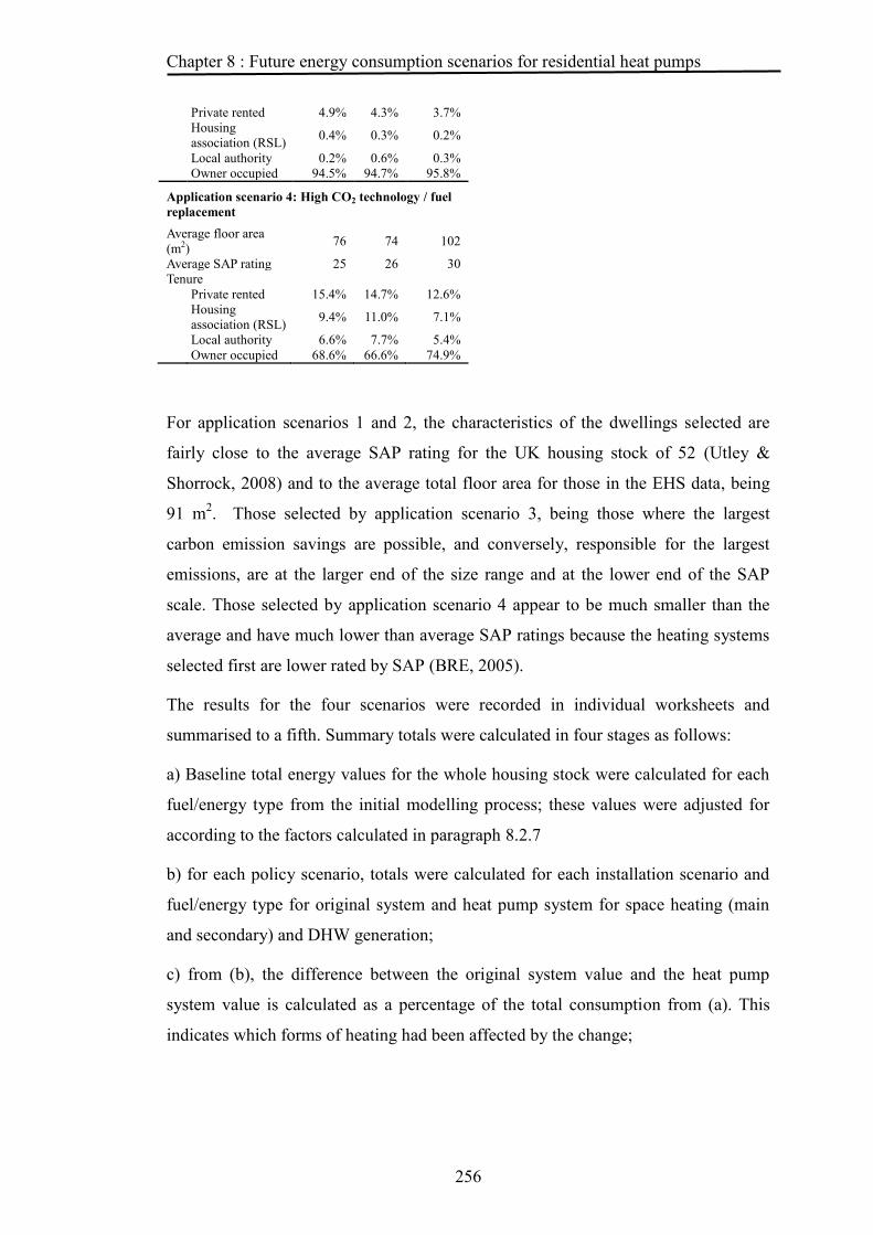
Chapter 8 : Future energy consumption scenarios for residential heat pumps
256
Private rented 4.9% 4.3% 3.7%
Housing
association (RSL) 0.4% 0.3% 0.2%
Local authority 0.2% 0.6% 0.3%
Owner occupied 94.5% 94.7% 95.8%
Application scenario 4: High CO2 technology / fuel
replacement
Average floor area
(m2) 76 74 102
Average SAP rating 25 26 30
Tenure
Private rented 15.4% 14.7% 12.6%
Housing
association (RSL) 9.4% 11.0% 7.1%
Local authority 6.6% 7.7% 5.4%
Owner occupied 68.6% 66.6% 74.9%
For application scenarios 1 and 2, the characteristics of the dwellings selected are
fairly close to the average SAP rating for the UK housing stock of 52 (Utley &
Shorrock, 2008) and to the average total floor area for those in the EHS data, being
91 m2. Those selected by application scenario 3, being those where the largest
carbon emission savings are possible, and conversely, responsible for the largest
emissions, are at the larger end of the size range and at the lower end of the SAP
scale. Those selected by application scenario 4 appear to be much smaller than the
average and have much lower than average SAP ratings because the heating systems
selected first are lower rated by SAP (BRE, 2005).
The results for the four scenarios were recorded in individual worksheets and
summarised to a fifth. Summary totals were calculated in four stages as follows:
a) Baseline total energy values for the whole housing stock were calculated for each
fuel/energy type from the initial modelling process; these values were adjusted for
according to the factors calculated in paragraph 8.2.7
b) for each policy scenario, totals were calculated for each installation scenario and
fuel/energy type for original system and heat pump system for space heating (main
and secondary) and DHW generation;
c) from (b), the difference between the original system value and the heat pump
system value is calculated as a percentage of the total consumption from (a). This
indicates which forms of heating had been affected by the change;

Chapter 8 : Future energy consumption scenarios for residential heat pumps
257
d) similarly, the effect of each installation scenario is calculated by adding the
difference between the original system and heat pump system values to the total from
(a).
For CO2 emissions from operation, a baseline total estimate for the whole housing
stock covered by EHS was calculated as per (a) above. Totals for emissions for
application scenarios were calculated by summing the emissions for heat pumps and
for original systems grossed up by the scenario weight for each sample included in
the scenario.
The results are summarised in the following table:
Table 8.22 Summary of results for 2020 Scenarios
Deployment Scenario
2020 Scenarios
Change in net energy consumption
% change
Change in electricity consumption
% change
Reduction in CO2 emissions
% reduction
(GWh) (GWh) KTonnes 1 Centre 6,031 1.0 5,228 2.6 1,217 0.94
High 8,897 1.4 7,764 3.9 1,799 1.40
Stretch 19,240 3.1 16,288 8.2 3,898 3.03 2 Centre 5,766 0.9 5,070 2.6 1,081 0.86
High 8,486 1.4 7,515 3.8 1,594 1.27
Stretch 18,365 2.9 15,738 8.0 3,413 2.73 3 Centre 16,767 2.7 8,441 4.3 4,789 3.27
High 23,441 3.8 12,239 6.2 6,489 4.45
Stretch 41,168 6.6 23,366 11.8 10,936 7.60 4 Centre 9.653 1.5 -3,661 -1.8 3,150 2.10
High 15,555 2.5 245 0.1 5,048 3.41
Stretch 34,864 5.6 12,702 6.4 9,824 6.82
For embodied CO2, the grossed-up values for the heat pump system embodied energy
are totalled, with a total value for original systems calculated using a single value for
the embodied energy in a gas boiler, on the assumption that during the same 15-year
period either an existing system would be replaced by gas or an existing gas boiler
would be replaced.
8.3.3.1 Electricity consumption and energy mix
The following Figures 8.3 and Figure 8.4 indicate the overall estimated effect of the
four scenarios on overall electricity consumption.

Chapter 8 : Future energy consumption scenarios for residential heat pumps
258
Figure 8.3 Overall electricity consumption to 2020
Figure 8.4 Peak rate electricity consumption to 2020

Chapter 8 : Future energy consumption scenarios for residential heat pumps
259
Figure 8.5 Carbon dioxide emission reductions for 2015 & 2020 policy scenarios
Figure 8.5 indicates that the most substantial reductions in CO2 - well over 7% for
the “2020 Stretch” installation scenario - come from targeting the highest emitters,
but these reductions come with a substantial penalty in additional electricity
generation of some 23 TWh per annum as shown by Figure 8.3. Compared with the
'heat pumps only", Scenario 2 brings a slight increase in emissions, though only a
fraction of a percentage more even in the “2020 Stretch” scenario, but with
correspondingly reduced electricity consumption in all cases. Scenario 4, that of
targeting dwellings where the heating system utilises the highest emitting fuels, is not
as effective as Scenario 3 in reducing CO2, but increases electricity consumption
only by approxinately 13 TWh annually in return for a reduction of just under 7% in
carbon dioxide emissions.
Figure 8.6 indicates the changes which occur with greater numbers of heat pump
installations under this scenario, with, initially, energy consumption being reduced
with the replacement of systems burning fuel oil, then solid fuel systems burning
coal, and storage heater systems using off-peak electricity. Because of the
substantial load from lighting and appliances, the percentage change in electricity
demand is only about 8%. Systems burning gas in all forms and biomass remain
largely unaffected, though the dominance of mains (natural) gas-fired systems does

Chapter 8 : Future energy consumption scenarios for residential heat pumps
260
mean that changes to energy consumed by other system types have a limited effect
on overall energy consumption as indicated by Figure 8.7.
Figure 8.6 Percentage change in energy mix due to Policy Scenario 4
Figure 8.7 Energy consumption for Policy Scenario 4 - Fuel / technology replacement

Chapter 8 : Future energy consumption scenarios for residential heat pumps
261
8.3.3.2 Practicalities
In labelling the inner layer of scenarios as “application scenarios”, there is an
implication that these scenarios could be applied as the basis for government policy
for the implementation of the Renewable Heat Incentive or a similar incentive
scheme. However, for the rules governing these scenarios to function as policy, it is
necessary either that they apply to all dwellings within the housing stock or that, if
their success depends on applying the policy to a subset of the housing stock, then
that subset should be identifiable. Of the four policy scenarios, Scenarios 1 and 2
were applied randomly across the whole housing stock. Policy Scenario 3, with the
aim at an optimal assignment of installations to reduce carbon emissions, has no
obvious method of implementation. While the individual dwellings surveyed for the
EHS samples might be identifiable, those dwellings that are notionally grouped with
each sample by the grossing weights are very likely not, having no obvious defining
characteristics. However, Policy Scenario 4, which focuses on the type of heating
system to be replaced, does provide a fairly precise basis for such a policy and so this
type of scenario was used to examine monthly electricity loads for 2020. Policy
Scenarios 1 and 2, which basically constitute a ‘null’ option and a minimal approach
to improving energy efficiency, do not provide in these estimates any confidence that
the current targets for the reduction of carbon dioxide emissions will be met.
8.3.3.3 Peak loading - 2020
The estimates for changes in the January loads for electricity are presented in Table
8.23 for the Heat pumps only, Improved insulation, and Fuel / Technology
Replacement policy scenarios. The additional loads deriving from any of these
scenarios are not of very great magnitude and all amount to less than 4% of the UK
load of about 80 GW. As these scenarios cover a period when UK electricity supply
will be decreasing unless further capacity is built, the small increase in load or
consumption would be welcome. However, the use of heat pumps to replace off-
peak storage heating comes with the penalty of added day-time load if the practice of
operating the systems throughout the day is maintained, although the effect of large-
scale heat pump installation using weather-compensated controls would be to avoid
sudden peaking of load at the start of each low-charge period. That dwellings and
their occupants vary considerably in their heat demands would also mitigate against a

Chapter 8 : Future energy consumption scenarios for residential heat pumps
262
surge when external temperatures drop. Thus the emissions reduction of any heat
pump installation programme must be balanced against the change in load profile for
the electricity supply and, considering this, the “Fuel / technology replace”
installation policy is advantageous.
Table 8.23 Effects of Scenarios 1, 2, & 4 on primary energy consumption and load for month of January
Change in energy
consumption Change in power loading
2020 Stretch 2020 Stretch
Heat
pumps
only
+
improved
insulation
Fuel / tech
replace
Heat
pumps
only
+
improved
insulation
Fuel / tech
replace
(GWh) (GWh) (GWh) (GW) (GW) (GW)
Mains gas -3,978 -3,738 484 -4.65 -4.37 0.57
Bulk LPG 269 -17 -252 0.33 -0.02 -0.31
Bottled gas 514 360 -135 0.63 0.44 -0.16
Heating oil -1,084 -1,002 -3,466 -1.22 -1.13 -3.92
House coal -26 -24 -151 -0.03 -0.03 -0.19
Anthracite -12 -11 -86 -0.02 -0.01 -0.11
Manuf smokeless fuel -40 -38 -272 -0.04 -0.04 -0.28
Wood logs -35 -33 0 -0.04 -0.04 0.00
Electricity
Std tariff 2,385 2,361 1,684 3.21 3.17 2.26
Off-peak 7-hour -14 -20 -1,531 -0.02 -0.03 -2.06
Off-peak 10-hour 205 139 439 0.28 0.19 0.59
24-hour heating tariff -1 -1 -14 0.00 0.00 -0.02
All electricity
2,575 2,478 578 3.46 3.33 0.78

Chapter 8 : Future energy consumption scenarios for residential heat pumps
263
8.3.4 Scenarios for 2050
These scenarios take as their basis the position outlined towards the end of the
NERA document (NERA Economic Consulting, 2009) where an assumption is made
that the number of heat pump installations, having reached 1.8 million for the 2020
‘stretch’ scenario, will reach a saturation point for this technology in 2030 (NERA
Economic Consulting, 2009, p122).
This position leaves at least a further 16 million dwellings in England still using gas
heating. Reductions in carbon emissions could be made through the replacement of
older, less efficient gas systems, but if the intention is to take advantage of a
‘decarbonized’ electricity supply, this is best achieved by electrical systems in
general and heat pump systems in particular as Figure 8.8 illustrates.
Figure 8.8 Relative emissions of heat pump systems at different carbon intensities of electricity generation compared with fuel-burning systems
8.3.4.1 Forecasts of heat pump take-up
To provide estimates for possible heat pump installations in 2050, the main
precedent that exists in the UK is that of the current take-up of gas-fired central
heating which has been installed in about 90% of dwellings up to 2006 (Utley &
Shorrock, 2008) starting from almost 0% in 1964 (Utley & Shorrock, 2008). This
would indicate the possibility of 80% take-up of heat pump systems in the slightly
longer period up to 2050, equating to approximately 15.6 million installations for the
0.00
0.10
0.20
0.30
0.40
0.50
0.60
1 2 3 4 5
Kg
CO
2/
kW
h
Heat pump COP
Gas
Oil
2020
2050
2008

Chapter 8 : Future energy consumption scenarios for residential heat pumps
264
18 million dwellings for the EHS data in this study. If this value is taken as the “2050
Stretch” Deployment scenario and the proportions of “Stretch” to “Central” and of
ASHPs to GSHPs in the 2020 Deployment scenario retained, this gives estimates for
installations in 2050 as per Table 8.24. While the "2050 Stretch" level is within the
values proposed by Boardman (2007, p. 101) of 25 million LZC installations by
2050, Boardman's proposals contain a mix of other low-carbon technologies,
including 'green' - from anaerobic digestion - gas; solar thermal water heat heating;
and community or micro combined heat & power, with ground and air source heat
pumps as part of this mix. However, these proposals give no indication of the share
of each technology in this mix, providing no indication of a possible number of heat
pump installations. Mackay (2008) provides an estimate (Table 28.3, p229) for the
cost of heat pumps of £6 billion at £1000 per person, which, with Mackay's
allowance of two people per household, equates to 30 million systems, presumably
one for every dwelling in the UK.
Table 8.24 Installation scenarios for 2050
GSHP ASHP Total
Year Units Units Units
(000s) (000s) (000s)
Stretch growth scenario 2050 5,550 10,000 15,550
Central growth scenario 2050 1,600 3,900 5,500
8.3.4.2 Future temperature forecasts
A replacement table of monthly average temperatures by BRE Heating Degree Day
Region was created to allow for the effects of climate change. The adjustment values
were taken from the UKCP09 data (DEFRA, 2011) for 2050, “high emission”, 90%
probability data for GO Regions and further adjusted for the variations between the
GO Regions and the BRE Heating Degree day regions, with a maximum adjustment
of +5.2 ºC applied to the August temperature in the BRE Thames region and a
minimum adjustment of +3.4 ºC applied to both W. Pennines, North West, and
Borders regions throughout the first and last 4 months of the year. The average
adjustment was 4.25 ºC.
In the context of the UKCP09 projections, "90% probability" implies that there is a
90% chance that the temperature increase will less than or equal to the temperature
value. The selection of the "high emission", 90% probability data was made to
provide an 'upper' bound for the estimates made.

Chapter 8 : Future energy consumption scenarios for residential heat pumps
265
The resultant temperature table is in the worksheet 'tables' in the 'EHS Processing
2050 scenarios' spreadsheet and reports of the UKCP09 web pages from which the
adjustment values were obtained are in Appendix F.
8.3.4.3 Model assumptions
For these scenarios, the parameter was set in the model to require the estimation of
energy use for space cooling. In these calculations, the SAP default value of 2 is set
for the SEER (Seasonal Energy Efficiency Ratio) of the air conditioner. The model
assumes that air conditioning uses only standard rate electricity, since the hottest part
of any day is usually during peak hours. In calculating estimates for overall totals, it
is assumed that there is no element of space-cooling in the baseline estimates.
A further, more radical, assumption made is that all the heat pumps installed are
reversible, i.e. capable of both heating and cooling. In terms of the heat pump
systems themselves, this assumption is plausible, with such systems currently
available (ICS Renewable Energy ltd, 2011) and existing systems may be converted.
However, in the retro-fit installations in this study, the existing radiator distribution
systems are not recommended for cooling use. Ochsner (2007, p. 90) suggests that
convection fans may be used for cooling and it is possible that these may be adopted
over the 40 years to 2050, if cooling is found necessary.
In estimating the comparative energy use for space-cooling, the assumption made
above that the baseline estimates exclude this value implies that the total effects of
either separate air-conditioners or of heat pump systems are solely due to the values
estimated by the enhanced BREDEM model from the samples included in the
scenarios with estimates from the remainder excluded. This is deemed to be
legitimate on the basis that energy for residential space-cooling is not analysed
separately in UK statistics for energy consumption.
Output from roof-mounted photo-voltaic systems on each dwelling sample is also
included in the scenario outputs, calculated as per Section 5.6.9 Since output from
these systems is available directly for consumption in the dwelling, and is
independent of the dwelling occupants' behaviour, estimates of their output are used
unadjusted in calculations. Similarly, as minimal carbon dioxide emissions are
attributable to their operation, estimates from the emissions calculation must be

Chapter 8 : Future energy consumption scenarios for residential heat pumps
266
adjusted to reduce carbon dioxide emissions values by an amount equivalent to the
photo-voltaic system output. As noted in Section 5.6.9, the putative systems are
assumed to be as efficient as the best of those currently available, to allow for some
degree of technological improvement in the period to 2050.
The value used for carbon dioxide emissions for electricity generation was reduced
according to the current target for 80% reductions in carbon emissions by 2050,
reducing from 0.517 kgCOeq/kWh to 0.103 kgCOeq/kWh.
8.3.4.4 Application scenario
Since the “Fuel / Technology Replace” application scenario produced the ‘best’
results for 2015 and 2020, this is used for 2050. The data from the “2020 Central”
and “2020 Stretch” scenarios are also carried over into 2050 to illustrate the position
if heat pump take-up remained at the level envisaged for the earlier year.
8.3.5 2050 Scenario results
8.3.5.1 Distribution of installations in dwellings
A summary of these are shown in

Chapter 8 : Future energy consumption scenarios for residential heat pumps
267
Table 8.25. This also shows the 2020 equivalent installation scenarios for
comparison.
The effect of the de-carbonisation of the electricity supply is to complete the shift of
solid fuel systems to heat pumps, while, in the “centre” scenario at least, the
remaining direct electric systems remain in place. This is probably an anomaly, since
these systems are likely to have been replaced in the years following 2020. The 2050
Stretch scenario finds all forms of heating virtually eliminated other than heat pumps
(~85%) and gas central heating (~15%).

Chapter 8 : Future energy consumption scenarios for residential heat pumps
268
Table 8.25 Summary of dwelling / heat pump assignments for 2050 scenarios
Summary of dwellings in scenarios
2020 2050
Centre Stretch Centre Stretch No of ASHP installations (000's) 211 639 3,900 10,000
No of GSHP installations (000's) 190 960 1,600 5,550
Technology / fuel replacement
Average floor area (m2) 107 116 120 94
Average SAP rating 35 34 42 48
Tenure Percentage of scenario total Private rented 15.4 12.6 5.7 8.4
Housing association (RSL) 9.4 7.1 1.9 3.4
Local authority 6.6 5.4 1.5 2.3
Owner occupied 68.6 75.0 90.8 85.8
Original fuel Percentage of this fuel type in EHS weighted sample
01 mains gas 87.8 86.9 68.3 15.2
02 bulk LPG (propane or butane) 0.4 0.0 0.0 0.0
03 bottled gas (propane) 0.3 0.0 0.0 0.0
04 heating oil 4.7 0.0 0.0 0.0
05 house coal 0.5 0.3 0.0 0.0
06 anthracite 0.1 0.0 0.0 0.0
07 manufactured smokeless fuel 0.4 0.1 0.0 0.0
08 wood logs 0.2 0.2 0.2 0.2
11 wood chips 0.0 0.0 0.1 0.1
13 standard tariff 3.0 9.9 29.9 84.6
14 Off-peak 7-hour 2.0 2.0 1.3 0.0
15 Off-peak 10-hour 0.1 0.1 0.3 0.0
16 "24-hour"- heating tariff 0.0 0.0 0.0 0.0
Total dwellings in scenario 560,000 1,820,000 5,500,000 15,550,000
8.3.5.2 Energy consumption
These results assume that, by 2050, space cooling will be required utilising
conventional air condition equipment in estimating the "Business As Usual" values.
Results for overall energy consumption and electricity consumption are shown in
Figure 8.9 , Figure 8.10 and Figure 8.11 below.

Chapter 8 : Future energy consumption scenarios for residential heat pumps
269
These indicate that the substantial increase in heat pump installations, especially in
the 2050 Stretch scenario, has a correspondingly significant effect on the
consumption of mains gas, with a 40% decrease in gas consumption matching an
increase by 40% in electricity consumption at "Standard Tariff", on-peak rates. All
other forms of energy supplied to homes are substantially reduced while off-peak
electricity supply is virtually eliminated. The increase in electricity is off-set over the
course of a year by output from the photovoltaic systems resulting in net electricity
consumption for the "2050 Central" scenario of approximately 13 TWh more than
'Business as usual', while that for the "Stretch" scenario is very slightly less.
Figure 8.9 Primary energy consumption to 2050: Fuel / technology replace

Chapter 8 : Future energy consumption scenarios for residential heat pumps
270
Figure 8.10 Up to 2050 - percentage change in energy consumption
Figure 8.11 Primary energy consumption for electricity: scenarios up to 2050, including space cooling and output from photovoltaics
Of the estimated consumption for space cooling, the effect of heat pump installations
is to reduce the estimated consumption for this purpose by some 5.4 TWh / annum
(~19%) for the “2050 Stretch” scenario, and this, combined with the output from the
photo-voltaic systems, compensates for the 73 TWh added by these installations.

Chapter 8 : Future energy consumption scenarios for residential heat pumps
271
These figures indicate the energy directly consumed by the installed heating and
cooling systems in each dwelling and which are affected by the type of system
installed. They do not include a value for the energy consumed by cooking, lighting
and appliances, which, using the estimating method in BREDEM-8, was calculated
to be 56.6 TWH annually for the dwelling samples in '2050 Centre' scenario and
134.4 TWh for the '2050 Stretch', which equates to a total for the whole English
housing stock of 154 TWh which, if assumed to consist almost entirely of electricity,
substantially exceeds the consumption by the heating and cooling systems.
8.3.5.3 Peak loading
Primary energy consumption and loads for the peak heating month of January and
peak space cooling month of July are shown in

Chapter 8 : Future energy consumption scenarios for residential heat pumps
272
Table 8.26, along with monthly electricity supply values averaged over the years
1998 - 2011 and monthly natural gas production values for the years 1996 - 2011
obtained from the Digest of UK Energy Statistics (DECC, 2011a, 2011c)
Under the '2020 Stretch' scenario, the overall estimated effect of the heat pump
installations on electricity consumption is minimal, with a rise in standard or peak
rate electricity being matched by a fall of similar magnitude in 'off-peak - 7 hour'
supplies. Mains gas consumption also falls substantially, though the major reduction
is in the consumption of heating oil, which is to be expected due to its higher carbon
emission.
Under the '2050 Stretch' scenario, in January, there is a substantial transfer from gas
to electricity, particularly to standard rate, while in July, there is both a transfer from
gas to electricity and also a reduction in electricity due to the replacement of stand-
alone air conditioning. Thus in winter, electricity consumption rises by 31 - 34% of
the UK's current generation, while in summer it falls by approximately 20%. Gas
consumption falls by approximately 22% of current levels in winter and
approximately 10% in summer.

Chapter 8 : Future energy consumption scenarios for residential heat pumps
273
Table 8.26 Estimated primary energy consumption and loads for January and July
January July
2020 Stretch 2050 Stretch 2020 Stretch 2050 Stretch (against 'business as
usual') Change in energy consumption
Change in energy load
Change in energy consumption
Change in energy load
Change in energy consumption
Change in energy load
Change in energy consumption
Change in energy load
(GWh) (GW) (GWh) (GW) (GWh) (GW) (GWh) (GW)
Mains gas -946 -1.27 -23,018 -30.94 -88 -0.12 -4,056 -5.45
Bulk LPG -238 -0.32 708 0.95 -39 -0.05 -25 -0.03
Bottled gas -112 -0.15 -508 -0.68 -21 -0.03 -15 -0.02
Heating oil -3,169 -4.26 -4,818 -6.48 -931 -1.25 -574 -0.77
House coal -238 -0.32 -295 -0.40 -82 -0.11 -132 -0.18
Anthracite -154 -0.21 -121 -0.16 -53 -0.07 -52 -0.07
Manuf smokeless fuel -335 -0.45 -311 -0.42 -142 -0.19 -156 -0.21
Electricity
Std tariff -144 -0.19 11,387 15.31 -71 -0.10 -175 -0.24
Off-peak 7-hour -629 -0.85 -1,253 -1.68 -329 -0.44 -501 -0.67
Off-peak 10-hour -228 -0.31 653 0.88 -21 -0.03 -32 -0.04
24-hour- heating tariff -3 0.00 -20 -0.03 -2 0.00 -15 -0.02
Space cooling 0 0.00 0 0.00 0 0.00 2,862 3.85
All electricity -1,004 -1.35 11,013 14.80 -71 -0.10 2,385 3.21
January
% variation
(2020 stretch)
% variation
(2050 stretch) July
% variation
(2020 stretch)
% variation
(2050 stretch)
Actual electricity generation (1998-2011, TWh, from Dukes Table 5-4.) Average
Average
32.5 -3.09% 33.92%
25.4 -1.66% -9.39%
Maximum
Maximum
34.9 -2.87% 31.51%
27.3 -1.55% -8.74%
Natural gas production and supply (1996-2011, TWh, from Dukes Table 4.2.) Average
Average
118.8 0.80% -19.37%
52.7 -0.170% -7.70%
Minimum
Minimum
130.6 0.72% -17.62%
43.3 -0.20% -9.36%
8.3.5.4 System consumption by function
These estimates are shown in Figure 8.12 & Figure 8.13, below, which are scaled for
comparision and indicate the following:
that the output from the photo-voltaic systems comes close to balancing the
energy consumption for heating, cooling and DHW generation between May
and August in both scenarios;

Chapter 8 : Future energy consumption scenarios for residential heat pumps
274
an estimated 0.4 TWh monthly is consumed by heat distribution.
Figure 8.12 2050 Central - Monthly total effects of Fuel / Technology Change scenario
Figure 8.13 2050 Stretch - Monthly total effects of Fuel / Technology Change scenario
8.3.5.5 Carbon dioxide emissions
Embodied carbon dioxide estimates These were estimated using the method described in section 8.2.2.3 and the results
are summarised in Table 8.27, noting that if only one replacement gas boiler per
household was necessary over the period to 2050, then there would be a net reduction

Chapter 8 : Future energy consumption scenarios for residential heat pumps
275
in embodied carbon in heating systems with the higher numbers of installation. As
the life of a gas boiler is put at 15 years (Energy Saving Trust, 2010), an ASHP at 15
years, and a GSHP at 20 − 25 years, then the actual reduction may exceed this
estimate.
Table 8.27 Estimated carbon emissions to 2050
CO2 Emissions: embodied (Ktonnes)
Effects to 2020 Effects to 2050 Centre Stretch Centre Stretch
Gas boiler replacement 241 959 3,300 9,330
Heat pump + refrigerant 392 1,043 2,325 6,282
Net emissions 152 83 -975 -3,048
Carbon dioxide emissions from operation
These are summarised in

Chapter 8 : Future energy consumption scenarios for residential heat pumps
276
Table 8.28 and the detail of the reductions due to the change in fuel mix shown in
Figure 8.14. The estimates in

Chapter 8 : Future energy consumption scenarios for residential heat pumps
277
Table 8.28 are compiled starting from a total value based on the BREDEM-8
estimates for the entire weighted EHS survey data using current emission estimates
for electricity generation - line (1) in

Chapter 8 : Future energy consumption scenarios for residential heat pumps
278
Table 8.28. This total is then re-calculated for 2050 based on the emission estimated
for the “de-carbonised” electricity supply and the changed energy requirements of
the 2050 UKCP09 climate impacts as line (2), with the resulting reduction as line (3).
The emissions reductions due to each application scenario is calculated (lines 6 and
10) from the estimated emissions with existing systems (lines 4 and 10) and with
heat pumps (lines 5 and 11) and the overall reduction from 2006 to 2050 calculated
in lines (6) and (12). These results show that for the target emissions reduction of
80% to be approached, the adoption of domestic heat pumps is not only required to
reach the levels indicated in the “2050 Stretch” scenario but must be accompanied by
a corresponding 80% reduction on the carbon intensity of electricity generation.
Figure 8.14 indicates that the main difference between the two scenarios is the far
greater reduction due to the replacement of natural gas systems.

Chapter 8 : Future energy consumption scenarios for residential heat pumps
279
Table 8.28 Carbon emissions from operation 2020, 2050
Installation Scenario
Total emissions
Emissions reduction
Percent change
Emissions
reduction
Percent change
(Ktonnes) (Ktonnes) (Ktonnes)
1) Total estimated CO2 emissions based on EHS survey - 2006 values
151,350
2)
Total estimated CO2 emissions based on EHS survey - 2050 values
74,856
3) (1) - (2)
Reduction due to lower emissions from electricity generation
76,494 50.5%
2050 Centre
4) Effect of existing systems 30,060
5) Effect of heat pumps 9,863
6) (4) - (5) CO2 reduction due to
scenario 20,197 27.0% 96,690 63.9%
7) Reduction due to PV output 2,278
8) (4)-(5)-(7) Total reduction due to
scenario 22,475 30.0%
9) (8) + (3) Total CO2 reduction to 2050
98,968 65.4%
2050 Stretch
10) Effect of existing systems 65,199
11) Effect of heat pumps 22,210
12) (10)-(11) CO2 reduction due to
scenario 42,989 57.4% 119,483 78.9%
13) Reduction due to PV output 3,162
14) (12)-(13) Total reduction due to
scenario 48,042 64.2%
15) (12)+(13) Total CO2 reduction to 2050 124,536 82.3%
Figure 8.14 Change in CO2 emissions due to 2050 scenarios

Chapter 8 : Future energy consumption scenarios for residential heat pumps
280
However, while the '2050 Stretch' scenario apparently ensures that the UK reaches its
target of 80% reduction in CO2 emissions for the existing English housing stock,
achieving this requires the installation of an extra 10 million heat pump systems than
the '2050 Centre' scenario.
The substantial estimated cost of the CO2 savings (Table 8.29) contributes to the
anomalous position of heat pump heating systems, in that their status as low carbon
technology is dependent on the availability of a low-carbon electricity supply and, in
general, as the carbon intensity of the electricity supply reduces, the greater the
effectiveness of these systems becomes at reducing carbon compared to a fossil fuel-
fired system. However, as the carbon intensity of the electricity supply reduces, the
difference in effectiveness in carbon emissions reduction between heat pump and
direct electric systems reduces, even if the size of the heat pump COP is maintained.
If a sufficiently large photovoltaic system is installed, ie. 3 kWp, the average size
proposed here, the extra cost and complexity of installation of the heat pump system
compared with, say, electric resistance radiators, becomes even more difficult to
justify, since the value of the output from the photovoltaics will go some way to
defray the extra running cost of direct electric heating. The cost of more substantial
energy efficiency improvements to the building fabric than were considered earlier
Table 8.29 Annualised cost of carbon emissions reduction
System type
Cost per dwelling
Expected Life Annualised cost
Number of systems / year Total annualised cost
Annual savings
Low High
Low High (000's) Low High (operating)
£ £ Years £ £
(£ millions)
(£ millions) (£ millions)
ASHP 6,000 10000 15 400 667 6,100 2,440 4,067 764
GSHP 9,000 17000 25 360 680 3,950 1,422 2,686 648
Net annual cost of heat pumps (£millions) 2,450 5,340
Annual CO2 reduction (Ktonnes) 26,138
Cost of reduction £/tonne CO2 107 234
Heat pump installation costs (EST, 2011)
in this study is likely to be similar to that of a heat pump system and this, too, would
reduce running costs.
While direct electric systems lack the capability to provide space cooling, it is by no
means clear that this would be an absolute requirement, given the range of possible

Chapter 8 : Future energy consumption scenarios for residential heat pumps
281
outcomes in the UKCP09 forecasts, where estimates of summer temperature
increases range from 1.2ºC to 7.6ºC under three different emissions scenarios
(DEFRA, 2011). Temperature changes at the low end of this range would probably
eliminate the necessity for space cooling.
8.4 Discussion
8.4.1 Sample weights
The use of sample weights to gross-up sample estimates to housing stock estimates is
not supported well by the EHS documentation. The author has made extensive use of
these to gross-up sample level results to housing stock estimates, bearing in mind the
instructions in the EHS Technical Report (DCLG, 2010b), and the sample weights
are employed in the analysis of EHS data to estimate the proportion of dwellings that
meet the UK Government standard for thermal comfort - the "Decent Homes"
standard. However, the weights are calculated on a basis of the probability of a
given dwelling being selected for inclusion in the survey, with adjustment for non-
response by householders and scaling according to the relative to separate control
totals of the number of dwellings by tenure and region obtained from the last UK
Census in 2001. To be valid in this context, the sample weight value should be the
number of dwellings existing within the housing stock which are identical or very
similar to the sample. This is not necessarily true of the sample weight values in the
EHS data and it would not seem to be possible to estimate valid weights by the
method outlined in the Technical Report.
8.4.2 Reliability of estimates
The estimates from the BREDEM model were found to over-estimate energy
consumption, particularly of gas, as described in Section 8.2.7
The best explanation of this over-estimate is that a proportion of households are not
heating their dwellings to the standard demand temperature of 21 ºC, either from
personal requirements for thermal comfort or from finding the cost of heating the
house to that temperature unaffordable. This could be confirmed and the adjustment
process substantially refined if actual fuel expenditure and energy consumption data

Chapter 8 : Future energy consumption scenarios for residential heat pumps
282
was collected by the EHS, replacing or as well as the values estimated using SAP.
Actual income is already included in the EHS for assessment of household fuel
poverty status and the extra information would allow the estimation of income
available for expenditure on heating and, given the cost per kilowatt hour of the
installed heat, the maximum annual energy consumption by the household.
8.4.3 Scenarios for domestic heat-pump take-up
This research does not attempt to describe the process by which the capacity is
created to manufacture and finance the installation of the substantial number of heat
pumps in the stretch scenario to 2050. Neither does it attempt to describe what
motivation would bring about such a major change in heating systems.
The scale of heat pump take-up to 2050 (Table 8.24) is based approximately on the
take-up of gas central heating over the period 1964 to the present day as being the
closest and only precedent in the UK. Over this period, there was strong house price
inflation - Figure 8.15 - which enabled house owners to finance improvements such
as central heating by additional borrowing on mortgages at low interest rates -
sometimes with the benefit of tax concessions on interest payments, with substantial
deregulation of the mortgage industry in the 1980's also making this borrowing easier
(Miles, 1992). Since the financial crash of 2008, mortgage lending has been more
restricted and house prices have levelled out or fallen, as indicated by Figure 8.15.
Without this, possibly unsustainable, inflation, householders may not be able to
finance substantial purchases such as heat pumps. Moreover, the original motivation
to make the change no longer exists. In 1964, UK housing still had, in general, very
poor heating (Wright, 1964) and the installation of central heating of any kind
brought about a vast improvement, not only in convenience, but also in making more
rooms habitable. With some form of central heating already in place, its replacement
by a heat pump system would only be maintenance of the status quo and would not
provide the same degree of motivation. The UK government's financial incentives
via the current (2011) Renewable Heat Payment Premium (RHPP) and Renewable
Heat Incentive (RHI) (DECC, 2011d) which are documented in Chapter 1 do not yet
fully support domestic systems and cover only the period up to 2020. Boardman
(2007) suggests a combination of low-interest loans, house purchase tax ("Stamp
Duty") rebates, and 'green' mortgages to enable and encourage householders to

Chapter 8 : Future energy consumption scenarios for residential heat pumps
283
finance the improvements to make their properties more energy-efficient, "Low-
carbon Zones" covering lowest-income households within which local authorities
improve the energy efficiency of all houses. These measures are aimed at supporting
the take-up of low-and-zero-carbon technologies, including heat pumps, at 600,000
units per year up to 2050.
Figure 8.15 UK house prices, retail price index, earnings 1953 - 2010
((Nationwide Building Soc, 2011; Officer, 2011)
8.4.4 Openness, robustness and integrity of modelling
One of the subsidiary objectives of the development of this model (or models) was to
endeavour to make sure that the input data and resultant software was both publicly
available and as transparent as reasonably possible. This has only been achieved to a
limited extent. Equally, it was hoped that the software could be developed to be
reasonably robust, an aim which has been signally defeated by the software tool
used.
The English Housing Survey was selected because it is freely available and is the
most comprehensive survey of English housing. However, the only format in which
this data is available, for which the appropriate software was also available to the
author, was that of SPSS statistical software (SPSS Inc, 2010). This required extracts
from the EHS SPSS tables to be made to create initial MS Excel input for thermal
modelling. The choice of MS Excel was dictated by the provision by BRE of a basic

Chapter 8 : Future energy consumption scenarios for residential heat pumps
284
spreadsheet version of the BREDEM-8 model implemented on that software
platform and by the fact that the built-in 'Visual Basic for Applications' programming
environment is well-known.
The major part of the software for the analysis was formed by two routines, one of
which executes the BREDEM-8 model using the EHS extract as input and creates a
output table of energy consumption and CO2 estimates with one output entry for
sample, the second of which assigns a scenario weight to each sample selected for
the scenario. A third routine, a version of the first, calculates month-level estimates
for energy consumption.
The processing time for the first and third routines is lengthy as it requires each of
twelve thousand table entries to be processed. Moreover, there appeared to be a fault
in Excel whereby the model formulae were not fully calculated and output table rows
were created with the same values as the last. Coding was added to detect this
condition and stop the routine, which then required to be restarted at the last correct
entry.
To maintain the integrity of the central models, the author would have preferred to
hold the BREDEM-8 and associated heat pump models in separate spreadsheets, but
found that this was not possible because of the linkage methods in Excel which could
not be maintained when creating new versions of the spreadsheets.
8.4.5 Allocation of heat pump sources and bivalent operating modes
The rules documented in Table 8.7 allow for a vertical borehole ground loop to be
installed where the dwelling plot is too small to install an air source system. As the
requirements for borehole installations include: specific geological conditions; that
boreholes are not within 12 metres of each other, and a minimum ground area, this
allowance might be better omitted.
In
Chapter 8 : Future energy consumption scenarios for residential heat pumps
285
Table 8.8, the rules allow for a bivalent alternate mode installation in older houses
where there is an existing central heating system. As the combined systems would
occupy considerable space, this configuration should possibly be restricted to
dwellings with a minimum floor area.
8.5 Summary and conclusions
This chapter described the process of creating a Domestic Energy Model (DEM)
from extracts from the EHS data sets, linked to the enhanced BREDEM-8 model
described in Chapter 7 by employing 'data reduction' techniques. The base-line DEM
estimates were compared with actual values from UK energy statistics and
adjustment parameters calculated. Sets of scenarios for heat pump system
installations were created based, for the shorter term to 2020, on consultation values
for the current government ‘renewable heat’ incentive scheme and, for the longer
term to 2050, on the historic take-up of existing gas central heating systems. From
these scenarios, estimates were compiled of the energy mix changes, particularly of
the increased electricity demand, and of carbon dioxide emissions reductions for
these levels of heat pump take-up.
The main conclusions from this chapter are:
a domestic energy model for the English housing stock with the ability to generate
monthly energy, CO2 emissions and energy cost estimates can be created using a
BREDEM-8 model implemented in MS Excel to analyse extracts from the English
Housing Survey; this creates both existing system and heat pump system estimates at
dwelling sample level which are grossed-up by survey sample weights to calculate
stock-level estimates which form a baseline for the model; a process of "data
reduction" is employed to provide multiple BREDEM-8 model parameters from the
EHS samples by means of lookup tables keyed on one variable, built form or data of
construction, from the sample.
Scenarios for future heat pump energy use can be created in terms of numbers of
installations, by selection of samples under a application scenario, with or without
modification to the configuration of the sample dwelling, by means of modified
sample weighting. Stock level estimates for a scenario can be calculated by
modifying the baseline estimates by the difference between the existing system and
heat pump estimates for the scenario.

Chapter 8 : Future energy consumption scenarios for residential heat pumps
286
Existing government consultative reports can be analysed to provide three levels
("centre", "high", "stretch") of installation numbers to build scenarios for the period
to 2020, with application scenarios determined by the author, based on existing
policy, limited energy efficiency improvements, dwellings with highest emissions,
and dwellings with high emission heating systems (Policies 1, 2, 3 & 4) .
The results analysis of these application scenarios showed that, as the only scenario
that had a substantial emissions reduction effect (~8% in “2020 Stretch’), the third
scenario also caused a substantial increase in electricity consumption in all
deployment scenarios. The fourth application scenario was the only one that caused a
reduction in overall electricity consumption as well as in carbon dioxide emission. A
further analysis of peak electricity loads was carried out on application scenarios 1,
2, and 4, dropping 3 on grounds of impracticality, and this showed that the average
January peak load would increase negligibly in 2020 under scenario 4 with the other
scenarios creating a circa 3 per cent increase in 2020. These results would indicate
that if there are issues in maintaining the level of UK energy supply, then Application
Scenario 4 would provide a slightly better solution than the other scenarios.
A second set of deployment / application scenarios were built for the years to 2050,
with installation numbers based on the similar installations of gas-fired systems over
the period from 1964, though the policy scenario was restricted to Policy 4 above.
Analyses were carried out with scenarios to 2050, re-calculating energy consumption
and carbon emission estimates based on monthly average temperatures “morphed” to
those estimated for the UK CP09 predictions, reduced emissions from electricity
generation matching those required for 2050 by the UK Climate Change Act targets,
and including space cooling. The effect of electricity output from the installation of
photo-voltaic systems was also included in the estimates. Deployment scenarios for
heat pump systems were based on the 80% adoption of gas central heating in
dwellings between 1964 and 2010 and the application scenario used was that of
scenario 4 above, resulting in the deployment of a total of 5.5 million systems in the
'Central' scenario and 15.5 million in the 'Stretch'. Analysis of electricity
consumption showed an increase of approximately 50 TWh annually in electricity
consumption for space heating for the “2050 Stretch” installation scenario, a
substantial increase on the ~19 TWh of ‘business as usual”, but also showed a
reduction from 28 TWh to 12.5 TWh in consumption for space cooling. Estimates of

Chapter 8 : Future energy consumption scenarios for residential heat pumps
287
embedded carbon showed a substantial reduction - about 32% - from heat pump
systems compared with gas boilers and estimates of carbon emissions from operation
showed that the UK target of 80% reduction is approachable under the “2050 stretch”
scenario, but is dependent on the parallel decarbonisation of the UK electricity
supply. Estimates of the costs of these scenarios showed that, based on current fuel
costs, they would result in substantial costs per kilogramme of CO2 saved.
The next chapter presents reviews the main conclusions from the research and
explains its original contribution to knowledge. It also suggests further research
possibilities to improve knowledge of the factors influencing the performance of
domestic heat pump performance.

288
CHAPTER 9 CONCLUSIONS AND RECOMMENDATIONS
Chapter 9 Conclusions and Recommendations
289
9.1 Final conclusions
9.1.1 Fulfilment of objectives
In Chapter 2, in meeting the first part of Objective 1 of this study, a theoretical and
physical review of the of heat pump heating systems identified the following
characteristics as significant in estimating the energy use of heat pump heating
systems:
their efficiency (COP) is inversely related to the increase in temperature
required; dependence on external or ground temperatures for available energy
rather than fuel supply; the magnitude of the temperature increase is dependent
on the system source and sink, the characteristics of which are variable both
with source and sink type, and temperature changes during the year;
balancing low temperatures with direct electric heating disproportionately
increases energy use;
the status of heat pump systems as LZC technology is dependent on the carbon
intensity of electricity generation;
cooling season energy may increase since some types of heat pump systems are
capable of cooling as well as heating;
Other characteristics of heat pump systems which differ from fuel-fired systems are
that the installation cost is highly dependent on output rating due to the collector
size; uprating of a system is difficult and very expensive
In meeting the second part of Objective 1, Chapter 3 examined the modelling of heat
pump heating systems, reviewing research studies, the relevant British/EU Standard
and freely-available software. The research studies lacked generality in one aspect or
another, particularly in climate data and the heat pump systems modelled. The model
embedded in the British and European Standard was found to be very complex,
requiring the estimation or defaulting of many parameters. Examples of freely-
available software were found to be restricted to interactive use and hence not
available for embedding in another model. Useful and validated routines for
estimation of soil temperature (Jenkins, D. P., et al., 2009) and the generalised
relationship between COP and 'lift' (Staffel, 2009) were found to be applicable to the
current study.
Chapter 9 Conclusions and Recommendations
290
In meeting Objective 2, Chapter 4, a review of availability and structure of a wide
range of different domestic energy models found that their basic principles were
naturally similar but their structure varied according to their studies' objectives and
the software environment espoused by their developers.
The structure of models that were publicly available was found to be incompatible
with the deployment scenarios for heat pump heating system installations, requiring
allocation across the housing stock by percentage distribution and lacking the ability
to filter by dwelling plot size or heat loss coefficient required for this study. This
filtering requirement was found to be met by the methods used by the DECoRuM
system and by data from the English Housing Survey.
9.1.2 Overview of research methodology - chapter 5
Since the two main objectives (4 and 5) of this research are to develop a detailed
model of heat pump energy use and to study the effects of large scale installation of
heat pumps as residential heating systems, the overall approach adopted was the
'bottom-up' approach required to model the effect of such a technological change.
The monthly-based version of the BRE's dwelling energy model, BREDEM-8,
combined with elements of the SAP model, was selected as the basis for the study
model, with the heat pump model embedded therein. BREDEM-8 was chosen as a
starting point because of its position as an accepted standard for dwelling energy
modelling and for its provision of monthly estimates. It is also capable of being
implemented on the chosen platform of MicroSoft Excel and allowed the use of
existing work on parameter reduction techniques.
The approach adopted in the design of the heat pump model was :
identification of those characteristics by which heat pump systems differ
significantly from current UK heating system types;
identification of the main components and determinants of heat pump energy use
and the estimation of the theoretical relationships between them;
a long-term detailed study was made of heat pump systems from which to
estimate empirical relationships between the different determinants of the system's
energy use where these are not determinable from theory;

Chapter 9 Conclusions and Recommendations
291
A secondary source of heat pump performance data was identified from which the
central relationship between heat pump performance and 'lift' was built.
The English Housing Survey database was identified to be the most suitable basis for
a disaggregated building energy model because of its completeness and public
availability, being the definitive source of data for the English housing stock and the
basis for reporting from BRE. This choice allowed the use of included sample
weights to gross-up sample estimates to housing stock values.
9.1.3 Overview of heat pump energy data collection and analysis
9.1.3.1 Data collection and storage
To complete Objective 3 of the study, dataloggers were used to collect temperature,
energy, and status data for a period of 12 months from ground source heat pump
systems installed in three houses of different ages and built forms. The data was
sampled at fifteen minute intervals and included: heat output and electricity input
values; temperature values for the flow and return to the heat distribution system and
to the ground loop, for output from the compressor; and for external air; and status
values for the operation of the compressor, auxiliary heaters and hot water
generation. Data was downloaded fortnightly from the dataloggers and stored in a
spreadsheet for each dwelling with one entry for each 15-minute sample. Due to
faults in the measurement sensors and the loggers, heat output for one of the systems
had to be estimated from temperature and flow values and some samples were lost
from the others, requiring energy values to be estimated based on heating degree
days.
9.1.3.2 Data analysis
Data was summarised by day and month into total energy values and temperature
averages, using status values to exclude values when the heat pump was not
operating. Energy values were analysed according to function in terms of space heat,
hot water generation, heat distribution and auxiliary heater operation to provide
comparisons with SAP/BREDEM estimates. Monthly SPF values were calculated.

Chapter 9 Conclusions and Recommendations
292
9.1.3.3 Conclusions from data monitoring
These were limited by the restricted number of systems in the study since this
reduced the statistical significance of the results. The following was concluded from
the results:
the study indicated that the replacement of fossil-fuel-fired systems by heat
pumps could provide significant CO2 savings in existing houses, even if
existing radiators were retained; the performance of the two heat pump
systems in the retro-fit installations with radiation distribution reached a
Seasonal Performance Factor of ~2.6 for one dwelling, ~4.6 for the other,
despite being subject to more variable heating loads; compared with
counterfactual systems, estimated CO2 emission reductions were between 8 -
18% for dwelling 1 and between 37 - 53% for dwelling 2;
the SPFs from the above give some indication that the fitting of replacement,
double-glazed windows might be sufficient energy efficiency improvement to
allow the adequate heating of existing houses with GSHPs using existing
radiator distribution;
a penalty of using underfloor heating continues to be substantial electricity
consumption (~900 kWh annually, approx. 12%) by pumps for distribution,
in particular for monitoring internal temperatures, as has been noted
previously (BRECSU, 2000);
distribution temperatures, both average and maximum, in Dwelling 2 were
found to be considerably below the conventional value for radiator systems
(average 38 ºC as opposed to 55 ºC); distribution temperatures in Dwelling 1
were higher than the other dwellings, but still lower than the conventional 55
ºC value. As the average internal temperature in both dwellings was close to

Chapter 9 Conclusions and Recommendations
293
the required norm of 21ºC, this might indicate that the systems' weather
compensation controls are effective in maintaining internal temperatures
while allowing lower distribution temperatures and that the heat transfer rate
of the radiator distribution systems is adequate.
the proportion of electricity consumed by direct electric heating for bivalent
operation was sensitive to ambient temperatures and not a fixed proportion of
electricity consumption, being minimal outside the months of January and
February.
9.1.4 Overview of secondary data acquisition
To create a database of heat pump performance values, an extract was created from
standard performance test results performed by the Wärmenpumpen TestZentrum
(WaermenPumpen Testzentrum, 2011). This consisted of tables of heat pump
suppliers, air and ground source heat pump systems, and test results values. Each test
result consisted of values for source temperature, sink temperature, and COP. The
extraction process required considerable manual intervention and could not be
recommended as a long term solution.
9.1.5 Overview of heat pump model and enhanced building energy
model development
This section addresses Objective 4 of the study to develop a building energy
computer model for heat pump heating systems in meeting heating and cooling
demands for UK housing.
9.1.5.1 Development of heat pump model
The characterisation of heat pump heating systems in the current UK standard
dwelling energy models, BREDEM and SAP was analysed and compared to the
thermodynamic theory and physical characteristics of these systems in relation to
their use in residential heating. This generated a list of requirements for new
estimation methods and associated parameters to replace those in BREDEM to

Chapter 9 Conclusions and Recommendations
294
provide additional detail in the model estimates. It was identified that the BREDEM /
SAP parameters that were most in need of replacement were the single annual value
for Coefficient of Performance and the fixed parameter for the ratio between primary
and secondary space heating energy consumption. Use of the former precluded the
estimation of peak monthly loads that are sensitive to annual variations in source
temperature and both the former and the latter are insensitive to overall variations in
external temperature, due, for example, to climate change. It was also identified that,
as heat pump systems largely operate with weather compensation control, this
control system allows distribution system temperatures also to vary with external
temperatures according to the control 'slope' set in the controller.
The resultant heat pump model contains the following:
a routine to calculate a source temperature for each of the main source types:
air, ground loop, vertical borehole; the value for air source is the monthly
average external temperature, that for a vertical borehole is the annual average
temperature, that for a ground loop is calculated from a sinusoidal function
based on the annual amplitude of external temperature, soil thermal diffusivity,
minimum soil temperature day number, mean soil temperature; a differential
between the soil temperature and the return temperature from the ground loop
or borehole was obtained empirically from the monitoring data;
a routine to calculate the sink temperature based on whether weather
compensation control is present, on the type of distribution system and the
monthly external temperature; for weather compensation, a relationship based
on manufacturer's curves calculates the sick temperature; otherwise fixed
values are assumed;
the model then calculates a COP value based on the 'lift' value calculated from the
temperatures resulting from the above using a regression parameters calculated from
the performance test results database described in Section 9.1.4 The resultant heat
pump model was then embedded in a BREDEM-8 model, in the form of a fifth

Chapter 9 Conclusions and Recommendations
295
heating system type module, with the addition of routines to estimate energy use for
secondary heating, in either alternate or parallel mode. A module was added to
estimate space cooling energy consumption, parameterised to indicate the use of
standalone air-conditioning or reversible heat pump. The BREDEM-8 model was
structured such that both the original system and the heat pump system estimates are
available, displayed on a separate worksheet.
9.1.6 Overview of future energy mix and carbon emission reduction
scenarios
This part of the research addressess Objective 5 of the study by utilising English
Housing Survey data combine with the enhanced BREDEM-8 model to create
estimates for housing stock energy use and carbon emissions under different
scenarios for heat pump deployment for the periods to 2020 and to 2050. Estimates
are also created for the embodied CO2 of the heta pump systems and for the output of
roof-mounted photovoltaic systems installed simultaneously with the heat pump
systems.
9.1.6.1 Preprocessing of English Housing Survey data
The English Housing Survey was selected because it is the most comprehensive,
publically available source of data for housing. It is the basis of the BREHOMES and
other domestic energy models as detailed in Chapter 3. It contains data on
households, on their composition and income, on dwellings, on their built form,
services, surroundings, state of repair and valuation. The survey also contains
derived data on energy efficiency derived from SAP modelling of the dwellings. For
each sample, a weight has been calculated by means of which any survey variable
can be grossed up to provide an estimate for the whole English housing stock.
For this study, extracts were made from the EHS tables and amalgamated into a
single MicroSoft Excel table. The resultant table consisted of approximately 12,600
dwelling samples out of approximately 16,000 in the overall survey, the data having
been filtered to omit data for flats or apartments, for which BREDEM-8 cannot
calculate estimates. Variables were added and populated for: BRE heating degree

Chapter 9 Conclusions and Recommendations
296
day Region, based on the Government Office Region; for rear plot size, based on rear
plot depth and width.
9.1.6.2 Overview of domestic energy model development
The development of the domestic energy model based on the EHS extract is based on
a three part process. The initial stage is that of creating a linkage between the
BREDEM-8 model and the EHS extract to provide the parameters required by that
model. Since values for all the data variables required for BREDEM parameters are
not available from the EHS data, it is necessary to infer these values from others.
Values for the u-values (thermal conductivity) of the construction elements, number
of fireplaces, storey height, thickness of walls, presence or absence of draught
stripping, tightness of fit of doors have all been found by previous researchers to be
related to the dwelling's date of construction, while the built form of dwelling has
been found to determine the division of the floor, roof and window area between the
two heating zones assumed by BREDEM-8 and the thermal bridging characteristics.
In setting the built form parameters, the simplifying assumptions were made that the
dwelling has a rectangular plan and that windows and doors were only located on the
front and rear walls.
Further parameters for heating system characteristics were determined from look-up
tables relating the heating systems defined within the EHS samples to system
efficiency, responsiveness and secondary system fraction values.
The next stage was to create a baseline energy, emissions and costs estimates table
by processing the EHS extract table samples, generating an output results row for
each entry in the extract. Results were calculated for both existing and replacement
heat pump systems. Additional variables were added to this baseline table to provide
estimates of embodied carbon dioxide for heat pump systems. The overall total
energy consumption obtained for the existing systems was compared with actual
annual consumption over the period of the survey, adjusting for the exclusion of flats
from the model, from which adjustment factors ere calculated for each main
domestic fuel/energy type (natural gas, fuel oil, solid fuel, electricity). These
adjustment factors were applied throughout the consequent energy analyses.

Chapter 9 Conclusions and Recommendations
297
9.1.6.3 Scenario creation and results for period up to 2020
For this period, the following assumptions were made:
that there would be no concentrated programme of refurbishment of the UK
housing stock;
that there would be no reduction in carbon emissions from electricity
generation in the UK;
that heat pump installations will operate using electricity at peak rates taking
advantage of weather compensation control, rather than using off-peak rates for
cost savings.
Estimates were created for each of the deployment/application scenarios by firstly,
selecting samples according to the application rule, secondly, allocating weight
values to the selected samples to meet the number of installations to be deployed in
the scenario. The exact method by which these steps were carried out was dependent
on the definition of each scenario.
The installation scenarios to 2020 were taken from the background studies to the
Renewable Heat Incentive proposals (NERA Economic Consulting, 2009) with
values as per the following Table 9.1.
Table 9.1 NERA Scenarios for residential heat pump installations 2015, 2020 (taken from Tables C.5 & C.8)
Summary of Growth Scenarios
ASHP GSHP Year Units Heat output Units Heat output
thousand TWh thousand TWh
Stretch growth scenario 2015 81 1 140 1.7 2020 720 9.3 1,100 14
Central growth scenario 2015 59 0.8 100 1.3 2020 270 3.5 290 3.7
Higher growth scenario 2015 88 1.1 160 2 2020 410 5.3 440 5.6
The policy scenarios for which estimates were created were as follows:
Scenario 1 (Heat pumps only): installation of heat pump systems without any pre-
conditions or dwelling enhancements and consisting of the random selection of

Chapter 9 Conclusions and Recommendations
298
samples from the initial results table, followed by the allocation of a random weight
(less than or equal to the sample weight) to the selected samples.
Scenario 2 (Enhanced insulation): An alternative version of Scenario 1 where
energy use is re-estimated after implementing low-cost energy efficiency measures
applied to same samples selected and weighted as in Scenario 1.
Scenario 3 (Targetted on maximum CO reduction): to observe the effects of
selecting those dwellings having the highest carbon emissions over the weighted
sample. Samples are selected from the highest emissions downward allocating the
whole sample weight to the scenario.
Scenario 4 (Fuel / technology replacement): to observe the effects of selecting
dwellings with the highest emitting fuel or technology. Samples are selected from
the highest emitting fuel downwards allocating the whole sample weight to the
scenario.
For each of these Application scenarios, estimates are calculated for a set of three
deployment scenarios for each period, using the terminology from the NERA report,
as Centre, Higher, and Stretch, in order of increasing numbers of installations as per
Table 9.1. The results are summarised in Table 8.21, reproduced here as Table 9.2.
Table 9.2 Summary of results for 2020 Scenarios
Deployment Scenario
2020 Scenarios
Change in net energy consumption
% change
Change in electricity consumption
% change
Reduction in CO2 emissions
% reduction
(GWh) (GWh) KTonnes 1 Centre 6,031 1.0 5,228 2.6 1,217 0.94
High 8,897 1.4 7,764 3.9 1,799 1.40
Stretch 19,240 3.1 16,288 8.2 3,898 3.03 2 Centre 5,766 0.9 5,070 2.6 1,081 0.86
High 8,486 1.4 7,515 3.8 1,594 1.27
Stretch 18,365 2.9 15,738 8.0 3,413 2.73 3 Centre 16,767 2.7 8,441 4.3 4,789 3.27
High 23,441 3.8 12,239 6.2 6,489 4.45
Stretch 41,168 6.6 23,366 11.8 10,936 7.60 4 Centre 9.653 1.5 -3,661 -1.8 3,150 2.10
High 15,555 2.5 245 0.1 5,048 3.41
Stretch 34,864 5.6 12,702 6.4 9,824 6.82

Chapter 9 Conclusions and Recommendations
299
The scenario results indicate that Scenario 4 would be most appropriate policy to
apply for the period up to 2020, given the current forecasts for a reduction in UK
electricity generation capacity due to the closure of nuclear power stations (DECC,
2010e) and older conventional stations due to pollution concerns (EU Environment
Commission, 2001), along with the requirements to reduce carbon emissions under
the Climate Change Act (UK Parliament, 2008a).
Over the four scenarios, for this period to 2020, Scenario 3 generates the highest
CO2 reductions, at 7.6%. However, this is accompanied by an increase of just under
12% in electricity consumption. Scenario 4 generates around 7% CO2 reductions
accompanied by a increase of approximately 6% in electricity consumption. The
effect of Scenario 3 on the consumption of existing fuels is to displace some 27% of
each of heating oil and anthracite, and 17% of each of house coal and manufactured
smokeless fuel, while Scenario 4 displaces 41% of manufactured smokeless fuel and
16% of direct, off-peak electricity consumption. The latter combination makes the
application in this scenario preferable. Moreover, a 'real world' attempt to implement
Scenario 3 within energy policy for carbon emissions reduction would be hampered
by the lack of obvious features by which to identify the required 'highest emissions'
dwellings.
9.1.6.4 Scenario creation and results for 2050
A second set of analyses were carried out to model possible scenarios for the period
to 2050, allowing a much higher take-up of heat pump systems and including the
temperature effects of climate change in determining space heating and space
cooling.
Assumptions in the modelling were as follows:
as before, there would be no concentrated programme of refurbishment of the
UK housing stock; however it was assumed that any improvements in the energy
efficiency of the stock would be counterbalanced by the increase in stock over
the period; additions to the stock are assumed to be considerably more efficient
than the existing stock;
that there would be an 80% reduction in CO2 emissions from electricity
generation; this being consistent with the requirements of the Climate Change
Act;

Chapter 9 Conclusions and Recommendations
300
again, heat pump systems will operate using peak rate electricity;
where necessary, given external temperatures, space cooling will operate using
reversible heat pumps and stand-alone air-conditioners with existing heating
systems;
external temperatures were 'morphed' for the effects of climate change with
adjustment values from the UKCP09 data (DEFRA, 2011).
estimated values were also included for output from roof-mounted photo-voltaic
systems for each sample; these were assumed to be primary energy and carbon-
emission free.
The basis for the Deployment Scenarios for 2050 was much more speculative and
was based on the 90% uptake of gas central heating systems between 1964 and 2010,
being the only previous residential heating upgrade of this magnitude. For the
scenario, the uptake was restricted to 80%, with numbers of ASHP and GSHP
systems split in the same proportion as that in the "2020 Stretch" scenarios and the
"2050 Central" and "2050 Stretch" scenario values in the same proportion as the
equivalent values for 2020.
Table 9.3 Installation scenarios for 2050 (also Table 8.25)
GSHP ASHP Total
Year Units Units Units
(000s) (000s) (000s)
Stretch growth scenario 2050 5,550 10,000 15,550
Central growth scenario 2050 1,600 3,900 5,500
Choices for the selection/filtering for application scenarios were limited by the high
proportion of the housing stock in the '2050 Stretch' Installation scenario, and
therefore a single Application Scenario was used, limited to the same criteria as
Scenario 4 from the 2015/2020 analyses.
Results for these analyses show that:
carbon emission reductions, at 79%, through the '2050 Stretch' scenario,
approach the UK target of 80% reduction; the overall reduction is dependent on
the 43% reduction arising from the parallel 'decarbonisation' of the UK
electricity supply;

Chapter 9 Conclusions and Recommendations
301
including the effect of the output from photo-voltaic systems, carbon emissions
reductions reach 82%;
an increase in electricity consumption of 40% is matched by a reduction of gas
consumption by 40%, the extra electricity consumption being substantially
reduced by generation from photovoltaic systems;
the use of reversible heat pumps for space cooling reduces energy consumption
for this purpose by about 12 TWH over the 'Business as usual' position without
heat pump systems;
replacement of gas boilers by heat pump systems gives estimated savings of
embodied CO2 of ~970 KTonnes and ~3000 KTonnes for the "2050 Centre" and
"2050 Stretch" scenarios respectively.
The above constitute the results required to address Objective 5 of this study.
9.2 Contributions to the field
9.2.1 Heat pump and dwelling energy models
In the field of dwelling energy modelling, the heat pump model as defined in this
study represents what is thought to be the most detailed modelling of a generic heat
pump system, being based on a regression model relating COP to source temperature
and sink temperature, with source and sink temperatures based only on the type of
source, external temperature and the type of distribution used as sink. It also models
the effects of weather compensation control and the energy consumption due to
bivalent operation, in both parallel and alternate modes. The capability of the
embedded heat pump model of relating COP to the source sink differential also
allows the dwelling energy model to use a different system efficiency for DHW
generation and for space cooling.

Chapter 9 Conclusions and Recommendations
302
9.2.2 Domestic energy model
The main contribution of this part of the study is that it provides the estimates for
electricity consumption and carbon emissions for the installation of a single form of
heating system across the English housing stock for the periods to 2020 and 2050.
While these results are limited in the range of heating equipment to which they
apply, their significance lies in the fact that, of all the heating systems currently
available, heat pump systems in their various forms are the only type that can be
installed in nearly every dwelling without major modifications and without
additional storage or extra space requirement. The previous studies reviewed for this
thesis have included a range of different measures to reduce carbon emissions in their
modelling, including a variety of heating systems and energy efficiency
improvements. However, the sole precedent for the upgrade of heating systems in
UK dwellings has resulted in a 'monoculture' with some 90% of dwellings being
heated by gas central heating. This study has envisaged this process being repeated
with heat pump systems, which are currently the most efficient type of heating that
reproduces the convenience of the gas system, while utilising the existing wet
distribution systems and taking advantage of the de-carbonisation of the electricity
supply.
A second contribution of the domestic energy model in this study is that it indicates
that a significant domestic energy model can be developed using publicly-available
data and a comparatively simple dwelling energy model, to create useful estimates
for the English housing stock energy consumption. The creation of such model is
facilitated by using a proportion of the EHS sample weight to define the application
of heat pump installation scenarios to dwelling samples, a method which has, as far
the author knows, not been used in any other studies. This method provides a simple
way of allocating any required measure to a subset of the EHS samples.
The model is also significant in that it actively considers the plot size for the EHS
sample dwellings when making assigning heat pump types to the sample dwelling. In
the previous models reviewed in Section 4.5, this level of detail is omitted, with at
best an assumption made that the installation of GSHP systems, as a low carbon
measure, is confined to rural properties in the UKDCM model (Hinnells, Boardman,
Darby, Killip, & Layberry, 2007) .
Chapter 9 Conclusions and Recommendations
303
The model also considers the effect of combining photovoltaic systems - most
effective during the summer months - with the use of space-cooling by means of
reversible heat pumps.
9.3 Scope and limitations of the research
The BREDEM-8 model in this study is restricted to preparing estimates for single
family houses and cannot produce estimate for flats, either purpose-built or
converted. Modifying the model to accommodate these would not be easy as the
EHS database does not contain a sample for each dwelling in a block of flats.
The models were developed in Microsoft Excel, which, while it enabled them to be
created fairly quickly, did not prove to be resilient or easy to maintain. In some
routines, it appeared to be failing to complete the processing of tables and the
routines had to be re-run to ensure processing was completed.
Because of the structure chosen for the domestic energy model, it was necessary to
reprocess the EHS sample table either to create another scenario or correct a fault in
an existing one. This required a run time of about 12 hours and was prone to error. A
revised structure in which the main BREDEM-8 model was implemented in a Visual
Basic function could have been constructed, avoiding the reprocessing, but it is
possible that the recalculation time for this version of the spreadsheet would have
been too long to be useable.
The BREDEM-8 model, both in general and in this thesis, assumes that the main
living areas in dwellings are heated to the standard 21ºC. As quoted in the
appropriate section, this is very far from being the case, particularly in older harder-
to-heat homes. A more complex algorithm is required for the setting of this internal
temperature, possible related to the cost of heating as was defined by Clinch, Healy,
& King (2001).
The linking of the BREDEM-8 model to the EHS data extract made many
assumptions about the built form of the dwelling in each sample, eg. a rectangular
floor plan, windows and doors at front and back only, and some omissions which
were due to lack of data, viz. dimensions of built-in or attached garages or other
unheated spaces, and attached conservatories. The floor plan assumption, in

Chapter 9 Conclusions and Recommendations
304
particular, could cause inaccuracies, and especially, underestimation, of the dwelling
heat loss due to thermal bridging at the corner of house extensions.
In defining scenarios for take-up of heat pump system, this thesis does not describe
either the process by which householders and social or private landlords might be
motivated to make the change to heat pump systems or how the capacity to
manufacture and finance the substantial numbers of systems to fulfill these scenarios
might be created.
The model does not address future electricity consumption for cooking, lights and
appliances, where future changes are most probably dependent upon technology that
currently does not exist.
9.4 Recommendations for further research
9.4.1 Coefficient of performance / Season Performance Factor
measurement
It was observed during the data monitoring phase of this study that the COP of the
heat pump system (and longer term, the SPF) can be calculated fairly simply from
the data available from the loggers, though this information was not available from
the heat pump controller itself. It is proposed that research be carried out into the
feasibility of creating a stand-alone device to provide this information for heat pump
systems. Particular areas of research would be methods of acquiring flow rate and
temperature data from the distribution system and algorithms for maintaining the
volumes and currency of the performance data.
9.4.2 Heat pump performance
A further observation made during the monitoring phase was that it was not
immediately obvious which of the systems in the study was performing better than
the others or even performing satisfactorily.
Some further research is required into immediate symptoms of poor heat pump
performance, which it is considered might be evidenced by distribution system flow
rate, data which was not collected separately in this study. The heat pump trials by
the Energy Saving Trust (Dunbabin, Charlick, & Green, 2013; Dunbabin & Wickins,
2012) into the variation of performance between systems measured performance over

Chapter 9 Conclusions and Recommendations
305
a substantial period of monitoring before making a judgement as to their efficiency
and taking action to improve it. Since this implies that a householder may suffer
some months of poor heating or unexpectedly receive an excessive bill before
realising that their heating is performing badly, it is considered that this is not a
satisfactory situation and some form of immediate reporting is necessary to
overcome it.
9.4.3 Take-up of heat pump heating systems
In order to support the large numbers of installations envisaged in these scenarios,
research and development is required as follows:
the creation of an independently-funded heat pump system performance test
facility, with publicly-available results database;
incorporation of this database into SAP in the same manner as the existing gas
and oil boiler database.
9.4.4 Heat pump performance testing
Currently the specification of gas and oil boilers in the UK Standard Assessment
Procedure for dwellings is supported by the SEBUK (BRECSU, 2011) database of
boiler test results. No such database exists for heat pump systems, which are handled
by the SAP Appendix Q procedure, the deficiencies of which are documented in
chapters 2 and 7. It is unrealistic to expect the mass installation of such equipment in
the UK to succeed without such a facility
In order to provide a similar database for heat pump systems, it is recommended that
the performance results from the testing for certification under the Microgeneration
Certification Scheme (MCS, 2011) are made available in an online database similar
to that of SEDBUK. Currently, heat pump systems which are eligible for support
payments under the UK Renewable Heat Incentive are required to be certified under
the MCS and, once certified, are visible on its database, but without performance
data in the entries for each system. As this data relates to certification required for
subsidies or grant awards made by a public body, the Dept of Energy and Climate
Change, it is considered that the original performance test results should be made
publicly available.

Chapter 9 Conclusions and Recommendations
306
9.4.5 Heat pump module and associated database in SAP
It is suggested that the heat pump module as defined in this thesis should be added to
the SAP routine, including the facility to select a heat pump model and rating from
the database, including the regression model based on SPF and source / sink
temperature differential to replace the "Appendix Q" procedure.
(Gupta & Irving, 2013)

307
REFERENCES
:vivideconomics. (2011). The Green Investment Bank: Policy and Finance Context : Final report. UK: Dept for Business Innovation & Skills.
AHRI. (1998). AHRI Standard 330: Ground Source Closed-Loop Heat Pumps. Arlington, VA, USA: Air-Conditioning, Heating, and Refrigeration Institute.
Allsopp, C., & Fattouh, B. (2008). Oil prices: fundamentals or speculation? Oxford: Oxford Institute of Energy Studies.
Anderson, B. R. (2009a) Personal Communication - additional heat measurement in SAP. Personal communication to B. Irving. 26-March-2009
Anderson, B. R. (2009b) Personal Communication - illustration of distribution type effect on heating system efficiency in SAP. Personal communication to B. Irving. 15-January-2009
Anderson, B. R., Chapman, P. F., Cutland, N. G., Dickson, C. M., Doran, S. M., Henderson, G., et al. (2001). BREDEM-8 Model description 2001 update. Watford, UK: BRE.
Anderson, B. R., Chapman, P. F., Cutland, N. G., Dickson, C. M., Henderson, G., Henderson, J. H., et al. (2002). BREDEM-12 : model description, 2001 update London: CRC.
Armor, M. (1981). Heat pumps and houses. Dorchester, Dorset: Prism Press.
Bachman, S. (2012). Components for Heat Pumps – Part 2: Compressors. Retrieved 25/11/13, 2013, from http://www.danfoss.com/BusinessAreas/RefrigerationAndAirConditioning/Articles/ComponentsForHeatPumpsPart2.htm
Bai, T., Zhang, J., Zheng, M., Zhang, H., & He, M. (2009). Numerical Simulation of Soil Temperature Field Surrounding Vertical U Tube Heat Exchanger for Ground Coupled Heat Pump. Paper presented at the International Conference of Modelling and Simulation, Manchester, England.
Bangheri, A. (1994, Sep). Direct Expansion Ground Coupled Heat Pumps - Technology, Legislation and Operational Experience. Paper presented at the Utilities perspectives on heat pumps for retrofit and new applications in buildings, Baden; Switzerland.
Bennett, S. J. (2007). Review of Existing Life Cycle Assessment Studies of Microgeneration Technologies. London: Energy Saving Trust.
Boait, P. J., Fan, D., & Stafford, A. (2011). Performance and control of domestic ground-source heat pumps in retrofit installations. Energy and Buildings, 43(8), 1968-1976.
Boardman, B. (2007). Home truths : a low carbon strategy to reduce UK housing emissions by 80% by 2050. Oxford: Environmental Change Institute.
Boardman, B., Darby, S., Killip, G., Hinnells, M., Jardine, C., Palmer, J., et al. (2005). 40% House Project : Background material A, United Kingdom

308
Domestic Carbon Model (UKDCM) Description, method and analysis. Oxford: Environmental Change Institute.
Boardman, B., Killip, G., Darby, S., & Sinden, G. (Producer). (2005, 10th July 2006) The 40% house report. retrieved from http://www.eci.ox.ac.uk/lowercf/40house.html
Bolling, A., & Mathias, J. (2008). Investigation of optimal heating and cooling systems in residential buildings ASHRAE Transactions, 114(1), 128-139.
Bourke, G., & Bansal, P. (2010). Energy consumption modeling of air source electric heat pump water heaters. Applied Thermal Engineering, 30(13), 1769-1774.
BP. (2008). BP statistical review of world energy 2008 - spreadsheet. London: BP.
Bradford, J. (2009). Heat Pump Field Trials - Progress So Far. Retrieved from http://www.gshp.org.uk/documents/AGM2009/EST Heat Pump trials.pdf
Bradford, J., Carmichael, E., & Bean, F. (2011). The Energy Saving Trust heat pump field trial. Paper presented at the ECEEE 2011 Summer Study: Energy efficiency first: the foundation of a low-carbon society.
BRE. (2005). The Government’s Standard Assessment Procedure for Energy Rating of Dwellings. Retrieved from projects.bre.co.uk/sap2005/pdf/SAP2005.pdf.
BRE. (2008). The Government’s Standard Assessment Procedure for Energy Rating of Dwellings. Watford, UK: BRE.
BRE. (2009a). The Government’s Standard Assessment Procedure for Energy Rating of Dwellings V9.90. Watford: Dept of Energy & Climate Change.
BRE. (2009b). Standard Assessment Procedure - Appendix Q: Special features and specific data. Retrieved 10/06/2010, from http://www.sap-appendixq.org.uk/page.jsp?id=1
BRE. (2010a). The Government’s Standard Assessment Procedure for Energy Rating of Dwellings V9.90 (March 2010). Watford: Dept of Energy and Climate Change.
BRE. (2010b). SAP Appendix Q data entry process for heat pumps. Watford, UK: BRE.
BRE. (2010c). SAP Conventions. Watford, UK: Buildings Research Establishment,.
BRE. (2011). The Government’s Standard Assessment Procedure for Energy Rating of Dwellings : DRAFT 2012 edition. Watford, UK: BRE.
BRECSU. (2000). Heat pumps in the UK – a monitoring report (No. General Information Report 72). Watford, UK: BRE.
BRECSU. (2011). Seasonal efficiency of domestic boilers in the UK (SEDBUK). Retrieved from http://www.sedbuk.com
British Standards Institution. (2007). BS EN 14511-2:2007 Air conditioners, liquid chilling packages and heat pumps with electrically driven compressors for space heating and cooling - Part 2 : Test Conditions. London: BSI.
British Standards Institution. (2008a). BS EN 15316-4-2:2008 Heating systems in buildings — Method for calculation of system energy requirements and

309
system efficiencies Part 4-2: Space heating generation systems, heat pump systems. London: British Standards Institution.
British Standards Institution. (2008b). BS EN ISO 13790:2008 : Energy performance of buildings - calculation of energy use for space heating and cooling London: BSI Group.
Brown, R. (2009). Heat pumps : a guidance document. Bracknell: BSRIA.
BSRIA. (2004). Domestic ground source heat pumps: design and installation of closed-loop systems. London: Energy Saving Trust.
Butcher, T. (2007). Ground source heat pump systems – Benefits, drivers and barriers in residential developments. Amersham, Bucks UK: NHBC Foundation.
Byrne, P., Miriel, J., & Lenat, Y. (2009). Design and simulation of a heat pump for simultaneous heating and cooling using HFC or CO2 as a working fluid. International Journal of Refrigeration, 32(7), 1711-1723.
Calorex Heat Pumps ltd. (2008). Calorex domestic heat pumps. Retrieved 26/06/08, from http://www.calorex.com/Product_range/pdf08_downloads/Domestic_Heat_Pumps/Domestic_Heat_Pumps_En2.pdf
Cantor, J. (2008). Heat pump energy efficiency calculator. Machynlleth: John Cantor.
Cantor, J. (2011). Air source heat pumps - friend or foe. Llandysul, Wales, UK: AECB, the sustainable building association.
Cappaso, A., Grattieri, W., Lamedica, R., & Prudenzi, A. (1994). A bottom-up approach to residential load modeling. IEEE Transactions on Power Systems, 9(2), 957–964.
Carbon Compliance Task Group. (2011). Carbon compliance: setting an appropriate limit for zero carbon new homes : findings and recommendations. London, Miltin Keynes: Zero Carbon Hub.
Chapel, G. (2001). Gorrie's Fridge. Retrieved 30/06/2008, from http://www.phys.ufl.edu/~ihas/gorrie/fridge.htm
Chiasson, A. D. (1999). Advances in modelling of ground-source heat pump systems. Oklahoma State University.
CIBSE. (2005). Heating, CIBSE Guide B. London: Chartered Institute of Building Services Engineers.
CIBSE. (2006). TM41: Degree days: theory and application. London: CIBSE.
CIBSE. (2007). CIBSE Guide, Volume A (7th ed.). London: The Chartered Institute of Building Services Engineers.
Clausius, R. (1856). On a Modified Form of the Second Fundamental Theorem in the Mechanical Theory of Heat. Philosophical Magazine: Series 4, 12(77), 81–98.
Climate Change and Sustainable Energy Act(2006).
http://www.calorex.com/Product_range/pdf08_downloads/Domestic_Heat_Pumps/Domestic_Heat_Pumps_En2.pdf

310
Clinch, J. P., Healy, J. D., & King, C. (2001). Modelling improvements in domestic energy efficiency. Environmental Modelling and Software, 16(1), 87 - 106.
Committee on Climate Change. (2010). The Fourth Carbon Budget: reducing emissions through the 2020s. London, UK: Committee on Climate Change.
CORGI. (2008). Confederation of Registered Gas Installers - About CORGI. Retrieved 12/06/08, from http://www.trustcorgi.com/about/aboutcorgi.htmx
Cui, P., Yang, H., Spitler, J. D., & Fang, Z. (2008). Simulation of hybrid ground-coupled heat pump with domestic hot water heating systems using HVACSIM+. Energy and Buildings, 40(9), 1731-1736.
Curtis, R. (2001). Earth energy in the UK. Paper presented at the International Geothermal Days, Bad Urach, Germany.
Danfoss Refrigeration & Air Conditioning. (2008). Refrigerant Transfer and Compressor Damage Available from http://www.ra.danfoss.com/TechnicalInfo/Approvals/Files/RAPIDFiles/17/Article/RefTransfer/RefTransfer.pdf
DBERR. (2003). Our energy future – Creating a low carbon economy. Retrieved from http://www.dti.gov
DBERR. (2008). Quarterly energy prices.
DBIS. (2011). Ministerial Statement : Green Investment Bank.
DCLG. (2006). Approved Document L1A Conservation of fuel and power (New dwellings) (2006 edition).
DCLG. (2008a). Code for Sustainable Homes : Technical Guide DCLG. (2008b). The Government's Standard Assessment Procedure for Energy
Rating of Dwellings Version 9.81.
DCLG. (2010a). English House Condition Survey 2007: Database User Guide. London: Dept of Communities and Local Government.
DCLG. (2010b). English House Condition Survey 2007: Technical Report. London: Dept of Communities and Local Government.
DCLG. (2010c). English House Condition Survey, 2007 [computer file].
DCLG. (2010d). Table 100 Dwelling stock: Number of Dwellings by Tenure and district: England; 2008/09. London: Department for Communities and Local Government.
DCLG. (2011). English Housing Survey : Housing Stock Summary Statistics 2009. London: Department for Communities and Local Government.
DECC. (2009a). Heat and Energy Saving Strategy Consultation Document. DECC. (2009b). The UK Low Carbon Transition Plan - National strategy for climate
and energy. London: Dept of Energy & Climate Change.
DECC. (2010a). 2050 Pathways Analysis. London: Dept of Energy & Climate Change.
DECC. (2010b). Digest of UK Energy Statistics: Table 1.1.5. In DECC (Ed.). London, UK.

311
DECC. (2010c). Energy Consumption in the UK : Domestic data tables : 2010 Update.
DECC. (2010d). National Renewable Energy Action Plan for the United Kingdom : Article 4 of the Renewable Energy Directive 2009/28/EC.
DECC. (2010e). Nuclear power stations. Retrieved 10 Nov 2010, 2010, from http://www.decc.gov.uk/en/content/cms/what_we_do/uk_supply/energy_mix/nuclear/issues/power_stations/power_stations.aspx
DECC. (2010f). Renewable Heat Incentive : Consultation on the proposed RHI financial support scheme.
DECC. (2010g). Renewable Heat Incentive (RHI). Retrieved 22/10/10, from http://decc.gov.uk/en/content/cms/what_we_do/uk_supply/energy_mix/renewable/policy/renewable_heat/incentive/incentive.aspx
DECC. (2010h). Revised Draft Overarching National Policy Statement for Energy (EN-1).
DECC. (2011a). Electricity supply and consumption (DUKES 5.2)
DECC. (2011b). Planning our electric future: a White Paper for secure, affordable and low‐ carbon electricity.
DECC. (2011c). Supply and consumption of natural gas and colliery methane (DUKES 4.2).
DECC. (2011d). UK Renewable Energy Roadmap.
DECC. (2011e). World's first Renewable Heat Incentive launched to reduce emissions (Press Notice). Retrieved 10/3/2011, from http://www.decc.gov.uk/en/content/cms/news/pn2011_023/pn2011_023.aspx
DECC. (2013). Energy Consumption in the UK (ECUK) : All data tables : terawatt hours : 2013 update. In O. o. N. Statistics (Ed.). London: Dept of Energy & Climate Change.
DEFRA. (2007). Carbon emissions reduction target, April 2008 to March 2011, Consultation proposals, May 2007. Retrieved 23-Jan-2008, 2008, from http://www.defra.gov.uk/corporate/consult/cert2008-11/consultation.pdf
DEFRA. (2008). Guidelines to DEFRA’s greenhouse gas conversion factors for company reporting.
DEFRA. (2009). UK Climate Projections website : key findings. from http://ukclimateprojections.defra.gov.uk/content/view/515/499/
DEFRA. (2011). UK Climate projections : Maps & key findings. Retrieved 20/09/10, from http://ukclimateprojections.defra.gov.uk/content/view/515/499/
Dimplex UK. (2007). Dimplex heat pumps. Southampton, UK: Dimplex UK.
Dunbabin, P., Charlick, H., & Green, R. (2013). Detailed analysis from the second phase of the Energy Saving Trust’s heat pump field trial. London, UK: Energy Saving Trust / DECC.
Dunbabin, P., & Wickins, C. (2012). Detailed analysis from the first phase of the Energy Saving Trust’s heat pump field trial : Evidence to support the revision

312
of the MCS Installer Standard MIS 3005 Issue 3.1. London, UK: Energy Saving Trust / DECC.
E-ON Energy Services. (2008). Application for service alteration. Retrieved 19-Jan-2009
, from http://www.eon-uk.com/images/SERVICE_ALT_FORMv6_(2).pdf
Encraft Ltd. (2012). Heat Pump Calculator. Retrieved 02/12/12, from http://gateway.encraft.co.uk/apps/use_app/10
Energy Saving Trust. (2007). CE82 Domestic ground source heat pumps: design and installation of closed-loop systems (2007 edition). London: Energy Saving Trust.
Energy Saving Trust. (2010). Heating and hot water. Retrieved 14/2/11, 2011, from http://www.energysavingtrust.org.uk/Home-improvements-and-products/Heating-and-hot-water
Energy Saving Trust. (2011). Home energy renewables selector Retrieved 10 Dec 2010, from http://www.energysavingtrust.org.uk/renewableselector/heatpumps
Environmental Change Network. (2009). Meteorological data. Retrieved 20-April-2009, from http://www.ecn.ac.uk/Database/index.html
Esen, H., & Inalli, M. (2009). Modelling of a vertical ground coupled heat pump system by using artificial neural networks. Expert Systems with Applications, 36(7), 10229-10238.
Esen, H., Inalli, M., & Esen, Y. (2009). Temperature distributions in boreholes of a vertical ground-coupled heat pump system. Renewable Energy, 34(12), 2672-2679.
Esen, H., Inalli, M., Sengur, A., & Esen, M. (2008a). Forecasting of a ground-coupled heat pump performance using neural networks with statistical data weighting pre-processing. International Journal of Thermal Sciences, 47(4), 431-441.
Esen, H., Inalli, M., Sengur, A., & Esen, M. (2008b). Modelling a ground-coupled heat pump system using adaptive neuro-fuzzy inference systems. International Journal of Refrigeration, 31(1), 65-74.
Esen, H., Inalli, M., Sengur, A., & Esen, M. (2008c). Performance prediction of a ground-coupled heat pump system using artificial neural networks. Expert Systems with Applications, 35(4), 1940-1948.
Eskilson, P. (1987). Thermal analysis of heat extraction boreholes. Lund Institute of Technology, Sweden, Lund.
EST. (2011). A buyer's guide to heat pumps. London: Energy Saving Trust.
EST. (2012). Generate your own energy. Retrieved 1/05/12, from http://www.energysavingtrust.org.uk/Generate-your-own-energy/Financial-incentives/Renewable-Heat-Premium-Payment-Phase-2
ETSAP. (2008). Energy Technology Systems Analysis Programme: MARKAL. Retrieved 10 Oct 2008, from http://www.iea-etsap.org/web/Markal.asp

313
EU Environment Commission. (2001). Large Combustion Plants Directive : summary. Brussels: European Parliament,.
EU Parliament. (2002). Directive 2002/91/EC of the European Parliament and of the Council of 16 December 2002 on the energy performance of buildings.
Farahbakhsh, H., Ugursal, V. I., & Fung, A. S. (1998). A residential end-use energy consumption model for Canada. [10.1002/(SICI)1099-114X(19981025)22:13<1133::AID-ER434>3.0.CO;2-E]. International Journal of Energy Research, 22(13), 1133-1143.
Fawcett, T. (2005). Investigating carbon rationing as a policy for reducing carbon dioxide emissions from UK household energy use. University College, London.
Fawcett, T. (2011). The future role of heat pumps in the domestic sector. Paper presented at the ECEEE 2011 Summer Study: Energy efficiency first: the foundation of a low-carbon society.
Firth, S. K., Lomas, K. J., & Wright, A. J. (2010). Targeting household energy-efficiency measures using sensitivity analysis. [Article]. Building Research & Information, 38(1), 25-41.
Fishbone, L. G., & Abilock, H. (1981). Markal, a linear-programming model for energy systems analysis: Technical description of the bnl version. [10.1002/er.4440050406]. International Journal of Energy Research, 5(4), 353-375.
Fisher, D. E., & Rees, S. J. (2005). Modeling ground source heat pump systems in a building energy simulation program (EnergyPlus). Paper presented at the Ninth International IBPSA Conference, Montréal, Canada.
Fisher, D. E., Rees, S. J., Padhmanabhan, S. K., & Murugappan, A. (2006). Implementation and validation of ground-source heat pump system models in an integrated building and system simulation environment. HVAC&R Research, 12(3a), 693-710.
Fors n, M., Nowak, T. (2010). Outlook 2010 : European Heat Pump Statistics. Brussels: European Heat Pump Association.
Gadsden, S. J. (2001). Managing the urban environment : the solar potential for dwellings. De Montfort University, Leicester.
Gadsden, S. J., Rylatt, R. M., & Lomas, K. J. (2003a). Predicting the urban solar fraction: a method for energy advisors and planners based on GIS. Energy and Buildings, 35, 37 - 48.
Gadsden, S. J., Rylatt, R. M., & Lomas, K. J. (2003b). Putting solar energy on the urban map: a new GIS-based approach for dwellings. Solar Energy, 74(5), 397 - 407.
Google. (2012). Google Scholar. Retrieved 20/2/12, from http://scholar.google.co.uk/advanced_scholar_search?hl=en&as_sdt=0,5
Gram-Hanssen, K. (2010). Residential heat comfort practices: understanding users. Building Research & Information: The International Journal of Research, Development and Demonstration, 38(2), 175-186.

314
Grigg, P., & McCall, M. (1988). Domestic heat pumps : performance and economics. Watford, UK: Building Research Establishment.
Gupta, R. (2005a). Investigating the potential for local carbon dioxide emission reductions: developing a GIS-based domestic energy, carbon-counting and carbon-reduction model. Unpublished PhD, Oxford Brookes University, Oxford.
Gupta, R. (2005b). Investigating the potential for local carbon reductions: developing a GIS-based domestic energy, carbon-counting and carbon-reduction model. Refereed technical paper. Paper presented at the 2005 Solar World Congress.
Gupta, R. (2009a). Moving towards low-carbon buildings and cities : experiences from Oxford, UK. International Journal of Low-Carbon Technologies, 4(159–168).
Gupta, R. (2009b). A new geographical information system-based approach to map and reduce energy-related CO2 emissions from UK dwellings. Paper presented at the Building Simulation 2009 : Eleventh International IBPSA Conference.
Gupta, R., & Chandiwala, S. (2010). Understanding occupants: feedback techniques for large-scale low-carbon domestic refurbishments. Building Research & Information, 38(5), 530-548.
Gupta, R., & Irving, R. (2013). Development, validation and application of a domestic heat pump model for achieving CO2 emissions reductions from domestic space heating, hot water and potential cooling demand in the future. Energy and Buildings, 60, 60-74.
Haider Khan, M. (2004). Modeling, simulation and optimization of ground source heat pump systems. Oklahoma State University
Hamada, Y., Nakamura, M., Ochifuji, K., Nagano, K., & Yokoyama, S. (2001). Field performance of a Japanese low energy home relying on renewable energy. Energy and Buildings, 33(8), 805-814.
Harris, D. J. (2006). Ground temperatures in Britain. International Journal of Ambient Energy, 27(3), 149-159.
Harrogate Borough Council. (2007). Results of the Ground Source Heat Pump trial at Copt Hewick, Harrogate, North Yorkshire. Harrogate: Harrogate Borough Council.
Hayton, J. (2010). Calculation procedure for the SAP Appendix Q process for electrically driven heat pumps. Watford: Building Research Establishment.
Henderson, H., Huang, Y., & Parker, D. (1999). Residential equipment part load curves for use in DOE-2. LBL Report, 42175.
Henderson, J. (2011). Changes to the calculation of solar radiation in SAP 2012 (No. STP11/SR01). Watford, UK: BRE.
Hepbasli, A., & Tolga Balta, M. (2007). A study on modeling and performance assessment of a heat pump system for utilizing low temperature geothermal resources in buildings. Building and Environment, 42(10), 3747-3756.

315
Heppenstall, T. (2000). Refrigeration systems. Retrieved 26/06/08, from http://lorien.ncl.ac.uk/ming/cleantech/refrigeration.htm
Hinnells, M., Boardman, B., Darby, S., Killip, G., & Layberry, R. (2007). Transforming UK homes: achieving a 60 % cut in carbon emissions by 2050. Paper presented at the European Council for an Energy-Efficient Economy 2007 Summer Study, France, Oxford, UK.
Hirsch, R. L. (2007). Peaking of World Oil Production: Recent Forecasts: Dept of Energy, National Energy Technology Laboratory
Hitchin, R. (1983). Estimating monthly degree days. Building Services Engineering Research & Technology, 4(4), 159 - 162.
Hitchin, R. (1990). Developments in degree-day methods of estimating energy use. Building and Environment, 25(1), pp 1 - 6.
House of Lords : European Union Committee. (2008). The EU’s Target for Renewable Energy: 20% by 2020.
Hubbert, M. K. (1956). Nuclear energy and the fossil fuels. Paper presented at the Spring Meeting of the Southern District Division of Production, San Antonio, Texas.
Hydro-Quebec. (1994). Pro et A -IS : Rapport final sur le potentiel d’am lioration de l’enveloppe thermique des habitations du u bec,. Paper presented at the Service Conception de programmes - March r sidentiel, July 1994.
ICS Renewable Energy ltd. (2011). DeLonghi Professional BWR MTD ground source & geothermal heat pump ranges. Blackpool, UK: ICS Renewable Energy ltd,.
IEA Heat Pump Centre. (2008a). About heat pumps : Heat Pump Centre website. Retrieved 01-09-08, from http://www.heatpumpcentre.org/
IEA Heat Pump Centre. (2008b). Heat source. Retrieved 30/06/08, from http://www.heatpumpcentre.org/
IES. (2012). Virtual Environment. Glasgow, UK: IES (UK) Ltd.
IGSHPA. (1988). Closed-Loop/Ground-Source Heat Pump Systems – Installation Guide. Stillwater, Oklahoma, USA: Oklahoma State University.
IIFIIR (Producer). (2001, 17/07/08) Classification of refrigerants. retrieved from http://www.iifiir.org/en/doc/1034.pdf
Iles, P. J. (2002). Labelling and other measures for heating systems in dwellings : Final Technical report Watford: European Commission DG for Energy and Transport.
IVT Industrier AB. (2004). Greenline HT Plus C and E : Guide to installation, commissioning and maintenance. Tranås, Sweden: IVT Industrier AB,.
IVT Industrier AB. (2010). User heat pump display on the Husdata.se website. Retrieved 04-Jul-2010, 2010, from http://www.husdata.se
Jaccard, M., & Baille, A. (1996). CO2 emission reduction costs in the residential sector: behavioral parameters in a bottom-up simulation model. Energy Journal,, 17(4), 107–135.

316
Jenkins, D., Tucker, R., Ahadzi, M., & Rawlings, R. (2008). The performance of air-source heat pumps in current and future offices. Energy and Buildings, 40(10), 1901-1910.
Jenkins, D. P., Tucker, R., & Rawlings, R. (2009). Modelling the carbon-saving performance of domestic ground-source heat pumps. Energy and Buildings, 41(6), 587-595.
Jin, H., & Spitler, J. D. (2002). Parameter Estimation Based Model of Water-to-Water Heat Pumps with Scroll Compressors and Water/Glycol Solutions. Building Services Engineering Research and Technology., 24(3), 203-219.
Johnson, E. P. (2011). Air-source heat pump carbon footprints: HFC impacts and comparison to other heat sources. Energy Policy, 39(3), 1369-1381.
Johnston, D. (2003). A physically based energy and carbon dioxide emission model of the UK housing stock., Leeds Metropolitan University, UK.
Jones, P., Lannon, S., & Williams, J. (2001). Modelling building energy use at urban scale. Paper presented at the IBPSA, seventh international conference, Rio de Janeiro, Brazil.
Kadian, R., Dahiya, R. P., & Garg, H. P. (2007). Energy-related emissions and mitigation opportunities from the household sector in Delhi. Energy Policy, 35(12), 6195–6211.
Kannan, R., & Strachan, N. (2009). Modelling the UK residential energy sector under long-term decarbonisation scenarios: Comparison between energy systems and sectoral modelling approaches. Applied Energy, 86(4), 416-428.
Kavgic, M., Mavrogianni, A., Mumovic, D., Summerfield, A., Stevanovic, Z., & Djurovic-Petrovic, M. (2010). A review of bottom-up building stock models for energy consumption in the residential sector. Building and Environment, 45(7), 1683-1697.
Kelly, N. J., & Cockroft, J. (2010). Analysis of retrofit air source heat pump performance: Results from detailed simulations and comparison to field trial data. Energy and Buildings, 43(1), 239-245.
Kensa Engineering. (2007a). Fact Sheet – Weather Compensation of Kensa Compact Heat Pumps Truro: Kensa Engineering Ltd.
Kensa Engineering (Producer). (2007b, 03-08-2008) Kensa Compact technical details - for use with radiators. retrieved from http://www.kensaengineering.com/Technical Data/KensaCompactHeatPumpTechnical-Radiators.pdf
Kensa Engineering (Producer). (2007c, 03-08-2008) Kensa Compact technical details - for use with underfloor heating. retrieved from http://www.kensaengineering.com/Technical Data/KensaCompactHeatPumpTechnical-Underfloor.pdf
Kensa Engineering. (2007d). Technical details. Retrieved 26/06/08, from http://www.kensaengineering.com/architects/downloads.htm
Kummert, M., & Bernier, M. (2008). Sub-hourly simulation of residential ground coupled heat pump systems. Building Services Engineering Research and Technology, 29, 27-44.

317
Kusuda, T., & Achenbach, P. R. (1965). Earth temperature and thermal diffusivity at selected stations in the United States (No. 8972). Washington: National Bureau of Standards - Building Research Division.
Kyriakis, N., Michopoulos, A., & Pattas, K. (2006). On the maximum thermal load of ground heat exchangers. Energy and Buildings, 38(1), 25-29.
Labs, K. (1979). Underground building climate. Solar Age, 4(10), 44-50.
Lacey, D. (2010). Presentation to EcoBuild 2010 : North Blyth heat pump project. Boldon, Tyne and Wear, UK: Community Energy Solutions.
Larsen, B. M., & Nesbakken, R. (2004). Household electricity end-use consumption: results from econometric and engineering models. Energy Economics, 26(2), 179-200.
Likvern, R. (2008). Why UK Natural Gas Prices Will Move North of 100p/Therm This Winter. Retrieved 25/06/08, from http://www.theoildrum.com/node/4193
Ma, G. Y., & Chai, Q. H. (2004). Characteristics of an improved heat-pump cycle for cold regions. [Article]. Applied Energy, 77(3), 235-247.
Mackay, D. (2008). Renewable energy - without the hot air. Cambridge, England: UIT Cambridge.
Magraner, T., Montero, Quilis, S., & UrchueguÌa, J. F. (2010). Comparison between design and actual energy performance of a HVAC-ground coupled heat pump system in cooling and heating operation. Energy and Buildings, 42(9), 1394-1401.
McMullan, J. T., & Morgan, R. (1981). Heat pumps. Bristol: Adam Hilger Ltd.
MCS. (2011). Microgeneration Certification Scheme website.
Miara, M. (2007). Performance/optimization of state-of-the art residential heat pump. Paper presented at the IEA-Annex 32, Expert meeting. Retrieved from http://www.annex32.net/pdf/presentations/Annex32_workshop_HPC2008_Miara.pdf
Michopoulos, A., & Kyriakis, N. (2009). A new energy analysis tool for ground source heat pump systems. Energy and Buildings, 41(9), 937-941.
Miles, D. (1992). Housing and the wider economy in the short and long run. National Institute Economic Review(n139).
Minister of Natural Resources Canada. (2005a). Clean energy project analysis: RETScreen engineering & cases textbook Ground-source heat pump project analysis chapter
Minister of Natural Resources Canada. (2005b). Retscreen Internation Software: Online User Manual - Ground-Source Heat Pump Project Model Varennes, Quebec, CANADA J3X 1S6: Natural Resources Canada
Minister of Natural Resources Canada. (2011). RETScreen International (Version 4). Varennes, Canada: Ministry of Natural Resources Canada.
Nationwide Building Soc. (2011). House prices since 1952. Retrieved 10/6/11, from http://www.nationwide.co.uk/hpi/historical.htm
318
Neal, W. E. J. (1978). Heat pumps for domestic heating and heat conservation : new applications for old concepts Physics in technology, 9(4), 154 - 161.
NERA Economic Consulting. (2008). Qualitative evaluation of financial instruments for renewable heat. London: Dept of Business, Enterprise & Regulatory Reform.
NERA Economic Consulting. (2009). The UK Supply Curve for Renewable Heat : Study for the Department of Energy and Climate Change. London.
Nottingham Energy Partnership. (2006). Ground source heat pumps. Retrieved from http://www.nottenergy.com/files/energy_from_the_ground.pdf
Nottingham Energy Partnership. (2008). Energy costs comparison. Retrieved 01-May-2008, from http://www.nottenergy.com/energy-costs-comparison3
Nu-Heat Ltd. (2011). Heat Pump Selector tool. Retrieved 20/12/11, from http://www.nu-heat.co.uk/HP/HeatPumpTool.html
Ochsner, K. (2007). Geothermal Heat Pumps: A Guide for Planning and Installing. London: EarthScan.
Ochsner Wärmepumpen Gmbh. (2007). Heat Pumps (Heating & Cooling) Types and Performance Data Retrieved 28/06/08, from http://www.ochsner.com/typen_hk.htm
Office of National Statistics. (2008). UK energy in brief July 2008. Retrieved from http://www.berr.gov.uk/files/file46983.pdf.
Office of National Statistics. (2010). Retail Prices Index: annual index numbers of retail prices 1948-2007 (RPI) (RPIX). In Office of National Statistics (Ed.). London.
Officer, L. (2011). What Were the UK Earnings and Prices Then? Retrieved from http://www.measuringworth.com/ukearncpi/
Ofgem. (2011). The Renewable Heat Incentive - financial support for renewable heat technologies. London, UK: Ofgem.
Ozgener, O., & Hepbasli, A. (2007). Modeling and performance evaluation of ground source (geothermal) heat pump systems. Energy and Buildings, 39(1), 66-75.
Palmer, J., & Cooper, I. (2011). Great Britain’s housing energy fact file 2011. London: Dept of Energy & Climate Change.
Parker, J. D. (1985, Sep). The Design of Ground-Coupled Heat Pump Systems. Paper presented at the Improving building energy efficiency in hot and humid climates, College Station; TX.
Peacock, A. D., & Newborough, M. (2004). The 40% House Project - Task Two: Technical potential.
Peapell, J. (2007). Ground source heat pumps. In S. Roaf, M. Fuentes & S. Thomas (Eds.), Ecohouse 3 : a design guide. Oxford: Architectural Press.
Pearce, F. (2006). European trading in carbon-emission permits begins. Retrieved 11th July 2006, from http://www.newscientist.com/article.ns?id=dn6846

319
Rawlings, R. (1999). Ground source heat pumps : a technology review. Bracknell, Berks, UK: BSRIA.
Reay, D., & Macmichael, D. B. A. (1988). Heat pumps. Oxford. UK: Pergamon Press.
Recosoft. (2010). PDF2Office Osaka, Japan: Recosoft.
RenSMART Ltd. (2013). Solar PV Comparison Table. Retrieved 6/4/2013, from RenSMART Ltd,: http://www.rensmart.com/Products/SolarPV
Rylatt, R. M., Gadsden, S. J., & Lomas, K. J. (2003a). Methods of predicting urban domestic energy demand with reduced datasets: a review and a new GIS-based approach. Building Service Engineering Research & Technology, 24(2), 93-102.
Rylatt, R. M., Gadsden, S. J., & Lomas, K. J. (2003b). Using GIS to estimate the replacement potential of solar energy for urban dwellings. Environment and Planning B: Planning and Design, 30, 51-68.
Saidur, R., Masjuki, H. H., & Jamaluddin, M. Y. (2007). An application of energy and exergy analysis in residential sector of Malaysia. Energy Policy, 35(2), 1050-1063.
Sanaye, S., & Niroomand, B. (2010). Horizontal ground coupled heat pump: Thermal-economic modeling and optimization. Energy Conversion and Management, I51(12), 2600–2612.
Sanner, B., Karytsas, C., Mendrinos, D., & Rybach, L. (2003). Current status of ground source heat pumps and underground thermal energy storage in Europe. Geothermics, 32(4-6), 579-588.
Sanyo. (2011). Product range 2011. In Sanyo Airconditioners (Ed.).
SHERHPA. (2007). Sustainable Heat and Energy Research for Heat Pump Applications : about SHERHPA. Retrieved 12/07/08, from http://sherhpa.fiz-karlsruhe.de/en/themen/thema1.html
Shorrock, L. D., & Anderson, B. R. (1995). A guide to the development of BREDEM (No. IP 4/95). Watford: Building Research Establishment.
Shorrock, L. D., & Dunster, J. E. (1997). The physically-based model BREHOMES and its use in deriving scenarios for the energy use and carbon dioxide emissions of the UK housing stock. Energy Policy, 25(12), 1027-1037.
Shorrock, L. D., Henderson, J., & Utley, J. I. (2005). BR 480 Reducing carbon emissions from the UK housing stock (No. BR480). Watford, UK: BRE.
Smith, J. (2003). Mortgage equity withdrawal: evidence from CML market research. London: Council of Mortgage Lenders.
Spitler, J. D., Liu, X., Rees, S. J., & Yavuzturk, C. (2003). Simulation and Design of Ground Source Heat Pump Systems. Journal of Shandong University of Architecture and Engineering, 18(1), 1-10.
SPSS Inc. (2010). SPSS for Windows Version 16. IBM Inc.
Staffel, I. (2009). A Review of Domestic Heat Pump Coefficient of Performance.

320
Steemers, K., & Yun, G. Y. (2009). Household energy consumption: a study of the role of occupants. Building Research & Information: The International Journal of Research, Development and Demonstration, 37(5), 625-637.
Stene, J. (2005). Residential CO2 heat pump system for combined space heating and hot water heating. International Journal of Refrigeration-Revue Internationale Du Froid, 28(8), 1259-1265.
Strachan, N., Anandarajah, G., Pye, S., & Usher, W. (2010). UK Energy-economic modelling An overview of the UK MARKAL/TIMES family Available from http://www.ukerc.ac.uk/support/tiki-index.php?page=ES_MARKALModelFamily&structure=Energy+Systems
Sumner, J. A. (1980). An introduction to heat pumps (2nd ed ed.). Dorchester: Prism.
Swan, L. G., & Ugursal, V. I. (2009). Modeling of end-use energy consumption in the residential sector: A review of modeling techniques. Renewable and Sustainable Energy Reviews, 13(8), 1819-1835.
TESS. (2012). TRNSYS: Transient System Simulation Tool. Madison, WI: Thermal Energy System Specialists, LLC.
Thibault, H. (2010, 28/12/2010). Construction schedule on Chinese third-generation nuclear plants races ahead of European models. The Guardian. Retrieved from http://www.theguardian.com/environment/2010/dec/28/china-areva-taishan-nuclear-thibault
Thomson Reuters. (2012). Web of science. Retrieved 10/01/12, from http://apps.webofknowledge.com/UA_GeneralSearch_input.do?product=UA&search_mode=GeneralSearch&SID=N2OBfOJge21c4bo48K6&preferencesSaved=
Total Home Environment Ltd. (2012). Genvex Premium heat recovery ventilation appliances with integral air source heat pumps. Retrieved 22/1/12, from http://www.genvex.co.uk/genvexmp1.asp?pid=3432&cid=GENVEXmp1
UK Parliament. (2008a). Climate Change Act. UK.
UK Parliament. (2008b). The Electricity and Gas (Carbon Emissions Reduction) Order.
UKERC. (2007). UK MARKAL Model: Documentation - Chapter 6 Residential sector module Available from http://www.ukerc.ac.uk/support/tiki-index.php?page=ES_MARKAL_Documentation_2010&highlight=markal
Underwood, C. P., & Spitler, J. D. (2007). Analysis of vertical ground loop heat exchangers applied to buildings in the UK. Building Services Engineering Research & Technology, 28(2), 133-159.
UNFCCC. (2008). Kyoto Protocol : Essential Background. Retrieved 11th July 2006, from http://unfccc.int/essential_background/kyoto_protocol/items/3145.php
Utley, J. I., & Shorrock, L. D. (2006). Domestic energy fact file 2006. Watford: BRE.
Utley, J. I., & Shorrock, L. D. (2008). Domestic energy fact file 2008. Watford: Department of Energy and Climate Change.

321
Vaillant Ltd. (2011). Air to Water heat Pump Calculator. Retrieved 20/12/11, from http://www.vaillant.co.uk/homeowners/products/heat-pumps/air-to-water-heat-pumps/air-to-water-heat-pump-calculator/
Venkanna, B. K. (2010). Fundamentals of Heat and Mass Transfer. New Delhi: PHI Learning.
Viessmann UK. (2004). Technical series : heat pumps. Telford, Shropshire, UK: Viessmann UK.
WaermenPumpen Testzentrum. (2011). Test results (Prüfresultate). Retrieved 31 Jan 2009, from http://institute.ntb.ch/ies/waermepumpen-testzentrum-wpz/pruefresultate.html
Warren, A., Sunderland, L., & Croft, D. (2011). Dangers and unintended consequences of siloed renewable energy and energy efficiency policy making: Evidence from the UK. Paper presented at the ECEEE 2011 Summer Study - Energy Efficiency First: The foundation of a low-carbon society, Belambra Presqu'île de Giens, France.
Wemhöner, C., & Afjei, T. (2006a). Final Report IEA HPP Annex 28 : Test procedure and seasonal performance calculation for residential heat pumps with combined space and domestic hot water heating : Part 1. Proposals for calculation method and test procedure. Borås, Sweden: IEA Heat Pump Centre
Wemhöner, C., & Afjei, T. (2006b). Final Report IEA HPP Annex 28 : Test procedure and seasonal performance calculation for residential heat pumps with combined space and domestic hot water heating : Part 2. Project documentation. Borås, Sweden: IEA Heat Pump Centre
Westergren, K.-E. (2000). Energy use for heating in houses with a heat pump. Gävle: The Department of Mathematics, Natural and Computer Sciences and the Centre for Built Environment at the University of Gävle.
Wikipedia. (2008). Scroll Compressor. Retrieved 10/07/08, from http://en.wikipedia.org/wiki/Scroll_compressor
Wikipedia. (2011a). AP1000 nuclear reactor. Retrieved 10/7/11, from http://en.wikipedia.org/wiki/AP1000
Wikipedia. (2011b). European Pressurised Reactor. Retrieved 1/7/11, from http://en.wikipedia.org/wiki/European_Pressurized_Reactor - Progress_3
Wikipedia. (2011c). Rudolf Clausius. Retrieved 20/11/11, from http://en.wikipedia.org/wiki/Clausius
Wolsey Securities. (2006). Developers driven to build more on less land. Retrieved 02-May-2008, from http://www.wolseysecurities.co.uk/news.php?id=494
World Nuclear Association. (2013). Nuclear Power in China. from http://www.world-nuclear.org/info/Country-Profiles/Countries-A-F/China--Nuclear-Power/
Wright, L. (1964). Home fires burning : the history of domestic heating and cooking. London: Routledge & Kegan Paul.
Xu, X., & Spitler, J. D. (2006). Modeling of Vertical Ground Loop Heat Exchangers with Variable Convective Resistance and Thermal Mass of the Fluid. Paper

322
presented at the 10th International Conference on Thermal Energy Storage, Ecostock 2006, Pomona, NJ, USA.
Yavuzturk, C., & Spitler, J. D. (1999). A short time step response factor model for vertical ground loop heat exchangers. ASHRAE Transactions, 105(2), 475-485.
ZCH (Producer). (2011) Carbon Compliance technical modelling assumptions. retrieved from http://www.zerocarbonhub.org/resourcefiles/CC_Technical_Modelling_Assumptions.pdf
Zero Carbon Hub. (2011a). Allowable solutions for tomorrow’s new homes: towards a workable framework. London, UK: Zero Carbon Hub.
Zero Carbon Hub. (2011b). Carbon Compliance: What is the appropriate level for 2016? Interim Report. London: Zero Carbon Hub,.
Zero Carbon Hub. (2011c). E-news from the Zero Carbon Hub : What does the Budget mean for zero carbon homes? Retrieved 10/04/11, from http://www.novamedia1999.co.uk/zerocarbonhub/march2011/
Zogou, O., & Stamatelos, A. (1998). Effect of climatic conditions on the design optimization of heat pump systems for space heating and cooling. [Article]. Energy Conversion and Management, 39(7), 609-622.