EXPERIMENTAL INVESTIGATION INTO THE AERODYNAMIC GROUND EFFECT OF A TAILLESS CHEVRON-SHAPED UCAV

THESIS

Brett L. Jones, Ensign, USNR AFIT/GAE/ENY/05-J04

DEPARTMENT OF THE AIR FORCE

AIR UNIVERSITY

AIR FORCE INSTITUTE OF TECHNOLOGY Wright-Patterson Air Force Base, Ohio

APPROVED FOR PUBLIC RELEASE; DISTRUBUTION UNLIMITED

The views expressed in this thesis are those of the author and do not reflect the official policy or position of the United States Air Force, Department of Defense, or the United

States Government.

AFIT/GAE/ENY/05-J04

EXPERIMENTAL INVESTIGATION INTO THE AERODYNAMIC GROUND EFFECT OF A TAILLESS CHEVRON-SHAPED UCAV

THESIS

Presented to the Faculty

Department of Aeronautics and Astronautics

Graduate School of Engineering and Management

Air Force Institute of Technology

Air University

Air Education and Training Command

In Partial Fulfillment of the Requirements for the

Degree of Master of Science in Aeronautical Engineering

Brett L. Jones, BSE

Ensign, USNR

June 2005

APPROVED FOR PUBLIC RELEASE; DISTRUBUTION UNLIMITED

AFIT/GAE/ENY/05-J04

EXPERIMENTAL INVESTIGATION INTO THE AERODYNAMIC GROUND EFFECT OF A TAILLESS CHEVRON-SHAPED UCAV

Brett L. Jones, BSE Ensign, USNR

Approved:

/signed/ ____________________________________ _________ Dr. Milton E. Franke (Chairman) date

/signed/

____________________________________ _________ Dr. Mark F. Reeder (Member) date

/signed/

____________________________________ _________ Lt Col Eric J. Stephen (Member) date

AFIT/GAE/ENY/05-J04 Abstract

This experimental study adequately identified the ground effect region of an

unmanned combat air vehicle (UCAV). The AFIT 3’ x 3’ low-speed wind tunnel and a

ground plane were used to simulate the forces and moments on a UCAV model in ground

effect. The chevron planform used in this study was originally tested for stability and

control and the following extends the already existing database to incude ground effects.

The ground plane was a flat plate mounted with cylindrindrical legs. To expand the

capabilities of the AFIT 3’ x 3’ low-speed wind tunnel, hot-wire measurements and flow

visualization revealed an adequate testing environment for the use of the ground plane.

Examination of the flow through the test section indicated a significant difference

in test section transducer velocity and the hot-wire measured velocity. This disparity,

along with the velocity difference due to the ground plane, was accounted for as wind

tunnel blockage. In addition, the flow visualization revealed the horseshoe vortices that

built up on the front two mounted legs of the ground plane.

The ground effect region for the chevron UCAV was characterized by an increase

in lift, drag, and a decrease in lift-to-drag ratio. Previous studies of similar aspect ratio

and wing sweep noted these trends as well.

iv

AFIT/GAE/ENY/05-J04

To my parents and sister for their love and support in every endeavor of my life and to my girlfriend for her patience and encouragement throughout this entire project.

v

Acknowledgements

I would like to thank the Air Vehicles Directorate of the Air Force Research Lab

for their support and resources for this project. Also, I would like to thank my thesis

advisor, Dr. Franke for his insightfulness and vast amount of experience. I would also

like to express my sincere gratitude to Dwight Gehring, AFIT/ENY, and Jon Geiger,

AFRL/VAAI, for their work. Mr. Gehring helped immensely with the set-up, calibration,

and operation of the wind tunnel. Mr. Geiger is responsible for the Solid Works©

drawings and coordinating the ground plane construction. Additionally, Randy Miller

deserves the credit for the set-up and operation of the ENY rapid prototyping machine

and Vincent Parisi, AFRL/HECV, for his assistance with the 3-D digitizing. I want to

thank Dr. Reeder for taking the time out of his schedule to help me while in the tunnel

along with LtCol Stephen, USAF, for helping me with the analysis and writing the vortex

panel code. Lastly, I want to thank my Lord God for His strength and focus, without

which, I would not have completed this project.

Brett L. Jones

vi

Table of Contents

Page

Abstract.............................................................................................................................. iv

Acknowledgements............................................................................................................ vi

List of Figures.................................................................................................................... ix

List of Tables .................................................................................................................... xii

List of Symbols................................................................................................................ xiv

I. Introduction .................................................................................................................... 1

Section 1 – Ground Effect............................................................................................... 1 Section 2 – Wing-In-Ground Vehicles ........................................................................... 2 Section 3 – Unmanned Air Vehicles............................................................................... 3 Section 4 – UAVs and Ground Effect............................................................................. 4 Section 5 – Boeing AFRL/VAAA UCAV Program....................................................... 5

II. Literature Review.......................................................................................................... 7

Section 1 – Ground Effect Theory .................................................................................. 7 Section 2 – Static vs. Dynamic Wind Tunnel Testing.................................................... 8

Section 2.1 – Adverse Ground Effect ....................................................................... 12 Section 3 – Boundary Layer Removal .......................................................................... 13 Section 4 – Goals of the Experimental Effort............................................................... 16

III. Experimental Set-up & Procedures............................................................................ 18

Section 1 – UCAV Model............................................................................................. 18 Section 2 – Wind Tunnel .............................................................................................. 23

Section 2.1 – Equipment ........................................................................................... 23 Section 2.2 – Procedure ............................................................................................ 26 Section 2.3 – Data Analysis ...................................................................................... 29

Section 3 – Ground Plane Design and Construction..................................................... 30 Section 3.1 – Predicting the Leg Heights.................................................................. 33

Section 4 – Boundary Layer Calculations .................................................................... 34 Section 5 – Hot-wire Anemometry ............................................................................... 37

Section 5.1 – Equipment ........................................................................................... 37 Section 5.2 – Procedure ............................................................................................ 38 Section 5.3 – Data Analysis ...................................................................................... 40

Section 6 – Vortex Panel Code ..................................................................................... 41

VI. Results & Analysis .................................................................................................... 44

Section 1 – Hot-wire Anemometry ............................................................................... 44 Section 2 – Wind Tunnel Ground Effect Tests............................................................. 47

Section 2.1 – Model Only Runs................................................................................ 48 Section 2.2 – Varying Ground Plane Heights........................................................... 51

Section 2.2.1 – Lift Coefficient Variation .............................................................51

vii

Page

Section 2.2.2 – Drag Coefficient Variation ...........................................................56 Section 2.2.3 – Lift-to-Drag Ratio Variation.........................................................61

Section 3 – Test Section Flow Analysis ....................................................................... 64 Section 3.1 – Flow Visualization.............................................................................. 64 Section 3.2 – Boundary Layer Thickness ................................................................. 68

V. Conclusions & Recommendations.............................................................................. 70

Section 1 – Conclusions................................................................................................ 70 Section 2 - Recommendations ..................................................................................... 73

Appendix A: Chevron UCAV & Ground Plane Pictures ................................................ 74

Appendix B: Ground Plane Drawings ............................................................................. 76

Appendix C: Data Reduction Sample Calculation .......................................................... 79

Appendix D: Additional Ground Effect Plots.................................................................. 84

Appendix E: Data Tables................................................................................................. 90

Appendix F: MATLAB© Data Reduction Program......................................................... 97

Bibliography ................................................................................................................... 108

Vita.................................................................................................................................. 111

viii

List of Figures

Figure Page

Figure 1: KM Caspian Sea Monster (2)............................................................................. 3

Figure 2: McCormick's Induced Drag Factor (13)............................................................. 8

Figure 3: Incremental CL vs. AR for static and dynamic ground effect at h/b=0.3 (17) 10

Figure 4: Percent Increase in CL in Ground Effect vs. AR for Various Aircraft (18) ..... 11

Figure 5: Adverse Ground Effect for the F-106 at an AOA = 14 deg (20)...................... 12

Figure 6: Conditions Requiring an Endless-belt Ground Plane (22) ............................... 15

Figure 7: Original Chevron UCAV.................................................................................. 19

Figure 8: FARO Space Arm™.......................................................................................... 20

Figure 9: Solid Works Drawings of the 12 -scaled Chevron UCAV................................. 21

Figure 10: 12 -Scaled Chevron UCAV Model .................................................................. 22

Figure 11: 12 -Scaled Chevron UCAV in Test Section..................................................... 22

Figure 12: Wind Tunnel Intake and Convergent Sections with Dimensions (26).......... 24

Figure 13: Wind Tunnel Test Section and Components (28) .......................................... 25

Figure 14: Wind Tunnel Schematic (28) ......................................................................... 26

Figure 15: Test Section Coordinates (26) ....................................................................... 27

Figure 16: Ground Plane.................................................................................................. 30

Figure 17: Ground Plane and Model in Test Section....................................................... 31

Figure 18: Top View of Ground Plane with Front and Circular Pieces Separated.......... 32

Figure 19: Leading Edge of Ground Plane ...................................................................... 33

Figure 20: Schematic of Boundary Layer Build-up......................................................... 36

Figure 21: Schematic of Hot-wire Probe Configuration.................................................. 38

Figure 22: Removable Plexiglas Top for Hot-wire Anemometry (26)............................ 39

ix

Page

Figure 23: Hot-wire Test Grid ......................................................................................... 40

Figure 24: Method for Determining Panel Boundaries (32)............................................ 42

Figure 25: Open Tunnel Hot-wire and Transducer Velocity Comparison ...................... 44

Figure 26: Hot-wire Velocity Comparison ...................................................................... 46

Figure 27: Aerodynamic Comparison - CL vs. alpha....................................................... 48

Figure 28: Aerodynamic Comparison - CL vs. CD ........................................................... 49

Figure 29: Aerodynamic Comparison - CL vs. CD Zoomed In........................................ 50

Figure 30: Ground Effect - CL vs. (h/b) 40 mph.............................................................. 51

Figure 31: Ground Effect - CL vs. (h/b) 60 mph.............................................................. 52

Figure 32: Ground Effect - 2-D Vortex Panel Prediction - CL vs. (h/b) 40 mph............ 53

Figure 33: Contour Plot of CP Around an Airfoil in Reflection AOA=8 deg, h/b=0.15 . 54

Figure 34: Contour Plot of CP Around an Airfoil in Reflection AOA=2 deg, h/b=0.15 55

Figure 35: Ground Effect - CD vs. (h/b) 40 mph.............................................................. 57

Figure 36: Ground Effect - CD vs. (h/b) 60 mph.............................................................. 57

Figure 37: CD vs. CL2 - 40 mph........................................................................................ 59

Figure 38: Ground Effect - Induced Drag Factor Comparison, 40 mph.......................... 60

Figure 39: L/D vs. (h/b) 40 mph ..................................................................................... 62

Figure 40: L/D vs. (h/b) 60 mph ..................................................................................... 62

Figure 41: Ground Effect - L/D vs. alpha, 40 mph.......................................................... 63

Figure 42: Tufts Across Circular Gap.............................................................................. 65

Figure 43: Tufts Beneath the Model ................................................................................ 66

Figure 44: Tufts Attached to Leading and Side Edges .................................................... 67

Figure 45: Hot-wire Location in Test Section Relative to Model ................................... 69

Figure 46: Model & Ground Plane at h/b = 0.3 ............................................................... 74

x

Page

Figure 47: Ground Plane - Top View & Separated View................................................ 74

Figure 48: Original Chevron UCAV - Top View ............................................................ 75

Figure 49: 1/2 Scaled Chevron UCAV ............................................................................ 75

Figure 50: Cm vs. (h/b) 40 mph....................................................................................... 84

Figure 51: L/D vs. (h/b) 40 mph ..................................................................................... 84

Figure 52: Cm vs. (h/b) 60 mph....................................................................................... 85

Figure 53: L/D vs. (h/b) 60 mph ..................................................................................... 85

Figure 54: CL vs. (h/b) 80 mph ....................................................................................... 86

Figure 55: CD vs. (h/b) 80 mph....................................................................................... 86

Figure 56: Cm vs. (h/b) 80 mph....................................................................................... 87

Figure 57: L/D vs. (h/b) 80 mph ..................................................................................... 87

Figure 58: CL vs. (h/b) 100 mph ..................................................................................... 88

Figure 59: CD vs. (h/b) 100 mph..................................................................................... 88

Figure 60: Cm vs. (h/b) 100 mph..................................................................................... 89

Figure 61: L/D vs. (h/b) 100 mph ................................................................................... 89

xi

List of Tables

Table Page

Table 1: Justification for a Flat-plate Ground Plane........................................................ 16

Table 2: Original and Scaled UCAV Model Properties................................................... 18

Table 3: Fan and Controller Specifications ..................................................................... 23

Table 4: AFIT-1 Balance Maximum Loads..................................................................... 25

Table 5: Experimental Test Matrix .................................................................................. 28

Table 6: Ground Plane Dimensions ................................................................................. 31

Table 7: Ground Plane Heights and Corresponding h/b .................................................. 34

Table 8: Velocity Correction Factors Used for Blockage................................................ 47

Table 9: Summary of Flight Conditions .......................................................................... 47

Table 10: Boundary Layer Growth on the Ground Plane ................................................ 68

Table 11: U=40mph, h/b=0.93 (OGE)............................................................................. 90

Table 12: U=40mph, h/b=0.3........................................................................................... 90

Table 13: U=40 mph, h/b=0.15........................................................................................ 91

Table 14: U=40 mph, h/b=0.10........................................................................................ 91

Table 15: U=40 mph, h/b=0.05........................................................................................ 92

Table 16: U=60 mph, h/b=0.93 (OGE)............................................................................ 92

Table 17: U=60 mph, h/b=0.3.......................................................................................... 93

Table 18: U=60 mph, h/b=0.15........................................................................................ 93

Table 19: U=60 mph, h/b=0.10........................................................................................ 93

Table 20: U=60 mph, h/b=0.05........................................................................................ 94

Table 21: U=80 mph, h/b=0.93 (OGE)............................................................................ 94

Table 22: U=80 mph, h/b=0.3.......................................................................................... 94

xii

Page

Table 23: U=80 mph, h/b=0.15........................................................................................ 95

Table 24: U=80 mph, h/b=0.10........................................................................................ 95

Table 25: U=80, h/b=0.05................................................................................................ 95

Table 26: U=100 mph, h/b=0.93 (OGE).......................................................................... 95

Table 27: U=100 mph, h/b=0.3........................................................................................ 96

Table 28: U=100 mph, h/b=0.15...................................................................................... 96

Table 29: U=100 mph, h/b=0.10...................................................................................... 96

Table 30: U=100 mph, h/b=0.05...................................................................................... 96

xiii

List of Symbols

Symbol Name

a Speed of Sound A Axial Force (Body Axis)

A1 Balance Axial Sensor AR Aspect Ratio b Wing Span C Tunnel Test Area c Wing Mean Chord CD Drag Force Coefficient CG Center of Gravity CL Lift Coefficient CLα Lift Curve Slope Cm Pitch Moment Coefficient CP Pressure Coefficient cr Wing Root Chord D Drag Force (Wind Axis) e Oswald’s Efficiency Factor h Height Above Ground k Induced Drag Constant L Lift Force (Wind Axis) l1 Balance Roll Moment Sensor l Roll Moment lbf Pounds Force L/D Lift-to-Drag Ratio M Mach Number m Pitch Moment N Normal Force (Body Axis)

N1 & N2 Balance Normal Sensors P Test Room Pressure

q∞ Free Stream Dynamic Pressure R Ideal Gas Constant Re Reynolds Number S* Side Force (Wind Axis)

S Wing Area S1 & S2 Balance Side Sensors T Test Room Temperature

U Boundary Layer Velocity U∞ Free Stream Velocity

UCAV Unmanned Combat Air Vehicle Y Side Force (Body Axis) α, AOA Angle of Attack (α = θ) γ Ratio of Specific Heats (cp / cT)

δ* Displacement Thickness

xiv

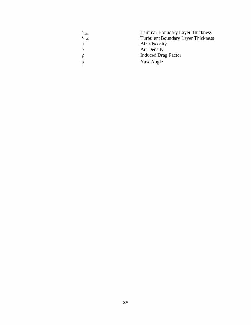
δlam Laminar Boundary Layer Thickness δturb Turbulent Boundary Layer Thickness μ Air Viscosity ρ Air Density φ Induced Drag Factor

ψ Yaw Angle

xv

EXPERIMENTAL INVESTIGATION INTO THE AERODYNAMIC GROUND

EFFECT OF A TAILLESS CHEVRON-SHAPED UCAV

I. Introduction

Section 1 – Ground Effect

Ever since the early days of aviation, pilots have experienced a phenomenon

while operating an aircraft very close to the ground. Either during take-off or landing,

any air vehicle will experience improved efficiency near the ground in the form of

increased lift. However, this poses a problem because most aircraft are not designed for

this flight condition and therefore can behave very awkwardly.

A typical aircraft is in-ground-effect (IGE) when it is within one wingspan of the

ground (1). The amount of ground effect experienced by an aircraft is dependent on the

induced drag. When the height of an aircraft is below one wingspan of the ground, the

induced drag significantly decreases due to the wingtip vortices interacting with the

ground (1). During normal flight, wingtip vortices are cylindrical in shape, but while

interfering with the ground, they tend to flatten out which improves the effective

wingspan and aspect ratio. Since aspect ratio has a strong inverse effect on induced drag,

an aircraft flying very near the ground will experience a reduction in induced drag

reducing the total drag of the aircraft (1).

In addition to a reduction in drag, an increase in lift and pitching moment are

characteristics of an aircraft in ground effect. The increase in lift along with the

reduction of drag significantly increases the lift-to-drag ratio, which intuitively increases

1

the overall aircraft efficiency. The discovery of this improved efficiency led to the

development of Wing-In-Ground vehicles (2).

Section 2 – Wing-In-Ground Vehicles

Wing-In-Ground (WIG) vehicles take advantage of all the benefits of ground

effect because they are designed to operate at very low altitudes. As knowledge and

technology improved during the 20th century, WIG vehicles increased in popularity and

many thought they were the future of marine transportation.

In the 1960’s, Russian scientist Rostislav Alexeiev led the development of WIG

boats. With his background in hydrofoil ship design, Alexeiev’s research led to the

development of ekranoplans. ('skimmer' in English) The Soviet Union saw the military

potential in these vessels, and so Alexeiev received practically unlimited funding for his

then top-secret project (2). Only a few years later, in 1966, Alexeiev unveiled the KM

Caspian Sea Monster, a 550-ton WIG vehicle designed heavy loading and fast

transportation over water. The KM was far more advanced than the ekranoplans

developed earlier by Alexeiev mainly because its weight was 100 times that of the

heaviest ekranoplan at that time. Several other crafts were developed and built for the

Russian Navy in the decades to follow, but in the late 1980’s, funding was lost due to the

fall of the Soviet Union and the end of the Cold War (2).

2

Figure 1: KM Caspian Sea Monster (2)

To meet the growing demands of the U.S. Army Mobility Command, Boeing

Phantom Works is evaluating a similar concept with the Pelican project. Like the

Russians concept of WIG vehicles, the Pelican would have twice the external dimensions

of the world’s largest aircraft and would utilize ground effect to produce the necessary

lift-to-drag ratio for flight operations. It would have the cargo capacity to carry an entire

Army division of supplies and soldiers or up to 17 M-1 tanks (3). The WIG vehicle

concept could revolutionize marine transportation thanks to the beneficial effects of

flying low.

Section 3 – Unmanned Air Vehicles

Ever since the beginning of aviation, the concept of unmanned flight has intrigued

engineers and scientists. The first unmanned air vehicles (UAV) were built to be used as

guided missiles. The Kettering “Bug” and Sperry aerial torpedo were the first two

combat UAVs but were never used in operation due to inaccuracy. As technology

advanced, researchers investigated the use of radio and eventually television control links

to correct the erroneous navigation issues. During the last quarter-century, significant

3

advances in computing capabilities, electronics miniaturization, communications,

guidance, navigation, and control have allowed for successful flight operations of the

Global Hawk and Predator UAVs, which are currently being used daily in conflicts

around the world (4).

The next development of unmanned flight is the unmanned combat air vehicle

(UCAV). Currently, the primary program for UCAV exploration is the joint unmanned

air systems (J-UCAS) program, which is a joint Darpa, Air Force, and Navy program.

The J-UCAS program is designed to

demonstrate the technical feasibility, military utility and operational value for a networked system of high performance, weaponized unmanned air vehicles to effectively and affordably prosecute 21st century combat missions, including Suppression of Enemy Air Defenses (SEAD), surveillance, and precision strike within the emerging global command and control architecture. (5)

The two leading UCAVs are the Boeing X-45 and the Northrop Grumman X-47. Each

one has an unconventional configuration including a blended wing body with swept

wings and no tail. Even though today’s advanced control systems allow for such

unconventional designs, the ground effect phenomenon still poses problems.

Section 4 – UAVs and Ground Effect

Understanding the location and the extent of the ground effect region is of

particular interest for UAVs because of the shear fact that they are unmanned. Pilots use

sight and feel when operating a conventional aircraft near the ground. During a landing,

a pilot will normally flare the aircraft to ensure that the rear landing gear strikes first. If

necessary, the pilot can make small adjustments to the aircraft attitude for the drag

reduction and increase in lift while in the ground effect region. The pilot for a UAV

4

operates the craft from a Ground Control Station (GCS) and uses real time video and

sensors. The removed operator or UAV pilot cannot feel the effects of the ground during

take off and landing and depends entirely on the automatic control system. Therefore, it

is important to identify the ground effect region in order to ensure safe flight. Normally,

since the ground effect region is a small portion of time compared to the entire glide

slope to land, it is not factored into the landing control system design. However, with

sufficient data from flight tests or wind tunnel tests, the control engineer will make gain

adjustments to account for the ground effect region (6).

Unmanned flight brought with it numerous mishaps near the ground. One of

particular interest was on 22 April 1996, when the Lockheed Martin/Boeing RQ-3A

DarkStar’s fight control system did not properly account for ground effect. It ‘porpoised’

during take-off, pitched up, and stalled due to over-correction by ailerons (7).

Section 5 – Boeing AFRL/VAAA UCAV Program

In an effort to expand the database for unconventional aircrafts, Capt. Shad Reed

of the Air Vehicles Directorate (VAAA) of the Air Force Research Laboratory (AFRL)

conducted a low-speed wind tunnel investigation on three generic UCAV planforms. The

test program defined the stability and control characteristics of moderately swept, low

aspect ratio, tailless, blended wing body planforms. The three planforms tested were a

chevron, lambda, and diamond shape. Their characteristics are found in reference (8).

Of the three configurations tested, the chevron-shaped planform had the highest

maximum lift coefficient, lift-to-drag ratio, and lowest minimum drag coefficient.

However, due to the chevron planform’s lack of fuselage, Reed concluded that subsystem

5

integration would be difficult since engines, weapons, and other components are

normally located in the fuselage (8).

Despite Reed’s conclusions about the possible subsystem integration problems of

the chevron-shaped planform, a ground effects test is still of interest because improved

technology can solve the apparent subsystem integration problems (8).

6

II. Literature Review

Section 1 – Ground Effect Theory

Since the beginning of flight, aircraft designers noticed the decrease in landing

speed due to an increase in lift while in close proximity to the ground. Engineers

conducted numerous wind tunnel and flight test experiments around the world in order to

investigate this phenomenon called ground effect.

In 1922, Wieselsberger developed his famous theoretical equation for estimating

the induced drag reduction of aircraft near the ground. He used Prandl’s three-

dimensional wing theory and the reflection method to establish a relatively simple

relationship between height above ground and induced drag (9). His equation became the

standard for predicting ground effect and was verified throughout the 1930s and 1940s in

references 10-12, among others.

Another theoretical approach to estimating the decrease in induced drag due to the

presence of the ground is to apply McCormick’s induced drag factor. In his section on

ground roll and takeoff distance, McCormick derived Equation [1] by replacing a

rectangular wing with a simple horseshoe vortex modeled with its image so the vertical

velocities cancel each other simulating the ground. The height was the distance between

the reflection plane to the horseshoe vortices. McCormick then used the Biot-Savart Law

to estimate the velocity induced at a point from each horseshoe vortex. This led him to

identify a ratio between the induced drag in ground effect and the induced drag out-of-

ground effect (13).

7

( )( )

2

2

16

1 16

h b

h bφ

⎡ ⎤⎣ ⎦=+ ⎡ ⎤⎣ ⎦

[1]

As discussed in Chapter I, ground effect is normally experienced at heights above

ground less than one wingspan, and the effect is increased exponentially as the aircraft

travels below half of a wingspan as demonstrated in references 17, 20, and 21. Equation

[1], when when multiplied by the induced drag, provides a prediction for ground effect.

Figure 2 is a plot of McCormick’s induced drag factor.

0

0.2

0.4

0.6

0.8

1

1.2

0 0.1 0.2 0.3 0.4 0.5 0.6

h/b

Indu

ced

Dra

g Fa

ctor

Figure 2: McCormick's Induced Drag Factor (13)

Section 2 – Static vs. Dynamic Wind Tunnel Testing

Experimental methods for ground effects have become more sophisticated during

the past several decades. One of the first wind tunnel investigations was Raymond’s

8

study at the Massachusetts Institute of Technology in 1921 (14). He analyzed ground

effect by testing three different airfoils in a wind tunnel using a flat plate for a ground

plane. He also attempted to create an imaginary ground plane by means of reflection.

Both methods revealed similar results except at high angles of attack. This test

confirmed that when near the ground, an airfoil will increase in lift and decrease in drag

(14).

As testing techniques advanced, Raymond’s flat plate method took the name of

static wind tunnel testing. A static wind tunnel test involves a fixed ground plane height

and model. Moving the model closer to the ground plane is normally how various

heights above ground are tested. In order to validate these tests, test pilots flew ground

effect testing routes, called ‘fly-by’ patterns. To determine the extent and location of the

ground effect region, altitude and angle of attack were held constant. However, in 1967,

William Schweikhard developed a method for measuring the ground effects of an aircraft

as it approached a runway (15). A test pilot would maintain a constant angle of attack

and power setting, but would let the sink rate vary; this ensured that lift, drag, and

pitching moment were constant just before approaching the ground. Once in the ground

effect region, flight test engineers measured any changes in flight path angle, velocity, or

control surface deflection. They found that this flight test technique saved time and data

analysis over standard fly-by or static tests (15).

In an effort to reduce flight test costs, engineers developed methods to

dynamically test for ground effect in a wind tunnel. A dynamic wind tunnel test for

ground effect attempts to better simulate a landing approach or a take off by manually or

mechanically moving the model towards the ground plane. Chang et al. found relevance

9

in dynamic wind tunnel testing as he noted the disparity between static tests and landing

data (16). He tested delta wings of 60, 70, and 75 deg sweep, the XB-70, and the F-104A

both statically and dynamically. He, along with Baker et al., concluded that at heights of

h/b < 0.4, the static wind tunnel results for the delta wings and XB-70 significantly over

predicted the change in lift due to ground effect (17). However, he also pointed out that

the amount of difference between static and dynamic results decreased as aspect-ratio

increased. See Figure 3.

Figure 3: Incremental CL vs. AR for static and dynamic ground effect at h/b=0.3 (17)

Additionally, Corda, et al. (18) performed a dynamic ground effect test on the F-

15. Their results are mentioned because the chevron UCAV has a similar aspect ratio to

that of the F-15. They fit the following equation to the dynamic ground effect tests for

the delta wings presented in Figure 4:

10

,0.2% 0.04L GECAR

⎛ ⎞Δ = +⎜ ⎟⎝ ⎠

*100 [2]

Equation [2] quanifies the relationship between percent increase in lift due to ground

effect and aspect ratio for a wing. Based on this prediction the chevron UCAV should

experience a 10.9% increase in lift due to ground effect.

More importantly, this relationship and results presented in Figure 4 suggest that a

staic ground effect test for the chevron UCAV should produce similar results as a

dynamic test.

Figure 4: Percent Increase in CL in Ground Effect vs. AR for Various Aircraft (18)

A common tool used to predict and verify ground effect tests is the U.S. Air Force

Data Compendium (DATCOM) (19). This analytical program uses equations, charts, and

flight data to predict stability and control characteristics of aircraft. Since the static

ground effect prediction for the F-15 lies almost directly on the curve based on dynamic

11

results for wings (Equation [2]), a static ground effect test for the chevron UCAV should

produce similar results to that of a dynamic test.

Section 2.1 – Adverse Ground Effect

While ground effect is normally characterized by an increase in lift and a decrease

in drag, not all aircraft configurations experience these beneficial traits. Lee, et al. (20)

reported an increase in lift along with an increase in drag as height above ground

decreased.

They performed dynamic and static wind tunnel tests on models of a 60 deg delta

wing, F-106, and XB-70-1. Re was varied from 3x105 to 7.5x105 and height above

ground ranged from h/b=1.6 to h/b=0.2 for all three models. Their focused primarily on

the differences between the static and dynamic results, so no emphasis was placed on the

increasing lift or drag. The CD vs. (h/b) plot for the F-106 in Figure 5 represents their

results.

Figure 5: Adverse Ground Effect for the F-106 at an AOA = 14 deg (20)

12

Although Lee, et al. did not show any L/D results, the static data were

extrapolated from their CD vs. (h/b) plots (similar to Figure 5) and CL vs. (h/b) for each

model to analyze the trends. The 60 deg delta wing experienced a subtle decrease in L/D.

The F-106 and XB-70-1 both experienced a decrease and a slight increase in L/D at the

lowest height above ground. The downward trend of CD between h/b=0.3 and 0.2 in

Figure 5 was common for the XB-70-1 and explained the increase in L/D.

It is possible that aspect ratio and wing sweep played a role in these results. The

60 deg delta wing, F-106, and XB-70-1 had aspect ratios equal to 2.3, 2.4, and 1.78,

respectfully. The F-106 had a wing sweep of 60 deg and the XB-70-1 had wing sweep of

65 deg. Again, these considerations were not discussed in their report, but are mentioned

because the chevron UCAV has similar characteristics.

Similarly, the F-16 XL aircraft was flight tested and wind tunnel tested for ground

effects by Curry (6). He found an increase in CD as height above ground decreased and

explained that an increase or a decrease in drag is possible for aircraft flying close to the

ground. Curry and Owens (21) also discovered an increase in drag when the Tu-144

supersonic transporter flew in close proximity to the ground.

Section 3 – Boundary Layer Removal

One limitation using a ground plane in a wind tunnel to simulate ground effect is

the boundary layer build-up across the top surface. Boundary layers form on any surface

where a moving fluid has direct contact, so they cause an unrealistic test condition in

13

wind tunnels when a ground plane is used to simulate the ground. A boundary layer

removal system is typically employed to resolve this issue.

One method of removing the boundary layer in a wind tunnel is to use a moving-

belt ground plane. A moving-belt would better simulate an aircraft flying over the

ground because the belt would spin at the same velocity of the air, which in turn removes

the boundary layer.

While it seems that boundary layer removal with a moving-belt ground plane is

essential to achieve proper flight dynamics, two different studies were conducted that

showed the necessity of a moving-belt ground plane depends on the maximum lift

coefficient of the air vehicle. Turner (22) investigated the use of conventional ground

planes for ground effect wind tunnel testing. Specifically, he examined the possible use

of endless-belt ground planes and determined the conditions under which it would be

preferable. He concluded that the use of a moving-belt ground plane depended on

spanwise lift coefficient and height above ground (22).

14

Figure 6: Conditions Requiring an Endless-belt Ground Plane (22)

The shaded box in Figure 6 indicates the region tested in the present study, and

the CL max line indicates the maximum lift coefficient found in Reed’s study (8). Thus,

according to Turner, a moving-belt ground plane was not required for this experiment.

Kemmerly and Paulson, Jr. did a similar study comparing the use of a

conventional ground plane (23). While Turner studied high-lift, high-aspect-ratio models,

Kemmerly and Paulson, Jr’s study evaluated an F-18 and delta wing models. They

concluded that if the condition in Equation [3] was satisfied, then an engineer must use a

moving-belt ground plane to study ground effects.

( ) 0.05L

h bC

< [3]

15

According to the heights used in this study and the maximum lift coefficient according to

Reed, a conventional flat-plate ground plane without a moving-belt was adequate to

properly measure ground effects, Table 1 shows that Equation [3] was not satisfied.

Table 1: Justification for a Flat-plate Ground Plane

h/b CL max * (h/b) / CL max < 0.05 ?0.3 0.9 0.33 No

0.15 0.9 0.17 No0.1 0.9 0.11 No

0.05 0.9 0.06 No* as denoted in Reed's study

Section 4 – Goals of the Experimental Effort

Reed concluded that the chevron shaped planform performed the best with respect

to aerodynamics and longitudinal/lateral stability. A ground effect analysis will further

the investigation of the aerodynamics of an advanced aircraft configuration.

The goal of this effort is to:

• identify the ground effect region of the chevron-shaped planform with respect to height above the ground;

• expand the existing aerodynamic database for moderately swept, low

aspect ratio, tailless, blended wing body UAVs; • analyze the test section flow characteristics of the AFIT 3’ x 3’ wind

tunnel with a ground plane; • verify McCormick’s equation for induced drag factor, and

• compare aerodynamic out-of-ground effect data with Reed’s study.

The following will include an overview of the research considered, a description

16

of the equipment and procedures used, results and analysis of the experimental data,

concluding remarks, and recommendations.

17

III. Experimental Set-up & Procedures

The following chapter will explain the various resources and materials used to test

the chevron-shaped UCAV in ground effect. It will also include an outline of the wind

tunnel testing procedures.

Section 1 – UCAV Model

As mentioned previously, the wing planform used in this study was originally

tested by Capt. Shad Reed of AFRL/VAAA. The original model was built by Dynamic

Engineering, Inc. in 1996 and was tested in the Boeing St. Louis Low Speed Wind

Tunnel (LSWT) and in the AFRL Subsonic Aerodynamic Research Laboratory (SARL).

It was built out of Ren 450, a woodlike epoxy resin board, and 7075-T6 aluminum. Its

dimensions can be found in Table 2.

Table 2: Original and Scaled UCAV Model Properties

Original Model Scaled ModelMaterial Ren 450 & Aluminum Photopolymer Plastic

Wing Area, in2 364.87 87.396Span, in 32 16

Root Chord, in 14.85 7.42MAC, in 13.35 5.20

Aspect Ratio 2.806 2.929Leading Edge Sweep, deg 45 45

Chevron UCAV Dimensions

18

Figure 7: Original Chevron UCAV

The original chevron UCAV model (shown in Figure 7) has a 32-in wingspan,

making it just small enough to fit it the AFIT 3’ x 3’ wind tunnel. Because its wingtips

would extend too close to the test section walls to produce accurate results, so a scaled

down version was created. The original electronic drawings could not be found, a 3-D

scanner digitized the original model. The engineers and technicians of AFRL/Human

Effectiveness Branch (HECV) allowed the author to use a 3-D digitizer and software to

digitize the chevron UCAV model.

19

Figure 8: FARO Space Arm™

The digitizer set up included the FARO Space Arm™ (shown in Figure 8) along

with Caliper 3D™ Version 2.43. After probe calibration, the pivoting arm was moved so

that the probe touched the surface of the model. The points collected were transposed

into an IGES file, which was then read into the drawing program Solid Works©. Only

points along the top surface of the right wing were collected. Since the chevron UCAV is

perfectly symmetrical, the surfaces were mirrored across the centerline, and then again to

form the bottom surface. Once the model was in Solid Works©, the hole for the balance

was added so that the model center of gravity (CG) was precisely located 2.5 inches from

the back edge of the hole. A scaling factor of 12 was selected, allowing the model to be

small enough to fit into the wind tunnel, but large enough to compare and gather

aerodynamic data.

20

Figure 9: Solid Works Drawings of the 1

2 -scaled Chevron UCAV

The final step in producing the scaled-down version was converting the file

into .stl format and then printing it with the AFIT/ENY 3-D rapid prototyping machine.

The Stratasys Objet EDEN 333 rapid prototyping machine uses eight small jets that lay

down UV plastic (also known as photopolyer plastic) material and a gel-like UV plastic

for support material in 0.0006-in layers. The eight jets transverse across the printed

region in 2-in strips followed by a UV light which cures the plastic simultaneously (24).

The Full Cure 700 series photopolymer plastic model material can be machined, drilled,

and chrome-plated; used as a mold; and absorb paint (25). Three images of the scaled

down rapid prototyped model are shown in Figure 10 and Figure 11 . Refer to Appendix

A for more pictures.

21

Figure 10: 1

2 -Scaled Chevron UCAV Model

Figure 11: 1

2 -Scaled Chevron UCAV in Test Section

22

Section 2 – Wind Tunnel

Section 2.1 – Equipment

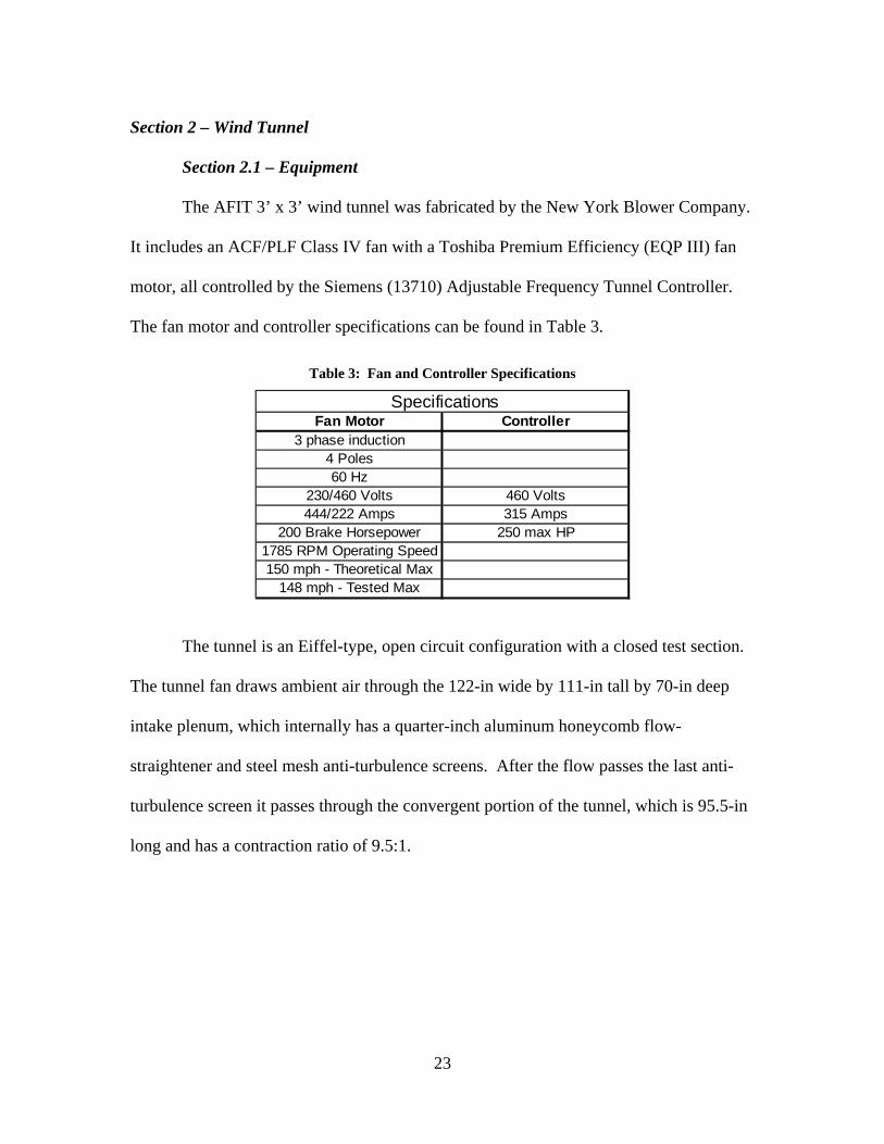
The AFIT 3’ x 3’ wind tunnel was fabricated by the New York Blower Company.

It includes an ACF/PLF Class IV fan with a Toshiba Premium Efficiency (EQP III) fan

motor, all controlled by the Siemens (13710) Adjustable Frequency Tunnel Controller.

The fan motor and controller specifications can be found in Table 3.

Table 3: Fan and Controller Specifications

Fan Motor Controller3 phase induction

4 Poles60 Hz

230/460 Volts 460 Volts444/222 Amps 315 Amps

200 Brake Horsepower 250 max HP1785 RPM Operating Speed150 mph - Theoretical Max

148 mph - Tested Max

Specifications

The tunnel is an Eiffel-type, open circuit configuration with a closed test section.

The tunnel fan draws ambient air through the 122-in wide by 111-in tall by 70-in deep

intake plenum, which internally has a quarter-inch aluminum honeycomb flow-

straightener and steel mesh anti-turbulence screens. After the flow passes the last anti-

turbulence screen it passes through the convergent portion of the tunnel, which is 95.5-in

long and has a contraction ratio of 9.5:1.

23

Figure 12: Wind Tunnel Intake and Convergent Sections with Dimensions (26)

After the convergent section, the flow passes through the test section. The test

section is octagonal in shape to eliminate the corner interference effects and has

dimensions of 31.5-in tall, 44-in wide, and 72-in long. The chevron UCAV has a span-

to-tunnel width ratio of 0.37, which is well below the recommended value of 0.8 (27). In

addition, the ground plane frontal area is 6.7% of the test-section cross-sectional area,

which is below the recommended value of 7.5% (27).

The model sting support is positioned in the test section through a slot in the

traverse circular plate. This remotely controlled device can vary the angle of attack of the

model from -25o to +25o. For yaw angle, the traverse circular plate rotates and moves the

entire sting mechanism and can be rotated from -20o to +20o.

24

Figure 13: Wind Tunnel Test Section and Components (28)

The balance used for this test was the AFIT-1 Balance, an internal six-component

balance manufactured by Modern Machine & Tool Co, Inc. See the complete capacity of

strain gage rosettes listed in Table 4. Refer to reference 29 for a more thorough

description of the AFIT-1 Balance.

Table 4: AFIT-1 Balance Maximum Loads

Component Maximum LoadNormal Force (N1) 10 lbsPitch Moment (N2) 10 in-lbs

Side Force (S1) 5 lbsYaw Moment (S2) 5 in-lbsAxial Force (A1) 5 lbsRoll Moment (L1) 4 in-lbs

After the flow travels through the test section, it enters the 26-ft long divergent

section, which includes a model catcher in case of any component failure. Once through

25

the divergent section, the flow goes through the fan and exits vertically up through the

exhaust pipe. See Figure 14 for complete schematic of the wind tunnel.

Figure 14: Wind Tunnel Schematic (28)

Section 2.2 – Procedure

A static weight calibration process was carried out first. Known weights were

attached to the balance and the calibration constants were adjusted in the data collection

software by manually matching the loads on the balance to the loads registered in the

software. Linearity was verified by ensuring that the voltages corresponded linearly to

the increases in weights attached. LabView Virtual Instrument© interface was used to

control all tunnel parameters including angle of attack, yaw angle, and tunnel speed.

While this interface controlled these parameters, analog backups of angle of attack and

sideslip angle were also monitored with sting mounted optical encoders. The analog

measurement for velocity was a pressure transducer and pitot-static tube and was the

main guide for tunnel velocity throughout all the test runs.

26

The measured data from the balance was stored in the form of two normal force

components (N1 & N2), two side force components (S1 & S2), an axial force component

(A1), and a roll moment (l1). Voltage was continuously applied to the strain gage rosette,

and resistance was measured across the wire filament. The applied load elongated the

wire causing an increase in the resistance. Output voltages from the increased resistance

were equated to strain and finally force through a series of calibration equations. A

conventional coordinate system was used in the tunnel with +x-direction pointing

towards the intake, +y-direction pointing out towards the access door, and +z-direction

pointing down towards the tunnel floor. See Figure 15 for a better understanding of the

coordinate system.

Figure 15: Test Section Coordinates (26)

After the balance was calibrated, the chevron UCAV was mounted to the balance

using two 2-56 screws. Because of the symmetrical wing planform of the UCAV model,

27

the balance was in line with the longitudinal x-axis and at the y- and z-axis centers of

gravity.

The chevron UCAV model was tested in two different flight conditions: Out-of-

Ground-Effect (OGE) and In-Ground-Effect (IGE). The OGE tests examined the

longitudinal forces and moments on the UCAV away from the ground, whereas the IGE

tests explored the same criteria except the ground plane was placed at four different

heights. The proposed test conditions called for four different wind tunnel speeds each

with angle of attack sweeping from -10 deg to +20 deg. However, these conditions were

not met for most of the test runs due to balance capacity limitations and potential model

or sting mechanism collision with the ground plane. Table 5 shows the actual test matrix

for each test run. A tare or wind-off run was completed to calculate the effect of the

UCAV’s static weight on the balance. This effect was necessary to remove the tare

effects on the axial sensor, which affects the drag coefficient calculation.

Table 5: Experimental Test Matrix

Tunnel Speed:(mph) UCAV only

Plane 1h/b = 0.3

Plane 2h/b = 0.15

Plane 3h/b = 0.10

Plane 4h/b = 0.05

40 -10o<α<+20o -10o<α<+17o -10o<α<+17o -10o<α<+11o -5o<α<+6o

60 -10o<α<+14o -10o<α<+14o -10o<α<+13o -8o<α<+11o -5o<α<+6o

80 -8o<α<+7o -7o<α<+7o -5o<α<+6o -4o<α<+6o -3o<α<+5o

100 -5o<α<+4o -4o<α<+4o -3o<α<+3o -3o<α<+3o -1o<α<+3o

The test matrix in Table 5 shows that as the height above ground decreased, angle

of attack variation declined due to the extra forces and moments on the model as it

entered into the ground effect region. To avoid damaging the balance due to these added

loads, the alpha sweeps were limited.

28

Section 2.3 – Data Analysis

A data acquisition program was set up within the control computer to store the

data in a tab delimited text file at a rate of two data points per second (2 Hz sampling

rate). For the alpha sweeps, the flow velocity was slowly increased until the desired

speed was reached. After ensuring that the balance was taking accurate data, the model

was dropped to its least negative alpha setting and data were acquired for 30 sec. The

angle of attack then increased 2 deg and held for another 30 sec. This was repeated until

either the balance reached its capacity or the ground plane interfered with the sting

mechanism.

A MATLAB® code, written by Capt. DeLuca (26), Lt. Gebbie (28), and altered

for the AFIT-1 balance by Lt. Rivera Parga (29) was used to reduce the acquired force

and moment data. The data reduction program received the tare file and one of the

experimental test files simultaneously. It then combined the similar measured forces and

moments and averaged them to a single test point for each angle of attack. Before this

data were exported as aerodynamic coefficients, the physical testing conditions, balance

interactions, and blockage correction factors were calculated. For more detail regarding

the data reduction program, see references 26, 28, and 29.

After the MATLAB® program reduced the data, an EXCEL® output file was

created that consisted of Mach number, Reynolds number, dynamic pressure, velocity,

angle of attack, lift, drag, roll moment, pitching moment, yaw moment, and side force

coefficients for every angle of attack tested. Standard aerodynamic plots were then

created. See Appendix C for a sample calculation of the data reduction.

29

Section 3 – Ground Plane Design and Construction

In order to properly represent the model flying close to the ground, a ground plane

was built and mounted in the wind tunnel. The ground plane was composed of two plates

and eight cylindrical legs. The plates were hot-rolled steel and the legs were cold-rolled

steel. The dimensions are shown in Table 6 and pictures of the ground plane are shown

in Figure 16 andFigure 17. Refer to Appendix A for more pictures and to Appendix B for

detailed drawings of the ground plane.

Figure 16: Ground Plane

30

Figure 17: Ground Plane and Model in Test Section

thickness, in 0.25diameter/width, in 35.313max length, in 44.313

diameter, in 1.5length, in height 1 9.77 height 2 12.17 height 3 12.97 height 4 13.77

Ground Plane Dimensions

Legs

Plate

Table 6: Ground Plane Dimensions

The circular plate is identical to the traverse circular plate on the floor of the test

section, which rotates to simulate yaw angle. By mounting the circular ground plane

piece on top of the circular floor plate, the model being tested with the ground plane can

31

also experience the same yaw deflection as a model not tested with the ground plane.

The circular piece also has a cut 11-in by 1.5-in in the rear to allow the sting mechanism

to rotate to alter the angle of attack of the model. Figure 18 shows the two pieces

separated.

Figure 18: Top View of Ground Plane with Front and Circular Pieces Separated

The front piece of the ground plane provides a straight leading edge that is

rounded and beveled cut as shown in Figure 19.

32

Figure 19: Leading Edge of Ground Plane

A pair of screws mounted in counter-bored holes was used to attach each

cylindrical leg to the flat plate. Sixteen holes were drilled in the test section floor so that

the eight legs were mounted securely. A stress analysis was completed to ensure that the

maximum dynamic pressure of the wind tunnel’s maximum velocity (150 mph) would

not sever the screws and overturn the ground plane. Four quarter-inch screws were used

to mount each leg, which resulted in a factor of safety of 18.

Section 3.1 – Predicting the Leg Heights

Not having the flexibility of altering the model height with the sting, the ground

plane height was changed to vary the height above ground. Various methods were

considered including using hollow cylinders with varying rows of holes held together by

pins to allow for a changing ground plane height. With the uncertainty of how the

33

dynamic pressure would affect the ground plane, it was decided to use four different leg

heights that were interchanged for each height.

The ground plane heights were selected to ensure the greatest effect from the

ground on the model. Based on McCormick’s ground effect prediction for induced drag

along with the ground effect regions discovered in references 17, 20, and 21, the four

heights were chosen and can be seen in Table 7.

Table 7: Ground Plane Heights and Corresponding h/b

GP Designator height h / bPlane 1 10.02 0.3Plane 2 12.42 0.15Plane 3 14.22 0.1Plane 4 14.02 0.05

Model height above ground was referenced from the root quarter-chord.

Section 4 – Boundary Layer Calculations

While time constraints did not allow for boundary layer measurements,

conventional flat plate boundary layer equations were used to predict the boundary layer

height and displacement thickness at the model location.

Typically, boundary layers are divided into two types: laminar and turbulent.

Each type has a no slip and solid surface boundary condition, which means that the fluid

particles touching the surface have zero velocity and the flow can not travel through the

surface.

The laminar boundary layer calculations utilized the Falkner-Skan method (30).

While this method can be used for flows around a wide range of configurations, the

simplest form, flow past a flat plate, was used in this study. The laminar boundary layer

34

thickness was defined as the distance from the flat plate to where the velocity equaled

99% of the free-stream velocity. Assuming an inviscid, incompressible flow, the laminar

calculations used the following equation:

5.0Relam

x

xδ = [4]

As the boundary layer builds up in the streamwise direction, a transition process takes

place due to disturbances in the flow. This transition segment can vary widely in length

and strength, but normally depends on pressure gradient, surface roughness,

compressibility effects, surface temperature, suction or blowing on the surface, and free-

stream turbulence (30). For this study, it will be assumed that this process occurs

instantaneously.

For incompressible flow past a flat plate, transition is function of Reynolds

number. It is customary to use a Reynolds number of 500,000 to locate the transition

point (30). For each tunnel velocity used for the experiment, a different transition point

was located. The laminar boundary layer thickness was noted at this location, and the

turbulent boundary layer was set equal to this thickness.

Exact calculations of the turbulent boundary layer normally involve differential

equations of motion for computational fluid dynamic models. For this study, time-

averaged (or mean-flow) properties were assumed and the flow velocity was represented

by the power law approximation, noted in Equation [5].

1

7U yU δ∞

⎛ ⎞= ⎜ ⎟⎝ ⎠

[5]

35

From this estimate, the turbulent boundary layer thickness could be derived based

on Blasius’ skin friction coefficient for a turbulent boundary layer on a flat plate. To see

the actual derivation, see reference 31.

( )0.2

0.3747Re

turbxδ = [6]

As mentioned before, an instantaneous transition was assumed, and so Equation

[6] was set equal to Equation [4] at the transition point. Solving this equation for x and

subtracting the result from the transition point gave the pseudo-starting point for the

turbulent boundary layer build-up. Figure 20 illustrates the assumptions.

Figure 20: Schematic of Boundary Layer Build-up

The boundary layer thickness results were most relevant for the streamwise x

locations from the nose of the model to the trailing edge. In order to determine the

36

distance the external streamlines were shifted due to the presence of the boundary layer,

the displacement thickness was calculated using Equation [7].

*

0

1 U dyU

δ

δ∞

⎛ ⎞= −⎜ ⎟

⎝ ⎠∫ [7]

The displacement thickness is largely dependent on the velocity profile.

Substituting Equation [5] into Equation [7] with δ equal to the turbulent boundary layer

thickness at the trailing edge of the model, the displacement thickness was estimated.

Section 5 – Hot-wire Anemometry

A hot-wire anemometry experiment was used to determine the difference between

the indicated transducer velocity and the actual velocity at the model. Also, it was used

to examine the blockage effects due to the ground plane. The following describes the

equipment, procedure, and data analysis.

Section 5.1 – Equipment

The AFIT low-speed 3’ x 3’ wind tunnel is equipped with a Dantec-Dynamics

Streamline 90N10 Constant Temperature Anemometer (CTA). It is fully motorized and

programmable with a 3-axis traversing system. The probe type used was a single wire 55

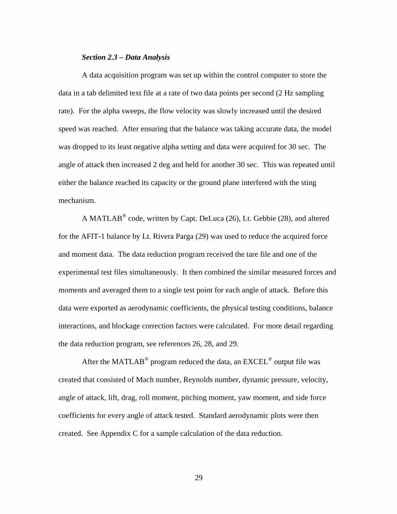
P11 and was used with the vertical attachment. Figure 21 is a drawing of the probe with

the single wire parallel to the y-axis.

37

Figure 21: Schematic of Hot-wire Probe Configuration

The maximum range of the probe is 19.7 inches in the horizontal (y-direction) and

vertical (z-direction) direction. It also has the capability to traverse longitudinally in the

x-direction approximately 3 ft. The Dantec hot-wire anemometer came with a data

acquisition program called Streamware® which was used to collect, process, and format

data.

Section 5.2 – Procedure

The hot-wire anemometer was calibrated using the Dantec automatic calibrator

system. While the hot-wire is outside the tunnel, the automatic calibrator with attaching

nozzle blew air across the single wire probe. The velocity was controlled by the

Streamware® software in the control room and was increased from 4.5 mph to 161 mph.

As the known velocity increased, the anemometer measured the voltage across the single

wire. The calibration program within the Streamware® software automatically created

38

the conversion factor between volts and metric-based velocity, which was manually

converted to mph for consistency.

For the hot-wire anemometry experiment, the top Plexiglas window was removed

and replaced by one with slotted groves specifically designed for the hot-wire. The slots

were plugged according to the longitudinal station of interest. Figure 22 illustrates slot

number 1 open for hot-wire velocity measurements.

Open Slot (#1) Plugged Slots (#2 - #6)

Figure 22: Removable Plexiglas Top for Hot-wire Anemometry (26)

Slot number 2 was used for this experiment because it was the closest station to

the model CG. Its exact location was 2 inches in front of the model CG. Velocity was

measured without the ground plane, at the lowest ground plane height, and the highest

ground plane height at speeds of 40, 60, 80, and 100 mph.

39

The probe started at a position 1-in outside the left wing and 1-in above the top

surface. It first descended 2.36-in collecting velocity data every 0.40-in to a location

0.36-in below the bottom surface of the model. It then translated 1.89-in in the positive

y-direction, collected data, and then ascended 2.36-in again collecting data every 0.40-in.

It continued on this pattern across the entire span of the model stopping at 1-in outside

the right wingtip. See Figure 23 for the nominal probe grid test pattern.

Figure 23: Hot-wire Test Grid

Section 5.3 – Data Analysis

The Dantec Streamware® software stored the data files from each test run as a

Comma Separated File (.csv). The software converted the raw test data, as voltages into

40

mean velocities at each test point. The mean velocities were compared to the transducer

indicated velocities to illustrate the differences.

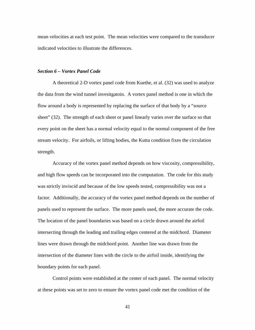
Section 6 – Vortex Panel Code

A theoretical 2-D vortex panel code from Kuethe, et al. (32) was used to analyze

the data from the wind tunnel invesitgatoin. A vortex panel method is one in which the

flow around a body is represented by replacing the surface of that body by a “source

sheet” (32). The strength of each sheet or panel linearly varies over the surface so that

every point on the sheet has a normal velocity equal to the normal component of the free

stream velocity. For airfoils, or lifting bodies, the Kutta condition fixes the circulation

strength.

Accuracy of the vortex panel method depends on how viscosity, compressibility,

and high flow speeds can be incorporated into the computation. The code for this study

was strictly inviscid and because of the low speeds tested, compressibility was not a

factor. Additionally, the accuracy of the vortex panel method depends on the number of

panels used to represent the surface. The more panels used, the more accurate the code.

The location of the panel boundaries was based on a circle drawn around the airfoil

intersecting through the leading and trailing edges centered at the midchord. Diameter

lines were drawn through the midchord point. Another line was drawn from the

intersection of the diameter lines with the circle to the airfoil inside, identifying the

boundary points for each panel.

Control points were established at the center of each panel. The normal velocity

at these points was set to zero to ensure the vortex panel code met the condition of the

41

airfoil being a streamline. Figure 24 is a picture of the method by which the panel

boundaries were determined along with the location of the control points.

Figure 24: Method for Determining Panel Boundaries (32)

Figure 24 shows how 12 souce panels represent an airfoil. The vortex panel code used in

this experiment utilized 100 panels and control points.

The vortex panel method used reflection to analyze ground effect. Two airfoils

were placed a certain distance from each other, and a region of zero vertical velocity

forms half way between each airfoil, which simulates the ground. The code inputs airfoil

chord length, thickness, camber, max camber location, and angle of attack. Also,

airspeed, density, and distance from the ground (measured from the quarter-chord) were

inputted. The four plots outputted were surface pressure coefficient distribution, pressure

42

field, streamlines representing the flow field, and velocity field. Additionally, the code

calculated lift coefficient, circulation, lift force, pitching moment.

43

VI. Results & Analysis

This chapter presents the data gathered from the wind tunnel experiments for the

chevron UCAV. The hot-wire anemometry data will be presented first followed by the

flow visualization and ground effect results.

Section 1 – Hot-wire Anemometry

The results from the hot-wire anemometry experiment exposed a significant

difference in the velocity measured by the pressure transducer and the hot-wire

anemometer. Figure 25 shows the transducer measured velocity compared to the hot-

wire measured velocity for the open tunnel or OGE test condition.

40.0

60.0

80.0

43.8

65.6

86.7

108.9

100.0

0

10

20

30

40

50

60

70

80

90

100

110

120

Win

d Tu

nnel

Vel

ocity

(mph

)

Transducer Open Tunnel Vel. (mph)

Hot-wire Open Tunnel Vel. (mph)

Figure 25: Open Tunnel Hot-wire and Transducer Velocity Comparison

44

The first observation from the data in Figure 25 is the averaged 9% difference in

the open tunnel hot-wire velocities compared to the transducer velocities at each test

condition. Although, there was no blockage in the test section during the open tunnel

hot-wire runs, this difference was accounted for in the MATLAB© data reduction code in

the form of a blockage correction. It was later discovered that the pressure transducer

tube had a leak, which perhaps attributed to this error. The leak was patched, but due to

time constraints, re-testing was not done, so the hot-wire measured velocities were

considered the reference wind tunnel speeds.

To measure the blockage effect due to the ground plane, the wind tunnel velocity,

as indicated by the pressure transducer, was held constant while the hot-wire measured

the tunnel velocity with the ground plane in the test section. The ground plane was set at

its lowest height (h/b = 0.3) and its highest height (h/b = 0.05) for the blockage

measurements. Figure 26 are the results of the ground plane hot-wire measuments

compared to the open tunnel hot-wire measurements.

45

65.6

86.791.2

43.8

108.9113.1

47.2

68.7

0

10

20

30

40

50

60

70

80

90

100

110

120

Win

d Tu

nnel

Vel

ocity

(mph

)

Hot-wire Open Tunnel Vel. (mph)

Hot-wire w/ GP Vel. (mph)

Figure 26: Hot-wire Velocity Comparison

The percent difference between the average velocities measured at the two ground

plane heights was less than 1%, so the ground plane hot-wire velocities in Figure 26 were

averaged.

With the ground plane in the test section, the airflow was forced to speed up to

satisfy the conservation of mass. Blockage correction factors consisted of ratios between

the open tunnel and ground plane velocities.

The total blockage correction facors between the tunnel velocity with the ground

plane and the transducer velocity were computed as follows:

*GP OT GPTr Tr OT

= [8]

where

46

hot-wire measured velocity with ground plane

pressure transducer measured velocityopen tunnel hot-wire measured velocity

GPTrOT

===

Table 8 summarizes the correction factors.

Table 8: Velocity Correction Factors Used for Blockage

Correction Factors 40 mph 60 mph 80 mph 100 mphOT-to-Tr 1.094 1.093 1.084 1.089

Plane 1-to-OT 1.075 1.052 1.055 1.042Plane 2-to-OT 1.077 1.049 1.052 1.040Plane 3-to-OT 1.078 1.046 1.050 1.038Plane 4-to-OT 1.080 1.043 1.047 1.036

Section 2 – Wind Tunnel Ground Effect Tests

The following is the wind tunnel data collected during this test on the chevron

UCAV. The ground effect region was examined and identified from the lift and drag

coefficient with respect to the longitudinal axis. Table 9 presents the flight parameters at

the various test speeds. It should be noted that the wind tunnel velocities labeled on

figures in this section and in the Appendix E are 40, 60, 80, and 100 mph, but the

corrected velocities accounting for the blockage and measurement error are in Table 8.

Table 9: Summary of Flight Conditions

OGE IGE OGE IGE OGE IGE OGE IGE43.65 46.20 0.056 0.060 4.57 5.09 2.37x105 2.50x105

66.00 68.05 0.085 0.088 10.44 11.04 3.59x105 3.68x105

87.88 91.60 0.114 0.119 18.51 20.01 4.77x105 4.95x105

109.30 113.29 0.141 0.147 28.63 30.60 5.94x105 6.12x105

* = corrected velocity

U∞* (mph) Mach No. qc (lbf / ft2) Rec

47

Section 2.1 – Model Only Runs

The purpose of the tunnel tests without the ground plane was to establish OGE

data and also to verify the results with the longitudinal characteristics Reed (8) identified.

Figure 27 shows similarities between the lift coefficients measured with the original

chevron UCAV and the scaled down version.

-1

-0.8

-0.6

-0.4

-0.2

0

0.2

0.4

0.6

0.8

1

1.2

-20 -15 -10 -5 0 5 10 15 20 25 30

alpha (deg)

CL

Reed Re=1.3E6

OGE Re=2.4E5

OGE Re=3.6E5

OGE Re=4.8E5

OGE Re=5.9E5

Figure 27: Aerodynamic Comparison - CL vs. alpha

The lift curve slope, CLα, as approximated from Figure 27, is 0.044 per deg, and is

relatively the same for both tests. Another comparison from Figure 27 is the lower CL

max for the scaled chevron UCAV. Reed’s data indicates a CL max of 0.917 which is 0.1

higher than the inferred CL max of the scaled model at 40 mph (8). This difference

agrees with the convention that higher Re, the higher CL max for similar planform shapes

(27). Reed conducted his experiments at a Reynolds number based on the root chord of

48

1.30x106 which makes it reasonable to suggest that the CL max values for the chevron

UCAV of this study would be less than 0.917.

In the same fashion, the drag coefficient of Reed’s study (8) and the one measured

on the scaled UCAV differ, but again it is most likely because the models were tested at

different Reynolds numbers. Figure 28 and Figure 29 are the drag polars of the original

chevron UCAV and the scaled version at each test speed.

-1

-0.8

-0.6

-0.4

-0.2

0

0.2

0.4

0.6

0.8

1

1.2

0 0.05 0.1 0.15 0.2 0.25 0.3 0.35 0.4

CD

CL

Reed Re=1.3E6

OGE Re=2.5E5

OGE Re=3.6E5

OGE Re=4.8E5

OGE Re=5.9E5

Figure 28: Aerodynamic Comparison - CL vs. CD

49

-0.4

-0.3

-0.2

-0.1

0

0.1

0.2

0.3

0.4

0 0.005 0.01 0.015 0.02 0.025 0.03 0.035 0.04

CD

CL

Reed Re=1.3E6

OGE Re=2.5E6

OGE Re=3.6E5

OGE Re=4.8E5

OGE Re=5.9E5

Figure 29: Aerodynamic Comparison - CL vs. CD Zoomed In

As can better be seen from the reduced range plot of Figure 29, as Re decreases,

CD increases. This is consistent with convention that at lower Re, more flow separation

occurs causing more drag (27).

On another note, the balances used for each respective test were stressed close to

their full capacity. The previous study used a 200-lb balance whereas the AFIT-1

balance had a capacity of 10-lbs, but due to the significant weight difference between the

two models, each balance was stretched to its full capacity, which decreases the

uncertainties of the data (8).

50

Section 2.2 – Varying Ground Plane Heights

The following plots illustrate the effects of the decreasing height above ground

with respect to lift and drag. The height above ground was measured from the root

quarter-chord. The data presented is only for the two lowest speeds, 40 and 60 mph,

because the balance limitations were exceeded at the two faster speeds. Refer to

Appendix E for plots of the data collected at the two faster speeds.

Section 2.2.1 – Lift Coefficient Variation

The OGE data is shown in the following plots as the far right point or the point

where h/b = 0.93. Figure 30 Figure 31 show the variation in lift at four different angles

of attack as a function of height above ground at 40 and 60 mph, respectfully.

0

0.05

0.1

0.15

0.2

0.25

0.3

0.35

0.4

0.45

0 0.2 0.4 0.6 0.8 1

h/b

C L

alpha = 2 deg

alpha = 4 deg

alpha = 6 deg

alpha = 8 deg

Figure 30: Ground Effect - CL vs. (h/b) 40 mph

51

0

0.05

0.1

0.15

0.2

0.25

0.3

0.35

0.4

0.45

0.5

0 0.2 0.4 0.6 0.8 1

h/b

C L

alpha = 2 deg

alpha = 4 deg

alpha = 6 deg

alpha = 8 deg

Figure 31: Ground Effect - CL vs. (h/b) 60 mph

Since the OGE or model-only test runs were at a slightly slower velocity than the

runs with the ground plane, as shown in Figure 25, the points corresponding to OGE were

omitted from the analysis of the ground effect region.

The overall trend in CL as height above ground decreases is consistent in Figure

30 and Figure 31. At 6 and 8 deg angle of attack (AOA) CL increases steadily below h/b

of 0.3. This increase is typical and expected for most aircraft flying in ground effect.

Also, rate of change in CL increases from 0.095 to 0.11 per h/b at 40 mph and from 0.13

per to 0.22 per h/b at 60 mph. At an AOA of 4 deg the lift coefficient does not change

much as the height above ground is decreased, but at 2 deg AOA CL clearly drops.

The behavior of the lift coefficient as height above ground decreases suggests that

the influence of the ground on the chevron UCAV wing planform can be explained using

52

a 2-D theoretical prediction. The model’s airfoil, the NACA 0015, was inserted into the

vortex panal code described in Chapter III. Figure 32 shows the section lift coefficient as

a function of height above ground for 40 mph.

-1.5

-1

-0.5

0

0.5

1

1.5

0 0.2 0.4 0.6 0.8 1

h/b

C L

VP alpha = 2 deg

VP alpha = 4 deg

VP alpha = 6 deg

VP alpha = 8 deg

Figure 32: Ground Effect - 2-D Vortex Panel Prediction - CL vs. (h/b) 40 mph

The values of lift coefficient in Figure 32 do not match up to those in Figure 30

and Figure 31 because section lift coefficient is generally higher compared to a wing of

finite span with the same airfoil (27). Nevertheless, the trends of the curves are similar.

The increase in lift at AOA of 8 deg suggests that the airfoil is behaving like a standard

airfoil with flow traveling faster across the top surface compared to the lower surface

producing a positive pressure differential. A pressure coefficient, CP, contour plot is

shown in Figure 33, which was calculated with the vortex panel code.

53

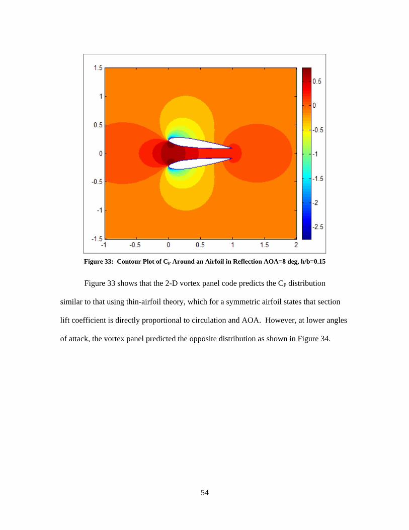
Figure 33: Contour Plot of CP Around an Airfoil in Reflection AOA=8 deg, h/b=0.15

Figure 33 shows that the 2-D vortex panel code predicts the CP distribution

similar to that using thin-airfoil theory, which for a symmetric airfoil states that section

lift coefficient is directly proportional to circulation and AOA. However, at lower angles

of attack, the vortex panel predicted the opposite distribution as shown in Figure 34.

54

Figure 34: Contour Plot of CP Around an Airfoil in Reflection AOA=2 deg, h/b=0.15

At the same height above ground as in Figure 33, Figure 34 shows a negative

pressure coefficient beneath the airfoil. This CP distribution suggests that airflow was

traveling faster across the lower surface of the airfoil compared to the upper surface,

which produces negative circulation and negative lift. Whereas the 8 deg AOA CP

distribution was due to the airfoil producing lift agreeing with thin airfoil theory, the CP

distribution in Figure 31 suggests that the thickness of the airfoil was the reason for the

negative lift.

As the air attempted to travel between the airfoil and the ground, or streamline of

zero vertical velocity, the air speed increased. This is called the Venturi effect, which

55

states that as a fluid travels through a decreasing cross-sectional area, conservation of

mass forces the fluid’s velocity to increase for incompressible flow.

The percent increase in lift coefficient is another valuable reason for studying the

ground effect. The magnitude of the increase in lift can be used to classify certain types

of aircraft configurations. For example, it has been shown that the amount of ground

effect experienced is a function of aspect ratio and wing sweep. Figure 4 shows that

aircraft with aspect ratios near 3 can expect a change in lift coefficient around 10% when

at a height above ground of h/b = 0.3 (18). Since the OGE data (h/b = 0.93) was

measured at a different Re due to the velocity measurement error and ground plane

blockage, the data from this study can not be compared directly to Figure 4. The only

reasonable increase in lift occurred below h/b = 0.3. The 40 mph test runs showed an

increase in lift from h/b = 0.3 to h/b = 0.05 of 8.6% while the 60 mph test runs increased

14.0% both at an AOA of 6 and 8 deg.

Section 2.2.2 – Drag Coefficient Variation

Unlike the lift coefficient, the drag coefficient generally increased for all four

angles of attack measured. Figures Figure 35 and Figure 36 show the effect of the

ground plane on the CD of the chevron UCAV model.

56

0

0.005

0.01

0.015

0.02

0.025

0.03

0.035

0.04

0.045

0 0.2 0.4 0.6 0.8 1

h/b

C D

alpha = 2 deg

alpha = 4 deg

alpha = 6 deg

alpha = 8 deg

Figure 35: Ground Effect - CD vs. (h/b) 40 mph

0

0.005

0.01

0.015

0.02

0.025

0.03

0.035

0.04

0 0.2 0.4 0.6 0.8 1

h/b

C D

alpha = 2 deg

alpha = 4 deg

alpha = 6 deg

alpha = 8 deg

Figure 36: Ground Effect - CD vs. (h/b) 60 mph

57

The CD at all four angles of attack steadily increased roughly at the same rate as

height above ground decreased. For the AOA of 6 and 8 deg, this result was expected

after noticing the behavior of the lift. The induced drag component of CD is a function of

CL2, so when the lift increases as the UCAV enters ground effect, the drag should also

increase. However, this relationship was not consistent at all heights above ground. At

h/b = 0.05, CD drops slightly at an AOA of 6 deg and possibly at 8 deg, balance

limitations prevented the full range of testing at an AOA of 8 deg.

The CD data shown in Figure 35, specifically for AOA of 6 deg, was applied to

the following equation from Bertin (30) in order to analyze the various components of the

drag.

20D DC C kC= + L [9]

Equation [9] assumes a linear relationship between CD and CL2, but the experimental data

revealed more of a weak quadratic relationship for all the data gathered. Figure 37 shows

this non-linear relationship.

58

0

0.05

0.1

0.15

0.2

0.25

0.3

0 0.1 0.2 0.3 0.4 0.5 0.6 0.7

CL2

CD

OGE

h/b = 0.3

h/b = 0.15

h/b = 0.10

h/b = 0.05

k approximated here

Figure 37: CD vs. CL

2 - 40 mph

The factor k, in Equation [9] typically equals the slope of the CD vs. CL

2 curve

(27), but because of the non-linear relationship in Figure 37, k was approximated to be

0.115 from the nearly linear curves in the lower CD and CL2 region (see arrow in Figure

37).

After k was determined, and the minimum measured CD was inserted for CD0, the

total drag coefficient was calculated. Additionally, McCormick’s induced drag factor,

Equation [1], was multiplied by the induced drag term of Equation [9] to evaluate the

accuracy of its prediction as shown in Equation [10].

20D DC C kCφ= + L [10]

59

Figure 38 shows the total CD calculated from Equations [9] and [10] plotted

adjacent to the CD measured at an AOA of 6 deg.

0

0.005

0.01

0.015

0.02

0.025

0.03

0.035

0 0.2 0.4 0.6 0.8h/b

CD

CD measured, alpha = 6deg

CD (k=.115) w /o factor

CD (k=.115) w / factor

Figure 38: Ground Effect - Induced Drag Factor Comparison, 40 mph

The curves in Figure 38 suggested that McCormick’s induced drag factor over

predicted the reduction in total drag for the chevron UCAV at 6 deg AOA. This

overprediction was because McCormick developed his factor assuming a rectangular

wing and inviscid flow conditions.

Without analyzing the viscous forces on the model to quantify the friction drag, it

is reasonable to suggest that further investigation be conducted on the wing tip vortices

induced by the chevron UCAV. This would provide a better explanation for CD behavior

in the ground effect region.

60

The percent increase in CD of the chevron UCAV was on the order of 30% which

is comparable to the F-106 model tested by Lee, et al. (20). Curry (6), Curry and Owens

(21) found that the Tu-144 and F-16 XL aircraft experienced an increase in drag on the

order of 5-15%. This is mentioned to illustrate that other aircraft of similar aspect ratio

and wing sweep can experience an increase in CD while in the ground effect region.

Section 2.2.3 – Lift-to-Drag Ratio Variation

In an effort to draw some conclusions to the above analysis and further

understand the complexities of the ground effect region for the chevron UCAV, lift-to-

drag ratios (L/D) were calculated. Typically, L/D is directly correlated to aircraft

efficiency, and is normally analyzed in ground effect studies to illustrate the improved, or

in this case, unimproved efficiency of the ground effect region. Figure 39 and Figure 40

illustrate the negative trend of L/D for the chevron UCAV while in the ground effect

region.

61

0

2

4

6

8

10

12

14

16

0 0.2 0.4 0.6 0.8 1

h/b

L/D alpha = 2 deg

alpha = 4 deg

alpha = 6 deg

alpha = 8 deg

Figure 39: L/D vs. (h/b) 40 mph

0

2

4

6

8

10

12

14

16

0 0.2 0.4 0.6 0.8 1

h/b

L/D alpha = 2 deg

alpha = 4 deg

alpha = 6 deg

alpha = 8 deg

Figure 40: L/D vs. (h/b) 60 mph

62

The only positive slope was at an AOA of 6 deg while at the lowest height above

ground. Not only did the AOA of 6 deg have the maximum value for L/D, as seen in

Figure 41, it also was the only AOA that experienced a reduction in drag while in close

proximity to the ground.

-15

-10

-5

0

5

10

15

20

-15 -10 -5 0 5 10 15 20 25

alpha (deg)

L/D

OGEh/b = 0.3h/b = 0.15h/b = 0.10h/b = 0.05

Figure 41: Ground Effect - L/D vs. alpha, 40 mph

Refering to Figures Figure 39 and Figure 40 L/D increased 3.3% at 40 mph and 5.9% at

60 mph at h/b = 0.05. This increase is consistent with the slight decrease in CD at the

same height.

The L/D variation for the chevron UCAV illustrated that the increase in lift at

AOA of 6 and 8 deg was not enough to overcome the increase in drag. However, the

slight L/D increase at AOA of 6 deg at h/b = 0.05 suggests that possible reduction in

63

induced drag caused an increased L/D. At AOA of 2 and 4 deg, the decreasing L/D

suggests that the significant loss of lift from the Venturi effect as shown in Figure 30 and

Figure 31 played a role in the L/D variation of the UCAV while in the ground effect

region.

In addition, the increase in CD played a significant role in the behavior of the L/D

variation for the chevron UCAV and comparisons were drawn from previous studies.

The resulting L/D for the F-106 model decreased (20), and the L/D for the Tu-144 (21)

and F-16 XL (6) increased which can be attributed to differences in percent increase of

CD as mentioned before.

Section 3 – Test Section Flow Analysis

Section 3.1 – Flow Visualization

To ensure the air flow over the ground plane was uniform, a flow visualization

experiment was conducted. Small tufts were attached on the top surface of the ground

plane covering the leading edge, side edges, across the circular gap, and uniformly across

the remainder of the surface. To see how the tufts were placed on the ground plane refer

to Figure 42 - Figure 44.

64

Figure 42: Tufts Across Circular Gap

When the ground plane was mounted in the tunnel test section, the circular piece

and the front piece did not exactly fit perfectly together. This imperfection needed to be

analyzed, so tufts were placed just before and over the small gap as shown in Figure 42.

Since the circular piece was slightly lower than the front piece, the flow beneath the

ground plane contacted the front edge and traveled up through the gap. The tufts across

the gap illustrated this effect and the tufts downstream of the gap showed that the flow

remained uniform not having any apparent effect on the balace data.

Figure 43 is a top view of the model and ground plane during testing.

65

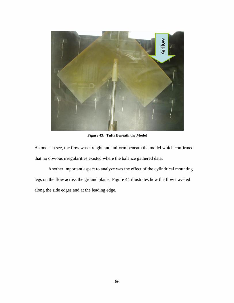
Figure 43: Tufts Beneath the Model

As one can see, the flow was straight and uniform beneath the model which confirmed

that no obvious irregularities existed where the balance gathered data.

Another important aspect to analyze was the effect of the cylindrical mounting

legs on the flow across the ground plane. Figure 44 illustrates how the flow traveled

along the side edges and at the leading edge.

66

Figure 44: Tufts Attached to Leading and Side Edges

Tufts were placed along each side in order to determine if the flow beneath the

ground plane rolled around the side edges. The near tufts in Figure 44 are a good

representation of the uniform flow that resulted along the edges of the ground plane,

which suggests that the flow beneath the ground plane did not roll over the side edges.

Also shown in Figure 44 is the only unusual outcome from the flow visualization.

The second tuft from the side at the leading edge was 90 deg inward and the third tuft

from the side edge was 90 deg outward compared to the remainder of the tufts. Although

not shown in Figure 44, the tufts above the opposite front leg acted identical to the ones

shown. This can best be explained by discussing the horseshoe vortex system that results

from the boundary layer on the underside of the flat plate interacting with a circular

cylinder (33). In subsonic flow, any disturbance downstream is experienced to some

degree upstream as well, which strongly suggests that the effects of the counter-rotating

67

horseshoe vortices caused the two tufts in Figure 44 to turn towards each other. Although

not shown in Figure 44, the tufts further downstream indicate that the horseshoe vortices

diminished or dampened out prior to the model location, which reduced the likelihood of

this phenomenon affecting the balance data.

Section 3.2 – Boundary Layer Thickness

In order to qualify the data gathered at the low heights above ground, the

boundary layer growth on the ground plane was estimated. Using the incompressible

laminar and turbulent boundary layer equations for a flat plate outlined in Chapter III, the

following results were obtained:

Table 10: Boundary Layer Growth on the Ground Plane

U∞ (mph) xtr (ft) dl.e. (in) dt.e. (in) d* (in) % disp.

47.2 1.1366 0.2148 0.4809 0.0601 12.497468.7 0.7806 0.2760 0.5105 0.0638 12.497691.2 0.5880 0.2980 0.5146 0.0643 12.4951113.1 0.4739 0.3061 0.5109 0.0639 12.5073

Table 10 indicates a relatively consistent turbulent boundary layer and displacement

thickness for the various test speeds. This consistency is attributable to the transition

location moving closer to the leading edge of the ground plane as the velocity increased.

The far right column is the percent of δt.e.that δ* displaces. Since the boundary layer was

not measured, the estimated thicknesses in Table 10 were not validated, but the hot-wire

results suggested a thicker boundary layer than estimated.

While the hot-wire anemometry experiment was not intended to identify the

boundary layer on the ground plane, the results clearly offer a boundary layer thickness

result. During the hot-wire runs with tallest ground plane (h/b = 0.05), there was an

68

averaged 7% difference in measurements when the probe was at its lowest position

compared to the higher readings( 2.36 inz = − ) ( )0 1.97 iz≤ ≤ − n . Figure 45 illustrates

the probe location relative to the model and the highest ground plane setting.

Figure 45: Hot-wire Location in Test Section Relative to Model

As stated in Chapter III, the 2.36-in location of the probe corresponded to a

distance below the model CG of 0.36-in, which means that if the 7% difference is due to

the boundary layer, then the boundary layer thickness could be larger than 0.44-in at the

model CG. Comparing this to the calculated values in Table 10, one can clearly see that

the calculated thicknesses are slightly lower than the hot-wire results which may indicate

that further investigation is necessary in order to accurately identify the boundary layer

build up on the ground plane.

69

V. Conclusions & Recommendations

Section 1 – Conclusions

Investigating the ground effect region for the chevron UCAV took a lot of

coordination, but in the end, all the established goals were achieved. The goals, as

explained in Chapter I, will be re-iterated below followed by a discussion of how each

goal was met.

The first goal was to expand the test capabilities of the AFIT 3’ x 3’ wind tunnel

by analyzing the flow characteristics through the test section with the ground plane. This

was accomplished primarily by three different methods, hot-wire measurements, flow

visualization, and boundary layer calculations. The hot-wire results indicated a

significant disparity between the indicated transducer speed and the hot-wire measured

speed. An average correction factor of 9% was applied to the data reduction program for

the test runs without the ground plane. Adding the ground plane revealed more of a

difference between indicated transducer speed and the actual speed at the model location

in the wind tunnel. Additional correction factors ranging from 3.5 to 7.9% were

multiplied by the 9% correction factor to form the complete blockage correction.

The flow visualization results revealed a uniform flow over the top of the ground

plane, especially beneath the model. The circular gap where the two pieces of the ground

plane came together caused a small updraft of air, but the effect seemed negligible. The

only unusual occurrence was at the leading edge directly above the front two cylindrical

70

legs, which was believed to be the result of the horseshoe vortices that developed at the

junction of a cylinder and a flat plate.

The boundary layer build-up across the ground plane was modeled using

conventional flat-plate laminar and turbulent boundary layer equations. Beneath the

model, which was the area of most concern, the boundary layer was turbulent with an

instantaneous transition point well in front of the model. The boundary layer thickness

was on the order of 0.5-in, which corresponded to a displacement thickness on the order

of 0.06-in. An interesting result from the hot-wire experiments indicated that the

boundary layer at the model CG was approximately 0.44-in thick based on an obvious

drop in mean velocity.

Since the idea for this project originated with Reed’s thesis (8), another goal was

to compare his data with the OGE data collected in this study. Although, not all test

conditions could be matched due to the constraints of the balance limitations, the data

still compared to a reasonable degree of accuracy. Reynolds number differences were the

likely reason for the slight variations.

During the experiment, the ground plane had no major installation or testing

issues. The airflow traveled across the ground plane with uniform flow, but blockage

corrections for wind tunnel speed were necessary. Boundary layer build-up on the

ground plane was a concern, but it appeared as though it did not affect the aerodynamic

test results.

Identifying the ground effect region for the chevron UCAV planform with respect

to height above ground will be the next goal discussed. Force and moment data was

collected and reduced to calculate the aerodynamic coefficients while the UCAV was in

71

close proximity to the ground plane. The data was presented by analyzing the change in

CL and CD near the ground.

The CL variation with height above ground for AOA of 6 and 8 deg suggested that

the chevron UCAV performed as a typical aircraft would according to standard

convention. At lower AOA of 2 and 4 deg, the lift responded in the opposite fashion and

decreased with the 2 deg case decreasing at a greater rate. This behavior was explained

by analyzing the CP contour plot of the 2-D airfoils in reflection. The negative CP

beneath airfoil suggested that the flow was traveling faster due to the Ventri effect. This

higher velocity caused lift to decrease. The trends from a 2-D vortex panel program

agreed with the experimental results.

CD variation with height above ground for AOA equal to 6 deg showed that the

drag increased and then decreased as the UCAV got closer to the ground plane. The

increase in CD most likely came from the increase in CL and the slight decrease at h/b =

0.05 was probably because of the flattening out of the wingtip vortices. At lower AOA,

CD increased as height above ground decreased, which was not the expected result since

the lift decreased.

Another goal was to verify McCormick’s induced drag factor with the

experimental results. It was concluded after analyzing the variation in CD with height

above ground that at AOA equal to 6 deg that McCormick’s induced drag factor over

predicted the decrease in induced drag for the chevron UCAV.

Finally, the last goal of this experiment was to expand the existing aerodynamic

database for moderately swept, low aspect ratio, tailless, blended wing body UAVs. This

72

was accomplished for small angles of attack and low speeds. Further analysis is required

to complete the ground effect data for higher angles of attack.

Section 2 - Recommendations

While this thesis only provided a first-cut analysis in many of the aspects studied,

it should lay the foundation for further experiments with the chevron UCAV and the

ground plane in the AFIT 3’ x 3’ wind tunnel. Based on the findings of this study, the

following are recommendations for further experiments and analysis:

• use a 100-lb balance to expand the test results. Higher angles of attack could be analyzed which would allow for more of a comparison to previous studies;

• take measurements of the boundary layer on the ground plane to better analyze

possible effects. Also, measurements or better predictions of the boundary layer transition will further the analysis significantly;

• ensure that the test speed is adjusted properly when testing in the OGE region.

The tunnel should be sped up according to the factors calculated in Table 8 for each ground plane height;

• measure the wake and/or vortices shed by the UCAV at all ground plane heights

in order to better analyze the reduction in induced drag; • use another flow visualization technique to verify the findings found in this study; • set up a boundary layer removal system, such as blowing or sucking air along the

top surface of the ground plane, to better simulate an actual aircraft flying over the ground;

• analyze the effects of sideslip and lateral stability of the chevron UCAV in ground

effect; • compare the results found in this study with a dynamic ground effect experiment.

73

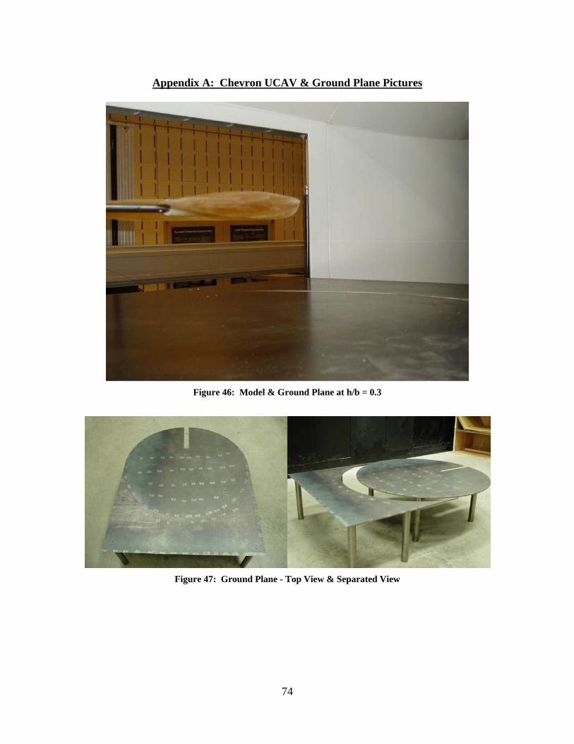
Appendix A: Chevron UCAV & Ground Plane Pictures

Figure 46: Model & Ground Plane at h/b = 0.3

Figure 47: Ground Plane - Top View & Separated View

74

Figure 48: Original Chevron UCAV - Top View

Figure 49: 1/2 Scaled Chevron UCAV

75

Appendix B: Ground Plane Drawings

Below are the drawings with dimensions of the circular plate, front plate, and the

mounting legs for the ground plane.

76

77

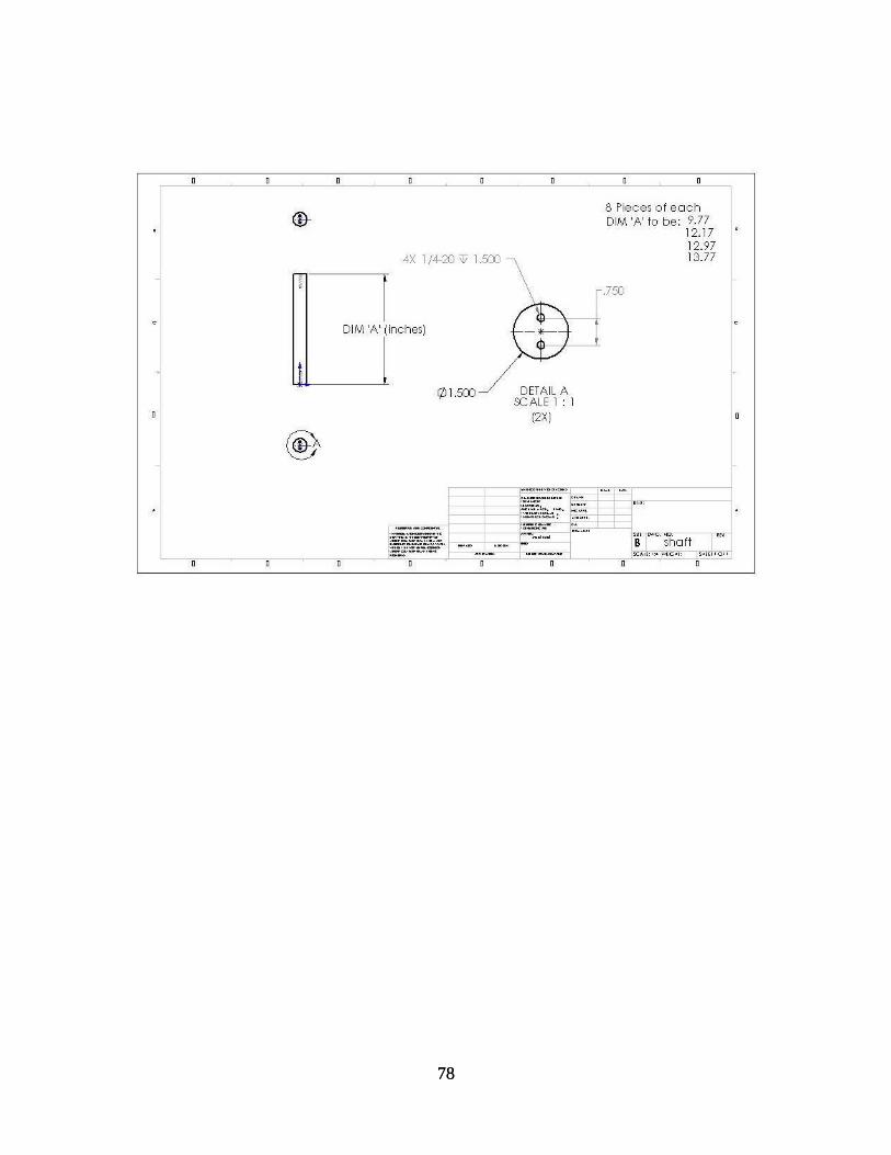
78

78

Appendix C: Data Reduction Sample Calculation

The following is a sample calculation for the MATLAB© data reduction program

used for this experiment for the following test condition:

40 mph

0.15

6 deg

Uh

bα

∞ =

=

=

Test room conditions and model specifics:

f

3

f2

o

ft-lbslug-R

slug-6ft-sec

2

2

slugsft

lb2ft

ftsec

533.7 R14.066 psia

1716

0.372x10 0.6183 ft

0.607 ft1.333 ft

2.93

1.4

0.0022*

1 * * 3.633 2

* * 1132.3

r

TP

R

c

Sb

bARS

PR T

q U

a R T

μ

γ

ρ

ρ

γ

∞ ∞

==

=

=

=

==

= =

=

= =

= =

= =

79

Blockage / Velocity Corrections:

1

1

3

blockage correction termsolid blockageground plane

transducer correctionbody shape factor 1.04

2b(test section shape & ) 0.86B

0.03668 fttunnel cross section

sbgptcK

f

Wing volume Body volumeC

ε

τ

===== =

= =

= =

=

( )

2

1 1, 3 2

area 9.4722 ft* * 0.001125

1.077 (calculated from hot-wire results)

1.090 (calculated from hot-wire results)

* 1 0.17476

sb wing

gp

tc

Total sb gp tc

K Wing volumeC

τε

ε

ε

ε ε ε ε

=

= =

=

=

= + − =

Note: solid blockage correction equations taken from Barlow, et al. (27) Calculating the flight parameters with corrections applied:

f2

ft, sec

lb2, ft

,

, 5

*(1 ) 67.4286 45.9740 mph

*(1 ) 5.0279

0.0593

* *Re 2.468x10

corr Total

corr Total

corr

corr r

U U

q q

UM

aU c

ε

ε

ρμ

∞ ∞

∞ ∞

∞

∞

= + = =

= + =

= =

= =

The raw data from the control computer contained the following measurements:

[N1, N2, S1, S2, A1, l ]. These force and moment measurements were subtracted from the

tare effects and corrected for the balance interactions. Refer to DeLuca (26) or Rivera

(29) see a complete procedure of data reduction program. The remainder of the sample

80

calculation will carry on after the balance and tare effects were removed from the

inputted data.

The corrected data was originally in the UCAV’s body axis frame. The following

equations converted the drag, side, and lift forces * D S L⎡ ⎤⎣ ⎦ ; and roll, pitch, and yaw

moments [ ] m nl into the wind axis frame:

*

,

*cos *cos *sin *sin *cos*sin *cos *cos *sin *sin

*sin *cos

*cos *cos *sin *sin *cos*sin *cos *cos *sin *sin

*sin *cos

wind

wind bc

D A Y NS A Y NL A N

m nm m nn n

θ ψ ψ θ ψψ θ ψ θ ψ

θ θ

θ ψ ψ θ ψψ θ ψ θ ψ

θ θ

+ +⎡ ⎤ ⎡ ⎤⎢ ⎥ ⎢ ⎥= − + −⎢ ⎥ ⎢ ⎥⎢ ⎥ ⎢ ⎥− +⎣ ⎦ ⎣ ⎦

− +⎡ ⎤ ⎡⎢ ⎥ = + +⎢ ⎥⎢ ⎥ − +⎣ ⎦

l l

l

l,

1 f

1 f

1 f

f

2 f

2 f

where: corrected 0.02698 lb corrected 0.00122 lb corrected 0.93839 lb

= corrected 0.02889 lb -in corrected 2.28160 lb -in

corrected 0.03048 lb -in= pitch angl

body bc

A AY SN N

m Nn Sθ

⎤⎢ ⎥⎢ ⎥⎢ ⎥⎣ ⎦

= = −= == =

== == =

l l

-3

e (AOA) = 0.1078 rads = 6.17 deg= yaw angle = -0.7330x10 rads = -0.042 deg (negligible)ψ

Carrying out the above force equations for drag and lift: (side force was treated as

negligible and not used in the analysis)

f

f

0.07409 lb0.93585 lb

DL==

Before the moments were calculated, the reference point was adjusted from the

balance CG to the model CG. The chevron UCAV’s CG was found in the Solid Works©

program and verified by hanging it with a small string through the drilled balance holes.

81

Since the model CG was located along the x-axis, the y and z locations were zero. The

following were the equations used to correct the pitching moment: (roll and yaw moment

were negligible and not used in the analysis).

, f

,

0,

0, f

2.28156 lb indist. between model CG and balance CG 1.3725 in

* cos( ) tan 1.3645 in

where:angle between and -axis at 0

* * 1.02632 lb

wind bc

cg dist

cm cg dist

cg

cg wind bc cm cm

mX

X X w

w X x

m m L X D Z

θ ψ

α

= −

= =

⎡ ⎤= + + =⎣ ⎦

= =

= − + = in−

Non-dimensionalizing the lift and pitching moment yields:

,

,

0.3067*

0.06467* *

w

cg

Lcorr

cgm

corr

LCq S

mC

q S c

∞

∞

= =

= =

These values for lift and moment coefficient agree to those in Table 13 to 0.02%.

The drag coefficient was corrected for test section geometry and flow field interference

as such:

2

0.3636Tunnel span ( )

* ( ) 0.00219w wD L

bB

SC CC

δ

δ

= =

Δ = =

The final drag coefficient is as follows:

, *uDcorr

DCq S∞

=

, 0.02647u wD corr D DC C C= + Δ =

82

The corrected drag coefficient disagrees with the value in Table 13 by 6.07%. This was

due to an incorrect model span-to-test section width ratio, δ. The δ used for the CD in

Table 13 was 0.1125, which was from a previous experiment.

83

Appendix D: Additional Ground Effect Plots

0

0.01

0.02

0.03

0.04

0.05

0.06

0.07

0.08

0.09

0 0.2 0.4 0.6 0.8 1

h/b

Cm

alpha = 2 deg

alpha = 4 deg

alpha = 6 deg

alpha = 8 deg

Figure 50: Cm vs. (h/b) 40 mph

0

2

4

6

8

10

12

14

16

0 0.2 0.4 0.6 0.8 1

h/b

L/D alpha = 2 deg

alpha = 4 deg

alpha = 6 deg

alpha = 8 deg

Figure 51: L/D vs. (h/b) 40 mph

84

0

0.01

0.02

0.03

0.04

0.05

0.06

0.07

0.08

0.09

0.1

0 0.2 0.4 0.6 0.8 1

h/b

Cm

alpha = 2 deg

alpha = 4 deg

alpha = 6 deg

alpha = 8 deg

Figure 52: Cm vs. (h/b) 60 mph

0

2

4

6

8

10

12

14

16

0 0.2 0.4 0.6 0.8 1

h/b

L/D

alpha = 2 deg

alpha = 4 deg

alpha = 6 deg

alpha = 8 deg

Figure 53: L/D vs. (h/b) 60 mph

85

0

0.05

0.1

0.15

0.2

0.25

0.3

0.35

0.4

0.45

0 0.2 0.4 0.6 0.8 1

h/b

CL

alpha = 2 deg

alpha = 4 deg

alpha = 6 deg

alpha = 8 deg

Figure 54: CL vs. (h/b) 80 mph

0

0.005

0.01

0.015

0.02

0.025

0.03

0 0.2 0.4 0.6 0.8 1

h/b

CD

alpha = 2 deg

alpha = 4 deg

alpha = 6 deg

alpha = 8 deg

Figure 55: CD vs. (h/b) 80 mph

86

0

0.01

0.02

0.03

0.04

0.05

0.06

0.07

0.08

0.09

0 0.2 0.4 0.6 0.8 1

h/b

C m

alpha = 2 deg

alpha = 4 deg

alpha = 6 deg

alpha = 8 deg

Figure 56: Cm vs. (h/b) 80 mph

0

2

4

6

8

10

12

14

16

18

0 0.2 0.4 0.6 0.8 1

h/b

L/D alpha = 2 deg

alpha = 4 deg

alpha = 6 deg

alpha = 8 deg

Figure 57: L/D vs. (h/b) 80 mph

87

0

0.05

0.1

0.15

0.2

0.25

0 0.2 0.4 0.6 0.8 1

h/b

C Lalpha = 1 deg

alpha = 2 deg

alpha = 3 deg

alpha = 4 deg

Figure 58: CL vs. (h/b) 100 mph

0

0.002

0.004

0.006

0.008

0.01

0.012

0.014

0.016

0.018

0 0.2 0.4 0.6 0.8 1

h/b

C D

alpha = 1 deg

alpha = 2 deg

alpha = 3 deg

alpha = 4 deg

Figure 59: CD vs. (h/b) 100 mph

88

0

0.01

0.02

0.03

0.04

0.05

0.06

0 0.2 0.4 0.6 0.8 1

h/b

Cm

alpha = 1 deg

alpha = 2 deg

alpha = 3 deg

alpha = 4 deg

Figure 60: Cm vs. (h/b) 100 mph

0

2

4

6

8

10

12

14

16

18

20

0 0.2 0.4 0.6 0.8 1

h/b

L/D alpha = 1 deg

alpha = 2 deg

alpha = 3 deg

alpha = 4 deg

Figure 61: L/D vs. (h/b) 100 mph

89

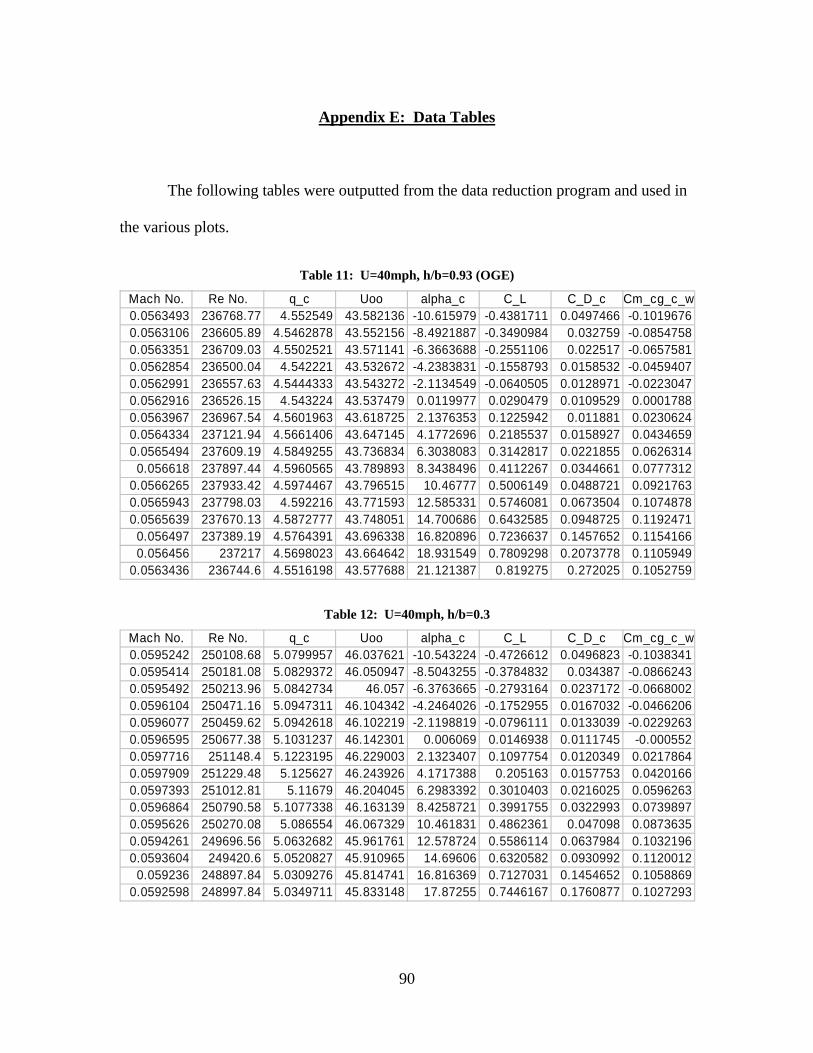
Appendix E: Data Tables The following tables were outputted from the data reduction program and used in the various plots.

Table 11: U=40mph, h/b=0.93 (OGE)

Mach No. Re No. q_c Uoo alpha_c C_L C_D_c Cm_cg_c_w0.0563493 236768.77 4.552549 43.582136 -10.615979 -0.4381711 0.0497466 -0.10196760.0563106 236605.89 4.5462878 43.552156 -8.4921887 -0.3490984 0.032759 -0.08547580.0563351 236709.03 4.5502521 43.571141 -6.3663688 -0.2551106 0.022517 -0.06575810.0562854 236500.04 4.542221 43.532672 -4.2383831 -0.1558793 0.0158532 -0.04594070.0562991 236557.63 4.5444333 43.543272 -2.1134549 -0.0640505 0.0128971 -0.02230470.0562916 236526.15 4.543224 43.537479 0.0119977 0.0290479 0.0109529 0.00017880.0563967 236967.54 4.5601963 43.618725 2.1376353 0.1225942 0.011881 0.02306240.0564334 237121.94 4.5661406 43.647145 4.1772696 0.2185537 0.0158927 0.04346590.0565494 237609.19 4.5849255 43.736834 6.3038083 0.3142817 0.0221855 0.0626314

0.056618 237897.44 4.5960565 43.789893 8.3438496 0.4112267 0.0344661 0.07773120.0566265 237933.42 4.5974467 43.796515 10.46777 0.5006149 0.0488721 0.09217630.0565943 237798.03 4.592216 43.771593 12.585331 0.5746081 0.0673504 0.10748780.0565639 237670.13 4.5872777 43.748051 14.700686 0.6432585 0.0948725 0.1192471

0.056497 237389.19 4.5764391 43.696338 16.820896 0.7236637 0.1457652 0.11541660.056456 237217 4.5698023 43.664642 18.931549 0.7809298 0.2073778 0.1105949

0.0563436 236744.6 4.5516198 43.577688 21.121387 0.819275 0.272025 0.1052759

Table 12: U=40mph, h/b=0.3

Mach No. Re No. q_c Uoo alpha_c C_L C_D_c Cm_cg_c_w0.0595242 250108.68 5.0799957 46.037621 -10.543224 -0.4726612 0.0496823 -0.10383410.0595414 250181.08 5.0829372 46.050947 -8.5043255 -0.3784832 0.034387 -0.08662430.0595492 250213.96 5.0842734 46.057 -6.3763665 -0.2793164 0.0237172 -0.06680020.0596104 250471.16 5.0947311 46.104342 -4.2464026 -0.1752955 0.0167032 -0.04662060.0596077 250459.62 5.0942618 46.102219 -2.1198819 -0.0796111 0.0133039 -0.02292630.0596595 250677.38 5.1031237 46.142301 0.006069 0.0146938 0.0111745 -0.0005520.0597716 251148.4 5.1223195 46.229003 2.1323407 0.1097754 0.0120349 0.02178640.0597909 251229.48 5.125627 46.243926 4.1717388 0.205163 0.0157753 0.04201660.0597393 251012.81 5.11679 46.204045 6.2983392 0.3010403 0.0216025 0.05962630.0596864 250790.58 5.1077338 46.163139 8.4258721 0.3991755 0.0322993 0.07398970.0595626 250270.08 5.086554 46.067329 10.461831 0.4862361 0.047098 0.08736350.0594261 249696.56 5.0632682 45.961761 12.578724 0.5586114 0.0637984 0.10321960.0593604 249420.6 5.0520827 45.910965 14.69606 0.6320582 0.0930992 0.1120012

0.059236 248897.84 5.0309276 45.814741 16.816369 0.7127031 0.1454652 0.10588690.0592598 248997.84 5.0349711 45.833148 17.87255 0.7446167 0.1760877 0.1027293

90

Table 13: U=40 mph, h/b=0.15

Mach No. Re No. q_c Uoo alpha_c C_L C_D_c Cm_cg_c_w0.0592916 246886.83 4.9860239 45.775671 -10.58134 -0.5649449 0.0600204 -0.1303680.0593069 246950.36 4.9885901 45.787449 -8.5347541 -0.4521546 0.0422714 -0.10527520.0593351 247067.61 4.9933283 45.809189 -6.3980328 -0.3317732 0.0293093 -0.07829140.0593534 247144.16 4.9964232 45.823383 -4.2642517 -0.2185103 0.02125 -0.0513460.0594209 247425.05 5.0077866 45.875462 -2.1307351 -0.1058881 0.0167997 -0.02510150.0594615 247594 5.014628 45.906787 0.0018163 0.0043975 0.0143157 -0.0007070.0595227 247849.12 5.0249675 45.95409 2.13378 0.1132601 0.0150956 0.02234030.0595636 248019.19 5.0318661 45.985623 4.17506 0.2132041 0.0190337 0.04405880.0595458 247945.24 5.0288658 45.971912 6.3006456 0.3066244 0.0249541 0.06465640.0594446 247523.83 5.011786 45.893777 8.4254263 0.3980962 0.0362443 0.08295480.0593805 247256.62 5.0009713 45.844234 10.465052 0.4940338 0.0520775 0.09657560.0592909 246883.87 4.9859044 45.775122 12.585908 0.5760055 0.0778245 0.10955030.0591293 246210.89 4.9587589 45.650342 14.711443 0.6693032 0.118345 0.1146984

0.059026 245780.79 4.9414497 45.570598 16.83377 0.754832 0.1730153 0.11545390.0589733 245561.13 4.9326208 45.52987 17.893599 0.795579 0.2027972 0.1147111

Table 14: U=40 mph, h/b=0.10

Mach No. Re No. q_c Uoo alpha_c C_L C_D_c Cm_cg_c_w0.0593961 247339.46 5.0033435 45.850618 -10.715638 -0.6794595 0.0708169 -0.16062850.0594063 247381.67 5.0050512 45.858442 -8.5747996 -0.5491094 0.0481446 -0.12275670.0594745 247665.64 5.0165482 45.911082 -6.4297099 -0.4084673 0.0334862 -0.08627260.0594555 247586.66 5.0133494 45.896442 -4.2883376 -0.2768253 0.023895 -0.0527131

0.059513 247826.23 5.0230562 45.940853 -2.1468838 -0.144986 0.0182399 -0.02351150.0595456 247961.8 5.028553 45.965983 -0.0084812 -0.0205341 0.0151624 0.00279390.0595826 248115.92 5.0348061 45.994554 2.1285901 0.1006946 0.0156193 0.02725150.0595768 248091.62 5.03382 45.99005 4.174591 0.2120685 0.0193513 0.04853150.0595688 248058.58 5.0324791 45.983924 6.3062164 0.320112 0.0257437 0.06714370.0595578 248012.57 5.0306124 45.975394 8.3475319 0.4201418 0.0381225 0.08331220.0594876 247720.28 5.0187619 45.921211 10.472638 0.5124024 0.0525048 0.09871920.0594555 247586.53 5.0133441 45.896418 11.534999 0.5592771 0.062699 0.1050568

91

Table 15: U=40 mph, h/b=0.05

Mach No. Re No. q_c Uoo alpha_c C_L C_D_c Cm_cg_c_w0.0609787 253929.79 5.2735224 47.072301 -5.3153772 -0.4488207 0.0369975 -0.09152990.0609763 253919.5 5.2730951 47.070394 -4.3341646 -0.3877781 0.0312391 -0.07053960.0609691 253889.49 5.2718486 47.064831 -3.2561235 -0.3053603 0.0265582 -0.04808980.0610154 254082.28 5.2798579 47.100569 -2.1791458 -0.2230961 0.0226368 -0.0279568

0.061025 254122.53 5.2815309 47.108031 -1.1021426 -0.1431914 0.0195427 -0.010680.0610619 254276.14 5.2879179 47.136506 -0.0272113 -0.0658818 0.0174281 0.00485050.0611316 254566.21 5.2999894 47.190278 1.0458775 0.0069669 0.016479 0.0200090.0610926 254403.95 5.2932353 47.1602 2.1190142 0.0775104 0.0166352 0.03352490.0610806 254353.95 5.2911548 47.150931 3.1029269 0.1450903 0.018572 0.04539440.0610962 254419.02 5.2938623 47.162993 4.1727272 0.207556 0.0199655 0.05673330.0610837 254366.66 5.2916837 47.153287 5.240402 0.2672967 0.0220701 0.0669891

0.061113 254489.04 5.2967765 47.175972 6.3090425 0.3269543 0.0254208 0.0757002

Table 16: U=60 mph, h/b=0.93 (OGE)

Mach No. Re No. q_c Uoo alpha_c C_L C_D_c Cm_cg_c_w0.0852575 358235.04 10.421781 65.940489 -10.605667 -0.4132066 0.0428261 -0.0996435

0.085202 358001.77 10.408212 65.897551 -8.4841958 -0.3297467 0.0291728 -0.08280460.0851239 357673.58 10.389139 65.837142 -6.3616074 -0.2435828 0.0197456 -0.06335410.0851384 357734.72 10.392691 65.848396 -4.2379765 -0.1548948 0.0140115 -0.04245040.0851458 357765.65 10.394488 65.854088 -2.1130218 -0.0630019 0.0107352 -0.02111630.0851896 357949.73 10.405187 65.887973 0.0097684 0.0236504 0.0093042 0.0010019

0.085258 358237.39 10.421917 65.940921 2.1353034 0.1169484 0.010267 0.02209620.0853344 358558.31 10.440598 65.999993 4.1728534 0.2078615 0.0137409 0.04259230.0854645 359104.85 10.472452 66.100597 6.2976885 0.2994649 0.0197258 0.06094560.0855913 359637.47 10.50354 66.198635 8.3326231 0.384046 0.029481 0.07966030.0856216 359764.91 10.510985 66.222094 10.457118 0.4748258 0.0433697 0.09280190.0855669 359535.25 10.49757 66.179821 12.579934 0.5615398 0.0606825 0.1047430.0855108 359299.22 10.483791 66.136374 14.697441 0.6354007 0.0889606 0.1131428

92

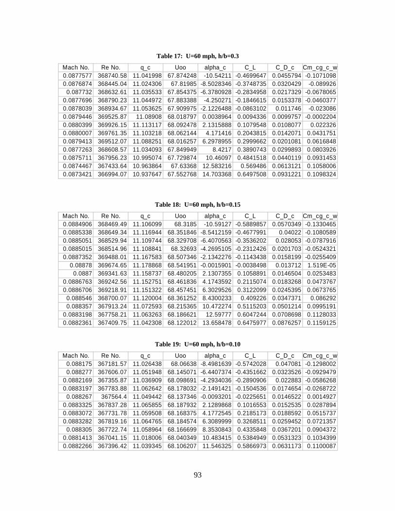
Table 17: U=60 mph, h/b=0.3

Mach No. Re No. q_c Uoo alpha_c C_L C_D_c Cm_cg_c_w0.0877577 368740.58 11.041998 67.874248 -10.54211 -0.4699647 0.0455794 -0.10710980.0876874 368445.04 11.024306 67.81985 -8.5028346 -0.3748735 0.0320429 -0.089926

0.087732 368632.61 11.035533 67.854375 -6.3780928 -0.2834958 0.0217329 -0.06780650.0877696 368790.23 11.044972 67.883388 -4.250271 -0.1846615 0.0153378 -0.04603770.0878039 368934.67 11.053625 67.909975 -2.1226488 -0.0863102 0.011746 -0.0230860.0879446 369525.87 11.08908 68.018797 0.0038964 0.0094336 0.0099757 -0.00022040.0880399 369926.15 11.113117 68.092478 2.1315888 0.1079548 0.0108077 0.0223260.0880007 369761.35 11.103218 68.062144 4.171416 0.2043815 0.0142071 0.04317510.0879413 369512.07 11.088251 68.016257 6.2978955 0.2999662 0.0201081 0.06168480.0877263 368608.57 11.034093 67.849949 8.4217 0.3890743 0.0299893 0.08039260.0875711 367956.23 10.995074 67.729874 10.46097 0.4841518 0.0440119 0.09314530.0874467 367433.64 10.963864 67.63368 12.583216 0.569486 0.0613121 0.10580060.0873421 366994.07 10.937647 67.552768 14.703368 0.6497508 0.0931221 0.1098324

Table 18: U=60 mph, h/b=0.15

Mach No. Re No. q_c Uoo alpha_c C_L C_D_c Cm_cg_c_w0.0884906 368469.49 11.106099 68.3185 -10.59127 -0.5889857 0.0570349 -0.13304650.0885338 368649.34 11.116944 68.351846 -8.5412159 -0.4677991 0.04022 -0.10805890.0885051 368529.94 11.109744 68.329708 -6.4070563 -0.3536202 0.028053 -0.07879160.0885015 368514.96 11.108841 68.32693 -4.2695105 -0.2312426 0.0201703 -0.05243210.0887352 369488.01 11.167583 68.507346 -2.1342276 -0.1143438 0.0158199 -0.0255409

0.08878 369674.65 11.178868 68.541951 -0.0015901 -0.0038498 0.013712 1.519E-050.0887 369341.63 11.158737 68.480205 2.1307355 0.1058891 0.0146504 0.0253483

0.0886763 369242.56 11.152751 68.461836 4.1743592 0.2115074 0.0183268 0.04737670.0886706 369218.91 11.151322 68.457451 6.3029526 0.3122099 0.0245395 0.0673765

0.088546 368700.07 11.120004 68.361252 8.4300233 0.409226 0.0347371 0.0862920.088357 367913.24 11.072593 68.215365 10.472274 0.5115203 0.0501214 0.0995191

0.0883198 367758.21 11.063263 68.186621 12.59777 0.6047244 0.0708698 0.11280330.0882361 367409.75 11.042308 68.122012 13.658478 0.6475977 0.0876257 0.1159125

Table 19: U=60 mph, h/b=0.10

Mach No. Re No. q_c Uoo alpha_c C_L C_D_c Cm_cg_c_w0.088175 367181.57 11.026438 68.06638 -8.4981639 -0.5742028 0.047081 -0.12980020.088277 367606.07 11.051948 68.145071 -6.4407374 -0.4351662 0.0323526 -0.0929479

0.0882169 367355.87 11.036909 68.098691 -4.2934036 -0.2890906 0.022883 -0.05862680.0883197 367783.88 11.062642 68.178032 -2.1491421 -0.1504536 0.0174654 -0.0268722

0.088267 367564.4 11.049442 68.137346 -0.0093201 -0.0225651 0.0146522 0.00149270.0883325 367837.28 11.065855 68.187932 2.1289868 0.1016553 0.0152535 0.02878940.0883072 367731.78 11.059508 68.168375 4.1772545 0.2185173 0.0188592 0.05157370.0883282 367819.16 11.064765 68.184574 6.3089999 0.3268511 0.0259452 0.0721357

0.088305 367722.74 11.058964 68.166699 8.3530843 0.4335848 0.0367201 0.09043720.0881413 367041.15 11.018006 68.040349 10.483415 0.5384949 0.0531323 0.10343990.0882266 367396.42 11.039345 68.106207 11.546325 0.5866973 0.0631173 0.1100087

93

Table 20: U=60 mph, h/b=0.05

Mach No. Re No. q_c Uoo alpha_c C_L C_D_c Cm_cg_c_w0.0878673 365899.87 10.949593 67.828784 -5.3337948 -0.4934122 0.0362124 -0.10446730.0878775 365942.6 10.952151 67.836704 -4.3504798 -0.4272792 0.0306678 -0.08185980.0878791 365949.07 10.952538 67.837905 -3.2695584 -0.3378878 0.0261103 -0.05585080.0878294 365742.01 10.940147 67.79952 -2.1895989 -0.2484044 0.0222617 -0.03295040.0878995 366034 10.957623 67.853649 -1.1092203 -0.1603274 0.019224 -0.01347820.0879399 366202.55 10.967716 67.884893 -0.0320459 -0.077587 0.0171998 0.00445670.0878659 365894.19 10.949254 67.827731 0.9580701 0.0025909 0.0171179 0.02112170.0878946 366013.81 10.956414 67.849906 2.1195443 0.0787937 0.0166742 0.03599970.0879674 366316.75 10.974558 67.906063 3.1049536 0.1499971 0.0180378 0.04912440.0878429 365798.57 10.943532 67.810006 4.1769343 0.217742 0.0197591 0.06125370.0879027 366047.25 10.958416 67.856104 5.2454578 0.2795375 0.0221139 0.07207950.0878483 365820.72 10.944857 67.814112 6.3153132 0.3421365 0.0256089 0.0822973

Table 21: U=80 mph, h/b=0.93 (OGE)

Mach No. Re No. q_c Uoo alpha_c C_L C_D_c Cm_cg_c_w0.1135256 477012.22 18.47842 87.80386 -8.3950958 -0.3246622 0.0267817 -0.07935880.1134721 476787.35 18.461001 87.762467 -6.3616688 -0.2437315 0.0182695 -0.06201310.1134653 476758.78 18.45879 87.75721 -4.2379745 -0.15489 0.0128594 -0.04142450.1134468 476681.07 18.452772 87.742904 -2.1129214 -0.0627588 0.0095276 -0.0207820.1134053 476506.37 18.439249 87.710747 0.010876 0.026332 0.0081677 0.00090230.1135782 477233.16 18.495541 87.844529 2.136655 0.1202209 0.0092027 0.0223120.1138108 478210.32 18.57136 88.024395 4.1735547 0.2095595 0.0124688 0.0428250.1138867 478529.34 18.596146 88.083117 6.298045 0.300328 0.0182342 0.06215710.1139898 478962.31 18.629812 88.162813 8.3344164 0.3883877 0.0271564 0.0801304

Table 22: U=80 mph, h/b=0.3

Mach No. Re No. q_c Uoo alpha_c C_L C_D_c Cm_cg_c_w0.1183958 497475.63 20.097842 91.570569 -7.3499575 -0.3219064 0.0239747 -0.07485290.1183793 497406.4 20.092249 91.557827 -6.3769536 -0.2807378 0.0198621 -0.06607320.1184245 497596.41 20.107602 91.592801 -4.2500249 -0.1840655 0.0139694 -0.0444810.1184581 497737.25 20.118987 91.618726 -2.1221812 -0.085178 0.0104484 -0.02274570.1185552 498145.57 20.152009 91.693886 0.0044069 0.0106696 0.0088905 -0.0002410.1187092 498792.29 20.204368 91.812928 2.1326515 0.1105278 0.0096963 0.02209110.1186915 498718.18 20.198365 91.799287 4.172043 0.2058994 0.0127929 0.04320020.1185856 498273.35 20.162349 91.717406 6.2974945 0.2989952 0.0185571 0.06246370.1184239 497593.63 20.107377 91.592289 7.3599201 0.3460269 0.0224835 0.0711328

94

Table 23: U=80 mph, h/b=0.15

Mach No. Re No. q_c Uoo alpha_c C_L C_D_c Cm_cg_c_w0.1190355 495656.66 20.096498 91.900471 -5.3428349 -0.3046617 0.022464 -0.0643911

0.119049 495712.76 20.101048 91.910873 -4.2748952 -0.2442797 0.019379 -0.0507280.119084 495858.75 20.112889 91.937941 -2.1404591 -0.129431 0.014987 -0.0243636

0.1190707 495803.23 20.108385 91.927646 -0.0073857 -0.0178816 0.0127662 0.0016950.1192273 496455.46 20.161325 92.048578 2.1260379 0.0945154 0.0133935 0.02745010.1191347 496069.83 20.130016 91.977078 4.1711718 0.2037902 0.0167178 0.05002950.1191052 495946.85 20.120037 91.954275 5.2356858 0.2558782 0.0192129 0.06050480.1190077 495540.93 20.087114 91.879012 6.3016549 0.3090681 0.0225594 0.0702218

Table 24: U=80 mph, h/b=0.10

Mach No. Re No. q_c Uoo alpha_c C_L C_D_c Cm_cg_c_w0.1186701 494169.94 19.97221 91.606882 -4.2980018 -0.3002234 0.0219597 -0.057995

0.118652 494094.62 19.966122 91.592918 -2.1537123 -0.1615185 0.0168119 -0.02608420.118693 494265.31 19.97992 91.624561 -0.0127737 -0.0309268 0.014089 0.0031676

0.1187284 494412.71 19.991838 91.651885 2.1270981 0.0970823 0.0145929 0.03108720.1187141 494353.17 19.987024 91.640849 4.1761079 0.2157412 0.0177931 0.05489280.1186485 494079.98 19.964939 91.590205 6.3100319 0.3293498 0.0239302 0.0751337

Table 25: U=80, h/b=0.05

Mach No. Re No. q_c Uoo alpha_c C_L C_D_c Cm_cg_c_w0.118176 492112.49 19.80625 91.225482 -3.2746529 -0.3502222 0.0242969 -0.0602632

0.1181629 492058.21 19.801881 91.21542 -2.1928686 -0.2563207 0.0206904 -0.03594620.1182146 492273.28 19.819195 91.255287 -1.1110859 -0.1648444 0.0179007 -0.01536580.1182087 492248.88 19.81723 91.250765 -0.0326367 -0.0790174 0.016058 0.0041170.1182273 492326.28 19.823463 91.265113 0.9594491 0.0059297 0.0156724 0.02162220.1182607 492465.32 19.834662 91.290888 2.1218648 0.084412 0.0155605 0.03704340.1180905 491756.66 19.777618 91.159519 3.1075059 0.1561767 0.0166432 0.05084750.1180784 491706.26 19.773565 91.150177 4.1795792 0.2241456 0.0182679 0.06285080.1181152 491859.36 19.785879 91.178557 5.2487791 0.2875787 0.0206057 0.0738153

Table 26: U=100 mph, h/b=0.93 (OGE)

Mach No. Re No. q_c Uoo alpha_c C_L C_D_c Cm_cg_c_w0.141231305 593425.9012 28.59820711 109.2321803 -5.21124914 -0.19671408 0.014447095 -0.05106740.141167017 593155.7752 28.57217736 109.182458 -4.23836948 -0.15584636 0.012224947 -0.041804640.141115703 592940.1639 28.55140925 109.1427704 -2.11223095 -0.0610872 0.00899534 -0.021158240.141209104 593332.6167 28.58921674 109.2150093 0.01182641 0.02863318 0.007706787 0.0007272980.141353997 593941.4288 28.647917 109.3270737 2.138266302 0.124121969 0.008755936 0.0231498520.14156359 594822.0991 28.73293573 109.4891791 4.177115971 0.218181756 0.011889424 0.04412849

0.141598418 594968.4366 28.74707516 109.5161155 4.265491509 0.2215121 0.012046845 0.044865116

95

Table 27: U=100 mph, h/b=0.3

Mach No. Re No. q_c Uoo alpha_c C_L C_D_c Cm_cg_c_w0.147571682 620066.9059 31.22359583 114.1360023 -4.25380002 -0.19320559 0.013880798 -0.046785650.147651361 620401.7038 31.25732257 114.1976287 -2.12311445 -0.08743748 0.010419231 -0.024374020.147788464 620977.7822 31.31539794 114.3036677 0.005412058 0.013103251 0.008949285 -0.000658810.147757897 620849.3466 31.30244547 114.2800265 2.13591104 0.118419593 0.009844068 0.0238926630.147885749 621386.5533 31.35663949 114.3789104 3.200124827 0.169780757 0.011164261 0.0352511690.147783907 620958.6355 31.31346686 114.3001434 4.178249131 0.220925273 0.012940881 0.046110574

Table 28: U=100 mph, h/b=0.15

Mach No. Re No. q_c Uoo alpha_c C_L C_D_c Cm_cg_c_w0.146818981 611345.3488 30.57255403 113.3504901 -3.21084875 -0.19574467 0.016916351 -0.039663580.146860937 611520.0503 30.5900297 113.3828817 -2.14228444 -0.13385038 0.015018615 -0.026261310.146899832 611682.006 30.60623485 113.4129102 -1.07392477 -0.07487263 0.013648389 -0.012340840.146830287 611392.423 30.57726245 113.3592182 -0.00650675 -0.01575363 0.012884893 0.0014734950.146826409 611376.2784 30.57564761 113.3562248 1.061904483 0.045770059 0.012786065 0.0161721270.146911178 611729.2502 30.61096287 113.4216698 2.130658903 0.105703527 0.01348142 0.0295157470.146831176 611396.1278 30.57763302 113.3599051 3.110482643 0.163383707 0.014768572 0.041690309

Table 29: U=100 mph, h/b=0.10

Mach No. Re No. q_c Uoo alpha_c C_L C_D_c Cm_cg_c_w0.146520132 610144.1688 30.44657276 113.1056347 -3.1414843 -0.23844251 0.018372928 -0.043016140.146433566 609783.688 30.41060696 113.0388105 -2.15700624 -0.16949364 0.016523885 -0.028560140.146529868 610184.7122 30.45061918 113.1131505 -1.08419422 -0.09973624 0.014905483 -0.012741570.146457637 609883.9247 30.42060561 113.0573919 -0.01253696 -0.03035352 0.013946574 0.0030367460.146454673 609871.5834 30.41937448 113.0551041 0.973661318 0.040339083 0.013925471 0.0190699410.146520782 610146.8733 30.44684267 113.1061361 2.131578385 0.107929705 0.01444742 0.0334084560.146405417 609666.4681 30.3989163 113.0170808 3.113643483 0.171036488 0.015559293 0.046464367

Table 30: U=100 mph, h/b=0.05

Mach No. Re No. q_c Uoo alpha_c C_L C_D_c Cm_cg_c_w0.145747349 606926.117 30.12625415 112.5090875 -1.11609281 -0.17696661 0.017819193 -0.017999120.145673662 606619.269 30.09579956 112.4522055 -0.03404163 -0.08241894 0.016082691 0.0036307190.145695435 606709.9367 30.1047967 112.4690131 0.961528214 0.010963359 0.015509789 0.023506010.145713014 606783.1381 30.11206161 112.4825828 1.047710958 0.011405805 0.01532111 0.0235491310.145701497 606735.1795 30.10730184 112.4736925 2.126305179 0.095162632 0.01546496 0.0404809990.14560401 606329.222 30.06702662 112.398438 3.11445585 0.173003327 0.016334041 0.05478849

96

Appendix F: MATLAB© Data Reduction Program %************************************************************************** %************************************************************************** %********** Lt. Gebbie & Capt Anthony DeLuca **************************** %****** Adapted for the Balance AFIT 1 by Lt. Rivera Parga ************************ %********* re-adapted by Troy Leveron, ENS, USNR *************************** %****** re-adapted by Brett Jones, ENS, USNR for UCAV Ground Effects Test********** %***************Calculation of Lift, Drag, Moments *************************** %************************************************************************** %************************************************************************** %************************************************************************** %This Code will transfer measured Forces and Moments on the AFIT-1 balance to Wind %(earth) centered frame of reference by correcting for tare effects, balance %interactions, and wind tunnel irregularities, then gives a file with all the %corrected data clear; clc; close all; format long %########################################################################## % INPUT DECK %FIRST FILL THE FOLLOWING INFORMATION Masskg=1.235; % Mass of the UCAV in KGS (~3lbs for now until I weigh it) T_room = mean([73.4 74 74.7]) + 459.67 %deg R ****Changed for each day of testing**** P_barro = mean([28.6823 28.6130 28.6228]) * 0.4911541 %Psi ****Changed for each day of testing**** % INPUT DATA FILE AND INPUT DATA TARE FILE load tarefile.txt; %tarefile GP42005tearA-10to+20B0model TareFile = tarefile(:,1:9); load datafile.txt; %datafile (Raw Data file name here) DataFile = datafile(:,1:9); %Offset distances from the Mounting Block to the Model C.G. (inches) Y_cmb = 0; X_cmb = 1.3725; %inches (from origin @ balance center w/ + right) Z_cmb = 0; % Required for the Solid body blockage corrections due to wing % and fuselage Body_Volume = 63.39038 / 12^3 ; %ft^3: From Solid Works "Mass Properties" Wing_Area = 87.3958 / 12^2 %ft^2 %####################################################################### %I.- Room Conditions and Model Specifics : % UNITS are in Ft, Sec, lbm, Psf, Rankine, fps %#######################################################################

97

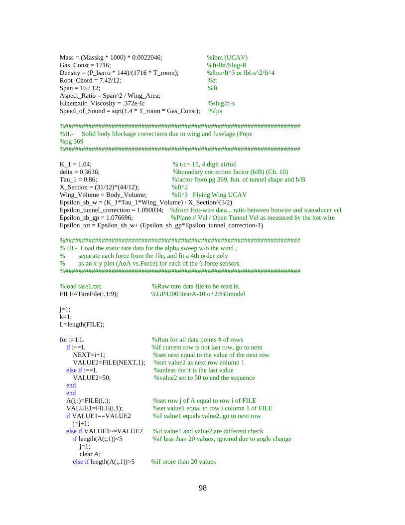
Mass = (Masskg * 1000) * 0.0022046; %lbm (UCAV) Gas_Const = 1716; %ft-lbf/Slug-R Density = (P_barro * 144)/(1716 * T_room); %lbm/ft^3 or lbf-s^2/ft^4 Root_Chord = 7.42/12; %ft Span = 16 / 12; %ft Aspect_Ratio = Span^2 / Wing_Area; Kinematic_Viscosity = .372e-6; %slug/ft-s Speed_of_Sound = sqrt(1.4 * T_room * Gas_Const); %fps %####################################################################### %II.- Solid body blockage corrections due to wing and fuselage (Pope %pg 369 %####################################################################### K_1 = 1.04; % t/c=.15, 4 digit airfoil delta = 0.3636; %boundary correction factor (b/B) (Ch. 10) Tau_1 = 0.86; %factor from pg 369, fun. of tunnel shape and b/B X_Section = (31/12)*(44/12); %ft^2 Wing_Volume = Body_Volume; %ft^3 Flying Wing UCAV Epsilon_sb_w = (K_1*Tau_1*Wing_Volume) / X_Section^(3/2) Epsilon_tunnel_correction = 1.090034; %from Hot-wire data... ratio between hotwire and transducer vel Epsilon_sb_gp = 1.076696; %Plane # Vel / Open Tunnel Vel as measured by the hot-wire Epsilon_tot = Epsilon_sb_w+ (Epsilon_sb_gp*Epsilon_tunnel_correction-1) %####################################################################### % III.- Load the static tare data for the alpha sweep w/o the wind , % separate each force from the file, and fit a 4th order poly % as an x-y plot (AoA vs.Force) for each of the 6 force sensors. %####################################################################### %load tare1.txt; %Raw tare data file to be read in. FILE=TareFile(:,1:9); %GP42005tearA-10to+20B0model j=1; k=1; L=length(FILE); for i=1:L %Run for all data points # of rows if i~=L %if current row is not last row, go to next NEXT=i+1; %set next equal to the value of the next row VALUE2=FILE(NEXT,1); %set value2 as next row column 1 else if i==L %unless the it is the last value VALUE2=50; %value2 set to 50 to end the sequence end end A(j,:)=FILE(i,:); %set row j of A equal to row i of FILE VALUE1=FILE(i,1); %set value1 equal to row i column 1 of FILE if VALUE1==VALUE2 %if value1 equals value2, go to next row j=j+1; else if VALUE1~=VALUE2 %if value1 and value2 are different check if length(A(:,1))<5 %if less than 20 values, ignored due to angle change j=1; clear A; else if length(A(:,1))>5 %if more than 20 values

98

C=length(A(:,1)); %find length of A for m=1:9 %Average all rows of the like values in A B(k,m)=mean(A(4:C,m)); %disregarding first 10 for vibrations end j=1; k=k+1; clear A end end end end end if B(k-1,1)<B((k-2),1) B=B(1:(k-2),:) end tare=[B]; %_________________________________End of inserted code [row,col] = size(tare); for k = 1:row; theta_tare(k,:,:) = tare(k,1).* (pi/180); NF_tare(k,:,:) = tare(k,4); PM_tare(k,:,:) = tare(k,5); SF_tare(k,:,:) = tare(k,7); YM_tare(k,:,:) = tare(k,8); AF_tare(k,:,:) = tare(k,6); RM_tare(k,:,:) = tare(k,9); end NF_poly = polyfit(theta_tare,NF_tare,4); PM_poly = polyfit(theta_tare,PM_tare,4); SF_poly = polyfit(theta_tare,SF_tare,4); YM_poly = polyfit(theta_tare,YM_tare,4); AF_poly = polyfit(theta_tare,AF_tare,4); RM_poly = polyfit(theta_tare,RM_tare,4); %####################################################################### %IV.- Load the specific test run files, %####################################################################### clear ('AA','B','C','L') %load data1.txt; %Raw data file to be read in: FILE=DataFile(:,:); %Same as above j=1; k=1;

99

L=length(FILE); for i=1:L %Run for all data points # of rows if i~=L %if current row is not last row, go to next NEXT=i+1; %set next equal to the value of the next row VALUE2=FILE(NEXT,1); %set value2 as next row column 1 else if i==L %unless the it is the last value VALUE2=50; %value2 set to 50 to end the sequence end end A(j,:)=FILE(i,:); %set row j of A equal to row i of FILE VALUE1=FILE(i,1); %set value1 equal to row i column 1 of FILE if VALUE1==VALUE2 %if value1 equals value2, go to next row j=j+1; else if VALUE1~=VALUE2 %if value1 and value2 are different check if length(A(:,1))<5 %if less than 20 values, ignored due to angle change j=1; clear A; else if length(A(:,1))>5 %if more than 20 values C=length(A(:,1)); %find length of A for m=1:9 %Average all rows of the like values in A B(k,m)=mean(A(4:C,m)); %disregarding first 10 for vibrations end j=1; k=k+1; clear A end end end end end if B(k-1,1)<B((k-2),1) B=B(1:(k-2),:) end sample_data=[B]; %_________________________________End of inserted code [row2,col2] = size(sample_data); for i = 1:row2; %Angles of the model during test runs (Roll, Pitch {AoA}, Yaw {Beta}): phi = 0; theta(i,:) = sample_data(i,1) .* (pi/180); %radians si(i,:) = sample_data(i,2) .* (pi/180); %radians Wind_Speed(i,:) = sample_data(i,3) .* (5280/3600); %fps %Flight Parameters (Re#, Ma#, Dynamic Pressure): q = (.5 * Density) .* Wind_Speed.^2; %lbf/ft^2

100

q_Corrected = q .* (1 + Epsilon_tot)^2; %lbf/ft^2 Wind_Speed_Corrected = Wind_Speed .* (1 + Epsilon_tot); %fps Wind_Speed_Corrected_mph = Wind_Speed_Corrected.*(3600/5280); Mach_Number = Wind_Speed_Corrected ./ Speed_of_Sound; %NonDimensional Reynolds_Number = ((Density * Root_Chord) .* Wind_Speed_Corrected) ./ Kinematic_Viscosity; %NonDimensional Flight_Parameters = [Mach_Number Reynolds_Number q_Corrected]; %individual forces and moments for each sensor: %NEW NOTATION NF_test(i,:,:) = sample_data(i,4); PM_test(i,:,:) = sample_data(i,5); SF_test(i,:,:) = sample_data(i,7); YM_test(i,:,:) = sample_data(i,8); AF_test(i,:,:) = sample_data(i,6); RM_test(i,:,:) = sample_data(i,9); %####################################################################### %V.- Subtract the effect of the static % weight with the tare polynominals above %####################################################################### %Evaluating the actual test theta angle (AoA) in the tare polynominal to %determine the tare values for the angles tested in each run. NF_eval = polyval(NF_poly,theta); PM_eval = polyval(PM_poly,theta); SF_eval = polyval(SF_poly,theta); YM_eval = polyval(YM_poly,theta); AF_eval = polyval(AF_poly,theta); RM_eval = polyval(RM_poly,theta); %The Time-Averaged (raw) forces and momentums NF,AF,SF,PM,YM AND RM measurd in the wind %tunnel (body axis) with the tare effect of the weight subtracted off. NF_resolved = NF_test - (NF_eval); PM_resolved = PM_test - (PM_eval); SF_resolved = SF_test - (SF_eval); YM_resolved = YM_test - (YM_eval); AF_resolved = AF_test - (AF_eval); RM_resolved = RM_test - (RM_eval); Forces_minus_tare = [NF_resolved, AF_resolved, PM_resolved, RM_resolved, YM_resolved, SF_resolved]'; %####################################################################### %VI.- CORRECT FORCES AND MOMENTS FOR BALANCE INTERATIONS (body axis) %########################################################################## %USING THE REDUCTION EQUATIONS %LET US SET A MAXIMUN NUMBER OF INTERATIONS (FOR AVOIDING AN INFINIT LOOP) MAXIT=100;

101

%SET THE LIMIT FOR THE DIFFERENCE BETWEEN INTERATIONS(CRITERIA FOR FINISH %THE INTERATIONS) LIMIT= 10E-14; %MATCHING EACH NAME WITH THE DATA % Prof. Reeder added :i MNF=NF_resolved(i); MAF=AF_resolved(i); MPM=PM_resolved(i); MRM=RM_resolved(i); MYM=YM_resolved(i); MSF=SF_resolved(i); %INPUT OF THE CONSTANTS VALUES FROM THE MATRIX FOR SENSITIVITIES AND %INTERATIONS K=[0 -1.3567E-03 -3.8021E-03 -4.2814E-03 -1.6966E-03 1.7567E-03 ... 5.3167E-05 -1.3867E-04 -5.5629E-05 3.5181E-05 1.0601E-05 -2.5271E-04... 5.6693E-05 -1.9537E-04 1.7908E-05 -3.6606E-05 -4.9934E-05 4.1205E-05... 2.5648E-05 -1.9289E-05 8.9661E-05 -1.9594E-05 -4.9859E-04 -1.1599E-03... 5.7163E-05 8.9798E-05 -7.8591E-05 9.3187E-03 0 -3.8421E-03 3.5740E-03... 9.7714E-05 -2.7776E-03 -1.3552E-04 5.1538E-04 2.2082E-04 -1.2706E-05... -2.3637E-05 1.3686E-05 1.1085E-04 -3.6557E-06 4.9876E-06 8.1085E-06... 3.7381E-05 1.2791E-04 -9.4527E-06 -2.3083E-06 -1.2046E-06 7.8161E-04... -1.1997E-03 -3.0560E-05 -6.6202E-05 3.7227E-04 -2.1469E-04 4.8386E-03... -3.7387E-03 0 -1.8479E-02 3.9077E-03 9.9165E-04 -1.4825E-05 -1.4830E-06... 6.0845E-05 8.0667E-05 1.8547E-05 -5.0212E-05 1.0539E-04 -2.2676E-04... 4.3793E-05 -1.0456E-05 -8.1186E-06 -2.1653E-05 -3.3070E-05 1.7280E-05... -7.4509E-05 -3.4399E-05 -8.2999E-04 -6.7962E-04 4.0521E-05 -5.1604E-05... 9.1132E-06 -5.7360E-03 -2.2213E-04 9.9131E-04 0 -9.5790E-03 6.7114E-03... 3.6824E-05 1.0056E-04 -3.7105E-05 -9.0295E-05 -7.4580E-05 1.4814E-04... 7.2634E-05 -8.4778E-06 6.3486E-05 5.6328E-05 -1.3617E-04 2.2196E-05... 1.3606E-05 -3.6689E-05 8.3283E-05 1.1865E-04 1.8544E-05 -1.9831E-05... 1.7894E-05 -6.8164E-05 -7.0892E-05 1.2378E-03 1.6961E-03 -6.5102E-03... -9.3202E-03 0 5.1349E-03 1.3612E-05 -1.3175E-04 7.2442E-06 5.6705E-04... -1.4723E-05 -4.8656E-05 -1.4282E-04 5.9711E-05 5.9046E-05 -3.6490E-04... 7.4881E-05 5.4601E-06 1.0129E-03 -1.3867E-04 8.1617E-05 6.6053E-05... -1.3417E-05 9.0025E-05 -4.5362E-05 -4.4672E-06 9.5087E-05 -3.4077E-02... 7.9142E-04 1.6667E-03 -6.6512E-03 8.1538E-03 0 -1.4185E-05 7.3209E-05... -2.5849E-05 1.2325E-03 -4.1696E-05 4.6266E-05 8.6146E-05 2.1436E-05... 5.0874E-05 -3.2738E-04 2.2218E-04 8.6478E-06 7.3395E-04 -4.1453E-05... 3.5719E-05 2.5313E-05 1.5182E-04 3.6007E-05 -2.8844E-05 8.9741E-05... -7.3257E-05]; %COMPUTE THE UNCORRECTED FORCES AND MOMENTS BY %CONSIDERING THAT THE PRIME SENSITIVITY CONSTANTS ARE ALREADY APLIED: NF1=MNF; AF1=MAF; PM1=MPM; RM1=MRM; YM1=MYM; SF1=MSF; %FOR THE FIRST INTERACTION LET US INIZIALICE THE VALUES OF FORCES AND

102

%MOMENTS WITH THE VALUES OF THE UNCORRECTED FORCES AND MOMENTS NF(1)=NF1; AF(1)=AF1; PM(1)=PM1; RM(1)=RM1; YM(1)=YM1; SF(1)=SF1; %DOING THE INTERACTION EQUATIONS: for n=2:MAXIT; NF(n)=NF1-((K(2)*AF(n-1))+(K(3)*PM(n-1))+(K(4)*RM(n-1))+(K(5)*YM(n-1))+(K(6)*SF(n-1))+(K(7)*NF(n-1)^2)+... (K(8)*(NF(n-1)*AF(n-1)))+(K(9)*(NF(n-1)*PM(n-1)))+(K(10)*(NF(n-1)*RM(n-1)))+(K(11)*(NF(n-1)*YM(n-1)))+... (K(12)*(NF(n-1)*SF(n-1)))+(K(13)*(AF(n-1)^2))+(K(14)*(AF(n-1)*PM(n-1)))+(K(15)*(AF(n-1)*RM(n-1)))+... (K(16)*(AF(n-1)*YM(n-1)))+(K(17)*(AF(n-1)*SF(n-1)))+(K(18)*(PM(n-1)^2))+(K(19)*(PM(n-1)*RM(n-1)))+... (K(20)*(PM(n-1)*YM(n-1)))+(K(21)*(PM(n-1)*SF(n-1)))+(K(22)*(RM(n-1)^2))+(K(23)*(RM(n-1)*YM(n-1)))+... (K(24)*(RM(n-1)*SF(n-1)))+(K(25)*(YM(n-1)^2))+(K(26)*(YM(n-1)*SF(n-1)))+(K(27)*(SF(n-1)^2))); AF(n)=AF1-((K(28)*NF(n-1))+(K(30)*PM(n-1))+(K(31)*RM(n-1))+(K(32)*YM(n-1))+(K(33)*SF(n-1))+(K(34)*NF(n-1)^2)+... (K(35)*(NF(n-1)*AF(n-1)))+(K(36)*(NF(n-1)*PM(n-1)))+(K(37)*(NF(n-1)*RM(n-1)))+(K(38)*(NF(n-1)*YM(n-1)))+... (K(39)*(NF(n-1)*SF(n-1)))+(K(40)*(AF(n-1)^2))+(K(41)*(AF(n-1)*PM(n-1)))+(K(42)*(AF(n-1)*RM(n-1)))+... (K(43)*(AF(n-1)*YM(n-1)))+(K(44)*(AF(n-1)*SF(n-1)))+(K(45)*(PM(n-1)^2))+(K(46)*(PM(n-1)*RM(n-1)))+... (K(47)*(PM(n-1)*YM(n-1)))+(K(48)*(PM(n-1)*SF(n-1)))+(K(49)*(RM(n-1)^2))+(K(50)*(RM(n-1)*YM(n-1)))+... (K(51)*(RM(n-1)*SF(n-1)))+(K(52)*(YM(n-1)^2))+(K(53)*(YM(n-1)*SF(n-1)))+(K(54)*(SF(n-1)^2))); PM(n)=PM1-((K(55)*NF(n-1))+(K(56)*AF(n-1))+(K(58)*RM(n-1))+(K(59)*YM(n-1))+(K(60)*SF(n-1))+(K(61)*NF(n-1)^2)+... (K(62)*(NF(n-1)*AF(n-1)))+(K(63)*(NF(n-1)*PM(n-1)))+(K(64)*(NF(n-1)*RM(n-1)))+(K(65)*(NF(n-1)*YM(n-1)))+... (K(66)*(NF(n-1)*SF(n-1)))+(K(67)*(AF(n-1)^2))+(K(68)*(AF(n-1)*PM(n-1)))+(K(69)*(AF(n-1)*RM(n-1)))+... (K(70)*(AF(n-1)*YM(n-1)))+(K(71)*(AF(n-1)*SF(n-1)))+(K(72)*(PM(n-1)^2))+(K(73)*(PM(n-1)*RM(n-1)))+... (K(74)*(PM(n-1)*YM(n-1)))+(K(75)*(PM(n-1)*SF(n-1)))+(K(76)*(RM(n-1)^2))+(K(77)*(RM(n-1)*YM(n-1)))+... (K(78)*(RM(n-1)*SF(n-1)))+(K(79)*(YM(n-1)^2))+(K(80)*(YM(n-1)*SF(n-1)))+(K(81)*(SF(n-1)^2)));

103

RM(n)=RM1-((K(82)*NF(n-1))+(K(83)*AF(n-1))+(K(84)*PM(n-1))+(K(86)*YM(n-1))+(K(87)*SF(n-1))+(K(88)*NF(n-1)^2)+... (K(89)*(NF(n-1)*AF(n-1)))+(K(90)*(NF(n-1)*PM(n-1)))+(K(91)*(NF(n-1)*RM(n-1)))+(K(92)*(NF(n-1)*YM(n-1)))+... (K(93)*(NF(n-1)*SF(n-1)))+(K(94)*(AF(n-1)^2))+(K(95)*(AF(n-1)*PM(n-1)))+(K(96)*(AF(n-1)*RM(n-1)))+... (K(97)*(AF(n-1)*YM(n-1)))+(K(98)*(AF(n-1)*SF(n-1)))+(K(99)*(PM(n-1)^2))+(K(100)*(PM(n-1)*RM(n-1)))+... (K(101)*(PM(n-1)*YM(n-1)))+(K(102)*(PM(n-1)*SF(n-1)))+(K(103)*(RM(n-1)^2))+(K(104)*(RM(n-1)*YM(n-1)))+... (K(105)*(RM(n-1)*SF(n-1)))+(K(106)*(YM(n-1)^2))+(K(107)*(YM(n-1)*SF(n-1)))+(K(108)*(SF(n-1)^2))); YM(n)=YM1-((K(109)*NF(n-1))+(K(110)*AF(n-1))+(K(111)*PM(n-1))+(K(112)*RM(n-1))+(K(114)*SF(n-1))+(K(115)*NF(n-1)^2)+... (K(116)*(NF(n-1)*AF(n-1)))+(K(117)*(NF(n-1)*PM(n-1)))+(K(118)*(NF(n-1)*RM(n-1)))+(K(119)*(NF(n-1)*YM(n-1)))+... (K(120)*(NF(n-1)*SF(n-1)))+(K(121)*(AF(n-1)^2))+(K(122)*(AF(n-1)*PM(n-1)))+(K(123)*(AF(n-1)*RM(n-1)))+... (K(124)*(AF(n-1)*YM(n-1)))+(K(125)*(AF(n-1)*SF(n-1)))+(K(126)*(PM(n-1)^2))+(K(127)*(PM(n-1)*RM(n-1)))+... (K(128)*(PM(n-1)*YM(n-1)))+(K(129)*(PM(n-1)*SF(n-1)))+(K(130)*(RM(n-1)^2))+(K(131)*(RM(n-1)*YM(n-1)))+... (K(132)*(RM(n-1)*SF(n-1)))+(K(133)*(YM(n-1)^2))+(K(134)*(YM(n-1)*SF(n-1)))+(K(135)*(SF(n-1)^2))); SF(n)=SF1-((K(136)*NF(n-1))+(K(137)*AF(n-1))+(K(138)*PM(n-1))+(K(139)*RM(n-1))+(K(140)*YM(n-1))+(K(142)*NF(n-1)^2)+... (K(143)*(NF(n-1)*AF(n-1)))+(K(144)*(NF(n-1)*PM(n-1)))+(K(145)*(NF(n-1)*RM(n-1)))+(K(146)*(NF(n-1)*YM(n-1)))+... (K(147)*(NF(n-1)*SF(n-1)))+(K(148)*(AF(n-1)^2))+(K(149)*(AF(n-1)*PM(n-1)))+(K(150)*(AF(n-1)*RM(n-1)))+... (K(151)*(AF(n-1)*YM(n-1)))+(K(152)*(AF(n-1)*SF(n-1)))+(K(153)*(PM(n-1)^2))+(K(154)*(PM(n-1)*RM(n-1)))+... (K(155)*(PM(n-1)*YM(n-1)))+(K(156)*(PM(n-1)*SF(n-1)))+(K(157)*(RM(n-1)^2))+(K(158)*(RM(n-1)*YM(n-1)))+... (K(159)*(RM(n-1)*SF(n-1)))+(K(160)*(YM(n-1)^2))+(K(161)*(YM(n-1)*SF(n-1)))+(K(162)*(SF(n-1)^2))); % SET THE LIMIT FOR THE DIFFERENCE BETWEEN INTERATIONS(CRITERIA FOR FINISH THE INTERATIONS) DIFFNF(n)=abs(NF(n)-NF(n-1)); DIFFAF(n)=abs(AF(n)-AF(n-1)); DIFFPM(n)=abs(PM(n)-PM(n-1)); DIFFRM(n)=abs(RM(n)-RM(n-1)); DIFFYM(n)=abs(YM(n)-YM(n-1)); DIFFSF(n)=abs(SF(n)-SF(n-1)); if DIFFNF(n)&DIFFAF(n)&DIFFPM(n)&DIFFRM(n)&DIFFYM(n)&DIFFSF(n) < LIMIT break

104

end end Corrected_Data(:,i)= [NF(n);AF(n);PM(n);RM(n);YM(n);SF(n)]; %####################################################################### %VII.- Calculation of the Axial, Side, & Normal Forces from the corrected balance % forces in the Body Axis reference frame %####################################################################### Forces_b(:,i) = [Corrected_Data(2,i); Corrected_Data(6,i); Corrected_Data(1,i)]; %Calculation of the Drag, Side, & Lift Forces in the Wind Axis reference %frame Forces_w = [Forces_b(1,:).*cos(theta').*cos(si')+Forces_b(2,:).*sin(si')+Forces_b(3,:).*sin(theta').*cos(si'); -Forces_b(1,:).*sin(si').*cos(theta')+Forces_b(2,:).*cos(si')-Forces_b(3,:).*sin(theta').*sin(si'); -Forces_b(1,:).*sin(theta')+Forces_b(3,:).*cos(theta')]; %First entry is the moments calculated by the balance or direct calculation %in the Body Reference Frame. Balance measures Roll (l), Yaw is about the %z-axis (n), and Pitch is about the y-axis (m). Distances from strain %gages to C.G. are in INCHES. Moments are in-lbf m = Corrected_Data(3,i); n = Corrected_Data(5,i); l = Corrected_Data(4,i); Moments_b(:,i) = [l; m; n]; %Second entry is the conversion from the "Balance Centeric" moments to the %Wind Reference monments with respect to the Balance Center (bc) Moments_w_bc = [Moments_b(1,:).*cos(theta').*cos(si')-Moments_b(2,:).*sin(si') +Moments_b(3,:). *sin(theta').*cos(si'); Moments_b(1,:).*sin(si').*cos(theta')+Moments_b(2,:).*cos(si')+Moments_b(3,:).*sin(theta').*sin(si'); -Moments_b(1,:).*sin(theta')+Moments_b(3,:).*cos(theta')]; %Finally, the balance centered moments are converted to moments about the %Model's Center of Mass (cm) or Center of Gravity (CG) cgdist=sqrt((X_cmb)^2+(Z_cmb)^2); %Obtaining the direct distance between the center of the balance and %the center of mass w=atan(-Z_cmb/X_cmb); %Obtaining the angle between cgdist and the x axes at zero angle of %attack X_cm(i,:)= cos(theta(i,:)+w)*cos(si(i,:))*(cgdist); Y_cm(i,:) = Y_cmb + X_cm(i,:)*tan(si(i,:)); Z_cm(i,:)= -sin(theta(i,:)+w)*(cgdist);

105

Moments_w_cg_u = [Moments_w_bc(1,:) + Z_cm(i,:)*Forces_w(2,:) + Forces_w(3,:)* Y_cm(i,:); Moments_w_bc(2,:) - Forces_w(3,:)* X_cm(i,:) + Forces_w(1,:)* Z_cm(i,:); Moments_w_bc(3,:) - Forces_w(1,:)* Y_cm(i,:) - Forces_w(2,:)* X_cm(i,:)]; %####################################################################### %VIII.- Calculation of the actual Lift and Drag nondimensional Coefficients, uncorrected for tunnel effects, %(Cl and Cd) %####################################################################### C_D_u = Forces_w(1,:) ./ (q_Corrected' .* Wing_Area); C_Y_u = Forces_w(2,:) ./ (q_Corrected' .* Wing_Area); C_L_u = Forces_w(3,:) ./ (q_Corrected' .* Wing_Area); %Keuthe & Chow pg 178 Coefficients = [C_L_u; C_D_u; C_Y_u]'; Ave_Cl = mean(Coefficients(:,1)); Ave_Cd = mean(Coefficients(:,2)); end %####################################################################### %IX Drag Coefficient Correction %####################################################################### C_D_o = min(Coefficients(:,2)); C_L_u_sqrd = Coefficients(:,1).^2; Delta_C_D_w = ((delta * Wing_Area) / X_Section) .* C_L_u_sqrd; C_D_Corrected = C_D_u' + Delta_C_D_w; %####################################################################### %X.- Angle of Attack due to upwash Correction %####################################################################### alpha = sample_data(:,1); Delta_alpha_w = ((delta * Wing_Area) / X_Section) .* (57.3 * C_L_u); alpha_Corrected = alpha + Delta_alpha_w'; %####################################################################### %XI.- Pitching Moment Correction %####################################################################### c_bar = (mean([7.42, 7.42, 7.42, 3.7442, 0])) / 12; %ft = Mean Chord of wing taken at five equal stations Cl_w_cg = Moments_w_cg_u(1,:) ./ (q_Corrected' .* (Wing_Area * Span*12)); Cm_w_cg_u = Moments_w_cg_u(2,:) ./ (q_Corrected' .* (Wing_Area * c_bar*12)); Cn_w_cg = Moments_w_cg_u(3,:) ./ (q_Corrected' .* (Wing_Area * Span*12)); Cm_w_cg_corrected = Cm_w_cg_u; %No Tail Corrected_Moment_Coefficients = [Cl_w_cg' Cm_w_cg_corrected' Cn_w_cg']; %OBTAINING THE MOMENTS COEFFICIENTS CORRECTED ABOUT THE CENTER OF THE %BALANCE Cl_w_bc = Moments_w_bc(1,:) ./ (q_Corrected' .* (Wing_Area * Span*12)); Cm_w_bc_u = Moments_w_bc(2,:) ./ (q_Corrected' .* (Wing_Area * c_bar*12));

106

Cn_w_bc = Moments_w_bc(3,:) ./ (q_Corrected' .* (Wing_Area * Span*12)); Cm_w_bc_corrected = Cm_w_bc_u; Corrected_Moment_Coefficients_bc = [Cl_w_bc' Cm_w_bc_corrected' Cn_w_bc']; %####################################################################### %XII.- OUTPUT VARIABLES FORMATING %####################################################################### alpha = sample_data(:,1); fprintf(' Mach Number Reynolds Number Dynamic Pressure(Psf)\r') Flight_Parameters fprintf(' \r'); fprintf(' Loads are in lbf and arranged [D S L] across the top and increments of alpha down the side \r') Forces_w' fprintf(' \r') fprintf(' Moments are in in-lbf and arranged [L M N] down the side and increments of alpha along the top \r') Moments_w_cg_u fprintf(' \r') fprintf(' Cl_u Cd_u CY_u \r'); Coefficients fprintf(' \r') fprintf(' Del_CD_w CD_u CD_Corrected \r'); Compare_CD = [Delta_C_D_w C_D_u' C_D_Corrected] fprintf(' \r') fprintf(' Del_alpha_w alpha_g alpha_Corrected \r'); Compare_alpha = [Delta_alpha_w' alpha alpha_Corrected ] fprintf(' \r') fprintf(' Cl_cg_wind Cm_cg_corrected_w Cn_cg_wind \r'); Corrected_Moment_Coefficients fprintf(' \r') fprintf(' M# Re# q_c Uoo alpha_c C_L C_D_c Cl_cg_w Cm_cg_c_w Cn_cg_w C_Y\r'); YY=[Flight_Parameters (Wind_Speed_Corrected .* (3600/5280)) alpha_Corrected C_L_u' C_D_Corrected Corrected_Moment_Coefficients C_Y_u']%pressure] %XX=['M#' 'Re#' 'q_c' 'Uoo' 'alpha_c' 'C_L' 'C_D_c' 'Cl_cg_w' 'Cm_cg_c_w' 'Cn_cg_w \r']; %ZZ=[XX; YY]; wk1write('output.xls',YY,2,1)

107

Bibliography 1. Pendleton, Linda D. “Ground Effect.” AV Web. Aviation Publishing Group, 2005.

2 April 2005 http://www.avweb.com/news/airman/185905-1.html. 2. van Opstal, Edwin and others. The WIG Page. 2 April 2005 http://www.se-

technology.com/wig/index.php. 3. Cole, William. “The Pelican: A Big Bird for the Long Haul,” Boeing Frontiers

Online, 1 (5) (September 2002) n.pag. 7 April 2005 http://www.boeing.com/news/frontiers/archive/2002/september/i_pw.html.

4. Wyatt, Earl C. and Michael J. Hirschberg. “Transforming the Future Battlefield:

The DARPA / Air Force Unmanned Combat Air Vehicle (UCAV) Program,” AIAA/ICAS International Air and Space Symposium and Exposition: The Next 100 Years, AIAA 2003-2616: 1-8 (July 2003).

5. “Joint Unmanned Combat Air Systems.” Excerpt from unpublished article. n.pag.

6 April 2005 http://www.darpa.mil/j-ucas/. 6. Curry, Robert E. Dynamic Ground Effect for a Cranked Arrow Wing Airplane.

NASA TM 4799, 1997. 7. Tirpak, John A. “The Robotic Air Force,” Journal of the Air Force Association,

80 (9) (September 1997) n.pag. 4 April 2005 http://www.afa.org/magazine/sept1997/0997robot.asp.

8. Reed, Shad A. Subsonic Aerodynamic Stability and Control Assessment of

Advanced Aerial Vehicle Configurations. MS thesis, School of Graduate Studies, Wright State University, Dayton, OH, March 1998.

9. Wieselsberger, C. Wing Resistance Near the Ground. NACA TM 77, 1922. 10. Fink, Marvin P. and James L. Lastinger. Aerodynamic Characteristics of Low-

Aspect-Ratio Wings in Close Proximity to the Ground. NASA TN D-926, 1961. 11. Le Sueur, Maurice. Ground Effect on the Take-off and Landing of Airplanes.

NACA TM 771, 1934. 12. Recant, Isidore G. Wind-tunnel Investigation of Ground Effect on Wings with Flaps.

NACA TN 705, 1939. 13. McCormick, Barnes W. Aerodynamics, Aeronautics, and Flight Mechanics. New

York: John Wiley and Sons, Inc, 1995.

108

14. Raymond, Arthur E. Ground Influence on Aerofoils. NACA TN 67, 1921. 15. Schweikhard, William. “A Method for In-Flight Measurement of Ground Effect on

Fixed-Wing Aircraft,” Journal of Aircraft, 4 (2): 101-104 (March-April 1967). 16. Chang, Ray Chung and Vincent U. Muirhead. “Effect of Sink Rate on Ground

Effect of Low-Aspect-Ratio Wings,” Journal of Aircraft, 24 (3): 176-180 (March 1986).

17. Baker, Paul A., William G. Schweikhard, and William R. Young. Flight

Evaluation of Ground Effect on Several Low-Aspect-Ratio Airplanes. NASA TN D-6053, 1970.

18. Corda, Stephen and others. Dynamic Ground Effects Flight Test of an F-15 Aircraft.

NASA TM 4604, 1994. 19. McDonnell Douglas Corporation, USAF Stability and Control DATCOM, U.S. Air

Force Flight Dynamics Laboratory, Wright-Patterson AFB, OH, Oct. 1960 (Revised Apr. 1976).

20. Lee, Pai Hung, C. Edwards Lan, and Vincent U. Muirhead. An Experimental

Investigation of Dynamic Ground Effect. NASA CR 4105, 1987. 21. Curry, Robert E. and Lewis R. Owens. Ground-Effect Characteristics of the Tu-144

Supersonic Transport Airplane. NASA TM 2003-212035, 2003. 22. Turner, Thomas R. “Endless-belt Technique for Ground Simulation,” Proceedings

of Conference on VTOL/STOL Aircraft, NASA SP 116, Paper 25: 445, (1966). 23. Kemmerly, Guy T. and John W. Paulson, Jr. Investigation of a Moving-Model

Technique for Measuring Ground Effects. NASA TM 4080, 1989. 24. Eden 333. Technical Specifications. Stratasys Inc. © 2003. 3 May 2005

http://www.stratasys.com/NA/pdfs/PS_eden333.pdf. 25. FullCure™ 700 Series. Technical Specifications. Stratasys Inc. © 2005. 25 March

2005 http://www.stratasys.com/NA/pdfs/Eden_FullCure700.pdf. 26. DeLuca, Anthony M. Experimental Investigation into the Aerodynamic

Performance of Both Rigid and Flexible Wing Structured Micro-Air-Vehicles. MS thesis, AFIT/GAE/ENY/04-M06, Department of Aeronautics and Astronautics, Air Force Institute of Technology (AU), Wright-Patterson AFB, OH, March 2004.

27. Barlow, Jewel B. and others. Low-Speed Wind Tunnel Testing (3rd Edition). New

York: John Wiley and Sons, 1999.

109

28. Gebbie, David A. Experimental Study of the Subsonic Aerodynamics of a Blended

Wing Body Air Vehicle with a Focus on Rapid Technology Assessment. MS thesis, AFIT/GAE/ENY/05-M09, Department of Aeronautics and Astronautics, Air Force Institute of Technology (AU), Wright-Patterson AFB, OH, March 2005.

29. Rivera Parga, Jose R. Wind Tunnel Investigation of the Static Stability and Control

Effectiveness of a Rotary Tail in a Portable UAV. MS thesis, AFIT/GAE/ENY/04-D02, Department of Aeronautics and Astronautics, Air Force Institute of Technology (AU), Wright-Patterson AFB, OH, December 2004.

30. Bertin, John J. Aerodynamics for Engineers (4th Edition). New Jersey: Prentice-

Hall, 2002. 31. Schlichting, Hermann. Boundary-Layer Theory (6th Edition). New York:

McGraw-Hill Book Company, 1968. 32. Kuethe, Arnold M. and Chuen-Yen Chow. Foundations of Aerodynamics (4th

Edition). New York: John Wiley and Sons, 1986. 33. Belik, L. “The Secondary Flow about Circular Cylinders Mounted Normal to a Flat

Plate,” Aeronautical Quarterly, 24: 47-54 (February 1973.

110

Vita

Brett Lewis Jones was born in Visalia, CA. He graduated from Tulare Union

High School in 1999 and received an appointment to the United States Naval Academy in

2000. He earned a degree in Ocean Engineering and received a Commission into the

United States Navy designated a Navy pilot. After graduation in May 2004, he began his

officer career at the Air Force Institute of Technology. Brett enjoys competitive sports,

recreational activities, and long walks along the beach.

111

REPORT DOCUMENTATION PAGE Form Approved OMB No. 074-0188

The public reporting burden for this collection of information is estimated to average 1 hour per response, including the time for reviewing instructions, searching existing data sources, gathering and maintaining the data needed, and completing and reviewing the collection of information. Send comments regarding this burden estimate or any other aspect of the collection of information, including suggestions for reducing this burden to Department of Defense, Washington Headquarters Services, Directorate for Information Operations and Reports (0704-0188), 1215 Jefferson Davis Highway, Suite 1204, Arlington, VA 22202-4302. Respondents should be aware that notwithstanding any other provision of law, no person shall be subject to an penalty for failing to comply with a collection of information if it does not display a currently valid OMB control number. PLEASE DO NOT RETURN YOUR FORM TO THE ABOVE ADDRESS. 1. REPORT DATE (DD-MM-YYYY) 13 Jun 05

2. REPORT TYPE Master’s Thesis

3. DATES COVERED (From – To) 28 JUN 04 – 26 MAY 05

5a. CONTRACT NUMBER

5b. GRANT NUMBER

4. TITLE AND SUBTITLE Experimental Investigation Into the Aerodynamic Ground Effect of a Tailless Chevron-shaped UCAV

5c. PROGRAM ELEMENT NUMBER

5d. PROJECT NUMBER 5e. TASK NUMBER

6. AUTHOR(S) JONES, BRETT L., Ensign, USNR

5f. WORK UNIT NUMBER

7. PERFORMING ORGANIZATION NAMES(S) AND ADDRESS(S) Air Force Institute of Technology Graduate School of Engineering and Management (AFIT/EN) 2950 Hobson Way WPAFB OH 45433-7765

8. PERFORMING ORGANIZATION REPORT NUMBER AFIT/GAE/ENY/05-J04

10. SPONSOR/MONITOR’S ACRONYM(S)

9. SPONSORING/MONITORING AGENCY NAME(S) AND ADDRESS(ES) AFRL/VAAA Attn: Mr. Dieter Multhopp 3550 Aberdeen Rd. SE WPAFB OH 45433 DSN: 246-2871

11. SPONSOR/MONITOR’S REPORT NUMBER(S)

12. DISTRIBUTION/AVAILABILITY STATEMENT APPROVED FOR PUBLIC RELEASE; DISTRIBUTION UNLIMITED.

13. SUPPLEMENTARY NOTES 14. ABSTRACT This experimental study adequately identified the ground effect region of an unmanned combat air vehicle (UCAV). The AFIT 3’ x 3’ low-speed wind tunnel and a ground plane were used to simulate the forces and moments on a UCAV model in ground effect. The chevron planform used in this study was originally tested for stability and control and the following extends the already existing database to incude ground effects. The ground plane was a flat plate mounted with cylindrindrical legs. To expand the capabilities of the AFIT 3’ x 3’ low-speed wind tunnel, hot-wire measurements and flow visualization revealed an adequate testing environment for the use of the ground plane. Examination of the flow through the test section indicated a significant difference in test section transducer velocity and the hot-wire measured velocity. This disparity along with the velocity difference due to the ground plane were accounted for as wind tunnel blockage. In addition, the flow visualization revealed the horseshoe vortices that built up on the front two mounted legs of the ground plane. The ground effect region for the chevron UCAV was characterized by an increase in lift, drag, and a decrease in lift-to-drag ratio. These trends were also noted in previous studies of similar aspect ratio and wing sweep. 15. SUBJECT TERMS Ground Effect, Ground Plane Flow Analysis, Chevron UCAV

16. SECURITY CLASSIFICATION OF:

19a. NAME OF RESPONSIBLE PERSON MILTON E. FRANKE

REPORT U

ABSTRACT U

c. THIS PAGE U

17. LIMITATION OF ABSTRACT UU

18. NUMBER OF PAGES

128 19b. TELEPHONE NUMBER (Include area code) (937) 255-6565, e-mail: MILTON.FRANKE@afit.edu

Standard Form 298 (Rev: 8-98) Prescribed by ANSI Std. Z39-18

112