CHAPTER 1 - D.A.V. Chennai

D.A.V GROUP OF SCHOOLS

1

CHAPTER 1 INTRODUCTION TO MS EXCEL

Basically Excel is a spread sheet program that allows storing, organizing and analyzing the

data. A major strength of Excel is that you can perform mathematical calculations and format

your data. It can be used to create reports, charts, automate tasks and much more.

Here is the main window of Excel 2007. The main components of this window are.

1. WorkBook and WorkSheet

2. Quick Access toolbar

3. Ribbon

4. Name Box

5. Formula Bar

6. Office Button

A WORKBOOK is a file created in Excel. It is made up of many worksheets. The extension

of an Excel WorkBook is .xlsx . Each worksheet has its own grid full of “Cells.” Cell is the

basic unit of a work sheet. A Cell is a container for data and each little rectangle you see in

the worksheet is a cell. Cells are organized by columns (A, B, C, …) and rows (1, 2, 3, …).

They can hold plain text, or calculate data with formulas (more on formulas later). Every cell

is associated with a Cell Reference( a name given to the cell using the column name

followed by the row number it belongs to). Eg. B12.. This kind of reference is called

Relative Reference.

QUICK ACCESS TOOLBAR

The Quick Access Toolbar lets you add commands that

are always visible to you while working with the

Workbook. Commonly found commands are

Save, Undo, Redo, and the New Workbook

commands.

Also, if you’re looking for the “File” button, here

is none. However, you can use the new Office

button as shown in the picture.

RIBBON: The Ribbon is the display you see at

the top of the Microsoft Excel window. It is your

primary interface with Excel. It allows you to

access most of the commands available to you

in Excel. The Ribbon is composed of three parts:

# Recap of Excel Basic concepts done in Class V

(Worksheet layout and navigation, editing cells, copying data, worksheet

operations, basic functions, formatting, autofill )


2

Tabs, Groups, and Commands.`

NAME BOX: is located to the left of the formula bar.(Formula bar is located immediately

below the Ribbon). The Name Box displays the name (or cell reference).

FORMULA BAR: This bar is located immediately above the spreadsheet labeled with

function symbol (fx). The formula bar comes very handy when you are dealing with a pretty

long formula you want to view it entirely without overlaying the contents of the neighbor

cells. The formula bar gets activated as soon as you type an equal sign in any cell or click

anywhere within the bar.

Navigating within a worksheet

Using the mouse:

Use the vertical and horizontal scroll bars if you want to move to an area of the screen

that is not currently visible.

To move to a different worksheet, just click on the tab below the worksheet.

Using the keyboard:

Use the arrow keys, or [PAGE UP] and [PAGE DOWN], to move to a different area

of the screen.

[CTRL] + [HOME} will take you to cell A1.

[CTRL] + [PAGE DOWN] will take you to the next worksheet, or use [CTRL] +

[PAGE UP] for the preceding worksheet.

You can jump quickly to a specific cell by pressing [F5] and typing in the cell address.

You can also type the cell address in the name box above column A, and press

ENTER].

Data entry cell by cell

To enter either numbers or text:

1. Click on the cell where you want the data to be stored, so that the cell becomes active.

2. Type the number or text.

3. Press [ENTER] to move to the next row, or [TAB] to move to the next column. Until

you’ve pressed [ENTER] or [TAB], you can cancel the data entry by pressing [ESC].To

enter a date, use a slash or hyphen between the day, month and year, for example

14/02/2009. Use a colon between hours, minutes and seconds, for example 13:45:20.

Remember that useful Undo button on the Quick Access toolbar!

Deleting data

You want to delete data that’s already been entered in a worksheet? Simple!

1. Select the cell or cells containing data to be deleted.

2. Press the [DEL] key on your keyboard.

3. The cells remain in the same position as before, but their contents are deleted.

Moving data

You’ve already entered some data, and want to move it to a different area on the worksheet?

Select the cells you want to move (they will become highlighted).

Move the cursor to the border of the highlighted cells. When the cursor changes from

a white cross to a four-headed arrow (the move pointer), hold down the left mouse

button.

You can undo the last 100 actions


3

Drag the selected cells to a new area of the worksheet, then release the mouse button.

You can also cut the selected data using the ribbon icon or [CTRL] + [X], then click in

the top left cell of the destination area and paste the data with the ribbon icon or

[CTRL] + [V].

Copying data

To copy existing cell contents to another area on the worksheet:

Select the cells you want to copy (they will become highlighted).

Move the cursor to the border of the highlighted cells while holding down the

[CTRL] key. When the cursor changes from a white cross to a hollow left-pointing

arrow (the copy pointer), hold down the left mouse button.

Drag the selected cells to a second area of the worksheet, then release the mouse

button.

You can also copy the selected data using the ribbon icon or [CTRL] + [C], then click in the

top left cell of the destination area and paste the data with the ribbon icon or [CTRL] + [V].

To copy the contents of one cell to a set of adjacent cells, select the initial cell and then

move the cursor over the small square in the bottom right-hand corner (the fill handle).

The cursor will change from a white cross to a black cross. Hold down the mouse button

and drag to a range of adjacent cells. The initial cell contents will be copied to the other cells.

Note that if the original cell contents end with a number, then the number will be

incremented in the copied cells.

If the original cell that you are moving or copying contains a reference to a cell address, then

the copied cell address will be adjusted relative to the target cell.

Refer to Formulas –Referencing later in this book for details.

ACTIVITY : - CREATING THE MARK SHEET TABLE

Step 1: To Create a MarkSheet Table with the following fields – Sno., Name, Eng, Lang,

Maths, Sci, Soc. Enter 10 records for the given table.

Step 2: To add the following fields to the table – Total, Average, And update these new

fields using appropriate formulae. ( Use the SUM() and AVERAGE() functions)

Step 3: Also generate the subject totals and averages, and the Max and Min marks obtained

in each subject.

Step 4 : Format the column headings. Also merge and center the Table headings between the

Columns A and Column G.

Step 5: Use Conditional Formatting and show marks that are less than 40 in red colour and

100 marks in green colour.

Step 6 : Apply grid lines for the tabular data of the table.

Activity - CHART Type the data for the given

table from cell A1 to cell F6.

Generate the total population

using the sum() function in

the cellsB7 to F7.


4

Format the table as shown in the picture.

Select the data from A3 to F6 and click Insert

tab→Chart →Column charts→Stacked Column chart type under Illustrations.

EXERCISE

I. CHOOSE THE CORRECT ANSWERS:-

1. The name box a. Shows the location of the previously active cell

b. Appears to the left of the formula bar

c. Appears below the status bar

d. Appears below the menu bar

2. You can use the format painter multiple times before you turn it off by

a. You can use the format painter button only one time when you click it

b. Double clicking the format painter button

c. Pressing the Ctrl key and clicking the format painter button

d. Pressing the Alt key and clicking the format painter button

3. An excel workbook is a collection of

a. Workbooks b. Worksheets

c. Charts d. Worksheets and charts

4. Excel 2007 files have a default extension of

a. Xls b. Xlsx

c. Both a. and b. d. 123

6. If you begin typing an entry into a cell and then realize that you don’t want

your entry placed into a cell, you: a. Press the Erase key b. Press Esc

c. Press the Enter button d. Press the Edit Formula button

8. Without using the mouse or the arrow keys, what is the fastest way of getting

to cell A1 in a spreadsheet? a. Press Ctrl +Home b. Press Home

c. Press Shift + Home d. Press Alt + Home

9. It is acceptable to let long text flow into adjacent cells on a worksheet when

a. Data will be entered in the adjacent cells

b. No data will be entered in the adjacent cells

c. There is no suitable abbreviation of the text

d. There is not time to format the next

10. Which of the following methods cannot be used to edit the contents of a cell?

a. Press the Alt key b. Clicking the formula bar

By default the cell

pointer moves down

when you press

Enter. You can

change this setting

by clicking Tools >>

Options >> Edit tab


5

c. Pressing the F2 key d. Double clicking the cell

11. To copy cell contents using drag and drop press the

a. End key b. Shift key c. Ctrl key d. Esc key

12. Which Function is used to calculate Remainder in MS Excel?

a. INT ( ) b. FACT ( )

c. MOD ( ) d. DIV ( )

13. A spreadsheet is a collection of pages is called a _______

a. Workbook b. Art book

c. Worksheet d. Documents

14. Where does the active cell’s contents display in Excel?

a. Name Box b. Row Headings

c. Formula Bar d. Task Pane

15. If you want a blank line after the title in the worksheet, which of these

methods will be the best?

a. Re-Format the spreadsheet b. Insert the Row

c. Increase the column Width d. Use the Space bar

16. Which tool you will use to join some cells and place the content at the middle

of joined cell?

a. From Format Cells dialog box click on Merge Cells check box

b. From Format Cells dialog box select the Centered alignment

c. From Format Cells dialog box choose Merge and Center check box

d. Click on Merge and Center tool on formatting toolbar

17. How can you show or hide the gridlines in Excel Worksheet? a. Go to Tools >> Options >> View tab and mark or remove the check box

named Gridline b.Click Border tool on Font group of Home tab

c. Both of above d. None of above

18. Which command will you choose to convert a column of data into row?

a. Cut and Paste b. Right Click >> Paste Special >> Transpose

c. Both of above d. None of above

19. It is acceptable to let long text flow into adjacent cells on a worksheet when

a. data will be entered in the adjacent cells

b. no data will be entered in the adjacent cells

c. there is no suitable abbreviation for the text

d. there is not time to format the text

20. Which of the cell pointer indicates you that you can make selection?

a. Doctor’s symbol (Big Plus) b. small thin plus icon

c. Mouse Pointer with anchor at the tip d. None of above

21. Which of the cell pointer indicates that you can fill series?

a. Doctor’s symbol (Big Plus) b. small thin plus icon c. Mouse Pointer with anchor at the tip d. None of above 22. What is entered by the function =today() a. The date value for the day according to system clock b. The time value according to system clock c. Today’s date as Text format d. All of above

Teacher’s Signature

There are

1024 Global

Fonts


6

CHAPTER 2

USING ABSOLUTE AND RELATIVE REFERENCES IN EXCEL

FORMULAS ESSENTIAL LEARNING SKILLS :

What is a cell reference in Excel?

A cell reference or cell address is a combination of a column letter

and a row number that identifies a cell on a worksheet.-- For example,

A1 refers to the cell at the intersection of column A and row 1; B2

refers to the second cell in column B, and so on.

When used in a formula, cell references help Excel find the values the

formula should calculate.. For instance, to pull the value of A1 to another cell, you use this

simple formula: =A1. To add up the values in cells A1 and A2, you use this one: =A1+A2

What is a range reference in Excel?

In Microsoft Excel, a range is a block of two or

more cells. A range reference is epresented by

the address of the upper left cell and the lower

right cell separated with a colon. For example, the range A1:C2 includes 6 cells from A1

through C2.

How to create a reference in Excel

To make a cell reference on the same sheet, this is what you need to do:

1. Click the cell in which you want to enter the formula.

2. Type the equal sign (=).

3. Do one of the following:

Type the reference directly in the cell or in the formula bar, or

Click the cell you want to refer to.

4. Type the rest of the formula

and press the Enter key to complete

it. For example, to add up the

values in cells A1 and A2, you type

the equal sign, click A1, type the

plus sign, click A2 and press Enter:

To create a range reference, select a range of cells on the worksheet:-

For example, to add up the values in cells A1, A2 and A3, type the equal sign followed by

the name of the SUM function and

the opening parenthesis, Select the

cells from A1 through A3, type the

# Using Absolute Reference In A Formula

# Referencing A Cell On A Different Worksheet

# Referencing A Cell On A Different Workbook

# Activities 1.1 to 1.5


7

closing parenthesis, and press Enter.

Relative, absolute and mixed cell references:

There are three types of cell references in Excel: relative, absolute and mixed. When

writing a formula for a single cell, you can go with any type. But if you intend to copy your

formula to other cells, it is important that you use an appropriate address type because

relative and absolute cell references behave differently when filled to other cells.

Relative cell reference in Excel:

A relative reference is the one without the $ sign in the row

and column coordinates, like A1 or A1:B10. By default, all

cell addresses in Excel are relative.

When moved or copied across multiple cells, relative

references change based on the relative position of rows and

columns. So, if you want to repeat the same calculation

across several columns or rows, you need to use relative cell references.For example, to

multiply numbers in column A by 5, you enter this formula in B2: =A2*5. When copied

from row 2 to row 3, the formula will change to =A3*5.

Absolute cell reference in Excel

An absolute reference is the one with the dollar sign ($) in the row or column coordinates,

like $A$1 or $A$1:$B$10. An absolute cell reference remains unchanged when filling other cells with the same

formula. Absolute addresses are especially useful when you want to perform multiple

calculations with a value in a specific cell or when you need to copy a formula to other cells

without changing references.

For example, to multiply the numbers in column A by the number in B2, you input the

following formula in row 2, and then copy the formula down the column by dragging the fill

handle: =A2*$B$2

*****The relative reference (A2) will change

based on a relative position of a row where the

formula is copied, while the absolute reference

($B$2) will always be locked on the same cell:

How to switch between different reference types:

To switch from a relative reference to absolute and vice versa, you can either type or delete

the $ sign manually, or use the F4 shortcut:

a. Double-click the cell that contains the formula.

b. Select the reference you want to change.

c. Press F4 to toggle between the four reference types.

Repeatedly hitting the F4 key switches the references in this order: A1 > $A$1 > A$1 >

$A1.


8

How to cross reference in Excel:

To refer to cells in another worksheet or a different Excel file, you must identify not only the

target cell(s), but also the sheet and workbook where the cells are located. This can be done

by using so-called external cell reference.

How to reference another sheet in Excel:

To refer to a cell or a range of cells in another worksheet, type the name of the target

worksheet followed by an exclamation point (!) before the cell or range address.

For example, here's how you can refer to cell A1 on Sheet2 in the same workbook:

=Sheet2!A1 If the name of the worksheet contains spaces or nonalphabetical characters, you must enclose

the name within single quotation marks, e.g.: ='Target sheet'!A1

To prevent possible typos and mistakes, you can get Excel to create an external reference for

you automatically. Here's how:

1. Start typing a formula in a cell.

2. Click the sheet tab you want to cross-reference and select the cell or range of cells.

3. Finish typing your formula and press Enter key

How to reference another workbook in Excel:

To refer to a cell or range of cells in a different Excel file, you need to include the workbook

name in square brackets, followed by the sheet name, exclamation point, and the cell or a

range address. For example:

=[Book1.xlsx]Sheet1!A1

If the file or sheet name contains non-alphabetical characters, be sure to enclose the path in

single quotation marks, e.g.:

='[Target file.xlsx]Sheet1'!A1

As with a reference to another sheet, you don't have to type the path manually. A faster way

is to switch to the other workbook and select a cell or a range of cells there.


9

Activity 1.1

Prepare the T- Shirt Sales report excel sheet with daily total, product wise total and weekly

total

a) Click cell H4 and

type - =sum(B4:G4) … to

find total number of Extra

small T-Shirts.

b) Click H4 cell -

Using the fill handle copy

the formula to cells H5 to

H8.

c) Click cell B9 and type =sum(B4:B8)…to find total sales for Monday

d) Copy this formula to the cells C9 to G9 to find total sales for the other days

of the week.

e) Also copy the formula to the cell H9 to find the Weekly Total sales for all

the T-Shirts.

Activity 1.2

Type the given data.

Merge and center the title

Center align the S.No

Change the font color of Avg Price to Blue if it exceeds 5000

Give Comma separator to numeric values of columns E and F

Use Indian Currency symbol for Avg Price

Use formulas to calculate amount, total, average, highest and lowest sales.

Copy the contents of Sheet1 to Sheet2

Rename Sheet2 to New Sheet

Sort the contents of New Sheet in the ascending order of AvgPrice


10

Solution:

Click on cell B1 and drag till cell F1.Click Merge & Center tool from

Alignment group of Home tab.

Select the S.No. column (from B2 to B14) and click the center tool from

Alignment group of Home tab.

Select the Avg Price column (from E2 to E14) and click Conditional Formatting and

set the appropriate condition.

Select the datas from the cells E3 to F14, Click the comma style tool from

the Number group of Home tab.

Select the Avg Price column from E3 to E14 and select the rupee symbol under

currency category of Number tab in the Format Cells dialog Box.(to open the

Format Cells dialog Box–right click in the cell, choose Format cell)

Activity 1.3 Prepare the following worksheet

a) Use absolute referencing to calculate Sales Tax.

b) Line total is to be recalculated as Unit Price * Quantity + Sales Tax

You can switch between two excel files by pressing ctrl+tab


11

Solution:

Step 1: Type the above data from cell A2 to D13.

Step 2: Click the cell E5 and type = C5*$F$3/100 to calculate Sales Tax for the Item - 10.5"

Extra Thick Dinner Plates.

Step 3: Copy this formula from cell E5 to cells E13.

Step 4: Click cell F5 and type the formula =C5*D5+E5 to calculate the Line total for 10.5"

Extra Thick Dinner Plates

Step 5: To calculate the total cost click cell F14 and type =sum(F5:F13)

Format the Table according to specifications.

Activity 1.4 Prepare the following worksheet

a) Calculate total using auto sum–Click cell F10 and click the ∑Auto Sum tool from the

Home tab.

b) Calculate Tax using the tax percentage saved in sheet 2( cell F3) created in activity 4 –

Click in cell F11 and type the formula - =F10*'Sheet 2'!F3.

c) Calculate the grand total as =F10+F11

Activity 1.5

Fill the content of

cell E4 using the

grand total,

created in

Activity 1.4

- Type the formula - =’Sheet 3’!F12 in cell E4 of Sheet 4.


12

EXERCISE

1. There are three types of cell references. Relative and Mixed are two of them.

__________________ is the third type.

2. Which cell reference will not change if copied or moved?

a. A#2 b. &A&2

b. $A$2 c. %A%2

3. If in D3 you have =A1, What cell does D3 refer to?

a. D3 c. A1

b. D1 d. A3

4. Getting data from a cell located in a different cell sheet is called …

a. Accessing b. Referencing

c. Updating d. Functioning

5. Which of the following is an absolute cell reference?

a. !A!1 b. $A$1

c. #a#1 d. A1

6. The cell address that we use in the formula is known as ________________.

7. In Absolute Referencing, the relative position of rows and columns changes

when you copy a formula. ( TRUE OR FALSE? )

8. To use the sheet reference, which address is appropriate out of the following

option?

a. D4! Sheet1 b. Sheet! D4 c. Sheet! D4

9. Which of the following references can be used in a relative reference.

a. $D6 b. A3 c. A$1

10. You can edit existing Excel data by pressing the

a. F1 key b. F2 key c. F3 key d. F4 key

11. The cell reference for a range of cells that starts in cell B1 and goes over to

column G and down to row 10 is ….

a. G1-G10 b. B1.G10 c. B1;G10 d. B1:G10

12. A quick way to return to a specific area of a worksheet is to type in the

a. Name box b. Formula bar c. Zoom box d. None of these

13. NOT, AND, OR and XOR are

a. Logical Operators b. Arithmetic operators

c. Relational operators d.. None of the above

14. What is represented by the small, black square in the lower-right corner of an

active cell or range?

a. Copy handle b. Fill handle c. Insert handle d. Border

15. To calculate the remainder after a number is divided by a divisor in EXCEL

we use the function? a. ROUND ( ) b. FACT ( ) c. MOD ( ) d. DIV ( )


CTRL+` - View formulas

instead of values

in the cells in a worksheet.


13

CHAPTER 3

EXCEL IF FUNCTION

Essential Learning Skills:

# Activities 2.1, 2.2

The IF function can perform a logical test and return one value for a TRUE result, and

another for a FALSE result. For example, to "pass" scores above 70:

=IF(A1>70,"Pass","Fail"). More than one condition can be tested by nesting IF functions.

The IF function can be combined with logical functions like AND and OR.

Purpose : Test for a specific condition

Return value : The values you supply for TRUE or FALSE

Syntax : =IF (logical_test, [value_if_true], [value_if_false])

Arguments :

logical_test - A value or logical

expression that can be evaluated

as TRUE or FALSE.

value_if_true - [optional] The

value to return when logical_test

evaluates to TRUE.

value_if_false - [optional] The

value to return when logical_test

evaluates to FALSE.

Usage notes:

Use the IF function to test for or evaluate certain conditions, and then react differently

depending on whether the test was TRUE or FALSE.

In the example shown in above, we want to assign either "Pass" or "Fail" based on a test

score. A passing score is 70 or higher. The formula in D6, copied down, is:

=IF(C6>=70,"Pass","Fail")

# Using If Condition In A Formula

# Using If With And & Or

# Using Average if, Sum if And Count if Functions

# Removing Duplicate values

# Adding Comments to a cell

https://exceljet.net/excel-functions/excel-if-function


14

Translation: If the value in C6 is greater than or equal to 70, return "Pass". Otherwise,

return "Fail".

The logical flow in this formula can be reversed. The formula below returns the same result:

=IF(C6<70,"Fail","Pass")

Translation: If the value in C6 is less than 70, return "Fail". Otherwise, return "Pass".

Comparison Operators

When you are constructing a test with IF, you can use any of the following logical operators:

Comparison

Operator Meaning Example

= equal to A1=D1

> greater than A1>D1

>= greater than or equal to A1>=D1

< less than A1<D1

<= less than or equal to A1<=D1

<> not equal to A1<>D1

IF with AND, OR (Logical Operators)

The IF function can be combined with the AND operator and the OR operator. For example,

to return "OK" when A1 is between 7 and 10, you can use use a formula like this:

=IF(AND(A1>7,A1<10),"OK","")

Translation: if A1 is greater than 7 and less than 10, return "OK". Otherwise, return

nothing ("").

To return B1+10 when A1 is "red" or "blue" you can use the OR function like this:

=IF(OR(A1="RED",A1="BLUE"),B1+10,B1)

Translation: if A1 is red or blue, return B1+10, otherwise return B1.

Notes: To count things conditionally, use the COUNTIF

To sum things conditionally, use the SUMIF

Excel COUNTIF Function

COUNTIF is a function to count

cells that meet a single criterion.

COUNTIF can be used to count

cells with dates, numbers, and text

that meet specific criteria. The

COUNTIF function supports

logical operators (>,<,<>,=) and

wildcards (*,?) for partial

matching.



https://exceljet.net/excel-functions/excel-and-function


https://exceljet.net/excel-functions/excel-or-function

https://exceljet.net/excel-functions/excel-countif-function

https://exceljet.net/excel-functions/excel-sumif-function


15

Purpose : Count cells that match criteria

Return value : A number representing cells counted.

Syntax : =COUNTIF (range, criteria)

Arguments : Range - The range of cells to count.

Criteria - The criteria that controls which cells should be counted.

Usage notes : The COUNTIF function in Excel counts the number of cells in a range that match one

supplied condition. Criteria can include logical operators (>,<,<>,=) and wildcards (*,?) for

partial matching. Criteria can also be based on a value from another cell, as explained below.

Examples

In the example show, the following formulas are used:

=COUNTIF(D5:D12,">100") // count sales over 100

=COUNTIF(B5:B12,"jim") // count name = "jim"

=COUNTIF(C5:C12,"ca") // count state = "ca"

**Notice COUNTIF is not case-sensitive.

Double quotes ("") in criteria

In general, text values need to be enclosed in double quotes, and numbers do not. However,

when a logical operator is included with a number, the number and operator must be

enclosed in quotes, as seen in the second example below:

=COUNTIF(A1:A10,100) // count cells equal to 100

=COUNTIF(A1:A10,">32") // count cells greater than 32

=COUNTIF(A1:A10,"jim") // count cells equal to "jim"

Value from another cell

A value from another cell can be included in criteria using concatenation. In the example

below, COUNTIF will return the count of values in A1:A10 that are less than the value in

cell B1. Notice the less than operator (which is text) is enclosed in quotes.

=COUNTIF(A1:A10,"<"&B1) // count cells less than B1

Notes COUNTIF returns incorrect results when used to match strings longer than 255

characters.

COUNTIF will return a #VALUE error when referencing another workbook

that is closed.

EXCEL SUMIF FUNCTION

The Excel SUMIF function returns the sum of cells that meet a single condition. Criteria can

be applied to dates, numbers, and text. The SUMIF function supports logical operators

(>,<,<>,=) and wildcards

(*,?) for partial matching.

Purpose : Sum numbers in a

range that meet supplied

criteria

https://exceljet.net/glossary/logical-operators

https://exceljet.net/glossary/wildcard







https://exceljet.net/glossary/concatenation



16

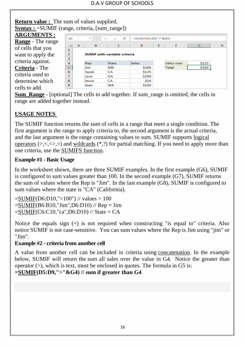
Return value : The sum of values supplied.

Syntax : =SUMIF (range, criteria, [sum_range])

ARGUMENTS :

Range - The range

of cells that you

want to apply the

criteria against.

Criteria - The

criteria used to

determine which

cells to add.

Sum_Range - [optional] The cells to add together. If sum_range is omitted, the cells in

range are added together instead.

USAGE NOTES

The SUMIF function returns the sum of cells in a range that meet a single condition. The

first argument is the range to apply criteria to, the second argument is the actual criteria,

and the last argument is the range containing values to sum. SUMIF supports logical

operators (>,<,<>,=) and wildcards (*,?) for partial matching. If you need to apply more than

one criteria, use the SUMIFS function.

Example #1 - Basic Usage

In the worksheet shown, there are three SUMIF examples. In the first example (G6), SUMIF

is configured to sum values greater than 100. In the second example (G7), SUMIF returns

the sum of values where the Rep is "Jim". In the last example (G8), SUMIF is configured to

sum values where the state is "CA" (California).

=SUMIF(D6:D10,">100") // values > 100

=SUMIF(B6:B10,"Jim",D6:D10) // Rep = Jim

=SUMIF(C6:C10,"ca",D6:D10) // State = CA

Notice the equals sign (=) is not required when constructing "is equal to" criteria. Also

notice SUMIF is not case-sensitive. You can sum values where the Rep is Jim using "jim" or

"Jim".

Example #2 - criteria from another cell

A value from another cell can be included in criteria using concatenation. In the example

below, SUMIF will return the sum all sales over the value in G4. Notice the greater than

operator (>), which is text, must be enclosed in quotes. The formula in G5 is:

=SUMIF(D5:D9,">"&G4) // sum if greater than G4



https://exceljet.net/glossary/wildcard

https://exceljet.net/excel-functions/excel-sumifs-function




https://exceljet.net/glossary/concatenation



17

Example #3 – SUMIF - not equal to

To express "not equal to" criteria, use the "<>" operator surrounded by double

quotes (""):

=SUMIF(B5:B9,"<>red",C5:C9) // not equal to "red"

=SUMIF(B5:B9,"<>blue",C5:C9) // not equal to "blue"

=SUMIF(B5:B9,"<>"&E7,C5:C9) // not equal to E7

Again notice SUMIF is not case-sensitive.

Example #4 - SUMIF with dates

The best way to use SUMIF with dates is to refer to a valid date in another cell, or use

the DATE function. The example below shows both methods:

=SUMIF(B5:B9,"<"&DATE(2019,3,1),C5:C9)

=SUMIF(B5:B9,">="&DATE(2019,4,1),C5:C9)

=SUMIF(B5:B9,">"&E9,C5:C9)

Notice we must concatenate an operator to the date in E9.

EXCEL AVERAGEIF FUNCTION

The Excel AVERAGEIF function computes the average of the numbers in a range that meet

the supplied criteria. The criteria for AVERAGEIF supports logical operators (>,<,<>,=) and

wildcards (*,?) for partial matching.

Purpose : Get the average of numbers that meet criteria

Return value : A number representing the average.






https://exceljet.net/excel-functions/excel-date-function


https://exceljet.net/excel-functions/excel-date-function



18

Syntax: =AVERAGEIF (range, criteria, [average_range])

Arguments :

range - One or more cells, including numbers or names, arrays, or references.

criteria - A number, expression, cell reference, or text.

average_range - [optional] The cells to average. When omitted, range is used.

USAGE NOTES

AVERAGEIF computes the average of the numbers in a range that meet the

supplied criteria. If average_range is not supplied, the cells in range are averaged.

If average_range is supplied, cells in average_range that correspond to cells in range are

averaged. To determine which cells are averaged, criteria is applied to range. Criteria can

be supplied as numbers, strings, or references. For example, valid criteria could be 10,

"10" ">10", or A1.

NOTES: Cells in range that contain TRUE or FALSE are ignored.

Empty cells are ignored in range and average_range when calculating averages.

AVERAGEIF returns #DIV/0! if no cells in range meet criteria. Average_range does not have to be the same size as range. The top left cell

in average_range is used as the starting point, and cells that correspond to cells in range are

averaged. Activity 2.1 – (Using IF condition in a Formula)

a. Enter the age of a person in cell A2. Display if he/she is eligible to vote in cell B2 using IF

Step 1: Click on cell A2

Step 2: Enter the age of a person

Step 3: Click on cell B2

Step 4 : Enter =if(A2>=18,”Eligible to

vote”, “Not Eligible”)


19

b. Enter the points scored by 5 people and display the badge they are eligible to receive.

A person gets a GREEN badge if the points scored are above 80 otherwise gets a BLUE

badge.Also calculate the number of blue and green

badges (using COUNTIF)

Step1: Click on B3 and enter Points

Step2 : Click on C3 and enter Badge

Step 3: Enter the values as shown above in cells to B8

Step 4: Click on C4 and enter

=IF(B4>80,"GREEN","BLUE")

Step 5: Click and drag till C8 to get the

badge colours for other cells.

Step 6: Click on cell B10 and enter Blue Badges

Step 7: Click on cell B11 and enter Green Badges

Step 8: Click on cell C10 and enter =COUNTIF(C4:C8,"BLUE")

Step 9: Click on cell C11 and enter

=COUNTIF(C4:C8,"GREEN")

c. Enter the age of 5 people. Calculate discount

in train ticket of 8% for minors and senior

citizens and 5% for the rest.

Step 1: Click on B2 and enter Age

Step 2: Click on C2 and enter Amount

Step 3: Click on D2 and enter Discount

Step 4: Enter the values 87,25,56,15,34 in

cells B3 to B7

Step 5: Enter the values 580,450,200,560

and 180 in cells C3 to C7

Step 6: Click on cell D2 and enter Discount

Step 7: Click on cell D3 and enter =IF(B3>=18,8,5)

and press Enter Key.

Step 8: Drag till cells D7 to get discount for other

cells

Step 9: Click on cell E2 and enter Discount

amount

Step10: Click on cell E3 and enter =C3*D3/100

and press Enter key

Step 11: Drag till cells E7 to get discount for other

cells

d. Enter ten number values (positive and negative). Calculate and display the total of

only positive numbers. Calculate and display the average of all negative numbers.

Step 1: Enter numbers 1 to 10 in cells B4 to B13

Step 2: Enter 10 numbers ( positive and negative numbers) in cells C4 to C13

B C

3 Points Badge

4 56 BLUE

5 92 GREEN

6 87 GREEN

7 67 BLUE

8 52 BLUE

9

10 Blue Badges 3

11 Green Badges 2


20

Step 3: Click on cell C14 and enter = Sumif(C4..C13, “>0”)

Step 4 : Click on cell C15 and enter =Averageif(C4..C13, “<0”)

e. Prepare the below worksheet of 5

students to find the eligibility for

rank

Step 1: Enter the row header as Student

sub1 sub2 sub3 sub4 sub5 Eligible for

rank in cells B2 to H2

Step 2: Enter student details in cells B3

to G7

Step 3: Click on H3 and enter

=IF(AND(C3>40,D3>40,E3>40,F3>40,G3>40),"Yes","No")

Step 4: Click and drag till H7 to get eligibility for all students.

Activity 2.2 (Removing duplicate values) a) Enter few numbers with repetition in column B. Copy the values to Column D and remove

the duplicate values.

Step 1: Enter some numbers with repetition in cells B4 to B18 with heading Actual values

Step 2: Click on Cell D3 and enter Unique values

Step 3: Copy the numbers from cells B4 to B18 and paste it in cells D4 to D18

Step 4: Click on Data tab and select Remove duplicates

The values after removing the duplicates will be as below:

b) Enter 50 names in a worksheet and remove the duplicate values. (Based on the steps in

activity 2.2 a) try to remove the duplicate values)

c) Enter comments as below RED- ShivajiHouse , BLUE – Tagore House, GREEN –

Bharathi House , YELLOW – Pratap House.


21

Step 1: Click on cell C1 and enter ROLLNO

Step 2: Click on cell D1 and enter COLOUR

Step 3: Click on cell C2 and enter 8345, Click on cell C4 and enter 8152, Click on cell C6

and enter 8215 and Click on cell C6 and enter 8438

Step 4: Enter the colours RED, BLUE, GREEN and YELLOW in cells D2, D4, D6 and D8

respectively.

Step 5: Click on cell D2 click Review Tab and select New Comment and type SHIVAJI

HOUSE in the comment box

Step 6: Repeat step 5 to enter comments for other colours

EXERCISES

1. Which function in Excel checks whether a condition is true or not ?

a. SUM b. COUNT

c. IF d. AVERAGE

2. Which of the following is a comparison operator for inserting a not equal to argument in

an IF, COUNTIF or SUMIF function?

a. <= b. <> c. >= d. ><

3. Study the screenshot on the right. Which of the

following functions, when inserted in the highlighted

cell (C2) above, will return the word “yes” ?

a. =IF(B2>50,"yes")

b. =IF(C2=”yes”)

c. =IF(B2=C2, “yes”)

d. =IF(B2=50, “yes”)

4. Which of the following represent the correct

arguments for the SUMIF function?

a. =SUMIF(criteria, range, criteria_range)

b. =SUMIF(criteria_range, true, false)

c. =SUMIF(range, criteria, [sum_range])

d. =SUMIF(range, sum_range, [criteria])

5. Which of the following is the correct formula syntax for using the COUNTIF function?

a. =COUNTIF(criteria, range)

b. =COUNTIF(criteria, range, [count_range])

c. =COUNT(IF(range, criteria))

d. =COUNTIF(range, criteria)

6. The ________________ function finds average for the cells specified by a given set of

conditions or criteria.

a. =averageif() b. =sumif()

c. =countif() d. =if()

7. The function used for adding the cells specified by a given set of condition or criteria




22

8. The function used to count the entries in a range based on a criteria.



9. >, <, =, >=, <=, <> are

a. Logical Operators b. Comparison Operators

c. Arithmetic Operators

10. And, Or, Not are



11. +, -, *, / are



12. =AND(A2>A3, A2<A4)

Determines if the value in cell A2 is ____ the value in A3____ also if the value in A2 is

___the value in A4.

( Fill in the blanks with the following – greater than, less than, And, Or)

13. =Not(A2+A3=24)

a. Determines if the sum of the values in the cells A2 and A3 is not equal to 24.

b. Determines if the sum of the values in the cells A2 and A3 is equal to 24.

c. Determines if A2+A3 is equal to 24 d. Both a. and c.

__________________________________________________________________________



23

CHAPTER 4

WHAT…IF ANALYSIS:

Essential Learning Skills:

By using What-If Analysis tools in Excel, you can use several different sets of values in one

or more formulas to explore all the various results.

For example, you can do What-If Analysis to build two budgets that each assumes a certain

level of revenue. Or, you can specify a result that you want a formula to produce, and then

determine what sets of values will produce that result. Excel provides several different tools

to help you perform the type of analysis that fits your needs.

Three kinds of What-If Analysis tools come with Excel:- Scenarios, Goal Seek, and

Data(Pivot) Tables. Scenarios and Data tables take sets of input values and determine

possible results.

EXCEL PIVOT TABLES:

Pivot table is a reporting engine built into Excel. They are the single best tool in Excel for

analyzing data without formulas. You can create a basic pivot table in about one minute, and

begin interactively exploring your data.

With very little effort (and no formulas) you can look at the same data from many different

perspectives. You can group data into categories, break down data into years and months,

filter data to include or exclude categories, and even build charts.

The beauty of pivot tables is they allow you to interactively explore your data in different

ways.

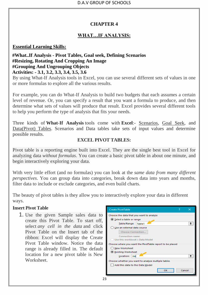
Insert Pivot Table

1. Use the given Sample sales data to

create this Pivot Table. To start off,

select any cell in the data and click

Pivot Table on the Insert tab of the

ribbon: Excel will display the Create

Pivot Table window. Notice the data

range is already filled in. The default

location for a new pivot table is New

Worksheet.

#What..If Analysis - Pivot Tables, Goal seek, Defining Scenarios

#Resizing, Rotating And Cropping An Image

#Grouping And Ungrouping Objects

Activities: - 3.1, 3.2, 3.3, 3.4, 3.5, 3.6


24

2. Override the default location and enter H4 to place the pivot table on the current

worksheet:

3. Click OK, and Excel builds an empty pivot table starting in cell H4.

4. Excel also displays the PivotTable Fields pane,

which is empty at this point. Note all

five fields are listed, but unused.

5. To build a pivot table, drag fields into one the Columns, Rows, or Values area. The

Filters area is used to apply global filters to a pivot table.

6. The pivot table below shows

total sales by product, but you

can easily rearrange fields to

show total sales by region, by

category, by month, and so

on.

NOTE: Source data should

have no blank rows or

columns, and no subtotals.

Each column should have a

unique name (on one row

only) and represent a field for each row/record in the data:

Use a pivot table to count things

By default, a Pivot Table will count any text field. This can be a really handy feature in a lot

of general business situations. For example, suppose you have a list of employees and want

to get a count by department? To get a breakdown by department, follow these steps:

a. Create a pivot table normally


25

b. Add the Department as a Row Label

c. Add the employee Name field as a Value

d. The pivot table will display a count of employee by Department

Employee breakdown by department

Show totals as a percentage In many pivot tables, you'll want to show a percentage rather than a count. For example,

perhaps you want to show a breakdown of sales by product. But, rather than show the total

sales for each product, you want to show sales as a percentage of the total sales. Assuming

you have a field called Sales in your data, just follow these steps:

a. Add Product to the pivot table as a Row Label

b. Add Sales to the pivot table as a Value

c. Right-click the Sales field, and set "Show Values As" to "% of Grand Total"

See the tip below "Add a field more than once to a pivot table" to learn how to show total

sales and sales as a percent of total at the same time.

Changing value display to % of total

Sum of employees displayed as % of total


26

GOAL SEEK If you know the result you want from a formula, use Goal Seek in Excel to find the input

value that produces this formula result. Goal Seek requires a single input cell and a single

output (formula) cell.

Goal Seek Example 1

Use Goal Seek in Excel to find the grade on the

fourth exam that produces a final grade of 70.

1. The formula in cell B7 calculates the final

grade.

3. On the Data tab, in the Data tools group, click

What-If Analysis.

4. Click Goal Seek. The Goal Seek dialog box

appears.

5. Select cell B7.

6. Click in the 'To value' box and type 70.

7. Click in the 'By changing cell' box and select cell B5.

8. Click OK.

Try it & You will notice that a grade of 90 on the fourth exam produces a final grade of 70.

Activity 3.1

Bond Election

Option Votes Percentage

YES 4478 63.90

NO 2530 36.10

Total 7008

a) To win the election the percentage of YES votes has to be 70.

b) Change the percentage of YES votes to 70 and accordingly the votes has to be changed

automatically using Goal Seek. The final output should be as below:

To retain the leading zeros in a number, begin the

entry with an apostrophe


27

Solution:

Step 1:Type the above data from A1 to D5

Step 2: Click What-if Analysis Goal Seek tool from Data tab

Step 3: Type D3 in the Set cell box and 70 in the To value box and c3 in the By changing

cell

Step 4: Click OK - the number of votes is required to get 70% in cell D3 appears in cell C3.

Activity 3.2:

Using Goal Seek Set the total of students of Roll no 1 and 2 to 375 by changing the maths

marks.

ROLL NO 1

Step 1: Type the above data/formulae from A1 to I12

Step 2: Click What-if Analysis Goal Seek tool from the Data tab

Step 3: Type H3 in the Set cell box and 375 in the To value box and E3 in the By

changing cell box

Step 4: Click OK - the MATH mark that is required to get a 375 total in cell H3 appears

in cell E3.

NOTE: Similarly repeat the above steps for ROLL NO 2. (Math mark for Roll no 2 is in

cell E4

SCENARIO MANAGER What-If Analysis in Excel allows you to try out different values (scenarios) for formulas. The

following example helps you master what-if

analysis quickly and easily.

Assume you own a book store and have 100

books in storage. You sell a certain % for the

highest price of 50/- and a certain % for the

lower price of 20/-.

If you sell 60% for the highest price, cell

D10 calculates a total profit of 60 * Rs.50 +

MARK SHEET FOR 2017-18

R.

N

O. NAME

E

N

G LANG MATH SCI SOC TOT AVG

1 ADITI 74 65 66 71 89 365 73

2 AKSHAYA ANAND 78 65 44 67 78 356 66.4

3 ANUSHREE 80 78 67 55 76 369 71.2

4 ARSHANA 49 67 80 86 87 420 73.8

5 ARUTHRA 98 78 87 67 90 393 84

6 DIVYA 65 76 87 76 89 404 78.6

7 KANISHKA 76 78 84 90 76 397 80.8

8 KEERTHANA 78 85 67 78 89 397 79.4

9 KEERTHIGAMBIGAI 89 87 78 87 56 397 79.4

10 KRITI 91 97 96 99 98 481 96.2


28

40 * Rs.20 = Rs.3800.

Create Different Scenarios

But what if you sell 70% for the highest price? And

what if you sell 80% for the highest price? Or 90%,

or even 100%? Each different percentage is a

different scenario. You can use the Scenario

Manager to create these scenarios.

Note: You can simply type in a different percentage

into cell C4 to see the corresponding result of a

scenario in cell D10. However, what-if analysis

enables

you to

easily

compare the results of different scenarios.

1. On the Data tab, in the Data Tools group,

click What-If Analysis.

2. Click Scenario Manager.

The Scenario Manager dialog box appears.

3. Add a scenario by clicking on Add.

4. Type a name (60% highest), select cell C4 (%

sold for the highest price) for the Changing cells

and click on OK.

5. Next, add 4 other scenarios (70%, 80%, 90% and 100%).

Finally, your Scenario Manager should be consistent with the picture below:

Scenario Summary To easily compare the results of these scenarios,

execute the following steps.

1. Click the Summary button in the Scenario Manager.

2. Next, select cell D10 (total profit) for the result

cell and click on OK.

Result:

Conclusion: if you sell 70% for the highest price,

you obtain a total profit of Rs.4100, if you sell

80% for the highest price, you obtain a total profit

of Rs.4400, etc. That's how easy what-if analysis

in Excel can be.


29

Activity 3.3 Prepare the statement as below. Use Scenario manager and create changes and also show

the scenario summary .

Change Food to 400 , Transportation to 120 , monthly income to 2000 for Scenario named

modify 1 and Change Food to 400 , Transportation to 120 , monthly income to 1500 for

Scenario named modify 2.

Step 1: Type the above data/formulae (Budget Plan) from A1 to B14

Step 2: Click What-if Analysis Scenario Manager tool from the Data tab and Click the

Add button

Step 3: Type the Scenario name as Current Values and type $B$3:$B$9 in the Changing

cells box and click OK button.

Step 4: Check and change the values of the cells (if required) that need to be changed for

the given scenario and click Add button.

Step 5: Repeat the Step 3 and 4 for Scenario called modify 1 and Scenario called modify 2.

Step 6: Click the Summary button - A Scenario Summary sheet is added to the workbook.

Activity 3.4 Change the picture shape and border. Change the

picture border weight to 3pts and dashes too.

Step 1: Select the picture.

Step 2:Click Picture tools tab

BUDGET PLAN

RENT 500

FOOD 300

TRANSPORTATION 80

OTHER EXP 100

MONTHLY

INCOME 1500

OTHER INCOME 0

TOTAL INCOME 1500

TOTAL EXPENSES 980

SAVINGS 520


30

Step 3: Click Picture Shape tool from the

Picture Styles group.

Step 4:Select the Basic ShapesClick TearDrop

Step 5: Click Picture Border and set weight to 3 pts

and select a Dashed line from Dashes.

Activity 3.5 - Resize and Crop the picture as below

Step 1: Select the picture and click Picture

Tools tab on top of window.

Step 2: Repeat the steps given for Activity

3.4

Activity 3.6 Insert a picture in excel. Place a textbox and group

them together as below.

Step 1: Click Insert tab.

Step 2: Choose TextBox tool from Text group of

Insert tab

Step 3: Click and drag a rectangle on the

Picture and type tulips in it.

Step 4: Click the border of this Text Box and keeping the Ctrl key pressed, click the picture

(to Select both the Text and the picture simultaneously )

Step 5: Click the Format tabclick Group tool from Arrange group.


31

EXERCISE 1. The arrangement of arguments in a function

a. Structure b. Grammar c. Syntax

2. A logical function that returns true if any of the conditions are true.

a. AND b. NOT c. OR

3. A ________________________ is an interactive Excel report that summarizes and

analyzes large amounts of data.

4. The _______________________________ an area to position fields by which you

want to filter the PivotTable report.

5. The __________________________ is an area to position fields that contain data that

is summarized in a PivotTable.

6. The __________________________ is the upper portion of the PivotTable Fields

pane containing the column titles from your source data.

7. ____________________________ is a logical function that counts the cells that meet

specific criteria in a specified range.

8. _______________________ is a what-if analysis tool that compares alternatives.

9. ______________ function contains one logic test—it will add values in a specified

range that meet certain conditions or criteria.

10. The __________________ logical function takes only one argument and is used to

test one condition. If the condition is true, the function returns the logical opposite

false. If the condition is false, true is returned.

11. ________________is a what-if analysis tool that finds the input needed in one cell to

arrive at the desired result in another cell.

12. Under which tab and in which function group will you find the option to insert a Pivot

Table?

a. Under the Insert tab in the Tables group

b. Under the Formulas tab in the Data Analysis group

c. In the Data group in the Pivot Tables group

d. In the Data group in the Tables group

13. Which of the following is NOT a box in the PivotTable Fields List?

a. Column Labels b. Values c. Report Filter d. Formula

14. What function displays row data in a column or column data in a row?

a. Hyperlink b. Transpose c. Index d. Rows

15. Which of the following tool you will use in Excel to see what must be the value of a

cell to get required result?

a. Formula Auditing b. Research c. Track Change d. Goal Seek

16. To apply Goal Seek command your cell pointer must be in

A) The Changing cell whose value you need to find

B) The Result Cell where formula is entered

C) The cell where your targeted value is entered D) None of above

17. Which of the following is not What IF analysis tool in Excel?

a. Goal Seek b. Scenarios c. Macros d. None of above



32

CHAPTER 5

Protecting Worksheet

Essential learning skills:

Use Cell Protection to Prevent Editing an Area of the Spreadsheet: If you share a workbook with other users, it’s important to prevent accidental edits. There are

multiple ways you can protect a sheet, but if you just want to protect a group of cells, here is

how you do it. First, you need to turn on Protect Sheet. Click the Review Tab, then

click Protect Sheet. Choose the type of modifications you want to prevent other users from

making. Enter your password, click OK then click OK to confirm.

Protect a WorkSheet: Excel 2007 includes a Protect Workbook command that prevents others from making

changes to the layout of the worksheets in a workbook. You can assign a password when you

protect a workbook so that only those who know the password can unprotect the workbook

and make changes to the structure and layout of the worksheets.

Activity 4.1 a) Open the file created in activity 14. Protect the worksheet by giving a password. Close

the file. Open the file again and make

changes

Step 1: On the Review tab, in the Changes

group, click Protect Sheet.

Step 2: In the Allow all users of this

worksheet to list, select the elements that

you want users to be able to change.

Step 3: In the Password to unprotect sheet

box, type a password for the sheet, click

OK, and then retype the password to

confirm it.

This will protect the worksheet not allowing users to insert or delete rows & Columns

b) Protect the workbook with a password to open.

1. Click the Microsoft Office Button , and then click Save As.

2. Click Tools, and then click General Options.

3. Do one or both of the following:

# Protecting The Worksheet

# Protecting a workbook from being opened and modified

# More Activities


33

a. If you want reviewers to enter a password before they can view the workbook, type a

password in the Password to open box.

b. If you want reviewers to enter a password before they can save changes to the

workbook, type a password in the Password to modify box.

Unprotecting a Workbook:

a. Click the Unprotect Workbook command button in the Changes group on the Review tab.

b. If you assigned a password when protecting the workbook, type the password in the

Password text box and click OK.

More Activities a) Prepare the consolidated mark statement of students (minimum 100 students) with

columns as below

SNO NAME DEPT SEC TERM1 TERM2 AVG RESULT RANK

Use Sum function to find the total of TERM1 and TERM2

Calculate AVG as (Term1 + Term2)/2

Result is displayed as PASS if marks scored in Term1 and Term2 is above 50%. Else

Result is displayed as FAIL.

Calculate Rank for students whose result is PASS

b) Copy the worksheet data of first 10 students to Sheet2 and prepare a chart to show their

performance.


34

c) Copy the worksheet data of first 20 students to Sheet 3 and sort them in ascending order of

Rank

d) Copy the worksheet data of last 30 students to Sheet4 and display the number of students

with PASS result. Also display the Pass Percentage.

e) For the students in Sheet4 use Conditional formatting and change font color for different

Departments as below

ME – Red , EE – Blue , CE - Green , CHE – Yellow

f) Add Comments to at least 5 cells in Sheet2

g) Copy the contents of Sheet3 to Sheet 5 and perform GoalSeek analysis.

h) Copy the last 10 contents of Sheet 4 to Sheet 6 and perform scenario analysis for at least

2 situations with minimum 5 changes.

g) Protect the worksheet by giving it a password.

EXERCISE

1. In order for the Lock or Unlock Cells function to work, which option should be

enabled?

a) The Protect Workbook function needs to be enabled.

b. No functions need to be enabled other than the lock or unlock cells options.

c. The worksheet must be saved before the cells will become locked or unlocked.

d. The Protect Worksheet function needs to be enabled.

2. What is the only way of removing password encryption on an Excel file?

a. Resaving the workbook as a new document or making a copy of it.

b. Opening the workbook as Read Only and resaving it without a password.

c. Opening the workbook in Protected View and resaving it without a password.

d. Entering the password to open the Workbook and then deleting the password

created in the Permissions – Encrypt with Password box.

3. To protect a worksheet, you can choose Protection and the Protect Sheet from the

….. Tab

a. Home b. Data c. Review d. Tools


CHAPTER 1 - D.A.V. Chennai

Documents

Transcript of CHAPTER 1 - D.A.V. Chennai