Chapter 1 - CORE
91
THREE-DIMENSIONAL INVERSION OF AIRBORNE ZTEM AND AIRMT DATA by Muran Han A thesis submitted to the faculty of The University of Utah in partial fulfillment of the requirements for the degree of Master of Science in Geophysics Department of Geology and Geophysics The University of Utah December 2017
-
Upload
khangminh22 -
Category
Documents
-
view
1 -
download
0
Transcript of Chapter 1 - CORE

THREE-DIMENSIONAL INVERSION OF
AIRBORNE ZTEM AND AIRMT DATA
by
Muran Han
A thesis submitted to the faculty of
The University of Utah
in partial fulfillment of the requirements for the degree of
Master of Science
in
Geophysics
Department of Geology and Geophysics
The University of Utah
December 2017

Copyright © Muran Han 2017
All Rights Reserved

T h e U n i v e r s i t y o f U t a h G r a d u a t e S c h o o l
STATEMENT OF THESIS APPROVAL
The thesis of Muran Han
has been approved by the following supervisory committee members:
Michael S. Zhdanov , Chair 03/23/2017
Date Approved
Erich U. Petersen , Member 10/07/2013
Date Approved
Alexander V. Gribenko , Member 09/11/2013
Date Approved
and by Thure E. Cerling , Chair of
the Department of Geology and Geophysics
and by David B. Kieda, Dean of The Graduate School.
ABSTRACT
In this thesis, an interpretation technique is developed and presented for two new
airborne geophysical methods which are used for measuring natural magnetic fields:
ZTEM and AirMt. The z-axis tipper electromagnetic (ZTEM) system measures the fields
of natural audio-frequency sources using an airborne vertical magnetic field receiver and a
pair of horizontal, magnetic field ground receivers at a base station. The AirMt method
employs three orthogonal airborne magnetic field receivers and three horizontal orthogonal
magnetic-field ground receivers at a base station. The magnetic field components acquired
during the AirMt survey are converted into an amplification parameter, which is invariant
to receiver reference systems. The airborne deployment makes it possible to acquire ZTEM
and AirMt data over large areas for a relatively low cost compared to equivalent ground
surveys. This makes it a practical method for mapping large-scale geological structures.
This thesis develops the methods of three-dimensional (3D) forward modeling and
inversion of ZTEM and AirMt data. For the forward modeling, I apply the integral equation
method, while the inversion is based on Tikhonov regularization method. The model study
in this thesis is conducted under different conditions which can affect accurate modeling
and inversion of the data. In the final chapter of the thesis, I present the results of inversion
of the field ZTEM data from the Cochrane test site in Ontario, Canada.

To my parents and my wife, Xiao

TABLE OF CONTENTS
ABSTRACT ...................................................................................................................... iii
ACKNOWLEDGMENTS .............................................................................................. vii
Chapters
1. INTRODUCTION ......................................................................................................... 1
2. FOUNDATIONS OF THE AIRBORNE MAGNETOVARIATIONAL
METHODS .................................................................................................................... 5
2.1 Magnetic transfer functions ...................................................................................... 6
2.2 Induction vectors and tippers .................................................................................. 11 2.3 Principles of the ZTEM method ............................................................................. 14
2.4 Principles of the AirMt method .............................................................................. 15
3. FORWARD MODELING OF ZTEM AND AIRMT DATA .................................. 21
3.1 Principles of EM forward modeling using the integral equation method ............... 22
3.2 Forward modeling of ZTEM data ........................................................................... 24 3.3 Forward modeling of AirMt data ............................................................................ 27
4. INVERSION OF ZTEM AND AIRMT DATA ........................................................ 28
4.1 Principles of regularized geophysical inversion ..................................................... 29 4.2 Frechet derivative calculation and inversion of ZTEM data .................................. 31
4.3 Frechet derivative calculation and inversion of AirMt data ................................... 33
5. MODEL STUDY OF THE INVERSION ALGORITHM ...................................... 37
5.1 Inversion with true background conductivity ......................................................... 37
5.2 Inversion with inaccurate background conductivity ............................................... 38
5.3 Inversion with reference station anomaly ............................................................... 39
5.4 Inversion with variable flight elevation .................................................................. 40 5.5 Inversion of the noisy data ...................................................................................... 40
6. CASE STUDY: COCHRANE ZTEM SURVEY ..................................................... 64

vi
6.1 Description of the survey area ................................................................................ 64 6.2 Practical ZTEM data ............................................................................................... 65 6.3 Inversion results ...................................................................................................... 68
7. CONCLUSIONS ......................................................................................................... 77
REFERENCES ................................................................................................................ 79

ACKNOWLEDGMENTS
Before I joined the Consortium for Electromagnetic Modeling and Inversion
(CEMI) at the Department of Geology and Geophysics, University of Utah, I didn’t have
much knowledge about electromagenetic methods, especially of forward modeling and
inversion, which requires good math skills. There are too many people to thank. Therefore,
I will be lengthy here and brief elsewhere.
I am deeply indebted to my advisor and committee chair, Dr. Michael Zhdanov, who
made this work possible and shared his vast knowledge of EM and inversion, for giving
me a chance to work under his guidance and for ultimately leading me along an academic
path. Dr. Le Wan not only sacrificed a lot of time to explain the problems of EM theory to
me, but also made many invaluable insights into the application of my research in the real
world and forced me to look beyond my work. Dr. Alexander V. Gribenko, who is an EM
expert in my mind, provided helpful guidance for this work and answered numerous
questions about programming and inversion techniques.
I would also like to thank my advisor, Dr. Erich Petersen, who guided me to connect
geophysics with geology, especially when it comes to minerals and rocks.
I also thank Dr. Martin Cuma and Dr. Xiaojun Liu for sharing the techniques and
skills of parallel computation, discussing things related to my thesis research, addressing
questions related to practical geophysical situations, and providing invaluable codes to
refer to for this research. I also thank Mrs. Kim Atwater. Without her help, I would have a

viii
lot of trouble in life.
Finally, my family provided empathy and encouragement along the way. I
especially thank my parents. Without their encouragement and help, I could not have
focused on my work completely. Most of all, I would like to thank my wife, Xiao, for
supporting my study, which was a long journey from beginning to the end。
1
CHAPTER 1
INTRODUCTION
ZTEM is a novel electromagnetic (EM) geophysical technique used in measuring
the natural magnetic field, similar to magnetotelluric (MT) methods and coupled with rapid
spatial acquisition from an airborne system. In understanding the electrical conductivity of
the upper regions of the earth, the MT method plays a very important role. The primary
advantage of natural source EM, especially the airborne method, compared with the
controlled source method, is the large depth of penetration due to the relatively low
frequencies used. Particularly, the MT method plays a significant role in crustal studies as
well as in hydrocarbon and mineral exploration. However, the MT technique and other
deep-probing controlled source EM methods have some obvious practical limitations,
related to the cost of the survey and the time required for the data acquisition. Measuring
the MT field from an airborne platform is very attractive, because it allows us to cover
large areas very quickly and it does not require using a controlled source. The main problem
with the airborne implementation of the MT method is related to the fact that the airborne
measurement of an electric field is extremely difficult; therefore, the airborne method
should be based on magnetic data only. It has long been recognized that tipper data, the
ratio of the local vertical magnetic field to the horizontal magnetic field, provide
information about the anomalies of the three-dimensional (3D) electrical conductivity. The
2
fundamental reason for this is that the inducing electromagnetic fields are vertically
propagating plane waves, so if the earth is one-dimensional (1D), the vertical component
of the magnetic field will be zero. Nonzero values of the tipper data are directly related to
anomalous currents. It was this understanding that prompted the development of the audio
frequency magnetics (AFMAG) technique (Ward, 1959). The original airborne AFMAG
technique used the amplitude outputs from two orthogonal coils towed behind an aircraft
to determine the tilt of the plane and the polarization of the natural magnetic field.
To improve the AFMAG method, Labson and others (1985) developed a technique
that used ground-based horizontal and vertical coils to measure the reference magnetic
fields. They used MT processing techniques to show how tipper data could be obtained
from the measured magnetic fields.
A further improvement to the original AFMAG technique combines improved
instrumentation and MT data processing techniques. This has resulted in the z-axis tipper
electromagnetic method (ZTEM) (Lo and Zang, 2008). In this method, the vertical
component of the magnetic field is recorded over the entire survey area, while the
horizontal fields are recorded at a ground-based reference station (Holtham and Oldenburg,
2010). The MT processing technique produces the frequency domain transfer functions
that relate the vertical fields over the survey area to the horizontal fields at the reference
station. By taking ratios of the two fields (similar to taking ratios of the E and H fields in
MT), the effect of the unknown source function is removed. Since new instrumentation
exists to measure the vertical magnetic fields by helicopter, the magnetic data over large
survey areas can quickly be collected. The result is a cost-effective procedure for collecting
natural source EM data that provide information about the 3D conductivity structure of the
3
earth. Over the last several years, industry has recognized the potential of this technique
and the need to be able to invert these data (Zhdanov and Golubev, 2003).
Another airborne MT method considered in this thesis is called AirMt (Gribenko et
al., 2012). In general, the 3D magnetic field variations measured at the airborne receiver
platform are related to the horizontal incident fields at a base station by an AirMt tensor.
The AirMt system measures the magnetic field within some frequency bands at the base
station and from the airborne system. Using these measurements, one can derive the
components of the AirMt tensor. The compact amplification parameter P is further
established as a function of the cross product of the two columns of the AirMt tensor. It
can be shown that parameter P is invariant under any rotation of the airborne frame of
reference or the base station frame of reference, thus making AirMt measurements immune
to tilt errors (Kuzmin et al., 2010).
Zhdanov et al. (2011) presented an inversion algorithm for both individual ZTEM
data and for joint MT and ZTEM data. In this thesis, a 3D AirMT data inversion capability
is developed, extending the two-dimensional (2D) expressions of the AirMT Fréchet
derivative presented by Wannamaker (1984) to a 3D case.
I have also developed a 3D inversion algorithm for ZTEM and AirMt data. Forward
modeling is fundamental to any inversion algorithm, and a simple forward model was used
to produce the results of the ZTEM and AirMt data. Next, algorithms were developed for
inverting ZTEM and AirMt data. Finally, the output data of the forward modeling were
used as the input for the ZTEM and AirMt inversion to invert the model data, and both
inversions were compared with each other to test the program. Synthetic modeling is used
to study the effects of background conductivity variations, different flight elevations, and

4
noise for both ZTEM and AirMt inversions. The results of 3D ZTEM data inversion over
the Cochrane test site in Ontario, Canada, and the effectiveness of developed methods and
codes is demonstrated and presented in this thesis as well.
CHAPTER 2
FOUNDATIONS OF THE AIRBORNE
MAGNETOVARIATIONAL METHODS
Long-term observations show that the magnitude and direction of the earth’s
magnetic field continuously change with time. These alterations are called geomagnetic
variations. There are two types of geomagnetic variations: one is caused by internal sources
while the other one is due to an external origin (Campbell, 2003).
According to electromagnetic induction laws, geomagnetic variations induce a
transient electromagnetic field in the conductive earth, and the corresponding electric
current. Note that the external geomagnetic variations vary rapidly and can induce a strong
current, which is easy to measure. This current is called a telluric current (from the Latin
word telluric for earth’s). As a result, the entire field of geomagnetic variations and telluric
currents is called the magnetotelluric field (Zhdanov, 2009) .
The magnetotelluric field at frequencies below 1 hertz is of particular importance,
primarily because it can be used as an energy source to probe the earth to great depths. At
these low frequencies, the magnetotelluric field originates almost entirely from complex
interactions between the earth’s magnetosphere and the flow of plasma from the sun (solar
wind) (Zhdanov, 2009).
In this chapter, the concept of transfer functions will be considered, and the
6
principles of the two different airborne EM methods, ZTEM and AirMt, will be discussed.
2.1 Magnetic transfer functions
Variations of the natural MT field can be separated into two parts: telluric (electric)
and geomagnetic (magnetic) variations. These variations are caused by ionospheric and
magnetospheric currents arising from interactions between the solar and a magnetosphere
plasma with a constant geomagnetic field (Berdichevskii and Dmitriev, 2008). Practical
MT data are observed over a range of periods from a fraction of a second to several hours.
Such fields can penetrate into the earth at a depth from several hundred meters to several
hundred kilometers, which is of great importance to the study of the geoelectrical structure
of the earth’s deep interior.
The intensity of the natural source in the MT method is unknown. In order to
eliminate this source effect, scientists study the ratio of the electric and magnetic fields,
which is defined as the impedance, rather than the natural electromagnetic field itself. The
concept of impedance (Cagniard, 1953; Tikhonov, 1950) helps to build the fundamental
principles of magnetotellurics and makes the MT method a powerful tool to study the
geoelectrical structure of the earth.
The expression for impedance is misleadingly simple:
Z = Ex Hy⁄ = −Ey Hx⁄ , (2.1)
where {Ex, Ey} and {Hx, Hy} represent the horizontal components of the electric and
magnetic fields. We assume a linearity in the relationships between the mutually
orthogonal electric and magnetic field components which are used in determining the
Tikhonov-Cagniard impedance:
7
Ex = ZHy,
Ey = −ZHx . (2.2)
It is most important to consider the question of the validity of this assumption of
linearity when we are dealing with a real, inhomogeneous earth. The answer to this question
rests on a detailed analysis of the linearity between the various components of the
magnetotelluric field. We will make this analysis using some elementary concepts of linear
algebra.
In a general case, a monochromatic field satisfies the following equations:
curlH = σE + jQ ,
curlE = iωμ0H , (2.3)
where jQ is the volume density of the external ionospheric and magnetospheric currents
which give rise to the magnetotelluric field. On the strength of Maxwell’s equations being
linear, it is possible to write the electric and magnetic fields as linear transformations of
the current density vector jQ :
E (r) = ∭ GE(r |r′ , ω, σ)jQ (r′ )
Qdv′,
H (r) = ∭ GH(r |r′ , ω, σ)jQ (r′ )Q
dv′, (2.4)
where is the region within which the currents jQ are present, and GE and GHare linear
operators related to the radius vector r defining the location at which the field is observed
and the radius vectors r′ defining the points at which the source currents jQ (r′ ) are
flowing. These operators are functions only of the field frequency ω and the distribution
of electrical conductivity in the medium, σ. A prime indicates that integration has been
Q
8
carried out with respect to r′ .
In the theory of linear relationships between the components of magnetotelluric
fields (Zhdanov, 2009), it has been shown that for most types of geomagnetic variations
(pulsations, microstorms, quiet-day diurnal variations, and worldwide storms), jQ can be
represented as a linear transformation of some independent vector A (either real or
complex) realized using a linear operator a:
jQ (r ) = a(r )A /𝑇, (2.5)
The vector A is independent of the coordinate system. It characterizes the
polarization and strength of the currents flowing in the ionosphere and magnetosphere, and
is called the vector field characteristic.
The operator a in a general case depends on the spatial coordinates and
characterizes the geometry of the external currents, that is, the excitation of the magneto-
telluric field. It is called the excitation operator. The excitation operator does not change
for one specific type of variations (micropulsations, microstorms, Sqvariations, worldwide
storms), but may change from one type of variation to another.
Equation (2.5) is substituted into (2.4). Then
E (r , ω) = e(r , ω, σ)A ,
H (r , ω) = h(r , ω, σ)A , (2.6)
where
e(r , ω, σ) = ∭GE
Q
(r |r′ , ω, σ) a (r′ ) dv′,
h(r , ω, σ) = ∭ GHQ
(r |r′ , ω, σ) a (r′ ) dv′. (2.7)
9
One can see that the operators e and h depend on the coordinates of the observation
point, r , the frequency, ω, and the distribution of electrical conductivity in the medium, σ.
These are called the electrical and magnetic characteristic field operators. It must be
stressed that, while these operators, as well as the excitation operator, a, are constant with
respect to a given type of excitation, they can change as one type of variation is replaced
by another (as, for example, the transition from observations of storm-time variations to
quiet-time variations).
If it is assumed that both characteristic operators, e and h , are invertible (that is,
inverse operators e−1 and h−1 exist), then, in accord with equations (2.6) and (2.7),
A = {e−1(r , ω, σ)E (r , ω)
h−1(r , ω, σ)H (r , ω)}. (2.8)
Substituting the bottom expression from equation (2.8) into (2.6) and the top
expression from equation (2.8) into (2.7), the following is obtained:
E (r , ω) = e(r , ω, σ)h−1(r ,ω, σ)H (r , ω) = Z(r ,ω, σ)H (r , ω),
H (r , ω) = h(r , ω, σ)e−1(r ,ω, σ)E (r , ω) = Y(r , ω, σ)E (r ,ω). (2.9)
Here, Z and Y are operators representing impedance and admittance, respectively:
Z(r , ω, σ) = e(r , ω, σ)h−1(r , ω, σ),
Y(r , ω, σ) = h(r , ω, σ)e−1(r , ω, σ). (2.10)
If E and H are measured at several points on the earth’s surface (with radius vectors
r and r0 ), then, using equations (2.6), (2.7), and (2.8), one can write
E (r , ω) = e(r , ω, σ)e−1(r0 , ω, σ)E (r0 , ω) = t(r |r0 , ω, σ)E (r0 ),
H (r , ω) = h(r , ω, σ)h−1(r0 , ω, σ)H (r0 , ω) = m(r |r0 , ω, σ)H (r0 ). (2.11)
Here, t and m are telluric and magnetic operators:
10
t(r |r0 , ω, σ) = e(r ,ω, σ)e−1(r0 , ω, σ),
m(r |r0 , ω, σ) = h(r , ω, σ)h−1(r0 ω, σ). (2.12)
The operators Z, Y, t, and m, are called the magnetotelluric operators. The four
operators evoke the transformation of the electric and magnetic fields one to the other. Each
type of magnetotelluric variation is characterized by its own set of operators, Z, Y, t, and
m, which depends only on frequency, the location of the observation point, the strength
and orientation of the ionospheric and magnetospheric currents, and the distribution of
electrical conductivity in the medium, σ.
The magnetotelluric operators on a given set of basic functions have corresponding
matrices, which are called the magnetotelluric matrices. Differences in these matrices
reflect differences in the types of variations being observed. For micropulsations and
storm-time excitation observed at low to mid-latitudes (that is, for the variations which are
most commonly used in geophysical exploration because of the frequency window), the
dimensionality of the magnetotelluric matrix is twofold (Berdichevskiĭ and Zhdanov, 1984).
For such fields, if the horizontal components of the electric and magnetic fields are
recorded, the matrix operators Z, Y, t, and m, in accord with the rules of linear algebra, take
the following forms:
[Zαβ] = [Zxx Zxy
Zyx Zyy], (2.13)
[Yαβ] = [Yxx Yxy
Yyx Yyy], (2.14)
[tαβ] = [txx txytyx tyy
], (2.15)
[mαβ] = [mxx mxy
myx myy]. (2.16)
11
Consequently, in cases of operator relationships, equations (2.13), (2.14), (2.15), and
(2.16), one can write (Berdichevskiĭ and Zhdanov, 1984)
Ex = ZxxHx + ZxyHy,
Ey = ZyxHx + ZyyHy, (2.17)
Hx = YxxEx + YxyEy,
Hy = YyxEx + YyyEy, (2.18)
Ex = txxEx(r0 ) + txyEy(r0 ),
Ey = tyxEx(r0 ) + tyyEy(r0 ), (2.19)
Hx = mxxHx(r0 ) + mxyHy(r0 ),
Hy = myxHx(r0 ) + myyHy(r0 ). (2.20)
2.2 Induction vectors and tippers
Besides the MT method, modern magnetotellurics consists of another branch, the
magnetovariational (MV) method, which studies the linear transformation of the magnetic
field.
Zhdanov (2009) has demonstrated that, when surveys are carried out in regions with
a horizontally inhomogeneous geoelectric structure, the magnetic field H will have a
significant vertical component (of course, the earth’s steady magnetic field has a significant
vertical component, Hz, almost everywhere, but it does not contribute to electromagnetic
induction). In the case of a sea-bottom magnetoteluric survey over an area with a
horizontally inhomogeneous geoelectric structure, the electric field E will have a
significant vertical component Ez. In the theory of linear relationships, it can be shown that,
12
in cases of linear correlations of the type given in equations (2.17) through (2.20),
supplementary formulas can be used (Zhdanov, 2009):
Hz = WzxHx + WzyHy, (2.21)
Ez = VzxEx + VzyEy. (2.22)
Relationship (2.21) bears the name Wiese-Parkinson relationship. Formula (2.22)
is an electric analog of the Wiese-Parkinson relationship (Parkinson, 1959, 1962). These
relationships reflect the fact that the vertical components of the magnetic field Hz or the
electric field Ez at every point are linearly related to the horizontal components of the same
field. As was the case with the various linear relationships described earlier, the coefficients
of the Wiese-Parkinson relationship and its electric analog depend only on the coordinates
of the observation point, r , the frequency, ω, and the distribution of electrical conductivity
in the medium. The values Wzx and Wzy, Vzx, and Vzy form complex vectors:
W = Wzxdx + Wzydy
, (2.23)
V = Vzxdx + Vzydy
. (2.24)
in which the real and imaginary parts are as follows:
Re(W ) = ReWzxdx + ReWzydy
, Im(W ) = ImWzxdx + ImWzydy
, (2.25)
Re(V ) = ReVzxdx + ReVzydy
, Im(V ) = ImVzxdx + ImVzydy
. (2.26)
Vector W is named the Wiese-Parkinson vector, or the induction vector. Vector W is often
called a (magnetic) tipper.
By analogy, we will call vector V an electric tipper. Note that on land, the vertical
component of an electric field is negligibly small, Ez = 0 , which results in a linear
relationship between the horizontal components of the electric field:
13
VzxEx + VzyEy
= 0. (2.27)
However, in the case of measurements conducted on the sea bottom, Ez = 0, and
the electric tipper reflects the horizontal inhomogeneities of the sea-bottom formations.
In summary, it has been shown that for an arbitrary distribution of electrical
conductivity in the earth, a linear functional relationship of the type in equations (2.17)
through (2.22) exists between the components of the magnetotelluric field. The coefficients
in these linear relationships (that is, the elements of the magnetotelluric matrix) are transfer
functions. The elements of the magnetotelluric matrix are invariant on rotation: they reflect
the distribution of electrical conductivity in the earth, but are independent of changes in the
sources of the field, the magnetospheric and ionospheric currents. The transfer functions
are also called electrical conductivity functions. The electrical conductivity functions, in
contrast to measured electric and magnetic fields, carry information about the internal
geoelectric structure of the earth only. Determining the electrical conductivity function is
the basic step in application of the magnetotelluric method.
Determination of the conductivity function can be accomplished through the use of
statistical analysis methods including cross- and auto-correlation of field components and
calculation of the coefficients of multiple linear regressions. The techniques currently in
use for determining the magnetotelluric matrix will be reviewed in detail in the following
sections.
It is noted in conclusion that the linear operators can be considered as examples of
rather more esoteric objects in linear algebra: tensors. Frequently, magnetotelluric
operators are called magnetotelluric tensors, and we speak of tensor impedance, tensor
admittance, and telluric and magnetic tensors. In this thesis, in order to retain some
14
simplicity in mathematical presentation, we will accept the linear operator approach and
only mention the use of the tensor terminology (Zhdanov, 2009).
2.3 Principles of the ZTEM method
The z-axis tipper electromagnetic (ZTEM) system measures the transfer functions
(tippers) of audio-frequency natural sources using an airborne receiver at the vertical
magnetic field and a pair of orthogonal horizontal magnetic field receivers at a base station.
Data are typically measured from 30 Hz to 720 Hz, giving detection depths down to 1 km
or more, depending on the conductivity of the terrain. The airborne deployment makes it
possible to acquire ZTEM data over large areas for a relatively low cost compared to
equivalent ground surveys. This makes it a practical method for mapping large-scale
geological structures. As an airborne extension of the magnetovariational (MV) method,
the ZTEM transfer functions contain information about the 3D conductivity distribution
within the earth. A rigorous 3D inversion algorithm for regularized inversion of ZTEM
data based on the integral equation method (Zhdanov et al., 2011) is presented in this
section.
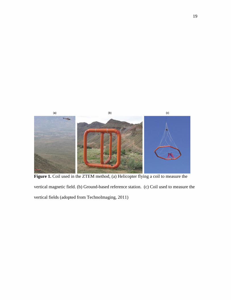
In the air, ZTEM instrumentation uses a helicopter to tow a coil developed by
Geotech Inc., which measures the vertical component of the magnetic field. The horizontal
magnetometers located in the reference station measure horizontal components of the
magnetic field. The essential components of the system are shown in Figure 1.
As mentioned above, the ZTEM system measures the transfer functions that relate
the vertical magnetic fields observed above the earth to the horizontal magnetic field at
some fixed reference station. This relation is given by the following formula:
15
Hz(r ) = Tzx(r , r0 )Hx(r0 ) + Tzy(r , r0 )Hy(r0 ),
(2.28)
where r is the location of the airborne station, r0 is the location of the ground-based
reference station, and Tzx and Tzy are the vertical field transfer functions. In order to
determine two unknown transfer functions, the vertical fields are measured for two
independent polarizations of the magnetic field. The fields for each polarization are given
by the following expressions:
{Hz
1 = TzxHx1 + TzyHy
1
Hz2 = TzxHx
2 + TzyHy2 , (2.29)
or in matrix form:
(Hz
1(r )
Hz2(r )
) = (Hx
1(r0 ) Hy1(r0 )
Hx2(r0 ) Hy
2(r0 )) (
Tzx
Tzy), (2.30)
where the superscript in equations (2.28) and (2.29) refer to the source field polarizations
in the x and y directions, respectively. Solving equation (2.30), one finds the following
expressions for the transfer functions:
{Tzx =
Hy2Hz
1−Hy1Hz
2
Hx1Hy
2−Hx2Hy
1
Tzy =−Hx
2Hz1+Hx
1Hz2
Hx1Hy
2−Hx2Hy
1
. (2.31)
2.4 Principles of the AirMt method
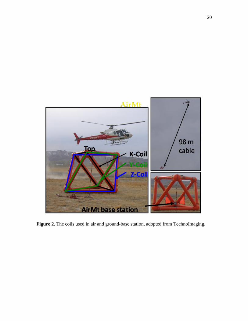
The AirMt method has been developed by Geotech LTD. Figure 1 and Figure 2
show the coil which is used in AirMt method. It is based on measuring all three orthogonal
components (Hx, Hy, and Hz) by airborne platform. However, it is difficult to keep the
system frame fixed in the moving airborne platform. This difficulty is overcome by
calculating the transfer functions as the ratio of the magnetic field components in the
16
airborne station and the horizontal magnetic field components in the reference ground
station (Legault et al., 2012). The standard frequencies are between 30 and 720 Hz. The
AirMt transfer functions can be calculated using the same principles as the conventional
magnetovariational (MV) transforms (Berdichevskiĭ and Zhdanov, 1984).
Following Berdichevskii and Zhdanov (1984), the 3D magnetic field variations at
an airborne platform can be related to the components of the horizontal magnetic fields
measured at a base station by a three-row by two-column tensor T (Kuzmin et al., 2010):
H = TH0 , (2.32)
where H is the vector of the magnetic field measured at the receiver location, and H0 is the
vector of the magnetic field measured at the reference station. Expression (2.32) can be
written in matrix notation as follow:
[
Hx
Hy
Hz
] = [
Txx Txy
Tyx Tyy
Tzx Tzy
] [Hx
0
Hy0]. (2.33)
Similar to the tipper components (2.28), it is possible to express AirMT tensor
components using two modes of the incident field: TM and TE. This expression uses the
assumption that the reference field is measured far away from the anomalous region. The
conductivity distribution below the reference station does not change in the inversion
process and thus can be approximated by 1D distribution. It is known that in a 1D case, the
TM mode Hx0 component is zero, as is the TE mode Hy
0 component. This results in the
following expressions for the receiver field components:
Hx1 = TxxHx
0 + TxyHy0 = TxyHy
0
Hx2 = TxxHx
0 + TxyHy0 = TxxHx
0
17
Hy1 = TyxHx
0 + TyyHy0 = TyyHy
0
Hy2 = TyxHx
0 + TyyHy0 = TyxHx
0
Hz1 = TzxHx
0 + TzyHy0 = TzyHy
0
Hz2 = TzxHx
0 + TzyHy0 = TzxHx
0, (2.34)
where superscript 1 indicates the TM mode, and superscript 2 stands for the TE mode. Note
that, in a case of the conductivity distributions close to the 1D reference station’s
distribution, the AirMt tensor components take the following values:
Txy ≈ Tyx ≈ Tzx ≈ 0
Txx ≈ Tyy ≈ Tzz ≈ 1. (2.35)
Based on (2.34), the AirMt tensor takes the following form:
T = [T1 T2
] =
[ Hx
2
Hx0
Hx1
Hy0
Hy2
Hx0
Hy1
Hy0
Hz2
Hx0
Hz1
Hy0]
. (2.36)
The cross product of the AirMt vectors T1 and T2
can be written as follows:
K = T1 × T2
=1
Hx0Hy
0 [Hy2Hz
1 − Hy1Hz
2 Hx1Hz
2 − Hx2Hz
1 Hx2Hy
1 − Hx1Hy
2]. (2.37)
Finally, compact amplification parameter P is expressed as the function of K :
P = K ∙ Re(K ) |Re(K )| =K1Re(K1)+K2Re(K2)+K3Re(K3)
√Re(K1)2+Re(K2)2+Re(K3)2⁄ (2.38)
It can be shown (Kuzmin et al., 2010) that P is invariant under any rotation of the
airborne frame of reference or the base station frame of reference. This fact gives AirMt an
advantage from both measurement and interpretation standpoints. During the
measurements, an operator does not need to keep the aircraft and airborne receiver aligned

18
with the reference system. An interpretation specialist can use a coordinate system
independent of the measurement.
19
Figure 1. Coil used in the ZTEM method, (a) Helicopter flying a coil to measure the
vertical magnetic field. (b) Ground-based reference station. (c) Coil used to measure the
vertical fields (adopted from TechnoImaging, 2011)
20
Figure 2. The coils used in air and ground-base station, adopted from TechnoImaging.

21
CHAPTER 3
FORWARD MODELING OF ZTEM AND AIRMT DATA
In the final decade of the twentieth century and in the beginning of the twenty-first
century, methods for numerical and analytical modeling of the interaction of
electromagnetic fields with the earth structures were developed rapidly. This development
was driven by the availability of high-performance computers, including PC clusters, with
which such models could be constructed. This modeling capability made possible the
extraction of much more information from the field data than had been possible previously
when only heuristic interpretation was feasible. The modern capability of geoelectrical
methods is based on two technological developments: the ability to acquire great volumes
of data with high accuracy, and the possibility of extracting sophisticated models of
geoelectrical structures from these data using advanced numerical modeling and inversion
methods (Zhdanov, 2009).
There are several techniques available for electromagnetic forward modeling. The
finite-difference and integral equation methods are the most widely used. Other
methodologies include the finite-element and finite-volume methods. The integral equation
method is a powerful tool in three-dimensional (3D) electromagnetic modeling for
geophysical applications. It was introduced originally in the pioneering paper by Dmitriev
22
(1969), which was published in Russian and long remained unknown to Western
geophysicists (as well as the work of Tabarovsky, 1975). More than 40 years ago,
practically simultaneously, Raiche (1974), Weidelt (1975), and Hohmann (1975) published
their famous papers on the IE method. Many more researchers have contributed to the
improvement and development of this method in recent years (Abubakar and van den Berg,
2004; Avdeev, 2005; Dmitriev and Nesmeyanova, 1992; Singer and Fainberg, 1997;
Wannamaker, 1991; Xiong, 1992; Xiong and Kirsch, 1992; Zhdanov, 2002). The main
advantage of the IE method in comparison with the FD and FE methods is the fast and
accurate simulation of the EM response in models with relatively local 3D anomalies in a
layered background.
In this chapter, the principles of the IE method and how to forward model ZTEM
and AirMt data by using the IE method will be introduced.
3.1 Principles of EM forward modeling using the integral equation method
This section considers a 3D geoelectrical model with a normal (background)
complex conductivity σb and local inhomogeneity with an arbitrarily varying complex
conductivity σ = σb + ∆σ. Our study will be confined to consideration of nonmagnetic
media and, hence, it will be assumed that μ = μ0= 4π × 10−7 H m⁄ , where μ0 is the free-
space magnetic permeability. The model is excited by an electromagnetic field generated
by an arbitrary source with an extraneous current distribution jQ concentrated within some
local domain Q . This field is time harmonic as e−iωt. In order to derive the integral
equations for the electromagnetic field for this model, the normal (background) and
anomalous electromagnetic fields must be introduced.
D
23
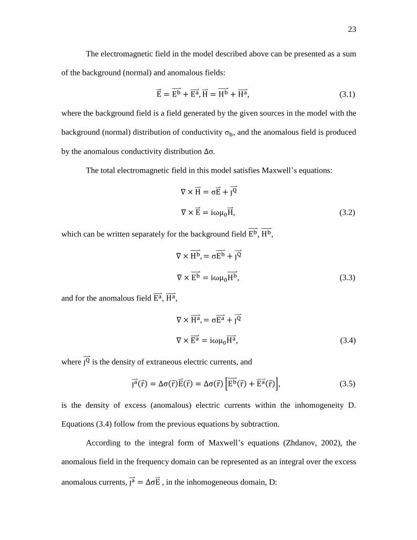
The electromagnetic field in the model described above can be presented as a sum
of the background (normal) and anomalous fields:
E = Eb + Ea , H = Hb + Ha , (3.1)
where the background field is a field generated by the given sources in the model with the
background (normal) distribution of conductivity σb, and the anomalous field is produced
by the anomalous conductivity distribution ∆σ.
The total electromagnetic field in this model satisfies Maxwell’s equations:
∇ × H = σE + jQ
∇ × E = iωμ0H , (3.2)
which can be written separately for the background field Eb , Hb ,
∇ × Hb , = σEb + jQ
∇ × Eb = iωμ0Hb , (3.3)
and for the anomalous field Ea , Ha ,
∇ × Ha , = σEa + jQ
∇ × Ea = iωμ0Ha , (3.4)
where jQ is the density of extraneous electric currents, and
ja (r ) = ∆σ(r )E (r ) = ∆σ(r ) [Eb (r ) + Ea (r )], (3.5)
is the density of excess (anomalous) electric currents within the inhomogeneity D.
Equations (3.4) follow from the previous equations by subtraction.
According to the integral form of Maxwell’s equations (Zhdanov, 2002), the
anomalous field in the frequency domain can be represented as an integral over the excess
anomalous currents, ja = ∆σE , in the inhomogeneous domain, D:
24
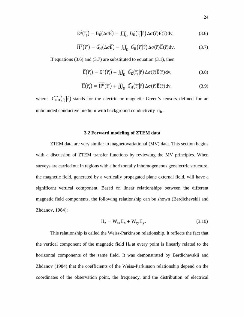
Ea (rj ) = GE(∆σE ) = ∭ GE(rj |r )D∆σ(r )E (r )dv, (3.6)
Ha (rj ) = GH(∆σE ) = ∭ GH(rj |r )D∆σ(r )E (r )dv. (3.7)
If equations (3.6) and (3.7) are substituted to equation (3.1), then
E (rj ) = Eb (rj ) + ∭ GE(rj |r )D∆σ(r )E (r )dv, (3.8)
H (rj ) = Hb (rj ) + ∭ GH(rj |r )D∆σ(r )E (r )dv, (3.9)
where GE,H(rj |r ) stands for the electric or magnetic Green’s tensors defined for an
unbounded conductive medium with background conductivity σb .
3.2 Forward modeling of ZTEM data
ZTEM data are very similar to magnetovariational (MV) data. This section begins
with a discussion of ZTEM transfer functions by reviewing the MV principles. When
surveys are carried out in regions with a horizontally inhomogeneous geoelectric structure,
the magnetic field, generated by a vertically propagated plane external field, will have a
significant vertical component. Based on linear relationships between the different
magnetic field components, the following relationship can be shown (Berdichevskii and
Zhdanov, 1984):
Hz = WzxHx + WzyHy. (3.10)
This relationship is called the Weiss-Parkinson relationship. It reflects the fact that
the vertical component of the magnetic field Hz at every point is linearly related to the
horizontal components of the same field. It was demonstrated by Berdichevskii and
Zhdanov (1984) that the coefficients of the Weiss-Parkinson relationship depend on the
coordinates of the observation point, the frequency, and the distribution of electrical
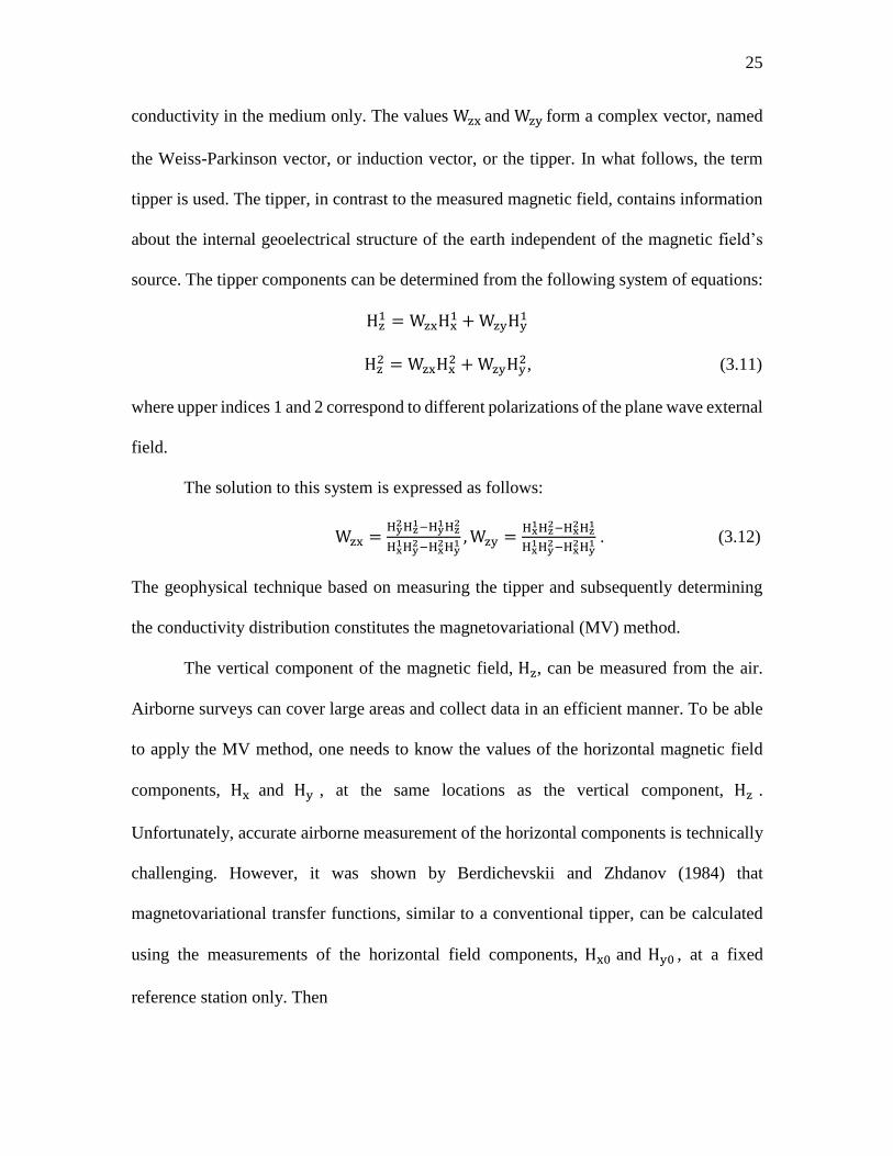
25
conductivity in the medium only. The values Wzx and Wzy form a complex vector, named
the Weiss-Parkinson vector, or induction vector, or the tipper. In what follows, the term
tipper is used. The tipper, in contrast to the measured magnetic field, contains information
about the internal geoelectrical structure of the earth independent of the magnetic field’s
source. The tipper components can be determined from the following system of equations:
Hz1 = WzxHx
1 + WzyHy1
Hz2 = WzxHx
2 + WzyHy2, (3.11)
where upper indices 1 and 2 correspond to different polarizations of the plane wave external
field.
The solution to this system is expressed as follows:
Wzx =Hy
2Hz1−Hy
1Hz2
Hx1Hy
2−Hx2Hy
1 ,Wzy =Hx
1Hz2−Hx
2Hz1
Hx1Hy
2−Hx2Hy
1 . (3.12)
The geophysical technique based on measuring the tipper and subsequently determining
the conductivity distribution constitutes the magnetovariational (MV) method.
The vertical component of the magnetic field, Hz, can be measured from the air.
Airborne surveys can cover large areas and collect data in an efficient manner. To be able
to apply the MV method, one needs to know the values of the horizontal magnetic field
components, Hx and Hy , at the same locations as the vertical component, Hz .
Unfortunately, accurate airborne measurement of the horizontal components is technically
challenging. However, it was shown by Berdichevskii and Zhdanov (1984) that
magnetovariational transfer functions, similar to a conventional tipper, can be calculated
using the measurements of the horizontal field components, Hx0 and Hy0 , at a fixed
reference station only. Then
26
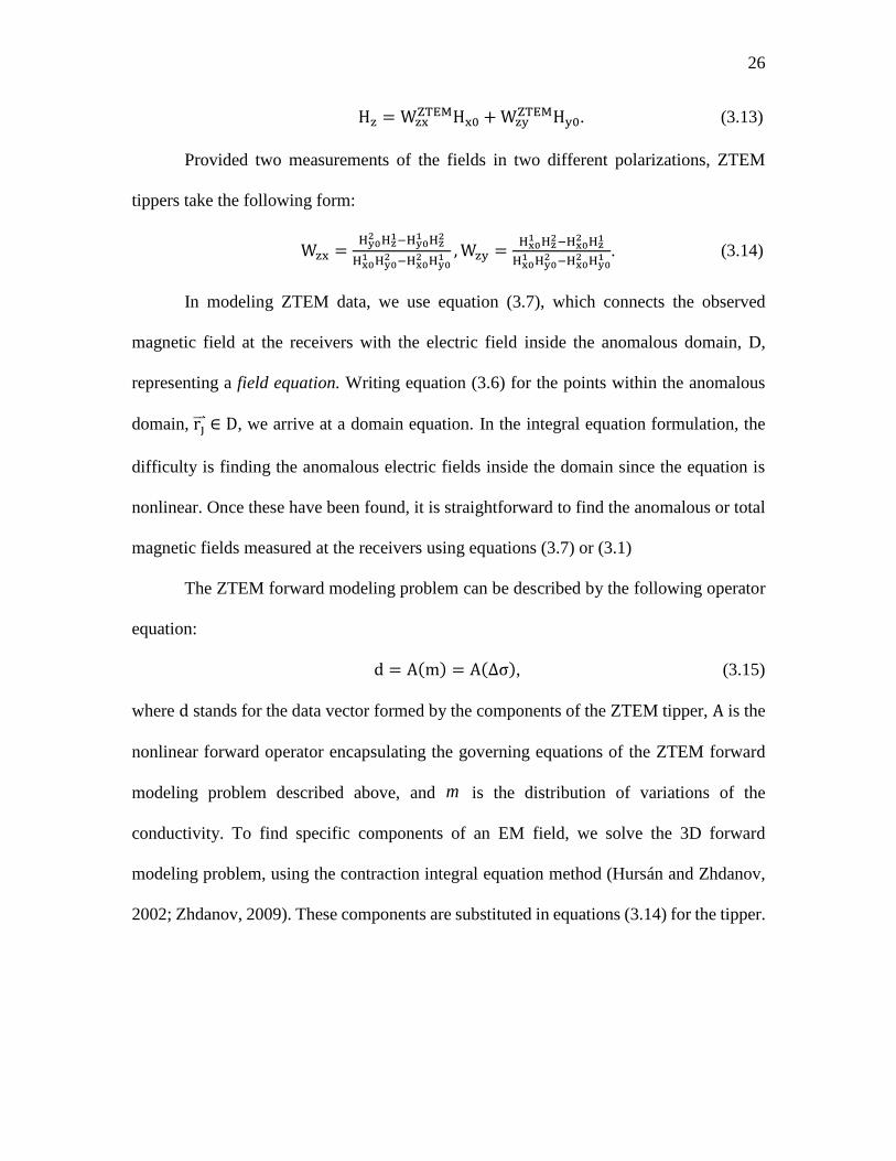
Hz = WzxZTEMHx0 + Wzy
ZTEMHy0. (3.13)
Provided two measurements of the fields in two different polarizations, ZTEM
tippers take the following form:
Wzx =Hy0
2 Hz1−Hy0
1 Hz2
Hx01 Hy0
2 −Hx02 Hy0
1 ,Wzy =Hx0
1 Hz2−Hx0
2 Hz1
Hx01 Hy0
2 −Hx02 Hy0
1 . (3.14)
In modeling ZTEM data, we use equation (3.7), which connects the observed
magnetic field at the receivers with the electric field inside the anomalous domain, D,
representing a field equation. Writing equation (3.6) for the points within the anomalous
domain, rj ∈ D, we arrive at a domain equation. In the integral equation formulation, the
difficulty is finding the anomalous electric fields inside the domain since the equation is
nonlinear. Once these have been found, it is straightforward to find the anomalous or total
magnetic fields measured at the receivers using equations (3.7) or (3.1)
The ZTEM forward modeling problem can be described by the following operator
equation:
d = A(m) = A(∆σ), (3.15)
where d stands for the data vector formed by the components of the ZTEM tipper, A is the
nonlinear forward operator encapsulating the governing equations of the ZTEM forward
modeling problem described above, and is the distribution of variations of the
conductivity. To find specific components of an EM field, we solve the 3D forward
modeling problem, using the contraction integral equation method (Hursán and Zhdanov,
2002; Zhdanov, 2009). These components are substituted in equations (3.14) for the tipper.
m
27
3.3 Forward modeling of AirMt data
In a general case, the 3D magnetic field variations at an airborne receiver platform
to the horizontal fields measured at a base station are related by a three-row by two-column
tensor T (Berdichevskiĭ and Zhdanov, 1984):
H = TH0 , (3.16)
which can be expressed in a matrix notation as follows:
[
Hx
Hy
Hz
] = [
Txx Txy
Tyx Tyy
Tzx Tzy
] [Hx
0
Hy0]. (3.17)
This results in the expressions (2.34), (2.35), and (2.36). According to the formula
(2.37), finally, compact amplification parameter P is expressed as the function of K :
P = K ∙ Re(K ) |Re(K )| =K1Re(K1)+K2Re(K2)+K3Re(K3)
√Re(K1)2+Re(K2)2+Re(K3)2⁄ . (3.18)
where K is determined by formula (2.37), substituting expression (3.6) and (3.7) into
formula (3.23), we calculate the compact amplification parameter, P , using IE method.
28
CHAPTER 4
INVERSION OF ZTEM AND AIRMT DATA
Electromagnetic (Berdichevskiĭ and Zhdanov) inverse methods are widely used in
the interpretation of geophysical EM data in mineral, hydrocarbon, and groundwater
exploration. During the last decade, we have observed remarkable progress in the
development of a multidimensional interpretation technique. Many papers have been
published during the last 20 years on 3D inversion of EM geophysical data (Alumbaugh
and Newman, 1997; Gribenko and Zhdanov, 2007; Mackie and Watts, 2004; Madden and
Mackie, 1989; Newman and Alumbaugh, 1997; Siripunvaraporn et al., 2005; Zhdanov and
Fang, 1996; Zhdanov et al., 2000; Zhdanov and Golubev, 2003; Zhdanov and Tartaras,
2002). However, EM inversion is still one of the most difficult problems of EM geophysics.
Nowadays there are several algorithms available for rigorous 3D MT inversion, such
as the Gauss-Newton method (Farquharson et al., 2002; Sasaki, 2004; Siripunvaraporn et
al., 2005), the quasi-Newton method (Avdeev and Avdeeva, 2006), and the nonlinear
conjugate gradient method (Gribenko et al., 2010; Newman and Alumbaugh, 2000;
Zhdanov and Golubev, 2003). In this chapter, the reweighted regularized conjugate
gradient (RRCG) method will be introduced to formulate the ZTEM and AirMt data
inversion problem. The regularized conjugate gradient method based on the adaptive
regularization and minimum-norm (MN) stabilizer is used to solve the minimization
29
problem of this parametric functional. The quasi-Born (QB) approximation and the receiver
footprint approach for computing and storing Frechet derivatives will also be discussed in
this chapter, and how to calculate the Frechet derivative for both ZTEM and AirMt data
will be presented as well.
4.1 Principles of regularized geophysical inversion
The ZTEM and AirMt forward modeling problem can be described by the following
operator equation:
dZTEM = AZTEM(∆σ), dAirMt = AAirMt(∆σ), (4.1)
where d stands for the data vector formed by the components of the ZTEM tipper and/or
AirMt amplification parameter, and A is the nonlinear forward operator encapsulating the
governing equations of the ZTEM and AirMt forward modeling problem described in the
previous sections.
The inverse problem described by equation (4.1) is ill posed, i.e., the solution is
nonunique and unstable. As per the MT and MV methods, Tikhonov regularization is used
to solve this problem which is based on minimization of the Tikhonov parametric
functional:
P(∆σ) = ‖A(∆σ) − d‖22 + α‖Wm(∆σ) − Wm∆σapr‖2
2 = min, (4.2)
where Wm is some real weighting matrix of model parameters, ∆σapr is some a priori
anomalous conductivity distribution, ‖…‖ denotes the Euclidean norm in the spaces of
data and models, and α is the regularization parameter. The model weights are frequency
dependent.
It was demonstrated in Zhdanov (2002) that the optimal choice of the model
30
parameter weighting matrix, Wm, is the square root of the integrated sensitivity matrix
according to the following formula:
A = √FTF, (4.3)
Wm = √diag(A), (4.4)
Wm = √diag(FTF)4
. (4.5)
where F is Frechet derivative.
Gradient-type methods are commonly used as an iterative way to solve the
minimization problem of the parametric functional, such as the steepest descent method,
the Newton method, the generalized minimum residual (GMRES) method, the minimum
residual (MINRES) method, etc. In this thesis, the reweighted regularized conjugate
gradient (RRCG) method is used to find the solution which minimizes the parametric
functional with the minimum-norm stabilizer. The RRCG algorithm can be summarized as
follows (Zhdanov, 2002):
rn = A(mn) − d
Inαn = Iαn(mn) = Fmn
T rn + αnWm2 (mn − mapr)
βnαn =
‖Inαn‖
2
‖In−1αn−1‖
2 , Inαn = In
αn + βnαn In−1
αn−1
knαn =
(InαnT
Inαn)
{‖FmnInαn‖
2+ α‖WmIn
αn‖2}
mn+1 = mn − knαn In
αn, (4.6)
where knαn
is the step length, Inαn
is the gradient direction computed using an adjoint
operator.
In a practical inversion, knαn is computed using the following modified formula:

31
knαn = kc ∙
(InαnT
Inαn)
{‖Fmn Inαn‖
2+α‖WmIn
αn‖2} , (4.7)
where kc is the step length coefficient. It is a constant which can be set manually. This
iterative process is terminated when the misfit reaches the given noise level ε0:
∅(mN) = ‖rN‖2 ≤ ε0 . (4.8)
To apply the adaptive regularization method, the regularization parameter α is
updated in the process of the iterative inversion as follows:
αn = α1qn−1, n = 1,2,3, … , 0 < 𝑞 < 1. (4.9)
4.2 Frechet derivative calculation and inversion of ZTEM data
As I demonstrated in Chapter 3, the tippers can be determined. The observed data
in the ZTEM method consists of the components of the Wi vector, so in the ZTEM method,
the Weiss-Parkinson relationship (3.12) is also used. It reflects the fact that the vertical
component of the magnetic field Hz at every point is linearly related to the horizontal
components of the same field:
Hz = WzxZTEMHx0 + Wzy
ZTEMHy0. (4.10)
which can be found accords to the formulas:
Wzx =Hy0
2 Hz1−Hy0
1 Hz2
Hx01 Hy0
2 −Hx02 Hy0
1 ,Wzy =Hx0
1 Hz2−Hx0
2 Hz1
Hx01 Hy0
2 −Hx02 Hy0
1 . (4.11)
In order to use the RRCG method for the minimization of the parametric functional
(4.2), it is necessary to calculate the derivative of the data parameters with respect to the
model parameters, i.e., the Fréchet derivatives, otherwise known as the Jacobians or
sensitivities. To calculate the Fréchet derivative of the ZTEM tippers with respect to the
anomalous conductivity, ∆σ , we apply a variational operator to equation (4.12). For the
32
WzxZTEM
component, the following is obtained:
δWzxZTEM = ∑ (
∂WzxZTEM
∂Hzi FHz
i [δ∆σ] + ∑∂Wzx
ZTEM
∂Hαiα=x0,y0 FHα
i [δ∆σ])i=1,2 . (4.12)
The expressions for the partial derivatives of the tippers with respect to the field
components, necessary for the computation of equation (4.13), take the following forms:
∂Wzx
ZTEM
∂Hx01 = −
Hy02 [Hy0
2 Hz1−Hy0
2 Hz1]
[Hx01 Hy0
2 −Hx02 Hy0
1 ]2 , (4.13)
∂Wzx
ZTEM
∂Hx02 =
Hy01 [Hy0
2 Hz1−Hy0
1 Hz2]
[Hx01 Hy0
2 −Hx02 Hy0
1 ]2 , (4.14)
∂Wzx
ZTEM
∂Hy01 =
Hy02 [Hx0
2 Hz1−Hx0
1 Hz2]
[Hx01 Hy0
2 −Hx02 Hy0
1 ]2 , (4.15)
∂Wzx
ZTEM
∂Hy02 =
Hy01 [Hx0
1 Hz1−Hx0
2 Hz1]
[Hx01 Hy0
2 −Hx02 Hy0
1 ]2 , (4.16)
∂Wzx
ZTEM
∂Hz1 =
Hy02
Hx01 Hy0
2 −Hx02 Hy0
1 , (4.17)
∂Wzx
ZTEM
∂Hz2 =
−Hy01
Hx01 Hy0
2 −Hx02 Hy0
1 . (4.18)
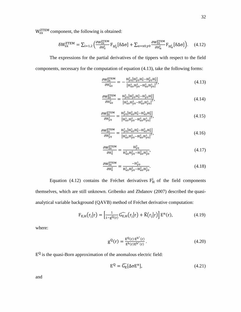
Equation (4.12) contains the Fréchet derivatives FHi of the field components
themselves, which are still unknown. Gribenko and Zhdanov (2007) described the quasi-
analytical variable background (QAVB) method of Fréchet derivative computation:
FE,H(rj|r) = [1
1−gQ(r)GE,H(rj|r) + K(rj|r)] E
n(r), (4.19)
where:
gQ(r) =EQ(r)∙Eb∗
(r)
Eb(r)Eb∗(r) . (4.20)
EQ is the quasi-Born approximation of the anomalous electric field:
EQ = GE[∆σEn], (4.21)
and
33
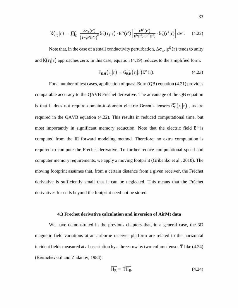
K(rj|r) = ∭∆σα(r′)
(1−gQ(r′))2DGE(rj|r) ∙ Eb(r′) [
Eb∗(r′)
Eb(r′)∙Eb∗(r′)∙ GE(r
′|r)] dv′. (4.22)
Note that, in the case of a small conductivity perturbation, ∆σα, gQ(r) tends to unity
and K(rj|r) approaches zero. In this case, equation (4.19) reduces to the simplified form:
FE,H(rj|r) = GE,H(rj|r)En(r). (4.23)
For a number of test cases, application of quasi-Born (QB) equation (4.21) provides
comparable accuracy to the QAVB Fréchet derivative. The advantage of the QB equation
is that it does not require domain-to-domain electric Green’s tensors GE(rj|r) , as are
required in the QAVB equation (4.22). This results in reduced computational time, but
most importantly in significant memory reduction. Note that the electric field En is
computed from the IE forward modeling method. Therefore, no extra computation is
required to compute the Fréchet derivative. To further reduce computational speed and
computer memory requirements, we apply a moving footprint (Gribenko et al., 2010). The
moving footprint assumes that, from a certain distance from a given receiver, the Fréchet
derivative is sufficiently small that it can be neglected. This means that the Fréchet
derivatives for cells beyond the footprint need not be stored.
4.3 Frechet derivative calculation and inversion of AirMt data
We have demonstrated in the previous chapters that, in a general case, the 3D
magnetic field variations at an airborne receiver platform are related to the horizontal
incident fields measured at a base station by a three-row by two-column tensor T like (4.24)
(Berdichevskiĭ and Zhdanov, 1984):
HR = THB
. (4.24)
34
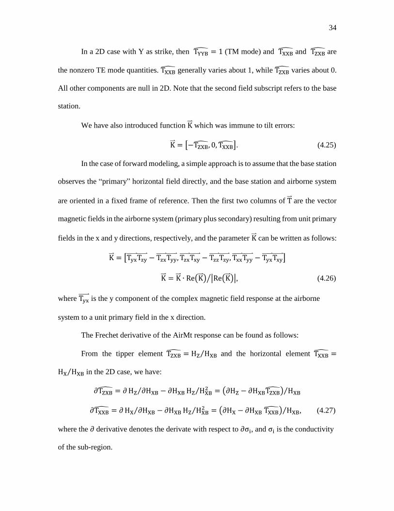
In a 2D case with Y as strike, then TYYB = 1 (TM mode) and TXXB and TZXB are
the nonzero TE mode quantities. TXXB generally varies about 1, while TZXB varies about 0.
All other components are null in 2D. Note that the second field subscript refers to the base
station.
We have also introduced function K which was immune to tilt errors:
K = [−TZXB, 0, TXXB]. (4.25)
In the case of forward modeling, a simple approach is to assume that the base station
observes the “primary” horizontal field directly, and the base station and airborne system
are oriented in a fixed frame of reference. Then the first two columns of T are the vector
magnetic fields in the airborne system (primary plus secondary) resulting from unit primary
fields in the x and y directions, respectively, and the parameter K can be written as follows:
K = [Tyx Tzy
− Tzx Tyy
, Tzx Txy
− Tzz Tzy
, Txx Tyy
− Tyx Txy
]
K = K ∙ Re(K ) |Re(K )|⁄ , (4.26)
where Tyx is the y component of the complex magnetic field response at the airborne
system to a unit primary field in the x direction.
The Frechet derivative of the AirMt response can be found as follows:
From the tipper element TZXB = HZ HXB⁄ and the horizontal element TXXB =
HX HXB⁄ in the 2D case, we have:
∂TZXB = ∂HZ ∂HXB⁄ − ∂HXB HZ HXB2⁄ = (∂HZ − ∂HXBTZXB) HXB⁄
∂TXXB = ∂HX ∂HXB⁄ − ∂HXB HZ HXB2⁄ = (∂HX − ∂HXB TXXB) HXB⁄ ,
(4.27)
where the ∂ derivative denotes the derivate with respect to ∂σi, and σi is the conductivity
of the sub-region.
35
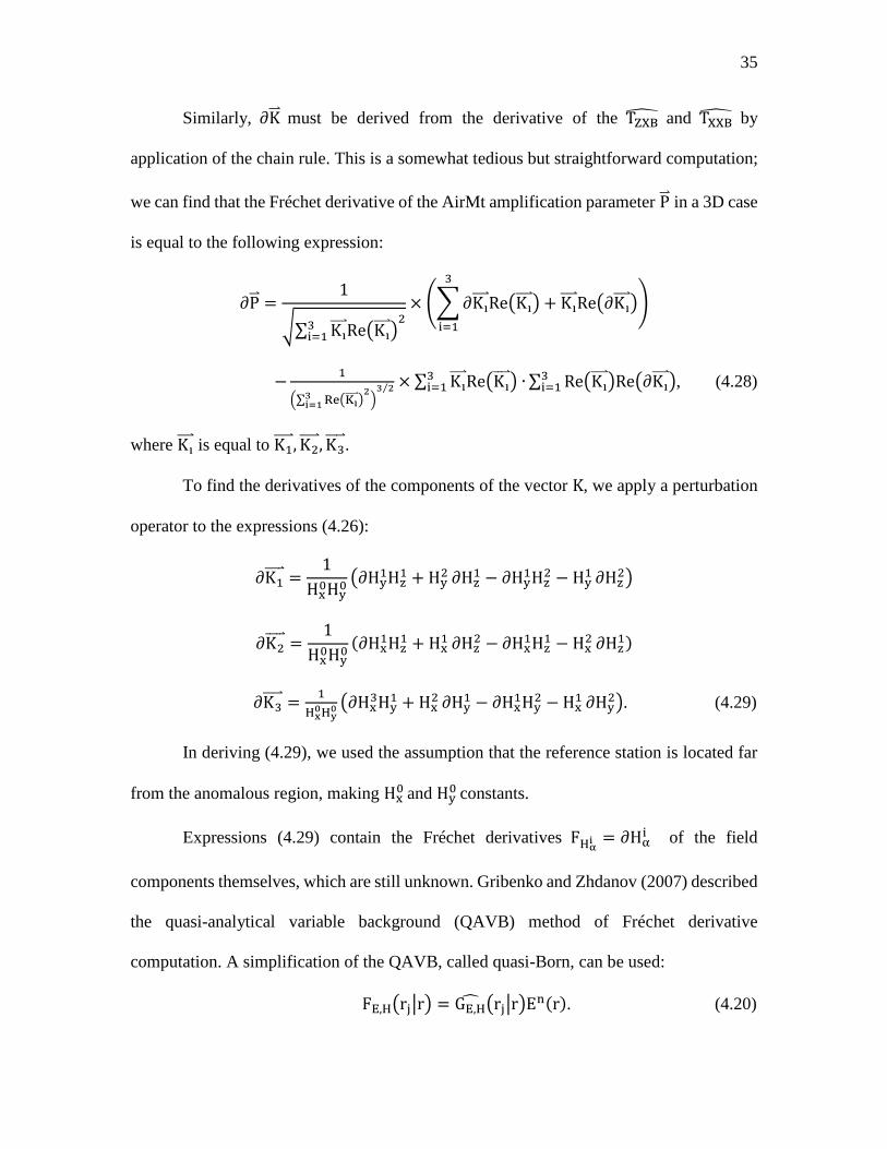
Similarly, ∂K must be derived from the derivative of the TZXB and TXXB by
application of the chain rule. This is a somewhat tedious but straightforward computation;
we can find that the Fréchet derivative of the AirMt amplification parameter P in a 3D case
is equal to the following expression:
∂P =1
√∑ Ki Re(Ki
)2
3i=1
× (∑∂Ki Re(Ki
) + Ki Re(∂Ki
)
3
i=1
)
−1
(∑ Re(Ki )23
i=1 )3 2⁄ × ∑ Ki
Re(Ki ) ∙3
i=1 ∑ Re(Ki )Re(∂Ki
)3i=1 ,
(4.28)
where Ki is equal to K1
, K2 , K3
.
To find the derivatives of the components of the vector K, we apply a perturbation
operator to the expressions (4.26):
∂K1 =
1
Hx0Hy
0(∂Hy
1Hz1 + Hy
2 ∂Hz1 − ∂Hy
1Hz2 − Hy
1 ∂Hz2)
∂K2 =
1
Hx0Hy
0(∂Hx
1Hz1 + Hx
1 ∂Hz2 − ∂Hx
1Hz1 − Hx
2 ∂Hz1)
∂K3 =
1
Hx0Hy
0 (∂Hx3Hy
1 + Hx2 ∂Hy
1 − ∂Hx1Hy
2 − Hx1 ∂Hy
2). (4.29)
In deriving (4.29), we used the assumption that the reference station is located far
from the anomalous region, making Hx0
and Hy0
constants.
Expressions (4.29) contain the Fréchet derivatives FHαi = ∂Hα
i
of the field
components themselves, which are still unknown. Gribenko and Zhdanov (2007) described
the quasi-analytical variable background (QAVB) method of Fréchet derivative
computation. A simplification of the QAVB, called quasi-Born, can be used:
FE,H(rj|r) = GE,H(rj|r)En(r). (4.20)
36
For the majority of test cases, application of the quasi-Born (QB) equation (4.30)
provides the same accuracy as the QAVB Fréchet derivative. The advantage of the QB
equation is that it does not require the domain-to-domain electric Green’s tensors
GE,H(rj|r) , which are required in the QAVB equation. This results in reduced
computational time, but most importantly in significant memory reduction. Note that the
electric field En is computed from the IE forward modeling method. Therefore, no extra
computation is required to compute the Fréchet derivative. To further reduce computational
speed and computer memory requirements, we apply a moving footprint approach (Cox et
al., 2011). The moving footprint assumes that, from a certain distance from a given
receiver, the Fréchet derivative is sufficiently small that it can be neglected. This means
that the Fréchet derivatives for cells beyond the footprint need not be stored.
37
CHAPTER 5
MODEL STUDY OF THE INVERSION ALGORITHM
The ZTEM and AirMt transfer functions and the inversion algorithm have been
discussed in the previous two chapters. In this chapter, the accuracy and stability of these
two inversion algorithms will be tested for several different synthetic models and compared
with the results based on two different sets of data. The basic test model is shown in Figure
3. The model consists of a 1 Ohm-m conductive L-shaped anomaly located inside a 100
Ohm-m host rock. Depth to the top of the anomaly is 600 m, and the thickness of the body
is 400 m. The receivers are located in a 5×5 km2 area, separated by 200 m for a total of 676
receiver positions with flight elevation 75 m above the surface. The reference receiver is
placed on the surface about 7 km away from the modeling domain (X = 7500 m, Y = 7500
m). Synthetic data were computed at the standard set of ZTEM and AirMt frequencies: 30,
45, 90, 180, and 360 Hz. The parameters used in the basic model are listed in Table 1.
5.1 Inversion with true background conductivity
First, I have applied the inversion to the noise-free synthetic data using the true
background conductivity, which was known.
The inversion domain was 6 × 6 × 3 km3, with inversion cell sizes 100 × 100 × 50
m3. The parameters used in the true model parameters inversion both in ZTEM and AirMt
38
data are shown in Table 2.
In the corresponding figures of inversion results, the white dashed line indicates the
true model location of the L-shaped conductive target. Figure 4 shows the result of
inversion of the synthetic ZTEM data. Both the location and conductivity of the L-shaped
anomaly are recovered well. Figures 5 and 6 present maps of the observed and predicted
ZTEM components, Wzx and Wzy. The result of inversion of the synthetic AirMt data is
shown in Figure 7. AirMt inversion also recovered the L-shaped anomaly reasonably well.
Maps of the observed and predicted AirMt amplification parameters are shown in Figure
8.
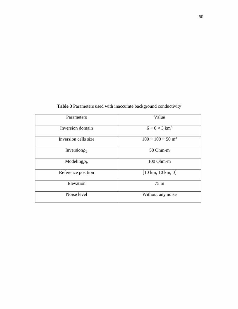
5.2 Inversion with inaccurate background conductivity
In real field application, we do not know the accurate background conductivity
beneath the earth. In order to simulate this situation, in this section, it is assumed that the
true background conductivity is unknown. The goal of this study is to test whether
inaccurate background conductivity will affect the results of inversion for both ZTEM and
AirMt data sets.
As noted above, both ZTEM and AirMt are not sensitive to variations of the 1D
background conductivity, and show no response in the case of the large, horizontal 1D
geoelectrical model. It is very difficult if not impossible to infer an accurate estimation of
the background conductivity from ZTEM or AirMt data. In the next set of experiments, it
is assumed that background resistivities differ in inversion from the true model in order to
study their effect on inversion results. First we assume a more conductive background of
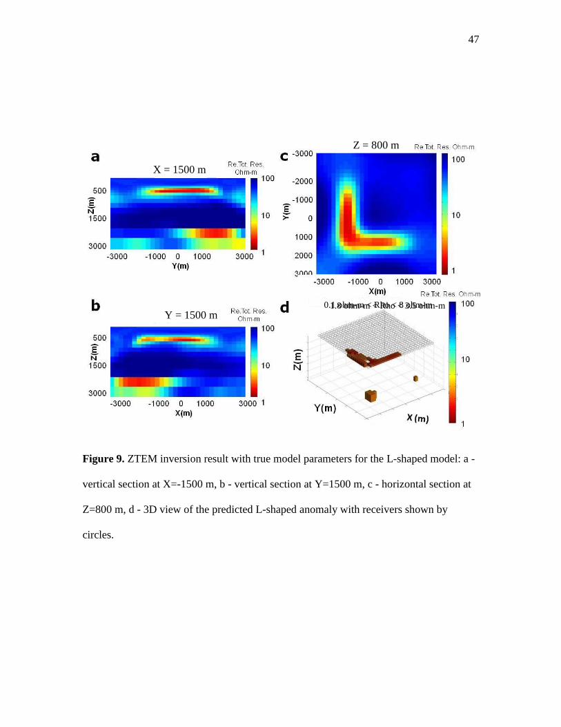
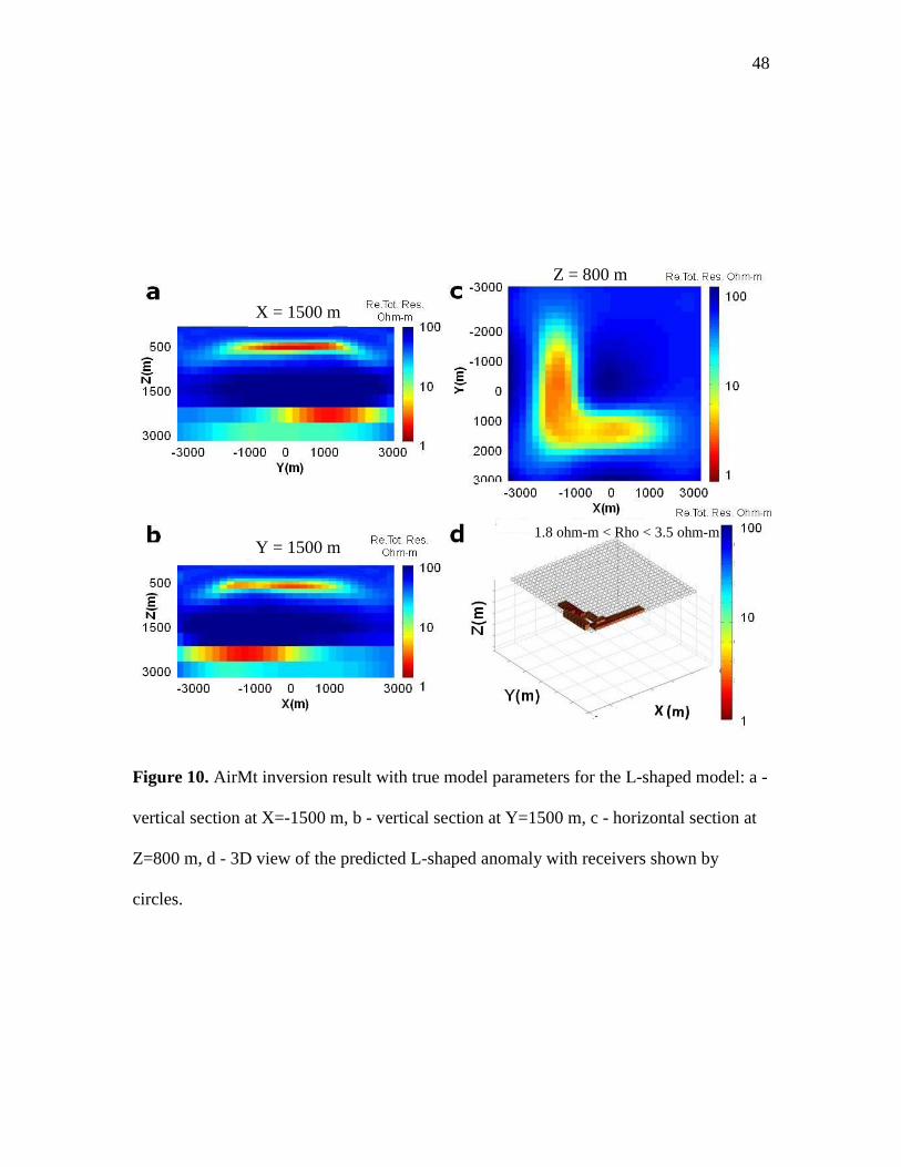
50 Ohm-m in the inversion compared to the true conductivity 100 Ohm-m. Figures 9 and
39
10 show the inversion results for the ZTEM and AirMt data, respectively. Both methods
recover the shape of the anomaly well, but its depth is underestimated. There is also an
apparent artifact at the bottom of the inversion domain not present in the true model. A
case (not shown here) was also considered in which the background resistivity in the
inversion was assumed higher than the one in the true model, which resulted in
overestimation of the depth of the anomaly.
In this situation, the parameters used in the inversion are shown in Table 3.
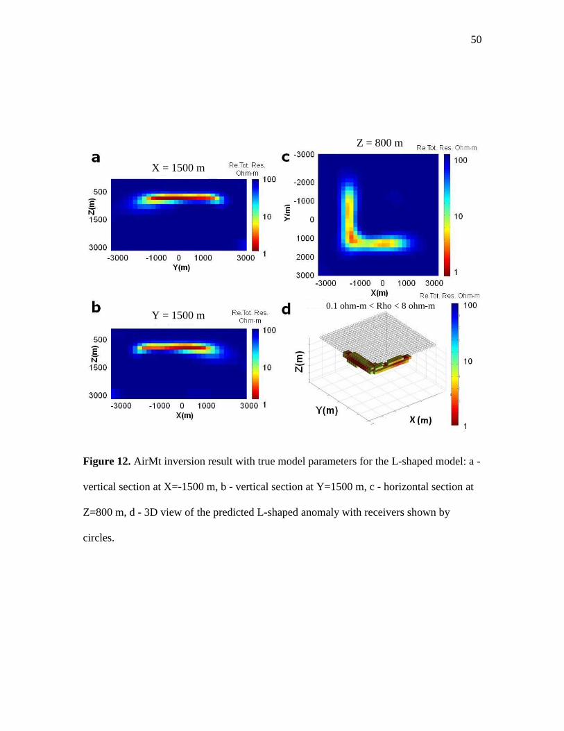
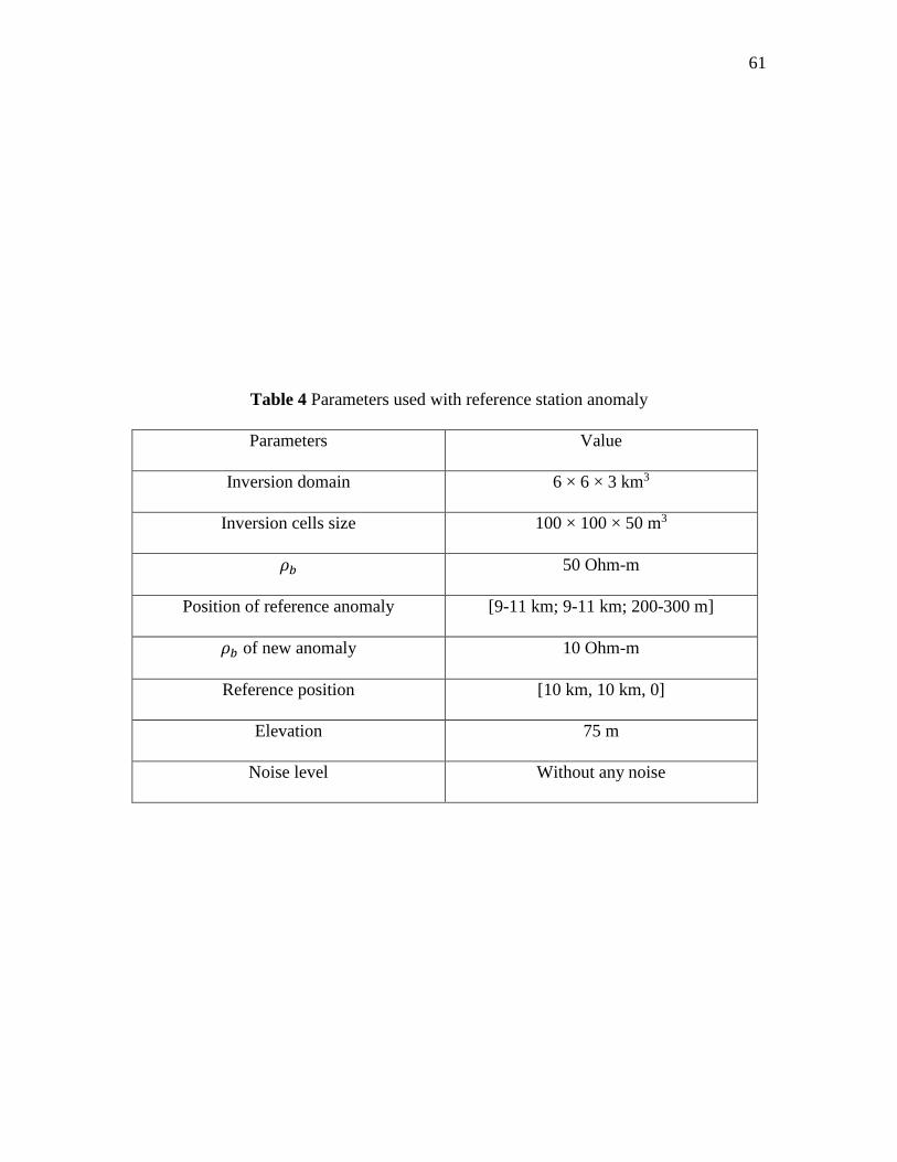
5.3 Inversion with reference station anomaly
In this section, it is assumed that there is another conductivity anomaly located
closes to the reference station. The purpose of this model study is to test whether a small
anomaly under the reference position will change the results of inversion for both the
ZTEM and AirMt data sets.
The inversion algorithm assumes the same 1D background model in both inversion
regions as well as under the reference receiver. In the next numerical experiments, the
synthetic ZTEM and AirMt data were computed assuming a 10 Ohm-m conductive
anomaly 2000 × 2000 × 100 m2 100 m deep under the reference receiver. The other
parameters of the model were kept constant. The data were inverted assuming no anomalies
under the reference station. The results of the ZTEM and AirMt inversions are shown in
Figures 11 and 12, respectively. Both inversion results recovered the L-shaped anomaly
well, which indicates that conductivity variations under the reference receiver did not
significantly affect the inversion results.
The parameters of the inversion are listed in Table 4.
40
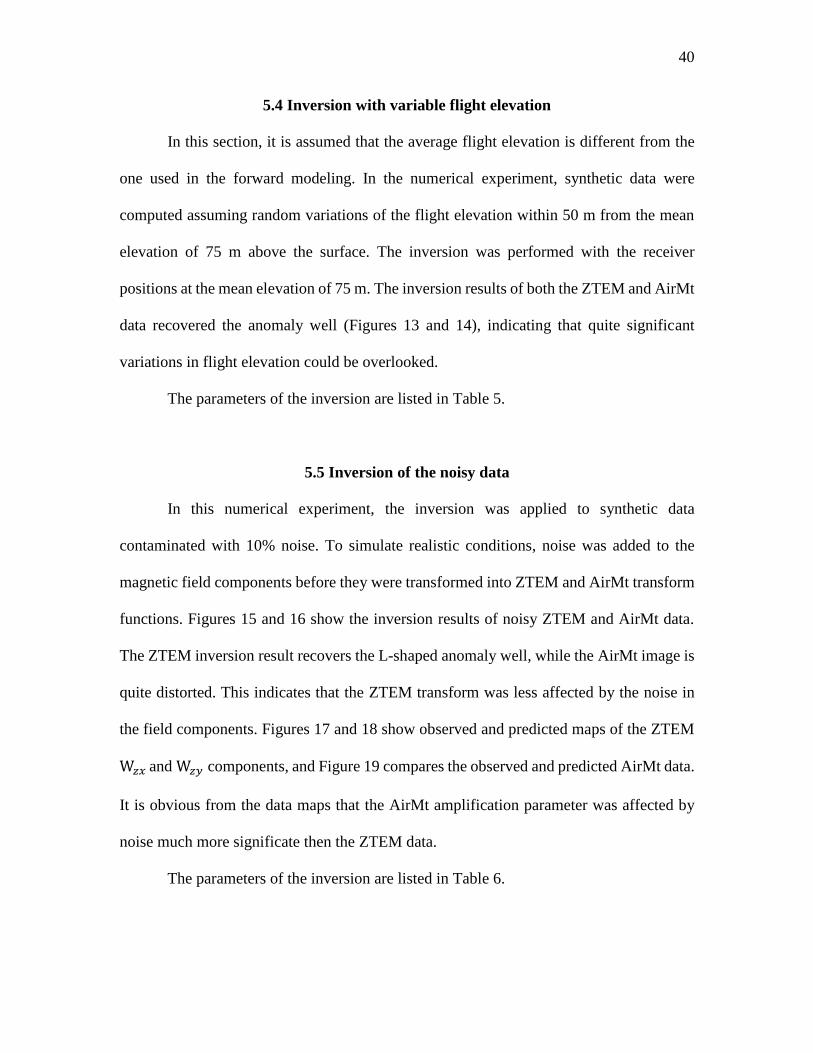
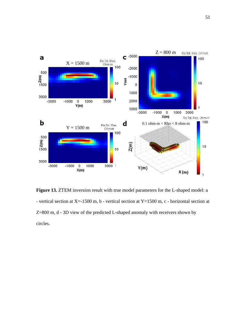
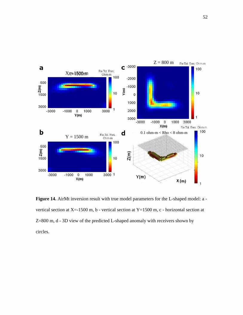
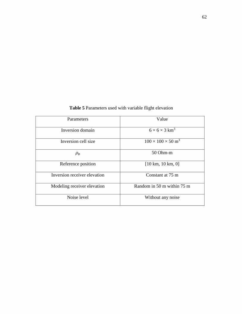
5.4 Inversion with variable flight elevation
In this section, it is assumed that the average flight elevation is different from the
one used in the forward modeling. In the numerical experiment, synthetic data were
computed assuming random variations of the flight elevation within 50 m from the mean
elevation of 75 m above the surface. The inversion was performed with the receiver
positions at the mean elevation of 75 m. The inversion results of both the ZTEM and AirMt
data recovered the anomaly well (Figures 13 and 14), indicating that quite significant
variations in flight elevation could be overlooked.
The parameters of the inversion are listed in Table 5.
5.5 Inversion of the noisy data
In this numerical experiment, the inversion was applied to synthetic data
contaminated with 10% noise. To simulate realistic conditions, noise was added to the
magnetic field components before they were transformed into ZTEM and AirMt transform
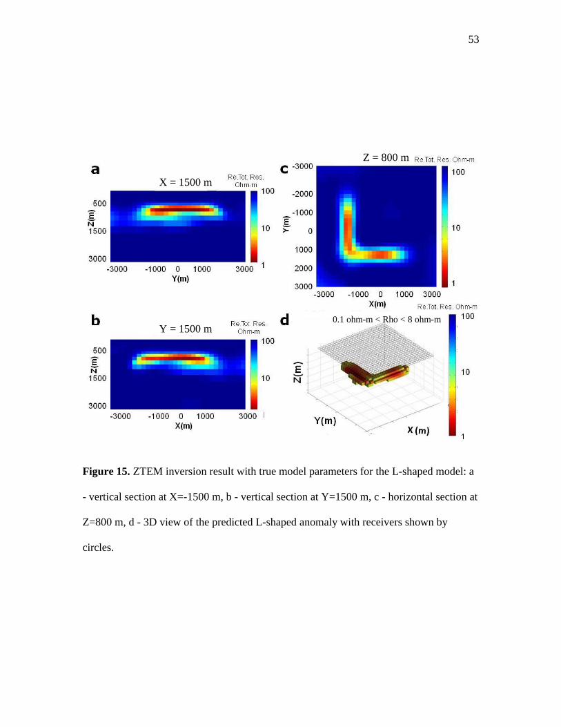
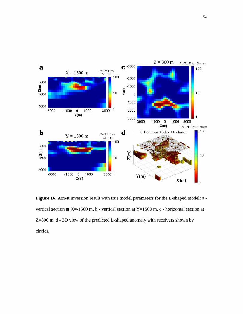
functions. Figures 15 and 16 show the inversion results of noisy ZTEM and AirMt data.
The ZTEM inversion result recovers the L-shaped anomaly well, while the AirMt image is
quite distorted. This indicates that the ZTEM transform was less affected by the noise in
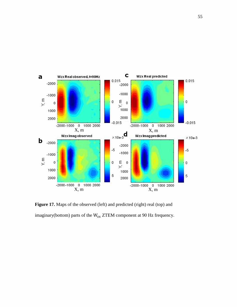
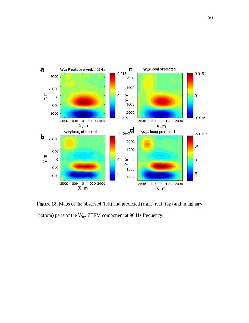
the field components. Figures 17 and 18 show observed and predicted maps of the ZTEM
W𝑧𝑥 and W𝑧𝑦 components, and Figure 19 compares the observed and predicted AirMt data.
It is obvious from the data maps that the AirMt amplification parameter was affected by
noise much more significate then the ZTEM data.
The parameters of the inversion are listed in Table 6.

41
Figure 3. Basic L-shaped model: a - vertical section at X=-1500 m, b - vertical section at
Y=1500 m, c - horizontal section at Z=800 m, d - 3D view of the L-shaped anomaly with
receivers shown by circles.
X = 1500 m
Y = 1500 m
0.1 ohm-m to 1000 ohm-m
Z = 800 m
42
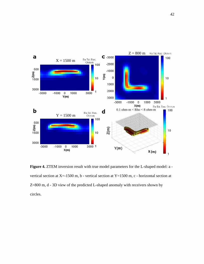
Figure 4. ZTEM inversion result with true model parameters for the L-shaped model: a -
vertical section at X=-1500 m, b - vertical section at Y=1500 m, c - horizontal section at
Z=800 m, d - 3D view of the predicted L-shaped anomaly with receivers shown by
circles.
X = 1500 m
Y = 1500 m
0.1 ohm-m < Rho < 8 ohm-m
Z = 800 m
43
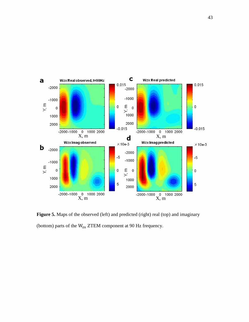
Figure 5. Maps of the observed (left) and predicted (right) real (top) and imaginary
(bottom) parts of the Wzx ZTEM component at 90 Hz frequency.
X, m
X, m
X, m
X, m
44
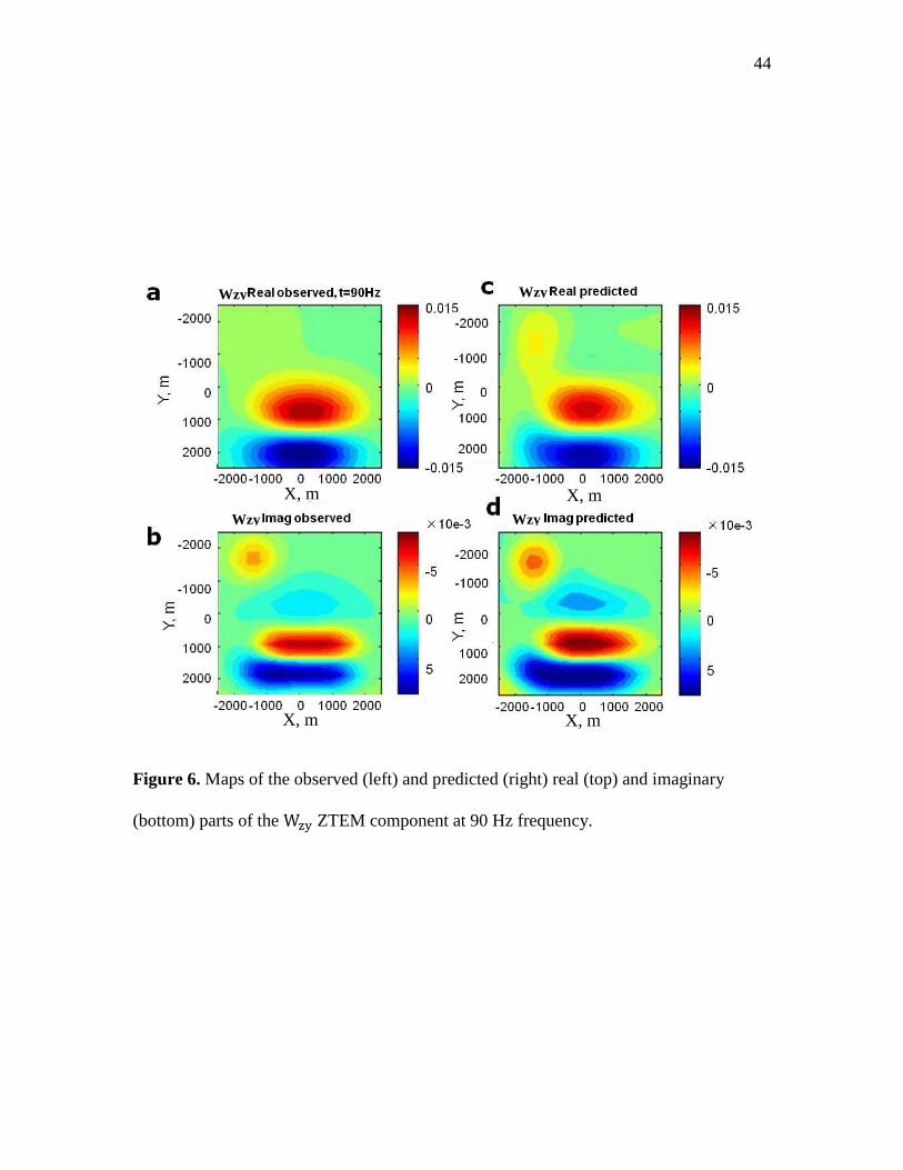
Figure 6. Maps of the observed (left) and predicted (right) real (top) and imaginary
(bottom) parts of the Wzy ZTEM component at 90 Hz frequency.
X, m
X, m
X, m
X, m
Wzy
Wzy
Wzy
Wzy
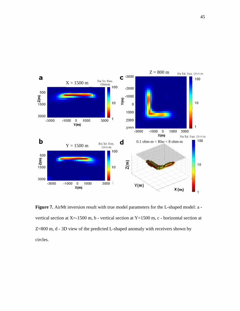
45
Figure 7. AirMt inversion result with true model parameters for the L-shaped model: a -
vertical section at X=-1500 m, b - vertical section at Y=1500 m, c - horizontal section at
Z=800 m, d - 3D view of the predicted L-shaped anomaly with receivers shown by
circles.
X = 1500 m
Y = 1500 m
Z = 800 m
0.1 ohm-m < Rho < 8 ohm-m
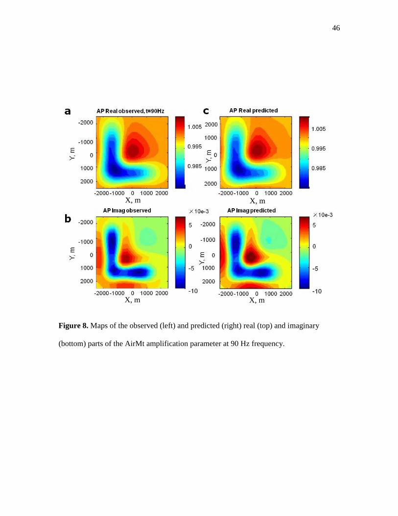
46
Figure 8. Maps of the observed (left) and predicted (right) real (top) and imaginary
(bottom) parts of the AirMt amplification parameter at 90 Hz frequency.
X, m
X, m
X, m
X, m
47
Figure 9. ZTEM inversion result with true model parameters for the L-shaped model: a -
vertical section at X=-1500 m, b - vertical section at Y=1500 m, c - horizontal section at
Z=800 m, d - 3D view of the predicted L-shaped anomaly with receivers shown by
circles.
X = 1500 m
Y = 1500 m 1.8 ohm-m < Rho < 3.5 ohm-m
Z = 800 m
0.1 ohm-m < Rho < 8 ohm-m
48
Figure 10. AirMt inversion result with true model parameters for the L-shaped model: a -
vertical section at X=-1500 m, b - vertical section at Y=1500 m, c - horizontal section at
Z=800 m, d - 3D view of the predicted L-shaped anomaly with receivers shown by
circles.
X = 1500 m
Y = 1500 m 1.8 ohm-m < Rho < 3.5 ohm-m
Z = 800 m
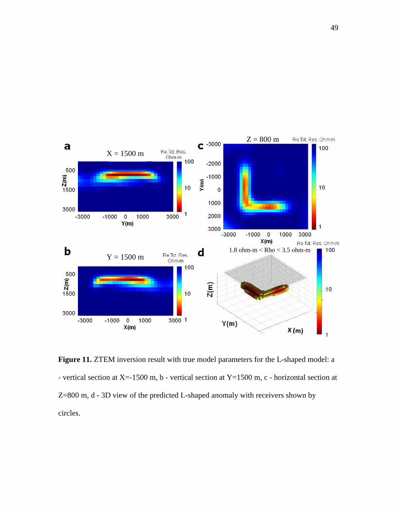
49
Figure 11. ZTEM inversion result with true model parameters for the L-shaped model: a
- vertical section at X=-1500 m, b - vertical section at Y=1500 m, c - horizontal section at
Z=800 m, d - 3D view of the predicted L-shaped anomaly with receivers shown by
circles.
X = 1500 m
Y = 1500 m 1.8 ohm-m < Rho < 3.5 ohm-m
Z = 800 m
50
Figure 12. AirMt inversion result with true model parameters for the L-shaped model: a -
vertical section at X=-1500 m, b - vertical section at Y=1500 m, c - horizontal section at
Z=800 m, d - 3D view of the predicted L-shaped anomaly with receivers shown by
circles.
X = 1500 m
Y = 1500 m
Z = 800 m
0.1 ohm-m < Rho < 8 ohm-m
51
Figure 13. ZTEM inversion result with true model parameters for the L-shaped model: a
- vertical section at X=-1500 m, b - vertical section at Y=1500 m, c - horizontal section at
Z=800 m, d - 3D view of the predicted L-shaped anomaly with receivers shown by
circles.
X = 1500 m
Y = 1500 m
Z = 800 m
0.1 ohm-m < Rho < 8 ohm-m
52
Figure 14. AirMt inversion result with true model parameters for the L-shaped model: a -
vertical section at X=-1500 m, b - vertical section at Y=1500 m, c - horizontal section at
Z=800 m, d - 3D view of the predicted L-shaped anomaly with receivers shown by
circles.
X = 1500 m
Y = 1500 m
Z = 800 m
0.1 ohm-m < Rho < 8 ohm-m
53
Figure 15. ZTEM inversion result with true model parameters for the L-shaped model: a
- vertical section at X=-1500 m, b - vertical section at Y=1500 m, c - horizontal section at
Z=800 m, d - 3D view of the predicted L-shaped anomaly with receivers shown by
circles.
X = 1500 m
Y = 1500 m
Z = 800 m
0.1 ohm-m < Rho < 8 ohm-m
54
Figure 16. AirMt inversion result with true model parameters for the L-shaped model: a -
vertical section at X=-1500 m, b - vertical section at Y=1500 m, c - horizontal section at
Z=800 m, d - 3D view of the predicted L-shaped anomaly with receivers shown by
circles.
X = 1500 m
Y = 1500 m
Z = 800 m
0.1 ohm-m < Rho < 6 ohm-m
55
Figure 17. Maps of the observed (left) and predicted (right) real (top) and
imaginary(bottom) parts of the Wzx ZTEM component at 90 Hz frequency.
X, m
X, m
X, m
X, m
56
Figure 18. Maps of the observed (left) and predicted (right) real (top) and imaginary
(bottom) parts of the Wzy ZTEM component at 90 Hz frequency.
Wzy
Wzy
Wzy
Wzy
X, m
X, m
X, m
X, m
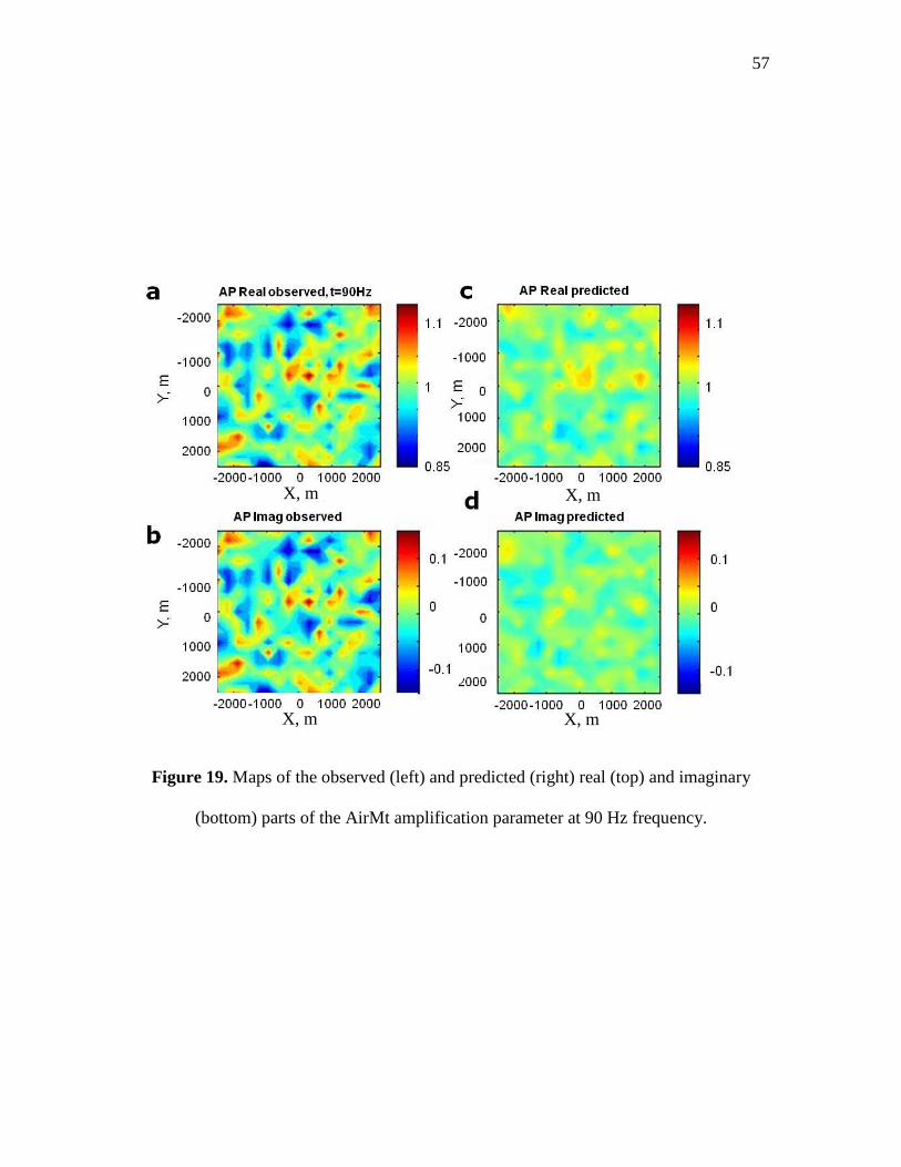
57
Figure 19. Maps of the observed (left) and predicted (right) real (top) and imaginary
(bottom) parts of the AirMt amplification parameter at 90 Hz frequency.
X, m
X, m
X, m
X, m

58
Table 1 Parameters used in the basic model
Parameters Value
𝜌𝑏 100 Ohm-m
𝜌𝑎 1 Ohm-m
Number of receivers 676
Elevation 75m
Frequency [30, 45, 90, 180, 360] Hz

59
Table 2 Parameters used in the true model inversion parameters
Parameters Value
Inversion domain 6 × 6 × 3 km3
Inversion cells size 100 × 100 × 50 m3
𝜌𝑏 100 Ohm-m
Reference position [10 km, 10 km, 0]
Elevation 75 m
Noise level Without any noise
60
Table 3 Parameters used with inaccurate background conductivity
Parameters Value
Inversion domain 6 × 6 × 3 km3
Inversion cells size 100 × 100 × 50 m3
Inversion𝜌𝑏 50 Ohm-m
Modeling𝜌𝑏 100 Ohm-m
Reference position [10 km, 10 km, 0]
Elevation 75 m
Noise level Without any noise
61
Table 4 Parameters used with reference station anomaly
Parameters Value
Inversion domain 6 × 6 × 3 km3
Inversion cells size 100 × 100 × 50 m3
𝜌𝑏 50 Ohm-m
Position of reference anomaly [9-11 km; 9-11 km; 200-300 m]
𝜌𝑏 of new anomaly 10 Ohm-m
Reference position [10 km, 10 km, 0]
Elevation 75 m
Noise level Without any noise
62
Table 5 Parameters used with variable flight elevation
Parameters Value
Inversion domain 6 × 6 × 3 km3
Inversion cell size 100 × 100 × 50 m3
𝜌𝑏 50 Ohm-m
Reference position [10 km, 10 km, 0]
Inversion receiver elevation Constant at 75 m
Modeling receiver elevation Random in 50 m within 75 m
Noise level Without any noise

63
Table 6 Parameters used with variable flight elevation
Parameters Value
Inversion domain 6 × 6 × 3 km3
Inversion cells size 100 × 100 × 50 m3
𝜌𝑏 50 Ohm-m
Reference position [10 km, 10 km, 0]
Elevation Constant at 75 m
Noise level With 10% random noise in field
64
CHAPTER 6
CASE STUDY: COCHRANE ZTEM SURVEY
6.1 Description of the survey area
On June 4th, 2011, Geotech Ltd. carried out a helicopter-borne geophysical survey
over the Cochrane geophysical test site situated 20 kilometers southwest of Cochrane,
Ontario.
Principal geophysical sensors included a z-axis tipper electromagnetic (ZTEM)
system, and a caesium magnetometer. Ancillary equipment included a GPS navigation
system and a radar altimeter. A total of 117.5 line kilometers of geophysical data were
acquired during the survey.
The block is located approximately 20 kilometers southwest of Cochrane, Ontario,
as shown in Figure 20.
The geology of the site is typically Archaen, with various bands of mafic to felsic
metavolcanics and metasedimentary units (Figure 21). Topographically, the Cochrane
survey block exhibits minimal relief with elevations ranging from 275 to 301 meters above
mean sea level over an area of 22 square kilometers (Figure 22). There are some small
rivers and streams found throughout the block, as well as a number of small roads. Special
care is recommended in identifying any potential cultural features from other sources that
might be recorded in the data.
65
6.2 Practical ZTEM data
The crew was based out of Cochrane, Ontario, for the acquisition phase of the
survey. Survey flying was started and completed on June 4th, 2009.
The data quality control and quality assurance and preliminary data processing were
carried out during the acquisition phase of the project. Final reporting, data presentation,
and archiving were completed from the Aurora office of Geotech Ltd. in November, 2011.
During the survey, the helicopter was maintained at a mean height of 140 meters
above the ground with a nominal survey speed of 80 km/hour for the block survey. This
allowed for a nominal EM sensor terrain clearance of 70 meters and a magnetic sensor
clearance of 85 meters.
The on-board operator was responsible for monitoring the system integrity. He also
maintained a detailed flight log during the survey, tracking the times of the flights as well
as any unusual geophysical or topographic features.
On return of the aircrew to the base camp, the survey data were transferred from a
compact flash card (PCMCIA) to the data processing computer. Trained personnel then
uploaded the data via ftp to the Geotech office in Aurora for daily quality assurance and
quality control.
The survey was flown using a Eurocopter A-Star B2 helicopter, registration number
C-GSSS.
The airborne ZTEM receiver coil measured the vertical component (Z) of the EM
field. The receiver coil is a Geotech z-axis tipper (ZTEM) loop sensor which is isolated
from most vibrations by a patented suspension system and is encased in a fiberglass shell.
It was towed from the helicopter using an 85 meter long cable as shown in Figure 23. The

66
cable was also used to transmit the measured EM signals back to the data acquisition
system.
The coil has a 7.4 meter diameter with an orientation to the vertical dipole. The
digitizing rate of the receiver was 2000 Hz. Attitudinal positioning of the receiver coil was
enabled using 3 GPS antennas mounted on the coil. The output sampling rate was 0.4
seconds.
The Geotech ZTEM base station deployed in this survey consisted of three
orthogonal coils as shown in Figure 2. The field measured by these coils provided
horizontal X and Y components of the EM reference field, which was further used with the
airborne coil data to calculate the in-line and cross-line components of the Wzx and Wzy
fields. One side of each coil was 3.04 meters.
The base station for the survey was installed near the survey block away from any
cultural sources. The azimuth of the reference coil was N0o E (named as A) and for the
orthogonal component it was N90o E (named as B). Angles A and B were taken into account
together with azimuth of the survey lines to calculate the in-line and cross-line and
fields utilizing a proprietary software.
The ZTEM data were processed using proprietary software. Processing steps
consisted of the following preliminary and final processing steps:
a. Airborne EM, Mag, radar altimeter, and GPS data were first merged with EM
base station data into one file.
b. Merged data were viewed and examined for consistency in an incorporated
viewer.
c. In the next processing phase, the following factors were taken into account:
zxW
zyW
67
• The base station coils orientation with respect to the magnetic north,
• The local declination of the magnetic field,
• The suggested direction of the X-coordinate (north or line direction),
• The sensitivity coefficient that compensates for the difference in geometry
between the base station and the airborne coils,
• Rejection filters for the 60 Hz and helicopter-generated frequencies.
d. Six frequencies (30, 45, 90, 180, 360, and 720 Hz) were extracted from the
airborne EM time series coil response using windows of 0.4 seconds and from
the base station coils using windows of 1.0 seconds.
e. The real (in-phase) and imaginary (quadrature) parts of the tipper transfer
functions were derived from the in-line (X or Wzx) and cross-line (Y or Wzy)
components.
f. Such processed EM data were then merged with the GPS data and magnetic
base station data and exported into a Geo soft xyz file.
The next stage of the preliminary data processing was done in a Geosoft TM
environment, using the following prescribed steps:
a. Import the output xyz file from the AFMAG processing, as well as the base
Mag data, into one database.
b. Split lines according to the recorded line channel.
c. Perform GPS processing, flight path recovery (correcting, filtering, calculating
Bird GPS coordinates, and line splitting).
d. Perform radar altimeter processing, yielding the altitude values in meters.
e. Remove magnetic spike, and filter airborne and base station data. Calculate

68
the base station corrected mag.
f. Apply preliminary altitude corrections to EM data (in phase and quadrature),
filter and make preliminary grids and profiles of all channels.
Final data processing and quality control were undertaken by Geotech Ltd.
headquarterd in Aurora, Ontario, by qualified senior data processing personnel.
A quality control step consisted of re-examining all data in order to validate the
preliminary data processing and to allow for final adjustments to the data.
Altitude corrections were re-evaluated and re-applied, on component-by-
component, flight-by-flight, and frequency-by-frequency bases. Any remaining line-to-line
system noise was removed by applying a mild additional level correction.
6.3 Inversion results
The geophysical surveys consisted of helicopter-borne AFMAG z-axis tipper
electromagnetic (ZTEM) and aeromagnetic systems using a caesium magnetometer. A total
of 117.5 line kilometers of geophysical data were acquired during the survey.
In a ZTEM survey, a single vertical-dipole air-core receiver coil is flown over the
survey area in a grid pattern, similar to regional airborne EM surveys. Three orthogonal-
axis, air-core coils are placed close to the survey site to measure the horizontal EM
reference fields. Data from the three coils are used to obtain the Wzx and Wzy tipper
components at six frequencies in the 30 to 720 Hz band. The ZTEM was useful in mapping
geology using resistivity contrasts, and magnetometer data provided additional information
on geology using magnetic susceptibility contrasts.
For data collecting, the airborne method has 561 receivers totally, and the range is
69
1.29e4*7.72e3 m2 in horizontal direction. The helicopter is around 78 m above the earth
surface, and receiver is located around 76 m above the earth surface.
Before the inversion, the proper inversion parameter setting is necessary. For the
inversion domain, it has 9000*3000 m2 in the horizontal direction and around 2300m depth
in the vertical direction, they have 100*100 m and increasing in log space with depth: log
space (1,2.5,24), respectively. ZTEM uses 6 frequencies from 30 to 720 Hz to satisfy the
sounding depth.
A significant response with respect to the felsic to intermediate metavolanic rocks
responses can be observed in the ZTEM data (Figure 24). It was noted that the 3D inversion
was able to fit the subtle trends on the observed ZTEM data. Figure 25 presents a horizontal
cross section of the 3D resistivity at -300 m above sea level. As shown in Figure 24 and
26, the conductive features are associated with the felsic to intermediate metavolanic rocks.
The actual source of this conductivity is unknown. Our future work will involve inversion
of the AirMt and ZTEM data, and quantitative comparison with the ZTEM results obtained
thus far.
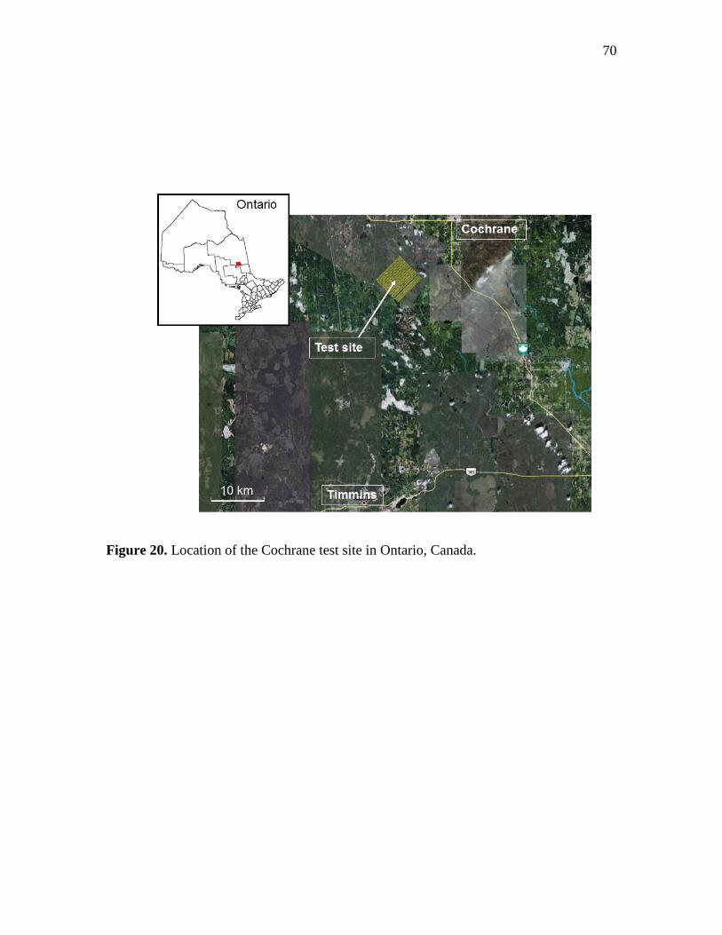
70
Figure 20. Location of the Cochrane test site in Ontario, Canada.

71
Figure 21. Geology of the Cochrane test site.
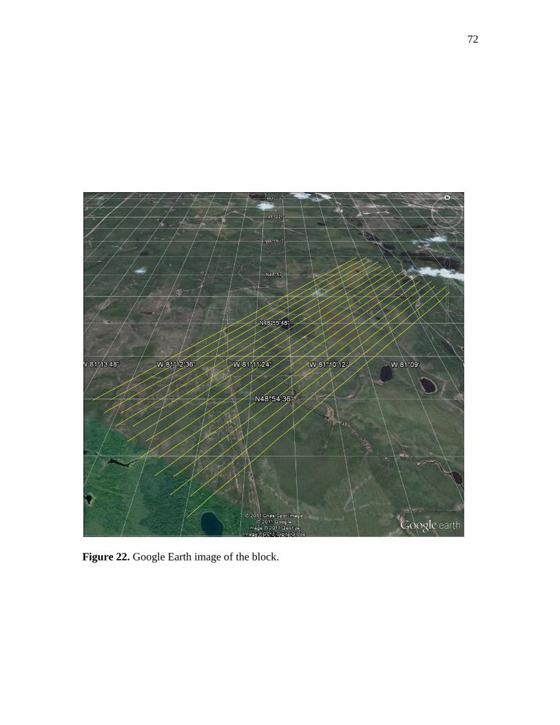
72
Figure 22. Google Earth image of the block.
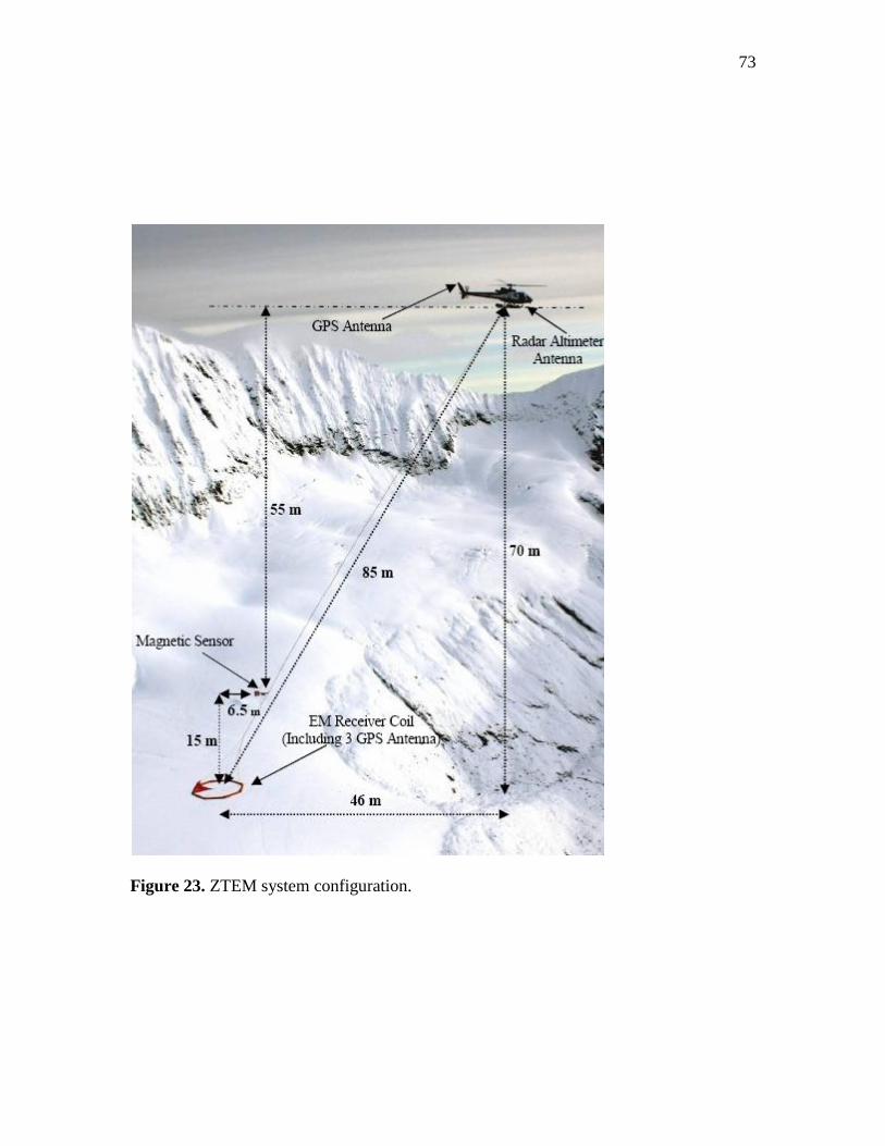
73
Figure 23. ZTEM system configuration.
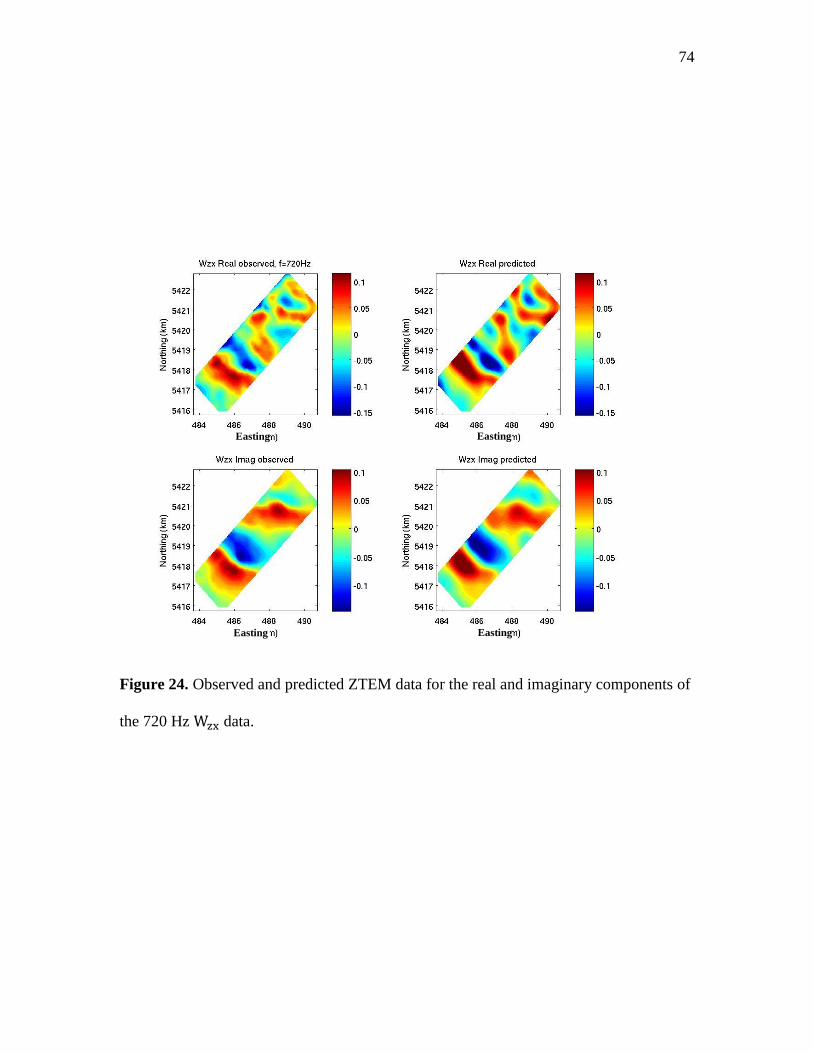
74
Figure 24. Observed and predicted ZTEM data for the real and imaginary components of
the 720 Hz Wzx data.
Easting
Easting
Easting
Easting
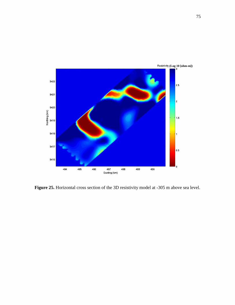
75
Figure 25. Horizontal cross section of the 3D resistivity model at -305 m above sea level.
(Log 10 [ohm-m])
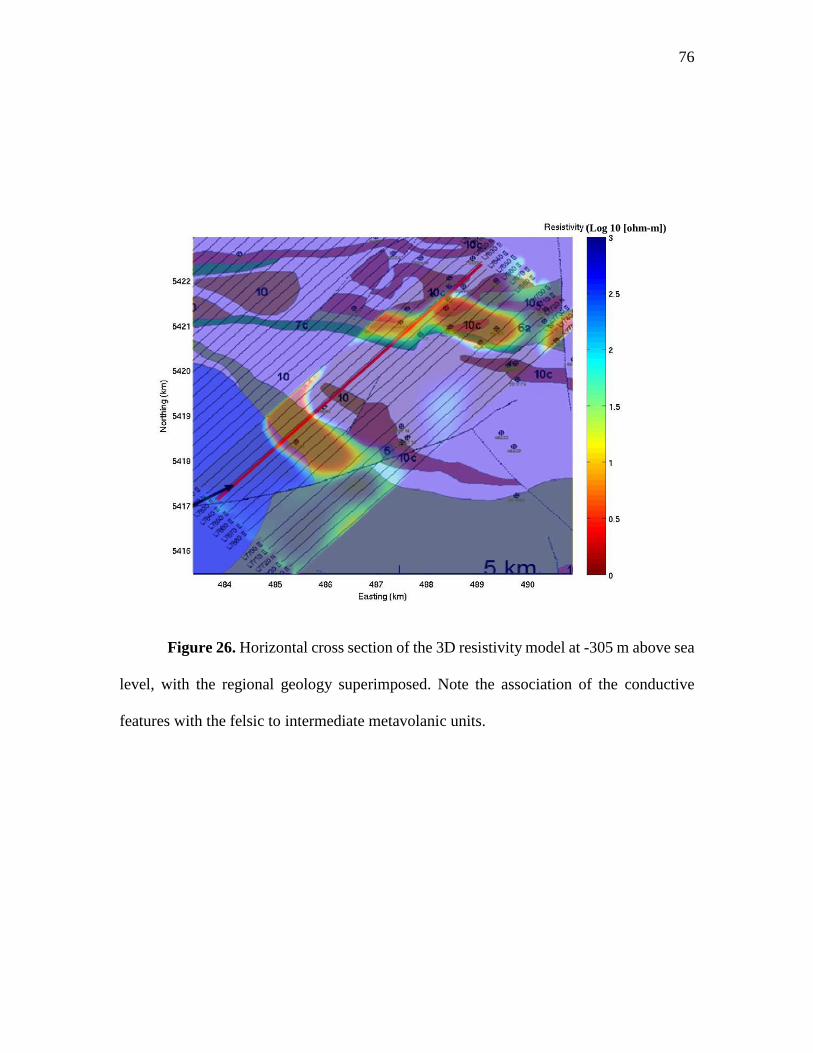
76
Figure 26. Horizontal cross section of the 3D resistivity model at -305 m above sea
level, with the regional geology superimposed. Note the association of the conductive
features with the felsic to intermediate metavolanic units.
(Log 10 [ohm-m])
77
CHAPTER 7
CONCLUSIONS
It has long been recognized that tipper data (the ratio of the local vertical magnetic
field to the horizontal magnetic field) provide information about 3D electrical conductivity.
However, the practical application of the tipper for airborne surveys was originated with
developing the ZTEM scheme only. In ZTEM, the vertical component of the magnetic field
is recorded above the entire survey area, while the horizontal fields are recorded at a
ground-based reference station. The interpretation and 3D inversion of ZTEM data is still
a challenge of airborne geophysics.
In this thesis, a 3D inversion algorithm using both tipper and compact amplification
parameter data were introduced and applied. It is based on the nonlinear conjugate gradient
algorithm and the contraction integral equation methods. To improve efficiency and reduce
memory requirement, the inversion algorithm was parallelized and a receiver footprint
approach was applied.
This inversion technique was first tested using synthetic data. Conductive
anomalies in a half-space background were analyzed. It is shown that the inversion
algorithm was able to give the accurate location and shape of the conductive anomaly. By
using both the tippers and the compact amplification parameter data in the inversion, the
boundaries between the anomaly and the background were well delineated. The regularized
78
inversions using a minimum-norm stabilizer for the tipper and compact amplification
parameter data was also tested for different synthetic models. The inversion results yielded
a predicted model with accurate conductivity contrast and a compact model shape.
The numerical model study conducted in this thesis made it possible to draw the
following conclusion. Inaccurate assumptions about the background conductivity in
inversion may lead to an erroneous estimation of the depths of the recovered conductivity
structures. At the same time, the ZTEM data were quite stable to a significant noise level,
while the AirMt data were more easily distorted, which could result in deterioration of the
inverse model.
This developed 3D joint inversion algorithm was implemented for analysis of the
field data in the Cochrane test site in Ontario, Canada. The inversion contained a large
number of cells due to the large inversion domain and relatively fine grid. The
parallelization of the code and the receiver footprint approach effectively sped up the
inversion process and reduced the memory requirement. Benefitting from the application
of the proper model weighting, the ZTEM inversion recovered conductive features, which,
compared to those shown on a local geology map, were associated with felsic to
intermediate metavolanic units.
79
REFERENCES
Abubakar, A., and P. M van den Berg, 2004, Iterative forward and inverse algorithms based
on domain integral equations for three-dimensional electric and magnetic objects:
Journal of Computational Physics, v. 195, no. 1, p. 236-262.
Alumbaugh, D., and G. Newman, 1997, Three-dimensional massively parallel
electromagnetic inversion—II. Analysis of a crosswell electromagnetic
experiment: Geophysical Journal International, v. 128, no. 2, p. 355-363.
Avdeev, D. B., 2005, Three-dimensional electromagnetic modelling and inversion from
theory to application: Surveys in Geophysics, v. 26, no. 6, p. 767-799.
Avdeev, D. B., and A. D. Avdeeva, 2006, A rigorous three-dimensional magnetotelluric
inversion: Progress in Electromagnetics Research, v. 62, p. 41-48.
Berdichevskii, M. M. N., and V. I. Dmitriev, 2008, Models and methods of
magnetotellurics, Springer.
Berdichevskiĭ, M. N., and M. S. Zhdanov, 1984, Advanced theory of deep geomagnetic
sounding: Elsevier Science Ltd., v. 19.
Cagniard, L., 1953, Basic theory of the magneto-telluric method of geophysical
prospecting: Geophysics, v. 18, no. 3, p. 605-635.
Campbell, W. H., 2003, Introduction to geomagnetic fields: Cambridge University Press.
Cox, L. H., G. A. Wilson, and M. S. Zhdanov, 2011, 3D inversion of airborne
electromagnetic data using a moving footprint: Exploration Geophysics, v. 41, no.
4, p. 250-259.
Dmitriev, V., 1969, Electromagnetic fields in inhomogeneous media: Moscow State
University.
Dmitriev, V., and N. Nesmeyanova, 1992, Integral equation method in three-dimensional
problems of low-frequency electrodynamics: Computational Mathematics and
Modeling, v. 3, no. 3, p. 313-317.
Farquharson, C. G., D. W. Oldenburg, E. G. Haber, and R. G. Shekhtman, 2002, An
`
80
algorithm for the three-dimensional inversion of magnetotelluric data: Proceedings,
SEG Annual Meeting.
Gribenko, A., A. M. Green, M. Cuma, and M. S. Zhdanov, 2010, Efficient 3D inversion of
MT data using integral equations method and the receiver footprint approach:
application to the large-scale inversion of the EarthScope MT data: Expanded
Abstracts of the SEG meeting: Denver, Colorado, p. 644-649.
Gribenko, A., and M. S. Zhdanov, 2007, Rigorous 3D inversion of marine CSEM data
based on the integral equation method: Geophysics, v. 72, no. 2, p. WA73-WA84.
Gribenko, A. V., M. S. Zhdanov, J. Legault, S. Zhao, L. H. Cox, G. A. Wilson, and K. Fisk,
2012, 3D inversion of AirMt AFMAG data: SEG Technical Program Expanded
Abstracts, Society of Exploration Geophysicists, p. 1-5.
Hohmann, G. W., 1975, Three-dimensional induced polarization and electromagnetic
modeling: Geophysics, v. 40, no. 2, p. 309-324.
Holtham, E., and D. W. Oldenburg, 2010, Three-dimensional inversion of ZTEM data:
Geophysical Journal International, v. 182, no. 1, p. 168-182.
Kuzmin, P. V., G. Borel, E. B. Morrison, and J. Dodds, 2010, Geophysical prospectin using
rotationally invariant parameters of natural electromagnetic fields, WO Patent
2,010,071,991.
Labson, V. F., A. Becker, H. Morrison, and U. Conti, 1985, Geophysical exploration with
audiofrequency natural magnetic fields: Geophysics, v. 50, no. 4, p. 656-664.
Legault, J., G. A. Wilson, A. V. Gribenko, M. S. Zhdanov, S. Zhao, and K. Fisk, 2012, An
overview of the ZTEM and AirMt airborne electromagnetic systems: a case study
from the Nebo–Babel Ni–Cu–PGE deposit, West Musgrave, Western Australia:
Preview, v. 2012, no. 158, p. 26-32.
Lo, B., and M. Zang, 2008, Numerical modeling of Z-TEM (airborne AFMAG) responses
to guide exploration strategies: Proceedings, SEG Annual Meeting.
Mackie, R., and M. Watts, 2004, The use of 3D magnetotelluric inversion for exploration
in complex geologic environments: Potential pitfalls and real world examples:
Proceedings, AGU Fall Meeting Abstracts, Volume 1, p. 01.
Madden, T., and R. L. Mackie, 1989, Three-dimensional magnetotelluric modelling and
inversion: Proceedings of the IEEE, v. 77, no. 2, p. 318-333.
Maris, V., and P. E. Wannamaker, 2010, Parallelizing a 3D finite difference MT inversion
algorithm on a multicore PC using OpenMP: Computers & Geosciences, v. 36, no.
10, p. 1384-1387.
`
81
Newman, G., and D. Alumbaugh, 1997, Three‐dimensional massively parallel
electromagnetic inversion—I. Theory: Geophysical Journal International, v. 128,
no. 2, p. 345-354.
Newman, G. A., and D. L. Alumbaugh, 2000, Three‐dimensional magnetotelluric
inversion using non‐linear conjugate gradients: Geophysical Journal International,
v. 140, no. 2, p. 410-424.
Parkinson, W., 1959, Directions of rapid geomagnetic fluctuations: Geophysical Journal
International, v. 2, no. 1, p. 1-14.
Parkinson, W., 1962, The influence of continents and oceans on geomagnetic variations:
Geophysical Journal of the Royal Astronomical Society, v. 6, no. 4, p. 441-449.
Raiche, A., 1974, An integral equation approach to three-dimensional modelling:
Geophysical Journal International, v. 36, no. 2, p. 363-376.
Sasaki, Y., 2004, Three-dimensional inversion of static-shifted magnetotelluric data: Earth,
planets and space, v. 56, no. 2, p. 239-248.
Singer, B. S., and E. Fainberg, 1997, Fast and stable method for 3-D modelling of
electromagnetic field: Exploration Geophysics, v. 28, no. 2, p. 130-135.
Siripunvaraporn, W., G. Egbert, Y. Lenbury, and M. Uyeshima, 2005, Three-dimensional
magnetotelluric inversion: data-space method: Physics of the Earth and Planetary
Interiors, v. 150, no. 1, p. 3-14.
Stanley, S. M., 2005, Earth system history: Macmillan.
Tabarovsky, L., 1975, The method of integral equations: geoelectric applications [in
Russian, Nauka, Novosibirsk, 140 pp.]
Tikhonov, A., 1950, On determining electrical characteristics of the deep layers of the
earth’s crust: Proceedings Sov. Math. Dokl, v. 2, p. 295-297.
Wannamaker, P. E., 1991, Advances in three-dimensional magnetotelluric modeling using
integral equations: Geophysics, v. 56, no. 11, p. 1716-1728.
Wannamaker, P. E., G. W. Hohmann, and S. H. Ward, 1984, Magnetotelluric responses of
three-dimensional bodies in layered earths: Geophysics, v. 49, no. 9, p. 1517-1533.
Ward, S. H., 1959, AFMAG-airborne and ground: Geophysics, v. 24, no. 4, p. 761-787.
Weidelt, P., 1975, Electromagnetic induction in three-dimensional structures: Jouranl of
Geophysics, v. 41, no. 85, p. 109.
`
82
Xiong, Z., 1992, Electromagnetic modeling of 3-D structures by the method of system
iteration using integral equations: Geophysics, v. 57, no. 12, p. 1556-1561.
Xiong, Z., and A. Kirsch, 1992, Three-dimensional earth conductivity inversion: Journal
of computational and applied mathematics, v. 42, no. 1, p. 109-121.
Zhdanov, M., 2002, Geophysical inverse theory and regularization problems: Methods in
geochemistry and geophysics: Elsevier Amsterdam.
Zhdanov, M. S., 2009, Geophysical electromagnetic theory and methods: Access online
via Elsevier.
Zhdanov, M. S., and S. Fang, 1996, Quasi-linear approximation in 3-D electromagnetic
modeling: Geophysics, v. 61, no. 3, p. 646-665.
Zhdanov, M. S., 1999, Three-dimensional quasi-linear electromagnetic modeling and
inversion: Three-Dimensional Electromagnetics, p. 233-255.
Zhdanov, M. S., S. Fang, and G. Hursán, 2000, Electromagnetic inversion using quasi-
linear approximation: Geophysics, v. 65, no. 5, p. 1501-1513.
Zhdanov, M. S., and N. Golubev, 2003, Three dimensional inversion of magnetotelluric
data in complex geological structures: ASEG Extended Abstracts, v. 2003, no. 1,
p. 1-39.
Zhdanov, M. S., A. Green, A. Gribenko, and M. Cuma, 2010, Large-scale three-
dimensional inversion of Earthscope MT data using the integral equation method:
Izvestiya, Physics of the Solid Earth, v. 46, no. 8, p. 670-678.
Zhdanov, M. S., R. B. Smith, A. Gribenko, M. Cuma, and M. Green, 2011, Three-
dimensional inversion of large-scale EarthScope magnetotelluric data based on the
integral equation method: Geoelectrical imaging of the Yellowstone conductive
mantle plume: Geophysical Research Letters, v. 38, no. 8.
Zhdanov, M. S., and E. Tartaras, 2002, Three-dimensional inversion of multitransmitter
electromagnetic data based on the localized quasi-linear approximation:
Geophysical Journal International, v. 148, no. 3, p. 506-519.