Geochemistry: Exploration, Environment, Analysis Online First

10.1144/geochem2013-198, first published February 4, 2014; doiGeochemistry: Exploration, Environment, Analysis

 WolffR. M. Conrey, M. Goodman-Elgar, N. Bettencourt, A. Seyfarth, A. Van Hoose and J. A. of archaeological samples using influence coefficientsCalibration of a portable X-ray fluorescence spectrometer in the analysis

serviceEmail alerting to receive free e-mail alerts when new articles cite this article hereclick

requestPermission to seek permission to re-use all or part of this article hereclick

SubscribeAnalysis or the Lyell Collection

to subscribe to Geochemistry: Exploration, Environment,hereclick

How to citearticles

for further information about Online First and how to citehereclick

Notes

© The Geological Society of London 2014

by guest on February 5, 2014http://geea.lyellcollection.org/Downloaded from by guest on February 5, 2014http://geea.lyellcollection.org/Downloaded from

Geochemistry: Exploration, Environment, Analysishttp://dx.doi.org/10.1144/geochem2013-198Published Online First

© 2014 AAG/The Geological Society of London

The development of the miniaturized XRF tube and the sili-con drift detector (SDD) has led to an explosion of new appli-cations for portable X-ray fluoresence (pXRF) devices in the past decade. Archaeologists have widely adopted pXRF units to source obsidian and to chemically characterize many archae-ological materials both in the field and the laboratory (Wil-liams-Thorpe et al. 1999; Craig et al. 2007; De Francesco et al. 2008; Nazaroff et al. 2010; Forster et al. 2011; Sheppard et al. 2011; Speakman et al. 2011; Forster & Grave 2012; Glascock 2012). Unfortunately the factory-provided calibrations for these instruments are often not well suited to the quantitative analysis of complex archaeological materials (Hall et al. in press), which often pose considerable analytical challenges. Archaeological applications of geochemistry vary widely between projects and include sourcing raw materials, estimat-ing composition (e.g. of metal alloys), sorting artifacts (e.g. ceramics) and characterizing in-situ anthropogenic deposits (e.g. features, excavation profiles). We find that a lack of stand-ards in analytical methods within archaeology has conflated these applications with the result that published data vary widely in analytical uncertainty. Two schools of practice have arisen, one that proposes to simply use the instruments as is ‘out of the box’ or with only minor modification (Frahm 2013a, b), and the other (Shackley 2010; Speakman & Shackley 2013) that proposes the instruments be calibrated so that the

chemical data generated may be reliably compared with that obtained using more standard analytical methods. Some of the first user group use raw intensity data with no calibration to concentrations (De Francesco et al. 2008; Forster et al. 2011). Presentation of such results without clearly stating that con-centrations are relative to instrument parameters, rather than determinations of actual concentrations, counters standard practice in the geosciences. These internally referenced data sets cannot be effectively combined with normalized data from multiple users and therefore limit inter-project comparability. Portable XRF data obtained simply for the purpose of local comparison and application to sorting needs to be clearly labeled as such, and not reported as chemical concentrations. If concentration data are reported, the standard reporting requirements for such data should be enforced: that is, with inclusion of the uncertainties in the data, which includes an assessment of bias v. reference or known materials. Archaeo-logical users of pXRF appear to assume that the uncertainties in their measurements are equivalent to the estimates provided by manufacturers' software (e.g. Davis et al. 2012). This is an incorrect assumption, as the software values only reflect the internal counting statistics of the instrument, and do not cap-ture the total uncertainty of the measurement. Modern analyti-cal practice discourages the use of the terms ‘bias’, ‘precision’, and ‘accuracy’ and subsumes those terms under the single term

Calibration of a portable X-ray fluorescence spectrometer in the analysis of archaeological samples using influence coefficients

R. M. Conrey1*, M. Goodman-Elgar2, N. Bettencourt2, A. Seyfarth3, A. Van Hoose1 & J. A. Wolff1

1Peter Hooper Geoanalytical Laboratory School of the Environment Box 642812 Washington State University Pullman, WA 99164-2812, USA

2Department of Anthropology Box 644910 Washington State University Pullman, WA 99164-4910, USA3Bruker Elemental 415 N. Quay Street #1 Kennewick, WA 99336, USA

*Corresponding author (e-mail: geolab@mail.wsu.edu)

ABStRACt: This paper responds to the expanding interest in archaeology in the use of portable X-Ray fluorescence (pXRF) technologies. Accurate analysis using pXRF requires correction for absorbance and secondary enhancement of the excited ele-ment X-rays by the other elements present. Several correction methods are widely used, including fundamental parameters, influence coefficients, Compton ratioing, multi-variate statistical analysis, and dilution. Most pXRF calibrations use either fundamental parameters or multi-variate statistics. However, influence coefficients are known to be the most certain calibration method for XRF analysis of geological materials. Portable XRF calibrations using influence coefficients in the analysis of obsidian, flint, mudbrick, and sediment have far less bias and include a wider range of elements (Mg through Ce) than multi-variate statistical or fundamental parameter calibrations using beam filtered spectra. Bias v. wavelength dispersive XRF data using influence coefficients is mostly less than 1 % for obsidian and flint, and less than 2 % for mudbrick and sediment, in contrast with the large biases (up to 36 %) found using fundamental parameters or multi-variate statistical methods.

KEyWoRdS: portable XRF, influence coefficients, accuracy, fundamental parameters, archaeological materials

2013-198 research-articlethematic set: portable XRFXXX10.1144/geochem2013-198R. M. Conrey et al.pXRF calibration with influence coefficients2014

by guest on February 5, 2014http://geea.lyellcollection.org/Downloaded from

R. M. Conrey et al.2

‘measurement uncertainty’ (Magnusson et al. 2004). The term measurement uncertainty thus gauges both the ability to repli-cate measurements and the bias of those measurements against ‘true’ values. The ‘true’ value is the certified value of a refer-ence material, but that value also has some uncertainty so can never be truly known. In this paper we will chiefly use the older terminology for ease of understanding. Assessment of measurement uncertainty (including bias in the older terminol-ogy) is more difficult for pXRF analysis than for other types of geochemical analysis because there are few or no appropriate solid reference materials. In this work we employ wavelength dispersive XRF (WDXRF) analysis as the benchmark for com-parison with pXRF data. Wavelength dispersive XRF has proven to be among the most certain and simplest means of analysis of geological materials, and the largest proportion of laboratories in the world that offer bulk analyses of geological samples use WDXRF.

The purpose of our paper is to navigate between the accu-mulated experience of analysts in the geosciences and the rela-tively new, but avid, user group comprised of archaeologists, many of whom have no formal training in earth science instru-mentation. To this end, we compare the options available to archaeologists for the calibration of pXRF instruments, and present two calibrations of common materials that are widely used in archaeological studies. We demonstrate that pXRF is capable of far less measurement uncertainty and far more ana-lytical range, than is evident in the current archaeological litera-ture. Portable XRF devices are unique in that, unlike virtually all other analytical instruments, the users usually do not have any control of the analytical parameters or calibrations. The single exception is the line of pXRF devices manufactured by Bruker, and we have used their TracerIV GEO instrument to collect the data shown herein.

CoRRECtioN StRAtEGiESMatrix correction strategies for pXRFCorrection for the elements present in addition to the target analyte is referred to as ‘matrix correction’. This is essential in almost all analytical XRF spectrometry because the measured intensity of an element depends upon how much of its X-rays are either absorbed or secondarily enhanced by the other ele-ments present in the sample. Absorption is the predominant process and needs correction both for the absorption of the exciting polychromatic X-rays emitted by the X-ray tube by the elements in the sample, and for the absorption of the X-rays from the fluoresced elements on their paths to the detector. If fluoresced elements are present that emit higher energy X-rays than those of the analyte element, the latter will be secondarily fluoresced (enhanced) by those X-rays. Thus the corrections for these effects are all sample dependent. Portable XRF is no different from other XRF spectrometry in that a variety of

correction procedures for these fundamental physical effects may be used. We list several established methods in Table 1 along with their strengths and weaknesses. For thorough reviews see Chapter 10 in Jenkins et al. (1995) or de Vries & Vrebos (2002).

The fundamental parameters (FP) approach (Criss & Birks 1968) is employed by several pXRF manufacturers and extolled by archaeologists wishing to avoid the use of external refer-ence materials (Frahm & Doonan 2013). Yet it has been shown that two different FP-based calibrations from the same manu-facturer yield different results, neither of which agree with more robust WDXRF data (Goodale et al. 2012). Other FP-based correction systems show significant biases for sev-eral elements (e.g. Ti, Mn, Fe, Zn & Sr) when compared to reference values (Williams-Thorpe et al. 1999; Craig et al. 2007; Sheppard et al. 2011). As FP calculations improve this approach may become the calibration method of choice in future. However, based on present options, the study by Goodale et al. (2012) clearly demonstrates that manufacturer-furnished FP calibration does not provide a robust correction applicable to the range of materials studied by archaeologists.

Other published calibrations of pXRF instruments employ multi-variate statistical analysis (MVA; Urbanski & Kowalska 1995; Van Espen & Lemberge 2000) to convert intensities to concentrations (Jia et al. 2010; Forster & Grave 2012; Rowe et al. 2012). The MVA methods are often used to correct both matrix effects and spectral interference. Their great advantage is the lack of any analytical training required for their use, but unskilled users can fail to recognize spurious data as well. A large number of known materials need to be analysed to con-struct robust MVA calibrations because they fail when any analyte concentration exceeds its calibration range. This requirement is often impractical for archaeological applica-tions unless a large geochemical database already exists. In the case of manufactured materials, the expected ranges of indi-vidual elements are unknown and cannot be expected to fol-low patterns of predictability based on geological principles since humans alter and combine raw materials for cultural ends.

Compton ratio (and sometimes elastic Rayleigh ratio) methods (Anderman & Kemp 1958; Reynolds 1963), that use the intensity of the Compton scatter peak (from the tube target) to correct the measured intensities of other analyte intensities is another strategy employed in pXRF work because the filtered spectra often used (see section below) only allow an approximate absorption correction (e.g. Davis et al. 2012). Ratioing is valuable for analysis of irregular sur-faces such as intact artifacts that cannot be subjected to destructive analyses (Potts et al. 1997; Speakman et al. 2011), because it can correct for the loss of intensity with increased distance from the detector. However, it is more difficult to apply to light elements below the Fe absorption edge, and so

table 1. Comparison of calibration strategies for PXRF

Method Advantages Disadvantages

Fundamental Parameters Standardless analysis of any material using fundamental X-ray physics

Not the most accurate for particular materials; require considerable computing power

Influence coefficients Most accurate method for particular materials; useful for all elements

Require full X-ray spectrum

Compton ratioing Helps correct for analysis of irregular surfaces; useful for analysis of medium to heavy Z elements with simple matrices

Approximate correction for absorbance only, not enhancement; difficult to apply to light elements

Multi-variate statistical analysis No analytical training required Require large number of standards; inaccurate if compositions exceed calibration ranges

Dilution Remove need for corrections Not always practical; reduces ability to measure trace elements

by guest on February 5, 2014http://geea.lyellcollection.org/Downloaded from

pXRF calibration with influence coefficients 3

is typically used only for determination of the medium or high atomic number (Z ≥ 28 or Ni) trace elements where the secondary enhancement correction due to the more abun-dant lighter elements diminishes to zero (Rousseau et al. 1996). The lack of secondary enhancement correction (up to c. 20 % of the correction necessary for Si in the presence of Ca, for example) using Compton ratioing degrades its ulti-mate accuracy for light elements in comparison with FP or influence coefficient methods (Tertian & Claisse 1982). It is thus also challenging to determine trace elements such as Cr and V (and Ba and Ce using similar L line energies) using Compton ratios.

Influence coefficients (‘alphas’; Tertian 1986) are by far the most common method used to correct for both absorption and secondary enhancement effects in WDXRF spectrometry. Most commonly, influence coefficients are calculated theoreti-cally for the expected range of analytical concentrations using FP formulas and databases and knowledge of the spectrometer geometry. Influence coefficients vary with concentration so the use of simple numerical coefficients is restricted to dilute materials such as pellets fused with a light element flux. More concentrated materials, for example oxide mixtures or alloys, require successively more complex expressions of the coeffi-cients as functions of concentration. Archaeological materials, even when powdered, are dense oxide mixtures and thus require the use of variable influence coefficients for the most accurate analysis.

Empirically determined influence coefficients (obtained through MVA) are not often employed in WDXRF analysis of geological materials for several reasons (K. Norrish, cited in Eastell & Willis 1993): (1) such materials usually have cross-correlated element concentrations (e.g. Si with K or Fe with Mn) that render independent calculation of empirical coeffi-cients impossible; (2) the range in element concentrations in the analysed materials is often too restricted to yield robust coefficients; and (3) the errors in the fitted coefficients often exceed the coefficients themselves. As with any MVA method, empirical coefficients fail when the concentration of any of the analytes exceeds the calibrated concentration ranges, and thus a very large number of known materials of diverse com-positions must be used to construct reliable empirical calibra-tions. In our experience empirical influence coefficients give much better fits to calibration data than do theoretical influ-ence coefficients, but are dangerous to use on unknown samples. Despite an apparent excellent match, empirical cali-brations are simply mathematical artifacts that are not based upon experimental or theoretical data, and thus can mask

potentially severe and unexpected effects on elemental deter-minations.

Influence coefficient corrections require iteration as shown using the following expression, the Lachance-Traill equation (Lachance & Traill 1966; see Lachance 1993 for a review of influence coefficient methods), which is a frequently employed version of the correction. C is concentration, K is calibration constant (chiefly sensitivity or counts per second per wt% or ppm), I is measured intensity, and mij is the influence coeffi-cient (determined either theoretically or empirically and includ-ing both the effect of absorbance and secondary enhancement) of element j on element i. The expression in brackets is the matrix correction, in its absence the concentration would be a linear function of intensity.

Ci = Ki Ii [1 + ∑j(mijCj)]

To use the expression, one first measures reference materials to establish the K terms, the calibration slopes (chiefly sensitivity). To analyse unknowns, one measures their intensities and calcu-lates initial concentrations from the calibration curves. The expressions within the brackets are then calculated with those concentrations, and then the full equation is calculated to yield new estimates of the concentrations. Those new estimates are then applied within the brackets and a new set of estimated concentrations is calculated. This sequence is iterated until con-vergence on a solution is reached, typically after four or five iterations. The ‘variable alphas’ option in the Bruker SpectraEDX software iterates the influence coefficient values as functions of concentration while it iterates the concentration calculations, but the exact mathematics used are proprietary.

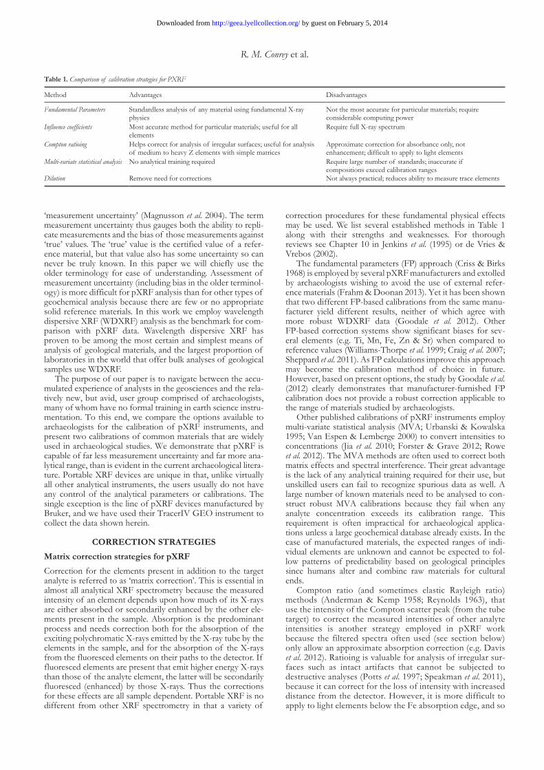
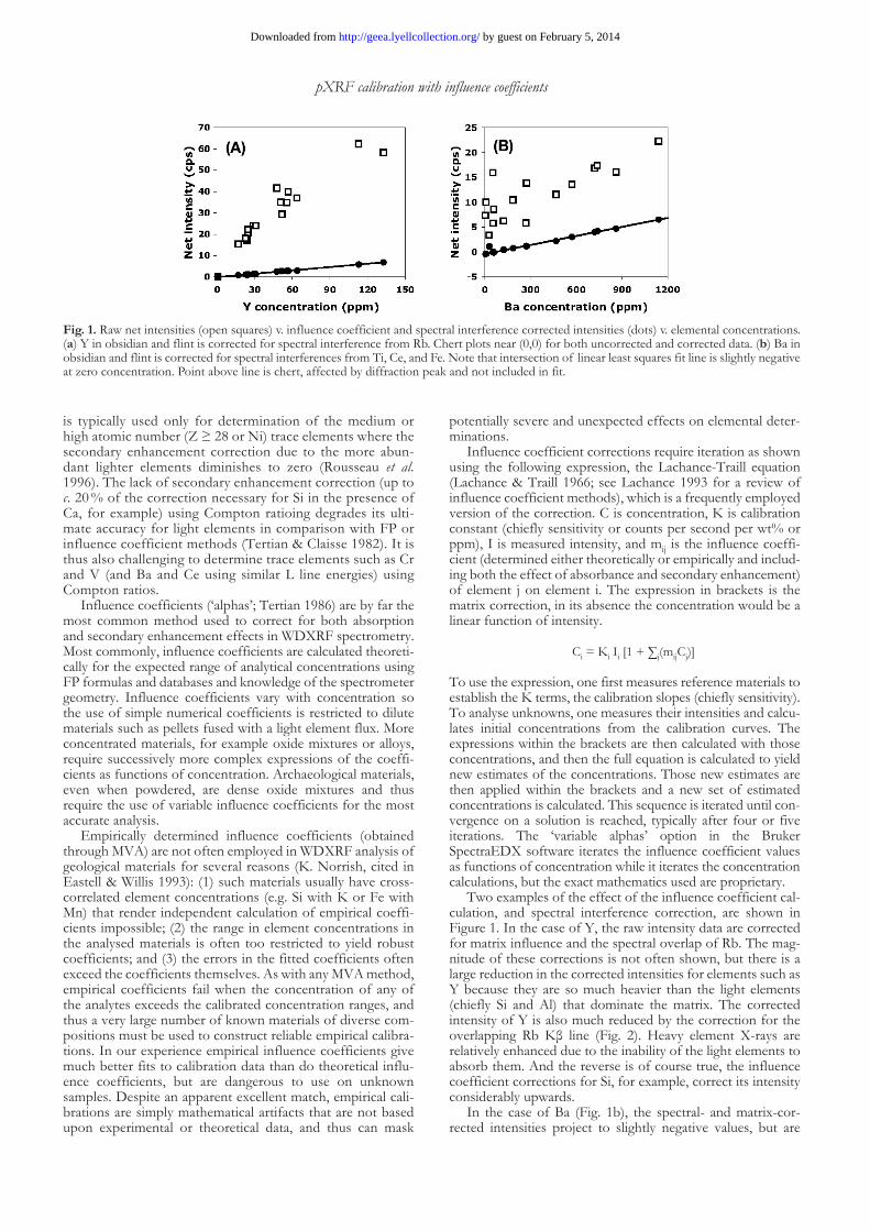
Two examples of the effect of the influence coefficient cal-culation, and spectral interference correction, are shown in Figure 1. In the case of Y, the raw intensity data are corrected for matrix influence and the spectral overlap of Rb. The mag-nitude of these corrections is not often shown, but there is a large reduction in the corrected intensities for elements such as Y because they are so much heavier than the light elements (chiefly Si and Al) that dominate the matrix. The corrected intensity of Y is also much reduced by the correction for the overlapping Rb Kβ line (Fig. 2). Heavy element X-rays are relatively enhanced due to the inability of the light elements to absorb them. And the reverse is of course true, the influence coefficient corrections for Si, for example, correct its intensity considerably upwards.

In the case of Ba (Fig. 1b), the spectral- and matrix-cor-rected intensities project to slightly negative values, but are

Fig. 1. Raw net intensities (open squares) v. influence coefficient and spectral interference corrected intensities (dots) v. elemental concentrations. (a) Y in obsidian and flint is corrected for spectral interference from Rb. Chert plots near (0,0) for both uncorrected and corrected data. (b) Ba in obsidian and flint is corrected for spectral interferences from Ti, Ce, and Fe. Note that intersection of linear least squares fit line is slightly negative at zero concentration. Point above line is chert, affected by diffraction peak and not included in fit.

by guest on February 5, 2014http://geea.lyellcollection.org/Downloaded from

R. M. Conrey et al.4

clearly strongly linear and thus still useful. Calibration curves that do not project to zero are typically due to the lack of proper background or spectral interference correction and so are not desirable. We are unsure of the reasons in this case, where we rely on software fitting rather than experiment to estimate the magnitudes of the corrections. One can force the calibration through zero but in this case that yields a much poorer fit to the data.

Spectral interferences with pXRFEnergy dispersive (ED) detection devices used in pXRF are subject to potential interferences from overlapping spectral peaks. The low resolution of the energy dispersive detectors employed, on the order of 200 eV, means that interference often cannot be avoided and must be corrected if accurate data are to be obtained. The interferences are several and include peak-on-peak overlaps, especially common where the Kβ peak of an element overlaps the Kα peak of the element with one or two higher Z (Fig. 2). Other interferences arise because the medium to high Z L or M line energies are simi-lar to the K line energies of low Z elements. Another poten-tial interference is from Compton scatter ‘tailing’ from high intensity peaks (Arai 1991). This scatter is similar to the ubiq-uitous tube target Compton scatter peak, and is generated in the same fashion by inelastic scattering of the fluoresced X-rays in the sample to lower energies. Other effects, such as radiative Auger emission (where instead of emitting a charac-teristic line X-ray, the atom emits a lower energy X-ray and also ejects an Auger electron) and Si detector effects, also result in tailing to lower energy of light element lines (Van Espen et al. 1980). Herein we refer to all of these low energy tails as Compton tails.

Peak-on-peak and Compton tailing interference are com-mon to all XRF spectrometry but pXRF spectra suffer from additional overlaps that are sample and instrument dependent. These include escape peaks, sum peaks, diffraction peaks, and peaks from materials within the X-ray path of the instrument (Van Espen et al. 1980; Ellis 2002; Ferretti 2004). Escape peaks are due to the loss of a fraction of the analyte energy to excite the Si in the detector and so are always displaced to the low energy side of the primary peak by 1.74 KeV, the Kα energy of Si. Sum peaks are due to the finite time response of the detec-tor volume and its electronics to large fluxes of incoming X-rays. A small fraction of any two intense lines will be seen by the detector as the sum of the energies of the incoming pho-tons. Diffraction peaks are common in pXRF analysis when-ever material that is not glass is analysed. For archaeological applications this generally applies when substances other than obsidian or manufactured glass are analysed. The Bragg condi-tion for diffraction may be met by some wavelengths of the broad spectrum tube X-rays interacting with the crystalline material in the sample.

Correction or reduction of spectral interference can be accomplished in several ways in pXRF spectrometry. One can try to avoid or minimize the interference by limiting the energy range of the measured peak or switching to another spectral line free from interference. In WDXRF spectrometry it is common practice to measure the magnitude of the interference for indi-vidual spectrometers with materials doped with the interfering element and free of the overlapped element, but this is not commonly done in EDXRF work. Instead, the interference is usually corrected by the use of peak-fitting mathematical rou-tines (generally proprietary) and subtraction of the calculated peak interference from the measured peak. The correction can also be done empirically with least squares best fitting to a num-ber of reference materials. Table 2 shows the spectral interfer-ence corrections we found necessary for this work.

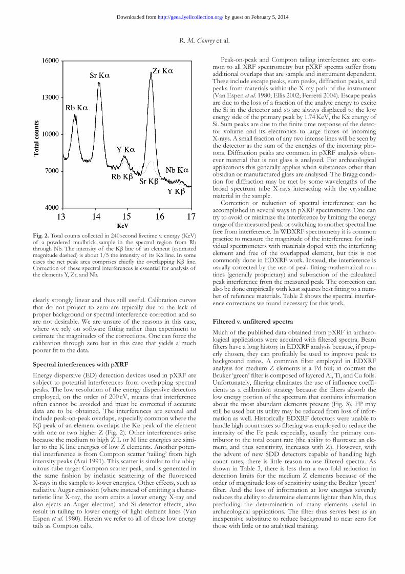
Filtered v. unfiltered spectraMuch of the published data obtained from pXRF in archaeo-logical applications were acquired with filtered spectra. Beam filters have a long history in EDXRF analysis because, if prop-erly chosen, they can profitably be used to improve peak to background ratios. A common filter employed in EDXRF analysis for medium Z elements is a Pd foil; in contrast the Bruker ‘green’ filter is composed of layered Al, Ti, and Cu foils. Unfortunately, filtering eliminates the use of influence coeffi-cients as a calibration strategy because the filters absorb the low energy portion of the spectrum that contains information about the most abundant elements present (Fig. 3). FP may still be used but its utility may be reduced from loss of infor-mation as well. Historically EDXRF detectors were unable to handle high count rates so filtering was employed to reduce the intensity of the Fe peak especially, usually the primary con-tributor to the total count rate (the ability to fluoresce an ele-ment, and thus sensitivity, increases with Z). However, with the advent of new SDD detectors capable of handling high count rates, there is little reason to use filtered spectra. As shown in Table 3, there is less than a two-fold reduction in detection limits for the medium Z elements because of the order of magnitude loss of sensitivity using the Bruker ‘green’ filter. And the loss of information at low energies severely reduces the ability to determine elements lighter than Mn, thus precluding the determination of many elements useful in archaeological applications. The filter thus serves best as an inexpensive substitute to reduce background to near zero for those with little or no analytical training.

Fig. 2. Total counts collected in 240 second livetime v. energy (KeV) of a powdered mudbrick sample in the spectral region from Rb through Nb. The intensity of the Kβ line of an element (estimated magnitude dashed) is about 1/5 the intensity of its Kα line. In some cases the net peak area comprises chiefly the overlapping Kβ line. Correction of these spectral interferences is essential for analysis of the elements Y, Zr, and Nb.

by guest on February 5, 2014http://geea.lyellcollection.org/Downloaded from

pXRF calibration with influence coefficients 5

An example of the limitations to overfiltering pXRF spec-tra comes from the Taraco Archaeological Project, Lake Titicaca, Bolivia. Roddick (2009) employed pXRF on ceram-ics, clays, archaeological sediments, and experimental clay-sand mixtures using filtered spectra and was able to analyse for only 10 elements: K, Ca, Ti, Mn, Fe, Zn, Rb, Sr, and Pb. The analyses provided only limited discrimination of ceramic types and could not discriminate different geographic locales on the Taraco Peninsula (Roddick 2009, p. 305). In contrast, use of the method described herein with unfiltered spectra and the Bruker IV instrument allowed for the determination of 17 elements and the discrimination of different localities on the peninsula using natural and anthropogenic sediments (Goodman-Elgar & Bettencourt 2012).

CAliBRAtioNCalibration methodsWe performed calibrations employing theoretical influence coefficients of a BrukerIV GEO with a SDD detector using the following procedure. We chose tube voltage and amper-age settings to keep total raw count rates below 150 Kcps to

preserve the detector and minimize deadtime. We collected raw spectra using the Bruker software package S1PXRF for 240 seconds livetime (total count time is livetime plus dead-time). We converted the raw pdz formatted spectral files to the ssd format suitable for use with the Bruker software package, SpectraEDX, using one of the tools available in that package. The SpectraEDX software allows the user to construct calibrations with almost any choice of methods and also allows the user to calculate concentrations from the spectra obtained from unknowns using the constructed cali-brations. In constructing the calibration method in SpectraEDX we specified volatile-free normalized standard reference values (in our case the WDXRF data for the same samples using oxide wt% values for major and minor ele-ments and ppm values for traces) and the physical properties of the materials. The use of normalized values reduces the differences that result from the presence of variable amounts of un-determinable light volatile elements such as H, C, and O. Na2O is undetectable with pXRF unless over c. 20 wt% so we chose to use it as a ‘balance’ element to make up the sum of all of the elemental concentrations to 100 %. In effect, Na2O serves then as a substitute for all un-determined ele-ments and the influence coefficients for Na2O are applied to all un-determined species. In practice the error introduced by these assumptions turned out to be small. In EDXRF calibration, one can choose how wide an energy range to allow for peak integration, and we chose fairly wide limits (usually wider than full width at half the maximum peak height) that captured most of the peak to increase sensitiv-ity. Narrower bands were chosen in certain cases to reduce spectral interferences. SpectraEDX allows the user to also set background energy bands or to apply software fitting to the background curve. In either case background needs to be subtracted from the raw peak areas to obtain net peak areas. We chose to allow (proprietary) mathematical fitting because of the difficulty of finding clean background in many cases. SpectraEDX allows the user to choose either empirical (based upon the known values of the calibration samples) or theoretical calculation of the spectral interferences,

Fig. 3. Total pulses (log scale) collected for 240 second livetime at 45 KeV from a solid dacite rock surface. The upper spectrum was collected unfiltered, the lower spectrum was collected with a Bruker ‘green’ filter. Note the near total loss of signal at low energy and the huge loss of sensitivity with filtering.

table 2. PXRF interference corrections for archaeological materials

Line* Peak overlap Compton tail Escape peak Sum peak

Mg Kα Al Kα Al Kα Mg Kβ Si Kα K Kα Si Kα Al Kβ, Rb Lβ, Zr L1 P Kα K Kβ P Kα Si Kβ, Zr Lβ Ca Kα K Kα Ca Kα Si Kα+ΚαCa Kα K Kβ Si Kα+ΚβTi Kα Ba Lα, Ce Lα Fe Kα V Kα Ti Kβ, Ba Lβ, Ce Lα Cr Kα V Kβ, Ce Lβ Mn Kα Fe Kα Fe Kα Zn Kα Ga Kα Zn Kβ Ti Kα+KαRb Kα Fe Kα+KβSr Kα Y Kα Rb Kβ Zr Kα Sr Kβ Nb Kα Y Kβ Ba Lβ Ti Kβ, Ce Lα Fe Kα Ba Kα Ce Lβ Ti Kβ5, BaLβ2 Fe Kβ

* Lines listed in order of atomic number

by guest on February 5, 2014http://geea.lyellcollection.org/Downloaded from

R. M. Conrey et al.6

and we opted for the latter in all cases. The software also allows the choice of fixed or variable theoretical influence coefficients, and we opted for the variable theoretical coef-ficients to better correct for the complex oxide mixtures we were calibrating. Good calibrations should intercept zero on the concentration axis at zero net intensity. The SpectraEDX software offers the choice of fixing the calibration curves at that (0,0) point or allowing the curves to float free of zero. We allowed the curves to float free whenever possible to see if they intersected zero within the standard deviations of the curves. In some cases we forced the curves through zero to reduce bias v. the calibration WDXRF data. Forcing the curves through zero gave a worse fit but resulted in a more useful calibration.

obsidian and flint calibrationObsidian is a near ideal material for XRF analysis because it is a homogeneous glass largely free of crystals. Very fine grained flint is similar to glass and is thus also a preferred material, but some crypto-crystalline chert may produce diffraction peaks, which indeed we found.

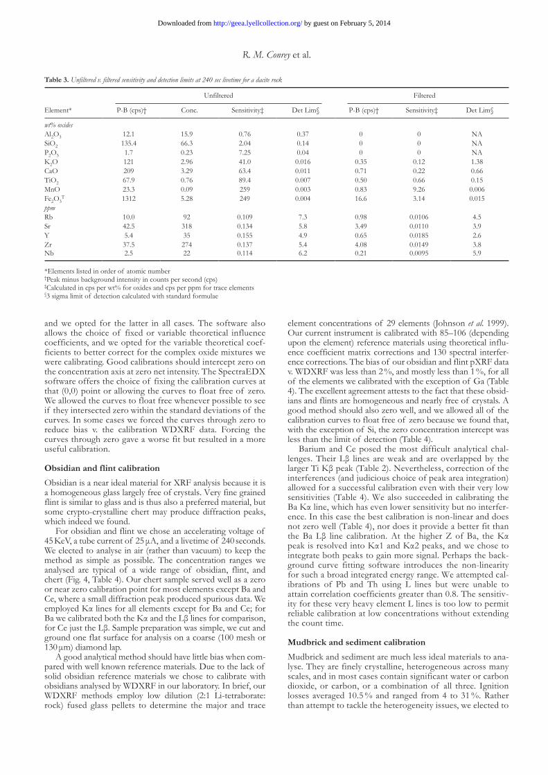
For obsidian and flint we chose an accelerating voltage of 45 KeV, a tube current of 25 μA, and a livetime of 240 seconds. We elected to analyse in air (rather than vacuum) to keep the method as simple as possible. The concentration ranges we analysed are typical of a wide range of obsidian, flint, and chert (Fig. 4, Table 4). Our chert sample served well as a zero or near zero calibration point for most elements except Ba and Ce, where a small diffraction peak produced spurious data. We employed Kα lines for all elements except for Ba and Ce; for Ba we calibrated both the Kα and the Lβ lines for comparison, for Ce just the Lβ. Sample preparation was simple, we cut and ground one flat surface for analysis on a coarse (100 mesh or 130 μm) diamond lap.

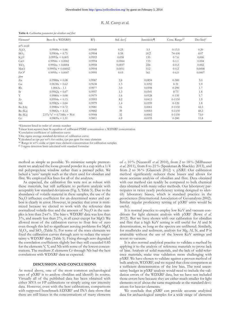
A good analytical method should have little bias when com-pared with well known reference materials. Due to the lack of solid obsidian reference materials we chose to calibrate with obsidians analysed by WDXRF in our laboratory. In brief, our WDXRF methods employ low dilution (2:1 Li-tetraborate: rock) fused glass pellets to determine the major and trace

element concentrations of 29 elements (Johnson et al. 1999). Our current instrument is calibrated with 85–106 (depending upon the element) reference materials using theoretical influ-ence coefficient matrix corrections and 130 spectral interfer-ence corrections. The bias of our obsidian and flint pXRF data v. WDXRF was less than 2 %, and mostly less than 1 %, for all of the elements we calibrated with the exception of Ga (Table 4). The excellent agreement attests to the fact that these obsid-ians and flints are homogeneous and nearly free of crystals. A good method should also zero well, and we allowed all of the calibration curves to float free of zero because we found that, with the exception of Si, the zero concentration intercept was less than the limit of detection (Table 4).

Barium and Ce posed the most difficult analytical chal-lenges. Their Lβ lines are weak and are overlapped by the larger Ti Kβ peak (Table 2). Nevertheless, correction of the interferences (and judicious choice of peak area integration) allowed for a successful calibration even with their very low sensitivities (Table 4). We also succeeded in calibrating the Ba Kα line, which has even lower sensitivity but no interfer-ence. In this case the best calibration is non-linear and does not zero well (Table 4), nor does it provide a better fit than the Ba Lβ line calibration. At the higher Z of Ba, the Kα peak is resolved into Kα1 and Kα2 peaks, and we chose to integrate both peaks to gain more signal. Perhaps the back-ground curve fitting software introduces the non-linearity for such a broad integrated energy range. We attempted cal-ibrations of Pb and Th using L lines but were unable to attain correlation coefficients greater than 0.8. The sensitiv-ity for these very heavy element L lines is too low to permit reliable calibration at low concentrations without extending the count time.

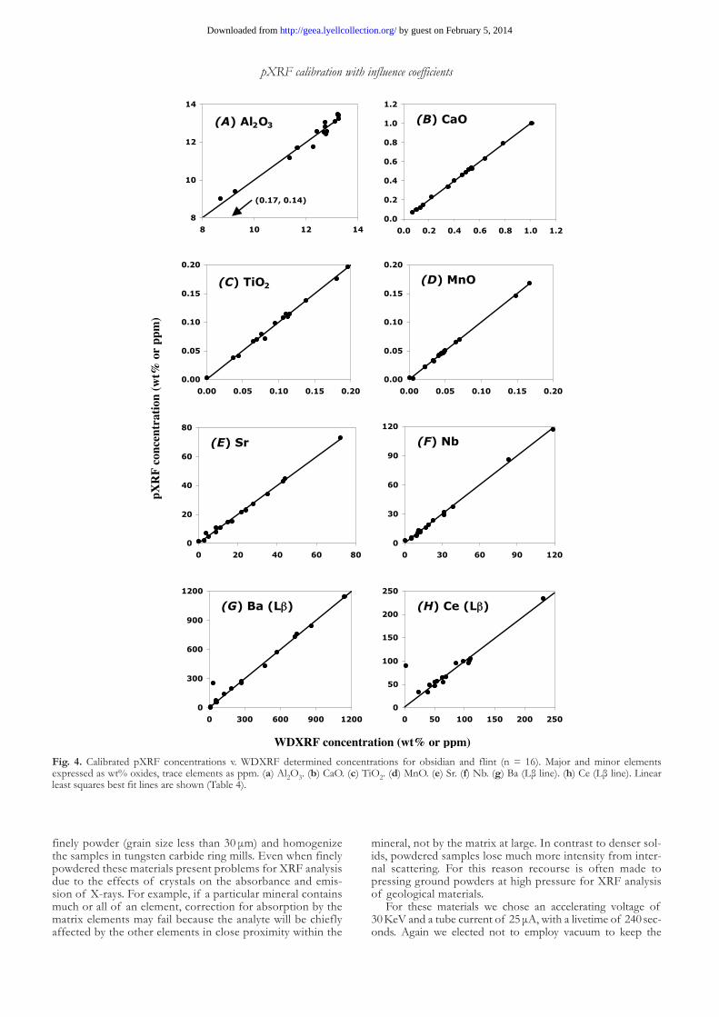
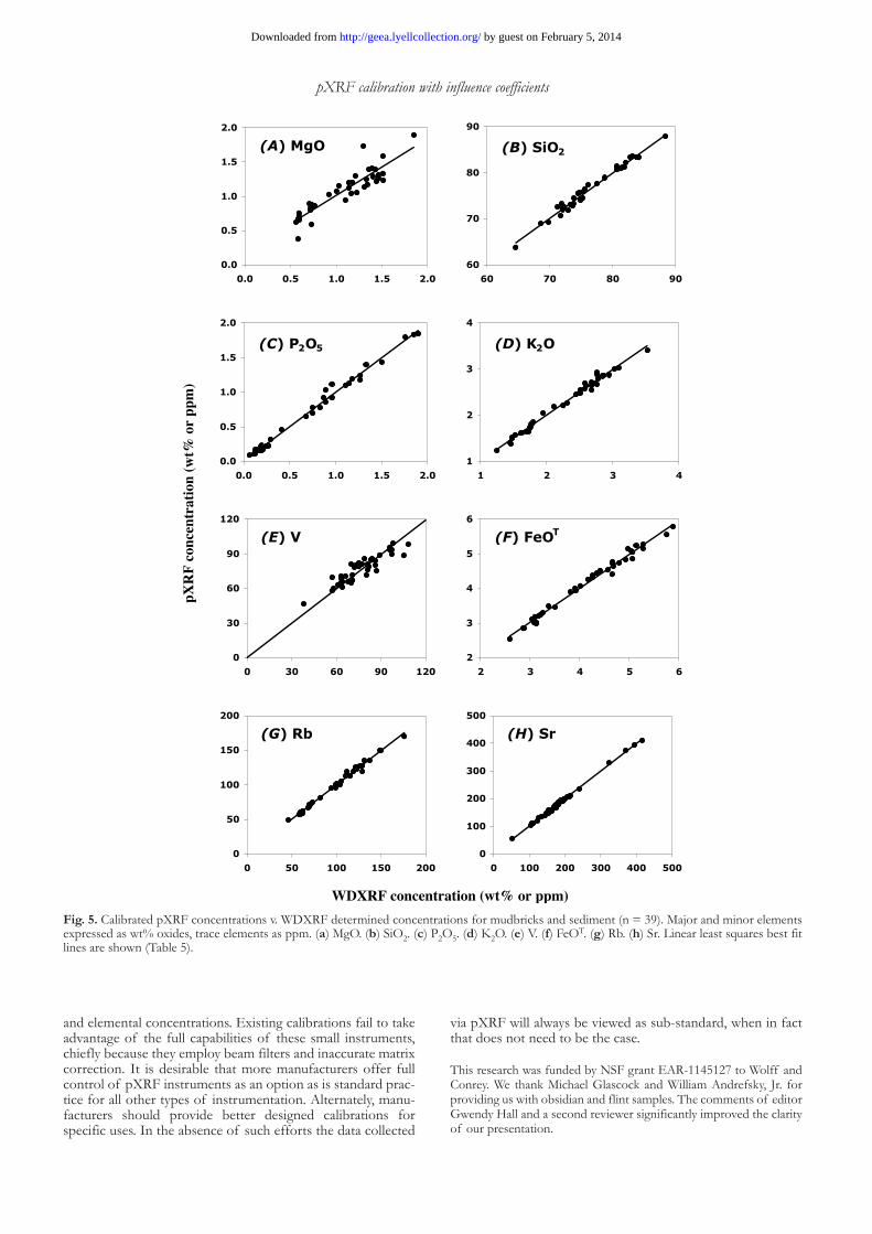
Mudbrick and sediment calibrationMudbrick and sediment are much less ideal materials to ana-lyse. They are finely crystalline, heterogeneous across many scales, and in most cases contain significant water or carbon dioxide, or carbon, or a combination of all three. Ignition losses averaged 10.5 % and ranged from 4 to 31 %. Rather than attempt to tackle the heterogeneity issues, we elected to

table 3. Unfiltered v. filtered sensitivity and detection limits at 240 sec livetime for a dacite rock

Unfiltered Filtered

Element* P-B (cps)† Conc. Sensitivity‡ Det Lim§ P-B (cps)† Sensitivity‡ Det Lim§

wt% oxides Al2O3 12.1 15.9 0.76 0.37 0 0 NASiO2 135.4 66.3 2.04 0.14 0 0 NAP2O5 1.7 0.23 7.25 0.04 0 0 NAK2O 121 2.96 41.0 0.016 0.35 0.12 1.38CaO 209 3.29 63.4 0.011 0.71 0.22 0.66TiO2 67.9 0.76 89.4 0.007 0.50 0.66 0.15MnO 23.3 0.09 259 0.003 0.83 9.26 0.006Fe2O3

T 1312 5.28 249 0.004 16.6 3.14 0.015ppm Rb 10.0 92 0.109 7.3 0.98 0.0106 4.5Sr 42.5 318 0.134 5.8 3.49 0.0110 3.9Y 5.4 35 0.155 4.9 0.65 0.0185 2.6Zr 37.5 274 0.137 5.4 4.08 0.0149 3.8Nb 2.5 22 0.114 6.2 0.21 0.0095 5.9

*Elements listed in order of atomic number†Peak minus background intensity in counts per second (cps)‡Calculated in cps per wt% for oxides and cps per ppm for trace elements§3 sigma limit of detection calculated with standard formulae

by guest on February 5, 2014http://geea.lyellcollection.org/Downloaded from

pXRF calibration with influence coefficients 7

finely powder (grain size less than 30 μm) and homogenize the samples in tungsten carbide ring mills. Even when finely powdered these materials present problems for XRF analysis due to the effects of crystals on the absorbance and emis-sion of X-rays. For example, if a particular mineral contains much or all of an element, correction for absorption by the matrix elements may fail because the analyte will be chiefly affected by the other elements in close proximity within the

mineral, not by the matrix at large. In contrast to denser sol-ids, powdered samples lose much more intensity from inter-nal scattering. For this reason recourse is often made to pressing ground powders at high pressure for XRF analysis of geological materials.

For these materials we chose an accelerating voltage of 30 KeV and a tube current of 25 μA, with a livetime of 240 sec-onds. Again we elected not to employ vacuum to keep the

Fig. 4. Calibrated pXRF concentrations v. WDXRF determined concentrations for obsidian and flint (n = 16). Major and minor elements expressed as wt% oxides, trace elements as ppm. (a) Al2O3. (b) CaO. (c) TiO2. (d) MnO. (e) Sr. (f) Nb. (g) Ba (Lβ line). (h) Ce (Lβ line). Linear least squares best fit lines are shown (Table 4).

by guest on February 5, 2014http://geea.lyellcollection.org/Downloaded from

R. M. Conrey et al.8

method as simple as possible. To minimize sample pretreat-ment we analysed the loose ground powder in a cup with a 1/4 mil polypropylene window rather than a pressed pellet. We lacked a ‘zero’ sample such as the chert used for obsidian and flint. We employed Kα lines for all of the analytes.

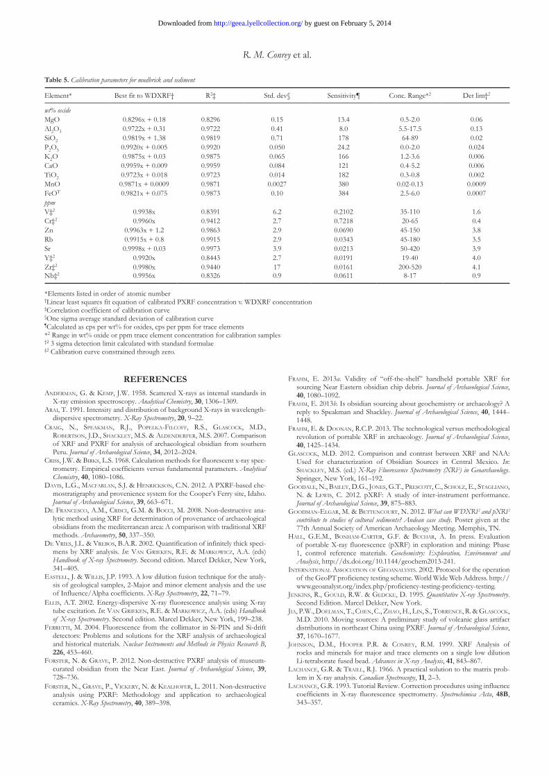
As expected, the calibration fits were not as robust with these materials, but still sufficient to perform analysis with acceptably low standard deviations (Fig. 5, Table 5). Due to the abundance of volatile material in these samples, the use of the Na2O influence coefficient for un-determined water and car-bon is clearly in error. However, in practice that error is mini-mized because we elected to work with the reference data normalized volatile-free and the amount of Na2O in the sam-ples is less than 2 wt%. The bias v. WDXRF data was less than 3 %, and mostly less than 2 %, in all cases except for MgO. We allowed most of the calibration curves to float free of zero even though this led to significant zeroing problems for MgO, Al2O3, and SiO2 (Table 5). For some of the trace elements we fixed the calibration curves through zero to reduce the uncer-tainty v. WDXRF data (Table 5). Fixing through zero degraded the correlation coefficients slightly but they still exceeded 0.85 for the elements V, Y, and Nb with some of the lowest concen-trations. The medium Z elements Cr through Nb had the best correlations with WDXRF data as expected.

diSCuSSioN ANd CoNCluSioNSAs noted above, one of the most common archaeological uses of pXRF is to analyse obsidian and identify its source. Virtually all of the published data has been obtained with either MVA or FP calibrations or simply using raw intensity data. However, even with the best calibrations, comparisons with supposed benchmark EDXRF and INA data show that there are still biases in the concentrations of many elements

of c. 10 % (Nazaroff et al. 2010), from 2 to 18 % (Millhauser et al. 2011), from 8 to 21 % (Speakman & Shackley 2013), and from 2 to 36 % (Glascock 2012) v. pXRF. Our calibration method significantly reduces these biases and allows for more accurate analysis of obsidian and flint. Data obtained with our method can readily be compared to bulk chemical data obtained with many other methods. Our laboratory par-ticipates in twice yearly proficiency testing designed to iden-tify laboratory biases, which is standard practice in the geosciences (International Association of Geoanalysts 2002). Similar regular proficiency testing of pXRF units would be useful.

It is normal practice to employ low KeV and vacuum con-ditions for light element analysis with pXRF (Rowe et al. 2012). But we have shown with our calibration for obsidian and flint that a high KeV setting is still useful for Al and Si determination, so long as the spectra are unfiltered. Similarly, for mudbricks and sediment, analysis for Mg, Al, Si, and P is attainable without the use of the lowest KeV settings and resort to vacuum.

It is also normal analytical practice to validate a method by applying it to the analysis of reference materials to prove lack of bias. Analysis of solid materials, and the lack of solid refer-ence materials, make true validation more challenging with pXRF. We have chosen to validate against a proven method of bulk analysis, WDXRF, and we regard that close comparison as a sufficient demonstration of the low bias. The total uncer-tainty budget in pXRF analysis would need to include the vali-dation errors of the WDXRF data, but we have not included those errors here because they are either much smaller for light elements or of about the same magnitude as the standard devi-ations for heavier elements.

We conclude that pXRF can provide accurate analytical data for archaeological samples for a wide range of elements

table 4. Calibration parameters for obsidian and flint

Element* Best fit v. WDXRF† R2‡ Std. dev§ Sensitivity¶ Conc. Range*2 Det lim†2

wt% oxide Al2O3 0.9949x + 0.06 0.9949 0.23 5.5 0-13.5 0.20SiO2 0.9904x + 0.75 0.9904 0.58 18.2 74-100 0.07K2O 0.9993x + 0.003 0.9993 0.038 135 0-7.6 0.006CaO 0.9994x + 0.0002 0.9994 0.0064 133 0-1.1 0.004TiO2 0.9956x + 0.0004 0.9958 0.0037 224 0-0.2 0.002MnO 0.9993x + 0.00002 0.9994 0.0011 512 0-0.2 0.0008FeOT 0.9995x + 0.0007 0.9995 0.03 561 0-6.0 0.0007ppm Zn 0.9988x + 0.08 0.9987 2.8 0.0854 0-300 3.0Ga 0.9638x + 0.62 0.9638 1.3 0.1092 0-31 1.9Rb 1.0063x - 1.1 0.9977 3.0 0.0598 0-290 1.7Sr 0.9962x + 0.07 0.9957 1.3 0.0541 0-75 1.8Y 0.9980x + 0.08 0.9979 1.6 0.0528 0-135 1.7Zr 0.9994x + 0.15 0.9993 8.2 0.0413 0-1150 1.9Nb 0.9982x + 0.04 0.9979 1.4 0.0359 0-120 1.8Ba (Lb) 0.9980x + 0.72 0.9981 16 0.0061 0-1150 42.3Ba (Ka) 0.9882x + 4.12 0.9882 39 0.0003 0-1150 60.2Ba (Ka) 2.57e-4x2 + 0.7348x + 30.4 0.9944 32 0.0002 0-1150 73.0Ce 0.9809x + 1.51 0.9811 6.9 0.0195 0-240 11.8

*Elements listed in order of atomic number†Linear least squares best fit equation of calibrated PXRF concentration v. WDXRF concentration‡Correlation coefficient of calibration curve§One sigma average standard deviation of calibration curve¶Calculated as cps per wt% for oxides, cps per ppm for trace elements*2 Range in wt% oxide or ppm trace element concentration for calibration samples†2 3 sigma detection limit calculated with standard formulae

by guest on February 5, 2014http://geea.lyellcollection.org/Downloaded from

pXRF calibration with influence coefficients 9

and elemental concentrations. Existing calibrations fail to take advantage of the full capabilities of these small instruments, chiefly because they employ beam filters and inaccurate matrix correction. It is desirable that more manufacturers offer full control of pXRF instruments as an option as is standard prac-tice for all other types of instrumentation. Alternately, manu-facturers should provide better designed calibrations for specific uses. In the absence of such efforts the data collected

via pXRF will always be viewed as sub-standard, when in fact that does not need to be the case.

This research was funded by NSF grant EAR-1145127 to Wolff and Conrey. We thank Michael Glascock and William Andrefsky, Jr. for providing us with obsidian and flint samples. The comments of editor Gwendy Hall and a second reviewer significantly improved the clarity of our presentation.

Fig. 5. Calibrated pXRF concentrations v. WDXRF determined concentrations for mudbricks and sediment (n = 39). Major and minor elements expressed as wt% oxides, trace elements as ppm. (a) MgO. (b) SiO2. (c) P2O5. (d) K2O. (e) V. (f) FeOT. (g) Rb. (h) Sr. Linear least squares best fit lines are shown (Table 5).

by guest on February 5, 2014http://geea.lyellcollection.org/Downloaded from

R. M. Conrey et al.10

REFERENCESAndermAn, G. & Kemp, J.W. 1958. Scattered X-rays as internal standards in

X-ray emission spectroscopy. Analytical Chemistry, 30, 1306–1309.ArAi, T. 1991. Intensity and distribution of background X-rays in wavelength-

dispersive spectrometry. X-Ray Spectrometry, 20, 9–22.CrAig, N., SpeAKmAn, R.J., popelKA-FilCoFF, R.S., glASCoCK, M.D.,

robertSon, J.D., ShACKley, M.S. & AldenderFer, M.S. 2007. Comparison of XRF and PXRF for analysis of archaeological obsidian from southern Peru. Journal of Archaeological Science, 34, 2012–2024.

CriSS, J.W. & birKS, L.S. 1968. Calculation methods for fluorescent x-ray spec-trometry. Empirical coefficients versus fundamental parameters. Analytical Chemistry, 40, 1080–1086.

dAviS, L.G., mACFArlAn, S.J. & henriCKSon, C.N. 2012. A PXRF-based che-mostratigraphy and provenience system for the Cooper’s Ferry site, Idaho. Journal of Archaeological Science, 39, 663–671.

de FrAnCeSCo, A.M., CriSCi, G.M. & boCCi, M. 2008. Non-destructive ana-lytic method using XRF for determination of provenance of archaeological obsidians from the mediterranean area: A comparison with traditional XRF methods. Archaeometry, 50, 337–350.

de vrieS, J.L. & vreboS, B.A.R. 2002. Quantification of infinitely thick speci-mens by XRF analysis. In: vAn grieKen, R.E. & mArKowiCz, A.A. (eds) Handbook of X-ray Spectrometry. Second edition. Marcel Dekker, New York, 341–405.

eAStell, J. & williS, J.P. 1993. A low dilution fusion technique for the analy-sis of geological samples, 2-Major and minor element analysis and the use of Influence/Alpha coefficients. X-Ray Spectrometry, 22, 71–79.

elliS, A.T. 2002. Energy-dispersive X-ray fluorescence analysis using X-ray tube excitation. In: vAn grieKen, R.E. & mArKowiCz, A.A. (eds) Handbook of X-ray Spectrometry. Second edition. Marcel Dekker, New York, 199–238.

Ferretti, M. 2004. Fluorescence from the collimator in Si-PIN and Si-drift detectors: Problems and solutions for the XRF analysis of archaeological and historical materials. Nuclear Instruments and Methods in Physics Research B, 226, 453–460.

ForSter, N. & grAve, P. 2012. Non-destructive PXRF analysis of museum-curated obsidian from the Near East. Journal of Archaeological Science, 39, 728–736.

ForSter, N., grAve, P., viCKery, N. & KeAlhoFer, L. 2011. Non-destructive analysis using PXRF: Methodology and application to archaeological ceramics. X-Ray Spectrometry, 40, 389–398.

FrAhm, E. 2013a. Validity of “off-the-shelf” handheld portable XRF for sourcing Near Eastern obsidian chip debris. Journal of Archaeological Science, 40, 1080–1092.

FrAhm, E. 2013b. Is obsidian sourcing about geochemistry or archaeology? A reply to Speakman and Shackley. Journal of Archaeological Science, 40, 1444–1448.

FrAhm, E. & doonAn, R.C.P. 2013. The technological versus methodological revolution of portable XRF in archaeology. Journal of Archaeological Science, 40, 1425–1434.

glASCoCK, M.D. 2012. Comparison and contrast between XRF and NAA: Used for characterization of Obsidian Sources in Central Mexico. In: ShACKley, M.S. (ed.) X-Ray Fluorescence Spectrometry (XRF) in Geoarchaeology. Springer, New York, 161–192.

goodAle, N., bAiley, D.G., JoneS, G.T., preSCott, C., SCholz, E., StAgliAno, N. & lewiS, C. 2012. pXRF: A study of inter-instrument performance. Journal of Archaeological Science, 39, 875–883.

goodmAn-elgAr, M. & bettenCourt, N. 2012. What can WDXRF and pXRF contribute to studies of cultural sediments? Andean case study. Poster given at the 77th Annual Society of American Archaeology Meeting. Memphis, TN.

hAll, G.e.m., bonhAm-CArter, g.F. & buChAr, A. In press. Evaluation of portable X-ray fluorescence (pXRF) in exploration and mining: Phase 1, control reference materials. Geochemistry: Exploration, Environment and Analysis, http://dx.doi.org/10.1144/geochem2013-241.

internAtionAl ASSoCiAtion oF geoAnAlyStS. 2002. Protocol for the operation of the GeoPT proficiency testing scheme. World Wide Web Address. http://www.geoanalyst.org/index.php/proficiency-testing-proficiency-testing.

JenKinS, R., gould, R.W. & gedCKe, D. 1995. Quantitative X-ray Spectrometry. Second Edition. Marcel Dekker, New York.

JiA, P.W., doelmAn, T., Chen, C., zhAo, H., lin, S., torrenCe, R. & glASCoCK, M.D. 2010. Moving sources: A preliminary study of volcanic glass artifact distributions in northeast China using PXRF. Journal of Archaeological Science, 37, 1670–1677.

JohnSon, D.M., Hooper P.R. & Conrey, R.M. 1999. XRF Analysis of rocks and minerals for major and trace elements on a single low dilution Li-tetraborate fused bead. Advances in X-ray Analysis, 41, 843–867.

lAChAnCe, G.R. & trAill, R.J. 1966. A practical solution to the matrix prob-lem in X-ray analysis. Canadian Spectroscopy, 11, 2–3.

lAChAnCe, G.R. 1993. Tutorial Review. Correction procedures using influence coefficients in X-ray fluorescence spectrometry. Spectrochimica Acta, 48B, 343–357.

table 5. Calibration parameters for mudbrick and sediment

Element* Best fit to WDXRF† R2‡ Std. dev§ Sensitivity¶ Conc. Range*2 Det lim†2

wt% oxide MgO 0.8296x + 0.18 0.8296 0.15 13.4 0.5-2.0 0.06Al2O3 0.9722x + 0.31 0.9722 0.41 8.0 5.5-17.5 0.13SiO2 0.9819x + 1.38 0.9819 0.71 178 64-89 0.02P2O5 0.9920x + 0.005 0.9920 0.050 24.2 0.0-2.0 0.024K2O 0.9875x + 0.03 0.9875 0.065 166 1.2-3.6 0.006CaO 0.9959x + 0.009 0.9959 0.084 121 0.4-5.2 0.006TiO2 0.9723x + 0.018 0.9723 0.014 182 0.3-0.8 0.002MnO 0.9871x + 0.0009 0.9871 0.0027 380 0.02-0.13 0.0009FeOT 0.9821x + 0.075 0.9873 0.10 384 2.5-6.0 0.0007ppm V‡2 0.9938x 0.8391 6.2 0.2102 35-110 1.6Cr‡2 0.9960x 0.9412 2.7 0.7218 20-65 0.4Zn 0.9963x + 1.2 0.9863 2.9 0.0690 45-150 3.8Rb 0.9915x + 0.8 0.9915 2.9 0.0343 45-180 3.5Sr 0.9998x + 0.03 0.9973 3.9 0.0213 50-420 3.9Y‡2 0.9920x 0.8443 2.7 0.0191 19-40 4.0Zr‡2 0.9980x 0.9440 17 0.0161 200-520 4.1Nb‡2 0.9956x 0.8326 0.9 0.0611 8-17 0.9

*Elements listed in order of atomic number†Linear least squares fit equation of calibrated PXRF concentration v. WDXRF concentration‡Correlation coefficient of calibration curve§One sigma average standard deviation of calibration curve¶Calculated as cps per wt% for oxides, cps per ppm for trace elements*2 Range in wt% oxide or ppm trace element concentration for calibration samples†2 3 sigma detection limit calculated with standard formulae‡2 Calibration curve constrained through zero.

by guest on February 5, 2014http://geea.lyellcollection.org/Downloaded from

pXRF calibration with influence coefficients 11

mAgnuSSon, B., näyKKi, T., hovind, H. & KrySell, M. 2004. Handbook for Calculation of Measurement Uncertainty in Environmental Laboratories. Edition 2. Nordtest Report TR 537.

millhAuSer, J.K., rodriguez-AlegriA, E. & glASCoCK, M.D. 2011. Testing the accuracy of portable X-ray fluorescence to study Aztec and Colonial obsid-ian supply at Xaltocan, Mexico. Journal of Archaeological Science, 38, 3141–3152.

nAzAroFF, A.J., pruFer, K.M. & drAKe, B.L. 2010. Assessing the applicabil-ity of portable X-ray fluorescence spectrometry for obsidian provenance research in the Maya lowlands. Journal of Archaeological Science, 37, 885–895.

pottS, P.J., webb, P.C. & williAmS-thorpe, O. 1997. Investigation of a Correction Procedure for Surface Irregularity Effects Based on Scatter Peak Intensities in the Field Analysis of Geological and Archaeological Rock Samples by Portable X-ray Fluorescence Spectrometry. Journal of Analytical Atomic Spectrometry, 12, 769–776.

reynoldS, R.C. 1963. Matrix corrections in trace element analysis by X-ray Fluorescence: Estimation of the mass absorption coefficient by Compton scattering. American Mineralogist, 48, 1133–1143.

roddiCK, A. 2009. Communities of pottery production and consumption on the Taraco Peninsula, Bolivia, 200 BC–AD 300. PhD thesis, University of California, Berkeley.

rouSSeAu, R., williS, J.P. & dunCAn, A.R. 1996. Practical XRF calibration procedures for major and trace elements. X-Ray Spectrometry, 25, 179–189.

rowe, H., hugheS, N. & robinSon, K. 2012. The quantification and applica-tion of handheld energy-dispersive x-ray fluorescence (ED-XRF) in mudrock chemostratigraphy and geochemistry. Chemical Geology, 324–325, 122–131.

ShACKley, M.S. 2010. Is There Reliability And Validity In Portable X-Ray Fluorescence Spectrometry (PXRF)? The SAA Archaeological Record, 10, 17–20.

SheppArd, P.J., irwin, G.J., lin, S.C. & mCCAFFrey, C.P. 2011. Characterization of New Zealand obsidian using PXRF. Journal of Archaeological Science, 38, 45–56.

SpeAKmAn, R.J. & ShACKley, M.S. 2013. Silo science and portable XRF in archaeology: A response to Frahm. Journal of Archaeological Science, 40, 1435–1443.

SpeAKmAn, R.J., littel, N.C., Creel, D., miller, M.R. & iñAñez, J.G. 2011. Sourcing ceramics with portable XRF spectrometers? A comparison with INAA using Mimbres pottery from the American Southwest. Journal of Archaeological Science, 38, 3483–3496.

tertiAn, R. 1986. Mathematical matrix correction procedures for X-Ray Fluorescence analysis. A critical survey. X-Ray Spectrometry, 15, 177–190.

tertiAn, R. & ClAiSSe, F. 1982. Principles of Quantitative X-ray Fluorescence Analysis. Heyden & Son, Ltd, London.

urbAnSKi, P. & KowAlSKA, E. 1995. Application of partial least-squares calibration methods in low resolution EDXRS. X-Ray Spectrometry, 24, 70–75.

vAn eSpen, P. & lemberge, P. 2000. ED-XRF Spectrum Evaluation And Quantitative Analysis Using Multivariate And Nonlinear Techniques. Advances in X-ray Analysis, 43, 560–569.

vAn eSpen, P., nullenS, H. & AdAmS, F. 1980. An in-depth study of energy-dispersive X-ray spectra. X-Ray Spectrometry, 9, 126–133.

williAmS-thorpe, O., pottS, P.J. & webb, P.C. 1999. Field-Portable Non-Destructive Analysis of Lithic Archaeological Samples by X-Ray Fluorescence Instrumentation using a Mercury Iodide Detector: Comparison with Wavelength-Dispersive XRF and a Case Study in British Stone Axe Provenancing. Journal of Archaeological Science, 26, 215–237.

Received 30 January 2013; revised typescript accepted 25 March 2013.

by guest on February 5, 2014http://geea.lyellcollection.org/Downloaded from