Calculation of the Uncertainty in the CO2 Emissions Factor in ...

Paper 3.2

Calculation of the Uncertainty in the CO2 Emissions Factor in Flare Lines with

Nitrogen Injection

Jeff Gibson

TUV NEL

Richard Paton TUV NEL

Pål Jaghø

Talisman Energy Norge AS

28th International North Sea Flow Measurement Workshop 26th – 29th October 2010

1

Calculation of the Uncertainty in the CO2 Emission Factor in Flare Lines with Nitrogen Injection

Jeff Gibson, TUV NEL

Richard Paton, TUV NEL Pål Jaghø, Talisman Energy Norge AS

1 INTRODUCTION North Sea oil and gas operators are under both environmental and financial pressure to reduce CO2 emissions from process and production facilities. Talisman Energy in Norway (Talisman Energy Norge AS) are reducing the amount of gas flared on their Gyda and Varg facilities using various process improvements. In order to do this a proportion of the fuel gas, used to keep the flare line pressurised and the flame burning during low-flaring conditions, is being replaced with injected nitrogen. This has the effect of reducing the CO2 emissions. Talisman have installed ultrasonic flare gas meters as the primary flow measurement devices in the flare lines on their Gyda platform. The output of molecular weight from the ultrasonic flare gas meters is being used to determine the composition and, hence, the CO2 emission factor. Accounting for the gas flared, and therefore the CO2 produced, requires measurement and calculation methods which account for the proportion of injected nitrogen. A similar system is proposed for the Varg FPSO. Following an initial evaluation of the uncertainty calculations for emission factor undertaken in May 2009, TUV NEL was further commissioned to provide a calculation procedure to allow the CO2 emissions to be reported from Talisman’s Gyda and Varg platforms. This included an analysis of the flow-weighted mean emission factor for each of the flare lines. This paper focuses on the work done for the Gyda platform. A review of the measurement and data collection/reduction methods was carried out, followed by an uncertainty analysis. A calculation spreadsheet was developed by TUV NEL in order to determine the emission factor, the CO2 produced and the accompanying uncertainty over a specific reporting period. This paper outlines the findings from the study expressed in a generic way in order to highlight the issues with measurements, data reduction and uncertainty that would apply equally to other operators’ facilities. The analysis has highlighted that the measurement of the flare and nitrogen flow rates are of equal importance to the calculations of the emission factor as the algorithm used to calculate the molecular weight. 2 BACKGROUND Gyda is a fixed oil production and drilling facility located in the southern-Norwegian sector of the North Sea. Gyda incorporates emergency flare systems which release CO2 to atmosphere when this excess hydrocarbon gas is burned. Gyda has two flare lines, a high pressure (HP) flare and a low pressure (LP) flare. These flare lines are both injected with nitrogen to maintain a positive pressure on the flare whilst reducing the amount of gas burned and, therefore, the amount of CO2 released to atmosphere. Both the flow rate of gas to flare, and the appropriate CO2 emission factor (tonnes CO2 per tonne of gas flared), are required to calculate the amount of CO2 emitted to atmosphere. One method for determining an installation-specific emission factor is to obtain the gas composition by extracting samples for subsequent lab analysis. It is, however, generally impractical to extract samples from flare lines, mainly due to health and safety constraints. In most cases the only opportunity is to sample from the fuel (or export) gas line to give an estimate of the flare gas composition. This approach effectively ignores the variations in gas


2

composition that will occur during flaring incidents and does not directly account for the injected nitrogen. An alternative solution is to use a combination of online molecular weight measurement from flare gas ultrasonic meters, in combination with sampling of the fuel gas, to determine the hydrocarbon content and percentage of inert gases in the mixture (such as CO2, nitrogen (N2), water vapour etc.). This is the approach that Talisman are proposing to use for determining the emission factor. 2.1 Regulatory Requirements Gas flaring has been heavily regulated in Norway since the introduction of a CO2 taxation regime in 1991. Norway also participates in the EU ETS through the incorporation of the EU ETS Directive 2003/87/EC (as amended) [1] within the European Economic Area (EEA) agreement. The requirements of the MRG are implemented at a National level by the Norwegian regulator of the EU ETS - the Climate and Pollution Agency (KLIF) (formerly SFT). The EU ETS Measurement and Reporting Guidelines 2007 (MRG) Annex 2.1.1.3 [2] requires the mass of CO2 released to atmosphere from flaring to be calculated via the product of the annual volume flared (referred to as the “activity data”) (Sm3), emission factor (tCO2/Sm3 of gas flared) and oxidation factor (-)

CO2 emissions = Activity data × Emission factor × Oxidation factor

(tCO2) (Sm3) (tCO2/Sm3) (-) Activity data (and emission factor) has to be based on specified standard conditions of the gas as defined in the EU ETS as ‘normal’ conditions of 1.01325 bar and 273.15 K (0°C). It is noted that activity data and emission factor based on mass units is also widely accepted. Oxidation factor, a measure of the amount of CO2 produced through burning, is generally specified as a constant (and is currently accepted as being set equal to 1). The EU ETS MRG states that: “The highest tier approach shall be used by all operators to determine all variables for all source streams for all Category B or C installations. Only if it is shown to the satisfaction of the competent authority that the highest tier approach is technically unfeasible, or will lead to unreasonably high costs, may a next tier be used for that variable within a monitoring methodology”. Gyda is a category B installation. Of note is the stipulation that activity data and emission factor are to be reported to the highest tier for both category B and C installations (i.e. flow rate and emission factor both to tier 3 as per category C installations). This requires uncertainty to be determined to within 7.5% (k=2), for activity data, and therefore 2.5% (k=2) for emissions factor. It is recognised that installations warrant review on a case-by-case basis and, in some instances, a lower-tier approach may be applied. 2.2 Observations on Uncertainty Specifications in EU ETS MRG The MRG states that the uncertainty is on the data submitted over the reporting period. This is currently annual to EU ETS but may change in future phases of the scheme. The regulator may also require reporting at more frequent intervals. As will be discussed in this paper, the variability of the conditions in a flare line make it especially important to ensure that the calculations take into account variations in both flowrate and emissions factor. When these conditions change, the associated uncertainty changes. This makes it difficult to assess the uncertainty over any reporting period as a constant value.


3

The EU ETS MRG does not detail how the uncertainty of a variable emission factor should be derived and reported. In the absence of clear regulator guidance it has been decided that the most practical determination for the reportable figure is:

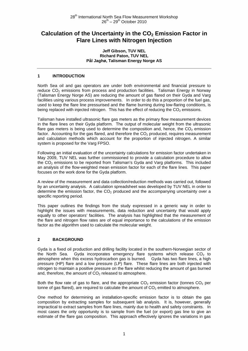
The flow-weighted mean of the emission factors across the reporting period It is also noted that how the uncertainty is attributed (i.e. to activity data or emission factor) can affect whether the EU ETS uncertainty targets can be met. In reality, it is the amount of CO2 emitted to atmosphere, and therefore the uncertainty on the reported mass of CO2, that is important. Under the current regime, an operator has to report activity data and emission factor. Therefore, it is possible to meet uncertainty requirements as calculated for total CO2 but fail the target uncertainty on the precursor measurements of activity data or emission factor. An example of this is given in Appendix A. In addition, it is not always convenient (or possible) to split the uncertainty into two parts. Any correlation needs to be considered to avoid double-accounting. 3 FLARE SYSTEMS ON THE GYDA PLATFORM The analyses described in the following sections use terms that are described in the definitions section of this paper. The Gyda installation has two flare systems - the high and low pressure flares designated LP and HP. These flares are continuously purged with a nominally constant flow of nitrogen (as shown in Fig. 1). Both LP and HP flare systems have GE Sensing ultrasonic flare gas meters (FGMs) installed configured to return both flowrate and the molecular weight of the emission gas (i.e. the total gas going to the flare).

Figure 1 – Simplified diagram showing nitrogen purge and metering systems on Gyda The nitrogen is injected upstream of the flare gas meter; therefore, the total volume of gas going to the flare tip (the emission gas) is a mixture of process gas (i.e. hydrocarbon with low levels of inherent CO2 and nitrogen) and additional injected nitrogen. The emission gas flowrate, Qve, can be expressed as:

2Nvvpve QQQ

Where Qvp is the volume flowrate of gas generated by the process and discharged to the flare line and QvN2 is the volume flowrate of the nitrogen used to purge the flare line. The gas


4

streams also have molecular weights associated with them (Me, Mp and MN2 respectively) as depicted in Fig. 1. Since QvN2 is nominally fixed, this means that the percentage nitrogen reduces as the process gas flowrate increases. It is therefore important to take account of the effect of nitrogen on the emission factor during periods of low flaring, but less important during periods of high flaring. The ultrasonic meters on Gyda make use of pressure and temperature measurements in internal calculations so as to calculate the output in mass units, but currently only the pressure is returned separately to the data recording system, along with the mass flow rate. Density of the emission gas is calculated from p, T and its molecular weight, Me. Me can be entered as a constant value or estimated from speed of sound measurements as per the proposed method detailed in this paper. The nitrogen flow is measured by variable area flowmeters (VAMs). These measurements are then used, in conjunction with emission gas flowrate, to give values for emission factor, volumetric flowrate and, hence, the estimated mass of CO2 being produced. Currently, and in common with other installations, the pressure and temperature of the nitrogen at the VAM is not being measured. A VAM scale is normally configured to read in standard volume units assuming a particular gas and assumed line conditions. Any variation in the pressure and temperature about these assumed values should therefore be allowed for. The mass flowrate of nitrogen is computed assuming an ideal gas from the volume flowrate at standard conditions. 4 CALCULATION OF THE EMISSION FACTOR WITH NITROGEN INJECTION The amount of CO2 emitted during combustion arises from the oxidation of carbon with the oxygen in ambient air. In addition, any CO2 inherent in the flare gas will also pass through the flare to atmosphere. Therefore, the mass of CO2 emitted can be calculated from the overall carbon content of the flare gas and the molecular weight of the various components. The quantity of nitrogen in the flare gas must also be taken into account in order to calculate the correct amount of CO2 released per unit quantity of gas burned. One approach is to infer the nitrogen content from changes in the molecular weight of the emission gas compared with that of the process gas. Although this method has some advantages, it will be inaccurate if the molecular weight of the hydrocarbon gas is close to that of nitrogen. One way of dealing with this is to segregate the data into “purging” and “flaring” modes and then analyse the molecular weight accordingly [3]. In the current case this is done by measuring the flow rate of nitrogen in addition to the flow rate of emission gas measured by the flare gas meters. There are two ways of calculating the amount of CO2 released from knowledge of the flowrate of flare gas and its molecular weight:

1) Subtract the nitrogen flow from the activity data and express the emission factor as a function of carbon content of the fuel gas (tCO2/Sm3 of hydrocarbon gas)

2) Include the nitrogen flow in the activity data and recalculate the emission factor to

effectively reduce the amount of CO2 emitted per unit of gas flared

Method 1) Involves reducing the activity data figures that will be output from the flare gas meter and is discussed by other authors [3], whilst method 2) reduces the emission factor accordingly.


5

It is not clear from regulatory guidance whether activity data reported to the regulator should be the total gas measured by the metering systems or whether this can be a modified figure as is the case in method 1. The choice of method may affect which uncertainty value is increased – activity data or emissions factor; however, provided the same methodology is applied to determine molecular weight etc. the overall uncertainty in reported mass of CO2 emitted should be the same (as discussed previously in Section 2.1 and the example shown in Appendix A). 4.1 Calculation Procedure for Emission Factor TUV NEL have developed a methodology that can be used be used to calculate the emission factor directly using the measured molecular weight of emissions gas, Me, and various other inputs including flowrates. This is given in Appendix B. The methodology is based on the following underlying assumptions:

The volume fraction of water vapour and other non-hydrocarbons (such as He, H2S etc.) is insignificant.

Liquid levels (e.g. water and any liquid hydrocarbons) are negligible in the flare lines

The relative proportions of hydrocarbons, CO2 and N2 found in the process gas, as

measured at the fuel or export gas lines, are representative of what is found in the flare line and these remain fixed across the flow range.

It is assumed that only light, alkane hydrocarbons of the form CnH(2n+2) are present in

the gas (i.e. no significant amounts of aromatic compounds or alkenes are present).

Any variation in compressibility (Z) of the mixture is negligible and an ideal gas compressibility Z=1 can be assumed. A more accurate estimate of Z could be calculated provided the gas composition can be estimated.

Complete combustion occurs with all carbon being oxidized to form CO2 (as implied

by the oxidation factor being set to 1.0 in the MRG). Other factors may be used as appropriate.

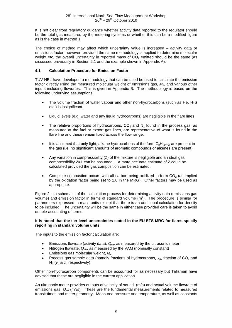
Figure 2 is a schematic of the calculation process for determining activity data (emissions gas volume) and emission factor in terms of standard volume (m3). The procedure is similar for parameters expressed in mass units except that there is an additional calculation for density to be included. The uncertainty will be the same in either case provided care is taken to avoid double-accounting of terms. It is noted that the tier-level uncertainties stated in the EU ETS MRG for flares specify reporting in standard volume units The inputs to the emission factor calculation are:

Emissions flowrate (activity data), Qve, as measured by the ultrasonic meter Nitrogen flowrate, QvN, as measured by the VAM (nominally constant) Emissions gas molecular weight, Me Process gas sample data (namely fractions of hydrocarbons, xp, fraction of CO2 and

N2 (yp & zp respectively). Other non-hydrocarbon components can be accounted for as necessary but Talisman have advised that these are negligible in the current application. An ultrasonic meter provides outputs of velocity of sound (m/s) and actual volume flowrate of emissions gas, Qve (m

3/s). These are the fundamental measurements related to measured transit-times and meter geometry. Measured pressure and temperature, as well as constants


6

such as the pressure and temperature at standard conditions (ps, Ts) and Z/Zs (assumed = 1.0 at low pressures found in the flare lines), allow conversion to standard volume (Sm3) in the meter’s flow computer. The molecular weight of emissions gas, Me, is calculated in the meter’s flow computer using a proprietary algorithm which also corrects speed of sound for temperature and output to the supervisory computer. The supervisory computer records and stores this data using a proprietary data base; the OSIsoft “PI database”. In theory at least, the uncertainty in the emissions gas flowrate (i.e. activity data) will be unaffected by the addition of nitrogen. However, the molecular weight correlation will be affected to some degree by the introduction of significant amounts of inert gas which tends to move the composition away from a typical hydrocarbon gas. This was considered in the analysis. Talisman are currently in dialogue with the meter vendor as regards ways to optimise the molecular weight correlation.

Figure 2 – Suggested calculation procedure for determining activity data and emission factor

on the Gyda platform (a similar calculation is planned for other facilities) 4.2 Data Analysis Gas flaring is not a continuous or steady-state activity; therefore, the emission factor is not a constant value. A simple arithmetic mean of emission factor over the reporting period may not be accurate because it does not take account of periods of high flow. During significant process events large volumes of gas are flared and the associated molecular weight is likely to be significantly different than that found during day-to-day flaring. Therefore, the emission factor is not a single value, but must be evaluated continuously and then used to estimate the CO2 produced. The flow-weighted mean and the associated uncertainty can be derived in two ways:

1) A running average of the flow-weighted mean value can be calculated across a reporting period.

2) The mean emission factor is calculated from the total standard volume of emission gas and total CO2 generated.


7

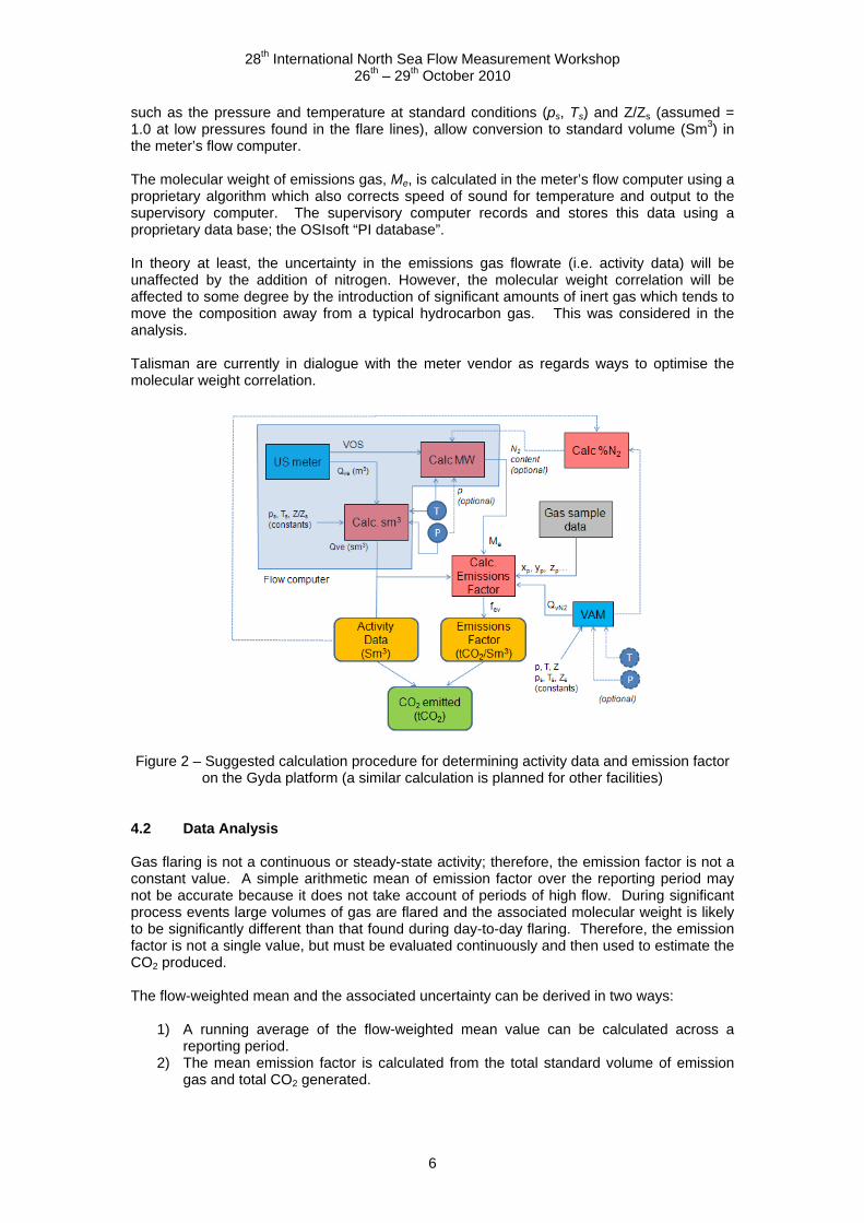
The second method is the simpler of the two. The above approach required an algorithm to be programmed and TUV NEL created this using VBA coding within Excel. The VBA code analyses the raw data from an input file and can be generalised to cope with data from various flare systems. The results are output into Excel worksheets in the form of tables. In order to determine the uncertainty, a raw data file was extracted from the PI database and the algorithm then calculated all the relevant parameters. The sheet generates values for activity data, emission factor, and quantity of CO2 produced for each data point. It also generates, in absolute terms, the uncertainty in emission factor and CO2 for each point. The mean emission factor uncertainty (see later discussion) and the total absolute CO2 uncertainty are then calculated for the chosen calculation period. The uncertainty was carried out by inserting each data point in turn into a Excel-based uncertainty budget table. The uncertainty calculations followed the methodology set out in ISO 5168 (2004) [4]. 4.2.1 Process Gas Composition (Gyda) Table 1 shows export gas sample data on Gyda over a 5-month period. It can be seen that the export gas stream is relatively stable with an average molecular weight of about 22.6 g/mol. The hydrocarbon content is about 97% by volume, the remaining 3% being made up of N2 (0.5%) and CO2 (2.5%). As discussed previously, this gas is viewed to be largely representative of the process gas that enters the flare line during normal operation. Thus, in calculating the CO2 emission factor, the inherent assumptions are made that, regardless of the source of the gas (e.g. first stage separator, suction scrubbers etc.), the N2 and CO2 level will be fixed, no additional inorganic gases will be present and, by inference, the hydrocarbon content of the process gas will also be fixed at around 97% by volume.

Table 1 – Gyda export gas sample data as supplied to TUV NEL by Talisman Energy

4.3 Examination of Data from Gyda Flare Gas Meters The flow and molecular weight data was analysed for the Gyda LP and HP flares over a period of 50 days (July 01 – Aug 19 2009) (as given in Table 2). These data have been derived from the flow meter data supplied to TUV NEL and were obtained from interrogation of the customer’s database (the “PI database”).


8

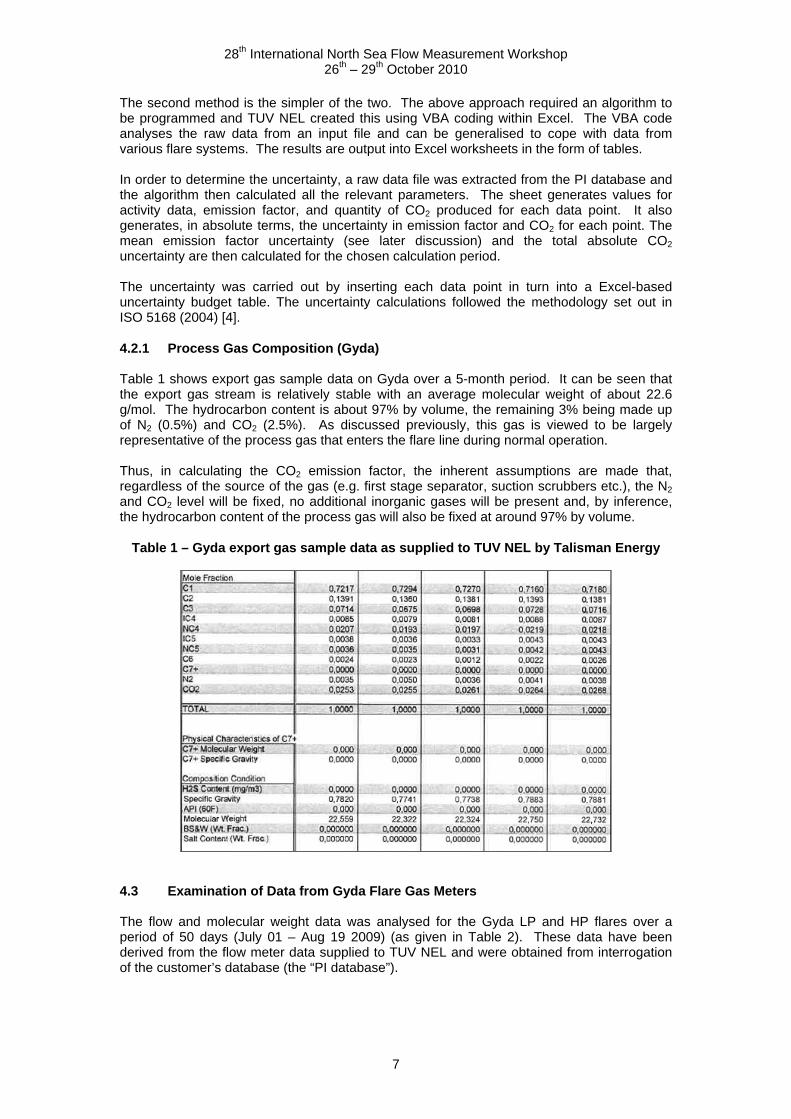
Flow data is taken from the actual archived flow values whilst the molecular-weight values are interpolated from the recorded molecular weight values to coincide with the same time points as the flow rate (see later description of PI data collection method). The gas appears to be heavier and more variable on the LP flare (varying from 25.6 – 37.3 g/mol) than on the HP flare (23.5 – 32.0 g/mol). What is immediately apparent is that the molecular weight of the gas on both the LP and HP flares always exceeds the molecular weight of the export gas (22.6 g/mol). This can be explained, in part, by the addition of the nitrogen which, at a molecular weight of 28 g/mol, will tend to increase the average molecular weight of the emission gas. However, some of the increase in molecular weight is likely due to heavier hydrocarbons entering the process gas during specific flaring events. The data given in Table 2 appears to show that the flow rates through the Gyda LP and HP flare lines are moderately low and the risk of liquids occurring due to carry-over from the separators and/or condensation, due to temperature drops, is minimal. However, the Reynolds numbers are very low in both installations and this causes other issues for uncertainty as discussed later.

Table 2 - Summary of flow and molecular weight data for Gyda LP and HP flares based on 50-days’ worth of data

LP flare HP flare

Min Average Max Min Average Max Qme (kg/hr) 15.0 47.3 198.9 48.8 93.1 448.8

Qve (Sm3/day) 294 931 5298 1057 1962 8552

Me (g/kmol) 25.6 27.1 37.3 23.5 25.3 32.0

p (bar abs) 0.99 1.00 1.03 1.07 1.09 1.11 ReD (approx) 3303 10,421 43,803 2634 5028 24,250

Velocity (m/s) 0.2 0.65 3.7 0.04 0.08 0.33 N2 content (%) 2.0 11.6 36.7 5.6 24.5 45.4 Notes: 1 The values for max/min values for N2 content and Me do not necessarily correspond to max/min flow rate values 2 Pipe Reynolds number, ReD, based on assumed viscosity for methane of 1.1 x 10-5 kg/m-s 3 Velocity based on average pressure & ambient temperature

It should be noted that the above observations are based on a limited set of data spanning only 50-days and it is recognised that more variable conditions may occur on occasion during a given year. In addition, changes to the facility (e.g. tie-backs to subsea platforms, system upgrades etc.) in subsequent years may also change the flow rates, line conditions and gas composition. There may be a requirement to revisit the uncertainty analysis in such cases. 5 FLOW MEASUREMENT As previously discussed the flow rate of the total gas flared (the emission gas) and the nitrogen injected is needed to determine the emission factor. These measurements are discussed in more detail below. 5.1 Emission Gas Flow Rate The emission gas flow rate is measured using single-path flare gas ultrasonic meters. The flare gas meters installed on Gyda are single-path transit time ultrasonic meters with the beams at an angle of 45° to the flow. The primary measurement is the transit time difference, t, which varies as a function of the velocity.


9

The volume flowrate is calculated within the meter from knowledge the pipe diameter, an assumption of an ‘ideal’ flow profile, and the measured velocity along the path. Volume flowrate can be calculated at standard reference conditions using the following equation

ss

sve Z

Z

T

T

p

p

tt

tLkAQ

1221cos2

(Sm3/s) (1)

From an uncertainty point of view, the key input parameters in the above equation are the transit times, t12 and t21, correction factor, k, and pipe area, A. The path length, L, and beam angle,, should be known to a reasonable accuracy. Velocity of sound, c, can also be determined from the transit times and path length, L, using

1221

1221

2 tt

ttLc (2)

The molecular weight is calculated from c using a proprietary algorithm which was supplied to TUV NEL for analysis. The algorithm calculates the molecular weight of emission gas, Me, from c and measured temperature assuming that the gas is mostly made up of hydrocarbons. There is currently no facility for correcting molecular weight for significant nitrogen content or increased gas pressure. However, recent advances to the technology allow these corrections to be made so there is the option to upgrade the meters in the future. For this application, the meters used are configured to measure and return the mass flowrate. Since the calculation of mass is an intermediate step in determining mass of CO2 emissions, the uncertainty analysis is effectively carried out on the fundamental measurements of standard volume. 5.2 Nitrogen Purge Meters The flow of nitrogen is reportedly maintained at a constant rate and measured using on-line variable area flowmeters (VAMs). The nitrogen flowrate is read and recorded manually once a day for quality control and monitoring purposes and to ensure the flare remains safely purged. This is a typical installation in the North Sea sector where low accuracy meters, originally installed for process control, are now being used as part of the measurement system. There was no indication of the standard conditions which have been assumed when setting the VAM flow scale (range). It was assumed that ‘normal’ conditions of 0°C and 1.01325 bar were specified, however it is known that the manufacturer of these particular meters normally use 15°C or 20°C. In common with many purge gas meters, the calibration and traceability of these VAMs was not as strictly controlled as might be expected for a regulated system. As no measurements of pressure and temperature were taken at the VAM it was assumed that the meter operates marginally above the flare gas pressure (approximately atmospheric pressure) and is assumed to operate at ambient temperature. No correction for errors due to incorrect standard conditions is being applied. 5.3 Data Logging and Reduction Before embarking on an uncertainty analysis it is important to appreciate the method of data logging and reduction. This requires a comprehensive understanding of the measurement process from the instrumentation, data acquisition and any subsequent calculations, through to the PI database.


10

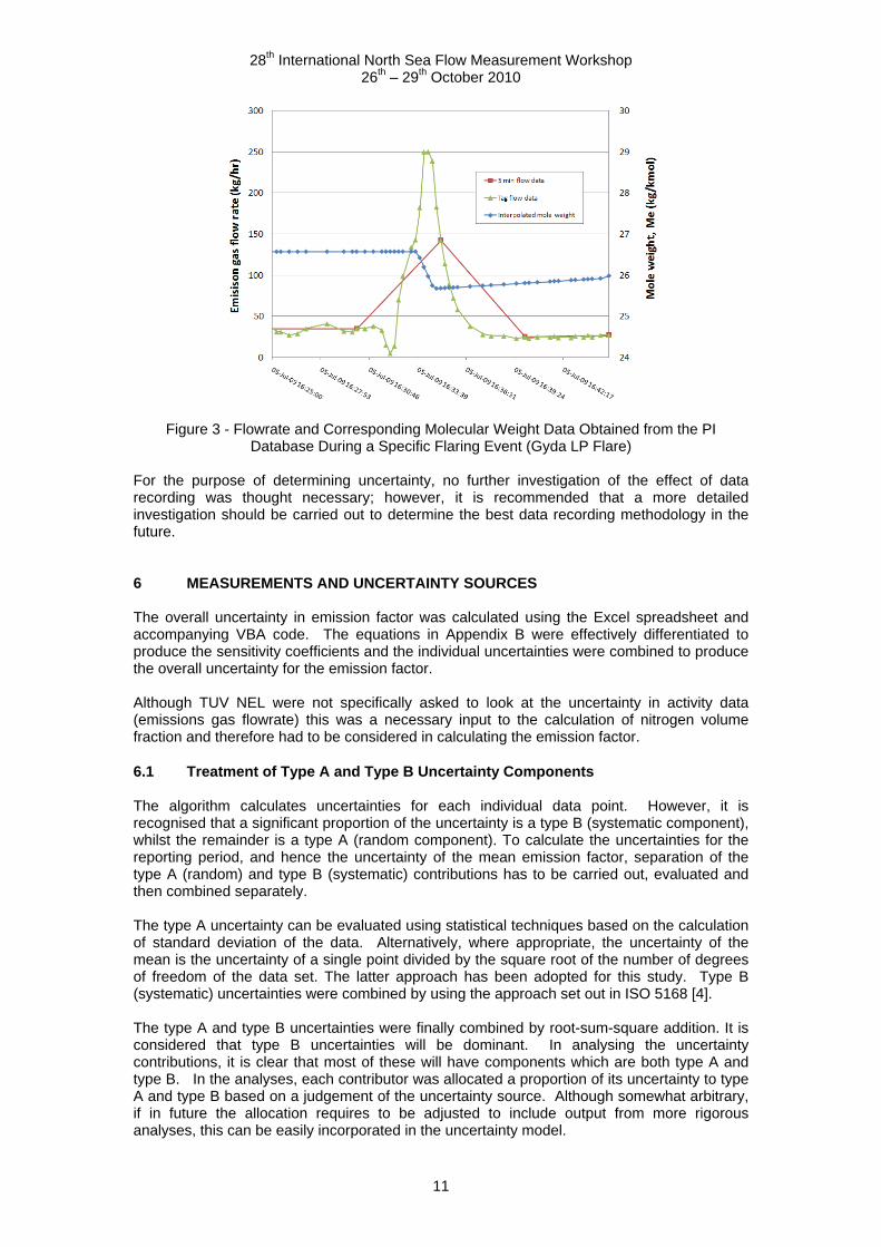
The measurements associated with the measurement of the emission gas are pressure, temperature, flowrate and molecular weight. Typically, pressure is measured well upstream of the meter (in the current case at the knock-out drum) and is read by the ultrasonic meter’s flow computer and returned to the supervisory computer (in this case a Honeywell DCS system). Flowrate and molecular weight are calculated by the meter’s flow computer and also returned to the DCS. Temperature is measured by a probe located downstream of the ultrasonic meter and read by the meter flow computer. This is not currently being returned to the DCS (all calculations being carried out within the flow computer). The DCS interrogates the meter at a given sample rate (believed to be 15 seconds). The DCS returns these values to the PI database for archiving. The PI interface software then carries out ‘exception filtering’ allowing only measured data points which change significantly from the previous reading to be sent to the main PI server application. This reduces the amount of data sent to the main PI database server. Data sent to the PI database server is subject to further ‘data compression’ whereby data not following a specific linear trend is excluded, once again allowing a reduction in data archived, without any (apparent) loss of significant information. All stored points are archived with a date and time-stamp. 5.3.1 Examination of the Recorded Mass Flow Rate from the Gyda LP Flare Archive data can be retrieved in different ways from the database and this will have been archived from raw data with different degrees of filtering and analyses. It is noted, however, that only the archived data, after exception and compression filtering, can be retrieved. The first retrieval method used was to request data at specific time intervals. This is the method employed in previous analyses and was initially proposed to be used in this work. Data at five-minute intervals was proposed to best follow the perceived frequency and magnitude of the flare flowrate variations. This information was generated based on a linear interpolation between the archived data before and after each selected time value. Figure 3 shows the emission gas flow rate, and corresponding molecular weight, during a flare event occurring in the LP line. If data is collected from the archive at 5-minute intervals, then it can be seen that the high flare event is not adequately resolved. The second retrieval method is to return each archived flowrate value. It is noted that these are not regular intervals owing to the data compression being applied; however each value carries an accompanying time stamp or tag. Similar data for molecular weight is available but the data points would be asynchronous with the flow data. For this examination, molecular weight data was returned as interpolated data at the same tag times as the flow data. It would be difficult to obtain molecular weight data coincident with each flowrate in any other way unless the sequence of data logging was changed and flow and molecular weight data were recorded together. The archived data appears to follow what would be expected from an event. It is noted that molecular weight variation follows the flow event – in this case it reduces as the flow increases (and the percentage of nitrogen reduces). This reflects the situation where the hydrocarbon content is significantly above that of the export gas, but the percentage of the nitrogen has reduced. As molecular weight at this time is based on interpolated values taken between successive flowrates, some damping of the variation is observed.


11

Figure 3 - Flowrate and Corresponding Molecular Weight Data Obtained from the PI Database During a Specific Flaring Event (Gyda LP Flare)

For the purpose of determining uncertainty, no further investigation of the effect of data recording was thought necessary; however, it is recommended that a more detailed investigation should be carried out to determine the best data recording methodology in the future. 6 MEASUREMENTS AND UNCERTAINTY SOURCES The overall uncertainty in emission factor was calculated using the Excel spreadsheet and accompanying VBA code. The equations in Appendix B were effectively differentiated to produce the sensitivity coefficients and the individual uncertainties were combined to produce the overall uncertainty for the emission factor. Although TUV NEL were not specifically asked to look at the uncertainty in activity data (emissions gas flowrate) this was a necessary input to the calculation of nitrogen volume fraction and therefore had to be considered in calculating the emission factor. 6.1 Treatment of Type A and Type B Uncertainty Components The algorithm calculates uncertainties for each individual data point. However, it is recognised that a significant proportion of the uncertainty is a type B (systematic component), whilst the remainder is a type A (random component). To calculate the uncertainties for the reporting period, and hence the uncertainty of the mean emission factor, separation of the type A (random) and type B (systematic) contributions has to be carried out, evaluated and then combined separately. The type A uncertainty can be evaluated using statistical techniques based on the calculation of standard deviation of the data. Alternatively, where appropriate, the uncertainty of the mean is the uncertainty of a single point divided by the square root of the number of degrees of freedom of the data set. The latter approach has been adopted for this study. Type B (systematic) uncertainties were combined by using the approach set out in ISO 5168 [4]. The type A and type B uncertainties were finally combined by root-sum-square addition. It is considered that type B uncertainties will be dominant. In analysing the uncertainty contributions, it is clear that most of these will have components which are both type A and type B. In the analyses, each contributor was allocated a proportion of its uncertainty to type A and type B based on a judgement of the uncertainty source. Although somewhat arbitrary, if in future the allocation requires to be adjusted to include output from more rigorous analyses, this can be easily incorporated in the uncertainty model.


12

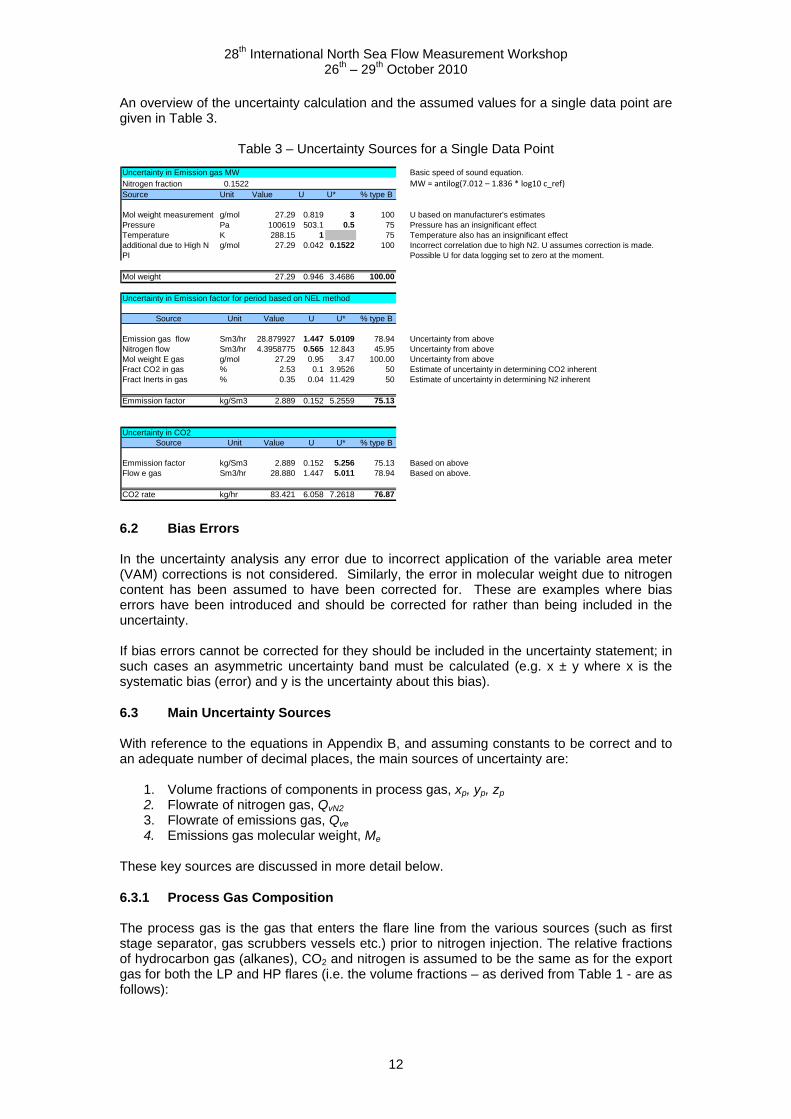
An overview of the uncertainty calculation and the assumed values for a single data point are given in Table 3.

Table 3 – Uncertainty Sources for a Single Data Point

Uncertainty in Emission gas MW Basic speed of sound equation.Nitrogen fraction 0.1522 MW = antilog(7.012 – 1.836 * log10 c_ref)Source Unit Value U U* % type B

Mol weight measurement g/mol 27.29 0.819 3 100 U based on manufacturer's estimates Pressure Pa 100619 503.1 0.5 75 Pressure has an insignificant effect Temperature K 288.15 1 75 Temperature also has an insignificant effect additional due to High N g/mol 27.29 0.042 0.1522 100 Incorrect correlation due to high N2. U assumes correction is made. PI Possible U for data logging set to zero at the moment.

Mol weight 27.29 0.946 3.4686 100.00

Uncertainty in Emission factor for period based on NEL method

Source Unit Value U U* % type B

Emission gas flow Sm3/hr 28.879927 1.447 5.0109 78.94 Uncertainty from aboveNitrogen flow Sm3/hr 4.3958775 0.565 12.843 45.95 Uncertainty from aboveMol weight E gas g/mol 27.29 0.95 3.47 100.00 Uncertainty from aboveFract CO2 in gas % 2.53 0.1 3.9526 50 Estimate of uncertainty in determining CO2 inherentFract Inerts in gas % 0.35 0.04 11.429 50 Estimate of uncertainty in determining N2 inherent

Emmission factor kg/Sm3 2.889 0.152 5.2559 75.13

Uncertainty in CO2 Source Unit Value U U* % type B

Emmission factor kg/Sm3 2.889 0.152 5.256 75.13 Based on aboveFlow e gas Sm3/hr 28.880 1.447 5.011 78.94 Based on above.

CO2 rate kg/hr 83.421 6.058 7.2618 76.87 6.2 Bias Errors In the uncertainty analysis any error due to incorrect application of the variable area meter (VAM) corrections is not considered. Similarly, the error in molecular weight due to nitrogen content has been assumed to have been corrected for. These are examples where bias errors have been introduced and should be corrected for rather than being included in the uncertainty. If bias errors cannot be corrected for they should be included in the uncertainty statement; in such cases an asymmetric uncertainty band must be calculated (e.g. x ± y where x is the systematic bias (error) and y is the uncertainty about this bias).

6.3 Main Uncertainty Sources With reference to the equations in Appendix B, and assuming constants to be correct and to an adequate number of decimal places, the main sources of uncertainty are:

1. Volume fractions of components in process gas, xp, yp, zp 2. Flowrate of nitrogen gas, QvN2 3. Flowrate of emissions gas, Qve 4. Emissions gas molecular weight, Me

These key sources are discussed in more detail below. 6.3.1 Process Gas Composition The process gas is the gas that enters the flare line from the various sources (such as first stage separator, gas scrubbers vessels etc.) prior to nitrogen injection. The relative fractions of hydrocarbon gas (alkanes), CO2 and nitrogen is assumed to be the same as for the export gas for both the LP and HP flares (i.e. the volume fractions – as derived from Table 1 - are as follows):


13

Hydrocarbon fraction, xp = 97% CO2 fraction, yp = 2.5% N2 fraction, zp = 0.5%. The uncertainty of this assumption must include any estimated differences in the composition of the process gas from that of the export gas. If a process upset occurs, the flowrate of gas increases markedly and the composition of the gas changes, depending on the nature of the event. The uncertainty in the CO2 and N2 fractions (expressed as a percentage) are taken to be 0.04 and 0.1% respectively. The hydrocarbon content is simply determined as xp = 1 – (yp + zp) and its uncertainty is subsumed in the calculation of Me. Note: The uncertainty in compressibility is assumed to be negligible as the line pressure and temperature will be close to ambient the majority of the time. 6.3.2 Uncertainty in the Nitrogen Flowrate, QvN2 (as measured by a variable area

meter) The nitrogen flowmeters are variable area meters set up to indicate in standard volume units (Sm3/hr). These devices have a stated uncertainty of 2% of span. The LP meter has span of 25 Sm3/hr while HP meter has span of 100 Sm3/hr. The set flowrate was 4.5 Sm3/hr for the LP meter and 20 Sm3/hr for the HP meter. Therefore 2% of span equates to an uncertainty of reading of 11% for the LP meter and 10% for the HP meter respectively. In the absence of any significant meter data, the set value is taken to be nominally constant. Therefore, the consistency of the manual reading and setting, any effect of changes in nitrogen supply and pressure and temperature, can only be speculative. Pressure, temperature and barometric pressure are not currently recorded. Correction is not applied for actual density of the nitrogen and, in fact, some doubt remained as to the actual meter conditions. The lack of correction is considered to generate an error. The magnitude of the error has been assessed, however only the uncertainty in the error has been included in the budget. However these errors were included within a list of bias errors. It would be advisable to measure temperature and pressure at the nitrogen meters (even at a relatively low accuracy), and to correct the readings in order to reduce uncertainty and remove a potential source of bias. 6.3.3 Uncertainty in the Emission Gas Flowrate, Qve (as measured by flare gas

ultrasonic meter) Detailed uncertainty analyses of the performance of ultrasonic meters had been carried out previously [5] and from this, and the manufacturers estimate of uncertainty, an uncertainty of 4% was assumed as a baseline value for the Gyda flare gas meters. Additional uncertainty needs to be included to account for deviations from ideal, fully developed flow conditions. The meter vendor quotes an uncertainty of between 2.5% to 5% between the limits 0.3 m/s to 100 m/s. Uncertainty will increase at velocities below 0.3 m/s and this is an area where the meters are operating. Although the meter is specified to work between 0.03 – 0.3 m/s, the uncertainty will be a lot higher because the timing resolution starts to dominate. To cover this, each meter was allocated a “low-flow cut-off point” below which the uncertainty starts to rapidly increase. An additional increase in uncertainty is encountered if the Reynolds numbers are such that the flow regime becomes laminar/transitional. This is due to incorrect flow profile corrections. Bias errors will be evident in such cases; however, these are difficult to quantify in the transition region.


14

Currently the uncertainty analysis assumes that this error will be within the increased uncertainty already included at low-velocity. This may require more detailed examination if uncertainty is to be more accurately determined. Additional uncertainty will be introduced if an “non-ideal” flow profile is evident across the measurement plane. An uncertainty due to installation effect has to be recognised; however, this is difficult to assess without detailed drawings of the installation. CFD simulations of the installation can be carried out determine the installation error [6]. Some additional uncertainty was included to take account of pipe roughness at high Reynolds numbers which will affect the flow profile and, therefore, the meter factor. Temperature and pressure uncertainties also are included in the uncertainty budget. As absolute transducers are used for pressure, no uncertainty needs to be considered for variations in barometric pressure. Although pressure is measured at the knock-out drum upstream of the meter it is assumed there is no pressure loss between the drum and the meter. It is not currently known where the temperature is measured but it is assumed to be close to or near the meter. A nominal value has been included to cover installation (non-ideal flow profile) effects and pipe diameter variation has been included but may require modification following a full assessment of the metering installation. 6.3.4 Uncertainty in Molecular Weight Correlation, Me The molecular weight correlation is known to be affected by the volume fraction of inert and non-hydrocarbon (inorganic) gases, such as nitrogen, water vapour, hydrogen etc. The presence of these gases will cause the calculated molecular weight to be in error. In addition, the presence of liquids will cause serious problems with the molecular weight correlation (and also the measured flow rate). It is currently assumed that the meter algorithm is configured to assume a typical hydrocarbon gas and has not been adjusted to recognise the high nitrogen concentration, nor the variability of this concentration with flowrate. If the nitrogen concentration is not accounted for, a significant error in the molecular weight (and indeed the mass flowrate) will be evident. A proprietary algorithm is used to correlate the measurement of speed of sound and local temperature. The algorithm is based on an empirical fit to various hydrocarbon gas mixtures. The overall uncertainty in Me owing to timing resolution, path length, temperature correction and curve-fit to the gas data is stated as 3% in the uncertainty reports (for activity data in mass units) supplied to TUV NEL from Talisman [5]. In addition to this there will be uncertainty in Me due to pressure and the presence of non-hydrocarbons. The main issue for the molecular weight correlation is the injected nitrogen which is not currently being accounted for. Effect of Nitrogen on the Molecular Weight Correlation The error in the molecular weight correlation was assessed by calculating speed of sound for a range of gas mixtures using the AGA 10 method. This sound speed was then input to the equations at 0°C, 20°C and 30°C and the calculated value of Me was compared with the actual molecular weight of the gas mixture. The percentage error (referred to the case where no nitrogen is injected into the flare line) was seen to be linear with nitrogen content. Thus, at 50% N2, the error is -5.2% and it is -2.6% at 25% N2. Discussions with the meter vendor reveal this to be a realistic number, comparing well with their own analyses with methane/N2 mixtures which showed a -5.8% difference between 50% and 0% N2 (i.e. 100% methane) [7].


15

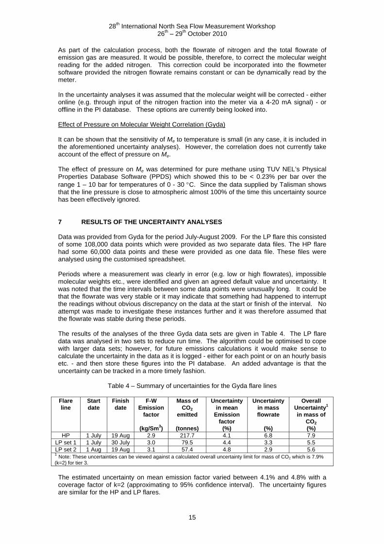
As part of the calculation process, both the flowrate of nitrogen and the total flowrate of emission gas are measured. It would be possible, therefore, to correct the molecular weight reading for the added nitrogen. This correction could be incorporated into the flowmeter software provided the nitrogen flowrate remains constant or can be dynamically read by the meter. In the uncertainty analyses it was assumed that the molecular weight will be corrected - either online (e.g. through input of the nitrogen fraction into the meter via a 4-20 mA signal) - or offline in the PI database. These options are currently being looked into. Effect of Pressure on Molecular Weight Correlation (Gyda) It can be shown that the sensitivity of Me to temperature is small (in any case, it is included in the aforementioned uncertainty analyses). However, the correlation does not currently take account of the effect of pressure on Me. The effect of pressure on Me was determined for pure methane using TUV NEL’s Physical Properties Database Software (PPDS) which showed this to be < 0.23% per bar over the range 1 – 10 bar for temperatures of 0 - 30 C. Since the data supplied by Talisman shows that the line pressure is close to atmospheric almost 100% of the time this uncertainty source has been effectively ignored. 7 RESULTS OF THE UNCERTAINTY ANALYSES Data was provided from Gyda for the period July-August 2009. For the LP flare this consisted of some 108,000 data points which were provided as two separate data files. The HP flare had some 60,000 data points and these were provided as one data file. These files were analysed using the customised spreadsheet. Periods where a measurement was clearly in error (e.g. low or high flowrates), impossible molecular weights etc., were identified and given an agreed default value and uncertainty. It was noted that the time intervals between some data points were unusually long. It could be that the flowrate was very stable or it may indicate that something had happened to interrupt the readings without obvious discrepancy on the data at the start or finish of the interval. No attempt was made to investigate these instances further and it was therefore assumed that the flowrate was stable during these periods. The results of the analyses of the three Gyda data sets are given in Table 4. The LP flare data was analysed in two sets to reduce run time. The algorithm could be optimised to cope with larger data sets; however, for future emissions calculations it would make sense to calculate the uncertainty in the data as it is logged - either for each point or on an hourly basis etc. - and then store these figures into the PI database. An added advantage is that the uncertainty can be tracked in a more timely fashion.

Table 4 – Summary of uncertainties for the Gyda flare lines Flare line

Start date

Finish date

F-W Emission

factor

(kg/Sm3)

Mass of CO2

emitted

(tonnes)

Uncertainty in mean

Emission factor

(%)

Uncertainty in mass flowrate

(%)

Overall Uncertainty1 in mass of

CO2 (%)

HP 1 July 19 Aug 2.9 217.7 4.1 6.8 7.9 LP set 1 1 July 30 July 3.0 79.5 4.4 3.3 5.5 LP set 2 1 Aug 19 Aug 3.1 57.4 4.8 2.9 5.6 1 Note: These uncertainties can be viewed against a calculated overall uncertainty limit for mass of CO2 which is 7.9% (k=2) for tier 3. The estimated uncertainty on mean emission factor varied between 4.1% and 4.8% with a coverage factor of k=2 (approximating to 95% confidence interval). The uncertainty figures are similar for the HP and LP flares.


16

Although this uncertainty is higher than the tier 3 limit of 2.5%, it is noted that the overall uncertainty on mass of CO2 is between 5.5% and 7.9% and therefore falls within the overall uncertainty limit on CO2 (7.9%) as calculated from the tier 3 limits for activity data and emission factor. Once again, it is noted that the above results are based on 50-day’s worth of data which may not be enough to completely define the limits on the process conditions. 8 CONCLUSIONS AND RECOMMENDATIONS The uncertainty on the Gyda and Varg flare systems was assessed for Talisman Energy Norge AS [8]. This paper concentrates on the results from the Gyda flares. A significant part of this work was in producing a revised calculation procedure for emission factor. Logging and data handling were looked into in detail and, based on these findings, a more appropriate methodology for extracting the data was suggested. The analysis highlighted the importance of calculating the mean, flow-weighted emission factor from the raw data rather than a constant value. Since conditions can vary widely in a flare line, the importance of analysing the emissions factor based on all the available data is clear. The analysis and archiving of the data should reflect the need to have coincident values of flowrate, molecular weight and properties. It may be advisable to have the calculation of uncertainty carried out at the data collection stage allowing a cumulative uncertainty to be generated for any time period, thus doing away with the need for retrospective analyses The measurements of the flowrate of nitrogen need to be examined in detail. The effect of not correcting for pressure at the variable area meter has the potential for producing a very large error depending on line pressure. It would be prudent to replace the current flowmeters with more modern and accurate technology. The effect of ignoring the nitrogen content of the gas on molecular weight will be an error of about 3 - 4% at low flare flowrates. This can be corrected offline if it cannot be incorporated in the meter in some way (e.g. live feedback of nitrogen content to flow computer). The effect of not measuring or accurately accounting for temperature and pressure of the nitrogen is relatively small, of the order of 0.5%. Although the calculated uncertainty in the emission factor lies outside the EU ETS tier 3 limits for the LP and HP flares, the overall uncertainty on mass of CO2 is within the limits if the values for activity data and emission factor are duly combined. However, it is noted that these figures are based on limited data. The calculation would need to be carried out for the agreed EU ETS reporting period. At time of writing Talisman are currently in discussion with the regulator as to whether the methodology of calculating emission factor using speed of sound output from the flare gas meter will be accepted. 9 DEFINITIONS The following definitions have been used to describe the various parameters in the calculation process for emission factor: Activity data: the quantity of gas flared (this redefined here as the quantity of Emissions Gas as below) Emission Factor: factor relating the quantity of CO2 produced from the emission gas after combustion to the total quantity of emission gas produced. Although emission factor may be


17

expressed in relative to mass or volume of emission gas, under EU ETS guidelines this is expressed as the mass of CO2 for each Standard cubic meter of emission gas. (kg of CO2/Sm3) Emissions Gas: the gas discharged to the flare. This is the Process gas combined with the nitrogen purge gas. Hydrocarbon Gas: the mixed hydrocarbon gas components within the Process Gas. Process Gas: The gas generated by the process and discharged to the flare line. This excludes any measured purge gas. Standard Volume: the volume occupied by a quantity of gas if it was at defined conditions. The Standard conditions for this application are 273.15 K (0 °C) and 101325 Pa. Normal Volume: an alternative to Standard volume conventionally applied to the conditions specified above. This is the term used in the EU ETS guidelines and as stated above. 10 ACKNOWLEDGEMENTS TUV NEL wishes to thank Pål Jaghø, Vidar Gabrielsen and Alice Baker at Talisman Energy Norge AS for their support during the project, and Jed Matson at GE Sensing for his advice on the molecular weight correlation. 11 REFERENCES [1] Directive 2003/87/EC of the European Parliament and of the Council of 13 October

2003 establishing a scheme for greenhouse gas emission allowance trading within the Community and amending Council Directive 96/61/EC

[2] 2007/589/EC: Commission Decision of 18 July 2007 Establishing Guidelines for the

Monitoring and Reporting of Greenhouse Gas Emissions Pursuant to Directive 2003/87/EC of the European Parliament and of the Council (notified under document number C(2007) 3416) (Text with EEA relevance) http://eur-lex.europa.eu/LexUriServ/LexUriServ.do?uri=CELEX:32007D0589:en:NOT

[3] Frøysa, K-E et al, Nitrogen subtraction on reported CO2 emissions using ultrasonic

flare gas meters, In 27th International North Sea Flow Measurement Workshop, 20 - 23 October, Tonsberg, Norway, 2009

[4] International Standards Organisation ISO 5168:2005, Measurement of fluid flow –

procedures for the evaluation of uncertainties [5] Usikkerhets analyse for USM flare/vent gas flowmeters: PEM-3431-UNCERT-HP-

GYDA and PE M-3431-UNCERT-LP-GYDA. [6] Gibson, J. Validation of the CFD method for determining the measurement error in

Flare Gas Ultrasonic meter installations, In 27th International North Sea Flow Measurement Workshop, 20 - 23 October, Tonsberg, Norway, 2009

[7] Private Communication - Jed Matson, GE Sensing, Billerica, MA, Sept 2009. [8] TUV NEL Report No. 2009/240 for Talisman Energy Norge AS, Evaluation of

Uncertainty in Emission Factor for Gyda and Varg Oil and Gas Facilities, September 2009 (Commercially Restricted)


18

APPENDIX A - SAMPLE CALCULATION OF UNCERTAINTY ON TOTAL CO2 Assuming activity data and emission factor uncertainties to be uncorrelated, the limit on overall expanded (k=2) uncertainty in CO2 can be calculated from the limits given in the EU ETS MRG [2] for the highest tier approach (i.e. 7.5% on activity data (flow) and 2.5% on emission factor) as

%...UCO 975257 222

Hence, 7.9% (k=2) represents the highest uncertainty on the reported mass of CO2 that can be tolerated. Two possible scenarios are shown in the example below. Operator A’s uncertainty values for activity data and emission factor happen to equate to the tier 3 limits and has, therefore, only just complied with the MRG on both counts. Operator B has failed to meet the minimum uncertainty requirement for the emission factor of 2.5%. This is despite the overall uncertainty in mass of CO2 being 1.5% lower than Operator A’s who has met the individual requirements. Obviously if the uncertainty on activity data is already close to the 7.5% limit then operator B would fail both the individual requirement on emission factor and would exceed the 7.9% uncertainty value for overall CO2 emission. In this case an uncertainty of up to 6.8% on activity data can be tolerated before Operator B will exceed 7.9% (as shown by the values in brackets). Operator A Uncertainty on activity data = 7.5% Uncertainty on emission factor = 2.5% Total uncertainty on tCO2 = 7.9% Operator B Uncertainty on activity data = 5.0% (6.8%) Uncertainty on emission factor = 4.0% (4.0%) Total uncertainty on tCO2 = 6.4% (7.9%)


19

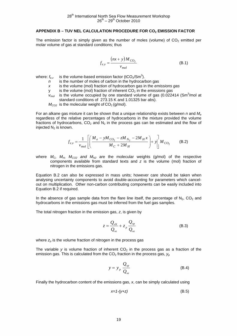
APPENDIX B – TUV NEL CALCULATION PROCEDURE FOR CO2 EMISSION FACTOR The emission factor is simply given as the number of moles (volume) of CO2 emitted per molar volume of gas at standard conditions; thus

mol

COv,e v

Mynxf 2

(B.1)

where: fe,v is the volume-based emission factor (tCO2/Sm3). n is the number of moles of carbon in the hydrocarbon gas x is the volume (mol) fraction of hydrocarbon gas in the emissions gas y is the volume (mol) fraction of inherent CO2 in the emissions gas vmol is the volume occupied by one standard volume of gas (0.022414 (Sm3/mol at

standard conditions of 273.15 K and 1.01325 bar abs). MCO2 is the molecular weight of CO2 (g/mol). For an alkane gas mixture it can be shown that a unique relationship exists between n and Me regardless of the relative percentages of hydrocarbons in the mixture provided the volume fractions of hydrocarbons, CO2 and N2 in the process gas can be estimated and the flow of injected N2 is known.

2

22

2

21CO

HC

HNCOe

molv,e My

MM

xMzMyMM

vf

(B.2)

where MC, MH, MCO2 and MN2 are the molecular weights (g/mol) of the respective

components available from standard texts and z is the volume (mol) fraction of nitrogen in the emissions gas.

Equation B.2 can also be expressed in mass units; however care should be taken when analysing uncertainty components to avoid double-accounting for parameters which cancel-out on multiplication. Other non-carbon contributing components can be easily included into Equation B.2 if required. In the absence of gas sample data from the flare line itself, the percentage of N2, CO2 and hydrocarbons in the emissions gas must be inferred from the fuel gas samples. The total nitrogen fraction in the emission gas, z, is given by

ve

vpp

ve

vN

Q

Qz

Q

Qz (B.3)

where zp is the volume fraction of nitrogen in the process gas The variable y is volume fraction of inherent CO2 in the process gas as a fraction of the emission gas. This is calculated from the CO2 fraction in the process gas, yp

ve

vpp Q

Qyy (B.4)

Finally the hydrocarbon content of the emissions gas, x, can be simply calculated using

x=1-(y+z) (B.5)

Calculation of the Uncertainty in the CO2 Emissions Factor in ...

Documents

Transcript of Calculation of the Uncertainty in the CO2 Emissions Factor in ...