Building and Characterizing Regional and Global EmissionInventories of Toxic PollutantsStefano Cucurachi,*,† Serenella Sala,‡ Alexis Laurent,§ and Reinout Heijungs†,⊥

†Institute of Environmental Sciences (CML), Leiden University, P.O. Box 9518, 2300 RA Leiden, The Netherlands‡Sustainability Assessment Unit, European Commission, DG Joint Research Centre, Institute for Environment and Sustainability, ViaEnrico Fermi, 2749, 21027 Ispra Varese, Italy§Division for Quantitative Sustainability Assessment (QSA), Department of Management Engineering, Technical University ofDenmark (DTU), Anker Engelunds Vej 1, 2800 Kongens Lyngby, Denmark⊥Department of Econometrics and Operations Research, VU University Amsterdam, De Boelelaan 1105, 1081 HV Amsterdam, TheNetherlands

*S Supporting Information

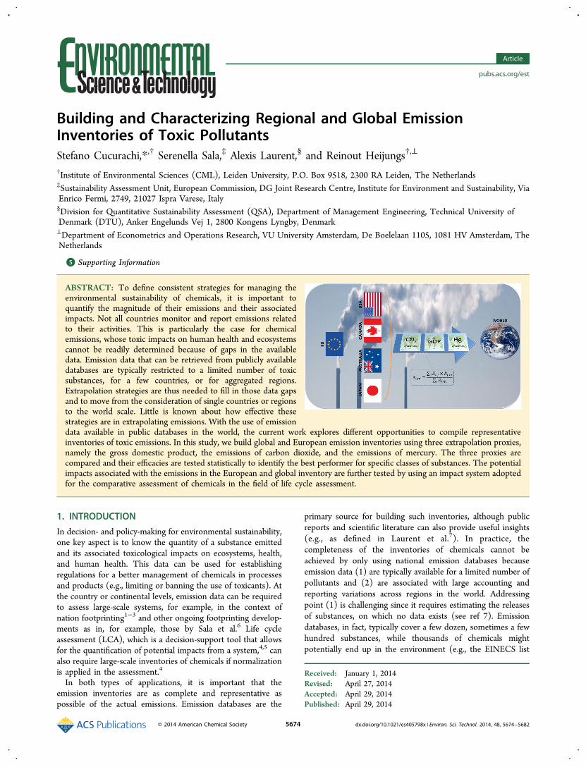
ABSTRACT: To define consistent strategies for managing theenvironmental sustainability of chemicals, it is important toquantify the magnitude of their emissions and their associatedimpacts. Not all countries monitor and report emissions relatedto their activities. This is particularly the case for chemicalemissions, whose toxic impacts on human health and ecosystemscannot be readily determined because of gaps in the availabledata. Emission data that can be retrieved from publicly availabledatabases are typically restricted to a limited number of toxicsubstances, for a few countries, or for aggregated regions.Extrapolation strategies are thus needed to fill in those data gapsand to move from the consideration of single countries or regionsto the world scale. Little is known about how effective thesestrategies are in extrapolating emissions. With the use of emissiondata available in public databases in the world, the current work explores different opportunities to compile representativeinventories of toxic emissions. In this study, we build global and European emission inventories using three extrapolation proxies,namely the gross domestic product, the emissions of carbon dioxide, and the emissions of mercury. The three proxies arecompared and their efficacies are tested statistically to identify the best performer for specific classes of substances. The potentialimpacts associated with the emissions in the European and global inventory are further tested by using an impact system adoptedfor the comparative assessment of chemicals in the field of life cycle assessment.

1. INTRODUCTION

In decision- and policy-making for environmental sustainability,one key aspect is to know the quantity of a substance emittedand its associated toxicological impacts on ecosystems, health,and human health. This data can be used for establishingregulations for a better management of chemicals in processesand products (e.g., limiting or banning the use of toxicants). Atthe country or continental levels, emission data can be requiredto assess large-scale systems, for example, in the context ofnation footprinting1−3 and other ongoing footprinting develop-ments as in, for example, those by Sala et al.6 Life cycleassessment (LCA), which is a decision-support tool that allowsfor the quantification of potential impacts from a system,4,5 canalso require large-scale inventories of chemicals if normalizationis applied in the assessment.4

In both types of applications, it is important that theemission inventories are as complete and representative aspossible of the actual emissions. Emission databases are the

primary source for building such inventories, although publicreports and scientific literature can also provide useful insights(e.g., as defined in Laurent et al.7). In practice, thecompleteness of the inventories of chemicals cannot beachieved by only using national emission databases becauseemission data (1) are typically available for a limited number ofpollutants and (2) are associated with large accounting andreporting variations across regions in the world. Addressingpoint (1) is challenging since it requires estimating the releasesof substances, on which no data exists (see ref 7). Emissiondatabases, in fact, typically cover a few dozen, sometimes a fewhundred substances, while thousands of chemicals mightpotentially end up in the environment (e.g., the EINECS list

Received: January 1, 2014Revised: April 27, 2014Accepted: April 29, 2014Published: April 29, 2014

Article

pubs.acs.org/est

© 2014 American Chemical Society 5674 dx.doi.org/10.1021/es405798x | Environ. Sci. Technol. 2014, 48, 5674−5682

currently contains ca. 100 000 chemicals of potential use on theEuropean market). Mitigating this limitation is not addressed inthe present study.With regard to point (2), extrapolations can be performed to

fill in the gaps and to estimate emission inventories in countriesor regions where data are not available. The key in this exerciseis to find out the appropriate extrapolation parameters orproxies. The appropriateness of a proxy is defined by itsavailability for the regions that are considered and its ability tomatch the trends in the emissions of given pollutants. Proxiescan be differentiated according to different criteria, for example,the type of emitted pollutant, the source of the emissions, andthe type of activities.Until now, very little was known about the appropriateness

of different proxies for building emission inventories. Inprevious applications from the field of LCA, most worksrelated to the building of inventories of chemicals have used thegross domestic product (GDP) to extrapolate emissions fromone or several countries to a full region or to the entire world,although other proxies have also been used for specificsubstances, for example, a harvested area used as proxy forpesticide application from one country to another.8 In thisstudy, together with the GDP (reference year 20109) we testand compare the validity of the extrapolation of toxic emissionsbased on the emissions of carbon dioxide (CO2, reference year200910), and alternatively, based on the emissions of mercury(Hg, reference year 201011). We aim to address some of theseknowledge gaps and to explore different opportunities to buildcomprehensive inventories from the emission data available inpublic databases in a selection of countries of the world. Thefocus of the study is primarily centered on the generation of aEuropean and a global inventory of toxic emissions and thetesting of the proxies and assumptions used for the creation ofsuch inventories. These considerations could broadly be appliedto extrapolations at a country level. The creation of theEuropean inventory is determined by the greater availability ofdata for this region.In the following section, the procedure for the composition

of the European and global inventories are detailed, togetherwith the basis for the extrapolation process. The uncertaintiesrelated to the process of the collection of national data andtheir extrapolations to the world are discussed with examplesubstances showing great statistical correlation to a specificproxy. In the remainder of the study, the results are comparedand discussed, and recommendations are provided topractitioners and researchers with approaches for buildingemission inventories of toxic pollutants.Regional and global inventories of toxic emissions support

decision-makers, allowing them to improve environmentalregulations and to identify toxic emissions for which controland limits are needed. A possible use for the created inventoriesis to quantify the impacts associated with the emissionsrecorded in a certain area. The use of specific sets ofcharacterization factors elaborated in the field of LCA,USEtox,12 allows for the calculation of a total impact scorefor the inventories obtained for the 27 European countries plusSwitzerland, Norway, Iceland, and Serbia (EU) and the globe.The process of characterization of the inventory allows us tocheck the importance of the inclusion or the exclusion of somepollutant emissions (e.g., due to lack of data) and to identifythe most contributing substances to the overall impacts.Incidentally, the resulting impact scores can also be regardedas normalization references, which are thus directly applicable

to the normalization practice in LCA studies. Threeextrapolation proxies are investigated in the present study,namely GDP (reference year 20109), the emissions of carbondioxide (CO2, reference year 200910), and the emissions ofmercury (Hg, reference year 201011).

2. MATERIALS AND METHODS: BUILDING THEINVENTORY, DATA COLLECTION, ANDEXTRAPOLATIONS

The assessment of the quantity of chemicals emitted at theglobal scale was based on the development of extrapolationstrategies applied to existing chemical inventories at the countryscale. First, an inventory of toxic emissions for Europe wasdeveloped by enlarging currently available inventories in termsof the number of chemicals and updating the data to 2010, thatis, the year in which emissions occurredsee section 2.1.Details on the data sources, necessary extrapolations,limitations, and uncertainties of the emission data are reported.Second, additional chemical inventories were collected fromalready compiled national registries for the United States,Canada, Japan, and Australiasee section 2.2. Theseinventories were used to extrapolate global emissions usingthree different proxies as presented in section 2.3.

2.1. EU Toxic Emissions Inventory. The emissioninventory for Europe primarily covers the EU-27 countriesplus Switzerland, Norway, Iceland, and Serbia (EU). Theinventory covers releases to all emission compartments, that is,air, water, and soil. In Table 1, the substance groups consideredin the inventory are detailed, with the relative sources of thedata and an estimate of the goodness of the coverage obtainedfor each group. A detailed table presenting further uncertaintiesand limitations as well as the added value of the presentinventory compared to previous emission inventories ispresented in Table S1 of the Supporting Information.

2.1.1. Airborne Emissions. Data on HM and POPsemissions were collected from the EMEP/CEIP Centre13

(see Table S2 in the Supporting Information). Only the set ofemissions reporting “Officially reported emission data” wasused. The set of “Emissions as used in the EMEP models”13

was excluded because of potential inconsistencies between thetwo sets of data determined by recalculations and different gap-filling procedures. The completeness of the official registrydiffers from one country to another and from one sector toanother.13 Uncertainties are strongly dependent on theaggregation level that was used. Since only the totals for thewhole EU region were used, without any further country andsector disaggregation, these uncertainties are believed to benegligible.The total NMVOC emission data were retrieved from the

“Officially reported emission data” reports.13 The data wereextracted at the country level and 107 activity sectors weredistinguished. For each country, the sector-specific totalNMVOC emissions were combined with speciation profiles,that is, distributions of the NMVOC in single substances persector of activity, to derive single NMVOC emissions. Detailson the data sources and the methodology for assigning thespeciation profiles to the total NMVOC emissions can be foundin the publication by Laurent and Hauschild (2014).22 The dataon industrial emissions of HMs and organics were taken fromthe EMEP database13 and established through Regulation (EC)No 166/2006 on releases from industries. The databasecontains data on the main pollutant releases of about 28 000industrial facilities across the European Union and EFTA

Environmental Science & Technology Article

dx.doi.org/10.1021/es405798x | Environ. Sci. Technol. 2014, 48, 5674−56825675

countries. The available data represent the total annualemission releases during normal operations and accidents.The substances identified as not present in the data extractedfrom EMEP13 but reported in E-PRTR18 were added to theinventory (see Table S4 in the Supporting Information).2.1.2. Water-Borne Emissions. Emissions into water were

assessed by considering the industrial emissions of HMs andorganics and the emissions coming from wastewater treatmentplants. The data available on oil spills were too incomplete tobe added.The data on water-borne emissions of HMs and organics

were extracted from the E-PRTR database,18 accounting for90% of water-borne emissions. With regard to water-borneemissions, the data for 62 substances (9 HMs, 53 organics)were retrieved; however, large discrepancies in the countrycoverage at the EU level occurred as a result of variations inindustrial activities from one country to another or incompletereporting for some countries. Table S5 in the SupportingInformation provides an overview of the country coverage persubstance.The Waterbase15 database was used to estimate the releases

into freshwater of HMs and organics via wastewater, includingwastewater releases from industries covered in the E-PRTR.18

The risk of double-counting was avoided by a careful analysis ofthe data. The data for 2009 were used because they were morecomplete than those for the year 2010 at the time of datacollection. The emissions reported in the Waterbase15 wereaggregated at a country level and regarded as profiles, whichwere normalized with the population either connected or not toWWTP. These normalized numbers were used for extrapolat-ing to unreported countries.

Data were available mainly for The Netherlands and for alimited set of other countries, for which complete emissionprofiles could typically not be retrieved (e.g., in case of apopulation not connected to WWTP). Furthermore, data gapsregarding the apportionment of different wastewater handlingfacilities were identified for a number of countries. Source typesare reported in Tables S6a and S6b of the SupportingInformation. A framework was developed to estimate thereleases from households and institutional or commercialactivities. The framework relies on the assumption that releasescan be defined on a per-capita basis, accounting for adifferentiation of the countries, and the percentage ofpopulation connected to WWTP. The framework is reportedin Figure S1 of the Supporting Information and detailed in ref16. In Table S7 of the Supporting Information, water emissionsfrom all other sources included in the inventory are reported,although their country coverage was limited.

2.1.3. Soil-Borne Emissions. Soil-borne emissions are relatedmainly to industrial releases, to the direct application on soil ofsewage sludge (i.e., as soil amendment after specific treatment)and manure (i.e., as fertilizer on agricultural land), and topesticide use. For soil-borne industrial emissions, data wereextracted from E-PRTR,18 which reports emissions for 23substances (8 HMs, 15 organics). Large limitations in thecountry coverage were observed due to variations in industrialactivities from one country to another or incomplete reportingfor some countries (Table S8 of the Supporting Information).Sewage sludge was included in the inventory as a substantial

source of releases of organics and HMs. The data on the use ofsewage sludge applied to agricultural land was retrieved fromthe OECD.14 Extrapolations of data from one country to

Table 1. Overview of Substance Groups, Data Sources, and Coverage Estimates

substance groups data sources coverage estimatea

Air EmissionHM CLTAP/EMEP (EMEP 2013)13 ***organics (non-NMVOC) (e.g.,dioxins, PAH, HCB)

CLTAP/EMEP (EMEP 2013)13 *** (EMEP)

NMVOC E-PRTR (EEA 2012)17 ** (E-PRTR)total NMVOC per sector from EMEP/CORINAIR (EMEP 2013)13 ***literature sources (speciation per sectors) ***databases + CORINAIR23,24 for sector activity modeling

Water Emissionindustrial releases of HM + organics E-PRTR (EEA 2012)17 *** (HM)

waterbase (EEA 2013)15 * (organics)urban WWTP (HM + organics) waterbase (EEA 2013),15 OECD (2013),14 EUROSTAT (2013)16 * (EU covered via extrapolations from

few countries)Soil Emission

industrial releases (HM, POPs) E-PRTR (E-PRTR 2012)17 *sewage sludge (containing organicsand metals)

EEA (2012)17 + EUROSTAT (2013)17 for usage *** (HM)EC (2010)17 for HM compositionPistocchi et al. (2011) for dioxins17

manure FAOSTAT (2013),17 Amlinger et al. (2004),20 Chambers et al. (2001)21 ***Pesticides

active ingredients (AI) breakdown pesticide usage data: FAO (2012)10 and (F, H, I, O + chemical classes) +EUROSTAT (2013)16 for second check

**

use of extrapolations for AI differentiationsEUROSTAT (2013)16 for crop harvested areas

aThe values represent the completeness of the background data in terms of geographical coverage in Europe. The coverage of the emission data isestimated with respect to the countries covered (out of the EU-27) and the substances included (e.g., the number of substances considered) basedon expert judgment. The symbols used in the table are as follows: *** = good coverage; ** = medium coverage; and * = poor coverage. Thefollowing acronyms are used in the table: HM = heavy metals; NMVOC = nonmethane volatile organic compounds; WWTP = wastewater treatmentplants; POPs = persistent organic pollutants; PAH = polycyclic aromatic hydrocarbon; and HCB = hexachlorobenzene.

Environmental Science & Technology Article

dx.doi.org/10.1021/es405798x | Environ. Sci. Technol. 2014, 48, 5674−56825676

another were performed by coupling the emission data withaverage country-specific concentrations of HMs (Zn, Cu, Pb,Ni, Cr, Hg, Cd) and dioxins.17

For the emissions of HMs present in manure and slurry,country-specific concentrations were coupled with therespective national use of manure and slurries. The use ofmanure can be a substantial source of HMs in particularbecause of the mineral additives present in the feedstock foranimals (e.g., pig manure and slurry is typically associated withhigh levels of zinc and copper17). The data on animal livestock,obtained from FAOSTAT,17 was matched to the metalsassociated with the production of manure per type of livinganimal (e.g., mule, goat, or sheep) per year, as reported byDelahaye et al.25 The soil manure figures are reported as tons ofnitrogen content for nine different animal types (see Table S9in the Supporting Information). The content of nitrogen wasevaluated per weight of dry matter. The data for solid manureretrieved from Chambers et al.21 were used for that purposeand were differentiated according to the nine types of livestockconsidered. HM concentrations were extracted from Amlingeret al.20 When no further specification was available, averageswere assumed to be representative for the other countries.For the inventory of pesticides, emission data were

disaggregated on a single-substance basis, that is, brokendown into AI. This information is rarely available because ofconfidentiality issues and commercial interests from thechemical-producing companies. The main data source used inthe present study is a report by the EU Commission26 thatcontains detailed information on pesticide usage disaggregatedinto EU countries (minus Bulgaria and Romania) and majortypes of crops (e.g., cereals, maize).From the report, the top-five amounts of active ingredients

used and the top-five chemical classes with their associatedaverage dosage (e.g., in kg AI/ha) were collected for eachcountry and for each type of crop (year 2003). The top-fivechemical classes with their associated average dosage for eachtype of crop and for each of the three major classes ofpesticides, namely fungicides, insecticides, and herbicides wereadditionally retrieved (year assumed to be 2003).The outcome after the gap-filling procedure was the applied

quantity of five active ingredients in 2003 for each country andcrop system. With knowledge of the harvested areas per type ofcrops in 2003 and 2010, an extrapolation was performed usingthe same AI composition and dosage in 2010 as in 2003.Several gaps occurred in the data set because of confidentialityissues related to specific active ingredients that were flagged as“confidential” in the report with no further data provided. Agap-filling procedure was therefore developed to derive apesticide inventory as complete and consistent as possibleseethe documentation in the Supporting Information.2.2. Regional Inventories for the United States,

Canada, Australia, and Japan. Only a restricted numberof countries outside the EU provide and organize data on toxicemissions.27,28 Public efforts of data collection and reportingvary in their details across different countries. Only a selectednumber of toxic substances are monitored in most countries.While it was possible to operate an ad hoc compilation of theinventory combining data from a number of European agenciesat the EU level (see section 2.1), it was possible to use only theavailable combined information from national registries for afew other countries in the world for the chosen reference year.Of these, the publicly available national pollutant release andtransfer registers (PRTRs) of the United States,29 Canada,30

Japan,31 and Australia32 provided a coherent data set to beused. Data were collected for the compartments of air,freshwater, industrial soil, and natural soil (including landfills).In general, the US-EPA provided the biggest coverage in

terms of number of substances, with detailed information onemission and disposal of over 650 chemicals from more than 20000 U.S. facilities.29 The transfer registry collects data onchemical emissions directly from selected sectors (e.g.,manufacturing, mining, power generation) with a certainproduction throughput of enlisted chemicals (includingpesticides). Emissions are registered per compartment (i.e.,air, water, soil, landfill) on-site and off-site. Information onrecycling and recovery is also available.Information on the emission of 346 substances from 8096

facilities was obtained from the Canadian NPRI,30 with detailson emissions, disposal, and recycling. The sectors with thelargest reported emissions were oil and gas extraction;electricity generation, transmission, and distribution; andprimary metal smelting.The Australian registry was used to inventory emission

estimates for 93 toxic substances with details on the source andlocation of these emissions. The selection conducted by theregistry on the chemical to be reported was conducted based ona risk score, defined as a function of the environment hazardand the human health, and the exposure to a certain substance.In Japan, a total of 354 substances reported by the PRTR

registry31with data directly recorded from relevant sectors ofthe economywere included in the inventory. For theJapanese database, it was possible to integrate into thecalculations the percentage of facilities (e.g., a specific chemicalfactory in the Honshu region) that reported emissions for eachsubstance.Each of the extra-EU data sets was then analyzed and the

emissions were recorded by an automated search using theunique numerical identifiers assigned by the Chemical AbstractsService (CAS). When no CAS number was available, eachsubstance was searched by name in each different database andwas added consequently. In all cases where no match was found(e.g., misspelled name or different acronym), substances weresearched by their names and acronyms in the different registers.For some substances, a greater coverage was available inregistries other than the EU registry. In this case, the relativename and specifications were added to the original list, and therelative emissions were recorded.We refered to the original sources for the details on the

composition of the inventories and the assumptions that weremade in the process. In the Supporting Information, the finalinventories used are reported and are available for consultation.

2.3. Extrapolation of the Regional Inventories to theGlobe. The limited availability of data required us to useestimation factors or proxies, as recommended by Sleeswijk etal.,8 in order to populate the inventory of the world emissions.In the EU inventory, extrapolations were used to fill gaps due tolimited country coverage, thanks to the information reported bythe consulted registries. Extrapolation strategies were alsoapplied for the extrapolation from the EU, United States,Canada, Japan, and Australia to the world. GDP, CO2emissions, and Hg emissions allowed for the filling of datagaps and for the quantification of the total emissions.The use of a GDP-based strategy can be supported by the

fact that emissions of a pollutant may be associated witheconomic growth and economic activities of different regions.Empirical evidence has been available since the early nineties

Environmental Science & Technology Article

dx.doi.org/10.1021/es405798x | Environ. Sci. Technol. 2014, 48, 5674−56825677

and concepts such as the Environmental Kuznets curve (seeStern33) may support the use of the GDP as a proxy for fillingdata gaps and for the extrapolation of local and regional data tothe entire world, since the measure is related to the magnitudeof industrial production and, thus, to the relative releases oftoxins. In the context of normalization in LCA, GDP hasproven to have a good correlation with emissions of certaintoxic substances, but a correlation not as strong for, forexample, pesticides (see ref 8). As an alternative, a CO2-emission-based strategy is proposed, which may be moresuitable for certain sectors and substances (Davis andCaldeira34,35). Additionally, the global effort to quantify andcontain anthropogenic emissions of Hg11 provided a solid datasource to test Hg emissions as an extrapolation basis. Hgemissions were tested as a proxy related to activities in certaincountries for emissions that are difficult to catch using CO2emissions or the GDP (e.g., small-scale gold mining, treatmentof electronic waste11).The extrapolations were based on the formula

=∑ ×

∑X

X R

Ri mj i j j m

j j m;

, ;

;

where Xi,j is the amount of substance i emitted to the region j,Rj;m is the extrapolation factor for the region j with theextrapolation principle m (i.e., CO2, GDP, Hg), and Xi;m is theamount of substance i emitted to the world, estimated with theextrapolation principle m.At the EU level, the extra details on the country where the

emissions took place allowed us to proceed with a furtherextrapolation of the data. For certain substances, largediscrepancies, in fact, in the country coverage occurred becauseof variations in industrial activities or the incomplete reportingof emissions. To fill in the data gaps in the inventory, the GDPwas used to interpolate in space (i.e., across countries) theavailable emission data from E-PRTR18 in order to obtain morerepresentative estimates of the emissions of substances to thelevel of the EU region as a whole. For those emissions forwhich data were obtained from European statistical data (i.e.,from EEA, EUROSTAT, EU, EMEP), the countries reporting acertain emission were used as a proxy for the calculation of theEuropean region as a whole. Inventories from the regionalregistries other than the EU were not subject to extrapolation.Extrapolations to the world were then conducted based on theformula provided in the previous section (section 2.3).Inventories were compiled for the two macroregions, the EUand the world. For the world, three different global inventorieswere defined using the three different extrapolators (i.e., worldextrapolated with CO2 emissions, world extrapolated with theGDP, world extrapolated with Hg emissions). Alternativecompositions of the world inventory are reported in section 3of the Supporting Information.

3. RESULTS3.1. Inventories. For the composition of the inventories of

toxic emissions, it was necessary to deal with data from varioussources, all with a different coverage across substance groupsand across countries. Information on the emissions of chemicalswas not equal for all of the countries that were used for thecreation of the global inventory; thus, the highest level ofuncertainty in the process of composing the global inventoryregards the extrapolation to the world of data that refers to alimited region within a specific economic system.

In the process of the creation of the global inventory, it isunrealistically assumed that all emission data have beencollected according to a common standard and to commonselection and validation criteria. However, the sheer differencesin the data collection processes across countries bias the finalresults. Some national registries are not reporting monitored ormeasured data, but rather the result of a previous process ofdata extrapolation and the result of a series of assumptions. Thevariability of substance coverage determines unavoidable over-and under-estimations of substances when data is extrapolatedfrom one region to the entire world. It is in this sensesignificant that the final global quantity of pesticides is mostlydriven by data that was, with few exceptions, elaborated at theEU level, thus increasing the level of uncertainty of the finalresult. Other pesticides were used, or not used, in other regions.Moreover, as reported in section 2.1, the limited possibility ofobtaining accurate data on active ingredients used in thepesticides complicated the modeling process because of the lackof information in EU case, also. Other substance groups maysuffer from the same bias, which needs to be further analyzed.

3.2. Goodness of Fit of the Used Proxies. Theextrapolation proxies used in this paper were selected eitherbecause their correlations with emissions had been already usedand proven by other studies (i.e., the GDP measure and CO2emission) or because of the presence of an internationalcoordinated effort to produce a rigorous and complete databaseof emissions for a wide set of countries of the world (i.e., thecase of Hg). Other extrapolation parameters may be tested inthe future and used in specific cases (e.g., cultivated crop areaper country as a proxy for the use of pesticides).To investigate the assumption behind the extrapolation work,

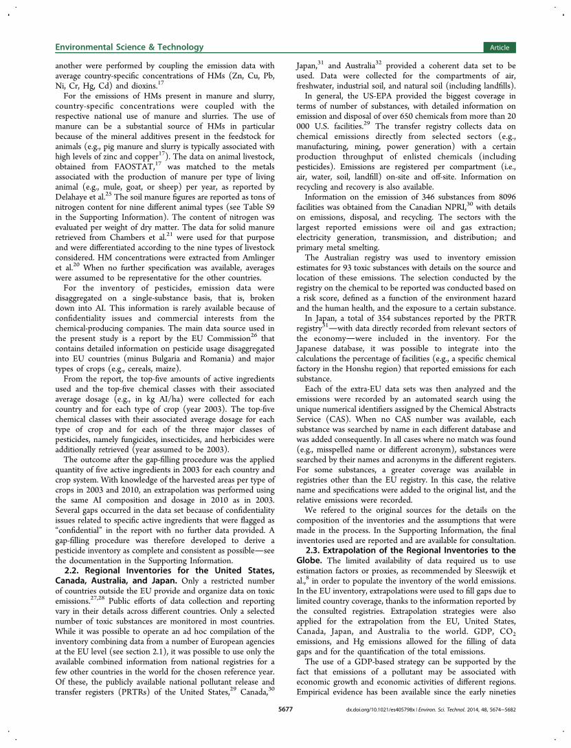
data available for 234 countries relative to the estimators werecrossed to investigate the direct correlation among the factorsused in this paper. A high overall correlation was found at aglobal level between the GDP and CO2 (Pearson coefficient,0.8), suggesting that the two predictors (both stronglycorrelated to energy production) may both be usedinterchangeably in the extrapolation of the data. A significantlylower correlation was found between emissions of Hg for thecountries analyzed and both the GDP and CO2 (Pearsoncoefficient, 0.4), suggesting that both predictors may not be thebest possible estimator when used for the extrapolation of Hgemissions, or, assuming a correlation among heavy metals, theywould not be the best predictors also for other metals. Thecomparison of residual errors highlighted the cases of over- orunder-estimation of emissions of Hg, using the GDP or CO2 asa predictor. A country-by-country analysis of the goodness of fitis shown in Figure 1 below.The analysis of the prediction suggests that the regions used

in this paper as extrapolation bases were precisely estimated orslightly overestimated (see, e.g., EU and Australia). The highestlevel of underestimation affects countries with a lower GDP(e.g., central African countries and a number of South Americancountries). The pattern seems to correspond to the hypothesisthat for countries in which the extraction of resources (e.g.,gold11) that are related to mercury release is not conductedaccording to controlled standards, GDP and CO2 (see FigureS4 in the Supporting Information) do not function as the bestpossible predictors. On the other hand, no strong over-estimation of Hg was detected in any country. The datasuggests that care should be taken when dealing withextrapolation strategies for certain substances. The use ofGDP-based and CO2-based strategies can be supported by the

Environmental Science & Technology Article

dx.doi.org/10.1021/es405798x | Environ. Sci. Technol. 2014, 48, 5674−56825678

coupling of many pollutant emissions with the economicactivities of a region; however, the Hg-based extrapolationstrategy is recommended for use for those countries with a lowGDP and CO2, but in which some activities poorly correlatedwith the GDP and CO2 (e.g., mining) are very relevant andotherwise underestimated.3.3. Uncertainty. To further analyze the strength of

prediction obtained using the three estimators, a subset ofrepresentative substances, including the top-contributors to theEU and world impact scores, was selected based on theavailability of sufficient recorded data in the EU and the rest ofthe countries accounted for in the composition of the globalinventory. To guide future extrapolations and analyses, the

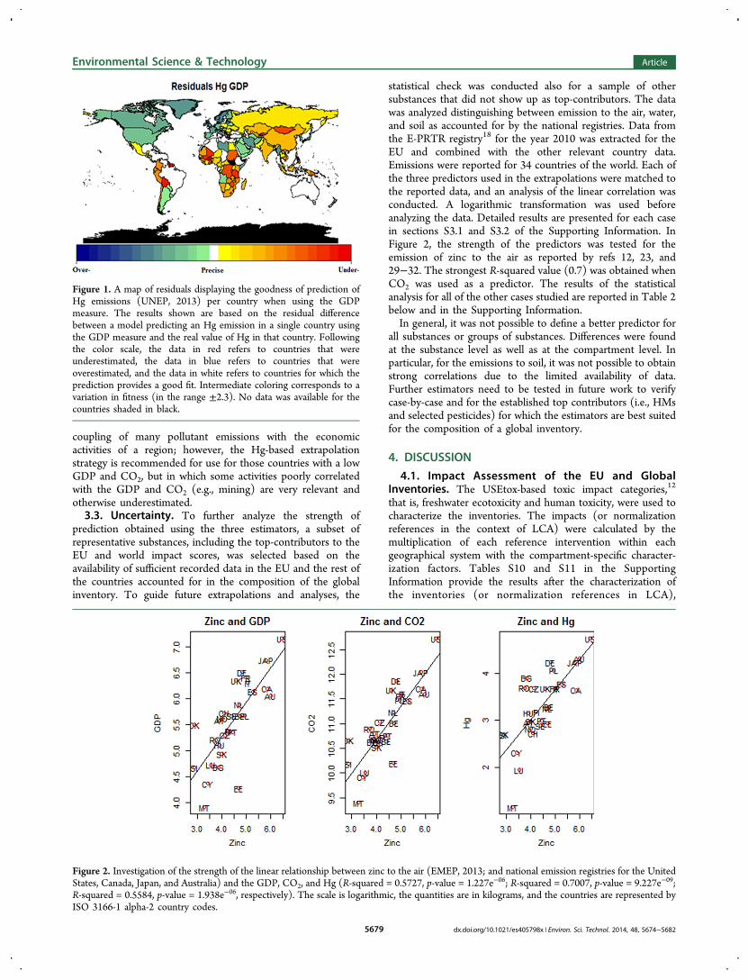
statistical check was conducted also for a sample of othersubstances that did not show up as top-contributors. The datawas analyzed distinguishing between emission to the air, water,and soil as accounted for by the national registries. Data fromthe E-PRTR registry18 for the year 2010 was extracted for theEU and combined with the other relevant country data.Emissions were reported for 34 countries of the world. Each ofthe three predictors used in the extrapolations were matched tothe reported data, and an analysis of the linear correlation wasconducted. A logarithmic transformation was used beforeanalyzing the data. Detailed results are presented for each casein sections S3.1 and S3.2 of the Supporting Information. InFigure 2, the strength of the predictors was tested for theemission of zinc to the air as reported by refs 12, 23, and29−32. The strongest R-squared value (0.7) was obtained whenCO2 was used as a predictor. The results of the statisticalanalysis for all of the other cases studied are reported in Table 2below and in the Supporting Information.In general, it was not possible to define a better predictor for

all substances or groups of substances. Differences were foundat the substance level as well as at the compartment level. Inparticular, for the emissions to soil, it was not possible to obtainstrong correlations due to the limited availability of data.Further estimators need to be tested in future work to verifycase-by-case and for the established top contributors (i.e., HMsand selected pesticides) for which the estimators are best suitedfor the composition of a global inventory.

4. DISCUSSION

4.1. Impact Assessment of the EU and GlobalInventories. The USEtox-based toxic impact categories,12

that is, freshwater ecotoxicity and human toxicity, were used tocharacterize the inventories. The impacts (or normalizationreferences in the context of LCA) were calculated by themultiplication of each reference intervention within eachgeographical system with the compartment-specific character-ization factors. Tables S10 and S11 in the SupportingInformation provide the results after the characterization ofthe inventories (or normalization references in LCA),

Figure 1. A map of residuals displaying the goodness of prediction ofHg emissions (UNEP, 2013) per country when using the GDPmeasure. The results shown are based on the residual differencebetween a model predicting an Hg emission in a single country usingthe GDP measure and the real value of Hg in that country. Followingthe color scale, the data in red refers to countries that wereunderestimated, the data in blue refers to countries that wereoverestimated, and the data in white refers to countries for which theprediction provides a good fit. Intermediate coloring corresponds to avariation in fitness (in the range ±2.3). No data was available for thecountries shaded in black.

Figure 2. Investigation of the strength of the linear relationship between zinc to the air (EMEP, 2013; and national emission registries for the UnitedStates, Canada, Japan, and Australia) and the GDP, CO2, and Hg (R-squared = 0.5727, p-value = 1.227e−06; R-squared = 0.7007, p-value = 9.227e−09;R-squared = 0.5584, p-value = 1.938e−06, respectively). The scale is logarithmic, the quantities are in kilograms, and the countries are represented byISO 3166-1 alpha-2 country codes.

Environmental Science & Technology Article

dx.doi.org/10.1021/es405798x | Environ. Sci. Technol. 2014, 48, 5674−56825679

considering the impacts on human toxicity and freshwaterecotoxicity in the EU geographic system and for the worldsystem. As in Sleeswijk et al.,8 an emission total consists of thesummed emissions of a substance to a specific compartment inone of the geographic systems. The results are reported peryear using the notation suggested by Heijungs.36

The characterization of the inventory by means of an impactsystem such as USEtox allows for testing of the inventory andidentifying the effects of the extrapolations on the outcome ofthe characterization and the calculation of the impacts. As aresult, under all of the extrapolations the incompleteness of thedata in regions other than the EU is likely to be the cause of adisproportional emission attributed to the EU compared to therest of the world. The composition of the economic systems inthe extrapolation region (i.e., the EU plus other availablenational registries) influences the final result. The extrapolationbased on the CO2 emissions attributed one-third of the globalemissions to the EU region (with the EU accounting for a totalof 36% of the world CO2 emissions). The GDP-basedextrapolation provided a weight of the EU compared to theworld emissions in the range of 50% for human toxicity (cancer,noncancer, and total), and 37% for ecotoxicity, with a globalGDP of the region accounting for about 27% of the worldGDP.9 A limited contribution of the EU to the world wasobtained in the case of the Hg-emissions-based extrapolationbecause of the limited share of mercury emissions that the EUaccounts for compared to the rest of the world (i.e., 11%). Theextrapolation of Hg emissions gave also the highest total impactfor the world; an order of magnitude higher than the GDP andCO2 for the impact of human toxicity and one order ofmagnitude higher than the GDP for the total impact ofecotoxicity. As reported by Sleeswijk et al.,8 the reliability of theestimation factors depends on the strength of the correlationbetween the emissions and the predictor used to extrapolatethem from a limited geographic extent to the entire globe (orpotentially from a bigger macroregion to a country level).A list of the top-contributing substances was extracted from

the data (see Table S12 in the Supporting Information). Thecomparison of the three strategies did not highlight thedifferences in the top-substances that contributed to the totals,while the share of the contribution was slightly different amongthem. This is a logical result from the extrapolation strategydescribed in section 3. Logically, the ratios of GDP, CO2emissions, and Hg emissions in the extrapolation regions and inthe world are identical for all substances; therefore, the

emission of a substance is transferred from the extrapolationregion to the world based on all predictors geometrically. Slightdifferences arise when a particular substance has a differentinitial geographical coverage than the other substances. Thenearly perfect matching of the top contributors for the threepredictors (see Table S12 of the Supporting Information) alsoreflects the fact that most emissions are driven by energyprocesses, which are likely to be the best covered processesacross all databases. Other processes may actually contribute totoxic emissions without being related to energy processes, inwhich case the extrapolations based on Hg emissions wouldlead to decoupled results from the ones obtained with CO2emissions and the GDP. However, such sectors may not be wellcovered in national or regional registries. The type of activitiesthat are related to the emissions of Hg may be more relevantfor other economic systems than for the ones used for thecomposition of the global inventory. Such sectors are bettercovered in life cycle (LC) inventories, in which a number ofchemical releases are still missing. Similarly, it is possible toobserve a decoupling between the climate footprint and toxicimpacts when using LC inventories (see Laurent et al.37), whichare in most cases deemed more complete than the national orregional databases.

4.2. Outlook and Implications. This study provides adetailed analysis of the process of the compilation of regionaland global inventories of toxic emissions and may be of interestalso for the reverse process of extrapolations from a bigger to asmaller scale. During the process of building the emissioninventory, the modeler has to deal with a limited internationalaccounting of emission data and with different standards ofcollection (e.g., substance groups reported in one region only).Extrapolations, thus, were required to fill data gaps. Certainsubstances are likely to be underestimated by the process; someothers are likely to be overestimated. Particularly relevant arethe cases of substances that are not necessarily an integral partof the economic system of developed countries. In these cases,the extrapolation process is possibly ignoring activities that arenot recorded in those countries but would be relevant on theglobal scale (e.g., processing of electronic waste in thedeveloping world). Of similar importance is the case ofsubstances that have already been banned in certain countries,but still used in others, and thus, would not appear in the resultof the extrapolation process.The three estimators used for the extrapolations, while

convenient for the population of the emission database, were

Table 2. Investigation of the Strength of the Correlation between the Prediction of a Linear Model Relating the EmittedAmount of a Substance to Air, Water, and Soil to the Extrapolation Factors

adjusted R-squared value

GDP CO2 Hg

emission air water soil air water soil air water soil

zinc 0.57 0.59 0.46 0.7 0.7 0.48 0.56 0.7 0.01mercury 0.48 0.42 0.63 0.69 0.51 0.57 0.82 0.43 0.26lead 0.15 0.45 0.18 0.37 0.59 0.21 0.43 0.61 0.05cadmium 0.37 0.36 0.36 0.58 0.48 0.46 0.57 0.63 0.01chromium 0.27 0.29 0.15 0.49 0.46 0.25 0.69 0.55 0.04arsenic 0.29 0.41 0.32 0.48 0.51 0.37 0.52 0.48 0.1copper 0.49 0.48 0.36 0.69 0.63 0.45 0.68 0.65 0.19benzo(a)pyrene 0.17 0.12 0.27NMVOC 0.55 0.73 0.541,2- dichloroethane 0.04 0.26 0.05 0.01 0.05 0.3polychlorinated biphenyl 0.23 0.23 0.29 0.3 0.21 0.21

Environmental Science & Technology Article

dx.doi.org/10.1021/es405798x | Environ. Sci. Technol. 2014, 48, 5674−56825680

not in all cases representative of the global reality that they tryto picture. The analysis of the direct correlation between theestimators for 234 countries of the world showed thattheoretically the GDP and CO2 could be used alternatively asestimators, while neither the GDP nor CO2 would be suitableto predict Hg emissions. Such a consideration could beextended to other metals and substances that are emitted incombination with Hg.We showed, for a sample of relevant substances, that the

correlation between each estimator and a substance greatlyvaries across substances and also across compartments for thesame substance. The theoretical strong correlation between theGDP and CO2 in the country-by-country analysis was notreproduced by this analysis. The statistical analysis highlightedthat it is not possible to select a single best predictor on thebasis of the correlation between the reported data and the valueof the predictor. A case-by-case analysis may help in the futureto develop more stable predictors for a cluster of substances orfor a cluster of countries with a similar economic structure. Amore in-depth analysis should be conducted to evaluate if adhoc extrapolation factors (e.g., crop production area assumed tobe related to pesticide use) are needed for a better coverage ofemissions.Future work should be oriented to quantifying more accurate

emission inventories for the top-contributors that arise fromdifferent characterization methods. Some other approachessuch as bottom-up data extrapolation using, for example,technology and energy correction factors or the use ofenvironmentally extended input−output tables (see in Tukkeret al.38), where available, could be helpful for extrapolations.Future work should explore where better correlations might befound. The EU and global inventories compiled in this studymay be used as a basis for such an analysis. The comparison ofthe impacts and the top-contributors should then be used asguidance for future data collection efforts. Once enough datahas been gathered on a shortlist of top-contributors, theanalysis can move to the remaining ∼5−10% contributors indetermining the total impact. This approach would likelyincrease the possibility of having valuable results in a short-termperspective, obviating the slow process of gathering of data bynational and regional authorities, and lowering the risk ofincurring one of the potential biases of the process.

■ ASSOCIATED CONTENT

*S Supporting InformationInventory data and the template used for the characterization ofthe inventory. This material is available free of charge via theInternet at http://pubs.acs.org.

■ AUTHOR INFORMATION

Corresponding Author*E-mail: cucurachi@cml.leidenuniv.nl.

NotesThe authors declare no competing financial interest.

■ ACKNOWLEDGMENTS

The present research was funded by the European Commissionunder the seventh Framework Programme on Environment;ENV.2009.3.3.2.1: LC-IMPACTImproved Life Cycle ImpactAssessment methods (LCIA) for better sustainability assess-ment of technologies, Grant Agreement Number 243827.

■ REFERENCES(1) Life cycle indicators framework: development of life cycle basedmacro-level monitoring indicators for resources, products and waste for theEU-27 (a); European Commission, Joint Research Centre, Institute forEnvironment and Sustainability: Ispra, Italy, 2012.(2) Life cycle indicators framework: development of life cycle basedmacro-level monitoring indicators for resources, products and waste for theEU-27 (b); European Commission, Joint Research Centre, Institute forEnvironment and Sustainability: Ispra, Italy, 2012.(3) Life cycle indicators framework: development of life cycle basedmacro-level monitoring indicators for resources, products and waste for theEU-27 (c); European Commission, Joint Research Centre, Institute forEnvironment and Sustainability: Ispra, Italy, 2012.(4) ISO 14040:2006 environmental management−life cycle assessment−principles and framework; International Standards Organization:Geneva, Switzerland, 2006.(5) Guinee, J. B.; Gorree, M.; Heijungs, R.; Huppes, G.; Kleijn, R.;De Koning, A. Handbook on life cycle assessment. Operational guide tothe ISO standards; Kluwer Academic Publishers: Dordrecht, TheNetherlands, 2002; 1−708.(6) Sala, S.; Goralczyk, M. Chemical footprint: A methodologicalframework for bridging life cycle assessment and planetary boundariesfor chemical pollution. Integr. Environ. Assess. Manage. 2013, 9 (4),623−632.(7) Laurent, A.; Olsen, S. I.; Hauschild, M. Z. Normalization inEDIP97 and EDIP2003: Updated European inventory for 2004 andguidance towards a consistent use in practice. Int. J. Life Cycle Assess.2011, 16 (5), 401−409.(8) Sleeswijk, A. W.; Huijbregts, M. A. J.; Van Oers, L. F. C. M.;Guinee, J. B.; Struijs, J. Normalisation in product life cycle assessment:An LCA of the global and European economic systems in the year2000. Sci. Total Environ. 2008, 390 (1), 227−240.(9) World development indicators; World Bank: Washington D.C.,2010.http://data.worldbank.org/data-catalog/world-development-indicators/wdi-2010.(10) FAOSTAT. Statistical data; Food and Agriculture Organizationof the United Nations (FAO): Rome, Italy. http://faostat3.fao.org/home/index.html (accessed April 2013).(11) UNEP. Global mercury assessment. Sources, emissions, releases, andenvironmental transport; UNEP Chemicals Branch: Geneva, Switzer-l and , 2013 . ht tp ://www.unep .org/PDF/PressRe leases/GlobalMercuryAssessment2013.pdf.(12) Rosenbaum, R. K.; Bachmann, T. M.; Gold, L. S.; Huijbregts, M.A. J.; Jolliet, O.; Juraske, R.; Koehler, A.; Larsen, H. F.; MacLeod, M.;Margni, M.; McKone, T. E.; Payet, J.; Schuhmacher, M.; Van deMeent, D.; Hauschild, M. Z. USEtoxthe UNEP-SETAC toxicitymodel: Recommended characterization factors for human toxicity andfreshwater ecotoxicity in life cycle impact assessment. Int. J. Life CycleAssess. 2008, 13, 532−546.(13) EMEP. Country- and sector-specific pollutant emission data; Centreon Emission Inventories and Projections (CEIP). http://www.ceip.at/.Link to database: http://webdab1.umweltbundesamt.at/scaled_country_year.html?cgiproxy_skip=1 (accessed April 2013).(14) OECD. StatExtractsdatabases providing statistics on wastewatertreatment. http://stats.oecd.org/Index.aspx?QueryId=28857# (ac-cessed June 2013).(15) EEA. Waterbase for rivers. http://www.eea.europa.eu/data-and-maps/data/waterbase-rivers-8 (accessed February 2013).(16) EUROSTAT Eurostat statistics database. http://ec.europa.eu/eurostat (accessed April 2013).(17) European Commission. Environmental, economic, and socialimpacts of the use of sewage sludge on land. Final reportpart III: Projectinterim reports; Milieu Ltd, WRc, RPA: Brussels, Belgium, 2008.(18) E-PRTR. The European pollutant release and transfer register (E-PRTR). http://prtr.ec.europa.eu/ (accessed June 2013).(19) Pistocchi A.; Alamo C.; Castro-Jimenez J.; Katsogiannis A.;Pontes S.; Umlauf G.; Vizcaino P. A compilation of Europe-widedatabases from published measurements of pcbs, dioxins, and furans;European Union: Luxembourg, 2010. http://publications.jrc.ec.

Environmental Science & Technology Article

dx.doi.org/10.1021/es405798x | Environ. Sci. Technol. 2014, 48, 5674−56825681

europa.eu/repository/bitstream/111111111/22703/1/lb-na-24266-en-c.pdf.(20) Amlinger F., Pollak M.; Favoino E. Heavy metals and organicscompounds from wastes used as organic fertilisers. Final report. REF.NR.:TEND/AML/2001/07/20; EU Commission: Perchtoldsdorf, Austria,2004. http://ec.europa.eu/environment/waste/compost/pdf/hm_finalreport.pdf.(21) Chambers B.; Nicholson N.; Smith K.; Pain B.; Cumby T.;Scotford I. Managing livestock manuresbooklet 1: Making better use oflivestock manures on arable land [Online]; 2nd ed.; ADAS GleadthorpeResearch Centre: Nottinghamshire, England, 2001. http://archive.defra.gov.uk/foodfarm/landmanage/land-soil/nutrient/documents/manure/livemanure1.pdf (accessed February 25, 2013).(22) Laurent, A.; Hauschild, M. Z. Impacts of NMVOC emissions onhuman health in European countries for 2000−2010: Use of sector-specific substance profiles. Atmos. Environ. 2014, 85, 247−255, http://dx.doi.org/10.1016/j.atmosenv.2013.11.060.(23) CORINAIR. 2007. http://reports .eea .europa.eu/EMEPCORINAIR5/en/B1090vs2.pdf (accessed April 2013).(24) CORINAIR. Emission inventory guidebook. Technical report No. 9;European Environmental Agency: Copenhagen, Denmark, 2009.http://reports.eea.eu.int/EMEPCORINAIR4/en.(25) Delahaye, R., Fong, P. K. N., Van Eerdt, M. M., Van der Hoek,K. W., Olsthoorn, C. S. M. Emissie van zeven zware metalen naarlandbouwgrond (Emission of seven heavy metals to the agriculturalsoil (in Dutch). Centraal Bureau voor de Statistiek (CBS). Voorburg/Heerlen: The Netherlands, 2003; 33 http://www.cbs.nl/NR/rdonlyres/837282FD-9AC2-4529-AB2C-340444892528/0/zwaremetaleneindrapport.pdf.(26) The use of plant protection products in the European Union.Data, 1992−2003. epp.eurostat.ec.europa.eu (accessed March 2013).(27) Cucurachi S., Hejiungs R., Laurent A., Sala S. Normalisationfactors for ecotoxicity and human toxicity. Deliverable 2.4 of LC-impactproject, 2013. http://www.lc-impact.eu (accessed December 2013).(28) Pollutant release and transfer registers of the world. http://www.prtr.net/en/links/ (accessed March 2013).(29) Toxics release inventory (TRI) program. TRI explorer. UnitedStates Environmental Protection Agency (US-EPA): Washington DC,USA. http://www.epa.gov/triexplorer/ (accessed March 2013).(30) Environment Canada National Pollutant Release Inventory(NPRI). http://www.ec.gc.ca/inrp-npri/ (accessed April 2013).(31) Chemical Management Field; National Institute of Technologyand Evaluation (NITE): Japan, http://www.safe.nite.go.jp/english/index.html (accessed March 2013).(32) Australian National Pollutant Inventory. http://www.npi.gov.au/ (accessed March 2013).(33) Stern, D. I. The rise and fall of the environmental Kuznets curve.World Dev. 2004, 32 (8), 1419−1439.(34) Davis, S. J.; Caldeira, K. Consumption-based accounting of CO2emissions. P. Natl. Acad. Sci. 2010, 107 (12), 5687−5692.(35) Davis, S. J.; Caldeira, K.; Matthews, H. D. Future CO2 emissionsand climate change from existing energy infrastructure. Science 2010,329 (5997), 1330−1333.(36) Heijungs, R. On the use of units in LCA. Int. J. Life Cycle Assess.2005, 10 (3), 173−176.(37) Laurent, A.; Olsen, S. I.; Hauschild, M. Z. (2012) Limitation ofcarbon footprint as indicator of environmental sustainability. Environ.Sci. Technol. 2012, 46, 4100−4108.(38) Tukker, A.; Poliakov, E.; Heijungs, R.; Hawkins, T.; Neuwahl,F.; Rueda-Cantuche, J. M.; Bouwmeester, M. Towards a global multi-regional environmentally extended input−output database. Ecol. Econ.2009, 68 (7), 1928−1937.

Environmental Science & Technology Article

dx.doi.org/10.1021/es405798x | Environ. Sci. Technol. 2014, 48, 5674−56825682