econstorMake Your Publications Visible.

A Service of

zbwLeibniz-InformationszentrumWirtschaftLeibniz Information Centrefor Economics

Humphreys, Brad R.; Maccini, Louis J.; Schuh, Scott

Working Paper

Input and output inventories

Working Paper, No. 426

Provided in Cooperation with:Department of Economics, The Johns Hopkins University

Suggested Citation: Humphreys, Brad R.; Maccini, Louis J.; Schuh, Scott (2000) : Input andoutput inventories, Working Paper, No. 426, The Johns Hopkins University, Department ofEconomics, Baltimore, MD

This Version is available at:http://hdl.handle.net/10419/72031

Standard-Nutzungsbedingungen:

Die Dokumente auf EconStor dürfen zu eigenen wissenschaftlichenZwecken und zum Privatgebrauch gespeichert und kopiert werden.

Sie dürfen die Dokumente nicht für öffentliche oder kommerzielleZwecke vervielfältigen, öffentlich ausstellen, öffentlich zugänglichmachen, vertreiben oder anderweitig nutzen.

Sofern die Verfasser die Dokumente unter Open-Content-Lizenzen(insbesondere CC-Lizenzen) zur Verfügung gestellt haben sollten,gelten abweichend von diesen Nutzungsbedingungen die in der dortgenannten Lizenz gewährten Nutzungsrechte.

Terms of use:

Documents in EconStor may be saved and copied for yourpersonal and scholarly purposes.

You are not to copy documents for public or commercialpurposes, to exhibit the documents publicly, to make thempublicly available on the internet, or to distribute or otherwiseuse the documents in public.

If the documents have been made available under an OpenContent Licence (especially Creative Commons Licences), youmay exercise further usage rights as specified in the indicatedlicence.

www.econstor.eu

Input and Output Inventories

Brad R. Humphreys

University of Maryland

Baltimore County

Louis J. Maccini

Johns Hopkins University

Scott Schuh 1

Federal Reserve Bank of Boston

November, 1997

1Send correspondence to Schuh, P.O. Box 2076, Boston, MA 02106-2076; Internet:

scott.schuh@bos.frb.org. We are especially grateful to Je� Fuhrer for advice and technical assistance.

We also thank Jeremy Berkowitz, David Bivin, Spencer Krane, Andy Levin, Adrian Pagan, Bob Rossana,

Ken West, John Williams, and participants at numerous seminars for helpful comments. Brian Doyle and

Kevin Daly provided excellent research assistance; Hoyt Bleakley also provided valuable technical assistance.

Maccini thanks the National Science Foundation for �nancial support. The opinions expressed in this paper

are those of the authors and do not necessarily re ect the opinions of the Federal Reserve Bank of Boston

or the Board of Governors of the Federal Reserve System.

Abstract

This paper builds and estimates a new model of �rm behavior that includes decisions to order, use,

and stock input materials in a stage-of-fabrication environment with either gross production or value

added technology. The model extends the traditional linear-quadratic model of output (�nished

goods) inventories by incorporating delivery and usage of input materials plus input inventory

investment { features which largely have been ignored in the literature. Stylized facts indicate that

input inventories are empirically more important than output inventories, especially in business

cycle uctuations. Firms simultaneously choose input and output inventories; thus, the model

exhibits feedback between stocks induced by dynamic stage-of-fabrication linkages. Estimation of

inventory decision rules shows the model is reasonably consistent with data in nondurable and

durable goods industries. The results reveal inventory stock interaction, convex costs, viability of

gross production and value added speci�cations, industrial di�erences, and input inventory-saving

technology.

JEL Classi�cation: E22, E23

Keywords: Inventories, raw materials, work-in-process, �nished goods, stage-of-fabrication, gross

production, value added, linear-quadratic

1 Introduction

Most �rms produce goods in stages. A typical �rm orders input materials from a supplier, takes

delivery, and combines the materials with other factor inputs to produce �nished output. Often

during the production process the �rm generates its own intermediate product as well. In addition,

many �rms sell their �nished output to other �rms, which view the output as input material. These

stage-of-fabrication linkages { within and between �rms { imply that rational, optimizing �rms will

be characterized by joint interaction among all aspects of production. Yet studies of �rm behavior

generally ignore such dynamic linkages, considering materials only to measure productivity. This

paper begins to redress this oversight.

Nowhere is the neglect of stage-of-fabrication linkages more evident than in the inventory lit-

erature, where the vast bulk of work has focused almost exclusively on �nished goods, or output,

inventories. The literature, as summarized by Blinder and Maccini (1991), has been devoted pri-

marily to understanding why the rational expectations version of the pure production smoothing

model of output inventories seems to be inconsistent with the data.1 Such intense scrutiny of out-

put inventory investment largely has \crowded out" consideration of stage-of-fabrication linkages,

such as ordering and usage of material inputs. As a consequence, input inventories { de�ned as

raw materials and work-in-process { have been neglected almost entirely.

Neglect of input inventories is problematic for two main reasons. The �rst reason is conceptual:

input inventories are the linchpin of the stage-of-fabrication production process. Input inventories

arise whenever the delivery and usage of input materials di�er; in other words, �rms do not instan-

taneously obtain and use materials in production. Furthermore, since the usage of input materials

is a factor of production, decisions about smoothing production and output inventory investment

inherently are related to decisions about drawing down input inventories. In turn, the ability of

the �rm to draw down input inventories depends on supplier relationships (domestic and foreign),

material prices, and factor substitutability { i.e., the spectrum of production decision making.

The second reason is empirical: simply put, input inventories are more important than output

inventories. The Blinder-Maccini survey documents that inventory investment changes almost one-

for-one with GDP during the average recession; Ramey (1989) shows that this recessionary decline in

1Various authors working with aggregate data have modi�ed the basic model. Blanchard (1983), West (1986),

Kahn (1987, 1992) and Fuhrer, Moore and Schuh (1995) add a stockout avoidance motive; Maccini and Rossana

(1984), Blinder (1986), Miron and Zeldes (1988), and Durlauf and Maccini (1995) add cost shocks in the form of

real input prices; Eichenbaum (1989) and Kollintzas (1992) add unobservable technology shocks; Ramey (1991)

adds nonconvexities in production and West (1988) adds backlogs of un�lled orders. Other authors have turned to

alternative data sources including Fair (1989), Ghali (1987), Haltiwanger and Maccini (1989), Kashyap and Wilcox

(1993), Krane and Braun (1991), and Schuh (1996). A consensus explanation, however, is still lacking.

1

inventory investment occurs predominantly among input inventories. Romer (1986) demonstrates,

in our terminology, that input inventory investment is strongly procyclical and thus the ordering and

usage of input materials are not closely synchronized over the business cycle { a �nding that argues

for separate modeling of orders and usage. The Blinder-Maccini evidence, and our extended stylized

facts, indicate that input inventories are twice as large as output inventories, and three times more

variable. Moreover, the dominance of input inventories occurs primarily in durable goods industries,

which typically have been excluded from applied inventory research. Finally, some econometric work

with output inventories suggests interaction between inventory stocks. For example, Durlauf and

Maccini (1995) �nd an important role for observable cost shocks (raw materials prices) in explaining

output inventories, which likely arises through stage-of-fabrication linkages.

Despite the conceptual importance and empirical dominance of input inventories, the literature

on input inventories is remarkably thin. Moreover, the limited attempts to develop optimizing

models of stage-of-fabrication inventories invariably treat stocks as factors of production that yield

service ows to the �rm. Ramey (1989) includes materials, work-in-process, and �nished goods

inventory stocks in the production function and, using a restricted cost function, derives demand

functions for each stock. Bils and Kahn (1996) propose a model in which procyclical work e�ort

rationalizes procyclical marginal cost and inventory investment; the work-in-process inventory stock

enters their production function (materials inventories are not considered). Furthermore, both

studies involve estimation of Euler equations with generalized method of moments (GMM), which

may give rise to small sample biases, as we discuss below.2

Three problems arise from treating inventory stocks as factors of production. First, �nished

goods inventories provide services to the distribution, not production, of goods. Second, the relevant

factor of production is not the stock of materials and work-in-process inventories but the ow of

these materials drawn out of inventory and used in production; the ow may not be well-described

as a constant proportion of the stock, as assumed implicitly by previous work. Third, focussing on

the stock of materials precludes examination of the separate decisions to order, take delivery of,

and use input materials, which are integral aspects of dynamic �rm behavior.

This paper extends the literature by developing and estimating a new simultaneous equations

model of input and output inventories with separate decisions to order, use, and stock input ma-

2Related literature includes Husted and Kollintzas (1987), who o�er a rational expectations model of the purchase

and holding of imported raw materials inventories but ignore interaction with work-in-process or �nished goods in-

ventories, and West (1988), who introduces order backlogs and work-in-process inventories into the standard output

inventory model. See also the unpublished work of Auerbach and Green (1980) and Mosser (1989). Other work

explaining interaction among inventory types includes Lovell (1961), Maccini and Rossana (1984), Reagan and Shee-

han (1985), Blinder (1986), Nguyen and Andrews (1988), Rossana (1990), and Bivin (1993), which rely on stock

adjustment and reduced-form models.

2

terials. As a �rst step, we assume that materials and intermediate goods are inputs purchased

from outside the �rm, and that there are no input delivery lags or output order backlogs.3 The

model then makes several advances. First, and most prominently, only the ow usage of input

materials enters the production function, as in the productivity literature.4 Second, including the

ow of materials admits alternative assumptions about the separability of materials in produc-

tion: nonseparable (gross production) and separable (value added). Third, the �rm simultaneously

chooses output inventory investment and { as a consequence of choosing both deliveries and usage

of raw materials { input inventory investment; thus linking output and inventory investment with

cross-equation restrictions.

The model is fully structural with intertemporal cost minimization under rational expectations,

but the total cost function employs several quadratic approximations similar to those employed in

conventional output inventory models. The main reason for employing quadratic approximations is

to obtain linear decision rules that can be estimated via maximum likelihood (ML). Recent Monte

Carlo work by West and Wilcox (1994) and Fuhrer, Moore and Schuh (1995) demonstrates the

existence of substantial small sample biases in generalized method of moments (GMM) parameter

estimates of conventional output inventory Euler equations. In contrast, Fuhrer et al. demonstrate

that ML estimation of conventional output inventory decision rules produces relatively unbiased and

considerably more signi�cant parameter estimates. Thus, we conduct the �rst joint ML estimation

of input and output inventory decision rules.5

By and large, the data yield relatively strong econometric support for the model. Exploiting

model identities, we overcome the lack of high-frequency data on deliveries and usage of materials

and estimate versions of the model corresponding to: gross production and value added; nondurable

and durable goods industry data; and joint and single-equation estimates of inventory decision

rules. For all combinations of these features, the vast majority of parameter estimates are signed

correctly and estimated signi�cantly { in sharp contrast to most previous estimates of structural

inventory models. Furthermore, joint estimation reveals substantial e�ciency gains and provides

evidence that the failure to impose stage-of-fabrication linkages may lead to misspeci�cation biases.

3To some degree, of course, intermediate goods { and thus work-in-process inventories { are produced within the

�rm. Hence, an important extension of this paper is to model production of both intermediate and �nished goods,

which will require the �rm to hold separate stocks of materials and work-in-process inventories. Extending the model

to incorporate delivery lags and order backlogs may further improve the model's ability to �t the data.4See Bruno (1984), Baily (1986), Basu (1996), Basu and Fernald (1995), and Basu and Kimball (1997), for

discussions of the speci�cation of materials in production functions and its role in explaining productivity movements.5Eichenbaum (1984) also jointly estimated multiple decision rules for labor (hours) and output inventories, but

did not consider input inventories. Although we do not explicitly estimate a labor equation, the model contains labor

demand.

3

Although the data generally reject the overidentifying restrictions of the joint model, the degree

of rejection is comparable to that experienced by similar previous estimation of output inventory

models.

The econometric results generate numerous broad implications. First, the data clearly reveal

evidence of stage-of-fabrication interactions between inventory stocks, and among inventory stocks

and other facets of production. In particular, when the �rm chooses output inventories it takes

into consideration the gap between actual and target input inventories; at the same time, the �rm's

choice of output inventories a�ects the input inventory target stock and thus its choice of input

inventories. Second, the data indicate that aggregate cost functions are convex, even for durable

goods industries and even in the presence of input inventories. Third, gross production and value

added speci�cations of the model both generally �t the data and provide evidence of inventory

stock interaction. But the value added restrictions lead to a signi�cantly simpler model that

excludes some channels of propagation that are in the gross production model. Fourth, the model

generally �ts the data from both nondurable and durable goods industries; industrial di�erences

may, however, stem from the model's simplifying assumptions. Finally, the data show evidence of

input inventory-saving technology in both industries, especially in durable goods.

The remainder of the paper proceeds as follows. Section 2 updates and expands the stylized

facts about inventory movements at di�erent stages of fabrication. Section 3 presents the new stage-

of-fabrication inventory model. Section 4 describes the econometric speci�cation and estimation,

and section 5 reports the econometric results. The paper concludes with a discussion of some

implications for future research.

2 Motivation and Stylized Facts

This section presents key empirical facts about manufacturers' input and output inventories that

motivate the stage-of-fabrication model developed in the next section. Table 1 lists the main

variables in the paper. Data for these variables are in constant 1987 dollars, seasonally adjusted,

and monthly for the period 1959:1 through 1994:5 (except for Dt and Ut, which are unobserved).

All data are standard published government series except the materials price index, which we

constructed from detailed price indexes. The data appendix contains complete details.

Tables 2 and 3 reveal several stylized facts about manufacturers' input and output inventories in

nondurable goods and durable goods industries. Table 2 reports the change in inventory investment

relative to the change in manufacturing sales during post-war recessions (changes measured from

peak to trough). Table 3 reports the means and variances of inventory investment and inventory-

to-sales ratios.

4

Table 1 | Variable De�nitions

Dt = Deliveries of input materials

Lt = Labor input

Mt = Input inventories (materials and work-in-process)

Nt = Output inventories (�nished goods)

Tt = Time trend (proxy for inventory technological change)

Ut = Usage of input materials

Vt = Real materials price

Wt = Real hourly wage rate

Xt = Sales (shipments)

Yt = Production of �nished goods (Xt + �Nt)

Table 2

Change in Inventory Investment during Postwar Recessions

(Expressed as a Share (%) of the Change in Manufacturing Sales)

Recessions

60:2- 69:4- 73:4- 80:1- 81:3- 90:3-

61:1 70:4 75:1 80:3 82:4 91:1 Average

Total Manufacturing 27 31 27 82 51 3 37

Input 7 30 32 54 26 10 27

Output 20 0 �5 28 25 �7 10

Nondurable Goods �5 �3 6 40 8 �18 5

Input 5 �10 7 23 6 �6 4

Output �10 7 �1 17 2 �12 0

Durable Goods 32 34 21 42 43 21 32

Input 1 40 26 31 20 17 22

Output 30 �6 �5 11 23 5 10

NOTES: The data are monthly, $1987 �xed-weighted. Recessions are de�ned by the National Bureau of

Economic Research (NBER). Changes are calculated from business cycle peak (�rst date) to trough (second

date).

5

Fact #1: Input inventories are larger and more volatile than output inventories in manufacturing.

Table 2 shows that changes in input inventory investment account for the bulk of the changes

in total manufacturing inventory investment during recessions. During a typical recession, the

decline in manufacturing inventory investment is more than one-third as large as the decline in

manufacturing sales. Moreover, the decline in input inventory investment is responsible for nearly

three-fourths of the overall inventory investment change. Table 3 indicates that input inventories

are at least twice as large as output inventories in manufacturing, as measured by average inventory

investment and inventory-to-sales ratios. Most importantly, the table shows that input inventory

investment is more than three times more variable than output inventory investment in manufac-

turing. These facts suggest that an analysis of the cyclical behavior of manufacturing inventory

investment should focus on input rather than output inventories, contrary to the overwhelming

practice in the literature.

Fact #2: Durable goods inventories are larger and more volatile than nondurable goods inventories.

Table 2 shows that the decline in durable goods inventory investment during a typical recession

accounts for nearly 90 percent of the decline in manufacturing inventory investment. Table 3 indi-

cates that durable goods inventories are up to two times larger than nondurable goods inventories,

as measured by average inventory investment and inventory-to-sales ratios. Moreover, the table

shows that durable goods inventory investment is nearly �ve times more variable than nondurable

goods inventory investment. These facts point to durable goods industries as the appropriate tar-

get of research on inventories, but empirical work has invariably emphasized nondurable goods

industries.

Fact #3: Input inventories are much larger and more volatile than output inventories in durable

goods industries, but input and output inventories are similar in size and volatility in nondurable

goods industries.

This fact is a byproduct of the �rst two. Table 2 shows that the decline in input inventory

investment during a typical recession accounts for the bulk of the decline in total inventory in-

vestment in both durable goods and nondurable goods industries. However, Table 3 indicates that

input inventories are much larger than output inventories in durable goods industries, as measured

by average inventory investment and inventory-to-sales ratios. Further, the table shows that input

inventory investment is more than six times more variable than output inventory investment in

durable goods industries. In nondurable goods industries, on the other hand, the magnitude and

variability of input inventories are more even with those of output inventories. In nondurables,

input inventory investment is a bit larger but a bit less variable than output inventory investment.

The fact that output inventory investment is a bit more variable than input inventory investment

6

provides some rationale for literature's focus on output inventory investment in nondurable goods

industries. Nevertheless, it is di�cult to rationalize the complete lack of attention to input in-

ventories. More generally, if the ultimate goal of research is understanding the variability of total

manufacturing investment, then the focus should be on input inventories, especially in durables.

Fact #4: Interactions between input and output inventories are quantitatively signi�cant, especially

in durable goods industries.

Table 3 reveals inventory stock interaction. Fifteen percent of the variance in manufacturing

inventory investment is accounted for by the covariance between input and output inventory invest-

ment. When the inventory stocks are disaggregated into the three stages of processing (materials,

work-in-process, and �nished goods), the covariance term accounts for 25 percent of the variance.

The table also shows that covariance among types of inventory investment is greater in durable

goods industries than nondurable goods industries.

Together, these stylized facts suggest: (1) a complete analysis of inventory behavior requires the

modeling of input inventories; (2) interaction between input and output inventories is empirically

evident and potentially a signi�cant feature of �rm behavior; and (3) tests of the model should be

conducted with durable goods, as well as nondurable goods, industries.

Before turning to the model, however, it is useful to point out a few additional features of the

data from the time series plots in Figure 1. The upper panels of inventory ratios exhibit two notable

features.6 First, the output inventory ratio is more countercyclical than the input inventory ratio

(correlations with detrended sales of �:20 versus �:10 in nondurables and �:78 versus �:26 in

durables). Whereas the output inventory ratio rises sharply in virtually every recession, the input

inventory ratio does not always rise in every recession. Furthermore, the increase in the input

inventory ratio during recessions varies in magnitude considerably more than does the increase in

the output inventory ratio. Second, the input inventory ratios in both industries appear somewhat

to exhibit negative trends since the 1970s, trends which may re ect the introduction of inventory-

saving technologies and production techniques.

The lower panels of real prices (the nominal price relative to the price of output) also exhibit

some notable features. First, the real wage trends up in both industries, but it is much more

cyclically sensitive in nondurables goods industries than in durable goods industries. Second, the

real materials prices are essentially trendless in both industries, but they exhibit large, persistent

increases during the 1970s and early 1980s. Most of these prices also are consistent with a split

trend around 1973, as argued by Perron (1989). The trends in these prices turn out to have direct

6The input inventory ratio is calculated with production, rather than sales, in the denominator because production

is assumed to be the primary target variable for input inventory stocks.

7

Table 3

Stylized Facts About Inventories

MEAN INVENTORY INVESTMENT

Mfg. % Dur. % Non. %

Total 0.51 100.0 0.33 100.0 0.18 100.0

Finished Goods 0.18 35.3 0.09 27.3 0.09 50.0

Input 0.33 64.7 0.24 72.7 0.09 50.0

Work-In-Process 0.17 33.3 0.14 42.4 0.03 16.7

Materials & Supplies 0.17 33.3 0.11 33.3 0.06 33.3

VARIANCE DECOMPOSITION OF INVENTORY INVESTMENT

Mfg. % Dur. % Non. %

Total 1.441 100.0 1.047 100.0 .210 100.0

Finished Goods .264 18.3 .117 11.2 .114 54.3

Input .958 66.5 .793 75.7 .079 37.6

Covariance .218 15.1 .138 13.2 .017 8.1

Finished Goods .264 18.3 .117 11.2 .114 54.3

Work-In-Process .417 28.9 .384 36.7 .018 8.6

Materials and Supplies .387 26.9 .276 26.4 .058 27.6

Covariance Terms .373 25.9 .271 25.9 .019 9.0

MEAN INVENTORY/SALES RATIO (Std. Dev.)

Mfg. Dur. Non.

Total 1.66 (0.11) 1.98 (0.20) 1.29 (0.05)

Finished Goods 0.54 (0.03) 0.52 (0.04) 0.57 (0.03)

Input 1.11 (0.09) 1.46 (0.16) 0.73 (0.03)

Work-In-Process 0.53 (0.05) 0.83 (0.10) 0.19 (0.01)

Materials and Supplies 0.58 (0.04) 0.63 (0.07) 0.53 (0.03)

NOTES: Statistics are calculated with monthly $1987 data over the period 1959:01 to 1994:05.

8

implications for the input inventory target stock speci�cation in the econometric estimation of the

SOF model. Finally, a comparison of coe�cients of variation indicates that the real materials price

is relatively more variable than the real wage, especially in durables. This feature suggests that real

materials price movements may play a more important role in explaining inventory movements.

3 The Stage-of-Fabrication Model

3.1 Overview

The model, illustrated schematically in Figure 2, focuses on ows through the stage-of-fabrication

(SOF) production process employed by a �rm to transform input inventories (raw materials and

work-in-process) into output inventories (�nished goods). Each period, the �rm combines labor

(L), materials used in production (U), and capital (K) to produce �nished goods. Materials used

in production are obtained from the on-hand stock of input inventories (M), which is continually

replenished by deliveries (D) of materials from foreign and domestic suppliers. Production (Y ) of

�nal goods is added to the stock of output inventories (N), which are used to meet �nal demand

(X). The �rm takes �nal demand, the price of labor (W ), and the price of deliveries (V ) as

exogenous (denoted by thin lines).

The �rm optimizes in a dynamic stochastic environment. Five random shocks (�) bu�et the

�rm's production process. One shock is the traditional demand shock (�x). The other four shocks

comprise a disaggregation of the traditional \supply" shock: (1) a technology shock (�y) a�ects

the production function; (2) a holding cost shock (�h) a�ects the cost of carrying inventory stocks;

(3) a real wage shock (�w) a�ects labor costs ; and (4) a real materials price shock (�v) a�ects the

supply of materials. In the short run, with the capital stock �xed, the �rm chooses U , M , and N

to minimize the present value of total costs.7 The �rst-order conditions are used to substitute out

materials usage, which is empirically unobservable at high frequencies.

7Actually, the �rm chooses L, U , and D, but because U and D are unobservable empirically we exploit the model

ow identities to recast the problem with inventory stocks as choice variables.

9

Foreign

Domestic

Raw Materials,Intermediate

Goods

InputInventory

�M = D � U�h

ProductionFunction

F (L;U; �y;K)

OutputInventory

�N = Y �X�h

FinalDemand

(Wholesale,

Retail, and

Consumers)

Labor Market

TechnologyShocks

?

6

- - -?

�

6

6

-D

V; �v

U Y X; �x

L W; �w

�y

Figure 2

The SOF model generalizes the traditional linear-quadratic framework that has served as the

workhorse for models of output inventories and production. The central extension in the SOF

model is the explicit introduction of input inventories, which must be chosen simultaneously with

output inventories. Input inventory investment is controlled by varying the usage of materials in

production and the deliveries of materials. Total costs|labor costs, inventory holding costs, and

delivery costs|are approximated with a generalized quadratic form. The SOF model di�ers from

the few inventory papers that include inventories other than �nished goods by specifying the ow,

rather than stock, of materials in the production function. For the purpose of testing the model

with aggregate data, we adopt the convention of a representative �rm, as is customary in the

inventory literature.8

3.2 The Production Function

Following the literature on production functions and productivity { for example, Bruno (1984) and

Baily (1986) { we assume that the production function contains as an input the ow of materials

used in the production process. Speci�cally, the production function is

Yt = F (Kt; Lt; Ut; �yt) : (1)

Note that Ut is the ow of materials used in the production process. Because Yt is gross output,

we refer to equation (1) as the gross production function.

An important speci�cation issue for the production function is whether Ut is additively separable

from the other factors of production. For example, Basu and Fernald (1995) show that evidence

of externalities caused by productive spillovers exists in value added data but not gross production

8In future work, we intend to estimate the model with SOF inventory data from the �rm-level M3LRD data base

originally developed by Schuh (1992).

10

data. If Ut is separable, then the production function can be written as

Yt � Ut = G (Kt; Lt; �yt) (2)

where Yt � Ut is value added. We refer to this form of the production function as the value added

production function. Observe that equation (2) is a special case of equation (1) with the restrictions

FU = 1 and FKU = FLU = F�yU = 0.

To date, the limited number of inventory models that account for both input and output in-

ventories have all, implicitly or explicitly, included the stock of input inventories as a factor of

production. For example, the production functions in Ramey (1989) and Bils and Kahn (1996) are

of the form

Yt = F (Kt; Lt;Mt; �yt) : (3)

Ramey also includes the stocks of work-in-process and �nished goods inventories in the production

function. Bils and Kahn de�ne input inventories to include only work-in-process, ignoring the larger

and more volatile materials stock.

Three problems arise from including inventory stocks in the production function. First, as

Ramey points out, �nished goods inventories do not provide services to the production of goods

because they are �nal goods. Finished goods inventories do provide services to the distribution of

goods, and could be justi�ed if \production" refers broadly to both production and distribution.

Second, and more important, the production function is a ow concept; it expresses the ow of

output produced during a period as a function of the ow of inputs used in the production process.

Speci�cation (3) implicitly presumes that the ow of materials used in the production process is

proportional to the stock of materials held in inventories and that the factor of proportionality is

constant over time. This presumption is accurate only under rather extreme conditions. Third,

the speci�cation precludes distinguishing among materials ordered, delivered, used, and held in

storage. These individual actions comprise a richer and more realistic characterization of the �rm's

production environment. Dividing the input inventory decision into two parts { how much to order

and how much to use { permits a more detailed analysis of the dynamics and a better opportunity

to understand the sources of volatility in input inventories.

Two simplifying assumptions get the model o� the ground. First, because inventory investment

is a short-run decision, the capital stock is a fully �xed factor of production and hereafter suppressed

in the functional form. Further, the remaining factors|materials usage and labor|possess positive

and nonincreasing marginal products. Second, the �rm purchases intermediate goods (work-in-

process) from outside suppliers rather than producing them internally.9 Thus, intermediate goods

9To allow for production of intermediate goods within the �rm requires extending the production function to

11

are analogous to raw materials so work-in-process inventories can be lumped together with materials

inventories.

3.3 The Cost Structure

The �rm's total cost structure consists of three major components: labor costs, inventory holding

costs, and materials costs. This section describes each component.

3.3.1 Labor Costs

Labor costs are

LCt = WtLt +A(�Lt) (4)

withA0 7 0 as �Lt 7 0

A00 > 0

where �Lt = Lt � Lt�1. The �rst component, WtLt, is the standard wage bill. The second

component, A(�Lt), is an adjustment cost function intended to capture the hiring and �ring costs

associated with changes in labor inputs. The adjustment cost function has the usual properties,

including a rising marginal adjustment cost.

To reduce the number of decision variables and focus on the inventory decisions, we eliminate

labor input. Inverting the production function, equation (1), yields

Lt = L(Yt; Ut; �yt) (5)

withLY = 1=FL > 0

LU = �FU=FL < 0

L�y = �(F�y=FL) < 0

(6)

where FL, FU , and F�y are the marginal products of production with respect to the factor inputs.

Substituting (5) into (4) yields

LCt = WtL(Yt; Ut; �yt) +A(L(Yt; Ut; �yt)� L(Yt�1; Ut�1; �y;t�1)) (7)

which is the central portion of the �rm's cost function.

To construct an econometric model, it is necessary to parameterize the labor cost function,

equation (7). In principle, we could use a speci�c model of production, such as Cobb-Douglas, to

incorporate joint production of �nal and intermediate goods. This extension is a substantial modi�cation of the

standard production process that we leave for future work.

12

parameterize the inverted production function, equation (5). However, such a speci�cation would

introduce nonlinearities and preclude estimation of the decision rules (unless the decision rules were

linearized, which also entails approximation error). Instead, we follow the tradition of the inventory

literature, which exploits generalized quadratic approximations of the form de�ned in Chambers

(1988). Speci�cally, the quadratic approximation to labor costs is

LCt =� 12

�Y 2t +

� 22

�U2t + 3YtUt +Wt[ 4Yt + 5Ut]

+�'2

�[ 6�Yt + 7�Ut]

2 + �yt( 8Yt + 9Ut) :

(8)

This equation omits products of inputs involving squared terms that would appear in a completely

generalized quadratic approximation of equation (7). Such terms vitiate certainty equivalence and

make it di�cult|perhaps impossible|to solve for decision rules, which is necessary for our econo-

metric strategy. Nevertheless, the approximation captures the essential elements of the production

and adjustment cost functions, and is comparable to the most general approximations found in

previous inventory work.

The signs of some, but not all, parameters in equation (8) are known without further assump-

tions. Parameters 1, 6, 8, and ' are all positive from the assumed convexity of the production

and adjustment cost functions. Abstracting from dynamics, @LC=@Y = 1Y + 4W should be

positive from (6); given 1 > 0, 4 > 0 is a su�cient, though not necessary, condition. But

@LC=@W = 4Y should also be positive from the wage bill, which indicates that 4 must be posi-

tive. In contrast, the signs of 2, 3, 5, 7, and 9 are unknown a priori because they depend on

the speci�cation of the production function.

3.3.2 Inventory Holding Costs

In line with much of the output inventory literature, holding costs for output inventories are a

quadratic approximation to actual costs of the form

HCNt = (�0 + �ht)Nt +

��

2

�(Nt �N�

t )2 (9)

where �ht is a white noise innovation to holding costs, N�t is the target level of output inventories

that minimizes output inventory holding costs, and � > 0. We adopt an analogous formulation for

input inventories; holding costs for these stocks are a quadratic approximation of the form

HCMt = (�0 + �ht)Mt +

��2

�(Mt �M�

t )2 (10)

where M�t is the target level of input inventories that minimizes input inventory holding costs, and

� > 0.

13

The quadratic inventory holding cost structure balances two forces. Holding costs rise with the

level of inventories, Mt and Nt, due to increased storage costs, insurance costs, etc. But holding

costs fall with Mt and Nt because|given expected M�t and N�

t |higher Mt and Nt reduce the

likelihood that the �rm will stock out of inventories. Note that equations (9) and (10) admit only

a single homogeneous innovation to total inventory (Mt +Nt) holding costs.

Finally, it remains to specify the inventory target stocks. Again following the literature, the

output inventory target stock is

N�t = �Xt (11)

where � > 0. The output inventory target depends on sales because the �rm incurs costs due to lost

sales when it stocks out of output inventories. For the input inventory target stock, the literature

provides little guidance aside from Lovell's (1961) speci�cation as a function of production, rather

than sales. We adopt the more general input inventory target

M�t = �Y Yt + �TT + �V Vt + �WWt (12)

where T is a linear time trend and �Y > 0. The input inventory target depends mainly on pro-

duction (Yt = Xt + �Nt) because stocking out of input inventories also entails costs associated

with production disruptions|lost production, so to speak|that are distinct from the cost of lost

sales. Lost production may be manifest in reduced productivity or even failure to realize production

plans.

To summarize, the input and output inventory targets di�er because the �rm holds the two

inventory stocks for di�erent reasons. The �rm stocks output inventories to guard against ran-

dom demand uctuations, but it stocks input inventories to guard against random uctuations in

productivity, materials prices and deliveries, and other aspects of production. Although sales and

production are highly positively correlated, they di�er enough at high frequencies for the di�erence

in the target stock speci�cation to be important.

The input inventory target also includes some variables that do not appear in the output inven-

tory target. The time trend is included as a proxy for the introduction of technologies that a�ect the

cost-minimizing level of stocks on hand. If �rms adopt inventory-saving technologies or organiza-

tional processes, such as the so-called just-in-time production technique, then �T < 0. Factor prices

also in uence the cost-minimizing level of materials inventories, given production and technology,

because materials usage is a factor of production and there is likely to be substitutability among

factors (especially in a representative agent model that encompasses heterogeneous industries). All

else equal, higher material prices should reduce M�t , so �V < 0. But the sign of �W is ambiguous

because it depends on the relationship between labor and material usage. If labor and material

14

usage are substitutes, a higher wage should increase M�t , so �W > 0. But if labor and material

usage are complements, then �W < 0.10

3.3.3 Materials Costs

Input materials costs consist of purchase costs and adjustment costs. Speci�cally, materials costs

are

MCt = VtDt +��2

�(�Mt)

2 : (13)

Deliveries include materials used in the production process and materials inventory investment:

Dt = Ut + �Mt. The �rst term on the right side of equation (13) is the cost of ordering input

materials at the \base" price each period. The second term is a quadratic approximation for

adjustment costs on investment in materials inventories.

One rationale for the adjustment costs is that they are internal to the �rm. They re ect the

fact that, when the �rm uses resources to bring about changes in the normal ow of materials

rather than to produce output, it su�ers the cost of forgone output. Examples include using labor

to engage in the search cost of �nding new suppliers of materials or the cost of �nding buyers or

otherwise getting rid of excess materials. Another rationale for the adjustment costs is that they

are external to the �rm. They re ect the idea that, due to monopoly power, the �rm may face a

rising supply price and thus an increasing marginal cost of acquiring materials more quickly.11

3.4 Cost Minimization

In standard output inventory theory, the �rm maximizes pro�ts given the demand curve it faces

from consumers of its (�nal) product. Most applied work on output inventories avoids the di�culties

of specifying the consumer's demand curve by assuming that demand is exogenous and recasting

the problem in terms of cost minimization. Introducing input inventories adds another, equally

complicated, dimension to the �rm's pro�t maximization problem: the supply curve it faces from

10One �nal assumption has been made implicitly regarding both inventory types, namely that there is no deprecia-

tion of the inventory stock. This simplifying assumption may be unrealistic for certain industries and types of goods,

such as food, but could easily be added to the model.11The adjustment costs can also be motivated by aggregation. One rationale is that aggregation across heteroge-

neous �rms induces persistence in aggregate inventories that requires an adjustment cost type of term in an aggregate

model. This view is supported by the evidence in Schuh (1996) of aggregation bias in adjustment speeds of output

inventory models. Another rationale pertains to aggregation across S,s policy rules. In this model, we ignore any

�xed costs associated with the ordering of materials, which presumably would lead to S,s policies at the micro level.

However, aggregation may smooth the micro S,s behavior into a relationship that looks like the partial adjustment

mechanisms arising from quadratic costs of adjustment. Both of these issues raise di�cult aggregation problems that

we intend to explore in future work.

15

input materials producers. As a �rst step, we emulate the output inventory literature and assume

that the �rm not only takes �nal demand as exogenous but also the supply of materials (speci�cally,

the materials price). Analogously, the wage is taken as exogenous, although the �rm may in uence

the labor market as well.

Given demand (Xt) and factor prices (Vt and Wt) the �rm's problem reduces to one of mini-

mizing the discounted present value of total costs (TC),

E0

1Xt=0

�t(LCt +HCNt +HCM

t +MCt) ; (14)

where � = (1 + r)�1 is the discount factor implied by the constant real rate of interest r. The two

laws of motion governing inventory stocks,

�Nt = Yt �Xt (15)

for output inventories and

�Mt = Dt � Ut (16)

for input inventories, can be used to substitute for production (Yt) and deliveries (Dt). Thus, the

�rm chooses fUt;Mt; Ntg1t=0 to minimize equation (14).

The model is derived as follows. Solve equation (15) for Yt and equation (16) for Dt and then

substitute these variables into equation (14). Take the derivatives of equation (14) with respect to

Ut, Mt, and Nt to obtain the Euler equations. De�ne �2 as the second-di�erence operator, i.e.,

�2Xt = �Xt ��Xt�1.

Then the Euler equation for materials usage, Ut, is

Et

���' 7[ 6(�Xt+1 + �2Nt+1) + 7�Ut+1]

+ 2Ut + 3(Xt + �Nt) + 5Wt + ' 7[ 6(�Xt +�2Nt) + 7�Ut] + Vt + 9�yt= 0 :

(17)

This optimality condition shows that the �rm balances the marginal cost of ordering and using ma-

terials this period (second line) against the marginal cost of using materials next period (�rst line).

Note that in period t+1 the only cost is the marginal cost of usage in production. All intertemporal

costs associated with materials occur through the input inventory optimality condition.

The Euler equation for input inventories, Mt, is

Et f��[Vt+1 + ��Mt+1]

+Vt + ��Mt + �(Mt �M�t ) + �ht + �0g = 0 :

(18)

16

This optimality condition shows that the �rm balances the marginal cost of ordering and holding

input inventories this period (second line) against the cost of ordering input inventories next period

(�rst line).

Finally, the Euler equation for output inventories, Nt, is

Et

��2' 6[ 6(�Xt+2 +�2Nt+2) + 7�Ut+2]

��[ 1(Xt+1 +�Nt+1) + 3Ut+1 + 4Wt+1

+2' 6( 6(�Xt+1 +�2Nt+1) + 7�Ut+1) + 8�y;t+1 � ��Y (Mt+1 �M�t+1)]

+ 1(Xt +�Nt) + 3Ut + 4Wt + ' 6( 6(�Xt +�2Nt) + 7�Ut)

+�(Nt �N�t )� ��Y (Mt �M�

t ) + 8�yt + �ht + �0g = 0 :

(19)

This optimality condition shows that the �rm balances the marginal cost of producing a good and

storing it as output inventory this period (last two lines) against the cost of producing the good in

the future (�rst three lines). The presence of adjustment costs on labor introduces an additional

period over which costs are balanced.

Next, solve equation (17) for EtUt and substitute it into equations (18) and (19) to eliminate the

unobservable materials usage variable from the system. De�ne the lag operator as L, which works

as a lead operator when inverted: e.g., L�1Xt = Xt+1. Then, after substituting and collecting terms

around common parameters, the Euler equation for input inventories, equation (18), becomes

Et

�(1� �L�1)Vt + �(1� �L�1)�Mt + �(Mt �M�

t ) + �ht + �0= 0 (20)

and the Euler equation for output inventories, equation (19), becomes

Et

�( 1 2 � 23)(1� �L�1)(Xt + �Nt)

+'( 2 26 + 1

27 � 2 3 6 7)(1� �L�1)2(�Xt +�2Nt)

+( 4 2 � 3 5)(1� �L�1)Wt + ' 7( 4 7 � 5 6)(1� �L�1)2�Wt

+�[ 2(Nt �N�t ) + ' 27(1� �L�1)(�Nt ��N�

t )]

���Y [ 2(1� �L�1)(Mt �M�t ) + ' 27(1� �L�1)2(�Mt ��M�

t )]

+( 2 8 � 3 9)(1� �L�1)�yt + ' 7( 8 7 � 9 6)(1� �L�1)2��yt

+ 2�ht + ' 27(1� �L�1)��ht= 0 :

(21)

Terms involving (1� �L�1) are called quasi-di�erences.

17

Observe that the interaction between input and output inventories operates somewhat di�er-

ently in the two Euler equations. In equation (20), output inventories a�ect input inventories

indirectly through the target stock,M�t . All else equal, an increase in output inventories raises pro-

duction, Yt, and M�t , thereby reducing the input inventory gap. In equation (21), input inventories

a�ect output inventories directly, as an increase in input inventories raises the input inventory gap

Mt�M�t (and its �rst di�erence), all else equal. Note, however, that the same parameter product,

��Y , governs the stock interaction in both equations, although other parameters also a�ect the

output inventory equation.

3.5 Two Econometric Models

Euler equations (20) and (21) represent the most general form of the model that can be confronted

with the available data. After substituting the target stocks M�t and N�

t into the Euler equations,

this general form contains eighteen parameters (excluding constants) to be estimated. Input inven-

tory equation (20) is relatively parsimonious and contains: �; the adjustment cost parameter on

materials investment; � , the holding cost parameter on input inventories; and the target stock pa-

rameters, �Y , �T ; �W , and �V . Output inventory equation (21) includes the remaining parameters:

1 through 9, the labor cost parameters; ', the labor adjustment cost parameter; �, the holding

cost parameter on output inventories; and �, the target stock parameter.

Although derivation of the general model is instructive, it is impractical for econometric work.

Extensive parameterization induced by the generalized quadratic approximations and collinearity

induced by the dynamics portend econometric di�culties. The number of parameters is large

compared to variables in the system (M , N , V , W , and X), and estimation will rely heavily

on multiple lags. Also, the output inventory equation is signi�cantly more complex than the

traditional model and it would be di�cult to pinpoint whether di�erences between the general

and traditional models were due to the generalizations or the SOF linkages. Consequently, we

impose some parametric restrictions to achieve more parsimonious econometric models. Another

advantage of these restrictions is the ability to distinguish between gross production and value

added technologies.

3.5.1 Gross Production

One set of parameter restrictions pertains to a more parsimonious version of the gross production

model. Speci�cally, let

5 = 7 = 9 = 0 6 = 8 = 1 :

18

Then the Euler equation for output inventories, equation (21), becomes

Et

�'(1� �L�1)2(�Xt + �2Nt) + (1� �L�1)(Xt +�Nt) + 4(1� �L�1)Wt

+�(Nt �N�t )� ��Y (1� �L�1)(Mt �M�

t ) + (1� �L�1)�yt + �ht + �0= 0

(22)

where the entire equation has been divided through by 2 and = ( 1� 23

2). Regardless of the sign

of 3, should be positive because 1 > 0 and 2 < 0 from the inverted production function. Here

the parameters to be estimated are , the parameter attached to the cost of producing output;

', the adjustment cost parameter on labor and thus output; �, the output inventory holding cost

parameter; 4, the parameter capturing shifts in the real wage rate and thus marginal cost; and

�nally the product ��Y , the parameter attached to the input inventory input gap. The input

inventory gap allows an excess (or a de�ciency) of input inventories to in uence output inventory

decisions.

Equation (22) is essentially the same as the standard output inventory equation except for

the quasi-di�erence of the input inventory gap. The standard output inventory Euler equation is

obtained by setting

� = 0 or �Y = 0

which eliminates the input inventory gap term. The former assumption rules out input inventory

stockout costs; the latter captures the interaction between input and output inventories. Such a

restricted equation is equivalent to that �t by Eichenbaum (1984) and Durlauf and Maccini (1995).

If one further restricts 4 = 0, then one obtains the Euler equations used by Blanchard (1983) and

West (1986), among others.12

3.5.2 Value Added

The second set of parameter restrictions pertains to the value added production model. Speci�cally,

let 1 = 2 = � 3 = 4 = � 5

6 = � 7 = 8 = 1 9 = 0:

This corresponds to the case where Yt � Ut becomes a factor in the inverted production function,

rather than Yt and Ut separately. Again, the Euler equation for input inventories remains the same,

12To elaborate, the standard output inventory model found in the inventory literature is a special case of the SOF

model. The standard labor cost approximation can be obtained from equation (8) by letting Ut = 0 for all t. Then,

equation (8) reduces to

LCt =� 12

�Y 2

t + 4WtYt +�'2

� 6(�Yt)

2 + 8�ytYt

which is the cost function used in studies that allow input prices, such as the real wage, to impact production costs.

19

but the Euler equation for output inventories, equation (21), now becomes

Et

��[ (Nt�N�

t ) + '(1� �L�1)(�Nt��N�t )]

���Y [ (1� �L�1)(Mt �M�t ) + '(1� �L�1)2(�Mt ��M�

t )]

+ [(1� �L�1)�yt + �ht] + '[(1� �L�1)2��yt + (1� �L�1)��ht] + �0= 0 :

(23)

Here is the parameter attached to the cost of producing \value added", while ', �, and � are

the adjustment cost, the output inventory holding cost, and target stock parameters. Further, ��Y

again captures the interaction between input and output inventories, which in this model includes

the input inventory gap and its �rst di�erence.

Equation (23) is markedly di�erent from the standard output inventory models found in the

literature, where there are no attempts to grapple with the distinction between gross production

and value added. However, by introducing the ordering and usage of materials we are able to

examine the impact of alternation production technologies. Unlike the gross production model,

equation (23) includes only input and output inventory gaps and it includes �rst-di�erences of the

technology and holding cost shocks. Note that (23) excludes 4, which does not appear as a result

of the value added restrictions. By starting with the general model and imposing these restrictions,

we can obtain an equation that permits testing of the value added assumption.

3.5.3 Complete SOF Models

Given our full-information approach to estimation, a complete SOF inventory model comprises �ve

equations: an Euler equation for input inventories; an Euler equation for output inventories; and

auxiliary equations for the exogenous variables Vt, Wt, and Xt. We consider two SOF models,

gross production (GP) and value added (VA), which di�er only in the output inventory equation

(equation (22) for gross production and equation (23) for value added). The auxiliary equations

for exogenous variables are speci�ed as simple univariate autoregressive processes.

For comparison purposes, we also estimate single-equation SOF models for input and output

inventories. Each single equation model is derived from the joint equation models by assuming

all parameters and data associated with the other inventory stock are zero. This assumption

implies that the single equation input inventory target, M�t , becomes a function of sales instead

of production (i.e., �Nt = 0). Consequently, there are two single equation models for output

inventories (GP and VA) but only one single equation model for input inventories.

In principle, it would be informative to solve analytically for the decision rules of the com-

plete SOF system. The decision rules would show the conceptual impact of the dynamic linkages

imposed by the model on the behavior of production and inventory investment. Unfortunately,

20

however, the SOF models are sixth-order di�erence equation systems in M and N . Such a system

is very di�cult|perhaps impossible|to solve analytically, though the numerical algorithm we use

in estimation quickly and easily solves the model.

4 Econometric Speci�cation and Estimation

4.1 Strategy

Following the tradition of Blanchard (1983) and Eichenbaum (1984), we estimate the SOF model

using maximum likelihood on decision rules rather than generalized method of moments (GMM)

on Euler equations. Three factors argue for maximum likelihood. First, instrumental variables

estimators such as GMM tend to exhibit substantial biases and imprecision in small samples.13

Second, Fuhrer, Moore, and Schuh (1995) demonstrates that maximum likelihood estimates of

a benchmark linear-quadratic output inventory model are less biased and more signi�cant than

GMM estimates in small samples. Third, (unreported) attempts to estimate the SOF models with

GMM produced the typical di�culties { parameter estimates are unstable, being highly sensitive

to variations in normalization, instrument set, and other asymptotically irrelevant speci�cations 14.

Estimation of the new SOF model is the most comprehensive { and successful, as shown in

the next section { to date. Key features are: (1) estimation of underlying structural parameters;

(2) estimation of decision rules for both output and input inventories; and (3) joint estimation of

input and output inventory equations, imposing all cross-equation restrictions. Furthermore, the

joint estimation approach permits examination of the dynamic properties of the inventory system.

Eichenbaum's (1984) joint estimation of labor and output inventories is the only other instance

of joint estimation in the inventory literature. However, we extend Eichenbaum's work along two

dimensions. First, we study input inventories in addition to output inventories and labor. Second,

we attempt to link the parametric structure of the cost function approximations to the nature of

the production function by considering gross production and value added.

Prior attempts to estimate SOF inventory models exhibit drawbacks relative to our approach.

Ramey (1989), Mosser (1989), and Bils and Kahn (1996) estimate Euler equations with GMM.Many

of their parameter estimates are imprecise or the wrong sign, and the overidentifying restrictions

13See West and Wilcox (1994) and Fuhrer, Moore, and Schuh (1995), and references therein. These studies suggest

that the biases and imprecision can lead the econometrician to incorrectly reject the model or, perhaps worse, to draw

incorrect conclusions about the signs of key structural parameters. Instrument irrelevance { a type of misspeci�cation

{ appears to lead to poor small sample properties.14See Humphreys (1995) for a discussion of problems associated with using GMM to estimate a similar inventory

model.

21

usually are rejected. Husted and Kollintzas (1987) estimate a decision rule for input inventories

with maximum likelihood, but they do not include output inventories. Maccini and Rossana (1984),

Auerbach and Green (1980), Bivin (1989), (1993), Rossana (1990), Nguyen and Andrews (1988),

and Reagan and Sheehan (1985) use various reduced-form estimation techniques. Although these

studies �nd evidence of interaction between input and output inventories, they do not identify

structural parameters.

4.2 Parametric Normalizations and Restrictions

In the recent applied inventory literature, which has been dominated by GMM estimation of Euler

equations, parametric normalization is an important issue. The reason is that estimators such as

GMM minimize an objective function formed from moments of the Euler equations derived from

linear-quadratic approximations to the cost function. The Euler equations are homogeneous of de-

gree zero in the structural parameters, and thus there is no \left-hand-side" variable determined by

theory. Single equation GMM estimation of output inventory Euler equations requires at least one

parametric restriction { for example, normalizing by one parameter. Thus only relative parameters

are identi�ed.

In contrast, maximum likelihood estimation of the decision rules identi�es structural parameters

from the restricted reduced-form parameters of the decision rules. These reduced-form parameters

are functions of both the structural parameters of the SOF model and the parameters of the aux-

iliary models for the exogenous variables, as shown in section 7 of West (1993). For the SOF

models, then, su�ciently long lags of the autoregressive models for the exogenous variables permit

identi�cation of all structural parameters. The extent to which the SOF models are overidenti�ed

depends on the di�erence between the number of reduced-form parameters and structural param-

eters. Using AR(1) models, we are able to estimate all equations with at least one overidentifying

restriction, and as many as four, except for the single-equation input inventory model which is

exactly identi�ed.

For joint equation estimation of the gross production model, all structural parameters in equa-

tion (22) are estimated and identi�ed. For all other estimation, it is necessary to further normalize

by one parameter (we chose ' = 1; the choice is irrelevant for the maximum likelihood estimation).

Although we estimated ' directly in the joint equation estimation of the gross production model,

we report the parameters from the joint equation estimation relative to ' (where necessary) for

comparability with parameters from the single equation estimation.

The discount factor, �, is preset at .995 rather than estimated. This assumption is common

practice for structural estimation of this sort, and previous work indicates that estimates typically

22

are not sensitive to sensible alternative values of �.

4.3 Model Speci�cation

The SOF model can be written in matrix di�erence equation form as

Et

8<:

leadsXi=�lags

HiSt+i � G�tjt

9=; = 0 (24)

where

St = [Mt; Nt; Vt;Wt; Xt; 1; T ]0

is the vector of system variables (1 refers to a constant); the Hi are conformable square matrices

containing model parameters;

�t = [�yt; �ht; �xt; �vt; �wt; 0; 0]0

is the vector of structural disturbances; G is a conformable square matrix that may contain model

parameters and/or the lag operator; and t is the information set available at time t.

The fundamental random shock �t is distributed iid N(0,�) and the rank of � equals the number

of stochastic equations in the model (�ve). For the gross production (g) model, G is

Gg =

266666666666664

g1 g2 0 0 0 0 0

0 1 0 0 0 0 0

0 0 1 0 0 0 0

0 0 0 1 0 0 0

0 0 0 0 1 0 0

0 0 0 0 0 0 0

0 0 0 0 0 0 0

377777777777775

where

g1 = (1� �L�1)

g2 = 1 :

23

For the value added (v) model, G is

Gv =

266666666666664

v1 v2 0 0 0 0 0

0 1 0 0 0 0 0

0 0 1 0 0 0 0

0 0 0 1 0 0 0

0 0 0 0 1 0 0

0 0 0 0 0 0 0

0 0 0 0 0 0 0

377777777777775

where

v1 = (1� �L�1) + '(1� L)(1� �L�1)2

v2 = + '(1� L)(1� �L�1) :

Although the G matrices are relatively simple for this model, they embody three novel aspects

of the error structure: (1) the holding cost shock appears in multiple equations; (2) structural

parameters appear in Gv; and (3) Gg and Gv are dynamic and forward-looking.

4.4 Information, Expectations, and Innovations

The �rm forms expectations rationally using all available information, t, and the full model,

equation (24). Further, the �rm's information set includes all variables dated period t and earlier;

in particular, Xt 2 t.15 Under these assumptions, the model can be rewritten as:

0Xi=�lags

H iSt+i +leadsXi=1

HiEt fSt+ijtg = �t : (25)

where H i = (G)�1Hi and G is de�ned by: EtfG�tg = G�t.16 Because �t is white noise and not

serially correlated, Etf�tjtg = �t and Etf�t+ijtg = 0 for all i > 0. Therefore, g1 = g2 = 1 and

v1 = v2 = +'(1�L). Unfortunately, the model solution and estimation procedures employed

in this study (described next) cannot handle G matrices with nonzero o�-diagonal elements or

15The information set assumption is standard for most maximum likelihood applications and consistent with the

Blanchard and Fuhrer et al. studies. However, it is inconsistent with the traditional bu�er stock assumption in the

output inventory literature that current sales are unknown when the �rm chooses production plans (i.e., Xt 3 t). If

current-period variables are unknown, equation (25) also would include an expectational error term. See Blanchard

(1983), pp. 382-385, for details.16Although not indicated explicitly, premultiplication of Hi by (G)�1 is restricted to the model's stochastic equa-

tions so as not to introduce innovations into deterministic equations (the constant and time trend).

24

diagonal elements other than zero or one. Thus we are forced to assume that g1 = v1 = 1 and

g2 = v2 = 0 in the estimation reported in section 5. These assumptions prohibit identi�cation

of the technology and inventory holding cost shocks, �yt and �ht. Instead, we de�ne �mt and �nt as

innovations for the Euler equations.

4.5 Solution and Estimation

The SOF model is a system of linear, rational expectations equations which can be solved using

the numerical procedure developed by Anderson and Moore (1985).17 In contrast to GMM, which

substitutes actual data for (unobserved) expectations of future variables, the Anderson-Moore

procedure relies on model-consistent expectations. It does so by converting equation (25) into

�rst-order companion form then performing an eigensystem calculation to generate stable, model-

consistent expectations. Using these expectations, the procedure solves the model and derives the

observable structure, which is a set of decision rules containing only current and lagged variables:

0Xi=�lags

AiSt+i = �t (26)

where the Ai matrices embody all of the parametric restrictions implied by the structural model.

Multiplying equation (26) by A�10 produces the restricted reduced-form system.

The observable structure is used to form the concentrated log likelihood function

L = T (log jJ j � 0:5 log j�̂j) (27)

where

�̂ = T�1TXt=1

�̂t�̂0t (28)

is the estimated covariance matrix, �t = [�mt; �nt; �xt; �vt; �wt]0 is the subset of �t pertaining to

the structural disturbances of the stochastic equations, and J is the Jacobian linking �̂t to the

portion of the St data pertaining to the stochastic equations. The likelihood function is maximized

with a sequential quadratic programming algorithm using numerical derivatives. The Hessian of

the log-likelihood function is computed with the optimization routine's BFGS update formula.

The covariance matrix is obtained by numerically evaluating the Hessian at the �nal parameter

estimates.18 Standard errors are the roots of the diagonal elements of the inverted Hessian.

17The Anderson-Moore procedure is a generalization of Blanchard and Kahn (1980), and is similar to the methods

of Sims (1996) and King and Watson (1995). Solution and estimation of the SOF model follows the technique

described in Fuhrer et al (1995), to which the reader is referred for more complete details.18The Hessian is evaluated with di�erencing intervals equal to 1 percent of the estimated parameter values. In

25

Following Blanchard (1983), we use a two-step approximation to full-information maximum

likelihood estimation. In the �rst step, parameters of the AR(1) auxiliary models are estimated

with OLS. In the second step, the structural parameters are estimated with maximum likelihood

conditional on the OLS estimates of the AR(1) models. The two-step estimator is asymptotically

equivalent to full-information estimation but less e�cient; the standard errors are not corrected

for the �rst stage uncertainty. More importantly, the two-step estimator is considerably faster|a

major consideration given the increased complexity of the SOF model over the standard output

inventory model. Relative to a standard single-equation output inventory equation, the joint SOF

model takes much longer to estimate (a few minutes versus an hour|or much more|on a Sparc

10 workstation).

5 Econometric Results

This section reports the econometric results for the SOF inventory models. It contains results

for the following variations of the SOF model: (1) gross production (GP) and value added (VA)

assumptions; (2) single equation estimation and jointly estimated equations; and (3) nondurable

goods and durable goods industry data.19 All regressions cover the period 1959:1 through 1994:5,

less appropriate lags. The appendix spells out the data sources and details.

5.1 Auxiliary Equation Estimates

Table 4 contains regression results for the �rst-step OLS estimates of the auxiliary equations for

the exogenous variables. Following the bulk of the applied inventory literature, each variable is

assumed to be a trend-stationary autoregressive process. The results shown for AR(1) models

generally support this assumption. All lagged coe�cients are signi�cant and less than one. As

expected, the trend is signi�cant for sales and real wages, except for the nondurables real wage

some instances, notably smaller di�erencing intervals increase standard error estimates enough to cause a small

number of parameter estimates to become insigni�cant. The reason is that although the likelihood surface of the

SOF model has a globally well-de�ned maximum, it becomes at very near the maximum due to the extensive

parameterization induced by the quadratic approximations. Di�erencing intervals of 1 percent represent parameter

changes of economically meaningful magnitude in the SOF model.19For several reasons, we deviate from tradition in the output inventory literature of estimating the model with

data for the six production-to-stock 2-digit SIC industries. First, joint decision-rule estimation is much more intricate

and time consuming than previous estimation methods. Second, including the remainder of the manufacturing sector

increases the number of industries to twenty, many of which have interesting idiosyncrasies worth studying in more

detail. Third, this simple version of the model omits features that ultimately will be required for a more complete

understanding of inventory uctuations. Our strategy is to brie y investigate whether the simple model is roughly

consistent with all manufacturing data and leave more detailed industry-based investigations for future work.

26

(t-statistic of 1.3). However, the materials price does not exhibit a signi�cant trend.20 The main

shortcoming is serial correlation in the errors, which largely can be eliminated with additional lags.

However, we found the parameter estimates of the SOF models generally to be insensitive to lag

length, which is consistent with the �ndings of Fuhrer et al. (1995). 21 The estimates in Table 4

are imposed on the maximum likelihood estimation of the SOF models.

Table 4

Auxiliary Equation Estimates for Exogenous Variables

Nondurables Durables

X V W X V W

Xt�1 .943�� .964��

(.016) (.014)

Vt�1 .971�� .977��

(.012) (.010)

Wt�1 .989�� .978��

(.007) (.011)

T (�1000) 8.79�� �.012 .071 6.46�� .003 .181��

(2.53) (.009) (.056) (2.51) (.007) (.091)

R2 .998 .955 .994 .992 .957 .993

S.E.E. .875 .020 .077 1.95 .018 .090

Q(36) 156. 50.7 207. 139. 93.8 137.

(.00) (.05) (.00) (.00) (.00) (.00)

NOTES: The models are estimated over the period 1959:1 through 1994:5, less appropriate lags.

Asymptotic standard errors and p-values are in parentheses. Q(p) is the Box-Pierce statistic for

serial correlation with p lags. A * indicates signi�cance at the 10 percent level, and ** indicates

signi�cance at the 5 percent level. See the text for more details.

20Data for all exogenous variables exhibit evidence of a split trend with a break around 1973, as argued by Perron

(1989). However, two problems arise from a split trend speci�cation. First, the timing of the split is much less

well-de�ned in these monthly data than in Perron's annual data. Second, the split trend introduces a nonlinearity

that cannot be handled by our model solution methodology.21We also experimented with more general auxiliary equations for exogenous variables, including vector autore-

gressive (VAR) and vector error correction (VEC) models. These vector auxiliary models do not change the SOF

model results dramatically, but some of the SOF parameter estimates and standard errors vary a bit across auxiliary

models. The data clearly exhibit evidence of interaction among the exogenous variables, as well as among exogenous

variables and the inventory stocks. However, our sense is that unrestricted reduced-form speci�cations such as VAR

and VEC models are not likely to yield satisfactory and interpretable results. We leave the task of imposing more

structure and endogenizing Vt, Wt, and Xt for future work.

27

5.2 Parameter Estimates

Tables 5a and 5b report the results from the maximum likelihood estimation of the SOF models.

The parameters are from equations (20), (22), and (23) and the parameter sign predicted by the

theory is included in the tables. The tables also report the product, ��Y , which captures the

interaction between input and output inventories in equation (22). The slope of the marginal cost

of production in the tables is obtained from the second derivative of the total cost function, which

is

@2TC=@Y 2 = + (1 + �)'

for the gross production model; the formula for value added is the same except that replaces .

This statistic is also reported relative to the parameter ' in the tables. The term 2(L � LR) is

the �2 statistic from the likelihood ratio test of the model's overidentifying restrictions (p-values

in parentheses), where R indicates the likelihood obtained from restrictions imposed by the SOF

model. The Q(12) number is a �2 test statistic for general serial correlation at 12 lags (10 percent

critical value of 18.6).

5.2.1 Single Equations

Column one shows the estimates from a conventional single-equation output inventory model with

gross production. In general, the parameter estimates are quite consistent with the model, with all

but one parameter positive and signi�cant. Furthermore, the estimates indicate that the marginal

cost of production slopes upward. These results are consistent with ML estimates of decision rules

for �nished goods inventories reported in the literature.

Two shortcomings are apparent in the estimates, however. First, the point estimates of the

wage cost parameter, 4, are negative { signi�cantly so in nondurables-which is inconsistent with

the model. A second shortcoming is the overall rejection of the model apparent from the tests

of overidentifying restrictions and serial correlation. Although discouraging, these test results are

nevertheless comparable to similar results reported in the literature for estimation of structural

models like the SOF model.

Column two shows the estimates from the single-equation output inventory model under the

value added restriction. A �rst look at this novel form of the output inventory model shows that the

literature seems to have overlooked a viable alternative to the gross production speci�cation. The

parameter estimates are all correctly signed and signi�cantly estimated, and hence quite supportive

of the model as well. Test statistics for overidentifying restrictions and serial correlation are better

relative to the gross production model, but still weigh against the model.

28

Table 5a { SOF Model Estimates for Nondurables

Single Equations Joint Equations

Predicted N M M & N M & N

Parameter Sign GP VA GP & VA GP VA

� + .68�� .64�� .66�� .65��

(.02) (.04) (.01) (.03)

�Y + 3.59�� 3.75�� 3.79��

(1.03) (.09) (.07)

�T � �.35�� �.38�� �.39��

(.16) (.02) (.02)

�V � 81.0�� 65.3�� 66.0��

(22.9) (10.5) (8.3)

�W ? �1.34 �1.47 �1.29

(2.03) (.98) (.85)

=' + .120�� .060

(.043) (.037)

=' + .0014� .0026�

(.0008) (.0014)

4=' + �2.12�� �1.97��

(.71) (.69)

�=' + .015�� .015�� .084

(.004) (.004) (.060)

� + .0024 .230�� .122��

(.0020) (.005) (.002)

� + 1.33 133.3�� 70.4��

(1.23) (30.6) (15.6)

��Y + .0086 .864�� .462��

(.0075) (.058) (.006)

@2TC=@Y 2 + 2.115�� 1.996�� 2.055�� 1.998��

(.043) (.001) (.037) (.001)

2(L �LR) 78.3 18.1 0 110.0 42.5

(.00) (.00) (na) (.00) (.00)

Q(12) �M 19.6 19.5 19.4

Q(12) �N 53.9 47.5 53.6 31.7

NOTES: The models are estimated over the period 1959:1 through 1994:5, less appropriate

lags. GP stands for gross production, and VA stands for value added. Asymptotic standard

errors are in parentheses. Q(p) is the Box-Pierce statistic for serial correlation with p lags. A

* indicates signi�cance at the 10 percent level, and ** indicates signi�cance at the 5 percent

level. See the text for more details.

29

Table 5b { SOF Model Estimates for Durables

Single Equations Joint Equations

Predicted N M M & N M & N

Parameter Sign GP VA GP & VA GP VA

� + .74�� .66�� .74�� .66��

(.01) (.02) (.01) (.02)

�Y + 24.1�� 23.2�� 24.1��

(11.9) (2.2) (1.5)

�T � �2.59 �2.43�� �2.58��

(1.60) (.40) (.10)

�V � 436.3�� 429.4�� 429.7��

(179.7) (87.8) (155.5)

�W ? �165.6�� �165.7�� �167.6��

(76.5) (9.9) (30.3)

=' + .434�� .421��

(.106) (.115)

=' + .0024�� .0033��

(.0005) (.0005)

4=' + �.48 �.22

(.71) (.66)

�=' + .024�� .025�� 2.69

(.006) (.007) (17.6)

� + .016 .0014�� .033

(.042) (.0004) (.031)

� + 59.1 4.69�� 114.0

(156.9) (.66) (110.6)

��Y + .392 .033�� .786

(1.03) (.011) (.744)

@2TC=@Y 2 + 2.429�� 1.997�� 2.416�� 1.998��

(.106) (.001) (.115) (.001)

2(L �LR) 202.0 135.2 0 97.5 20.0

(.00) (.00) (na) (.00) (.00)

Q(12) �M 152.0 149.9 149.6

Q(12) �N 56.6 45.2 57.0 42.8

NOTES: The models are estimated over the period 1959:1 through 1994:5, less appropriate lags. GP

stands for gross production, and VA stands for value added. Asymptotic standard errors are in paren-

theses. Q(p) is the Box-Pierce statistic for serial correlation with p lags. A * indicates signi�cance at

the 10 percent level, and ** indicates signi�cance at the 5 percent level. See the text for more details.

30

Single-equation estimation of the new input inventory equation, shown in column three, yields

decidedly mixed results. In support of the model, the target stock parameter estimates are mostly

of the correct sign and signi�cantly estimated.22 The key parameter, �Y , is positive and signi�cant,

although here sales replaces production because output inventory investment is assumed to be zero.

In addition, �T is negative in both industries (nearly signi�cant in durables), suggesting the pres-

ence of inventory-saving technological change. Negative estimates of �W indicate complementarity

between labor and materials, but the coe�cient is only signi�cant in durables.

Less encouraging results are that the non-target stock parameters are not signi�cantly estimated

and that estimates of �V have the wrong sign. The point estimates of the input inventory holding

cost parameter, � , and adjustment cost parameter, �, are correctly signed but all are estimated

insigni�cantly. Further, the estimate of �V is positive and signi�cant, contrary to the predictions of

the model. Finally, the single-equation input inventory equation exhibits serial correlation, though

it is nearly insigni�cant in nondurables.

5.2.2 Joint Equations

Columns four and �ve report the joint estimation of the input and output inventory equations.

Before turning to speci�c results, two general points are worth noting about the joint estimates

relative to the single-equation estimates. First, joint estimates of some key parameters di�er con-

siderably in magnitude. This result suggests that the single-equation estimates may su�er from

misspeci�cation bias because they fail to account for stock interaction. Second, most joint estimates

are estimated considerably more precisely. This result indicates signi�cant e�ciency gains from ac-

counting for stock interaction. Together, these points provide evidence of important interaction

between input and output inventories, and highlight the bene�ts of joint estimation.

Joint estimates of the target stock parameters are virtually identical to the single-equation

estimates but even more signi�cant. The output inventory target parameter, �, is essentially

unchanged in magnitude or precision, but all of the input inventory target parameters (the �'s)

are more precisely estimated. Note especially that the magnitude of �Y is about the same but is

now much more precisely estimated. This �nding is particularly important because in the joint

model the input inventory target depends on production, not just sales, and the data indicate that

production is the more appropriate variable. Thus, output inventories in uence input inventory

22Estimation with �V = �W = �T = 0 does not converge in single equation or joint equations estimation because the

adjustment cost parameter � diverges from zero. The reason is that the restricted input inventory gap (Mt��Y Yt) is

extremely persistent, exhibits a negative trend, and rarely crosses zero. The only way for the SOF model to rationalize

this behavior is for adjustment costs on Mt to become in�nitely large. Thus, empirically, it appears that M�

t must

include variables other than Yt.

31

decisions by raising output and the input inventory target stock. Similarly, the negative estimate of

�T in durables becomes signi�cant in the joint estimation as well. Estimates of �V decline a bit in

the joint estimation for both industries, but nowhere near enough to become negative as predicted

by the model. Finally, observe that there is little di�erence between target stock estimates for the

gross production and value added models.

Joint estimates of the remaining parameters, however, are generally di�erent from the single-

equation estimates, especially the key parameters � and �. These parameters, which were insignif-

icant in the single equation estimation, are signi�cant in three out of the four cases in the joint

estimation. Furthermore, the magnitudes of the joint estimates are notably di�erent from those of

the single equation estimates, unlike other parameters of the model.

A particularly important result is that the product, ��Y , which captures the interaction between

input and output inventories in the output inventory equation, is now highly signi�cant in all but one

case. This is strong evidence that input inventories in uence output inventory decisions. Further,

the labor cost parameters, in the gross production model and in the value added model, are

generally signi�cant (though is not quite so in nondurables), and the slope of marginal cost is

clearly positive and very signi�cant in all cases.

The impact of joint estimation on the models' overidentifying restrictions and residual serial

correlation is, however, modest. The jointly estimated equations result in very small improvement,

if any, in tests of overidentifying restrictions and serial correlation.

5.2.3 Comparisons and Implications

Looking beyond speci�c parameters, the econometric results generate a number of broad implica-

tions:

1. Stage-of-fabrication interactions { Input and output inventories are intertwined through

SOF production linkages. The data provide strong evidence that output inventories in uence

input inventory holdings through the target stock for input inventories. At the same time,

input inventory gaps in uence output inventory decisions. In other words, �rms do not choose

each stock in isolation, but jointly consider both stocks { as well as other factors of production

{ when making production plans. Excluding the dynamic interactions associated with the

delivery and usage of material inputs appears to be inconsistent with the data and limits our

understanding of total inventory movements.

2. Convexity { Aggregate cost functions are convex. Our results recon�rm the important

�nding that the marginal cost of production slopes upward, not downward. This issue has

32

been debated in the inventory literature at least since Ramey's (1991) claim to the contrary,

but is also of interest to macroeconomics in general. Our results extend the evidence against

aggregate nonconvexity in two ways. First, we �nd aggregate convex costs even in durable

goods industries, where nonconvexities are most often surmised to arise, at least at the micro

level.23 In fact, the key parameters ( =' and =') are actually more signi�cantly positive

in durables than nondurables. Second, the results indicate convex costs even in the presence

of input inventories. If material costs are linear, or there are �xed ordering costs, input

inventories would follow nonconvex (S,s) rules. Presumably, this nonconvexity could spill

over into production behavior through SOF linkages.

3. Production function { The speci�cation of materials usage does not a�ect the model's

ability to �t the data but it does a�ect the nature of the model's dynamics. Gross production

and value added speci�cations of the model are both reasonably consistent with the data,

though statistical tests indicate the value added model �ts modestly better. However, the

dynamics implied by the two speci�cations are notably more distinct. The value added

restrictions signi�cantly simplify the model and eliminate some channels of propagation that

are present in the gross production model. These di�erences are particularly notable in the

models' ability to generate bu�er stock behavior in response to demand shocks. This result

suggests that a more detailed treatment of the production environment, as in Basu (1996)

and Basu and Kimball (1997), may yield even more di�erent implications from the materials

speci�cation. In general, though, broad inferences from the model about SOF interactions,

convexity, etc., are insensitive to the materials speci�cation.

4. Industrial heterogeneity { Nondurable and durable goods industries exhibit some inter-

esting di�erences. First, the input inventory target stock parameter �Y is considerably larger

than the output inventory target stock parameter � in both industries, but the disparity is

much larger in durables. Second, input inventory stockout costs, measured by � , are larger in

nondurables, but output inventory stockout costs, measured by (unreported) � from the joint

gross production model, are larger in durables. Third, input inventory adjustment costs, mea-

sured by �, are larger in nondurables, but labor adjustment costs, measured by (unreported)

' from the joint estimates of the gross production model, are larger in durables.

5. Inventory-saving technology { Manufacturing �rms tend to conserve on input inventories

over time. The data show that, conditional on other factors, the input inventory target

23See, for example, Bresnahan and Ramey (1994) who report evidence of nonconvexities in auto production plants

resulting from �xed costs.

33

stock has a negative trend in both nondurable and durable goods industries. The trend is

more pronounced in durable goods industries, presumably because the technological advances

designed to reduce inventory holdings are concentrated in these industries. There does not

appear to be such a trend in output inventories.

6. Prices { The SOF models' predictions regarding real wages and materials prices generally

are not con�rmed. Regarding wages, perhaps the incompleteness of the quadratic labor

cost approximation or simpli�cations of the model eliminated important wage terms and

introduced a misspeci�cation bias. Or perhaps the real wage (i.e., productivity) needs to be

adjusted for variation in capacity utilization, as argued by Bils and Kahn (1996). Regarding

materials prices, the results suggest that a more complex role for speculative forces may be

at work.

5.3 Dynamic Properties

This section explores the dynamic properties of the SOF models and their unrestricted reduced

form by examining impulse response functions, which appear in Figure 3.24 The gross production

and value added models are compared with each other and with the reduced form of the gross

production model (the more general of the two SOF models). The analysis focuses on the observable

endogenous variables, input and output inventories (M and N). Recall that the solution and

estimation procedures prohibit identi�cation of the fundamental technology and holding cost shocks,

�yt and �ht, so we identify �nt and �mt instead. These latter shocks are less interpretable and thus

not discussed in any detail.

A broad conclusion emerging from Figure 3 is that the behavioral restrictions imposed by the

SOF models a�ect output inventory dynamics much more than input inventory dynamics. The

input inventory responses (rows two and four) of the SOF and reduced-form models are virtually

identical in eight out of ten cases. However, the output inventory responses vary widely across

models and industries in terms of their shape, persistence and even sign.

Perhaps the most striking behavior is the dynamic response of inventories to a positive sales

24The responses are calculated under the assumption that the innovations (�t) are fundamental to the SOF model

and therefore do not require orthogonalization. This assumption is sensible from the point of view of the SOF model,

where two of the innovations come from Euler equations and the remainder rest on the assumption of exogeneity.For

the unrestricted reduced form model, one might argue for orthogonalized innovations because the model is a \near"

VAR. We elected not to do so for two main reasons. First, given the extensive number of zero restrictions, the

unrestricted reduced form is more \near" the structural model than it is \near" a VAR in M , N , V , W , and X.

Second, impulse responses are notoriously sensitive to aspects of orthogonalization (e.g., variable ordering) and such

additional assumptions reduce our ability to isolate the implications of the SOF theory.

34

shock (�x), shown in the last column of the �gure. In the gross production model, output inventories

drop sharply before returning to equilibrium after one year { about the length of an average reces-

sion. This response is the kind of \bu�er stock" behavior long hypothesized for output inventories

but rarely, if ever, documented in the data. Neither the value added nor the unrestricted reduced

form model exhibits this bu�er stock behavior. In contrast, the response of input inventories to

a sales shock is quite similar across models. Input inventories build up slowly in both industries,

peaking after about two years.

Real materials price shocks (�v) evoke asymmetric responses across inventory types. Output

inventories tend to decline following the shock, but the response is very weak, particularly in

the SOF models. Given �rms' ability to alter deliveries of materials and (potentially) the mix

of materials and labor in production, it seems reasonable for output inventories to be largely

una�ected by materials price shocks. However, input inventories increase notably in response to

the price shock, rather than decreasing. This feature of the model is puzzling and remains to be

explained.

Real wage shocks, �w , also tend to evoke asymmetric responses across inventory types. Output

inventories are at in the value added model, which has no substantive channel for wage dynamics,

and increase only mildly in the gross production model. In contrast, input inventories decline in

response to a wage shock, especially in durable goods industries where the decline is large and

protracted. If the wage shock signaled a rise in underlying labor productivity, the �rm would draw

down input inventories by increasing production (materials usage) and build up output inventories.

To get the observed mild response of output inventories, though, demand also would have to rise

almost in tandem with production. On the other hand, if the wage shock signaled a rise in the cost

of labor, then presumably the �rm would draw down input inventories by substituting materials for

labor in production { if such substitutions were technologically feasible. In this case, production

and output inventories would not respond to the shock.

6 Summary

This paper takes a step toward redressing the inventory literature's general neglect of input (ma-

terials and work-in-process) inventories. The paper presents stylized facts about input inventories

that show they play a more important role empirically than do output inventories. It also o�ers a

viable new stage-of-fabrication (SOF) model that extends the venerable linear-quadratic inventory

model for output inventories. Finally, the paper provides econometric evidence that the SOF model

does reasonably well at matching the data, although there is obvious room for improvement, as

with all econometric models. This evidence is particularly striking in light of the tight restrictions

35

imposed by the joint estimation of input and output inventory decision rules.

Several broad conclusions emerge. First and foremost, it seems exceedingly clear that material

inputs play an important role in understanding producer behavior both theoretically and empir-

ically. Producers' decisions of how much materials to order and how much materials to use in

production a�ect { and are a�ected by { all aspects of production through dynamic SOF linkages.

Failure to impose these linkages appears to be inconsistent with the data. Less clear, at least

empirically, is the extent to which the speci�cation of materials usage in the production function

matters. This conclusion is attributable to the limitations of the approximations underlying the

model. The data con�rm evidence of industrial di�erences, but the simpli�cations of the model do

not permit a full and precise accounting of them yet.

By all means, the model in this paper should be viewed as a �rst step toward a more general SOF

theory. Several simpli�cations need to be relaxed. First, order backlogging (un�lled orders) needs

to be introduced. Second, input inventories need to be disaggregated into materials and work-in-

process, and the production process must be generalized to yield production of intermediate goods.

Third, it would be desirable to incorporate general equilibrium linkages by explicitly modeling

both sides of the upstream (materials) and downstream (�nished goods) markets. Finally, further

complexity of the model will put increasing stress on the heavily parameterized linear-quadratic

framework and may necessitate taking a more direct approach to specifying production and cost

functions.

A Data Appendix

The real inventory and shipments (sales) data are from the Census Bureau's Manufacturers' Ship-

ments, Inventories, and Orders (M3) survey. The M3 data are seasonally adjusted and de ated in

constant $1987 by the Bureau of Economic Analysis (BEA), as described by Hinrichs and Eckman

(1981). Also, we marked up the inventory data from cost basis to market basis using the procedure

outlined by West (1983). An implicit price index for shipments (�nal goods) is obtained from the

ratio of real shipments to nominal shipments.

The nominal wage data are average hourly earnings of production or nonsupervisory workers

from the Bureau of Labor Statistics' (BLS) establishment survey. The wage data are seasonally

adjusted. Real wages are obtained by de ating with the shipments implicit price index.

For raw materials prices, we had to construct new indexes for disaggregated industries because

the BLS's Producer Price Program contains only aggregate manufacturing materials price indexes.

Our materials price indexes are constructed from highly detailed commodity Producer Price Indexes

(PPI) aggregated to the 2-digit SIC industry level using the information on the manufacturing

36

industrial input-output structure from the 1982 Benchmark Input-Output Tables of the United

States. These disaggregated materials price indexes are available upon request.

To elaborate, the indexes are constructed as follows. Let i index 2-digit industries and j index

raw material inputs (typically de�ned as groupings of 3- and 4-digit SIC industries) for the 2-digit

industries.25 Using the input-output tables, construct the dollar-value shares of material inputs

into industry i, denoted Mij , as

sij =PjMijPJij=1 PjMij

where Pj denotes the detailed input materials price. Then the industry materials price (Pi) is the

weighted sum of materials prices:

Pi =

JiXj=1

sijPj :

In practice, a di�culty arises in calculating Pi because the input-output analysis (sij) is based

on SIC industries but the PPI program (Pj) is based on commodity groupings. However, these

classi�cation systems correspond at low levels of aggregation, as described in the BLS \PPI-SIC

Translator."26 We imposed the following criteria for matching PPI and SIC commodities:

1. The SIC code commodity must match a PPI code commodity at the 4- or 5-digit SIC level

or above.

2. The corresponding PPI code commodity must appear as one of the \Crude Materials for

Further Processing" or \Intermediate Materials, Supplies and Components" price indexes.

3. The PPI data series must be available from 1959 through 1995.

Table A.1 lists the detailed PPIs, and their weights, which were used to construct the materials

price indexes.

Finally, the product durability level materials price indexes are weighted aggregates of the

2-digit industry level indexes. Let k index product durability, i.e., nondurable (n) and durable

(d) goods industries. Using the materials purchased data from the Census Bureau's 1994 Annual

Survey of Manufactures, construct the dollar-value share of materials purchased as

si =PiMiPi2k PiMi

:

25Materials inputs excludes: (1) output from industry i that is an input into industry i, to remove intra-industry

prices; and (2) commodities comprising less than 5% of total inputs to a given industry.26SIC-based prices became part of the Producer Price Program in the mid 1980s, but these data series do not go

back far enough in time to use with the inventory and shipments data (available from 1959).

37

Table A.1 { Materials Price Indexes and Weights

Nondurable Goods Durable Goods

SIC Industry PPI Component Weight SIC Industry PPI Component Weight

20 Food Livestock 0.50 25 Furniture Mill Work 0.71

Fluid Milk 0.19 Dressed Wood, other 0.13

Grains 0.17 Dressed Douglas Fir 0.09

Live Poultry 0.07 Dressed Southern Pine 0.07

Fruits & Vegetables 0.03 32 Stone/Clay/Glass Concrete Ingredients 0.58

Raw Cane Sugar 0.01 Gypsum Products 0.23

Eggs 0.01 Ceramic Products 0.19

Unprocessed Fin Fish 0.01 33 Primary Metals Iron and Steel Scrap 0.51

21 Tobacco Leaf Tobacco 1.00 Nonferrous Scrap 0.41

22 Textiles Raw Cotton 0.97 Iron Ore 0.08

Wool 0.03 34 Fabricated Metals Iron and Steel 0.83

23 Apparel Raw Cotton 0.53 Primary Nonferrous Metals 0.17

Cattle Hides 0.44 35 Nonelect. Machinery Misc. Metal Products 0.86

Wool 0.03 Secondary Nonferrous Metals 0.11

26 Paper Wastepaper 0.68 Blast/Electric Furnace Prod. 0.03

Woodpulp 0.32 36 Electrical Machinery Iron and Steel 0.52

27 Printing Pulp and Paper Prod. 0.85 Nonferrous Metals 0.48

Industrial Chemicals 0.15 37 Transportation Automotive Components 0.29

28 Chemicals Fertilizer Materials 0.81 Iron and Steel Foundry Prod. 0.27

Paint Materials 0.19 Blast Furnace Products 0.14

29 Petroleum Crude Petroleum 0.71 Engines 0.13

Bituminous Coal 0.29 Primary Nonferrous Metals 0.09

30 Rubber Crude Rubber 1.00 Tires 0.08

31 Leather Beef and Veal 0.78 38 Instruments Misc. Electronic Prod. 0.35

Hides and Skin 0.22 Primary Copper 0.35

Instr. to Measure Electricity 0.15

Other Electrical Components 0.15

NOTES: Industries 24 (Lumber) and 39 (Miscellaneous) are excluded because no PPI commodities met the required

criteria.

38

Then the durability level materials price index is

Pk =Xi2k

siPi

Real materials prices also are obtained by de ating with the shipments implicit price index.

39

Figure 1Basic Data For the Stage of Fabrication Model

NondurablesInventory Ratios

59 63 67 71 75 79 83 87 910.64

0.66

0.68

0.70

0.72

0.74

0.76

0.78

0.80

0.82

0.50

0.52

0.54

0.56

0.58

0.60

0.62

0.64

0.66MYNONNXNON

DurablesInventory Ratios

59 63 67 71 75 79 83 87 911.1

1.2

1.3

1.4

1.5

1.6

1.7

1.8

1.9

0.40

0.45

0.50

0.55

0.60

0.65

0.70MYDUR

NXDUR

NondurablesReal Prices

59 63 67 71 75 79 83 87 9188

96

104

112

120

128

136

144

152

5.5

6.0

6.5

7.0

7.5

8.0

8.5

9.0

9.5

10.0VNON

WNON

DurablesReal Prices

59 63 67 71 75 79 83 87 9190

100

110

120

130

140

150

7.2

8.0

8.8

9.6

10.4

11.2

12.0

12.8VDUR

WDUR

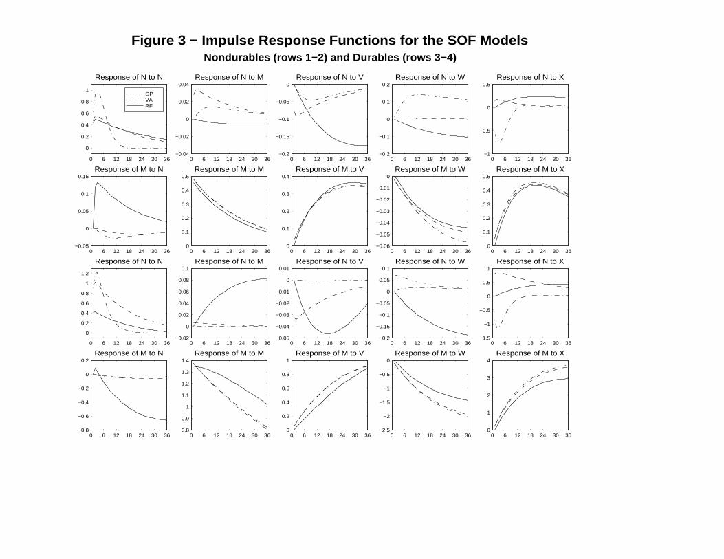
GPVARF

0 6 12 18 24 30 36−0.04

−0.02

0

0.02

0.04Response of N to M

0 6 12 18 24 30 36−0.2

−0.15

−0.1

−0.05

0Response of N to V

0 6 12 18 24 30 36−0.2

−0.1

0

0.1

0.2Response of N to W

0 6 12 18 24 30 36−1

−0.5

0

0.5Response of N to X

0 6 12 18 24 30 36−0.05

0

0.05

0.1

0.15Response of M to N

0 6 12 18 24 30 360

0.1

0.2

0.3

0.4

0.5Response of M to M

0 6 12 18 24 30 360

0.1

0.2

0.3

0.4Response of M to V

0 6 12 18 24 30 36−0.06

−0.05

−0.04

−0.03

−0.02

−0.01

0Response of M to W

0 6 12 18 24 30 360

0.1

0.2

0.3

0.4

0.5Response of M to X

0 6 12 18 24 30 36

0

0.2

0.4

0.6

0.8

1

1.2

Response of N to N

0 6 12 18 24 30 36−0.02

0

0.02

0.04

0.06

0.08

0.1Response of N to M

0 6 12 18 24 30 36−0.05

−0.04

−0.03

−0.02

−0.01

0

0.01Response of N to V

0 6 12 18 24 30 36−0.2

−0.15

−0.1

−0.05

0

0.05

0.1Response of N to W

0 6 12 18 24 30 36−1.5

−1

−0.5

0

0.5

1Response of N to X

0 6 12 18 24 30 36−0.8

−0.6

−0.4

−0.2

0

0.2Response of M to N

0 6 12 18 24 30 360.8

0.9

1

1.1

1.2

1.3

1.4Response of M to M

0 6 12 18 24 30 360

0.2

0.4

0.6

0.8

1Response of M to V

0 6 12 18 24 30 36−2.5

−2

−1.5

−1

−0.5

0Response of M to W

0 6 12 18 24 30 360

1

2

3

4Response of M to X

Figure 3 − Impulse Response Functions for the SOF Models

Nondurables (rows 1−2) and Durables (rows 3−4)

0 6 12 18 24 30 36

0

0.2

0.4

0.6

0.8

1

Response of N to N

References

Anderson, G. and G. Moore (1985). A Linear Algebra Procedure for Solving Linear Perfect

Foresight Models. Economics Letters 17 (3), 247{252.

Auerbach, A. J. and J. R. Green (1980). Components of Manufacturing Inventories. NBER

Working Paper No. 491.

Baily, M. N. (1986, February). Productivity Growth and Materials Use in U.S. Manufacturing.

Quarterly Journal of Economics 101 (1), 185{95.

Basu, Susanto (1996, August). Procyclical Productivity: Increasing Returns or Cyclical Utiliza-

tion? Quarterly Journal of Economics 111 (3), 719{751.

Basu, Susanto and John G. Fernald (1995, August). Are Apparent Productive Spillovers a Fig-

ment of Speci�cation Error? Journal of Monetary Economics 36 (1), 165{188.

Basu, Susanto and Miles S. Kimball (1997, February). Cyclical Productivity with Unobserved

Input Variation. NBER Working Paper No. 5915.

Bils, M. and J. A. Kahn (1996, August). What inventory behavior tells us about business cycles.

Unpublished paper, University of Rochester.

Bivin, D. (1989). Disaggregation and the Speed of Adjustment in Inventory Models. Unpublished

paper, Indiana University-Purdue University at Indianapolis.

Bivin, D. (1993, Fall). The In uence of Inventories on Output and Prices: A Stage of Fabrication

Approach. Journal of Macroeconomics 15 (4), 627{651.

Blanchard, O. J. (1983, June). The Production and Inventory Behavior of the American Auto-

mobile Industry. Journal of Political Economy 91 (3), 365{400.

Blanchard, O. J. and C. M. Kahn (1980, July). The Solution of Linear Di�erence Models Under

Rational Expectations. Econometrica 48 (5), 1305{1311.

Blinder, A. S. (1986, August). Can the Production Smoothing Model of Inventory Behavior Be

Saved? Quarterly Journal of Economics 101 (3), 431{453.

Blinder, A. S. and L. J. Maccini (1991, Winter). Taking Stock: A Critical Assessment of Recent

Research on Inventories. Journal of Economic Perspectives 5 (1), 73{96.

Bresnahan, Timothy F. and Valerie A. Ramey (1994, August). Output Fluctuations at the Plant

Level. Quarterly Journal of Economics 109 (3), 593{624.

Bruno, Michael (1984, February). Raw Materials, Pro�ts, and the Productivity Slowdown. Quar-

terly Journal of Economics 99 (1), 1{30.

42

Chambers, R. G. (1988). Applied Production Analysis: A Dual Approach. New York, NY: Cam-

bridge University Press.

Durlauf, S. N. and L. J. Maccini (1995, December). Measuring noise in inventory models. Journal

of Monetary Economics 36 (1), 65{89.

Eichenbaum, M. (1984, July). Rational expectations and the smoothing properties of inventories

of �nished goods. Journal of Monetary Economics 14 (1), 71{96.

Eichenbaum, M. (1989, September). Some Empirical Evidence on the Production Level and Pro-

duction Cost Smoothing Models of Inventory Investment. American Economic Review 79 (4),

853{864.

Fair, R. C. (1989, May). The Production Smoothing Model is Alive andWell. Journal of Monetary

Economics 24 (3), 353{370.

Fuhrer, J. C., G. R. Moore, and S. D. Schuh (1995). Estimating the Linear-Quadratic Inventory

Model: Maximum Likelihood versus Generalized Method of Moments. Journal of Monetary

Economics 35, 115{157.

Ghali, M. A. (1987, June). Seasonality, Aggregation, and the Testing of the Production Smooth-

ing Hypothesis. American Economic Review 77 (3), 464{469.

Haltiwanger, J. C. and L. J. Maccini (1989). Inventories, Orders, Temporary and Permanent

Layo�s: An Econometric Analysis. Carnegie-Rochester Conference Series on Public Policy 30,

301{366.

Hinrichs, J. C. and A. D. Eckman (1981, September). Constant-Dollar Manufacturing Inventories.

Survey of Current Business 61 (9), 16{23.

Humphreys, B. (1995). The Behavior of Manufacturers' Inventories, Deliveries, and Prices of

Purchased Materials: Evidence, Theory, and Empirical Tests. Ph. D. thesis, Johns Hopkins

University, Baltimore, MD.

Husted, S. and T. Kollintzas (1987, October). Linear Rational Expectations Equilibrium Laws

of Motion for Selected U.S. Raw Material Imports. International Economic Review 28 (3),

651{670.

Kahn, J. A. (1987, September). Inventories and the Volatility of Production. American Economic

Review 77 (4), 667{679.

Kahn, J. A. (1992, May). Why is production more volatile than sales? theory and evidence on

the stockout-avoidance motive for inventory holding. Quarterly Journal of Economics 107 (2),

481{510.

43

Kashyap, A. K. and D. W.Wilcox (1993, June). Production and Inventory Control at the General

Motors Corporation During the 1920's and 1930's. American Economic Review 83 (3), 383{

401.

King, R. G. and M. W. Watson (1995, April). The Solution of Singular Linear Di�erence Systems

Under Rational Expectations. Unpublished paper, University of Virginia and Northwestern

University.

Kollintzas, T. A. (1992). A Generalized Variance Bounds Test with an Application to the Holt

et al. Inventory Model. Athens University of Economics and Business.

Krane, S. D. and S. N. Braun (1991, June). Production Smoothing Evidence from Physical-

Product Data. Journal of Political Economy 99 (3), 558{581.

Lovell, M. (1961, July). Manufacturers' Inventories, Sales Expectations, and the Acceleration

Principle. Econometrica 29 (3), 293{314.

Maccini, L. J. and R. J. Rossana (1984, May). Joint Production, Quasi-Fixed Factors of Produc-

tion, and Investment in Finished Goods Inventories. Journal of Money, Credit, and Bank-

ing 16 (2), 218{236.

Miron, J. A. and S. P. Zeldes (1988, July). Seasonality, Cost Shocks, and the Production Smooth-

ing Model of Inventories. Econometrica 56 (4), 877{908.

Mosser, P. (1989, December). On the Production Smoothing Properties of Work-In-Progress

Inventories. Columbia University Working Paper.

Nguyen, S. V. and S. H. Andrews (1988, February). Stage-of-Fabrication Inventory Behavior: A

General Target-Adjustment Model. Applied Economics 21 (1), 175{192.

Perron, P. (1989, November). The Great Crash, the Oil Price Shock, and the Unit Root Hypoth-

esis. Econometrica 57 (6), 1361{1401.

Ramey, V. A. (1989, June). Inventories as Factors of Production and Economic Fluctutations.

American Economic Review 79 (3), 338{354.

Ramey, V. A. (1991, April). Nonconvex Costs and the Behavior of Inventories. Journal of Political

Economy 99 (2), 306{334.

Reagan, P. and D. P. Sheehan (1985, March). The Stylized Facts about the Behavior of Man-

ufacturers' Inventories and Backorders over the Business Cycle. Journal of Monetary Eco-

nomics 15, 217{246.

Romer, C. D. (1986, June). Is the stabilization of the postwar economy a �gment of the data?

American Economic Review 76 (3), 314{334.

44

Rossana, R. (1990, February). Interrelated Demands for Bu�er Stocks and Productive Inputs:

Estimates for Two Digit Manufacturing Industries. The Review of Economics and Statis-

tics 72 (1), 19{29.

Schuh, S. (1992). Aggregation E�ects in Production Smoothing and Other Linear Quadratic In-

ventory Models. Ph. D. thesis, Johns Hopkins University, Baltimore, MD.

Schuh, S. (1996, November). Evidence on the link between �rm-level and aggregate inventory

behavior. Federal Reserve Board FEDS Working Paper 1996-46.

Sims, C. A. (1996, August). Solving Linear Rational Expectations Models. Unpublished paper,

Yale University.

U.S. Department of Commerce (1991).The 1982 Benchmark Input-Output Accounts of the United

States. Washington, D.C.: Government Printing O�ce.

West, K. D. (1983). A Note on the Econometric Use of Constant Dollar Inventory Series. Eco-

nomics Letters 13 (4), 337{341.

West, K. D. (1986, April). A Variance Bounds Test of the Linear Quadratic Inventory Model.

Journal of Political Economy 94 (2), 374{401.

West, K. D. (1988). Order backlogs and production smoothing. In A. Chikan and M. Lovell

(Eds.), The Economics of Inventory Management, Amsterdam. Elsevier.

West, K. D. (1993, September). Inventory Models. NBER Technical Working Paper No. 143.

West, K. D. and D.W.Wilcox (1994, December). Some Evidence on Finite Sample Behavior of an

Instrumental Variables Estimate of the Linear Quadratic Inventory Model. NBER Technical

Working Paper No. 139.

45