UNIVERSIDADE ESTADUAL PAULISTA “JÚLIO DE MESQUITA FILHO”

INSTITUTO DE BIOCIÊNCIAS – RIO CLARO unesp

PROGRAMA DE PÓS-GRADUAÇÃO EM ECOLOGIA E BIODIVERSIDADE

FENOLOGIA REMOTA E OS PADRÕES DE TROCAS FOLIARES AO LONGO DE UM

GRADIENTE DE SAZONALIDADE

BRUNA DE COSTA ALBERTON

Tese apresentada ao Instituto de Biociências do Campus de Rio Claro, Universidade Estadual Paulista, como parte dos requisitos para obtenção do título de Doutor em Ecologia e Biodiversidade.

Agosto – 2018

BRUNA DE COSTA ALBERTON

FENOLOGIA REMOTA E OS PADRÕES DE TROCAS FOLIARES AO LONGO DE UM

GRADIENTE DE SAZONALIDADE

Tese de Doutorado apresentada ao

Instituto de Biociências da

Universidade Estadual Paulista

“Júlio de Mesquita Filho”, Campus

de Rio Claro, para obtenção do título

de Doutora em Ecologia e

Biodiversidade.

Orientadora: Profa. Dra. LEONOR PATRICIA CERDEIRA MORELLATO

Co-orientador: Prof. Dr. RICARDO DA SILVA TORRES

Rio Claro – SP

2018

Alberton, Bruna de Costa Fenologia remota e os padrões de trocas foliares ao longo de umgradiente de sazonalidade / Bruna de Costa Alberton. - Rio Claro, 2018 252 f. : il., figs., gráfs.

Tese (doutorado) - Universidade Estadual Paulista, Instituto deBiociências de Rio Claro Orientadora: Leonor Patricia Cerdeira Morellato Coorientador: Ricardo da Silva Torres Agência de fomento e n. de processo: FAPESP: 2014/00215-0,FAPESP: 2016/01413-5, FAPESP: 2013/50155-0

1. Ecologia vegetal. 2. Fenocâmeras. 3. Sazonalidade. 4. Fenologiavegetativa. 5. Produtividade do ecossistema. 6. Imagens digitais. I. Título.

581.5A334f

Ficha Catalográfica elaborada pela STATI - Biblioteca da UNESPCampus de Rio Claro/SP - Adriana Ap. Puerta Buzzá / CRB 8/7987

Powered by TCPDF (www.tcpdf.org)

À minha família, Pai, Mãe e Lucas

AGRADECIMENTOS

À minha família, que é o meu alicerce e o meu refúgio, onde sei que sempre poderei voltar e

ser bem acolhida. Meu pai Antônio, minha mãe Janete e meu irmão Lucas, agradeço ao suporte de

cada um e por tudo que representam em minha vida. Ao meu companheiro de vida, amigo, namorado,

colega de profissão, Renan, que nunca mediu esforços em me ajudar e me apoiar, sobretudo nos

últimos meses de finalização desta tese. É um prazer dividir a vida contigo. Eu amo vocês. Obrigada

por tudo.

Agradeço aos meus orientadores, Patrícia e Ricardo, aos quais sou eternamente em débito, por

todo o aprendizado, conselhos, lições e network que me foi passado ao longo destes anos de mestrado

e doutorado. Gratidão.

Patrícia tem papel fundamental na construção de minha carreira científica ao longo da pós-

graduação. Foi ela quem me apresentou as fenocâmeras e me incentivou a desenvolver meus estudos

sobre a fenologia remota próxima. Graças à sua visão de carreira, pude aproveitar grandes

oportunidades, interagir com excelentes pesquisadores e entrar no universo multidisciplinar da

pesquisa acadêmica, que muito me inspira. São inúmeros os motivos para lhe agradecer, não somente

como orientadora, mas como uma grande amiga que tive nestes últimos anos. Em especial neste final

de tese, minha gratidão pelo esforço em me ajudar nos tópicos de maior dificuldade e pela paciência

com todas as correções.

Meu co-orientador, Ricardo Torres, com quem tive a oportunidade de aprender muito e poder

contar sempre com sua disposição em me ajudar. Foram muitas reuniões, presenciais ou por Skype,

com orientações muito bem direcionadas, esclarecedoras e sempre incentivadoras.

Um agradecimento mais do que especial aos meus amigos. Àqueles de longa data e que ainda

permanecem próximos, mesmo que distantes (fisicamente), e àqueles que se tornaram minha família

ao longo dos lugares onde vivi e passei nestes últimos anos. Por sorte, tenho muitos, especialmente

nesta cidade (Rio Claro), a qual tem sido minha casa na maior parte destes últimos sete anos. A minha

amizade inabalável do sul do país, minha amiga e irmã da vida Mainara Cascaes, e minhas amigas

“bioloukas”: Thereza Garbelotto, Patricia Correa, Gabriela Thomaz e Beatriz Wessler. Aos meus

colegas de laboratório que se tornaram grandes amigos e por muito tempo minha família rio-clarense:

Gabriela Camargo, Vanessa Staggemeier, Nathália Miranda, Daniel Carstensen, Irene Mendoza e

Natália Costa, com quem não somente dividi o mesmo laboratório, mas também foi minha grande

companheira ao dividirmos o mesmo teto por quase cinco anos. A todos os meus queridos amigos que

o forró me trouxe, em especial a Thais Helena Condez e sua família, pela amizade sincera, leve e tão

cheia de amor. Um agradecimento especial aos amigos incríveis que fiz durante minha vivência em

Boston, os quais foram essenciais para tornar minha vida norte-americana mais leve, mais divertida e

um pouco menos fria, em especial à Laura Zoffoli, por sua amizade e companheirismo.

Agradeço ao Laboratório de Fenologia, a todos os membros que já passaram por ele e aos

atuais, por sempre proporcionarem um ambiente leve e inspirador para o trabalho, pelas trocas de

conhecimentos e colaborações ao longo de todos os encontros e workshops realizados. É realmente

um prazer fazer parte deste grupo e um orgulho tê-lo dentro de minha carreira profissional. Agradeço

especialmente aos meus queridos amigos e colegas, Bruno Defane e Leonardo Cancian, por todo o

suporte técnico ao longo dos trabalhos de campo, processamento das imagens digitais e auxilio em

SIG. Agradeço também aos alunos de graduação, os quais tive a oportunidade de auxiliar na

orientação de seus trabalhos, e que se interessaram pela fenologia remota próxima me auxiliando no

processamento das imagens: Marina Muller, Carolina Crivelin e Rodrigo Lacerda.

Agradeço aos colaboradores na pesquisa desta tese. Ao Professor Dr. Andrew Richardson, por

aceitar ser meu supervisor e me receber em seu laboratório durante os 12 meses de estágio na

Universidade de Harvard, entre maio de 2016 e maio de 2017. Foi sob a supervisão de Andrew, que

aprendi a manipular e processar os dados de alta frequência de fluxo de carbono, bem como associá-

los aos dados da fenologia remota próxima das câmeras digitais e estabelecer as primeiras questões

ecológicas dentro do trabalho que viria a se tornar o capítulo 3 desta tese. Agradeço ao Professor Dr.

Humberto Rocha, da Universidade de São Paulo (USP), por colaborar disponibilizando os dados das

estações meteorológicas e os dados de fluxo de carbono das áreas do cerrado Pé-de-Gigante e de

Santa Virgínia, bem como pela disponibilidade presencial e remota com a qual vem auxiliando no

desenvolvimento desta tese, através de sua experiência nas trocas de fluxos de energia em

ecossistemas tropicais. Também agradeço à sua equipe, Emília Brasilio pela compilação e pré-

processamento dos dados meteorológicos e de fluxo de carbono, e ao Eduardo Gomes Lopes e Helber

Freitas pelo suporte técnico indispensável nos trabalhos realizados de instalação e manutenção das

câmeras digitais nas torres de fluxo. Agradeço por toda colaboração da EMPRABA Semi-árido, em

especial à Magna Soelma Bezerra de Moura, por todo o suporte técnico na instalação, manutenção e

coleta dos dados da câmera digital na torre de fluxo da área de caatinga, por disponibilizar os dados

meteorológicos e de fluxo de carbono, e por colaborar no desenvolvimento dos trabalhos desta tese,

contando com sua experiencia em ecossistemas áridos.

Agradeço aos pesquisadores que participaram e aos que ainda participam do projeto e-

Phenology, com os quais tive a oportunidade de trabalhar, aprender e colaborar. Um agradecimento

especial aos professores Jurandy Almeida, Jefersson dos Santos, Fabio Faria, João Comba e Lucas

Schnorr, e aos colegas que também desenvolveram suas teses e dissertações dentro do projeto:

Greice Mariano, Roger Leite e Alexandre Almeida.

Agradeço ao Departamento de Botânica e a todos os técnicos que auxiliaram nos trabalhos de

campo ao longo do doutorado, em especial ao Rafael Consolmagno, que participou ativamente das

instalações, manutenções e reparos das câmeras digitais, pelos muitos quilômetros rodados por todas

as áreas monitoradas e pela parceria leve e pró ativa sempre presente.

Agradeço ao Instituto Florestal (IF) do Estado de São Paulo, bem como aos dirigentes das

unidades, pela liberação concedida de desenvolver as pesquisas desta tese nas áreas da Estação

Ecológica de Itirapina, do Parque Estadual do Vassununga (área do cerrado Pé-de-gigante), e no

Parque Estadual da Serra do Mar Núcleo Santa Virgínia (área da Mata Atlântica). Também agradeço

aos donos da Fazenda São José e do Instituto Arruda Botelho (IAB) por permitir o trabalho de campo

realizado em sua fazenda (área de cerrado) em Itirapina.

Agradeço à Seção de Pós-Graduação do Instituto de Biociências da UNESP, pelo suporte ao

longo de todos os anos de doutorado, e ao conselho do Programa de Pós-Graduação em Ecologia e

Biodiversidade, pelo suporte, boa relação e abertura estabelecida aos alunos matriculados, no intuito

de sempre melhorar as normativas do curso.

Agradeço à Fundação de Amparo à Pesquisa do Estado de São Paulo (FAPESP) pelas bolsas

de doutorado e de estágio de pesquisa no exterior concedidas (#2014/00215-0, #2016/01413-5); pelo

financiamento dos projetos e-Phenology (#2010/52113-5, #2013/50155-0, FAPESP-Microsoft

Research Virtual Institute); e pelo financiamento de projetos paralelos que contribuíram nesta tese

(#2007/59779-6, e FAPESP-VALE-FAPEMIG # #2010/51307-0). Ao CNPq pelo apoio dado por

meio das bolsas de produtividade de meus orientadores (#306243/2010-5 #306587/2009-2). Ao

Programa de Apoio à Pós-Graduação (PROAP) pelo auxílio concedido para participação em eventos

científicos durante o período de doutorado.

A maior riqueza

do homem

é sua incompletude.

Nesse ponto

sou abastado.

Palavras que me aceitam

como sou

— eu não aceito.

Não aguento ser apenas

um sujeito que abre

portas, que puxa

válvulas, que olha o

relógio, que compra pão

às 6 da tarde, que vai

lá fora, que aponta lápis,

que vê a uva etc. etc.

Perdoai. Mas eu

preciso ser Outros.

Eu penso

renovar o homem

usando borboletas.

(Manuel de Barros)

RESUMO

O estudo da fenologia vegetal busca monitorar, compreender e prever os ciclos de vida

recorrentes das plantas, principalmente influenciados pelo clima. O monitoramento das fenofases

vegetativas de brotamento e senescência foliar são essências para a compreensão de processos

ecossistêmicos importantes como, a produtividade primária, as trocas de energia entre atmosfera e

superfície terrestre, o fluxo de carbono, e a ciclagem de nutrientes. Logo, entender a resposta das

plantas ao clima e ser capaz de prever alterações em sua fenologia, é essencial para o entendimento

das dinâmicas de comunidades vegetais e da funcionalidade dos ecossistemas em frente a cenários de

mudanças climáticas. Nos últimos anos, a busca por novas tecnologias dentro de estudos científicos

vem crescendo com o intuito de tornar mais viável e amplo o monitoramento fenológico. Neste

trabalho, buscamos incorporar novas tecnologias de observações fenológicas com o uso de câmeras

digitais (fenocâmeras) instaladas em campo para o monitoramento de dados fenológicos de

brotamento e senescência foliar em ambientes tropicais. Os objetivos gerais deste trabalho de tese,

dividida em quatro seções, foram de : (i) compilar informações sobre conceitos e propriedades da

técnica de fotografias repetidas (repeated photograph technic), criando um protocolo para o uso de

câmeras digitais nos trópicos e levantar suas principais contribuições no âmbito na biologia da

conservação; (ii) monitorar e descrever os padrões da fenologia vegetativa em diferentes comunidades

vegetais sazonais, através dos dados obtidos de imagens digitais e investigar os principais gatilhos

ambientais atuando nas diferentes vegetações; (iii) associar dados de fenologia foliar juntamente com

dados de produtividade primária bruta dentro de ecossistemas sob diferentes pressões de sazonalidade

para um melhor entendimento das respostas entre vegetação-atmosfera mediadas pela fenologia foliar;

e (iv) apresentar resultados das principais iniciativas em análises de imagens digitais para o

monitoramento da fenologia foliar desenvolvidas dentro da rede de fenocâmeras do projeto e-

phenology, no âmbito da colaboração e-science. As vegetações estudadas neste trabalho estão

distribuídas ao longo de um gradiente de sazonalidade de distribuição de chuvas e incluem: uma

vegetação de caatinga; três diferentes fisionomias de cerrado que correspondem a um cerrado campo

sujo, um cerrado sensu stricto, e um cerrado denso; e uma vegetação de Mata Atlântica. Séries

temporais relacionadas às fenofases vegetativas foram extraídas do conjunto de imagens digitais

coletadas em cada uma das áreas e analisadas dentro do contexto de cada um dos objetivos deste

trabalho. Demonstramos que o estabelecimento de uma rede de fenocâmeras é uma poderosa

ferramenta para a biologia da conservação, através da capacidade de obtermos dados de alta

frequência temporal associados a uma ampla gama de dados ambientais monitorados. Através da

aplicação de fenocâmeras pode-se obter novas informações sobre prática de manejo e restauração de

ambientes, além de sua potencial contribuição nas esferas de educação ambiental e ciência cidadã.

Observamos que a disponibilidade de água e luz no ambiente são os fatores mais importantes para o

desenvolvimento foliar ao longo de diferentes comunidades sazonais. Relações hídricas em plantas

foram mais importantes para vegetações mais áridas, como a caatinga, enquanto que a disponibilidade

de luz, quantificada através da sazonalidade do comprimento do dia, teve maior influência no gatilho

do desenvolvimento foliar nas comunidades de cerrado. No âmbito dos ecossistemas, demonstrou-se

uma nova abordagem ao se relacionar a fenologia foliar derivada de câmeras com a produtividade de

ecossistemas tropicais. A dinâmica fenológica analisada através da variabilidade de sinais fenológicos

encontrados dentro das diferentes vegetações, foram importantes para explicar os padrões temporais

de produtividade dos ecossistemas. A compilação de trabalhos realizados através da colaboração e-

science, apresentados na seção 4, foram de grande importância para o desenvolvimento dos métodos e

análises, bem como para o alcance dos resultados obtidos dentro desta tese. Este trabalho oferece uma

nova ferramenta para o monitoramento fenológico em vegetações tropicais, e sugere novos desafios a

serem desenvolvidos bem como incentiva uma maior abrangência no uso de fenocâmeras a fim de

cobrir um maior número de áreas e diferentes tipos de vegetação, além de associar estes estudos com

abordagens desenvolvidas em diferentes escalas como as observações diretas, a aplicação de imagens

de drones, bem como com as imagens de satélite. A comparação de diferentes escalas espaciais e

temporais irá nos ajudar a entender melhor a própria escala de informações provenientes das

fenocâmeras em termos de abrangência e detalhamento dos ecossistemas.

Palavras-chave: fenocâmeras, sazonalidade, fenologia vegetativa, produtividade do ecossistema,

imagens digitais

ABSTRACT

Plant phenology is a traditional science focused on monitoring, understanding, and predicting

recurrent life cycles events, which are mainly related to climate Leaf development stages are essential

plant phenophases for the better understanding of ecosystems processes such as carbon and water

fluxes, regulation of productivity, and nutrient cycling. Through the investigation of plant responses

to climate and phenological shifts prediction, we can better forecast climatic change effects on

vegetation dynamics and prevent loss of ecosystems functionalities. Aiming to become the

phenological collection wider and more feasible worldwide, the seek for new technologies has

stimulated several research centers of plant phenology monitoring. Here, we incorporated a new

technology of field phenological observations using digital cameras for the monitoring of leaf

exchanges in tropical vegetations. On this work, divided into four sections, we aimed to: (i) compile

information about concepts and properties of the repeated photograph technic, create guidelines for

the phenocams setup in tropical vegetation sites, and to provide key contributions of daily imagery

monitoring on biological conservation; (ii) to stablish a monitoring of different seasonal vegetations,

describing the phenological trends, and identify the environmental cues which are triggering the leaf

flushing and senescence for each vegetation type; (iii) analyze the canopy greenness obtained from

digital cameras in relation to gross primary productivity measurements, to better understand the role

of leaf phenology controlling ecosystem productivity in the tropics; and (iv) present some results of

phenocam image analysis research initiatives and tools devised in the context of e-Science

collaborations and built in the framework of the e-phenology project and the e-phenology network of

phenocams. The selected study sites belong to different seasonal biomes, which comprehends areas

from caatinga, savanna grasslands, savanna woodlands and Atlantic rainforest. Temporal series

representing foliar phenology were extracted from the data imagery of each vegetation site and were

analyzed into the context of each section of this work. We demonstrated that the establishment of

phenocam networking is a powerful tool for biological conservation through its capability of fine

temporal resolution data associated with wide spatial monitoring coverage. Besides, phenocams

applications can bring new information for management and restoration practices at several sites and

environments and contribute for the education for conservation and citizen science initiatives. We

observed that water and light were the most important predictors for the leaf phenological patterns

across seasonal vegetation communities. Water-plant relationships were more important for the

caatinga community, and light, through day-length seasonality, had more influence in the leafing

patterns of the cerrado communities. Regarding the ecosystem, we demonstrated a novel approach to

relate leaf phenology to seasonality of tropical ecosystems productivity. The phenological dynamics

regarding the variability of species phenological signals, and how they are built in into each

contrasting vegetation communities explains drivers of leaf phenology and productivity. A

compilation of articles developed through the e-science collaboration, presented in Section 4, were of

great importance for the generation of methods and analytical work, as well as for the results

achievements in this thesis. This work will offer a new tool for the phenological monitoring in the

tropics, and suggests next challenges to be addressed and the continuity of the e-phenology network

and the spread of new cameras covering new vegetation types; the development of bottom-up studies,

integrating on-the-ground observations, cameras, drones, and satellites, inter-comparing them and

placing camera-derived phenology in its own scale, by understanding how much and what kind of

information can be retrieved from ecosystems.

Key words: phenocameras, seasonality, leaf phenology, ecosystem productivity, digital images

SUMÁRIO

INTRODUCTION.................................................................................................................................12

SECTION 1: Introducing digital cameras to monitor plant phenology in the tropics: applications for

conservation…………………………………………………………………………………………...17

SECTION 2: Leafing patterns and drivers across seasonally dry tropical communities……………...50

SECTION 3: Leaf phenology correlates to gross primary productivity: an inter-comparison across

tropical biomes.………………………………...……………………………………………………...94

SECTION 4: e-Science and the multidisciplinary research built on the integrations of big data

ecological research and computational science……………………...………………………………142

CONCLUSIONS……………………………………………………………………………………..146

REFERENCES……………………………………………………………………………………….148

APPENDIX A: Leafing patterns and leaf exchange strategies of a cerrado woody

community…………….……………………………………………………………………………..150

APPENDIX B: Phenological visual rhythms: Compact representations for fine-grained plant species

identification…………...………………………………………………….…………………………189

APPENDIX C: Time series-based classifier fusion for fine-grained plant species

recognition…...………………………………………………………………………………………201

APPENDIX D: Fusion of Time Series Representations for Plant Recognition in Phenology

Studies.………………………………………………………………………………………………211

APPENDIX E: PhenoVis – Visual Phenological Analysis of Forest Ecosystems.....……………….222

APPENDIX F: Unsupervised distance learning for plant species identification.......………...……...238

12

1 INTRODUCTION

Plant phenology is a traditional science focused on monitoring, understanding, and predicting

recurrent life cycles events, which are mainly related to climate (Morellato et al., 2016). Leaf

development stages are plant phenophases responsible for indicating the growth season and for

controlling crucial ecosystems processes such as carbon and water fluxes, regulation of productivity,

and nutrient cycling (Reich, 1995; Baldocchi et al., 2005). Tropical ecosystems have significant

importance in the global carbon budget (Field et al., 1998; Ometto et al., 2005). By understanding

phenological patterns of tropical vegetations and what drives leaf production seasonality within tropical

communities, we can better forecast climatic change effects on vegetation dynamics and prevent loss

of ecosystems functionalities (Polgar and Primack, 2011).

Phenological studies in the tropics preclude the observation of many species across several sites

with intense human labor and costs (Alberton et al., 2014; Morellato et al., 2016). The scarcity of long-

term monitoring in tropical regions, necessary to understand the effects of global warming on organisms

(Abernethy et al., 2018) has stimulated several research centers to seek for new tools of plant phenology

monitoring. The near-surface remote phenology consists in the application of sensors in the ground for

the monitoring of plant to ecosystem-scale vegetation changes. The use of digital cameras to track leaf

exchanges came to fill the gap between the traditional on-the-ground monitoring by human direct

observation and remote sensing derived land surface phenology (Richardson et al., 2007; Morisette et

al., 2009; Morellato et al., 2016).

The technique of repeated photographs using digital cameras for phenology monitoring, or

phenocams, has increased in the last 10 years due its advantages of low cost investment, reduction in

size, easy set-up installation, the reduced human labor, increased temporal resolution, and the

opportunity of simultaneously monitoring several sites improving the spatial resolution of ground-based

phenology monitoring and offering the possibility of handling high resolution data (Crimmins and

Crimmins, 2008, Morisette et al., 2009; Graham et al., 2010; Alberton et al., 2017), leading phenocams

to a widely range of ecological applications worldwide.

The ongoing addition of new devices, high-resolution data survey, and sensor networks has

been improving the quality of data collected in biological studies, but at the same time increasing the

13

magnitude of scientific data collected. Near-surface monitoring systems in the tropics, for instance, are

necessarily complex since the environmental conditions are harsh and the diversity of species is usually

high. This leads to a next generation of scientific problems, which will require the establishment of

multidisciplinary teams (Hey and Hey 2006). To the process of data retrieval, management, and analysis

it will be required the collaboration between ecologists and computer scientists. e-Science is about the

collaboration of key areas of science, not considered a discipline, but a network of research initiative

focused on the specification and implementation of a set of tools and technologies capable of

supporting, improving, and speeding up data analysis, knowledge discovery, and decision making (Hey

and Hey 2006).

In Brazil, we have the e-phenology Network (http://www.recod.ic.unicamp.br/ephenology - As

of June 2018), introduced in this thesis, that comprehends the application of digital cameras as tools to

detect leaf flushing and senescence across different vegetation types from drylands, grasslands, and

cerrado savannas to rainforests. This project is innovative and puts Brazil in the state of the art of near-

remote phenology monitoring, already established in areas of temperate forests in northern hemisphere.

The e-phenology project also integrates the development of computational tools for the methodological

applications of algorithms for data mining and time series analysis (e.g., Almeida et al., 2014; Almeida

et al., 2016).

In this context, the present thesis is divided into four sections that all together, aim to present

the development of phenocams tools in tropical systems, their application in ecological studies and the

integration of e-science insights on peripherical approaches that contributed for this work. Sections are

described below.

Section 1 - Introducing digital cameras to monitor plant phenology in the tropics: applications

for conservation

Digital-camera-based monitoring phenology is growing in the tropics (e.g., Alberton et al.,

2014; Nagai et al., 2016; Moore et al., 2017; Lopes et al., 2017), but it is still sparse when compared

with temperate regions (Brown et al., 2017). Protocols and methodological approaches developed for

camera systems were launched from networks researchers of these regions. We aimed to spread our

14

experience of using digital cameras to monitor tropical vegetations across multiple sites to encourage,

among the scientific community of Brazil and tropics worldwide, their potential usability in a broader

ecological context.

This section brings a published article with compiled information about concepts and properties

of the technic, guidelines for the phenocams setup in tropical vegetation sites, and to provide key

contributions of daily imagery monitoring on biological conservation (Alberton et al., 2017).

Section 2 - Leafing patterns and drivers across seasonally dry tropical communities

Investigating the main drivers of plant phenology is of paramount importance for a better

understanding of plant shifts in response to a changing climate and for effective biodiversity

conservation from species to ecosystems (Polgar and Primack, 2011; Morellato et al., 2016). As already

mentioned, plant phenology remains poorly understood for the tropics, and so the triggers of

phenological transitions (Morellato et al., 2013; Chambers et al., 2013; Abernethy et al., 2018).

The traditional phenology monitoring, made by direct observations, provides confident data

from individuals species to vegetation communities that contribute with pattern validation for remote-

monitoring methods such as phenocameras and satellite images. Despite the coarse time-scale of

observations (monthly), long-term on-the-ground phenology may be used for the investigation of leaf

development drivers and further analysis of climatic changes impacts. A study using a 7-year on-the-

ground phenological time series, compiled with leaf flushing and senescence monthly data, aimed to

investigate the main environmental drivers of a cerrado sensu stricto community and their leaf exchange

strategies species. This work, which I co-authored, was conducted in one of the sites, where an e-

phenology camera was installed and was carried out in parallel along this thesis development (Appendix

A).

By tracking daily images combined with environmental measurements, we can fine-tune plant

color changes to leafing exchange patterns and unravel the influence of climatic variables. A wide range

of questions might be investigated. In this section, we conducted, for the first time, a phenological

research across multiple-sites monitoring leafing exchange patterns using phenocams. We aimed to

15

describe the leaf phenological patterns across seasonally dry tropical communities monitored by digital

cameras, investigating the main environmental factors influencing the timing and length of growing

seasons, and intercompare vegetations under distinct severity of dry season and across key life forms

(grassy – woody), regarding their phenological dynamics and drivers of leaf phenology.

Section 3 - Leaf phenology correlates to gross primary productivity: an inter-comparison across

tropical Biomes.

Tropical leaf phenology is regarded as a first order mechanism regulating seasonality of carbon

assimilation in tropical evergreen forests (Restrepo-Coupe et al., 2013; Restrepo-Coupe et al., 2017;

Wu et al., 2016; Wu et al., 2017). Studies in temperate ecosystems have demonstrated that the camera-

derived Gcc index, a measure of vegetation greenness, is well related to the gross primary productivity

(GPP) curves (Richardson et al., 2010; Migliavacca et al., 2011; Keenan et al., 2014; Toomey et al.,

2015). Phenocams have played an important role in those ecosystem-scale studies, contributing to link

ground observed changes to ecosystem scale accessments derived from flux towers and remote sense

indices (Ahrends et al., 2009; Migliavacca et al., 2011; Tomey et al., 2016). Leaf phenology should also

be considered on Dynamic Global Vegetation Models (DGVMs). These models are based on coupled

information between plant biogeography and biogeochemical processes to simulate ecosystem fluxes

and climate shifts in a climatic change scenario (Foley et al., 1998; Restreppo-Coupe et al., 2017). In

this context, understanding vegetative phenological transitions is essential to better estimate

measurements of gross primary productivity (GPP), because there is still a gap of knowledge about the

drivers of productivity in the tropics (Restreppo-Coupe et al., 2017). In this context, camera-derived

phenological time series might provide key information to understand the photosynthetic seasonality of

tropical forests and atmospheric-vegetation feedbacks to a changing climate (Richardson et al., 2013;

Restreppo-Coupe et al., 2017).

In this section, we propose to analyze the relationship between the leaf phenology extracted

from phenocameras and the ecosystem photosynthetic activity from GPP measurements of eddy-

covariance towers across three distinct Neotropical biomes: Caatinga, Cerrado, and Rainforest. We

16

aim to inter-compare the phenology-GPP dynamics across sites belonging to each vegetation domain

and contrasting seasonality.

Section 4 – e-Science and the multidisciplinary research built on the integrations of big data

ecological research and computational science

Throughout this section, we present some results of phenocam image analysis research

initiatives and tools devised in the context of e-Science collaborations and built in the framework of the

e-phenology project and the e-phenology network of phenocams. The published papers are presented

in Section 4 and all are directly connected to the development of this thesis and opened up the possibility

to explore the results presented in Sections 1 to 3.

17

Section 1

Article published in the Journal of Perspectives in Ecology and Conservation:

ALBERTON, B.C. et al. Introducing digital cameras to monitor plant phenology in the tropics:

Applications for conservation. Perspectives in Ecology and Conservation, v. 15, p. 82-90,

2017.

18

Introducing digital cameras to monitor plant phenology in the tropics: applications for

conservation

Authors: Bruna Alberton1*, Ricardo da S. Torres2, Leonardo F. Cancian1, Bruno D. Borges1,

Jurandy Almeida3, Greice Mariano2, Jefersson dos Santos4, Leonor Patricia C. Morellato1

1 UNESP Universidade Estadual Paulista, Instituto de Biociências, Departamento de Botânica,

Laboratório de Fenologia, Rio Claro, São Paulo, Brazil.

*Corresponding author

Email address: brualberton@gmail.com

2 RECOD Lab, Institute of Computing, University of Campinas – UNICAMP

13083-852, Campinas, SP – Brazil

3 Institute of Science and Technology, Federal University of São Paulo – UNIFESP, 12247-014,

São José dos Campos, SP, Brazil

4 Department of Computer Science, Universidade Federal de Minas Gerais – UFMG, 31270-

010, Belo Horizonte, MG, Brazil

Short title: Introducing phenocams and their applications on conservation biology.

19

Keywords: leaf phenology; repeated photography; RGB color channels; conservation biology;

e-science

Abstract

The application of digital cameras to monitor the environment is becoming global and

changing the way of phenological data collection. The technique of repeated digital photographs

to monitor plant phenology (phenocams) has increased due to its low-cost investment, reduced

size, easy set up installation, and the possibility of handling high-resolution near-remote data.

Considering the widespread use of phenocams worldwide, our main goals here are: (i) to provide

a step-by-step guide for phenocam set up in the tropics, reinforce its appliance as an efficient tool

for monitoring tropical phenology and foster networking, (ii) to discuss phenocam applications

for biological conservation, management, and ecological restoration. We provide the concepts

and properties for image analysis which allow representing the phenological status of the

vegetation. The association of a long-term imagery data with local sensors (e.g., meteorological

stations and surface-atmosphere flux towers) allows a wide range of studies, especially linking

phenological patterns to climatic drivers; and the impact of climate changes on plant responses.

We show phenocams applications for conservation as to document disturbances and changes on

vegetation structure, such as deforestation, fire events, and flooding and the vegetation recovery.

Networks of phenocams are growing globally and represent an important tool for conservation

and restoration, as it provides hourly to daily information of monitored systems spread over

several sites, ecosystems, and climatic zones. Moreover, websites enriched by vegetation dynamic

imagery data can promote science knowledge by engaging citizen science participation.

20

1 INTRODUCTION

The use of digital cameras to document plant changes is not novel. Photographs have been

used to monitor landscape since 1965 by Hastings and Turner to verify changes in the ecosystem

dynamics and structure of the arid southwest region of the US. Thompson et al. (2002) used

photographic registers for the long-term study of glacial retreat in the Antarctic ice sheet.

Repeated digital images have been used to document changes in cultural landscapes (Peñuelas &

Boada 2003, Webb et al. 2007); to measure vegetation growth and biomass (Crimmins &

Crimmins 2008, Graham et al. 2009); to detect plant stress and nitrogen status (Wang et al. 2004)

and to monitor crops (Slaughter et al. 2008). More recently, the application for monitoring leaf

exchanges patterns or leafing phenology (Richardson et al. 2007, 2009, Nagai et al. 2011) has

brought the technique to the agenda of global change research and conservation (Richardson et al

2013, Morellato et al. 2016).

Phenology is an integrative environmental science focused on monitoring, understanding,

and predicting recurrent life cycles events of organisms, which are mainly related to climate

(Morellato et al. 2016). Leafing is the plant phenological event that defines the growth season and

controls crucial ecosystems processes such as, nutrient cycling, water storage, regulates

productivity in terrestrial ecosystems, and the dynamics of carbon sequestration (Reich 1995,

Baldocchi et al. 2005).

Phenological studies have been efficiently applied to track effects of environmental

changes on plants and animals in temperate regions, answering questions about the current

scenario of global climate change and stimulating the search for innovative tools of plant

monitoring (Polgar & Primack 2011). Detect plant responses to environmental changes across

tropical systems, especially in the Southern Hemisphere, is an important question on the global

agenda since few studies have addressed trends related to global warming (Rosenzweig et al.

2008, Morellato et al. 2013, 2016, Chambers et al. 2013). However, the tropical high diversity of

species precludes the observation of many species across several sites due to the intense human

labor and costs (Alberton et al. 2014, Morellato et al. 2016).

21

The technique of repeated photographs to monitor plant phenology may overcome those

difficulties. The application has increased due to its low-cost, reduced size, easy set up, and the

possibility of handling high-resolution data, making digital cameras reliable tools for a wide range

of ecological applications (Crimmins & Crimmins 2008, Morisette et al. 2009, Graham et al.

2010, Nasahara et al. 2015, Brown et al. 2016). Digital cameras for plant phenology observation,

also called phenocams, have allowed the detection of leaf phenological events through the

analysis of color changes along time. By quantifying the red, green, and blue (RGB) color

channels, it is possible to estimate, for instance, leaf flushing and senescence, using the green and

red channels, respectively (Ahrends et al. 2009, Morisette et al. 2009, Richardson et al. 2009).

The term “Near-surface remote phenology” consists in the use of sensors installed on the

ground, as the phenocams, with the objective of monitoring ecosystem-scale vegetation changes.

Digital cameras monitoring canopy vegetation has an important role by filling the “gap of

observations” between satellite monitoring and the traditional on-the-ground phenology

(Alberton et al. 2014, Brown et al. 2016, Morellato et al. 2016, Morisette et al. 2009). The use of

imagery data over the traditional phenological observations allows simultaneous multi-sites

monitoring, long-term monitoring collecting high-frequency data (daily, hourly), and reduced

human labor fieldwork for data acquisition. Phenocams networks are already covering a wide

range of ecosystems in the world (Richardson et al. 2013, Brown et al. 2016). The main networks

websites are the Phenocam Network in the United States (http://phenocam.sr.unh.edu - as of Jan.

2017), the EuroPhen in Europe (http://european-webcam-network.net - as of Jan. 2017) and the

Phenological Eyes Network (PEN) in Japan (http://pen.agbi.tsukuba.ac.jp - as of Jan. 2017).

Together these initiatives combine more than 250 outdoor cameras (Brown et al. 2016, Nasahara

& Nagai et al. 2015). For the tropics, we have the Tropidry project as a successful example of

ecological project with intense multidisciplinary data collection, including the use of phenology

towers with phenocams, covering dry tropical sites (http://tropi-dry.eas.ualberta.ca/ - as of May

2017). In Brazil, the e-phenology Network (http://www.recod.ic.unicamp.br/ephenology - as of

Jan. 2017) introduced in this paper, target the challenge of monitoring different vegetation types

from dry forest, grasslands, and cerrado savannas to rainforests.

22

Therefore, considering the worldwide applications of phenocams in ecological studies,

our main goals here are: (i) to provide a step-by-step guide for phenocam set up in the tropics,

reinforce its appliance as an efficient tool for monitoring tropical phenology, (ii) to show how

phenocams can provide key contributions to biological conservation, and (iii) to encourage this

promising research field in Brazil and tropical areas based on the e-phenology project experience,

and foster networking and e-science collaborative research.

2 PHENOCAMS AS TOOLS FOR THE MONITORING OF PLANT PHENOLOGY

Digital images are typically based on the RGB color model (red, green, and blue color

channels). These channels encode the brightness values of the scene and can be combined in more

than 16 million of colors, representing basically all the colors perceived by humans (Cheng 2001).

Through the quantification of the RGB color channels, it is possible to calculate vegetation

indices, which are related to leaf color changes representing the phenological status of the

vegetation (Richardson et al. 2007, Sonnentag et al. 2012) (Fig. 1).

By capturing daily digital images of a given site, we derivate time series encoding RGB

color changes over time. Thus, the leaf patterns can be described based, for instance, on the

proportion of the green fraction in the images (Richardson et al. 2007). The association of digital

imagery data with local sensors (e.g., meteorological stations and surface-atmosphere fluxes)

uncovers a wide range of research opportunities, especially linking phenological patterns to

climatic drivers, and analyzing long-term data to detect phenological shifts due to the impact of

anthropogenic changes (Polgar & Primack 2011, Brown et al. 2016, Morellato et al. 2016).

The collection of daily vegetation color changes has been motivated also by the need to

understand ecosystem-scale energy fluxes (Baldocchi et al. 2005, Richardson et al. 2007). Studies

from temperate vegetation have found the start of the vegetation greenness controls the gross

primary productivity (GPP) curves (Richardson et al. 2010, Migliavacca et al. 2011, Keenan et

al. 2014). Therefore, temporal changes in the vegetation drive carbon exchange processes via

influencing the photosynthesis process, respiration, and litter production (Peichl et al. 2014).

23

Most of the studies using phenocams have been developed in the Northern hemisphere,

covering mainly deciduous forests (Richardson et al. 2007, 2009, Nagai et al. 2011). However,

the application of repeated digital photographs is also efficient for the phenology monitoring of

temperate grasslands (Inoue et al. 2015, Julitta et al. 2014), peatland (Peich et al. 2015), and

evergreen forest (Toomey et al. 2015). Its reliability for tropical vegetation was recently validated

for woody cerrado savanna (Alberton et al. 2014) and applied for tropical forest (Nagai et al.

2016, Lopes et al. 2016). The use of camera-derived vegetation indices in association with leaf

demography-ontogeny models has been recently applied in the Amazon forest to investigate

ecosystem-scale photosynthetic seasonality (Wu et al. 2016). However, there is still little focus

on the species level analysis and on grasslands, mountains and other tropical vegetation.

3 PROCEDURES FOR PHENOLOGICAL MONITORING USING DIGITAL CAMERAS

Digital cameras are reliable tools for the monitoring of vegetation because they have low

price and easy setup, while providing high frequency and resolution data. Here, we introduce the

main steps for phenology camera set up and basic information about image processing for data

analysis (Fig. 1). A detailed protocol is available in the Supplementary Material.

3.1 Camera set up and image settings

In general, the camera is placed in a tower built in the middle of vegetation (Fig. 2a and b). The

choice of the site and the field of view must maximize the vegetation to be monitored.

Hemispherical lens cameras are reliable for capturing images of the canopy, reducing crown cover

among individual species (Fig. 2c). Cameras should be positioned facing North - Northeast to

maximize the light over the canopy and to minimize lens flare. Cameras can be set up on small

towers, close to the ground, to capture landscape images (Fig. 2d and e) when the focus are

shrublands, grasslands, or other vegetations with short canopies and across heterogeneous

landscapes as rupestrian grasslands (Fig. 2f).

Different digital cameras have been used in repeated photography monitoring (see

Sonnentag et al. 2012, Steenweg et al. 2017). Internet protocol (IP) cameras are ideal because

they can be connected to a network and the image download performed remotely. For instance,

24

Stardot IP cameras record landscape images, have been successfully applied in temperate

ecosystem monitoring, and were chosen as the standard camera for two of the major networks in

North Hemisphere (Brown et al. 2016). Hemispherical lens (also called fish-eye) have been

chosen for monitoring tropical vegetation sites (Alberton et al. 2014, Nagai et al. 2016) and by

PEN (Nasahara & Nagai et al. 2015). The fish-eyes lens (360o) improve the selection of crowns

with more precision and less covered areas (see Alberton et al. 2014).

We recommend capturing a high frequency of images (a set of 3-5 images per hour, from

6 a.m. to 6 p.m.), which provides fine-tuned information about phenology, a confident quality

data collection, and also a high volume of data for light calibration, smoothing and the

development of computational tools (Alberton et al. 2014, Almeida et al. 2014, 2015, 2016).

When it is not possible due to storage constraints, we recommend taking at least one image per

hour during the midday hours (10 a.m. to 2 p.m., for more details see the SM). A complete

meteorological station or at least some minimum set of sensors (rain gauge, thermometers, and

Photosynthetically Active Radiation (PAR) sensors) is an important additional component to

phenology towers. If not possible, it is important to search for the closest meteorological station

to the study site.

3.2 Color information analysis

The image analysis usually depends on the definition of regions of interest (ROI). The

ROI is a region within the input images defined for analysis (Fig. S1 and see Alberton et al.

(2014). After defining a ROI, we can remove irrelevant areas, such as those lacking vegetation or

depicting the tower structure. Therefore, we define the sample size as ROIs from crowns of

several species, a population, a portion of the canopy, a community profile, or a habitat or

vegetation type in a heterogeneous landscape (Fig. S1).

Several indexes have been applied to detect leaf color changes in time series of digital

images exploring the RGB color channels (Richardson et al. 2007, Nagai et al. 2011, Sonnentag

et al. 2012, Zhao et al. 2012, Zhou et al. 2013). Woebbecke (1995) was one of the first to calculate

several indexes using RGB channels of digital images to evaluate which are better to detect weeds

considering different types of soil, residue, and light conditions. A normalized index called RGB

25

chromatic coordinates (RGBcc) was developed by Gilespie et al. (1987) and it is considered up to

now the most efficient to detect the color of plants in relation to their background (Sonnentag et

al. 2012).

The RGB chromatic coordinates (Rcc, Gcc, and Bcc) is a normalized index, defined by

dividing each component (R, G, or B) by the sum of all components (R + G + B):

(1)

𝑅𝑐𝑐 =𝑅

𝑅 + 𝐺 + 𝐵

𝐺𝑐𝑐 =𝐺

𝑅 + 𝐺 + 𝐵

𝐵𝑐𝑐 =𝐵

𝑅 + 𝐺 + 𝐵

The Excess Green (ExG) index is also applied in color time series analysis (Sonnentag et

al. 2012). This metric has proved to be a consistent color index, able to distinguish between green

plants and their background (soil, residue), as well as to minimize variations in illumination,

enhancing the green signal of the plants (Woebbecke 1995).

(2)

𝐸𝑥𝐺 = 2𝐺 − (𝑅 + 𝐵)

After performing the RGB color extraction and the vegetation index computation, it is

necessary a data filtering to minimize noise in the time-series information (RGBcc) caused by

illumination effects of seasonal changes and time of day (Sonnentag et al. 2012). To that end, the

90th percentile value is calculated from all daily values in a 3-day window (Sonnentag et al. 2012).

4. PHENOCAMS CONTRIBUTIONS FOR BIOLOGICAL CONSERVATION

The importance of phenology for biodiversity conservation and ecological restoration has

been recently explored by Morellato et al. (2016) and Buisson et al. (2017) respectively, with a

special focus on conservation of tropical systems (Morellato et al. 2016). Phenology is recognized

as an essential biodiversity variable required for study, report, and manage biodiversity (Pereira

et al., 2013), pointing out the potential of remote sensing phenology and phenocam networks.

26

Therefore, near-surface phenology with cameras can play a key role for biodiversity conservation

at several scales. On the other hand, phenology has not yet been included in the formal guidelines

or recommendations for ecological restoration by SER (Society for Ecological Restoration), but

Buisson et al. (2017) bring a fresh perspective on why and how phenology should be incorporated

to ecological restoration guidelines. Systematic, long-term phenological monitoring programs are

needed at local to large spatial scales to ensure conservation and effective management and for

the success of ecological restoration programs.

Plant responses to climate

The search for the main factors triggering plant phenology is of paramount importance

for better understanding plant responses facing climate changes and the conservation of species

to ecosystems (Polgar & Primack 2011, Morellato et al. 2016). Plant phenology triggers remain

poorly understood across the tropics. Therefore, systematic and long-term phenological

observations are needed at large spatial scales for tropical ecosystems (Morellato et al. 2013,

Chambers et al. 2013). However, high diversity of species precludes the observation of many

species across several sites, due to the intense human labor and high costs (Alberton et al. 2014,

Morellato et al. 2016).

The e-phenology network was built based first on a core cerrado area where we tested

and validated all protocols considering the local long-term cerrado phenology project (Alberton

et al. 2014). We expanded the network, integrating flux measurements towers and larger research

projects, choosing sites across a seasonality gradient. We are reaching out several key tropical

vegetations from Amazon forest, Atlantic rainforest, Cerrado, to Caatinga, tracking changes and

investigating drivers for phenology. Also, within the Amazon-FACE project, we will be able to

monitor vegetation phenological responses to CO2 enrichment on Amazon forest. Elevated CO2

(eCO2) would affect photosynthesis biochemistry leading to an increase of productivity for

tropical ecosystems. (Norby et al. 2016)

Through daily color changes information in association with daily measurements of

climatic variables (Fig. 3a and b), a wide range of questions might be investigated. For instance,

27

modeling leaf phenology patterns of multi sites and time series to investigate drivers of leaf

development and senescence. Another important approach is in the ecosystem scale studies.

Vegetative phenology has a significant role in the Dynamic Global Vegetation Models (DGVM).

These models are based on a coupled information between plant biogeography and

biogeochemical process to simulate ecosystem fluxes and climate shifts in a climatic change

scenario (Noormets, 2010). In the tropics, understand leaf phenological stages is essential to better

estimate measurements of gross primary productivity (GPP), because there is a gap of knowledge

about drivers of carbon fluxes (Restreppo-Coupe 2017). Camera derived color time series might

provide high frequency and quality information to understand photosynthetic seasonality as the

vegetation responses and feedbacks to a changing climate (Richardson et al 2013, Restreppro-

Coupe et al 2017).

Beyond phenology: repeated photography monitoring for conservation, management and

restoration

Phenocams can monitor one to several tropical vegetation types and species with a

reduced manpower and high temporal scale (daily basis). Near remote monitoring systems using

digital repeated photograph can be also one of the most powerful tools to observe and detect shifts

on vegetation structure to land-use changes, disturbances, climate warming and pre- and post-

restoration of natural and agroecosystem. Changes detected by cameras such as events of

deforestation, fire, flooding, vegetation recovery after disturbances, and species invasion, likely

help to take fast and appropriated conservation and management measures.

For example, digital cameras from e-phenology project have been integrated into the

Brazilian long-term ecological program (PELD) conducted in the fire-prone vegetation mosaic of

campo rupestre of Serra do Cipó, Minas Gerais, Southeastern Brazil (PELD CRSC, Fernandes

2016, http://labs.icb.ufmg.br/leeb/index_peld.html). The resulting time series are the first

description of the leafing patterns across four campo rupestre vegetations (Borges in prep.). The

phenocam monitoring system has also allowed detecting the time of fire occurrence and

vegetation recovery after fire in real time at Serra do Cipó (Fig. 4) (Alberton et al. in prep.).

28

Through a set of daily photographs, it is possible to visualize the process of post fire vegetation

recovery showing the regrowth response of this wet grassland vegetation (Fig. 5, see legend for

more details), also tracked by the camera derived vegetation index (Fig. 5 a and b). Anthropogenic

fire may threat even the campo rupestre fire-prone vegetation, since the time, intensity, and

frequency of human-induced fires impose additional stress on plants (Alvarado et al. 2017). The

time lapse cameras are therefore accessible tools to monitor, manage and prevent fire.

Phenological information has a key role in restoration process, such as timing

improvement for restoration implementation, provides suitable indicator to assess restoration

success, and allows schedule restoration actions through continuum monitoring (Buisson et 2017).

Phenocams can improve restoration by matching key steps raised by Buisson et al. (2017) for

restoration projects, such as: identifying and monitoring fire regime; using phenological metrics

as indicators of restoration success, optimizing fire management; and improving restoration

monitoring with continuum vegetation record that might be used to evaluate predefined goals and

future practices of the restoration process. Successful restoration ideally requires previous

knowledge of the vegetation structure and species’ phenology, a critical information to define

restoration practices, access the post-restoration success, plan management actions and improve

new restoration procedures (e.g., Carter and Blair 2012).

Biological conservation in a digital world

Phenocams networks built in interactive websites enriched with dynamic vegetation

imagery may engage volunteer participation of population to generate science knowledge, playing

an important role in education for conservation and citizen science programs. One example is the

project called Season Spotter (Kosmala et al. 2016). Through volunteer participation involving

tasks as detection of flowers and new leaves in an image database, the project has gained useful

science knowledge. The main results were related to: detection of reproductive phenophases;

selection of tree individuals by the users, facilitating the scaling from organisms to ecosystems;

and the validation of phenological observations by the images, which improves the development

of new algorithms for automatic detection. Besides, these initiatives go beyond scientific

knowledge valuing citizen participation and boosting population interest for nature conservation.

29

The growth of cameras sensors technology has the potential to build global networks able

to monitor not only plants, but also all biodiversity. A worldwide system with standardized

metadata, field protocols, and databases developed by scientific community and integrated with

citizen science participation, is one of the actions needed to achieve the objectives of the

Convention on Biological Diversity’s 2011-2020 plans. Current applications to collect ecological

data using remote cameras have been used by eMammal and TEAM projects (Steenweg et al.

2017). Examples of focal species included were: grizzly bear (Ursus arctos), tragopan (Tragopan

blythii), wolverine (Gulo gulo), mule deer (Odocoileus hemionus), coyote (Canis latrans),

African bush elephant (Loxodonta Africana), and others. The studies involved not only

biodiversity measurements, but also the underlying causes of biodiversity changes (e.g., impacts

of climate change and trophic interactions in a cervid in Brodie et al. 2014; evaluating landscape

connectivity in Barrueto et al. 2014; camera surveys including large carnivors and herbivores

communities, and the effects in food webs respectively in Ripple et al. 2014, Hooper et al. 2012;

and evaluate reproductive success in female grizzly bears in Fisher et al 2014).

The ongoing addition of new devices, high-resolution data survey, and sensor networks

has improving the quality of data collected in biological studies, but at the same time increasing

the magnitude of scientific data collected. Big data is one important challenge for biodiversity

conservation. This leads to the next generation of scientific problems, which will require the

establishment of multidisciplinary teams (Hey & Hey 2006). e-Science is about the collaboration

of key areas of science, as a network of research initiative focused on the specification and

implementation of a set of tools and technologies capable of supporting, improving, and speeding

up data analysis, knowledge discovery, and decision making (Hey & Hey 2006). The e-phenology

was designed as an e-Science project, and we present some examples of our research on digital

camera image analysis and the tools devised in the context of e-Science collaboration. We use

machine learning algorithms to plant species identification concerning the identification of each

tree crown of the vegetation in the image (Almeida et al. 2014). The tool helps important steps

from plant identification in the field to the definition of new ROIs for the image analysis speeding

up the process and allowing grouping similar species in an image even with no previous

30

identification, a useful tool for conservation remote monitoring systems. Through the years,

several approaches have been proposed to support the identification of individuals of particular

species (Almeida et al. 2015, Almeida el al. 2016, Faria et al. 2016a, Faria et al. 2016b). We

developed a tool to map the greenness in the image time series, the chronological percent map by

PhenoVis (Leite et al. 2016). A database specific for phenolgical data was also developed in the

framework of e-phenology project do deal big-data issues and improve access to information

(Mariano et al, 2016).

5 Conclusions

We have presented a first-step protocol with the main information about repeated

photography method and set up (Supplementary Material), to increase the potential of a new

tropical phenology research program in this promising area, fostering network and collaboration

(Box 1).

Phenology has its well-defined role in conservation biology (Morellato et al. 2016) and,

in this context, we demonstrate that near-surface remote phenology and phenocam networks are

powerful tools for conservation. Besides the capability of a fine temporal resolution associated

with wide spatial monitoring coverage, phenocams can bring new information for management

and restoration practices at several sites and environments, and can also be applied in education

for conservation and citizen science through websites with phenological databases enriched by

imagery data. The creation of phenology networks, still lacking for tropical countries, will broader

and fine-tune research on phenological drivers and long-term monitoring to investigate and model

the impacts of climate changes in the tropics. The pioneer e-phenology is the venue to reach those

goals in Brazil. Lastly, phenocams could be easily integrated as a monitoring tool at any

conservation unity, aggregating invaluable information of wide use for researchers and managers,

from phenology to ecosystem dynamics and changes over space and time.

6 Acknowledgements

31

Our research is supported by the São Paulo Research Foundation (FAPESP), the FAPESP -

Microsoft Research Virtual Institute (grants #2010/52113-5, #2011/51523-8 and #2013/50155-

0). LPCM and RST receive a Research Productivity Fellowship from CNPq (grants

#306243/2010-5 and #306587/2009-2). FAPESP also provided fellowships to BA (grants

#2014/00215-0 PhD and #2016/01413-5 BEPE), LFC (grant #2014/13354-8), BDB (grant

#2014/07700) and GM (grant #2011/51523-8). GM receives a PhD fellowship from CNPq (grant

#162312/2015-6). We have also been benefited from funds of CNPq, CAPES, and FAPESP

(grants #2007/52015-0, #2007/59779-6, #2009/18438-7, #2010/51307-0, and #2016/06441-7).

We thank the members of the Phenology Laboratory from UNESP, and RECOD Laboratory from

UNICAMP and all our collaborators, especially: Dr Magna Soelma from Embrapa Petrolina and

leader of the Caatinga Flux Project, Dr. Humberto Rocha and his technical-team from the IAG

(USP), Dr GW Fernandes, Reserva Vellozia and the PELD-SC and research team supported by

CNPq, the Cedro Company, the Parque Nacional da Serra do Cipó, private land owners, and the

Instituto Florestal de São Paulo for allowing the research in the ecological stations, reserves and

sites.

7 REFERENCES

Ahrends, H., Etzold, S., Kutsch, W., Stoeckli, R., Bruegger, R., Jeanneret, F., Wanner,

H., Buchmann, N., Eugster, W., 2009. Tree phenology and carbon dioxide fluxes: use of

digital photography at for process-based interpretation the ecosystem scale. Clim. Res.

39, 261–274.

Alberton, B., Almeida, J., Helm, R., da Torres, S.R., Menzel, A., Morellato, L.P.C.,

2014. Using phenological cameras to track the green up in a cerrado savanna and its on-

theground validation. Ecol. Inform. 19, 62–70.

32

Almeida, J., dos Santos, J.A., Alberton, B., da S. Torres, R., Morellato, L.P.C., 2014.

Applying machine learning based on multiscale classifiers to detect remote phenology

patterns in cerrado savanna trees. Ecol. Inform. 23, 49–61.

Almeida, J., Santos, J. A., Alberton, B., Morellato, L. P. C., Torres, R. S. 2015.

Deriving Vegetation Indices for Phenology Analysis using Genetic Programming. Ecol.

Inform., 26:61–69.

Almeida, J., Santos, J. A., Alberton, B., Morellato, L. P. C., Torres, R. S. 2015.

Phenological visual rhythms: Compact representations for fine-grained plant species

identification, Pattern Recognit. Lett., vol. 81, pp. 90–100.

Almeida J, Pedronette, D.C.G., Alberton, B., Morellato, L. P. C., Torres, R. S. 2016b.

Unsupervised Distance Learning for Plant Species Identification. IEEE J. Sel. Top.

Appl. EARTH Obs. Remote Sens., 9:1–14.

Alvarado, S. T., Fornazari, T., Cóstola, A., Morellato, L. P. C., & Silva, T. S. F. 2017.

Drivers of fire occurrence in a mountainous Brazilian cerrado savanna: Tracking long-

term fire regimes using remote sensing. Ecological Indicators, 78, 270-281.

Baldocchi, D.D., Black, T.A., Curtis, P.S., Falge, E., Fuentes, J.D., Granier, A., Gu, L.,

Knohl, A., Pilegaard, K., Schmid, H.P., Valentini, R., Wilson, K., Wofsy, S., Xu, L.,

Yamamoto, S., 2005. Predicting the onset of net carbon uptake by deciduous forests

with soil temperature and climate data: A synthesis of FLUXNET data. Int. J.

Biometeorol. 49, 377–387.

33

Barrueto M, Ford AT, and Clevenger AP. 2014. Anthropogenic effects on activity

patterns of wildlife at crossing structures. Ecosphere 5: art27.

Brodie J, Post E, Berger J, and Watson F. 2014. Trophic interactions and dynamic

herbivore responses to snowpack. Clim Change Response 1: 4.

Brown, T.B., Hultine, K.R., Steltzer, H., Denny, E.G., Denslow, M.W., Granados, J.,

Henderson, S., Moore, D., Nagai, S., Sanclements, M., Sánchez-Azofeifa, A.,

Sonnentag, O., Tazik, D., Richardson, A.D., 2016. Using phenocams to monitor our

changing earth: Toward a global phenocam network. Front. Ecol. Environ. 14, 84–93.

Buisson, E., Alvarado, S.T., Le Stradic, S., Morellato, L.P.C., 2016. Plant phenological

research enhances ecological restoration. Restor. Ecol. 1–8.

Chambers, L.E., Altwegg, R.E.S., Barbraud, C., Barnard, P., Beaumont, L.J., Crawford,

R.J.M., Durant, J.M., Hughes, L., Keatley, R.M., Low, M., Morellato, P.C.,

Poloczanska, E.S., Ruoppolo, V., Vanstreels, R.E.T., Woehler, E.J., Wolfaardt, A.C.

2013. Phenological Changes in the Southern Hemisphere. Plos One, 8: 1-12

Cheng, H. D., Jiang, X. H., Sun, Y., & Wang, J. 2001. Color image segmentation:

advances and prospects. Pattern recognition, 34(12), 2259-2281.

Crimmins, M.A., Crimmins, T.M., 2008. Monitoring plant phenology using digital

repeat photography. Environ. Manage., 41:949–958.

34

Fernandes, G.W., 2016. Ecology and conservation of mountaintop grasslands in Brazil.

Springer, Switzerland. DOI 10.1007/978-3-319-29808-5

Faria, F.A., Almeida, J., Santos, J. A., Alberton, B., Morellato, L. P. C., Torres, R.S.

2016a. Fusion of time series representations for plant recognition in phenology studies.

Pattern Recognit. Lett., 0:1–10.

Faria, F.A., Almeida, J., Santos, J. A., Alberton, B., Morellato, L. P. C., Torres, R.S.

2016b. Time series-based classifier fusion for fine-grained plant species recognition.

Pattern Recognit. Lett., 81:101–109.

Fisher, J.T., Wheatley, M., Mackenzie, D. 2014. Spatial patterns of breeding success of

grizzly bears derived from hierarchical multistate models. Conserv Biol 28: 1249–59.

Gillespie AR, Kahle AB & Walker RE, 1987. Color enhancement of highly correlated

images. II. Channel ratio and “chromaticity” transformation techniques. Remote Sens.

Environ., 22:343–365.

Graham, E.A., Riordan, E.C., Yuen, E.M., Estrin, D., Rundel, P.W., 2010. Public

Internet-connected cameras used as a cross-continental ground-based plant phenology

monitoring system. Glob. Chang. Biol. 16, 3014–3023.

35

Graham, E.A., Yuen, E.M., Robertson, G.F., Kaiser, W.J., Hamilton, M.P., Rundel,

P.W., 2009. Budburst and leaf area expansion measured with a novel mobile camera

system and simple color thresholding. Environ. Exp. Bot. 65, 238–244.

Hastings, J.R., Turner, R.M. 1965. The changing mile. An ecological study of

vegetation change with time in the lower mile of an arid and semiarid region. Tucson,

Arizona: Univ. Arizona Press.

Hey, T., Hey, J., 2006. e-Science and its implications for the library community. Libr.

Hi Tech, 24:515–528.

Hooper, D.U., Adair, E.C., Cardinale, B.J., 2012. A global synthesis reveals

biodiversity loss as a major driver of ecosystem change. Nature 486: 105–08.

Inoue, T., Nagai, S., Kobayashi, H., Koizumi, H., 2015. Utilization of ground-based

digital photography for the evaluation of seasonal changes in the aboveground green

biomass and foliage phenology in a grassland ecosystem. Ecol. Inform. 25, 1–9.

Julitta, T., Cremonese, E., Migliavacca, M., Colombo, R., Galvagno, M., Siniscalco, C.,

Rossini, M., Fava, F., Cogliati, S., Morra di Cella, U., Menzel, A., 2014. Using digital

camera images to analyse snowmelt and phenology of a subalpine grassland. Agric. For.

Meteorol. 198–199, 116–125

Keenan, T.F., Darby, B., Felts, E., Sonnentag, O., Friedl, M.A., Hufkens, K., O’Keefe,

J., Klosterman, S., Munger, J.W., Toomey, M., Richardson, A.D., 2014. Tracking forest

36

phenology and seasonal physiology using digital repeat photography: A critical

assessment. Ecol. Appl. 24, 1478–1489.

Kosmala, M., Crall, A., Cheng, R., Hufkens, K., Henderson, S., Richardson, A., 2016.

Season Spotter: Using Citizen Science to Validate and Scale Plant Phenology from

Near-Surface Remote Sensing. Remote Sens. 8, 726

Leite, R.A., Schnorr, L, Almeida Jr, Torres, R.S., Alberton, B., Morellato, LPC, &

Comba, J. 2016. PhenoVis: A tool for visual phenological analysis of digital camera

images using chronological percentage maps. Inf. Sci. (Ny), 372:181-195.

Lopes, A.P., Nelson, B.W., Wu, J., Graça, P.M.L. de A., Tavares, J.V., Prohaska, N.,

Martins, G.A., Saleska, S.R., 2016. Leaf flush drives dry season green-up of the Central

Amazon. Remote Sens. Environ. 182, 90–98.

Mariano, G., Morellato, LPC, Almeida J. Alberton, B, Camargo, MGG & Torres,

RS. 2016. Modeling plant phenology database: Blending near-surface remote phenology

with on-the-ground observations. Ecol. Eng., 91:396–408.

Migliavacca, M., Galvano, M., Cremonese, E., Rossini, M., Meroni, M., Sonnentag, O.,

Cogliati, S., Manca, G., Diotri, F., Busetto, L., Cescatti, A., Colombo, R., Fava, F.,

Mora Di Cella, U., Pari, E., Siniscalco, C., Richardson, A.D. 2011. Using digital repeat

digital photography and eddy covariance data to model grassland phenology and

photosynthetic CO2 uptake. Agric. Forest Metereol. 151:1325-1337

37

Morellato, L.P.C., Camargo, M.G.G., Gressler, E., 2013. A review of plant phenology

in South and Central America, in: Schwartz MD (ed.). Phenology: An Integrative

Environmental Science. Springer Netherlands. p. 91–113.

Morellato L.P.C., Alberton B., Alvarado S.T., Borges B.D., Buisson E., Camargo

M.G.G., Cancian L.F., Carstensen D.W., Escobar D.F.E., Leite P.T.P., Mendoza I.,

Rocha N.M.W.B., Silva T.S.F., Soares N.C., Staggemeier V.G., Streher A.S., Vargas

B.C., Peres C.A. 20162016. Linking plant phenology to conservation biology. Biol.

Conserv., 195:60-72.

Morisette, J.T., Richardson, A.D., Knapp, A.K., Fisher, J.I., Graham, E.A., Abatzoglou,

J., Wilson, B.E., Breshears, D.D., Henebry, G.M., Hanes, J.M., Liang, L. 2009.

Tracking the rhythm of the seasons in the face of global change: phenological research

in the 21st century. Front. Ecol. Environ.7: 253-260

Nagai, S., Maeda, T., Gamo, M., Muraoka, H., Suzuki, R., Nasahara, K.N., 2011. Using

digital camera images to detect canopy condition of deciduous broad-leaved trees. Plant

Ecol. Divers. 4, 79–89.

Nagai, S., Ichie, T., Yoneyama, A., Kobayashi, H., Inoue, T., Ishii, R., Suzuki, R.,

Itioka, T., 2016. Usability of time-lapse digital camera images to detect characteristics

of tree phenology in a tropical rainforest. Ecol. Inform. 32, 91–106.

38

Nasahara, K.N., Nagai, S., 2015. Review: Development of an in situ observation

network for terrestrial ecological remote sensing: the Phenological Eyes Network

(PEN). Ecol. Res., 30:211–223.

Peichl, M., Sonnentag, O., Nilsson, M.B., 2014. Bringing Color into the Picture: Using

Digital Repeat Photography to Investigate Phenology Controls of the Carbon Dioxide

Exchange in a Boreal Mire. Ecosystems, 18:115–131.

Peñuelas, J., Boada, M., 2003. A global change-induced biome shift in the Montseny

mountains (NE Spain). Glob. Chang. Biol., 9:131–140.

Pereira, H.M., Ferrier, S., Walters, M., Geller, G.N., Jongman, R.H.G., Scholes, R.J.,

Bruford, M.W., Brummitt, N., Butchart, S.H.M., Cardoso, A.C., Coops, N.C., Dulloo,

E., Faith, D.P., Freyhof, J., Gregory, R.D., Heip, C., Höft, R., Hurtt, G., Jetz, W., Karp,

D.S., McGeoch, M.A., Obura, D., Onoda, Y., Pettorelli, N., Reyers, B., Sayre, R.,

Scharlemann, J.P.W., Stuart, S.N., Turak, E.,Walpole, M.,Wegmann, M., 2013.

Essential biodiversity variables. Science 339, 277–278.

Polgar, C.A. & Primack, R.B., 2011. Leaf-out phenology of temperate woody plants:

From trees to ecosystems. New Phytol., 191:926–941.

Reich, P.B., 1995. Phenology of tropical forests: patterns, causes, and consequences.

Can. J. Bol., 73:164-174.

39

Restrepo‐Coupe, N., Levine, N. M., Christoffersen, B. O., Albert, L. P., Wu, J., Costa,

M. H., Galbraith D., Imbuzeiro H., Martins, G., Araujo, A. C., Malhi, Y. S. Zeng, X.,

Moorcroft, P., Saleska, S. R. 2017. Do dynamic global vegetation models capture the

seasonality of carbon fluxes in the Amazon basin? A data‐model

intercomparison.Global change biology, 23(1), 191-208.

Richardson, A.D., Jenkins, J.P., Braswell, B.H., Hollinger, D.Y., Ollinger, S.V., Smith,

M.L. 2007. Use of digital webcam images to track spring green-up in a deciduous

broadleaf forest. Oecologia 152: 323–334

Richardson, A.D., Braswell, B.H., Hollinger, D.Y., Jenkins, J.P., Ollinger, S.V. 2009.

Near-surface remote sensing of spatial and temporal variation in canopy phenology.

Ecol. Appl. 19: 1417–1428

Richardson, A.D.A.D., Black, T.A.. A., Ciais, P.. P., Delbart, N.. N., Friedl, M.A.M.A..,

Gobron, N.. N., Hollinger, D.Y.. D.Y., Kutsch, W.L.. W.L., Longdoz, B.B.., Luyssaert,

S.S.. j, Migliavacca, M.M.., Montagnani, L.L.. m, Munger, J.W.. W., Moors, E.. E.,

Piao, S.. S., Rebmann, C.. C., Reichstein, M.. M., Saigusa, N.. N., Tomelleri, E.E..,

Vargas, R.R.., Varlagin, A.A.., 2010. Influence of spring and autumn phenological

transitions on forest ecosystem productivity. Philos. Trans. R. Soc. B Biol. Sci. 365,

3227–3246.

Richardson, A.D., Keenan, T.F., Migliavacca, M., Ryua, Y., Sonnentag, O., Toomey,

M. 2013. Climate change, phenology, and phenological control of vegetation feedbacks

to the climate system. Agric. Forest Meteorol. 169: 156– 173

40

Ripple, W. J., Estes, J. A., Beschta, R. L., Wilmers, C. C., Ritchie, E. G., Hebblewhite,

M., Schmitz, O. J. 2014. Status and ecological effects of the world’s largest

carnivores.Science,343 1241484.

Rosenzweig, C., Karoly, D., Vicarelli, M., Neofotis, P., Wu, Q., Casassa, G., Menzel,

A., Root, T.L., Estrella, N., Seguin, B., Tryjanowski, P., Liu, C., Rawlins, S., Imeson,

A. 2008. Attributing physical and biological impacts to anthropogenic climate change.

Nature 453: 353-357

Slaughter, D.C., Giles, D.K., Downey, D., 2008. Autonomous robotic weed control

systems: A review. Comput. Electron. Agric., 61:63–78.

Sonnentag, O., Hufkens, K., Teshera-Sterne, C., Young, A.M., Friedl, M., Braswell,

B.H. 2012 Digital repeat photography for phenological research in forest ecosystems.

Agric. Forest Meteorol., 22: 152

Thompson, L.G., Mosley-thompson, E., Davis, M.E., Henderson, K.A., Brecher, H.H.,

Zagorodnov, V.S., Mashiotta, T.A., Lin, P., Mikhalenko, V.N., Hardy, D.R., 2015.

Kilimanjaro Ice Core Records : Evidence of Holocene Climate Change in Tropical

Africa. Science (80-. ). 298, 589–593.

Toomey, M., Friedl, M.A., Frolking, S., Hufkens, K., Klosterman, S., Sonnentag, O.,

Baldocchi, D.D., Bernacchi, C.J., Biraud, S.C., Bohrer, G., Brzostek, E., Burns, S.P.,

41

Coursolle, C., Hollinger, D.Y., Margolis, H.A., McCaughey, H., Monson, R.K.,

Munger, J.W., Pallardy, S., Phillips, R.P., Torn, M.S., Wharton, S., Zeri, M.,

Richardson, A.D., 2015. Greenness indices from digital cameras predict the timing and

seasonal dynamics of canopy-scale photosynthesis. Ecol. Appl. 25, 99–115.

Webb, R.H., Leake, S.A.,Turner, R.M., 2007. The ribbon of green: change in riparian

vegetation in the southwestern United States. University of Arizona Press.

Woebbecke, D.M., Meyer, G.E., Vonbargen, K., Mortensen, D.A. 1995. Color indexes

for weed identification under various soil, residue, and lighting conditions. Trans.

ASAE 38: 259–269

Wu, J., Albert, L.P., Lopes, A.P., Restrepo-Coupe, N., Hayek, M., Wiedemann, K.T.,

Guan, K., Stark, S.C., Christoffersen, B., Prohaska, N., Tavares, J. V., Marostica, S.,

Kobayashi, H., Ferreira, M.L., Campos, K.S., Silva, R. da, Brando, P.M., Dye, D.G.,

Huxman, T.E., Huete, A.R., Nelson, B.W., Saleska, S.R., 2016. Leaf development and

demography explain photosynthetic seasonality in Amazon evergreen forests. Science

(80-. ). 351, 972–976.

Zhao, J., Zhang, Y., Tan, Z., Song, Q., Liang, N., Yu, L., Zhao, J., 2012. Using digital

cameras for comparative phenological monitoring in an evergreen broad-leaved forest

and a seasonal rain forest. Ecol. Inform. 10, 65–72.

42

Zhou, L., He, H.L., Sun, X.M., Zhang, L., Yu, G.R., Ren, X.L., Wang, J.Y., Zhao, F.H.,

2013. Modeling winter wheat phenology and carbon dioxide fluxes at the ecosystem

scale based on digital photography and eddy covariance data. Ecol. Inform. 18, 69–78.

43

8 BOX

Recommended Procedures

• install phenocams in a wide variety of landscapes and ecosystems, taking

advantage of low-cost cameras when necessary

• use electricity in the towers whenever it is possible, when setting up powerful

cameras

• choose sensors with good seal capability, adopt careful procedures in the

installation process considering problems as excess of humidity, sun

exposition, and invasion by bugs

• standardize images formats and settings for multi-site monitoring

• integrate your phenocams to a network, facilitating wide-scale collaborative

research, enabling combine information across biomes and climatic zones,

and widening the applicability for biodiversity conservation

• set up new cameras in association with sites where long-term studies are

being developed, such as the Brazilian Long-term Ecological Research

PELD (Projetos Ecológicos de Longa Duração) and flux towers

• explore tools or even create your own software and scripts for images

processing, to support and facilitate data analysis

• establish a e-Science collaborative research with computer scientists,

improving visual and image analysis techniques, big-data management,

investing in a new generation of “hybrid” scientists with a multidisciplinary

profile and larger spectrum of actuation.

44

9 FIGURES LEGENDS

Figure 1 Workflow showing the steps of a protocol for implementation of a repeated

photograph monitoring system.

Figure 2 Brazilian sites from e-phenology network and their different phenology monitoring

setups for woody and open vegetation: (a) sketch of the hemispherical lens camera mounting

design for forest canopy; (b) camera set up in the field; (c) sample image captured by the

hemispherical lens digital camera in the cerrado sensu stricto vegetation (Itirapina, SP); (d) sketch

of the camera mounting design for a landscape perspective; (e) camera set up in the field, (f)

sample image of the heterogeneous landscape in the Serra do Cipó mountain range (Santana do

Riacho, Minas Gerais State, Brazil).

Figure 3 Vegetation canopy greenness, as quantified by green chromatic coordinate (Gcc; green

dots) using phenocam imagery, in relation to local seasonal patterns of daily precipitation (blue

bars) and air temperature (black line). In both graphics, Gcc values represent a 3-day window

filter time-series of the growing season length (from day of the year DOY 152 to 214, 2013-2014)

of two cerrado physiognomies, a grassland savanna vegetation (a) and a woody savanna (b), both

in the same location in Itirapina city, São Paulo State, Brazil.

Figure 4 Sequence of photographs showing timing of burn and the post-fire vegetation recovery

process in a heterogeneous landscape, Serra do Cipó, Minas Gerais, Southeasten Brazil.

Figure 5 Visual analysis showing post-fire vegetation recovery scheme of a wet grassland habitat

(red dots selection) in Serra do Cipó, southern part of the Espinhaço Mountain Range, Minas

Gerais State, Brazil. The graphic represents a camera derived vegetation index (Excess Green)

from a set of photographs showing the green curve after a fire event. (a) first day after fire event;

(b) vegetation recovered after 34 days; Green dots represent Green daily value of the 90th

percentile of the Excess green index (90th ExcG) from digital images taken every hour (6:00 h to

18 h)

45

Fig. 1

46

Fig. 2

47

Fig. 3

48

Fig. 4

49

Fig. 5

50

Section 2

51

LEAFING PATTERNS AND DRIVERS ACROSS SEASONALLY DRY TROPICAL

COMMUNITIES

Bruna Alberton1, L., Ricardo da S. Torres2, Thiago S. F. Silva3, Humberto Rocha4, Magna Soelma5,

Patricia C. Morellato1

1 Laboratório de Fenologia, Universidade Estadual Paulista (Unesp), Instituto de Biociências, Rio

Claro, São Paulo, Brazil

2 Institute of Computing, University of Campinas, Brazil

3 Ecosystem Dynamics Observatory, Universidade Estadual Paulista (Unesp), Instituto de Geociências

e Ciências Exatas, Rio Claro, São Paulo, Brazil;

4 Instituto de Astronomia, Geofísica e Ciências Atmosféricas, USP, São Paulo (Brasil)

5 EMBRAPA Empresa Brasileira de Pesquisas Agropecuárias, Semi Árido, Petrolina, Pernambuco

(Brasil)

1 ABSTRACT

The study of phenology is a key component to track vegetation transitions that respond to climate

changes, since plants are mainly constrained by the environment. Water and light availability are

considered the main abiotic limitations for leaf production in the tropics. The search for answering

questions about the environmental triggers of tropical phenology has stimulated the application of new

tools for plant monitoring. Digital cameras have been applied for the monitoring of leaf temporal

changes in seasonal tropical environments. We conducted, for the first time, a multi-site phenological

monitoring across tropical vegetations using leaf phenology derived by digital cameras. An analytical

procedure was used to unravel the main drivers influencing leaf phenology time series across seasonally

dry vegetations using digital cameras to describe the leafing patterns of seasonally dry tropical

vegetation communities. Our main questions are: (i) Can community growing seasons be detected by

near-surface remote cameras in tropical vegetation sites? (ii) Do the growing seasons vary across

different seasonality conditions? (iii) Do the environmental factors driving leaf phenology differ and

how they vary across sites? Growing seasons from each vegetation type were delineated using

derivatives. From our results, we demonstrated that water and light were the most important predictors

52

for the leaf phenological patterns across the sites. Water-plant relationships were more important for

the Caatinga community, and light, through day-length seasonality, had more influence in the leafing

patterns of the cerrado communities. An interesting outcome was the increasing variability of

phenological signals (leafing behaviors) and predictor-response relationships (distinct smooth

functions) across sites where seasonality was less pronounced and/or distinct species life-form were

capable of overcoming drought-effects, such as deep root systems trees from woodland cerrado

compared to grassy cerrado.

2 INTRODUCTION

The patterns of temporal leaf replacement or vegetative phenology is of major importance to

understand ecosystem processes, such as carbon, water, and energy exchanges controlling seasonal

cycles of photosynthetic activity (REICH, 1995; RÖTZER et al., 2004; RICHARDSON et al., 2013).

Leafing patterns of plant species define the growing season of a vegetation community, and are mainly

constrained by environmental cues, from temperature in temperate regions to water in the tropical realm

(REICH, 1995). Therefore, the study of leaf phenology is a key component to track vegetation

transitions that respond to climate changes (POLGAR and PRIMACK, 2011; MORELLATO et al.,

2016). There is high heterogeneity among leafing patterns across tropical forests, mostly related to the

intensity and length of the dry season (REICH, 1995, CAMARGO et al., 2018). A wide range of studies

are necessary to identify the main factors regulating leaf phenology across the tropics and, therefore,

understand vegetation dynamics, and efficiently forecast climate change impacts (POLGAR and

PRIMACK, 2011; CHAMBERS et al., 2013). The majority of phenology studies have accessed

reproductive and leafing patters through the direct observation of individual trees (MORELLATO et

al., 2013, 2016; ABERNETHY et al., 2018), and try to access the cues for leaf fall and leaf flushing.

Water and light availability have been considered the main abiotic cues regulating the time and

periodicity of leaf production in the tropics (VAN SCHAIK; TERBORGH; WRIGHT, 1993; WRIGHT

and VAN SCHAIK, 1994; MORELLATO et al., 2000; RIVERA et al., 2002; BORCHERT et al., 2015;

CAMARGO et al., 2018). A major factor regulating the length of growing season and species

synchronicity is the seasonal availability of water. Seasonal tropical forests, with increasing dry season

53

severity, present a marked annual periodicity of the community leaf flushing and senescence, and as a

consequence, a greater proportion of deciduous species (MURPHY and LUGO, 1986; REICH, 1995,

WILLIAMS et al., 2008). In fact, in the seasonally-dry tropical forests or dry forests, nearly the entire

assemblage of individuals of their species lose all leaves in a synchronic deciduous behavior during the

dry season (REICH and BORCHERT, 1984; REICH, 1995; QUESADA et al., 2009; SINGH and

SINGH, 1992). Under a reduced rainfall seasonality and less pronounced dry season, species and

individuals may display different degrees of deciduity, forming communities with a widely range of

leafing behaviors, that may change in proportion according to conditions of soil moisture, topography

(BORCHERT 1994; RIVERA et al., 2002), and intensity of dry season (CAMARGO et al., 2018 and

references therein). Regarding light, the consistent signal of day length seasonality in the tropics would

have a major importance towards higher latitudes, triggering the input of new leaves (WRIGHT and

VAN SCHAIK 1994; RIVERA et al., 2002). Day length seasonality has also been reported as a trigger

for the onset of the community early leaf flushing in the dry season, anticipating the rains, in seasonal

tropical vegetations, as semideciduous forests and savannas (RIVERA ET AL., 2002; MORELLATO

ET AL., 1989, SINGH and KUSHWAHA, 2005, HIGGINGS et al., 2011; CAMARGO et al., 2018).

Conversely, in tropical rain or moist forests, where moisture is not a constrain, elevated irradiance due

reduced cloud cover during the dry season can promote a species synchronicity of leaf production (VAN

SCHAIK; TERBORGH; WRIGHT, 1993; WRIGHT and VAN SCHAIK, 1994, RIVERA et al., 2002).

Plant life forms have direct implications on water and light species adaptation and thereby on

leafing phenology (ARCHIBALD and SCHOLES, 2007, HIGGINGS et al., 2011, WHITECROSS et

al., 2017). The temporal niche separation hypothesis proposed by Scholes and Walker (1993) indicates

that trees would deploy leaves earlier than grasses, even before the start of the growing season, given

trees a competitive advantage over grasses. Trees can input new leaves still in the dry season due to

stored carbon reserves and their better capacity to access and accumulate groundwater sources (rooting

depths), allowing plant growth when radiation is maximum (ELLIOTT ET AL., 2006; EAMUS, 1999;

ARCHIBALD and SCHOLES, 2007). On the contrary, grasses are much more dependent on the rainfall

seasonality given their shallow root system, and can present multiple peaks of leaf production along the

54

growing season as a fast response to rainfall events in seasonally dry environments (BATALHA and

MANTOVANI, 2000; ARCHIBALD and SCHOLES, 2007).

A comprehensive survey of phenology data and trends over the Southern Hemisphere (SH)

highlights the gaps in the phenology knowledge of tropical species and ecosystems (CHAMBERS et

al., 2013). The search for answering questions about the environmental triggers of tropical phenology

and the potential changes in the current scenario of climatic changes has stimulated the application of

new tools of plant monitoring. Imagery based on satellite and digital cameras imagery has been

considered alternative methods for successfully monitoring plant greening continuously across the

landscape (RICHARDSON et al., 2007; MORISETTE et al., 2009). In particular, repeated photographs

taken by digital cameras (phenocams) have been applied for the monitoring of leafing temporal changes

in seasonal tropical environments (ALBERTON et al., 2014; ALBERTON et al., 2017; MOORE et al.,

2017). The application of phenocams to monitor leaf phenology reduces human labor, increases

accuracy by eliminating possible discrepancies related to observer subjectivity, improves temporal

resolution to hourly/daily basis and the special resolution, allowing simultaneous monitoring of

different vegetations and sites (CRIMMINS and CRIMMINS, 2008, RICHARDSON et al., 2007;

BROWN et al., 2016; ALBERTON et al., 2017).

We conducted, for the first time, a phenological multi-site monitoring across Neotropical

seasonal vegetations using digital cameras or phenocams to describe the leafing patterns of four

seasonally dry tropical vegetation communities: three cerrado savanna vegetations and one xeric

shrubland, the Brazilian Caatinga. We combined the camera-derived phenology with local

environmental variables to evaluate the constraints imposed by temperature, water, and light on the

patterns of leaf flushing and senescence across different seasonality condition and vegetation structure.

Our main questions are: (i) Can we detect distinct community growing seasons across the four tropical

vegetations? We expect leafing season at caatinga responding to immediate rainfall while cerrado may

present a more variable response due to mild and shorter dry season; wood cerrado would have reserves

or access to underground water and may be able to start leafing earlier in the dry season, before the first

rains; (ii) Do the growing seasons vary according to the vegetation structure (woody-grassy) and degree

of seasonality? We expect a cerrado vegetation response differs between woody and grassy dominated

55

vegetations in accordance with the temporal niche separation hypothesis (SCHOLES and WALKER,

1993), while Caatinga response is restricted to the first rains starting the wet season; and (iii) Do the

main environmental drivers of start and length of growing season differ according to environmental

seasonality and vegetations? We expect light and accumulated rainfall to be the main drivers for cerrado

and immediate rainfall the cue for the start of caatinga growing season. The proportion of woody species

and individuals at each leaf exchange strategy (deciduous, semideciduous, or evergreen) may also vary

among the vegetations studied and influence the plant responses to environmental cues and were

considered in our analyses (EAMUS, 1999; WILLIAMS et al., 2008, CAMARGO et al., 2018).

3 METHODS

3.1 Sites description

Sites are geographically distributed across two main vegetational domains (VELOSO et al.,

1991) or biomes (OLSON et al., 2001), the Caatinga or desert and xeric shrubland and, the Cerrado or

grasslands, savannas and shrublands, respectively (see map in Fig. 1). We collected near-surface leaf

phenology of four sites, one from Caatinga and three belonging to different vegetation types of Cerrado.

Table 1 summarizes the study sites characteristics and phenocam monitoring period analyzed here. The

four study sites are part of the e-phenology network

(http://www.recod.ic.unicamp.br/ephenology/client/index.html#/home - As of June 2018).

Caatinga - The first site is the exclusive Brazilian vegetation, the caatinga, a xeric,

sclerophyllous vegetation located in the Semi-Arid region distributed mostly in Northeastern Brazil,

denominated the xeric shrubland Biome according to Olsen et al., (2001). The area of phenocam

monitoring has approximately 600 ha, 342 m a.s.l, and belongs to the Reserva Legal da Embrapa

Semiárido (9°05’S; 40°19’ W), Petrolina municipality, Pernambuco State, Northeastern Brazil. (KILL,

2017). The climate is classified as semiarid (KÖPPEN, 1931) and, according to the normal climate from

1970 to 2014 (source: Experimental station of Bebedouro, 10km from the site), the total annual mean

precipitation is 510 mm distributed mainly from January to April, and the mean annual temperature is

26.2°C. During our three-years of study, annual mean precipitation was around 260mm, and annual

mean temperature 27.05°C (Fig. 2A), characterizing a period even drier than usual. Local vegetation is

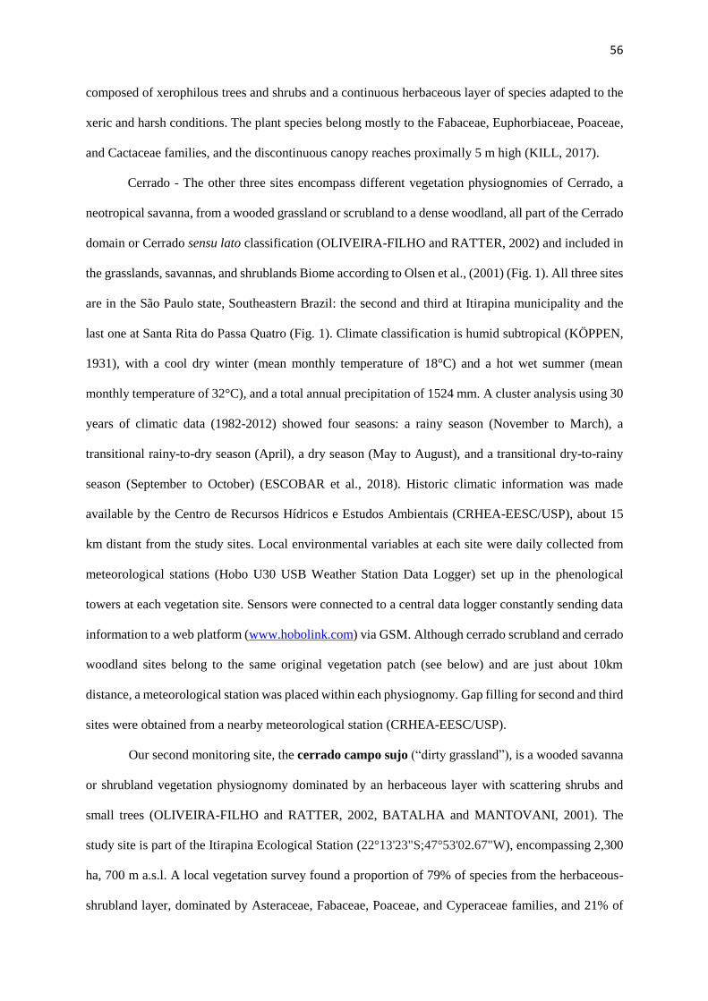
56

composed of xerophilous trees and shrubs and a continuous herbaceous layer of species adapted to the

xeric and harsh conditions. The plant species belong mostly to the Fabaceae, Euphorbiaceae, Poaceae,

and Cactaceae families, and the discontinuous canopy reaches proximally 5 m high (KILL, 2017).

Cerrado - The other three sites encompass different vegetation physiognomies of Cerrado, a

neotropical savanna, from a wooded grassland or scrubland to a dense woodland, all part of the Cerrado

domain or Cerrado sensu lato classification (OLIVEIRA-FILHO and RATTER, 2002) and included in

the grasslands, savannas, and shrublands Biome according to Olsen et al., (2001) (Fig. 1). All three sites

are in the São Paulo state, Southeastern Brazil: the second and third at Itirapina municipality and the

last one at Santa Rita do Passa Quatro (Fig. 1). Climate classification is humid subtropical (KÖPPEN,

1931), with a cool dry winter (mean monthly temperature of 18°C) and a hot wet summer (mean

monthly temperature of 32°C), and a total annual precipitation of 1524 mm. A cluster analysis using 30

years of climatic data (1982-2012) showed four seasons: a rainy season (November to March), a

transitional rainy-to-dry season (April), a dry season (May to August), and a transitional dry-to-rainy

season (September to October) (ESCOBAR et al., 2018). Historic climatic information was made

available by the Centro de Recursos Hídricos e Estudos Ambientais (CRHEA-EESC/USP), about 15

km distant from the study sites. Local environmental variables at each site were daily collected from

meteorological stations (Hobo U30 USB Weather Station Data Logger) set up in the phenological

towers at each vegetation site. Sensors were connected to a central data logger constantly sending data

information to a web platform (www.hobolink.com) via GSM. Although cerrado scrubland and cerrado

woodland sites belong to the same original vegetation patch (see below) and are just about 10km

distance, a meteorological station was placed within each physiognomy. Gap filling for second and third

sites were obtained from a nearby meteorological station (CRHEA-EESC/USP).

Our second monitoring site, the cerrado campo sujo (“dirty grassland”), is a wooded savanna

or shrubland vegetation physiognomy dominated by an herbaceous layer with scattering shrubs and

small trees (OLIVEIRA-FILHO and RATTER, 2002, BATALHA and MANTOVANI, 2001). The

study site is part of the Itirapina Ecological Station (22°13'23"S;47°53'02.67"W), encompassing 2,300

ha, 700 m a.s.l. A local vegetation survey found a proportion of 79% of species from the herbaceous-

shrubland layer, dominated by Asteraceae, Fabaceae, Poaceae, and Cyperaceae families, and 21% of

57

small trees species most from families, Fabaceae, Myrtaceae, and Melastomataceae (TANNUS et al.,

2006). During the three years of monitoring, local climatic time series show a mean annual total

precipitation of 1,272 mm and mean annual temperature of 23.5°C (Fig. 2B).

The third study site is located in a nearby private area of 260 hectares and 700 m a.s.l.

(22°10′52″ S, 47°52′25″ W), belonging to the same original “patch” of cerrado that once covered all

that region. The associated vegetation is a cerrado sensu stricto, a woody cerrado savanna dominated

by trees and shrubs from 3 to 8 m tall, sometimes reaching up to 12 m, with crowns arranged in a

discontinuous canopy, and a presence of a fair amount of herbaceous vegetation (REYS et al., 2013).

From the local 5-year meteorological data (2011 - 2015), mean annual total precipitation was 1,478 mm

and mean annual temperature 22.9 °C (Fig. 2C). Plant species composition is distributed mostly in the

Myrtaceae, Fabaceae, and Malpighiaceae families (REYS et al., 2013), and vegetation was classified

as a semideciduous, according to the species long-term leaf exchange strategies (CAMARGO et al.,

2018).

The last site it is also a woody cerrado formation that belongs to the Reserva Ecológica Pé-de-

Gigante (PEG), located within the Parque Estadual do Vassununga, at Santa Rita do Passa Quatro

county. The PEG reserve comprehends a contiguous area of 1,060 ha and 649 m a.s.l. (47° 34’ – 47°

41’ W; 21° 36’ – 21° 44’ S), covered by a heterogeneous landscape of savanna vegetations, from open

grasslands to woody dense cerrado. The seasonal humid subtropical climate (KÖPPEN, 1931) presents

a dry season from May to September and the wet season from October to April, a total annual rainfall

of 1,499 mm and mean temperature 21.5°C (BATALHA and MANTOVANI, 2000). Our local climatic

data from 2013 to 2015 shows a total annual average precipitation of 1,150 mm and mean air

temperature of 22.5°C (Fig. 2D). The study site, where the camera system is located, is a transition

from woody cerrado to a cerradão (OLIVEIRA-FILHO and RATTER, 2002), that we classified as a

dense cerrado, characterized by a discontinuous canopy, nearly without an herbaceous layer and high

density of shrubs and trees (RIBEIRO and WALTER, 1998). The site has a predominant woody layer

reaching 10m to 15m high, composed mainly of the species Ptedoron pubecens, Copaifera langsdofii,

and Anadenanthera peregrina var. falcata from the Fabaceae family. The closed canopy results in a

shading and cooler understory covered by a scattered herbaceous component (PIVELLO et al., 1998).

58

The vegetation communities studied here differ in their seasonality, from a very constrained

climate in the Caatinga domain with an 8-month dry season to less restricted conditions of the Cerrado

domain physiognomies with a 6-month dry season length. Sites also differ in the structure of vegetation,

from a dominant to equivalent herbaceous component (cerrado campo sujo and caatinga) to woody

formations of cerrado sensu stricto (woody cerrado and dense cerrado). To facilitate the identification

of the four studied sites and vegetation, hereafter we will name site one to four according to the

vegetation monitored, respectively, as follows: caatinga, cerrado shrubland, woody cerrado, and

dense cerrado. We can order our study sites into a sequence that corresponds to their degree of

seasonality and woody cover, from caatinga and cerrado shrubland, to woody cerrado and dense

cerrado.

3.2 Camera set up and near-surface phenology monitoring

For each one of the study sites, a digital hemispherical lens camera Mobotix Q 24 (Mobotix

AG — Germany) was placed at the top of a phenological tower attached to an extension arm facing

northeast at a mean vertical distance of 10 m from the tree canopy, except for the cerrado shrubland,

where the camera system is based 3 meters distance from the vegetation in a landscape standing point

(see ALBERTON et al., 2017). Energy supply is a 12V battery charged by a solar panel. Cameras are

configured to automatically take a daily sequence of five JPEG images (at 1280 × 960 pixels of

resolution) in the first 10 min of each hour, from 6:00 to 18:00 h (UC−3; Universal Time Coordinated)

as described in Alberton et al., (2014). The camera system installation occurred at different times

among sites (see Table1). For data analysis, we used time series spanning from 2013 to 2015 for all

sites, with the exceptional of the woody cerrado, where time-series started at 2011. Due to a sequence

of energy supply issues along the years in the woody cerrado site, we gap filled sequences of more

than 7 days with no images recorded using an algorithm that we created (see Supplementary material

for more details) in R language (R CORE TEAM, 2017).

Raw images were firstly processed with a visual filter to remove interferences, disturbing the

canopy viewing. Image analysis was conducted as described by Richardson et al., (2009), Ahrends et

al., (2009) and Alberton et al., (2014). We carried out field trips for plant identification to compile a

list of the main species captured by the field of view of the cameras (see Supplementary material).

59

Then, we matched the plant identification information with the crowns identified within the images.

This information, associated with imagery visual inspections, was essential for the classification of

individual crowns into plant functional groups based on plant leaf exchange strategies.

Regions of interest (ROIs) were defined for each site considering that time series from the

whole image can encompass phenological signals from many species with different leafing exchange

strategies (deciduous, semideciduous, and evergreen) and dominant life forms (woody vs grassy).

Thus, the ROIs defined for the community took into account the woody and grassy-dominated

vegetation, and individuals’ crowns of woody species were grouped by leaf exchange strategy

following Camargo et al., (2018) into deciduous, semideciduous, and evergreen. Since Camargo et al.,

(2018) did not consider in their functional classification the time of leaf flushing, we add that

information and refine their proposed strategy splitting the deciduous and semideciduous strategies

into two categories. All ROIs’ names, description, and their coverage (% of pixels) in relation to the

vegetation community ROI, are follow: community = region representing the community or the

complete image area, excluding tower and the exposed ground; deciduous = ROIs from crowns that

represent individuals of deciduous species (caatinga = 19.80% / cerrado shrubland = 16.16% / woody

cerrado = 5.44% / dense cerrado = 21.5%), fast deciduous = ROIs representing individuals of

deciduous fast-responsive species (caatinga = 7.20%); semideciduous wet = ROIs representing

individuals of semideciduous species and start of wet season leaf flushing (woody cerrado = 5.77% /

dense cerrado = 2.50%); semideciduous dry = ROIs from crowns that represent individuals of

semideciduous species, and a dry season leaf flushing (woody cerrado = 3.90%); evergreen = ROIs

from crowns that represent individuals of evergreen species (woody cerrado = 1.15% / dense cerrado

= 6.17%); and grass = ROIs representing the herbaceous layer of the cerrado scrubland (23.70%).

We analyzed the ROIs of each image in terms of the contribution of the relative brightness of

the green, red, and blue color channels (RGB chromatic coordinates in WOEBBECKE et al., (1995))

in relation to the primary colors (red, green, and blue). The normalized RGB chromatic coordinate

(RGBcc) index is referred to as the most suitable index to detect leaf color changes, and the most

efficient to suppress light variation (GILLESPIE et al., 1987; WOEBBECKE et al., 1995). The Green

chromatic coordinate (Gcc) index has been applied to relate changes on the vegetation greenness,

60

tracking phenological transitions of leaf development as well as ecosystem photosynthetic dynamics

and the search for environmental cues (RICHARDSON et al., 2009; AHRENDS et al., 2009;

MIGLIAVACCA et al., 2011; ALBERTON et al., 2014; MOORE et al., 2017; RICHARDSON et al.,

2018). We calculated the normalized index of the green color channel (Gcc), as:

𝑇𝑜𝑡𝑎𝑙𝑎𝑣𝑔 = 𝑅𝑒𝑑𝑎𝑣𝑔 + 𝐺𝑟𝑒𝑒𝑛𝑎𝑣𝑔 + 𝐵𝑙𝑢𝑒𝑎𝑣𝑔

𝐺𝑐𝑐 = Greenavg

Totalavg

The Gcc index was calculated for all images taken by the camera at each day. One single

measurement was extracted by taking the 90th percentile of the values every three days, a procedure that

has been shown to minimize noise in the color channels series (RGBcc) related to the illumination effects

of seasonal changes and time of the day (SONNENTAG et al., 2012).

3.3 Defining the growing season

We extracted some phenological metrics for the definition of the growing seasons. There are

several methods for modelling phenological time series (e.g., thresholds, derivatives, smoothing

algorithms, model fitting) allowing the detection of phenological transitions (DE BEURS and

HENEBRY, 2010). A critical issue raised for most of the methods is the lack of a statistical error

structure that promotes an analysis of the significance or robustness of the model (DE BEURS and

HENEBRY, 2010). Tropical vegetation time series are often more difficult to deal with, because they

are mostly rain-green systems, where vegetation green-up responses are coupled with precipitation

events, resulting in noisier observations (DE BEURS and HENEBRY, 2010). In the attempt to

overcome these problems, we propose an approach for the calculus of derivatives with significant

chances of occurrence along the time. The first step was the fitting of Generalized Additive models

(GAM) over the Gcc community time series. Time (sequence of days) was used as a smoother

independent variable. Assuming that errors are not independent, an inherent condition of time series

structure, we nested an auto-regressive moving average (ARMA) of order 1, as a correlation structure,

into our fitting models. Then, we build confidence intervals (95%) for the rate changes along the curve

applying montecarlo simulations to perform the curve fitting and calculate the time derivatives

(MOULIN, 1996) that significantly differed from zero, making sure that changes were happening in

61

these particular regions. From the derivatives calculations, we were able to extract phenological metrics

corresponding to vegetation transitions along the curves. Based on previous classification of land

surface phenology time series (ZHANG et al., 2003; JONSSON and EKLUNDH, 2004) and to conform

to the classical nomenclature of direct observation phenological variables (MORELLATO et al., 2000),

we define the phenological metrics as:

Start of growing season (SOS) – represents the beginning of the growing season. It is measured

as the first day detected by the significant derivative from the total seasonal amplitude on the left side

of the curve.

End of growing season (EOS) - represents the termination of the growing season. It represents

the last day detected by the significant derivative from the total seasonal amplitude on the right side of

the curve.

Length of growing season (LOS) – represents the duration of growing season and it is calculated

as the difference SOS and EOS.

Peak of the growing season (POS) – represents the highest percentage greenness or species

flushing new leaves. It is measured as the highest value of the seasonal curve.

3.4 Environmental cues of leafing phenology

Photoperiod, temperature, water availability, and a water-energy interaction were chosen as the

potential environmental factors to characterize the leafing phenological patterns across sites. The set of

explanatory variables was selected based on a priori assumptions and published literature on tropical

plant leaf phenological responses to seasonal environmental conditions summarized in the introduction.

Day-length, the number of sunlight hours, was chosen as the variable to represent the seasonality of

photoperiod and was calculated using the latitude of each location (geosphere package for R). The

variables of daily maximum and minimum temperature were used to calculate the variation of

temperature amplitude along the year, as:

𝑇𝑚𝑎𝑥 − 𝑇𝑚𝑖𝑛 = 𝑇𝑎𝑚𝑝

All other local climatic variables were derived from the weather station at each particular site.

Rainfall effects were tested using the variables of cumulative precipitation (mm) from the last 30 days

62

(Rainfall_cum30), and lagged rainfall events from the last seven (Rainfall_Lag7) and 30

(Rainfall_Lag30) days.

The water and energy interactions were calculated to evaluate the effects of the dry season

intensity through the Cumulative Water Deficit (CWD) calculation, as:

𝐶𝑊𝐷𝑛 = 𝐶𝑊𝐷(𝑛−1) + 𝑃𝑛 − 𝐸𝑇𝑛

The CWDn is the computed cumulative water deficit for a given time n, where Pn is the

precipitation of the day (mm) and ETn is the evapotranspiration of the day (mm day-1). When a positive

value of (P-ET) is identified, zero is used to set a starting point. Every time 𝐶𝑊𝐷𝑛 ≥ 0, then CDWn is

set to zero again (more details in STEPHENSON, 1998; MURRAY-TORTAROLO et al., 2016;

JAMES et al., 2013). The interactions between the vegetation evapotranspiration demand induced by

the energy in the system (able to heat and/or stress the plant) and the water availability reaching the soil

are explained by the climatic water balance (see STEPHENSON, 1990 and STEPHENSON, 1998).

When the evaporative demand does not meet the available water, a deficit situation occurs, which

explains the CWD, a measure of absolute drought (STEPHENSON, 1998; MURRAY-TORTAROLO

et al., 2016; JAMES et al., 2013).

Environmental variables were aggregated in a three-day 90th percentile window approach

(SONNENTAG et al., 2012), the same applied for the Gcc time series.

3.5 Data Analysis

Phenological metrics extracted from Gcc community time series were identified and compared

in terms of the growing season dynamics among the different vegetations. To investigate the

relationship between leafing phenology and environmental cues, we fitted Generalized Additive Mixed

Models (GAMMs) using the Gcc time series (community, leaf exchange strategy, and dominant life-

form) separately as dependent variables (Y) and the abiotic variables as the explanatory terms (X). The

main reason for the additive models application in this study is related to its potential of dealing with

nonlinear functions among multiple covariates and its reliability of handling time-series structural data

in ecological studies and vegetation modelling analysis (FRESCINO et al., 2001;WOOD, 2011; YANG

et al., 2012).

63

The general formula of a GAM is:

𝑔(𝜇) = 𝛼 + ∑ 𝑓𝑗𝑥𝑗

𝑃

𝑗=1

where 𝑔 is a specified link function and (𝜇) the expected mean response, 𝛼 is the linear model

components, and 𝑓𝑗 are smooth functions of the covariates 𝑥𝑗 (Yang et al. 2012). Basically, generalized

additive models aim to maximize the quality of prediction of Y, from various exponential families, by

estimating non-parametric functions of the predictor variables (X), through a connection with the

dependent variable stablished by a link function (WOOD, 2011, MARRA and WOOD, 2011). The

degree of smoothing of an additive model is expressed by the effective degrees of freedom (edf), which

mean that the higher the edf, the lower is the linearity of the curve interaction.

Initially, scatterplots among covariates were verified for the identification of linear and non-

linear relationships. After running a multicollinearity inspection, we entered all the chosen explanatory

variables in a full model for each dependent variable. The variable selection, which means a smooth

component selection when dealing with the additive models, was carried out using a shrinkage

approach. Shrinkage procedures are considered continuous processes where variable selection is

running in one single step, opposed to other used algorithms as the subset selection and stepwise

approaches (MARRA and WOOD, 2011). The method here applied, named double penalty, relies on

the fact that that the space of the smoother (a spline basis) can be decomposed into the components of

a range space and a null space. The method penalizes both components shrinking them to zero. By

introducing a penalty in the null space, the model smoothing parameter estimator is able to select the

most significant terms from the model (for more details about the method, see MARRA and WOOD,

2011). By analyzing the approximate smooth estimators from the models, we can verify the terms that

are not influential, with no significance achieved at P<0.001. Finally, to understand how each term is

related with the response variable, we plot the partial fits of each smoother parameter and evaluate the

edf and F-test from the model’s outcomes.

4 RESULTS

4.1 Growing seasons detection across sites

64

The Gcc index calculated for the community time series tracked the seasonality of leafing

patterns among all sites (Fig. 3). The timing of vegetation phenological transitions was found for all the

cycles, using the derivatives (Table 2). In general, growing seasons differed among vegetations in

relation to initial and end of growing season dates, length of growing season and the shape of the

growing season curves related to the leafing response of the species community. According to the

expectations, there was a constraint of leaf production to the wet period for extreme seasonal vegetation

(caatinga), as well as the grassy dominated vegetation (cerrado shrubland).

The start of the growing season (SOS) occurred earlier among the cerrado physiognomies,

ranging from doy 147 to doy 239. The woody cerrado was the vegetation with the earliest SOS (mean

doy 163), mid of June, in the dry season. The dense cerrado and the cerrado shrubland were more

similar, with a SOS mean date on doy 221 and doy 233, respectively, but the first with a more marked

seasonality. The start of the season in the Caatinga occurred by the end of October (mean doy 296),

only after the first rainfall events. Vegetation biomes reached the peak of season (POS), in the average,

78 days after the SOS. Caatinga and dense cerrado were the first to reach the highest values of the

growing season (69 and 67 days, respectively), while for the cerrado shrubland and the woody cerrado

the average mean was of 80 to 96 days for the POS, respectively. For the two woodland cerrado

vegetations, POS occurred earlier in the transition from the dry to the wet periods. Conversely, for the

caatinga and cerrado shrubland, POS dates were within the wet season.

The end of season (EOS) was faster and earlier in the caatinga vegetation, with just about a

month of difference (31 days) between the first and the second cycles (2013/2014 = 183, 2014/2015 =

214). The length of the season (LOS) was also the shortest in caatinga, with a mean LOS of 274 days.

The green-down was more abrupt in the xeric caatinga, with the EOS right after the end of the wet

season. The cerrado physiognomies showed a lower transition and extended green-down curve,

reaching their lowest values from the mid to the end of the dry season (Fig. 3). Woody cerrado presented

a different EOS among the years, ranging from mid-May (doy134) to mid-June (doy 170), and a LOS

from 314 to 342 days. There was one LOS registered for the grassland and the dense cerrado sites,

because there was only one complete year cycle. They presented the longest LOS, with 345 days.

4.2 Model predictions

65

Predictor variables entered as smooth terms in most of the models produced. Two of the

explanatory variables (Rainfall_lag7 and Tamp) showed a linear relationship when modelling ROIs data

from the caatinga and the woody cerrado, respectively. In general, GAM procedure produced models

with medium to high explanation (R2 values ranging from 0.29 to 0.88). The variables day-length and

the cumulative water deficit (CWD) were the most recurrent predictors with the highest significance

achieved among models across all vegetations (Table 3). All the plots from figures 5 and 6 show the

significant variables resulted from the GAM models explaining leaf phenology time-series. The most

important relationships are described with more details below.

The CWD and rainfall (lag7 and cum_30) showed the main relationships with the caatinga

community pattern of greening (Fig. 5A). The partial fits between predictors and Gcc demonstrated a

vegetation sensitive to low values of precipitation rates and increases of Gcc values in a threshold

between -10 and -5 of CWD values. The day-length, also included in the model as a significant variable

(edf = 7.83, F-test = 12.324, P<0.001), demonstrated to affect the community Gcc after reaching 12.5

hours of sunlight.

Day-length was the variable that best interacted with the community Gcc time series from the

cerrado physiognomies (Table 3). The same values, ranging from 11.5 and 12.0 hours, were observed

as a sensitive threshold for Gcc transitions across all vegetations (Fig. 5 B, C and D). CWD presented

different smooth functions of interaction among the cerrado sites, where we can notice a sensitive point

of change around values between -150 and -100 more strength for the cerrado shrubland and the dense

cerrado (Fig. 5B and D) and less for the woody cerrado (Fig. 3C).

The cumulative rainfall (Rainfall_Cum_30) was significant for the cerrado shrubland and the

dense cerrado (6.678, 13.189, P<0.001; 7.94, 8.317, P<0.001, respectively). Both demonstrated

sensitive to changes in Gcc after accumulated precipitation rates of 25 to 30 mm (Fig. 5 B and D). The

Gcc time-series from the woody cerrado community was the only one to relate with the temperature

amplitude (Tamp – 3.558, 17.05, P<0.001). The relationship between the covariates was positive and

linear with Gcc values rising as Tamp increases (Fig. 5 C).

In general, the ROIs separated according to leaf exchange strategies interacted with different

variables across vegetations and among groups. The deciduous and fast deciduous species from caatinga

66

demonstrated high similarity to the community pattern, with CWD and the lagged seven days of

accumulated rainfall (Rainfall_lag7) variables being more important for both ROIs and presenting

similar thresholds in points of transition (Fig. 5 A and Fig. 6 A). The fast deciduous presented a high

significant relation to rainfall_lag7 (1.00, 30.309, P<0.001), and demonstrated an oscillated relation

with the day-length variable (Fig. 6 A).

The CWD was the most significant smooth term to interact with the leaf phenology of the

deciduous ROIs (dec = 8.302, 23.169, P<0.001) from caatinga; evergreen (ever = 4.569, 21.991,

P<0.001) and wet flushing semideciduous (semi = 7.881, 40.59, P<0.001) from the woody cerrado, and

semideciduous (semi = 8.717, 29.203, P<0.001) and deciduous (dec = 8.264, 28.548, P<0.001) from

the dense cerrado (Fig. 6 A, C, and D).

Day-length was more significant for the evergreen (ever – 7.288, 38.316, P<0.001) and dry

flushing semideciduous (semi dry = 2.693, 32.952, P<0.001) ROIs from the woodland sites of dense

and woody cerrado, respectively. In the first, curve inflection was sensitive to daylight hours from 12.0

to 12.5 (Fig. 6 D). In the latter, an inverse relationship was found, with decreasing of Gcc as daylight

increases, starting from 11.5 hours (Fig. 6 C). Photoperiod also presented positive relationship (5.948,

41.807, P<0.001) with the deciduous ROI (dec), composed mostly of shrubs, from the cerrado

shrubland (Fig. 6 B).

The dominant grassy component (grass) from the cerrado shrubland and deciduous (dec) ROIs

from the woody cerrado, were significant related to the Tamp (1.00, 19.53, P<0.001; 3.663, 25.49,

P<0.001, respectively). Grass ROI showed an inverse sigmoid relationship with a range of Tamp values

increasing from 5 to 10°C (Fig. 6 B), while deciduous crowns (dec) demonstrated a negative linear

relationship with rising Tamp starting in 10°C (Fig. 6 D).

5 DISCUSSION

5.1 Leafing phenological patterns across vegetations

The Gcc index extracted from the digital images allowed tracking the leafing seasonality of the

vegetations and the definition of the growing seasons through phenological metrics detected from the

derivatives of generalized additive models fitting. As expected, Gcc curves followed the wet periods

67

fluctuations from their climatic zones, leading to differences on phenological dates and the growing

seasons among vegetations, mainly between the caatinga vegetation and the three cerrado vegetations.

Within sites, SOS and EOS presented more discrepancies in the Caatinga (28 and 31 days of

difference between years, respectively) and the woody cerrado (38 and 36 days difference among years,

respectively). For the caatinga, the phenomenon of the Atlantic Dipole (a temperature variation of the

Atlantic Ocean) can cause a high interannual variability in the precipitation rates (GUTIÉRREZ et al.,

2014), which would lead to the seasonality dynamics of the growing seasons among years. Given that

plant species from this ecosystem are influenced mainly by the water availability, there is an

immediately response of the reproductive and vegetative phenophases to rainfall events (CARVALHO

and BARBOSA, 1989; ARAÚJO et al., 2007).

Despite the differences among years, the woody cerrado site was the more dissimilar to the

other savanna vegetations regarding the SOS and EOS detected dates. Studies in cerrado vegetations

usually report the start of the community leaf flushing (SOS) for the transition period from the dry to

the wet season, around the month of September (e.g., MONASTERIO and SARMIENTO, 1976;

WILLIAMS et al., 1997; PIRANI et al., 2009; MUNHOZ and FELFILI, 2005, CAMARGO et al.,

2018). We relate the high variations of SOS and EOS among years (from 36 to 38 days) in this

vegetation to two main reasons. One could be related to the smoothing procedures over parts of the gap-

filled Gcc time series, what could be responsible for the earlier SOS and EOS in the cycles of 2013/2014

and 2014/2015, while the second to the massive presence, in the camera field of view, of crowns from

species flushing out the community flushing, during dry season, influencing the overall outcomes of

Gcc curve patterns.

The shape of the growing season also differed among vegetations, clearly influenced by the

LOS, much shorter for the Caatinga and longer for the cerrado vegetations. The green-up and green-

down curves were more abrupt for the caatinga, explained by the predominance and high synchrony of

strongly seasonal and many fast deciduous species in this vegetation, as pointed out by few dry forest

studies (MURPHY and LUGO, 1986; PEZZINI et al., 2014). On the other hand, the moister cerrrado

vegetations were composed of a different proportion of deciduous, semideciduous and evergreen,

maintaining partially green coverage of the vegetation even during the dry season and smoothing Gcc

68

curve changes along the wet season as supporting direct observations of leaf exchange patterns and the

definition of the Cerrado as a semideciduous vegetation (MORELLATO et al., 2013; CAMARGO et

al., 2018).

5.2 Environmental cues of leafing phenology

The models’ predictions found non-linear relationships between phenology and the most

recurrent significant variables, day-length and CWD. Day length was the most present variable to

explain the Gcc time series of vegetation communities. As expected, daylength was more important for

the cerrado vegetations than caatinga. In this context, light-related changes that precede the wet season,

such as the photoperiod seasonality, could be triggering leaf flushing in the cerrado communities.

Photoperiod has been reported to trigger the start of leaf flushing for seasonal dry tropical vegetations

(BORCHERT; RIVERA and HAGNAUER, 2002; RIVERA et al., 2002; HIGGINS et al., 2011;

ROSSATTO et al., 2013; GARCIA et al., 2017). The consistent signal has been suggested to trigger

and synchronize leaf flushing for tropical seasonal ecosystems despite the species leaf exchange strategy

(BORCHERT and RIVERA, 2001; RIVERA et al., 2002; ROSSATTO et al., 2013). The peak of the

community flushing before the onset of the wet season supports the hypothesis that cerrado trees have

access to underground water due their deep root system or their capability to use the precedent leaf fall

for rehydration for an early leaf production (EAMUS and PRIOR, 2001; GOLDSTEIN et al., 2008).

The community leaf flushing before the rainy season would also avoid nutrient loss by leaching during

leaf development and the threat of high herbivory rates to young leaves (SARMIENTO et al., 1985;

ROSSATTO et al., 2009).

The skewness pattern of the Gcc curves from Caatinga indicates a link between time and

duration of the irregular leafing cycles, restricted within the wet period, following the precipitation

pulses in the system. A similar pattern has been detected by digital cameras for dry grasslands,

confirming the high dependency of the interannual precipitation variability (BROWN et al., 2016;

RICHARDSON et al., 2018). The likely thresholds indicated in the plant-water relationships in the

catinga community shown low rates of acumulated precipitation stimulating Gcc time series changes,

what could explain the fast response pattern of leaf flushing, reflected in the growing season curve

oscillations of this site.

69

The cumulative water deficit (CWD) relationships, explained the seasonality of leaf production

in the four tropical seasonal vegetations investigated in this study. This variable can be considered of

major biological meaningful to the understand of physiological plant responses, given that it integrates

water and energy interactions, primary effects of climate on plants (STEPHENSON, 1998). According

to our results, CWD influenced leaf phenological responses of all four vegetations. Among the leaf

exchange strategies groups, CWD was the most recurrent variable to better explain leaf phenology

patterns.

Thermal amplitude had a positive relationship with the community pattern of Gcc in the woody

cerrado. This variable was also positive correlated with the rates of green-up and senescence across a

gradient of snow-free mountain vegetations (STREHER et al., 2017). The amplitude of temperature at

the woody cerrado reached 20°C, with high values found in the periods of transition between dry and

wet seasons. Temperature would play a significant role speeding plant development and their organs

(KORNER, 2006), what could be influencing the rates of green-up and green-down in the cerrado

curves.

Regarding the leafing patterns according to the leaf exchange strategies, variables of day-length

and CWD were also the most influential factors across sites. Our results indicated that both predictors

are about the same across the vegetations, except for the short cumulative seven-day rainfall necessary

for leaf flushing in the caatinga. The relationship between predictors-response varied and became more

heterogenous from the highest to the least seasonal sites. Woodland cerrado vegetations have shown

more discrepancies among leaf exchange strategies and predictors in their smooth function. For

instance, deciduous ROIs from the Dense and Woody cerrado were explained by thermal amplitude,

but the relationship stablished between the covariates were opposite, one being positive and the other

negative (Fig. 6 C and D). We could notice that different phenological behaviors presented variations

on timing and rate of Gcc values among groups and within vegetations (Fig. 4 C and D). This pattern

was less marked for the caatinga and the cerrado shrubland, where phenological behaviors from ROIs

groups were more similar in terms of Gcc time series patterns and relationship response to predictors.

This phenological dynamic can be explained by the fact that high seasonal constrained environments

tend to be more synchronic, due species (caatinga) or life forms (open cerrado scrubland) adapted to

70

the limited favorable time for plant development (wet season). As long as the environment becomes

less constrained by the climate, leaf exchange patterns would become more independent from seasonal

environmental constrains, given that soil water sources availability increases (BORCHERT, 1998), as

we observed across our four vegetation biomes.

At the Itirapina Ecological Station (cerrado scrubland site), different physiognomies from open

grassland to woodland cerrado occur over a groundwater depth lower than 4 m, and a recent study has

found that soil fertility did not define the occurrence of woody physiognomies (LEITE et al., 2018).

Besides, grasses typically require rainfall events to start leaf growth after rains (ANDREW and MOTT,

1983; COOK et al., 2002). However, leaf phenology of the grassland layer (grass ROI) in the cerrado

shrubland was not significant predicted by water relationships, which contradicted our expectations

about different response between woody and grassy dominated vegetations in accordance with the

temporal niche separation hypothesis (SCHOLES and WALKER, 1993). Grass ROI model reached

around 50% of explanation by day-length and thermal amplitude. The Brazilian cerrado is considered

a “wet” neotropical savanna, with regions of South America reaching up to 2,500 mean annual

precipitation (MAP), contrasting in more than 500 mm from the African and Australian savannas, and

where the influence of fire frequency would be an important determinant of the grasslands and closed

savannas distribution, besides climate seasonality (LEHMANN et al., 2011).

Woodland cerrado vegetation communities (woody cerrado and dense cerrado) presented

discrepancies regarding their leaf phenology patterns and environmental predictors. In fact, dense

cerrado demonstrated to be more similar with the cerrado shrubland than with the woody cerrado. We

suggest that this difference may be related to the species composition and the leaf exchange strategies

predominant within each vegetation community.

In conclusion, water and light were the most important predictors for the leaf phenological

patterns across the sites. Water-plant relationships were more important for the caatinga community,

and light effects, through day-length seasonality, had more influence in the leafing patterns of the

cerrado communities. The CWD variable appeared as an important predictor for the drought effects on

the leafing responses, although the previous 30 days of accumulated precipitation and thermal amplitude

had also significant contributions. Phenological signals and predictor-response relationships have

71

increased in variability across sites, where woodland cerrado physiognomies have shown increased

capability to sustain a greater complexity in their species leafing strategies than caatinga. One of the

major benefits that came from the near-surface remote phenology, using digital cameras, is the

reliability of acquiring continuous good quality phenological data from multiple sites and the potential

to stablish long-term phenological datasets. Through long-term monitoring, we will be able to consent

in the main drivers influencing plant communities and forecasting shifts in the face of climate change

scenarios. For now, with this study, we can collaborate with phenology for seasonal tropical vegetations,

corroborate hypothesis from literature and have more insights about tropical vegetation dynamics.

Acknowledgments - the present study was supported by São Paulo Research Foundation FAPESP

(grants #2009/54208-6, #2010/52113-5 and #2013/50155-0), Microsoft Research and CNPq. We

thank the Instituto Florestal for the permissions to work at the cerrado shrubland and dense cerrado

sites, and Embrapa for all the support and collaboration in the Caatinga site. We thank Marina Muller

Corrêa and Carolina Crivelin for the help in the image processing of the cerrado shrubland and woody

cerrado sites. BA receives fellowship from FAPESP (#2014/00215-0 and #2016/01413-5). LPCM,

RST, and HR receive a research productivity fellowship from CNPq.

6 REFERENCES

ABERNETHY, K. et al. Current issues in tropical phenology: a synthesis. Biotropica, v. 50 (3), p.

477-482, 2018.

AHRENDS, H.E. et al. Tree phenology and carbon dioxide fluxes: Use of digital photography for

process-based interpretation at the ecosystem scale. Climate Research, v. 39(3), p. 261–274, 2009.

ALBERTON, B.C. et al. Introducing digital cameras to monitor plant phenology in the tropics:

Applications for conservation. Perspectives in Ecology and Conservation, v. 15, p. 82-90, 2017.

ALBERTON, B.C. et al. Using phenological cameras to track the green up in a cerrado savanna and

its on-the-ground validation. Ecological Informatics, v. 19, p .62–70, 2014.

ANDREW, M.H.; MOTH, J.J. Annuals with transient seed banks: the population biology of

indigenous Sorghum species of tropical north‐west Australia. Australian Journal of Ecology, v. 8

(3), p. 265-276, 1983.

ARAÚJO, E.L.; CASTRO, C.C. and ALBUQUERQUE, U.P. Dynamics of Brazilian Caatinga – A

Review Concerning the Plants, Environment and People. Functional Ecosystems and Communities,

1(October 2015), p.15–28, 2007.

72

ARCHIBALD, S. and SCHOLES, R.J. Leaf green-up in a semi-arid African savanna –separating tree

and grass responses to environmental cues. Journal of Vegetation Science, v. 18 (4), p.583, 2007.

BATALHA, M.A. and MANTOVANI, W. Reproducive Phenological Patterns of Cerrado Plant

Species At the Pé-De-Gigante Reserve (Santa Rita Do Passa Quatro, SP, Brazil): a Comparision

Between the Herbaceous and Woody Floras. Revista Brasileira de Biologia, v. 60 (1), p.129–145,

2000.

de BEURS, K. and HENEBRY, G.M. Spatial-Temporal statistical methods for modelling land surface

phenology. In I. L. Hudson & M. R. Keatley, eds. Phenological Research: Methods for

Environmental and Climate Change Analysis. Springer Netherlands, p. 177–208, 2010.

BORCHERT, R. et al. Insolation and photoperiodic control of tree development near the equator.

New Phytologist, v. 205 (1), p.7–13, 2015.

BORCHERT, R. Responses of tropical trees to rainfall seasonality and its long-term changes.

Climatic Change, v. 39 (2), p.381–393, 1998.

BORCHERT, R. Soil and stem water storage determine phenology and distribution of tropical dry

forest trees. Ecology, v. 75 (5), p. 1437-1449, 1994.

BORCHERT, R.; RIVERA, G. and HAGNAUER, W. Modification of vegetative phenology in a

tropical semi-deciduous forest by abnormal drought and rain. Biotropica, v. 34 (1), p.27–39, 2002.

BROWN, T.B. et al. Using phenocams to monitor our changing earth: Toward a global phenocam

network. Frontiers in Ecology and the Environment, v. 14 (2), p.84–93, 2016.

CAMARGO, M.G.G. et al. Leafing patterns and leaf exchange strategies of a cerrado woody

community. Biotropica, v. 50 (3), p.442–454, 2018.

CARVALHO, D. and BARBOSA, D.A. Dados fenológicos de 10 espécies arbóreas de uma área de

caatinga (Alagoinha-PE). Acta bot. bras., v. 3 (2), p.109–117, 1989.

CHAMBERS, L.E. et al. Phenological Changes in the Southern Hemisphere. PLoS ONE, v. 8 (10),

2013.

COOK, G.D. et al. Variation in vegetative water use in the savannas of the North Australian Tropical

Transect. Journal of Vegetation Science, v. 13 (3), p. 413-418, 2002.

CRIMMINS, M.A.; CRIMMINS, T.M. Monitoring plant phenology using digital repeat photography.

Environmental management, v. 41 (6), p. 949-958, 2008.

EAMUS, D. Ecophysiological traits of deciduous and evergreen woody species in the seasonally dry

tropics. Trends in Ecology and Evolution, 14(1), pp.11–16, 1999.

EAMUS, D. and PRIOR, L. Ecophysiology of trees of seasonally dry tropics: Comparisons among

phenologies, 2001.

ELLIOTT, S.; BAKER, P.J. and BORCHERT, R. Leaf flushing during the dry season: The paradox

of Asian monsoon forests. Global Ecology and Biogeography, v. 15 (3), p.248–257, 2006.

ESCOBAR, D.F.E; SILVEIRA, F.A.O and MORELLATO, L.P.C. Timing of seed dispersal and seed

dormancy in Brazilian savanna: two solutions to face seasonality. Annals of botany, v. 121 (6), p.

1197-1209, 2018.

FRESCINO, T.S.; EDWARDS, T.C. and MOISEN, G.G. Modeling spatially explicit forest structural

attributes using Generalized Additive Models. Journal of Vegetation Science, v. 12 (1), p.15–26,

2001.

73

GARCIA, L.C.; BARROS, F. V. and LEMOS-FILHO, J.P. Environmental drivers on leaf phenology

of ironstone outcrops species under seasonal climate. Anais da Academia Brasileira de Ciências, v.

89 (1), p.131–143, 2017.

GILLESPIE, A.R.; KAHLE, A.B. and WALKER, R.E. Color enhancement of highly correlated

images. II. Channel ratio and “chromaticity” transformation techniques. Remote Sensing of

Environment, v. 22 (3), p.343–365, 1987.

GOLDSTEIN, G. et al. Water economy of Neotropical savanna trees: Six paradigms revisited. Tree

Physiology, v. 28 (3), p.395–404, 2008.

GUTIÉRREZ, A.P.A. et al. Drought preparedness in Brazil. Weather and Climate Extremes, v. 3,

p. 95-106, 2014.

HIGGINS, S.I. et al. Is there a temporal niche separation in the leaf phenology of savanna trees and

grasses? Journal of Biogeography, v. 38 (11), p.2165–2175, 2011.

JAMES, R. et al. Implications of global warming for the climate of African rainforests. Phil. Trans.

R. Soc. B, v. 368 (1625), p. 20120298, 2013.

JÖNSSON, P. and EKLUNDH, L. TIMESAT—a program for analyzing time-series of satellite sensor

data. Computers & Geosciences, v. 30 (8), p. 833-845, 2004.

Kill, L.H.P. Caracterização da vegetação da reserva legal da embrapa semiárido. Documentos online,

v. 5 (2003), p.121–124, 2017.

KÖPPEN, W.P. Grundriss der klimakunde. 1931.

KÖRNER, C. Significance of temperature in plant life. Plant growth and climate change, p. 48-69,

2006.

LEITE, M.B. et al. Groundwater depth as a constraint on the woody cover in a Neotropical Savanna.

Plant and Soil, v. 426 (1-2), p. 1-15, 2018.

LEHMANN, C.E.R et al. Deciphering the distribution of the savanna biome. New Phytologist, v. 191

(1), p. 197-209, 2011.

MARRA, G. and WOOD, S.N. Practical variable selection for generalized additive models.

Computational Statistics and Data Analysis, v. 55 (7), p.2372–2387, 2011.

MIGLIAVACCA, M. et al. Using digital repeat photography and eddy covariance data to model

grassland phenology and photosynthetic CO2 uptake. Agricultural and Forest Meteorology, v. 151

(10), p.1325–1337, 2011.

MONASTERIO, M. and SARMIENTO, G. Phenological strategies of plants species in the tropical

savanna and semi-deciduous forest of the Venezuelan Lianos. Journal of Biogeography, v. 3 (4),

p.325–356, 1976.

MOORE, C.E. et al. Tree – grass phenology information improves light use efficiency modelling of

gross primary productivity for an Australian tropical savanna. Biogeosciences, v. 14, p.111–129,

2017.

MORELLATO, L.P.C. et al. Linking plant phenology to conservation biology. Biological

Conservation, v. 195, p.60–72, 2016.

MORELLATO, L.P.C.; CAMARGO, M.G.G. and GRESSLER, E. A review of plant phenology in

South and Central America. In: Phenology: An integrative environmental science. Springer,

Dordrecht, p. 91-113, 2013.

74

MORELLATO, L.P.C. et al. Phenology of Atlantic Rain Forest Trees: A Comparative Study

Biotropica, v. 32(4), p.811–823, 2000.

MORELLATO, L.P.C. et al. Estudo comparativo da fenologia de espécies arbóreas de floresta de

altitude e floresta mesófila semidecídua na Serra do Japi, Jundiaí, São Paulo. Revista brasileira de

Botânica, v. 12 (1), p. 85-98, 1989.

MORISETTE, J.T. et al. Tracking the rhythm of the seasons in the face of global change:

Phenological research in the 21 st century. Frontiers in Ecology and the Environment, v. 7 (5),

p.253–260, 2009.

MOULIN, S. et al. Global-scale assessment of vegetation phenology using NOAA/AVHRR satellite

measurements. Journal of Climate, v. 10 (6), p. 1154-1170, 1997.

MUNHOZ, C.B.R. and FELFILI, J.M. Fenologia do estrato herbáceo-subarbustivo de uma

comunidade de campo sujo na Fazenda Água Limpa no Distrito Federal, Brasil. Acta Botanica

Brasilica, v. 19 (4), p.979–988, 2005.

MURPHY, P.G. and LUGO, A.E. Ecology of Tropical Dry Forest. An. Rev. Ecol. Syst., v. 17, p.67–

88, 1986.

MURRAY-TORTAROLO, G. et al. Changes in the dry season intensity are a key driver of regional

NPP trends. Geophysical Research Letters, 2016.

OLIVEIRA-FILHO, A.T. and RATTER, J.A. Vegetation physiognomies and woody flora of the

cerrado biome. The cerrados of Brazil: ecology and natural history of a neotropical savanna, p. 91-

120, 2002.

OLSON, D.M. et al. Terrestrial Ecoregions of the World: A New Map of Life on EarthA new global

map of terrestrial ecoregions provides an innovative tool for conserving biodiversity. BioScience, v.

51 (11), p. 933-938, 2001.

PEZZINI, F.F. et al. Changes in tree phenology along natural regeneration in a seasonally dry tropical

forest. Plant Biosystems, v. 148 (5), p.965–974, 2014.

PIRANI, F.R.; SANCHEZ, M. and PEDRONI, F. Fenologia de uma comunidade arbórea em cerrado

sentido restrito, Barra do Garças, MT, Brasil. Acta Botanica Brasilica, v. 23 (4), p.1096–1110, 2009.

PIVELLO, V. et al. Proposta de zoneamento ecológico para a reserva de cerrado Pé-de-Gigante

(Santa Rita do Passa Quatro, SP). Brazilian Journal of Ecology, v. 2 (2), p. 108-118, 1998.

POLGAR, C.A.; PRIMACK, R.B. Leaf‐out phenology of temperate woody plants: from trees to

ecosystems. New Phytologist, v. 191 (4), p. 926-941, 2011.

QUESADA, M. et al. Succession and management of tropical dry forests in the Americas: Review

and new perspectives. Forest Ecology and Management, v. 258 (6), p. 1014-1024, 2009.

REICH, P.B. Phenology of tropical forests: patterns, causes, and consequences. Canadian Journal of

Botany, v. 73(2), p. 164-174, 1995.

REICH, P.B. and BORCHERT, R. Water Stress and Tree Phenology in a Tropical Dry Forest in the

Lowlands of Costa Rica. The Journal of Ecology, v. 72 (1), p.61–74, 1984.

REYS, P. et al. Estrutura e composição florística de um Cerrado sensu stricto e sua importância para

propostas de restauração ecológica. Hoehnea, p. 449-464, 2013.

RIBEIRO, J.F.; WALTER, B.M.T. Fitofisionomias do bioma Cerrado. Embrapa Cerrados (ALICE),

1998.

75

RICHARDSON, A.D. et al. Use of digital webcam images to track spring green-up in a deciduous

broadleaf forest. Oecologia, v. 152 (2), p.323–334, 2007.

RICHARDSON, A.D.R. et al. Near-surface remote sensing of spatial and temporal variation.

Ecological Applications, v. 19(6), p.1417–1428, 2009.

RICHARDSON, A.D. et al. Climate change, phenology, and phenological control of vegetation

feedbacks to the climate system. Agricultural and Forest Meteorology, v. 169, p.156–173, 2013.

RICHARDSON, A.D. et al. Tracking vegetation phenology across diverse North American biomes

using PhenoCam imagery. Scientific Data, v. 5, p.180028, 2018.

R Core Team. A language and environment for statistical computing. R Foundation for Statistical

Computing, Vienna, Austria, 2017.

RIVERA, G. et al. Increasing day-length induces spring flushing of tropical dry forest trees in the

absence of rain. Trees - Structure and Function, v. 16 (7), p.445–456, 2002.

ROSSATTO, D.R. et al. Seasonal variation in leaf traits between congeneric savanna and forest trees

in Central Brazil: Implications for forest expansion into savanna. Trees - Structure and Function, v.

27 (4), p.1139–1150, 2013.

ROSSATTO, D.R.; HOFFMANN, W.A. and FRANCO, A.C. Differences in growth patterns between

co‐occurring forest and savanna trees affect the forest–savanna boundary. Functional Ecology, v. 23

(4), p. 689-698, 2009.

RÖTZER, T.; GROTE, R. and PRETZSCH, H. The timing of bud burst and its effect on tree growth.

International Journal of Biometeorology, v. 48 (3), p.109–118, 2004.

SARMIENTO, G.; GOLDSTEIN, G. and MEINZER, F. Adaptive strategies of woody species in

neotropical savannas. Biological Reviews, v. 60 (3), p. 315-355, 1985.

SCHOLES, R.J. and ARCHER, S.R. Tree-grass interactions in savannas. Annual review of Ecology

and Systematics, v. 28 (1), p. 517-544, 1997.

SINGH, J.S. and SINGH, V.K. Phenology of seasonally dry tropical forest. Current science, p. 684-

689, 1992.

SINGH, K.P. and KUSHWAHA, C.P. Emerging paradigms of tree phenology in dry tropics. Current

Science, p. 964-975, 2005.

SONNENTAG, O. et al. Digital repeat photography for phenological research in forest ecosystems.

Agricultural and Forest Meteorology, v. 152 (1), p.159–177, 2012.

STEPHENSON, N.L. Climatic control of vegetation distribution: the role of the water balance. The

American Naturalist, v. 135 (5), p. 649-670, 1990.

STEPHENSON, N. Actual evapotranspiration and deficit: biologically meaningful correlates of

vegetation distribution across spatial scales. Journal of Biogeography, v. 25 (5), p. 855-870, 1998.

STREHER, A.S. et al. Land Surfce Phenology in the Tropics: The Role of Climte nd Topogrphy in

Snow-Free Mountin. Ecosystems, v. 20 (8), p. 1436-1453, 2017.

TANNUS, J.L.S; ASSIS, M.A. and MORELLATO, L.P.C. Fenologia reprodutiva em campo sujo e

campo úmido numa área de cerrado no sudeste do Brasil, Itirapina-SP. Biota Neotropica, 2006.

76

VAN SCHAIK, C.P.; TERBORGH, J.W. and WRIGHT, S.J. the Phenology of Tropical Forests -

Adaptive Significance and Consequences for Primary Consumers. Annual Review of Ecology and

Systematics, v. 24 (1993), p.353–377, 1993.

VELOSO, H.P.; FILHO, A.L.R.R. & LIMA, J.C.A. Classificação da vegetação brasileira, adaptada a

um sistema universal. Instituto Brasileiro de Geografia e Estatística, Diretoria de Geociências,

Departamento de Recursos Naturais e Estudos Ambientais, 1991.

WILLIAMS, R.J. et al. Leaf phenology of woody species in a north Australian tropical savanna.

Ecology, v. 78 (8), p. 2542-2558, 1997.

WILLIAMS, L.J.; BUNYAVEJCHEWIN, S. and BAKER, P.J. Deciduousness in a seasonal tropical

forest in western Thailand: interannual and intraspecific variation in timing, duration and

environmental cues. Oecologia, v. 155 (3), p. 571-582, 2008.

WHITECROSS, M.A.; WITKOWSKI, E.T.F. and ARCHIBALD, S. Savanna tree-grass interactions:

A phenological investigation of green-up in relation to water availability over three seasons. South

African Journal of Botany, v. 108, p. 29-40, 2017.

WOEBBECKE, D.M. et al. Color indices for weed identification under various soil, residue, and

lighting conditions. Transactions of the ASAE, v. 38 (1), p.259–269, 1995.

WOOD, S.N. Fast stable restricted maximum likelihood and marginal likelihood estimation of

semiparametric generalized linear models. Journal of the Royal Statistical Society. Series B:

Statistical Methodology, v. 73 (1), p.3–36, 2001.

WRIGHT, S.J. and VAN SCHAIK, C.P. Light and the Phenology of Tropical Trees. The American

Naturalist, v. 143 (1), p.192–199, 1994.

YANG, L. et al. Using a generalized additive model with autoregressive terms to study the effects of

daily temperature on mortality. BMC Medical Research Methodology, v. 12, 2012.

ZHANG, X. al. Monitoring vegetation phenology using MODIS. Remote sensing of environment, v.

84 (3), p. 471-475, 2003.

77

Figures legends

Figure 1 Geographic distribution of study sites according to the Biome (following OLSON et al., 2011)

denoted by the background color, and the vegetation types considered in this study: caatinga, cerrado

shrubland and woody cerrado: cerrado and dense cerrado.

Figure 2 Month average of local environmental variables of day-length, maximum and minimum

temperature (Tmax and Tmin), thermal amplitude (Tamp) and rainfall for each vegetation site of this

study – A, B and C caatinga; D, E, and F cerrado shrubland; G, H, and I woody cerrado; J, K, and L

dense cerrado.

Figure 3 Three-day 90th percentil Gcc time series of the xeric (A) and savanna (B – D) vegetations fitted

by generalized additive models. (A) caatinga, (B) cerrrado shrubland, (C) woody cerrado and (D) dense

cerrado. Derivatives were calculated for the growing seasons detection. Green lines represent the start

of the growing season and red lines the end of the growing season. Black line represents the model

fitted, gray shadow the confident interval and dark dots the observed data.

Figure 4 Three-day 90th percentil Gcc time series of the community and the selected ROIs for xeric (A)

and savanna (B – D) vegetations fitted by generalized additive mixed models (GAMM). (A) caatinga,

(B) cerrado shrubland, (C) woody cerrado, and (D) dense cerrado. Continuous colored lines represent

the GAM model fitting, gray shadow represent the confidence interval and dark dots the observed data.

Light blue lines represent the crowns for woody deciduous ROIs, yellow line for fast-response

deciduous, green line for evergreen, blue line for spring flushing semideciduous, and dark orange for

the winter flushing semideciduous; pink line represents the GAMM fit for dominant grassy vegetation,

and orange for the community ROI of each vegetation site.

Figure 5 Response of fitted generalized additive mixed models for the three-day 90th percentil Gcc

community time-series to each environmental variable: day-length, rainfall_lag7 (rainfall of the

previous seven days), rainfall_cum30 (accumulated precipitation of the last 30 days), CWD (cumulative

water deficit) and Tamp (thermic amplitude) and vegetation– caatinga (A), cerrado shrubland (B), and

woody cerrado (C), dense cerrado (D).

Figure 6 Response of fitted generalized additive mixed models for the three-day 90th percentil Gcc of

species´ leaf strategies and life-form time-series to the environmental variables: (day-length,

78

rainfall_lag7, rainfall_cum30, CWD and Tamp) of each vegetation site – caatinga (A), cerrado

shrubland (B), woody cerrado (D), and dense cerrado (C). deciduous = dec; fast-response deciduous =

dec_fast; wet flushing semideciduous = semi_wet; dry flushing semideciduous = semi_dry; evergreen

= ever; grassy layer = grass.

79

Table 1 Study sites summary description including the general vegetation name (Name), site

designation and coordinates, location in Brazil (City, state and region), vegetation type, period of study

(phenocam monitoring), mean annual total precipitation according to the normal climate and length of

dry season in months (for estimation, see methods)

Name Study site designation

Lat/Long. Location Vegetation type

Phenocam

Monitoring

Mean Annual Total

Precipitation (mm)

Dry Season

Length

(months)

caatinga Embrapa Semi-árido -

9°05’S / 40°19’ W

Petrolina, PE,

Northeast

Brazil

Xeric shrubland

(Caatinga)

10/May/2013

to

31/Dec/2015

510 mm 8

cerrado

shrubland

Itirapina Ecological

Station - 22°13'23"S /

47°53'02.67"W

Itirapina, SP,

Southeastern,

Brazil

grasslands, savannas

and shrublands

(Cerrado campo

sujo)

28/Mar/2013

to

28/May/2015

1,524 mm 6

woody

cerrado

Botelho Farm -

22°10′49.18″S /

47°52′16.54″W

Itirapina, SP,

Southeastern,

Brazil

grasslands, savannas

and shrublands

(Cerrado sensu

stricto)

02/Sep/2011

to

03/Feb/2015

1,524 mm 6

dense

cerrado

Pé de Gigante - 47° 34’-

47° 41’ W / 21° 36’- 21°

44’ S

Santa Rita do

Passa Quatro,

SP,

Southeastern

Brazil

grasslands, savannas

and shrublands

(Cerrado sensu

stricto denso)

26/Aug/2013

to

31/Dec/2015

1499 mm 6

80

Table 2 Phenological metric dates (day of year) derived from digital cameras Gcc time series for each

vegetation. SOS = Start of growing season, POS = Peak of growing season, EOS = End of growing

season and LOS = Length of growing season.

SITE/YEAR SOS POS EOS LOS

caatinga

2013/2014 296 6 183 252

2014/2015 282 360 214 297

2015/2016 310 364 NA NA

cerrado shrubland

2013/2014 NA NA 230 NA

2014/2015 239 317 219 345

2015/2016 228 309 NA NA

woody cerrado

2011/2012 NA NA 170 NA

2012/2013 185 284 134 314

2013/2014 158 254 135 342

2014/2015 147 240 NA NA

dense cerrado

2013/2014 NA 290 204 NA

2014/2015 213 279 223 345

2015/2016 229 298 NA NA

81

Table 3 Approximate significance of smooth terms from the generalized additive models (GAM)

between the Gcc time series from the ROIs of each vegetation and the environmental predictors.

Effective degrees of freedom (edf) and F-test values are presented for each variable: Day-length,

Cumulative water deficit (CWD), Precipitation lagged seven days (Raifall_lag7), Cumulative

precipitation from the last 30 days (Rainfall_Cum30), Temperature amplitude (Tamp), followed by the

coefficient of determination (R2) of each model. All variables were significant at P values < 0.001.

deciduous = dec; fast-response deciduous = dec_fast; wet flushing semideciduous = semi_wet; dry

flushing semideciduous = semi_dry; evergreen = ever; grassy layer = grass.

Site location ROI

Day-length

(hours) CWD (mm)

Rainfall_ lag7

(mm)

Rainfall_Cum_30

(mm) ampT ( C)

R²

edf F-test edf F-test edf F-test edf F-test edf F-test

caatinga

comu 7.83 12.324 8.559 28.565 1.0 36.02 6.91 16.36 N.S N.S 0.86

dec 1.599 14.34 8.302 23.169 1.818 18.289 7.681 9.731 N.S N.S 0.79

dec_fast 7.388 6.045 6.33 15.276 1.0 30.309 7.143 13.125 N.S N.S 0.74

cerrado

shrubland

comu 5.726 39.535 6.678 13.189 N.S N.S 3.907 4.617 N.S N.S 0.88

grass 2.114 9.535 N.S N.S N.S N.S N.S N.S 1.00 19.53 0.56

dec 5.948 41.807 5.216 7.841 N.S N.S 3.773 6.384 1.434 8.575 0.87

woody

cerrado

comu 5.218 22.436 7.097 8.484 N.S N.S N.S N.S 3.558 17.05 0.51

ever 1.00 7.441 4.569 21.991 N.S N.S N.S N.S N.S N.S 0.29

semi_wet 3.602 21.105 7.881 40.59 N.S N.S 5.32 12.9 3.7 7.288 0.75

semi_dry 2.693 32.952 7.309 18.228 N.S N.S N.S N.S 3.184 19.95 0.66

dec N.S N.S 7.665 5.904 N.S N.S N.S N.S 3.663 25.49 0.42

dense

cerrado

comu 7.773 36.383 7.94 8.317 N.S N.S 6.745 3.156 N.S N.S 0.79

ever 7.288 38.316 8.163 16.224 N.S N.S 5.671 5.699 N.S N.S 0.76

semi_wet 7.837 19.284 8.717 29.203 N.S N.S 5.138 10.109 1.00 9.502 0.82

dec 7.144 30.9 8.264 28.548 2.719 6.734 5.884 3.857 1.00 6.772 0.82

82

Figure 1

83

Figure 2

84

Figure 3

85

Figure 4

86

Figure 5

87

Figure 6

88

Supplementary Material

LEAFING PATTERNS AND ENVIRONMENTAL DRIVERS ACROSS SEASONAL

TROPICAL COMMUNITIES

Bruna Alberton, L. Humberto Rocha, Magna Soelma, Thiago S. F. Silva, Ricardo S. Torres, Patricia

C. Morellato

Figure S1 Performance of the gap-filling algorithm on the daily Gcc time-series of the woody cerrado

site. The algorithm created, based on an Auto-regressive moving average model (ARMA) fitting over

the Gcc time-series, consists of three steps: first, the optimal order of the ARMA model is chosen based

on physical principles; secondly, data segments before and after a given gap are fitted using an ARMA

model of the order selected in the first step; and next, the gap is interpolated using a weighted function

of a forward and a backward prediction based on the models of the selected data segments. The second

and third steps are repeated for each gap contained in the entire time series.

89

Table S1 List of plant species identified in the field of view of the digital camera from the Dry forest

vegetation site.

Family Scientific name Life form

Anacardiaceae Spondias tuberosa Arruda Shrub|Tree

Anacardiaceae Myracrodruon urundeuva Allemão Tree

Anacardiaceae Schinopsis brasiliensis Engl. Tree

Apocynaceae Aspidosperma pyrifolium Mart. & Zucc. Tree

Bignoniaceae Handroanthus spongiosus (Rizzini) S.Grose Tree

Burseraceae Commiphora leptophloeos (Mart.) J.B.Gillett Shrub|Tree

Cactaceae Pilosocereus Byles & Rowley NA

Euphorbiaceae Sapium argutum (Müll.Arg.) Huber Shrub|Tree

Euphorbiaceae Sapium glandulosum (L.) Morong Shrub|Tree

Euphorbiaceae Cnidoscolus quercifolius Pohl Shrub|Tree

Euphorbiaceae Manihot pseudoglaziovii Pax & K.Hoffm. NA

Euphorbiaceae Croton conduplicatus Kunth Shrub|Sub-Shrub

Fabaceae Mimosa tenuiflora (Willd.) Poir. Shrub|Tree|Sub-Shrub

Fabaceae Poincianella microphylla (Mart. ex G.Don) L.P.Queiroz Shrub|Tree

Fabaceae Senegalia piauhiensis (Benth.) Seigler & Ebinger Shrub|Tree

Fabaceae Poincianella pyramidalis (Tul.) L.P.Queiroz Tree

Malvaceae Pseudobombax simplicifolium A.Robyns Tree

90

Table S2 List of plant species identified in the field of view of the digital camera from the Grassland

savanna vegetation site.

Family Scientific name Life form

Apocynaceae Aspidosperma tomentosum Mart. Tree

Asteraceae Gochnatia pulchra Cabrera Schrub | Tree

Bignoniaceae Jacaranda decurrens Cham. Schrub

Caryocaraceae Caryocar brasiliense Cambess. Tree

Cyperaceae Bulbostylis Kunth Herb

Erythroxylaceae Erythroxylum suberosum A.St.-Hil. Schrub|Tree|Sub-Schrub

Fabaceae Machaerium acutifolium Vogel Tree

Fabaceae Andira humilis Mart. ex Benth. Schrub|Tree

Lamiaceae Aegiphila verticillata Vell. Schrub|Tree|Sub-Schrub

Malpighiaceae Byrsonima intermedia A.Juss. Schrub

Myrtaceae Eugenia pyriformis Cambess. Schrub|Tree|Sub-Schrub

Myrtaceae Campomanesia pubescens (Mart. ex DC.) O.Berg Schrub|Tree

Arecaceae Syagrus petraea (Mart.) Becc. Herb | Palm

Poaceae Andropogon L. Herb

Poaceae Loudetiopsis Conert Herb

Poaceae Trachypogon spicatus (L.f.) Kuntze Herb

Sapotaceae Pouteria torta (Mart.) Radlk. Schrub|Tree

Sapotaceae Pradosia brevipes (Pierre) T.D.Penn. SubSchrub

Verbenaceae Lippia origanoides Kunth Schrub|Sub-Schrub

Vochysiaceae Qualea grandiflora Mart. Schrub|Tree

Vochysiaceae Vochysia tucanorum Mart. Tree

91

Table S3 List of plant species identified in the field of view of the digital camera from the PDG

woodland savanna site.

Family Scientific name Life form

Annonaceae Xylopia aromatica (Lam.) Mart. Schrub|Tree

Caryocaraceae Caryocar brasiliense Cambess. Tree

Fabaceae Pterodon pubescens (Benth.) Benth. Tree

Fabaceae Leptolobium dasycarpum Vogel Tree

Fabaceae Diptychandra aurantiaca Tul. Tree

Fabaceae Anadenanthera peregrina var. falcata (Benth.) Altschul Schrub|Tree

Fabaceae Copaifera langsdorffii Desf. Tree

Fabaceae Vatairea macrocarpa (Benth.) Ducke Tree

Sapotaceae Pouteria ramiflora (Mart.) Radlk. Schrub|Tree

92

Table S4 List of plant species identified in the field of view of the digital camera from the CORE woodland

savanna site.

Family Scientific name Life form

Annonaceae Xylopia aromatica (Lam.) Mart. Schrub|Tree

Apocynaceae Aspidosperma tomentosum Mart. Tree

Caryocaraceae Caryocar brasiliense Cambess. Tree

Fabaceae Pterodon pubescens (Benth.) Benth. Tree

Fabaceae Bowdichia virgilioides Kunth Schrub|Tree

Melastomataceae Miconia rubiginosa (Bonpl.) DC. Schrub|Tree

Myrtaceae Myrcia splendens (Sw.) DC. Tree

Myrtaceae Myrcia guianensis (Aubl.) DC. Tree

Sapotaceae Pouteria torta (Mart.) Radlk. Schrub|Tree

Sapotaceae Pouteria ramiflora (Mart.) Radlk. Schrub|Tree

Vochysiaceae Qualea grandiflora Mart. Schrub|Tree

94

Section 3

95

LEAF PHENOLOGY CORRELATES TO GROSS PRIMARY PRODUCTIVITY: AN INTER-

COMPARISON ACROSS SEASONALLY CONTRASTING TROPICAL BIOMES

Bruna Alberton1

, Andrew Richardson2,3

, Ricardo da S. Torres4

, Humberto Rocha5

, Magna S. B. De

Moura6

, Leonor Patricia Cerdeira Morellato1

1 Laboratório de Fenologia, Universidade Estadual Paulista (Unesp), Instituto de Biociências, Rio

Claro, São Paulo, Brazil

2 School of Informatics, Computing and Cyber Systems, Northern Arizona University, Flagstaff, AZ,

USA

3 Center for Ecosystem Science and Society, Northern Arizona University, Flagstaff, AZ, USA.

4

Institute of Computing, University of Campinas, Brazil

5 Departamento de Ciências Atmosféricas, IAG, Universidade de São Paulo, Brazil

6

Empresa Brasileira de Pesquisa Agropecuária, Embrapa Semiárido, Brazil

*

Corresponding author

Email address: bru.alberton@gmail.com

1 ABSTRACT

Tropical forests play a key role in the global carbon budget, but temporal patterns of productivity, their

drivers, and constrains remain under discussion. Leaf phenology, the temporal patterns of leaf flushing

and senescence, is essential to the understanding of ecosystems processes and has a key role in the

seasonality of ecosystems productivity. Understanding the interplay of water and light, the main

climatic drivers over tropical vegetation, and the importance of leaf phenology controlling ecosystem

productivity under seasonal climates are still on debate. Monitoring phenology over multi-sites may be

infeasible, especially for high diverse tropical sites, what motivated the search for new tools. The use

of phenocams has been proven an accurate method to monitor leaf phenology continuously over time

and simultaneously at different sites or vegetations, tracking vegetation greenness seasonality through

96

vegetation indices extracted from repeated photographs. Recent studies have reported the correlation

between greenness index with GPP curves. Here we proposed a study to investigate the key role of leaf

phenology defining temporal patterns of gross primary productivity across contrasting seasonal tropical

extra-Amazonian vegetations: the nearly non-seasonal, light limited, evergreen Atlantic Forest; the

Cerrado, a neotropical savanna under a wet – dry alternated seasons and; the Caatinga, a xeric vegetation

exclusive from Brazil, representing a water-limited, extreme seasonally dry ecosystem. Our main

questions are: (i) Does leaf phenology explain GPP patterns across seasonally contrasting biomes? (ii)

what is the relative importance of water and light over leaf phenology controlling GPP seasonality? and

(iii) How can spatial-temporal dynamics of crown’s leafing behaviors contribute to the community

leafing patterns? Do these relationships change over contrasting environments that are under different

seasonality constraints? We monitored temporal patterns of leaf phenology (leaf flushing and

senescence phenophases) derived from digital repeated photograph and partitioned gross primary

productivity (GPP) from eddy covariance measurements of CO2 fluxes. We describe the temporal

patterns of leaf production and ecosystem productivity of the three biomes and modeled the relative

importance of phenology and the environmental factors over the productivity across sites. The

significance of phenology, water and light cues, changes across biomes. Coupled effects of phenology

and water availability are observed on the caatinga, while environmental variability and phenology are

equally contributing in the cerrado productivity, and phenology is the better explaining factor of GPP

in the rainforest vegetation. Through this inter-comparison analysis, we could uncover temporal patterns

and drivers of ecosystem productivity across seasonal tropical biomes and disentangle the interplay

between phenology and water relations across contrasting seasonal sites, with phenology imposing

different influences on vegetations according to their dominant leafing exchange strategies.

2 INTRODUCTION

Tropical forests play a key role in the global carbon budget, but we still need to understand

some uncertainties regarding the temporal patterns, drivers, and constraints of tropical forests

photosynthetic seasonality, a topmost issue in the climate change research agenda, essential to forecast

and mitigate effects of the changing climate on carbon cycles. Temporal patterns of leaf development

97

and senescence are essential to the understanding of ecosystems processes and how the global carbon

balance may respond to shifts in climate and atmospheric composition (WILLIAMS et al., 1998; GASH

et al., 2004; POLGAR and PRIMACK, 2011; RICHARDSON et al., 2013).

Plant leaf exchange patterns define the seasonality of vegetation communities, which is evident

in the proportion of deciduous and evergreen species (REICH, 1995; CAMARGO et al., 2018).

Furthermore, leaf phenology, can be related to the vegetation physiology, temporal variations of

biomass, leaf area index (LAI), leaf age, deciduousness, length of growing season (LOS),

(MIGLIAVACCA et al., 2011; RICHARDSON et al., 2013; PEICHL; SONNENTAG; NILSSON,

2014) and ultimately, driving ecosystem photosynthetic metabolism and carbon budget (RESTREPO-

COUPE et al., 2013; SALESKA et al., 2003; WU et al., 2016).

Light and water are the key factors related to the control of photosynthetic seasonality and

primary production in the tropics (SALESKA et al., 2003; HUETE et al., 2006; MYNENI et al., 2007;

BRANDO et al., 2010), generating a debate around the interplay between water and light limitations

depending on the duration and intensity of the dry season. Spatial analysis reported water supply

demands as the main constrain controlling seasonal productivity in tropical vegetations globally

(KANNIAH et al., 2011; GUAN et al., 2015; WAGNER et al., 2016), and across biomes (ROCHA et

al., 2009; RESTREPO-COUPE et al., 2013), defining the boundaries of ecosystems and the transition

zones between wet and drylands (OLSON et al., 2001; OLIVEIRAS and MAHLI, 2017). A mean annual

precipitation around 2,000 mm yr-1 was proposed as a threshold that would distinguish water limited

systems from those responsive to daylength or other non-environmental cues (GUAN et al., 2015;

WAGNER et al., 2016). The importance of leaf phenology controlling ecosystem productivity under

seasonal climates are still on debate, since plants respond mainly to climatic variability, but leaf

exchange strategies combined with plant functional adaptations, rather than their physiology, are

capable of dominating plant-water-carbon relations (VICO et al., 2015).

Near-surface phenology, the use of repeated photographs taken by digital cameras to track

vegetation greenness, has been proven an accurate method to monitor leaf phenology continuously

over time and simultaneously at different sites or vegetations (RICHARDSON et al., 2007;

RICHARDSON et al., 2009; AHRENDS et al., 2009; MORISETTE et al., 2009; MIGLIAVACCA et

98

al., 2011; ALBERTON et al., 2017). A handful of studies have demonstrated that camera-derived Gcc

index, a measure of vegetation greenness, characterizes the changes in canopy leaf phenology and are

temporally related to the ecosystem gross primary productivity (GPP) curves estimated from local

eddy flux measurements in temperate forests and grasslands (RICHARDSON et al., 2010;

MIGLIAVACCA et al., 2011; KLOSTERMAN et al., 2014; KEENAN et al., 2014; TOOMEY et al.,

2015). Leaf phenology has therefore been regarded as the main driver of ecosystem gross primary

productivity (GPP) but, contrasting to temperate zones, for high-diverse tropical vegetations the

seasonality of photosynthetic activity is not always evident, and environmental drivers and cues for

leaf flush and senescence are still unclear and may not be related only to the environmental variability

(BORCHERT, 1998; WRIGHT and VAN SCHAIK, 1994; RESTREPO-COUPE et al., 2013;

MORTON et al., 2014; CAMARGO et al., 2018).

Phenocams monitoring tropical ecosystems are still sparse when compared with temperate

zones, but its use is growing widely. For studies in seasonally dry tropical ecosystems, camera-derived

information was able to track leaf seasonal changes for the community and individual species of

savanna vegetations (ALBERTON et al., 2014; MOORE et al., 2017). For low seasonal tropical areas

as the rainforests of Borneo (NAGAI et al., 2016) or Amazon basin in Brazil (LOPES et al., 2016),

Gcc index was less sensitive at the whole community level, but instead, was able to track seasonal

vegetation changes when each individual crown at a time were analyzed (LOPES et al., 2016; NAGAI

et al., 2016).

Here we proposed a study to investigate the key role of leaf phenology defining temporal

patterns of gross primary productivity across contrasting seasonal tropical extra-Amazonian

vegetations. Study sites represent three tropical biomes contrasting in the amount and distribution of

precipitation along the year, with marked differences regarding the wet and dry season intensity and

duration (Fig. 1). Therefore, sites may characterize well the hydroclimate control on tropical vegetations

(GUAN et al., 2015) and were used to verify the relative importance of the interplay water and light

defining seasonal patterns of gross primary productivity. They are (Fig. 1): the nearly non-seasonal,

light limited evergreen Atlantic Forest; the Cerrado, a neotropical savanna under a wet – dry alternated

seasons and; the Caatinga, a xeric vegetation exclusive from Brazil, representing a water-limited,

99

extreme seasonally dry ecosystem (Fig. 1) (OLSON et al., 2001; VELOSO et al., 1991). Since we are

analyzing three high diverse vegetations under distinct climatic pressures, we also investigated the role

of the crowns leafing behaviors that compose the plant community patterns, by assessing their spatial-

temporal dynamics during leafing season.

We monitored temporal patterns of leaf phenology (leaf flushing and senescence phenophases)

derived from digital repeated photograph and performed eddy covariance measurements of CO2 fluxes

at three sites of caatinga vegetation, cerrado woodland, and Atlantic rainforest. Our main questions

are: (i) Does leaf phenology explain GPP patterns across seasonally contrasting biomes? We expect

that camera-derived pattern of leaf production and senescence would be the primary factors explaining

ecosystem productivity (GPP) across all sites despite their seasonal status. (ii) what is the relative

importance of water and light over leaf phenology controlling GPP seasonality? We expect a light

demand response and dry season leaf flush in the rainforest and an increasing water limitation towards

cerrado and caatinga. The hydroclimate constrains would interact more with the GPP patterns from

the driest to the wettest ecosystems; and (iii) How can spatial-temporal dynamics of crown’s leafing

behaviors contribute to the community leafing patterns? Do these relationships change over contrasting

environments that are under different seasonality constraints? We expect high synchronicity among

Caatinga species under extreme water-limited climate and a lower degree of synchrony towards

cerrado and rainforest; we aimed to incorporate this approach into the context of the ecosystem

productivity patterns, evaluating how phenological dynamics among tropical communities can

influence the relationship between Gcc and GPP.

1 METHODS

Sites description

Sites belong to different vegetation types geographically distributed across three main tropical

biomes (VELOSO et al., 1991; OLSON et al., 2001): the Caatinga or the desert and xeric shrubland

biome, the Cerrado or the grasslands, savannas and shrublands biome, and the tropical rainforest or

the moist broadleaf forests biome (Fig. 1). Camera-derived monitoring were conducted in thee extra-

Amazonian sites, where flux towers with ongoing eddy covariance measurements were placed (Table

100

1) measuring leaf phenology and carbon fluxes: caatinga, cerrado woodland, and rainforest.

Caatinga – the first site is the exclusive Brazilian vegetation named caatinga, a xeric

sclerophyllous vegetation from the Semi-Arid region, mostly distributed in the Northeastern Brazil.

The study area has approximately 600 ha, at 342 m a.s.l, and belongs to the Reserva Legal da Embrapa

Semiárido (9°05’S; 40°19’ W), Petrolina municipality, Pernambuco State, Northeastern Brazil (KILL,

2017). According to the 30 years of normal climate data (from 1960 to 1990), compiled from the

WorldClim database v.1.0, mean temperature is 24.7°C with minimum of 15.9°C and maximum

temperature of 32.9°C, and a mean annual precipitation of 566 mm. Dry season extends along 8 months

(May to December), and the wet season is usually from January to April, when precipitation surpass

100 mm (Fig.1). Local vegetation presents a 5 m high canopy composed by xerophilous trees and

shrubs and a continuous herbaceous layer adapted to the xeric and harsh conditions, and the richest

botanical families are Fabaceae, Euphorbiaceae, Poaceae and Cactaceae (KILL, 2017).

Cerrado – the second site is a woody cerrado formation located in the Reserva Ecológica Pé-

de-Gigante (PEG) (47° 34’ – 47° 41’ W; 21° 36’ – 21° 44’ S) at 649 m a.s.l. The area belongs to the

Parque Estadual do Vassununga, at Santa Rita do Passa Quatro county, São Paulo State, Southeastern

Brazil. According to the 30 years of normal climate data (1960-1990), mean annual temperature is of

21.1°C, with minimum and maximum ranges of 10.7°C and 29.0°C, respectively. Mean annual

precipitation is of 1421 mm, with a wet season extended from October to March (precipitation above

100 mm), and a dry season from April to September (Fig. 1). The PEG Reserve comprehends a

heterogenous landscape, covered by open grasslands to woody dense cerrado formations. The

vegetation where the flux tower in installed along with the phenocamera system corresponds to the

physiognomy classified as a dense cerrado (LATANSIO-AIDAR et al., 2010). This formation is

characterized by a dense, dominant woody component, with a high density of shrubs and trees, a

discontinuous canopy and a sparse herbaceous layer (RIBEIRO and WALTER, 1998). The dense

cerrado dominant woody layer reaches 10 m to 15 m high and are composed mainly of the species

Ptedoron pubescens (Benth.) Benth., Copaifera langsdorffii Desf., and Anadenanthera peregrina var.

falcata (Benth.) Altschul from the Fabaceae family. The nearly-closed canopy results in a shaded and

cooler understory and the scattered herbaceous component (PIVELLO et al., 1998; LATANSIO-

101

AIDAR et al., 2010).

Rainforest – the last site belongs to the Atlantic Forest or moist broadleaf biome (OLSON et

al., 2001; VELOSO et al., 1991; OLIVEIRA-FILHO and FONTES, 2000). Site is located at the Núcleo

Santa Virginia (SVG) (coordinates between 23º17'-23º24'S and 45º03'-45º11'W), 1056 m a.s.l, within

the area of the Parque Estadual da Serra do Mar, São Paulo State, Southeastern Brazil. The 30-year

normal climate data (1960-1990) show a mean annual temperature of 16°C, with minimum of 5.8°C

and maximum temperature of 23.8°C, and a mean annual precipitation of 1,692 mm. There is an 8-

month wet season extended from September to April and a 4-month drier and colder season from May

to August (Fig. 1) but accompanied by a constant mist the stays late in the morning, up to 9:00-10:00

hs and is back around 16:00 – 17:00 hs in the afternoon (pers. obs.). According to the phytosociological

survey carried out in the footprint area of the flux tower where phenocamera is installed, the study site

is characterized as a mature vegetation, preserved from disturbances for the last 35 years, and under

the influence of fog events. The closed canopy is about 20 to 30 m high, Lauraceae and Myrtaceae are

the richest plant families, with the occurrence of a high percentage of palm trees represented only by

Euterpe edulis Mart. species and ferns from the Cyatheaceae family and a rich, dense, herbaceous

understory (MARCHIORI et al., 2016).

Local climate and environmental variables

For the local climate description, we collected three years of data (2013-2015) from sensors

of the meteorological stations located at the flux towers of each site. Environmental variables

summarized or extracted from local meteorological sensors were: mean air temperature (Tair),

cumulative precipitation (P), photosynthetically active radiation (PAR), evapotranspiration (ET), and

vapor pressure deficit (VPD). To evaluate dry season intensity, we calculated the cumulative water

deficit (CWD), based on the cumulative difference of ET-P. Every time the result from ET-P is

positive, CWD is set to zero (more details in JAMES et al., 2013; MURRAY-TORTAROLO et al.,

2016). Time series of environmental variables were weekly aggregated for data analysis.

To further characterize the dry season experienced by each ecosystem studied, we calculated

the dry season precipitation (DSP), as the three-year average of total accumulated precipitation along

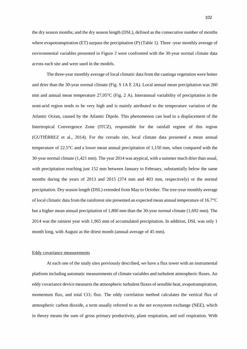
102

the dry season months; and the dry season length (DSL), defined as the consecutive number of months

where evapotranspiration (ET) surpass the precipitation (P) (Table 1). Three -year monthly average of

environmental variables presented in Figure 2 were confronted with the 30-year normal climate data

across each site and were used in the models.

The three-year monthly average of local climatic data from the caatinga vegetation were hotter

and drier than the 30-year normal climate (Fig. S 1A E 2A). Local annual mean precipitation was 260

mm and annual mean temperature 27,05°C (Fig. 2 A). Interannual variability of precipitation in the

semi-arid region tends to be very high and is mainly attributed to the temperature variation of the

Atlantic Ocean, caused by the Atlantic Dipole. This phenomenon can lead to a displacement of the

Intertropical Convergence Zone (ITCZ), responsible for the rainfall regime of this region

(GUTIÉRREZ et al., 2014). For the cerrado site, local climate data presented a mean annual

temperature of 22.5°C and a lower mean annual precipitation of 1,150 mm, when compared with the

30-year normal climate (1,421 mm). The year 2014 was atypical, with a summer much drier than usual,

with precipitation reaching just 152 mm between January to February, substantially below the same

months during the years of 2013 and 2015 (374 mm and 403 mm, respectively) or the normal

precipitation. Dry season length (DSL) extended from May to October. The tree-year monthly average

of local climatic data from the rainforest site presented an expected mean annual temperature of 16.7°C

but a higher mean annual precipitation of 1,800 mm than the 30-year normal climate (1,692 mm). The

2014 was the rainiest year with 1,965 mm of accumulated precipitation. In addition, DSL was only 1

month long, with August as the driest month (annual average of 45 mm).

Eddy covariance measurements

At each one of the study sites previously described, we have a flux tower with an instrumental

platform including automatic measurements of climate variables and turbulent atmospheric fluxes. An

eddy covariance device measures the atmospheric turbulent fluxes of sensible heat, evapotranspiration,

momentum flux, and total CO2 flux. The eddy correlation method calculates the vertical flux of

atmospheric carbon dioxide, a term usually referred to as the net ecosystem exchange (NEE), which

in theory means the sum of gross primary productivity, plant respiration, and soil respiration. With

103

half-hourly data provided from each site´s operators, we calculated NEE (in mol CO2m−2 s−1). The

partitioning of the CO2 NEE flux measurements into Respiration and Gross Primary Productivity

(GPP) was calculated following the nighttime approach using the Loyd-Taylor function

(REICHSTEIN et al., 2005). The MDS algorithm (REICHSTEIN et al., 2005) was applied for gap-

filling of the variables: net ecosystem exchange (NEE), air temperature (Tair), and vapor pressure

deficit (VPD). All the eddy covariance data processing and analysis were developed in R (R CORE

TEAM, 2017), using the package ReddyProc (REICHSTEIN et al., 2016). Daily sum of GPP time-

series were weekly aggregated.

Digital camera monitoring

For each one of the study sites, a digital hemispherical lens camera Mobotix Q 24 (Mobotix

AG —Germany) was placed at the top of the Flux Tower attached to an extension arm facing northeast

at a mean vertical distance of 10 m from the tree canopy. Energy supply is a 12V battery charged by a

solar panel. Cameras were configured to automatically take a daily sequence of five JPEG images (at

1280 × 960 pixels of resolution) in the first 10 min of each hour, from 6:00 to 18:00 h (UTC−3;

Universal Time Coordinated). The installation of each camera occurred at different times (see Table1).

For data analysis, we used a time series spanning from 2013 to 2015 for the caatinga and the cerrado

sites. Due to a sequence of gaps in data collection since camera setup, we decided to use only one year

and three months of data from the rainforest site. We filled gap sequences of more than 7 days with no

images recorded using the StructTS algorithm with a structure model fitted by maximum likelihood

(see HYNDMAN and KHANDAKAR, 2008) in R language (R CORE TEAM, 2017) with package

imputeTS.

Image data analysis was conducted by defining regions of interest (ROI), as described by

Richardson et al. (2007, 2009) and Alberton et al. (2014). For our main analysis, ROIs were based on a

community approach, which encompasses the entire image excluding the portion of the field of view

obstructed by the tower. A second approach was used to select our ROIs based on the trees crowns

within the community ROI (see ALBERTON et al., 2014, 2017). Each individual crown selected from

the original image was processed separately (Fig. S1). As high diverse tropical ecosystems may

104

encompass dozens of species in one single image, we aimed with this approach to verify and scrutinize

the greening signals or the crows leafing behaviors within the community pattern among sites. The

spatial and temporal variation of the crowns leafing behavior was considered to evaluate their influence

in the camera-derived phenological pattern and in the context of the GPP analysis among sites. Time

series associated with crowns (ROIs within the images) belonging to a given vegetation domain were

analyzed in function of time, by evaluating their synchronicity, and rate of the Gcc curve values. We

highlight that this perspective is based on analyzing tree crowns for the understanding of the overall

community pattern. We did not examine species by species, since high diverse tropical forests may have

not sufficient replicates for a meaningful interpretation of species behavior in the community fraction

represented by the single image.

Vegetation index time-series

ROIs were analyzed in terms of the contribution of the relative brightness of the green, red,

and blue color channels (RGB chromatic coordinates in WOEBBECKE et al., 1995) in relation to the

primary colors (red, green, and blue). The normalized RGB chromatic coordinate (RGBcc) index is

referred to as the most suitable index to detect leaf color changes, and the most efficient to suppress

light variation (GILLESPIE et al., 1987; WOEBBECKE et al., 1995). We calculate the normalized

index of the green and red color channels (Gcc and Rcc), as:

𝑇𝑜𝑡𝑎𝑙𝑎𝑣𝑔 = 𝑅𝑒𝑑𝑎𝑣𝑔 + 𝐺𝑟𝑒𝑒𝑛𝑎𝑣𝑔 + 𝐵𝑙𝑢𝑒𝑎𝑣𝑔

% 𝑜𝑓 𝐺𝑟𝑒𝑒𝑛 = Greenavg

Totalavg

% 𝑜𝑓 𝑅𝑒𝑑 = Redavg

Totalavg

Vegetation indexes were calculated for each of the five hourly images taken by the camera at

each day, with a daily measurement extracted by taking the 90th percentile of all calculated daytime

values. This procedure has been shown to minimize noise in the color channels series (RGBcc) related

to the illumination effects of seasonal changes and time of the day (adapted by SONNENTAG et al.,

2012). Finally, time series were weekly aggregated.

105

Data Analysis

Temporal models

We examined temporal dynamics of leaf phenology and productivity, as well the effects

between them and with the environmental factors, using additive mixed models (GAMM), applying a

normal distribution, and an identity-link function. As initial scatterplots indicated, response variables

GPP and Gcc (y-axis) presented multiple non-linear relationships with the covariates (time and

environmental cues). As inherent to time series structure, we tested our data for some temporal

autocorrelation among observations. Then, we nest our models with an Auto-Regressive Moving

Average (ARMA) time series model, meaning that instead of assuming that errors are independently

distributed, we assume that they are indeed correlated. Importantly, generalized additive models

(GAM) or smoothing models are considered highly useful for modelling nonparametric responses.

Their main assumption is that additive functions can be of smoothing, linear, step, quadratic or other

function (HASTIE and TIBSHIRANI, 1990). We did not presume an a priori model for the association

between response and predictors but instead allowed the data to inform this relationship. Also, the

degree of smoothing of an additive model is expressed by the effective degrees of freedom (edf), which

mean that the higher the edf, the lower is the linearity of the curve interaction.

To describe the temporal patterns of the variables representing leaf phenology (Gcc and Rcc)

and productivity (GPP) across the biomes, we fitted models using time as the smooth explanatory term.

To investigate our main question, we first fitted single-variable models between GPP and the biotic

(Gcc and Rcc) and abiotic (precipitation, CWD, PAR, and Tair) explanatory variables to evaluate the

contribution of each factor separated on the productivity. Then, to understand the relative importance

of phenology and the environmental variability over GPP across contrasting seasonal biomes, we fitted

two multivariate full models: an abiotic model using the explanatory terms related to water (P and

CWD), light demands (PAR), and mean air temperature (Tair), and a biotic-abiotic model by adding

phenology as an explanatory term. All terms included in the multivariate models were previously

checked for multicollinearity. By assessing the approximate significance parameters of the smooth

and/or linear terms and the coefficient of determination from the models, we could compare the

106

performance between the single-variable, abiotic, and the biotic-abiotic models. All analysis were run

in R language (R CORE TEAM, 2017) using base package mgcv (WOOD, 2006) for the generalized

additive models.

Spatial-temporal phenological dynamics

To answer our third question, we carried out a visual analysis into the complete set of crowns

ROIs in order to extract the onset date of phenological stages transitions. We select the leaf flushing

onset as the phenophase to test the degree of synchrony of the crowns time series greening, and we

analyze all the ROIs crows in function of time to evaluate timing and rate of the Gcc time series within

each vegetation site. We applied circular statistics to calculate the mean angle or date correspondent to

the most frequent date of leaf flushing onset (see MORELLATO et al., 2000; MORELLATO et al.,

2010). We divided the 360o of a circumference by 12 and each month of the year is represented by a

range of 30o starting on January (midpoint 15o, see MORELLATO et al., 2010 for details). Then, we

tested whether the mean onset data are significantly concentrated around the mean angle or date, as a

proxy of seasonality by applying the Rayleigh test (Z), as suggested by Morellato et al. (2000, 2010). If

the mean onset data are significantly concentrated around the mean angle or date, we consider the

leafing pattern seasonal. The degree of synchrony represented by the length of the vector r has no unity

and ranges from 0 (no synchronicity) to 1 (perfect synchrony). We performed circular analyses per

study site, for all the crowns using Oriana 4.0 (Kovach Computing Services).

3 RESULTS

3.1 Temporal patterns of phenology and productivity across sites

Phenocam indices revealed seasonal patterns for all sites despite their degree of seasonality

(Fig. 3). In general, Gcc and Rcc indexes showed inverse relationship, with Gcc presenting higher values

from the late dry season towards the wettest months, which are related to the leaf flushing of the

vegetation community, while Rcc highest values were prevalent along the driest periods, which are

mainly related to the process of senescence and the decrease of green biomass. Curve oscillations,

which means the peaks and valleys of Gcc and Rcc values along time, presented different patterns across

107

sites.

The Gcc pattern for the caatinga vegetation presented marked seasonality, with an abrupt green-

up precisely at the beginning of the wet season and a relatively abrupt green-down starting at the end

of the wet season. During the dry season, low values of Gcc were nearly constant giving a flat pattern

to the curve. Within the wet period, Gcc showed oscillations with peaks and valleys that followed

precipitation events (Fig 3 A). The rest season corresponding to the driest months was long (from April

to November) presenting few or none Gcc oscillations, but not reaching zero, which indicates the

presence of some green biomass. Cactaceae family species as the Facheiro (Pilosocereus pachycladus

F.Ritter) can be found through all the year in the images and are likely responsible for sustaining Gcc

values during dry season. In the cerrado vegetation, Gcc presented a market green-up earlier, yet in the

dry season, and a slower green-down, in comparison to the caatinga site. The cerrado green-down

started by the end of the wet season and extended until the end of the dry season (Fig. 3 C). For the

rainforest, green-up started right in the driest month with a progressive increase towards the wet period

(Fig. 3 E). Green-down started from the middle of the wet season and was less abrupt than the caatinga

but with a higher decrease in a shorter time if compared with the cerrado site.

Rcc curves demonstrated an inverse pattern to Gcc in the wet seasons across all sites. Within

the dry periods, Rcc for the caatinga peaked at the beginning of the dry season followed by a linear

decrease towards the mid to the end of the dry season (Fig. 3 B). Inversely, in the cerrado site, Rcc time

series increased by the end of the wet season peaking by the end of the dry season (Fig. 3D). In the

late dry season (August), red increasing did not follow the inverse pattern with Gcc; in fact, they

increased together (Fig.2C and D). This pattern is linked to the colorful, reddish new leaves, produced

right at the start of the community leaf flushing. Rcc curve from rainforest site was higher for winter

time, just when Gcc scores have decreased, and showed the lowest range of values of all sites (min=

0.3074/max= 0.3176). This may indicate an absence of a massive leaf senescence in the community.

Instead, species leaf turnover may be occurring along the all year.

As occurred for the camera-vegetation indices, sites also presented differences regarding GPP

seasonality (Fig. S4). Productivity started to increase within the wet season in the caatinga and cerrado

sites (Fig. S4 A and B), while in the rainforest GPP, curve oscillations did not present a tightly link

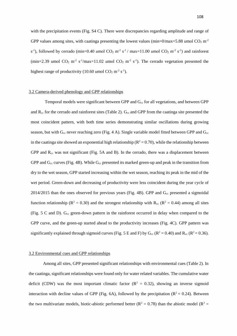
108

with the precipitation events (Fig. S4 C). There were discrepancies regarding amplitude and range of

GPP values among sites, with caatinga presenting the lowest values (min=0/max=5.88 umol CO2 m-2

s-1), followed by cerrado (min=0.40 umol CO2 m-2 s-1 / max=11.00 umol CO2 m-2 s-1) and rainforest

(min=2.39 umol CO2 m-2 s-1/max=11.02 umol CO2 m-2 s-1). The cerrado vegetation presented the

highest range of productivity (10.60 umol CO2 m-2 s-1).

3.2 Camera-derived phenology and GPP relationships

Temporal models were significant between GPP and Gcc for all vegetations, and between GPP

and Rcc for the cerrado and rainforest sites (Table 2). Gcc and GPP from the caatinga site presented the

most coincident pattern, with both time series demonstrating similar oscillations during growing

season, but with Gcc never reaching zero (Fig. 4 A). Single variable model fitted between GPP and Gcc

in the caatinga site showed an exponential high relationship (R2 = 0.70), while the relationship between

GPP and Rcc was not significant (Fig. 5A and B). In the cerrado, there was a displacement between

GPP and Gcc curves (Fig. 4B). While Gcc presented its marked green-up and peak in the transition from

dry to the wet season, GPP started increasing within the wet season, reaching its peak in the mid of the

wet period. Green-down and decreasing of productivity were less coincident during the year cycle of

2014/2015 than the ones observed for previous years (Fig. 4B). GPP and Gcc presented a sigmoidal

function relationship (R2 = 0.30) and the strongest relationship with Rcc (R2 = 0.44) among all sites

(Fig. 5 C and D). Gcc green-down pattern in the rainforest occurred in delay when compared to the

GPP curve, and the green-up started ahead to the productivity increases (Fig. 4C). GPP pattern was

significantly explained through sigmoid curves (Fig. 5 E and F) by Gcc (R2 = 0.40) and Rcc (R2 = 0.36).

3.2 Environmental cues and GPP relationships

Among all sites, GPP presented significant relationships with environmental cues (Table 2). In

the caatinga, significant relationships were found only for water related variables. The cumulative water

deficit (CDW) was the most important climatic factor (R2 = 0.32), showing an inverse sigmoid

interaction with decline values of GPP (Fig. 6A), followed by the precipitation (R2 = 0.24). Between

the two multivariate models, biotic-abiotic performed better (R2 = 0.78) than the abiotic model (R2 =

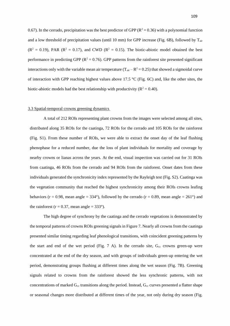
109

0.67). In the cerrado, precipitation was the best predictor of GPP (R2 = 0.36) with a polynomial function

and a low threshold of precipitation values (until 10 mm) for GPP increase (Fig. 6B), followed by Tair

(R2 = 0.19), PAR (R2 = 0.17), and CWD (R2 = 0.15). The biotic-abiotic model obtained the best

performance in predicting GPP (R2 = 0.76). GPP patterns from the rainforest site presented significant

interactions only with the variable mean air temperature (Tair – R2 = 0.25) that showed a sigmoidal curve

of interaction with GPP reaching highest values above 17.5 °C (Fig. 6C) and, like the other sites, the

biotic-abiotic models had the best relationship with productivity (R2 = 0.40).

3.3 Spatial-temporal crowns greening dynamics

A total of 212 ROIs representing plant crowns from the images were selected among all sites,

distributed along 35 ROIs for the caatinga, 72 ROIs for the cerrado and 105 ROIs for the rainforest

(Fig. S1). From these number of ROIs, we were able to extract the onset day of the leaf flushing

phenophase for a reduced number, due the loss of plant individuals for mortality and coverage by

nearby crowns or lianas across the years. At the end, visual inspection was carried out for 31 ROIs

from caatinga, 46 ROIs from the cerrado and 94 ROIs from the rainforest. Onset dates from these

individuals generated the synchronicity index represented by the Rayleigh test (Fig. S2). Caatinga was

the vegetation community that reached the highest synchronicity among their ROIs crowns leafing

behaviors (r = 0.98, mean angle = 334°), followed by the cerrado (r = 0.89, mean angle = 261°) and

the rainforest (r = 0.37, mean angle = 333°).

The high degree of synchrony by the caatinga and the cerrado vegetations is demonstrated by

the temporal patterns of crowns ROIs greening signals in Figure 7. Nearly all crowns from the caatinga

presented similar timing regarding leaf phenological transitions, with coincident greening patterns by

the start and end of the wet period (Fig. 7 A). In the cerrado site, Gcc crowns green-up were

concentrated at the end of the dry season, and with groups of individuals green-up entering the wet

period, demonstrating groups flushing at different times along the wet season (Fig. 7B). Greening

signals related to crowns from the rainforest showed the less synchronic patterns, with not

concentrations of marked Gcc transitions along the period. Instead, Gcc curves presented a flatter shape

or seasonal changes more distributed at different times of the year, not only during dry season (Fig.

110

7C).

4 DISCUSSION

4.1 Leaf phenology, water/light relationship and the GPP across contrasting tropical biomes

Temporal patterns of tropical ecosystem productivity and leaf phenology production were

significant correlated across all vegetations studied, and presented the strongest relationships, when

compared with the GPP and environmental variables interactions. Across our contrasting biomes, we

reported a much stronger coupled relation between GPP and Gcc for the caatinga site (R2 = 0.70), when

compared to the cerrado (R2 = 0.30) and rainforest (R2 = 0.40). The only comparable study on seasonal

tropics reporting GPP-Gcc relationships for an Australian savanna (MOORE et al., 2017) showed that

community Gcc had different performances for understory and overstory layers, with the grasslands

component better coupled with carbon fluxes (R2 = 0.65) than shrubs and trees (R2 = 0.23). Studies

investigating GPP prediction by camera-derived indices are concentrated on the north hemisphere (e.g.:

RICHARDSON et al., 2007; AHRENDS et al., 2009; MIGLIAVACCA et al., 2011; PEICHL et al.,

2014). Gcc index performed well by correlating with GPP across temperate deciduous forests, explaining

over 80% of the carbon fluxes seasonality (RICHARDSON et al., 2007; AHRENDS et al., 2009;

TOOMEY et al., 2015).

We confirmed the strong relationships between GPP and phenology in our results. In spite of

that, there was also an important influence of climatic constrains over productivity on the seasonal

ecosystems of caatinga and cerrado. In fact, when we compared abiotic (just environmental factors) and

biotic-abiotic models (environmental factors and greening), we notice an improvement of explanation

when phenology and environmental terms are added together in the model. For the caatinga vegetation,

the GPP patterns closely following the precipitation presented similarity to the few records of

productivity rates derived from MODIS products, also characterized by the fast vegetation response to

moisture pulses (SILVA et al., 2013; MORAIS et al., 2017). The caatinga greening and GPP curve

oscillations during the wet season have been also described for carbon fluxes from other high seasonal

ecosystems, such as temperate grasslands (BROWN et al., 2016; MURRAY-TORTAROLO et al.,

2016).

111

The cerrado productivity observed here followed the expected pattern for wet savannas

(MIRANDA et al., 1997; CHEN et al., 2003), with GPP likely constrained by a wet-dry climate, high

rates of GPP along the wet season, and a steep decrease in the driest months. For savannas, seasonal

patterns of rainfall and changes in soil water content have been tightly coupled with productivity indices

as GPP (CHEN et al., 2003). Rainfall plays a critical role in determining the distribution of GPP of

distinct tropical vegetation types, ranging from rainforests to arid grasslands (KANNIAH et al., 2010).

We did not find any previous publications reporting GPP patterns from Atlantic Forest.

However, for evergreen tropical sites across the world as well as Central Amazon forests, seasonality

increases photosynthetic capacity during dry season, indicating not prevalent climatic constrains

(BRANDO et al., 2010; GUAN et al., 2015; WU et al., 2016). In the case of our Atlantic rainforest, we

notice a decrease of ecosystem photosynthesis during the coldest and driest months, characterized by a

lowest mean air temperature when compared with other tropical evergreen forests, which are explained

by the local elevated altitude of 1,056 m a.s.l (MARCHIORI et al., 2016). Ground biomass studies

carried out in the same site indicated an increase in the stocks of carbon and nitrogen along a gradient

of elevation, suggesting a relationship of decreasing temperature with reduced photosynthetic activity,

since colder soil temperatures would tend to lose less carbon to the atmosphere (RAICH et al., 2002;

VIEIRA et al., 2011; MARCHIORI et al., 2016). Also, temperature has been reported as an important

factor influencing several biogeochemical terrestrial processes (WU et al., 2011). The interaction of

temperature and rainfall and its influence on tropical productivity has been recently reported, where

high rainfall can decrease C cycling rates when interacting with cool temperatures (< 20°C), while in

warm forests (> 20°C), rainfall and temperature interaction produces the opposite effect (TAYLOR et

al., 2017).

4.2 Leaf phenology spatiotemporal dynamics and ecosystem productivity across seasonal biomes

Through the crowns greening analysis carried out in the present study, we teased apart the

composite greening signals of the vegetation communities and indicated, for each vegetation, the

dominant patterns that represent the community and affect carbon fluxes, providing us insights about

how phenological dynamics were triggering or dampening photosynthesis dynamics of each

112

ecosystems. The evaluation of the spatial and temporal phenological dynamics from individual crowns

greening patterns within digital images have been reported for other studies involving camera-derived

leafing patterns description and spatial variability (RICHARDSON, 2009; LOPES et al., 2016;

NAGAI et al., 2016), as well as to investigate GPP patterns (AHRENDS et al., 2009).

Caatinga and cerrado, the most seasonal sites, presented higher synchronicity in terms of time

and rate of crowns greening signals, while rainforest has demonstrated a non-seasonal pattern with

crowns Gcc curves distributed along the all period or with no marked seasonality and synchronicity

among crowns. Based on theories of community and phenology dynamics, we made inferences

regarding the synchronicity dynamics across sites. Shorter growing seasons would concentrate species

occurrence at the same time, while longer growing seasons would facilitate species life cycles to

different times of the year. This could affect the way competition influence species dynamics as well,

swinging from a relative strength of interspecific competition in the first case, to a intraspecific

competition in the latter (see more in MITTELBACH, 2017). Climatic constrains appear to underlie

this effect with more strength from the Equator towards higher latitudes (USINOWICZ et al., 2017).

Due the high variation of seasonal and inter-annual climatic conditions in tropical vegetations,

there is a high diversity of physiological and phenological strategies of plants to cope with changes in

water availability (MURPHY and LUGO, 1986; LEHMANN et al., 2009; VICO et al., 2015). While

evergreen species would be favored by short dry seasons length or by the ability to access groundwater

or water stores, on the other hand, high inter-annual seasonality of wetter periods would be favoring

the occurrence of different deciduous phenological strategies (REICH, 1995; RIVERA et al., 2002;

VICO et al., 2015; CAMARGO et al., 2018).

There is a lack of knowledge regarding the mechanisms controlling leaf phenology strategies

of individual plants due their complexity (BORCHERT and RIVERA, 2001; CAMARGO et al., 2018)

and the high diversity of plant species and strategies in the tropics. Nevertheless, we can classify our

plants into three main leaf phenological strategies (EAMUS and PRIOR, 2001; SINGH and

KUSHWAHA, 2005; ELLIOT et al., 2006): (i) opportunistic drought deciduous species, mainly driven

by water availability and leaf flushing following the first rainfall events indicating the start of the wet

season; (ii) schedule drought deciduous species, independent of water availability and mainly driven

113

by photoperiod, temperature, or radiation, with leaf flushing before or early the wet season; and (iii)

evergreen species, able to shed new leaves asynchronously throughout the year. Each strategy imposes

its own risks to plants given the ecological tradeoffs of each case. That is why a nuanced of species

strategies may be found in the tropics rather than the prevalence of one, given the variation in changes

of rainfall availability and predictability (VICO et al., 2015; CAMARGO et al., 2018).

Hereafter, we discuss based on the climatic seasonality imposed on each biome and by

assessing the crows leafing behavior within the vegetation communities, how leaf phenology

controlling productivity may change across the biomes.

4.2.1 High synchronic leaf phenology and productivity in seasonally constrained vegetation: the

caatinga case

The temporal patterns of leaf production and ecosystem productivity in the caatinga were very

coincident with both presenting multiple seasonal cycles within the wet period. This irregular pattern

visually followed shortly the moisture pulses) or tracked the reduced deficit of water as by the temporal

models. Similar patterns were detected by cameras across other ecosystems such as the grasslands,

where there is a vegetation dependent on the inter-annual variation of precipitation rates (BROWN et

al., 2016; RICHARDSON et al., 2018). Phenological direct observations of caatinga commonly

recorded flowering and flushing phenophases as a consequence of precipitation with formation of new

leaves immediately after the rainfall event (CARVALHO and BARBOSA, 1989; MACHADO et al.,

1997; ARAÚJO; CASTRO; ALBUQUERQUE, 2007).

High synchronicity among crowns leafing behaviors suggests a common high influence of

climatic factors triggering leaf phenophases. The harsh seasonal conditions lead the caatinga to be

mainly composed of opportunistic drought deciduous species described above, avoiding dry season

stress and constrained their leafing to periods of water availability (see VICO et al., 2015). Leaf flushing

in opportunistic drought deciduous species are usually synchronous and responsive to water availability.

There are cases, where species may respond to other precedent cues such as atmospheric water

decreases, but in general still associated with small rainfall events (MURPHY and LUGO, 1986;

BORCHERT, 1994; WILLIAMS et al., 1997). Year-to-year high interannual variability in the

114

precipitation rates contribute to the variability of the onset community leaf flushing and occasionally to

be more or less intense (MACHADO et al., 1997). Thus, climatic constrains in the caatinga and leaf

phenology are tightly coupled and then varying together, what mostly explains the high correlation

between phenology and GPP in a very water dependent ecosystem. Despite that, we highlight the model

improvement when phenology is added in the biotic-abiotic model (R2 = 0.78).

4.2.2 Leaf phenology synchronicity and productivity in a mid-seasonal ecosystem

The woodland cerrado temporal patterns of leaf production and productivity demonstrated a

marked seasonality with a lower degree of asynchrony between crowns compared to caatinga. Green-

up onset occurred yet in the late dry season, a pattern shared by savannas, with the input of new leaves

preceding the massive rainfall events (e.g.: MONASTERIO and SARMIENTO, 1976; WILLIAMS et

al., 1999; PIRANI et al., 2009; MUNHOZ and FELFILI, 2005; RYAN et al., 2016; ADOLE et al.,

2016). The onset of GPP occurred after entering the wet season and demonstrated to be mainly

correlated with the seasonal patterns of precipitation, following the leaf flushing.

Plant species from less harsh climatic conditions, as our study cerrado, may be able to cope

with water limitations and find longer and wetter periods to produce new leaves still during the dry

season (BORCHERT, 1998). Cerrado trees, for example, may use deep roots to exploit deeper soil

water sources and be able to flush new leaves in the late dry season (EAMUS, 1999; SCHOLZ et al.,

2008; ROSSATO et al., 2012). A high synchronic pattern was demonstrated by the crowns greening

behaviors from the studied cerrado community and a timing concentration of leafing onset at the end of

the dry season in September. This behavior characterizes schedule drought deciduous species, or those

capable of enduring droughts by developing adaptations to maximize their carbon gains without

experiencing stress (SCHOLZ et al., 2002; VICO et al., 2015; ELLIOT et al., 2006). Schedule drought

deciduous are mainly driven by consistent factors such as photoperiod and demonstrate high

interspecific synchronicity and low inter-annual variability on the leaf flushing dates (VICO et al., 2015;

CAMARGO et al., 2018).

We conclude from our results that both: climate, mainly through water relations, and

phenology, represented by a larger range of leaf strategies including schedule drought deciduous

115

species, contribute to the seasonal patterns of GPP in the cerrado. Our finding concurs with general

expectation that savanna productivity would be predicted by a complex interaction of climatic and

phenological factors (KANNIAH et al., 2011; WHITLEY et al., 2011; MA et al., 2013, 2014; MOORE

et al., 2017).

4.2.3 Leaf phenology asynchrony explains productivity of less seasonal ecosystems

The degree of synchronicity of rainforest crowns greening, calculated based on the visual

inspection of the crowns greening signals was the lowest among the three ecosystems studied, typical

for a non-seasonal vegetation. In fact, leaf flushing dates were concentrated in two main periods

(December and March), demonstrating a bimodal pattern. The production of new leaves slowed down

during the colder and driest months, with most of Gcc curves presented a flat pattern in the driest month

(August). Seasonality in the phenological transitions of leafing and flowering were demonstrated by

other Atlantic Rainforest locations, belonging to the same latitude of our study site (e.g.:

MORELLATO et al., 2000; BENCKE and MORELLATO, 2002; PEREIRA et al., 2008). The driest

months are also the colder ones, concentrated in June, July, and August, and the community leaf

flushing increase is marked in the transition from the driest to the wettest months, during September

and October (MORELLATO et al., 2000), which coincides with the pattern tracked by the cameras in

our study.

The Gcc and Rcc values detected for our rainforest were the highest and lowest, respectively,

among our three vegetations. This outcome, in association with the low degree of synchronicity of the

crowns greening are explained by the predominance of evergreen species in this vegetation biome

(MORELLATO et al., 2000; BENCKE and MORELLATO, 2002). The dominance of evergreen

species strategists, or plants retaining their foliage year-round and simultaneously exchanging new

foliage and senescing old ones, may sustain vegetation indices values due persistent green biomass

along the all year (see RICHARDSON et al., 2018). The evergreen species show asynchronous activity

throughout the year, without apparent seasonal changes in their leaf are index (LAI) and, therefore,

endure drought by physiological adaptations that are not yet well clear in the literature (BORCHERT,

1994; NEPSTAD et al., 1994; REICH, 1995; BORCHERT, 1998).

116

Despite the influence of low temperatures in the GPP patterns, the Atlantic rainforest showed

a reduced influence of environmental factors. Given that evergreen species tend to be more

independent from seasonal environmental constrains (BORCHERT, 1998), we suggest that leafing

phenology is exerting the main control over the temporal patterns of ecosystem productivity in the less

seasonal biome of Atlantic rainforest.

We also suggest that the moderate effect between phenology and GPP in the rainforest

vegetation is partially influenced by the seasonal low ranges of temperature during dryer months. We

also recognize the fact that evergreen phenological patterns may be underestimated for being more

complicated to be tracked by camera-derived indices (TOOMEY et al., 2015; NAGAI et al., 2016;

LOPES et al., 2016; RICHARDSON et al., 2018). Also, the vegetation index here applied, derived

from RGB color channels sensors as the phenocams, may not be able to follow the stages of leaf

maturation precisely, since that the chromatic coordinates are more sensitive to light colors and would

better indicate the seasonality of leaf production (see LOPES et al., 2016). The importance to consider

leaf aging stages on the response of productivity has been reported for tropical evergreen forests (WU

et al., 2016).

5 CONCLUSIONS

A fine-scale phenological monitoring using the repeated photograph technic is unprecedent

for the Caatinga dry forest, Brazilian savanna and the Atlantic Rainforest. In the case of the Cerrado,

cameras have already been applied for species and community levels of tropical savannas, used in the

context of method validation with ground observations for woody cerrado (ALBERTON et al., 2014)

and in ecosystem productivity studies in Australian savannas (MOORE et al., 2017). The addressed

questions in this study, involving tropical sites under different seasonality constraints, are a significant

step towards the understanding of ecosystem functionality. Accordingly, phenology and its confident

representation is a key parameter to be considered in climate e biogeochemical cycle models (MA et

al., 2013). Carbon fluxes relationships with the canopy development are still underexplored and not

well described for the tropics. Despite the existence of record from GPP seasonality and dynamics for

tropical seasonal sites, the actual knowledge about how phenology and GPP covary is still limited, and

117

we offer the first strong evidence of leafing phenology shaping GPP patters across seasonally dry

tropical biomes. Even considering GPP patterns and controls still need further investigation, the data

analyzed here, combining hourly digital images and high frequency eddy covariance measurements,

is unprecedent for the tropics and brings the first modeling of biotic and abiotic controls of productivity

and photosynthesis seasonality.

We bring evidences of a complex interaction of both environmental and phenology controlling

productivity in tropical ecosystems. Temporal patterns of GPP across biomes varied and presented

distinct differences that at some extent confirmed the hydroclimate hypothesis initially proposed.

Caatinga vegetation was constrained by the strong dry season and leafing and GPP patterns were

coupled in a climatic-phenological interaction, while reduced influence of climatic and phenological

seasonality defined GPP seasonality for the cerrado, and a strong relation of GPP and phenology in

the less seasonal rainforest. Camera-derive phenology is, therefore, a good proxy for productivity in

high synchronic and seasonal tropical ecosystems, as the caatinga.

Importantly, the outcomes reported on this study were only possible due a multi-site

comparison analysis, enabling the observation of the nuances of the leaf phenology dynamics and GPP

patterns across biomes. We highlight the impacts of future changes on water regimes for the tropics

over the productivity of seasonal vegetations, also affecting phenological responses of species, on

seasonal tropical ecosystems (VICO et al., 2015; MORELLATO et al., 2016, RESTREPPO-COUPE

et al., 2017).

Acknowledgments – the present study was supported by São Paulo Research Foundation - FAPESP

(grants #2009/54208-6, #2010/52113-5 and #2013/50155-0), Microsoft Research and CNPq. We

thank the Instituto Florestal for the permissions to work at the Cerrado and Atlantic Rainforest sites,

and Embrapa for all the support and collaboration in the Caatinga site. BA receives fellowship from

FAPESP (#2014/00215-0 and #2016/01413-5). LPCM, RST and HR receive a research productivity

fellowship from CNPq.

6 REFERENCES

118

ADOLE, T.; JADU, D.; ATKINSON, P.M. A systematic review of vegetation phenology in Africa.

Ecological informatics, v. 34, p. 117-128, 2016.

AHRENDS, H.E. et al. Tree phenology and carbon dioxide fluxes: Use of digital photography for

process-based interpretation at the ecosystem scale. Climate Research, v. 39(3), p. 261–274, 2009.

ALBERTON, B.C. et al. Introducing digital cameras to monitor plant phenology in the tropics:

Applications for conservation. Perspectives in Ecology and Conservation, v. 15, p. 82-90, 2017.

ALBERTON, B.C. et al. Using phenological cameras to track the green up in a cerrado savanna and

its on-the-ground validation. Ecological Informatics, v. 19, p .62–70, 2014.

ARAÚJO, E.L.; CASTRO, C.C.; ALBUQUERQUE, U.P. Dynamics of Brazilian Caatinga – A

Review Concerning the Plants, Environment and People. Functional Ecosystems and Communities,

v. 1, p. 15–28, 2007.

BENCKE, C.S.C.; MORELLATO, L.P.C. Estudo comparativo da fenologia de nove espécies arbóreas

em três tipos de floresta atlântica no sudeste do Brasil. Revista Brasileira de Botânica, v. 25(2), p.

237–248, 2002.

BORCHERT, R. Water status and development of tropical trees during seasonal drought. Trees, v. 8

(3), p. 115-125, 1994.

BORCHERT, R. Responses of tropical trees to rainfall seasonality and its long-term changes.

Climatic Change, v. 39(2), p. 381–393, 1998.

BORCHERT, R.; RIVERA, G. Photoperiodic control of seasonal development and dormancy in

tropical stem-succulent trees. Tree Physiology, v. 21 (4), p. 213-221, 2001.

BRANDO, P. M. et al. Seasonal and interannual variability of climate and vegetation indices across

the Amazon. Proc. Natl Acad. Sci., USA, v. 107, p. 14685–14690, 2010.

BROWN, T.B. et al. Using phenocams to monitor our changing earth: Toward a global phenocam

network. Frontiers in Ecology and the Environment, v. 14(2), p. 84–93, 2016.

CAMARGO, M.G.G. et al. Leafing patterns and leaf exchange strategies of a cerrado woody

community. Biotropica, v. 50 (3), p. 442-454, 2018.

CARVALHO, D.; BARBOSA, D.A. Dados fenológcos de 10 espécies arbóreas de uma área de

caatinga (Alagoinha-PE ). Acta bot. bras, v. 3(2), p. 109–117, 1989.

CHEN, X.; HUTLEY, L.B.; EAMUS, D. Carbon balance of a tropical savanna of northern Australia.

Oecologia, v. 137(3), p. 405–416, 2003.

EAMUS, D. Ecophysiological traits of deciduous and evergreen woody species in the seasonally dry

tropics. Trends in Ecology and Evolution, v. 14(1), p. 11–16, 1999.

119

EAMUS, D.; PRIOR, L. Ecophysiology of trees of seasonally dry tropics: comparisons among

phenologies. Advances in Ecological Research, v. 32, p. 113-197, 2001.

ELLIOTT, S.; BAKER, P.; BORCHERT, R. Leaf flushing during the dry season: the paradox of

Asian monsoon forests. Global Ecology and Biogeography, v. 15 (3), p. 248-257, 2006.

GASH, J.H.C. et al. Amazonian climate: Results and future research. Theoretical and Applied

Climatology, v. 78(1–3), p. 187–193, 2004.

GILLESPIE, A.R.; KAHLE, A.B.; WALKER, R.E. Color enhancement of highly correlated images.

II. Channel ratio and “chromaticity” transformation techniques. Remote Sensing of Environment, v.

22(3), p. 343–365, 1987.

GUAN, K. et al. Photosynthetic seasonality of global tropical forests constrained by hydroclimate.

Nature Geosci, v. 8(4), p. 284–289, 2015. Available at: http://dx.doi.org/10.1038/ngeo2382.

GUTIÉRREZ, A.P.A. et al. Drought preparedness in Brazil. Weather and Climate Extremes, v. 3,

p. 95–106, 2014. Available at: http://dx.doi.org/10.1016/j.wace.2013.12.001.

HASTIE, T.J.; TIBSHIRANI, R. Generalized additive models. Statistical Science, v. 1(3), p. 297–

318, 1990.

HUETE, A.R. et al. Amazon rainforests green-up with sunlight in dry season. Geophys. Res. Lett., v.

33, 2006.

HYNDMAN, R.J.; KHANDAKAR, Y. Automatic time series forecasting: The forecast package for

R. Journal Of Statistical Software, v. 27(3), p. C3–C3, 2008. Available at:

http://www.robjhyndman.com/papers/forecastpackage.pdf.

JAMES, R. et al. Implications of global warming for the climate of African rainforests. Phil Trans R

Soc B, 2013

KANNIAH, D. et al. The comparative role of key environmental factors in determining savanna

productivity and carbon fluxes: A review, with special reference to northern Australia. Progress in

Physical Geography, v. 34 (4), p. 459-490, 2010.

KANNIAH, K.D.; BERINGER, J.; HUTLEY, L.B. Environmental controls on the spatial variability

of savanna productivity in the Northern Territory, Australia. Agricultural and Forest Meteorology,

v. 151(11), p. 1429–1439, 2011.

KEENAN, T.; GRAY, J.; FRIEDL, M. Net carbon uptake has increased through warming-induced

changes in temperate forest phenology. Nature Climate Change, v. 4 (June), p. 598–604, 2014.

KILL, L.H.P. Caracterização da vegetação da reserva legal da Embrapa semiárido. Documentos

online, v. 5, p. 121–124, 2017

KLOSTERMAN, S.T. et al. Evaluating remote sensing of deciduous forest phenology at multiple

120

spatial scales using PhenoCam imagery. Biogeosciences, v. 11(16), p. 4305–4320, 2014.

LEHMANN, C.E.R; PRIOR, L.D.; BOWMAN, D.M.J.S. Decadal dynamics of tree cover in an

Australian tropical savanna. Austral Ecology, v. 34 (6), p. 601-612, 2009.

LOPES, A.P. et al. Leaf flush drives dry season green-up of the Central Amazon. Remote Sensing of

Environment, v. 182, p. 90–98, 2016. Available at: http://dx.doi.org/10.1016/j.rse.2016.05.009.

MA, X. et al. Spatial patterns and temporal dynamics in savanna vegetation phenology across the

North Australian Tropical Transect. Remote sensing of Environment, v. 139, p. 97-115, 2013.

MA, X. et al. Parameterization of an ecosystem light-use-efficiency model for predicting savanna

GPP using MODIS EVI. Remote Sensing of Environment, v. 154, p. 253-271, 2014.

MACHADO, I.C.S.; BARROS, L.M.; SAMPAIO, E.V.S.B. Phenology of Caatinga Species at Serra

Talhada , PE , Northeastern Brazil. Biotropica, v. 29(1), p. 57–68, 1997.

MARCHIORI, N.M. et al. Tree Community Composition and Aboveground Biomass in a Secondary

Atlantic Forest, Serra Do Mar State Park, São Paulo, Brazil. Cerne, v. 22(4), p. 501–514, 2016.

MIGLIAVACCA, M. et al. Using digital repeat photography and eddy covariance data to model

grassland phenology and photosynthetic CO2 uptake. Agricultural and Forest Meteorology, v.

151(10), p. 1325–1337, 2011.

MIRANDA, A.C. et al. Fluxes of carbon, water and energy over Brazilian cerrado: an analysis using

eddy covariance and stable isotopes. Plant, Cell & Environment, v. 20 (3), p. 315-328, 1997.

MITTELBACH, G.G. A matter of time for tropical diversity. Nature, v. 550(7674), p. 51–52, 2017.

MONASTERIO, M.; SARMIENTO, G. Phenological strategies of plants species in the tropical

savanna and semi-deciduous forest of the Venezuelan Lianos. Journal of Biogeography, v. 3(4), p.

325–356, 1976.

MOORE, C.E. et al. Tree – grass phenology information improves light use efficiency modelling of

gross primary productivity for an Australian tropical savanna. Biogeosciences, v. 14, p.111–129,

2017.

MORAIS, Y. et al. Análise do sequestro de carbono em áreas de Caatinga do Semiárido

pernambucano. Revista Brasileira de Meteorologia, v. 32 (4), p. 585-599, 2017.

MORELLATO, L.P.C. et al. Linking plant phenology to conservation biology. Biological

Conservation, v. 195, p. 60–72, 2016.

MORELLATO, L.P.C. et al. Phenology of Atlantic Rain Forest Trees: A Comparative Study.

Biotropica, v. 32(4b), p.811–823, 2000.

MORELLATO, L.P.C.; ALBERTI, L.F.; HUDSON, I.L. Applications of circular statistics in plant

121

phenology: a case studies approach. In I. L. Hudson & M. R. Keatley, eds. Phenological Research.

Springer Netherlands, p. 339–359, 2010.

MORISETTE, J.T. et al. Tracking the rhythm of the seasons in the face of global change:

Phenological research in the 21 st century. Frontiers in Ecology and the Environment, v. 7(5), p.

253–260, 2009.

MORTON, D.C. et al. Amazon forests maintain consistent canopy structure and greenness during the

dry season. Nature, v. 506(7487), p.221–224, 2014.

MUNHOZ, C.B.R.; FELFILI, J.M. Fenologia do estrato herbáceo-subarbustivo de uma comunidade

de campo sujo na Fazenda Água Limpa no Distrito Federal, Brasil. Acta Botanica Brasilica, v. 19(4),

p. 979–988, 2005.

MURPHY, P.G.; LUGO, A.E. Ecology of Tropical Dry Forest. Annual Review of Ecology and

Systematics, v. 17, p. 67–88, 1986.

MURRAY-TORTAROLO, G. et al. Changes in the dry season intensity are a key driver of regional

NPP trends. Geophysical Research Letters, 2016.

MYNENI, R.B. et al. Large seasonal swings in leaf area of Amazon rainforests. Proc. Natl Acad.

Sci., USA, v. 104, p. 4820–4823, 2007.

NAGAI, S. et al. Usability of time-lapse digital camera images to detect characteristics of tree

phenology in a tropical rainforest. Ecological Informatics, v. 32, p. 91–106, 2016.

NEPSTAD, D.C. et al. The role of deep roots in the hydrological and carbon cycles of Amazonian

forests and pastures. Nature, v. 372 (6507), p. 666, 1994.

OLIVEIRA‐FILHO, A.T.; FONTES, M.A.L. Patterns of floristic differentiation among Atlantic

Forests in Southeastern Brazil and the influence of climate. Biotropica, v. 32(4b), p. 793-810, 2000.

OLSON, D.M. et al. Terrestrial Ecoregions of the World: A New Map of Life on EarthA new global

map of terrestrial ecoregions provides an innovative tool for conserving biodiversity. BioScience, v.

51 (11), p. 933-938, 2001.

PEICHL, M.; SONNENTAG, O.; NILSSON, M.B. Bringing Color into the Picture: Using Digital

Repeat Photography to Investigate Phenology Controls of the Carbon Dioxide Exchange in a Boreal

Mire. Ecosystems, v. 18(1), p. 115–131, 2014.

PEREIRA, T.S. et al. Fenologia de espécies arbóreas em Floresta Atlântica da Reserva Biológica de

Poço das Antas, Rio de Janeiro, Brasil. Iheringia, Série Botânica, Porto Alegre, v. 63(2), p. 329–339,

2008.

PIRANI, F.R., SANCHEZ, M. & PEDRONI, F. Fenologia de uma comunidade arbórea em cerrado

sentido restrito, Barra do Garças, MT, Brasil. Acta Botanica Brasilica, v. 23(4), p. 1096–1110, 2009.

122

PIVELLO, V. et al. Proposta de zoneamento ecológico para a reserva de cerrado Pé-de-Gigante

(Santa Rita do Passa Quatro, SP). Brazilian Journal of Ecology, v. 2 (2), p. 108-118, 1998.

POLGAR, C.A.; PRIMACK, R.B. Leaf‐out phenology of temperate woody plants: from trees to

ecosystems. New Phytologist, v. 191 (4), p. 926-941, 2011.

REICH, P.B. Phenology of tropical forests : patterns, causes, and consequences. Canadian Journal

of Botany, v. 73(2), p. 164-174, 1995.

REICHSTEIN, M. et al. On the separation of net ecosystem exchange into assimilation and ecosystem

respiration: Review and improved algorithm. Global Change Biology, v. 11(9), p. 1424–1439, 2005.

REICHSTEIN, M. et al. REddyProc: Data processing and plotting utilities of (half-) hourly eddy-

covariance measurements. R package version 0.8-2/r15, 2016

RESTREPO-COUPE, N. et al. Do dynamic global vegetation models capture the seasonality of

carbon fluxes in the Amazon basin? A data-model intercomparison. Global Change Biology, v.

23(1), p. 191–208, 2017.

RESTREPO-COUPE, N. et al. What drives the seasonality of photosynthesis across the Amazon

basin? A cross-site analysis of eddy flux tower measurements from the Brasil flux network.

Agricultural and Forest Meteorology, v. 182–183, p. 128–144, 2013.

RIBEIRO, J.F.; WALTER, B.M.T. Fitofisionomias do bioma Cerrado. Embrapa Cerrados (ALICE),

1998.

RICHARDSON, A.D. et al. Climate change, phenology, and phenological control of vegetation

feedbacks to the climate system. Agricultural and Forest Meteorology, v. 169, p. 156–173, 2013.

RICHARDSON, A.D. et al. Intercomparison of phenological transition dates derived from the

PhenoCam Dataset V1.0 and MODIS satellite remote sensing. Scientific Reports, p. 1–12, 2018.

RICHARDSON, A.D. et al. Use of digital webcam images to track spring green-up in a deciduous

broadleaf forest. Oecologia, v. 152(2), p.323–334, 2007.

RICHARDSON, A.D.A.D. et al. Influence of spring and autumn phenological transitions on forest

ecosystem productivity. Philosophical Transactions of the Royal Society B: Biological Sciences, v.

365(1555), p. 3227–3246, 2010.

RICHARDSON, A.D.R. et al. Near-surface remote sensing of spatial and temporal variation.

Ecological Applications, v. 19(6), p.1417–1428, 2009.

RIVERA, G. et al. Increasing day-length induces spring flushing of tropical dry forest trees in the

absence of rain. Trees - Structure and Function, v. 16(7), p.445–456, 2002.

R Core Team. A language and environment for statistical computing. R Foundation for Statistical

Computing, Vienna, Austria, 2017.

123

ROCHA, H.R. et al. Patterns of water and heat flux across a biome gradient from tropical forest to

savanna in Brazil. Journal of Geophysical Research: Biogeosciences, v. 114 (G1), 2009.

ROSSATTO, D.R. et al. Depth of water uptake in woody plants relates to groundwater level and

vegetation structure along a topographic gradient in a neotropical savanna. Environmental and

Experimental Botany, v. 77, p. 259-266, 2012.

SALESKA, S.R. et al. Carbon in Amazon forests: unexpected seasonal fluxes and disturbance-

induced losses. Science, v. 302 (5650), p. 1554-1557, 2003

SCHOLZ, F.G. et al. Biophysical and life-history determinants of hydraulic lift in Neotropical

savanna trees. Functional Ecology, v. 22(5), p.773–786, 2008.

SILVA, B.B. et al. Determinação por sensoriamento remoto da produtividade primária bruta do

perímetro irrigado São Gonçalo–PB. Revista Brasileira de Meteorologia, v. 28 (1), p. 57-64, 2013.

SCHOLZ, F.G. et al. Hydraulic redistribution of soil water by neotropical savanna trees. Tree

Physiology, v. 22(9), p.603–612, 2002.

SONNENTAG, O. et al. Digital repeat photography for phenological research in forest ecosystems.

Agricultural and Forest Meteorology, v. 152(1), p.159–177, 2012.

TAYLOR, P.G. et al. Temperature and rainfall interact to control carbon cycling in tropical forests.

Ecology Letters, v. 20(6), p.779–788, 2017.

TOOMEY, M. et al. Greenness indices from digital cameras predict the timing and seasonal dynamics

of canopy-scale photosynthesis. Ecological Applications, v. 25(1), p.99–115, 2015.

USINOWICZ, J. et al. Temporal coexistence mechanisms contribute to the latitudinal gradient in

forest diversity. Nature, v. 550(7674), p.105–108, 2017.

VELOSO, H.P.; FILHO, A.L.R.R.; LIMA, J.C.A. Classificação da vegetação brasileira, adaptada a

um sistema universal. Instituto Brasileiro de Geografia e Estatística, Diretoria de Geociências,

Departamento de Recursos Naturais e Estudos Ambientais, 1991.

VIEIRA, S.A. et al. Stocks of carbon and nitrogen and partitioning between above‐and belowground

pools in the Brazilian coastal Atlantic Forest elevation range. Ecology and Evolution, v. 1 (3), p.

421-434, 2011.

WAGNER, F.H. et al. Climate seasonality limits leaf carbon assimilation and wood productivity in

tropical forests. Biogeosciences, v. 13 (8), p. 2537-2562, 2016.

WHITLEY, R.J. et al. Is productivity of mesic savannas light limited or water limited? Results of a

simulation study. Global Change Biology, v. 17 (10), p. 3130-3149, 2011.

WILLIAMS, R.J. et al. Leaf phenology of woody species in a north Australian tropical savanna.

Ecology, v. 78 (8), p. 2542-2558, 1997.

124

WILLIAMS, M. et al. Seasonal variation in net carbon exchange and evapotranspiration in a Brazilian

rain forest: A modelling analysis. Plant, Cell and Environment, v. 21(10), p.953–968, 1998.

WILLIAMS, R.J. et al. Reproductive Phenology of Woody Species in a North Australian Tropical

Savanna. Biotropica, v. 31, pp.626–636, 1999.

WOEBBECKE, D.M. et al. Color indices for weed identification under various soil, residue, and

lighting conditions. Transactions of the ASAE, v. 38(1), p.259–269, 1995.

WOOD, S.N. Generalized additive models: an introduction with R. Texts in statistical science,

Chapman and Hall/CRC, p. 392, 2006.

WRIGHT, S.J.; VAN SCHAIK, C.P. Light and the Phenology of Tropical Trees. The American

Naturalist, v. 143(1), p.192–199, 1994.

WU, Z. et al. Responses of terrestrial ecosystems to temperature and precipitation change: a meta‐

analysis of experimental manipulation. Global Change Biology, v. 17 (2), p. 927-942, 2011.

WU, J. et al. Leaf development and demography explain photosynthetic seasonality in Amazon

evergreen forests. Science, v. 351(6276), p.972–976, 2016.

125

Figure legends

Figure1 Map showing the location of the study sites and flux towers (circles) of each vegetation type

belonging to a biome (following of Olson et a. 2001 classification) with its respective Walter & Lieth

climate diagram. A) caatinga; B) cerrado; C) rainforest

Figure 2 Mean monthly time series across the ecosystem sites with contrasting seasonality conditions.

From upper to bottom panels: Photosynthetic Active Radiation (PAR umol m-2 s-1) on the primary y

axis, with mean air temperature (Tair °C) and vapor pressure deficit (VPD kPa) on the secondary y

axis; followed by, on the primary y axis, cumulative precipitation (Precipitation mm/mo-1),

Evapotranspiration (ET mm/mo-1), and cumulative water deficit (CWD mm).

Figure 3 Weekly time series of the camera-derived color indices, Gcc and Rcc, for each vegetation

community site: caatinga (A and B panels), cerrado (C and D panels) and rainforest (D and E panels).

Blue bars represent weekly cumulative precipitation time series (Precipitation mm), and gray shaded

areas, the dry season length.

Figure 4. Weekly Time series of gross primary productivity (GPP - black circles, umol CO2 m-2 s-1)

and Gcc (green chromatic coordinate, green circles) for the (a) caatinga; (b) cerrado; and (c) rainforest.

All data period of measurements of each variable is featured in each plot.

Figure 5 Partial fits of the temporal additive mixed models between the GPP and the explanatory

variables of Gcc and Rcc across the vegetation sites with contrasting seasonality conditions: caatinga

(A and B), cerrado (C and D), rainforest (D and E).

Figure 6 Partial fits of the temporal additive mixed models from the best relationships between GPP

and the environmental terms of CWD, Precipitation and mean air temperature (Tair) across the

vegetation sites with contrasting seasonality conditions: caatinga (A and B), cerrado (C and D),

rainforest (D and E).

Figure 7 Temporal additive mixed models representing the crowns ROIs Gcc time series of each

vegetation site: caatinga (A); cerrado (B); and rainforest (C).

126

Table 1 Sites descriptions.

Vegetation

type

Site name –

Lat/Long.

Location Canopy

height

Biome

Measurement period Mean

Annual

Precipitation

(MAP) (mm

year -1)

Dry

Season

Precipita

tion

(DSP)

(mm

month -1)

Dry

Seaso

n

Lengt

h

(DSL)

(mont

hs)

Eddy

Covariance

Phenocam

Caatinga

Embrapa

Semi-árido

- 9°05’S;

40°19’ W

Petrolina

, PE,

Northeas

t Brazil

5 m

desert

and

xeric

shrubl

and

01/Jan/2013

to

31/Dec/2015

10/May/20

13 to

31/Dec/201

5

260 mm

75 mm

8

Cerrado

Pé de

Gigante -

47° 34’ –

47° 41’ W,

21° 36’ –

21° 44’ S

Santa

Rita do

Passa

Quatro,

SP,

Southeas

tern

Brazil

12 m

grassla

nds,

savann

as &

shrubl

ands

01/Jan/2013

to

31/Dec/2015

26/Aug/201

3 to

31/Dec/201

5

1,150 mm

289 mm

6

Rainforest

Santa

Virgínia -

23º17'-

23º24'S;

45º03'-

45º11'W

São Luiz

do

Paraiting

a, SP

30 m

Moist

broadl

eaf

forest

01/Jan/2013

to

31/Dec/2015

17/Out/201

4 to

31/Dec/201

5

1,800 mm 45 mm 1

127

Table 2 Temporal additive mixed models analysis of variables (that is, Green chromatic coordinate,

Gcc; Red chromatic coordinate, Rcc; Cumulative Precipitation, Rain; Cumulative water deficit, CWD;

Photosynthetic active radiation, PAR; mean air temperature, Tair) explaining Gross Primary Productivity

(GPP) for each ecosystem site. All the p values were < 0.001.

Models

Sites

caatinga cerrado rainforest

edf F test Adj. R² edf F test Adj. R² edf F test Adj. R²

Single-variable model

GPP = s(Gcc) 3.57 65.91 0.71 2.90 14.84 0.30 3.18 10.44 0.40

GPP = s(Rcc) n.s n.s n.s 3.14 25.02 0.45 2.77 3.90 0.36

GPP = s(Rain) 3.79 10.75 0.25 3.24 7.84 0.37 n.s n.s n.s

GPP = s(CWD) 3.46 16.22 0.32 2.89 2.44 0.15 n.s n.s n.s

GPP = s(Tair) n.s n.s n.s 2.69 3.19 0.19 2.21 2.30 0.25

GPP = s(PAR) n.s n.s n.s 2.93 2.52 0.18 n.s n.s n.s

Abiotic model - - 0.67 - - 0.57 - - 0.25

Biotic-abiotic model - - 0.78 - - 0.76 - - 0.40

Adj. R2 = adjusted coefficient of determination; n.s = not significant at P < 0.001 Abiotic final models: caatinga, GPP = s(CWD) + s(rain); cerrado, GPP = s(rain) + s(PAR) + s(Tair); rainforest, GPP = s(Tair).

Biotic-abiotic final models: caatinga, GPP = s(Gcc) + s(rain); cerrado, GPP = s(Gcc) + s(Rcc) + s(rain) + s(Tair); rainforest, GPP = s(Gcc) + s(Rcc) + s(Tair).

128

Fig. 1

129

Fig.2

130

Fig.3

131

Fig. 4

132

Fig. 5

133

Fig.6

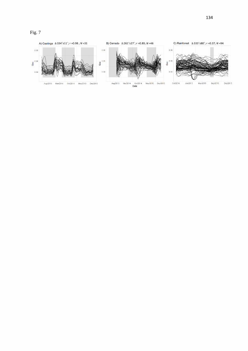
134

Fig. 7

135

Supplementary Material

LEAF PHENOLOGY CORRELATES TO GROSS PRIMARY PRODUCTIVITY: AN INTER-

COMPARISON ACROSS SEASONALLY CONTRASTING TROPICAL BIOMES

Bruna Alberton1*

, Andrew Richardson2,3

, Ricardo Torres4

, Humberto Rocha5

, Magna S. B. De

Moura6

, Leonor Patricia Cerdeira Morellato1

Figure S1 Original hemispherical images showing the single crowns manually selected within each one

of the vegetation sites. A - caatinga with 31 crowns ROIs selected; B - cerrado with 46 crowns ROIs

selected; and C -rainforest with 94 crowns ROIS selected in the image.

136

Figure S2 Circular histograms of leaf flushing onset for the years of study from the crowns ROIs

selected within the images of each site: a) caatinga; b) cerrado; and c) rainforest. The arrows point to

the mean angle or date (ᾱ) where most of the crows’ ROIs were considering flushing new leaves from

the visual inspection; the length of the arrow indicates the value of the r vector and represents the

synchronicity of the crowns ROIs leafing around the mean date. The r variable has no units and varies

from zero to one (when all the data are concentrated at the same direction or angle; see Methods for

details). N represents the number of crowns ROIs observed during visual inspection.

137

Figure S3 A sample of the original hemispherical images taken during wet (upper panels) and dry season

(below panels) for each vegetation site representing a different biome – A Caatinga – B Cerrado – C

Atlantic Rainforest.

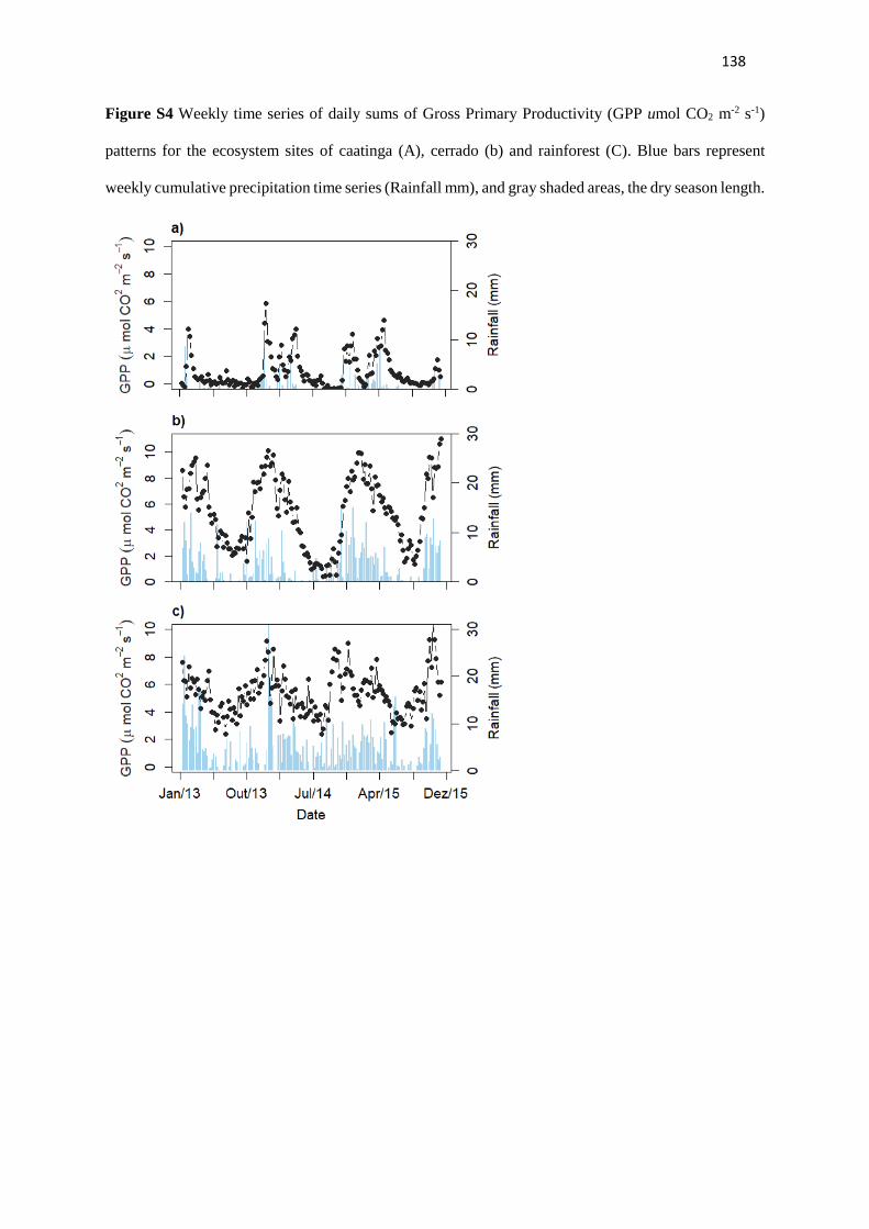
138

Figure S4 Weekly time series of daily sums of Gross Primary Productivity (GPP umol CO2 m-2 s-1)

patterns for the ecosystem sites of caatinga (A), cerrado (b) and rainforest (C). Blue bars represent

weekly cumulative precipitation time series (Rainfall mm), and gray shaded areas, the dry season length.

139

Figure S5 Temporal additive mixed models of the crowns ROIs daily Gcc time series from the caatinga

vegetation site.

140

Figure S6 Temporal additive mixed models of the crowns ROIs daily Gcc time series from the cerrado

vegetation site.

141

Figure S7 Temporal additive mixed models of the crowns ROIs daily Gcc time series from the rainforest

site.

142

Section 4

143

Here, I present the key results, developed during my doctoral thesis, related to the e-science

framework where my thesis was developed. Our studies were conducted in the context of the e-

phenology project (see Mariano et al., 2016) and were associated with the e-phenology phenocam

network.

First, the development of a phenological database was one of the first devised goals, due to the

need of organize the enormous bulk of information generated and aggregated to the e-phenology project.

The database was delineated in the context of the e-phenology network and it is the starting point of the

management of our high-volume imagery and ecological and phenological associated dataset (Mariano

et al. 2016). It integrates the ground-based direct phenological observations carried out in a long-term

monitoring program (Long-term Cerrado Phenology project –

http://www.recod.ic.unicamp.br/ephenology/) and the repeated daily imagery from the digital cameras.

It also includes site base information, sensor derived-data from the site´s weather stations and plant

ecological traits from individuals and species.

The automatization of data processing was also an important step to make analysis of thousands

of hundreds of images faster and to create a standard protocol of image processing. A Java interface,

called PhenoViewer (unpublished software), was created by the computer scientists team (J. Almeida

Jr and collaborators) and optimized by the user group according to the user’s feedbacks and tasks needed

along the last years. The image processing tool was developed with the purpose of pre-processing

(organization with unfolder and renaming tasks) and processing (vegetative indexes calculation) the

high volume of images of the e-phenology network.

The further steps relate to several analytical tool explored to the analyses of phenocam images.

The use of machine learning algorithms to plant species identification in the image data provides

important steps of image analysis, which is the automatic identification of each plant crown of the within

the vegetation image (Almeida et al., 2014). Through the years, several approaches have been proposed

to support the identification of individuals of particular species from phenocam imagery (Almeida et

al., 2014; Almeida et al., 2015, Almeida et al., 2016; Faria et al., 2016a; Faria et al., 2016b). Works

related to this task can be divided into two main groups: those based on the use of machine learning

fusion approaches, and those based on time series representations. Examples of initiatives of the first

144

group are the works of Almeida et al., (2014) and Faria et al., (2016a). Almeida et al., (2014), for

example, proposed an Adaboost-based framework for combining multiscale classifiers with the

objective of recognizing plant species within vegetation images. The other trend is focused on time

series representations (Almeida et al., 2016, Faria et al., 2016b). Almeida et al., (2016), for example,

proposed two different time-series-based visual rhythm representations to support plant species

identification. These representations are more efficient to be processed and yielded effective results in

plant species identification tasks. All those works use general-purpose color and texture descriptors to

represent image regions.

Regarding the visualization of phenological time-series, the PhenoVis, a visual analytics tool,

was developed to provide a more insightful way to deal with camera-derived phenological time-series.

Its application is based on the problematization of using average pixels values for the vegetation index

(e.g.: Gcc) calculated from a given Region of interest (ROI) in the image. Different images representing

distinct phenological stages of the vegetation may share the same average of Gcc values. In the work of

Leite et al., (2016), we introduced the Chronological Percentage Maps (CPMs), a visual mapping

technique that combines pixels derived distribution from all images of a given time period to create a

normalized stacked bar chart. Thus, the PhenoVis tool encompasses the CPMs, designed for a more

expressive representation of phenological time series combined with a color-coded information, and

supports comparative analysis of phenological data for multiple years with algorithms allowing search

for phenological patterns similarity and filters for specific time periods or regions.

List of published articles originated from the e-science collaborations described above:

ALMEIDA J., SANTOS, JA, ALBERTON, B., MORELLATO, L.P.C., TORRES, R.S. Phenological

visual rhythms: compact representations for fine-grained plant species Identification. Pattern

Recognition Letters, v. 81, p. 90-100, 2016. (APPENDIX B)

FARIA F. A., ALMEIDA, J., ALBERTON, B., MORELLATO, L.P.C., ROCHA, A., TORRES, R.S.

Time series-based classifier fusion for fine-grained plant species recognition. Pattern Recognition

Letters, v. 81, p. 101-109, 2016. (APPENDIX C)

145

FARIA F. A., ALMEIDA, J., ALBERTON, B., MORELLATO, L.P.C., TORRES, R.S. Fusion of

Time Series Representations for Plant Recognition in Phenology Studies. Pattern Recognition

Letters, v. 83, p. 205-214, 2016. (APPENDIX D)

LEITE, R.A., SCHNORR, L, ALMEIDA JR, TORRES, R.S., ALBERTON, B., MORELLATO, LPC,

COMBA, J. PhenoVis – Visual Phenological Analysis of Forest Ecosystems. Information Sciences,

v. 372, p. 181-195, 2016. (APPENDIX E)

ALMEIDA, J., PEDRONETTE, D., ALBERTON, B., MORELLATO, L.P.C., TORRES, R.S.

Unsupervised distance learning for plant species identification. JSTARS Journal of Selected Topics in

Applied Earth Observations and Remote Sensing, v. 9 (12), p. 5325-5338, 2016. (APPENDIX F)

146

CONCLUSIONS

In the present thesis, I intended to incorporate a novel approach as a consistent tool for the

monitoring of the vegetative phenology in tropical ecosystems. In the first section, I established a first-

step protocol with main guidelines for the camera system method and setup in the tropics. We

demonstrated that the establishment of phenocam networking is a powerful tool for biological

conservation through its capability of fine temporal resolution data associated with wide spatial

monitoring coverage. Besides, phenocams applications can bring new information for management and

restoration practices at several sites and environments and contribute for the education for conservation

and citizen science initiatives.

Next sections (2 and 3), I approached ecological questions to be tested applying repeated digital

photographs on tropical ecosystems. In section 2, leaf phenology derived by digital cameras were used

in an analytical procedure to unravel the main drivers influencing Gcc time series across seasonally dry

vegetations. Water and light were the most important predictors for the leaf phenological patterns across

the sites. Water-plant relationships were more important for the Caatinga community, and light, through

day-length seasonality, had more influence in the leafing patterns of the cerrado communities. An

interesting outcome was the increasing variability of phenological signals (leafing behaviors) and

predictor-response relationships (distinct smooth functions) across sites where seasonality was less

pronounced and/or distinct species life-form were capable of overcoming drought-effects, such as deep

root systems trees from woodland cerrado compared to grassy cerrado. Following this idea, section 3

has shown a novel approach to relate leaf phenology to seasonality of ecosystems productivity. The

phenological dynamics regarding the variability of species phenological signals, and how they are built

in into each contrasting vegetation communities explains drivers of leaf phenology and productivity.

Besides, the comparison of tropical biomes under different hydroclimatic conditions is essential to the

understanding of ecosystem functionality and access future responses to climate change.

The so-called near-surface remote phenology using digital cameras is an opportunity to obtain

an impartial and comparable assessment of leaf seasonal changes in tropical environments and has

becoming more and more common for phenological research. The arrivals of novel technologies

followed by the advance of e-science methods for dealing with large data sets are changing the scenario

147

of plant ecology studies, from species to ecosystems. Next challenges to be addressed are the continuity

of the e-phenology network and the spread of new cameras covering new vegetation types; and the

development of bottom-up studies, integrating on-the-ground observations, cameras, drones, and

satellites, inter-comparing them and placing camera-derived phenology in its own scale, by

understanding how much and what kind of information can be retrieved from ecosystems. I believe the

thesis innovates by providing original ecological research outcomes from an e-science perspective,

which led to a unique research profile for a young scientist.

148

REFERENCES

ALBERTON, B. et al. Using phenological cameras to track the green up in a cerrado savanna and its

on-the-ground validation. Ecological Informatics, v. 19, p. 62–70, 2014.

BALDOCCHI, D. D. et al. Predicting the onset of net carbon uptake by deciduous forest with soil

temperature and climate data: A synthesis of FLUXNET data. International Journal of

Biometereology, v. 49, p. 377-387, 2005.

CHAMBERS, L.E. et al. Phenological Changes in the Southern Hemisphere. Plos One, v. 8, p. 1-12,

2013.

CRIMMINS, M.A.; CRIMMINS, T.M. Monitoring plant phenology using digital repeat photography.

Environ. Manage, v. 41, p. 949–958, 2008.

FIELD, C.B. et al. Primary production of the biosphere: integrating terrestrial and oceanic

components. Science, v. 281, p. 237–240, 1998.

GRAHAM, E.A. et al. Public Internet-connected cameras used as a cross-continental ground-based

plant phenology monitoring system. Glob. Change Biol. v. 16, p. 3014–3023, 2010.

HEY, T.; HEY, J.e-Science and its implications for the library community. Libr.Hi Tech, v. 24, p.

515–528, 2006.

KEENAN, T. F. et al. Tracking forest phenology and seasonal physiology using digital repeat

photography: a critical assessment. Ecological Applications, v. 24(6), p. 1478-1489, 2014.

LOPES, A.P. et al. Leaf flush drives dry season green-up of the Central Amazon. Remote Sensing of

Environment, v. 182, p. 90–98, 2016.

MIGLIAVACCA, M. et al. Using digital repeat photography and eddy covariance data to model

grassland phenology and photosynthetic CO2 uptake. Agricultural and Forest Meteorology, v.

151(10), p. 1325–1337, 2011.

MARIANO, G., MORELLATO, LPC, ALMEIDA J. ALBERTON, B., CAMARGO, MGG; &

TORRES, RS. Modeling plant phenology database: blending near-surface remote phenology with on-

the-ground observations. Ecological Engineering, v. 91, p. 396-408, 2016.

MOORE, C.E. et al. Tree – grass phenology information improves light use efficiency modelling of

gross primary productivity for an Australian tropical savanna. Biogeosciences. v. 14, p. 111–129,

2017.

MORELLATO, L.P.C.; GRESSLER, E.; CAMARGO, M.G.G. A review of plant phenology in South

and Central America. In: M.D. Schwartz (ed.). Phenology: An Integrative Environmental Science,

Springer, New York, 91-113, 2013.

MORELLATO, L.P.C. et al. Linking plant phenology to conservation biology. Biological

Conservation,v. 195, p. 60–72, 2016.

MORISETTE, J.T. et al. Tracking the rhythm of the seasons in the face of global change:

phenological research in the 21st century. Front. Ecol. Environ. v. 7, p. 253-260, 2009.

149

NAGAI, S. et al. Usability of time-lapse digital camera images to detect characteristics of tree

phenology in a tropical rainforest. Ecological Informatics, v. 32, p. 91–106, 2016.

OMETTO, J.P.H.B. et al. Amazonia and the modern carbon cycle: Lessons learned. Oecologia, v.

143(4), p. 483–500, 2005.

POLGAR, C.A.; PRIMACK, R.B. Leaf-out phenology of temperate woody plants: From trees to

ecosystems. New Phytologist, v. 191(4), p. 926–941, 2011.

REICH, P.B. Phenology of tropical forests: patterns , causes , and consequences. Can. J. Bot. v. 73,

p. 164–174, 1995.

RESTREPO-COUPE, N. et al. What drives the seasonality of photosynthesis across the Amazon

basin? A cross-site analysis of eddy flux tower measurements from the Brasil flux network.

Agricultural and Forest Meteorology, v. 182–183, p.128–144, 2013.

RESTREPO-COUPE, N. et al. Do dynamic global vegetation models capture the seasonality of

carbon fluxes in the Amazon basin? A data-model intercomparison. Global Change Biology, v.

23(1), p.191–208, 2017.

RICHARDSON, A.D. et al. Influence of spring and autumn phenological transitions on forest

ecosystem productivity. Philosophical Transactions of the Royal Society B: Biological Sciences, v.

365(1555), p.3227–3246, 2010.

TOOMEY, M. et al. Greenness indices from digital cameras predict the timing and seasonal dynamics

of canopy-scale photosynthesis. Ecological Applications, v. 25(1), p.99–115, 2015.

WU, J. et al. Leaf development and demography explain photosynthetic seasonality in Amazon

evergreen forests. Science, v. 351(6276), p.972–976, 2016.

WU, J. et al. The phenology of leaf quality and its within-canopy variation is essential for accurate

modeling of photosynthesis in tropical evergreen forests, New Phytologist, p.1–14, 2017.

150

Appendix A

Article published in the Journal Biotropica:

CAMARGO, M.G.G. et al. Leafing patterns and leaf exchange strategies of a cerrado woody

community. Biotropica, v. 50 (3), p.442–454, 2018.

151

LRH: Camargo et al.

RRH: Leafing Patterns of a Cerrado Community

Leafing patterns and leaf exchange strategies of a cerrado woody community

Maria Gabriela Gutierrez de Camargo1, Gustavo Henrique de Carvalho1, Bruna de Costa

Alberton1,2,4, Paula Reys1, 3, Leonor Patrícia Cerdeira Morellato1

1. UNESP — Universidade Estadual Paulista, Instituto de Biociências, Departamento de

Botânica, Laboratório de Fenologia, Rio Claro, São Paulo, Brasil; 2. UNESP —

Universidade Estadual Paulista, Instituto de Biociências, Programa de Pós-graduação em

Ecologia e Biodiversidade, Rio Claro, São Paulo, Brasil; 3. Universidade de Rio Verde,

Campus I, Rio Verde, Goiás, Brasil; 4. brualberton@gmail.com

152

ABSTRACT

The deciduousness of tropical trees and communities depend on ecosystems characteristics

such as plant species diversity, and strength of the dry season. Based on seven-years of

phenological observations we provide the first long-term description of leafing patterns of a

woody cerrado community, aiming to investigate: (i) the leaf exchange strategies considering

the inter-annual variation on the degree of deciduousness of individuals and species and

quantify the community deciduousness; (ii) the relationship between inter-annual patterns of

leaf fall and leaf flush according to the species` leaf exchange strategies and climate; (iii) the

onset of cerrado growing season and its relation to climate seasonality. To detect seasonality

and leafing onset we applied circular statistics and to understand the relationships between

environmental predictors and leaf exchange strategies, we used generalized additive models.

From 106 species observed, we classified 69 as deciduous (26 species), semi-deciduous (25)

or evergreen (18) and defined the studied cerrado as a semi-deciduous vegetation. Leaf

phenology was markedly seasonal, and similar among years. Leaf fall peaked in the dry

season, and leaf flush in the dry-to-wet transition. Leaf fall patterns related to temperature

and leaf flush to day length and rainfall. Semi-deciduous and deciduous species were more

constrained by climate then the evergreen ones. The cerrado growing season started in the

dry-to-wet season transition. Inter-annual variations in rainfall and temperature affected the

individuals’ and, consequently, species’ degree of deciduousness, highlighting individual and

species variability, and suggesting that cerrado leafing patterns is likely susceptible to future

climate change scenarios.

Key-words: climatic drivers; deciduous; evergreen; generalized additive models; growing

season; leaf phenology; savanna; seasonality; semi-deciduous.

RESUMO

153

A deciduidade das árvores e comunidades tropicais depende de características do ecossistema

como a diversidade de espécies de plantas e a intensidade da estação seca. Baseados em sete

anos de observações fenológicas, apresentamos uma descrição de longo prazo de padrões

vegetativos de uma comunidade lenhosa de cerrado com o objetivo de investigar: (i) as

estratégias de trocas foliares considerando a variação interanual no grau de deciduidade dos

indivíduos e espécies e quantificar a deciduidade da comunidade; (ii) as relações entre

padrões interanuais de queda e brotamento foliar conforme a estratégia de trocas foliares das

espécies e o clima; (iii) o início da estação de crescimento da comunidade de cerrado

estudada e sua relação com a sazonalidade climática. Utilizamos estatística circular para

analisar a sazonalidade fenológica e o início do brotamento foliar na comunidade, e modelos

aditivos generalizados para entender as relações entre variáveis ambientais e as estratégias de

trocas foliares. Dentre as 106 espécies observadas, 69 foram classificadas como decíduas (26

espécies), semi-decíduas (25) ou sempre-verdes (18) e definimos o cerrado estudado como

uma vegetação semi-decídua. A fenologia vegetativa foi marcadamente sazonal e similar

entre anos. O pico de queda foliar ocorreu na estação seca e o de brotamento na transição

entre as estações seca e chuvosa. O padrão de queda de folhas foi relacionado à temperatura e

o de brotamento ao comprimento do dia e pluviosidade. As espécies decíduas e semi-

decíduas foram mais afetadas pelo clima do que as sempre-verdes. A estação de crescimento

no cerrado começou na transição entre as estações seca e úmida. As variações interanuais na

precipitação e temperatura afetaram o grau de deciduidade de indivíduos e consequentemente

das espécies, ressaltando a alta variabilidade individual e específica, sugerindo que os

padrões de troca foliar das espécies do cerrado podem ser afetados por mudanças climáticas

futuras.

DECIDUOUSNESS, DEFINED AS EITHER A PARTIAL OR A FULL LOSS OF LEAVES, IS A KEY

FUNCTIONAL trait dependent on ecosystems characteristics such as soils and species diversity,

154

essential for estimating dry season length and intensity in tropical ecosystems (Condit et al.

2000). Leaf development and senescence, as well as leaf exchange strategies of plant species,

are recognized to have important effects at the ecosystem scale because they are linked to a

range of processes, including carbon uptake, water and energy fluxes, resource availability,

and nutrient cycling (Reich 1995, Lavorel et al. 2007, Polgar & Primack 2011, Richardson et

al. 2013). Additionally, the degree of deciduousness of a community is an indicator of shifts

in the intensity and timing of species activities due to inter-annual shifts in the weather, for

instance, leaf loss can be more intense during severe dry seasons (Reich 1995, Condit et al.

2000, Williams et al. 1997). Since savannas are the world’s second most important type of

vegetation, contributing to carbon flux and storage (Archibald & Scholes 2007), studies of

the vegetative phenology in these ecosystems have a global reach.

The Brazilian Cerrado, a neotropical savanna, is the second largest vegetation type in

the Brazilian territory and presents a gradient of physiognomies, ranging from grasslands to

tall woodlands (Overbeck et al. 2015, Durigan & Ratter 2016, Coutinho 2006). The cerrado

harbors the world’s highest woody plant diversity among savannas (Ratter et al. 1996,

Sarmiento 1984, Munhoz & Felfili 2006), and is generally under a seasonal climate with

well-defined wet and dry seasons (Ratter et al. 1996). The seasonal climate is known to

influence the phenology of plant populations and communities (Monasterio & Sarmiento

1976, Morellato et al. 2013, 2016). To reduce transpiration and avoid plant collapse related to

water status, plants subjected to seasonal climates tend to lose their leaves during the dry

season, facilitating the re-hydration process for the growing season (Reich & Borchert 1984,

Franco et al. 2005). Most cerrado trees produce new leaves and flowers at the end of the dry

season, just before the start of the raining season, indicating that individuals have access to

water at greater depth to permit their maintenance even when rainfall is low (Monasterio &

Sarmiento 1976, Williams et al. 1997, Jackson et al. 1999, Batalha & Mantovani 2000,

155

Batalha & Martins 2004, Lenza & Klink 2006, Tannus et al. 2006, Pirani et al. 2009).

Few studies have addressed leaf exchange patterns in cerrado communities (Miranda

1995, Munhoz & Felfili 2005, Lenza & Klink 2006, Alberton et al. 2014, Pirani et al. 2009).

Most of them either focused on reproductive phenophases or in describing general aspects of

the community phenology, providing only inferences about the relationship between leafing

patterns and environmental cues (e.g. Mantovani & Martins 1988, Batalha et al. 1997,

Batalha & Mantovani 2000, Batalha & Martins 2004, Damascos et al. 2005, Tannus et al.

2006, Bulhão & Figueiredo 2002, Dalmolin et al. 2015). Others, however, have found

negative correlations between leaf fall and precipitation (Munhoz & Felfili 2005, Pirani et al.

2009). The investigation of vegetative phenology, its causes, and the quantification of leaf

exchange strategies at a community level in the cerrado are, thus, still missing. In addition,

leaf exchange strategies in communities are mainly defined based on the leafing patterns of

few species and in short-term phenological observations (Franco et al. 2005, Lenza & Klink

2006), which may include bias related to some punctual plant response to local weather

conditions. Therefore, the use of long-term phenology leafing data series is essential to the

definition of the species’ leaf exchange strategies.

Here, we describe, for the first time, the seven-year long leaf phenology of a cerrado

community, aiming to (i) identify the leaf exchange strategies considering the inter-annual

variation in the degree of deciduousness of individuals and species and quantify the

community deciduousness; (ii) investigate the relationship between inter-annual patterns of

leaf fall and leaf flush according to the species` leaf exchange strategies and the climate

conditions; (iii) uncover the onset of the cerrado growing season and the relation to climate

seasonality.

We expect to find a dominance of leaf-exchange species (deciduous and semi-

deciduous) and a higher deciduousness degree over years due to the length and severity of

156

the dry season (Reich & Borchert 1984, Franco et al. 2005, Reich 1995, Condit et al. 2000,

Williams et al. 1997). Based on few short-term phenology studies describing leaf exchange

strategies of woody cerrado species (Alberton et al. 2014, Pirani et al. 2009, Lenza & Klink

2006), we expected leaf fall during the dry season and leaf flush peaking in the transition

between dry and wet seasons, defining the onset of the growing season. We also expected

rainfall and day length as the main environmental factors related to leafing seasonality, as

previously suggested for tropical seasonal vegetations (Condit et al. 2000, Borchert & Rivera

2001).

METHODS

STUDY SITE — We developed our study in an area of woody cerrado in the municipality of

Itirapina, São Paulo state, Southeastern Brazil (22°10′31″S; 47°52′26″W). The study site is

located 770 m above sea level and covers an area of 260 ha. The climate is characterized by

two markedly regular seasons: a dry (winter) season from April to September and a wet

(summer) season from October to March (Fig. 1). Average annual total rainfall was 1524 mm

and the mean annual temperature was 20.7 °C between 1972 and 2011 (Camargo et al. 2011).

The vegetation is a woody savanna classified as a cerrado sensu stricto (Coutinho 1978), with

a discontinuous woody layer reaching 6 to 8 m high and a continuous herbaceous stratum. A

woody species survey in the area indicated that Myrtaceae, Fabaceae, and Malpighiaceae are

the richest families and Bauhinia rufa, Xylopia aromatica, Miconia rubiginosa, Virola

sebifera, and Myrcia guianensis the most abundant species (Reys et al. 2013).

PHENOLOGICAL DATA — To describe and analyze woody species leafing patterns we used a

phenological dataset of monthly surveys conducted from January 2005 to December 2011.

During this period, we directly observed leaf fall and leaf flush (following Morellato et al.

1989) in 2112 marked individuals with at least 30 cm of stem circumference on the ground

157

level, sampled over 36 transects (25 m x 2 m) (see Reys et al. 2013, Vogado et al. 2016). We

took circumference and height measurements of all individuals sampled.

To estimate leaf fall and leaf flush phenophases, we monthly recorded the

phenological activity of each individual in a qualitative binary scale, with “0” indicating

absence of the phenophase and “1” the phenophase presence. We also estimated the intensity

of leaf fall and flush based on a semi-quantitative scale with three classes in which “0”

indicates the absence of a phenophase, “1” indicates the presence of a phenophase with low

to intermediate intensity (up to 50% of the crown flushing new leaves or of the crown with no

leaves or senescent leaves) and “2” the presence of a phenophase with high intensity (more

than 50% of the crown flushing new leaves or with senescent leaves) (Opler et al. 1980,

Morellato et al. 2000, Vogado et al. 2016). Despite the use of a monthly frequency of

observations to record and classify the leaf exchange strategies in this study, it is unlikely that

we have missed the occurrence of the total absence of leaves in an individual (a 100%

deciduous event, see below) or a leaf fall increase from one month to another that, of course,

we could also infer from the coverage of newly emerged leaves. We recorded for all years of

observations when individuals were totally leafless (100% of leaf fall). The definition of

100% fall category also helped us to define the occurrence of leaf flush, since sometimes one

month of leaf fall was followed by new young leaves on the subsequent month. From March

2007 to December 2008, we did not score leafing intensity; we only recorded phenological

activity using the qualitative scale. The qualitative and semi-quantitative individual

observations were independently collected and provide complementary information which

improve the analyses of phenological patterns (Bencke & Morellato 2002).

To calculate the intensity index, we adapted the Fournier index (Fournier 1974),

considering “2” as the class of maximum intensity (Vogado et al. 2016). We choose to use

only three intensity classes instead of five, as suggested by Fournier (1974), and commonly

158

used in tropical plant phenology, to facilitate the definition of phenological changes at

monthly intervals.

LEAF EXCHANGE STRATEGIES AND THE DEGREE OF DECIDUOUSNESS — We classified

the individual and species leaf exchange strategy for each of the five years we scored leaf fall

intensity (2005, 2006, 2009 to 2011). For each individual, we classified as deciduous the

individual recorded with no leaves (100% leaf fall) in at least one month, in a year. We

classified as semi-deciduous the individual recorded with more than half of the branches

without leaves (intensity score “2”) in at least one month in a year. Finally, we classified as

evergreen the individual observed with up to half of the branches without leaves (“0” or “1”

intensity score) throughout a given year. To estimate de degree of deciduousness, we

calculated the proportion of deciduous, semi-deciduous and evergreen individuals in the

community in each of the five years we evaluated leaf fall intensity.

We classified all species with more than five individuals sampled as deciduous, semi-

deciduous, or evergreen based on the above individual’s annual leaf exchange strategies. A

species was classified as deciduous if more than half of all individuals sampled were

classified as deciduous in at least one of the five years; semi-deciduous if more than half of

all individuals were classified as semi-deciduous in at least one of the five years; and as

evergreen all the remaining species.

DATA ANALYSES — Since we scored the intensity of phenology using an ordinal scale

ranging from 0 to 2, we applied ordinal multinomial regressions to assess the drivers of leaf

fall and flush. We fitted two models (leaf fall and flush) for species grouped according with

leaf exchange strategies, analyzing the number of individuals with 0, 1, 2, and 100% of leaf

fall intensities and and 0, 1, and 2 of leaf flush intensities. We also fitted multinomial models

159

for the whole community, regardless of leaf strategies. All models had monthly rainfall, mean

temperature, monthly day length difference (longest minus shortest day within the month),

and an interaction between rainfall and temperature as predictors. Monthly rainfall,

maximum, mean, and minimum temperatures for the study period (January 2005 to

December 2011) were obtained from the climatic station at Estação Climatológica do Centro

de Recursos Hídricos e Ecologia Aplicada (CRHEA – Universidade de São Paulo), 4 km

from the study site. We used day length data for the latitude -22°17’S; -47°87’W (maptools

package for R).

To better understand the nature of the relationships between predictors and leaf

exchange strategies, we further fitted generalized additive models (GAM) using intensity

data. These models allowed us to identify threshold regions in environmental variables and

long-term trends for leaf fall (number of individuals with 100% leaf fall) and presenting leaf

flushing. We fitted all additive models with a correlation structure based on years. We

evaluated the ordinal models by looking at the significance of each variable and the

generalized additive models with R2 and variable significance. We carried out all analyses in

R (R Core Team 2017) using base packages ordinal (Christensen 2016) for the ordinal

regressions and mgcv (Wood 2011) for the generalized additive models.

Considering that recurrent temporal events, such as phenological data, are circular in

nature, with no true starting point (Zar 1999), to infer the beginning of the growing season,

we applied circular statistics to the individuals’ onset month of leaf flush following Morellato

et al. (2000, 2010). To do that, first we define the start of leafing season of each individual

and year as the first month we recorded leaf flush in each year. Then we divided the 360o of a

circumference by 12 and each month of the year is represented by a range of 30o starting on

January (mid point 15o, see Morellato et al. 2010, for details). Then we calculate the angle or

date (month) correspondent to the most frequent leaf flush onset (circular mode), the mean

160

angle or onset date (the mean angle or mean onset data of the frequency distribution of

individuals around the circle). Finally, we tested whether the mean onset data are

significantly concentrated around the mean angle or date, as a proxy of seasonality by

applying the Rayleigh test (Z) as suggested by Morellato et al. 2000, 2010. If the mean onset

data is significantly concentrated around the mean angle or date, we consider the leafing

pattern seasonal and the degree of synchrony or seasonality is represented by the length of the

vector r. The vector r has no unity and ranges from 0 (no seasonality or synchronicity) to 1

(perfect seasonal or synchronous),(Morellato et al. 2010). We performed circular analyses per

study year, for all the community, and by leaf exchange strategies using Oriana 4.0 (Kovach

Computing Services).

RESULTS

We sampled 2112 individuals and 106 species (Table S1). Over the seven years of

observations, some individuals died or were lost, leading to the final sample of 1651

individuals and 102 species. The community phenological patterns were described based on

the total number of individuals observed per month, in each year.

Out of the 106 species initially surveyed, 69 species presented more than five

individuals and were classified as deciduous (26 species; total basal area= 1.46 m2), semi-

deciduous (25 species; total basal area= 6.10 m2) and evergreen (18 species; total basal area=

2.29 m2) (Fig. 2; Table S1). Species and individual’s degree of deciduousness varied among

years (Fig. 2). Only five species presented the same deciduousness degree over the five years:

Jacaranda caroba, which reached deciduity in all the years (most of individuals with no

leaves or 100% leaf fall) and, Anadenanthera peregrina var. falcata, Byrsonima

coccolobifolia, Campomanesia pubescens and Dalbergia miscolobium, which reached semi-

deciduity in all the years (most individuals lose more than half of their leaves). Individuals

161

and consequently, the species, rarely lose all their leaves, maintaining at least half of the

leaves in most of the years (Fig. 2). We observed the lowest deciduousness degree in the

community in 2005 and the highest one in 2010, (Fig. 2). The number of deciduous

individuals responded to both: mean temperature and total rainfall when intra and inter-

annual seasonality components were considered (R2=0.70; P<0,01).

Leafing patterns were seasonal and similar among years and within leaf exchange

strategies (Fig. 3 and 4). Leaf fall predominated in the dry season, peaking in July (Fig. 3),

while leaf flush was concentrated in the transition between dry to wet seasons, peaking in

September (Fig. 4). We observed an unexpected increase of leaf fall on December 2009 and,

on 2010 mainly in the middle of the wet season, related to a larger number of individuals

losing leaves but at a low intensity (Fig. 3).

Leafing patterns according to the leaf exchange strategies were similar among years,

overlapping during the periods of higher activity and intensity in the community (Fig. 3 and

4). Deciduous species presented a seasonal leaf exchange patterns highly constricted to the

one period of the year, concurrent with the highest phenological activity and intensity in the

community (Fig. 3 and 4). During the peaks of leaf fall and leaf flush in the community,

deciduous species presented the highest synchrony among individuals and phenophases

intensity followed by semi-deciduous and evergreen species. Conversely, semi-deciduous,

and mainly evergreen species, presented more individual's activity outwith the community

peaks of leaf exchange (Fig. 3 and 4).

In general, for both phenophases, leaf fall and flush, the effects of abiotic variables

increased from evergreen to deciduous species (Table 1). The exceptions were the influence

of the day length difference on the leaf fall, almost the same for all leaf exchange strategies;

and the rainfall on the leaf flush, similar between evergreen and semi-deciduous species, but

higher for deciduous species (Table 1). Leaf fall patterns of all strategies were negatively

162

related to the rainfall and temperature, and positively related to the day length difference

(Table 1). The strongest relations were among leaf fall and temperature and temperature-

rainfall interaction (Table 1).

When analyzing the variables separately with generalized additive models, we

confirm a higher climatic influence and seasonality in the deciduity of semi and, mainly,

deciduous species (Fig.5). All leaf fall models had high coefficients of determination

(evergreen R2 = 0.53; semi-deciduous R2 = 0.70; deciduous R2 = 0.77). Similarly, all variables

but rainfall in the evergreen model presented a significant nonlinear effect on leaf fall. A

higher proportion of individuals lost leaves when the rainfall was around 50 mm, the

temperature between 16 and 19oC and the day length between 11 and 11.5 h (Fig. 5), which

corresponds to the dry season conditions (see Fig. 1). Individuals deciduity decreased when

precipitation was around 100 mm, the temperature 22oC and the day length 12 h (Fig. 5),

corresponding to the transition from dry to wet seasons.

Leaf flush patterns were positively related to the day length difference, but also to the

rainfall, and negatively related to the temperature (Table 1). Even with a stronger effect of

abiotic variables on deciduous and semi-deciduous species (Table 1), when analyzed

separately with generalized additive models, individuals of species with different leaf

exchange strategies responded in a similar way to the environmental variables, showing

seasonality over the 7 y of observations. Leaf flush for all strategies responded non-linearly

to the abiotic variables (evergreen R2 = 0.55; semi-deciduous R2 = 0.56; deciduous R2 = 0.62;

Fig. 6). We observed the first increase in leaf flush activity when precipitation was around

100 mm, and the day length about 11.5 h, in the transition from dry to wet season. The

proportion of individuals flushing peaked at around 200 mm, 19oC and a day length close to

12 h (Fig. 6), which corresponds, to the middle of the wet season, when the differences in the

amount of sunlight are highest (see Fig. 1). Particularly, rainy months (> 300mm) also seem

163

to trigger flushing, although months with such amounts of accumulated rain are rare (Fig.

6A).

We determined the leaf flush onset for half of the individuals observed (Table 2), with

no evident onset for all remaining trees. The community growing season started in early

September in four out the seven years and otherwise in late August, with the mean angle

between 20 August and 10 September (Table 2). When analyzed by leaf exchange strategy,

the beginning of the growing season was observed mainly on September for deciduous

species and between August and September for semi-deciduous and evergreen species (Table

S2). Individuals synchronicity or concentration around the mean onset date were higher for

deciduous species, with r vector around 0.82, followed by semi-deciduous and evergreen

species, with the length of vector r around 0.69 and 0.62, respectively (Table S2).

DISCUSSION

Cerrado is the most species-rich savanna in the world and second largest Brazilian

vegetation type, after Amazonia (Overbeck et al. 2015, Durigan & Ratter 2016, Coutinho

2006). However, the studies investigating cerrado seasonal patterns are still sparse,

representing less than 10% of the phenological studies surveyed for neotropical region

(Mendoza et al. 2017), and less than half of those include leafing phenology (Morellato et al.

2013, unpublished data). Based on our unique seven-year phenological data we showed the

predominance of deciduous and semi-deciduous leaf exchange strategies and established the

woody cerrado as an overall seasonal, semi-deciduous vegetation. The individual's degree of

deciduousness was highly explained by the climate conditions, with individuals rarely

reaching the full deciduity. The cerrado leaf exchanging patterns were consistently seasonal

and similar among the years, confirming the expected seasonality described by short-term

studies on savannas and other tropical seasonal vegetation (Miranda 1995, Williams et al.

164

1999, Munhoz & Felfili 2005, Lenza & Klink 2006, Pirani et al. 2009). Leaf fall and flush of

cerrado species were related to all abiotic variables, but mainly to temperature and day length

difference, and semi-deciduous and deciduous species were the most constrained by the

climate. The onset of the community growing season, here defined based on a subset of the

species, started in the transition from dry to wet season (August-September), and it is

sustained by the overall larger number of individuals putting out new leaves at this time in the

community.

In the cerrado community studied, the predominance of deciduous or semi-deciduous

species (74%), in relation to the evergreen ones (26%), was related to the climate seasonality

with a marked dry season, and has also been associated to soil properties and species’ leaf-

economy strategies (Franco et al. 2005, Souza, Franco, et al. 2015). Studies in cerrado sensu

stricto sites in Brazil Central, also found a high proportion of deciduous and semi-deciduous

woody species (Rossatto et al. 2009, Pirani et al. 2009), while in West African and Australian

savannas the strategies are more evenly distributed in the community (Eamus & Prior 2001).

Semi-deciduous species predominate in Australia, and evergreen and semi-deciduous species

in West Africa, (Williams et al. 1997, De Bie et al. 1998). Different definitions have been

used to classify leaf exchange strategies, constraining the comparisons regarding to the

amount of deciduity of cerrado savanna and other seasonal dry vegetation (e.g. Reich 1995,

Eamus & Prior 2001). A common definition brings deciduous, brevi-deciduous (differing in

the length of total leafless period) and evergreen with short or long leaf flush strategies or low

or no deciduity (Williams et al. 1997, Franco et al. 2005, Lenza & Klink 2006), but their

analyses are usually performed contrasting deciduous and evergreens. Reich (1995) propose

deciduous with synchronous leaf flush, deciduous with asynchronous leaf flush and

evergreens. We chose the large accepted, more inclusive, deciduous class including both,

brevi- and deciduous species, all losing all leaves or 100% regardless the length of leafless

165

phase and leaf flushing at the end of dry season; a semi-deciduous strategy that implies in the

loss of a representative amount of leaves, never above a 50% canopy cover, and evergreens

that retain all or almost all leaves year round (Eamus and Prior 2001). That choice facilitates

our comparisons and fit well to our monthly direct observations (see also Williams et al.

1997).

Here we demonstrated, based on our long-term phenology data, that independently of

the leaf exchange strategy, individuals and, consequently, species’ deciduousness degree vary

among years according to the climate conditions, mostly the inter-annual rainfall variability.

That variability is expected for seasonally dry forest and savannas (Reich 1995, Eamus &

Prior 2001, Goldstein et al. 2008), but has never been demonstrated for tropical savannas

based on individual long-term leaf exchange patterns. Therefore, it is necessary exercise

caution when classification of species leaf exchange strategies is derived from short-term

observation of vegetative phenology, since it can be underestimated whether the survey is

conducted in a “wet” year. Considering the number of leaf exchangers species, their basal

area and on the fact that individuals’ deciduousness degrees rarely reached100% leaf fall, we

classified the studied cerrado community as a semi-deciduous vegetation and that assumption

might apply for general cerrado woodlands (cerrado sensu stricto).

The consistent seasonal leafing patterns observed over seven years for the studied

cerrado community substantiated the patterns described for other cerrado vegetation based on

short-term observations, with leaf fall largely in the middle of the dry season and the leaf

flush in the transition from dry to wet season, beginning at the end of dry season, after the

first shower rains, but before the period of high rainfall intensity (Lenza & Klink 2006,

Rossatto et al. 2009, Silvério & Lenza 2010, Alberton et al. 2014, Pirani et al. 2009). This

leafing pattern is also found for the Australian savannas (Prior et al. 2004, Williams et al.

1997). The observed peak of leaf fall in the dry season is expected for seasonally dry

166

vegetations and species, since it is a strategy to improve water use and avoid water losses by

transpiration (Monasterio & Sarmiento 1976, Reich & Borchert 1984, Reich 1995, Pedroni et

al. 2002, Lenza & Klink 2006, Goldstein et al. 2008). Other effects acting as drivers of leaf

fall such as seasonal dust accumulation and herbivory, were not assessed in this study.

Despite this being a less explores topic, a few studies investigated the effects of biomass

harvesting by leaf-cutter ants, showing partial or total defoliation in some cerrado’s plant

species (Costa et al. 2008, Mundim et al. 2012). Also, the damage by insects was also more

intense in young leaves during the late dry season, corresponding to the main period of leaf

flushing in the cerrado (Marquis et al. 2001). Therefore, herbivory might change leaves

exchanges patterns by accelerating leaf aging due to damage or reducing photosynthetic

activity. Moreover, insect-related damage and parasitism have negative effects on plant

reproduction (Marquis et al. 2002, Franco 1998), factors that could lead to changes on

cerrado phenological dynamics.

The peak of leaf flush preceding the start of the rainy season, observed in cerrado

woody plants, is still an intriguing pattern. The predominance of species flushing at the end

of the dry season supports the hypothesis that cerrado trees have constant access to the water

in the soil due to the deep root system of most species, and that the preceding leaf fall

contributes to rehydration and the early production of new leaves (Goldstein et al. 2008,

Eamus & Prior 2001). The positive correlations with the rainfall and day length difference

may indicate the favorable conditions in the transition season to the production of cerrado

new leaves. Day length difference was the main factor positively predicting the leaf flushing

pattern of cerrado, mainly for deciduous species, and explains the certainty of the leafing

season. For tropical seasonal dry vegetation, day length is suggested as the main trigger for

leaf flush, independently of the leaf exchange strategy (Borchert 2000, Borchert & Rivera

2001, Rivera et al. 2002, Higgins et al. 2011, Rossatto et al. 2013, but see Reich 1995,

167

Goldstein et al. 2008). Flushing before the more intense rainfall can also avoid loss of

nutrient by leaching during the leaf development and favor nutrient uptake before the rainy

season, the flowering and fruiting time of many species, due to the high luminance and

photosynthetic activity of emerging new leaves (Rossatto et al. 2009, Sarmiento et al. 1985).

Deciduous species presented leaf fall mostly constrained to the middle of the dry

season and leaf flush to the transition between dry to wet seasons. Although semi-deciduous

and evergreen species also presented a seasonal leafing pattern, some individuals showed leaf

exchange activity out of these periods. These results agree with the individual’s response to

abiotic variables, since we found a gradual response from deciduous to evergreen species,

with evergreens significantly, but less constrained, by the climate and day length difference,

mainly for leaf fall. Leaf fall restricted to the dry season has been described for several short-

term savanna studies (e.g. Lenza & Klink 2006, Williams et al. 1997, Pirani et al. 2009).

Rossatto et al. (2013) also observed a coincident leaf flush onset in cerrado species, but with

an extended leaf flush into the wet season for cerrado evergreen species. At some savannas,

the evergreen species seem to have a more diversified leaf exchange strategy, some flushing

new leaves all year long while others concentrating the leaf production in the dry-to-wet

season transition (Reich 1995, Franco et al. 2005).

Independent of the leaf strategy, if we simulate the GAM analyses with abiotic

variables constant over time, the cerrado leafing pattern is still seasonal (Fig. 5 D and 6 D).

This resilient seasonal pattern in addition to the high correlation with all the abiotic variables,

makes it hard to establish the triggers and constraints of vegetative patterns in cerrado, as for

other savanna communities (Higgins et al. 2011). Some authors suggest that the

predominance of woody deciduous or semi-deciduous species, that seasonally change

completely or partially their leaves, is an adaptation to the seasonal water restrictions, not

directly related to the rainfall but also to the soil water availability and air humidity (Borchert

168

1994a, 1994b, Reich 1995, Eamus and Prior 2001, Franco et al. 2005a). Apart from abiotic

factors, the cerrado woody species leafing patterns have been related to herbivory avoidance

strategies and plant physiology, according to the different leaf exchange strategies or for

aluminum accumulating or non-accumulating species (Franco et al. 2005, Borges & Prado

2014, Souza et al. 2015b).

We defined the community growing season onset as the dry to wet season, transition

(August-September). This finding was based on a subset of the community’ species showing

a well-defined rest season and flushing onset, but also in the overall community significant

seasonality and, increase of leaf flushing on early September. The observed decrease in the

leaf fall activity, mainly for deciduous and semi-deciduous species, and the peak of leaf flush

activity, for all strategies, when the climatic conditions corresponds to the dry-to-wet season

transition also indicates the end of the cerrado resting season and start of the growing season

(Table 1; Fig. 5). The absence of a marked resting season for half of the species was related

to the fact that, even for deciduous species, individuals rarely lose all their leaves (100% leaf

fall), and that leaf fall, for some semi-deciduous and mainly evergreen species, is observed in

small intensities all year long. Another point is that, the absence of a community wide, well-

defined leaf flush onset for all species is not expected for tropical communities, due to the

high diversity of species and phenological patterns (Morellato et al. 2013, 2016), even for

seasonal dry vegetations. Alberton et al. (2014), working with digital cameras daily repeated

photographs or near surface phenology at the same cerrado site, detected an identical timing

of the growing season as revealed in the present study. Their cross-validation with the direct

monthly observations rules out any inherent subjectivity of our leaf exchange direct

observations.

The predominance of a distinct leaf flushing season was demonstrated for some

seasonal dry vegetations around the world, the marked dry seasons favoring fast response,

169

opportunistic species flushing new leaves at the end of dry season, after the first rains (Vico

et al. 2015). We argue that cerrado could integrate the ecohydrological framework proposed

by Vico et al. (2015) for seasonally dry ecosystems. Considering the interannual variability in

the degree of deciduousness of cerrado individuals and, consequently species over this 7y

study, the importance of temperature and rainfall as drivers of leaf fall and flush, and the

similarity to other seasonally dry ecosystems, the cerrado leaf exchange phenology is likely

susceptible to future climate changes scenarios of raising temperature and reduced rainfall

(Vico et al. 2015, Reich 1995, Eamus & Prior 2001, IPCC 2004).

ACKNOWLEDGMENTS

We thank the owners of Fazenda São José and the Instituto Arruda Botelho (IAB) for

allowing us to conduct field work at the farm. We also thank all the former and actual

members of Phenology Laboratory for their invaluable contribution to phenological data

collection in the field and for the many fruitful discussions. Our research was supported by

São Paulo Research Foundation (FAPESP) grants #2007/59779-6; FAPESP-Microsoft

Research #2013/50155-0 and #2010/52113-5; FAPESP-VALE-FAPEMIG #2010/51307-0

and #2009/54208-6. LPCM holds a research productivity fellowship from CNPq (National

Council for Scientific and Technological Development). BA (#2014/00215-0 and

#2016/01413-5), MGGC (#2010/01762-3 and #2015/10754-8) and GHC (#2015/14292-9)

receive fellowships from FAPESP.

Data Availability: The data used in this study are archived at the Dryad Digital Repository

LITERATURE CITED

ALBERTON, B., J. ALMEIDA, R. HELM, R. S. TORRES, A. MENZEL, and L. P. C. MORELLATO.

2014. Using phenological cameras to track the green up in a cerrado savanna and its on-

170

the-ground validation. Ecol. Inform. 19: 62–70.

ARCHIBALD, S., and R. J. SCHOLES. 2007. Leaf green-up in a semi-arid African savanna–

separating tree and grass responses to environmental cues. J. Veg. Sci. 18: 583–594.

BALDOCCHI, D., E. FALGE, L. GU, R. OLSON, D. HOLLINGER, S. RUNNING, P. ANTHONI, C.

BERNHOFER, K. DAVIS, and R. EVANS. 2001. FLUXNET: A new tool to study the

temporal and spatial variability of ecosystem–scale carbon dioxide, water vapor, and

energy flux densities. Bull. Am. Meteorol. Soc. 82: 2415–2434.

BATALHA, M. A., S. ARAGAKI, and W. MANTOVANI. 1997. Phenological variations ofthe

cerrado species in Emas - Pirassununga, SP. Acta Bot. Bras 11: 61–78.

BATALHA, M. A., and W. MANTOVANI. 2000. Reproducive phenological patterns of cerrado

plant species at the Pé-De-Gigante Reserve (Santa Rita Do Passa Quatro, SP, Brazil): a

comparision between the herbaceous and woody floras. Rev. Bras. Biol. 60: 129–145.

BATALHA, M. A., and F. R. MARTINS. 2004. Reproductive phenology of the cerrado plant

community in Emas National Park (Central Brazil). Aust. J. Bot. 52: 149–161.

BENCKE, C. S. C., and L. P. C. MORELLATO. 2002. Comparison of two methods of plant

phenology estimation, their interpretation and representation. Rev. Bras. Botânica 25:

269–275.

DE BIE, S., P. KETNER, M. PAASSE, and C. GEERLING. 1998. Woody plant phenology in the

West Africa savanna. J. Biogeogr. 25: 883–900.

BORCHERT, R. 2000. Organismic and environmental controls of bud growth in tropical trees.

Garden 87–108.

BORCHERT, R., and G. RIVERA. 2001. Photoperiodic control of seasonal development and

dormancy in tropical stem-succulent trees. Tree Physiol. 21: 213–221.

BORGES, M. P., and C. H. B. A. PRADO. 2014. Relationships between leaf deciduousness and

flowering traits of woody species in the Brazilian neotropical savanna. Flora Morphol.

171

Distrib. Funct. Ecol. Plants 209: 73–80.

BULHÃO, C. F., and P. S. FIGUEIREDO. 2002. Phenology of leguminous trees in an area of

cerrado in the northeast of Maranhão. Rev. Bras. Botânica 25: 361–369.

CAMARGO, M. G. G., R. M. SOUZA, P. REYS, and L. P. C. MORELLATO. 2011. Effects of

environmental conditions associated to the cardinal orientation on the reproductive

phenology of the cerrado savanna tree Xylopia aromatica (Annonaceae). An. Acad.

Bras. Cienc. 83: 1007–1019.

CHRISTENSEN, R. H. B. 2016. Regression Models for Ordinal Data [R package ordinal version

2015.6-28].

CONDIT, R., K. WATTS, S. A. BOHLMAN, R. PÉREZ, R. B. FOSTER, and S. P. HUBBELL. 2000.

Quantifying the deciduousness of tropical forest canopies under varying climates. J.

Veg. Sci. 11: 649–658.

COSTA, A. N., H. L. VASCONCELOS, E. H. M. VIEIRA-NETO, and E. M. BRUNA. 2008. Do

herbivores exert top-down effects in Neotropical savannas? Estimates of biomass

consumption by leaf-cutter ants. J. Veg. Sci. 19: 849–854.

COUTINHO, L. M. 1978. The concept of Cerrado. Rev. Bras. Bot 1: 17–23.

COUTINHO, L. M. 2006. The biome concept. Acta Bot. Brasilica 20: 13–23.

DALMOLIN, Â. C., F. DE ALMEIDA LOBO, G. VOURLITIS, P. R. SILVA, H. J. DALMAGRO, M. Z.

ANTUNES, and C. E. R. ORTÍZ. 2015. Is the dry season an important driver of phenology

and growth for two Brazilian savanna tree species with contrasting leaf habits? Plant

Ecol. 216: 407–417.

DAMASCOS, M. A., C. H. B. A. PRADO, and C. C. RONQUIM. 2005. Bud composition,

branching patterns and leaf phenology in Cerrado woody species. Ann. Bot. 96: 1075–

1084.

DURIGAN, G., and J. A. RATTER. 2016. The need for a consistent fire policy for Cerrado

172

conservation. J. Appl. Ecol. 53: 11–15.

EAMUS, D., and L. PRIOR. 2001. Ecophysiology of trees of seasonally dry tropics:

comparisons among phenologies. Adv. Ecol. Res. 32: 113–197.

FOUNIER, L. 1974. Un método cuantitativo para la medición de características fenológicas en

árboles. Turrialba 24: 422–423.

FRANCO, A. C. 1998. Seasonal patterns of gas exchange, water relations and growth of it

Roupala montana, an evergreen savanna species. Plant Ecol. 136: 69–76.

FRANCO, A. C., M. BUSTAMANTE, L. S. CALDAS, G. GOLDSTEIN, F. C. MEINZER, A. R.

KOZOVITS, P. RUNDEL, and V. T. R. CORADIN. 2005. Leaf functional traits of

Neotropical savanna trees in relation to seasonal water deficit. Trees - Struct. Funct. 19:

326–335.

GOLDSTEIN, G., F. C. MEINZER, S. J. BUCCI, F. G. SCHOLZ, A. C. FRANCO, and W. A.

HOFFMANN; 2008. Water economy of Neotropical savanna trees: six paradigms

revisited. Tree Physiol. 28: 395–400.

HIGGINS, S. I., M. D. DELGADO-CARTAY, E. C. FEBRUARY, and H. J. COMBRINK. 2011. Is

there a temporal niche separation in the leaf phenology of savanna trees and grasses? J.

Biogeogr. 38: 2165–2175.

IPCC. 2004. Climate change 2014: impacts, adaptation, and vulnerability. Part A: global and

sectoral aspects C. of working G. I. to the F. A. R. of the I. P. on C. Change (Ed.).

Cambridge University Press, Cambridge, United Kingdom and New York, NY, USA.

JACKSON, P. C., F. C. MEINZER, M. BUSTAMANTE, G. GOLDSTEIN, A. FRANCO, P. W. RUNDEL,

L. CALDAS, E. IGLER, and F. CAUSIN. 1999. Partitioning of soil water among tree species

in a Brazilian Cerrado ecosystem. Tree Physiol. 19: 717–724.

LAVOREL, S., S. DÍAZ, J. H. C. CORNELISSEN, E. GARNIER, S. P. HARRISON, S. MCINTYRE, J.

G. PAUSAS, N. P. CATHERINE, and R. CARLOS. 2007. Plant functional types : are we

173

getting any closer to the Holy Grail? In Terrestrial ecosystems in a changing world. pp.

149–164, Springer Berlin, Heidelberg.

LENZA, E., and C. A. KLINK. 2006. Phenological behavior of woody species in a “cerrado”

sensu stricto of Brasília, DF. Brazilian J. Bot. 29: 627–638.

MANTOVANI, W., and F. R. MARTINS. 1988. Phenological variations in species of the

“cerrado” of the Moji Guaçu Biological Reserve, São Paulo State. Revta. Bras. Bot 11:

101–112.

MARQUIS, R. J., I. R. DINIZ, and H. C. MORAIS. 2001. Patterns and correlates of interspecific

variation in foliar insect herbivory and pathogen attack in Brazilian cerrado. J. Trop.

Ecol. 17: 127–148.

MARQUIS, R. J., H. C. MORAIS, and I. R. DINIZ. 2002. Interactions among cerrado plants and

their herbivores: unique or typical. The cerrados of Brazil 306–328.

MENDOZA, I., C. A. PERES, L. PATRÍCIA, and C. MORELLATO. 2017. Continental-scale patterns

and climatic drivers of fruiting phenology : A quantitative Neotropical review. Glob.

Planet. Change 148: 227–241.

MIRANDA, I. S. 1995. Phenology of the arboreal stratum of a savanna community at Alter-do-

Chão, PA. Rev. Bras. Botânica 18: 235–240.

MONASTERIO, M., and G. SARMIENTO. 1976. Phenological strategies of plants species in the

tropical savanna and semi-deciduous forest of the Venezuelan Lianos. J. Biogeogr. 3:

325–356.

MORELLATO, L. P. C., L. F. ALBERTI, and I. L. HUDSON. 2010. Applications of circular

statistics in plant phenology: a case studies approach. In I. L. Hudson and M. R. Keatley

(Eds.) Phenological Research. pp. 339–359, Springer Netherlands.

MORELLATO, L. P. C., B. ALBERTON, S. T. ALVARADO, B. BORGES, E. BUISSON, M. G. G.

CAMARGO, L. F. CANCIAN, D. W. CARSTENSEN, D. F. E. ESCOBAR, P. T. P. LEITE, I.

174

MENDOZA, N. M. W. B. ROCHA, N. C. SOARES, T. S. F. SILVA, V. G. STAGGEMEIER, A. S.

STREHER, B. C. VARGAS, and C. A. PERES. 2016. Linking plant phenology to

conservation biology. Biol. Conserv. 195.

MORELLATO, L. P. C., M. G. G. CAMARGO, and E. GRESSLER. 2013. A review of plant

phenology in south and central america.

MORELLATO, L. P. C., and H. F. LEITÃO-FILHO. 1989. Estratégias fenológicas de espécies

arbóreas em floresta mesófila na Serra do Japi, Jundiaí, São Paulo. Rev. Bras. Biol. 50:

163–173.

MORELLATO, L. P. C., D. C. TALORA, A. TAKAHASI, C. C. BENCKE, E. C. ROMERA, and V. B.

ZIPPARRO. 2000. Phenology of Atlantic Rain Forest Trees: A Comparative Study.

Biotropica 32: 811–823.

MUNDIM, F. M., E. M. BRUNA, E. H. M. VIEIRA-NETO, and H. L. VASCONCELOS. 2012. Attack

frequency and the tolerance to herbivory of Neotropical savanna trees. Oecologia 168:

405–414.

MUNHOZ, C. B. R., and J. M. FELFILI. 2005. Phenology of the herbaceous layer in a campo

sujo community in the Fazenda Água Limpa, Federal District, Brazil. Acta Bot.

Brasilica 19: 979–988.

MUNHOZ, C. B. R., and J. M. FELFILI. 2006. Phytosociology of the herb-subshrub layer in an

area of campo sujo, Distrito Federal, Brazil. Acta Bot. Brasilica 20: 671–685.

OPLER, P. A., G. W. FRANKIE, H. G. BAKER, S. JOURNAL, N. MAR, H. G. BAKER, D. C. RICA,

C. UNIVERSITARIA, S. JOSE, and C. RICA. 1980. Comparative phenological studies of

treelet and shrub species in tropical wet and dry forests in the lowlands of Costa Rica.

68: 167–188.

OVERBECK, G. E., E. VÉLEZ-MARTIN, F. R. SCARANO, T. M. LEWINSOHN, C. R. FONSECA, S.

T. MEYER, S. C. MÜLLER, P. CEOTTO, L. DADALT, G. DURIGAN, G. GANADE, M. M.

175

GOSSNER, D. L. GUADAGNIN, K. LORENZEN, C. M. JACOBI, W. W. WEISSER, and V. D.

PILLAR. 2015. Conservation in Brazil needs to include non-forest ecosystems. Divers.

Distrib. 21: 1455–1460.

PEDRONI, F., M. SANCHEZ, and F. A. M. SANTOS. 2002. Phenology of copaíba (Copaifera

langsdorffii Desf. – Leguminosae, Caesalpinioideae) in a semideciduous forest,

southeastern Brazil. Rev. Bras. Botânica 25: 183–194.

PIRANI, F. R., M. SANCHEZ, and F. PEDRONI. 2009. Phenology of a tree community in a

cerrado sensu stricto, Barra do Garças, Mato Grosso state, Brasil. Acta Bot. Brasilica 23:

1096–1110.

POLGAR, C. A., and R. B. PRIMACK. 2011. Leaf‐out phenology of temperate woody plants:

from trees to ecosystems. New Phytol. 191: 926–941.

PRIOR, L. D., D. M. J. S. BOWMAN, and D. EAMUS. 2004. Seasonal differences in leaf

attributes in Australian tropical tree species: Family and habitat comparisons. Funct.

Ecol. 18: 707–718.

RATTER, J. A., S. BRIDGEWATER, R. ATKINSON, and J. F. RIBEIRO. 1996. Analysis of the

floristic composition of the Brazilian cerrado vegetation II: comparison of the woody

vegetation of 98 areas. Edinburgh J. Bot. 53: 153–180.

REICH, P. B. 1995. Phenology of tropical forests: patterns, causes, and consequences. Can. J.

Bot. 73: 164–174.

REICH, P. B., and R. BORCHERT. 1984. Water stress and tree phenology in a tropical dry forest

in the lowlands of Costa Rica. J. Ecol. 61–74.

REYS, P., M. G. G. CAMARGO, M. T. GROMBONE-GUARATINI, A. D. P. TEIXEIRA, M. A. ASSIS,

and L. P. C. MORELLATO. 2013. Structure and floristic composition of a Cerrado sensu

stricto and its relevance to ecological restauration. Hoehnea 40: 449–464.

RICHARDSON, A. D., T. F. KEENAN, M. MIGLIAVACCA, Y. RYU, O. SONNENTAG, and M.

176

TOOMEY. 2013. Climate change, phenology, and phenological control of vegetation

feedbacks to the climate system. Agric. For. Meteorol. 169: 156–173.

RIVERA, G., S. ELLIOTT, L. S. CALDAS, G. NICOLOSSI, V. T. CORADIN, and R. BORCHERT.

2002. Increasing day-length induces spring flushing of tropical dry forest trees in the

absence of rain. Trees-Structure Funct. 16: 445–456.

ROSSATTO, D. R., W. A. HOFFMANN, and A. C. FRANCO. 2009. Differences in growth patterns

between co-occurring forest and savanna trees affect the forest-savanna boundary.

Funct. Ecol. 23: 689–698.

ROSSATTO, D. R., W. A. HOFFMANN, L. DE C. R. SILVA, M. HARIDASAN, L. S. L. STERNBERG,

and A. C. FRANCO. 2013. Seasonal variation in leaf traits between congeneric savanna

and forest trees in Central Brazil: implications for forest expansion into savanna. Trees

27: 1139–1150.

SARMIENTO, G. 1984. The ecology of neotropical savannas. Harvard University Press.

SARMIENTO, G., G. GOLDSTEIN, and F. MEINZER. 1985. Adaptive strategies of woody species

in neotropical savannas. Biol. Rev. 60: 315–355.

SILVÉRIO, D. V., and E. LENZA. 2010. Phenology of woody species in a typical cerrado in the

Bacaba Municipal Park, Nova Xavantina, Mato Grosso, Brazil. Biota Neotrop. 10: 205–

216.

SOUZA, M. C. DE, P. C. P. BUENO, L. P. C. MORELLATO, and G. HABERMANN. 2015.

Ecological strategies of Al-accumulating and non-accumulating functional groups from

the cerrado sensu stricto. An. Acad. Bras. Cienc. 87: 813–823.

SOUZA, M. C., A. C. FRANCO, M. HARIDASAN, D. R. ROSSATTO, J. F. ARAÚJO, L. P. C.

MORELLATO, and G. HABERMANN. 2015. The length of the dry season may be associated

with leaf scleromorphism in cerrado plants. An. Acad. Bras. Cienc. 87: 1691–1699.

TANNUS, J. L. S., M. A. ASSIS, and L. P. C. MORELLATO. 2006. Reproductive phenology in

177

dry and wet grassland in an area of Cerrado at Southeastern Brazil, Itirapina - SP. Biota

Neotrop. 6: 0–0.

VICO, G., S. E. THOMPSON, S. MANZONI, A. MOLINI, J. D. ALBERTSON, J. S.

ALMEIDA‐CORTEZ, P. A. FAY, X. FENG, A. J. GUSWA, and H. LIU. 2015. Climatic,

ecophysiological, and phenological controls on plant ecohydrological strategies in

seasonally dry ecosystems. Ecohydrology 8: 660–681.

VOGADO, N. O., M. G. G. CAMARGO, G. M. LOCOSSELLI, and L. P. C. MORELLATO. 2016.

Edge effects on the phenology of the guamirim, Myrcia guianensis (Myrtaceae), a

cerrado tree, Brazil. Top. Conserv. Sci. 9: 291–312.

WILLIAMS, R. J., B. A. MYERS, W. MÜLLER, G. A. DUFF, and D. EAMUS. 1997. Leaf

phenology of woody species in a north Australian tropical savanna. Ecology 78: 2542–

2558.

WOOD, S. N. 2011. Fast stable restricted maximum likelihood and marginal likelihood

estimation of semiparametric generalized linear models. J. R. Stat. Soc. Ser. B

(Statistical Methodol. 73: 3–36.

ZAR, J. H. 1999. Biostatistical analysis 4th ed. Pearson Education India.

178

TABLE 1. Results of the ordinal multinomial models for the relation between leaf fall and

leaf flush (individuals’ activity) and total rainfall, mean temperature, monthly day length

difference and rainfall-temperature interaction, according to species leaf exchange patterns.

All the p values were < 0.001.

Leaf exchange

pattern Models Estimate

Standard

error Z value

Leaf fall

Evergreen Total rainfall -0.031 0.009 -3.313 Mean temperature -0.271 0.009 -30.755 Day length difference 0.067 0.006 10.655 Rainfall * temperature 0.258 0.010 25.372

Semi-deciduous Total rainfall -0.151 0.008 -19.896

Mean temperature -0.352 0.007 -49.048

Day length difference 0.051 0.005 9.957

Rainfall * temperature 0.375 0.008 45.301

Deciduous Total rainfall -0.287 0.010 -28.350

Mean temperature -0.416 0.010 -43.700

Day length difference 0.068 0.007 10.040

Rainfall * temperature 0.469 0.011 42.940

Leaf flush

Evergreen Total rainfall 0.135 0.010 13.010 Mean temperature -0.086 0.010 -8.780 Day length difference 0.317 0.008 42.023 Rainfall * temperature -0.095 0.012 -8.001

Semi-deciduous Total rainfall 0.093 0.009 10.265

Mean temperature -0.290 0.009 -33.285

Day length difference 0.424 0.007 62.288

Rainfall * temperature -0.075 0.010 -7.185

Deciduous Total rainfall 0.351 0.012 28.760

Mean temperature -0.385 0.012 -32.030

Day length difference 0.567 0.010 55.570

Rainfall * temperature -0.307 0.015 -20.220

179

TABLE 2. Circular statistics analyses of the leaf flush onset, per year, in the individuals of a

cerrado woody community, Southeastern Brazil. Individuals with marked onset: number of

individuals, from the total of observed individuals, for which we could define the leaf flush onset

date and include in the circular analyses; (n) number of individuals which presented the leaf

flush onset in the indicated month; onset mean angle: mean angle of data distribution around the

circle; onset mean date: month correspondent to the mean angle; *p<0.05.

2005 2006 2007 2008 2009 2010 2011

Observed individuals 2112 2111 2100 2046 1979 1947 1891

Individuals with marked onset 1300 1384 1000 876 816 778 994

Most frequent onset month (n) Sep (665) Aug (537) Sep (447) Aug (423) Sep (348) Sep (290) Aug (359)

Onset mean angle (µ) 236.4° 229.6° 249.8° 238.3° 245.8° 248.4° 236.0°

Onset mean date Aug Aug Sep Aug Sep Sep Aug

Length of mean vector (r) 0.69 0.64 0.59 0.82 0.76 0.72 0.74

Rayleigh test (Z) 617.21* 560.45* 346.05* 583.44* 468.37* 399.08* 550.24*

180

FIGURE LEGENDS

FIGURE 1. Climate between 2005 and 2011 in Itirapina, São Paulo, Brazil. The rainfall as

daily (circles) and monthly (bars) accumulated precipitation. Temperature as monthly mean

(line) and daily means (black circles). Day length is shown as daily values and monthly

difference.

FIGURE 2. Percentage of species (A) and individuals (B) per deciduousness degree in each

year according to the leaf fall intensity and the percentage of species per leaf exchange

strategy (C) in a cerrado woody community, Southeastern Brazil. Deciduous: individuals or

species which more than half of individuals reached 100% of leaf fall; semi-deciduous:

individuals or species which more than half of individuals reached “2” of leaf fall intensity;

evergreen individuals or species which the individuals reached only “1” of leaf fall intensity.

FIGURE 3. Leaf fall phenology on percent of individuals (A) and percent of intensity (B) in a

cerrado woody community according to the species’ leaf exchange strategy: deciduous (26

species), semi-deciduous (25 species) and evergreen (18 species). The blue bars indicate the

wet season.

FIGURE 4. Leaf flush phenology on percent of individuals (A) and percent of intensity (B) in

a cerrado woody community according to the species’ leaf exchange strategy: deciduous (26

species), semi-deciduous (25 species) and evergreen (18 species). The blue bars indicate the

wet season.

FIGURE 5. Fitted generalized additive models’ responses of the proportion of individuals

without leaves to the abiotic variables - rainfall (A), temperature (B) and day length

difference (C) - and since the first phenological observation in the field (D).

FIGURE 6. Fitted generalized additive models’ responses of the proportion of individuals

flushing new leaves to the abiotic variables - rainfall (A), temperature (B) and day length

difference (C) - and since the first phenological observation in the field (D).

181

Figure 1

182

Figure 2

183

Figure 3

184

Figure 4

185

Figure 5

186

Figure 6

187

Appendix B

Article published in the Journal Pattern Recognition Letters:

ALMEIDA J., SANTOS, JA, ALBERTON, B., MORELLATO, L.P.C., TORRES, R.S. Phenological visual

rhythms: compact representations for fine-grained plant species Identification. Pattern Recognition Letters, v.

81, p. 90-100, 2016.

188

Text formatting according to the Journal Pattern Recognition Letters

Phenological visual rhythms: Compact representations for fine-grained plant species identification

Jurandy Almeida a,d,∗, Jefersson A. dos Santos b, Bruna Albertonc, Leonor Patricia C. Morellatoc, Ricardo da S.

Torres d

a Institute of Science and Technology, Federal University of São Paulo – UNIFESP, 12247-014 São José dos Campos,

SP, Brazil b Department of Computer Science, Federal University of Minas Gerais – UFMG, 31270-010 Belo Horizonte, MG,

Brazil c Department of Botany, Institute of Biosciences, São Paulo State University – UNESP, 13506-900 Rio Claro, SP,

Brazil

d Institute of Computing, University of Campinas – UNICAMP, 13083-852 Campinas, SP, Brazil

Abstract

Plant phenology, the study of recurrent life cycles events and its relationship to climate, is a key disci- pline

in climate change research. In this context, digital cameras have been effectively used to monitor leaf

flushing and senescence on vegetations across the world. A primary condition for the phenological

observation refers to the correct identification of plants by taking into account time series associated with

their crowns in the digital images. In this paper, we present a novel approach for representing phenolog- ical

patterns of plant species. The proposed method is based on encoding time series as a visual rhythm. Here,

we focus on applications of our approach for plant species identification. In this scenario, visual rhythms are

characterized by image description algorithms. A comparative analysis of different descrip- tors is

conducted and discussed. Experimental results show that our approach presents high accuracy on

identifying individual plant species from its specific visual rhythm. Additionally, our representation is

compact, making it suitable for long-term data series.

Keywords:

Remote phenology, Plant identification, Image analysis, Time series, Visual rhythm

1. Introduction

Plant phenology, the study of recurrent life cycles events and its

relationship to climate, is a key discipline in climate change re-

search [34]. One key component of phenology research is the leaf

exchange patterns from leaf budding to senescence, due to its rel-

evance to comprehend ecosystem processes, such as growth, water

and gas exchange, and nutrient cycling [24]. The dynamics of plant

growing seasons define the spatial and temporal patterns of carbon

balance and water exchange, and ultimately the productivity of

terrestrial ecosystems [22,35].

Recently, digital cameras have been effectively applied as multi-

channel imaging sensors to estimate color changes (RGB channels)

that are related to leaf flushing and senescence phenology [1,2,30].

The technique allows to increase the range of study sites and

∗ Corresponding author at: Institute of Science and Technology, Federal

Uni- versity of São Paulo – UNIFESP, 12247-014 São José dos

Campos, SP, Brazil. Tel.: +55 12 3309 9500; fax: +55 12 3921 8857.

E-mail addresses: jurandy.almeida@unifesp.br (J. Almeida),

jefersson@dcc.ufmg.br (J.A. dos Santos), bru.alberton@gmail.com (B.

Alberton), pmorella@rc.unesp.br (L.P.C. Morellato),

rtorres@ic.unicamp.br (R. da S. Torres).

species and the accuracy of phenological observations, and a clear

perception of the start and end of the growing season [2,16].

We have monitored leaf changing patterns of a tropical cerrado-

savanna vegetation by taking daily digital images [2]. We extracted

image color information from the RGB (red, green, and blue) chan-

nels and correlated the changes in pixel levels over time with leaf

phenology patterns [2]. The analysis was conducted after we de-

fined regions of interest (ROI) based on the random selection of

plant species crowns identified in the digital image [29]. We ob-

tained a time series associated with each ROI, raising the need of

using appropriate tools for mining patterns of interest in a given

digital image [7,11,32,33].

The plant species identification is a key issue for the pheno-

logical observation of tree crowns using phenocams, especially in

tropical vegetations where one single image may include a high

number of species [2,6,7]. This task is time consuming since first

each crown in the image has to be matched to the tree in the soil and

then the tree is identified at species level. In this sense, we have

developed and deployed computational methods to find similar

patterns in the digital images and then we checked if they

correspond to similar species or leaf functional groups [5,6].

The major challenge of designing automatic tools for address-

ing the plant identification task is to deal with fine-grained

189

recognition, where the categories are visually similar. In general,

different plant species may have an analogous behavior with re-

spect to leaf color change and, hence, the differences between their

time series are quite subtle and hard to be detected, even for hu-

mans without careful training. Usually, plant identification is based

on the analysis of huge volumes of sequential vegetation images,

i.e., vegetation images obtained over time. In this scenario, an-

other challenge refers to efficiency aspects, both in terms of stor-

age requirements and processing time. Typical existing solutions

for plant identification based on vegetation images [6,28] do not

scale properly for handling ever-growing collections.

In this paper, we present an effective and efficient approach for

capturing phenological patterns from time series generated by

digital images. Our strategy consists of encoding time series as a

visual rhythm [25]. This simple, yet effective, approach offers rich

information regarding spatio-temporal data, which is useful in

many fields of applicability. Here, we focus on applications of the

proposed method to identify and distinguish the behavior of plant

species. In this scenario, visual rhythms are characterized by

traditional and recently proposed image description algorithms.

Such methods are able to codify key image features into fixed-size

representations.

The proposed method was evaluated in a dataset recorded dur-

ing the main leaf flushing season composed of about 2,700 images

[2]. We performed a detailed experimental comparison of several

image descriptors. The results show that our approach presents high

accuracy on identifying regions in the images be- longing to a same

plant species. In addition, our strategy provides a compact

representation for time series. The improvement of the computation

makes it suitable for long-term data sets.

This paper extends substantially our preliminary works pre-

sented in [3,4]. Here, we introduce several innovations. First, we

present a review of the state-of-the-art approaches for process- ing

spatio-temporal data. In addition, we discuss new strategies of

generating visual rhythms from time series. Finally, after a much

more thorough presentation of the proposed method, we extend the

experimental evaluation of our technique, including a statisti- cal

analysis of its performance.

The remainder of this paper is organized as follows. Section 2

briefly describes related work. Section 3 discusses the method-

ology adopted for acquiring time series. Section 4 presents our

approach and shows how to apply it to characterize time se- ries.

Section 5 presents the adopted experimental protocol, while Section

6 reports the results of our experiments and compares our technique

with other methods. Finally, we offer our conclusions and

directions for future work in Section 7.

2. Related work

The increasing accessibility to data with high spatio-temporal

resolution has enabled a detailed analysis of vegetation properties.

At the same time, it requires feature extraction techniques able to

represent such properties, taking into account storage aspects.

Time series-based vegetation indices from remote sensing im-

ages (RSIs) are widely used for phenological and land cover change

studies [10,13,17,31]. Rodrigues et al. [31] presented a software to

extract phenological parameters (e.g., maturity and senescence)

from Normalized Difference Vegetation Index (NDVI) time series.

Foster et al. [13] also applied NDVI time series to detect grassland

vegetation. Brooks et al. [10], in turn, proposed a Fourier-based al-

gorithm to fit NDVI multitemporal curves and reduce missing data

effects in the analysis. Hmimina et al. [17] exploited NDVI time-

series to evaluate the potential use of MODerate resolution Imag-

ing Spectroradiometer (MODIS) remote sensing data for monitoring

phenological patterns in a African savanna.

Fig. 1. Sample image of the cerrado savanna recorded by the digital camera on Oc-

tober 5th, 2011.

In [6,8,23,28], the authors consider not only temporal but also

spatial properties. For that, they extract time series from segmented

regions. Petitjean et al. [28] proposed a strategy to en- code spatial

data over time. Their strategy consists of segment- ing each image

of the series in order to characterize each pixel of the data with

spatial properties. The time series are computed for each pixel

based on the properties extracted from the segmented regions.

Ardila et al. [8], in turn, used time series based on spa- tial

properties, from pre-defined regions to monitor urban trees.

Almeida et al. [6] exploited a multiscale segmentation structure to

compute time series with spatial information, which were used to

detect phenological patterns in a cerrado-savanna vegetation. Ma

et al. [23] analyzed spatial and temporal patterns in savanna veg-

etation phenology in Australia by comparing image datasets from

different spatial resolutions.

In spite of all the advances, existing strategies for processing

spatio-temporal data usually require a considerable amount of stor-

age space. A traditional phenology database storing information

from just one event per individual per year, for several species and

observation stations may encompass a enormous amount of data.

For instance, the data set of phenological observations of plant

species from Central Europe, largely Germany, from about 9000

stations, covering 130 years (1880–2009), includes more than 16

millions observations [12]. This paper aims to fill such a gap. Here,

we introduce a compact representation for identifying and char-

acterizing plant species in time series obtained from phenological

observations.

3. Time series acquisition

The near-remote phenological system was set up in an 18 m

tower in a Cerrado sensu stricto, a savanna-like vegetation located

at Itirapina, São Paulo State, Brazil. We set up the camera to au-

tomatically take a daily sequence of five JPEG images (at 1280 ×

960 pixels of resolution) in the first 10 min of each hour, from 6:00

to 18:00 h (UTC3), totalizing 65 images per day. The present study

was based on the analysis of over 2,700 images (Fig. 1), recorded at

the end of the dry season, between August 29th and October 3rd

2011, day of year (DOY) 241 to 278, during the main leaf flushing

season [2].

The image analysis was conducted by defining different regions

of interest (ROI), as described in [1,2,29,30]. For each ROI, a binary

image with the same dimensions of the original image was cre-

ated. These images are later used as masks. A mask of white pixels

indicates the ROI, and the remaining area is filled by black pixels.

As defined in [2], we selected six ROIs (Fig. 2) of six plant species

described as follow: (1) Aspidosperma tomentosum (Fig. 2(a)), (2)

Caryocar brasiliensis (Fig. 2(b)), (3) Myrcia guianensis (Fig. 2(c)), (4)

190

{ | }

Fig. 3. Visual rhythm: (a) simplification of a video content by mapping each frame

into one column of an image; (b) a real example produced by sampling the central

vertical line of the digital images.

Fig. 2. Regions of interest (ROIs) defined for the analysis of cerrado-savanna digital

images: (a) Aspidosperma tomentosum, (b) Caryocar brasiliensis, (c) Myrcia guianensis,

(d) Miconia rubiginosa, (e) Pouteria ramiflora, and (f) Pouteria torta.

Miconia rubiginosa (Fig. 2(d)), (5) Pouteria ramiflora (Fig. 2(e)), and

(6) Pouteria torta (Fig. 2(f)).

According to the leaf exchange data from the on-the-ground

field observations on leaf fall and leaf flush at our study site, those

species were classified into three functional groups [2]: (i) decid-

uous: Aspidosperma tomentosum and Caryocar brasiliensis; (ii) ever-

green: Myrcia guianensis and Miconia rubiginosa; and (iii) semide-

ciduous: Pouteria ramiflora and Pouteria torta.

4. Visual rhythm-based description

Visual rhythms [25] are an effective way to analyze temporal

properties from video data. It consists of an abstraction of a video

that encodes the temporal change of pixel values along a specific

sampling line [21], as illustrated in Fig. 3(a). In this example, the

central column of a set of images are put together to create a sin-

gle image, the visual rhythm. A clear advantage of this approach is

the reduction of the storage space of the extracted features. There-

fore, it also speeds up data processing.

Formally, a visual rhythm is a simplification of a video V =

{ ft }, t ∈ [1, T ], in domain 2D + t, with T frames of dimensions

WV × HV , in which each frame ft is transformed into a vertical line

on an image R, in domain 1D + t, such that,

R(t, z) = ft (rx × z + a, ry × z + b), t ∈ [1, WR], z ∈ [1, HR],

where WR (WR = T ) and HR are its width and height, respectively;

rx and ry are the sampling rates along the horizontal and vertical

directions; a and b are the horizontal and vertical offsets on each

frame, respectively.

Without loss of generality, a time series comprised of images

taken by digital cameras at fixed time intervals can be viewed as a

video of the vegetation. Therefore, a visual rhythm can be used to

simplify a time series into a single image, as illustrated in Fig. 3(b).

This example shows the visual rhythm produced by sampling the

central vertical line of vegetation digital images such as the one

showed in Fig. 1. The parameters rx, ry, a, and b used to gener-

ate the visual rhythm are 0, 1, WV /2, and 0, respectively. In this

paper, we propose to take advantage of existing image descriptors

to identify and characterize phenological changes in visual rhythm

images.

The major problem with the previous definition of visual rhythms is

that it has been designed for the pixel sampling of specific lines

(e.g., diagonal, horizontal, and vertical). Here, we are interested in

analyzing unshapely regions related to plant species that are

identified by phenology experts (see Fig. 2). However, it is

impossible to adjust values for the parameters rx, ry, a, and b so that

we can transform a ROI into a vertical line of a visual rhythm. The

novelty of this paper is to generalize the notion of visual rhythms.

From a generic point of view, this approach relies on tak- ing

samples of the information to be analyzed and then grouping them

in an orderly manner. The key contribution of our idea is the

mapping function we design to encode the temporal change of a

ROI into a single image. In the following, we present different

strategies of generating visual rhythms from time series obtained

by digital images of vegetation data.

4.1. Pixel-based visual rhythm

Let S = {Sh}, h ∈ [1, H] be a set of H image sequences, in which

each Sh = {Idh}, d ∈ [1, D] is composed of D images Idh, with di-

mensions WS × HS , taken by the digital camera at the day of year

d and the hour h; and M be a binary image, with the same di-

mensions of S, in which white pixels indicate an area of interest.

Fig. 4 shows how pixel-based visual rhythm images are created.

Initially, we convert the binary image M into a list of Cartesian

coordinates Lxy = (x, y) M(x, y) = 1 . Next, we use this list for

computing the geometric center (xc, yc) of the area of interest. After that, we translate the Cartesian coordinate system of the elements in the list Lxy to have its origin at the point (xc, yc) and then we convert them to the polar coordinate system, creat- ing a list of polar coordinates Lrθ . Thereafter, we create an index

K = {k | ∀(r, θ ) ∈ Lrθ , k = 2πr + θ } which assigns a unique value to each element in the list Lrθ Finally, we sort the keys in the in-

dex K in an increasing order and then we use them to arrange the

elements in the list Lxy.

Thus, we can define a visual rhythm as a mapping of an image

sequence Sh into a single image Rh, in which each image Idh is a

column (i.e., vertical line) at the row d, such that

Rh(d, z) = Idh(Lxy(z)), d ∈ [1, WR], z ∈ [1, HR],

191

| |

.

Fig. 4. Overview of the pixel-based strategy. For each hour, the pixel set of the

segmented region is linearized. At the end of the process, the pixel values of the

segmented region along the time is a column in a new image: the visual rhythm.

One visual rhythm is computed for each hour of the day along the time.

Fig. 5. Visual rhythms obtained for each ROI by using the pixel-based strategy.

where WR = D and HR = Lxy are its width and height, respec-

tively. Fig. 5 presents the visual rhythms produced by the pixel

sampling of the digital images using each ROI from Fig. 2.

Fig. 6. Overview of the area-based strategy. This representation encodes the color

intensity of each region in each hour (vertically) along the year (horizontally). The

color intensity of a entire region is computed by using statistical moments.

Fig. 7. Visual rhythms obtained for each ROI by using the area-based strategy. Each

ROI was encoded by the first-order moment.

tribution, i.e.,

4.2. Area-based visual rhythm ., .

[Idh (x, y) − Edh]

Let S = {Idh }, d ∈ [1, D], h ∈ [1, H] be an image sequence com- Fdh

= σdh = .

(x,y)∈Lxy

.

|Lxy| posed of D × H images Idh, with dimensions WS × HS , taken by

the digital camera at the day of year d and the hour h; and M be

a binary image, with the same dimensions of S, in which white

pixels indicate an area of interest. Fig. 6 shows how area-based vi-

sual rhythm images are created.The third-order moment is the

skewness. It measures how asymmetric the color distribution is, and

thus it gives information about the shape of the color distribution. It

can be computed with the following formula:

Initially, we convert the binary image M into a list of Cartesian

coordinates Lxy = {(x, y) | M(x, y) = 1}. After that, we use this list

to draw a sample of the pixels from an input image Idh. Finally, we

,...3

(x,

.

y)∈

[Idh (x, y) − Edh]

tribution of all those pixels by calculating color moments of this

segmented region.

Here, we use the three central moments of a color distribu- tion

[37]. The first-order moment can be interpreted as the average color

intensity, and it can be calculated by using the formula:

. Idh(x, y)

Thus, we can define a visual rhythm as a mapping of an image

sequence S into a single image R, in which each feature Fdh is a

pixel at the position (d, h), i.e.,

R(d, h) = Fdh, d ∈ [1, WR], h ∈ [1, HR],

Fdh = Edh (x,y)∈Lxy

.

|Lxy|

where WR = D and HR = H are its width and height, respectively.

Figs. 7–9 present the visual rhythms produced by the pixel sam-

pling of the digital images using each ROI from Fig. 2, where each

The second-order moment is the standard deviation, which is

obtained by taking the square root of the variance of the color dis-

ROI was encoded by the first-order, second-order, and third-order

moments, respectively.

= dh = s F that uniquely characterizes the natural dis- dh extract a feature F

=

dh

Lxy

|Lxy|

2

3

192

Fig. 8. Visual rhythms obtained for each ROI by using the area-based strategy. Each

ROI was encoded by the second-order moment.

Fig. 10. Flowchart of a content-based region retrieval system used in the evaluation

protocol.

Fig. 9. Visual rhythms obtained for each ROI by using the area-based strategy. Each

ROI was encoded by the third-order moment.

5. Experimental protocol

This section presents the adopted experimental protocol. First,

we introduce the region-based image retrieval scenario used in our

evaluation in Section 5.1. Next, we present the used evaluation

metrics and the baseline considered in our study in Sections 5.2

and 5.3, respectively.

5.1. Image retrieval protocol

We carried out experiments to identify plant species in the

image using the proposed visual rhythm representations. In this

work, we approach the plant identification as an image retrieval

problem, in contrast to some initiatives that have addressed this

task in the context of image classification [5,6]. Our objective is

to use the proposed representations in search services that could

leverage the understanding of phenological changes over time by

providing areas of plant individuals whose visual features are sim-

ilar to those of a region of interest defined as input.

We adopted a content-based region retrieval approach in our

evaluation protocol. This approach relies on the execution of simi-

larity searches [41], according to which image regions are ranked in

order of their distance from a given query region. From each image

region, feature vectors are extracted by taking into account differ-

ent representations (e.g., pixel-based or area-based visual rhythm)

and descriptors (e.g., Global Color Histogram). Two regions are con-

sidered similar to each other, if the distance of their feature vectors

are small. The more effective a descriptor is, the more relevant im-

age regions are ranked at top positions of the returned ranked list.

The flowchart of the content-based region retrieval system is

illustrated in Fig. 10. The process is composed of offline and on-

line steps. The offline steps comprise: (1) the representation of

each labeled segmented regions in the multitemporal data by

using visual rhythms; (2) the extraction of features from each vi-

sual rhythm through descriptors; and (3) the indexing of features

in a data repository. The online steps consists of a query search

composed of the following steps: (4) the selection of a query pat-

tern, which is a segmented region along the multitemporal images;

(5) the computation of the query’s visual rhythm; (6) the extrac-

tion of features by using descriptors; (7) the search computation

by similarity; and (8) the final similarity ranking, including all pat-

terns learned at the offline stages.

In this system, we provide a time series extracted from an im-

age area associated with a given species and we query for simi-

lar time series computed from other image areas that belong to

the same species. For describing time series encoded into a vi-

sual rhythm, we used six traditional and recently proposed im-

age descriptors: Auto Color Correlogram (ACC) [18], Color Coher-

ent Vector (CCV) [26], Border/Interior pixel Classification (BIC) [36],

and Global Color Histogram (GCH) [38], for encoding color infor-

mation; Generic Fourier Descriptor (GFD) [42] and Haar-Wavelet

Descriptor (HWD) [20], for analyzing spectral properties. The dis-

tance function used for feature comparison is the Manhattan

(L1) distance. For more details regarding those image descriptors,

refer to [27].

Our strategy to evaluate image descriptors in the context of

time series description is based on assessing the similarity among

regions associated with individuals of a same species. For that, we

used the Guigues algorithm [15] to segment the hemispheric im-

age into small polygons, obtaining 8, 849 segmented regions (SR).

Then, we associated each SR with a single ROI aiming to label it. A

193

Table 1

MAP scores obtained by each of the image descriptors along all the available periods of the day.

Pixel-based visual rhythm Baseline

Hour ACC BIC CCV GCH GFD HWD RGB ExG NDI

6 0.587 0.601 0.601 0.608 0.338 0.374

0.739 0.523 0.490

7 0.561 0.555 0.549 0.545 0.353 0.377 0.720 0.515 0.569

8 0.571 0.555 0.554 0.546 0.355 0.385 0.716 0.480 0.532

9 0.572 0.574 0.548 0.569 0.353 0.380 0.733 0.422 0.619

10 0.620 0.612 0.588 0.614 0.354 0.382 0.741 0.407 0.644

11 0.607 0.586 0.562 0.585 0.345 0.372 0.744 0.398 0.640

12 0.535 0.528 0.519 0.534 0.342 0.356 0.731 0.381 0.632

13 0.542 0.526 0.506 0.513 0.334 0.364 0.718 0.407 0.628

14 0.577 0.577 0.553 0.554 0.341 0.387 0.723 0.419 0.625

15 0.567 0.562 0.542 0.542 0.346 0.395 0.718 0.427 0.633

16 0.558 0.548 0.530 0.524 0.347 0.386 0.700 0.434 0.615

17 0.554 0.555 0.531 0.548 0.358 0.388 0.686 0.464 0.610

18 0.576 0.590 0.596 0.595 0.338 0.376 0.688 0.498 0.656

Table 2

P@5 scores obtained by each of the image descriptors along all the available periods of the day.

Pixel-based visual rhythm Baseline

Hour ACC BIC CCV GCH GFD HWD RGB ExG NDI

06 0.761 0.795 0.769 0.767 0.451 0.502

0.878 0.779 0.728

07 0.779 0.778 0.729 0.782 0.495 0.523 0.922 0.764 0.848

08 0.805 0.742 0.713 0.749 0.506 0.513 0.878 0.724 0.777

09 0.778 0.757 0.706 0.735 0.500 0.521 0.856 0.661 0.800

10 0.807 0.824 0.788 0.818 0.494 0.532 0.834 0.642 0.816

11 0.833 0.817 0.765 0.770 0.466 0.503 0.852 0.639 0.806

12 0.785 0.743 0.728 0.749 0.471 0.449 0.860 0.620 0.809

13 0.810 0.788 0.743 0.775 0.463 0.466 0.835 0.675 0.792

14 0.780 0.768 0.763 0.794 0.475 0.517 0.872 0.702 0.814

15 0.714 0.711 0.751 0.736 0.466 0.523 0.862 0.700 0.798

16 0.697 0.729 0.732 0.725 0.480 0.518 0.866 0.676 0.800

17 0.738 0.740 0.724 0.762 0.505 0.538 0.866 0.676 0.817

18 0.798 0.787 0.788 0.777 0.432 0.520 0.906 0.720 0.908

labeled region is created if there is at least 80% of overlapped area

between a SR and a ROI. In the remainder of this paper, when we

refer to regions of interest related to tree crowns of plant species

identified manually in the digital image, we use the acronym ROI;

and when we refer to segmented regions obtained from the seg-

mentation algorithm, we use the acronym SR. The similarity be-

tween two SRs is computed as a function of the distance between

the feature vectors extracted from their visual rhythms. An image

descriptor is better than another if it ranks more SRs belonging to

the same ROI of a query SR at the first positions.

For each ROI, we randomly selected twenty percent of its total

number of SRs to be used as queries. Five replications were per-

formed in order to ensure statistically sound results. Presented re-

sults consider the average performance of the evaluated image de-

scriptors, which were computed based on the mean and standard

deviation of each replication.

5.2. Evaluation metrics

We assess the effectiveness of each approach using the metrics

of Precision and Recall. Precision is the ratio of the number of rel-

evant SRs retrieved to the total number of irrelevant and relevant

SRs retrieved. Recall is the ratio of the number of relevant SRs re-

trieved to the total number of relevant SRs in the database. Here,

a given SR is considered as relevant only if it belongs to the same

ROI of a query SR. However, there is a trade-off between Precision

and Recall. Greater Precision decreases Recall and greater Recall

leads to decreased Precision. So, we choose to report the results

using unique-value measurements: Mean Average Precision (MAP),

which is the mean of the precision scores obtained at the ranks of

each relevant SR; and Precision at 5, which is the average precision

after 5 SRs are returned. These metrics combine Preci-

sion and Recall into a single measure, which makes the comparison

easier.

5.3. Baseline

We compare the visual rhythm-based techniques against three

approaches widely used by phenology experts for characterizing leaf-

changing patterns of plant species from digital images. The first

approach is a normalized index called RGB chromatic coor- dinates

(RGBcc), which was developed by Gillespie et al. [14] and is

considered the most efficient index to detect the color of plants in

relation to their background [40]. The normalized RGBcc index

undergoes a nonlinear transform, as follows:

r = R/(R + G + B), g = G/(R + G + B), b = B/(R + G + B);

where R, G, and B are the average pixel intensity of the red, green,

and blue bands, respectively.

The second approach is a contrast index named as Excess Green

(ExG), which was introduced by Woebbecke et al. [40] and is com-

monly applied to separate green plants from soil and residue back-

ground. The ExG index is defined as: ExG = 2g − r − b. Similarly,

the third approach, known as Normalized Difference Index (NDI),

uses only green and red channels and is given by [39]:

NDI =(G − R)/(G + R).

6. Experimental results

The objective of our evaluation is to confirm that the use of

the proposed visual rhythm representations yields comparable re-

sults, in terms of search result effectiveness, when compared with

the traditional RGBcc index. The evaluation results are discussed

in Sections 6.1 and 6.2, for the pixel-based and area-based visual

rhythm representations, respectively. The correlation analysis and

feature combination between different approaches is discussed in

194

Table 3

Differences between MAP of the different image descriptors by con-

sidering the best result of each approach.

Confidence interval (99%)

Approach Min. Max.

RGB@11h - ACC@10h −0.236 0.401

RGB@11h - BIC@10h −0.291 0.461

RGB@11h - CCV@06h −0.290 0.475

RGB@11h - GCH@10h −0.282 0.441

RGB@11h - GFD@17h 0.022 0.744

RGB@11h - HWD@15h −0.045 0.757

Table 4

Differences between P@5 of the different image descriptors by con-

sidering the best result of each approach.

Confidence interval (99%)

Approach Min. Max.

RGB@07h - ACC@11h 0.012 0.378

RGB@07h - BIC@10h 0.085 0.298

RGB@07h - CCV@10h −0.001 0.316

RGB@07h - GCH@10h −0.006 0.207

RGB@07h - GFD@08h 0.201 0.750

RGB@07h - HWD@17h 0.109 0.730

Fig. 11. MAP scores obtained for each ROI.

Section 6.3. Finally, in Section 6.4, we discuss on efficiency aspects

of the visual rhythm-based techniques, highlighting the main ad-

vantages of using the proposed approaches.

6.1. Pixel-based visual rhythm

Tables 1 and 2 compare the pixel-based visual rhythm tech-

niques and the baseline methods with respect to the MAP and P@5

measures, respectively. MAP is a good indication of the effective-

ness considering all positions of obtained ranked lists. P@5, in turn,

focuses on the effectiveness of the methods considering only the

first positions of the ranked lists. For each approach, we highlight

the hour of day that provided the best result.

Those results indicate that the performance of the different

evaluated approaches is similar, with a small advantage to the

RGB-based baseline. Notice that early hours (from 8h to 11h) are

better to characterize the phenological changes of plant species by

using color descriptors. As we can observe, the best performances

were achieved using the digital images taken at ten in the morn-

ing. This finding disagrees with the general suggestion of extract-

ing color information from midday hours (from 11h to 14h) for

ecological studies [1,19,29].

Paired t-tests were performed to verify the statistical signifi-

cance of those results. For that, the confidence intervals for the

differences between paired means of each ROI were computed to

compare every pair of approaches. If the confidence interval in-

cludes zero, the difference is not significant at that confidence level.

If the confidence interval does not include zero, then the sign of the

difference indicates which alternative is better.

Tables 3 and 4 present the 99% confidence intervals of the

differences between the RGB-based baseline and the pixel-based

visual rhythm techniques for the MAP and P@5 measures, re-

spectively. For simplicity and readability purposes, we report only

the results for the hour of day that provided the best result of

each approach. Such analyses confirm that the pixel-based visual

rhythm techniques and the RGB-based baseline exhibit similar per-

formance. Notice that the confidence intervals include zero and,

hence, the differences between those approaches are not signifi-

cant at that confidence level.

Figs. 11 and 12 compare the individual scores obtained for each

ROI considering the best results of the evaluated methods in terms

Fig. 12. P@5 scores obtained for each ROI.

of the MAP and P@5 measures, respectively. It is interesting to note

the differences in responsiveness of the different approaches with

respect to each of the species individually. The main reason for

those results is the different patterns of the leaf color change of

each species. In general, different image descriptors are designed

to capture different visual features.

6.2. Area-based visual rhythm

In Fig. 13, we compare the effectiveness of the baseline meth-

ods and the area-based visual rhythm techniques by consider-

ing different image descriptors. The graphs present the individual

scores obtained for visual rhythms encoded by the first-order (first

column), second-order (second column), and third-order (third col-

umn) moments. We show the results for the MAP (top row) and

P@5 (bottom row) measures.

In general, those graphs demonstrate that visual rhythms en-

coded by lower order moments (left column) outperform the

higher order ones (right column). On the other hand, for a

same statistics, the performance of different image descriptors of a

same type (color or texture) is similar. Unlike the results obtained

for the pixel-based visual rhythm techniques, the texture descrip-

tors (GFD and HWD) are more effective than the color ones (ACC,

BIC, CCV, and GCH).

Table 5 presents the 99% confidence intervals of the differences

between the RGB-based baseline and the area-based visual rhythm

195

,

| |

Fig. 13. Comparison between the effectiveness measures obtained by the evaluated approaches. These graphs present the results for visual rhythms encoded by the first-

order (first column), second-order (second column), and third-order (third column) moments. They report the MAP (top row) and P@5 (bottom row) scores. .

Table 5

Differences between MAP and P@5 scores of the different image descriptors by con-

sidering visual rhythms encoded by different color moments.

This behavior reflects their contrasting leaf phenology [2]: the

Myrcia guianensis is an evergreen species and, therefore, the leaf

senescence is a continuous process and color changes are more MAP P@5

Method Min. Max. Min. Max.

First-Order RGB - ACC −0.062 0.311 −0.084 0.407

RGB - BIC −0.087 0.267 −0.047 0.314

RGB - CCV −0.048 0.276 −0.097 0.437

RGB - GCH −0.086 0.306 −0.093 0.360

RGB - GFD −0.181 0.145 −0.094 0.059

RGB - HWD −0.134 0.198 −0.141 0.161

Second-Order RGB - ACC 0.010 0.475 −0.020 0.654

RGB - BIC −0.066 0.434 0.001 0.513

RGB - CCV −0.089 0.445 −0.031 0.529

RGB - GCH −0.105 0.457 −0.015 0.494

RGB - GFD −0.134 0.444 −0.066 0.265

RGB - HWD −0.199 0.361 −0.125 0.239

Third-Order RGB - ACC 0.082 0.520 0.131 0.518

RGB - BIC 0.087 0.384 0.035 0.496

RGB - CCV 0.098 0.414 0.041 0.511

RGB - GCH 0.083 0.386 0.071 0.471 RGB - GFD 0.029 0.566 0.050 0.550

RGB - HWD −0.002 0.540 0.065 0.570

techniques for the MAP and P@5 measures, respectively. Such anal-

yses confirm that the area-based visual rhythm techniques and the

RGB-based baseline exhibit similar performance. Note that the con-

fidence intervals include zero and, hence, the differences between

those approaches are not significant at that confidence level.

In Fig. 14, we compare the individual scores obtained for

each ROI in terms of the MAP (top row) and P@5 (bottom row)

measures, respectively. We show the results for visual rhythms

encoded by the first-order (first column), second-order (second

column), and third-order (third column) moments by considering

different image descriptors. Notice the differences in responsive-

ness of the evaluated methods with respect to each of the species

individually. For instance, despite the overall performance of the

first-order visual rhythms outperform the second-order ones, these

latter have achieved the best results for the Pouteria torta. On the

other hand, they have obtained the worst results for the Myrcia

guianensis.

subtle over time; in contrast, the Pouteria torta is semideciduous,

thus the color change reflects the rapid leaf senescence and the

flush of new leaves.

6.3. Correlation analysis and descriptor combination

One important issue with regard the evaluation of multiple rep-

resentations and descriptors concerns the investigation of their

correlation. The objective is to somehow confirm if the differ-

ent representations/descriptions provide complementary informa-

tion regarding the image visual properties.

Figs. 15 (a) and 16(a) present the correlation among the ranked

lists defined by the most effective descriptors associated with the

pixel-based and area-based visual rhythm representations, respec-

tively. The correlation score is computed using the Kendall rank

correlation coefficient, defined as:

τ (x, y) = (P − Q)

(P + Q + T ) × (P + Q + U)

where P is the number of concordant pairs, Q the number of dis-

cordant pairs, T the number of ties only in rank x, and U the num-

ber of ties only in rank y. If a tie occurs for the same pair in both

x and y, it is not added to either T or U.

The RGB-based baseline is referred at the first line and column

in both figures. Notice that the proposed descriptors are not cor-

related to each other. More importantly, they are not correlated to

the RGB-based baseline. That opens a novel possibility of investi-

gation concerning their combination.

In this sense, we have combined the ranked lists associated

with the two best descriptors for the pixel-based and area-based

visual rhythm representations with the RGB-based baseline using

the traditional Borda Count rank aggregation approach [9]. The

Borda Count algorithm is an order-based method, according to

which a score is assigned to an element x in the ranked list ri,

equal to ri − ri(x), where ri(x) is the position of the element x in

ri. The final score of an element is the sum of the scores obtained

in each ranked list.

196

Fig. 14. Individual scores obtained for each ROI. These graphs present the results for visual rhythms encoded by the first-order (first column), second-order (second column),

and third-order (third column) moments. They report the MAP (top row) and P@5 (bottom row) measures.

Fig. 15. (a) Correlation scores and (b and c) Combination results of the two best pixel-based descriptions with the RGB-based baseline.

Fig. 16. (a) Correlation scores and (b and c) Combination results of the two best area-based descriptions with the RGB-based baseline.

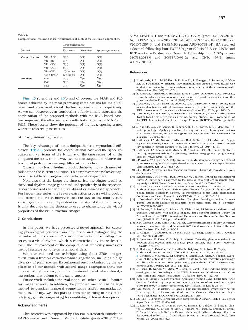
197

Table 6

Computational costs and space requirements of each of the evaluated approaches.

Computational cost

Method Extraction Matching Space requirements

Visual rhythm VR + ACC O(n) O(1) O(1)

VR + BIC O(n) O(1) O(1)

VR + CCV O(n) O(1) O(1)

VR + GCH O(n) O(1) O(1)

VR + GFD O(nlog n) O(1) O(1)

VR + HWD O(nlog n) O(1) O(1)

Baseline RGB

ExG

NDI

O(n)

O(n)

O(n)

K(n)

K(n)

K(n)

K(n)

K(n)

K(n)

Figs. 15 (b and c) and 16(b and c) present the MAP and P10

scores achieved by the most promising combinations for the pixel-

based and area-based visual rhythm representations, respectively.

As we can observe, even considering a fairly simple approach, the

combination of the proposed methods with the RGB-based base-

line improved the effectiveness results both in terms of MAP and

P@5. These results show the potential of the idea, opening a new

world of research possibilities.

6.4. Computational efficiency

The key advantage of our technique is its computational effi-

ciency. Table 6 presents the computational cost and the space re-

quirements (in terms of the length n of the time series) of all the

compared methods. In this way, we can investigate the relative dif-

ference of performance among different approaches.

Clearly, the visual rhythm-based techniques are much more ef-

ficient than the current solutions. This improvement makes our ap-

proach suitable for long-term collections of image data.

Note also that the larger the time series, the bigger would be

the visual rhythm image generated, independently of the represen-

tation considered (either the pixel-based or area-based approach).

For larger time series, the feature extraction process will probably

take more time. Note, however, that the size of the final feature

vector generated is not dependent on the size of the input image.

It only depends on the descriptor used to characterize the visual

properties of the visual rhythm images.

7. Conclusions

In this paper, we have presented a novel approach for captur-

ing phenological patterns from time series and distinguishing the

behavior of plant species. Our technique relies on encoding time

series as a visual rhythm, which is characterized by image descrip-

tors. The improvement of the computational efficiency makes our

method suitable for long-term temporal data.

We have validated our technique using about 2700 images,

taken from a tropical cerrado-savanna vegetation, including a high

diversity of plant species. Experimental results obtained by the ap-

plication of our method with several image descriptors show that

it presents high accuracy and computational speed when identify-

ing regions that belong to the same species.

Future work includes the evaluation of other visual features

for image retrieval. In addition, the proposed method can be aug-

mented to consider temporal segmentation and/or summarization

methods. Finally, we also plan to consider learning-to-rank meth-

ods (e.g., genetic programing) for combining different descriptors.

Acknowledgments

This research was supported by São Paulo Research Foundation

FAPESP–Microsoft Research Virtual Institute (grants #2010/52113-

5, #2013/50169-1 and #2013/50155-0), CNPq (grant 449638/2014-

6), FAPESP (grants #2007/52015-0, #2007/59779-6, #2009/18438-7,

#2010/51307-0), and FAPEMIG (grant APQ-00768-14). BA received

a doctoral fellowship from FAPESP (grant #2014/00215-0); LPCM and

RST receive a Productivity Research Fellowship from CNPq (grants

310761/2014-0 and 306587/2009-2) and CNPq PVE (grant

400717/2013-1).

References

[1] H. Ahrends, S. Etzold, W. Kutsch, R. Stoeckli, R. Bruegger, F. Jeanneret, H. Wan-

ner, N. Buchmann, W. Eugster, Tree phenology and carbon dioxide fluxes: Use

of digital photography for process-based interpretation at the ecosystem scale,

Climate Res. 39 (2009) 261–274.

[2] B. Alberton, J. Almeida, R. Henneken, R. da S. Torres, A. Menzel, L.P.C. Morellato,

Using phenological cameras to track the green up in a cerrado savanna and its on-the-

ground validation, Ecol. Inform. 19 (2014) 62–70.

[3] J. Almeida, J.A. dos Santos, B. Alberton, L.P.C. Morellato, R. da S. Torres, Plant

species identification with phenological visual rhythms, in: Proceedings of the

IEEE International Conference on eScience (eScience’13), 2013a, pp. 148–154.

[4] J. Almeida, J.A. dos Santos, B. Alberton, L.P.C. Morellato, R. da S. Torres, Visual

rhythm-based time series analysis for phenology studies, in: Proceedings of

the IEEE International Conference Image Process. (ICIP’13), 2013b, pp. 4412–

4416.

[5] J. Almeida, J.A. dos Santos, B. Alberton, R. da S. Torres, L.P.C. Morellato, Re-

mote phenology: Applying machine learning to detect phenological patterns

in a cerrado savanna, in: Proceedings of the IEEE International Conference on

(eScience’12), 2012, pp. 1–8.

[6] J. Almeida, J.A. dos Santos, B. Alberton, R. da S. Torres, L.P.C. Morellato, Apply-

ing machine learning based on multiscale classifiers to detect remote phenol-

ogy patterns in cerrado savanna trees, Ecol. Inform. 23 (2014) 49–61.

[7] J. Almeida, J.A. Santos, W.O. Miranda, B. Alberton, L.P.C. Morellato, R.S. Torres,

Deriving vegetation indices for phenology analysis using genetic programming,

Ecol. Inform. 26 (2015) 61–69.

[8] J.P. Ardila, W. Bijker, V.A. Tolpekin, A. Stein, Multitemporal change detection of

urban trees using localized region-based active contours in vhr images, Remote

Sens. Environ. 124 (2012) 413–426.

[9] J.C. Borda, Mémoire sur les élections au scrutin, Histoire de l’Acadmie Royale

des Sciences, 1781.

[10] E.B. Brooks, V.A. Thomas, R.H. Wynne, J.W. Coulston, Fitting the multitemporal

curve: A fourier series approach to the missing data problem in remote sens-

ing analysis, IEEE Trans. Geosci. Remote Sens. 50 (2012) 3340–3353.

[11] J.C. Conti, F.A. Faria, J. Almeida, B. Alberton, L.P.C. Morellato, L. Camolesi Jr.,

R. da S. Torres, Evaluation of time series distance functions in the task of de-

tecting remote phenology patterns, in: Proceedings of the IEEE International

Conference on Pattern Recognition (ICPR’14), 2014, pp. 3126–3131.

[12] J. Dierenbach, F.W. Badeck, J. Schaber, The plant phenological online database

(ppodb): An online database for long-term phenological data, Int. J. Biometeo-

rol. 57 (2013) 805–812.

[13] M. Forster, T. Schmidt, C. Schuster, B. Kleinschmit, Multi-temporal detection of

grassland vegetation with rapideye imagery and a spectral-temporal library, in:

Proceedings of the IEEE International Geoscience and Remote Sensing Sympo-

sium (IGARSS’12), 2012, pp. 4930–4933.

[14] A.R. Gillespie, A.B. Kahle, R.E. Walker, Color enhancement of highly correlated

images. ii. channel ratio and “chromaticity” transformation techniques, Remote

Sens. Environ. 22 (1987) 343–365.

[15] L. Guigues, J. Cocquerez, H. Le Men, Scale-sets image analysis, Intl. J. Comput

Vis. 68 (2006) 289–317.

[16] R. Henneken, V. Dose, C. Schleip, A. Menzel, Detecting plant seasonality from

webcams using bayesian multiple change point analysis, Agr. Forest Meteorol.

168 (2013) 177–185.

[17] G. Hmimina, E. Dufrêne, J.Y. Pontailler, N. Delpierre, M. Aubinet, B. Caquet,

A. de Grandcourt, B. Burban, C. Flechard, A. Granier, P. Gross, B. Heinesch,

B. Longdoz, C. Moureaux, J.M. Ourcival, S. Rambal, L.S. Andr, K. Soudani, Evalu-

ation of the potential of MODIS satellite data to predict vegetation phenology

in different biomes: An investigation using ground-based NDVI measurements,

Remote Sens. Environ. 132 (2013) 145–158.

[18] J. Huang, R. Kumar, M. Mitra, W.J. Zhu, R. Zabih, Image indexing using color

correlograms, in: Proceedings of the IEEE International Conference on Com-

puter Vision and Pattern Recognition (CVPR’97), 1997, pp. 762–768.

[19] R. Ide, H. Oguma, A cost-effective monitoring method using digital time-lapse

cameras for detecting temporal and spatial variations of snowmelt and vege-

tation phenology in alpine ecosystems, Ecol. Inform. 16 (2013) 25–34.

[20] C.E. Jacobs, A. Finkelstein, D. Salesin, Fast multiresolution image querying, in:

Proceedings of the International Conference on Computer Graphics and Inter-

active Techniques (SIGGRAPH’95), 1995, pp. 277–286.

[21] J.S. Lee, T. Ebrahimi, Perceptual video compression: A survey, IEEE J. Sel. Topics

Signal Process. 6 (2012) 684–697.

[22] D. Loustau, A. Bosc, A. Colin, H. Davi, C. François, E. Dufrêne, M. Équé, E. Clop-

pet, D. Arrouays, C. Le Bas, N. Saby, G. Pignard, N. Hamza, A. Granier, N. Breda,

P. Ciais, N. Viovy, J. Ogée, J. Delage, Modeling the climate change effects on

the potential reduction of french plains forests at the sub regional level, Tree

Physiol 25 (2005) 813–823.

198

[23] X. Ma, A. Huete, Q. Yu, N.R. Coupe, K. Davies, M. Broich, P. Ratana, J. Beringer,

L.B. Hutley, J. Cleverly, N. Boulain, D. Eamus, Spatial patterns and temporal

dynamics in savanna vegetation phenology across the north australian tropical

transect, Remote Sens. Environ. 139 (2013) 97–115.

[24] G.C.S. Negi, Leaf and bud demography and shoot growth in evergreen

and deciduous trees of central himalaya, india, Trees 20 (2006) 416–

429.

[25] C.W. Ngo, T.C. Pong, R.T. Chin, Detection of gradual transitions through tem-

poral slice analysis, in: IEEE International Conference on Computer Vision and

Pattern Recognition (CVPR’99), 1999, pp. 1036–1041.

[26] G. Pass, R. Zabih, J. Miller, Comparing images using color coherence vectors,

in: Proceedings of the ACM International Conference on Multimedia (ACM-

MM’96), 1996, pp. 65–73.

[27] O.A.B. Penatti, E. Valle, R. da S. Torres, Comparative study of global color and

texture descriptors for web image retrieval, J. Vis. Commun. Image Represent.

23 (2012) 359–380.

[28] F. Petitjean, C. Kurtz, N. Passat, P. Gançarski, Spatio-temporal reasoning for

the classification of satellite image time series, Pattern Recognit. Lett. 33

(2012) 1805–1815.

[29] A.D. Richardson, B.H. Braswell, D.Y. Hollinger, J.P. Jenkins, S.V. Ollinger, Near-

surface remote sensing of spatial and temporal variation in canopy phenology,

Ecol. Appl. 19 (2009) 1417–1428.

[30] A.D. Richardson, J.P. Jenkins, B.H. Braswell, D.Y. Hollinger, S.V. Ollinger,

M.L. Smith, Use of digital webcam images to track spring greep-

up in a deciduous broadleaf forest, Oecologia 152 (2007) 323–

334.

[31] A. Rodrigues, A.R.S. Marcal, M. Cunha, Phenology parameter extraction from

time-series of satellite vegetation index data using phenosat, in: Proceedings

of the IEEE International Symposium on Geoscience and Remote Sensing Soci-

ety (IGARSS’12), 2012, pp. 4926–4929.

[32]

R. da S. Torres, M. Hasegawa, S. Tabbone, J. Almeida, J.A. dos Santos, B. Alber-

ton, L.P.C. Morellato, Shape-based time series analysis for remote phenology

studies, in: Proceedings of the IEEE International Symposium on Geoscience

and Remote Sensing Society (IGARSS’13), 2013, pp. 3598–3601.

[33] L.C.B. Santos, J. Almeida, J.A. dos Santos, S.J.F. Guimar aes, A.A. Araújo, B. Al-

berton, L.P.C. Morellato, R. da S. Torres, Phenological event detection by visual

rhythm dissimilarity analysis, in: Proceedings of the IEEE International Confer-

ence on eScience (eScience’14), 2014, pp. 263–270.

[34] M.D. Schwartz, Phenology: An Integrative Environmental Science, second,

Springer, 2013.

[35] M.D. Schwartz, B.C. Reed, M.A. White, Assessing satellite derived start-of-

season measures in the coterminous, Int. J. Climatol. 22 (2002) 1793–1805.

[36] R.O. Stehling, M.A. Nascimento, A.X. Falc ao, A compact and efficient image re-

trieval approach based on border/interior pixel classification, in: Proceedings

of the ACM International Conference on Information and Knowledge Manage-

ment (CIKM’02), 2002, pp. 102–109.

[37] M.A. Stricker, M. Orengo, Similarity of color images, in: Proceedings of the

SPIE International Conference on Storage and Retrieval for Image and Video

Databases, 1995, pp. 381–392.

[38] M.J. Swain, B.H. Ballard, Color indexing, Intl J. Comput Vis 7 (1991) 11–32.

[39] D.M. Woebbecke, G.E. Meyer, K. Von-Bargen, A.D. Mortensen, Plant species

identification, size, and enumeration using machine vision techniques on near-

binary images, SPIE Opt. Agr. For. 1836 (1992) 208–219.

[40] D.M. Woebbecke, G.E. Meyer, K. Von-Bargen, A.D. Mortensen, Color indices for

weed identification under various soil, residue, and lighting conditions, Trans.

ASAE 38 (1995) 259–269.

[41] P. Zezula, G. Amato, V. Dohnal, M. Batko, Similarity Search: The Metric Space

Approach, first, Springer Publishing Company, Incorporated, 2010.

[42] D. Zhang, G. Lu, Shape-based image retrieval using generic fourier descriptor,

Signal Process. Image Commun. 17 (2002) 825–848.

199

Appendix C

Article published in the Journal Pattern Recognition Letters:

FARIA F. A., ALMEIDA, J., ALBERTON, B., MORELLATO, L.P.C., ROCHA, A., TORRES, R.S. Time series-

based classifier fusion for fine-grained plant species recognition. Pattern Recognition

Letters, v. 81, p. 101-109, 2016.

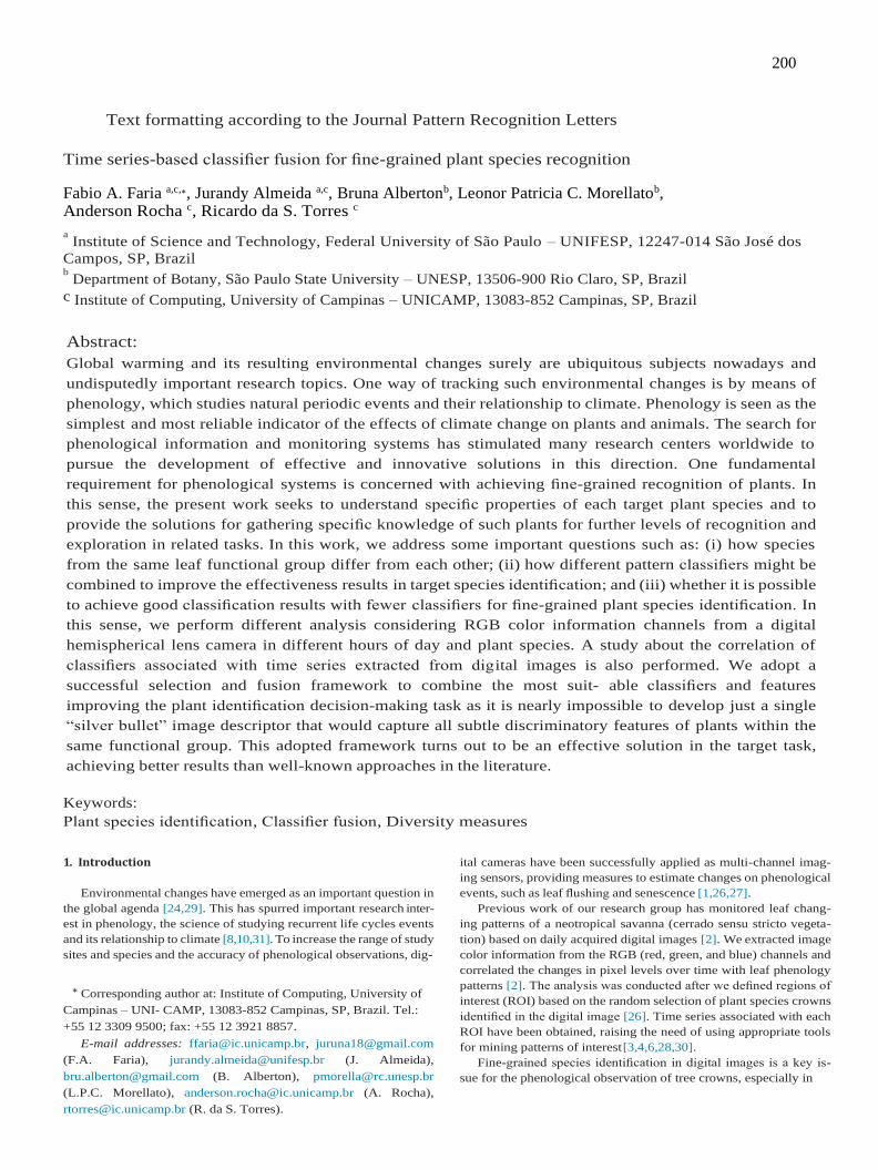
200

Text formatting according to the Journal Pattern Recognition Letters

Time series-based classifier fusion for fine-grained plant species recognition

Fabio A. Faria a,c,∗, Jurandy Almeida a,c, Bruna Albertonb, Leonor Patricia C. Morellatob, Anderson Rocha c, Ricardo da S. Torres c

a Institute of Science and Technology, Federal University of São Paulo – UNIFESP, 12247-014 São José dos

Campos, SP, Brazil b Department of Botany, São Paulo State University – UNESP, 13506-900 Rio Claro, SP, Brazil

c Institute of Computing, University of Campinas – UNICAMP, 13083-852 Campinas, SP, Brazil

Abstract:

Global warming and its resulting environmental changes surely are ubiquitous subjects nowadays and

undisputedly important research topics. One way of tracking such environmental changes is by means of

phenology, which studies natural periodic events and their relationship to climate. Phenology is seen as the

simplest and most reliable indicator of the effects of climate change on plants and animals. The search for

phenological information and monitoring systems has stimulated many research centers worldwide to

pursue the development of effective and innovative solutions in this direction. One fundamental

requirement for phenological systems is concerned with achieving fine-grained recognition of plants. In

this sense, the present work seeks to understand specific properties of each target plant species and to

provide the solutions for gathering specific knowledge of such plants for further levels of recognition and

exploration in related tasks. In this work, we address some important questions such as: (i) how species

from the same leaf functional group differ from each other; (ii) how different pattern classifiers might be

combined to improve the effectiveness results in target species identification; and (iii) whether it is possible

to achieve good classification results with fewer classifiers for fine-grained plant species identification. In

this sense, we perform different analysis considering RGB color information channels from a digital

hemispherical lens camera in different hours of day and plant species. A study about the correlation of

classifiers associated with time series extracted from digital images is also performed. We adopt a

successful selection and fusion framework to combine the most suit- able classifiers and features

improving the plant identification decision-making task as it is nearly impossible to develop just a single

“silver bullet” image descriptor that would capture all subtle discriminatory features of plants within the

same functional group. This adopted framework turns out to be an effective solution in the target task,

achieving better results than well-known approaches in the literature.

Keywords:

Plant species identification, Classifier fusion, Diversity measures

1. Introduction

Environmental changes have emerged as an important question in

the global agenda [24,29]. This has spurred important research inter-

est in phenology, the science of studying recurrent life cycles events

and its relationship to climate [8,10,31]. To increase the range of study

sites and species and the accuracy of phenological observations, dig-

∗ Corresponding author at: Institute of Computing, University of

Campinas – UNI- CAMP, 13083-852 Campinas, SP, Brazil. Tel.:

+55 12 3309 9500; fax: +55 12 3921 8857.

E-mail addresses: ffaria@ic.unicamp.br, juruna18@gmail.com

(F.A. Faria), jurandy.almeida@unifesp.br (J. Almeida),

bru.alberton@gmail.com (B. Alberton), pmorella@rc.unesp.br

(L.P.C. Morellato), anderson.rocha@ic.unicamp.br (A. Rocha),

rtorres@ic.unicamp.br (R. da S. Torres).

ital cameras have been successfully applied as multi-channel imag-

ing sensors, providing measures to estimate changes on phenological

events, such as leaf flushing and senescence [1,26,27].

Previous work of our research group has monitored leaf chang-

ing patterns of a neotropical savanna (cerrado sensu stricto vegeta-

tion) based on daily acquired digital images [2]. We extracted image

color information from the RGB (red, green, and blue) channels and

correlated the changes in pixel levels over time with leaf phenology

patterns [2]. The analysis was conducted after we defined regions of

interest (ROI) based on the random selection of plant species crowns

identified in the digital image [26]. Time series associated with each

ROI have been obtained, raising the need of using appropriate tools

for mining patterns of interest [3,4,6,28,30].

Fine-grained species identification in digital images is a key is-

sue for the phenological observation of tree crowns, especially in

201

tropical vegetations where one single image may include a high num-

ber of species [2]. Usually, this task is very time consuming since it

has to be done in the field, first by matching each crown in the image

to the tree in the soil and then by identifying the tree at species level

[5]. In this sense, we have designed and deployed machine learn-

ing methods to find similar patterns in the digital images and then

we checked if they correspond to similar species or leaf functional

groups [5].

Our first studies have focused on the intraspecies analysis, i.e.,

on detecting different individuals of the same species [5]. However,

different species from the same leaf functional group may exhibit

similar phenological traits, confusing the classifiers as discrimina-

tive features among the classes are more subtle, hardening the iden-

tification process. Hence many questions arise when considering

interspecies interactions, i.e., the recognition of individuals from

different species belonging to the same leaf functional group [2]

spurring the need for the proper design and development of fine-

grained recognition algorithms to tackle the problem. Therefore, in

this paper, we aim at addressing the following questions: (i) how to

distinguish different species from the same leaf functional group us-

ing a pattern classification scheme for proper fine-grained decision-

making; (ii) how the individual responses of classifiers built upon

different phenological features are correlated to each other; and

(iii) how to combine such phenological features so as to improve

the responsiveness of all plant species as it is unlikely that just

one phenological treat would be enough for complete and proper

identification.

We start by evaluating the performance of classification models

built upon a single phenological feature. Thereafter we perform a cor-

relation analysis in order to understand the responsiveness of each

plant species regarding multiple phenological features. Based on the

observations made, we adopted a successful fusion framework [12] to

collect complementary features and better solve the multiclass clas-

sification problem. This kind of problem has never been addressed

in our studies before. Finally, we analyze the impact of increasing

the number of classifiers in the individual responses of each plant

species.

The most important contributions of our work are: (1) A correla-

tion analysis between different time series-based classifiers for each

species. In this vein, we can identify correlations between classifiers

and relationship intra/inter species, which show to be very important

for the problem we are tackling in this paper; (2) The exploration and

proper custom-tailoring of a classifier fusion framework [12] to im-

prove the effectiveness results in a new application (species recogni-

tion); (3) The exploration of this classifier fusion framework for com-

bining time series-based classifiers. Unlike the previous work of ours

[12], which has used visual properties (e.g., color, texture, and shape)

as input data to training base classifiers, our new proposal uses time

series, a much different problem with its own intrinsic particulari-

ties and reduced information when compared to images; (4) Finally,

in this work, we have considered a multi-class classification problem

differently from the previous work.

2. Time series acquisition

A digital hemispherical lens camera (Mobotix Q24) was set up in

an 18 m-high tower in a Cerrado sensu stricto, a neotropical savanna

vegetation located at Itirapina, São Paulo State, Brazil [2,25]. Fig. 1

shows all steps of the time series acquisition process used in our

work.

First, we set up the RGB digital camera to take a daily sequence of

five JPEG images (at 1280 × 960 pixels of resolution) per hour, from

6:00 to 18:00 h (UTC-3). The present study was based on the analysis

of over 2700 images (Fig. 1(a)), recorded at the end of the dry season,

between August 29 and October 3, 2011, day of year 241 to 278, during

the main leaf flushing season [2].

Next, the image analysis has been conducted by defining differ-

ent regions of interest (ROI), as described in [26] and defined by [2]

for our target species. Then, we analyzed 22 ROIs (Fig. 1(b)) obtained

from a random selection of six plant species identified manually by

phenology experts in the hemispheric image [2]: (i) three regions

associated with Aspidosperma tomentosum (green areas), (ii) four re-

gions for Caryocar brasiliensis (blue areas), (iii) two regions for Myrcia guianensis (orange areas), (iv) six regions for Miconia rubiginosa (ma-

genta areas), (v) two regions for Pouteria ramiflora (cyan areas), and

(vi) four regions for Pouteria torta (red areas).

We analyzed each ROI in terms of the contribution of the primary

colors (R, G, and B), as proposed by [27] and described in [2]. Ini-

tially, we analyze each color channel and compute the average value

of the pixel intensity (Fig. 1(c)). After that, we compute the normal-

ized brightness of each color channel (RGB Chromatic coordinates)

(Fig. 1(d)). The normalization of those values reduces the influence

of the incident light, decreasing the color variability due to changes

on illumination conditions [9,34]. Finally, by computing those values

along the whole period (August 28 to October 3, 2011), we obtained

time series to use as input data for a learning method (Fig. 1(e)).

Fig. 1. The time series acquisition process pipeline. (a) Sample image of the Cerrado savanna; (b) Different segmentation scales are computed and the coarse scale is selected;

(c) Hemispherical image with the selected ROI’s species; (d) Channel representation are extracted from ROI’s; (e) RGB chromatic coordinates are computed; (f) Phenological time

series extracted from digital images. (For interpretation of the references to color in this figure text, the reader is referred to the web version of this article.)

202

t

| |

| | | | | |

According to the leaf exchange data from the on-the-ground field

observations on leaf fall and leaf flush at our study site, those species

were classified on three functional groups [2,23]: (i) deciduous, A. to-

mentosum and C. brasiliensis; (ii) evergreen, M. guianensis and M. ru-

biginosa; and (iii) semideciduous, P. ramiflora and P. torta.

3. Framework for time series-based classifier fusion

The objective of adopting a classifier fusion approach is to exploit

the degree of agreement/disagreement among different classifiers,

concept known as diversity and to improve the effectiveness results

in the target task. In this sense, we adapt a successful selection and

fusion framework, originally proposed for multimedia recognition,

to be used as a combiner of times series-based classifier [12]. This

framework selects the most suitable classifiers to be used in a meta-

learning approach. In this work, we define a classifier as a tuple con-

taining a simple learning method (e.g., k-Nearest Neighbors – kNN)

and a description technique (e.g., a color channel from the RGB color

channels).

3.1. Classifier fusion approach

Fig. 2 illustrates the used framework [12] for plant identification.

First, classifiers learn patterns from a training set (T) that contains

samples of time series. Next, C classification models are created.

They are applied on a validation set V, resulting in a matrix of clas-

sifier outcomes MV, where MV = V × C and |V| is the number of

time series extracted from a validation set V (Fig. 2(a)).

Thereafter, in the selection of the most appropriate time series-

based classifiers to be combined, MV is used to calculate different di-

versity measures (D). These measures compute the degree of agree-

ment and disagreement all of |C| available classifiers [20].

The main objective of this selection process is to select a set C∗ ⊂ C of classifiers that are more suitable to be fused/combined (Fig. 2(b)).

Note that a new matrix MV∗ ⊂ MV is computed. Finally, given a new

time series extracted from I, a fusion technique (e.g., Support Vec- tor

Machines) uses the newly created matrix MV∗ to learn patterns and

thus define the final class of I through a meta-learning approach

(Fig. 2(c)).

3.2. Classifier selection approach

Fig. 3 illustrates the adopted five-step approach for selecting clas-

sifiers based on diversity measures, previously introduced in [12].

First, set D of diversity measures are used to assess the degree of

agreement among available classifiers in C by taking into account the

MV matrix previously computed. In this approach, five different mea-

sures have been used (Correlation Coefficient p, Double-Fault Measure,

Disagreement Measure, Interrater Agreement k, and Q-Statistic [20,21]).

That step is represented by arrow (a) in Fig. 3. Pairs of classifiers are

then ranked according to their diversity score. Each diversity mea-

sure defines a different ranked list and, at the end of this step, a set

R of ranked lists is produced (arrow (b)). In the following, a novel set

of ranked lists Rt is computed by selecting the top t pairs of classi-

fiers from each ranked list in R (arrow (c)), and a histogram H that

counts the number of occurrences of a classifier in all ranked lists of

R is computed (arrow (d)). Finally, the most frequent classifiers in H,

whose accuracy is greater that a given threshold T , are combined by

a fusion approach (arrow (e)). T is a threshold defined in terms of the

average accuracy among all classifiers using the validation set V.

4. Experimental protocol

This section presents the experimental protocol used in this work.

4.1. Dataset

In this work, we have applied the same evaluation method used in

[2]. It relies on the classification of time series extracted from pixels

associated with individuals of a same species. For that, we used the

algorithm introduced by [15] to segment the hemispheric image into

small polygons, obtaining 8849 segmented regions (SR). Then, we as-

sociated each SR with a single ROI aiming to label it. A labeled region

is created if there is at least 80% of overlapped area between an SR

and a ROI.

Finally, we extracted a time series from each labeled region using

the approach described in Section 2. In this way, we built a dataset of

892 time series separated into six classes, one for each plant species:

A. tomentosum (96), C. brasiliensis (346), M. guianensis (36), M. rubigi-

nosa (195), P. ramiflora (50), and P. torta (169).

Fig. 2. Time series-based classifier selection and fusion framework adapted from [12]. In (a), given a classification problem with training examples, different classifiers are trained

using data from training set T. In (b), the most discriminating classifiers are selected (C∗) by taking into account diversity measures (D). Finally, in (c), classifiers are combined in a

meta-level approach using any other classifier. In this particular example, both the SVM and Majority Voting (MV) techniques can be used as the classifier fusion technique.

Fig. 3. The five steps for classifier selection are: (a) Computation of diversity measures from the validation matrix MV; (b) Ranking of pairs of classifiers by their diversity measures

scores; (c) Selection of the top t ranked pairs of classifiers; (d) Computation of a histogram H that counts the number of occurrences of each classifier; (e) Select the most appropriate

classifiers |C∗| based on their occurrence in H and satisfy a defined threshold T .

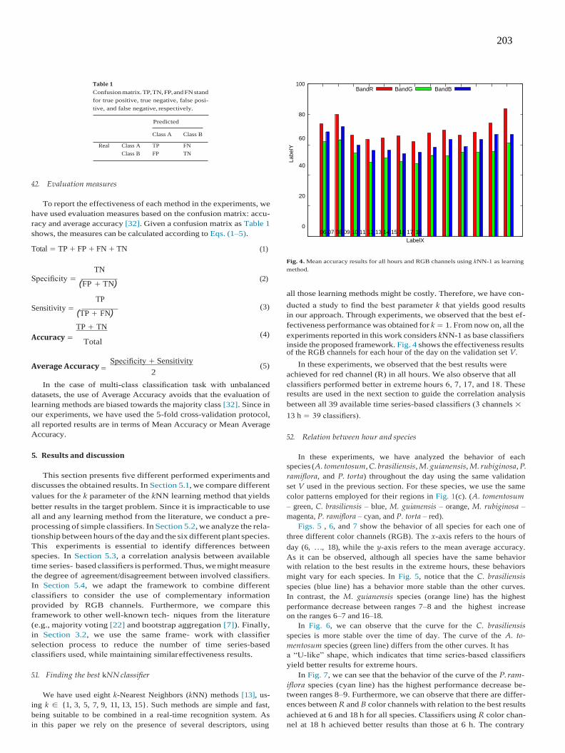
203

=

Table 1

Confusion matrix. TP, TN, FP, and FN stand

for true positive, true negative, false posi-

tive, and false negative, respectively.

Predicted

100

80

BandR BandG BandB

Class A Class B 60

Real Class A TP FN

Class B FP TN

4.2. Evaluation measures

To report the effectiveness of each method in the experiments, we

have used evaluation measures based on the confusion matrix: accu-

racy and average accuracy [32]. Given a confusion matrix as Table 1

shows, the measures can be calculated according to Eqs. (1–5).

Total = TP + FP + FN + TN (1)

40

20

0

06 07 08 09 10 11 12 13 14 15 16 17 18

LabelX

TN

Specificity = (FP + TN)

(2)

Fig. 4. Mean accuracy results for all hours and RGB channels using kNN-1 as learning

method.

all those learning methods might be costly. Therefore, we have con- TP

Sensitivity = (TP + FN)

TP + TN

(3) ducted a study to find the best parameter k that yields good results

in our approach. Through experiments, we observed that the best ef-

fectiveness performance was obtained for k = 1. From now on, all the

Accuracy = (4) Total

experiments reported in this work considers kNN-1 as base classifiers

inside the proposed framework. Fig. 4 shows the effectiveness results of the RGB channels for each hour of the day on the validation set V.

Average Accuracy Specificity + Sensitivity

2 (5) In these experiments, we observed that the best results were

achieved for red channel (R) in all hours. We also observe that all

In the case of multi-class classification task with unbalanced

datasets, the use of Average Accuracy avoids that the evaluation of

learning methods are biased towards the majority class [32]. Since in

our experiments, we have used the 5-fold cross-validation protocol,

all reported results are in terms of Mean Accuracy or Mean Average

Accuracy.

5. Results and discussion

This section presents five different performed experiments and

discusses the obtained results. In Section 5.1, we compare different

values for the k parameter of the kNN learning method that yields

better results in the target problem. Since it is impracticable to use

all and any learning method from the literature, we conduct a pre-

processing of simple classifiers. In Section 5.2, we analyze the rela-

tionship between hours of the day and the six different plant species.

This experiments is essential to identify differences between

species. In Section 5.3, a correlation analysis between available

time series- based classifiers is performed. Thus, we might measure

the degree of agreement/disagreement between involved classifiers.

In Section 5.4, we adapt the framework to combine different

classifiers to consider the use of complementary information

provided by RGB channels. Furthermore, we compare this

framework to other well-known tech- niques from the literature

(e.g., majority voting [22] and bootstrap aggregation [7]). Finally,

in Section 3.2, we use the same frame- work with classifier

selection process to reduce the number of time series-based

classifiers used, while maintaining similar effectiveness results.

5.1. Finding the best kNN classifier

We have used eight k-Nearest Neighbors (kNN) methods [13], us-

ing k ∈ {1, 3, 5, 7, 9, 11, 13, 15}. Such methods are simple and fast,

being suitable to be combined in a real-time recognition system. As

in this paper we rely on the presence of several descriptors, using

classifiers performed better in extreme hours 6, 7, 17, and 18. These

results are used in the next section to guide the correlation analysis

between all 39 available time series-based classifiers (3 channels ×

13 h = 39 classifiers).

5.2. Relation between hour and species

In these experiments, we have analyzed the behavior of each

species (A. tomentosum, C. brasiliensis, M. guianensis, M. rubiginosa, P.

ramiflora, and P. torta) throughout the day using the same validation

set V used in the previous section. For these species, we use the same

color patterns employed for their regions in Fig. 1(c). (A. tomentosum

– green, C. brasiliensis – blue, M. guianensis – orange, M. rubiginosa –

magenta, P. ramiflora – cyan, and P. torta – red).

Figs. 5 , 6, and 7 show the behavior of all species for each one of

three different color channels (RGB). The x-axis refers to the hours of

day (6, …, 18), while the y-axis refers to the mean average accuracy.

As it can be observed, although all species have the same behavior

with relation to the best results in the extreme hours, these behaviors

might vary for each species. In Fig. 5, notice that the C. brasiliensis

species (blue line) has a behavior more stable than the other curves.

In contrast, the M. guianensis species (orange line) has the highest

performance decrease between ranges 7–8 and the highest increase

on the ranges 6–7 and 16–18.

In Fig. 6, we can observe that the curve for the C. brasiliensis

species is more stable over the time of day. The curve of the A. to-

mentosum species (green line) differs from the other curves. It has

a “U-like” shape, which indicates that time series-based classifiers

yield better results for extreme hours.

In Fig. 7, we can see that the behavior of the curve of the P. ram-

iflora species (cyan line) has the highest performance decrease be-

tween ranges 8–9. Furthermore, we can observe that there are differ-

ences between R and B color channels with relation to the best results

achieved at 6 and 18 h for all species. Classifiers using R color chan-

nel at 18 h achieved better results than those at 6 h. The contrary

La

be

lY

204

i j

(a + b)(c + d)(a + c)(b + d) 20

100

80

60

40

20

0

6 7 8 9 10 11 12 13 14 15 16 17 18

Hour

All Classes

A.tomentosum C.brasiliensis M.guianensis M.rubiginosa

P.ramiflora P.torta

100

80

60

40

20

0

6 7 8 9 10 11 12 13 14 15 16 17 18

Hour

All Classes

A.tomentosum C.brasiliensis M.guianensis M.rubiginosa

P.ramiflora P.torta

Fig. 5. Mean accuracy results for all hours and R color channel using kNN-1 as learning

method for each class. (For interpretation of the references to color in this figure text,

the reader is referred to the web version of this article.)

Fig. 7. Mean accuracy results for all hours and B channel using kNN-1 as learning

method for each class. (For interpretation of the references to color in this figure text,

the reader is referred to the web version of this article.)

100

All Classes

A.tomentosum C.brasiliensis M.guianensis M.rubiginosa

5.3. Correlation analysis between time series-based classifier

80 P.ramiflora P.torta

60

40

0 6 7 8 9 10 11 12 13 14 15 16 17 18

This section shows a correlation analysis of each pair of classi-

fiers for all 39 available time series-based classifiers aiming at find-

ing which of them might be combined by the framework described

in Section 3.

The Correlation Coefficient ρ (COR) [20] has been used to assess the

correlation of two classifiers ci and cj:

COR(c , c ) = , ad − bc

, (6)

where a is the percentage of time series that both classifiers ci and cj

Hour

Fig. 6. Mean accuracy results for all hours and G channel using kNN-1 as learning

method for each class. (For interpretation of the references to color in this figure text,

the reader is referred to the web version of this article.)

was observed for the G channel. In this case, the best results were ob-

served at 6 h. Note also that the curves of the species M. guianensis

presents the lower mean average accuracy for all color channels. We

might attribute these consistent difference to its leafing phenology:

M. guianensis (orange line) is the only species reducing the percent-

age of green over the period of study [2].

In summary, each species has a particular behavior with regard to

different RGB color channels throughout the day. This phenomenon

might be justified by scattering of solar radiation and canopy re-

flectance [33]. Moreover, the leaf biochemical contents (e.g., chloro-

phyll, water, and dry matter) and canopy architecture (e.g., leaf area

index, leaf angle distribution, and relative leaf size) might have im-

pacted the spectral response of leaves [17].

This study might reinforce the importance of the R channel for

the identification of these plant species as pointed out in [11]. How-

ever, the G channel has shown also to be important for some species

(e.g., M. guianensis, P. ramiflora, and P. torta) for some hours of the day.

The difference in behavior of the time series-based classifiers led us

to consider their combination as a suitable alternative for improving

the classification results in plant identification systems. We therefore

performed a correlation analysis between all those classifiers to guide

us in the time series-based classifier selection process.

classified correctly in a validation set V. Value b is the percentage of

time series that cj hit and ci missed, c is the opposite of b. The value d

is the percentage of time series that both classifiers missed. The pairs

of classifiers with lower COR values have greater degree of comple-

mentarity and are more likely to yield better results when combined.

Range of COR is in [−1, +1].

Fig. 8 presents the COR values for all possible combinations of

pairs of classifiers considering the six classes. The lowest correlation

coefficients are closer to the purple color (−1) and the highest coef-

ficients are closer to the yellow color (+1). Furthermore, in this fig-

ure, there are seven important regions that have been highlighted and

they are explained below.

As we can observe in Fig. 8(a), in region (1), there are few classi-

fiers with high correlation between the channels R and G which are

closer to their extreme hours (16–18 h). However, outside of region (1),

the classifier from channels R and G are less correlated with chan- nel

B. We can see some points in purple, which means lower corre- lation

coefficients. Fig. 8(b) shows a more homogeneous behavior of the

classifiers, since instances of class C. brasiliensis are not difficult to be

correctly classified. Furthermore, we can notice that there are a few

yellow strips meaning high correlation of the same classifier with all

other classifiers. Fig. 8(c) shows many purple points, which mean a

low correlation between almost all classifiers used in this

work. This phenomenon can be explained by the difficulty of clas-

sifying instances of the class M. guianensis. In region (2), we found

the lowest correlation coefficient for all experiments. Fig. 8(d) shows

a similar behavior to Fig. 8(a) with coefficients more homogeneous.

We can observe in region (3) that classifiers of the same color channel

G are more correlated between them. However, in region (4), R and G

Mea

n A

ver

age

Acc

ura

cy (%

) M

ean

Aver

age

Acc

ura

cy (%

)

Mean

Avera

ge A

ccu

racy

(%)

205

Fig. 8. Correlation analysis considering all 39 available time series-based classifiers (3 channels × 13 h = 39 classifiers). The lowest correlation coefficients are closer to the purple

color (−1) and the highest coefficients are closer to the yellow color (+1). (For interpretation of the references to color in this figure legend, the reader is referred to the web version

of this article.)

are less correlated with B. Fig. 8(e) shows the second most difficult

class to be classified: P. ramiflora. In regions (5) and (6), we found the

lowest correlation coefficients between almost all classifiers of R × G

and all classifiers of the color channels R and G with part of classifiers

of channel B (9–12 h). Finally, in Fig. 8(f), which refers to the class

P. torta, we can notice that the classifiers achieve similar behavior to

Fig. 8(a) and (b). In region (7), there are the less correlated classifiers

within Fig. 8(f).

5.4. Time series-based classifier fusion

In these experiments, 12 fusion techniques were compared: four

techniques that use the adopted framework [12] (FSVM-ALL-39,

FSVM-R-13, FSVM-G-13, and FSVM-B-13), four majority voting tech-

niques [22] (MV-ALL-39, MV-R-13, MV-G-13, and MV-B-13), and

four bootstrap aggregation approaches [7] (BAGG-MERGE-ALL-39,

BAGG-MERGE-R-13, BAGG-MERGE-G-13, and BAGG-MERGE-B-13).

206

| |

| | { }

100

80

A.tomentosum C.brasiliensis

78.66 77.93

73.02 72.99

M.guianensis M.rubiginosa

P.ramiflora P.torta

68.30 67.87 65.14 63.42 62.10

60

57.20

52.51

48.49

40

20

0

Fig. 9. Mean average accuracy of all fusion techniques.

ALL means that all color channels, hours, and features have been used.

R, G, and B refer to the color channels that compose the RGB channel.

Furthermore, the number after a name (e.g., 13 in FSVM-B-13) refers

to amount of time series-based classifiers considered in the fusion

process. MERGE denotes a binding of the all available channels, hours,

and feature vectors.

The proposed framework aims at finding suitable combinations

of time series-based classifiers formed by descriptors and learning

methods. We have used the implementation of those learning meth-

ods available in the WEKA [16] data mining library. All learning meth-

ods were used with default parameters which means we did not op-

timize them.

Figs. 9 and 10 show the effectiveness results of all fusion tech-

niques considered in this work. Two evaluation measures have been

adopted, mean average accuracy (Fig. 9) e mean accuracy (Fig. 10).

Balanced mean accuracy per class considers the mean accuracy of

each class using the 5-fold cross validation protocol and the final ef-

fectiveness result is the average of these accuracies. Mean accuracy is

the principal diagonal from confusion matrix, which counts the num-

ber of correct classification cases with respect to the total instances

using the 5-fold cross validation protocol.

As it can be observed, two of our approaches (FSVM-ALL-39 and

FSVM-R-13) achieved the best results among all involved fusion tech-

niques. FSVM-ALL-39 approach obtained a mean average accuracy of

Fig. 10. Mean accuracy of all fusion techniques.

Fig. 11. Behavioral analysis of the framework for different numbers of classifiers. On

the x-axis are the numbers of selected classifiers C∗ = 2, . . . , 39 and y-axis are the

mean accuracy achieved in the experiments. (For interpretation of the references to

color in this figure text, the reader is referred to the web version of this article.)

78.66% and mean accuracy of 85.87% against the best baseline MV-R-

13 that yielded 73.02% and 83.18%, respectively. A fine-grained anal-

ysis considering mean average accuracy showed that FSVM-ALL-39

approach achieved better results in two classes (M. guianensis and P.

torta), FSVM-R-13 approach is the best for other two classes (A. to-

mentosum and M. rubiginosa). Finally, MV-ALL-39 achieved better re-

sults in the classes C. brasiliensis and P. ramiflora. Thus, our approaches

achieved better results in four out of six possible classes from the

dataset used.

5.5. Time series-based classifier selection

This section describes a behavioral analysis of the proposed

framework using different numbers of time series-based classifiers

C∗ for the six classes from the dataset. Fig. 11 shows this analysis

per class as well as all classes together.

In these experiments, we can notice that the classes C. brasilien-

sis, A. tomentosum, M. rubiginosa, and P. torta have a stable behavior

with the increasing number of selected time series-based classifiers.

This fact cannot be observed in the classes M. guianensis and P. ram-

iflora. The class M. guianensis achieved an increase of more than 10%

of mean accuracy in the range [3, 7]. However, the curve of the class P.

ramiflora decreases more than 15% for the same ranges. Furthermore,

note that the framework using only six classifiers achieves similar re-

sults to those observed when 39 time series-based classifiers are used

(see brown line in Fig. 11). In summary, the investigation for mini-

mizing the misclassification rate per class seems to be a promising

research venue and a classifier selection approach based on balanced

classes might be a good solution to address this problem.

Fig. 12 depicts the histogram H created in the selection process,

while Fig. 13 shows the accuracy performances of all simple/non-

complex classifiers using the validation set V. We highlight in gold

bars the six time series-based classifiers (see brown line in Fig. 11)

that have been selected by our selection process. In Fig. 12, although

classifiers kNN1-09G, kNN1-09B, and kNN1-12G have achieved the

higher frequency than kNN1-06R and kNN1-07G, our selection ap-

proach does not choose any of those classifiers as candidate for fu-

sion (gold bars). This is due to the policy of also considering the

individual accuracy performance of classifiers in the selection pro-

cess. As the accuracy performances of kNN1-09G, kNN1-09B, and

kNN1-12G are below than the employed threshold values (dark blue

line, T = 61.97%), these classifiers are not selected. Selected classi-

fiers are kNN1-06R, kNN1-06B, kNN1-07R, kNN1-07G, kNN1-07B, and

Mea

n A

ccu

racy

(%

) M

ean A

ver

age

Acc

ura

cy (

%)

207

Fig. 12. Histogram H related to the occurrence of classifiers in the selection process.

(For interpretation of the references to color in this figure text, the reader is referred to

the web version of this article.)

Fig. 13. Average accuracy performances of all non-complex classifiers used in our ex-

periments. The dark blue line defines the employed threshold (T ) value. (For interpre-

tation of the references to color in this figure legend, the reader is referred to the web

version of this article.)

kNN1-18R. In these experiments, three selected classifiers use the R

channel, two classifiers use the B channel, and one classifier uses the

G channel. We can observe also a huge impact of the extreme hours

(06, 07, and 18) in the selection process.

6. Conclusions

In this paper, we proposed a time series-based classifier selec-

tion and fusion framework to address problems in fine-grained plant

identification tasks. We validated such framework with phenology

studies. Recalling the objectives of our work, we addressed some

very important questions, such as: (i) how species from the same

leaf functional group differ from each other; (ii) how different pat-

tern classifiers might be combined to improve the effectiveness re-

sults in target fine-grained species identification as just one classi-

fier or feature would not be discriminatory enough for the task; and

(iii) whether it is possible to achieve good classification results with

fewer classifiers for plant identification improving the efficiency of

the whole decision-making process. To answer such questions, we

have performed five different analyses: (1) Investigation of the best

value for the k parameter of the kNN learning method that yields

better results in the target problem; (2) An analysis of the relation-

ship between hours of the day and the six different plant species

considered in this study; (3) A correlation analysis measuring the

degree of agreement/disagreement between available time series-

based classifiers; (4) Use of a classifier selection and fusion frame-

work aiming at exploring complementary information provided by

different descriptions and learning methods, thus improving the ef-

fectiveness results; (5) Investigation of the impact of using the same

framework with classifier selection process to decrease the number

of time series-based classifiers used, while maintaining similar effec-

tiveness results.

The experiments performed in this work confirm that there are

some differences in terms of classification performance depending

on the plant species considered, as well as, the correlation that exists

between RGB channels and hours of the day using kNN-1 classifiers.

Also, in the experiments, it was possible to note the importance of

the red channel for plant species identification, in spite of the good

contribution observed for the blue channel for some species (e.g., M.

guianensis, P. ramiflora, and P. torta). Furthermore, the adopted frame-

work achieved excellent results when compared with other well-

known fusion techniques of the literature (Bootstrap Aggregation-

BAGG [7] and Majority Voting-MV [22]). This framework, extended

upon [12], brings an essential and important property different from

those techniques in the literature: it is highly flexible and paralleliz-

able. Regarding flexibility, our adopted approach can use any descrip-

tion technique or learning methods as base classifier. In addition, the

method is able to use any learning method in the late fusion (meta-

learning process), such as a simple majority voting or more complex

techniques such as support vector machines (SVMs). As for paral-

lelization, each combination of description and learning methods can

be used in different parallel approaches (e.g., thread, processor, and

GPU) due the framework structure being designed independently (in

modules). With that, the more important modules are the training

classifiers, the classifier selection, and the meta-learning. Further-

more, other important advantage of the adopted approach is that it

considers each description and learning method as a single represen-

tation thus it does not incur in the common normalization problems

and, consequently reduces the risk the “the curse of dimensionality”

that may result of direct combination of features (e.g., by means of

concatenating feature vectors).

A fine-grained analysis using time series-based classifier selection

showed that the framework using fewer classifiers (i.e., six) achieved

similar results to those observed when 39 time series-based classi-

fiers are used. Therefore, our proposed method might be able to per-

form real-time plant identification in different domains such as when

monitoring plants through intelligent autonomous vehicles (e.g., un-

manned aerial vehicles and drones).

Another important contribution of this work is related to the use

of multiclass classification approaches, which was not used in previ-

ous phenology work [5]. The main take-home message of our work is

that the adopted framework might be a good solution to address com-

plex problems such as the ones involving phenology derived from se-

quential digital images and fine-grained recognition of plants from

the same functional leaf groups. This framework takes advantage of

different and complementary information provided by RGB channels

and combine them for a better decision-making process. In addition,

it achieves good effectiveness results with fewer classifiers, which is

paramount for efficient plant recognition.

Future work may consider the use of the proposed framework in

semi-automatic plant identification tasks, in which users may pro-

vide relevance feedback that may tune the used classification mod-

els for better fine-grained categorization that always includes hu-

mans (specialists) in the loop. Also, we may consider the use of the

proposed framework for real-time plant identification systems. Fur-

thermore, other vegetation indices might be studied and combined

18B

18B

18G

18G

18R

18R

17B

17B

17G

17G

17R

17R

16B

16B

16G

16G

16R

16R

15B

15B

15G

15G

15R

15R

14B

14B

14G

14G

14R

14R

13B

13B

13G

13G

13R

13R

12B

12B

12G

12G

12R

12R

11B

11B

11G

11G

11R

11R

10B

10B

10G

10G

10R

10R

09B

09B

09G

09G

09R

09R

08B

08B

08G

08G

08R

08R

07B

07B

07G

07G

07R

07R

06B

06B

06G

06G

06R

06R

208

such as Color Index of Vegetation Extraction (CIVE) [19], Excess Green

(ExG) [14], and the Plant Phenology Index (PPI) [18]. Regarding the

generalization, with the proposed approach in this work for dealing

with time-series based problems, we believe that other application

domains, still in the realm of time series as input data, may include

crop monitoring, recognizing different plant growth rates and also

for plague control. Other applications also may tap on snowmelt and

comparison of species or different kinds of vegetation.

Acknowledgments

We thank the financial support of the São Paulo Research Foun-

dation FAPESP (grants #2010/14910-0 and #2010/05647-4), the

FAPESP-Microsoft Research Virtual Institute (grants #2010/52113-5,

#2011/51523-8, #201313/20169-1, and #2013/50155-0), CNPq (grants

#477662/2013-7 and #304352/2012-8), CAPES (grant #1260-12-0),

and Microsoft Research. LPCM and RST receive a Productivity Re-

search Fellowship from CNPq (grants #306243/2010-5 and #306587/

2009-2). BA receives a PhD fellowship (FAPESP grant #2014/00215-

0). Also, we have been benefited by funds from CNPq, CAPES, and

FAPESP (grants #2007/52015-0, #2007/59779-6, #2009/18438-7, and

#2010/51307-0). The authors thank Prof. Dr. Thiago Sanna Freire Silva

for his pertinent and helpful comments on the paper.

References

[1] H. Ahrends, S. Etzold, W. Kutsch, R. Stoeckli, R. Bruegger, F. Jeanneret, H. Wanner,

N. Buchmann, W. Eugster, Tree phenology and carbon dioxide fluxes: use of digital

photography for process-based interpretation at the ecosystem scale, Clim. Res.

39 (2009) 261–274.

[2] B. Alberton, J. Almeida, R. Henneken, R. da S. Torres, A. Menzel, L.P.C. Morellato,

Using phenological cameras to track the green up in a Cerrado savanna and its on-

the-ground validation, Ecol. Inform. 19 (2014) 62–70.

[3] J. Almeida, J.A. dos Santos, B. Alberton, L.P.C. Morellato, R. da S. Torres, Plant

species identification with phenological visual rhythms, in: Proceedings of the

IEEE International Conference on eScience (eScience’13), 2013, pp. 148–154.

[4] J. Almeida, J.A. dos Santos, B. Alberton, L.P.C. Morellato, R. da S. Torres, Visual

rhythm-based time series analysis for phenology studies, in: Proceedings of the

IEEE International Conference on Image Processing (ICIP’13), 2013, pp. 4412–4416.

[5] J. Almeida, J.A. dos Santos, B. Alberton, R. da S. Torres, L.P.C. Morellato, Applying

machine learning based on multiscale classifiers to detect remote phenology pat-

terns in Cerrado savanna trees, Ecol. Inform. 23 (2014) 49–61.

[6] J. Almeida, J.A. Santos, W.O. Miranda, B. Alberton, L.P.C. Morellato, R.S. Torres, De-

riving vegetation indices for phenology analysis using genetic programming, Ecol.

Inform. 26 (2015) 61–69.

[7] L. Breiman, Bagging predictors, Mach. Learn. 24 (1996) 123–140.

[8] L.E. Chambers, R. Altwegg, C. Barbraud, P. Barnard, L. Beaumont, R. Crawford,

J.M. Durant, L. Hughes, M.R. Keatley, M. Low, L.P.C. Morellato, E. Poloczanska,

V. Ruoppolo, R.E.T. Vanstreels, E.J. Woehler, A. Wolfaardt, Changes in southern

hemisphere phenology, PlosOne 8 (2013) e75514.

[9] H.D. Cheng, X. Jiang, Y. Sun, J. Wang, Color image segmentation: advances and

prospects, Pattern Recognit. 34 (2001) 2259–2281.

[10] E.E. Cleland, I. Chuine, A. Menzel, H.A. Mooney, M.D. Schwartz, Shifting plant phe-

nology in response to global change, Trends Ecol. Evol. 22 (7) (2007) 357–365.

[11] J.C. Conti, F.A. Faria, J. Almeida, B. Alberton, L.P.C. Morellato, L. Camolesi Jr., R. da

S. Torres, Evaluation of time series distance functions in the task of detecting re-

mote phenology patterns, in: Proceedings of the IEEE International Conference on

Pattern Recognition (ICPR’14), 2014, pp. 3126–3131.

[12] F.A. Faria, J.A. dos Santos, A. Rocha, R. da S. Torres, A framework for selection and

fusion of pattern classifiers in multimedia recognition, Pattern Recognit. Lett. 39

(2014) 52–64.

[13] J. Friedman, T. Hastie, R. Tibshirani, The Elements of Statistical Learning, first ed.,

Springer, 2001.

[14] C. Gée, J. Bossu, G. Jones, F. Truchetet, Crop/weed discrimination in perspective

agronomic images, Comput. Electron. Agric. 60 (2008) 49–59.

[15] L. Guigues, J. Cocquerez, H. Le Men, Scale-sets image analysis, Int. J. Comput. Vis.

68 (2006) 289–317.

[16] M. Hall, E. Frank, G. Holmes, B. Pfahringer, P. Reutemann, I.H. Witten, The weka

data mining software: an update, ACM SIGKDD Explor. Newsl. 11 (2009) 10–18.

[17] S. Jacquemoud, W. Verhoef, F. Baret, C. Bacour, P.J. Zarco-Tejada, G.P. Asner, C. Fra-

nois, S.L. Ustin, Prospect + sail models: a review of use for vegetation characteri-

zation, Remote Sens. Environ. 113 (Suppl. 1) (2009) S56–S66.

[18] H. Jin, L. Eklundh, A physically based vegetation index for improved monitoring

of plant phenology, Remote Sens. Environ. 152 (2014) 512–525.

[19] T. Kataoka, T. Kaneko, H. Okamoto, S. Hata, Crop growth estimation system using

machine vision, in: Proceedings of the 2003 IEEE/ASME International Conference

on Advanced Intelligent Mechatronics, vol. 2, 2003, pp. b1079–b1083.

[20] L.I. Kuncheva, Combining Pattern Classifiers: Methods and Algorithms, Wiley-

Interscience, 2004.

[21] L.I. Kuncheva, C.J. Whitaker, Measures of diversity in classifier ensembles and

their relationship with the ensemble accuracy, Mach. Learn. 51 (2003) 181–207.

[22] L. Lam, S.Y. Suen, Application of majority voting to pattern recognition: an analy-

sis of its behavior and performance, IEEE Trans. Syst., Man, Cybern., Part A: Syst.

Hum. 27 (1997) 553–568.

[23] L.P.C. Morellato, R.R. Rodrigues, H.F. Leit ao Filho, C.A. Joly, Estudo comparativo da

fenologia de espécies arbóreas de floresta de altitude e floresta mesófila semidecí-

dua na serra do iapí, jundiaí, são paulo, Braz. J. Bot. 12 (1989) 85–98.

[24] M. Parry, O. Canziani, J. Palutikof, P. van der Linden, C. Hanson, IPCC (2007) Cli-

mate Change 2007: Impacts, Adaptation and Vulnerability. Contribution of Work-

ing Group II to the Fourth Assessment Report of the Intergovernmental Panel on

Climate Change, Cambridge UK: Cambridge University Press, 2007.

[25] P. Reys, M.G.G. Camargo, A.P. Teixeira, M.A. Assis, M.T. Grombone-Guaratini,

L.P.C. Morellato, Estrutura e composio florstica entre borda e interior de um cer-

rado sensu stricto e sua importância para propostas de recuperação, Hoennea 40

(2013) 437–452.

[26] A.D. Richardson, B.H. Braswell, D.Y. Hollinger, J.P. Jenkins, S.V. Ollinger, Near-

surface remote sensing of spatial and temporal variation in canopy phenology,

Ecol. Appl. 19 (2009) 1417–1428.

[27] A.D. Richardson, J.P. Jenkins, B.H. Braswell, D.Y. Hollinger, S.V. Ollinger, M.L. Smith,

Use of digital webcam images to track spring greep-up in a deciduous broadleaf

forest, Oecologia 152 (2007) 323–334.

[28] R. da S. Torres, M. Hasegawa, S. Tabbone, J. Almeida, J.A. dos Santos, B. Alberton,

L.P.C. Morellato, Shape-based time series analysis for remote phenology studies,

in: Proceedings of the IEEE International Geoscience and Remote Sensing Sympo-

sium (IGARSS’13), 2013, pp. 3598–3601.

[29] R. da S. Torres, C.B. Medeiros, M.A. Gonçalves, E.A. Fox, A digital library framework

for biodiversity information systems, Int. J. Digit. Libr. 6 (2006) 3–17.

[30] L.C.B. Santos, J. Almeida, J.A. dos Santos, S.J.F. Guimar aes, A.A. Araújo, B. Alberton,

L.P.C. Morellato, R. da S. Torres, Phenological event detection by visual rhythm

dissimilarity analysis, in: Proceedings of the IEEE International Conference on

eScience (eScience’14), 2014, pp. 263–270.

[31] M.D. Schwartz, Phenology: An Integrative Environmental Science, Springer, 2013.

[32] M. Sokolova, G. Lapalme,A systematic analysis of performance measures for clas-

sification tasks, Inf. Process. Manag. 45 (2009) 427–437.

[33] M.M. Verstraete, Radiation transfer in plant canopies: scattering of solar radiation

and canopy reflectance, J. Geophys. Res.: Atmos. 93 (1988) 9483–9494.

[34] D.M. Woebbecke, G.E. Meyer, K. Von Bargen, D.A. Mortensen, Color indices for

weed identification under various soil, residue, and lighting conditions, Trans.

ASAE 38 (1995) 259–269.

209

Appendix D

Article published in the Journal Pattern Recognition Letters:

FARIA F. A., ALMEIDA, J., ALBERTON, B., MORELLATO, L.P.C., TORRES, R.S. Fusion of Time Series

Representations for Plant Recognition in Phenology Studies. Pattern Recognition Letters, v. 83, p. 205-214,

2016.

210

Text formatting according to the Journal Pattern Recognition Letters

Fusion of time series representations for plant recognition in phenology studies

Fabio A. Faria a,b,∗, Jurandy Almeida a,b, Bruna Albertonc, Leonor Patricia C. Morellatoc, Ricardo da S. Torres b

a Institute of Science and Technology, Federal University of São Paulo – UNIFESP, São José dos Campos

12247-014, SP, Brazil

b Institute of Computing, University of Campinas – UNICAMP, Campinas 13083-852, SP, Brazil

c Dept. of Botany, Sao Paulo State University – UNESP Rio Claro, 13506-900, SP, Brazil

Abstract:

Nowadays, global warming and its resulting environmental changes is a hot topic in different biology re-

search area. Phenology is one effective way of tracking such environmental changes through the study of

plant’s periodic events and their relationship to climate. One promising research direction in this area relies

on the use of vegetation images to track phenology changes over time. In this scenario, the creation of

effective image-based plant identification systems is of paramount importance. In this paper, we propose the

use of a new representation of time series to improve plants recognition rates. This representation, called

recurrence plot (RP), is a technique for nonlinear data analysis, which represents repeated events on time

series into a two-dimensional representation (an image). Therefore, image descriptors can be used to

characterize visual properties from this RP images so that these features can be used as input of a classifier.

To the best of our knowledge, this is the first work that uses recurrence plot for plant recognition task.

Performed experiments show that RP can be a good solution to describe time series. In addition, in a

comparison with visual rhythms (VR), another technique used for time series representation, RP shows a

better performance to describe texture properties than VR. On the other hand, a correlation analysis and the

adoption of a well successful classifier fusion framework show that both representations provide

complementary information that is useful for improving classification accuracies

Keywords:

Plant species identification, Classifier fusion, Diversity measures

1. Introduction

Global warming and its resulting environmental changes have

raised important research topics of different disciplines. Among

those is phenology that studies recurrent life cycles events and its

relationship to climate [35]. To increase the range of study sites and

species and the effectiveness of phenological observations,

technological devices (e.g., multi-channel imaging sensors) have

been successfully applied to provide metrics for estimating changes

on phenological events, such as leaf development and senescence

[3,4,33].

Plant species recognition in the digital images is not a triv- ial

task, especially in tropical vegetations, where one single image

∗ Corresponding author at: Institute of Science and Technology, Federal

University of São Paulo – UNIFESP, 12247-014 São José dos Campos, SP,

Brazil. Tel.: +55 12 3309 9500; fax: +55 12 3921 8857.

E-mail addresses: ffaria@unifesp.br, juruna18@gmail.com (F.A. Faria),

jurandy. almeida@unifesp.br (J. Almeida), bru.alberton@gmail.com (B.

Alberton), pmorella@rc.unesp.br (L.P.C. Morellato), rtorres@ic.unicamp.br

(R. da S. Torres).

may include a huge number of species [4]. This task is very time

consuming since it has to be done in the field, first by matching

each crown in the image to the tree in the soil and then by iden-

tifying the tree at species level.

Our goal in this work is to support automatic plant species

recognition tasks based on phenological pattern information. Dif-

ferent patterns correspond to different species, as well as similar

patterns can be grouped in one species type or in a leaf func-

tional group that encompasses several species. This may not just

save time for phenologists but also complement the phenological

interpretation of the data collected.

Almeida et al. [7] have proposed the use of machine-learning

methods to find similar patterns in the digital images and then check

if those patterns correspond to similar species or functional groups.

Their work was focused on the intraspecies analysis, i.e., on

detecting different individuals of a same species. However, dif-

ferent species from a same functional group may exhibit a similar

phenological pattern [4], confounding the classifiers. Hence, many

questions arise when considering interspecies interactions, i.e., the

recognition of individuals from different species but belonging to

the same functional group [4].

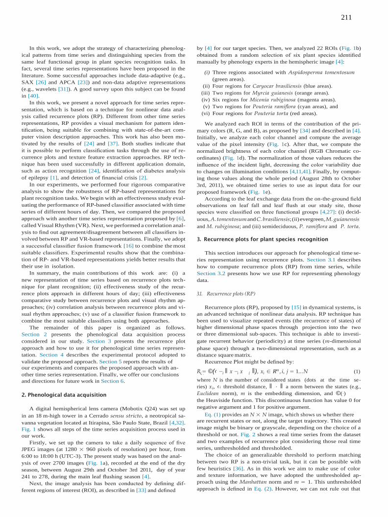
211

m i, j i i i other time series representation. Finally, we offer our conclusions

In this work, we adopt the strategy of characterizing phenolog-

ical patterns from time series and distinguishing species from the

same leaf functional group in plant species recognition tasks. In

fact, several time series representations have been proposed in the

literature. Some successful approaches include data-adaptive (e.g.,

SAX [26] and APCA [23]) and non-data adaptive representations

(e.g., wavelets [31]). A good survey upon this subject can be found

in [40].

In this work, we present a novel approach for time series repre-

sentation, which is based on a technique for nonlinear data anal-

ysis called recurrence plots (RP). Different from other time series

representations, RP provides a visual mechanism for pattern iden-

tification, being suitable for combining with state-of-the-art com-

puter vision description approaches. This work has also been mo-

tivated by the results of [24] and [37]. Both studies indicate that

it is possible to perform classification tasks through the use of re-

currence plots and texture feature extraction approaches. RP tech-

nique has been used successfully in different application domain,

such as action recognition [24], identification of diabetes analysis

of epilepsy [1], and detection of financial crisis [2].

In our experiments, we performed four rigorous comparative

analysis to show the robustness of RP-based representations for

plant recognition tasks. We begin with an effectiveness study eval-

uating the performance of RP-based classifier associated with time

series of different hours of day. Then, we compared the proposed

approach with another time series representation proposed by [6],

called Visual Rhythm (VR). Next, we performed a correlation anal-

ysis to find out agreement/disagreement between all classifiers in-

volved between RP and VR-based representations. Finally, we adopt

a successful classifier fusion framework [16] to combine the most

suitable classifiers. Experimental results show that the combina-

tion of RP- and VR-based representations yields better results that

their use in isolation.

In summary, the main contributions of this work are: (i) a

new representation of time series based on recurrence plots tech-

nique for plant recognition; (ii) effectiveness study of the recur-

rence plots approach in different hours of day; (iii) effectiveness

comparative study between recurrence plots and visual rhythm ap-

proaches; (iv) correlation analysis between recurrence plots and vi-

sual rhythm approaches; (v) use of a classifier fusion framework to

combine the most suitable classifiers using both approaches.

The remainder of this paper is organized as follows.

Section 2 presents the phenological data acquisition process

considered in our study. Section 3 presents the recurrence plot

approach and how to use it for phenological time series represen-

tation. Section 4 describes the experimental protocol adopted to

validate the proposed approach. Section 5 reports the results of

by [4] for our target species. Then, we analyzed 22 ROIs (Fig. 1b)

obtained from a random selection of six plant species identified

manually by phenology experts in the hemispheric image [4]:

(i) Three regions associated with Aspidosperma tomentosum

(green areas).

(ii) Four regions for Caryocar brasiliensis (blue areas).

(iii) Two regions for Myrcia guianesis (orange areas).

(iv) Six regions for Miconia rubiginosa (magenta areas).

(v) Two regions for Pouteria ramiflora (cyan areas), and

(vi) Four regions for Pouteria torta (red areas).

We analyzed each ROI in terms of the contribution of the pri-

mary colors (R, G, and B), as proposed by [34] and described in [4].

Initially, we analyze each color channel and compute the average

value of the pixel intensity (Fig. 1c). After that, we compute the

normalized brightness of each color channel (RGB Chromatic co-

ordinates) (Fig. 1d). The normalization of those values reduces the

influence of the incident light, decreasing the color variability due

to changes on illumination conditions [4,11,41]. Finally, by comput-

ing those values along the whole period (August 28th to October

3rd, 2011), we obtained time series to use as input data for our

proposed framework (Fig. 1e).

According to the leaf exchange data from the on-the-ground field

observations on leaf fall and leaf flush at our study site, those

species were classified on three functional groups [4,27]: (i) decid-

uous, A. tomentosum and C. brasiliensis; (ii) evergreen, M. guianensis

and M. rubiginosa; and (iii) semideciduous, P. ramiflora and P. torta.

3. Recurrence plots for plant species recognition

This section introduces our approach for phenological time se-

ries representation using recurrence plots. Section 3.1 describes

how to compute recurrence plots (RP) from time series, while

Section 3.2 presents how we use RP for representing phenology

data.

3.1. Recurrence plots (RP)

Recurrence plots (RP), proposed by [15] in dynamical systems, is

an advanced technique of nonlinear data analysis. RP technique has

been used to visualize repeated events (the recurrence of states) of

higher dimensional phase spaces through projection into the two

or three dimensional sub-spaces. This technique is able to investi-

gate recurrent behavior (periodicity) at time series (m-dimensional

phase space) through a two-dimensional representation, such as a

distance square matrix.

Recurrence Plot might be defined by:

our experiments and compares the proposed approach with an- R = ©(‹ − ǁ x − x ǁ), x ∈ R , i, j = 1...N (1)

and directions for future work in Section 6.

2. Phenological data acquisition

A digital hemispherical lens camera (Mobotix Q24) was set up

in an 18 m-high tower in a Cerrado sensu stricto, a neotropical sa-

vanna vegetation located at Itirapina, São Paulo State, Brazil [4,32].

Fig. 1 shows all steps of the time series acquisition process used in

our work.

Firstly, we set up the camera to take a daily sequence of five

JPEG images (at 1280 × 960 pixels of resolution) per hour, from

6:00 to 18:00 h (UTC-3). The present study was based on the anal-

ysis of over 2700 images (Fig. 1a), recorded at the end of the dry

season, between August 29th and October 3rd 2011, day of year

241 to 278, during the main leaf flushing season [4].

Next, the image analysis has been conducted by defining dif-

ferent regions of interest (ROI), as described in [33] and defined

where N is the number of considered states (dots at the time se-

ries) xi, ‹i threshold distance, ǁ · ǁ a norm between the states (e.g.,

Euclidean norm), m is the embedding dimension, and ©(·)

the Heaviside function. This discontinuous function has value 0 for

negative argument and 1 for positive argument.

Eq. (1) provides an N × N image, which shows us whether there

are recurrent states or not, along the target trajectory. This created

image might be binary or grayscale, depending on the choice of a

threshold or not. Fig. 2 shows a real time series from the dataset

and two examples of recurrence plot considering those real time

series, unthresholded and thresholded.

The choice of an generalizable threshold to perform matching

between two RP is a non-trivial task, but it can be possible with

few heuristics [36]. As in this work we aim to make use of color

and texture information, we have adopted the unthresholded ap-

proach using the Manhattan norm and m = 1. This unthresholded

approach is defined in Eq. (2). However, we can not rule out that

j

212

{ | }

Fig. 1. The time series acquisition process pipeline. (a) Sample image of the cerrado savanna; (b) Different segmentation scales are computed and the coarse scale is selected;

(c) Hemispherical image with the selected ROI’s species; (d) Channel representation are extracted from ROI’s; (e) RGB chromatic coordinates are computed; (f) Phenological

time series extracted from digital images.

Fig. 2. In (a), example of time series, (b) is an example of unthresholded RP, and (c) is an example of thresholded RP with ©(·) < 20, N = 37, and m = 1.

the extraction of shape information [13] is a research line to be

explored in future work.

Ri, j = |xi − x j|, xi ∈ R1, i, j = 1...N (2)

3.2. Recurrence plot for phenological time series representation

From phenology time series, it is possible to estimate changes

on phenological events, such as leaf flushing when analyzing

the green channel, or leaf color change and senescence using

values from the red channel [3,33]. It requires the analysis of

time series related to different color channels. The changing pat-

terns along time are then validated with on-the-ground phenology

observations.

However, color information in the RGB channels are highly

correlated (i.e., changes in one channel may lead to variations in

another), making harder to detect temporal changes in recurrent

phenology events.

The novelty of this paper is to extend the notion of recurrence

plots for the context of phenology. Here, we combine the time se-

ries into a single representation, making the phenological change

analysis easier. The key contribution of our idea is the combination

process we design to encode the time series into a single image.

Fig. 3 (a)–(c) illustrates the process of computing RP-based rep-

resentations. In (a), given the obtained time series in Fig. 1, the

recurrence plot algorithm is applied on these time series to cre-

ate their two-dimensional representation (distance matrix). Even

at this step, a normalization technique is applied to convert real

values to integer values in the typical range of grayscale images

([0, 255]). Then, in (b), a merging process is performed to join

the three distance matrices into a single color image. Finally, in

(c), many image descriptors may be used to encode visual proper-

ties (e.g., color, texture, and shape) from this color image into fea-

ture vectors. The feature vectors created through the use of image

descriptors are later used as input to a machine learning method

(e.g., support vector machine and k-Nearest Neighbors).

Fig. 4 shows the recurrence plots computed using the defined

ROIs. As RP provides a two-dimensional representation (distance

square matrix), we can observe many different colors in the matri-

ces, which are associated with the distance values between plots

on the time series. The lowest distance values are closer to the

blue color and the highest distance values are closer to the red

color. Notice that there are pattern differences among all of species

used in this work.

4. Experimental setup

This section describes the baseline used, which is based on vi-

sual rhythms (Section 4.1); presents the classifier fusion frame-

work adopted to combine VR-based and RP-based classifiers

(Section 4.2), and, finally, introduces the experimental protocol

(Section 4.3).

4.1. Baseline: visual rhythms (VR)

An effective way to analyze temporal properties from video

data is by means of visual rhythms [28]. The objective is to create

an abstraction of a video by coding the temporal change of pixel

values along a specific sampling line [20].

In the context of phenology, a time series comprised of images

taken by digital cameras at fixed time intervals can be viewed as

a video of the vegetation, as proposed by [5]. However, instead of

specific lines (e.g., diagonal, horizontal, and vertical), the interest

here is to analyze unshapely regions related to plant species that

are identified by phenology experts (see the initial step in Fig. 3).

Motivated by such limitations, [6] have generalized the notion

of visual rhythms. From a generic point of view, a visual rhythm

consists of temporal data samples grouped in an orderly manner.

For that, they have designed a mapping function to convert a ROI

into a vertical line. In the following, we briefly describe their strat-

egy for extracting visual rhythms from phenology time series. For

more details regarding their approach, refer to [9].

Let V = { ft }, t ∈ [1, T ] be a video, in domain 2D + t, with T

frames of dimensions WV × HV ; and I be a binary image, with the

same dimensions of V, in which white pixels indicate a ROI. Ini-

tially, the image I is converted into a list of Cartesian coordinates

Lxy = (x, y) I(x, y) = 1 . Next, this list is used for computing the

geometric center (xc, yc) of the ROI. Then, the Cartesian coordi-

nate system of the elements in Lxy is translated to have its ori-

gin at the point (xc, yc). After that, the Cartesian coordinates Lxy are converted to the polar coordinate system, creating a list of

213

| |

Fig. 3. The steps for feature extraction from the recurrence plot representation.

Fig. 4. Examples of recurrence plots for ROIs of each plant specie. These images

were created using the Octave software [14] with one-dimensional interpolation

method.

Fig. 5. Visual rhythms obtained for ROIs of some plant species. Text and figure have

been extracted from [6].

polar coordinates Lrθ . Thereafter, an index K = {k | ∀(r, θ ) ∈

Lrθ , k = 2πr + θ } is created to assign a unique value to each el-

ement in Lrθ . Finally, the keys in the index K are sorted in an in- creasing order and then used to arrange the elements in Lxy.

In this way, they defined a visual rhythm as a mapping of each

frame ft into a vertical line on an image R∗, in domain 1D + t, such

that [6]:

R∗ (t, z) = ft (Lxy(z)), t ∈ [1, WR∗ ], z ∈ [1, HR∗ ],

where WR∗ = T and HR∗ = Lxy are its width and height, respec-

tively. Figure 5 presents the visual rhythms produced by their ap-

proach using the ROIs from Fig. 3(b).

4.2. The classifier fusion framework

This section presents a framework for classifier selection and

fusion (FSVM), as devised in [16]. The objective of the fusion

framework is to exploit the degree of agreement/disagreement

among classifiers, concept known as diversity, with the objective

of selecting the most suitable ones to be used in a combination

scheme.

In the context of classifier fusion area and in this work, a classi-

fier might be defined as a tuple containing a learning method (e.g.,

kNN) and a description technique (e.g., Color Histogram). Classi-

fiers learn patterns from training instances and use learned models

to assign unseen instances to appropriate classes. Once the train-

ing step is finished, a selection process is performed to define

214

| |

{ }

Fig. 6. Time series-based classifier selection and fusion framework adapted from [16]. In (a), given a classification problem with training examples, different classifiers are

trained using data from training set T. In (b), the most discriminating classifiers are selected (C∗) by taking into account diversity measures (D). Finally, in (c), classifiers are

combined in a meta-learning approach using a SVM technique.

Fig. 7. The five steps for classifier selection are: (a) Compute diversity measures from the validation matrix MV; (b) R lists sorted by diversity measures scores; (c) Rt lists

with top t; (d) counts the number of occurrences of each classifier that satisfies a defined threshold; (e) Selected classifiers C∗ . Text and figure have been extracted from

[16].

classifiers whose combination, usually based on another learning

method (meta-learning), is more promising. The objective is to de-

termine the most discriminative methods, and, at the same time,

boosting the classification performance at test time by selecting

less, but more effective, classifiers.

Fig. 6 illustrates the framework FSVM for combining classifiers,

while Fig. 7 illustrates the adopted five-step approach for selecting

classifiers based on diversity measures, previously introduced by

Faria et al. [16].

First, diversity measures (set D in Fig. 7) are used to assess the

degree of agreement among available classifiers in C by taking into

account the MV matrix previously computed. That step is repre-

sented by arrow (a) in Fig. 7. Pairs of classifiers are then ranked

according to their diversity score. Each diversity measure defines a

different ranked list and, at the end of this step, a set R of ranked

lists is produced (arrow (b)). In the following, a novel set of ranked

lists Rt is computed by selecting the top t pairs of classifiers from

each ranked list in R (arrow (c)), and a histogram H that counts

the number of occurrences of a classifier in all ranked lists of Rt

is computed (arrow (d)). Finally, the most frequent classifiers in H,

whose accuracy is greater that a given threshold T , are combined

by a fusion approach (arrow (e)). T is a threshold defined in terms

of the average accuracy among all classifiers using the validation

set V.

4.3. Experimental protocol

In this work, we adopted the evaluation method used in [7].

It relies on the classification of time series extracted from pixels

associated with individuals of a same species. For that, we used

the algorithm introduced by [19] to segment the hemispheric im-

age into small polygons, obtaining 8, 849 segmented regions (SR).

Then, we associated each SR with a single ROI aiming to label it. A

labeled region is created if there is at least 80% of overlapped area

between an SR and a ROI. Finally, we extracted a time series from

each labeled region using the approach described in Section 2. In

this way, we built a dataset of 892 time series separated into six

classes, one for each plant species: A. tomentosum (96), C. brasilien-

sis (346), M. guianensis (36), M. rubiginosa (195), P. ramiflora (50),

and P. torta (169).

In the following, we present four experiments performed to val-

idate the use of the RP representation in plant recognition tasks.

First, in Section 5.1, we performed an effectiveness study con-

cerning the performance of classifiers that exploit RP-based fea-

tures associated with time series of different hours of day. In

this experiment, we used the k-Nearest Neighbors (kNN) learning

method. We set k = 1 , which achieved the best results in [12].

For describing time series encoded into a RP representation, we

used seven traditional and recently proposed image descriptors:

ACC [21], BIC [38], CCV [30], and GCH [39], for encoding color in-

formation; GFD [42], GIST [29], and HWD [22], for analyzing tex-

ture properties.

In the second experiment, in Section 5.2, we compared the pro-

posed RP-based approach with another time series representation

proposed by [6], called Visual Rhythm (VR). Two different effec-

tiveness experiments have been done:

(1) Coarse-grained Analysis (Section 5.2.1) that evaluates the ef-

fectiveness results of the recurrence plot-based and visual

rhythms-based classifiers; and

(2) Fine-grained Analysis (Section 5.2.2) that evaluates the best

effectiveness results achieved by both representations (RP

and VR) using different image descriptors (GFD and BIC).

In the third experiment, in Section 5.3, we performed a cor-

relation analysis to find out agreement/disagreement between all

classifiers involved in the previous experiment using RP and VR

representations.

In the fourth experiment, in Section 5.4, we adopt a success-

ful classifier fusion framework [16] to combine the most suitable

classifiers using both approaches (RP and VR) representations.

215

Means

Accu

racy

(%

) M

eans

Accu

racy

(%

)

A.tomentosum

70 C.brasiliensis

M.guianesis

M.rubiginosa

P.ramiflora

P.torta

A.tomentosum

70 C.brasiliensis

M.guianesis

M.rubiginosa

P.ramiflora

P.torta

60 60

50 50

40

30 29.03

20

27.07

23.75

20.49

25.01

23.69

25.91

23.42 23.73 22.93 21.02

25.92

31.47

40

30.96

30

20

26.67 25.12 24.92 25.91

22.69 22.13

23.64

24.29

22.61 23.24

31.05 30.85

10 10

0 6 7 8 9 10 11 12 13 14 15 16 17 18

Hours

(a) ACC

0 6 7 8 9 10 11 12 13 14 15 16 17 18

Hours

(b) BIC

A.tomentosum 70 C.brasiliensis

M.guianesis M.rubiginosa

P.ramiflora P.torta

A.tomentosum 70 C.brasiliensis

M.guianesis M.rubiginosa

P.ramiflora P.torta

60 60

50 50

40

32.24

30

20

26.35 25.65 25.59

23.46

22.77

20.78

23.55 25.01

19.55

23.05

30.69

29.69

40

30.87

30

20

27.61

24.81 23.93

26.58

20.88 20.46 22.78

24.83

21.20

23.47

32.92

27.72

10 10

0 6 7 8 9 10 11 12 13 14 15 16 17 18

Hours

(c) CCV

0 6 7 8 9 10 11 12 13 14 15 16 17 18

Hours

(d) GCH

A.tomentosum 70 C.brasiliensis

59.92

60 56.13

50

45.47

40

30

39.95

37.69

M.guianesis M.rubiginosa

37.08 36.19

32.68

P.ramiflora P.torta

52.67

41.05 41.06 42.48

65.09

A.tomentosum 70 C.brasiliensis

60.78

60

53.34

50

39.72

40

30

33.78 32.78

M.guianesis M.rubiginosa

35.34

29.96 31.51

37.60

35.79

P.ramiflora P.torta

42.50

39.64

58.51

20 20

10 10

0 6 7 8 9 10 11 12 13 14 15 16 17 18

Hours

(e) GFD

0

6 7 8 9 10 11 12 13 14 15 16 17 18

Hours

(f) GIST

A.tomentosum 70 C.brasiliensis

60

54.08

50 46.34

40

35.43

M.guianesis M.rubiginosa

35.11 35.64 34.27

34.92

39.16

P.ramiflora P.torta

42.90

36.33

50.47

70 66.82

60

50

40

58.72

A.toment C.brasil

48.90

39.13

41.91

M.guiane M.rubigi

40.83

34.91

38.15

P.ramifl P.torta

44.24 41.67

46.54

52.38

63.57

30 28.98 31.35

30

20 20

10 10

0 6 7 8 9 10 11 12 13 14 15 16 17 18

Hours

(g) HWD

0 6 7 8 9 10 11 12 13 14 15 16 17 18

Hours

(h) Merge of the seven descriptors

Fig. 8. In (a)–(g), effectiveness results of the kNN learning method using each of seven different image descriptors and in (f), results for all seven descriptors together..

Means

Accu

racy

(%

) M

eans

Accu

racy

(%

) M

eans

Accu

racy

(%

) M

eans

Accu

racy

(%

)

Means

Accu

racy

(%

) M

eans

Accu

racy

(%

)

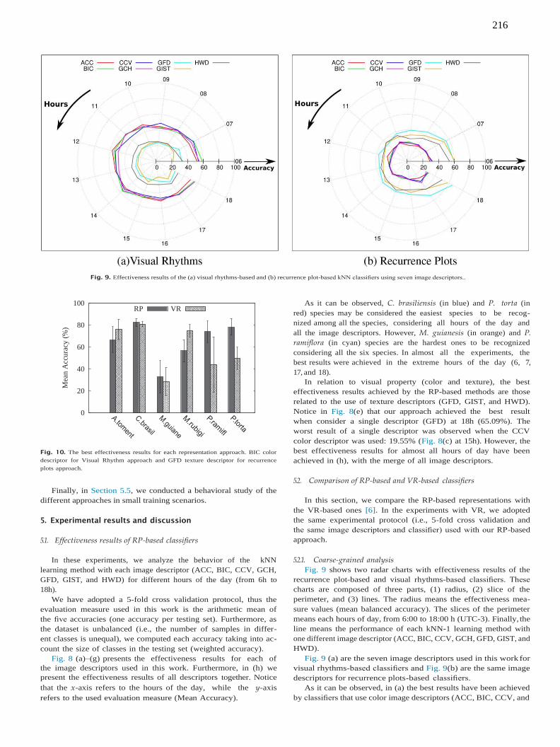
216

Fig. 9. Effectiveness results of the (a) visual rhythms-based and (b) recurrence plot-based kNN classifiers using seven image descriptors..

100

80

60

40

20

0

Fig. 10. The best effectiveness results for each representation approach. BIC color

descriptor for Visual Rhythm approach and GFD texture descriptor for recurrence

plots approach.

Finally, in Section 5.5, we conducted a behavioral study of the

different approaches in small training scenarios.

5. Experimental results and discussion

5.1. Effectiveness results of RP-based classifiers

In these experiments, we analyze the behavior of the kNN

learning method with each image descriptor (ACC, BIC, CCV, GCH,

GFD, GIST, and HWD) for different hours of the day (from 6h to

18h).

We have adopted a 5-fold cross validation protocol, thus the

evaluation measure used in this work is the arithmetic mean of

the five accuracies (one accuracy per testing set). Furthermore, as

the dataset is unbalanced (i.e., the number of samples in differ-

ent classes is unequal), we computed each accuracy taking into ac-

count the size of classes in the testing set (weighted accuracy).

Fig. 8 (a)–(g) presents the effectiveness results for each of

the image descriptors used in this work. Furthermore, in (h) we

present the effectiveness results of all descriptors together. Notice

that the x-axis refers to the hours of the day, while the y-axis

refers to the used evaluation measure (Mean Accuracy).

As it can be observed, C. brasiliensis (in blue) and P. torta (in

red) species may be considered the easiest species to be recog-

nized among all the species, considering all hours of the day and

all the image descriptors. However, M. guianesis (in orange) and P.

ramiflora (in cyan) species are the hardest ones to be recognized

considering all the six species. In almost all the experiments, the

best results were achieved in the extreme hours of the day (6, 7,

17, and 18).

In relation to visual property (color and texture), the best

effectiveness results achieved by the RP-based methods are those

related to the use of texture descriptors (GFD, GIST, and HWD).

Notice in Fig. 8(e) that our approach achieved the best result

when consider a single descriptor (GFD) at 18h (65.09%). The

worst result of a single descriptor was observed when the CCV

color descriptor was used: 19.55% (Fig. 8(c) at 15h). However, the

best effectiveness results for almost all hours of day have been

achieved in (h), with the merge of all image descriptors.

5.2. Comparison of RP-based and VR-based classifiers

In this section, we compare the RP-based representations with

the VR-based ones [6]. In the experiments with VR, we adopted

the same experimental protocol (i.e., 5-fold cross validation and

the same image descriptors and classifier) used with our RP-based

approach.

5.2.1. Coarse-grained analysis

Fig. 9 shows two radar charts with effectiveness results of the

recurrence plot-based and visual rhythms-based classifiers. These

charts are composed of three parts, (1) radius, (2) slice of the

perimeter, and (3) lines. The radius means the effectiveness mea-

sure values (mean balanced accuracy). The slices of the perimeter

means each hours of day, from 6:00 to 18:00 h (UTC-3). Finally, the

line means the performance of each kNN-1 learning method with

one different image descriptor (ACC, BIC, CCV, GCH, GFD, GIST, and

HWD).

Fig. 9 (a) are the seven image descriptors used in this work for

visual rhythms-based classifiers and Fig. 9(b) are the same image

descriptors for recurrence plots-based classifiers.

As it can be observed, in (a) the best results have been achieved

by classifiers that use color image descriptors (ACC, BIC, CCV, and

RP VR

Mea

n A

ccu

racy

(%

)

217

Fig. 11. Correlation analysis considering all 182 available classifiers (2 representation approaches × 7 image descriptors × 13 hours = 182 classifiers). The lowest correlation

coefficients are closer to the purple color (−1) and the highest coefficients are closer to the yellow color (+1). (For interpretation of the references to color in this figure

legend, the reader is referred to the web version of this article)..

100

95

90

85

80

75

70

65

60

55

100

90

80

70

60

50

Number of Classifiers |C*|

(a) MeanAccuracy

Number of Classifiers |C*|

(b) MeanAverage Accuracy

Fig. 12. Effectiveness performance considering (a) the mean accuracy and (b) the mean average accuracy when classifiers using RGB channels, RP, VR and both representa-

tions are combined.

GCH). However, in (b) the classifiers with texture image descriptors

have achieved the best results (GFD, GIST, and HWD).

5.2.2. Fine-grained analysis

For a more detailed analysis, we performed a comparison be-

tween the RP and VR approaches considering their performance

per class for the best achieved results. The best results of the RP

and VR approaches were observed when used with GFD (texture)

at 18h and BIC (color) at 6h, respectively. Fig. 10 shows this fined-

grained analysis.

We can observe that the RP approach achieved better results

in four (C. brasiliensis, M. guianensis, P. ramiflora, and P. torta) out

of the six species (see Fig. 10). The VR approach, in turn, yields

better results for A. tomentosum and M. rubiginosa. Furthermore, in

the experiments with P. ramiflora, and P. torta species, it is possible

to notice a large difference between results achieved by the RP-

based and VR-based approaches, around 30% of accuracy in both

species.

5.3. Correlation analysis between RP-based and VR-based classifiers

This section presents the correlation analysis of each pair

of classifiers for all 182 available classifiers aiming to identify

FSVM−RP+VR

FSVM−RP FSVM−VR

FSVM−RGB

FSVM−RP+VR

FSVM−RP FSVM−VR

FSVM−RGB

Mean

Accura

cy

(%

)

Mean

Avera

ge A

ccura

cy (

%)

218

| | { }

{ }

{ }

{ }

i j

(a + b)(c + d)(a + c)(b + d)

100

90

80

70

60

50

Training Set Size (%)

task. In additional, we consider the fusion of RGB channels as a

baseline approach [17].

Fig. 12 shows four curves, FSVM-RGB, FSVM-RP, FSVM-VR,

and FSVM-RP+VR, which refer to the fusion of the RGB channels,

recurrence plot, visual rhythms, and combination of RP and VR,

respectively. The suffix FSVM refers to the selection and fusion

framework, which was implemented using the SVM classifier in

the fusion step (meta-learning).

Two evaluation measures, Accuracy and Average Accuracy, are

considered. In these experiments, the framework combines each

approach for different numbers of classifiers |C∗|. In pink, the

framework combines |C∗| = {1, . . . , 39} RGB channels-based classi-

fiers (39 = 3 channels × 13 h). In green, the framework combines RP-

based classifiers |C∗| = {2, . . . , 91} (91 = 7 descriptors × 13 h). In

blue, it uses the VR-based classifiers C∗ = 2, . . . , 91 . Finally, in

red, the framework combines all available classifiers (91 RP-based

plus 91 VR-based classifiers, leading to a total of 182 classifiers).

As we can observe, the fusion framework using both representa- Fig. 13. Mean accuracy results of the best amount of classifiers for each approach

using training sets with different sizes.

whether them might be combined by any fusion technique (e.g.,

Adaboost [18], Bagging [10], and meta-learning approach [16]).

The Correlation Coefficient ρ (COR) [25] has been used to assess

the correlation of two classifiers ci and cj:

COR(c , c ) = , ad − bc

, (3)

tion (RP+VR) achieved a huge improvement when compared to the

use of the two representations in isolation.

As it can be observed, the FSVM-RGB approach has achieved the

better results on the range 1, . . . , 8 classifiers. However, FSVM-

RP+VR achieved the best results when more than 8 classifiers

are considered ( 9, . . . , 182 ). Therefore, we could show that re-

currence plot and visual rhythms representations address different

and complementary information that might be combined to im-

prove the effectiveness of plant identification systems.

where a is the percentage of time series that both classifiers ci and

cj classified correctly in a validation set. Value b is the percent-

age of time series that cj hit and ci missed, c is the opposite of b.

The value d is the percentage of time series that both classifiers

missed. The pairs of classifiers with lower COR values have greater

degree of complementarity and are more likely to yield better re-

sults when combined. Range of COR is in [−1, +1].

Fig. 11 presents the COR values for all possible combinations of

pairs of classifiers considering the six classes. The lowest correla-

tion coefficients are closer to the purple color (−1) and the highest

coefficients are closer to the yellow color (+1). Furthermore, in this

figure, there are six important regions that have been highlighted

and they are explained below.

As we can observe in Fig. 11(a), in region (1), the RP-based clas-

sifiers with texture descriptors are more correlated among them. In

region (2), the VR-based classifiers with color descriptors are more

correlated among them. This fact means that different classifiers

that use the same kind of visual proporties (color or texture) in

these approaches have predicted similar instances of the A. tomen-

tosum species. However, outside these two regions, the same sce-

nario can not be observed.

In general, although there are classifiers with high correlation

(regions 3, 4, 5, and 6), the great majority of classifiers are non-

correlated to each other (see purple color) for different species.

Thus, there is a strong indication that the RP-based and VR-based

classifiers used in this work might be combined to achieve better

results for plant recognition task.

In this sense, we adopt a well successfull classifier fusion

framework [16] (Section 4.2) to address complementary informa-

tion provided by RP-based and VR-based classifiers.

5.4. Fusion of RP-based and VR-based classifiers

In this section, we adopt the framework reported in

Section 4.2 (FSVM), with the objective of demonstrating that

is possible to combine different RP-based and VR-based classifiers

and to improve the effectiveness results in the plant recognition

In this section, we have conducted a study considering three

different sizes for the training set (25%, 50%, and 100%), which rep-

resents 15%, 30% and 60% of the entire datasets, respectively. These

subsets have been selected from original training set.

Fig. 13 shows comparative analysis of the four different

approaches FSVM-RGB-32, FSVM-RP-90, FSVM-VR-7, and FSVM-

RP+VR-91. Notice that FSVM approaches show up with a numerical

suffix N (e.g., N = 7, 32, 90, 91 ), which means the number of

classifiers each approach has used achieving the best effectiveness

results. Furthermore, we used again the 5-fold cross-validation

protocol.

Notice that the FSVM-RP+VR-91 approach, which combines RP-

based and VR-based classifiers, has achieved better results than

other approaches for any training set size.

6. Conclusion

In this work, we proposed the use of a technique of nonlin- ear

data analysis for time series representation in plant species

recognition task. This technique, called recurrence plot, allows us

to represent repeated events (the recurrence of states) on time se-

ries into two-dimensional representation. We have extracted fea-

ture vector from this new representation through use of different

kinds of image descriptor (e.g., color and texture). The created fea-

ture vector is then used as input to a learning method, in our case,

the k-Nearest Neighbor method.

The experiments performed in this work showed that there are

differences in terms of classification performance depending on the

plant species considered, as well as, the low correlation that exists

between almost all used classifiers. In these experiments, we ob-

served that texture descriptors describe better the image provided

from recurrence plots representation. However, the visual rhythms

achieved better results when used in color descriptors.

A correlation analysis between all of classifiers have been per-

formed and we could observe that recurrence plot-based and vi-

sual rhythms-based classifiers have low correlation coefficients, i.e.,

5.5. Training set size impact

FSVM−RP+VR−91 FSVM−RP−7

FSVM−VR−90 FSVM−RGB−32

Mea

n A

ccu

racy

(%

)

219

both approaches describe complementary information that might

be combined by fusion techniques with the objective of producing

better effectiveness results in plant recognition tasks.

Furthermore, we have adopted a successful classifier fusion

framework [16] to combine RP-based and VR-based classifiers and

then improve the effectiveness results. We could show in practice

the huge complementarity degree between those time-series rep-

resentations.

Future work includes the use of other image descriptors

to extract different visual features (e.g., shape description ap-

proaches based on contour and regions [13]). In addition, the

proposed framework can be augmented to consider learning- to-

rank methods (e.g., genetic programming [8]) for combining

different descriptors. Another point to be explored is the use of

RP for multispectral images or multisensor systems, which have

more than three time series. In these scenarios, remote sensing

approaches for channel selection and combination can be used.

Finally, we also plan to perform an extensive study on different

strategies for feature selection and classifier fusion.

Acknowledgments

This research was supported by the São Paulo Research Foun-

dation FAPESP and Microsoft Research Virtual Institute (grants

#2010/52113-5, #2013/50169-1, and #2013/50155-0). BA received

a master scholarship from CAPES and a doctoral fellowship from

FAPESP (grant #2014/00215-0); LPCM and RST receive a Produc-

tivity Research Fellowship from CNPq (grants 310761/2014-0

and 306580/2012-8). Also, we have been benefited from

funds of CAPES, CNPq, and FAPESP (grants #2009/18438-7 and

#2010/51307-0).

References

[1] U.R. Acharya, S. Vinitha Sree, G. Swapna, R.J. Martis, J.S. Suri, Automated eeg

analysis of epilepsy: a review, Knowl. Based Syst. 45 (2013) 147–165.

[2] P.M. Addo, M. Billio, D. Guegan, Nonlinear dynamics and recurrence plots for

detecting financial crisis. Documents de travail du Centre d’Economie de la

Sorbonne 13024, Universit Panthon-Sorbonne (Paris 1), Centre d’Economie de

la Sorbonne, 2013.

[3] H. Ahrends, S. Etzold, W. Kutsch, R. Stoeckli, R. Bruegger, F. Jeanneret, H. Wan-

ner, N. Buchmann, W. Eugster, Tree phenology and carbon dioxide fluxes: Use

of digital photography for process-based interpretation at the ecosystem scale,

Clim. Res. 39 (2009) 261–274.

[4] B. Alberton, J. Almeida, R. Henneken, R. da S. Torres, A. Menzel, L.P.C. Morellato,

Using phenological cameras to track the green up in a cerrado savanna and its on-

the-ground validation, Ecol. Inform. 19 (2014) 62–70.

[5] J. Almeida, J.A. dos Santos, B. Alberton, L.P.C. Morellato, R. da S. Torres, Plant

species identification with phenological visual rhythms, in: Proceedings of the

IEEE International Conference on eScience (eScience’13), 2013a, pp. 148–154.

[6] J. Almeida, J.A. dos Santos, B. Alberton, L.P.C. Morellato, R. da S. Torres, Vi-

sual rhythm-based time series analysis for phenology studies, in: Proceed-

ings of the IEEE International Conference on Image Processing (ICIP’13), 2013,

pp. 4412–4416.

[7] J. Almeida, J.A. dos Santos, B. Alberton, R. da S. Torres, L.P.C. Morellato, Apply-

ing machine learning based on multiscale classifiers to detect remote phenol-

ogy patterns in cerrado savanna trees, Ecol. Inform. 23 (2014) 49–61.

[8] J. Almeida, J.A. dos Santos, W.O. Miranda, B. Alberton, L.P.C. Morellato, R. da S.

Torres, Deriving vegetation indices for phenology analysis using genetic pro-

gramming, Ecol. Inform. 26 (2015) 61–69.

[9] J. Almeida, J.A. dos Santos, B. Alberton, L.P.C. Morellato, R. da S. Torres, Pheno-

logical visual rhythms: compact representations for fine-grained plant species

identification, Pattern Recogn. Lett. (2016), doi:10.1016/j.patrec.2015.11.028.

[10] L. Breiman, Bagging predictors, Mach. Learn. 24 (2) (1996) 123–140.

[11] H.-D. Cheng, X. Jiang, Y. Sun, J. Wang, Color image segmentation: advances and

prospects, Pattern Recogn. 34 (12) (2001) 2259–2281.

[12] J.C. Conti, F.A. Faria, J. Almeida, B. Alberton, L.P.C. Morellato, J.L. C., R. da S.

Torres, Evaluation of time series distance functions in the task of detecting re-

mote phenology patterns, in: Proceedings of the IEEE International Conference

on Pattern Recognition (ICPR’14), 2014, pp. 3126–3131.

[13] R. da S. Torres, M. Hasegawa, S. Tabbone, J. Almeida, J.A. dos Santos, B. Al-

berton, L.P.C. Morellato, Shape-based time series analysis for remote phenol-

ogy studies, in: Proceedings of the IEEE International Geoscience and Remote

Sensing Symposium (IGARSS’13), 2013, pp. 3598–3601.

[14] J.W. Eaton, D. Bateman, S. Hauberg, GNU Octave Manual Version 3, Network

Theory Ltd., 2008.

[15] J.-P. Eckmann, S.O. Kamphorst, D. Ruelle, Recurrence plots of dynamical sys-

tems, Europhys. Lett. 4 (9) (1987) 973.

[16] F.A. Faria, J.A. dos Santos, A. Rocha, R. da S. Torres, A framework for selection

and fusion of pattern classifiers in multimedia recognition, Pattern Recogn.

Lett. 39 (2014) 52–64.

[17] F.A. Faria, J. Almeida, B. Alberton, L.P.C. Morellato, A. Rocha, R. da S. Torres,

Time series-based classifier fusion for fine-grained plant species recognition,

Pattern Recogn. Lett (2016), doi:10.1016/j.patrec.2015.10.016.

[18] Y. Freund, R.E. Schapire, Experiments with a new boosting algorithm, Update

(1996) 148–156.

[19] L. Guigues, J. Cocquerez, H. Le Men, Scale-sets image analysis, Int. J. Comput.

Vis. 68 (2006) 289–317.

[20] S.J.F. Guimar aes, M. Couprie, A.A. Araújo, N.J. Leite, Video segmentation based

on 2D image analysis, Pattern Recogn. Lett. 24 (7) (2003) 947–957.

[21] J. Huang, R. Kumar, M. Mitra, W. Zhu, R. Zabih, Image indexing using color cor-

relograms, in: Proceedings of the IEEE International Conference on Computer

Vision and Pattern Recognition (CVPR’97), 1997, pp. 762–768.

[22] C.E. Jacobs, A. Finkelstein, D.H. Salesin, Fast multiresolution image querying, in:

Proceedings of the International Conference on Computer Graphics and Inter-

active Techniques (SIGGRAPH’95), 1995, pp. 277–286.

[23] E.J. Keogh, K. Chakrabarti, S. Mehrotra, M.J. Pazzani, Locally adaptive dimen-

sionality reduction for indexing large time series databases, in: Proceedings

of the ACM SIGMOD International Conference on Management of Data (ACM

SIGMOD’01), 2001, pp. 151–162.

[24] K. Kulkarni, P. Turaga, Recurrence textures for human activity recognition from

compressive cameras, in: Proceedings of the IEEE International Conference on

Image Processing (ICIP’12), 2012, pp. 1417–1420.

[25] L.I. Kuncheva, Combining Pattern Classifiers: Methods and Algorithms, Wi- ley-

Interscience, 2004.

[26] J. Lin, E.J. Keogh, L. Wei, S. Lonardi, Experiencing SAX: a novel symbolic repre-

sentation of time series, Data Min. Knowl. Discov. 15 (2) (2007) 107–144.

[27] L.P.C. Morellato, R.R. Rodrigues, H.F. Leit ao Filho, C.A. Joly, Estudo comparativo

da fenologia de espécies arbóreas de floresta de altitude e floresta mesófila

semidecídua na serra do iapí, jundiaí, são paulo, Brazil. J. Botany 12 (1989) 85–

98.

[28] C.W. Ngo, T.C. Pong, R.T. Chin, Detection of gradual transitions through tem-

poral slice analysis, in: Proceedings of the IEEE International Conference on

Computer Vision and Pattern Recognition (CVPR’99), 1999, pp. 1036–1041.

[29] A. Oliva, A. Torralba, Modeling the shape of the scene: a holistic representation

of the spatial envelope, Int. J. Comput. Vis. 42 (3) (2001) 145–175.

[30] G. Pass, R. Zabih, J. Miller, Comparing images using color coherence vec-

tors, in: Proceedings of the ACM International Conference on Multimedia (ACM-

MM’96), 1996, pp. 65–73.

[31] I. Popivanov, R.J. Miller, Similarity search over time-series data using wavelets,

in: Proceedings of the IEEE International Conference on Data Engineering

(ICDE’02), 2002, pp. 212–221.

[32] P. Reys, M.G.G. Camargo, A.P. Teixeira, M.A. Assis, M.T. Grombone-Guaratini,

L.P.C. Morellato, Estrutura e composição florística entre borda e interior de um

cerrado sensu stricto e sua importância para propostas de recuperação, Hoen-

nea 40 (3) (2013) 437–452.

[33] A.D. Richardson, B.H. Braswell, D.Y. Hollinger, J.P. Jenkins, S.V. Ollinger, Near–

surface remote sensing of spatial and temporal variation in canopy phenology,

Ecol. Appl. 19 (2009) 1417–1428.

[34] A.D. Richardson, J.P. Jenkins, B.H. Braswell, D.Y. Hollinger, S.V. Ollinger,

M.L. Smith, Use of digital webcam images to track spring greep-up in a de-

ciduous broadleaf forest, Oecologia 152 (2007) 323–334.

[35] M.D. Schwartz, Phenology: An Integrative Environmental Science, Springer,

2013.

[36] D.F. Silva, V.M.A. de Souza, G.E.A.P.A. Batista, Time series classification using

compression distance of recurrence plots, in: Proceedings of the IEEE Interna-

tional Conference on Data Mining (ICDM’13), 2013, pp. 687–696.

[37] V.M.A. Souza, D.F. Silva, G.E.A.P.A. Batista, Extracting texture features for time

series classification, in: Proceedings of the IEEE International Conference on

Pattern Recognition (ICPR’14), 2014, pp. 1425–1430.

[38] R. Stehling, M. Nascimento, A. Falcao, A compact and efficient image retrieval

approach based on border/interior pixel classification, in: Proceedings of the

ACM International Conference on Information and Knowledge Management

(CIKM’02), 2002, pp. 102–109.

[39] M. Swain, D. Ballard, Color indexing, Int. J. Comput. Vis. 7 (1) (1991) 11–32.

[40] X. Wang, A. Mueen, H. Ding, G. Trajcevski, P. Scheuermann, E.J. Keogh, Experi-

mental comparison of representation methods and distance measures for time

series data, Data Min. Knowl. Discov. 26 (2) (2013) 275–309.

[41] D.M. Woebbecke, G.E. Meyer, K. Von Bargen, D.A. Mortensen, Color indices for

weed identification under various soil, residue, and lighting conditions, Trans.

ASAE 38 (1995) 259–269.

[42] D. Zhang, G. Lu, Shape-based image retrieval using generic fourier descriptor,

Signal Process.: Image Commun. 17 (10) (2002) 825–848.

220

Appendix E

Article published in the Journal Pattern Recognition Letters:

LEITE, R.A., SCHNORR, L, ALMEIDA JR, TORRES, R.S., ALBERTON, B., MORELLATO, LPC, COMBA,

J. PhenoVis – Visual Phenological Analysis of Forest Ecosystems. Information Sciences, v. 372, p. 181-195,

2016.

223

Text formatting according to the Journal Information Sciences.

PhenoVis – A tool for visual phenological analysis of digital camera images using chronological percentage

maps

Roger A. Leitea, Lucas Mello Schnorra, Jurandy Almeida b,d, Bruna Albertonc, Leonor Patricia C. Morellatoc, Ricardo da

S. Torres d, João L.D. Comba a,∗

a Institute of Informatics, Federal University of Rio Grande do Sul – UFRGS, Porto Alegre RS–91501-970 Brazil

b Institute of Science and Technology, Federal University of São Paulo – UNIFESP, São José dos Campos, SP–

12247-014 Brazil

c Dept. of Botany, São Paulo State University – UNESP, Rio Claro, SP–13506-900 Brazil

d Institute of Computing, University of Campinas – UNICAMP Campinas, SP–13083-852 Brazil

Keywords: Phenology, Remote sensing, Vegetation index, Visual analytics, Similarity ranking

1. Introduction

Phenology studies the periodic phenomena of plants and their relationship to environmental conditions [39].

This analy- sis is crucial for accessing the impact on vegetation and ecosystem processes [29,32,39,42].

Examples of cyclic phenomena include flowering and fruiting in plants and the breeding season of birds and

frogs, among others. The remote monitoring of vegetations using cameras has proved to be a promising

approach to the study of plant phenology [30,38,40]. In this scenario, cameras capture daily pictures from a

specific viewpoint at a specific time of the day. By comparing a sequence of images over time, it is possible to

identify changes that are associated with phenological events [38]. For example, images that have a high number

of pixels with dominant shades of green are often associated with areas mostly covered by leaves.

Due to the large number of images (at least 365 images per year), the visual analysis of large collections of

images becomes too complex to be performed interactively. Instead, a single chromatic value is computed to

represent the average color in each image. Among several chromatic coefficients described in the literature, the

green chromatic coefficient (gcc) is widely used by the phenology community to understand periodic leafing

patterns extracted from digital images [40]. The collection of values computed in the period of interest (usually

one year) is displayed as a 2D line plot [3], and the analysis

∗ Corresponding author. Fax: +55 (51) 3308-7308.

E-mail addresses: rogeraleite@gmail.com (R.A. Leite), schnorr@inf.ufrgs.br (L.M. Schnorr), jurandy.almeida@unifesp.br (J.

Almeida), bru.alberton@gmail.com (B. Alberton), pmorella@rc.unesp.br (L.P.C. Morellato), rtorres@ic.unicamp.br (R.d.S. Torres),

comba@inf.ufrgs.br, joao.comba@gmail.com (J.L.D. Comba).

Fig. 1. Images of the Takayama forest from different years (2004, 2007, 2012, and 2013) and days (281, 288, 293, and 291), generated by the Phenological

Eyes Network (PEN). Although the images look very different, they have the same average gcc = 0.3905.

224

of this plot is used to identify interesting phenological events. It is well known that using the average as a

comparison metric to analyze the images can potentially overlook important patterns and thus lead to wrong

conclusions [14]. One motivation for this research is to address the shortcomings of using average scores in

near-surface remote phenology.

Fig. 1 illustrates the problem with the average in four different images captured by the same device on

different dates. Each image looks different when compared to the others, but all of them share the same gcc

average of 0.3905 (the pixels associated with the metallic structure are discarded). Therefore, by using the

traditional average-based approach, phenolo- gists will be led to conclude that these four images are the same

even if they are completely different in reality. The similar distribution of the shades of green, yellow and

brown in the images indicates that 2012 was a full fall season, whereas in 2004 the levels of green were much

higher (Fig. 1).

In this work, we introduce PhenoVis, a visual analytics tool that aims at providing insightful ways to analyze

phenological data. The main idea behind PhenoVis is the creation of more expressive visual encodings for

phenological data visualization. We introduce the Chronological Percentage Maps (CPMs), a visual mapping

technique that combines derived distributions from all images of a given year to create normalized stacked bar

charts. Another problem we address is the lack of automa- tion in the search for regular patterns in plant

phenology. Current research in the field frequently uses the analyst’s intuition to find patterns of plant

phenology. This approach is potentially time-consuming, error-prone and unable to scale to larger datasets.

PhenoVis uses the additional information encoded to support similarity searches, which is useful for comparing

data from different years. It also provides a customizable multi-rank comparison of data from different years,

with filters of specific periods within a year or sub-regions associated with given plant species.

In summary, we offer the following contributions: (a) PhenoVis, a visual analytics tool to perform a

comparative analysis of phenological data for multiple years; (b) the design of CPMs, in which a more

expressive representation of phenological data using percentage distributions is combined with a visual

expression of this information using color-coded normalized stacked bar charts; (c) similarity algorithms that

allow the search for similar phenological patterns across years, occurring in either a fixed or moving

window of time; (d) customizable ranking comparison of years, with filters that allow selections of specific

time periods or regions; and (e) case studies that validate PhenoVis in phenological analysis tasks such as

pattern and outlier identification.

2. Related work

Below, we review visual analytics and information visualization techniques and approaches to analyse

phenological data extracted from images.

2.1. Visualization and data Analysis There is an extensive literature in the information visualization and visual analytics community on different

ways to visually present information and to extract patterns from data [25]. Rectangular regions such as

matrices are a common alternative for presenting aggregated data to allow identification of patterns. Pixel bar

charts extend traditional bar charts by coloring pixels inside bars to represent information derived from data

attributes [26]. The visual presentation of data follows a pixel-placement ordering, which was demonstrated to

reveal patterns in data [24] as well as provide support for data mining queries. The underlying motivation

behind pixel bars was an inspiration when designing PhenoVis, particularly the CPM representation and the

ability to search for similar patterns in CPMs of different years.

There are several works that use matrix-encoded information to perform visual analysis. Stacked bar charts

are used to display the temporal changes of traffic speed data in [8]. The normalized stacked bar charts used in

CPMs resemble the images showed in their work, especially when using a categorical color mapping. The

analysis of visual traffic also appears in [43], with trajectory information chronologically encoded into a

225

matrix. Matrices are used to compare genomic sequences in [2,34]. BallotMaps encode the votes received by

politicians into matrices to identify voting patterns [46]. The Flowstrates approach encodes origin-destination

data into a heatmap matrix, re-ordering rows to reveal interesting patterns [9]. In [36], a matrix encoding

heart-rate information is used to identify unusual patterns during a running race. The exploration of dynamic

graphs using matrix-encoded information is given in [12] and [18]. Climate change comparison using a

global

radial map is presented in [27]. Although it uses a radial representation, the compact representation

resembles the CPM stacked bar charts. ThemeRiver [11,19,20] offers an alternative to stacked bar charts by

displaying information in layers that are stacked in a symmetrical shape centered around the x-axis. This

approach allows easy identification of predominant layers in time, particularly for datasets comprising a

great number of layers. LineUp describes different ways to present multi-ranking attributes [17]. The

multi-ranking visualization used in our work reveals the need for ranking visualization when performing

comparative phenology analysis. We refer the reader to [1] for a comprehensive survey of other ways to

perform visual analysis of time-oriented data.

2.2. Phenological analysis Phenology analysis of satellite images often relies on average plots of computed vegetation indices. A web-

based in- terface described in [10] displays time-series obtained from phenological and meteorological

observations. TimeStats is a free software that offers tools for the visualization of long-term remote sensing

data archives such as parametric and non- parametric methods for trend detection, linear regression, and

frequency analysis [41]. EcoIP, a toolkit to estimate the onset and ending dates of phenological phases of plant

species, relies on a Naïve Bayesian model created from a set of training images, which is used to provide

temporal estimators [16]. A variety of color transformations is used to adjust the accuracy of the estimations.

Another recent trend refers to the construction of toolboxes. Eerens, for example, developed SPIRITS, a stand-

alone toolbox to produce evidence-based information for crop production analysts [13]. It includes a large

number of features to analyze image time series and to create maps and graphs for vegetation status analysis.

Different from those initiatives, our proposal relies on visual encodings designed to capture distribution aspects

from vegetation data. A similar approach is taken in [5] and [6], which presented different strategies for

encoding image time series as visual rhythms [33]. Such representations have proven to be a powerful tool for

distinguishing the behavior of different plant species. The visual rhythm construction is similar to the CPM

extraction process in the sense that they summarize image sequences in a single image representation. Despite

the good results observed concerning the use of visual rhythm, no visual analytics tool has been proposed.

3. PhenoVis

PhenoVis is a visualization tool that includes a visual mapping representation called CPM, data analysis

algorithms for identifying similar patterns in different years, and a ranking visualization module to present the

similarity results. In this section, we describe each of these modules.

3.1. Chronological percentage maps (CPMs) CPM is the main concept behind PhenoVis. Its construction consists of six steps that transform a sequence of

images into a normalized stacked bar chart, as shown in Fig. 2. We detail these steps in the following

sections.

Step 1: Filtering by region of interest (ROI) The region of interest (ROI) (also called mask) is a portion of the input image that is the focus of the analysis,

thus removing irrelevant areas that lack vegetation such as the observation tower. The ROI is user-configurable

and implemented through a mask with the same dimensions as the input images. The mask is composed of black

226

and white pixels (a stencil

image), where white represents selected regions. Two types of masks are used in PhenoVis: a community mask

[21], which considers all plant species in the image; and a species mask [30], associated with a given plant

species.

Step 2: Data transformation using a vegetation index

The phenophases and length of the growing season (from start to end) are indicators of plant development

across dif- ferent years. The phenological analysis from images focuses on the following four checkpoints (or

phenophases) of plant development [21,30]:

• Leaf expansion: plants start to turn green, and leaves are expanding;

• Peak or maturity: leaf growth reaches a plateau; i.e., leaves reach full size;

• Leaf fall or senescence: leaves change colors and start to fall;

• Post leaf fall: there are no leaves on the tree, representing the end of the growing season.

Among the several images taken at different times of the day, the image taken at noon is preferred for the

analysis because it minimizes shadow effects. Therefore, only one image per day is used. The analysis

considers the chromatic co- efficients associated with each pixel in the image. Different vegetation indexes are

described in [40]. The RGB chromatic coefficients (rcc, gcc and bcc) are defined by respectively dividing each

component (R, G, or B) by the sum of the other com- ponents (R + G + B). The average plot of gcc is a good

indicator of phenophases due to the encoding of green pigments (e.g., chlorophyll) in leaves. Although most of

our analysis used the gcc chromatic coefficient, we also experimented with the hue index discussed in [15]. To

use this index, it is necessary to convert colors from the RGB color space into the HSV (also called HSI) color

space [44], which represents colors as hue (H), saturation (or lightness) (S), and value (or brightness) (V).

HSV is associated with a single line of the CPM. In this example, all lines of the CPM are stacked in

landscape mode.

Fig. 2. The Chronological Percentage Map’s six-step construction: (1) images are filtered by the community mask that defines the region of interest

(ROI); (2) phenology metric (gcc) is computed; (3) interval of interest (IOI) filters the resulting values; (4) selection of the distribution granularity and

associated color values; (5) percentage distribution is computed; (6) mapping color values to the percentage distribution. Each image generates a

stacked bar chart defined in a cone using cylindrical coordinates, with shading variations defined by the angle around the central vertical axis of the cone (the hue

component).

Step 3: Filtering by interval of interest (IOI)

227

Each vegetation index has values in a particular range. For example, gcc is normalized between 0 and 1. In

practice, the range of gcc found in vegetation images is much smaller, usually between 0.3 and 0.5 [47]. Since we

compute a histogram of vegetation indexes, we narrow the limits of the histogram to a user-specified interval of

interest (IOI), as shown in Fig. 2, step 3.

Step 4: Color palette and histogram granularity

Selecting a good color palette is essential in data analysis [28]. In PhenoVis we associate different colors

with each bucket of the percentage histogram. The histogram granularity defines the size of a given bucket of

the percentage distribution. The number of buckets is given by the number of colors available, and the range

of the distribution is given by the IOI. There

are trade-offs when selecting the size of the IOI, granularity, and the number of colors. For example, if the interval is small

and the number of colors is large, each dimension of the IOI will be semantically irrelevant because of the

resultant tiny grain size. The same problem appears if the interval is too large and the number of colors is

small. The best situation arises when there is a balance between the size of the IOI and the number of colors.

The typical IOI for the gcc varies from 0.3 to 0.5. Therefore, we chose 20 colors, with each bucket size being 0.01 wide.

For convenience, we have pre-defined a set of palettes. From this set, the categorical color table in Fig. 2,

step 4 was the preferred choice when using gcc indexes. The palette has four categories with different colors.

Each of the five internal divisions of these four zones has distinct levels of saturation (from dark to light brown,

for example). On the other hand, the standard hue color table is the choice when using hue indexes.

Step 5: Calculating the percentage data distribution

Each pixel in a given input image contributes one vegetation index value to the analysis, and when this

value is multi- plied by the number of images in a year (365), a huge amount of data is generated. Instead,

the average of all indexes in an image is used, leading to only 365 indexes. Average plots of these indexes

help identify phenophases; however, this analysis may be misleading since different images might have the

same index (see Fig. 1). In PhenoVis, we store more information about each image than a single vegetation

index. We use a histogram instead to encode the percentage distribution of veg-

etation indexes in an image. The range of the histogram is defined by the IOI, and the number of buckets

by the size of color palette used. For indexes outside the IOI, we either discard the values or clamp them to

the nearest extreme bucket. We repeat this process to compute one percentage distribution for each image.

In some situations two distinct RGB colors may have the same gcc (Fig. 3), and would therefore be accumulated

in the same histogram bin and mapped to the same color. In these situations, the hue index can be used

alternatively. The corresponding hue values in Fig. 3 are different and can be mapped to distinct colors. Shades of green can be found around hue values of 120. In addition, the mapping of hues into colors can use the

standard HSV palette at fixed S and V values. We did not replace gcc by the hue index, but used it to gain

additional insights when looking at the data.

Fig. 3. Colors with the same gcc of 0.4 (RGB codes are shown above each color). On the other hand, the corresponding hue values are distinct. By using the hue

values to separate these colors, the histogram can better aggregate shades of green into closer bins.

228

Step 6: Creating the normalized stacked bar chart

The percentage map of a single input image consists of a normalized stacked bar chart (vertical bar in Fig. 2,

step 6). In this example, the height of the chart is proportional to the frequency count in the percentage

distribution of the vegetation indexes. The width is associated with the number of pixels available for drawing

the percentage map. Colors are defined by the palette being used and their corresponding histogram entries.

The chronological percentage map consists of a sequence of percentage maps stacked in chronological order,

from top to bottom (portrait) or left to right (landscape). In our analysis, each CPM corresponds to all images

from a single year. Fig. 4 and Fig. 5 demonstrate the percentage map and CPM chart for images captured in Japan

(the TKY dataset [31,35]). Fig. 4 illustrates percentage maps for individual days of 2006; each map uses two

vegetation indexes. The first one uses gcc

and a categorical color table where shades of green, blue, and purple respectively correspond to gcc values between 35 −40%, 40 − 45%, and 45 − 50%. The second one uses the hue index and the hue color mapping. The color mapping is applied over the input camera to illustrate the shading variations for each chromatic coefficient. Fig. 5 shows the complete CPM for all days in 2006. Higher gcc values are associated with greener regions, and a clear pattern of growing season emerges in the middle of the year. In the hue mapping, the growing season is associated with shades of green. Fig. 5 illustrates CPM charts that use different vegetation indexes for the year 2006. This CPM allows us to investigate interesting patterns outside the growing season, which displays shades of red and blue.

3.2. Multi-year phenological analysis The comparative analysis of data from different years is one question that drives plant phenological analysis.

The com- parison of the starting dates of a given phenophase (e.g. start of leaf growing season) allows us to

identify how these values changed with the progression of the years. Automated similarity comparison of

different phenophases is important in this process. PhenoVis provides an automatic similarity analysis, because

more data is encoded in percentage distributions. The user can select a time interval directly over the CPM of

one year, and PhenoVis will suggest a similarity rank of the other years based on this pattern. In this section, we

describe how PhenoVis performs the similarity search and displays the visualization results.

3.2.1. Search period and ROIs

PhenoVis allows the user to define any period of a given year to serve as the basis of comparison against

other years. This period of interest used for searches can be manually configured in the interface by specifying

start and end dates. Since most queries are related to the analysis of pattern variations in specific phenophases,

such as the leaf expansion or fall period, we allowed the user to select the period of interest from pre-defined

phenophases. The search can be performed over the ROI of all plant specifies in the image (community mask),

other pre-defined masks of any given species, or any region in general specified by the user.

3.2.2. Similarity metrics

PhenoVis offers four similarity techniques for automatic search: Mean Absolute Error (MAE), Mean Square Error

(MSE), Mean Absolute Percentage Error (MAPE), and the Kullback-Leibler Divergence (KLD) as described in the

supplementary ma- terial. The MAE is a usual estimator of the difference between two matrices. Used for the same

reasons, MSE highlights significant gaps between values due to squared distance computations and is not

recommended for noisy datasets. MAPE is a normalized solution based on the percentage of the similarity for two

samples, while the KLD is a non-symmetric measure of the difference between probability distributions. The

similarity is computed using two CPMs as input. The first parameter is the CPM query, defined by its start and end

dates. The second parameter is the CPM candidate, which will necessarily have the same number of days as the

target, but the start date may differ. The percentage distribution associated with each CPM subset is interpreted as a

matrix of values in which the similarity metric is computed. Errors are computed for each matrix entry and

accumulated in the resulting similarity error.

229

030 085 117 128 137 142

Fig. 4. Percentage maps for 12 days: original data for the respective days (row 1 and 4), recoloring of pixels using gcc and a brown-green-blue-purple

color mapping (rows 2 and 5), and recoloring using the hue index and hue mapping (rows 3 and 6). The percentage maps for the gcc (left) and hue (right)

indexes are shown.

3.2.3. Searching windows and filters

The query defines a time period in the CPM of a given year. The search for similar patterns looks for CPM

subsets that have the same number of days as the query pattern. This search is implemented in two configurable

ways. The first one, referred to as fixed window, looks for CPM subsets with matching start and end dates. The

result of this comparison gives the years in which the same pattern occurred on the same days of the year. In the

second way, referred to as moving window, the search looks for the same pattern but does not fix the starting

day, allowing the window to move throughout the year. This search finds patterns that happened at a different

time of the year (e.g., a late growing season) in other years. We also implemented a filter that allows a subset of

the percentage distribution to be considered. If the analysis is interested only in gcc values in the interval of 40%

to 45%, the similarity search can be set to filter out values outside this interval. We also have an outlier filter that

removes outliers (missing data or odd days) from the similarity search. An automatic outlier detection was

implemented by taking into account the percentage distribution of a given day and the distribution of adjacent

days.

187 284 288 300 336 349

030 085 117 128 137 142 187 284 288 300 336 349

230

Fig. 5. CPM example for 365 days displayed in portrait mode. Each line corresponds to a normalized stacked bar chart mapped to the predefined color table:

(a) categorical color table using the gcc index, (b) HSV color table using the hue index.

3.3. Single and multi-year ranking PhenoVis is also capable of creating a single or multi-year ranking according to the query and selected

similarity tech- nique. The ranking includes the distributions for different years in order of similarity and the

similarity error, which allows the evaluation of how the years differ among them. The single-year ranking

generates a histogram plot that allows the comparison of one specific year’s distribution against all others. The

goal of this ranking is to compare the phenophases of one year against the others. In the case of a moving

window, the ranking also includes the distance (in days) of the closest pattern.

The multi-year ranking creates similarity searches between a pair of ROIs in a given period of time for every

pair of years. This process first results several histogram plots, one for each year, that indicate how close or

distant the other years are. These histograms can be normalized as needed; in PhenoVis we use three

normalizations: single-year normalization, multi-year normalization, and global normalization (using the data for

all years and all pairwise comparisons). The resulting histograms are drawn in red, green and blue, respectively.

The second result is a histogram plot that summarizes the indi- vidual yearly histogram plots by associating a

distance from one year to the others. In other words, this histogram displays the most common year and the most

different years as distances between each other, which allows us to easily identify the average years. The resultant

histogram is drawn in magenta. Fig. 6 illustrates the interface of PhenoVis, and samples of these histograms are

shown in Fig. 6(b).

4. Visualization results and discussion

PhenoVis was implemented using the programming language Processing [37]. The input to the system is a

collection of raw images grouped by year and a mask image that defines the region of interest. In off-line computation,

the mask is applied for all input images, and the percentage distributions are computed and stored. PhenoVis was

tested, under permission, with the Takayama Flux Site (TKY) dataset of the Phenological Eyes Network (PEN)

[31,35]1. TKY is located in Japan, which has images from multiple years (from 2004 onward) of a deciduous

broadleaf forest [30]. For the results below we used the 600 × 600 image resolution database due to its reduced

pre-processing time. Experiments conducted with the larger resolution dataset (2272 × 1704) showed similar results

to the smaller dataset. We aim to extend our prototype for the larger resolution datasets, possibly using

parallel computation to speed-up pre-processing time. We used the same regions of interest defined by [30] to

identify three species: Betula Ermanii, Quercus Crispula, and Acer Rufinerve. Fig. 7 illustrates the location of the

species in the image. A discussion of the results obtained using the TKY dataset can also be found in [22,23]. Our

results use the following phenological phases described in [30] to evaluate the TKY dataset:

• Bud dormancy (BD): from January to early April (days 1 to 100);

• Leaf Expansion (LE): from late May to late June (days 140 to 180);

• Peak period (Peak): from early July to mid-September (days 181 to 258);

• Leaf Fall (LF): from late September to early November (days 263 to 315);

• Post Leaf Fall (PLF): from mid-November to late December (days 319 to 365);

1 (http://www.pheno-eye.org).

231

Fig. 6. Selected screenshots of the PhenoVis interface: (A) CPM analysis mode, with interaction to inspect individual images and specify query windows; (B)

multi-rank results with pairwise comparison of all years; (C) single-rank results using fixed and moving windows. In (D), we display additional windows for

configuring search parameters.

Fig. 7. Species location (a) and their masks: (b) community, (c) and (d) Betula ermanii (A1 and A2), (e) and (f) Quercus crispula (B1 and B2), and (g) Acer

rufinerve (C)

The realization and evaluation of experiments received feedback from the phenology experts involved in this

research. Selected screenshots of the interface are shown in Fig. 6. To increase the reproducibility of our work,

we prepared a git repository with the core programs of PhenoVis2.

4.1. CPM evaluation In this section, we compare the CPM representation against average plots used in phenological studies, an

evaluation of the CPM expressive power, and a novel outcome that consists of using the CPM as a species

signature.

4.1.1. Comparison against average-based plots

We use an example to illustrate how the CPM better displays changes in the data throughout the year than

average plots. Fig. 8 shows the average plot based on the gcc and rcc (displayed as a green or red line) over the

CPM for 2006. While the average has changed over time, it fails to illustrate the data’s composition as CPM

does. In the rcc plot, we observe that the shading variations during the leaf-fall period can be easily spotted in

the CPM. The red channel indicates the leaf senescence, which occurs in the fall; an expanded discussion on

this can be found in [40].

Fig. 9 shows the difference between percentage maps and plots that have the same average. It shows four

percentage maps of different days with the same gcc = 0.3905. Although they have the same gcc average, the

percentage map is clearly different. Percentage maps and CPMs allow us to inspect differences in ways that average plots can not.

232

Fig. 8. CPM (landscape mode) and the corresponding gcc and rcc for the year (DOY) of 2006. The CPM better expresses the changes in the data than the average

plots,

Fig. 9. Four percentage maps with the same gcc average (0.3905). In the CPM representation, they show different aspects. The color palette is described in Step 4,

Section 3.1.

4.1.2. CPM expressive power

The side-by-side comparison of CPMs can reveal relevant patterns on the data. In Fig. 10, we give

CPMs for the years 2004-2012. We observe that the years of 2004 and 2009 are different from the

others. One possible explanation is that 2004 had the highest temperature and humidity indexes of all

years. Another possible explanation is that the TKY site was attacked by typhoons. On the other ha nd,

2009 had the lowest humidity of all years and the lowest snow index, which reveals more of the

terrain around trees during winter time.3 Note that the hue index natural color associations have a

direct relation to leaf exchange patterns.

4.1.3. CPM as species visual signature

In this section, we evaluate how the expressive power of CPMs can be used as a species’ visual signature. For this

analysis, we used the manual species identification of [30] for the TKY dataset described before.

The placement of adjacent percentage maps in the CPM generates visual cues along the time axis. By exploiting this characteristic, we can see that different species create different CPM patterns. Fig. 11 shows the

CPM for the Betula, Quercus and Acer species using the gcc index for 2007 and 2008. In this analysis, we use gcc

and the categorical color table to identify different patterns. The three most relevant gcc intervals in the categorical

mapping are 35 − 40% (colored in green), 40 − 45%

(colored in blue), and 45 − 50% (colored in purple). The patterns we observe for each species is consistent for the two years. However, they have distinct patterns when comparing one species against the other, especially during leaf growth and senescence phases. Quercus has a purple zone that shows a peak for the greening phase, which stabilizes in the rest of the growing season.

4.2. Multi-year data analysis We investigate in this section the ability of PhenoVis to perform data analysis and search for similar

phenological pat- terns. The identification of inter-annual variability in phenological data series is of key

importance to identify changes and trends that can be related to environmental drivers.

4.2.1. Searching for similar phenological patterns

PhenoVis allows the user to specify a window of time over the CPM to define an interesting pattern to be

searched. This pattern will be used as a query for similar patterns in other years. Fig. 12 shows the results of

a search that uses as its query window the leaf expansion period of 2009 and the MSE similarity metric. The

obtained results show that this pattern was most similar to the years 2008 and 2004 when using a fixed

window. On the other hand, it was closer to 2007 and 2006 when using a moving window. As we can see,

the ranking results can be different when the fixed and moving window searches are compared against each

other. Moreover, as expected, the moving window approach presents a smaller error than the fixed window.

2 https://github.com/schnorr/phenology. 3 Both temperature and humidity information were obtained at http://www.data.jma.go.jp, using the station TAKAYAMA WMO Station ID:47617 (As of May

233

2015).

Fig. 10. CPMs for years 2004-2012 using the gcc (rows 1, 3 and 5) and hue (rows 2, 4, and 6) indexes. We observe in the hue CPMs that years 2004 and

2009 were distinct from other years, while green colors consistently identify the leafing period.

4.2.2. Multi-year ranking

In a single-rank analysis, the user selects a query pattern of a given year. Results are ordered by the distance

computed using the similarity metric. The multi-rank performs pairwise comparisons of all years. Fig. 13 shows

the results obtained with the multi-year ranking using the entire year as the time interval, and pairwise

comparisons of the community and species ROIs. For each ROI (community, Betula, Quercus and Acer), the 9

histograms display in green the normalized distance of every year from 2004 to 2012 against the others. The

histogram is sorted according to the error, with the most similar year on top and the most different year on the

bottom. For example, in the community mask, the most different years were 2014 (for 5 other years), 2009 (for

3 years) and 2012 (for 1 year). For Betula, the most different years were 2012 (for 5 other years), 2009 (for 3

years) and 2004 (for 1 year); for Quercus, 2004 (for 8 other years) and 2009 (for 1 year); and for Acer, 2004

(for 6 other years) and 2009 (for 3 years). The purple histogram shows the combined information of all the

histogram plots of a given ROI in a single summary plot. This summary plot confirms the information seen in

the individual plots, which show that 2004, 2009 and 2012 were the most different years, while 2007 was the

most similar year. For Betula, we observe that the most different year was 2012, as noted previously.

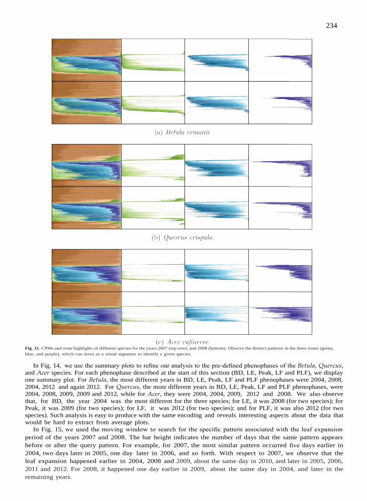
234

Fig. 11. CPMs and zone highlights of different species for the years 2007 (top row), and 2008 (bottom). Observe the distinct patterns in the three zones (green,

blue, and purple), which can serve as a visual signature to identify a given species.

In Fig. 14, we use the summary plots to refine our analysis to the pre-defined phenophases of the Betula, Quercus,

and Acer species. For each phenophase described at the start of this section (BD, LE, Peak, LF and PLF), we display

one summary plot. For Betula, the most different years in BD, LE, Peak, LF and PLF phenophases were 2004, 2008,

2004, 2012 and again 2012. For Quercus, the most different years in BD, LE, Peak, LF and PLF phenophases, were

2004, 2008, 2009, 2009 and 2012, while for Acer, they were 2004, 2004, 2009, 2012 and 2008. We also observe

that, for BD, the year 2004 was the most different for the three species; for LE, it was 2008 (for two species); for

Peak, it was 2009 (for two species); for LF, it was 2012 (for two species); and for PLF, it was also 2012 (for two

species). Such analysis is easy to produce with the same encoding and reveals interesting aspects about the data that

would be hard to extract from average plots.

In Fig. 15, we used the moving window to search for the specific pattern associated with the leaf expansion

period of the years 2007 and 2008. The bar height indicates the number of days that the same pattern appears

before or after the query pattern. For example, for 2007, the most similar pattern occurred five days earlier in

2004, two days later in 2005, one day later in 2006, and so forth. With respect to 2007, we observe that the

leaf expansion happened earlier in 2004, 2008 and 2009, about the same day in 2010, and later in 2005, 2006,

2011 and 2012. For 2008, it happened one day earlier in 2009, about the same day in 2004, and later in the

remaining years.

235

Fig. 12. Searching for similar phenological pattern using MSE: (a) query pattern; and top two results using (b) fixed and (c) moving window. Comparison errors

are given after the letter ‘e’; red numbers show the temporal shift in days from the matching pattern.

Fig. 13. Multi-rank comparisons of four ROIs (Community, Betula, Quercus and Acer) for the entire year: (a)-(d) normalized distance of every year from

2004 to 2012 against the others; (e)-(h) combined information of the green histogram plots of a given ROI into a single summary plot; the year 2007 was

the year most similar to the others, while the years 2004, 2012, and 2009 were the most different ones.

236

Fig. 14. Summary histograms of the community mask for specific phenological phases. The year 2004 was the most different for the three species; for LE, it

was 2008 (for two species); for Peak, it was 2009 (for two species); for LF, it was 2012 (for two species); and for PLF, it was also 2012 (for two species).

Fig. 15. The leaf-expansion period was used as input pattern in the moving window approach for the years 2007 and 2008: the bar heights represent the

number of days that the result happened before (blue) or after (red) the query pattern.

5. Conclusions and future work

Plant phenology studies are based on the analysis of several years of data. Average yearly plots of vegetation

indexes are the preferred approach to evaluate phenological changes. Despite good results, the analysis based on

average values is limited and can constraint the knowledge discovery process.

In this paper, we present PhenoVis, a framework for the visual phenological analysis of forest ecosystems. It

contains the chronological percentage maps (CPM), a novel representation that is capable of discovering

additional patterns by encoding percentage distributions of the data. We demonstrated CPM in a number of

analysis scenarios, showing the additional in- sights that CPMs can bring to the analysis and how it can be used

to identify species. The evaluation showed how automatic pattern searches can facilitate the detection of

phenological singularities related to weather variations.

As future work, we intend to automatically detect phenological patterns. Currently this process is manual: the

user in- forms the start and end dates of the query pattern. Automatic suggestions can improve the analysis using,

for example, a box-plot [45] of the distribution. Another possibility is to use more images per day, decreasing

lighting variations and artifacts. We also plan to investigate the integration of the CPM representation with

machine learning techniques [4,7] to perform automatic species identification.

Acknowledgments

We thank the Phenological Eyes Network (PEN) for giving authorisation to use the TKY dataset (http://www.pheno-eye.org). We

thank Shin Nagai and Kenlo Nishida Nasahara for the revision of this manuscript and suggestions to improve the final format. This

research was supported by the São Paulo Research Foundation FAPESP and Microsoft Research Virtual Institute (grants

#2010/52113-5, #2013/50169-1, and #2013/50155-0). BA received a master scholarship from CAPES and a doctoral fellowship from

FAPESP (grant #2014/00215-0); LPCM and RST receive a Productivity Research Fellowship from CNPq. Also, we have benefited

from funds given by CAPES, CNPq (grants 476685/2012-5, 309483/2011-5, 308851/2015-3), and FAPESP (grants #2007/52015-0,

#2007/59779-6, #2009/18438-7, #2010/51307-0, and #2009/54208-6).

237

Supplementary material

Supplementary material associated with this article can be found, in the online version, at 10.1016/j.ins.2016.08.052.

References

[1] W. Aigner, S. Miksch, H. Schumann, C. Tominski, Visualization of time-oriented data, Springer Science & Business Media, 2011.

[2] D. Albers, C. Dewey, M. Gleicher, Sequence surveyor: Leveraging overview for scalable genomic alignment visualization, Visual. Comput. Graphics, IEEE

Trans. 17 (12) (2011) 2392–2401.

[3] B. Alberton, J. Almeida, R. Henneken, R.S. Torres, A. Menzel, L.P.C. Morellato, Using phenological cameras to track the green up in a cerrado savanna

and its on-the-ground validation, Ecol. Inf. 19 (2014) 62–70.

[4] J. Almeida, J.A. dos Santos, B. Alberton, R. da S. Torres, L.P.C. Morellato, Applying machine learning based on multiscale classifiers to detect remote

phenology patterns in cerrado savanna trees, Ecol. Inf. 23 (0) (2014) 49–61. Special Issue on Multimedia in Ecology and Environment

[5] J. Almeida, J.A. Santos, B. Alberton, L.P.C. Morellato, R.S. Torres, Plant species identification with phenological visual rhythms, in: IEEE International

Conference on eScience (eScience’13), 2013, pp. 148–154.

[6] J. Almeida, J.A. Santos, B. Alberton, L.P.C. Morellato, R.S. Torres, Visual rhythm-based time series analysis for phenology studies, in: IEEE International

Conference on Image Processing (ICIP’13), 2013, pp. 4412–4416.

[7] J. Almeida, J.A. Santos, W.O. Miranda, B. Alberton, L.P.C. Morellato, R.S. Torres, Deriving vegetation indices for phenology analysis using genetic pro-

gramming, Ecol. Inf. 26 (2015) 61–69.

[8] G. Andrienko, N. Andrienko, Spatio-temporal aggregation for visual analysis of movements, in: Visual Analytics Science and Technology, 2008. VAST

’08. IEEE Symposium on, 2008, pp. 51–58.

[9] I. Boyandin, E. Bertini, P. Bak, D. Lalanne, Flowstrates: An approach for visual exploration of temporal origin-destination data, Comput. Graphics Forum

30 (3) (2011) 971–980.

[10] E. Bradley, D. Roberts, C. Still, Design of an image analysis website for phenological and meteorological monitoring, Environ. Modell. Software 25 (1)

(2010) 107–116.

[11] L. Byron, M. Wattenberg, Stacked graphs – geometry & aesthetics, IEEE Trans. Visual. Comput. Graphics 14 (6) (2008) 1245–1252, doi:10.1109/TVCG.

2008.166.

[12] W. Cui, X. Wang, S. Liu, N. Riche, T. Madhyastha, K.L. Ma, B. Guo, Let it flow: A static method for exploring dynamic graphs, in: Pacific Visualization

Symposium (PacificVis), 2014 IEEE, 2014, pp. 121–128.

[13] H. Eerens, D. Haesen, F. Rembold, F. Urbano, C. Tote, L. Bydekerke, Image time series processing for agriculture monitoring, Environ. Modell. Software

53 (2014) 154–162.

[14] K. Fung, Numbers Rule Your World: The Hidden Influence of Probabilities and Statistics on Everything You Do, McGraw-Hill Education, 2010.

[15] A.R. Gillespie, A.B. Kahle, R.E. Walker, Color enhancement of highly correlated images. I. Decorrelation and HSI contrast stretches, Remote Sens. Environ.

20 (3) (1986) 209–235.

[16] J.A. Granados, E.A. Graham, P. Bonnet, E.M. Yuen, M.P. Hamilton, Ecoip: An open source image analysis toolkit to identify different stages of plant

phenology for multiple species with pan-tilt-zoom cameras, Ecol. Inf. 15 (2013) 58–65.

[17] S. Gratzl, A. Lex, N. Gehlenborg, H. Pfister, M. Streit, Lineup: Visual analysis of multi-attribute rankings, Visual. Comput. Graphics, IEEE Trans. 19 (12)

(2013) 2277–2286.

[18] S. Hadlak, H. Schumann, C. Cap, T. Wollenberg, Supporting the visual analysis of dynamic networks by clustering associated temporal attributes, Visual.

Comput. Graphics, IEEE Trans. 19 (12) (2013) 2267–2276.

[19] S. Havre, B. Hetzler, L. Nowell, Themeriver: visualizing theme changes over time, in: Information Visualization, 2000. InfoVis 2000. IEEE Symposium

on, 2000, pp. 115–123, doi:10.1109/INFVIS.2000.885098.

[20] S. Havre, E. Hetzler, P. Whitney, L. Nowell, Themeriver: visualizing thematic changes in large document collections, IEEE Trans. Visual. Comput. Graphics

8 (1) (2002) 9–20, doi:10.1109/2945.981848.

[21] R. Ide, H. Oguma, Use of digital cameras for phenological observations., Ecol. Inf. 5 (5) (2010) 339–347.

[22] T. Inoue, S. Nagai, T.M. Saitoh, H. Muraoka, K.N. Nasahara, H. Koizumi, Detection of the different characteristics of year-to-year variation in foliage

phenology among deciduous broad-leaved tree species by using daily continuous canopy surface images, Ecol. Inf. 22 (2014) 58–68. http://dx.doi.org/

10.1016/j.ecoinf.2014.05.009.

[23] A. Ito, N. Saigusa, S. Murayama, S. Yamamoto, Modeling of gross and net carbon dioxide exchange over a cool-temperate deciduous broad-leaved forest

in japan: Analysis of seasonal and interannual change, Agric. For. Meteorol. 134 (1-4) (2005) 122–134. http://dx.doi.org/10.1016/j.agrformet.2005.11.002.

Long-Term Carbon Exchange at the Takayama, Japan Forest

[24] D.A. Keim, Designing pixel-oriented visualization techniques: Theory and a.0pplications, IEEE Trans. Visual. Comput. Graphics 6 (1) (2000) 59–78.

[25] D.A. Keim, Information visualization and visual data mining, IEEE Trans. on Vis. and Comp. Graph. 8 (1) (2002).

[26] D.A. Keim, M.C. Hao, U. Dayal, M. Hsu, Pixel bar charts: A visualization technique for very large multi-attribute data sets, Inf. Visual. 1 (1) (2002) 20–

34.

[27] J. Li, K. Zhang, Z.-P. Meng, Vismate: Interactive visual analysis of station-based observation data on climate changes, in: Visual Analytics Science and

Technology (VAST), 2014 IEEE Conference on, 2014, pp. 133–142.

[28] S. Lin, J. Fortuna, C. Kulkarni, M. Stone, J. Heer, Selecting semantically-resonant colors for data visualization, Comput. Graphics Forum 32 (3pt4) (2013) 401–410.

[29] J.T. Morisette, A.D. Richardson, A.K. Knapp, J.I. Fisher, E.A. Graham, J. Abatzoglou, B.E. Wilson, D.D. Breshears, G.M. Henebry, J.M. Hanes, L. Liang,

Tracking the rhythm of the seasons in the face of global change: phenological research in the 21st century, Front. Ecol. Environ. 7 (5) (2009) 253–260.

[30] S. Nagai, T. Maeda, M. Gamo, H. Muraoka, R. Suzuki, K.N. Nasahara, Using digital camera images to detect canopy condition of deciduous broad-leaved

trees, Plant Ecology & Diversity 4 (1) (2011) 79–89.

[31] K.N. Nasahara, S. Nagai, Review: Development of an in situ observation network for terrestrial ecological remote sensing: the phenological eyes net-

work (PEN), Ecol. Res. 30 (2) (2015) 211–223.

[32] G. Negi, Leaf and bud demography and shoot growth in evergreen and deciduous trees of central himalaya, india, Trees 20 (4) (2006) 416–429.

[33] C.W. Ngo, T.C. Pong, R.T. Chin, Detection of gradual transitions through temporal slice analysis, in: IEEE International Conference on Computer Vision

and Pattern Recognition (CVPR’99), 1999, pp. 1036–1041.

[34] K.T. Nguyen, T. Ropinski, Large-scale multiple sequence alignment visualization through gradient vector flow analysis, in: Biological Data Visualization

(BioVis), 2013 IEEE Symposium on, 2013, pp. 9–16.

[35] K. Nishida, Phenological eyes network (PEN) - a validation network for remote sensing of the terrestrial ecosystems., AsiaFlux Newslett. 21 (2007)

9 13.

[36] G. Oliveira, J. Comba, R. Torchelsen, M. Padilha, C. Silva, Visualizing running races through the multivariate time-series of multiple runners, 2012 25th

SIBGRAPI Conf. Graphics, Patterns Images 0 (2013) 99–106.

[37] C. Reas, B. Fry, Processing: A Programming Handbook for Visual Designers and Artists, MIT Press, 2014.

[38] A.D. Richardson, B.H. Braswell, D.Y. Hollinger, J.P. Jenkins, S.V. Ollinger, Near-surface remote sensing of spatial and temporal variation in canopy phe-

nology, Ecol. Appl. 19 (6) (2009) 1417–1428.

[39] M.D. Schwartz, Phenology: an integrative environmental science, 2nd, Springer, 2013.

[40] O. Sonnentag, K. Hufkens, C. Teshera-Sterne, A.M. Young, M. Friedl, B.H. Braswell, T. Milliman, J. O Keefe, A.D. Richardson, Digital repeat photography for

phenological research in forest ecosystems, Agric. For. Meteorol. 152 (2012).

[41] T. Udelhoven, Timestats: A software tool for the retrieval of temporal patterns from global satellite archives, IEEE J. Selected Topics Appl. Earth Observ. Remote

Sens. 4 (2) (2011) 310–317.

238

Appendix F

Article published in the Journal Pattern Recognition Letters:

ALMEIDA, J., PEDRONETTE, D., ALBERTON, B., MORELLATO, L.P.C., TORRES, R.S. Unsupervised

distance learning for plant species identification. JSTARS Journal of Selected Topics in Applied Earth

Observations and Remote Sensing, v. 9 (12), p. 5325-5338, 2016.

239

P

Text Formatting according to the JSTARS Journal of Selected Topics in Applied Earth Observations and

Remote Sensing

Unsupervised Distance Learning for Plant Species Identification

Jurandy Almeida1, Daniel C. G. Pedronette2, Bruna C. Alberton3, Leonor Patricia C. Morellato3, Ricardo da S. Torres4

1 Institute of Science and Technology, Federal University of Sao Paulo (UNIFESP), Sao Jose dos Campos 12247-014, Brazil (e-mail:

jurandy.almeida@unifesp.br).

2 Department of Statistics, Applied Mathematics and Computation, Sao Paulo State University (UNESP), Rio Claro 13506-900, Brazil (e-mail:

daniel@rc.unesp.br).

3 Department of Botany, Sao Paulo State University (UNESP), Rio Claro 13506-900, Brazil (e-mail: bru.alberton@gmail.com;

pmorella@rc.unesp.br).

4 Institute of Computing, University of Campinas (UNICAMP), Campinas 13083-852, Brazil (e-mail: rtorres@ic.unicamp.br).

Abstract:

Phenology is among the most trustworthy indicators of climate change effects on plants and animals. The recent application of repeated digital photographs to monitor vegetation phenology has provided accurate measures of plant life cycle changes over time. A fundamental requirement for phenology studies refers to the correct recognition of phenological patterns from plants by taking into account time series associated with their crowns. This paper presents a new similarity measure for identifying plants based on the use of an unsupervised distance learning scheme, instead of using traditional approaches based on pairwise similarities. We experimentally show that its use yields considerable improvements in time-series search tasks. In addition, we also demonstrate how the late fusion of different time series can improve the results on plant species identification. In some cases, significant gains were observed (up to +8.21% and +19.39% for mean average precision and precision at 10 scores, respectively) when compared with the use of time series in isolation.

Index Terms—Image analysis, plant identification, remote phenology, time series, unsupervised distance learning.

I. INTRODUCTION

LANT phenology studies recurrent plant life cycle events

and is among the most trustworthy indicators of the impact

of climate change on plants and animals [1]. Recently, digital

repeated photographs have been applied to monitor vegetation

phenology increasing the range of study sites and species and

the accuracy of estimated changes on phenological events [1]–

[3]. The proper identification of plant species based on their

particular phenological patterns is a key issue for the

phenolog- ical observation of tree crowns using phenocams

[4], especially in tropical vegetations where one single image

may encompass a large number of species [3]. Each crown in

the image has to be match with the tree in the soil and then

identified at species level, and further phenological patterns

are identified to that species and analyzed [3], [5].

Existing approaches to cope with the task of plant

identifica- tion based on phenological patterns rely on a

feature extractor for encoding visual properties into feature

vectors and on a sim- ilarity measure for comparing image

data from their vectors, a pair known as descriptor [6]. In

phenology studies, a common approach used for feature

extraction is to compute for each im- age a chromatic or

lighting coefficient associated with a visual property from all

pixels of a given region of interest. Thus, a time series is

obtained by computing this index for all days in an time

period of interest [4], [7].

Besides the time-series modeling, the similarity measure

adopted for comparing different times series also plays an

important role, directly affecting the quality of retrieval results.

Given the broad application of time series, various similarity

measures have been employed [8] for comparison and retrieval.

In addition to the traditional Manhattan (L1 ) and Euclidean (L2 ) distances, other measures, such as the dynamic time warp- ing

distance and longest common subsequence, are commonly used

[8]. In [9], shape descriptors are used to characterize time

series. In [10], visual rhythms are used to simplify time series,

enabling the use of image descriptors.

However, traditional solutions often perform only pairwise

analysis, that is, the similarity measure considers only the in-

formation given by the pairs of time series being compared. In

this scenario, the relationships among objects modeled by the

time series are not considered. Therefore, the intrinsic struc-

ture of the collection is ignored. In this scenario, one suitable

alternative relies on the use of methods that are capable of en-

coding information of the dataset structure. Relevance feedback

approaches [11], for example, have been proposed for using the

information obtained from user interactions for improving the

quality of time-series retrieval tasks. Although effective, such

supervised approaches require a lot of user intervention.

In this paper, we present a novel approach for redefining the

similarity from time series and identifying plant species based

on phenological patterns, without the use of any training data.

We approach the plant identification task as a similarity-based

time-series retrieval problem using unsupervised learning, in

contrast to some supervised initiatives that have addressed this

task in the context of image classification [5], [12]. For this, we

240

×

introduce the use of an unsupervised distance learning method

called reciprocal k-nearest neighbor (kNN) distance [13] for

plant species identification. The method exploits the relation-

ships among time series, using a contextual rank-based approach

for improving the effectiveness of retrieval tasks.

Unsupervised learning approaches have been used in time-

series retrieval in order to learn a layer of feature repre-

sentations from unlabeled data [14]. In opposite, the proposed

approach does not require intermediary feature learning steps.

A traditional distance measure is obtained based on the original

features, giving rise to a set of ranked lists. Subsequently, a

more effective distance is computed by analyzing the reciprocal

references encoded in the rankings. Although common in

image retrieval systems [15], [16], to the best of our knowledge,

this is the first approach that exploits contextual rank-based

measures [13] in time-series retrieval scenarios.

The proposed approach was validated on a dataset recorded

during the main leaf flushing season [3], which is composed

of about 2700 images. Several time series extracted from the

digital image were evaluated and a large experimental evalua-

tion was conducted. Various aspects are analyzed, considering

individual features and fusion tasks. An approach for selecting

the most discriminative features is also discussed. The experi-

mental results show that our approach can improve the retrieval

effectiveness considerably. While the best feature in isolation

yields a precision of 73.12% at top-ten positions, the proposed

approach achieves precision scores up to 87.30%.

This paper is organized as follows. Section II describes

the time-series acquisition procedure. Section III describes the

methodology adopted in this work. Section IV discusses the

unsupervised distance learning approach. Section V discusses

the experimental protocol, while Section VI presents achieved

results. Finally, Section VII presents our conclusions and draws

possible future work.

Fig. 1. ROIs defined for the analysis of cerrado-savanna digital images, fol- lowing [3]. Each color represents a species: red = Aspidosperma tomentosum; green = Caryocar brasiliensis; blue = Myrcia guianensis; orange = Miconia rubiginosa; magenta = Pouteria ramiflora; cyan = Pouteria torta.

5) two regions for Pouteria ramiflora (magenta areas);

6) four regions for Pouteria torta (cyan areas).

According to the leaf exchange data from the on-the-ground

field observations on leaf fall and leaf flush at our study site,

those species were classified into three functional groups [3]:

1) deciduous, A. tomentosum and C. brasiliensis;

2) evergreen, M.guianensis and M. rubiginosa;

3) semideciduous, P. ramiflora and P. torta.

We analyzed each ROI by means of a normalized index devel-

oped by Gillespie et al.[18], called RGB chromatic coordinates

(RGBcc). It is considered the most efficient index to distinguish

leaves between monocots and dicots and to suppress light envi-

ronment variation [19]. The normalized RGBcc indices undergo

a nonlinear transform, as follows [18], [19]:

R

II. TIME-SERIES ACQUISITION

We have been acquiring time series from digital images of

a phenological monitoring, called near-surface remote phenol-

ogy [17], in a cerrado savanna vegetation since August 2011.

A digital camera was set up in the top of 18-m-high tower in

rcc =

gcc =

bcc =

(R + tt + B) (1)

tt (2)

(R + tt + B)

B (3)

(R + tt + B)

an area of a cerrado sensu stricto, located at Itirapina, South-

eastern Brazil. Camera was set up for taking a sequence of five

JPEG images (at 1280 960 pixels of resolution) per hour,

from 6:00 to 18:00 h (UTC-3). This study was based on a sam-

ple sequence of the time series, recorded between August 29th

and October 3rd, 2011 (day of year 241 to 278), totalizing 2700

images, which corresponds to the main leaf flushing season of

the cerrado community [3].

The image analysis was conducted by defining different re-

gions of interest (ROIs), as described in [4] and defined in [3]

for our target species (see Fig. 1). We analyzed 22 ROIs of six

plant species randomly selected in the hemispheric image:

1) three regions for Aspidosperma tomentosum (red areas);

2) four regions for Caryocar brasiliensis (green areas);

3) two regions for Myrcia guianesis (blue areas);

4) seven regions for Miconia rubiginosa (orange areas);

where R, tt, and B are the average pixel intensity of the red,

green, and blue bands, respectively. By computing those values

along the whole period, we obtained time series to use as input

data for our proposed framework.

III. TIME-SERIES RETRIEVAL

This section presents the methodology used to handle the

plant identification task as a similarity-based time-series re-

trieval problem. First, Section III-A presents an overview of the

time-series retrieval system. In the following, the main compo-

nents of this system are formalized in Section III-B.

A. Overview

In this work, the plant identification task is approached as a

time-series retrieval problem, as proposed in [20]. In this

241

∈ R R { }

⊂ |R|

D

× ∈R

∈R

X { } H { }

C { } { }

T T

C { } R

X × X →

C× H × R→ X

In the search step, the similarity computation considers only

pairs of objects (regions and the respective times series). The

post-processing step exploits more global relationships among

time series with the aim of improving the effectiveness of re-

trieved results. In the data insertion module, the postprocessing

step comprises: (7) a similarity search considering every re-

gion as a query; and (8) the computation of a ranked list for

all queries. In the query processing module, the ranked lists are

redefined by the following steps: (9) the unsupervised learning

method compute more effective ranked lists; and (10) the final

retrieval results are returned to the user.

B. Formalization

Let I be a digital image. Let = r1 ,r2 , . . . , rn be a

collection of regions, such that for each region ri , we have

ri I and each region contains a single species. Let n = denote the number of regions considered. Let X be a time series,

defined as follows:

Fig. 2. Flowchart of the time-series retrieval system.

method, we provide a time series extracted from an image area

associated with a given species, and we query for similar time

series computed from other image areas that belong to the same

species. The flowchart of the time-series retrieval system is

illustrated in Fig. 2. Two main functionalities are supported by

this system: data insertion and query processing. Each of those

subsystems is composed of two basic steps: (i) search and (ii)

post-processing.

In the search step, the data insertion module comprises:

(1) the encoding of leaf change patterns from labeled image

regions into time series by computing the normalized RGBcc

indices along multitemporal data; and (2) the indexing of the

extracted time series in a data repository. The query processing

module consists of a query search, which are composed of the

following steps: (3) the selection of a query pattern, which is an

image area along the multitemporal images; (4) the extraction

of the query’s time series by computing the normalized RGBcc

indices; (5) the search computation by similarity; (6) the final

similarity ranking, including all patterns learned at the offline

stages.

X = {xt,t ∈T } (4)

where denotes a discrete index set. Let m be the num- ber

of days of observations; the index set is defined as = d1 , d2 , . . . , dm .

Let = r, g, b be the set of chromatic indexes (defined

by the normalized RGBcc indices). L et = 0, 1 , . . . , 23 be a

set defined by the hours of the day. Let = X1 , X2 , . . . , Xz

denote a set of all time series obtained for every combination of

chromatic index, hour of day and region.

We can define a function ψ : , which ex-

tracts a time series for a given chromatic index, hour of day, and

region.1 For example, the time series observed for the region

“ri” by considering the gcc index at “6 h” can be defined by

Xi,g,6 = ψ(ri, g, 6).

Let be a time-series descriptor for a region, which can be

defined as a tuple (ψ, ρ), where ψ extracts a time series for

a region ri considering a chromatic index and a hour of

day; ρ: R is a distance function that computes the

distance between two regions according to the distance between

their respective time series. Formally, the distance between two

regions ri and rj considering a chromatic index c and a hour

h is defined by ρ(ψ(ri, c, h), ψ(rj , c, h)). For simplicity and

readability purposes, we use the notation ρ(i, j) along the paper

for denoting the distance between regions ri and rj , considering

their respective times series.

The distance ρ(i, j) among all regions ri, rj can be

computed to obtain a squared n n distance matrix A, such

that Aij = ρ(i, j). Also based on the distance function ρ , a

ranked list τq can be computed in response to a query region rq .

The goal consists in retrieving the most similar regions ri

considering the respective time series.

The ranked list τq = (r1 , r2 , ... , rn ) can be defined as a

permutation of the collection . A permutation τq is a bijection

from the set onto the set [N ] = 1, 2,... , n . For a permu-

tation τq , we interpret τq (i) as the position (or rank) of region

1The extracted time series can be seen as feature vectors associated with an image area.

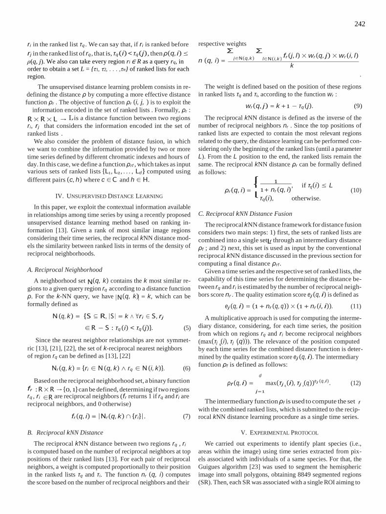
242

R ×R ×L →

N

|N |

⎩

L

d

∈R

1+ nr (q, i) q

: R×R → {0, 1} can be defined, determining if two regions j =1

q i

⎧⎨

ri in the ranked list τq . We can say that, if ri is ranked before

rj in the ranked list of rq , that is, τq (i) < τq (j), then ρ(q, i) ≤

ρ(q, j). We also can take every region ri ∈ R as a query rq, in

order to obtain a set L = {τ1, τ2, . . . ,τn} of ranked lists for each

region.

respective weights Σ Σ

fr (j, l) × wr (q, j) × wr (i, l)

The unsupervised distance learning problem consists in re-

defining the distance ρ by computing a more effective distance

function ρr . The objective of function ρr (i, j, ) is to exploit the

information encoded in the set of ranked lists . Formally, ρr :

L is a distance function between two regions

ri, rj that considers the information encoded int the set of

ranked lists .

We also consider the problem of distance fusion, in which

we want to combine the information provided by two or more

time series defined by different chromatic indexes and hours of

day. In this case, we define a function ρrf , which takes as input various sets of ranked lists {L1 , L2 , . . . , Ld } computed using

different pairs (c, h) where c ∈C and h ∈ H.

IV. UNSUPERVISED DISTANCE LEARNING

In this paper, we exploit the contextual information available

in relationships among time series by using a recently proposed

unsupervised distance learning method based on ranking in-

formation [13]. Given a rank of most similar image regions

considering their time series, the reciprocal kNN distance mod-

els the similarity between ranked lists in terms of the density of

reciprocal neighborhoods.

A. Reciprocal Neighborhood

A neighborhood set (q, k) contains the k most similar re-

gions to a given query region rq according to a distance function

ρ. For the k-NN query, we have (q, k) = k, which can be

formally defined as

N (q, k) = {S ⊆ R, |S| = k ∧ ∀ri ∈ S, rj

∈R − S : τq (i) < τq (j)}. (5)

Since the nearest neighbor relationships are not symmet-

The weight is defined based on the position of these regions

in ranked lists τq and τi, according to the function wr :

wr (q, j) = k +1 − τq (j). (9)

The reciprocal kNN distance is defined as the inverse of the

number of reciprocal neighbors nr . Since the top positions of

ranked lists are expected to contain the most relevant regions

related to the query, the distance learning can be performed con-

sidering only the beginning of the ranked lists (until a parameter

L). From the L position to the end, the ranked lists remain the

same. The reciprocal kNN distance ρr can be formally defined

as follows:

1 , if τ (i) ≤ L

τq (i), otherwise.

C. Reciprocal kNN Distance Fusion

The reciprocal kNN distance framework for distance fusion

considers two main steps: 1) first, the sets of ranked lists are

combined into a single set f through an intermediary distance

ρf ; and 2) next, this set is used as input by the conventional

reciprocal kNN distance discussed in the previous section for

computing a final distance ρrf .

Given a time series and the respective set of ranked lists, the

capability of this time series for determining the distance be-

tween rq and ri is estimated by the number of reciprocal neigh-

bors score nr . The quality estimation score ej (q, i) is defined as

ej (q, i) = (1 + nr (q, q)) × (1 + nr (i, i)). (11)

A multiplicative approach is used for computing the interme-

diary distance, considering, for each time series, the position

from which on regions rq and ri become reciprocal neighbors

(max(τj (i), τj (q))). The relevance of the position computed q i

ric [13], [21], [22], the set of k-reciprocal nearest neighbors

of region rq can be defined as [13], [22]

Nr (q, k) = {ri ∈ N (q, k) ∧ rq ∈ N (i, k)}. (6)

Based on the reciprocal neighborhood set, a binary function

rq , ri are reciprocal neighbors (fr returns 1 if rq and ri are

reciprocal neighbors, and 0 otherwise)

fr (q, i) = |Nr (q, k) ∩ {ri}|. (7)

B. Reciprocal kNN Distance

The reciprocal kNN distance between two regions rq , ri

is computed based on the number of reciprocal neighbors at top

positions of their ranked lists [13]. For each pair of reciprocal

neighbors, a weight is computed proportionally to their position

in the ranked lists τq and τi. The function nr (q, i) computes

the score based on the number of reciprocal neighbors and their

by each time series for the combined distance function is deter-

mined by the quality estimation score ej (q, i). The intermediary

function ρf is defined as follows:

ρf (q, i) =

max(τj (i), τj (q))ej (q ,i) . (12)

The intermediary function ρf is used to compute the set f

with the combined ranked lists, which is submitted to the recip-

rocal kNN distance learning procedure as a single time series.

V. EXPERIMENTAL PROTOCOL

We carried out experiments to identify plant species (i.e.,

areas within the image) using time series extracted from pix-

els associated with individuals of a same species. For that, the

Guigues algorithm [23] was used to segment the hemispheric

image into small polygons, obtaining 8849 segmented regions

(SR). Then, each SR was associated with a single ROI aiming to

k

j ∈N (q,k ) n (q, i) = l∈N (i,k )

.

ρr (q, i) = (10)

fr

243

{ }

label it. A labeled region is created if there is at least 80% of over-

lapped area between an SR and an ROI.2 Thus, we built a dataset

of 892 SRs separated into six classes, one for each species: A.

tomentosum (96), C. brasiliensis (346), M. guianensis (36), M.

rubiginosa (195), P. ramiflora (50), and P. torta (169).

For each SR, we extracted 39 different time series by consid-

ering the available periods during the day (13 hours: from 6:00 to

18:00 h) and the normalized RGBcc indices (three components:

rcc , gcc , and bcc ). The similarity between two SRs is computed

as a function of the distance between the time series extracted

from their SRs. A time series is better than another if it ranks

more SRs belonging to the same ROI of a query SR at the first

positions. The distance function used for time-series compari-

son is the Manhattan (L1 ) distance, as suggested by Conti et al.

[24]. In this way, we created 39 different time-series descriptors

(features) to be used as input in our proposed framework.

The effectiveness of each approach was assessed using the

metrics of precision and recall. Precision is the ratio of the

relevant SRs in the retrieved set of SRs. Recall is the ratio of

relevant SRs retrieved to the total number of relevant SRs in

the database. A given SR is considered as relevant only if it

belongs to the same ROI of a query SR. There is a tradeoff

between precision and recall, i.e., increasing recall may decrease

precision and vice versa. For this reason, we consider unique-

value measurements in the validation: mean average precision

(MAP), which is the mean of the precision scores obtained at

the ranks of each relevant SR; and Precision at 10 (P10), which

is the average precision after ten SRs are returned. MAP is a

good indication of the effectiveness considering all positions of

obtained ranked lists. P10, in turn, focuses on the effectiveness

of the methods considering only the first positions of the ranked

lists. Experiments were conducted using all the SRs from the

dataset as queries. Reported results represent the average scores

of all the SRs.

VI. EXPERIMENTAL RESULTS

Various experiments were conducted, aiming at analyzing

the proposed approach under different aspects. This section dis-

cusses the collected experimental results.

Our experiments are generally intended to:

1) compare the effectiveness achieved by individual time

series before and after the unsupervised distance learning

procedure;

2) evaluate the impact of distance fusion steps using the

reciprocal kNN distance for combining time series;

3) analyze the improvements in the plant identification task

obtained by the reciprocal kNN distance.

Section VI-A presents an evaluation of the input features.

In Section VI-B, we perform a parameter space analysis of

our approach. Section VI-C presents the experimental results

regarding the use of reciprocal kNN distance for individual

features, while Section VI-D addresses its use for distance fu-

2In the remainder of this paper, when we refer to segmented regions obtained

by the Guigues algorithm, we use the acronym SR, whereas when we refer to regions of interest related to tree crowns of plant species identified in the image, we use the acronym ROI.

sion. Section VI-E discusses the results obtained for most dis-

criminative features. In Section VI-F, we compare our approach

with other methods. Section VI-G presents a visual analysis of

the results. Finally, Section VI-H describes performed experi-

ments considering the use of a hyperspectral dataset targeting

the classification of remote sensing pixels as belonging to two

classes: savanna and forest. This is an important research prob-

lem as it may help on understanding vegetation-related land

cover changes over time.

A. Quantitative Feature Evaluation

As discussed in Section V, 39 different features are considered

given by periods of the day (13 h: from 6:00 to 18:00 h) and

the normalized RGBcc indices (three components: rcc , gcc , and

bcc ). This sections aims at evaluating the effectiveness of each

input feature for identification of plant species.

In Fig. 3, we report and compare the time series with respect to

the MAP and P10 effectiveness measures, respectively. Note that

the initial effectiveness values are low for both measures, which

turns more challenging the use of unsupervised distance learning

methods. The MAP scores varied from 28.95% to 42.16%, while

P10 scores varied from 44.30% to 73.12%.

We can observe that the extreme hours (6 and 18 h) present

the best effectiveness results, considering all the normalized

RGBcc indices. This is probably due to sun illumination angle

variations observed along the day. Slightly better effectiveness

results can also be observed for the rcc index.

B. Impact of Parameters

The reciprocal kNN distance requires only two parameters:

1) k, which represents the size of the neighborhood set; and

2) L, which defines until which position the ranked lists are

considered in the distance learning procedure. In general, the

parameter L represents a tradeoff between effectiveness and

efficiency, since higher values of L generally provide higher

accuracy while requires higher computational efforts.

The size of the neighborhood set is the most important pa-

rameter of the method, defining the extension of the reciprocal

neighborhood analysis. Therefore, we conducted an experiment

aiming at determining the best value for the parameter k. We

computed the MAP and P10 measures for each feature in isola-

tion considering k = 5 , 10, 15, 20 . Fig. 4 presents two radar charts which show the impact of the

parameter k on the MAP and P@10 measures obtained by each

of the time series after using the reciprocal kNN distance. These

charts are composed of three parts: radius, slice of the perimeter,

and lines. The radius denotes the effectiveness score. The slices

of the perimeter represent each of the time series. Finally, a line

indicates the performace obtained by each time series when the

parameter k is set to a given value.

As we can observe, the effectiveness scores were similar for

different values of the parameter k, with a small advantage to

k = 10. Therefore, the value of k = 10 was used for all other

experiments, demonstrating the robustness of our approach. For

the parameter L, we used L = 400, as suggested in [13].

244

Fig. 3. Initial effectiveness scores obtained by each of the time series.

Fig. 4. Effectiveness results obtained for each of the time series after unsupervised distance learning by varying the parameter k. (a) MAP. (b) P10.

C. Unsupervised Learning for Individual Features

Experiments were conducted for evaluating the use of the

unsupervised distance learning for individual features. The main

motivation consists in the conjecture that the reciprocal kNN

distance can improve the effectiveness results, even considering

information given by a single feature.

For evaluation purposes, we considered the MAP and P10

measures and report the relative gain, which is computed by

the absolute gain divided by the initial score. Fig. 5 presents

the individual relative gains obtained by each of the time series

considering the MAP and P10 measures, respectively.

Despite of low effectiveness of the input individual features,

positive gains were obtained in 35 and 22 out of 39 time series

for MAP and P10, respectively. We can observe significant gains

for MAP, reaching +6.72%. For P10, the gains are lower, but

still significant, reaching +4.15%. Notice that the higher gains

were obtained for features, which presented the higher initial

effectiveness, e.g., features of the beginning and ending of the

day and the rcc index.

D. Distance Fusion With Unsupervised Learning

Different features are expected to encode complementary in-

formation about the phenomenon modelled by the time series.

Therefore, we conducted an experiment to evaluate the use of

unsupervised distance learning for combining features. The con-

sidered combinations are:

1) all the normalized RGBcc indices for each hour of the day

(13 combinations);

2) all the hours of the day for each of the normalized RGBcc

indices (three combinations);

3) all hours of the day and all the normalized RGBcc indices

(one combination).

Fig. 6 shows the MAP and P10 scores achieved by different

time-series combinations. The results were sorted from higher

to lower scores. The bars in gray indicate the combination of

different chromatic indexes while bars in red, green, and blue

indicate combination of different hours of the day. The percent-

age value at the top of each bar refers to the relative gain with

respect to initial values for the best feature used for combination.

245

Fig. 5. Relative effectiveness gains obtained for each of the time series after unsupervised distance learning. (a) MAP. (b) P10.

Fig. 6. Effectiveness results obtained by unsupervised distance learning for combining different time series. (a) MAP. (b) P10.

TABLE I SUMMARY RESULTS OF UNSUPERVISED DISTANCE LEARNING FOR PLANT

SPECIES IDENTIFICATION BY CONSIDERING THE COMBINATION OF DIFFERENT

TIME SERIES

Measure Time

Series

Initial

Value

Reciprocal

k NN Distance

Relative

Gain

MAP Single (r18 ) 42.16% 44.15% +4.72%

Fusion (r6 −18 ) - 44.71% +6.05%

P10 Single (r18 ) 73.12% 75.38% +3.09%

Fusion (r6 −1 8 ) - 83.33% +13.96%

Notice the significant relative gains obtained for both measures,

reaching +6.05% for MAP and +18.11% for P10.

In Table I, we compare the best results obtained for the com-

bination and for each time series isolated with respect to the

MAP and P10 measures, respectively. The relative gain of the

combination was computed over initial values for the best fea-

ture in isolation. We can observe that the combination achieved

the best effectiveness scores, for both MAP and P10, reaching

a relative gain of +13.96%.

E. Distance Fusion of Most Discriminative Features

The previous experiment has demonstrated the potential of

the unsupervised learning to improve the results on plant identi-

fication tasks by combining different time series. In this section,

we discuss more elaborate strategies to deal with distance fusion.

According to the results presented in previous sections, the

extreme hours (early in the morning and late in the afternoon)

outperformed the remaining ones. This finding is in accordance

with results reported in previous works [5], [24]–[26]. It has mo-

tivated us to evaluate the use of unsupervised distance learning

for combining only the most discriminative features.

Initially, we tested different combinations considering fea-

tures of the beginning and ending of the day and the normalized

RGBcc indices. The MAP and P10 scores achieved by the most

promising combinations are presented in Fig. 7. We sorted the

results from higher to lower scores, which makes the comparison

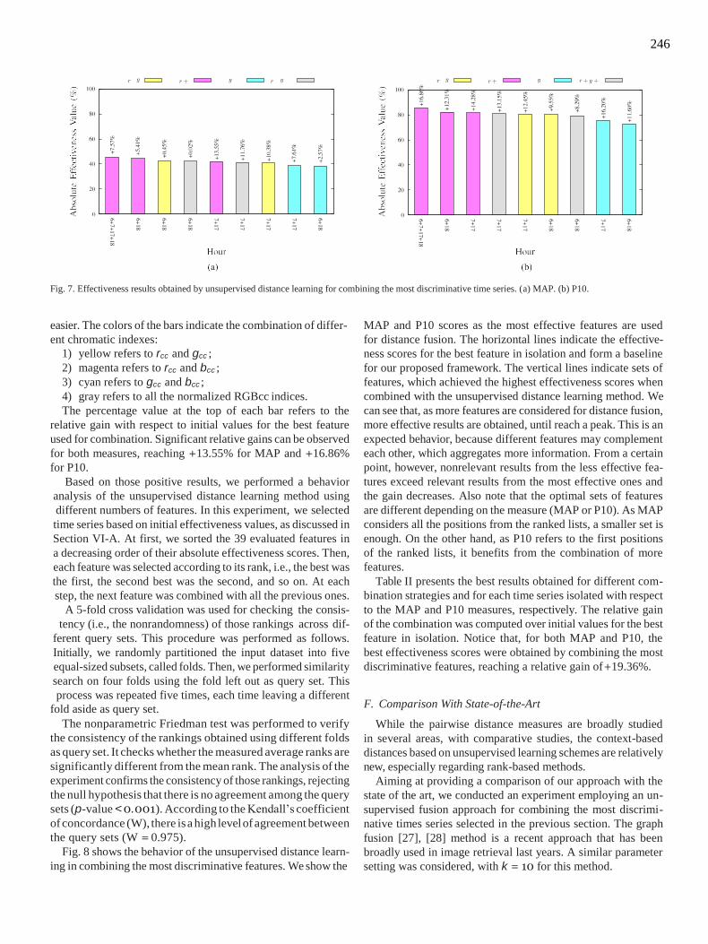
246

Fig. 7. Effectiveness results obtained by unsupervised distance learning for combining the most discriminative time series. (a) MAP. (b) P10.

easier. The colors of the bars indicate the combination of differ-

ent chromatic indexes:

1) yellow refers to rcc and gcc ;

2) magenta refers to rcc and bcc ;

3) cyan refers to gcc and bcc ;

4) gray refers to all the normalized RGBcc indices.

The percentage value at the top of each bar refers to the

relative gain with respect to initial values for the best feature

used for combination. Significant relative gains can be observed

for both measures, reaching +13.55% for MAP and +16.86%

for P10.

Based on those positive results, we performed a behavior

analysis of the unsupervised distance learning method using

different numbers of features. In this experiment, we selected

time series based on initial effectiveness values, as discussed in

Section VI-A. At first, we sorted the 39 evaluated features in

a decreasing order of their absolute effectiveness scores. Then,

each feature was selected according to its rank, i.e., the best was

the first, the second best was the second, and so on. At each

step, the next feature was combined with all the previous ones.

A 5-fold cross validation was used for checking the consis-

tency (i.e., the nonrandomness) of those rankings across dif-

ferent query sets. This procedure was performed as follows.

Initially, we randomly partitioned the input dataset into five

equal-sized subsets, called folds. Then, we performed similarity

search on four folds using the fold left out as query set. This

process was repeated five times, each time leaving a different

fold aside as query set.

The nonparametric Friedman test was performed to verify

the consistency of the rankings obtained using different folds

as query set. It checks whether the measured average ranks are

significantly different from the mean rank. The analysis of the

experiment confirms the consistency of those rankings, rejecting

the null hypothesis that there is no agreement among the query

sets (p-value < 0.001). According to the Kendall’s coefficient

of concordance (W), there is a high level of agreement between

the query sets (W = 0.975).

Fig. 8 shows the behavior of the unsupervised distance learn-

ing in combining the most discriminative features. We show the

MAP and P10 scores as the most effective features are used

for distance fusion. The horizontal lines indicate the effective-

ness scores for the best feature in isolation and form a baseline

for our proposed framework. The vertical lines indicate sets of

features, which achieved the highest effectiveness scores when

combined with the unsupervised distance learning method. We

can see that, as more features are considered for distance fusion,

more effective results are obtained, until reach a peak. This is an

expected behavior, because different features may complement

each other, which aggregates more information. From a certain

point, however, nonrelevant results from the less effective fea-

tures exceed relevant results from the most effective ones and

the gain decreases. Also note that the optimal sets of features

are different depending on the measure (MAP or P10). As MAP

considers all the positions from the ranked lists, a smaller set is

enough. On the other hand, as P10 refers to the first positions

of the ranked lists, it benefits from the combination of more

features.

Table II presents the best results obtained for different com-

bination strategies and for each time series isolated with respect

to the MAP and P10 measures, respectively. The relative gain

of the combination was computed over initial values for the best

feature in isolation. Notice that, for both MAP and P10, the

best effectiveness scores were obtained by combining the most

discriminative features, reaching a relative gain of +19.36%.

F. Comparison With State-of-the-Art

While the pairwise distance measures are broadly studied

in several areas, with comparative studies, the context-based

distances based on unsupervised learning schemes are relatively

new, especially regarding rank-based methods.

Aiming at providing a comparison of our approach with the

state of the art, we conducted an experiment employing an un-

supervised fusion approach for combining the most discrimi-

native times series selected in the previous section. The graph

fusion [27], [28] method is a recent approach that has been

broadly used in image retrieval last years. A similar parameter

setting was considered, with k = 10 for this method.

247

Fig. 8. Effectiveness results obtained by unsupervised distance learning for combining the most discriminative time series. (a) MAP. (b) P10.

TABLE II SUMMARY RESULTS OF UNSUPERVISED DISTANCE LEARNING FOR PLANT SPECIES IDENTIFICATION BY CONSIDERING THE COMBINATION OF THE MOST

DISCRIMINATIVE TIME SERIES

Measure Time Series Initial Value Reciprocal k NN Distance Relative Gain

MAP Single (r18 ) 42.16% 44.15% +4.72%

Fusion (r6 −18 ) Fusion (r18 + r6 + r14 )

- -

44.71% 45.62%

+6.05% +8.21%

P10 Single (r18 ) 73.12% 75.38% +3.09% Fusion (r6 −18 ) - 83.33% +13.96%

Fusion (r18 + r7 + r6 + b6 + b9 + r 17 + r1 4 ) - 87.30% +19.39%

TABLE III COMPARISON WITH STATE-OF-THE-ART BASED ON GRAPH FUSION

Measure Time Series Reciprocal k NN Distance Graph Fusion

MAP Fusion (r18 + r6 + r14 ) 45.62% 37.36%

P10 Fusion (r18 + r7 + r6 + b6 + b9 + r17 + r14 ) 87.30% 70.22%

The results of conducted comparison are presented in Table

III. As we can observe, the effectiveness results achieved by

our approach are higher considering both P10 and MAP

measures. It is worth mentioning that, if effectiveness results

are higher than those obtained for the best individual features,

it is commonly considered positive for unsupervised fusion ap-

proaches, once there is no training data available. Notice that

the proposed approach yielded effectiveness results significantly

higher than the best feature in isolation.

G. Qualitative and Visual Analysis

Once the quantitative results demonstrated significant gains

for effectiveness measures, this section conduct a qualitative

analysis using visual representations for evaluating the impact

of the use of unsupervised distance learning. First, we analyze

the neighborhood relationships among regions and species. In

the following, we present the visualization of identified species

in the original images used for extraction the time series.

For the neighborhood relationships analysis, a binary image

representation is employed. In the binary image, each pixel

p(i, j) has its color defined as black if the region rj is among the

k-NN of region ri. In addition, the axis of the image is defined

with regions sorted according to the plant species, such that an

effective retrieval is expected to produce blocks of black pixels.

In order to explicitly highlight the potential of the unsuper-

vised distance learning, we chose the g12 feature to conduct

those analyses. Such a feature was chosen due to the following

reasons: first, it is in agreement with the general standard of

analyzing the green color change at midday hours adopted in

ecological studies [4], [29], [30], and moreover, the worst result

in the plant identification task was obtained by this feature in

isolation, as reported in Section VI-A.

Fig. 9 shows the binary image representation of the neighbor-

hood relationships for the gcc index at 12 h. Different neigh-

borhood sizes are considered, with k = 10, 20, and 50 in

Fig. 9(a)–(c), respectively. Small and very diffuse blocks can

be observed, mainly for 50-NN.

248

Fig. 9. Neighborhood relationship among the regions for the g12 feature and various sizes. (a) 10-NN. (b) 20-NN. (c) 50-NN.

Fig. 10. Neighborhood relationship: Reciprocal kNN distance fusion and various sizes. (a) 10-NN. (b) 20-NN. (c) 50-NN.

Fig. 11. Impact of the reciprocal kNN distance fusion on plant identification tasks, considering 50-NN neighborhood.

Fig. 10 illustrates an analogous representation considering

the reciprocal kNN distance fusion and the best combination of

features identified in previous section. We can clearly observe

very distinct blocks for 50-NN and even for 20-NN.

Fig. 11 presents the 50-NN representation with a legend in-

dicating the plant species in the axis of the image. As expected,

the majority of the blocks are localized in the main diagonal,

which demonstrates that regions of the same species are among

the nearest neighbors of each other. Blocks out of the main di-

agonal may indicate functional groups and constitute a future

line of investigation.

Figs. 12 and 13 present a different view of the results, showing

the performance without and with the unsupervised distance

learning for the individual queries (i.e., specific lines of the

previous images) that achieved the best and the worst result,

respectively. In those figures, each region is colored according

to its distance to the query using a colormap from blue to red,

where the red colors denote nearest regions (i.e., associate with

similar species) and the blue ones represent furthest regions

(i.e., relate to different species). The yellow circles indicate the

relevant regions to the query (i.e., are from a same species).

249

×

Fig. 12. Results obtained for the query that achieved the highest score, showing the performance without and with the unsupervised distance learning. Each region is colored according to its distance to the query using a colormap from blue to red. The red colors denote nearest regions whereas the blue ones represent furthest regions. The yellow circles indicate the relevant regions to the query. (a) g12 feature in isolation. (b) Reciprocal kNN distance fusion.

Fig. 13. Results obtained for the query that achieved the lowest score, showing the performance without and with the unsupervised distance learning. Each region is colored according to its distance to the query using a colormap from blue to red. The red colors denote nearest regions whereas the blue ones represent furthest regions. The yellow circles indicate the relevant regions to the query. (a) g12 feature in isolation. (b) Reciprocal kNN distance fusion.

Ideally, the regions inside the yellow circles should be colored

in red and all the remaining ones should be colored in blue, in-

dicating a perfect prediction of individuals from a same species.

Observe that it is hard to distinguish whether species are similar

or not by considering only the g12 feature, since the areas in

red and blue colors are diffuse [see Figs. 12(a) and 13(a)]. Re-

gardless of the initial performance, we can notice the significant

improvements yielded by the reciprocal kNN distance fusion,

which clearly separates the plant species, thus producing large

same-colored areas [see Figs. 12(b) and 13(b)].

H. Experiments With Hyperspectral Data

Also, we evaluated the proposed method on a hyperspectral

dataset, i.e., with more than three bands. For that, experiments

were conducted on data collected by the sensor USGS Land-

sat 5 TM Raw Scenes (Orthorectified) in various regions from

South America, between January 2000 and December 2011. The

sensor offers images composed of seven spectral bands at 30-m

spatial resolution with a temporal frequency of 16 days.3

The geographical coordinates used as ground truth in this

study are a modified subset of the inventory data used by [31].

These data correspond to centroid coordinates of field sampled

quadrants of tropical vegetation labeled either as forest or sa-

vanna. We selected the subset of these quadrants corresponding

to tropical South America and visualized each of the quadrants

using Google Earth images from 2016 superimposed with the

MODIS pixel grid of 250 250 m using Series Views [32]. For

each of those quadrants, we visually assessed whether a MODIS

pixel was or not completely filled with a labeled vegetation type

(i.e., savannas or forests). Pixels that were not entirely filled

with the corresponding vegetation type were either replaced by

a neighboring pixel fulfilling these criteria or discarded (when a

suitable pixel could not be found nearby). In addition, locations

3http://landsat.usgs.gov (As of July 2016)

250

{ }

Fig. 14. Classification accuracy obtained for each of the bands after unsuper- vised distance learning by using a k-NN classifier with different values of k.

at which the label assigned to that vegetation type could not

be visually confirmed were also discarded. The centroid coor-

dinate of each remaining pixel was then obtained and used to

extract the satellite data used for classification purposes. There-

fore, subsequent analyses were performed using 183 savannas

and 110 forest locations.

For each location, we extracted seven different time series

by considering the available bands (seven components: B1 to

B7 ). The distance function used for time-series comparison is

the Manhattan (L1) distance. In the experiments, we adopted

the evaluation protocol used in [33] and [34]. It relies on the

classification of time series extracted from locations associated

with a given vegetation type. For that, we used a k-NN classifi-

cation model: a given location is classified by a majority vote of

its neighbors, being assigned to the class most common among

its k-NN.

Our experiments intend to evaluate the accuracy of a k-NN

classifier before and after the use of the unsupervised distance

learning procedure. For that, we adopted the same value of the

parameter k used both for the k-NN classifier and the reciprocal

kNN distance algorithm. Similar to the retrieval-based proto-

col, the size of the neighborhood set plays an important role,

defining the extension of the reciprocal neighborhood analysis.

Therefore, the first experiment was conducted aiming at deter-

mining the best value for the parameter k. We computed the

classification accuracy for each band in isolation considering

k = 5, 10, 15 . Fig. 14 presents the classification accuracy obtained by dif-

ferent bands and different values of k. We can clearly observe

that the accuracy of k = 5 achieved the higher scores for all

the bands. Therefore, we choose the value of k = 5 for next

experiments.

Fig. 15 shows the accuracy scores of a 5-NN classifier ob-

tained for each band based on the initial distance. Observe that

the best result in isolation was achieved by the band B7 , reaching

a classification accuracy of 89.08%.

The next experiment was conducted to evaluate the use of the

unsupervised distance learning for each individual band. Fig. 16

presents the relative gains obtained by the use of the reciprocal

Fig. 15. Initial accuracy scores obtained for each band using a 5-NN classifier.

Fig. 16. Relative effectiveness gains obtained for each of the bands after unsupervised distance learning.

Fig. 17. Classification accuracy obtained by unsupervised distance learning for combining the most discriminative bands.

kNN distance algorithm for each band. The best gains can be

observed for the band B4 , which obtained a relative gain of

+2.36%, reaching a final accuracy of 88.74%. On other hand,

the band B7 obtained a relative gain of +1.15%, reaching a

final accuracy score of 90.10%. This score is higher than any

accuracy score obtained by the initial distance, considering all

the bands.

251

Finally, we also evaluated the combination of different bands.

For that, an experimental protocol similar to the previous fu-

sion experiments (see Section VI-E) was considered. Thus,

we selected the most discriminative bands by ordering their

classification accuracy after the unsupervised distance learning.

Fig. 17 shows the classification accuracy obtained by our pro-

posed framework. The horizontal line indicates the accuracy

score for the best band in isolation and the vertical line indicates

the best fusion result (obtained for the bands B7 + B6 + B4 ). We can observe that the curve presents a very similar behavior to

the previous fusion experiments (see Fig. 8), achieving a higher

accuracy result than the best band in isolation.

VII. CONCLUSION

This paper presented a new similarity measure for plant iden-

tification tasks involved in remote monitoring of phenology with

digital cameras. In order to obtain global measures that encode

information of the dataset structure, we proposed the use of a

unsupervised distance learning method called reciprocal kNN

distance [13].

A comparative analysis of different features, as well as their

possible combinations created by our approach, has been con-

ducted in our experiments. Results obtained with our proposed

framework applied to about 2700 images taken from a tropi-

cal cerrado savanna vegetation demonstrate that it can largely

improve the plant identification results, reaching gains of more

than 19%.

One possible limitation of the work refers to the problems

caused by distortions within the generated images. For exam-

ple, the visual properties associated with regions close to the

borders probably contain a lot of noise, which may impact the

effectiveness of the method. This is reason that we have avoided

using them in our evaluation protocol (see the selected regions

in Fig. 1). Another issue refers to parameter settings of the pro-

posed method. An in-depth evaluation of suitable values for

them is left for future work. Another issue refers to the time

span of images used. We expect to check the consistence of the

results with longer time series in future work.

Future work includes the evaluation of other features for iden-

tifying plants based on phenological time series and a rigorous

analysis of the influence of parameters employed in our ap-

proach in order to determine which configuration produces the

best results, as well as perform an extensive study on different

strategies for feature selection and distance fusion.

ACKNOWLEDGMENT

The authors are grateful to J. F. H. Albarrac ın and V. de Lima

Dantas for their assistance with the hyperspectral dataset.

REFERENCES

[1] M. D. Schwartz, Phenology: An Integrative Environmental Science, 2nd ed. New York, NY, USA: Springer, 2013.

[2] L. P. C. Morellato, M. G. G. Camargo, and E. Gressler, “A review of plant phenology in South and Central America,” in Phenology: An Inte- grative Environmental Science, M. D. Schwartz, Ed. New York, NY, USA: Springer, 2013, ch. 6, pp. 91–113.

[3] B. Alberton, J. Almeida, R. Henneken, R. S. Torres, A. Menzel, and L. P. C. Morellato, “Using phenological cameras to track the green up in a cerrado savanna and its on-the-ground validation,” Ecol. Informat., vol. 19, pp. 62–70, 2014.

[4] A. D. Richardson, B. H. Braswell, D. Y. Hollinger, J. P. Jenkins, and S. V. Ollinger, “Near-surface remote sensing of spatial and temporal variation in canopy phenology,” Ecol. Appl., vol. 19, pp. 1417–1428, 2009.

[5] J. Almeida, J. A. dos Santos, B. Alberton, R. da S. Torres, and L. P. C. Morellato, “Applying machine learning based on multiscale classifiers to detect remote phenology patterns in Cerrado savanna trees,” Ecol. Infor- mat., vol. 23, pp. 49–61, 2014.

[6] R. da S. Torres and A. X. Falcao, “Content-based image retrieval: Theory and applications,” J. Theor. Appl. Informat., vol. 13, no. 2, pp. 161–185, 2006.

[7] O. Sonnentag, “Digital repeat photography for phenological research in forest ecosystems,” Agricultural Forest Meteorol., vol. 152, pp. 159–177, 2012.

[8] T. Skopal and B. Bustos, “On nonmetric similarity search problems in complex domains,” ACM Comput. Surveys, vol. 43, no. 4, pp. 34:1–34:50, 2011.

[9] R. da S. Torres, “Shape-based time series analysis for remote phenology studies,” in Proc. IEEE Int. Geosci. Remote Sens. Symp., 2013, pp. 3598– 3601.

[10] J. Almeida, J. A. Santos, B. Alberton, L. P. C. Morellato, and R. S. Torres, “Phenological visual rhythms: Compact representations for fine-grained plant species identification,” Pattern Recognit. Lett., vol. 81, pp. 90–100, 2015, [Online]. Available: http://doi: 10.1016/j.patrec.2015.11.028.

[11] B. Eravci and H. Ferhatosmanoglu, “Diversity based relevance feedback for time series search,” Proc. VLDB Endowment, vol. 7, no. 2, pp. 109–120, Oct. 2013.

[12] J. Almeida, J. A. dos Santos, B. Alberton, R. da S. Torres, and L. P. C. Morellato, “Remote phenology: Applying machine learning to detect phenological patterns in a Cerrado savanna,” in Proc. IEEE Int. Conf. eSci., 2012, pp. 1–8.

[13] D. C. G. Pedronette, O. A. B. Penatti, R. T. Calumby, and R. da S. Torres, “Unsupervised distance learning by reciprocal kNN distance for image retrieval,” in Proc. Int. Conf. Multimedia Retrieval, 2014, p. 345.

[14] M. Lngkvist, L. Karlsson, and A. Loutfi, “A review of unsupervised feature learning and deep learning for time-series modeling,” Pattern Recognit. Lett., vol. 42, pp. 11–24, 2014.

[15] M. Donoser and H. Bischof, “Diffusion processes for retrieval revisited,” in Proc. IEEE Conf. Comput. Vis. Pattern Recog., 2013, pp. 1320–1327.

[16] D. C. G. Pedronette, O. A. B. Penatti, and R. da S. Torres, “Unsupervised manifold learning using reciprocal knn graphs in image re-ranking and rank aggregation tasks,” Image Vis. Comput., vol. 32, no. 2, pp. 120–130, 2014.

[17] A. D. Richardson, J. P. Jenkins, B. H. Braswell, D. Y. Hollinger, S. V. Ollinger, and M. L. Smith, “Use of digital webcam images to track spring greep-up in a deciduous broadleaf forest,” Oecologia, vol. 152, pp. 323– 334, 2007.

[18] A. R. Gillespie, A. B. Kahle, and R. E. Walker, “Color enhancement of highly correlated images. ii. channel ratio and “chromaticity” transfor- mation techniques,” Remote Sens. Environ., vol. 22, no. 3, pp. 343–365, 1987.

[19] D. M. Woebbecke, G. E. Meyer, K. Von-Bargen, and A. D. Mortensen, “Color indices for weed identification under various soil, residue, and lighting conditions,” Trans. ASAE, vol. 38, pp. 259–269, 1995.

[20] J. Almeida, J. A. Santos, W. O. Miranda, B. Alberton, L. P. C. Morellato, and R. S. Torres, “Deriving vegetation indices for phenology analysis using genetic programming,” Ecol. Informat., vol. 26, pp. 61–69, 2015.

[21] H. Jegou, C. Schmid, H. Harzallah, and J. Verbeek, “Accurate image search using the contextual dissimilarity measure,” IEEE Trans. Pattern Anal. Mach. Intell., vol. 32, no. 1, pp. 2–11, Jan. 2010.

[22] D. Qin, S. Gammeter, L. Bossard, T. Quack, and L. van Gool, “Hello neighbor: Accurate object retrieval with k-reciprocal nearest neighbors,” in Proc. IEEE Conf. Comput. Vision Pattern Recognit., Jun. 2011, pp. 777– 784.

[23] L. Guigues, J. Cocquerez, and H. Le Men, “Scale-sets image analysis,” Int. J. Comput. Vis., vol. 68, pp. 289–317, 2006.

[24] J. C. Conti, “Evaluation of time series distance functions in the task of detecting remote phenology patterns,” in Proc. IEEE Int. Conf. Pattern Recog., 2014, pp. 3126–3131.

[25] J. Almeida, J. A. dos Santos, B. Alberton, L. P. C. Morellato, and R. da S. Torres, “Visual rhythm-based time series analysis for phenology studies,” in Proc. IEEE Int. Conf. Image Process., 2013, pp. 4412–4416.

252

[26] J. Almeida, J. A. dos Santos, B. Alberton, L. P. C. Morellato, and R. da S. Torres, “Plant species identification with phenological visual rhythms,” in Proc. IEEE Int. Conf. eSci., 2013, pp. 148–154.

[27] S. Zhang, M. Yang, T. Cour, K. Yu, and D. N. Metaxas, “Query specific fusion for image retrieval,” in Proc. 12th Eur. Conf. Comput. Vision, 2012, pp. 660–673.

[28] S. Zhang, M. Yang, T. Cour, K. Yu, and D. Metaxas, “Query specific rank fusion for image retrieval,” IEEE Trans. Pattern Anal. Mach. Intell., vol. 37, no. 4, pp. 803–815, Apr. 2015.

[29] H. Ahrends, “Tree phenology and carbon dioxide fluxes: Use of digi- tal photography for process-based interpretation at the ecosystem scale,” Climate Res., vol. 39, pp. 261–274, 2009.

[30] R. Ide and H. Oguma, “A cost-effective monitoring method using dig- ital time-lapse cameras for detecting temporal and spatial variations of snowmelt and vegetation phenology in alpine ecosystems,” Ecol. Infor- mat., vol. 16, pp. 25–34, 2013.

[31] V. L. Dantas, M. Hirota, R. S. Oliveira, and J. G. Pausas, “Disturbance maintains alternative biome states,” Ecol. Lett., vol. 19, pp. 12–19, 2016.

[32] R. M. Freitas, “Virtual laboratory of remote sensing series: Visualization of MODIS EVI2 data set over south america,” J. Comput. Interdisciplinary Sci., vol. 2, pp. 57–64, 2011.

[33] F. A. Faria, J. Almeida, B. Alberton, L. P. C. Morellato, A. Rocha, and R. S. Torres, “Time series-based classifier fusion for fine-grained plant species recognition,” Pattern Recognit. Lett., vol. 81, pp. 101–109, 2015, [Online]. Available: http://doi: 10.1016/j.patrec.2015.10.016.

[34] F. A. Faria, J. Almeida, B. Alberton, L. P. C. Morellato, and R. S. Torres, “Fusion of time series representations for plant recognition in phenology studies,” Pattern Recognit. Lett., 2016, [Online]. Available: http://doi: 10.1016/j.patrec.2016.03.005, to be published.