Boundary-Integral Calculations of Two-Dimensional Electromagnetic Scattering in Infinite Photonic...

BOUNDARY-INTEGRAL CALCULATIONS OF TWO-DIMENSIONALELECTROMAGNETIC SCATTERING IN INFINITE PHOTONICCRYSTAL SLABS: CHANNEL DEFECTS AND RESONANCES∗

MANSOOR A. HAIDER† , STEPHEN P. SHIPMAN‡ , AND STEPHANOS VENAKIDES§

SIAM J. APPL. MATH. c© 2002 Society for Industrial and Applied MathematicsVol. 62, No. 6, pp. 2129–2148

Abstract. We compute the transmission of two-dimensional (2D) electromagnetic waves througha square lattice of lossless dielectric rods with a channel defect. The lattice is finite in the directionof propagation of the incident wave and periodic in a transverse direction. We revisit a boundary-integral formulation of 2D electromagnetic scattering [Venakides, Haider, and Papanicolaou, SIAMJ. Appl. Math., 60 (2000), pp. 1686–1706] that is Fredholm of the first kind and develop a second-kindformulation. We refine the numerical implementation in the above paper by exploiting separabilityin the Green’s function to evaluate the far-field influence more efficiently. The resulting cost savingsin computing and solving the discretized linear system leads to an accelerated method. We use itto analyze E-polarized electromagnetic scattering of normally incident waves on a structure with aperiodic channel defect. We find three categories of resonances: waveguide modes in the channel,high-amplitude fields in the crystal at frequencies near the edge of the frequency bandgap, and veryhigh-amplitude standing fields at frequencies in a transmission band that are normal to the directionof the incident wave. These features are captured essentially identically with the first-kind as withthe second-kind formulation.

Key words. EM scattering, photonic crystal, photonic bandgap, channel defect, boundaryintegral, boundary element method, Ewald representation, resonances

AMS subject classifications. 78, 45, 65, 42

PII. S003613990138531X

1. Introduction. Calculations of electromagnetic (EM) scattering in photoniccrystal lattices play a central role in the design of optical and electronic devices in-cluding filters, lasers, and microwave antennas. The manner in which waves propagatethrough a photonic crystal is highly dependent on the geometry of the lattice, the lossproperties of the component dielectrics, and the dielectric contrast. Under conditionsof high dielectric contrast, it is well known that infinite two-dimensional (2D) latticesexhibit photonic bandgaps, which are frequency intervals in which there are no wavespropagating through the lattice (see, e.g., [5], [9]).

In the practical case of a truncated photonic crystal, in particular a photoniccrystal slab, the bandgaps appear as frequency intervals of very low transmission.When defects are introduced into the geometry, large fields at resonant frequenciesarise in the structure, causing irregular behavior in the transmission coefficient atthese frequencies.

In the present study, we consider EM scattering by a photonic crystal slab com-prised of a square lattice of lossless dielectric rods. The slab is finite in one directionX and periodic in the other direction Y . We first compute the effects of nonnormal

∗Received by the editors February 21, 2001; accepted for publication (in revised form) December19, 2001; published electronically July 24, 2002.

http://www.siam.org/journals/siap/62-6/38531.html†Department of Mathematics, North Carolina State University, Box 8205, Raleigh, NC 27695-8205

([email protected]). The research of this author was supported by NSF grant DMS-9705931.‡Department of Mathematics, Box 90320, Duke University, Durham, NC 27708-0320 (shipman@

math.duke.edu).§Department of Mathematics, Box 90320, Duke University, Durham, NC 27708-0320 (ven@math.

duke.edu). The research of this author was supported by grants ARO-DAAD19-99-1-0132 and NSFDMS-9500623.

2129

2130 M. A. HAIDER, S. P. SHIPMAN, AND S. VENAKIDES

incidence and consider briefly the effect of random perturbations of the perfect latticeon the transmission coefficient. Then, as our primary focus, we analyze the scatteringof normally incident waves by a structure with a periodic channel defect (Figure 4.3)that is parallel to the X-axis. We find three categories of resonances in the chan-nel structure (Figure 4.5): waveguide modes in the channel at higher frequencies inthe bandgap, high-amplitude 2D modes in the structure at lower frequencies in thebandgap, and very high-amplitude Y -resonating modes at frequencies to the left ofthe bandgap. The last category of resonances is of particular interest as such reso-nances have very high quality factors and exhibit characteristics similar to channeldrop filters [2], [3], which reflect incident radiation at a particular frequency whileallowing neighboring frequencies to penetrate the lattice.

In previous work [1], [8], we studied transmission through Fabry–Perot laser cav-ities formed by two parallel mirrors comprised of circular dielectric rods in air. Incontrast to the channel in the present study, the Fabry–Perot cavity runs parallel tothe Y direction. In that case, resonant frequencies arise in the bandgap only. In [8],the location of peaks in the transmission graph and their quality factor (Q-value),which measures laser efficiency, were traced as a function of cavity width for the caseof lossless dielectrics. In the present study, we are concerned not only with charac-teristics in the transmission coefficient at various types of resonant frequencies in theband and the gap but also with the behavior of the electromagnetic field inside thestructure at these frequencies.

For our studies, we use a numerical implementation of a boundary-integral for-mulation of the scattering problem that we developed in [8]. We also use a well-posedformulation that we develop in section 2.2. The boundary-integral approach reducesthe problem from 2D to 1D and automatically enforces radiation conditions that areinherent to the scattering problem through the choice of appropriate radiating Green’sfunctions. In this study, we refine our previous model by exploiting separability inthe Green’s function to evaluate the far-field influence more efficiently. As in the pre-vious study, an Ewald representation of the Green’s function is used to ensure rapidconvergence of the representation in the near field. The primary consequence of ourrefined approach is that the (previously) dense matrix in the assembled system oflinear equations is reduced to a banded matrix, resulting in an accelerated method.This simplification leads to significant cost savings in both computing and solving thediscretized integral system.

2. The scattering problem and its mathematical formulation. We de-scribe in this section our extension of the boundary-integral formulation of the elec-tromagnetic scattering problem, which was developed in [8]. The photonic crystalunder consideration is a mixed dielectric structure that is periodic in one directionY and finite in the other direction X. It is constant in the Z-direction. One periodconsists of a finite number of parallel rods Dj transverse to the XY -plane, each havinga uniform dielectric permittivity εj . We call the period of the structure a cell, or asupercell in the case in which it involves a finer periodic structure (Figure 2.1). Thespace exterior to the rods has a uniform dielectric permittivity εext. We refer to thisstructure as a photonic crystal slab.

We consider scattering by the structure of time-harmonic electric and magneticfields with either electric or magnetic polarization. In the former, the electric fieldpoints parallel to the rods, and the magnetic field lies parallel to the XY -plane,transverse to the rods. We refer to this as Ez-polarization. (In [8], these fieldswere called transverse magnetic, or TM, fields.) We define Hz-polarization (TE) in

BOUNDARY-INTEGRAL CALCULATIONS OF 2D EM SCATTERING 2131

incident field transmitted field

supercell

angle of incidence

Fig. 2.1. A plane cross-section of a y-periodic photonic crystal. The supercell enclosed in arectangle represents one period.

a corresponding fashion, with the magnetic field parallel to the rods. In either case,the field component parallel to the rods has the form Ψ(X,Y )e−iωt, and Ψ satisfiesthe Helmholtz equation

(∂2X + ∂2

Y )Ψ +ω2

c2ε(X,Y )Ψ = 0,

in which c is the speed of light. This equation is valid in the interiors of the rodsand in the exterior, and matching conditions described below apply on the interface.Because of the periodicity of the structure, the domain of the mathematical problemis the strip {(X,Y ) : −∞ < X < ∞, 0 ≤ Y ≤ P}, where P is the period.

2.1. Equations for the electromagnetic field. In dimensionless form, wescale the period to 2π, and we let ψ(x, y) denote the electric (Ez case) or magneticfield (Hz case). Here ψ satisfies the nondimensional Helmholtz equation

(∂2x + ∂2

y)ψ + k2ε(x, y)ψ = 0,(2.1)

in which k, the reduced (nondimensional) frequency, is given by k = ωp/(2πc), wherep is the Y -period of the structure. ε = εint/εext is the dielectric contrast between theinterior and the exterior and is equal to 1 in the exterior to the rods. The followingconditions also apply:

• The field ψext in the exterior is the sum of an incident plane wave ψinc and ascattered wave ψsc.

• ψsc satisfies a radiation condition at x = ±∞.• Let ψint denote the field inside rod Dj . On the boundary ∂Dj , the followingmatching conditions hold:

ψext = ψinc + ψsc = ψint, ∂nψext = ∂nψinc + ∂nψsc = ν−1∂nψint,(2.2)

where ν = 1 for Ez waves and ν = ε for Hz waves.If the incident field is produced at an angle of θ with the normal to the surface of

the crystal (x-axis), then, by requiring that it satisfy the Helmholtz equation (2.1),we find that it has the form

ψinc = exp(i√k2 − (m+ β)2x+ i(m+ β)y

),

in which θ = arcsin((m + β)/k), m is an integer, and −1/2 < β ≤ 1/2. ψinc ispseudoperiodic in the sense that

ψinc = eiβyψinc(x, y),


where ψinc is 2π-periodic in y. Requiring that the scattered field also be pseudo-periodic, so that ψsc = eiβyψsc(x, y), where ψsc is 2π-periodic in y, we find that, inthe exterior,

(∂2x + ∂2

y)ψsc + 2iβ∂yψsc + (k2 − β2)ψsc = 0.(2.3)

The radiating Green’s function for the exterior is then the pseudoperiodic function

G(r − r) = eiβ(y−y)G(r − r),

in which G is the field at the point r = (x, y) produced by a radiating periodicmonopole of (2.3):

G(r − r; k2, β) =1

4π

∞∑m=−∞

e−√−λm |x−x|√−λm

eim(y−y),(2.4)

where λm = k2 − (m+ β)2.Considering the matching conditions (2.2), the radiation condition on ψsc, and

the pseudoperiodicity of the incident and scattered fields and the Green’s function,Green’s identity results in the following system of boundary-integral equations for thetotal exterior field ψext and its normal derivative ∂nψext:

1 For any point r ∈ ∂Dj ,

1

2ψext(r) +

∫∂D

[−∂G(r − r)

∂n(r)ψext(r) +G(r − r)

∂ψext

∂n(r)(r)

]ds(r) = ψinc(r),(2.5a)

1

2ψext(r) +

∫∂Dj

[∂Φj(r − r)

∂n(r)ψext(r)− νΦj(r − r)

∂ψext

∂n(r)(r)

]ds(r) = 0,(2.5b)

in which Φj is a Green’s function for the interior of rod j and ∂D is the union ofall ∂Dj .

This system (2.5) is Fredholm of the first kind in the functional variable ∂nψext.

2.2. A well-posed formulation of the boundary-integral equations. Wehave developed a well-posed formulation of the problem, in which the boundary-integral equations are Fredholm of the second kind.

Theorem 2.1. Suppose that the matching conditions (2.2), the radiating condi-tion on ψsc, and the pseudoperiodicity of ψsc and ψinc are satisfied. Then the followingsystem of integral equations for ψext holds:

ψext(r) +

∫∂D

[∂(Φ−G)(r − r)

∂n(r)ψext(r)− (νΦ−G)(r − r)

∂ψext

∂n(r)(r)

]ds(r) = ψinc(r),

(2.6a)

1 + ν

2

∂ψext

∂n(r)(r) +

∫∂D

[∂2(Φ−G)(r − r)

∂n(r)∂n(r)ψext(r)

− ∂(νΦ−G)(r − r)

∂n(r)

∂ψext

∂n(r)(r)

]ds(r) =

∂ψinc

∂n(r)(r).(2.6b)

1In [8], an extra term with a factor of β appears erroneously in equation 4.6 and propagates intoequations 4.12, 4.15, and 5.6. The error does not affect the results of that paper because only thecase β = 0 is considered. The authors apologize for the error.


The notation ∂/∂n(r) refers to differentiation with respect to the variable r in thenormal direction to the boundary at the point r, and ∂/∂n(r) refers to differentiationwith respect to the variable r in the normal direction to the boundary at the pointr. It is also understood that the interior Green’s function Φ(r − r) is zero wheneverr and r are on different rods.

These equations can be generalized to a system in which the scatterer has amagnetic permeability that is different from the external medium.

Similar formulations for 3D EM scattering problems are derived in Muller [7].Our formulation is derived below from the first-kind system (2.5).

Proof. We start with the equation for the external field for values of r in thedomain exterior to the rods:

ψext(r) +

∫∂D

[−∂G(r − r)


∂ψext

∂n(r)(r)

]ds(r) = ψinc(r).(2.7)

Let r lie on a vector n(r) emanating normally from some point on the boundary of oneof the rods, and take the derivative of this equation with respect to r in the directionof n(r):

∂ψext

∂n(r)(r) +

∫∂D

[− ∂2G(r − r)

∂n(r)∂n(r)ψext(r) +

∂G(r − r)

∂n(r)

∂ψext

∂n(r)(r)

]ds(r) =

∂ψinc

∂n(r)(r).

The following identity holds:

∂2G(r − r)

∂n(r)∂n(r)+

∂2G(r − r)

∂t(r)∂t(r)= −n(r) · n(r)(∂2

x + ∂2y)G(r − r),

in which ∂t denotes a tangent derivative. The minus sign occurs because ∂n(r) and∂t(r) denote derivatives with respect to r. Using this together with the Helmholtzequation

(∂2x + ∂2

y)G(r − r) + k2G(r − r) = 0 for r �= r,

we eliminate the term containing two normal derivatives of G. Then, integrating byparts in the term with the tangent derivatives, we obtain

∂ψext

∂n(r)(r) +

∫∂D

[− n(r) · n(r)k2G(r − r)ψext(r)

− ∂G(r − r)

∂t(r)

∂ψext

∂t(r)(r) +

∂G(r − r)

∂n(r)

∂ψext

∂n(r)(r)

]ds(r) =

∂ψinc

∂n(r)(r).

We now allow r to approach the boundary along the vector n(r), and the term con-taining ∂G

∂n produces a singular contribution of − 12∂ψext

∂n(r) (r). Thus, for r ∈ ∂D, we

obtain

1

2

∂ψext

∂n(r)(r) +

∫∂D

[− n(r) · n(r)k2G(r − r)ψext(r)

− ∂G(r − r)

∂t(r)

∂ψext

∂t(r)(r) +

∂G(r − r)

∂n(r)

∂ψext

∂n(r)(r)

]ds(r) =

∂ψinc

∂n(r)(r).(2.8)


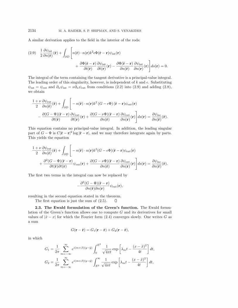
A similar derivation applies to the field in the interior of the rods:

(2.9)1

2

∂ψint

∂n(r)(r) +

∫∂D

[n(r) · n(r)k2εΦ(r − r)ψint(r)

+∂Φ(r − r)

∂t(r)

∂ψint

∂t(r)(r)− ∂Φ(r − r)

∂n(r)

∂ψint

∂n(r)(r)

]ds(r) = 0.

The integral of the term containing the tangent derivative is a principal-value integral.The leading order of this singularity, however, is independent of k and ε. Substitutingψint = ψext and ∂nψint = ν∂nψext from conditions (2.2) into (2.9) and adding (2.8),we obtain

1 + ν

2

∂ψext

∂n(r)(r) +

∫∂D

[− n(r) · n(r)k2 (G− εΦ) (r − r)ψext(r)

− ∂(G− Φ)(r − r)

∂t(r)

∂ψext

∂t(r)(r) +

∂(G− νΦ)(r − r)

∂n(r)

∂ψext

∂n(r)(r)

]ds(r) =

∂ψinc

∂n(r)(r).

This equation contains no principal-value integral. In addition, the leading singularpart of G− Φ is C|r − r|2 log |r − r|, and we may therefore integrate again by parts.This yields the equation

1 + ν

2

∂ψext

∂n(r)(r) +

∫∂D

[− n(r) · n(r)k2(G− εΦ)(r − r)ψext(r)

+∂2(G− Φ)(r − r)

∂t(r)∂t(r)ψext(r) +

∂(G− νΦ)(r − r)

∂n(r)

∂ψext

∂n(r)(r)

]ds(r) =

∂ψinc

∂n(r)(r).

The first two terms in the integral can now be replaced by

−∂2(G− Φ)(r − r)

∂n(r)∂n(r)ψext(r),

resulting in the second equation stated in the theorem.The first equation is just the sum of (2.5).

2.3. The Ewald formulation of the Green’s function. The Ewald formu-lation of the Green’s function allows one to compute G and its derivatives for smallvalues of |x − x| for which the Fourier form (2.4) converges slowly. One writes G asa sum

G(r − r) = G1(r − r) +G2(r − r),

in which

G1 =1

2π

∞∑m=−∞

ei(m+β)(y−y)∫ E2

0

1√4πt

exp

[λmt− (x− x)2

4t

]dt,

G2 =1

2π

∞∑m=−∞

ei(m+β)(y−y)∫ ∞

E2

1√4πt

exp

[λmt− (x− x)2

4t

]dt,


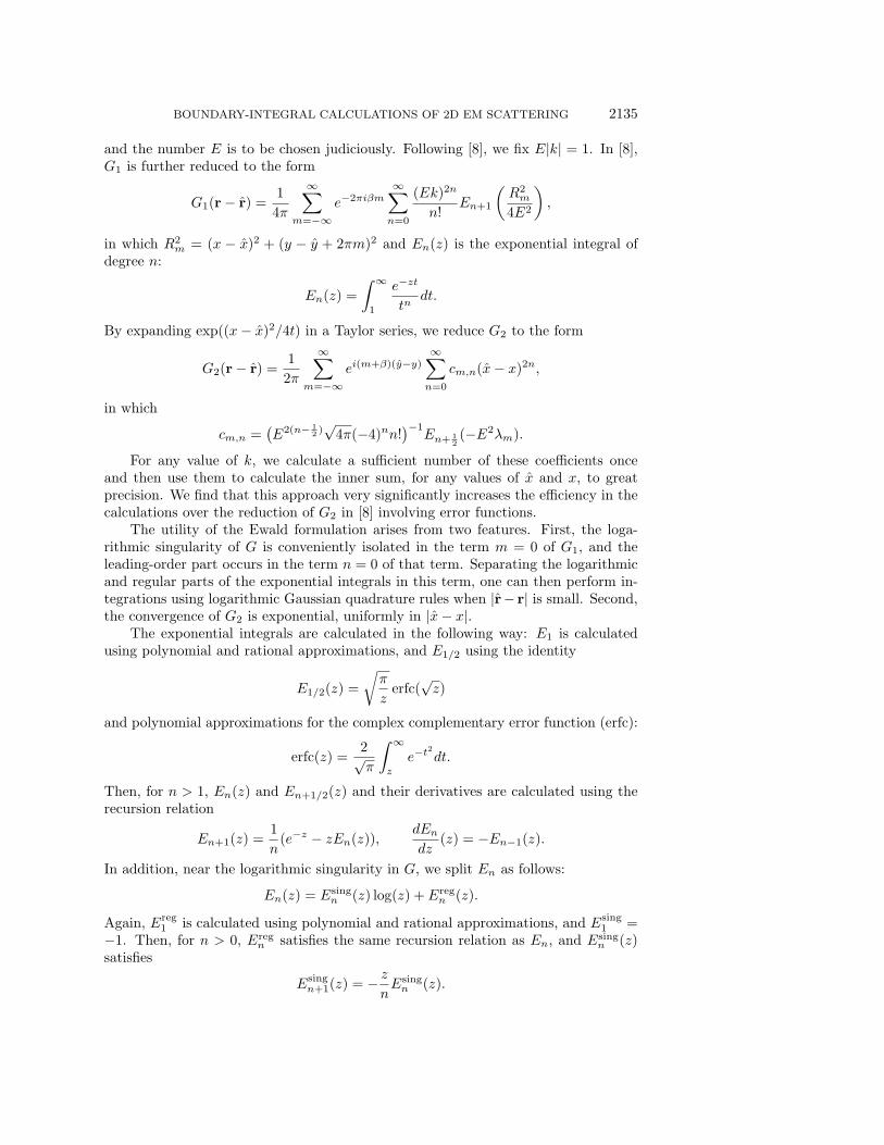
and the number E is to be chosen judiciously. Following [8], we fix E|k| = 1. In [8],G1 is further reduced to the form

G1(r − r) =1

4π

∞∑m=−∞

e−2πiβm∞∑n=0

(Ek)2n

n!En+1

(R2m

4E2

),

in which R2m = (x − x)2 + (y − y + 2πm)2 and En(z) is the exponential integral of

degree n:

En(z) =

∫ ∞

1

e−zt

tndt.

By expanding exp((x− x)2/4t) in a Taylor series, we reduce G2 to the form

G2(r − r) =1

2π

∞∑m=−∞

ei(m+β)(y−y)∞∑n=0

cm,n(x− x)2n,

in which

cm,n =(E2(n− 1

2 )√4π(−4)nn!)−1

En+ 12(−E2λm).

For any value of k, we calculate a sufficient number of these coefficients onceand then use them to calculate the inner sum, for any values of x and x, to greatprecision. We find that this approach very significantly increases the efficiency in thecalculations over the reduction of G2 in [8] involving error functions.

The utility of the Ewald formulation arises from two features. First, the loga-rithmic singularity of G is conveniently isolated in the term m = 0 of G1, and theleading-order part occurs in the term n = 0 of that term. Separating the logarithmicand regular parts of the exponential integrals in this term, one can then perform in-tegrations using logarithmic Gaussian quadrature rules when |r− r| is small. Second,the convergence of G2 is exponential, uniformly in |x− x|.

The exponential integrals are calculated in the following way: E1 is calculatedusing polynomial and rational approximations, and E1/2 using the identity

E1/2(z) =

√π

zerfc(

√z)

and polynomial approximations for the complex complementary error function (erfc):

erfc(z) =2√π

∫ ∞

z

e−t2

dt.

Then, for n > 1, En(z) and En+1/2(z) and their derivatives are calculated using therecursion relation

En+1(z) =1

n(e−z − zEn(z)),

dEndz

(z) = −En−1(z).

In addition, near the logarithmic singularity in G, we split En as follows:

En(z) = Esingn (z) log(z) + Ereg

n (z).

Again, Ereg1 is calculated using polynomial and rational approximations, and Esing

1 =−1. Then, for n > 0, Ereg

n satisfies the same recursion relation as En, and Esingn (z)

satisfies

Esingn+1(z) = − z

nEsingn (z).


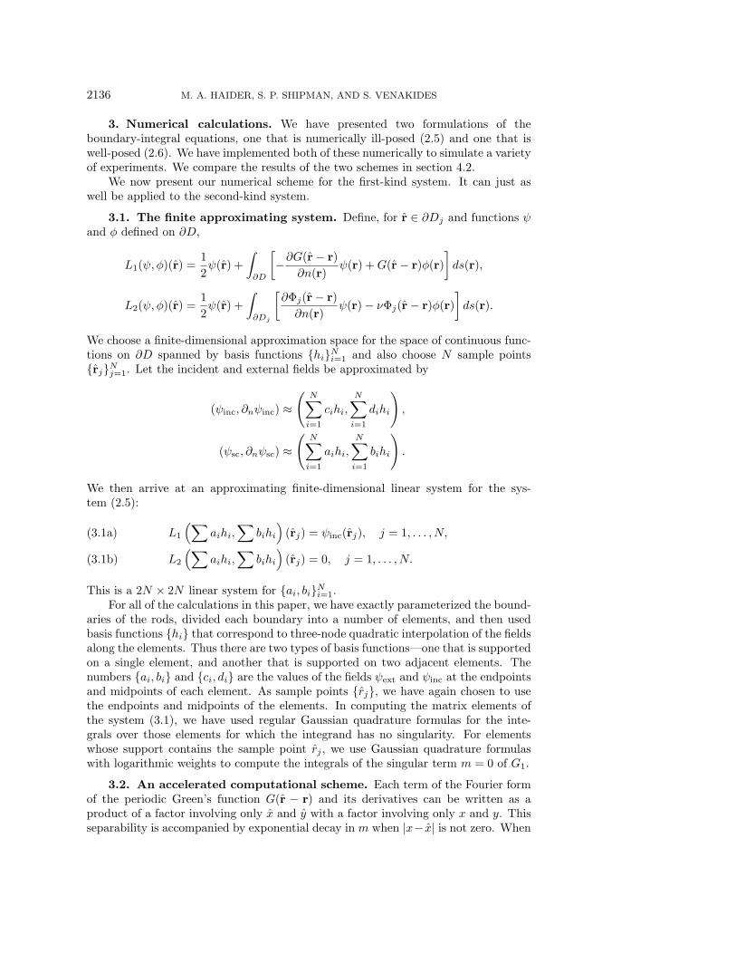
3. Numerical calculations. We have presented two formulations of theboundary-integral equations, one that is numerically ill-posed (2.5) and one that iswell-posed (2.6). We have implemented both of these numerically to simulate a varietyof experiments. We compare the results of the two schemes in section 4.2.

We now present our numerical scheme for the first-kind system. It can just aswell be applied to the second-kind system.

3.1. The finite approximating system. Define, for r ∈ ∂Dj and functions ψand φ defined on ∂D,

L1(ψ, φ)(r) =1

2ψ(r) +

∫∂D

[−∂G(r − r)

∂n(r)ψ(r) +G(r − r)φ(r)

]ds(r),

L2(ψ, φ)(r) =1

2ψ(r) +

∫∂Dj

[∂Φj(r − r)

∂n(r)ψ(r)− νΦj(r − r)φ(r)

]ds(r).

We choose a finite-dimensional approximation space for the space of continuous func-tions on ∂D spanned by basis functions {hi}Ni=1 and also choose N sample points{rj}Nj=1. Let the incident and external fields be approximated by

(ψinc, ∂nψinc) ≈(

N∑i=1

cihi,

N∑i=1

dihi

),

(ψsc, ∂nψsc) ≈(

N∑i=1

aihi,

N∑i=1

bihi

).

We then arrive at an approximating finite-dimensional linear system for the sys-tem (2.5):

L1

(∑aihi,

∑bihi

)(rj) = ψinc(rj), j = 1, . . . , N,(3.1a)

L2

(∑aihi,

∑bihi

)(rj) = 0, j = 1, . . . , N.(3.1b)

This is a 2N × 2N linear system for {ai, bi}Ni=1.For all of the calculations in this paper, we have exactly parameterized the bound-

aries of the rods, divided each boundary into a number of elements, and then usedbasis functions {hi} that correspond to three-node quadratic interpolation of the fieldsalong the elements. Thus there are two types of basis functions—one that is supportedon a single element, and another that is supported on two adjacent elements. Thenumbers {ai, bi} and {ci, di} are the values of the fields ψext and ψinc at the endpointsand midpoints of each element. As sample points {rj}, we have again chosen to usethe endpoints and midpoints of the elements. In computing the matrix elements ofthe system (3.1), we have used regular Gaussian quadrature formulas for the inte-grals over those elements for which the integrand has no singularity. For elementswhose support contains the sample point rj , we use Gaussian quadrature formulaswith logarithmic weights to compute the integrals of the singular term m = 0 of G1.

3.2. An accelerated computational scheme. Each term of the Fourier formof the periodic Green’s function G(r − r) and its derivatives can be written as aproduct of a factor involving only x and y with a factor involving only x and y. Thisseparability is accompanied by exponential decay in m when |x− x| is not zero. When


✲

✻

�

�

�

�

�

�

�

�

�

�

r−��

r+�

group /

y

x

�r

�

r

❇❇

❇❇

❇❇❇

✔✔✔✔✔

❇❇

❇❇

❍❍ ❊❊❊❊❊❊❊❊

��✁✁✁✁

✆✆✆✆✆✆✆✆

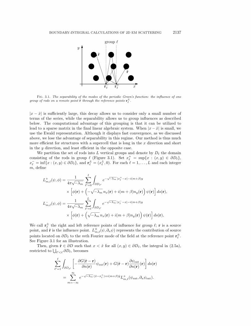
Fig. 3.1. The separability of the modes of the periodic Green’s function: the influence of onegroup of rods on a remote point r through the reference points r±

�.

|x − x| is sufficiently large, this decay allows us to consider only a small number ofterms of the series, while the separability allows us to group influences as describedbelow. The computational advantage of this grouping is that it can be utilized tolead to a sparse matrix in the final linear algebraic system. When |x− x| is small, weuse the Ewald representation. Although it displays fast convergence, as we discussedabove, we lose the advantage of separability in this regime. Our method is thus muchmore efficient for structures with a supercell that is long in the x direction and shortin the y direction, and least efficient in the opposite case.

We partition the set of rods into L vertical groups and denote by D� the domainconsisting of the rods in group / (Figure 3.1). Set x+

� = sup{x : (x, y) ∈ ∂D�},x−� = inf{x : (x, y) ∈ ∂D�}, and r±� = (x±

� , 0). For each / = 1, . . . , L and each integerm, define

L+m,�(ψ, φ) =

1

4π√−λm

�∑�′=0

∫∂D�′

e−√−λm |x+

�−x|−i(m+β)y

×[φ(r) +

(−√−λm nx(r) + i(m+ β)ny(r)

)ψ(r)

]ds(r),

L−m,�(ψ, φ) =

1

4π√−λm

L∑�′=�

∫∂D�′

e−√−λm |x−

�−x|−i(m+β)y

×[φ(r) +

(√−λm nx(r) + i(m+ β)ny(r)

)ψ(r)

]ds(r),

We call r±� the right and left reference points of influence for group /; r is a sourcepoint, and r is the influence point. L±

m,�(ψ, ∂nψ) represents the contribution of source

points located on ∂D� to the mth Fourier mode of the field at the reference point r±� .See Figure 3.1 for an illustration.

Then, given r ∈ ∂D such that x < x for all (x, y) ∈ ∂D�, the integral in (2.5a),restricted to

⋃�′<� ∂D�, becomes

�∑�′=1

∫∂D�′

[−∂G(r − r)


∂ψext

∂n(r)(r)

]ds(r)

=

∞∑m=−∞

e−√−λm (x−x+

�)+i(m+β)yL+

m,�(ψext, ∂nψext).


If instead x < x for all (x, y) ∈ ∂D�, then the integral in (2.5a), restricted to⋃�′>� ∂D�′ , becomes

L∑�′=�

∫∂D�′

[−∂G(r − r)

∂n(r)ψext(r) +G(r − r)∂nψext(r)

]ds(r)

=

∞∑m=−∞

e√−λm (x−x−

�)+i(m+β)yL−

m,�(ψext, ∂nψext).

By using the reference points r±� , we compute exponentials only of quantities hav-ing a negative real part, both in the definition of L±

m,� and in the separated factorsinvolving r.

Let us now augment the finite approximating system (3.1) by introducing theauxiliary variables

ζ±m,� = L±m,�

(∑aihi,

∑bihi

).(3.2)

We then approximate G using M = 2m0+1 values of m so that, for any sample pointr that is at a sufficient distance from group / of rods, say x− x+

� > δ2, we may write

∑i:supp(hi)∈

⋃�′≤�

∂D�′

∫ [−∂G(r − r)

∂n(r)aihi(r) +G(r − r)bihi(r)

]ds(r)

≈m0∑

m=−m0

e−√−λm |x±

�−x|−i(m+β)yζ±m,�.

(3.3)

If x−� − x > δ2, a similar approximation holds. In setting up the finite linear system,

we make use of the following recursion relations for the variables ζ±m,�:

ζ+m,� = e−

√−λm (x+�−x+

�−1)ζ+m,�−1, / = 2, . . . , L,

ζ−m,� = e−√−λm (x−

�+1−x−

�)ζ−m,�+1, / = 1, . . . , L− 1.

(Actually, ζ+m,L and ζ−m,1 are not needed.)

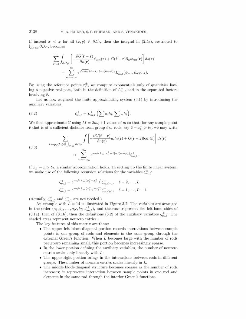
An example with L = 14 is illustrated in Figure 3.2. The variables are arrangedin the order (a1, b1, . . . , aN , bN , ζ

±m,�), and the rows represent the left-hand sides of

(3.1a), then of (3.1b), then the definitions (3.2) of the auxiliary variables ζ±m,�. Theshaded areas represent nonzero entries.

The key features of this matrix are these:• The upper left block-diagonal portion records interactions between samplepoints in one group of rods and elements in the same group through theexternal Green’s function. When L becomes large with the number of rodsper group remaining small, this portion becomes increasingly sparse.

• In the lower portion defining the auxiliary variables, the number of nonzeroentries scales only linearly with L.

• The upper right portion brings in the interactions between rods in differentgroups. The number of nonzero entries scales linearly in L.

• The middle block-diagonal structure becomes sparser as the number of rodsincreases; it represents interaction between sample points in one rod andelements in the same rod through the interior Green’s functions.


(2LRJ)(RJ)

(2LRJ)J

(2LRJ)(2(M+R))

2LRJ 2L(M+R)

LRJ 2(M+R)(LRJ)

Fig. 3.2. The matrix for an L × R supercell of rods. J is the number of basis elements andthe number of sample points per rod, and M is the number of Fourier modes used in the auxiliaryvariables ζ±

m,�in the case for which R = 1. The numbers in the figure on the right bound the number

of nonzeros in each block of the matrix.

We have chosen, for the simulations in this paper, to solve the system using Gaussianelimination with partial pivoting. With this method, the auxiliary variables providethe most efficiency in the case in which the crystal consists of one horizontal row ofrods repeated periodically in y.

Let us now consider crystals that consist of L vertical groups of rods, each con-taining R rods, each with J nodes. Suppose that we wish to calculate transmissionfor actual incident frequencies up to a fixed maximal value. Since one period ofthe structure contains R rods in the y-direction, the maximal value of the reducedfrequency k scales linearly in R, thereby increasing the number of penetrating (non-decaying) modes of the Fourier form of the exterior Green’s function. The number ofmodes M(R) used in the auxiliary variables must therefore also increase with R, sayM(R) = M + R. Figure 3.2 illustrates this case, with the number of nonzero entriesindicated as functions of L, R, and J .

If we fix R and J and use a Gaussian elimination method of solution, the multipli-cation count of our algorithm is a linear function of L. However, since the separabilitydoes not apply to the y-variable, it is not linear in R.

The separability can also be used to gain efficiency in the calculation of the matrixentries. Let hi be a basis function, and let r±∗ = (x±

∗ , y∗) denote points on supp(hi)such that x+

∗ = max{x : (x, y) ∈ supp(hi)} and x−∗ = min{x : (x, y) ∈ supp(hi)}.

Then, for any sample point r = (x, y), one has

L1(aihi, bihi)(r) =

∞∑m=−∞

e−√−λm |x−x±

∗ |+i(m+β)(y−y±∗ )

× 1

4π√−λm

∫supp(hi)

e−√−λm |x±

∗ −x|−i(m+β)y

×[ai +

(∓√−λm nx(r) + i(m+ β)ny(r)

)bi

]h(r)ds(r),

(3.4)

in which x+∗ (x−

∗ ) is taken if x > x+∗ (x < x−

∗ ). This means that, if the crystal containsseveral rods of the same shape and size and basis functions are chosen identically on


all these rods, then the integrals in (3.4) need to be computed only once. They maythen be used for each identical (but shifted) basis function and each sample pointr = (x, y) such that δ1 < x−x+

∗ < δ2 or δ1 < x−∗ − x < δ2. In addition, the computed

integrals for all basis elements in a group of rods may be used to build the auxiliaryvariables ζ±m,�.

4. Computations and results. We use our computational model to simulateEz transmission (electric field normal to the xy-plane) through various crystals andto analyze the electric fields generated inside the crystals. Our primary concern is aninvestigation of the effects of introducing a periodic horizontal channel through thecrystal. We study various types of resonances that arise, and consider a theoreticalunderstanding of them. We also show some simulations of transmission through aperfect crystal and through a randomly perturbed crystal at all angles of incidence.

We compute the transmission coefficient in the following way: At a point (x, 0)located at a sufficient distance from the photonic crystal slab, we compute the pene-trating plane-wave modes of the exterior field,

ψext =

∞∑m=−∞

cme−√−λm x+i(β+m)y,

that is, the modes m for which√−λm is imaginary. The coefficients cm are given by

cm ≈L∑�=1

e−√−λm |x+

�−x|ζ+

m,� + δm,me−√−λm x,

in which δ is the Kronecker delta symbol. The square of the transmission coefficientis the ratio of the energy transmitted through the crystal, divided by the energy ofthe incident wave:

T 2(k; θ) =

∑m2

m=m1|cm|2√λm√λm

,

where the sum is over propagating modes.

4.1. Advantages of the boundary-integral method. The boundary-integralmethod is particularly well suited to studying resonant phenomena. We have seenconfirmation by a finite-difference time domain (FDTD) method [4] of all the featuresin the transmission graph in Figure 4.5; however, the sharper features could not beresolved in a reasonable amount of time. In addition, the shapes of the spikes thatwe observe in the transmission graph for a photonic crystal with a channel defect(see section 4.4) are not predictable, so the sharpness-enhancement methods used inFDTD schemes cannot be applied effectively.

Our method also provides us with a theoretical and numerical tool to study fieldsinduced by arbitrary harmonic EM sources. In particular, it is interesting to investi-gate the existence of EM waves in the absence of any source at all. These are surfacewaves, which, in the case of photonic crystal slabs, would be EM states localized inthe crystal and traveling along its length. We are now investigating these problems,which will be the subject of further communication.

4.2. Comparison of the first- and second-kind formulations. In our ex-periments, we have used both the first-kind system (2.5) and the second-kind system(2.6). In all the cases for which we have compared the two formulations, we find that


0.2 0.3 0.4 0.5Reduced frequency

0

0.2

0.4

0.6

0.8

1

Tra

nsm

issio

n First−kind system

0.2 0.3 0.4 0.5Reduced frequency

0

0.2

0.4

0.6

0.8

1

Tra

nsm

issio

n Second−kind system

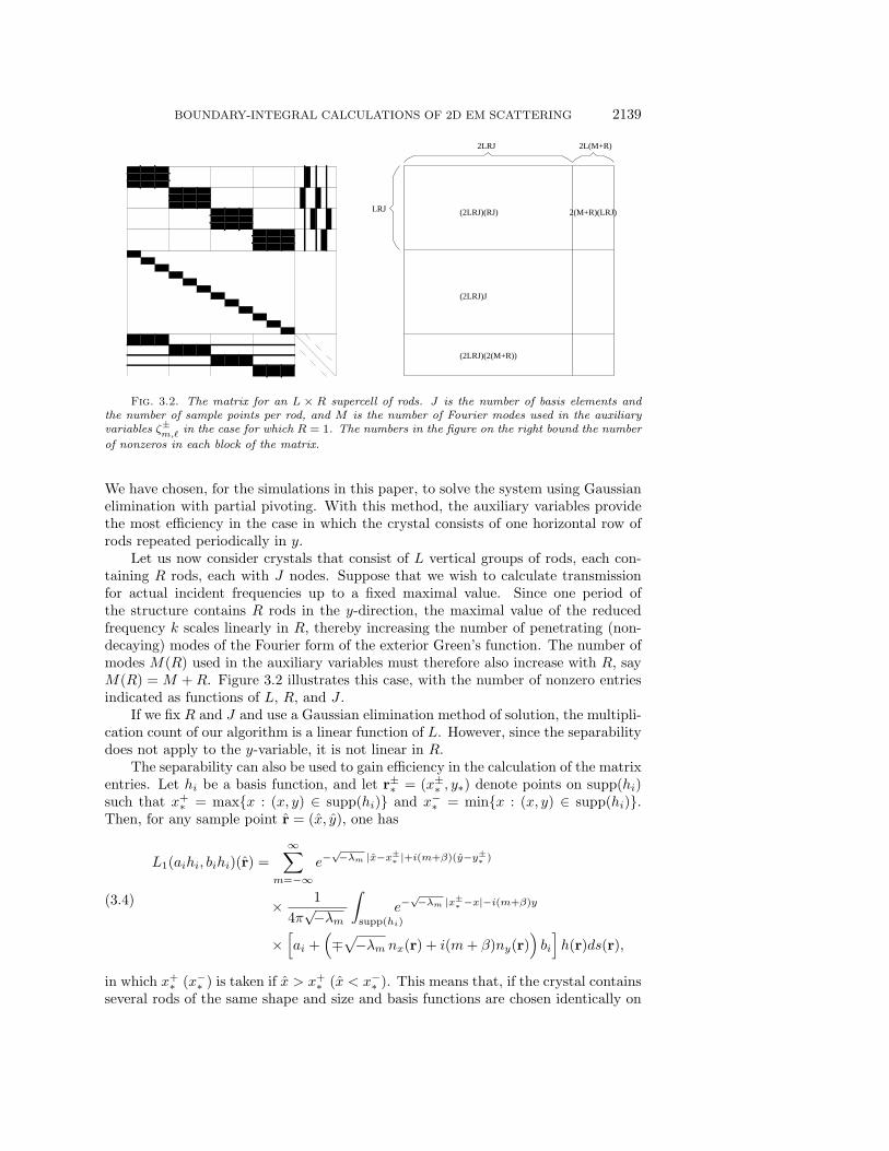
Fig. 4.1. A comparison between Fredholm of the first kind and Fredholm of the second kindresults for the transmission graph of an E-polarized field through a 6 × 4 supercell with a channeldefect of width 0.5.

the transmission graphs are, practically speaking, identical. In particular, we observethat the spikes that appear in the transmission graph of a crystal with a channeldefect are captured essentially identically with both systems. A comparison of resultsis shown in Figure 4.1.

The deviation between the results from the first-kind and second-kind systems ismost apparent near the sharp features of the graph. Even so, with a discretizationof 12 elements per rod, the two systems give a difference of less than 10−6 in thereduced frequency k at which the spike (c) in Figure 4.5 occurs. The width of thespike at half its length is about 8× 10−6. The results for the transmission at the tipof the spike differ by about 0.005, and the relative error between the results for themaximal amplitude of the field in the crystal is less than 0.15%. Moreover, the twoformulations produce contour plots of the fields that look identical.

Thus, we demonstrate that, for systems of the size that we consider in this paper,in which the matrix for the discretized system is typically around 1000×1000, the twoformulations give practically identical results. In computing the quadrature integralsto set up the discrete system, it is faster to use the first-kind system. However,at very sharp resonances ((c) and (d) in Figure 4.5), we find that, to match theresults obtained from the second-kind formulation at a certain discretization, a finerdiscretization of the first kind is required. Some of the figures shown in this sectionwere computed using the first kind and others using the second; that information isindicated in the captions.

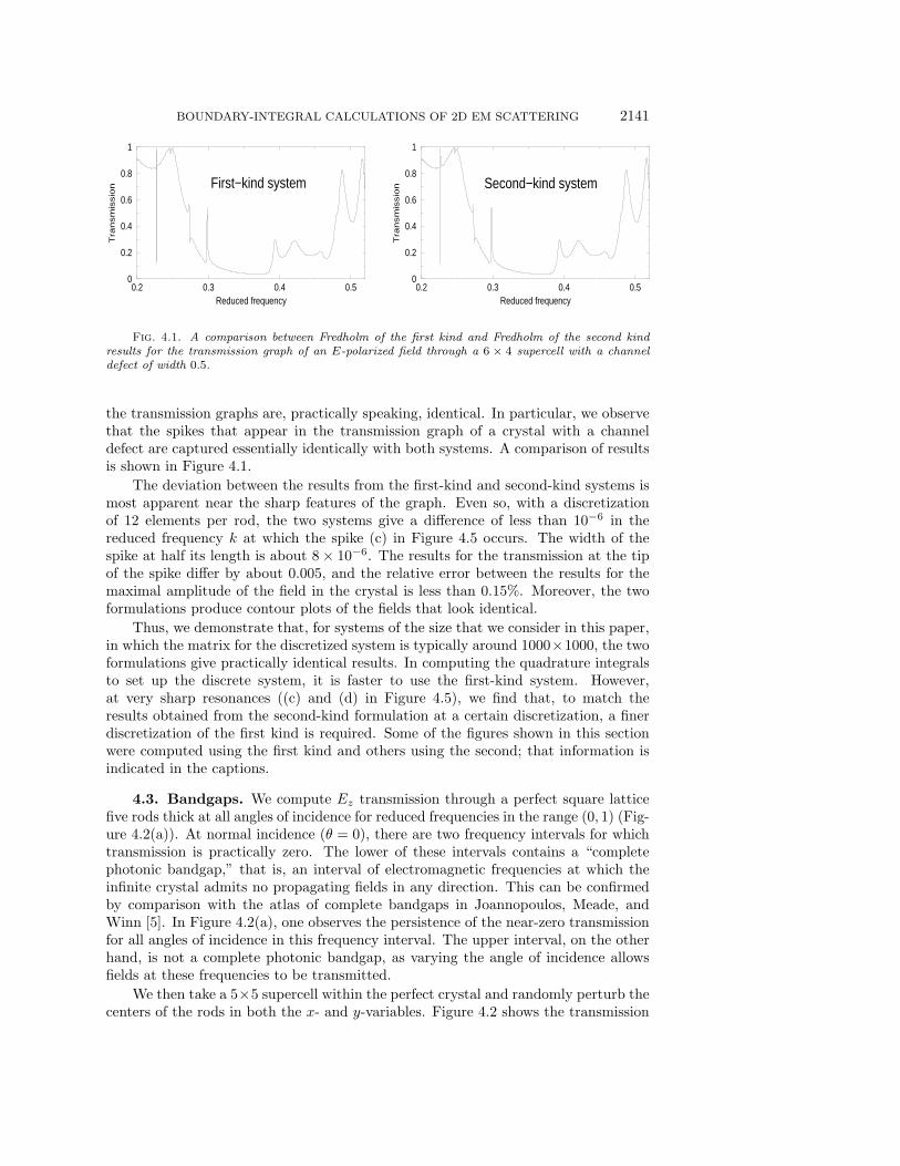
4.3. Bandgaps. We compute Ez transmission through a perfect square latticefive rods thick at all angles of incidence for reduced frequencies in the range (0, 1) (Fig-ure 4.2(a)). At normal incidence (θ = 0), there are two frequency intervals for whichtransmission is practically zero. The lower of these intervals contains a “completephotonic bandgap,” that is, an interval of electromagnetic frequencies at which theinfinite crystal admits no propagating fields in any direction. This can be confirmedby comparison with the atlas of complete bandgaps in Joannopoulos, Meade, andWinn [5]. In Figure 4.2(a), one observes the persistence of the near-zero transmissionfor all angles of incidence in this frequency interval. The upper interval, on the otherhand, is not a complete photonic bandgap, as varying the angle of incidence allowsfields at these frequencies to be transmitted.

We then take a 5×5 supercell within the perfect crystal and randomly perturb thecenters of the rods in both the x- and y-variables. Figure 4.2 shows the transmission


0 0.1 0.2 0.3 0.4 0.5 0.6 0.7 0.8 0.9 10

10

20

30

40

50

60

70

80

90

00.20.40.60.8

1

a.

0 0.1 0.2 0.3 0.4 0.5 0.6 0.7 0.8 0.9 10

10

20

30

40

50

60

70

80

90

00.20.40.60.8

1

b.

0 0.1 0.2 0.3 0.4 0.5 0.6 0.7 0.8 0.9 10

10

20

30

40

50

60

70

80

90

00.20.40.60.8

1

c.

0 0.1 0.2 0.3 0.4 0.5 0.6 0.7 0.8 0.9 10

10

20

30

40

50

60

70

80

90

00.20.40.60.8

1

d.

Fig. 4.2. Transmission through a square lattice with a randomly perturbed 5 × 5 supercell.The graphs show transmission as a function of frequency and angle of incidence: (a) no perturba-tion, (b) perturbation of the centers up to 10% of the lattice constant, (c) perturbation up to 20%,(d) perturbation up to 30%. The system of the first kind was used.

graph for all angles of incidence through three realizations, using different amountsof perturbation.

Our most striking observation is the robustness of the complete bandgap underperturbations. Whereas the incomplete gap disappears quickly under small randomperturbations, the complete gap persists even for perturbations up to 30% of thelattice constant. Although the frequency interval over which the transmission is prac-tically zero shrinks with increasing perturbation, all of our realizations have shown thepersistence of an interval for which transmission is blocked for all angles of incidence.

In [6], various types of perturbations are considered, and the bandgap interval forboth Ez and Hz waves is studied as the amount of perturbation increases.

4.4. Lattice with a channel defect. We analyze Ez EM scattering in a y-periodic structure with a periodic channel defect, as depicted in Figure 4.3. In contrastto the Fabry–Perot cavity considered in [8], the cavity in the current structure isparallel to the x-axis, resulting in more complex 2D interactions of EM waves inthe structure. Our primary interest in this study is the characterization of resonantfrequencies that arise in the transmission coefficient. We limit our analysis to the caseof normal incidence.

We compute the transmission coefficient T (k) using several values of the channel


a(d+1)

Per

iod

of th

e su

perc

ell

channel

channel

a

Fig. 4.3. A crystal with a channel defect of size d in a 4 × 3 supercell. In the numericalcalculations, the period of the supercell is scaled to 2π.

0.2 0.3 0.4 0.50

0.2

0.4

0.6

0.8

1

d = 0

0.2 0.3 0.4 0.50

0.2

0.4

0.6

0.8

1

d = 0d = 0.1

0.2 0.3 0.4 0.50

0.2

0.4

0.6

0.8

1

d = 0.25

0.2 0.3 0.4 0.50

0.2

0.4

0.6

0.8

1

d = 0.5

0.2 0.3 0.4 0.50

0.2

0.4

0.6

0.8

1

d = 1.0

0.2 0.3 0.4 0.50

0.2

0.4

0.6

0.8

1

d = 1.5

Fig. 4.4. Transmission of Ez fields of normal incidence through crystals with channel defects ofvarious sizes d in a 6× 4 supercell. Relative transmission T is plotted against the reduced frequencyk with θ = 0. The system of the first kind was used.

width d in a 6 × 4 supercell of circular dielectric rods (Figure 4.4). The ratio of theradius of the rods to the distance between closest rods is 1/2π. We use eight elements(sixteen nodes) per rod in the discretization, with eight quadrature points per elementin the integrations.

In plotting the transmission, we make physically meaningful comparisons of scat-tering in the channel structure to scattering in the defect-free structure by fixing ourdefinition of the reduced frequency to be k = ωa/(2πc), where a is the lattice con-stant or the distance between nearest rod centers. The introduction of a periodicchannel into the otherwise perfect structure results in “resonances” that are manifestin the transmission graph as various sorts of spikes and humps that are absent in thetransmission graph of the perfect crystal. At these special frequencies, the electricfield in the crystal assumes various characteristics that are not present at a typicalfrequency. The most notable of these are amplification and a departure from thetypical field pattern that resembles generally x-directional wave interference patterns.(Figure 4.5(a) shows a typical field pattern in a near-transmission region of the latticewith a channel.) We find three categories of resonances in the channel structure. Allof these categories have been confirmed by a finite-difference time domain numerical


0.2 0.3 0.4 0.5Reduced frequency k

0

0.2

0.4

0.6

0.8

1

Tran

smis

sion

T(k

)

a

b

c

d

ef

g

h i

0.22662 0.22666k

0

0.2

0.4

0.6

0.8

1

d

c

a. max = 1.54

b. max = 1.77 c. max = 118 d. max = 72.7 e. max = 2.03

f. max = 2.98 g. max = 10.3 h. max = 3.65 i. max = 2.23

Fig. 4.5. The electric field produced by Ez fields normally incident to a crystal with a channeldefect of size d = 0.5 in a 6 × 4 supercell. One period of the crystal is shown, with the channelat the top. The grey-scale indicates the magnitude of the electric field, with white representing thehighest value, and its maximum amplitude relative to the incident field is shown above each figure.The system of the second kind was used.

method [4].

The first category of resonances (Figure 4.5(h, i)) appear at higher frequencies ofthe bandgap and are characterized by local maxima in the transmission graph. Theyare those that one might expect in a channel structure. Plots of the electric fieldsin the structure at these frequencies typically show a low amplitude throughout thecrystal except for the area in the channel, in which larger-amplitude resonating fieldsare present. We refer to these resonances as waveguide modes. The transmissionmaxima at these resonances are diffuse and shift to lower frequencies as the channelwidth d increases (Figure 4.4). With increasing d, the transmission also increasesas electromagnetic waves propagate more freely through the channel with the reso-nances eventually disappearing. The low quality factor (Q-value) of these resonancesindicates that they are of limited practical interest in the design of photonic crystalfilters. (The Q-value is defined as Q = k/∆k, where ∆k is the width of the spike at


half of its height.)

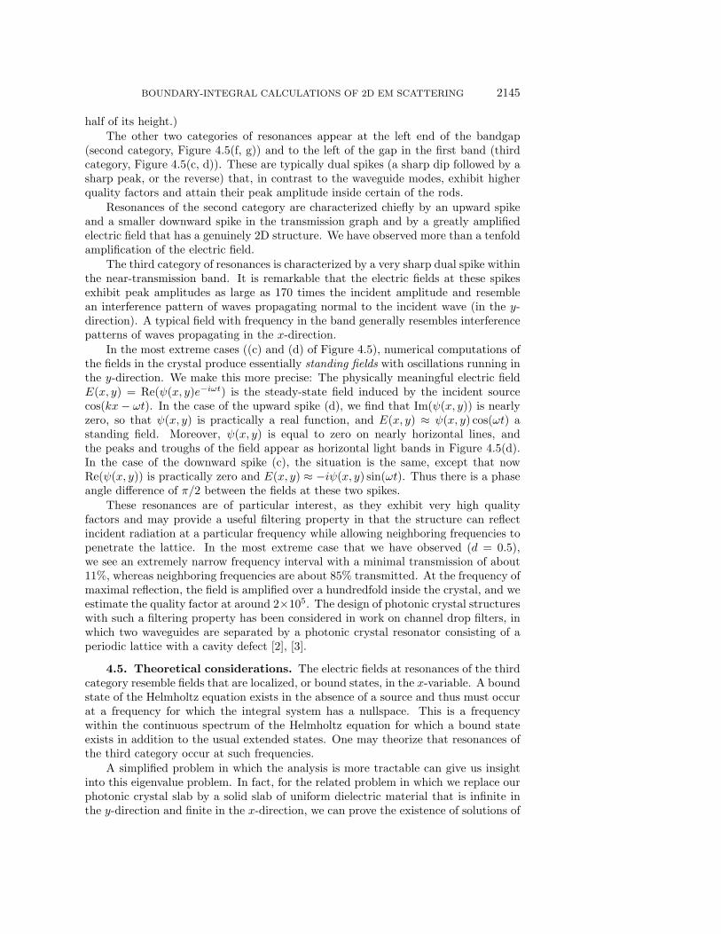
The other two categories of resonances appear at the left end of the bandgap(second category, Figure 4.5(f, g)) and to the left of the gap in the first band (thirdcategory, Figure 4.5(c, d)). These are typically dual spikes (a sharp dip followed by asharp peak, or the reverse) that, in contrast to the waveguide modes, exhibit higherquality factors and attain their peak amplitude inside certain of the rods.

Resonances of the second category are characterized chiefly by an upward spikeand a smaller downward spike in the transmission graph and by a greatly amplifiedelectric field that has a genuinely 2D structure. We have observed more than a tenfoldamplification of the electric field.

The third category of resonances is characterized by a very sharp dual spike withinthe near-transmission band. It is remarkable that the electric fields at these spikesexhibit peak amplitudes as large as 170 times the incident amplitude and resemblean interference pattern of waves propagating normal to the incident wave (in the y-direction). A typical field with frequency in the band generally resembles interferencepatterns of waves propagating in the x-direction.

In the most extreme cases ((c) and (d) of Figure 4.5), numerical computations ofthe fields in the crystal produce essentially standing fields with oscillations running inthe y-direction. We make this more precise: The physically meaningful electric fieldE(x, y) = Re(ψ(x, y)e−iωt) is the steady-state field induced by the incident sourcecos(kx− ωt). In the case of the upward spike (d), we find that Im(ψ(x, y)) is nearlyzero, so that ψ(x, y) is practically a real function, and E(x, y) ≈ ψ(x, y) cos(ωt) astanding field. Moreover, ψ(x, y) is equal to zero on nearly horizontal lines, andthe peaks and troughs of the field appear as horizontal light bands in Figure 4.5(d).In the case of the downward spike (c), the situation is the same, except that nowRe(ψ(x, y)) is practically zero and E(x, y) ≈ −iψ(x, y) sin(ωt). Thus there is a phaseangle difference of π/2 between the fields at these two spikes.

These resonances are of particular interest, as they exhibit very high qualityfactors and may provide a useful filtering property in that the structure can reflectincident radiation at a particular frequency while allowing neighboring frequencies topenetrate the lattice. In the most extreme case that we have observed (d = 0.5),we see an extremely narrow frequency interval with a minimal transmission of about11%, whereas neighboring frequencies are about 85% transmitted. At the frequency ofmaximal reflection, the field is amplified over a hundredfold inside the crystal, and weestimate the quality factor at around 2×105. The design of photonic crystal structureswith such a filtering property has been considered in work on channel drop filters, inwhich two waveguides are separated by a photonic crystal resonator consisting of aperiodic lattice with a cavity defect [2], [3].

4.5. Theoretical considerations. The electric fields at resonances of the thirdcategory resemble fields that are localized, or bound states, in the x-variable. A boundstate of the Helmholtz equation exists in the absence of a source and thus must occurat a frequency for which the integral system has a nullspace. This is a frequencywithin the continuous spectrum of the Helmholtz equation for which a bound stateexists in addition to the usual extended states. One may theorize that resonances ofthe third category occur at such frequencies.

A simplified problem in which the analysis is more tractable can give us insightinto this eigenvalue problem. In fact, for the related problem in which we replace ourphotonic crystal slab by a solid slab of uniform dielectric material that is infinite inthe y-direction and finite in the x-direction, we can prove the existence of solutions of


0 1 2 3k

0

1

2

3

4

5

6

7

8

9

10

|m|

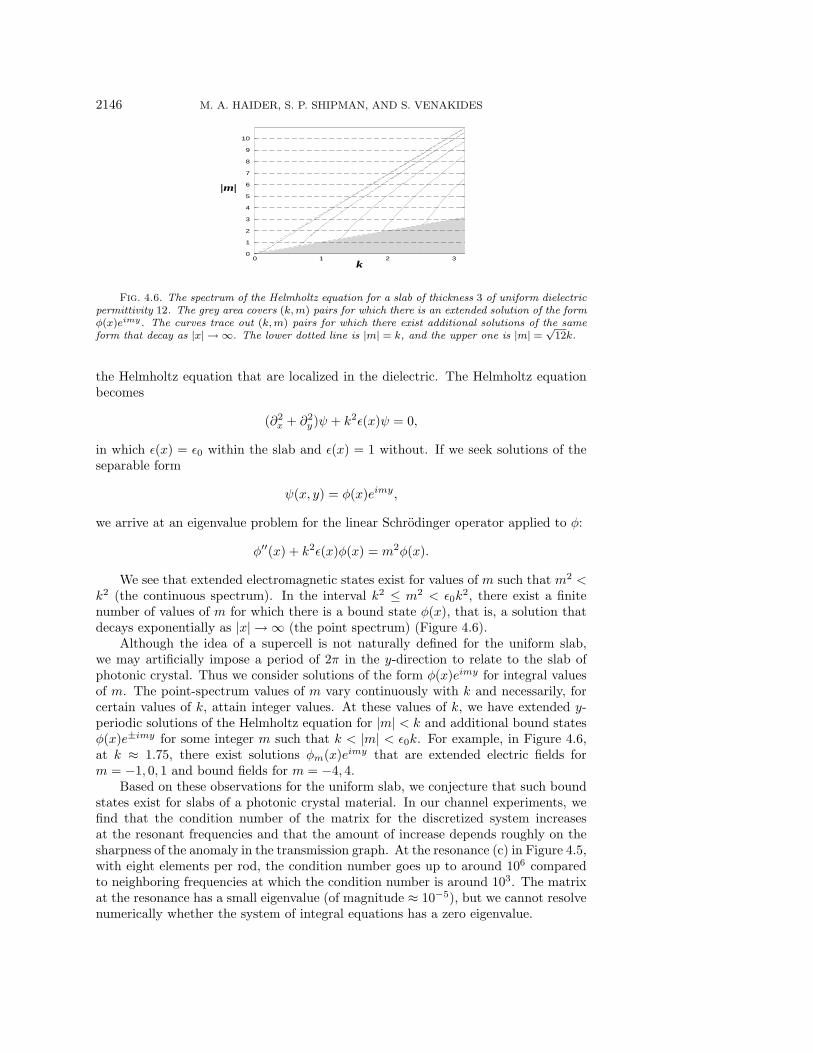
Fig. 4.6. The spectrum of the Helmholtz equation for a slab of thickness 3 of uniform dielectricpermittivity 12. The grey area covers (k,m) pairs for which there is an extended solution of the formφ(x)eimy. The curves trace out (k,m) pairs for which there exist additional solutions of the sameform that decay as |x| → ∞. The lower dotted line is |m| = k, and the upper one is |m| = √

12k.

the Helmholtz equation that are localized in the dielectric. The Helmholtz equationbecomes

(∂2x + ∂2

y)ψ + k2ε(x)ψ = 0,

in which ε(x) = ε0 within the slab and ε(x) = 1 without. If we seek solutions of theseparable form

ψ(x, y) = φ(x)eimy,

we arrive at an eigenvalue problem for the linear Schrodinger operator applied to φ:

φ′′(x) + k2ε(x)φ(x) = m2φ(x).

We see that extended electromagnetic states exist for values of m such that m2 <k2 (the continuous spectrum). In the interval k2 ≤ m2 < ε0k

2, there exist a finitenumber of values of m for which there is a bound state φ(x), that is, a solution thatdecays exponentially as |x| → ∞ (the point spectrum) (Figure 4.6).

Although the idea of a supercell is not naturally defined for the uniform slab,we may artificially impose a period of 2π in the y-direction to relate to the slab ofphotonic crystal. Thus we consider solutions of the form φ(x)eimy for integral valuesof m. The point-spectrum values of m vary continuously with k and necessarily, forcertain values of k, attain integer values. At these values of k, we have extended y-periodic solutions of the Helmholtz equation for |m| < k and additional bound statesφ(x)e±imy for some integer m such that k < |m| < ε0k. For example, in Figure 4.6,at k ≈ 1.75, there exist solutions φm(x)e

imy that are extended electric fields form = −1, 0, 1 and bound fields for m = −4, 4.

Based on these observations for the uniform slab, we conjecture that such boundstates exist for slabs of a photonic crystal material. In our channel experiments, wefind that the condition number of the matrix for the discretized system increasesat the resonant frequencies and that the amount of increase depends roughly on thesharpness of the anomaly in the transmission graph. At the resonance (c) in Figure 4.5,with eight elements per rod, the condition number goes up to around 106 comparedto neighboring frequencies at which the condition number is around 103. The matrixat the resonance has a small eigenvalue (of magnitude ≈ 10−5), but we cannot resolvenumerically whether the system of integral equations has a zero eigenvalue.


0 0.25 0.5 1.0Channel width d

0.221

0.2310

0.740

170

maximum field amplitude

transmission spike depth

reduced frequency k at spike

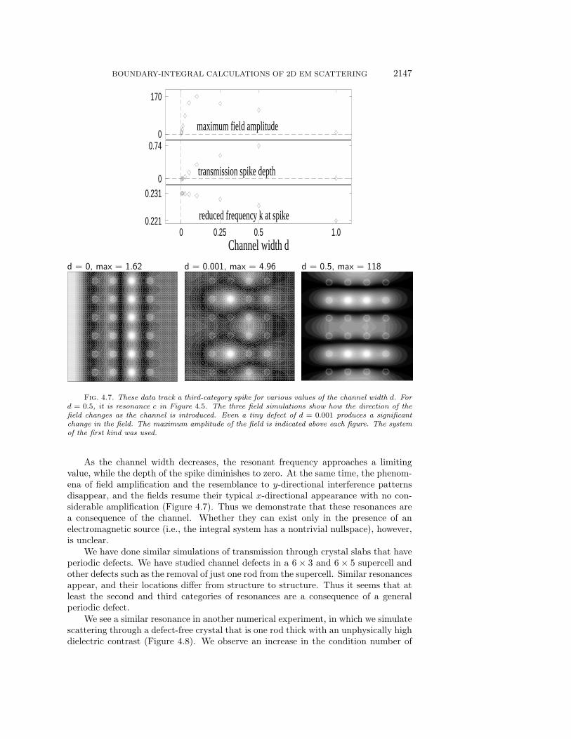
d = 0, max = 1.62 d = 0.001, max = 4.96 d = 0.5, max = 118

Fig. 4.7. These data track a third-category spike for various values of the channel width d. Ford = 0.5, it is resonance c in Figure 4.5. The three field simulations show how the direction of thefield changes as the channel is introduced. Even a tiny defect of d = 0.001 produces a significantchange in the field. The maximum amplitude of the field is indicated above each figure. The systemof the first kind was used.

As the channel width decreases, the resonant frequency approaches a limitingvalue, while the depth of the spike diminishes to zero. At the same time, the phenom-ena of field amplification and the resemblance to y-directional interference patternsdisappear, and the fields resume their typical x-directional appearance with no con-siderable amplification (Figure 4.7). Thus we demonstrate that these resonances area consequence of the channel. Whether they can exist only in the presence of anelectromagnetic source (i.e., the integral system has a nontrivial nullspace), however,is unclear.

We have done similar simulations of transmission through crystal slabs that haveperiodic defects. We have studied channel defects in a 6× 3 and 6× 5 supercell andother defects such as the removal of just one rod from the supercell. Similar resonancesappear, and their locations differ from structure to structure. Thus it seems that atleast the second and third categories of resonances are a consequence of a generalperiodic defect.

We see a similar resonance in another numerical experiment, in which we simulatescattering through a defect-free crystal that is one rod thick with an unphysically highdielectric contrast (Figure 4.8). We observe an increase in the condition number of


0.33 0.380732 0.43Reduced frequency k

0

0.2

0.4

0.6

0.8

1

Tran

smis

sion

T (k

)

k = 0.380732, max = 9.16

k = 0.429, max = 1.97

Fig. 4.8. Ez transmission through a crystal that is one rod thick with dielectric contrast 100.The field produced by an incident wave at the resonant frequency is shown (top right) along withthe field for a typical frequency of low transmission (bottom right). The maximum amplitude of thefield is indicated. The system of the second kind was used.

the discretized integral system at the frequency that corresponds to a downward spikein the transmission graph and a high-amplitude localized field inside the rods. Again,it is not clear that the integral system has a nontrivial nullspace at this resonantfrequency.

We are now making a theoretical and numerical study of bound states and reso-nances, which will be the subject of further communication.

Acknowledgment. This study benefitted from several fruitful discussions withV. Papanicolaou.

REFERENCES

[1] M. M. Beaky, J. B. Burk, H. O. Everitt, M. A. Haider, and S. Venakides, Two di-mensional photonic crystal Fabry-Perot resonators with lossy dielectrics, IEEE Trans. Mi-crowave Theory Techniques, 47 (1999), pp. 2085–2091.

[2] S. Fan, P. R. Villeneuve, J. D. Joannopoulos, and H. A. Haus, Channel drop filters inphotonic crystals, Optics Express, 3 (1998), pp. 4–11.

[3] S. Fan, P. R. Villeneuve, J. D. Joannopoulos, and H. A. Haus, Channel drop tunnelingthrough localized states, Phys. Rev. Lett., 80 (1998), pp. 960–963.

[4] C. Hale, personal communication, Mathematics Department, Duke University, Durham, NC,2000.

[5] J. D. Joannopoulos, R. D. Meade, and J. N. Winn, Photonic Crystals: Molding the Flowof Light, Princeton University Press, Princeton, NJ, 1995.

[6] E. Lidorikis, M. M. Sigalas, E. N. Economou, and C. M. Soukoulis, Gap deformationand classical wave localization in disordered two-dimensional photonic-band-gap materials,Phys. Rev. B, 61 (2000), pp. 13458–13464.

[7] C. Muller, Foundations of the Mathematical Theory of Electromagnetic Waves, Springer-Verlag, Berlin, New York, 1969.

[8] S. Venakides, M. A. Haider, and V. Papanicolaou, Boundary integral calculations of two-dimensional electromagnetic scattering by photonic crystal Fabry–Perot structures, SIAMJ. Appl. Math, 60 (2000), pp. 1686–1706.

[9] E. Yablonovitch, Photonic band-gap structures, J. Opt. Soc. Amer. B Opt. Phys., 10 (1993),pp. 283–295.

Boundary-Integral Calculations of Two-Dimensional Electromagnetic Scattering in Infinite Photonic...

Documents

Transcript of Boundary-Integral Calculations of Two-Dimensional Electromagnetic Scattering in Infinite Photonic...