Acoustofluidics in microsystems: investigation of resonances

Master Thesis, s032091

Acoustofluidics in microsystems:investigation of resonances

Rune Barnkob

frequency

acou

stic

ener

gyde

nsity

Supervisor: Professor Henrik Bruus

Department of Micro– and NanotechnologyTechnical University of Denmark

June 30, 2009

ii

Frontpage illustrationThe illustration at the frontpage shows (left) color plots by 2D and 3D models of acous-tic resonances in a microchip, and (right) a Lorentzian shape line fit to experimentallymeasured acoustic energy density in a straight water-filled microchannel.

Abstract

The use of ultrasound standing waves for particle manipulation and separation has gainedrenewed interest and widespread use in the past decade since its application in the emergingfield microfluidics.

In many silicon-based separation devices the so-called acoustic pressure force is uti-lized to separate particles in aqueous solutions by establishing transverse half-wavelengthpressure modes in microchannels. In the present we work apply theoretical analyses andnumerical simulations to investigate the acoustic resonances in such microchannels. Aspecial emphasis is put on taking the surrounding chip material into account, thus goingbeyond the traditional transverse half-wavelength picture. We show that the localizationof acoustic energy in the active channels can be optimized by choosing the width of thechannel in the right proportion relative to the width of the surrounding silicon chip. Thisanalysis provides a simple but important design tool, which is applied in numerical simu-lations of two application schemes; (i) a high throughput many-channel separation chip,and (ii) a three-channel chip for in situ calibration of the acoustic pressure force.

Moreover, we present modeling of a point-actuation device. We study how the posi-tion of a piezo transducer on the chip surface influences the acoustic resonances in themicrochannels. For a fixed position of the point transducer, we analyze the total acousticenergy in the system as a function of the driving frequency, the radiative energy loss tothe surroundings, and the viscous energy dissipation in the liquid. This work has led tothe fabrication of a point-actuation device by our collaborators in the group of Laurellat Lund University. Additionally, we theoretically investigate the basic conditions forcreating straight water-filled channels acting as acoustic waveguides in microchips.

In addition to the theoretical work, we present results from experiments carried outthrough visits in the laboratory in the group of Laurell. Here we obtained measurements ofthe acoustic energy densities and the corresponding Q-values of ultrasound resonances inmicrofluidic chips. The acoustic energy was obtained by tracking individual polystyrenemicrobeads undergoing acoustophoresis in straight water-filled channels in silicon/glasschips. From the measurements we obtain that the acoustic energy density as a function ofapplied frequency behaves as Lorentzian line shapes, and that the acoustic energy densityscales with the applied transducer voltage to the power of two.

iii

iv ABSTRACT

Resume

Anvendelse af staende ultralydsbølger til partikelmanipulering og separation, har vundetny interesse og udbredt anvendelse indenfor det seneste arti, siden dets udnyttelse i dethurtigt udviklende omrade, mikrofluidik.

I mange siliciums-baseret separationsaggregater benyttes den sakaldte akustiske tryk-kraft til at separere partikler opløst i en væske, ved at etablere en halv trykbølge pa tværsaf en mikrokanal. I dette arbejde anvender vi teoretisk analyse og numeriske simuleringertil at udforske de akustiske resonanser i sadanne mikrokanaler. Analyserne lægger storvægt pa at tage det omgivende chip materiale med i betragtning, og tager derfor skridtetvidere fra det sædvanlige halvbølgebillede. Vi viser, at lokaliseringen af den akustiskeenergitæthed i de aktive kanaler kan optimeres ved at vælge passende dimensioner forkanalbredden i forhold til den omgivende siliciumschip. Dette har givet et simpelt menvigtigt designredskab, som vi benytter til numerisk analyse af to applikationer: (i) enmangekanals separationschip til opnaelse af høj gennemstrømning og (ii) en trekanalschip til in situ kalibrering af den akustiske trykkraft.

Ydermere præsenterer vi modellering af et punktaktueringsapparat. Vi studerer, hvor-dan positionen af en punktaktuator pa chipoverfladen pavirker de akustiske resonanser imikrokanalerne. For en fast position af punktaktuatoren analyserer vi den totale akustiskeenergitæthed i systemet som funktion af aktueringsfrekvens, tab af transmitteret energitil omgivelserne og tab af energi fra de viskøse gnidninger i væsken. Dette arbejde harresulteret i fremstillingen af sadan et punktaktueringsapparat af vores samarbejdspart-nere i Laurells forskningsgruppe ved Lunds Universitet. Yderligere undersøger vi de teo-retiske betingelser for at skabe lige vandfyldte mikrokanaler, som fungerer som akustiskebølgeledere i en mikrochip.

Udover det teoretiske arbejde præsenterer vi eksperimentielle resultater udført vedbesøg hos Laurells gruppe. I disse forsøg har vi malt den akustiske energitæthed ogtilsvarende Q-værdier for de akustiske resonanser i de mikrofluide chips. Den akustiskeenergitæthed er malt ved at følge partikelbanerne for polystyren mikropartikler udsat forakustophorese i lige vandfyldte kanaler i siliciumschips. Ved disse malinger finder vi, atden akustiske energitæthed som funktion af aktueringsfrekvens følger Lorentz-kurver, ogat den akustiske energitæthed skalerer som kvadratet pa spændingen over den aktuerendepiezokrystal.

v

vi RESUME

Preface

This thesis is submitted as fulfillment of the prerequisites for obtaining the degree in Masterof Science in Engineering at the Technical University of Denmark (DTU). The thesis workis carried out at the Department of Micro- and Nanotechnology (DTU Nanotech) in theTheoretical Microfluidics group (TMF) headed by Professor Henrik Bruus. The durationof the thesis work was 10 months from 1 September 2008 to 30 June 2009 correspondingto a credit of 50 ECTS points.

During the project work many people have been of great help and support. Firstof all, I would like to thank my supervisor Henrik Bruus for his huge enthusiasm whensupervising his students, as well as his eager to understand the world of physics. Henrikhas been of magnificent inspiration with his large knowledge, but also with his competencesin scientific writing and professional working approaches.

In part of the project I carried out experiments in Professor Thomas Laurell’s labo-ratory at the Department of Electrical Measurements (Elmat), Lund University (LTH),during eight days in April and May. I would like to thank Professor Thomas Laurell, hisentire research group and especially PhD student Per Augustsson for great collaboration,help and assistance in the laboratory. I find the atmosphere very pleasant in the Swedishgroup and I look forward to further collaboration in my continuation of the project as aPhD student.

I would like to thank the three BSc students (known as the Gorkov-boys), Lasse MejlingAndersen, Anders Nysteen and Mikkel Settnes, for many fruitful discussions on the acous-tic pressure force and for their inspirational enthusiasm and skills within physics. More-over, I would like to thank the TMF group for an exceptional working atmosphere beingboth professional and social rewarding. I also thank DTU Nanotech for a pleasant andpositive working environment and my fellow student Mathias Bækbo Andersen for hissuperb support and company throughout the entire period of the studies at DTU.

At last I would like to thank my family and friends for their support throughout theproject.

Rune BarnkobDepartment of Micro– and Nanotechnology

Technical University of Denmark30 June 2009

vii

viii PREFACE

Contents

List of Figures xiii

List of Tables xv

List of Symbols xvii

1 Introduction 1

1.1 Lab-on-a-chip systems . . . . . . . . . . . . . . . . . . . . . . . . . . . . . . 1

1.2 Acoustofluidics . . . . . . . . . . . . . . . . . . . . . . . . . . . . . . . . . . 2

1.3 Experimental motivation . . . . . . . . . . . . . . . . . . . . . . . . . . . . . 2

1.4 Theoretical foundation and goals . . . . . . . . . . . . . . . . . . . . . . . . 4

1.5 Outline of the thesis . . . . . . . . . . . . . . . . . . . . . . . . . . . . . . . 5

1.6 Publications during the MSc thesis studies . . . . . . . . . . . . . . . . . . . 6

2 Basic theory 7

2.1 Governing acoustofluidic equations . . . . . . . . . . . . . . . . . . . . . . . 7

2.1.1 Perturbation of governing equations . . . . . . . . . . . . . . . . . . 8

2.1.2 Zeroth-order perturbation equations . . . . . . . . . . . . . . . . . . 8

2.1.3 First-order perturbation equations . . . . . . . . . . . . . . . . . . . 9

2.1.4 Second-order perturbation equations . . . . . . . . . . . . . . . . . . 9

2.2 First-order acoustofluidics . . . . . . . . . . . . . . . . . . . . . . . . . . . . 9

2.2.1 Inviscid theory . . . . . . . . . . . . . . . . . . . . . . . . . . . . . . 9

2.2.2 Single-domain analysis of water cube . . . . . . . . . . . . . . . . . . 11

2.2.3 Viscous theory . . . . . . . . . . . . . . . . . . . . . . . . . . . . . . 12

2.2.4 Acoustic energy density . . . . . . . . . . . . . . . . . . . . . . . . . 14

2.3 Second-order acoustofluidics . . . . . . . . . . . . . . . . . . . . . . . . . . . 15

2.3.1 The acoustic pressure force . . . . . . . . . . . . . . . . . . . . . . . 15

2.4 Multiple-domain systems . . . . . . . . . . . . . . . . . . . . . . . . . . . . . 16

2.4.1 Acoustic impedances . . . . . . . . . . . . . . . . . . . . . . . . . . . 16

2.4.2 Boundary and matching conditions . . . . . . . . . . . . . . . . . . . 16

2.5 Elastic wave acoustics in solids . . . . . . . . . . . . . . . . . . . . . . . . . 19

2.5.1 Isotropic solids . . . . . . . . . . . . . . . . . . . . . . . . . . . . . . 19

2.5.2 Sound velocities . . . . . . . . . . . . . . . . . . . . . . . . . . . . . 21

ix

x CONTENTS

3 Numerical simulations in Comsol Multiphysics 233.1 The general form . . . . . . . . . . . . . . . . . . . . . . . . . . . . . . . . . 23

3.1.1 The 3D Helmholtz wave equation on general form . . . . . . . . . . 243.2 Structure of 3D translational invariant acoustics problem . . . . . . . . . . 24

3.2.1 Validation of analytical solution . . . . . . . . . . . . . . . . . . . . 27

4 Actuation of acoustic resonances 294.1 1D double-actuated liquid slab . . . . . . . . . . . . . . . . . . . . . . . . . 29

4.1.1 Perturbation parameter and first-order pressure field . . . . . . . . . 304.1.2 The energy of an acoustic resonator . . . . . . . . . . . . . . . . . . 31

4.2 Point-actuation model . . . . . . . . . . . . . . . . . . . . . . . . . . . . . . 334.2.1 Model system . . . . . . . . . . . . . . . . . . . . . . . . . . . . . . . 334.2.2 Results . . . . . . . . . . . . . . . . . . . . . . . . . . . . . . . . . . 334.2.3 Concluding remarks . . . . . . . . . . . . . . . . . . . . . . . . . . . 37

5 Analysis of transverse half-wavelength resonances 395.1 Analysis of 1D models . . . . . . . . . . . . . . . . . . . . . . . . . . . . . . 39

5.1.1 Qualitative analysis . . . . . . . . . . . . . . . . . . . . . . . . . . . 405.1.2 Quantitative analysis . . . . . . . . . . . . . . . . . . . . . . . . . . . 425.1.3 Energy densities . . . . . . . . . . . . . . . . . . . . . . . . . . . . . 45

5.2 Analysis of 2D models . . . . . . . . . . . . . . . . . . . . . . . . . . . . . . 475.3 Analysis of 3D models . . . . . . . . . . . . . . . . . . . . . . . . . . . . . . 49

5.3.1 Estimation of frequency shift from 2D to 3D models . . . . . . . . . 495.3.2 Full 3D-simulation . . . . . . . . . . . . . . . . . . . . . . . . . . . . 505.3.3 Translational invariant geometries . . . . . . . . . . . . . . . . . . . 50

5.4 Concluding remarks . . . . . . . . . . . . . . . . . . . . . . . . . . . . . . . 52

6 Many-channel chips 536.1 Parallel channel chips . . . . . . . . . . . . . . . . . . . . . . . . . . . . . . 536.2 In situ calibration of acoustic pressure forces on particles . . . . . . . . . . 54

6.2.1 The acoustic potential experienced by a particle . . . . . . . . . . . 556.2.2 Chip design for in situ calibration of the acoustic pressure force . . . 56

7 Waveguide analysis 597.1 2D acoustic waveguide . . . . . . . . . . . . . . . . . . . . . . . . . . . . . . 59

7.1.1 Estimation of waveguide conditions . . . . . . . . . . . . . . . . . . . 597.1.2 Numerical verification of 2D waveguide conditions . . . . . . . . . . 61

7.2 3D acoustic waveguide . . . . . . . . . . . . . . . . . . . . . . . . . . . . . . 627.3 Concluding remarks . . . . . . . . . . . . . . . . . . . . . . . . . . . . . . . 64

8 Experimental investigations 658.1 Experimental setup . . . . . . . . . . . . . . . . . . . . . . . . . . . . . . . . 658.2 Investigation of the piezo transducer . . . . . . . . . . . . . . . . . . . . . . 678.3 Sedimentation of microbeads . . . . . . . . . . . . . . . . . . . . . . . . . . 698.4 Measuring the acoustic energy density . . . . . . . . . . . . . . . . . . . . . 70

0.0 CONTENTS xi

8.4.1 Theoretical transverse bead trajectory . . . . . . . . . . . . . . . . . 718.4.2 Analysis of data . . . . . . . . . . . . . . . . . . . . . . . . . . . . . 718.4.3 Acoustic energy density versus driving voltage . . . . . . . . . . . . 738.4.4 Acoustic energy density versus driving frequency . . . . . . . . . . . 77

8.5 Concluding remarks . . . . . . . . . . . . . . . . . . . . . . . . . . . . . . . 78

9 Conclusion 819.1 Outlook . . . . . . . . . . . . . . . . . . . . . . . . . . . . . . . . . . . . . . 82

A Peer-reviewed conference proceeding published at 157th meeting of theAcoustical Society of America 83

B Impedance condition at cylindrical boundary 91

C Comsol/Matlab script for pressure eigenmodes in 2D chip model 95

D Comsol/Matlab script for eigenmodes in translational inv. 3D model 99

E Comsol/Matlab script for resonances in point-actuated 3D model 103

F Comsol/Matlab script for investigating 2D waveguide modes 109

Bibliography 115

xii CONTENTS

List of Figures

1.1 Acoustofluidic separation of blood cells and lipids in straight microchannel. 21.2 Experimental images of acoustic streaming and acoustic pressure force. . . . 31.3 Demonstration of selective retention and positioning by ultrasound. . . . . . 41.4 Comparison of theoretical and PIV-determined ultrasound resonance. . . . 5

2.1 Color plot of pressure eigenmodes in single-domain microchannel. . . . . . . 11

3.1 Geometry and meshgrid of Comsol Multiphysics model example. . . . . 253.2 Eigensolutions for pressure field in Comsol Multiphysics model example. 28

4.1 Model sketch of 1D double-actuated liquid slab. . . . . . . . . . . . . . . . . 304.2 Image of point-actuation device fabricated in the group of Laurell. . . . . . 324.3 Model of point-actuated chip with an inside liquid-filled microchamber. . . 344.4 Comsol meshgrid and eigensolution for the point-actuation model. . . . . . 354.5 Acoustic energy spectra versus viscous damping and impedance radiation. . 354.6 Acoustic energy as function of position of point transducer. . . . . . . . . . 36

5.1 1D model of water-filled channel in silicon chip. . . . . . . . . . . . . . . . . 395.2 Lowest 1D pressure eigenmodes for water-filled channel in silicon chip. . . . 415.3 1D Comsol simulations of the seven lowest eigenmodes. . . . . . . . . . . . 435.4 Plot of transcendental equation to give perfect matching of wavelength. . . 445.5 Design graphs for perfectly matching odd half-wavelength modes. . . . . . . 445.6 Pressure eigenmodes of four special cases for 1D silicon/water model . . . . 455.7 2D Comsol simulations of six pressure eigenmodes in a water-filled channel. 485.8 Sketch and geometrical parameters of analyzed 3D model. . . . . . . . . . . 495.9 3D Comsol calculation of transverse antisymmetric eigenmode. . . . . . . . 515.10 3D translational invariant Comsol calculation of eigenmode in -chips. . . 52

6.1 Image of eight-channel separation chip from group of Laurell. . . . . . . . . 536.2 2D Comsol calculations of chip with eight parallel channels. . . . . . . . . 556.3 Contour plot of normalized acoustic potential for a polystyrene particle. . . 566.4 Triple-channel chip for in situ calibration of acoustic pressure force. . . . . 57

7.1 2D Comsol simulations of waveguide modes in water-filled microchannel. . 617.2 3D Comsol simulations of waveguide modes in water-filled microchannel. . 63

xiii

xiv LIST OF FIGURES

8.1 Microfluidic silicon/glass chips of the -type fabricated by Per Augustsson. 668.2 Experimental setup of microfluidic chip and laboratory equipment. . . . . . 678.3 Electrical impedance measurements of piezo transducer. . . . . . . . . . . . 688.4 Example of extracting acoustic energy density from microbead trajectory. . 728.5 Experimentally measured acoustic energy density vs. transducer voltage. . . 758.6 Experimentally measured acoustic energy density vs. transducer frequency. 768.7 Modeling of frequency change by adding an extra axial pressure node. . . . 79

List of Tables

2.1 Material parameters used throughout the thesis. . . . . . . . . . . . . . . . 132.2 Sound velocities for elastic waves in pyrex glass and cubic silicon crystal. . . 20

5.1 Results from 1D Comsol simulations of wa/2-modes. . . . . . . . . . . . . 465.2 Results from 2D Comsol simulations of wa/2-modes. . . . . . . . . . . . . 47

6.1 Results of 2D Comsol simulations of many-channel separation chip. . . . . 54

7.1 Results of 2D Comsol simulations of waveguide modes. . . . . . . . . . . . 62

8.1 Geometric parameters of fabricated -chips and the piezo transducer. . . . 668.2 Experimental sedimentation times of polystyrene microbeads. . . . . . . . . 698.3 Acoustic energy density and transverse wavelength vs. transducer voltage. . 748.4 Acoustic energy density and transverse wavelength vs. transducer frequency. 77

xv

xvi LIST OF TABLES

List of Symbols

Symbol Description Unit

≡ Equal to by definition∼ Of the same order≈ Approximately equal to∝ Proportional to≪,≫ Much smaller than, much greater than⋅ Scalar product× Cross-product or multiplication sign

∂i = ∂/∂i Partial derivative with respect to i [i]−1

∇ Nabla or gradient vector operator m−1

∇⋅ Divergence vector operator m−1

∇× Rotation vector operator m−1

∇2 Laplacian scalar operator m−2

O(xn) Terms of order xn and higher powers

⟨∘⟩ Time average of ∘⟨∘⟩i Average of ∘ over i∣ ∘ ∣ Absolute value of ∘(∘)∗ Complex conjugate of ∘Δ∘ A change in ∘∘ An infinitesimal change in ∘Re ∘ Real part of ∘Im ∘ Imaginary part of ∘i Imaginary unite Euler’s constant, ln (e) = 1

x, y, z Rectangular coordinatesei Unit vector in i-directionr Position vector mn Surface normal vector mΩ Domain of interestdΩ Boundary of domain Ω

Continued on next page

xvii

xviii LIST OF SYMBOLS


an Normal acceleration m s−2

g, g Gravitational acceleration m s−2

l, L Length of channel, length of chip mw,W Width of channel, width of chip mℎ,H Height of channel, height of chip ma Radius of spherical particle mR Radius of point transducer or fixation pin mV Volume m3

ℓ Actuator displacement m

per Perturbation parameter mpi i’th order acoustic pressure kg m−1s−2

i i’th order acoustic mass density kg m−3

vi i’th order acoustic velocity m s−1

vi i’th order acoustic velocity vector m s−1

i i’th order velocity potential m2 s−1

t Time sf Frequency s−1

! = 2f Angular frequency s−1

= 1/f Period s

ni Number of /2 in spatial direction i Acoustic wavelength m∗ Perfect /2-mode wavelength m Relative change in wavelength Aspect ratio parameterk Complex-valued wave vector m−1

k0 Real-valued wave vector m−1

Dimensionless wavenumberca Speed of sound in material a m s−1

Za Acoustic impedance of material a kg m−2s−1

z Acoustic impedance ratiopA, Aj Pressure amplitudes kg m−1s−2

Q Q-value of acoustic resonance peakΔfi FWHM of frequency for the i’th resonance s−1

Δf Frequency shift between two resonance peaks s−1

Continued on next page

0.0 LIST OF SYMBOLS xix


Eac Time-averaged acoustic energy density kg m−1s−2

ℰac Spatially- and time-averaged energy density kg m−1s−2

c Speed of sound ratio Density ratiof1, f2 Pre-factors in pressure force expressionU0 Amplitude of acoustic potential kg m2 s−2

Uac Time-averaged acoustic pressure force potential kg m2 s−2

Fac Time-averaged acoustic pressure force vector kg m s−2

Fdrag Stokes drag force vector kg m s−2

Fg Gravitational force vector kg m s−2

Viscosity kg m−1s−1

Bulk viscosity kg m−1s−1

Viscous damping factor

Upp Driving peak-to-peak voltage kg m2 C−1 s−2

Zel Electric impedance kg m2 C−2 s−1

el Electric phase

kB Boltzmann’s constant kg m2 s−2 K−1

T Temperature KD Diffusion constant m2 s−1

ldiff Diffusion length m

N,M Number of measurementsx Weighted mean of variable xsx Sample standard deviation of variable x2x Variance of variable x

u Displacement vector m Cauchy stress tensor kg m−1s−2

iklm Elasticity tensor kg m−2s−2

cL Longitudinal sound velocity (elastic theory) m s−1

cT Transverse sound velocity (elastic theory) m s−1

cav Average sound velocity (elastic theory) m s−1

E Young’s modulus kg m−1s−2

Poisson’s ratio

xx LIST OF SYMBOLS

Chapter 1

Introduction

In this chapter we introduce the concepts of acoustofluidics; the art of combining acousticswith microfluidics to obtain handling and manipulation tools for lab-on-a-chip systems. Webriefly review the experimental as well as the theoretical state-of-the-art within acoustoflu-idics. Next, we point out the needs for theoretical insight, and thus the motivation forcarrying out this thesis work.

1.1 Lab-on-a-chip systems

Lab-on-a-chip technology concerns the scaling down of laboratory setups below millimeterscale or smaller. It is a product of the invention of microelectronic chips, which duringthe past 50 years has led to an entirely new framework within micro- and nanofabrication.The obvious advantages of lab-on-a-chip systems are (i) the allowance of small samplequantities and volumes which is often encountered in modern biology and biotechnology,(ii) fast biological and chemical reactions and processes due to the high surface to volumeratios, (iii) increased possibilities for developing compact and portable point-of-a-caredevices, and (iv) the utilization of mass production to manufacture cheap devices.

Lab-on-a-chip systems are often incorporating microfluidics, which is the technology ofhandling fluids on sub-millimeter scales. Dealing with fluids on this scale induces differentphysics than observed on a macroscopic scale. Microflows are in particular characterizedby having a very low Reynolds number (on the order of unity or smaller), correspond-ing to highly laminar flows, where viscous forces dominate. The laminar flow ensuresthat flow streamlines do not cross, which leads to high controllability when handling mi-crofluidic systems. But the introduction of laminar flow leads to new challenges, e.g. themissing ability to mix fluids by turbulence. This and other challenges has led to researchwithin areas such as pumping, detection and mixing, utilizing various techniques such likeelectroosmostic pumping, magnetophoresis, electrophoresis and geometrically controlledmixing. For textbooks and review papers on microfluidics, see [1–8].

1

2 Introduction

alternative is to change the properties of the medium. This ismore difficult and in some applications even impossible. Thebest way to increase the acoustic force is to decrease theultrasound wavelength and the width of the separation channelaccordingly.

3 Method and materials

3.1 Micro machining

The separation chips were manufactured in silicon since thematerial displays good acoustic properties and the highprecision fabrication process is well known. By using photo-lithography and anisotropic wet etching techniques a separa-tion channel with perfectly vertical walls was obtainedaccording to the method used in ref. 4. A structure with a350 mm wide and 125 mm deep separation channel and a tri-furcation outlet was designed (Fig. 4) and fabricated. A boron-silicate glass lid was attached to the silicon chip by anodicbonding to provide closed flow channels.

3.2 Experimental arrangement

The piezoceramic element (PZ26, Ferroperm PiezoceramicsAS, Kvistgard, Denmark) was powered by an in-house builtsinusoidal signal power amplifier. The transducer was acous-tically coupled to the rear side of the separation chip usingultrasound gel (Aquasonic Clear, Parker Laboratories Inc.,Fairfield, NJ, USA). Silicone rubber tubings were glued to theinlets and outlets on the back side of the separation chip, actingas docking ports to the syringe pump (WPI SP260P, WorldPrecision Instruments Inc., Sarasota, FL, USA) via standard1/16’ od teflon tubings. The flow rates through all three outletswere identical. The 5 mm polyamide spheres used were sus-pended in a doppler blood phantom (Dansk Fantom ServiceAS, Jyllinge, Denmark) containing 20% particles. The bovineblood used was mixed with saline solution (9 mg ml21,Fresenius Kabi Norge AS, Halden, Norway) in order toachieve different concentrations of erythrocytes. The lipidparticles used were derived from a phospholipid-stabilizedemulsion of triolein, which was prepared as described in detail

in ref. 16 with some modifications. Briefly, a total amount of320 mg triolein, tritium labelled and unlabelled, and 3.2 mg ofphospholipids were sonicated in 7.2 ml of PBS. Followingsonication, 0.8 ml of 20% BSA in PBS was added. The lipidemulsions were always used within 5 h from the time ofpreparation. The degree of hemolysis was measured using aHemoCue Plasma/Low Hb meter (HemoCue AB, Angelholm,Sweden).

To measure the fraction of particles (polyamide spheres orerythrocytes) recovered, i.e. the separation efficiency, samplesfrom the centre and side outlets were collected in capillaries(Bloodcaps 50 ml, VWR International AB, Stockholm,Sweden). Each sample was centrifuged (Haematokrit 2010,Hettich Zentrifugen, Tuttlingen, Germany) for 2 min at13000 rpm after which the height of the particle pillars in thecapillaries were measured, A (fluid collected from centrechannel) and B (fluid collected from side channel). Theseparation efficiency was defined as A/(A 1 2B).

The lipid content was measured by a scintillation counter(Wallac Guardian 1414 Liquid Scintillation Counter, Perkin-Elmer Life and Analytical Sciences Inc., Boston, MA, USA),according to standard scintillation counting protocol,17 withthe modification of using Ultima Gold (Packard Biosciences,Boston, MA, USA) as scintillation liquid. The lipid separationefficiency was calculated in line with that of the other particletypes.

4 Results and discussion

4.1 Separator design

The earlier reported separation channel (750 mm wide and250 mm deep) was operated in a single wavelength standingwave mode.4 The new design (350 mm wide and 125 mm deep),allowed the system to use a half wavelength standing wave inthe 2 MHz range for acoustic separation. The use of a singlepressure node made it possible to collect the particles in 1/3 ofthe total fluid volume. Another improvement was the use ofultrasound gel as an interface between the piezo ceramicelement and the silicon, instead of epoxy. The advantage of notgluing the transducer to the chip was the possibility to reusethe same transducer several times. The Reynolds number forthe 350 mm channel was calculated to 40, as compared to 20for the earlier reported larger separation channel,4 which stillguarantees a stable laminar flow

4.2 Separator performance

As seen in Fig. 5, the particle separation efficiency was found tobe very close to 100% at 12 Vpp (voltage peak-to-peak). It canbe noted that voltage needed was lower as compared to theearlier design yet obtaining a high separation efficiency. Thefast decrease in separation efficiency as the voltage wasdecreased can be explained by the fact that the force is pro-portional to the square of the voltage, i.e. applied pressure.

The flow rate tests (Fig. 6) showed that low flow ratesresulted in high separation efficiencies. The reason for this wasthat the suspended particles were exposed to the ultrasound

Fig. 3 (a) Two particle types positioned, by the acoustic forces, in the pressure nodal and anti-nodal planes of a standing wave. (Cross section of thechannel in (b), dashed line.) (b) Top view of a continuous separation of two particle types from each other and/or a fraction of their medium.

Fig. 4 Schematic drawing and scanning electron microscopy image ofthe trifurcation region of the 350 mm wide separation chip.

9 4 0 A n a l y s t , 2 0 0 4 , 1 2 9 , 9 3 8 – 9 4 3

Continuous separation of lipid particles from erythrocytes by means oflaminar flow and acoustic standing wave forces

Filip Petersson,a Andreas Nilsson,a Cecilia Holm,b Henrik Jonssonc and Thomas Laurell*a

Received 16th April 2004, Accepted 8th June 2004

First published as an Advance Article on the web 17th September 2004

DOI: 10.1039/b405748c

Improved continuous acoustic particle separation (separation

efficiency close to 100%) and separation of erythrocytes (red

blood cells) from lipid microemboli in whole blood is reported.

Introduction

It is a well-known fact that particles in fluid suspensions may be

enriched at defined positions by means of forces generated by

acoustic standing wave fields. Theoretical pioneers in this discipline

were King,1 Gorkov,2 and Yosioka and Kawasima.3 Their

acoustic force theories have since been used by several groups of

researchers in particle separation applications.4–9 A new approach

to continuous separation of particles in microfluidic channels was

recently proposed by Nilsson et al.,4 enriching particles in the

pressure nodes of an ultrasonic standing wave in a continuously

perfused microchannel. Earlier version of the system4 reported

particle enrichment in a double pressure node configuration,

collecting enriched particles in the side outlets of a triple channel

outlet. The current set-up described in this communication

demonstrates improved particle separation efficiency, defined as

the fraction of particles collected in the centre outlet. Also,

successful separation of particles having different physical proper-

ties is reported, i.e. lipid vesicles were separated from erythrocytes.

These accomplishments were attributed to the further miniaturisa-

tion of the separation device to a channel width of 350 mm, a depth

of 125 mm and operation in a half wave length resonance mode,

providing higher acoustic forces on the particles.

During cardiac surgery supported by a heart-lung machine a

massive embolization of lipid particles occur in the brain when

shed blood is returned to a patient via a filter.10 The lipid particles

are derived from triglycerides leaking from fat cells during surgery

in adipose tissue. The embolization is associated with cognitive

dysfunction observed after surgery.11 The techniques currently

available for blood wash do not meet the demand to remove these

lipid particles. The most common method to wash blood is based

on centrifuges which are burdened with a number of drawbacks,

i.e. they only handle larger amounts of blood (# 0.5 l), are harmful

for the blood cells,12 need specially trained personnel, are not

continuous and display a limited lipid particle elimination.

The technology presented in this communication offers a

solution to the embolization problem by employing the possibility

of discriminating erythrocytes from lipid particles. In addition,

when fully developed and implemented clinically, it reduces the

demand for allogenic blood and reduces or eliminates blood

transfusion related incompatibilities. The primary acoustic

radiation force equation13 tells us that the acoustic force can

move particles either towards a node or an anti-node of a standing

wave depending on their densities and compressibilities. If the

particles are red blood cells and lipid droplets in blood plasma,

the erythrocytes gather in the pressure node (in the centre of the

channel) while the lipid particles gather in the pressure anti-nodes

(by the side walls), Fig. 1. At the end of the channel the red blood

cells exit through the centre outlet while the lipid particles exit

through the side outlets, separating the two particle types, Fig. 2.

Experiments and results

The experiments were performed as reported in ref. 4 with the

modification that a half wavelength standing wave was used.

In vitro experiments were performed on a particle suspension

composed of a 2% concentration of 5 mm polyamide spheres

(blood phantom), see ref. 4 for details.

All separations were performed at low Reynolds numbers, (Re ,

40). Considerably improved separation efficiencies (close to 100%

*[email protected]

Fig. 1 Cross-section of channel with erythrocytes and lipid particles.

When the ultrasound is turned on the two particle types are separated.

Fig. 2 If the main channel is split into three outlet channels the laminar

flow properties makes it possible to collect erythrocytes and lipid particles

separately.

COMMUNICATION www.rsc.org/loc | Lab on a Chip

20 | Lab Chip, 2005, 5, 20–22 This journal is The Royal Society of Chemistry 2005

1.3. EXPERIMENTAL MOTIVATION 3

a)

Chip

Lid

Chamber

Actuator *b)

ChannelCCCCCCOActuator * Chamber

Chip

Figure 1.1: Sketch of an acoustic microfluidic resonator system. a) Side view showing a resonancechamber etched into the chip and bonded by a lid. Chip and lid are acoustically hard, commonlysilicon and glass [1]. An external piezoelectric actuator clamped underneath the chip excitesthe resonance modes. b) Top view showing an arbitrarily shaped chamber with inlet and outletchannels. Fluidic access to channels can be made either through bottom or top of chip. The typicaldimension are measured in millimeters for the lateral plane and hundreds of microns in chamberdepth.

Finally, a resonance mode is typically very well-defined within a given geometry, whichcan be exploited when designing to obtain a specific acoustic field pattern.

As reference for the theoretical work we will use the paper by Hagsäter et al. [1], whohave reported on experimental results of streaming and radiation as shown in Fig. 1.2. Thetwo images a) and c) show both streaming and radiation forces occurring simultaneouslyfor the same eigenmode, where the radiation force dominates large particles and the viscousstreaming drag is dominating for the small particles as will be shown later. The utilizedsystem is constructed as sketched in Fig. 1.1 where chambers and channels are etched intoa 49× 15 mm2 silicon chip sealed by a glass lid. The chamber we will use for reference isa square with side length L = 2 mm etched h = 200 µm into the 500 µm thick silicon andconnected to 400 µm wide channels with a length of 11.84 mm. Under normal operatingconditions the wavelength λ obeys the condition h < λ < L, corresponding to frequenciesof a few MHz.

a) b) c)

6

300

µm

/s

400

µm

61000

µm

/s

400

µm

Figure 1.2: Experimental results obtained by particle image velocimetry (PIV) of a) acousticstreaming with 1 µm tracer beads and b) radiation forces on 5 µm beads. The radiation forcepushes the large particles towards pressure nodal lines in a resonance mode at 2.17 MHz whereasthe streaming dominates for small particles dragging these in a 6× 6 vortex pattern. Both effectsoccur simultaneously, and a) and b) correspond to the same eigenmode illustrated by the simulationc) of the acoustic pressure at 2.23 MHz with arbitrary amplitude; red areas correspond to positiveand blue to negative values. Images a) and b) courtesy of Hagsäter et al. [1].

(a) (b) (c)

Figure 1.1: (a,b) Illustration of highly functional acoustic separation device to split red blood cellsfrom lipids by utilizing standing acoustic waves in combination with laminar microfluidic flow anda three way flow splitter (trifurcation). (c) Sketch of the traditional transverse half-wavelengthpicture and the separation of blood cells (node) and lipids (antinodes). Illustrations are fromPetersson et al. [24, 25].

1.2 Acoustofluidics

Another technique for manipulation and separation is the use of acoustics in fluids leadingto the field acoustofluidics. Primarily two non-linear effects are of importance, namelythe acoustic pressure force and the acoustic streaming. The acoustic pressure is a time-averaged force acting on particles or cells as they are exposed to an acoustic field. Theresulting particle motion is called acoustophoresis. Acoustic streaming is time-averagedmotion of the entire carrier fluid due to energy transfer from the acoustic field. Both theacoustic pressure force and acoustic streaming has been known since their description byFaraday in 1831 [9]. Regarding the acoustic pressure force, Kundt is often cited for thedemonstration by his famous cork dust experiment in 1874 [10], known as Kundt’s tubefor determination of the speed of sound in gases. Both phenomena has been theoreticallytreated in the past [11–23].

1.3 Experimental motivation

The field of acoustofluidics has received renewed interest in the past decade since its appli-cation in microfluidics, where the geometric length scales are in the sub-millimeter regimethus requiring acoustic waves in the ultrasonics regime when dealing with water. Theresearch area is constantly developing, as the method is a promising tool for gentle manip-ulation of cells and particles. Among many already suggested applications are pumping,trapping and sorting devices [24–40]. It is common for the ongoing research that it hasmainly been based on experimental studies, while equivalent theoretical understanding islacking. Most of the research relies on a silicon chip containing an etched channel or cavitystructure, which is then bonded with a transparent lid of pyrex glass attached to makevisual inspection possible. One or more external piezo transducers are attached and anacoustic resonance pattern is induced in the channels or cavities by tuning the driving fre-quency of the transducer(s). By careful design of the device geometry, different resonanceproperties can be achieved.

1.3 Experimental motivation 3


a)

Chip

Lid

Chamber

Actuator *b)


Chip




a) b) c)

6300

µm

/s

400

µm

6

1000

µm

/s

400

µm



a)

Chip

Lid

Chamber

Actuator *b)


Chip




a) b) c)

6300

µm

/s

400

µm

6

1000

µm

/s

400

µm



a)

Chip

Lid

Chamber

Actuator *b)


Chip




a) b) c)

6300

µm

/s

400

µm

6

1000

µm

/s

400

µm



a)

Chip

Lid

Chamber

Actuator *b)


Chip




a) b) c)

6300

µm

/s

400

µm

6

1000

µm

/s

400

µm


(a) (b) (c)

Figure 1.2: (a,b) Experimental images obtained by particle image velocimetry (PIV) fromHagsater et al. [37] at DTU. The images show (a) the acoustic streaming of 1 µm beads and(b) acoustic pressure forces on 5 µm beads. (c) Modeling image of the acoustic pressure for bothimage (a) and (b); red areas correspond to positive pressures, whereas blue areas correspond tonegative pressures. The acoustic streaming and pressure forces occur simultaneously and for sameacoustic resonance. Thus the acoustic streaming dominates for small particles, while the acousticpressure force dominates for larger particles.

Separation of blood cells and fat particles

In 2004 pioneering work within sorting of microparticles was done in the group of Laurellat Lund University, Sweden [24,25,32]. Ultrasonic waves from a piezo transducer was forthe first time used in combination with a microchannel trifurcation to obtain separationof blood cells from lipid particles, see Fig. 1.1 (a). This application can be a majoradvancement within e.g. cardiovascular surgery, where it is of crucial importance to beable to clean patients blood from fat particles in a fast, continuous and efficient way.

The now well-known separation technique makes use of the acoustic pressure force,which forces particles to either pressure nodes or pressure antinodes depending on theiracoustic properties, such as their size, density and compressibility relative to those ofthe surrounding fluid. Red blood cells and lipid particles have opposite acoustophoreticproperties: the red blood cells move towards the pressure nodes, while conversely the lipidsmove to the pressure antinodes. To separate the particles a standing half-wavelengthpressure mode is applied across a liquid-filled channel with the node in the center ofthe channel and the antinodes at the channel walls, namely a so-called antisymmetric(odd) mode, see Fig. 1.1 (c). Pumping an axial laminar flow, while acoustic actuatingtransversely, then separates the particles. The laminar flow is divided by a three wayflow splitter (trifurcation) at the end of the channel thus separating the different types ofparticles, see Fig. 1.1 (b).

The half-wavelength pressure mode is applied by matching the channel width w withrespect to the applied actuation frequency f as f = ca/(2w), where ca is the speed of soundin the liquid-filled channel. This approximation comes from a simple analytical estimatebased only on the channel in one dimension as being the acoustic resonator. By theapplication discussed above and many others, this traditional transverse half-wavelengthpicture has proven to be well defined in chip designs of low geometric complexity. Though,thorough theoretical as well as experimental determination of its limitations still remainto be done.

4 Introduction

2004). The latter method has been used for sequentialtrapping of beads above three channel-integrated ultrasonictransducers (Lilliehorn et al., 2005). However, currentultrasonic retention devices cannot be used for the selectionof a discrete subpopulation from a continuous sample flow.

Confocal or hemispherical ultrasonic cavities are focusedstanding-wave resonators based on curved reflector ele-ments. Such resonator designs have previously beenemployed in macro-scale systems for trapping of millimetersize objects in air (Brandt, 1989; Xie and Wei, 2001), and ofmicrometer size objects in fluid suspensions (Hertz, 1995;Wiklund et al., 2001, 2004). The curved reflector elements

create a focused resonant acoustic field with a highlyconfined force field, which makes it possible to accuratelyposition objects three-dimensionally (3D) (Hertz, 1995).However, confocal ultrasonic cavities have not yet beeninvestigated in microfluidic chips.

In the present study, we demonstrate and investigate anintegrated confocal ultrasonic cavity in a microfluidic chipfor selective retention and optical characterization of cells orother bioparticles (Fig. 1). The ultrasound is coupled to thechip by external wedge transducers (Manneberg et al.,2008a; Wiklund et al., 2006b) that are fully compatible withany kind of high-resolution optical microscopy (Manneberget al., 2008b). In the present work, we investigate theresonant modes in the confocal cavity by theoreticalmodeling and experimental verification during no-flowconditions. Furthermore, we demonstrate the flow-throughoperational modes (the manipulation functions) of ourdevice based on triple-transducer actuation, which are (1)pre-alignment and bypassing of cells, (2) selective injectionof cell by pre-alignment frequency shift, (3) trapping,retention, and positioning of cells in the center of theexpansion chamber, and finally (4) label-free transillumina-tion optical microscopy of a monolayer aggregate of retainedcells. The purpose of our design is to select, retain, andposition a discrete subpopulation of up to 100 cells from acontinuous feeding sample flow for dynamic opticalcharacterization.

Device

The device (Fig. 1a) consists of a dry-etched silicon structuresandwiched between two glass layers (GeSim, Dresden,Germany), and three external transducers with refractiveelements (Manneberg et al., 2008a) placed on top of the chipfor efficient coupling of ultrasound into the channel. Thelayer dimensions of the chip were 200/110/1,100 mm(bottom glass, silicon, upper glass), respectively. Theresonator elements are illustrated in Figure 1b. The328 mm wide inlet channel was used as a plane-parallelresonator (indicated with blue solid lines in Fig. 1b) forparticle pre-alignment, bypassing and selection, and wasoperated in either dual-node (at 4.6 MHz) or single-node(at 2.1 MHz) mode (see blue dashed and solid lines,respectively, in Fig. 1c). The expansion chamber, intendedfor sample retention and positioning, was designed as aresonant confocal cavity with two cylindrical segmentsseparated by twice their radius of curvature 2R¼ 4.92 mm(indicated with red solid lines in Fig. 1b), for maximum axialfocusing of the standing wave (indicated with red dashedlines in Fig. 1b). The chamber width was chosen as 15 thewidth of the pre-alignment channel, which results inapproximately the same factor of reduction in the viscousdrag on a trapped particle without reducing the flow rate.The chamber was actuated at a frequency close to 6.9 MHz,which also matched with a half wavelength along the channelheight for vertical centering (levitation) in the whole chip atthis frequency. All actuation voltages were 10 Vpp.

Figure 1. a: Photograph of the transducer-chip system. b: Illustration of the

resonator design: the confocal ultrasonic cavity (in red), and the plane-parallel pre-

alignment channel (in blue). The red and blue solid lines indicate the primary reflecting

walls of the resonators. The red and blue dashed lines indicate the approximate

boundaries of the generated force fields. c: Schematic of the available manipulation

functions during sample flow: (1) bypass, (2) injection/selection, (3) retention/position-

ing. The particle paths are defined by the pressure nodes in the pre-alignment channel.

324 Biotechnology and Bioengineering, Vol. 103, No. 2, June 1, 2009





Device














Device










Figure 1.3: Demonstration of selective retention and positioning of cells by ultrasonic manipula-tion in a microfluidic chamber done by collaboration between the group of Wiklund at KTH andthe group of Bruus at DTU. The images are from Svennebring et al. [40].

Acoustic effects in microsystems

At DTU in 2007 Hagsater et al. [37] studied experimentally the acoustic effects on particlesin liquid-filled microchambers, see Fig. 1.2. By using microparticle image velocimetry(PIV) the transient behavior was recorded, when applying an acoustic field to a silicon chipwith a liquid-filled cavity. At a specific acoustic resonance is was shown that the acousticstreaming dominates for small particles, whereas the acoustic pressure force dominates forlarger particles.

Acoustic cell handling

Acoustic handling of cells has been extensively studied in the group of Wiklund at KTH,Sweden. In 2009 they demonstrated selective retention and positioning of cells by ultra-sonic manipulation in a microfluidic chamber backed up by a theoretical analysis done inthe group of Bruus at DTU [40]. They utilized a confocal chamber to establish a centeredultrasonic force field, where they were able to acoustically trap cells as well as demon-strate several other manipulation functions, see Fig. 1.3. Moreover the Wiklund/Bruusteam presented in 2009 the ability to spatially separate and confine particle tracks by theuse of multiple piezo transducers [39].

1.4 Theoretical foundation and goals

The aim of the current thesis work is to continue the theoretical work done in the group ofBruus at DTU by the two former MSc students, Thomas Glasdam Jensen (TGJ) [41] andPeder Skafte-Pedersen (PSP) [42]. TGJ inialitized the theoretical work on acoustofluidicsat DTU Nanotech analyzing the results by Hagsater et al. [37] as presented in Fig. 1.2. Inthe following MSc project by PSP a thorough analysis of the theoretical background wascarried out. Here, PSP showed that energy loss due to transmission of waves plays a majorrole in the description of the acoustic streaming. Additionally, PSP carried out calculationsdirectly related to the work done in the group of Laurell [38] and the group of Wiklund [40],see Fig. 1.3 and 1.4. Futhermore, during the work of this thesis, three bachelor studentsLasse Mejling Andersen, Anders Nysteen and Mikkel Settnes, have worked extensively ontreating the trajectories of particles subject to acoustic pressure forces [43].

1.5 Outline of the thesis 5

90 CHAPTER 8. APPLICATION TO A SEPARATION CHIP

a)

b)

c)

400 µm

Figure 8.5: Comsol simulation of three first-order pressure eigenmodes at a) 1.89 MHz, b)1.97 MHz, and c) 2.09 MHz. The images show the same selection of the channel system asin Fig. 8.2 and we recognize some correspondence between measurements and simulations bothfor frequency and spatial appearance of the modes, although a) deviates significantly from themeasurement at the intersection. Simulations are made with water at 20C as medium and redareas are pressure maxima and blue are minima.

not been taken into account, but the resonance has been assumed to be a single standingwave transverse to the channel without any longitudinal variation. However, in realitywe do have standing waves along the channel as well, and the system dynamics are thusgoverned by two length scales being the transverse wavelength λt and the longitudinal λl.Due to these length scales we can thereby estimate the expected resonance frequenciesfrom Eq. (3.10), rewritten as

f = ca√λ−2t + λ−2

l . (8.3)

Since we are only interested in the standing waves confined to the separation channel wecan make a rough estimate of the possible resonance frequencies by assuming λt to befractions of the channel width w and λl to be fractions of the length L, which are takento be w = 400 µm and L = 18.35 mm. Based on Eq. (8.3) we can find the first 50eigenfrequencies for both λt = 2w and λt → ∞, which are shown in Fig. 8.6 togetherwith the first 150 eigenfrequencies for the numerical simulation including the asymmetricintersection and the three outlet channels.

Although the two graphs cannot be directly compared due the difference in geometricalcomplexity we do observe some similarities. They both exhibit a kink near 1.85 MHzcaused by the first transition into a transverse mode of λt = 2w. This gives the plateau ofsmall frequency gaps between two adjacent longitudinal modes as long as the transversemode dominates, that is λt < λl. If a specific longitudinal mode for some reason turnsout to be better suited for a specific purpose it is important that we are able to exciteand maintain this mode during operation. However, due to the small frequency gap thepresent system is quite sensitive towards for instance temperature variations.

As an example we can calculate the transition from λl = 15L to λl = 1

4L for λt = 2w,which for constant temperature gives f5/f4 = 1.008. This frequency ratio is equivalentto the ratio of the speed of sound for a temperature change from 25C to 20C [40]amounting to ca25/ca20 = 1497/1485 = 1.01, whereby an actuated system can change

8.3. COMPARING THEORY AND EXPERIMENT 95

a)

b)

400 µm

Figure 8.7: Close-up on the radiation a) on 2.5 µm particles and streaming b) measurementswith 0.5 µm particles for the eigenmode at 1.96 MHz corresponding to Fig. 8.2 b) and Fig. 8.3 b).Vortices in the radiation measurement a), indicating that the large particles are also affected bythe streaming, are marked by the red circles. Measurements courtesy of Hagsäter et al. [2].

8.3.4 Radiation forces and separation efficiency

Based on the numerically computed eigenmode from Fig. 8.5 we can compare the inducedvelocity calculated from the radiation force Eq. (8.8) to the measured radiation forcevelocity from Fig. 8.2 b). A close-up near the intersection is shown in Fig. 8.8, wherea partial agreement between measurement and simulation can be observed. There arehowever discrepancies, which calls for the use of a model geometrically in better agreementwith the real device. Similar plots for the circular chambers used in [1] are given inApp. F, where better correspondence is found. From this we can deduce that the inviscid2d models combined with the radiation force equation Eq. (4.34) can be used as a designtool for geometrically well-defined shallow devices, whereas the results are more uncertainfor devices that are not height invariant and include unknown asymmetric geometries.

If we intend to combine the radiation force field with a Poiseuille flow for particletracing in order to predict the separation efficiency we cannot simply superpose the twofields in a numerical simulation, since the radiation force is based on an eigensolution.Thus for a prediction of the separation efficiency we must determine the radiation ampli-tude by either making an extended numerical model including an actuator, which is bothcomputationally heavy and doubtful to give a sufficiently precise description of the real

a) b)

400 µm

Figure 8.8: Close-up of the radiation force illustrated by vector plots scaling with velocity. Ina) the numerically computed solution at 1.97 MHz is combined with a gray-scale surface plot ofthe first-order pressure field and corresponding black nodal lines, and in b) the measured force at1.96 MHz is combined with micrographs of the particle formation at nodal lines. The pressure ina) has local maxima at white areas and minima at black with an arbitrary amplitude. Image b) isadapted from Hagsäter et al. [2].

(a) (b)

Figure 1.4: Demonstration of (a) color plot (red is positive, blue is negative) of calculatedresonance mode corresponding to (b) PIV measurements of a separation chip done in collaborationbetween the group of Laurell at LTH and the group of Bruus at DTU. The images are fromHagsater et al. [38].

It is clear from the former theoretical work that more extensive resonator modelsare needed to describe the acoustic pressure fields and energies and thus to understandthe acoustic forces. The treatment of acoustic resonances is the main objective of thecurrent thesis. Enabling better understanding of the resonances leads to the possibility tooptimize and design future acoustofluidic applications. In these studies we put emphasison taken into account the physics of the full experimental silicon/glass chip. We givea detailed theoretical analysis of the usual half-wavelength assumption and the relativeacoustic energy densities in a silicon/water chip system.

Besides the theoretical work, a part of the thesis has been to carry out simple exper-iments in the laboratory of the group of Laurell. In this work some of the theoreticalpredictions were tested and the acoustic energy density was investigated.

1.5 Outline of the thesis

Chap. 2: Governing acoustofluidic theory

We set up the framework of the thesis by introducing the governing acoustofluidic equa-tions. We describe the first-order theory and discuss the acoustic energies and boundaryconditions for an acoustic resonator system. Moreover, we analyze the simple analyticalresonator example of a single-domain box. Though it is not utilized in the thesis work,we set up the governing elastic equations for isotropic solids, as the experimental work inthis thesis has indicated a need for this in future work.

Chap. 3: Numerical simulations in Comsol Multiphysics

The finite element software Comsol Multiphysics is the main tool in this thesis work.Numerical analysis is needed as we consider acoustic resonances of multi-domain systemsof complex geometries. This chapter describes the basic concepts for the use of Comsol inthis work. It presents an example of an implemented script, and the benchmarking of thescript to analytical results.

Chap. 4: Actuation and energy losses

We investigate the influence of taking into account the acoustic energy losses due toradiation of waves to the surroundings and to internal viscous attenuation in a three-dimensional (3D) model system. We discuss the validity of the perturbation approach

6 Introduction

and the theoretical prediction of a Lorentzian line-shape fit for energies in lossy systems.Finally, we examine a model system of a point-actuated silicon chip with an internalwater-filled microchamber.

Chap. 5: Anti-symmetric single-channel system

In this chapter we study the usual transverse half-wavelength picture. We carry outcomprehensive analyses by one-dimensional (1D) and two-dimensional (2D) calculationsof the acoustic pressure eigenmodes in a multi-domain chip system. We end the chapterby extending the analysis by 3D Comsol calculations, and we introduce translationalinvariant chips.

Chap. 6: Many-channel chips

We carry out two-dimensional Comsol calculations in order to investigate many-channelsystems, which is of high interest due to the need of high throughput in separation devices.Finally, we suggest a three-channel in situ calibration chip to measure the acoustic energydensity in a given separation chip.

Chap. 7: Waveguide analysis

As a preliminary treatment for future work, we investigate the conditions for a water-filled channel to act as an acoustic waveguide in a surrounding silicon/glass chip. Theconditions are tested by 2D and 3D Comsol models.

Chap. 8: Experimental investigations

Experiments have been carried out at Lund University in collaboration with the group ofLaurell. We present investigations of (i) the electrical impedances of the piezo transducer,(ii) the sedimentation of polystyrene particles, and (iii) measurements of the acoustic en-ergy density. Finally, the experiments have acted as an eye-opener to the actual laboratoryconditions, which are important to keep in mind when carrying out theoretical analyses.

1.6 Publications during the MSc thesis studies

Peer-reviewed conference proceedings

1. Rune Barnkob, and Henrik Bruus, ”Acoustofluidics: theory and simulation of radi-ation forces at ultrasound resonances in microfluidics devices”, ASA 2009,Paper no. 2pBB2 in the 157th meeting of the Acoustical Society of America, Port-land, Oregon, 18-22 May 2009

Other conference proceedings

1. Rune Barnkob, and Henrik Bruus, ”Theoretical analysis of ultrasound resonances inlab-on-a-chip systems”, DFS 2009, Danish Physical Society, Nordic Meeting, Copen-hagen, 16-18 June 2009

Chapter 2

Basic theory

In this chapter we describe the governing equations of acoustofluidics, which is the foun-dation for the work presented in the current thesis. The thesis work is based on the simplepressure wave model, where all media are modeled as liquids only sustaining pressurewaves and not any shear waves. This is of course not accurate when with dealing elasticsolids such as silicon and pyrex glass, however the main qualitative features can be studied.At the end of this chapter we briefly describe the full theory of elastic waves in isotropicsolids.

The fundamental acoustofluidic theory is summarized mainly based on acoustic theoryfound in Lighthill [44], and the theoretical aspects of acoustics in microfluidics found inBruus [5] and Skafte-Pedersen [42].

2.1 Governing acoustofluidic equations

The governing equations of fluid dynamics are derived from conservation laws, Newtonssecond law and the continuum hypothesis. The governing equations are the dynamicNavier–Stokes equation for a compressible viscous Newtonian fluid; the kinematic conti-nuity equation; and the thermodynamic equation of state relating pressure and density.Ignoring thermal effects for simplicity and using the Eulerian field description, they be-come

∂tv = −∇p− (v ⋅∇

)v + ∇2v + ∇

(∇ ⋅ v

), (2.1a)

∂t = −∇ ⋅(v), (2.1b)

p = p(), (2.1c)

where p = p(r, t) is the pressure field, = (r, t) is the density field, v = v(r, t) isthe velocity field, the viscosity and ≈ 5/3 is the ratio between the compressionalbulk viscosity and the dynamic viscosity. Together the governing equations comprisea set of non-linear coupled partial differential equations, which is hard to solve bothanalytically as well as numerically. In the following the equations are combined to derivethe approximate linear acoustic wave equation. This is done using perturbation theory as

7

8 Basic theory

the acoustic pressure waves are generated by slightly perturbing the equilibrium pressurein a compressible fluid.

2.1.1 Perturbation of governing equations

For a compressible fluid we consider a quiescent state p0,0,v0, which corresponds toa homogeneous liquid at rest and in thermal equilibrium. The velocity in the quiescentstate is zero v0 = 0 and the density and pressure are constants. The pressure p0 in thequiescent state corresponds to the internal energy per volume in the fluid, which for watercorresponds to the energy per volume it takes to free a water molecule into the gas phase,which at room temperature is estimated to pwa

0 ≈ 2.6× 109 J m−3.

Assuming the acoustic perturbations of the quiescent state are small, the pressure p,density and particle velocity v can be written as the perturbation expansions

p = p0 + p1 + p2 + . . . , (2.2a)

= 0 + 1 + 2 + . . . , (2.2b)

v = 0 + v1 + v2 + . . . , (2.2c)

where the perturbation parameter per is made implicit. The first-order perturbation fieldsp1, 1 and v1 are the time-dependent linear fields describing the fundamental acousticwave, whereas the second-order perturbation fields lead to time-independent effects suchas the acoustic pressure force and the acoustic streaming.

Second-order Taylor expansion of Eq. (2.1c) in p around p0 = p(0) gives

p = p0 + c2a1 + c2

a2 +1

2∂(c

2a)

21, (2.3)

where the speed of sound ca to first order in medium a has been introduced as the isentropicderivative

c2a =

(∂p

∂

)s

. (2.4)

As we handle fluids, ca is a longitudinal sound velocity. Fluids cannot sustain shear stressesand thus do not have transverse sound velocities.

2.1.2 Zeroth-order perturbation equations

Substituting the perturbation fields Eqs. (2.2) into the set of governing Eqs. (2.1) weobtain the zeroth-order equations

0 = −∇p0, (2.5a)

∂t0 = 0, (2.5b)

p = p0, (2.5c)

which are seen only to have solutions being constant zeroth-order terms.

2.2 First-order acoustofluidics 9

2.1.3 First-order perturbation equations

Similarly considering the first-order terms we get the first-order equations

0∂tv1 = −c2a∇1 + ∇2v1 + ∇

(∇ ⋅ v1

), (2.6a)

∂t1 = −0∇ ⋅ v1, (2.6b)

p1 = c2a1. (2.6c)

2.1.4 Second-order perturbation equations

Considering only second order terms we obtain the second-order equations

0∂tv2 = −1∂tv1 − 0

(v1 ⋅∇

)v1 −∇p2 + ∇2v2 + ∇

(∇ ⋅ v2

), (2.7a)

∂t2 = −0∇ ⋅ v2 −∇ ⋅(1v1

), (2.7b)

p2 = c2a2 +

1

2∂(c

2a)

21. (2.7c)

2.2 First-order acoustofluidics

To describe first-order linear acoustics, the first-order perturbation equations are used toderive the acoustic wave equation.

2.2.1 Inviscid theory

We first limit ourselves to consider the inviscid case by neglecting the viscous dampingterms in Eqs. (2.6). Taking the divergence of the Navier–Stokes equation Eq. (2.6a) andinserting the continuity equation Eq. (2.6b) gives the wave equation for the density 1

∂2t 1 = c2

a∇21. (2.8)

By use of Eq. (2.6c) this leads to the wave equation for the pressure p1

∂2t p1 = c2

a∇2p1. (2.9)

Taking the gradient of Eq. (2.6b), inserting the inviscid case of Eq. (2.6a) and requiringan irrotational flow i.e. ∇× v = 0, the wave equation for the velocity v1 can be derived

∂2t v1 = c2

a∇2v1. (2.10)

The assumption of an irrotational flow is valid for the important case of a velocity fieldvarying time-harmonically as v1 = v1(r) e−i!t, where ! = 2f is the angular frequencyand f the frequency. This is directly seen from the fact that v1 becomes a gradientfield when substituted into Eq. (2.6a). Note that the assumption of a time-harmonicallyvarying solution changes the time-differential operator into a simple multiplicative factor∂t → −i!.

In order to connect the three fields 1, p1 and v1, we use the irrotational nature ofv1 to introduce the first-order velocity potential 1. Inserting the velocity potential into

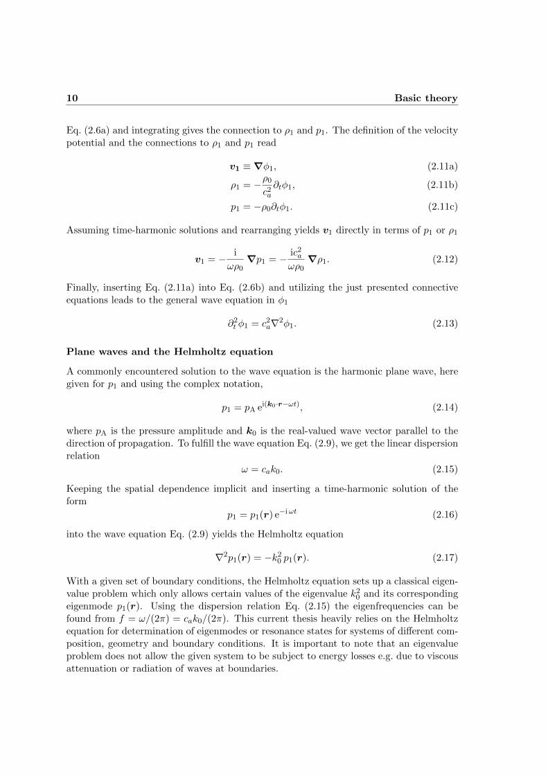
10 Basic theory

Eq. (2.6a) and integrating gives the connection to 1 and p1. The definition of the velocitypotential and the connections to 1 and p1 read

v1 ≡∇1, (2.11a)

1 = −0

c2a

∂t1, (2.11b)

p1 = −0∂t1. (2.11c)

Assuming time-harmonic solutions and rearranging yields v1 directly in terms of p1 or 1

v1 = − i

!0∇p1 = − ic2

a

!0∇1. (2.12)

Finally, inserting Eq. (2.11a) into Eq. (2.6b) and utilizing the just presented connectiveequations leads to the general wave equation in 1

∂2t 1 = c2

a∇21. (2.13)

Plane waves and the Helmholtz equation

A commonly encountered solution to the wave equation is the harmonic plane wave, heregiven for p1 and using the complex notation,

p1 = pA ei(k0⋅r−!t), (2.14)

where pA is the pressure amplitude and k0 is the real-valued wave vector parallel to thedirection of propagation. To fulfill the wave equation Eq. (2.9), we get the linear dispersionrelation

! = cak0. (2.15)

Keeping the spatial dependence implicit and inserting a time-harmonic solution of theform

p1 = p1(r) e−i!t (2.16)

into the wave equation Eq. (2.9) yields the Helmholtz equation

∇2p1(r) = −k20 p1(r). (2.17)

With a given set of boundary conditions, the Helmholtz equation sets up a classical eigen-value problem which only allows certain values of the eigenvalue k2

0 and its correspondingeigenmode p1(r). Using the dispersion relation Eq. (2.15) the eigenfrequencies can befound from f = !/(2) = cak0/(2). This current thesis heavily relies on the Helmholtzequation for determination of eigenmodes or resonance states for systems of different com-position, geometry and boundary conditions. It is important to note that an eigenvalueproblem does not allow the given system to be subject to energy losses e.g. due to viscousattenuation or radiation of waves at boundaries.


(a) f1,1,1 = 5.33 MHz

soft

(b) f3,1,1 = 5.43 MHz

soft

(c) f1,2,1 = 6.31 MHz

soft

(f) f1,1,1 = 5.33 MHz

hard

(e) f2,1,0 = 2.09 MHz

hard

(d) f0,1,0 = 1.95 MHz

hard

Figure 2.1: Sliced color plot of resonance pressure fields p1 (red is positive, blue is neg-ative, green is neutral) for a water-filled microchannel of length l = 2 mm along x, widthw = 380 µm along y and height ℎ = 150 µm along z. The speed of sound in water iscwa = 1483 m s−1 as given in Table 2.1. (a,b,c) The water-filled channel is surrounded by aninfinitely soft acoustic material making the pressure going to zero at all boundaries, see Eq. (2.19).(a) Resonance (nx, ny, nz) = (1, 1, 1) with f1,1,1 = 5.33 MHz, (b) (nx, ny, nz) = (3, 1, 1) withf3,1,1 = 5.43 MHz and (c) (nx, ny, nz) = (1, 2, 1) with f1,2,1 = 6.31 MHz. (d,e,f) The water-filled channel is surrounded by an infinitely hard acoustic material, see Eq. (2.20). (d) Resonance(nx, ny, nz) = (0, 1, 0) with f0,1,0 = 1.95 MHz, (e) (nx, ny, nz) = (2, 1, 0) with f2,1,0 = 2.09 MHzand (f) (nx, ny, nz) = (1, 1, 1) with f1,1,1 = 5.33 MHz.

2.2.2 Single-domain analysis of water cube

We now consider a specific geometrical setup forming an acoustic resonator. Having anacoustic resonator Ω implies that acoustic resonances (or eigenmodes) occurs for certainspecific frequencies fj = !j/(2). An acoustic resonance at angular frequency !j is a statewhere the acoustic energy density Eac inside the resonator is several orders of magnitudelarger than at other frequencies ! ∕= !j . In the general case, the resonance frequenciescan only be calculated using numerical methods, however, in few cases they may be foundanalytically.

A simple example of an acoustic resonator is that of a 3D single-domain rectangularbox, of which the single-domain plane (2D) and single-domain line (1D) are special cases.Applying the rectangle faces with either zero pressure (soft wall) or zero velocity (hardwall), yields an eigenvalue problem easily solved analytically by applying the method ofseparation of variables.

As an example we consider a rectangular water-filled channel placed in a silicon chipalong the coordinate axes with its opposite corners at (0, 0, 0) and (l, w, ℎ). The siliconchip is surrounded by acoustically soft air. If we imagine that the surrounding silicon chipis infinitely thin, we thus have the water in direct acoustic contact with the air, which iswell-approximated by the soft wall condition at all boundaries. Oppositely, if we imagine

12 Basic theory

the surrounding silicon chip to be acoustically infinitely hard material, we apply the hardwall condition at all boundaries. In both cases the eigenvalue solution to the Helmholtzequation in Eq. (2.17) becomes

fnx,ny ,nz =cwa

2

√n2x

l2+n2y

w2+n2z

ℎ2,

nx, ny, nz = 1, 2, 3, . . . , (2.18)

where the three indexes nx, ny, nz are the number of half-wavelengths in x, y and z,respectively. For pure soft boundary conditions, the corresponding eigenfunction psoft

1

becomes

psoft1 (x, y, z) = pA sin

(nx

x

l

)sin(ny

y

w

)sin(nz

z

ℎ

),

nx, ny, nz = 0, 1, 2, 3, . . . , (2.19)

whereas for pure hard conditions the corresponding eigenfunction phard1 is

phard1 (x, y, z) = pA cos

(nx

x

l

)cos(ny

y

w

)cos(nz

z

ℎ

),

nx, ny, nz = 1, 2, 3, . . . , (2.20)

where pA is the pressure amplitude. In Fig. 2.1 are seen examples of the resonant ultra-sound waves for the rectangle having pure soft boundary conditions and pure hard bound-ary conditions, respectively. We notice how the largest contribution to the frequency stemsfrom the modes along the small dimensions as given from Eq. (2.18).

2.2.3 Viscous theory

We move on by including viscous attenuation. Using same approach as in the inviscid casewe obtain the modified wave equation for the pressure p1

∂2t p1 = c2

a∇2p1 +1

0[1 + ]∇2(∂tp1). (2.21)

Note the mixed time and space derivatives in the last term representing the effects ofviscosity.

Lossy Helmholtz equation

Assuming a time-harmonic first-order pressure field of the form p1 = p1(r) e−i!t leads tothe lossy Helmholtz equation,

∇2p1(r) = −k2p1(r), (2.22)

where the wave vector k now is complex

k = k01√

1− i 2 ≈ k0(1 + i ), (2.23)


Table 2.1: Acoustic parameters for various materials considered in the thesis. All sound velocitiesare longitudinal sound velocities. Values for air, water, pyrex glass, polystyrene and iron arefrom [45]. Values for silicon and PMMA are from [41]. The values are given at T = 20 ∘C. In thelast part of the table, the viscous parameters for water are given from [5].

Material (j) density speed of sound impedancej [kg m−3] cj [m s−1] Zj = jcj [kg m−2 s−1]

air (air) 1.16 343.4 3.99× 105

water (wa) 998 1483 1.48× 106

silicon (si) 2331 8490 1.98× 107

pyrex glass (py) 2230 5640 1.25× 107

PMMA polymer (PMMA) 1190 1588 1.89× 106

polystyrene (ps) 1050 2350 2.47× 106

iron (iron) 7874 5950 4.03× 107

copper (cu) 8960 3750 3.36× 107

aluminum (al) 2700 6420 1.73× 107

Dynamic viscosity, water 1.0 mPa sBulk viscosity, water 1.7 mPa s

where we have introduced the dimensionless viscous damping coefficient ,

≡ (1 + )!

20c2a

. (2.24)

Considering MHz ultrasonics in water gives ≈ 10−5, and we thus use k = k0(1 + i )throughout the thesis. The difference between the inviscid and viscous equations is thechange in wave vector k0 → k0(1 + i ). If we consider the inviscid case = 0, the lossyHelmholtz Eq. (2.22) reduces to the Helmholtz Eq. (2.17).

Possible solutions to the lossy Helmholtz equation are damped harmonic plane waves,which are found directly by substituting k0 with k0(1 + i ) in Eq. (2.14)

p1 = pAei(k0⋅r−!t)e− k0⋅r = p1(r)e−i!te− k0⋅r. (2.25)

These waves are damped on the length-scale of 1/(k0 ) ≈ 100 m. Since the system containsenergy losses, an external driving force has to be applied in order to sustain time-harmonicmotion. As described in later chapters, this is done experimentally by applying an ACdriving voltage at MHz frequency to a piezo transducer, which then vibrates with a time-harmonical acceleration a e−i!t and thereby induces an ultrasound pressure field into thesystem. In order to investigate systems yielding energy losses, we have to solve the givensystem in time. This will be be introduced in Chap. 4 on acoustic actuation.

The wave equation does not cover the case of arbitrary perturbation velocities. We aretherefore limited to consider irrotational velocity fields, ∇ × v = 0, which can be shownto be valid for time-harmonic fields and to first-order in the viscosity . As in the inviscidcase we again express the velocity by a first-order scalar potential 1 as in Eq. (2.11a).

14 Basic theory

Using same approach as in the inviscid case the connection between the three fields 1, p1

and v1, can be shown to be

v1 ≡∇1, (2.26a)

1 = −0k2

!2∂t1, (2.26b)

p1 = −c2a0k

2

!2∂t1. (2.26c)

Finally utilizing this, the lossy Helmholtz equation can be derived for 1

∇21 = −k21. (2.27)

2.2.4 Acoustic energy density

The acoustic energy density can be used to indicate the strength of the acoustic fieldsof an acoustic resonator and to characterize the loss of acoustic energy due to viscousdamping and radiation losses. Thus we need to define the acoustic energies in a resonatorsystem. Employing the perturbation approach in Eq. (2.2) the lowest order acoustic energydensities become expressions of second order. The kinetic energy density is given by thestandard formulation of kinetic energy for a fluid as

Ekin =1

20v

21 =

1

20(∇1)2, (2.28)

whereas the potential energy is derived from the energy stored due to compression andexpansion

Epot =

∫ V

V0

p1

VdV =

1

2

p21

c2a0

. (2.29)

As we in the experiments do not resolve the fast oscillatory motion in ultrasonic waves inthe MHz regime, we are interested in describing the time-averaged acoustic energy. Thetime average of a periodic function f = f(t) is defined as

⟨f⟩ =1

∫ t+

tf dt, (2.30)

where is the time of a full oscillation period. This definition will also be used laterwhen considering other second-order effects. Combining Eq. (2.28) and Eq. (2.29), thetime-averaged acoustic energy density Eac = Eac(r) becomes

Eac =1

20

[⟨∣v1∣2⟩+

1

20c

2a

⟨p21⟩]

=1

20

[1

!2⟨∣∇p1∣2⟩+

1

c2a

⟨p21⟩], (2.31a)

=1

40

[1

!2∣∇p1(r)∣2 +

1

c2a

∣p1(r)∣2], (2.31b)

where we in the last equality introduce a factor of 12 by use of the relation of the time

average of the product of two time-harmonic fields ⟨A(t)B(t)⟩ = 12Re A0B

∗0.

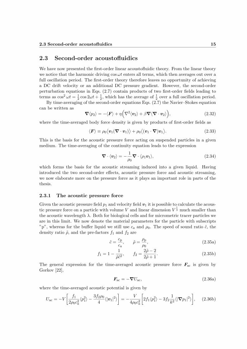
2.3 Second-order acoustofluidics 15

2.3 Second-order acoustofluidics

We have now presented the first-order linear acoustofluidic theory. From the linear theorywe notice that the harmonic driving cos!t enters all terms, which then averages out over afull oscillation period. The first-order theory therefore leaves no opportunity of achievinga DC drift velocity or an additional DC pressure gradient. However, the second-orderperturbation equations in Eqs. (2.7) contain products of two first-order fields leading toterms as cos2 !t = 1

2 cos 2!t+ 12 , which has the average of 1

2 over a full oscillation period.By time-averaging of the second-order equations Eqs. (2.7) the Navier–Stokes equation

can be written as∇⟨p2⟩ = −⟨F ⟩+

(∇2⟨v2⟩+ ∇⟨∇ ⋅ v2⟩

), (2.32)

where the time-averaged body force density is given by products of first-order fields as

⟨F ⟩ ≡ 0

⟨v1(∇ ⋅ v1)

⟩+ 0

⟨(v1 ⋅∇)v1

⟩. (2.33)

This is the basis for the acoustic pressure force acting on suspended particles in a givenmedium. The time-averaging of the continuity equation leads to the expression

∇ ⋅ ⟨v2⟩ = − 1

0∇ ⋅ ⟨1v1⟩, (2.34)

which forms the basis for the acoustic streaming induced into a given liquid. Havingintroduced the two second-order effects, acoustic pressure force and acoustic streaming,we now elaborate more on the pressure force as it plays an important role in parts of thethesis.

2.3.1 The acoustic pressure force

Given the acoustic pressure field p1 and velocity field v1 it is possible to calculate the acous-tic pressure force on a particle with volume V and linear dimension V

13 much smaller than

the acoustic wavelength . Both for biological cells and for micrometric tracer particles weare in this limit. We now denote the material parameters for the particle with subscripts”p”, whereas for the buffer liquid we still use ca and 0. The speed of sound ratio c, thedensity ratio , and the pre-factors f1 and f2 are

c =cp

ca, =

p

0, (2.35a)

f1 = 1− 1

c2, f2 =

2− 2

2+ 1. (2.35b)

The general expression for the time-averaged acoustic pressure force Fac is given byGorkov [22],

Fac = −∇Uac, (2.36a)

where the time-averaged acoustic potential is given by

Uac = −V[

f1

20c2a

⟨p21⟩ −

3f20

4⟨∣v1∣2⟩

]= − V

40c2a

[2f1⟨p2

1⟩ − 3f21

k2⟨∣∇p1∣2⟩

], (2.36b)

16 Basic theory

where the latter form is obtained by use of Eq. (2.12) and the wave vector k2 = k2x+k2

y+k2z .

In the case of a single transverse standing pressure wave p1 = pA cos(kyy) exp (i!t), itfollows from Eq. (2.12) and ! = kca that the time-average of the field squares are relatedby

⟨∣v1∣2⟩ =⟨p2

1⟩0c2

a

. (2.37)

This simplifies Eq. (2.36) to

Fac(y) = EackyV

[5− 2

5+ 1− 1

c2

]sin(2kyy) ey, (2.38)

where ey is the unit vector along the transverse y-direction of the standing ultrasoundwave, and where Eac is the time-averaged acoustic energy density Eq. (2.31) which in thisone-dimensional case reduces to

Eac =p2

A

40c2a

. (2.39)

2.4 Multiple-domain systems

The main objective of the thesis is to investigate chip systems, which are multiple-domainsystems normally consisting of a silicon chip containing water-filled channels/cavities andbonded with a lid of pyrex glass. The chip in connection with its surroundings, such asholder, piezo-actuator, air, etc., makes up a complex acoustic resonator system. In orderto model such systems we need to study matching through the boundary conditions. Aswe consider acoustic resonances, we omit the notation of the perturbation order of a givenfield. For material j we denote the zeroth-order density j , the speed of sound cj and thefirst-order pressure field pj = pj(r, t).

2.4.1 Acoustic impedances

Besides the acoustic energy, another important acoustic property is the acoustic impedance.The acoustic impedance is especially important when treating transmission and reflectionof acoustic waves which occurs in multiple-domain systems, where the acoustic matchingof materials plays a major role. For material j we define the characteristic impedance Zjin terms of density j and speed of sound cj as

Zj ≡ jcj . (2.40)

For more elaborate descriptions of the acoustic impedance, see [5, 44,46,47].

2.4.2 Boundary and matching conditions

In the current thesis we employ six types of boundary and matching conditions: (i) the con-tinuity condition for pressure and velocity across interior boundaries, (ii) the impedancecondition, (iii) the soft wall condition (zero pressure), (iv) the hard wall condition (zero

2.4 Multiple-domain systems 17

velocity), (v) symmetry condition, and (vi) the time-harmonic condition at an oscillatingsurface. The impedance condition, soft wall condition and hard wall condition are allspecial cases of the continuity condition. In the following n denotes the local, outwardpointing, surface normal vector to the interface under consideration.

Continuity condition

At interfaces between two liquid media we cannot have net forces and regions of no con-tact. Across an interface this results in continuity of the pressure and continuity in thenormal component of the velocity. Expressed in terms of the pressure field, the continuitiesbetween the two opposing media a and b read

pa = pb, (2.41a)

1

an ⋅∇pa =

1

bn ⋅∇pb, (2.41b)

where we notice that the pressure field gradients are discontinuous across the interface fora ∕= b.

Impedance condition

We consider a two-domain system consisting of medium a surrounded by medium b. If thesurrounding medium b is not infinitely acoustic hard, there will be both transmission andreflection of waves going from medium a to medium b. Assuming that the surroundingmedium b (e.g. vacuum or a gas) only carries the transmitted waves from medium a, thepressure waves in our system read

pa(r, t) =[pAeika⋅r + pBe−ika⋅r

]e−i !t, r ∈ Ωa, (2.42a)

pb(r, t) = pCeikb⋅re−i !t, r ∈ Ωb, (2.42b)

where pA, pB and pC are pressure amplitudes. Utilizing this set of waves the continuityconditions in Eqs. (2.41) can be written into one single condition

1

an ⋅∇pa =

1

bn ⋅ kb pa, (2.43)

which by assuming the boundary to be a plane wall gives the final impedance condition

1

an ⋅∇pa =

i!

Zbpa, (2.44)

where Zb is the acoustic impedance of the surrounding medium. As mentioned this con-dition is valid only for harmonic plane waves and thus only for plane boundaries. Butnevertheless the condition is used as a simplifying approximation when dealing with solidsor liquids bounded by a gas. An investigation for the impedance condition at curvedboundaries is seen in Appendix B.

18 Basic theory

Hard wall condition

If we consider the surrounding medium at an external boundary to be infinitely acousticallyhard (Zb → ∞), ideally it has an infinite acoustic impedance. Making use of the justpresented impedance, the so-called hard wall condition appears

n ⋅∇pa = 0. (2.45)

The hard wall condition is a good approximation in systems where the surrounding mediumhas a much larger acoustic impedance than that of the subject medium.

Soft wall condition

Oppositely to the hard wall condition, a surrounding medium can be considered to beinfinitely soft (Zb → 0), which is the case of vacuum. If the ratio of the impedance ofthe subject medium to the impedance of the surrounding medium is close to zero, theimpedance boundary condition (2.44) forces the pressure to be close to zero. This givesthe so-called soft wall condition

pa = 0. (2.46)

Both the hard wall and the soft wall conditions keep the system free of losses at a givenboundary, as both conditions do not allow transmissions of waves in or out of the subjectmedium.

Symmetry condition

If the interface is a symmetry plane, symmetry conditions can be imposed to limit thesize of the modeling problem. Depending on the parity, +1 (even/symmetric) or −1(odd/antisymmetric), of the pressure field around e.g. a symmetry line through mediuma, the conditions read

n ⋅∇pa = 0 (even), (2.47a)

pa = 0 (odd), (2.47b)

which is seen to be identical to the hard wall condition and the soft wall condition, re-spectively.

Time-harmonic acceleration condition

Finally, at a medium/actuator interface we approximate the oscillation of the piezo trans-ducer by a time-harmonic normal acceleration an,

1

an ⋅∇pa = an e

−i!t, (2.48)

where we assume that the elastic deformation of the interface is negligible during theactuation and that the transducer delivers a lossless constant acceleration independent of

2.5 Elastic wave acoustics in solids 19

the load is pushes. This boundary condition is naive, but it will not be considered intogreater detail in this thesis work. For more information, see [42].

We here end the description of the simple pressure wave model used throughout theentire thesis. Nevertheless, we describe the elastic wave theory in the next section for usein future work. Hereafter, we present our numerical tool Comsol Multiphysics.

2.5 Elastic wave acoustics in solids

During experiments in the group of Laurell, we encountered a discrepancy between theexperiments and the above presented simple pressure wave model, where shear waves areneglected. Motivated by this, we in this section briefly describe the theory of elastic wavesin solids and we setup the governing equations for elastic waves in isotropic homogeneoussolids. Solving these equations is outside the scope of this thesis work, but will be a maintopic in continuation of the project. The presented theory is based on Landau and Lif-shitz [48].

Linear elastic theory describes how solids deform and build up internal stresses due toloading. The theory relies on deformations being small and that the relationship betweenstress and strain is linear. The basic entity is the displacement u(r, t) of a solid elementaway from its equilibrium position r to its new temporary position r(r, t) = r+u(r, t). Aspreviously we assume a steady harmonic oscillation of the form u(r, t) = u(r) exp(−i!t).

In the classical theory of elastic waves, Newton’s second law is expressed in terms offorce densities. The inertial term is ∂2

t u = −!2u, while the force density is relatedto the divergence of the stress tensor . For linear elastic theory with small-amplitudeoscillations, the Cauchy stress tensor ik = ki (ik’th component ) is linearly related tothe symmetric strain field component ulm = uml = ∂lum + ∂mul through the rank fourelasticity tensor iklm. The linear relation is known as Hooke’s law

ik = iklmulm. (2.49)

2.5.1 Isotropic solids

For an isotropic solid the elasticity tensor is fully described by two parameters, Young’smodulus E and Poisson’s ratio , or equivalently by the longitudinal and transverse wavevelocities cL and cT, respectively,

c2L =

1− (1 + )(1− 2)

E

, c2

T =1

2(1− 2)

E

. (2.50)

In the isotropic case the Cauchy stress tensor becomes

ik =[∂iuk + ∂kui +

1− 2(∇ ⋅ u) ik

] E

1 + . (2.51)

The usual equation of motion, where the inertial force density is equated to the divergenceof the stress tensor giving

∂2t ui = ∂kik. (2.52)

20 Basic theory

Table 2.2: Parameters for elastic waves in solids. Listed are the sound velocities for isotropicpyrex glass (borosilicate) and the anisotropic cubic silicon crystal. The elastic coefficients for cubicsilicon is found in [49]. Young’s modulus and Poisson’s ratio is found in [50]. The sound velocitiesare calculated from these as given in the text. The parameters are given at atmospheric pressureand room temperature.

Speed of sound, pyrex glass cL 5603 m s−1

cT 4852 m s−1

cav 5155 m s−1

Speed of sound, silicon c[100]L 8430 m s−1

c[100]T 5840 m s−1

c[110]L 9130 m s−1

c[110]T 5840 m s−1

c[110]T 4670 m s−1

c[111]L 9360 m s−1

c[111]T 5100 m s−1

c[100]av 6814 m s−1

c[110]av 6812 m s−1

c[111]av 6822 m s−1

Young’s modulus, pyrex glass Epy 63 GPaPoisson’s ratio, pyrex glass py 0.2

Elastic coefficients, silicon C11 1.6564× 1011 N m−2

C12 0.6394× 1011 N m−2

C44 0.7951× 1011 N m−2

The resulting eigenvalue vector equation for the harmonic oscillating eigenmodes becomes

∇2u+1

1− 2∇(∇ ⋅ u) +

!2

c2T

u = 0. (2.53)

In an infinite solid it is easy to identify two types of elastic waves. The longitudinalpressure waves appears by taking the divergence of Eq. (2.53), resulting in a displacementformulation of the Helmholtz equation ∇2(∇ ⋅ u) + (!2/c2

L)(∇ ⋅ u) = 0. Likewise thetransverse shear waves appears by taking the rotation giving the stress formulation of theHelmholtz equation ∇2(∇ × u) + (!2/c2

T)(∇ × u) = 0. We note here how cL and cT

becomes the propagation speeds of these two types of waves.However, in finite solids the elastic waves are reflected at boundaries and generally

reflected into both longitudinal and transverse waves. This mixing of longitudinal andtransverse waves at boundaries is often expressed through the stress tensor ik. If theboundary of the solid is air or vacuum, ik = 0, which implies that the various componentscomponents of ulm are coupled, some which are part of (∇⋅u) and others which are part of(∇×u). This mixing of the purely longitudinal and purely transverse waves complicatesthe theory of elastic waves in solids.

2.5 Elastic wave acoustics in solids 21

2.5.2 Sound velocities

As just described we consider both longitudinal and transverse sound velocities whenconsidering elastic waves in solids. Table 2.2 lists the speeds of sound for the primarilyconsidered solids in this thesis, namely pyrex glass and cubic silicon crystal.

The sound velocity for pyrex glass is calculated according to Eqs. (2.50). As thesilicon is an anisotropic solid, the sound velocities is based on the elastic coefficients inthe corresponding stress tensor. Cubic silicon crystal belongs to the simplest anisotropicgroup, and it therefore has only three independent elastic coefficients C11, C12 and C44 [51].Various combinations [49] of the elastic coeffients and the density gives the sound velocities.The elastic coefficients and the sound velocities for cubic silicon are listed in Table 2.2.

We finally define an average speed of sound for the longitudinal and transverse veloc-ities

cav =√c2

L + c2T1 + c2

T2. (2.54)

The average values of the sound velocities are given in Table 2.2. From the average speedsof sound, we get a rough estimate of the frequency shift from using the simple pressuremodel utilizing longitudinal velocities to using the elastic wave theory in solids, whereboth longitudinal and transverse sound velocities are present. Comparison between theaverage and longitudinal speed of sound for pyrex glass and the [100] crystal direction insilicon, respectively, gives

cpyav = 0.87 cpy

L , csi[100]av = 0.81 c

si[100]L . (2.55)

It is seen that the average sound velocity cpyav for pyrex glass is approximately 13% lower

than its longitudinal sound velocity cpyL . For the [100] crystal direction in silicon, this

difference is approximately 19%.

22 Basic theory

Chapter 3

Numerical simulations in ComsolMultiphysics

To solve acoustic problems more complex than the single-domain box presented in Sec. 2.2.2we employ numerical tools. For this purpose we use the program Comsol Multi-physics Version 3.5 (Comsol), which is a powerful tool for solving partial differentialequations (PDEs) using the finite element method (FEM) [52]. The really strong side ofComsol is its ability to solve coupled multi-physics problems.

Comsol is equipped with a large number of predefined application modes for variousphysics problems. The problems are solved using either the graphical user interface (GUI)or by scripting using Matlab. In both cases the user can modify the governing equationsor choose to set up the equations from scratch. In this work the GUI has been usedas an initial approach to new problems, while scripting in Matlab has been the maintool, as it enables the maximum flexibility when it comes to e.g. systematic investigations,postprocessing and utilization of remote high perfomance computing (HPC) facilities.

The governing PDEs and boundary conditions can be represented by three differentsyntaxes; (i) coefficient form, (ii) general form, and (iii) weak form. We will in this thesisnot discuss the advantages of the individual representations, but just turn to the generalform which we employ. In the following we describe the general form and show an exampleof the implementation for solving the Helmholtz equation for a 3D translational invariantsilicon/pyrex/water chip geometry, which will be treated in later chapters to investigatethe acoustic resonances.

3.1 The general form

The general form for bulk equations in a domain Ω for the m’th variable writes

dam∂um∂t

+ ∇ ⋅ Γm = fm, (x, y, z) ∈ Ω, (3.1)

where um is the dependent variable, while dam , the flux vector Γm and source field fm arecoefficients specified by the user, that can be functions of spatial coordinates, dependentvariables and time.

23

24 Numerical simulations in Comsol Multiphysics

The bulk equations are solved subject to the boundary conditions at boundary ∂Ω,which on general form are written as

Rm = 0, (x, y, z) ∈ ∂Ω, (3.2a)

−n ⋅ Γm = Gm + k∂Rk∂um

, (x, y, z) ∈ ∂Ω, (3.2b)

where n is the normal vector pointing outward from the boundary ∂Ω, um is the dependentvariable and k is a Lagrange multiplier for the n’th boundary element. Rm and Gm arespecified by the user. Eq. (3.2a) is a Dirichlet boundary condition and Eq. (3.2b) is aNeumann boundary condition. If ∂Rk/∂um ∕= 0, Comsol makes sure that Eq. (3.2b) issatisfied by internally adjusting the Lagrange multiplier k. We notice that Γm is presentin both the bulk equations and boundary equations, and it is therefore the users taskto choose the variables such that the equations and boundary conditions are mutuallyfulfilled.

3.1.1 The 3D Helmholtz wave equation on general form

To illustrate the implementation of the general form, we state the implementation of the3D Helmholtz equation for the acoustic pressure p as given in Eq. (2.17). For a single-domain system with only one flux vector Γ and one source field f we write

Γ ≡

⎡⎣ ∂xp∂yp∂zp

⎤⎦ , f ≡ −k20p, (3.3)

which is seen to make up the Helmholtz equation when substituted into Eq. (3.1).

3.2 Structure of 3D translational invariant acoustics prob-lem

In the following we describe a Comsol/Matlab -script implemented and used in thethesis work to solve eigensolutions for the Helmholtz equation for a multi-domain 3Dtranslational invariant chip geometry as described in Fig. 5.8 in Sec. 5.3. The geometryis a y-symmetric (y, z) cross-section of a silicon chip with an etched water-filled channeland bonded with a pyrex glass lid. We use the material parameters as given in Table 2.1.The full script is seen in Appendix D.

We start by clearing the workspace.

2 clear all , flclear fem , close all

We then define our material and geometric parameters for later use, which we load intothe fem-struct.

3.2 Structure of 3D translational invariant acoustics problem 25

0 0.5 1 1.5 2

0

0.5

1

y [mm]

z[m

m]

(a)

0 0.5 1 1.5 2

0

0.5

1

y [mm]

z[m

m]

(b)

Figure 3.1: (a) Representation of the geometry investigated in the Comsol example. Thegeometry is a y-symmetric (y, z) cross-section of a silicon chip with an etched water-filled channeland bonded with a lid of pyrex glass. The origin (0, 0) of the system is placed in the center alongy at the interface between the pyrex lid and the water-filled channel. Each material constitutesa domain group. The figure shows the numbering of the boundaries. (b) Illustration of the meshgrid stemming from requiring the presence of 50 mesh elements per wavelength (in this case ata frequency of 2 MHz). Notice that the acoustic wavelength is shortest (many elements) in thewater-filled channel and longest (few elements) in the silicon chip.

21 % Constants into fem -struct

22 fem.const = struct(’cWa’,cWa ,’cSi’,cSi ,’cPy’,cPy ,...

23 ’rhoWa’,rhoWa ,’rhoSi’,rhoSi ,’rhoPy’,rhoPy ,’kx’,kx);

Here kx = /L is the wave number for a standing half-wavelength mode along the transla-tional invariant x-direction with L being the chip length. We hereafter draw the geometryconsisting of three rectangles; g1 (pyrex lid), g2 (water-filled channel), and g3 (siliconchip). The origin (0, 0) of the system is placed in the center along y at the interfacebetween the pyrex lid and the water-filled channel, see Fig. 3.1 (a).

25 % Geometry

26 g1 = rect2(W/2,hPy ,’base’,’corner ’,’pos’ ,[0 0]);

27 g2 = rect2(w/2,hWa ,’base’,’corner ’,’pos’ ,[0 -hWa]);

28 g3 = rect2(W/2,hSi ,’base’,’corner ’,’pos’ ,[0 -hSi]);

29 s.objs=g1,g2,g3;

30 fem.draw=struct(’s’,s);

31 fem.geom=geomcsg(fem);

Having drawn the geometry we allocate the domains (fem.equ.ind) and boundaries(fem.bnd.ind) into domain groups and boundary groups, respectively. The domains andboundaries are automatically numbered by Comsol. We have a domain group for eachmaterial; the water, the silicon and the pyrex. For the boundaries, we have four boundarygroups, namely one for the continuity condition Eqs. (2.41), one for the soft wall condi-tion Eqs. (2.46), one for the hard wall condition Eqs. (2.45) and one for the y-symmetriccondition Eqs. (2.47).


46 fem.equ.ind = 2 1 3;

47 fem.bnd.ind = [4 8 6 9] [7 10 11] [1 3 5] [2];

We choose our (y, z)-coordinate system (fem.sdim), our dependent variable to be thepressure p (fem.dim) and our shape functions to be second-order Lagrange elements(fem.shape).

49 % Variables

50 fem.sdim = ’y’,’z’;

51 fem.dim = ’p’;

52 fem.shape = 2;

We choose the representation of the equations to general form (fem.form). We usefem.equ.expr to define different material parameters (speed of sound and density) forthe three domain groups. We define p in all the domain groups (fem.equ.shape) andchoose the flux vector Γ by fem.equ.ga and the source field f by fem.equ.f. Due tothe definition of rho and c, the three domain groups have the same Γ and f . We theninitialize p = 0 by the command fem.equ.init.

54 % Governing equations on general form

55 fem.form = ’general ’;

56 fem.equ.expr = ’c’,’cWa’,’cSi’,’cPy’,’rho’,’rhoWa’,’rhoSi’,’

rhoPy ’;

57 fem.equ.shape = 1 1 1; % Defining p in all domain groups

58 fem.equ.ga = ’py/rho’;’pz/rho’;

59 fem.equ.f = ’-(omega ˆ2/cˆ2-kxˆ2)*p/rho’;

60 fem.equ.init = ’0’; % p is initially set to 0 everywhere

Notice the apparent unnecessary presence of the density rho in the Helmholtz equationdefined in fem.equ.ga and fem.equ.f. The presence of the density rho is implementedin order to fulfill certain boundary conditions.

The command fem.bnd.shape defines p in all the four boundary groups. The boundaryconditions for each boundary group are defined by R (fem.bnd.r) and g (fem.bnd.g)in Eq. (3.2). Boundary group 1 states the continuity condition between the interfacebetween two domains, and R and g are put to zero, such that Comsol fulfills the condition−n ⋅ (Γi−Γj) = G+(∂R/∂p) for two opposing domains i an j. Boundary group 2 givesthe soft boundary condition by setting R = 0 ≡ 0−p and boundary group 4 gives the hardboundary condition by setting R and g to zero. Boundary group 3 sets the even (hard)y-symmetric condition or odd (soft) y-symmetric condition.

62 % Boundary conditions on general form

63 fem.bnd.shape = 1,1,1,1; % Defining p on all boundaries

64 fem.bnd.r = ...

65 ’0’, ... % BC group [1] Interface , continuity

66 ’0-p’, ... % BC group [2] Air -interface , soft

67 ’0-1*p’, ... % BC group [3] y-symm.: -1*p (even), 0*p (odd)

68 ’0’; % BC group [4] Piezo , hard wall

69 fem.bnd.g = ...

3.2 Structure of 3D translational invariant acoustics problem 27


71 ’0’, ... % BC group [2] Air -interface , soft

72 ’0’, ... % BC group [3] y-symm.


The mesh grid is created by the mesh initialization routine meshinit. We set a maxi-mum element size for each domain by the ’hmaxsub’-parameter. The maximum elementssizes mWa, mSi and mPy we define such that we have approximately 50 mesh elements perwavelength. According to Comsol we must use at least 6 elements per wavelength inorder to resolve the acoustic wave dynamics properly. The mesh is extended onto thefinite element problem by use of the meshextend command.

79 fem.mesh = meshinit(fem ,’hmaxsub ’ ,[2 1 3; mWa mSi mPy]);

80 fem.xmesh = meshextend(fem);

Finally the problem is fully defined and ready to be solved. This is done by the eigen-value solver femeig. The properties ’solcomp’ and ’outcomp’ determine which equationcomponent to solve for and which solutions to store. The property ’eigname’ defines oureigenvalue to be solved for, the property ’shift’ sets the value of the eigenvalue in whichvicinity the eigensolutions are searched, the property ’neigs’ gives the number of wantedeigensolutions, the property ’linsolver’ chooses the numerical solver and the property’etol’ sets the eigenvalue tolerance. It is important to remark that solving an eigenvalueproblem does not give a meaningful amplitude of the eigenfunction.

85 % Solving EVP

86 fem.sol=femeig(fem , ...

87 ’solcomp ’,’p’, ...

88 ’outcomp ’,’p’, ...

89 ’eigname ’,’omega’ ,...

90 ’shift’ ,2*pi*0,...

91 ’neigs’,1, ...

92 ’linsolver ’,’spooles ’ ,...

93 ’etol’,1e-8);

Besides femeig Comsol has a collection of other solvers. In the current thesis we make useof femeig and the stationary solver femstatic. By femstatic we time-harmonically solvethe system for a defined actuation frequency imposed by a time-harmonically vibratingboundary condition with a certain amplitude as defined in Eq. (2.48).

After solving the implemented problem we can use various commands to postprocessthe solutions. In this example we use the postplot-command to visualize the pressurefield, which in Fig. 3.2 (a) is plotted as a color plot.

3.2.1 Validation of analytical solution

In order to benchmark the presented code, we validate our results against the analyticalsolution for acoustic eigenmodes in the single-domain box presented in Sec. 2.2.2. Inthe code, we set the all the material parameters to that of water, namely rhoPy=rhoWa,

rhoSi=rhoWa and cPy=cWa, cSi=cWa, while we leave the remaining code unchanged. The


0 0.5 1 1.5 2

0

0.5

1

y [mm]

z[m

m]

(a)

0 0.5 1 1.5 2

0

0.5

1

y [mm]

z[m

m]

(b)

Figure 3.2: Color plot (red is positive, green is neutral) of the eigensolutions for the pressurefield p. (a) Pressure eigenmode for the three domains being different materials, namely water,silicon and pyrex glass. The eigenfrequency is f = 1.9088 MHz. (b) Pressure eigenmode for alldomains being water. The eigenfrequency is f = 0.4478 MHz and validates well with the analyticprediction.

expected outcome is the (nx, ny, nz) = (1, 2, 1/2) mode as we search for the eigenmodewith the lowest frequency. The eigenmode calculated by the Comsol code is illustratedas a color plot in Fig. 3.2 (b) with a frequency fComsol = 0.4478 MHz. The analyticallycalculated frequency from Eq. (2.18) becomes

fbox =cwa

2

√n2x

L2+

n2y

W 2+

n2z

(ℎsi + ℎpy)2= 0.4478 MHz, (3.4)

for which the Comsol calculated frequency fComsol approximates up till the tenth digitwith the employed mesh fineness. The implemented numerical code is thus validated andready for use in the resonance analyses in the thesis.

With the numerical tools set we are now ready to study the acoustofluidic equationsin time-harmonically actuated systems.

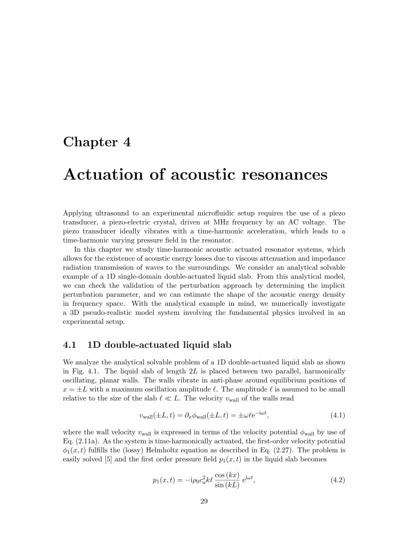
Chapter 4

Actuation of acoustic resonances

Applying ultrasound to an experimental microfluidic setup requires the use of a piezotransducer, a piezo-electric crystal, driven at MHz frequency by an AC voltage. Thepiezo transducer ideally vibrates with a time-harmonic acceleration, which leads to atime-harmonic varying pressure field in the resonator.

In this chapter we study time-harmonic acoustic actuated resonator systems, whichallows for the existence of acoustic energy losses due to viscous attenuation and impedanceradiation transmission of waves to the surroundings. We consider an analytical solvableexample of a 1D single-domain double-actuated liquid slab. From this analytical model,we can check the validation of the perturbation approach by determining the implicitperturbation parameter, and we can estimate the shape of the acoustic energy densityin frequency space. With the analytical example in mind, we numerically investigatea 3D pseudo-realistic model system involving the fundamental physics involved in anexperimental setup.

4.1 1D double-actuated liquid slab

We analyze the analytical solvable problem of a 1D double-actuated liquid slab as shownin Fig. 4.1. The liquid slab of length 2L is placed between two parallel, harmonicallyoscillating, planar walls. The walls vibrate in anti-phase around equilibrium positions ofx = ±L with a maximum oscillation amplitude ℓ. The amplitude ℓ is assumed to be smallrelative to the size of the slab ℓ≪ L. The velocity vwall of the walls read

vwall(±L, t) = ∂xwall(±L, t) = ±!ℓe−i!t, (4.1)

where the wall velocity vwall is expressed in terms of the velocity potential wall by use ofEq. (2.11a). As the system is time-harmonically actuated, the first-order velocity potential1(x, t) fulfills the (lossy) Helmholtz equation as described in Eq. (2.27). The problem iseasily solved [5] and the first order pressure field p1(x, t) in the liquid slab becomes

p1(x, t) = −i0c2akℓ

cos (kx)

sin (kL)ei!t, (4.2)

29

30 Actuation of acoustic resonances

x

0 L-L

vwall = !ℓe−i!tvwall = −!ℓe−i!t

Figure 4.1: Sketch of the 1D single-domain resonator of a liquid slab (blue) between two parallel,harmonically oscillating, planar walls at x = ±L. The walls are vibrating with maximum amplitudeℓ in anti-phase with the velocity vwall(±L, t) = ±!ℓe−i!t.

where k = k0(1 + i ) is the complex wavenumber. As discussed in Chap. 2 this definitionof k assumes the viscosity to be small. Expanding p1(x, t) to first order in k around k0

and making use of k0L≪ 1 yields

p1(x, t) ≈ −i0!caℓcos(k0x)− i k0x sin (k0x)

sin (k0L) + i k0L cos (k0L)e−i!t. (4.3)

As the acoustic resonances acquires large pressure amplitudes, the resonances are identifiedby the minimum in the denominator in Eq. (4.3), i.e. for k0L = n for n = 1, 2, 3, . . . giving

k0 = kn = n

L, n = 1, 2, 3, . . . , (4.4a)

!0 = !n = ncaL, n = 1, 2, 3, . . . , (4.4b)

which gives the resonance frequency fn = (can)/2L, which we recognize as the 1D casef1,0,0 of the eigenfrequency for the single-domain box in Eq. (2.18). In the inviscid case → 0 the pressure goes to infinity on resonance.

4.1.1 Perturbation parameter and first-order pressure field

We assume that the walls are Ferroperm Pz26 piezo-electric transducers, the displacementamplitude is estimated to ℓ ≈ 1 nm. The value is the estimated static displacementutilizing Ferroperm’s online piezo electric calculator [53] for a freely vibrating actuator ofsize 50× 12× 1 mm applied a static voltage of 2 V. Moreover, we consider the vibrationalfrequency in the low MHz range and the liquid to be water.

Off-resonance we have sin (k0L) = 1 and by use of ≪ 1 we get the magnitude of thefirst-order pressure field off-resonance

∣p1∣ = 0!caℓ ≈ 1.5 kPa. (4.5)

4.1 1D double-actuated liquid slab 31

We then find the corresponding first-order density field ∣1∣ = 1c2a∣p1∣ = !ℓ

ca0, from which

we directly read off the implicit perturbation parameter off-resonance as

offper =

!ℓ

ca≈ 6.7× 10−7, (4.6)

which gives that the perturbation approach is valid as offper ≪ 1. On-resonance sin (k0L) =

0 and by insertion of the resonance condition Eq. (4.4b) into Eq. (4.3), we get the pressureamplitude

∣p1∣ =1

n 0!caℓ ≈ 5× 107 Pa, (4.7)

where the numerical estimate is for n = 1. The only change from the off-resonancemagnitude is the multiplication of 1/(n ), and the implicit perturbation parameter on-resonance becomes

onper =

1

n

!ℓ

ca≈ 2.2× 10−2, (4.8)

The on-resonance calculations are close to invalidate the perturbation approach. Nev-ertheless the estimate of the displacement amplitude is considered to be an upper limit,as it might not reach the static displacement through a MHz oscillation and due to factthat the calculation is based on the piezo transducer being unloaded. We therefore in thisnaive boundary model assume that the piezo transducer is lossless and perfectly coupled.Secondly, an experimental system includes impedance loss from transmission of waves,which increases the effective damping coefficient , leading to a lower estimated pressureamplitude.

4.1.2 The energy of an acoustic resonator

With the objective of calculating the time-averaged acoustic energy density, the square ofthe absolute pressure field and its corresponding derivative become

∣p1(x)∣2 ≈ (0!caℓ)2 cos2(k0x) + 2k2

0x2 sin2 (k0x)

sin2(k0L) + 2k20L

2 cos2(k0L), (4.9)

∣∂xp1(x)∣2 ≈ (0!2ℓ)2 sin2(k0x) + 2k2

0x2 cos2(k0x)

sin2(k0L) + 2k20L

2 cos2(k0L). (4.10)

Using the definition of the acoustic energy density in Eq. (2.31), we calculate the spatiallyaveraged acoustic energy density ℰac over the length of the liquid slab

ℰac(!) =1

2L

∫ L

x=−L

1

40

[1

!2∣∂xp1(x)∣2 +

1

c2a

∣p1(x)∣2]dx, (4.11)

which by insertion of the pressure field and its derivative followed by integration gives

ℰac(f) =0!

2ℓ2

8L

L+ 13

2k20L

3

sin2(k0L) + 2k20L

2 cos2(k0L). (4.12)


We now drive the resonator close to the resonance frequency !0, namely ! = !0 + !,where ! is a small perturbation such that ! ≪ !0. Further rewriting utilizing ≪ 1yields

ℰac(!) =ℰ0[

2Qf0

(f − f0)]2

+ 1, (4.13)

which shows that the acoustic energy density with these assumptions are described by aLorentzian line-shape fit, which we know from the description of the classical harmonicoscillator. The energy density is centered around the resonance frequency f0 with maxi-mum amplitude of the energy density ℰ0 = ℰac(f0) = 0c

2aℓ

2/(8L2 2). The full width athalf maximum (FWHM) Δf0 is defined by ℰac(f0 ±Δf0) = ℰ0/2 and the correspondingQ-value is defined as Q = f0/Δf0 = 1/(2 ).

The numerical value of the maximum amplitude is estimated to ℰ0 ≈ 2.7× 103 J m−3,which is approximately a factor of fifty larger than observed experimentally in the currentthesis work, see Chap. 8. Again we explain the discrepancy by the naive lossless andperfectly coupled transducer model and the low value of the damping coefficient , whichdoes not take into account the impedance losses. Calculating the Q-value for this modelsystem we get Q = 1/(2 ) = 5× 104.

Having investigated a simple analytical actuation model we are now ready to numeri-cally analyze a more realistic model system.

(a) (b)

Figure 4.2: Point-actuation device fabricated in the group of Laurell as a result of the analysesin this thesis work. The setup limits the influence from acoustic transmission loss and it limits thetransducer area, which is hard to theoretically model properly. The point-actuation device willplay an important role in future quantitative comparison between experimental and theoreticalmodels. (a) Full image of the point-actuation device having a spatially-movable chip stage. Thechip is acoustically actuated from above by the fixed aluminum horn. (b) Zoom-in of the actuatedchip being clamped by four brass pins on top and bottom. The aluminum horn is actuated by aninternal air-backed piezo transducer of the type PZ26 from Ferroperm Piezoceramics A/S.

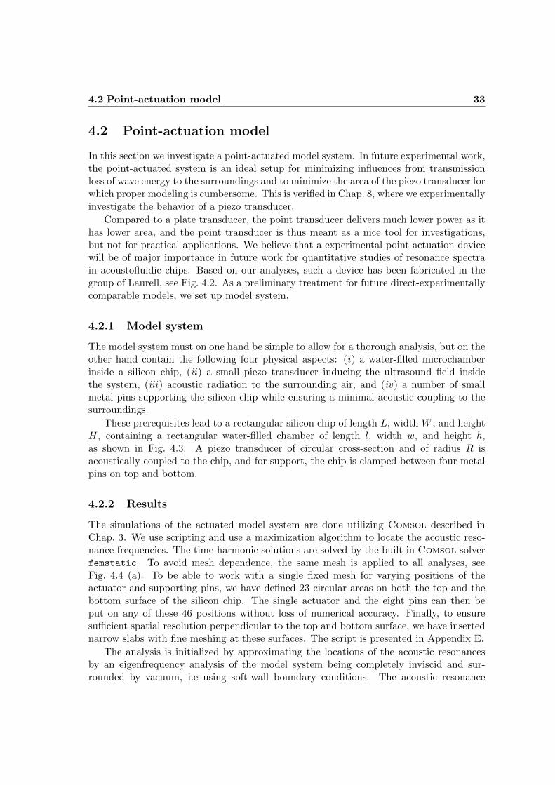
4.2 Point-actuation model 33

4.2 Point-actuation model

In this section we investigate a point-actuated model system. In future experimental work,the point-actuated system is an ideal setup for minimizing influences from transmissionloss of wave energy to the surroundings and to minimize the area of the piezo transducer forwhich proper modeling is cumbersome. This is verified in Chap. 8, where we experimentallyinvestigate the behavior of a piezo transducer.

Compared to a plate transducer, the point transducer delivers much lower power as ithas lower area, and the point transducer is thus meant as a nice tool for investigations,but not for practical applications. We believe that a experimental point-actuation devicewill be of major importance in future work for quantitative studies of resonance spectrain acoustofluidic chips. Based on our analyses, such a device has been fabricated in thegroup of Laurell, see Fig. 4.2. As a preliminary treatment for future direct-experimentallycomparable models, we set up model system.

4.2.1 Model system

The model system must on one hand be simple to allow for a thorough analysis, but on theother hand contain the following four physical aspects: (i) a water-filled microchamberinside a silicon chip, (ii) a small piezo transducer inducing the ultrasound field insidethe system, (iii) acoustic radiation to the surrounding air, and (iv) a number of smallmetal pins supporting the silicon chip while ensuring a minimal acoustic coupling to thesurroundings.

These prerequisites lead to a rectangular silicon chip of length L, width W , and heightH, containing a rectangular water-filled chamber of length l, width w, and height ℎ,as shown in Fig. 4.3. A piezo transducer of circular cross-section and of radius R isacoustically coupled to the chip, and for support, the chip is clamped between four metalpins on top and bottom.

4.2.2 Results

The simulations of the actuated model system are done utilizing Comsol described inChap. 3. We use scripting and use a maximization algorithm to locate the acoustic reso-nance frequencies. The time-harmonic solutions are solved by the built-in Comsol-solverfemstatic. To avoid mesh dependence, the same mesh is applied to all analyses, seeFig. 4.4 (a). To be able to work with a single fixed mesh for varying positions of theactuator and supporting pins, we have defined 23 circular areas on both the top and thebottom surface of the silicon chip. The single actuator and the eight pins can then beput on any of these 46 positions without loss of numerical accuracy. Finally, to ensuresufficient spatial resolution perpendicular to the top and bottom surface, we have insertednarrow slabs with fine meshing at these surfaces. The script is presented in Appendix E.

The analysis is initialized by approximating the locations of the acoustic resonancesby an eigenfrequency analysis of the model system being completely inviscid and sur-rounded by vacuum, i.e using soft-wall boundary conditions. The acoustic resonance


f1,1,1 = 761 kHz in the water-filled chamber is shown in Fig. 4.4 (b). Note that the acous-tic energy completely confines in the water-filled microchamber. We set up the conditionsfor such confined modes in Chap. 7 on acoustic waveguides.

Viscous damping, impedance radiation and resonance shape

Among the 46 possible circular areas, the actuator is placed at that particular one, whichgives the largest resonance energy Etot. Note, that in this example we treat the totalacoustic energy in the system, meaning that the energy amplitude is only for internalcomparison in the current model example. The amplitude scales with the applied nor-mal acceleration an in Eq. (2.48) at the transducer boundary. In this model examplean = 1 m s−2, corresponding to a transducer amplitude of approximately l ≈ 40 fm at afrequency of f1,1,1 = 761 kHz.

First, we study the lowest resonance mode for an unsupported chip surrounded by air.We vary the viscous damping coefficient from 10−6 to 10−3 as shown in Fig. 4.5 (a). Asexpected, due to weak damping in the harmonically driven system, the resonance peakEtot(f) is well approximated by a Lorentzian line shape as given in Eq. (4.13). Theresonance frequency f0 and maximum energy amplitude are found from the maximiza-tion algorithm and the Q-values are obtained by fitting the numerical data points to theLorentzian line shape. We note that the Q-values are large, up to Q ≈ 104. The resonancepeaks are very sharp with a width of Δf0 ≈ 102 Hz for f0 ≈ 106 Hz.

The amplitude and the Q-value of the acoustic resonance decrease significantly as theviscous damping coefficient increases from slightly below the value for water ( ≈ 10−6

corresponds to acetone or heated water) to 1000 times this value ( ≈ 10−3 corresponds toglycerol). For > 10−3 the damping is so high that the acoustic energy in the water-filledmicrochamber is negligible, and the acoustic resonance disappears completely.

To study the influence of the surrounding air for the unsupported chip we change the

z

H

0

yW

x

L

wh

Chip length L 10.5 mmChip width W 3.2 mmChip height H 1.0 mmCavity length l 4.7 mmCavity width w 1.4 mmCavity height ℎ 0.3 mmRadius, actuator and pins R 0.3 mm

Figure 4.3: Sketch of the model system and the geometrical parameters. The used materialparameters are given in Table 2.1. Inside the rectangular silicon chip (light gray) of length L,width W , and height H, is placed a rectangular water-filled chamber (blue) of length l, width w,and height ℎ. The lower left corner of the chip is at (0, 0, 0) mm and the lower left corner of thechamber is at (1.30, 0.68, 0.30) mm. The chip is supported by being clamped between four circularmetal pins on the top (black disks) and on the bottom (gray disks), just modeled by the silicon/pininterface of circular shape. The acoustic actuation is provided by a cylindrical piezo-element, heremodeled by the silicon/actuator interface of circular shape (red disk) shown on the top of thesilicon chip. All disks have the radius R.


Figure 4.4: (a) The fixed mesh contains 21340 elements, which for the solution at any givenfrequency yields 33605 degrees of freedom. On the top surface is seen the 23 pre-defined actua-tor/pin positions. The two slabs with refined mesh ensures a good resolution near the actuator/pinpositions. The water-filled microchamber inside the silicon chip is not visible. (b) The pressu´reeigenmode has frequency f1,1,1 = 761 kHz for the system in vacuum, i.e., p = 0 at the chip surface.

7.5675 7.568 7.5685 7.569 7.5695 7.57 7.5705 7.571 7.5715 7.572

x 105

0

0.2

0.4

0.6

0.8

1

1.2

1.4

1.6

1.8

f [Hz]

Eto

t(f)

[fJ]

γ = 10−6, Q = 10225

γ = 10−5, Q = 8661

γ = 10−4, Q = 3326

γ = 10−3, Q = 476

10−6

10−5

10−4

10−3

103

104

7.5688 7.569 7.5692 7.5694 7.5696 7.5698 7.57 7.5702 7.5704

x 105

0

1

2

3

4

5

6

7

f [Hz]

Eto

t(f)

[fJ]

z = 0.5, Q = 22314z = 1.0, Q = 10410z = 2.0, Q = 5160z = 3.0, Q = 3452z = 4.0, Q = 2583

0 0.5 1 1.5 2 2.5 3 3.5 410

3

104

7.5674 7.5676 7.5678 7.568 7.5682 7.5684 7.5686 7.5688 7.569

x 105

0

0.5

1

1.5

2

2.5

f [Hz]

Eto

t(f)

[fJ]

z = 0.5, Q = 12903z = 1.0, Q = 8889z = 2.0, Q = 5364z = 3.0, Q = 3381z = 4.0, Q = 2779

0 0.5 1 1.5 2 2.5 3 3.5 410

3

104

7.5674 7.5676 7.5678 7.568 7.5682 7.5684 7.5686 7.5688 7.569

x 105

0

0.5

1

1.5

2

f [Hz]

Eto

t(f)

[fJ]

z = 0.5, Q = 9321z = 1.0, Q = 8381z = 2.0, Q = 4768z = 3.0, Q = 3317z = 4.0, Q = 2535

0.5 1 1.5 2 2.5 3 3.5 410

3

104

(a) (b)

(c) (d)

Figure 4.5: The acoustic energy Etot as a function of frequency f for various values of (a) viscousdamping coefficient without pins for support, (b) normalized impedance z = Z/Zair without pinsfor support, (c) normalized impedance z = Z/Zair with iron pins for support and (d) normalizedimpedance z = Z/Zair with silicon pins for support. The numerical data points are clusteredaround the resonance frequency as a consequence of the method employed to locate the resonancepeak. The dashed lines are fits to Lorentzian line shapes. The insets shows Q as a function of (a) and (b,c,d) z.


0.33 0.92 1 0.56 6×10−3 3×10−6 4×10−7

7×10−3

0.024

0.16

0.60

0.27

0.91

0.21

0.70

0.033

0.13

4×10−5

9×10−5

5×10−7

5×10−7

< 5 × 10−7

< 5 × 10−7

0.44 0.50 0.58 0.54 0.47 0.57 0.99

0.48

0.45

0.49

0.53

0.50

0.55

0.48

0.48

0.48

0.47

0.96

0.98

(a) (b)

Figure 4.6: (a) The normalized acoustic energy Etot(f0)/Emax for the lowest resonance mode inan unsupported rectangular silicon chip (thick black line) for 23 different positions (gray disks) ofthe circular actuator on the bottom surface. The energies are normalized by the maximum valueEmax = 1.78 fJ, which is the resonance energy obtained for the actuator positioned at the diskwith the value 1. The position of the water-filled microchamber is indicated by the rectangle (thinblack line). The resonance energy decreases rapidly as a function of increasing distance betweenthe actuator and the water-filled chamber. (b) The same for a supported chip, where the positionof the four silicon support pins are marked by black disks. The numbers are the ratios betweenthe resonance energy for the cases with and without supporting pins.

impedance Z from 0.5Zair to 4Zair corresponding to changes in air pressure from 0.5 barto 4 bar or gas densities from 0.25 kg m−3 to 16 kg m−3 at 1 bar. The results for behaviorof the resonance peak is similar to the previous sweep in , as seen in Fig. 4.5 (b), andthe amplitude and Q-value decrease for increasing impedance.

The next step is to include the supporting pins and the associated energy loss throughtheir impedance. We place the pins at the four corner positions at the top and at thebottom surface (the black/gray disks in Fig. 4.6). In Fig. 4.5 (c) we show the resonancepeak of the chip supported by iron pins in analogy to the one shown in Fig. 4.5 (b) foran unsupported chip. The iron pins are modeled by changing the impedance boundarycondition from Z = Zair to Z = Ziron. All other other parameters remain unchanged.The main observation is that the resonance amplitude is decreased. This is expected,since the impedance mismatch at the eight pin positions has been decreased from Zair/Zsi

to Ziron/Zsi thus making a larger energy out-flux possible. This trend continues in thecase of silicon pins, which of course are ideally matched acoustically to the silicon chip.In Fig. 4.5 (d), where the eight iron pins have been replaced by eight silicon pins, theresonance energies decrease even further.

Resonance energy and actuator position

Finally, we show the results of changing the position of the actuator on the surface.For simplicity, we begin by considering the unsupported chip. We have calculated theresonance amplitudes for all 46 possible actuator positions. The maximum amplitudeEmax = 1.78 fJ was found on the bottom surface, where the water-filled chamber isclosest to the surface. All 46 resonance amplitudes Etot(f0) was normalized by Emax, andthe resulting values Etot(f0)/Emax are shown in Fig. 4.6 (a); each value is placed at thecorresponding position on the surface. The resulting values clearly show how the resonanceamplitude rapidly decreases as the distance between the microchamber and the actuatorincreases.

The same calculation was then repeated in the case of supporting silicon pins, the case


of largest loss due to impedance matching between pins and chip. Fig. 4.6 (b) shows therelative decrease in resonance amplitude for each individual actuator position comparingthe case with and without support. In most cases the relative energy loss is around 50 %with minor variations.

4.2.3 Concluding remarks

We have established a model, which includes the most significant physical aspects ofacoustically driven microfluidic systems near resonance. It acts as a preliminary treatmentfor future work concerning the quantitative comparison of acoustic frequency spectrum inacoustofluidic chip systems investigated by the point-actuation device shown in Fig. 4.2.

We have shown the presence of the expected decrease of the resonance amplitude as afunction of increased viscous damping in the water-filled microchamber and of decreasedacoustical impedance mismatch with the surroundings. In particular, we have shown thatthe position of the actuator has a significant influence of the amplitude of the acoustic res-onance. In our simple system we have observed a relative change in resonance amplitudesof about 103 by moving the actuator a distance of twice the diameter of the actuator, andabout 106 for distances of four times the diameter. Moreover, the analysis clearly showsthe dominance of the systems eigenresonance as the type of the eigenmode is independentof the position of the actuator.

Chapter 5

Analysis of transversehalf-wavelength resonances

In the current chapter we investigate the usual transverse half-wavelength picture by 1Dand 2D models. Moreover, we present numerical 3D models for future analysis. The majorpart of the work is summarized in a peer-reviewed conference proceeding published for the157th meeting of the Acoustical Society of America, Portland, Oregon, May 2009. Thepaper is included in Appendix A.

5.1 Analysis of 1D models

For experimental applications it is desirable to work with half-wavelength waves of oddsymmetry in the transverse y-direction of the water-filled channel, i.e. w = /2 and thusa resonance frequency f0,1,0 ≈ cwa/(2w). A perfect transverse half-wavelength pressureeigenmode is seen in Fig. 2.1 (d), where the surrounding silicon is assumed to be infinitelyhard. This is not entirely correct and the question now arises how the width W of a

symmetry

∂ypwa = 0 (even)

pwa = 0 (odd)

continuity

pwa = psi1ρwa

∂ypwa = 1ρsi

∂ypsi

soft wall

psi = 0

−a 0 b

wa si airy

Figure 5.1: Sketch of the 1D model containing half the water-filled channel (wa) and the siliconchip (si). The model includes three boundaries; a symmetric point in the center of the channel(y = −a), an interface between channel and chip (y = 0), and the outer boundary of the siliconchip (y = b). Notice that the boundary condition at the symmetry point gives either even or oddpressure-modes across the channel.

39

40 Analysis of transverse half-wavelength resonances

surrounding silicon chip affects this simple estimate for f0,1,0.In Fig. 5.1 is sketched a 1D model for the transverse y-direction, where for simplicity

we introduce the lengths a ≡ w/2 and b ≡ (W − w)/2 for half the width of the channeland the width of the silicon chip from the channel to the edge, respectively. The modelis symmetric around the center of the channel, thus leading to two classes of solutions forthe pressure, namely even and odd modes.

Using the proper symmetry boundary condition Eq. (2.47) at y = −a and the softboundary condition Eq. (2.46) at y = b, results in cosine (even) or sine (odd) solutions forthe pressure waves,

pwa(y) = Awa cos [kwa(y + a)] (even), (5.1a)

pwa(y) = Awa sin [kwa(y + a)] (odd), (5.1b)

psi(y) = Asi sin [ksi(b− y)], (5.1c)

where Awa and Asi are pressure amplitudes. Employing the interface conditions Eq. (2.41)at y = 0 and utilizing that ksi = kwacwa/csi, results in transcendental equations for evenand odd pressure eigenmodes

cot () = z tan () (even), (5.2a)

cot () = −1

zcot () (odd), (5.2b)

where ≡ kwaa is the dimensionless wavenumber, z = Zsi/Zwa ≈ 13.4 is the acousticimpedance ratio, and is the aspect ratio parameter given by

≡ cwa

csi

b

a=

number of wavelengths in the silicon chip

number of wavelengths in the water-filled channel. (5.3)

From Eq. (5.2) it is now possible for a given to determine which value of that mostaccurately approximates a perfect /2-mode of wavelength ∗wa = 4a in the water-filledchannel. Expressing the actual wavelength wa as a function of the ideal wavelength ∗wa

and a relative shift in the wavelength, we get

wa = ∗wa(1 + ), (5.4)

=

2(1 + )−1, (5.5)

where = /2 for = 0 thus corresponds to a perfect half-wavelength mode inside thewater-filled channel.

5.1.1 Qualitative analysis

Without detailed calculations we can for a fixed value of a immediately give the solutionsof this two-domain problem in the extreme limits b≪ a, an infinitely thin shell of silicon,and b≫ a, an infinitely wide shell of silicon.

For b ≪ a the lowest modes are M1 (even, a = wa/4), M2 (odd, a = 2wa/4),M3 (even, a = 3wa/4), M4 (odd, a = 4wa/4), M5 (odd, a = 5wa/4), etc. all being

5.1 Analysis of 1D models 41

approximately zero at the water/silicon interface. The resonance frequency f0,n,0 for moden is thus f0,n,0 ≈ ncwa/(4a), for → 0. Modes for b≪ a are illustrated in the left columnof Fig. 5.2.

b a b for perfect λwa/2 b a

M1

α = 0.001

−0.2 −0.1 0 0.1 0.2−1

0

1

wa

p/p

max

no λwa/2 mode

α = 400

−400 −200 0 200 400−1

0

1

si

M2

α = 0.001

−0.2 −0.1 0 0.1 0.2−1

0

1

wa

p/p

max

α = 1

−1 0 1−1

0

1α = 400

−400 −200 0 200 400−1

0

1

si

M3

α = 0.001

−0.2 −0.1 0 0.1 0.2−1

0

1

wa

p/p

max

α = 2

−2−1 0 1 2−1

0

1α = 400

−400 −200 0 200 400−1

0

1

si

M4

α = 0.001

−0.2 −0.1 0 0.1 0.2−1

0

1

wa

p/p

max

α = 3

−3 −1 0 1 3−1

0

1α = 400

−400 −200 0 200 400−1

0

1

si

M5

α = 0.001

−0.2 −0.1 0 0.1 0.2−1

0

1

wa

y [mm]

p/p

max

α = 4

−4 −2 0 2 4−1

0

1

y [mm]

α = 400

−400 −200 0 200 400−1

0

1

si

y [mm]

Figure 5.2: Five lowest pressure eigenmodes M1-M5 for varying width W = w(1 + csicwa

) of thesilicon chip and fixed water-filled channel of width w = 2a = 0.38 mm. Left column shows thepressure modes in the extreme limit b ≪ a corresponding to an infinitely thin shell of silicon. Inthis finite valued case = 1/1000, thus making b ≈ a × 10−3. Right column shows the pressuremodes in the extreme limit b≫ a corresponding to an infinitely wide shell of silicon. Here = 400,thus making b ≈ a × 103. Center column shows the pressure modes for the optimal b/a aspectratio to give perfect half-wavelength modes in the water-filled channel. Every second wa/2-modeis odd and even, respectively.


For b ≫ a, i.e. when b is stretched towards infinity, these modes deform continuouslyinto M1 (even, b = si/4), M2 (odd, b = 2si/4), M3 (even, b = 3si/4), M4 (odd,b = 4si/4), M5 (odd, b = 5si/4), all being zero at the outer edge of the silicon. Theresonance frequency f0,n,0 for mode n is thus f0,n,0 ≈ n csi/(4b), for →∞, which clearlydecreases towards zero as b increases. Modes for b ≫ a are seen in the right column ofFig. 5.2.

Consequently, for any given mode there exists exactly one value of b for which thedesired perfect half-wavelength resonance mode with frequency f = cwa/(4a) is obtained.However, since the ideal resonance is an odd mode with exactly one half wavelength insidethe water-filled channel, there exists only such a mode in every second case. This isillustrated in the center column of Fig. 5.2.

Fig. 5.3 (a) plots the lowest seven eigenfrequencies as a function of the aspect ratioparameter . We clearly see that the eigenfrequencies decrease for increasing values of ,and we notice how each mode has the desired value of f0,1,0 ≈ 2 MHz for exactly one valueof . Fig. 5.3 (b) shows the corresponding deviations in wavelength from the perfecthalf-wavelength wa/2 = 2a.

5.1.2 Quantitative analysis

Bearing in mind the qualitative expectations, we quantitatively solve the problem. Insert-ing = /2 into Eq. (5.2) to find solutions for = 0, requires to be an odd positiveinteger for odd pressure modes, while is required to be an even positive integer for evenpressure modes. These solutions are illustrated in Fig. 5.4, where the components of thetranscendental equations are plotted. It is observed in Fig. 5.4 (a) that for = 1, an odd/2-mode is perfectly matching the channel width with = 0, while even /2-modes have ∕= 0. For = 2 as seen in Fig. 5.4 (b), the opposite is the case. From Fig. 5.4 it is alsodeducted that the largest deviations in occurs for the above discussed values of . Thisis also observed in the versus frequency plot in Fig. 5.3 (b). To sum up, the limits ofgetting either well-defined or ill-defined modes, forces the aspect ratio b/a to be

= 0 :b

a=

csi

cwa, = 1, 3, 5 . . . odd,

= 2, 4, 6 . . . even, (5.6a)

large :b

a=

csi

cwa, = 1, 3, 5 . . . even,

= 2, 4, 6 . . . odd. (5.6b)

In Fig. 5.5 the relative change as function of is plotted as in Fig. 5.3 (b). But onlyodd half-wavelength modes are plotted and only the mode having the smallest ∣∣ for agiven . Thus this graph acts as an design graph in order to optimize the half-wavelengthmodes. As already discussed the size of the relative change ∣∣ periodically has regionswith large and small values as a function of . As increases, the maximum values of ∣∣decreases. It is seen that well-defined odd modes with ∣∣ ≤ 0.1 exist for aspect ratios aslow as = 1 and thus b/a = csi/cwa ≈ 5.7. The value of the relative change for odd modes


0 1 2 3 4 5 6 7 80

1

2

3

4

5

6f0,3,0

f0,2,0

f0,1,0

f[M

Hz]

(a)

0 200 400 600 8000

5

10

15

20

f[kHz]

M1M2M3M4M5M6M7

0 1 2 3 4 5 6 7 8−0.4

−0.2

0

0.2

0.4

αδ

M1

M2

M3

M4

M5

M6

M7

(b)

0 2 4 6 80

10

20

30

40

50

60

70

ℰ wa/E

max

si

M1

M2

M3

M4

(c)

10 50 100 1500

10

20

30

40

50

60

70

ℰ wa/E

max

si

M1

M2

M3

M4

Figure 5.3: 1D Comsol simulations of the seven lowest eigenmodes, M1-M7. (a) Frequencies asa function of the aspect ratio parameter . Indicated are f0,1,0, f0,2,0 and f0,3,0. The inset showsf for 100 < < 1000. (b) Relative change in wavelength from the perfect half-wavelength inthe water-filled channel ∗ = 4a as a function of aspect ratio parameter . (c) Ratio ℰwa/E

maxsi of

the average acoustic energy density ℰwa in water to the maximum acoustic energy density Emaxsi in

silicon as a function of aspect ratio parameter . Four clarity, only the four lowest modes M1-M4are plotted. The inset shows ℰwa/E

maxsi for 10 < < 200.

approaches −1/2 for → 0, which corresponds to a full-wavelength sine-mode within thechannel. b/a = csi/cwa is thus a lower limit for the aspect ratio when considering oddhalf-wavelength modes.

We observe the fact that is numerically largest when it is positive, which thus cor-responds to a wavelength longer than the channel width. For fixed aspect ratios, modeswith frequencies higher than f0,1,0 are therefore leading to lower than those modes havingfrequencies lower than f0,1,0.

Fig. 5.5 (a) shows marks for the four modes shown in Fig. 5.6. Modes A and B areperfectly matching half-wavelength modes with = 0 and show up for the frequency


0 0.2 0.4 0.6 0.8 1−25

−20

−15

−10

−5

0

5

10

15

20

25

θ/π

func

tion

cot (θ)− 1

z cot (αθ)z tan (αθ)

even odd

A even

α = 1(a)

0 0.2 0.4 0.6 0.8 1−25

−20

−15

−10

−5

0

5

10

15

20

25

θ/πfu

ncti

on

cot (θ)− 1


evenoddC−

evenBoddC+ even

α = 2(b)

Figure 5.4: Plot of the components in the governing transcendental equation Eq. (5.2) for twovalues of . Solutions to the transcendental equation Eq. (5.2a) are marked by filled circles andlabeled ”even”, while solutions to Eq. (5.2b) are marked ”odd”. (a) = 1 leading to perfectlymatching odd mode at = /2. (b) = 2 leading to perfectly matching even mode at = /2.

0 2 4 6 8

−0.3

−0.2

−0.1

0

0.1

= 0

Odd

Even

A B

C−

C+ b/a = (csi/cwa) ≈ 5.7(a)

0 2 4 6 8

10

20

30

40

50

60

70

ℰ wa/E

max

si

A

C−C+

(b)

Figure 5.5: Design graphs plotting only for the modes best approximating perfect odd half-wavelength mode in the water-filled channel. These plots are ideal for using as design tool ifone wants to create an odd standing half-wavelength transverse mode across the channel. (a)Minimum relative change found by numerical solutions to Eq. (5.2) as a function of . Each(, ) stems from the mode having the smallest value of for that . Indicated are the even(black crosses) and odd (black dots) integer values of . The labels A, B, C+ and C− link to thecorresponding modes shown in Fig. 5.6. The labels illustrate that e.g. a perfect even mode at pointB is surrounded by two non-perfect odd modes at point C+ and C−. (b) Average acoustic energydensity in water to the maximum acoustic energy density in silicon ℰwa/E

maxsi as a function of .

Notice in this 1D approximation how the perfectly matching odd half-wavelength mode A has highℰwa/E

maxsi , whereas the corresponding ill-matching modes C+ and C− has low ℰwa/E

maxsi .


−1

0

1

wasi siair air

p/p

max

−2 −1 0 1 2−1

0

1

wasi si airair

y [mm]

p/p

max

−1

0

1

wasi si airair

p/p

max

−2 −1 0 1 2−1

0

1

wasi si airair

y [mm]

p/p

max

(A) α = 1, f = 1.9513 MHz, δ = 0

(B) α = 2, f = 1.9513 MHz, δ = 0

(C+) α = 2, f = 1.7182 MHz, δ = 0.136

(C−) α = 2, f = 2.1844 MHz, δ = −0.107

Figure 5.6: Pressure eigenmodes p(y) of the four special cases marked in Figs. 5.4 and 5.5 forthe 1D silicon/water (gray/blue) model given a water-filled channel of width w = 2a = 0.38 mm.(A) The perfectly matched silicon chip with = 1 (W = 2.6 mm) supporting the anti-symmetrichalf-wavelength pressure mode in the water-filled channel at frequency f = 1.9513 MHz. (B) Thesilicon chip with = 2 (W = 4.7 mm) also supports a perfect half-wavelength pressure mode atfrequency f = 1.9513 MHz, however this mode is symmetric. (C+) An anti-symmetric eigenmodein the chip with = 2 with a frequency as close as possible, but lower, to the ideal frequency ofsubfigure (A). Here f = 1.7182 MHz and the wavelength in the water-filled channel is 13.6 % toolong ( = 0.136). (C−) An anti-symmetric eigenmode in the chip with = 2 with a frequency asclose as possible, but higher, to the ideal frequency of subfigure (A). Here f = 2.1844 MHz andthe wavelength in the water-filled channel is 10.7 % too short ( = −0.107).

f0,1,0 = 1.9513 MHz. Mode A is odd and exists for = 1, while mode B is even and existsfor = 2. For = 2, we get no perfect odd modes, but two odd modes, C+ and C−,surrounding mode B. Mode C+ has f = 1.7182 MHz and = 10.6%, while mode C− hasf = 2.1844 MHz and = −10.7%. These numerical values and corresponding acousticenergy densities are presented in Table 5.1. For the mode C− we have wa < w/2, and weobserve that the pressure antinodes are positioned a little distance from the channel walls.This may result in bad sorting for devices like that depicted in Fig. 1.1, since particlesattracted towards pressure nodes, will be pushed towards the walls if they get to close.

Moreover, we notice that mode A corresponds to mode M2, where the width b of thesilicon layer has been chosen to give the perfect odd half-wavelength mode in the water-filled channel. Mode C+ is mode M2 after stretching b with a factor of 2. The mode isantisymmetric and is not perfect since wa is too long. Mode B is the even mode M3 forthe same geometry as mode C+. The wavelength matches perfect, but it is symmetric.Finally, mode C− is an antisymmetric mode M4, which has too short a wavelength wa.

5.1.3 Energy densities

A quantitative measure of the quality of a given eigenmode can be obtained from theexpression for the acoustic energy density Eac in Eq. (2.31). The higher the averageacoustic energy density ℰwa is in the water-filled channel relative to the maximum acoustic


Table 5.1: Values of 1D Comsol simulations of wa/2-modes. y-symm. denotes the symmetry.

Mode y-symm. f [MHz] [%] ℰwa/Emaxsi

A 1 odd 1.9513 0 76.5B 2 even 1.9513 0 0.4C+ 2 odd 1.7182 13.6 10.7C− 2 odd 2.1844 -10.7 10.7

energy density Emaxsi in the surrounding silicon chip, the better. This ratio is a direct

measure of the amount of useful acoustic energy in the water-filled channel to the amountof useless acoustic energy in the silicon chip. The acoustic energy density is relevant,since it is directly proportional to the acoustic pressure force on suspended particles, seeEq. (2.38)

For the four specific modes A, B, C+, and C− shown in Fig. 5.6 we find numerically thatℰwa/E

maxsi = 76.5, 0.4, 10.6, and 10.6, respectively. Clearly, the perfect anti-symmetric

half-wavelength mode in the = 1 chip has the best figure of merit. The perfectlymatching mode A gives a larger channel-pressure to chip-pressure, which thus leads tothe largest maximum acoustic energy density, see Table 5.1. Better match therefore leadsto higher relative energy densities in the channel. The difference from the perfect oddmode A to the least perfect odd modes C+ and C− shows to be a factor of seven in thissimple 1D approximation. This thus underestimates the importance of correct matchingof wavelengths in separation chip designs as this corresponds to the need of a separationchannel seven times longer if designed with = 2 instead of = 1.

To get the full overview of the distribution of the 1D energy densities, these are plottedin Fig. 5.3 (c) for the modes M1-M4 as a function of . It is seen that the energy densityratio varies strongly as a function of the aspect ratio parameter for the different modes.We clearly see that mode M2 has maximum energy density in the water-filled channel as = 1, where it is a perfect half-wavelength mode with = 0, see Fig. 5.3 (b). Observingmode M4 we see that ℰwa/E

maxsi has two maxima for the interval 0 < < 8; one for

= 0.2 being a perfect three-half-wavelength mode in the channel and one for = 3being a perfect half-wavelength mode in the channel.

Fig. 5.5 (b) plots the energy density ratio ℰwa/Emaxsi versus only for the modes

being the best approximating odd half-wavelength modes in the channel. We thus get anoverview of which values of that gives high energy density ratio in the case of designingthe widespread acoustic separator utilizing odd half-wavelength modes. For odd thewa/2 mode has maximum energy density ratio, while for even the wa/2 mode hasminimum energy density ratio. Note as in general increases, the minimum of energydensity ratio increases too.

The just presented 1D models acts as a preliminary treatment of the usual transversehalf-wavelength picture. They show that 1D wave solutions only exist for propagation inboth the water-filled channel and the surrounding silicon chip. For these types of wavesolutions the need for geometrically matching was illuminated based on a quantitativemeasure of the acoustic energy density and the relative deviation from a perfect transverse


half-wavelength mode.


We now extend our analysis of the half-wavelength modes from 1D to 2D by extending theanalysis with the length direction of the system along the x-axis. As shown in Fig. 5.7,the most prominent change from 1D to 2D is the appearance of oscillations in the axialx-direction, a feature not possible in 1D.

The introduction of axial modes leads to the possibility of having special modes fallingoff exponentially in the surrounding silicon chip. These modes confine in the water-filledchannel and will be treated in Chap. 7. In this section we restrict ourselves to considerresonance modes living in both the water-filled channel and the surrounding silicon chip.

If we consider a translational invariant system along the x-axis, the channel length lequals the chip length L. The pressure wave solutions are then easily obtained by the 1Dsolutions in Eq. (5.1) multiplied by a standing wave solution cos (kxx) with nx = 2L/xnumber of half-wavelengths. In the following we consider a system having L > l, whichis solved using 2D Comsol simulations. The Comsol-script is seen in Appendix C. Themodel is implemented as shown in Chap. 3 with continuity conditions between the twodomains and soft wall condition at the edge of the chip.

To enable direct comparison we reuse the 1D widths in 2D for the transverse y-direction. Some of the resulting pressure eigenmodes are shown in Fig. 5.7. We notehow the modes (A), (B), (C+), and (C−) from the 1D case in Fig. 5.6 also can be identi-fied in the 2D case of Fig. 5.7. However, due to the extra degree of freedom for oscillationsin the axial x-direction, it is now possible even in the ”bad” = 2 chip to find eigenmodes(D+ and D−), which are both close to the ideal frequency f = 1.95 MHz of the = 1 chipin panel (A) and at the same time possess the wanted odd (one-node) symmetry in thetransverse y-direction. The only drawback is the appearance of several nodes in the axialdirection. It is found experimentally that pressure modes with a lower number of axialnodes lead to higher separation efficiencies [38].

As in the 1D case, we can study the quality of the 2D pressure eigenmodes by evalu-ating the ratio of the acoustic energy density in the water channel relative to that in the

Table 5.2: Data for the six 2D pressure eigenmodes shown in Fig. 5.7. Listed are the value ofthe aspect parameter and the symmetries, as well as the resulting frequency f , relative shift inwavelength , and energy density ratio obtained by Comsol simulations.

Mode x-symm. y-symm. f [MHz] [%] ℰwa/Emaxsi

A 1 even odd 1.9518 0.0 39.2B 2 even even 1.9560 1.2 0.2C+ 2 even odd 1.7209 13.4 6.3C− 2 even odd 2.1870 −11.7 5.1D+ 2 even odd 1.9430 1.4 32.0D− 2 odd odd 1.9616 0.5 36.1


(A) α = 1, f = 1.9518 MHz, δ = 0

6

y

- x

−1

0

1

wasi siair air

p/pm

ax

(B) α = 2, f = 1.9560 MHz, δ = 0.012

6

y

- x

−1

0

1

wasi si airair

p/pm

ax

(C+) α = 2, f = 1.7209 MHz, δ = 0.134

6

y

- x

−1

0

1

wasi si airair

p/pm

ax

(C−) α = 2, f = 2.1870 MHz, δ = −0.117

6

y

- x

−2 −1 0 1 2−1

0

1

wasi si airair

y [mm]

p/p

max

(D+) α = 2, f = 1.9430 MHz, δ = 0.014

6

y

- x

−1

0

1

wasi si airair

p/pm

ax

(D−) α = 2, f = 1.9616 MHz, δ = 0.005

6

y

- x

−2 −1 0 1 2−1

0

1

wasi si airair

y [mm]

p/p

max

Figure 5.7: 2D Comsol simulations of six pressure eigenmodes in a water-filled channel (wa/blue)of width w = 0.38 mm and length l = 29.30 mm. The channel is placed in a silicon chip (si/gray)of width W = w[1 + (csi/cwa)] and length L = 55.00 mm. The widths here are as in the 1Dsystem of Fig. 5.6. For each mode the pressure amplitude is plotted along the indicated red linein the corresponding 2D color plot of the pressure amplitude. (A) = 1, W = 2.6 mm: perfectlymatching mode at the ideal frequency f = 1.95 MHz having odd (one-node) transverse symmetryand even (zero-node) axial symmetry. (B) = 2, W = 4.7 mm: matching mode at f = 1.95 MHzvery near the ideal frequency, but having the un-wanted even (two-node) transverse symmetry andeven (zero-node) axial symmetry. (C+) and (C−) = 2, W = 4.7 mm: as in Fig. 5.6 non-matchingmodes with frequencies far below/above the ideal frequency having the wanted odd (one-node)transverse symmetry and even (zero-node) axial symmetry. (D+) and (D−) = 2, W = 4.7 mm:almost matching modes with frequencies near the ideal frequency having the wanted odd (one-node)transverse symmetry, but with many nodes in the axial direction.

silicon chip. The results are listed in Table 5.2. Again, the perfectly matched A-mode hasthe best figure of merit, however it is seen that also the new D+ and D− perform well.These three modes have high energy density ratios of 39.2, 32.0 and 36.1, respectively,while the other three modes have ratios around 6 or lower.

The presented 2D models reproduce the transverse half-wavelength picture, but the


models clearly show the presence of pressure oscillations along the axial direction, un-less the geometries of the surrounding chip is designed correctly. In Chap. 8 we presentexperimental investigations of -chips based on the 2D models to compare the qualita-tive behaviors of the pressure resonances. Unfortunately, direct comparison of resonancepatterns have not yet been possible as a better experimental imaging system is needed.

The quantitative behavior of real chip systems is believed to be poorly approximatedby the 2D models as typical experimental chips do have pressure dynamics along thevertical z-direction. We therefore turn our attention to 3D models in the next section.


The next natural step is to investigate the antisymmetric half-wavelength modes in 3Dmodels. We consider the system in Fig. 5.8 corresponding to -chips experimentallyinvestigated in Chap. 8. In the 3D models we consider the height of the silicon chip andthe pyrex glass lid. In this section we (i) give a rough estimate of the frequency shiftfrom 2D to 3D models, (ii) carry out a full 3D Comsol simulation, and (iii) introducetranslational invariant geometries.

5.3.1 Estimation of frequency shift from 2D to 3D models

Typical experimental chips consist of a silicon chip bonded with a pyrex glass lid, wherethe bottom of the chip has the acoustically hard piezo transducer as neighboring domain,whereas the top of the pyrex lid has the acoustically soft air as neighboring domain. Thisenforces a standing pressure wave of approximately the quarter of a wavelength along thevertical z-direction. This will contribute to the chips resonance frequencies.

(a) (b)

α = 1α = 2α = 3

α = 4

xy-view

yz-view

3D view

WwL

l

hpy

hsi

W

whwa

Length, chip L 50.00 mm

Length, channel l 40.00 mm

Width, chip: W = w(1 + csi

cwa)

= 1 W=1 2.52 mm

= 2 W=2 4.67 mm

Width, channel w 0.375 mm

Height, silicon chip ℎsi 0.350 mm

Height, pyrex lid ℎpy 1.13 mm

Height, water channel ℎwa 0.157 mm

Figure 5.8: Sketch of the 3D chip model. The chip geometries corresponds to -chips experimen-tally investigated in Chap. 8. The material parameters are given in Table 2.1. The model systemconsists of a water-filled channel having width w, length l and height ℎwa. The channel is etchedinto a surrounding silicon chip of width W , length L and height ℎsi, and the silicon chip is bondedwith a pyrex glass lid of width W , length L and height ℎpy. The origin of the coordinate systemis placed at the center of the chip at the interface between the channel and the lid.


We estimate this contribution by making use of the analytical result of the frequencyin Eq. (2.18) for a single-domain box. Using Eq. (2.18) we write

f3D ≈ f2D

√1 +

( cH2H

nzf2D

)2, (5.7)

where cH = (csiℎsi + cpyℎpy)/H is a weighted approximate average speed of sound alongthe chip height H = ℎsi +ℎpy and nz is the estimated number of vertical half-wavelengths.Notice that f3D reduces to f2D for nz → 0 corresponding to no pressure dynamics alongthe height of the chip. Inserting nz = 1/2 and using the material parameters of Table 2.1we get f3D ≈ 2.26 MHz for f2D = 2.00 MHz. The estimated frequency from the 2D to 3Dmodels is therefore an increase of ∼ 13%.

5.3.2 Full 3D-simulation

Full 3D simulations of the acoustic chip systems are computational very expensive inmemory, which limits the accuracy of the calculations. In this section, we thus carryout a full 3D simulation for comparison to computational cheap models making use oftranslational invariance along the axial x-direction.

Utilizing symmetry along x and y, we present in Fig. 5.9 a full 3D Comsol calculationof the lowest transverse antisymmetric pressure eigenmode for the chip having = 1.The model is implemented in the same manner as given in Chap. 3. We apply continuityconditions at the interfaces between the water and silicon domains, soft wall condition atthe silicon/air interfaces and hard wall condition at the silicon/piezo transducer interface.

The frequency of the mode is f = 2.4501 MHz, which is approximately 0.45 MHzlarger than frequencies calculated in the 2D models in Sec. 5.2, and it is about double thesize as estimated by Eq. (5.7). Though, we see from the (x, y, 0)-projection in Fig. 5.9 (c)that the qualitative behavior of the pressure mode is identical to the 2D calculation inFig. 5.7 (A).

In Chap. 8 we show experimentally, that the corresponding -chip is able to fo-cus polystyrene particles to the center of the channel for frequencies at least as lowf ≈ 2.0 MHz. Antisymmetric transverse modes therefore exist experimentally for thisfrequency and we conclude that there is a discrepancy between the theoretical 3D modeland the experiments. We believe that the discrepancy is due to the neglect of the elasticshear waves in the solids in the chip. The size of the discrepancy in frequency is 0.45 MHz,which can be qualitatively justified by the estimated 15–20% drop in speeds of sound be-tween the longitudinal sound velocities and the average of the longitudinal and transversevelcocities in the solids Eq. (2.55). Unfortunately the use of the average speeds of soundin the 3D model, does not contribute to a significant decrease in frequency. We thereforeleave the discrepancy for explanation in future work including the elastic wave theory forthe solids.

5.3.3 Translational invariant geometries

With the preliminary treatment of the full 3D models, we now turn our focus to transla-tional invariant geometries along the x-axis, such that the length of the chip equals the


0 0.5 1

0

0.5

1

y [mm]

z[m

m]

(a) 3D view (b) (0, y, z)-view

(c) (x, y, 0)-view

Figure 5.9: 3D Comsol calculation of the lowest antisymmetric pressure eigenmode for the chipwith = 1 with geometrical parameters as in Fig. 5.8 and material parameters as in Table 2.1.The frequency is f = 2.4501 MHz. The origin of the coordinate system is placed at the center ofthe chip at the interface between the channel and the lid, and symmetry at y = 0 and x = 0 isutilized. The color plots (red positive, green neutral) show the acoustic pressure eigenmodes in (a)three dimensions, (b) a cross-sectional cut at (0, y, z) and (c) a cross-sectional cut at (x, y, 0).

length of the channel L ≡ l. This is done (i) to reduce the size of the computations, and(ii) to avoid the presence of the empty areas at the end of the channel. The latter is be-lieved to enable more direct comparison between theory and experiments, as it lowers thenumber of resonances of low importance. It is seen in Fig. 5.7 that many of the resonancesare living in the unimportant area at the chip ends outside the channel. Moreover, duringthe experimental work of the current thesis, PhD student Per Augustsson from the groupof Laurell proved the possibility of realizing translational invariant experimental chips.

We describe the translational invariant problem by choosing the solution of the x-component of the pressure field to p(x) ∝ cos (kxx) with nx = 2L/x. This reduces the3D Helmholtz equation to a 2D problem in the (y, z)-plane

[− k2

x +∇2]pi(y, z) = −!

2

c2i

pi(y, z), (5.8)

for the i’th domain material.

The implementation of the translational invariant model is shown in Chap. 3 on thenumerical calculations in Comsol Multiphysics. The translational solution for thelowest transverse pressure eigenmode with nx = 1 is plotted in Fig. 5.10 (a) for the chiphaving = 1. The translational invariant calculation reproduces the full 3D simulationin Fig. 5.9, but the frequencies deviate with ∼ 60 kHz. This deviation is believed mainlyto stem from the poor mesh resolution in the full 3D model. The results from the full 3Dmodel uses 6 elements per wavelength, whereas the results from the translational invariantmodel uses 50 elements per wavelength.


0 0.5 1

0

0.5

1

y [mm]

z[m

m]

0 0.5 1 1.5 2

0

0.5

1

y [mm]

z[m

m]

(a) = 1, f = 2.4474 MHz (b) = 2, f = 1.7507 MHz

Figure 5.10: 3D Comsol calculations of the lowest transverse antisymmetric pressure eigenmodeswith nx = 1 for translational invariant chips with (a) = 1 and f = 2.442 MHz and (b) = 2 andf = 1.742 MHz. The geometrical parameters are given in Fig. 5.8, while the material parametersare given in Table 2.1. The origin of the (y, z)-coordinate system is placed at the center of the chipat the interface between the channel and the lid, and we utilize symmetry at y = 0.

In Fig. 5.10 (b) we show the calculation of the lowest transverse pressure eigenmodewith nx = 1 for the translational invariant model of the chip having = 2. The frequencyis f = 1.742 MHz, which is lower than the frequency for the corresponding mode for thechip having = 1. We recognize this behavior from Fig. 5.3 (a) in Sec. 5.1 for the 1Dmodel, which predicts that the frequency of each mode decreases, as we increase the sizeof the surrounding silicon chip.

5.4 Concluding remarks

We have conducted a thorough analysis of the transverse half-wavelength picture in awater-filled channel surrounded by a silicon/glass chip. The 1D and 2D models are wellunderstood, but the 3D analysis must be subject for further extensions, due to the ob-tained quantitative discrepancy to experimental results. We also need to investigate thedistribution of the acoustic energy densities in the 3D models. Moreover, further workwith the 3D models can result in a correction for the -parameter, such that dimensionsof the chip can be optimized to give the best possible resonance modes in the water-filledchannel.

We are now ready to investigate chip designs of higher complexity, which will be thetopic of the next section where we qualitatively analyze two chip applications by our 2Dmodel.

Chapter 6

Many-channel chips

We turn our attention to consider chip systems with two or more channels. As discussed inChap. 5 it is of importance to match the dimensions of the surrounding chip to that of aninternal channel in order to optimize the acoustic resonance. The investigation of many-channel chips is thus the natural extension of the previous analysis on the transversehalf-wavelength analysis. We examine two many-channel applications; (i) a separationchip with eighth parallel channels for high throughput and (ii) a three-channel chip for insitu calibration of the acoustic pressure force.

6.1 Parallel channel chips

A natural way to increase throughput is to use parallel channels. A photo of a eight-channel separation chip from the group of Laurell is shown in Fig. 6.1 [35]. For simplicitywe study a similar chip design, but we omit the joints at the end of the channels. The mainfocus of the study is to examine the acoustic energy density in the system for different chipgeometries. The analysis is carried out by the 2D Comsol model as used in Chap. 5 forwater-filled channels in a surrounding silicon chip. The used material parameters are givenin Table 2.1. It is the hope to couple this study to future experimental measurements in

collecting the erythrocytes in the standing-wave pressurenode and the lipid particles in the antinode [15, 16]. Atthe end of each separation channel, a trifurcation dividesthe flow of fluid and particles according to their spatialdistribution in the channel (Fig 3) because the flow iscompletely laminar. Particles collected in the node of thestanding wave (erythrocytes) are collected in the centeroutlet, and the lipid particles are collected in the sideoutlets of the microseparator.

Study ModelA lipid–blood phantom was constructed for the separa-tion experiments. Bovine blood was anticoagulated withcitrate and diluted with 0.9% saline solution to obtainpredetermined hematocrit levels. Lipid particles mimick-ing lipid emboli were produced according to a standardprotocol for sonicating tritium-labeled triolein with phos-pholipids [17] with minor modifications. A total amountof 800 mg of triolein (of which 1.875 mg was radioactive;61 Ci/mg) and 8 mg of phospholipids were sonicated in18 mL of phosphate-buffered saline. After sonication, 2mL of 20% fatty-acid-free bovine serum albumin inphosphate-buffered saline was added. The resulting 4%triolein emulsion was diluted to obtain the various work-

ing solutions of triolein used in the experiments. Thisprocedure yielded emulsified triglycerides with a meandiameter of 0.3 m. Both blood and lipid emulsions werealways used within 48 hours of preparation.

Eighteen different aliquots of blood and lipid withincreasing concentrations of erythrocytes (hematocrits of5%, 10%, 15%, 20%, 25%, and 30%) and lipid particles(0.5%, 1%, and 2%) were prepared. However, the aliquotwith a hematocrit of 30% and 2% lipids would not mixowing to the high concentrations of particles, and had tobe excluded from the study. For each of the 17 uniquemixtures of blood and lipid particles, we made threeindependent measurements of hematocrit, hemolysis(measured as free hemoglobin in plasma), and lipidcontent (measured as beta radiation) in samples taken atthe center and the side outlets, and before separation.

The flow was controlled with syringe pumps, and theflow rate was maintained at 0.5 mL/min for both centerand side outlets by applying the syringe pumps after thestructure. The ultrasonic transducer was operated withan 18.0 to 28.3 Voltage peak to peak sinusoidal signal atfrequencies between 1.9739 and 2.0343 MHz.

The separation efficiency was measured as the ratio ofparticles collected from the center and the side outletsdivided by particles collected in the side and centeroutlets combined, that is, the ratio of lipid particles in theside outlets to the center and side outlets, and the ratio oferythrocytes in the center outlet to the center and sideoutlets. This method for determining efficiency wouldyield 100% if all erythrocytes were recovered. Hematocritdeterminations were performed with a standard hemat-ocrit centrifuge. The lipid particle load was determinedby measuring the radioactivity in whole blood, accordingto a standard scintillation counting protocol [18]. Hemo-lysis was determined using a HemoCue Low-HB device(Hemocue, Angelholm, Sweden). The cutoff level for thedevice was 0.3 g/L. Levels below this value were set to 0.2g/L for calculations.

StatisticsGroup values are expressed as the mean standarddeviation. For measurements of hemolysis (Table 1), datawere grouped according to their predetermined hemat-

Fig 4. Photograph of a structure consisting of eight parallel chan-nels, which was used in the study. The parallel channels are a pre-requisite for increased throughput.

Table 1. Concentration of Red Blood Cells Expressed as Hematocrit, Before Separation and After Separation at Different InitialConcentrations, Together With the Hemolysis Before Separation and After Separation in Both Center and Side Outletsa

PredeterminedHematocrit

Measured Hematocrit in Phantom (%) Hemolysis (g/L)

Before Separation Center Outlet Before Separation Center Outlet Side Outlets

5% 4.65 0.40 7.89 0.41 0.47 0.21 0.41 0.32 0.48 0.2910% 9.14 0.03 15.14 2.63 0.67 0.40 0.56 0.26 0.6 0.3815% 13.86 0.34 21.62 1.54 0.67 0.45 0.58 0.24 0.69 0.3920% 20.25 4.95 25.09 2.90 0.70 0.40 0.64 0.26 0.79 0.4225% 23.31 2.68 30.64 1.94 0.9 0.0 1.41 0.81 1.07 0.2630% 28.16 0.58 38.06 2.61 1.35 0.21 1.05 0.05 1.35 0.23

a Values are grouped according to their predetermined hematocrit, ie, different lipid particle concentrations are in the same group. No significantdifference was found between preseparation and postseparation hemolysis.

1574 JONSSON ET AL Ann Thorac SurgPARTICLE SEPARATION AND EMBOLIC LOAD 2004;78:1572–8

CA

RD

IOV

AS

CU

LA

R

Figure 6.1: Eight-channel separation chip designed and fabricated in the group of Laurell. Photois from Jonsson et al. [35].

53

54 Many-channel chips

Table 6.1: 2D Comsol simulations of antisymmetric transverse modes in silicon chip containingeight parallel water-filled channels. For two chip designs, = 1 and = 0.47, we present the

energy density ratio for the i’th channel ℰ(i)wa/Emax

si and the average energy density ratio for all thechannels ℰav

wa/Emaxsi .

f [MHz] ℰavwa/E

maxsi ℰ(1)

wa /Emaxsi ℰ(2)

wa /Emaxsi ℰ(3)

wa /Emaxsi ℰ(4)

wa /Emaxsi

1.00 1.9520 39.4 39.4 39.4 39.4 39.40.47 1.9496 16.4 13.2 20.0 6.9 25.5

the group of Laurell.

We reuse the former channel geometries from the 2D models in Chap. 5 to createthe chip with eight parallel channels. Resulting modes for two chips of different valuesof are shown in Fig. 6.2. Between two neighboring channels we have the distance2b = w(csi/cwa). The pressure eigenmodes are plotted as color plots (red is positive, blueis negative) and for each color plot we plot the pressure along the transverse y-direction atl/2 for one symmetric half. Besides the pressure distributions, we compare the chips basedon the spatially averaged energy density for the i’th water-filled channel to the maximum

acoustic energy density in the silicon chip ℰ(i)wa/Emax

si .

We note the obvious difference in homogeneity in pressure amplitudes from the per-fectly matching mode in the = 1 chip to the badly matching mode in the arbitrarilychosen = 0.47 chip. Regarding the energy ratios, the perfectly matching chip modehas an homogeneous average energy density ratio of 39.4, whereas the mode in the non-matching chip has an inhomogeneous energy density with an average ratio of 16.4. Theresults are listed in Table 6.1. The two examples presented clearly demonstrate the im-portance of designing the chip surrounding the water-filled channel properly. The nextstep for this analysis is thus to verify the calculations by 3D simulations, which is not apart of the current thesis.

6.2 In situ calibration of acoustic pressure forces on parti-cles

When applying standing ultrasound waves in microfluidic systems, it is difficult to measureor calibrate the acoustic pressure force exerted on a particle in solution. Acoustic powersent from the transducer to the microfluidic system suffers losses due to heating in thesystem and acoustic radiation to the surroundings. These losses are hard to measure, andat the same time it is difficult to mount pressure sensors inside the microfluidic system fordirect determination of the acoustic power actually present. Based on the insight obtainedin Chap. 5, regarding the global wave nature of the pressure eigenmodes, we present in thefollowing a possible chip design for in situ calibration of the acoustic pressure force from astanding ultrasound wave on suspended spherical particles in a microfluidic channel. Themethod relies on determining the critical flow velocity above which the particles cease tobe trapped by the ultrasound forces.

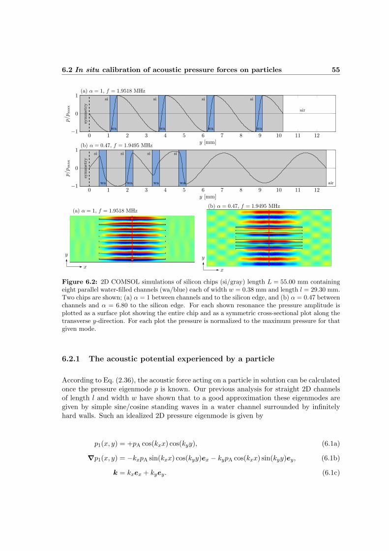
6.2 In situ calibration of acoustic pressure forces on particles 55

(a) α = 1, f = 1.9518 MHz

0 1 2 3 4 5 6 7 8 9 10 11 12−1

0

1

sym

met

ry

si

wa

si

wa

si

wa

si

wa

air

y [mm]

p/p

max

6

y

- x

(b) α = 0.47, f = 1.9495 MHz

0 1 2 3 4 5 6 7 8 9 10 11 12−1

0

1

sym

met

ry

si

wa

si

wa

si

wa

si

wa air

y [mm]

p/p

max

6

y

- x

(a) α = 1, f = 1.9518 MHz(b) α = 0.47, f = 1.9495 MHz

Figure 6.2: 2D COMSOL simulations of silicon chips (si/gray) length L = 55.00 mm containingeight parallel water-filled channels (wa/blue) each of width w = 0.38 mm and length l = 29.30 mm.Two chips are shown; (a) = 1 between channels and to the silicon edge, and (b) = 0.47 betweenchannels and = 6.80 to the silicon edge. For each shown resonance the pressure amplitude isplotted as a surface plot showing the entire chip and as a symmetric cross-sectional plot along thetransverse y-direction. For each plot the pressure is normalized to the maximum pressure for thatgiven mode.

6.2.1 The acoustic potential experienced by a particle

According to Eq. (2.36), the acoustic force acting on a particle in solution can be calculatedonce the pressure eigenmode p is known. Our previous analysis for straight 2D channelsof length l and width w have shown that to a good approximation these eigenmodes aregiven by simple sine/cosine standing waves in a water channel surrounded by infinitelyhard walls. Such an idealized 2D pressure eigenmode is given by

p1(x, y) = +pA cos(kxx) cos(kyy), (6.1a)

∇p1(x, y) = −kxpA sin(kxx) cos(kyy)ex − kypA cos(kxx) sin(kyy)ey, (6.1b)

k = kxex + kyey. (6.1c)


(a)

0 0.2 0.4 0.6 0.8 1.00.0

0.5

1.0y/w

x/l

(b)

0 0.2 0.4 0.6 0.8 1.00.0

0.5

1.0y/w

x/l

Figure 6.3: (a) Contour plot with 10% contour lines from low (dark) to high (light) of thenormalized acoustic potential Uac/U0 from Eq. (6.3a) for a polystyrene sphere in water given theideal 1D pressure field p1 of Eq. (6.1a) with (kx, ky) = (0, /w) so that = 90∘. (b) Similar plotfor the 2D pressure field with (kx, ky) = (/(2w), /w) so that ≈ 63∘. The parameter valuesused are given in Table 2.1.

This standing wave can be interpreted as the result of two counter-propagating wavesalong the direction k, which forms the angle with the x-axis,

cos =kxk, sin =

kyk, k =

√k2x + k2

y. (6.2)

Inserting this in Gorkov’s expression Eq. (2.36), we find the acoustic potential Uac and itsamplitude U0

Uac = U0

[2f1 cos2(kxx) cos2(kyy)− 3f2 sin2(kxx) cos2(kyy) cos2

− 3f2 cos2(kxx) sin2(kyy) sin2 ], (6.3a)

U0 =p2

AV

8wac2wa

. (6.3b)

Two numerical examples of the acoustic potential Uac for a polystyrene sphere areshown in Fig. 6.3.

6.2.2 Chip design for in situ calibration of the acoustic pressure force

The acoustic pressure force on a suspended particle can be measured in situ if it is anti-parallel to the Stokes drag force from the flow of the carrier liquid along the axial x-direction. By gradually increasing the flow velocity v from zero, a critical value v∗ can bedetermined, where the acoustic pressure force no longer traps the particle. At this point∣Fac∣ ≈ 6av∗, and the unknown pre-factor U0 can be determined. The calibration setuprequires that k and ex are parallel, thus kx ∕= 0 while ky = 0. By combining Eq. (2.35b)and Eq. (6.3) with this form of the wave vector, we obtain the acoustic potential and theassociated pressure force for calibration purposes on the form

U calibac = U0

[2f1 cos2(kxx)− 3f2 sin2(kxx)

], (6.4a)

F calibac = 2kxU0

[5− 2

2+ 1− 1

c2

]sin(2kxx) ex. (6.4b)

6.2 In situ calibration of acoustic pressure forces on particles 57

(a)

0 0.2 0.4 0.6 0.8 1.00.0

0.5

1.0y/w

x/l

(b)−3

−1

01

3−

1 0 1

α = 3

Figure 6.4: (a) Contour plot with 10% contour lines from low (dark) to high (light) of thenormalized acoustic potential U calib

ac /U0 from Eq. (6.4a) for a polystyrene sphere in water giventhe pressure field p1 = pA cos(x/2w). The parameter values are given in Table 2.1, and moreoverkx = /(2w) while ky = 0 so that = 0. (b) Color plot of the pressure eigenmode in the triple-channel = 3 chip. A transverse potential, as in panel (a), suitable for in situ acoustic forcecalibration is set up in the two side channels, while the center channel supports a transverse modeof odd symmetry as in Fig. 5.7 (D+). The left insert shows the single-channel = 3 chip. Notethe two anti-nodes in the silicon chip (gray) above and below the water-filled channel (blue).

The potential U calibac is shown in Fig. 6.4 (a). The condition for trapping becomes Fdrag =

max∣F calibac ∣ or

6av∗ = 2kxU0

[5− 2

2+ 1− 1

c2

]. (6.5)

If v∗ is measured experimentally, we are therefore able to determine the acoustic energyscale U0 by

U0 = 3av∗

kx

[5− 2

2+ 1− 1

c2

]−1

. (6.6)

We propose a specific chip design which supports a pressure eigenmode close to theone depicted in Fig. 6.4 (a). The idea is to fabricate an = 3 chip. In such a chip astrong pressure eigenmode of odd symmetry exists in the channel as the = 1 chip inFig. 5.7 (a) but it will also have a strong anti-node in the silicon as the = 2 chip inFig. 5.7 (b). Now, if two auxiliary side channels parallel to the first channel is placed atthese anti-nodes, the pressure mode inside these side channels is very close to the wantedmode of Fig. 6.4 (a). The correctness of this line of reasoning is proved by numericalsimulation of the eigenmodes in such a triple-channel = 3 chip as shown in Fig. 6.4 (b).

Chapter 7

Waveguide analysis

In this chapter we investigate the conditions for which a straight water-filled channel ofuniform cross-section will act as a waveguide within its surrounding silicon/pyrex chip,such that the acoustic pressure confines in the channel, while it decays exponentially intothe surrounding silicon chip and restrain from living outside the water-filled channel.

We first carry out analytical estimates for the geometric requirements, whereafter wenumerically examine the predictions by 2D and 3D Comsol models.

7.1 2D acoustic waveguide

7.1.1 Estimation of waveguide conditions

We consider the case where the length L of the silicon/pyrex chip equals the length l ofthe water-filled channel. This makes the system translational invariant along the axial x-direction as discussed in Sec. 5.3.3. We search solutions for the pressure p(x, y) = p(x)p(y)to the Helmholtz equation Eq. (2.17). We describe the x-component of the solution by thestanding resonance wave p(x) ∝ cos (kxx) with nx = 2L/x. This reduces the problem to1D along the transverse y-direction as sketched in Fig. 5.1 and described as

[− k2

x + ∂2y

]pi(y) = −!

2

c2i

pi(y), (7.1)

for the i’th domain material. We notice that pi(y) may be a hyperbolic function, else onlysine/cosine solutions are valid as described in 1D calculations in Sec. 5.1.

Using the proper symmetry boundary condition Eq. (2.47) at y = −a and the softboundary condition Eq. (2.46) at y = b, while demanding that the pressure must fall offexponentially in the chip outside the channel, results in

pwa(x, y) = Awa cos [kwa(y + a)] cos (kxx) (even), (7.2a)

pwa(x, y) = Awa sin [kwa(y + a)] cos (kxx) (odd), (7.2b)

psi(x, y) = Asi sinh [ksi(y − b)] cos (kxx). (7.2c)

59

60 Waveguide analysis

where Awa and Asi are pressure amplitudes. Inserting Eqs. (7.2) in Eq. (7.1) gives theequations for the wave vectors kwa and ksi

−k2x − k2

wa = − !2

c2wa

, (7.3a)

−k2x + k2

si = −!2

c2si

. (7.3b)

Notice that Eq. (7.3b) cannot be fulfilled for kx ≤ ksi if ! ∕= 0. Employing the interfaceconditions Eq. (2.41) at y = 0, results in transcendental equations for even and oddpressure eigenmodes

cot (kwaa)

kwaa=

si

wa

b

a

tanh (ksib)

ksib(even), (7.4a)

tan (kwaa)

kwaa= − si

wa

b

a

tanh (ksib)

ksib(odd), (7.4b)

which together with Eqs. (7.3) describe the full problem for even and odd pressure eigen-modes that decay exponentially into the silicon.

Critical limit

We consider the critical limit where the wave in silicon starts decaying exponentially. Wedefine this critical limit where the curvature of the pressure field in the silicon disappears∂2ypsi(x, y) = 0 and thus decays linearly

psi(x, y) = Asiksi(y − b) cos (kxx). (7.5)

At the critical limit the wave stops propagating in the silicon giving the wave vectorksi → 0. As tanh (ksib)/ksib→ 1 for ksi → 0, Eqs. (7.4) become

cot (kwaa)

kwaa=

si

wa(even), (7.6a)

tan (kwaa)

kwaa= − si

wa(odd), (7.6b)

which have solutions for kwaa ≈ (even) and kwaa ≈ /2 (odd), respectively. Togetherwith Eqs. (7.3) we get the waveguide conditions

L ≤ w

2

csi

cwanx (even), (7.7a)

L ≤ w csi

cwanx (odd), (7.7b)

where nx is the number of axial half-wavelengths. We see that the constraint on obtainingwaveguide modes is determined by the correct relation between between nx and L.

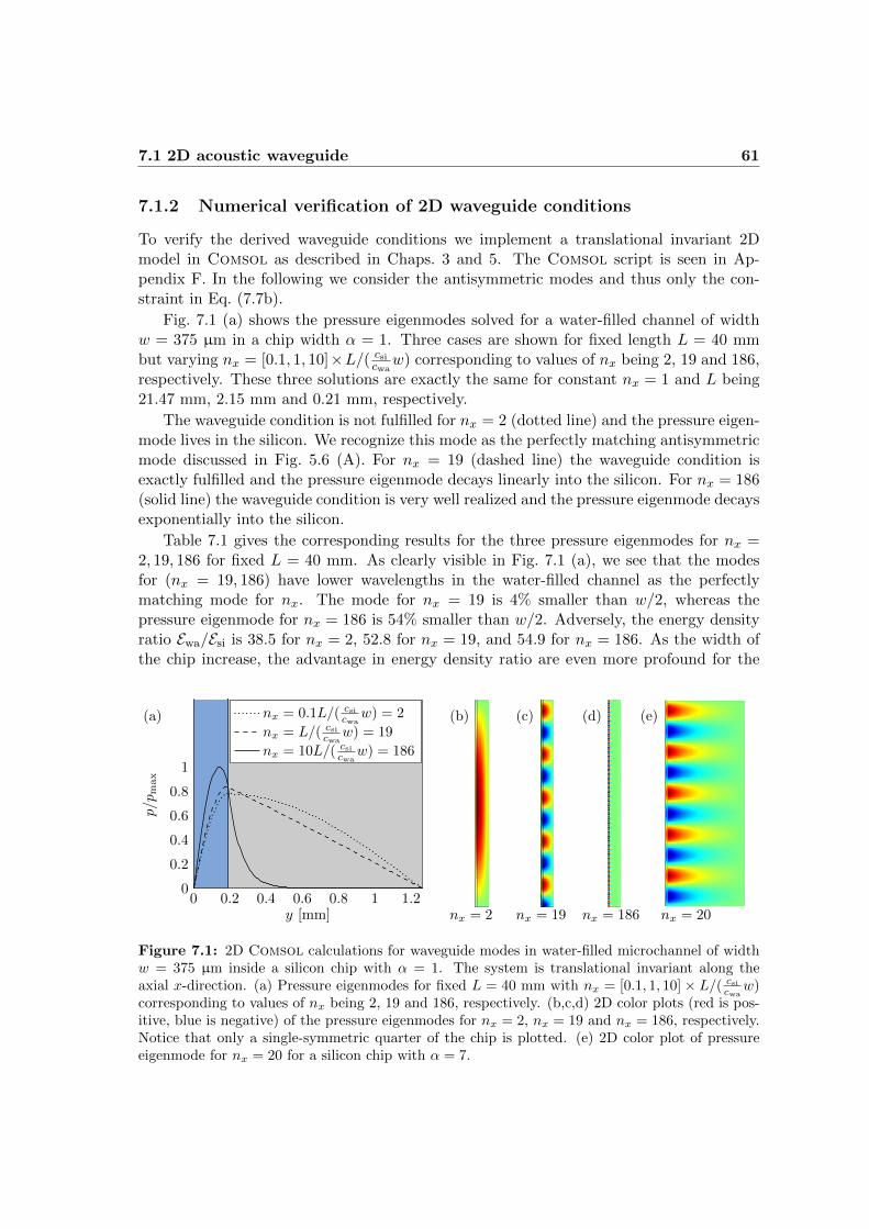
7.1 2D acoustic waveguide 61

7.1.2 Numerical verification of 2D waveguide conditions

To verify the derived waveguide conditions we implement a translational invariant 2Dmodel in Comsol as described in Chaps. 3 and 5. The Comsol script is seen in Ap-pendix F. In the following we consider the antisymmetric modes and thus only the con-straint in Eq. (7.7b).

Fig. 7.1 (a) shows the pressure eigenmodes solved for a water-filled channel of widthw = 375 µm in a chip width = 1. Three cases are shown for fixed length L = 40 mmbut varying nx = [0.1, 1, 10]×L/( csicwa

w) corresponding to values of nx being 2, 19 and 186,respectively. These three solutions are exactly the same for constant nx = 1 and L being21.47 mm, 2.15 mm and 0.21 mm, respectively.

The waveguide condition is not fulfilled for nx = 2 (dotted line) and the pressure eigen-mode lives in the silicon. We recognize this mode as the perfectly matching antisymmetricmode discussed in Fig. 5.6 (A). For nx = 19 (dashed line) the waveguide condition isexactly fulfilled and the pressure eigenmode decays linearly into the silicon. For nx = 186(solid line) the waveguide condition is very well realized and the pressure eigenmode decaysexponentially into the silicon.

Table 7.1 gives the corresponding results for the three pressure eigenmodes for nx =2, 19, 186 for fixed L = 40 mm. As clearly visible in Fig. 7.1 (a), we see that the modesfor (nx = 19, 186) have lower wavelengths in the water-filled channel as the perfectlymatching mode for nx. The mode for nx = 19 is 4% smaller than w/2, whereas thepressure eigenmode for nx = 186 is 54% smaller than w/2. Adversely, the energy densityratio ℰwa/ℰsi is 38.5 for nx = 2, 52.8 for nx = 19, and 54.9 for nx = 186. As the width ofthe chip increase, the advantage in energy density ratio are even more profound for the

0 0.2 0.4 0.6 0.8 1 1.20

0.2

0.4

0.6

0.8

1

y [mm]

p/p

max

nx = 0.1L/( csicwa

w) = 2

nx = L/( csicwa

w) = 19

nx = 10L/( csicwa

w) = 186

(a) (b) (c) (d) (e)

nx = 2 nx = 19 nx = 186 nx = 20

Figure 7.1: 2D Comsol calculations for waveguide modes in water-filled microchannel of widthw = 375 µm inside a silicon chip with = 1. The system is translational invariant along theaxial x-direction. (a) Pressure eigenmodes for fixed L = 40 mm with nx = [0.1, 1, 10]× L/( csicwa

w)corresponding to values of nx being 2, 19 and 186, respectively. (b,c,d) 2D color plots (red is pos-itive, blue is negative) of the pressure eigenmodes for nx = 2, nx = 19 and nx = 186, respectively.Notice that only a single-symmetric quarter of the chip is plotted. (e) 2D color plot of pressureeigenmode for nx = 20 for a silicon chip with = 7.


Table 7.1: Results of 2D Comsol simulations of antisymmetric waveguide modes for a water-filled channel of width w = 375 µm in a silicon chip having = 1. Presented are results for threemode types; a non-guiding mode, a mode exactly at the guiding limit and a mode strongly guidingthe acoustic energy. is the relative deviation in half-wavelength from w/2 and ℰwa/ℰsi is theenergy density ratio between the average acoustic energy density in the water-filled channel to theaverage acoustic energy density in the silicon chip.

Mode type L [mm] nx L [mm] nx f [MHz] [%] ℰwa/ℰsi

No guide L > w csicwanx 40.0 2 21.47 1 1.9783 -0.1 38.5

Limit L = w csicwanx 40.0 19 2.15 1 2.0606 -4.0 52.8

Guide L < w csicwanx 40.0 186 0.21 1 4.3307 -54.3 54.9

wave guiding modes as no acoustic energy exists in the silicon. Note that the consideredenergy density ratio ℰwa/ℰsi is the ratio between the spatially averaged energy densitiesas the maximum energy density in silicon Emax

si is no longer a proper measure due to thedecaying modes in the silicon.

In Figs. 7.1 (b,c,d) are shown the three discussed pressure eigenmodes as color plots(red is positive, blue is negative) for the chip having = 1. Notice that only a single-symmetric quarter of the chip is plotted. Fig. 7.1 (e) shows the pressure eigenmode fornx = 20 for a chip having = 7. From this it is clear that the pressure eigenmode confinescompletely into the water-filled channel.

As a last remark, it is clear that waveguide modes may be of high importance, sincethey confine the energy into the water no matter the width of the surrounding silicon.

7.2 3D acoustic waveguide

We turn to the case of creating a three-dimensional waveguide in the water-filled channelsurrounded by the silicon/pyrex chip. In a translational invariant chip as discussed inSec. 5.3 and described in Fig. 5.8, the problem reduces to a two-dimensional problemof three different domains. As we cannot solve the problem analytically, we rely on theformer 1D estimate for the 2D waveguide condition and the use of Comsol.

We modify the 2D waveguide condition to give a rough estimate for the 3D waveguidecondition. The modification consists of simply substituting the speed of sound for siliconcsi to an approximated weighted average speed of sound cH = (csiℎsi + cpyℎpy)/H of thesilicon/glass chip with its total height H = ℎsi + ℎpy

L ≤ w

2

cH

cwanx (even), (7.8a)

L ≤ w cH

cwanx (odd). (7.8b)

Using the chip parameters as given in Fig. 5.8 and Table 2.1, we get the average speed ofsound cH ≈ 6300 m s−1 for the silicon/glass chip. If we consider a chip of length L = 40 mm

7.2 3D acoustic waveguide 63

0 1 2 3

0

0.5

1

y [mm]

z[m

m]

(a) nx = 1, f = 1.4506 MHz

0 1 2 3

0

0.5

1

y [mm]

z[m

m]

(b) nx = 25, f = 2.4246 MHz

0 1 2 3

0

0.5

1

y [mm]

z[m

m]

(c) nx = 30, f = 2.7033 MHz

0 1 2 3

0

0.5

1

y [mm]z[m

m]

(d) nx = 35, f = 2.8396 MHz

0 1 2 3

0

0.5

1

y [mm]

z[m

m]

(e) nx = 40, f = 2.9096 MHz

0 1 2 3

0

0.5

1

y [mm]

z[m

m]

(f) nx = 80, f = 3.3954 MHz

Figure 7.2: 3D Comsol simulations of water-filled channel acting as an acoustic waveguide withina surrounding silicon/glass chip as sketched in Fig. 5.8. The chip has = 3 and is translationalinvariant along the axial x-direction with identical channel and chip lengths of L = l = 40 mm.The color plots (red is positive, green is neutral) show the lowest transverse antisymmetric pressureeigenmodes plotted for one symmetric half along the transverse y-direction. The chip length Lis constant, while nx is varied from (a) nx = 1 to (f) nx = 80. As nx increases, the pressureeigenmode moves from mainly living in the silicon/glass chip to be almost completely confinedinside the water-filled channel. For the fixed length of L = 40 mm, the main transition betweentwo mode types occurs for nx between 30 and 35.

we get the approximate requirement on the number nx for antisymmetric modes

nx ⪆1

w

cwa

cHL ≈ 25 (odd). (7.9)

We test the estimate of the 3D waveguide condition by Comsol calculations shownin Fig. 7.2. The model chip has = 3 and is translational invariant along the axial x-direction with identical chip and channel lengths of L = l = 40 mm. The color plots (a–f)show the lowest transverse antisymmetric pressure eigenmodes plotted for one symmetrichalf along the transverse y-direction. The chip length L is kept constant, while the numbernx is varied from panel (a) nx = 1 to panel (f) nx = 80. As nx increases, the pressureeigenmode moves from mainly living in the silicon/glass chip to be almost completelyconfined inside the water-filled channel. For the fixed length of L = 40 mm, the main


transition between two mode types occurs for nx between 30 and 35. The estimate inEq. (7.9) deviates 15–20% from the waveguide condition on nx obtained by the numericalComsol calculations. This is not bad if we recall that the estimate is based on a 1Dmodel.


We have carried out basic studies of the conditions for the water-filled channel to act as anacoustic waveguide within a surrounding silicon/glass chip. The conditions state a rela-tionship between the channel/chip length L and the number nx of axial half-wavelengthsnodes in the pressure mode. The utilization of the water-filled channel as an acousticwaveguide seems to be promising as more acoustic energy can be obtained and more inter-esting, it opens the possibility for the creation of channel structures of higher geometriccomplexity as known from e.g. waveguides in optics. More analysis therefore has to bedone within this field.

Chapter 8

Experimental investigations

In the current chapter we describe a series of experiments carried out by the authorduring eight days in April and May in Professor Laurell’s laboratory at the Departmentof Electrical Measurements, Lund University. The experiments were set up and executedin close collaboration with PhD-student Per Augustsson.

The purpose of the experiments was to test theoretical predictions of resonance modes,the acoustic focusing force and the acoustic energy density. In the following we (i) describethe involved chips and the experimental setup, (ii) investigate the electrical impedanceof the piezo transducer for different mechanical loads, (iii) describe sedimentation ex-periments of spherical polystyrene microbeads to calibrate the experimental parametersand (iv) finally determine the acoustic energy density and the corresponding transverseseparation mode by simple stop-flow ultrasonic experiments.

8.1 Experimental setup

A microfluidic silicon/glass chip is acoustically actuated by a piezo transducer. The chipsare fabricated by standard photolithography technique by Per Augustsson in the groupof Laurell. The chips are shown in Fig. 8.1. Panel (a) shows a photograph of the foursilicon/glass chips and panel (b) shows the corresponding sketch with marked dimensionalparameters found in Table 8.1. The four chips are of the -type treated in Chap. 5. Each-chip consists of a glass-bonded silicon chip etched with a single straight rectangularchannel. The four -chips only differ by their widths. The microchannel is entered throughinlet and outlet holes on top of the chip through the glass lid. At each hole a silicone tubehas been attached using silicone glue.

Photographs of the experimental setup are seen in Fig. 8.2. In panel (a) is shown afull view of the setup including pump, syringe, chips, holder and microscope. Panel (b)shows how the chip is mounted on the piezo transducer and fixed in a PMMA holder, suchthat the chip is only in contact with the holder through its inlet/outlet silicone tubingand the piezo transducer. The chip is acoustically coupled to the transducer by a thinintermediate layer of glycerol.

The piezo transducer is made of hard PZT and is of the type Pz26 from Ferrop-

65

66 Experimental investigations

Table 8.1: Geometric parameters of fabricated -chips and the piezo transducer.

Width, channel w 0.377 mm Length, channel l 40.0 mmWidth, chip: W = w

(1 + csi

cwa)

Length, chip L 50.0 mm

= 1 W=1 2.5 mm Length, piezo LPZT 50.0 mm = 2 W=2 4.7 mm Height, channel ℎwa 0.157 mm = 3 W=3 6.8 mm Height, si-chip ℎsi 0.350 mm = 4 W=4 9.0 mm Height, glass-lid ℎpy 1.13 mm

Width, piezo WPZT 12.0 mm Height, piezo ℎPZT 1.0 mmRadius, lid holes R=1,2 0.5 mm Radius, lid holes R=3,4 1 mm

erm Piezoceramics A/S. The piezo transducer is actuated by applying a harmonicallyoscillating voltage drop generated from a tone generator Hewlett Packard 33120A. Thevoltage is amplified by a T&C Power Conversion Inc AG Series Amplifier, while the ap-plied peak-to-peak voltage across the piezo transducer is measured by a Tektronix TDS1002 oscilloscope. The channel is observed by an Olympus BX51WI microscope with anattached CCD camera of the type Infinity 1 from MediaCybernetics.

To carry out the ultrasonic experiments a liquid sample is led through the channelof the chip. The sample liquid is distilled water mixed with 0.01 % Tween20, whichis a polysorbate surfactant reducing the adhesion of microbeads to the channel walls.As shown by the sedimentation experiments described in Sec. 8.3 below, the influenceof the added Tween20 on the density and viscosity is negligible. In the sample liquidare 5 µm polystyrene microbeads from Sigma-Aldrich. The calibrated diameter of thepolystyrene microbeads is (5.16 µm±0.08 µm). We use bead concentrations between 0.01and 0.05 g/mL. The sample liquid is held in a 1 mL plastic syringe, where a small magnetis added. By stirring with an external magnet we avoid sedimentation of the microbeads

(a) (b)

α = 1α = 2α = 3

α = 4

xy-view

yz-view

3D view

WwL

l

hpy

hsi

W

whwa

Figure 8.1: Microfluidic silicon/glass chips of the -type fabricated by Per Augustsson in thegroup of Laurell. (a) Photograph of the four -chips. (b) Sketch of the four -chips with indicateddimensional parameters presented in Table 8.1. The four -chips consist of a glass-bonded siliconchip etched with a straight single channel.

8.2 Investigation of the piezo transducer 67

(a) (b)

microscope

camera

chip + holder

pump+syringe

chip+piezo

microscope

PMMA holder

inlet

outlet

Figure 8.2: (a) Full view of the experimental setup showing a silicon/glass chip in a PMMAholder investigated by microscope with attached CCD camera. A microflow is pumped into thechip by a syringe pump. (b) Close up of the microfluidic silicon/glass chip and PMMA holderilluminated by external light sources. The microfluidic inlet and outlet are shown.

in the syringe, which reduces the chance of getting an inhomogenous distribution of mi-crobeads in the liquid channel. A syringe pump of the type WPI SP210IWZ is used topump the sample liquid into the microfluidic chip through plastic tubes.

8.2 Investigation of the piezo transducer

The piezo transducer, 50 mm× 12 mm× 1 mm, has its ideal acoustic resonance frequencyat fpiezo = 2.075 MHz obtained by the Ferroperm online piezo electric calculator [53].The displacement amplitude and the energy delivered from the piezo transducer dependon its applied frequency. This fact complicates the experiments as the frequency cannotjust be tuned arbitrarily away from fpiezo without a significant decrease in the acousticenergy density. The energy loss may be compensated by amplifying the applied voltage,but this induces other complications such as additional heating of the system. Ideally weare interested in knowing the exact behavior of the piezo transducer, as it will enable usto compare energy/frequency spectra for various chips. Such a thorough investigation isoutside the scope of this thesis and in the following we present an investigation limited tothe electrical impedances of the piezo transducer at different acoustic loads.

Fig. 8.3 presents the measured frequency spectra of the electrical impedance Zel andphase el of the piezo transducer as the piezo transducer is subject to different acousticloads. The spectra are shown in six cases added up chronologically as; (i) the piezotransducer hangs freely, (ii) the piezo transducer rests on the holder, (iii) glycerol is addedon top of the piezo transducer, (iv) the chip is added on the piezo with an intermediatelayer of glycerol, (v) the PMMA-lid is pressing down the chip through the silicone tubingsor (vi) the PMMA-lid pressing down the chip in direct contact. The chip has = 3 anda water-filled channel.

The frequency spectra clearly illustrate that the piezo transducer has a large number ofresonance frequencies, which is seen via the many local minima in electric impedance Zel


1.9 1.94 1.98 2.02 2.06 2.10

10

20

30

40

f [MHz]

Zel

[Ω]

(i) freely hanging piezo(ii) piezo + holder(iii) piezo + holder + glycerol(iv) piezo + holder + glycerol + chip(v) piezo + holder + glycerol + chip + lid without contact(vi) piezo + holder + glycerol + chip + lid with full contact

1.9 1.94 1.98 2.02 2.06 2.1

−75

−25

0

25

75

f [MHz]

φel[d

egre

es]

(a)

(b)

Figure 8.3: Frequency spectrum of the (a) electric impedance Zel and (b) electric phase el forthe piezo transducer, while the piezo transducer is mechanically loaded in various combinations.Six cases of loads are shown.

accompanied by shifts in the electric phase el. In addition we notice that the location andbehavior of the resonances are very sensitive to the given load. Only similar cases are case(i) the piezo transducer hanging freely and case (ii) the piezo transducer resting on theholder. This justifies a disregarding of the acoustic influence from the holder. Additional,it is observed that the increase in load decreases the amount of local resonances resultingin more smooth spectra.

To sum up, the impedance measurements illuminate that the resonances of the piezotransducer are highly sensitive to different loads. This makes the acoustic behavior ofthe resonance systems hard to predict without being able to predict the behavior of theactuating piezo transducer itself. An opportunity for higher piezo stability is to switchthe type of the piezo transducer from a Pz26 to a Pz27 as the Pz27 model has a much

8.3 Sedimentation of microbeads 69

lower Q-value [54].

8.3 Sedimentation of microbeads

To calibrate the liquid sample containing the microbeads, a series of sedimentation exper-iments were carried out.

Theoretical sedimentation times

The sedimentation time t for a microbead of radius a is theoretically approximated byassuming a non-accelerating flow. The resulting Newtons second law for the bead inthe vertical z-direction includes the viscous Stokes drag Fdrag = 6avz and the specificgravitational force Fg = −4

3a3g(p − wa) [5]. We get

t =9

2

a2g(p − wa)ℎwa, (8.1)

where ℎwa is the sedimentation depth, is the liquid viscosity, g is the gravitationalacceleration and p and wa is the density of the particle and liquid, respectively. Forpolystyrene microbeads in water we have a = 5.16/2 µm and material parameters as givenin Table 2.1. We get a sedimentation time

t ≈ 208 s. (8.2)

A phenomenon that might play a role during the sedimentation experiments is diffu-sion. Utilizing the Einstein relation for the diffusion constant D [5] at room temperatureyields

D =kBT

6a≈ 8.5× 10−14 m2 s−1, (8.3)

which used to estimate the diffusion length ldiff during a sedimentation time of t ≈ 200gives

ldiff =√D t ≈ 4 µm. (8.4)

The approximated diffusion length ldiff is small in comparison to the channel height ℎwa

and for this reason we neglect diffusion in the sedimentation experiments as well as in thelatter experiments.

Table 8.2: Experimental sedimentation times for (5.16 µm ± 0.08 µm) polystyrene microbeads.Listed are the average sedimentation time t, the uncertainty Δt and the number of measurementsN .

Liquid sample t±Δt [s] N

Distilled water 182± 5 4Distilled water (0.01 % Tween20) 179± 6 3


Experimentally measured sedimentation times

The liquid sample was pumped through the channel while the microbeads were focusedto the channel center by acoustically actuating the chip. Due to the presence of a verticalacoustic pressure gradient as discussed in Chap. 5, the microbeads were vertically pushedtowards the channel lid. The flow was stopped and some microbeads were trapped atthe channel lid, while the remaining microbeads sedimented to the channel bottom. Theultrasound were turned off, and the sedimentation times were determine by following thebeads in the microscope focus until they reached the bottom of the channel.

The sedimentation times t and the uncertainty Δt are presented in Table 8.2 as aresult of a number of measurements N . The experiments deviate 13− 14 % from the the-oretical prediction in Eq. (8.2). The small deviations may be found due to the theoreticalapproximation of constant flow velocity. Other uncertainties may be the channel heightℎwa, sizes of the microbeads and other parameters such as the viscosity and densities. Themeasurements show fair accuracy in applying the Stokes drag in this confined system.

Additionally, the sedimentation times were measured for the sample liquid being eitherpure distilled water or distilled water with 0.01 % Tween20. The sedimentation times forthe microbeads in the two mixtures did not differ significant and hence we conclude thatthe addition of 0.01 % Tween20 does not influence the water parameters such as densityand viscosity.

8.4 Measuring the acoustic energy density

The acoustic energy density is crucial to determine as theoretical and experimental com-parison of acoustic energy densities are needed in order to understand and hence optimizethe experimental configurations. Possible optimization parameters can be the acousticimpedances of the surroundings to the chip. Also the chip design itself can be optimizedto support local resonances with high relative acoustic energy densities, which is e.g. impor-tant in focus/separation experiments, where the acoustic energy density in the liquid-filledchannels is directly proportional to the pressure force Eq. (2.38). However, the acousticenergy density is rarely determined in applications in the acoustofluidic literature. Theobjective of the current section is thus to determine the acoustic energy density and toexamine its physical dependencies. Prior to the investigation two main expectations areset up.

Firstly, from Eq. (2.31) we expect the acoustic energy density to be proportional tothe square of the applied pressure. If the voltage across the piezo transducer is directlyproportional to the pressure delivered, we expect the acoustic energy density to be directlyproportional to the square of the voltage applied to the piezo transducer. Secondly, fromEq. (4.13) we expect the acoustic energy density near a resonance to behave as a Lorentzianshape-line as function of the applied frequency.

The acoustic energy density is measured by observing the transient acoustophoreticfocusing of the microbeads. First, the driving frequency is tuned to an acoustic resonancethat strongly focuses the polystyrene microbeads to the center of the channel. The ul-trasound field is turned off and a fresh solution of the liquid sample is pressed into the

8.4 Measuring the acoustic energy density 71

channel. Then the ultrasound field is turned back on, and the transient focusing of themicrobeads to the channel center is recorded by a CCD camera. From the frames of theresulting movie we can then determine the transverse paths y(t) of the microbeads.

8.4.1 Theoretical transverse bead trajectory

The path of a microbead moving under acoustophoresis is given by the position vector(x(t), y(t)

). For more elaboration on acoustophoretic bead trajectories, see [43]. We set

up a simple analytical expression for the transverse part y(t) in the limit of a long axialwavelength kx ≈ 0. By neglecting inertial effects at the low microbead speeds, we balancethe acoustophoretic force Fac in Eq. (2.38) with the Stokes drag force Fdrag = 6ady

dt [5].This results in a first-order non-linear differential equation for the transverse path y = y(t)

dy

dt= y sin(2kyy), (8.5)

where

y =2kya

2Eac

9

[5− 2

5+ 1− 1

c2

]. (8.6)

Separating the variables y and t, and using the fact that d tan(s/2)ds = 1

sin(s) leads to the

expression for the time t it takes a particle starting at y(t0) = y0 to reach within amicrobead radius a of the position y(t)

t = t0 −1

2ky ylog

(tan

[kyy0

]tan

[kyy(t)

]), (8.7)

which is derived assuming y0 and y(t) to have same sign. Additional rewriting gives themicrobead position y(t)

y(t) =1

kyarctan

[eky y(t−t0) tan(kyy0)

], (8.8)

which will be used later to fit the acoustic energy density Eac and wavelength y = 2/kyto the experimental (t, y)-data of the particle trajectories.

8.4.2 Analysis of data

The transverse path y(t) is extracted from the video recordings by employing the free videoanalysis tool Tracker 2.6 [55]. This software enables tracking a polystyrene microbead bysimple manual mouse-clicking on the microbead position y for each movie frame for whichthe time t is known. First, the initial and end frames are chosen. Next a reference frameis chosen and the width of the channel is used to set a reference length scale. Due tothe manual selection of microbeads, reference frame and length scale, the approach isconnected with high uncertainties. Also the probable existence of axial modes leads toinhomogeneities in strength of the acoustic focusing force along the x-direction. With


0 1 2 3 4 50

40

80

120

160

Set values:f = 1.9940 MHzUpp = 1.52 V

Fitted parameters:

E(i)ac = 6.69 J/m3

λ(i)/2 = 375.4 µm

t [s]

y[µ

m]

ExperimentalTheoretical

(a) (b) (c)

6

x

- y

Figure 8.4: Example of extracting the acoustic energy density E(i)ac and the acoustic half-

wavelength (i)/2 from tracking the i’th single microbead at driving frequency f = 1.9940 MHzand driving voltage Upp = 1.52 V. The experimental data is a movie with a series of framesanalyzed by the free video analysis tool Tracker 2.6 [55]. (a) First image frame before applyingultrasound to focus the microbeads (colored circles) horizontally to the center of the channel. Areference frame (red) and a reference length scale (blue) are chosen. (b) Last image frame showingthe paths of the focused microbeads. Notice the overall flow of the microbeads in the negativex-direction. This is assumed to be due to drifting in the flow caused by trapped bubbles etc. Theseflows are neglected as we only consider the transverse focusing. (c) Transverse trajectory curve y(t)(blue points) resulting from tracking the i’th microbead and the fitted path (black line) based on

Eq. (8.8) with the two fitting parameters: the acoustic energy density E(i)ac and the half-wavelength

(i)/2 of the transverse standing pressure wave.

these uncertainties in mind, at least five microbead tracks have been determined for eachgiven movie to result in better statistics.

An example of tracking a bead trajectory is seen in Fig. 8.4 for a driving frequency off = 1.9940 MHz and a driving voltage of Upp = 1.52 V. Panel (a) shows starting position,panel (b) shows the microbead trajectories and panel (c) shows the resulting path fittedby the theoretical expression for y(t) Eq. (8.8). The theoretical fitting path y(t) for the

i’th particle track from Eq. (8.8) is obtained by fitting the acoustic energy density E(i)ac

and the half-wavelength (i)/2 = /k(i)y . The is done utilizing the MATLAB least-squares

routine lsqcurvefit(). In the given case we find E(i)ac = 6.69 J/m3. We also note that

the fitted value for (i)/2 = 0.375 mm is very close to the expected value of the channelwidth w = 0.377 mm.

Uncertainties

For each focus movie of N particle tracks the weighted average of the acoustic energydensity ⟨Eac⟩N and half-wavelength ⟨⟩N /2 are calculated from the fitted energy densities


E(i)ac and fitted half-wavelengths (i)/2 with respect to the number of tracking points n(i)

for the i’th particle path. The weighted average ⟨x⟩N for N particle paths is calculated as

⟨x⟩N =

∑Ni=1 x

(i) n(i)∑Ni=1 n

(i), (8.9)

for which the corresponding sample standard deviation sx is calculated as

sx =

√∑Ni=1(x(i) − ⟨x⟩N )2

N − 1. (8.10)

For each movie we extract ⟨Eac⟩N , ⟨⟩N /2, sE and s/2. In the latter when analyzing thewavelength from a number of movies M , we make use of the weighted mean given by

x = 2x

M∑j=1

⟨x⟩(j)N(

s(j)x

)2 , (8.11)

where the variance 2x of the weighted mean is given by

1

2x

=

M∑j=1

1(s

(j)x

)2 . (8.12)

Finally we adopt the notation Δx for the standard deviation of the weighted mean givenby Δx ≡

√2x. We therefore expect our measured x-values to be within x = x±Δx.

In the next subsections we fit theoretical curves to our data points. For each fit werun a goodness-of-fit test by the CHI2GOF()-function in Matlab and make sure that thenull-hypothesis is never rejected at 5% significance.

8.4.3 Acoustic energy density versus driving voltage

In the current section we determine the acoustic energy density Eac as a function of thedriving voltage Upp. In the experiments we tuned the piezo frequency to a resonanceyielding a strong transverse focusing force; in this case f = 1.9976 MHz. The valuesof ⟨Eac⟩N , ⟨⟩N /2, sE and s/2 are listed in Table 8.3. The extracted acoustic energy

densities⟨Eac

(U

(j)pp

)⟩N

are fitted to a power function of the form

Efitac(Upp) = a1U

a2pp , (8.13)

where the fitting parameters are a1 and a2.In Fig. 8.5 are seen Upp-sweeps for two chips; = 1 (a,b) and = 2 (c,d). For = 1

the fitting parameters have values of (a1, a2) = (12.13, 2.09), whereas for = 2 the fittingparameters have values of (a1, a2) = (3.64, 2.4). From the data points for = 1 it isevident that the exponent a2 ≈ 2 meaning that the acoustic energy density is proportionalto the square of the driving voltage. This result is clearly indicating that the delivered


pressure from the piezo transducer is directly proportional to its applied peak-to-peakvoltage.

For = 2 the exponent a2 ≈ 2.4 deviates a bit from the expected, which is assumedto be an outcome of the poor number of fitting points. Though, it is still clear thatthe acoustic energy density is approximately a factor of 3 lower for = 2 than for =1. This might be experimental evidence for the -analysis in Chap. 5, stating that forantisymmetric resonances at these frequencies, the acoustic energy density in the channelwill be stronger for = 1 than for = 2. Though, we keep in mind the experimental andtheoretical lack in information about the influence on the piezo transducer when changinge.g. chips and glycerol.

The vertical uncertainty bars show the standard deviations sE and s/2 defined inEq. (8.10), while the horizontal uncertainty bars show the estimated experimental un-certainty ΔUpp ≈ 0.04 V on Upp. Notice that the vertical uncertainty increases withincreasing Upp leading to lower frame-resolution as the beads move faster.

In Fig. 8.5 (b,c) are shown the measured half-wavelengths⟨(U

(j)pp

)⟩N/2. The experi-

mental half-wavelength is close to the expected width of the channel w = 0.377 mm andthe majority of the data points are within the interval of uncertainty = ±Δx.

Perturbation parameter and magnitude of first-order fields

From the quantitative measurements of the acoustic energy density, we can determine thefirst-order fields and the implicit perturbation parameter. We consider the Upp-sweep forthe chip with = 1, where we have that the acoustic energy density is Eac ≈ 50 J/m3 forUpp = 2 V. We use the 1D energy expression in Eq. (2.39) to estimate the magnitude pA

of the corresponding first-order pressure field in the water-filled channel

pA = 2√wac2

waEac ≈ 7× 105 Pa, (8.14)

Table 8.3: Extracted values of the acoustic energy density ⟨Eac⟩N and the half-wavelength ⟨⟩N/2

as function of driving voltage Upp across the piezo transducer at driving frequency f = 1.9976 MHz.sE and s/2 are the standard deviations of the acoustic energy density and the half-wavelength,respectively. The data is plotted in Fig. 8.5.

Upp [V] ⟨Eac⟩N [J/m3] sE [J/m3] ⟨⟩N /2 [µm] s/2 [µm]

0.44 0.65 0.06 383.45 17.820.60 4.00 0.67 387.97 20.520.80 7.30 0.67 373.96 7.620.80 8.17 1.33 375.10 20.151.00 15.24 2.61 380.97 5.391.04 12.23 3.60 380.86 12.001.28 22.61 3.27 397.14 21.301.32 17.81 3.01 378.76 10.291.60 32.16 6.00 382.57 9.291.88 45.30 6.00 377.07 17.06


0.4 0.6 0.8 1 1.2 1.4 1.6 1.8 20

10

20

30

40

50

= 1

Upp [V]

Eac[J/m

3]

Experiment

Efitac (Upp) = 12.16 U2.07

pp

0.4 0.6 0.8 1 1.2 1.4 1.6 1.8 2

360

370

380

390

400

410

420 = 1

Upp [V]

/2

[µm

]

⟨⟩N/2 w /2 (±Δ)/2

0.6 0.7 0.8 0.9 1 1.1 1.2 1.3 1.4 1.50

1

2

3

4

5

6

7

8

9

10

11

= 2

Upp [V]

Eac[J/m

3]

Experiment

Efitac (Upp) = 3.64 U2.41

pp

0.6 0.7 0.8 0.9 1 1.1 1.2 1.3 1.4 1.5360

370

380

390 = 2

Upp [V]

/2

[µm

]⟨⟩

N/2 w /2 (±Δ)/2

(a) (b)

(c) (d)

Figure 8.5: Experimentally measured acoustic energy density Eac and half-wavelength /2 versusdriving voltage Upp for the chip with = 1 (a,b) and for the chip with = 2 (c,d). The appliedpiezo frequency is f = 1.9976 MHz. The vertical uncertainty bars show the standard deviationssE and s/2 defined in Eq. (8.10), while the horizontal uncertainty bars show the experimental

uncertainty ΔUpp ≈ 0.04 V on Upp. (a,c) Plot of the experimentally measured⟨Eac

(U

(j)pp

)⟩N

(red

circles) with its corresponding uncertainties (thin black lines). The data are fitted well with thefitting function Efit

ac (Upp) (blue curve) Eq. (8.13). For = 1 the fitting parameters are (a1, a2) =(12.13, 2.09), whereas for = 2 the fitting parameters are (a1, a2) = (3.64, 2.4). The fit is poorfor = 2 due to the few experimental points, but it is still clear that the acoustic energy densityis approximately a factor of 3 lower for = 2 than for = 1. (b,d) Plot of the experimentally

measured⟨(U

(j)pp

)⟩N/2 (red circles) with its corresponding uncertainties (thin black lines). In

addition is plotted the weighted mean average (thick black line), the channel width w = 377 µm(thin blue line) and the uncertainty interval (±Δ)/2 (dashed lines). The plotted data is listedin Table 8.3.

for which the implicit perturbation parameter per = pA/p0 ≈ 3× 10−4 if we assume thatp0 ≈ 2.6 × 109 Pa as stated in Chap. 2. For the magnitude A of the first-order density


1.99 1.995 2 2.005 2.010

2

4

6

8

10

12

14

16

18 = 2

f1 = 2.0021 MHz

E1 = 14.8 J/m3

Q1 = 180

f1

f [MHz]

Eac

[J/m

3]

ExperimentOne-peak fit

1.99 1.995 2 2.005 2.010

2

4

6

8

10

12

14

16

18 = 2Upp corrected

f1 = 2.0019 MHz

E1 = 15.3 J/m3

Q1 = 188

f1

f [MHz]E

ac

[J/m

3]

ExperimentOne-peak fit

1.99 1.995 2 2.005 2.010

2

4

6

8

10

12

14

16

18 = 2Upp corrected

f2 = 1.9927 MHz

E2 = 3.3 J/m3

Q2 = 577

f1 = 2.0021 MHz

E1 = 15.5 J/m3

Q1 = 209

f1

f2

f [MHz]

Eac

[J/m

3]

ExperimentTwo-peak fit

1.99 1.995 2 2.005 2.01

350

360

370

380

390

400

410

420

f [MHz]

/2

[µm

]

⟨⟩N/2 w /2 (±Δ)/2

(a) (b)

(c) (d)

Figure 8.6: Experimentally extracted acoustic energy density Eac and half-wavelength versusapplied piezo frequency f . The chip has = 2. (a,b,c) Plot of the measured

⟨Eac

(f (j)

)⟩N

. The

uncertainty bars show the standard deviation sE defined in Eq. (8.10) (a,b) Fitting of the datapoints to the one-peak Lorentzian fit Efit1

ac (f) in Eq. (8.16). (b) The data points are corrected forvariations in Upp resulting in a slightly better fit. (c) The data points are fitted to the two-peakLorentzian fit Efit2

ac (f) in Eq. (8.17). We consequently consider the presence of two resonances inthe investigated frequency interval located at frequencies f1 = 1.992 MHz and f2 = 2.002 MHzwith Q-values Q1 ≈ 570 and Q2 ≈ 210. (d) Plot of the experimentally measured

⟨(f (j)

)⟩N/2

(red circles) with its corresponding standard deviation s (thin black lines). In addition is plottedthe weighted mean average (thick black line), the channel width w = 377 µm (thin blue line)and the uncertainty interval Δ (dashed lines). The plotted data is listed in Table 8.4.

we get

A =1

c2wa

pA ≈ 0.30 kg m−3, (8.15)

for which we get approximately the same value of the implicit perturbation parameterper. With this, we conclude that the perturbation approach is well fulfilled for thesespecific experiments as the perturbation parameter is less than a promille.


Table 8.4: Extracted values of the acoustic energy density ⟨Eac⟩N and the half-wavelength ⟨⟩N/2

as function of driving frequency f . sE and s/2 are the standard deviations of the acoustic energydensity and the half-wavelength, respectively. The data is plotted in Fig. 8.6.

f MHz Upp [V] ⟨Eac⟩N [J/m3] sE [J/m3] ⟨⟩N /2 [µm] s/2 [µm]

1.9900 1.40 3.11 0.33 386.21 27.281.9920 1.48 5.42 0.36 382.51 14.921.9940 1.52 6.73 1.20 365.08 19.151.9960 1.52 5.33 0.38 367.31 10.031.9976 1.44 8.92 1.70 389.77 9.141.9980 1.44 8.48 2.06 376.40 11.872.0000 1.44 12.53 1.33 367.09 18.192.0020 1.48 15.82 3.43 372.93 17.072.0030 1.48 13.85 1.96 385.93 17.872.0040 1.48 12.48 2.52 377.54 20.892.0050 1.48 13.10 1.70 364.07 11.272.0060 1.56 10.50 3.90 384.99 20.392.0070 1.52 7.96 1.57 380.08 11.982.0080 1.52 5.87 2.11 379.12 10.602.0100 1.60 4.07 1.59 372.55 18.62

8.4.4 Acoustic energy density versus driving frequency

In this section we resolve the acoustic energy density Eac as a function of the appliedfrequency f across the piezo transducer. The experiment is carried out using the chiphaving = 2. The driving frequency is varied between 1.9900 MHz and 2.0100 MHz,while the applied peak-to-peak voltage tentatively is kept constant, but varied between1.44 V and 1.60 V. We later use the dependency of Eac on Upp to correct all the measuredvalues of ⟨Eac⟩N to correspond to the same average driving voltage Upp = 1.48 V. Thevalues of ⟨Eac⟩N , ⟨⟩N /2, sE and s/2 are listed in Table 8.4.

The measured⟨Eac

(f (j)

)⟩N

are now fitted to a Lorentzian shape line as expected from

Eq. (4.13). In the following we utilize two fitting functions; (i) a one-peak Lorentzian fit

Efit1ac (f) =

E1[2Q1

f1(f − f1)

]2+ 1

, (8.16)

which is fitted by the three unknown variables E1, f1 andQ1 and (ii) a two-peak Lorentzianfit

Efit2ac (f) =

E1[2Q1

f1(f − f1)

]2+ 1

+E2[

2Q2

f2(f − f2)

]2+ 1

, (8.17)

where the additional three fitting variables E2, f2 and Q2 are introduced.In Fig. 8.6 are shown the results from the frequency sweep. (a) and (b) show fitting to

experimental data by the one-peak Lorentzian fit Efit1ac (f). The plot in (b) has been cor-

rected relatively for its variations in peak-to-peak voltage Upp, whereas the plot in (a) has


not. It is seen that the correction makes the fitting slightly better. Though the correction,data points having small uncertainties around f = 1.992 MHz are off the fit. In (c) theexperimental data are corrected for variations in Upp and the data are now fitted by thetwo-peak Lorentzian fit Efit2

ac (f) meaning that we consider the presence of two resonancefrequencies. The large peak around f1 = 2.002 MHz fits much better, but the smallerpeak around f2 = 1.992 MHz is poorly fitted due to the low number of data points. TheQ-values are fitted to be Q2 ≈ 570 and Q1 ≈ 210. Using the definition of Qi = fi/Δfi thefull widths at half maximum are Δf1 ≈ 9.6 kHz and Δf2 ≈ 3.5 kHz.

The frequency shift Δf between the two resonances is Δf =∣∣f1−f2

∣∣ ≈ 10 kHz. As theexperiments show continuous focusing in the entire frequency range we assume that thetwo resonance modes are both of antisymmetric type. Additionally we know from Chap. 5that the acoustic energy densities for symmetric resonance modes are significantly lowerthan those for antisymmetric resonance modes, thus leading to antisymmetric resonancepeaks dominating the frequency spectrum. A reasonable assumption is that f2 has nx axialhalf-wavelengths along l, while f1 has nx+1. In Fig. 8.7(a) are seen three neighboring axialmodes calculated in the non-shear simple pressure wave 2D model used in Chap. 5. Themodes are calculated based on the geometric parameters in Table 8.1 and the longitudinalsound velocities for water and silicon stated in Table 2.1. The frequency shifts are around12 kHz, which are close to Δf . In Fig. 8.7(b) are seen three modes calculated in thenon-shear 3D translational invariant model used in Chap. 5. The results for this modelare listed in Table 8.5 for nx ∈ [1 ; 21]. As discussed previously there is a discrepancybetween the two models. For this model the internal frequency shifts between the axialmodes are 40 to 45 for the same number of axial half-wavelengths as in (a). Based on theresults from the two models, the size of Δf seems reasonably enough to state that theresonance modes at f1 and f2 differ by a single half-wavelength in the axial direction.

As observed in Fig. 8.7(a) the resonance peak at f2 has a lower acoustic energy densitythan the resonance peak at f2. A reasonably explanation may be found due to the factthat the axial modes shifts along x as a new half-wavelength is contributed.


We have measured the acoustic energy density and Q-values of the ultrasound resonancesin -chips. We have shown as expected that the acoustic energy density scales with theapplied piezo voltage to the power of two. Furthermore, we obtain that the acoustic energydensity versus driving frequency are fitted well to Lorentzian shape lines. From these wecan obtain the resonance frequency and the corresponding Q-value for the resonance. Bythe acoustic energy density, we also know the magnitude of all the first-order fields. Thesequantitative measurements are the first of their kind within the use of ultrasound wavesin microfluidic, and thus the results will be sent for publishing in a peer-reviewed journalpaper.

Though the determination of useful results, the experiments can be improved substan-tially by using particle image velocimetry (PIV) making use of a high speed camera. PIV

8.5 Concluding remarks 79

6

y

- x

nx = 16, f = 1.9959 MHz, ∆f = 12.7 kHz

nx = 17, f = 2.0081 MHz, ∆f = 12.2 kHz

nx = 18, f = 2.0201 MHz, ∆f = 12.0 kHz

6

z

- y

nx = 12, ∆f = 34.5 kHz

f = 1.9700 MHz

nx = 13, ∆f = 36.6 kHz

f = 2.0064 MHz

nx = 14, ∆f = 38.60 kHz

f = 2.0450 MHz

6

(a) 2D (b) 3D translational invariant

Figure 8.7: Model of Δf between neighboring resonance modes for a chip of = 2. The modesare calculated based on the geometric parameters in Table 8.1 and the longitudinal sound velocitiesfor water and silicon stated in Table 2.1. (a) Non-shear 2D model. (b) Non-shear 3D translationalinvariant model. The corresponding results are listed in Table 8.5.

Table 8.5: Model of shift in resonance frequencies Δf = fnx− fnx−1 as a function of axial

half-wavelengths nx for a chip of = 2. The model is a 3D translational invariant non-shearmodel introduced in Chap. 5. The calculations are done using the geometric parameters listed inTable 8.1 and the longitudinal sound velocities given in Table 2.1. Three of the modes are shownin Fig. 8.7(b).

nx fnx [MHz] Δf [kHz] nx fnx [MHz] Δf [kHz] nx fnx [MHz] Δf [kHz]

1 1.7419 0.00 8 1.8465 24.26 15 2.0854 40.412 1.7470 5.15 9 1.8735 27.04 16 2.1275 42.053 1.7556 8.54 10 1.9032 29.67 17 2.1710 43.514 1.7674 11.88 11 1.9353 32.20 18 2.2158 44.785 1.7826 15.14 12 1.9700 34.47 19 2.2612 45.846 1.8009 18.26 13 2.0064 36.62 20 2.3083 46.677 1.8222 21.34 14 2.0450 38.60 21 2.3083 47.23

will allow a higher accuracy on measuring the acoustic energy and it will allow for thepossibility to identify the resonance patterns, which have not been possible in the currentsetup. A combination of PIV and the point-actuation device in Fig. 4.2 is promising forrecording energy versus frequency spectra suitable for direct quantitative comparison totheory.

Chapter 9

Conclusion

In this thesis we have described the basic theory for a simple pressure wave model foracoustic resonances in microsystems where shear waves are neglected. Throughout thethesis, the simple pressure wave model is used to investigate acoustic resonances in fullchip models.

We have investigated a three-dimensional pseudo-realistic full-resonator model of apoint-actuation system, which has led to the fabrication of a point-actuation system inthe group of Laurell. This device will play a major role in future work to compare theoryand experiments.

We have theoretical and numerical analyzed the widely used transverse half-wavelengthpicture and shown that, although not entirely correct, this picture is accurate enough tobe useful. Furthermore, we have shown that it is crucial to take the entire geometry of thechip into account and match the dimensions of the surrounding silicon to those of the waterchannel. The analyses are based on 1D, 2D and 3D models. From the modeling of thethree-dimensional chip structures, we suggest to use translational invariant experimentalchips as these are easier modeled theoretically, and since they avoid the existence of areaswithout acoustic importance for the resonances in the water-filled channel. The analysisof the transverse half-wavelength picture is numerically applied for the simulation of twoapplications; (i) a many-channel separation chip to achieve larger throughput, and (ii) athree-channel in situ calibration chip.

Moreover, 2D and 3D theoretical and numerical approaches are used to investigate thefundamental conditions for establishing acoustic waveguides in acoustofluidic systems.

Additional to the theoretically modeling work, the author has carried out experimentsin the laboratory of the group of Laurell. The electrical impedances of the utilized piezotransducer was investigated when being subject to different acoustic loads, and the sedi-mentation times for polystyrene microbeads were calibrated. The acoustic energy densityand Q-values were measured by tracking of individual polystyrene particles undergoingacoustophoresis in straight water-filled channels in silicon/pyrex microchips. The acous-tic energy densities were obtained by fitting the microbead tracks to a theoretical curvepredicted by the balance between the acoustic pressure force and the Stokes drag force.It was found as expected that the acoustic energy density scales with the applied piezo

81

82 Conclusion

voltage to the power of two. Furthermore, it was shown that the acoustic energy densitiesas function of applied ultrasound frequency behave as Lorentzian line shapes, from whichthe resonance frequencies and resonance Q-values can be obtained. For these quantita-tive measurements, it is found that the theoretical perturbation approach is valid, as theimplicit perturbation parameter is less than a promille.

During the experimental work a discrepancy between the three-dimensional simplepressure wave model and the experiments was found. The discrepancy is assumed to bedue to shear waves in the solids being neglected. Thus, we have presented the basic theoryfor elastic waves in isotropic solids, which creates the basis for future calculations of theacoustic resonances in the investigated microchip systems.

9.1 Outlook

Although we have treated many aspects of the ultrasound resonances in microchips, plentyof work are still to be done. The theoretical acoustofluidic work will continue in the groupof Bruus in the PhD-project ”Acoustofluidics: ultrasound manipulation of biomoleculesand cells in microfluidic systems” with the author of this thesis as the PhD student.

As concluded, the simple pressure wave model has proven to be useful, but futuremodeling work needs to take into account the theory of elastic waves in solids in orderto account for the discrepancy in frequency between the simple pressure wave model andexperiments.

Also, the experimental measurements of the acoustic energy density has to be extendedwith the objective to measure acoustic frequency spectra, which will make a solid basisfor comparison between theory and experiments. The experiments can be obtained usingthe point-actuation device fabricated in the group of Laurell as it eliminates the loss ofacoustic energy due to transmission of waves and because the use of a point transducerlimits the transducer boundary, which is still a weak point in the theoretical models.

As just mentioned, effective modeling of the piezo transducer is still a weak point wheninvestigating the acoustic resonances. Here more work has to be done both theoretical aswell as experimental. An interesting experiment is to directly measure the displacementamplitude of the piezo transducer by e.g. laser techniques.

Moreover, a promising topic is the creation of acoustic waveguides in the microchips,but more work is needed as we only state the basics in this thesis. The first objectives isto carry out more thorough investigations of the waveguide conditions and to verify theseby numerically modeling taking into account the elastic wave theory in solids. Finally, theinvestigations must be verified experimentally.

Also the influence of temperature on the acoustic resonances is of major importance,and here both theoretical as well as experimental investigations has to be done and mu-tually verified.

More generally for the acoustofluidic theory, we need to fully understand the phe-nomenon of acoustic streaming and the secondary Bjerknes forces, as they are shown tobe non-negligible for particles of radii < 1 µm and radii > 20 µm, respectively [43].

Appendix A

Peer-reviewed conferenceproceeding published at 157thmeeting of the Acoustical Societyof America

83

Proceedings of Meetings on Acoustics

Volume 6, 2009 http://asa.aip.org

157th MeetingAcoustical Society of America

Portland, Oregon 18 - 22 May 2009

Session 2pBB: Biomedical Ultrasound/Bioresponse to Vibration

2pBB2. Acoustofluidics: theory and simulation of radiation forces at ultrasound resonances in microfluidic devices

Rune Barnkob and Henrik Bruus*

*Corresponding author’s address: Department of Micro- and Nanotechnology, Technical University of Denmark,DTU Nanotech, Building 345 east, Kongens Lyngby, 2800, -, Denmark, [email protected]

Theoretical analysis is combined with numerical simulations to optimize designs and functionalities of acoustofluidicdevices, i.e. microfluidic devices in which ultrasound waves are used to anipulate biological particles. The resonance frequencies and corresponding modes of the acoustic fields are calculated for various specific geometries of glass/siliconchips containing water-filled microchannels. A special emphasis is put on taking the surrounding glass/silicon materialinto account, thus going beyond the traditional transverse half-wavelength picture. For the resonance frequencies, wherethe largest possible acoustic powers are obtained in the microfluidic system, the time-averaged acoustic radiation force onsingle particles is determined. Schemes for in situ calibration of this force are presented and discussed.

Published by the Acoustical Society of America through the American Institute of Physics

R. Barnkob and H. Bruus

© 2009 Acoustical Society of America [DOI: 10.1121/1.3186746]Received 27 May 2009; published 6 Jul 2009Proceedings of Meetings on Acoustics, Vol. 6, 020001 (2009) Page 1

84Peer-reviewed conference proceeding published at 157th meeting of the

Acoustical Society of America

1. INTRODUCTION

The studies of acoustic radiation forces on particles have a long history. The analysis of incompressible particles in

acoustic fields dates back to the work in 1934 by King [1], while the forces on compressible particles were calculated

in 1955 by Yosioka and Kawasima [2]. Their work was admirably summarized in 1962 in a short paper by Gorkov [3].

The use of ultrasound standing waves for particle manipulation and separation has received renewed interest in the

past decade since its application in the emerging field microfluidics [4]–[20].

In these recent papers, standing ultrasound resonances have been established in flat microfluidic channels of height

h ≈ 150 µm, width w ≈ 400 µm, and length ≈ 4 cm embedded in a silicon/glass chip with an area several square

centimeter large and a height H ≈ 1 mm. A wide spread assumption is that due to the large acoustic impedance ratio of

the order of 13 between silicon/glass and water, the leading resonance at frequency f is given by the half-wavelength

condition λ/2 = cwa/(2 f ) = w. This leads to f ≈ 2 MHz. This is of course not exactly true. By taking the whole

silicon/glass/water resonator into account, we study theoretically the deviations from this idealization to be expected

in actual devices.

Another particular problem with the application of standing ultrasound waves in microfludic systems concerns the

calibration of the acoustic radiation force. Acoustic power sent from the actuator to the microfluidic system suffers

losses due to heating in the system and acoustic radiation to the surroundings. These losses are hard to measure,

and at the same time it is difficult to mount pressure sensors inside the microfluidic system for direct determination

of the acoustic power actually present. We present a possible in situ calibration of the acoustic radiation force from a

standing ultrasound wave on suspended spherical particles in a microfluidic channel. The method relies on determining

the critical flow velocity above which the particles cease to be trapped by the ultra sound forces.

2. BACKGROUND THEORY

Linear acoustics and acoustic radiation forces are treated in many textbooks. Basic theory can be found in Lighthill [21]

and theoretical aspect of acoustics in microfluidics, acoustofluidics, can be found in Bruus [22]. In this work we rely

on the formulation of Gorkov [3].

2.1. Governing equations and boundary conditions

We consider a silicon/glass chip containing a microchannel filled with an aqueous solution of particles. A piezo

actuator is glued to the chip, such that when applying an AC voltage at MHz frequency, the piezo element vibrates

and induces a time-harmonic ultrasound pressure field p1 exp(−iωt), where ω = 2π f is the angular frequency and fthe frequency. Here, we use the complex representation of the harmonic time dependence. In the following the time-

harmonic factor is implicitly assumed, and we just write the amplitude p1. Likewise for the velocity field vvv1 of the

carrier liquid.

Before the onset of the external ultrasound field the solution is in a quiescent state at constant uniform pressure

pwa and zero velocity. The viscosity of the carrier liquid has a negligible influence on the acoustic radiation forces.

Consequently, to a good approximation, the pressure field p1 and velocity field vvv1 inside the chip and the microchannel

are governed by simple linear acoustics of inviscid fluids, i.e. the Helmholtz wave equation for the pressure and

potential flow for the velocity,

∇2 p1 = − ω2

c2wa

p1, (1a)

vvv1 = − i

ωρwa

∇∇∇p1. (1b)

Here, cwa and ρwa is the speed of sound and the density of the carrier liquid, respectively. Note that in this simple

model we neglect the shear waves in the solids.

At a boundary characterized by the surface normal vector nnn, we employ three different boundary conditions in this

work: the hard wall (zero velocity) condition, the soft wall (zero pressure) condition, and the continuity condition for


Proceedings of Meetings on Acoustics, Vol. 6, 020001 (2009) Page 2

TABLE 1. Physical parameters used in the model for polystyrene beads in water inside a silicon chip.

Speed of sound, water cwa 1483 ms−1 Density, water ρwa 998 kg m−3

Speed of sound, silicon csi 8490 ms−1 Density, silicon ρsi 2331 kg m−3

Speed of sound, pyrex cpy 5647 ms−1 Density, pyrex ρps 2230 kg m−3

Speed of sound, polystyrene cps 1700 ms−1 Density, polystyrene ρps 1050 kg m−3

Speed of sound ratio cps/cwa βps 1.15 Density ratio ρps/ρwa γps 1.05

Compressibility factor, polystyrene f1 0.276 Density factor, polystyrene f2 0.034

pressure and velocity across interior boundaries,

nnn ·∇∇∇p1 = 0, (hard wall), (2a)

p1 = 0, (soft wall), (2b)

1

ρannn ·∇∇∇p

(a)1 =

1

ρbnnn ·∇∇∇p

(b)1 , and p

(a)1 = p

(b)1 , (continuity). (2c)

2.2. Acoustic resonances

The acoustically soft water inside the channel surrounded by the acoustically hard silicon/glass chip forms an

acoustic cavity. This implies that acoustic resonances occur for certain specific frequencies ω j, j = 1,2,3, . . .. An

acoustic resonance at frequency ω j is a state where the average acoustic energy density inside the cavity is several

orders of magnitude larger than at other frequencies ω = ω j. By tuning the applied frequency to one of these resonance

frequencies, the acoustic forces become so strong that they in a reliable way can be used to manipulate particles

suspended in the carrier liquid.

The exact values of the resonance frequencies ω j depend on the geometry of the acoustic cavity and of the material

parameters of the liquid in the cavity as well as the surrounding material. Specifically, the relevant material parameters

are the speed of sound cwa and density ρwa of the water and likewise the speed of sound csi and density ρsi of the silicon

chip, see Table 1. In the general case, the resonance frequencies can only be calculated using numerical methods,

however, in few cases they may be found analytically.

For a rectangular channel of length l, width w, and height h, surrounded by an acoustically infinitely hard material,

the resonance frequencies may be found analytically. This case approximates our experimental system reasonably

well. Neglecting the inlet and outlet, our microchannel is indeed rectangular. Moreover, since the parameters listed in

Table 1 yields an acoustic impedance ratio (ρsicsi)/(ρwacwa) = 13.4 much larger than unity, the silicon surrounding our

rectangular water channel can to a good approximation be treated as an infinitely hard material. In that case the normal

velocity on all walls is zero, which according to Eq. (1b) is equivalent to Neumann boundary conditions nnn ·∇∇∇p1 = 0

for the pressure. It is easily verified that with this boundary condition the pressure p1 solving Eq. (1a) for a rectangular

box placed along the coordinate axes with its opposite corners at (0,0,0) and (l,w,h) is

p1(x,y,z) = pa cos(kxx)cos(kyy)cos(kzz), with k j = n jπL j

, n j = 0,1,2,3, . . . (3)

(a) (b)

FIGURE 1. Color plot (red positive, blue negative) of the pressure field p1 at resonance in a water-filled microchannel of length

l = 5 mm along x, width w = 0.5 mm along y, and height h = 0.2 mm along z, surrounded by an infinitely hard acoustic material,

see Eq. (3). (a) Resonance (nx,ny,nz) = (0,1,0) with f0,1,0 = 1.48 MHz, and (b) (nx,ny,nz) = (3,1,0) with f3,1,0 = 1.55 MHz.



A.0

85

where pa is the pressure amplitude, and where Lx = l, Ly = w, and Lz = h. The corresponding three-index resonance

frequencies fnx,ny,nz = ωnx,ny,nz/(2π) are given by

fnx,ny,nz =cwa

2

√n2

x

l2+

n2y

w2+

n2z

h2, with nx,ny,nz = 1,2,3,4, . . . . (4)

Two examples of resonant standing ultrasound waves are shown in Fig. 1.

2.3. The acoustic radiation force

Given the acoustic pressure field p1 and velocity field vvv1 it is possible to calculate the acoustic radiation force on

a particle with volume V and linear dimension V13 much smaller than the acoustic wavelength λ . Both for biological

cells and for micrometric tracer particles we are in this limit. The material parameters, with subscripts "wa" for the

water and "p" for the particle, enter as the speed of sound ratio β and the density ratio γ ,

β =cp

cwa

, γ =ρp

ρwa

, (5)

which appear in the pre-factors f1 and f2 as

f1 = 1− 1

γβ 2, f2 =

2γ −2

2γ +1. (6)

The general expression for the time-averaged acoustic radiation force FFFac is given by Gorkov [3],

FFFac = −V ∇∇∇[

f1

2ρwac2wa

〈p21〉−

3 f2ρwa

4〈|vvv1|2〉

]= − V

4ρwac2wa

∇∇∇[

2 f1〈p21〉−3 f2

1

k2〈|∇∇∇p1|2〉

], (7)

where the latter form is obtained by use of Eq. (1b) and k2 = k2x + k2

y + k2z .

3. ANALYSIS OF TRANSVERSE HALF-WAVELENGTH MODES

For experimental applications it is desirable to work with half-wavelength waves of odd symmetry in the transverse

y-direction of the water-filled channel, i.e. w = λ/2 and thus a resonance frequency f0,1,0 ≈ cwa/(2w). For such modes

the acoustic radiation force focuses hard particles at the pressure node in the vertical xz-plane along the center line of

the channel, see Fig. 1(a). The question now arises how the width W of surrounding silicon chip affects this simple

estimate for f0,1,0.

3.1. Analysis of 1D models

In Fig. 2 is sketched a 1D model for the transverse y-direction, where for simplicity we introduce the lengths a≡w/2

and b ≡ (W −w)/2 for half the width of the channel and the width of the silicon chip from the channel to the edge,

respectively. The model is symmetric around the center of the channel thus leading to two classes of solutions for the

pressure, namely even and odd modes.

Using the proper symmetry boundary condition at y = −a, either Eq. (2a) for even or Eq. (2b) for odd modes, and

the soft boundary condition Eq. (2b) at y = b, results in cosine (even) or sine (odd) solutions for the pressure waves,

pwa(y) = Awa cos [kwa(y+a)], (even), (8a)

pwa(y) = Awa sin [kwa(y+a)], (odd), (8b)

psi(y) = Asi sin [ksi(y−b)], (8c)



symmetry

∂ypwa = 0 (even)

pwa = 0 (odd)

continuity

pwa = psi1

ρwa∂ypwa = 1

ρsi∂ypsi

soft wall

psi = 0

−a 0 b

wa si airy

FIGURE 2. Sketch of the 1D model containing half the water-filled channel (wa) and the silicon chip (si). The model includes

three boundaries; a symmetric point in the center of the channel (y = −a), an interface between channel and chip (y = 0), and

the outer boundary of the silicon chip (y = b). Notice that the boundary condition at the symmetry point gives either even or odd

pressure-modes across the channel.

where Awa and Asi are pressure amplitudes. Employing the continuity condition Eq. (2c) at y = 0 and utilizing that

ksi = kwacwa/csi, results in transcendental equations for even and odd pressure eigenmodes

cot(θ) = z tan(αθ), (even), and cot(θ) = −1

zcot(α θ), (odd), (9)

where θ = kwaa is the dimensionless wavenumber, z = (ρsicsi)/(ρwacwa) ≈ 13.4 is the acoustic impedance ratio, and

α is the aspect ratio parameter given by

α ≡ cwa

csi

b

a=

number of wavelengths in the silicon chip

number of wavelengths in the water channel. (10)

From Eq. (9) it is now possible for a given value of α to determine which value of kwa = 2π/λwa that most accurately

approximates a perfect half-wavelength mode λ ∗wa = 4a in the water-filled channel. Expressing the actual wavelength

λwa as a function of the ideal wavelength λ ∗wa and a relative shift δ in the wavelength, we get

λwa = λ ∗wa(1+δ ). (11)

For a perfect half-wavelength mode we have θ = π/2, and the relative shift in wavelength is zero, δ = 0.

In Fig. 3 is shown a graphic representation of the even and odd pressure eigenmode solutions for α = 1 and 2. The

perfect half-wavelength solution, θ/π = 0.5 is odd in the case of α = 1 (marked A) and even for α = 2 (marked B).

In the latter case two odd solutions (marked C− and C+) are nearly half-wavelength modes with values of θ/π close

to 0.5. The actual pressure modes p(y) for the four cases A, B, C+, and C− are shown in Fig. 4.

A quantitative measure of the quality of a given eigenmode can be obtained from the expression for the acoustic

energy density E ,

E (rrr, f ) =1

4ρ(rrr)

[1

(2π f )2|∇∇∇p1(rrr)|2 +

1

c2|p1(rrr)|2

]. (12)

The higher the average acoustic energy density 〈Ewa〉 is in the water-filled channel relative to the maximum acoustic

energy density E maxsi in the surrounding silicon chip, the better. For the four specific modes A, B, C+, and C− shown

in Fig. 4 we find numerically that 〈Ewa〉/E maxsi = 76.5, 0.4, 10.6, and 10.6, respectively. Clearly, the perfect anti-

symmetric half-wavelength mode in the α = 1 chip has the best figure of merit.

3.2. Analysis of 2D models

We now extend our analysis of the half-wavelength modes from 1D to 2D by taking the length direction of the

system along the x-axis into account on top of the transverse direction along the y-axis. As shown in Fig. 5, the most

prominent change from 1D to 2D is the appearance of oscillations in the axial direction along the x-axis, a feature not

possible in 1D. The third dimension can be neglected due to the absence of dynamics in this direction for channels

with a height less than half a wavelength [17].



86

Peer-re

vie

wed

con

fere

nce

pro

ceed

ing

pu

blish

ed

at

157th

meetin

gof

the

Acou

stical

Socie

tyof

Am

eric

a

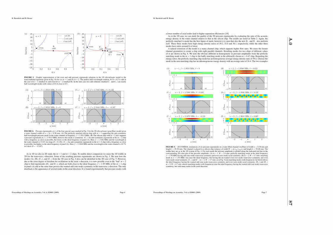
0 0.2 0.4 0.6 0.8 1−25

−20

−15

−10

−5

0

5

10

15

20

25

θ/π

func

tion

cot (θ)− 1


even odd

even

α = 1(a)

0 0.2 0.4 0.6 0.8 1−25

−20

−15

−10

−5

0

5

10

15

20

25

θ/π

func

tion

cot (θ)− 1


oddeven

even

evenodd

α = 2(b)

A C− B

C+

FIGURE 3. Graphic representation of the even and odd pressure eigenmode solutions in the 1D silicon/water model to the

transcendental equations given in Eq. (9) for (a) α = 1 and (b) α = 2. The perfect half-wavelength solution, θ/π = 0.5 is odd in

the case of α = 1 (marked A) and even for α = 2 (marked B). In the later case two odd solutions (marked C− and C+) are nearly

half-wavelength modes with values of θ/π close to 0.5.

−1

0

1

wasi siair air

p/p

max

−2 −1 0 1 2−1

0

1

wasi si airair

y [mm]

p/p

max

−1

0

1

wasi si airair

p/p

max

−2 −1 0 1 2−1

0

1

wasi si airair

y [mm]

p/p

max

(A) α = 1, f = 1.9513 MHz, δ = 0

(B) α = 2, f = 1.9513 MHz, δ = 0

(C+) α = 2, f = 1.7182 MHz, δ = 0.136

(C−) α = 2, f = 2.1844 MHz, δ = −0.107

FIGURE 4. Pressure eigenmodes p(y) of the four special cases marked in Fig. 3 for the 1D silicon/water (gray/blue) model given

a water channel width of w = 2a = 0.38 mm. (A) The perfectly matched silicon chip with α = 1 supporting the anti-symmetric

half-wavelength pressure mode in the water channel at frequency f = 1.9513 MHz. (B) The silicon chip with α = 2 also supports

a pressure eigenmode at f = 1.9513 MHz, however this mode is symmetric. (C+) An anti-symmetric eigenmode in the α = 2 chip

with a frequency as close as possible, but lower, to the ideal frequency of panel (A). Here f = 1.7182 MHz and the wavelength in

the water channel is 13.6% too long (δ = 0.136). (C−) An anti-symmetric eigenmode in the α = 2 chip with a frequency as close

as possible, but higher, to the ideal frequency of panel (A). Here f = 2.1844 MHz and the wavelength in the water channel is 10.7%

too short (δ = −0.107).

As in 1D we also in 2D study the α = 1 and α = 2 chips. To enable direct comparison we reuse the 1D widths in

2D for the transverse y-direction. Some of the resulting pressure eigenmodes are shown in Fig. 5. We note how the

modes (A), (B), (C+), and (C−) from the 1D case in Fig. 4 also can be identified in the 2D case of Fig. 5. However,

due to the extra degree of freedom for oscillations in the axial x-direction, it is now possible even in the "bad" α = 2

chip to find eigenmodes (D+ and D−), which are both close to the ideal frequency f = 1.95 MHz of the α = 1 chip

in panel (A) and at the same time possess the wanted odd (one-node) symmetry in the transverse y-direction. The only

drawback is the appearance of several nodes in the axial direction. It is found experimentally that pressure modes with



a lower number of axial nodes lead to higher separation efficiencies [18].

As in the 1D case, we can study the quality of the 2D pressure eigenmodes by evaluating the ratio of the acoustic

energy density in the water channel relative to that in the silicon chip. The results are listed in Table 2. Again, the

perfectly matched A-mode has the best figure of merit, however it is seen that also the new D+ and D− also perform

well. These three modes have high energy density ratios of 39.2, 32.0 and 36.1, respectively, while the other three

modes have ratios around 6 or lower.

A natural extension of the model is a many-channel chip, which supports higher flow rates. We reuse the former

channel geometries to create a chip with eight parallel channels. Resulting modes for two chips of different values

of α are shown in Fig. 6. We note the obvious different in homogeneity in pressure amplitudes from the perfectly

matching mode in the α = 1 chip to the badly matching mode in the arbitrarily chosen α = 0.47 chip. Regarding the

energy ratios, the perfectly matching chip mode has an homogeneous average energy density ratio of 39.4, whereas the

mode in the non-matching chip has an inhomogeneous energy density with an average ratio of 16.4. The two examples

(A) α = 1, f = 1.9518 MHz, δ = 0

y

x

−1

0

1

wasi siair air

p/p

max

(B) α = 2, f = 1.9560 MHz, δ = 0.012

y

x

−1

0

1

wasi si airair

p/p

max

(C+) α = 2, f = 1.7209 MHz, δ = 0.105

y

x

−1

0

1

wasi si airair

p/p

max

(C−) α = 2, f = 2.1870 MHz, δ = −0.118

y

x

−2 −1 0 1 2−1

0

1

wasi si airair

y [mm]

p/p

max

(D+) α = 2, f = 1.9430 MHz, δ = 0.132

y

x

−1

0

1

wasi si airair

p/p

max

(D−) α = 2, f = 1.9616 MHz, δ = 0.005

y

x

−2 −1 0 1 2−1

0

1

wasi si airair

y [mm]

p/p

max

FIGURE 5. 2D COMSOL simulations of six pressure eigenmodes in a water-filled channel (wa/blue) of width w = 0.38 mm and

length l = 29.30 mm. The channel is placed in a silicon chip (si/gray) of width W = α (csi/cwa)w and length L = 55.00 mm. The

widths here are as in the 1D system of Fig. 4. For each mode the pressure amplitude is plotted along the indicated red line in the

corresponding 2D color plot of the pressure amplitude. (A) α = 1, W = 2.6 mm: perfectly matching mode at the ideal frequency

f = 1.95 MHz having odd (one-node) transverse symmetry and even (zero-node) axial symmetry. (B) α = 2, W = 4.7 mm: matching

mode at f = 1.95 MHz very near the ideal frequency, but having the un-wanted even (two-node) transverse symmetry and even

(zero-node) axial symmetry. (C+) and (C−) α = 2, W = 4.7 mm: as in Fig. 4 non-matching modes with frequencies far below/above

the ideal frequency having the wanted odd (one-node) transverse symmetry and even (zero-node) axial symmetry. (D+) and (D−)

α = 2, W = 4.7 mm: almost matching modes with frequencies near the ideal frequency having the wanted odd (one-node) transverse

symmetry, but with many nodes in the axial direction.



A.0

87

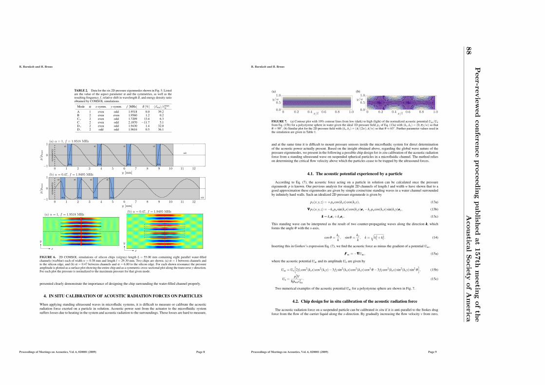
TABLE 2. Data for the six 2D pressure eigenmodes shown in Fig. 5. Listed

are the value of the aspect parameter α and the symmetries, as well as the

resulting frequency f , relative shift in wavelength δ , and energy density ratio

obtained by COMSOL simulations.

Mode α x-symm. y-symm. f [MHz] δ [%] 〈Ewa〉/E maxsi

A 1 even odd 1.9518 0.0 39.2

B 2 even even 1.9560 1.2 0.2

C+ 2 even odd 1.7209 13.4 6.3

C− 2 even odd 2.1870 −11.7 5.1

D+ 2 even odd 1.9430 1.4 32.0

D− 2 odd odd 1.9616 0.5 36.1

(a) α = 1, f = 1.9518 MHz

0 1 2 3 4 5 6 7 8 9 10 11 12−1

0

1

sym

met

ry

si

wa

si

wa

si

wa

si

wa

air

y [mm]

p/p

max

y

x

(b) α = 0.47, f = 1.9495 MHz

0 1 2 3 4 5 6 7 8 9 10 11 12−1

0

1

sym

met

ry

si

wa

si

wa

si

wa

si

wa air

y [mm]

p/pm

ax

y

x

(a) α = 1, f = 1.9518 MHz(b) α = 0.47, f = 1.9495 MHz

FIGURE 6. 2D COMSOL simulations of silicon chips (si/gray) length L = 55.00 mm containing eight parallel water-filled

channels (wa/blue) each of width w = 0.38 mm and length l = 29.30 mm. Two chips are shown; (a) α = 1 between channels and

to the silicon edge, and (b) α = 0.47 between channels and α = 6.80 to the silicon edge. For each shown resonance the pressure

amplitude is plotted as a surface plot showing the entire chip and as a symmetric cross-sectional plot along the transverse y-direction.

For each plot the pressure is normalized to the maximum pressure for that given mode.

presented clearly demonstrate the importance of designing the chip surrounding the water-filled channel properly.

4. IN SITU CALIBRATION OF ACOUSTIC RADIATION FORCES ON PARTICLES

When applying standing ultrasound waves in microfludic systems, it is difficult to measure or calibrate the acoustic

radiation force exerted on a particle in solution. Acoustic power sent from the actuator to the microfluidic system

suffers losses due to heating in the system and acoustic radiation to the surroundings. These losses are hard to measure,



(a)

0 0.2 0.4 0.6 0.8 1.00.0

0.5

1.0y/w

x/l

(b)

0 0.2 0.4 0.6 0.8 1.00.0

0.5

1.0y/w

x/l

FIGURE 7. (a) Contour plot with 10% contour lines from low (dark) to high (light) of the normalized acoustic potential Uac/Uo

from Eq. (15b) for a polystyrene sphere in water given the ideal 1D pressure field p1 of Eq. (13a) with (kx,ky) = (0,πy/w) so that

θ = 90. (b) Similar plot for the 2D pressure field with (kx,ky) = (π/(2w),π/w) so that θ ≈ 63. Further parameter values used in

the simulation are given in Table 1.

and at the same time it is difficult to mount pressure sensors inside the microfluidic system for direct determination

of the acoustic power actually present. Based on the insight obtained above, regarding the global wave nature of the

pressure eigenmodes, we present in the following a possible chip design for in situ calibration of the acoustic radiation

force from a standing ultrasound wave on suspended spherical particles in a microfluidic channel. The method relies

on determining the critical flow velocity above which the particles cease to be trapped by the ultrasound forces.

4.1. The acoustic potential experienced by a particle

According to Eq. (7), the acoustic force acting on a particle in solution can be calculated once the pressure

eigenmode p is known. Our previous analysis for straight 2D channels of length l and width w have shown that to a

good approximation these eigenmodes are given by simple cosine/sine standing waves in a water channel surrounded

by infinitely hard walls. Such an idealized 2D pressure eigenmode is given by

p1(x,y,z) = +pa cos(kxx)cos(kyy), (13a)

∇∇∇p1(x,y,z) = −kx pa sin(kxx)cos(kyy)eeex − ky pa cos(kxx)sin(kyy)eeey, (13b)

kkk = kxeeex + kyeeey. (13c)

This standing wave can be interpreted as the result of two counter-propagating waves along the direction kkk, which

forms the angle θ with the x-axis,

cosθ =kx

k, sinθ =

ky

k, k =

√k2

x + k2y . (14)

Inserting this in Gorkov’s expression Eq. (7), we find the acoustic force as minus the gradient of a potential Uac,

FFFac = −∇∇∇Uac, (15a)

where the acoustic potential Uac and its amplitude Uo are given by

Uac = Uo

[2 f1 cos2(kxx)cos2(kyy)−3 f2 sin2(kxx)cos2(kyy)cos2 θ −3 f2 cos2(kxx)sin2(kyy)sin2 θ

], (15b)

Uo =p2

aV

8ρwac2wa

. (15c)

Two numerical examples of the acoustic potential Uac for a polystyrene sphere are shown in Fig. 7.

4.2. Chip design for in situ calibration of the acoustic radiation force

The acoustic radiation force on a suspended particle can be calibrated in situ if it is anti-parallel to the Stokes drag

force from the flow of the carrier liquid along the x-direction. By gradually increasing the flow velocity v from zero,



88

Peer-re

vie

wed

con

fere

nce

pro

ceed

ing

pu

blish

ed

at

157th

meetin

gof

the

Acou

stical

Socie

tyof

Am

eric

a

(a)

0 0.2 0.4 0.6 0.8 1.00.0

0.5

1.0y/w

x/l

(b)

α = 3

FIGURE 8. (a) Contour plot with 10% contour lines from low (dark) to high (light) of the normalized acoustic potential Ucalibac /Uo

from Eq. (16a) for a polystyrene sphere in water given the pressure field p1 = pa cos(πx/2w). The parameter values are given in

Table 1, and moreover kx = π/(2w) while ky = 0 so that θ = 0. (b) Color plot of the pressure eigenmode in the triple-channel α = 3

chip. A transverse potential, as in panel (a), suitable for in situ acoustic force calibration is set up in the two side channels, while

the center channel supports a transverse mode of odd symmetry as in Fig. 5(D+). The left insert shows the single-channel α = 3

chip. Note the two anti-nodes in the silicon chip (gray) above and below the water-filled channel (blue).

a critical value v∗ of v can be determined, above which the acoustic radiation force no longer can trap the particle. At

this point |FFFac| ≈ 6πηav∗, and the unknown pre-factor Uo can be determined. The calibration setup requires that kkk and

eeex are parallel, thus kx = 0 while ky = 0. By combining Eqs. (6) and (15) with this form of the wave vector, we obtain

the acoustic potential and the associated radiation force for calibration purposes on the form

Ucalibac = Uo

[2 f1 cos2(kxx)−3 f2 sin2(kxx)

], (16a)

FFFcalibac = 2kxUo

[5γ −2

2γ +1− 1

γβ 2

]sin(2kxx) eeex. (16b)

The potential Ucalibac is shown in Fig. 8(a).

If a particle is subject to a Stokes drag force Fdrag from a flow in the x-direction, then the critical flow velocity v∗,

where the acoustic radiation force no longer can trap the particle is given by the condition Fdrag = max|FFFcalibac | or

6πηav∗ = 2kxUo

[5γ −2

2γ +1− 1

γβ 2

]. (17)

If v∗ is measured experimentally, we are therefore able to determine the acoustic energy scale Uo by

Uo = 3πηav∗

kx

[5γ −2

2γ +1− 1

γβ 2

]−1

. (18)

We propose a specific chip design which supports a pressure eigenmode close to the one depicted in Fig. 8(a). The

idea is to fabricate an α = 3 chip. In such a chip a strong pressure eigenmode of odd symmetry exists in the channel

as the α = 1 chip in Fig. 5(a) but it will also have a strong anti-node in the silicon as the α = 2 chip in Fig. 5(b).

Now, if two auxiliary side channels parallel to the first channel is placed at these anti-nodes, the pressure mode inside

these side channels is very close to the wanted mode of Fig. 8(a). The correctness of this line of reasoning is proved

by numerical simulation of the eigenmodes in such a triple-channel α = 3 chip as shown in Fig. 8(b).

5. CONCLUDING REMARKS

By theoretical and numerical analysis we have studied the applicability of the widely used transverse half-wavelength

picture. We have shown that, although not entirely correct, this picture is accurate enough to be useful. Furthermore,

we have shown that it is crucial to take the entire geometry of the chip into account and match the dimensions of

the surrounding silicon to those of the water channel, i.e. a global wave picture must be employed. Finally, we have

presented two examples of applying this global wave picture: (i) a many-channel chip, which by correct matching

performs significantly better in terms of amplitude and homogeneity of the acoustic energy density, and (ii) a three-

channel chip, which enables in situ calibration of the acoustic radiation force.

ACKNOWLEDGMENTS

We thank Thomas Laurell and Per Augustsson at Lund University for many illuminating discussions.



REFERENCES

1. L.V. King, Proc. R. Soc. London, Ser. A 147, 212 (1934).

2. K. Yosioka and Y. Kawasima, Acustica 5, 167 (1955).

3. L.P. Gorkov, Sov. Phys. Doklady 6, 773 (1962).

4. K. Yasuda, S. Umemura, and K. Takeda, Jpn. J. Appl. Phys. 34, 2715 (1995).

5. K. Yasuda, K. Takeda, and S. Umemura, Jpn. J. Appl. Phys. 35, 3295 (1996).

6. J. Spengler and M. Jekel, Ultrasonics 38, 624 (2000).

7. M. Saito, N. Kitamura and M. Terauchi, J. Appl. Phys. 92, 7581 (2002).

8. M. Wiklund, P. Spégel, S. Nilsson and H. M. Hertz, Ultrasonics 41, 329 (2003).

9. J.F. Spengler, W.T. Coakley, and K.T. Christensen, AIChE J. 49, 2773 (2003).

10. L. A. Kuznetsova and W. T. Coakley, J. Acoust. Soc. Am. 116, 1956 (2004).

11. H. Li and T. Kenny, Conf. Proc. 26 Ann. Int. Conf. IEEE Engineering in Medicine and Biology, 3(4), 2631 (2004).

12. M. Bengtsson and T. Laurell, Anal. Chem. 378, 1716 (2004).

13. J. J. Hawkes, R. W. Barber, D. R. Emerson and W. T. Coakley, Lab Chip 4, 446 (2004).

14. A. Nilsson, F. Petersson, H. Jonsson, and T. Laurell, Lab Chip 4, 131 (2004).

15. H. Jonsson, C. Holm, A. Nilsson, F. Petersson, P. Johnsson, and T. Laurell, Ann. Thoracic Surgery 78, 1572 (2004).

16. T. Lilliehorn, U. Simu, M. Nilsson, M. Almqvist, T. Stepinski, T. Laurell, J. Nilsson, S. Johansson, Ultrasonics 43, 293 (2005).

17. S. M. Hagsäter, T. G. Jensen, H. Bruus, and J. P. Kutter, Lab Chip 7, 1336 (2007).

18. S. M. Hagsäter, A. Lenshof, P. Skafte-Pedersen, J. P. Kutter, T. Laurell and H. Bruus, Lab Chip 8, 1178 (2008).

19. O. Manneberg, S.M. Hagsäter, J. Svennebring, H.M. Hertz, J.P. Kutter, H. Bruus, M. Wiklund Ultrasonics 49, 112-119 (2009).

20. J. Svennebring, O. Manneberg, P. Skafte-Pedersen, H. Bruus, and M. Wiklund Biotechnol. Bioeng. 103, 323 (2009).

21. J. Lighthill, Waves in fluid, (Cambridge University Press, Cambridge, 2005).

22. H. Bruus, "Acoustofluidics" in Theoretical Microfluidics, (Oxford University Press, Oxford, 2008).



A.0

89

90Peer-reviewed conference proceeding published at 157th meeting of the

Acoustical Society of America

Appendix B

Impedance condition at cylindricalboundary

To model acoustic impedance conditions of curved boundaries, a cylindrically shapedboundary, between two domains, is investigated. We imagine the cylinder to be infinitelyhigh, which thus leads to translational invariance in the z-direction. Inside the cylinderis one medium (1), while outside is another but infinitely extending medium (2). Leavingout the angular dependence due to angular invariance, the Helmholtz equation reads

∇2(r, t) = −k2(r, t), (B.1)

where is the velocity potential and k = !c is the wave number of the medium. The

Laplacian is

∇2 = ∂2 +1

r∂r. (B.2)

As the solution can be expressed as a product between the solution to the spatial part anda solution to the time part, (r, t) = R(r)T (t), we now focus on the spatial part as timesolution is already assumed to be hamonic in the above stated Helmholtz equation. Thespatial solution to the polar wave equation in Eq. (B.2) is known to be a linear combinationof Bessel functions in zeroth order (zeroth order because we have no angular dependence)

R(r) = AJ0(kr) +BY0(kr), (B.3)

where A and B are constants. In order to describe cylindrical waves the linear combinationof Bessel functions is given by the so-called Hankel functions. The zeroth order Hankelfunctions are

H(1)0 (kr) = J0(kr) + iY0(kr), (B.4)

H(2)0 (kr) = J0(kr)− iY0(kr), (B.5)

which obeys same algebraic rules as the ordinary Bessel functions and where H(1)0 is

the outward going wave and H(2)0 is the inward going wave. In order to consider waves

91

92 Impedance condition at cylindrical boundary

propagating from the cylinder, we envisage a thin cylindrical piezo-actuator placed in thecenter of the boundary between the two media. We can therefore now write the velocitypotential in each of the two media/domains

1(r, t) =

[A1H

(1)0 (k1r) +B1H

(2)0 (k1r)

]e−i!t, a0 < r < a, (B.6)

2(r, t) = A2H(1)0 (kr)e−i!t, r > a, (B.7)

where a0 is the radius of the piezo-actuator inside domain 1 and a is the radius of theboundary between the two domains. Notice that we only consider outwards going waves indomain 2 as we consider it to extend infinitely. The boundary conditions at the interfaceof the domains are, by the demanding continuity in velocity and pressure, given as

∂r1(a, t) = ∂r2(a, t), continuity in velocity, (B.8)

11(a, t) = 22(a, t), continuity in pressure. (B.9)

With the objective of rewriting the interface conditions into one single requirement on thepressure p1 in domain 1, the spatial derivative of 2 is found

∂r2(a, t) = −k2A2H(1)1 (k2a)e−i!t, (B.10)

which is seen not to be a linear combination of 2(a, t). Asymptotic forms are thereforeneeded to continue.

Asymptotic expansion for large a The asymptotic form in the case of ∣z∣ → ∞ for

the H(1) (z) Hankel function of order is

H(1) (z) ≈

√2

zei(z−

2 −

4 )

[1 +

∞∑n=1

(12 + )(1

2 − )n

n!(2iz)n

], (B.11)

where the notation () = Γ(+)Γ() is used [56]. Using this to expand H

(1)0 (k2a) and

H(1)1 (k2a) to n = 1 (or order (k2a)−3/2) gives

H(1)0 (k2a) ≈

√2

k2aei(k2a−/4)

[1− i

4

1

k2a

], (B.12)

H(1)0 (k2a) ≈ i

√2

k2aei(k2a−/4)

[1 + 3i

1

k2a

]. (B.13)

Keeping the order of (k2a)−3/2, the spatial derivative of 2(a, t) in Eq.(B.10) is rewrittento

∂r2(a, t) ≈ −ik22(a, t)

[1− i11

4

1

k2a

], (B.14)

which rewritten into a condition on p1(a, t) gives

1

1∂rp1(a, t) = − i!

Z2p1(a, t)

[1− i11

4

1

k2a

]+O

[(k2a)−5/2

], (B.15)

B.0 93

where Z2 = 2c2 is the impedance of medium 2. As the curvature of the cylinder = 1a → 0

the condition on p1(a, t) is seen to equal the condition when considering a plane wallinterface. This makes qualitatively good sense as the cylindrical waves reduces to planewaves as the distance from the origin of the wave is large.

94 Impedance condition at cylindrical boundary

Appendix C

Comsol/Matlab script for pressureeigenmodes in 2D chip model

Below we show the script for solving the pressure eigenmodes for a 2D chip geometry. Thescript uses x- and y-symmetry.

1 % 2D symmetric chip model , eigenvalue analysis

2 %

3 % Rune Barnkob , DTU Nanotech 2009

4

5 %% Initialization


7 disp(’Fem2D_SymmetricBox.m’);

8

9 %% Constants

10 N = 2; % Number of resonance frequencies to investigate

11

12 cWa = 1483; % Water: speed of sound

13 cSi = 8490; % Silicon: speed of sound

14 rhoWa = 998; % Water: density

15 rhoSi = 2331; % Silicon: density

16

17 alpha = 2;

18 L = 55.00e-3; % Length , silicon chip

19 l = 29.30e-3; % Length , water channel

20 w = 380e-6; % Width , water channel

21 W = w*(1+ cSi/cWa*alpha); % Width , water chamber

22

23 f0 = cWa /2/w;

24 fs = f0; % Frequency to search for

25 points_mesh = 60; % Number of mesh points per wavelength

26 points = 100; % Additional number of points to evaluate

27 y0 = 0.0; % Crosssection -line to investigate

28

29 % Parity factors

95

96 Comsol/Matlab script for pressure eigenmodes in 2D chip model

30 paX = +1; % +1 even , -1 odd

31 paY = +1; % +1 even , -1 odd

32

33 if paX == -1

34 BCX = 1;

35 else

36 BCX = 0;

37 end

38

39 if paY == -1

40 BCY = 1;

41 else

42 BCY = 0;

43 end

44

45 const = struct(’cWa’,cWa ,’cSi’,cSi ,’rhoWa ’,rhoWa ,’rhoSi ’,rhoSi ,...

46 ’w’,w,’l’,l,’W’,W,’L’,L,’y0’,y0 ,’BCX’,BCX ,’BCY’,BCY);

47

48 %% EVP - determining resonance frequencies near lambda /2

49 fem.const = const;

50

51 % Geometry %%

52 g1 = rect2(w/2,l/2,’base’,’corner ’,’pos’ ,[0 0]);

53 g2 = rect2(W/2,L/2,’base’,’corner ’,’pos’ ,[0 0]);

54 s.objs=g1,g2;



57 % sfigure (1),geomplot(fem ,’sublabels ’,’on’,’edgelabels ’,’off ’)

58 % axis equal

59 % return

60

61 % Equations %%

62 % Subdomain Groups:

63 % [1] Water subdomain

64 % [2] Silicon subdomain

65 % Boundary Groups:

66 % [1] Si-water interface , continuity

67 % [2] Si-air interface , soft

68 % [3] Symmetry -X

69 % [4] Symmetry -Y

70 fem.equ.ind = 1 2;

71 fem.bnd.ind = [4 6] [5 8] [1 3] [2 7];

72

73 % Variables

74 fem.sdim = ’x’,’y’;


76 fem.shape = 2;

77

78 % Governing equations

C.0 97


80 fem.equ.expr = ...

81 ’c’,’cWa’,’cSi’,...

82 ’rho’,’rhoWa’,’rhoSi’,...

83 ’Eaco’,’((abs(px)ˆ2+ abs(py)ˆ2)/omegaˆ2 + abs(p)ˆ2/cˆ2) /(4* rho)

’;

84 fem.equ.shape = 1 1; % define p in both domain groups

85 fem.equ.ga = ’px/rho’;’py/rho’;

86 fem.equ.f = ’-omega ˆ2*p/(rho*cˆ2)’;


88

89 % Boundary conditions

90 fem.bnd.shape = 1,1,1,1; % define p on all boundaries

91 fem.bnd.r = ... % only looking for uneven modes!

92 ’0’, ... % BC group [1]

93 ’0-p’, ... % BC group [2]

94 ’0-BCX*p’, ... % BC group [3]

95 ’0-BCY*p’; % BC group [4]

96

97 fem.bnd.g = ...

98 ’0’, ... % BC group [1]

99 ’0’, ... % BC group [2]

100 ’0’, ... % BC group [3]

101 ’0’; % BC group [4]

102

103 % Meshing

104 mSi = cSi/f0/points_mesh;

105 mWa = cWa/f0/points_mesh;

106 fem.mesh = meshinit(fem ,’report ’,’off’,’hmaxsub ’ ,[1 2; mWa mSi]);


108 DOF = flngdof(fem);

109 % sfigure (2); meshplot(fem);

110 % axis equal

111 % return

112

113 % Solving EVP


115 ’solcomp ’,’p’, ...

116 ’outcomp ’,’p’, ...


118 ’shift’ ,2*pi*fs ,...

119 ’neigs’,N, ...

120 ’linsolver ’,’spooles ’ ,... %’pardiso ’,... %

121 ’etol’,1e-10);

122

123 omega_vec = fem.sol.lambda;

124

125 %% Postprocessing for all resonance frequencies

126 Ewa = zeros(1,length(omega_vec));

98 Comsol/Matlab script for pressure eigenmodes in 2D chip model

127 Esi = Ewa;

128

129 xvwa = (0+ mWa/points):mWa/points :(w/2-mWa/points); % points channel

130 xvsi = (w/2+ mSi/points):mSi/points :(W/2-mSi/points); % points chip

131 Edens_wa = zeros(length(omega_vec),length(xvwa));

132 Edens_si = zeros(length(omega_vec),length(xvsi));

133

134 for j = 1: length(omega_vec)

135

136 % Surface plots of pressure field in different p limits

137 sfigure (3);

138 postplot(fem ,’tridata ’,’p’,’solnum ’,j)

139 xlabel(’x’),ylabel(’y’)

140 axis equal

141

142 % Aquiring acoustic energies

143 yv0wa = y0*ones(1,length(xvwa));

144 yv0si = y0*ones(1,length(xvsi));

145 Edens_wa(j,:) = postinterp(fem ,’Eaco’,[xvwa;yv0wa ],...

146 ’solnum ’,j,’Dl’,1,’edim’ ,2);

147 Edens_si(j,:) = postinterp(fem ,’Eaco’,[xvsi;yv0si ],...

148 ’solnum ’,j,’Dl’,2,’edim’ ,2);

149 EmaxWa = max(Edens_wa(j,:));

150 EmaxSi = max(Edens_si(j,:));

151 Awa = w*l; % total area of water channels

152 Asi = W*L-w*l; % total area of silicon chip

153 Ewa(j) = 1/(Awa/4)*postint(fem ,’Eaco’,’Dl’,1,’edim’,2,’solnum ’,

j);

154 Esi(j) = 1/(Asi/4)*postint(fem ,’Eaco’,’Dl’,2,’edim’,2,’solnum ’,

j);

155

156 % Plot pressure along y0

157 p_wa = postinterp(fem ,’p’,[xvwa;yv0wa],’solnum ’,j);

158 p_si = postinterp(fem ,’p’,[xvsi;yv0si],’solnum ’,j);

159 sfigure (4);

160 plot(xvwa/1e-3,p_wa/max(p_si),’-r’,xvsi/1e-3,p_si/max(p_si),’-b

’);

161 xlabel(’y [mm]’),ylabel(’p/pmax [Pa]’)

162 delta = cWa/( omega_vec(j)/2/pi)/2/w-1;

163

164 % Writing info to screen

165 fprintf(1,’f0: %6.4f MHz , DOF: %i, alpha: %2.3f\n’,f0/1e6 ,DOF ,

alpha);

166 fprintf (1,[’No.: %i/%i, f: %6.4f MHz , delta: %6.8f, ’ ...

167 ’EmaxWa/EmaxSi: %2.3f, Ewa/EmaxSi: %2.3f\n’],...

168 j,length(omega_vec),omega_vec(j)/2/pi/1e6 ,delta ,...

169 EmaxWa/EmaxSi ,Ewa(j)/EmaxSi);

170 pause

171 end

Appendix D

Comsol/Matlab script foreigenmodes in translational inv.3D model

Below we show the script for solving the pressure eigenmodes for a chip geometry ofa translational invariance along its axial direction. This script is described in detail inChap. 3 on Comsol Multiphysics.

1 %% Initialization


3

4 % Material parameters


6 cPy = 5603; % Pyrex: speed of sound




10 rhoPy = 2230; % Pyrex: density

11 % Geometric parameters

12 L = 40e-3; % Length , silicon/pyrex chip

13 w = 0.375e-3; % Width , water -filled channel

14 W = 4e-3; % Width , silicon/pyrex chip

15 hSi = 0.350e-3; % Height , silicon chip

16 hPy = 1.13e-3; % Height , pyrex lid

17 hWa = 0.157e-3; % Height , water -filled channel

18 % Wave number in x-direction

19 kx = pi/L; % nx=1

20

21 % Constants into fem -struct

22 fem.const = struct(’cWa’,cWa ,’cSi’,cSi ,’cPy’,cPy ,...

23 ’rhoWa’,rhoWa ,’rhoSi’,rhoSi ,’rhoPy’,rhoPy ,’kx’,kx);

24

25 % Geometry

26 g1 = rect2(W/2,hPy ,’base’,’corner ’,’pos’ ,[0 0]);

99

100 Comsol/Matlab script for eigenmodes in translational inv. 3D model

27 g2 = rect2(w/2,hWa ,’base’,’corner ’,’pos’ ,[0 -hWa]);

28 g3 = rect2(W/2,hSi ,’base’,’corner ’,’pos’ ,[0 -hSi]);

29 s.objs=g1,g2,g3;



32 % figure (1),geomplot(fem ,’sublabels ’,’off ’,’edgelabels ’,’on ’)

33 % axis equal % xlabel(’y [m]’),ylabel(’z [m]’)

34 % return

35

36 % Equations %%




40 % [3] Pyrex subdomain


42 % [1] Interface , continuity

43 % [2] Air -interface , soft

44 % [3] y-symmetry

45 % [4] Piezo , hard wall

46 fem.equ.ind = 2 1 3;

47 fem.bnd.ind = [4 8 6 9] [7 10 11] [1 3 5] [2];

48

49 % Variables

50 fem.sdim = ’y’,’z’;


52 fem.shape = 2;

53

54 % Governing equations on general form


56 fem.equ.expr = ’c’,’cWa’,’cSi’,’cPy’,’rho’,’rhoWa’,’rhoSi’,’

rhoPy ’;

57 fem.equ.shape = 1 1 1; % Defining p in all domain groups

58 fem.equ.ga = ’py/rho’;’pz/rho’;



61

62 % Boundary conditions on general form

63 fem.bnd.shape = 1,1,1,1; % Defining p on all boundaries

64 fem.bnd.r = ...


66 ’0-p’, ... % BC group [2] Air -interface , soft

67 ’0-1*p’, ... % BC group [3] y-symm.: -1*p (even), 0*p (odd)


69 fem.bnd.g = ...


71 ’0’, ... % BC group [2] Air -interface , soft

72 ’0’, ... % BC group [3] y-symm.


74

D.0 101

75 % Meshing

76 mSi = cSi/2e6/50; % 50 meshes per silicon wavelength at 2 MHz

77 mWa = cWa/2e6/50; % 50 meshes per water wavelength at 2 MHz

78 mPy = cPy/2e6/50; % 50 meshes per pyrex wavelength at 2 MHz

79 fem.mesh = meshinit(fem ,’hmaxsub ’ ,[2 1 3; mWa mSi mPy]);


81 % figure (2); meshplot(fem);% xlabel(’y [m]’),ylabel(’z [m]’)

82 % axis equal

83 % return

84

85 % Solving EVP


87 ’solcomp ’,’p’, ...

88 ’outcomp ’,’p’, ...


90 ’shift’ ,2*pi*0,...

91 ’neigs’,1, ...

92 ’linsolver ’,’spooles ’ ,...

93 ’etol’,1e-8);

94

95 omega_vec = fem.sol.lambda;

96 f_vec = omega_vec /2/pi

97

98 %% Postprocessing

99 figure (1);

100 postplot(fem ,’tridata ’,’p’,’tridlim ’ ,[-2.1 2.1],’solnum ’ ,1)

101 xlabel(’y [m]’),ylabel(’z [m]’)

102 axis equal

103 axis ([0 2e-3 -4e-4 12e-4])

102 Comsol/Matlab script for eigenmodes in translational inv. 3D model

Appendix E

Comsol/Matlab script forresonances in point-actuated 3Dmodel

Below we show the script for the computation of the acoustic resonances for the point-actuated 3D model treated in Chap. 4.

1 %% COMSOL -MATLAB -script: CircAct_func_Zair.m

2 % Driven 3D acoustic resonance analysis

3 % MSc -student Rune Barnkob , TMF , DTU Nanotech , 2008/2009

4 % 22 -10 -2008

5 %

6 % Script for sweeping in frequencies and in Zair

7 %

8 % The system consists of a silicon chip containing a water cavity.

Acoustic

9 % resonances in the chip is actuated by a circular actuator , which

is

10 % applied to the top surface of the chip.

11 % Variation possibilities: position of actuator and BCs on the chip

12 % surface (last mentioned can create circular fixations by choosing

proper

13 % impedance conditions).

14 %

15 %%

16 function CircAct_func_Zair

17

18 disp(’ ’)

19 disp(’CircAct_func_Zair_Pins.m started ’);

20 flreport(’off’)

21

22 %% Initialization

23 clear all , close all , flclear fem

24

103

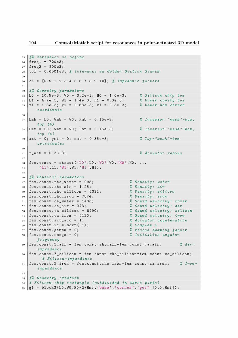
104 Comsol/Matlab script for resonances in point-actuated 3D model

25 %% Variables to define

26 freq1 = 720e3;

27 freq2 = 800e3;

28 tol = 0.0001 e3; % tolerance in Golden Section Search

29

30 ZZ = [0.5 1 2 3 4 5 6 7 8 9 10]; % Impedance factors

31

32 %% Geometry parameters

33 L0 = 10.5e-3; W0 = 3.2e-3; H0 = 1.0e-3; % Silicon chip box

34 L1 = 4.7e-3; W1 = 1.4e-3; H1 = 0.3e-3; % Water cavity box

35 x1 = 1.3e-3; y1 = 0.68e-3; z1 = 0.3e-3; % Water box corner

coordinate

36

37 Lmb = L0; Wmb = W0; Hmb = 0.15e-3; % Interior "mesh"-box ,

top (b)

38 Lmt = L0; Wmt = W0; Hmt = 0.15e-3; % Interior "mesh"-box ,

top (t)

39 xmt = 0; ymt = 0; zmt = 0.85e-3; % Top -"mesh"-box

coordinates

40

41 r_act = 0.3E-3; % Actuator radius

42

43 fem.const = struct(’L0’,L0 ,’W0’,W0 ,’H0’,H0 , ...

44 ’L1’,L1 ,’W1’,W1 ,’H1’,H1);

45

46 %% Physical parameters

47 fem.const.rho_water = 998; % Density: water

48 fem.const.rho_air = 1.25; % Density: air

49 fem.const.rho_silicon = 2331; % Density: silicon

50 fem.const.rho_iron = 7874; % Density: iron

51 fem.const.ca_water = 1483; % Sound velocity: water

52 fem.const.ca_air = 343; % Sound velocity: air

53 fem.const.ca_silicon = 8490; % Sound velocity: silicon

54 fem.const.ca_iron = 5120; % Sound velocity: iron

55 fem.const.act_acc = 1; % Actuator acceleration

56 fem.const.ic = sqrt(-1); % Complex i

57 fem.const.gamma = 0; % Viscos damping factor

58 fem.const.omega = 0; % Initialize angular

frequency

59 fem.const.Z_air = fem.const.rho_air*fem.const.ca_air; % Air -

impendance

60 fem.const.Z_silicon = fem.const.rho_silicon*fem.const.ca_silicon;

% Silicon -impendance

61 fem.const.Z_iron = fem.const.rho_iron*fem.const.ca_iron; % Iron -

impendance

62

63 %% Geometry creation

64 % Silicon chip rectangle (subdivided in three parts)

65 g1 = block3(L0 ,W0 ,H0 -2*Hmt ,’base’,’corner ’,’pos’ ,[0,0,Hmt]);

E.0 105

66 g3 = block3(Lmb ,Wmb ,Hmb ,’base’,’corner ’,’pos’ ,[0,0,0]);

67 g4 = block3(Lmt ,Wmt ,Hmt ,’base’,’corner ’,’pos’,[xmt ,ymt ,zmt]);

68 % Water cavity rectangle

69 g2 = block3(L1,W1,H1,’base’,’corner ’,’pos’,[x1 ,y1 ,z1]);

70

71 % Embedding array of cirles on chip surface

72 ChessGeometry_input % loading array of circles

73 g5 = embed(c1+c2+c3+c4+c5+c6+c7+c11+c21+c12+c22+c13+c23+c14+c24+

...

74 c15+c25+c16+c26+c17+c27+c18+c28 ,’Wrkpln ’ ,[0 1 0;0 0 1;0 0 0]);

% embed bottom

75 g6 = embed(c1+c2+c3+c4+c5+c6+c7+c11+c21+c12+c22+c13+c23+c14+c24+

...

76 c15+c25+c16+c26+c17+c27+c18+c28 ,’Wrkpln ’ ,[0 1 0;0 0 1;H0 H0 H0

]); % embed top

77

78 % Analyzed geometry

79 s.objs=g1-g2,g2,g3,g4;

80 f.objs=g5,g6;

81

82 fem.draw=struct(’s’,s,’f’,f);


84

85 %% Equations





90 % [1] Si-air interface , impedance


92 % [3] Actuator , normal acceleration

93 % [4] Si-fixations interface , impedance

94

95 fem.equ.ind = 1:3 4;

96 fem.bnd.ind = [66:68 1:5 7:8 10:13 23:34 36:46 48:61] [18:22 47]

35 [14:17 62:65]; % (1) with interiors , 6 9 is excluded

97

98 % Variables

99 fem.sdim = ’x’,’y’,’z’;

100 fem.dim = ’p’;

101 fem.shape = 2;

102

103 % Governing equations


105 fem.equ.shape = 1 1; % define p in both subdomains

106 fem.equ.ga = ...

107 ’px/rho_silicon ’;’py/rho_silicon ’;’pz/rho_silicon ’, ...

108 ’px/rho_water ’;’py/rho_water ’;’pz/rho_water ’;

109 fem.equ.f = ...


110 ’-omega ˆ2*p/( rho_silicon*ca_silicon ˆ2)’, ... % no gamma for

Si

111 ’-(omega *(1+ic*gamma))ˆ2*p/( rho_water*ca_water ˆ2)’;

112 fem.equ.init = ’0’,’0’; % p is initially set to 0 everywhere

113


115 fem.bnd.shape = 1,1,1,1; % define p on all boundaries

116 fem.bnd.r = 0, 0, 0, 0; % no Dirichlet conditions

117 fem.bnd.g = ...

118 ’-ic*omega*p/( Z_fact*Z_air)’, ... % BC group [1]

119 ’0’, ... % BC group [2]

120 ’act_acc ’, ... % BC group [3]

121 ’-ic*omega*p/( Z_fact*Z_iron)’; % BC group [4]

122

123 %% Meshing

124 % load ( ’../../ Mesh_CircGrid_hauto =3_DOF =56811.mat ’)

125 file = load(’../../ Mesh_CircGrid_hauto =4_DOF =33605. mat’);

126 fem.mesh = file.mesh;


128

129 %% Sweeping in Z_fact

130

131 for i = 1: length(ZZ)

132

133 fem.const.Z_fact = ZZ(i); % Impedance factor


135

136 %% Golden section search

137 a = freq1; b = freq2;

138

139 x = a + (b-a)/2;

140 [Ewa_x ,Esi_x ,Etot_x] = func(x,fem);

141 [Ewa_a ,Esi_a ,Etot_a] = func(a,fem);

142 [Ewa_b ,Esi_b ,Etot_b] = func(b,fem);

143

144 ff = [a;b;x];

145 Ewa = [Ewa_a;Ewa_b;Ewa_x];

146 Esi = [Esi_a;Esi_b;Esi_x];

147 Etot = [Etot_a;Etot_b;Etot_x ];

148

149 j = 0;

150 while b-a > tol

151 j = j + 1;

152 if Etot_a > Etot_x

153 b = x;

154 x = a + (b-a)/2;

155 [Ewa0 ,Esi0 ,Etot0 ,time] = func(x,fem);

156 Etot_x = Etot0;

157 f0 = x;

E.0 107

158 elseif Etot_b > Etot_x

159 a = x;

160 x = a + (b-a)/2;

161 [Ewa0 ,Esi0 ,Etot0 ,time] = func(x,fem);

162 Etot_x = Etot0;

163 f0 = x;

164 else

165 if Etot_a > Etot_b

166 b = b - (b-x)/2;

167 [Ewa0 ,Esi0 ,Etot0 ,time] = func(b,fem);

168 Etot_b = Etot0;

169 f0 = b;

170 else

171 a = a + (x-a)/2;

172 [Ewa0 ,Esi0 ,Etot0 ,time] = func(a,fem);

173 Etot_a = Etot0;

174 f0 = a;

175 end

176 end

177 ff = [ff;f0];

178 Ewa = [Ewa;Ewa0];

179 Esi = [Esi;Esi0];

180 Etot = [Etot;Etot0 ];

181 fprintf(1,’Z no. %i/%i, Z: %i, f no. %i, f: %6.4f kHz , Etot

: %6.6f aJ, (b-a)/tol: %6.6f, time: %6.0f\n’ ,...

182 i,length(ZZ),ZZ(i),j,f0/1e3 ,Etot0/1e-18,(b-a)/tol ,time)

;

183

184 % Implement stop criteria: old(b-a) less than (b-a)

185

186 plot(ff,Etot ,’ro’),shg

187

188 name = [’SweepGold_ ’ num2str(freq1/1e3) ’kHz_’ num2str(

freq2/1e3) ’kHz’];

189 save([name ’Z’ num2str(ZZ(i)) ’_energy.mat’],’ff’,’Ewa’,’

Esi’,’Etot’)

190 save([name ’Z’ num2str(ZZ(i)) ’_fem.mat’],’fem’)

191 end

192 fprintf(1,’\n’);

193 end

194

195 disp(’CircAct_func_Zair_pins.m ended’);

196 disp(’ ’);

197

198

199 %% Function to solve system by "femstatic"

200 function [Ewa ,Esi ,Etot ,time] = func(f,fem)

201 tic

202 fem.const.omega = 2*pi*f;


203 fem.sol=femstatic(fem , ...

204 ’solcomp ’,’p’, ...

205 ’outcomp ’,’p’, ...

206 ’ntol’,1e -006);

207 Ewa = postint(fem , ...

208 ’((abs(px)ˆ2+ abs(py)ˆ2+ abs(pz)ˆ2)/omegaˆ2 + (abs(p)/ca_water)

ˆ2) /(4* rho_water)’, ...

209 ’Dl’,4,’edim’ ,3); % Water cavity energy

210 Esi = postint(fem , ...

211 ’((abs(px)ˆ2+ abs(py)ˆ2+ abs(pz)ˆ2)/omegaˆ2 + (abs(p)/ca_silicon)

ˆ2) /(4* rho_silicon)’, ...

212 ’Dl’ ,1:3,’edim’ ,3); % Silicon chip energy

213 Etot = Ewa + Esi;

214 time = toc;

Appendix F

Comsol/Matlab script forinvestigating 2D waveguide modes

1 % 2D eigenvalue simulation of 2D waveguide modes

2 %

3 % y-direction: parallel to channel

4 % x-direction: perpendicular to channel

5 %

6 % Rune Barnkob , DTU Nanotech 2009

7

8 %% Initialization


10 disp(’waveguide2D_transinv.m’);

11

12 %% Constants

13 N = 1; % Number of resonance frequencies to investigate

14





19

20 w = 375e-6; % Width , water -filled channel

21 alpha = 1;

22 W = w*(1+ cSi/cWa*alpha); % Width , silicon chip

23

24 f0 = 2e6;

25 fs = 0*2.000 e6; % Frequency to search for

26 points_mesh = 100; % Number of mesh points per wavelength

27 points = 1000; % Additional number of points to "postinterp"

28 mSi = cSi/f0/points_mesh;

29 mWa = cWa/f0/points_mesh;

30

31 % Postprocessing for all resonance frequencies

32 yvwa = (0+ mWa/points):mWa/points :(w/2-mWa/points); % points channel

109

110 Comsol/Matlab script for investigating 2D waveguide modes

33 yvsi = (w/2+ mSi/points):mSi/points :(W/2-mSi/points); % points chip

34

35 % y-parity factors

36 paY = -1; % +1 even , -1 odd

37

38 if paY == -1

39 BCY = 1;

40 else

41 BCY = 0;

42 end

43

44 % L_On = 0;

45 % L = 40e-3; % Length , silicon chip

46 % nx = [0.1 ,1 ,10]*L/(cSi/cWa)/w;

47 % for j = 1: length(nx)

48 % n = nx(j);

49

50 L_On = 1;

51 n = 1;

52 Lx = [0.1 ,1 ,10]*( cSi/cWa)*w;

53 p_wa = zeros(length(Lx),length(yvwa));

54 p_si = zeros(length(Lx),length(yvsi));

55 for j = 1: length(Lx)

56 L = Lx(j);

57

58 % Wave number in x-direction

59 kx = n*pi/L; % kx = n*pi/L, n odd - sym. paX=+1, n even -

antisym. paX=-1

60

61 const = struct(’cWa’,cWa ,’cSi’,cSi ,’rhoWa ’,rhoWa ,’rhoSi ’,rhoSi

,...

62 ’w’,w,’W’,W,’BCY’,BCY ,’kx’,kx);

63

64 %% EVP - determining resonance frequencies near lambda /2

65 fem.const = const;

66

67 % Geometry %%

68 g1 = solid1 ([0,w/2]);

69 g2 = solid1 ([w/2,W/2]);

70 s.objs=g1 ,g2;



73 % figure (1),geomplot(fem ,’sublabels ’,’off ’,’pointlabels ’,’on ’)

74 % axis equal

75 % return

76

77 % Equations %%



F.0 111




83 % [2] Si-air interface , soft

84 % [3] Symmetry -Y

85 fem.equ.ind = 1 2;

86 fem.bnd.ind = 2 3 1;

87

88 % Variables

89 fem.sdim = ’y’;


91 fem.shape = 2;

92

93 % Governing equations (can be reduced to only one type of

equations)


95 fem.equ.expr = ...

96 ’c’,’cWa’,’cSi’,...

97 ’rho’,’rhoWa’,’rhoSi’,...

98 ’Eaco’,’(abs(py)ˆ2/ omegaˆ2 + abs(p)ˆ2/cˆ2) /(4* rho)’;

99 fem.equ.shape = 1 1; % define p in both domain groups

100 fem.equ.ga = ’py/rho’;



103


105 fem.bnd.shape = 1,1,1; % define p on all boundaries

106 fem.bnd.r = ... % only looking for uneven modes!

107 ’0’, ... % BC group [1]

108 ’0-p’, ... % BC group [2]

109 ’0-BCY*p’; % BC group [3]

110

111 fem.bnd.g = ...

112 ’0’, ... % BC group [1]

113 ’0’, ... % BC group [2]

114 ’0’; % BC group [3]

115

116 % Meshing

117 fem.mesh = meshinit(fem ,’report ’,’off’,’hmaxsub ’ ,[1 2; mWa mSi

]);


119 DOF = flngdof(fem);

120 % figure (2); meshplot(fem);

121 % axis equal

122 % return

123

124 % Solving EVP


126 ’solcomp ’,’p’, ...


127 ’outcomp ’,’p’, ...


129 ’shift’ ,2*pi*fs ,...

130 ’neigs’,N, ...

131 ’linsolver ’,’spooles ’ ,... %’pardiso ’,... %

132 ’etol’,1e-10);

133

134 omega = fem.sol.lambda;

135 f = omega /2/pi;

136

137 %% Get pressures

138 p_wa(j,:) = postinterp(fem ,’p’,yvwa ,’solnum ’ ,1);

139 p_si(j,:) = postinterp(fem ,’p’,yvsi ,’solnum ’ ,1);

140 %% Get energy densities

141 Ewa(j) = 1/(w/2)*postint(fem ,’Eaco’,’Dl’,1,’edim’,1,’solnum ’ ,1)

;

142 Esi(j) = 1/(W/2-w/2)*postint(fem ,’Eaco’,’Dl’,2,’edim’,1,’solnum

’ ,1);

143 delta = cWa/( omega /2/pi)/2/w-1;

144

145 fprintf(1,’L: %3.2f mm , nx: %1.0f, f: %2.5f MHz , alpha: %i, Ewa

/Esi: %2.3f, delta: %1.2f\n’ ,...

146 L/1e-3,n,f/1e6 ,alpha ,Ewa(j)/Esi(j)/2,delta *100);

147

148 end

149

150 pmaxsi = max(max(p_si));

151 pmaxwa = max(max(p_wa));

152 pmax = max([ pmaxwa pmaxsi ]);

153

154 if L_On == 1

155 % Plot pressure

156 plot (...

157 [yvwa yvsi ]/(W/2) ,[p_wa (1,:) p_si (1,:)]/pmax ,’-b’ ,...

158 [yvwa yvsi ]/(W/2) ,[p_wa (2,:) p_si (2,:)]/pmax ,’-r’ ,...

159 [yvwa yvsi ]/(W/2) ,[p_wa (3,:) p_si (3,:)]/pmax ,’-k’ ,...

160 [w/2/(W/2) w/2/(W/2)],[0 1],’--k’)

161 axis ([0 1 0 1])

162 xlabel(’y/(W/2)’),ylabel(’p/pmax’)

163 % L legend

164 legend( [’L=0.1*( cSi/cWa)*w=’ num2str(Lx(1)/1e-3) ’mm’],...

165 [’L=1*( cSi/cWa)*w=’ num2str(Lx(2)/1e-3) ’mm’],...

166 [’L=10*( cSi/cWa)*w=’ num2str(Lx(3)/1e-3) ’mm’])

167 else

168 % Plot pressure

169 plot (...

170 [yvwa yvsi ]/(W/2) ,[p_wa (1,:) p_si (1,:)]/pmax ,’-b’ ,...

171 [yvwa yvsi ]/(W/2) ,[p_wa (2,:) p_si (2,:)]/pmax ,’-r’ ,...

172 [yvwa yvsi ]/(W/2) ,[p_wa (3,:) p_si (3,:)]/pmax ,’-k’ ,...

F.0 113

173 [w/2/(W/2) w/2/(W/2)],[0 1],’--k’)

174 axis ([0 1 0 1])

175 xlabel(’y/(W/2)’),ylabel(’p/pmax’)

176 % n legend

177 legend( [’nx=0.1*L/(cSi/cWa)/w=’ num2str(nx(1))],...

178 [’nx=1*L/(cSi/cWa)/w=’ num2str(nx(2))],...

179 [’nx=10*L/(cSi/cWa)/w=’ num2str(nx(3))])

180 end

181 disp(’ ’)

182 return

Bibliography

[1] G. Karniadakis and A. Beskok, Micro flows: fundamentals and simulation. Springer-Verlag, New York, 2002.

[2] O. Geschke, H. Klank, and P. Telleman, Microsystem engineering of lab-on-a-chipdevices. Wiley-VCH Verlag, Weinheim, 2004.

[3] P. Tabeling, Introduction to microfluidics. Oxford University Press, Oxford, 2005.

[4] J. Berthier and P. Silberzan, Microfluidics for biotechnology. Artech House, Boston,2006.

[5] H. Bruus, Theoretical microfluidics. Oxford University Press, 2008.

[6] H. Stone, A. Stroock, and A. Ajdari, “Engineering flows in small devices: Microfluidicstoward a lab-on-a-chip,” Annu. Rev. Fluid Mech., vol. 36, pp. 381–411, 2004.

[7] T. M. Squires and S. R. Quake, “Microfluidics: Fluid physics at the nanoliter scale,”Review of modern physics, vol. 77, pp. 977–1026, 2005.

[8] G. M. Whitesides, “The origins and the future of microfluidics,” Nature, vol. 442,pp. 368–373, 2006.

[9] M. Faraday, “On a Peculiar Class of Acoustical Figures; and on Certain Forms As-sumed by Groups of Particles upon Vibrating Elastic Surfaces,” Philosophical Trans-actions of the Royal Society of London, vol. 121, pp. 299–340, 1831.

[10] A. Kundt and O. Lehmann, “Longitudinal vibrations and acoustic figures in cylin-drical columns of liquids,” Ann. Phys. Chem., vol. 153, p. 1, 1874.

[11] L. Rayleigh, “On the Circulation of Air Observed in Kundt’s Tubes, and on SomeAllied Acoustical Problems,” Philosophical Transactions Series I, vol. 175, pp. 1–21,1884.

[12] L. V. King, “On the Acoustic Radiation Pressure on Spheres,” Proceedings of theRoyal Society of London. Series A, Mathematical and Physical Sciences, vol. 147(861), pp. 212–240, 1934.

[13] C. Eckart, “Vortices and Streams Caused by Sound Waves,” Phys. Rev., vol. 73,pp. 68–76, Jan 1948.

115

116 BIBLIOGRAPHY

[14] J. Markham, “Second-Order Acoustic Fields: Relations between Energy and Inten-sity,” Physical Review, vol. 89, no. 5, pp. 972–977, 1953.

[15] J. Markham, “Second-Order Acoustic Fields: Relations Between Density and Pres-sure,” Physical Review, vol. 86, no. 5, pp. 710–711, 1952.

[16] J. Markham, “Second-Order Acoustic Fields: Energy Relations,” Physical Review,vol. 86, no. 5, pp. 712–714, 1952.

[17] J. Markham, “Second-Order Acoustic Fields: Streaming with Viscosity and Relax-ation,” Physical Review, vol. 86, no. 4, pp. 497–502, 1952.

[18] J. Markham, R. T. Beyer, and R. B. Lindsay, “Absorption of Sound in Fluids,”Reviews of Modern Physics, vol. 23, no. 4, pp. 353–411, 1951.

[19] W. L. Nyborg, “Acoustic streaming due to attenuated plane waves,” Journal of theAcoustical Society of America, vol. 25, pp. 68–75, 1953.

[20] W. L. Nyborg, “Acoustic streaming near a boundary,” Journal of the AcousticalSociety of America, vol. 30, no. 4, pp. 329–339, 1958.

[21] W. L. Nyborg, “Radiation pressure on a small rigid sphere,” Journal of the AcousticalSociety of America, vol. 42, no. 5, pp. 947–952, 1967.

[22] L. P. Gor’kov, “On the Forces Acting on a Small Particle in an Acoustical Field inan Ideal Fluid,” Soviet Physics Doklady, vol. 6, pp. 773–775, 1962.

[23] K. Yosioka and Y. Kawasima, “Acoustic radiation pressure on a compressible sphere,”Acustica, vol. 5, no. 3, pp. 167–173, 1955.

[24] F. Petersson, A. Nilsson, C. Holm, H. Jonsson, and T. Laurell, “Separation of lipidsfrom blood utilizing ultrasonic standing waves in microfluidic channels,” The Analyst,vol. 129, no. 10, pp. 938–943, 2004.

[25] F. Petersson, A. Nilsson, C. Holm, H. Jonsson, and T. Laurell, “Continuous separationof lipid particles from erythrocytes by means of laminar flow and acoustic standingwave forces,” Lab on a Chip, vol. 5, no. 1, pp. 20–22, 2005.

[26] K. Yasuda, S.-i. Umemura, and K. Takeda, “Concentration and fractionation of smallparticles in liquid by ultrasound,” Japanese Journal of Applied Physics, Part 1: Reg-ular Papers & Short Notes & Review Papers, vol. 34, no. 5B, pp. 2715–2720,1995.

[27] K. Yasuda, K. Takeda, and S.-i. Umemura, “Studies on particle separation by acousticradiation force and electrostatic force,” Japanese Journal of Applied Physics, Part 1:Regular Papers & Short Notes & Review Papers, vol. 35, no. 5B, pp. 3295–3299, 1996.

[28] J. Spengler and M. Jekel, “Ultrasound conditionering of suspensions - studies ofstreaming influence on particle aggregation on a lab- and pilot-plant scale,” Ultrason-ics, vol. 38, p. 624, 2000.

F.0 BIBLIOGRAPHY 117

[29] M. Wiklund, P. Spegel, S. Nilsson, and H. Hertz, “Ultrasonic-trap-enhanced selectiv-ity in capillary electrophoresis,” Ultrasonics, vol. 41, no. 4, pp. 329–333, 2003.

[30] J. Spengler, W. Coakley, and K. Christensen, “Microstreaming effects on particle con-centration in an ultrasonic standing wave,” AIChE Journal, vol. 49, no. 11, pp. 2773–2782, 2003.

[31] L. A. Kuznetsova and W. T. Coakley, “Microparticle concentration in short pathlength ultrasonic resonators: Roles of radiation pressure and acoustic streaming,”Journal of the Acoustical Society of America, vol. 116, no. 4, pp. 1956–1966, 2004.

[32] A. Nilsson, F. Petersson, H. Jonsson, and T. Laurell, “Acoustic control of suspendedparticles in micro fluidic chips,” Lab on a Chip, vol. 4, no. 2, pp. 131–135, 2004.

[33] H. Li and T. Kenny, “High speed particles separation using ultrasound for microtasand lab-on-a-chip application,” in Proc. 26th Annual International Conference of theEngineering in Medicine and Biology Society EMBC 2004, vol. 1, pp. 2631–2634,2004.

[34] M. Bengtsson and T. Laurell, “Ultrasonic agitation in microchannels,” Analytical andBioanalytical Chemistry, vol. 378, no. 7, pp. 1716–1721, 2004.

[35] H. Jonsson, C. Holm, A. Nilsson, F. Petersson, P. Johnsson, and T. Laurell, “Particleseparation using ultrasound can radically reduce embolic load to brain after cardiacsurgery,” Ann. Thoracic Surgery, vol. 78, p. 1572, 2004.

[36] T. Lilliehorn, U. Simu, M. Nilsson, M. Almqvist, T. Stepinski, T. Laurell, J. Nils-son, and S. Johansson, “Trapping of microparticles in the near field of an ultrasonictransducer,” Ultrasonics, vol. 43, no. 5, pp. 293–303, 2005.

[37] S. M. Hagsater, T. G. Jensen, H. Bruus, and J. P. Kutter, “Acoustic resonancesin microfluidic chips: full-image micro-PIV experiments and numerical simulations,”Lab on a Chip, vol. 7, no. 10, pp. 1336–1344, 2007.

[38] S. M. Hagsater, A. Lenshof, P. Skafte-Pedersen, J. Kutter, T. Laurell, and H. Bruus,“Acoustic resonances in straight microchannels: Beyond the 1D-approximation,” Labon a Chip, vol. 8, pp. 1178–1184, 2008.

[39] O. Manneberg, S. M. Hagsater, J. Svennebring, H. M. Hertz, J. P. Kutter, H. Bruus,and M. Wiklund, “Spatial confinement of ultrasonic force fields in microfluidic chan-nels,” Ultrasonics, vol. 49, pp. 112–119, 2009.

[40] J. Svennebring, O. Manneberg, P. Skafte-Pedersen, H. Bruus, and M. Wiklund, “Se-lective bioparticle retention and characterization in a chip-integrated confocal ultra-sonic cavity,” Biotechnology and Bioengineering, vol. 103, pp. 323–328, 2009.

[41] T. G. Jensen, “Acoustic radiation in microfluidic systems,” Master’s thesis, MIC —Department of Micro and Nanotechnology, DTU — Technical University of Denmark,April 2007. http://www.nanotech.dtu.dk/microfluidics.

118 BIBLIOGRAPHY

[42] P. Skafte-Pedersen, “Acoustic forces on particles and liquids in mi-crofluidic systems,” Master’s thesis, DTU Nanotech, January 2008.http://www.nanotech.dtu.dk/microfluidics.

[43] L. M. Andersen, A. Nysteen, and M. Settnes, “Forces acting on micropar-ticles in acoustofluidic systems,” bachelor thesis, DTU Nanotech, June 2009.http://www.nanotech.dtu.dk/microfluidics.

[44] J. Lighthill, Waves in fluid. Cambridge University Press, 2005.

[45] CRCnetBASE Product, Copyrigth© 2009 Taylor and Francis Group, LLC,“CRC Handbook of Chemistry and Physics, 89th edition.” Online ver-sion, accessed through DTV: Technical Knowledge Center of Denmark,http://www.hbcponline.com.globalproxy.cvt.dk/, 2009.

[46] L. E. Kinsler, A. R. Frey, A. B. Coppens, and J. V. Sanders, Fundamentals of Acous-tics. John Wiley & Sons, Inc., fourth ed., 2000. ISBN 978-0471-84789-2.

[47] F. Jacobsen, T. Poulsen, J. H. Rindel, A. C. Gade, and M. Ohlrich, “Fundamen-tals of acoustics and noise control.” Department of Electrical Engineering, TechnicalUniversity of Denmark, December 2008. Note no 31200.

[48] L. D. Landau and E. M. Lifshitz, Theory of Elasticity, 3rd Edition. Course of Theo-retical Physics, vol. 7. Oxford: Pergamon Press, 1986.

[49] O. Nielsen, Properties of silicon - 1.5 Stiffness of Si. 4, London and New York:INSPEC, The Institution of Electrical Engineers, 1980.

[50] Schott, “Borosilicat-flachglas.” http://www.naugatuckglass.com/downloads/borofloat.pdf.

[51] Ioffe Physical Technical Institute, Silicon — Mechanical properties, elastic constants,lattice vibrations. http://www.ioffe.rssi.ru/SVA/NSM/Semicond/Si/mechanic.html.

[52] COMSOL AB, COMSOL Multiphysics User’s Guide, September 2008. Version 3.5.

[53] FERROPERM PIEZOCERAMICS A/S, “Ferroperm piezo-electric calculator.”www.ferroperm-piezo.com, Jan 2003. Ver. 1.2.

[54] FERROPERM PIEZOCERAMICS A/S, “High quality components and materials forthe electronic industry.” www.ferroperm-piezo.com, May 2003. Full Catalogue, pdf.

[55] D. Brown, “Tracker 2.60 — free video analysis and modeling tool for physics educa-tion.” Online open source: http://www.cabrillo.edu/ dbrown/tracker/, April 2009.

[56] Z. Wang and D. Guo, Special Functions. World Scientific, 1988.

Acoustofluidics in microsystems: investigation of resonances

Documents

Transcript of Acoustofluidics in microsystems: investigation of resonances